saddles, indeterminacy and bifurcations in an overlapping generations economy with
TRANSCRIPT

Erkki Koskela* - Markku Ollikainen* - Mikko Puhakka**
Saddles, Indeterminacy and Bifurcations in an Overlapping
Generations Economy with a Renewable Resource***
January 2000
* Department of Economics P.O. Box 54, FIN-00014 University of Helsinki.
E-mail: [email protected] and [email protected].
** Finnish Postgraduate Programme in Economics FPPE, P.O. Box 54, FIN-00014
University of Helsinki. E-mail: [email protected].

2
Abstract We incorporate a renewable resource into an overlapping generations model with standard, well-behaved utility and constant returns to scale production functions. Besides being a factor of production the resource serves as a store of value. We characterize dynamics, efficiency and stability of steady state equilibria and show that the nature of steady state equilibrium depends on the value of the intertemporal elasticity of substitution in consumption. In particular, if that elasticity is at least half, but differs from one, then stationary equilibria are saddle points. For smaller values of intertemporal elasticity of substitution we use a parametric example to demonstrate the existence of Flip bifurcations and stable spiral equilibria. This result is possible only for inefficient economies. Hence, an overlapping generations economy with a renewable resource can display indeterminacy even in the absence of externalities or imperfect competition. Keywords: overlapping generations, renewable resources, bifurcations. JEL classification: D90, Q20, C62.

3
1. Introduction
The stability properties of overlapping generations models have been subject to a fairly
large amount of research since the mid 1980’s. It has been shown how idealized
business cycles may appear in a purely endogenous fashion even though
“fundamentals” of the system, i.e., tastes, endowments and technologies or economic
policies, do not vary over time. Endogenous business cycles have been known to be
possible in overlapping generations models since Gale (1973). To mention a few more
recent examples, Farmer (1986) and Reichlin (1986) have shown using slightly
different models the existence of limit cycles (Hopf bifurcations) in planar systems,
especially in the one-sector overlapping generations model of capital accumulation.
Grandmont (1985) has shown by applying the theory of Flip bifurcations how in a
particular version of this class of models periodic equilibria can occur. Grandmont
(1998) presents an intuitive survey of some recent developments which have utilized
geometric methods. For a comprehensive survey of the field, the reader may consult
Azariadis (1993).
Another issue associated with the properties of dynamic systems is
indeterminacy. It has been shown more recently that, for instance, a one-sector real
business cycle model with sufficient aggregate increasing returns to scale or a
multisector model that have constant returns to scale and market imperfections may
exhibit indeterminate steady state (i.e. sink) that can be exploited to generate business
cycles driven by “animal spirits”.1 Benhabib and Farmer (1999) provide a recent survey
of this literature from the macroeconomics viewpoint.
To demonstrate either bifurcation or indeterminacy in an overlapping
generations model, or in a real business cycle model one usually has to make either
quite specific assumptions about the fundamentals or to postulate either increasing
returns to scale or externalities.
These stability and indeterminacy issues have not been studied carefully in
models with renewable resources like forests or fisheries. Traditional theories of
renewable resource use assume an infinitely lived agent or a social planner, and
demonstrate that there is one steady state equilibrium, which is a saddle. Equilibrium is

4
a function of resource price and exogenous real interest rate (for economics of forestry
and fisheries, see e.g. Clark 1990 and Johansson and Löfgren 1985). These models do
not account for the fact that in practice renewable resources are important stores of
value between different generations.2 Hence, one can ask whether this standard
renewable resource analysis is robust in an overlapping generations economy, where
agents have a finite life but resource stock may grow forever, and where the real
interest rate is endogenously determined.
Recent studies (Kemp and Long 1979, Löfgren 1991, and Mourmouras 1991,
1993) focusing on the sustainable use of renewable resources within the overlapping
generations framework have established the generally well-known fact that competitive
equilibria in overlapping generations economies may be inefficient.3 These papers
share the common feature that they study the steady state equilibrium without
analyzing its transition dynamics and thereby the stability properties. This is an
unfortunate drawback for several reasons. First, it is not obvious what the dynamic
properties of a steady state equilibrium are, in particular when the model includes a
renewable resource which has its own dynamics. Second, one may argue that stability
properties of the renewable resource exploitation are important especially for policy. If
the utilization of the resource tends to be unstable, competition may more easily lead
to the destruction of the whole resource, which naturally necessitates a more careful
resource management.4
Our purpose is to examine the dynamic properties of a conventional
overlapping generations economy augmented with a renewable resource which serves
both as a factor of production and as a store of value. Because a renewable resource
has its own dynamics and growth function, we will get a planar system with harvesting
1 Also the terms “sunspots” and “self-fulfilling beliefs” are used interchangeably in the literature to refer to the same phenomenon. 2 Tobin (1980), for instance, pointed out that “land and durable goods, or claims upon them are principal stores of value” (p. 83). 3 Kemp and Long (1979) demonstrate that a competitive economy with constant population may under-harvest its renewable resources as a consequence of the resource being inessential for production. In a different vein, Mourmouras (1993) shows that both a low rate of resource regeneration relative to population growth and a low level of saving may lead to unsustainable use of renewable resources, so that consumption declines over time. 4 In addition to the above references, see e.g. Amacher et al (1999) for an analysis of the effects of forest and inheritance taxation on harvesting stand investment and timber bequests in an OLG model with one-sided altruism.

5
and the resource stock as dynamic variables. We characterize the steady state
equilibrium of this overlapping generations economy, compare competitive and
efficient solutions, and in particular study its stability properties, which has not been
studied in the literature.
We construct a general equilibrium overlapping generations model where
agents live two periods and there is no population growth. The young are endowed
with one unit of labor and earn a competitive wage, which can be consumed or save in
the financial asset or buy the available stock of the renewable resource from the firm.
During the first period of their lives the young inelastically supply labor to firms, which
transforms labor and resource, which they buy from the old, into output by constant
returns to scale technology. As the focus is entirely on the extractive use of resource,
we omit amenity services provided by the resource. The resource stock may be
interpreted as either forests or fisheries (with well-defined property rights over fishing
stocks). Unlike Kemp and Long (1979) and Mourmouras (1993), who make the
unrealistic assumptions of constant and linear growth, respectively, we utilize a general
strictly concave resource growth function, which captures in a better way the essential
features of renewable resources.
To anticipate our results, we demonstrate that the nature of steady state
equilibrium depends on the value of the intertemporal elasticity of substitution in
consumption. In particular, if the size of the intertemporal elasticity of substitution is at
least half, but differs from one (the case of the logarithmic utility function), then
stationary equilibria are saddle points. Interestingly, for smaller values of the
intertemporal elasticity of substitution, however, we use a parametric example to show
the existence of Flip bifurcation and stable spiral equiliria, which are inefficient.
Obtaining indeterminacy from a model with standard well-behaved utility function and
constant returns to scale production function in the absence of externalities or
imperfect competition is, as far as we know, a new result.
We proceed as follows: The elements of a conventional overlapping
generations economy augmented by dynamics and growth of a renewable resource is
presented, and the equilibrium conditions of the economy characterized in section 2.
Conditions for unique steady states and their efficiency properties are described in
section 3. In section 4 we study dynamic equilibria of a planar system consisting of
harvesting and stock of a renewable resource, and end up with a characterization under

6
which conditions all the stationary equilibria are saddle points. Since saddle point
equilibria may not hold if the intertemporal elasticity of substitution in consumption is
low enough, in this case less than one half, section 5 turns to study what happens in
this case. Flip bifurcation and stable spiral equilibria are shown to occur under certain
parametric constellations. Finally, section 6 summarizes our findings.
2. The Model and the Equilibrium Conditions
We consider an overlapping generations economy where agents live for two periods.
There is no population growth. Agents maximize the following intertemporally
additive lifetime utility function
(1) )()( 21tt cucuV β+= ,
where cit denotes the period i (=1,2) consumption of consumer-worker born at time t
and 1)1( −+= δβ with δ being the rate of time preference. We assume that 0>′u ,
0<′′u and the Inada conditions, i.e. 0)('lim =∞→
cuc
and ∞=→
)('0
lim cuc
. The young
are endowed with one unit of labor, which they supply inelastically to firms in
consumption goods sector. The labor earns a competitive wage. The representative
consumer-worker uses the wage to buy consumption good and to save. He can save in
the financial asset or buy the available stock of the renewable resource.
The firms in the consumption good sector have a constant returns to scale
technology, ),( tt LHF , to transform the harvested resource ( tH ) and labor ( tL ) into
output. This technology can be expressed in factor intensive form to give
)(/),( tttt hfLLHF = , where th (= tt LH / ) is the per capita level of the harvest. The
per capita production function has the standard properties: 0>′f and 0<′′f .
Furthermore, we assume ∞=′→ )(0lim
th hf .
The renewable resource in our model has two roles. It is both a store of value
and an input in the production of consumption good. The market for the resource
operates in the following manner. At the beginning of the period the old agents own

7
the stock, and also receive that period’s growth of the stock. They sell the stock
(growth included) to the firms, which then decide how much of that resource to
harvest and use as an input in the production of the consumption good. The firm will
sell the remaining stock of the resource to the young at the end of the period.
Alternatively we could think of the old deciding how much to harvest of the resource
and how much to sell to the young.
The growth of the resource (the growth function) is )( txg , where tx denotes
the beginning of period t stock of the resource. )( txg is assumed to be a strictly
concave function, i.e. 0<′′g . Besides owning the stock the current old generation
(generation t-1 in period t) will also get its growth, i.e. the stock they have available
for trading is )( tt xgx + . Furthermore, we assume that there are two values 0=x and
xx = for which 0)()0( == xgg . Consequently, there is a unique value x̂ at which
0)̂( =′xg . Hence, x̂ denotes the level of stock where the growth rate is maximized,
providing the maximum sustained yield (MSY), and x is the level at which the stock is
so large that growth is zero. It is the maximal stock that the natural environment can
sustain. For instance a quadratic growth function ( 2)2/1()( bxaxxg −= ) reflecting
logistic growth for renewable resources fulfills these natural assumptions.
The transition equation for the resource is
(2) )(1 tttt xghxx +−=+ ,
where th denotes that part of the resource stock which has been harvested for use as
an input in production. The initial stock and its growth, )( txg , can be conserved for
the next period’s stock or used for this period’s harvest.
In addition to trading in the resource markets, the young can also participate in
the financial markets by borrowing or lending, the amount of which is denoted by ts .
The periodic budget constraints are thus
(3) ttttt wsxpc =++ + 11

8
(4) [ ] tttttt sRxgxpc 11112 )( ++++ ++=
where tp is the price of the resource stock in terms of period t’s consumption, tw is
the wage rate, and 11 1 ++ += tt rR is the interest factor. The young generation buys an
amount 1+tx of the resource stock from the representative firm. The firm has harvested
an amount th of the stock, and 1+tx has been left to grow. According to (4) the old
generation consumes their savings including the interest, and the income they get from
selling the resource next period to the firm, [ ])( 111 +++ + ttt xgxp .
The periodic budget constraints (3) and (4) imply the lifetime budget constraint
(5) [ ]
1
11111
1
21
)(
+
+++++
+
−++=+t
ttttttt
t
tt
RxpRxgxp
wRc
c
Maximizing (1) subject to (5) and to the appropriate nonnegativity constraints (which
we do not have to worry about because of our assumptions on the utility, production
and growth functions) leads to the following first-order conditions for ts and 1+tx
(6) )(')(' 211t
tt cuRcu β+=
(7) [ ] )(')('1)(' 2111t
ttt
t cuxgpcup β++ += .
These conditions have straightforward interpretations. (6) is the Euler equation
which says that the marginal rate of substitution between today’s and tomorrow’s
consumption should be equal to the interest factor. According to (7) the marginal rate
of substitution between consumptions in two periods should be equal to the resource
price adjusted growth factor. (6) and (7) together imply the arbitrage condition for two
assets
(8) [ ]t
ttt p
pxgR 1
11 )('1 +++ += ,

9
according to which the interest factor is equal to the resource price adjusted growth
factor. Using (8) we can rewrite the lifetime budget constraint as
(9) [ ]
1
1111
1
21
)(')(
+
++++
+
−+=+t
ttttt
t
tt
Rxxgxgp
wRc
c .
The term in the square brackets is positive, since the growth function is strictly
concave.
After presenting the elements of the model, we turn next to characterize the
equilibria and dynamical system of the model. The competitive equilibrium is defined as
follows.
Definition. A sequence of a price system and a feasible allocation,
{ }∞=−1
121 ,,,,,, ttttt
ttt xhccwRp is a competitive equilibrium, if
(i) given the price system consumers maximize subject to their budget
constraints
and
(ii) markets clear for all t = 1,2,...,T,...
Market clearing conditions are
(10a) )(121 ttt hfcc =+ −
(10b) )(1 tttt xgxhx +=++
(10c) 0=ts
(10d) tt phf =′ )(
(10e) tttt whfhhf =′− )()(
(10a) is the resource constraint for all t, and (10b) is the transition equation for the
renewable resource stock. The fact that there is only one type of a consumer per
generation and no government debt forces the asset market clearing condition to be

10
such that saving st = 0 for all t. Equations (10d) and (10e) in turn are the first-order
conditions for profit maximization, and determine the evolution of prices, tp and tw .
Market clearing condition (10b) and the first-order condition (7) for the
resource stock and harvesting imply the following planar system that describes the
dynamics of the model.
(11) )(1 tttt xghxx +−=+
(12) [ ]=−− + 1)(')(')(')(' tttttt xhfhhfhfuhf
[ ][ ])('1))()(('')(' 11111 +++++ ++ ttttt xgxgxhfuhfβ
We have used the periodic budget constraints (3) and (4), and the equilibrium
conditions (10d) and (10e), to arrive at equation (12). Equations (11) and (12) are the
main objects of our study. Before analyzing the qualitative properties of this system we
characterize the stationary equilibrium.
3. Stationary Equilibria and Efficiency
In the steady states ( 0=∆ th and 0=∆ tx ) the following equations hold
(13) )(xgh =
(14) [ ] [ ][ ])('1))()(('')(')(')(' xgxgxhfuxhfhhfhfu ++=−− β .
Given the properties of the growth function, the curve defined by (13) is not
monotonic. Totally differentiating (14) we get
(14a) 0)('')('')(''
'')('')'1(')('''')('
1
22
22 >+−+−
+++=hxfhxfcu
fcugfcugcudxdh
βββ
.

11
This means that the Euler equation is an increasing curve in the hx -space. Next we
show that the curve defined by (14) goes through the origin in the hx -space.
Lemma. The point { }0,0 == xh fulfills equation (14).
Proof. Suppose the Euler equation does not go through the origin. Since the curve is
upward sloping, there are two possibilities for the limiting behavior. First, if we let
0→x , then h must go towards some positive number. Secondly, if we let 0→h ,
then x must approach some positive number. In the first case the right-hand side of
(14) approaches infinity (if )(' xg approaches infinity when x approaches zero, this
effect will reinforce the argument), because ∞=→ )('0lim cuc , but the left-hand side
approaches some finite number. Thus equation (14) cannot hold. In the second case
when 0→h the right-hand side approaches zero, since 0)('lim =∞→ cuc , but the
argument for the left-hand side (the first period consumption) approaches a negative
number, which is not a feasible solution to the consumer’s optimization problem.
Q.E.D.
It is quite straightforward to see that the steady state in our model is not
necessarily unique. When the growth rate is 0)(' >xg , the upward sloping Euler
equation can cross the growth curve in many points. If it cuts the growth curve from
below in the steady state, then the steady state is unique, but if it cuts the growth curve
from above, there are more than one equilibrium. For growth rate 0)(' ≤xg the
stationary equilibrium is necessarily unique because of decreasing resources growth
curve. In the subsequent analysis we will concentrate on the nontrivial unique steady
state.5
We will describe the loci 0=∆ tx and 0=∆ th in the hx -space. The slope of
the locus, )( tt xgh = , evaluated at the steady state is
5 It can also be the case that the only point where the curves cross is the origin, especially, since we have not imposed Inada conditions on the growth function.

12
(15) )('0
xgdxdh
txt
t ==∆
.
The slope of the locus (derived in Appendix 1) determined by equation (12), and
evaluated at the steady state is
(16)
[ ])'1(')('')'1)(('''')(')('')(''')('')'1(')('')'1('')(')'1(')(''
2211
3221
0gfgxfgcugcugxfcufcu
gfcuggcugfcudxdh
tht
t
+−++−++−+++++=
=∆ ββββ
The slope in (15) can be positive, zero or negative. The slope in (16) is always positive
given our assumptions on the utility function and the fact that '1 g+ needs to be
always positive, because in the stationary equilibrium '1 g+ equals the interest factor
(c.f. arbitrage equation (8)).
The fact that we concentrate on the unique steady state means that the
following holds in the stationary equilibrium
(17) 00 =∆=∆
>tt xt
t
ht
t
dxdh
dxdh .
This means that Euler equation cuts the growth curve from below, see Figures 1 and 2.
To summarize, we have argued that a unique stationary equilibrium exists,
when the growth rate, )(' xg , is nonpositive, or when it is positive and the upward
sloping Euler equation cuts the resource growth curve from below. But the steady
state consists of multiple equilibria if )(' xg is positive and Euler equation cuts the
resource growth curve from above.
Are the stationary equilibria efficient? It is a well-known fact that the
competitive equilibria in overlapping generations models can be inefficient. Keeping in
mind that )(' xg is the rate of interest in a steady state and the population growth rate
is zero in our model, we conclude that all those steady states for which 0)(' ≥xg are
efficient. This is the case where the real interest rate exceeds population growth rate.
Steady states in which 0)( <′xg are inefficient, since consumption could be
increased for every generation by harvesting some of the resource stock during any

13
period. This case corresponds to the situation where the real interest rate is less than
the population growth rate. This overaccumulation is inefficient.6
4. Dynamical Equilibria: Saddles
To study the qualitative properties of our model we start by considering paths for
which tt xx ≥+ 1 and tt hh ≥+ 1 . It follows from (11)
(18) tttttt xxghxxx ≥+−⇔≥+ )(1 tt hxg ≥⇔ )( .
This means that x is increasing below the growth curve, and it is decreasing above the
curve.
Considering paths for which tt hh ≥+ 1 , requires more work. In Appendix 1
(equation A.3) we derive the following expression (evaluated at the steady state) for
the derivative of the right-hand side of equation (12) with respect to 1+th (denoted also
by A )
(19) Ac
ufgh
RHS
t
≡
−+=
∂∂
+ )(11''')'1(
21 ρβ ,
where )(cρ ( [ ])(''/)(' ccucu−= ) is the reciprocal of the elasticity of the marginal
utility of consumption. This quantity is also known as the intertemporal elasticity of
substitution, and it depends inversely on the curvature of the periodic utility function.
We can see that given the values of tx and th , the right-hand side of equation (12) is
an increasing (decreasing) function of 1+th , if ρ is less (greater) than unity.7
If 1>ρ we get from (12)
6 Efficiency outside steady states is a more involved problem. One can study the efficiency of nonstationary paths by modifying the criterion developed by Cass (1972) to the needs of the model at hand. 7 When the utility function belongs to the class of constant relative risk aversion (CRRA) functions, the inverse of the relative risk aversion measure is the intertemporal elasticity of substitution. See e.g Deaton (1991) for further discussion.

14
(20) [ ]≤−−⇔≥ ++ 11 )(')(')(')(' tttttttt xhfhhfhfuhfhh
[ ][ ])('1))()(('')(' 111 +++ ++ ttttt xgxgxhfuhfβ
Equation (20) is equivalent to the following statement
(21) [ ]
[ ][ ] 1)('1)()((''
)(')(')('
111
1 ≤++
−−+++
+
tttt
ttttt
xgxgxhfuxhfhhfhfu
β
If 1<ρ , the inequalities in (20) and (21) are reversed. All this means that the motion
of h on both sides of the curve, where tt hh =+ 1 , depends on the value of intertemporal
elasticity of substitution. This fact points out to the possibility that dynamics of the
system can drastically change when ρ passes through unity. When 1=ρ , the
preferences are logarithmic.8 The crucial role of ρ is illustrated in Figures 1 and 2. In
Figure 1, where the intertemporal elasticity of substitution is greater than one, the
arrows indicate a possibility of saddle point equilibrium.9 In this section we give a
formal proof for this intuition. In Figure 2, where the intertemporal elasticity of
substitution is less one, the arrows describing the motion of harvesting are reversed.
This suggests a possibility for a stable equilbrium. One should notice, however, that
orbits in discrete dynamical systems are sequences of points in the relevant state
spaces. This qualitative information drawn from discrete phase diagrams is quite
tentative and must be confirmed analytically, which we will do in detail in the next
section.
8 With logarithmic preferences we can see that 1+th disappears from the Euler equation (12), which
then yields a relationship between th and tx . We can thus reduce our planar system to the first-order
nonlinear difference equation in x . Once the evolution of x is determined, the behavior of h can then be determined from equation (12). It is rather straightforward to show that the model with logarithmic preferences can have stable equilibria. 9 The direction of h on both sides of the hh curve in diagrams 1 and 2 can be obtained as follows. Consider equation (20) as an equality. Differentiate both sides with respect to h keeping x fixed. E.g . in the case of 1>ρ , the left-hand-side decreases and the right-hand side increases, which means that above
the curve, h is increasing and below it is decreasing (c.f. equation (20) again). Analogously, it can be shown that the arrows go the other way round when ρ <1.

15
x
xx
hh
h
∗xx̂
Figure 1. Elasticity of intertemporal substitution greater than one

16
x
xx
hh
h
∗xx̂Figure 2. Elasticity of substitution less than one
In order to study formally the stability properties of dynamical equilibrium, we
first rewrite equation (11) as follows
(22) ),()(1 tttttt hxGxghxx ≡+−=+
Substituting the RHS of (11) for 1+tx in (12) gives an implicit equation for 1+th ,
(23) ),(1 ttt hxFh =+
The planar system describing the dynamics of the renewable resource stock and
harvesting consists now of equations (22) and (23). The Jacobian matrix of the of the
partial derivatives of the system (11)-(12) can be written as
(24)
−+=
=
AB
AC
g
FFGG
Jhx
hx1'1
,
17
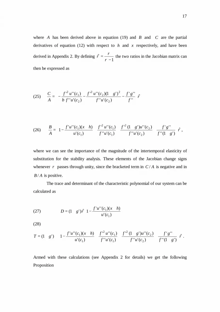
where A has been derived above in equation (19) and B and C are the partial
derivatives of equation (12) with respect to h and x respectively, and have been
derived in Appendix 2. By defining 1
ˆ−
=ρρρ the two ratios in the Jacobian matrix can
then be expressed as
(25) ρβ
ˆ'''''
)(''')'1)(('''
)(''')('''
2
22
2
2
12
−+−−=fgf
cufgcuf
cufcuf
AC
(26) ρ̂)'1(''
''')('''
)('')'1(')(''')('''
)('))(('''
12
22
1
12
1
1
++++++−=
gfgf
cufcugf
cufcuf
cuhxcuf
AB
,
where we can see the importance of the magnitude of the intertemporal elasticity of
substitution for the stability analysis. These elements of the Jacobian change signs
whenever ρ passes through unity, since the bracketed term in AC / is negative and in
AB / is positive.
The trace and determinant of the characteristic polynomial of our system can be
calculated as
(27)
+−+=
)('))(('''
1ˆ)'1(1
1
cuhxcuf
gD ρ
(28)
ρ̂)'1(''
''')('''
)('')'1(')(''')('''
)('))(('''
1)'1(2
22
1
12
1
1
++++++−++=
gfgf
cufcugf
cufcuf
cuhxcuf
gT .
Armed with these calculations (see Appendix 2 for details) we get the following
Proposition

18
Proposition. If the intertemporal elasticity of substitution is at least one half, and
differs from unity, all the stationary equilibria are saddle points.
Proof. See Appendix 3.
Stationary equilibria are saddle points for a wide range of the values for the
intertemporal elasticity of substitution. Empirical evidence on the size of this elasticity
does not, however, necessarily coincide with the parameter values stated in
Proposition, but often points out to lower values.10 It is therefore of interest to study
also the characteristics of equilibria when 2/1<ρ .11 Next we turn to examine this
case.
5. Dynamical Equilibria: Indeterminacy and Flip Bifurcations
In the above discussion we found that when 1>ρ , the determinant (D) and the trace
(T) of the system are positive, and furthermore that D-T+1 < 0. Stationary equilibria
are thus saddles (these equilibria are in area C in Figure 3 in which we have reproduced
the familiar graphical description of dynamical equilibria in a planar system, see e.g.
Azariadis 1993). Thus complex roots are not possible in our model, which in turn
means that we cannot get Hopf bifurcations.
When 1<ρ , the determinant of the system becomes negative, and D-T+1
positive. This means that the saddle-node bifurcations (they require among other things
that D-T+1 = 0) are not possible. We already proved that stationary equilibria are
saddles for 2/11 ≥> ρ . Since D+T+1 cannot be unambiguously signed, it is possible
to have Flip bifurcations in our model (see areas A and B in Figure 3).
In the following we assume 2/1<ρ (i.e. 0ˆ<ρ and 1ˆ <ρ ). Inspecting the
general case above seems to point out that it is possible to get stable equilibria and Flip
10 See the discussion e.g. in Deaton (1991, pp. 63-75). 11 It is interesting to note that Grandmont (1985) showed in a different overlapping generations model with money that no cycles can exist when the Arrow-Pratt relative risk aversion is smaller than or equal to 2 This is equivalent to the condition that the intertemporal elasticity of substitution is greater than or equal to one half.

19
bifurcations. Since 0ˆ<ρ , we consider the case where D < 0. We have also established
in the proof of Proposition that, when 2/1≥ρ (and 1≠ρ ) D-T+1 > 0. To get
stability, we need to have D+T+1 > 0 as well. Because we have rigorously shown the
existence of saddles when D < 0, we can also show the existence of Flip bifurcations, if
we can show the stability of equilibria.
D
T
D+T+1=0D-T+1=0
A
B
C
1
-1
2-1 1-2
Figure 3. Characteristics of stability in a planar system
To proceed we rewrite D+T+1 as follows
(29) { }1ˆ)'1( ++= MgD ρ
(30) { }1ˆ)'1( ++++= NMgT ρ ,
where
0)('
))(('''
1
1 >+−=cu
hxcufM
0)'1(''
''')('''
)('')'1(')(''')('''
2
22
1
12
>
++++=
gfgf
cufcugf
cufcuf
N .

20
Using this shorthand notation we can express D+T+1 after some manipulation
(31) D+T+1 = )̂1)('2(ˆˆ)'2( ρρρ +++++ gNMg .
This shows that at least in principle D+T+1 can be zero or positive, if the last term, the
only positive term in the expression, dominates. Note that when D <0, D-T+1 > 0 and
D+T+1 = 0 we have a Flip bifurcation.
Since the existence of a Flip bifurcation cannot be proved analytically in our
model we consider a parametric example. We use the following standard explicit
functional forms:
−+=′+−=′′−=′⇒−=
−=′′=′⇒=
−==⇒−
=
−−
−−−−
bxagbgbxagbxaxxg
hfhfhhf
ccuccuc
cu
11,,21
)(
)1(,)(
1)('',)('
11)(
2
21
111
11
ααα
ρρρ
ααα
ρρ
Note that ρ in the utility function is exactly the intertemporal elasticity of substitution.
In the stationary equilibrium 2)2/1( bxaxh −= . Using this expression for h , the Euler
equation and budget constraints, we end up with the following expression (see
Appendix 4) for the stock of the renewable resource in a stationary equilibrium
(32) ααβ ρρ −=
−+
−++1
21)1(1
1
bxabxa.
A straightforward but tedious calculation yields the expression for D+T+1

21
(33)
−−−++
−−−
−+−+
−=++
ρρ
αα
α
ρ 121)2(
)21)(1(
)211()2(
111 bxa
bxa
bxabxaTD
[ ] [ ]
−+
−+−++−++−++
−
−+
−
bxa
bxaxbbxabxabxa1
)21()1(1)1()1(1
11
11
21 ρ
ββαβα
ρα ρ
ρρρρρ
.
In the sequel we undertake a numerical analysis for a calibrated version of the
parametric example of our model. We assume the following values for parameters of
the growth function and the discount factor: 1== ba and 2/1=β .12 The values for
growth parameters mean that 1ˆ=x and 2=x , and furthermore that the condition
0)('1 ≥+ xg holds for all 20 ≤≤x . Economically more interesting parameters are the
marginal product of resource (α ), which determines the price elasticity of resource
demand, and the intertemporal elasticity of substitution ( ρ ). For this reason our focus
will be to find out for what values of these parameters we will get stability and Flip
bifurcations.
Solving α from equation (32) and plugging that value into (33) we find out for
what combinations of x and ρ D+T+1 is greater or less than zero or exactly zero.
Solving α from (32) we get
(34)
−++−+−−
−+−= ρρ β
α)1(1
122
222
2bxabxa
bxabxa
bxa .
Plugging this relationship (34) into (33) gives the following relatively complicated
expression
12 If we want to interpret literally the length of the period in our overlapping generations economy to be around 25 years, then the annual discount factor 0.975 (or the rate of time preference about 2.6 percent) means that the discount factor for 25 years should be around ½.

22
(35)
−−−++−+−+
−=++
ρρβ
ρρρ
121)2()1)(2(
111 bxabxabxaTD
[ ][ ][ ]
−+++−−+−++−+−
−+ ρρ
ρρ
ββρ
ρ )1(122)1(2)1(1)22)(2(
11
bxabxabxabxabxabxabx
[ ] +
−+++−−++−+−
−+ ρρ
ρρρρ
βββ
ρ )1(122))1(1()1)(2(
11
bxabxabxabxabxa
[ ]
−+++−−++−+−
−+ ρρ
ρρ
ββ
ρ )1(122))1(1)(1)(2(
11
bxabxabxabxabxa .
To get a more precise idea where to look for stable equilibria, note that the
only positive term in that expression (35) is the second term. Combining this term and
the first term we get after rearranging
(36) [ ]ρρ βρρ
)1()21(1
2 bxabxa −+−−
−−+ .
As we have already mentioned, we assume that 2/1=β and 2/10 <<ρ . Consider first
the efficient allocations, which lie on the left-hand side of the maximum sustained yield,
i.e. bax /0 ≤≤ . It is quite straightforward to see that the term in the square brackets
of (36) is negative. This means that all the stationary equilibria are saddles. Therefore,
we should look for possible stable equilibria from the right-hand side of the MSY,
where equilibrium is inefficient.
The stationary equilibrium condition (32) indicates that there is an inverse
relationship between α and x. Because we will now concentrate on such allocations
for which bax /> , the value of α must be relatively small for equation (32) to hold.
Our approach will be the following. We will first graph the plane defined by
equation (35) in the (D+T+1) ρx - space. Then we set D+T+1 = 0, and graph those
values of x and ρ for which D+T+1 = 0 holds.

23
FIGURE 4. D+T+1.
Figure 4 is the three dimensional graph of equation (35) (when α has been substituted
in for the expression of D+T+1). It points out to the fact that D+T+1 will be positive
only for extremely high (i.e. values which are close to x (= 2) levels of the renewable
resource stock.
FIGURE 5. Characterization of Flip Bifurcations

24
In Figure 5 we have projected those values of the resource stock x and the
elasticity of intertemporal substitution ρ for which D+T+1 is exactly zero, i.e., for
which we have Flip bifurcations. Values of x and ρ , which lie on the right-hand side
of the curve depicted in Figure 5, will yield stable equilibria, and for the values of x
and ρ on the left-hand side we have saddlepoint equilibria.
FIGURE 6. Equation (34).
In Figure 6 we have depicted α , x and ρ in the same diagram, i.e. we have
graphed equation (34). This figure indicates that to get stable equilibria and Flip
bifurcations the value of α needs to be quite small. E.g. if 01.0=α and 03.0=ρ we
get the level of the stationary equilibrium stock to be 1.95664. We also get
00119886.01=++ TD . And if we let 011.0=α , we get the equilibrium stock to be
1.95228, and 00373852.01 −=++ TD .
We have shown that there is a nontrivial set of values for parameters α and
ρ , for which our parametrized economy exhibits stable equilibria and Flip bifurcations.

25
This means that there can be endogenous cycles in our model, since the characteristic
roots are of different sign.13 The dynamics of our model is thus rather rich.
The parameter values for the intertemporal elasticity of substitution for which
we get stability and Flip bifurcations are empirically quite plausible. The parameter
values for the production function parameter (α ), for which we obtain stability and
bifurcations, are quite small. The parameter α measures the share of natural resources
in total output. It varies across countries and can be relatively low.
6. Conclusions
The stability properties of an overlapping generations model with capital accumulation,
like periodic equilibria and indeterminacy of equilibria, have been subject to a fairly
large amount of research since the mid 1980s. These issues have not, however, been
studied carefully in models with renewable resources like forests or fisheries. Our
purpose in this paper has been to do just that. We have examined the dynamic
properties of an overlapping generations economy under the standard assumptions
about the utility and production functions, but augmented with a renewable resource.
In addition to a factor of production it serves as a store of value. Because a renewable
resource has its own growth function and dynamics, we get a planar system consisting
of harvesting and the resource stock. After having characterized the steady state
equilibrium and efficiency we turned to our main focusing to studying the stability
properties of our model.
We showed that the nature of steady state equilibrium depends on the value of
intertemporal elasticity of substitution in consumption. In particular, if the
intertemporal elasticity of substitution is at least one half, but different from unity (the
case of the logarithmic utility function), then stationary equilibria are saddle points.
Interestingly, for smaller values of the intertemporal elasticity of substitution, which
are equally plausible on the basis of empirical evidence from consumption behavior, we
use a parametric example to demonstrate the existence of Flip bifurcation and stable
13 Interestingly, Grandmont (1985) has shown in a different overlapping generations model with money that a succession of Flip bifurcations may occur when the Arrow-Pratt relative risk version exceeds two, which is equivalent to the condition that the intertemporal elasticity of substitution is smaller than one half.

26
spiral equilibria. This result is possible only for inefficient economies. Hence, an
overlapping generations economy with a renewable resource may display
indeterminacy and stable spiral equilibria under standard well-behaved utility and
constant returns to scale production functions without externalities or imperfect
competition as is usually required to get bifurcations and indeterminacy from stability
analyses.

27
Appendix 1. The slope of equation [16] and the RHS of equation [12] as a function of 1+th • The right-hand side of equation (12) as a function of 1+th . The RHS of (12) is A.1 [ ][ ])('1))()(('')(')( 111111 ++++++ ++= tttttt xgxgxhfuhfhRHS β
Differentiating this with respect to 1+th we get (dropping the arguments) A.2 [ ]))(('')(''')'1(''')'1()(' 21 xgxfcufgufghRHS t ++++=+ ββ [ ]''))(('''')'1( uxgxfufg +++= β Keeping in mind that ))(('2 xgxfc += we get
A.3
−+=+ )(
11''')'1()('
21 c
ufghRHS t ρβ
where )('')(')(
ccucuc −=ρ . In the case of constant Arrow-Pratt relative risk aversion utility
functions )(cρ is exactly the inverse of elasticity of intertemporal substitution. From A.3 it is now easy to see that )0(0)(' 1 <>+thRHS when )1(1)( <>cρ . • The derivation of the slope of equation (16) We first rewrite equation (12), and take into account the fact that we consider paths, where tt hh =+ 1 for all t but tx may vary. A.4 [ ] [ ] ))('1())()(('')(')(')(' 1111 ++++ ++=−− ttttttttt xgxgxhfuxhfhhfhfu β Totally differentiating A.4 and taking into account equation (10) we get A.5 { [ ] −+++− + )('')(''))(('')('' 121 t
ttt
t xgcufxgxfcu β [ ] } ttttt
t dhxgxgfxgxfcu ))('1()('1('))(('')('' 11112 ++++ ++++β = { ++++ + ))('1)(('')(')('1(')('' 121 tt
tt
t xgxgcuxgfcu β [ ][ ] } ttttt
t dxxgxgxgxgfcu ))('1())('1)((')('1')('' 112 ++ ++++β . Rearranging and evaluating A.5 at the stationary point, tt hh =+ 1 and tt xx =+ 1 , yields equation (16) in the text.

28
Appendix 2. Development of the Jacobian Matrix of the Partial Derivatives For the purposes of stability analysis we develop the Jacobian matrix, its determinant and trace. A.6 ),(1 ttt hxGx =+ A.7 ),(1 ttt hxFx =+ The stability of the steady-state depends on the eigenvalues of the Jacobian matrix of the partial derivatives
=
hx
hx
FFGG
J .
Calculating the partial derivatives of the Jacobian matrix we first obtain )('1),( tttx xghxG += , 1),( −=tth hxG . To get the partials of ),(1 ttt hxFh =+ we first do the implicit differentiation in the following manner A.8 ttt CdxBdhAdh +=+ 1 , where A, B and C are appropriate partial derivatives to be presented in a moment. Calculating these we take into account the other dynamical equation of our system:
)(1 tttt xghxx +−=+ . Given the definitions of A, B and C we will then have
AChxF ttx =),( ,
ABhxF tth =),( .
As for A (as evaluated at the steady state) we get from A.3
A.9 ρ
ρβ 1)(''')'1( 2−+= cufgA ,
where ρ has been defined in the text. For the future developments we define
1ˆ
−=
ρρρ . Clearly, 0)(<>A , as 1)(><ρ . Totally differentiating (12) with respect to
th (again taking into account the transition equation) we obtain A.10 [ ]+++−+= )('))()(('')('')(')(')('' 11 tttt
tt
tt hfxgxhfcuhfcuhfB
[ ] [ ] 0)('')(')(')('1)('')(' 1212
122
1 <++ ++++ tt
ttt
t xgcuhfxgcuhf ββ ,

29
and totally differentiating (12) with respect to tx (again taking into account the transition equation) we have A.11 [ ] [ ] [ ]−+−+−= ++ )('1)('')(')(')('1)('')(' 1211
2tt
ttt
tt xgxgcuhfxgcuhfC β
[ ] [ ][ ] 0)('1)('1)('')(' 212
21 >++ ++ tt
tt xgxgcuhfβ .
Next we evaluate A, B and C at the steady state. By taking into account the Euler condition at the steady state )(')'1()(' 21 cugcu β+= , we get
A.12i ρβ
ˆ'''''
)(''')'1)(('''
)(''')('''
2
22
2
2
12
−+−−=fgf
cufgcuf
cufcuf
AC
A.12ii ρ̂)'1(''
''')('''
)('')'1(')(''')('''
)('))(('''
12
22
1
12
1
1
++++++−=
gfgf
cufcugf
cufcuf
cuhxcuf
AB
.
Clearly, 0)(/ <>AC when )1(1 ><ρ , and 0)(/ <>AB when )1(1 <>ρ . We can now rewrite the Jacobian as follows
A.13
−+=
AB
AC
gJ
1'1.
The determinant (D) and the trace (T) of the Jacobian matrix, J, are D =
AC
ABg ++ )'1( and T =
ABg ++ '1 respectively. Using equations A.9, A.10 and A.11 we
have the following expressions
A.14
+−+=
)('))(('''
1ˆ)'1(1
1
cuhxcuf
gD ρ
A.15
ρ̂)'1(''
''')('''
)('')'1(')(''')('''
)('))(('''
1)'1(2
22
1
12
1
1
++++++−++=
gfgf
cufcugf
cufcuf
cuhxcuf
gT .

30
Appendix 3. Proof of Saddle-Point Stability We analyze the stability of system (22) and (23) on the basis of (11) and (12). The characteristic polynomial associated with the system (22) – (23) expressed in terms of D and T is A.16 0)( 2 =+−= DTp λλλ It is known from the stability theory of difference equations (for an elementary treatment, see e.g. Azariadis, 1993, pp. 63-67) that for a saddle point the roots of
0)( =λp need to be on both sides of unity. Thus for a saddle we need that D-T+1 < 0 and D+T+1 > 0 or D-T+1 > 0 and D+T+1 < 0. When ρ̂ is positive, i.e. 1>ρ , it is easy to conclude that both the determinant and the trace in A.14 and A.15, respectively, are positive, which also means that that D+T+1 > 0 holds. Making inferences about the sign of D-T+1 requires more work. A straightforward calculation yields A.17 D-T+1=
+−+−−+−+−
)'1('''''
)(''')('')'1('
)(''')('''
)(''))(('''ˆ)1ˆ('
2
22
1
12
1
1
gfgf
cufcugf
cufcuf
cughxcuf
g ρρ .
A.17 cannot be signed yet for 0ˆ>ρ (i.e. 1>ρ ). To get the sign of D-T+1 we use the assumption that our steady state is unique. This is assured by comparing slopes of the curves, where tt hh =+ 1 and tt xx =+ 1 . We develop the condition
A.18 00 =∆=∆
>tt xt
t
ht
t
dxdh
dxdh ,
as A.19
[ ] ')'1(')('')'1)(('''')(')('')(''')(''
)'1(')('')'1('')(')'1(')(''
2211
3221 g
gfhxfgcugcuhxfcufcugfcuggcugfcu >
+−++−++−+++++
ββββ .
Multiplying both sides of A.19 by the denominator (negative sign) on the left-hand side we get A.20 <+++++ 3
221 )'1(')('')'1('')(')'1(')('' gfcuggcugfcu ββ

31
')('')'1)((''''')(''''))(('''')('' 2211 ghxfgcuggcugfhxcugfcu ++−++− ββ
'')'1)(('' 22 gfgcu ++ β .
and collecting terms A.20 can be re-expressed as A.21 '''))(('')'1(')('''')('')('' 1
2221 gfhxcugfcugcufcu +++++ ββ
0')('')'1)(('' 2 <+++ ghxfgcuβ . Dividing by ( 0)(''' 2 <cuf β ), using Euler condition and the fact that )('2 hxfc += yields A.22
0'
')'1(1)('
)'1('))(('')('''
)'1(')(''''''
)(''')'1(')(''
1
1
2
22
1
1 >+−+++++++f
ggcu
gghxcucuf
gfcufg
cufgfcu
ρ. Now we multiply both sides by )'1/(' gf + (>0) to get
A.23 0'1
)('''))((''
)(''')'1(')(''
)'1('''''
)('''')(''
1
1
2
22
1
21 >−++++
++ g
cufghxcu
cufgfcu
gfgf
cuffcu
ρ.
Rearranging and taking into account the definition of ρ̂ yields A.24
0)'1(''
''')('''
)('')'1(')(''')('''
)(''))(('''
')ˆ
1ˆ(
2
22
1
12
1
1 <
+−+−−+−+−
gfgf
cufcugf
cufcuf
cughxcuf
gρ
ρ.
If 0>̂ρ (i.e. 1>ρ ) we get by multiplying with ρ̂ A.25
0)'1(''
''')('''
)('')'1(')(''')('''
)(''))(('''ˆ)1ˆ('
2
22
1
12
1
1 <
+−+−−+−+−
gfgf
cufcugf
cufcuf
cughxcuf
g ρρ .
Note that this is exactly D-T+1, which means that we have a saddle when 1>ρ . If 0ˆ <ρ (i.e. 1<ρ ) we get by multiplying with ρ̂ A.26
0)'1(''
''')('''
)('')'1(')(''')('''
)(''))(('''ˆ)1ˆ('
2
22
1
12
1
1 >
+−+−−+−+−
gfgf
cufcugf
cufcuf
cughxcuf
g ρρ

32
which means that D-T+1 is positive. To get a saddle in this case, we need to have D+T+1 to be negative. To explore this possibility we check the sign of D+T+1 when
0<̂ρ (i.e. 1<ρ ). To make this calculation more transparent we rewrite D and T as follows A.27i { }1ˆ)'1( ++= MgD ρ A.27ii { }1ˆ)'1( ++++= NMgT ρ , where
0)('
))(('''
1
1 >+−=cu
hxcufM
0)'1(''
''')('''
)('')'1(')(''')('''
2
22
1
12
>
++++=
gfgf
cufcugf
cufcuf
N .
Using this shorthand notation D+T+1 can be expressed after some manipulation A.28 D+T+1 = )̂1)('2(ˆˆ)'2( ρρρ +++++ gNMg . Note that, we are now considering the case, where 0ˆ <ρ (i.e. 1<ρ ). The first two terms in (A28) are negative. The third term is also negative when 0ˆ1 <+ ρ . This happens when 2/1>ρ . So we have a saddle in this case, too. This completes the proof of Proposition. Q.E.D. Appendix 4. Derivation of equation (32) Given the assumed functional forms, the Euler equation can be written A.29 [ ] 12 )'1( cgc ρβ+= . Plugging this into the equilibrium condition, )(21 hfcc =+ and using the budget constraint ))()(('2 xgxhfc += gives
[ ]ρρ
α
β)1(1))2/1((
1 bxabxaxc
−++−= and [ ][ ]
))2/1(()2/1(1))2/1((
2 bxabxabxaxc
−−+−=
αα .
If we plug these expressions for consumption back into the equilibrium condition we get equation (32) in the text.

33
References
Amacher G., R. Brazee, E. Koskela and M. Ollikainen. 1999. Taxation, Bequests,
and Short and Long Run Timber Supplies: An Overlapping Generations
Problem. Environmental and Resource Economics, 13, 269-288.
Azariadis, C. 1993. Intertemporal Macroeconomics. Basil Blackwell, Oxford.
Benhabib, J. and R.E.A. Farmer 1999. Indeterminacy and Sunspots in
Macroeconomics, pp. 387- 448 in Taylor, J. and M. Woodford (ed.) Handbook
of Macroeconomics. Amsterdam. North-Holland.
Cass, D. 1972. On Capital Overaccumulation in the Aggregative, Neoclassical Model
of Economic Growth: A Complete Characterization. Journal of Economic
Theory 4, 200-223.
Clark, C.W. 1990. Mathematical Bioeconomics. The Optimal Management of
Renewable Resources. Second Edition. New York, John Wiley & Sons, Inc.
Deaton, A. 1992. Understanding Consumption. Clarendon Lectures in Economics.
Clarendon Press, Oxford.
Farmer, R. 1986. Deficits and Cycles. Journal of Economic Theory, 40, 77-88.
Gale, D. 1973. Pure Exchange Equilibrium of Dynamic Economic Models. Journal of
Economic Theory, 6, 12-36.
Grandmont, J.-M. 1985. On Endogenous Competitive Business Cycles.
Econometrica, 53, 995-1045.
Grandmont, J.-M. 1998. Introduction to Market Psychology and Nonlinear
Endogenous Business Cycles. Journal of Economic Theory 80, 1-13.
Johansson, P.-O. and K.-G. Löfgren 1985. The Economics of Forestry and Natural
Resources, Oxford, Basil Blackwell.
Kemp, M. and N Van Long. 1979. “The Under-Exploitation of Natural Resources: A
Model with Overlapping Generations,” Economic Record, 55, 214-221.
Lofgren, K.-G. 1991. “Another Reconcialition between Economists and Forestry
Experts: OLG-Arguments”. Environmental and Resource Economics, 1, 83-
95.
Mourmouras, A. 1991. Competitive Equilibria and Sustainable Growth in a Life-
Cycle Model with Natural Resources. Scandinavian Journal of Economics, 93,
585-591.

34
Mourmouras, A. 1993. Conservationist Government Policies and Intergenerational
Equity in an Overlapping Generations Model with Renewable Resources.
Journal of Public Economics, 51, 249-268.
Reichlin, P. 1986. Equilibrium Cycles and Stabilization Policies in an Overlapping
Generations Economy with Production. Journal of Economic Theory, 40, 89-
102.
Tobin, J. 1980. Discussion, in Kareken, J.H. and N. Wallace (eds): Models of
Monetary Economies, Federal Reserve Bank of Minneapolis, 83-90.

35
FIGURE 1. Elasticity of intertemporal substitution greater than one
FIGURE 2. Elasticity of intertemporal substitution less than one
x xx
hh h
∗xx̂

36