Fiscal Policy under Indeterminacy

and Tax Evasion.

∗

Francesco Busato† Bruno Chiarini‡ Enrico Marchetti§

First Draft: May 2004

This Draft: May 30, 2005

Abstract

This paper shows under indeterminacy and tax evasion, an increase in corporate, laboror income tax rates pushes the economy into an expansionary pattern. These effects arereversed when the steady state is saddle-path stable.

Journal of Economic Literature Classification Numbers: E320, E13, E260, O40Keywords : Dynamic General Equilibrium Models, Fiscal Policy, Tax Evasion and Under-ground Activities, Indeterminacy and Sunspots.

1 Introduction

The equilibrium effects and the role of fiscal policy in dynamic general equilibrium models

of fluctuations have been object of thorough investigations in the last decade. Significant

work has been done in fiscal policy analysis within neoclassical growth models.1. Fiscal policy

implications have been investigated also in the context of dynamic equilibrium models of fluc-

tuations induced by indeterminacy in the equilibrium path, which is in turn due to increasing

∗We are grateful to Torben M. Andersen, John B. Donaldson, Marco Maffezzoli, Luca Stanca, Claus Vastrupfor many conversations and to the participants at Seminars at University of Aarhus, University of Rome “LaSapienza”, at the III Workshop on Macroeconomic Dynamics at Bocconi University and at the XLV Conferenceof the Italian Economic Assciation for comments on earlier drafts of the paper. Of course all errors are ours.Enrico Marchetti gratefully acknowledges the financial support of University of Rome “La Sapienza” and MIUR.

†Corresponding Author. Department of Economics, School of Economics and Management, Building 322,University of Aarhus, DK-8000 Aarhus C. Email: fbusato@econ.au.dk.

‡University of Naples Parthenope, Naples, Italy.§Department of Public Economics, University of Rome “La Sapienza”, Rome, Italy.1Aschauer [2] and Baxter and King [5] are seminal contributions sharing an emphasis on the supply-side

response of labor and capital to shifts in government demand and tax rates. Recent related contributions are:Braun [7], McGrattan [22], and Burnside Eichenbaum and Fisher [8].

1

return to scale at aggregate level. In this case, particular attention has been put on the impact

of changes in the steady state levels of tax rates on the topological properties of the model’s

attractor (Guo and Lansing [19]; Christiano and Harrison [11]).2

The main finding of this paper is that recessionary fiscal policies (i.e. an increase in

corporate, income or labor tax rates) induce expansionary effects for a class of dynamic general

equilibrium models augmented with increasing returns to scale in production and tax evasion;

these effects are reversed when the steady state is saddle path stable.

We analyze a one-sector dynamic general equilibrium model in which there are three agents:

Firms, Households and a Government; furthermore, there is one homogeneous consumption

good. The government levies proportional taxes on corporate revenues, labor and capital in-

come flows, payroll taxes on labor services and balances its budget (in expected terms) for each

period. Firms and households, being subject to distortionary taxation, use the underground

labor market to evade taxes. Government faces tax evasion originating from the underground

sector, and coordinates strategy to address abusive trust schemes. The models displays en-

dogenous fluctuation due to increasing returns to scale and well behaved demand schedules for

production inputs (in the sense that slope down).

Motivations for our analysis are theoretical and empirical.

As for the first one, the standard Farmer and Guo [15] models with indeterminacy and

increasing returns to scale suffer from a number of undesirable features: e.g. a too high

degree of increasing returns to scale in aggregate production, and an upward sloping labor

demand schedule.3 Busato et. al. [10] show how the introduction of an even tiny underground

sector (justified by the incentive to evade distortionary taxation) can overcome some of the

above mentioned undesirable features. Furthermore, this modification entails a theoretical

mechanism allowing self-fulfilling prophecies to propel the business cycle, which is different

from that proposed in the literature.

On the empirical side, underground activities are a fact in many countries, and there are

2Devereux et al. [14] study the dynamic response to changes in government spending under increasing returnsto scale, when the attractor is still a saddle point.

3This class of one sector models requires returns to scale greater that 1.6, while recent estimates suggest thatUS economy returns to scale are no larger than 1.2 (see, among the others, Basu and Fernald [4], Sbordone [24],Jimenez and Marchetti [20]).

2

significant indications that this phenomenon is large and increasing.4 The estimated average

size of the underground sector (as a percentage of total GDP) over 1996-97 in developing

countries is 39 percent, in transition countries 23 percent, and in OECD countries about 17

percent (Schneider and Enste [25]). For the United States, the average size of underground

activities ranges between 5 percent of GNP (in the Seventies: Tanzi [26]) and 9 percent of the

GDP (in the Eighties, early Nineties: Paglin [23]; Schneider and Enste [25]).

The paper is organized as follows. Section 2 details the theoretical model, while Section

3 presents the topological properties of stationary state and discusses conditions for indeter-

minacy. Section 4 presents and discusses the model’s response to fiscal policy shocks. Finally

Section 5 concludes.

2 Structure of the model

2.1 Firms’ sector

Production technology for the homogenous good yj,t uses three inputs: physical capital, regular

labor services, and underground labor services. The production function of firm j reads:

yj,t = Atkαj,t(n

Mj,t)

1−α−ρ(nUj,t)ρ, 0 < α+ ρ < 1, (1)

where kj,t denotes capital stock, nMj,t is regular labor, nUj,t represents irregular labor, and the

quantity

At ={Kαt (NM

t )1−α−ρ}η

︸ ︷︷ ︸“Regular” Ext.

{(NU

t )ρ}ζ

︸ ︷︷ ︸“Underground” Ext.

, (2)

represents an aggregate production externality: it passes through aggregate-average level of

output (K,NM and NU are the economy-wide levels of the three inputs) and has two different

sources.

4There is no universal agreement on what defines the underground economy, and obviously, the difficulty indefining the sector extends to the estimation of its size. There exist several synonyms for describing undergroundactivities: underground activities, shadow or hidden economy. We are concerned with the size of the undergroundeconomy as encompassing activities which are otherwise legal but go unreported or unrecorded.

3

The quantity{Kαt (NM

t )1−α−ρ}η

(the “regular” externality) is related to an external effect

to that of standard one-sector models (e.g. Farmer and Guo [15]). The quantity{(NU

t )ρ}ζ

(the “underground” externality) is specifically related to underground activities.5 Externality

parameter for regular labor η can be different from that of the underground one (ζ). This

formulation adds generality to the analysis: when η = ζ and there are neither tax evasion nor

distortionary taxation, the model reduces to Farmer and Guo’s one.

As firms are homogeneous, overall level of output for a given (and equal for all firms) level

of inputs utilization is given by:

Yt = At

∫

j

{kαj,t(n

Mj,t)

1−α−ρ(nUj,t)ρ}dj = K

α(1+η)t (NM

t )(1−α−ρ)(1+η)(NUt )ρ(1+ζ)

Increasing returns to scale are a pure aggregate phenomenon (as equation (1) suggests),

and returns to scale are constant at firm level, as each firm takes K, NM and NU as given.

Firms evade taxes on total revenues and on labor services, by allocating labor demand

to underground labor market. Firms, however, may be detected evading, with probability

p ∈ (0, 1), and forced to pay the statutory tax rates on revenues and the payroll tax rate on

labor (τΠt and τNt respectively), increased by a surcharge factor, s > 1, applied to the standard

tax rate. 6

When a firm is not detected evading (with probability 1− p), its profit are denoted with

πNDj,t . If detected evading (with probability p), we denote firm’s profits as πDj,t; both are

defined below:

5Underground labor services use the same capital stock that is used by regular labor. We could imaginethat the same firm produces in the regular economy in the day, and in the underground economy by night,by using the same employees. This production scheme is denoted as “moonlighting ” production. Bajada [3]loosely defines the underground economy to be all economic activity that contributes to value added and “goesunreported by a society’s measurement technique”. Bajada outlines several different activities that would leadto a distorted measure of national measurements: moonlighting is defined as failure to report income from asecond job; or profit-businesses that are paid in cash and do not report this additional income i.e. hair dressersmay report fewer clients than they really service; the failure to report interest earnings and barter. Cowell [13]offers additional details.

6The hypothesis that firms always evade is related to the use of underground labor. It must be noticedthat such hypothesis is encapsulated in the definition of the production function: in order to have nonzeroproduction, NU

j,t must be positive in equilibrium.

4

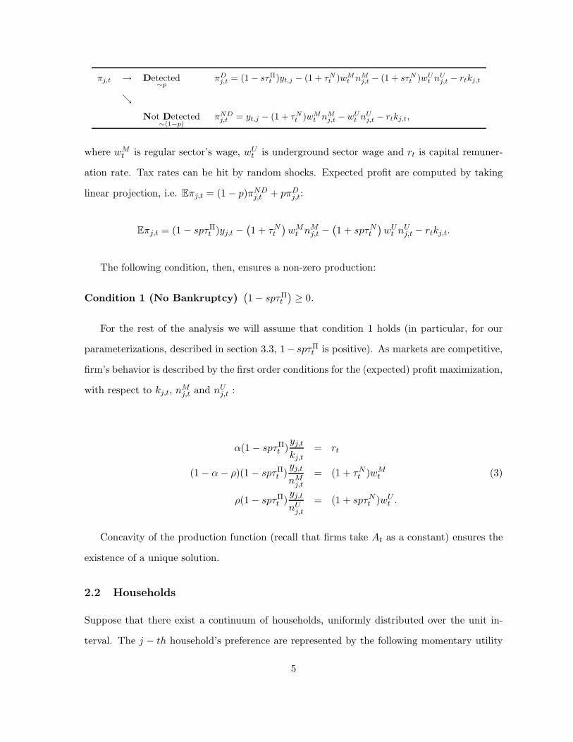
πj,t → Detected∼p

πDj,t = (1 − sτΠ

t )yt,j − (1 + τNt )wM

t nMj,t − (1 + sτN

t )wUt n

Uj,t − rtkj,t

ց

Not Detected∼(1−p)

πNDj,t = yt,j − (1 + τN

t )wMt nM

j,t − wUt n

Uj,t − rtkj,t,

where wMt is regular sector’s wage, wUt is underground sector wage and rt is capital remuner-

ation rate. Tax rates can be hit by random shocks. Expected profit are computed by taking

linear projection, i.e. Eπj,t = (1 − p)πNDj,t + pπDj,t:

Eπj,t = (1 − spτΠt )yj,t −

(1 + τNt

)wMt n

Mj,t −

(1 + spτNt

)wUt n

Uj,t − rtkj,t.

The following condition, then, ensures a non-zero production:

Condition 1 (No Bankruptcy)(1 − spτΠ

t

)≥ 0.

For the rest of the analysis we will assume that condition 1 holds (in particular, for our

parameterizations, described in section 3.3, 1− spτΠt is positive). As markets are competitive,

firm’s behavior is described by the first order conditions for the (expected) profit maximization,

with respect to kj,t, nMj,t and nUj,t :

α(1 − spτΠt )yj,tkj,t

= rt

(1 − α− ρ)(1 − spτΠt )yj,t

nMj,t= (1 + τNt )wMt (3)

ρ(1 − spτΠt )yj,t

nUj,t= (1 + spτNt )wUt .

Concavity of the production function (recall that firms take At as a constant) ensures the

existence of a unique solution.

2.2 Households

Suppose that there exist a continuum of households, uniformly distributed over the unit in-

terval. The j − th household’s preference are represented by the following momentary utility

5

function:

u(cj,t, nj,t, nUj,t) = ln cj,t −B0

(nj,t)1+ξ

1 + ξ−B1

(nUj,t)1+ψ

1 + ψ,

where cj,t denotes household’s consumption flow, nj,t and nUj,t denote aggregate and under-

ground labor supplies; the term B0(nj,t)

1+ξ

1+ξ with B0 ≥ 0, represents the overall disutility of

working, while the last term, B1(nUj,t)

1+ψ

1+ψ with B1 ≥ 0, reflects the idiosyncratic cost of work-

ing in the underground sector7. Finally, the parameters ξ and ψ represent the inverse labor

supply elasticities of aggregate and underground labor supplies, respectively.8

Aggregate labor supply equals sum of regular and underground labor flows:

nj,t = nMj,t + nUj,t. (4)

The household evade income taxes by reallocating labor services from regular to under-

ground sector. Underground-produced income flows(wUt n

Uj,t

)are, therefore, not subject to

distortionary income tax rate τYt , as the feasibility constraint below suggests:

cj,t + ij,t = (1 − τYt )(wMt n

Mj,t + rtkj,t

)+wUt n

Uj,t. (5)

Capital stock is accumulated according to a customary state equation, i.e.

kj,t+1 = (1 − δ)kj,t + ij,t, (6)

where ij,t represents net investments, and δ denotes a quarterly capital stock depreciation rate.

Imposing a constant subjective discount rate 0 < β < 1, and defining µj,t as the costate

variable, the Lagrangian of the household control problem reads:

7Specifically, this cost may be associated with the lack of any social and health insurance in the undergroundsector.

8Assuming that ψ ≥ ξ implies that the inequality is reversed when looking at the labor supply elasticities,i.e. ψ−1 ≤ ξ−1. It must be noticed that a reasonable hypothesis would rather be: ξ ≥ ψ, so that overall laborsupply elasticity is smaller than that of the underground-specific one. Furthermore, in our parameterizations (seesection 3.3) we use ξ = ψ = 0, but results for the analysis of impulse response functions would be substantiallyanalogous when allowing for a small difference ξ ≷ ψ above the common zero value. Finally, recall that ξ relatesto total labor supply, regular nMj,t plus underground one nUj,t.

6

L0,j = E0

∞∑

t=0

βtu(cj,t, nj,t, nUj,t) + E0

∞∑

t=0

µj,t[(1 − τYt )(wMt n

Mj,t + rtkj,t

)+ wUt n

Uj,t − cj,t +

−kj,t+1 + (1 − δ)kj,t],

and the first order conditions obtain:

βtc−1j,t = µj,t (7)

βtB0(nMj,t + nUj,t)

ξ = µj,t(1 − τYt )wMt (8)

βtB0(nMj,t + nUj,t)

ξ + βtB1(nUj,t)

ψ = µj,twUt (9)

Et{µj,t+1

[(1 − δ) + (1 − τYt+1)rt+1

]}= µj,t (10)

limT→∞

ETµj,Tkj,T = 0. (11)

2.3 Government

The government budget, balanced in each period, is given by:

τYt (wMt NMt + rtKt) + spτΠ

t Yt + spτNt wUt N

Ut + τNt w

Mt N

Mt = EtREVt = Gt, (12)

where EtREVt denote expected government revenues, which are allocated to government ex-

penditure Gt. Notice that government balances its budget in expected terms since tax revenues

collected from the underground sector depend on the probability of being detected p. Govern-

ment expenditure is assumed to be wasteful, an the fiscal authority collects taxes in corporate

sector after that production takes place.

Tax shocks - which are a source of intrinsic uncertainty - are defined by the following set

of stochastic difference equations:

τt+1 = Qτt + et, (13)

where τt =[τYt , τ

Nt , τ

Πt

]′. Q is a matrix with elements

[ϕVii], i = 1, 2, 3; V = {Y,N,Π} on the

7

principal diagonal and zeroes elsewhere; et is a 3 × 1 vector of i.i.d. random shocks and the

covariance matrix∑

is a diagonal matrix[σ(e)Vii

], i = 1, 2, 3; V = {Y,N,Π}.

3 Model’s Topological Properties

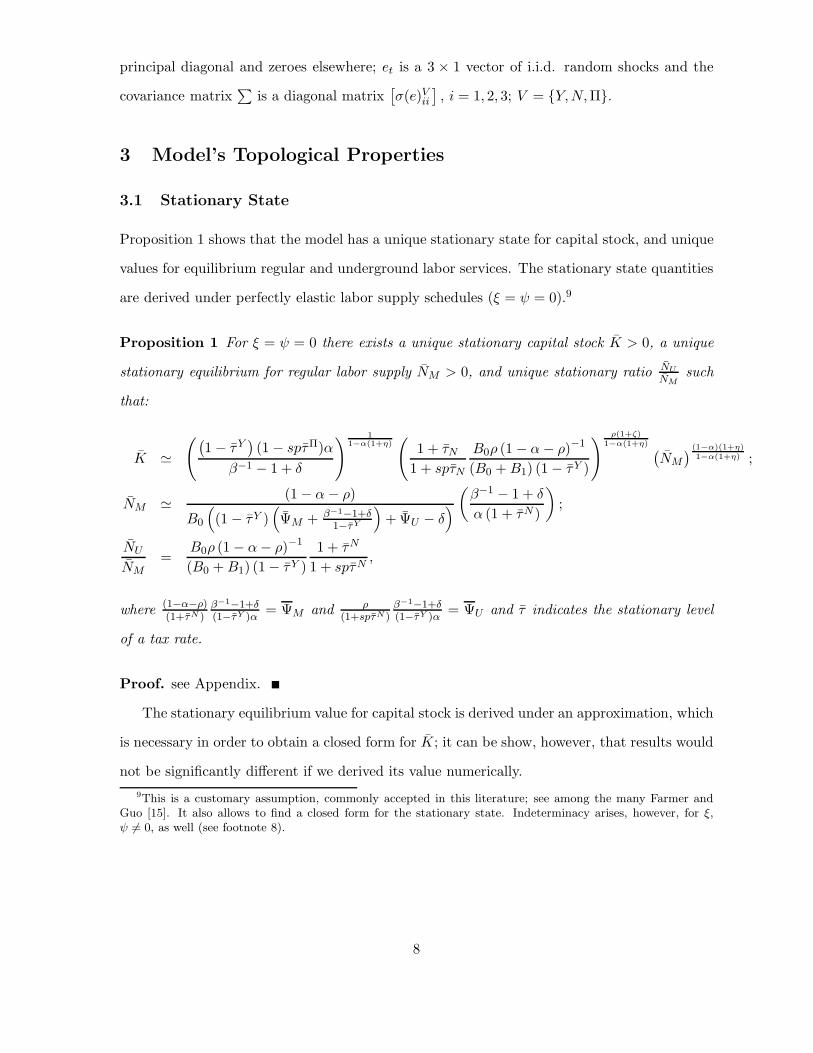
3.1 Stationary State

Proposition 1 shows that the model has a unique stationary state for capital stock, and unique

values for equilibrium regular and underground labor services. The stationary state quantities

are derived under perfectly elastic labor supply schedules (ξ = ψ = 0).9

Proposition 1 For ξ = ψ = 0 there exists a unique stationary capital stock K > 0, a unique

stationary equilibrium for regular labor supply NM > 0, and unique stationary ratio NUNM

such

that:

K ≃

((1 − τY

)(1 − spτΠ)α

β−1 − 1 + δ

) 11−α(1+η)

(1 + τN

1 + spτN

B0ρ (1 − α− ρ)−1

(B0 +B1) (1 − τY )

) ρ(1+ζ)1−α(1+η) (

NM

) (1−α)(1+η)1−α(1+η) ;

NM ≃(1 − α− ρ)

B0

((1 − τY )

(ΨM + β−1−1+δ

1−τY

)+ ΨU − δ

)(β−1 − 1 + δ

α (1 + τN )

);

NU

NM

=B0ρ (1 − α− ρ)−1

(B0 +B1) (1 − τY )

1 + τN

1 + spτN,

where (1−α−ρ)(1+τN )

β−1−1+δ(1−τY )α

= ΨM and ρ(1+spτN )

β−1−1+δ(1−τY )α

= ΨU and τ indicates the stationary level

of a tax rate.

Proof. see Appendix.

The stationary equilibrium value for capital stock is derived under an approximation, which

is necessary in order to obtain a closed form for K; it can be show, however, that results would

not be significantly different if we derived its value numerically.

9This is a customary assumption, commonly accepted in this literature; see among the many Farmer andGuo [15]. It also allows to find a closed form for the stationary state. Indeterminacy arises, however, for ξ,ψ 6= 0, as well (see footnote 8).

8

3.2 Conditions for Indeterminacy

For our parameterization (see Section 3.3 below), the model’s attractor is a sink: the eigenval-

ues characterizing the stability properties of the unique stationary state are equal to 0.8211 ±

0.2123i. The topological properties of the model’s attractor depend upon some crucial pa-

rameters; we restrict our attention to those characterizing the labor inputs’ heterogeneity:

particularly on η and ζ and the tax rates. It can be shown that the model can display inde-

terminacy only if the following conditions are satisfied:10

Condition 2 (NC) (necessary): β < (1+η){(

1 − (1 − α− ρ) τN

1+τN

)+ ρ

(1

(1−τY )(1+spτN )− 1)}

Condition 3 (SC) (sufficient): max{

1β(1−δ) ,

RR−1

}< ε

LDMbNU+ ε

LDUbNM< R

R−1.

Condition SC is expressed in terms of the cross-elasticities of the (inverse) inputs demand

functions; from equations (3) we have: εLDMbNU

=∂ bwMt∂ bNU

t

= ∂brt∂ bNU

t

= (1 + ζ) ρ, εLDUbNM

=∂ bwUt∂ bNM

t

= ∂brt∂ bNM

t

=

(1 + η) (1 − α − ρ); variables with the hat denote percentage deviations from the stationary

state. The quantities R and R read:

R =δ(M − sI) [1 − β(1 − δ)] (1 − α(1 + η)) + 2 [δα(1 + η)M + sI(2 − δ)]

δ(M − sI) [1 − β(1 − δ)] (1 − α(1 + η)) + 2 [δα(1 + η)M + sI(1 − β(1 − δ))]> 1,

R =δsI − δα(1 + η)M

sI [1 − β(1 − δ)] − δα(1 + η)M> 1,

while M = 1 − G/Y = sI + sC ; sI = I/Y ; sC = C/Y .

The Condition NC suggests that in order to have indeterminacy it is necessary that

the term sI+sC1−τY

=(1 − (1 − α− ρ) τN

1+τN

)+ ρ

(1

(1−τY )(1+spτN )− 1)–, augmented by the the

“regular” externality parameter η, must be large enough; in other words, distortionary taxation

should not drain too much resources away from the private sector, in order to allow the latter

to form self-fulfilling beliefs.11

Taking τY as given, the higher the probability of being detected evading p (and/or the

penalty surcharge factor s), the more difficult it becomes to allocate resources to the under-

ground sector, and the smaller the quantity(

1(1−τY )(1+spτN )

− 1)

gets. Consider the extreme

10See Busato et al. [10]11Recall that government expenditure is wasteful in the model. It is difficult to figure out, off hand, whether

our results still hold if government were rebating tax revenues either as consumption of private goods, or asinvestment to augment private inputs’ productivity. This analysis is left for future investigation.

9

case where tax evaders are punished with an infinitely large penalty (that is s→ ∞). The NC

reads: β < (1+η){(

1 − (1 − α− ρ) τN1+τN

)− ρ}

, suggesting that the parameter region for inde-

terminacy shrinks when tax evasion becomes extremely costly, and it fails if labor taxes are too

high (τN > β−(1+η)(1−ρ)α(1+η)−β , for example).12 Indeed, when tax evasion is extremely costly/risky,

and when taxes are higher than a certain threshold, they “tax away” the externality, in the

spirit of Guo and Lansing [19].

The picture is different if we take τN as given. An increase in income tax rate τY monoton-

ically increases the quantity(

1(1−τY )(1+spτN )

− 1), easing, by this hand, the necessary condi-

tion. That happens because there is no probability of being detected evading income taxation

(on the households’ side). Therefore, the higher the income tax rate, the higher would be the

underground labor supply; in this sense, resources would be reallocated toward an input that

ensures a tax-free externality. In this case we cannot claim that higher income tax rates tax

away the externality.

The Condition SC is more enlightening about the nature of the economic process at basis

of indeterminacy in our model. It suggests that the labor demand schedules should have a

sufficiently large response to changes in equilibrium employment (i.e. the upper bound of SC),

but, at the same time, that this response should not be too large (that is the Condition SC’s

upper bound). In particular, the upper inequality in Condition SC can be rewritten in terms

of elasticity of labor demand schedules to changes in capital stock (εLDMbK and ε

LDUbK ); it yields:

εLDUbK , ε

LDMbK >sI

sI + sC

{1 +

(1 − δ)(1 − β)

δ

(εLDMbNU

+ εLDUbNM

)},

suggesting that regular and underground labor demands should react more strongly to changes

in capital stocks rather than changes in labor services. In other words, the shifts of labor

demands driven by changes in capital stock should be “larger” than those driven by changes

in labor services. Both labor demand schedules are well behaved (in the sense that they

slope down), compared to standard one-sector economy models where labor demand is upward

12The NC condition fails when β > (1 + η)n�

1 − (1 − α− ρ) τN

1+τN

�− ρ

o. This inequality can be recast in

terms of τN obtaining τN >β−(1−ρ)(1+η)α(1+η)−β

. Notice, moreover, that the quantity β−(1−ρ)(1+η)α(1+η)−β

is quite small forreasonable parameters’ value.

10

sloping. Just observe that∂ bwMt∂ bNM

t

= (1 + η)(1 − α − ρ) − 1 and∂ bwUt∂ bNU

t

= (1 + ζ)ρ − 1 are both

negative, for our parameterization.13

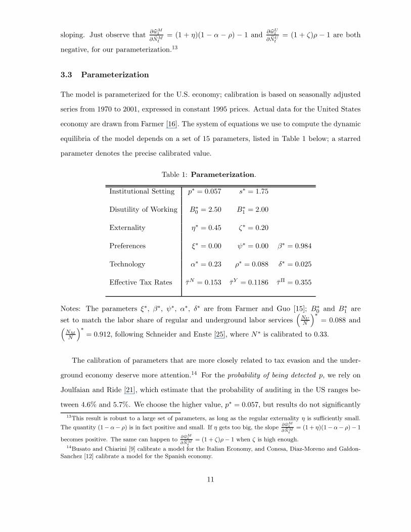
3.3 Parameterization

The model is parameterized for the U.S. economy; calibration is based on seasonally adjusted

series from 1970 to 2001, expressed in constant 1995 prices. Actual data for the United States

economy are drawn from Farmer [16]. The system of equations we use to compute the dynamic

equilibria of the model depends on a set of 15 parameters, listed in Table 1 below; a starred

parameter denotes the precise calibrated value.

Table 1: Parameterization.

Institutional Setting p∗ = 0.057 s∗ = 1.75

Disutility of Working B∗0 = 2.50 B∗

1 = 2.00

Externality η∗ = 0.45 ζ∗ = 0.20

Preferences ξ∗ = 0.00 ψ∗ = 0.00 β∗ = 0.984

Technology α∗ = 0.23 ρ∗ = 0.088 δ∗ = 0.025

Effective Tax Rates τN = 0.153 τY = 0.1186 τΠ = 0.355

Notes: The parameters ξ∗, β∗, ψ∗, α∗, δ∗ are from Farmer and Guo [15]; B∗0 and B∗

1 are

set to match the labor share of regular and underground labor services(NUN

)∗= 0.088 and

(NMN

)∗= 0.912, following Schneider and Enste [25], where N∗ is calibrated to 0.33.

The calibration of parameters that are more closely related to tax evasion and the under-

ground economy deserve more attention.14 For the probability of being detected p, we rely on

Joulfaian and Ride [21], which estimate that the probability of auditing in the US ranges be-

tween 4.6% and 5.7%. We choose the higher value, p∗ = 0.057, but results do not significantly

13This result is robust to a large set of parameters, as long as the regular externality η is sufficiently small.

The quantity (1−α− ρ) is in fact positive and small. If η gets too big, the slope∂ bwM

t

∂ bNMt

= (1 + η)(1−α− ρ)− 1

becomes positive. The same can happen to∂ bwM

t

∂ bNMt

= (1 + ζ)ρ− 1 when ζ is high enough.14Busato and Chiarini [9] calibrate a model for the Italian Economy, and Conesa, Diaz-Moreno and Galdon-

Sanchez [12] calibrate a model for the Spanish economy.

11

change if we consider the lower value 4.7%.

To stop Abusive Trust Promoters, the Internal Revenue Service has recently undertaken a

national coordinated strategy to address abusive trust schemes.15 Violations of the Internal

Revenue Code may result in civil penalties, which includes a fraud penalty up to 75% of the

underpayment of tax attributable to the fraud in addition to the taxes owed. Therefore we set

the surcharge factor s∗ = 1.75.16

As for the average-long run levels of taxation the effective income tax rate τY and corporate

tax rate τΠ are computed from the “Effective Tax Rates, 1979-1997”, Table H-1a, prepared by

the Congressional Budget Office; social security tax rate is taken from www.socialsecurity.com;

we choose the value applying for the 1990s and later, which equals τN = 0.153.17

The externality parameters are set following Busato et al. [10]; aggregate level of returns

to scale equals 1.42, which is lower than the original Farmer and Guo [15] calibration (1.61).

Shocks to tax rates are assumed to be permanent, that is the autocorrelation coefficients

in (13) equal unity: ϕY11 = ϕN22 = ϕΠ33 = 1. It is therefore assumed that unexpected increases in

tax rates is maintained in all subsequent periods, i.e. fiscal policy is based on a commitment

to a non-transitory tax increase. Such hypothesis is not particularly restrictive, as the impulse

response would maintain analogous qualitative features also in the case of purely temporary

shocks (ϕY11 = ϕN22 = ϕΠ33 = 0); the qualitative nature of the economy’s response only depends

upon the topological properties of the attractor. In all exercises the size of each shock equals

one unit standard deviation.

4 Fiscal Policy Implications

4.1 Impulse Response Functions

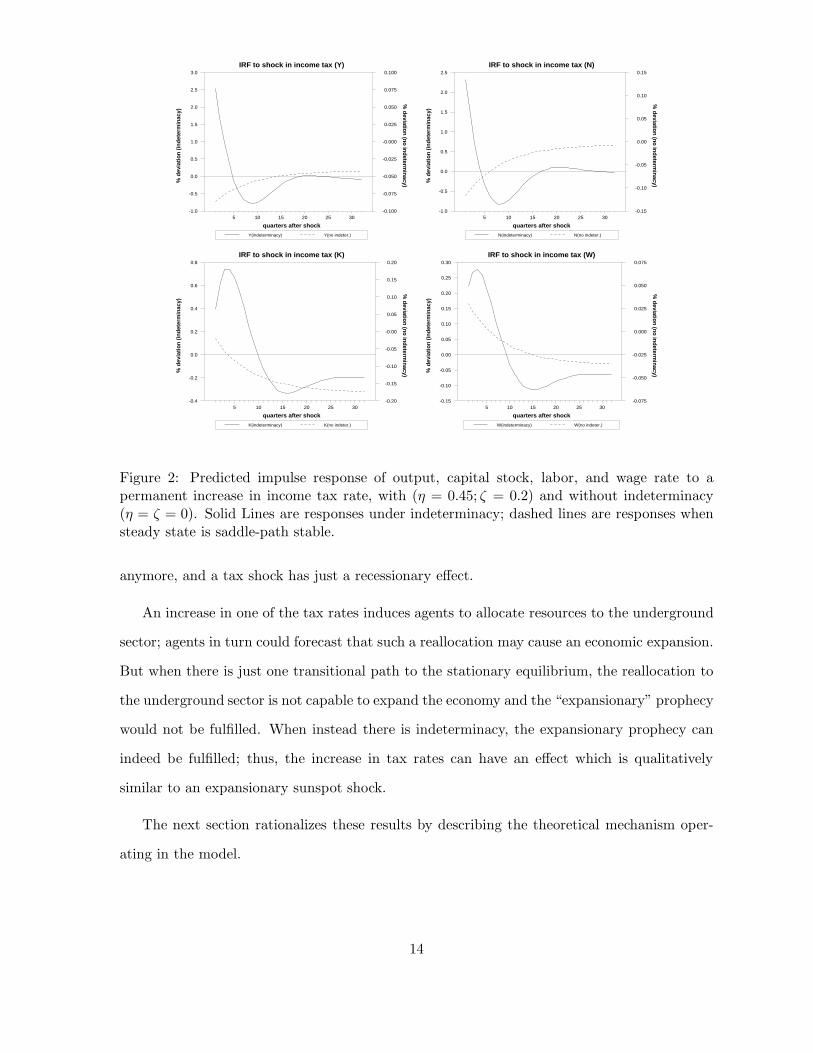
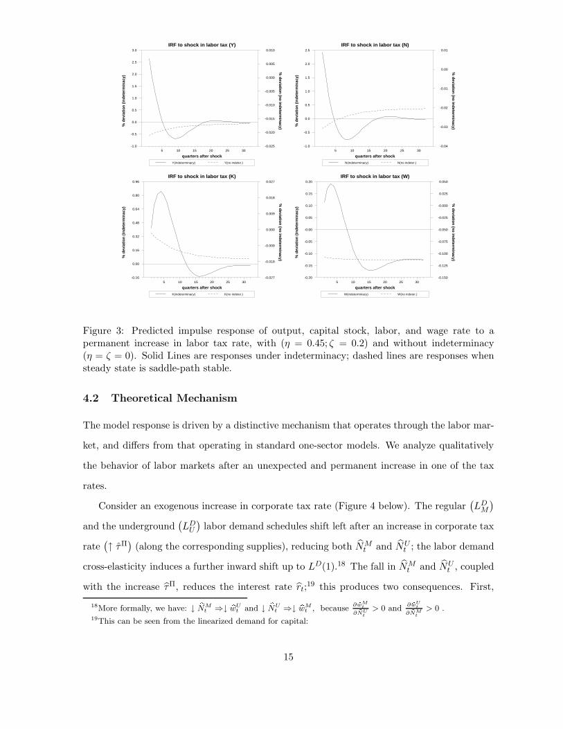
Figures 1, 2 and 3 include model’s response to a permanent increase in the three tax rates

(specifically, after a positive one unit standard deviation innovation in τΠ, τY and τN ). In

15For more details about the Internal Revenue Service policy regarding abusive trusts, refer to InternalRevenue Service Public Announcement Notice 97-24, which warns taxpayers to avoid abusive trust schemesthat advertise bogus tax benefits.

16Violations may also result in criminal prosecution; in this case there are penalties up to five years in prisonfor each offense.

17See http://www.ssa.gov/OACT/ProgData/taxRates.html

12

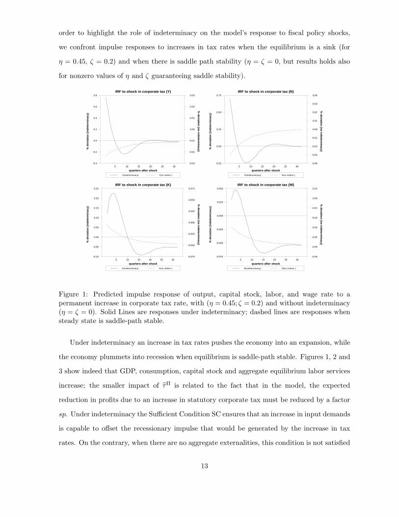
order to highlight the role of indeterminacy on the model’s response to fiscal policy shocks,

we confront impulse responses to increases in tax rates when the equilibrium is a sink (for

η = 0.45, ζ = 0.2) and when there is saddle path stability (η = ζ = 0, but results holds also

for nonzero values of η and ζ guaranteeing saddle stability).

Y(indeterminacy) Y(no indeter.)

IRF to shock in corporate tax (Y)

quarters after shock

% d

evia

tion

(inde

term

inac

y)

% deviation (no indeterm

inacy)

5 10 15 20 25 30-0.4

-0.2

0.0

0.2

0.4

0.6

0.8

-0.03

-0.02

-0.01

0.00

0.01

0.02

0.03

N(indeterminacy) N(no indeter.)

IRF to shock in corporate tax (N)

quarters after shock

% d

evia

tion

(inde

term

inac

y)

% deviation (no indeterm

inacy)

5 10 15 20 25 30-0.25

0.00

0.25

0.50

0.75

-0.04

-0.03

-0.02

-0.01

0.00

0.01

0.02

0.03

0.04

K(indeterminacy) K(no indeter.)

IRF to shock in corporate tax (K)

quarters after shock

% d

evia

tion

(inde

term

inac

y)

% deviation (no indeterm

inacy)

5 10 15 20 25 30-0.10

-0.05

0.00

0.05

0.10

0.15

0.20

0.25

-0.075

-0.050

-0.025

0.000

0.025

0.050

0.075

W(indeterminacy) W(no indeter.)

IRF to shock in corporate tax (W)

quarters after shock

% d

evia

tion

(inde

term

inac

y)

% deviation (no indeterm

inacy)

5 10 15 20 25 30-0.075

-0.050

-0.025

0.000

0.025

0.050

-0.06

-0.05

-0.04

-0.03

-0.02

-0.01

0.00

0.01

Figure 1: Predicted impulse response of output, capital stock, labor, and wage rate to apermanent increase in corporate tax rate, with (η = 0.45; ζ = 0.2) and without indeterminacy(η = ζ = 0). Solid Lines are responses under indeterminacy; dashed lines are responses whensteady state is saddle-path stable.

Under indeterminacy an increase in tax rates pushes the economy into an expansion, while

the economy plummets into recession when equilibrium is saddle-path stable. Figures 1, 2 and

3 show indeed that GDP, consumption, capital stock and aggregate equilibrium labor services

increase; the smaller impact of τΠ is related to the fact that in the model, the expected

reduction in profits due to an increase in statutory corporate tax must be reduced by a factor

sp. Under indeterminacy the Sufficient Condition SC ensures that an increase in input demands

is capable to offset the recessionary impulse that would be generated by the increase in tax

rates. On the contrary, when there are no aggregate externalities, this condition is not satisfied

13

Y(indeterminacy) Y(no indeter.)

IRF to shock in income tax (Y)

quarters after shock

% d

evia

tion

(inde

term

inac

y)

% deviation (no indeterm

inacy)

5 10 15 20 25 30-1.0

-0.5

0.0

0.5

1.0

1.5

2.0

2.5

3.0

-0.100

-0.075

-0.050

-0.025

-0.000

0.025

0.050

0.075

0.100

N(indeterminacy) N(no indeter.)

IRF to shock in income tax (N)

quarters after shock

% d

evia

tion

(inde

term

inac

y)

% deviation (no indeterm

inacy)

5 10 15 20 25 30-1.0

-0.5

0.0

0.5

1.0

1.5

2.0

2.5

-0.15

-0.10

-0.05

0.00

0.05

0.10

0.15

K(indeterminacy) K(no indeter.)

IRF to shock in income tax (K)

quarters after shock

% d

evia

tion

(inde

term

inac

y)

% deviation (no indeterm

inacy)5 10 15 20 25 30

-0.4

-0.2

0.0

0.2

0.4

0.6

0.8

-0.20

-0.15

-0.10

-0.05

-0.00

0.05

0.10

0.15

0.20

W(indeterminacy) W(no indeter.)

IRF to shock in income tax (W)

quarters after shock

% d

evia

tion

(inde

term

inac

y)

% deviation (no indeterm

inacy)

5 10 15 20 25 30-0.15

-0.10

-0.05

0.00

0.05

0.10

0.15

0.20

0.25

0.30

-0.075

-0.050

-0.025

0.000

0.025

0.050

0.075

Figure 2: Predicted impulse response of output, capital stock, labor, and wage rate to apermanent increase in income tax rate, with (η = 0.45; ζ = 0.2) and without indeterminacy(η = ζ = 0). Solid Lines are responses under indeterminacy; dashed lines are responses whensteady state is saddle-path stable.

anymore, and a tax shock has just a recessionary effect.

An increase in one of the tax rates induces agents to allocate resources to the underground

sector; agents in turn could forecast that such a reallocation may cause an economic expansion.

But when there is just one transitional path to the stationary equilibrium, the reallocation to

the underground sector is not capable to expand the economy and the “expansionary” prophecy

would not be fulfilled. When instead there is indeterminacy, the expansionary prophecy can

indeed be fulfilled; thus, the increase in tax rates can have an effect which is qualitatively

similar to an expansionary sunspot shock.

The next section rationalizes these results by describing the theoretical mechanism oper-

ating in the model.

14

Y(indeterminacy) Y(no indeter.)

IRF to shock in labor tax (Y)

quarters after shock

% d

evia

tion

(inde

term

inac

y)

% deviation (no indeterm

inacy)

5 10 15 20 25 30-1.0

-0.5

0.0

0.5

1.0

1.5

2.0

2.5

3.0

-0.025

-0.020

-0.015

-0.010

-0.005

0.000

0.005

0.010

N(indeterminacy) N(no indeter.)

IRF to shock in labor tax (N)

quarters after shock

% d

evia

tion

(inde

term

inac

y)

% deviation (no indeterm

inacy)

5 10 15 20 25 30-1.0

-0.5

0.0

0.5

1.0

1.5

2.0

2.5

-0.04

-0.03

-0.02

-0.01

0.00

0.01

K(indeterminacy) K(no indeter.)

IRF to shock in labor tax (K)

quarters after shock

% d

evia

tion

(inde

term

inac

y)

% deviation (no indeterm

inacy)5 10 15 20 25 30

-0.16

0.00

0.16

0.32

0.48

0.64

0.80

0.96

-0.027

-0.018

-0.009

0.000

0.009

0.018

0.027

W(indeterminacy) W(no indeter.)

IRF to shock in labor tax (W)

quarters after shock

% d

evia

tion

(inde

term

inac

y)

% deviation (no indeterm

inacy)

5 10 15 20 25 30-0.20

-0.15

-0.10

-0.05

-0.00

0.05

0.10

0.15

0.20

-0.150

-0.125

-0.100

-0.075

-0.050

-0.025

-0.000

0.025

0.050

Figure 3: Predicted impulse response of output, capital stock, labor, and wage rate to apermanent increase in labor tax rate, with (η = 0.45; ζ = 0.2) and without indeterminacy(η = ζ = 0). Solid Lines are responses under indeterminacy; dashed lines are responses whensteady state is saddle-path stable.

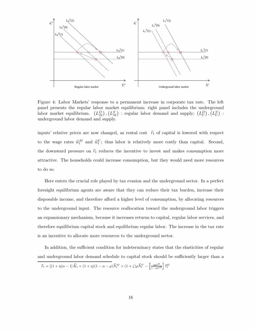
4.2 Theoretical Mechanism

The model response is driven by a distinctive mechanism that operates through the labor mar-

ket, and differs from that operating in standard one-sector models. We analyze qualitatively

the behavior of labor markets after an unexpected and permanent increase in one of the tax

rates.

Consider an exogenous increase in corporate tax rate (Figure 4 below). The regular(LDM)

and the underground(LDU)

labor demand schedules shift left after an increase in corporate tax

rate(↑ τΠ

)(along the corresponding supplies), reducing both NM

t and NUt ; the labor demand

cross-elasticity induces a further inward shift up to LD(1).18 The fall in NMt and NU

t , coupled

with the increase τΠ, reduces the interest rate rt;19 this produces two consequences. First,

18More formally, we have: ↓ bNMt ⇒↓ bwUt and ↓ bNU

t ⇒↓ bwMt , because∂ bwM

t

∂ bNUt

> 0 and∂ bwU

t

∂ bNMt

> 0 .19This can be seen from the linearized demand for capital:

15

LMD(0)

LMD(2)

LMD(1)

Regular labor market

LMS(1)

LMS(0)

MtN

Mtw

LUD(0)

LUD(2)

LUD(1)

Underground labor market

LUS(1)

LUS(0)

UtN

Utw

Figure 4: Labor Markets’ response to a permanent increase in corporate tax rate. The leftpanel presents the regular labor market equilibrium; right panel includes the undergroundlabor market equilibrium.

(LDM),(LSM)

: regular labor demand and supply;(LDU),(LSU)

:underground labor demand and supply.

inputs’ relative prices are now changed, as rental cost rt of capital is lowered with respect

to the wage rates wMt and wUt ; thus labor is relatively more costly than capital. Second,

the downward pressure on rt reduces the incentive to invest and makes consumption more

attractive. The households could increase consumption, but they would need more resources

to do so.

Here enters the crucial role played by tax evasion and the underground sector. In a perfect

foresight equilibrium agents are aware that they can reduce their tax burden, increase their

disposable income, and therefore afford a higher level of consumption, by allocating resources

to the underground input. The resource reallocation toward the underground labor triggers

an expansionary mechanism, because it increases returns to capital, regular labor services, and

therefore equilibrium capital stock and equilibrium regular labor. The increase in the tax rate

is an incentive to allocate more resources to the underground sector.

In addition, the sufficient condition for indeterminacy states that the elasticities of regular

and underground labor demand schedule to capital stock should be sufficiently larger than abrt = [(1 + η)α− 1] bKt + (1 + η)(1 − α− ρ) bNMt + (1 + ζ)ρ bNU

t −h

spτΠ

1−spτΠ

i bτΠt

16

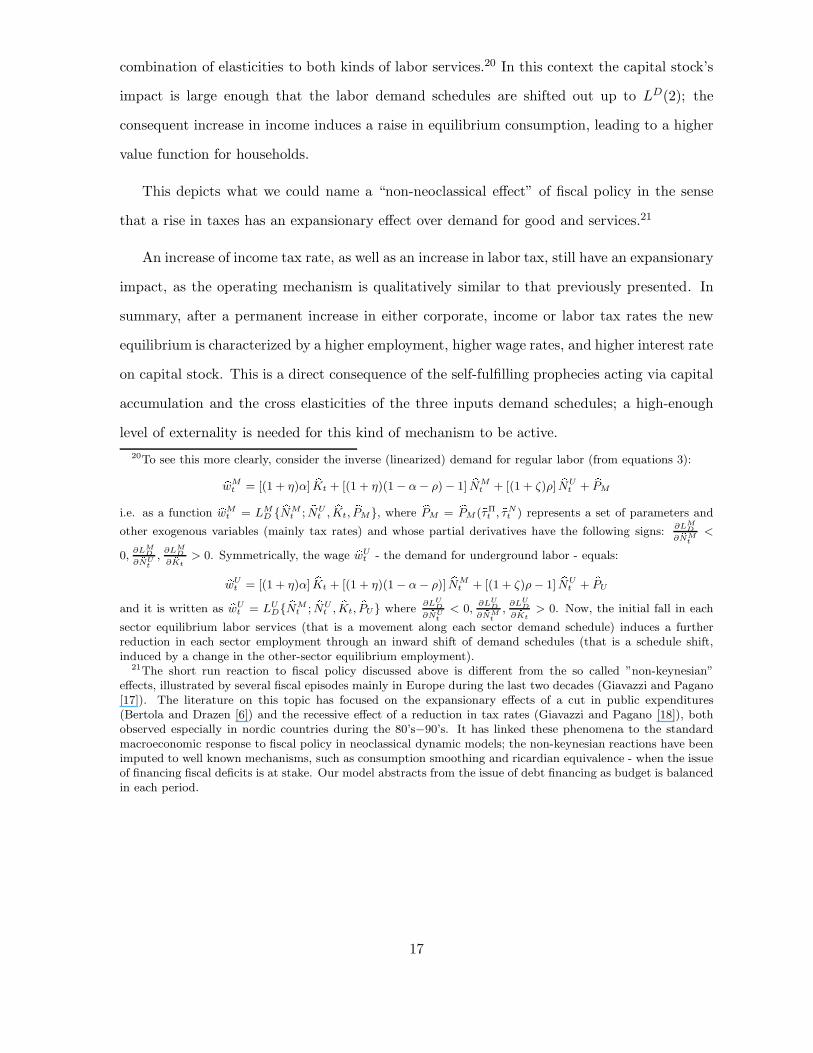
combination of elasticities to both kinds of labor services.20 In this context the capital stock’s

impact is large enough that the labor demand schedules are shifted out up to LD(2); the

consequent increase in income induces a raise in equilibrium consumption, leading to a higher

value function for households.

This depicts what we could name a “non-neoclassical effect” of fiscal policy in the sense

that a rise in taxes has an expansionary effect over demand for good and services.21

An increase of income tax rate, as well as an increase in labor tax, still have an expansionary

impact, as the operating mechanism is qualitatively similar to that previously presented. In

summary, after a permanent increase in either corporate, income or labor tax rates the new

equilibrium is characterized by a higher employment, higher wage rates, and higher interest rate

on capital stock. This is a direct consequence of the self-fulfilling prophecies acting via capital

accumulation and the cross elasticities of the three inputs demand schedules; a high-enough

level of externality is needed for this kind of mechanism to be active.

20To see this more clearly, consider the inverse (linearized) demand for regular labor (from equations 3):bwMt = [(1 + η)α] bKt + [(1 + η)(1 − α− ρ) − 1] bNMt + [(1 + ζ)ρ] bNU

t + bPMi.e. as a function bwMt = LMD { bNM

t ; bNUt , bKt, bPM}, where bPM = bPM (bτΠ

t , bτNt ) represents a set of parameters and

other exogenous variables (mainly tax rates) and whose partial derivatives have the following signs:∂LM

D

∂ bNMt

<

0,∂LM

D

∂ bNUt

,∂LM

D

∂ bKt

> 0. Symmetrically, the wage bwUt - the demand for underground labor - equals:bwUt = [(1 + η)α] bKt + [(1 + η)(1 − α− ρ)] bNMt + [(1 + ζ)ρ− 1] bNU

t + bPUand it is written as bwUt = LUD{ bNM

t ; bNUt , bKt, bPU} where

∂LU

D

∂ bNUt

< 0,∂LU

D

∂ bNMt

,∂LU

D

∂ bKt

> 0. Now, the initial fall in each

sector equilibrium labor services (that is a movement along each sector demand schedule) induces a furtherreduction in each sector employment through an inward shift of demand schedules (that is a schedule shift,induced by a change in the other-sector equilibrium employment).

21The short run reaction to fiscal policy discussed above is different from the so called ”non-keynesian”effects, illustrated by several fiscal episodes mainly in Europe during the last two decades (Giavazzi and Pagano[17]). The literature on this topic has focused on the expansionary effects of a cut in public expenditures(Bertola and Drazen [6]) and the recessive effect of a reduction in tax rates (Giavazzi and Pagano [18]), bothobserved especially in nordic countries during the 80’s−90’s. It has linked these phenomena to the standardmacroeconomic response to fiscal policy in neoclassical dynamic models; the non-keynesian reactions have beenimputed to well known mechanisms, such as consumption smoothing and ricardian equivalence - when the issueof financing fiscal deficits is at stake. Our model abstracts from the issue of debt financing as budget is balancedin each period.

17

5 Conclusions

This paper studies fiscal policy in a one-sector dynamic general equilibrium model augmented

with tax evasion and underground activities. The model displays increasing returns to scale

due to externalities in regular and underground inputs, capable to induce sunspots and inde-

terminacy.

The main results depend on the combined presence of indeterminacy and tax evasion. We

analyze the effect of shocks to taxation structure on the dynamic response of the economy,

highlighting the differences with respect to the case of constant returns to scale. An increase

in corporate, income or labor tax rates has an expansionary effect under local indeterminacy

of the equilibrium path (i.e. when aggregate production technology displays increasing returns

to scale high enough for producing indeterminacy). When instead there is saddle-path sta-

bility (returns to scale are low enough), the effects of tax shocks are customary, inducing a

recession. This difference is due to a specific economic mechanism, which is distinctive of the

indeterminacy case and acts through the cross elasticities of the inputs’ demand functions.

18

References

[1]

[2] Aschauer, D.A., (1988), The Equilibrium Approach to Fiscal Policy, Journal of MoneyCredit and Banking, 20, 41-62.

[3] Bajada, C. (1999) Estimates of the Underground Economy in Australia, Economic Record,75, 369-84.

[4] Basu, S. Fernald, J. (1997) Returns to Scale in U.S. Production: Estimates and Implica-tions, Journal of Political Economy, 105, 249-83.

[5] Baxter M. and R. King, (1993) Fiscal policy in general equilibrium, American EconomicReview 83, 315-334.

[6] Bertola, G. Drazen, A. (1993) Trigger Points and Budget Cuts: Explaining the Effects ofFiscal Austerity, American Economic Review, 83, 11-26.

[7] Braun A.R., 1994, Tax disturbances and real economic activity in the postwar UnitedStates, Journal of Monetary Economics, 3, 441-62.

[8] Burnside C., Eichenbaum M. and Fisher J., (2003), Fiscal shocks and their consequences,NBER Working Paper, No 9772.

[9] Busato, F. Chiarini, B. (2004) Market and underground activities in a two-sector dynamicequilibrium model, Economic Theory, 23, 831-861.

[10] Busato, F. Chiarini, B. Marchetti, E. (2004) Indeterminacy, tax evasion and undegroundactivities, University of Aarhus, Working papers of the Department of Economics, n.12-2004.

[11] Christiano, L. Harrison S. (1999) Chaos, sunspots and automatic stabilizers, Journal ofMonetary Economics 44, 3-31

[12] Conesa, J. C. Diaz-Moreno, C. Galdon-Sanchez, J. (2001) Underground Economy andAggregate Fluctuations, Spanish Economic Review, 3, 41-53.

[13] Cowell, A. (1990) Cheating the Government The Economics of Evasion, MIT Press, Cam-bridge.

[14] Devereux, M. Head, A. Lapham, J. (1996), Monopolistic Competition, Increasing Returns,and the Effects of Government Spending, Journal of Money, Credit, and Banking, 28, 233-254.

[15] Farmer, R. Guo, J. (1994) Real Business Cycle and the Animal Spirit Hypothesis, Journalof Economic Theory, 63, 42-72.

[16] Farmer, R. (1999) The macroeconomics of self-fulfilling prophecies, Cambridge, MITPress.

[17] Giavazzi, F. Pagano, M. (1990) Can Severe Fiscal Contractions be Expansionary? Talesof Two Small European Countries. NBER Macroeconomics Annual, 75-110.

19

[18] Giavazzi, F. Pagano, M. (1996) Non-Keynesian Effects of Fiscal Policy Changes: Interna-tional Evidence and the Swedish Experience. Swedish Economic Policy Review, 3, 67-103.

[19] Guo, J., Lansing. K., (1998) Indeterminacy and Stabilisation Policy, Journal of EconomicTheory, 82, 481-490.

[20] Jimenez, M. Marchetti, D. (2002) Interpreting the procyclical productivity of manufac-turing sectors: can we really rule out external effects?, Applied Economics, 34, 805-817.

[21] D. Joulfaian, M. Rider, (1998) Differential Taxation and Tax Evasion by Small Business,National Tax Journal, 4, 675-687.

[22] McGrattan E.R., (1994), The Macroeconomic Effects of Distortionary Taxation. Journalof Monetary Economics 33, 559-71.

[23] Paglin, T. (1994) The Underground Economy: New Estimates from Household Incomeand Expenditure Surveys, Yale Law Journal, 103, 2239-57.

[24] Sbordone, A. (1997) Interpreting the procyclical productivity of manufacturing sectors:external effects or labour hoarding?, Journal of Money, Credit and Banking, 29, 26-45.

[25] Schneider, F. Enste, D. (2000) Shadow Economies: Size, Causes and Consequences, Jour-nal of Economic Literature XXXVIII, 77–114.

[26] Tanzi, V. (1980), The Underground Economy in the United States: Estimates and Impli-cations, Banca Nazionale del Lavoro Quarterly Review, 135, 427-53.

20

Appendix

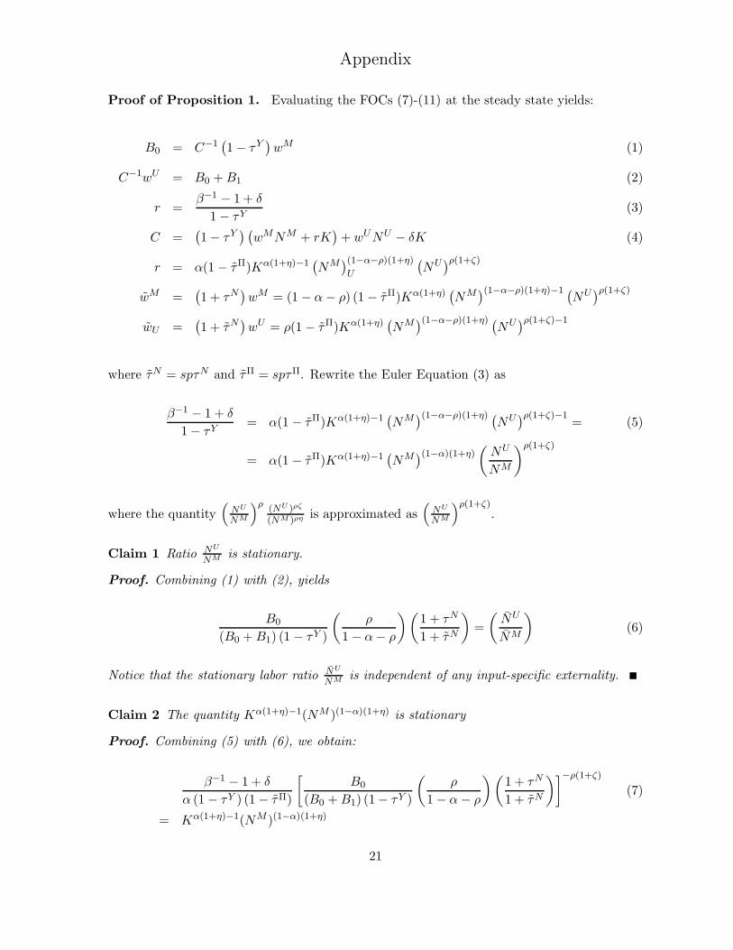
Proof of Proposition 1. Evaluating the FOCs (7)-(11) at the steady state yields:

B0 = C−1(1 − τY

)wM (1)

C−1wU = B0 +B1 (2)

r =β−1 − 1 + δ

1 − τY(3)

C =(1 − τY

) (wMNM + rK

)+ wUNU − δK (4)

r = α(1 − τΠ)Kα(1+η)−1(NM

)(1−α−ρ)(1+η)U

(NU)ρ(1+ζ)

wM =(1 + τN

)wM = (1 − α− ρ) (1 − τΠ)Kα(1+η)

(NM

)(1−α−ρ)(1+η)−1 (NU)ρ(1+ζ)

wU =(1 + τN

)wU = ρ(1 − τΠ)Kα(1+η)

(NM

)(1−α−ρ)(1+η) (NU)ρ(1+ζ)−1

where τN = spτN and τΠ = spτΠ. Rewrite the Euler Equation (3) as

β−1 − 1 + δ

1 − τY= α(1 − τΠ)Kα(1+η)−1

(NM

)(1−α−ρ)(1+η) (NU)ρ(1+ζ)−1

= (5)

= α(1 − τΠ)Kα(1+η)−1(NM

)(1−α)(1+η)(NU

NM

)ρ(1+ζ)

where the quantity(NU

NM

)ρ (NU )ρζ

(NM )ρηis approximated as

(NU

NM

)ρ(1+ζ).

Claim 1 Ratio NU

NM is stationary.

Proof. Combining (1) with (2), yields

B0

(B0 +B1) (1 − τY )

(ρ

1 − α− ρ

)(1 + τN

1 + τN

)=

(NU

NM

)(6)

Notice that the stationary labor ratio NU

NM is independent of any input-specific externality.

Claim 2 The quantity Kα(1+η)−1(NM )(1−α)(1+η) is stationary

Proof. Combining (5) with (6), we obtain:

β−1 − 1 + δ

α (1 − τY ) (1 − τΠ)

[B0

(B0 +B1) (1 − τY )

(ρ

1 − α− ρ

)(1 + τN

1 + τN

)]−ρ(1+ζ)(7)

= Kα(1+η)−1(NM )(1−α)(1+η)

21

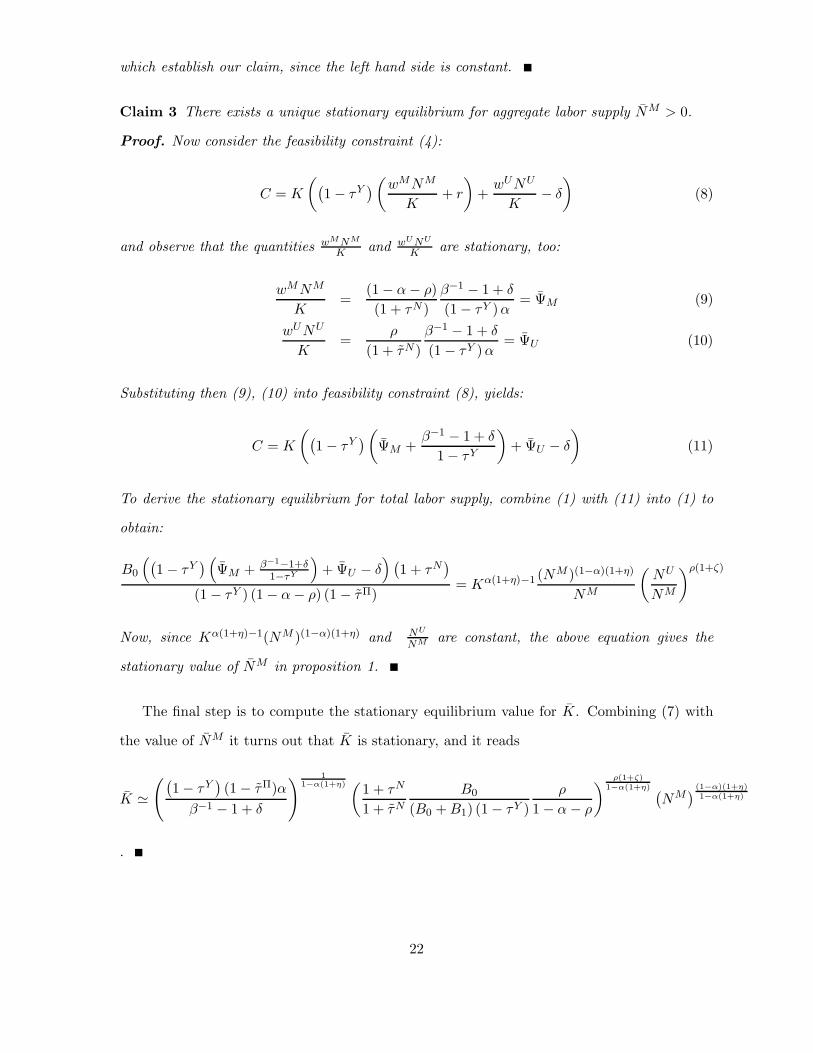
which establish our claim, since the left hand side is constant.

Claim 3 There exists a unique stationary equilibrium for aggregate labor supply NM > 0.

Proof. Now consider the feasibility constraint (4):

C = K

((1 − τY

)(wMNM

K+ r

)+wUNU

K− δ

)(8)

and observe that the quantities wMNM

Kand wUNU

Kare stationary, too:

wMNM

K=

(1 − α− ρ)

(1 + τN )

β−1 − 1 + δ

(1 − τY )α= ΨM (9)

wUNU

K=

ρ

(1 + τN )

β−1 − 1 + δ

(1 − τY )α= ΨU (10)

Substituting then (9), (10) into feasibility constraint (8), yields:

C = K

((1 − τY

)(ΨM +

β−1 − 1 + δ

1 − τY

)+ ΨU − δ

)(11)

To derive the stationary equilibrium for total labor supply, combine (1) with (11) into (1) to

obtain:

B0

((1 − τY

) (ΨM + β−1−1+δ

1−τY

)+ ΨU − δ

) (1 + τN

)

(1 − τY ) (1 − α− ρ) (1 − τΠ)= Kα(1+η)−1 (NM )(1−α)(1+η)

NM

(NU

NM

)ρ(1+ζ)

Now, since Kα(1+η)−1(NM )(1−α)(1+η) and NU

NM are constant, the above equation gives the

stationary value of NM in proposition 1.

The final step is to compute the stationary equilibrium value for K. Combining (7) with

the value of NM it turns out that K is stationary, and it reads

K ≃

((1 − τY

)(1 − τΠ)α

β−1 − 1 + δ

) 11−α(1+η) (1 + τN

1 + τNB0

(B0 +B1) (1 − τY )

ρ

1 − α− ρ

) ρ(1+ζ)1−α(1+η) (

NM) (1−α)(1+η)

1−α(1+η)

.

22