Optimization and Metaheuristic Algorithms in Engineering

Xin-She Yang

Mathematics and Scientific Computing, National Physical Laboratory,

Teddington TW11 0LW, UK (email: xin-she.yang@npl.co.uk)

Abstract: Design optimization in engineering tends to be very challenging, partly due to

the complexity and highly nonlinearity of the problem of interest, partly due to stringent design

codes in engineering practice. Conventional algorithms are not the best tools for highly

nonlinear global optimization, as they are local search algorithms, and thus often miss the

global optimality. In addition, design solutions have to be robust, subject to uncertainty in

parameters and tolerance of available components and materials. Metaheuristic algorithms

have become increasingly popular in the last two decades. This chapter reviews some of the

latest metaheuristics.

Key words: algorithm, ant algorithm, bee algorithm, bat algorithm, cuckoo search, firefly

algorithm, harmony search, particle swarm optimization, metaheuristics.

Citation Details: X. S. Yang, Optimization and Metaheuristic Algorithms in Engineering,

in: Metaheursitics in Water, Geotechnical and Transport Engineering (Eds. X. S. Yang, A. H.

Gandomi, S. Talatahari, A. H. Alavi), Elsevier, (2013), pp. 1-23.

http://dx.doi.org/10.1016/B978-0-12-398296-4.00001-5

1 Introduction

Optimization is everywhere, and is thus an important paradigm itself with a wide range

of applications. In almost all applications in engineering and industry, we are always trying to

optimize something -- whether to minimize the cost and energy consumption, or to maximize

the profit, output, performance and efficiency. In reality, resources, time and money are always

limited; consequently, optimization is far more important in practice (Yang, 2010b; Yang and

Koziel, 2011). The optimal use of available resources of any sort requires a paradigm shift in

scientific thinking, this is because most real-world applications have far more complicated

factors and parameters to affect how the system behaves.

Contemporary engineering design is heavily based on computer simulations. This

introduces additional difficulties to optimization. Growing demand for accuracy and

ever-increasing complexity of structures and systems results in the simulation process being

more and more time consuming. In many engineering fields, the evaluation of a single design

can take as long as several days or even weeks. Any methods that can speed up the simulation

time and optimization process can thus save time and money.

For any optimization problem, the integrated components of the optimization process

are the optimization algorithm, an efficient numerical simulator and a realistic-representation

of the physical processes we wish to model and optimize. This is often a time-consuming

process, and in many cases, the computational costs are usually very high. Once we have a

good model, the overall computation costs are determined by the optimization algorithms used

for search and the numerical solver used for simulation.

Search algorithms are the tools and techniques of achieving optimality of the problem of

interest. This search for optimality is complicated further by the fact that uncertainty almost

always presents in the real-world systems. Therefore, we seek not only the optimal design but

also robust design in engineering and industry. Optimal solutions, which are not robust enough,

are not practical in reality. Suboptimal solutions or good robust solutions are often the choice in

such cases.

Simulations are often the most time-consuming part. In many applications, an

optimization process often involves the evaluation of objective function many times, often

thousands and even millions of configurations. Such evaluations often involve the use of

extensive computational tools such as a computational fluid dynamics simulator or a finite

element solver. Therefore, an efficient optimization in combination with an efficient solver is

extremely important.

Optimization problems can be formulated in many ways. For example, the commonly

used method of least-squares is a special case of maximum-likelihood formulations. By far the

most widely formulation is to write a nonlinear optimization problem as

minimize ( ), ( = 1,2,..., ),if x i M (1)

subject to the constraints

( ) 0, ( = 1,2,..., ),jh x j J= (2)

( ) 0, ( = 1,2,..., ),kg x k K≤ (3)

where ,i jf h and kg are in general nonlinear functions. Here the design vector

1 2= ( , ,..., )nx x x x can be continuous, discrete or mixed in n -dimensional space. The functions

if are called objective or cost functions, and when > 1M , the optimization is multiobjective

or multicriteria (Sawaragi, 1985; Yang, 2010b). It is possible to combine different objectives into

a single objective, though multiobjective optimization can give far more information and insight

into the problem. It is worth pointing out that here we write the problem as a minimization

problem, it can also be written as a maximization by simply replacing ( )if x by ( )if x− .

When all functions are nonlinear, we are dealing with nonlinear constrained problems.

In some special cases when , ,i j kf h g are linear, the problem becomes linear, and we can use

the widely linear programming techniques such as the simplex method. When some design

variables can only take discrete values (often integers), while other variables are real

continuous, the problem is of mixed type, which is often difficult to solve, especially for

large-scale optimization problems.

A very special class of optimization is the convex optimization, which has guaranteed

global optimality. Any optimal solution is also the global optimum, and most importantly, there

are efficient algorithms of polynomial time to solve such problems (Conn et al., 2009). These

efficient algorithms such the interior-point methods (Karmarkar, 1984). are widely used and

have been implemented in many software packages.

2 Three Issues in Optimization

There are three main issues in the simulation-driven optimization and modelling, and they are:

the efficiency of an algorithm, and the efficiency and accuracy of a numerical simulator, and

assign the right algorithms to the right problem. Despite their importance, there is no

satisfactory rule or guidelines for such issues. Obviously, we try to use the most efficient

algorithms available, but the actual efficiency of an algorithm may depending on many factors

such as the inner working of an algorithm, the information needed (such as objective functions

and their derivatives) and implementation details. The efficiency of a solver is even more

complicated, depending on the actual numerical methods used and the complexity of the

problem of interest. As for choosing the right algorithms for the right problems, there are many

empirical observations, but there is no agreed guidelines. In fact, there is no universally

efficient algorithms for all types of problems. Therefore, the choice may depending on many

factors and sometimes subjective to personal preferences of researchers and decision makers.

2.1 Efficiency of an Algorithm

An efficient optimizer is very important to ensure the optimal solutions are reachable.

The essence of an optimizer is a search or optimization algorithm implemented correctly so as

to carry out the desired search (though not necessarily efficiently). It can be integrated and

linked with other modelling components. There are many optimization algorithms in the

literature and no single algorithm is suitable for all problems, as dictated by the No Free Lunch

Theorems (Wolpert and Macready, 1997).

Optimization algorithms can be classified in many ways, depending on the focus or the

characteristics we are trying to compare. Algorithms can be classified as gradient-based (or

derivative-based methods) and gradient-free (or derivative-free methods). The classic methods

of steepest descent and Gauss-Newton methods are gradient-based, as they use the derivative

information in the algorithm, while the Nelder-Mead downhill simplex method (Nelder and

Mead, 1965) is a derivative-free method because it only uses the values of the objective, not

any derivatives.

Algorithms can also be classified as deterministic or stochastic. If an algorithm works in a

mechanically deterministic manner without any random nature, it is called deterministic. For

such an algorithm, it will reach the same final solution if we start with the same initial point.

Hill-climbing and downhill simplex are good examples of deterministic algorithms. On the other

hand, if there is some randomness in the algorithm, the algorithm will usually reach a different

point every time we run the algorithm, even though we start with the same initial point.

Genetic algorithms and hill-climbing with a random restart are good examples of stochastic

algorithms.

Analyzing stochastic algorithms in more detail, we can single out the type of

randomness that a particular algorithm is employing. For example, the simplest and yet often

very efficient method is to introduce a random starting point for a deterministic algorithm. The

well-known hill-climbing with random restart is a good example. This simple strategy is both

efficient in most cases and easy to implement in practice. A more elaborate way to introduce

randomness to an algorithm is to use randomness inside different components of an algorithm,

and in this case, we often call such algorithm heuristic or more often metaheuristic (Yang, 2008;

Talbi, 2009; Yang, 2010b). A very good example is the popular genetic algorithms which use

randomness for crossover and mutation in terms of a crossover probability and a mutation rate.

Here, heuristic means to search by trial and error, while metaheuristic is a higher level of

heuristics. However, modern literature tends to refer all new stochastic algorithms as

metaheuristic. In this book, we will use metaheuristic to mean either. It is worth pointing out

that metaheuristic algorithms form a hot research topics and new algorithms appear almost

yearly (Yang, 2008; Yang, 2010b).

From the mobility point of view, algorithms can be classified as local or global. Local

search algorithms typically converge towards a local optimum, not necessarily (often not) the

global optimum, and such algorithms are often deterministic and have no ability of escaping

local optima. Simple hill-climbing is an example. On the other hand, we always try to find the

global optimum for a given problem, and if this global optimality is robust, it is often the best,

though it is not always possible to find such global optimality. For global optimization, local

search algorithms are not suitable. We have to use a global search algorithm. Modern

metaheuristic algorithms in most cases are intended for global optimization, though not always

successful or efficiently. A simple strategy such as hill-climbing with random restart may change

a local search algorithm into a global search. In essence, randomization is an efficient

component for global search algorithms. In this chapter, we will provide a brief review of most

metaheuristic optimization algorithms.

Straightforward optimization of a given objective function is not always practical. In

particular, if the objective function comes from a computer simulation, it may be

computationally expensive, noisy or non-differentiable. In such cases, so-called surrogate-based

optimization algorithms may be useful where the direct optimization of the function of interest

is replaced by iterative updating and re-optimization of its model - a surrogate. The surrogate

model is typically constructed from the sampled data of the original objective function,

however, it is supposed to be cheap, smooth, easy to optimize and yet reasonably accurate so

that it can produce a good prediction of the function's optimum. Multi-fidelity or

variable-fidelity optimization is a special case of the surrogate-based optimization where the

surrogate is constructed from the low-fidelity model (or models) of the system of interest

(Koziel and Yang, 2011). Using variable-fidelity optimization is particularly useful is the

reduction of the computational cost of the optimization process is of primary importance.

Whatever the classification of an algorithm is, we have to make the right choice to use

an algorithm correctly and sometime a proper combination of algorithms may achieve far

better results.

2.2 The Right Algorithms?

From the optimization point of view, the choice of the right optimizer or algorithm for a

given problem is crucially important. The algorithm chosen for an optimization task will largely

depend on the type of the problem, the nature of an algorithm, the desired quality of solutions,

the available computing resource, time limit, availability of the algorithm implementation, and

the expertise of the decision-makers (Yang, 2010b; Yang and Koziel, 2011).

The nature of an algorithm often determines if it is suitable for a particular type of

problem. For example, gradient-based algorithms such as hill-climbing are not suitable for an

optimization problem whose objective is discontinuous. Conversely, the type of problem we are

trying to solve also determines the algorithms we possibly choose. If the objective function of

an optimization problem at hand is highly nonlinear and multimodal, classic algorithms such as

hill-climbing and downhill simplex are not suitable, as they are local search algorithms. In this

case, global optimizers such as particle swarm optimization and cuckoo search are most

suitable (Yang, 2010a; Yang and Deb, 2010).

Obviously, the choice is also affected by the desired solution quality and available

computing resource. As in most applications, computing resources are limited, we have to

obtain good solutions (not necessary the best) in a reasonable and practical time. Therefore, we

have to balance the resource and solution quality. We cannot achieve solutions with

guaranteed quality, though we strive to obtain the quality solutions as best as we possibly can.

If time is the main constraint, we can use some greedy methods, or hill-climbing with a few

random restarts.

Sometimes, even with the best possible intention, the availability of an algorithm and

the expertise of the decision-makers are the ultimate defining factors for choosing an algorithm.

Even though some algorithms are better for the given problem at hand, we may not have that

algorithm implemented in our system or we do not have such access, which limits our choice.

For example, Newton's method, hill-climbing, Nelder-Mead downhill simplex, trust-region

methods (Conn et al., 2009), interior-point methods are implemented in many software

packages, which may also increase their popularity in applications. In practice, even with the

best possible algorithms and well-crafted implementation, we may still do not get the desired

solutions. This is the nature of nonlinear global optimization, as most of such problems are

NP-hard, and no efficient (in the polynomial sense) exist for a given problem. Thus the

challenges of research in computational optimization and applications are to find the right

algorithms most suitable for a given problem so as to obtain good solutions, hopefully also the

global best solutions, in a reasonable timescale with a limited amount of resources. We aim to

do it efficiently in an optimal way.

2.3 Efficiency of a Numerical Solver

To solve an optimization problem, the most computationally extensive part is probably

the evaluation of the design objective to see if a proposed solution is feasible and/or if it is

optimal. Typically, we have to carry out these evaluations many times, often thousands and

even millions of times (Yang, 2008; Yang, 2010b). Things become even more challenging

computationally, when each evaluation task takes a long time via some black-box simulators. If

this simulator is a finite element or CFD solver, the running time of each evaluation can take

from a few minutes to a few hours or even weeks. Therefore, any approach to save

computational time either by reducing the number of evaluations or by increasing the

simulator's efficiency will save time and money.

In general, a simulator can be a simple function subroutines, a multiphysics solver, or

some external black-box evaluators.

The main way to reduce the number of objective evaluations is to use an efficient

algorithm, so that only a small number of such evaluations are needed. In most cases, this is not

possible. We have to use some approximation techniques to estimate the objectives, or to

construct an approximation model to predict the solver's outputs without actual using the

solver. Another way is to replace the original objective function by its lower-fidelity model, e.g.,

obtained from a computer simulation based on coarsely-discretized structure of interest. The

low-fidelity model is faster but not as accurate as the original one, and therefore it has to be

corrected. Special techniques have to be applied to use an approximation or corrected

low-fidelity model in the optimization process so that the optimal design can be obtained at a

low computational cost (Koziel and Yang, 2011).

3 Metaheuristics

Metaheuristic algorithms are often nature-inspired, and they are now among the most

widely used algorithms for optimization. They have many advantages over conventional

algorithms, as we can see from many case studies presented in later chapters in this book.

There are a few recent books which are solely dedicated to metaheuristic algorithms (Yang,

2008; Talbi, 2009; Yang, 2010a; Yang, 2010b). Metaheuristic algorithms are very diverse,

including genetic algorithms, simulated annealing, differential evolution, ant and bee

algorithms, particle swarm optimization, harmony search, firefly algorithm, cuckoo search and

others. Here we will introduce some of these algorithms briefly.

3.1 Ant Algorithms

Ant algorithms, especially the ant colony optimization (Dorigo and Stütle, 2004), mimic

the foraging behaviour of social ants. Primarily, ants use pheromone as a chemical messenger

and the pheromone concentration can also be considered as the indicator of quality solutions

to a problem of interest. As the solution is often linked with the pheromone concentration, the

search algorithms often produce routes and paths marked by the higher pheromone

concentrations, and therefore, ants-based algorithms are particular suitable for discrete

optimization problems.

The movement of an ant is controlled by pheromone which will evaporate over time.

Without such time-dependent evaporation, ant algorithms will lead to premature convergence

to the (often wrong) solutions. With proper pheromone evaporation, they usually behave very

well.

There are two important issues here: the probability of choosing a route, and the

evaporation rate of pheromone. There are a few ways of solving these problems, although it is

still an area of active research. For a network routing problem, the probability of ants at a

particular node i to choose the route from node i to node j is given by

, =1

= ,ij ij

ij n

ij ij

i j

dp

d

α β

α β

φ

φ∑ (4)

where > 0α and > 0β are the influence parameters, and their typical values are

2α β≈ ≈ . Here, ijφ is the pheromone concentration on the route between i and j , and

ijd the desirability of the same route. Some a priori knowledge about the route such as the

distance ijs is often used so that 1/ij ijd s∝ , which implies that shorter routes will be selected

due to their shorter traveling time, and thus the pheromone concentrations on these routes are

higher. This is because the traveling time is shorter, and thus the less amount of the

pheromone has been evaporated during this period.

3.2 Bee Algorithms

Bees-inspired algorithms are more diverse, and some use pheromone and most do not.

Almost all bee algorithms are inspired by the foraging behaviour of honey bees in nature.

Interesting characteristics such as waggle dance, polarization and nectar maximization are often

used to simulate the allocation of the foraging bees along flower patches and thus different

search regions in the search space. For a more comprehensive review, please refer to Yang

(2010a) and Parpinelli and Lope (2011).

Different variants of bee algorithms use slightly different characteristics of the behavior

of bees. For example, in the honeybee-based algorithms, forager bees are allocated to different

food sources (or flower patches) so as to maximize the total nectar intake (Nakrani and Tovey,

2004; Yang, 2005; Karaboga, 2005; Pham et al., 2006). In the virtual bee algorithm (VBA),

developed by Xin-She Yang in 2005, pheromence concentrations can be linked with the

objective functions more directly (Yang, 2005). On the other hand, the artificial bee colony (ABC)

optimization algorithm was first developed by D. Karaboga in 2005. In the ABC algorithm, the

bees in a colony are divided into three groups: employed bees (forager bees), onlooker bees

(observer bees) and scouts. Unlike the honey bee algorithm which has two groups of the bees

(forager bees and observer bees), bees in ABC are more specialized (Afshar et al., 2007;

Karaboga, 2005).

Similar to the ants-based algorithms, bee algorithms are also very flexible in dealing

with discrete optimization problems. Combinatorial optimization such as routing and optimal

paths has been successfully solved by ant and bee algorithms. In principle, they can solve both

continuous optimization and discrete optimization problems; however, they should not be the

first choice for continuous problems.

3.3 Bat Algorithm

Bat algorithm is a relatively new metaheuristic, developed by Xin-She Yang in 2010

(Yang, 2010c). It was inspired by the echolocation behaviour of microbats. Microbats use a type

of sonar, called, echolocation, to detect prey, avoid obstacles, and locate their roosting crevices

in the dark. These bats emit a very loud sound pulse and listen for the echo that bounces back

from the surrounding objects. Their pulses vary in properties and can be correlated with their

hunting strategies, depending on the species. Most bats use short, frequency-modulated signals

to sweep through about an octave, while others more often use constant-frequency signals for

echolocation. Their signal bandwidth varies depends on the species, and often increased by

using more harmonics.

Inside the bat algorithm, it uses three idealized rules: 1) All bats use echolocation to

sense distance, and they also `know' the difference between food/prey and background

barriers in some magical way; 2) A bat flies randomly with a velocity iv at position ix with a

fixed frequency range min max[ , ]f f , varying its emission rate [0,1]r∈ and loudness 0A to

search for prey, depending on the proximity of their target; 3) Although the loudness can vary

in many ways, we assume that the loudness varies from a large (positive) 0A to a minimum

constant value minA . The above rules can be translated into the following formulas:

1 1

min max min ,( ) , ( *) ,t t t t t t

i i i i i i i if f f f v v x x f x x vε + += + − = + − = + (5)

where ε is a random number drawn from a uniform distribution, and x* is the current best

solution found so far during iterations. The loudness and pulse rate can vary with iteration t in

the following way:

1 0, [1 exp( )].t t t

i i i iA A r r tα β+ = = − − (6)

Here α and γ are constants. In fact, α is similar to the cooling factor of a cooling schedule in the

simulated annealing to be discussed later. In the simplest case, we can use α = β, and we have

in fact used α = β = 0.9 in most simulations.

BA has been extended to multiobjective bat algorithm (MOBA) by Yang (2011a), and

preliminary results suggested that it is very efficient (Yang and Gandomi, 2012).

3.4 Simulated Annealling

Simulated annealing developed by Kirkpatrick et al. in 1983 is among the first

metaheuristic algorithms (Kirkpatrick et al., 1983). It was essentially an extension of traditional

Metropolis-Hastings algorithm but applied in a different context. The basic idea of the

simulated annealing algorithm is to use random search in terms of a Markov chain, which not

only accepts changes that improve the objective function, but also keeps some changes that are

not ideal.

In a minimization problem, for example, any better moves or changes that decrease the

value of the objective function f will be accepted; however, some changes that increase f

will also be accepted with a probability p . This probability p , also called the transition

probability, is determined by

= exp[ ],B

Ep

k T

∆− (7)

where Bk is the Boltzmann's constant, and T is the temperature for controlling the

annealing process. E∆ is the change of the energy level. This transition probability is based on

the Boltzmann distribution in statistical mechanics.

The simplest way to link E∆ with the change of the objective function f∆ is to use

= ,E fγ∆ ∆ where γ is a real constant. For simplicity without losing generality, we can use

= 1Bk and = 1γ . Thus, the probability p simply becomes

/( , ) = .f Tp f T e−∆∆ (8)

Whether or not a change is accepted, a random number r is often used as a threshold. Thus,

if >p r , the move is accepted.

Here the choice of the right initial temperature is crucially important. For a given change

f∆ , if T is too high (T →∞ ), then 1p→ , which means almost all the changes will be

accepted. If T is too low ( 0T → ), then any > 0f∆ (worse solution) will rarely be accepted

as 0p→ , and thus the diversity of the solution is limited, but any improvement f∆ will

almost always be accepted. In fact, the special case 0T → corresponds to the classical

hill-climbing because only better solutions are accepted, and the system is essentially climbing

up or descending along a hill. So a proper temperature range is very important.

Another important issue is how to control the annealing or cooling process so that the

system cools down gradually from a higher temperature to ultimately freeze to a global

minimum state. There are many ways of controlling the cooling rate or the decrease of the

temperature. Geometric cooling schedules are often widely used, which essentially decrease

the temperature by a cooling factor 0 < < 1α so that T is replaced by Tα or

0( ) = , = 1,2,..., ,t

fT t T t tα (9)

where ft is the maximum number of iterations. The advantage of this method is that

0T → when t→∞ , and thus there is no need to specify the maximum number of iterations if

a tolerance or accuracy is prescribed.

3.5 Genetic Algorithms

Genetic algorithms are a class of algorithms based on the abstraction of Darwin's

evolution of biological systems, pioneered by J. Holland and his collaborators in the 1960s and

1970s (Holland, 1975). Holland was probably the first to use genetic operators such as the

crossover and recombination, mutation, and selection in the study of adaptive and artificial

systems. Three main components or genetic operators in genetic algorithms are: crossover,

mutation, and selection of the fittest. Each solution is encoded in a string (often binary or

decimal), called a chromosome. The crossover of two parent strings produce offsprings (new

solutions) by swapping part or genes of the chromosomes. Crossover has a higher probability,

typically 0.8 to 0.95. On the other hand, mutation is carried out by flipping some digits of a

string, which generates new solutions. This mutation probability is typically low, from 0.001 to

0.05. New solutions generated in each generation will be evaluated by their fitness which is

linked to the objective function of the optimization problem. The new solutions are selected

according to their fitness -- selection of the fittest. Sometimes, in order to make sure that the

best solutions remain in the population, the best solutions are passed onto the next generation

without much change, this is called elitism.

Genetic algorithms have been applied to almost all area of optimization, design and

applications. There are hundreds of good books and thousand of research articles. There are

many variants and hybridization with other algorithms, and interested readers can refer to

more advanced literature such as Goldberg (1989).

3.6 Differential Evolution

Differential evolution (DE) was developed by R. Storn and K. Price (Storn, 1996; Storn

and Price, 1997). It is a vector-based evolutionary algorithm, and can be considered as a further

development to genetic algorithms. As in genetic algorithms, design parameters in a

d -dimensional search space are represented as vectors, and various genetic operators are

operated over their bits of strings. However, unlikely genetic algorithms, differential evolution

carries out operations over each component (or each dimension of the solution). Almost

everything is done in terms of vectors. For a d -dimensional optimization problem with d

parameters, a population of n solution vectors are initially generated, we have ix where

= 1, 2,...,i n . For each solution ix at any generation t , we use the conventional notation as

1, 2, ,= ( , ,..., ),t t t t

i i i d ix x x x (10)

which consists of d -components in the d -dimensional space. This vector can be considered

as the chromosomes or genomes.

Differential evolution consists of three main steps: mutation, crossover and selection.

Mutation is carried out by the mutation scheme. For each vector ix at any time or

generation t , we first randomly choose three distinct vectors px , qx and rx at t , and

then generate a so-called donor vector by the mutation scheme

1= ( ),t t t t

i p q rv x F x x+ + − (11)

where [0, 2]F ∈ is a parameter, often referred to as the differential weight. This requires that

the minimum number of population size is 4n ≥ . In principle, [0, 2]F ∈ , but in practice, a

scheme with [0,1]F ∈ is more efficient and stable.

The crossover is controlled by a crossover probability [0,1]rC ∈ and actual crossover

can be carried out in two ways: binomial and exponential. Selection is essentially the same as

that used in genetic algorithms. It is to select the most fittest, and for minimization problem,

the minimum objective value. Therefore, we have

1 1

1 ( ) ( ),=

otherwise.

t t t

t i i i

i t

i

u if f u f xx

x

+ ++ ≤

(12)

Most studies have focused on the choice of F , rC and n as well as the modification of (11).

In fact, when generating mutation vectors, we can use many different ways of formulating (11),

and this leads to various schemes with the naming convention: DE/x/y/z where x is the

mutation scheme (rand or best), y is the number of difference vectors, and z is the crossover

scheme (binomial or exponential). The basic DE/Rand/1/Bin scheme is given in (11). Following a

similar strategy, we can design various schemes. In fact, Over 10 different schemes have been

formulated in the literature (Price et al., 2005).

3.7 Particle Swarm Optimization

Particle swarm optimization (PSO) was developed by Kennedy and Eberhart in 1995

(Kennedy and Eberhart, 1995), based on the swarm behaviour such as fish and bird schooling in

nature. Since then, PSO has generated much wider interests, and forms an exciting,

ever-expanding research subject, called swarm intelligence. This algorithm searches the space

of an objective function by adjusting the trajectories of individual agents, called particles, as the

piecewise paths formed by positional vectors in a quasi-stochastic manner.

The movement of a swarming particle consists of two major components: a stochastic

component and a deterministic component. Each particle is attracted toward the position of

the current global best *g and its own best location *

ix in history, while at the same time

it has a tendency to move randomly. Let ix and iv be the position vector and velocity for

particle i , respectively. The new velocity vector is determined by the following formula

1 * *

1 2= [ ] [ ].t t t t

i i i i iv v g x x xα ε β ε+ + − + −⊙ ⊙ (13)

where 1ε and 2ε are two random vectors, and each entry taking the values between 0

and 1. The Hadamard product of two matrices u v⊙ is defined as the entrywise product,

that is [ ] =ij ij iju v u v⊙ . The parameters α and β are the learning parameters or

acceleration constants, which can typically be taken as, say, 2α β≈ ≈ .

The initial locations of all particles should distribute relatively uniformly so that they can

sample over most regions, which is especially important for multimodal problems. The initial

velocity of a particle can be taken as zero, that is, =0= 0t

iv . The new position can then be

updated by

1 1= .

t t t

i i ix x v+ ++ (14)

Although iv can be any values, it is usually bounded in some range max[0, ]v .

There are many variants which extend the standard PSO algorithm (Kennedy et al., 2001;

Yang, 2008; Yang, 2010b), and the most noticeable improvement is probably to use inertia

function ( )tθ so that t

iv is replaced by ( ) t

it vθ

1 * *

1 2= [ ] [ ],t t t t

i i i i iv v g x x xθ α ε β ε+ + − + −⊙ ⊙ (15)

where θ takes the values between 0 and 1. In the simplest case, the inertia function can be

taken as a constant, typically 0.5 0.9θ ≈ ∼ . This is equivalent to introducing a virtual mass to

stabilize the motion of the particles, and thus the algorithm is expected to converge more

quickly.

3.8 Harmony Search

Harmony Search (HS) is a music-inspired algorithm, first developed by Z. W. Geem et al.

in 2001 (Geem et al., 2001). Harmony search can be explained in more detail with the aid of the

discussion of the improvisation process by a musician. When a musician is improvising, he or

she has three possible choices: (1) play any famous piece of music (a series of pitches in

harmony) exactly from his or her memory; (2) play something similar to a known piece (thus

adjusting the pitch slightly); or (3) compose new or random notes. If we formalize these three

options for optimization, we have three corresponding components: usage of harmony memory,

pitch adjusting, and randomization.

The usage of harmony memory is important as it is similar to choose the best fit

individuals in the genetic algorithms. This will ensure the best harmonies will be carried over to

the new harmony memory. An important step is the pitch adjustment, which can be considered

a local random walk. If oldx is the current solution (or pitch), then the new solution (pitch)

newx is generated by

n o= (2 1),ew ld px x b ε+ − (16)

where ε is a random number drawn from a uniform distribution [0,1] . Here pb is the

bandwidth, which controls the local range of pitch adjustment. In fact, we can see that the pitch

adjustment (16) is a random walk.

Pitch adjustment is similar to the mutation operator in genetic algorithms. Although

adjusting pitch has a similar role, but it is limited to certain local pitch adjustment and thus

corresponds to a local search. The use of randomization can drive the system further to explore

various regions with high solution diversity so as to find the global optimality.

3.9 Firefly Algorithm

Firefly Algorithm (FA) was first developed by Xin-She Yang in 2007 (Yang, 2008; Yang,

2009) which was based on the flashing patterns and behaviour of fireflies. In essence, FA uses

the following three idealized rules:

• Fireflies are unisexual so that one firefly will be attracted to other fireflies regardless

of their sex.

• The attractiveness is proportional to the brightness and they both decrease as their

distance increases. Thus for any two flashing fireflies, the less brighter one will move

towards the brighter one. If there is no brighter one than a particular firefly, it will move

randomly.

• The brightness of a firefly is determined by the landscape of the objective function.

As a firefly's attractiveness is proportional to the light intensity seen by adjacent fireflies,

we can now define the variation of attractiveness β with the distance r by

2

0= ,re γβ β − (17)

where 0β is the attractiveness at = 0r .

The movement of a firefly i is attracted to another more attractive (brighter) firefly j

is determined by

2

1

0= ( ) ,rt t t t tij

i i j i ix x e x xγ

β α ε−+ + − + (18)

where the second term is due to the attraction. The third term is randomization with α being

the randomization parameter, and t

iε is a vector of random numbers drawn from a

Gaussian distribution or uniform distribution at time t. If 0 = 0β , it becomes a simple random

walk. Furthermore, the randomization t

iε can easily be extended to other distributions such as

Lévy flights.

The Lévy flight essentially provides a random walk whose random step length is drawn

from a Lévy distribution

(1 )( , ) = , (0 < 2),L s s λλ λ− + ≤ (19)

which has an infinite variance with an infinite mean. Here the steps essentially form a random

walk process with a power-law step-length distribution with a heavy tail. Some of the new

solutions should be generated by Lévy walk around the best solution obtained so far, this will

speed up the local search (Pavlyukevich, 2007).

A demo version of firefly algorithm implementation, without Lévy flights, can be found

at Mathworks file exchange web site.1 Firefly algorithm has attracted much attention (Sayadi et

al., 2010; Apostolopoulos and Vlachos, 2011; Gandomi et al., 2011). A discrete version of FA can

efficiently solve NP-hard scheduling problems (Sayadi et al., 2010), while a detailed analysis has

demonstrated the efficiency of FA over a wide range of test problems, including multobjective

load dispatch problems (Apostolopoulos and Vlachos, 2011). A chaos-enhanced firefly

algorithm with a basic metod for automatic parameter tuning is also developed (Yang, 2011b).

3.10 Cuckoo Search

Cuckoo search (CS) is one of the latest nature-inspired metaheuristic algorithms,

developed in 2009 by Xin-She Yang and Suash Deb (Yang and Deb, 2009). CS is based on the

1 http://www.mathworks.com/matlabcentral/fileexchange/29693-firefly-algorithm

brood parasitism of some cuckoo species. In addition, this algorithm is enhanced by the

so-called Lévy flights (Pavlyukevich, 2007), rather than by simple isotropic random walks.

Recent studies show that CS is potentially far more efficient than PSO and genetic algorithms

(Yang and Deb, 2010).

Cuckoo are fascinating birds, not only because of the beautiful sounds they can make,

but also because of their aggressive reproduction strategy. Some species such as the ani and

Guira cuckoos lay their eggs in communal nests, though they may remove others' eggs to

increase the hatching probability of their own eggs. Quite a number of species engage the

obligate brood parasitism by laying their eggs in the nests of other host birds (often other

species).

For simplicity in describing the standard Cuckoo Search, we now use the following three

idealized rules:

• Each cuckoo lays one egg at a time, and dumps it in a randomly chosen nest;

• The best nests with high-quality eggs will be carried over to the next generations;

• The number of available host nests is fixed, and the egg laid by a cuckoo is discovered

by the host bird with a probability [0,1]ap ∈ . In this case, the host bird can either get

rid of the egg, or simply abandon the nest and build a completely new nest.

As a further approximation, this last assumption can be approximated by a fraction ap

of the n host nests are replaced by new nests (with new random solutions).

For a maximization problem, the quality or fitness of a solution can simply be

proportional to the value of the objective function. Other forms of fitness can be defined in a

similar way to the fitness function in genetic algorithms.

For the implementation point of view, we can use the following simple representations

that each egg in a nest represents a solution, and each cuckoo can lay only one egg (thus

representing one solution), the aim is to use the new and potentially better solutions (cuckoos)

to replace a not-so-good solution in the nests. Obviously, this algorithm can be extended to the

more complicated case where each nest has multiple eggs representing a set of solutions. For

this present introduction, we will use the simplest approach where each nest has only a single

egg. In this case, there is no distinction between egg, nest or cuckoo, as each nest corresponds

to one egg which also represents one cuckoo.

Based on these three rules, the basic steps of the Cuckoo Search (CS) can be

summarized as the pseudo code shown in Fig. 1.

Objective function 1( ), = ( ,..., )Tdf x x x x

Generate initial population of n host nests ix

while ( <t MaxGeneration) or (stop criterion)

Get a cuckoo randomly/generate a solution by Lévy flights

and then evaluate its quality/fitness iF

Choose a nest among n (say, j ) randomly

if ( >i jF F ),

Replace j by the new solution

end

A fraction ( ap ) of worse nests are abandoned

and new ones/solutions are built/generated

Keep best solutions (or nests with quality solutions)

Rank the solutions and find the current best

end while

Figure 1: Pseudo code of the Cuckoo Search (CS).

This algorithm uses a balanced combination of a local random walk and the global

explorative random walk, controlled by a switching parameter ap . The local random walk can

be written as

1= ( ) ( ),t t t t

i i a j kx x s H p x xα ε+ + ⊗ − ⊗ − (20)

where t

jx and t

kx are two different solutions selected randomly by random permutation,

( )H u is a Heaviside function, ε is a random number drawn from a uniform distribution, and

s is the step size. On the other hand, the global random walk is carried out by using Lévy

flights

1= ( , ),t t

i ix x L sα λ+ + (21)

where

01

( )sin( / 2) 1( , ) = , ( > 0).L s s s

s λ

λ λ πλλ

π +

Γ≫ (22)

Here > 0α is the step size scaling factor, which should be related to the scales of the problem

of interests. In most cases, we can use = ( /10)O Lα where L is the characteristic scale of

the problem of interest, while in some case = ( /100)O Lα can be more effective and avoid

flying too far. The above equation is essentially the stochastic equation for a random walk. In

general, a random walk is a Markov chain whose next status/location only depends on the

current location (the first term in the above equation) and the transition probability (the

second term). However, a substantial fraction of the new solutions should be generated by far

field randomization and whose locations should be far enough from the current best solution,

this will make sure that the system will not be trapped in a local optimum (Yang and Deb,

2010).

The pseudo code given here is sequential, however, vectors should be used from an

implementation point of view, as vectors are more efficient than loops. A Matlab

implementation is given by the author, and can be downloaded.2 Cuckoo search is very

efficient in solving engineering optimization problems (Gandomi et al., 2012).

3.11 Other Algorithms

There are many other metaheuristic algorithms which are equally popular and powerful,

2www.mathworks.com/matlabcentral/fileexchange/29809-cuckoo-search-cs-algorithm

and these include Tabu search (Glover and Laguna, 1997), artificial immune system (Farmer et

al., 1986), and others (Yang, 2010a; Yang, 2010b; Koziel and Yang, 2011).

The efficiency of metaheuristic algorithms can be attributed to the fact that they imitate

the best features in nature, especially the selection of the fittest in biological systems which

have evolved by natural selection over millions of years.

Two important characteristics of metaheuristics are: intensification and diversification

(Blum and Roli, 2003). Intensification intends to search locally and more intensively, while

diversification makes sure the algorithm explores the search space globally (hopefully also

efficiently). A fine balance between these two components is very important to the overall

efficiency and performance of an algorithm. Too little exploration and too much exploitation

could cause the system to be trapped in local optima, which makes it very difficult or even

impossible to find the global optimum. On the other hand, if there is too much exploration but

too little exploitation, it may be difficult for the system to converge and thus slows down the

overall search performance. A proper balance itself is an optimization problem, and one of the

main tasks of designing new algorithms is to find an optimal balance concerning this optimality

and/or tradeoff.

Furthermore, just exploitation and exploration are not enough. During the search, we

have to use a proper mechanism or criterion to select the best solutions. The most common

criterion is to use the Survival of the Fittest, that is to keep updating the the current best found

so far. In addition, certain elitism is often used, and this is to ensure the best or fittest solutions

are not lost, and should be passed onto the next generations.

4 Artificial Neural Networks

As we will see, artificial neural networks are in essence optimization algorithms, working in

different context (Yang, 2010a).

4.1 Artificial Neuron

The basic mathematical model of an artificial neuron was first proposed by W. McCulloch and

W. Pitts in 1943, and this fundamental model is referred to as the McCulloch-Pitts model. Other

models and neural networks are based on it. An artificial neuron with n inputs or impulses

and an output ky will be activated if the signal strength reaches a certain threshold θ . Each

input has a corresponding weight iw . The output of this neuron is given by

=1

= ( ),n

l i i

i

y wuΦ ∑ (23)

where the weighted sum =1

=n

i iiwuξ ∑ is the total signal strength, and Φ is the so-called

activation function, which can be taken as a step function. That is, we have

1 ,

( ) =0 < .

if

if

ξ θξ

ξ θ≥

Φ

(24)

We can see that the output is only activated to a non-zero value if the overall signal strength is

greater than the threshold θ .

The step function has discontinuity, sometimes, it is easier to use a nonlinear, smooth

function, called a Sigmoid function

1

( ) = ,1

Se ξξ −+

(25)

which approaches 1 as U →∞ , and becomes 0 as U → −∞ . An interesting property of

this function is

( ) = ( )[1 ( )].S S Sξ ξ ξ′ − (26)

4.2 Neural Networks

A single neuron can only perform a simple task -- on or off. Complex functions can be

designed and performed using a network of interconnecting neurons or perceptrons. The

structure of a network can be complicated, and one of the most widely used is to arrange them

in a layered structure, with an input layer, an output layer, and one or more hidden layer (see

Fig. 2). The connection strength between two neurons is represented by its corresponding

weight. Some artificial neural networks (ANNs) can perform complex tasks, and can simulate

complex mathematical models, even if there is no explicit functional form mathematically.

Neural networks have developed over last few decades and have been applied in almost all

areas of science and engineering.

The construction of a neural network involves the estimation of the suitable weights of a

network system with some training/known data sets. The task of the training is to find the

suitable weights ijw so that the neural networks not only can best-fit the known data, but also

can predict outputs for new inputs. A good artificial neural network should be able to minimize

both errors simultaneously -- the fitting/learning errors and the prediction errors.

The errors can be defined as the difference between the calculated (or predicated)

output ko and real output

ky for all output neurons in the least-square sense

2

=1

1= ( ) .

2

no

k k

k

E o y−∑ (27)

Here the output ko is a function of inputs/activations and weights. In order to minimize this

error, we can use the standard minimization techniques to find the solutions of the weights.

A simple and yet efficient technique is the steepest descent method. For any initial

random weights, the weight increment for hkw is

= = ,khk

hk k hk

oE Ew

w o wη η

∂∂ ∂∆ − −

∂ ∂ ∂ (28)

where η is the learning rate. Typically, we can choose = 1η .

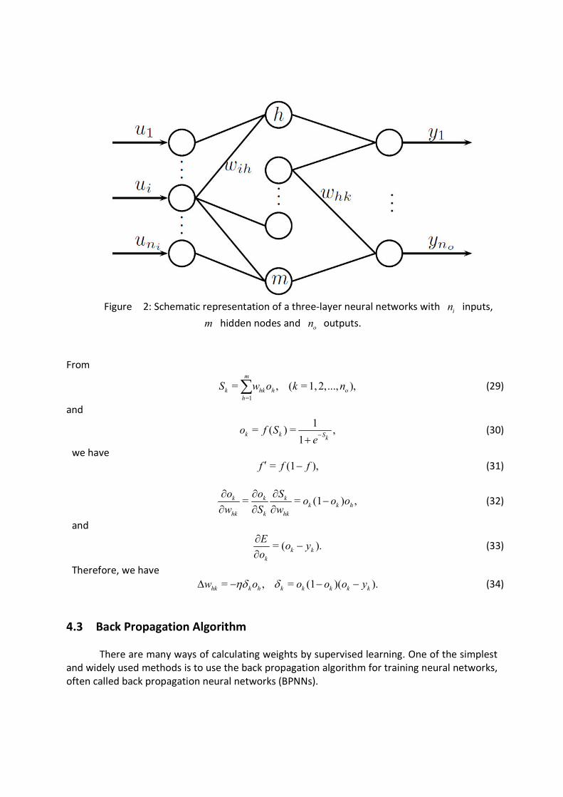
Figure 2: Schematic representation of a three-layer neural networks with

in inputs,

m hidden nodes and on outputs.

From

=1

= , ( = 1, 2,..., ),m

k hk h o

h

S w o k n∑ (29)

and

1

= ( ) = ,1

k k Sk

o f Se−

+ (30)

we have

= (1 ),f f f′ − (31)

= = (1 ) ,k k kk k h

hk k hk

o o So o o

w S w

∂ ∂ ∂−

∂ ∂ ∂ (32)

and

= ( ).k k

k

Eo y

o

∂−

∂ (33)

Therefore, we have

= , = (1 )( ).hk k h k k k k kw o o o o yηδ δ∆ − − − (34)

4.3 Back Propagation Algorithm

There are many ways of calculating weights by supervised learning. One of the simplest

and widely used methods is to use the back propagation algorithm for training neural networks,

often called back propagation neural networks (BPNNs).

The basic idea is to start from the output layer and propagate backwards so as to

estimate and update the weights. From any initial random weighting matrices ihw (for

connecting the input nodes to the hidden layer) and hkw (for connecting the hidden layer to

the output nodes), we can calculate the outputs of the hidden layer ho

=1

1= , ( = 1, 2,..., ),

1 exp[ ]

h ni

ih i

i

o h m

w u+ −∑ (35)

and the outputs for the output nodes

=1

1= , ( = 1,2,..., ).

1 exp[ ]k om

hk h

h

o k n

w o+ −∑ (36)

The errors for the output nodes are given by

= (1 )( ), ( = 1, 2,..., ),k k k k k oo o y o k nδ − − (37)

where ( = 1, 2,..., )k oy k n are the data (real outputs) for the inputs ( = 1, 2,..., )i iu i n . Similarly,

the errors for the hidden nodes can be written as

=1

= (1 ) , ( = 1, 2,..., ).

no

h h h hk k

k

o o w h mδ δ− ∑ (38)

The updating formulae for weights at iteration t are

1 = ,t t

hk hk k hw w oηδ+ + (39)

and

1 = ,t t

ih ih h iw w uηδ+ + (40)

where 0 < 1η ≤ is the learning rate.

Here we can see that the weight increments are

= ,ih h iw uηδ∆ (41)

with similar updating formulae for hkw . An improved version is to use the so-called weight

momentum α to increase the learning efficiency

= ( 1),ih h i ihw u wηδ α τ∆ + − (42)

where τ is an extra parameter. There are many good software packages for artificial neural

networks, and there are dozens of good books fully dedicated to implementation. ANN has

been very useful in solving problems in civil engineering (Gandomi and Alavi, 2011; Alavi and

Gandomi, 2011).

5 Genetic Programming

Genetic programming is a systematic method of using evolutionary algorithms to

produce computer programs in a Darwinian manner. L. J. Fogel was probably one of the

pioneers in primitive genetic programing (Fogel, 1966), as he first used evolutionary algorithms

to study finite-state automata. However, the true formulation of modern genetic programming

was introduced and pioneered by J. R. Koza in 1992, and the publication of his book on `Genetic

Programming' was a major milestone (Koza, 1992).

In essence, genetic programming intends to evolve computer programs in an iterative

manner by chromosome representations, often in terms of tree structures where each node

corresponds a mathematical operator, and end nodes represent operands. Evolution is carried

out by genetic operators such as crossover, mutation and selection of the fittest. In the

tree-structured representation, crossover often takes the form of subtree exchange crossover,

while mutation may take the form of subtree replacement mutation.

According to Koza et al. (1992), there are three stages in the process: preparatory steps,

genetic programming engine, and a new computer program. The genetic programming engine

has preparatory steps as inputs and a computer program as its output. First, we have to specify

a set of primitive ingredients such as the function set and terminal set. For example, we if we

wish a computer program to be able to design an electronic circuit, we have to specify the basic

components such as transistors, capacitors and resistors and their basic functions. Then, we

have to produce a fitness measure, that is to define what solutions are better than others by

that measure such as time, cost, stability and performance. In addition, we have to produce

some initialization of algorithm-dependent parameters such as population size and number of

generations, and the termination criteria which essentially controls when the evolution should

stop.

Though computationally expansive, genetic programming has aleady produced

human-competitive, novel results in many areas such as electronic design, game playing,

quantum computing, invention generation. New invention often requires illogical steps in

producing new ideas, and this can often be mimicked as a randomization process in

evolutionary algorithms. As pointed out by Koza et al. (2003), genetic programming is a

systematic method for `getting computers to automatically solve a problem’, starting from a

high-level statements outlining what needs to be done, this virtually turns computers into an

`automated invention machine'. Obviously, that is the ultimate aim of genetic programming.

For applications in engineering, readers can use more specialized literature (Alavi and

Gandomi, 2011; Gandomi and Alavi, 2012a, 2012b). There is an extensive literature concerning

genetic programming, interested readers can refer to more advantage literature such as Koza

(1992) and Langdon (1998).

References

[1] Afshar, A., Haddad, O. B., Marino, M. A., Adams, B. J., (2007). Honey-bee mating

optimization (HBMO) algorithm for optimal reservoir operation, J. Franklin Institute, 344,

452-462.

[2] Alavi, A. H., Gandomi, A. H., (2011). Prediction of principal groud-motion parameters using a

hybrid method coupling artifical neural networks and simualted annealing, Computers and

Structures, 89(23/24), 2176-2194.

[3] Alavi, A. H., Gandomi, A. H., (2011). A robust data mining approach for formulation of

geotechnical engineering systems, Engineering Computations, 28(3), 242-274.

[4] Apostolopoulos, T. and Vlachos, A., (2011). Application of the Firefly Algorithm for Solving

the Economic Emissions Load Dispatch Problem, International Journal of Combinatorics,

Volume 2011, Article ID 523806. http://www.hindawi.com/journals/ijct/2011/523806.html

[5] Blum, C. and Roli, A., (2003). Metaheuristics in combinatorial optimization: Overview and

conceptural comparision, ACM Comput. Surv., 35 , 268--308.

[6] Conn, A. R., Schneinberg, K., and Vicente, L. N., (2009). Introduction to Derivative-Free

Optimization, MPS-SIAM Series on Optimization, SIAM, Philadelphia, USA.

[7] Dorigo, M. and Stütle, T., (2004). Ant Colony Optimization, MIT Press.

[8] Farmer, J. D., Packard, N. and Perelson, A., (1986). The immune system, adapation and

machine learning, Physica D, 2 , 187--204.

[9] Fogel, L. J., Owens, A. J. and Walsh, M. J., (1966). Artificial Intelligence Through Simulated

Evolution, John Wiley & Sons, New York.

[10] Gandomi, A. H., Yang, X. S., Alavi, A. H., (2011). Cuckoo search algorithm: a metaheuristic

approach to solve structural optimization problems, Engineering with Computers, (in press).

DOI: 10.1007/s00366-011-0241-y

[11] Gandomi, A. H., Yang, X. S., Alavi, A. H., (2011). Mixed variable structural optimization using

firefly algorithm, Computers and Structures, 89(23/24), 2325-2336.

[12] Gandomi, A. H., Alavi, A. H., (2011). Applications of computation intelligence in behaviour

simulation of concrete maerials, in: Computational Optimization and Applications in

Engineering and Industry (Eds. X. S. Yang and S. Koziel), Springer SCI 359, 221-243.

[13] Gandomi, A. H., Alavi, A. H., (2012a). A new mult-gene genetic programming appoach to

nonlinear system modelin, Part I: materials and structural engineering, Neural Computing and

Applications, 21(1), 171-187.

[14] Gandomi, A. H., Alavi, A. H., (2012b). A new mult-gene genetic programming appoach to

nonlinear system modelin, Part II: Geotechnical and Earthquake Engineering, Neural Computing

and Applications, 21(1), 189-201.

[15] Geem, Z. W., Kim, J. H. and Loganathan, G. V., (2001). A new heuristic optimization:

Harmony search, Simulation, 76 , 60--68.

[16] Glover, F. and Laguna, M. (1997). Tabu Search, Kluwer Academic Publishers, Boston, USA.

[17] Goldberg, D. E. (1989). Genetic Algorithms in Search, Optimization and Machine Learning,

Reading, Mass., Addison Wesley.

[18] Holland, J., (1975). Adaptation in Natural and Artificial Systems, University of Michigan

Press, Ann Anbor.

[19] Kennedy, J. and Eberhart, R. C., (1995). Particle swarm optimization, in: Proc. of IEEE

International Conference on Neural Networks, Piscataway, NJ. pp. 1942--1948.

[20] Kennedy, J., Eberhart, R. C. & Shi, Y., (2001). Swarm intelligence, San Francisco: Morgan

Kaufmann Publishers.

[21] Karaboga, D., (2005). An idea based on honey bee swarm for numerical optimization,

Technical Report TR06, Erciyes University, Turkey.

[22] Karmarkar, N., (1984). A new polynomial-time algorithm for linear programming,

Combinatorica, 4 (4), 373--395.

[23] Kirkpatrick, S., Gelatt, C. D., and Vecchi, M. P., (1983). Optimization by simulated

annealing, Science, 220 (4598), 671--680.

[24] Nakrani, S. and Tovey, C., (2004). On Honey Bees and Dynamic Server Allocation in

Internet Hosting Centers. Adaptive Behaviour, 12(3-4), 223-240.

[25] Nelder, J. A. and Mead, R.: A simplex method for function optimization, Computer Journal,

7, 308-313 (1965)

[26] Koziel, S. and Yang, X. S., (2011). Computational Optimization, Methods and Algorithms,

Springer, Germany.

[27] Yang, X. S. and Koziel, S., (2011). Computational Optimization and Applications in

Engineering and Industry, Springer, Germany.

[28] Koza, J. R., (1992). Genetic Programming: On the Programming of Computers by Means of

Natural Selection, MIT Press.

[29] Koza, J. R., Keane, M. A., Streeter, M. J., Yu, J.. Lanza, G., (2003). Genetic Computing IV:

Routine Human-Competitive Machine Intelligence, Kluwer Academic Publishers.

[30] Langdon, W. B., (1998). Genetic Programming + Data Structures = Automatic

Programming!, Kluwer Academic Publishes.

[31] Pavlyukevich, I., (2007). Lévy flights, non-local search and simulated annealing, J.

Computational Physics, 226 , 1830--1844.

[32] Parpinelli, R. S., and Lopes, H. S., New inspirations in swarm intelligence: a survey, Int. J.

Bio-Inspired Computation, 3, 1-16 (2011).

[33] Pham, D.T., Ghanbarzadeh, A., Koc, E., Otri, S., Rahim, S., and Zaidi, M., (2006). The Bees

Algorithm: A Novel Tool for Complex Optimisation Problems, Proceedings of IPROMS 2006

Conference, pp.454-461

[34] Price, K., Storn, R. and Lampinen, J., (2005). Differential Evolution: A Practical Approach

to Global Optimization, Springer.

[35] Sawaragi, Y., Nakayama, H., Tanino, T. (1985). Theory of Multiobjective Optimisation,

Academic Press

[36] Sayadi, M. K., Ramezanian, R. and Ghaffari-Nasab, N., (2010). A discrete firefly

meta-heuristic with local search for makespan minimization in permutation flow shop

scheduling problems, Int. J. of Industrial Engineering Computations, 1 , 1--10.

[37] Storn, R., (1996). On the usage of differential evolution for function optimization,

Biennial Conference of the North American Fuzzy Information Processing Society (NAFIPS), pp.

519--523.

[38] Storn, R. and Price, K., (1997). Differential evolution - a simple and efficient heuristic for

global optimization over continuous spaces, Journal of Global Optimization, 11 , 341--359.

[39] Talbi, E.G. (2009). Metaheuristics: From Design to Implementation, John Wiley & Sons.

[40] Wolpert, D. H. and Macready, W. G.: No free lunch theorems for optimization, IEEE Trans.

Evolutionary Computation, 1, 67--82 (1997)

[41] Yang, X.S., (2005). Engineering optimization via nature-inspired virtual bee algorithms. in:

Artificial Intelligence and Knowledge Engineering Applications: A Bioinspired Approach, Lecture

Notes in Computer Science, 3562, pp. 317-323, Springer Berlin / Heidelberg.

[42] Yang, X. S. (2008). Nature-Inspired Metaheuristic Algorithms, First Edition, Luniver Press,

UK.

[43] Yang, X. S., (2009). Firefly algorithms for multimodal optimization, 5th Symposium on

Stochastic Algorithms, Foundation and Applications (SAGA 2009) (Eds Watanabe O. and

Zeugmann T.), LNCS, 5792 , pp. 169--178.

[44] Yang, X. S. (2010a). Nature-Inspired Metaheuristic Algoirthms, 2nd Edition, Luniver Press,

UK.

[45] Yang, X. S. (2010b). Engineering Optimization: An Introduction with Metaheuristic

Applications, John Wiley & Sons.

[46] Yang, X. S., (2010c). A new metaheuristic bat-inspired algorithm, in: Nature-Inspired

Cooperative Strategies for Optimization (NICSO 2010) (Eds. Gonzalez J. R. et al.), Springer, SCI

284 , pp. 65--74.

[47] Yang, X. S., (2011a), Bat algorithm for multi-objective optimisation, Int. J. Bio-Inspired

Computation, 3 (5), 267-274 (2011).

[48] Yang, X. S. and Deb, S., (2009). Cuckoo search via Lévy flights, in: Proc. of World

Congress on Nature & Biologically Inspired Computing (NaBic 2009), IEEE Publications, USA, pp.

210--214.

[49] Yang, X. S., & Deb, S. (2010). Engineering optimization by cuckoo search, Int. J. Math.

Modelling Num. Optimisation, 1 (4), 330--343.

[50] Yang, X. S., Gandomi, A. H., (2012). Bat algorithm: a novel approach for global engineering

optimization, Engineering Computations, 29(5), 1-18.

[51] Yang, X. S., (2011b). Chaos-enhanced firefly algorithm with automatic parameter tuning, Int.

J. Swarm Intelligence Research, 2(4), 1-11.