efficient break-away friction ratio and slip prediction based on haptic surface exploration

IEEE Transactions on Robotics, 2013

1

Abstract— The break-away friction ratio (BF-ratio), which is

the ratio between friction force and the normal force at slip

occurrence, is important for the prediction of incipient slip and

the determination of optimal grasping forces. Conventionally,

this ratio is assumed constant and approximated as the static

friction coefficient. However, this ratio varies with acceleration

rates and force rates applied to the grasped object and the

object material, leading to difficulties in determining optimal

grasping forces that avoid slip. In this paper, we propose a novel

approach based on the interactive forces to allow a robotic hand

to predict object slip before its occurrence. The approach only

requires the robotic hand to have a short haptic surface

exploration over the object surface before manipulating it. Then

the frictional properties of the finger-object contact can be

efficiently identified and the BF-ratio can be real time predicted

to predict slip occurrence under dynamic grasping conditions.

Using the predicted BF-ratio as a slip threshold is demonstrated

to be more accurate than using the static/Coulomb friction

coefficient. The presented approach has been experimentally

evaluated on different object surfaces showing good

performance in terms of prediction accuracy, robustness and

computational efficiency.

Index Terms — break-away ratio, haptic surface exploration,

slip prediction.

I. INTRODUCTION

HE study of human grasping reveals that incipient slip is very important for stable and dexterous grasping of objects [1][2]. To enable robotic hands to perform as

dexterous as human hands, the determination of the onset of slip between robotic fingers and grasped objects is essential [3], especially when grasping and manipulating fragile or slippery objects. Without slip information, optimal grasping forces cannot be appropriately determined and it is difficult to prevent unexpected slippage or object damage.

The ratio between the friction and normal forces at the onset of slip is referred to as break-away friction ratio (BF-ratio). This ratio is a property of the dynamic interactions between the fingers and objects. It is normally assumed constant in robotic grasping and approximated as the static friction coefficient. When the ratio between friction and normal forces is less than the static coefficient, grasping is considered stable; otherwise, slip occurs [4]. However, in

Manuscript received January 10, 2012. This work was supported by the

HANDLE project which is funded by the European Commission within the Seventh Framework Programme FP7 (FP7/2007-2013) under grant agreement ICT 231640.

X. Song, H. Liu, K. Althoefer, T. Nanayakkara and L.D. Seneviratne are with Center for Robotics Research, Department of Informatics, King’s College London, UK, WC2R 2LS. * indicates the corresponding author {[email protected]}

practice, the BF-ratio is not constant. The variability of the BF-ratio depends on the acceleration rate, the rate of force applied on the object and the material the object is made from [5]. Humans seem to be subconsciously aware of this phenomenon; and studies on human grasping have shown that humans would adjust their lifting acceleration if incipient slip is perceived during manipulation [1]. This varying BF-ratio brings difficulties in determining a stable grasp [6] and applying optimal grasping forces, since an overestimated BF-ratio could increase the risk of slip; while an underestimated BF-ratio could result in an over-applied gripping force. In this paper, we propose a novel force-based approach to accurately predict the BF-ratio and slip for a given robotic grasping task. Our approach first employs a simple but efficient force-based surface exploration procedure by sliding a robotic fingertip over an unknown object surface with two short strokes (one at a low acceleration and the other at a higher acceleration) to identify the friction properties of the finger-object contact. Once the full set of friction coefficients of the LuGre model is established, the BF-ratio can be accurately predicted in real time, given the acceleration rate or force rate applied on the object. To the best knowledge of the authors, it is the first time that the full set of friction parameters of the LuGre model has been identified only through a simple haptic surface exploration and moreover to use these parameters for slip prediction during dynamic grasping.

The detection of slip has been always of interest for robotics research. A soft fingertip embedded with a micro-scale force/torque sensor was proposed in [7]. The incipient slip was determined when a local minimum in the normal force was observed. Another interesting attempt for detecting the incipient slip used vision to analyze the change of stick and slip regions of the contact interface under a transparent plate [8]. Inspired by the slip sensing mechanism of human fingers, several sensors constructed with distributed ridges and sensing elements have been proposed. The use of the strain difference between two adjacent strain gauges for the detection of the incipient of slip was described in [9]. In [10], the measured strain distribution inside a deformable elastic finger was used to estimate the friction coefficients of contact surfaces, and thus identify the threshold for slip prediction. A fibre optics based sensor with concentric circular ridges was presented in [11]. Incipient slip was monitored based on the change in light signals caused by partial deformation of ridges. However, this type of sensors is hard to fabricate and difficult to miniaturize.

One popular method for the detection of slip is based on the analysis of vibrations during slip occurrence. This method often uses the embedded strain gauges or accelerometers to

Efficient Break-Away Friction Ratio and Slip Prediction Based on Haptic Surface Exploration

Xiaojing Song, Hongbin Liu* Member, IEEE, Kaspar Althoefer Member, IEEE, Thrishantha Nanayakkara Member, IEEE and Lakmal D Seneviratne Member, IEEE

T


2

perceive the subtle high frequency vibrations; an elastic skin dotted with nibs is used for enhancing signal vibration. The slip is detected based on either the direct analysis of the vibration amplitudes or the recognition of signal pattern in the frequency spectrum domain. Based on this concept, a number of slip sensors have been developed using different sensing principles, such as the center of pressure (CoP) tactile sensor made of conductive rubber [12, 13], the slip sensor composed of four layers of polyvinylidene fluoride (PVDF) film [14], sensors made of thick-film piezoelectric materials [15] and the fast piezo-resistive materials [16] as well as slip sensors equipped with accelerometers [17, 18].

Compared to the vibration-based (v-b) approaches, the proposed method provides the following advantages. First, the v-b approaches detects the onset of slip rather than predict slip before it occurs. Thus it requires high-speed data communication and processing to prevent gross slippage. In contrast, the proposed model-based approach is capable of predicting slip in advance, thus providing sufficient time for the slip avoidance control. Second, the proposed slip prediction method is based on the surface frictional parameters, thus it is robust against unexpected vibrations. On the other hand, using the v-b approaches is challenging to isolate slip occurrences from other sources of vibration, such as the change of external forces or hand chattering during operations. Furthermore, careful calibrations through repeated tests are often required with v-b approaches, since the vibration pattern of slip may change with different material surfaces. Applying the proposed method, the surface frictional parameters could be rapidly determined through a short surface exploration, thus simplifying the calibration procedures. In this study, experimental results obtained from different object surfaces are presented, indicating good accuracy, robustness and efficiency of the proposed approach. Also, the performances of different methods for frictional property identification are compared experimentally.

Estimating static coefficients of the LuGre model through force-based surface exploration for surface recognition has been presented in [19][20]. In this paper, we further extend our previous work to identify the full set of coefficients of the LuGre model and use these coefficients for BF-ratio and slip prediction. Part of this work has been presented in [21], however this paper provides more methods to identify the dynamic coefficients of the LuGre model and more thorough experimental evaluation and discussion of the proposed methods.

II. DYNAMIC MODELLING OF FRICTION

A. Dynamic LuGre Friction Model

To predict the BF-ratio between fingers and objects, it is necessary to consider the dynamic friction interactions between two surfaces in contact. Well-known dynamic friction models include the Dahl model [22], the bristles model [23], the LuGre model [5], and the Leuven model [24]. The LuGre model describes both the pre-sliding and sliding regimes with good accuracy and low computational complexity [5]. Thus, it is chosen for the BF-ratio prediction in our study.

Fig. 1. The interaction between two contacting surfaces A and B is modeled as elastic bristles by the LuGre model [5]; simulation results of the LuGre model for different sliding accelerations; (rate=0) curve represents the quasi-static LuGre model.

The LuGre model assumes the asperities of two contacting surfaces as elastic bristles [5], as illustrated in Fig. 1. Relative motion between the two surfaces will lead to the deflection of the bristles. The average displacement of the bristles, denoted as z, is modeled by Equ. (1) [5]. Variable v is the relative velocity between the contacting surfaces. Function s(v) given by Equ. (2) describes the Stribeck effect. In Equ. (2), v0 is the Stribeck velocity; �c and �s are Coulomb friction and static friction coefficients; and Fn is the interaction force in the contact normal direction.

�� ||�� (1)

�� (2)

The friction force Ft is generated from both the bending of the bristles and the viscous friction, as described in Equ. (3). Variable σ0 and σ1 are constant stiffness and damping coefficients respectively; σ2 is the viscosity coefficient.

�� (3) bending force of bristles viscous friction

If the sliding acceleration is low, the LuGre model can be simplified as [20]: �� sgn�� !�� " � ��(4)

Equation (4) is the quasi-static form of the LuGre model, only containing four coefficients, �s, �c, v0 and σ2.

Simulation results illustrate that different sliding accelerations result in different hysteresis loops, Fig. 1. It can be seen that for small accelerations, the means of friction forces obtained at increasing and decreasing velocities agree well with the quasi-static LuGre model (red curve in Fig. 1 (b)). Thus, the friction-velocity curve at low sliding accelerations can be approximated by the quasi-static form of the LuGre model, Equ. (4) [20]; and this will be utilized here for estimating �s, �c, v0 and σ2.

B. Varying Break-Away Friction Ratio

The simulation results in Fig. 2 demonstrate that the acceleration and force rates affect the break-away friction ratio (BF-ratio). Figure 2 illustrates two cases: in the first case (Fig. 2 (a)), the robotic hand lifts the object with an acceleration rate of $� . Let aof denote the sliding acceleration


3

of the object with respect to fingers, m be the mass of the object, and Ft be the total friction force. Applying Newton’s

second law yields aof =a+ %&�'(% . For the second case, an

external force is applied on the object with a drag force rate of �� , thus: aof ='% � %&�'(% . The second case is equivalent to the

first case. For both cases, the gripping force Fn (the normal force) remains constant. In the simulations, various $� and �� values are input to the LuGre model (Equs. (1)-(3)) with coefficients listed in Table I.

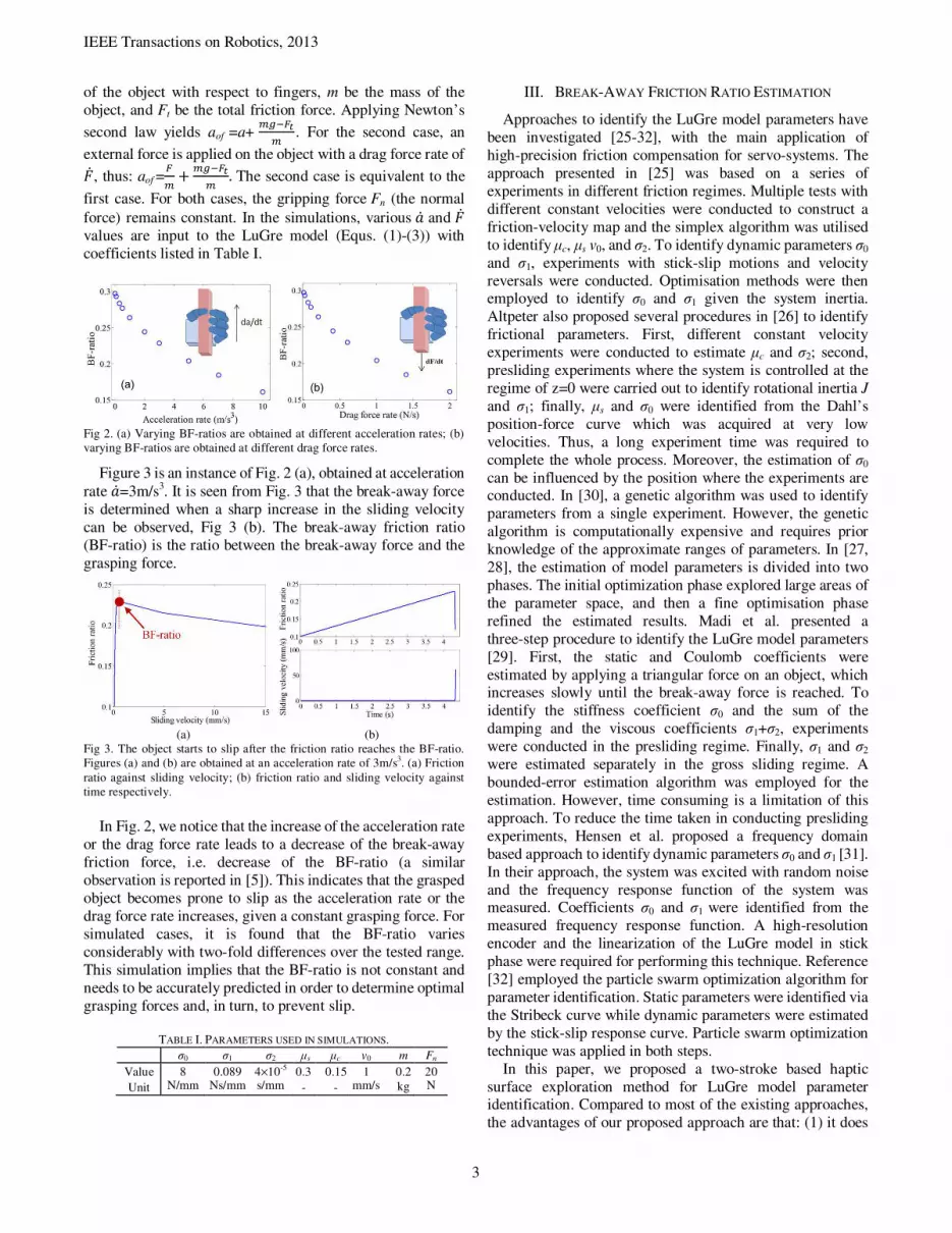
Fig 2. (a) Varying BF-ratios are obtained at different acceleration rates; (b) varying BF-ratios are obtained at different drag force rates.

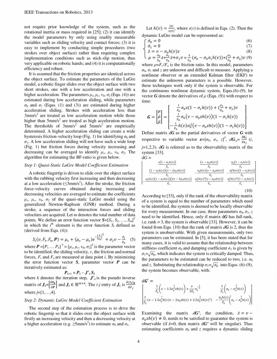
Figure 3 is an instance of Fig. 2 (a), obtained at acceleration rate $�=3m/s3. It is seen from Fig. 3 that the break-away force is determined when a sharp increase in the sliding velocity can be observed, Fig 3 (b). The break-away friction ratio (BF-ratio) is the ratio between the break-away force and the grasping force.

(a) (b) Fig 3. The object starts to slip after the friction ratio reaches the BF-ratio. Figures (a) and (b) are obtained at an acceleration rate of 3m/s3. (a) Friction ratio against sliding velocity; (b) friction ratio and sliding velocity against time respectively.

In Fig. 2, we notice that the increase of the acceleration rate or the drag force rate leads to a decrease of the break-away friction force, i.e. decrease of the BF-ratio (a similar observation is reported in [5]). This indicates that the grasped object becomes prone to slip as the acceleration rate or the drag force rate increases, given a constant grasping force. For simulated cases, it is found that the BF-ratio varies considerably with two-fold differences over the tested range. This simulation implies that the BF-ratio is not constant and needs to be accurately predicted in order to determine optimal grasping forces and, in turn, to prevent slip.

TABLE I. PARAMETERS USED IN SIMULATIONS.

σ0 σ1 σ2 �s �c v0 m Fn Value Unit

8 N/mm

0.089 Ns/mm

4×10-5 s/mm

0.3 -

0.15 -

1 mm/s

0.2 kg

20 N

III. BREAK-AWAY FRICTION RATIO ESTIMATION

Approaches to identify the LuGre model parameters have been investigated [25-32], with the main application of high-precision friction compensation for servo-systems. The approach presented in [25] was based on a series of experiments in different friction regimes. Multiple tests with different constant velocities were conducted to construct a friction-velocity map and the simplex algorithm was utilised to identify �c, �s v0, and σ2. To identify dynamic parameters σ0 and σ1, experiments with stick-slip motions and velocity reversals were conducted. Optimisation methods were then employed to identify σ0 and σ1 given the system inertia. Altpeter also proposed several procedures in [26] to identify frictional parameters. First, different constant velocity experiments were conducted to estimate �c and σ2; second, presliding experiments where the system is controlled at the regime of z=0 were carried out to identify rotational inertia J and σ1; finally, �s and σ0 were identified from the Dahl’s position-force curve which was acquired at very low velocities. Thus, a long experiment time was required to complete the whole process. Moreover, the estimation of σ0 can be influenced by the position where the experiments are conducted. In [30], a genetic algorithm was used to identify parameters from a single experiment. However, the genetic algorithm is computationally expensive and requires prior knowledge of the approximate ranges of parameters. In [27, 28], the estimation of model parameters is divided into two phases. The initial optimization phase explored large areas of the parameter space, and then a fine optimisation phase refined the estimated results. Madi et al. presented a three-step procedure to identify the LuGre model parameters [29]. First, the static and Coulomb coefficients were estimated by applying a triangular force on an object, which increases slowly until the break-away force is reached. To identify the stiffness coefficient σ0 and the sum of the damping and the viscous coefficients σ1+σ2, experiments were conducted in the presliding regime. Finally, σ1 and σ2

were estimated separately in the gross sliding regime. A bounded-error estimation algorithm was employed for the estimation. However, time consuming is a limitation of this approach. To reduce the time taken in conducting presliding experiments, Hensen et al. proposed a frequency domain based approach to identify dynamic parameters σ0 and σ1 [31]. In their approach, the system was excited with random noise and the frequency response function of the system was measured. Coefficients σ0 and σ1 were identified from the measured frequency response function. A high-resolution encoder and the linearization of the LuGre model in stick phase were required for performing this technique. Reference [32] employed the particle swarm optimization algorithm for parameter identification. Static parameters were identified via the Stribeck curve while dynamic parameters were estimated by the stick-slip response curve. Particle swarm optimization technique was applied in both steps.

In this paper, we proposed a two-stroke based haptic surface exploration method for LuGre model parameter identification. Compared to most of the existing approaches, the advantages of our proposed approach are that: (1) it does


4

not require prior knowledge of the system, such as the rotational inertia or mass required in [25]; (2) it can identify the model parameters by only using readily measurable variables such as sliding velocity and contact forces; (3) it is easy to implement by conducting simple procedures (two strokes over object surface) rather than requiring complex implementation conditions such as stick-slip motion, thus very applicable on robotic hands; and (4) it is computationally efficiency and robust.

It is assumed that the friction properties are identical across the object surface. To estimate the parameters of the LuGre model, a robotic finger slides over the object surface with two short strokes, one with a low acceleration and one with a higher acceleration. The parameters �s, �c, v0, σ2 (Equ. (4)) are estimated during low acceleration sliding, while parameters σ0 and σ1 (Equs. (1) and (3)) are estimated during higher acceleration sliding. Strokes with acceleration less than 3mm/s2 are treated as low acceleration motion while those higher than 5mm/s2 are treated as high acceleration motion. The thresholds of 3mm/s2 and 5mm/s2 are empirically determined. A higher acceleration sliding can create a wide hysteresis friction-velocity loop (Fig. 1) for identifying σ0 and σ1. A low acceleration sliding will not have such a wide loop (Fig. 1) but friction forces during velocity increasing and decreasing can be averaged to identify �s, �c, v0, σ2. The algorithm for estimating the BF-ratio is given below.

Step 1: Quasi-Static LuGre Model Coefficient Estimation

A robotic fingertip is driven to slide over the object surface with the rubbing velocity first increasing and then decreasing at a low acceleration (≤3mm/s2). After the stroke, the friction force-velocity curves obtained during increasing and decreasing velocities are averaged to estimate the coefficients �s, �c, v0, σ2 of the quasi-static LuGre model using the generalized Newton-Raphson (GNR) method. During a stroke, a sequence of the interaction forces and sliding velocities are acquired. Let m denotes the total number of data points. We define an error function vector S=[S1, S2, …, Sm]T in which the i

th element is the error function Si defined as (derived from Equ. (4)): *+��, �� , ��, -� � �� e�� '('/ (5)

where P =[P1 … P4] T = [�s, �c, v0, σ2]

T is the parameter vector to be identified; the sliding velocity, v, the friction and normal forces, Ft and Fn are measured at data point i. By minimizing the error function vector S, parameter vector P can be iteratively estimated as:

Pk+1 = Pk – J+k Sk

where k denotes the iteration step, J+k is the pseudo inverse

matrix of Jk=01231- 4 and Jk ∈ ℝ%×8. The i-j entry of Jk is 1�9:�31;<

where j=[1,…,4].

Step 2: Dynamic LuGre Model Coefficient Estimation

The second step of the estimation process is to drive the robotic fingertip so that it slides over the object surface with firstly an increasing velocity and then a decreasing velocity at a higher acceleration (e.g. ≥5mm/s2) to estimate σ0 and σ1.

Let ℎ�� ||��, where s(v) is defined in Equ. (2). Then the

dynamic LuGre model can be represented as: �� 0 (6) �� 0 (7) �� ℎ�� (8) � � ?�'/ �+?@'/ ��+�2� =

B'/ �� ℎ��+�?@'/ � �� (9)

where �=Ft /Fn is the friction ratio. In this model, parameters σ0, σ1 and z are unknown and difficult to measure. Applying a nonlinear observer or an extended Kalman filter (EKF) to estimate the unknown parameters is a possible. However, these techniques work only if the system is observable. For the continuous nonlinear dynamic system, Equs.(6)-(9), let vector G denote the derivatives of � (Equ. (9)) with respect to time:

C � D��EF � GHHHI �'/ ��1 � ��ℎ�� ?@'/ � ��'/ ��K� � ��ℎ��L�1 � ��ℎ�� '/ ℎ��K� � ��ℎ��L�1 � ��ℎ��MNN

NO.

Define matrix dG as the partial derivatives of vector G with

respective to variable vector x=[σ0, σ1, z]T, dGi,j= 1CP1Q< (i,

j=1,2,3). dG is referred as to the observability matrix of the system [33]. dG =

GHHHHHI �K1 � ��ℎ��L�� K� � ��ℎ��L�� K1 � ��ℎ��L��K1 � ��ℎ��LK� � 2��ℎ��L�� ℎ��K� � ��ℎ��L�� ℎ��K1 � ��ℎ��L��ℎ��K1 � ��ℎ��LK2� � 3��ℎ��L�� ℎ��K� � ��ℎ��L�� Sℎ��K1 � ��ℎ��L�� MN

NNNNO

(10) According to [33], only if the rank of the observability matrix of a system is equal to the number of parameters which need to be identified, the system is deemed to be locally observable for every measurement. In our case, three parameters σ0, σ1, z need to be identified. Hence, only if matrix dG has full rank, i.e. rank = 3, the system is observable [33]. However, it can be found from Equ. (10) that the rank of matrix dG is 2, thus the system is unobservable. With given measurements, only two parameters can be estimated. In [5], it has been stated that for many cases, it is valid to assume that the relationship between stiffness coefficient σ0 and damping coefficient σ1 is given by σ1=T��, which indicates the system is critically damped. Thus, the parameters to be estimated can be reduced to two, i.e. σ0 and z. Substituting the relationship σ1=T�� into Equs. (6)-(9), the system becomes observable, with: UC′ �

GHHHHI

1�� W� � 1.5��ℎ��Y � �2�� 1�� W�� S�ℎ��Y1�� 1.5��ℎ�� 2��ℎ�� 2.5��S��ℎ�� ℎ�� W�� S�ℎ��YMNNNNO

Examining the matrix dG’, the condition, �� ℎ�� ≠ 0, needs to be satisfied to guarantee the system is observable (if ��=0, then matrix dG’ will be singular). Thus estimating coefficients σ0 and z requires a dynamic sliding


5

operation where the deflection of bristles, z, has significant variations. Small variations in z may lead to poor observability of the system. Therefore, the robotic fingertip needs to slide over the object surface with an acceleration greater than 5mm/s2 (this value is obtained based on our experimental observation).

� Extended Kalman Filter based Estimation

Let the estimated vector be x = [σ0, z]T. Then the discrete nonlinear process model is: x(k) = f(x(k-1))+w(k-1)

� ! ��[ � 1�\��[ � 1� � ��[ � 1�ℎK��[ � 1�L��[ � 1�]^ � ��[ � 1�"�_�[ � 1� where w(k-1)~�� (0, Q(k-1)), and T is the time interval between adjacent steps. Let y=�. The measurement model is thus: `�[� � aKQ�[�L � b�[� =

�'/�c� 0��[� � ��[�d�ℎK��[�L4 ��[� � �'/�c��[�@��[� ��[� � b�[� where τ(k)~�� (0, Г(k)). Let Φ be the process sensitivity matrix obtained by linearising function f(x): e�[ � 1� � fgfQhQiQjk�c�� l 1 0�ℎK��[ � 1�L��[ � 1�^ 1 � �n��[ � 1�ℎK��[ � 1�L^o and R be the measurement sensitivity matrix obtained by linearising measurement function r(x): p�[� � fafQhQiQjk�c�� GHHI 1��[� l��[�q1� 1.5�n��[��ℎ��[��r � ��[��0.5�n��[��o1��[� l�n��[� � �n��[�S�ℎ��[��o MN

NOs

The unknown parameter vector, x, can be estimated using standard extended Kalman filter equations [34]: Qjt�[� � Qj��[� � u�[��`�[� � n�[�� where K(k) is the Kalman gain which is updated at each step, u�[� � -��[�p�[�s[p�[�-��[�p�[�s � w�[�]�� where P − is the priori error covariance matrix obtained from: -��[� � e�[ � 1�-t�[ � 1�e�[ � 1�s �y�[ � 1�, and posterior error covariance matrix P + is updated after attaining K(k) as-t�[� � [z � u�[�p�[�]-��[�.

With appropriate initial conditions and noise statistics knowledge, the unknown parameters can be estimated using the extended Kalman filter. However, when implementing the EKF, it is noted that, first, noise statistics knowledge (including process noise and measurement noise) is not easily obtained in practical situations; second, an initial guess that is far off from the final solution may affect the convergence speed or sometimes even result in divergence. In addition, due to bristle displacement z being in the order of micrometers, sliding velocity v being in the order of millimeters/second and sampling time T being in the order of milliseconds, elements in the process sensitivity matrix Φ, Φ(2,1)=zh(v)T is close to zero and Φ(2,2) =1-σ0h(v)T is close

to one. Thus, matrix Φ is very close to an identity matrix and observability matrix [R, RΦ]T for the discrete model is nearly singular, indicating poor observability of the system. To improve this, some variables in the model can be rescaled to new units [34]. The units for bristle displacement and sliding velocity can be changed from ‘m’ to ‘mm’ and from ‘m/s’ to ‘mm/s’ respectively. The sampling time can also be increased to improve the poor observability of the system; however, large sampling times will lose dynamic information of friction and sliding velocities. The performance of the extended Kalman filter is evaluated in Sections V and VI.

� Levenberg-Marquardt Method based Estimation

The extended Kalman filter estimates unknown states using differential equations of unknown states and sequential measurements. The estimated states are updated at each step to converge to a stable solution. In every step, only measurements at current step are used updating estimated states. Therefore, poor observability of the system at any step may lead to failure of state estimation. By contrast, a nonlinear least-square method is a global curve fitting tool, which uses measurements acquired at different time steps to estimate unknown parameters in an iterative way. In our study, we also propose a nonlinear Levenberg-Marquardt (LM) based method for estimating parameters σ0 and σ1. In order to apply the LM method, Equs. (6)-(9) are transformed into arithmetic equations. Defining the sampling time T, the discrete bristle displacement at time steps k and k-1 are linked by (refer to Equ. (8)):

��[� � \1 � ��ℎK��[ � 1�L^]��[ � 1� � ��[ � 1�^(10)

Thus, denoting z0 as the initial bristle displacement, the bristle displacement at each step z(k) can be expressed as: ��[� � ��[ � 1�^ � ��∏ K1 � ��ℎK��|�L^Lc��+i� � ∑ [c��~i� ��^∏ K1��ℎK��L^L]c��%i~t� (11) Consequently, the bristle displacement at each time step z(k) becomes a function of the initial displacement z0. Thus, instead of estimating z(k) for each step like the EKF does, it only needs to estimate the initial displacement z0. Let z(k)=Ψ(σ0, z0, k) (Equ. (11)), then Equ. (9) can be rewritten as: ��[� � 1��[� \�� ℎK��[�L]Ψ��, ��, [� �� ?@'/�c�� [� (12)

Define x=[σ0, σ1, z0]T as the parameter vector to be estimated.

Using sequential measurements of friction force, normal force and sliding velocities during a dynamic stroke, we can obtain a set of Equ. (12), i.e. �=[�(1), �(2),…, �(n)]T. Define the Chi-squared error function as [35]: �� ∑ [��|� � ��|�]��+i� � �� K� ��LsK��L(13)

where �� is the estimate of �. Estimating parameter vector x is thus the problem of minimising χ2. Applying the LM method, parameter vector x can be iteratively estimated using the following rule:


6

Qc � Qc�� [�s� � �diag��s��]��sK�� L(14)

where J=��Q is the Jacobian matrix, which can be

approximated using backwards differences. When the current estimate is far from its real value, the LM updating uses a large λ (leading to gradient descent update); when the current estimate gets close to its real value, then the value of λ is adaptively reduced (leading to Gauss-Newton update) [35]. It is noted that it is also possible to apply the LM method to simultaneously estimate all six coefficients of the LuGre model. Define estimated vector as x = [σ0, σ1, �s, �c, v0, σ2, z0]

T and substitute h(v(k)):

ℎ��[�� |��[�| !��[� �� "�� (15)

into Equs. (11) and (12). Parameter vector x can then be estimated by using Equs. (13)-(14). However, it will be demonstrated in Section V that estimating all coefficients together is prone to errors and computationally expensive.

Step 3: Break-Away Friction Ratio Estimation

With all the identified model coefficients, the BF-ratio can be predicted by using the following proposed algorithm given the acceleration rate or force rate applied on the grasped object. In practice, the acceleration and its rate can be obtained from accelerometers mounted on the robotic fingers. The external force and its rate can be inferred from the contacting forces between the object and fingers (which can be measured by force/tactile sensors integrated on the robotic fingers) and the object gravity, since the resultant force is zero before object slip. Both cases share the same principle, thus in our experimental study, we only evaluate the latter case.

Fig 4. An object is grasped by two fingers while a drag force F is applied to the object, Fn is the grasping force, Ft is the actual friction force between the finger and the object and G is the gravity of the grasped object.

As shown in Fig. 4, an external drag force F is applied on an object, which is grasped by two fingers. Fn is the grasping force, Ft is the friction force between each finger and the object, assuming friction forces on the two fingers are

identical. Before the object slips, the relationship Ft = ��(F+G)

holds. Hence, the measurement of Ft can be used to obtain F.

Define �e= 't��'/ ='('/ as the applied drag ratio, ρ as the rate of

applied drag ratio, ρ=��. To predict when slip will occur, the BF-ratio is predicted for every new measurement of �e and compared to the actual friction ratio. If the actual friction ratio reaches the predicted BF-ratio, then slip is considered to occur. For instance, at time t0, the applied drag ratio is �e(t0) with the rate of ρ(t0)=��(t0). To predict the BF-ratio under this given ρ(t0), in the predictor the drag ratio �e is assumed to change linearly with the rate ρ(t0), thus having:

�� (16) During the prediction, the following relationship needs to be used: �� %�'/ �� (17)

where ��is obtained from Equ. (16), �� denotes the predicted friction ratio computed by the LuGre model (Equ. (9)), m denotes the mass of the object which could be obtained using force sensors on the fingers when the object is vertically grasped, v denotes the sliding velocity of the object with respect to fingers. Let x1=�e, x2=v, x3=z. The differential equations representing the dynamics behavior of the object from static to slip, derived from Equs. (8), (9) and (17) are given below: �� (18)

�� '/% GHHI�� '/��S � �� ?�?@��d

'/W��t��kq��r�Y�� MNNO

(19) ��S � �� d'/��t��kq��r�� (20)

Equations (18)-(20) can be simulated by the Runge-Kutta forth-fifth order method, using the LuGre model coefficients identified from steps 1 and 2. The predicted friction ratio is determined as the predicted BF-ratio once the sliding velocity x2 is detected experiencing a sharp increase. Once the BF-ratio prediction for time t0 is completed, the predictor will take a new measurement of µe and carry out a new prediction process as described above.

TABLE II. PARAMETERS USED FOR IMPLEMENTING RUNGE-KUTTA

FORTH-FIFTH ORDER METHOD (ODE45 IN MATLAB). Parameters Values

start time t0 0 end time tf 50

initial values of [x1, x2, x3] [�'/∗,0,0]

absolute tolerance 10-6 relative tolerance 10-3

* G is the gravity of the object and Fn is the initial grasping force.

The parameters used for implementing the Runge-Kutta forth-fifth order solver (ode45) for the BF-ratio prediction are listed in Table II. Remaining parameters, such as the maximum, minimum and initial step sizes, which are also needed for implementing the solver use the default values in MATLAB and thus are not given. It is noted that although the predefined end time tf is given 50 as seen in Table II, the time of prediction process varies with the rate of the drag ratio and in fact it usually needs far less than tf. This is because the termination of the prediction process only depends on the time the BF-ratio taken to be determined.

IV. FORCE-SENSING FINGERTIP FOR BREAK-AWAY

FRICTION RATIO ESTIMATION

To estimate the BF-ratio, the robotic fingers need to be capable of robustly measuring friction and normal forces, which are required inputs for the proposed approach.


7

Fingertips having such functions have been designed in the study. The created fingertips are easy to implement and provide accurate measurements of contact location and contact normals regardless of the fingertip orientation and object surface curvature within 1.2 ms (833 Hz). Each fingertip has a hemispherical shape and is equipped with a 6-DoF force/torque sensor, Fig. 5. Rigid, single contact and no local moment are assumed. Force vector F = [Fx, Fy, Fz]

T is applied at a contact location p = [x, y, z]T, Fig. 5. The relationship between force and torque components are described by functions hi = 0 (i=1, 2, 3) where hi are:

Dℎ�ℎ�ℎS F � � 0 �B ��B 0 �� 0 � !��" � � � � B�. (21)

Solving only Equ. (21)=0 can not compute the contact location. The equation representing the geometry of the fingertip is needed. In this study, we focus the sensing area on the hemispherical surface. The hemispherical fingertip can be represented by:

ℎ8 � �¡� [�� `� � �� ¢��] � 1 � 0�� £ ¢�(22)

where r is the radius of the sphere, c is the distance from the top surface of the 6-DoF F/T sensor to the geometrical centre of the hemisphere in z axis (see Fig. 5 (a)). For extending the sensing area from the hemispherical surface to also the cylindrical surface where 0<z<c, the equation for representing the cylindrical surface needs to be used together with Equ. (22) to describe the geometry of the whole sensing area [36]. Define a vector function h = [h1, h2, h3, h4]

T, and the Jacobian

matrix of vector h is: ¤ � �¥�¦.

Fig 5. (a) Force F is applied at the contact location p; (b) Normal force and friction force can be computed based on the contact location. A gradient descent optimisation algorithm is used to compute the contact location p [36]. The contact location is iteratively updated using:

¦ct� �¦c � §¤s¥ (23)

where ξ denotes the step size. The value of ξ is a trade off between algorithm accuracy and computational cost. A large value may lead to non-convergence while a small value may increase the computational time.

Based on the estimated contact location, the friction and normal forces are readily obtained. Define y � ¨ℎ8s(p) as the contact normal, Fig. 5 (b). For a given contact location p0=[x0, y0, z0]

T, the friction force and normal force are :

©ª=© � y y«©y«y and ©¬ � y y«©y«y

where Q|p=p0=[�®�� , �®�� , �®�B ]T

|x=x0,y=y0,z=z0 =[��¯� , ��°� , �B�� ] T and

applied force F|p=p0=[Fx, Fy, Fz]T

|x=x0,y=y0,z=z0.

V. EXPERIMENTAL PROCEDURE AND RESULTS

A. Experimental Setup and Procedure

To evaluate the proposed approach, a test platform consisting of a three-fingered robotic hand (BH8-series BarrettHandTM), 6-DoFs robot arm (RV-6SL MitsubishiTM), force-torque sensors and a DC motor is used, Fig. 6. Each robotic finger has a hemispherical tip (18mm in diameter and made from ABS plastic) and is instrumented with an ATI-Nano17 6-axis force/torque sensor. The sensor has a resolution of 0.003N and the sampling rate is set to 50Hz. The sliding velocity of the finger is measured by the built-in encoders of the robot arm. Three different types of finger-object interactions are tested:

(i) plastic fingertip – object with rubber tape surface; (ii) plastic fingertip covered by rubber tape – object with

glass surface; (iii) plastic fingertip – object with wood surface.

The test procedure is: (1) slide a fingertip over the object surface with one stroke of a few centimeters length, Fig. 6 (a). Within the stroke, the sliding velocity is increased and then decreased with an acceleration less than 3mm/s2 to estimate coefficients �s, �c, v0, σ2, following the approach given in Section III, Step 1. (2) Then the fingertip is navigated to slide over the surface at an acceleration higher than 5mm/s2 (and practically ≤10mm/s2 due to the constraint of sensor sampling rates) with a velocity profile that is increasing first and then decreasing to create a hysteresis loop of friction force (Fig. 1). The friction ratios obtained from this stroke are used for estimating coefficients σ0 and σ1 by implementing the algorithm presented in Section III, Step 2. (3) The BF-ratio estimation algorithm is evaluated using the platform shown in Fig. 6 (b). The object is grasped by two fingers and an ATI-Mini40 F/T sensor is assembled on the object. A rubber band is connected to the Mini40 sensor and the DC motor (max. load: 5 volts).

Fig 6. Experimental platform

During experiments, the DC motor is driven to gradually tighten the rubber band until the object slips from the fingers. With different voltages applied on the DC motor, the rate of


8

the drag force can be changed. By making use of the damping property of the rubber band, the range of generated rates of the drag forces can be extended, compared to that using a stiff rope. The applied rate of the drag force is measured using the ATI-Mini40 F/T sensor in experiments. The BF-ratio is estimated using the algorithm given in Section III, Step 3.

B. Experimental Results

B.1 Results of Interaction (i): Plastic-Rubber Tape

B.1.1 Quasi-Static Coefficients (�s, �c, v0, σ2) Estimation

In this test, the object is rigid and covered by a rubber tape while the fingertip is plastic. To conduct a stroke over the object surface, the sliding acceleration, e.g. 2mm/s2 in this case, and the traveling distance of the fingertip, e.g. 15mm in this case, are used as inputs to the system. Based on our experimental experience, the optimal maximum velocity for the fingertip to achieve is between 5mm/s and 15mm/s (e.g. 8.2mm/s in this case, Fig. 7). The larger the maximum velocity is, the longer distance the fingertip has to travel; however an over small maximum velocity may not guarantee sufficient friction-velocity information for the model parameter identification. Thus, the optimal range of the maximum velocity needs taken into account when we set the sliding acceleration and traveling distance to conduct strokes. The friction ratios (i.e. Ft/Fn) measured at different velocities are used to estimate coefficients �s, �c, v0, σ2. Applying the GNR-based algorithm gives estimates of coefficients (�,��,�n�,�n�)=(0.36, 0.13, 1.6mm/s, -0.002s/mm). It can be seen from Fig. 7 that the identified parameters provide an accurate fitting for the measured friction ratios, with an overall RMSE of 0.003.

Fig. 7. Friction ratios computed using estimated coefficients �s, �c, v0, σ2 are compared to measured ones.

B.1.2 Dynamic Coefficients (σ0 and σ1) Estimation

In the second step, the fingertip slides over the object surface at an acceleration of 10mm/s2. This stroke creates varying bristle displacements and can be used to estimate coefficients σ0 and σ1 using the EKF.

� Results obtained from the EKF

As presented in Section III, to estimate coefficients σ0 and σ1 using the EKF, the change of bristle displacement ��≠0 is required; otherwise, σ0 and σ1 are unobservable. However, within the stroke which generates a friction-velocity hysteresis loop (as shown in Fig. 12), the situation of ��=0 may exist. Hence, it is needed to select appropriate data from the

stroke that the condition of ��≠0 is satisfied, for identifying σ0 and σ1. To achieve this, we can use the estimated parameters �s, �c, v0, σ2 and acquired interaction forces to give a rough approximation of the values of �� before implementing the EKF. The �� can be “guessed” using Equ. (8), i.e. �� ℎ�� by substituting estimated parameters and forces into Equ. (8). However, coefficient σ0 and initial bristle displacement z(0) are still unknown. Thus, various values of σ0 and z(0) and various combinations of them have been tried. For instance, σ0 values used includes 2N/mm, 4N/mm, 6N/mm, 8N/mm, 10N/mm, while tried z(0) includes 0mm, 0.2mm, 0.4mm, 0.6mm and 0.8mm (The values are within a reasonable range for corresponding variables). The tried values are not expected to cover the actual values of σ0 and z(0) but to give an indication of which data in this stroke may satisfy the condition of ��≠0.

Fig. 8. The change of bristle displacement �� is “guessed” under various combinations of σ0 and z0. In (a), z0 is set to zero while σ0 varies from 2N/mm to 10N/mm; in (b), σ0 is set to 6N/mm while z0 varies from 0mm to 0.8mm.

Figure 8 (a) and (b) show the “guessed” values of �� during the stroke for several different combinations of σ0 and z(0). It can be observed from Fig. 8 that the data segments highlighted using black dotted windows satisfy the condition of ��≠0. In particular, roughly from 1.8s to 2s (during which sliding velocity decreases from 3.6mm/s to 0mm/s), the condition of ��≠0 is met for all tried situations. Therefore, the data in this duration are selected for σ0 and σ1 estimation. In addition, it is noted that the relationship σ1=T��can be used when the units of the sliding velocity and the bristle displacement are in ‘m’ and ‘m/s’; however one needs to use

σ1=T��?�� = 0.0316T�� if their units are changed to ‘mm’ and

‘mm/s’. In our study, we use σ1= 0.0316T��.

Fig. 9. Estimated coefficient σ0 and

bristle displacement z using EKF.

Fig. 10. Diagonal entries of the error covariance P(1,1) and P(2,2).

For implementing the EKF, the process and measurement

noise covariance are experimentally set to diag(10-2, 10-9) and 10-3 respectively. Initial values of σ0=3.2, z0=0.3 and error

0 2 4 6 80.1

0.15

0.2

0.25

0.3

0.35

0.4

Sliding velocity (mm/s)

Fric

tion

ratio

Measured averaged friction ratioEstimated friction ratio

0 0.05 0.1 0.15 0.23

4

5

6

Est

imat

ed σ

0

0 0.05 0.1 0.15 0.20.3

0.35

0.4

Time (s)

Est

imat

ed b

rist

ledi

spla

cem

ent

z (m

m) 0 0.05 0.1 0.15 0.2

1

2

3

4

5

P(1,

1)

0 0.05 0.1 0.15 0.23.5

4

4.5

5

x 10-3

Time (s)

P(2,

2)


9

covariance matrix P0 = diag(4, 0.005) are used. The estimated friction ratio rapidly converges to the measured data in the first few steps and remains in good agreement with the measurements afterwards. It is seen from Fig. 9 that estimated σ0 quickly converges to 5.4 after a few steps and the estimated bristle displacement z keeps increasing in this duration. It is also observed from Fig. 10 that the diagonal entries of the error covariance P(1,1) and P(2,2) are always positive during estimation and tend to zero with increasing steps, indicating good convergence of the EKF estimation.

� Results obtained from the LM based method

The Levenberg-Marquardt (LM) method does not assume a fixed relationship between σ0 and σ1. It can estimate σ0 and σ1 independently and simultaneously using the data of a complete friction-velocity loop (Fig. 12). It does not require that all the data used meet ��≠0 condition. Estimated results obtained using the LM-based method are given in Fig. 11. It can be seen that the estimation quickly converges within seven iterations. It is also found from Fig. 11 that the Chi-squared error decreases with each iteration and parameter λ which controls the step size of each iteration is adapted in each step.

TABLE III. SUMMARISED ESTIMATED COEFFICIENTS FOR PLASTIC-RUBBER

TAPE INTERACTION. UNITS FOR COEFFICIENTS σ0, σ1, v0 AND σ2 ARE N/mm, Ns/mm, mm/s AND s/mm.

GNR EKF LM-1 LM-2 LM-6 � 0.36 �n� 5.47 5.06 4.13 � 0.98 �n� 4.05 �� 0.13 �� 0.13 �n� 1.6 �n� 0.07 0.07 0.23 �n� 1.15 �n� 0.18 �n� -0.002 �n� -0.0018

If assuming the relationship σ1=0.0316T�� as the EKF

does, then the LM method gives estimates of �n�=5.06, which is very close to those obtained using the EKF (�n�=5.47).

Fig. 11. Estimated coefficients σ0 and σ1 and initial bristle displacement z0, Chi-squared error (Equ. (13)) and parameter λ using the LM method.

We also implement the LM method to estimate six coefficients of the LuGre model simultaneously. In this case, the coefficients �s, �c, v0, σ2 within function h(v) in Eq.12 are considered as unknown parameters, and the parameter vector x is set as [σ0, σ1, �s, �c, v0, σ2, z0]

T . The parameter vector is iteratively estimated using Eq.14. Table III shows the summarised estimation results obtained from different methods. For brevity, ‘GNR’ represents the GNR method estimating coefficients �s, �c, v0 and σ2; ‘EKF’ represents the

EKF method estimating only σ0 and computing σ1 using σ1=0.0316T�� ; ‘LM-1’ represents the LM method estimating only σ0 and computing σ1 using σ1=0.0316T�� ; ‘LM-2’ represents the LM method estimating σ0 and σ1 independently and simultaneously; ‘LM-6’ represents the LM method estimating six coefficients of the LuGre model in one go. Using the coefficients estimated from different methods, the friction ratios are computed and compared to measured data. From Fig. 12, it can be seen that estimates obtained using different methods all have good agreement with the measurements (black solid line).

Fig. 12. Friction ratios are computed using estimated coefficients of the LuGre model and compared to measured values. The sliding acceleration for generating the friction-velocity loop is 10mm/s2. The normal force during the sliding is between 13.5N and 15.5N.

Although the friction ratios obtained using LM-6 method (blue crosses in Fig. 12) reach a good agreement with the measurements (R-square error = 0.9804), the estimated static coefficient �=0.98 is relatively large. This will result in relatively large deviations when estimating the BF-ratio (Table III). Therefore, the LM-6 method is less accurate for estimating the friction coefficients.

B.1.3 Break-Away Friction Ratio Estimation

Using estimated six coefficients from B.1.1 and B.1.2 and measured drag force rates, break-away friction force can be determined by solving Equs. (17)-(19). First, a set of tests with constant drag force rates are conducted. In each test, a constant drag force rate is applied to the grasped object. Various drag force rates are applied during different tests and the grasping force is maintained at 5N through PID control, leading to various drag ratio rates ρ (Equ. (17)) for different tests. To maintain the constant grasping force, the PID controller adjusts the joint angle of the finger based on the real-time feedback of the grasping force acquired from the fingertip. The error between the measured grasping force and the desired value is used to generate the proportional, integral, and derivative actions with the used parameters kp=500 1/N (proportional gain), ki=15 1/Ns (integral gain) and kd=200 s/N (derivative gain) to form the control signal – the joint angle of fingers (in pulses). The values of kp, ki and kd are finely tuned in the tests.

Figure 13 illustrates the estimation results. It can be seen from Fig. 13 that the BF-ratios estimated using coefficients obtained from the GNR+EKF, GNR+LM-1 and GNR+LM-2 methods coincide with the measurements reasonably well, with an overall percent error of 3.082%, 4.085% and 5.800%

0 2 4 6 8 10 12

0.11

0.12

0.13

0.14

0.15

0.16

0.17

0.18


Fric

tion

ratio

MeasurementEstimation using LM-6Estimation using EKFEstimation using LM-1Estimation using LM-2


10

respectively (Table IV). However, the LM-6 method results in significant errors, 117.984% (Table IV). This indicates that estimating all coefficients in one go is not accurate nor robust. From Fig. 13, it is also shown that over the tested range, the measured BF-ratio considerably decreases (from 0.339 to 0.219) with increasing drag ratio rate. This implies the need for accurately predicting the BF-ratio.

TABLE IV. PERCENT ERRORS (%) OF ESTIMATING BF-RATIOS USING DIFFERENT METHODS.

Drag ratio rate ρ (s-1)

GNR+EKF GNR+LM-1 GNR+LM-2 LM-6

0.019 2.065 2.360 3.245 153.982 0.033 2.417 3.021 4.230 147.432 0.077 2.414 1.034 0.690 142.759 0.112 4.152 5.882 7.958 114.533 0.136 3.887 5.300 7.420 112.721 0.160 7.706 9.319 11.828 94.624 0.242 0.826 1.653 3.719 102.479 0.334 1.187 4.110 7.306 75.342

Averaged error 3.082 4.085 5.800 117.984

Figure 14 shows results obtained from a test where the drag

ratio rate has some variations (the grasping force is not controlled). During this test, the friction ratio is measured by the fingertip at a sampling rate of 50Hz (for online slip prediction, the friction ratio needs to be measured in real time, since it is an input of the proposed algorithm). Results obtained using coefficients estimated by different methods are all illustrated in Fig. 14. It is seen from Fig. 14 (b) that the applied drag ratio rate varies during the test. The BF-ratio is predicted with the updated drag ratio rate at each step. The “predicted BF-ratio” at time step k shown in Fig. 14 (a) represents the predicted BF-ratio if the drag ratio rate at time step k continues to be applied to the object until slip occurs.

Fig. 13. Break-away ratios are estimated and compared to measured values.

When the actual friction ratio (black solid line Fig. 14 (a)) has not reached the predicted BF-ratio, the object grasp is considered stable; however, when the actual friction ratio is close to the predicted BF-ratio, the object is about to slip, Fig.

14 (a). It is also found that at the occurrence of slip, the actual BF-ratio is between static friction coefficient �s and Coulomb friction coefficient �c. This implies that using the proposed approach one can determine the BF-ratio more accurately than using conventional static friction models. In addition, it can also be observed from Fig. 14 (a) and (b) that decreasing or increasing the drag ratio rate ρ corresponsingly leads to the predicted BF-ratio changing in an opposite direction. This indicates if an object is applied a larger drag ratio rate ρ, it will more easily slip due to a low BF-ratio.

It is noted that given the predicted BF-ratio equals to the friction ratio, slip will occur if the drag ratio keeps unchanged in the next time. Thus this is a necessary but not a sufficient condition for slip to occur. The sufficient condition for slip to occur is: a) the friction ratio reaches the predicted BF-ratio in the current time step; b) the change rate of the drag ratio does not increase the BF-ratio in the next time step. As shown in Fig. 14, the predicted BF-ratio reaches the friction ratio at about 1.1 s. Although the friction ratio keeps increasing, slip does not immediately occur due to the fact that the drag ratio has a notable decrease after 1.1s, causing an immediate rise of the BF-ratio, which maintains a marginal balance with the friction ratio between 1.1 s to 1.2 s until slip occurs.

Fig. 14. Predicted BF-ratios using different methods.

B.2 Results of Interaction (ii): Rubber Tape-Glass

For the following experiments, the surfaces of the fingertips are covered with rubber tapes for interacting with a glass surface (a rigid plastic fingertip can not create sufficient friction to hold an object which has a slippery surface such as glass). Similar to the previous tests, the fingertip first slides over the surface at an acceleration of 2mm/s2. Sliding velocity is at first increased from 0mm/s to 19mm/s and then decreased to 0mm/s. Coefficients �s, �c, v0, σ2 are estimated using acquired friction ratios by applying the GNR-based algorithm. The results are given in Table V. The identified coefficients are then fed back to the quasi-static LuGre model. It can be seen from Fig. 15 that the identified parameters


11

provide a good fit for the measured friction ratios, with an overall RMSE of 0.006.

Fig. 15. Friction ratios computed using estimated coefficients �s, �c, v0, σ2 are compared to measured ones.

TABLE V. SUMMARISED ESTIMATED COEFFICIENTS FOR RUBBER TAPE-GLASS

INTERACTION. UNITS FOR COEFFICIENTS σ0, σ1, v0 AND σ2 ARE N/mm, Ns/mm, mm/s AND s/mm.

GNR LM-2 � �� n� �n� �n� �n� 0.08 0.28 0.70 3.3×10-3 7.68 2.84

It can be seen from Table V that the estimated static

coefficient is smaller than the Coulomb friction coefficient, leading to an increase of the friction ratio at low velocity range, Fig. 15. This observation is opposite to that obtained from the plastic-rubber tape interaction.

In the second step, the fingertip slides over the glass surface with a higher acceleration to create a hysteresis friction-velocity loop, Fig. 16. It is found that only the LM-2 method which estimates coefficients σ0 and σ1 independently and simultaneously can work well in this case. The estimated results are shown in Table V; it can be seen that the two parameters do not satisfy the relationship ��=0.0316T�� . That explains why the EKF and LM-1 methods which need to use this assumption can not generate reasonable results.

It can be seen from Fig. 16 that the friction-velocity loop (red crosses) computed using estimated coefficients listed in Table V reaches a good agreement with the corresponding measurements (black solid line).

Fig. 16. Friction ratios are computed using estimated coefficients of the LuGre model and compared to measured values.


The object with the glass surface is tested on the platform shown in Fig. 6 (b) for validating the BF-ratio estimation algorithm. Various drag ratio rates are used, Fig. 17, and with increased drag ratio rates, the estimated BF-ratios also increase. The mean percent error between estimated BF-ratios and measurements is 8.52% over the tested range. The test results imply that, in contrast to the plastic-rubber tape contact, for objects with glass surfaces, it is easier to slip with a lower drag ratio rate, whilst it is more difficult to slip with a higher drag ratio rate.

B.3 Results of Interaction (iii): Plastic-Wood

In the third set of tests, a plastic fingertip and an object with wood surface are used. With two short strokes (one with an acceleration of 2mm/s2 and one with an acceleration of 10mm/s2) over the object surface, a full set of coefficients of the LuGre model are identified, Table VI. In contrast to the previous two cases, for this case sliding with accelerations higher than 5mm/s2 (such as 10mm/s2 used in this case) does not produce obvious friction-velocity loops (thus the EKF method is unable to give estimation results), Fig. 18. This is mainly due to a small v0 of the plastic-wood interaction and a relatively small difference between the static coefficient and the Coulomb coefficient (compared to the previous two cases). A small v0 will limit the friction-velocity loop to a very low velocity range. In addition, a relative small σ1 also narrows the loop size.

TABLE VI. SUMMARISED ESTIMATED COEFFICIENTS FOR PLASTIC-WOOD

INTERACTION. UNITS FOR COEFFICIENTS σ0, σ1, v0 AND σ2 ARE N/mm, Ns/mm, mm/s AND s/mm.

GNR LM-1 LM-2 � 0.21 �n� 25.13 66.48 �� 0.14 �n� 0.58 �n� 0.16 1.44 �n� 1.6×10-3

The object with the wood surface is tested for BF-ratio

estimation, Fig. 6 (b). Various drag ratio rates are applied and Fig. 19 illustrates test results. The mean percent error obtained using the LM-2 method is 2.66 % over the tested range, while a mean percent error of 8.32% is achieved using the LM-1 method. Compared to previous cases, the BF-ratios are not considerably varied within the tested range (the applied ratio rate changes from 0.026 to 0.23), decreasing only from 0.215 to 0.18, Fig. 19. This is mainly due to a large

0 5 10 15 200.05

0.1

0.15

0.2

0.25

0.3

0.35

0.4


Frictio

n r

atio

Measured averaged friction ratio

Estimated friction ratio

0 0.5 1 1.5 2 2.5 3 3.5 40.18

0.2

0.22

0.24

0.26

0.28

0.3


Fri

ctio

n ra

tio

Measurement

Estimation using LM-2


12

value of coefficient σ0 for the plastic-wood interaction, Table VI. It has been found from experiments that the speed of BF-ratio variation with respect to the applied drag ratio rate highly depends on the value of coefficient σ0. A small value of σ0 will lead to a steep variation of the BF-ratio while a large one will lead to a gentle variation of the BF-ratio.

Fig. 18. Friction ratios are computed using estimated coefficients of the LuGre model and compared to measured values.


C. Analysis of Computational Cost

The proposed approach is implemented on a laptop with a 2.40GHz Intel® CoreTM 2 Duo processor and 2GB RAM, using MATLAB. For estimating coefficients �s, �c, v0, σ2, the GNR method usually converges within 20 iterations with 603�s needed for each iteration. Using a friction-velocity loop such the one shown as Fig. 12 (containing 205 measurements), the LM method needs seven iterations to estimate σ0 and σ1, with an averaged computational time of 350ms per iteration. The computational speed can be increased by using fewer measurement data. In fact, the LM based method can successfully estimate σ0 and σ1 with only three measurement points if they include different bristle displacements. Estimating the full set of coefficients of the LuGre model using the LM method requires 760ms per iteration and many more iterations (fifty iterations needed for the one shown as Fig. 12) than that needed for estimating only σ0 and σ1. Once a full set of coefficients is established, the BF-ratio can be predicted in real time at a high frequency of 333Hz (3ms).

TABLE VII. COMPUTATIONAL COST OF THE PROPOSED APPROACH.

Step 1 Step 2 Step 3

GNR 603�s/iteration EKF 390�s/step

3ms LM-1 265ms/iteration LM-2 350ms/iteration

LM-6: 760ms/iteration

VI. DISCUSSION

A. Performance Comparison of Parameter Identification

Methods

As demonstrated in Section III, to estimate dynamic coefficients σ0 and σ1, both the extended Kalman filter (EKF) and the Levenberg-Marquardt (LM) algorithm can be applied. Experimental results on the plastic-rubber tape interaction have shown that both methods can achieve similar accuracy. Their advantages and disadvantages are further compared and discussed below.

Fig. 20. Estimated friction ratios using identified coefficients are compared to actual values for robustness evaluation.

The disadvantages of the EKF are: (1) It can not estimate σ0 and σ1 independently. ��=T�� when units are ‘N/m’ and ‘Ns/m’ or ��=0.0316T�� when units are ‘N/mm’ and ‘Ns/mm’ is a necessary condition for EKF. (2) Its convergence highly depends on appropriate choice of noise covariance and initial guesses of the estimated parameters. Although the noise covariance information may be improved using an unscented Kalman filtering technique, it will still be sensitive to the initial guesses. The main reason behind this is the poor observability of the system model. (3) To estimate coefficient σ1, the EKF technique has to use sliding measurements with variations of the bristle displacement, i.e. ��≠0 (otherwise, the system model is unobservable). However, it is difficult to precisely select such measurement segments before knowing the parameter itself. In contrast, the LM based method can estimate σ0 and σ1 independently without relying on the assumption, �� =T�� . Besides, the LM method does not require knowledge of noise statistics and it is insensitive to the initial guesses. Moreover, the LM based method can use measurements of a complete friction-velocity loop (Fig. 12) even at ��=0. However, the EKF is more computationally

0.5 1 1.5 2 2.5 3 3.5 4

0.2

0.25

0.3

Fri

ctio

n r

atio

0.5 1 1.5 2 2.5 3 3.5 4

0.2

0.25

0.3


Fri

ctio

n ra

tio

MeasurementEstimation usingidentified coefficients

MeasurementEstimation usingidentified coefficients


13

efficient than the LM based method, as shown in Table VII. In summary, the LM based method is superior to the EKF, however computationally less efficient.

B. Robustness of Parameter Identification

The accuracy of the BF-ratio estimation depends on both the accuracy and robustness of the model coefficient identification. The experimental results given in Section V show good accuracy of the identification algorithm for three different interactions. We take interaction (ii): rubber tape – glass for instance to evaluate the robustness of the identification algorithm. With two strokes of the fingertip, the LuGre model coefficients are identified, Table V. To test the robustness, two more strokes with higher accelerations are conducted. The identified coefficients are then used, together with the measured sliding velocity and normal forces, to predict the friction ratios for the two tested strokes. It is seen from Fig. 20 that the predicted friction ratios have good agreement with actual values, with RMSEs of 0.0043 and 0.0045 for the tested two strokes. The results show that the parameter identification algorithm is robust and the friction property exploration through sliding has good repeatability.

C. Capability of Coping with External Force

For the situation of applying external force on the object to be grasped, the proposed approach can work without direct measurement of external forces, since any number of forces will have a resultant force that can be felt at the fingertips. Before the gross slip happens, the gross acceleration of the object can be considered as zero. The friction force between the fingertips and the object will change with the change of the external force until the friction force reaches the break-away force, causing gross slip. Hence before gross slip occurs, the interaction forces measured by the fingertips can reflect the external applied forces (because the resultant force is considered as zero). The measured forces from the fingertips can therefore be used as inputs of the proposed slip prediction algorithm. However, for complex situations such as external force abruptly applied and quickly released, the proposed approach might be challenged. Such situations are beyond the scope of this paper and will be investigated in the future.

D. Hardware Requirements and Computation Complexity

The implementation of the proposed slip prediction approach requires the accurate measurement of the instantaneous friction and normal forces. This is achieved by using a 6-DoF force/torque sensor in this study. Alternatively, a tactile array sensor with 3-axis force sensing capability can also be used. In addition, the measurement of finger acceleration is required for algorithm implementation. This could be achieved by either using manipulator’s encoder readings as in this study or by integrating a low-cost 3-axis accelerometer into the finger design.

The most computational cost of the method lies in the full set LuGre model parameter estimation after the initial surface exploration. Using the PC settings described in the paper, the full set of parameters of the dynamic LuGre model for

investigated surface (see section C, page 12) can be obtained then within 5 to 7 seconds in average, after the surface exploration. This speed is acceptable for practical implementation. Given the full set surface friction parameters, the computational time for estimating the friction and normal force on the contact surface is 1.2 ms; the predicted BF-ratio is updated within 3ms, so the overall update rate of the slip prediction is 4.2 ms (238 HZ). Figure 14 indicates that the slip occurrence can be predicted when the actual friction ratio is close to reaching the predicted BF-ratio. If the rate of the applied drag force has relatively small variations, such as in Fig. 14, then the updating speed of the proposed method is sufficient to predict the slip occurrence before it really happens. However, the rate of motion acceleration or applied drag force might change rapidly in practice. Using our proposed approach to predict the possibility of slip occurrence under such conditions needs to be explored as part of future work.

E. Method Advantages

Compared to slip prediction using a static friction-ratio threshold, the advantage of using the proposed dynamic model-based slip prediction method is that it significantly improves the accuracy of BF-ratio estimation as demonstrated by the experimental results in section-V. Moreover, the analysis in section VI.D shows that the proposed method is capable of precisely predicting the BF-ratio in real-time after an initial surface frictional parameter estimation. This is particularly useful for determining optimal grasping forces or achieving controlled slip in fine manipulation or precision grasps.

In addition, the proposed slip prediction method provides several advantages compared to the vibration-based slip detection techniques. First, while vibration-based techniques detect the onset of slip, the proposed method can predict the slip before its occurrence. Thus the proposed method could provide sufficient time for grasping control compensation. Second, the proposed slip prediction method is based on the surface friction parameters, thus it is robust against unexpected vibrations. Third, the proposed method can rapidly and accurately identify the frictional parameters of a surface through a short object surface exploration; this is particularly useful for handling unknown objects. Furthermore, the proposed method is based on the measurement of interactive forces only, thus it doesn’t require additional slip detection sensors to be integrated with the finger. The proposed approach will allow a robot to autonomously identify frictional properties of an unknown object surface after a short period of initial haptic surface exploration and predict slip before its occurrence, facilitating high-performance grasping and dexterous handling of objects.

F. Method Limitations

A limitation of the proposed model-based slip prediction method is that it is more sensitive to variations and uncertainties of surface friction properties compared to the frequency-based slip detection techniques. Thus the current


14

method is only applicable to homogenous and well-conditioned surfaces. To widen the method’s application and increase the method reliability, a possible solution is to combine the model-based slip prediction method with probabilistic state estimation algorithms or methods of stochastic process to increase the method robustness. This will be investigated in the future work.

Furthermore, this study assumes a smooth and rigid object surface with homogenous texture. However, if the surface of a grasped object surface is grooved, with an irregular local shape or deformable, the proposed method will have difficulties to provide accurate friction measurements, leading to errors in the BF-ratio estimation. It is preferable to cover a robotic hand with soft material. This is not only to imitate the human tissue but more importantly to increase interaction friction and the contact area, thus reducing the required grasping force and improving the grasping stability. To allow the algorithm to cope with soft finger grasping, the translational friction modelling of soft finger contact needs to be explored. Furthermore, rotational slip will be involved for soft-finger interactions [37]. For such cases, rotational friction modeling is also needed to predict the BF-ratio accurately.

VII. CONCLUSIONS

The finger-object slip tests show that the break-away friction ratio (BF-ratio) varies with materials, acceleration rates and force rates applied to the objects. In this paper, a novel approach has been proposed for the BF-ratio estimation and slip prediction based on information obtained from an initial haptic surface exploration. Experimental results show that the proposed approach achieves good prediction accuracy, robustness and computational efficiency. The proposed haptic surface exploration strategy can also be used to train the robot on different categories of object surfaces, so that the robot can directly apply Step 3 (Section III) to predict slip and adjust grasping forces when given a new object. This will be further investigated in the future. The proposed method could be particularly useful in applications where stable grasp needs to be maintained when the hand and the object are subjected to considerable changes of acceleration. For instance, when a robot throws an object, the object needs to be stably grasped while undergoing a high acceleration, until it reaches a desired velocity. To allow a rescue robot to wave a hammer to break a wall, slip has to be prevented when the hand experience significant change of acceleration.

In addition, compared to using a static threshold, the proposed method allows a robot to determine the optimal acceleration of its hand motion to avoid object slip with a minimum grasping force during object handling. This will be useful when a robot performs a grasping task with limited grasping force and power storage. In addition, this study reveals that when a rubber surface interacts with an object, the faster the drag ratio, the lower the predicted BF-ratio. It is well known that human intuitively apply stronger grasping forces to fast drag variations. This may be due to that human skin has similar dynamical friction properties as rubber; human learn this behavior from their grasping experiences

and use it for slip avoidance during manipulation. Applying the proposed method, a robot can also quickly learn this skill using the proposed surface exploration procedure. This is particularly useful when a robot handles unknown objects.

REFERENCES [1] R. S. Johansson and J. R. Flanagan, “Coding and Use of Tactile Signals

from the Fingertips in Object Manipulation Tasks,” Nature� Reviews

Neuroscience, vol. 10, pp. 345-359, 2009. [2] R. S. Johansson, G. Westling, “Roles of Glabrous Skin Receptors and

Sensorimotor Memory in Automatic Control of Precision Grip When Lifting Rougher and More Slippery Objects,” Exp Brain Res, vol.56, pp. 550-564, 1984.

[3] A. Bicchi, “Hands for dexterous manipulation and robust grasping: A difficult road towards simplicity,” IEEE Transaction on Robotics and

Automation, Vol. 16, 2000. [4] H. Yussof, J. Wada, M. Ohka, “Object Handling Tasks Based on Active

Tactile and Slippage Sensations in a Multi-Fingered Humanoid Robot Arm,” IEEE Conf. Robotics and Automation, pp. 502-507, 2009.

[5] C. Canudas de Wit, H. Olsson, K. Astrom, P. Lischinsky, “A New Model for Control of Systems with Friction,” IEEE Trans. Automatic

Control, vol.40, no. 3, pp. 419–425, 1995. [6] R. D. Howe and M. R. Cutkosky, “Practical Force-Motion Models for

Sliding Manipulation,” Int. J. Robotics Research, vol. 15, no. 6, pp. 557-572, 1996.

[7] V. Ho, D. V. Dao, S. Sugiyama, S. Hirai, “Development and Analysis of a Sliding Tactile Soft Fingertip Embeded with a Microforce/Moment Sensor,” IEEE Trans. Robotics, vol. 27, no. 3, 2011.

[8] J. Ueda, A. Ikeda, T. Ogasawara, “Grip-Force Control of an Elastic Object by Vision-Based Slip-Margin Feedback during the Incipient Slip,” IEEE Trans. Robotics, vol. 21, no. 6, 2005.

[9] D. Yamada, T. Maeno, Y. Yamada, “Artificial Finger Skin having Ridges and Distributed Tactile Sensors used for Grasp Force Control,” J. Robotics and Mechatronics, vol.14, no.2, pp. 140-146, 2002.

[10] T. Maeno, T. Kawamura and S. Cheng, “Friction Estimation by Pressing an Elastic Finger-Shaped Sensor Against a Surface,” IEEE

Trans. Robotics and Automation, vol. 20, no. 2, pp. 222–228, 2004. [11] H. William, Y. Ibrahim, Barry Richardson, “A Tactile Sensor for

Incipient Slip Detection,” Int. J. Optomechatronics, vol. 1, issue. 1, pp. 46-62, 2007.

[12] D. Gunji, Y. Mizoguchi, S. Teshigawara, A. Ming, A. Namiki, M. Ishikawa and M. Shimojo, “Grasping Force Control of Multi-Fingered Robot Hand based on Slip Detection using Tactile Sensor,” IEEE Conf.

Robotics and Automation, pp. 2605-2610, 2008. [13] S. Teshigawara, T. Tsutsumi, S. Shimizu, Y. Suzuki, A. Ming, M.

Ishikawa, M. Shimojo, “Highly Sensitive Sensor for Detection of Initial Slip and Its Application in a Multi-Fingered Robot Hand,” IEEE Conf.

Robotics and Automation, pp. 1097-1102, 2011. [14] J. S. Son, E. A. Monteverde and R.D. Howe,” A Tactile Sensor for

Localizing Transient Events in Manipulation,” IEEE Conf Robotics and

Automation, pp. 471-476, 1993. [15] D. P. J. Cotton, A. Cranny, N. M. White, P. H. Chappell and S. P. Beeby,

“A Novel Thick-Film Piezoelectric Slip Sensor for a Prosthetic Hand,” IEEE Sensors Journal, vol. 7, no. 5, pp. 752-761, 2007.

[16] M. Schöpfer, C. Schürmann, M. Pardowitz and H. Ritter, “Using a Piezo-Resistive Tactile Sensor for Detection of Incipient Slippage,” 41st International Symposium on Robotics and 6th German Conference on Robotics, pp. 1-7, 2010.

[17] M. R. Tremblay, M. R. Cutkosky, “Estimating Friction using Incipient Slip Sensing during Manipulation Task,” IEEE Int. Conf. Robotics and

Automation, pp. 429-434, 1993. [18] R. J. Lowe; P. H. Chappell; S. A. Ahmad, “Using Accelerometers to

Analyse Slip for Prosthetic Application,” Meas. Sci. Technol, 2010. [19] H. Liu, X. Song, T. Nanayakkara, K. Althoefer, L.D. Seneviratne,

“Friction Estimation Based Object Surface Classification for Intelligent Manipulation,” Workshop on Autonomous Grasping, IEEE Int. Conf.

Robotics and Automation, Shanghai, China, 2011. [20] H Liu, X Song, J Bimbo, K Althoefer and L D Seneviratne, Surface

Material Recognition through Haptic Exploration using an Intelligent Contact Sensing Finger, 2012 IEEE/RSJ Int. Conf. Intell. Robot. Syst., pp 52-57. 2012.

[21] X. Song, H. Liu, J. Bimbo, K Althoefer and L D Seneviratne, A Novel Dynamic Slip Prediction and Compensation Approach Based on Haptic


15

Surface Exploration, 2012 IEEE/RSJ Int. Conf. Intell. Robot. Syst., pp 4511-4516. 2012

[22] P. Dahl, “A Solid Friction Model,” Technical Report, 1968. [23] D. A. Haessig and B. Friedland, “On the Modelling and Simulation of

Friction,” J. Dyn. Sys., Meas., Control, vol. 113 (3), pp. 354–362, 1991. [24] J. Swevers, F. Al-Bender, C. Ganseman, T. Prajogo, “An Integrated

Friction Model Structure with Improved Presliding Behaviour for Accurate Friction Compensation,” IEEE Trans. Automatic Control, vol. 45, no. 4, pp. 675–686, 2000.

[25] C. Canudas De Wit, P. Lischinsky, “Adaptive Friction Compensation with Partially Known Dynamic Friction Model,” Int. J. Adaptive Control and Signal Processing, vol. 11 pp. 65-80, 1997.

[26] F.ALTPETER, “Friction Modeling, Identification and Compensation,” PhD thesis, École Polytechnique Fédérale De Lausanne, 1999.

[27] D.D. Rizos, S.D. Fassois, “Presliding Friction Identification Based upon the Maxwell Slip Model Structure,” Chaos: An Interdisciplinary Journal of Nonlinear Science, vol. 14, issue. 2, pp. 431-445, 2004.

[28] K. Worden, C. X. Wong, U. Parlitz, A. Hornstein, D. Engster, T. Tjahjowidodo, F. Al-Bender, D. D. Rizos, S.D. Fassois, “Identification of Pre-Sliding and Sliding Friction Dynamics: Grey Box and Black-Box Models,” Mechanical Systems and Signal Processing, vol. 21, pp. 514-534, 2007.

[29] M. S. Madi, K. Khayati and P. Bigras, “Parameter Estimation for the LuGre Friction Model using Interval Analysis and Set Inversion,” IEEE Int. Conf. Systems, Man and Cybernetics, pp. 428-433, 2004.

[30] H. N. Al-Duwaish, “Parameterization and Compensation of Friction Forces using Genetic Algorithms,” IEEE Industry Applications Conference, vol. 1, pp. 653-655, 1999.

[31] R. H. A. Hensen, M. J. G. Van De Molengraft and M. Steinbuch, “Frequency Domain Identification of Dynamic Friction Model Parameters,” IEEE Trans. Control Systems Technology, vol. 10, no. 2, pp. 191-196, 2002.

[32] W. Zhang, “Parameter Identification of LuGre Friction Model in Servo System Based on Improved Particle Swarm Optimization Algorithm,” Chinese Control Conference, pp. 135-139, 2007.

[33] J. K. Hedrick and A. Girard, “Controllability and Observability of Nonlinear Systems,” Control of Nonlinear Dynamic Systems: Theory

and Applications, pp. 62-83, 2005. [34] M. S. Grewal, A. P. Andrews, Kalman Filtering : Theory and Practice

Using MATLAB, Third Edition, 2008. [35] M.I.A. Lourakis. “A Brief Description of the Levenberg-Marquardt

Algorithm Implemented by Levmar,” Technical Report, 2005. [36] A. Bicchi, J. K. Salisbury, and D. L. Brock, “Contact Sensing from

Force Measurements”, Int. J. Robotics Research, vol. 12, pp. 249-262, 1993.

[37] C. Melchiorri, “Slip Detection and Control using Tactile and Force Sensors,” IEEE Trans. Mechatronics, vol. 5, no. 3, pp. 235-243, 2000.

Xiaojing Song obtained her PhD degree in mechanical engineering from King’s College London in 2010 and she is now a post-doc research associate at Centre for Robotics Research of King’s College London. Her research interests include dynamic modelling of mechatronics systems, slip detection and prediction for robotic hand grasping and manipulation, robotics in surgical application.

Hongbin Liu is currently a lecturer (Assistant Professor) in the department of Informatics, King’s College London, UK. He received the B.S. degree in 2005 from the Northwestern Polytechnique University, Xi’an, China, awarded the MSc degree from King’s College London in 2006. He received the PhD degree in 2010 from Kings College London, UK. He received the Chinese Government Award for Outstanding Self-Financed Students Abroad in 2009. He is a member of IEEE. His research interests

include the tactile/force perception based robotic cognition, the modelling of dynamic interaction, soft robotics and medical robotics.

Thrishantha Nanayakkara received the BSc and MSc degrees in electrical engineering from the University of Moratuwa (UM), Sri Lanka (1996), and Saga University (SU), Japan (1998), and PhD in robotics from SU (2001). He was a postdoctoral research fellow in the department of biomedical engineering, Johns Hopkins University, USA, 2001-2003; a senior lecturer in the faculty of engineering at the UM; a Radcliffe Fellow at Harvard University, USA (2008/09), and a

research affiliate at MIT (2008/09), USA. He is currently a senior lecturer in the department of Informatics, King’s College London. His research interests are in soft robotics, and robotic interaction with uncertain environments. He has published one textbook and more than 70 peer reviewed papers

Kaspar Althoefer (M’03) received the Dipl.-Ing. degree in electronic engineering from the University of Aachen, Aachen, Germany, and the Ph.D. degree in electronic engineering from King’s College London, London, U.K. He is currently a Professor of Robotics and Intelligent Systems and Head of the Center for Robotics Research (CoRe), Department of Informatics, King’s College London. He has been involved in research on mechatronics since 1992. He has authored or coauthored more than 180

refereed research papers related to mechatronics and robotics.

Lakmal D. Seneviratne (M’03) received the B.Sc. (Eng.) and Ph.D. degrees in mechanical engineering from King’s College London (KCL), London, U.K., in 1980 and 1985, respectively. He is currently a Professor of mechatronics at KCL and a Professor of Robotics at Khalifa University, Abu Dhabi, U.A.E. He has published over 250 refereed research papers related to robotics and mechatronics. His research interests include

robotics and intelligent autonomous systems. Prof. Seneviratne is a Fellow of the Institution of Engineering (IET) and Technology and the Institution of Mechanical Engineers (IMechE).

efficient break-away friction ratio and slip prediction based on haptic surface exploration

Documents