efficiency speed-up strategies for evolutionary computation: fundamentals and fast-gas

Efficiency speed-up strategiesfor evolutionary computation:fundamentals and fast-GAs

Zong-Ben Xu a, Kwong-Sak Leung b,*, Yong Liang b,Yee Leung c

a Research Center for Applied Mathematics and Institute for Information and System Science,

Xi’an Jiaotong University, Xi’an 710049, Chinab Department of Computer Science and Engineering, The Chinese University of Hong Kong,

Shatin, NT, Hong Kongc Department of Geography, The Chinese University of Hong Kong, Shatin, NT, Hong Kong

Abstract

Through identifying the main causes of low efficiency of the currently known evo-

lutionary algorithms, a set of six efficiency speed-up strategies are suggested, analyzed,

and partially explored, including those of the splicing/decomposable representation

scheme, the exclusion-based selection operators, the ‘‘few-generation-ended’’ EC search,

the ‘‘low-resolution’’ computation with reinitialization, and the coevolution-like de-

composition. Incorporation of the strategies with any known evolutionary algorithm

leads to an accelerated version of the algorithm. On the basis of problem space dis-

cretization, the proposed strategies accelerate evolutionary computation via a ‘‘best-so-

far solution’’ guided, exclusion-based space-shrinking scheme. With this scheme, an

arbitrarily high-precision (resolution) solution of a high-dimensional problem can be

obtained by means of a successive low-resolution search in low-dimensional search

spaces. As a case study, the developed strategies have been endowed with genetic al-

gorithms (GAs), yielding an accelerated genetic evolutionary algorithm: the fast GAs.

The fast-GAs are experimentally tested with a test suit containing 10 complex multi-

modal function optimization problems and a difficult real-life problem––the moment

matching problem for inverse to the fractal encoding of the spleenwort fern. The per-

formance of the fast-GA is compared against the standard GA (SGA) and the forking

GA (FGA) (that is one of the most recent and fairly established variants of GAs). The

*Corresponding author.

E-mail address: [email protected] (K.-S. Leung).

0096-3003/02/$ - see front matter � 2002 Elsevier Science Inc. All rights reserved.

doi:10.1016/S0096-3003(02)00309-0

Applied Mathematics and Computation 142 (2003) 341–388

www.elsevier.com/locate/amc

mail to: [email protected]

experiments all demonstrate that the fast-GAs consistently and significantly outperform

the SGA and FGA in efficiency and solution quality in the test cases. Besides the speed-

up of efficiency, other visible features of the fast-GAs include: (i) no premature con-

vergence occurs; (ii) better convergence capability to global optimum; and (iii) variable

high-precision solutions attainable. All these support the validity and usefulness of the

developed strategies.

� 2002 Elsevier Science Inc. All rights reserved.

Keywords: Evolutionary computation; Genetic algorithms; Efficiency speed-up; Space discretiza-

tion; Refined cellular partioning; Space shrinking; Splicing/decomposable representation scheme;

Exclusion-based selection operator; Reinitialization; Coevolution-like decomposition; Fractal

image compression

1. Introduction

Evolutionary computation (EC) comprises techniques that have been in-

spired by biological mechanism of evolution to develop strategies for search andoptimization. It attempts to find the best solution to a problem by generat-

ing a collection (population) of potential solutions (individuals) to the problem.

Through selection and recombination (mutation, crossover, etc.) operations,

better solutions are hopefully generated out of the current set of potential

solutions. This process continues until an acceptably good solution is found

[7,8,21,26,36]. Typical examples of such EC techniques include, e.g., genetic

algorithms (GAs), evolutionary strategies (ES) and evolution programming

(EP).For several reasons, EC is appealing as tools for search and optimization: (i)

It presents a powerful metaphor and abstraction of biological evolution that

represents a more effective way to adapt an individual to the environment. (ii)

It applies to complex (say, ill-defined or not explicitly expressed), irregular (say,

combinatorial or undifferentiable), and heterogeneous (say, with mixture-type

of variables) problems to which traditional optimization methods fail. (iii) It

employs random, yet directed search, and therefore, can be expected to be

robust and yield high-performance. (iv) As multi-point search procedures, it isinherently parallel, and hence, can be very efficiently implemented. EC has been

successfully applied to a wide variety of problems including multimodal,

multiobjective function optimization [1,4,10,12], machine learning [8,12], DNA

assembly [29], and the evolution of complex structures such as neural networks,

fuzzy controller and Lisp programs [2,21,36,43].

In spite of such broad applications and virtual successes, EC has not dem-

onstrated itself to be very efficient as expected. Particularly its efficiency has

been criticized recently [33,34]. We identify some of the main factors that causeless efficiency of the current EC algorithms (GAs, in particular) as follows:

342 Z.-B. Xu et al. / Appl. Math. Comput. 142 (2003) 341–388

1. The stochastic mechanism of EC yields unavoidable resampling, which

increases in great extent algorithm�s complexity and decelerates the search ef-ficiency. The EC algorithms are generally time-consuming because they needs

much trial and error. This computational overhead is much upgraded with the

resampling effect. (For example, this resampling increases the computational

complexity of GAs from OðNÞ to OðN lnNÞ for a simple minimization problem[33], leading to the additional lnðNÞ factor, where N is the search space di-

mension size used.)

2. EC performs the highest-resolution computation (that is, using a fixed

highest-resolution problem representation in search in order for a present high-precision solution to be obtained), resulting in huge size of search space to

which GAs, for example, apply rather inefficiently. Some researchers proposed

other strategies using shorter coding representation to solve the high-precision

problem, such as Delta-code in GAs [25], but it is difficult to handle. Another

strategy of the real coding was proposed by Eshelman and Schaffer [6]. It in-

creased precision of the solution efficiently, however, the genetic operators of

the real coding is complicated and hard for computation and analysis [12,16].

3. Most evolutionary operators in EC developed so far are ‘‘selection-based’’, aiming to find the optimal solution in a successive ‘‘selection for the

best’’ way (this is one way to simulate the ‘‘survival for the fittest’’ principle). In

most cases, however, finding the optimal solution in the successive selection

way might not be as efficient as in a successive ‘‘exclusion for the worst’’ way,

just like the case of finding the tallest out of 100 persons, where to successively

select taller person (that requires to select one from 100, and each selection

therefore is with 1% success probability) is clearly much harder than to suc-

cessively exclude ‘‘not tallest’’ (this then requires to exclude 99 persons from100, and hence, each action is with 99 success probability). This yields lower

efficiency (reliability) of the current EC techniques.

4. Any GA with fixed-length (say, L bits) binary representation solves an

optimization problem, say,

ðPÞ : minff ðxÞ: x 2 Xg

where f : X � Rn ! R1 is a function, in essence, through solving the combi-

natorial optimization problem minfgðV Þ: V 2 HLg with HL ¼ f0; 1gL � X and

g being such that

gðxÞ ¼ f ðxÞ whenever x 2 HL ð1Þ

The function g can be viewed as an implicit performance measure of GA be-

cause it characterizes real performance of GA when implemented with ðPÞ.There are infinitely many functions g that meet Eq. (1). Because of such one-to-

many (infinity) nature of performance measures, there would be a possibilitythat a very nice featured function f might correspond to a very bad perfor-

mance measure g, resulting in correspondingly very poor performance of the

Z.-B. Xu et al. / Appl. Math. Comput. 142 (2003) 341–388 343

GA. So an intrinsically easy problem ðPÞ may be extremely difficult for GA

search. This demonstrates, on one side, that performance of the current GAsdepends actually too much more on their search mechanism than on the ob-

jective function f to be optimized, and, on the other side, that any possibly

useful characteristic of f (say, continuity, differentiability) cannot be made ef-

fectively use in GA implementation. This is no doubt another factor leading to

low efficiency of GAs (particularly when applied to numerical optimization

problems).

The above identified factors (problems) causing low efficiency of EC have

been studied by many authors in the past years. Most of the studies considersto accelerate EC through finding the modification technique for the better

offsprings, such as using new evolutionary operators [17,18,26,28,42], chang-

ing problem representation during search [25,27,32,39], dynamically or adap-

tively adjusting EC parameters [14,26,35], hybridizing with other optimization

techniques [11,19,22,31], and so on. Typical such modifications in GAs, for

example, include the Messy GA [13], dynamic parameter encoding GA [32],

breeder GA [27] cooperative coevolutionary GA [30], real-coded GAs [6],

delta-coding GA [25], hybrid GA [5,31], forking GA [37], and so forth. With allthese improvements, we can indeed obtain the solution in the early generation,

but they still require a great of ‘‘actual time’’. In this paper we aim at devel-

oping a new method for accelerating traditional EC algorithms for function

optimization from another viewpoint.

We will explain our main ideas in the next section on how to circumvent the

above-listed efficiency-lower-down problems of EC. And then a series of novel

efficiency speed-up strategies for EC implementation is developed in Sections 3

and 4 (particularly, a splicing/decomposable problem representation scheme isestablished in Section 3 to ground the present research, and a set of ‘‘exclusion-

based’’ selection operators are proposed in Section 4 to more powerfully

simulate the survival for the fittest principle). Incorporation of the strategies

proposed with any known EC algorithm can lead to an accelerated version of

the algorithm. We present in Section 5, as an case study, the accelerated version

of genetic algorithms––the fast-GAs. The fast-GAs are then experimentally

examined, analyzed and compared in Section 6 with a set of typical, multi-

modal function optimization problems and and a rather difficult real-life ap-plication problem appeared in fractal image compression technology. The

paper concludes in Section 7 with some useful remarks on future research

related to the present work.

2. Motivation and strategies

The main ideas behind the accelerated EC technique (the fast-EAs) to be

developed are outlined in this section.


It is observed first that the efficiency-lower-down problems listed in the

previous section are, in essence, related to some fundamental dilemmas in ECimplementation, and any attempt of obviating those problems has to com-

promise these dilemmas. These dilemmas, for instance, include:

ii(i) The general applicability versus efficiency dilemma: EC (particularly, GAs)

has been conceived as general purpose heuristics validated for every prob-

lem spaces and optimization problems. It therefore asks for the use of uni-

fied problem representation scheme, random search operations as well as

the performance evaluation independent of characteristic of the functionto be optimized, as that in the currently known EC algorithms; these

EC features make them, on one side, generally applicable, but have, on

the other side, greatly lowered down the efficiency of EC, as analyzed in

Problems 1, 2, and 4 of the last section. Moreover, when the natural data

representation (like in ES) or pure deterministic search operations are ap-

plied, or further, some advantages of useful characteristics (say, differen-

tiability) of the function being optimized are taken, the efficiency of EC

(say, ES) then may be much improved, but the efficacy (applicability) willbe degraded (confined).

i(ii) The accuracy versus complexity dilemma:Whenever a specific problem rep-

resentation scheme (say, binary encoding) is fixed, the choice of represen-

tation precision (say, the encoding length L) is crucial to efficiency and

complexity of EC execution. If L is chosen to be small, for example, the

search space HL is then small and the GA searches with low complexity,

but the yielded solution may be inaccurate; whereas if L is large, the ob-

tained solution might be accurate but the resultant search space gets large,leading to then a very hard combinatorial optimization problem for which

GA searches rather inefficiently, as noted in Problem 2 of the last section.

(iii) The exploration versus exploitation dilemma: EC algorithms have been also

expected to be global optimizers, which ask then that the algorithms

should have unique global search capability so as to guarantee exploration

of the global optimum of a problem. This is normally realized via keeping

the selection pressure weak in implementation. A weak selection pressure

EC, however, makes the search ineffective (the weaker the selection pres-sure is, the more ineffective the search is in general). Furthermore, if the

selection pressure is excessively high, the EC search is then concentrated

on some ‘‘super’’ individuals in the population, leading to in turn the pre-

mature convergence.

Our idea in this study is to strike a tactical balance between the two con-

tradictory issues of all these three dilemmas through adaptation of a new series

of EC mechanism (problem representation scheme, selection strategies andevolutionary operators). More specifically, we propose to use the following


strategies to alleviate the efficiency-lower-down problems listed in the last

section, and then develop an accelerated family of EC algorithms––the fast-EAs.

2.1. Strategy 1: Using a splicing/decomposable problem representation scheme

A completely new problem representation scheme is to be proposed to un-

derlie the fast-EA search. This representation scheme, based on problem space

discretization, will realize: (a) a unified, joint binary representation of the

problem parameters of any type and the data structure of the space discreti-

zation processes; (b) a perfect one-to-one mapping (homeomorphism) between

the binary strings and the regular regions (the cells) of the problem space,

implying particularly that a binary string represents not only a point but anregion as well (in biological terms, this then means that a binary string stands

both for an individual and for a sub-population); (c) any fixed-resolution en-

coding can be obtained by splicing lower-resolution codes or tructing a higher-

resolution code, and the spliced and truncated codes both can be decoded in an

additive way; (d) the gene-position and -value of a code explicitly endow with

the information on the encoding resolution as well as the encoding significance.

Such an encoding/decoding system, called henceforth the splicing/decompos-

able representation scheme, will provide the unique framework under whichall other strategies take effect. This will particularly make it possible and re-

alistic that the problem representation can be adoptively changed during search

[39], the encoding can be decomposed and decoded, and a more powerful cell-

type selection operator––the ‘‘exclusion-based selection’’ operator can be ap-

plied in implementation of EC. It will pave a road of yielding ‘‘high-resolution’’

solutions through ‘‘low-resolution’’ computation and solving ‘‘large’’ (high-

dimension) problems via using ‘‘small’’ (low-dimension) algorithms; the strat-

egies are to be elucidated below.

2.2. Strategy 2: Using the ‘‘exclusion-based’’ selection operators

To simulate the natural selection principle in a more powerful way, the

exclusion-based selection operators are introduced and incorporated into the

EC implementation. Such type of operators, not only combine the chromo-

some strings to form higher-fitness individual(s) as usual, but carry out com-

putationally verifiable tests on ‘‘perspectives’’ (no existence) of global optimum

solution(s) in the cell corresponding uniquely to the string the operators are

being applied to (note that, according to strategy 1, any string in the splicing/

decomposable representation scheme represents a cell), so that any not or lessprospective cells (i.e., the individuals with zero or very low-perspective values)

can be excluded. This serves to provide a unique means of shrinking the search

space, undermining the resampling effect (Problems 1 and 2), and of adoptively


taking full advantages of characteristics of the function to be optimized

(Problem 4) in acceleration of EC implementation.

2.3. Strategy 3: Using the ‘‘few-generation-ended’’ EC search

Various applications of EC have revealed a fact that most of EC algorithmstend to converge (i.e., improve the fitness of individuals) very fast in the first

few generations of evolution, but as the evolution goes further, the convergence

gets slower and slower, exhibiting, finally, an unacceptable low efficiency (see,

e.g. Figs. 11–14 for an representative evolution chart of the standard GA

(SGA)). This, on one side, displays the inherent difficulties of EC to perform

local search and inability of generating high-precision solutions, and, on the

other side, suggests the high-suitability of utilizing EC algorithms as prepro-

cessors of performing the initial search, before turning the search over to otherlocal search procedures. In particular, we will suggest the use of EC algorithms

in the few-generation-ended fashion: To implement an EC algorithm only few

steps (such an EC algorithm henceforth is called the ‘‘few-generation-ended’’

EC search), yielding correspondingly relative lower-precision solutions, and

then turn to the exclusion-based selection procedure defined as in strategy 2, or

an EC algorithm with much higher-selection pressure. This strategy will play

an important part in accelerating the efficiency of EC and balancing the ex-

ploration–exploitation dilemma.

2.4. Strategy 4: Performing fixed low-resolution computation with reinitialization

to yield high-resolution solutions

For the purpose of attaining high-efficiency computation, we suggest the

application of EC being kept with low-resolution implementation. This means

that the EC algorithm should be executed always with low-resolution encoding

(i.e., with short-length strings and within an relatively small search space).

Because of the splicing and decomposable properties of the problem repre-

sentation scheme we will use (strategy 1), any high-resolution problem en-

coding can be spliced by means of lower-resolution encodings (or, equivalently,by means of successive refined fixed low-resolution partitioning), and, there-

fore, we propose to generate any high-precision solution of a problem through

a series of low-resolution coded EC computation with initialization. Thanks

to the splicing/decomposable representation scheme, which has bridged the

chromosome strings (i.e, individuals) with the cells in search space, the

variable-length problem representation and the arbitrarily high-resolution en-

coding/decoding needed for successive refinement of the solutions can be

straight-forwardly constructed through appropriate search space shrinkingstrategies and initialization. This will offer a useful means of compromising the


accuracy–complexity dilemma and inactivating the efficiency lower-down

problems (particularly, Problem 2) in Section 1.

2.5. Strategy 5: Solving large problems via small algorithms by using the

coevolution-like decomposition

To further speed up EC, we are to employ the coevolution-like strategy (see,

e.g., [30]) to help solving high-dimensional problems, the problems have been

challenging applicability and efficiency of EC application. More precisely,

through splitting the space Rn into the union of, say, K subspaces Xiði ¼ 1;2; . . . ;KÞ, such that Rn ¼ X1 [ X2 [ [ XK with Xi \ Xj ¼ ;ði 6¼ jÞ (the non-

overlapped decomposition) or Xi \ Xj 6¼ ; (the overlapped decomposition), and

letting Xi be the projection of X on Xi (therefore any x ¼ ðx1; x2; . . . ; xnÞ 2 Xcan be rewritten as x ¼ ðxð1Þ; xð2Þ; . . . ; xðKÞÞ with xðiÞ 2 Xiði ¼ 1; 2; . . . ;KÞÞ,we will transfer problem (P) into the following K low-dimensional subprob-

lems:

ðPiÞ : maxff ð�xxð1Þ;�xxð2Þ; . . . ;�xxði�1Þ; xðiÞ;�xxðiþ1Þ; . . . ;�xxðKÞÞ : xðiÞ 2 Xi;

�xxðjÞ ðj 6¼ iÞ fixedg

which will be circularly solved by a fast-EA (or simultaneously solved with a

parallel version of the fast-EAs) [44], where �xxðjÞ are all fixed and set to be the

currently known best solutions of the subproblem ðPjÞ. This strategy will en-

able us to apply the fast-EAs directly to high-dimensional problems.All these strategies will be shown to be effective and efficient in both com-

promising the fundamental dilemmas and in diminishing the efficiency lower-

down problems listed in the last section. We will explain these strategies in

great detail in subsequent sections.

3. The splicing/decomposable problem representation scheme

In this section we present the splicing/decomposable problem representation

scheme to underlie the fast-EAs to be proposed.

At the heart of problem representation is the choice of an alphabet from

which the strings that the EC manipulates are built. Although real (floating

point) codings are claimed recently to work well and faster in a number of

practical problems, such as evolutionary strategies [6,26], we suggest the use of

binary strings in the present paper. This is not only because binary represen-

tation has a stronger theoretical basis, but we also have for the following moredirect reasons: First, when we apply EC to data mining tasks (see, e.g., [9]), a

heterogeneous database including numerical (real and discrete), symbolic and

text attributes leads naturally to the search problems in which different type of


data have to be encoded in an unified fashion. In this case, binary represen-

tation may-be more applicable. Second, in the representation scheme to bedeveloped, binary strings, instead of merely as an approximate representations

of problem variables, offer a more suitable and irreplaceable data structure for

expressing the space discretization process. It then makes every bit-code (i.e.,

every gene) of the problem encoding geometrically interpretable and theoret-

ically valuable. These valuable information enable the representation to be

more flexible and useful.

For comparison purpose, we first briefly review the conventional binary

representation scheme below.

3.1. Conventional representation scheme

For simplicity, consider the problem ðPÞ with the domain X specified by

X ¼ ½a1; b1� � ½a2; b2� � � ½an; bn�

Suppose we wish to find solutions of problem ðPÞ with precision e (which canbe inverted, say, requiring k decimal places for every variable). Then, con-

ventionally, through encoding each variable xi as a binary string of length mi,

where mi is the smallest integer such that ðbi � aiÞ � 10k 6 2mi � 1, a binary

string representation for each potential solution (chromosome) of length

m ¼Pn

i¼1 mi is adopted. To be more precise, if eðiÞ ¼ ðe1ðiÞ; e2ðiÞ; . . . ; emiðiÞÞ,ejðiÞ 2 f0; 1g, is a code of variable xi which maps (is decoded) into a value fromthe range ½ai; bi� according to

xðeðiÞÞ ¼ ai þ decimal ðeðiÞÞ � bi � ai2mi � 1

with decimal ðeðiÞÞ ¼Xmi

j¼1ejðiÞ2j�1

then a general chromosome A is represented as

A ¼ ðeð1Þ; eð2Þ; . . . ; eðnÞÞ¼ ðe1ð1Þ; e2ð1Þ; . . . ; em1

ð1Þje1ð2Þ; e2ð2Þ; . . . ; em2ð2Þj . . . ;

e1ðnÞ; e2ðnÞ; . . . ; emnðnÞÞ

which maps to a vector xðAÞ ¼ ðxðeð1ÞÞ; xðeð2ÞÞ; . . . ; xðeðnÞÞÞ 2 X. It should be

noted that the m-bits string A is organized in such a way that the first m1 bits

encode the variable x1 and map into a value from the range ½a1; b1�; the nextgroup of m2 bits encode the variable x2 and map into a value from the range

½a2; b2�, and so on; the last group of mn bits encode the variable xn and map intoa value from the range ½an; bn�.

This conventional problem representation scheme, dominantly adopted inthe past applications of GAs, is simple, natural, and universally applicable. But

it has some serious disadvantages, among which, for instance, are (i) it un-

avoidably faces the accuracy versus complexity dilemma, and, most likely,


leads to the GA search at the highest resolution (cf. Problem 2 listed in Section

1); (ii) each bit-code (i.e., gene) of the representation lacks independent andtheoretical significance (at least, lacks a theoretically significant interpretation).

Such lack of significance, on one side, makes interpretation of GA manipu-

lations (say, crossover and mutation) difficult, and, on the other side, hampers

application of some more sophisticated genetic operations; (iii) the encoding is

not splicing and the decoding is not decomposable (particularly, no meaning of

ðA;BÞ exists whenever a ‘-bit code A and a j-bit code B are spliced into a longer

string ðA;BÞ; a long string cannot be deciphered indenpendently through de-

coding its substrings in a composition way). These disadvantages are the mainorigin of causing the low efficiency of the currently known GA implementa-

tions. In the subsequent subsection, we present a new binary representation

scheme which will dismisses all the above-mentioned disadvantages of the

traditional scheme.

3.2. The new representation scheme

The new scheme is based on the cellular partition methodology in combi-natorial topology.

Given an integer ‘, let L ¼ n� ‘, H ¼ f0; 1gL, I ¼ f0; 1; . . . ; 2‘ � 1g and

hið‘Þ ¼ ðbi � aiÞ=2‘, i ¼ 1; 2; . . . ; n. For any integer vector z ¼ ðz1; z2; . . . ; znÞ 2In (i.e., zi 2 I), we define

rðzÞ ¼ fx ¼ ðx1; x2; . . . ; xnÞ 2 X : zihið‘Þ6 xi � ai 6 ðzi þ 1Þhið‘Þg

and let

Cð‘Þ ¼ frðzÞ : z 2 Ing

The subset rðzÞ, for any z 2 In, is called a cell, and the cell collection Cð‘Þ iscalled a cellular partition of X with the partition size Hið‘Þ in i dimension, where

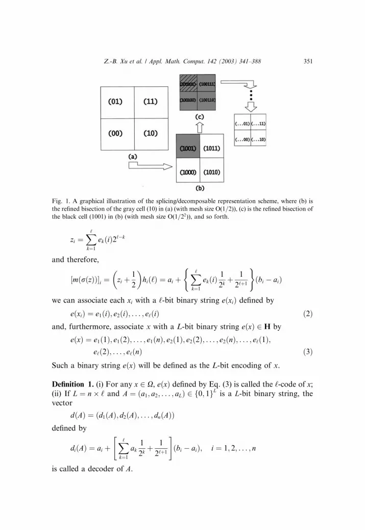
1 < i < n. (It is noted that Cð‘Þ ¼ X.) To emphasize the dependence of Cð‘Þ on‘, we also call Cð‘Þ as ‘th successive refinement partition (briefly, ‘-SRP) of Xbecause Cð‘Þ can be viewed as the consequence of ‘-times successive bisectionson X (cf. Fig. 1). Moreover, if ‘1 and ‘2 are two integers such that ‘2 P ‘1, thepartition Cð‘2Þ is said to be the ð‘2 � ‘1Þ times refinement of Cð‘1Þ, and, cor-respondingly, Cð‘1Þ is the ð‘2 � ‘1Þ times coarseness of Cð‘2Þ.

The center of a cell rðzÞ is the vector mðrðzÞÞ defined by

mðrðzÞÞ ¼ z1

�þ 1

2

�h1ð‘Þ; z2

�þ 1

2

�h2ð‘Þ; . . . ; zn

�þ 1

2

�hnð‘Þ

For any x ¼ ðx1; x2; . . . ; xnÞ 2 X, we now assign the center mðrðzÞÞ to stand forx whenever x 2 mðrðzÞÞ. Then a L-bit (L-length or ‘-resolution) encoding

of x can be obtained as follows: since there is a unique binary string ðe1ðiÞ;e2ðiÞ; . . . ; e‘ðiÞÞ, ek 2 f0; 1g, such that


zi ¼X‘k¼1

ekðiÞ2‘�k

and therefore,

½mðrðzÞÞ�i ¼ zi

�þ 1

2

�hið‘Þ ¼ ai þ

X‘k¼1

ekðiÞ1

2k

(þ 1

2‘þ1

)ðbi � aiÞ

we can associate each xi with a ‘-bit binary string eðxiÞ defined by

eðxiÞ ¼ e1ðiÞ; e2ðiÞ; . . . ; e‘ðiÞ ð2Þand, furthermore, associate x with a L-bit binary string eðxÞ 2 H by

eðxÞ ¼ e1ð1Þ; e1ð2Þ; . . . ; e1ðnÞ; e2ð1Þ; e2ð2Þ; . . . ; e2ðnÞ; . . . ; e‘ð1Þ;e‘ð2Þ; . . . ; e‘ðnÞ ð3Þ

Such a binary string eðxÞ will be defined as the L-bit encoding of x.

Definition 1. (i) For any x 2 X, eðxÞ defined by Eq. (3) is called the ‘-code of x;(ii) If L ¼ n� ‘ and A ¼ ða1; a2; . . . ; aLÞ 2 f0; 1gL is a L-bit binary string, the

vector

dðAÞ ¼ ðd1ðAÞ; d2ðAÞ; . . . ; dnðAÞÞdefined by

diðAÞ ¼ ai þX‘k¼1

ak1

2k

"þ 1

2‘þ1

#ðbi � aiÞ; i ¼ 1; 2; . . . ; n

is called a decoder of A.

Fig. 1. A graphical illustration of the splicing/decomposable representation scheme, where (b) is

the refined bisection of the gray cell (10) in (a) (with mesh size O(1=2)), (c) is the refined bisection of

the black cell (1001) in (b) (with mesh size O(1=22)), and so forth.


By Definition 1, the ‘-code eðxÞ of x is an approximate representation of

x with precision Oð2�‘Þ (more precisely, kxi �P‘

k¼1 eiðkÞ1=2kk1 6

max16 i6 nðbi � aiÞ2�‘), and any string A is the ‘-code of its decoder dðAÞ. Also,it is clear that for any binary string A, its decoder dðAÞ is nothing but the centerof the cell rðzÞ, where z ¼ ðz1; z2; . . . znÞ is specified by

zi ¼X‘k¼1

ak2‘�k

Thus, for any given x 2 X and any preset representation precision (say, e),through partitioning X with the size Hð‘Þ, where ‘ is such that 2�‘

6 e, a uniquecell rðzÞ ¼ hmðrðzÞ;Hð‘ÞÞi in Cð‘Þ can be related, which then leads to a unique

L-bit binary representation (i.e., ‘-code) eðxÞ of x in H ¼ f0; 1gL. Conversely,given a L-bit string A 2 H, via splitting L ¼ n� ‘, a unique vector dðAÞ 2 Xdefined as in (4) then can be corresponded, which, combined with the string-

length ‘, in turn uniquely mapped to a cell hdðAÞ;Hð‘Þi in Cð‘Þ. Accordingly,there are perfect, one-to-one and onto mappings (actually homeomorphisms)

among the problem domain X, the cell space Cð‘Þ and the encoding space H (cf.Fig. 2). It is noted that Cð‘Þ is identical with X in set theory viewpoint, but it

provides a much more powerful, cell-collection representation of X. Also, dueto the existed perfect correspondence, any binary string A in H now does not

serve to represent only a point (vector), but a subset (cell) in the problem

domain. In biological terms, this then means that a string now stand not only

for an individual but for a subpopulation as well. This is one of the exclusive

Fig. 2. The homeomorphisms among problem space X, cell space Cð‘Þ, and encoding (search space)H ¼ f0; 1gL.


features of the suggested representation scheme that distinguish himself from

other encoding system (particularly, the conventional representation scheme).The second exclusive feature of the suggested representation scheme is its

splicing and decomposable property. We state this as the following theorem.

Theorem 1. Assume A ¼ ða1; . . . ; aL1Þ is a ‘-code of dðAÞ, and B ¼ ðb1; . . . ; bL2Þ isa j-code of dðBÞ. If A _ B is the spliced string ðA;BÞ, then

(i) A _ B is a ‘-code of dðAÞ;(ii) A _ B is a ð‘þ jÞ-code of dðA _ BÞ;(iii) dðA _ BÞ ¼ dðAÞ þ ð1=2‘Þ½dðBÞ � ðbi þ aiÞ=2�.

Proof. This is direct from Definition 1 and Eqs. (2) and (3).

Theorem 1 (i) says that kA _ B� dðAÞk1 6Oð2�‘Þ for any binary string B.That is, the spliced encoding ðA;BÞ will always be in the cell hdðAÞ;Hð‘Þi inCð‘Þ. Together with Theorem 1 (ii), this then shows that a higher-resolutionrepresentation of the problem variables, when confined to the region hdðAÞ;Hð‘Þi, can be directly formed via splicing A with additional strings B. Fur-thermore, Theorem 1 (iii) says that such spliced (a long) string can be decoded

through a decomposable manner, that is, through independently decoding two

shorter strings A and B where the decoding of A ðdðAÞÞ is already known (or, atleast, its computation is in common). This splicing/decomposable property can

be shown to be very fundamental for any attempt to perform adaptive EC

computation (like using variable-length representation scheme) (cf. [39]).It particularly underlies applications of all strategies mentioned in the last

section.

The third feature of the suggested representation scheme is its bit-value-

significance interpretability. That is, the significance of each bit of the encoding

can be clearly and uniquely interpreted (hence, each gene of the encoded

chromosome has a specific meaning). Take X ¼ ½0; 1� � ½0; 1� and the binary

string A ¼ ð1; 0; 0; 1; 0; 1Þ as an example (in this case, L ¼ 6, n ¼ 2, ‘ ¼ 3, and

Hð‘Þ ¼ ð1=8; 1=8Þ). By Definition 1, A then is the 3-code of the vectordðAÞ ¼ ð9=16; 7=16Þ 2 X ¼ Cð3Þ. Let us look through the 3-SRP process, i.e.,

Cð1Þ, Cð2Þ, Cð3Þ performed on X (cf. Fig. 1) and see what each bit value of Ameans. In the 1-SRP, Cð1Þ, the domain X is bisected into four 1/2-cells (i.e., the

cells with uniform size 1/2). According to the left-0 and right-1 correspondencerule in each coordinate direction, these four 1/2-cells then can be identified with

(0,0), (0,1), (1,0) and (1,1), as shown in Fig. 1(a). As dðAÞ lies in the cell (1,0)

(the gray square), its 1-code, by Definition 1, should be A1 ¼ ð1; 0Þ. This leadsto the first two bits of A. Likewise, in the 2-SRP, Cð2Þ, X is partitioned into22�2ð1=22Þ-cells which are obtained through further bisecting each cell in Cð1Þalong each direction. Particularly this further divides the 1/2-cell (1,0) into four

1/4-cells that can be respectively labelled by ðA1; 0; 0Þ, ðA1; 0; 1Þ, ðA1; 1; 0Þ and


ðA1; 1; 1Þ (Fig. 1(b)). The dðAÞ is in ðA1; 0; 1Þ-cell (the black square), so its 2-

code should be A2 ¼ ð1; 0; 0; 1Þ, coinciding with the first four positions of A. Inthe same way, X is partitioned into 22�3ð1=23Þ-cells in the 3-SRP, r(3), with the

1/4-cell A2 particularly partitioned into four 1/8-cells labelled by ðA2; 0; 0Þ,ðA2; 0; 1Þ, ðA2; 1; 0Þ and ðA2; 1; 1Þ (Fig. 1(c)). So the 3-code of dðAÞ is found to beðA2; 0; 1Þ, that is, identical with string A. This shows that for any 3-code

A ¼ ða1; a2; a3; a4; a5; a6Þ, each bit value ai can be interpreted geometrically as

follows: a1 ¼ 0ða2 ¼ 0Þ means dðAÞ is in the left half along the x-coordinatedirection (the y-coordinate direction) in Cð1Þ partition, and a1 ¼ 1ða2 ¼ 1Þmeans dðAÞ is in the right half. Therefore, the first two bits A1 ¼ ða1; a2Þ givethe 1-code of dðAÞ and determine the 1/2-precision location of dðAÞ (i.e,

dðAÞ 2 hA1;Hð1ÞiÞ. If a3 ¼ 0 ða4 ¼ 0Þ, it then further indicates that when the

Cð1Þ is refined into Cð2Þ, the dðAÞ lies in the left half of hA1;Hð1Þi in the x-direction (y-direction), and it lies in the right half if a3 ¼ 1 ða4 ¼ 1Þ. Thus amore accurate geometric location, hA2;Hð2Þi, (i.e., the 1/4-precision location)

and a more refined representation, 2-code of dðAÞ, is obtained from

A2 ¼ ða1; a2; a3; a4Þ ¼ ðA1; a3; a4Þ. Similarly we can explain a5 and a6 and con-

clude that A3 ¼ ðA2; a5; a6Þ ¼ A is the 3-code of dðAÞ, and hA;Hð3Þi offers the 1/8-precision location of dðAÞ. This interpretation holds for any high-resolution

Lð¼ n� ‘Þ-bits encoding.The above interpretation reveals an important fact that in the new repre-

sentation scheme the significance of the gene value varies as its position goes

from front to back, and, in particular, the more in front the gene position lies,

the more significantly it functions. We refer such delicate feature of the new

scheme to as the gene-significance-variable property. Actually, it is seen from

the above interpretation that the first n genes of an encoding are responsible forthe location of the variable dðAÞ in a global way (particularly, with Oð1

2Þ-pre-

cision); the next group of n bits are responsible for the location of dðAÞ in a lessglobal (might be called �local�) way, with Oð1

4Þ-precision, and so forth; the last

group of n-bits then locate dðAÞ in an extremely local (might be called �mi-crocosmic�) way (particularly, with O 1

2‘

-precision). Thus, we have seen that as

the encoding length L increases, the representation

ða1; a2; . . . ; an; anþ1; anþ2; . . . ; a2n; . . . ; að‘�1Þn; að‘�1Þnþ1 . . . ; aLÞ

can provide a successive refined (from global, to local, and to microcosmic),

more and more accurate representation of problem variables. This gene-

significance-variable property of the representation scheme embodies many

important information useful to EC search. We will partially explore this in-

formation in the subsequent sections and in [23,24,44]. �

Remark 1. It is worthwhile to note the difference of the concatenation strate-

gies used in the new representation scheme and the conventional scheme: In the

conventional scheme (Eq. (2)), the encoding eðxÞ of a vector x ¼ ðx1; x2; . . . ; xnÞ


is organized in the purely component-wise manner, i.e., the code of x1; eðx1Þ,is collected first, then followed by that of x2; eðx2Þ, and then, by eðx3Þ;eðx4Þ; . . . ; eðxnÞ in order (cf. Eq. (2)). However, in the new representation

scheme, the vector encoding eðxÞ is concatenated in the gene-significance or-

dering way, that is, the most significant bits of all components of x are collectedtogether first, then, less significant, and then, less and less significant bits of all

the components are organized in order (cf. Eq. (3)). This difference has led to

the differences of not only the decoding mappings but also the representation

significance of the two systems.

In the subsequent sections we will demonstrate the usefulness and promise

of the new representation scheme suggested in this section. Particularly, we

show in the next section that with the new scheme, it is possible to define a

much more powerful operator, exclusion-based operator, to emulate the

‘‘survival for the fittest’’ principle.

4. Exclusion-based selection operators

This section defines and explores a somewhat different selection mecha-

nism––the exclusion-based selection operators. We first formalize the exclusion

operators with reference to the cellular partition Cð‘Þ of X.

Definition 2. An exclusion operator is a computationally verifiable test for non-

existence of solution to problem (P) which can be implemented on every cells ofCð‘Þ.

For an immediate example, assume that f satisfies the Lipschitz condition:jf ðxÞ � f ðyÞj6 akx� yk. Then, for any r 2 Cð‘Þ, there is a global maximizer x�in r only if jf ðmðrÞ � f ðx�ÞÞj6 akmðrÞ � x�k6 a=2xðrÞ, where xðrÞ is themesh size of Cð‘Þ, defined by

xðrÞ ¼ 1

2‘max 16 i6 nfbi � aig

This implies that for any reference value fc ¼ f ðxcÞ, fc 6 f ðx�Þ6 f ðmðrÞÞþa=2xðrÞ is a necessary condition for existence of global optimum of ðPÞ. Thusfc P f ðmðrÞÞ þ a=2xðrÞ gives an non-existence test for solution. This test is an

exclusion operator because it can be computationally verified in each cells of

Cð‘Þ.By Definition 2, any exclusion operator can serve to computationally test

non-existence of solution of ðPÞ in any given cells of Cð‘Þ. It therefore can be

used to check if a given string (that is, a cell in Cð‘Þ) is prospective or not as aglobal optimum (or, as a portion of attraction basin of a global optimum) of


ðPÞ. Accordingly, the non-global optimum, or, more loosely, less prospective

strings (cells) can be identified and can be deleted from further consideration.This is the key mechanism that is adopted in the present work to accelerate EC.

Hereafter any selection mechanism based on such exclusion principle will be

called an exclusion-based selection operator.Let r be an arbitrary cell in Cð‘Þ with its centre mðrÞ and the mesh size xðrÞ.

The following provides us with a series of exclusion operators for maximization

problems. Please note that these operators (tests) can be equally applied to

minimization problems by reversing the inequality signs.

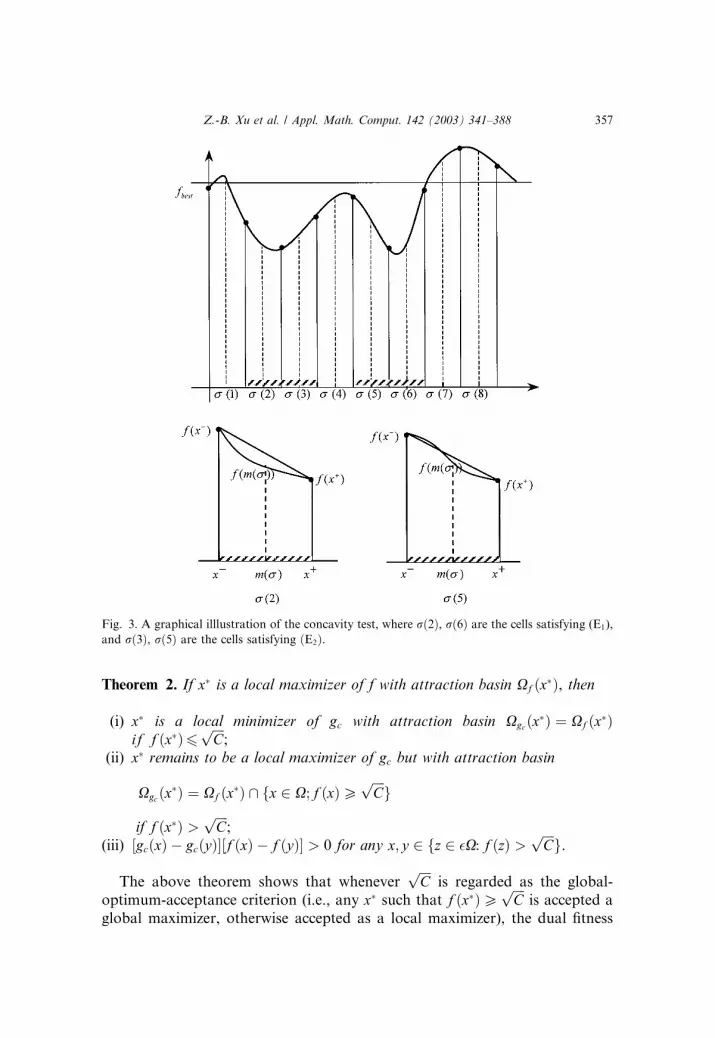
Example 1 [Concavity test]

Suppose f is continuous, then a necessary condition for a string x ¼ mðrÞ tobe global maximizer is that f is concave at neighborhood of x. Therefore, when‘ is sufficiently large, the following tests (E1)–(E2) are exclusion operators.

(E1) There is a direction e 2 RN such that

f ðmðrÞÞ < 1

2½f ðxþÞ þ f ðx�Þ�

where x� ¼ x� ge, xþ ¼ xþ ge and 0 < g6 12xðrÞ.

(E2) There is a direction e 2 RN such that maxff ðxþÞ; f ðx�Þg < fbest and

½f ðxþÞ � f ðmðrÞÞ�½f ðx�Þ � f ðmðrÞÞ� < 0

where xþ and x� are the same as in (E1), and fbest is the current known bestfitness value.

The tests (E1)–(E2) can immediately follow from the observations that every

mðrÞ is in the interior of X, the (E1) features the convex property of f on cell r,and (E2) characterizes the convex and concave overlapped property in which

no global optimum of f exists. See Fig. 3, e.g., for an illustration.

Example 2 [Dual fitness test]

Given an reference value C, we can relate the fitness function f to a new

function gc, called the dual fitness function, defined by

gcðxÞ ¼�f ðxÞ

f 2ðxÞ þ C

It is easy to justify that these two functions are tightly related and there holds

the following basic identity:

gcðxÞ � gcðyÞ ¼f ðxÞf ðyÞ � C

½f 2ðxÞ þ C�½f 2ðyÞ þ C� ½f ðxÞ � f ðyÞ�

Based on this identity, the following properties of gc can be verified:


Theorem 2. If x� is a local maximizer of f with attraction basin Xf ðx�Þ, then

ii(i) x� is a local minimizer of gc with attraction basin Xgcðx�Þ ¼ Xf ðx�Þif f ðx�Þ6

ffiffiffiffiC

p;

i(ii) x� remains to be a local maximizer of gc but with attraction basin

Xgcðx�Þ ¼ Xf ðx�Þ \ fx 2 X; f ðxÞPffiffiffiffiC

pg

if f ðx�Þ >ffiffiffiffiC

p;

(iii) ½gcðxÞ � gcðyÞ�½f ðxÞ � f ðyÞ� > 0 for any x; y 2 fz 2 �X: f ðzÞ >ffiffiffiffiC

pg.

The above theorem shows that wheneverffiffiffiffiC

pis regarded as the global-

optimum-acceptance criterion (i.e., any x� such that f ðx�ÞPffiffiffiffiC

pis accepted a

global maximizer, otherwise accepted as a local maximizer), the dual fitness

Fig. 3. A graphical illlustration of the concavity test, where rð2Þ, rð6Þ are the cells satisfying (E1),

and rð3Þ, rð5Þ are the cells satisfying ðE2Þ.


function gc then provides us a such novel transformation that inverts every

local maximizers (of f) into minimizers (of gc) while retaining global maxi-

mizers (of f) intact (cf. Fig. 4 for an illustration). Consequently, if we takeffiffiffiffiC

p¼ fbest � e be the ‘‘acceptable-so-far’’ optimum criterion, where e is a very

small real number, the gc then can be used as a quick discriminator of whether

or not a string x lies in an attraction basin of a local maximizer (the less

prospective area), or in a global attraction basin (the high-prospective area)

that needs to be further searched. This analysis then shows that whenever theencoding length ‘ satisfies the minimal resolution requirement (i.e., the dis-

cretization is fine enough so that no global and local optima lie in the same cell

of Cð‘Þ) [32], the following test (E3) defines another exclusion operator:

(E3) For a fixed y 2 r andffiffiffiffiC

p¼ fbest � e,

½gcðmðrÞÞ � gcðyÞ�½f ðmðrÞÞ � f ðyÞ� < 0

Fig. 4. An illustration of the dual fitness function transformation, where f ðxÞ ¼ sinð3pxÞþ0:75x2 � 4:6xþ 8:35 and gðc; xÞ ¼ f ðxÞ=½f 2ðxÞ þ c�. It is seen that under the global-optimum-

acceptance criterionffiffiffic

p, any local maximizer of f is inverted into a local minimizer of gðc; xÞ,

while any ‘‘global’’ maximizer of f remains intact.


Example 3 [Lipschitz test]

Let £ðf ; aÞ denote the family of all continuous functions that satisfies the

Lipschitz conditions: jf ðxÞ � f ðyÞj6 aðXÞkx� yk, x; y 2 X 2 Cð‘Þ. Then the

following tests (E3)–(E4) are exclusion operators.

(E4) fbest > f ðmðrÞÞ þ aðrÞ2;wðrÞ if f 2 £ðf ; aÞ

(E5) fbest > f ðmðrÞÞ þ aðrÞ8

x2ðrÞ; if f 0 2 £ðf ; aÞ

where fbest is again the ‘‘best-so-far’’ fitness value, and f 0 is the derivative of f .The (E4) has been given as the immediate example of Definition 2. The (E5)

can be justified as follows: Assume x� ¼ mðrÞ is a global maximizer of f, thenf 0ðx�Þ ¼ 0. The well known Taylor formula then implies

f ðx�Þ � f ðxÞ ¼ jf ðxÞ � f ðx�Þj

¼ f 0ðx�Þðx�� x�Þ þ 1

2

Z 1

0

½f 0ðx� þ nðx� x�ÞÞ � f 0ðx�Þ�ðx� x�Þdn��

61

2

Z 1

0

kf 0ðx� þ nðx� x�ÞÞ � f 0ðx�Þkkðx� x�Þkdn

61

2ðrÞkðx� x�Þk2 6 1

8aðrÞxðrÞ2 8x 2 r:

So f ðx�Þ6 f ðmðrÞÞ þ ð1=8ÞaðrÞx2ðrÞ holds, and, whenever (E5) is satisfied, we

get f ðx�Þ6 f ðmðrÞÞ þ ð1=8ÞaðrÞx2ðrÞ < fbest and arrive to a contradiction:

f ðx�Þ < fbest.

Example 4 [Formal series test]

Let J be the class of all functions that can be expressed as a finite number

of superpositions of formal series and their absolute values, i.e., J ¼ff : RN ! R; 9k formal series f ðjÞ; j ¼ 1; 2; . . . ; k, such that f ðxÞ ¼ f ð1ÞðxÞþPk

j¼2 jf ðjÞðxÞjg. For any f 2 J, the absolute value Aðf Þ of f is defined by

Aðf Þ ¼ Aðf ð1ÞÞ þXkj¼2

Aðf ðjÞÞðxÞ

and, if gðxÞ ¼P1

jaj¼0 caxa is a formal series, AðgÞ is defined by

AðgÞðxÞ ¼X1jaj¼0

jcajxa

where, as usual, the notations a ¼ ða1; a2; . . . ; aNÞ 2 ZNþ , jaj ¼ ja1j þ ja2j þ þ

jaN j, xa ¼ ðx1Þa1ðx2Þa2 ðxN ÞaN , and ca 2 R. Given two formal series gð1Þ andgð2Þ, we presume that gð1Þ � gð2Þ if and only if


gð1ÞðxÞ ¼X1jaj¼0

cð1Þa xa; gð2ÞðxÞ ¼X1jaj¼0

cð2Þa xa with jcð1Þa jP jcð2Þa j

Also we define jxj ¼ ðjx1j; jx2j; . . . ; jx3jÞ for any x 2 RN .

For any f 2 J and g � Aðf Þ, it is known [41] that there holds the following

basic inequality:

jf ðxÞ � f ðyÞj6AðgÞðjyj þ jx� yjÞ � AðgÞðjyjÞ 8x; y 2 RN ð4Þ

This implies, similar to test (E4), that the following test (E6) is an exclusion

operator.

(E6) There is a formal series g � Aðf Þ such that

fbest P f ðmðrÞÞ þ AðgÞ jmðrÞj�

þ 1

2xðrÞ

�� AðgÞðjmðrÞjÞ

Various other exclusion operators may also be constructed by virtue of

other delicate mathematical tools such as interval arithmetic [15] and the cell

mapping methods [40,41].

Remark 2

(i) The exclusion-based selection is the main component and contributor

to the accelerated evolutionary algorithms (the fast-EAs). Aiming at sup-pressing the resampling effect of EC, such type of selection provides a smart

guidance to EC search towards promising areas through eliminating non-

promising areas. Different in principle from the conventional selection opera-

tors, the construction of which is based on sufficient condition for existence of

solution to ðPÞ, the exclusion-based selection operators can be constructed

based on necessary condition. This presents a general methodology of con-

structing exclusion operators. The above listed (E1)–(E6) show such examples

of the construction.(ii) The application of exclusion-based operator has another advantage: It

can very naturally incorporate some useful properties of the objective function

into the EC search, providing other acceleration means whenever possible.

Indeed, Examples 1–4 all have taken advantage of properties of f in certain

ways (say, continuity in Examples 1 and 2, Lipschitz conditions in Example 3

and analyticity in Example 4). As a general rule, the more exclusive property of

f is utilized, the more sharp (accurate) test could be deduced (for example, (E5)

is sharper than (E4) when the Lipschitz condition was applied for the derivativef 0 instead of for f). These different tests deduced from different properties by

no means have to be applied for a problem in the same time. They can, for

instance, be applied either independently, or with several together, or totally


simultaneously, depending on the available information on f that can actually

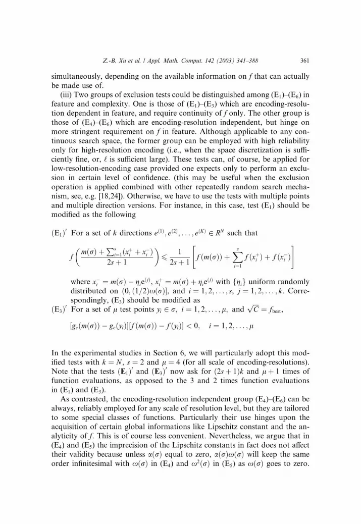
be made use of.(iii) Two groups of exclusion tests could be distinguished among (E1)–(E6) in

feature and complexity. One is those of (E1)–(E3) which are encoding-resolu-

tion dependent in feature, and require continuity of f only. The other group is

those of (E4)–(E6) which are encoding-resolution independent, but hinge on

more stringent requirement on f in feature. Although applicable to any con-

tinuous search space, the former group can be employed with high reliability

only for high-resolution encoding (i.e., when the space discretization is suffi-

ciently fine, or, ‘ is sufficient large). These tests can, of course, be applied forlow-resolution-encoding case provided one expects only to perform an exclu-

sion in certain level of confidence. (this may be useful when the exclusion

operation is applied combined with other repeatedly random search mecha-

nism, see, e.g. [18,24]). Otherwise, we have to use the tests with multiple points

and multiple direction versions. For instance, in this case, test (E1) should be

modified as the following

ðE1Þ0 For a set of k directions eð1Þ; eð2Þ; . . . ; eðKÞ 2 RN such that

fmðrÞ þ

Psi¼1ðxþi þ x�i Þ

2sþ 1

� �6

1

2sþ 1f ðmðrÞÞ"

þXsi¼1

f ðxþi Þ þ f ðx�i Þ#

where x�i ¼ mðrÞ � gieðjÞ, xþi ¼ mðrÞ þ gie

ðjÞ with fgig uniform randomly

distributed on ð0; ð1=2ÞxðrÞ�, and i ¼ 1; 2; . . . ; s, j ¼ 1; 2; . . . ; k. Corre-spondingly, (E3) should be modified as

ðE3Þ0 For a set of l test points yi 2 r; i ¼ 1; 2; . . . ; l; andffiffiffiffiC

p¼ fbest,

½gcðmðrÞÞ � gcðyiÞ�½f ðmðrÞÞ � f ðyiÞ� < 0; i ¼ 1; 2; . . . ; l

In the experimental studies in Section 6, we will particularly adopt this mod-

ified tests with k ¼ N , s ¼ 2 and l ¼ 4 (for all scale of encoding-resolutions).Note that the tests ðE1Þ0 and ðE3Þ0 now ask for ð2sþ 1Þk and l þ 1 times of

function evaluations, as opposed to the 3 and 2 times function evaluations

in (E1) and (E3).

As contrasted, the encoding-resolution independent group (E4)–(E6) can be

always, reliably employed for any scale of resolution level, but they are tailored

to some special classes of functions. Particularly their use hinges upon the

acquisition of certain global informations like Lipschitz constant and the an-

alyticity of f. This is of course less convenient. Nevertheless, we argue that in(E4) and (E5) the imprecision of the Lipschitz constants in fact does not affect

their validity because unless aðrÞ equal to zero, aðrÞxðrÞ will keep the same

order infinitesimal with xðrÞ in (E4) and x2ðrÞ in (E5) as xðrÞ goes to zero.


Therefore, in practical applications, a coarse estimation of the Lipschitz

constants can be applied (note however that the coarseness of the estimationmay have impact on efficiency of exclusion, in spite of not so sensitive, [40]).

The test (E6) is a tactical modification of the Lipschitz test (E4) in the sense that

Lipschitz constant does not involved any more in (E6). This is because the basic

inequality (4) presents a very useful localized generalization of the Lipschitz

condition jf ðxÞ � f ðyÞj6 akx� yk in the sense that the right-hand side of the

inequality will go to zero whenever kx� yk does. In applications of test (E6), a

function g satisfying g � Aðf Þ must be chosen a priori. To facilitate this, let us

notice that the definition of absolute value of a formal series can yield thefollowing estimations:

R1:Pki¼1

jcijAðfiÞ � APki¼1

cifi

� �

and

R2: AðhÞðAðQÞÞ � AðhðQÞÞ;

where fi, h, Q are all formal series. And, furthermore, we easily find the ab-solute values of all elementary functions given as in Table 1. Therefore for any

given function f 2 J, a function g ¼ Nðf Þ satisfying g � Aðf Þ can be con-

structed straightforwardly. The procedure may be as follows (cf. [41]):

Step 1: split f : into basic terms so that each basic term is an elementary

function composition of elementary functions and f is a finite number of su-

perposition of basic terms and their absolute values;

Step 2: write down the absolute value of each respective elementary func-

tions according to Table 1;

Table 1

Absolute value of elementary functions

f ðxÞ jf ðxÞjexpðxÞ expðxÞlnðxÞ � lnð1� xÞsinðxÞ shðxÞcosðxÞ chðxÞtgðxÞ tgðxÞsecðxÞ secðxÞarcsinðxÞ arcsinðxÞarctgðxÞ th�1ðxÞthðxÞ tgðxÞsh�1ðxÞ arcsinðxÞPn

i¼1 cixi

Pni¼1 jcijxi


Step 3: g ¼ Nðf Þ is defined according to NðPk

i¼1 cifiÞ ¼Pk

i¼1 jcijNðfiÞ andNðhðQÞÞ ¼ AðhÞðAðQÞÞ.

For example, assume

f ðx1; x2; x3Þ ¼ 2 sinðx1Þ þ expððx21 þ lnðx1Þ þ x3ÞÞ� jx1 þ x2x3 þ arctgðx2 þ 3Þj

Then we can express f ðxÞ ¼ 2f1ðxÞ þ f2ðxÞ � jf3ðxÞj with the basic terms defined

by f1ðxÞ ¼ sinðx1Þ, f2ðxÞ ¼ expððx21 þ lnðx1Þ þ x3ÞÞ and f3ðxÞ ¼ jx1 þ x2x3 þarctgðxþ 3Þj. Table 1 shows that the absolute values of elementary functions et,sinðx1Þ, lnðx1Þ and arctgðx2 þ 3Þ are et, shðx1Þ, � lnð1� x1Þ and th�1ðx2Þ, re-spectively. Consequently, Nðf1Þ ¼ shðx1Þ; Nðf2Þ ¼ expðx21 � lnð1� x1Þ þ x3ÞÞand Nðf3Þ ¼ th�1ðx2Þ, and, according to step 3,

g ¼ Nðf Þ ¼ 2shðx1Þ þ expðx21 � lnð1� x1Þ þ x3ÞÞ þ th�1ðx2Þ

5. A case study: fast-GAs

In this section we present a case study to show how all the strategies de-

veloped in the previous sections can be embedded into the known evolutionary

algorithms, to yield accelerated versions of the algorithms. We will particularlyconsider GAs as an example. Consequently, an accelerated genetic algorithm

called the fast-GA will be developed. The incorporation of the developed

strategies with other known evolutionary algorithms might be straightforward,

and could be done similarly as that in the example presented below.

5.1. The fast-GA

5.1.1. I. Initialization step

I.1. Set k ¼ 0, Xð0Þ ¼ X, nð0Þ ¼ 1 and f ð0Þbest ¼ f ð�1Þ

best ¼ f ð�2Þbest ¼ 0; determine the

encoding resolution ‘, and stopping criteria e1 and e2, where e1 is the solu-tion precision requirement and e2 is the space discretization precision tol-

erance.

I.2. Assign the GA parameters, such as

Pc––the crossover rate; Pm––the mutation rate;

N––the population size;

M––the maximum number of GA evolution.

5.1.2. II. Iteration step

Assume XðkÞ consists of nðkÞ subregions, say, XðkÞ ¼ XðkÞ1 [ XðkÞ

2 [ [ XðkÞnðkÞ.

For each subregion XðkÞi , do the following


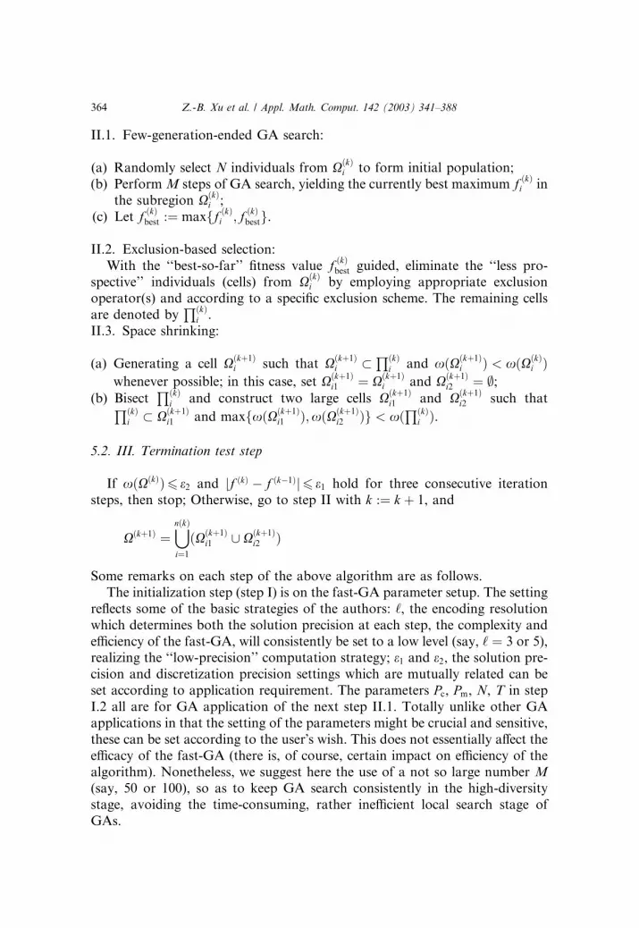
II.1. Few-generation-ended GA search:

(a) Randomly select N individuals from XðkÞi to form initial population;

(b) PerformM steps of GA search, yielding the currently best maximum f ðkÞi in

the subregion XðkÞi ;

(c) Let f ðkÞbest :¼ maxff ðkÞ

i ; f ðkÞbestg.

II.2. Exclusion-based selection:

With the ‘‘best-so-far’’ fitness value f ðkÞbest guided, eliminate the ‘‘less pro-

spective’’ individuals (cells) from XðkÞi by employing appropriate exclusion

operator(s) and according to a specific exclusion scheme. The remaining cells

are denoted byQðkÞ

i .

II.3. Space shrinking:

(a) Generating a cell Xðkþ1Þi such that Xðkþ1Þ

i �QðkÞ

i and xðXðkþ1Þi Þ < xðXðkÞ

i Þwhenever possible; in this case, set Xðkþ1Þ

i1 ¼ Xðkþ1Þi and Xðkþ1Þ

i2 ¼ ;;(b) Bisect

QðkÞi and construct two large cells Xðkþ1Þ

i1 and Xðkþ1Þi2 such thatQðkÞ

i � Xðkþ1Þi1 and maxfxðXðkþ1Þ

i1 Þ;xðXðkþ1Þi2 Þg < xð

QðkÞi Þ.

5.2. III. Termination test step

If xðXðkÞÞ6 e2 and jf ðkÞ � f ðk�1Þj6 e1 hold for three consecutive iteration

steps, then stop; Otherwise, go to step II with k :¼ k þ 1, and

Xðkþ1Þ ¼[nðkÞi¼1

ðXðkþ1Þi1 [ Xðkþ1Þ

i2 Þ

Some remarks on each step of the above algorithm are as follows.

The initialization step (step I) is on the fast-GA parameter setup. The setting

reflects some of the basic strategies of the authors: ‘, the encoding resolution

which determines both the solution precision at each step, the complexity and

efficiency of the fast-GA, will consistently be set to a low level (say, ‘ ¼ 3 or 5),realizing the ‘‘low-precision’’ computation strategy; e1 and e2, the solution pre-

cision and discretization precision settings which are mutually related can be

set according to application requirement. The parameters Pc, Pm, N, T in step

I.2 all are for GA application of the next step II.1. Totally unlike other GA

applications in that the setting of the parameters might be crucial and sensitive,

these can be set according to the user�s wish. This does not essentially affect theefficacy of the fast-GA (there is, of course, certain impact on efficiency of the

algorithm). Nonetheless, we suggest here the use of a not so large number M(say, 50 or 100), so as to keep GA search consistently in the high-diversity

stage, avoiding the time-consuming, rather inefficient local search stage of

GAs.


The iteration step (step II) is the core of the algorithm. Step II.1 performs

the ‘‘few (M)-generation-ended’’ GA search, aiming to find the best individualsin each subregion of the current search space in a most economic and efficient

way, and then update the ‘‘best-so-far’’ fitness value fbest. This ‘‘best-so-far’’fitness value is used as reference in the next step II.2 to eliminate the ‘‘less-

prospective’’ areas in the current search space, guiding the fast-GA search to

promising areas. In the exclusion-based selection step (step II.2), two key op-

tional strategies have to be made: the choice of exclusion operator(s) and the

design of the specific exclusion scheme. As noted in Remark 2, which and how

many exclusion operators should be applied in this step depend on user�s choiceand on a prior understanding on the feature of the problem in consideration. In

general, the more exclusion operators are employed, the more ‘‘less-prospec-

tive’’ areas could be excluded, but the more function evaluation (cost) must be

paid. (It is noted that to implement the exclusion-based selection on all cells in

XðkÞi requires a total of 2‘n times function evaluations when an exclusion op-

erator with complexity of one function evaluation is applied.) Therefore there

is a trade-off between the exclusion efficiency and exclusion complexity. To

compromise these two contradictive factors, an appropriate exclusion schemethat specifies how many and in what manner the cells in XðkÞ are excluded thus

should be developed. We propose a such scheme called ‘‘orange-peelingscheme’’ in Remark 3, which instead of performing exclusion test on every cells,

a portion of cells are carefully selected for possible elimination.

The space-shrinking step (step II.3) presents two somewhat different un-

derlying search space reduction schemes. One is that could be named as

merging scheme (II.3-(1)): all the remaining cells are merged into one big cell, asthe next step search space, whenever it shrinks. The other is the forking scheme(II.3-(2)): the remaining cells are forked into two groups, with each being en-

closed by a size-shrunk cell. The two size-shrunk cells are then taken as the next

step search space. These space shrinking strategies, schematically shown as in

Fig. 5, seem conservative, but are quite appropriate in preventing the re-

maining cells from possibly exponential growth in number. The simulations

provided in the next section all strongly support these strategies.

The ‘‘few-generation-ended’’ GA search step (step II.1) combined with the

low-encoding-resolution setting (step I.1) embodies the low-resolution com-putation with reinialization strategy. The space shrinking together with the

reinitialization amount in principle, to adaptively controlling the mapping

from the fixed-length binary genes to real numbers and dynamically changing

the problem representation with successive higher resolution (geometrically,

through partitioning the shrunk space with refined mesh size). Thus with the

suggested schemes, an arbitrary precision solution can be expected to be found

via the low-precision computation.

Finally, we remark that the common use of the static binary place-valuecoding for real-valued parameters of the phenotypes usually forces either the


sacrifice of efficiency of search for representation precision or vice versa. The

fast-GA proposed above, however, provides a mechanism that avoids this

dilemma, and it demonstrates that a sacrifice of search resolution need notnecessarily lead to an identical loss of precision in the search result. There have

been several other GA variants that possess the same feature (e.g., [25,32]). But

all of them have used the convergence statistics of evolution to guide search

(specifically, to trig their search until the diversity of the current population is

exhausted), thereby time-consuming and unavoidably encountering premature

convergence [26,37]. In contrast, the fast-GA reinitializes its focused search

after a fixed (M)-generation evolution, independent of the convergence sta-

tistics, and, there would hardly be any premature convergence due to the searchspace shrinking scheme and use of exclusion-based selection operators.

Remark 3. To compromise the search space shrinking speed (exclusion effi-

ciency) and the exclusion complexity, a partial exclusion strategy may be more

beneficial that performs possible exclusion in a portion instead of whole cells

in XðkÞi . We suggest particularly the following ‘‘orange-peeling scheme’’:

orange-peeling scheme: Successively test the boundary cells of XðkÞi (layer

by layer) until one cell is met in a husk layer that cannot be eliminated.

Fig. 5. A schematic illustration for the search space shrinking (merging/forking) procedure in the

fast-GA.


If there is no husk layer, all cells of which are justified to be eliminated,

bisect XðkÞi into two smaller subregions.

Here a husk layer is a face of XðkÞi (viewed as a hyperrectangle in Rn), or,

equivalently, the cells bounded by a schema of the form:

R ¼fða1; . . . ; a‘nÞ : 9an is such that ai ¼ anþi ¼ ¼ að‘�1Þnþi

¼ 0 ðor 1Þ:aj ¼ � for any other indices jg

(cf. Fig. 6). This scheme offers not only a partial exclusion way but a specific

space shrinking scheme as well. Actually, whenever one husk layer of XðkÞi is

justified to be able to delete, the remaining cellsQðkÞ

i are covered naturally bya big cell with the mesh size ð2‘n � 2‘ÞxðrðkÞ

i Þ, which is strictly less than

2‘nxðrðkÞi Þ of XðkÞ

i . In this case, the search space XðkÞi is naturally shrunk to

Xðkþ1Þi ¼

QðkÞi (step II.3-(1)). It is observed that with this scheme, the complexity

of the exclusion-based selection significantly reduced, at least from 2‘n to

2‘n � ð2‘ � 2Þn times of function evaluation.

6. Simulation and comparison

We now experimentally evaluate performance of the fast-GA, with its per-formance compared again the SGA, and other latest, fairly established variants

of GAs in terms of solution quality and computational efficiency. All experi-

ments are conducted on a Pentium II 300 computer.

Fig. 6. The husk larges of a search space X (cellularly partitioned by l ¼ 3). They respectively

correspond to the schemata: (0 � 0 � 0) (the left) (1 � 1 � 1) (the right) (0 � 0 � 0) (the lower)

(1 � 1 � 1) (the upper).


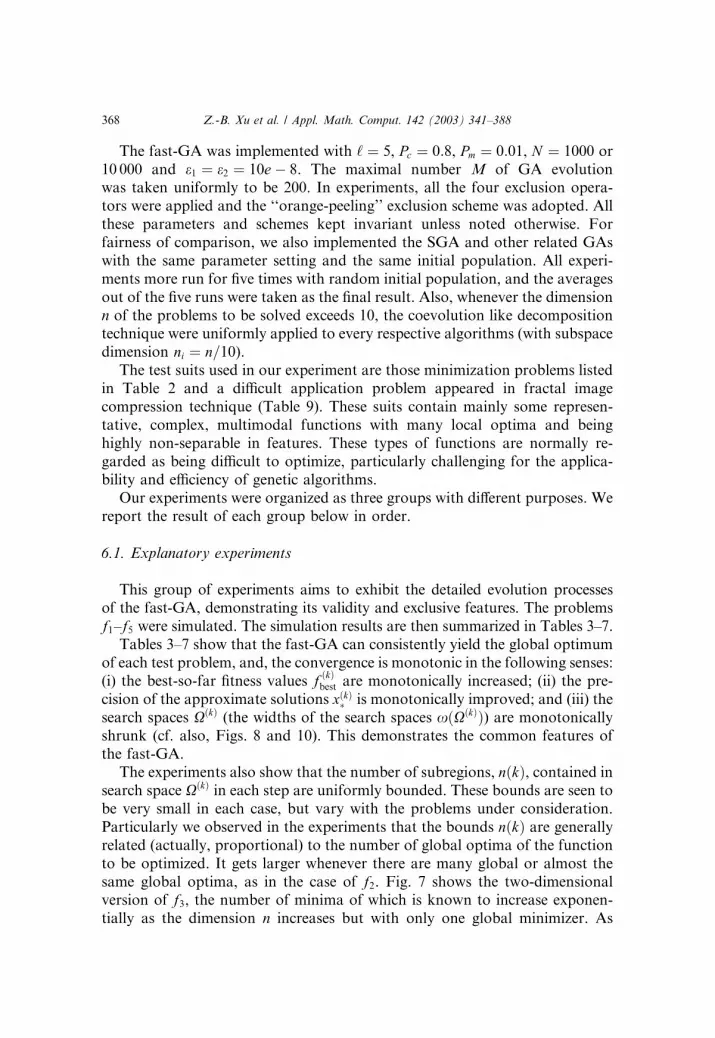
The fast-GA was implemented with ‘ ¼ 5, Pc ¼ 0:8, Pm ¼ 0:01, N ¼ 1000 or

10 000 and e1 ¼ e2 ¼ 10e� 8. The maximal number M of GA evolutionwas taken uniformly to be 200. In experiments, all the four exclusion opera-

tors were applied and the ‘‘orange-peeling’’ exclusion scheme was adopted. All

these parameters and schemes kept invariant unless noted otherwise. For

fairness of comparison, we also implemented the SGA and other related GAs

with the same parameter setting and the same initial population. All experi-

ments more run for five times with random initial population, and the averages

out of the five runs were taken as the final result. Also, whenever the dimension

n of the problems to be solved exceeds 10, the coevolution like decompositiontechnique were uniformly applied to every respective algorithms (with subspace

dimension ni ¼ n=10).The test suits used in our experiment are those minimization problems listed

in Table 2 and a difficult application problem appeared in fractal image

compression technique (Table 9). These suits contain mainly some represen-

tative, complex, multimodal functions with many local optima and being

highly non-separable in features. These types of functions are normally re-

garded as being difficult to optimize, particularly challenging for the applica-bility and efficiency of genetic algorithms.

Our experiments were organized as three groups with different purposes. We

report the result of each group below in order.

6.1. Explanatory experiments

This group of experiments aims to exhibit the detailed evolution processesof the fast-GA, demonstrating its validity and exclusive features. The problems

f1–f5 were simulated. The simulation results are then summarized in Tables 3–7.Tables 3–7 show that the fast-GA can consistently yield the global optimum

of each test problem, and, the convergence is monotonic in the following senses:

(i) the best-so-far fitness values f ðkÞbest are monotonically increased; (ii) the pre-

cision of the approximate solutions xðkÞ� is monotonically improved; and (iii) the

search spaces XðkÞ (the widths of the search spaces xðXðkÞÞ) are monotonicallyshrunk (cf. also, Figs. 8 and 10). This demonstrates the common features ofthe fast-GA.

The experiments also show that the number of subregions, nðkÞ, contained insearch space XðkÞ in each step are uniformly bounded. These bounds are seen to

be very small in each case, but vary with the problems under consideration.

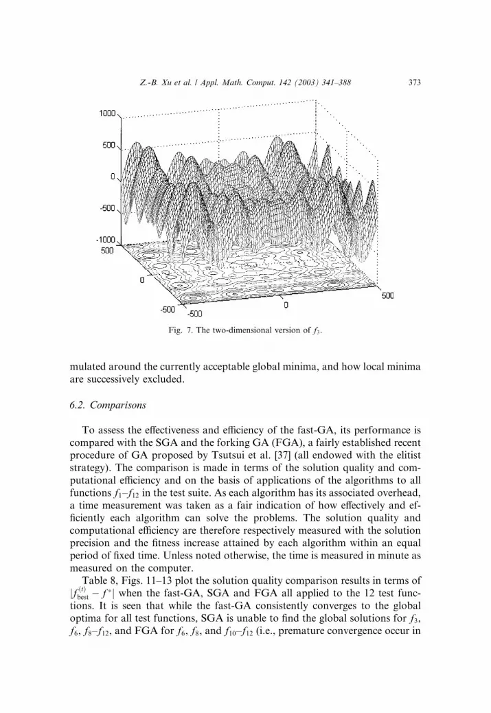
Particularly we observed in the experiments that the bounds nðkÞ are generallyrelated (actually, proportional) to the number of global optima of the function

to be optimized. It gets larger whenever there are many global or almost the

same global optima, as in the case of f2. Fig. 7 shows the two-dimensionalversion of f3, the number of minima of which is known to increase exponen-

tially as the dimension n increases but with only one global minimizer. As


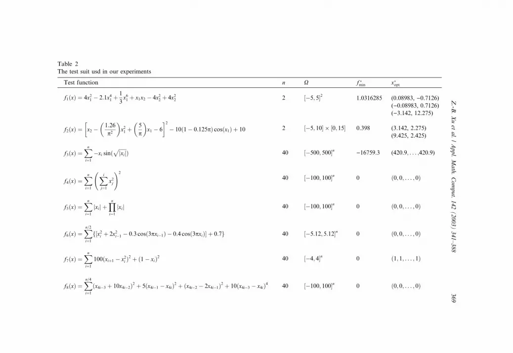
Table 2

The test suit usd in our experiments

Test function n X f �min x�opt

f1ðxÞ ¼ 4x21 � 2:1x41 þ1

3x61 þ x1x2 � 4x22 þ 4x22 2 ½�5; 5�2 1.0316285 (0.08983, )0.7126)

()0.08983, 0.7126)()3.142, 12.275)

f2ðxÞ ¼ x2

�� 1:26

p2

� �x21 þ

5

p

� �x1 � 6

�2� 10ð1� 0:125pÞ cosðx1Þ þ 10 2 ½�5; 10� � ½0; 15� 0.398 (3.142, 2.275)

(9.425, 2.425)

f3ðxÞ ¼Xni¼1

�xi sinðffiffiffiffiffiffijxij

pÞ 40 ½�500; 500�n )16759.3 (420.9; . . . ;420.9)

f4ðxÞ ¼Xni¼1

Xi

j¼1x2j

!2

40 ½�100; 100�n 0 ð0; 0; . . . ; 0Þ

f5ðxÞ ¼Xni¼1

jxij þYni¼1

jxij 40 ½�100; 100�n 0 ð0; 0; . . . ; 0Þ

f6ðxÞ ¼Xn=2i¼1

f½x2i þ 2x2i�1 � 0:3 cosð3pxi�1Þ � 0:4 cosð3pxiÞ� þ 0:7g 40 ½�5:12; 5:12�n 0 ð0; 0; . . . ; 0Þ

f7ðxÞ ¼Xni¼1

100ðxiþ1 � x2i Þ2 þ ð1� xiÞ2 40 ½�4; 4�n 0 ð1; 1; . . . ; 1Þ

f8ðxÞ ¼Xn=4i¼1

ðx4i�3 þ 10x4i�2Þ2 þ 5ðx4i�1 � x4iÞ2 þ ðx4i�2 � 2x4i�1Þ2 þ 10ðx4i�3 � x4iÞ4 40 ½�100; 100�n 0 ð0; 0; . . . ; 0Þ

Z.-B

.Xuet

al./Appl.Math.Comput.142(2003)341–388

369

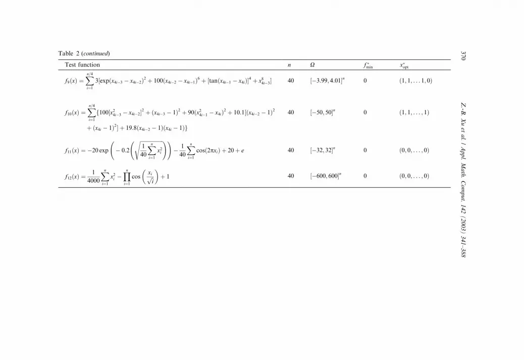
Table 2 (continued)

Test function n X f �min x�opt

f9ðxÞ ¼Xn=4i¼1

3½expðx4i�3 � x4i�2Þ2 þ 100ðx4i�2 � x4i�1Þ6 þ ½tanðx4i�1 � x4iÞ�4 þ x84i�3� 40 ½�3:99; 4:01�n 0 ð1; 1; . . . 1; 0Þ

f10ðxÞ ¼Xn=4i¼1

f100½x24i�3 � x4i�2�2 þ ðx4i�3 � 1Þ2 þ 90ðx24i�1 � x4iÞ2 þ 10:1½ðx4i�2 � 1Þ2

þ ðx4i � 1Þ2� þ 19:8ðx4i�2 � 1Þðx4i � 1Þg

40 ½�50; 50�n 0 ð1; 1; . . . ; 1Þ

f11ðxÞ ¼ �20 exp

� 0:2

ffiffiffiffiffiffiffiffiffiffiffiffiffiffiffiffiffiffi1

40

Xni¼1

x2i

s !!� 1

40

Xni¼1

cosð2pxiÞ þ 20þ e 40 ½�32; 32�n 0 ð0; 0; . . . ; 0Þ

f12ðxÞ ¼1

4000

Xni¼1

x2i �Yni¼1

cosxiffiffii

p� �

þ 1 40 ½�600; 600�n 0 ð0; 0; . . . ; 0Þ

370

Z.-B

.Xuet

al./Appl.Math.Comput.142(2003)341–388

Table 3

The evolution process of the fast-GA applied to f1

Iteration (k) Width of

research space

xðXðkÞÞ

jf ðkÞbest � f �j Percentage of

deleted cells in

XðkÞ

Number of

subregions

contained in XðkÞ

1 10 5.198905 97.7 1

2 1.875 0.683846 84.8 1

3 1.523 0.060562 0 1

4 0.7615 0.020697 99.6 2

5 0.05 10e)5 Stopping criteria

are met

2

xmin ¼ ð�0:089226; 0:712423Þ; ð0:089226;�0:712546Þ

Table 4



research space

xðXðkÞÞ


deleted cells in

XðkÞ

Number of

subregions

contained in XðkÞ

1 15 1.236906 29.8 1

2 12.767 0.103892 16.8 1

3 12.767 0.003590 0 1

4 10.783 0.001807 94.1 2

5 10.717 0.000232 0 2

6 6.158 0.000203 97.3 3


are met

3

x ¼ ð�3:140701; 12:275548Þ; ð3:137760; 2:279323Þ; ð9:415894; 2:467756Þ

Table 5



research space

xðXðkÞÞ


deleted cells in

XðkÞ

Number of

subregions

contained in XðkÞ

1 1000 3304.91874 22.0 1

2 780 1338.30647 97.6 1

3 31 992.34704 98.4 1

4 5 226.43583 76.0 1


are met

1

x ¼ ð421:1; 421:1; . . . ; 421:1Þ


compared, Fig. 9 shows the function f1 that has not so many local optima but

with two global minimizers. The evolution details (particularly, the search

space shrinking details) of the fast-GA when applied to minimization of these

two functions are presented respectively in Figs. 8 and 10 (corresponding toTables 3 and 5), which demonstrate clearly how the remaining cells are accu-

Table 6



research

space xðXkÞ


deleted cellsin

X�

Number of

subregions

contained in Xk

1 200 1.1eþ04 86.2 1

2 25 9.4eþ01 75.9 1

3 6.0 3.8eþ00 83.3 1

4 0.99 2.3e)01 80.0 1

5 0.19 3.0e)02 73.7 1

6 0.05 7.3e)03 86.0 1

7 0.007 3.3e)04 71.4 1

8 0.002 2.3e)06 85.0 1

9 0.0003 6.9e)07 66.7 1

10 0.0001 8.4e)08 71.5 1

11 0.00003 4.9e)09 Stopping criteria

are met

1

x ¼ ð0:000001;�0:000063; 0:000027; . . . ; 0:000031Þ

Table 7



research space

xðXkÞ


deleted cells in

X�

Number of

subregions

contained in Xk

1 200 9.43eþ01 95.5 1

2 9 5.42e)01 88.9 1

3 1 1.20e)01 69.0 1

4 0.3 1.62e)02 68.8 1

5 0.09 1.17e)03 50.3 1

6 0.03 1.37e)04 76.7 1

7 0.004 9.81e)06 75.0 1

8 0.001 1.12e)06 96.0 1

9 0.00003 8.97e)08 Stopping criteria

are met

1

x ¼ ð0:000089;�0:000254; 0:000327; . . . ; 0:000007Þ


mulated around the currently acceptable global minima, and how local minima

are successively excluded.

6.2. Comparisons

To assess the effectiveness and efficiency of the fast-GA, its performance is

compared with the SGA and the forking GA (FGA), a fairly established recent

procedure of GA proposed by Tsutsui et al. [37] (all endowed with the elitist

strategy). The comparison is made in terms of the solution quality and com-

putational efficiency and on the basis of applications of the algorithms to all

functions f1–f12 in the test suite. As each algorithm has its associated overhead,

a time measurement was taken as a fair indication of how effectively and ef-ficiently each algorithm can solve the problems. The solution quality and

computational efficiency are therefore respectively measured with the solution

precision and the fitness increase attained by each algorithm within an equal

period of fixed time. Unless noted otherwise, the time is measured in minute as

measured on the computer.

Table 8, Figs. 11–13 plot the solution quality comparison results in terms of

jf ðtÞbest � f �j when the fast-GA, SGA and FGA all applied to the 12 test func-

tions. It is seen that while the fast-GA consistently converges to the globaloptima for all test functions, SGA is unable to find the global solutions for f3,f6, f8–f12, and FGA for f6, f8, and f10–f12 (i.e., premature convergence occur in

Fig. 7. The two-dimensional version of f3.


these cases). So while the fast-GA can successively solve all the problems, SGA

can only solve 5/12 and FGA 7/12 of the problems. In the cases when all al-

gorithms converge, Table 8 shows that the fast-GA can always attains higher-

solution precision. That is, the fast GA outperforms SGA and FGA in solution

quality (particularly in the senses of obviating premature convergence and

wider applicability).

The computational efficiency comparison results are shown in Figs. 11–13. Itis clear from these figures that the fast-GA exhibits also a very significant

outperformance over the SGA and FGA for all the test functions. Particularly

the efficiency speed-up of the fast-GA can be seen to be at least more than four

times higher, as compared with SGA, and more than 2.5 (averagingly 6) times

higher, as compared with FGA the cases where all algorithms converge. In

addition, we can observe from Figs. 11–13 that such efficiency acceleration

becomes even more and more striking when the function to be optimized gets

more and more complex. Even with such efficiency speed-up, the guaranteed

Fig. 8. The search space (containing all the cells) shrinking process when the fast-GA is applied to

f3 ðn ¼ 2Þ, where ‘‘�’’ is the location of the global minimiza, and ‘‘�’’ is the best-so-far solutionfound by the algorithm. The darker part of (b) consists of the cells excluded by the algorithm in the

first iteration (step). Correspondingly, the darkest parts in (c) and (d) are excluded respectively in

the second and third steps. The algorithm finds the global optimum with precision 10�4 in the

fourth step.


monotonic convergence of the fast-GA is still clearly observed in all theseexperiments.

All these comparisons show the superior performance of the fast-GA in

efficacy and efficiency.

6.3. An application

The fast-GEA, SGA and FGA have been further compared with application

to a difficult real-life application problem: the inverse problem of fractal en-

coding related to fractal image compression technique [3,20]. Given an image,the problem is to find a set of so-called fractal codes with which the image can

be compressedly approximated (expressed, stored and further transferred) by a

fractal image. As known, a fractal image occurs very frequently as an attractor

(or an invariant measure) of an iterated function system (IFS) (or a probabi-

listic iterative function system-PIFS). Here an IFS fK;W g means a set of

contraction mappings wi : K ! K, i ¼ 1; 2; . . . ; n, with the properties

dðwiðxiÞ;wiðyÞÞ6 sidðx; yÞ8x; y 2 K for some 06 si < 1

where dð:; :Þ is the metric of the compact metric space K, and, a PIFS fK;W ; Pgis a system excepted to give an IFS fK;W g, a probabilistic distribution vector

Fig. 9. The function f1. It has two global minimizers.


P ¼ fpi; 16 i6 ng is also attached. It is known that any IFS (PIFS) has a

unique attractor A (an invariant measure l) that satisfies

A ¼ W ðAÞ ¼[ni¼1

wiðAÞ

ðl ¼Pn

i¼1 pil w�1i ; suppðlÞ ¼ AÞ and the attractor (the invariant measure)

can be computed through the iteration:

W ðkþ1ÞðSÞ ¼ W ðW ðkÞðSÞÞ; W ðSÞ ¼[ni¼1

wiðSÞ; k ¼ 1; 2; . . . ;

ðM ðkþ1ÞðmÞÞ ¼ MðM ðkÞðmÞÞ; MðmÞ ¼Xni¼1

pim w�1i ; k ¼ 1; 2; . . . ;

It is known also in fractal geometry (see, e.g. [3]) that given an objectiveimage S and any e > 0, there is an IFS fK;W g (a PIFS) fK;W ; Pg such that theattractor A of the IFS (the invariant measure l of the PIFS) approaches S in

Fig. 10. The search space (the white cells) shrinking process when the fast-GA applied to f1. (a)Shows the location of the global optima of f1 (denoted by ‘‘�’’); (b) and (c) show the cells excluded

by the algorithm in steps 1 and 2. In step 3, the search space is forked into two subregions in (d)

because of that the two global optima all lie in the husk layer of the search space. After forking, one

more iteration (step) yields the two global optima with precision 10�8 (e).


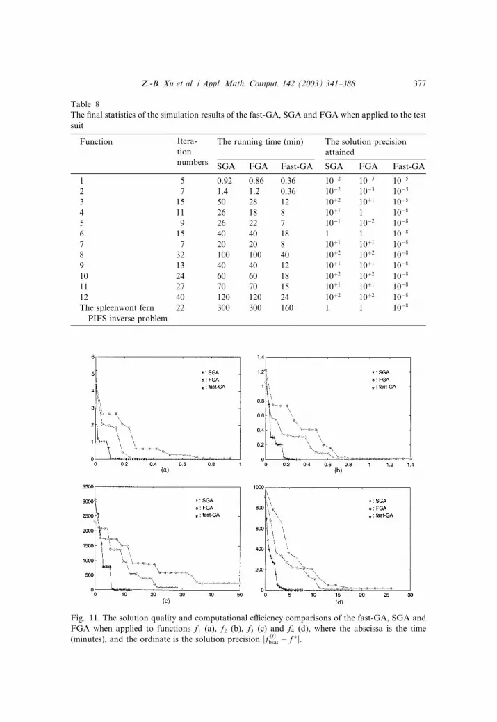
Table 8

The final statistics of the simulation results of the fast-GA, SGA and FGA when applied to the test

suit

Function Itera-

tion

numbers

The running time (min) The solution precision

attained

SGA FGA Fast-GA SGA FGA Fast-GA

1 5 0.92 0.86 0.36 10�2 10�3 10�5

2 7 1.4 1.2 0.36 10�2 10�3 10�5

3 15 50 28 12 10þ2 10þ1 10�5

4 11 26 18 8 10þ1 1 10�8

5 9 26 22 7 10�1 10�2 10�8

6 15 40 40 18 1 1 10�8

7 7 20 20 8 10þ1 10þ1 10�8

8 32 100 100 40 10þ2 10þ2 10�8

9 13 40 40 12 10þ1 10þ1 10�8

10 24 60 60 18 10þ2 10þ2 10�8

11 27 70 70 15 10þ1 10þ1 10�8

12 40 120 120 24 10þ2 10þ2 10�8

The spleenwont fern

PIFS inverse problem

22 300 300 160 1 1 10�8

Fig. 11. The solution quality and computational efficiency comparisons of the fast-GA, SGA and

FGA when applied to functions f1 (a), f2 (b), f3 (c) and f4 (d), where the abscissa is the time

(minutes), and the ordinate is the solution precision jf ðtÞbsat � f �j.


the sense of hðS;AÞ < eðdHðS; lÞ < eÞ, where hð:; :Þ is the Hausdorff metric be-tween sets and dHð:; :Þ is the Hutchinson metric between measures. By this

theory, any objective image then can be approximately viewed as an attractor

of an IFS (therefore, a fractal image) and therefore can be coded as simple

fractal codes (this is the underlying principle of the fractal image compression).

To specify such fractal codes, assume each contraction mapping xi in the IFS

(PIFS) is a linear affine transformation of the form:

xixy ¼ a11a12a21a22xy þ bi1bi2 8xy 2 K � R2

Then the IFS (PIFS) is characterized uniquely by the parameters a ¼ ðai1; ai2;ai3; ai4; bi1; bi2; i ¼ 1; 2; . . . ; ng 2 R6n (the parameters a ¼ ðai1; ai2; ai3; ai4; bi1; bi2;pi; i ¼ 1; 2; . . . ; ng 2 R7n). Such parameters are then referred to as the fractal

codes of the objective image S. Given an objective image, finding its fractalcodes is the IFS inverse problem, which is central to the fractal image com-

pression technology.

There are several approaches to the IFS (or PIFS) inverse problems. One of

such approaches is the moment matching: Consider the PIFS encoding case. If





the moments fGijg of the objective image S is known (which is the case in mostof applications), then the PIFS codes of S can be obtained as a solution of the

optimization problem modeled as in Table 9 [38].This PIFS inverse problem is well recognized to be one of the most chal-

lenging optimization problems to solve, especially by traditional gradient

methods and the classical genetic algorithm [38]. Here we do not attempt to




Table 9

The PIFS inverse problem

min F ðaÞ ¼PM1

i¼0PM2

j¼0½gijðaÞ � Gij�2with g00 ¼ 1 and

gij ¼Xnk¼1

pkXi

i1¼0ii1a

i1k1

Xi�i1

12¼0i

"� i1i2a

i2k2b

i�i1�i2k1

# Xjj1¼0

jj1aj1k3

Xj�j1

j2¼0j

"� j1j2a

j2k4b

j�j1�j2k2 gði1 þ j1Þði2 þ j2Þ

#

Where fgij : i; j > 1g are the moments of the invariant measure l of PIFS.


provide general solutions to this problem, rather we attempt to assess appli-

cability and performance of the fast-GA, SGA and FGA when all applied tothis real-life difficult problem. Our simulation was with the following specific

spleenwort fern image [20,38]:

The spleenwort fern IFS inverse problem: Given a spleewort fern S, asshown in Fig. 16(f), whose up-to (5,5)-order moments fGijg5�5 are listedin Table 10, to find a set of PIFS codes a ¼ ðai1; ai2; ai3; ai4; bi1;bi2; pi; i ¼ 1; 2; 3; 4g 2 R28 of S through solving the PIFS inverse problem

in the region X ¼ ½�1; 1�24 � ½0; 1�4.

Considering the known poor performance of CGA in [38], we have set the

solution precision requirement e1 ¼ jfbest � f �j ¼ 10e� 2, and the mutation

rate Pm ¼ 0:9 for SGA and FGA, the maximal generation number of evolutionM ¼ 500 for the fast-GA in this experiment but kept other parameters intact as

before. With such parameter setup, implementations of the fast-GA, CGA and

FGA yield the solutions shown as in Table 8. The actual PIFS codes of the

spleenwort fern are those listed in Table 12. Comparing Table 11 with Table 12

(also Fig. 15), we see that the fast-GA again successfully finds the global so-

lution with the required precision, while, in contrast, SGA and FGA both fail.

Fig. 14 shows the comparisons of these three algorithms in terms of solution

quality and efficiency. Fig. 15 shows the images reconstructed from the solu-

Table 10

The moments of the spleenwort fern

m Gm0 Gm1 Gm2 Gm3 Gm4 Gm5

0 1.000000 0.608444 0.467175 0.403542 0.374759 0.364592

1 0.592843 0.377998 0.303892 0.271990 0.259448 0.262724

2 0.367721 0.244500 0.203987 0.187878 0.183665 0.190515

3 0.236229 0.163092 0.140316 0.132420 0.132156 0.138869

4 0.155983 0.111419 0.098330 0.096107 0.097635 0.103079

5 0.105882 0.079268 0.051057 0.054156 0.058486 0.064014

Table 11

The PIFS codes of the spleenwort fern

i a�i1 a�i2 a�i3 a�i4 b�i1 bi2� p�i

1 0.00 0.00 0.00 0.16 0.50 0.00 0.01

2 0.20 )0.26 0.23 0.22 0.40 0.05 0.07

3 )0.15 0.28 0.26 0.24 0.57 )0.12 0.07

4 0.85 0.04 )0.04 0.85 0.08 0.18 0.85


tions respectively yielded by the SGA, FGA and the fast GA, and Fig. 16

shows the evolution details of the fast-GA.

Note that the spleenwort fern IFS inverse problem is strongly non-linear

and highly non-separable. This experiment strongly supports the superior

performance (especially the fast convergence) of the fast-GA when compared

with other two GAs.

7. Conclusion

This paper has suggested, analyzed, and partially explored a set of six

efficiency speed-up strategies for evolutionary computation. The strategies


FGA when applied to the spleenwort fern PIFS inverse problem.

Table 12

The PIFS codes found by the fast-GEA

i ai1 ai2 ai3 ai4 bi1 bi2 pi

1 0.01228 0.01563 0.00736 0.16424 0.52809 0.00483 0.01022

2 0.22212 )0.26037 0.24796 0.23542 0.42136 0.06202 0.07076

3 )0.14071 0.30123 0.27256 0.24584 0.59374 )0.10677 0.07082

4 0.85351 0.04056 )0.03874 0.85280 0.08896 0.18464 0.84820


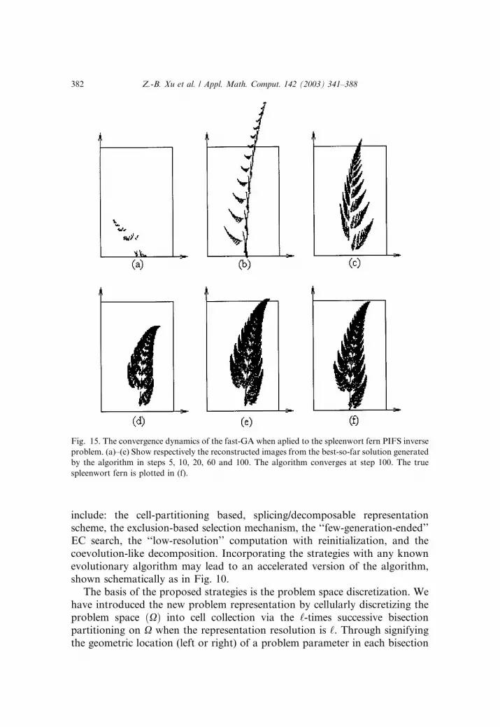
include: the cell-partitioning based, splicing/decomposable representationscheme, the exclusion-based selection mechanism, the ‘‘few-generation-ended’’

EC search, the ‘‘low-resolution’’ computation with reinitialization, and the

coevolution-like decomposition. Incorporating the strategies with any known

evolutionary algorithm may lead to an accelerated version of the algorithm,

shown schematically as in Fig. 10.

The basis of the proposed strategies is the problem space discretization. We

have introduced the new problem representation by cellularly discretizing the

problem space ðXÞ into cell collection via the ‘-times successive bisectionpartitioning on X when the representation resolution is ‘. Through signifying

the geometric location (left or right) of a problem parameter in each bisection

Fig. 15. The convergence dynamics of the fast-GA when aplied to the spleenwort fern PIFS inverse

problem. (a)–(e) Show respectively the reconstructed images from the best-so-far solution generated

by the algorithm in steps 5, 10, 20, 60 and 100. The algorithm converges at step 100. The true

spleenwort fern is plotted in (f).


procedure, the new representation scheme provides both a unique binary en-

coding of the problem parameters and a useful data structure of expressing the

cellular partitioning. Three exclusive properties of the new representation

scheme have been shown: (i) There are homeomorphisms among the problem

space X, the cell space Cð‘Þ and the encoding space f0; 1gn‘ (the search space),

which in particular implies that in the scheme a binary string denotes both aproblem variable and a cell in Cð‘Þ (it therefore stands not just for an individualbut for a subpopulation in simulated biology terms); (ii) the encoding is

splicing and decoding is decomposable, detailed as in Theorem 1, and (iii) there

holds specific meaning of each bit of a binary code, and the significance varies

from left to right in descent order, corresponding to approximating a problem

parameter from coarse to fine (macro to micro, global to local) manner. All

these properties feature the new representation scheme, distinguish itself from

the traditional binary representation scheme, and underlie the applicability andeffectiveness of the present research.

The core mechanism and step of an accelerated evolutionary algorithm is the

space shrinking (cf. Fig. 10). Functionally it guides the EC search to more and

more promising area and assures convergence of the algorithm. This has been

realized in this work through using the best-so-far solution guided, and ex-

clusion-based selection operations (cf. Fig. 10). The best-so-far solution is very

loosely required in precision and therefore we generate it via a time-saving,

fast EC search procedure endowed with the ‘‘few-generation-ended’’ searchstrategy and the ‘‘low-resolution’’ computation with reinitialization strategy,

both of which are known to be the most economic and efficient ways for use of

EC. The exclusion-based selection is the main contributor to efficiency accel-

eration of EC, which are carried out by employing exclusion operators com-

bined with a specified exclusion scheme. We have developed four exclusion

operators, based respectively on the concavity test, the dual fitness test, the

Fig. 16. A comparision of the reconstructed spleenwort ferns from the final solutions yielded by the

SGA, FGA and fast-GA.


Lipschitz test and the formal series test, and one exclusion scheme called the

orange-peeling scheme. All these have made the exclusion-based selectiontheoretically sound and practically powerful, both as a new way to simulate the

‘‘survival for the fittest’’ principle and in guiding EC search to monotonically

converging to the global optimum. It is noted that in this step, the exclusion-

based selection has used the exclusion for the worst mechanism, whereas the

best-so-far solution guided search employed the selection for the best principle.

The combinative use of these two complementary selection mechanism has also

contributed a lot of efficiency speed-up to the accelerated evolutionary algo-

rithm.The focused search in the accelerated algorithm (Fig. 10) means that in the

next step of evolution the algorithm will perform search focused on the shrunk

Fig. 17. A schematic representation of an accelerated evolutionary algorithm (the fast-EA).


space (the reinitialization corresponds to an refined cellular partition on the

shrunk space).This, in essence, amounts to performing search with lengthened (longer)

encoding (i.e., changing representation during search). So we can conclude

that the proposed acceleration algorithms finds the global optimum via the

space-shrinking directed search with successively increased representation

length (or, to be more precise, via successively finding the significant bits of its

chromosome representation, from the most significant to less significant, with

sucesssively increased precision). During this process, the reintialization (suc-

cessively refined partitioning) plays a role of compensation for the lack of localsearch capability of the traditional EC. This is the underlying principle of the

proposed strategies, and explains in particular why an arbitrarily high-preci-

sion (resolution) solution can be obtained by means of the successive low-

resolution search.

As an example, we have endowed all the strategies with genetic algorithms,

yielding an accelerated genetic algorithm––the fast-GA (see Fig. 17). The fast-

GA then is experimentally tested with a difficult test suite consisted of 10

complex multimodal function optimization examples and a real-life applica-tion problem––the moment matching problem of fractal encoding of the

spleenwort fern. The performance of the fast-GA is compared against the SGA

and one of the most recently and fairly established variants of GAs, the FGA.

The experiments all have demonstrated that the fast-GA consistently and

significantly outperforms the SGA and FGA in efficiency and solution quality.

Besides the speed-up of efficiency, other visible features of the fast-GA have

been also observed in the experimental studies including: (i) no premature

convergence occurs; (ii) guaranteed convergence to global optimum; and (iii)variable high-precision solution attainable. All these support the validity and

the power of the strategies developed in the present work.

The limitation of the developed strategies is clear: they can only apply to the

continuous problem space. We plan on relaxing this limitation in our near

future investigation. There are also many other opportunities for further re-

search related to the developed strategies: fully comparing the four exclusion

operators, developing new generic, more efficient exclusion operators and ex-

clusion schemes; specializing the developed strategies to other evolutionaryalgorithms (like ES); exploring other more powerful efficiency speed-up strat-

egies, and so on. In addition, the cell partitioning based representation scheme

suggested in this paper has provided a unique geometric language for signifying

schema-related concepts in GAs (say, a cell hdðAÞ; hð‘Þi corresponds to the

family of schemata of the form (A; �; �; . . . ; �), where A is a binary string). It is

therefore plausible to expect that with the new representation scheme, the

classical schema theory (particularly, the building block hypothesis) can be

more precisely explained and clarified, which may constitute another part offuture study.


Acknowledgements

This research is partially supported by the Hi-Tech, R&D (863) Program(No. 2001AA113182), the Natural Science Foundation Project (No. 69975016)

and the earmarked grant CUHK4212/01E of the Hong Kong Research Grant

Council.

References

[1] T. B€aack, H.P. Schwefel, An overview of evolutionary algorithm for parameter optimization,

Evolutionary Computation 1 (1) (1993) 1–23.

[2] T. B€aack, F. Kursawe, Evolutionary algorithms for fuzzy logic: a brief overview, in: B.

Bouchon-Meunier, R.R. Yager, L.A. Zadeh (Eds.), Fuzzy Logic and Soft Computing, World

Scientific, Singapore, 1995, pp. 3–10.

[3] M.F. Barnsley, S. Demoko, Iterated function systems and the global construction of fractals,

Proceedings of Royal Soceity London A 399 (1985) 243–275.

[4] K. Deb, Multi-objective genetic algorithms: problem difficulties and construction of test

problems, Evolutionary Computation 7 (3) (1999) 205–231.

[5] T.E. Davis, J.C. Principle, A simulated annealing like convergence theory for the simple

genetic algorithm, in: Proceedings of Fourth International Conference on Genetic Algorithms,

Morgan Kaufmann, San Mateo, 1991, pp. 174–218.

[6] L.J. Eshelman, J.D. Schaffer, Real-coded genetic algorithms and interval schemate, in: L.D.

Whitley (Ed.), Foundations of Genetic Algorithms, II, Morgan Kaufmann, San Mateo, CA,

1993, pp. 187–202.

[7] D.B. Fogel, An introduction to simulated evolutionary optimization, IEEE Transactions on

Neural Networks 5 (1994) 3–13.

[8] D.B. Fogel, Evolutionary Computation: Towards a New Philosophy of Machine Intelligence,

IEEE Press, New York, 1995.

[9] U.M. Fayyad, G. Piatetsky-Shapire, P. Smyth, R. Uthurusamy (Eds.), Advances in Knowl-

edge Discovery and Data Mining, MIT Press, Cambridge, MA, 1996.

[10] C.M. Fonseca, P.J. Fleming, An overview of evolutionary algorithms in multiobjective

optimization, Evolutionary Computation 3 (1995) 1–16.

[11] O. Francois, An evolutionary strategy for global minimization and its Markov chain analysis,

IEEE Transactions on Evolutionary Computation 2 (30) (1998) 77–90.

[12] D.E. Goldberg, Genetic Algorithms in Search, Optimization and Machine Learning, Addison-

Wesley, Reading, MA, 1989.

[13] D.E. Goldberg, B. Korb, K. Deb, Messy genetic algorithm: motivation, analysis, and the first

result, Complex System 3 (1989) 493–530.

[14] J.J. Grefenstette, Optimization of control parameters for genetic algorithms, IEEE Transac-

tions on System, Man, and Cybernetics 16 (1) (1986) 122–128.

[15] E. Hansen, Global Optimization Using Interval Analysis, Marcel Dekker, New York, 1992.

[16] J.H. Holland, Adaption in Natural and Artificial Systems, The university of Michigan Press,

Ann Arbor, 1975.

[17] Y. Hanaki, T. Hashiyama, S. Okuma, The acceleration of evolutionary computation using

fitness estimation, in: Proceedings of the 1999 IEEE/ASME International Conference on

Advanced Intelligent Mechtronics, Atlanta, USA, 1999, pp. 776–781.

[18] G.R. Harik, F.G. Lobo, D.E. Goldberg, The compact genetic algorithm, IEEE Transactions

on Evolutionary Computation 3 (1999) 287–297.


[19] C.R. Houck, J.A. Joines, M.G. Kay, J.R. Wilson, Empirical investigation of the benefits of

partial Lamarckiansim, Evolutionary Computation 5 (1) (1997) 31–60.

[20] A.E. Jacquin, Fractal image coding: a review, Proceedings of IEEE 10 (1993) 1451–1465.

[21] J.R. Koza, Genetic Programming II: Automatic Discovery of Reusable Subprograms, MIT

Press, Cambridge, MA, 1994.

[22] G. Li, Y. Leung, Z.B. Xu, K.S. Leung, Hybrid genetic algorithms for global optimization of

functions, Evolutionary Computation (in press).

[23] K.S. Leung, Q.H. Duan, Z.B. Xu, C.K. Wong, A new model of simulated evolutionary

computation: convergence analysis and specifications, IEEE Transactions on Evolutionary

Computation 5 (2001) 3–16.

[24] K.S. Leung, J.Y. Seng, Z.B. Xu, Efficiency speed-up strategies for evolutionary computation:

an adaptive implementation, Engineering Computations 19 (2002) 272–304.

[25] K.E. Mathias, L.D. Whitely, Changing representation during search: a comparative study of

delta coding, Evolutionary Computation 2 (1995) 249–278.

[26] Z. Michelewicz, Genetic AlgorithmþData Structure ¼ Evolutionary Programs, third ed.,

Springer-Verlag, New York, 1996.

[27] H. Muhlenbein, D. Schliekamp-Voosen, Predictive models for the breeder genetic algorithm I:

continuous parameter optimization, Evolutionary Computation 1 (1993) 25–49.

[28] Jesus Marin, R.V. Sole, Macroevolutionary algorithms: a new optimization method on fitness

landscapes, IEEE Transactions on Evolutionary Computation 3 (1999) 272–286.

[29] R.J. Parsons, S. Forrest, C. Burks, Genetic algorithms, and DNA fragment assembly, Machine

Learning 21 (1995) 11–33.

[30] M.A. Potter, K.A. De Jong, A cooperative coevolutionary approach to function optimization,

in: Y. Davidor, H.-P. Schwefel, R. Manner (Eds.), Parallel Problem Solving from Nature,

Springer-Verlag, Berlin, 1994, pp. 249–257.

[31] J.M. Renders, S.P. Flasse, Hybrid method using genetic algorithms for global optimization,

IEEE Transactions on Systems, Man, and Cybernetics––Part B: Cybernetics 26 (2) (1996) 243–

258.

[32] N.N. Schraudolph, R.K. Belew, Dynamic parameter encoding for genetic algorithms, Machine

Learning 9 (1992) 9–21.

[33] R. Salomon, Raising theoretical questions about the utility of genetic algorithms, in: P.J.

Angeline, R.G. Reynolds, J.R. McDonnell, R. Eberhart, (Eds.), Proceedings of Sixth Annual

Conference on Evolutionary Programming VI, 1997, pp. 275–284.

[34] R. Salomon, Reevaluating genetic algorithm performance under coordinate rotation of

benchmark functions: a survey of some theoretical and practical aspects of genetic algorithms,

Biological Systems 39 (3) (1996) 263–278.

[35] M. Srinivas, L.M. Patnaik, Adaptive probabilities of crossover and mutation in genetic

algorithms, IEEE Transactions on System, Man and Cybernetics 24 (4) (1994) 17–26.

[36] H.P. Schwefel, Evolution and Optimum Seeking, John Wiley, Chichester, UK, 1995.

[37] S. Tsutsui, Y. Fujimoto, A. Ghosh, Forking genetic algorithms: GAs with search space

division schemes, Evolutionary Computation 5 (1) (1997) 61–80.

[38] E.R. Vrscay, Iterated function systems: theory, applications and the inverse problem, in:

J. Belair, S. Dubuc (Eds.), Fractal Geometry and Analysis, Kluwer Academic Publishers,

Dordrecht, 1991, pp. 405–468.

[39] A.S. Wu, W. Banzhaf, Introduction to the special issue: variable-length representation and

noncoding segments for evolutionary algorithms, Evolutionary Computation 6 (1999) 4, iii–vi.

[40] Z.B. Xu, J.S. Zhang, W. Wang, A cell exclusion algorithm for finding all the solutions of a

nonlinear system of equation, Applied Mathematics and Computation 80 (1996) 181–208.

[41] Z.B. Xu, J.S. Zhang, Y.W. Leung, A general CDC formulation for specializing the cell

exclusion algorithms of finding all zeros of vector functions, Applied Mathematics and

Computation 86 (2&3) (1997) 235–259.


[42] X. Yao, Y. Liu, G.M. Lin, Evolutionary programming made faster, IEEE Transactions on

Evolutionary Computation 3 (1999) 82–97.

[43] X. Yao, L. Liu, Towards designing artificial neural networks by evolution, Applied

Mathematics and Computation 91 (1998) 83–90.

[44] Z.Y. Zhou, K.S. Leung, Z.B. Xu, Exclusion-based cooperative coevolution genetic algorithm,

2001 WSES International Conference on Evolutionary Computations (EC�01), 2001, 637(1)–637(6).


efficiency speed-up strategies for evolutionary computation: fundamentals and fast-gas

Documents