effects of index insurance on demand and supply of credit

EFFECTS OF INDEX INSURANCE ON DEMAND

AND SUPPLY OF CREDIT: EVIDENCE FROM

ETHIOPIA

TEMESGEN BELISSA, ROBERT LENSINK, AND ANNE WINKEL

Index-based insurance offers a climate risk management strategy that can benefit the poor. This articlefocuses on whether adopting index insurance improves access to financial markets and reduces creditrationing, using empirical analyses focused on Ethiopia. With different identification strategies, includ-ing a newly developed method that leverages the varying availability of index insurance across areas,the authors control for potential selection biases by forecasting potential insurance adopters; they applya cross-sectional double-difference method. Credit rationing can take the form of either supply-sidequantity rationing, in which case potential borrowers who need credit are involuntarily excluded fromthe credit market, or demand-side rationing, such that borrowers self-select and voluntarily withdraw toavoid transaction costs and threats to their collateral. By differentiating supply-side and demand-sideforms and employing a direct elicitation method to determine credit rationing status, this study revealsthat 38% of sample households are credit constrained. The preferred estimation techniques suggestthat index insurance significantly reduces supply-side rationing.

Key words: Credit Rationing, Ethiopia, Index Insurance; Smallholders.

JEL codes: D82, G21, G22, O13, O16, O55.

Index-based insurance (IBI) is an innovativehedging instrument that can mitigate the risksof drought or seasonality-based weather varia-tions due to climate change.As an attractive fea-ture of this innovation, the insurance payoutoccurs when an objective index falls below (orexceeds, depending on the criterion) a thresh-old. The index usually is based on a measure ofthe intensity of rainfall or direct yield measuresfor a specific geographic zone covered by theinsurance contract (Carter et al. 2017). Ideally,the index correlates closely with insured losses,is objectively quantifiable, and is publicly verifi-able, such that it cannot be manipulated by the

insurer or the insured (Barnett, Barrett, andSkees 2008; Zant 2008).Although the uptake of IBIs remains low1

(Cole et al. 2012, 2013; Hill, Hoddinott, andKumar 2013; Dercon et al. 2014; Takahashiet al. 2016) and demand is generally sluggish(Carter et al. 2017), several studies point toits potentially substantial income, investment,or wealth effects (Janzen and Carter 2019;Elabed and Carter 2014; Karlan et al. 2014).For example, IBI adoption could inducehouseholds to make more prudent invest-ments or manage their consumption risk bet-ter (by stabilizing savings or accumulatingassets), which then could protect them from

Temesgen K. Belissa is an Assistant professor of Development Eco-nomics at HaramayaUniversity, Ethiopia. Robert Lensink is Profes-sor of Finance and Financial Markets at the Faculty of Economicsand Business of the University of Groningen. He is also Professorof Finance and Development at the development economics groupof Wageningen University. Anne Winkel is a Consultant in Tradeand Private Sector Development at Ecorys, The Netherlands.Correspondence to be sent to: [email protected]

Amer. J. Agr. Econ. 102(5): 1511–1531; doi:10.1111/ajae.12105Published online June 11, 2020

© 2020 The Authors. American Journal of Agricultural Economics published by Wiley Periodicals LLC. on behalf ofAgricultural & Applied Economics Association.This is an open access article under the terms of the Creative Commons Attribution License, which permits use, distribu-tion and reproduction in any medium, provided the original work is properly cited.

1 The low uptake of IBI might stem from the so-called basisrisk, which arises due to the imperfect correlation between com-puted indices and actual losses (Cummins, Lalonde, and Phillips2004; Jensen, Mude, and Barrett 2018). Especially in developingcountries, where terrestrial weather stations are sparse, the dis-crepancy between losses indicated by the index and actual lossesrealized at the farm level is high (Clarke et al. 2012).

mailto:[email protected]

http://creativecommons.org/licenses/by/4.0/

http://crossmark.crossref.org/dialog/?doi=10.1111%2Fajae.12105&domain=pdf&date_stamp=2020-06-11

sliding into poverty traps (Barnett, Barrett,and Skees 2008). Moreover, because IBIunlinks loss assessments from individualbehavior, it can avoid moral hazard andadverse selection problems (Barnett, Barrett,and Skees 2008; Skees 2008), which also mightimprove credit access. However, virtually noempirical evidence exists regarding how IBIadoption affects the demand for and supplyof credit. This article offers initial insights intothe impacts of IBI on credit rationing, usingdata from a drought-prone area in the RiftValley zone of Ethiopia.Despite the lack of empirical evidence, some

studies offer initial insights into the potentialeffects of IBI on credit rationing. In a framedfield experiment in China, Cheng (2014) studiesthe effect of offering IBI to households that vol-untarily withdraw from the credit market; all thestudy participants participate in both control andtreatment games. The results demonstrate thatmore than half of the farmers decide to applyfor credit when IBI is available, and roughlytwo-thirds of credit diverters choose to use theirloan for productive investments rather than con-sumption. This behavior could be explained inseveral ways, with the recognition that IBIreduces production risk, but the risk associatedwith using the loan for consumption remainsconstant or even might increase. In addition,Giné and Yang (2009) randomly offered maizefarmers in Malawi either a loan or a loan withinsurance, which indemnifies them if rainfall isinsufficient. The insurance could be bought atan actuarially fair premium. Although theyexpected that farmers would prefer the insuredloan, demand for the basic loan was 13% higherthan that for the insured loan. To explain why,these authors propose that the limited liabilityclause of the basic loan provided an implicitform of insurance. However, in contrast withthe current study, Giné and Yang (2009) donot address the impact of a stand-alone insur-ance product. As Carter, Cheng, and Sarris(2016) suggest, a stand-alone insurance productprovides no additional benefits to farmers withlimited collateral. If no formal insurance is avail-able, farmers with high collateral might be theonly ones who choose not to borrow, becausethey do not want to put their collateral at risk.Other studies focus on the impact of IBI on

credit supplies, with conflicting results. That is,some research suggests that IBI relaxes sup-ply-side constraints and quantity rationing,because lenders tend to lower interest ratesand lend more to insured clients due to thereduced default risk (Mahul and Skees 2007;

Giné and Yang 2009; McIntosh, Sarris, andPapadopoulos 2013). But other studies suggestthat insurance could decrease both demandfor and supply of credit. Because IBI contractssometimes are unable to trigger payouts, evenif the insured incurs significant yield losses dueto weather risk, an inability to repay the loancan lead to loan defaults, because cash out-flows go to paying the premium. Alternatively,a stand-alone insurance product couldincrease the minimum welfare level to whichdefaulting households can retreat. In this situ-ation, incentives to repay diminish, becausethe welfare costs of defaulting are lower.Lenders who take loan default potential intoaccount thus might limit credit supply in areaswhere IBI is available (Banerjee 2000; Clarkeand Dercon 2009; Farrin and Miranda 2015).

With this study, we seek to provide actual,empirical evidence of the impact of IBI ondemand-side (i.e. risk and transaction costrationing) and supply-side credit rationing.The insurance contract is a stand-alone prod-uct, for which indemnities are paid directly tofarmers. Hence, the insurance intervention inEthiopia that we study is not an insurance–credit interlinked contract. As the majority ofsmallholders lack any valuable collateral tooffer, there is no real collateral at risk for mostformal borrowers.2 Thus, the interventionseems unlikely to exert any considerableimpact on risk rationing, because insurancecannot make borrowers who are insured by azero collateral default clause borrow morenor should it have any impact on transactioncost rationing. Therefore, we expect the adop-tion of IBI mainly reduces supply-side, ratherthan demand-side, rationing.

We use different identification strategies,including a newly developed hybrid method.The preferred methods suggest that indexinsurance has a large, significant effect ondecreasing supply-side credit rationing. Butthe impact of IBI uptake on demand-siderationing is statistically insignificant. To estab-lish these findings, we start in the next sectionwith a description of the study setting, howIBI works, and the sampling procedure. Next,we explain the method used to determinecredit rationing and provide estimates of creditrationing in our sample. We present a new,hybrid method based on a double-difference(fixed effects) technique to estimate the impact

2 In the Online Appendix we provide more information aboutthe nature of the insurance contract and liability rules in Ethiopia.

1512 October 2020 Amer. J. Agr. Econ.

of IBI on credit rationing; we outline how ithelps address issues with traditional regressiontechniques. Finally, we note some limitationsof our hybrid method, offer robustness ana-lyses, and conclude with relevant insights.

Study Setting, Data, and Sampling

This study took place in the central Rift Valleyzone of the Oromia regional state in south-eastern Ethiopia. The area is characterizedby plain plateaus and lowland agro-ecology.The pattern and intensity of rainfall exhibitsconsiderable spatial and temporal variation,with a bimodal distribution. Rainfall seasonsare from May to August and during Octoberand November. However, moisture stressand drought frequently cause devastating cropfailures, rampant livestock mortality, and herdcollapse (Dercon, Hoddinott, and Wolde-hanna 2005; Takahashi et al. 2016). Majordroughts in the area occurred in 2015–16, fol-lowing historical drought trends during 1973–74, 1983–84, 1991–92, 1999–2000, 2005–6, and2011–12 (Dercon 2004; Takahashi et al.2016). Households are smallholders and sub-sistence farmers who often face drought-induced income shocks that translate intoerratic consumption patterns (Dercon andChristiaensen 2011; Biazin and Sterk 2013).Formal risk management mechanisms areinaccessible, requiring informal methods. Expost coping mechanisms include reducing thefrequency of meals, distress livestock sales,halting the purchase of fertilizer and improvedseeds, forcing pupils to withdraw from schoolfor casual labor, renting land and family laborto local landlords, and seeking wage-basedemployment on floriculture farms held by for-eign investors. These mechanisms are costlyand limited in scope (Dercon 2004).

IBI in the Study Area

In 2013, the Japan International CooperationAgency (JICA) and Oromia Insurance Com-pany (OIC) jointly implemented IBI for cropsin the Rift Valley zone of Ethiopia to improvethe resilience of households, in the face of cli-mate change. The product was designed byCelsiusPro Ag and Swiss Re using satelliteweather data with 10 × 10 km grids for theperiod 1983–2012. It was implemented in fivedistricts: Boset, Bora, Ilfata, Adamitullu-

Jido-Kombolcha (AJK), and Arsi Negele.The selection of which kebeles3 to cover in eachdistrict reflected several criteria, including rain-fall shortages, the relevance of the area for cropproduction, and food security. The specific selec-tion process worked as follows: first, before theinitial intervention in 2013, the OIC, JICA, andEthiopian Ministry of Agriculture discussedand identified districts in which drought shocksare common. Most of these districts are locatedin theRiftValley zone. Second, the three organi-zations entered into focus group discussionswithrepresentative farmers from each kebele withineach selected district. From these discussions,they identified kebeles with severe droughtexperience in the past. Third, the financial sup-port that JICA allotted for the 2013 weatherindex insurance intervention was not adequateto cover all the identified drought-prone kebelesat the same time, so the kebeles that would besubject to the first intervention in 2013 versusduring later interventions were selected throughdiscussion among the three organizations.4

The product is marketed and sold twice peryear, in April and September, which are themonths preceding the two rainy seasons. Itprovides coverage against losses during theseedling and flowering stages of crop growth.Major targeted stable food crops includemaize, wheat, barley, and teff. During eachsales period, a household that decides to buyIBI pays a premium of ETB5 100 per policy.The payout is determined according to thelevel of normalized difference vegetationindex, measured using satellite data for a spec-ified period. The exact trigger and exit leveldiffer for each kebele and in each season. A20%markup on the actuary fair premium alsois included in the contract, to cover selling andadministrative costs (loading factor).6 Sellingcosts are incurred by the sales agents, such as

3 A kebele is the smallest administrative unit, within districts(Woreda), in Ethiopia.

4 We tried to obtain details about how the kebeles to be servedfirst were selected. The official answer of OIC was that it was ran-dom, but the organization could not specify how the randomiza-tion was conducted. It seems more likely that the final selectionwas based on informal criteria, influenced by the groupdiscussions.

5 ETB (Ethiopian Birr), 1USD = 32 ETB.6 This mark-up rate is relatively low compared with other prod-

ucts in developing countries, which reflects a practical challenge: ahigher mark-up rate that takes all catastrophic risks and uncer-tainty into account would increase the product price too high, rel-ative to farmers’ reservation prices. Thus, the product does notmeet safe minimum quality standards, in the sense that high insur-ance prices might prompt farmers to prefer self-insurance (Carteret al. 2017).

Belissa, Lensink and Winkel Index Insurance and Credit Rationing 1513

cooperative unions. The actuarially fair pre-mium of the insurance product is ETB 100per policy for a maximum payout of aboutETB 667 to cover full losses. The 20%markupis paid by JICA, so farmers only pay the actu-arially fair premium of ETB 100 per policy.According to OIC sales records, before Sep-tember 2014 (start of the data collectionperiod), approximately 5,000 households inmore than thirty kebeles across five districtshad purchased IBI; plans were in place toexpand into many other adjacent kebeles ineach district. The intervention plan in subse-quent periods involved intensifying coverageof the kebeles in the five districts, then expand-ing into other districts. Our newly developedhybrid identification strategy, which weexplain subsequently, reflects these expansionplans.

Sampling

We used a multistage, random sampling tech-nique with probability proportional to size.Concretely, we selected three districts (Bora,AJK, and Arsi Negele) out of the five districtscovered by the IBI project. Then we identifieda random sample of kebeles covered by IBI inthese three districts. From the AJK district, wealso selected two kebeles (Qamo Garbi andDesta Abijata) where IBI was not yet avail-able.7 Noting our available budget, we decidedto survey approximately 1,200 households,selected proportional to the sample size ofthe study from all kebeles identified. We alsooversampled households from the treatmentkebeles to ensure sufficient actual adopters inthe sample. That is, we took larger samples inthe treatment kebeles than the controlkebeles, proportional to the size of the kebelesin both groups. We used random samplingwithin the treatment and control kebeles. Foreach kebele, we randomly selected the samplefrom a roster of farmers; for simplicity, weadopted a systematic random sampling tech-nique and randomly selected the first farmerfrom the roster then the next nth farmers fromthe list.

Prior to our study, JICA andOIC organizedproduct promotion campaigns in both thetreatment and expansion kebeles to enhanceuptake (and future uptake). In both the treat-ment and control kebeles, an estimated 70%of the farmers attended a product promotionmeeting. Such product promotion campaignsare common tactics to roll out new insuranceproducts.

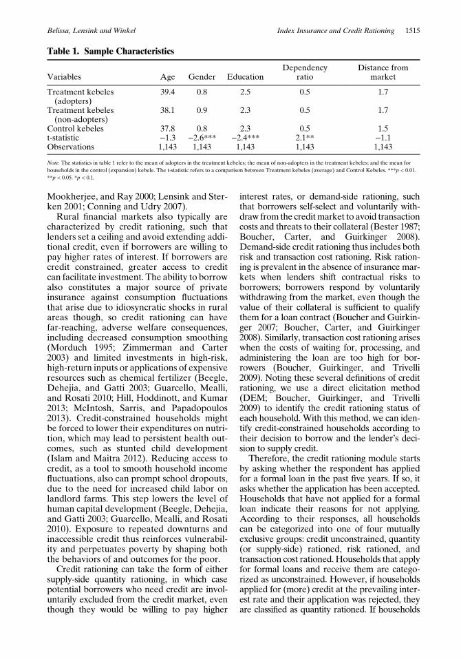
The final sample consists of 1,143 house-holds: 812 from the treatment and 331 fromthe control kebeles. Of the 812 householdsfrom the treatment kebeles, 459 adopted and353 did not adopt IBI over the 2013–14 period.This relatively high percentage of adopterscan be explained by the well-attended productpromotion campaigns. As table 1 indicates, anaverage household in the treatment kebelesthat bought IBI was headed by a 39-year-oldmanwho had about two years of formal educa-tion. The average number of family membersis seven, four of whom have reached produc-tive age, with three who are either preschoolchildren or aged dependents. On average,these households travel approximately twohours to access public services, including mar-ket centers and financial institutions.Although some differences arise with house-holds that do not buy insurance in the treat-ment kebeles compared with households inthe control kebeles, these differences aresmall. Yet, as will also be shown in table 4below, this does not imply that treatment andcontrol kebeles are similar in terms of variouspoverty indicators.

Methodology

If rural financial markets were perfectly com-petitive, with symmetric information and cost-less enforcement, lenders could arrangeconditional credit contracts according to bor-rowers’ behaviors. However, rural financialmarkets in developing countries often featureinformation asymmetries, leading to moralhazard and adverse selection problems, as wellas higher transaction costs associated withloan monitoring and contract enforcement(Jaffee and Russell 1976; Stiglitz and Weiss1981; Vandell 1984; Bester 1985; Williamson1986; Besanko and Thakor 1987; Lensinkand Sterken 2002; Boucher, Carter, and Guir-kinger 2008). These classic incentive problemsmake conditional credit contracts restrictiveand infeasible (Dowd 1992; Ghosh,

7 These two kebeles had been identified for potential futureinterventions. The presence of just two kebeles in the control con-dition reflects our assumption that between-kebele variationexplains only minimal differences across individuals. However,as local administrative boundaries in Ethiopia, kebeles have vary-ing size, and the two kebeles we selected to serve as controls bothcontain large populations, such that the samples taken from themconstitutes about one-third of the total respondents, proportionalto the total households, in both groups of kebeles.


Mookherjee, and Ray 2000; Lensink and Ster-ken 2001; Conning and Udry 2007).

Rural financial markets also typically arecharacterized by credit rationing, such thatlenders set a ceiling and avoid extending addi-tional credit, even if borrowers are willing topay higher rates of interest. If borrowers arecredit constrained, greater access to creditcan facilitate investment. The ability to borrowalso constitutes a major source of privateinsurance against consumption fluctuationsthat arise due to idiosyncratic shocks in ruralareas though, so credit rationing can havefar-reaching, adverse welfare consequences,including decreased consumption smoothing(Morduch 1995; Zimmerman and Carter2003) and limited investments in high-risk,high-return inputs or applications of expensiveresources such as chemical fertilizer (Beegle,Dehejia, and Gatti 2003; Guarcello, Mealli,and Rosati 2010; Hill, Hoddinott, and Kumar2013; McIntosh, Sarris, and Papadopoulos2013). Credit-constrained households mightbe forced to lower their expenditures on nutri-tion, which may lead to persistent health out-comes, such as stunted child development(Islam and Maitra 2012). Reducing access tocredit, as a tool to smooth household incomefluctuations, also can prompt school dropouts,due to the need for increased child labor onlandlord farms. This step lowers the level ofhuman capital development (Beegle, Dehejia,and Gatti 2003; Guarcello, Mealli, and Rosati2010). Exposure to repeated downturns andinaccessible credit thus reinforces vulnerabil-ity and perpetuates poverty by shaping boththe behaviors of and outcomes for the poor.

Credit rationing can take the form of eithersupply-side quantity rationing, in which casepotential borrowers who need credit are invol-untarily excluded from the credit market, eventhough they would be willing to pay higher

interest rates, or demand-side rationing, suchthat borrowers self-select and voluntarily with-draw from the creditmarket to avoid transactioncosts and threats to their collateral (Bester 1987;Boucher, Carter, and Guirkinger 2008).Demand-side credit rationing thus includes bothrisk and transaction cost rationing. Risk ration-ing is prevalent in the absence of insurance mar-kets when lenders shift contractual risks toborrowers; borrowers respond by voluntarilywithdrawing from the market, even though thevalue of their collateral is sufficient to qualifythem for a loan contract (Boucher and Guirkin-ger 2007; Boucher, Carter, and Guirkinger2008). Similarly, transaction cost rationing ariseswhen the costs of waiting for, processing, andadministering the loan are too high for bor-rowers (Boucher, Guirkinger, and Trivelli2009). Noting these several definitions of creditrationing, we use a direct elicitation method(DEM; Boucher, Guirkinger, and Trivelli2009) to identify the credit rationing status ofeach household. With this method, we can iden-tify credit-constrained households according totheir decision to borrow and the lender’s deci-sion to supply credit.Therefore, the credit rationing module starts

by asking whether the respondent has appliedfor a formal loan in the past five years. If so, itasks whether the application has been accepted.Households that have not applied for a formalloan indicate their reasons for not applying.According to their responses, all householdscan be categorized into one of four mutuallyexclusive groups: credit unconstrained, quantity(or supply-side) rationed, risk rationed, andtransaction cost rationed.Households that applyfor formal loans and receive them are catego-rized as unconstrained. However, if householdsapplied for (more) credit at the prevailing inter-est rate and their application was rejected, theyare classified as quantity rationed. If households

Table 1. Sample Characteristics

Variables Age Gender EducationDependency

ratioDistance from

market

Treatment kebeles(adopters)

39.4 0.8 2.5 0.5 1.7

Treatment kebeles(non-adopters)

38.1 0.9 2.3 0.5 1.7

Control kebeles 37.8 0.8 2.3 0.5 1.5t-statistic −1.3 −2.6*** −2.4*** 2.1** −1.1Observations 1,143 1,143 1,143 1,143 1,143

Note: The statistics in table 1 refer to the mean of adopters in the treatment kebeles; the mean of non-adopters in the treatment kebeles; and the mean forhouseholds in the control (expansion) kebele. The t-statistic refers to a comparison between Treatment kebeles (average) and Control Kebeles. ***p < 0.01.**p < 0.05. *p < 0.1.


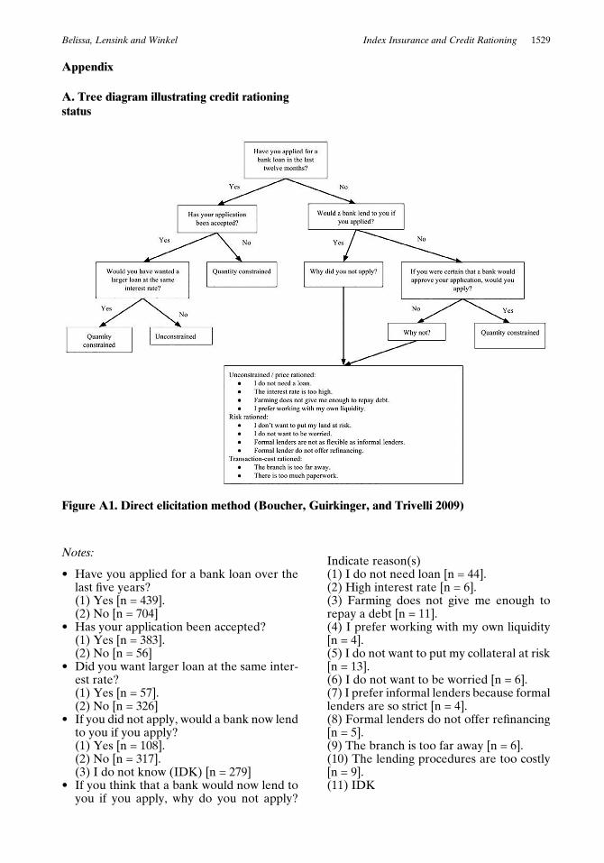
have not applied for a formal loan in the past fiveyears, because the bank branch is too far fromtheir homes or the application procedure involvestoomuchpaperwork andwaiting time,we catego-rize them as transaction cost rationed. If insteadhouseholds do not apply for loans because theydo not want to offer their house or other assetsas collateral that might be taken by the bank, weconsider them risk rationed. Some householdsthat are able to borrow do not apply because theydo not need credit; they are credit unconstrained.Finally, households that would have applied forloan, had they known the bank would lend tothem, are another group of supply-side rationedhouseholds.We combine the risk- and transactioncost–rationed households into a group ofdemand-constrained households; then we com-bine the demand-constrained and supply-con-strained households into a larger group of credit-constrained households. Figure A1 in AppendixI presents a tree diagram of questions leading tothe final categorization of each household.

Credit Access in the Sample

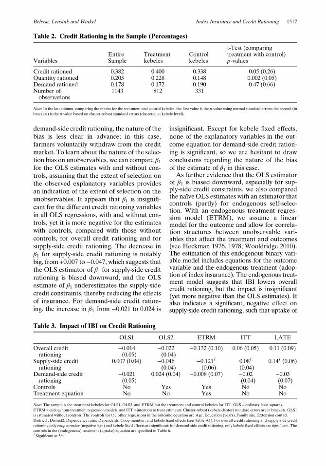
Using the DEM, we identify the credit rationingstatus of each household in our sample. Table 2summarizes the results. Approximately 38% ofthe households are credit constrained, of which20.5% are quantity constrained and 18% aredemand constrained.8 The table also differenti-ates kebeles with and without access to indexinsurance, revealing that the percentage ofhouseholds that are credit constrained is higherin the kebeles with access to index insurancethan in the kebeles without it. The same trendholds for the percentage of households that arequantity constrained. However, we hasten toadd that this finding does not necessarily meanthat access to index insurance (like an intentionto treat analysis) leads to more credit rationing.

Specification of the Regression Model

To clarify our approach, we specify the follow-ing fixed effect model:

ð1Þ yi = β0 + β1Ii + αtDti + αwDw

i + μi� �

,

where the dependent variable y refers to afarmer-level outcome (credit rationing) forfarmer (observation) i; Ii is a binary variablethat takes a value of 1 if i is insured; Dt

i is abinary variable equal to 1 if i is the type whowould endogenously buy insurance, such thatit reflects a fixed effect for those who wouldbuy, irrespective of whether insurance is avail-able; Dw

i refers to a fixed effect for treatmentkebeles, which is also a binary variable, equalto 1 if i is in a kebele where index insuranceis available, indicating the program wasendogenously placed; and μi is an error term.Note that Ii equals the interaction termDt

i*Dwi

� �, so Equation 1 is equivalent to a dou-

ble difference model (as we explain subse-quently when detailing the preferredmethod).

Our main aim is to obtain an unbiased esti-mate of β1, which may be hindered by self-selection or program placement biases. There-fore, before presenting our preferredapproach, we briefly discuss the nature ofthese biases, as they arise under standard esti-mation techniques. Table 3 presents theresults of these estimates. To start, we runnaïve ordinary least square (OLS) regressionswith and without controls, using only datafrom the treatment kebeles where the pro-gram was endogenously placed, which impliesthat from Equation 1, the termsαtDt

i + αwDwi

drop out. By using data from the treatmentkebeles only, we compare credit rationing byfarmers who bought insurance against thecredit rationing of their neighbors who delib-erately decided not to take part in the insur-ance program. An OLS estimator in this caseis likely biased due to self-selection. Self-selec-tion based on unobservable variables is theproblem; adding explanatory variables maycontrol for selection on observables. TheOLS estimators of β1 would be downwardlybiased if participants in the insurance programare previously more credit constrained, evenbefore they have the option to buy insurance,and if credit constrained farmers are morewilling to participate in the insurance program.This bias is particularly likely for supply-sidecredit constraints, in that intuitively, supply-side–constrained farmers (with observableand unobservable characteristics that makethem credit constrained) would want to buyinsurance, because they lack the option touse credit to protect themselves against croploss, such as due to a drought. Regarding

8 This credit rationing level (38%) is relatively lower than thatfound in Peru (55.4% in 1997; 43.6% in 2003; Boucher, Guirkin-ger, and Trivelli 2009). Quantity rationing accounts for 20.5% inour study, versus 36.6% in 1997 and 10.4% in 2003 in Peru. Simi-larly, demand rationing is 17.8% in our case but was 18.8% in1997 and 33.2% in 2003 in Peru.


demand-side credit rationing, the nature of thebias is less clear in advance; in this case,farmers voluntarily withdraw from the creditmarket. To learn about the nature of the selec-tion bias on unobservables, we can compare β1for the OLS estimates with and without con-trols, assuming that the extent of selection onthe observed explanatory variables providesan indication of the extent of selection on theunobservables. It appears that β1 is insignifi-cant for the different credit rationing variablesin all OLS regressions, with and without con-trols, yet it is more negative for the estimateswith controls, compared with those withoutcontrols, for overall credit rationing and forsupply-side credit rationing. The decrease inβ1 for supply-side credit rationing is notablybig, from +0.007 to−0.047, which suggests thatthe OLS estimator of β1 for supply-side creditrationing is biased downward, and the OLSestimate of β1 underestimates the supply-sidecredit constraints, thereby reducing the effectsof insurance. For demand-side credit ration-ing, the increase in β1 from −0.021 to 0.024 is

insignificant. Except for kebele fixed effects,none of the explanatory variables in the out-come equation for demand-side credit ration-ing is significant, so we are hesitant to drawconclusions regarding the nature of the biasof the estimate of β1 in this case.As further evidence that the OLS estimator

of β1 is biased downward, especially for sup-ply-side credit constraints, we also comparedthe naïveOLS estimates with an estimator thatcontrols (partly) for endogenous self-selec-tion. With an endogenous treatment regres-sion model (ETRM), we assume a linearmodel for the outcome and allow for correla-tion structures between unobservable vari-ables that affect the treatment and outcomes(see Heckman 1976, 1978; Wooldridge 2010).The estimation of this endogenous binary vari-able model includes equations for the outcomevariable and the endogenous treatment (adop-tion of index insurance). The endogenous treat-ment model suggests that IBI lowers overallcredit rationing, but the impact is insignificant(yet more negative than the OLS estimates). Italso indicates a significant, negative effect onsupply-side credit rationing, such that uptake of

Table 2. Credit Rationing in the Sample (Percentages)

VariablesEntireSample

Treatmentkebeles

Controlkebeles

t-Test (comparingtreatment with control)p-values

Credit rationed 0.382 0.400 0.338 0.05 (0.26)Quantity rationed 0.205 0.228 0.148 0.002 (0.05)Demand rationed 0.178 0.172 0.190 0.47 (0.66)Number ofobservations

1143 812 331

Note: In the last column, comparing the means for the treatment and control kebeles, the first value is the p-value using normal standard errors; the second (inbrackets) is the p-value based on cluster-robust standard errors (clustered at kebele level).

Table 3. Impact of IBI on Credit Rationing

OLS1 OLS2 ETRM ITT LATE

Overall creditrationing

−0.014(0.05)

−0.022(0.04)

−0.132 (0.10) 0.06 (0.05) 0.11 (0.09)

Supply-side creditrationing

0.007 (0.04) −0.046(0.04)

−0.1211(0.06)

0.081

(0.04)0.141 (0.06)

Demand-side creditrationing

−0.021(0.05)

0.024 (0.04) −0.008 (0.07) −0.02(0.04)

−0.03(0.07)

Controls No Yes Yes No NoTreatment equation No No Yes No No

Note: The sample is the treatment kebeles for OLS1, OLS2, and ETRM but the treatment and control kebeles for ITT. OLS = ordinary least squares,ETRM = endogenous treatment regression models, and ITT = intention to treat estimator. Cluster-robust (kebele cluster) standard errors are in brackets. OLS1is estimated without controls. The controls for the other regressions in the outcome equation are Age, Education (years), Family size, Extension contact,District1, District2, Dependency ratio, Dependents, Coop member, and kebele fixed effects (see Table A1). For overall credit rationing and supply-side creditrationing only coopmember (negative sign) and kebele fixed effects are significant; for demand-side credit rationing, only kebele fixed effects are significant. Thecontrols in the (endogenous) treatment (uptake) equation are specified in Table 6.1 Significant at 5%.


IBI reduces credit rationing by approximately12%, whereas the effect on demand-side creditrationing remains insignificant. The substantialdifference between the OLS regression resultsand the endogenous treatment model resultsimply that selection on unobservables probablyhas an important role.9

Considering the difficulty of ruling outselection biases using observations in thetreatment kebeles only, we derive estimatesusing data from the control kebeles as well.A straightforward method to address selectionbiases is to conduct intention to treat (ITT)analyses. For Equation 1, this method wouldexclude β1Ii + αtDt

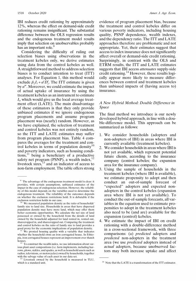
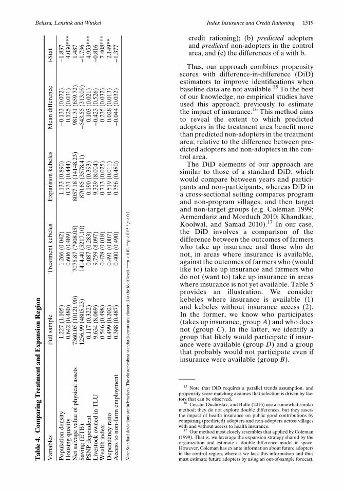
i. The ITT estimate is givenby αw. Moreover, we could estimate the impactof actual uptake of insurance by using thetreatment kebeles as an instrument to estimateIi, which would give us the local average treat-ment effect (LATE). The main disadvantageof these estimators is that they only provideunbiased estimates if we ignore endogenousprogram placements and assume programplacement was (nearly) random. However, aswe have explained, the selection of treatmentand control kebeles was not entirely random,so the ITT and LATE estimates may sufferfrom program placement bias. Table 4 com-pares the averages for the treatment and con-trol kebeles in terms of population density10

and poverty indicators, such as housing condi-tions,11 being a beneficiary of a productivesafety net program (PSNP), a wealth index,12

livestock sizes,13 and an indicator of access tonon-farm employment. The table offers strong

evidence of program placement bias, becausethe treatment and control kebeles differ onvarious poverty indicators, including housingquality, PSNP dependence, wealth indexes,and the dependency ratio. The ITT and LATEapproaches therefore are problematic and notappropriate. Yet, their estimates suggest thataccess to index insurance does not significantlyaffect overall or demand-side credit rationing.Surprisingly, in contrast with the OLS andETRM results, the ITT and LATE estimatessuggests that IBI access attenuates supply-sidecredit rationing.14 However, these results logi-cally appear more likely to measure differ-ences between control and treatment kebelesthan unbiased impacts of (having access to)insurance.

A New Hybrid Method: Double Difference inSpace

The final method we introduce is our newlydeveloped hybrid approach, in line with a dou-ble-difference model. This approach can besummarized as follows:

1. We consider households (adopters andnon-adopters of IBI) in areas where IBI iscurrently available (treatment kebeles).

2. We consider households in areaswhere IBI isnot yet available, which represent potentialfuture clients, according to the insurancecompany (control kebeles; the expansionarea for the insurance company).

3. Using the sample of households in thetreatment kebeles (where IBI is available),we estimate propensity to adopt and thenconduct an out-of-sample forecast of“expected” adopters and expected non-adopters in the control kebeles (expansionarea where IBI is not yet available). Toconduct the out-of-sample forecasts, all var-iables in the equation used to estimate pro-pensities to adopt in the treatment kebelesalso need to be (and are) available for theexpansion (control) kebeles.

4. We estimate the impact of IBI on creditrationing with a double-difference methodin a cross-sectional framework, with threecomparisons: (a) predicted adopters andpredicted non-adopters in the treatmentarea (we use predicted adopters instead ofactual adopters, because unobserved fac-tors may both increase uptake and affect

9 The advantage of the endogenous treatment model is clear: itprovides, with certain assumptions, unbiased estimates of theimpact in the case of endogenous selection. However, the reliabil-ity of this model depends on the variables used to determine theendogenous treatment. The reliability of the outcomes dependson whether the exclusion restrictions hold. It is debatable if theexclusion restriction holds in our case.

10 We measured population density as the ratio of households’family size to land size. Households in areas that have dispersedpopulation density may have more land, which may offer thembetter economic opportunities. We calculate the net size of landpossessed or owned by the household from the details of landowned by the household adjusted for land rented in, rented out,sharecropped in, and sharecropped out. Comparing the treatmentand control kebeles on the ratio of family size to land provides agood proxy for the economic implications of population density.

11 We proxied housing quality with a variable that indicateswhether the household owns an iron corrugated house. In Ethio-pia, iron corrugated houses represent an improvement over thatchhouses.

12 To construct the wealth index, we use information about var-ious plant asset compositions (i.e. farm implements, including har-rows, plows, sickles, and spades, as well as household assets such asradios, televisions, or motorcycles) owned by households, togetherwith the salvage value of each asset in our data set.

13 Livestock owned by the household is measured in TLU,which is a standard unit. 14 Note that the LATE is a transformation of the ITT estimator.


credit rationing); (b) predicted adoptersand predicted non-adopters in the controlarea, and (c) the differences of a with b.

Thus, our approach combines propensityscores with difference-in-difference (DiD)estimators to improve identifications whenbaseline data are not available.15 To the bestof our knowledge, no empirical studies haveused this approach previously to estimatethe impact of insurance.16 This method aimsto reveal the extent to which predictedadopters in the treatment area benefit morethan predicted non-adopters in the treatmentarea, relative to the difference between pre-dicted adopters and non-adopters in the con-trol area.

The DiD elements of our approach aresimilar to those of a standard DiD, whichwould compare between years and partici-pants and non-participants, whereas DiD ina cross-sectional setting compares programand non-program villages, and then targetand non-target groups (e.g. Coleman 1999;Armendariz and Morduch 2010; Khandkar,Koolwal, and Samad 2010).17 In our case,the DiD involves a comparison of thedifference between the outcomes of farmerswho take up insurance and those who donot, in areas where insurance is available,against the outcomes of farmers who (wouldlike to) take up insurance and farmers whodo not (want to) take up insurance in areaswhere insurance is not yet available. Table 5provides an illustration. We considerkebeles where insurance is available (1)and kebeles without insurance access (2).In the former, we know who participates(takes up insurance, group A) and who doesnot (group C). In the latter, we identify agroup that likely would participate if insur-ance were available (group D) and a groupthat probably would not participate even ifinsurance were available (group B).

Tab

le4.

Com

paring

Treatmen

tand

Exp

ansion

Reg

ion

Variables

Fullsam

ple

Treatmen

tke

beles

Exp

ansion

kebe

les

Meandifferen

cet-Stat

Pop

ulationde

nsity

1.227(1.105)

1.266(0.042)

1.133(0.890)

−0.133(0.072)

−1.837

Hou

sing

quality

0.642(0.480)

0.606(0.489)

0.731(0.444)

0.125(0.031)

4.030***

Net

salvagevalueof

physical

assets

7360.05(10121.90)

7075.87(7908.05)

8057.18(14148.23)

981.31

(659.72)

1.487

Saving

(ETB)

1256.99(4805.23)

1414.40(5217.10)

870.85

(3578.41)

−543.55

(313.09)

−1.736

PSN

Pde

pend

ent

0.117(0.322)

0.087(0.283)

0.190(0.393)

0.103(0.021)

4.953***

Livestock

owne

din

TLU

9.634(8.069)

9.759(8.097)

9.329(8.004)

−0.423(0.526)

−0.816

Wealthinde

x0.546(0.498)

0.478(0.018)

0.713(0.025)

0.235(0.032)

7.408***

Dep

ende

ncyratio

0.499(0.202)

0.491(0.007)

0.519(0.011)

0.028(0.013)

2.149**

Accessto

non-farm

employ

men

t0.388(0.487)

0.400(0.490)

0.356(0.480)

−0.044(0.032)

−1.377

Note:Stan

dard

deviations

arein

bracke

ts.T

hecluster-robu

ststan

dardserrors

areclusteredat

theiddirleve

l.**

*p<0.01

.**p

<0.05

.*p<0.1.

15 Note that DiD requires a parallel trends assumption, andpropensity score matching assumes that selection is driven by fac-tors that can be observed.

16 Cecchi, Duchoslav, and Bulte (2016) use a somewhat similarmethod; they do not explore double differences, but they assessthe impact of health insurance on public good contributions bycomparing (predicted) adopters and non-adopters across villageswith and without access to health insurance.

17 Our method most closely resembles that applied by Coleman(1999). That is, we leverage the expansion strategy shared by theorganization and estimate a double-difference model in space.However, Coleman has ex ante information about future adoptersin the control region, whereas we lack this information and thusmust estimate future adopters by using an out-of-sample forecast.


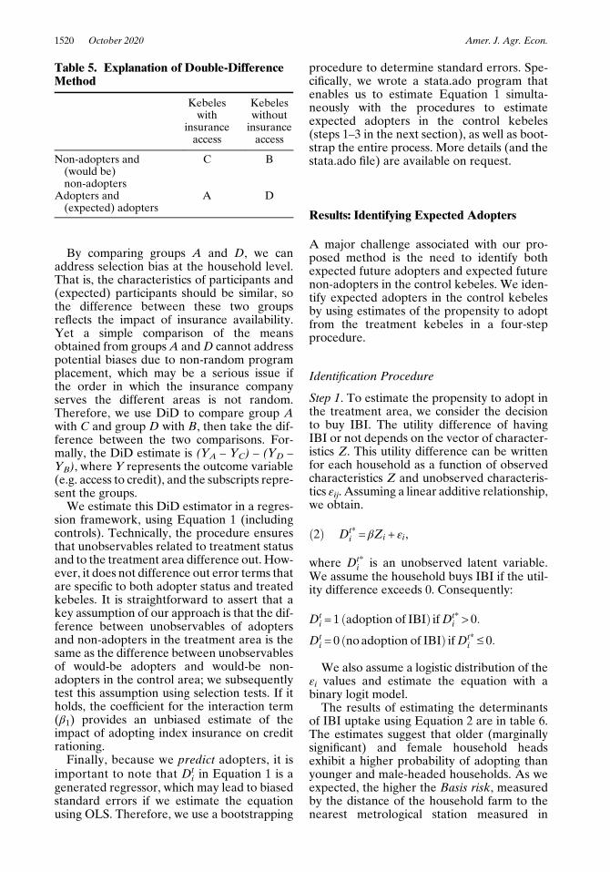
By comparing groups A and D, we canaddress selection bias at the household level.That is, the characteristics of participants and(expected) participants should be similar, sothe difference between these two groupsreflects the impact of insurance availability.Yet a simple comparison of the meansobtained from groupsA andD cannot addresspotential biases due to non-random programplacement, which may be a serious issue ifthe order in which the insurance companyserves the different areas is not random.Therefore, we use DiD to compare group Awith C and group D with B, then take the dif-ference between the two comparisons. For-mally, the DiD estimate is (YA – YC) – (YD –

YB), where Y represents the outcome variable(e.g. access to credit), and the subscripts repre-sent the groups.We estimate this DiD estimator in a regres-

sion framework, using Equation 1 (includingcontrols). Technically, the procedure ensuresthat unobservables related to treatment statusand to the treatment area difference out. How-ever, it does not difference out error terms thatare specific to both adopter status and treatedkebeles. It is straightforward to assert that akey assumption of our approach is that the dif-ference between unobservables of adoptersand non-adopters in the treatment area is thesame as the difference between unobservablesof would-be adopters and would-be non-adopters in the control area; we subsequentlytest this assumption using selection tests. If itholds, the coefficient for the interaction term(β1) provides an unbiased estimate of theimpact of adopting index insurance on creditrationing.Finally, because we predict adopters, it is

important to note that Dti in Equation 1 is a

generated regressor, which may lead to biasedstandard errors if we estimate the equationusing OLS. Therefore, we use a bootstrapping

procedure to determine standard errors. Spe-cifically, we wrote a stata.ado program thatenables us to estimate Equation 1 simulta-neously with the procedures to estimateexpected adopters in the control kebeles(steps 1–3 in the next section), as well as boot-strap the entire process. More details (and thestata.ado file) are available on request.

Results: Identifying Expected Adopters

A major challenge associated with our pro-posed method is the need to identify bothexpected future adopters and expected futurenon-adopters in the control kebeles. We iden-tify expected adopters in the control kebelesby using estimates of the propensity to adoptfrom the treatment kebeles in a four-stepprocedure.

Identification Procedure

Step 1. To estimate the propensity to adopt inthe treatment area, we consider the decisionto buy IBI. The utility difference of havingIBI or not depends on the vector of character-istics Z. This utility difference can be writtenfor each household as a function of observedcharacteristics Z and unobserved characteris-tics εij. Assuming a linear additive relationship,we obtain.

ð2Þ Dt*i = βZi + εi,

where Dt*i is an unobserved latent variable.

We assume the household buys IBI if the util-ity difference exceeds 0. Consequently:

Dti = 1 adoption of IBIð Þ ifDt*

i > 0:

Dti = 0 noadoption of IBIð Þ ifDt*

i ≤ 0:

We also assume a logistic distribution of theεi values and estimate the equation with abinary logit model.

The results of estimating the determinantsof IBI uptake using Equation 2 are in table 6.The estimates suggest that older (marginallysignificant) and female household headsexhibit a higher probability of adopting thanyounger and male-headed households. As weexpected, the higher the Basis risk, measuredby the distance of the household farm to thenearest metrological station measured in

Table 5. Explanation of Double-DifferenceMethod

Kebeleswith

insuranceaccess

Kebeleswithoutinsuranceaccess

Non-adopters and(would be)non-adopters

C B

Adopters and(expected) adopters

A D


walking hours, the lower the probability toadopt insurance. However, this effect is insig-nificant,18 probably because of its high correla-tion with Present-bias or procrastination,measured by a binary dummy, equal to 1 forhouseholds that indicate that, if insurance isavailable, they would postpone the uptakedecision until the final insurance sales day tomake a better estimate of future weather con-ditions. This indicator measures whetherhouseholds wait until the sales deadline, sothat they can better forecast future weatherconditions and then make their insuranceuptake decisions.19 Attending insurance pro-motion meetings positively affects uptake,according to the positive, significant coeffi-cient for Insurance product promotion mea-sured by a dummy variable equal to 1 forhouseholds that participated in a product pro-motion meeting (campaign) of JICA and OICand 0 for those that did not participate. Weconsider Education, Family size, Cooperativemembership, and Draft oxen, but only Familysize and Draft oxen (marginally) are signifi-cant. The uptake equation thus appears ableto separate adopters from non-adopters, asreflected by the area under the receiver oper-ating characteristic (ROC) curve, which isequal to 0.84.

A crucial assumption of our proposedmethod is that selection effects due to unob-servables can be controlled for by adding adummy variable that indicates which farmersare adopters and would-be adopters. How-ever, if our results turn out to be sensitive toa misclassification of (would-be) adopters,selection effects may seriously bias the results.To determine whether the results are sensitiveto the precise specification of the uptake equa-tion, we consider two alternative specifica-tions, in which we add more variables tocontrol for the potential omitted variable bias.First, we add three control variables: Peerinfluence, Risk aversion (CRRA), and Timepreference. Peer influence is measured by adummy, equal to 1 for households that indi-cate that their peers, relatives, or neighbors

who have bought insurance have influencedthem to buy IBI, and 0 for others. In theexpansion area, households indicated whetherpeer influence has convinced them to buy atthe moment the insurance becomes available.For exact definitions of Risk and Time prefer-ence, see Table A1. Households may be morewilling to adopt insurance if some of theirpeers already have bought it (Peer influence).Risk aversion likely negatively affects uptake,which may sound counterintuitive but is in linewith studies that cite trust issues;20 apparently,more risk-averse households do not trustinsurance, so they are less willing to adopt it.Finally, the relationship between Time prefer-ence and uptake is positive21 but insignifi-cant.22 Second, in another uptake regression,we ignore Peer influence, which could beaffected by insurance: if somebody buys IBI,there are potentially more peers available thatmay positively affect other purchasers or non-purchasers. As we show in the online Appen-dix, Table S1 (Equations 1 and 2), the perfor-mance of the alternative uptake equations, interms of R-square values and the ROC curve,are similar to that of our preferred uptakeequation.Step 2. Using Equation 2 and the estimation

specified in table 6, we conduct an out-of-sam-ple forecast to predict the propensity to adoptin the control area.23

Step 3. To identify expected future adoptersand expected future non-adopters in the con-trol area, we endogenously set a thresholdvalue of the probability to adopt, above whicha farmer is classified as an expected adopteraccording to the optimization of the so-calledYouden Index (Youden 1950). This index esti-mates the probability of an informed decision,rather than a random guess and thus providesa measure of discriminatory power. It is calcu-lated as sensitivity + specificity − 1, where sen-sitivity (or true positive rate) measures theproportion of correctly classified positives,

18 Basis risk becomes significant if we drop the Present-bias orprocrastination variable from the model. The main results holdfor three alternative models: (a) both variables included, (b) onlybasis risk included, or (c) only Present-bias or procrastinationincluded.

19 In a given insurance sales period (e.g., 45 days), some house-holds might wait to make their purchase decision until the 44th or45th day, at which point they have the most updated informationabout future rainfall. Similar behavior, such that farmers updatetheir rainfall beliefs in response to external forecasts, is documen-ted by Lybbert et al. (2007).

20 Risk aversion is derived from an incentivized lab-in-the-fieldexperiment that we conducted to assess risk attitudes. It includes amultiple price list protocol that requires participants to choosebetween a safe and a risky option (50/50 probability; Binswanger1980). More details are available on request.

21 Our time preference indicator comes from a time preferencegame we played with all households in the sample.

22 We do not drop insignificant variables from the uptake equa-tions, so they still may affect the predicted outcomes.

23 All variables in Step 1 are available for both the treatmentand control kebeles, so out-of-sample forecasts are possible. Thisoption also holds for the binary variable Insurance product promo-tion, because during our survey, the insurance company alreadyhad conducted promotional meetings in the expansion (control)kebeles.


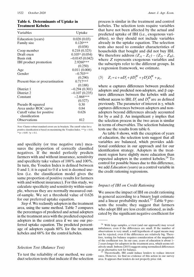
and specificity (or true negative rate) mea-sures the proportion of correctly classifiednegatives. If the model perfectly predictsfarmers with and without insurance, sensitivityand specificity take values of 100% and 100%.In turn, the Youden Index is defined between0 and 1; it is equal to 0 if a test is deemed use-less (i.e. the classification model gives thesame proportion of positive results for farmerswith and without insurance). For this study, wecalculate specificity and sensitivity within-sam-ple, whereas they are normally measured out-of-sample. We set a threshold value of 0.626for our preferred uptake equation.Step 4. We reclassify adopters in the treatment

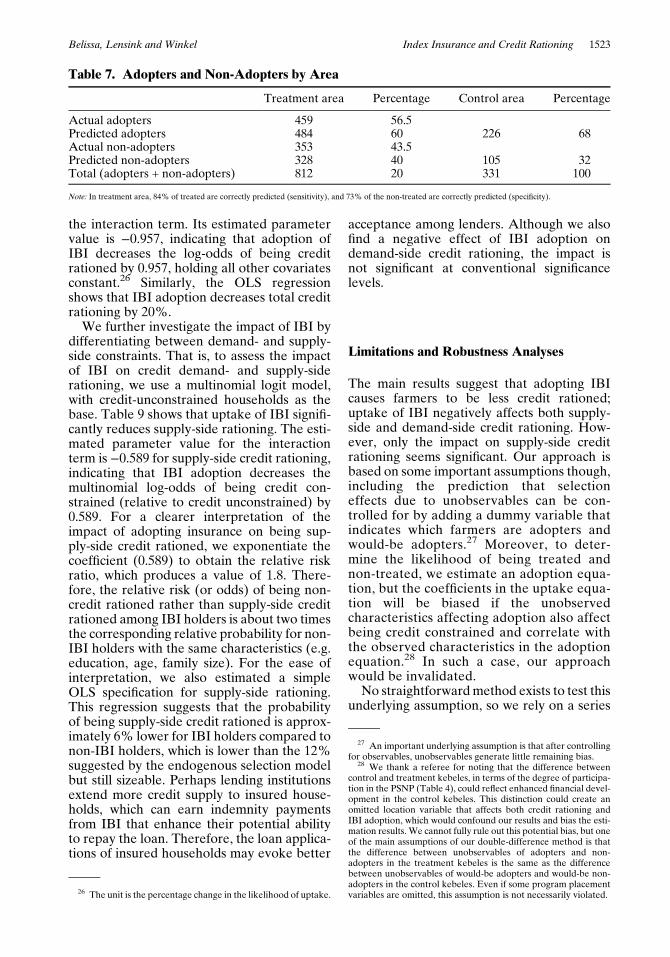
area, using the same method. Table 7 comparesthe percentages of predicted and actual adoptersin the treatment areawith thepredicted expectedadopters in the control area if we use our pre-ferred uptake equation. The predicted percent-age of adopters equals 60% for the treatmentkebeles and 68% for the control kebeles.

Selection Test (Balance Test)

To test the reliability of our method, we con-duct selection tests that indicate if the selection

process is similar in the treatment and controlkebeles. The selection tests require variablesthat have not been affected by the actual andpredicted uptake of IBI (i.e., exogenous vari-ables), so they should not include variablesalready in the uptake equation. The selectiontests also need to consider characteristics ofhouseholds that bought and did not buy IBI.We therefore address (ZA – ZC) – (ZD – ZB),where Z represents exogenous variables andthe subscripts refer to the different groups. Ina regression framework, we estimate.

ð3Þ Zi = c+ αDti + βDW

i + γDtiD

Wi + μi,

where α captures differences between predictedadopters and predicted non-adopters, and β cap-tures differences between the kebeles with andwithout access to IBI;Dt

i and DWi are as defined

previously. The parameter of interest is γ, whichcaptures differences between adopters and non-adopters beyond differences already accountedfor by α and β. An insignificant γ implies thatthe selection process in the two areas is similarin terms of observables. The selection balancingtests use the results from table 6.

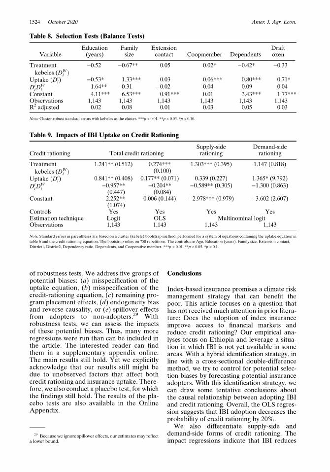
As table 8 shows, with the exception of yearsof education, the selection tests suggest that allvariables are balanced, which provides addi-tional confidence in our approach and for ouridentification strategy. Adopters in the treat-ment region have slightly more education thanexpected adopters in the control kebeles.24 Tocontrol for possible biases due to this difference,we addEducation (years) as a control variable inthe credit rationing regressions.

Impact of IBI on Credit Rationing

We assess the impact of IBI on credit rationingin general according to a binary logit estimateand a linear probability model.25 Table 9 pre-sents the results; they suggest that farmerswho adopt IBI are less credit rationed, as indi-cated by the significant negative coefficient for

Table 6. Determinants of Uptake inTreatment Kebeles

Variables Uptake

Education (years) 0.028 (0.03)Family size 0.120***

(0.038)Coop member 0.218 (0.325)Draft oxen 0.105* (0.054)Basis risk −0.0145 (0.042)IBI product promotion 2.9260***

(0.250)Age 0.011 (0.008)Gender −0.703**

(0.290)Present-bias or procrastination 0.717***

(0.188)District 1 −0.294 (0.301)District 2 −0.107 (0.235)Constant −2.868***

(0.527)Pseudo R-squared 0.30Area under ROC curve 0.84Cutoff value for positiveclassification

0.626

Observations 812

Note: Cluster-robust standard errors are in brackets. The cutoff value for apositive classification is based on maximizing the Youden Index. ***p < 0.01.**p < 0.05. *p < 0.1.

24 With large samples, a t-test (and our approach) may revealimbalances, even if the differences are small. If the number ofobservations is very small, a null hypothesis of equal means maynot be rejected, even if the differences are relatively big. There-fore, testing for balance requires consideration of the magnitudeof the coefficient too. In our case, years of education is about 1–2 years longer for adopters in the treatment area, which seems rel-atively small. Imbens (2015) suggests using normalized differencesas an alternative test for balance.

25 Theoretically, IBI could induce lenders to reduce interestrates. However, we find no evidence of this action in our surveyarea. It appears that lenders do not properly price risk.


the interaction term. Its estimated parametervalue is −0.957, indicating that adoption ofIBI decreases the log-odds of being creditrationed by 0.957, holding all other covariatesconstant.26 Similarly, the OLS regressionshows that IBI adoption decreases total creditrationing by 20%.

We further investigate the impact of IBI bydifferentiating between demand- and supply-side constraints. That is, to assess the impactof IBI on credit demand- and supply-siderationing, we use a multinomial logit model,with credit-unconstrained households as thebase. Table 9 shows that uptake of IBI signifi-cantly reduces supply-side rationing. The esti-mated parameter value for the interactionterm is −0.589 for supply-side credit rationing,indicating that IBI adoption decreases themultinomial log-odds of being credit con-strained (relative to credit unconstrained) by0.589. For a clearer interpretation of theimpact of adopting insurance on being sup-ply-side credit rationed, we exponentiate thecoefficient (0.589) to obtain the relative riskratio, which produces a value of 1.8. There-fore, the relative risk (or odds) of being non-credit rationed rather than supply-side creditrationed among IBI holders is about two timesthe corresponding relative probability for non-IBI holders with the same characteristics (e.g.education, age, family size). For the ease ofinterpretation, we also estimated a simpleOLS specification for supply-side rationing.This regression suggests that the probabilityof being supply-side credit rationed is approx-imately 6% lower for IBI holders compared tonon-IBI holders, which is lower than the 12%suggested by the endogenous selection modelbut still sizeable. Perhaps lending institutionsextend more credit supply to insured house-holds, which can earn indemnity paymentsfrom IBI that enhance their potential abilityto repay the loan. Therefore, the loan applica-tions of insured households may evoke better

acceptance among lenders. Although we alsofind a negative effect of IBI adoption ondemand-side credit rationing, the impact isnot significant at conventional significancelevels.

Limitations and Robustness Analyses

The main results suggest that adopting IBIcauses farmers to be less credit rationed;uptake of IBI negatively affects both supply-side and demand-side credit rationing. How-ever, only the impact on supply-side creditrationing seems significant. Our approach isbased on some important assumptions though,including the prediction that selectioneffects due to unobservables can be con-trolled for by adding a dummy variable thatindicates which farmers are adopters andwould-be adopters.27 Moreover, to deter-mine the likelihood of being treated andnon-treated, we estimate an adoption equa-tion, but the coefficients in the uptake equa-tion will be biased if the unobservedcharacteristics affecting adoption also affectbeing credit constrained and correlate withthe observed characteristics in the adoptionequation.28 In such a case, our approachwould be invalidated.No straightforwardmethod exists to test this

underlying assumption, so we rely on a series

Table 7. Adopters and Non-Adopters by Area

Treatment area Percentage Control area Percentage

Actual adopters 459 56.5Predicted adopters 484 60 226 68Actual non-adopters 353 43.5Predicted non-adopters 328 40 105 32Total (adopters + non-adopters) 812 20 331 100

Note: In treatment area, 84% of treated are correctly predicted (sensitivity), and 73% of the non-treated are correctly predicted (specificity).

26 The unit is the percentage change in the likelihood of uptake.

27 An important underlying assumption is that after controllingfor observables, unobservables generate little remaining bias.

28 We thank a referee for noting that the difference betweencontrol and treatment kebeles, in terms of the degree of participa-tion in the PSNP (Table 4), could reflect enhanced financial devel-opment in the control kebeles. This distinction could create anomitted location variable that affects both credit rationing andIBI adoption, which would confound our results and bias the esti-mation results. We cannot fully rule out this potential bias, but oneof the main assumptions of our double-difference method is thatthe difference between unobservables of adopters and non-adopters in the treatment kebeles is the same as the differencebetween unobservables of would-be adopters and would-be non-adopters in the control kebeles. Even if some program placementvariables are omitted, this assumption is not necessarily violated.


of robustness tests. We address five groups ofpotential biases: (a) misspecification of theuptake equation, (b) misspecification of thecredit-rationing equation, (c) remaining pro-gram placement effects, (d) endogeneity biasand reverse causality, or (e) spillover effectsfrom adopters to non-adopters.29 Withrobustness tests, we can assess the impactsof these potential biases. Thus, many moreregressions were run than can be included inthe article. The interested reader can findthem in a supplementary appendix online.The main results still hold. Yet we explicitlyacknowledge that our results still might bedue to unobserved factors that affect bothcredit rationing and insurance uptake. There-fore, we also conduct a placebo test, for whichthe findings still hold. The results of the pla-cebo tests are also available in the OnlineAppendix.

Conclusions

Index-based insurance promises a climate riskmanagement strategy that can benefit thepoor. This article focuses on a question thathas not receivedmuch attention in prior litera-ture: Does the adoption of index insuranceimprove access to financial markets andreduce credit rationing? Our empirical ana-lyses focus on Ethiopia and leverage a situa-tion in which IBI is not yet available in someareas. With a hybrid identification strategy, inline with a cross-sectional double-differencemethod, we try to control for potential selec-tion biases by forecasting potential insuranceadopters. With this identification strategy, wecan draw some tentative conclusions aboutthe causal relationship between adopting IBIand credit rationing. Overall, the OLS regres-sion suggests that IBI adoption decreases theprobability of credit rationing by 20%.

We also differentiate supply-side anddemand-side forms of credit rationing. Theimpact regressions indicate that IBI reduces

Table 8. Selection Tests (Balance Tests)

VariableEducation(years)

Familysize

Extensioncontact Coopmember Dependents

Draftoxen

Treatmentkebeles (DW

i Þ−0.52 −0.67** 0.05 0.02* −0.42* −0.33

Uptake ðDti) −0.53* 1.33*** 0.03 0.06*** 0.80*** 0.71*

DtiD

Wi

1.64** 0.31 −0.02 0.04 0.09 0.04Constant 4.11*** 6.53*** 0.91*** 0.01 3.43*** 1.77***Observations 1,143 1,143 1,143 1,143 1,143 1,143R2 adjusted 0.02 0.08 0.01 0.03 0.05 0.03

Note: Cluster-robust standard errors with kebeles as the cluster. ***p < 0.01. **p < 0.05. *p < 0.10.

Table 9. Impacts of IBI Uptake on Credit Rationing

Credit rationing Total credit rationingSupply-siderationing

Demand-siderationing

Treatmentkebeles (DW

i Þ1.241** (0.512) 0.274***

(0.100)1.303*** (0.395) 1.147 (0.818)

Uptake ðDti) 0.841** (0.408) 0.177** (0.071) 0.339 (0.227) 1.365* (9.792)

DtiD

Wi

−0.957**(0.447)

−0.204**(0.084)

−0.589** (0.305) −1.300 (0.863)

Constant −2.252**(1.074)

0.006 (0.144) −2.978*** (0.979) −3.602 (2.607)

Controls Yes Yes Yes YesEstimation technique Logit OLS Multinominal logitObservations 1,143 1,143 1,143 1,143

Note: Standard errors in parentheses are based on a cluster (kebele) bootstrap method, performed for a system of equations containing the uptake equation intable 6 and the credit rationing equation. The bootstrap relies on 750 repetitions. The controls are Age, Education (years), Family size, Extension contact,District1, District2, Dependency ratio, Dependents, and Cooperative member. ***p < 0.01. **p < 0.05. *p < 0.1.

29 Because we ignore spillover effects, our estimates may reflecta lower bound.


both supply-side rationing (quantity rationing)and demand-side credit rationing, but the lat-ter does not appear robust. The nonsignificantimpact on demand-side credit rationing is notsurprising as the insurance contract is astand-alone product, for which indemnitiesare paid directly to farmers, and the majorityof smallholders lack any valuable collateralto offer.

The study findings suggest a relatively largeimpact of IBI uptake on reducing supply-sidecredit rationing. Across various regressions,we find that the relative risk of being non-credit rationed rather than supply-side creditrationed among IBI holders is about two timesthe corresponding relative probability for non-IBI holders. Thus, IBI adoption appears toenhance smallholders’ access to credit. It alsoprovides mutual benefits to farmers (bor-rowers) and lenders. Alleviating supply-sidecredit constraints enables farmers to acquireinputs and enhance productivity. Becausetheir access to credit overcomes their liquidityconstraints, farmers can employ other riskmanagement strategies to hedge againstdownside production risks. For lenders, lend-ing to insured farmers reduces the default riskof lending. In presenting these outcomes, wetake care to note that the findings are basedon the results after one year of program imple-mentation. It is not necessarily the case thatlenders are more willing to provide credit spe-cifically to insured applicants. Alternatively,increased lending could reflect decreasedtransaction costs when lenders combine creditsupply with IBI provisioning. Further researchis needed to determine the precise empiricalimplications.

Our proposed hybrid method can be used insettings in which an intervention already hastaken place, such that no pre-interventionbaseline survey is possible. Such a situation,which is common in reality, precludes eithera standard double-difference method or a ran-domized controlled trial. Yet our proposedmethod is not without limitations. In particu-lar, the ability to estimate adopters correctlyand obtain unbiased estimates of the coeffi-cients in the adoption equation is crucial. Thismethod also relies on the important assump-tion that unobserved characteristics that affectboth adoption and credit rationing are not cor-related with observed characteristics thataffect IBI uptake. There is no straightforwardmethod to test this assumption, so we presentvarious robustness analyses to increase confi-dence in the plausibility of our main results;

such analyses might not offer similar confi-dence in other settings. Because the robust-ness of our hybrid method approach has notbeen tested in alternative settings, it cannotoffer an alternative to well-known, rigorousmethods, like randomized trials. However,we hope this article encourages continuedresearch that tests whether our method isappropriate in various settings, if our resultshold in other settings, andwhether the findingsare robust to the use of other identificationstrategies, such as randomized controlledtrials.

Supplementary Material

Supplementary material are available atAmerican Journal of Agricultural Economicsonline.

References

Armendariz, Beatriz, and Jonathan Morduch.2010. The Economics of Microfinance.Cambridge, MA: MIT Press.

Banerjee, Abhijit V. 2000. The Two Poverties.Nordic Journal of Political Economy 26(2): 129–41.

Barnett, Bary J, Christopher B Barrett, andJerry R Skees. 2008. Poverty Traps andIndex-Based Risk Transfer Products.World Development 36(10): 1766–85.

Beegle, Kathleen, Rajeev H. Dehejia, andGatti, Roberta 2003. Child Labor, IncomeShocks, and Access to Credit. PolicyResearch Working Paper 3075, WorldBank.

Besanko, David, and Anjan V Thakor. 1987.Competitive Equilibrium in the CreditMarket Under Asymmetric Information.Journal of Economic Theory 42(1):167–82.

Bester, Helmut. 1985. Screening vs. Rationingin Credit Markets with Imperfect Infor-mation. American Economic Review 74(4): 850–5.

. 1987. The Role of Collateral in CreditMarkets with Imperfect Information.European Economic Review 31(4):887–99.

Biazin, Birhanu, and Geert Sterk. 2013.Drought Vulnerability Drives Land-Useand Land Cover Changes in the Rift


Valley Dry Lands of Ethiopia. Agricul-ture, Ecosystems and Environment 164:100–13.

Binswanger, Hans P. 1980. Attitudes towardRisk: Experimental Measurement inRural India.American Journal of Agricul-tural Economics 62(3): 395–407.

Boucher, Steve, and Catherine Guirkinger.2007. Risk, Wealth, and Sectoral Choicein Rural Credit Markets. American Jour-nal of Agricultural Economics 89(4):991–1004.

Boucher, Stephen R, Michael R Carter, andCatherine Guirkinger. 2008. Risk Ration-ing and Wealth Effects in Credit Markets:Theory and Implications for AgriculturalDevelopment. American Journal of Agri-cultural Economics 90(2): 409–23.

Boucher, StephenR, CatherineGuirkinger, andCarolina Trivelli. 2009. Direct Elicitation ofCredit Constraints: Conceptual and Practi-cal Issues with an Application to PeruvianAgriculture. Economic Development andCultural Change 57(4): 609–40.

Carter, Michael R, Lan Cheng, andAlexandros Sarris. 2016. Where andHow Index Insurance Can Boost theAdoption of Improved Agricultural Tech-nologies. Journal of Development Eco-nomics 118(C): 59–71.

Carter, Michael, Alain de Janvry, ElisabethSadoulet, and Alexandros Sarris. 2017.Index Insurance for Developing CountryAgriculture: A Reassessment. AnnualReview of Resource Economics 9: 421–38.

Cecchi, Francesco, Jan Duchoslav, and ErwinBulte. 2016. Formal Insurance and theDynamics of Social Capital: ExperimentalEvidence from Uganda. Journal of Afri-can Economics 25(3): 418–38.

Cheng, Lan. 2014. The Impact of IndexInsurance on Borrower’s Moral HazardBehavior in Rural Credit Markets.Working Paper, University of Californiaat Davis. Available at: https://arefiles.ucdavis.edu/uploads/filer_public/2014/06/20/lan-cheng-jmp-11-27.pdf.Accessed April 2018.

Clarke, Daniel, and Stefan Dercon 2009.Insurance, Credit and Safety Nets for thePoor in a World of Risk. Working Paper81, United Nations, Department of Eco-nomics and Social Affairs.

Clarke, Daniel, Olivier Mahul, Kolli N. Rao,and Niraj Verma 2012. Weather BasedCrop Insurance in India. Working Paper5985, World Bank Policy Research.

Cole, Shawn, Gautam G. Bastian, SangitaVyas, Carina Wendel, and Daniel Stein2012. Systematic Review. The effective-ness of index-based micro-insuranceinhelping smallholders manage weather-related risks. London, UK: EPPI-Centre,Social Science Research Unit, Institute ofEducation, University of London.

Cole, Shawn, Xavier Giné, Jeremy Tobacman,Robert Townsend, Petia Topalova, andJames Vickery. 2013. Barriers to House-hold Risk Management: Evidence fromIndia. American Economic Journal:Applied Economics 5(1): 104–35.

Coleman, Brett E. 1999. The Impact of GroupLending in Northeast Thailand. Journal ofDevelopment Economics 60(1): 105–41.

Conning, Jonathan, and Christopher Udry.2007. Rural Financial Markets in Devel-oping Countries. InHandbook of Agricul-tural Economics, Vol 3 2857–908. TheNetherlands: Elsevier.

Cummins, J David, David Lalonde, andRichard D Phillips. 2004. The Basis Riskof Catastrophic-Loss Index Securities.Journal of Financial Economics 71(1):77–111.

Dercon, Stefan. 2004. Growth and Shocks:Evidence from Rural Ethiopia. Journalof Development Economics 74(2):309–29.

Dercon, Stefan, and Luc Christiaensen. 2011.Consumption Risk, TechnologyAdoptionand Poverty Traps: Evidence from Ethio-pia. Journal of Development Economics96(2): 159–73.

Dercon, Stefan, Ruth V Hill, Daniel Clarke,Ingo Outes-Leon, and Alemayehu STaffesse. 2014. Offering Rainfall Insur-ance to Informal Insurance Groups: Evi-dence from a Field Experiment inEthiopia. Journal of Development Eco-nomics 106: 132–43.

Dercon, Stefan, John Hoddinott, and TassewWoldehanna. 2005. Shocks and Consump-tion in 15 Ethiopian Villages, 1999-2004.Journal of African Economies 14(4):559–85.

Dowd, Kevin. 1992. Optimal Financial Con-tracts. Oxford Economic Papers 44(4):672–93.

Elabed, Ghada, and Michael R. Carter 2014.Ex-ante Impacts of Agricultural Insurance:Evidence from a Field Experiment in Mali.University of California at Davis. Avail-able at: https://arefiles.ucdavis.edu/uploads/filer_public/2014/08/29/impact_


https://arefiles.ucdavis.edu/uploads/filer_public/2014/06/20/lan-cheng-jmp-11-27.pdf



https://arefiles.ucdavis.edu/uploads/filer_public/2014/08/29/impact_evaluation_0714_vdraft.pdf


evaluation_0714_vdraft.pdf. AccessedJanuary 2018.

Farrin, Katie, and Mario J Miranda. 2015. AHeterogeneous Agent Model of Credit-Linked Index Insurance and Farm Tech-nologyAdoption. Journal of DevelopmentEconomics 116: 199–211.

Ghosh, Parikshit, Dilip Mookherjee, andDebraj Ray. 2000. Credit Rationing inDeveloping Countries: An Overview ofthe Theory. Readings in the Theory ofEconomic Development: 383–401.

Giné, Xavier, and Dean Yang. 2009. Insur-ance, Credit, and Technology Adoption:Field Experimental Evidence fromMalawi. Journal ofDevelopment Econom-ics 89(1): 1–11.

Guarcello, Lorenz, Fabrizia Mealli, and FurioC Rosati. 2010. Household Vulnerabilityand Child Labor: The Effect of Shocks,Credit Rationing, and Insurance. Journalof Population Economics 23(1): 169–98.

Heckman, James. 1976. The Common Struc-ture of Statistical Models of Truncation,Sample Selection and Limited DependentVariables and a Simple Estimator forSuch Models. Annals of Economic andSocial Measurement 5: 475–92.

. 1978. Dummy Endogenous Variablesin a Simultaneous Equation System.Econometrica 46: 931–59.

Hill, Ruth V, John Hoddinott, and NehaKumar. 2013. Adoption ofWeather-IndexInsurance: Learning from Willingness toPay among a Panel of Households inRural Ethiopia. Agricultural Economics44(4–5): 385–98.

Imbens, GuidoW. 2015. Matching Methods inPractice: Three Examples. Journal ofHuman Resources 50(2): 373–419.

Islam, Asadul, and Pushkar Maitra. 2012.Health Shocks and Consumption Smooth-ing in Rural Households: Does Microcre-dit Have a Role to Play? Journal ofDevelopment Economics 97(2): 232–43.

Jaffee, Dwight M, and Thomas Russell. 1976.Imperfect Information, Uncertainty, andCredit Rationing. Quarterly Journal ofEconomics 90(4): 651–66.

Janzen, Sarah A, and Michal R Carter. 2019.After the Drought: The Impact of Micro-insurance on Consumption Smoothingand Asset Protection. American Journalof Agricultural Economics 101(3): 651–671.

Jensen, Nathaniel D, Andrew Mude, andChristopher B Barrett. 2018. How Basis

Risk and Spatiotemporal Adverse Selec-tion Influence Demand for Index Insur-ance: Evidence from Northern Kenya.Food Policy 74: 172–98.

Karlan, Dean, Robert Osei, Isaac Osei-Akoto,and Christopher Udry. 2014. AgriculturalDecisions after Relaxing Credit and RiskConstraints. Quarterly Journal of Eco-nomics 129(2): 597–652.

Khandkar, Shahidur R, Gayatri B Koolwal, andHussain A Samad. 2010. Handbook onImpact Evaluation: Quantitative Methodsand Practices.Washington, DC:World Bank.

Lensink,Robert, andElmer Sterken. 2001.Asym-metric Information, Option to Wait to Investand theOptimalLevel of Investment. Journalof Public Economics 79(2): 365–74.

. 2002. The Option toWait to Invest andEquilibrium Credit Rationing. Journal ofMoney, Credit, and Banking 34(1): 221–5.

Lybbert, Travis J, Christopher B Barrett, JohnG McPeak, and Winnie K Luseno. 2007.Bayesian Herders: Updating of RainfallBeliefs in Response to External Forecasts.World Development 35(3): 480–97.

Mahul, Olivier, and Jerry Skees 2007. Manag-ing Agricultural Risk at the CountryLevel: The Case of Index-Based Live-stock Insurance in Mongolia. WorkingPaper 4325, World Bank.

McIntosh, Craig, Alexander Sarris, and FotisPapadopoulos. 2013. Productivity, Credit,Risk, and the Demand for Weather IndexInsurance in Smallholder Agriculture inEthiopia. Agricultural Economics 44(4–5):399–417.

Morduch, Jonathan. 1995. Income Smoothingand Consumption Smoothing. Journal ofEconomic Perspectives 9(3): 103–14.

Skees, Jerry R. 2008. Innovations in IndexInsurance for the Poor in Lower IncomeCountries. Agricultural and ResourceEconomics Review 37(1): 73–100.

Stiglitz, Joseph E, and Andrew Weiss. 1981.Credit Rationing in Markets with Imper-fect Information. American EconomicReview 71(3): 393–410.

Takahashi, Kazushi, Munenobu Ikegami,Megan Sheahan, and Christopher BBarrett. 2016. Experimental Evidence onthe Drivers of Index-Based LivestockInsurance Demand in Southern Ethiopia.World Development 78: 324–40.

Vandell, Kerry D. 1984. Imperfect Informa-tion, Uncertainty, and Credit Rationing:Comment and Extension. Quarterly Jour-nal of Economics 99(4): 841–63.



Williamson, Stephen D. 1986. Costly Monitor-ing, Financial Intermediation, and Equi-librium Credit Rationing. Journal ofMonetary Economics 18(2): 159–79.

Wooldridge, Jeffrey M. 2010. EconometricAnalysis of Cross Section and PanelData, 2nd ed. Cambridge, MA: MITPress.

Youden, WJ. 1950. Index for Rating Diagnos-tic Tests. Cancer 3: 32–5.

Zant, Wouter. 2008. Hot Stuff: Index Insur-ance for Indian Smallholder PepperGrowers. World Development 36(9):1585–606.

Zimmerman, Frederick J, and Michael RCarter. 2003. Asset Smoothing, Consump-tion Smoothing and the Reproduction ofInequality Under Risk and SubsistenceConstraints. Journal of Development Eco-nomics 71(2): 233–60.


Appendix

A. Tree diagram illustrating credit rationingstatus

Notes:

• Have you applied for a bank loan over thelast five years?(1) Yes [n = 439].(2) No [n = 704]

• Has your application been accepted?(1) Yes [n = 383].(2) No [n = 56]

• Did you want larger loan at the same inter-est rate?(1) Yes [n = 57].(2) No [n = 326]

• If you did not apply, would a bank now lendto you if you apply?(1) Yes [n = 108].(2) No [n = 317].(3) I do not know (IDK) [n = 279]

• If you think that a bank would now lend toyou if you apply, why do you not apply?

Indicate reason(s)(1) I do not need loan [n = 44].(2) High interest rate [n = 6].(3) Farming does not give me enough torepay a debt [n = 11].(4) I prefer working with my own liquidity[n = 4].(5) I do not want to put my collateral at risk[n = 13].(6) I do not want to be worried [n = 6].(7) I prefer informal lenders because formallenders are so strict [n = 4].(8) Formal lenders do not offer refinancing[n = 5].(9) The branch is too far away [n = 6].(10) The lending procedures are too costly[n = 9].(11) IDK

Figure A1. Direct elicitation method (Boucher, Guirkinger, and Trivelli 2009)


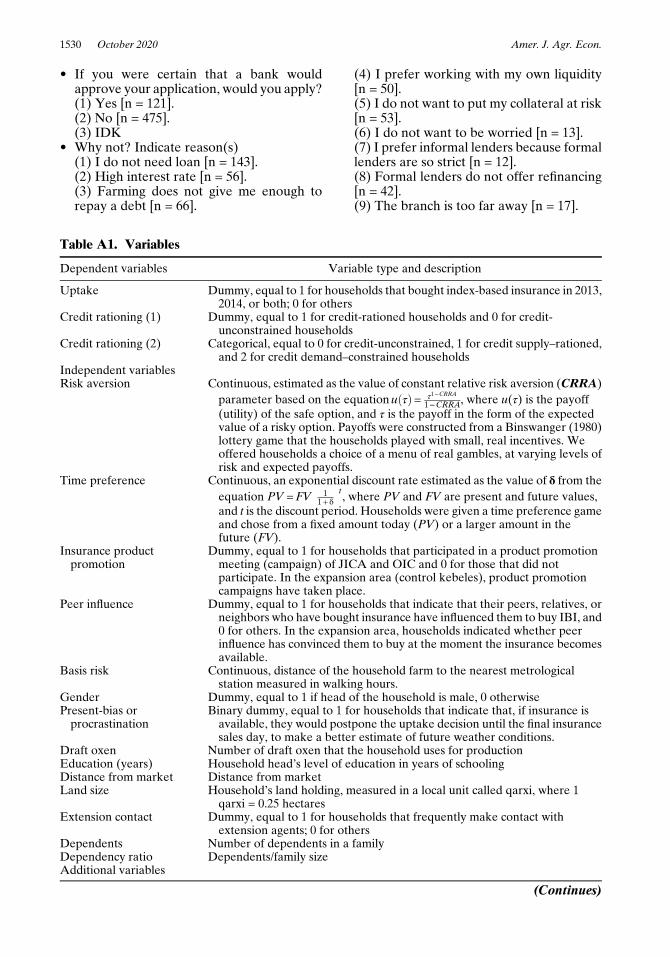
• If you were certain that a bank wouldapprove your application, would you apply?(1) Yes [n = 121].(2) No [n = 475].(3) IDK

• Why not? Indicate reason(s)(1) I do not need loan [n = 143].(2) High interest rate [n = 56].(3) Farming does not give me enough torepay a debt [n = 66].

(4) I prefer working with my own liquidity[n = 50].(5) I do not want to put my collateral at risk[n = 53].(6) I do not want to be worried [n = 13].(7) I prefer informal lenders because formallenders are so strict [n = 12].(8) Formal lenders do not offer refinancing[n = 42].(9) The branch is too far away [n = 17].

Table A1. Variables

Dependent variables Variable type and description

Uptake Dummy, equal to 1 for households that bought index-based insurance in 2013,2014, or both; 0 for others

Credit rationing (1) Dummy, equal to 1 for credit-rationed households and 0 for credit-unconstrained households

Credit rationing (2) Categorical, equal to 0 for credit-unconstrained, 1 for credit supply–rationed,and 2 for credit demand–constrained households

Independent variablesRisk aversion Continuous, estimated as the value of constant relative risk aversion (CRRA)

parameter based on the equationu τð Þ= τ1−CRRA

1−CRRA, where u(τ) is the payoff(utility) of the safe option, and τ is the payoff in the form of the expectedvalue of a risky option. Payoffs were constructed from a Binswanger (1980)lottery game that the households played with small, real incentives. Weoffered households a choice of a menu of real gambles, at varying levels ofrisk and expected payoffs.

Time preference Continuous, an exponential discount rate estimated as the value of δ from theequation PV =FV 1

1 + δ

� �t, where PV and FV are present and future values,

and t is the discount period. Households were given a time preference gameand chose from a fixed amount today (PV) or a larger amount in thefuture (FV).

Insurance productpromotion

Dummy, equal to 1 for households that participated in a product promotionmeeting (campaign) of JICA and OIC and 0 for those that did notparticipate. In the expansion area (control kebeles), product promotioncampaigns have taken place.

Peer influence Dummy, equal to 1 for households that indicate that their peers, relatives, orneighbors who have bought insurance have influenced them to buy IBI, and0 for others. In the expansion area, households indicated whether peerinfluence has convinced them to buy at the moment the insurance becomesavailable.

Basis risk Continuous, distance of the household farm to the nearest metrologicalstation measured in walking hours.

Gender Dummy, equal to 1 if head of the household is male, 0 otherwisePresent-bias orprocrastination

Binary dummy, equal to 1 for households that indicate that, if insurance isavailable, they would postpone the uptake decision until the final insurancesales day, to make a better estimate of future weather conditions.

Draft oxen Number of draft oxen that the household uses for productionEducation (years) Household head’s level of education in years of schoolingDistance from market Distance from marketLand size Household’s land holding, measured in a local unit called qarxi, where 1

qarxi = 0.25 hectaresExtension contact Dummy, equal to 1 for households that frequently make contact with

extension agents; 0 for othersDependents Number of dependents in a familyDependency ratio Dependents/family sizeAdditional variables

(Continues)


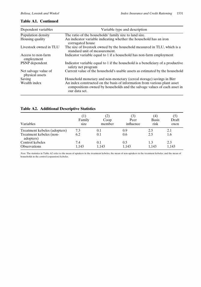
Table A2. Additional Descriptive Statistics

(1) (2) (3) (4) (5)

VariablesFamilysize

Coopmember

Peerinfluence

Basisrisk

Draftoxen

Treatment kebeles (adopters) 7.3 0.1 0.9 2.5 2.1Treatment kebeles (non-adopters)

6.2 0.1 0.6 2.5 1.6

Control kebeles 7.4 0.1 0.5 1.3 2.3Observations 1,143 1,143 1,143 1,143 1,143

Note: The statistics in Table A2 refer to the mean of uptakers in the treatment kebeles; the mean of non-uptakers in the treatment kebeles; and the mean ofhouseholds in the control (expansion) kebeles.

Table A1. Continued

Dependent variables Variable type and description

Population density The ratio of the households’ family size to land size.Housing quality An indicator variable indicating whether the household has an iron

corrugated houseLivestock owned in TLU The size of livestock owned by the household measured in TLU, which is a

standard unit of measurement.Access to non-farmemployment

Indicator variable equal to 1 if a household has non-farm employment

PSNP dependent Indicator variable equal to 1 if the household is a beneficiary of a productivesafety net program

Net salvage value ofphysical assets

Current value of the household’s usable assets as estimated by the household

Saving Household monetary and non-monetary (cereal storage) savings in BirrWealth index An index constructed on the basis of information from various plant asset

compositions owned by households and the salvage values of each asset inour data set.


effects of index insurance on demand and supply of credit

Documents