arX

iv:q

-bio

/050

8013

v1 [

q-bi

o.N

C]

13

Aug

200

5

Effects of Fast Presynaptic Noise in Attractor Neural Networks

J. M. Cortes†‡, J. J. Torres†, J. Marro†, P. L. Garrido† and H. J. Kappen‡

†Institute Carlos I for Theoretical and Computational Physics, and

Departamento de Electromagnetismo y Fısica de la Materia,

University of Granada, E-18071 Granada, Spain.‡Department of Biophysics, Radboud University of Nijmegen,

6525 EZ Nijmegen, The Netherlands

April 5, 2007

To appear in Neural Computation, 2005

Corresponding author: Jesus M. Cortes

mailto:jcortes@ugr.es

Abstract

We study both analytically and numerically the ef-fect of presynaptic noise on the transmission of in-formation in attractor neural networks. The noiseoccurs on a very short–time scale compared to thatfor the neuron dynamics and it produces short–time synaptic depression. This is inspired in recentneurobiological findings that show that synapticstrength may either increase or decrease on a short–time scale depending on presynaptic activity. Wethus describe a mechanism by which fast presynap-tic noise enhances the neural network sensitivity toan external stimulus. The reason for this is that,in general, the presynaptic noise induces nonequi-librium behavior and, consequently, the space offixed points is qualitatively modified in such a waythat the system can easily scape from the attrac-tor. As a result, the model shows, in addition topattern recognition, class identification and catego-rization, which may be relevant to the understand-ing of some of the brain complex tasks.

1 Introduction

There is multiple converging evidence[Abbott and Regehr, 2004] that synapses de-termine the complex processing of information in

the brain. An aspect of this statement is illustratedby attractor neural networks. These show thatsynapses can efficiently store patterns that are af-terwards retrieved with only partial information onthem. In addition to this long–time effect, artificialneural networks should contain some “synapticnoise”, however. That is, actual synapses exhibitshort–time fluctuations, which seem to competewith other mechanisms during the transmissionof information, not to cause unreliability but toultimately determine a variety of computations[Allen and Stevens, 1994, Zador, 1998]. In spiteof some recent efforts, a full understanding ofhow the brain complex processes depend on suchfast synaptic variations is lacking —see belowand [Abbott and Regehr, 2004], for instance—.A specific matter under discussion concerns theinfluence of short–time noise on the fixed pointsand other details of the retrieval processes inattractor neural networks [Bibitchkov et al., 2002].

The observation that actual synapses endureshort–time depression and/or facilitation is likelyto be relevant in this context. That is, onemay understand some observations by assumingthat periods of elevated presynaptic activity maycause either decrease or increase of the neuro-transmitter release and, consequently, that thepostsynaptic response will be either depressed orfacilitated depending on presynaptic neural ac-tivity [Tsodyks et al., 1998, Thomson et al., 2002,Abbott and Regehr, 2004]. Motivated by the neu-robiological findings, we report in this paper on ef-fects of presynaptic depressing noise on the func-

1

tionality of a neural circuit. We study in detail anetwork in which the neural activity evolves at ran-dom in time regulated by a “temperature” param-eter. In addition, the values assigned to the synap-tic intensities by a learning (e.g., Hebb’s) rule areconstantly perturbed with microscopic fast noise.A new parameter is involved by this perturbationthat allows for a continuum transition from depres-sion to normal operation.

As a main result, this paper illustrates that,in general, the addition of fast synaptic noise in-duces a nonequilibrium condition. That is, oursystems cannot asymptotically reach equilibriumbut tend to nonequilibrium steady states whosefeatures depend, even qualitatively, on dynamics[Marro and Dickman, 1999]. This is interesting be-cause, in practice, thermodynamic equilibrium israre in nature. Instead, the simplest conditionsone observes are characterized by a steady flux ofenergy or information, for instance. This makesthe model mathematically involved, e.g., there isno general framework such as the powerful (equi-librium) Gibbs theory, which only applies to sys-tems with a single Kelvin temperature and a uniqueHamiltonian. However, our system still admits ana-lytical treatment for some choices of its parametersand, in other cases, we discovered the more intri-cate model behavior by a series of computer simula-tions. We thus show that fast presynaptic depress-ing noise during external stimulation may inducethe system to scape from the attractor, namely,the stability of fixed point solutions is dramaticallymodified. More specifically, we show that, for cer-tain versions of the system, the solution destabi-lizes in such a way that computational tasks such asclass identification and categorization are favored.It is likely this is the first time such a behavior isreported in an artificial neural network as a con-sequence of biologically–motivated stochastic be-havior of synapses. Similar instabilities have beenreported to occur in monkeys [Abeles et al., 1995]and other animals [Miller and Schreiner, 2000], andthey are believed to be a main feature in odor en-coding [Laurent et al., 2001], for instance.

2 Definition of model

Our interest is in a neural network in whicha local stochastic dynamics is constantly influ-

enced by presynaptic noise. Consider a setof N binary neurons with configurations S ≡{si = ±1; i = 1, . . . , N} . 1 Any two neurons areconnected by synapses of intensity: 2

wij = wijxj ∀i, j. (1)

Here, wij is fixed, namely, determined in a pre-vious learning process, and xj is a stochasticvariable. This generalizes the hypothesis in previ-ous studies of attractor neural networks with noisysynapses; see, for instance, [Sompolinsky, 1986,Garrido and Marro, 1991, Marro et al., 1999].Once W ≡{wij} is given, the state of the systemat time t is defined by setting S and X ≡ {xi}.These evolve with time —after the learning processwhich fixes W— via the familiar Master Equation,namely,

∂Pt(S,X)

∂t= −Pt(S,X)

∫

X′

∑

S′

c[(S,X) → (S′,X′)]

+

∫

X′

∑

S′

c[( S′,X′) → (S,X)]Pt(S

′,X′). (2)

We further assume that the transition rate or prob-ability per unit time of evolving from (S,X) to(S′,X′) is

c[(S,X) → (S′, X′)] = p cX[S → S

′]δ(X − X′)

+(1 − p) cS[X → X′]δS,S′ . (3)

This choice [Garrido and Marro, 1994,Torres et al., 1997] amounts to consider com-peting mechanisms. That is, neurons (S) evolvestochastically in time under a noisy dynamicsof synapses (X), the latter evolving (1 − p)/ptimes faster than the former. Depending on thevalue of p, three main classes may be defined[Marro and Dickman, 1999]:

1. For p ∈ (0, 1) both the synaptic fluctua-tion and the neuron activity occur on the

1Note that such binary neurons, although a crude sim-plification of nature, are known to capture the essentials ofcooperative phenomena, which is the focus here. See, forinstance [Abbott and Kepler, 1990, Pantic et al., 2002].

2For simplicity, we are neglecting here postsynaptic de-pendence of the stochastic perturbation. There is someclaim that plasticity might operate on rapid time–scaleson postsynaptic activity; see [Pitler and Alger, 1992]. How-ever, including xij in (1) instead of xj would impede someof the algebra in sections 3 and 4.

2

same temporal scale. This case has alreadybeen preliminary explored [Pantic et al., 2002,Cortes et al., 2004].

2. The limiting case p → 1. This corresponds toneurons evolving in the presence of a quenchedsynaptic configuration, i.e., xi is constantand independent of i. The Hopfield model

[Amari, 1972, Hopfield, 1982] belongs to thisclass in the simple case that xj = 1, ∀j.

3. The limiting case p → 0. The rest of this paperis devoted to this class of systems.

Our interest for the latter case is a consequence ofthe following facts. Firstly, there is adiabatic elim-ination of fast variables for p → 0 which decou-ples the two dynamics [Garrido and Marro, 1994,Gardiner, 2004]. Therefore, some exact analyticaltreatment —though not the complete solution— isthen feasible. To be more specific, for p → 0, theneurons evolve as in the presence of a steady distri-bution for X. If we write P (S,X) = P (X|S)P (S),where P (X|S) stands for the conditional probabil-ity of X given S, one obtains from (2) and (3),after rescaling time tp → t (technical details areworked out in [Marro and Dickman, 1999], for in-stance) that

∂Pt(S)

∂t= −Pt(S)

∑

S′

c[S → S′]

+∑

S′

c[S′ → S]Pt(S′). (4)

Here,

c[S → S′] ≡

∫

dXP st(X|S) cX[S → S′], (5)

and P st(X|S) is the stationary solution that satis-fies

P st(X|S) =

∫

d X′ cS[X′ → X] P st(X′|S)

∫

dX′ cS[X → X′]. (6)

This formalism will allows us for modelling fastsynaptic noise which, within the appropiate con-text, will induce sort of synaptic depression, as ex-plained in detail in section 4.

The superposition (5) reflects the fact that ac-tivity is the result of competition between differ-ent elementary mechanisms. That is, different un-derlying dynamics, each associated to a different

realization of the stochasticity X, compete and,in the limit p → 0, an effective rate results fromcombining cX[S → S

′] with probability P st(X|S)for varying X. Each of the elementary dynamicstends to drive the system to a well-defined equi-librium state. The competition will, however, im-pede equilibrium and, in general, the system willasymptotically go towards a nonequilibrium steadystate [Marro and Dickman, 1999]. The question isif such a competition between synaptic noise andneural activity, which induces nonequilibrium, is atthe origin of some of the computational strategiesin neurobiological systems. Our study below seemsto indicate that this is a sensible issue. As a matterof fact, we shall argue below that p → 0 may be re-alistic a priori for appropriate choices of P st(X|S).

For the sake of simplicity, we shall be concernedin this paper with sequential updating by meansof single neuron or “spin–flip” dynamics. That is,the elementary dynamic step will simply consist oflocal inversions si → −si induced by a bath at tem-perature T. The elementary rate cX[S → S

′] thenreduces to a single site rate that one may write asΨ[u X(S, i)]. Here, uX(S, i) ≡ 2T−1sih

Xi (S), where

hX

i (S) =∑

j 6=i wijxjsj is the net presynaptic cur-rent arriving to —or local field acting on— the(postsynaptic) neuron i. The function Ψ(u) is ar-bitrary except that, for simplicity, we shall assumeΨ(u) = exp(−u)Ψ(−u), Ψ(0) = 1 and Ψ(∞) = 0[Marro and Dickman, 1999]. We shall report onthe consequences of more complex dynamics in aforthcomming paper [Cortes et al., 2005].

3 Effective local fields

Let us define a function Heff(S) through the con-dition of detailed balance, namely,

c[S → Si]

c[Si → S]= exp

{

−[

Heff(Si) − Heff(S)]

T−1}

.

(7)Here, S

i stands for S after flipping at i, si → −si.We further define the “effective local fields” heff

i (S)by means of

Heff(S) = −1

2

∑

i

heffi (S) si. (8)

Nothing guaranties that Heff(S) and heffi (S) have

a simple expression and are therefore analytically

3

useful. This is because the superposition (5), un-like its elements Ψ(u X), does not satisfy detailedbalance, in general. In other words, our system hasan essential nonequilibrium character that preventsone from using Gibbs’s statistical mechanics, whichrequires a unique Hamiltonian. Instead, there ishere one energy associated with each realization ofX ={xi}. This is in addition to the fact that thesynaptic weights wij in (1) may not be symmetric.

For some choices of both the rate Ψ andthe noise distribution P st(X|S), the functionHeff(S) may be considered as a true effec-tive Hamiltonian [Garrido and Marro, 1989,Marro and Dickman, 1999]. This means thatHeff(S) then generates the same nonequilibriumsteady state than the stochastic time–evolutionequation which defines the system, i.e., equation(4), and that its coefficients have the propersymmetry of interactions. To be more explicit,assume that P st(X|S) factorizes according to

Pst (X|S) =

∏

j

P (xj |sj) , (9)

and that one also has the factorization

c[S → Si] =

∏

j 6=i

∫

dxj P (xj |sj)Ψ(2T−1siwijxjsj).

(10)The former amounts to neglect some global de-pendence of the factors on S = {si} (see below),and the latter restricts the possible choices forthe rate function. Some familiar choices for thisfunction that satisfy detailed balance are: theone corresponding to the Metropolis algorithm,i.e., Ψ(u) = min[1, exp(−u)]; the Glauber caseΨ(u) = [1 + exp(u)]−1; and Ψ(u) = exp(−u/2)[Marro and Dickman, 1999]. The latter fulfillsΨ(u + v) = Ψ(u)Ψ(v) which is required by (10)3. It then ensues after some algebra that

heffi = −T

∑

j 6=i

[

α+ijsj + α−

ij

]

, (11)

3In any case, the rate needs to be properly normalized.In computer simulations, it is customary to divide Ψ(u) byits maximum value. Therefore, the normalization happensto depend on temperature and on the number of stored pat-terns. It follows that this normalization is irrelevant for theproperties of the steady state, namely, it just rescales thetime scale.

with

α±ij ≡ 1

4ln

c(βij ; +) c(±βij ;−)

c(−βij ;∓) c(∓βij ;±), (12)

where βij ≡ 2T−1wij , and

c(βij ; sj) =

∫

dxj P (xj |sj)Ψ(βijxj). (13)

This generalizes a case in the litera-ture for random S –independent fluc-tuations [Garrido and Munoz, 1993,Lacomba and Marro, 1994,Marro and Dickman, 1999]. In this case, onehas c(±κ; +) = c(±κ;−) and, consequently,α−

ij = 0 ∀i, j. However, we here are concerned withthe case of S–dependent disorder, which results ina non–zero threshold, θi ≡

∑

j 6=i α−ij 6= 0.

In order to obtain a true effective Hamiltonian,the coefficients α±

ij in (11) need to be symmetric.Once Ψ(u) is fixed, this depends on the choice forP (xj |sj), i.e., on the fast noise details. This is stud-ied in the next section. Meanwhile, we remark thatthe effective local fields heff

i defined above are veryuseful in practice. That is, they may be computed—at least numerically— for any rate and noise dis-tribution. As far as Ψ(u + v) = Ψ(u)Ψ(v) andP

st (X|S) factorizes,4 it follows an effective transi-tion rate as

c[S → Si] = exp

(

−siheffi /T

)

. (14)

This effective rate may then be used in computersimulation, and it may also serve to be substitutedin the relevant equations. Consider, for instance,the overlaps defined as the product of the currentstate with one of the stored patterns:

mν(S) ≡ 1

N

∑

i

siξνi . (15)

Here, ξν = {ξνi = ±1, i = 1, . . . , N} are M

random patterns previously stored in the system,ν = 1, . . . , M. After using standard techniques[Hertz et al., 1991, Marro and Dickman, 1999]; see

4The factorization here does not need to be inproducts P (xj |sj) as in (9). The same result (14)holds for the choice that we shall introduce in thenext section, for instance.

4

also [Amit et al., 1987], it follows from (4) that

∂tmν = 2N−1

∑

i

ξνi sinh

(

heffi /T

)

−si cosh(

heffi /T

)

.

(16)which is to be averaged over both thermal noise andpattern realizations. Alternatively, one might per-haps obtain dynamic equations of type (16) by us-ing Fokker-Planck like formalisms as, for instance,in [Brunel and Hakim, 1999].

4 Types of synaptic noise

The above discussion and, in particular, equations(11) and (12), suggest that the system emergentproperties will importantly depend on the details ofthe synaptic noise X. We now work out the equa-tions in section 3 for different hypothesis concerningthe stationary distribution (6).

Consider first (9) with the following specificchoice:

P (xj |sj) =1 + sjFj

2δ(xj +Φ)+

1 − sjFj

2δ(xj −1).

(17)This corresponds to a simplification of the stochas-tic variable xj . That is, for Fj = 1 ∀j, the noisemodifies wij by a factor −Φ when the presynapticneuron is firing, sj = 1, while the learned synap-tic intensity remains unchanged when the neuronis silent. In general, wij = −wijΦ with probability12

(1 + sjFj) . Here, Fj stands for some informa-tion concerning the presynaptic site j such as, forinstance, a local threshold or Fj = M−1

∑

ν ξνj .

Our interest for case (17) is two fold, namely,it corresponds to an exceptionally simple situationand it reduces our model to two known cases. Thisbecomes evident by looking at the resulting localfields:

heffi =

1

2

∑

j 6=i

[(1 − Φ) sj − (1 + Φ) Fj ] wij . (18)

That is, exceptionally, symmetries here are suchthat the system is described by a true effectiveHamiltonian. Furthermore, this corresponds to theHopfield model, except for a rescaling of temper-ature and for the emergence of a threshold θi ≡∑

j wijFj [Hertz et al., 1991]. On the other hand,it also follows that, concerning stationary prop-erties, the resulting effective Hamiltonian (8) re-produces the model as in [Bibitchkov et al., 2002].

In fact, this would correspond in our notation toheff

i = 12

∑

j 6=i wijsjx∞j , where x∞

j stands for thestationary solution of certain dynamic equation forxj . The conclusion is that (except perhaps concern-ing dynamics, which is something worth to be in-vestigated) the fast noise according to (9) with (17)does not imply any surprising behavior. In anycase, this choice of noise illustrates the utility ofthe effective–field concept as defined above.

Our interest here is in modeling the noise consis-tent with the observation of short-time synaptic de-pression [Tsodyks et al., 1998, Pantic et al., 2002].In fact, the case (17) in some way mimics that in-creasing the mean firing rate results in decreasingthe synaptic weight. With the same motivation, amore intriguing behavior ensues by assuming, in-stead of (9), the factorization

P st(X|S) =∏

j

P (xj |S) (19)

with

P (xj |S) = ζ ( ~m) δ(xj +Φ)+ [1 − ζ ( ~m)] δ(xj −1).(20)

Here, ~m = ~m(S) ≡(

m1(S), . . . , mM (S))

is theM -dimensional overlap vector, and ζ ( ~m) standsfor a function of ~m to be determined. The de-pression effect here depends on the overlap vec-tor which measures the net current arriving topostsynaptic neurons. The non–local choice (19)–(20) thus introduces non–trivial correlations be-tween synaptic noise and neural activity, whichis not considered in (17). Note that, therefore,we are not modelling here the synaptic depres-sion dynamics in an explicity way as, for instance,in [Tsodyks et al., 1998]. Instead, equation (20)amounts to consider fast synaptic noise which nat-urally depresses the strengh of the synapses afterrepeated activity, namely, for a high value of ζ (~m) .

Several further comments on the significance of(19)-(20), which is here a main hypothesis togetherwith p → 0, are in order. We first mention thatthe system time relaxation is typically orders ofmagnitude larger than the time scale for the var-ious synaptic fluctuations reported to account forthe observed high variability in the postsynapticresponse of central neurons [Zador, 1998]. On theother hand, these fluctuations seem to have differ-ent sources such as, for instance, the stochasticity

5

of the opening and closing of the vesicles (S. Kil-fiker, private communication), the stochasticity ofthe postsynaptic receptor, which has its own severalcauses, variations of the glutamate concentration inthe synaptic cleft, and differences in the potency re-leased from different locations on the active zone ofthe synapses [Franks et al., 2003]. Is this complexsituation the one that we try to capture by intro-ducing the stochastic variable x in (1) and subse-quent equations. It may be further noticed thatthe nature of this variable, which is ”microscopic”here, differs from the one in the case of familiarphenomenological models. These often involve a”mesoscopic” variable, such as the mean fractionof neurotransmitter, which results in a determinis-tic situation, as in [Tsodyks et al., 1998]. The de-pression in our model rather naturally follows fromthe coupling between the synaptic ”noise” and theneurons dynamics via the overlap functions. Thefinal result is also deterministic for p → 0 but only,as one should perhaps expect, on the time scalefor the neurons. Finally, concerning also the real-ity of the model, it should be clear that we arerestricting ourselves here to fully connected net-works just for simplicity. However, we already stud-ied similar systems with more realistic topologiessuch as scale-free, small-world and diluted networks[Torres et al., 2004], which suggests one to general-ize the present study in this sense.

It is to be remarked that our case (19)-(20) alsoreduces to the Hopfield model but only in the limitΦ → −1 for any ζ ( ~m) . Otherwise, the competitionresults in a rather complex behavior. In particular,the noise distribution P st(X|S) lacks with (20) thefactorization property which is required to have aneffective Hamiltonian with proper symmetry. Nev-ertheless, we may still write

c[S → Si]

c[Si → S]=

∏

j 6=i

∫

dxj P (xj |S)Ψ(sixjsjβij)∫

dxj P (xj |Si)Ψ(−sixjsjβij).

(21)Then, using (20), we linearize around wij = 0,i.e., βij = 0 for T > 0. This is a good approxi-mation for the Hebbian learning rule [Hebb, 1949]wij = N−1

∑

ν ξνi ξν

j , which is the one we use here-after, as far as this rule only stores completely un-correlated, random patterns. In fact, fluctuationsin this case are of order

√M/N for finite M (or

order 1/√

N for finite α) which tends to vanish fora sufficiently large system, e.g., in the macroscopic

0

0.5

1

0.4 0.8 1.2

m

T

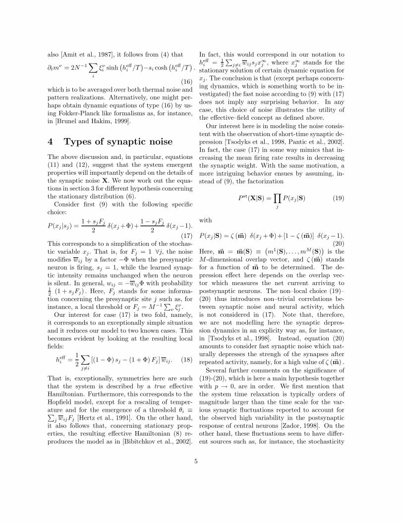
Figure 1: The steady overlap m(T ), as predicted by equa-

tion (25), for different values of the noise parameter, namely,

Φ = −2.0, −1.5, −1.0, −0.5, 0, 0.5, 1.0, 1.5, 2.0, from top

to bottom, respectively. (Φ = −1 corresponds to the Hop-

field case, as explained in the main text.) The graphs depict

second order phase transitions (solid curves) and, for the

most negative values of Φ, first order phase transitions (the

discontinuities in these cases are indicated by dashed lines).

The symbols stand for Monte Carlo data corresponding to a

network with N = 1600 neurons for Φ = −0.5 (filled squares)

and −2.0 (filled circles).

(thermodynamic) limit N → ∞. It then follows theeffective weights:

weffij =

{

1 − 1 + Φ

2

[

ζ ( ~m) + ζ(

~mi)]

}

wij , (22)

where ~m = ~m(S), ~mi ≡ ~m(Si) = ~m−2si~ξi/N, and

~ξi =(

ξ1i , ξ2

i , ..., ξMi

)

is the binary M–dimensionalstored pattern. This shows how the noise modifiessynaptic intensities. The associated effective localfields are

heffi =

∑

j 6=i

weffij sj . (23)

The condition to obtain a true effective Hamilto-nian, i.e., proper symmetry of (22) from this, is

that ~mi = ~m − 2si~ξi/N ≃ ~m. This is a good ap-

proximation in the thermodynamic limit, N → ∞.Otherwise, one may proceed with the dynamic

equation (16) after substituting (23), even thoughthis is not then a true effective Hamiltonian. Onemay follow the same procedure for the Hopfield casewith asymmetric synapses [Hertz et al., 1991], for

6

-3

-2.5

-2

-1.5

-1

0.8 1.2 1.6 2

Φ

T

F

P

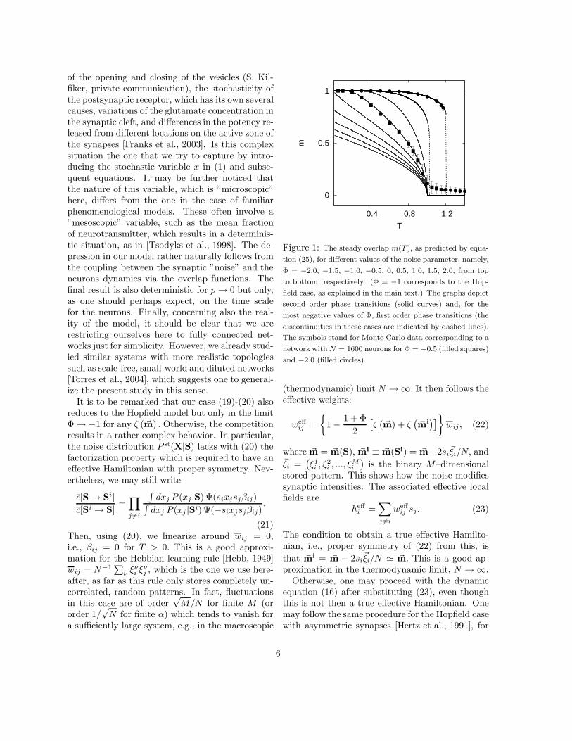
Figure 2: Phase diagram depicting the transition temper-

ature Tc as a function of T and Φ. The solid (dashed) curve

corresponds to a second (first) order phase transition. The

tricritical point is at (Tc, Φc) = (1,−4/3). F and P stand

for the ferromagnetic–like and paramagnetic–like phases, re-

spectively. The best retrieval properties of our model system

occur close to the left–lower quarter of the graph.

instance. Further interest on the concept of localeffective fields as defined in section 3 follows fromthe fact that one may use quantities such as (23)to importantly simplify a computer simulation, asit is made below.

To proceed further, we need to determine theprobability ζ in (20). In order to model activity–dependent mechanisms acting on the synapses,ζ should be an increasing function of the net presy-naptic current or field. In fact, ζ ( ~m) simply needsto depend on the overlaps, besides to preserve the±1 symmetry. A simple choice with these require-ments is

ζ ( ~m) =1

1 + α

∑

ν

[mν (S)]2, (24)

where α = M/N. We describe next the behaviorthat ensues from (22)–(24) as implied by the noisedistribution (20).

5 Noise induced phase transi-

tions

Let us first study the retrieval process in a sys-tem with a single stored pattern, M = 1, when theneurons are acted on by the local fields (23). One

-3

-2

-1

0

1

2

3

0 0.5 1

F(m

,Φ,δ

)

m

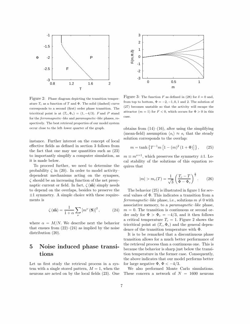
Figure 3: The function F as defined in (28) for δ = 0 and,

from top to bottom, Φ = −2,−1, 0, 1 and 2. The solution of

(27) becomes unstable so that the activity will escape the

attractor (m = 1) for F < 0, which occurs for Φ > 0 in this

case.

obtains from (14)–(16), after using the simplifying(mean-field) assumption 〈si〉 ≈ si that the steadysolution corresponds to the overlap:

m = tanh{

T−1m[

1 − (m)2 (1 + Φ)]}

, (25)

m ≡ mν=1, which preserves the symmetry ±1. Lo-cal stability of the solutions of this equation re-quires that

|m| > mc(T ) =1√3

(

Tc − T

Φ − Φc

)1

2

. (26)

The behavior (25) is illustrated in figure 1 for sev-eral values of Φ. This indicates a transition from aferromagnetic–like phase, i.e., solutions m 6= 0 withassociative memory, to a paramagnetic–like phase,m = 0. The transition is continuous or second or-der only for Φ > Φc = −4/3, and it then followsa critical temperature Tc = 1. Figure 2 shows thetricritical point at (Tc, Φc) and the general depen-dence of the transition temperature with Φ.

It is to be remarked that a discontinuous phasetransition allows for a much better performance ofthe retrieval process than a continuous one. This isbecause the behavior is sharp just below the transi-tion temperature in the former case. Consequently,the above indicates that our model performs betterfor large negative Φ, Φ < −4/3.

We also performed Monte Carlo simulations.These concern a network of N = 1600 neurons

7

-1

-0.5

0

0.5

1

0 4000 8000

mA

0

0.5

1

0 1500 3000

m

B

-1-0.5

0 0.5

1

0 4000 8000

m

time (MCS)

C

0

0.5

1

0 3000 6000

m

time (MCS)

D

Figure 4: Time evolution of the overlap, as defined in (15),

between the current state and the stored pattern in Monte

Carlo simulations with 3600 neurons at T = 0.1. Each graph,

for a given set of values for (δ, Φ) shows different curves cor-

responding to evolutions starting with different initial states.

The two top graphs are for δ = 0.3 and Φ = 1 (graphs A and

C) and Φ = −1 (graphs B and D), the latter corresponding

to the Hopfield case lacking the fast noise. This shows the

important effect noise has on the network sensitivity to ex-

ternal stimuli. The two bottom graphs illustrate the same

for a fixed initial distance from the attractor as one varies

the external stimulation, namely, for δ = 0.1, 0.2, 0.3, 0.4 and

0.5 from top to bottom.

acted on by the local fields (23) and evolving bysequential updating via the effective rate (14). Ex-cept for some finite–size effects, figure 1 shows agood agreement between our simulations and theequations here; in fact, the computer simulationsalso correspond to a mean–field description giventhat the fields (23) assume fully connected neurons.

6 Sensitivity to the stimulus

As shown above, a noise distribution such as (20)may model activity-dependent processes reminis-cent of short-time synaptic depression. In this sec-tion, we study the consequences of this type offast noise on the retrieval dynamics under exter-nal stimulation. More specifically, our aim is tocheck the resulting sensitivity of the network to ex-ternal inputs. A high degree of sensibility will fa-cilitate the response to changing stimuli. This is an

1

0

-1

160 180 200 220 240

m1

Fast Noise

Hopfield

P1 P2 P3 P1 P2 P3 P1 P2 P3 δ=0 Input

time (103 MCS)

Figure 5: Time evolution during a Monte Carlo simulation

with N = 400 neurons, M = 3 correlated patterns (as de-

fined in the main text), and T = 0.1. The system in this case

was let to relaxe to the steady sate, and then perturbed by

the stimulus −δξν , δ = 0.3, with ν = 1 for a short time in-

terval, and then with ν = 2, and so on. After suppresing the

stimulus, the system is again allowed to relaxe. The graphs

show as a function of time, from top to bottom, (i) the num-

ber of the pattern which is used as the stimulus at each time

interval; (ii) the resulting response of the network, measured

as the overlap of the current state with pattern ν = 1, in the

absence of noise, i.e., the Hopfield case Φ = −1; (iii) the

same for the relevant noisy case Φ = 1.

important feature of neurobiological systems whichcontinuously adapt and quickly respond to varyingstimuli from the environment.

Consider first the case of one stored pattern,M = 1. A simple external input may be simu-lated by adding to each local field a driving term−δξi, ∀i, with 0 < δ ≪ 1 [Bibitchkov et al., 2002].A negative drive in this case of a single pattern as-sures that the network activity may go from theattractor, ξ, to the “antipattern”, −ξ. It then fol-lows the stationary overlap:

m = tanh[T−1F (m, Φ, δ)] (27)

with

F (m, Φ, δ) ≡ m[1 − (m)2(1 + Φ) − δ]. (28)

Figure 3 shows this function for δ = 0 and vary-ing Φ. This illustrates two different types of behav-ior, namely, (local) stability (F > 0) and instabil-ity (F < 0) of the attractor, which corresponds to

8

m = 1. That is, the noise induces instability, result-ing in this case in switching between the patternand the antipattern. This is confirmed in figure 4by Monte Carlo simulations.

The simulations corresponds to a network of N =3600 neurons with one stored pattern, M = 1. Thisevolves from different initial states, correspondingto different distances to the attractor, under an ex-ternal stimulus −δξ1 for different values of δ. Thetwo left graphs in figure 4 show several indepen-dent time evolutions for the model with fast noise,namely, for Φ = 1; the two graphs to the right arefor the Hopfield case lacking the noise (Φ = −1).These, and similar graphs one may obtain for otherparameter values, clearly demonstrate how the net-work sensitivity to a simple external stimulus isqualitatively enhanced by adding presynaptic noiseto the system.

Figures 5 and 6 illustrate a similar behavior inMonte Carlo simulations with several stored pat-terns. Figure 5 is for M = 3 correlated patternswith mutual overlaps |mν,µ| ≡ |1/N

∑

i ξνi ξµ

i | =1/3 and |〈ξν

i 〉| = 1/3. More specifically, each pat-tern consits of three equal initially white (silentneurons) horizontal stripes, with one of them blackcolored (firing neurons) located in a different posi-tion for each pattern. The system in this case be-gins with the first pattern as initial condition and,to avoid dependence on this choice, it is let to re-lax for 3x104 Monte Carlo steps (MCS). It is thenperturbed by a drive −δξν , where the stimulus νchanges (ν = 1, 2, 3, 1, ...) every 6x103 MCS. Thetop graph shows the network response in the Hop-field case. There is no visible structure of this signalin the absence of fast noise as far as δ ≪ 1. As amatter of fact, the depth of the basins of attractionare large enough in the Hopfield model, to preventany move for small δ, except when approaching acritical point (Tc = 1), where fluctuations diverge.The bottom graph depicts a qualitatively differentsituation for Φ = 1. That is, adding fast noise ingeneral destabilizes the fixed point for the interest-ing case of small δ far from criticality.

Figure 6 confirms the above for uncorrelated pat-terns, e.g. mν,µ ≈ δν,µ and 〈ξν

i 〉 ≈ 0. That is, thisshows the response of the network in a similar sim-ulation with 400 neurons at T = 0.1 for M = 3random, othogonal patterns. The initial conditionis again ν = 1, and the stimulus is here +δξν withν changing every 1, 5x105 MCS. Thus, we conclude

1

0

-1

0 5 10 15

mµ

Time (105 MCS)

δ=0 P1 P2 P3 P1 P2 P3 P1 δ=0

Figure 6: The same as in figure 5 but for three stored

patterns that are orthogonal (instead of correlated). The

stimulus is +δξν , δ = 0.1, with ν = ν (t) , as indicated at

the top. The time evolution of the overlap mν is drawn

with a different color (black, dark-grey and light-grey, re-

spectively) for each value of ν to illustrate that the system

keeps jumping between the patterns in this case.

that the switching phenomena is robust with re-spect to the type of pattern stored.

7 Conclusion

The set of equations (4)–(6) provides a generalframework to model activity–dependent processes.Motivated by the behavior of neurobiological sys-tems, we adapted this to study the consequencesof fast noise acting on the synapses of an attrac-tor neural network with a finite number of storedpatterns. We present in this paper two differ-ent scenarios corresponding to noise distributionsfulfilling (9) and (19), respectively. In particu-lar, assuming a local dependence on activity asin (17), one obtains the local fields (18), while aglobal dependence as in (20) leads to (23). Un-der certain assumptions, the system in the first ofthese cases is described by the effective Hamilto-nian (8). This reduces to a Hopfield system —i.e.,the familiar attractor neural network without anysynaptic noise— with rescaled temperature and athreshold. This was already studied for a Gaus-sian distribution of thresholds [Hertz et al., 1991,Horn and Usher, 1989, Litinskii, 2002]. Concern-ing stationary properties, this case is also similar to

9

the one in [Bibitchkov et al., 2002]. A more intrigu-ing behavior ensues when the noise depends on thetotal presynaptic current arriving to the postsynap-tic neuron. We studied this case both analytically,by using a mean–field hypothesis, and numericallyby a series of Monte Carlo simulations using single-neuron dynamics. The two approaches are fullyconsistent with and complement each other.

Our model involves two main parameters. Oneis the temperature T which controls the stochasticevolution of the network activity. The other pa-rameter, Φ, controls the depressing noise intensity.Varying this, the system describes from normal op-eration to depression phenomena. A main result isthat the presynaptic noise induces the occurrence ofa tricritical point for certain values of these param-eters, (Tc, Φc) = (1,−4/3). This separates (in thelimit α → 0) first from second order phase transi-tions between a retrieval phase and a non–retrievalphase.

The principal conclusion in this paper is thatfast presynaptic noise may induce a nonequilib-rium condition which results in an important in-tensification of the network sensitivity to exter-nal stimulation. We explicitly show that the noisemay turn unstable the attractor or fixed pointsolution of the retrieval process, and the systemthen seeks for another attractor. In particular,one observes switching from the stored pattern tothe corresponding antipattern for M = 1, andswitching between patterns for a larger numberof stored patterns, M. This behavior is most in-teresting because it improves the network abilityto detect changing stimuli from the environment.We observe the switching to be very sensitive tothe forcing stimulus, but rather independent ofthe network initial state or the thermal noise. Itseems sensible to argue that, besides recognition,the processes of class identification and catego-rization in nature might follow a similar strategy.That is, different attractors may correspond to dif-ferent objects, and a dynamics conveniently per-turbed by fast noise may keep visiting the attrac-tors belonging to a class which is characterized bya certain degree of correlation between its elements[Cortes et al., 2005]. In fact, a similar mechanismseems at the basis of early olfactory processingof insects [Laurent et al., 2001], and instabilities ofthe same sort have been described in the corticalactivity of monkeys [Abeles et al., 1995] and other

cases [Miller and Schreiner, 2000].Finally, we mention that the above complex

behavior seems confirmed by preliminary MonteCarlo simulations for a macroscopic number ofstored patterns, i.e., a finite loading parameter α =M/N 6= 0. On the other hand, a mean–field approx-imation (see below) shows that the storage capacityof the network is αc = 0.138, as in the Hopfield case[Amit et al., 1987], for any Φ < 0, while it is alwayssmaller for Φ > 0. This is in agreement with previ-ous results concerning the effect of synaptic depres-sion in Hopfield–like systems [Torres et al., 2002,Bibitchkov et al., 2002]. The fact that a positivevalue of Φ tends to shallow the basin thus destabi-lizing the attractor may be understood by a sim-ple (mean–field) argument which is confirmed byMonte Carlo simulations [Cortes et al., 2005]. As-sume that the stationary activity shows just oneoverlap of order unity. This corresponds to the con-

densed pattern; the overlaps with the rest, M − 1stored patterns is of order of 1/

√N (non–condensed

patterns) [Hertz et al., 1991]. The resulting prob-ability of change of the synaptic intensity, namely,(1 + α)

∑P

ν=1(mν)2 is of order unity, and the local

fields (23) follow as heffi ∼ −ΦhHopfield

i . Therefore,the storage capacity, which is computed at T = 0,is the same as in the Hopfield case for any Φ < 0,and always lower otherwise.

Acknowledgments

We acknowledge financial support from MCyT–FEDER (project No. BFM2001-2841 and a Ramon

y Cajal contract).

References

[Abbott and Kepler, 1990] Abbott, L. F. and Ke-pler, T. B. (1990). Model neurons: FromHodgkin-Huxley to Hopfield. Lectures Notes in

Physics, 368,5–18.

[Abbott and Regehr, 2004] Abbott, L. F. andRegehr, W. G. (2004). Synaptic computation.Nature, 431,796–803.

[Abeles et al., 1995] Abeles, M., Bergman, H.,Gat, I., Meilijson, I., Seidelman, E., Tishby, N.,and Vaadia, E. (1995). Cortical activity flips

10

among quasi-stationary states. Proc. Natl. Acad.

Sci. USA, 92,8616–8620.

[Allen and Stevens, 1994] Allen, C. and Stevens,C. F. (1994). An evaluation of causes for un-reliability of synaptic transmission. Proc. Natl.

Acad. Sci. USA, 91,10380–10383.

[Amari, 1972] Amari, S. (1972). Characteristicsof random nets of analog neuron-like elements.IEEE Trans. Syst. Man. Cybern., 2,643–657.

[Amit et al., 1987] Amit, D. J., Gutfreund, H., andSompolinsky, H. (1987). Statistical mechanicsof neural networks near saturation. Ann. Phys.,173,30–67.

[Bibitchkov et al., 2002] Bibitchkov, D., Her-rmann, J. M., and Geisel, T. (2002). Patternstorage and processing in attractor networkswith short-time synaptic dynamics. Network:

Comput. Neural Syst., 13,115–129.

[Brunel and Hakim, 1999] Brunel, N., and Hakim,V. (1999). Fast Global Oscillations in Networksof Integrate-and-Fire Neurons with Low FiringRates. Neural Comp., 11,1621–1671.

[Cortes et al., 2005] Cortes, J. M., Garrido, P. L.,Kappen, H. J., Marro, J., Morillas, C., Navidad,D., and Torres, J. J. (2005). Algorithms for iden-tification and categorization. AIP Conf. Proc.,In Press.

[Cortes et al., 2004] Cortes, J. M., Garrido, P. L.,Marro, J., and Torres, J. J. (2004). Switching be-tween memories in neural automata with synap-tic noise. Neurocomputing, 58-60,67–71.

[Franks et al., 2003] Franks, K. M., Stevens, C. F.,and Sejnowski, T. J. (2003). Independent sourcesof quantal variability at single glutamatergicsynapses. J. Neurosci., 23(8),3186–3195.

[Gardiner, 2004] Gardiner, C. W. (2004). Hand-

book of Stochastic Methods: for Physics, Chem-

istry and the Natural Sciences. Springer-Verlag.

[Garrido and Marro, 1989] Garrido, P. L. andMarro, J. (1989). Effective Hamiltonian descrip-tion of nonequilibrium spin systems. Phys. Rev.

Lett., 62,1929–1932.

[Garrido and Marro, 1991] Garrido, P. L. andMarro, J. (1991). Nonequilibrium neural net-works. Lecture Notes in Computer Science,540,25–32.

[Garrido and Marro, 1994] Garrido, P. L. andMarro, J. (1994). Kinetic lattice models of dis-order. J. Stat. Phys., 74,663–686.

[Garrido and Munoz, 1993] Garrido, P. L. andMunoz, M. A. (1993). Nonequilibrium latticemodels: A case with effective Hamiltonian in ddimensions. Phys. Rev. E, 48,R4153–R4155.

[Hebb, 1949] Hebb, D. O. (1949). The Organiza-

tion of Behavior: A Neuropsychological Theory.Wiley.

[Hertz et al., 1991] Hertz, J., Krogh, A., andPalmer, R. (1991). Introduction to the theory

of neural computation. Addison-Wesley.

[Hopfield, 1982] Hopfield, J. J. (1982). Neural net-works and physical systems with emergent col-lective computational abilities. Proc. Natl. Acad.

Sci. USA, 79,2554–2558.

[Horn and Usher, 1989] Horn, D. and Usher, M.(1989). Neural networks with dynamical thresh-olds. Phys. Rev. A, 40,1036–1044.

[Lacomba and Marro, 1994] Lacomba, A. I. L. andMarro, J. (1994). Ising systems with conflictingdynamics: Exact results for random interactionsand fields. Europhys. Lett., 25,169–174.

[Laurent et al., 2001] Laurent, G., Stopfer, M.,Friedrich, R. W., Rabinovich, M. I., Volkovskii,A., and Abarbanel, H. D. I. (2001). Odor en-coding as an active, dynamical process: Exper-iments, computation and theory. Annu. Rev.

Neurosci., 24,263–297.

[Litinskii, 2002] Litinskii, L. B. (2002). Hopfieldmodel with a dynamic threshold. Theoretical and

Mathematical Physics, 130,136–151.

[Marro and Dickman, 1999] Marro, J. and Dick-man, R. (1999). Nonequilibrium Phase Transi-

tions in Lattice Models. Cambridge UniversityPress.

11

[Marro et al., 1999] Marro, J., Torres, J. J., andGarrido, P. L. (1999). Neural network in whichsynaptic patterns fluctuate with time. J. Stat.

Phys., 94(1-6),837–858.

[Miller and Schreiner, 2000] Miller, L. M. andSchreiner, C. E. (2000). Stimulus-based statecontrol in the thalamocortical system. J. Neu-

rosci., 20,7011–7016.

[Pantic et al., 2002] Pantic, L., Torres, J. J., Kap-pen, H. J., and Gielen, S. C. A. M. (2002). Asso-ciative memmory with dynamic synapses. Neural

Comp., 14,2903–2923.

[Pitler and Alger, 1992] Pitler, T. and Alger, B. E.(1992). Postsynaptic spike firing reduces synap-tic gaba(a) responses in hippocampal pyramidalcells. J. Neurosci., 12,4122–4132.

[Sompolinsky, 1986] Sompolinsky, H. (1986). Neu-ral networks with nonlinear synapses and a staticnoise. Phys. Rev. A, 34,2571–2574.

[Thomson et al., 2002] Thomson, A. M., Bannis-ter, A. P., Mercer, A., and Morris, O. T. (2002).Target and temporal pattern selection at neo-cortical synapses. Philos. Trans. R. Soc. Lond.

B Biol. Sci., 357,1781–1791.

[Torres et al., 1997] Torres, J. J., Garrido, P. L.,and Marro, J. (1997). Neural networks with fasttime-variation of synapses. J. Phys. A: Math.

Gen., 30,7801–7816.

[Torres et al., 2004] Torres, J. J., Munoz, M. A.,Marro, J., and Garrido, P. L. (2004). Influence oftopology on the performance of a neural network.Neurocomputing, 58-60,229–234.

[Torres et al., 2002] Torres, J. J., Pantic, L., andKappen, H. J. (2002). Storage capacity of attrac-tor neural networks with depressing synapses.Phys. Rev. E., 66,061910.

[Tsodyks et al., 1998] Tsodyks, M. V., Pawelzik,K., and Markram, H. (1998). Neural networkswith dynamic synapses. Neural Comp., 10,821–835.

[Zador, 1998] Zador, A. (1998). Impact of synapticunreliability on the information transmitted byspiking neurons. J. Neurophysiol., 79,1219–1229.

12