Attractor Landscapes and Reaction Functions in Escalation and De-escalation

Dean Pruitt (George Mason University) Andrzej Nowak (University of Warsaw/Florida Atlantic University)

Paper Presented at the

23rd Annual International Association of Conflict Management Conference Boston, Massachusetts

June 24 – 27, 2010 Abstract: This paper presents a dynamical systems model of escalation and de-escalation and shows how it relates to and is enriched by a reaction function model of escalation.

1

ATTRACTOR LANDSCAPES AND REACTION FUNCTIONS IN ESCALATION AND DE-ESCALATION

ABSTRACT

Two complementary models of escalation and de-escalation are presented: the attractor landscape model and the reaction function model. Though developed independently, these models make remarkably similar assumptions, among them that that low and high levels of escalation tend to be stable, persisting over a period of time; that this stability varies as a function of conditions; and that movement from stable low to stable high levels of escalation and vice versa results from crossing points-of-no-return. Despite these similarities, the models are fundamentally quite different The reaction function model looks at individual parties rather than the dyad as a whole and thus offers a dynamic for the phenomena described by the attractor landscape model. The differences between the models lead to different predictions; hence each model has potential value. The article ends with an enumeration of conditions impacting the stability of low and high escalation.

Escalation occurs when participants in conflict adopt heavier, more contentious tactics than they used before. Escalation sequences are sometimes found, in which escalation occurs again and again; for example, requests are followed by demands, which are followed by threats, which are followed by physical combat. Level of escalation refers to the severity of a conflict, how heavy are the tactics that are typically used by the parties to the conflict. Escalation sequences may be either unilateral or bilateral (Pruitt, 2007a). In unilateral sequences, one party1 is the driving force, seeking to impose its will by means of increasingly harsh tactics, and the other party is engaged in defensive or retaliatory behavior. Thus Nazi Germany was the motor that drove the military escalation in the late 1930s and the behavior of the other European states was reaction to this aggression. In bilateral sequences, which are the more common type, both parties are reacting to each other in a conflict spiral. This is the way the First World War and the Cold War began, though these escalations are commonly seen as unilateral sequences since that is the way people ordinarily explain escalation.2 Escalation sequences are usually temporary—escalation takes place followed by a return to normalcy. Couples argue and may briefly yell at each other but then return to their usual low level of hostilities. Countries trade accusations and may 1 “Parties” can be individuals, groups, organizations, or states.

2 In a larger sense, the rise of Nazism and hence Nazi aggression can be viewed as a reaction to the harsh treatment Germany received at the end of World War I and hence as part of a bilateral sequence, a conflict spiral. But in the time frame of the late 1930s, the military escalation in Europe was unilateral in nature.

2

issue threats and counter-threats, but then negotiate a settlement of the issues producing the conflict. However, runaway escalation sometimes takes place, in which the parties spiral up and then get stuck at a high level of escalation. They enter what is known as intractable conflict. The Cold War is again an example. After an initial conflict spiral, the eastern and western alliances remained at swords points for years. De-escalation and de-escalation sequences are also commonly found. Again, the latter ordinarily involve a spiraling pattern, with each side reacting to the other side’s conciliatory moves.3 Such a spiral can be called a benevolent circle. Runaway de-escalation is sometimes found in which a profound benevolent circle is followed by a persistent amicable relationship. This paper will sketch two complementary models that help to conceptualize escalation and de-escalation sequences: the attractor landscape model and the S-shaped reaction function model. These models have in common that they view low escalation and high escalation as quasi-stable, self-reinforcing states and discuss the conditions that affect the likelihood of movement from one state to the other—of runaway escalation and de-escalation. They differ in that the first model looks at the parties collectively whereas the second model distinguishes the separate parties to the conflict. After describing these models, the paper will review a number of conditions that encourage or inhibit runaway escalation and show how they relate to those models.

THE ATTRACTOR LANDSCAPE MODEL

Escalation and de-escalation are well modeled by the fixed-point attractor landscape model in dynamical systems theory (see Nowak & Vallacher, 1998; Vallacher & Nowak, 2007). Dynamical systems theory is a basket of models that describe the way systems change or remain stable over time. These models have intrinsic dynamics, that is, elements of the models influence each other quite apart from the impact of external forces. The relationship between these elements is usually non-linear. A fixed-point attractor is “a state…toward which a dynamical system evolves over time and to which the system returns after it has been perturbed” (Vallacher & Nowak, 2006, p. 11). An example would be a good mood in a persistently happy individual. Unpleasant circumstances may occasionally push that individual into a bad mood; but when these circumstances are gone, he or she will quickly revert to a good mood, which is the fixed-point attractor in his or her emotional system. Systems often have more than one attractor. For instance, some people swing from a good mood to a bad mood and back again in the course of a few days, weeks, or months. Both good and bad moods tend to be stable in their periods of ascendancy, quickly re-establishing themselves after a momentary disturbance. 3 Pruitt (2007b) has identified the elements of a spiraling de-escalation that took place during the Northern Ireland peace process.

3

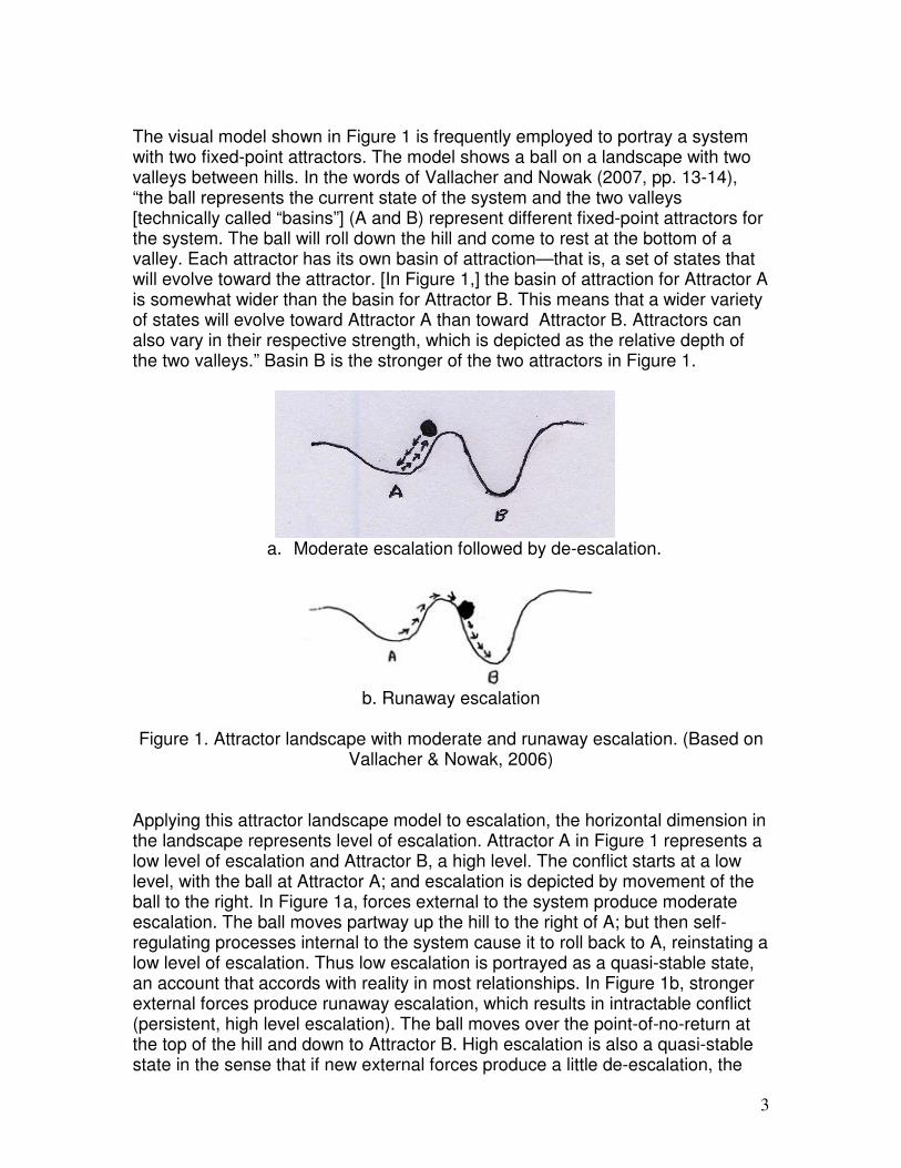
The visual model shown in Figure 1 is frequently employed to portray a system with two fixed-point attractors. The model shows a ball on a landscape with two valleys between hills. In the words of Vallacher and Nowak (2007, pp. 13-14), “the ball represents the current state of the system and the two valleys [technically called “basins”] (A and B) represent different fixed-point attractors for the system. The ball will roll down the hill and come to rest at the bottom of a valley. Each attractor has its own basin of attraction—that is, a set of states that will evolve toward the attractor. [In Figure 1,] the basin of attraction for Attractor A is somewhat wider than the basin for Attractor B. This means that a wider variety of states will evolve toward Attractor A than toward Attractor B. Attractors can also vary in their respective strength, which is depicted as the relative depth of the two valleys.” Basin B is the stronger of the two attractors in Figure 1.

a. Moderate escalation followed by de-escalation.

b. Runaway escalation

Figure 1. Attractor landscape with moderate and runaway escalation. (Based on

Vallacher & Nowak, 2006) Applying this attractor landscape model to escalation, the horizontal dimension in the landscape represents level of escalation. Attractor A in Figure 1 represents a low level of escalation and Attractor B, a high level. The conflict starts at a low level, with the ball at Attractor A; and escalation is depicted by movement of the ball to the right. In Figure 1a, forces external to the system produce moderate escalation. The ball moves partway up the hill to the right of A; but then self-regulating processes internal to the system cause it to roll back to A, reinstating a low level of escalation. Thus low escalation is portrayed as a quasi-stable state, an account that accords with reality in most relationships. In Figure 1b, stronger external forces produce runaway escalation, which results in intractable conflict (persistent, high level escalation). The ball moves over the point-of-no-return at the top of the hill and down to Attractor B. High escalation is also a quasi-stable state in the sense that if new external forces produce a little de-escalation, the

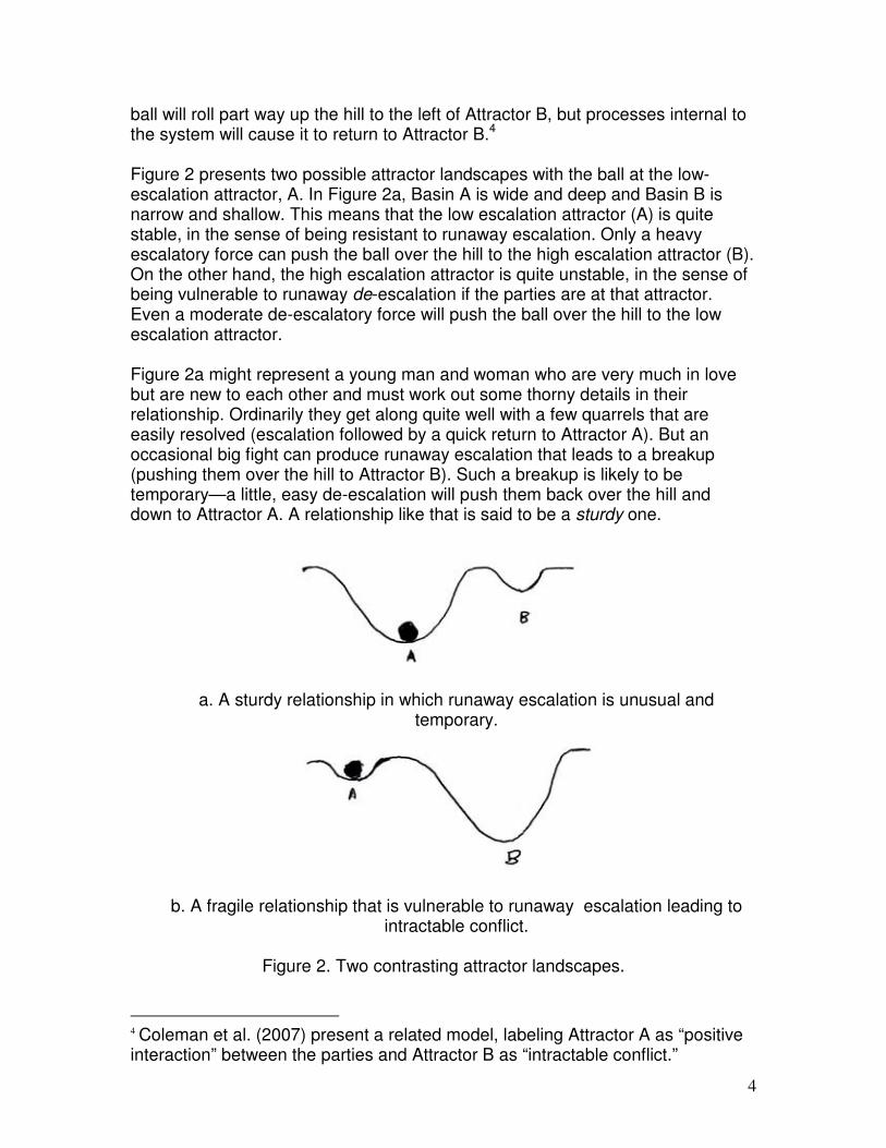
4

ball will roll part way up the hill to the left of Attractor B, but processes internal to the system will cause it to return to Attractor B.4 Figure 2 presents two possible attractor landscapes with the ball at the low-escalation attractor, A. In Figure 2a, Basin A is wide and deep and Basin B is narrow and shallow. This means that the low escalation attractor (A) is quite stable, in the sense of being resistant to runaway escalation. Only a heavy escalatory force can push the ball over the hill to the high escalation attractor (B). On the other hand, the high escalation attractor is quite unstable, in the sense of being vulnerable to runaway de-escalation if the parties are at that attractor. Even a moderate de-escalatory force will push the ball over the hill to the low escalation attractor. Figure 2a might represent a young man and woman who are very much in love but are new to each other and must work out some thorny details in their relationship. Ordinarily they get along quite well with a few quarrels that are easily resolved (escalation followed by a quick return to Attractor A). But an occasional big fight can produce runaway escalation that leads to a breakup (pushing them over the hill to Attractor B). Such a breakup is likely to be temporary—a little, easy de-escalation will push them back over the hill and down to Attractor A. A relationship like that is said to be a sturdy one.

a. A sturdy relationship in which runaway escalation is unusual and temporary.

b. A fragile relationship that is vulnerable to runaway escalation leading to intractable conflict.

Figure 2. Two contrasting attractor landscapes.

4 Coleman et al. (2007) present a related model, labeling Attractor A as “positive interaction” between the parties and Attractor B as “intractable conflict.”

5

In Figure 2b, Basin A is narrow and shallow and Basin B is wide and deep. This means that low escalation is quite unstable and high escalation quite stable. Here we are talking about a fragile relationship in which runaway escalation can easily occur and, once it has occurred, is hard to escape. The parties are highly vulnerable to an intractable conflict, as were the Soviet Union and the West at the beginning of the Cold War. The attractor landscape model is realistic in its recognition that both low and high states of escalation are, to some extent, self-perpetuating. The extent of this self-perpetuation depends on more lasting forces that shape the geography of the system in contrast to more temporary forces that move the ball around. The model is also heuristic, by encouraging distinctions and raising questions that might not otherwise be asked. For example, it suggests a distinction between two kinds of stability (resistance to runaway escalation) in non-escalated relationships: (a) a high level of escalation is required to reach a point-of-no-return (Basin A is wide) and (b) the forces against escalation are strong (Basin A is deep). These two kinds of resistance are illustrated by two types of happily married couples identified by Raush et al. (1974): (a) those that often argue vehemently but quickly reconcile after the argument is over (their relationship can withstand a moderately high level of escalation) and (b) those that talk through the issues rather than argue (they avoid escalation). Nevertheless, the model is only a starting point for understanding escalation and de-escalation—a useful but incomplete metaphor—because it ignores two crucial elements of these phenomena: (a) escalation and de-escalation involve two or more parties and (b) escalation and de-escalation often follow a spiraling course, with each party reciprocating the other’s recent behavior. For all of its interest and heuristic value, the attractor landscape model does not embody multiple parties or spiraling.

THE S-SHAPED REACTION FUNCTION MODEL

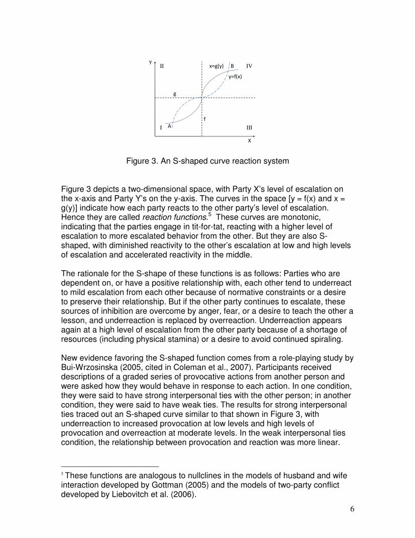
The theoretical gaps just mentioned are filled by the author’s S-shaped reaction function model (Pruitt, 1967), which applies to dyadic conflict (conflict between two parties). This model dovetails nicely with the attractor landscape model, but it treats the behavior of the parties separately (rather than jointly as in the attractor landscape model) and predicts a spiraling interaction. Hence it offers a dynamic—an account of the mechanisms underlying—the phenomena described by the attractor landscape model. A version of this model is shown in Figure 3.

6

x=g(y)

y=f(x)

II

I

IV

III

X

Y

g

f

A

B

Figure 3. An S-shaped curve reaction system Figure 3 depicts a two-dimensional space, with Party X’s level of escalation on the x-axis and Party Y’s on the y-axis. The curves in the space [y = f(x) and x = g(y)] indicate how each party reacts to the other party’s level of escalation. Hence they are called reaction functions.5 These curves are monotonic, indicating that the parties engage in tit-for-tat, reacting with a higher level of escalation to more escalated behavior from the other. But they are also S-shaped, with diminished reactivity to the other’s escalation at low and high levels of escalation and accelerated reactivity in the middle. The rationale for the S-shape of these functions is as follows: Parties who are dependent on, or have a positive relationship with, each other tend to underreact to mild escalation from each other because of normative constraints or a desire to preserve their relationship. But if the other party continues to escalate, these sources of inhibition are overcome by anger, fear, or a desire to teach the other a lesson, and underreaction is replaced by overreaction. Underreaction appears again at a high level of escalation from the other party because of a shortage of resources (including physical stamina) or a desire to avoid continued spiraling. New evidence favoring the S-shaped function comes from a role-playing study by Bui-Wrzosinska (2005, cited in Coleman et al., 2007). Participants received descriptions of a graded series of provocative actions from another person and were asked how they would behave in response to each action. In one condition, they were said to have strong interpersonal ties with the other person; in another condition, they were said to have weak ties. The results for strong interpersonal ties traced out an S-shaped curve similar to that shown in Figure 3, with underreaction to increased provocation at low levels and high levels of provocation and overreaction at moderate levels. In the weak interpersonal ties condition, the relationship between provocation and reaction was more linear.

5 These functions are analogous to nullclines in the models of husband and wife interaction developed by Gottman (2005) and the models of two-party conflict developed by Liebovitch et al. (2006).

7

Figure 3 puts the reaction functions for Parties X and Y together in the same space, producing a reaction system which shows how the two parties react to each other’s level of escalation. The heavy dot represents the joint location (JL), that is, the current levels of escalation for the two parties. The JL is shown near the lower crossing of the curves, in a relatively non-escalated state; but it can be anywhere else in the space. The curves in Figure 3 cross at three points, which are equilibria or steady states. If the JL is at any of these crossings and is not impacted by forces external to the system, it will stand still. If the JL is at any other point in the space, it will move toward the two reaction functions as the parties adjust to one another’s level of escalation. The parties are assumed to take turns. First one of them will move to its reaction function, then the other will respond by moving to its reaction function, and so on until they reach either the lower (low escalation) or the upper (high escalation) crossing. They may occasionally reach the middle crossing, but this is exceedingly rare. The lower and upper crossings (A and B) are quasi-stable equilibria, in the sense that if a moderate external force knocks the JL off one of them, it will return to that crossing once that force is gone. The middle crossing is an unstable equilibrium, in the sense that the JL will not return to that crossing if displaced by an external force. Instead, the JL will move to one of the other crossings.6 The reader may have guessed by now how the reaction function model is related to the attractor landscape model. The JL in Figure 3 is analogous to the ball in Figure 1. The lower crossing is analogous to the low escalation attractor, both being labeled A; and the upper crossing is analogous to the high escalation attractor, B. The middle crossing might be seen as analogous to the top of the hill between the two basins, the point-of-no-return beyond which the ball will move into the adjacent basin. This is, in a way, true; but the situation is more complicated, requiring additional analysis that will be presented in the next section. The reaction function model depicts each party’s behavior separately, which allows us to use ideas from individual and group psychology for analyzing escalation. This model also portrays runaway escalation and de-escalation as 6 Not all S-shaped curves cross each other three times, as in Figure 3. There are two kinds of exceptions: (1) Sometimes there is only one crossing, which is always a quasi-stable equilibrium. This can happen if one or both of the parties is exceedingly non-aggressive or reluctant to retaliate, in which case the single equilibrium will be at a low level of escalation. It also can happen if one or both of them is exceedingly aggressive or prone to retaliate, in which case the equilibrium will be at a high level of escalation. (2) At other times, there is a single crossing, which is a stable equilibrium, and the curves are tangent to each other at another point. The point of tangency is an odd equilibrium, attracting or repelling JLs depending on where they are located in the space and which party has the next move.

8

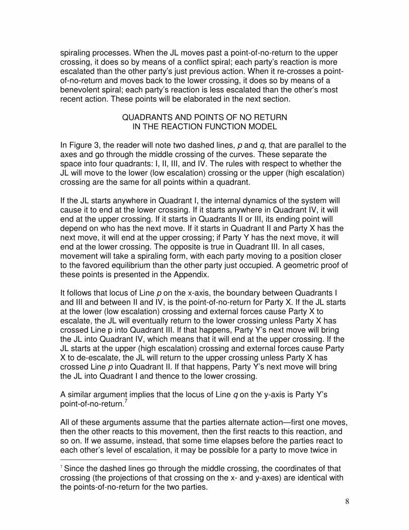
spiraling processes. When the JL moves past a point-of-no-return to the upper crossing, it does so by means of a conflict spiral; each party’s reaction is more escalated than the other party’s just previous action. When it re-crosses a point-of-no-return and moves back to the lower crossing, it does so by means of a benevolent spiral; each party’s reaction is less escalated than the other’s most recent action. These points will be elaborated in the next section.

QUADRANTS AND POINTS OF NO RETURN IN THE REACTION FUNCTION MODEL

In Figure 3, the reader will note two dashed lines, p and q, that are parallel to the axes and go through the middle crossing of the curves. These separate the space into four quadrants: I, II, III, and IV. The rules with respect to whether the JL will move to the lower (low escalation) crossing or the upper (high escalation) crossing are the same for all points within a quadrant. If the JL starts anywhere in Quadrant I, the internal dynamics of the system will cause it to end at the lower crossing. If it starts anywhere in Quadrant IV, it will end at the upper crossing. If it starts in Quadrants II or III, its ending point will depend on who has the next move. If it starts in Quadrant II and Party X has the next move, it will end at the upper crossing; if Party Y has the next move, it will end at the lower crossing. The opposite is true in Quadrant III. In all cases, movement will take a spiraling form, with each party moving to a position closer to the favored equilibrium than the other party just occupied. A geometric proof of these points is presented in the Appendix. It follows that locus of Line p on the x-axis, the boundary between Quadrants I and III and between II and IV, is the point-of-no-return for Party X. If the JL starts at the lower (low escalation) crossing and external forces cause Party X to escalate, the JL will eventually return to the lower crossing unless Party X has crossed Line p into Quadrant III. If that happens, Party Y’s next move will bring the JL into Quadrant IV, which means that it will end at the upper crossing. If the JL starts at the upper (high escalation) crossing and external forces cause Party X to de-escalate, the JL will return to the upper crossing unless Party X has crossed Line p into Quadrant II. If that happens, Party Y’s next move will bring the JL into Quadrant I and thence to the lower crossing. A similar argument implies that the locus of Line q on the y-axis is Party Y’s point-of-no-return.7 All of these arguments assume that the parties alternate action—first one moves, then the other reacts to this movement, then the first reacts to this reaction, and so on. If we assume, instead, that some time elapses before the parties react to each other’s level of escalation, it may be possible for a party to move twice in 7 Since the dashed lines go through the middle crossing, the coordinates of that crossing (the projections of that crossing on the x- and y-axes) are identical with the points-of-no-return for the two parties.

9

succession before the other reacts. That would allow for cancelation of a move that has strayed beyond a point-of-no-return and, hence, avoidance of runaway escalation or de-escalation. Consider, for example, a case in which the JL starts at the lower crossing and an external force causes Party X to escalate to Point b beyond Line p, bringing the JL into Quadrant III. If Party Y gets a chance to react, the JL will move from there to Quadrant IV, producing a runaway escalation to the upper crossing. However, if the external force dissipates rapidly or Party X quickly recognizes the jeopardy of his or her position, it may be possible for X to retreat fast enough to avert Y’s overreaction—to scurry back into Quadrant I and allow the JL to return to the lower crossing. A real-life case in which that could have happened but did not can be seen in the 1970 student crisis at the author’s university. The events began with campus policemen beating some student demonstrators in full view of a number of other students. The next day, student radicals held a large protest rally in which it was decided to stage a student strike in protest. This set off a conflict spiral that culminated in severe conflict: with students flooding the administration building, the president calling in the city police, angry students confronting the police, and a police riot in which a number of students were injured. There was a brief window of opportunity between the police riot and the next day’s protest rally in which the university administration might have been able to forestall this escalation—by publicly apologizing to the students who were beaten and suspending the offending campus policemen (Pruitt & Kim, 2004). Unfortunately, the administration was not nimble enough to take advantage of this window.

RESISTANCE TO RUNAWAY ESCALATION AND DE-ESCALATION

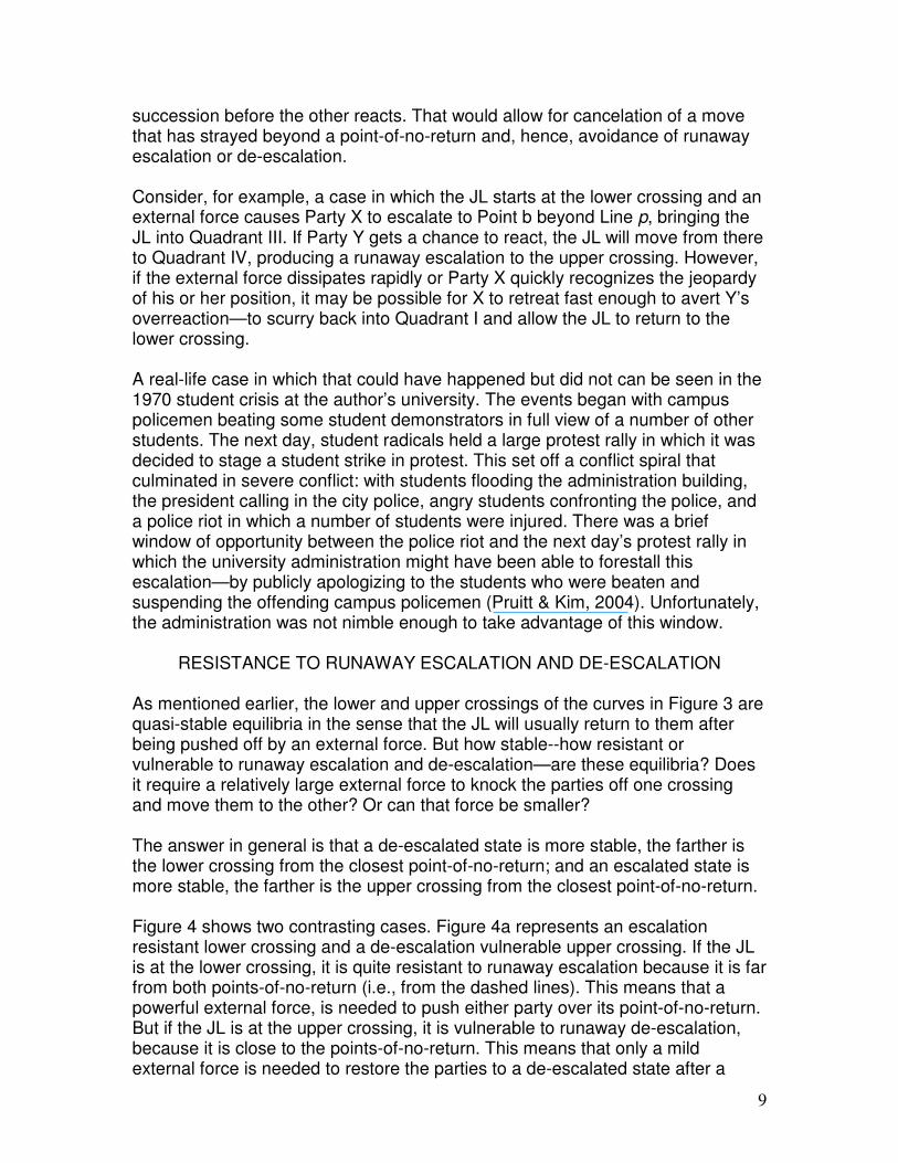
As mentioned earlier, the lower and upper crossings of the curves in Figure 3 are quasi-stable equilibria in the sense that the JL will usually return to them after being pushed off by an external force. But how stable--how resistant or vulnerable to runaway escalation and de-escalation—are these equilibria? Does it require a relatively large external force to knock the parties off one crossing and move them to the other? Or can that force be smaller? The answer in general is that a de-escalated state is more stable, the farther is the lower crossing from the closest point-of-no-return; and an escalated state is more stable, the farther is the upper crossing from the closest point-of-no-return. Figure 4 shows two contrasting cases. Figure 4a represents an escalation resistant lower crossing and a de-escalation vulnerable upper crossing. If the JL is at the lower crossing, it is quite resistant to runaway escalation because it is far from both points-of-no-return (i.e., from the dashed lines). This means that a powerful external force, is needed to push either party over its point-of-no-return. But if the JL is at the upper crossing, it is vulnerable to runaway de-escalation, because it is close to the points-of-no-return. This means that only a mild external force is needed to restore the parties to a de-escalated state after a

10

runaway escalation. The overall implication of Figure 4a is the same as that of Figure 2a: a sturdy relationship between the parties that is relatively impervious to runaway escalation and easily able to recover if that kind of escalation occurs.8

II

I

IV

III

X

Y

g’

f’

y=f’(x)

x=g’(y)

A

B

a. A sturdy relationship in which runaway escalation is unusual and temporary

x=g’’(y)

y=f’’(x)

II

I

IV

III

X

Y

g’’

p’’

A

B

b. A fragile relationship which is vulnerable to runaway escalation leading to intractable conflict

Figure 4. Two contrasting S-shaped curve reaction systems

In Figure 4b, the lower crossing is close to the points-of-no-return; hence the parties are much more vulnerable to runaway escalation than in Figure 4a. By contrast, the upper crossing is far from the middle crossing, making the parties resistant to de-escalation when their JL occupies the upper crossing. The overall implication of Figure 4b is the same as that of Figure 2b: a fragile relationship that is prone to runaway escalation and in danger of falling into intractable conflict.

8 Closeness of the upper or lower crossing to the points-of-no-return is analogous to the narrowness of a basin in the attractor landscape model. The reaction function model contains no analogy to the depth of basin in the attractor landscape model.

11

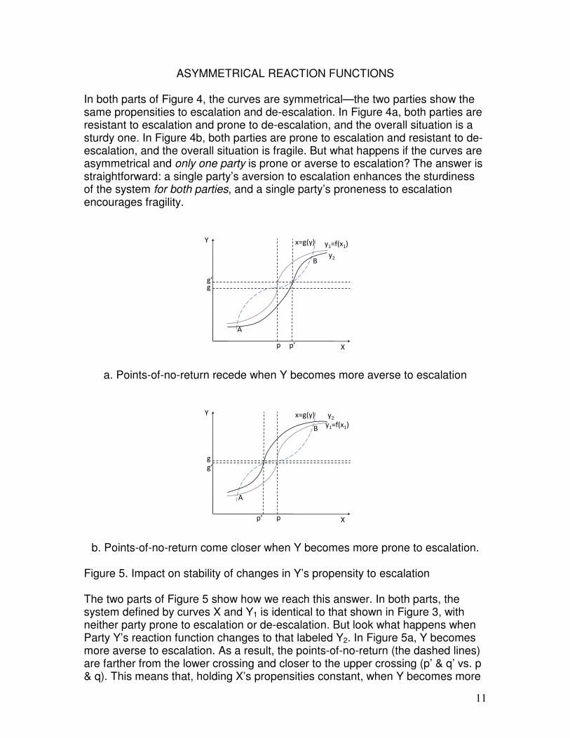
ASYMMETRICAL REACTION FUNCTIONS In both parts of Figure 4, the curves are symmetrical—the two parties show the same propensities to escalation and de-escalation. In Figure 4a, both parties are resistant to escalation and prone to de-escalation, and the overall situation is a sturdy one. In Figure 4b, both parties are prone to escalation and resistant to de-escalation, and the overall situation is fragile. But what happens if the curves are asymmetrical and only one party is prone or averse to escalation? The answer is straightforward: a single party’s aversion to escalation enhances the sturdiness of the system for both parties, and a single party’s proneness to escalation encourages fragility.

x=g(y) y1=f(x1)

X

Y

p

A

By2

p’

gg’

a. Points-of-no-return recede when Y becomes more averse to escalation

x=g(y)

y1=f(x1)

X

Y

p

A

B

y2

p’

g

g’

b. Points-of-no-return come closer when Y becomes more prone to escalation. Figure 5. Impact on stability of changes in Y’s propensity to escalation The two parts of Figure 5 show how we reach this answer. In both parts, the system defined by curves X and Y1 is identical to that shown in Figure 3, with neither party prone to escalation or de-escalation. But look what happens when Party Y’s reaction function changes to that labeled Y2. In Figure 5a, Y becomes more averse to escalation. As a result, the points-of-no-return (the dashed lines) are farther from the lower crossing and closer to the upper crossing (p’ & q’ vs. p & q). This means that, holding X’s propensities constant, when Y becomes more

12

averse to escalation (changes from Y1 to Y2), the system becomes more sturdy—less prone to runaway escalation and more prone to runaway de-escalation. Likewise in Figure 5b, we see that when Y becomes more prone to escalation, the system becomes more fragile. There is no analog to this finding in the attractor landscape model, which does not allow us to look at the two parties separately.

THE IMPACT OF NOISE

The reaction functions shown in Figures 3 to 5 suggest a precision that is practically never found in reality. Random variation or noise is almost always a factor in the way each party reacts to the other’s behavior. The source of this noise may be perceptual—the exact level of the other’s escalation is not clearly perceived. Or it may be due to the many conditions that can influence behavior, such as comments by third parties present during the interaction, environmental conditions (high ambient temperature, soft music), recent events (exercise, unpleasant interaction with a third party), or internal states (positive mood, arthritic pain). It is possible to generalize about the impact of noise on the behavior of reaction systems of the kind discussed here. The greater the noise, the less stable will be both low and high levels of escalation, that is, the greater the likelihood of runaway escalation and runaway de-escalation. This is because parties whose reactions are more variable, for whatever reason, are more likely to cross points-of-no-return and thus initiate spiraling to the opposite extreme. Another way of putting this is that noise is a source of chaotic relationships. CONDITIONS AFFECTING THE STABILITY OF LOW AND HIGH ESCALATION

This section will discuss the more lasting forces that mold the geography of attractor landscapes and the shape of reaction functions. These are the forces that determine the stability of high and low escalation or, conversely, the likelihood of runaway escalation and de-escalation—the forces that determine whether a system will look like Figure 2a or 2b, like Figure 4a or 4b. We will start with conflict reducing conditions that encourage the stability of low escalation and the instability of high escalation (Figures 2a and 4a), and then move on to conflict inducing conditions that encourage the instability of low escalation and the stability of high escalation (Figures 2b and 4b). Conflict Reducing Conditions Most conflicts do not escalate, or if they escalate they do not move far up the escalation ladder and quickly return to a non-escalated state. In other words, the circumstances portrayed in Figures 2a and 4a are much more common than those portrayed in Figures 2b and 4b. Runaway escalation and intractable conflict are relatively uncommon. Several pervasive conditions account for this.

13

Conflict-limiting norms and bonds. One reason for the scarcity of intractable conflict is that most societies, including the international community, have strong conflict-limiting norms that encourage conflict resolution and discourage heavy escalation. Such norms help to preserve group solidarity. It follows that there is less likelihood of runaway escalation for individuals who are well socialized, those who need approval, and those who are being watched closely by other members of society, because these conditions encourage conformity to norms.9 If norms are not strong enough to prevent severe escalation and the solidarity of the group (at whatever level of society, including international alliances) is threatened, third parties will often step in to stop the fighting and try to solve the problem. This is more likely to happen, the greater the group solidarity (Schachter, 1951) and the more important this solidarity is to the group. Conflict limiting norms are particularly strong when there are certain kinds of bonds between the parties—when they are close relatives or members of the same group, organization, or community. Such norms probably have evolutionary origins as well as origins in the way society has developed. The bonds just described—and those of friendship, liking, commitment, and dependence—are reinforced in their effect by positive feelings and fear of disrupting relationships. If bonds are reciprocal (i.e., the other party is also bonded to oneself), the parties are also likely to trust each other’s intentions, which should lead to less felt need to retaliate in the face of annoyance from the other and hence less runaway escalation. There are bonds between groups as well as between individuals, in the sense that some members of one group are blood relatives or share a common identity or subgroup membership (e.g., belonging to the same labor union, political party, business group) with members of the other group. These bonds are called “cross-cutting ties.” When intergroup conflict arises, people with cross-cutting ties tend to become active, counseling moderation, opposing militant sectarian leadership, and acting as mediators (Gluckman, 1955; Varshney, 2002). This reduces the likelihood of heavy escalation (Pruitt & Kim, 2004). Conflict-limiting institutions. Most communities provide forums and third-party services to help their members resolve conflicts peacefully. Such institutions reduce the likelihood of heavy escalation by giving people and groups a nonviolent and face-saving way to escape conflict (Glasl, 1982). Examples include legislative bodies, courts, and other third-party services. 9 Researchers have identified a few exceptions to these rules. In American society, runaway escalation becomes more common when men are watching other men in conflict than when men are watching women or women are watching men, because macho norms tend to substitute for non-aggressive norms (Felson, 1982). Also in societies that have a culture of honor, norms require an escalative reaction when someone insults you or demeans your status (Nisbett & Cohen, 1996).

14

Fish & Kroenig (2008) have argued, on the basis of statistical evidence, that countries that lack crosscutting ties between ethnic groups are nevertheless protected from severe escalation if they have strong national legislatures that allow conflict to be addressed in a peaceful fashion. Conflict Inducing Conditions Prior escalation. Escalation tends to feed on escalation, in the sense that earlier runaway escalation in a relationship increases the likelihood of later runaway escalation. This happens, in part, through the erosion of some of the safeguards mentioned earlier in this section. Normative protection tends to reduce because the parties see each other as less worthy than before. Bonds of friendship and attraction tend to erode and people often reduce their interdependence and withdraw from common group membership. If the parties are groups, cross-cutting ties tend to wither. Furthermore, trust often diminishes, causing the other party to be seen as more hostile and blameworthy the next time conflict arises. In addition, prior runaway escalation frequently produces self-perpetuating “structural changes” in the parties, which further increase the likelihood of severe escalation in the next conflict episode (Bar Tal, 2008; Pruitt & Kim, 2004). These can occur at the psychological level, for example, negative perceptions of the other party, fear and hostility, or a desire to defeat or hurt the other. They can also occur at the group level, for example, strengthened ingroup identity and solidarity, and the development of collective grievances, militant group leadership, and subgroups to implement hostile group goals. Finally, they can occur at the level of the community surrounding the parties, which can become polarized into two hostile camps, each supporting one of the disputants (Coleman, 1957). These effects are likely to be more profound the more time is spent in a highly escalated state. Safeguards against severe escalation will be progressively eroded and structural changes will become more profound. Conditions producing aggression. There is a copious research-based literature on the conditions that encourage aggressive behavior in people who have been annoyed in some way (see Berkowitz, 1993; Geen, 1990; Huesmann, 1994). All of these conditions—working on one or both parties in a dyadic conflict—should increase the likelihood of runaway escalation. Prominent examples include prior annoyance, extremes of temperature, autonomic arousal, the presence of aggressive cues, prior reward for aggression, exposure to aggressive media presentations and live aggressive models, and the ingestion of alcohol. Other conditions, such as positive mood and the engagement of higher mental processes, have been shown to dampen aggressive responding; and these should diminish the likelihood of runaway escalation.

15

HYSTERESIS

The points made just above suggests that runaway escalation makes subsequent de-escalation harder to achieve. If Figure 4a represents a period before any runaway escalation has occurred and Figure 4b, a period after there has been some runaway escalation, this means that runaway escalation shifts X’s point-of-no-return to the left (from p’ to p”) and Y’s point-of-no-return downward (from q’ to q”). The implication is that the path back from escalation does not simply retrace the path to escalation, a point made by Mitchell (1999) within the framework of international conflict. More particularly, recrossing a level of escalation that was sufficient to propel the parties to the high escalation crossing will not be sufficient to bring them back to the low escalation crossing. Rather, one or both parties must de-escalate further. This is the phenomenon of hysteresis, in which the path back from a dramatic change in a system is more remote than was the path to that change (Coleman et al., 2008; Gottman et al., 2002; Nowak & Vallacher, 1998).

CONCLUSIONS

We have presented two models that shed light on the phenomena of escalation and de-escalation in social conflict: the attractor landscape model and the reaction function model. These models were developed independently at very different times,10 but they are nevertheless similar in many ways. Both treat low escalation and high escalation as quasi-stable states, with moderate deviation always followed by a return to the original state. Both assume the existence of points-of-no-return which, if crossed over, will produce runaway escalation or de-escalation to the opposite state. Both assume that the stability of these states is variable and that points-of-no-return are more easily crossed under some conditions than other, And both distinguish between (a) temporary external forces that induce escalation and de-escalation and thus push the parties off the quasi-stable states and (b) more lasting external forces that determine the ease or difficulty of crossing the points-of-no-return and hence the likelihood of runaway escalation and de-escalation. Despite these similarities, the models have very different dynamics, and each has its strengths as an account of escalation and de-escalation. The attractor landscape model is easier to grasp and suggests a distinction between two kinds of stability—breadth and depth—that are found in reality. The reaction function model distinguishes between the individual parties to a dyadic conflict, allowing examination of the impact of their separate proclivities. Assuming the latter model, it can be shown that each party’s proneness to escalation separately increases the likelihood of runaway escalation for the dyad as a whole. The latter model also predicts that runaway escalation and de-escalation will take the form of vicious and benevolent circles, with each party reacting to the other’s recent behavior, as is usually found in reality. 10

The attractor landscape model of escalation was first presented by Coleman et al. (2007), the reaction function model by Pruitt (1969).

16

In short, the two models are complementary, and both have potential value.

APPENDIX

Consider a JL (X0, Y0) that initially lies anywhere in Quadrant I and assume that Party Y has the next move (from Y0 to Y1) and Party X has the move after that (from X0 to X2). At all points in Quadrant I, the curve y = f(x) is bounded by the lower and middle crossings and is concave to the X axis. Hence Party Y’s move will keep the JL in Quadrant I and take Party Y closer to the lower crossing point than is Party X, i.e., Y1 < X0 (assuming < means closer to the lower crossing). At all points in Quadrant I, the curve x = g(y) is also bounded by the lower and middle crossings and is concave to the Y axis. Hence Party X’s subsequent move will also keep the JL in Quadrant I and will move Party X closer to the lower crossing than is Party Y, i.e., X2 < Y1. It follows from simple algebra that X2 < X0; in other words, in these two moves, the JL has stayed in Quadrant 1 and Party X has moved closer to the lower crossing than it was before. Conversely, by the same reasoning, if X has the next move and Y the one after it, the result will move Party Y closer to the lower crossing than it was before. If we assume that the parties alternate moves until they reach an equilibrium, it follows that any JL that starts in Quadrant I will eventually move to the lower crossing. Parallel reasoning can be employed to show that any JL that starts in Quadrant IV will eventually move to the upper crossing. Quadrants II and III are a little trickier but not a lot. If the JL starts in Quadrant II and Party Y has the next move, the JL will move into Quadrant I. By the reasoning given above, the JL cannot subsequently escape from Quadrant I and must eventually move to the lower equilibrium. By the same reasoning, if Party X has the next move, the JL will move into Quadrant IV and thence to the upper equilibrium. Parallel reasoning leads to the conclusion that if the JL starts in Quadrant III, it will move to the lower equilibrium if Party X has the next move and to the upper equilibrium if Party Y has the next move.

REFERENCES Bar-Tal, D. (2007). Sociopsychological foundations of intractable conflict. American Behavioral Scientist, 50, 1430-1453. Bui-Wrzosinska, L. (2005). The dynamics of conflict in a school setting. Unpublished masters thesis, Warsaw School for Social Psychology, Warsaw, Poland. Coleman, J. S. (1957). Community conflict. New York: Free Press. Coleman, P. T., Vallacher, R., Nowak, A., & Bui-Wrzosinska, L. (2007). Intractable conflict as an attractor: A dynamical systems approach to conflict, escalation, and intractability. American Behavioral Scientist, 50, 1454-1475.

17

Felson, R. B. (1982). Impression management and the escalation of aggression and violence. Social Psychology Quarterly, 45, 245-254. Fish, M. S. & Kroenig, M. (2008). Kenya’s real problem (it’s not ethnic). Washington Post, 1/9/08, p. A15. Gottman, J. M., Murray, J. D., Swanson, C. C., Tyson, R., & Swanson, K. R. (2005). The mathematics of marriage: Dynamic nonlinear models. Cambridge, MA: MIT Press. Glasl, F. (1982). The process of conflict escalation and roles of third parties. In G. B. F. Bomers & R. B Peterson (Eds.), Conflict management and industrial relations (pp. 119-140). Boston: Kluwer-Nijhoff. Gluckman, M. (1955). Custom and conflict in Africa. Glencoe, IL: Free Press. Liebovitch, L. S., Vallacher, R. R., Nowak, A., Bui-Wrzosinska, L., & Coleman, P. (2007). Dynamics of two-actor cooperation-competition conflict models. Unpublished manuscript. Mitchell, C. (1999). The anatomy of de-escalation. In H.-W. Jeong (Ed.), Conflict resolution: Dynamics, process and structure (pp. 37-58). Aldershot, England & Brookfield, VT: Ashgate. Nisbett, R. E., & Cohen, D. (1996). Culture of honor. Boulder, CO Westview. Nowak, A., & Vallacher, R. R. (1998). Dynamical social psychology. New York: Guilford. Pruitt, D. G. (1969). Stability and sudden change in interpersonal and international affairs. Journal of Conflict Resolution, 13, 18-38.

Pruitt, D. G. (2007a). Conflict escalation in organizations, Chapter 6 in C. K. W. De Dreu & M. J. Gelfand (Eds.), The psychology of conflict and conflict management in organizations. Mahwah, NJ: Erlbaum. Pruitt, D. G. (2007b). Readiness theory and the Northern Ireland peace process. American Behavioral Scientist, 50, 1520-1541. Pruitt, D. G., & Kim, S. H. (2004). Social conflict: Escalation, stalemate, and settlement, 3rd ed. New York: McGraw-Hill. Raush, H. L., Barry, W. A., Hertel, R. K., Swain, M. A. (1974). Communication, conflict and marriage. San Francisco, CA: Jossey-Bass. Schachter, S. (1951). Deviation, rejection, and communication. Journal of Abnormal and Social Psychoplogy, 46, 190-207.

18

Vallacher, R. R., & Nowak, A. (2006). Dynamical social psychology: Finding order in the flow of human experience, In A. W. Kruglanski & E. T. Higgins (Eds.), Social psychology: Handbook of basic principles. New York: Guilford. Varshney, A. (2002). Ethnic conflict and civil life: Hindus and Muslims in India. New Haven, CT: Yale University Press. February 1, 2010