economics in crisis: severe and logical contradictions of classical, keynesian, and popular trade...

Economics in Crisis: Severe and LogicalContradictions of Classical, Keynesian,and Popular Trade Models

Ravi Batra*

AbstractThe paper examines three popular models that form the foundation of modern economics. The author con-cludes that two of the three, the classical and the Keynesian, are seriously deficient in logic, whereas thethird, dealing with gains from trade, is partially lacking in logic. Classical and neo-Keynesian approachesrequire desired investment to expand during recessions, whereas the trade model requires real GDP to risewithout any rise in employment, capital stock, or technology. The paper offers an alternative macro frame-work that is free from the limitations of conventional models. Money is either neutral or non-neutral,depending on whether the economy is operating below or at full capacity. Wages are strictly determined inthe labor market, yet employment is influenced by aggregate demand. The alternative model thus combinesthe attractive features of classical and Keynesian frameworks.

1. Introduction

We live in a global economy where economic analysis has also become global, in fol-lowing and nature. Almost everywhere the same theories and doctrines are taught andexplored. A university in Japan is likely to teach the same economic models as one in the United States, Germany, or India. The global village is by definition a macroeconomy, which has three major pillars, namely the closed- and open-economy macromodels that are supported by a popular theory of gains from trade.

The macro theory in turn has two main branches, the classical and the Keynesian.A standard menu of economics thus includes a classical model, the Keynesian model,and the hypothesis of gains from trade. Economists often disagree, especially when itcomes to assumptions and public policy, but they rarely examine the consistency ofaccepted theories.This paper points out that popular economic ideas are seriously defi-cient in logic, not just in their lack of reality. They suffer from severe internal contra-dictions and have periodically offered irrational prescriptions. For this reason they are dangerous to social welfare, which ironically is a concept they themselves haveinvented. The paper also offers an alternative framework to offset the flaws of con-ventional theories.

2. The Classical Model

Let us begin with the classical model, which has had several reincarnations. It almostdied from the assault of the Keynesian revolution born in the 1930s, but then resur-faced in the 1970s and thereafter when the disciples of John Maynard Keynes carried

Review of International Economics, 10(4), 623–644, 2002

*Batra: Economics Department, Southern Methodist University, Dallas, TX 75275-0496, USA. Tel:214-768-2707; Fax: 214-750-7886; E-mail: [email protected]. I am thankful to Nathan Balke, Prasanta Pattanaik, Kamal Sagi, Per Fredrikson, Rajat Deb, and Abdullah Khawaja for their help in preparing thismanuscript.

© Blackwell Publishers Ltd 2002, 108 Cowley Road, Oxford OX4 1JF, UK and 350 Main Street, Malden, MA 02148, USA

his message to the extreme, asserting that a country could permanently banish unem-ployment, and possibly poverty, just by printing bushels of money and living with someinflation. When inflation became intolerable, the Keynesian revolution misfired, andthe old ideas made a comeback. Today the classical model forms the basis of countlessarticles in economic journals in the guise inter alia of rational expectations and realbusiness cycles. It even provides the foundation of a popular macroeconomic text fromBarro (2000).

Whatever its guise, the basic message of the classical theory is that supply createsits own demand, at least in what Blanchard (2000) calls the short to medium run, sothat government intervention in the self-healing economy should be minimal, andpreferably zero. It turns out that the classical logic of a flexible interest rate quicklyensuring the equality of supply and demand is seriously deficient, even if you grant allits assumptions that savings and investment are highly responsive to variations in thereal rate of interest. Its logic is inconsistent with reality as well as common sense,whether or not the economy is closed or open. The contradictions of this model turnout to be so severe that all its propositions and prescriptions are open to serious question.

The original or the basic classical model, as for instance explored by Gardner (1961)or Branson (1979), is given by the following equations:

(social utility function) (1)

(leisure) (2)

(production function) (3)

(labor demand) (4)

(labor supply) (5)

(quantity theory of money) (6)

(savings function) (7)

(investment function) (8)

(goods market equilibrium) (9)

where U is social utility; Z is leisure; Y is output or real income; is total, fixed numberof hours in a day; Ko is the constant stock of capital; w is the real wage rate; L is labordemand in (4) and labor supply in (5); FL is the marginal product of labor; G is themarginal disutility of labor; M is the supply of money; P is the price level; V is thevelocity of money assumed to be constant; S is real saving; I is desired real investment;and r is the real rate of interest. The stock of capital is assumed to be constant in theshort run, over the course of the business cycle, or during the period in question. Themarginal product of labor is positive but diminishing; that is, FLL < 0; G is positive butincreasing, so G¢ > 0. Similarly, S¢ > 0 and I¢ < 0.

Equation (1) says that social utility depends positively on real income and leisure;(3) says that output depends positively on employment and the stock of capital; (4)derives from the behavior of competitive firms maximizing their profit; and (5) comesfrom the maximization of social utility, yielding the labor supply function, which impliesthat labor supply rises with a rise in the real wage.

The system consists of nine equations in nine variables, U, Z, Y, w, L, P, S, I, and r,and two parameters, Ko and M. With all these equations, the classical framework givesan appearance of great complexity, but its beauty is that it is extremely simple to solve

H

S I=

I I r= ( )S S r= ( )MV PY=

w G L= ( )w F L KL= ( ), o

Y L K= ( ), o

Z H L= -

U U Y Z= ( ),

624 Ravi Batra

© Blackwell Publishers Ltd 2002

and comprehend. The system can be divided into three watertight branches with noneintruding upon the other. From (3), (4), and (5), we can solve for Y, L, and w. From(4) and (5) we obtain

(10)

which yields the equilibrium value of L or employment.1 With L known, the real wageand output can be determined from (3) and (4). Thus output and employment dependonly on the labor market equilibrium. Once Y is so determined, P can be computedfrom (6), where V is constant and M is money supply determined exogenously.

The real rate of interest can be determined from (7), (8), and (9) without anyrecourse to the rest of the system. From the real wage and the price level, nominal ormoney wage w can be computed, because w = W/P. Similarly, in the original classicalmodel, r = i/P, where i is the nominal rate of interest, or r = 1 - p, where p is the exoge-nously determined expected rate of inflation.With L known, leisure can be determinedfrom (2), and then U is determined in (1).2

Even though the model can be divided into three separate compartments, they allstand or fall together. For instance, if the goods market is not in equilibrium and suffersfrom excess supply or recession, then the labor market will also be out of equilibriumand suffer from excess supply or unemployment. The division of the system into threecompartments does not mean that they are completely independent of each other, onlythat they can be solved and analyzed in three easy steps.

The classical model is simple as well as profound. That is why it has endured in themidst of strong challenges time and again. Given its assumptions of perfect flexibilityin wages, prices, and interest rates, among others, its logic is considered impeccable andunassailable.Today the model is a favorite among macroeconomists and underlies newclassical economics, real business cycles, and much of the current research in macropolicy. In the simplest version analyzed in this section, government spending, taxation,and international trade are ignored, but they can be easily incorporated without modi-fying its central message—namely, a market economy is best left to itself so that gov-ernments should not intervene in the economy through deficit budgets, high marginaltaxes on income of individuals and corporations, tariffs, or excessive printing of money.Government interference, in the classical model, only spawns inflation or generatesinefficiencies without improving upon the general living standard. The profundity ofthis thought belies the simplicity of its underlying framework.

Yet the model has serious flaws. Take a look at Figure 1, which is a must item in anytextbook on macroeconomics. One attraction of the classical model is that it is sup-posed to have a solid foundation in microeconomics, and reminds one of the simplemicro logic of supply and demand. Figure 1 actually deals with the market for loan-able funds, where loan demand comes from business and other investment and loansupply from households, who deposit their savings with commercial banks. The realrate of interest is the price in this market. Thus Figure 1 is a straightforward extensionof the microeconomic formula of supply and demand.

The micro analysis is quite simple. Suppose r is the price of a product, the I-line isthe demand curve and the S-line is the supply curve. Then equilibrium price occurs atr*, with quantity exchanged settling at I*.

The equilibrium price is no fluke. Even if price deviates from its equilibrium, itquickly reverts to this level in a competitive industry, because of the self-interest ofbuyers and suppliers. For instance, suppose the price is at X, then excess supply appearsin the market, because producers offer XB of the product, while consumers want onlyXA of the good at that price. In their self-interest, sellers announce a sale and reduce

F L K G LL , ,o( ) = ( )

ECONOMICS IN CRISIS 625


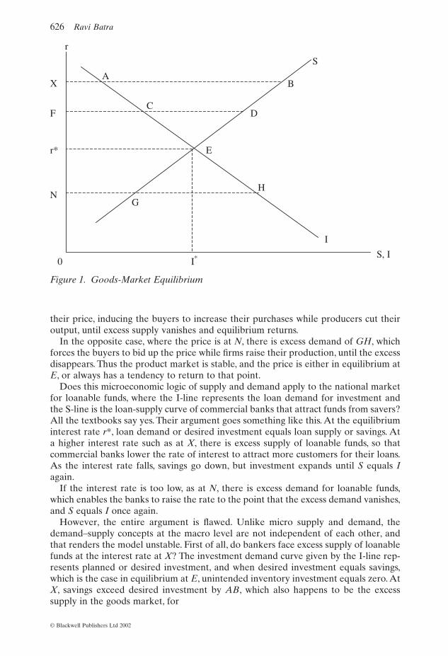
their price, inducing the buyers to increase their purchases while producers cut theiroutput, until excess supply vanishes and equilibrium returns.

In the opposite case, where the price is at N, there is excess demand of GH, whichforces the buyers to bid up the price while firms raise their production, until the excessdisappears. Thus the product market is stable, and the price is either in equilibrium atE, or always has a tendency to return to that point.

Does this microeconomic logic of supply and demand apply to the national marketfor loanable funds, where the I-line represents the loan demand for investment andthe S-line is the loan-supply curve of commercial banks that attract funds from savers?All the textbooks say yes. Their argument goes something like this. At the equilibriuminterest rate r*, loan demand or desired investment equals loan supply or savings. Ata higher interest rate such as at X, there is excess supply of loanable funds, so thatcommercial banks lower the rate of interest to attract more customers for their loans.As the interest rate falls, savings go down, but investment expands until S equals Iagain.

If the interest rate is too low, as at N, there is excess demand for loanable funds,which enables the banks to raise the rate to the point that the excess demand vanishes,and S equals I once again.

However, the entire argument is flawed. Unlike micro supply and demand, thedemand–supply concepts at the macro level are not independent of each other, andthat renders the model unstable. First of all, do bankers face excess supply of loanablefunds at the interest rate at X? The investment demand curve given by the I-line rep-resents planned or desired investment, and when desired investment equals savings,which is the case in equilibrium at E, unintended inventory investment equals zero. AtX, savings exceed desired investment by AB, which also happens to be the excesssupply in the goods market, for

626 Ravi Batra


0

S

I

r

S, I

X

F

r*

N

I*

A

C

B

D

E

G

H

Figure 1. Goods-Market Equilibrium

where AD denotes aggregate demand and AS denotes aggregate supply or output. Inequilibrium S and I are the same, and unintended inventory investment is zero. Thatis why, as Barro (2000, p. 333) points out, “the commodity market clears” at the equi-librium interest rate.

In equilibrium, when the interest rate is at r*, loan demand (or desired investment)and savings each equal Er*, and at the higher interest rate at X, savings exceed desiredinvestment by AB, which also equals the excess supply in the goods market as well asunintended inventory investment. The loan demand then is not XA, as contended bythe textbooks, but XB, of which XA is for desired investment and AB is for unintendedor undesired inventory investment. The banks have no excess supply of loanable fundsat the higher interest rate, so there is no reason for them to bring the rate down. Thisis not like a fire-sale that occurs at the micro level where sellers, stuck with unsoldgoods, have to lower prices to clear their excess inventory. The micro logic does notapply to the interest rate, because macro demand and supply concepts are not inde-pendent of each other.

On the other side of the spectrum, at the lower interest rate at N, there is a dearthof savings that fall short of desired investment by GH, which is also the excess demandfor goods as well as the depletion of inventories, so that loan demand is not NH butNG. Desired investment is, of course, NH, but intended or desired inventory invest-ment has fallen by GH. In other words, business borrowing for their normal stock ofinventories has declined by GH. So now the banks, facing low loan demand, are unableto raise the interest rate towards the equilibrium rate.

Thus in both cases of disequilibrium, the first step in the classical argument that theinterest rate varies quickly to clear the goods market or to ensure that supply auto-matically creates its own demand is not supported by the logic of the macro economy.

However, the flaw in the classical argument does not end here. There is plenty more.Contrary to the textbook logic of the macro model, let us grant that the interest ratedoes fall when savings exceed desired investment, or aggregate demand falls short ofaggregate supply. This is a situation of recession, and interest rates do eventually comedown in this situation. Firms trim production, unsold goods are gradually cleared away,so that inventory investment drops; consumer borrowing also falls for the purchase ofdurable goods. All this generates a fall in loan demand relative to loan supply, and theinterest rate, after a while, begins to fall.

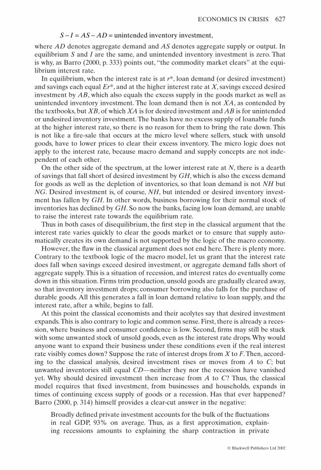
At this point the classical economists and their acolytes say that desired investmentexpands.This is also contrary to logic and common sense. First, there is already a reces-sion, where business and consumer confidence is low. Second, firms may still be stuckwith some unwanted stock of unsold goods, even as the interest rate drops. Why wouldanyone want to expand their business under these conditions even if the real interestrate visibly comes down? Suppose the rate of interest drops from X to F.Then, accord-ing to the classical analysis, desired investment rises or moves from A to C; butunwanted inventories still equal CD—neither they nor the recession have vanishedyet. Why should desired investment then increase from A to C? Thus, the classicalmodel requires that fixed investment, from businesses and households, expands intimes of continuing excess supply of goods or a recession. Has that ever happened?Barro (2000, p. 314) himself provides a clear-cut answer in the negative:

Broadly defined private investment accounts for the bulk of the fluctuationsin real GDP, 93% on average. Thus, as a first approximation, explain-ing recessions amounts to explaining the sharp contraction in private

S I AS AD- = - = unintended inventory investment,



investment components. . . . Consumer spending on nondurables and services is relatively stable and accounts on average for only 24% of theshortfall of real GDP.

Barro also points the way to another flaw in the classical logic, wherein savingsdecline as the real rate of interest falls in a recession, which means the consumer spend-ing is supposed to rise in a recession to bring about the equality between S and I. Butas Barro himself notes, the opposite happens, and consumer spending comes down.

Does it mean that desired investment or savings are unresponsive to falling interestrates? No. Ordinarily, with output or inventory constant, savings and investmentperhaps would respond quickly to interest rates in ways postulated by the old andmodern classical economists. All I am saying is that I does not rise or S does not fallin a recessionary environment, where S exceeds I, even if the real interest rate goesdown.

On the other side of the equilibrium, the classical model requires desired fixedinvestment and consumer spending to contract just when business is booming underconditions of excess demand, where I exceeds S. Again that happens only in classicaltheory but not in reality. Ordinarily, investment would fall and savings possibly rise ina static economy, as interest rates go up, but not when inventories have sharply fallenand new orders are multiplying. Plainly speaking, we cannot blindly apply micromethodology to macro concepts, because micro demand and supply curves do not shiftin disequilibrium, whereas the macro counterparts do. When S > I at a higher interestrate, the I-line would shift to the left because of falling output (and the S-line couldshift to the right), and the economy will not return to old equilibrium, or may not con-verge to any such point. Even if it does, it could take a long time before it arrives atany equilibrium at all.

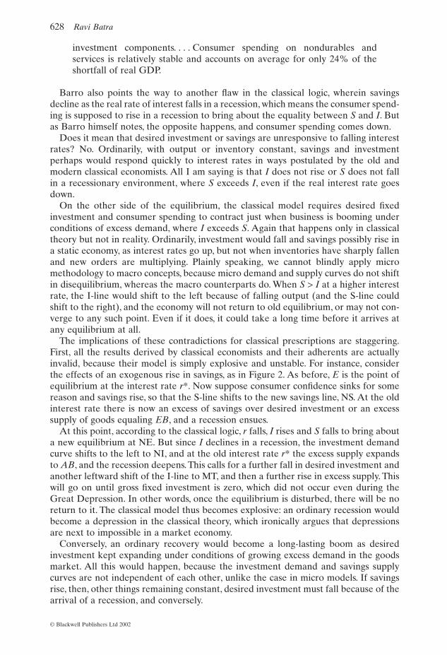
The implications of these contradictions for classical prescriptions are staggering.First, all the results derived by classical economists and their adherents are actuallyinvalid, because their model is simply explosive and unstable. For instance, considerthe effects of an exogenous rise in savings, as in Figure 2. As before, E is the point ofequilibrium at the interest rate r*. Now suppose consumer confidence sinks for somereason and savings rise, so that the S-line shifts to the new savings line, NS. At the oldinterest rate there is now an excess of savings over desired investment or an excesssupply of goods equaling EB, and a recession ensues.

At this point, according to the classical logic, r falls, I rises and S falls to bring abouta new equilibrium at NE. But since I declines in a recession, the investment demandcurve shifts to the left to NI, and at the old interest rate r* the excess supply expandsto AB, and the recession deepens. This calls for a further fall in desired investment andanother leftward shift of the I-line to MT, and then a further rise in excess supply. Thiswill go on until gross fixed investment is zero, which did not occur even during theGreat Depression. In other words, once the equilibrium is disturbed, there will be noreturn to it. The classical model thus becomes explosive: an ordinary recession wouldbecome a depression in the classical theory, which ironically argues that depressionsare next to impossible in a market economy.

Conversely, an ordinary recovery would become a long-lasting boom as desiredinvestment kept expanding under conditions of growing excess demand in the goodsmarket. All this would happen, because the investment demand and savings supplycurves are not independent of each other, unlike the case in micro models. If savingsrise, then, other things remaining constant, desired investment must fall because of thearrival of a recession, and conversely.

628 Ravi Batra


Another implication of classical contradictions is that the government must con-stantly intervene in the economy to stabilize the situation. For example, the state mustraise aggregate demand in times of rising savings, and lower it when savings decline.None of this is music to classical ears.

3. The Classical Model in an Open Economy

Mankiw (2000) offers a classical type of model in an open economy. Unfortunately, hismodel is subject to the same shortcomings as the original classical model. Only its formchanges somewhat, but its failures remain the same.

In an open economy, without the government sector, the goods-market equilibriumoccurs when

(11)

where Q is domestic investment plus net foreign investment (NFI), which in turnequals net exports (NX):

(12)

NFI also depends negatively on the domestic interest rate (r), because a lower rinduces home savers to shift funds abroad and encourages foreign savers to keep theirfunds at home. With NFI negatively related to r, Q is a negative function of r as well.

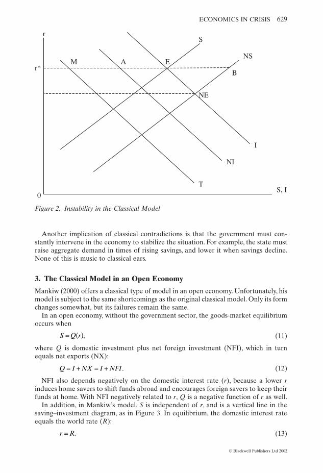
In addition, in Mankiw’s model, S is independent of r, and is a vertical line in thesaving–investment diagram, as in Figure 3. In equilibrium, the domestic interest rateequals the world rate (R):

(13)r R= .

Q I NX I NFI= + = + .

S Q r= ( ),



r

r*

S, I

M A E

NE

S

NS

B

0

I

NI

T

Figure 2. Instability in the Classical Model

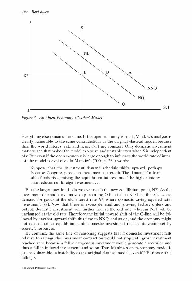
Everything else remains the same. If the open economy is small, Mankiw’s analysis isclearly vulnerable to the same contradictions as the original classical model, becausethen the world interest rate and hence NFI are constant. Only domestic investmentmatters, and that makes the model explosive and unstable even when S is independentof r. But even if the open economy is large enough to influence the world rate of inter-est, the model is explosive. In Mankiw’s (2000, p. 230) words:

Suppose that the investment demand schedule shifts upward, perhapsbecause Congress passes an investment tax credit. The demand for loan-able funds rises, raising the equilibrium interest rate. The higher interestrate reduces net foreign investment . . .

But the larger question is: do we ever reach the new equilibrium point, NE. As theinvestment demand curve moves up from the Q-line to the NQ line, there is excessdemand for goods at the old interest rate R*, where domestic saving equaled totalinvestment (Q). Now that there is excess demand and growing factory orders andoutput, domestic investment will further rise at the old rate, whereas NFI will beunchanged at the old rate. Therefore the initial upward shift of the Q-line will be fol-lowed by another upward shift, this time to NNQ, and so on, and the economy mightnot reach another equilibrium until domestic investment reaches its zenith set bysociety’s resources.

By contrast, the same line of reasoning suggests that if domestic investment falls relative to savings, the investment contraction would not stop until gross investmentreached zero, because a fall in exogenous investment would generate a recession andthus a fall in induced investment, and so on. Thus Mankiw’s open-economy model isjust as vulnerable to instability as the original classical model, even if NFI rises with afalling r.

630 Ravi Batra


r

S, I0

Q

NQ

NNQ

R* E B A

S

NE

Figure 3. An Open-Economy Classical Model

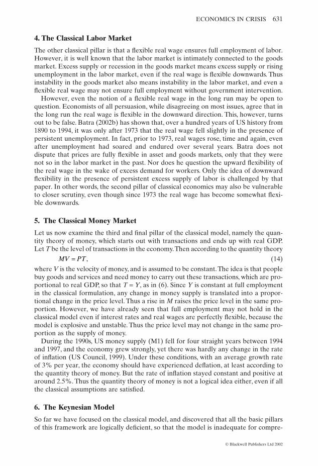
4. The Classical Labor Market

The other classical pillar is that a flexible real wage ensures full employment of labor.However, it is well known that the labor market is intimately connected to the goodsmarket. Excess supply or recession in the goods market means excess supply or risingunemployment in the labor market, even if the real wage is flexible downwards. Thusinstability in the goods market also means instability in the labor market, and even aflexible real wage may not ensure full employment without government intervention.

However, even the notion of a flexible real wage in the long run may be open toquestion. Economists of all persuasion, while disagreeing on most issues, agree that inthe long run the real wage is flexible in the downward direction. This, however, turnsout to be false. Batra (2002b) has shown that, over a hundred years of US history from1890 to 1994, it was only after 1973 that the real wage fell slightly in the presence ofpersistent unemployment. In fact, prior to 1973, real wages rose, time and again, evenafter unemployment had soared and endured over several years. Batra does notdispute that prices are fully flexible in asset and goods markets, only that they werenot so in the labor market in the past. Nor does he question the upward flexibility ofthe real wage in the wake of excess demand for workers. Only the idea of downwardflexibility in the presence of persistent excess supply of labor is challenged by thatpaper. In other words, the second pillar of classical economics may also be vulnerableto closer scrutiny, even though since 1973 the real wage has become somewhat flexi-ble downwards.

5. The Classical Money Market

Let us now examine the third and final pillar of the classical model, namely the quan-tity theory of money, which starts out with transactions and ends up with real GDP.Let T be the level of transactions in the economy.Then according to the quantity theory

(14)

where V is the velocity of money, and is assumed to be constant.The idea is that peoplebuy goods and services and need money to carry out these transactions, which are pro-portional to real GDP, so that T = Y, as in (6). Since Y is constant at full employmentin the classical formulation, any change in money supply is translated into a propor-tional change in the price level. Thus a rise in M raises the price level in the same pro-portion. However, we have already seen that full employment may not hold in theclassical model even if interest rates and real wages are perfectly flexible, because themodel is explosive and unstable. Thus the price level may not change in the same pro-portion as the supply of money.

During the 1990s, US money supply (M1) fell for four straight years between 1994and 1997, and the economy grew strongly, yet there was hardly any change in the rateof inflation (US Council, 1999). Under these conditions, with an average growth rateof 3% per year, the economy should have experienced deflation, at least according tothe quantity theory of money. But the rate of inflation stayed constant and positive ataround 2.5%. Thus the quantity theory of money is not a logical idea either, even if allthe classical assumptions are satisfied.

6. The Keynesian Model

So far we have focused on the classical model, and discovered that all the basic pillarsof this framework are logically deficient, so that the model is inadequate for compre-

MV PT= ,



hending the economy. Let us now turn to the other workhorse of macroeconomics,the Keynesian model, especially its modern or neo-Keynesian version of aggregatedemand and aggregate supply. It will now be shown that the Keynesian frameworkused in all textbooks is just as riddled with contradictions as the classical model.

The modern Keynesian framework is portrayed by the well-known IS–LM model,which is described by the following equations:

(15)

(16)

(17)

(18)

(IS curve) (19)

(20)

(21)

(LM curve) (22)

(AD curve) (23)

(AS curve) (24)

(goods-market equilibrium) (25)

where C is consumption; I is desired investment; the subscript (o) indicates theautonomous part of spending; c is marginal propensity to consume; s is the marginalpropensity to save; Ao = Co + Io is aggregate autonomous spending; b, h, and k are positive constants; and Md is money demand. All these variables are defined in realterms. In nominal terms are: Mo or money supply; P, the price level; Pe, the expectedprice level; and i, the interest rate, which equals r + p, with p being the expected rateof inflation. Both Pe and p are exogenously given parameters. For simplicity, we ignoregovernment and foreign trade in this section, but note that their presence will notchange the results one bit.

Equation (15) is the consumption function, (16) is the investment function, (17)yields the IS curve which is obtained by equating real income to aggregate demand,or by equating I to S, as in (18). The solution of (17) yields (19). Equation (20) is thereal money demand function. In the money-market equilibrium, Md equals the realsupply of money supply, and in turn yields the LM curve presented in (22). The solu-tion of (22) and (19) yields the standard textbook variety of aggregate demand, whichis a negative function of P, whereas (24) displays an aggregate supply curve. If P risesabove Pe, then output rises above the full-employment or natural level, Y*; if P = Pe,output is constant at Y*, and if P falls below Pe, output drops below Y*. Finally, in thegoods-market equilibrium, aggregate demand and supply are equal.

AD AS=

Y Y g P P g= + -( ) >* ,e 0

YM P h A b

k s=

( ) + +( )+

o op

YM P h r

k=

+ +( )o p

= - +( )=

kY h r

M P

p

o

M kY hid = -

YA br

s=

-o

S I=

AD

o o

= += +( ) + -=

C I

C I cY br

Y

I I br= -o

C C cY= +o

632 Ravi Batra


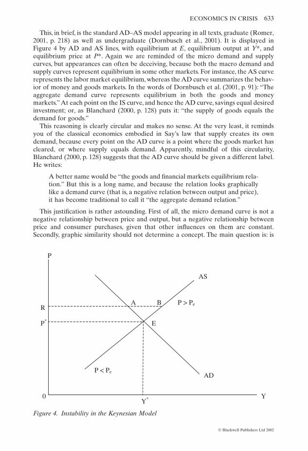
This, in brief, is the standard AD–AS model appearing in all texts, graduate (Romer,2001, p. 218) as well as undergraduate (Dornbusch et al., 2001). It is displayed in Figure 4 by AD and AS lines, with equilibrium at E, equilibrium output at Y*, andequilibrium price at P*. Again we are reminded of the micro demand and supplycurves, but appearances can often be deceiving, because both the macro demand andsupply curves represent equilibrium in some other markets. For instance, the AS curverepresents the labor market equilibrium, whereas the AD curve summarizes the behav-ior of money and goods markets. In the words of Dornbusch et al. (2001, p. 91): “Theaggregate demand curve represents equilibrium in both the goods and moneymarkets.”At each point on the IS curve, and hence the AD curve, savings equal desiredinvestment; or, as Blanchard (2000, p. 128) puts it: “the supply of goods equals thedemand for goods.”

This reasoning is clearly circular and makes no sense. At the very least, it remindsyou of the classical economics embodied in Say’s law that supply creates its owndemand, because every point on the AD curve is a point where the goods market hascleared, or where supply equals demand. Apparently, mindful of this circularity,Blanchard (2000, p. 128) suggests that the AD curve should be given a different label.He writes:

A better name would be “the goods and financial markets equilibrium rela-tion.” But this is a long name, and because the relation looks graphicallylike a demand curve (that is, a negative relation between output and price),it has become traditional to call it “the aggregate demand relation.”

This justification is rather astounding. First of all, the micro demand curve is not anegative relationship between price and output, but a negative relationship betweenprice and consumer purchases, given that other influences on them are constant.Secondly, graphic similarity should not determine a concept. The main question is: is



AS

AD

A B

E

P > Pe

P < Pe

Y

P

Y*

R

P*

0

Figure 4. Instability in the Keynesian Model

it aggregate demand or not? The answer is that it is not. It is both aggregate demandand supply.

Is this model stable? In some ways it is worse than the classical model. Suppose the price level is at R, where there is excess supply in the goods market as well as un-desired inventory investment equaling AB; this means savings must exceed desiredinvestment by the amount of the excess supply. However, this contradicts the fact thatat point A, which lies on the AD curve, S = I by the very definition of this AD curve.

If indeed there is excess supply and hence a recession at R, then we run into thesame difficulty as we did in the classical framework, namely the movement towardsequilibrium requires an expansion in desired investment in a recessionary environ-ment. This is because in this model as the price level falls, the interest rate falls, desiredinvestment expands and so does AD, just as in the classical model. Thus the modernrendition of the Keynesian model suffers from the same logical contradiction as theclassical variety, but it is subject to circular reasoning as well. In fact, desired invest-ment should contract and AD should move further away from its equilibrium level,when the price level is at R.

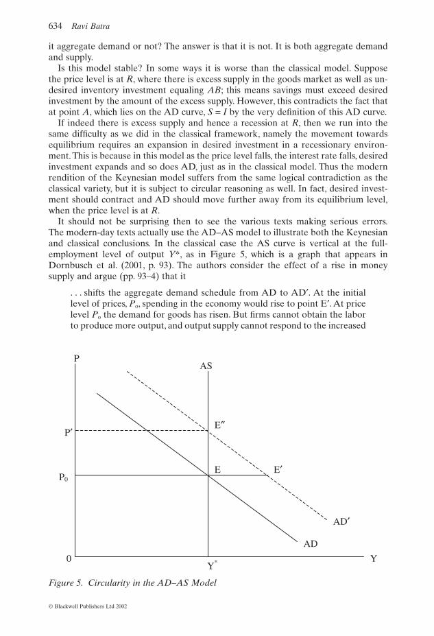
It should not be surprising then to see the various texts making serious errors.The modern-day texts actually use the AD–AS model to illustrate both the Keynesianand classical conclusions. In the classical case the AS curve is vertical at the full-employment level of output Y*, as in Figure 5, which is a graph that appears in Dornbusch et al. (2001, p. 93). The authors consider the effect of a rise in money supply and argue (pp. 93–4) that it

. . . shifts the aggregate demand schedule from AD to AD¢. At the initiallevel of prices, Po, spending in the economy would rise to point E¢. At pricelevel Po the demand for goods has risen. But firms cannot obtain the laborto produce more output, and output supply cannot respond to the increased

634 Ravi Batra


P

Y Y*

P¢

P0

0

AD¢

AD

E E¢

E≤

AS

Figure 5. Circularity in the AD–AS Model

demand. As firms try to hire more workers, they bid up wages and theircosts of production, so they must charge higher prices for their output. Theincrease in demand for goods therefore leads only to higher prices, and notto higher output.

The increase in prices reduces the real money stock and leads to a reduc-tion in spending.The economy moves up the AD¢ schedule until prices haverisen enough, and the real money stock has fallen enough, to reduce spend-ing to a level consistent with full employment output. This is the case atprice level P¢.

The conclusion that monetary expansion only raises prices and not output underconditions of full employment is reasonable and accords with common sense, but itsunderlying argument is inconsistent with the authors’ construction of the AD sched-ule. For instance, with monetary expansion desired investment at E¢ is higher than atE, but since E¢ lies on an AD curve where savings and investment are always equal,savings must have risen by the same amount as investment. However, the economy isalready at full employment, so real income and hence savings cannot rise in the IS–LMframework examined by the authors. Nor can aggregate demand ever exceed aggre-gate supply at Po, because at each point on the AD curve, old or new, output equalsreal spending.

Even if we grant that aggregate demand exceeds aggregate supply at E¢, there is noreason for desired investment to fall in an environment of excess demand even if theprice level goes up, so that E¢ need not move toward E≤.

7. A Logical and Stable Macro Model

In order to construct a consistent macro model, of an open or closed economy, savingsand investment must be directly linked to output or real income, and not indirectly asis done in the classical framework or the modern-day neo-Keynesian model.There maybe other influences on S and I, but the paramount impact comes from real income.Thus we write:

(26)

(27)

(28)

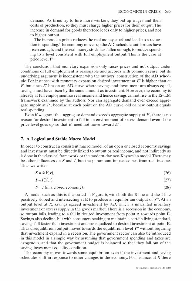
A model such as this is illustrated in Figure 6, with both the S-line and the I-linepositively sloped and intersecting at E to produce an equilibrium output of Y*. At anoutput level at R, savings exceed investment by AB, which is unwanted inventoryinvestment or excess supply in the goods market. There is a recession in the economy,so output falls, leading to a fall in desired investment from point A towards point E.Savings also decline, but with consumers seeking to maintain a certain living standard,savings fall faster than investment and are equalized to desired investment at point E.Thus disequilibrium output moves towards the equilibrium level Y* without requiringthat investment expand in a recession. The government sector can also be introducedin this model in a simple way by assuming that government spending and taxes areexogenous, and that the government budget is balanced so that they fall out of thesaving–investment equality condition.

The economy moves towards some equilibrium even if the investment and savingschedules shift in response to other changes in the economy. For instance, at R there

S I= ( )in a closed economy .

I I Y r= ( ), ,

S S Y r= ( ), ,



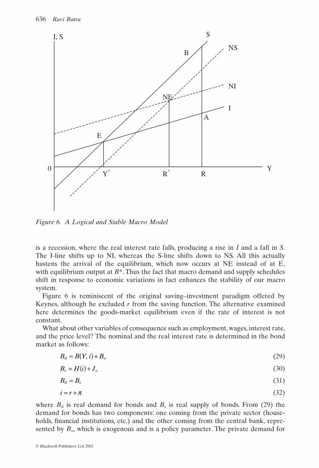
is a recession, where the real interest rate falls, producing a rise in I and a fall in S.The I-line shifts up to NI, whereas the S-line shifts down to NS. All this actually hastens the arrival of the equilibrium, which now occurs at NE instead of at E,with equilibrium output at R*. Thus the fact that macro demand and supply schedulesshift in response to economic variations in fact enhances the stability of our macrosystem.

Figure 6 is reminiscent of the original saving–investment paradigm offered byKeynes, although he excluded r from the saving function. The alternative examinedhere determines the goods-market equilibrium even if the rate of interest is not constant.

What about other variables of consequence such as employment, wages, interest rate,and the price level? The nominal and the real interest rate is determined in the bondmarket as follows:

(29)

(30)

(31)

(32)

where Bd is real demand for bonds and Bs is real supply of bonds. From (29) thedemand for bonds has two components: one coming from the private sector (house-holds, financial institutions, etc.) and the other coming from the central bank, repre-sented by Bo, which is exogenous and is a policy parameter. The private demand for

i r= + p

B Bd s=

B H i Js o= ( ) +

B B Y i Bd o= ( ) +,

636 Ravi Batra


I, S

NS

S

B

A I

NI

0 Y* R* R

E

NE

Y

Figure 6. A Logical and Stable Macro Model

bonds, B(.), is linked negatively to real income and positively to the rate of interest(Motley, 1977). In (30) the supply of bonds also has two components. The first, H(.),coming primarily from firms and home buyers, depends negatively on the interest rate;the second, Jo, coming from the government is exogenous. In equilibrium, bond demandand supply are equal. For a given Y, the bond market determines the nominal inter-est rate, which, for an exogenous rate of expected inflation, determines the real rate ofinterest.

Combining the goods and the bond markets, we determine equilibrium output andinterest rates. These two markets are described by seven equations, such as those from(26) to (32), in seven variables: Y, S, I, r, Bd, Bs, and i. As shown in Figure 6, the equi-librium is consistent with common sense and is stable.

In an open economy, the graphical description of the goods market does not change,because the I-line may simply be replaced by a line representing domestic and foreigninvestment (Q), so that in an open economy

(33)

Nor does the analysis change much, because all we do is add one more variable andone more equation.

The real wage is determined in the labor market as follows:

(production function) (34)

(labor demand) (35)

(labor supply) (5)

(labor-market equilibrium) (36)

where n is the rate of capacity utilization, which is determined inside our framework.This model of the labor market differs slightly from the classical analysis in that,

while capital stock is constant in the short to medium run, its rate of utilization dependson output and hence aggregate demand.The production function in (34) makes it clearthat, for any given L and Ko, output depends on n, or n depends on Y. The capacityutilization rate, which has an upper limit of one, in turn affects the marginal productof the two factors and labor demand. Specifically, as aggregate demand rises, Y and nrise, and so do labor’s marginal product and its demand. Otherwise, the real wage isstill determined by the equality of labor demand and labor supply, as in (36). There-fore employment in this framework is determined eventually by the level of aggregatedemand, even though the real wage is fully flexible.

Output reaches an upper limit, when capital is fully utilized. Such a level of outputmay be called “full-capacity output,” which contrasts with the “full-employmentoutput” of the classical model. Finally, the price level and the money wage are deter-mined as follows:

(37)

(38)

Equation (37) is the same as the classical quantity equation, except that V is not con-stant in this framework; instead it depends on the rate of interest (Barro, 2000). Thereason for selecting the quantity equation is that it is an identity and true by defini-tion. You cannot go wrong with it in determining the price level, because the rela-tionship in (37) is always valid. With M known exogenously, and with Y and i alreadydetermined, P can be computed from (37), and then the money wage (W) can be

W wP= .

MV i PY( ) = ,

F L nK G LL , o( ) = ( )w G L= ( )w F L nKL= ( ), o

Y F L nK n= ( ), ,o � 1

S Q Y r= ( ) ( ), .open economy



obtained from (38). In this way all the variables are determined in the present paradigm.

This closed- or open-economy macro model displays features of both the classicaland Keynesian frameworks. The real wage is perfectly flexible, yet employment isdetermined by aggregate demand. Money is either neutral or non-neutral in this model.

As an illustration, suppose there is a rise in money supply, as the central bank buysgovernment bonds. The demand for bonds goes up, causing a rise in bond price or afall in the nominal rate of interest. In the short run, with expected inflation unchanged,the real interest rate falls and desired investment goes up, raising the level of aggre-gate demand. If the economy is operating at full capacity, output remains constant, andthe only change then is in the price level, as in the classical model. But if capital stockis not fully utilized, firms decide to raise their output as a result of the influx of neworders stemming from increased aggregate demand. At first they increase their capac-ity utilization, which in turn raises the marginal product of labor and thus shifts thelabor demand curve outwards, leading to new hiring and a rise in the real wage. So apart of the increase in output comes from increased utilization of capital, and anotherpart from increased employment. Thus, money is neutral if capacity is fully utilized;otherwise, it is not.

In a recession, output is below its full-capacity level. Therefore, monetary expansionstimulates the economy, expands employment and eases, and possibly eliminates, therecession. But the monetary stimulus should not be overdone, because once full capac-ity is reached, output and employment cannot expand.

In technical terms, the labor market adds four more equations, (34), (35), (5), and (36), and four more variables: L, n, w, and G, where G(.), as before, is the labor supplyfunction.Thus, in all, factory orders and aggregate demand or output are determined ingoods and bond markets, whereas capacity utilization and employment to meet thoseorders are determined in the labor market.That completes the analysis of this model.

Mathematically, the following equations illustrate what has been explained above.Let us differentiate the equations of the model totally with respect to Bo, the centralbank’s demand for government bonds. Then from the bond market, noting that di =dr:

whereas from the goods market:

where b = (Br - H¢) > 0, and l = (Sr - Ir)/(Sy - Iy) > 0. Here Sy is the marginal propen-sity to save, and Iy may be called the marginal propensity to invest. Figure 6 shows thatSy should exceed Iy for the system to be consistent and stable. The solution of thesetwo equations yields

(39)

(40)

Since By < 0, b - lBy > 0, so that an increase in bond purchase or money supply bythe central bank lowers the rate of interest. Clearly, dY/dBo > 0, so that an increase inmoney supply creates new factory orders for firms, and the potential for a higher

dYdB Byo

=-

>1

0b l

.

drdB Byo

= --

<1

0b l

,

dY dr+ =l 0,

B dY dr dBy + = -b o,

638 Ravi Batra


output. Whether or not the output actually goes up is determined by conditions in thelabor market. Differentiating the labor-market equations, (34) and (36), totally, weobtain

(41)

(42)

where

(43)

Equation (41) makes clear that, if n is below its upper limit, it will rise with a rise innew factory orders. On the other hand, if dn = 0, or if capital is already fully utilized,output cannot rise. Equation (42) shows that if dn > 0, then with FLK > 0, dL > 0 aswell, so that employment will rise. What about the real wage? Clearly, the real wagewill then also rise, as from (5) we have

(44)

8. Merits of the Alternative Macro Model

The open- and closed-economy macro model presented above is not only logical, con-sistent with common sense and stable, it also has other merits that have long eludedthe classical and Keynesian frameworks. The main inadequacy of the classical modelis considered to be its property that money is completely neutral, whereas experiencetells us that the rise in money supply leads economies out of recession, so that moneycannot be completely neutral (Abel and Bernanke, 1995, p. 355). Similarly the modelcannot adequately explain the business cycle where unemployment rises periodically.The macro alternative presented here is free from these strictures. It is a market-clearing model, so that labor supply and demand determine employment and the realwage, yet unemployment can arise from the inadequacy of money supply or aggregatedemand, which determines the rate of capacity utilization. Money in this model can beneutral and non-neutral.

The Keynesian model is the direct opposite of the classical framework. It can ade-quately explain recessions, depressions, and the business cycle resulting from insuffi-cient aggregate demand, but it has a number of flaws that render it unappealing tomany economists. For instance, it has to rely on the fact that markets do not clear attimes and thus cause unemployment. Real and nominal wages are then determinednot by labor supply and demand but by some nonmarket forces, which does not seemto pertain to common sense, especially in the United States, where the nonmarketforces or unions have progressively become weaker. Nonmarket forces may bestronger in developing economies that are plagued by a shortage of capital and over-population, but not in advanced economies, where unemployment is periodic and nota permanent fact of life.

The Keynesian model also suggests that by constantly raising money supply, unem-ployment can be reduced permanently. In fact, this prescription, irrational on its face,was taken seriously by economists and governments alike during the 1960s and the1970s, with disastrous consequences in terms of heated inflation in the end (Batra, 1996,pp. 30–2). However, the alternative model offered here suggests that a monetary injec-tion will not reduce unemployment once excess capacity in the economy disappears.At that point, only rising investment and capital stock will do the job.

dw G dL= ¢ .

D K F F F G F GL LK LL LL= - - ¢( )[ ] > = - - ¢( ) >o and0 0, .a

dL K F dnLK= o a ,

dn dY D= a ,



Another big problem is that the real wage falls with output expansion and rises withoutput contraction in the Keynesian model. This also is contrary to experience andcommon sense. However, in the present model the real wage falls in a recession, ascapacity utilization and hence the marginal product of labor decline, and rises withrecovery, where capacity utilization and hence the marginal product of labor go up.Thus the macro alternative presented here gets rid of many flaws arising in traditionalmacro models.

9. The Popular Model of the Gains from Trade

So far this paper has examined some lacunae of conventional macro models. Let usnow turn to the question of the gains from trade, which also is essentially a macro issuedealing with the well-being of entire society. Unfortunately, the popular framework oftrading gains explored in textbooks also suffers from logical deficiencies. No macroeconomist, or a layman, would believe that output at the firm, industry, or nationallevel can rise without a rise in capital stock, employment, or technology. A productionfunction has three main ingredients: capital, labor, and technology. At least one of thethree has to augment for output to rise at any level. But trade theorists, it turns out,constantly argue that a country’s real GDP goes up just by exchanging goods aroundthe world.

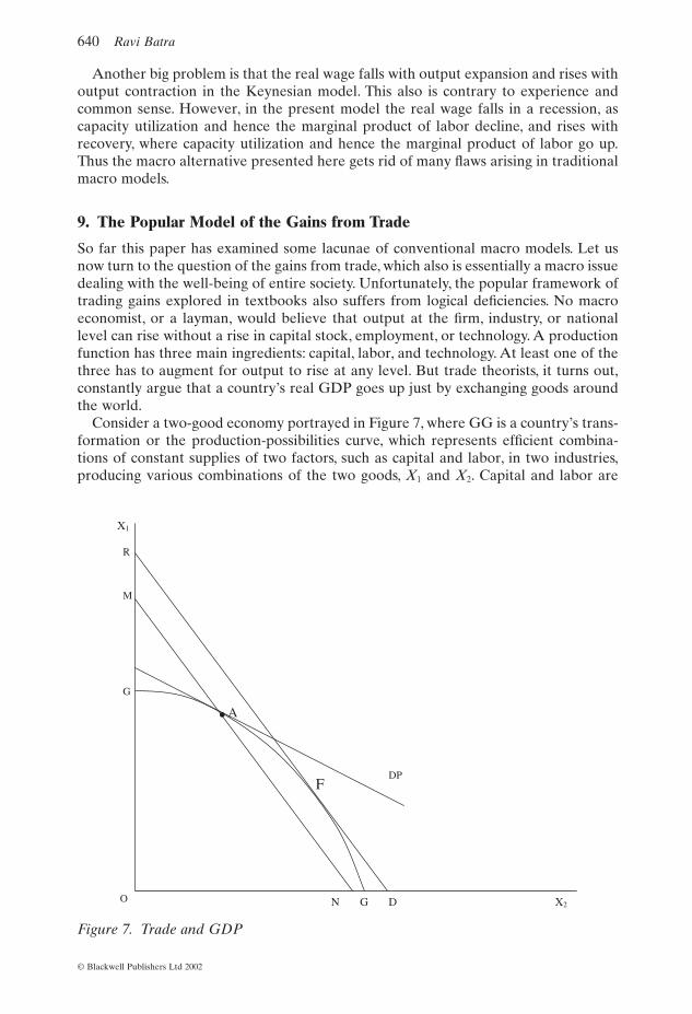
Consider a two-good economy portrayed in Figure 7, where GG is a country’s trans-formation or the production-possibilities curve, which represents efficient combina-tions of constant supplies of two factors, such as capital and labor, in two industries,producing various combinations of the two goods, X1 and X2. Capital and labor are

640 Ravi Batra


O

F

.A

G D N

M

G

R

X2

X1

DP

Figure 7. Trade and GDP

fully employed at any point on GG, while technology in each industry stays constant.The initial production point is at A, where a price line DP is tangential to the trans-formation curve. Now suppose consumer preferences change in favor of X2, so that therelative price of this good rises from the slope of the line DP to that of line RD. Theproduction point then moves to F.

What happens to the real value of output, as society moves from A to F? The con-ventional answer in this case is: “We don’t know.” At each point on GG, productionefficiency is maximum, while the output of one good is higher and that of the othergood lower than at any other point. So it is not possible to compare real GDP at dif-ferent points on GG. However, I will show that real GDP is constant along all pointson GG.

For the time being, it may be noted that no one would argue that a shift in consumerpreferences that altered relative prices of the two goods improves the living standardof the consumer. As Browning and Browning (1986, p. 559) point out, only the pro-duction point and income distribution then change. Now suppose point A is a point ofself-sufficiency in autarky, and the country switches to free trade at the new price lineRD, which prevails in the rest of the world. Production shifts to F, and the populartrade model says that real GDP is now higher than at point A. Most economists suchas Kemp (1969) among others call this change the “specialization” or “production”gain. Their argument is that under free trade the value of GDP is represented by theposition of the line RD, and at that price ratio the production bundle available at Ayields a GDP represented by MN, which is drawn parallel to RD, so that the productprice ratio is the same. Since MN clearly lies below RD, free trade, according to thisargument, has unambiguously produced a rise in real GDP.

Why don’t we apply the same logic to the case of the change in consumer prefer-ences? Suppose the economy is closed, and as consumers prefer more of X2, the pro-duction point shifts from A to F. If production at both F and A is valued at the newprice line, real GDP is clearly larger at F. But then if output at both points is valuedat the relative price prevailing at A, real GDP would be larger at point A. So consumerpreferences or relative-price changes alone cannot generate GDP gains, because allpoints on GG are efficient production points.

If the relative price change from consumer preferences does not create any pro-duction gain, then why should the relative-price change from a switch to free tradecreate any production gain? Both A and F continue to be efficient production points.Actually both points, as it turns out, generate the same level of real GDP. In a two-good economy, nominal GDP (N) is given by

(45)

whereas real GDP is

(46)

Here P, the general price level, is the weighted average of the two prices pi (i = 1, 2):

(47)

where h is the proportion of X1 consumption in nominal GDP (p1C1/N) and 1 - h isthe proportion of X2 consumption in nominal GDP (p2C2/N). Y becomes

(48)YX pX

p=

++ -( )

1 2

1h h,

P p p= + -( )h h1 21 ,

Y p X p X P= +( )1 1 2 2 .

N p X p X= +1 1 2 2 ,



where p = p2/p1 is the relative price of X2. For simplicity, we assume that initially pi

equals one, so that P = p = 1. Differentiating (48) totally and assuming that the twoweights are constant, we obtain

(49)

The first two terms of the right-hand side of (49) equal zero, because the marginal rateof transformation equals the price ratio, whereas the last term of (49) equals X2dpbecause X2 = C2 in the initial situation of a closed economy, so that dY = 0. Thus evenif the price ratio (p) changes because of a shift of the economy from a closed stanceto free trade, there is no change in real GDP. Then what changes in the conventionaltrade model? It turns out that GDP expressed in terms of a good, as in a barter model,increases with a rise in the price of an exportable good. For instance, suppose real GDPis defined in terms of the first good, so that

(50)

(51)

where Y1 is nominal GDP deflated by the price of the first good, and p is the relativeprice of the second good, which is exported after the introduction of trade that raisesp. Here dY1 > 0, for dp > 0. This is the production or GDP gain arising in the conven-tional trade model, but it requires a barter framework, which does not prevail in reality.In a real world where values are expressed in money terms and the general price levelis not constant, real GDP does not change with relative prices, and cannot rise withouta rise in employment, capital, or technology. It may also be noted that the change in pcould have come from any source other than free trade and generated a productiongain in the barter framework.

What then is left of the gains from trade? If we adopt a macro approach to socialwelfare, as portrayed in the utility function presented in (1), there is no gain or lossfrom trade. Social well-being then depends on real GDP and leisure, which is normallyassumed to be constant in the popular trade model. In that case, only GDP matters,and since real GDP is unchanged with a change in relative prices, there is no gain orloss from trade. It is possible to argue that the macro approach to social welfare is thesuperior approach, because it deals with a well-known concept that is subject to mea-surement. Most macro texts suggest that real income, or real per capita GDP, is a soundmeasure of social welfare, or is better than any other objective measure (Landsburgand Feinstone, 1997, p. 9). In terms of this objective index then, trade neither hurts norbenefits a nation, unless of course the country cannot produce raw materials, whichhave to be imported for the production of other goods.

In the popular trade model, however, social welfare derives from the consumptionof individual commodities and improves because of two trading gains, namely the pro-duction gain and the consumption gain, which arises from the fall in the relative priceof importables. Even though the first component turns out to be zero, the secondremains. Thus the consumption gain is still positive, but it is not subject to measure-ment. In the absence of the production gain, the trading gain may be miniscule, andmay not be worth all the dislocation to workers that arises from rising trade. Nor mayit be enough to compensate the trading world for increased global pollution stemmingfrom a rise in transportation of goods over vast seas (Batra et al., 1998). Indeed in thereal world, welfare losses from pollution and family dislocation may outweigh the mereconsumption gain from trade.

dY dX pdX X dp X dp1 1 2 2 2= + + = ,

Y X pX1 1 2= + ,

dY dX pdX X dp Y dp= + + - -( )1 2 2 1 h .

642 Ravi Batra


10. Conclusions

This paper has examined three popular models that form the foundation of moderneconomics taught around the world. It turns out that two of the three models, the clas-sical and the Keynesian, are seriously deficient, whereas the third, namely the analyticframework of the gains from trade, is partially lacking in logic. The classical and neo-Keynesian approaches require desired investment to expand during recessions anddepressions, whereas the trade model calls for real GDP to rise without any rise inemployment, capital stock, or technology. None of this accords with reality andcommon sense.

The paper offers alternative frameworks for macroeconomics as well as interna-tional trade, which is also essentially a macro issue.The alternative macro model is freefrom the limitations of conventional models. Thus, money is either neutral or non-neutral, depending on whether the economy is operating below or at full capacity. Realand money wages are strictly determined in the labor market, yet employment is influ-enced by aggregate demand. Thus, the macro alternative presented here combines theattractive features of both the classical and Keynesian frameworks.

The paper also offers a macro theory of the gains from trade, and shows that ifsociety’s well-being depends on real per capita income or GDP, then free trade is nobetter or worse than in a closed economy. If the closed economy is already Pareto-efficient, then the introduction of trade does not raise its productive efficiency. Trademay, of course, offer an additional improvement, namely the consumption gain, butthis alone may be too small to be outweighed by welfare losses generated by trans-portation-related pollution and dislocation of workers and their families.

References

Abel, Andrew and Ben Bernanke, Macroeconomics, 2nd edn, Reading, MA: Addison-Wesley(1995).

Barro, Robert, Macroeconomics, 4th edn, New York: John Wiley (2000).Batra, Ravi, The Great American Deception, New York: John Wiley (1996).———, “Neutrality and Non-Neutrality of Money in a Classical Type of Model,” Pacific Eco-

nomic Review 7 (2002a): 250–64.———, “The Long-Run Real-Wage Rigidity and Full-Employment Adjustment in the Classical

Model,” International Review of Economics and Finance 11 (2002b):1–21.Batra, Ravi, Hamid Beladi, and Ralph Frasca, “Environmental Pollution and World Trade,”

Ecological Economics 27 (1998):171–82.Blanchard, Oliver, Macroeconomics, 2nd edn, Upper Saddle River: Prentice Hall (2000).Branson, William H., Macroeconomic Theory and Policy, 2nd edn, New York: Harper & Row

(1979).Browning, Edgar and Jacquelene Browning, Microeconomic Theory and Applications, 2nd edn,

New York: Little Brown (1986).Dornbusch, Rudiger, Stanley Fischer, and Richard Startz, Macroeconomics, 8th edn, Boston:

McGraw-Hill Irwin (2001).Gardner, Ackley, Macroeconomic Theory, New York: Macmillan (1961).Kemp, Murray, The Pure Theory of International Trade and Investment, Englewood Cliffs:

Prentice Hall (1969).Landsburg, Steven and Lauren Feinstone, Macroeconomics, New York: McGraw-Hill

(1997).Mankiw, N. Gregory, Macroeconomics, New York: Worth (2000).Motley, Brian, Money, Income, and Wealth, Lexington, MA: D. C. Heath (1977).Romer, David, Advanced Macroeconomics, Boston: McGraw-Hill Irwin (2001).



US Council of Economic Advisers, Economic Report of the President, Washington, DC (1999).

Notes

1. Actually, there are ten equations, but from Walras’ law only nine are independent.2. A variant of this model appeared in Batra (2002a).

644 Ravi Batra


economics in crisis: severe and logical contradictions of classical, keynesian, and popular trade...

Documents