logical relations for monadic types
TRANSCRIPT
arX
iv:c
s/05
1100
6v2
[cs
.LO
] 4
Mar
200
8
Under consideration for publication in Math. Struct. in Comp. Science
Logical Relations for Monadic Types†
J E A N G O U B A U L T - L A R R E C Q1 ‡
S L A W O M I R L A S O T A2§
D A V I D N O W A K3¶
1 LSV, ENS Cachan, CNRS, INRIA
2 Institute of Informatics, Warsaw University
3 Research Center for Information Security, AIST
Received June 2005
Logical relations and their generalizations are a fundamental tool in proving properties
of lambda-calculi, e.g., yielding sound principles for observational equivalence. We
propose a natural notion of logical relations able to deal with the monadic types of
Moggi’s computational lambda-calculus. The treatment is categorical, and is based on
notions of subsconing, mono factorization systems, and monad morphisms. Our approach
has a number of interesting applications, including cases for lambda-calculi with
non-determinism (where being in logical relation means being bisimilar), dynamic name
creation, and probabilistic systems.
Keywords: logical relations, monads, semantics, typed lambda-calculus.
Contents
1 Introduction 3
1.1 Motivation and context. 3
1.2 Outline. 4
2 Preliminaries 4
3 Lifting of a Monad to a Scone 5
† A preliminary version of this paper was presented at the 11th Annual Conference of the Euro-pean Association for Computer Science Logic (CSL’02), Edinburgh, Scotland, 22–25 September 2002(Goubault-Larrecq et al., 2002).
‡ Work partially supported by the RNTL project EVA, and the ACI jeunes chercheurs “Securite infor-matique, protocoles cryptographiques et detection d’intrusions”.
§ Work partially supported by the Polish KBN grant 7 T11C 002 21, and the IST-2005-16004 IntegratedProject SENSORIA: Software Engineering for Service-Oriented Overlay Computers.
¶ Work partially supported by the ACI jeunes chercheurs “Securite informatique, protocoles cryp-tographiques et detection d’intrusions”.

4 Lifting of a Monad to a Subscone 7
4.1 T on objects. 9
4.2 T on morphisms. 9
4.3 Unit η. 9
4.4 Multiplication µ. 10
5 Lifting of a Monad to Relations 11
6 Lifting Monoidal Structures 13
6.1 Monoidal Categories 13
6.2 Unit element I. 15
6.3 Tensor product ⊗. 15
6.4 Associativity α. 15
6.5 Left unit ℓ. 16
6.6 Right unit r. 17
6.7 Symmetric Monoidal Categories 17
6.8 Commutativity ℓ. 18
6.9 Lifting Cartesian Products 19
6.10 Terminal object 1. 19
6.11 Binary product ×. 20
7 Lifting Strong, Monoidal, and Commutative Monads to a Scone and a Subscone 20
7.1 Lifting Strong Monads 20
7.2 Monoidal Monads 23
7.3 Commutative Monads 26
8 Building Monad Morphisms from Adjunctions 27
8.1 Eilenberg-Moore algebras. 27
8.2 Kleisli category. 28
8.3 Monad Morphisms from Adjunctions 28
8.4 Monoidal, and Strong Monad Morphisms from Monoidal Adjunctions 29
9 Lifting Closed Structures to the Subscone 34
10 Examples 39
10.1 Lift, Exceptions, State, Non-Determinism, and Continuations in SetSetSet 40
10.2 Labelled transition systems and bisimulations 42
10.3 Discrete Probabilities and Subprobabilities 42
10.4 Logical relations for dynamic name creation 44
10.5 Fun With Categories I: Taking CCC 6= SetSetSet, the Example of CpoCpoCpo 47
10.6 Fun With Categories II: Making CCC and C Distinct, e.g., CCC = CpoCpoCpo, C = OrdOrdOrd 49
10.7 Fun With Categories III: The Case CCC = FSFSFS, C = TopTopTop 53
10.8 Fun With Categories IV: Metric Spaces 58
11 Related work. 63
12 Conclusions 64
Appendix A Monoidal Monads, Commutative Monads 68
A.1 From Mediators to Strengths and Dual Strengths 68
A.2 From Strengths and Dual Strengths to Mediators 70
A.3 Monoidal Monad Morphisms 72
A.4 Commutative Monads are Monoidal 73
2

Appendix B Proof of Lemma 8.3 74
Appendix C Composition of Monoidal Adjunctions 77
Appendix D Proof of Proposition 8.6 79
1. Introduction
1.1. Motivation and context.
Logical relations and their generalizations (Mitchell, 1996) are a fundamental tool in
proving properties of lambda-calculi, e.g., characterizing lambda-definability (Plotkin, 1980;
Jung and Tiuryn, 1993; Alimohamed, 1995; Fiore and Simpson, 1999), proving equational
completeness (Statman, 1985; Mitchell, 1996), studying parametric polymorphism (Reynolds, 1983;
Ma and Reynolds, 1992; Lazic and Nowak, 2000) notably. On the other hand, Moggi’s
computational lambda-calculus (Moggi, 1991) has proved useful to define various notions
of computations on top of the lambda-calculus: side-effects, input-output, continuations,
non-determinism (Wadler, 1992), probabilistic computation (Ramsey and Pfeffer, 2002)
in particular.
What should then be a natural notion of logical relation for Moggi’s computational
lambda-calculus? Although there is no unique answer to this question, we propose one
that is satisfying in practice. We shall demonstrate the relevance of our approach by
illustrating our construction on monads for non-determinism, dynamic name creation,
and probabilistic computation.
Moggi’s insight is based on categorical semantics: while categorical models of the λ-
calculus are cartesian closed categories (CCCs), the computational lambda-calculus re-
quires CCCs with a strong monad (TTT ,ηηη,µµµ, ttt). The monadic types of the computational
lambda-calculus are given by the syntax:
τ ::= b|τ → τ |τ × τ |TTT (τ)
where b ranges over a set B of so-called base types, and TTT (τ) is meant to denote the type
of computations of type τ . Compared to the lambda-calculus, Moggi’s calculus has an
additional val operation, of type τ → TTT (τ), and an additional let x = u in v construct,
of type TTT (τ ′) provided u has type TTT (τ) and v has type TTT (τ ′) under the assumption x : τ .
Every computational lambda-term has a unique interpretation as a morphism in a CCC
with a strong monad. In fact the category CompCompComp whose objects are types and whose
morphisms are terms up to βη-conversion is the free CCC-with-a-strong-monad over the
set B.
Accordingly, our study will rest on categorical principles. While there is a flurry of
generalizations of logical relations (Kripke logical relations (Mitchell, 1996), lax logical
relations (Plotkin et al., 2000), pre-logical relations (Honsell and Sannella, 2002), etc.),
we use subscones (Mitchell and Scedrov, 1993) as a unifying framework for defining
logical relations. Recall that subscones over SetSetSet allow one to define logical relations,
and subscones over the presheaf category SetSetSetI lead to I-indexed Kripke logical rela-
tions (Mitchell and Scedrov, 1993). Technically, the development in (Mitchell and Scedrov, 1993)
3

is based on unique lifting of the CCC structure to the subscone. Our whole endeavor then
reduces to finding appropriate liftings of monads on categories CCC to the subscone category
(C ∩ | |) (see Section 4).
The important property of logical relations is the so-called Basic Lemma (Mitchell, 1996):
meanings of a lambda-term in different models w.r.t. related environments are related.
This is immediate for subscones, and stems from the fact that CompCompComp is the free CCC-with-
a-strong-monad on B (a trivial adaptation of Proposition 5.2 in (Mitchell and Scedrov, 1993)).
In particular, that any two closed terms that are in logical relation are observationally
equivalent is immediate.
1.2. Outline.
We return to preliminaries in Section 2. We then define liftings of monads to scones in Sec-
tion 3; this is simpler than for subscones, and of independent interest. The construction
is based on the use of monad morphisms. We then lift monads to subscones in Section 4,
using a mono factorization system. The important case where the target category CCC is
a product of two categories is investigated in Section 5: this is where binary logical re-
lations arise, allowing us to compare two models. We terminate our lifting construction
by lifting the monoidal structure and monad strength in Sections 6 and 7, respectively.
Section 8 establishes a result by which adjunctions give rise to monad morphisms. In
Section 9, we return to the basics of subscone theory. While the standard construction
of the CCC structure over the subscone requires a functor | | that commutes with finite
products, we show that the use of mono factorization systems, as in Section 4, allows us
to relax this requirement to | | being only monoidal. While we do not make any use here
of this observation, monoidal functors are more natural from a categorical point of view
than product preserving ones, and we feel it should be interesting in future applications
(we have some already, but we refrain from including them in this paper).
It remains to test the relevance of our construction (Section 10): the logical rela-
tions thus defined characterize bisimulations when TTT is the non-determinism monad (as
suggested in (Lazic and Nowak, 2000)), a generalization of Larsen and Skou’s proba-
bilistic bisimulations (Larsen and Skou, 1991) when TTT is a measure monad (Giry, 1981;
Jones, 1990), and a notion close to Pitts and Stark’s logical relations for observational
equivalence of programs that create names dynamically (Pitts and Stark, 1993; Stark, 1998).
We comment on related work in Section 11 and conclude in Section 12.
2. Preliminaries
Fix two categories CCC and C and a functor | | : CCC → C.
Consider the comma category (C ↓ | |), whose objects
are tuples 〈S, f, A〉, with f : S → |A| in C and whose
morphisms are pairs 〈g, h〉 : 〈S, f, A〉 → 〈S′, f ′, A′〉, g :
S → S′ in C and h : A → A′ in CCC, such that the diagram
on the right commutes in C.
S
g
f // |A|
|h|
S′f ′
// |A′|
(1)
This category is the scone of CCC over C via | |, (C ↓ | |). (We extend here terminology of
4

(Mitchell and Scedrov, 1993), where the name scone was reserved to the case C = SetSetSet,
| | = CCC(1, ) only.) The projection functor U : (C ↓ | |) → CCC maps 〈S, f, A〉 to A and the
morphism 〈g, h〉 to h.
In the sequel we shall be especially interested in the case where C = SetSetSet, and | | =
CCC(1, ) is the global section functor, where 1 is terminal in CCC. Another interesting situation
arises when CCC = C×C and |(A, B)| = A×B, assuming that C has finite products. Objects
of the scone then represent binary relations between objects in C. In this case, given two
functors | |1 : CCC1 → C and | |2 : CCC2 → C, we may define | | : CCC → C, for CCC = CCC1×CCC2,
by |(A1, A2)| = |A1|1×|A2|2.
Further assume we are given a monad (TTT ,ηηη,µµµ) on CCC. When CCC = CCC1×CCC2, the monad
TTT on CCC will be usually defined pointwise, by two monads TTT 1 and TTT 2 on CCC1 and CCC2,
respectively: TTT (A1, A2) = (TTT 1(A1),TTT 2(A2)).
3. Lifting of a Monad to a Scone
By lifting of a monad (TTT ,ηηη,µµµ) to the scone (C ↓ | |) of CCC over C we mean a monad
(T , η, µ) on (C ↓ | |) such that the diagram
(C ↓ | |)eT //
U
(C ↓ | |)
U
CCCTTT
// CCC
(2)
commutes, i.e. U T = TTT U and moreover
Uη = ηηηU and Uµ = µµµU . (3)
By Uη and ηηηU we mean the two
possible compositions of a natural
transformation with U, similarly Uµ
and µµµU . The equations (3) amount
to the requirement that the two dia-
grams on the right commute, for all
objects X in (C ↓ | |):
TTT 2UX
(2)µµµUX
zzuuuuu
uuu
TTTUX
(2)
TTTUX
(2)
TTTU eTX
(2)
UXUeηX
//
ηηηUX
<<yyyyyyyU eTX U eTX U eT 2X
UeµX
oo
In other words, the functor U together with the identity natural transformation is a
morphism of monads from T to TTT . (We recall monad morphisms shortly.) Note that
the equations (3) determine the CCC-components of η and µ unambiguously. Moreover,
diagram (2) determines the CCC-component of the action of T on objects and morphisms,
i.e. 〈S, f, A〉 is necessarily mapped to 〈S, f ,TTTA〉, for some S, f and a morphism 〈g, h〉 is
necessarily mapped to 〈g,TTTh〉, for some g.
Our notion of lifting could be stated more generally, for an arbitrary pair of categories,
a functor from the first one to the second one and a monad on the second category. In
fact, in the next section we consider a lifting of TTT to another category, namely a suitable
subcategory of (C ↓ | |).
To be able to give an appropriate lifting we assume another monad (T,,) on C such
5

that the two monads TTT and T are related by a monad morphism from TTT to T, i.e. a
natural transformation
σ : T| | ⇒ |TTT |
making the following two diagrams commute, for each object A in CCC:
T2|A||A|
vvvv
vvv
TσA
T|A|
σA
T|A|
σA
T|TTTA|
σTTT A
|A|
|A|==
|ηηηA|// |TTTA| |TTTA|
∣∣TTT 2A∣∣
|µµµA|oo
(4)
To be formal, a monad morphism is a pair (| |, σ) satisfying the equations above. We
shall however continue to say that σ is a monad morphism, when | | is understood.
Having σ , we define T on objects by
〈S, f, A〉 // 〈TS, σA Tf,TTTA〉
exploiting that if Sf // |A| then TS
Tf // T|A|σA // |TTTA| is a morphism. On mor-
phisms we define T by
〈g, h〉 // 〈Tg,TTTh〉
since from
Sf //
g
|A|
|h|
S′f ′
// |A′|
we deduce that
TSTf //
Tg
T|A|σA // |TTTA|
|TTTh|
TS′Tf ′
// T|A′|σ
A′
// |TTTA′|
commutes,
by naturality of σ. Moreover, we put
η〈S,f,A〉 = 〈S , ηηηA〉 and µ〈S,f,A〉 = 〈S ,µµµA〉.
Checking that this defines a monad is straight-
forward. First, to check that unit and mul-
tiplication are well defined it is sufficient to
merge the commuting diagrams (4) and com-
plete them with naturality squares for and as shown on the right.
Unit η and multiplication µ are natural since
they are defined pointwise and ηηη, µµµ, and are. Verifying monad laws is immediate, by
the same argument.
S
f
S // TS
Tf
T2S
T2f
Soo
T2|A||A|
vvvv
vvv
TσA
T|A|
σA
T|TTTA|
σTTT A
|A|
|A|==
|ηηηA|// |TTTA|
∣∣TTT 2A∣∣
|µµµA|oo
The monad morphism (4) can be equivalently given by a lifting of | | to the categories
6

of algebras of the monads, i.e. by a functor | | : CCCTTT → CT making the diagram commute:
CCCTTT
f| | //
UTTT
CT
UT
CCC
| |// C
where CCCTTT and CT denote categories of algebras of the monads and UTTT and UT denote
the obvious forgetful functors. In fact, for fixed monads TTT and T and a fixed functor | |,
there is a one-to-one correspondence between the monad morphisms σ and liftings of | | to
algebras. The proof of this fact can be found in (Appelgate, 1965) or in (Johnstone, 1975).
4. Lifting of a Monad to a Subscone
Following, and slightly extending (Mitchell and Scedrov, 1993), we may call the subscone
of CCC over C the full subcategory (C ∩ | |) of (C ↓ | |) consisting of all objects 〈S, f, A〉
with f a mono, written S f // |A| . (We shall actually define the subscone slightly
differently below.)
When C = SetSetSet and |A| is given by CCC(1, A), each object S // |A| in the subscone
represents a subset of global elements of A. In the binary case, i.e. when CCC = CCC1×CCC2 and
|(A1, A2)| = CCC1(11, A1)×CCC2(12, A2), S // |(A1, A2)| corresponds to a binary relation
on global elements of A1 and A2—when A1 and A2 are the respective denotations of
type τ in two given models, this will be the logical relation at type τ .
For technical reasons, we require that C has a mono factorization system. This is
essentially an epi-mono factorization (Adamek et al., 1990), except we relax part of the
definition: we keep the mono part but do not require the epis in the sequel. Alternately,
this is a factorization system where one of the classes of morphisms is required to consist
of monos only.
Formally, a mono factorization system is given by two distinguished subclasses of mor-
phisms in C, the so-called pseudoepis // // and the so-called relevant monos // .
The latter must be monos, while the former are not required to be epis. Both classes
must be closed under composition with isomorphisms.
Each morphism f in C must factor as f = m e for some
pseudoepi e and some relevant mono m; and each commut-
ing square (5) has a diagonal making both triangles com-
mute as in (6). We call this diagonal morphism the diagonal
fill-in. Note that the diagonal fill-in is necessarily unique
and that whenever the lower-right triangle commutes, the
upper-left triangle does too. Furthermore, the latter prop-
erty guarantees that the factorization f = m e is unique
up to iso.
· // //
·
· // ·
(5)
· // //
·
· // ·
(6)
In particular, we do not require neither pseudoepis nor relevant monos to be closed under
composition, which holds true for an epi-mono factorization system, see e.g. (Adamek et al., 1990,
7
Chapter 14). But it is easy to deduce from the diagonal fill-in property that a composi-
tion of two pseudoepis is pseudoepi indeed, and similarly a composition of two relevant
monos is a relevant mono, see e.g. (Barr, 1998). It is also proved there that both classes
contain all isomorphisms.
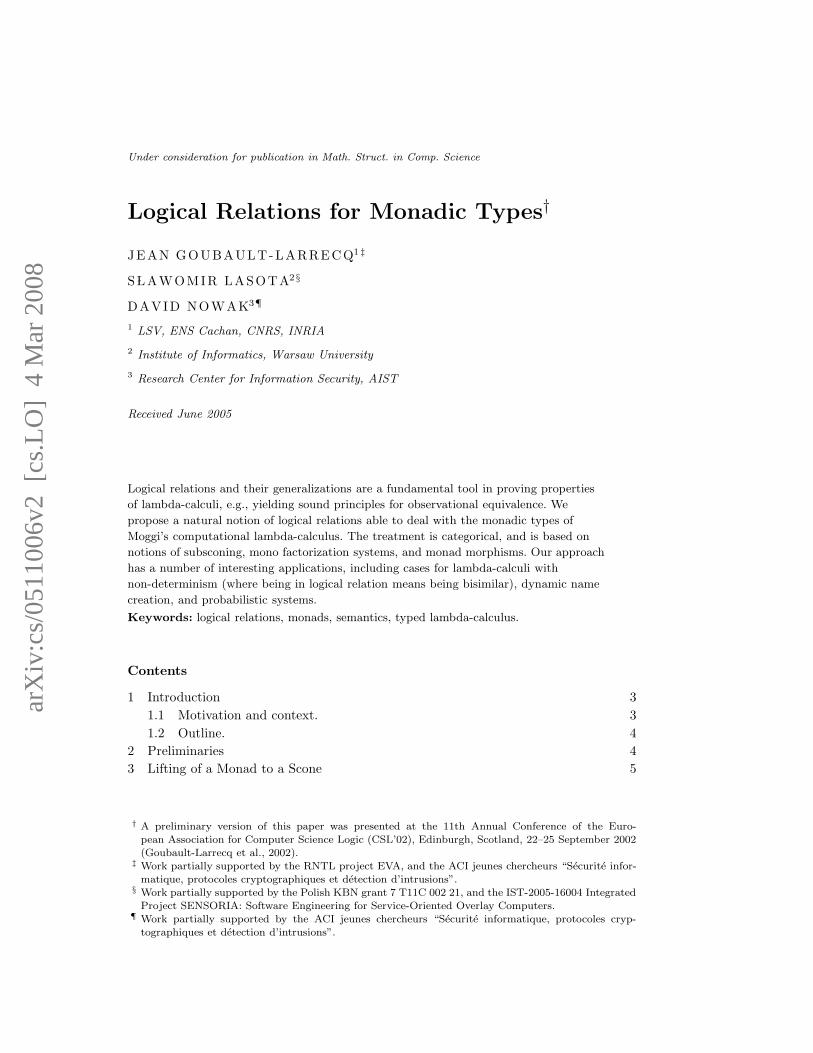
In fact, the factorization of f as me determines uniquely a so-called relevant subobject
of the codomain, defined as follows. Two relevant monos in C with the same codomain,
S1 f1 // S and S2
f2 // S are called equivalent if and only if there exist g1 and g2
making the two triangles commute:
S1
g2 // o
f1 @@@
@@@
S2g1
oo oO
f2~~~~~~
~~
S
i.e., f1 g1 = f2 and f2 g2 = f1. A relevant subobject of S is an equivalence class of
relevant monos with codomain S. Equivalently, we could take as objects of the subscone
all relevant subobjects of |A|, for all objects A in CCC. We prefer to keep the simpler
presentation, despite the fact that this implies that some constructions in the sequel are
only determined up to isomorphism, e.g., (7) below.
We come back to the definition of the subscone:
Definition 4.1. Given two categories CCC, C, a functor | | : CCC → C, and a mono factoriza-
tion system on C, the subscone of CCC over C is the full subcategory (C ∩ | |) of (C ↓ | |)
consisting of all objects 〈S, f, A〉 with f a relevant mono S f // |A| .
It may seem that the notation (C ∩ | |) is too vague, as it does not mention CCC or the
mono factorization system explicitly. It will be clear that making all parameters explicit
would make the notation extremely heavy.
Additionally, we shall assume that Te is pseudoepi for every morphism e in a subclass
of all pseudoepis called relevant pseudoepis, which we shall define shortly. This will be
used in Diagram (11) below. In most applications, it will suffice to check that T preserves
pseudoepis.
Note the following simple and important fact:
Fact 4.2. The first component g of a morphism 〈g, h〉 (recall that
S
g
// |A|
|h|
S′ // |A′|
com-
mutes) in a subscone is uniquely determined by the second component h.
This is because the bottom arrow is now mono.
Let us define a lifting of the monad to the subscone by analogy with (2) and (3) for the
scone. In the binary case mentioned at the beginning of this section, this corresponds to a
lifting of a monad to the category of binary relations (as objects) and relation preserving
functions (as morphisms).
8

4.1. T on objects.
The lifting T on objects is given by the mono
part of the mono factorization of the lifting
of the previous section: 〈S, f, A〉 is taken to
〈S, m,TTTA〉 given by the diagram on the right.
TSTf //
e
T|A|
σA
S
m// |TTTA|
(7)
We call pseudoepis e arising in this way T, σ-relevant pseudoepis. That is, a T, σ-relevant
pseudoepi is the pseudoepi part of a factorization of a morphism of the form σA Tf ,
where f is a relevant mono. For short, we shall call them relevant pseudoepis when T
and σ are clear from context.
Clearly T is defined only up to iso. Formally, the construction would be unambiguous if
we worked with subobjects of |TTTA|, which are determined uniquely.
4.2. T on morphisms.
Given a morphism 〈g, h〉, the diagram on the
right commutes. Then the action of T on 〈g, h〉
will be obtained from the unique diagonal guar-
anteed by (6). We construct diagram (9) below
from two copies of (7).
S
g <<<
< f // |A|
|h|
!!DDD
S′
f ′// |A′|
(8)
All four given faces of the cube com-
mute. Both front and back faces com-
mute by definition of T on objects: they
are copies of diagram (7). The right-
hand face is a naturality square of σ ;
the top face is by application of T to
diagram (8), hence commutes by defi-
nition of morphisms in the subscone.
TSTf //
e
Tg !!DDD
D T|A|
σA
T|h|
$$IIII
TS′Tf ′
//
e′
T|A′|
σA′
S
m // |TTTA||TTT h|
$$IIII
S′
m′// |TTTA′|
(9)
Now, an instance of diagram (5) can be found in (9) by two walks from TS to |TTTA′|: one
starts with the pseudoepi TSe // // S , the other ends with the relevant mono S′
m′// |TTTA′| .
Since all faces commute, there is an arrow S // S′ as in diagram (6), making the two
newly created faces of the cube commute. This arrow is unique by Fact 4.2. Now T 〈g, h〉
is given by the bottom face. Functoriality follows immediately from uniqueness of the
diagonal arrow in (6).
4.3. Unit η.
The (C-component of the) unit η〈S,f,A〉 is de-
fined by post-composing S with the pseu-
doepi part of the mono factorization in (7).
This is well-defined since everything in sight
in the diagram on the right commutes. Indeed,
the right triangle is the monad morphism dia-
gram (4) (left), the upper square is the natu-
rality of while the lower one is a copy of (7).
S f //S
|A|
|ηηηA|
|A|
xxxx
xxx
TSTf //
e
T|A|σA
##FFF
FFFF
S
m// |TTTA|
(10)
9

4.4. Multiplication µ.
The (C-component of the) multiplication µ〈S,f,A〉 will be induced by a diagram similar
to (9) (below).
Again, all the faces not having the
dashed arrow or the required dotted ar-
row as edge commute. The front face
and the lower half of the back face
are instances of (7), defining T 〈S, f, A〉
and T 2〈S, f, A〉, respectively. The up-
per half of the back face is by appli-
cation of T to the front face. The right-
hand face is the other monad morphism
diagram (4) (right), which we had not
used yet, while the upper one is a nat-
urality square for .
T2ST2f //
Te S
222
2222
2222
2 T2|A|
TσA |A|
666
6666
6666
TSTm //
ee
++
++
++
++
+T|TTTA|
σTTT A
TSTf //
e
T|A|
σA
˜S
em //
! !!
∣∣TTT 2A∣∣
|µµµA|
##HHHHH
S
m// |TTTA|
(11)
Note that Te is a pseudoepi, since e is a relevant pseudoepi by construction, and T maps
relevant pseudoepis to pseudoepis. The composition e Te is necessarily a pseudoepi as
well (Barr, 1998). We may use this result, or use a diagonal (6) twice. Here, and in some
other cases later, we prefer to do so.
First, similarly as in diagram (9) we find an instance of diagram (5) by two walks
from T2S to |TTTA|, one starting with Te and the other ending with m. Hence, the unique
dashed arrow exists and makes the two triangles commute. One of them, involving the
pseudoepi Te, is the upper part of the left-hand side. The other one, namely that involving
the relevant mono m, allows us to apply (5) again, since the following two walks from
TS to |TTTA| commute: one starting with the pseudoepi e and the other consisting of
the dashed arrow followed by m. Hence, the unique dotted arrow exists and makes the
bottom face as well as the triangle in the left-hand face commute. The multiplication
µ〈S,f,A〉 is then defined by the bottom face of the cube.
Verification of the monad laws is a formality due to the following:
Fact 4.3. Given two parallel arrows in (CCC ∩ | |), say 〈g1, h1〉 and 〈g2, h2〉, they are equal
whenever the second components h1 and h2 are.
The proof is immediate by Fact 4.2. Using this fact, and knowing that second components
of η and µ satisfy the monad laws (as they are unit and multiplication of TTT , respectively),
we deduce immediately that η and µ satisfy the monad laws too. Similarly one proves
naturality of η and µ. We shall use this argument extremely often in the sequel.
It is useful to summarize the ingredients we have used here. To lift a monad (TTT ,ηηη,µµµ)
on CCC to (C ∩ | |), we need:
10

(i) a category C and a functor | | : CCC → C,
(ii) a monad (T,,) on C,
related to (TTT ,ηηη,µµµ) by a monad morphism (| |, σ) from TTT to T,
(iii) a mono factorization system on C,
(iv) T maps relevant pseudoepis to pseudoepis.
Recall that to lift the CCC structure of CCC to the subscone, we additionally require C to
be a CCC with pullbacks, and | | to preserve finite products (Mitchell and Scedrov, 1993).
Description of the construction can be found e.g., in (Goubault-Larrecq and Goubault, 2003),
Section 5.4. We shall see in Section 9 that the existence of a mono factorization system
on C allows us to relax the requirements on | | somewhat.
5. Lifting of a Monad to Relations
Recall that we would like to lift monads to categories of binary relations as objects.
Hence, assume in this section that CCC is a product category, CCC = CCC1×CCC2 and that both
CCC1 and CCC2 are equipped with monads TTT 1 and TTT 2, and functors | |1 : CCC1 → C and
| |2 : CCC2 → C. A monad TTT on CCC can be defined pairwise: TTT 〈A1, A2〉 = 〈TTT 1A1,TTT 2A2〉 and
similarly we define | | : CCC → C by |(A1, A2)| = |A1|1×|A2|2.To this aim we assume binary products
in C, i.e., for each pair of objects A1, A2
of C, an object A1 × A2 in C, together
with two morphisms π1 : A1×A2 → A1
and π2 : A1 × A2 → A2 satisfying the
requirement that for every morphisms
f1 and f2, there is a unique morphism
h making the whole diagram commute.
We write 〈f1, f2〉 for h.
Cf1
))TTTTTTTTTTTTTTTTTTTT
h
##
f2
555
5555
5555
5555
5
A1 × A2π1 //
π2
A1
A2
In the same vein monad morphisms from TTT 1 to T and from TTT 2 to T induce a monad
morphism from TTT to T. Indeed, given any two monad morphisms
σ1 : T| |1 ⇒ |TTT 1|1 and σ2 : T| |2 ⇒ |TTT 2|2,
we can define σ(A1,A2): T(|A1|1×|A2|2) → |TTT 1A1|1×|TTT 2A2|2 by
σ(A1,A2)= 〈σ1
A1 Tπ1, σ
2A2
Tπ2〉, (12)
where π1 and π2 denote the projections from |A1|1×|A2|2.
The situation gets much simpler when C = SetSetSet, | |1 = CCC1(11, ) and | |2 = CCC2(12, ),
where we assume that CCC1 and CCC2 have terminal objects, 11 and 12 respectively. Each
object S // |(A1, A2)| in the subscone defines a binary relation (again noted S) on
global elements of A1 and A2. Obviously SetSetSet satisfies all requirements from previous
sections, with surjections as pseudoepis and injections as relevant monos.
For a moment imagine that TTT 1 and TTT 2 are strong monads and that we are able to lift
strong monads to subscones – this will be tackled in detail in the following Sections 6
and 7. Given two CCCs CCC1 and CCC2 with respective strong monads TTT 1 and TTT 2, the fact
11

that CompCompComp is the free CCC with strong monad on the set B of base types means that
there are two representations of CCCs-with-strong-monads, J K1 and J K2, from CompCompComp to
CCC1 and CCC2 respectively: they are the natural meaning functions for monadic types and
computational λ-terms.
Our construction of a lifting together
with standard constructions on sub-
scones (Mitchell and Scedrov, 1993)
yield another representation of CCCs-
with-strong-monads J K from CompCompComp to
(SetSetSet ∩ | |). That J K is a lifting means that
U J K = 〈J K1, J K2〉, i.e., the diagram on
the right commutes. When CCC1 and CCC2 are
concrete categories, this means that
(SetSetSet ∩ | |)
U
CompCompComp
J K 55lllllllll
〈J K1,J K2〉// CCC1 ×CCC2
∀a1 ∈ JΓK1 , a2 ∈ JΓK2 .(a1, a2) ∈ JΓK ⇒ (JtK1 (a1), JtK2 (a2)) ∈ JτK (13)
for all terms t of type τ in the context Γ = x1 : τ1, . . . , xn : τn; representations of Γ are
taken to be products of the representations of τ1, . . . , τn; JτK is a relation between JτK1and JτK2, defined by induction on types τ (the case where τ is a base type is arbitrary):
(f1, f2) ∈ Jτ → τ ′K ⇐⇒ ∀(a1, a2) ∈ JτK .(f1(a1), f2(a2)) ∈ Jτ ′K
((a1, a′1), (a2, a
′2)) ∈ Jτ × τ ′K ⇐⇒ (a1, a2) ∈ JτK ∧ (a′
1, a′2) ∈ Jτ ′K
(B1, B2) ∈ JTTTτK ⇐⇒ (B1, B2) ∈ T JτK
These equations (except possibly the last one) are the standard definition of a logical
relation. (13) is the already cited Basic Lemma.
Further simplification is gained when CCC1 = CCC2 = SetSetSet, the three monads TTT 1, TTT 2 and T
are identical and both | |1 and | |2 are identity functors. The monad morphism σ reduces
to distributivity of the monad T over binary product, and (12) rewrites to
σ(A1,A2)= 〈Tπ1, Tπ2〉 : T(A1×A2) → TA1×TA2
where by T we denote a given single monad on SetSetSet. This is a particularly important
special case, so we study it in more detail.
Every binary relation S ⊆ A1 × A2 has a representation S 〈πS
1,πS2〉 // A1×A2 where
the arrow is the inclusion induced by two projections πS1 : S → A1 and πS
2 : S → A2. In
fact, the full subcategory of the subscone consisting exclusively of inclusions instead of all
injections is equivalent to the whole subscone, so without loss of generality we consider
only inclusions in the rest of this section.
Recall the action of a lifted monad T
on a relation S 〈πS
1,πS2〉 // A1×A2 :
TST〈πS
1,πS2〉//
T(A1×A2)σ(A1,A2)
S // TA1×TA2
The functor T maps a relation S to the relation between sets TA1 and TA2 defined
as the direct image of the function 〈TπS1, TπS
2〉 : TS → TA1×TA2, since the middle
(dashed) triangle in the following diagram commutes by the universal property of product
12

(together with all other triangles):
TS
T〈πS1,πS
2〉
〈TπS1,TπS
2〉
~
TπS1
zz
TπS2
T(A1×A2)eeeeee
Tπ1
rreeeeeeeeeeeeeeeeeeeeee〈Tπ1,Tπ2〉
o o
wwo o Tπ2 %%LLLLLLLL
TA1 TA1×TA2π′1
ooπ′2
// TA2
where by π′1 and π′
2 we denote two projections from TA1×TA2.
It is instructive to look at some concrete example before going to more technical
Sections 6 and 7. Further examples are presented in more detail in Section 10. Consider
TA = Pfin(A), the finite powerset monad on SetSetSet. If we assume for simplicity that πS1
and πS2 are simply inclusions, then the function TπS
1 takes a finite relation R ⊂ S to its
domain, i.e. x|∃y ·(x, y) ∈ R, and TπS2 takes R to its codomain, i.e., y|∃x·(x, y) ∈ R.
Hence, the image of the function 〈TπS1, TπS
2〉 is a relation S between finite subsets of A1
and A2 that contains precisely domain-codomain pairs of finite relations R ⊆ S. Hence
(B1, B2) ∈ S iff
∀b1 ∈ B1.∃b2 ∈ B2.(b1, b2) ∈ S ∧ ∀b2 ∈ B2.∃b1 ∈ B1.(b1, b2) ∈ S.
(Pitts, 1996) also considers lifting of certain constructions on objects to corresponding
constructions on relations over these objects. The concept of lifting is similar to ours,
although technically different. The notion of ”relation” used in the paper is given by a so
called relational structure on a category, and is fairly abstract. On the other hand, Pitts
restricts to categories of domains, usually defined as least solutions of recursive domain
equations. The interest of the author is mainly in questions related to domain theory.
One of main results gives conditions for existence of lifting of the solution of an equation
in the following sense: given a domain defined by D = Φ(D), is there a relation ∆ on D
such that ∆ = Φ(∆)? Strong monads and their liftings are not considered in the work
of Pitts. Although, for certain types of relational structures the approach of Pitts seems
to yield similar liftings as ours. E.g., in the case of binary relations, the function space
is lifted precisely as logical relations are usually defined on a function type, and hence
exactly like in the case of lifting to subscones.
6. Lifting Monoidal Structures
6.1. Monoidal Categories
In this section, and the following ones, we assume that each of the categories CCC and C is
equipped with a monoidal structure. In other words, we assume that (CCC,⊗⊗⊗, III,ααα,ℓℓℓ,rrr) and
(C,⊗, I, , l, r) are monoidal categories (Mac Lane, 1971). This will allow us to extend
our lifting of a monad to one of a strong monad in the following Section 7.
This means that I is an object of C, ⊗ is a functor from C × C to C, and A,B,C :
13

(A ⊗ B) ⊗ C → A ⊗ (B ⊗ C), lA : I ⊗ A → A, rA : A ⊗ I → A are natural isomorphisms
called the associativity, the left unit and the right unit laws respectively, making the
following squares commute.
((A ⊗ B) ⊗ C) ⊗ DA⊗B,C,D//A,B,C⊗idD
(A ⊗ B) ⊗ (C ⊗ D)A,B,C⊗D// A ⊗ (B ⊗ (C ⊗ D))
(A ⊗ (B ⊗ C)) ⊗ D A,B⊗C,D
// A ⊗ ((B ⊗ C) ⊗ D)
idA⊗B,C,D
OO(14)
(A ⊗ I) ⊗ BA,I,B //rA⊗idB &&MMMMMMMMMM
A ⊗ (I ⊗ B)
idA⊗lBxxqqqqqqqqqq
A ⊗ B
(15)
And similarly for III, ⊗⊗⊗, ααα, ℓℓℓ, rrr.
We prefer to work in a slightly more general setting compared to (Mitchell and Scedrov, 1993),
where cartesian structure was assumed. In Section 9 we show how this added generality
can be exploited for a fragment of linear lambda calculus. Typically, our categories will
have finite products, then I will be a terminal object, ⊗ will be binary product, and , land r will be the obvious isomorphisms.
We also assume that | | is a monoidal functor (Eilenberg and Kelly, 1966). That is,
there is a mediating pair (, i), composed of a natural transformation A,B : |A| ⊗ |B| →
|A⊗⊗⊗ B| and a morphism i : I → |III| satisfying the following coherence conditions:
(|A| ⊗ |B|) ⊗ |C||A|,|B|,|C| //A,B⊗id|C|
|A| ⊗ (|B| ⊗ |C|)
id|A|⊗B,C
|A⊗⊗⊗ B| ⊗ |C|A⊗⊗⊗B,C
|A| ⊗ |B ⊗⊗⊗ C|A,B⊗⊗⊗C
|(A⊗⊗⊗ B)⊗⊗⊗ C|
|αααA,B,C |// |A⊗⊗⊗ (B ⊗⊗⊗ C)|
(16)
I ⊗ |A|i⊗id|A|
l|A|
##HHH
HHHHH
H
|III| ⊗ |A|III,A
|A|
|III ⊗⊗⊗ A|
|ℓℓℓA|
;;vvvvvvvvv
(17) |A| ⊗ I
id|A|⊗i
r|A|
##HHH
HHHHH
H
|A| ⊗ |III|A,III
|A|
|A⊗⊗⊗ III|
|rrrA|
;;vvvvvvvvv
(18)
Finally, we assume that pseudoepis and relevant monos form a so-called monoidal mono
factorization system, i.e., for every two pseudoepis e1, e2, then e1⊗e2 is again a pseudoepi.
This name stems from (Ambler, 1991), Definition 5.2.1, p.91.
We define below a lifting of the monoidal structure to the subscone: we show that the
14
subscone is a monoidal category ((C ∩ | |), ⊗, I, α, ℓ, r) in such a way that U(A⊗B) =
UA⊗⊗⊗ UB, UI = III, Uα eA, eB, eC = αααU eA,U eB,U eC , Uℓ eA = ℓℓℓU eA, Ur eA = rrrU eA. Lifting to scones is
omited here but can be easily extracted from diagrams below by dropping all factoriza-
tions.
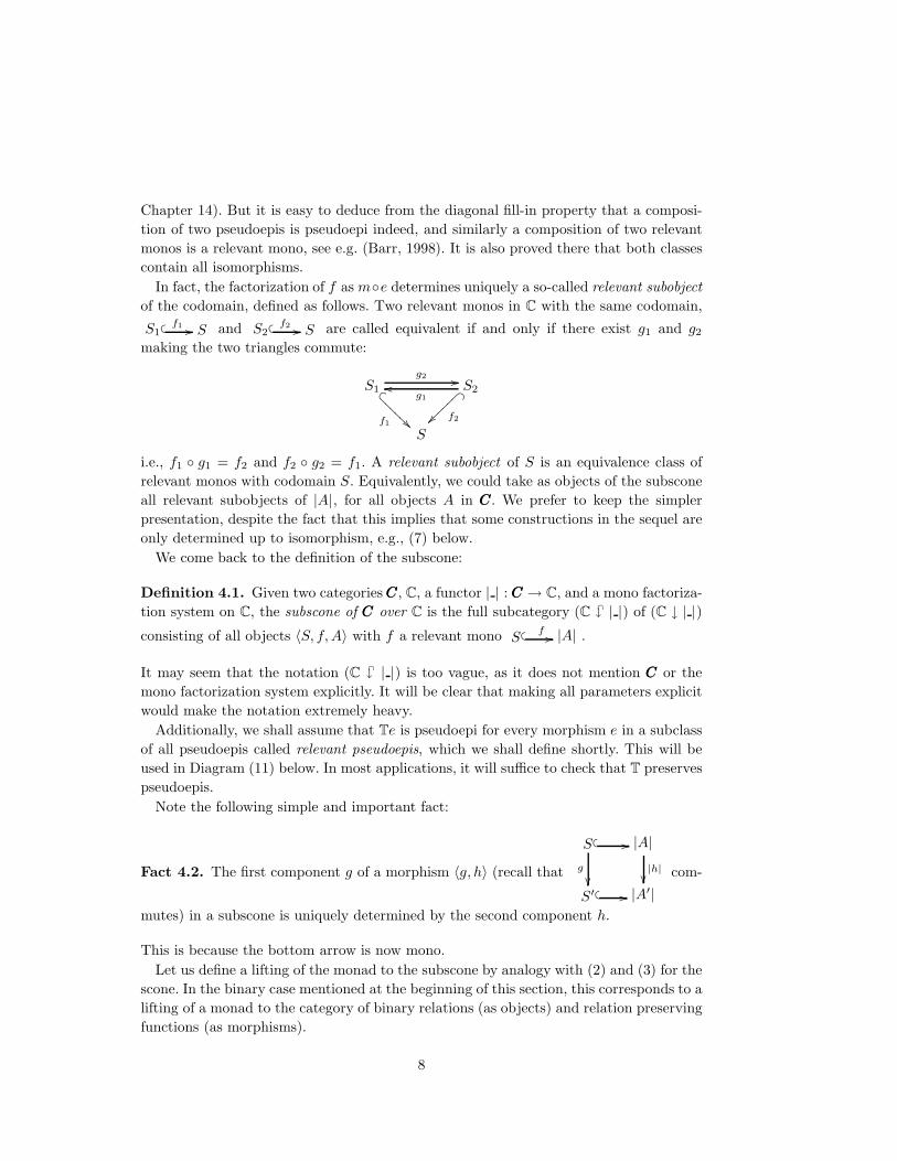
6.2. Unit element I.
Let I be the triple 〈I, i, III〉 as built from the diagram on
the right, obtained from a factorization of i. I i?
????
?
eI I i // |III|
(19)
6.3. Tensor product ⊗.
We build the tensor product 〈S1, m1, A1〉⊗〈S2, m2, A2〉 in the obvious way: compose
m1 ⊗ m2 with the mediating natural transformation , and factorize.
The tensor product is then given by
〈S12, m12, A1 ⊗⊗⊗ A2〉 on the right. This
is similar to the construction of T .
S1 ⊗ S2m1⊗m2//
e12
|A1| ⊗ |A2|A1,A2
S12
m12
// |A1 ⊗⊗⊗ A2|
(20)
6.4. Associativity α.
This is more involved, but basically similar to the construction of the multiplication of
the monad in the subscone. In the diagram below, e12 ⊗ idS3 is pseudoepi because both
e12 (given by Diagram 20) and idS3 are pseudoepis, and because our mono factorization
system is monoidal. The two front faces and the two back faces are derived from the
definition of ⊗, the top face is a naturality square for , the right face is the coherence
condition (16). The dashed arrow, and then the dotted arrow α, are by the diagonal
fill-in property of our factorization system. The desired associativity morphism is then
the pair (α,αααA1,A2,A3) (bottom face).
15

(S1 ⊗ S2) ⊗ S3(m1⊗m2)⊗m3 //
e12⊗idS3
S1,S2,S3
((PPPPPPP(|A1| ⊗ |A2|) ⊗ |A3|A1,A2⊗idA3
|A1|,|A2|,|A3|
))TTTTTTTTT
S1 ⊗ (S2 ⊗ S3)m1⊗(m2⊗m3)//
idS1⊗e23
|A1| ⊗ (|A2| ⊗ |A3|)
id|A1|⊗A2,A3
S12 ⊗ S3m12⊗m3 //
e(12)3
66
66
66
66
66
|A1 ⊗⊗⊗ A2| ⊗ |A3|A1⊗⊗⊗A2,A3
S1 ⊗ S23m1⊗m23 //
e1(23)
|A1| ⊗ |A2 ⊗⊗⊗ A3|A1,A2⊗⊗⊗A3
S(12)3
m(12)3
//
bα ((
|(A1 ⊗⊗⊗ A2)⊗⊗⊗ A3|
|αααA1,A2,A3 |))TTTTTTTTT
S1(23)
m1(23)
// |A1 ⊗⊗⊗ (A2 ⊗⊗⊗ A3)|
(21)
The inverse is given by a very similar diagram (below).
(S1 ⊗ S2) ⊗ S3(m1⊗m2)⊗m3 //
e12⊗idS3
(|A1| ⊗ |A2|) ⊗ |A3|A1,A2⊗idA3
S1 ⊗ (S2 ⊗ S3)m1⊗(m2⊗m3)//
idS1⊗e23
S1,S2,S3−1hhPPPPPPP
|A1| ⊗ (|A2| ⊗ |A3|)
id|A1|⊗A2,A3
|A1|,|A2|,|A3|−1iiTTTTTTTTT
S12 ⊗ S3m12⊗m3 //
e(12)3
|A1 ⊗⊗⊗ A2| ⊗ |A3|A1⊗⊗⊗A2,A3
S1 ⊗ S23m1⊗m23 //
e1(23)
vvn nn
n|A1| ⊗ |A2 ⊗⊗⊗ A3|A1,A2⊗⊗⊗A3
S(12)3
m(12)3
// |(A1 ⊗⊗⊗ A2)⊗⊗⊗ A3|
S1(23)
m1(23)
//bα−1
hh
|A1 ⊗⊗⊗ (A2 ⊗⊗⊗ A3)||αααA1,A2,A3
−1|
iiTTTTTTTTT
(22)
6.5. Left unit ℓ.
Let 〈S, m, A〉 be any object of the subscone. We build the diagram below. The left triangle
in the upper back face is the definition of I, the rest of this face corresponds to two ways
of writing i⊗m, the lower back face is the definition of I⊗〈S, m, A〉. The upper, slanted
face is a naturality square for l.16

Finally, the right-
most triangle is
the coherence
condition (17).
As usual, we first
derive the dashed,
then the dotted ar-
row l by diagonal
fill-ins. The desired
left unit is (l, ℓℓℓA).
I ⊗ SidI⊗m //i⊗idS
$$HHHHHHHHH
eI⊗idS
lS.
....
....
....
....
....
... I ⊗ |A|i⊗id|A|
l|A|
...
....
....
....
....
....
.
III ⊗ Si⊗idS //
e12
66
66
66
66
6|III| ⊗ S
id|III|⊗m// |III| ⊗ |A|III,A
S12
m12
//
bl$$
|III ⊗⊗⊗ A||ℓℓℓA|
##HHHH
HHHHH
S
m// |A|
(23)
The inverse to l is also given by a diagonal fill-in. Start from S, then go to S (again) by
the identity morphism—this is a pseudoepi—, then follow m,∣∣∣ℓℓℓA
−1∣∣∣ to |III ⊗⊗⊗ A|; or start
from S, climb along l−1S , then follow eI ⊗ idS , e12, m12 (a mono) to |III ⊗⊗⊗ A|. The diagonal
fill-in is then an arrow from S to S12, which is inverse to l by Fact 4.3.6.6. Right unit r.
This works exactly
as for the left unit,
see diagram on the
right. The right tri-
angle is the coher-
ence condition (18).
The desired right
unit is given by
(r, rrrA).
The inverse of r is
built as for l.S ⊗ I
m⊗idI //
idS⊗i$$H
HHHHHHHH
idS⊗eI
rS
...
....
....
....
....
....
. |A| ⊗ I
id|A|⊗i r|A|
...
....
....
....
....
....
.
S ⊗ IIIidS⊗i //
e12
66
66
66
66
6S ⊗ |III|
m⊗id|III|// |A| ⊗ |III|A,III
S12
m12
//
br$$
|A⊗⊗⊗ III||rrrA|
##HHHH
HHHHH
S
m// |A|
(24)
Finally, all required naturality, isomorphism, and coherence conditions hold by Fact 4.3.
We recap what we need to lift monoidal structure to the subscone:
(i.a) monoidal categories (CCC,⊗⊗⊗, III,ααα,ℓℓℓ,rrr) and (C,⊗, I, , l, r),
and a monoidal functor | | : CCC → C,
(iii.a) a monoidal mono factorization system on C.
6.7. Symmetric Monoidal Categories
We now assume that we have got, and want to preserve symmetric monoidal structure.
Recall that a symmetric monoidal category (C,⊗, I, , l, r, ) is a monoidal category
(C,⊗, I, , l, r), together with a commutativity natural transformation A,B : A ⊗ B →
B ⊗ A obeying the following coherence conditions.
The first coherence condition is B,A A,B = idA⊗B, which implies that is actually
17
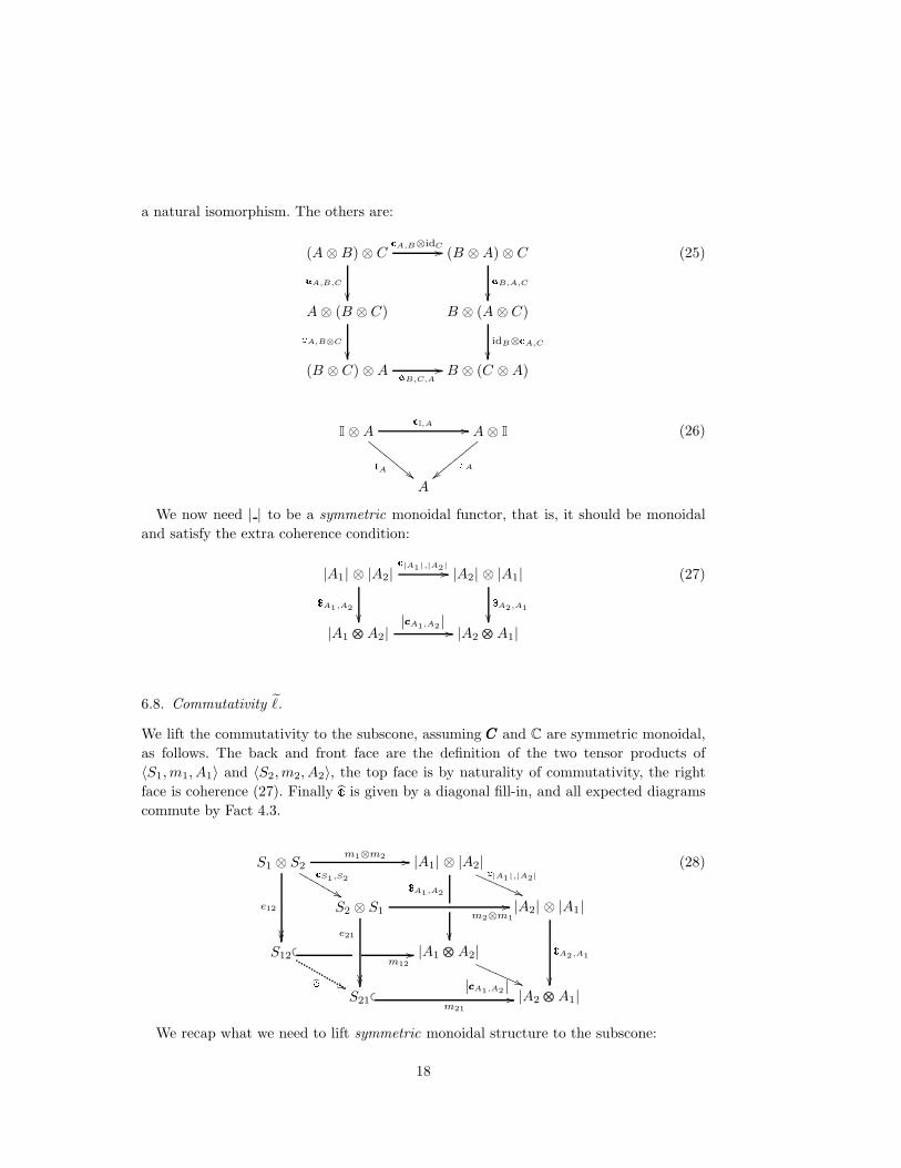
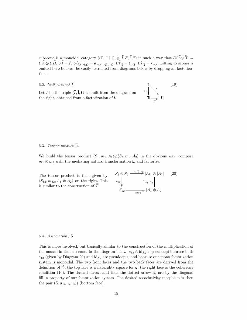
a natural isomorphism. The others are:
(A ⊗ B) ⊗ C A,B⊗idC//A,B,C
(B ⊗ A) ⊗ CB,A,C
A ⊗ (B ⊗ C) A,B⊗C
B ⊗ (A ⊗ C)
idB⊗ A,C
(B ⊗ C) ⊗ A B,C,A
// B ⊗ (C ⊗ A)
(25)
I ⊗ A I,A //lA ""E
EEEEE
EEA ⊗ IrA
||yyyyy
yyy
A
(26)
We now need | | to be a symmetric monoidal functor, that is, it should be monoidal
and satisfy the extra coherence condition:
|A1| ⊗ |A2| |A1|,|A2| //A1,A2
|A2| ⊗ |A1|A2,A1
|A1 ⊗⊗⊗ A2|
|cccA1,A2 | // |A2 ⊗⊗⊗ A1|
(27)
6.8. Commutativity ℓ.
We lift the commutativity to the subscone, assuming CCC and C are symmetric monoidal,
as follows. The back and front face are the definition of the two tensor products of
〈S1, m1, A1〉 and 〈S2, m2, A2〉, the top face is by naturality of commutativity, the right
face is coherence (27). Finally is given by a diagonal fill-in, and all expected diagrams
commute by Fact 4.3.
S1 ⊗ S2m1⊗m2 //
e12
S1,S2
&&MMMMMMM|A1| ⊗ |A2|A1,A2
|A1|,|A2|
((QQQQQQQ
S2 ⊗ S1 m2⊗m1
//
e21
|A2| ⊗ |A1|A2,A1
S12
b &&
m12
// |A1 ⊗⊗⊗ A2|
|cccA1,A2 |((QQQQQQQ
S21
m21
// |A2 ⊗⊗⊗ A1|
(28)
We recap what we need to lift symmetric monoidal structure to the subscone:
18

(i.b) symmetric monoidal categories (CCC,⊗⊗⊗, III,ααα,ℓℓℓ,rrr, ccc)
and (C,⊗, I, , l, r, ),
and a symmetric monoidal functor | | : CCC → C,
(iii.a) a monoidal mono factorization system on C.
6.9. Lifting Cartesian Products
An important special case of symmetric monoidal structure is that given by finite prod-
ucts. This is given by one terminal object 111 such that, for every object A in CCC, there is
a unique morphism A!
−→111, and by a binary product operation as explained in Section 5.
For any two morphisms f from A to A′, g from B to B′, we write f ×g for the morphism
〈f π1, g π2〉 from A × B to A′ × B′.
It is well-known that binary product can be turned into a functor from CCC × CCC to CCC,
which is symmetric monoidal with unit 1, associativity 〈π1 π1, 〈π2 π1, π2〉〉, left unit
π2, right unit π1, and commutativity 〈π2, π1〉.
When CCC and C are both equipped with finite products, and | | is a functor from CCC to
C that is monoidal with respect to these products, then the construction of Sections 6.1
and 6.7 yields a symmetric monoidal structure on (C ∩ | |) that we claim stems from a
finite product structure on the subscone.
To this end, we assume that | | satisfies
the coherence condition on the right,
for i ∈ 1, 2. We shall say that such a
functor is cartesian monoidal. (Then | |
is automatically symmetric monoidal.)
|A1| × |A2|
πi
%%JJJJJ
JJJJJA1,A2
|A1 × A2|
|πi|// |Ai|
(29)
6.10. Terminal object 1.
Let 1 be the object 〈I, i,111〉 given by dia-
gram (19). Specializing this diagram to
the case at hand, this is given as the
unique object up to iso making the fol-
lowing diagram commute:
1 i?
????
?
eI I i // |111|
(30)
For any object 〈S, m, A〉 of the
subscone, there is a unique arrow
〈u, v〉 from 〈S, m, A〉 to 〈I, i,111〉.Indeed, v is the unique arrow !
from A to 111, and u is given by
eI!; u is also unique, by Fact 4.3.
1 i!!B
BBBB
BB
eI I i // |111|
S
m//
!
::
u
??
|A||v|
>>
19

6.11. Binary product ×.
Specializing the definition (20) of the
lifted tensor product ⊗ to the case at
hand yields the object 〈S12, m12, A1 ⊗⊗⊗
A2〉 = 〈S1, m1, A1〉×〈S2, m2, A2〉 de-
fined by the diagram on the right.
S1 × S2m1×m2//
e12
|A1| × |A2|A1,A2
S12
m12
// |A1 × A2|
(31)
The ith projection 〈πi, πi〉 is
then given by the diagram on
the right. The back square is
a copy of (31), the right trian-
gle is an instance of the coher-
ence condition (29), while the
top, slanted face is by stan-
dard properties of πi. From
two routes from S1 × S2 to
|Ai|, we get πi by a diagonal
fill-in.
S1 × S2m1×m2//
πi
???
????
????
????
????
e12
|A1| × |A2|A1,A2
πi
<<<
<<<<
<<<<
<<<<
<<<
S12
m12
//
eπi
''
|A1 × A2|
|πi|MMM
M
&&MMMMM
Si
mi
// |Ai|
It remains to show that whenever we have two subscone morphisms 〈f1, f1〉 from 〈S, m, A〉
to 〈S1, m1, A1〉 and 〈f2, f2〉 from 〈S, m, A〉 to 〈S2, m2, A2〉, there is a unique morphism
〈h, h〉 from 〈S, m, A〉 to the product 〈S12, m12, A1×A2〉 such that 〈πi, πi〉〈h, h〉 = 〈fi, fi〉
(i ∈ 1, 2). Existence is assured: take h = 〈f1, f2〉, h = e12 〈f1, f2〉, which satisfies
the claim: this is an easy consequence of the diagram above. Uniqueness follows from
the uniqueness of h given by the definition of binary product in CCC, and from Fact 4.3
guaranteeing the uniqueness of h.
As is now usual, we recap what we need to lift products to the subscone:
(i.c) categories CCC and C with finite products,
and a cartesian monoidal functor | | : CCC → C,
(iii.a) a monoidal mono factorization system on C.
7. Lifting Strong, Monoidal, and Commutative Monads to a Scone and a
Subscone
Once we have got a monoidal structure on CCC and C, we may consider strong monads
TTT and T instead of just monads on each category. This is what we need to develop a
theory of logical relations for Moggi’s monadic λ-calculus. We shall also consider the
more demanding cases of monoidal monads, and of commutative monads.
7.1. Lifting Strong Monads
That T is a strong monad means that a strength natural transformation tA,B : A⊗TB →
T(A ⊗ B) is given such that the diagrams in Definition 3.2 in (Moggi, 1991) commute,
that is:
20

I ⊗ TBtI,B //lTB &&LLLLLLLLLL T(I ⊗ B)
TlB
TB
(32) A ⊗ BidA⊗B//A⊗B %%LLLLLLLLLL A ⊗ TBtA,B
T(A ⊗ B)
(33)
(A ⊗ B) ⊗ TCA,B,TC
tA⊗B,C // T((A ⊗ B) ⊗ C)
TA,B,C
A ⊗ (B ⊗ TC)
idA⊗tB,C
// A ⊗ T(B ⊗ C) tA,B⊗C
// T(A ⊗ (B ⊗ C))
(34)
A ⊗ T2B
tA,TB //
idA⊗B
T(A ⊗ TB)TtA,B // T2(A ⊗ B)A⊗B
A ⊗ TB tA,B
// T(A ⊗ B)
(35)
Formally, a strong monad is a four-tuple (T,,, t) where (T,,) is a monad and tis a strength making the above diagrams commute.
By lifting of TTT to (C ↓ | |) we now mean a strong monad, i.e. a monad (T , η, µ)
together with a strength tX,Y : X⊗T Y → T (X⊗Y ), such that diagram (2) commutes,
equations (3) hold and
UtX,Y = tttUX,UY ,
i.e., U preserves strength.
To be able to give an appropriate lifting, we extend the monad morphism to a strong
monad morphism, i.e., a monad morphism making the following additional diagram
commute, which relates the strengths tttA1,A2 and t|A1|,|A2| :
|A1| ⊗ T|A2|t|A1|,|A2|//
id|A1|⊗σA2
T(|A1| ⊗ |A2|)
T(A1,A2 )
|A1| ⊗ |TTTA2|A1,TTTA2
T|A1 ⊗⊗⊗ A2|σA1⊗⊗⊗A2
|A1 ⊗⊗⊗ TTTA2||tttA1,A2 |
// |TTT (A1 ⊗⊗⊗ A2)|
(36)
Having lifted TTT to scones and subscones in previous sections, we only need to give a
lifting of the strength ttt. For scones this is straightforward—define t pointwise by
t〈S1,m1,A1〉,〈S2,m2,A2〉 = 〈tS1,S2 , tttA1,A2〉.
Verifying that this is well-defined amounts to pasting together a naturality square for
21

t and a diagram (36):
S1 ⊗ TS2m1⊗Tm2 //tS1,S2
|A1| ⊗ T|A2|t|A1|,|A2|
A1,TTT A2(id|A1|⊗σA2
)// |A1 ⊗⊗⊗ TTTA2|
|tttA1,A2 |
T(S1 ⊗ S2)T(m1⊗m2) // T(|A1| ⊗ |A2|)
σA1⊗A2T(A1,A2)
// |TTT (A1 ⊗⊗⊗ A2)|
The upper side of this diagram is precisely 〈S1, m1, A1〉⊗T 〈S2, m2, A2〉 in the scone while
the lower side is T (〈S1, m1, A1〉⊗〈S2, m2, A2〉). (We let the interested reader define for
herself the tensor product ⊗ in the scone.) Checking naturality of t and strength laws is
immediate since t, α, r, η and µ are all defined pointwise.
Now we move to subscones. Call T the lifted monad defined in (7), (9), (10) and (11)
in Section 4.
As in previous sections, t in subscones will differ from the case of scones only in its
C-component t, and this component will be induced as a unique diagonal guaranteed by
diagram (6) in the diagram below.
S1 ⊗ TS2
idS1⊗Tm2 //
idS1⊗e′2
tS1,S2
&&MMMMMMMS1 ⊗ T|A2|
m1⊗idT|A2|//
idS1⊗σA2
|A1| ⊗ T|A2|
id|A1|⊗σA2
t|A1|,|A2|
((QQQQQQQ
T(S1 ⊗ S2)T(m1⊗m2)
//
Te12
T(|A1| ⊗ |A2|)
T(A1,A2 )
S1 ⊗ S2
idS1⊗m′2 //
e′12
22
22
22
22
2S1 ⊗ |TTTA2|
m1⊗id|TTT A2|// |A1| ⊗ |TTTA2|A1,TTT A2
TS12Tm12 //
e′
T|A1 ⊗⊗⊗ A2|
σA1⊗⊗⊗A2
S′12
m′12 //t &&
|A1 ⊗⊗⊗TTTA2||tttA1,A2 |
((QQQQQQQQ
S12
m′// |TTT (A1 ⊗⊗⊗ A2)|
(37)
As ingredients of this diagram we have used:
— An instance TS2Tm2 //
e′2
T|A2|
σA2
S2
m′2
// |TTTA2|
of Diagram (7) defining T 〈S2, m2, A2〉; this is tensored
by S1 on the left to get the upper left square of the back face. Notice that idS1 ⊗ e′2is pseudoepi because our mono factorization system is monoidal.
— An instance S1 ⊗ S2
m1⊗m′2 //
e′12
|A1| ⊗ |TTTA2|A1,TTT A2
S′
12
m′12
// |A1 ⊗⊗⊗TTTA2|
of Diagram (20) defining the tensor
22

product of 〈S1, m1, A1〉 with T 〈S2, m2, A2〉 = 〈S2, m′2,TTTA2〉; this is the lower square of
the back face. (Note that the upper right square of the back face commutes trivially.)
— Another instance S1 ⊗ S2m1⊗m2 //
e12
|A1| ⊗ |A2|A1,A2
S12
m12
// |A1 ⊗⊗⊗ A2|
of Diagram (20) defining the ten-
sor product 〈S12, m12, A1 ⊗⊗⊗A2〉 of 〈S1, m1, A1〉 with 〈S2, m2, A2〉; we apply T to this
square to get the upper half of the front face.
— Another instance of Diagram (7) defining the application of T to the just mentioned
tensor product 〈S12, m12, A1 ⊗⊗⊗ A2〉: this is the lower half of the front face.
— A naturality square for t (top face), and
— An instance of Diagram (36), which defines the right face.
As usual, the dashed and the dotted arrows are given by diagonal fill-ins, therefore
t = (t, ttt) is well-defined. Again, checking naturality of t and strength laws is immediate
by Fact 4.3.
Here is the final set of ingredients for lifting a strong monad (TTT ,ηηη,µµµ, ttt) on category CCC
to (C ∩ | |):
(i.a) monoidal categories (CCC,⊗⊗⊗, III,ααα,ℓℓℓ,rrr) and (C,⊗, I, , l, r),
and a monoidal functor | | : CCC → C,
(ii.a) a strong monad (T,,, t) on C, related to (TTT ,ηηη,µµµ, ttt) by
a strong monad morphism (| |, σ) defined in (4) and (36),
(iii.a) a monoidal mono factorization system on C.
(iv) T maps relevant pseudoepis to pseudoepis.
7.2. Monoidal Monads
Several strong monads are in fact monoidal—in fact all the monads of Section 10 are
monoidal, except the continuation and continuation-like monads. While this notion is
not needed in Moggi’s account of computation (Moggi, 1991), this occurs naturally, and
will be used in Section 8.4. A monoidal monad is a four-tuple (T,,, d), where dA,B :
TA ⊗ TB → T(A ⊗ B) is a mediator natural transformation, making the following
diagrams commute:
I ⊗ TB lTB
AAA
AAAA
AAAA
AI⊗idTB TI ⊗ TBdI,B T(I ⊗ B)
TlB // TB
(38) TA ⊗ I rTA
AAA
AAAA
AAAA
AidTA⊗I
TA ⊗ TIdA,I T(A ⊗ I)
TrA
// TA
(39)
23

A ⊗ BA⊗B//A⊗B ((QQQQQQQ TA ⊗ TBdA,B
T(A ⊗ B)
(40)
(TA ⊗ TB) ⊗ TCTA,TB,TC
dA,B⊗idTC// T(A ⊗ B) ⊗ TCdA⊗B,C// T((A ⊗ B) ⊗ C)
TA,B,C
TA ⊗ (TB ⊗ TC)
idTA⊗dB,C
// TA ⊗ T(B ⊗ C) dA,B⊗C
// T(A ⊗ (B ⊗ C))
(41)
T2A ⊗ T2BdTA,TB//A⊗B
T(TA ⊗ TB)TdA,B // T2(A ⊗ B)A⊗B
TA ⊗ TB dA,B
// T(A ⊗ B)
(42)
Diagrams (38), (39), (41) state that T is a monoidal functor with mediating pair
(d,I). Diagram (40) states that is a so-called monoidal natural transformation, while
Diagram (42) states that is another monoidal natural transformation.
Given any monoidal monad (T,,, d) on C, it is easy to check that (T,,, t) is a
strong monad, where tA,B = dA,B (A ⊗ idTB). Furthermore, t′A,B defined as dA,B
(idTA⊗B) is a dual strength, that is, a natural transformation t′A,B : TA⊗B → T(A⊗B)
obeying the obvious duals of the strength laws (32), (33), (34), (35). (Formally, a dual
strength is a strength on the dual monoidal category (C, I,⊗op, −1, r, l), where A⊗op B
is defined as B ⊗ A.)
Moreover, the strength t and the dual strength t′ are compatible with the associativity,
in the sense that the diagram below commutes.
(A ⊗ TB) ⊗ CtA,B⊗idC //A,TB,C
T(A ⊗ B) ⊗ Ct′A⊗B,C // T((A ⊗ B) ⊗ C)
TA,B,CA ⊗ (TB ⊗ C)
idA⊗t′B,C // A ⊗ T(B ⊗ C)tA,B⊗C // T(A ⊗ (B ⊗ C))
(43)
Finally, the strength and
the dual strength commute,
in the sense that the di-
agram on the right com-
mutes. In fact, the common
diagonal from TA ⊗ TB to
T(A ⊗ B) is just dA,B.
TA ⊗ TBtTA,B //t′A,TB
T(TA ⊗ B)
Tt′A,BT
2(A ⊗ B)A⊗B
T(A ⊗ TB)
TtA,B
// T2(A ⊗ B)A⊗B
// T(A ⊗ B)
(44)
In general, a monoidal monad can be defined equivalently as a monad with a strength
and a dual strength that make the diagrams (43) and (44) commute. See Appendix A,
in particular Appendix A.1 and Appendix A.2, for a proof.
It is natural to define a monoidal monad morphism from (TTT ,ηηη,µµµ,ddd) to (T,,, d) as
24
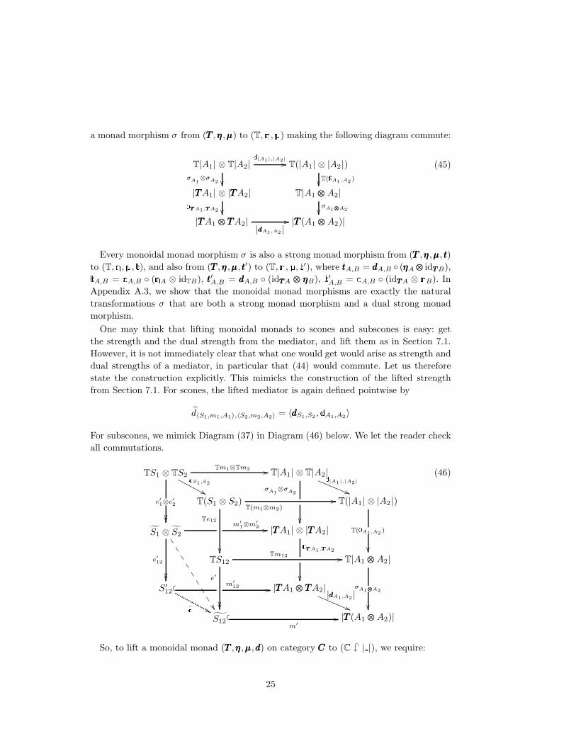
a monad morphism σ from (TTT ,ηηη,µµµ) to (T,,) making the following diagram commute:
T|A1| ⊗ T|A2|d|A1|,|A2| //
σA1⊗σA2
T(|A1| ⊗ |A2|)
T(A1,A2)
|TTTA1| ⊗ |TTTA2|TTT A1,TTT A2
T|A1 ⊗⊗⊗ A2|σA1⊗⊗⊗A2
|TTTA1 ⊗⊗⊗TTTA2||dddA1,A2 |
// |TTT (A1 ⊗⊗⊗ A2)|
(45)
Every monoidal monad morphism σ is also a strong monad morphism from (TTT ,ηηη,µµµ, ttt)
to (T,,, t), and also from (TTT ,ηηη,µµµ, ttt′) to (T,,, t′), where tttA,B = dddA,B (ηηηA⊗⊗⊗ idTTTB),tA,B = dA,B (A ⊗ idTB), ttt′A,B = dddA,B (idTTTA ⊗⊗⊗ ηηηB), t′A,B = dA,B (idTTTA ⊗ B). In
Appendix A.3, we show that the monoidal monad morphisms are exactly the natural
transformations σ that are both a strong monad morphism and a dual strong monad
morphism.
One may think that lifting monoidal monads to scones and subscones is easy: get
the strength and the dual strength from the mediator, and lift them as in Section 7.1.
However, it is not immediately clear that what one would get would arise as strength and
dual strengths of a mediator, in particular that (44) would commute. Let us therefore
state the construction explicitly. This mimicks the construction of the lifted strength
from Section 7.1. For scones, the lifted mediator is again defined pointwise by
d〈S1,m1,A1〉,〈S2,m2,A2〉 = 〈dddS1,S2 , dA1,A2〉
For subscones, we mimick Diagram (37) in Diagram (46) below. We let the reader check
all commutations.
TS1 ⊗ TS2Tm1⊗Tm2 //
e′1⊗e′
2
dS1,S2
&&NNNNNNNT|A1| ⊗ T|A2|
σA1⊗σA2
d|A1|,|A2|
((RRRRRRRR
T(S1 ⊗ S2)T(m1⊗m2)
//
Te12
T(|A1| ⊗ |A2|)
T(A1,A2 )
S1 ⊗ S2
m′1⊗m′
2 //
e′12
33
33
33
33
3|TTTA1| ⊗ |TTTA2|TTT A1,TTT A2
TS12Tm12 //
e′
T|A1 ⊗⊗⊗ A2|
σA1⊗⊗⊗A2
S′12
m′12 //d &&
|TTTA1 ⊗⊗⊗TTTA2||dddA1,A2 |
((QQQQQQQQ
S12
m′// |TTT (A1 ⊗⊗⊗ A2)|
(46)
So, to lift a monoidal monad (TTT ,ηηη,µµµ,ddd) on category CCC to (C ∩ | |), we require:
25

(i.a) monoidal categories (CCC,⊗⊗⊗, III,ααα,ℓℓℓ,rrr) and (C,⊗, I, , l, r),
and a monoidal functor | | : CCC → C,
(ii.b) a monoidal monad (T,,, d) on C, related to
the monoidal monad (TTT ,ηηη,µµµ,ddd) on CCC by
a monoidal monad morphism (| |, σ) defined in (4) and (45),
(iii.a) a monoidal mono factorization system on C.
(iv) T maps relevant pseudoepis to pseudoepis.
7.3. Commutative Monads
In the case of symmetric monoidal categories CCC and C, recall that if we also want to
make the subscone a symmetric monoidal category, it suffices to replace (i.a) by (i.b),
which requires | | to be a symmetric monoidal functor. This case occurs notably if we
want to lift a commutative monad to the subscone.
Recall that a strong monad (T,,, t) is commutative if and only if, letting t′A,B be
the dual strength T B,A tB,A TA,B, then Diagram (44) commutes.Let dA,B be the common diagonal A⊗B
Tt′A,B tTA,B = A⊗B TtA,B t′A,TB.
We can check that d is then a media-
tor , whence every commutative monad
is monoidal. In fact, a monoidal monad
is commutative if and only if the follow-
ing additional diagram commutes (see Ap-
pendix A.4).
TA ⊗ TB TA,TB
dA,B // T(A ⊗ B)
T A,B
TB ⊗ TA dB,A
// T(B ⊗ A)
(47)
For convenience, we shall now understand commutative monads as monoidal monads
satisfying (47). The lifting of monoidal monads of Section 7.2 then yields a lifting of
commutative monads, by Fact 4.3. Therefore, to lift a commutative monad (TTT ,ηηη,µµµ, ttt) on
category CCC to (C ∩ | |), we require:
(i.b) symmetric monoidal categories (CCC,⊗⊗⊗, III,ααα,ℓℓℓ,rrr, ccc) and (C,⊗, I, , l, r, ),
and a symmetric monoidal functor | | : CCC → C,
(ii.c) a commutative monad (T,,, d) on C, related to
the commutative monad (TTT ,ηηη,µµµ,ddd) on CCC by
a monoidal monad morphism (| |, σ) defined in (4) and (45),
(iii.a) a monoidal mono factorization system on C.
(iv) T maps relevant pseudoepis to pseudoepis.
When C has all finite products and we consider the induced symmetric monoidal struc-
ture, we might require that the monoidal monad (T,,, d) is not just commutative but
even cartesian, by which we mean that T is a cartesian monoidal functor with mediating
pair (d,I). (Recall that T is always a monoidal functor with this very mediating pair.)
This means that TπidA,B = πi, i ∈ 1, 2. We just do not need this in our constructions;
but it is often easier to prove that a monad is cartesian and infer that it is commutative
26

than to prove that it is commutative directly: we shall see examples of cartesian monads
in Section 10.
8. Building Monad Morphisms from Adjunctions
It is often the case that we have a (strong) monad on CCC, and wish to build another one
on C related to the latter by a monad morphism. The following results are then of some
help.
Recall that, given two categories C and D, a pair of functors F : C → D and U : D → C
is an adjunction F ⊣ U if and only if there are natural transformations η. : . → UF. (the
unit of the adjunction) and ǫ. : FU. → . (the counit) such that ǫF (A) FηA = idF (A) and
UǫA ηU(A) = idU(A). F is said to be left adjoint to U , U is right adjoint to F .
Then any adjunction F ⊣ U gives rise to a monad (UF, η., UǫF.) on C. Conversely,
there are two standard ways of retrieving an adjunction from a monad (T, η, µ) on C,
from Eilenberg-Moore algebras, or from the Kleisli category of the monad.
8.1. Eilenberg-Moore algebras.
A T -algebra is a morphism T (A)s // A , for some object A of C, satisfying the com-
mutativity conditions:
T 2(A)µA
wwooooo T (s)
T (A)s
T (A)s
T (A)s
A
ηA 88rrrrr
idA
// A A A
(48)
A is called the support of the algebra, s its structure map. A morphism from T (A)s // A
to T (B)u // B is a morphism f : A → B in C that commutes with structure maps, i.e.,
such that f s = u T (f). T -algebras together with these morphisms forms a category
T -Alg.
Then FT ⊣ UT is an adjunction, where UT : T -Alg → C maps objects T (A)s // A
to A and morphisms f from T (A)s // A to T (B)
u // B to the underlying morphism
f from A to B in C; and where FT : C → T -Alg maps the object A to the T -algebra
T 2(A)µA // T (A) , and the morphisms A
f // B to f seen as morphism from FT (A)
to FT (B). The unit of the adjunction is η, while the counit ǫ is given on each T -algebra
T (A)s // A as the morphism s itself, from FT UT ( T (A)
s // A ) = T 2(A)µA // T (A)
to T (A)s // A .
Moreover, the monad of this adjunction is the original monad (T, η, µ).
27

8.2. Kleisli category.
The objects of Kleisli(T ) are the objects of C, while the morphisms Af // B of
Kleisli(T ) are the morphisms Af // T (B) of C. To avoid confusion, we write f the
morphisms f seen as a morphism in Kleisli(T ). The identity idA on the object A in
Kleisli(T ) is ηA, while composition g f is µC T (g) f , where Af // T (B) and
Bg // T (C) in C.
Define FT : C → Kleisli(T ) as mapping the object A to A, and the morphism
Af // B to the morphism from A to B in Kleisli(T ) defined as ηB f . Define UT :
Kleisli(T ) → C as mapping the object A to T (A), and the morphism f from A to B in
Kleisli(T ) to µB T (f). Then FT ⊣ UT is an adjunction, whose unit is η, and whose
counit ǫ is the identity morphism from FT UT (A) to T (A) in C, seen as a morphism from
FT UT (A) to A in Kleisli(T ). The monad of FT ⊣ UT is again (T, η, µ).
8.3. Monad Morphisms from Adjunctions
Proposition 8.1. Let (TTT ,ηηη,µµµ) be a monad on a category CCC, | | : CCC → C be a functor
with a left adjoint DDD : C → CCC. Let ǫA : DDD|A| → A be the counit of the adjunction,
ηE : E → |DDD(E)| be the unit of the adjunction.
Define T = | | TTT DDD = |TTTDDD|, E =∣∣ηηηDDD(E)
∣∣ ηE , E =∣∣µµµDDD(E) TTT ǫTTTDDD(E)
∣∣. Finally,
let σA = |TTT ǫA| : T|A| → |TTTA|. Then (T,,) is a monad on C and (| |, σ) is a monad
morphism from TTT to T.
Proof. Let F ⊣ U be any adjunction generating the monad, i.e., such that UF = TTT ,
whose unit is ηηη, and whose counit ǫ is such that µµµ = UǫF . We may choose, e.g., FT ⊣ UT
or FT ⊣ UT . Compose the adjunction DDD ⊣ | | with F ⊣ U , yielding an adjunction
FDDD ⊣ |U |. The unit of this adjunction (on object E) is∣∣ηηηDDD(E)
∣∣ ηE, its counit (on object
A) is ǫA F (ǫUA).
The monad of this adjunction is (|UFDDD|,∣∣ηηηDDD(.)
∣∣ η.,∣∣U(ǫFDDD(.) F (ǫUFDDD(.)))
∣∣). But
the monad of F ⊣ U is (TTT ,ηηη,µµµ), so UF = TTT and µµµ = UǫF . It follows that the monad of
FDDD ⊣ |U | is (|TTTDDD|,∣∣ηηηDDD(.)
∣∣ η.,∣∣µµµDDD(.) TTT (ǫTTTDDD(.))
∣∣). This is (T,,), which is therefore a
monad.
It remains to show that σ = |TTT ǫ| is a monad morphism from TTT to T. This is checked
using the following diagrams. In the left diagram, the top triangle is one of the adjunction
laws, the bottom square is by naturality of |ηηη|; so σA (bottom arrow) composed with|A| (leftmost vertical path) equals |ηηηA| (rightmost path from |A| to |TTTA|).
28

In the right diagram, the
top square is by naturality
of |TTT ǫ|, the bottom square
is by naturality of |µµµ|, so
σA (bottom arrow) com-
posed with |A| (leftmost
vertical path) equals |µµµA|
σTTT A TσA (the other path
from top left to bottom
right).
|A|
η|A|
id|A|
HHHH
$$HHHH
˛
˛DDD|A|˛
˛
|ǫA|//
|ηηηDDD|A| |
|A|
|ηηηA|
˛
˛TTTDDD|A|˛
˛
|TTT ǫA|
// |TTTA|
˛
˛TTTDDD˛
˛TTTDDD|A|˛
˛
˛
˛
|TTTDDD|TTT ǫA||//
|TTT ǫTTTDDD|A| |
˛
˛TTTDDD|TTTA|˛
˛
|TTT ǫTTT A|
˛
˛TTTTTTDDD|A|˛
˛
|TTTTTT ǫA| //
|µµµDDD|A| |
|TTTTTTA|
|µµµA|
˛
˛TTTDDD|A|˛
˛
|TTT ǫA|// |TTTA|
Note that we could have checked the required diagrams directly; the proof would be
longer than going through adjunctions, as we did.
8.4. Monoidal, and Strong Monad Morphisms from Monoidal Adjunctions
We first reproduce the argument of Proposition 8.1 in the monoidal case. While monads
correspond to adjunctions in well-defined ways, only monoidal monads can be linked to
so-called monoidal adjunctions. This is the reason why we deal with monoidal monads
first.
Let (C, IC ,⊗C , αC , ℓC , rC) and (D, ID,⊗D, αD, ℓD, rD) be two monoidal categories. Let
F ⊣ U be an adjunction, where F : C → D, U : D → C, with unit η, and counit ǫ. This
is a monoidal adjunction if and only if F and U are monoidal functors (with respective
mediating pairs (θF , ιF ) and (θU , ιU )), and the unit η and the counit ǫ are monoidal
natural transformations, by which we mean that the following diagrams commute:
ICιU
//
ηIC ""F
FFFF
FFFF
U(ID)
U(ιF )
UF (IC)
(49)
A ⊗C BηA⊗CηB //
ηA⊗CB
UF (A) ⊗C UF (B)
θUF (A),F (B)wwnnnnnnn
U(F (A) ⊗D F (B))
U(θFA,B)xxrrrrrr
UF (A ⊗C B)
(50)
ID
ιF
F (IC)
F (ιU )
// FU(ID)
ǫID
ccFFFFFFFF
(51)FU(A) ⊗D FU(B)
θFU(A),U(B)xxqqqqqq
ǫA⊗DǫB
F (U(A) ⊗C U(B))
FθUA,Bzzuuuuu
FU(A ⊗D B) ǫA⊗DB
// A ⊗D B
(52)
The value of monoidal adjunctions is their relation with monoidal monads (Section 7.2).
Recall that a monoidal monad on C is a tuple (T, η, µ, d), where (T, η, µ) is a monad on
C and dA,B is a natural transformation from TA ⊗C TB to T (A ⊗C B) such that the
following diagrams commute:
29

IC ⊗C TB
ℓCT B
!!CCC
CCCC
CCCC
CCη
IC⊗CidT B TIC ⊗C TBd
IC,B T (IC ⊗C B)
TℓCB
// TB
(38) TA ⊗C IC
rCT A
!!CCC
CCCC
CCCC
CCidT A⊗Cη
IC TA ⊗C TIC
dA,IC
T (A ⊗C IC)TrC
A
// TA
(39)
A ⊗C BηA⊗CηB//
ηA⊗CB ((QQQQQQQQ TA ⊗C TB
dA,BT (A ⊗C B)
(40)
(TA ⊗C TB) ⊗C TC
αCT A,TB,T C
dA,B⊗CidT C// T (A ⊗C B) ⊗C TCd
A⊗CB,C// T ((A ⊗C B) ⊗C C)
TαCA,B,C
TA⊗C (TB ⊗C TC)
idT A⊗CdB,C
// TA ⊗C T (B ⊗C C)d
A,B⊗CC
// T (A ⊗C (B ⊗C C))
(41)
T 2A ⊗C T 2BdT A,TB//
µA⊗CµB
T (TA⊗C TB)TdA,B // T 2(A ⊗C B)
µA⊗CB
TA⊗C TB
dA,B
// T (A ⊗C B)
(42)
The following lemmas show respectively that every monoidal adjunction gives rise to
a monoidal monad, that every monoidal monad yields a monoidal adjunction between
the base category and the Kleisli category of the monad, and that monoidal adjunctions
compose to yield monoidal adjunctions. Except for the first, the arguments are tedious
computations, and therefore relegated to appendices†.
Lemma 8.2. Let F ⊣ U be a monoidal adjunction, with unit η and counit ǫ, where
F : C → D, U : D → C. Let T be UF , µA be UǫF (A), and dA,B be UθFA,B θU
F (A),F (B).
Then (T, η, µ, d) is a monoidal monad on C.
Proof. (T, η, µ) is a monad by Proposition 8.1. We check the mediator laws (38), (39),
(40), (41), (42) for d.
Diagram (38) is obtained by considering the following diagram. The top left triangle isa copy of (49), tensored by UF (B) on the right. The square next to it on its right is anaturality square for θU . The next trapezoid on the right (the top right trapezoid) is Uapplied to a coherence square (17) for θF , ℓC and ℓD. The bottom face, atop the curved
† These results are folklore, and were confirmed in discussions with Paul-Andre Mellies, FrancoisLamarche, and Albert Burroni notably. However, we have been unable to find references on this.We have often been directed to the pioneering paper (Street, 1972), but could not find the expectedresults therein.
30

arrow ℓCUF (B), is another instance of a coherence square (17) for θF , ℓC and ℓD.
IC ⊗C UF (B)η
IC⊗C idUF (B)//
ιU⊗C idUF (B)
UU
**UU
ℓCUF (B) 22
UF (IC) ⊗C UF (B)θU
F (IC),F (B)// U(F (IC) ⊗D F (B))U(θF
IC,B)// UF (IC ⊗C B)
UF (ℓCB)
U(ID) ⊗C UF (B)
U(ιF )⊗C idUF (B)
OO
θU
ID ,F (B)
// U(ID ⊗D F (B))
U(ιF ⊗DidF (B))
OO
U(ℓDF (B)) **UUUUUUUUUUUU
UF (B)
Now the topmost composition of arrows is tIC,B, the bottommost arrow from IC ⊗C
UF (B) to UF (B) is ℓCTB, and the rightmost vertical arrow is T ℓCB.
Diagram (39). This is checked by similar arguments, replacing the coherence square (17)
by (18).
Diagram (40). This is the diagram
on the right, an instance of Di-
agram (50), stating that η is a
monoidal natural transformation.
We recognize dA,B as the right-
most composition of vertical arrows,
hence the desired Diagram (33).
A ⊗C BηA⊗CηB//
ηA⊗CB
##HHH
HHHHHHHHHHHHH UF (A) ⊗C UF (B)
θU (F (A),F (B))U(F (A) ⊗D F (B))
UθFA,B
UF (A ⊗C B)
Diagram (41). For space reasons, we flip the diagram so that arrows involving strengthsare vertical, and arrows involving associativities are horizontal. Also, we drop most sub-scripts, which are inferrable from context.
(UF (A) ⊗C UF (B))
⊗CUF (C)
αC//
θU⊗C idUF (C)
(coherence (16) for θU )
UF (A)⊗C
(UF (B) ⊗C UF (C))
idUF (A)⊗CθU
U(F (A) ⊗D F (B))
⊗CUF (C)θU
''PPPPPPPPUθF ⊗C idUF (C)
UF (A)⊗C
U(F (B) ⊗D F (C))θU
vvnnnnnnnnidUF (A)⊗
CUθF
UF (A ⊗C B)
⊗CUF (C)
θU
(natur-ality of
θU )
(U applied to coherence (16) for θF )
U((F (A)
⊗DF (B))
⊗DF (C))
UαD//
U(θF ⊗DidF (C))wwnnnnnnnn
U(F (A)⊗D
(F (B)⊗D
F (C)))
U(idF (A)⊗DθF ) ((PPPPPPPP
(natur-ality of
θU )
UF (A)⊗C
UF (B ⊗C C)
θU
U(F (A ⊗C B)
⊗DF (C))
UθF
U(F (A)⊗D
F (B ⊗C C))
UθFUF ((A ⊗C B)
⊗CC) UF αC
// UF (A⊗C
(B ⊗C C))
The vertical arrows on the left compose to form dA⊗CB,C (dA,B ⊗C idUF (C)), while the
vertical arrows on the right compose to form dA⊗CB,C (idUF (A) ⊗C dB,C), whence the
result.
31

Diagram (42). Similarly, we flip the diagram so that vertical arrows become horizontaland conversely:
UFUF (A) ⊗C UFUF (B)UǫF (A)⊗
CUǫF (B) //
θU (naturality of θU )
UF (A) ⊗C UF (B)
θU
U(FUF (A) ⊗D FUF (B))U(ǫF (A)⊗
DǫF (B))[[[
--[[[[[[UθF UF (UF (A) ⊗C UF (B))
UF θU
(U applied to (52)) U(F (A) ⊗D F (B))
UθF
UFU(F (A) ⊗D F (B))
UǫF (A)⊗DF (B)cccccc
11ccccccc
UF UθF UFUF (A ⊗C B)
UǫF (A⊗CB)
//
(naturality of Uǫ)
UF (A ⊗C B)
We recognize TdA,B dTA,TB as the leftmost composition of vertical arrows, and the
rightmost vertical composition is dA,B. Also, the top horizontal arrow is µA ⊗C µB, while
the bottom arrow is µA⊗CB.
Lemma 8.3. Let (C, IC,⊗C , αC , ℓC , rC) be a monoidal category, and let (T, η, µ, d) be a
monoidal monad on C.
Let D be the Kleisli category of T , ID = IC , ⊗D be defined on objects by A ⊗D B =
A ⊗C B and on morphisms by letting f ⊗D g (in D) be the morphism d (f ⊗C g) in C;
let αD = η αC , ℓD = η ℓC , rD = η rC . Then (D, ID,⊗D, αD, ℓD, rD), is a monoidal
category.
Moreover, FT ⊣ UT is a monoidal adjunction. The mediating pairs of FT and UT are
(θFT , ιFT ) and (θUT , ιUT ) respectively, where θFT
A,B : FT (A) ⊗D FT (B) → FT (A ⊗C B)
(in Kleisli(T )) is the morphism ηA⊗CB in C, ιFT : ID → FT (IC) (in Kleisli(T )) is ηIC ,
θUT
A,B : UT (A) ⊗C UT (B) → UT (A ⊗D B) (in C) is dA,B, and ιUT : IC → UT (ID) (in C) is
ηIC .
Finally, FT ⊣ UT generates the monoidal monad, in the sense that UT FT = T , η is the
unit of the adjunction and of T , µA = UT ǫF (A) where ǫ is the counit of the adjunction,
and dA,B = UT θFT
A,B θUT
FT (A),FT (B).
Proof. Tedious. See Appendix B.
Lemma 8.4. Let C
DDD //CCC
| |oo
F //D
Uoo be a diagram of functors. Assume that these
functors are monoidal; let (, i) be the mediating pair of | |, (θθθ, iii) that of DDD, (θU , ιU ) that
of U , (θF , ιF ) that of F .
Then FDDD and |U | are monoidal functors, with respective mediating pairs (FθθθθF , Fiii
ιF ) and (∣∣θU
∣∣ , ∣∣ιU ∣∣ i).Furthermore, if DDD ⊣ | | and F ⊣ U are monoidal adjunctions, then FDDD ⊣ |U | is a
monoidal adjunction, too.
Proof. Straightforward. See Appendix C.
32

The following proposition is then both similar and proved similarly to Proposition 8.1.
Proposition 8.5. Let (CCC,⊗⊗⊗, III,ααα,ℓℓℓ,rrr) and (C,⊗, I, , l, r) be monoidal categories.
Let (TTT ,ηηη,µµµ,ddd) be a monoidal monad on CCC, | | : CCC → C and DDD : C → CCC be monoidal
functors, yielding a monoidal adjunction DDD ⊣ | |. Let ǫA : DDD|A| → A be the counit of the
adjunction, ηE : E → |DDD(E)| be the unit of the adjunction. Let (, i) be the mediating
pair of | |, (θθθ, iii) be the mediating pair of DDD.
Define T = | | TTT DDD = |TTTDDD|, E =∣∣ηηηDDD(E))
∣∣ ηE , E =∣∣µµµDDD(E) TTT ǫTTTDDD(E)
∣∣, dE,F =
|TTTθθθE,F dddDDDE,DDDF | TTTDDDE,TTTDDDF . Finally, let σA = |TTT ǫA| : T|A| → |TTTA|. Then (T,,, d)
is a monoidal monad on C and (| |, σ) is a monoidal monad morphism from TTT to T.
Proof. Let F = FTTT , U = UTTT . By Lemma 8.3, F ⊣ U is a monoidal adjunction which
generates the monoidal monad (TTT ,ηηη,µµµ,ddd). Compose the monoidal adjunction DDD ⊣ | |
with the monoidal adjunction F ⊣ U , yielding the adjunction FDDD ⊣ |U |. This is also a
monoidal adjunction by Lemma 8.4.
By Lemma 8.3, this monoidal adjunction generates a monoidal monad, and this is
(T,,, d) as stated in the Proposition. Indeed, all cases except the mediator have been
dealt with in Proposition 8.1, and the mediator is by definition∣∣U(Fθθθ θF )
∣∣ ∣∣θU
∣∣ =
|UFθθθ| ∣∣UθF θU
∣∣ = |TTTθθθ| |ddd| .It remains to check the monoidal monad morphism Diagram (45). This is given by the
following diagram:
˛
˛TTTDDD|A1|˛
˛
⊗˛
˛TTTDDD|A2|˛
˛
//
|TTT ǫA1 |⊗|TTT ǫA2 |
(naturality of |ddd| )˛
˛
˛
˛
˛
TTTDDD|A1|
⊗⊗⊗TTTDDD|A2|
˛
˛
˛
˛
˛
|ddd| //
˛
˛
˛
˛
˛
TTT
DDD|A1|
⊗⊗⊗DDD|A2|
!˛
˛
˛
˛
˛
|TTTθθθ| //
|TTT (ǫA1⊗⊗⊗ǫA2
)|
""EEE
EEEE
EEEE
EEEE
EEE
(52)
˛
˛TTTDDD(|A1| ⊗ |A2|)˛
˛
|TTTDDD|
|TTTA1| ⊗ |TTTA2|
˛
˛TTTDDD|A1 ⊗⊗⊗ A2|˛
˛
|TTT ǫA1⊗⊗⊗A2 |
|TTTA1 ⊗⊗⊗TTTA2||ddd|
// |TTT (A1 ⊗⊗⊗ A2)|
We can in fact prove something similar with just strong monads. Unfortunately, it
seems that we cannot use the nice trick of going through some adjunction generating the
strong monad. The proof therefore goes through extremely tedious diagram checking.
Proposition 8.6. Let (CCC,⊗⊗⊗, III,ααα,ℓℓℓ,rrr) and (C,⊗, I, , l, r) be monoidal categories.
Let | | be a monoidal functor from CCC to C, with mediating pair (, i), DDD be a monoidal
functor from C to CCC, with mediating pair (θθθ, iii), and assume that DDD ⊣ | | is a monoidal
adjunction.
Define T = | | TTT DDD = |TTTDDD|, E =∣∣ηηηDDD(E))
∣∣ ηE , E =∣∣µµµDDD(E) TTT ǫTTTDDD(E)
∣∣, σA =
|TTT ǫA| : T|A| → |TTTA|.
Define also tE,F as the composite |TTTDDDθθθE,F tttDDDE,DDDF | DDDE,TTTDDDF (ηE ⊗ idTF ).
Then (T,,, t) is a strong monad on C and (| |, σ) is a strong monad morphism from
TTT to T.
33

Proof. Because of Proposition 8.1, we only have to check the strength laws (32), (33),
(34), (35) for t, and the strong monad morphism law (36). As we said, this is tedious,
hence relegated to Appendix D.
9. Lifting Closed Structures to the Subscone
If we are to lift the whole structure of a cartesian-closed category together with a strong
monad on it, to the subscone, the only thing that remains is to lift exponential objects.
As this is essentially the subject of (Mitchell and Scedrov, 1993) (together with the fact
that subscones generalize logical relations), it would be legitimate to skip over this con-
struction, knowing that it has been dealt with elsewhere.
However, we notice that the standard lifting construction of exponentials to the sub-
scone requires | | to preserve products, at least up to natural isos. That is, it requires
|111| ∼= 1, |A × B| ∼= |A| ×|B|. This is certainly the case for the functor | | = CCC(111, ), which
is the standard choice in sconing constructions (Mitchell and Scedrov, 1993).
Until now, we have only assumed that | | was a monoidal (Section 6.1), resp. a sym-
metric monoidal (Section 6.7), resp. a cartesian monoidal (Section 6.9) functor. It would
therefore be nice if we could dispense with the stringent requirement that | | preserved
monoidal or cartesian structure exactly. This would also afford us some added generality.
It turns out that having a monoidal mono factorization system is all we need: expo-
nentials lift to the subscone without any additional requirements compared to Section 6.
This only requires a slight adjustment of the standard exponential lifting diagrams.
Recall that an exponential, or internal hom object (on the right), in a monoidal category
(C,⊗, I, , l, r), is an object BA together with a morphism App from BA ⊗ A to B and,
for every morphism u from C ⊗ A to B, a morphism Λ(u) from C to BA satisfying the
two equations
C ⊗ AΛ(u)⊗idA //
u
''PPPPPPPPPPPPPP BA ⊗ A
App
B
(53)
for every morphism u from C ⊗ A to B (β-equivalence), and
Λ
(C ⊗ A
v⊗idA // BA ⊗ AApp // B
)= v (54)
for every morphism v from C to BA (η-equivalence). Λ(u) is called the currification or
the abstraction of u.
A more traditional definition is to require the existence of a unique morphism Λ(u) as
in Diagram (53). Uniqueness is indeed implied by (54): if there were two morphisms v
and v′ such that u = App (v ⊗ idA) = App (v′ ⊗ idA), then v = Λ(App (v ⊗ idA)) =
Λ(u) = Λ(App (v′ ⊗ idA)) = v′. Conversely, uniqueness of Λ(u) implies Diagram (54):
take u = App (v ⊗ idA) in Diagram (53).
Exponentials on the right are unique up to iso when they exist. A monoidal category
34

is said to be monoidal closed (on the right) if and only if the exponential BA exists for
all objects A and B. Similarly, we call exponential on the left any object AB with a
morphism qqA from A ⊗ AB to B such that, for every morphism u from A ⊗ C to B,
there is a unique morphism (u)Λ from C to AB such that u = qqA (idA ⊗ (u)Λ). In
a symmetric monoidal category, it is equivalent to require the existence of exponentials
on the right or on the left, and they coincide up to iso. A category with finite products
that is also monoidal closed (for the monoidal structure induced by the product) is called
cartesian closed.
Note that, in a monoidal closed category, there is a functor A for each object A, which
maps every object B to BA, and every morphism Bf
−→B′ to fA = Λ(f App), from BA
to B′A. In fact, there is a bifunctor from Cop × C to C mapping A, B to BA.
Moreover, the functor A preserves monos: if m is mono, then so is mA = Λ(mApp). It
suffices to show that there is at most one morphism f such that Λ(mApp)f = h where
h is given. Indeed, App(h⊗ id) = App(Λ(mApp)⊗ id)(f⊗ id) = mApp(f⊗ id) by
(53); if there were two such morphisms f and f ′, then mApp(f⊗id) = mApp(f ′⊗id),
so App (f ⊗ id) = App (f ′ ⊗ id) since m is mono. Applying Λ on both sides implies
f = f ′ by (54).
Once this is known, the standard way of lifting exponentials to the subscone is to
require that CCC and C are cartesian closed, C has pullbacks, and that | | preserves finite
products (exactly, or up to natural iso). This standard construction actually does not
require cartesian closedness, and works equally well with monoidal closed categories,
assuming C has pullbacks and | | preserves unit and tensor.
We recall this construction now. As | | preserves unit, the unit (terminal object in the
cartesian closed case) I is 〈I, idI, III〉 witness by the arrow IidI−→|III| = I, tensor product
(binary product in the cartesian closed case) is given by 〈S1, m1, A1〉⊗〈S2, m2, A2〉 =
〈S1⊗S2, m1⊗m2, A1⊗⊗⊗A2〉, and the exponential 〈S12 , m1
2, A2A1〉 = 〈S2, m2, A2〉
〈S1,m1,A1〉
is given by the square on the left below.
S12
em12 //
ℓ12
∣∣A2A1
∣∣
Λ
|App|
id|A2
A1 |⊗m1
!!
∣∣A2A1
∣∣ ⊗ S1id|A2
A1 |⊗m1∣∣A2A1
∣∣ ⊗ |A1|
∣∣A2A1 ⊗⊗⊗ A1
∣∣|App|
S2S1 m2
S1// |A2|
S1 |A2|
where the vertical morphism Λ(|App|
(id|A2
A1 | ⊗ m1
))is Λ applied to the composition
of vertical morphisms on the right, the morphism m2S1 is mono because S1 preserves
monos, and m12 is mono because pullbacks preserve monos. (We temporarily revert to
the notation // to denote all monos.)
35
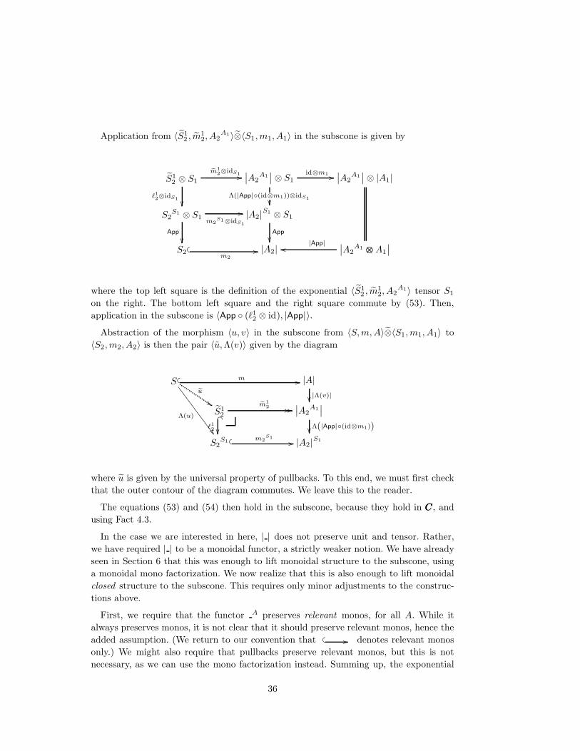
Application from 〈S12 , m1
2, A2A1〉⊗〈S1, m1, A1〉 in the subscone is given by
S12 ⊗ S1
em12⊗idS1 //
ℓ12⊗idS1
∣∣A2A1
∣∣ ⊗ S1id⊗m1 //
Λ(|App|(id⊗m1))⊗idS1
∣∣A2A1
∣∣ ⊗ |A1|
S2S1 ⊗ S1
m2S1⊗idS1
//
App
|A2|S1 ⊗ S1
App
S2
m2
// |A2|∣∣A2
A1 ⊗⊗⊗ A1
∣∣|App|oo
where the top left square is the definition of the exponential 〈S12 , m1
2, A2A1〉 tensor S1
on the right. The bottom left square and the right square commute by (53). Then,
application in the subscone is 〈App (ℓ12 ⊗ id), |App|〉.
Abstraction of the morphism 〈u, v〉 in the subscone from 〈S, m, A〉⊗〈S1, m1, A1〉 to
〈S2, m2, A2〉 is then the pair 〈u, Λ(v)〉 given by the diagram
S m //eu
$$Λ(u)
777
7777
7777
77|A|
|Λ(v)|S1
2
em12 // //
_
ℓ12
∣∣A2A1
∣∣Λ(|App|(id⊗m1))
S2S1 m2
S1// |A2|
S1
where u is given by the universal property of pullbacks. To this end, we must first check
that the outer contour of the diagram commutes. We leave this to the reader.
The equations (53) and (54) then hold in the subscone, because they hold in CCC, and
using Fact 4.3.
In the case we are interested in here, | | does not preserve unit and tensor. Rather,
we have required | | to be a monoidal functor, a strictly weaker notion. We have already
seen in Section 6 that this was enough to lift monoidal structure to the subscone, using
a monoidal mono factorization. We now realize that this is also enough to lift monoidal
closed structure to the subscone. This requires only minor adjustments to the construc-
tions above.
First, we require that the functor A preserves relevant monos, for all A. While it
always preserves monos, it is not clear that it should preserve relevant monos, hence the
added assumption. (We return to our convention that // denotes relevant monos
only.) We might also require that pullbacks preserve relevant monos, but this is not
necessary, as we can use the mono factorization instead. Summing up, the exponential
36

〈S12 , m1
2, A2A1〉 = 〈S2, m2, A2〉
〈S1,m1,A1〉 is given by the diagram on the left below.
S12
ee12 // //
S12
em12 //
ℓ12
∣∣A2A1
∣∣
Λ(|App|(id⊗m1))
∣∣A2A1
∣∣ ⊗ S1id|A2
A1 |⊗m1∣∣A2
A1∣∣ ⊗ |A1|
A2A1 ,A1∣∣A2
A1 ⊗⊗⊗ A1
∣∣|App|
S2S1 m2
S1// |A2|
S1 |A2|
(55)
where the vertical morphism Λ (|App| (id ⊗ m1)) is Λ applied to the composition of
vertical morphisms on the right, the morphism m2S1 is a relevant mono by our assumption
that S1 preserves relevant monos, the topmost horizontal composition of arrows (from
S12 to
∣∣A2A1
∣∣) is given by pullback, and is factored as e12 followed by m1
2; and finally the
morphism ℓ12 is given by a diagonal fill-in, from two paths from S1
2 to |A2|S1 .
Application from 〈S12 , m1
2, A2A1〉⊗〈S1, m1, A1〉 is then given by 〈App, |App|〉 as given
in the diagram below.
S12 ⊗ S1
em12⊗idS1 //
ℓ12⊗idS1
eApp
∣∣A2A1
∣∣ ⊗ S1id⊗m1 //
Λ(|App|(id⊗m1))⊗idS1
∣∣A2A1
∣∣ ⊗ |A1|A2
A1 ,A1
S2S1 ⊗ S1
m2S1⊗idS1
//
App
|A2|S1 ⊗ S1
App
S2
m2
// |A2|∣∣A2
A1 ⊗⊗⊗ A1
∣∣|App|oo
SApp#
mApp
11
dApp
77
(56)
The top left square comes from the definition of the exponential 〈S12 , m1
2, A2A1〉, tensored
by S1 on the right. The bottom left square commutes because App (m2S1 ⊗ idS1) =
App (Λ(m2 App)⊗ idS1) = m2 Appby (53). The right square commutes by (53) again.
The outer contour, defined by m12⊗m1 on the top, A2
A1 ,A1on the right, eApp on the left,
mApp at the bottom, is the definition of the tensor product 〈S12 , m1
2, A2A1〉⊗〈S1, m1, A1〉
in the subscone. App is given by a diagonal fill-in, considering the two paths eApp followed
by |App| mApp and App (ℓ12 ⊗ idS1) followed by m2 from S1
2 ⊗ S1 to |A2|.
Given any morphism 〈u, v〉 in the
subscone from 〈S, m, A〉⊗〈S1, m1, A1〉
to 〈S2, m2, A2〉, by definition the
following diagram commutes. The
top square is the definition of
〈S, m, A〉⊗〈S1, m1, A1〉.
S ⊗ S1m⊗m1//
e.1
|A| ⊗ |A1|A,A1 S.1
m.1
//
u
|A⊗⊗⊗ A1|
|v|
S2 m2
// |A2|
(57)
37

Abstraction of the
morphism 〈u, v〉 in
the subscone from
〈S, m, A〉⊗〈S1, m1, A1〉
to 〈S2, m2, A2〉 is then
the pair 〈e12 u, Λ(v)〉
given by the diagram:
S m //eu
##Λ(ue.1)
444
4444
4444
4444
|A|
|Λ(v)|
S12
ee12 // //
_
S12
em12 //
ℓ12www
w
www
∣∣A2A1
∣∣
Λ(|App|(id⊗m1))
S2S1 m2
S1// |A2|
S1
(58)
In this diagram, u is given by the universal property of pullbacks, and this will be justified
by the fact that the two outer paths from S to |A2|S1 are equal, which we have to check.
First, we note the identity
Λ(s) t = Λ(s (t ⊗ idC)) (59)
whenever t is a morphism from A to B, and s from B ⊗ C to D. Indeed, Λ(s) t =
Λ(App((Λ(s)t)⊗idC)) (by (54)) = Λ(App(Λ(s)⊗idC)(t⊗idC)) = Λ(s(t⊗idC))(by
(53)). It follows that the lower path from S to |A2|S1 in Diagram 58 is
m2S1 Λ(u e.1) = Λ(m2 App) Λ(u e.1)
= Λ(m2 App (Λ(u e.1) ⊗ idS1)) (by (59))
= Λ(m2 u e.1) (by (53))
while the upper one is
Λ(|App| (id ⊗ m1)) |Λ(v)| m
= Λ(|App| (id ⊗ m1) ((|Λ(v)| m) ⊗ idS1)) (by (59))
= Λ(|App| (|Λ(v)| ⊗ id|A1|) (m ⊗ m1))
= Λ(|App| |Λ(v)⊗⊗⊗ idA1 | (m ⊗ m1)) (by naturality of )
= Λ(|v| (m ⊗ m1)) (by (53))
and these two quantities are equal by Diagram (57).
Finally, the equations (53) and (54) then hold in the subscone, because they hold in
CCC, and using Fact 4.3.
We sum up what we need to lift exponentials to the subscone, as usual. To lift expo-
nentials on the right:
(i.a.r) monoidal closed (on the right) categories (CCC,⊗⊗⊗, III,ααα,ℓℓℓ,rrr)
and (C,⊗, I, , l, r), and a monoidal functor | | : CCC → C,
(iii.a) a monoidal mono factorization system on C.
(v) C has pullbacks.
(vi.r) A preserves relevant monos.
Exponentials are given by (55), application by (56), abstraction by (58).
The construction works equally well to lift exponentials on the left, reversing arguments
to tensor products, so we require in this case:
38

(i.a.l) monoidal closed (on the left) categories (CCC,⊗⊗⊗, III,ααα,ℓℓℓ,rrr)
and (C,⊗, I, , l, r) and a monoidal functor | | : CCC → C,
(iii.a) a monoidal mono factorization system on C.
(v) C has pullbacks.
(vi.l) A preserves relevant monos.
Clearly, in the symmetric monoidal closed case we require the following to get a sym-
metric monoidal closed subscone:
(i.b) symmetric monoidal closed categories (CCC,⊗⊗⊗, III,ααα,ℓℓℓ,rrr, ccc)
and (C,⊗, I, , l, r, ), and a symmetric monoidal functor | | : CCC → C,
(iii.a) a monoidal mono factorization system on C.
(v) C has pullbacks.
(vi) A preserves relevant monos.
And in the cartesian closed case, we require:
(i.c) cartesian closed categories CCC and C,
and a cartesian monoidal functor | | : CCC → C,
(iii.a) a monoidal mono factorization system on C.
(v) C has pullbacks.
(vi) A preserves relevant monos.
Putting all conditions together, we get a notion of subscone for categorical models
of Moggi’s meta-language, i.e., for cartesian closed categories with a strong monad, we
require:
(i.c) cartesian closed categories CCC and C,
and a cartesian monoidal functor | | : CCC → C,
(ii.a) a strong monad (T,,, t) on C, related to (TTT ,ηηη,µµµ, ttt) by
a strong monad morphism (| |, σ) defined in (4) and (36),
(iii.a) a monoidal mono factorization system on C.
(iv) T maps relevant pseudoepis to pseudoepis.
(v) C has pullbacks.
(vi) A preserves relevant monos.
10. Examples
At this point, we suspect the reader is relatively fed up with categorical diagrams and
general abstract nonsense. It is therefore time to instantiate our constructions. We start
with fairly easy cases in the category SetSetSet of sets in Section 10.1. We examine in more
detail the non-determinism monad in Section 10.2, then the discrete probability monad
in Section 10.3. A more demanding case is the name creation monad, which involves
presheaves, and which we deal with in Section 10.4. We then engage in a series of examples
demonstrating the difficulties of finding the right mono factorization system, and the
need for varying categories, in particular for choosing CCC and C distinct, in situations of
practical interest. Doing this, we shall see that our construction often produces definitions
39

in the style of bisimulation, sometimes in the style of observational equivalence, and will
in one case assume yet another style (existence of related refinements, see the end of
Section 10.7). This will keep us busy from Section 10.5 to Section 10.8. These sections
will unfortunately be rather mathematically demanding; it does not seem there was any
escaping it.
10.1. Lift, Exceptions, State, Non-Determinism, and Continuations in SetSetSet
As in Section 5, suppose C1 = C2 = C = SetSetSet, and | |1 and | |2 are identities. In
particular, | | is the cartesian product functor from SetSetSet×SetSetSet to SetSetSet. Below we summarize
the action of T on a relation S // A1×A2 , for different computational monads T of
Moggi (Moggi, 1991). This is parameterized by a binary relation RE on exceptions in E
in the exception monad A + E, by a binary relation RSt on states in the state monad
(A×St)St, and by a binary relation RR in the continuation monad RRA
.
Monad T relation eS ⊆ TA1×TA2
TA = A⊥ = A ∪ ⊥ eS = S ∪ (⊥,⊥)
TA = A + E (v1, v2) ∈ eS ⇐⇒ (v1, v2) ∈ S ∨ (v1, v2) ∈ RE
TA = (A×St)St (f, g) ∈ eS ⇐⇒ ∀s1, s2 ∈ St.
(s1, s2) ∈ RSt ⇒ (π1(fs1), π1(gs2)) ∈ S ∧ (π2(fs1), π2(gs2)) ∈ RSt
TA = Pfin(A) (B1, B2) ∈ eS ⇐⇒
∀b1 ∈ B1.∃b2 ∈ B2.(b1, b2) ∈ S ∧
∀b2 ∈ B2.∃b1 ∈ B1.(b1, b2) ∈ S
TA = RRA
(α1, α2) ∈ eS ⇐⇒`
∀k1, k2.(∀a1, a2.(a1, a2) ∈ S ⇒ (k1(a1), k2(a2)) ∈ RR) ⇒
(α1(k1), α2(k2)) ∈ RR
´
We examine each case in more detail. We take surjections as pseudoepis, injections as
relevant monos. This is the canonical choice for an epi-mono factorization system on
SetSetSet. Note that condition (iv), that T maps relevant pseudoepis to pseudoepis, is always
satisfied when C = SetSetSet. In fact, T preserves pseudoepis: every pseudoepi (surjective
function) e : A → B has a section m : B → A (i.e., em = idB), by the Axiom of Choice.
Then Te Tm = idTB, showing that Te is surjective, hence pseudoepi.
10.1.1. Lift monad A⊥. The monad morphism σ from (A × B)⊥ to A⊥ × B⊥ maps ⊥
to (⊥,⊥), and every pair (x, y) ∈ A × B to itself. This is a commutative monad, hence
monoidal, hence strong. The mediator dA,B from A⊥×B⊥ to (A×B)⊥ maps (⊥, y) and
(x,⊥) to ⊥, and (x, y) where x ∈ A and y ∈ B to itself. Note that it is not a cartesian
monad, because (π2)⊥ dA,B maps (⊥, y) to ⊥, while π2(⊥, y) = y. Nonetheless, all
required conditions are satisfied to lift T to a commutative monad on the subscone.
10.1.2. Exception monad A + E. The monad morphism σ from (A × B) + E to (A +
E) × (B + E) maps the pair (x, y) ∈ A × B to itself, and the exception e ∈ E to the
40
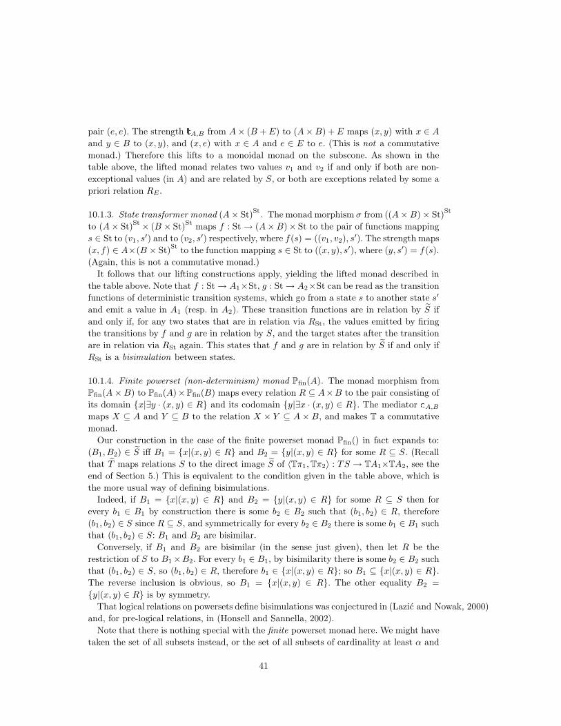
pair (e, e). The strength tA,B from A × (B + E) to (A × B) + E maps (x, y) with x ∈ A
and y ∈ B to (x, y), and (x, e) with x ∈ A and e ∈ E to e. (This is not a commutative
monad.) Therefore this lifts to a monoidal monad on the subscone. As shown in the
table above, the lifted monad relates two values v1 and v2 if and only if both are non-
exceptional values (in A) and are related by S, or both are exceptions related by some a
priori relation RE .
10.1.3. State transformer monad (A × St)St
. The monad morphism σ from ((A × B) × St)St
to (A × St)St × (B × St)
Stmaps f : St → (A×B)× St to the pair of functions mapping
s ∈ St to (v1, s′) and to (v2, s
′) respectively, where f(s) = ((v1, v2), s′). The strength maps
(x, f) ∈ A×(B × St)St
to the function mapping s ∈ St to ((x, y), s′), where (y, s′) = f(s).
(Again, this is not a commutative monad.)
It follows that our lifting constructions apply, yielding the lifted monad described in
the table above. Note that f : St → A1×St, g : St → A2×St can be read as the transition
functions of deterministic transition systems, which go from a state s to another state s′
and emit a value in A1 (resp. in A2). These transition functions are in relation by S if
and only if, for any two states that are in relation via RSt, the values emitted by firing
the transitions by f and g are in relation by S, and the target states after the transition
are in relation via RSt again. This states that f and g are in relation by S if and only if
RSt is a bisimulation between states.
10.1.4. Finite powerset (non-determinism) monad Pfin(A). The monad morphism from
Pfin(A × B) to Pfin(A)×Pfin(B) maps every relation R ⊆ A×B to the pair consisting of
its domain x|∃y · (x, y) ∈ R and its codomain y|∃x · (x, y) ∈ R. The mediator dA,B
maps X ⊆ A and Y ⊆ B to the relation X × Y ⊆ A × B, and makes T a commutative
monad.
Our construction in the case of the finite powerset monad Pfin() in fact expands to:
(B1, B2) ∈ S iff B1 = x|(x, y) ∈ R and B2 = y|(x, y) ∈ R for some R ⊆ S. (Recall
that T maps relations S to the direct image S of 〈Tπ1, Tπ2〉 : TS → TA1×TA2, see the
end of Section 5.) This is equivalent to the condition given in the table above, which is
the more usual way of defining bisimulations.
Indeed, if B1 = x|(x, y) ∈ R and B2 = y|(x, y) ∈ R for some R ⊆ S then for
every b1 ∈ B1 by construction there is some b2 ∈ B2 such that (b1, b2) ∈ R, therefore
(b1, b2) ∈ S since R ⊆ S, and symmetrically for every b2 ∈ B2 there is some b1 ∈ B1 such
that (b1, b2) ∈ S: B1 and B2 are bisimilar.
Conversely, if B1 and B2 are bisimilar (in the sense just given), then let R be the
restriction of S to B1 ×B2. For every b1 ∈ B1, by bisimilarity there is some b2 ∈ B2 such
that (b1, b2) ∈ S, so (b1, b2) ∈ R, therefore b1 ∈ x|(x, y) ∈ R; so B1 ⊆ x|(x, y) ∈ R.
The reverse inclusion is obvious, so B1 = x|(x, y) ∈ R. The other equality B2 =
y|(x, y) ∈ R is by symmetry.
That logical relations on powersets define bisimulations was conjectured in (Lazic and Nowak, 2000)
and, for pre-logical relations, in (Honsell and Sannella, 2002).
Note that there is nothing special with the finite powerset monad here. We might have
taken the set of all subsets instead, or the set of all subsets of cardinality at least α and
41

strictly less than β, where α < β are two cardinal numbers such that α ≤ 1, and every
finite product of cardinals between α (inclusive) and β (exclusive) is again so. The finite
powerset monad is the case α = 0, β = ℵ0; the lift monad is the case α = 0, β = 2.
Note also that although this monad is always commutative, it is a cartesian monad if
and only if α ≥ 1. Indeed, T is a cartesian monad if and only if the domain of the relation
X × Y is X , and its codomain is Y . This is wrong if Y or X is allowed to be empty,
but holds as soon as X and Y are non-empty. In particular, the finite-and-non-empty
powerset monad (for serial non-determinism—no state is final) is cartesian.
10.1.5. The continuation monad RRA
. The monad morphism σ from RRA×B
to RRA
×
RRB
maps α : RA×B → R to the pair (α1, α2), where α1 maps k1 ∈ RA to α(k1 π1)
and α2 maps k2 ∈ RB to α(k2 π2). The strength tA,B maps (x, α) ∈ A ×RRB
to the
function mapping k ∈ RA×B to α(λy ∈ B · k(x, y)). This monad is not commutative.
Our construction yields the rather opaque condition in the table above, where a1, a2
are values, k1, k2 are continuations, and α1, α2 are programs, taking continuations to
answers in R. Intuitively, think of continuations as computation environments (a toplevel
loop, a shell) that take the result of a program and print something (called an answer,
in R) on a computer terminal. To evaluate a program α in continuation (environment)
k, apply α to k. For simplicity, assume that the relation RR on answers is equality. The
condition then states that two programs are related by S if and only if they give identical
answers when evaluated in related continuations (environments), where two environments
are related if and only if they print the same answer on values that are related by S, i.e.,
if and only if they do not make any difference between S-related values. This is a form
of observational equivalence.
10.2. Labelled transition systems and bisimulations
The case TA = Pfin(A) allows one to define labelled transition systems as elements of(TA)A×L, with labels in L and states in A, as functions mapping states a and labels ℓ to
the set of states a′ such that aℓ
−→a′. Our monad lifting S in this case is parameterizedby a binary relation on RL on labels and is defined by:
(f1, f2) ∈ eS ⇐⇒ ∀a1, a2, ℓ1, ℓ2 · (a1, a2) ∈ S ∧ (ℓ1, ℓ2) ∈ RL ⇒(
∀b1 ∈ f1(a1, ℓ1).∃b2 ∈ f2(a2, ℓ2).(b1, b2) ∈ S ∧
∀b2 ∈ f2(a2, ℓ2).∃b1 ∈ f1(a1, ℓ1).(b1, b2) ∈ S
In case RL is the equality relation, the relation S relates f1 and f2 iff S is a strong
bisimulation between the labelled transition systems f1 and f2.
10.3. Discrete Probabilities and Subprobabilities
Defining TTTA to be space of all probability distributions over the space A allows us to
define probabilistic transition systems as objects of (TTTA)A
. In principle, this should work
just like ordinary transition systems (Section 10.2).
In fact, defining what the right spaces should be, and ensuring that the required monads
42

exist and have the required properties, is much subtler. For one, as far as we know, the
category of measurable spaces and measurable functions is not known to be cartesian
closed. As we don’t want to delve into measure theoretic considerations at this point, let
us deal with a simpler case: the monad of discrete (sub-)probability distributions over
SetSetSet.
A discrete sub-probability distribution ν over some set A is simply a function mapping
each element x ∈ A to some non-negative number ax ∈ R+, so that∑
x∈A ax ≤ 1. This
sum, which is in general infinite, denotes the supremum of all partial sums∑
x∈B ax,
when B ranges over the finite subsets of A. It is an easy exercise to show that only
countably many coefficients ax can be non-zero, then. A discrete probability distribution
additionally satisfies∑
x∈A ax = 1. The Dirac distribution δx0 at x0 maps x0 to 1 and
every x 6= x0 to 0. Accordingly, we write∑
x∈A axδx for the discrete distribution mapping
x to ax. The measure of a subset B of A under ν =∑
x∈A axδx is ν(B) =∑
x∈B ax.
Let TTTA be the set of all discrete (sub-)probability distributions over A, ηηηA map x ∈ A
to δx ∈ TTTA, and µµµA be defined as mapping ν2 =∑
ν∈TTTA aνδν ∈ TTT 2A to the discrete
distribution µµµA(ν2) such that µµµA(ν2)(B) =∑
ν∈TTTA aνν(B) for every B ⊆ A; in other
words, µµµA(ν2) =∑
x∈A
(∑ν∈TTTA aνν(x)
)δx. It is easy to check that (TTT ,ηηη,µµµ) is a monad
on SetSetSet. Moreover, it is strong: the strength tttA,B maps x ∈ A and ν =∑
y∈B byδy ∈ TTTB
to∑
y∈B byδ(x,y).
Our construction in the case of the (sub-)probability distribution monad on SetSetSet yields
the following. Again, TTT = T, and recall that T maps relations S on A1 ×A2 to the direct
image S of 〈Tπ1, Tπ2〉 : TS → TA1×TA2. In other words, given ν1 ∈ TTTA1, ν2 ∈ TTTA2,
(ν1, ν2) ∈ S if and only if there is a discrete (sub-)probability distribution ν on S such
that ν1(B1) = ν((B1 × A2) ∩ S) for every B1 ⊆ A1 and ν2(B2) = ν((A1 × B2) ∩ S) for
every B2 ⊆ A2.
Write ν1 as∑
x1∈A1ax1δx1 , ν2 as
∑x2∈A2
bx2δx2 . Then (ν1, ν2) ∈ S if and only if there
is a discrete (sub-)probability distribution ν =∑
x1∈A1,x2∈A2
(x1,x2)∈S
cx1,x2δ(x1,x2) on S such
that ax1 =∑
x2∈A2/(x1,x2)∈S cx1,x2 for all x1 ∈ A1 and bx2 =∑
x1∈A1/(x1,x2)∈S cx1,x2 for
all x2 ∈ A2. This may be pictured by requiring that we have a matrix of non-negative
reals cx1,x2 such that: the only non-zero entries (x1, x2) of this matrix are such that
(x1, x2) ∈ S; the sum of the x1 row is ax1 ; the sum of the x2 column is bx2 . This is a
well-known problem in probability theory: find ν on the product A1 × A2 having given
marginals ν1 and ν2 and whose support (x1, x2) ∈ A1×A2|ν((x1, x2)) 6= 0 is included
in S.
Let us play with the definition of S for a moment. Consider the disjoint sum A1 ⊕A2,
and the smallest equivalence ≡S relation containing S. It is easy to see that, for every
≡S-equivalence class C,
((C ∩ A1) × A2) ∩ S = (A1 × (C ∩ A2)) ∩ S (60)
It follows that if there is a discrete distribution ν with support contained in S and whose
marginals are ν1 and ν2, then for any ≡S-equivalence class C, ν1(C ∩A1) = ν2(C ∩A2).
Indeed, ν1(C ∩A1) = ν(((C ∩A1)×A2)∩S), ν2(C ∩A2) = ν((A1 × (C ∩A2))∩S); then
use (60).
43

Conversely, if ν1(C∩A1) = ν2(C∩A2) for every ≡S-equivalence class C, then whenever
x1 ≡S x2, let dx1,x2 = ν1(C ∩ A1) = ν2(C ∩ A2), where C is the equivalence class of x1
(equivalently, of x2). Now define ν as∑
(x1,x2)∈A1×A2x1≡Sx2dx1,x2 6=0
ax1bx2
dx1,x2δ(x1,x2). Clearly the support
of ν is contained in the relation ≡S , and ν1 and ν2 are the marginals of ν. So (ν1, ν2) ∈ ≡S.
Let S be saturated if and only if, for any x1 ∈ A1, x2 ∈ A2, x1 ≡S x2 implies
(x1, x2) ∈ S. We have just shown the following: for any saturated relation S ⊆ A1 × A2,
(ν1, ν2) ∈ S if and only if ν1(C ∩A1) = ν2(C ∩A2) for every ≡S-equivalence class C. The
restriction to saturated relations is not too demanding; indeed, we can always saturate
any binary relation S by considering the restriction of ≡S to A1 × A2 instead.
Analogously with Section 10.2, we may define a probabilistic labelled transition systemas an element of (TTTA)
A×L. Then two such transition systems f1 and f2 are in relation if
and only if:
∀x1 ∈ A1, x2 ∈ A2, ℓ1, ℓ2 ∈ L.(x1, x2) ∈ S ∧ (ℓ1, ℓ2) ∈ RL ⇒ (61)
(f1(x1, ℓ1), f2(x2, ℓ2)) ∈ eS
When S is saturated, this condition is equivalent to: for every x1 ∈ A1, x2 ∈ A2, ℓ1, ℓ2 ∈
L, if x1 ≡S x2 and (ℓ1, ℓ2) ∈ RL then for every ≡S-equivalence class C, f1(x1, ℓ1)(C ∩
A1) = f2(x2, ℓ2)(C ∩ A2). This is exactly Larsen and Skou’s (Larsen and Skou, 1991)
notion of probabilistic bisimulation, when L1 = L2, RL is the equality relation, and A1
and A2 are finite. To see this, write pℓ(x) = f1(x, ℓ) if x ∈ A1, pℓ(x) = f2(x, ℓ) if x ∈ A2,
and rewrite the condition above as: if x1 ≡S x2 then for every ≡S-equivalence class C,
pℓ(x1)(C) = pℓ(x2)(C).
It is therefore fair to say that any saturated relation S (and by extension, any relation
at all) such that f1 and f2 are in relation at type A × L → TTTA, as defined in (61), is
again a probabilistic bisimulation.
A note on discreteness: the monad of discrete (sub-)probability distributions is enough
to model coin flips∑
x∈0,1 1/2δx. One may argue that, in any finite computation of
a λ-term augmented with coin flips, only finite linear combinations of Dirac measures
(simple valuations) will ever crop up, so that discrete distributions are general enough to
accomodate all practical forms of probabilistic choice. This would not be true in the case
of infinite computations, where at least all least upper bounds of directed chains of sim-
ple distributions (quasi-simple valuations (Goubault-Larrecq, 2005)) would be needed.
Notwithstanding the fact that we should incorporate fixpoints in the language and re-
place SetSetSet with some other category such as CpoCpoCpo, this would exceed the realm of discrete
distributions anyway: for example, the Lebesgue measure on [0, 1] is a quasi-simple val-
uation but is definitely not discrete.
10.4. Logical relations for dynamic name creation
Consider the categorical model of dynamic name creation defined in (Stark, 1996). Let I
be the category of finite sets and injective functions, and SetSetSetI be the category of functors
from I to SetSetSet and natural transformations (the category of covariant presheaves over I).
44

For short, write TTTAs for TTT (A)(s) and similarly for other notations. Let + denote disjoint
union in I.‡
We define the strong monad (TTT ,ηηη,µµµ, ttt) on SetSetSetI by:
— TTTA = colims′ A( + s′) : I → SetSetSet.
On objects, this is given by TTTAs = colims′ A(s + s′), i.e., TTTAs is the set of all
equivalence classes of pairs (s′, a) with s′ ∈ I and a ∈ A(s + s′) modulo the smallest
equivalence relation ≡ such that (s′, a) ≡ (s′′, A(ids+j)a) for every morphism s′j
−→s′′
in I (intuitively, given a set of names s, elements of TTTAs are formal expressions (νs′)a
where all names in s′ are bound and every name free in a is in s + s′—modulo the
fact that (νs′, s′′)a ≡ (νs′)a for any additional set of new names s′′ not free in a). We
shall write [s′, a] the equivalence class of (s′, a).
On morphisms s1i
−→s2, TTTAi maps [s′, a] to the equivalence class of [s′, A(i + ids′)a].
— For any f : A → B in SetSetSetI , TTTfs : TTTAs → TTTBs is defined by TTTfs[s′, a] = [s′, f(s +
s′)a]. This is compatible with ≡ because f is natural.
— ηηηAs : As → TTTAs is defined by ηηηAsa = [∅, a].
— µµµAs : TTT 2As → TTTAs is defined by µµµAs[s′, [s′′, a]] = [s′ + s′′, a].
— tttA,Bs : As×TTTBs → TTT (A×B)s is defined by tttA,Bs(a, [s′, b]) = [s′, (Ainlss′a, b)] where
inlss′ : s → s + s′ is the canonical injection.
Furthermore, TTT is a commutative monad, whose mediator dA,Bs : TTTAs×TTTBs → TTT (A×
B)s maps ([s′, a], [s′′, b]) to [s′ + s′′, (A(ids + inls′s′′)a, A(ids + inrs′′s′)b)], where inrs′′s′ :
s′′ → s′ + s′′ is the other canonical injection. In fact, TTT is a cartesian monad. Indeed,
(TTTπ1dA,B)s maps ([s′, a], [s′′, b]) to [s′+s′′, A(ids+inls′s′′)a] = [s′, a], so TTTπ1dA,B = π1,
and similarly TTTπ2 dA,B = π2.
It is important to note how ≡ works. The category I has pushouts: in particular, if
s0i1−→s1 and s0
i2−→s2 are two morphisms in I, then there is a finite set s1 +s0 s2 and two
morphisms s1j1−→s1 +s0 s2, s2
j2−→s1 +s0 s2 such that j1 i1 = j2 i2—take s1 +s0 s2 to
be the disjoint sum s1 + s2 modulo the equivalence relation relating i1(a0) = i2(a0) for
every a0 ∈ s0.
It follows that (∗) for every a1 ∈ A(s + s1), a2 ∈ A(s + s2), (s1, a1) ≡ (s2, a2) if
and only if there is a finite set s12 and two arrows s1j1−→s12 and s2
j2−→s12 such that
A(ids1 + j1)a1 = A(ids2 + j2)a2.
We take CCC1 = CCC2 = C = SetSetSetI , hence objects in the subscone give rise to I-indexed
Kripke logical relations. Furthermore, | |1 = | |2 = | | is the identity functor and T is just
TTT . The category SetSetSetI has a mono factorization consisting of pointwise surjections and
pointwise injections.
As in Section 5, the monad morphism σ〈A1,A2〉s : T(A1 × A2)s → TTTA1s × TTTA2s is
equal to 〈Tπ1, Tπ2〉s. That is to say
σ〈A1,A2〉s[s′, (a1, a2)] = ([s′, a1], [s′, a2])
where s′ ∈ I, a1 ∈ A1(s + s′), a2 ∈ A2(s + s′).
‡ Note that + is not a coproduct in I. In fact, I does not have a coproduct. However + is functorialin both components, associative, and has a neutral element, and this is all we need.
45

Again as in SetSetSet, every functor S from I to A1 × A2 has a representation
〈πS1, π
S2〉 : S → A1 × A2
where each arrow 〈πS1, π
S2〉s : Ss → A1s × A2s is an inclusion.
Hence, S is a family of relations Ss between A1s and A2s, functorial in s (for each
s′i
−→s′′, Si is the appropriate restriction of A1i × A2i). Recall from Section 5 that S
is defined as the direct image of 〈TπS1, TπS
2〉. So, (†) [s1, a1] Ss [s2, a2] if and only
if for some s′ ∈ I, a′1 ∈ A1s
′, a′2 ∈ A2s
′, (s1, a1) ≡ (s′, a′1), (s2, a2) ≡ (s′, a′
2) and
a′1 S(s + s′) a′
2.
Using (∗) above, (s1, a1) ≡ (s′, a′1) means that there is a finite set s′1 and two arrows
s1j1−→s′1, s′
j′1−→s′1 in I such that: (a) A1(ids + j1)a1 = A1(ids + j′1)a′1. Similarly, (s2, a2) ≡
(s′, a′2) means there is a finite set s′2 and two arrows s2
j2−→s′2, s′
j′2−→s′2 in I such that: (b)
A2(ids + j2)a2 = A2(ids + j′2)a′2. Consider arrows j′1 and j′2, which both have s′ as source,
and build their pushout s0 = s′1 +s′ s′2, with arrows s′1j′′1−→s0, s′2
j′′2−→s0. Let j be j′′1 j′1 =
j′′2 j′2. By applying A1(ids +j′′1 ) to both sides of (a), A1(ids +(j′′1 j1))a1 = A1(ids +j)a′1.
By applying A2(ids + j′′2 ) to both sides of (b), A2(ids + (j′′2 j2))a2 = A2(ids + j)a′2.
Since a′1 S(s + s′) a′
2 and S is functorial, A1(ids + j)a′1 S(s + s0) A2(ids + j)a′
2, so
A1(ids + (j′′1 j1))a1 S(s + s0) A2(ids + (j′′2 j2))a2.
So if (s1, a1) Ss (s2, a2) then there are arrows s1i1−→s0 and s2
i2−→s0, namely i1 = j′′1 j1and i2 = j′′2 j2, such that A1(ids + i1)a1 S(s + s0) A2(ids + i2)a2.
Conversely, if the latter holds, then (†) above clearly holds for s′ = s0, a′1 = A1(ids +
i1)a1 and s′2 = A2(ids + i2)a2.
Ss → TTTA1s × TTTA2s is thus given by
[s1, a1] Ss [s2, a2] ⇐⇒ ∃s0 ∈ I · ∃i1 : s1 → s0 ∈ I · ∃i2 : s2 → s0 ∈ I·
(A1(ids + i1)a1) S(s + s0) (A2(ids + i2)a2)(62)
where a1 ∈ A1(s + s1) and a2 ∈ A2(s + s2).
From (62) we define a logical relation for Moggi’s metalanguage, as suggested in Sec-
tion 5, by induction on types τ . Each relation JτK is a functor from I to SetSetSet × SetSetSet, so
that JτK s is a binary relation for each type τ and each finite set s. We have:
(f1, f2) ∈ Jτ → τ ′K s ⇐⇒ ∀s′, i : s → s′ ∈ I, (a1, a2) ∈ JτK s′ ·
(f1s′(i, a1), f2s
′(i, a2)) ∈ Jτ ′K s′
((a1, a′1), (a2, a
′2)) ∈ Jτ × τ ′K s ⇐⇒ (a1, a2) ∈ JτK s ∧ (a′
1, a′2) ∈ Jτ ′K s
([s1, a1], [s2, a2]) ∈ JTTTτK s ⇐⇒ ∃s0, i1 : s1 → s0, i2 : s2 → s0 ∈ I ·
(A1(ids + i1)a1, A2(ids + i2)a2) ∈ JτK (s + s0)
This is similar to the logical relations of (Pitts and Stark, 1993; Stark, 1998). While
(62) is roughly similar to the notion of logical relation of (Pitts and Stark, 1993), this
paper does not rest on Moggi’s computational λ-calculus. On the other hand (Stark, 1998)
does rest on the computational λ-calculus but does not define a suitable notion of logical
relation.
Zhang and Nowak show in (Zhang and Nowak, 2003) that the logical relation above is
46
in fact strictly weaker than Pitts and Stark’s logical relation (Pitts and Stark, 1993) when
restricted to the latter’s nu-calculus; Zhang and Nowak also claim that by reinstantiating
our construction of the subscone with CCC1 = CCC2 = SetSetSetI as above but C = SetSetSetI→
, where
I→ is the comma category whose objects are the morphisms of I, another Kripke logical
relation is obtained that coincides with Pitts and Stark’s on the nu-calculus up to first
order. This is in fact wrong, but Zhang (Zhang, 2005) shows that this can be repaired by
replacing I→ by the category PI→ whose objects are, again, morphisms of I, but whose
morphisms are pullback diagrams in I. It extends it to the full monadic meta-language,
and rests purely on semantic principles, while Pitts and Stark’s definition of their logical
relation relies on normalization properties of the nu-calculus.
10.5. Fun With Categories I: Taking CCC 6= SetSetSet, the Example of CpoCpoCpo
The constructions of this paper apparently allow for some considerable degree of freedom.
We may choose distinct categories for CCC and C, different monads TTT and T, several monad
morphisms σ, several mono factorization systems, and so on.
However, the examples we have given until now used none of these degrees of freedom.
By taking CCC = C = SetSetSet notably, we have essentially narrowed down our possible choices
to just one. So let us have fun, trying to vary various parameters, and see what happens.
We start by keeping CCC = C, but with categories CCC other than SetSetSet or presheaf categories.
We shall then look at several mono factorization systems.
The aim of this section is to show that, at least if we keep CCC = C, our freedom is
considerably restricted.
Imagine CCC is CpoCpoCpo, the category of cpos and continuous maps. By cpo we mean any
ordered set such that any directed family of elements has a least upper bound. See
(Abramsky and Jung, 1994; Gierz et al., 1980; Gierz et al., 2003) for background infor-
mation on cpos and related topics. We always assume cpos to be equipped with their
Scott topology.
Imagine the monad we are interested in on CpoCpoCpo is that of demonic non-determinism,
whereby intuitively, non-deterministic choices are in the hand of a malevolent external
adversary. The traditional monad TTT modeling this is the Smyth powerdomain construc-
tion: TTTA = Q(A) consists of all compact non-empty upward-closed subsets of A, ordered
by reverse inclusion ⊇. One problem here is that Q(A) need not be a cpo. It is one
if A, equipped with its Scott topology, is a sober topological space; for example, if A
is a continuous cpo. So we should restrict to some cartesian-closed category consisting
of continuous cpos only. We know what these categories should be, by Jung’s results
(Jung, 1990), but this is a bit complicated for an illustration. (We shall return to these
categories anyway in Section 10.7, out of necessity, but will avoid them as long as we
can.)
Instead, take Heckmann’s characterization of the upper power domain (Heckmann, 1990)
(without the top element, which would be the empty compact in Q(A) above). Let
2 = 0, 1 be the Sierpinski space, i.e., the two-element cpo with 0 < 1. Let [A → 2] be
the set of Scott-continuous functions from A to 2; this is canonically isomorphic to the
space of Scott opens of A, through the map sending f ∈ [A → 2] to f−11. Define ⊤
47

as λx · 1 in [A → 2], ⊥ as λx · 0; least upper bounds ⊔ and greatest lower bounds ⊓ are
defined pointwise. Following Heckmann, U∗(A) is the set of continuous linear non-trivial
second-order predicates, i.e., the set of Scott-continuous functionals F from [A → 2]
to 2 that preserve ⊤ and meets ⊓ (linearity), and map ⊥ to 0 (non-triviality). (See
(Heckmann, 1990, Chapter 19) for the rationale behind this construction, and for related
theorems. While our constructions will work for several other power constructions, we
only take one as illustration.)
U∗ is a monad TTT on CpoCpoCpo. Its action on morphisms h : A → B is given by TTT (h) =
λF ∈ U∗(A), f ∈ [B → 2] · F (f h). Its unit is given by ηηηA(x) = λf ∈ [A → 2] · f(x)
(x ∈ A), and its multiplication is given by µµµA(G) = λf ∈ [A → 2] ·G(λF ∈ U∗(A) ·F (f))
(G ∈ U2∗ (A)). The strength is given by tttA,B = λ(x, F ) ∈ A × U∗(B) · λf ∈ [A × B →
2] · F (λy ∈ B · f(x, y)). Note that these are the same formulae as those defining the
continuation monad.
It turns out that if A is a continuous cpo, then U∗(A) and Q(A) are naturally isomor-
phic. They key result here is the Hofmann-Mislove Theorem (Abramsky and Jung, 1994,
Corollary 7.2.10). The isomorphism maps any upward-closed compact subset Q of A
to the continuous linear functional λf ∈ [A → 2] · Q ⊆ f−11, and conversely, maps
any continuous linear functional F to the intersection of all opens O of A such that
F (χO) = 1. (The hard part of the Hofmann-Mislove theorem is to show that this is
compact, as soon as A is sober.) While this shows the connection between U∗ and Q, we
shall not use this until Section 10.7.
To apply our construction of logical relations, we need a mono factorization system.
In CpoCpoCpo, there are at least three:
— The trivial mono factorization. Here, relevant monos are isos, and pseudoepis are
arbitrary morphisms. This exists in every category, and is completely uninteresting in
every category: given any binary relation S between A1 and A2, i.e., S m// A1 × A2 ,
then S is in fact the whole of A1 × A2 (up to iso).
— The epi / regular mono factorization. Recall that a mono is regular if and only if it
is the equalizer of a parallel pair. Let us describe regular monos more concretely in
CpoCpoCpo.
A regular mono m : C // B in CpoCpoCpo is a Scott-closed subset of B, up to isomor-
phism. More precisely, m is the composite of an iso from C to some Scott-closed
subset m(C) of B, with the canonical inclusion of m(C) in B.
An epi is any continuous function e : A // // C such that e(A) is dense in C, i.e.,
such that cl(e(A)) = C, where cl denotes the (Scott) topological closure operator.
Equivalently, such that e−1(U) 6= ∅ for any non-empty Scott-open U of C.
It is well-known that this yields a mono factorization system on CpoCpoCpo. We skip the
details, which are not very interesting at this point.
— The extremal epi / mono factorization. Recall that the extremal pseudoepis are
the morphisms Ae // B such that, whenever e can be written as the composite
A // B′ m // B where m is mono, then m is actually iso.
Many categories CCC have a mono factorization system where the pseudoepis are the ex-
tremal pseudoepis, as shown by Freyd and Kelly: by Proposition 2.3.4 of (Freyd and Kelly, 1972),
48

this is the case if CCC has all finite limits and admits intersections of monos (i.e., limits
of all classes of monos ( Xα mα // B )
α∈Ω); or if CCC has all finite colimits and admits
colimits of all classes of extremal pseudoepis ( Beα // // Yα )
α∈Ω; or if CCC has all finite
limits, all finite colimits, and composites of coequalizers are coequalizers. In all these
cases, extremal pseudoepis are in fact epis; in the third case, they are regular, i.e.,
coequalizers of parallel pairs. By the way, the argument of Freyd and Kelly in fact
shows that CCC has a mono factorization system as soon as CCC has pullbacks (not nec-
essarily all limits) and admits non-empty intersections of monos: the factorization of
any given morphism Af // B is the intersection of the class of all monos mα such
that f factors through mα, i.e., such that f can be written Aeα // Cα
mα // B . (In
this case, it is unknown whether pseudoepis are epi.)
While monos in CpoCpoCpo are simple to characterize—they are just the injective continuous
maps—extremal epis have a much more complicated structure, which we therefore
elude.
It turns out that we have been unable to show that the functor TTT = U∗ mapped relevant
pseudoepis to pseudoepis, despite our efforts. We shall see in the next sections that this is
not needed. All we have to do is make C slightly different from CCC, and T slightly different
from TTT .
10.6. Fun With Categories II: Making CCC and C Distinct, e.g., CCC = CpoCpoCpo, C = OrdOrdOrd
Consider C = OrdOrdOrd, the category of partial orders and monotonic maps. There is an
obvious forgetful functor | |0 : CpoCpoCpo → OrdOrdOrd. In the following, if A ⊆ B, we write ↑B A
the subset x ∈ B|∃y ∈ A · y ≤ x.
In any partial order A, say that a subset is finitary if and only if it is of the form
↑A E with E finite. In the following, we take TA as the space of non-empty finitary
subsets of A, ordered by reverse inclusion ⊇. Why should we take this? Well, we have
seen above that the space TTTA = U∗(A) could be identified with the space of compact
non-empty upward-closed subsets of A, ordered by reverse inclusion. For our construction
to work out, in particular to be able to find a suitable monad morphisms, T should in
a sense mimic TTT in the category C. By going from CCC = CpoCpoCpo to C = OrdOrdOrd, we keep the
ordering but forget about the (Scott-) topology. It turns out that, if we just know about
the ordering ≤, there are many possible topologies from which it may arise. Precisely,
there are many topologies with ≤ as specialization quasi-ordering — the one defined so
that x is less than or equal to y if and only if every open containing x must also contain
y. One is the Scott-topology. The finest is the Alexandroff topology, whose opens are
all upward-closed subsets. In all these topologies, the only subsets that are guaranteed
to be compact upward-closed are the finitary subsets. The latter then intuitively form a
concept similar to the notion of compact upward-closed subsets. This should be checked
formally, by verifying the axioms for monad morphisms, which we do right away.
Note in passing that there is a slightly distinct presentation of TA, as set of finite
non-empty antichains (sets E where no two distinct elements are comparable), ordered
49

in the Smyth ordering ≤♯ defined by E ≤♯ E′ if and only if every element of E′ is greater
than or equal to some element of E.
For every map f : A → B, Tf maps the finitary subset ↑A x1, . . . , xn to ↑B
f(x1), . . . , f(xn). This defines a monad on OrdOrdOrd, together with unit A : A → TA
defined by A(x) =↑A x, multiplication A : T2A → TA defined by A(↑TA ↑A
E1, . . . , ↑A En) =↑A
⋃ni=1 Ei. This is in fact a commutative monad, with mediatordA,B : TA × TB → T(A × B) defined by dA,B(↑A E, ↑B F ) =↑A×B (E × F ). The
corresponding strength maps (x, ↑B y1, . . . , ym) to ↑A×B (x, y1), . . . , (x, ym).
The required monad morphism σA0 : T|A|0 → |TTTA|0 maps ↑A E to the function
λf ∈ [A → 2] · E ⊆ f−11. (We identify truth with 1, so that E ⊆ f−11 denotes 1
if true, 0 if false.) The latter function is continuous, because E is finite, so this indeed
defines a map to |TTTA|0. This is clearly natural in A. Let us check the monad morphism
laws (4). First, σA0 |A|
0maps x ∈ A to λf ∈ [A → 2] · x ⊆ f−11 = λf ∈ [A →
2] · f(x) = |ηηηA|0(x). Second, fix an element ↑TA ↑A E1, . . . , ↑A En in T2|A|0. This is
mapped by TσA0 to ↑|TTTA|
0λf · E1 ⊆ f−11, . . . , λf · En ⊆ f−11; then by σTTT A
0
to λF ∈ [TTTA → 2] · ∀i, 1 ≤ i ≤ n · (λf · Ei ⊆ f−11) ⊆ F−11 = λF · ∀i, 1 ≤ i ≤
n · F (λf · Ei ⊆ f−11) = 1; then by |µµµA|0 to λf · ∀i, 1 ≤ i ≤ n · Ei ⊆ f−11. On the
other hand, ↑TA ↑A E1, . . . , ↑A En is mapped by A to ↑A (E1 ∪ . . .∪En), then by σA0
to λf · E1 ∪ . . . ∪ En ⊆ f−11, so the diagram on the right of (4) commutes.
We may also check that σA0 is a strong monad morphism. Diagram (36) states that
we may indeed compute the map sending (x, ↑|A2|0y1, . . . , ym) ∈ |A1|0 × T|A2|0 to
λf ∈ [A1 × A2 → 2] · (x, y1), . . . , (x, ym) ⊆ f−11 in two different ways.
Now we have at least three mono factorization systems on OrdOrdOrd, which are much simpler
as in CpoCpoCpo:
1 The trivial mono factorization system, which is, as usual, uninteresting.
2 The epi / regular mono factorization. Here the epis are just the surjective monotone
maps, while the regular monos are embeddings, i.e., maps m such that x ≤ y if and
only if m(x) ≤ m(y).
It is not quite obvious that the epis are the surjective monotone maps. Here is a quick
proof of the difficult implication. Assume e epi from A to C. For any two upward-
closed subsets U , V of C, the characteristic functions χU , χV : C → 2 are monotone.
If χU e = χV e then U = V . In other words, if e(A) ∩ U = e(A) ∩ V then U = V .
Consider any z ∈ C, and build U =↑C z, V =↑C (e(A) ∩ U). It is easy to check that
V ⊆ U , so e(A) ∩ V ⊆ e(A) ∩ U ; the converse inclusion is obvious. So U = V . It
follows that z ∈ V , i.e., there is an element z′ ≤ z such that z′ ∈ e(A)∩ ↑C z, whence
z ∈ e(A).
The factorization of Af // B goes through the middle object C defined as the image
f(A) of A by f , equipped with the ordering inherited from B.
This is a monoidal mono factorization (condition (iii.a)): the product of two surjective
monotone maps e1 : A1 → C1 and e2 : A2 → C2 is clearly again surjective.
Condition (vi), that A preserves regular monos, is obvious from the remark that A
is a right-adjoint, so it preserves limits, in particular equalizers.
It remains to show that T preserves epis (condition (iv)). Fix an epi e from A to B in
50

OrdOrdOrd. It is clear that every ↑B y1, . . . , yn ∈ TB is the image of ↑A x1, . . . , xn ∈ TA
by Te, where for each i, xi is any element such that e(xi) = yi. So Te is surjective,
that is, epi.3 The extremal epi / mono factorization. The monos are just the injective monotone
maps, while the extremal epis are the quotient maps. A quotient map Aq // // C is
by definition the map sending x ∈ A to its equivalence class in C = A/≡, for some
equivalence relation ≡ on A. (This is up to post-composition with an iso, naturally.)
The ordering on C is then given as the smallest transitive relation ≤C such that x ≤ y
in A implies q(x) ≤C q(y) in C. Equivalently, q is a quotient map if and only if it is
surjective and, for every subset V of C, V is upward-closed in C if and only if q−1(V )
is upward-closed in A. The factorization of Af // B goes through the middle object
C defined as the image f(A) of A by f , equipped with the ordering ≤C defined as
the smallest transitive relation such that x ≤ y in A implies f(x) ≤C f(y) in C.
This is also a monoidal mono factorization (condition (iii.a)): if q1 : A1 → A1/≡1 and
q2 : A2 → A2/≡2 are quotient maps, then q1 × q2 is the quotient map from A1 × A2
to (A1 × A2)/≡, where (x1, x2) ≡ (y1, y2) if and only if x1 ≡1 y1 and x2 ≡ y2.
T also preserves extremal epis (condition (iv)). Indeed, let q : A → C be an extremal
epi, that is, a quotient map, for some equivalence relation ≡ on A. In particular,
C = A/≡. By construction, q(x) ≤ q(x′) if and only if x(≤ ∪ ≡)∗y, where (≤ ∪ ≡)
∗
is the reflexive transitive closure of the union of the two relations ≤ and ≡. For any
y ∈ C, let x be any element such that q(x) = y. To show that Tq is quotient, we must
show that for any subset U of TC, if (Tq)−1(U) is upward-closed then so is U . Let
↑C y1, . . . , ym be an element of TC, and ↑C y′1, . . . , y
′n any larger element (wrt.
⊇, i.e., a smaller subset). We may assume without loss of generality that y1, . . . , ym
and y′1, . . . , y
′n are antichains, and that y1, . . . , ym ≤♯
C y′1, . . . , y
′n: for each j,
1 ≤ j ≤ n, there is i, 1 ≤ i ≤ m, such that yi ≤C y′j . Since q is surjective, write
yi = q(xi), y′j = q(x′
j). In particular: (∗) for each j there is i such that xi(≤ ∪ ≡)∗x′
j .
Then (Tq)−1(↑C y1, . . . , ym) is the set of elements x ∈ A such that xi(≤ ∪ ≡)∗x
for some i, 1 ≤ i ≤ m. Similarly, (Tq)−1(↑C y′1, . . . , y
′n) is the set of elements
x ∈ A such that x′j(≤ ∪ ≡)∗x for some j, 1 ≤ j ≤ n. By (∗) above, every such x is
also such that xi(≤ ∪ ≡)∗x for some i, 1 ≤ i ≤ m. So (Tq)
−1(↑C y1, . . . , ym) con-
tains (Tq)−1
(↑C y′1, . . . , y
′n). Since (Tq)
−1(U) is upward-closed (for the ⊇ ordering),
(Tq)−1
(↑C y′1, . . . , y
′n) must also be in (Tq)
−1(U), that is, ↑C y′
1, . . . , y′n is in U .
So U is upward-closed, and Tq is therefore quotient.
Explicitly, one can show that the equivalence relation ≡′ defined by the quotient map
Tq on TA, that is the relation defined by ↑A x1, . . . , xm ≡′↑A x′1, . . . , x
′n if and
only if Tq(↑A x1, . . . , xm) = Tq(↑A x′1, . . . , x
′n), can be defined equivalently by:
for every i there is j such that xi(≤ ∪ ≡)∗x′
j , and for every j there is i such that
x′j(≤ ∪ ≡)
∗xi.
This much gives us an instance of our construction for logical predicates, i.e., logical
relations of arity one. As for the SetSetSet example, binary predicates are obtained by letting
CCC be CpoCpoCpo × CpoCpoCpo, keeping C = OrdOrdOrd, defining |A1, A2| = A1 × A2, TTT as T × T, and the
monad morphism σA1,A2by σA1,A2
(↑A1×A2 (x1, y1), . . . , (xm, ym)) = (λf1 ∈ [A1 →
51

2] · x1, . . . , xm ⊆ f−11 1, λf2 ∈ [A2 → 2] · y1, . . . , ym ⊆ f−1
2 1). Take for mediat-
ing pair A1,A2,B1,B2 : |A1, A2| ⊗ |B1, B2| → |(A1, A2) × (B1, B2)| defined as mapping
((x1, x2), (y1, y2)) to ((x1, y1), (x2, y2)), and the obvious morphism i : 1 → |1|. Then
checking that σ is a strong monad morphism presents no difficulty.
Let’s now look at the form of the binary logical relations we get in this setting, de-
pending on the mono factorization system we consider.
Epi / regular mono factorization, binary case. In this setting, a binary relation
S m// A1 × A2 between A1 and A2 is just a subset S of A1×A2, up to iso. The ordering
on S is inherited from that on A1 × A2.
Given such a subset S ⊆ A1 × A2, with inclusion embedding m, our construction first
builds σA1,A2 Tm: this maps any finitary subset ↑S (x1, y1), . . . , (xm, ym) ∈ TS (i.e.,
where (xi, yi) ∈ S for every i) to (λf1 ∈ [A1 → 2] · x1, . . . , xm ∈ f−11 1, λf2 ∈ [A1 →
2] · y1, . . . , ym ∈ f−12 1). Then factor this arrow through an object S, which embeds
into TTTA1 ×TTTA2: S is the subset of all (F1, F2) ∈ TTTA1 ×TTTA2 such that there are finitely
many pairs of related elements (x1, y1) ∈ S, . . . , (xm, ym) ∈ S having the property that
F1(f1) = 1 if and only if f1 maps every xi to 1, and F2(f2) = 1 if and only if f2 maps
every yi to 1.
Extremal epi / mono factorization, binary case. In this framework, and up to
iso, a binary relation S m// A1 × A2 between A1 and A2 is again a subset S of A1×A2,
together with an ordering such that (x1, x2) (y1, y2) implies x1 ≤ y1 and x2 ≤ y2.
Call (S,) a sub-order of A1 × A2.
Given such a sub-order, it can be checked that S relates exactly the same func-
tions as with the epi / regular mono factorization. Only the ordering on S changes:
instead of being inherited from that on TTTA1 × TTTA2, it is the ordering ≤C defined
above, with C = S. In other words, ≤eS is the smallest transitive relation such that
(λf1 ∈ [A1 → 2] · x1, . . . , xm ∈ f−11 1, λf2 ∈ [A1 → 2] · y1, . . . , ym ∈ f−1
2 1) ≤eS(λf1 ∈ [A1 → 2] · x′
1, . . . , x′n ∈ f−1
1 1, λf2 ∈ [A1 → 2] · y′1, . . . , y
′n ∈ f−1
2 1) when-
ever ↑S(x1, y1), . . . , (xm, ym) ⊇ ↑S(x′1, y
′1), . . . , (x′
n, y′n), that is whenever for every j,
1 ≤ j ≤ n, there is an i, 1 ≤ i ≤ m, such that (xi, yi) (x′j , y
′j).
We now make two remarks.
Remark. Comparing the effect of the two mono factorizations above, it is clear that
they define exactly the same relations, i.e., the same sets underlying the space S. The
two constructions only differ in the orderings on S. This is due to the fact that the set
underlying the middle object C in a factorization Ae // // C m // B of a map f : A → B
is the image of A under f in both cases. This need not be the case in all categories, see
the epi / regular mono case in CpoCpoCpo (Section 10.5).
Remark. The binary relation S that we got above, for whichever of the two mono
factorizations we examined, is a bit disappointing. Indeed, it only relates functionals of
the form λf ∈ [A → 2] · x1, . . . , xm ∈ f−11, where A is A1 or A2; equivalently, of
the form λf ∈ [A → 2] · ∀i · f(xi) = 1. The latter only encodes finite non-deterministic
choice, among x1, . . . , xm, while elements of TTTA encode general non-deterministic choice,
typically among the elements of a compact saturated subset, which is not necessarily
finitary. S does not relate any element of TTTA to any other, unless it encodes finite non-
52

determinism. The core of the problem is our choice of the category C as OrdOrdOrd, which keeps
all ordering information, but forgets about all continuity properties.
10.7. Fun With Categories III: The Case CCC = FSFSFS, C = TopTopTop
This can be repaired by choosing another category for C, which will keep all necessary
information related to continuity. The obvious choice is TopTopTop, the category of topological
spaces. One of the novelties here is that for one choice of mono factorization, the pseu-
doepis won’t be surjective maps. Another one is that we shall see cases where T maps
relevant pseudoepis to pseudoepis but does not preserve pseudoepis.
Before we delve into the subject proper, we must note that choosing C = TopTopTop incurs
several problems.
First, TopTopTop is not cartesian closed. This is not too serious. We can for example define a
logical relation at arrow types τ1 → τ2 that would be defined only when the denotation of
τ1 is exponentiable. Recall that a topological space X is exponentiable if and only if the
exponential object Y X exists for every topological space Y . It is well-known that the ex-
ponentiable spaces are exactly the core-compact spaces (Escardo and Heckmann, 2002),
i.e., those whose lattice of opens is continuous. In particular, every continuous cpo is
locally compact, hence core-compact, when seen as a topological space. Another possi-
bility is to replace TopTopTop by one of its cartesian-closed subcategories TopTopTopC , of which there
are many: Day’s Theorem indeed states that, given any class C of topological spaces,
the category TopTopTopC of so-called C-generated spaces, with continuous maps as morphisms,
is cartesian-closed as soon as C is a productive class. See (Escardo et al., 2004) for de-
tails. Examples of productive classes include continuous cpos (domain generated spaces),
or compact spaces (compactly generated spaces). In all these cases, TopTopTopC is coreflective
in TopTopTop, meaning that there is a functor C : TopTopTop → TopTopTopC that is right adjoint to the
inclusion functor ⊆ from TopTopTopC into TopTopTop. This immediately implies that any mono fac-
torization system on TopTopTop transports to one on TopTopTopC : if Af // B in TopTopTopC factors as
Ae // // C m // B in TopTopTop, then it factors as A
e // // C(C) m // B in TopTopTopC , and m is
clearly again a mono in TopTopTopC . Since product ×C in TopTopTopC is given by A×C B = C(A×B)
(Escardo and Heckmann, 2002, Section 5), the adjunction ⊆⊣ C is monoidal: C preserves
product on the nose. It follows that we can transport a strong monad on TopTopTop to one on
TopTopTopC , gaining a cartesian-closed structure along the way.
We will refrain from doing so explicitly, since we wouldn’t learn much. We shall there-
fore concentrate on the TopTopTop case. Note in passing that, taking C consisting of just the
Sierpinski space 2, TopTopTopC will be the category of Alexandroff spaces (Escardo and Heckmann, 2002,
Example (2)), which is equivalent to OrdOrdOrd; in other words, taking C = 2 gives back the
construction of Section 10.6.
Second, the product of cpos in TopTopTop does not coincide with their product in CpoCpoCpo.
Precisely, any cpo A defines a topological space |A|, where A is equipped with its Scott
topology. But the product topology, i.e., that of |A| × |B|, is in general strictly coarser
than the Scott topology on the product, i.e., the topology on |A × B|. The obvious
choice of mediating morphism A,B : |A| × |B| → |A × B|, namely the identity map, will
53

therefore fail to be continuous in general. We repair this by considering CCC to be some
cartesian-closed subcategory of continuous cpos, instead of the whole of CpoCpoCpo. Indeed,
in this case it is well-known that the Scott topology and the product topologies agree:
|A| × |B| = |A × B|.
There are many choices for CCC, then. The first, historically, is the category of Scott
domains, i.e., algebraic bounded-complete cpos. Other candidates are Jung’s category
FSFSFS of FS-domains, or that cLcLcL of continuous L-domains (Jung, 1990). We observe that
TTTA is an FS-domain as soon as A is, because TTTA is a closed subset of [[A → 2] → 2],
and closed subsets of FS-domains are again FS-domains. So TTT defines a monad on FSFSFS.
We shall therefore use CCC = FSFSFS is the rest of this section. It won’t be necessary to know
exactly what FS-domains really are. The interested reader is refered to (Jung, 1990).
We take the corresponding monad T on C = TopTopTop as follows. Let TA be the set of
continuous linear non-trivial second-order predicates on A, just as TTTA, but equipped
with the weak topology instead of the Scott topology. The weak topology is the topology
generated by the basis of opens 2O = F ∈ TA|F (χO) = 1, where χO is the indicator
function of the open O of A. Note in passing that any f ∈ [A → 2] must be of the form
χO for some open O of A. Our choice of the weak topology is justified by the fact that
T will preserve pseudoepis (condition (iv)), see below.
The weak topology is in general coarser than the Scott topology, which thwarts the
existence of a monad morphism σA : T|A| → |TTTA|. (The identity map does not fit, as it
would fail to be continuous.) However, when A is a continuous cpo, the two topologies
coincide—another good reason to take CCC to consist solely of continuous cpos. The classical
argument is as follows. Since TTTA is a continuous cpo, its Scott topology has a basis
consisting of opens of the form ↑↑F , where F ∈ TTTA, ↑↑F = G ∈ TTTA|F ≪ G, and
≪ is the usual way-below relation: F ≪ G if and only if every directed family whose
supremum is above G contains an element above F . By the Hoffman-Mislove theorem,
we may equate linear functionals with upward-closed compacts, and then Q ≪ Q′ if and
only if the interior
Q of Q contains Q′. Then ↑↑Q = Q′|Q′ ⊆
Q = 2
Q is a weak open.
It follows that, when A is continuous, the identity map from T|A| to |TTTA| is continuous,
and therefore defines a monad morphism from TTT to T.
Now we have at least four mono factorization systems on TopTopTop:
1 The trivial mono factorization system, which is, as usual, uninteresting.
2 The epi / regular mono factorization. This is close to the corresponding one in CpoCpoCpo
or in OrdOrdOrd: regular monos are embeddings of closed subsets (i.e., m : C // B is a
regular mono if and only if m is a homeomorphism onto a closed subset of B), and
epis are continuous maps with dense image. Note that e : A → C is epi if and only
if C equals the closure of e(A) in C, or equivalently, e−1(V ) is non-empty for every
non-empty open V of C.
3 The extremal epi / mono factorization. This is much simpler to describe as in CpoCpoCpo,
and is similar to OrdOrdOrd. The monos are just the injective continuous maps, while the
extremal epis are the quotient maps. A quotient map Aq // // C is by definition the
map sending x ∈ A to its equivalence class in C = A/≡, for some equivalence relation
≡ on A. (Again, up to postcomposition with isos.) Equivalently, q is a quotient map
54

if and only if q is surjective and, for every subset V of C, V is open in C if and only
if q−1(V ) is open in A.
4 What we shall call the intermediate mono factorization: the pseudoepis are the con-
tinuous surjective maps, and the relevant monos are the embeddings of subspaces
(i.e., m : C // B is an embedding, that is, a homeomorphism onto some subspace,
not necessarily closed, of B).
All of these are candidates for our construction. As usual, the main property to check
is that T should preserve pseudoepis, or at least map relevant pseudoepis to pseudoepis.
Epi / regular mono factorization. Let e be a pseudoepi from A to C, that is, an
epi: for every non-empty open V of C, e−1(V ) is non-empty. It suffices to show that
Te−1(2O) is non-empty for any non-empty open O of C. (This is the point in choosing
to equip TC with the weak topology.) Now Te−1(2O) is the set of all F ∈ TA such
that λf ∈ [C → 2] · F (f e) is in 2O, i.e., such that F (χO e) = 1, or equivalently
F (χe−1(O)) = 1. By assumption, e−1(O) is non-empty: let x ∈ e−1(O), then F = A(x) =
λf ∈ [A → 2] · f(x) is in Te−1(2O).
Condition (iv) obtains. We also have to check condition (iii.a), that this mono fac-
torization system is monoidal. But products of epis are always epi, so this is clear.
Intermediate mono factorization. Here pseudoepis are surjective continuous maps.
This is one case where T does not preserve pseudoepis. Take A = N with the discrete
topology, and C = N with the cofinite topology, whose opens are ∅ and all complements
of finite sets of integers. Now consider e : A → C the identity map. Since the topology of
A is finer than that of C, e is continuous; e is also clearly surjective. We claim that Te is
not surjective. It is an easy exercise to show that the elements of TA are all of the form
λf ∈ [A → 2] · E ⊆ f−11, where E is some finite non-empty subset of A. (And this
comes from free if we consider that A is sober, from the correspondence between TA and
Q(A), and the fact that the upward-closed compacts of A are the finite subsets E of A.)
Now consider the functional G ∈ TC that maps f ∈ [C → 2] to 1 if f is not identically
0, and maps the zero function to 0. G is trivially continuous, and preserves ⊤. That
G preserves binary infima rests on the fact that the intersection of any two non-empty
opens is again non-empty in C. Assume now that G is the image by Te of some functional
λf ∈ [A → 2]·E ⊆ f−11, in other words, G = λg ∈ [C → 2]·E ⊆ (g e)−11. For any
integer n ∈ N, G(χC\n) = 1, so E cannot contain n; i.e., E is empty, a contradiction.
However, T maps relevant pseudoepis to pseudoepis. The crucial, albeit trivial, obser-
vation is:
Fact 10.1. If T preserves relevant monos and σA is a relevant mono, then all relevant
pseudoepis are iso. In particular, T maps relevant pseudoepis to isos, hence to pseudoepis.
Indeed, a relevant pseudoepi is the pseudoepi part of the factorization of σA Tm, where
m is a relevant mono. Since by assumption σA Tm is a relevant mono, we conclude by
uniqueness of factorizations up to iso.
In our case, σA is the identity map between T|A| and |TTTA|; remember these two
coincide because the Scott topology agrees with the weak topology on continuous cpos.
It remains to show that Tm is a relevant mono as soon as m : C → B is. Remember
55

that a relevant mono m is a homeomorphism onto its image, i.e., an injective, continuous
and open map. Tm is continuous. It is injective, too: if Tm(F ) = Tm(F ′), then for
every open O′ of A, F (χ0′ m) = F ′(χ0′ m). In particular, for every open O of C,
taking O′ = m(O) (since m is an open map), F (χm(O) m) = F ′(χm(O) m). Now
χm(O) m = χm−1(m(O)) = χO since m is injective, so F (χ0) = F ′(χO): so F = F ′.
Finally, Tm is open. Since 2O ∩2O′ = 2(O ∩O′), the sets 2O form a basis of the weak
topology, that is, every open subset of TC is a union⋃
i∈I 2Oi. It is easy to check that
Tm(⋃
i∈I 2Oi) equals⋃
i∈I 2m(Oi), which is clearly open. So Tm is a relevant mono.
We have therefore established condition (iv): T maps relevant pseudoepis to pseu-
doepis, although T does not map pseudoepis to pseudoepis.
To lift the cartesian structure to the subscone, we also have to check condition (iii.a),
that this mono factorization system is monoidal. This is again clear: the product of two
surjective continuous maps is again surjective and continuous.
Extremal epi / mono factorization. Since T does not preserve surjective maps,
it is unlikely that it will preserve extremal epis. Moreover, Fact 10.1 does not apply,
since T does not preserve injective maps. Take indeed m : C → B be the identity from
C = N with the discrete topology, to B = N with its Alexandroff topology. Then Tm
maps λf · 2 ⊆ f−11 and λf · 2, 3 ⊆ f−11 to the same element λg · 2 ⊆ g−11,
because for any Alexandroff-continuous (i.e., monotone) function g : B → 2, g(2) = 1 if
and only if g(2) = g(3) = 1.
Let us now consider the form of binary logical relations in the above topological set-
tings. Again, we look at each available mono factorization. We will not consider the
extremal epi / mono factorization. We will in fact also avoid the intermediate mono
factorization system. In the intermediate system, T does not preserve pseudoepis, and
Fact 10.1 does not apply, because σA1,A2will not be a relevant mono in general.
In the binary case, |A1, A2| = A1 × A2 (there is no ambiguity in writing × here,
as products of continuous cpos coincide with topological products), and for every FS-
domains A1 and A2, σA1,A2maps F ∈ T(A1 × A2) to the pair of maps λf1 ∈ [A1 →
2] · F (f1 π1) and λf2 ∈ [A2 → 2] · F (f2 π2). Here π1 and π2 denote first and second
projections, respectively.
Epi / regular mono factorization, binary case. A binary relation S m// A1 × A2
between A1 and A2 is, up to iso, a closed subset S of A1 × A2. It is easy to check that
our construction builds a lifted relation S between TA1 and TA2 defined by (F1, F2) ∈ S
if and only if (F1, F2) is in the closure of the set
S0 =
(G1, G2) ∈ TA1 × TA2|∃G ∈ TS · (63)
∀f1 ∈ [A1 → 2] · G1(f1) = G(λ(x1, x2) ∈ S · f1(x1))
∧∀f2 ∈ [A2 → 2] · G2(f2) = G(λ(x1, x2) ∈ S · f2(x2))
It is easier to understand this through the Hofmann-Mislove isomorphism. Any element
Gi of TAi can be written as λχO · Qi ⊆ O for some non-empty compact upward-closed
56

subset Qi of Ai, i = 1, 2. Similarly G corresponds to some non-empty compact upward-
closed subset Q of S. The condition ∀f1 ∈ [A1 → 2] · G1(f1) = G(λ(x1, x2) ∈ S · f1(x1))
is then equivalent to: for every open subset O1 of A1, Q1 ⊆ O1 if and only if Q ⊆
(O1×A2)∩S. Since the upward-closed subsets of a topological space are exactly those that
are the intersection of all opens containing them, this is equivalent to Q ⊆ (Q1×A2)∩S.
Summing this up,
S0 = (λχO · Q1 ⊆ O, λχO · Q2 ⊆ O)|
∃Q non-empty compact upward-closed subset of S · Q ⊆ (Q1 × Q2) ∩ S
By Tychonoff’s Theorem, Q1 × Q2 is compact, so (Q1 × Q2) ∩ S is compact since S is
closed. Since Q1 ×Q2 is upward-closed in A1 ×A2, (Q1 ×Q2)∩S is upward-closed in S,
so in fact S0 consists of those pairs (λχO ·Q1 ⊆ O, λχO ·Q2 ⊆ O) such that (Q1×Q2)∩S
is non-empty. In other words, and up to the Hofmann-Mislove Theorem, S0 relates those
compacts Q1 and Q2 such that Q1 contains an element x1 and Q2 contains x2 so that
(x1, x2) are related by S.
Remember, then, that S is the topological closure of S0. However, we claim that S0 is
closed in the weak topology. To show this, it is enough to show that S0 is Scott-closed,
since the weak topology and the Scott topology coincide on TA for any continuous
cpo A. First, S0 is downward-closed (with respect to the product ⊇ × ⊇ of reversed
inclusion). Second, if (Q1i, Q2i), i ∈ I, forms a directed family (wrt. ⊇) of pairs of
non-empty compact upward-closed subsets such that (Q1i × Q2i) ∩ S 6= ∅ for all i, we
note that ((Q1i × Q2i) ∩ S)i∈I forms a directed family of non-empty compact subsets of
A1 × A2, because S is closed in A1 × A2. Since A1 × A2 is sober, its least upper bound
(its intersection) is again non-empty and compact, see e.g., (Abramsky and Jung, 1994,
Corollary 7.2.11). It follows that(⋂
i∈I Q1i ×⋂
i∈I Q2i
)∩S =
⋂i∈I(Q1i×Q2i)∩S, so the
least upper bound⋂
i∈I Q1i×⋂
i∈I Q2i is again in S0. We conclude that S0 is Scott-closed,
hence closed, so that S = S0.
Note that S does not have the form of a bisimulation relation; rather, Q1 and Q2 are
related by S if and only if Q1 and Q2 have related refinements, where a refinement x of
a compact Q is an element x ∈ Q, i.e., if ↑ x is an element above Q in Q(X).
Transposing this back to the realm of functionals, we see that (G1, G2) ∈ S if and only
if there is a refinement x1 of G1, i.e., an element x1 of A1 such that G1 ≤ A1(x1), and
a refinement x2 of G2 such that (x1, x2) ∈ S.
It would have been tempting to guess that S would be characterized by the following
relationS, in the style of observational equivalence. Define S as the set of all (f1, f2) such
that whenever (x1, x2) ∈ S then f1(x1) = f2(x2); thenS is the set of (G1, G2) such that
whenever (f1, f2) ∈ S, G1(f1) = G2(f2). Clearly, (G1, G2) ∈ S0 implies (G1, G2) ∈S.
However, the converse does not seem to hold.
57

10.8. Fun With Categories IV: Metric Spaces
Among the degrees of freedom afforded by our constructions, observe that we have the
option to consider categories that are not cartesian-closed, but, say, just symmetric
monoidal closed.
The categories of ultrametric spaces, and of complete ultrametric spaces, are cartesian-
closed. It is even possible to equip these categories with a probability monad. The main
difficulty is to show that the space of all probability measures on an ultrametric space can
be equipped with a distance that makes it ultrametric. See (de Vink and Rutten, 1999,
Lemma 4.3). Let us take the stance of working inside the larger category MetMetMet of metric
spaces—for whatever practical reason. Our reason is to provide an example: we wish to
show how our construction works on the symmetric monoidal closed, but not cartesian-
closed, category MetMetMet.
Precisely, we consider the category MetMetMet of metric spaces and non-expansive maps. We
write dA for the distance on A, and allow distances to take the value +∞. (This is as in
(Lawvere, 1973), who considers additional relaxations on the notion of distance.) In other
words, a distance dA on A is any function from A to R+ ∪+∞, such that dA(x, y) = 0
if and only if x = y, for every x, y ∈ A; dA(x, y) = dA(y, x) for every x, y ∈ A; and
dA(x, z) ≤ dA(x, y) + dA(y, z) for every x, y, z ∈ A. A map f is non-expansive from A to
B if and only if dB(f(x), f(x′)) ≤ dA(x, x′) for every x, x′ ∈ A.
Every metric space A has a topology, generated by its open balls B(x, ǫ) = y|dA(x, y) <
ǫ, for which it is Hausdorff. There is a cartesian product on MetMetMet: A × B is the set
of pairs (x, y), x ∈ A, y ∈ B, with distance dA×B defined by dA×B((x, y), (x′, y′)) =
max(dA(x, x′), dB(y, y′)). There is no corresponding notion of exponential.
On the other hand, MetMetMet is symmetric monoidal closed. The tensor product A⊗⊗⊗B is the
set of pairs (x, y), x ∈ A, y ∈ B, with distance dA⊗⊗⊗B defined by dA⊗⊗⊗B((x, y), (x′, y′)) =
dA(x, x′) + dB(y, y′). The exponential CB is the set of non-expansive maps f from B to
C, with distance dCB (f, f ′) = supx∈B dC(f(x), f ′(x)). (This is well-defined because we
allow distances to take the value +∞.) The underlying topology of A⊗⊗⊗ B, as well as of
A × B, is the product topology of A and B.
As far as monads are concerned, we shall look at the probability monad on MetMetMet. I.e., we
consider general, not just discrete probabilities. This will provide a non-trivial example
of our construction. A measure on A is by convention a measure on the Borel σ-algebra
of its topology. A probability measure maps A to 1. A natural choice for a probability
monad M1 on MetMetMet is to let M1(A) be the set of all probability measures on A, equipped
with the Hutchinson metric:
dTTT A(ννν,ξξξ) = supg∈MetMetMet(A,[0,1])
∣∣∣∣∫
x∈A
g(x)dννν −
∫
x∈A
g(x)dξξξ
∣∣∣∣
making M1(A) a metric space. (Some call it the Kantorovitch metric; one may also call
it the L1 metric.) It can be checked that M1 gives rise to a monoidal monad. We skip
the details.
Now take C = CCC = MetMetMet. There is a natural epi-mono factorization on MetMetMet: relevant
monos are isometric embeddings, that is, maps m : C → B such that dB(m(x), m(y)) =
58

dC(x, y) for all x, y ∈ C. Pseudoepis from A to C are surjective non-expansive maps from
A to C. It is fairly easy to see that this yields a monoidal mono factorization system on
MetMetMet.
It is then tempting to choose T and TTT to be M1, but this would expose some difficul-
ties. Indeed, we know that M1 preserves pseudoepis (condition (iv)), that is, surjective
non-expansive maps, in some cases but not in general. E.g., if f is continuous surjec-
tive from A to B, and both A and B are compact Hausdorff, then M1(f) is surjective
(Bourbaki, 1969, 2.4, Lemma 1); similarly if the underlying topological space of A is an
analytic space (Bourbaki, 1969, 2.4, Proposition 9).
Instead, we choose T as a continuation-like monad that is as close to M1 as possible.
(Remember the Q and U∗ monads in TopTopTop.) Let Cb(A) be the vector space of all bounded
non-expansive functions from the metric space A to R, with the sup norm: for all g ∈
Cb(A), ||g|| = supx∈A |g(x)|. Let LA be the vector space of all continuous linear forms
on Cb(A), that is, of all continuous linear functions F : Cb(A) → R. Recall that a linear
function F from Cb(A) to R is continuous if and only if it is Lipschitz, i.e., if and only if
||F || = sup||g||=1 |F (g)| is a well-defined real (i.e., not +∞). Then ||F || is called the norm
of F . Let L1A be the subset of those F in LA of norm 1. Finally, let TA be the subset of
those F in L1A which are positive, i.e., such that g ≥ 0 implies F (g) ≥ 0. Both L1
A and
TA inherit the distance on LA that is induced by norm. Equivalently, TA is a metric
space whose distance is defined by dTA(F, G) = supg∈MetMetMet(A,[−1,1]) |F (g) − G(g)|. T then
defines an endofunctor on MetMetMet by letting Tf map F ∈ TA to λg ∈ Cb(B) · F (g f), for
every non-expansive map f from A to B.
The space M1(A) of all probability measures on A embeds in TA by ννν 7→ λg ∈
Cb(A) ·∫
x∈Ag(x)dννν. In fact, the distance on probability measures on A inherited from
the metric structure on TA is a slight variant of the Hutchinson metric introduced above.
Moreover, if A is compact, then every element of TA arises from a probability measure
in this way, by the Riesz Representation Theorem. This makes TA a metric space that
is arguably close enough to a space of probability measures.
The point of this definition of T is that T preserves pseudoepis in MetMetMet. The proof is
similar to that of (Bourbaki, 1969, 2.4, Lemma 1).
Lemma 10.2. If f is any surjective non-expansive map from A to B, then Tf is surjective
from TA to TB.
Proof. Let λf be the function mapping g ∈ Cb(B) to g f . Note that λf (g) is bounded
and non-expansive, hence in Cb(A). Also, ||λf (g)|| = supx∈A |g(f(x))| = supy∈B |g(y)|
(since f is surjective) = ||g||, so that λf is an isometric embedding of Cb(B) into Cb(A).
Let H be the range of λf in Cb(A). H is a linear subspace of Cb(A), which is by
construction isometrically isomorphic to Cb(B). In particular, λ−1f is a continuous linear
map from H to Cb(B).
Given G ∈ TB, Gλ−1f is therefore a continuous linear form on H . By the Hahn-Banach
Theorem, Gλ−1f can be extended to a continuous linear form F on Cb(A), with the same
norm, i.e., ||F || = ||G λ−1f ||. The latter means that ||F || = suph∈Cb(A),||h||=1 |F (h)| =
suph∈H,||h||=1 |G(λ−1f (h))| = supg∈Cb(B),||gf ||=1 |G(g)| = ||G|| = 1.
59

As far as positivity is concerned, we first note that ||G|| = G(λy ∈ B · 1). Indeed, first,
||λy ∈ B ·1|| = 1, so ||G|| ≥ G(λy ∈ B ·1). To show the converse inequality, note first that
for every g ∈ Cb(B), we may write g as the difference g+ − g− of two positive functions,
so |G(g)| = |G(g+)−G(g−)| ≤ max(G(g+), G(g−)) (since G(g+), G(g−) ≥ 0); if ||g|| = 1,
then g+(y) ≤ 1 and g−(y) ≤ 1 for all y ∈ B, so |G(g)| ≤ G(λy ∈ B · 1); taking the sup
over all g, ||G|| ≤ G(λy ∈ B · 1).
Then F (λx ∈ A · 1) = F (λf (λy ∈ B · 1)) = G(λy ∈ B · 1). So F (λx ∈ A · 1) = ||G|| =
||F ||. If F was not positive, there would be some g ∈ Cb(A), g ≥ 0, with F (g) < 0. We
may assume without loss of generality that g ≤ 1, so λx ∈ A ·1− g(x) is of norm at most
1. But then ||F || ≥ F (λx ∈ A · 1 − g(x)) = F (λx ∈ A · 1) − F (g) > F (λx ∈ A · 1), a
contradiction. So F is positive.
Finally, Tf(F ) = λg ∈ Cb(B) ·F (gf) = λg ∈ Cb(B) ·G(η(gf)) = λg ∈ Cb(B) ·G(g) =
G. Since G is arbitrary, Tf is surjective.
T can be used to form a monoidal monad on MetMetMet. Define A as the function mapping
x ∈ A to λg ∈ Cb(A) · g(x). This is natural in A, and non-expansive in x. Define A as
mapping F ∈ T2A to λg ∈ Cb(TA) · F (λG ∈ TA · G(g)). It requires a bit more work
to show that A is well-defined and non-expansive in F ; it is however clear that this is
natural in A. Furthermore, the monad laws are satisfied, so that (T,,) is a monad on
MetMetMet. The strength tA,B maps (x, G) ∈ A ⊗ TB to λh ∈ Cb(A ⊗ B) · G(λy ∈ B · h(x, y)).
To define a notion of binary metric logical relations, we take CCC = MetMetMet ×MetMetMet, define
a monad TTT on CCC pointwise (i.e., TTT (A1, A2) = (TA1, TA2)). It remains to define a monad
morphism from TTT to T.
Define |A1, A2| as the cartesian product A1 × A2, much as in SetSetSet. Note that the
only difference between cartesian product and tensor product is that their distances
differ: dA1×A2((x, y), (x′, y′)) is the max of the distances dA1(x, x′) and dA2(y, y′), while
dA1⊗A2((x, y), (x′, y′)) is the sum of the same distances.
Similarly as in SetSetSet, define the monad morphism σA1,A2as 〈Tπ1, Tπ2〉. That is, for every
F ∈ T(A1 ×A2), σA1,A2(F ) = (λg1 ∈ Cb(A1) ·F (λ(x, y) · g1(x)), λg2 ∈ Cb(A2) ·F (λ(x, y) ·
g2(y))). We let the reader check all required properties. Then (| |, σ) is a monoidal monad
morphism. It is also easy to check that MetMetMet has pullbacks: the pullback of f : A → C
and g : B → C is the subspace of A × B consisting of all (x, y) such that f(x) = g(y);
and A preserves relevant monos: A maps f : B → C to λg ∈ BA · f g, which is an
isometric embedding as soon as f is.
This yields the following notion of binary metric logical relation JτK between metric
spaces JτK1 and JτK2 indexed by types in a linear version of Moggi’s meta-language. The
types are:
τ ::= b|1|τ ⊗ τ |τ − τ |TTT (τ)
where b ranges over base types, − is linear implication, and TTT () is a syntactic, strong
monad. It is easy to craft a calculus based on this type algebra. The linear λ-terms are
60

given by:
s, t, u, v, ... ::= x| ∗ | let∗ = s in t|s ⊗ t| letx ⊗ y = s in t|st|λx · s
| val s| letvalx = s in t
The typing rules are those of Moggi’s calculus, except for its linear flavor. Contexts Γ are
multisets of bindings x : τ , with pairwise distinct variable parts x, and comma denotes
multiset union.
(V ar)x : A ⊢ x : A
Γ ⊢ s : 1 ∆, x : 1 ⊢ t : τ(1E)
Γ, ∆ ⊢ let ∗ = s in t : τ(1)
⊢ ∗ : 1
Γ ⊢ s : τ ⊗ τ ′ ∆, x : τ, y : τ ′ ⊢ t : τ ′′
(⊗E)Γ, ∆ ⊢ letx ⊗ y = s in t : τ ′′
Γ ⊢ s : τ ∆ ⊢ t : τ ′
(Pair)Γ, ∆ ⊢ s ⊗ t : τ ⊗ τ ′
Γ ⊢ s : τ − τ ′ ∆ ⊢ t : τ(App)
Γ, ∆ ⊢ st : τ ′
Γ, x : τ ⊢ s : τ ′
(Abs)Γ ⊢ λx · s : τ − τ ′
Γ ⊢ s : TTT (τ) ∆, x : τ ⊢ t : TTT (τ ′)(Let)
Γ, ∆ ⊢ let valx = s in t : TTT (τ ′)
Γ ⊢ s : τ(V al)
Γ ⊢ val s : TTT (τ)
Conversion rules are given by judgments Γ ⊢ s → t : τ (which we write s → t when Γ
and τ are clear or irrelevant), of which the most important are:
let ∗ = ∗ in s → s ⊢ s → ∗ : 1
letx ⊗ y = s ⊗ t in u → u[x := s, y := t] letx ⊗ y = s in x ⊗ y → s
(λx · s)t → s[x := t] λx · sx → s (x not free in s)
let valx = val s in t → t[x := s] letvalx = s in valx → s
let valx = let val y = s in t in u → letval y = s in let valx = t in u
There are other rules, notably the infamous commutative conversion rules—which orig-
inate in (Prawitz, 1965)—and which we won’t state. The interpretation in symmetric
monoidal closed categories follows the same lines as those of the ordinary λ-calculus with
a monadic type, replacing cartesian products by tensor products. Our constructions then
yield a notion of subscone for this kind of calculus and models, requiring conditions (i.b),
(iii.a), (iv), (v), and (vi).
Note that Jτ ⊗ τ ′Ki = JτKi ⊗ Jτ ′Ki, Jτ − τ ′Ki = Jτ ′KiJτKi , JTTT (τ)Ki = T JτKi. Then the
definition of the subscone specializes to:
(f1, f2) ∈ Jτ − τ ′K ⇐⇒ ∀a1 ∈ JτK1 , a2 ∈ JτK2 ·
(a1, a2) ∈ JτK ⇒ (f1(a1), f2(a2)) ∈ Jτ ′K
((a1, a′1), (a2, a
′2)) ∈ Jτ ⊗ τ ′K ⇐⇒ (a1, a2) ∈ JτK ∧ (a′
1, a′2) ∈ Jτ ′K
Finally, (F1, F2) ∈ JTTT (τ)K if and only if there is F ∈ T JτK such that
F1(g1) = F (λ(x, y) ∈ JτK · g1(x)) for every g1 ∈ Cb(JτK1)
F2(g2) = F (λ(x, y) ∈ JτK · g2(y)) for every g2 ∈ Cb(JτK2)
61
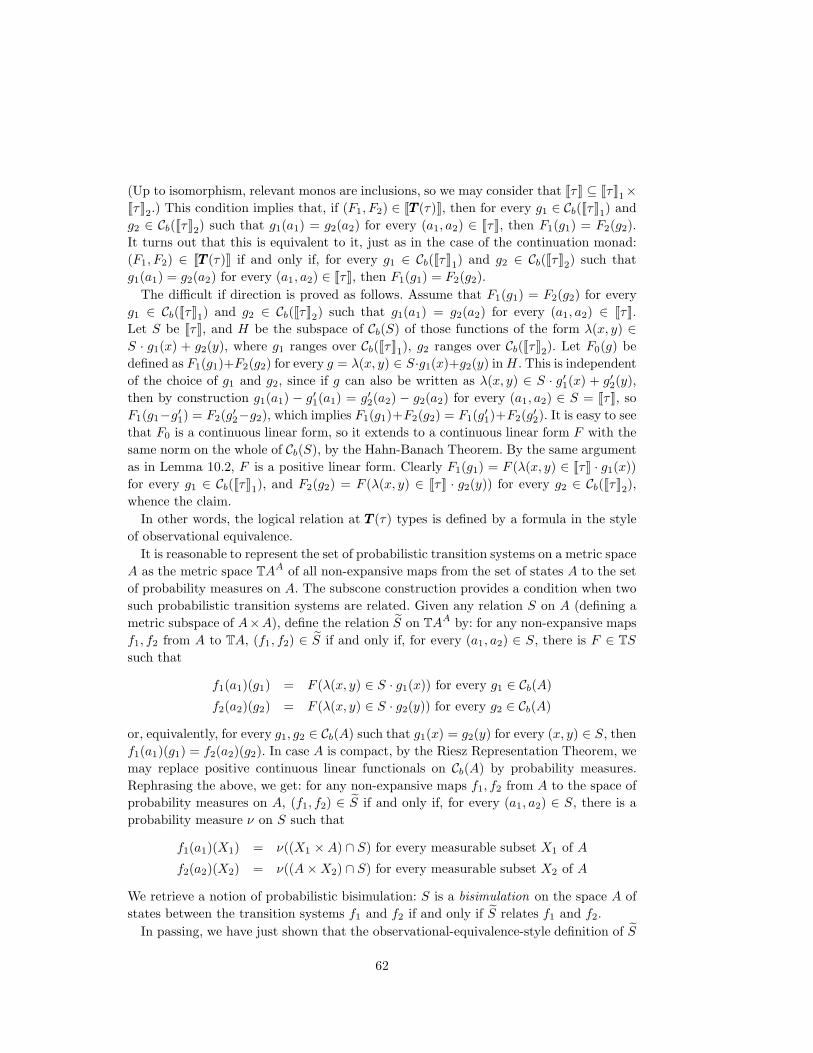
(Up to isomorphism, relevant monos are inclusions, so we may consider that JτK ⊆ JτK1×
JτK2.) This condition implies that, if (F1, F2) ∈ JTTT (τ)K, then for every g1 ∈ Cb(JτK1) and
g2 ∈ Cb(JτK2) such that g1(a1) = g2(a2) for every (a1, a2) ∈ JτK, then F1(g1) = F2(g2).
It turns out that this is equivalent to it, just as in the case of the continuation monad:
(F1, F2) ∈ JTTT (τ)K if and only if, for every g1 ∈ Cb(JτK1) and g2 ∈ Cb(JτK2) such that
g1(a1) = g2(a2) for every (a1, a2) ∈ JτK, then F1(g1) = F2(g2).
The difficult if direction is proved as follows. Assume that F1(g1) = F2(g2) for every
g1 ∈ Cb(JτK1) and g2 ∈ Cb(JτK2) such that g1(a1) = g2(a2) for every (a1, a2) ∈ JτK.
Let S be JτK, and H be the subspace of Cb(S) of those functions of the form λ(x, y) ∈
S · g1(x) + g2(y), where g1 ranges over Cb(JτK1), g2 ranges over Cb(JτK2). Let F0(g) be
defined as F1(g1)+F2(g2) for every g = λ(x, y) ∈ S·g1(x)+g2(y) in H . This is independent
of the choice of g1 and g2, since if g can also be written as λ(x, y) ∈ S · g′1(x) + g′2(y),
then by construction g1(a1) − g′1(a1) = g′2(a2) − g2(a2) for every (a1, a2) ∈ S = JτK, so
F1(g1−g′1) = F2(g′2−g2), which implies F1(g1)+F2(g2) = F1(g′1)+F2(g′2). It is easy to see
that F0 is a continuous linear form, so it extends to a continuous linear form F with the
same norm on the whole of Cb(S), by the Hahn-Banach Theorem. By the same argument
as in Lemma 10.2, F is a positive linear form. Clearly F1(g1) = F (λ(x, y) ∈ JτK · g1(x))
for every g1 ∈ Cb(JτK1), and F2(g2) = F (λ(x, y) ∈ JτK · g2(y)) for every g2 ∈ Cb(JτK2),
whence the claim.
In other words, the logical relation at TTT (τ) types is defined by a formula in the style
of observational equivalence.
It is reasonable to represent the set of probabilistic transition systems on a metric space
A as the metric space TAA of all non-expansive maps from the set of states A to the set
of probability measures on A. The subscone construction provides a condition when two
such probabilistic transition systems are related. Given any relation S on A (defining a
metric subspace of A×A), define the relation S on TAA by: for any non-expansive maps
f1, f2 from A to TA, (f1, f2) ∈ S if and only if, for every (a1, a2) ∈ S, there is F ∈ TS
such that
f1(a1)(g1) = F (λ(x, y) ∈ S · g1(x)) for every g1 ∈ Cb(A)
f2(a2)(g2) = F (λ(x, y) ∈ S · g2(y)) for every g2 ∈ Cb(A)
or, equivalently, for every g1, g2 ∈ Cb(A) such that g1(x) = g2(y) for every (x, y) ∈ S, then
f1(a1)(g1) = f2(a2)(g2). In case A is compact, by the Riesz Representation Theorem, we
may replace positive continuous linear functionals on Cb(A) by probability measures.
Rephrasing the above, we get: for any non-expansive maps f1, f2 from A to the space of
probability measures on A, (f1, f2) ∈ S if and only if, for every (a1, a2) ∈ S, there is a
probability measure ν on S such that
f1(a1)(X1) = ν((X1 × A) ∩ S) for every measurable subset X1 of A
f2(a2)(X2) = ν((A × X2) ∩ S) for every measurable subset X2 of A
We retrieve a notion of probabilistic bisimulation: S is a bisimulation on the space A of
states between the transition systems f1 and f2 if and only if S relates f1 and f2.
In passing, we have just shown that the observational-equivalence-style definition of S
62

coincides with the bisimulation-style definition, using the Riesz Representation Theorem.
This can be seen as a form of a completeness theorem.
The notion above is formally analogous to the notion of probabilistic bisimulation of
(Desharnais et al., 2002); i.e., the formulas we use and theirs for defining bisimulations
is the same. This is also formally analogous to metric bisimulations as introduced by
de Vink and Rutten (de Vink and Rutten, 1999) for ultrametric spaces, and extended
by Worrell (Worrell, 2000) to generalized metric spaces. A difference is that the latter
authors use a coalgebraic approach; in particular, their construction requires a T functor
that preserves isometric embeddings (our relevant monos), while we require it to preserve
pseudoepis (surjective non-expansive maps).
11. Related work.
One succesful approach to categorical generalization of logical relations is the setting
of (Hermida, 1993) based on fibrations. We do not assume in this paper the forgetful
functor to be a fibration, similarly to other authors (e.g. (Plotkin et al., 2000)). Even if
we lose thereby the equivalence to logic, this is justified, since we do not focus on logical
rules corresponding to logical relations in this paper.
We have already said that there is no unique notion of monad lifting. One of the
simplest is the lifting, proposed in (Crole and Pitts, 1992), T of TTT , which maps the object
〈S, f, A〉 of the scone to 〈S, |ηηηA|f,TTTA〉. This is a special case of our notion of lifting on the
scone (C ↓ | |) (Section 3), taking T the identity monad and σA = |ηηηA|. Turi (Turi, 1996)
considers lifting monads to the category of coalgebras of a given endofunctor. This is a
special case of our framework, when CCC = C (and TTT = T) and moreover only objects of
the form Sf // |S| are taken into consideration, and only morphisms of the form 〈g, g〉.
This defines the category of | |-coalgebras as a proper subcategory of scones. Turi uses
a simpler version of our monad morphisms, namely distributivity law of a monad over
an endofunctor; monad morphisms involve two monads and a functor between distinct
categories. Turi’s distributivity laws are similar enough to monad morphisms that we had
called the latter distributivity laws for monads in the conference version of this paper. This
also influenced (Goubault-Larrecq and Goubault, 2003), where comonad morphisms are
used, but are called distributivity laws for comonads. (This relies on pullbacks, whereas we
use mono factorization systems.) Calling these monad morphisms distributivities turned
out to be a bad choice, as distributivity laws denote a close but different concept, due to
Jon Beck (Beck, 1969); also, while distributivity laws tend to be rare, monad morphisms
abound.
In (Power and Watanabe, 2002) different possible ways to combine a monad and a
comonad were studied in a systematic way. In particular, the authors used a notion of a
distributivity of a monad over a comonad (and dual distributivity of the comonad over the
monad). This is a stronger notion than monad morphisms, as it requires commutativity
of two copies of diagrams (4), one for the monad and another one for the comonad. On
the other hand, both the monad and the comonad live in a single category, unlike in our
case.
We also note that neither Pitts nor Turi deal with subscones.
63

(Kinoshita and Power, 1999) consider lifting a monad on SetSetSet to the category of rela-
tions in SetSetSet. This is a particular case of our setting. However, the main topic of this
paper is a more complex situation of lax logical relations and data-refinement for the
computational lambda calculus. A subsequent paper (Power and Tanaka, 2000) develops
further the ideas of (Kinoshita and Power, 1999). It addresses in particular lax logical
relations for the computational lambda calculus and for the linear lambda calculus.
In the same way that we lift a monad to relations, Rutten (Rutten, 1998) defines an
extension of an endofunctor in SetSetSet to a category of relations. The latter has relations as
morphisms between sets. An endofunctor extends to relations iff it preserves weak pull-
backs(which in particular implies preserving monos), and if so, the extension is unique.
(This is actually a special case of a more general fact, proved in (Carboni et al., 1990)
for regular categories.) The approach taken by Rutten is different from ours, where rela-
tions are objects rather than morphisms. Hence, Rutten imposes a different functoriality
condition: the action of a lifted endofunctor on a composition of two relations must coin-
cide with a composition of actions of the lifted endofunctor on these two relations. This
amounts to closedness under composition of relations yielded by the lifted endofunctor.
(Pitts, 1991) proposes the Evaluation Logic for reasoning about programs with com-
putational effects. It is based on the computational lambda-calculus (Moggi, 1991). Se-
mantics of Pitts’ Evaluation Logic is studied further in (Moggi, 1995).
(Pitts, 1996) considers litfing of certain constructions on domains to relations on these
domains. He focuses on categories on domains and does not consider (strong) monads.
Instead of category of relations he assumes a relational structure, relaxing a notion of
mapping (morphism) of relations.
12. Conclusions
The main contribution of this paper is a natural extension of logical relations able to
deal with monadic types. We illustrate its naturality and its practical value by demon-
strating that various notions of bisimulations and a non-trivial notion of logical relation
for dynamic name creation are instances of our construction. Besides, our construction
provides a natural integration between notions of simulations for transition systems (pos-
sibly probabilistic), higher-order computation (the import of the λ-calculus), and limited
forms of side-effects (e.g., dynamic names), yielding streamlined criteria for observational
equivalence of those combined systems.
Acknowledgments
We are grateful to Masahito Hasegawa, John Power, Ian Stark, Paul-Andre Mellies,
Francois Lamarche, Vincent Danos, and Albert Burroni, and the anonymous referees for
their useful comments.
64

References
Abramsky, S. and Jung, A. (1994). Domain theory. In Abramsky, S., Gabbay, D. M.,
and Maibaum, T. S. E., editors, Handbook of Logic in Computer Science, volume 3,
pages 1–168. Oxford University Press.
Adamek, J., Herrlich, H., and Strecker, G. (1990). Abstract and Concrete Categories.
Wiley, New York.
Alimohamed, M. (1995). A characterization of lambda definability in categorical models
of implicit polymorphism. Theoretical Computer Science, 146(1–2):5–23.
Ambler, S. J. (1991). First Order Linear Logic in Symmetric Monoidal Closed Categories.
PhD thesis, University of Edinburgh.
Appelgate, H. (1965). Acyclic models and resolvent functors. PhD thesis, Columbia
University.
Barr, M. (1998). The separated extensional Chu category. Theory and Applications of
Categories, 4(6):137–147.
Beck, J. (1969). Distributive laws. In Seminar on Triples and Categorical Homology
Theory, pages 119–140. Springer-Verlag LNM 80.
Bourbaki, N. (1969). Integration, volume IX. Diffusion CCLS.
Carboni, A., Kelly, G. M., and Wood, R. J. (1990). A 2-categorical approach to change
of base and geometric morphisms I. Report 90-1, Department of Pure Mathematics,
University of Sydney.
Crole, R. and Pitts, A. (1992). New foundations for fixpoint computations: Fix-
hyperdoctrines and the fix-logic. Information and Computation, 98:171–210.
de Vink, E. P. and Rutten, J. J. M. M. (1999). Bisimulation for probabilistic transition
systems: A coalgebraic approach. Theoretical Computer Science, 221(1–2):271–293.
Desharnais, J., Edalat, A., and Panangaden, P. (2002). Bisimulation for labelled Markov
processes. Information and Computation, 179(2):163–193.
Eilenberg, S. and Kelly, G. M. (1966). Closed categories. In Proceedings of the Conference
on Categorical Algebra at La Jolla, pages 421–562. Springer-Verlag.
Escardo, M. and Heckmann, R. (2001–2002). Topologies on spaces of continuous func-
tions. Topology Proceedings, 26(2):545–564.
Escardo, M., Lawson, J., and Simpson, A. (2004). Comparing cartesian closed categories
of (core) compactly generated spaces. Topology and Its Applications, 143(1–3):105–
146.
Fiore, M. and Simpson, A. (1999). Lambda definability with sums via Grothendieck log-
ical relations. In Proceedings of the 4th International Conference on Typed Lambda-
Calculi and Applications (TLCA’99), pages 147–161. Springer-Verlag LNCS 1581.
Freyd, P. J. and Kelly, G. M. (1972). Categories of continuous functors i. Journal of
Pure and Applied Algebra, 2(3):169–191.
Gierz, G., Hofmann, K. H., Keimel, K., Lawson, J. D., Mislove, M., and Scott, D. S.
(1980). A Compendium of Continuous Lattices. Springer Verlag.
Gierz, G., Hofmann, K. H., Keimel, K., Lawson, J. D., Mislove, M., and Scott, D. S.
(2003). Continuous lattices and domains. In Encyclopedia of Mathematics and its
Applications, volume 93. Cambridge University Press.
65

Giry, M. (1981). A categorical approach to probability theory. In Banaschewski, B.,
editor, Categorical Aspects of Topology and Analysis, pages 68–85. Springer Verlag
LNM 915.
Goubault-Larrecq, J. (2005). Extensions of valuations. Mathematical Structures in Com-
puter Science, 15(2):271–297. An early version is available as LSV Research Report
LSV-02-17, Nov. 2002.
Goubault-Larrecq, J. and Goubault, E. (2003). On the geometry of intuitionistic S4
proofs. Homology, Homotopy and Applications, 5(2):137–209.
Goubault-Larrecq, J., Lasota, S., and Nowak, D. (2002). Logical relations for monadic
types. In Proceedings of the 16th International Workshop on Computer Science Logic
(CSL’02). Springer-Verlag LNCS 2471.
Heckmann, R. (1990). Power Domain Constructions (Potenzbereich-Konstruktionen).
PhD thesis, Universitat des Saarlandes.
Hermida, C. A. (1993). Fibrations, logical predicates and indeterminates. PhD thesis,
University of Edinburgh, Department of Computer Science. Also published as ECS-
LFCS-93-277.
Honsell, F. and Sannella, D. (2002). Prelogical relations. Information and Computation,
178:23–43.
Johnstone, P. (1975). Adjoint lifting theorems for categories of algebras. Bulletin of the
London Mathematical Society, 7:294–297.
Jones, C. (1990). Probabilistic Non-Determinism. PhD thesis, University of Edinburgh.
Technical Report ECS-LFCS-90-105.
Jung, A. (1990). The classification of continuous domains. In Proc. IEEE Symp. Logic
in Computer Science (LICS’90), pages 35–40. IEEE Computer Society Press.
Jung, A. and Tiuryn, J. (1993). A new characterization of lambda definability. In Proceed-
ings of the 1st International Conference on Typed Lambda-Calculi and Applications
(TLCA’93), pages 245–257. Springer Verlag LNCS 664.
Kinoshita, Y. and Power, J. (1999). Data-refinement for call-by-value programming lan-
guages. In Computer Science Logic, 13th International Workshop, CSL ’99, 8th
Annual Conference of the EACSL, Madrid, Spain, September 20-25, 1999, Proceed-
ings, pages 562–576.
Larsen, K. G. and Skou, A. (1991). Bisimulation through probabilistic testing. Informa-
tion and Computation, 94:1–28.
Lawvere, F. W. (1973). Metric spaces, generalized logic, and closed categories. Rendiconti
del Seminario Matematico e Fisico di Milano, 43:135–166.
Lazic, R. and Nowak, D. (2000). A unifying approach to data-independence. In Pro-
ceedings of the 11th Internal Conference on Concurrency Theory (CONCUR’2000),
pages 581–595. Springer-Verlag LNCS 1877.
Ma, Q. and Reynolds, J. C. (1992). Types, abstraction, and parametric polymorphism,
part 2. In 7th International Conference on Mathematical Foundations of Program-
ming Semantics (MFPS’91), pages 1–40. Springer-Verlag LNCS 598.
Mac Lane, S. (1971). Categories for the Working Mathematician, volume 5 of Graduate
Texts in Mathematics. Springer-Verlag.
Mitchell, J. C. (1996). Foundations for Programming Languages. MIT Press.
66

Mitchell, J. C. and Scedrov, A. (1993). Notes on sconing and relators. In Borger, E.,
Jager, G., Kleine Buning, H., Martini, S., and Richter, M. M., editors, Proceedings
of the 6th International Workshop on Computer Science Logic (CSL’92), pages 352–
378. Springer Verlag LNCS 702.
Moggi, E. (1991). Notions of computation and monads. Information and Computation,
93:55–92.
Moggi, E. (1995). A semantics for evaluation logic. Fundam. Inform, 22(1/2):117–152.
Pitts, A. and Stark, I. (1993). Observable properties of higher order functions that dy-
namically create local names, or: What’s new? In Borzyszkowski, A. and Soko lowski,
S., editors, Proceedings of the 18th International Symposium on Mathematical Foun-
dations of Computer Science (MFCS’93), pages 122–141. Springer-Verlag LNCS 711.
Pitts, A. M. (1991). Evaluation logic. In Birtwistle, G., editor, IVth Higher Order
Workshop, Banff 1990, Workshops in Computing, pages 162–189. Springer-Verlag,
Berlin.
Pitts, A. M. (1996). Relational properties of domains. Information and Computation,
127(2):66–90.
Plotkin, G., Power, J., Sannella, D., and Tennent, R. (2000). Lax logical relations.
In Proceedings of the 7th International Colloquium on Automata, Languages and
Programming (ICALP’2000), pages 85–102. Springer Verlag LNCS 1853.
Plotkin, G. D. (1980). Lambda-definability in the full type hierarchy. In Seldin, J. and
Hindley, J., editors, To H. B. Curry: Essays on Combinatory Logic, Lambda Calculus
and Formalism, pages 363–373. Academic Press.
Power, J. and Tanaka, M. (2000). Axiomatics for data refinement in call by value pro-
gramming languages.
Power, J. and Watanabe, H. (2002). Combining a monad and a comonad. Theoretical
Computer Science, 280(1–2):137–162.
Prawitz, D. (1965). Natural Deduction, A Proof-Theoretical Study. Almqvist and Wiskell,
Stockholm.
Ramsey, N. and Pfeffer, A. (2002). Stochastic lambda calculus and monads of proba-
bility distributions. In Proceedings of the 29th Annual ACM SIGPLAN-SIGACT
Symposium on Principles of Programming Languages (POPL’02), pages 154–165.
Reynolds, J. C. (1983). Types, abstraction and parametric polymorphism. In Proceedings
of the 9th World Computer Congress (IFIP’83), pages 513–523. North-Holland.
Rutten, J. (1998). Relators and metric bisimulations. In Proceedings of the 1th Workshop
on Coalgebraic Methods in Computer Science (CMCS ’98), volume 11 of ENTCS,
pages 1–7. Elsevier Science.
Stark, I. (1996). Categorical models for local names. Lisp and Symbolic Computation,
9(1):77–107.
Stark, I. (1998). Names, equations, relations: Practical ways to reason about new. Fun-
damenta Informaticae, 33(4):369–396.
Statman, R. (1985). Logical relations and the typed λ-calculus. Information and Control,
65(2–3):85–97.
Street, R. (1972). The formal theory of monads. Journal of Pure and Applied Algebra,
2:149–168.
67

Turi, D. (1996). Functorial Operational Semantics and its Denotational Dual. PhD thesis,
Free University, Amsterdam.
Wadler, P. (1992). Comprehending monads. Mathematical Structures in Computer Sci-
ence, 2:461–493.
Worrell, J. (2000). On Coalgebras and Final Semantics. PhD thesis, Keble College,
Oxford University Computing Laboratory.
Zhang, Y. (2005). Relations logiques cryptographiques — Qu’est-ce que l’equivalence
contextuelle des protocoles cryptographiques et comment la prouver ? PhD thesis,
Laboratoire Specification et Verification, Ecole Normale Superieure de Cachan.
Zhang, Y. and Nowak, D. (2003). Logical relation for dynamic name creation. In Pro-
ceedings of the 17th International Workshop on Computer Science Logic (CSL’03),
pages 575–588. Springer-Verlag LNCS 2803.
Appendix A. Monoidal Monads, Commutative Monads
A.1. From Mediators to Strengths and Dual Strengths
Let (T,,, d) be a monoidal monad. Let tA,B = dA,B (A ⊗ idTB), t′A,B = dA,B
(idTA ⊗ B). We show that t is a strength, t′ a dual strength, and that Diagrams (43)
and (44) commute.
Diagram (32). This is exactly Diagram (38).
Diagram (33). This is exactly Diagram (40).
Diagram (34). This is shown by the diagram below. The topmost row is tA⊗B,C , while
the bottommost composition of morphisms from T((A ⊗ B) ⊗ C) to T(A ⊗ (B ⊗ C)) is
idA ⊗ tB,C followed by tA,B⊗C .
(A ⊗ B) ⊗ TCA⊗B⊗id//A,B,TC
(A⊗B)⊗id
(40)
))RRRRRRRRRRR
(naturalityof )
T(A ⊗ B) ⊗ TCdA⊗B,C //
(mediator law (41))
T((A ⊗ B) ⊗ C)
TA,B,C
(TA ⊗ TB) ⊗ TC
dA,B⊗id
OO TA,TB,TC
TA ⊗ (TB ⊗ TC)
id⊗dB,C
//
(functorialityof ⊗)
TA ⊗ T(B ⊗ C)dA,B⊗C
// T(A ⊗ (B ⊗ C))
A ⊗ (B ⊗ TC)
A⊗(B⊗id)55lllllllllll
id⊗(B⊗id)// A ⊗ (TB ⊗ TC)
id⊗dB,C
// A ⊗ T(B ⊗ C)
A⊗id
OO
68

Diagram (35).
A ⊗ T2B
A⊗id//
id⊗B
(functorialityof ⊗)
TA ⊗ T2B
dA,TB//
TA⊗Tid ''OOOOOOOOO(naturality
of d)
id⊗B
(monadlaw)
++
T(A ⊗ TB)T(A⊗id)// T(TA ⊗ TB)
TdA,B// T2(A ⊗ B)A⊗B
T2A ⊗ T2B
dTA,TB
77nnnnnnnnnA⊗B
A ⊗ TB A⊗id
// TA ⊗ TB dA,B
//
(mediatorlaw (42))
T(A ⊗ B)
So is a strength. That ′ is a dual strength is proved similarly. We use Diagram (39)
instead of Diagram (38) to prove the dual form of Diagram (32).
Diagram (43). In the diagram below, the top row is tA,B ⊗ id followed by t′A⊗B,C , while
the bottom row is id ⊗ t′B,C followed by tA,B⊗C .
(A ⊗ TB)
⊗C
(A⊗id)
⊗id//
A,TB,C
(A⊗id)⊗C ++WWWWWWWWWWWWWWWWWWWWWW(functoriality
of ⊗)
(TA ⊗ TB)
⊗C
dA,B⊗id// T(A ⊗ B)
⊗C
id⊗C // T(A ⊗ B)
⊗TC
dA⊗B,C// T((A ⊗ B)
⊗C)
TA,B,C
(TA ⊗ TB) ⊗ TC
dA,B⊗id
77oooooooooTA,TB,TC
TA ⊗ (TB ⊗ TC)
id⊗dB,C
''OOOOOOOOO
A⊗
(TB ⊗ C)
id⊗
(id⊗C)//
A⊗(id⊗C)33gggggggggggggggggggggg
(functorialityof ⊗)
(naturalityof )
A⊗
(TB ⊗ TTTC) id⊗dB,C
// A⊗
T(T ⊗ C) A⊗id// TA⊗
T(B ⊗ C) dA,B⊗C
//
(mediatorlaw (41))
T(A⊗
(B ⊗ C))
Diagram (44). This is the diagram below, where the top row is tTA,B, the leftmost vertical
arrows form t′A,TB, the rightmost ones form Tt′A,B followed by A⊗B, and the bottom
row is TtA,B followed by A⊗B. Note that, as announced, the common diagonal from the
69

top left corner to the bottom right corner is dA,B.
TA ⊗ TBTA⊗id //
id⊗TB
id⊗idPPPPPPPPPPPP
(monad laws
and functor-iality of ⊗)
''PPPPPPPPPPPP
T2A ⊗ TB
dTA,B //
id⊗TB
(natur-ality ofd)
T(TA ⊗ B)
T(id⊗B)
T2A ⊗ T2BA⊗B
dTA,TB
WWWWWWW
++WWWWWW(mediatorlaw (42))
TA ⊗ T2BdA,TB
TA⊗id//
(natur-ality ofd)
T2A ⊗ T2BA⊗B //dTA,TB
@@@@
@@@@
@@@
@@@@
(mediatorlaw (42))
TA ⊗ TB dA,B
OOOOOOOOOOOO
''OOOOOOOOOOO
T(TA ⊗ TB)
TdA,B
T2(A ⊗ B)A⊗B
T(A ⊗ TB)
T(A⊗id)// T(TA ⊗ TB)
TdA,B
// T2(A ⊗ B) A⊗B
// T(A ⊗ B)
A.2. From Strengths and Dual Strengths to Mediators
Let (T,,) be a monad such that t is a strength and t′ is a dual strength making
Diagrams (43) and (44) commute. Let d be the common diagonal of Diagram (44), i.e.,dA,B = A⊗B Tt′A,B tTA,B = A⊗B TtA,B t′A,TB. We show that d is a mediator,
which means that we check Diagrams (38), (39), (40), (41), and (42). By convention, call
(32’), (33’), (34’), (35’) the dual diagrams satisfied by the dual strength t′.First, notice that tA,B = dA,B (A ⊗ idTB). Indeed, using the definition dA,B =A⊗B Tt′A,B tTA,B, dA,B (A ⊗ idTB) is the top row of the following diagram, whiletA,B is the bottom composition of arrows from A ⊗ TB to T(A ⊗ B).
A ⊗ TBA⊗idTB// tA,B
))RRRRRRRRRRRRRRRRRRRRRRR TA ⊗ TBtTA,B // TTA ⊗ B
Tt′A,B // T2(A ⊗ B)A⊗B // T(A ⊗ B)
T(A ⊗ B)
T(A⊗idB)
OO(naturality
of t) TA⊗Bwwwwww
(33′)
;;wwwwww
idT(A⊗B)
(monad law)
??
Diagram (38) is then just Diagram (32).
Diagram (39). Similarly, t′A,B = dA,B(idTA⊗B) (here we use the other characterization
of dA,B as A⊗B TtA,B t′A,TB and (33)), so Diagram (39) is just Diagram (32’).
Diagram (40). Immediate using (33) and tA,B = dA,B (A ⊗ idTB): dA,B (A ⊗ B) =tA,B (A idB) = A⊗B.
Diagram (41). This one is harder, and is proved by considering the diagram below. Thetop row is dA,B ⊗ idTC , the rightmost vertical arrows form dA⊗B,C followed by TA,B,C ,while the leftmost ones form TA,TB,TC followed by idTA ⊗ dB,C , and the bottommost
70

row is dA,B⊗C .
(TA ⊗ TB)
⊗TC
t′A,TB
⊗id//
TA,TB,TC
(dualstrength
law(34’))
T(A ⊗ TB)
⊗TC
TtA,B
⊗id//t′A⊗TB,TC
(natur-alityof t′) T
2(A ⊗ B)
⊗TCt′T(A⊗B),TC
A⊗B⊗id //
(dual strengthlaw (35’))
T(A ⊗ B)
⊗TCt′A⊗B,TC
T((A ⊗ TB)
⊗TC)
T(tA,B
⊗id)
//
TA,TB,TC
((43))
T(T(A ⊗ B)
⊗TC)
Tt′A⊗B,TC
T((A ⊗ B)
⊗TC)
TtA⊗B,C
TA⊗
(TB ⊗ TC)
t′A,TB⊗TC//
id⊗t′B,TC
(natur-alityof t′)
T(A⊗
(TB ⊗ TC))
T(id⊗t′B,TC)
T2((A
⊗B)
⊗TC)
T2A,B,TC
T2tA⊗B,C
//
(T2 ofstrength
law(34))
(A⊗B)⊗TChhhhhhhhhhhhhhhh
33hhhhhhhhhhhhhh
T3((A
⊗B)
⊗C)
T3A,B,C
T""E
EEEE
EEE
(natur-ality of
T)
T((A⊗B)⊗C) //
(monad law)
(naturality of )
T2((A ⊗ B)
⊗C)
TA⊗
T(B ⊗ TC)
id⊗TtB,C
T(A⊗
T(B ⊗ TC))
T(id⊗TtB,C )
TtA,B⊗TC//
(natur-alityof Tt) T
2(A⊗
(B ⊗ TC))
T2(id⊗tB,C )
T2((A ⊗ B)
⊗C)
T2A,B,C
(natur-alityof )
// T((A ⊗ B)
⊗C)
TA,B,C
TA⊗
T2(B ⊗ C)
id⊗B⊗C
T(A⊗
T2(B ⊗ C))
T(id⊗B⊗C )
TtA,T(B⊗C)//
(T of strengthlaw (35))
T2(A⊗
T(B ⊗ C))
T2tA,B⊗C// T
3(A⊗
(B ⊗ C))
TA⊗(B⊗C)
HHH
##HHH
TA⊗
T(B ⊗ C)
t′A,T(B⊗C)// T(A⊗
T(B ⊗ C)) TtA,B⊗C
// T2(A⊗
(B ⊗ C)) // T(A⊗
(B ⊗ C))
Diagram (42). First, we notice thatA⊗B TdA,B t′TA,TB = dA,B (A ⊗ idTB) (64)
This is shown using the
diagram on the right.
The left-hand side is the
path from the top left
corner to the bottom
right corner on the right
that goes down then
right, and the right-
hand side is the path go-
ing right then down.
T2A ⊗ TB
A⊗id //t′TA,TB (dual strength
law (35’))
TA ⊗ TBt′A,TBT(TA ⊗ TB)
TtA,TB
T(A ⊗ TB)
TtA,BT2(A ⊗ TB)
A⊗TBhhhh
33hhhhh
T2tA,B
(naturalityof )
T2(A ⊗ B)A⊗B
T3(A ⊗ B)
T(A⊗B)hhhhh
33hhhhh
TA⊗B
(monad law)
T2(A ⊗ B) A⊗B
// T(A ⊗ B)
By symmetry, the following also holds:A⊗B TdA,B tTA,TB = dA,B (idTA ⊗ B) (65)
Diagram (42) then follows. The top row below is dTA,TB, while the leftmost vertical
71

arrows form A ⊗ B.
T2A ⊗ T2Bt
T2A,TB//A⊗idT2B
(natur-alityof t)T(T2A ⊗ TB)
Tt′TA,TB//
T(A⊗idTB)
(64)
T2(TA ⊗ TB)TA⊗TB//
T2dA,B
(naturalityof )
T(TA ⊗ TB)
TdA,B
T3(A ⊗ B)
T(A⊗B) //
TA⊗B
(monadlaw)
T2(A ⊗ B)A⊗B
TA ⊗ T2B tTA,TB
//
idTA⊗B
(65)
T(TA ⊗ TB)TdA,B
// T2(A ⊗ B)A⊗B ''OOOOOOOOOOOO
TA ⊗ TB dA,B
// T(A ⊗ B)
A.3. Monoidal Monad Morphisms
We first show that every monoidal monad morphism from (TTT ,ηηη,µµµ,ddd) to (T,,, d) is
both a strong monad morphism from (TTT ,ηηη,µµµ, ttt) to (T,,, t) and (by symmetry) a dual
strong monad morphism from (TTT ,ηηη,µµµ, ttt′) to (T,,, t′), where tA,B = dA,B(A⊗idTB),t′A,B = dA,B (idTA ⊗ B). This is by the following diagram.
|A1| ⊗ T|A2||A1|⊗id
//
|ηηηA1 |⊗σA2
(4)
((RRRRRRRRRRRRR
id⊗σA2
T|A1| ⊗ T|A2|d|A1|,|A2| //
σA1⊗σA2
(monoidal
monadmorphism
(45))
T(|A1| ⊗ |A2|)
T(A1,A2 )
|A1| ⊗ |TTTA2|
|A1|⊗id//A1,TTT A2
(naturalityof )
|TTTA1| ⊗ |TTTA2|TTT A1,TTT A2
T|A1 ⊗⊗⊗ A2|
σA1⊗⊗⊗A2
|A1| ⊗⊗⊗ TTTA2
|ηηηA1⊗⊗⊗id|// |TTTA1 ⊗⊗⊗TTTA2|
|dddA1,A2 |// |TTT (A1 ⊗⊗⊗ A2)|
Conversely, let σ be both a strong monad morphism from (TTT ,ηηη,µµµ, ttt) to (T,,, t) and
a dual strong monad morphism from (TTT ,ηηη,µµµ, ttt′) to (T,,, t′). Let d be the common
diagonal of Diagram (44), i.e., dA,B = A⊗B Tt′A,B tTA,B = A⊗B TtA,B t′A,TB.
Define ddd similarly.
In the diagram below, the top row is d|A1|,T|A1| , while the leftmost vertical arrows from
72

σA1⊗ σA2
followed by TTTA1,TTTA2. The bottom row is |dddA1,A2 | followed by |µµµA1⊗⊗⊗A2 |.
T|A1| ⊗ T|A2|t′|A1|,T|A2|//
id⊗σA2
(naturalityof t′) T(|A1| ⊗ T|A2|)
Tt|A1|,|A2|//
T(id⊗σA2)
(strongmonad
morphism(45))
T2(|A1| ⊗ |A2|)
|A1|⊗|A2|//
T2A1,A2
(natur-alityof )
T(|A1| ⊗ |A2|)
TA1,A2
T|A1| ⊗ |TTTA2|t′|A1|,|TTTA2|
//
σA1⊗id
(dualstrongmonad
morphism(45’))
T(|A1| ⊗ |TTTA2|)
TA1,TTT A2
T2|A1 ⊗⊗⊗ A2|
TσA1⊗⊗⊗A2
|A1⊗⊗⊗A2|
//
(monadmorph-ism (4))
T|A1 ⊗⊗⊗ A2|
σA1⊗⊗⊗A2
|TTTA1| ⊗ |TTTA2|TTT A1,TTT A2
T|A1 ⊗⊗⊗TTTA2|
σA1⊗⊗⊗TTT A2
T|tttA1,A2 |//
(naturalityof σ)
T|TTT (A1 ⊗⊗⊗ A2)|
σTTT (A1⊗⊗⊗A2)
|TTTA1 ⊗⊗⊗ TTTA2|
|ttt′A1,TTTA2|// |TTT (A1 ⊗⊗⊗ TTTA2)|
|TTTtttA1,A2 |//∣∣TTT 2(A1 ⊗⊗⊗ A2)
∣∣|µµµA1⊗⊗⊗A2 |
// |TTT (A1 ⊗⊗⊗ A2)|
A.4. Commutative Monads are Monoidal
Let (T,,, ) be a strong monad on a symmetrical monoidal category. Let t′A,B be
the dual strength T B,A tB,A TA,B. That T is a commutative monad means that
Diagram (44) commutes. To show that dA,B = A⊗BTt′A,BtTA,B = A⊗BTtA,Bt′A,TB
is a mediator, it then suffices to show that Diagram (43) commutes. In the diagram below,
the top row is tA,B ⊗ idC followed by t′A⊗B,C , the bottom row is idA ⊗ t′B,C followed
by tA,B⊗C . The two triangles involving on the left side are instances of the identity = id.
(A ⊗ TB)
⊗C
tA,B⊗id// $$I
IIIIIIII
id
T(A ⊗ B)
⊗C // C⊗
T(A ⊗ B)
tC,A⊗B // T(C⊗
(A ⊗ B))T //
(T ofcoher-ence(25))
T((A ⊗ B)
⊗C)
TA,B,C
(A ⊗ TB)
⊗CA,TB,C
(coher-ence(25))
C⊗
(A ⊗ TB)
id⊗tA,B
::uuuuuuuuu
(naturalityof ) oo T((C ⊗ A)
⊗B)
TC,A,B
OO
T( ⊗id)
(C ⊗ A)
⊗TB
C,A,TB
OO
⊗id
tC⊗A,B
(strengthlaw
(34))44jjjjjjjjjjjjjjjjjjjjjjjj
T((A ⊗ C)
⊗B)
TA,C,B
A⊗
(TB ⊗ C)
id
(A ⊗ C)
⊗TBA,C,TB
tA⊗C,B
(naturalityof t) 44jjjjjjjjjjjjjjjjjjjjjjjj
T(A⊗
(C ⊗ B))
T(id⊗ )%%J
JJJJJJJJ
A⊗
(TB ⊗ C) id⊗ // A⊗
(C ⊗ TB)
id⊗ ddIIIIIIIII
id⊗tC,B
//
(strengthlaw (34))
A⊗
T(C ⊗ B)
tA,C⊗B
::ttttttttt
id⊗T // A⊗
T(B ⊗ C) tA,B⊗C
//
(naturalityof t)
T(A⊗
(B ⊗ C))
73

We now observe that Diagram (47) commutes:
TA ⊗ TB //
TB ⊗ TAtTB,A// T(TB ⊗ A)
T // T(A ⊗ TB)TtA,B// T2(A ⊗ B)
A⊗B//
(naturalityof )
T(A ⊗ B)
T
TB ⊗ TA
id
99tttttttttt tTB,A
// T(TB ⊗ A)T // T(A ⊗ TB)
TtA,B
// T2(A ⊗ B)T2 //id
99ssssssssssT
2(B ⊗ A)B⊗A
// T(B ⊗ A)
Indeed, the leftmost triangle is by = id, the inner parallelogram obviously commutes,
and the top and bottom rows are the two ways of writing dA,B.
Conversely, given any monoidal monad
making Diagram (47) commute, we
claim that the derived strength t and
dual strength t′ are related by t′A,B =
T B,A tB,A TA,B. Equivalently, since = id, we check that t′A,B B,TA =
T B,A tB,A. This is obvious:
B ⊗ TA B,TA //B⊗idTA
(naturalityof )
TA ⊗ B
idTAB
TB ⊗ TA TB,TA
dB,A //
(47)
T(B ⊗ A)
T B,A
TA ⊗ TB dA,B
// T(A ⊗ B)
Appendix B. Proof of Lemma 8.3
We first check that (D, ID,⊗D, αD, ℓD, rD) is a monoidal category. Write the notion of
composition in D = Kleisli(T ), i.e., gf = µ Tg f .
— Functoriality of ⊗D. First, ⊗D applied to the identity on (A, B) is idA ⊗D idB =
idFT (A) ⊗D idFT (B) = FT (idA) ⊗D FT (idB) = FT (idA ⊗C idB) = FT (idA⊗CB) =
idFT (A⊗CB) = idA⊗DB.
Second, ⊗D preserves composition. Indeed, let f, f ′, g, g′ be morphisms from A to B,from A′ to B′, from B to C and from B′ to C′ respectively in D. Then the compositionof g⊗Dg′ with f⊗Df ′ in D is the morphism µC⊗CC′T (dC,C′(g⊗Cg′))dB,B′(f⊗Cf ′)in C. The following diagram then commutes:
A ⊗C A′f⊗Cf ′
//
(gf)⊗C(g′f ′)
--
TB ⊗C TB′dB,B′
//
Tg⊗CTg′
(naturality
of d)
T (B ⊗C B′)
T (g⊗Cg′)T 2C ⊗C T 2C′
dTC,T C′
//
µC⊗CµC′
IIIIIII
$$III
IIII
(42)
T (TC ⊗C TC′)
TdC,C′
T 2(C ⊗C C′)
µC⊗CC′
T (C ⊗C C′)
The top right route from A ⊗C A′ to T (C ⊗C C′) is (g ⊗D g′)(f ⊗D f ′), while the
straight line diagonal is (gf) ⊗D (g′f ′).— Naturality of αD. Let f , g, h be morphisms from A to A′, B to B′ and C to C′
respectively in D. Then αD composed in D with (f ⊗D g) ⊗D h is µ T (η αC) d ((d (f ⊗C g)) ⊗C h) = TαC d (d ⊗C id) ((f ⊗C g) ⊗C h) (the route going all theway down then right from the top left corner to the bottom right corner below), while
74

f ⊗D (g ⊗D h) composed with αD in D is µ T (d (f ⊗C (d (g ⊗C h)))) η αC =µTdT (id⊗C d)T (f ⊗C (g⊗C h))η αC (the other route, going right then down).
(A ⊗C B) ⊗C CαC
//
(f⊗Cg)⊗Ch
(naturality
of αC)
A ⊗C (B ⊗C C)η //
f⊗C(g⊗Ch)
(natur-alityof η)
T (A ⊗C (B ⊗C C))
T (f⊗C(g⊗Ch))
(TA′ ⊗C TB′)
⊗CTC′
dA′,B′⊗C idT C′
αC
//
(mediatorlaw (41))
TA′ ⊗C (TB′ ⊗C TC′)
idT A′⊗CdB′,C′
T (TA′⊗C
(TB′ ⊗C TC′))
T (idT A′⊗CdB′,C′ )
T (A′ ⊗C B′)
⊗CTC′
dA′⊗CB′,C′
TA′⊗C
T (B′ ⊗C C′)
dA′,B′⊗CC′
T (TA′⊗C
T (B′ ⊗C C′))
TdA′,B′⊗CC′
T ((A′ ⊗C B′)
⊗CC′) TαC
// T (A′ ⊗C (B′ ⊗C C′)) η//
idT (A′⊗C(B′⊗CC′))
(monad law)
''PPPPPPPPPPPPPPP
T 2(A′⊗C
(B′ ⊗C C′))
µA′⊗C(B′⊗CC′)
T (A′⊗C
(B′ ⊗C C′))
— Naturality of ℓD. Let f be any morphism from B to B′ in D. Then the composition off with ℓD in D is µ Tf η ℓC (route going right then down), while the compositionof ℓD with (idD ⊗D f) is µ T (η ℓC) d (η ⊗C f) (dented route going down thenright).
IC ⊗C BℓC //
idIC
⊗Cf
(naturality
of ℓC)
BηB //
f
(naturalityof η)
TB
Tf
IC ⊗C TB′ ℓCTB′
//
ηIC
⊗idT B′
TB′ ηTB′ //
idT B′
HHHHHH
H(monad
law)
$$HHHH
HHHTηB′
T 2B′
µB
TIC ⊗C TB′
dIC ,B′
(38)
T (IC ⊗C B′)
TℓCB′
99sssssssssssssssss
T 2B′µB′ // TB′
— Naturality of rD is obtained similarly, using (39) instead of (38).
— αD, ℓD, rD are isomorphisms: indeed αD = FT (αC), αC is an isomorphism, and every
functor preserves isomorphisms. Similarly for ℓD and rD. Since they are natural, they
are natural isomorphisms.
— Pentagon identity (14). We have to check that (dropping subscripts) αDαD =
(idD ⊗D αD)αD(αD ⊗D idD). Note that the left-hand side is µ T (η αC) η αC =
TαC η αC = η αC αC (by naturality of η, Tf η = η f for any f). Now notice
75

that by (40), d (η ⊗C η) = η. Also, µ Tη = id. So the right-hand side is:
µ T (d (η ⊗C (η αC))) [αD(αD ⊗D idD)]
= µ T (d (η ⊗C η)) T (id ⊗C αC) [αD(αD ⊗D idD)]
= µ Tη T (id ⊗C αC) [αD(αD ⊗D idD)] (by (40))
= T (id ⊗C αC) [αD(αD ⊗D idD)]
= T (id ⊗C αC) µ T (η αC) (αD ⊗D idD)
= T (id ⊗C αC) TαC (αD ⊗D idD)
= T (id ⊗C αC) TαC d ((η αC) ⊗C η)
= T (id ⊗C αC) TαC d (η ⊗C η) (αC ⊗C id)
= T (id ⊗C αC) TαC η (αC ⊗C id) (by (40))
= η (id ⊗C αC) αC (αC ⊗C id) (by naturality of η)
and we are done, since by the pentagon identity (14) for αC , αC αC = (id ⊗C αC)
αC (αC ⊗C id).
— Triangle identity (15). We must check that (idD ⊗D ℓD)αD = rD . The left-hand side
is µ T (d (η ⊗C (η ℓC)) η αC = µ T (d (η ⊗C η) (id ⊗C ℓC)) η αC =
µ T (η (id ⊗C ℓC)) η αC (by (40)) = T (id ⊗C ℓC) η αC (by the monad laws)
= η (id ⊗C ℓC) αC (by naturality of η) = η rC (by the triangle identity (15) in C)
= rD , which is the right-hand side.
We must now check that FT ⊣ UT is a monoidal adjunction. We already know that it
is an adjunction.
— (θFT , ιFT ) is mediating for F . Indeed, both θFT
A,B and ιFT are just identity morphisms
in D, from which the coherence conditions (16), (17) and (18) are clear. The first
reduces to showing that FT (αC) = αD, the second to FT (ℓC) = ℓD, the third to
FT (rC) = rD, which hold by construction.
— (θUT , ιUT ) is mediating for UT . Indeed, the first coherence condition (16) is just Di-
agram (41), since UT αD = UT FT αC = TαC. The second coherence condition (17) is
exactly Diagram (38), and the third, (18), is exactly Diagram (39).
— The unit η and the counit ǫ are monoidal natural transformations. (Recall that ǫA
is the identity morphism from TA to TA in C, seen as a morphism from TA to A
in D.) Indeed, Diagram (49) (in C) means that ηIC = UT (ιFT ) ιUT = UT (id) ηIC ,
which is obvious. Diagram (50) states that UT (θFT
A,B)θUT (ηA⊗C ηB) = ηA⊗CB, i.e.,
dA,B (ηA ⊗C ηB) = ηA⊗CB, which is just Diagram (40). Turning to diagrams in D,
Diagram (51) means that ǫIDFT (ιUT )ιFT is the identity in D; seen as a morphism
in C, this is
µ T (id) [FT (ιUT )ιFT ] = µ [FT (ιUT )ιFT ]
= µ µ T (FT (ιUT )) ιFT
= µ µ T (ηTIC ηIC) ηIC = ηIC
(by the monad laws), and the latter is just the identity on ID in D, as required. Finally,
Diagram (52) means that ǫA⊗DBFT θUT θFT = ǫA ⊗D ǫB. Seen as a morphism in C,
76

the left-hand side is
µA⊗CB T ǫA⊗DB [FT θUT θFT ]
= µA⊗CB T id [FT θUT θFT ]
= µA⊗CB [FT θUT θFT ]
= µA⊗CB µT (A⊗CB) T (FT θUT ) θFT
= µA⊗CB µT (A⊗CB) T (ηT (A⊗CB) dA,B) ηA⊗CB
which we recognize as the long trip in the diagram below from the top left cornerthat goes down, right, and up to the top right corner.
TA ⊗C TB
ηA⊗CB
dA,B //(natur-alityof η)
T (A ⊗C B)id
T (A⊗CB) //
ηT (A⊗CB)
(monad law)
T (A ⊗C B)
T (TA ⊗C TB)TdA,B
// T 2(A ⊗C B)
TηT (A⊗CB) ''OOOOOOOOOOO
idT2(A⊗CB)
(monad law)// T 2(A ⊗C B)
µA⊗CB
OO
T 3(A ⊗C B)
µT (A⊗CB)
77ooooooooooo
Then the composition of arrows from the top left corner to the top right corner is
dA,B. This is exactly the desired morphism ǫA⊗D ǫD of D, which, seen as a morphism
of C, is dA,B (idTA ⊗C idTB) by definition.
We check finally that FT ⊣ UT generates the monoidal monad. The only thing to check
is dA,B = UT θFT
A,B θUT
FT (A),FT (B). This is clear, since the right-hand side is UT (idA⊗DB)
dA,B = dA,B.
Appendix C. Composition of Monoidal Adjunctions
We first show that |U | is a monoidal functor, with mediating pair (∣∣θU
∣∣ , ∣∣ιU ∣∣ i).We must check all three coherence conditions (16), (17), (18).
77

Diagram (16).
(|U(A)| ⊗ |U(B)|)
⊗|U(C)|
//⊗id|U(C)|
(coherence (16) for ) |U(A)|⊗
(|U(B)| ⊗ |U(C)|)
id|U(A)|⊗|U(A)⊗⊗⊗ U(B)|
⊗|U(C)| ''OOOOOOOO
|θU |⊗id|U(C)|
|U(A)|⊗
|U(B)⊗⊗⊗ U(C)|wwoooooooo
id|U(A)|⊗|θU |
˛
˛U(A ⊗D B)˛
˛
⊗|U(C)| (natur-ality of)
(| | applied to coherence (16) for θU )
˛
˛
˛
˛
˛
˛
˛
(U(A)
⊗⊗⊗U(B))
⊗⊗⊗U(C)
˛
˛
˛
˛
˛
˛
˛
|ααα| //
|θU⊗⊗⊗idU(C)|wwpppppppp
˛
˛
˛
˛
˛
˛
˛
U(A)⊗⊗⊗
(U(B)⊗⊗⊗
U(C))
˛
˛
˛
˛
˛
˛
˛
|idU(A)⊗⊗⊗θU | ''NNNNNNNN
(natur-ality of) |U(A)|⊗
˛
˛U(B ⊗D C)˛
˛˛
˛
˛
˛
˛
U(A ⊗D B)
⊗⊗⊗U(C)
˛
˛
˛
˛
˛
|θU |
˛
˛
˛
˛
˛
U(A)⊗⊗⊗
U(B ⊗D C)
˛
˛
˛
˛
˛
|θU |˛
˛
˛
˛
˛
U((A ⊗D B)
⊗DC)
˛
˛
˛
˛
˛ |UαD|//
˛
˛
˛
˛
˛
U(A⊗D
(B ⊗D C))
˛
˛
˛
˛
˛
Diagram (17).
I ⊗ |UA| l|UA|
((RRRRRRRRRRRRRRRRRRRRRRRRRRRRRRRRRRRRi⊗id|UA|
|III| ⊗ |UA|
(coherencecondition
(17))|ιU |⊗id|UA|
III,UA
))SSSSSSSSSSSSSSS
˛
˛UID˛
˛ ⊗ |UA|UID ,UA
(natur-alityof ) |III ⊗⊗⊗ UA|
|ιU⊗⊗⊗idUA|uullllllllllllll|ℓℓℓUA| // |UA|
˛
˛UID ⊗⊗⊗ UA˛
˛
(coherencecondition
(17))
˛˛θU
ID ,A
˛˛
˛
˛U(ID ⊗D A)˛
˛
|UℓDA |
66mmmmmmmmmmmmmmmmmmmmmmmmmmmmmmmmmmmm
Diagram (18). This is checked by a diagram similar to the latter.
By the same reasoning, FDDD is also a monoidal functor, with mediating pair (Fθθθ
θF , Fiii ιF ).
We now check the monoidal adjunction conditions (49), (50), (51), (52). Let ǫ the
counit, and η the unit of DDD ⊣ | |, and ǫǫǫ the counit, and ηηη the unit of F ⊣ U .
78

Diagram (49).
Ii //
ηi((49) for DDD ⊣ | |)
))RRRRRRRRRRRRRRRRRRR |III||ιU |
//
|iii|
|ηηηIII |
((49) for F ⊣ U)
))TTTTTTTTTTTTTTTTTTTT˛
˛UID˛
˛
|UιF |
|DDDI|
|ηηηDDDI| ))TTTTTTTTTTTTTTTTTT(naturality
of |ηηη |)|UFIII|
|UF ID|
|UFDDDI|
Diagram (50).
A ⊗ BηA⊗ηB //
ηA⊗B
((50) forDDD ⊣ | |)
|DDDA| ⊗ |DDDB||ηηηDDDA|⊗|ηηηDDDB | //DDDA,DDDB
rrrr
yyrrrr
(natur-alityof ) |UFDDDA| ⊗ |UFDDDB|UFDDDA,UFDDDBxxqqqqqqqqqq
|DDDA⊗⊗⊗DDDB|
|θθθA,B|ww
w
www
|ηηηDDDA⊗⊗⊗ηηηDDDB | //
|ηηηDDDA⊗⊗⊗DDDB|
((50) forF ⊣ U)
|UFDDDA⊗⊗⊗ UFDDDB|
|θUFDDDA,FDDDB |xxrrrrrrrrrr
|DDD(A ⊗ B)|
|ηηηDDD(A⊗B)|
(natur-ality
of |ηηη |)
˛
˛U(FDDDA ⊗D FDDDB)˛
˛
|UθFDDDA,DDDB|yyssssssssss
|UF (DDDA⊗⊗⊗DDDB)|
|UFθθθA,B|vvvvv
vvvv
|UFDDD(A ⊗ B)|
Diagrams (51) and (52) are dealt with similar, and give rise to similar verifications.
Appendix D. Proof of Proposition 8.6
Diagram (32) is obtained by considering the following diagram. We drop subscripts onnatural transformations so as to save space; they can be inferred from context.
I ⊗ |TTTDDDF |ηI⊗id//i⊗idOOO
OO(49)
''OOOOO l|TTTDDDF | 22
(17)
|DDDI| ⊗ |TTTDDDF | // |DDDI⊗⊗⊗TTTDDDF |
|ttt| // |TTT (DDDI⊗⊗⊗DDDF )||TTTθθθ| // |TTTDDD(I ⊗ F )|
|TTTDDDlF |
|III | ⊗ |TTTDDDF |
|iii|⊗id
OO //
(natural-ity of )
|III ⊗⊗⊗ TTTDDDF |
|iii⊗⊗⊗id|
OO
|ttt|//
(natural-ity of |TTT |)
|ℓℓℓTTTDDDF | 11
|TTT (III ⊗⊗⊗DDDF )|
|TTT (iii⊗⊗⊗id)|
OO
|TTTℓℓℓDDDF |PPP
PP
''PPPPP
|TTT (17)|
(32)
|TTTDDDF |
We have also decorated the interior of each face with the justification why its edges
commute. For example, the top left triangle is a copy of (49), one of the diagrams stating
79
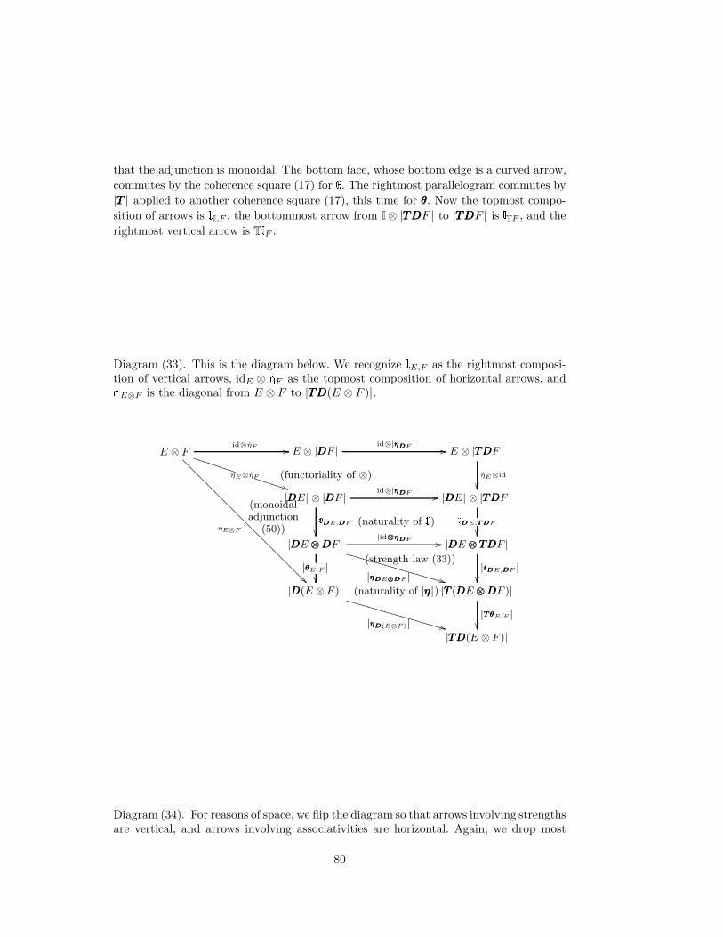
that the adjunction is monoidal. The bottom face, whose bottom edge is a curved arrow,
commutes by the coherence square (17) for . The rightmost parallelogram commutes by
|TTT | applied to another coherence square (17), this time for θθθ. Now the topmost compo-
sition of arrows is tI,F , the bottommost arrow from I⊗ |TTTDDDF | to |TTTDDDF | is lTF , and the
rightmost vertical arrow is TlF .
Diagram (33). This is the diagram below. We recognize tE,F as the rightmost composi-tion of vertical arrows, idE ⊗ F as the topmost composition of horizontal arrows, andE⊗F is the diagonal from E ⊗ F to |TTTDDD(E ⊗ F )|.
E ⊗ Fid⊗ηF //
ηE⊗ηF
TTTTTTTT
**TTTTTT (functoriality of ⊗)
ηE⊗F
???
????
????
????
????
????
????
???
(monoidaladjunction
(50))
E ⊗ |DDDF |id⊗|ηηηDDDF | // E ⊗ |TTTDDDF |
ηE⊗id
|DDDE| ⊗ |DDDF |
id⊗|ηηηDDDF | //DDDE,DDDF
(naturality of ) |DDDE| ⊗ |TTTDDDF |DDDE,TTTDDDF
|DDDE ⊗⊗⊗DDDF |
|id⊗⊗⊗ηηηDDDF | //
|ηηηDDDE⊗⊗⊗DDDF |
(strength law (33))
**VVVVVVVVVVVVVVVVVV
|θθθE,F |
|DDDE ⊗⊗⊗ TTTDDDF |
|tttDDDE,DDDF |
|DDD(E ⊗ F )|
|ηηηDDD(E⊗F )| **VVVVVVVVVVVVVVVVVV(naturality of |ηηη |) |TTT (DDDE ⊗⊗⊗DDDF )|
|TTTθθθE,F |
|TTTDDD(E ⊗ F )|
Diagram (34). For reasons of space, we flip the diagram so that arrows involving strengthsare vertical, and arrows involving associativities are horizontal. Again, we drop most
80
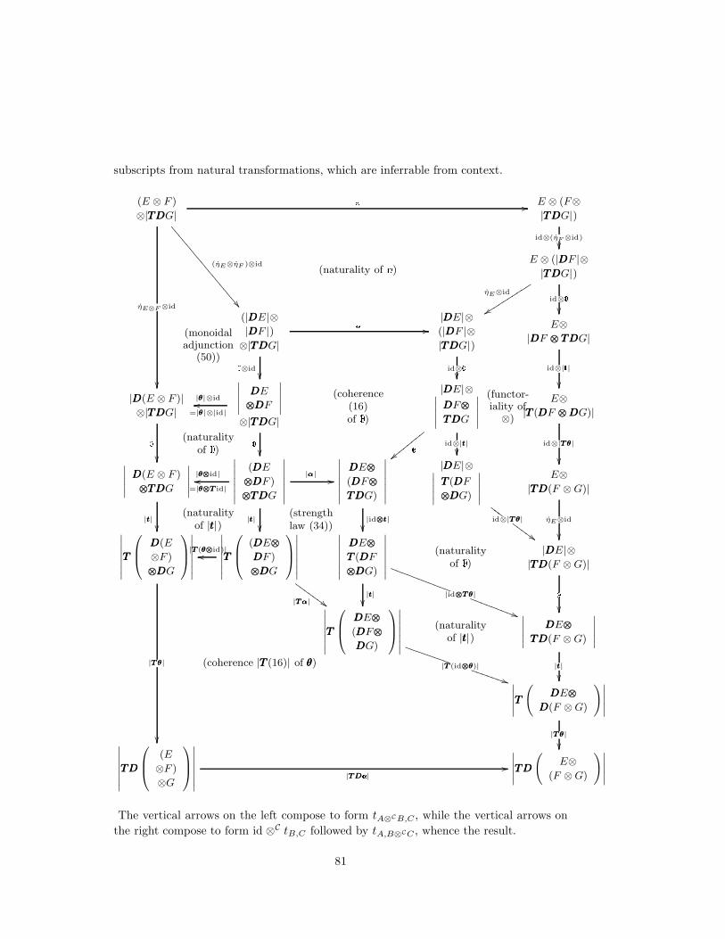
subscripts from natural transformations, which are inferrable from context.
(E ⊗ F )
⊗|TTTDDDG|
(naturality of )
(monoidaladjunction
(50))
//
(ηE⊗ηF )⊗id
:::
::::
::::
::::
:::
ηE⊗F ⊗id
E ⊗ (F⊗
|TTTDDDG|)
id⊗(ηF ⊗id)
E ⊗ (|DDDF |⊗
|TTTDDDG|)
ηE⊗id
yyssssssssssid⊗
(|DDDE|⊗
|DDDF |)
⊗|TTTDDDG|
//⊗id
(coherence(16)of )
|DDDE|⊗
(|DDDF |⊗
|TTTDDDG|)
id⊗
(functor-iality of
⊗)
E⊗
|DDDF ⊗⊗⊗TTTDDDG|
id⊗|t|
|DDD(E ⊗ F )|
⊗|TTTDDDG|
(naturalityof ) ˛
˛
˛
˛
˛
DDDE
⊗⊗⊗DDDF
˛
˛
˛
˛
˛
⊗|TTTDDDG|
|θθθ|⊗id
=|θθθ|⊗|id|
oo
|DDDE|⊗˛
˛
˛
˛
˛
DDDF⊗⊗⊗
TTTDDDG
˛
˛
˛
˛
˛||yy
yyyy
yyid⊗|ttt|
E⊗
|TTT (DDDF ⊗⊗⊗DDDG)|
id⊗|TTTθθθ|
˛
˛
˛
˛
˛
DDD(E ⊗ F )
⊗⊗⊗TTTDDDG
˛
˛
˛
˛
˛
|ttt|
(naturality
of |ttt|)
˛
˛
˛
˛
˛
˛
˛
(DDDE
⊗⊗⊗DDDF )
⊗⊗⊗TTTDDDG
˛
˛
˛
˛
˛
˛
˛
|θθθ⊗⊗⊗id|
=|θθθ⊗⊗⊗TTT id|oo
|ttt|
|ααα| //
˛
˛
˛
˛
˛
˛
˛
DDDE⊗⊗⊗
(DDDF⊗⊗⊗
TTTDDDG)
˛
˛
˛
˛
˛
˛
˛
|id⊗⊗⊗ttt|
|DDDE|⊗˛
˛
˛
˛
˛
TTT (DDDF
⊗⊗⊗DDDG)
˛
˛
˛
˛
˛
id⊗|TTTθθθ|GGG
##GGG
GG
E⊗
|TTTDDD(F ⊗ G)|
ηE⊗id
˛
˛
˛
˛
˛
˛
˛
TTT
0
B
@
DDD(E
⊗F )
⊗⊗⊗DDDG
1
C
A
˛
˛
˛
˛
˛
˛
˛
|TTTθθθ|
(coherence |TTT (16)| of θθθ)
˛
˛
˛
˛
˛
˛
˛
TTT
0
B
@
(DDDE⊗⊗⊗
DDDF )
⊗⊗⊗DDDG
1
C
A
˛
˛
˛
˛
˛
˛
˛
|TTT (θθθ⊗⊗⊗id)|oo
|TTTααα| ##HHH
HHHH
(strengthlaw (34))
˛
˛
˛
˛
˛
˛
˛
DDDE⊗⊗⊗
TTT (DDDF
⊗⊗⊗DDDG)
˛
˛
˛
˛
˛
˛
˛
|id⊗⊗⊗TTTθθθ|SSSSSSSSSSS
))SSSSSSSSS|ttt|
(naturalityof ) |DDDE|⊗
|TTTDDD(F ⊗ G)|˛
˛
˛
˛
˛
˛
˛
TTT
0
B
@
DDDE⊗⊗⊗
(DDDF⊗⊗⊗
DDDG)
1
C
A
˛
˛
˛
˛
˛
˛
˛
|TTT (id⊗⊗⊗θθθ)|TTTTTTTT
))TTTTTTT
(naturalityof |ttt|)
˛
˛
˛
˛
˛
DDDE⊗⊗⊗
TTTDDD(F ⊗ G)
˛
˛
˛
˛
˛
|ttt|
˛
˛
˛
˛
˛
TTT
DDDE⊗⊗⊗
DDD(F ⊗ G)
!˛
˛
˛
˛
˛
|TTTθθθ|
˛
˛
˛
˛
˛
˛
˛
TTTDDD
0
B
@
(E
⊗F )
⊗G
1
C
A
˛
˛
˛
˛
˛
˛
˛
|TTTDDD| //
˛
˛
˛
˛
˛
TTTDDD
E⊗
(F ⊗ G)
!˛
˛
˛
˛
˛
The vertical arrows on the left compose to form tA⊗CB,C , while the vertical arrows on
the right compose to form id ⊗C tB,C followed by tA,B⊗CC , whence the result.
81

Diagram (35). This is the diagram below. Again, the diagram is flipped sideways, andcertain subscripts have been dropped. The topmost arrow from E ⊗ |TTTDDD|TTTDDDF || to E ⊗|TTTDDDF | is idE ⊗F by definition, while the bottommost arrow from |TTTDDD|TTTDDD(E ⊗ F )|| to|TTTDDD(E ⊗ F )| is µµµE⊗F . The rightmost composition of vertical arrows, from E⊗|TTTDDDF | to|TTTDDD(E ⊗ F )| is µµµE⊗F , is tE,F , and the lefmost one is tE,TF followed by TtE,F . (Recallthat T = |TTTDDD|.)
E ⊗˛
˛TTTDDD|TTTDDDF |˛
˛
idE⊗|TTT ǫTTTDDDF | //
ηE⊗id
(functoriality of ⊗)
E ⊗˛
˛TTT 2DDDF˛
˛
idE⊗|µµµDDDF | // E ⊗ |TTTDDDF |
ηE⊗id|TTTDDDF |
|DDDE| ⊗˛
˛TTTDDD|TTTDDDF |˛
˛
id⊗|TTT ǫTTTDDDF |
=|id|⊗|TTT ǫTTTDDDF |//DDDE,TTTDDD|TTTDDDF |
(naturalityof ) |DDDE| ⊗
˛
˛TTT 2DDDF˛
˛DDDE,TTT2DDDF
|id|⊗|µµµDDDF |
))RRRRRRRRRRRRRR
(naturalityof )˛
˛DDDE ⊗⊗⊗TTTDDD|TTTDDDF |˛
˛ |id⊗⊗⊗TTT ǫTTTDDDF | //
|tttDDDE,DDD|TTTDDDF | |
(naturalityof |ttt|)
˛
˛DDDE ⊗⊗⊗TTT 2DDDF˛
˛
|tttDDDE,TTTDDDF |
|id⊗⊗⊗µµµDDDF |
!!CCC
CCCC
CCCC
CCCC
CCCC
CCCC
|DDDE| ⊗ |TTTDDDF |DDDE,TTTDDDF
˛
˛TTT (DDDE ⊗⊗⊗DDD|TTTDDDF |)˛
˛ |TTT (id⊗⊗⊗ǫTTTDDDF )| //
(adjunction law)|TTT (DDDηE⊗⊗⊗idDDD|TTTDDDF | )|
OOOOOO
''OO|TTTθθθE,|TTTDDDF | |
|TTT (DDDE ⊗⊗⊗TTTDDDF )|
|TTTtttDDDE,DDDF |
˛
˛TTTDDD(E ⊗ |TTTDDDF |)˛
˛
|TTTDDD(ηE⊗id|TTTDDDF | )|
(natur-ality
of |TTTθθθ|)
˛
˛
˛
˛
˛
TTT
DDD|DDDE|⊗⊗⊗
DDD|TTTDDDF |
!˛
˛
˛
˛
˛
|TTT (ǫDDDE⊗⊗⊗ǫTTTDDDF )|pp
88pppppp
|TTTθθθ|DDDE|,|TTTDDDF | |wwoooooooooooo
|DDDE ⊗⊗⊗TTTDDDF |
|tttDDDE,DDDF |
˛
˛TTTDDD(|DDDE| ⊗ |TTTDDDF |)˛
˛
|TTTDDDDDDE,TTTDDDF |
˛
˛TTT 2(DDDE ⊗⊗⊗DDDF )˛
˛
|µµµDDDE⊗⊗⊗DDDF |
))RRRRRRRRRRRRRR
(strength law |(35)|)
|TTT2θθθE,F |
˛
˛TTTDDD|DDDE ⊗⊗⊗ TTTDDDF |˛
˛
|TTT ǫDDDE⊗⊗⊗TTTDDDF |
FF
monoidaladjunctionlaw |TTT (52)|
˛˛TTTDDD|tttDDDE,DDDF |
˛˛
|TTT (DDDE ⊗⊗⊗DDDF )|
|TTTθθθE,F |
˛
˛TTTDDD|TTT (DDDE ⊗⊗⊗DDDF )|˛
˛
|TTT ǫTTT (DDDE⊗⊗⊗DDDF )|
==
(naturality of |TTT ǫ|)
˛˛TTTDDD|TTTθθθE,F |
˛˛
˛
˛TTTDDD|TTTDDD(E ⊗ F )|˛
˛
|TTT ǫTTTDDD(E⊗F )|//
(naturality of |TTT ǫ|)
˛
˛TTT 2DDD(E ⊗ F )˛
˛
|µµµDDD(E⊗F )|// |TTTDDD(E ⊗ F )|
(naturalityof |µµµ|)
Diagram (36). Again, we flip the diagram sideways. We recognize |tttA1,A2 | as the right-most vertical arrow, t|A1|,|A2| as the leftmost composition of vertical arrows, id|A1| ⊗σA2
followed by A1,TTTA2on the top row, and T(A1,A2) followed by σA1⊗⊗⊗A2
on the bottom
82

row.
|A1| ⊗˛
˛TTTDDD|A2|˛
˛
id|A1|⊗|TTT ǫA2 | //
η|A1|⊗id
(functorialityof ⊗)
|A1| ⊗ |TTTA2|id
(adjunction law)//
η|A1|⊗id
|A1| ⊗ |TTTA2|A1,TTTA2 // |A1 ⊗⊗⊗TTTA2|
|tttA1,A2 |
(naturalityof |ttt|)
˛
˛DDD|A1|˛
˛ ⊗˛
˛TTTDDD|A2|˛
˛
|id|⊗|TTT ǫA2 | //DDD|A1|,TTTDDD|A2|
(naturalityof ) ˛
˛DDD|A1|˛
˛ ⊗ |TTTA2|
|ǫA1 |⊗id|TTT A2|llll
66lllllDDD|A1|,TTT A2
˛
˛DDD|A1| ⊗⊗⊗ TTTDDD|A2|˛
˛
|id⊗⊗⊗TTT ǫA2 | //
(naturalityof |ttt|)
˛˛tttDDD|A1|,DDD|A2|
˛˛
˛
˛DDD|A1| ⊗⊗⊗TTTA2
˛
˛
|ǫA1⊗⊗⊗idTTTA2 |
66mmmmmmmmmmmmmmmmmmmmmmmmmmmmmmmmmm
(naturalityof )
˛˛tttDDD|A1|,A2
˛˛
˛
˛TTT (DDD|A1| ⊗⊗⊗DDD|A2|)˛
˛
|TTT (id⊗⊗⊗ǫA2)|//
˛˛TTTθθθ|A1|,|A2|
˛˛
(monoidal naturaltransformation law |TTT (52)|)
˛
˛TTT (DDD|A1| ⊗⊗⊗ A2)˛
˛
|TTT (ǫA1⊗⊗⊗idA2
)| ,,XXXXXXXXXXXXXXXXXXXXXXXXXX
˛
˛TTTDDD(|A1| ⊗ |A2|)˛
˛
|TTTDDDA1,A2 |//˛
˛TTTDDD|A1 ⊗⊗⊗ A2|˛
˛
|TTT ǫA1⊗⊗⊗A2 |// |TTT (A1 ⊗⊗⊗ A2)|
83