financial intermediation in a new keynesian dsge model

Financial Intermediation in a New Keynesian DSGE Model:

A Study on Consequences of Non-Systemic Bank Failure for

Monetary Policy

Von der Fakultät Wirtschafts- und Sozialwissenschaftender Universität Stuttgart zur Erlangung der Würde eines

Doktors der Wirtschafts- und Sozialwissenschaften (Dr. rer. pol.)genehmigte Abhandlung

Vorgelegt von

Konstanze Hülße

aus Leipzig

Hauptberichter: Prof. Dr. Frank C. Englmann

Mitberichter: Prof. Dr. Bernd Woeckener

Tag der mündlichen Prüfung: 10.07.2017

Institut für Volkswirtschaftslehre und Recht der Universität Stuttgart

2017

Danksagung

Diese Dissertationsschrift entstand während meiner Tätigkeit als akademische Mitarbeit-erin am Lehrstuhl für Theoretische Volkswirtschaftslehre an der Universität Stuttgart.

Ich danke meinem Doktorvater Herrn Prof. Dr. Frank C. Englmann, der mir imForschungsprozess die wissenschaftlichen Freiheiten eingeräumt hat und dabei stets bera-tend zur Seite stand. Herrn Prof. Dr. Bernd Woeckener danke ich für die Übernahme undErstellung des Zweitgutachtens. Darüber hinaus möchte ich mich bei meinen Kollegen amInstitut für die inspirierende Zusammenarbeit bedanken.

Mein besonderer Dank gilt meiner Mutter Kerstin und meinem Partner Michael, diemich durch die Höhen und Tiefen begleitet haben und damit entscheidend zum Gelingendieses Vorhabens beigetragen haben.

Contents

List of Tables VIII

List of Figures IX

List of Abbreviations X

List of Symbols XI

Abstract 1

Kurzzusammenfassung 4

1 Introduction 7

2 Financial Intermediaries and Monetary Policy in Macroeconomic Mod-elling 132.1 Monetary Policy in the New Neoclassical Synthesis . . . . . . . . . . . . . 142.2 Characterisation of Monetary Policy in Germany . . . . . . . . . . . . . . 212.3 Channels of Monetary Policy Transmission . . . . . . . . . . . . . . . . . . 252.4 Empirical Literature on Financial Intermediation and the Monetary Policy

Transmission Mechanism . . . . . . . . . . . . . . . . . . . . . . . . . . . . 322.5 Locate the Research: on Banking Sector Fragility in the Literature . . . . . 40

3 The Banking Model: A New Keynesian DSGE Model with FinancialFrictions and Portfolio Choice 513.1 General Modelling Assumptions . . . . . . . . . . . . . . . . . . . . . . . . 52

3.1.1 On Discrete- and Continuous-Time Modelling . . . . . . . . . . . . 523.1.2 On Representative and Heterogeneous Agents . . . . . . . . . . . . 55

3.2 General Overview: Markets and Actors . . . . . . . . . . . . . . . . . . . . 593.3 Entrepreneurs . . . . . . . . . . . . . . . . . . . . . . . . . . . . . . . . . . 62

3.3.1 Price Rigidities . . . . . . . . . . . . . . . . . . . . . . . . . . . . . 623.3.2 Wholesale Goods Production . . . . . . . . . . . . . . . . . . . . . 653.3.3 The Optimal Loan Contract . . . . . . . . . . . . . . . . . . . . . . 68

3.4 Retailers . . . . . . . . . . . . . . . . . . . . . . . . . . . . . . . . . . . . . 733.5 Capital Investment Funds . . . . . . . . . . . . . . . . . . . . . . . . . . . 783.6 Banks . . . . . . . . . . . . . . . . . . . . . . . . . . . . . . . . . . . . . . 79

3.6.1 The Financial Position of the Bank . . . . . . . . . . . . . . . . . . 813.6.2 The Derivation of the Bank Risk Premium . . . . . . . . . . . . . . 82

3.7 Workers . . . . . . . . . . . . . . . . . . . . . . . . . . . . . . . . . . . . . 863.7.1 Workers’ Utility Function . . . . . . . . . . . . . . . . . . . . . . . 87

V

3.7.2 The Budget Constraint . . . . . . . . . . . . . . . . . . . . . . . . . 893.7.3 First-Order Conditions . . . . . . . . . . . . . . . . . . . . . . . . . 903.7.4 Asset Demand Functions . . . . . . . . . . . . . . . . . . . . . . . . 92

3.8 The Government . . . . . . . . . . . . . . . . . . . . . . . . . . . . . . . . 963.8.1 Fiscal Policy . . . . . . . . . . . . . . . . . . . . . . . . . . . . . . . 963.8.2 Monetary Policy . . . . . . . . . . . . . . . . . . . . . . . . . . . . 98

3.9 Equilibrium and Functional Forms . . . . . . . . . . . . . . . . . . . . . . 101

4 Model Solution and Equilibrium Analysis 1034.1 The Non-Stochastic Steady State . . . . . . . . . . . . . . . . . . . . . . . 1044.2 Partial Equilibrium Analysis: Leverage and the Credit Spread . . . . . . . 1084.3 The Log-Linear New Keynesian DIS-PC-MP Representation . . . . . . . . 113

4.3.1 A Simple New Keynesian Model . . . . . . . . . . . . . . . . . . . . 1134.3.2 The Financial Accelerator Model . . . . . . . . . . . . . . . . . . . 115

4.3.2.1 The New Keynesian Phillips Curve . . . . . . . . . . . . . 1164.3.2.2 The New Keynesian Dynamic IS Curve . . . . . . . . . . . 1214.3.2.3 Completing the Financial Accelerator Model . . . . . . . . 124

4.3.3 The Banking Model . . . . . . . . . . . . . . . . . . . . . . . . . . . 1254.3.3.1 The New Keynesian Phillips Curve . . . . . . . . . . . . . 1254.3.3.2 The New Keynesian Dynamic IS Curve . . . . . . . . . . . 1264.3.3.3 Monetary Policy . . . . . . . . . . . . . . . . . . . . . . . 1284.3.3.4 Completing the Banking Model . . . . . . . . . . . . . . . 1294.3.3.5 The Nominal Policy Return and the Dynamic IS Curve . . 130

4.4 Determinacy and Stability Analysis . . . . . . . . . . . . . . . . . . . . . . 1314.4.1 Determinacy and Stability Conditions for DSGE Models . . . . . . 1314.4.2 The Taylor Principle . . . . . . . . . . . . . . . . . . . . . . . . . . 1344.4.3 Portfolio Choice Parameters . . . . . . . . . . . . . . . . . . . . . . 138

5 Estimation 1425.1 Estimation Methodology . . . . . . . . . . . . . . . . . . . . . . . . . . . . 143

5.1.1 Overview of Estimation Approaches . . . . . . . . . . . . . . . . . . 1435.1.2 Details on Bayesian Estimation of DSGE Models . . . . . . . . . . 146

5.2 Data and Prior Distributions . . . . . . . . . . . . . . . . . . . . . . . . . . 1495.2.1 Data . . . . . . . . . . . . . . . . . . . . . . . . . . . . . . . . . . . 1495.2.2 Prior Distributions . . . . . . . . . . . . . . . . . . . . . . . . . . . 153

5.3 Posterior Estimates of the Banking Model . . . . . . . . . . . . . . . . . . 1605.4 Evaluation of the Banking Model’s Empirical Performance . . . . . . . . . 167

5.4.1 Posterior Estimates of the Financial Accelerator Model . . . . . . . 1675.4.2 Banking vis-à-vis Financial Accelerator Model: Marginal Likelihoods

and Data Match . . . . . . . . . . . . . . . . . . . . . . . . . . . . 1715.5 Sensitivity Analysis . . . . . . . . . . . . . . . . . . . . . . . . . . . . . . . 178

6 Monetary Policy Transmission and Policy Trade-offs in the BankingModel 1856.1 Monetary Policy Transmission with Non-Systemic Bank Default . . . . . . 186

6.1.1 Reaction to a Monetary Policy Shock . . . . . . . . . . . . . . . . . 1866.1.2 Monetary Policy Transmission, Banks’ Default Probability and Eq-

uity Habits . . . . . . . . . . . . . . . . . . . . . . . . . . . . . . . 2026.1.3 Importance of Monetary Policy Shocks for the Model Economy . . . 207

VI

6.2 The Trade-off between Inflation and Output Gap Stabilisation with Non-Systemic Bank Default . . . . . . . . . . . . . . . . . . . . . . . . . . . . . 215

6.3 The Link between Non-Systemic Bank Default and Monetary Policy withMacroprudential Policies . . . . . . . . . . . . . . . . . . . . . . . . . . . . 2256.3.1 General Aspects of Macroprudential Policy . . . . . . . . . . . . . . 2256.3.2 Macroprudential Policy Regimes in the Banking Model . . . . . . . 2306.3.3 Macroprudential Policies and Monetary Policy Transmission . . . . 2356.3.4 Macroprudential Policies and the Inflation-Output Gap Stabilisation

Trade-off . . . . . . . . . . . . . . . . . . . . . . . . . . . . . . . . . 243

7 Conclusion 253

Appendix 259A Appendices to Chapter 3 . . . . . . . . . . . . . . . . . . . . . . . . . . . . 259

A.1 Aggregate Output with Price Dispersion . . . . . . . . . . . . . . . 259A.2 The New Keynesian Flexible-Price Model and the Output Gap . . . 260

B Appendices to Chapter 4 . . . . . . . . . . . . . . . . . . . . . . . . . . . . 262B.1 Default Probabilities and Leverage . . . . . . . . . . . . . . . . . . 262B.2 Details on Aggregate Retail Goods Demand . . . . . . . . . . . . . 263B.3 The Log-linear Approximation to Retailers’ Marginal Costs . . . . . 264

C Appendices to Chapter 5 . . . . . . . . . . . . . . . . . . . . . . . . . . . . 265C.1 Details on the Dataset . . . . . . . . . . . . . . . . . . . . . . . . . 265C.2 Prior and Posterior Distributions . . . . . . . . . . . . . . . . . . . 267C.3 Posterior Estimates of the Banking Model (Reduced Dataset) . . . 269C.4 Posterior Estimates of the Banking Model (Sensitivity Analysis) . . 271

D Appendices to Chapter 6 . . . . . . . . . . . . . . . . . . . . . . . . . . . . 276D.1 Comparison of Technology and Monetary Policy Shocks . . . . . . . 276D.2 FEVD for Asymmetric Risk Premiums Prior . . . . . . . . . . . . . 277D.3 Additional Taylor Curve Results . . . . . . . . . . . . . . . . . . . . 277D.4 Sensitivity Analysis for Macroprudential Parameters . . . . . . . . . 281D.5 Macroprudential Policies and Financial Stability . . . . . . . . . . . 284

References XVII

VII

List of Tables

3.1 Transactions Matrix of a Representative Non-Defaulting Bank . . . . . . . 80

4.1 Determinacy Boundaries for Taylor Rule Parameters (Prior Mean of theBanking Model) . . . . . . . . . . . . . . . . . . . . . . . . . . . . . . . . . 137

5.1 Parameter Calibration . . . . . . . . . . . . . . . . . . . . . . . . . . . . . 1555.2 Prior Distributions for Estimated Structural Parameters . . . . . . . . . . 1565.3 Prior Distributions for Estimated Shock Parameters . . . . . . . . . . . . . 1595.4 Banking Model: Structural Parameter Estimates . . . . . . . . . . . . . . . 1615.5 Banking Model: Shock Parameter Estimates . . . . . . . . . . . . . . . . . 1625.6 Financial Accelerator Model: Structural Parameter Estimates . . . . . . . 1695.7 Financial Accelerator Model: Shock Parameter Estimates . . . . . . . . . . 1705.8 Steady-State Values: Banking and Financial Accelerator Models . . . . . . 1745.9 Second Moments: Data, Banking and Financial Accelerator Models . . . . 176

6.1 Forecast Error Variance Decomposition for the Banking Model . . . . . . . 2086.2 Minimal Inflation Variance with Macroprudential Policies . . . . . . . . . . 246

C.1 Dataset Information: Data Sources and Adjustments . . . . . . . . . . . . 266C.2 Banking Model (Reduced Dataset): Posterior Estimates . . . . . . . . . . . 270C.3 Alternative Prior Distributions and Parameter Calibration: Asymmetric

Risk Premiums . . . . . . . . . . . . . . . . . . . . . . . . . . . . . . . . . 271C.4 Alternative Prior Distributions and Parameter Calibration: Equal Financial

Frictions Size . . . . . . . . . . . . . . . . . . . . . . . . . . . . . . . . . . 272C.5 Alternative Prior Distributions: Workers’ Asset Demand Parameters . . . . 272C.6 Banking Model (Prior Sensitivity): Posterior Estimates . . . . . . . . . . . 273C.7 Banking Model (Sensitivity to Time Periods I): Posterior Estimates . . . . 274C.8 Banking Model (Sensitivity to Time Periods II): Posterior Estimates . . . . 275D.1 FEVD Comparison of Entrepreneurs’ and Bank Risk Shocks: Benchmark

and Asymmetric Risk Premiums Prior Distributions . . . . . . . . . . . . . 277D.2 Consequences of Macroprudential Policies for Financial Stability . . . . . . 285

VIII

List of Figures

2.1 Channels of Monetary Policy Transmission . . . . . . . . . . . . . . . . . . 27

4.1 Real Capital Demand and Cost of Funds Curves . . . . . . . . . . . . . . . 1114.2 Determinacy Boundaries for Taylor Rule Parameters . . . . . . . . . . . . 1364.3 Determinacy Boundaries for Asset Demand Parameters . . . . . . . . . . . 139

5.1 Dataset Information: Time Series Used in Estimation . . . . . . . . . . . . 1505.2 Comparison of Monetary Policy and EONIA Interest Rates . . . . . . . . . 1515.3 Interest Rates on Entrepreneurial Liability Measures . . . . . . . . . . . . 152

6.1 Reaction of GDP, the Nominal Risk-Free Return and Inflation to a Con-tractionary Monetary Policy Shock . . . . . . . . . . . . . . . . . . . . . . 187

6.2 Reaction of Workers’ Consumption, Private Investment and EntrepreneurialNet Worth to a Contractionary Monetary Policy Shock . . . . . . . . . . . 191

6.3 Impact of Banks’ Default Probability on the Reaction to a ContractionaryMonetary Policy Shock . . . . . . . . . . . . . . . . . . . . . . . . . . . . . 203

6.4 Impact of Equity Habits on the Reaction to a Contractionary MonetaryPolicy Shock . . . . . . . . . . . . . . . . . . . . . . . . . . . . . . . . . . . 205

6.5 Taylor Curves for the Banking and Financial Accelerator Models I . . . . . 2196.6 Taylor Curves for the Banking and Financial Accelerator Models II . . . . 2226.7 Reaction to a Contractionary Monetary Policy Shock with Endogenous

Deposit Insurance Factor . . . . . . . . . . . . . . . . . . . . . . . . . . . . 2366.8 Reaction to a Contractionary Monetary Policy Shock with Macroprudential

Policies . . . . . . . . . . . . . . . . . . . . . . . . . . . . . . . . . . . . . . 2386.9 Taylor Curves with Macroprudential Policies . . . . . . . . . . . . . . . . . 245

C.1 Prior and Posterior Distributions: Structural Parameters . . . . . . . . . . 267C.2 Prior and Posterior Distributions: Shock Parameters . . . . . . . . . . . . 268D.1 Comparison of Reactions to Technology and Monetary Policy Shocks . . . 276D.2 Single-Shock Taylor Curve Simulations . . . . . . . . . . . . . . . . . . . . 279

IX

List of Abbreviations

AB agent-basedBGG Bernanke, Gertler and Gilchrist (1999)BM banking modelch. channeldev. deviationDGP data generating processDIS dynamic ISDSGE dynamic stochastic general equilibriumEA Euro areaECB European Central BankEinSiG Einlagensicherungsgesetzeq. equationeqs. equationsequ. equilibriumFAM financial accelerator modelFEVD forecast error variance decompositionfig. figureGDP gross domestic productGK Gertler and Karadi (2011)GMM generalised method of momentsHT Holmstrom and Tirole (1997)HPD highest posterior densityi.i.d. identically and independently distributedKM Kiyotaki and Moore (1997)MCMC Markov chain Monte CarloMCS macroprudential credit spread ruleMH Metropolis HastingsML maximum likelihoodMP monetary policyMTR macroprudential Taylor ruleNK New KeynesianNNS New Neoclassical SynthesisPC Phillips CurveRBC real business cycleSFC stock-flow consistentVAR vector autoregression

X

List of Symbols

Mathematical Operators and Functions

A parameter matrix (state-space form)

B parameter matrix (state-space form)

corr correlation

Δ difference operator

IE expectation operator

f(·) density function

L Lagrangian function

Pr probability

p(·) probability function

st.dev. standard deviation

var variance

Xt vector of predetermined endogenous variables (state-space form)

Yt vector of non-predetermined endogenous variables (state-space form)

Zt vector of exogenous variables (state-space form)

Variables and Parameters

B bank loans

Bψ bank shock interval parameter

CE entrepreneurs’ real consumption

CW workers’ real consumption

c retailers’ marginal cost parameter

cs credit spread

D bank deposits

DI deposit insurance fees

DIe deposit insurance fees with endogenous deposit insurance factor

Eψ entrepreneurial shock interval parameter

e bank equity

eto risky asset (Tobin mean variance model)

GAP output gap

XI

GB auxiliary bank function

GE auxiliary entrepreneurial function

GM auxiliary bank function

GN auxiliary bank function

H labour

I real private investment

J auxiliary variable for inflation determination

JJ auxiliary variable for inflation determination

K real capital stock

L leisure

MC retailers’ real marginal cost

MoC aggregate monitoring costs

MR minimum reserves

mcs macroprudential credit spread rule instrument

mtr macroprudential Taylor rule instrument

N b gross deposit insurance payouts

Nn net deposit insurance payouts

NE entrepreneurs’ net worth

nnx x = {b, e, r, w} index for individual bank, entrepreneur, retailer (retail goodvariety), or worker

P retail price index

P ∗ optimal retail price

PW wholesale price index

PO posterior odds ratio

p(ψB) bank shock probability function

p(ψE) entrepreneurial shock probability function

pe price of one bank equity share

Q price of real capital

qe number of shares of bank equity

R/Rn real/nominal risk-free return

Rb/Rbn real/nominal loan return

Rd/Rdn real/nominal deposit return

Re/Ren real/nominal return on bank equity

Red/Redn real/nominal effective deposit return

Rk real return on physical capital

Rp/Rpn real/nominal portfolio return

XII

Rw/Rwn real/nominal wholesale return

r/rn real/nominal risk-free interest rate

rd/rdn real/nominal deposit interest rate

re/ren real/nominal interest rate on equity

rp/rpn real/nominal portfolio interest rate

rrf safe rate of interest (Tobin mean variance model)

rto risky interest rate (Tobin mean variance model)

S investment adjustment cost function

s time index counter

T tax income

t time index counter

U workers’ period utility

UC workers’ marginal utility of consumption

UCC second derivative of workers’ utility function with respect to CW

UH workers’ marginal (dis-)utility of working

UHH second derivative of workers’ utility function with respect to H

V workers’ wealth

V e share of equity in workers’ wealth

Vto portfolio volume (Tobin mean variance model)

W nominal wage rate

XB aggregate retail goods demand less workers’ consumption (banking model)

XF aggregate retail goods demand less workers’ consumption (financial accel-erator model)

Y real output

Y W real wholesale output

Y WH marginal product of labour

Y WK marginal product of physical capital

zc NK DIS curve function of parameters

ze auxiliary variable in log-linear approximation of entrepreneurs’ consumption

zh NK DIS curve function of parameters

zxm x = {F,B} auxiliary variable in log-linear approximation of aggregatemonitoring costs

zy NK DIS curve function of parameters

α partial output elasticity with respect to labour

β workers’ discount rate

ΓB auxiliary bank function

ΓE auxiliary entrepreneurial function

XIII

γp price indexation rate

δ depreciation rate

εA technology shock

εB bank risk shock

εE entrepreneurial risk shock

εG government consumption shock

εI investment adjustment cost shock

εK capital quality shock

εM monetary policy shock

εMS mark-up shock

εP preference shock

ζ elasticity of substitution between retail goods

η utility function parameter (simple NK model)

ηE probability of staying entrepreneur

ηl weight of leisure in workers’ utility function

θπ Taylor rule parameter

θm macroprudential Taylor rule parameter

θy Taylor rule parameter

κ NK PC curve function of parameters (simple NK model)

κff NK PC curve function of parameters

κ NK PC curve function of parameters (simple NK model)

Λ/ΛN real/nominal stochastic discount factor

λF Lagrange multiplier of banks’ optimisation problem

λISx x = {1, 2, 3, 4, 5}, reduced-form NK DIS function parameter

λL Lagrange multiplier of entrepreneurs’ optimisation problem

λPCx x = {1, 2, 3, 4}, reduced-form NK PC function parameter

λW Lagrange multiplier of workers’ optimisation problem

μB transaction cost parameter

μE transaction cost parameter

μN transaction cost parameter

νd deposit insurance factor

νde endogenous deposit insurance factor

νπ Taylor rule parameter (simple NK model)

νy Taylor rule parameter (simple NK model)

Ξb bank profits

Ξc profits of capital investment funds

XIV

ξp Calvo pricing parameter

ξr minimum reserve ratio

ξE entrepreneurial net worth parameter

ξNE entrepreneurial net worth parameter

Op price dispersion

Π inflation

Π auxiliary variable for inflation determination

ρA autocorrelation in exogenous technology process

ρB autocorrelation in exogenous bank risk process

ρEH equity habit parameter

ρE autocorrelation in exogenous entrepreneurial risk process

ρG autocorrelation in exogenous government consumption process

ρI autocorrelation in exogenous investment adjustment cost process

ρK autocorrelation in exogenous capital quality process

ρMS autocorrelation in exogenous mark-up process

ρP autocorrelation in exogenous preference process

ρR persistence parameter in Taylor rule

�E entrepreneurial risk premium

�B bank risk premium

σ degree of risk aversion (simple NK model)

σA standard deviation of the technology shock

σB standard deviation of the bank risk shock

σE standard deviation of the entrepreneurial risk shock

σG standard deviation of the government consumption shock

σI standard deviation of the investment adjustment cost shock

σK standard deviation of the capital quality shock

σM standard deviation of the monetary policy shock

σMS standard deviation of the mark-up shock

σP standard deviation of the preference shock

σc degree of non-separability between consumption and leisure

σ2to variance of risky interest rate (Tobin mean variance model)

τ income tax rate

τM macroprudential credit spread rule parameter

ΥA technology process

ΥB bank risk shock process

ΥE entrepreneurial risk shock process

XV

ΥG government consumption (process)

ΥI exogenous investment adjustment cost process

ΥK exogenous capital quality process

ΥMS exogenous mark-up process

ΥP exogenous preference process

ΦB loan-to-deposit ratio

φB bank leverage ratio

φE entrepreneurs’ leverage ratio

φI investment adjustment cost parameter

χ consumption habit parameter

ψB idiosyncratic bank shock

ψE idiosyncratic entrepreneurial shock

ω1 workers’ portfolio function parameter



ωmpe endogenous deposit insurance factor parameter

ωmpp endogenous deposit insurance factor parameter

ωto utility function parameter (Tobin mean variance model)

XVI

Abstract

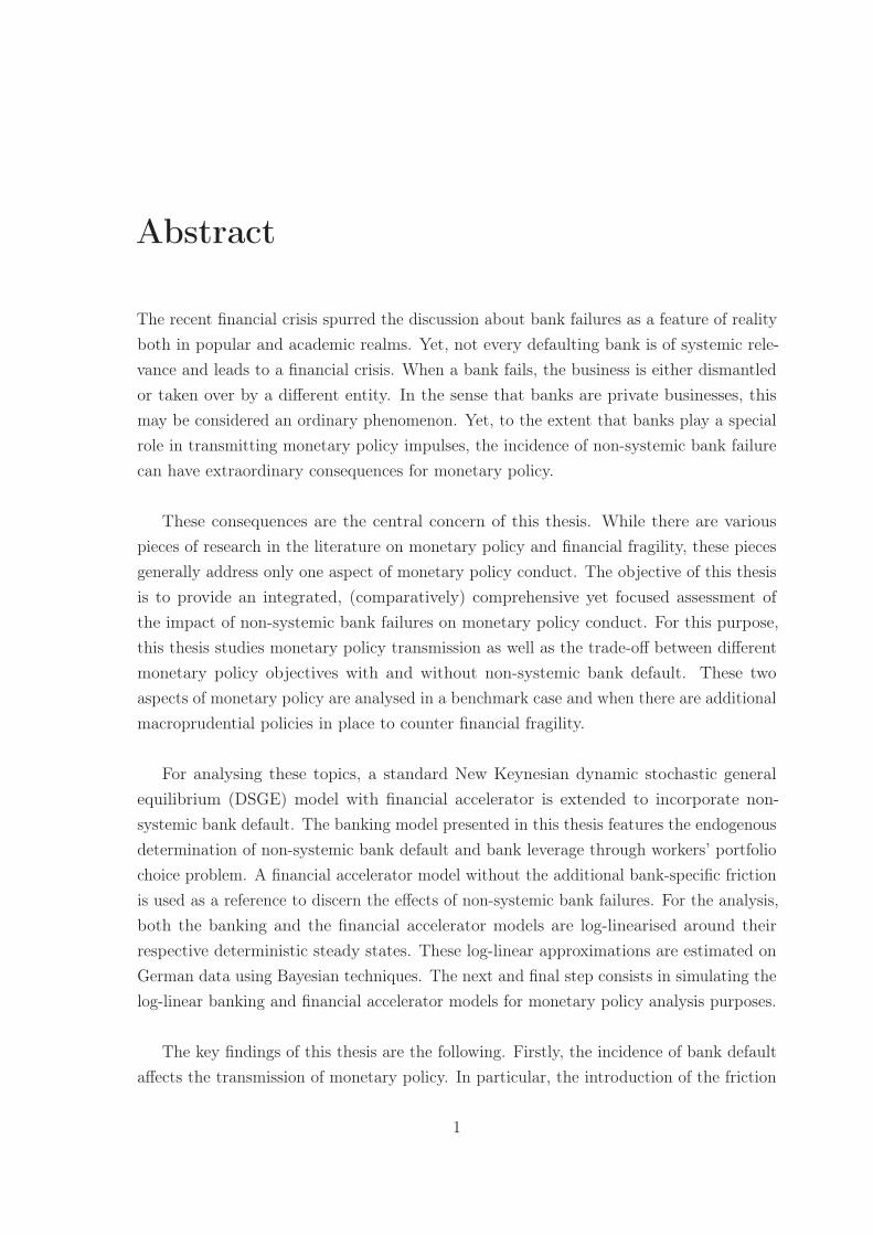
The recent financial crisis spurred the discussion about bank failures as a feature of realityboth in popular and academic realms. Yet, not every defaulting bank is of systemic rele-vance and leads to a financial crisis. When a bank fails, the business is either dismantledor taken over by a different entity. In the sense that banks are private businesses, thismay be considered an ordinary phenomenon. Yet, to the extent that banks play a specialrole in transmitting monetary policy impulses, the incidence of non-systemic bank failurecan have extraordinary consequences for monetary policy.

These consequences are the central concern of this thesis. While there are variouspieces of research in the literature on monetary policy and financial fragility, these piecesgenerally address only one aspect of monetary policy conduct. The objective of this thesisis to provide an integrated, (comparatively) comprehensive yet focused assessment ofthe impact of non-systemic bank failures on monetary policy conduct. For this purpose,this thesis studies monetary policy transmission as well as the trade-off between differentmonetary policy objectives with and without non-systemic bank default. These twoaspects of monetary policy are analysed in a benchmark case and when there are additionalmacroprudential policies in place to counter financial fragility.

For analysing these topics, a standard New Keynesian dynamic stochastic generalequilibrium (DSGE) model with financial accelerator is extended to incorporate non-systemic bank default. The banking model presented in this thesis features the endogenousdetermination of non-systemic bank default and bank leverage through workers’ portfoliochoice problem. A financial accelerator model without the additional bank-specific frictionis used as a reference to discern the effects of non-systemic bank failures. For the analysis,both the banking and the financial accelerator models are log-linearised around theirrespective deterministic steady states. These log-linear approximations are estimated onGerman data using Bayesian techniques. The next and final step consists in simulating thelog-linear banking and financial accelerator models for monetary policy analysis purposes.

The key findings of this thesis are the following. Firstly, the incidence of bank defaultaffects the transmission of monetary policy. In particular, the introduction of the friction

1

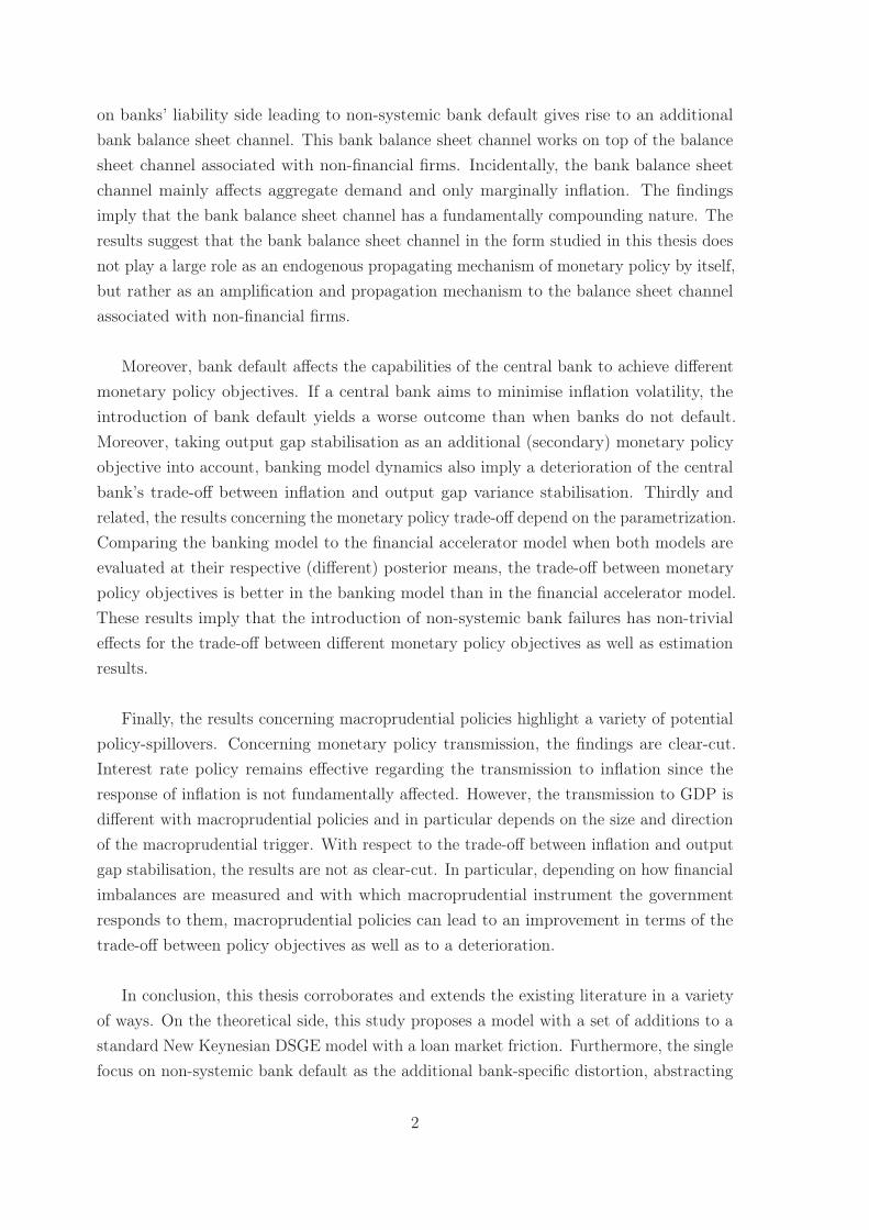
on banks’ liability side leading to non-systemic bank default gives rise to an additionalbank balance sheet channel. This bank balance sheet channel works on top of the balancesheet channel associated with non-financial firms. Incidentally, the bank balance sheetchannel mainly affects aggregate demand and only marginally inflation. The findingsimply that the bank balance sheet channel has a fundamentally compounding nature. Theresults suggest that the bank balance sheet channel in the form studied in this thesis doesnot play a large role as an endogenous propagating mechanism of monetary policy by itself,but rather as an amplification and propagation mechanism to the balance sheet channelassociated with non-financial firms.

Moreover, bank default affects the capabilities of the central bank to achieve differentmonetary policy objectives. If a central bank aims to minimise inflation volatility, theintroduction of bank default yields a worse outcome than when banks do not default.Moreover, taking output gap stabilisation as an additional (secondary) monetary policyobjective into account, banking model dynamics also imply a deterioration of the centralbank’s trade-off between inflation and output gap variance stabilisation. Thirdly andrelated, the results concerning the monetary policy trade-off depend on the parametrization.Comparing the banking model to the financial accelerator model when both models areevaluated at their respective (different) posterior means, the trade-off between monetarypolicy objectives is better in the banking model than in the financial accelerator model.These results imply that the introduction of non-systemic bank failures has non-trivialeffects for the trade-off between different monetary policy objectives as well as estimationresults.

Finally, the results concerning macroprudential policies highlight a variety of potentialpolicy-spillovers. Concerning monetary policy transmission, the findings are clear-cut.Interest rate policy remains effective regarding the transmission to inflation since theresponse of inflation is not fundamentally affected. However, the transmission to GDP isdifferent with macroprudential policies and in particular depends on the size and directionof the macroprudential trigger. With respect to the trade-off between inflation and outputgap stabilisation, the results are not as clear-cut. In particular, depending on how financialimbalances are measured and with which macroprudential instrument the governmentresponds to them, macroprudential policies can lead to an improvement in terms of thetrade-off between policy objectives as well as to a deterioration.

In conclusion, this thesis corroborates and extends the existing literature in a varietyof ways. On the theoretical side, this study proposes a model with a set of additions to astandard New Keynesian DSGE model with a loan market friction. Furthermore, the singlefocus on non-systemic bank default as the additional bank-specific distortion, abstracting

2

from other influences such as tax advantages or capital requirements, and its explicitmicrofoundation provide a rigorous foundation for the analysis. On this count, this thesiscontributes to the relevant literatures a comprehensive evaluation of the consequences ofnon-systemic bank failure for monetary policy, not only concerning transmission but alsothe central bank’s capabilities with respect to its objectives. On the empirical side thisthesis highlights the importance of sensitivity and robustness analyses as well as providingestimates for a New Keynesian DSGE model based on data for Germany. Finally, thisthesis contributes on the issues of macroprudential policies and their interactions withmonetary policy. The discussion of macroprudential policies in this thesis highlights theneed for a rigorous and transparent modelling approach as well as implementation of anyadditional policy so as to adequately gauge its impact and usefulness and to communicateany changes duly.

3

Kurzzusammenfassung

Die jüngste Finanzkrise verstärkte die Diskussion um Bankinsolvenzen als Teil der ökonomi-schen Wirklichkeit sowohl in der Allgemeinheit als auch im wissenschaftlichen Diskurs.Jedoch ist nicht jede Bankinsolvenz von systemischer Relevanz und führt zu einer Fi-nanzkrise. Im Falle einer Bankinsolvenz wird die Unternehmung entweder aufgelöstoder von einer anderen Institution übernommen. Betrachtet man Banken als privateUnternehmen, so kann dieser Prozess als gewöhnliches Phänomen interpretiert werden.Insofern Banken jedoch eine besondere Rolle im geldpolitischen Übertragungsprozessspielen, könnten nicht-systemrelevante Bankinsolvenzen außergewöhnliche Konsequenzenfür die Geldpolitik haben.

Die Untersuchung dieser Konsequenzen ist der zentrale Fokus der vorliegenden Dis-sertation. In der Literatur finden sich verschiedene Ansätze, die den Zusammenhangzwischen Geldpolitik und finanzieller Fragilität untersuchen. Allerdings betrachten dieseim Allgemeinen nur einen Aspekt der Geldpolitik. Das Ziel dieser Dissertation ist eineverhältnismäßig umfassende und gleichzeitig fokussierte Untersuchung des Einflusses derInsolvenz nicht-systemrelevanter Banken auf die Durchführung der Geldpolitik. Zu diesemZweck analysiert diese Dissertation den monetären Transmissionsmechanismus und dieZielmöglichkeiten-Kurve zwischen Inflationsraten- und Produktionslückenstabilisierungeiner Zentralbank mit und ohne Insolvenz nicht-systemrelevanter Banken. Diese beidenAspekte der Geldpolitik werden sowohl ohne als auch mit der Existenz makroprudenziellerInstrumente, die eingesetzt werden um finanzieller Fragilität entgegen zu wirken, evaluiert.

Dazu erweitert diese Dissertation ein Neu-Keynesianisches dynamisches, stochastisches,allgemeines Gleichgewichtsmodell (DSGE) mit finanziellem Akzelerator um eine zusätz-liche finanzielle Friktion, die die Insolvenz nicht-systemrelevanter Banken abbildet. DasBanking Modell, das in dieser Dissertation präsentiert wird, beinhaltet die endogene Bestim-mung von nicht-systemrelevanten Bankinsolvenzen und dem Fremdfinanzierungsgrad derBanken mithilfe des Portfolio-Optimierungsproblems privater Haushalte (Arbeitnehmer).Ein Modell mit finanziellem Akzelerator, jedoch ohne die zusätzliche bankbezogene fi-nanzielle Friktion, wird als Referenz verwendet um die Veränderungen zu unterscheiden,die sich aus der Insolvenz nicht-systemrelevanter Banken ergeben. Die Banking und

4

Finanzieller-Akzelerator Modelle werden zunächst um ihren jeweiligen nicht-stochastischenGleichgewichtspunkt log-linearisiert und dann mit Bayesianischen Methoden geschätzt.Schließlich werden beide Modelle zum Zweck der geldpolitischen Analyse simuliert.

Die wichtigsten Resultate dieser Dissertation sind die Folgenden. Die Insolvenz nicht-systemrelevanter Banken beeinflusst die geldpolitische Transmission insofern sie mit einemBankbilanzkanal einhergeht. Dieser Bankbilanzkanal wirkt zusätzlich zu dem Bilanzkanal,der mit nicht-finanziellen Unternehmen zusammenhängt. Tatsächlich wirkt der Bankbi-lanzkanal vorrangig auf die aggregierte Nachfrage und nur geringfügig auf die Inflation. DieErgebnisse implizieren, dass der Bankbilanzkanal, so wie er in dieser Dissertation modelliertist, keine übermäßige Signifikanz als eigenständiger, endogener Propagierungsmechanismusder geldpolitischen Transmission besitzt, sondern vor allem als ein Verstärkungs- undPropagierungsmechanismus des Bilanzkanals nicht-finanzieller Firmen zu begreifen ist.

Des Weiteren hat die Insolvenz nicht-systemrelevanter Banken Einfluss auf die Möglich-keiten einer Zentralbank verschiedene geldpolitische Ziele zu erreichen. Falls sich eineZentralbank darauf konzentriert die Inflationsratenvarianz zu minimieren, so führen nicht-systemrelevante Bankinsolvenzen im Modell zu einer Verringerung des Potenzials einer Zen-tralbank, da die minimale Inflationsratenvarianz höher ist als in einem Modell ohne Bank-insolvenzen. Wenn die Stabilisierung der Produktionslücke ein zusätzliches (sekundäres)geldpolitisches Ziel ist, dann führt die Dynamik des Banking Modells ebenfalls zu einerVerschlechterung des Zielkonfliktes zwischen Inflationsraten- und Produktionslückenstabil-isierung in Bezug auf das Finanzielle-Akzelerator Modell bei gleicher Parametrisierung.Die spezifischen Ergebnisse bezüglich des geldpolitischen Zielkonflikts sind jedoch abhängigvon der Parametrisierung. Wenn das Banking Modell mit dem Finanziellen-AkzeleratorModell unter der Verwendung des geschätzten Parametervektors des jeweiligen Modellsverglichen wird, so zeigt sich, dass sich hier der Zielkonflikt im Banking Modell bessergestaltet als im Finanziellen-Akzelerator Modell. Somit implizieren diese Ergebnisse, dassdie Einführung von Insolvenzen nicht-systemrelevanter Banken bedeutende Auswirkungenauf den Zielkonflikt der Zentralbank sowie auf die Schätzergebnisse der Modelle haben kann.

Abschließend zeigen die Ergebnisse bezüglich der Einführung makroprudenzieller In-strumente verschiedene Interaktionseffekte auf. Im Hinblick auf den geldpolitischen Trans-missionsmechanismus sind die Resultate eindeutig. Die Zinspolitik bleibt unverändertwirkungsvoll wenn die Übertragung geldpolitischer Impulse auf die Inflation betrachtet wird.Allerdings wird die Übertragung auf das Bruttoinlandsprodukt von makroprudenziellerPolitik beeinflusst und hängt besonders von der Größe und Richtung der makropruden-ziellen Steuerungsvariable ab. In Bezug auf den geldpolitischen Zielkonflikt zwischenInflationsraten- und Produktionslückenstabilisierung können die Ergebnisse nicht so ein-

5

deutig festgelegt werden, denn es zeigen sich Verbesserungen als auch Verschlechterungen.Dabei hängen die Veränderungen vorrangig davon ab, wie finanzielle Fragilität gemessenwird, sowie welches makroprudenzielles Instrument verwendet wird um dieser finanziellenFragilität entgegen zu wirken.

Zusammenfassend lässt sich feststellen, dass diese Dissertation die bestehende Liter-atur an verschiedenen Punkten untermauert und erweitert. Auf der theoretischen Seitepräsentiert diese Dissertation eine Erweiterung zu einem gängigen Neu-KeynesianischenDSGE Modell mit Kreditmarktfriktion. Des Weiteren bietet der Einzelfokus auf dieInsolvenz nicht-systemrelevanter Banken als einzige zusätzliche Banken-spezifische Friktionsowie deren explizite Mikrofundierung eine systematische Grundlage für die Analyse derAuswirkungen auf die Geldpolitik, indem von anderen Einflüssen wie Steuervorteilenoder Kapitalvorschriften abstrahiert wird. In diesem Sinne trägt diese Dissertation eineerweiterte Evaluation der Folgen der Insolvenz nicht-systemrelevanter Banken für dieGeldpolitik zur bestehenden Literatur bei, da sowohl die Transmission geldpolitischerImpulse als auch die Zielmöglichkeitenkurve der Zentralbank betrachtet werden. Aufder empirischen Seite stellt diese Dissertation die Bedeutung von Sensitivitätsanalysenhervor. Zudem werden Schätzergebnisse für ein DSGE Modell auf der Basis von Datenzu Deutschland präsentiert. Letztendlich trägt diese Dissertation zur Diskussion ummakroprudenzielle Politik und deren Einflüsse auf die Geldpolitik bei. Insbesondere zeigendie Ergebnisse, dass transparente und fundierte Modellierungs- und Umsetzungsansätzenötig sind, um die Auswirkung und Nützlichkeit der Instrumente adäquat einzuschätzenund zu kommunizieren.

6

Chapter 1

Introduction

The recent financial crisis of 2007-08 led to serious disruptions in financial markets and aglobal recession. In turn, the banking panic fuelled by concerns about banking liquidityand solvency was not least accelerated by the failure of several financial intermediaries.1

Yet, not every defaulting financial intermediary is of systemic relevance and leads to afinancial crisis. In the US, considering all years since the 1960s, the years 2005 and 2006have been the only ones where no bank covered under the Federal Deposit Insurance filedfor bankruptcy.2 Yet, the US banking system was not constantly in crisis during thistime.3 A similar argument can be made for the German banking system.4

Thus, banks fail in the real world, even though not yet as often in macroeconomicmodels. The banking business is then either dismantled or taken over by a differententity. In the sense that banks are private businesses, this may be considered an ordinaryphenomenon. Yet, to the extent that banks play a special role in transmitting monetarypolicy impulses, the incidence of bank failure can have extraordinary consequences formonetary policy.

Financial fragility and its interactions with monetary policy have been an especiallyprominent research area since the onset of the financial crisis 2007-08. One reason iscertainly that central banks responded to the financial crisis with unconventional measuresto restore the functioning of interbank markets, connected markets of financial intermedia-tion and to ensure the orderly transmission of monetary policy. However, the connection

1 See Ivashina and Scharfstein (2010: 319)2 See Federal Deposit Insurance Corporation (2015), URL in list of references3 Building a cross-country crisis database, Laeven and Valencia (2013: 258f) only declare the years 1988

and 2007 onwards as crisis years. Their dataset covers the years 1970 to 2011. Considering only thetime since the 1960s, Reinhart and Rogoff (2009: 346f, 390) find similarly that the US experiencedbanking crises in 1984-1988 and 2007. Their complete dataset covers 1800 to 2008.

4 See Blank, Buch and Neugebauer (2009: 359, 361) and de Graeve, Kick and Koetter (2008: 209) foryearly bank distress frequencies and Laeven and Valencia (2013: 255) and Reinhart and Rogoff (2009:365) for banking crisis incidence.

7

between banking sector fragility and monetary policy is not only relevant for systemicbanks or for crisis times. As economies are entering ‘post-’ or ‘non-financial-crisis’ times,questions arise about whether, how and when monetary policy should return to ‘normality’as well.5 Then, a logical next step is to ask how monetary policy conduct is affected bynon-systemic bank default, given that bank default is also a non-crisis phenomenon.

This next step is the central focus of this thesis. Given that bank default is not anew aspect, one may expect that this topic has already been examined thoroughly inmacroeconomic studies. Somewhat surprisingly, bank default and financial fragility moregenerally have only recently played a more prominent role in the research agenda onmonetary policy, particularly spurred by the latest financial crisis as noted above. Thereare various pieces of research on the role of banks and banking sector fragility in monetarypolicy transmission, as well as on governmental policies targeted at enhancing financialstability. As will be argued throughout this thesis, this thesis provides an extended andintegrated assessment based on the following key characteristics: (i) a focus on discerningthe consequences of non-systemic bank default for monetary policy, (ii) an analysis ofthese consequences both when there are measures to counter financial fragility in place andwhen they are not, and (iii) based on a model extension which is designed to concentrateon the incidence of non-systemic bank default as the only additional financial marketimperfection. In this sense, this study can be seen as a corroboration and expansion ofexisting research.

As evidenced by the wide variety of literatures, the connections between monetarypolicy and financial intermediaries in general and financial fragility in particular allowfor many research agendas. To focus the contribution, I pose the following researchquestions to summarise the objectives of this thesis. From the title it is clear that theprincipal research question focuses on how non-systemic bank failures impact the conductof monetary policy. This first research question is approached from two distinct but linkedperspectives. On the one hand, what are the consequences for monetary policy transmis-sion to the real economy? This essentially queries whether a monetary policy impulseaffects inflation and output in a different way when there are non-systemic bank failures.On the other hand, does bank default affect the capabilities of the central bank withregard to achieving its policy objective(s) more generally? This concerns both the primaryobjective of price stability as well as other policy objectives such as output gap stabilisation.

As a corollary, the incorporation of banking sector fragility into monetary policy analy-sis raises another research question. When default is possible both in the goods productionand the financial sectors, which market imperfection implies more serious consequences for

5 See, for example, Borio and Disyatat (2009: 22ff) for an early discussion.

8

monetary policy conduct? This research question aims to highlight potentially dissimilareffects of different financial frictions concerning monetary policy. For one, knowledge aboutdifferential impacts is crucial for monetary policy since it can benefit the analysis of macroe-conomic developments on which monetary policy decisions are based. Furthermore, thisknowledge also helps to evaluate how monetary policy decisions affect inflation and outputwhen different economic environments imply that one of the frictions has grown more severe.

Thirdly, what if there are governmental measures to enhance banking sector stabilityand resilience? How does the existence of such macroprudential measures, for instance,affect the link between non-systemic bank default and monetary policy transmission aswell as the trade-off between different monetary policy objectives? This third researchquestion goes hand in hand with a more thorough evaluation of the link between monetarypolicy and financial fragility. Furthermore, assessing additional policies allows to discernthe impact of potential spill-over or feedback effects on the conduct of monetary policy.

To answer these questions a New Keynesian dynamic stochastic general equilib-rium (DSGE) model with financial accelerator is extended to incorporate non-systemicbank default. The DSGE model allows for the focus on ‘normal’ business cycles in thatshort-run fluctuations are reproduced instead of long-run growth. The New Keynesianmodelling approach provides a specific rationale for monetary policy to have real effectsin the short term. Moreover, the financial frictions concern both the asset as well asthe liability sides of banks’ balance sheet. In particular, the financial friction concerningbanks’ liabilities is the core modelling contribution of this study. This financial frictioncharacterises the incidence of non-systemic bank default and provides the microfoundationfor the evaluation of its impact on monetary policy. Furthermore, this banking modelis log-linearised around its non-stochastic steady state and estimated using Bayesianmethods. Based on this estimated model, the consequences of non-systemic bank defaultfor monetary policy are analysed, both in terms of transmission and policy objectives. Thisanalysis crucially revolves around the comparison of the banking model proposed in thisstudy to a financial accelerator model which does not feature the additional bank-specificfriction leading to bank default.

As well as limiting the focus to short- and medium-term developments, the particularmodelling approach also draws boundaries to what this study can reasonably achieve.For one, the incidence of a financial crisis (or any other crisis) is not traced here. As aconsequence of the log-linearisation, only small perturbations from the equilibrium areconsidered. With the focus on non-systemic bank failures and non-crisis times comes theabstraction from the unconventional measures taken by central banks in the aftermath ofthe latest financial crisis. Thus, this thesis only deals with ‘conventional’ (interest-rate-

9

based) monetary policy. The main reason is that such a wider concept of monetary policyinstruments necessitates some treatment of systemic bank failures which is in turn notthe focus of this thesis. Thus, these two limitations are left to future research. Given themodel’s level of abstraction, there are many other, more specific restrictions placed onthe analysis, which will be subsequently discussed as necessary. For the general researchquestion, however, these two topics are considered the most important limits to be bornein mind.

Taking these limits into consideration, this thesis contributes to the existing literaturein the following ways. On the theoretical side, this study proposes a model with a set ofadditions to a standard New Keynesian DSGE model with a loan market friction. Theseadditions concern the endogenous determination of non-systemic bank default and bankleverage, and the specification of a portfolio choice problem on the part of households.This portfolio choice problem handles the choice between bank deposits, which are risk-freefrom the perspective of households due to a deposit insurance scheme, and bank equitywhich is risky because of the possibility of bank default. Undoubtedly, individual elementshave been studied in the literature before. Yet, to the best of my knowledge, a model withthe different features as presented in the following has not been proposed in a large-scaleNew Keynesian DSGE framework.

Furthermore, the single focus on non-systemic bank default as the additional bank-specific distortion, abstracting from other influences such as tax advantages or capitalrequirements, and its explicit microfoundation provide a rigorous foundation for the anal-ysis. On this count, this thesis contributes to the relevant literatures a comprehensiveevaluation of the consequences of non-systemic bank failure for monetary policy, notonly concerning transmission but also the central bank’s capabilities with respect to itsobjectives. This thesis will show that the particular modelling approach of non-systemicbank failures followed here produces a bank balance sheet channel in monetary policytransmission. Furthermore, the findings of this thesis suggest that this bank balance sheetchannel primarily affects the response of aggregate demand of goods and services. Incontrast, the response of inflation is not fundamentally affected by the introduction ofbank default. Moreover, bank default affects the capabilities of the central bank to achievedifferent monetary policy objectives. If a central bank aims to minimise inflation volatility,the introduction of bank default yields a worse outcome than when banks do not default.Moreover, taking output gap stabilisation as an additional (secondary) monetary policyobjective into account, banking model dynamics also imply a deterioration of the centralbank’s trade-off between inflation and output gap variance stabilisation.

However, the results on the trade-off between different monetary policy objectives

10

depend on the parametrization. This sensitivity links to the empirical contributions of thisthesis: highlighting the importance of sensitivity and robustness analyses as well as pro-viding estimates for a New Keynesian DSGE model based on data for Germany. In termsof sensitivity, this study maintains that some results in comparing the effects of monetarypolicy with and without non-systemic bank failures are affected by the parametrization.In particular, parameter values are argued to be one of the crucial elements for evaluatingcentral banks’ capabilities with respect the trade-off between monetary policy objectives.Comparing the banking model to the financial accelerator model when both models areevaluated at their respective (different) posterior means, the trade-off between differentobjectives is better in the banking model than in the financial accelerator model. Thus,different model dynamics and parameter estimates have non-trivial effects for the trade-offbetween different monetary policy objectives.

Furthermore, this thesis contributes to the empirical literature in that it providesestimates concerning Germany. To begin with, there are few comparable existing estimatesin the literature based on German data. Furthermore, the choice for using Germandata is not only based on their rarity in the literature, but rather on the particularitiesof the Euro area. While monetary policy is conducted considering the Euro area as awhole, financial systems are still disparate in Europe. Estimates based on aggregate Euroarea data may blur potentially asymmetric effects of monetary policy. Thus, these esti-mates, as well as the analysis based on these estimates, can be interpreted as one piece ofa larger puzzle to analyse how monetary policy in the Euro area is affected by fragile banks.

Finally, this thesis contributes on the issues of macroprudential policies and their inter-actions with monetary policy. This study argues that both the choice of macroprudentialinstrument and the measure of financial imbalances have non-trivial consequences formonetary policy conduct. While there appear general patterns in terms of monetary policytransmission, the results on the trade-off between monetary policy objectives do not fit aparticular pattern in that some combinations of macroprudential instrument and financialmeasure enhance and others constrain a central bank’s capabilities. Thus, the discussionof macroprudential policies in this thesis highlights the need for a rigorous and transparentmodelling approach as well as implementation of any additional policy so as to adequatelygauge its impact and usefulness and to communicate any changes duly.

To accomplish the research objectives and make aforementioned contributions, thisthesis is structured in the following way. Chapter 2 establishes the theoretical frameworkby reviewing the relevant literatures. The chapter starts with the general macroeconomicresearch paradigm, and continues to the areas of financial intermediation and financialmarket imperfections and their links to monetary policy. Based on the outline of theoretical

11

approaches, the review of the empirical results on this link corroborates the usefulnessand exigency of this thesis’ research agenda. Chapter 2 concludes with a review of closely-related research which underscores the theoretical contributions of this thesis.

Chapter 3 describes the banking model which is used in this study for analysing theresearch questions. The primary objective of chapter 3 is to explain the decision-makingproblems of the various agents which make up the model economy. The optimum conditionsare presented and the modelling choices are justified.

Chapters 4 to 6 use the banking model to examine the research questions. Chapter 4should be taken as an intermediate step which elaborates on some key features of the model.The chapter discusses the concept of the non-stochastic steady state and its stability anddeterminacy realms for the banking model. Furthermore, more details are provided onhow the banking model’s specificities affect the canonical DSGE model representationin terms of the New Keynesian Dynamic IS-Phillips Curve-Monetary Policy framework.Furthermore, chapter 4 compares the asymmetric roles of financial capital in the decisionproblems of non-financial firms and banks. This difference is argued to be crucial forunderstanding the specific consequences of bank failure as laid out in chapter 6.

Next, chapter 5 discusses the estimation of the banking model. Beginning with ashort discussion of the estimation method, chapter 5 presents the estimation results of thebanking model. In order to gauge the empirical fit of the banking model, it is comparedto the financial accelerator model which does not include the friction leading to bankdefault. The final section of chapter 5 reports the results of the sensitivity analyses of theestimation procedure.

Chapter 6 presents the simulation results to evaluate the consequences of non-systemicbank failure for monetary policy. It thus builds on the intermediate results from thepreceding chapters in terms of steady-state and estimation analyses. Chapter 6 starts withthe analysis of monetary policy transmission and the consequences for the trade-off betweendifferent monetary policy objectives assuming that the government has not introducedany instruments to enhance financial stability. Then, the experiments are repeated underthe assumption that there are macroprudential instruments in place in order to answerthe last research question. In sum, chapter 6 is an integrated presentation and discussionof the results relating them to the relevant literatures.

Finally, chapter 7 summarises and concludes. The results of the previous chapters arecombined to state the answers to the research questions succinctly. The conclusions to bedrawn are considered and avenues of future research are pointed out.

12

Chapter 2

Financial Intermediaries and MonetaryPolicy in Macroeconomic Modelling

The connection between financial intermediation and monetary policy is an active field of(macroeconomic) research. In particular, the financial crisis of 2007-08 has been a catalystfor research discerning the functioning of the different parts of the financial intermediationprocess. Thus, it is clear that this study is based on a large repertory of research which isthe focus of this chapter. There are a number of objectives this chapter aims to reach. Tobegin with, this chapter addresses various methodological choices. For one, this concernsthe New Neoclassical Synthesis (NNS) as the overarching theoretical framework. Also,it relates to the particular approach to describing the relationship between the financialsector and monetary policy. Furthermore, the review of the literature on theoretical andempirical aspects of this link aims to establish the warrant for the way monetary policyinteractions with the financial sector are modelled in this study. Overall, the core objectiveof this chapter is to place this study within the related literature and discern the gap thisstudy aims to fill.

This chapter is structured as follows. In section 2.1 the dynamic stochastic generalequilibrium (DSGE) modelling approach is justified by considering the role of monetarypolicy in the NNS as compared to other approaches. Section 2.2 discusses monetary policyconduct in Germany. The next two sections 2.3 and 2.4 deal with theoretical and empiricalstudies on monetary policy transmission justifying a non-trivial role for the financial sector.Finally, section 2.5 positions the present research within the relevant literature on bankingsector fragility and monetary policy.

13

2.1 Monetary Policy in the New Neoclassical Synthesis

This study’s research question presupposes a departure from monetary neutrality.6 For ifthe classical dichotomy held, monetary policy would not affect real variables. In turn, thefinancial sector and the real economy are connected, since banking sector developmentsimpact the financing available to private agents in the economy. So, with monetary policytargeting the price level (or inflation rate), if the price level and aggregate demand ofgoods and services7 are not linked to each other, and financial sector developments arelinked to aggregate demand, then the price level is not dependent on the financial sector.In this case, monetary policy targeting a stable price level will not be affected by thefinancial sector, that is also bank default. Thus, this study would be rather short.

Apart from this practical justification, what is the warrant for monetary non-neutrality?For one, the practice and communication of monetary policy in central banks supports theview that monetary policy affects the real economy. For instance, the Federal Reserve ismandated to aim for maximum employment in addition to price stability.8 Furthermore,in a recent press statement explaining the decision to keep the target range for the federalfunds rate fixed, the Federal Reserve explicitly stated that the loose monetary policy isintended to help improve labour market conditions.9 Moreover, there is a large theoreticalliterature evaluating the effects of monetary policy, as well as its optimal design andinterdependencies with other kinds of policy. As will become clear from the fraction of theliterature cited in the following sections, there are clear indications that monetary policy hasreal effects. Besides, the accumulated body of empirical research covering the last decadesshows that monetary developments do not only affect inflation, but also the real economy.10

To be more specific about the kind of monetary non-neutrality, the banking modelused to answer this study’s research questions belongs to the class of New Keynesian (NK)DSGE models. DSGE models embody the view that macroeconomic developments are theresult of the coordination of individual agents’ actions through markets based on rationaldecision-making.11 Furthermore, equilibrium is a defining feature of DSGE models: whilethe model economy may be disturbed from its long-run equilibrium due to exogenous

6 Monetary neutrality signifies that nominal and real variables develop independently of each other, seeWalsh (2003: 213) and Woodford (2003: 6).

7 Unless stated otherwise, the term ‘aggregate demand’ will be used to denote ‘aggregate demand ofgoods and services’ in this thesis.

8 See Board of Governors of the Federal Reserve System (2016b: 1), URL in list of references9 See Board of Governors of the Federal Reserve System (2016a), URL in list of references10 A very prominent narrative study is M. Friedman and Schwartz (1963), and subsequently, time-series

methods have become popular as exemplified in the work of Christiano, Eichenbaum and Evans (1999),see Galí (2008: 4). The empirical literature pertaining to this study is reviewed in section 2.4.

11 See Wickens (2008: 1)

14

shocks, it always rests in a short-run equilibrium.12 This kind of model is associatedwith the paradigm of the New Neoclassical Synthesis (NNS). Monetary non-neutralityis one of the key features of the NNS, in contrast to the classical paradigm, for example.Put in a nutshell, the central features of the NNS about monetary policy are: Monetarypolicy has short-term effects on real variables due to nominal rigidities, but little long-term effects.13 Reducing inflation yields gains due to lower relative price distortions andtransaction inefficiencies.14 Then, monetary policy does not only impact the economy,but the research paradigm creates a justification for a prominent role of monetary pol-icy in managing aggregate demand.15 Finally, central bank credibility plays a crucial role.16

The impact of monetary policy on the real economy is a direct consequence of oneof the main tenets of the NNS: price and nominal wage rigidities. This means that non-financial firms17 as price-setters, for example, face some form of constraint which limits thefrequency of price and/or wage adjustments.18 If prices cannot respond instantaneouslyand completely, then a central bank’ ability to manipulate the nominal risk-free interestrate transfers into (imperfect) manipulation of the real risk-free interest rate.19 Since thereal risk-free interest rate affects real investment and real consumption decisions, monetarypolicy has an impact on real variables. As long as there is no absolute impediment tochanging prices and nominal wages, the effects of monetary policy will dissipate over thelong term.20 This is referred to as short-term monetary non-neutrality.21

While the principal objective of monetary policy is generally considered to be pricestability, output (gap) stabilisation can be deemed an additional target. Aiming to avertexcessive business cycle swings and thus volatility in the real economy due to mechanicallyfulfilling the objective of price stability can be one justification.22 In fact, in simple NKDSGE models, price stability and output gap stability go hand in hand. There, monetarypolicy has the potential to stabilise output at its potential level through stabilising pricesby managing average marginal cost over time.23 As a consequence, non-financial firms do

12 See Wickens (2008: 1)13 See Goodfriend and King (1997: 232)14 See Goodfriend and King (1997: 232)15 See Goodfriend and King (1997: 256)16 See Goodfriend and King (1997: 232)17 The term non-financial firm is used to distinguish these firms from financial intermediaries.18 See Galí (2008: 5). This necessarily implies that the respective markets are not perfectly competitive.19 See Galí (2008: 5)20 See Galí (2008: 5)21 See Galí (2008: 5)22 See Galí (2008: 95)23 See Goodfriend and King (1997: 256, 262ff). However, monetary policy cannot change the steady-

state average mark-up, and consequently the level of potential output, since this is determined bynon-financial firms’ market power, see Goodfriend and King (1997: 262).

15

not have an incentive to change their prices.24 This implies that there is no trade-off formonetary policy between inflation and output stabilisation.25 However, in more elaboratemodels this accordance of objectives does not necessarily hold. Various possibilities for atrade-off between output gap and inflation stabilisation to arise have been considered. Awidely used concept to create such a trade-off is the introduction of exogenous randomnessin the mark-up process, often called cost-push or mark-up shocks.26 Also, the presence ofnominal wage stickiness in addition to price stickiness can result in a short-term trade-off.27

NK DSGE models are not the only kind of macroeconomic model which allows formonetary non-neutrality. Stock-flow consistent (SFC) modelling, for example, is onealternative approach to monetary policy analysis. SFC models are made up of interlinkedbalance sheets of the agents in the model paying particular attention that each financialasset is matched by a corresponding financial liability of another agent.28 The advantagesof the SFC approach include the ‘natural’ match to national accounts data as well as theability to check the logical consistency of the model.29 Given that SFC models are based onaccounting principles, no agent can accumulate financial assets which have no counterpartliability of another agent.30 The models are thus internally consistent.31 Godley andLavoie (2012), for example, provide a text-book style monograph building an increasinglycomplex SFC model. They show that monetary policy has real effects.32 However, SFCmodels also present a major drawback: by focusing on the aggregate balance sheet ofaggregate sectors, intra-sector and heterogeneous behaviour cannot be traced.33

To counter this last point, consider the other extreme: agent-based (AB) models.34 Thecentral tenets of AB models are heterogeneous agents, and agents being bounded-rational

24 As Galí (2008: 47) shows using a simple NK model, inflation is a function of expected marginal costs,defined as deviations from the steady state.

25 See Goodfriend and King (1997: 276)26 See Clarida, Gali and Gertler (1999: 1672)27 See Goodfriend (2004: 39). As will be discussed in chapter 6, the models considered in this thesis

feature such a trade-off. Furthermore, parametrization as well as model structure impact the trade-off.28 See Caiani et al. (2016: 378) and Caiani, Godin and Lucarelli (2014: 425). These accounting rules are

based on the quadruple entry principle, see Godley and Lavoie (2012: 47).29 See Caiani et al. (2016: 378). Also, Caiani et al. (2014: 426) argue that SFC models are prime

candidates for studying endogenous money because of their focus on keeping track of stocks andflows in the economy. As will be outlined in the next section, this study abstracts from the debate ofloanable funds vs. endogenous money. Thus, this issue will not be discussed further at this point.

30 See Caiani et al. (2016: 378)31 See Caiani et al. (2016: 378)32 Incidentally, the real effects produced by the model by Godley and Lavoie (2012) are conflicting

with conventional accounts: While contractionary monetary policy has negative short-term effects onreal output, over the medium and long terms real output is actually higher than at the outset. Theauthors attribute this behaviour to higher government expenditures due to higher interest rates. SeeGodley and Lavoie (2012: 116f, 122f, 151, 415)

33 See Caiani et al. (2016: 378)34 See Tesfatsion (2006) for a comprehensive introduction to AB models.

16

and behaving in an adaptive manner.35 AB models are advocated on the basis thatmacroeconomic developments are the outcome of an evolving system of individual agentsdirectly interacting with each other, not necessarily or rather seldom in equilibrium.36

Thus, there is no artificial representative agent. Furthermore, proponents argue that theirability to create crises endogenously and to study the dynamics of the economy even outsideequilibrium are advantages of AB models.37 The EURACE project is one of the mostprominent examples of this approach. The collaborative project aims to build a complexAB model of the European Union.38 In a related effort to build a comprehensive ABmodel, Dosi et al. (2015) study the interaction between monetary and fiscal policies. Theirsimulations reveal that the dynamics of the economy crucially depend on the combinationof fiscal and monetary policies.39 In particular, monetary policy which reacts to both un-employment and inflation performs better than one which is only concerned with inflation.40

Nevertheless, despite their alleged appeal of being more ‘realistic’, AB models haveweaknesses. Most importantly, Caiani et al. (2016) state that most AB models found in theliterature do not obey stock-flow consistency.41 This is critical since the simulation-basedapproach of AB models means that small discrepancies can build up over the simulationspan, potentially rendering the simulated paths of stocks and flows inconsistent.42 As aremedy to this problem, Caiani et al. (2014) and Caiani et al. (2016) have proposed tomerge the AB and SFC modelling paradigms.43 This combination would not only makeAB models stock-flow consistent but would also enrich SFC models by disaggregating theamplification effects due to a whole sector behaving in a homogeneous way.44

Yet, only considering stock-flow consistent AB models, there are still unresolved issuesand other drawbacks. For one, the treatment of expectations in AB models is a contentiousissue. AB models aim to incorporate scientific results from psychology, among others,

35 See Fagiolo and Roventini (2012: 88)36 See Fagiolo and Roventini (2016: 3), URL in list of references37 See Tesfatsion (2006: 843) and Dosi, Fagiolo, Napoletano, Roventini and Treibich (2015: 167)38 See Deissenberg, van der Hoog and Dawid (2008) and Dawid, Harting, van der Hoog and Neugart

(2016) as well as the references therein for more information.39 See Dosi et al. (2015: 182)40 See Dosi et al. (2015: 178). More specifically, Dosi et al. (2015: 176) find that there are merits to

monetary policy targeting both the unemployment rate and inflation even though this leads to anincrease in average inflation.

41 See Caiani et al. (2016: 379)42 See Caiani et al. (2016: 379). The issue of stock-flow consistency is important for any kind of model.

Note that given this criticism, care was taken in specifying the model. Also, the methodologicalapproach chosen here for the DSGE model, that is local stability and small perturbations from thesteady state, ensures that stocks cannot build up indefinitely. See section 4.4 for more details on thestability of the model.

43 See Caiani et al. (2014: 444) and Caiani et al. (2016: 377)44 See Caiani et al. (2014: 444)

17

in modelling agents as boundedly rational.45 Proponents of AB models emphasise theimportance of incorporating learning in agents’ decision rules.46 However, it has beencriticised that often the underlying assumptions and characteristics of heterogeneity andlearning are not explained thoroughly.47 Furthermore, learning can also be incorporatedinto DSGE models. De Grauwe (2010), for instance, also aims to include the results oflimited cognitive abilities from psychology and neural science into macroeconomic models.48

Similar to proponents of AB models, he argues that in reality, agents do not understandthe world entirely, and thus rely on rules-of-thumb in their decision-making process.49

To this end, de Grauwe (2010) includes additional forecasting equations in a simple NKmodel.50 The author argues that endogenous waves of optimism and pessimism createendogenous business cycles, as well output and inflation inertia and differential effects ofmonetary policy.51

What is more, the treatment of agents’ cognitive abilities and expectations in ABmodels poses problems when it comes to policy evaluation and regime changes. In contrast,the rational expectations paradigm incorporated into DSGE models is well equipped toanalyse the consequences of policy changes since the evolution of the economy is derivedfrom structural optimisation problems. Due to the explicit microfoundation, consequencesof monetary policy can be analysed avoiding the Lucas critique.52 Rational expectationsand agents’ optimisation problems as the basis of the model provide a way to address theissue of changing expectations, caused by an altered underlying model economy structure,as for example when new governmental policies are adopted.53 This is of particular im-portance in the present context since the research question revolves around a non-trivialchange in the economic structure. In each of the economic environments studied here,agents are fully informed and behave rationally, thus act optimally. Different consequencesfor monetary policy between models with and without bank failure are due to differentconstraints placed on rational economic agents. Therefore, the results are not blurred bymingling effects of agents not incorporating some features of the economic structure intotheir decision-making. Such additional effects are certainly an interesting topic for futureresearch.

Moreover, there are particular difficulties surrounding the calibration of AB (and

45 See Fagiolo and Roventini (2012: 88)46 See Fagiolo and Roventini (2012: 90)47 See Wäckerle (2013: 14)48 See de Grauwe (2010: 414)49 See de Grauwe (2010: 414)50 See de Grauwe (2010: 418f)51 See de Grauwe (2010: 438f)52 See Woodford (2003: 10f). Lucas (1976: 40ff) argues that predictable policy changes affect behavioural

parameters, therefore impacting the forecasting performance of models.53 See Woodford (2009: 272)

18

SFC) models. Firstly, AB models are generally over-parametrised.54 As such, this leadsto difficult choices when it comes to choosing the parameters and testing robustness.55

Secondly, the calibration of initial values for stocks and flows is critical since AB modelsproduce path-dependent dynamics.56 For this reason, a burn-in period of the simulationis usually discarded to remove the effects of initial values.57 At the same time, Caianiet al. (2016) argue that initial stock values have to be sufficiently high for the agents toaccommodate possible very large swings in the first periods of the simulation.58 Similarly,Tesfatsion (2006) argues that an extensive specification effort is necessary to avoid asituation in which the modeller would have to adjust the processes during the simulation.59

So, given that calibration is a very sensitive issue in AB models, it is rather disconcertingthat Caiani et al. (2016) state that the majority of the corresponding literature does notdiscuss the choice of calibration for initial stocks and flows adequately.60 While parameteridentification is a critical topic for DSGE models as well, the routines developed so farhelp in conducting efficient sensitivity and robustness analyses.

Finally and related, the modelling and evaluation approaches within the AB(-SFC)paradigm are still very disparate.61 Furthermore, AB models are generally very complexleading authors to present only the main intuition and assumptions without being able toclearly delineate different mechanisms.62 Given their dissimilar, specific foci and differentsolution methods, it is rather difficult to compare the results of different AB models.63 Incontrast, there exists a set of solution routines, evaluation and estimation tools for moreor less standard DSGE models.64

Furthermore, recent research on DSGE models has turned to addressing various criti-cisms which have been used as arguments in favour of alternative approaches. For one,the suggested advantage of AB models in modelling heterogeneous agents looses muchof its strength in the presence of the current efforts to build heterogeneous agent DSGE

54 See Fagiolo and Roventini (2012: 105f) and Dawid et al. (2016: 2)55 See Fagiolo and Roventini (2012: 105f)56 See Fagiolo and Roventini (2012: 90, 106)57 See Caiani et al. (2016: 390) and Fagiolo and Roventini (2012: 106)58 See Caiani et al. (2016: 380)59 See Tesfatsion (2006: 845)60 See Caiani et al. (2016: 380, 388)61 See Caiani et al. (2016: 379)62 See Dawid et al. (2016: 2f). This count may be equally true for large-scale DSGE models. However,

given that the core of most DSGE models tends to be made up of a known set of elements, only the newor amended elements need to be explained. In contrast, AB models tend to be more heterogeneous,see Dawid et al. (2016: 2). Notable contributions to streamline AB models include Caiani et al. (2016)and Dawid et al. (2016).

63 See Caiani et al. (2016: 379)64 Obviously, there are also issues which require more sophisticated solution and/or estimation techniques,

such as the modelling of non-linearities or heterogeneous agents, see section 3.1.2.

19

models.65 While the model presented here does not feature heterogeneous agents forreasons discussed in section 3.1.2, the fact that dynamic general equilibrium and hetero-geneity among agents can be linked in a single model shows that this research area is alsonot limited to AB models. Fagiolo and Roventini (2012) elaborate on another argumentagainst DSGE models by arguing that the reliance on external shock processes to createbusiness cycles in DSGE models implies that such models cannot explain how businesscycles or crises arise endogenously.66 Admittedly, the start of the business cycle or crisismay not arise endogenously in DSGE models. Yet, the evolution of the economy througha business cycle can still be traced. Moreover, recent research has also turned to globalsolution methods as an alternative to log-linearisation. Thus, issues such as modellingnon-linearities, for instance the zero-lower bound, become feasible in the realm of DSGEmodels. The possibility to incorporate such features into DSGE models, even though theyare not used here, is still an argument for the use of a DSGE model in the present context:As will be argued many times more, the focus is on a comparative exercise.67 The objectiveis not only to show how the presented model is different, but also to build a referencepoint for future research potentially incorporating heterogeneous agents and non-linearities.

It is due to the incorporation of rational expectations, and the comparability as wellas practicability in terms of parametrization, sensitivity and robustness analyses that thisstudy uses a DSGE model. Nevertheless, it is important to keep in mind the limits andcriticisms of DSGE models which also spurred the research in AB and SFC models. Theseconcern more technical issues such as the inclusion of ad-hoc assumptions about priceindexation to introduce persistence, as well as whether shocks in DSGE models should beinterpreted as structural.68 More fundamental criticisms relate, among others, to the useof rational expectations and the ‘representative agent’ as noted above. These issues arecertainly important and indicate that much work needs to be done. Yet, the same appliesto addressing the weaknesses of other approaches. To the extent that these criticismsare deemed relevant for this study, they will be addressed to enhance transparency. Forinstance, section 3.1.2 deals at length with the assumption of the representative agent,and more generally chapter 3 extensively discusses the particular modelling choices.

Furthermore, this discussion for the choice for a DSGE model should not be interpretedas discarding AB modelling and other approaches. The central concern of this study maybe equally studied in an AB model. As is true for many realms of methodology, there areadvantages and disadvantages to using a specific approach. Whether or not the results

65 For references to the literature, see section 3.1.2.66 See Fagiolo and Roventini (2012: 86)67 The comparison concerns both the characteristics of each model’s steady state and the models’

behaviour when disturbed from their respective steady states.68 See Chari, Kehoe and McGrattan (2009: 244f)

20

presented in this study hold in a different context is an interesting study for future research.In the end, any model can only be an abstraction from reality and is bound to be anincomplete representation. Then, the question is for which purpose the model is used. Inparticular, this study is primarily concerned with an additional feature of the economy,not a fundamental paradigm-shifting change in assumptions. Thus, it is imperative to beable to compare the results of this research with the literature. This concerns both theparallels with established results in the literature and the use of this study as a buildingblock and reference for future research. To this end, the body of work on NK DSGEmodels is sufficiently rich to clearly delineate the consequences of the additional feature.In conclusion, for the purposes of this study, in my view the advantages of DSGE modelsoutweigh the disadvantages.

2.2 Characterisation of Monetary Policy in Germany

After characterising the overarching paradigm under which monetary policy affects theeconomy, the next step is to characterise monetary policy itself. In particular, this con-cerns the principal objective(s) of monetary policy. While this is generally deemed tobe price stability, the exact definition and possible inclusion of further objectives varyacross countries. To this end, this section provides a short overview of the monetary policyarrangements of the Deutsche Bundesbank69 and the European Central Bank (ECB).Discussing both is necessary since the data used in the estimation spans the time be-tween 1994 and 2015.70 This section argues that monetary policy in Germany can berepresented by a common monetary policy rule in the banking model despite differententities being in charge of its conduct. Furthermore, the rationale for the focus on a partic-ular implementation of the monetary policy rule as well as the inflation target are discussed.

The policy objective of the Bundesbank had been long-term71 price stability since the1970s.72 To this end, the conduct of the Bundesbank centred on money supply control.73

The reasoning follows from money demand and quantity theoretic considerations. Inparticular, it was argued that money supply outgrowing the productive capacity of the69 Henceforth, the term ‘Bundesbank’ will be used.70 See chapter 5 for a discussion of the choice of time period.71 The distinction between short, medium and long term is not clear-cut in general. For the purposes of

this study, the short term is defined as a period of up to two years, the long term is a period of 8years and more, and the medium term is a period of length in between these two. The justification isloosely based on the business cycle literature as well as considerations that in the short term pricesare rigid, and in the long term prices are flexible. As outlined later in this study, estimates of pricefrequency changes in Germany roughly correspond to this definition.

72 See Buchheim (2007: 1024). Also, the Bundesbank was to support the general economic policy insofarthis was permitted by the primary objective being fulfilled, see Deutsche Bundesbank (1995: 18). Theconduct prior to the 1980s is not reviewed here. See Deutsche Bundesbank (1995: 14ff) and Buchheim(2007) for more details.

73 See Deutsche Bundesbank (2006: 28)

21

economy would lead to inflation over the long term.74 Then, the central bank should targeta money supply growth rate equalling the productivity growth rate of the economy.75

Overall, the Bundesbank conduct concurred with the monetarist approach.76

Similarly to the Bundesbank, the principal objective of the ECB is price stability.77

Yet, in contrast to the Bundesbank, the ECB does not consider money supply to be thesingle most important factor on which monetary policy decisions are based. Rather, it hasbeen argued that the ECB, at least partially, conducts flexible inflation targeting.78 Inparticular, monetary aggregates are only one part of the two-pillar strategy of the ECB todiscern long-term risks to price stability and to cross-check the results from the economicanalysis.79 An economic analysis forms the second pillar and concerns the analysis of thereal economy and financing conditions.80

Since both the Bundesbank and the ECB consider monetary aggregates in theirdecision-making, a case could be made for representing monetary policy by a moneysupply rule. Nevertheless, in this study as in much of the literature, monetary policywill be represented by a Taylor-type interest rate rule.81 The use of an interest rate ruleprovides a representation of both the money supply control era of the Bundesbank and thetwo-pillar strategy of the ECB. For one, even though the Bundesbank targeted a certainmoney growth rate, various authors have argued that Bundesbank policy may be betterrepresented by an interest rate rule than a monetary targeting regime.82 D. Romer (2000),for instance, argues that the Bundesbank formulated an explicit inflation target, whilealso taking account of output and exchange rate movements.83 Secondly, the majority ofobservations falls into the ECB policy period. Characterizing ECB monetary policy with

74 See Deutsche Bundesbank (1995: 81f). Also, a stable relationship between monetary aggregates andprices, and the capability of the Bundesbank to steer the target variable are mentioned as justificationsfor the money supply control policy, see Deutsche Bundesbank (1995: 67ff).

75 See Deutsche Bundesbank (2006: 28f)76 See Buchheim (2007: 1024)77 See The Member States (2012: Art. 127(1)). Also similar to the Bundesbank, the ECB is mandated

to support the general economic policy under the condition that it does not prejudice its primarytask, see European Central Bank (2002: 4).

78 See Svensson (1999, 2011) for a thorough discussion of (flexible) inflation targeting. Svensson (2000:98) argues that ECB policy resembled flexible inflation targeting in the early stages of the monetaryunion, as well as that there are further issues to be resolved or improved.

79 See European Central Bank (2016d), URL in list of references80 See European Central Bank (2016b), URL in list of references81 For more details on the discussion around interest rate vs. money supply rules, see for example

Woodford (2003: 44ff).82 See Clarida and Gertler (1997: 367, 404f) and D. Romer (2000: 154f). Also, Rohde (1995: 253, 263)

argues that the flexible money market control regime the Bundesbank had conducted since 1985 onlyallows for a control of the interest rate while monetary aggregates are only indirectly controllable bythe central bank.

83 See D. Romer (2000: 155). Deutsche Bundesbank (1995: 80), for example, states that while themonetary aggregate is the main subordinate target, other indicators and the economic situation playa role in setting monetary policy.

22

a money supply rule would be inadequate since monetary targeting is only one pillar ofthe ECB policy. Finally, monetary aggregates are regarded to be particular important incharacterising the long-run risks to price stability. By the very nature of DSGE modelsthis study is concerned with short-run fluctuations which are more clearly related to thesecond pillar of ECB policy.84

Another advantage of the use of an interest rate rule is the possibility to abstract fromthe process of money creation.85 Disyatat (2011), for instance, argues that the moneymultiplier becomes inconsequential with interest rates at the centre of monetary policyconduct.86 This is a result of central bank reserves being held for structural reasons andthus being interest-insensitive as well as independent of the monetary policy stance.87

Therefore, monetary policy can be characterised by the policy interest rate and the debatebetween loanable funds and endogenous money can be disregarded.88 Furthermore, thereare other features of the present model which agree with the delegation of the discussionof what is created first to a secondary topic. As will be shown, the process of financialintermediation is principally characterised by weighing different returns. Financial volumesplay a role insofar as they affect returns. Thus, the primary question does not concernthe order of loans and deposits. In fact, there is a great degree of simultaneity. Thisdoes not mean that the issue as such is secondary. Rather, it means that the particularapproach of this thesis allows to abstract from this distinction. The central concern is howbanks’ financing costs affect the financing costs of non-financial firms and in turn the realeconomy. In conclusion, the choice of interest rate rule supports the modelling approach.

Abstraction from the money market and the specific implementation of the interest ratepolicy in terms of the quantity of money means that the recent practice of unconventionalmonetary policies cannot be adequately traced in this study. On the one hand, this isanother simplification to contain the focus. On the other hand, it is a consequence of theparticular modelling approach which emphasises the links between various returns insteadof financial volumes. There are certainly possibilities to amend the model to incorporateunconventional monetary policies. However, since the focus of this study is on the conse-quences of non-systemic bank default, and not on the extraordinary situation since the startof the financial crisis, an adequate treatment of unconventional monetary policies is simply

84 A sensitivity analysis is conducted to discern the appropriateness of estimating the model usingcombined data from the Bundesbank and ECB periods, see section 5.5.

85 See D. Romer (2000: 162)86 See Disyatat (2011: 5)87 See Disyatat (2011: 5)88 Proponents of endogenous money argue that banks create deposits in the process of loan-granting, see

Howells (2006: 59), Dow (2006: 35) and Hannsgen (2006: 205). The loanable funds approach insteadassumes that saving precedes loans, see Lindner (2013: 8). On this distinction see also Werner (2005),especially pages 174ff.

23

out of the bounds of this study. Thus, the issue is left to other ongoing and future research.89

Irrespective of the specific formulation of monetary policy measures taken by the Bun-desbank and the ECB, the primary and ultimate aim is price stability. Specifically, pricestability is operationalised as targeting a 2% inflation rate per year.90 The Bundesbankjustified the 2% target instead of 0% inflation with reference to measurement errors dueto insufficient recording of substitution effects and quality changes.91 For the monetarypolicy target of the ECB, a recent speech gives further reasons. Firstly, a positive inflationtarget enables real adjustments in the presence of nominal rigidities, both in terms ofwages and external competitiveness. Secondly, this inflation target decreases the risk ofhitting the zero lower bound of interest rates.92

To the contrary, this study assumes a central bank inflation target of 0%.93 Thereare several reasons for this. For one, there is no measurement error in the steady stateof the model, thus agents’ expectations and the realisation of the inflation rate coincidein the steady state and inflation behaves according to the model otherwise. Thus, thereis no need for a buffer to accommodate unspecified features. Even in the presence ofunspecified influences the 0% target can be justified. Consider, for example, exogenousmonetary policy shocks as measurement errors. Monetary policy shocks in the model aresymmetrically distributed around 0. As a consequence, measurements are not biased inone direction. In contrast, the Bundesbank cites statistical measurement problems whichoverstate the changes in the price index.94

Furthermore, averting deflation is mentioned by Draghi (2016) as a justification forslightly positive target inflation.95 Yet, this does not need to be a priority for monetarypolicy in the banking model presented here. The reason is that financial contracts arewritten in real terms in the banking model. This study purposefully abstracts from thedebt-deflation channel for focus and simplicity.96 Thus, a buffer is not needed since positiveand negative shocks have symmetric consequences. Besides, the zero lower bound of theinterest rate is not relevant for the analysis and simulations considered in subsequent

89 Gertler and Karadi (2011) and Gertler, Kiyotaki and Queralto (2012), for example, analyse uncon-ventional monetary policies in an NK DSGE model with the possibility of bank default. See alsochapter 6 on this issue.

90 This is true of the Bundesbank period as well as the ECB period, see Deutsche Bundesbank (1995:83) and European Central Bank (2015a), URL in list of references.

91 See Deutsche Bundesbank (1995: 83)92 See Draghi (2016), URL in list of references93 To be precise, the model as such can incorporate any target inflation rate, but the simulations were

run under the assumption of a 0% inflation rate target.94 See Deutsche Bundesbank (1995: 83)95 See Draghi (2016), URL in list of references96 For example, Bailliu, Meh and Zhang (2015: 151) study a model with nominal loan contracts where

unexpected changes in inflation affect the real debt burden.

24

chapters. Thus, a buffer is also not needed in this case to accommodate manoeuvre spacewith very low interest rates.97 Finally, from a modelling perspective, an inflation rate of0% minimises the distortions from nominal rigidities.98 Thus, a 0% inflation target can bejustified in the present context.

In conclusion, for the purposes of this study, monetary policy is characterised by thefollowing features: the primary objective of price stability, the conduct according to aninterest rate rule, and a target inflation rate of 0%. The next step is to deal with thequestion of how monetary policy is transmitted through the financial system. Beforehand,one further qualification is necessary concerning the structure of the banking system. TheGerman banking system is usually characterised by a three-pillar structure: commercialbanks, and the systems of savings banks and cooperative banks. The distinctive features ofeach group concern the ownership structure, the principle of profit-maximisation and inter-group vs. intra-group competition.99 With respect to the empirical findings in section 2.4,some reference is made to this institutional structure. However, the macroeconomic modelin this study is too abstract to be able to reflect these structural issues. The question ofdifferent effects of bank default in different parts of the banking system is left to futureresearch. Heterogeneous agent models should provide the necessary tools to adequatelystudy such a three (or more) part structure. To this end, this study can be seen as a stepto unveil the consequences of non-systemic bank default for monetary policy (in Germany)more generally.

2.3 Channels of Monetary Policy Transmission

The knowledge about how monetary impulses are transmitted through the economy isinstrumental for the conduct and evaluation of monetary policy.100 This is the focus ofmonetary policy transmission analyses which aim to discern the relationship between themonetary policy instrument(s) on the one hand and real economic activity and prices onthe other hand.101 Research in this field has postulated a variety of so-called transmissionchannels each of which describes a particular chain of economic agents’ reactions triggered

97 Furthermore, given the closed economy framework, the external competitiveness argument does notapply here either. Another issue which is abstracted from is that ECB conducts monetary policywhich is targeted at the whole Euro area and not Germany only. This is warranted because this studyaims to discern potential effects of bank default, and not to describe how monetary policy has been orshould optimally be conducted in the Euro area.

98 On this point, see also Goodfriend and King (1997: 263).99 See R. H. Schmidt and Tyrell (2004: 31ff). See Hackethal (2004: 73ff) for an overview of the banking

sector in Germany.100 See Mishkin (1995: 4)101 See Belke, Eppendorfer and Heine (2002: 435)

25

by a monetary policy impulse.102 The channels are neither exclusive nor do they appearin isolation, that is a monetary policy impulse is transmitted through multiple channelssimultaneously and any (combination of) channel(s) may reinforce or counterbalance otherchannel(s).

Of particular use for this study is the fact that the variety of monetary transmissionchannels can be divided into two groups depending on whether financial intermediation isregarded as a veil or not. Boivin et al. (2011), for instance, group the channels of monetarytransmission into two categories: neoclassical and non-neoclassical channels.103 Neoclassi-cal channels104 transmit the monetary policy impulse assuming perfect financial markets,that is financial intermediation is portrayed as a veil.105 In contrast, non-neoclassicalchannels arise in imperfect financial markets.106 Non-neoclassical channels assume thatasymmetric information (or government intervention) in financial markets can generatenew channels of monetary policy transmission.107 The most prominent examples of non-neoclassical channels are the balance and bank lending channels as well as the risk-takingchannel. Given this thesis’ focus on an additional bank-specific friction, this discussionconcentrates on these non-neoclassical channels.

As a starting point, fig. 2.1 presents a highly stylised representation of monetary policytransmission. The figure traces a monetary policy action from the left to the economicvariables output and inflation on the right. Initially, a monetary policy action induceschanges in money market rates and/or private sector inflation expectations. On the onehand, inflation expectations of the private sector are an important factor in monetarypolicy transmission, not least through their impact on real interest rates according to theFisher equation.108 On the other hand, the various channels emphasise the relevance ofcontrolling a risk-free interest rate or the money supply to different extents. Accordingly,the impact of monetary policy on money market or other short-term rates is the startingpoint of many neoclassical channels, for instance the interest rate channel.109 In contrast,the evolution of central bank reserves as a consequence of monetary policy actions is crucial

102 For general summaries, see, for instance, Mishkin (1995), Worms (2004) and Boivin, Kiley and Mishkin(2011).

103 See Boivin et al. (2011: 374f.). Note that this classification overlaps nicely with the one proposedby Worms (2004: 167ff) of traditional channels and channels which arise when there is imperfectinformation in financial markets.

104 These include, for instance, the interest rate or exchange rate channels, see Boivin et al. (2011: 375).Mishkin (1995) provides an early summary of the various channels.

105 See Boivin et al. (2011: 374)106 See Boivin et al. (2011: 374)107 See Boivin et al. (2011: 380). A good example of government intervention based effects is so-called

‘Regulation Q’ in the US up to 1986 which produced a credit rationing channel, see Boivin et al. (2011:381). See McCarthy and Peach (2002) for more details on this regulation.

108 See Worms (2004: 168)109 See Boivin et al. (2011: 374ff)

26

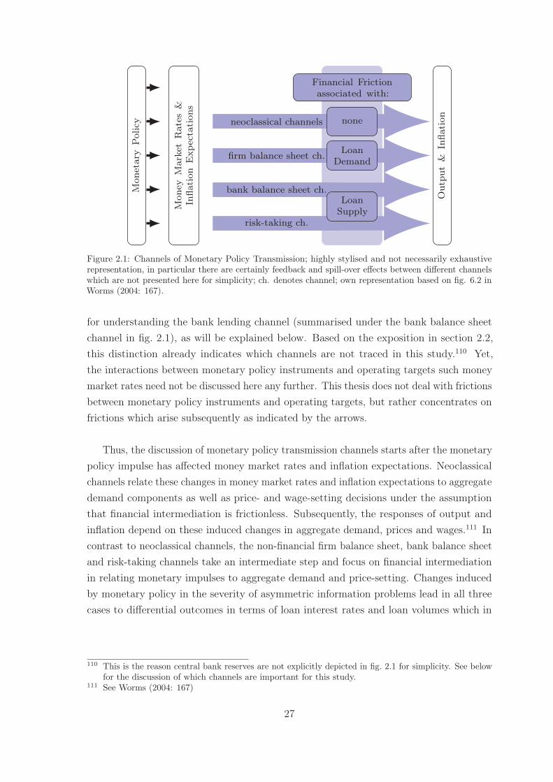
Mon

etar

yPol

icy

Mon

eyM

arke

tR

ates

&In

flati

onE

xpec

tati

ons

Out

put

&In

flati

on

Financial Frictionassociated with:

neoclassical channels none

firm balance sheet ch. LoanDemand

bank balance sheet ch.

risk-taking ch.

LoanSupply

Figure 2.1: Channels of Monetary Policy Transmission; highly stylised and not necessarily exhaustiverepresentation, in particular there are certainly feedback and spill-over effects between different channelswhich are not presented here for simplicity; ch. denotes channel; own representation based on fig. 6.2 inWorms (2004: 167).

for understanding the bank lending channel (summarised under the bank balance sheetchannel in fig. 2.1), as will be explained below. Based on the exposition in section 2.2,this distinction already indicates which channels are not traced in this study.110 Yet,the interactions between monetary policy instruments and operating targets such moneymarket rates need not be discussed here any further. This thesis does not deal with frictionsbetween monetary policy instruments and operating targets, but rather concentrates onfrictions which arise subsequently as indicated by the arrows.

Thus, the discussion of monetary policy transmission channels starts after the monetarypolicy impulse has affected money market rates and inflation expectations. Neoclassicalchannels relate these changes in money market rates and inflation expectations to aggregatedemand components as well as price- and wage-setting decisions under the assumptionthat financial intermediation is frictionless. Subsequently, the responses of output andinflation depend on these induced changes in aggregate demand, prices and wages.111 Incontrast to neoclassical channels, the non-financial firm balance sheet, bank balance sheetand risk-taking channels take an intermediate step and focus on financial intermediationin relating monetary impulses to aggregate demand and price-setting. Changes inducedby monetary policy in the severity of asymmetric information problems lead in all threecases to differential outcomes in terms of loan interest rates and loan volumes which in

110 This is the reason central bank reserves are not explicitly depicted in fig. 2.1 for simplicity. See belowfor the discussion of which channels are important for this study.

111 See Worms (2004: 167)

27

turn affect aggregate demand and price-setting.112 The non-financial firm balance sheetchannel mainly works through changes in loan demand, while both the bank balance sheetand risk-taking channels affect loan supply.

Consider first the (non-financial firm) balance sheet channel. In contrast to theModigliani-Miller Theorem113, this balance sheet channel starts from the premise thatexternal financing is more expensive than internal financing. Imperfect information andits associated problems of moral hazard, costly monitoring and enforcement are primecauses of this spread, also called the external finance premium.114 In this view, a borrow-ers’ net worth is crucial in alleviating these problems because it aligns, to some extent,the interests of borrowers and lenders.115 Monetary policy in turn impacts borrowers’balance sheets in a number of ways. Consider contractionary monetary policy: Thisleads to rising interest expenses on existing, flexible-rate debt as well as indirectly topotentially declining revenues through lower aggregate demand generated by monetarypolicy.116 Both of these mechanisms reduce non-financial firms’ cash flow.117 Furthermore,as rising interest rates tend to be linked to lower asset prices, the value of collateral forcredit contracts declines.118 Thus, the external finance premium increases, and capitaldemand and investment decrease.119 Since this mechanism has further feedback effectsover subsequent periods, this amplification and propagation mechanism through balancesheets has been termed ‘financial accelerator’.120

Next, turn to bank-based channels.121 The early literature on the balance sheet channelfocused on non-financial firms as borrowers. Even so, banks also played a role in theearly credit channel literature in terms of a bank lending channel.122 The bank lendingchannel is uniquely identified with financial intermediaries and is primarily associatedwith the loanable funds paradigm mentioned above. At the core of the bank lendingchannel is the availability of loanable funds which determine loan supply.123 The crucial

112 These channels have been related to aspects of financial intermediation other than the loan market.The fundamental mechanisms are most naturally explained with respect to the loan market, which isthe approach followed here for simplicity.

113 Under a specific set of assumptions Modigliani and Miller (1958: 268) find the capital structure to beirrelevant for a non-financial firm’s market value.

114 See Bernanke and Gertler (1995: 29)115 See Bernanke and Gertler (1995: 35)116 See Bernanke and Gertler (1995: 36). The latter effect presumes that in the short run, non-financial

firms’ costs do not adjust appropriately, see Bernanke and Gertler (1995: 36).117 See Bernanke and Gertler (1995: 36)118 See Bernanke and Gertler (1995: 36)119 See Bernanke and Gertler (1995: 35) and Bernanke et al. (1999: 1370)120 See Bernanke and Gertler (1995: 35)121 Henceforth, this study will be concerned with banks as defined as financial intermediaries granting

loans and deposits to the non-financial sector, unless specified otherwise.122 See Bernanke and Gertler (1995: 29, 40ff)123 See Bernanke and Gertler (1995: 40)

28

assumption of this channel is that banks as financial intermediaries and suppliers of creditto non-financial firms cannot easily substitute bank deposits with other forms of financialliabilities. The designation ‘easily’ is chosen purposefully. In the model by Bernanke andBlinder (1988), the key assumption is that banks do not issue any form of liability otherthan bank deposits.124 Subsequently, this strong assumption was moderated. As Kashyapand Stein (1994) emphasise, the relevant assumption for the lending channel to be at workis that there is no complete substitutability between bank deposits and other forms ofbank financing in the aggregate.125 In the case of contractionary monetary policy, bankdeposits fall due to a decline in central bank reserves.126 Thus, loanable funds and as aconsequence bank loan supply decrease. As non-financial firms potentially incur costs inestablishing new credit relationships when banks tighten loan supply, this can also lead toan increase in the external finance premium.127

The bank lending channel and its loanable funds basis have come under intense crit-icism. Especially the assumption that banks cannot easily accommodate a shortfall inbank deposits by other liquid funding options has been criticised.128 Furthermore, thereis a debate about whether central bank reserves play a crucial role for loan-grantingdecisions.129 In response to these criticisms, Disyatat (2011), for instance, argues for a newbank lending channel as the theoretical equivalent of the balance sheet channel describedabove for non-financial firms.130 Thus, there may exist a similar balance sheet channel forbanks.131 Elaborating on such a bank balance sheet channel, the balance sheet structurecan be further disaggregated to relate to other aspects such as bank liquidity or bankcapital. In this vein, Boivin et al. (2011) identify a bank capital channel as a separatebank-related channel.132 The negative effect of loan losses on bank capital may lead to adeleveraging process restricting credit availability and reducing aggregate demand.133

Finally, the risk-taking channel has come to prominence since the financial crisis 2007-8.This channel traces the effects of monetary policy on different risk perceptions and riskpricing by agents.134 The focus of the risk-taking channel is generally on expansionarymonetary policy to discern the effects of prolonged low interest rates on (bank) behaviour.

124 See Bernanke and Blinder (1988: 435f)125 See Kashyap and Stein (1994: 226)126 See Kashyap and Stein (1994: 221) and Disyatat (2011: 4)127 See Bernanke and Gertler (1995: 40f)128 See Disyatat (2011: 7)129 This is demonstrated by the discussion between loanable funds and endogenous money, see above.

See also Disyatat (2011)130 See Disyatat (2011: 8)131 This possibility had already been noted by Bernanke et al. (1999: 1379).132 See Boivin et al. (2011: 382)133 See Boivin et al. (2011: 382f)134 See Borio and Zhu (2012: 237)

29

According to this channel, expansionary monetary policy can increase bank risk-taking.135

This may increase the impact of monetary policy on the real economy and may also exacer-bate boom-bust cycles.136 Furthermore, the risk-taking channel can be disaggregated intodifferent sub-mechanisms which link asset prices, target rates of return and central bankcommunications to the perception of and tolerance to risk.137 As Dell‘Ariccia, Laevenand Marquez (2014) show, these sub-mechanisms do not necessarily work in the samedirection. In particular, with a fixed capital structure (as in the case of binding capitalrequirements, for instance), expansionary monetary policy induces banks with low leverageto lower their monitoring effort, while the reverse is true for banks with high leverageratios.138 Overall, the risk-taking channel appears to be a fertile ground for future research.

Importantly, none of the non-neoclassical channels of monetary policy works in isolationand independently of other channels. In particular, for any of the financial intermediationchannels to have real effects, some form of nominal rigidity is still necessary.139 Otherwise,nominal interest rate changes would only affect prices.140 Furthermore, expectationsconcerning the future path of monetary policy are important determinants of transmission,as indicated in fig. 2.1 through the term inflation expectations. Indeed, Woodford (2003)argues that monetary policy is successful if it can form expectations about the policy rateand the implied path of economic activity and prices.141 With policy interest rates at thezero lower bound, the issue of longer-term expectations has gained even more prominence.The shaping of these expectations by central bank communications has become knownas forward guidance.142 When policy rates are at the zero lower bound, there is no morepotential to cut interest rates to stimulate demand. The intention of forward guidance isthen to induce an increase in aggregate demand now by committing to keep policy rateslow even after economic conditions would suggest a monetary tightening.143

More generally, how does this discussion inform the particular characterisation ofmonetary policy transmission as used in this study? First of all, the use of an NK DSGEmodel ensures that expectations play a crucial role and nominal rigidities allow for mon-etary non-neutrality. Furthermore, monetary policy is not passed through the financialsector as if it were a veil. Financial market imperfections such as asymmetric informationincorporate the findings of the credit channel literature. To be specific, the model features

135 See Borio and Zhu (2012: 242)136 See Borio and Zhu (2012: 248)137 See Borio and Zhu (2012: 242ff)138 See Dell‘Ariccia et al. (2014: 66)139 See Kashyap and Stein (1994: 226)140 See Kashyap and Stein (1994: 226)141 See Woodford (2003: 15)142 See J. R. Campbell, Evans, Fisher and Justiniano (2012: 2f)143 See J. R. Campbell et al. (2012: 2)

30

the balance sheet channel, with respect to both non-financial firms and banks. Thisdouble balance sheet channel is the only non-neoclassical channel incorporated into themodel. This is not to say that other channels are not or even less important, but they areabstracted from in order to keep the model and its analysis tractable.

The reasons for concentrating on this double balance sheet channel are manifold.Separating the effects of various channels is not only of analytical convenience but alsohelps in uncovering which channels are important in specific contexts and times. Thisstudy should thus be taken as a piece of a larger puzzle. Furthermore, as more andmore channels are included, the contributions of the individual channels become moredifficult to separate. The singular attention to the balance sheet channel as it worksthrough non-financial firms’ and banks’ balance sheets helps to distinguish the impact ofbank default.144 The symmetric approach to modelling the financial friction associatedwith non-financial firms and banks facilitates the accomplishment of one of the researchquestions, namely discerning the relative importance of these two financial frictions. Thiswould be more difficult using, for example, the bank lending channel approach. Admittedly,bank default may also affect monetary policy through other channels. Yet, in this regard,this study can be seen as a baseline: as will be shown, even in the absence of potentiallyhigher bank fragility arising from a risk-taking channel, bank default and monetary policyare tightly interlinked. Therefore, for the purposes of this study, modelling the risk-takingchannel is not necessary and its complications are abstracted from for simplicity. Theadditional layer of risk-taking is an interesting topic to be analysed in future research.

Touching on the issue of bank default, the possibility that a bank may not generatesufficient revenues to pay its creditors raises the question of the rationale for banks’existence. According to standard banking theory, banks have the functions of provid-ing liquidity services and a payment system, asset transformation, risk management,information administration and monitoring.145 Concerning non-neoclassical channels ofthe monetary transmission mechanism in general, information asymmetries justify theexistence of financial intermediaries as separate economic entities. In this line of argument,banks are explained by referring to their ability to ameliorate asymmetric informationproblems or their consequences. Non-bank borrowers may have more information on theirfinancial position, but banks’ ability to collect information and monitor can moderate themoral hazard problem, for instance. In this sense, banks possess (superior) monitoring

144 A similar reasoning applies to not incorporating all possible neoclassical transmission channels. Forexample, given the closed economy set-up, there is no space for an exchange rate channel. The mostimportant neoclassical channel included in the banking model is the interest rate channel.

145 See Freixas and Rochet (2008: 2)

31

capabilities which other agents have not.146 Also, banks can be interpreted as specialisedinformation processing agents, such that banks can extract a higher value than otheragents in case projects (loans) are liquidated.147

Yet, if banks’ liabilities are also subject to asymmetric information, these argumentsare weaker. When banks have more information on their financial position, banks’ cred-itors must also collect information and monitor banks. In this study, the existence ofbanks is still justified by their specific skill-set. Banks possess superior knowledge andmonitoring skills than non-financial creditors with respect to lending to non-financialfirms.148 Accordingly, the financial friction associated with non-financial firms is moresevere than the one of banks in the sense that non-bank investors still find it optimal todelegate the monitoring of non-financial firms to banks. Non-bank investors save entirelythrough banks. The explicit reasons for these superior abilities are left unspecified. As aresult, banks are the only financial intermediaries and all financial funds are intermediatedby banks.

In conclusion, various channels have been proposed for characterising monetary policytransmission through the banking sector. This study will concentrate on one particularchannel, namely the balance sheet channel applied to non-financial firms and banks todiscern the consequences of bank default. Some reasons for this choice have already beenproposed in this section, with the following sections providing more. Before elaborating onthe references to the theoretical literature, the next section will provide a short overviewof the empirical literature on the link between monetary policy transmission and financialintermediation.

2.4 Empirical Literature on Financial Intermediation

and the Monetary Policy Transmission Mechanism

From a theoretical perspective, financial intermediation has the potential to impact mon-etary policy. Yet, is this reflected in empirical results? This is the focus of this section.There are two layers to this question. Firstly, there is the question of whether the fi-nancial sector can be represented as a veil. Is the monetary policy impulse transmittedby the financial system one-to-one? This is addressed in numerous studies of interest

146 Holmstrom and Tirole (1997: 670), for instance, argue that financial intermediaries are the onlyagents that can monitor borrowers, since they can commit sufficient own capital and/or have aninformational advantage.

147 See Angeloni and Faia (2009: 8) for a model where banks have superior extraction skills in the case ofnon-financial firm default due to an information advantage.

148 As will be shown in chapter 5, the absolute size of monitoring costs in percent of the collected assetsis smaller in case of bank default than a non-financial firm’s default for a given risk premium.

32

rate pass-through. As it turns out, pass-through is far from perfect, especially in theshort run. So if the financial sector transforms the monetary policy impulse, the secondlayer concerns the determinants of this transformation. Studies in this group concernempirical analyses of the channels discussed above, as well as other potential featuresof the financial system which are only loosely related to the channels, such as bank-ing sector competition. The following paragraphs will show that the empirical resultsare somewhat mixed concerning how features of the financial system affect monetary policy.

Pass-through of monetary policy impulses concerns the extent to which changes inthe policy interest rate are reflected in retail loan and deposit interest rates at financialinstitutions. The empirical literature on this topic is vast, the interested reader is referredto de Bondt, Mojon and Valla (2005) and Kopecky and van Hoose (2012) as a startingpoint to the relevant literature.149 The general result of this literature is that pass-throughis incomplete both over the short and the long run.150 For Germany, the studies by Weth(2002), Mueller-Spahn (2008) and Al-Eyd and Berkmen (2013) show that pass-through isincomplete and varying across bank products.151

One approach to explaining slow adjustment of retail interest rates is to consider thedegree of competition in the banking sector. Many studies have found banking systems invarious countries to be monopolistically competitive markets. For instance, Bikker andHaaf (2002) and Claessens and Laeven (2004) show that the banking sector in Germanyas well as in many other countries is a monopolistically competitive market.152 Therecent cross-country study by Weill (2013) also finds that the German banking sectoris a monopolistically competitive market.153 As to the reasons for why banks shouldpossess market power, switching costs as well as market concentration can be cited, forexample.154 The link between banking sector competition and monetary policy has also

149 See de Bondt et al. (2005: 25f) and Kopecky and van Hoose (2012: 1186) and the references therein.150 This applies to various countries and time spans, see Kopecky and van Hoose (2012: 1186).151 See Weth (2002: 18f), Mueller-Spahn (2008: 9f), and Al-Eyd and Berkmen (2013: 15). Weth (2002:

18) finds that almost complete pass-through is achieved for mortgage lending rates in a few months;the author estimates the model over the period 1993-2000. Mueller-Spahn (2008) uses data between2003 and 2006. The estimates of Al-Eyd and Berkmen (2013) are based on the time period 2003-2013.

152 Both Bikker and Haaf (2002) and Claessens and Laeven (2004) study cross-country panel datasetson banks over the years 1988-1998 and 1994-2001, respectively. Both studies indicate monopolisticcompetition in the German banking sector, see Bikker and Haaf (2002: 2202) and Claessens andLaeven (2004: 572f). Bikker and Haaf (2002) also analyse subsamples of the banking sector. InGermany, restricting the focus to small and medium-sized banks supports the finding of monopolisticcompetition, while including only large banks yields the finding of a perfectly competitive market, seeBikker and Haaf (2002: 2201f).

153 See Weill (2013: 106ff). Weill (2013) considers the time period between 2002 and 2010.154 See Gerali, Neri, Sessa and Signoretti (2010: 111). According to the structure-conduct-performance

paradigm, market power can be a result of market concentration; menu costs such as fees for usingspecific bank services as well as asymmetric information problems can give rise to switching costswhich make it costly for bank customers to switch banks, resulting in bank market power, see Geraliet al. (2010: 111).

33

been studied. In an early study, Cottarelli and Kourelis (1994) present empirical evidencethat, among others, regulatory impediments to competition in the banking sector inhibitpass-through by making loan rates stickier.155 Also, Mojon (2000) finds that competitionincreases monetary pass-through.156 From this perspective, the issue of limited interestrate pass-through can be treated in a similar way as prices and nominal wages in assuminga departure from perfect competition and some form of rigidities in the price-settingbehaviour of banks.157

In addition to this explanation in terms of market structure, various other factors havebeen studied in the literature. Given the vastness of the literature and the space limits here,the following examples are collected from studies about German banks. For one, Schlüter,Busch, Hartmann-Wendels and Sievers (2012) argue that cost efficiency affects the interestrate setting behaviour of banks and thus interest rate pass-through.158 Mueller-Spahn(2008) reports different pass-through estimates for different German banking groups.159

Also, bank size has been found to impact interest rate pass-through.160 Concerning otherbalance sheet characteristics, bank leverage, liquidity and the shares of saving depositsin banks’ liabilities and of long-term non-bank loans in banks’ balance sheets have beenreported as determinants of interest rate pass-through to lending rates.161 However, theresults on these different determinants are not unambiguous: For the shares of deposits andloans in banks’ balance sheet considered by Weth (2002), the higher the respective share,the lower is the interest rate pass-through.162 In contrast, Mueller-Spahn (2008) reportsthat a lower diversification of banks’ balance sheet leads to increased pass-through.163 Inconclusion, empirical studies suggest that the interest rate pass-through is not complete atleast in the short run, but the factors impacting the pass-through are manifold.

Nevertheless, analysing the pass-through from policy or money market rates to lendingand deposit rates and its potential determinants reflects only one part of the financialintermediation process. Another important part is the evolution of the credit volume.Based on the bank lending channel view, Kashyap and Stein (2000) argue, for example,

155 See Cottarelli and Kourelis (1994: 32). Cottarelli and Kourelis (1994) use a cross-country dataset forthe time between 1980 and 1993.

156 See Mojon (2000: 8). Mojon (2000) studies a subset of Euro area countries for the time period1979-1998.

157 Theoretical models on this issue have been proposed by Kopecky and van Hoose (2012) in a partialequilibrium setting, and Gerali et al. (2010) in a DSGE model framework.

158 See Schlüter et al. (2012: 47), URL in list of references, their dataset comprises the time between2003 and 2008.

159 See Mueller-Spahn (2008: 14, 18)160 See Weth (2002: 22) and Mueller-Spahn (2008: 14, 20)161 See Weth (2002: 22f), Mueller-Spahn (2008: 14) and Al-Eyd and Berkmen (2013: 15)162 See Weth (2002: 22f)163 See Mueller-Spahn (2008: 14). Diversification is defined as the degree to which total income originates

from interest income, see Mueller-Spahn (2008: 12).

34

that banks with a more liquid asset portfolio do not have to cut lending (as much) whendeposits are withdrawn, but can instead also reduce their liquid assets.164 Using bank-leveldata Kashyap and Stein (2000) provide empirical support for the existence of the banklending channel in the US.165 In particular, small banks with less liquid balance sheetscontract lending comparatively more after a monetary policy tightening.166 Furthermore,Kishan and Opiela (2006) found a similar result using bank capital as the determiningfeature of the bank lending channel.167 Concerning the Euro area (EA), studies conductedwithin the context of the Monetary Transmission Network at the turn of the century reportresults that are in line with both the balance sheet and the bank lending channels at adisaggregated level.168 Here, balance sheet liquidity appears to be a determinant of thebank lending channel, and not the level of bank capital.169

Concerning Germany, the empirical results on this topic are mixed. In early studies,Ehrmann et al. (2001), Hülsewig (2003) and Worms (2003) provide support for a creditchannel170 based on bank loan supply changes.171 Furthermore, in line with other EAcountries Ehrmann et al. (2001) and Worms (2003) show that liquidity is a determinant ofhow a bank’s loan volume changes after a monetary policy shock, while size is not.172 Incontrast, the results by Favero, Giavazzi and Flabbi (1999) and Küppers (2001) do notsupport the bank lending channel.173

What is more, not only do results differ concerning the existence of bank-specific influ-ences, but also on the direction of the effects. Küppers (2001) and Kakes and Sturm (2002)find that responses to monetary policy vary for different banking groups.174 In line withKashyap and Stein (2000), Kakes and Sturm (2002) find that lending by the largest banks

164 See Kashyap and Stein (2000: 409)165 See Kashyap and Stein (2000: 425), they use data ranging from 1976 to 1993.166 See Kashyap and Stein (2000: 424f)167 See Kishan and Opiela (2006: 282), the study uses US data for the time 1980 to 1999. The argument

for bank capital as a distinguishing feature is that banks with a lower capital base encounter moreproblems when trying to shift from insured to non-insured deposits following contractionary monetarypolicy, see Kishan and Opiela (2006: 262f).

168 See European Central Bank (2010: 86)169 See European Central Bank (2010: 86) and Ehrmann, Gambacorta, Martínez-Pagés, Sevestre and

Worms (2001: 29ff)170 In general, the credit channel is an umbrella term for both non-financial firms’ balance sheet channel

and the bank lending channel, see Bernanke and Gertler (1995: 34f).171 See Ehrmann et al. (2001: 29ff), Hülsewig (2003: 24), and Worms (2003: 192). The dataset of

Ehrmann et al. (2001) covers the years 1988 to 2000 for different European countries, 1994 to 1998for Germany. Hülsewig (2003) covers the time between 1975 and 1998. Worms (2003) uses the datarange 1992–1998.

172 See Worms (2003: 187) and Ehrmann et al. (2001: 29ff)173 See Favero et al. (1999: 12) and Küppers (2001: 1922ff). The study by Favero et al. (1999) uses a

case-study approach for the year 1992 where monetary tightening took place in Europe. Küppers(2001) uses data for the time 1969–1996.

174 See Küppers (2001: 1922ff) and Kakes and Sturm (2002: 2086f). Kakes and Sturm (2002) cover thetime between 1975 and 1997.

35

does not change much after a monetary policy shock while generally smaller credit cooper-atives decrease both their lending and liquid assets.175 To the contrary, Küppers (2001)finds that the largest banks in Germany experience a drop in their loan volume followingcontractionary monetary policy, while this is not true for generally smaller savings banksand credit-cooperatives.176 These conflicting results may be partially aligned by the resultsby Worms (2003) who emphasises that the structure of the banking sector is important andinterbank deposits are crucial for explaining the insignificance of bank size.177 Throughtheir integration into a large network, small savings and cooperative banks can reducetheir interbank deposits in the respective network in order to protect their loan portfolio.178

A similar conflicting picture arises from more recent studies. Eickmeier, Hofman andWorms (2009) do not find conclusive evidence in favour of a bank lending channel butpoint to the difficulties in disentangling loan supply and demand effects.179 In contrast,de Santis and Surico (2013) find evidence in favour of the bank lending channel.180 Also,the findings by Puri, Rocholl and Steffen (2011) support the existence of a bank lendingchannel during the financial crisis 2007-8. German savings banks affected by the crisisin the US subprime market accepted fewer loan applications than non-affected banks.181

Furthermore, they identify bank size and liquidity as further determinants of this effect.182

Somewhere in between, Arnold, Kool and Raabe (2011) find bank size and liquidity tobe indicators of the bank lending channel, but not capitalisation.183 However, Arnoldet al. (2011) emphasise that their results are dependent on the specific sector to whichloans are granted.184 Conceding the caveat that different results may be due to differingeconometric methodologies and datasets, these diverging results point to the difficulties indisentangling loan demand and supply effects.

To summarise the previous discussion, empirical studies indicate that banks’ balancesheets play a role in monetary policy transmission. Similar to the literature on pass-through,the determinants vary. The difficulties in separating demand and supply effects which

175 See Kakes and Sturm (2002: 2086). Yet lending by savings banks increases after a monetary policyshock, see Kakes and Sturm (2002: 2086f).

176 See Küppers (2001: 1922)177 See Worms (2003: 188f)178 See Worms (2003: 191)179 See Eickmeier et al. (2009: 216f), their data ranges from 1985 to 2005.180 See de Santis and Surico (2013: 440), they use a dataset for different European countries, among

them Germany, from 1999 to 2011. They find different variables (size, liquidity, capitalisation) tobe significant in different regressions, especially when the dataset is disaggregated to study bankheterogeneity, see de Santis and Surico (2013: 440ff).

181 See Puri et al. (2011: 566), they use data on German savings banks from July 2006 to June 2008.‘Affected’ banks are those whose corresponding Landesbank announced losses due to the financialcrisis, see Puri et al. (2011: 562).

182 See Puri et al. (2011: 578)183 See Arnold et al. (2011: 15f). They use data on Germany covering the years 1992 to 2002.184 See Arnold et al. (2011: 16)

36

come with the focus on volumes constitute a further reason for not explicitly modellingthe bank lending channel but to concentrate on the broader balance sheet channel.

However, how important is the effect of banks’ balance sheets vis-à-vis non-financialfirms’ balance sheets?185 Some studies have aimed to compare these two channels. Meisen-zahl (2014) compares the non-financial firm and bank balance sheet channels.186 Meisenzahl(2014) concludes that the non-financial firm balance sheet channel plays a large role whilethe bank balance sheet channel does not.187 In contrast, in a DSGE model-based exercise,Villa (2013) finds that the model in which imperfections arise from the interactions offinancial intermediaries with their stakeholders fits better to EA data than the modelwhere distortions arise from information asymmetries between non-financial firms andbanks.188

These contradictory findings suggest that the significance of either channel is context-dependent. In particular, Jimenéz, Ongena, Peydró and Saurina (2012) find that banks’balance sheets primarily play a role in crisis times, but not during normal times.189 Incontrast, non-financial firms’ balance sheets affect loan-granting both in normal andeven more in crisis times.190 Ciccarelli, Maddaloni and Peydró (2013) analyse monetarypolicy transmission in ‘stressed’ and ‘non-stressed’ EA countries beginning with the recentfinancial crisis. They find the non-financial firm balance sheet channel to be importantover the whole period for stressed countries, while the bank balance sheet channel isonly important during crisis times.191 The authors argue that the insignificance of bank-related characteristics after 2009 is due to the full allotment policy of the ECB.192 Finally,Ciccarelli, Maddaloni and Peydró (2010) find evidence in support of both parts of thecredit channel.193 Furthermore, the relative impact of the two sub-mechanisms of thecredit channel varies for different loan products.194 Taking these results together, there isan indication for a more prominent role of the non-financial firm balance sheet channelwhile banks’ balance sheets become especially important in financial crises.

185 In the spirit of a streamlined and focused exposition, the vast empirical literature on the non-financialfirm balance sheet channel is not reviewed here. The interested reader is referred to Beck, Colciagoand Pfajfar (2014: 3) as a starting point.

186 The non-financial firm balance sheet channel is based on a costly state verification problem, while thebank balance sheet channel is derived from a moral hazard problem along the lines of Holmstrom andTirole (1997), see Meisenzahl (2014: 60ff).

187 See Meisenzahl (2014: 75). The study is based on US data between 1998 and 2003.188 See Villa (2013: 5). Villa (2013: 5) compares a Bernanke et al. (1999) model to a Gertler and Karadi

(2011) model and estimates them on EA data from 1980 to 2008.189 See Jimenéz et al. (2012: 2). They use data on banks in Spain between 2002 and 2010.190 See Jimenéz et al. (2012: 3)191 See Ciccarelli et al. (2013: 23f), their study analyses EA countries over the time 2002-2011.192 See Ciccarelli et al. (2013: 24)193 See Ciccarelli et al. (2010: 11), their data span the years 2002 to 2009 for the EA and 1992 to 2009

for the US.194 See Ciccarelli et al. (2010: 12)

37

Given that only recently attention was directed to the risk-taking channel, the empiricalliterature is still developing. Maddaloni and Peydró (2011) find evidence that low policyrates induce softer lending standards in the US and European countries.195 Using US datafrom 1997 to 2008, Buch, Eickmeier and Prieto (2014) find that the banking system as awhole does not engage in additional risk-taking in response to looser monetary policy.196

However, when looking at different groups of banks, there are significant differences. Incontrast to large banks and foreign banks, small banks engage in additional risk-taking.197

Thus, while they do not find a risk-taking channel working in the aggregate, the risk-takingchannel appears to be active for small banks.198 Similarly, the studies by Dell‘Ariccia,Laeven and Suarez (2013) and Jiménez, Ongena, Peydró and Saurina (2014) both pro-vide support for a risk-taking channel of expansionary monetary policy, yet again withconflicting results.199 Dell‘Ariccia et al. (2013) show that the risk-taking channel is lessstrong for banks with a comparatively low capital base.200 This is in contrast to thefindings of Jiménez et al. (2014) which indicate that it is poorly capitalised banks to whomthe risk-taking channel appears to apply.201 Thus, research on the risk-taking channelso far has shown that banks’ balance sheet position is not only relevant in terms of thecredit channel, but can also be a factor in other aspects of bank behaviour. These resultsshow that there is space for a risk-taking channel, but more research is needed on itsdeterminants and specific characteristics.

Turning to the issue of banking sector fragility, Blank et al. (2009) study the interrelat-edness in the German banking system as a factor in a banks’ distress frequency.202 Theauthors find that adverse shocks to large banks lead to an increase in the probability ofdistress of small banks.203 Furthermore, de Graeve et al. (2008) find significant effectsof monetary policy on banks’ distress frequency.204 In particular, the authors find thatcontractionary monetary policy leads to an increase in banks’ distress probability.205

Besides, de Graeve et al. (2008) also find that the degree of bank capitalisation has an

195 See Maddaloni and Peydró (2011: 2150), they use bank lending surveys between 2002 and 2008.196 See Buch et al. (2014: 23)197 See Buch et al. (2014: 24)198 See Buch et al. (2014: 27). The authors also find that new riskier loans are shorter in maturity and

tend to be backed by collateral more frequently. Thus, the risk appears to be taken into account bythese small banks. See Buch et al. (2014: 27)

199 See Dell‘Ariccia et al. (2013: 18), who use US loan rating data for the period 1997 to 2011, andJiménez et al. (2014: 499), who use data on banks in Spain from 2002 to 2008.

200 See Dell‘Ariccia et al. (2013: 18)201 See Jiménez et al. (2014: 493, 499)202 Blank et al. (2009: 354) use data on individual German banks from 1994 to 2004. The term ‘distress’

covers a variety of situations not restricted to explicit default, from mandatory announcements toclosure, see Blank et al. (2009: 359).

203 See Blank et al. (2009: 354)204 de Graeve et al. (2008) use data on individual German banks for the time 1995–2004.205 See de Graeve et al. (2008: 207f)

38

impact on this effect.206 Thus, again banks liability structure is a significant feature.Therefore, there appears to be a link between monetary policy and banking sector fragility.

Taken together, these empirical studies suggest that banks play an important role inthe monetary transmission process. As is clear from sometimes contradictory results, theinvolved processes are highly complex. While there are indications for specific importantfactors, the exact details remain elusive, as well as time- and context-dependent. Aimingfor an even slightly exhaustive representation in this study would not only be presumptuousbut would also miss the point. On the one hand, banks’ balance sheets have appeared tobe an influential factor in many studies. On the other hand, the results are inconclusive asto the explanatory power of volume effects. This informs the focus on the broader balancesheet channel instead of the bank lending channel.

Particular aspects are also abstracted from to keep the analysis tractable, as has beenargued before. Apart from the focus on one non-neoclassical channel, this study willalso not deal with explicit interest rigidities as evidenced by interest rate pass-throughstudies.207 Consequently, the model also abstracts from imperfect banking sector competi-tion. The reasoning is similar to the exclusion of the risk-taking channel: interest raterigidities introduce a further layer of effects which are not essential to the research question.

Moreover, the fact that the financial friction on each side of banks’ balance sheetis modelled in a similar fashion helps contribute to another question raised above: therelative impact of information asymmetries in the loan market vis-à-vis the markets forbank liabilities. Therefore, as a corollary of the research question, this study can providemodel-based statements about the importance of the two financial frictions along thelines of Meisenzahl (2014), applied to German data. The fact that crisis times are notstudied here does not preclude such an analysis. The links between financial crises andmacroeconomic developments have been examined extensively before.208 The interest-ing question for this study is the relative importance of bank-related to non-financialfirm-related information asymmetries for macroeconomic developments in ‘normal’ busi-ness cycles. Financial crises have occurred relatively infrequently in the past. Thestart and end points of business cycles tend to have a higher frequency, which meansthat it is equally important to discern the effects of banking sector fragility in normal times.

Overall, the previous sections discussed the link between monetary policy and financial

206 See de Graeve et al. (2008: 208)207 A model with monopolistic competition in banking with sticky interest rates has been proposed by

Gerali et al. (2010) and is used frequently in the literature as a building block, see Angelini, Neri andPanetta (2012) and Hollander and Liu (2016), for instance.

208 See, for example, Reinhart and Rogoff (2009)

39

intermediation on a general basis. Also, various reasons have been presented for themethodological approach and features of the model used in this study. The justification forthe more specific aspects implemented in the model is delegated to chapter 3 along witha detailed presentation. Beforehand, the next section will conclude with the discussionabout various strands of the literature which are more closely-related to this study. Thepresentation will progress along the aspects of modelling financial sector frictions inmacroeconomic models, from general issues to specificities of the nature of bank default.

2.5 Locate the Research: on Banking Sector Fragility

in the Literature

This section surveys the literature on frictions associated with financial intermediaries’liabilities to show how the present study relates to various approaches in the literature.Since this study principally concerns the financial friction on banks’ liability side, theinterested reader is referred to Beck et al. (2014) and Gerke et al. (2013) for a guide tothe literature on financial frictions between non-financial firms and financial intermedi-aries.209 As is clear from previous discussions, this study is related to the literature onthe interconnections between monetary policy and financial intermediaries at a generallevel. However, at this level, comparisons are quite blunt.210 To this end, the followingparagraphs will relate several aspects of this study to similar or diverging approaches inthe literature. The section starts with a short overview of the approaches to modellingfinancial frictions. Then, key aspects are dealt with, concerning the question of endogenousor exogenous bank leverage, the nature of bank capital, possibilities for modelling bankdefault, and more specific issues of deposit insurance and the relationship between thereturns on different bank liabilities. This section closes by distinguishing the particularmodelling contribution of this thesis.

The literature on financial frictions in macroeconomic models is vast. There are fourprominent approaches to modelling financial frictions: Bernanke et al. (1999) (BGG),Kiyotaki and Moore (1997) (KM), Holmstrom and Tirole (1997) (HT) and Gertler andKaradi (2011) (GK).211 BGG postulate an agency problem between non-financial firmsand banks to derive a spread, the external finance premium, between internal and external

209 See Beck et al. (2014: 5f) and Gerke et al. (2013: 254)210 General overviews of the field are provided by Beck et al. (2014) and Gerke et al. (2013). Furthermore,

Borio and Zhu (2012) present a meta-analysis of the literature related to the study of bank capital.211 Both BGG and KM deal with the financial situation of non-financial firms. In the following years,

these approaches have been used and developed extensively. Nonetheless, both approaches are equallyapplicable to the financing situation of other agents such as banks.

40

financing costs of non-financial firms.212 Endogenous changes in borrowers’ leverage affectthe external finance premium and amplify the economy’s reaction to monetary policy.213

In contrast, the approach by KM is based on an explicit collateral constraint.214 Then,the value of the collateral asset determines the available loan volume and through this thelevel of investment.215 As a consequence, the economy’s response to exogenous shocks isboth more persistent and amplified.216

HT and GK propose models in which financial intermediaries play a key role. HTpostulate a double moral hazard problem affecting both non-financial firms and financialintermediaries.217 The HT model works as follows: non-financial firms (borrowers) canchoose projects with different risk profiles, with riskier projects being better from the pointof view of non-financial firms, while lenders prefer safer projects.218 To moderate the moralhazard problem, banks monitor non-financial firms so they cannot choose the worse ofthe risky projects.219 However, monitoring involves private costs for banks, thus creatinganother moral hazard problem.220 In the end, this set-up leads to both non-financial firmsand banks being capital-constrained.221 Then, the amount of capital of non-financial firmsand banks as well as their relative sizes affect real investment.222 Finally, GK postulate amodel of non-financial firm equity financing with a moral hazard problem between financialintermediaries and their investors. The possibility that bank managers can abscond partof their borrowed funds leads to an endogenous leverage constraint on banks.223 GK usethe model to analyse unconventional monetary policy and find benefits to direct centralbank intermediation in a financial crisis.224

This study uses the modelling approach of BGG for both sides of banks’ balance sheet.In addition to the reasons presented before, this choice is governed by the analytical ease

212 See Bernanke et al. (1999: 1345, 1348). See also the discussion about the balance sheet channel above.The work of Bernanke et al. (1999) itself draws, among others, on the previous work of Carlstrom andFuerst (1997) in a real business cycle model context, see Bernanke et al. (1999: 1378).

213 See Bernanke et al. (1999: 1345, 1371)214 See Kiyotaki and Moore (1997: 212)215 See Kiyotaki and Moore (1997: 212)216 See Kiyotaki and Moore (1997: 212)217 See Holmstrom and Tirole (1997: 663ff). The model by HT is essentially a partial equilibrium model,

but has been applied to a dynamic (stochastic) general equilibrium context, see for instance Chen(2001) and Meh and Moran (2010).

218 Non-financial firms enjoy private benefits by choosing projects with a low success probability, seeHolmstrom and Tirole (1997: 667f). Yet, only projects with higher success probabilities produce apositive pay-off when investment costs are taken into account, see Holmstrom and Tirole (1997: 668).

219 See Holmstrom and Tirole (1997: 667ff)220 See Holmstrom and Tirole (1997: 669)221 See Holmstrom and Tirole (1997: 663)222 See Holmstrom and Tirole (1997: 686)223 See Gertler and Karadi (2011: 21, 32)224 See Gertler and Karadi (2011: 32f)

41

of incorporating default.225 For instance, default of non-financial firms and bank defaultare not treated explicitly in GK and KM.226 In HT, the main model mechanism revolvesaround the respective volumes of bank (and non-financial firm) capital which determinethe degree to which banks can attract loanable funds.227 While projects and thus loanscan fail in HT, this loanable funds basis runs counter the intention to model the balancesheet channel for both non-financial firms and banks in this study. What is more, theresulting symmetry of financial frictions on both banks’ asset and liability sides using theBGG approach is well-suited to study the additional effect of bank default as well as tocompare the relative impact of each financial friction. Thus, the choice in favour of theBGG modelling approach is based on the specific research question of this study.228

Having presented general approaches to modelling financial frictions, the next para-graphs will turn to the more specific strands this study is related to. For one, this studyconcerns the literature on the determination of bank leverage. A popular approach isto assume explicit capital constraints. Exogenous capital constraints simplify the modelsolution when leverage is indeterminate in the steady state.229 Furthermore, in analysingmacroprudential policy an exogenous capital constraint allows for a simple mapping from(binding) banking regulation. Examples of this approach are Kollmann (2013) and Benes,Kumhof and Laxton (2014). In Kollmann (2013), banks face a capital constraint andhave to pay penalty fees if they fail to hold the required level of capital.230 They findthat adverse shocks to bank capitalisation lead to sizeable reductions in real activity.231

In Benes et al. (2014) banks also pay penalty fees if their capital is below a certainthreshold.232 Furthermore, Benes et al. (2014) argue that mistakenly optimistic banksin combination with negative shocks can result in a financial crisis in their model withadverse consequences for the real economy.233

Yet, in the banking model presented in the next chapter, bank leverage is determinedendogenously. This can be rationalised by arguing that exogenous capital constraintsimply that capital adequacy ratios are always binding which may not be an adequate

225 For more details on the specific model design, see chapter 3.226 See Gertler and Karadi (2011: 27f) and Kiyotaki and Moore (1997: 212f). In Gertler and Karadi

(2011: 21), the threat of bank resolution is part of the approach in rationalising the endogenousleverage constraint, but does not occur as such. Clerc et al. (2014: 6) argue that banks can possiblyfail in papers using the KM approach, but this possibility is excluded by equilibrium conditions.

227 See Holmstrom and Tirole (1997: 675f, 690) and Meh and Moran (2010: 555f)228 In contrast, a study on the risk-taking channel may be more adequately conducted using the HT

approach, for instance.229 See the discussion in section 4.1.230 See Kollmann (2013: 164f), they use an open-economy layout and estimate their model using US and

EA data.231 See Kollmann (2013: 182)232 See Benes et al. (2014: 22, 26f).233 See Benes et al. (2014: 47)

42

representation of reality. Furthermore, the primary focus here is on monetary policy, notmacroprudential policies. It is illustrative to examine the consequences of bank defaultwithout any bank capital regulation in place, and then extend and compare with the casewhen macroprudential policies are introduced.234 The analysis under the assumption thatbank leverage is unconstrained in the benchmark model allows to focus on the conse-quences of the financial friction under scrutiny. Moreover, various authors have proposedendogenous bank leverage models. As already mentioned above, models using the GKframework generate an endogenous leverage constraint as a result of the moral hazardproblem. Van der Kwaak and van Wijnbergen (2014), for example, extend the GK moralhazard problem to evaluate the link between sovereign risk and financial fragility.235 Intheir model, endogenous bank leverage, sovereign risk and financial fragility are tightlylinked and a deterioration in one or more of these factors has adverse consequences forthe real economy.236 Thus, the choice for endogenous bank leverage can additionally bejustified by the prominent role it plays in these models. Related, Nuño and Thomas (2012)build a model where one part of the banking sector faces a capital constraint while theother does not.237 On the basis of their results, Nuño and Thomas (2012) provide anargument for leverage to be determined endogenously in macroeconomic models.238

A second question relates to the nature of bank capital. The majority of papers assumesinside capital, that is bank capital accumulated from retained earnings of the bankingbusiness, such as in Benes et al. (2014) and Meh and Moran (2010). In applying the HTapproach to a DSGE model, Meh and Moran (2010) show that negative shocks to bank cap-ital have adverse effects for the economy.239 Moreover, van der Kwaak and van Wijnbergen(2014) use this definition of bank capital to study the effects of bank bail-outs.240 Whilethis definition of bank capital lends itself naturally to research questions about bail-outs,the concept of bank capital used in this study is better suited to analyse the choice ofliability structure as a result of supply and demand. Hence, this study is more closelyrelated to papers modelling bank capital as outside or marketable equity held by households.

In particular, this study is similar to Abbate and Thaler (2014) in its concept of bank

234 The analysis of macroprudential policies in chapter 6 aims to gauge how the benchmark results areaffected by potential macroprudential policies on an ad-hoc basis.

235 See van der Kwaak and van Wijnbergen (2014: 223, 236)236 See van der Kwaak and van Wijnbergen (2014: 236)237 See Nuño and Thomas (2012: 19), they calibrate their model to US data.238 See Nuño and Thomas (2012: 27). Nuño and Thomas (2012: 27) find that when leverage is exogenously

imposed, it moves acyclically with bank assets while an endogenous leverage specification leads leverageto move pro-cyclically with assets. As Nuño and Thomas (2012: 12) argue, only the latter observationis in line with the reported positive correlation of assets and leverage of financial intermediaries in thedata.

239 See Meh and Moran (2010: 574)240 See van der Kwaak and van Wijnbergen (2014: 233f)

43

equity in that equity holders enjoy limited liability and receive any profits from the bankingbusiness after deposit holders have been paid out.241 However, in contrast to this study,Abbate and Thaler (2014) posit an agency problem in that equity holders choose a moreor less risky project in order to study the risk-taking channel of monetary policy.242 Theauthors find that low policy rates lead to a higher bank leverage ratio and a riskier bankasset profile.243 The model presented in the next chapter will instead allow for a completediversification of individual loan risk. Banks are themselves subject to idiosyncratic shocksleading some banks to default. This assumption is in line with Kiley and Sim (2014),for example.244 Kiley and Sim (2014) study the impact of bank capitalisation on assetprices and the real economy and show that increasing costs associated with raising newequity lead to adverse consequences for the real economy.245 Yet, while Kiley and Sim(2014) assume marketable bank equity similar to this study, they include the possibility ofadditional equity issuance.246 In contrast, this study assumes limited liability for bankshareholders.247 Recent research has also aimed at combining these two concepts of bankcapital in a single model, as in Gertler et al. (2012).248

Furthermore, this study is not only concerned with different bank liabilities but morespecifically with banking sector fragility. There are a number of papers which addressbank default. Two of the approaches differ in their assumption about banks’ ability todiversify loan risk. The first approach assumes that bank default is a direct consequenceof non-financial firms’ default while the second approach uses idiosyncratic bank shocks togenerate bank default. As an example of the former approach, Dell‘Ariccia et al. (2014)propose a partial equilibrium model in which banks choose the level of monitoring toreduce loan risk.249 The authors analyse the risk-taking channel and find that expansionarymonetary policy results in higher bank leverage and lower monitoring effort.250

241 See Abbate and Thaler (2014: 13)242 See Abbate and Thaler (2014: 2, 13)243 See Abbate and Thaler (2014: 16)244 See Kiley and Sim (2014: 179)245 See Kiley and Sim (2014: 175, 186, 197)246 See Kiley and Sim (2014: 177f). In Kiley and Sim (2014: 180) banks face a binding capital constraint.247 Furthermore, this thesis does not deal with bank re-capitalisation. As will be explained in chapter 3,

if bank revenues plus bank equity are insufficient to cover a bank’s borrowing costs, then it defaultsand ceases to exist. Further governmental intervention, such as bank bailouts mentioned above, arenot considered here. This is consistent with the focus on non-systemic bank failures.

248 Gertler et al. (2012) provide an extended model of Gertler and Karadi (2011) which includes bothinside and outside bank equity. While a higher level of internal net worth allows for higher creditcreation (ceteris paribus), higher outside equity allows the bank to divert funds more easily and thustightens banks’ leverage constraint, see Gertler and Karadi (2011: 21) and Gertler et al. (2012: S22f).They argue that outside equity can act as a buffer when inside equity (due to lower accumulatedprofits or asset prices) declines, see Gertler et al. (2012: S23, S27). However, this depends on thelarger disciplinary power of deposits than outside equity which runs counter the modelling approachof risk-free deposits followed here, see Gertler et al. (2012: S22).

249 See Dell‘Ariccia et al. (2014: 66)250 See Dell‘Ariccia et al. (2014: 86f)

44

Several papers have used the second approach in applying the BGG framework, thatis idiosyncratic bank shocks. Darracq Pariès, Jacquinot and Papadopoulou (2016), forexample, propose a large scale, multi-country DSGE model with various layers of default in-cluding bank default along the lines of BGG.251 Darracq Pariès et al. (2016) use the modelto trace the financial crisis in the EA and argue that sovereign stress, fragile banks andcapital requirements were important factors contributing to the economic developments.252

Also, Clerc et al. (2014) propose a model incorporating default for multiple agents in thisway.253 Clerc et al. (2014) show that high bank leverage leads to more volatility in thereal economy and that capital regulation reduces leverage and bank fragility.254

Furthermore, these two approaches to modelling bank default are not mutually ex-clusive. In Badarau and Popescu (2015) bank default arises as a direct consequence ofnon-financial firms’ default and more generally if a bank’s revenues are insufficient to coverits liabilities.255 The authors examine how monetary policy can enhance financial stability.To this end, they study the monetary policy response to a financial bubble and find that astandard monetary policy rule cannot counter financial instability.256 Furthermore, evenin the cases when the central bank acted against financial imbalances, it had to foregoprice stability to some extent for the improvement in financial stability.257 In chapter 6,this study will also touch on these issues. Concerning the modelling approach, there is acrucial difference between this study and Clerc et al. (2014), Darracq Pariès et al. (2016)and Badarau and Popescu (2015): these authors use the concept of inside bank capital.258

Thus, the agency problem is more properly described as existing between deposit-holdersand the bank (even though there may be deposit insurance), whereas in the model proposedhere the agency problem à la BGG exists between the bank and equity-holders. Thisassumption will turn out to have a decisive impact on the role of bank equity.

251 See Darracq Pariès et al. (2016: 10ff)252 See Darracq Pariès et al. (2016: 38f)253 See Clerc et al. (2014: 6). The layout in Clerc et al. (2014) is similar to the model proposed in this

study in that there also exists a deposit insurance scheme. Yet, in Clerc et al. (2014: 13), the depositinsurance scheme is funded by lump-sum taxes and the return on bank deposits is subject to a riskpremium. In the model proposed in this study deposit insurance enters the optimisation problemof banks and bank deposits earn the risk-free return. Moreover, this study derives an incentivecompatibility constraint on the part of households which together with the asset demand equationsdetermines bank leverage. In contrast, Clerc et al. (2014: 13, 27) study capital regulation and to thisend determine leverage by (binding) regulation and introduce a separate agent who supplies bankequity.

254 See Clerc et al. (2014: 8)255 See Badarau and Popescu (2015: 362f)256 See Badarau and Popescu (2015: 372)257 See Badarau and Popescu (2015: 372). On this basis the authors argue for a separate (macroprudential)

instrument to counter financial instability.258 The framework with a separate agent who supplies bank equity in Clerc et al. (2014) can be deemed

more similar to the concept of internal bank capital, that is accumulated from retained earnings, thanto the one used in this study, see also footnote 253.

45

This relates to the matter of bank deposits being risk-free or not. The possibility ofbank deposits being subject to cuts connects to the third modelling approach to bankdefault: bank runs. In contrast to above approaches, default due to bank runs does notnecessarily need to be grounded in insufficient bank assets but rather in their illiquidity.For example, Angeloni and Faia (2013) use a model with bank runs to argue that therisk-taking channel is active following expansionary monetary policy.259 Meanwhile, bankruns are explicitly ruled out here due to a deposit insurance scheme. As Diamond andDybvig (1983) show in a multiple-equilibria model, deposit insurance can eliminate therisk of bank runs and thus improve on an undesirable equilibrium.260 Thus, in modellingthe liability structure of banks, deposit insurance is a means to generate a view amonghouseholds that bank deposits are risk-free even though banks are fragile.261

In this vein, Collard, Dellas, Diba and Loisel (2012) and Gornicka and van Wijnbergen(2013), for instance, propose models where households hold both bank deposits and bankequity, and deposit insurance ensures that bank deposits pay the risk-free policy return.262

While the deposit insurance scheme as such is not the most important feature in thesemodels, it constitutes a similarity with the study presented here. However, in contrast tothis study, Collard et al. (2012) and Gornicka and van Wijnbergen (2013) assume that theoutlays of the deposit insurance fund are financed by the general government budget orby lump-sum taxes.263 In contrast, as is practised in Germany, this study assumes thatdeposit insurance fees are levied on banks’ to cover outlays in case of bank default.264

Only any additional shortfall is borne by the government budget. Thus, deposit insuranceis explicitly incorporated in the optimisation problem of banks.265

259 See Angeloni and Faia (2013: 313, 317)260 See Diamond and Dybvig (1983: 402, 404)261 As argued by Clerc et al. (2014: 6f), deposit insurance may also create an incentive distortion for

banks to take on too much risk. Clerc et al. (2014: 27) approach this issue by imposing binding bankcapital regulation to offset this distortion. In contrast, in the model proposed here, deposit insurancefees aim to internalise part of the costs of bank default.

262 See Collard et al. (2012: 4, 9f) and Gornicka and van Wijnbergen (2013: 8). While the study byCollard et al. (2012) shares some characteristics with the present study (see below), there are somenotable differences. Firstly, Collard et al. (2012: 8, 10) impose a binding leverage constraint on banks.Secondly, the financial friction Collard et al. (2012: 6ff) impose on bank lending is different to theBGG approach in that the authors model loans with different risk profiles and constant monitoring ofsafe loan projects.

263 See Collard et al. (2012: 9f). Gornicka and van Wijnbergen (2013) do not specify the financingstructure of the deposit insurance fund in their partial equilibrium model.

264 See chapter 3 for more details on the particular implementation.265 Related, the model also features minimum reserves. However these are merely an auxiliary modelling

device. In general, the functioning and role of minimum reserves is a debated topic. One mayargue in favour that they increase the resilience of the payments system. Yet, the recourse to thisexplicit justification is not necessary. For example, Roger and Vlcek (2011: 6) assume a liquidityrequirement which mandates banks to hold a certain percentage of their balance sheet volume asliquid (government) securities. These government securities simply finance government spending, seeRoger and Vlcek (2011: 6).

46

The assumption about bank deposits being risk-free is tightly linked to the distribu-tion of returns on bank liabilities. In the papers considered, bank equity is generallyassumed to be more expensive than bank deposits. There are various motivations forthis spread. Firstly, in a partial equilibrium framework, Repullo and Suarez (2008) sim-ply assume an ad-hoc premium on equity financing.266 Secondly, Collard et al. (2012)assume that there is an ad-hoc tax distortion which favours debt.267 Thirdly, Abbateand Thaler (2014) produce an equity premium as in Dell‘Ariccia et al. (2014) due to anexogenous constant cost of holding equity.268 Fourthly, Covas and Fujita (2010) assumethat equity issuance costs lead to more expensive equity.269 Fifthly, Dib (2010) derive theequity premium as a function of capital adjustment costs and the possibility of divertingpart of the bank capital for personal gain.270 Sixthly, Aguiar and Drumond (2007) andAgénor, Alper and Pereira da Silva (2011) use a deposits-in-utility function approach toderive asset demand equations from households’ optimisation problem to create a spread.271

In contrast to these, I explicitly derive the different required returns on bank depositsand bank equity from the optimisation problems of banks and workers. In particular,differential returns on bank equity and risk-free bank deposits arise due the incidence ofnon-systemic bank default. The modelling approach which resembles the one presentedhere most closely is the partial equilibrium framework of Gornicka and van Wijnbergen(2013) who derive a no-arbitrage condition between risk-free insured bank deposits andrisky subordinate debt.272 There, holders of subordinate debt demand a risk-adjustedreturn which compensates them for the risk of default and in case funds are insufficientto pay them in full.273 However, Gornicka and van Wijnbergen (2013) follow the GKframework in a partial equilibrium setting, while this study uses the BGG approach.Furthermore, the focus of Gornicka and van Wijnbergen (2013) is to study the effects of

266 See Repullo and Suarez (2008: 7). Repullo and Suarez (2008: 1f) postulate a friction in that bankscannot recapitalise when they have an ongoing lending relationship.

267 See Collard et al. (2012: 9)268 See Abbate and Thaler (2014: 11)269 See Covas and Fujita (2010: 144). Covas and Fujita (2010) use a model without bank default and

with a binding capital constraint determining the bank leverage ratio.270 See Dib (2010: 7f)271 See Aguiar and Drumond (2007: 14f) as well as Agénor, Alper and Pereira da Silva (2009: 7ff) for the

description of this part of the model by Agénor et al. (2011). The models by Aguiar and Drumond(2007: 12ff) and Agénor et al. (2011: 9) do not feature bank default and determine banks’ leverageratio through regulation. A further contrast to this study is that in Aguiar and Drumond (2007: 15f)the expected real return on bank equity is set equal to the expected real return on real capital. InAgénor et al. (2011: 8) adjustment costs contribute to the spread between bank equity and bankdeposits.

272 See Gornicka and van Wijnbergen (2013: 10). Kiley and Sim (2012) also derive a no arbitragecondition for bank liabilities, but this concerns bank debt and not bank equity. Furthermore, thisno-arbitrage condition is not the cause of the spread between return on equity and the return ondeposits. In Kiley and Sim (2012) debt is cheaper due to a tax advantage and equity dilution costs.See Kiley and Sim (2012: 5ff)

273 See Gornicka and van Wijnbergen (2013: 10)

47

minimum capital requirements and regulatory penalties on banks’ capital structure.274

Finally, due to the focus on financial fragility, this study will also deal with macropru-dential policies in chapter 6. The literature on this topic has grown enormously especiallysince the financial crisis 2007-8. Since this study concentrates on monetary policy, therewill be no comprehensive modelling exercise concerning macroprudential policy. Rather,approaches from the literature will be incorporated to show some of the possible conse-quences for monetary policy of countering financial instability. The approaches proposedin the literature are taken as illustrative means, and this study does not aim for a thoroughevaluation of macroprudential policies themselves. Given the focus on monetary policy,the macroprudential policies are introduced as is, and coordination issues are not treatedexplicitly.275 For an overview of the literature on macroprudential policies see Loisel (2014),for instance.

In sum, this study is closely related to the papers by Clerc et al. (2014) and Collardet al. (2012) even though in different aspects. Both papers address the implications offinancial fragility. Similarities to the approach of Clerc et al. (2014) include bank defaultalong the lines of BGG and the existence of a deposit insurance scheme. The modelpresented in this study is similar to Collard et al. (2012) concerning the concept of bankequity and risk-free bank deposits. Yet, there are some noteworthy differences to thesetwo papers some of which have already been outlined in footnotes 253 and 262, centredon the modelling approach. Additionally, the focus in this study is specifically on theconsequences for monetary policy while Clerc et al. (2014) study capital regulation andCollard et al. (2012) focus on optimal policy and the interplay with prudential policies.276

As a final difference, the model proposed here is estimated using German data while thesetwo other models are calibrated.

In terms of the research question, this study is closely related to Markovic (2006).There, households hold risk-free bank deposits and bank equity with the possibility ofbank default.277 Markovic (2006) examines the bank balance sheet channel and finds thatthe effects of monetary policy are stronger when banks are fragile.278 Yet, there are someimportant differences: Bank default and the spread between the returns on bank equityand bank deposits are introduced in a relatively ad-hoc fashion in Markovic (2006). Forone, Markovic (2006) defines banks’ default probability as a linear function of output

274 See Gornicka and van Wijnbergen (2013: 2f)275 On the issue of coordination of macroprudential and monetary policies, see for example Angelini et al.

(2012).276 Further, neither Clerc et al. (2014) nor Collard et al. (2012) study monetary policy shocks.277 See Markovic (2006: 16f)278 See Markovic (2006: 30)

48

instead of providing explicit microfoundations.279 Moreover, bank default is simply anadd-on in the arbitrage condition between bank deposits and bank equity.280

What is more, Markovic (2006) uses a reduced-form representation of the BGG ap-proach in that the elasticity of the credit spread to non-financial firms’ leverage is atime-invariant function.281 In contrast, the model presented in the following chapterderives the risk premium on bank equity as well as the external finance premium ofnon-financial firms as functions of default risk using the BGG approach.282 Contrary toa reduced-form representation, default probabilities and premiums are time-varying andspecifically depend on the financial positions of the actors. They are thus explicitly derivedfrom microfoundations. In order to study the impact of bank default, the endogeneity andmicrofoundation of these variables is crucial. Furthermore, while Markovic (2006) concen-trates on impulse response analysis, this study will additionally consider policy trade-offsand the question of how results change when macroprudential policies are introduced.Thus, this study provides a more encompassing analysis. As a final point, the model byMarkovic (2006) is calibrated, while the model presented here is estimated on German data.

Overall, this section has shown that the banking sector features which are added toan NK DSGE model with financial accelerator as presented in this study (that is bankdefault, deposit insurance and bank liability structure) have parallels in the literature.283

Nevertheless, to the best of my knowledge, these elements have not been modelled aspresented in the next chapter to study the interaction between financial intermediationand monetary policy. The model is built to focus entirely on the effects of non-systemicbank default for monetary policy. To this end, the microfoundation for a pecking order ofbank liabilities in an NK DSGE model context is based on the incidence of non-systemicbank default in combination with a portfolio choice problem of workers who view bankdeposits as risk-free due to deposit insurance. This is a crucial difference to the literaturecited above who mostly use ad-hoc or utility based elements to justify a wedge betweenthe return on equity and deposits. Furthermore, this particular approach to modelling thefinancial friction is deliberately chosen and well-suited to answer the research questionof this study, namely the consequences of non-systemic bank default. A rigorous micro-foundation specifically designed to the research question is indispensable in the context of

279 See Markovic (2006: 24). Bank equity is separated into the volume of bank equity shares and theprice of these shares, see Markovic (2006: 17). There is no deposit insurance scheme in Markovic(2006).

280 See Markovic (2006: 17)281 See Markovic (2006: 20ff). Also, the impact of banks’ liability structure on the credit spread is ad-hoc

in Markovic (2006: 20).282 Also, the risk premium on bank equity does not only change when banks’ default probability changes,

but also depends on other developments as will be explained in the next chapter.283 The features of this NK DSGE model are standard and thus not discussed here. The modelling choices

concerning the NK core are explained in chapter 3.

49

DSGE modelling. As Darracq Pariès et al. (2016) argue in the context of their model, theparticular implementation of financial frictions has important consequences for the model’ssteady state and dynamics.284 In conjunction with the extensive analysis of the impact onmonetary policy, this constitutes the main theoretical contribution of this research.

284 See Darracq Pariès et al. (2016: 38)

50

Chapter 3

The Banking Model: A New KeynesianDSGE Model with Financial Frictionsand Portfolio Choice

The previous chapter introduced a wide variety of theoretical approaches on monetarypolicy and financial intermediation. One of the important functions of chapter 2 was theexplanation and justification of the particular modelling approach followed here, startingfrom the New Keynesian (NK) dynamic stochastic general equilibrium (DSGE) frameworkand the representation of monetary policy, to the precise notion of the interactions of thefinancial sector with monetary policy and non-financial agents. The core objective of thischapter is to present the banking model in detail, and thus to lay the foundation for theanalyses in subsequent chapters. Apart from presentation, the other main goal of thischapter is to justify the various modelling choices and explain the underlying assumptions.

This chapter starts with a discussion of the more general modelling assumptions withinthe realm of NK DSGE models which are made in this study in section 3.1. Section 3.2provides an overview of the model layout concerning the markets and actors that areincluded and indicates where the various frictions285 are located. Each actor’s decisionproblem(s) are treated individually in subsequent sections 3.3 to 3.8. The chapter will closewith the definition of equilibrium and the specification of functional forms in section 3.9.

285 Frictions are understood as impediments to a complete and immediate adjustment of actors’ controlvariables to unexpected events.

51

3.1 General Modelling Assumptions

3.1.1 On Discrete- and Continuous-Time Modelling

There is an ongoing debate among economists whether to use discrete- or continuous-timein modelling economic phenomena. DSGE models as the successors of the discrete-timereal business cycle (RBC) framework pioneered by Kydland and Prescott (1982) still havethis RBC model at their core and generally follow this timing structure. More recently,some DSGE models have been set in continuous time as potential analytical advantageshave been put forward. In the following I will start with a short summary of some proposedadvantages of continuous-time modelling and then present arguments for why I will usediscrete time in the model presented here.

The use of continuous time can be motivated by several factors. Assuming that deci-sions are made continuously instead of synchronised at a discrete point in time can beargued to be more realistic. Secondly, due to the extensive mathematical elaboration ofsystems of continuous-time equations, the modeller can access a wide variety of methods.286

In a similar vein, a further proposed analytical advantage is due to Ito’s Lemma, whichenables the researcher to find closed-form solutions for a broader set of economic modelsthan is possible with difference equations.287 Finally, Parra-Alvarez (2013) argues that thecomputational cost in terms of time needed to solve the model, which is the more importantthe more complex the model gets, is less for continuous-time than for discrete-time DSGEmodels when using popular perturbation methods.288

On the other hand, it should be clear that the decision to build a model in discrete orcontinuous time is eventually dictated by the economic problem at hand and the aim ofthe modelling exercise as there are several reasons in favour of the use of difference equations.

Firstly, the criticism against discrete-time modelling of having all decisions synchronisedat one point in time loses much of its strength when one wishes to take the model tomacroeconomic data. Some data such as on financial assets traded on stock exchangesis available at a daily frequency. Yet, this is not true for macroeconomic data in generaland of national accounts data more specifically which are assembled at a quarterly oreven yearly frequency. Hence for this kind of data all information about the transactionswithin a given time period is aggregated into a number at the end of the period. A secondcategory of data does not represent an aggregated representation of decisions taken duringthe period but simply the state of affairs as the average or at the end of the period. This

286 See Cochrane (2005: 26)287 See Parra-Alvarez (2013: 2)288 See Parra-Alvarez (2013: 28). Further details on this study are given below.

52

is true, for instance, for the interest rate statistics published by the European CentralBank (ECB).289 Thus, there is no information on how the interest rates moved within themonth. All the researcher has at his disposal are the states at discrete points in time. Thus,setting up a model in discrete time where each period corresponds to, say, a quarter, al-lows for a seamless mapping of coefficients and decision rules from the model to the data.290

Secondly, a first-order difference equation allows for a more diverse set of mathematicalmovements than a first-order differential equation.291 Thirdly, another argument fordiscrete-time modelling is the use of numerical methods. Cochrane (2005) maintainsthat in practice, a theoretical continuous-time model is frequently transformed into adiscrete-time model for simulation purposes. There, the use of a discrete-time model maybe more transparent.292 Complexity is a serious issue concerning large DSGE modelswhich are intentionally constructed to replicate a large variety of real-world economicphenomena. Thus, there is no certainty a priori that a specific continuous-time modelhas a closed-form solution. Also, developing an existing model through adding additionalfeatures might make the closed-form solution analytically unattainable even though it wasin the simpler model.

Furthermore, assuming that a continuous-time version of a discrete-time DSGE modelhas a closed-form solution while the discrete-time version has not, there is no reason whythe researcher should not be able to analyse various subsystems of the discrete-time modelanalytically. Stability analyses of subsystems or single equations is just as expedient withdiscrete time as within the framework of continuous time. The probably best-knownexample is the Taylor principle: if monetary policy in a discrete-time NK DSGE model ismodelled with a Taylor rule, the parameter governing the response of the policy interestrate to changes in current inflation need be larger than 1 for the economic equilibrium tobe unique.293

This result links to another important difference between discrete- and continuous-timemodels: determinacy regions for certain parameters may be diametrically opposed. Takeagain the Taylor rule: Dupor (2001) has shown by introducing capital investment intoa continuous-time NK framework that the monetary authority has to react passively tochanges in inflation to ensure determinacy.294 In contrast, using a similar NK model

289 See European Central Bank (2003: 47-48)290 See Fernández-Villaverde, Posch and Rubio-Ramírez (2013: 2)291 See Gandolfo (2010: 173)292 See Cochrane (2005: 26)293 See Galí (2008: 50). Galí (2008: 50) shows that this condition is necessary and sufficient. Note that

the exact parameter value for this uniqueness is model-dependent and also depends among others onother parameters in the Taylor rule, see Galí (2008: 50).

294 See Dupor (2001: 93ff)

53

in discrete time, Carlstrom and Fuerst (2005) show that only active monetary policyleads to a determinate unique equilibrium.295 I do not wish to comment on which valuesseem more plausible in reality; rather, I would like to point out that this difference ofdeterminacy conditions is not trivial for comparing results of various DSGE models. Sinceone of the purposes of this modelling exercise is to show the consequences of allowingfor non-systemic bank default in DSGE models, I believe it to be important to stay inreasonable comparative distance. Given that the pioneering papers developing financialfrictions as well as their successors are largely set in discrete-time, this is another reasonto follow this approach.

Furthermore, once the switch is made from first-order to second-order perturbationthe computational advantage of continuous-time modelling decreases significantly. Theaforementioned study by Parra-Alvarez (2013) compares various solution methods forcontinuous-time models (perturbation and projection methods) in terms of their accuracyand speed.296 In terms of speed he also compares his computations with the correspondingresults of a discrete-time version of the model from a paper by Aruoba, Fernández-Villaverdeand Rubio-Ramírez (2006). He shows that the time advantage of the continuous-timemodel decreases from being 40 times faster to 5 times for first-order and second-orderperturbation methods respectively.297 Though this is still significant, the absolute timeis only 0.03 and 0.08 seconds for the continuous-time version.298 Moreover, conducting asimilar study with a more complicated discrete-time model, Caldara, Fernández-Villaverde,Rubio-Ramírez and Yao (2012) show using a faster computer that a second-order perturba-tion needs only 0.02 seconds.299 Hence, technological advances should make this tentativeadvantage less significant.

Related to this is the computational cost in terms of programming itself. Efficientcoding can lead to faster computations. Appropriate vectorisation in Matlab for examplecan lead to fewer cache misses and thus a significant reduction of computing time.300

Secondly, and analogous to the argument that there is a plethora of mathematical resourcesfor continuous-time methods, DSGE modelling is predominantly done in discrete time.

295 See Carlstrom and Fuerst (2005: 10f, 16). Carlstrom and Fuerst (2005: 14) find that these opposingparameter conditions depend on the different timing of the arbitrage condition linking the real interestrate to the marginal productivity of capital.

296 See Parra-Alvarez (2013: 3)297 See Parra-Alvarez (2013: 28)298 See Parra-Alvarez (2013: 28). The results on time advantages are mixed for projection methods, see

Parra-Alvarez (2013: 28).299 See Caldara et al. (2012: 204). Parra-Alvarez (2013) used a 2.53 GHz Intel R Core TM2 Duo running

Windows 7 while Caldara et al. (2012) used a 3.3 GHz Intel computer with Windows 7. Admittedlythere is a myriad of factors influencing the speed of computations, but based on this information onecould tentatively argue that the latter computer is faster.

300 See McGarrity (2007), URL in list of references. Obviously, this applies to both discrete- andcontinuous-time modelling.

54

Given that this DSGE modelling has led to an established diverse set of routines, codesand programmes, the researcher does not need to reinvent the wheel when it comes to(computational) solution and estimation procedures. This can certainly be considered anadvantage in terms of computing costs.

Moreover, even though continuous-time modelling is more popular in finance, macroe-conomic modelling is still overwhelmingly set in discrete time.301 Hence, when introducingnew methods to advance the solution, estimation and testing procedures of DSGE modelsauthors have referenced this fact to justify the use of discrete time.302 Hence, if newmethods are first developed for discrete-time models this may equally function as an argu-ment for introducing new theoretical elaborations in discrete-time to facilitate comparisons.

As a final remark, note that in the majority of cases authors do not mention or explaintheir decision to use discrete or continuous time at all.303 In the end, the choice is ajudgement call which should be tailored to the particular task.304 As already noted byTobin (1982), neither discrete time nor continuous time provide a completely accuratecharacterisation of reality.305 Some aspects of economies and decision-making processesare more adequately represented by changes at discrete points at time, while for otherscontinuous time is a better characterisation.306 Hence, for the purposes of my model andthe reasons outlined above I consider the use of discrete time more advantageous.

3.1.2 On Representative and Heterogeneous Agents

Despite the widespread and profound criticism which is regularly directed at the represen-tative agent assumption in economic modelling it remains the most widely used techniquefor combining a microfounded model with a tractable mechanism for aggregation especiallyin medium- to large-scale models. The most basic representation of a DSGE model is itsRBC core: although there is a continuum of households, they all behave identically. Thisresult is due to the fact that they all have the same utility function and budget constraintand have access to a complete set of Arrow-Debreu securities. Thus they can be representedby one infinitely lived household who maximises lifetime utility from consumption, worksto produce a homogeneous consumption good and decides on investment to refurbish hisdepreciated capital stock. This is the single representative agent model.307

301 See Fernández-Villaverde, Guerrón-Quintana and Rubio-Ramírez (2015: 222)302 See Fernández-Villaverde et al. (2015: 222)303 This is probably more applicable to the former than the latter.304 See Cochrane (2005: 26)305 See Tobin (1982: 189)306 See Tobin (1982: 189)307 For textbook derivations see Galí (2008: 16ff, 41ff) for examples of basic RBC and NK models without

capital, and for instance Wickens (2008: 30ff) with capital as a production input.

55

This is in stark contrast to so-called heterogeneous agent models where individual agentsare allowed to differ in terms of preferences, beliefs, income or wealth. Heterogeneityamong agents may arise due to heterogeneity in terms of the preference structure oridiosyncratic risk, for instance.308 The key is that agents in heterogeneous agent modelscannot completely insure against idiosyncratic shocks and thus, income and wealth ofhousehold 1 is different from the wealth of household 2 at the end of a period (that is,after all shocks have realised).309 This difference is crucial, as once agents have accessto a complete set of state-contingent contracts such that all idiosyncratic risk may betraded away, there is no need to solve for the whole wealth distribution but agents can berepresented by a composite agent.310 This is valid even if preferences are heterogeneousas well.311 In contrast, in heterogeneous agents models this full insurance assumption ispurposely dropped. Then the wealth distribution becomes an additional state variablewhich affects aggregate real variables and prices.312

There is a third kind of modelling strategy which lies somewhere in between a singlerepresentative agent and heterogeneous agent models. I denote this intermediate frameworkrepresentative agents of multiple types model. It is a modification of the basic representativeagent in that it features different types of (representative) agents. The model economy maybe populated by a representative household, a representative consumption goods producingfirm, a representative capital goods producing firm, a government and others. However,in contrast to a heterogeneous agent model, this heterogeneity is introduced at a morerestricted level. Seen from this perspective, the multiple types model aggregates individualsinto different types and characterises these types by a representative agent. This kindof model might also involve differentiating one of those said types. Iacoviello (2005), forexample, assumed that there are two types of households, each of which modelled as arepresentative household, which differ in their time discount rates β such that one of thosetypes will always borrow and the other will always lend.313

The question is now: which modelling strategy to follow? As noted above the represen-tative agent framework has been criticised on many grounds. One of them is the neglectof inequality in the economy, and indeed the early heterogeneous agent model literaturesought to describe and explain the unequal distributions of wealth and income.314 Thedistribution of wealth among the population of households becomes a crucial variable in

308 See Guvenen (2011: 257)309 See Krusell and Smith (1998: 868)310 This result is due to Constantinides (1982: 253ff). Note that this composite agent does not necessarily

lead to an expression for aggregate demand, see Guvenen (2011: 262ff).311 See Guvenen (2011: 264)312 See Guvenen (2011: 258)313 See Iacoviello (2005: 742)314 See Heer and Maussner (2005: 275)

56

those models, which affects aggregate variables and prices. Despite this more realisticappeal, heterogeneous agent models, or rather the implementation in terms of modeldesign and computational limits, does have serious drawbacks which will be discussed inthe following paragraphs. As will be explained below, for a DSGE model the size of theone presented here, modelling heterogeneous agents is simply not (yet) feasible.

Satisfactorily modelling heterogeneity in one dimension most often necessitates simpli-fying assumptions in other parts of the model sphere so as to keep the number of statevariables to a reasonable limit. Heterogeneous agent models with a high-dimensionalwealth distribution may be more attractive from a real world view and it might alsoexplain the puzzles surrounding some incompatibilities between microeconomic evidenceand representative-agent DSGE model requirements for certain parameters, for examplethe equity premium puzzle and the risk aversion parameter.315 However, this richness indetail is also one of the most damaging disadvantages: An additional state variable per seis not a problem in terms of the analytical and computational burden. The problem resultsfrom the fact that with a high or infinite number of heterogeneous agents the set of statevariables becomes extremely high-dimensional or even infinite-dimensional.316 Analyticalsolutions are generally unattainable except for a small number of problems.317

Moreover, the very popular algorithm developed by Krusell and Smith (1998) forsolving heterogeneous agent models yields an approximate solution for the equilibriumwhere aggregate variables depend almost exclusively on the average wealth level andthe aggregate shock process.318 While the formulation of this approximate solution wascertainly a huge step forward in terms of computing heterogeneous agent models withincomplete markets and aggregate uncertainty, it presents also a tremendous drawback:The consequences for aggregate variables of ex-post heterogeneity do not seem very dif-ferent from the representative agent framework if there is a possibility to describe theapproximation of the equilibrium solution with the mean of the wealth distribution onlyand not any further distribution moments.319

The approximate solution in the model of Krusell and Smith (1998) depends on themarginal propensity of saving out of current wealth of the various agents to be similar.320

The realm of and departures from the approximate solution are areas of ongoing research

315 See section 3.7 for a short discussion.316 See Algan, Allais, Den Haan and Rendahl (2014: 278)317 See Heer and Maussner (2005: 247f). See Guvenen (2011: 305) for a list of models with an analytical

solution.318 See Krusell and Smith (1998: 869). Krusell and Smith (1998: 869) also argue that this result is not

overly sensitive to modifications in parameter values or model layout.319 See Guvenen (2011: 258)320 See Krusell and Smith (1998: 870) and Algan et al. (2014: 278)

57

with several new algorithms having been proposed more recently.321 However, the accuracyof the various methods is a serious concern.322 Moreover, there is no consensus on thespecific accuracy test to be used, since one test may detect inaccuracies when there arenone or vice versa.323 The accuracy of a given method vis-à-vis other methods appears tobe model-dependent.324 Having found one method to be accurate in a simple model doesnot necessarily imply that the same method is as accurate when the model is extended.325

Another point to consider is the modelling of idiosyncratic uncertainty. Heterogeneousagent models need an exogenous shock to model idiosyncratic uncertainty which is the ul-timate source of the heterogeneity. As noted above, the crucial difference to representativeagent models is that agents cannot insure completely against adverse idiosyncratic shockswhich leads to differing income and wealth levels. In the model considered here, there arealso idiosyncratic shocks to agents, but instead of solving for the whole wealth distributionof those agents, this study uses a shortcut: using first and second distribution momentsand the additional assumption that decision problems are linear functions of businessvolumes, the optimisation problems can be described as functions of probability densityfunctions. To see why linear functions avoid the need to solve for the whole distributionnote that with, for example, a linear propensity to consume out of wealth, aggregateconsumption does not depend on wealth heterogeneity.326 While this approach necessarilyprecludes any discussion of distributional issues, it allows nevertheless for the analysis ofaggregate quantities which are of interest here.

To sum up, while fully-fledged heterogeneous agent models appear attractive from areal-world perspective, they face various computational and analytical difficulties. One ofthe main goals of the research presented here is to evaluate the consequences of introducingnon-systemic bank default and portfolio choice into an otherwise standard NK model withfinancial accelerator. The exploration of potential differences between the approach ofusing linear functions for aggregation instead of a heterogeneous agent solution methodwould be interesting in its own right; however, it is beyond the scope of this researchand given the size of the model and the number of frictions, probably not yet feasible.Technological and methodological advances in the years to come will presumably openup the opportunity for such an exercise. In sum, these reasons justify the use of therepresentative agents of multiple types approach in this study, specified in the followingsections.

321 For an overview see Algan et al. (2014).322 See Algan et al. (2014: 306f)323 See Algan et al. (2014: 307f)324 See Kollmann, Maliar, Malin and Pichler (2011: 194)325 See Den Haan, Judd and Juillard (2010: 2)326 See Guvenen (2011: 303)

58

3.2 General Overview: Markets and Actors

At the core of the banking model is a state-of-the-art New Keynesian DSGE model.327

The derivation of the NK model core follows Cantore, Gabriel, Levine, Pearlman and Yang(2013).328 Thus, the model features a more or less standard model layout with variousnominal and real frictions to which a second financial friction and portfolio choice areadded. This section will provide an overview of the various agents that populate the modeleconomy and interact on different markets. It is a closed economy so as to focus on theinteractions between real and financial sectors. There is no explicit role for cash money,thus the implicit assumption is that the economy is at the cashless limit, as in Woodford(2003) and Gertler and Karadi (2011).329 The explicit derivation of the optimisationproblems and the optimality conditions will be explained in subsequent sections for eachactor and decision problem separately.

The Market(s) for Retail Goods Retail goods are produced by non-financial whole-sale goods producing firms, each run by an entrepreneur, in a perfectly competitive marketand are sold on the final retail goods market by retailers with a price mark-up.330 Inthe first phase of retail goods production, entrepreneurs combine labour and capital asproduction inputs. These wholesale goods are then sold on the wholesale market to acontinuum of retailers who diversify the homogeneous good into heterogeneous final retailgoods for sale on the final goods market. The final retail goods market is monopolisticallycompetitive and final retail prices exhibit nominal rigidities. Retail goods are demandedby workers and entrepreneurs who ex- or implicitly derive utility from consumption, thegovernment for consumption and by capital investment funds as investment goods (See“the Market for Capital Goods”).

The Market for Capital Goods Capital goods are an input in the production ofwholesale goods, thus demand for capital goods is determined by entrepreneurs’ profitmaximisation objective. Entrepreneurs combine their own net worth with bank loans topurchase capital goods. As in Bernanke et al. (1999) (BGG), the banking model featuresa financial accelerator. Entrepreneurs may become insolvent due to an idiosyncraticshock which in turn makes bank loans risky.331 This results in a spread between the

327 A textbook derivation of a stereotypical NK model can be found in, for example, Galí (2008: 41-70).328 Specifically, this concerns workers’ utility function, the production function, the labour market, and

the optimisation problems of retailers and capital investment funds. See Cantore et al. (2013: 415-417,421-427)

329 See Woodford (2003: 31f) and Gertler and Karadi (2011: 19)330 Henceforth, the terms (non-financial) wholesale goods producing firm and entrepreneur will be used

interchangeably to refer to wholesale goods production.331 In this context, there is no distinction between insolvency and illiquidity. Since all contracts last one

period, there are no long-term assets the entrepreneur can invest in, which have a longer commitmentperiod than the liability side of the entrepreneur’s balance sheet.

59

rate of interest on real capital and the risk-free rate (See “Financial Markets and BankIntermediation”). On the other hand, the supply of capital goods is determined by capitalinvestment funds’ profit maximisation objective. Capital investment funds buy periodt− 1 depreciated capital from entrepreneurs and period t investment goods from retailers,and combine these to build the period t capital stock subject to investment adjustmentcosts. They then sell the period t capital stock to entrepreneurs. The stock and price ofphysical capital are determined by equating capital demand and supply.

The Labour Market There are no frictions associated with this market.332 Workersare the only suppliers of labour in the economy. Workers supply their labour endowmentas a function of the real wage to earn wage income. The demand for labour is determinedby the profit maximisation objective of entrepreneurs. There are no other agents in thiseconomy which demand labour, since entrepreneurs (and by extension) retailers are theonly agents which feature a production function. Demand and supply on the labour marketdetermine the wage rate and the amount of labour used in the production process.

Financial Markets and Bank Intermediation There are two financial markets in-corporated into the banking model which are both subject to frictions: the market for bankloans and the market for bank liabilities. Concerning the former, the interaction betweenentrepreneurs demanding loans and banks supplying them constitutes the loan market.As noted above, entrepreneurs finance the purchase of capital goods with a combinationof internal and external finance. The only source of external finance for an entrepreneur isa bank loan. The financial friction introduced in the loan market is a financial acceleratorin the spirit of BGG which leads to a spread between the risk-free real return and the realreturn on real capital.

In turn, banks balance their assets on the liability side with bank deposits and externalbank equity collected from workers. The second financial friction of the model concernsthe relationship between banks and bank equity-holders: Banks may become insolventin a similar fashion to entrepreneurs. As any losses are absorbed by bank equity, bankequity as an asset becomes risky. A governmental deposit insurance scheme ensures thatbank deposits are viewed as risk-free by workers. The model thus features an endogenousportfolio decision on the part of workers between risk-free bank deposits and risky bankequity. The result of this model design is an even wider spread between the real risk-freereturn and the real return on real capital.

Eventually, all interest rates are related to the risk-free interest rate. The risk-free

332 This assumption is for simplicity and tractability. However, it would be straightforward to includefrictions such as wage rigidities into the decision problems concerning this market.

60

interest rate is the rate of interest that would be paid on hypothetical open marketoperations between the central bank and banks. However, the banking model abstractsfrom central bank money supply and open market operations, and only considers thecentral bank as setting the nominal policy rate which is equal to the nominal risk-freeinterest rate. Thus, a crucial assumption is that bank are indifferent between open marketoperations and bank deposits.333 This is only the case if the effective deposit rate is equalto the policy rate. Thus, the abstraction from open market operations implies that thesetwo interest rates are equal.

Equilibrium The sequence of events is as follows: at the beginning of any period agentsform expectations, and decide on the optimal quantities to supply and demand. Then,retail goods production starts. After wholesale goods have been produced, entrepreneurssell the wholesale output to retailers, pay wages and sell the part of the capital stockwhich remains after depreciation to capital investment funds. Then, retailers differentiatethe homogeneous wholesale good and sell the heterogeneous final retail goods on the finalgoods market. Subsequently, capital investment funds start refurbishing the real capitalstock.334 At the end of the period, banks collect equity and deposits to grant loans toentrepreneurs for them to buy the real capital stock from capital investment funds.

Looking at the economy from the perspective of national account statistics, the pro-duction account only includes retail goods production performed by entrepreneurs and, byextension, retailers. In line with standard practice in the literature neither the governmentnor banks feature a production function which adds to the production account, and neitherdoes the transformation of the old capital stock into the new one feature in the productionaccount. While admittedly this is an immense abstraction from reality, this simplificationhelps to keep the model tractable.

Economy-wide equilibrium is attained when all markets are simultaneously in equilib-rium, that is supply equals demand in the retail goods and capital goods markets, thelabour and financial markets. The analysis will focus on the model economy’s behaviourin the vicinity of the non-stochastic steady state. There is no economic growth andthus in the deterministic steady state, all variables are constant, and all shocks are zeroand are expected to stay zero in subsequent periods.335 Hence, the analysis presumes

333 Otherwise, the abstraction from open market operations would be harder to defend.334 For simplicity capital investment funds and retailers are assumed to be completely self-financing.

They keep the revenue from selling capital and final retail goods, respectively, as reserve funds, whichagain for simplicity are not subject to interest income, and which they then use to buy capital andwholesale goods from entrepreneurs and final retail goods from retailers in the next period. Thus,the financing situation of these two types of economic agents does not feature in the banking model.They are owned by workers, and thus any supernormal profits are distributed lump-sum to workers.

335 See chapter 4 for more details on the equilibrium concept used in this thesis.

61

that the economy rests in its deterministic steady state absent any disturbances.336 Theevolution of the economy to this steady state from, say, the beginning of time cannotbe traced in this framework. While this issue and the study of economic growth arecertainly important economic questions in their own right, the current study focuses onbusiness cycle developments.337 As noted in the introduction, a key motivation of thisstudy concerns the interaction of financial fragility and monetary policy in ‘normal’, thatis non-crisis, times. Therefore, this thesis can be seen as examining one dimension ofpotential interactions, that is the business cycle. The steady-state capital stock and allother variables are taken as given at this point in time and it is left to future researchto explore the links between banking sector fragility and monetary policy concerning theother dimension, namely economic growth, as well as the consequences of bank failureswhich are of systemic relevance.

3.3 Entrepreneurs

Final retail goods production consists of two phases: wholesale goods production byentrepreneurs, and differentiation into final retail goods by retailers. Entrepreneursare the key actor on the retail goods production side of the economy. Entrepreneursrun non-financial wholesale goods producing firms, and thus, decide on the wholesaleproduction volume and optimal capital and labour demand. However, as will be explainedin section 3.3.3, entrepreneurs are financially constrained in the sense that they cannotfully finance their real capital purchases and have to take out bank loans to this end. Thecomplexity of this financial friction is the motivation for introducing a separate agent, theretailer, to model nominal price stickiness in the production sector. The description of theproduction side of the banking model economy proceeds as follows: this section deals withthe optimisation problems of entrepreneurs, starting with a discussion of price rigiditiesand their specific incorporation into this model framework. The next section presents theoptimisation problem of retailers.

3.3.1 Price Rigidities

The key ingredient which separates NK DSGE models from RBC models is some sortof nominal friction. As mentioned in chapter 2 these nominal rigidities usually come inthe form of either sticky prices or wages.338 Fundamentally, this means that some or allprice-setters (wage-setters) are not able to change their price (wage) in a given period. As

336 The support for this assumption in terms of stability and determinacy of the steady state is providedin chapter 4. Note that part of the model design presupposes the equilibrium to be locally stable anddeterminate, as will be pointed out as necessary.

337 This focus on business cycle movements also justifies the methodological approach of using a log-linearapproximation of the model for estimation and simulation.

338 See D. Romer (2012: 238)

62

a result, monetary policy is no longer neutral in the short run, as incomplete adjustment ofprices after a change in the nominal policy interest rate leads to shifts in the real interestrate.339 Various explanations have been proposed in the literature for why producers maychoose not to change prices every period, such as menu costs or incomplete informationabout the aggregate price level.340 For the setting considered here, rigidity may also beexplained by costs of collecting the relevant information. While one might argue thatinformation on, for instance, aggregate inflation is costlessly available today, finding andprocessing information relevant for determining the optimal price is not as simple.

Price rigidities are only meaningful if there actually are producers who are able to set aprice to maximise profits. In a perfectly competitive market, all producers are price-takers,hence there is one market price. Thus, some form of departure from perfect competitionto make producers price-setters is a modelling prerequisite for stickiness in price-settingas a form of nominal friction. Moreover, monopolistic competition and staggered pricesetting in the retail sector introduce inefficiencies in the allocation of resources in theeconomy.341 For one, monopolistic competition with completely flexible prices introducesa wedge between the marginal cost and the price eventually charged for the final retailgood.342 Thus, employment and output will be lower than with marginal cost pricing.343

Staggered price setting on the other hand introduces the rationale for monetary policyaimed at price level stability.344 Staggered price setting leads to relative price dispersion(if there is non-zero inflation in long-run equilibrium, or if the economy is reacting toexogenous shocks and is thus not in long-run equilibrium), meaning that the efficientallocation is not attained due to deviations of relative prices from their optimal levels.345

Furthermore, relative price dispersion reduces final output because production inputsare not allocated efficiently between producers with low and high prices.346 However, ifmarginal costs are constant, producers do not have an incentive to change their prices(assuming a uniform and constant mark-up) and thus there is no relative price dispersion.347

339 See Galí (2008: 5). The concept of monetary policy neutrality is slightly different from the concept ofneutral monetary policy used by Goodfriend and King (1997) which concerns the outcome of monetarypolicy, even though they are connected. Goodfriend and King (1997: 232) define neutral monetarypolicy as a policy whereby stable prices and output equalling potential output can be attained. In asimple NK model monetary policy needs to stabilise the average mark-up between prices and marginalcosts, see Goodfriend and King (1997: 232). Here, monetary policy non-neutrality concerns monetarynon-neutrality and that monetary policy has non-negligible effects on the real economy.

340 See D. Romer (2012: 267f)341 See Galí (2008: 73)342 See Galí (2008: 71-75) and Wickens (2008: 207-215) for a mathematical derivation.343 See Galí (2008: 73)344 See Galí (2008: 75)345 See Galí (2008: 74)346 See Christiano, Trabandt and Walentin (2011: 294)347 See the derivation of retailers’ decision-making problem below.

63

There are various approaches to modelling price rigidities employed in the literature.348

However, the probably most common one is Calvo-style price staggering which is alsoemployed here.349 The procedure works in the following way: final retail goods producersin a monopolistically competitive market will set their price to the profit-maximizing level.However, assuming Calvo-style price staggering, not all producers are able to set their priceto the profit-maximizing level in each period.350 In fact, each producer faces a probabilityof ξp that he will not be able to optimise. If a producer cannot optimise in period t, theproducer will set the price in period t equal to the price in period t−1.351 Thus, the inverseof (1−ξp) is the average length a price stays in effect. While using a purely time-dependentpricing framework with an exogenously given frequency of price adjustment may not seemparticularly realistic, state-dependent pricing models do not fare much better when takento the data.352 Moreover, this approach is analytically tractable and offers the advantagethat the key parameter has a straightforward economic interpretation.

One final note about the implementation in terms of actors: Modelling monopolisticcompetition along with a financial accelerator complicates aggregation severely.353 This isdue to the non-linearity which arises from the financial friction.354 Thus, it is computation-ally and analytically much more tractable to introduce another agent, called retailer, whobuys the homogeneous good from the financially constrained entrepreneur. Therefore, theprice friction is modelled separately from the financial friction. The point of the formerfriction is to introduce a wedge between the perfectly competitive price and the priceeventually paid for the finished retail good, while the latter introduces a wedge betweenthe real rate of interest on real capital and the real risk-free rate of interest.

From an empirical point of view, price stickiness appears pervasive. Numerous studieshave been published describing the extent and sources of infrequent price adjustments. Ina meta study based on microeconomic data underlying producer price indices in variousEuro area (EA) countries, Vermeulen et al. (2012) report a frequency of price changes of20.8% as the monthly average.355 For the US, this frequency was reported to be roughlyequal to 25%.356 The corresponding frequency for Germany of 21.2% is only slightly higher

348 See D. Romer (2012: 319-337) for a survey.349 See Calvo (1983)350 See Calvo (1983: 383ff)351 See Calvo (1983: 385). The fact that those retailers who can optimise are chosen randomly is

an important assumption which enables the use of the law of large numbers in deriving aggregatedynamics, see Calvo (1983: 386).

352 See D. Romer (2012: 339)353 See Bernanke et al. (1999: 1348)354 See Bernanke et al. (1999: 1348)355 See Vermeulen et al. (2012: 1632)356 See Nakamura and Steinsson (2008: Table 11, Supplement), who report a frequency of 25.2% between

1988 and 1997 and of 24.7% between 1998 and 2005.

64

than the EA average.357 Other survey-based evidence for Germany suggests an averagequarterly frequency of price changes of 31.56%.358 While the former study implies an aver-age duration of fixed prices of just under 5 months, the latter implies an average durationof over 3 quarters. These distinct statistics may be due to differing periods under study,and the underlying data collection methodology (producer price index versus survey data).Nevertheless, these numbers show that price changes are infrequent. As a further note,Vermeulen et al. (2012) also state that consumer prices are changed less frequently than pro-ducer prices.359 Apart from the analytical convenience mentioned above, this fact providesan empirically-based reason for separating entrepreneurs and retailers in the model pre-sented here, and having the nominal friction reside within the latter’s optimisation problem.

The model design with Calvo-style sticky prices produces a representation of the supplyside in terms of the New Keynesian Phillips Curve. However, the results from econometricanalyses on the correct specification are contradictory.360 Moreover, the specification sofar cannot reproduce the phenomenon of inflation inertia, namely that inflation will tendto stay at high levels unless output is reduced.361 To the contrary, it implies the opposite,which is considered as a major limitation.362 However, inflation inertia can be introducedwith only a minor modification of the previous framework: instead of non-optimisedprices staying fixed, assume that they are indexed to past inflation.363 While this is anad-hoc assumption, it does fit with the aforementioned reasoning that producers’ choicenot to change prices is a reaction to search costs whereas a mechanical adjustment of aproducer’s price to lagged inflation does not involve major costs in terms of gatheringrelevant information.

3.3.2 Wholesale Goods Production

There is a continuum of mass 1 of entrepreneurs indexed by nne. Each of them runs aperfectly competitive wholesale goods producing firm. Each produces a homogeneouswholesale good using physical capital goods364 Kt(nne) and labour Ht(nne) with a givencommon technology ΥA

t . In line with the majority of the literature, capital goods are

357 See Vermeulen et al. (2012: 1636)358 See Bachmann, Born, Elstner and Grimme (2013: 17)359 See Vermeulen et al. (2012: 1632)360 See D. Romer (2012: 343)361 See D. Romer (2012: 341)362 See D. Romer (2012: 343f)363 See D. Romer (2012: 344f)364 The terms capital (goods), physical capital (goods) and real capital (goods) are used interchangeably

in this study, concerning volume, prices and returns of real, physical capital. When denoting financialvolumes, the term ‘financial capital’ is used explicitly to avoid confusion.

65

homogeneous and can move freely between wholesale goods producing firms.365 Technologyfollows a first-order autoregressive process with expectation equal to 1, perturbed bythe shock εA.366 Each entrepreneur faces the same decision problem: choosing labourand capital input to minimise costs subject to the production function. Given that allentrepreneurs are identical and act in a perfectly competitive market, and given thatthe decision problem is linear in balance sheet quantities, the problem can be solved inaggregate quantities. Thus, entrepreneur-specific indices are dropped. The aggregateoutput from entrepreneurs is the real wholesale output Y W

t . The production function isgiven by the following constant-returns-to-scale function:367

Y Wt = (ΥA

t Ht)αK1−α

t−1 (3.1)

where 0 ≤ α ≤ 1 and α is the labour share and equals the partial elasticity of output withrespect to labour input.

Capital goods are bought from capital investment funds at the end of period t− 1 foruse in the production process of period t. Labour services are bought from workers inperiod t for use in production in period t. Entrepreneurs are price-takers on factor andwholesale markets. The derivation of labour demand is then straightforward and given by:

Y WH,t =

Wt

PWt

(3.2)

Y WH,t is the partial derivative of the production function with respect to labour, that is the

marginal product of labour. Wt is the nominal wage rate and PWt is the wholesale price

level at which entrepreneurs sell their homogeneous output to retailers. The optimalitycondition states that the nominal wage rate adjusted by the wholesale price is equal tothe marginal product of labour.368

Similarly, optimal capital input is determined by equating marginal cost to marginalrevenue. Marginal revenue is the ex-post real return of holding one unit of physical capital

365 See, for example, Goodfriend and King (1997: 257). While this is still a gross simplification, thereare no capital reallocation problems omitted due to price stickiness since entrepreneurs produce ahomogeneous good and price distortions only arise in the final retail goods sector. See Woodford(2003: 353) on allocation problems with firm-specific capital.

366 See section 3.9 for details.367 See, for example, Cantore et al. (2013: 416), eq. 18.11, my notation.368 Note that in general it is not true that the marginal product of labour is equal to the real wage rate

even though PW enters the first-order conditions. PW is not the adequate price level to turn nominalvariables into real variables since the aggregate price level is a composite index of retailers’ prices,which are a constant mark-up over wholesale prices. Even in the absence of inflation and thus pricedispersion, the real wage will differ from the wholesale price-adjusted wage in eq. (3.2) by the mark-upof retailers.

66

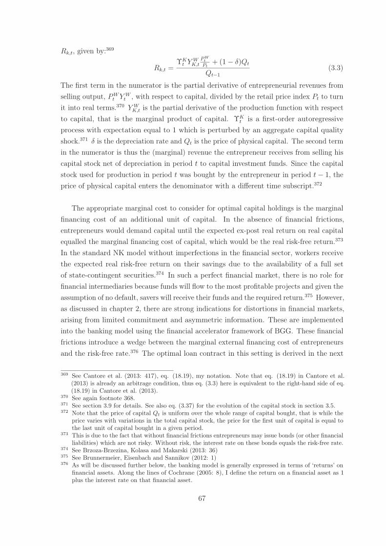
Rk,t, given by:369

Rk,t =ΥK

t YWK,t

PWt

Pt+ (1− δ)Qt

Qt−1

(3.3)

The first term in the numerator is the partial derivative of entrepreneurial revenues fromselling output, PW

t Y Wt , with respect to capital, divided by the retail price index Pt to turn

it into real terms.370 Y WK,t is the partial derivative of the production function with respect

to capital, that is the marginal product of capital. ΥKt is a first-order autoregressive

process with expectation equal to 1 which is perturbed by an aggregate capital qualityshock.371 δ is the depreciation rate and Qt is the price of physical capital. The second termin the numerator is thus the (marginal) revenue the entrepreneur receives from selling hiscapital stock net of depreciation in period t to capital investment funds. Since the capitalstock used for production in period t was bought by the entrepreneur in period t− 1, theprice of physical capital enters the denominator with a different time subscript.372

The appropriate marginal cost to consider for optimal capital holdings is the marginalfinancing cost of an additional unit of capital. In the absence of financial frictions,entrepreneurs would demand capital until the expected ex-post real return on real capitalequalled the marginal financing cost of capital, which would be the real risk-free return.373

In the standard NK model without imperfections in the financial sector, workers receivethe expected real risk-free return on their savings due to the availability of a full setof state-contingent securities.374 In such a perfect financial market, there is no role forfinancial intermediaries because funds will flow to the most profitable projects and given theassumption of no default, savers will receive their funds and the required return.375 However,as discussed in chapter 2, there are strong indications for distortions in financial markets,arising from limited commitment and asymmetric information. These are implementedinto the banking model using the financial accelerator framework of BGG. These financialfrictions introduce a wedge between the marginal external financing cost of entrepreneursand the risk-free rate.376 The optimal loan contract in this setting is derived in the next

369 See Cantore et al. (2013: 417), eq. (18.19), my notation. Note that eq. (18.19) in Cantore et al.(2013) is already an arbitrage condition, thus eq. (3.3) here is equivalent to the right-hand side of eq.(18.19) in Cantore et al. (2013).

370 See again footnote 368.371 See section 3.9 for details. See also eq. (3.37) for the evolution of the capital stock in section 3.5.372 Note that the price of capital Qt is uniform over the whole range of capital bought, that is while the

price varies with variations in the total capital stock, the price for the first unit of capital is equal tothe last unit of capital bought in a given period.

373 This is due to the fact that without financial frictions entrepreneurs may issue bonds (or other financialliabilities) which are not risky. Without risk, the interest rate on these bonds equals the risk-free rate.

374 See Brzoza-Brzezina, Kolasa and Makarski (2013: 36)375 See Brunnermeier, Eisenbach and Sannikov (2012: 1)376 As will be discussed further below, the banking model is generally expressed in terms of ‘returns’ on

financial assets. Along the lines of Cochrane (2005: 8), I define the return on a financial asset as 1plus the interest rate on that financial asset.

67

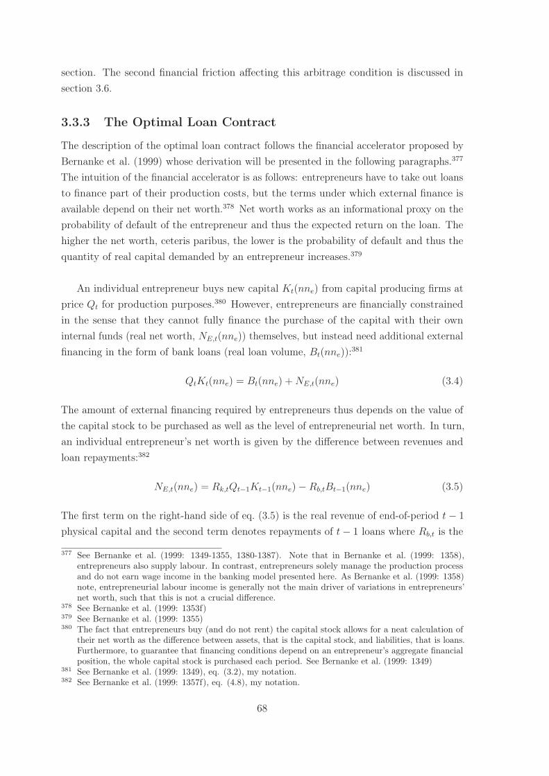
section. The second financial friction affecting this arbitrage condition is discussed insection 3.6.

3.3.3 The Optimal Loan Contract

The description of the optimal loan contract follows the financial accelerator proposed byBernanke et al. (1999) whose derivation will be presented in the following paragraphs.377

The intuition of the financial accelerator is as follows: entrepreneurs have to take out loansto finance part of their production costs, but the terms under which external finance isavailable depend on their net worth.378 Net worth works as an informational proxy on theprobability of default of the entrepreneur and thus the expected return on the loan. Thehigher the net worth, ceteris paribus, the lower is the probability of default and thus thequantity of real capital demanded by an entrepreneur increases.379

An individual entrepreneur buys new capital Kt(nne) from capital producing firms atprice Qt for production purposes.380 However, entrepreneurs are financially constrainedin the sense that they cannot fully finance the purchase of the capital with their owninternal funds (real net worth, NE,t(nne)) themselves, but instead need additional externalfinancing in the form of bank loans (real loan volume, Bt(nne)):381

QtKt(nne) = Bt(nne) +NE,t(nne) (3.4)

The amount of external financing required by entrepreneurs thus depends on the value ofthe capital stock to be purchased as well as the level of entrepreneurial net worth. In turn,an individual entrepreneur’s net worth is given by the difference between revenues andloan repayments:382

NE,t(nne) = Rk,tQt−1Kt−1(nne)−Rb,tBt−1(nne) (3.5)

The first term on the right-hand side of eq. (3.5) is the real revenue of end-of-period t− 1

physical capital and the second term denotes repayments of t− 1 loans where Rb,t is the

377 See Bernanke et al. (1999: 1349-1355, 1380-1387). Note that in Bernanke et al. (1999: 1358),entrepreneurs also supply labour. In contrast, entrepreneurs solely manage the production processand do not earn wage income in the banking model presented here. As Bernanke et al. (1999: 1358)note, entrepreneurial labour income is generally not the main driver of variations in entrepreneurs’net worth, such that this is not a crucial difference.

378 See Bernanke et al. (1999: 1353f)379 See Bernanke et al. (1999: 1355)380 The fact that entrepreneurs buy (and do not rent) the capital stock allows for a neat calculation of

their net worth as the difference between assets, that is the capital stock, and liabilities, that is loans.Furthermore, to guarantee that financing conditions depend on an entrepreneur’s aggregate financialposition, the whole capital stock is purchased each period. See Bernanke et al. (1999: 1349)

381 See Bernanke et al. (1999: 1349), eq. (3.2), my notation.382 See Bernanke et al. (1999: 1357f), eq. (4.8), my notation.

68

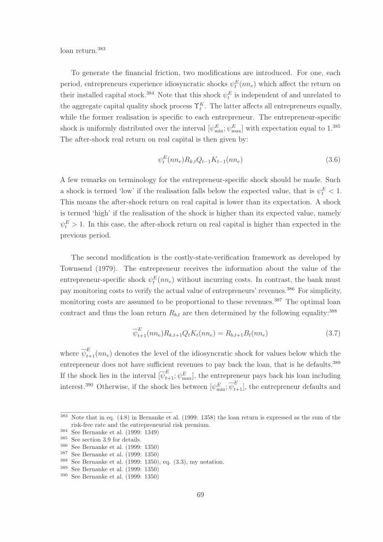
loan return.383

To generate the financial friction, two modifications are introduced. For one, eachperiod, entrepreneurs experience idiosyncratic shocks ψE

t (nne) which affect the return ontheir installed capital stock.384 Note that this shock ψE

t is independent of and unrelated tothe aggregate capital quality shock process ΥK

t . The latter affects all entrepreneurs equally,while the former realisation is specific to each entrepreneur. The entrepreneur-specificshock is uniformly distributed over the interval [ψE

min;ψEmax] with expectation equal to 1.385

The after-shock real return on real capital is then given by:

ψEt (nne)Rk,tQt−1Kt−1(nne) (3.6)

A few remarks on terminology for the entrepreneur-specific shock should be made. Sucha shock is termed ‘low’ if the realisation falls below the expected value, that is ψE

t < 1.This means the after-shock return on real capital is lower than its expectation. A shockis termed ‘high’ if the realisation of the shock is higher than its expected value, namelyψEt > 1. In this case, the after-shock return on real capital is higher than expected in the

previous period.

The second modification is the costly-state-verification framework as developed byTownsend (1979). The entrepreneur receives the information about the value of theentrepreneur-specific shock ψE

t (nne) without incurring costs. In contrast, the bank mustpay monitoring costs to verify the actual value of entrepreneurs’ revenues.386 For simplicity,monitoring costs are assumed to be proportional to these revenues.387 The optimal loancontract and thus the loan return Rb,t are then determined by the following equality:388

ψE

t+1(nne)Rk,t+1QtKt(nne) = Rb,t+1Bt(nne) (3.7)

where ψE

t+1(nne) denotes the level of the idiosyncratic shock for values below which theentrepreneur does not have sufficient revenues to pay back the loan, that is he defaults.389

If the shock lies in the interval [ψE

t+1;ψEmax], the entrepreneur pays back his loan including

interest.390 Otherwise, if the shock lies between [ψEmin;ψ

E

t+1], the entrepreneur defaults and

383 Note that in eq. (4.8) in Bernanke et al. (1999: 1358) the loan return is expressed as the sum of therisk-free rate and the entrepreneurial risk premium.

384 See Bernanke et al. (1999: 1349)385 See section 3.9 for details.386 See Bernanke et al. (1999: 1350)387 See Bernanke et al. (1999: 1350)388 See Bernanke et al. (1999: 1350), eq. (3.3), my notation.389 See Bernanke et al. (1999: 1350)390 See Bernanke et al. (1999: 1350)

69

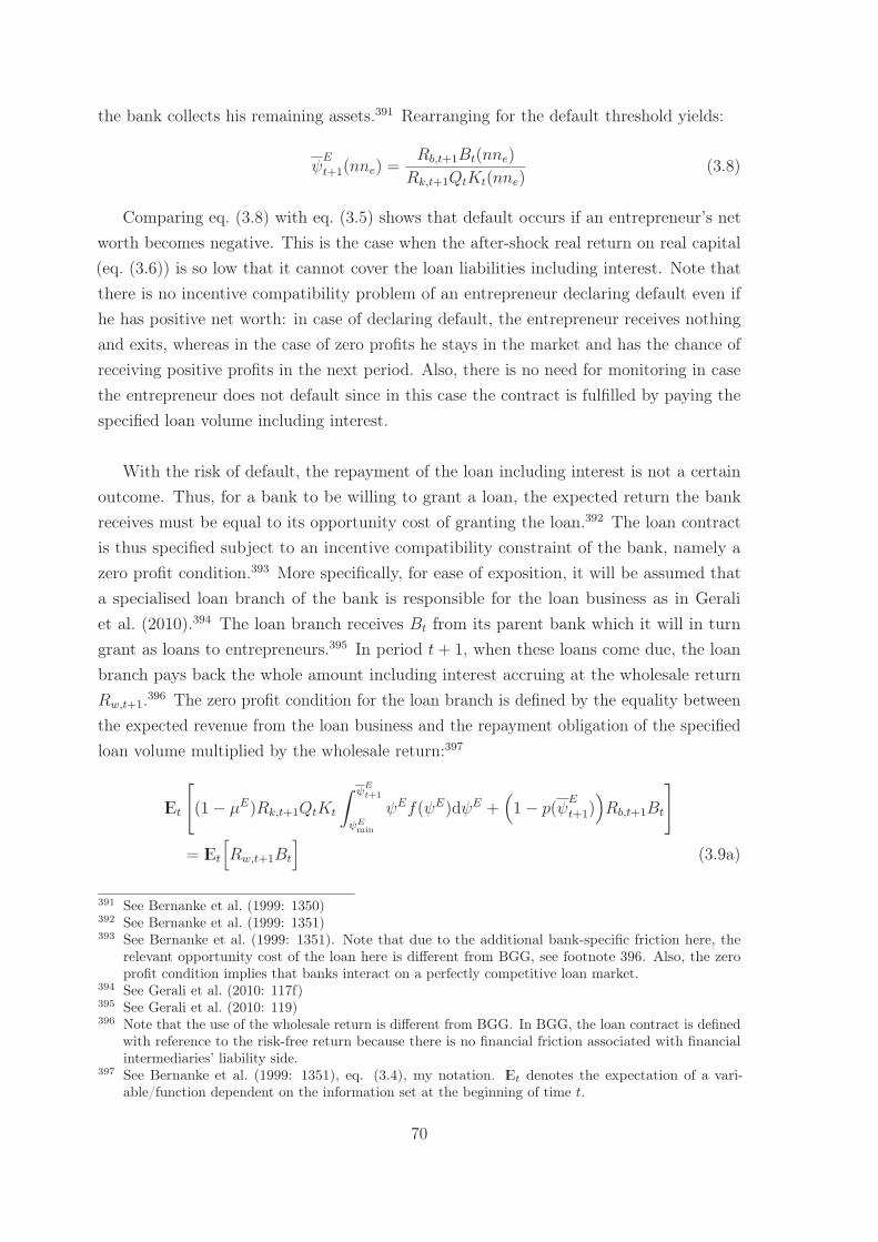
the bank collects his remaining assets.391 Rearranging for the default threshold yields:

ψE

t+1(nne) =Rb,t+1Bt(nne)

Rk,t+1QtKt(nne)(3.8)

Comparing eq. (3.8) with eq. (3.5) shows that default occurs if an entrepreneur’s networth becomes negative. This is the case when the after-shock real return on real capital(eq. (3.6)) is so low that it cannot cover the loan liabilities including interest. Note thatthere is no incentive compatibility problem of an entrepreneur declaring default even ifhe has positive net worth: in case of declaring default, the entrepreneur receives nothingand exits, whereas in the case of zero profits he stays in the market and has the chance ofreceiving positive profits in the next period. Also, there is no need for monitoring in casethe entrepreneur does not default since in this case the contract is fulfilled by paying thespecified loan volume including interest.

With the risk of default, the repayment of the loan including interest is not a certainoutcome. Thus, for a bank to be willing to grant a loan, the expected return the bankreceives must be equal to its opportunity cost of granting the loan.392 The loan contractis thus specified subject to an incentive compatibility constraint of the bank, namely azero profit condition.393 More specifically, for ease of exposition, it will be assumed thata specialised loan branch of the bank is responsible for the loan business as in Geraliet al. (2010).394 The loan branch receives Bt from its parent bank which it will in turngrant as loans to entrepreneurs.395 In period t+ 1, when these loans come due, the loanbranch pays back the whole amount including interest accruing at the wholesale returnRw,t+1.396 The zero profit condition for the loan branch is defined by the equality betweenthe expected revenue from the loan business and the repayment obligation of the specifiedloan volume multiplied by the wholesale return:397

IEt

[(1− μE)Rk,t+1QtKt

∫ ψEt+1

ψEmin

ψEf(ψE)dψE +(1− p(ψ

E

t+1))Rb,t+1Bt

]= IEt

[Rw,t+1Bt

](3.9a)

391 See Bernanke et al. (1999: 1350)392 See Bernanke et al. (1999: 1351)393 See Bernanke et al. (1999: 1351). Note that due to the additional bank-specific friction here, the

relevant opportunity cost of the loan here is different from BGG, see footnote 396. Also, the zeroprofit condition implies that banks interact on a perfectly competitive loan market.

394 See Gerali et al. (2010: 117f)395 See Gerali et al. (2010: 119)396 Note that the use of the wholesale return is different from BGG. In BGG, the loan contract is defined

with reference to the risk-free return because there is no financial friction associated with financialintermediaries’ liability side.

397 See Bernanke et al. (1999: 1351), eq. (3.4), my notation. IEt denotes the expectation of a vari-able/function dependent on the information set at the beginning of time t.

70

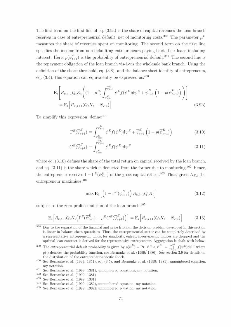
The first term on the first line of eq. (3.9a) is the share of capital revenues the loan branchreceives in case of entrepreneurial default, net of monitoring costs.398 The parameter μE

measures the share of revenues spent on monitoring. The second term on the first linespecifies the income from non-defaulting entrepreneurs paying back their loans includinginterest. Here, p(ψE

t+1) is the probability of entrepreneurial default.399 The second line isthe repayment obligation of the loan branch vis-à-vis the wholesale bank branch. Using thedefinition of the shock threshold, eq. (3.8), and the balance sheet identity of entrepreneurs,eq. (3.4), this equation can equivalently be expressed as:400

IEt

[Rk,t+1QtKt

((1− μE)

∫ ψEt+1

ψEmin

ψEf(ψE)dψE + ψE

t+1

(1− p(ψ

E

t+1)))]

= IEt

[Rw,t+1(QtKt −NE,t)

](3.9b)

To simplify this expression, define:401

ΓE(ψE

t+1) ≡∫ ψ

Et+1

ψEmin

ψEf(ψE)dψE + ψE

t+1

(1− p(ψ

E

t+1))

(3.10)

GE(ψE

t+1) ≡∫ ψ

Et+1

ψEmin

ψEf(ψE)dψE (3.11)

where eq. (3.10) defines the share of the total return on capital received by the loan branch,and eq. (3.11) is the share which is deducted from the former due to monitoring.402 Hence,the entrepreneur receives 1− ΓE(ψE

t+1) of the gross capital return.403 Thus, given NE,t theentrepreneur maximises:404

max IEt

[(1− ΓE(ψ

E

t+1))Rk,t+1QtKt

](3.12)

subject to the zero profit condition of the loan branch:405

IEt

[Rk,t+1QtKt

(ΓE(ψ

E

t+1)− μEGE(ψE

t+1))]

= IEt

[Rw,t+1(QtKt −NE,t)

](3.13)

398 Due to the separation of the financial and price friction, the decision problem developed in this sectionis linear in balance sheet quantities. Thus, the entrepreneurial sector can be completely described bya representative entrepreneur. Thus, for simplicity, entrepreneur-specific indices are dropped and theoptimal loan contract is derived for the representative entrepreneur. Aggregation is dealt with below.

399 The entrepreneurial default probability is given by p(ψE) = Pr

[ψE < ψ

E]=

∫ ψEt

ψEmin

f(ψE)dψE wherep(·) denotes the probability function, see Bernanke et al. (1999: 1380). See section 3.9 for details onthe distribution of the entrepreneur-specific shock.

400 See Bernanke et al. (1999: 1351), eq. (3.5), and Bernanke et al. (1999: 1381), unnumbered equation,my notation.

401 See Bernanke et al. (1999: 1381), unnumbered equations, my notation.402 See Bernanke et al. (1999: 1381)403 See Bernanke et al. (1999: 1381)404 See Bernanke et al. (1999: 1382), unnumbered equation, my notation.405 See Bernanke et al. (1999: 1382), unnumbered equation, my notation.

71

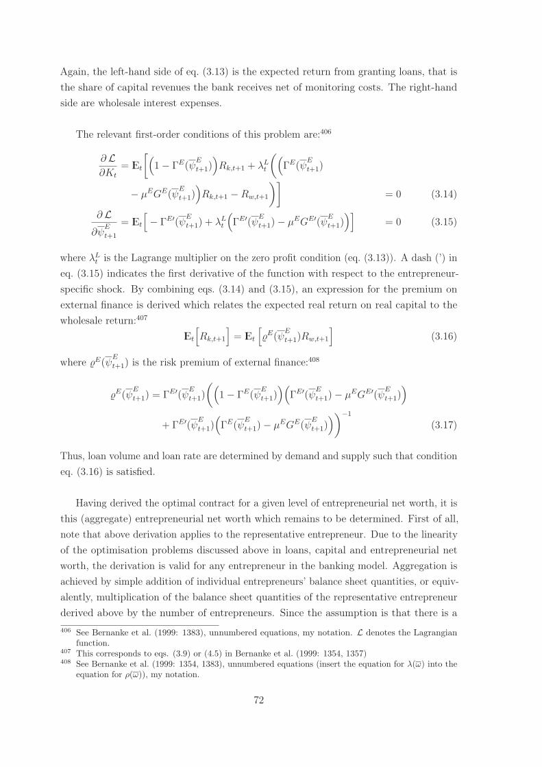
Again, the left-hand side of eq. (3.13) is the expected return from granting loans, that isthe share of capital revenues the bank receives net of monitoring costs. The right-handside are wholesale interest expenses.

The relevant first-order conditions of this problem are:406

∂ L∂Kt

= IEt

[(1− ΓE(ψ

E

t+1))Rk,t+1 + λL

t

((ΓE(ψ

E

t+1)

− μEGE(ψE

t+1))Rk,t+1 −Rw,t+1

)]= 0 (3.14)

∂ L∂ψ

E

t+1

= IEt

[− ΓE′(ψ

E

t+1) + λLt

(ΓE′(ψ

E

t+1)− μEGE′(ψE

t+1))]

= 0 (3.15)

where λLt is the Lagrange multiplier on the zero profit condition (eq. (3.13)). A dash (’) in

eq. (3.15) indicates the first derivative of the function with respect to the entrepreneur-specific shock. By combining eqs. (3.14) and (3.15), an expression for the premium onexternal finance is derived which relates the expected real return on real capital to thewholesale return:407

IEt

[Rk,t+1

]= IEt

[�E(ψ

E

t+1)Rw,t+1

](3.16)

where �E(ψE

t+1) is the risk premium of external finance:408

�E(ψE

t+1) = ΓE′(ψE

t+1)

((1− ΓE(ψ

E

t+1))(

ΓE′(ψE

t+1)− μEGE′(ψE

t+1))

+ ΓE′(ψE

t+1)(ΓE(ψ

E

t+1)− μEGE(ψE

t+1)))−1

(3.17)

Thus, loan volume and loan rate are determined by demand and supply such that conditioneq. (3.16) is satisfied.

Having derived the optimal contract for a given level of entrepreneurial net worth, it isthis (aggregate) entrepreneurial net worth which remains to be determined. First of all,note that above derivation applies to the representative entrepreneur. Due to the linearityof the optimisation problems discussed above in loans, capital and entrepreneurial networth, the derivation is valid for any entrepreneur in the banking model. Aggregation isachieved by simple addition of individual entrepreneurs’ balance sheet quantities, or equiv-alently, multiplication of the balance sheet quantities of the representative entrepreneurderived above by the number of entrepreneurs. Since the assumption is that there is a406 See Bernanke et al. (1999: 1383), unnumbered equations, my notation. L denotes the Lagrangian

function.407 This corresponds to eqs. (3.9) or (4.5) in Bernanke et al. (1999: 1354, 1357)408 See Bernanke et al. (1999: 1354, 1383), unnumbered equations (insert the equation for λ(ω) into the

equation for ρ(ω)), my notation.

72

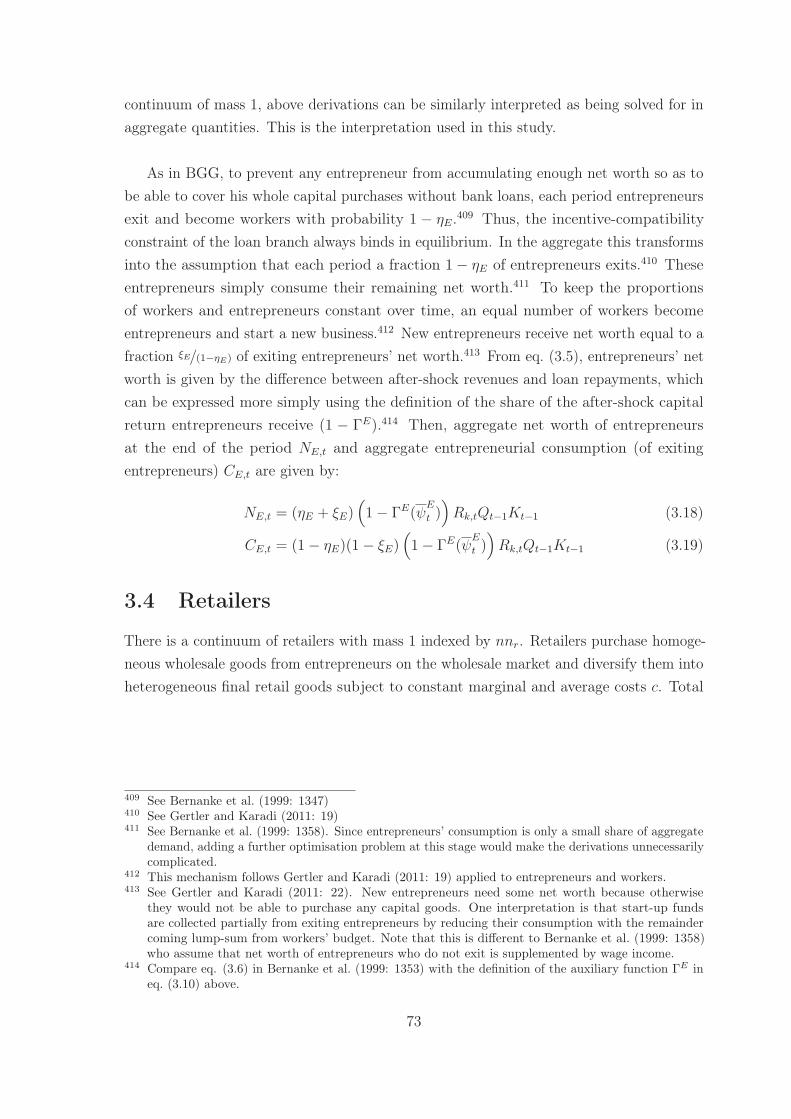
continuum of mass 1, above derivations can be similarly interpreted as being solved for inaggregate quantities. This is the interpretation used in this study.

As in BGG, to prevent any entrepreneur from accumulating enough net worth so as tobe able to cover his whole capital purchases without bank loans, each period entrepreneursexit and become workers with probability 1 − ηE.409 Thus, the incentive-compatibilityconstraint of the loan branch always binds in equilibrium. In the aggregate this transformsinto the assumption that each period a fraction 1− ηE of entrepreneurs exits.410 Theseentrepreneurs simply consume their remaining net worth.411 To keep the proportionsof workers and entrepreneurs constant over time, an equal number of workers becomeentrepreneurs and start a new business.412 New entrepreneurs receive net worth equal to afraction ξE/(1−ηE) of exiting entrepreneurs’ net worth.413 From eq. (3.5), entrepreneurs’ networth is given by the difference between after-shock revenues and loan repayments, whichcan be expressed more simply using the definition of the share of the after-shock capitalreturn entrepreneurs receive (1 − ΓE).414 Then, aggregate net worth of entrepreneursat the end of the period NE,t and aggregate entrepreneurial consumption (of exitingentrepreneurs) CE,t are given by:

NE,t = (ηE + ξE)(1− ΓE(ψ

E

t ))Rk,tQt−1Kt−1 (3.18)

CE,t = (1− ηE)(1− ξE)(1− ΓE(ψ

E

t ))Rk,tQt−1Kt−1 (3.19)

3.4 Retailers

There is a continuum of retailers with mass 1 indexed by nnr. Retailers purchase homoge-neous wholesale goods from entrepreneurs on the wholesale market and diversify them intoheterogeneous final retail goods subject to constant marginal and average costs c. Total

409 See Bernanke et al. (1999: 1347)410 See Gertler and Karadi (2011: 19)411 See Bernanke et al. (1999: 1358). Since entrepreneurs’ consumption is only a small share of aggregate

demand, adding a further optimisation problem at this stage would make the derivations unnecessarilycomplicated.

412 This mechanism follows Gertler and Karadi (2011: 19) applied to entrepreneurs and workers.413 See Gertler and Karadi (2011: 22). New entrepreneurs need some net worth because otherwise

they would not be able to purchase any capital goods. One interpretation is that start-up fundsare collected partially from exiting entrepreneurs by reducing their consumption with the remaindercoming lump-sum from workers’ budget. Note that this is different to Bernanke et al. (1999: 1358)who assume that net worth of entrepreneurs who do not exit is supplemented by wage income.

414 Compare eq. (3.6) in Bernanke et al. (1999: 1353) with the definition of the auxiliary function ΓE ineq. (3.10) above.

73

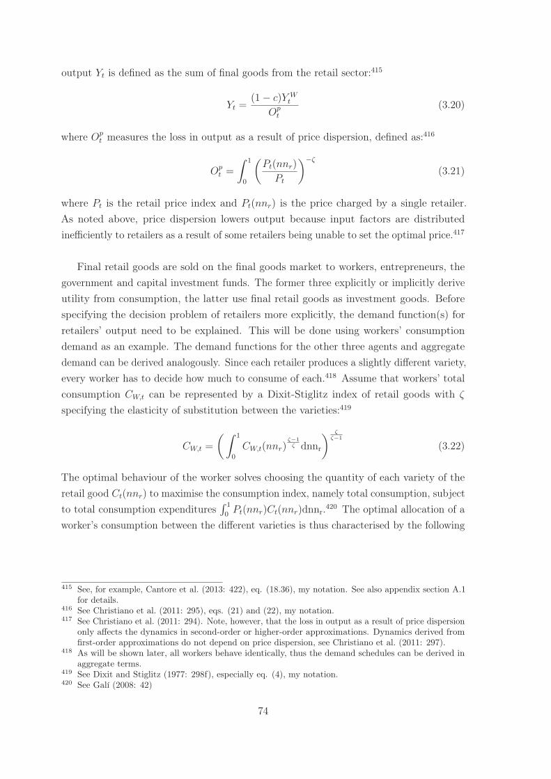
output Yt is defined as the sum of final goods from the retail sector:415

Yt =(1− c)Y W

t

Opt

(3.20)

where Opt measures the loss in output as a result of price dispersion, defined as:416

Opt =

∫ 1

0

(Pt(nnr)

Pt

)−ζ

(3.21)

where Pt is the retail price index and Pt(nnr) is the price charged by a single retailer.As noted above, price dispersion lowers output because input factors are distributedinefficiently to retailers as a result of some retailers being unable to set the optimal price.417

Final retail goods are sold on the final goods market to workers, entrepreneurs, thegovernment and capital investment funds. The former three explicitly or implicitly deriveutility from consumption, the latter use final retail goods as investment goods. Beforespecifying the decision problem of retailers more explicitly, the demand function(s) forretailers’ output need to be explained. This will be done using workers’ consumptiondemand as an example. The demand functions for the other three agents and aggregatedemand can be derived analogously. Since each retailer produces a slightly different variety,every worker has to decide how much to consume of each.418 Assume that workers’ totalconsumption CW,t can be represented by a Dixit-Stiglitz index of retail goods with ζ

specifying the elasticity of substitution between the varieties:419

CW,t =

(∫ 1

0

CW,t(nnr)ζ−1ζ dnnr

) ζζ−1

(3.22)

The optimal behaviour of the worker solves choosing the quantity of each variety of theretail good Ct(nnr) to maximise the consumption index, namely total consumption, subjectto total consumption expenditures

∫ 1

0Pt(nnr)Ct(nnr)dnnr.420 The optimal allocation of a

worker’s consumption between the different varieties is thus characterised by the following

415 See, for example, Cantore et al. (2013: 422), eq. (18.36), my notation. See also appendix section A.1for details.

416 See Christiano et al. (2011: 295), eqs. (21) and (22), my notation.417 See Christiano et al. (2011: 294). Note, however, that the loss in output as a result of price dispersion

only affects the dynamics in second-order or higher-order approximations. Dynamics derived fromfirst-order approximations do not depend on price dispersion, see Christiano et al. (2011: 297).

418 As will be shown later, all workers behave identically, thus the demand schedules can be derived inaggregate terms.

419 See Dixit and Stiglitz (1977: 298f), especially eq. (4), my notation.420 See Galí (2008: 42)

74

set of demand functions:421

CW,t(nnr) =

(Pt(nnr)

Pt

)−ζ

CW,t (3.23)

with the aggregate retail price index given by a Dixit-Stiglitz Index:422

Pt =

(∫ 1

0

Pt(nnr)1−ζdnnr

) 11−ζ

(3.24)

Thus, the demand function faced by a particular retailer nnr is given by:423

Yt(nnr) =

(Pt(nnr)

Pt

)−ζ

Yt (3.25)

Equation (3.25) states that the demand for a specific variety depends positively on theaggregate level of demand Yt, and negatively on the ratio of its price Pt(nnr) to the generalprice level Pt.

Retailers set their price to maximise profits subject to above demand schedule. This isnot a one-period problem since the crucial NK model friction enters here: sticky prices.Thus, not all retailers are able to change their price in every period. More specifically,Calvo-style sticky prices mean that with probability ξp a retailer cannot adjust its pricein period t to the (new) optimal level.424 With probability 1 − ξp he sets the price tothe optimal level P ∗

t .425 As in Christiano, Eichenbaum and Evans (2005a), there is somedegree of inflation indexation, that means retailers who cannot optimise their prices indextheir prices to the lagged inflation rate.426 The degree of this indexation is measured byγp.427 This allows for a flexible implementation of indexation: if γp is equal to 1, pricesare fully indexed, that is change 1 for 1 with observed last period’s inflation. In contrast,if γp = 0, there is no indexation which is equivalent to the original Calvo framework whenprices are kept completely constant.

Therefore, the decision problem of the representative retailer is to set the price P ∗t

to maximise the stream of profits for the periods for which this price is expected to stay

421 See Dixit and Stiglitz (1977: 299), eq. (14), my notation. See Galí (2008: 61f) as well as Dixit andStiglitz (1977: 298ff) for a detailed mathematical derivation.

422 See Dixit and Stiglitz (1977: 298), eq. (4), my notation.423 See Cantore et al. (2013: 421), eq. (18.24), my notation.424 See Calvo (1983: 383)425 Note that in the case of zero inflation and in the absence of shocks, P ∗

t is equal to P ∗t−1 and thus price

staggering does not have any consequences.426 See Christiano et al. (2005a: 10f)427 γp may take on any value between 0 and 1.

75

fixed given the probability ξp.428 Since retailers are owned by workers, all profits areredistributed as dividends to workers at the end of the period.429 Moreover, this ownershipassumption necessitates the inclusion of the nominal stochastic discount factor ΛN

t,t+s inthe objective function.430 Thus, retailers’ objective function can be written as:431

IEt

[ ∞∑s=0

(ξp)sΛNt,t+sYt+s(nnr)

(P ∗t (nnr)

(Pt+s

Pt

)γp

− Pt+sMCt+sΥMSt+s

)](3.26)

which is maximised subject to the demand function for the output of retailer nnr:432

Yt+s(nnr) =

(P ∗t (nnr)

Pt+s

)−ζ

Yt+s (3.27)

ΥMSt is a first-order autoregressive process with expectation equal to 1 which is perturbed

by a mark-up shock εMS.433 This mark-up process ΥMSt affects the steady-state mark-up.

ΛNt,t+s is the nominal stochastic discount factor given by:434

ΛNt,t+s = β

UC,t+s/Pt+s

UC,t/Pt

(3.28)

where β is workers’ discount rate and UC,t is workers’ marginal utility of consumption (seesection 3.7). MCt is retailers’ real marginal cost which is equal to the wholesale price PW

t

divided by the aggregate final retail good price index Pt.435 The first-order condition is,noting that Πt+s = Pt+s/Pt:436

IEt

[ ∞∑s=0

(ξp)sΛNt,t+sYt+s(nnr)

(P ∗t (nnr)Π

γp

t+s −ζ

ζ − 1MCt+sPt+sΥ

MSt+s

)]= 0 (3.29)

If we abstract from Calvo-style sticky prices, that is set s = 0, the first-order conditionreduces to (excluding the mark-up shock for simplicity):

P ∗t (nnr) =

ζ

ζ − 1MCt(nnr)Pt+s (3.30)

428 See Galí (2008: 44)429 See footnote 334 for more details on this assumption.430 The subscript t, t+ s denotes that the stochastic discount factor is defined over the interval t to t+ s.431 See Cantore et al. (2013: 421), eq. (18.25), my notation. Note that the objective function in Cantore

et al. (2013) does not include price indexation. See Christiano et al. (2005a: 11), eqs. (9) and (10) forhow indexation enters retailers’ objective function.

432 See Galí (2008: 44)433 See section 3.9 for details.434 See Cantore et al. (2013: 421), unnumbered equation, my notation.435 See Cantore et al. (2013: 422), eq. (18.32)436 See Cantore et al. (2013: 426), unnumbered equation, my notation. See Christiano, Eichenbaum and

Evans (2005b: 10f) for more details on the relationship between this condition and the standard NKPhillips Curve representation.

76

This means the optimal price is a mark-up over retailers’ nominal marginal cost. Noticethat the optimal mark-up ζ/(ζ−1) is constant over time since the elasticity of substitutionbetween the different varieties of the final retail good ζ is a constant.

The infinite sum of eq. (3.29) may be represented as a set of difference equations, andthe approach of Cantore et al. (2013) and Gabriel, Levine, Pearlman and Yang (2010) isused to derive it. To this end it is convenient to introduce the auxiliary variables Jt, JJtand Πt. Inflation dynamics are then described by:437

P ∗t

Pt

=JtJJt

(3.31)

JJt − ξpβIEt

[Πζ−1

t+1JJt+1

]= YtUC,t (3.32)

Jt − ξpβIEt

[Πζ

t+1Jt+1

]=

ζ

ζ − 1MCtΥ

MSt YtUC,t (3.33)

Πt =Πt

Πγp

t−1

(3.34)

Note that this representation in terms of the ratio of the optimal price to the current pricelevel is not arbitrary. In the steady state with for example zero inflation, this ratio has adefined value of 1, while the price level may not.438

The dynamics of the price index can be highlighted by decomposing the aggregateprice index given in eq. (3.24) into a share of those retailers that can and those that cannotoptimise in a given period. Note that the former set the new optimal price, and that thelatter set their price equal to the previous’ period price times the inflation indexationrate.439 The new optimal price is also equal across all optimising retailers due to the factthat they all buy the same homogeneous input at the same price and have the same costfunction. The aggregate price index can then be expressed as:440

P 1−ζt = ξp

(Pt−1Π

γp

t−1

)1−ζ

+ (1− ξp)(P ∗t

)1−ζ

(3.35)

dividing by P 1−ζt−1 and rearranging yields for the inflation rate Πt:

Πt =

(ξp(Πγp

t−1

)1−ζ

+ (1− ξp)

(P ∗t

Pt−1

)1−ζ) 11−ζ

(3.36)

437 See Cantore et al. (2013: 426), unnumbered equations, and Gabriel et al. (2010: 7), eqs. (25) to (27),my notation.

438 See Galí (2008: 44-45)439 See Christiano et al. (2011: 333). Invoking the law of large numbers and that retailers who can

optimise are drawn randomly, price index dynamics due to non-optimizing retailers’ prices reduce tothe lagged aggregate price index times the inflation indexing rate, see Christiano et al. (2011: 293)and Cantore et al. (2013: 421). See also footnote 351.

440 See Christiano et al. (2005b: 11), eq. (3.13), my notation.

77

3.5 Capital Investment Funds

The supply of capital is determined by specialised capital investment funds. After theretail goods production phase in period t, capital investment funds buy the period t stockof real capital net of depreciation from entrepreneurs. Capital investment funds buy finalretail goods as investment goods It and combine these cost-freely with the old capitalstock to generate the new period t+ 1 capital stock. The new capital stock is then sold toentrepreneurs.441 Capital investment funds manage investment without incurring resourcecosts in the long-run equilibrium; however, adjusting the level of investment in the shortrun is costly: if period t+ 1 investment is different from period t investment then only afraction of investment expenditures is added as new capital.442 Thus, the law of motionfor the capital stock is given by:443

Kt = ΥKt

((1− δ)Kt−1 +

(1− S(It/It−1)

)It

)(3.37)

where S(�) is the investment adjustment cost function. As outlined in the next paragraph,the function S satisfies S(1) = 0 and S ′(1) = 0, where S ′ denotes the first derivative ofthe investment adjustment cost function.444

Investment adjustment costs affect the optimal choice of investment. In a similar wayas habits work within the utility function (see below), investment adjustment costs areincluded to improve the empirical fit of the model. Admittedly, investment adjustmentcosts as introduced here are an ad-hoc feature of NK DSGE models not explicitly derivedfrom any maximisation problem. Intuitively, it might be argued that investment involvesinstallation costs in terms of setting up the machinery, which could yield an immediatecomplete adjustment to shocks to be suboptimal.445 Also, among others, Christiano et al.(2011) cite Matsuyama (1984) as an example for microfounding investment adjustmentcosts.446 Matsuyama (1984) argues that investment adjustment arise due to planningcosts involved; if non-financial firms want to increase investment, real resources need tobe spent in the planning and management processes.447 On the other hand, there is anoffsetting learning effect on the part of managers such that at constant investment levels,adjustment costs are zero.448 Hence, the argument is that adjustment costs matter in theshort but not in the long run.

441 Note that transaction costs for buying and selling capital are neglected for simplicity.442 See for example Christiano et al. (2005a: 15) and Gertler et al. (2012: S21)443 See also, for example, Cantore et al. (2013: 416), unnumbered equation, my notation.444 See section 3.9 for the specific functional form.445 See Wickens (2008: 33)446 See Christiano et al. (2011: 343)447 See Matsuyama (1984: 4)448 See Matsuyama (1984: 4)

78

More specifically, including investment adjustment costs has been shown to improve theresponses of investment, consumption and interest rates especially to a monetary policyshock in DSGE models.449 As Villa (2013) shows using Bayesian estimation techniques,including investment adjustment costs significantly improves the empirical fit in termsof the log data density.450 Moreover, Christiano et al. (2011) argue that an investmentadjustment cost function which depends on the rate of change of investment is in line withvector autoregression (VAR)-based evidence of a hump-shaped response of investment.451

In contrast, a specification of the investment adjustment cost function which depends ondifferences between the investment to capital ratio and the depreciation rate has beenargued to imply a large immediate response followed by small subsequent responses whichis not borne out by VAR-analyses.452 These considerations justify the particular form ofeq. (3.37).

The stream of expected discounted profits of capital investment funds Ξct is then given

by:453

IEt

[ ∞∑s=0

Ξct

]= IEt

[ ∞∑s=0

Λt,t+sQt+s

(1− S(It+s/It+s−1)

)It+s − It+s

](3.38)

Capital investment funds choose the level of investment to maximise profits (eq. (3.38)).The first order condition is given by:454

Qt

(1− S(It/It−1)− It

It−1

S ′(It/It−1)

)+ IEt

[Λt,t+1Qt+1S

′(It+1/It)(It+1

It

)2]= 1 (3.39)

As noted above, in the deterministic steady-state investment is constant, thus It = It−1

and investment adjustment costs are zero. Outside the long-run equilibrium, the price ofcapital varies inversely with investment adjustment costs, according to eq. (3.39).

3.6 Banks

Banks grant loans to entrepreneurs and balance these assets by issuing bank depositsand bank equity, which are held by workers. The optimal loan contract was presented insection 3.3.3, which follows the standard financial accelerator developed by Bernanke etal. (1999) between entrepreneurs and banks. This section deals with the overall financialposition of the bank, focusing in particular on the liability management of the bank. As

449 See Christiano et al. (2005a: 40)450 See Villa (2013: 28)451 See Christiano et al. (2011: 342f)452 See Christiano et al. (2011: 341ff)453 See Gertler et al. (2012: S21), unnumbered equation, and Cantore et al. (2013: 417), unnumbered

equation, my notation.454 See Gertler et al. (2012: S21), eq. (12), and Cantore et al. (2013: 417), unnumbered equation, my

notation.

79

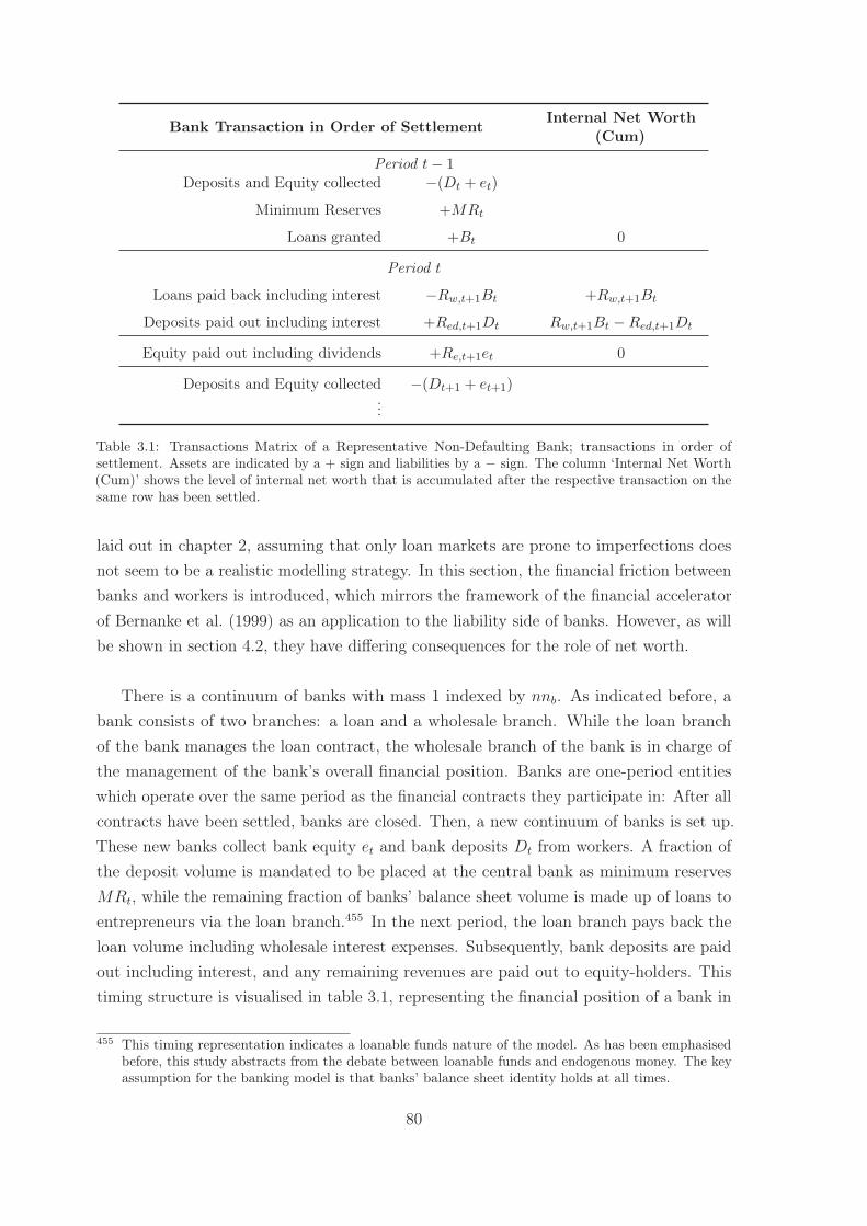
Bank Transaction in Order of Settlement Internal Net Worth(Cum)

Period t− 1Deposits and Equity collected −(Dt + et)

Minimum Reserves +MRt

Loans granted +Bt 0

Period t

Loans paid back including interest −Rw,t+1Bt +Rw,t+1Bt

Deposits paid out including interest +Red,t+1Dt Rw,t+1Bt −Red,t+1Dt

Equity paid out including dividends +Re,t+1et 0

Deposits and Equity collected −(Dt+1 + et+1)...

Table 3.1: Transactions Matrix of a Representative Non-Defaulting Bank; transactions in order ofsettlement. Assets are indicated by a + sign and liabilities by a − sign. The column ‘Internal Net Worth(Cum)’ shows the level of internal net worth that is accumulated after the respective transaction on thesame row has been settled.

laid out in chapter 2, assuming that only loan markets are prone to imperfections doesnot seem to be a realistic modelling strategy. In this section, the financial friction betweenbanks and workers is introduced, which mirrors the framework of the financial acceleratorof Bernanke et al. (1999) as an application to the liability side of banks. However, as willbe shown in section 4.2, they have differing consequences for the role of net worth.

There is a continuum of banks with mass 1 indexed by nnb. As indicated before, abank consists of two branches: a loan and a wholesale branch. While the loan branchof the bank manages the loan contract, the wholesale branch of the bank is in charge ofthe management of the bank’s overall financial position. Banks are one-period entitieswhich operate over the same period as the financial contracts they participate in: After allcontracts have been settled, banks are closed. Then, a new continuum of banks is set up.These new banks collect bank equity et and bank deposits Dt from workers. A fraction ofthe deposit volume is mandated to be placed at the central bank as minimum reservesMRt, while the remaining fraction of banks’ balance sheet volume is made up of loans toentrepreneurs via the loan branch.455 In the next period, the loan branch pays back theloan volume including wholesale interest expenses. Subsequently, bank deposits are paidout including interest, and any remaining revenues are paid out to equity-holders. Thistiming structure is visualised in table 3.1, representing the financial position of a bank in

455 This timing representation indicates a loanable funds nature of the model. As has been emphasisedbefore, this study abstracts from the debate between loanable funds and endogenous money. The keyassumption for the banking model is that banks’ balance sheet identity holds at all times.

80

a flow of funds table.

3.6.1 The Financial Position of the Bank

The bank’s balance sheet constraint is given by:456

Bt +MRt = Dt + et (3.40)

where MRt are minimum reserves457 held at the central bank, Dt is the bank depositvolume and et the bank equity volume. Given banking sector fragility, the governmentestablished a deposit insurance scheme which covers bank deposits in case a bank defaults.To alleviate the government budget at least partially from these costs, banks have topay deposit insurance fees DIt. Also, minimum reserves are introduced on an ad-hocbasis without any explicit reference to enhancing payment system stability. Minimumreserves mainly serve as a modelling device to ensure that the real deposit return does notnecessarily have to be smaller than the real risk-free return due to deposit insurance fees,as will become clearer below.

Then, the bank’s profit Ξbt is given by:

Ξbt = Rw,tBt−1 +RtMRt−1 −Rd,tDt−1 −DIt −Re,tet−1 (3.41)

Rt is the real risk-free return458 which is paid on minimum reserves, Rd,t is the real depositreturn and Re,t is the real equity return. Minimum reserves and deposit insurance fees aresimple linear functions of the (lagged) deposit volume:459

MRt = ξrDt (3.42)

DIt = νdDt−1 (3.43)

456 As in the case of entrepreneurs, the linearity of the decision problem in balance sheet quantities allowsfor the wholesale banking sector to be characterised by a representative bank. Therefore, the decisionproblem is solved in aggregate quantities in the following.

457 There are no excess reserves held, for instance due to a precautionary motive.458 The real risk-free return is given by the nominal policy return set by the central bank divided by

inflation, see section 3.8.2. The relationship between real and nominal returns is standard and specifiedfurther below.

459 This is in line with the practice in, for example, the EA where minimum reserves generally depend ona specified set of bank liabilities of the previous month(s), see European Central Bank (2002: 53).Yet, in order to simplify the derivations, the volume of period t minimum reserves is a function ofperiod t, and thus not lagged, deposit liabilities in the banking model. In Germany, according to §26(1) Einlagensicherungsgesetz (EinSiG) financial institutions pay deposit insurance fees on a yearlybasis, which according to §19 (2) EinSiG are calculated on the basis of deposit liabilities and riskconsiderations. Given that all banks have access to the same one asset the latter factor is omitted inthe benchmark model.

81

where ξr and νd are parameters to be determined. Using eqs. (3.42) and (3.43), bankprofits (eq. (3.41)) can alternatively be written as:

Ξbt = Rw,tBt−1 − (Rd,t + νd −Rtξ

r)Dt−1 −Re,tet−1 (3.44)

One can assume that theoretically, the bank has the ability to balance its assets withcentral bank financing, even though this is not explicitly incorporated into the bankingmodel (see below). This implies that there is an upper limit to the deposit return. If theeffective rate of return on bank deposits were higher than the rate of return on centralbank financing, banks would switch from deposit to central bank financing. This upperlimit is given by setting the effective deposits return Red,t, which takes into account depositinsurance fees and income from minimum reserves, equal to the risk-free return (in realterms):

Red,t = Rd,t −Rtξr + νd = Rt (3.45a)

with some simple manipulation this yields:

Rd,t = (1 + ξr)Rt − νd (3.45b)

So depending on the parameters ξr and νd, the deposit return will be higher or lower thanthe real risk-free return. For simplicity, assume that the real effective deposit return isalways set equal to the real policy return such that the bank is indifferent between depositor central bank financing at the margin.460

3.6.2 The Derivation of the Bank Risk Premium

There exists an agency problem between equity-holders and banks along the lines of thefinancial friction used in section 3.3.3.461 While bank deposits are completely insured bythe governmental deposit insurance scheme, it is bank equity which absorbs any unexpectedlosses.462 Note that bank equity is introduced here as a composite value variable, that isprice and volume effects are not treated separately. Hence, bank equity et is then equal to

460 Also, for simplicity, banks do not use central bank financing in this model. While this does notcapture the dynamics of the events following the recent financial crisis, this assumption helps keepingthe model tractable and focus on the portfolio choice of workers.

461 It is workers who hold both bank deposits and bank equity, no other agent has access to either ofthose two assets. However, to distinctly specify the source of the friction, the term equity-holders isused as a way of referring to workers in terms of their choice to hold bank equity.

462 The absorbing function of bank equity is similar to entrepreneurial net worth. In contrast toentrepreneurial net worth, bank equity is not accumulated from retained earnings. This allowsto postulate a demand for bank equity by workers, as will become clearer below. Conversely,entrepreneurial net worth is modelled as inside financial capital in order to focus on the markets forbank liabilities.

82

the product of the price of equity pe,t times the quantity of equity shares qe,t:

et = pe,tqe,t (3.46)

As any business, the bank seeks to maximise profits. Furthermore, each bank is subjectto an idiosyncratic shock ψB

t which affects its wholesale loan revenue. This shock isanalogous to the entrepreneur-specific shock ψE used for deriving the optimal loan contractabove. The bank-specific shock is uniformly distributed over the interval [ψB

min;ψBmax] with

expectation equal to 1. The interpretation of ‘low’ and ‘high’ values of this shock are thesame as for the entrepreneur-specific shock.463

This idiosyncratic bank shock might be thought of as a bank-specific ability to processloans with IEt[ψ

Bt+1] being average (or expected) productivity. As the intermediation process

is not modelled explicitly with a production function using real resources, it can alsobe argued that the shock represents bank-specific efficiency in terms of how loans (orloan revenue) are created. Another interpretation would be that the shock representsnon-interest income business, that is credit default swaps and other financial derivatives.The neat feature of this interpretation is its symmetric nature: some banks may be ‘lucky’on financial markets, while others did bad bets.

The difference between loan revenue and deposit liabilities (both including effectiveinterest) after all shocks have been settled is paid out to equity-holders. Thus, the expectedreturn on equity Re,t+1et is given by:464

IEt

[Re,t+1et

]= IEt

[ψ

B

Z,t+1Rw,t+1Bt −Red,t+1Dt

](3.47)

where ψB

Z,t+1 is the threshold level of the shock which equalises the expected returns onbank equity and bank deposits. As will become clearer subsequently, a worker will onlyhold bank equity if the return (including monitoring costs) is at least as high as the returnon bank deposits. Ex-post, that is in t + 1, values of ψB

t+1 which are above ψB

Z,t+1 leadto a higher Re,t+1. Conversely, values of ψB

t+1 below this threshold lead to a return onequity which is lower than expected, and thus lower than the expected return on bankdeposits. A bank defaults if the shock realisation falls below ψ

B

t which is the value whichrenders loan revenues insufficient to cover banks’ deposit liabilities. These two thresholdsare defined as:

ψB

t =Red,tDt−1

Rw,tBt−1

(3.48a)

463 See section 3.3.3 for details.464 Given that all profits are distributed as dividends, this equation holds true regardless of the level of

the shock, except for values below the bank default threshold where Re,tet−1 = 0.

83

ψB

Z,t =Re,tet−1 +Red,tDt−1

Rw,tBt−1

(3.48b)

and their respective probabilities as:

p(ψB

t ) = Pr[ψB < ψ

B]=

∫ ψBt

ψBmin

f(ψB)dψB (3.49a)

p(ψB

Z,t) = Pr[ψB < ψ

B

Z

]=

∫ ψBZ,t

ψBmin

f(ψB)dψB (3.49b)

where again p(·) denotes the probability function. To summarise: if ψBt+1 lies in the interval

[ψBmin;ψ

B

t+1] the bank defaults. Equity-holders will receive nothing, that is they lose theirinitial equity investment. Yet, they are also protected by limited liability as they do nothave to save the bank from failing. The deposit insurance fund takes over the remainingassets of the bank and pays out deposit liabilities in full (see below). If the shock realisationlies in the interval [ψB

t+1;ψB

Z,t+1] the bank does not default but the return on equity islower than expected. Finally, if the shock realisation lies in the interval [ψB

Z,t+1;ψBmax] the

bank will make supernormal profits and the return on bank equity is higher than expected.Except for the case of bank default, the return on equity times the volume of equity isequal to total bank profits less monitoring costs, if applicable.

The bank seeks to maximise total supernormal dividends Ξbt+1, defined as:

IEt

[Ξbt+1

]= IEt

[∫ ψBmax

ψBZ,t+1

ψBf(ψB)dψBRw,t+1Bt

−(1− p(ψ

B

Z,t+1))Red,t+1Dt

](3.50)

subject to an incentive compatibility constraint. The choice of having banks maximisesupernormal profits instead of total profits is motivated by the following reasoning. Dueto legal regulations of operating financial businesses, banks cannot operate without equity.The size of this implicit regulatory leverage ratio is left indeterminate as it does not affectthe derivations here. Since equity holders are risk-averse, banks know that bank equityhas to be remunerated at a higher rate than deposits in order to attract equity-holders.Thus, banks here have the objective to maximise the benefits of equity holding, whichleads them to maximise supernormal dividends instead of total profits.

As noted above, workers are only willing to hold bank equity if the revenue from holdinga unit of bank equity, that is including default and monitoring costs, is at least equal tothe revenue from holding a unit of bank deposits. Therefore, the incentive compatibility

84

constraint of equity-holders is:

IEt

[Rw,t+1Bt

∫ ψBmax

ψBZ,t+1

ψBf(ψB)dψB −∫ ψ

Bmax

ψBZ,t+1

f(ψB)dψBRed,t+1Dt

+ (1− μB)(Rw,t+1Bt

∫ ψBZ,t+1

ψBt+1

ψBf(ψB)dψB

−∫ ψ

BZ,t+1

ψBt+1

f(ψB)dψBRed,t+1Dt

)]≥ IEt

[Rd,t+1et

](3.51)

As banks in the case of defaulting entrepreneurs, equity-holders have to pay proportionalmonitoring costs on the funds they receive if the realisation of the shock leads to a return onequity lower than expected. The reasoning for monitoring is the same as for entrepreneurs:the bank-specific shock is private information and equity-holders have to verify the exactvalue if they receive a lower equity return than they had expected.465 This is the casewhen the shock falls in the interval between the default threshold ψ

B

t and the zero profitthreshold ψ

B

Z,t. This explains the separation into two terms in eq. (3.51). The first lineof eq. (3.51) is the return on equity for shocks falling above the zero profit threshold,while the second and third line show the return on equity net of monitoring costs forshocks below the zero profit threshold but above the default threshold. The term on theright-hand side is the opportunity cost of holding bank equity.

Define the supernormal dividend function as GM , the share of the loan revenue receivedby equity-holders as ΓB, and monitoring costs as the product of the scaling parameter μB

and the auxiliary function GB:

ΓB(ψB) =

∫ ψBmax

ψBt

ψBf(ψB)dψB − ψB

t

(1− p(ψ

B

t ))

(3.52)

GB(ψB) =

∫ ψBZ,t

ψBt


t

(p(ψ

B

Z,t)− p(ψB

t ))

(3.53)

GM(ψB) =

∫ ψBmax

ψBZ,t


t

(1− p(ψ

B

Z,t))

(3.54)

Combining eqs. (3.50) and (3.51) with the bank’s balance sheet constraint eq. (3.40) andeqs. (3.48a), (3.48b) and (3.52) to (3.54), the maximisation problem can be written as:

max IEt

[Ξbt+1

]= IEt

[GM(ψB

t+1)Rw,t+1Bt

](3.55)

465 Note that in contrast to entrepreneurial default, lenders to banks receive nothing in case of bankdefault since in this case the funds are insufficient to even pay out bank depositors.

85

subject to the incentive compatibility constraint:

IEt

[(ΓB(ψB

t+1)− μBGB(ψBt+1)

)Rw,t+1Bt

]≥ IEt

[Rd,t+1

(Bt − (1− ξr)Dt

)](3.56)

The first-order conditions of this optimisation problem are:

∂ L∂Bt

= IEt

[GM(ψB

t+1)Rw,t+1

+ λFt

((ΓB(ψB

t+1)− μBGB(ψBt+1)

)Rw,t+1 −Rd,t+1

)]= 0 (3.57)

∂ L∂ψB

t+1

= IEt

[GM ′(ψB

t+1) + λFt

(ΓB′(ψB

t+1)− μBGB′(ψBt+1)

)]= 0 (3.58)

where λFt is the Lagrange multiplier associated with the incentive compatibility constraint

of equity-holders. In eq. (3.58), a dash (’) denotes the first derivative of the function withrespect to the bank-specific shock. Combining eqs. (3.57) and (3.58) yields the relationshiplinking the real wholesale return to the real deposit return:

IEt

[Rw,t+1

]= IEt

[�Bt+1Rd,t+1

](3.59)

with the bank risk premium �Bt+1 given by:

�Bt+1 = −GM ′(ψB)

(−GM ′(ψB)

(ΓB(ψB)− μBGB(ψB)

)+GM(ψB)

(ΓB′(ψB)− μBGB′(ψB)

))−1

(3.60)

Hence, the financial friction between banks and workers increases the wedge betweenthe real return on real capital and the real risk-free return further. Without this friction,the wholesale return would be equal to the risk-free return. Finally, note that in contrastto the net worth of entrepreneurs, banks do not accumulate net worth but have to collectbank equity from workers each period. Thus, the liability structure of banks is not onlydetermined by banks’ optimisation problem, but also by the asset demand equations whichwill be derived in the next section together with the other decision problems workers face.

3.7 Workers

There is a continuum of workers with mass 1, indexed by nnw. Workers are agents whooffer labour services in exchange for wage income. They choose between consuming andsaving for later consumption. Workers may save their unconsumed income/wealth in twoforms: bank deposits and bank equity. The sum of workers’ wealth, that is the sum of bankequity and bank deposits, forms the financial capital of the economy. Deposits at banks are

86

risk-free from the perspective of workers. Even though banks may default, depositors areinsured against any deposit losses through the governmental deposit insurance scheme. Onthe other hand, bank equity may offer a higher return due to the fact that equity-holdersreceive the profit of the bank as dividends. If a bank has above-average profits, thenequity-holders will receive an above-average return on equity higher than the expectedreturn on bank deposits. However, bank equity is risky; not only in the case of bankdefault where all of the equity value is lost, but also if the bank is not very profitable andinterest income is not sufficient to cover the deposit liabilities and pay for the promisedhigher rate of return of equity. This section first deals with the utility maximisation of therepresentative worker and subsequently discusses the portfolio choice problem.

3.7.1 Workers’ Utility Function

The utility function of the representative worker is well-behaved, concave and twice non-separable: in consumption over time and in consumption and labour. There are severalreasons for choosing this representation. Firstly, Basu and Kimball (2002) test separableand non-separable utility functions against data and find that the former are clearlyrejected while the latter are not.466 The non-separability over time helps moderate theequity premium puzzle, and non-separability between consumption and labour may beargued to be the more general representation in which the separable case is nested.

Standard time-separable utility functions have been criticised for their failure to solvethe equity premium puzzle described by Mehra and Prescott (1985): with the standardrepresentative agent representation it is difficult to explain the large difference between thereturn on equity and the risk-free return.467 In models with a representative agent whoderives utility directly from consumption, the risk-aversion parameter would need to beextremely large (too large to be plausible) to account for the empirically observed equitypremium.468 With time-inseparabilities, for example in the form of habits, workers do notdirectly derive utility from consumption per se, but rather from ‘extra’ consumption, thatis consumption levels that are higher than usual. This feature makes the argument ofthe utility function more variable, and breaks the link between the coefficients of relativerisk aversion and the elasticity of intertemporal substitution.469 Furthermore, a utilityspecification with habits has been shown to be congruent with data on consumption andinterest rates.470

466 See Basu and Kimball (2002: 25) and Guerrón-Quintana (2008: 3613)467 See Mehra and Prescott (1985: 158) and Deaton (1992: 69)468 See Deaton (1992: 66, 68f)469 See R. E. Hall (1988: 343f) and J. Y. Campbell and Cochrane (1999: 238)470 See Cochrane (2005: 472)

87

In contrast, the significance of non-separability between leisure and consumption is stilla debated issue. As noted above, Basu and Kimball (2002) have shown it to be importantempirically.471 In contrast, Kiley (2010) presents evidence that this non-separability maybe of lesser importance when time non-separability in the form of habits is taken intoaccount.472 Yet again, Christiano et al. (2011) argue that this non-separability helps match-ing the hump-shaped response of consumption following shocks.473 Also, Guerrón-Quintana(2008) provides evidence that smaller values for habits and investment adjustment costsare necessary to match the responses to a monetary policy shock.474 Given that for thespecific utility function considered here, the separable case is nested in the non-separablecase the latter may be argued to be a more general approach.475 Therefore the utilityfunction features non-separability in both dimensions.

More specifically, the functional form of utility is a variant of King-Plosser-Rebelopreferences with habits.476 Utility of a worker U(nnw) is increasing in real consumption(CW,t), relative to external habits, and in leisure Lt. For simplicity, habits are modelledas lagged aggregate per capita consumption CW,t−1 as in much of the literature.477 Inaddition to the budget constraint discussed in the next subsection, workers are constrainedin maximizing their utility by their time endowment. Without loss of generality this timeendowment is normalised to 1. Workers can allocate their time endowment between leisureand labour, which can be expressed as: 1 = Ht + Lt. Incorporating this time endowmentconstraint, a worker’s utility function is given by:478

U(nnw) =ΥP

t

((CW,t(nnw)− χCW,t−1)

1−ηl(1−Ht(nnw))ηl

)1−σc − 1

1− σc

(3.61)

with the usual assumptions:479

UC > 0; UCC < 0; UH < 0; UHH < 0 (3.62)

that is, utility is increasing in consumption, but at a declining rate and utility is decreasing

471 See Basu and Kimball (2002: 25). Also, Cochrane (2005: 482) cites various studies which presentevidence in favour of goods non-separability.

472 See Kiley (2010: 683)473 See Christiano et al. (2011: 336f) and references therein.474 See Guerrón-Quintana (2008: 3628)475 For σc = 1 (see below), the utility function is separable in labour and consumption, see King, Plosser

and Rebelo (1988: 202).476 See King et al. (1988: 202)477 Note that in eq. (3.61), habits are modelled as external for analytical convenience, that is habits are

based on average consumption and not on an individual worker’s consumption history. See Cochrane(2005: 467ff) for the distinction between external and internal habits.

478 See Cantore et al. (2013: 425), eq. (18.42), my notation.479 See Barro and Sala-i Martin (2004: 427f) and Galí (2008: 16)

88

in hours worked at an increasing rate. A single-letter subscript denotes the first derivativeof the utility function with respect to the variable, and a double-letter subscript denotesthe second derivative. χ governs the degree of habit persistence, and σc the degree ofnon-separability between leisure and consumption.480 A higher degree of non-separability isrepresented by a higher value of σc.481 If σc is equal to one, the utility function above trans-forms into a logarithmic utility function separable in consumption and leisure.482 Finally,ηl represents the share of leisure vis-à-vis consumption in the utility function. ΥP

t is a first-order autoregressive process with expectation equal to 1 perturbed by a preference shock.483

All workers have the same utility function and budget constraint (see below) and haveaccess to a complete set of Arrow-Debreu securities to insure against idiosyncratic shocks tolabour and equity income.484 Thus, all workers behave identically; the worker-specific indexnnw can be dropped in the following derivations. Note that workers in the aggregate cannotinsure against negative shocks or developments. The marginal utility of consumption UC

and marginal disutility of labour UH are:

UC = ΥPt (1− ηl)

((CW,t − χCW,t−1)

(1−ηl)(1−σc)−1(1−Ht)ηl(1−σc)

)(3.63)

UH = −ΥPt ηl

((CW,t − χCW,t−1)

(1−ηl)(1−σc)(1−Ht)ηl(1−σc)−1

)(3.64)

3.7.2 The Budget Constraint

The maximisation of a worker’s utility is constrained by his time endowment and hisbudget.485 The time endowment constraint was already integrated in the utility functioneq. (3.61) above. The nominal budget constraint of the representative worker in period tis defined as:

(1− τ)WtHt + rdn,tDt−1 + ren,tet−1 =

∫ 1

0

Pt(nnr)CW,t(nnr)dnnr +Δet +ΔDt (3.65)

The worker receives nominal labour income WtHt net of income taxes and interest incomefrom past saving and uses these funds to consume and save.

∫ 1

0Pt(n)CW,t(n)dn is total

consumption expenditure. Income taxes are levied at an exogenous tax rate τ . et is thevalue of bank equity the worker holds, while the rest of his income and wealth which is notconsumed is held as bank deposits Dt. As discussed before, interest income from depositsaccrues at the nominal deposit interest rate rdn,t, while ren,t is the nominal rate of interest

480 See Guerrón-Quintana (2008: 3617)481 See Guerrón-Quintana (2008: 3617)482 See Guerrón-Quintana (2008: 3617)483 See section 3.9 for details.484 See section 3.1.2 for details.485 Additionally, the usual transversality condition applies, which rules out Ponzi games, see Galí (2008:

16) and Wickens (2008: 56f).

89

on equity. Note that the following convention is used here:486

Rx,t = 1 + rx,t (3.66)

where rx,t is the net return applied from period t to period t + 1 and Rx,t is the grossreturn from period t to period t+ 1, and x = {n, b, d, ed, e, k, p, w}. In the following, rx,tdenotes an interest rate and Rx,t denotes a return for simplicity.

The optimal allocation of consumption expenditures between the different retail goodvarieties was already described in section 3.4. The optimal allocation is characterised by aset of demand functions:487

CW,t(nnr) =

(Pt(nnr)

Pt

)−ζ

CW,t (3.67)

Given this optimal allocation, total consumption expenditures equal the product of theprice index eq. (3.24) and the consumption index:488

∫ 1

0

Pt(nnr)CW,t(nnr)dnnr = PtCW,t (3.68)

which allows the budget constraint to be written more simply as:

(1− τ)WtHt + rdn,tDt−1 + ren,tet−1 = PtCW,t +Δet +ΔDt (3.69a)

Concerning the wealth management of the worker, using the definitions of total workerwealth Vt = Dt + et and of the equity share in wealth V e

t = et/Vt one may equally writeeq. (3.69a) as:

(1− τ)WtHt + rpn,tVt−1 = PtCW,t +ΔVt (3.69b)

with rpn,t as the nominal portfolio interest rate, defined as:

rpn,t = rdn,t + V et−1(ren,t − rdn,t) (3.70)

3.7.3 First-Order Conditions

The Lagrangian of the workers’ optimisation problem is given by eq. (3.71). Note that it issimpler to use a slightly different notation with the nominal portfolio return Rpn,t insteadof the portfolio interest rate rpn,t, such that the difference operator Δ can be dropped:

486 This notation follows Cochrane (2005: 8).487 See Dixit and Stiglitz (1977: 299), eq. (14), my notation. See section 3.4 for more details.488 See Galí (2008: 42)

90

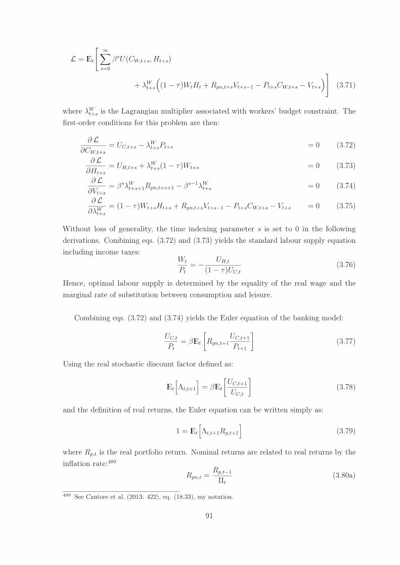
L = IEt

[ ∞∑s=0

βsU(CW,t+s, Ht+s)

+ λWt+s

((1− τ)WtHt +Rpn,t+sVt+s−1 − Pt+sCW,t+s − Vt+s

)](3.71)

where λWt+s is the Lagrangian multiplier associated with workers’ budget constraint. The

first-order conditions for this problem are then:

∂ L∂CW,t+s

= UC,t+s − λWt+sPt+s = 0 (3.72)

∂ L∂Ht+s

= UH,t+s + λWt+s(1− τ)Wt+s = 0 (3.73)

∂ L∂Vt+s

= βsλWt+s+1Rpn,t+s+1 − βs−1λW

t+s = 0 (3.74)

∂ L∂λW

t+s

= (1− τ)Wt+sHt+s +Rpn,t+sVt+s−1 − Pt+sCW,t+s − Vt+s = 0 (3.75)

Without loss of generality, the time indexing parameter s is set to 0 in the followingderivations. Combining eqs. (3.72) and (3.73) yields the standard labour supply equationincluding income taxes:

Wt

Pt

= − UH,t

(1− τ)UC,t

(3.76)

Hence, optimal labour supply is determined by the equality of the real wage and themarginal rate of substitution between consumption and leisure.

Combining eqs. (3.72) and (3.74) yields the Euler equation of the banking model:

UC,t

Pt

= βIEt

[Rpn,t+1

UC,t+1

Pt+1

](3.77)

Using the real stochastic discount factor defined as:

IEt

[Λt,t+1

]= βIEt

[UC,t+1

UC,t

](3.78)

and the definition of real returns, the Euler equation can be written simply as:

1 = IEt

[Λt,t+1Rp,t+1

](3.79)

where Rp,t is the real portfolio return. Nominal returns are related to real returns by theinflation rate:489

Rpn,t =Rp,t−1

Πt

(3.80a)

489 See Cantore et al. (2013: 422), eq. (18.33), my notation.

91

Rdn,t =Rd,t−1

Πt

(3.80b)

Ren,t =Re,t−1

Πt

(3.80c)

The difference of this Euler equation to conventional specifications is the type of return:in the banking model, the portfolio return enters the decision problem of the representativehousehold, whereas usually the Euler equation is derived in terms of the risk-free return.This difference will be explored further below.

3.7.4 Asset Demand Functions

In most DSGE models in which more than one type of asset is modelled, one asset isassumed to enter the utility function of the respective agent. Probably the most commonexample is the money-in-utility model to derive some form of liquidity preference, butthere are other possibilities such as housing or housing services.490 This approach may bemotivated by theoretical reasons, but it is also necessary due to analytical needs. DSGEmodels are generally approximated to first order around the deterministic steady state.This steady state is characterised by current and expected future shocks being set to zero.Hence, without risk in the deterministic steady state, all expected returns are equal.491

Thus, investors (in this case workers) are indifferent between the different types of assetsand portfolio shares are indeterminate.492 Hence, including money or another asset in theutility function determines a preference for one asset on the demand side.

Related, consider the choice between money and bonds. For workers to be indifferentbetween holding money or interest-bearing bonds, the real return of holding money mustbe equal to the real return of holding a bond. If these returns were different in equilibrium,then the worker would only hold the asset with the higher return, and none of the other. Ifnominal bonds are remunerated at a positive nominal interest rate, no worker wants to holdmoney - even in the absence of inflation - since it does not pay interest.493 On the otherhand, if money enters the utility function of workers, workers have a preference for holdingmoney, motivated by, for instance, liquidity preference. In this case the first-order condi-tions of workers’ optimisation problem determine the optimal amount of money holdings.494

Since the approach of approximating the banking model around its non-stochastic

490 See for example Iacoviello (2005)491 See Coeurdacier and Rey (2013: 69)492 See Coeurdacier and Rey (2013: 69)493 Note that this reasoning abstracts from other determinants of money demand such as transactions

demand or liquidity preference. These are theoretical justifications for including money in the utilityfunction in a DSGE framework.

494 For a textbook derivation of a money-in-utility model see Walsh (2003: 43ff).

92

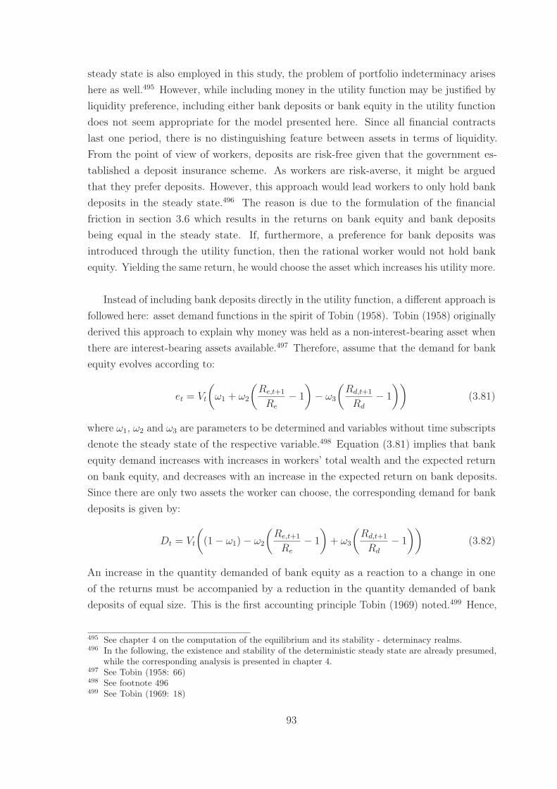
steady state is also employed in this study, the problem of portfolio indeterminacy ariseshere as well.495 However, while including money in the utility function may be justified byliquidity preference, including either bank deposits or bank equity in the utility functiondoes not seem appropriate for the model presented here. Since all financial contractslast one period, there is no distinguishing feature between assets in terms of liquidity.From the point of view of workers, deposits are risk-free given that the government es-tablished a deposit insurance scheme. As workers are risk-averse, it might be arguedthat they prefer deposits. However, this approach would lead workers to only hold bankdeposits in the steady state.496 The reason is due to the formulation of the financialfriction in section 3.6 which results in the returns on bank equity and bank depositsbeing equal in the steady state. If, furthermore, a preference for bank deposits wasintroduced through the utility function, then the rational worker would not hold bankequity. Yielding the same return, he would choose the asset which increases his utility more.

Instead of including bank deposits directly in the utility function, a different approach isfollowed here: asset demand functions in the spirit of Tobin (1958). Tobin (1958) originallyderived this approach to explain why money was held as a non-interest-bearing asset whenthere are interest-bearing assets available.497 Therefore, assume that the demand for bankequity evolves according to:

et = Vt

(ω1 + ω2

(Re,t+1

Re

− 1

)− ω3

(Rd,t+1

Rd

− 1

))(3.81)

where ω1, ω2 and ω3 are parameters to be determined and variables without time subscriptsdenote the steady state of the respective variable.498 Equation (3.81) implies that bankequity demand increases with increases in workers’ total wealth and the expected returnon bank equity, and decreases with an increase in the expected return on bank deposits.Since there are only two assets the worker can choose, the corresponding demand for bankdeposits is given by:

Dt = Vt

((1− ω1)− ω2

(Re,t+1

Re

− 1

)+ ω3

(Rd,t+1

Rd

− 1

))(3.82)

An increase in the quantity demanded of bank equity as a reaction to a change in oneof the returns must be accompanied by a reduction in the quantity demanded of bankdeposits of equal size. This is the first accounting principle Tobin (1969) noted.499 Hence,

495 See chapter 4 on the computation of the equilibrium and its stability - determinacy realms.496 In the following, the existence and stability of the deterministic steady state are already presumed,

while the corresponding analysis is presented in chapter 4.497 See Tobin (1958: 66)498 See footnote 496499 See Tobin (1969: 18)

93

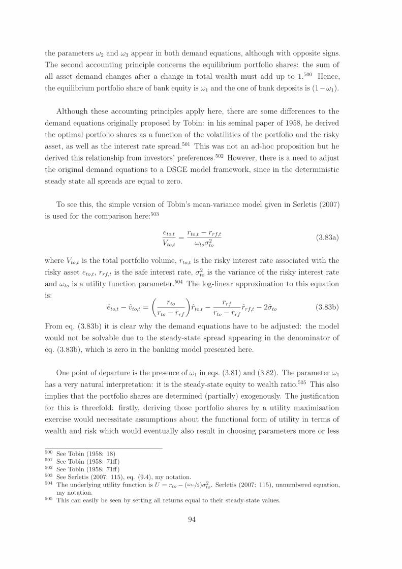
the parameters ω2 and ω3 appear in both demand equations, although with opposite signs.The second accounting principle concerns the equilibrium portfolio shares: the sum ofall asset demand changes after a change in total wealth must add up to 1.500 Hence,the equilibrium portfolio share of bank equity is ω1 and the one of bank deposits is (1−ω1).

Although these accounting principles apply here, there are some differences to thedemand equations originally proposed by Tobin: in his seminal paper of 1958, he derivedthe optimal portfolio shares as a function of the volatilities of the portfolio and the riskyasset, as well as the interest rate spread.501 This was not an ad-hoc proposition but hederived this relationship from investors’ preferences.502 However, there is a need to adjustthe original demand equations to a DSGE model framework, since in the deterministicsteady state all spreads are equal to zero.

To see this, the simple version of Tobin’s mean-variance model given in Serletis (2007)is used for the comparison here:503

eto,tVto,t

=rto,t − rrf,tωtoσ2

to

(3.83a)

where Vto,t is the total portfolio volume, rto,t is the risky interest rate associated with therisky asset eto,t, rrf,t is the safe interest rate, σ2

to is the variance of the risky interest rateand ωto is a utility function parameter.504 The log-linear approximation to this equationis:

eto,t − vto,t =

(rto

rto − rrf

)rto,t − rrf

rto − rrfrrf,t − 2σto (3.83b)

From eq. (3.83b) it is clear why the demand equations have to be adjusted: the modelwould not be solvable due to the steady-state spread appearing in the denominator ofeq. (3.83b), which is zero in the banking model presented here.

One point of departure is the presence of ω1 in eqs. (3.81) and (3.82). The parameter ω1

has a very natural interpretation: it is the steady-state equity to wealth ratio.505 This alsoimplies that the portfolio shares are determined (partially) exogenously. The justificationfor this is threefold: firstly, deriving those portfolio shares by a utility maximisationexercise would necessitate assumptions about the functional form of utility in terms ofwealth and risk which would eventually also result in choosing parameters more or less

500 See Tobin (1958: 18)501 See Tobin (1958: 71ff)502 See Tobin (1958: 71ff)503 See Serletis (2007: 115), eq. (9.4), my notation.504 The underlying utility function is U = rto − (ωto/2)σ2

to. Serletis (2007: 115), unnumbered equation,my notation.

505 This can easily be seen by setting all returns equal to their steady-state values.

94

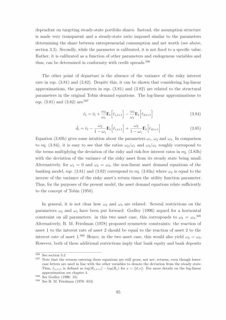
dependent on targeting steady-state portfolio shares. Instead, the assumption structureis made very transparent and a steady-state ratio imposed similar to the parametersdetermining the share between entrepreneurial consumption and net worth (see above,section 3.3). Secondly, while the parameter is calibrated, it is not fixed to a specific value.Rather, it is calibrated as a function of other parameters and endogenous variables andthus, can be determined in conformity with credit spreads.506

The other point of departure is the absence of the variance of the risky interestrate in eqs. (3.81) and (3.82). Despite this, it can be shown that considering log-linearapproximations, the parameters in eqs. (3.81) and (3.82) are related to the structuralparameters in the original Tobin demand equations. The log-linear approximations toeqs. (3.81) and (3.82) are:507

et = vt +ω2

ω1

IEt

[re,t+1

]− ω3

ω1

IEt

[rd,t+1

](3.84)

dt = vt − ω2

1− ω1

IEt

[re,t+1

]+

ω3

1− ω1

IEt

[rd,t+1

](3.85)

Equation (3.83b) gives some intuition about the parameters ω1, ω2 and ω3. In comparisonto eq. (3.84), it is easy to see that the ratios ω2/ω1 and ω3/ω1 roughly correspond tothe terms multiplying the deviation of the risky and risk-free interest rates in eq. (3.83b)with the deviation of the variance of the risky asset from its steady state being small.Alternatively, for ω1 = 0 and ω2 = ω3, the non-linear asset demand equations of thebanking model, eqs. (3.81) and (3.82) correspond to eq. (3.83a) where ω2 is equal to theinverse of the variance of the risky asset’s return times the utility function parameter.Thus, for the purposes of the present model, the asset demand equations relate sufficientlyto the concept of Tobin (1958).

In general, it is not clear how ω2 and ω3 are related. Several restrictions on theparameters ω2 and ω3 have been put forward: Godley (1996) argued for a horizontalconstraint on all parameters: in this two asset case, this corresponds to ω2 = ω3.508

Alternatively, B. M. Friedman (1978) proposed symmetric constraints: the reaction ofasset 1 to the interest rate of asset 2 should be equal to the reaction of asset 2 to theinterest rate of asset 1.509 Hence, in the two asset case, this would also yield ω2 = ω3.However, both of these additional restrictions imply that bank equity and bank deposits

506 See section 5.2507 Note that the returns entering these equations are still gross, not net, returns, even though lower-

case letters are used in line with the other variables to denote the deviation from the steady state.Thus, rx,t+1 is defined as log(Rx,t+1) − log(Rx) for x = {d, e}. For more details on the log-linearapproximation see chapter 4.

508 See Godley (1996: 18)509 See B. M. Friedman (1978: 613)

95

are perfect substitutes even when the economy does not rest in its steady state. Thismay be contentious concerning the banking model on the grounds that bank deposits arerisk-free while bank equity is risky from the perspective of workers. In sum, the relativeas well as the absolute sizes of the ω’s are not determined by these derivations, since thevolatility of the risky asset cannot be determined analytically in the banking model. Thus,this issue will be taken up again in chapter 5 when the model parameters are estimated.

Intuitively, eqs. (3.81) and (3.82) imply that workers will only change the portfolioweights if either one real return falls below or above its long-run value to take advantageof short-run fluctuations. With rational expectations and complete information, workersknow the underlying model and the underlying long-run equilibrium to which the economywill tend if all shocks were zero. So, if they observe an increase in returns, they willstill expect that returns are anchored at their equilibrium values in the long run. Thisreasoning contributes to the functional of form of eqs. (3.81) and (3.82). Furthermore, thespecification is similar to the reaction function of the central bank which is explained inthe next section.

3.8 The Government

3.8.1 Fiscal Policy

The last agent to be considered is the government which is in charge of fiscal and mon-etary policy. The specification of the governmental decision problem with respect tofiscal policy is kept to a minimum. The government is constrained to a balanced budgetin every period. More specifically, fiscal policy is passive and taxes are non-distortionary.510

This is without doubt a gross abstraction from reality. However, within the contextof this model, it is a reasonable and necessary simplification. For example, assume, forexample, that there were government bonds which are by assumption risk-free. How wouldthe representative worker choose between risk-free government bonds and insured bankdeposits which are risk-free as well from the perspective of workers? There would be a needfor a set of new assumptions, for instance determining the amount of government bondsfrom the supply sides since bank deposits and government bonds would in effect be perfectsubstitutes. In a similar vein, there would have to be some decision rule with respect tothe choice between tax and debt financing which necessitates a thorough treatment of its

510 More specifically, taxes are non-distortionary in the first-order log-linear approximation to thebanking model used for estimation and simulation in the following chapters. The assumption ofnon-distortionary taxes is not unusual for the standard NK model and for models focusing on monetarypolicy, see for instance Christiano, Motto and Rostagno (2003: 1120) and Herbst and Schorfheide(2016: 7f).

96

own. This is beyond the scope of this model.

Hence, the assumption is simply that there is no government debt. If the governmentchooses or is forced to increase its expenditures then taxes Tt must be raised in order tobalance the budget. Moreover, taxes are levied on wage income of workers at an exogenoustax rate τ . Government expenditures include government consumption of the retail goodΥG

t , net deposit insurance payouts Nnt and interest on minimum reserves.511 On the income

side the government also raises deposit insurance fees from banks DIt. So the governmentalbudget constraint can be expressed as:

ΥGt +Nn

t + (Rt − 1)MRt−1 = Tt +DIt (3.86)

where total taxes are:Tt = τWtHt (3.87)

Government consumption ΥGt follows an exogenous first-order autoregressive process

perturbed by a government consumption shock.512 Note that only net deposit payoutsenter the governmental budget constraint. Gross deposit payouts N b

t are equal to thedeposit liabilities of failed banks including interest (eq. (3.88)). Net deposit payouts aregross deposit payouts less the remaining assets of failed banks (eq. (3.89)):

N bt = GN(ψB

t )Rd,tDt−1 (3.88)

Nnt = N b

t − (1− μN)GN(ψBt )Rw,tBt−1 (3.89)

The auxiliary function GN measuring the share of failing banks is defined as:

GN =

∫ ψB

ψBmin

ψBf(ψB)dψB (3.90)

In the case of bank default, the government gains control over all remaining assets of thebank, and uses those funds to pay out depositors.513 Any additional bank deposit liabilitieswhich remain after these assets have been used up will be paid from the governmentalbudget. Note that the government also pays monitoring costs proportional to the loan

511 It is only interest which enters the government budget constraint because minimum reserves are not aform of income or expense for the government. Thus, there is no volume effect of changing minimumreserves over time. Minimum reserves are kept in a separate vault, and simply handed back to banksat the end of the reserve period.

512 On the specification see section 3.9.513 From the point of view of equity-holders, it is better to receive nothing in the case of default than to

gain access to the assets themselves and pay out depositors since bank default occurs only when bankassets are insufficient to pay out deposit liabilities.

97

revenue of insolvent banks.514 The share of bank assets used up in monitoring is scaled bythe parameter μN .

3.8.2 Monetary Policy

As observed in reality, there is a separate governmental entity, the central bank, which is incharge of monetary policy. In line with the mandate of, for instance, the ECB, its primaryobjective is price stabilisation.515 While the central bank is not independent concerningthe definition of its policy goal, it is independent in its choice of policy instruments andconduct. As in most of the literature, the central bank sets the nominal risk-free return,defined as 1 plus the nominal policy rate, using a monetary policy rule. The specific formconsidered here is a Taylor-type rule with interest rate persistence:516

Rn,t = R(1−ρR)n RρR

n,t−1

(Πt

Π

)(1−ρR)θπ(GAPt

GAP

)(1−ρR)θy

eεM,t (3.91)

where θπ and θy are parameters governing the responsiveness of the nominal risk-free returnto inflation and the output gap. εM,t is the monetary policy shock, which is discussedfurther below.517

The rule stipulates that the policy return will be adjusted for deviations of inflationΠt and the output gap GAPt from their respective steady-state values Π and GAP .518

Moreover, the monetary policy rule features interest rate inertia as long as the persistenceparameter is strictly positive, that is ρR > 0.519 Interest rate inertia can be motivated byvarious factors. This includes firstly, a larger impact of a change in the policy rate due toagents realizing that the change will last for several periods and secondly, lower interestrate volatility.520 Moreover, if inflation and the output gap are equal to their long-runequilibrium values, given that the nominal policy return was equal to its steady-state valuein the last period, then the central bank sets the policy return equal to the steady-state

514 Note that the government pays monitoring costs on the funds it gains control over in the process ofwinding-up, that is loan revenue. Equity-holders pay monitoring costs on the funds they receive aswell, in their case loan revenue less deposit liabilities. The parameters governing the size of monitoringcosts, μB and μN are allowed to differ, see chapter 5 for details.

515 See the Treaty on the Functioning of the European Union, Article 127 (1), The Member States (2012:102)

516 See, for example, Cantore et al. (2013: 422), eq. (18.34), my notation. Note that in contrast toCantore et al. (2013: 422), the central bank in the banking model responds to deviations of the outputgap, not actual output.

517 The dimension of nominal returns and inflation is per cent per annum, the output gap is measured interms of monetary units per quarter and the monetary shock is non-dimensional.

518 Similar to the workers’ asset demand functions, this specification presumes that the non-stochasticsteady state exists and is stable and determinate. Chapter 4 will present the results on steady-statecomputation and analysis.

519 By definition, ρR cannot be negative.520 See D. Romer (2012: 546)

98

nominal risk-free return Rn. Note that this specification is more flexible compared to aninterest rate rule which responds to any absolute level of inflation, for instance. While theanalysis in subsequent chapters deals with the zero-inflation steady state, in eq. (3.91),the steady-state level of inflation could as well be 2%. A key assumption in this respect isthat the central bank has gained credibility for maintaining low inflation so that inflationexpectations are well-anchored. In the following, I will assume that the central bank’sinflation target is a 0% inflation rate, so that private agents’ expectation of the inflationrate in the absence of any shocks is also 0%.521

So what is the long-run equilibrium value of the nominal risk-free return Rn. First,note that nominal and real returns are related to the inflation rate by the Fisher equation:

Rt =Rn,t−1

Πt

(3.92)

The real risk-free return is determined by the decision problem of workers, and given bythe inverse of the time preference rate of workers (see eq. (3.77)).522 When the (target)inflation rate in the steady state is zero, then the central bank sets the nominal policyreturn equal to the real equilibrium risk-free return. Given the long-term neutrality ofmonetary policy in the model, this is the optimal decision of the central bank for thezero inflation rate target.523 The central bank is free to set the policy interest return to adifferent level; this will lead to temporary movements of the economy around the steadystate, but the economy will eventually, gradually move back to its steady state.524 Hence,instead of permanently boosting the economy, the central bank risks losing its credibilityfor price stability if it were to use this latter strategy. In any event, setting the nominalpolicy return equal to the real risk-free return in the steady state is in accordance withprice stability, which is the primary objective of monetary policy.

The output gap in NK DSGE models is defined as the difference between actual outputand potential - or natural - output.525 The German Council of Economic Experts, forinstance, defines potential output as the output of the production process when the factors

521 See section 2.2 for a discussion of this point.522 Strictly speaking, workers choose consumption such that the real stochastic discount factor is equal to

the inverse of the real portfolio return. In the steady state, all real returns are equal, and consumption(and prices) are constant, such that eq. (3.79) reduces to 1 = βR, which leads to the result cited inthe text.

523 See Wickens (2008: 386). Long-term neutrality of monetary policy is due to the stationary nature ofthe model and the focus on the vicinity of the steady state in subsequent analyses, see also chapter 2on this issue.

524 This discussion presupposes that the steady state is a stable and determinate equilibrium. Seesection 4.4 for a discussion of stability and determinacy in NK DSGE models in general and thebanking model in particular.

525 See for example Galí (2008: 48)

99

of production are engaged at their normal capacity.526 Defining potential output in termsof an NK DSGE model with frictions is, however, not a trivial task. As Woodford (2003)points out, if nominal price rigidities are the only source of inefficiency, then optimalmonetary policy characterised by price stability achieves the optimal resource allocation.527

Although this result does not carry over to more complicated models with more frictions,output can be used as an instrumental variable for the efficient allocation if it is measuredby a model which does not incorporate such frictions which lead to a time-varying differencebetween the flexible price equilibrium and the efficient equilibrium.528 Thus, measuringpotential output by a non-distortionary small-scale NK model which achieves an efficientallocation allows monetary policy to respond to deviations of output from the efficientallocation.529

Another possibility for defining potential output in terms of a model measure would bethe long-run steady-state value of output. Remember that absent any shocks the economywill return to this equilibrium.530 So, the central bank would adjust the policy returnif actual output deviated from its equilibrium value. However, note that in case of, forinstance, a positive transitory technology shock, the reaction of monetary policy wouldceteris paribus be stronger using the steady-state value of output than using flexible priceoutput. The reason is that flexible price output increases whereas the long-run equilibriumdoes not change due to the stationarity of the model. Hence, the change in the output gapand by extension of the policy return is lower in the former than in the latter case. In sum,the mechanism is not fundamentally different.531 Thus, the output gap definition withrespect to potential output is used. Details on the derivation of this output gap measurefor the banking model are given in appendix section A.2.

As a final note on monetary policy implementation in the banking model, the transmis-sion process of the policy rate to the relevant rates of private agents in the model worksas follows: The policy rate is taken into account by banks who use the policy rate as areference to determine wholesale and loan interest rates. Moreover, the deposit rate isassumed to adjust immediately to the policy rate according to eq. (3.45b). The portfoliorate of workers, however, is a composite of the deposit and equity rates; hence, the direct

526 See Sachverständigenrat zur Begutachtung der Gesamtwirtschaftlichen Entwicklung (2014: 114)527 See Woodford (2003: 410)528 See Woodford (2003: 418)529 See also Galí (2008: 186) on this issue. Furthermore, another reason to exclude financial frictions

is that when comparing the banking model to a standard financial accelerator model, the latter’sdefinition of natural output would be different if financial frictions are included, which could potentiallydistort the analysis.

530 Again, this presupposes that the long-run steady state is stable and determinate, see footnote 524.531 This does not imply that different definitions lead to the exact same results, especially concerning

the magnitude of effects. This issue is considered in chapter 6 in describing objective trade-offs formonetary policy.

100

pass-through from the policy rate to the intertemporal decision problem of workers is notnecessarily complete nor immediate. The transmission of monetary policy impulses toinvestment decisions works through various channels of monetary transmission, which aremainly the interest rate, credit and expectations channels as specified before.

3.9 Equilibrium and Functional Forms

Market Clearing Equilibrium is characterised by simultaneous market clearing, namelywhen total supply equals total demand in the labour, retail goods, capital goods andfinancial markets. The final retail goods market is cleared when output by retailers equalsthe sum of workers’, entrepreneurs’ and governmental consumption demand, investmentdemand by capital investment funds and monitoring resource costs MoC:

Yt = CW,t + CE,t +ΥGt + It +MoCt (3.93)

MoCt is the sum of real resources banks, equity-holders and the government spend onmonitoring entrepreneurs and banks. An analytical expression can be found in appendixsection B.2.

The wholesale goods market is cleared if retailers’ demand equals entrepreneurs’ supply.The labour market is in equilibrium when entrepreneurs’ demand for labour is equalto workers’ supply of labour services. The market for capital goods is cleared whenentrepreneurs’ demand for capital is equal to capital investment funds’ supply of capital.Financial markets are in equilibrium if entrepreneurs’ demand for loans equals banks’supply, and banks’ supply of equity and deposits respectively equals the correspondingdemands of workers. Finally, the model closes with the monetary policy rule.

Functional Forms The functional form of the investment adjustment cost function S(�)is:532

S

(ItIt−1

)= φI

(ΥI

t

ItIt−1

− 1

)2

(3.94)

Given that in the deterministic steady state adjustment costs are zero and only the secondderivative of S(�) impacts dynamics, this specification is in line with many specifications inthe literature.533 The crucial parameter affecting dynamics is φI which scales the size of theadjustment costs. ΥI

t is an exogenous first-order autoregressive process with expectationequal to 1, perturbed by a shock.

532 The functional form is based on Cantore et al. (2013: 417), unnumbered equation, my notation.533 See for example Christiano et al. (2005a: 15)

101

The idiosyncratic financial shocks to entrepreneur’s capital return ψEt and banks’ loan

income ψBt are identically and independently distributed (i.i.d.) with mean 1, and are uni-

formly distributed over the intervals[1− EψΥ

Et , 1 + EψΥ

Et

]and

[1− BψΥ

Bt , 1 + BψΥ

Bt

],

respectively. Eψ and Bψ are parameters and ΥEt and ΥB

t are exogenous first-order autore-gressive processes, affecting the interval size of the idiosyncratic shocks of entrepreneursand banks, with expectation equal to 1 and perturbed by process-specific shocks.

The monetary policy shock εM,t is i.i.d. with mean zero and standard deviation σM .The aforementioned autoregressive processes ΥA

t , ΥBt , ΥE

t , ΥGt , ΥI

t , ΥKt , ΥMS

t , ΥPt take

the following form:

Υxt =

(Υx

)(1−ρx)(Υx

t−1

)ρxeεx,t (3.95)

where x = {A,B,E,G, I,K,MS, P}. The variable without time subscript denotes theequilibrium value, ρx determines the degree of persistence and εx,t is the shock to theprocess. εx,t is i.i.d. with mean zero and standard deviation σx. While both positive andnegative shocks hit the economy, the remainder of this text only reports the standarddeviation as the positive root of the variance.

102

Chapter 4

Model Solution and EquilibriumAnalysis

The previous chapter presented the banking model and justified the particular modellingchoices. It showed how non-systemic bank default extends a New Keynesian (NK) dynamicstochastic general equilibrium (DSGE) model with a financial accelerator to the bankingmodel. Furthermore, the previous chapter established that the friction on banks’ liabilityside, which gives rise to bank failures, affects the total credit spread and thus has thepotential to impact aggregate demand via the loan market. This chapter provides someeconomic intuition behind the banking model and explores some important aspects inmore detail. The objectives are firstly, to discuss the equilibrium concept and its stability,without which chapters 5 and 6 would lack the foundation. The second objective is toelucidate selected key relationships of the banking model both in a partial and a generalequilibrium setting.

For the essentially comparative purposes of this study it is convenient to separate thecomplexities due to the financial friction between banks and (bank) equity-holders andportfolio choice, which are specific to the banking model, from the complexities due toother frictions. Henceforth, the banking model presented in the previous chapter will becompared to a financial accelerator model. The financial accelerator model features thesame nominal and real frictions except for the friction between banks and their equity-holders. Thus, in the financial accelerator model banks do not default and only the loanmarket is subject to a financial friction. Also, there is no portfolio choice problem on thepart of workers. The separation between those two models will be a recurrent feature of thefollowing chapters and is intended to isolate the effects of the introduction of non-systemicbank default.

This chapter proceeds as follows. The concept of the non-stochastic steady state, aswell as its definition and computation for the non-linear banking model are discussed in

103

section 4.1. The relationship between bank and entrepreneurial leverage and the respectivecredit spread is dealt with in a partial equilibrium setting in section 4.2. Next, section 4.3focuses on general equilibrium, evaluating the changes due to various frictions on thesystem of difference equations in terms of the canonical NK dynamic IS-Phillips Curve-Monetary Policy (DIS-PC-MP) representation. Finally, section 4.4 evaluates the stabilityconsequences of certain parameter settings. In contrast to the preceding sections, theresults of section 4.4 are derived by numerical simulations, the reasons for which willbecome clear in sections 4.1 and 4.3.

4.1 The Non-Stochastic Steady State

For the estimation and simulation in chapters 5 and 6, the non-linear banking modelpresented in chapter 3 is log-linearly approximated around its zero-inflation non-stochasticsteady state in line with common practice in the literature. The non-stochastic (or de-terministic) steady state is equivalent to the perfect foresight solution in which agentsdo not foresee future shocks.534 That is, all shocks and their expected future values areequal to 0.535 Since there is no economic growth in the banking model, all endogenousvariables are constant in the non-stochastic steady state of the non-linear banking model.536

The portfolio choice problem of workers raises a difficulty for the computation ofthe deterministic steady-state if returns are equal in equilibrium. As noted above, theportfolio choice of households is indeterminate in the deterministic steady state. Severalauthors have proposed different solution algorithms to overcome this difficulty.537 Thetypical procedure is to append risk adjustments to the deterministic steady state and/orthe linear approximations of the dynamic equations.538 The result is, just as for thestandard procedure, a system of linear decision rules for adjusting the control variables todeviations from the steady state. Depending on the solution procedure and model layout,monetary policy may or may not affect portfolio decisions, and first-order dynamics of theportfolio can be described reasonably accurately. However, note that the procedure of,for instance, Devereux and Sutherland (2011) uses a low-order approximation around thedeterministic steady state for all equations, and higher-order approximations to solve for

534 See Coeurdacier, Rey and Winant (2011: 398)535 To be specific, the innovations to the exogenous autoregressive processes are 0, namely εx,t = 0, not

the exogenous processes Υx.536 Steady-state values of selected endogenous variables are discussed in chapter 5.537 An indicative list includes Coeurdacier and Rey (2013), Devereux and Sutherland (2011), Evans and

Hnatkovska (2012), and de Groot (2014).538 Coeurdacier et al. (2011) propose the concept of the risky steady state which is characterised by

current shocks being zero but agents anticipating future shocks. The procedure developed by Devereuxand Sutherland (2011) and Tille and van Wincoop (2010) appends risk adjustments to the portfolioproblem only, while the procedure proposed by de Groot (2014) adjusts all forward-looking equationsfor risk.

104

the portfolio weights.539 However, with local perturbation methods as used by Devereuxand Sutherland (2011), the approximated dynamics are only valid for small deviationsfrom the approximation point; this means that for medium to large risk adjustments thisprocedure may become inaccurate.540 In contrast, the approach followed here is to modelexplicit demand functions and estimate the parameters pertaining to portfolio choiceto facilitate the approximation around the deterministic steady state. Thus, instead ofredefining the approximation point for the dynamic description of the model I let the datadetermine the portfolio shares and dynamic adjustment parameters.541

Moreover, de Groot (2014) argues that the incorporation of risk into the steady stateallows for monetary policy to affect banks’ liability structure.542 However, as Bianchi(2014) notes, the portfolio choice is only relevant in the model of de Groot (2014) if banks’leverage constraint binds.543 In contrast, the banking model presented here does not linkthe willingness of workers to hold equity to the volume of liabilities and assets as in themodel by de Groot (2014).544 Rather, the demand for equity is determined by the actual re-turn of equity vis-à-vis the return of the alternative asset. Thus, as long as monetary policyaffects the returns on banks’ assets, and thus banks’ profitability, there will be feedback ef-fects on its liability structure with the approximation around the deterministic steady state.

Thus, this study uses the concept of the non-stochastic steady state. The non-stochasticsteady state of an NK DSGE model can usually be found recursively equation by equation.However, due to the complexity of the model presented here, this is not as straightforward.Instead, the method of Christiano et al. (2003) can be employed, whereby some of theendogenous variables are set exogenously guided by empirical data allowing to solve forsome of the parameters endogenously.545 This is useful since some parameters are highlymodel-specific and abstract, and thus difficult to calibrate. While the value of, for examplethe interval sizes of bank-specific and entrepreneur-specific shocks, Bψ and Eψ respectively,are difficult to determine, the spreads between various interest rates can be set guided byempirical data and previous studies. In the banking model, the endogenous variables set

539 See Devereux and Sutherland (2011: 346)540 See Bianchi (2014: 163). See Rabitsch, Stepanchuk and Tsyrennikov (2014) for a study on the accuracy

of various solution methods.541 Admittedly, the parameter determining the portfolio shares, ω1, is not estimated. However, it is

not calibrated to a single value either. Rather, the parameter is a function of other parameters andvariables. Thus, ω1 changes during the estimation procedure as the estimated parameters change.

542 See de Groot (2014: 118f)543 See Bianchi (2014: 163)544 See de Groot (2014: 125f). The model by de Groot (2014) is based on Gertler et al. (2012).545 See Christiano et al. (2003: 1171f). See, for example, Gabriel et al. (2010: 21, appendix B) for an

illustration of this approach. Cantore et al. (2013: 419f) use this approach for calibration of themodel’s parameters.

105

exogenously are: [�B p(ψB) �E p(ψE) φE CE/Y

](4.1)

where φE denotes entrepreneurs’ leverage ratio defined as QK/NE. The correspondingparameters solved for endogenously are:[

Bψ μB Eψ μE ξE ηE

](4.2)

Furthermore, the parameters ω1 and μN are set such that the model-implied steady stateleverage ratio of banks and the government’s budget constraint, respectively, are fulfilled.

Yet, for the computations in chapters 5 and 6, the exact computation of the completesteady state of the non-linear model is not necessary. As noted above, the estimationand subsequent simulations are based on the log-linear approximation of the bankingmodel. In turn, the log-linear approximation to the non-linear banking model is derivedby log-linearising the relevant model equations around the non-stochastic steady state.546

The steady state of the resulting log-linear model is characterised by all variables (definedas deviations from the steady state) being equal to 0. As a matter of notation, the steadystate of a variable Zt will be donated by Z, and the log-deviation of this variable from itssteady state by zt.

The constraints imposed by the use of the log-linear model overlap nicely with theresearch agenda of this thesis. The use of the local approximation is appropriate andsufficient since the focus of this study lies on the impact of non-systemic bank failures onmonetary policy. Since the log-linear approximation is only valid in the close vicinity ofthe non-stochastic steady state, large deviations or shocks cannot be traced. This alignswell with this study’s focus on a ‘normal’ business cycle instead of a financial crisis, as wellas the focus on non-systemic bank failures. Furthermore, permanent shocks, that is shockswhich entail a change in the non-stochastic steady state, are ruled out. As will be shownin the last section of this chapter, the relevant steady state, around which the model islog-linearly approximated, is locally stable and determinate. Thus, any displacement ofthe banking model economy from its steady state analysed in this thesis is transitory, thatis the model economy always returns to its stable, determinate long-run equilibrium. Theapproach also implies that fundamental, structural changes in the non-stochastic steadystate (other than the differences between the financial accelerator and banking models) arenot described in this study.547 Chapter 6 analyses the characteristics of this transition back

546 As before, this non-stochastic steady state is required to be locally stable and determinate, as will beshown later in this chapter.

547 Section 5.4 provides further details on the different non-stochastic steady states of the financialaccelerator and banking models.

106

to the original steady state from which the banking model is disturbed.548 The focus ison the responses of endogenous variables to exogenous disturbances, as is straightforwardusing the log-linear model. Again, this is in line with the focus on business cycles andnon-systemic bank failures.

So if the model is transformed, why is there a need to solve for the non-linear modelsteady state? In terms of the approximation, most variables only enter in terms of theirdeviation from the non-linear steady-state value while their steady-state values do notenter the system of equations. Thus, the non-stochastic steady state could be deemedirrelevant for subsequent analyses. Yet, to the contrary, there are various equations in thelog-linear model which include variables evaluated at their non-linear steady-state values.Again, in order to compute these steady-state values, the parameters in eq. (4.2) need to bedetermined. Thus, to calibrate these parameters or determine their prior distributions, thedeterministic steady state of the non-linear banking model is calculated for given valuesfor eq. (4.1) as described above.549 The only change is that the steady-state values of �B,p(ψB) and p(ψE) are calibrated as well.550 Then, the resulting values of the parametersin eq. (4.2) are taken as an indication for appropriate calibration and prior distributions.The exact details are discussed in section 5.2.2.

Against this background, section 4.3 describes the log-linear model in terms of thecanonical NK framework. The section in particular presents the changes which arise as aresult of incorporating financial frictions in this framework by comparing the banking andfinancial accelerator models to a simple NK model. Furthermore, section 4.4 explores theequilibrium stability and determinacy consequences of certain parameter constellations.Beforehand, however, the next section 4.2 takes a step back and explores the differentconcepts of entrepreneurial net worth and bank equity and their relationships with thecredit spread. Since some analytical results can be derived, in section 4.2 only, thenon-stochastic steady state of the banking model is used.

548 This equally applies to the financial accelerator model.549 In particular, σB , μB , σE , μE are estimated while ξE , and ηE are calibrated, see section 5.2.2.550 Note that these three are still endogenous variables, that is enter as deviations from the steady state.

However, during the log-linearisation it was not possible to eliminate the steady-state values of thesevariables, and others which depend on these variables, from the relevant equations such that thesteady state values of these three need to be determined. Given the complexity of the model, theycould only be calibrated.

107

4.2 Partial Equilibrium Analysis:

Leverage and the Credit Spread

In deriving the financial accelerator model in Bernanke et al. (1999) (BGG), the authorsargue that external financing via bank loans introduces a wedge between the risk-free rateof interest and the real return on real capital.551 This is because entrepreneurs cannotissue risk-free bonds to finance capital purchases. Instead, for banks to be willing to grantloans, they must expect to receive a return (including default costs) at least equal tothe risk-free rate. Thus, the resulting optimal state-contingent loan contract assigns allaggregate risk to the entrepreneur while the bank bears only idiosyncratic risk, which itcan diversify by offering loan contracts to many entrepreneurs.552 In equilibrium, optimalcapital purchases of entrepreneurs must satisfy an incentive compatibility constraint whichstates that the real return on real capital is equal to the product of the real risk-freereturn and the entrepreneurial risk premium.553 This leads to a spread between the realreturn on real capital and the real risk-free return formed by the entrepreneurial riskpremium. Furthermore and crucially, this risk premium is inversely related to the networth of entrepreneurs.554

The introduction of a second financial friction between banks and workers widens thespread between the real risk-free return and the real return on real capital further. In thebanking model, the relevant return for the specification of the optimal loan contract isnot the real risk-free return but the real wholesale return.555 The real wholesale returnis in turn the product of the bank risk premium and the real risk-free return.556 Thus,in equilibrium, the real return on real capital is equal to the real risk-free return timesthe product of entrepreneurial and bank risk premiums. Hence, as long as the bank riskpremium is strictly greater than 1, the spread between the real risk-free return and thereal return on real capital is larger in the banking model than in the financial acceleratormodel where only the entrepreneurial risk premium defines the spread.557

Furthermore, both entrepreneurs’ and banks’ default probabilities rise with their re-

551 See Bernanke et al. (1999: 1353f)552 See Bernanke et al. (1999: 1352)553 See 3.3 for more details.554 See Bernanke et al. (1999: 1354)555 For the derivations, see sections 3.3 and 3.6.556 The real deposit return is equal to the real risk-free return in equilibrium. According to eq. (3.45b),

the real deposit return is a linear function of the real risk-free return. Given that ξr and νd are small,the real deposit return and the real risk-free return differ only marginally in general.

557 Note that both risk premiums enter the arbitrage conditions eqs. (3.16) and (3.59) multiplicatively.In the log-linear approximation to the model used in the following chapters risk premiums enteradditively. Then, the condition is that the bank risk premium is strictly greater than 0 for the spreadto be larger in the banking model. Only non-negative risk premiums are considered.

108

spective leverage ratios.558 With higher default probabilities due to higher leverage, riskpremiums should rise. However, there is a crucial difference between entrepreneurs andbanks which leads to opposing relationships between leverage and the respective riskpremium. For entrepreneurs, net worth alleviates the agency problem as with higher networth the entrepreneur has a higher stake in his business. This reduces the entrepreneurialrisk premium for a given capital stock. For banks, the agency problem exists betweenthem and equity-holders. As will be shown here, the bank risk premium decreases with anincrease in leverage, ceteris paribus.

The link between the respective risk premiums and leverage ratios can be derivedanalytically from the incentive compatibility constraints, eqs. (3.13) and (3.56). Theincentive compatibility constraint for bank loans (eq. (3.13)) is:

(ΓE − μEGE)RkQK = Rw(QK −NE) (4.3)

Dividing through by R and NE yields:

(ΓE − μEGE)csφE = �B(φE − 1) (4.4)

rearranging for the entrepreneurial leverage ratio and noting that the credit spread cs isdefined as cs = �B�E gives:

φE =1

1− (ΓE − μEGE)cs(�B)−1(4.5)

where the first derivative of the leverage ratio with respect to the credit spread (keeping�B and the respective shares of the real capital return going to entrepreneurs and banksconstant at their steady-state values) is non-negative. Except for the presence of the riskpremium associated with banks, this is the same relationship as in the financial acceleratormodel of BGG.559 The higher is the entrepreneurial leverage ratio, the higher is the riskpremium. With higher leverage, entrepreneurs’ probability of default increases. Thus,credit conditions tighten so as to offset higher losses due to entrepreneurial default.

The corresponding link between the bank risk premium and bank leverage is derivedfrom equity-holders’ incentive compatibility constraint (eq. (3.56)):(

ΓB(ψB)− μBGB(ψB))RwB = Rd

(B − (1− ξr)D

)(4.6)

558 See appendix section B.1 for details.559 See Bernanke et al. (1999: 1353), eq. (3.8)

109

Dividing through by R and D leads to:(ΓB(ψB)− μBGB(ψB)

) cs�E

B

D=

(B

D− (1− ξr)

)(4.7)

rearranging, this yields for the loan-to-deposit ratio ΦB:

ΦB =1− ξr

1−(ΓB(ψB)− μBGB(ψB)

)cs(�E)−1

(4.8)

The derivative of the loan-to-deposit ratio with respect to the credit spread underthe corresponding assumptions as in the entrepreneurial case is non-negative as well.560

This means that the loan-to-deposit ratio increases with the credit spread. Conversely,the loan-to-equity ratio, that is banks’ leverage ratio, decreases with an increasing creditspread.561 Put differently, the bank risk premium decreases with an increasing share of de-posits in the loan volume.562 The diametrically opposed relationships between the leverageratios and the risk premiums of banks and entrepreneurs arise because the agency problemaffects the holdings of equity in the case of banks but the holdings of external finance inthe case of entrepreneurs. For entrepreneurs, a higher level of net worth moderates theasymmetric information problem. In contrast, for banks, a lower equity share lowers thedownside risks of holding bank equity, ceteris paribus. These downside risks involve thecomplete eradication of bank equity for failing banks. The costs of bank failure are smallerfor equity-holders if there is less bank equity to lose.563

The agency problem between banks and workers does only affect banks’ liabilitystructure, but also the quantity of physical capital demanded by entrepreneurs. In thefinancial accelerator and banking models the equilibrium credit spread and capital stockare determined at the intersection of the real capital demand and cost of funds curvesfor a given entrepreneurial net worth.564 Real capital demand is given by rearrangingeq. (3.3), the definition of the real return on real capital. The cost of funds curve is givenby eq. (4.5). They are depicted in fig. 4.1 which shows entrepreneurial capital demandand the cost of funds curves for the financial accelerator and banking models.

560 That is, assuming constant steady-state shares of bank auxiliary functions and a constant en-trepreneurial risk premium.

561 Whether or not a lower leverage ratio will also occur if the credit spread is low in the steady state,as compared to a steady state with both higher credit spread and leverage ratio, depends on thewhole system, especially the distribution of the bank-specific shock ψB , the resulting auxiliary bankfunctions, and finally the absolute levels of banks’ assets and liabilities. As noted above, for thederivations here the auxiliary bank functions and the entrepreneurial risk premium were explicitlykept fixed.

562 This can be seen by rearranging eq. (4.7) for the bank risk premium B (= cs/�E) and taking the firstderivative with respect to the deposit to loan share (D/B). This first derivative is negative.

563 To see this, see chapter 3, eq. (3.51).564 See Bernanke et al. (1999: 1355)

110

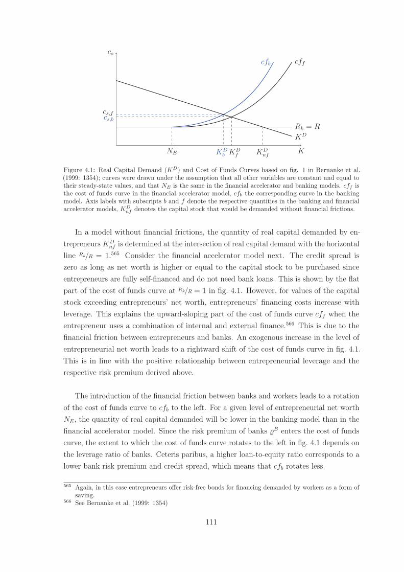
K

cs

Rk = R

cffcfb

KD

NE KDnfKD

b KDf

cs,fcs,b

Figure 4.1: Real Capital Demand (KD) and Cost of Funds Curves based on fig. 1 in Bernanke et al.(1999: 1354); curves were drawn under the assumption that all other variables are constant and equal totheir steady-state values, and that NE is the same in the financial accelerator and banking models. cff isthe cost of funds curve in the financial accelerator model, cfb the corresponding curve in the bankingmodel. Axis labels with subscripts b and f denote the respective quantities in the banking and financialaccelerator models, KD

nf denotes the capital stock that would be demanded without financial frictions.

In a model without financial frictions, the quantity of real capital demanded by en-trepreneurs KD

nf is determined at the intersection of real capital demand with the horizontalline Rk/R = 1.565 Consider the financial accelerator model next. The credit spread iszero as long as net worth is higher or equal to the capital stock to be purchased sinceentrepreneurs are fully self-financed and do not need bank loans. This is shown by the flatpart of the cost of funds curve at Rk/R = 1 in fig. 4.1. However, for values of the capitalstock exceeding entrepreneurs’ net worth, entrepreneurs’ financing costs increase withleverage. This explains the upward-sloping part of the cost of funds curve cff when theentrepreneur uses a combination of internal and external finance.566 This is due to thefinancial friction between entrepreneurs and banks. An exogenous increase in the level ofentrepreneurial net worth leads to a rightward shift of the cost of funds curve in fig. 4.1.This is in line with the positive relationship between entrepreneurial leverage and therespective risk premium derived above.

The introduction of the financial friction between banks and workers leads to a rotationof the cost of funds curve to cfb to the left. For a given level of entrepreneurial net worthNE, the quantity of real capital demanded will be lower in the banking model than in thefinancial accelerator model. Since the risk premium of banks �B enters the cost of fundscurve, the extent to which the cost of funds curve rotates to the left in fig. 4.1 depends onthe leverage ratio of banks. Ceteris paribus, a higher loan-to-equity ratio corresponds to alower bank risk premium and credit spread, which means that cfb rotates less.

565 Again, in this case entrepreneurs offer risk-free bonds for financing demanded by workers as a form ofsaving.

566 See Bernanke et al. (1999: 1354)

111

The model thus replicates the asymmetric financing situations of banks and en-trepreneurs that Admati and Hellwig (2013) describe. Admati and Hellwig (2013) arguethat borrowing is cheaper for banks than for non-financial firms because taxpayers par-tially cover the costs of bank borrowing.567 In the banking model, a higher bank equitybase increases, ceteris paribus, the bank risk premium. With a downward sloping loandemand curve, bank loans and by extension capital demand decrease. In contrast, higherentrepreneurial net worth reduces the entrepreneurial risk premium. Again, along thedownward sloping capital demand curve in fig. 4.1, this leads to an increase in the realcapital stock. As the real capital stock directly affects the productive capacity of theeconomy as well as financing constraints, the leverage ratios of banks and entrepreneurshave consequences for the real economy. The terms bank equity and entrepreneurial networth were purposefully chosen to highlight the different roles these have for the financialsituation of banks and entrepreneurs.

What is more, the fact that bank deposits are insured plays a role. In contrast to holdersof bank equity, deposit-holders do not view bank deposits as risky. This is because depositsare insured and are thus covered even in the case of bank failure. What is the implicationof the assumption of workers regarding bank deposits as risk-free? Assume for a momentthat bank deposits are not insured and deposit-holders would bear the consequences ofbank default similarly to equity-holders. Then, the distinguishing characteristic betweenbank deposits and bank equity becomes blurred. Furthermore, deposit-holders would alsodemand a risk premium, even though this may be lower than the one on bank equity ifbank deposits are served preferentially. Thus, the fundamental friction of the incidenceof bank failure exists independently of the deposit insurance scheme. The result of thedeposit insurance scheme is a more straightforward derivation of the credit spread. Thisdoes not, however, affect the structure workers’ consumption and leisure decisions, as theseare separate from the portfolio choice problem.568

As argued before, it is not clear how the choice between different (risky) financial assetsshould affect a worker’s utility other than through the realised portfolio return which isthe rationale for separating these optimisation problems. Nevertheless, there is anotherpossibility for workers to take into account the consequences of bank failure. This is accom-plished by a change in the modelling of taxes when the deposit insurance scheme is in place.In the banking model, taxes are non-distortionary in the first-order approximation. There-fore, workers as holders of bank deposits do not perceive that bank failures lead to higheroutlays in the governmental budget, and thus higher taxes. If taxes were endogenous in the

567 See Admati and Hellwig (2013: 8f), bank bailouts are argued to be one example of subsidies on bankborrowing, see Admati and Hellwig (2013: 9).

568 Chapter 6 will discuss the separation of workers’ optimisation problems and some of the consequencesfor the effects on monetary policy more thoroughly.

112

first-order approximation, workers’ consumption and leisure decisions would be affected bychanges in deposit insurance outlays. As will become clear in chapter 6, the ignorance ofdeposit-holders in terms of foreseeing and incorporating the tax-related consequences ofbank failure merely shuts off a further mechanism through which bank default can affect theconduct of monetary policy. Since the treatment of fiscal policy is intentionally kept shortin the banking model, the main part of this thesis abstracts from this additional mechanism.

In conclusion, entrepreneurial net worth and bank equity function differently in thebanking model. The next section aims to highlight how the banking model compares moregenerally to a model which does not feature bank failure. To facilitate comparability withthe literature, the changes are discussed in terms of the NK DIS-PC-MP framework.

4.3 The Log-Linear New Keynesian DIS-PC-MP Rep-

resentation

To gain an intuition for the workings of the banking model, this section will deal with thegeneric three-equation representation of NK DSGE models: the dynamic IS function, thePhillips Curve and a monetary policy rule. In contrast to classical economic theory, outputand inflation are not determined independently of the path of interest rates and thus amonetary policy rule for the interest rate is necessary to close the NK model even in thesimplest case.569 As will be shown below, this simple representation is not attainable forthe banking model due to the complexity surrounding portfolio choice and the frictions inthe banking sector. Nevertheless, it is possible to discuss the similarities and differencesbetween this simple NK DSGE layout and the financial accelerator and banking models inthis reduced form representation.

4.3.1 A Simple New Keynesian Model

A simple New Keynesian model with sticky prices can be represented by the followingsystem of three equations:570

πt = βIEt[πt+1] + κ gapt (4.9)

gapt = IEt[gapt+1]−1

σ

(rn,t − IEt[πt+1]

)(4.10)

rn,t = νππt + νygapt + εM,t (4.11)569 See Galí (2008: 49)570 See Walsh (2003: 244, 247), eqs. (5.68), (5.69) and (5.72), my notation. Note that while eq. (5.72) in

Walsh (2003: 247) does not include the output gap, the output gap is included here for comparabilitywith the banking model. See also Woodford (2003: 245f), eqs. (1.12), (1.13) and (1.14), my notation.Details on the derivation can be found in Galí (2008) or Walsh (2003), for instance.

113

This three-equation system is expressed in terms of the log-linear approximation to therelevant non-linear equations.571

Equation (4.9) is the NK Phillips Curve (PC) which constitutes the aggregate supplyblock of the model and determines inflation π for a given path of the output gap gap.572

It is derived from the optimal price setting behaviour of (consumption) goods producersresulting in an equation linking inflation to marginal costs.573 In a second step, marginalcosts can be linked to the output gap via the labour market equilibrium condition.574 κ isthus a function of production and utility function parameters.575

Equation (4.10) is the NK dynamic IS (DIS) equation. The DIS curve is derived bycombining the intertemporal consumption Euler equation with the economy’s budgetconstraint.576 σ is the coefficient of relative risk aversion.577 The NK DIS function linksthe evolution of the expected real interest rate and inflation to the output gap. Morespecifically, in the three equation framework the DIS equation determines the output gapfor a given real interest rate.578 It can thus be argued to be the analogue of the HicksianIS curve, written as a dynamic equation and derived from the maximisation problem ofindividual agents.579

These two equations determine inflation and the output gap, respectively, given theoutput gap on the one hand, and inflation and the nominal interest rate on the other. Toclose the model, an equation for the path of the nominal interest rate is necessary. Thestandard assumption is that there exists a central bank which is in charge of setting thenominal interest rate following a Taylor rule as in eq. (4.11). νπ and νy are parametersgoverning the central bank’s responsiveness to changes in inflation and the output gap.Hence, in the NK model, monetary policy is not neutral given that the path of the nominalinterest rate affects the output gap via the DIS equation.580

This system of three difference equations in three endogenous variables characterises

571 This presumes that the deterministic steady state is stable and determinate. For more details onthese issues see section 4.4.

572 See Woodford (2003: 241)573 See Galí (2008: 47). See King (2000: 90) for a simple mathematical derivation.574 Since labour is the only input of production, real marginal costs are given by the ratio of the real

wage to the marginal product of labour, see Walsh (2003: 238).575 See Galí (2008: 47ff) for a definition and derivation.576 See Wickens (2008: 365)577 See Wickens (2008: 361)578 See Galí (2008: 49)579 See Woodford (2003: 242)580 See Galí (2008: 49). As noted above, this use of neutrality differs slightly from the one used by

Goodfriend and King (1997), see footnote 339 in chapter 3. Here, monetary policy being non-neutralmeans that monetary policy impacts the real economy.

114

the whole model: equilibrium in the goods and labour markets, optimal saving/borrowingdecisions through the Euler equation and monetary policy. It is straightforward to analysedifferent monetary policy rules and the stability of this system. However, this simplicityis attained only by abstracting from key concepts. Since labour is the only productioninput, there is no physical capital and thus no investment. Similarly, there is no govern-ment except for the interest-rate setting central bank, and hence no taxes or governmentspending. Furthermore, the derivation of the DIS equation requires separability of theutility function in both time and consumption/leisure dimensions and a well-chosen powerfunctional form.581

In the context of a more complex model the complexity also transfers to the represen-tation in the DIS-PC-MP format. Including only investment (and hence physical capital)and the government extends above system to a system of seven difference equations.582

Furthermore, the inclusion of the financial sector with frictions in loan and bank liabilitymarkets enlarges this system even further. This makes an analytical derivation of, for ex-ample, the stability realm of various parameters impractical. This is the reason subsequentanalyses in section 4.4 and chapters 5 and 6 are conducted using numerical computations.Even considering only the simple three-equation system, there are various complications.The derivation of the DIS-PC-MP equations for the financial accelerator and bankingmodels in the following paragraphs allows to see the similarities and differences betweenthe simple model and the financial friction(s) models in condensed and accessible form.

The procedure in the following sections is to first include physical capital, investment,habit and indexation as well as the financial accelerator between entrepreneurs and banksas the financial accelerator model. In a second step the changes due to the inclusion ofthe financial friction between banks and workers and the portfolio choice problem arepresented. To ensure comparability, the monetary policy rule is the same in the financialaccelerator and banking models.583 Since it is simply the log-linear approximation to themonetary policy rule presented in chapter 3, it is discussed with the banking model.

4.3.2 The Financial Accelerator Model

The financial accelerator model is a standard NK DSGE model with financial acceleratorand features the same general layout and frictions as the banking model. To be precise,these are: the optimisation problems of entrepreneurs, retailers and capital investmentfunds, and the form of workers’ utility function, all as presented in chapter 3. However,

581 See the derivations in Galí (2008) or Walsh (2003).582 See Woodford (2003: 361)583 Optimal monetary policy is not as such dealt with in this study. See the discussions later in this

chapter and in chapter 6 for more details.

115

there is no agency problem between banks and workers, and thus no portfolio problem, inthe financial accelerator model. This means that in the financial accelerator model the loancontract is specified with respect to the real risk-free return, instead of the wholesale returnused in the banking model.584 Also, since there is no deposit insurance scheme, the fiscalpolicy is is simply described by the equality of the exogenous government consumptionprocess with the tax volume.

4.3.2.1 The New Keynesian Phillips Curve

For the financial accelerator model, the NK PC expressing inflation as the sum of expectedfuture inflation and the deviation of marginal cost from its steady-state value can be derivedsimilarly to the simple model, with the addition of lagged inflation in the relationship.The resulting Phillips Curve of the financial accelerator model is given by:585

πt =β

1 + βγpIEt[πt+1] +

γp

1 + βγpπt−1 + κffmct (4.12)

whereκff =

(1− βξp)(1− ξp)

(1 + βγp)ξp(4.13)

The mathematical derivation of this formula follows the same procedure as for thesimple NK model.586 The similarity is due to the fact that both models feature the samekind of price friction: Calvo-style price staggering. The introduction of lagged inflationin the NK PC curve in the financial accelerator model is the result of price indexation(governed by the parameter γp).587 Past inflation is more important in the NK PC curvewhen more prices that cannot be set optimally are indexed to inflation. Conversely, settingγp = 0, eq. (4.12) also held in the simple NK model if marginal costs were explicitlydefined as a separate endogenous variable and not substituted for the output gap in eq. (4.9).

Yet, while in the simple model marginal costs can be substituted to derive a relationshipbetween the output gap and inflation, this is not possible in the financial accelerator model.This is a result of the more complex definition of marginal costs. The steps for deriving therelationship between inflation and marginal costs are the same: The starting point is theprice-setting decision, which concerns retailers in the financial accelerator model. As canbe shown, retailers’ real marginal costs are equal to the ratio of wholesale prices to final

584 See Bernanke et al. (1999: 1349)585 See Smets and Wouters (2003: 1135), eq. (32), my notation. Note that the exogenous mark-up

shock process is left out for a clearer exposition. Strictly speaking, the mark-up shock process enterseq. (4.12) additively.

586 See Galí (2008: 46ff) and Walsh (2003: 234ff and 263ff) for derivations without price indexation andChristiano et al. (2005a: 26f) and D. Romer (2012: 345f) for derivations with price indexation.

587 See Smets and Wouters (2003: 1135)

116

retail goods prices.588 This latter ratio can be related to the labour demand equation ofentrepreneurs. Thus, as in the simple model, the derivation includes the use of the laboursupply and demand optimality conditions (eq. (3.76) and eq. (3.2)). The former equatesthe real wage to the marginal rate of substitution between consumption and leisure, andthe latter condition equates the real product wage (that is, in terms of wholesale prices)to the marginal product of labour.589 Then, in the next step, the final retail goods marketequilibrium condition is used to substitute for consumption.

In the simple NK model, these steps lead to an expression for marginal costs a a linearfunction of the output gap and utility and production function parameters.590 In contrast,in the financial accelerator model the expression for marginal costs is more complex dueto the inclusion of investment, government consumption and the terms associated withthe financial friction in the economy’s resource constraint as well as the inseparabilitiesintroduced in workers’ utility function. To see this, note that in the simple model withoutinvestment, government spending and a financial friction, the log-linear approximation tothe final retail goods market condition is simply:

yt = ct (4.14)

that is, changes in aggregate demand are equal to changes in consumption. In contrast, thelog-linear approximation to the final retail goods market equilibrium condition (eq. (3.93))in the financial accelerator model is given by:

yt =CW

Ycw,t +

CE

Yce,t +

I

Yit +

ΥG

Yυgt +

MoCF

YmocFt (4.15)

Thus, the expression for marginal costs becomes mathematically more cumbersome. In-stead of being able to substitute ct in the labour market equilibrium condition directlywith yt, ct is now replaced by 1

CW/Y(yt− (CE

Yce,t+

IYit+

ΥG

Yυgt +

MoCF

YmocFt )) where MoCF

stands for aggregate monitoring costs. While government consumption does not complicatethe simplification process much as it is assumed to be an exogenous autoregressive process,the log-linear approximation of investment, entrepreneurs’ consumption and monitoringcosts are complicated functions of the probability functions of the entrepreneur-specificshock and/or the capital stock, its price and real return, and thus impede an illustratingand meaningful equation reduction exercise (see appendix section B.2). As noted above,only including physical capital, investment and government consumption already increasesthe system to seven difference equations plus three exogenous processes.591 Furthermore,588 See Walsh (2003: 355)589 See Walsh (2003: 355)590 See Galí (2008: 48)591 This extended system appends dynamic equations for capital and investment and splits the NK (D)IS

and PC equations each into two separate difference equations. See Woodford (2003: 361)

117

the capital stock does not only impact marginal costs indirectly via above mentioned vari-ables, but also directly since it enters the production function, which is used for substitution.

Moreover, optimal labour supply depends on workers’ utility function which differs inthe financial accelerator model from the simple NK model. In particular, the financial ac-celerator model features a utility function that is time-inseparable and inseparable betweenconsumption and leisure. This matters because workers’ optimal labour supply conditionis used to substitute for the real wage and thus relate marginal costs to consumption andoutput.592 In the simple model, the log-linear approximation to the optimal labour supplycondition can be expressed as:593

wt − pt = ηht + σct (4.16)

where the left-hand side is the difference between the log-deviations of the nominal wageand the price level from their respective steady state level, η is the Frisch elasticity oflabour supply, and σ is the degree of risk aversion, as before.594 The counterpart to thisequation for the financial accelerator model is given by:

wt − pt =cw,t − χcw,t−1

1− χ+

H

1−Hht (4.17)

where H is the steady-state value of labour input in the production process. Combiningthese complications and defining XF

t as aggregate retail goods demand less workers’consumption demand, an expression for marginal costs can be derived.595 Marginal costsin the financial accelerator model are then:

mct =

(1

(CW/Y )(1− χ)+

(1

(1−H)α− 1

))yt − χ

(CW/Y )(1− χ)yt−1

− 1

(CW/Y )(1− χ)

XF

Y(xF

t − χxFt−1)−

1

α(1−H)(υa

t + (1− α)kt−1)

= λPC1 yt + λPC

2 yt−1 + λPC3 (xF

t − χxFt−1) + λPC

4 (υat + (1− α)kt−1) (4.18)

where the last line simplifies the parameter terms to single coefficients.596

592 Remember that in the simple model output was equal to consumption.593 See Walsh (2003: 238), unnumbered equation, my notation. The relevant derivations can be found in

Walsh (2003: 234ff).594 See Galí (2008: 52). The underlying utility function is: Ut = C1−σ

t /(1−σ) − N1+ηt /(1+η), see Galí (2008:

42), unnumbered equation, my notation.595 See appendix section B.3 for details. Note that although wholesale and final output are not the same,

the deviations around the steady state approximated up to first order are equal since Yt = (1− c)YWtwhere c is a constant, and as was noted above, price dispersion does not impact first-order dynamics,see Christiano et al. (2011: 297).

596 This means, λPC1 is a substitute parameter function for the whole term pre-multiplying yt in the firstline of the equation. The same applies to the remaining λPC ’s.

118

Strictly speaking, all variables except for the exogenous processes in eq. (4.18) shouldhave a financial accelerator model superscript F , since the deviations of output from theirsteady-state levels are different in the financial accelerator and the banking models. Forexample yt evolves differently in response to a shock in the financial accelerator modelthan in the banking model.597 However, to emphasise the changes, only those variableswhose mathematical definition changes in the banking model are marked with a modelsuperscript F .

Considering the coefficients of the deviations, there are some notable features. Bydefinition α, χ, H, and CW/Y take values between 0 and 1. Thus, λPC

1 , the coefficientmultiplying yt, is strictly positive while λPC

2 , λPC3 and λPC

4 are negative. This sign of λPC4

is consistent given that both technology and capital increase the marginal productivity oflabour. Thus, if the marginal productivity of labour increases, retailers’ real marginal costdecreases.

The relationship between the output gap and marginal costs in the simple modelcorresponding to eq. (4.18) is:598

mct = κ gapt (4.19)

where κ is a function of production and utility function parameters.599

What is more, there is a notational difference between eqs. (4.18) and (4.19). Thereference point for calculating deviations is natural output in eq. (4.19), while it is therespective steady-state value in eq. (4.18).600 The output gap could be introduced intoeq. (4.18), yet this would not reduce the complexity of eq. (4.18) as is the case in the simplemodel. In fact, the only term that would drop out with certainty is at given that it is anexogenous autoregressive process. In the simple model, writing the equation in terms of theoutput gap allows both for a natural economic interpretation, but also a simplification sincethe other component of marginal costs in the simple model - technology - drops out. Giventhat there are more variables in the financial accelerator and banking models that affectmarginal costs which do not drop out, the transformation would merely lead to redefiningthe deviation of the capital stock from its steady state into the deviation of the capital stockfrom its natural counterpart value. This latter value is not necessarily equal to the steadystate but also reacts to shocks. While the output gap is an established definition, redefining

597 See, for instance, chapter 6 for the evolution of different variables to a monetary policy shock.598 See Galí (2008: 48), eq. (20), my notation.599 More specifically, κ = σ + (η+α)/(1−α), where σ and η are defined as above, and 1− α is the partial

elasticity of output with respect to labour, see Galí (2008: 43, 48), eq. (20), my notation.600 Given that all model variables are stationary and the condition of a stable and determinate steady

state, the economy will return to the long-run equilibrium when displaced by exogenous shocks. Seesection 4.4 for details on stability and determinacy of equilibrium.

119

capital and other demand components in terms of their deviations from a natural coun-terpart does not make the dynamics more transparent. Hence, the notation here followsWoodford (2003) and considers deviations from the deterministic (long-run) steady state.601

Apart from this notational difference, there are various aspects to note concerning theNK PC of the financial accelerator model. Firstly, while they do not explicitly appearin eq. (4.18), workers’ discount rate and the elasticity of output with respect to labouraffect marginal costs indirectly via the steady-state value of labour input H. Thus, utilityfunction parameters affect the link between marginal cost and output deviations in boththe simple and the financial accelerator models although potentially to different extents.

Secondly, note that marginal cost deviations from the steady state increase with in-creases in the current deviation of output from its steady state yt, but decrease withincreases in lagged output deviations yt−1. The first observation is in line with the simplemodel where marginal costs are proportional to the output gap. The negative sign oflagged output deviations is due to habit persistence in the utility function. By definition,|λPC

1 | will be larger than |λPC2 |. Thus, increases in current retail goods demand will

increase marginal costs, but in general to a smaller extent than in the simple model dueto habit persistence. Given that habit persistence, as well as investment adjustment costs,were introduced to increase the persistence of consumption and investment, respectively,following shocks, and thus by extension output, the reaction of marginal costs should alsobe smoother within this framework.

Thirdly, factors of production affect the relationship between the output gap andmarginal costs. As noted before, marginal costs of retailers can be defined as the ratioof the nominal wage to the marginal product of labour. As both technology and thecapital stock raise the marginal productivity of labour, real marginal costs decrease givena negative λPC

4 . What is more, the capital stock affects other variables in eq. (4.18) andthus marginal costs also indirectly. Changes in the capital stock in period t affect marginalcosts indirectly via investment spending in period t, and the volume of entrepreneurs’consumption and monitoring costs through the endogenous price of capital and thus thereal return on real capital in period t. Hence the exact effect is unclear from this analyticalperspective, yet can be evaluated through numerical simulations.

Fourthly and related, aggregate demand components affect marginal costs. Since therelationship is derived using workers’ optimality conditions, the main effect is due toconsumption. The relationship between workers’ consumption demand and the real wage

601 Due to a similar reasoning the derivation of the DIS curve presented below would not simplify (exceptfor technology) further, too, if it were written in terms of output gap deviations.

120

can be seen in eq. (4.17): ceteris paribus (ht = 0), ct > 0 necessitates an increase in thereal wage wt − pt. For a set of preferences concerning intertemporal substitution and riskaversion, given hours worked and wealth, workers only consume more if they earn more inthe same period. Irrespective of whether this increase in the real wage is due to an increasein the nominal wage rate or a decrease in inflation, marginal costs of retailers will increase.602

However, other aggregate demand components may also affect marginal costs. Thisis due to the analytical derivation: hours worked are substituted for the productionfunction in deriving eq. (4.18) the result of which is the more complex definition of λPC

1

as compared to the other λPC ’s. The following equation must hold for an increase of oneof the components of aggregate demand other than workers’ consumption to not affectmarginal costs and thus inflation:

CE

Yce,t +

I

Yit +

ΥG

Yυgt +

MoCF

YmocFt = 0 (4.20)

If, on the other hand, the left-hand side of eq. (4.20) is positive (negative), then theseaggregate demand components increase (decrease) retailers’ real marginal cost. Therefore,it is not only the aggregate level of output (or demand) which affects marginal costs inthe financial accelerator model, but also its composition.

To sum up, in the financial accelerator model, inflation depends on past and expectedfuture inflation as well as deviations of real marginal cost from its steady state. Except forthe presence of lagged inflation, this is the same result that emerged from the simple NKmodel. Furthermore, lagged inflation enters because of price indexation. In contrast, thelink between real marginal costs and the output gap is complicated due to the financialfriction and the introduction of governmental consumption, physical capital and investment.As in the simple model, deviations of marginal cost are positively linked to deviations ofoutput. However, this relationship is affected by other aggregate demand components andproduction inputs.

4.3.2.2 The New Keynesian Dynamic IS Curve

As in the simple model, the NK DIS curve in the financial accelerator model is derived bycombining the consumption Euler equation with the economy’s resource constraint. Thelog-linear approximation to the consumption Euler equation in the financial acceleratormodel is given by:603

uc,t = IEt[rn,t+1]− IEt[πt+1] + IEt[uc,t+1] (4.21)602 To see this, note that marginal costs of retailers are given by (time subscripts were dropped for clearer

notation): MC = PW/P = WN

/αYW .603 This is essentially the log-linear approximation to eq. (3.77), where the real portfolio return is

substituted for the real risk-free return.

121

where the log-linear approximation to marginal utility of consumption in period t is givenby:

uc,t =((1− ηl)(1− σc)− 1

) cw,t − χcw,t−1

1− χ+ ηl(σc − 1)

H

1−Hht (4.22)

Combining eqs. (4.21) and (4.22) yields the consumption equation linking the path ofconsumption to the expected real interest rate:

cw,t =1

1 + χIEt[cw,t+1]− χ

1 + χcw,t−1 +

zh(1 + χ)zc

(IEt[ht+1]− ht

)+

1

(1 + χ)zc

(IEt[rn,t+1]− IEt[πt+1]

)(4.23)

where zh and zc are given by:

zh = ηl(σc − 1)H

1−H(4.24)

zc =(1− ηl)(1− σc)− 1

(1− χ)(4.25)

Similar to the discussion concerning the NK PC curve, the extended aggregate resourceconstraint complicates the derivation of the DIS curve as well. Combining the consumptioneq. (4.23) with the economy’s resource constraint yields:

yt =1

1 + χIEt

[yt+1 − XF

YxFt+1

]+

XF

YxFt +

χ

1 + χ

(yt−1 − XF

YxFt−1

)+

zh(1 + χ)zy

(IEt[ht+1]− ht

)+

1

(1 + χ)zy

(IEt[r

nt+1]− IEt[πt+1]

)(4.26)

where zy is given by:

zy =(1− ηl)(1− σc)− 1

(CW/Y )(1− χ)(4.27)

Using the production function to substitute for hours worked in eq. (4.26) yields:

yt =zyα + zh

(1 + χ)zyα + zhIEt[yt+1] +

α

(1 + χ)zyα + zh


)+

χzyα

(1 + χ)zyα + zh

(yt−1 − XF

YxFt−1

)− zyα

(1 + χ)zyα + zh

XF

Y

(IEt[x

Ft+1]− (1 + χ)xF

t

)− zh

(1 + χ)zyα + zh

(IEt[υ

at+1]− υa

t + (1− α)(IEt[kt]− kt−1

))= λIS

1 IEt[yt+1] + λIS2


)+ λIS

3

(yt−1 − XF

YxFt−1

)+ λIS

4

(IEt[x

Ft+1]− (1 + χ)xF

t

)122

+ λIS5

(IEt[υ

at+1]− υa

t + (1− α)(IEt[kt]− kt−1

))(4.28)

where again the last three lines following the second equality sign simplify the parameterterms to single coefficients.604

Comparing eqs. (4.10) and (4.28), it is clear that current and expected next period’sdeviation of output from its steady-state value and the expected real interest rate, namelythe difference between the expected risk-free nominal interest rate and expected inflation(first line of eq. (4.28)), are related in both models.

However, there are also several differences. Firstly, eq. (4.28) is a difference equationof second order. The presence of lags of output and aggregate demand components is theresult of time-inseparability in the utility function. The inseparability between leisure andconsumption in the utility function is the reason for the presence of current and expecteddeviations of hours worked from its steady state in eq. (4.26). Neither of these features ispresent in the simple model. Secondly, the NK DIS curve of the financial accelerator modelinvolves more variables which affect the mentioned relationship, similar to the NK PCabove. These are the factors of production (labour in eq. (4.26) or capital and technologyin eq. (4.28)), and the components of aggregate demand.

Thirdly, the relationship is furthermore not only affected by one utility functionparameter (σ) but by a whole range of utility and production function parameters. Bydefinition the following parameter ranges apply: 0 < ηl < 1, 0 < χ < 1, 0 < α < 1,0 < CW/Y < 1 and 0 < H < 1. The value of σc, however, cannot be determined by suchconsiderations. The derivation steps used for the simple NK model and the consumptionequation (eq. (4.23)) imply a positive value for λIS

1 . Thus, when σc > 1, the parameterconstellation must be such that zh is smaller in absolute value than αzy such that bothdenominator and numerator of λIS

1 are negative, and if σc < 1, then λIS1 > 0 for the bounds

of the other parameters as above.605 Thus, the signs of the λIS’s are:

λIS1 , λIS

3 , λIS5 > 0 & λIS

2 , λIS4 < 0 for σc > 1

λIS1 , λIS

3 > 0 & λIS2 , λIS

4 , λIS5 < 0 for 0 < σc < 1

Since σc is estimated, the exact size of the parameter σc will be discussed together with

604 The simplification is analogous to the NK PC curve above, see also footnote 596.605 There is a third possibility which leads to λIS1 > 0, which requires that zh is larger in absolute value

than (1 + χ)zy such that denominator and numerator become positive. However, this would not bein line with the sign of λIS2 which should be negative given the derivations in section 4.3.1 and theconsumption eq. (4.23).

123

all other parameters in the following chapter.606

To sum up, the time-inseparability of the utility function leads to a system of differenceequations of second order, the inseparability of consumption and leisure yields the presenceof production function variables as well as production and utility function parameters inthe DIS curve. Finally, government spending, investment and physical capital complicatethe substitution of consumption for output when deriving a link between inflation, interestrates and output as for the NK PC.

4.3.2.3 Completing the Financial Accelerator Model

In contrast to the simple NK model, the financial accelerator model is not completelycharacterised by this three equation system. The NK PC (eqs. (4.12) and (4.18)) determinesthe path of inflation for a given path of output y, entrepreneurs’ consumption ce, investmenti, capital k, monitoring costs moc, technology υa and the other exogenous processes.Monitoring costs and entrepreneurial consumption are functions of the threshold of theentrepreneur-specific shock ψE, the return rk and the lagged price of capital q, and capitalitself. Thus, these functions can be inserted into the definition of marginal costs whichnow depend on the entrepreneur-specific shock, capital, its real return and lagged price ofcapital instead of entrepreneurial consumption and monitoring costs. Thus, the log-linearapproximation to the equations for the path of capital (eq. (3.37)), investment (eq. (3.39))and the price of capital (eq. (3.3)) need to be added. The arbitrage condition for thereal return on real capital is given by a modified version of the banking model conditioneq. (3.16):607

IEt

[rk,t+1

]= IEt

[�Et+1 + rt+1

](4.29)

This equation links the expected real return on real capital to the expected risk-free return(eq. (3.92)) via the expected risk premium �E (eq. (3.17)). The risk premium in turnis a function of the threshold of the entrepreneur-specific shock which is determined byeq. (3.13). Since entrepreneurial net worth is again a function of lagged capital, its laggedprice and current return, the definition of the entrepreneur-specific shock threshold becomesa first-order difference equation in capital, its return and price. Finally, the log-linearapproximations to the definitions of the auxiliary financial functions ΓE (eq. (3.10)) andGE (eq. (3.11)) as well as their derivatives are needed.

Secondly, for a given path of inflation, the risk-free interest rate, investment, capital,

606 Incidentally, σc is estimated to be larger than 1, thus λIS5 is positive, implying that (expected) increasesin technology or physical capital increase output.

607 Since the financial accelerator model does not include the friction between banks and workers, therelevant reference return in the incentive compatibility constraint of banks to grant loans is the realrisk-free return, and not the real wholesale return.

124

the return and price of capital, the entrepreneur-specific shock threshold, risk premiumand the auxiliary financial functions as well as the exogenous processes, the NK DIScurve (eq. (4.28)) determines the path of output. Thirdly, the monetary policy functiondetermines the nominal risk-free interest rate (log-linear approximation of eq. (3.91)).

The rational expectations equilibrium is characterised by a set of paths for the 14endogenous variables:[

y π rn r i k q rk ψE �E GE ΓE GE′ ΓE′]

that satisfy eq. (4.12) (where mc is substituted using eq. (4.18)) eq. (4.28), and the log-linear approximations to eqs. (3.3), (3.13), (3.17), (3.37), (3.39), (3.91), (3.92) and (4.29)with above substitutions and the log-linear approximations to the auxiliary entrepreneurialfunctions eqs. (3.10) and (3.11) as well as derivatives of these auxiliary entrepreneurialfunctions, at all time periods, given the exogenous processes ΥA

t , ΥEt , ΥG

t , ΥIt , ΥK

t , ΥMSt ,

ΥPt .

4.3.3 The Banking Model

4.3.3.1 The New Keynesian Phillips Curve

The NK PC of the banking model is (using the same steps as for the simple and financialaccelerator models):

πt =β

1 + βγpIEt[πt+1] +

γp

1 + βγpπt−1 + κffmct (4.30)

with:κff =

(1− βξp)(1− ξp)

(1 + βγp)ξp(4.31)

where marginal costs mct are defined as:

mct =

(1

(CW/Y )(1− χ)+

(1

(1−H)α− 1

))yt − χ

(CW/Y )(1− χ)yt−1

− 1

(CW/Y )(1− χ)

XB

Y

(xBt − χxB

t−1

)− 1

(1−H)α

(υat + (1− α)kt−1

)= λPC

1 yt + λPC2 yt−1 + λPC

3

(xBt − χxB

t−1

)+ λPC

4

(υat + (1− α)kt−1

)(4.32)

125

and xBt is defined as:608

XB

YxBt =

CE

Yce,t +

I

Yit +

ΥG

Yυgt +

MoCB

YmocBt (4.33)

and mocBt is defined in appendix section B.2.

The relationships between marginal cost and inflation are the same in the bankingand financial accelerator models. In turn, marginal costs are defined very similarly inthe banking and financial accelerator models. The relevant change for the NK PC in thebanking model in terms of a formal definition are transactions costs. In the banking model,this term is the sum of transaction costs incurred by banks, workers and the governmentdue to insolvency of entrepreneurs and banks. In the financial accelerator model, this termonly included the costs incurred by banks in monitoring defaulting entrepreneurs.

Yet, in contrast to the banking model, the financial accelerator model introduced a newaggregate demand component: entrepreneurs’ consumption. While the banking model asan extension of the financial accelerator model also includes entrepreneurs’ consumption,there is no additional ‘banker’s consumption’ term in the resource constraint.609 Thisapproach was deliberately not taken so as to explicitly model the dynamics of the liabilityside of banks from the demand side instead of imposing them exogenously. Furthermore,in presenting the financial accelerator, Bernanke et al. (1999) emphasise that standardcalibration ranges should ensure that entrepreneurial consumption and monitoring costsremain of lesser importance for model dynamics.610 Hence, whether to include an extendedfamily approach or not is of lesser significance. Arguing in this vein obviously also reducesthe significance of the new definition of monitoring costs and thus the difference of the NKPC between the financial accelerator and banking models in terms of formal definitions.In conclusion, the formal definition of the NK PC curve is very similar in the banking andfinancial accelerator models.

4.3.3.2 The New Keynesian Dynamic IS Curve

The fundamental change in this three-equation representation which is triggered by thefinancial friction between banks and workers can be found in the DIS equation (eq. (4.34)).In the banking model the portfolio return enters the Euler equation, while in the simpleand financial accelerator models the Euler equation was in terms of a risk-free return.

608 Note that government spending ΥG is an autoregressive process both in the financial acceleratorand in the banking model. However, the governmental budget constraint in the financial acceleratormodel is simply that taxes are equal to government consumption, whereas in the banking model moreincome and expense items enter (see section 3.8).

609 This is because the extended family approach was not used for the banking business.610 See Bernanke et al. (1999: 1362)

126

Using the same steps as in the financial accelerator model, I arrive at the following DIScurve representation:

yt =zyα + zh

(1 + χ)zyα + zhIEt[yt+1] +

α

(1 + χ)zyα + zh

(IEt[rpn,t+1]− IEt[πt+1]

)+

χzyα

(1 + χ)zyα + zh

(yt−1 − XB

YxBt−1

)− zyα

(1 + χ)zyα + zh

XB

Y

(IEt[x

Bt+1]− (1 + χ)xB

t

)− zh

(1 + χ)zyα + zh

(IEt[υ

at+1]− υa

t + (1− α)(IEt[kt]− kt−1

))= λIS

1 IEt[yt+1] + λIS2

(IEt[rpn,t+1]− IEt[πt+1]

)+ λIS

3

(yt−1 − XB

YxBt−1

)+ λIS

4

(IEt[x

Bt+1]− (1 + χ)xB

t

)+ λIS

5

(IEt[υ

at+1]− υa

t + (1− α)(IEt[kt]− kt−1

))(4.34)

Note that again that XBt is defined in terms of the more complex transaction cost

definition as used for the NK PC of the banking model. More importantly, in contrast tothe simple and financial accelerator models where the central bank is able to manipulatethe nominal interest rate and thus the savings behaviour of households directly, this is notnecessarily true in the banking model. In the latter, the nominal portfolio rate is equalto the nominal interest rate set by the central bank only in the long-run deterministicequilibrium. In the long-run deterministic equilibrium all shocks are zero (presently andexpected in the future), thus there is no aggregate risk and for workers to be willing tohold bank equity, the nominal return must be at least as high as the nominal returnon bank deposits and vice versa.611 Hence, in the long-run deterministic equilibriumthe nominal return on equity is equal to the nominal deposit return, which is in turnequal to the nominal risk-free return. If the economy is outside its long-run deterministicsteady state and if equity and deposit holdings are both strictly positive, then develop-ments in the banking sector affect the nominal return on equity which in turn affectsthe nominal portfolio return, and finally the savings and consumption behaviour of workers.

Consider for example an increase in the policy return: this will tend to lower assetprices which will then lower the real return on real capital. This lowers profits in theentrepreneurial and banking sectors which tends to lower the return on equity. In thisscenario the portfolio return will certainly increase less than the initial impulse of thenominal policy rate, but depending on the portfolio composition of the representative

611 This line of argument presumes the non-stochastic steady state to be locally stable and determinate,see section 4.4 for the corresponding analysis.

127

worker may also decrease or remain the same if both effects exactly cancel out.612 Giventhat the intertemporal Euler equation characterises the optimal intertemporal consumptionbehaviour of workers, they will then only adjust their consumption/saving profile if the realportfolio return changes. Thus, if monetary policy induced changes in bank profitabilitylead to a situation where the portfolio return does not change, then monetary policydoes not affect workers’ consumption. In sum, monetary policy may still curb interestrate sensitive investment via the financial accelerator. In contrast, the transmission ofmonetary policy to the savings behaviour of workers may be seriously impeded.613

4.3.3.3 Monetary Policy

The specification of the Taylor rule in the banking model was already explained in sec-tion 3.8.2. The following paragraph is intended as a brief comparison with the specificationpresented for the simple NK model. The log-linear approximation to the Taylor rule inthe banking model (eq. (3.91)) is given by:

rn,t = ρRrn,t−1 + (1− ρR)θππt + (1− ρR)θygapt + εM,t (4.35)

The Taylor rule specification of the banking model shows that the central bank changesthe nominal policy return in response to deviations of inflation and output from theirrespective steady-state values as in the simple model. The only crucial change fromthe simple model is that the banking model Taylor rule features interest rate inertia asexplained in section 3.8.2. This means that the deviation of the policy return from itssteady-state value in period t depends on its own lag. Therefore, while the paths of outputand inflation may vary between the simple and banking models, the response of the centralbank to these variables is generally comparable.

The choice for an Taylor-type interest rate rule is common in monetary policy analysisusing DSGE models. Other kind of rules, for instance a money supply rule, are certainlypossible but would necessitate a different model layout.614 The evaluation of differentmonetary policy rules as well as the optimal policy reaction to banking sector fragility areinteresting topics. Nonetheless, such an encompassing agenda is out of the bounds of thisstudy. Rather, I focus on one kind of monetary policy rule to examine the consequencesof bank failure.615 While optimal policy is not treated explicitly, chapter 6 will dealextensively with the trade-off between different monetary policy objectives for the given

612 The consequences of monetary policy are analysed in detail in chapter 6 using simulation techniques.613 Note that a similar reasoning would probably apply if workers held entrepreneurial equity instead

of (or in addition to) bank equity since an increase in the policy rate would still tend to reduceentrepreneurial profits and thus the return on entrepreneurial equity.

614 See section 2.2 for a justification for using an interest rate rule.615 Note that the strength of monetary policy’s reaction to inflation, for example, is allowed to differ

between the banking and financial accelerator models. These parameters are estimated, see chapter 5.

128

monetary policy rule. Future research can build on this and determine optimal policycoefficients for a single rule, as well as compare different monetary policy rules.

4.3.3.4 Completing the Banking Model

The representation of the financial accelerator model in terms of 14 equations with 14endogenous variables is not sufficient to characterise the equilibrium in the banking model.First of all, the expression of monitoring costs includes transaction costs incurred byworkers and the government in the banking model, which is used for substituting mon-itoring costs in the NK DIS and PC functions. Nevertheless, monitoring costs in bothmodels can be described as functions of auxiliary entrepreneur-specific and/or bank-specificshock functions, capital, its return and price. Thus, only the auxiliary functions of banks’financial friction and their derivatives need to be added due to this complication (eqs. (3.52)to (3.54)). Secondly, the arbitrage condition (eq. (3.59)) between the real return on realcapital and the real risk-free return includes the risk premiums of both entrepreneursand banks in the banking model.616 Hence, the equation for the risk premium of banks(eq. (3.60)), as well as the threshold of the bank-specific shock (eq. (3.56) holding withequality) need to be added. Due to the definition of the threshold and the inclusion ofthe portfolio return in the NK DIS curve, the equation for the return on bank equity(eq. (3.48b)) enters the system.617 The previous variables depend on the financial volumesof loans, deposits and equity. Using the definition of entrepreneurial net worth again, loanscan be expressed as a first-order difference equation in capital, its return and price. Finally,bank equity and deposits are determined by workers’ asset demand equations (eqs. (3.81)and (3.82)). Using the balance sheet identity of banks, these can be transformed intodifference equations of first order to eliminate the aggregate wealth level.

The rational expectations equilibrium is characterised by a set of paths for the 25endogenous variables:[

D e re ψB �B GM GB ΓB GM ′ GB′ ΓB′]

and [y π rn r i k q rk ψE �E GE ΓE GE′ ΓE′

]that satisfy eq. (4.12) (where mc is substituted using eq. (4.32)) eqs. (4.34) and (4.35), andthe log-linear approximations to eqs. (3.3), (3.13), (3.16), (3.17), (3.37), (3.39), (3.48b),(3.56), (3.59), (3.60), (3.81), (3.82) and (3.92) with above substitutions and the log-linear

616 Equation (3.59) specifies a relationship between the real return on real capital and the real depositreturn. Since the real deposit return is a linear function of the real risk-free return (eq. (3.45b)), thereal deposit return can be substituted easily for the real risk-free return in eq. (3.59).

617 Equation (3.48b) solves for the return on bank equity given all other variables.

129

approximations to the auxiliary financial functions eqs. (3.10), (3.11) and (3.52) to (3.54)as well as derivatives of these auxiliary financial functions, at all time periods, given theexogenous processes ΥA

t , ΥBt , ΥE

t , ΥGt , ΥI

t , ΥKt , ΥMS

t , ΥPt .

Strictly speaking, 12 of these equations are not difference equations; however, tosubstitute for the threshold shock in the auxiliary financial function equations and the riskpremium involves both in the financial accelerator and the banking models the use of afirst-order difference equation. This would unnecessarily complicate the notation withoutenabling further insights. To finish this presentation and gain an initial understandingof the differences between these three models, the next section discusses the relationshipbetween the NK DIS and monetary policy shocks in these three models.

4.3.3.5 The Nominal Policy Return and the Dynamic IS Curve

Consider a positive, unexpected increase in the nominal policy return: this increases thepolicy interest rate and, ceteris paribus, in the simple and financial accelerator models thisshould lower output relative to its steady-state level.618 In particular, this channel assumesthat expectations about future output deviations and the composition of output, futureinflation, technology and capital are unaffected. Comparing the size of the effect the policyinterest rate may have on output in the simple and financial accelerator models, considerthe coefficients: −1/σ and λIS

2 in eqs. (4.10) and (4.28) respectively. For reasonable valuesof the utility function and production function parameters, the former will be larger inabsolute value than the latter.619 In the banking model, this direct effect is further reduceddue to the fact that the portfolio rate, which is given by rp,t = rd,t + V e

t (re,t − rd,t), entersthe NK DIS curve. Thus, only (1− V e

t ) of the increase of the policy rate affects outputdirectly. If, for example, workers distribute their wealth equally between bank equity anddeposits, then V e

t = 0.5, which means that the direct effect of an increase of the policyinterest rate reduces to 0.5λIS

2 .

However, this simple analysis neglects the fact that the relationship between the policyrate and output is affected not only by the expected inflation rate, but also by technologyand capital as well as other aggregate demand components, which in turn depend oncapital, its price and return. Both in the financial accelerator and banking models, thereal return on real capital must be equal to the sum of the real policy rate and the risk

618 This is usually implemented as a monetary policy shock. More details on this topic are provided inchapter 6. Yet, this discussion is not limited to monetary policy shocks but also an increase in thepolicy rate as stipulated by the Taylor rule. However, the latter would be a reaction of an increase ineither inflation of the output gap, making this discussion even more complex.

619 For instance, assume CW /Y = 0.5, ηl = 0.9, σc = σ = 1.5, H = 0.35, χ = 0.7, α = 0.7. ThenλIS2 = −.124.

130

premium (risk premiums).620 With an increase in the policy rate, the reaction of the realreturn on real capital will depend on the risk premiums of entrepreneurs and banks, whichin turn depend on the capital stock, its price and expected return. A similar reasoningapplies to the effect of the policy return on the return on bank equity in the bankingmodel. Thus, any statement about the actual effect of the policy rate on output dependson the dynamics of the other equations in this simultaneous system of difference equations.

Furthermore, the inherent simultaneity and the concept of rational expectations usedin this study makes the use of standard comparative statics in a graphical representationat least disadvantageous. As King (2000) notes, while a graphical representation of theDIS, PC and monetary policy (MP) curves is possible, the dynamics of the model cannotbe captured adequately by a comparative-statics analysis of these curves without regard ofthe potential feedback effects of expectations of future realisations.621 Crucially, the entire(expected) path of the model economy through time needs to be derived by solving for thevariables and expectations of future realisations of these variables simultaneously.622 Onlywith this knowledge can the effects of (un-)expected changes be depicted using curves.623

As a result, this study uses numerical solution and simulation techniques to derive the pathof the model economy in the following chapters. Based on this solution, various methods,such as impulse response analysis, are employed to discern and portray the dynamicsand characteristics of the banking model. Before developing this line of analysis the lastsection of this chapter will examine stability and determinacy issues of the banking modelequilibrium.

4.4 Determinacy and Stability Analysis

4.4.1 Determinacy and Stability Conditions for DSGE Models

The stable and determinate equilibrium of a model is often the focus of economic analyses.This is also the case in this study. While Gandolfo (2010) goes as far to assert thatunstable equilibria can be considered to be of minor importance for economic analysis,it has to be acknowledged that sunspot solutions, multiple equilibria and self-fulfillingprophecies are interesting research agendas in their own right.624 Yet, they are not themotivation of this study. The motivation of this study is to discern effects of non-systemicbank failure for the conduct of monetary policy. Thus, one crucial part of the analysis

620 That is, concerning the log-linear approximation. In the non-linear model presented in chapter 3, thereal return on real capital is equal to the product of the real policy rate and the risk premiums.

621 See King (2000: 54)622 See King (2000: 54)623 See King (2000: 54)624 See Gandolfo (2010: 334, 351). Gandolfo (2010: 351f) also acknowledges that there are cases where

instability is a desirable model feature or research focus.

131

concerns the transmission of monetary policy. Considering unstable and indeterminateequilibria would complicate severely or even impede this analysis. For instance, stable butindeterminate equilibria are characterised by the fact that the response of the economyto an exogenous shock cannot be traced uniquely.625 This is rather disadvantageous forcomparing the response to unexpected monetary policy changes in two different models.One may still compare, for example, whether the band of possible paths increases or not.Yet, this is not very helpful in answering the question of this study. It is crucially aboutthe consequences of the additional financial friction for monetary policy. For a sensibleanalysis of monetary policy effects in chapter 6 I require the parameters constellationto be such that the system is locally stable and determinate. This is the rationale forexploring the stability and determinacy implications of parameter constellations in thissection before proceeding with the estimation of the model.

Stability of equilibrium exists for a system if all motions from an arbitrary initial statelead to the stable point and if perturbations of the system from this point stay in thevicinity of this point.626 The system is indeterminate if there are many possible solutionsto the equilibrium conditions.627 Thus, determinacy requires a unique equilibrium. Theseconcepts are in global terms. If these definitions only hold in the vicinity of the equilibriumpoint, that is stability and determinacy require the perturbation and distance from theequilibrium point to be small, the equilibrium is deemed locally stable and determinate.628

The following analysis will be constrained to local stability. In recent years, global solu-tion methods and thus analyses of global stability have increased; however, local stabilityremains predominant. Global solution methods are advantageous for models where thereaction of the system to large deviations from the equilibrium state or the implications ofstrong non-linearities are of interest.629 Neither of these elements is critical in the financialaccelerator or banking models. Moreover, global solution methods are numerically andcomputationally more demanding and time-consuming.630 Hence, they quickly becomeinfeasible as the number of state variables increases.631 Furthermore, for the comparativepurposes of the present research, I deem local analysis to be sufficient. The focus is onhow non-systemic bank default in general affects the economy and monetary policy in

625 See Lubik and Schorfheide (2004: 190)626 See Gandolfo (2010: 353)627 See Woodford (2003: 45)628 See Gandolfo (2010: 353)629 See Holden and Paetz (2012: 3). An example is the modelling of the zero lower bound of the policy

interest rate, see Holden and Paetz (2012: 2).630 See Holden and Paetz (2012: 3)631 See Holden and Paetz (2012: 3f). This is similar to the discussion about heterogeneous agent models,

see section 3.1.2. There has been research on decreasing the ‘curse of dimensionality’ for globalsolution methods; yet, these other methods may come at the cost of low accuracy, see Holden andPaetz (2012: 4).

132

particular with respect to a model where bank default does not occur. These differencesalready surface in the vicinity of the steady state as indicated in the previous sectionand will be shown in subsequent chapters. The discussion in the previous section alreadyassumed the local concept, as a first-order log-linear approximation is only accurate in thevicinity of the point around which the equations are log-linearised.632 Other interestingquestions such as how the system reacts to a large number of defaulting banks whichrequire global methods are left to future research.633

Stability and determinacy are characteristics of a dynamic system, thus need to beanalysed in terms of all the parameters of a model.634 Given the large number of parametersin the banking and financial accelerator models, computing determinacy and stabilityregions are non-trivial issues. To this end, the widely-used method developed by Blanchardand Kahn (1980) is employed. Blanchard and Kahn (1980) consider models in the followingstate-space form:635 [

Xt+1

IEt[Yt+1]

]= A

[Xt

Yt

]+BZt (4.36)

This state-space form divides the model structure into a vector of predetermined endoge-nous variables X, and a vector of non-predetermined endogenous variables Y; the vector Zis composed of exogenous variables, and the matrices A and B contain functions of themodel’s parameters.636 The realisation of a predetermined variable in period t+1 dependson the information set at time t.637 It is thus independent of the variables updated inthe information set at time t+ 1.638 In contrast, the realisation of a non-predeterminedvariable in time t+ 1 is dependent on the information set at time t+ 1. In the bankingmodel, the endogenous variables Λ, ΛFP , I, IFP , Π, Rk, RFP

k , Rd, Re, Rw, Rp, �E, ΥK

and ΥI are non-predetermined variables collected in vector Y, all shocks (ε) are exogenousand thus included in Z, and the remaining variables belong to X.639

The condition for stability and determinacy of equilibrium depends on the number ofunstable roots or equivalently the number of explosive eigenvalues of the matrix A. Astable and determinate equilibrium exists for a given parameter vector under the condition

632 See Devereux and Sutherland (2011: 362)633 One such interesting question would be to trace and explain the financial crisis of 2007-8. Yet, to

make such a task worthwhile, a more elaborate model of the liability side of banks would be requiredand would possibly also need further agents such as specialised financial intermediaries to describeinvestment banking.

634 See Cochrane (2011: 593)635 See Blanchard and Kahn (1980: 1305), eq. (1a), my notation636 See Blanchard and Kahn (1980: 1305)637 See Blanchard and Kahn (1980: 1305)638 See Blanchard and Kahn (1980: 1305)639 The superscript FP denotes variables which belong to the simple flexible-price NK model used for

calculating the output gap, see appendix section A.2 for details.

133

that there are is an equal number of explosive eigenvalues and non-predetermined vari-ables.640 In contrast, if the number of eigenvalues outside the unit circle is larger than thenumber of non-predetermined variables, then the equilibrium point is unstable.641 Finally,the steady-state solution is indeterminate if there are fewer eigenvalues outside the unitcircle than the number of non-predetermined variables.642

This method involves solving a polynomial of an order which is equal to the sumof predetermined and non-predetermined endogenous variables, thus quickly becomesanalytically intractable.643 The financial accelerator model in its reduced form has 14endogenous variables, while the banking model contains 25 endogenous variables. Thistranslates into solving polynomials of 14th and 25th order for stability and determinacypurposes which is analytically impractical. Thus, the results presented in the next twosubsections were derived by numerical computations using the software package Dynare.644

Due to space limits, the presentation is limited to two sets of parameters. Due to the focuson monetary policy, the first set of parameters to be discussed are the reaction coefficientsin the Taylor rule in section 4.4.2. Furthermore, given the ad-hoc nature of workers’asset demand functions as well as the specificity to the banking model, section 4.4.3 willconcentrate on the reaction coefficients of workers’ portfolio allocation to the respectivereturns.

4.4.2 The Taylor Principle

The Taylor principle concerns the coefficients in the monetary policy rule. For the contem-poraneous type considered here (eq. (4.35)) it states that, ceteris paribus, for the solutionto be stable and determinate, the coefficients governing the reaction of the nominal policyinterest rate to deviations of inflation and the output gap must be large enough such thatthe real policy rate rises whenever inflation rises.645

The precise determinacy and indeterminacy regions for various parameters dependon the model structure. In the simple NK model of section 4.3.1, which reduces to

640 See Blanchard and Kahn (1980: 1308)641 See Blanchard and Kahn (1980: 1308)642 See Blanchard and Kahn (1980: 1308)643 See Blanchard and Kahn (1980: 1309)644 All computations were carried out with Matlab and the software platform Dynare. For coding (of

the model, of the estimation and analysis experiments in this and subsequent chapters) the Dynaremanual (Adjemian et al. (2011)), the Matlab help section, and the resources made available duringthe Summer School ‘The Science and Art of DSGE Modelling’ (2014) at the Centre for InternationalMacroeconomic Studies, School of Economics at the University of Surrey were helpful and valuable.The tool developed by Schlömer (2016), URL in list of references, was used to convert pictures.

645 See Galí (2008: 78f). ‘Contemporaneous’ means that the monetary policy rule stipulates a reaction tocurrent inflation. The determinacy condition for a model with a monetary policy rule which reacts toexpected future inflation additionally requires the reaction not to be too strong, see Galí (2008: 79).

134

two equations in two unknowns, the determinacy region can be represented analytically.Consider the monetary policy rule eq. (4.11), reprinted here for convenience:

rn,t = νππt + νygapt + εM,t (4.37)

which is a contemporaneous Taylor-type rule without interest rate persistence. Thenecessary and sufficient condition for equilibrium determinacy is given by:646

νπ +(1− β)

κνy > 1 (4.38)

Including interest rate persistence in the monetary policy rule where ρR controls the degreeof interest rate persistence gives a monetary policy rule of the kind:

rn,t = ρRrn,t−1 + νππt + νygapt + εM,t (4.39)

The condition for equilibrium determinacy is then:647

νπ +(1− β)

κνy > 1− ρR (4.40)

Thus, the boundary between the determinacy and indeterminacy regions shifts downwardsfor the model with interest rate persistence relative to the boundary of the model withoutinterest rate persistence.

As already noted above, such a neat analytical expression is not available for eitherthe banking model or the financial accelerator model. Instead, the determinacy andindeterminacy regions are numerically computed. The following discussion is limited totwo monetary policy rule parameters, θπ and θy. Interest rate persistence is a feature ofthe banking model. However, there are two reasons for keeping ρR fixed in this exercise.Firstly, ρR has the only effect of shifting the boundary in parallel in the simple NK model.Secondly, the Taylor principle is mainly concerned with the reaction to deviations ininflation and the output gap. Finally, the interest rate persistence parameter does notaffect the Taylor principle just discussed. To see this, note that the Taylor rule parametersin the banking and financial accelerator models are related to the respective parameters ineq. (4.39) above by the following identities:

νπ = (1− ρR)θπ (4.41a)

νy = (1− ρR)θy (4.41b)

646 See Woodford (2003: 254), eq. (2.7), and Galí (2008: 77), eq. (10), my notation, parameters aredefined as in section 4.3.

647 See Woodford (2003: 255), eq. (2.9), my notation.

135

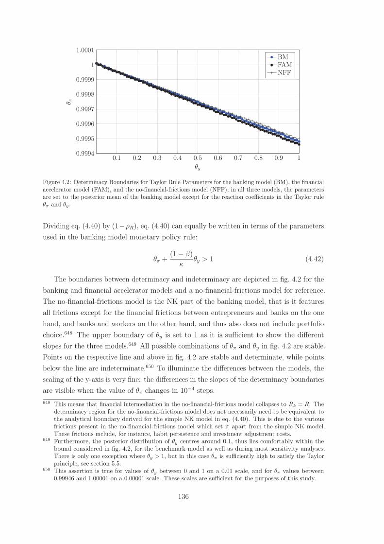
0.1 0.2 0.3 0.4 0.5 0.6 0.7 0.8 0.9 10.9994

0.9995

0.9996

0.9997

0.9998

0.9999

1

1.0001

θy

θ π

BMFAMNFF

Figure 4.2: Determinacy Boundaries for Taylor Rule Parameters for the banking model (BM), the financialaccelerator model (FAM), and the no-financial-frictions model (NFF); in all three models, the parametersare set to the posterior mean of the banking model except for the reaction coefficients in the Taylor ruleθπ and θy.

Dividing eq. (4.40) by (1−ρR), eq. (4.40) can equally be written in terms of the parametersused in the banking model monetary policy rule:

θπ +(1− β)

κθy > 1 (4.42)

The boundaries between determinacy and indeterminacy are depicted in fig. 4.2 for thebanking and financial accelerator models and a no-financial-frictions model for reference.The no-financial-frictions model is the NK part of the banking model, that is it featuresall frictions except for the financial frictions between entrepreneurs and banks on the onehand, and banks and workers on the other hand, and thus also does not include portfoliochoice.648 The upper boundary of θy is set to 1 as it is sufficient to show the differentslopes for the three models.649 All possible combinations of θπ and θy in fig. 4.2 are stable.Points on the respective line and above in fig. 4.2 are stable and determinate, while pointsbelow the line are indeterminate.650 To illuminate the differences between the models, thescaling of the y-axis is very fine: the differences in the slopes of the determinacy boundariesare visible when the value of θπ changes in 10−4 steps.648 This means that financial intermediation in the no-financial-frictions model collapses to Rk = R. The

determinacy region for the no-financial-frictions model does not necessarily need to be equivalent tothe analytical boundary derived for the simple NK model in eq. (4.40). This is due to the variousfrictions present in the no-financial-frictions model which set it apart from the simple NK model.These frictions include, for instance, habit persistence and investment adjustment costs.

649 Furthermore, the posterior distribution of θy centres around 0.1, thus lies comfortably within thebound considered in fig. 4.2, for the benchmark model as well as during most sensitivity analyses.There is only one exception where θy > 1, but in this case θπ is sufficiently high to satisfy the Taylorprinciple, see section 5.5.

650 This assertion is true for values of θy between 0 and 1 on a 0.01 scale, and for θπ values between0.99946 and 1.00001 on a 0.00001 scale. These scales are sufficient for the purposes of this study.

136

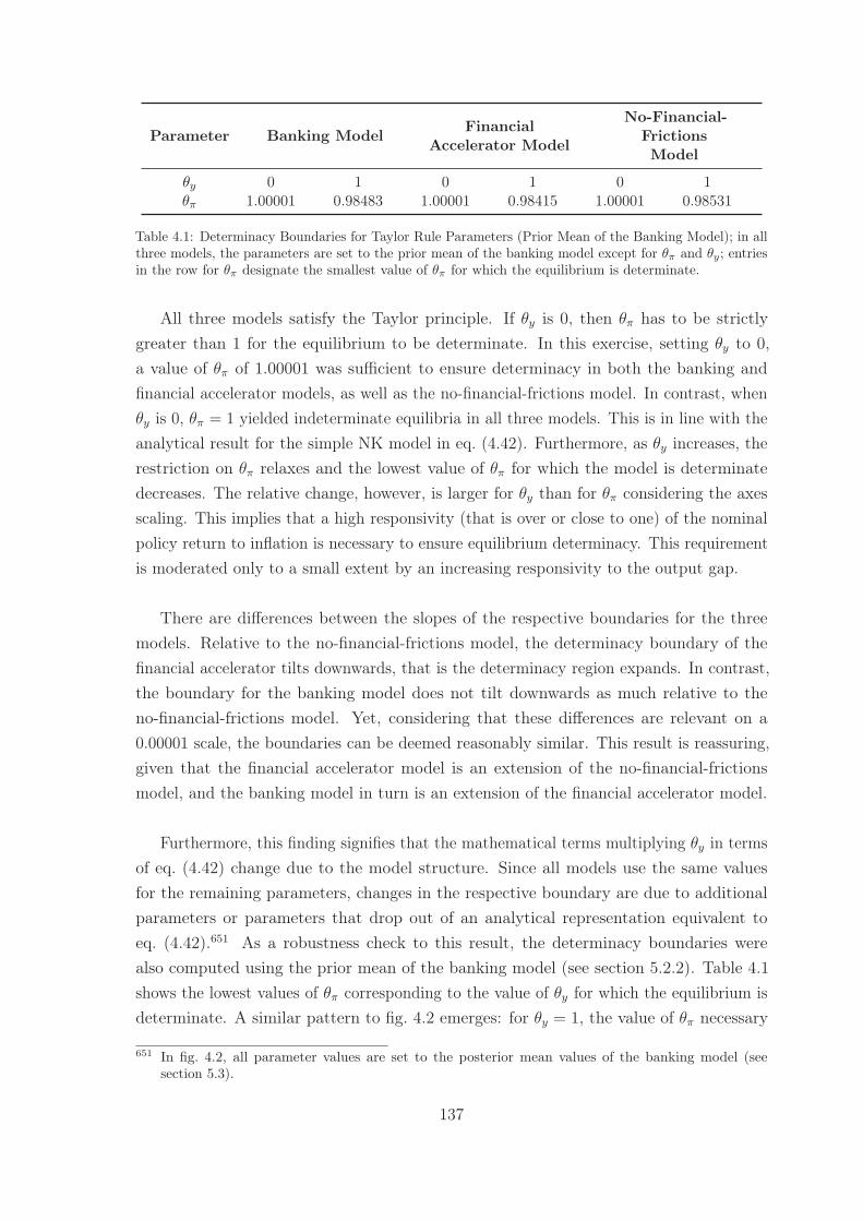
Parameter Banking Model FinancialAccelerator Model

No-Financial-FrictionsModel

θy 0 1 0 1 0 1θπ 1.00001 0.98483 1.00001 0.98415 1.00001 0.98531

Table 4.1: Determinacy Boundaries for Taylor Rule Parameters (Prior Mean of the Banking Model); in allthree models, the parameters are set to the prior mean of the banking model except for θπ and θy; entriesin the row for θπ designate the smallest value of θπ for which the equilibrium is determinate.

All three models satisfy the Taylor principle. If θy is 0, then θπ has to be strictlygreater than 1 for the equilibrium to be determinate. In this exercise, setting θy to 0,a value of θπ of 1.00001 was sufficient to ensure determinacy in both the banking andfinancial accelerator models, as well as the no-financial-frictions model. In contrast, whenθy is 0, θπ = 1 yielded indeterminate equilibria in all three models. This is in line with theanalytical result for the simple NK model in eq. (4.42). Furthermore, as θy increases, therestriction on θπ relaxes and the lowest value of θπ for which the model is determinatedecreases. The relative change, however, is larger for θy than for θπ considering the axesscaling. This implies that a high responsivity (that is over or close to one) of the nominalpolicy return to inflation is necessary to ensure equilibrium determinacy. This requirementis moderated only to a small extent by an increasing responsivity to the output gap.

There are differences between the slopes of the respective boundaries for the threemodels. Relative to the no-financial-frictions model, the determinacy boundary of thefinancial accelerator tilts downwards, that is the determinacy region expands. In contrast,the boundary for the banking model does not tilt downwards as much relative to theno-financial-frictions model. Yet, considering that these differences are relevant on a0.00001 scale, the boundaries can be deemed reasonably similar. This result is reassuring,given that the financial accelerator model is an extension of the no-financial-frictionsmodel, and the banking model in turn is an extension of the financial accelerator model.

Furthermore, this finding signifies that the mathematical terms multiplying θy in termsof eq. (4.42) change due to the model structure. Since all models use the same valuesfor the remaining parameters, changes in the respective boundary are due to additionalparameters or parameters that drop out of an analytical representation equivalent toeq. (4.42).651 As a robustness check to this result, the determinacy boundaries werealso computed using the prior mean of the banking model (see section 5.2.2). Table 4.1shows the lowest values of θπ corresponding to the value of θy for which the equilibrium isdeterminate. A similar pattern to fig. 4.2 emerges: for θy = 1, the value of θπ necessary

651 In fig. 4.2, all parameter values are set to the posterior mean values of the banking model (seesection 5.3).

137

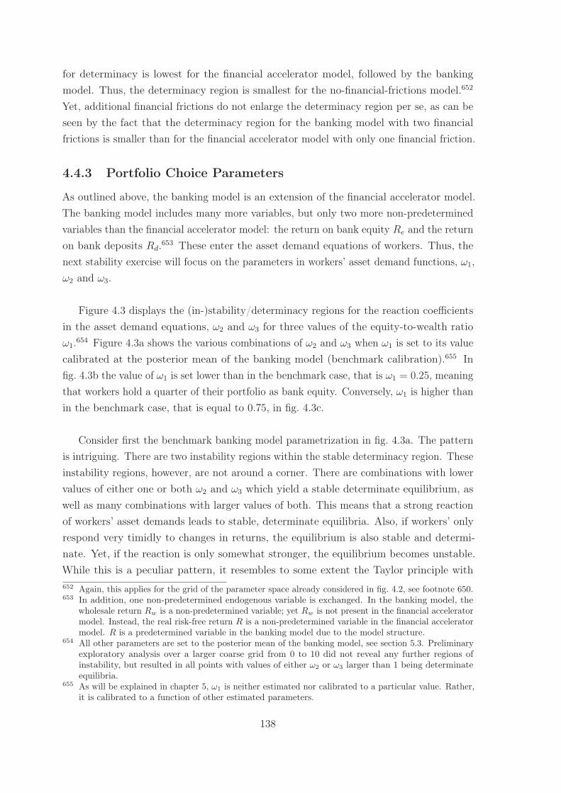
for determinacy is lowest for the financial accelerator model, followed by the bankingmodel. Thus, the determinacy region is smallest for the no-financial-frictions model.652

Yet, additional financial frictions do not enlarge the determinacy region per se, as can beseen by the fact that the determinacy region for the banking model with two financialfrictions is smaller than for the financial accelerator model with only one financial friction.

4.4.3 Portfolio Choice Parameters

As outlined above, the banking model is an extension of the financial accelerator model.The banking model includes many more variables, but only two more non-predeterminedvariables than the financial accelerator model: the return on bank equity Re and the returnon bank deposits Rd.653 These enter the asset demand equations of workers. Thus, thenext stability exercise will focus on the parameters in workers’ asset demand functions, ω1,ω2 and ω3.

Figure 4.3 displays the (in-)stability/determinacy regions for the reaction coefficientsin the asset demand equations, ω2 and ω3 for three values of the equity-to-wealth ratioω1.654 Figure 4.3a shows the various combinations of ω2 and ω3 when ω1 is set to its valuecalibrated at the posterior mean of the banking model (benchmark calibration).655 Infig. 4.3b the value of ω1 is set lower than in the benchmark case, that is ω1 = 0.25, meaningthat workers hold a quarter of their portfolio as bank equity. Conversely, ω1 is higher thanin the benchmark case, that is equal to 0.75, in fig. 4.3c.

Consider first the benchmark banking model parametrization in fig. 4.3a. The patternis intriguing. There are two instability regions within the stable determinacy region. Theseinstability regions, however, are not around a corner. There are combinations with lowervalues of either one or both ω2 and ω3 which yield a stable determinate equilibrium, aswell as many combinations with larger values of both. This means that a strong reactionof workers’ asset demands leads to stable, determinate equilibria. Also, if workers’ onlyrespond very timidly to changes in returns, the equilibrium is also stable and determi-nate. Yet, if the reaction is only somewhat stronger, the equilibrium becomes unstable.While this is a peculiar pattern, it resembles to some extent the Taylor principle with652 Again, this applies for the grid of the parameter space already considered in fig. 4.2, see footnote 650.653 In addition, one non-predetermined endogenous variable is exchanged. In the banking model, the

wholesale return Rw is a non-predetermined variable; yet Rw is not present in the financial acceleratormodel. Instead, the real risk-free return R is a non-predetermined variable in the financial acceleratormodel. R is a predetermined variable in the banking model due to the model structure.

654 All other parameters are set to the posterior mean of the banking model, see section 5.3. Preliminaryexploratory analysis over a larger coarse grid from 0 to 10 did not reveal any further regions ofinstability, but resulted in all points with values of either ω2 or ω3 larger than 1 being determinateequilibria.

655 As will be explained in chapter 5, ω1 is neither estimated nor calibrated to a particular value. Rather,it is calibrated to a function of other estimated parameters.

138

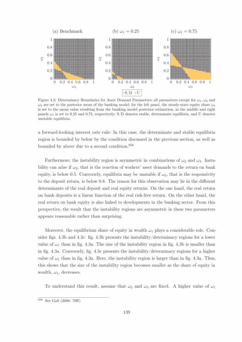
(a) Benchmark

0 0.2 0.4 0.6 0.8 10

0.2

0.4

0.6

0.8

1

ω3

ω2

(b) ω1 = 0.25

0 0.2 0.4 0.6 0.8 10

0.2

0.4

0.6

0.8

1

ω3

ω2

S/D U

(c) ω1 = 0.75

0 0.2 0.4 0.6 0.8 10

0.2

0.4

0.6

0.8

1

ω3

ω2

Figure 4.3: Determinacy Boundaries for Asset Demand Parameters; all parameters except for ω1, ω2 andω3 are set to the posterior mean of the banking model; for the left panel, the steady-state equity share ω1

is set to the mean value resulting from the banking model posterior estimation, in the middle and rightpanels ω1 is set to 0.25 and 0.75, respectively; S/D denotes stable, determinate equilibria, and U denotesunstable equilibria.

a forward-looking interest rate rule: In this case, the determinate and stable equilibriaregion is bounded by below by the condition discussed in the previous section, as well asbounded by above due to a second condition.656

Furthermore, the instability region is asymmetric in combinations of ω2 and ω3. Insta-bility can arise if ω2, that is the reaction of workers’ asset demands to the return on bankequity, is below 0.5. Conversely, equilibria may be unstable if ω3, that is the responsivityto the deposit return, is below 0.8. The reason for this observation may lie in the differentdeterminants of the real deposit and real equity returns. On the one hand, the real returnon bank deposits is a linear function of the real risk-free return. On the other hand, thereal return on bank equity is also linked to developments in the banking sector. From thisperspective, the result that the instability regions are asymmetric in these two parametersappears reasonable rather than surprising.

Moreover, the equilibrium share of equity in wealth ω1 plays a considerable role. Con-sider figs. 4.3b and 4.3c: fig. 4.3b presents the instability/determinacy regions for a lowervalue of ω1 than in fig. 4.3a. The size of the instability region in fig. 4.3b is smaller thanin fig. 4.3a. Conversely, fig. 4.3c presents the instability/determinacy regions for a highervalue of ω1 than in fig. 4.3a. Here, the instability region is larger than in fig. 4.3a. Thus,this shows that the size of the instability region becomes smaller as the share of equity inwealth, ω1, decreases.

To understand this result, assume that ω2 and ω3 are fixed. A higher value of ω1

656 See Galí (2008: 79ff)

139

means that the demand for bank equity holdings reacts less strongly to a change in eitherexpected return, ceteris paribus.657 Conversely, the effect of a change in either expectedreturn on bank deposit holdings is larger.658 This is because the log-linear model is writtenin terms of log-deviations from the steady-state value. If ω1 is larger, the share of equity inwealth is larger, thus the level of bank equity is larger and a given absolute change in levelsyields lower percentage deviations from the steady state. The fact that the size of theinstability regions is the larger, the higher is the share of equity in wealth may be explainedby the resulting consequences for banks’ liability management. Relative changes in bankequity and bank deposits have non-trivial effects for the arbitrage condition determiningthe bank risk premium and by extension entrepreneurs’ credit conditions.659 Then, ceterisparibus, a quantitatively smaller reaction of bank equity to real returns due to a higherbank equity share in wealth increases the chances for equilibrium instability, as shownin fig. 4.3. However, this relationship does not hold generally, since a high equity shareor a strong responsivity of deposit demand and conversely a small responsivity of equitydemand do not as such yield unstable equilibria. This can be seen in fig. 4.3, since asnoted above, instability regions appear in the middle of the parameter space, not at eitherlimit.

Counter-intuitively, a higher equity share in wealth leads to bigger instability regions inthe banking model. Yet, this result should not be interpreted as an outright contradictionwith the rationale of bank capital regulation.660 There are two reasons why the result infig. 4.3 should be taken with caution. Firstly, the incidence of more unstable combinationsof ω2 and ω3 does not necessarily mean that there are overall more unstable parametercombinations with a higher equity-to-wealth ratio since there are many more parameters inthe banking model. Moreover, one may argue that the alternative parameter calibrationsfor ω1 in figs. 4.3b and 4.3c are too far apart to be valid in terms of a first-order log-linearapproximation. In particular, ω1 is by definition tightly connected to banks’ leverageratio and by extension the bank risk premium. Related, the bank risk premium is verysensitive to bank leverage, or equivalently the bank equity to wealth ratio. This results in acomparatively small band of ‘permissible’ values of bank leverage. Incidentally, estimationyields a value of 0.568 for ω1 at the posterior mean of the parameter vector.661 Thus, thesealternative values for ω1 may be connected to counterfactual steady-state values for these

657 The reaction coefficients of bank equity demand are (ω2/ω1) and −(ω3/ω1) for the bank equity andbank deposit returns, respectively, see eq. (3.84) in chapter 3.

658 See eq. (3.85) in chapter 3659 As stated above, the steady-state bank risk premium is ceteris paribus positively related to the

steady-state equity-to-loan ratio and by extension to the steady-state equity share in workers’ wealth(in the non-linear banking model).

660 For an exposition for higher bank capital requirements see Admati and Hellwig (2013: 169).661 Introducing internal equity may be a possibility to align the banking model equity share with real

world observations.

140

variables, raising again validity questions of this stability exercise. Overall, the graphsin fig. 4.3 illustrate that all three asset demand equation parameters affect determinacyand stability of the banking model. While the exact influence of ω1 remains elusive, it isnevertheless important to note its potential.

Thus, these portfolio choice equations cannot be regarded in isolation to analysestability and determinacy. Unfortunately, given that an analytical derivation is intractablewithin the bounds of this study, the precise nature of how these parameters affect matrixA in eq. (4.36) and its eigenvalues remains ambiguous. The important result for thefollowing chapters is that there are parameter combinations which yield equilibriuminstability. The Markov chain Monte Carlo Metropolis Hastings estimation algorithmused in chapter 5 deals with this issue insofar that parameter vector draws which donot produce a determinate equilibrium are rejected and thus do not enter estimates ofparameter moments.662 Thus, only parameter combinations which produce determinateequilibria are considered henceforth.663

662 See An and Schorfheide (2007: 131). See chapter 5 for details on the estimation method.663 There has been research on including at least the indeterminate parameter space in estimation exercises

in recent years, see for example Farmer and Khramov (2013) and Lubik and Schorfheide (2004). Yet,for once this does not deal with instability and furthermore, such an exercise would not contributesubstantially to the principal research agenda of this study, and is thus left to future research.

141

Chapter 5

Estimation

The previous chapter determined the non-stochastic steady state of the banking model,as well as part of its determinacy and stability realms. Furthermore, it showed to whatextent the additional financial friction of the banking model changed the log-linear approx-imation of the dynamic stochastic general equilibrium (DSGE) model in terms of the NewKeynesian (NK) DIS-PC-MP framework. The previous chapter showed that the space forderiving results analytically is relatively limited, due to the complexity of the bankingmodel. In order to evaluate the dynamic properties of the banking model, specific valuesneed to be attached to the parameters which was accomplished by estimating the model.Thus, the primary objective of this chapter is to present the results of the estimation ofthe model’s parameters. Furthermore, this chapter aims to evaluate how well the bankingmodel fits the data. To this end, the estimation results of the financial accelerator modelare presented and used as a reference point.

This chapter is structured as follows. Section 5.1 presents the estimation methodologyand the reasons for choosing the Bayesian estimation technique. Next, section 5.2 describesthe data and prior distributions. The following section 5.3 reports the results of theestimation exercise. Section 5.4 assesses the empirical performance of the banking modelvis-à-vis the financial accelerator model. Finally, this chapter closes with a short discussionabout the sensitivity of the results to different prior distributions and time frames insection 5.5.

142

5.1 Estimation Methodology

5.1.1 Overview of Estimation Approaches

The eventual task of an estimation exercise is to determine the values of the various param-eters that enter the model. The following paragraphs are intended as a short discussion ofthe most prominent estimation methods, and the gain in using Bayesian methods. Forvarious reasons, Bayesian estimation has become increasingly popular in the last decadefor estimating DSGE models.664

There is a plethora of different estimation methods, each with its specific advantagesand disadvantages. Maximum likelihood (ML) has been one popular method before theonset and widespread use of Bayesian methods in (macro-)economics.665 Key tenets of MLare the assumption of the model being the true data generating process (DGP) and theuse of all model equations in the estimation process.666 Yet, there are two major problemswith using ML for estimating DSGE models. Firstly, the current generation of DSGEmodels, while becoming increasingly complex, are a highly stylised abstraction from reality- from ad-hoc assumptions such as investment adjustment costs to the specification ofexogenous shocks. This poses a problem for applying ML, since inference is only validfor a model representing the true DGP with the parameters being unknown.667 Secondly,the likelihood function of a DSGE model is generally not ‘well-behaved’: there are flatregions and kinks. This leads to serious problems for various maximisation routines sincethe maximisation algorithm may not be able to find the true maximum of the likelihoodover the parameter space.668

Another popular approach to estimating DSGE models is the generalised method ofmoments (GMM). GMM is an umbrella for various methods of which ML estimation maybe argued to be a special case.669 More generally, GMM is centred on the estimation ofpopulation moment conditions which state that the expectation of a vector of functions,defined over the parameter set and the data, is zero when the true parameter values areused.670 These conditions may require the distance between model and data momentsto be minimised but may also come in the form of maximum extremum conditions.671

Concerning the problem of stochastic singularity of DSGE models, GMM is argued to be

664 See Guerrón-Quintana and Nason (2013: 487ff) for a short history of DSGE model estimation.665 See Guerrón-Quintana and Nason (2013: 487)666 See Canova (2007: 213)667 See Canova (2007: 440)668 See Fernández-Villaverde (2010: 7) and Fernández-Villaverde, Guerrón-Quintana and Rubio-Ramírez

(2010: 370)669 See Greene (2012: 547)670 See A. R. Hall (2013: 313)671 See Canova (2007: 166)

143

more robust than ML since GMM only requires moments to be linearly independent whileML requires the much stronger restriction of linearly independent variables.672 Moreover,if the model is correctly specified, GMM has the same statistical properties as ML, buthas been shown to be faster and computationally less demanding than ML.673

However, the researcher’s flexibility in choosing moment conditions to be included in theestimation comes at a cost. A DSGE model will probably lead to restrictions on the DGPnot borne out by the data. Yet, choosing only a subset of the system for estimation mayneglect important cross-equations restrictions which are vital to the dynamics of the model.Secondly, care needs to be taken concerning the moments of the data the model is matchedto. Impulse-response-matching estimation, such as used among others by Christiano etal. (2005a), in particular requires that the impulse responses the model is matched toare a valid representation.674 The probably most prominent example of controversialimpulse responses is the so-called price puzzle in vector autoregression (VAR) analyses;thus, such an approach necessitates a detailed discussion of the construction of the VARbefore even starting the estimation of the model. Thirdly, the GMM estimator does notalways perform satisfactory in small samples which are pervasive in macroeconomics.675

Finally, Canova and Sala (2009) have noted that (weak) identification and observationalequivalence are a common problem in DSGE models.676 Since GMM and ML identifymodel parameters using the same information on theoretical first moments, identificationproblems apply to both ML and GMM.677

In light of these problems, the researcher may choose not to estimate the parameters atall but conduct a calibration exercise. Calibration does not assume that the model is a cor-rect representation of the DGP of the variables.678 Given the highly schematic specificationof DSGE models, this is a clear advantage. The difference between calibration and manyestimation procedures is that calibration does not necessarily entail exactly specifying howthe model diverges from reality.679 Instead, the calibration exercise is intended to ensurethat (some) features of the observables are met by the model.680 Put differently, using cali-bration, the researcher seeks to explain certain developments in observable variables using a

672 See Ruge-Murcia (2007: 2600). Stochastic singularity arises principally in linearised DSGE modelssince there are often fewer structural shocks than the number of observable variables in the model,see Ruge-Murcia (2007: 2600).

673 See Ruge-Murcia (2013: 464) and Ruge-Murcia (2007: 2633)674 Christiano et al. (2005a: 3, 15ff) estimate a subset of parameters minimizing the distance of model-

implied responses to the responses of a vector autoregression model to a monetary policy shock andcalibrate all other parameters.

675 See Fernández-Villaverde et al. (2010: 369)676 See Canova and Sala (2009: 448)677 See Guerrón-Quintana and Nason (2013: 488)678 See Canova (2007: 248)679 See Canova (2007: 248)680 See Canova (2007: 251)

144

model which he believes to be a highly stylised and incomplete characterisation of reality.681

Normally, these ‘developments’ are correlations and ratios of standard deviations. Thecalibration is deemed acceptable if these developments are indeed matched by the model.682

The problem in the present context is that this procedure of comparing correlationsand standard deviations is not very instructive for comparing model specifications. Giventhe size of the model and the number of parameters to be determined, it would be ratherdifficult to ensure that the results reflect different model specifications and not ‘lucky’parameter constellations. Even if various parameter constellations were computed, therewould have to be choices on what constitutes a good approximation and how to measuredeviations from actual data in terms of correlations and variances only in order to comparemodels.

This objection might be easier to decline if there existed some form of known reasonablerange for the parameters that are to be set. In fact, there are parameters which appearin many models and there exists some form of consensus for the value of the parameters.Other parameters may be directly related to observables; for instance, the calibration ofthe steady state share of hours worked in workers’ time endowment can be guided bystatistically collected labour market data.683 However, there are many other parameters,especially model-specific parameters, which are not as easy to determine. In the bankingmodel these include, for instance, the parameters governing the size of the entrepreneur-and bank-specific shock intervals. Therefore, above objection still holds.

In contrast, Bayesian estimation allows for the estimation of the complete system ofequations while at the same time addressing uncertainty about the model specificationand identification problems.684 Firstly, the Bayesian approach considers information fromoutside the dataset used for estimation, thus alleviating the problems associated witha flat likelihood function. Parameters are not unknown fixed values to be determined,but stochastic variables from the Bayesian point of view.685 The process of estimation isthus seen as updating old information with new data.686 In addition, as in the case of

681 See Canova (2007: 251)682 See Canova (2007: 251)683 Note that the models considered here abstract from unemployment. Furthermore, the share of leisure

vis-à-vis consumption ηl is the parameter in the utility function, and not the share of hours worked.Yet, as explained in section 4.1, the procedure to find the steady state endogenises some parameters(in this case ηl) by setting some steady-state variable (here H) to a specified value. While ηl is difficultto determine, H can be related to observables. Appendix section C.1 specifies the data sources.

684 Numerous authors have listed the advantages of Bayesian methods. See for example Lubik andSchorfheide (2006), Fernández-Villaverde (2010) and Fernández-Villaverde et al. (2010) for moreinformation.

685 See Koop (2003: 2) and Poirier (1995: 301)686 See Greene (2012: 697)

145

calibration, the Bayesian paradigm does not presuppose that the model represents theactual DGP.687 In particular, model misspecification does not render the results fromBayesian estimation inconsistent.688 However, in contrast to calibration, uncertainty aboutestimates and the specification of the model can be evaluated using Bayesian estimationresults since they come in the form of estimated posterior distributions.689 Finally, modelcomparisons are straightforward by computing posterior model odds or comparing thelog-likelihoods of different models.

Bayesian estimation is not without criticism. Apart from philosophical discussionsabout the subjectivity of the Bayesian approach, the specification of the parameters’ priordistributions is a contentious issue.690 Similar to setting parameters when using calibration,forming prior distributions for some parameters is relatively straightforward. However, forothers, especially considering the parameters entering the exogenous processes, it may bedifficult to find appropriate information from outside the dataset to substantiate the priordistribution. The major advantage of the Bayesian method is that in cases where thereis only limited information available, the researcher may always choose a very diffuse ora uniform prior. As the prior variance affects the weight of the prior mean vis-à-vis thelikelihood in computing the posterior mean, this implies that the influence of the priormean is reduced, ceteris paribus.691 In conclusion, making the process of forming the priordistribution as transparent as possible is a crucial issue. Thus, section 5.2.2 will explainthoroughly the prior distributions used for estimating the banking model.

5.1.2 Details on Bayesian Estimation of DSGE Models

As noted above, Bayesian analysis does not start from the presumption that the parametershave fixed unknown values. Rather, the process of estimation is characterised by updatingbeliefs by using new information.692 The central element is Bayes’ Theorem as applied toestimation purposes:693

p(parameters|data) = p(data|parameters)p(parameters)

p(data)(5.1)

687 See Canova (2007: 440)688 See Fernández-Villaverde and Rubio-Ramírez (2004: 154)689 See Canova (2007: 440)690 See Greene (2012: 695)691 See Herbst and Schorfheide (2016: 32)692 See Greene (2012: 697). The next paragraphs are intended as a short overview and account of the

methods used in this study. There are many introductory (and advanced) resources on Bayesianeconometrics and its application to DSGE models, and any list given here can only be arbitrary. Formore details on these issues see for example Canova (2007), An and Schorfheide (2007) and Herbstand Schorfheide (2016) as well as other references cited subsequently.

693 See Greene (2012: 696), unnumbered equation, my notation.

146

where the left-hand side is the distribution of interest, that is the posterior distributionof the parameters. p(data|parameters) is the joint distribution of the observed variablesconditional on the parameters, that is the likelihood function. p(parameters) is the priordistribution of the parameters and p(data) is the marginal likelihood of the data.694 Themarginal likelihood of the data does not change during estimation since it does not dependon the vector of parameters. Thus, eq. (5.1) can be simplified to:695

p(parameters|data) ∝ p(data|parameters)p(parameters) (5.2)

Equation (5.2) shows that the posterior distribution of the parameters given the data isproportional to the product of the prior distribution of the parameters and the likelihoodfunction.696 The prior distribution, that is the beliefs of the researcher before seeing thecurrent data, is updated using the current dataset to form a new set of beliefs, which isthe posterior distribution.697

While the right-hand side of eq. (5.2) is relatively straightforward to calculate, thedifficulty arises during the calculation of the left-hand side of eq. (5.2) for a DSGEmodel. The prior distributions for the individual parameters are set by the researcher.They are by definition known and their multivariate distribution is straightforward tocalculate. The likelihood function can be evaluated using the Kalman filter.698 Themain problem with applying eq. (5.2) to a DSGE model arises because there is usuallyno analytical expression for the posterior distribution.699 Thus, it is generally not pos-sible to sample from the posterior distribution directly to compute distribution moments.700

As a result of these analytical difficulties, various methods have been developed toremedy this problem numerically.701 The results in sections 5.3 to 5.5 are derived using the

694 See Greene (2012: 696) and Herbst and Schorfheide (2016: 29)695 See Greene (2012: 696)696 See Greene (2012: 696f)697 See Greene (2012: 697)698 See Guerrón-Quintana and Nason (2013: 497). There is a set of additional assumptions which make

the Kalman filter optimal in the linear case, these include normality conditions for shock innovationsand the initial state of the model, see Guerrón-Quintana and Nason (2013: 497).

699 See Fernández-Villaverde (2010: 21)700 See Fernández-Villaverde (2010: 21)701 See Canova (2007: 353ff) and Guerrón-Quintana and Nason (2013: 489ff) for a discussion of various

methods. The choice for the method used here is in particular based on its wide use in the relatedliterature, as well as because Canova (2007: 369) found methods based on Markov chains to outperformthose based on, among others, importance sampling.

147

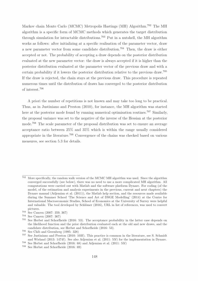
Markov chain Monte Carlo (MCMC) Metropolis Hastings (MH) Algorithm.702 The MHalgorithm is a specific form of MCMC methods which generates the target distributionthrough simulation for intractable distributions.703 Put in a nutshell, the MH algorithmworks as follows: after initializing at a specific realisation of the parameter vector, drawa new parameter vector from some candidate distribution.704 Then, the draw is eitheraccepted or not. The probability of accepting a draw depends on the posterior distributionevaluated at the new parameter vector: the draw is always accepted if it is higher than theposterior distribution evaluated at the parameter vector of the previous draw and with acertain probability if it lowers the posterior distribution relative to the previous draw.705

If the draw is rejected, the chain stays at the previous draw. This procedure is repeatednumerous times until the distribution of draws has converged to the posterior distributionof interest.706

A priori the number of repetitions is not known and may take too long to be practical.Thus, as in Justiniano and Preston (2010), for instance, the MH algorithm was startedhere at the posterior mode found by running numerical optimisation routines.707 Similarly,the proposal variance was set to the negative of the inverse of the Hessian at the posteriormode.708 The scale parameter of the proposal distribution was set to ensure an averageacceptance ratio between 25% and 35% which is within the range usually consideredappropriate in the literature.709 Convergence of the chains was checked based on variousmeasures, see section 5.3 for details.

702 More specifically, the random walk version of the MCMC MH algorithm was used. Since the algorithmconverged successfully (see below), there was no need to use a more complicated MH algorithm. Allcomputations were carried out with Matlab and the software platform Dynare. For coding (of themodel, of the estimation and analysis experiments in the previous, current and next chapters) theDynare manual (Adjemian et al. (2011)), the Matlab help section, and the resources made availableduring the Summer School ‘The Science and Art of DSGE Modelling’ (2014) at the Centre forInternational Macroeconomic Studies, School of Economics at the University of Surrey were helpfuland valuable. The tool developed by Schlömer (2016), URL in list of references, was used to convertpictures.

703 See Canova (2007: 359, 367)704 See Canova (2007: 367)705 See Herbst and Schorfheide (2016: 53). The acceptance probability in the latter case depends on

the likelihood function and the prior distribution evaluated each at the old and new draws, and thecandidate distribution, see Herbst and Schorfheide (2016: 53).

706 See Chib and Greenberg (1995: 328)707 See Justiniano and Preston (2010: 103f). This practice is common in the literature, see S. Schmidt

and Wieland (2013: 1474f). See also Adjemian et al. (2011: 55f) for the implementation in Dynare.708 See Herbst and Schorfheide (2016: 68) and Adjemian et al. (2011: 55f)709 See Herbst and Schorfheide (2016: 69)

148

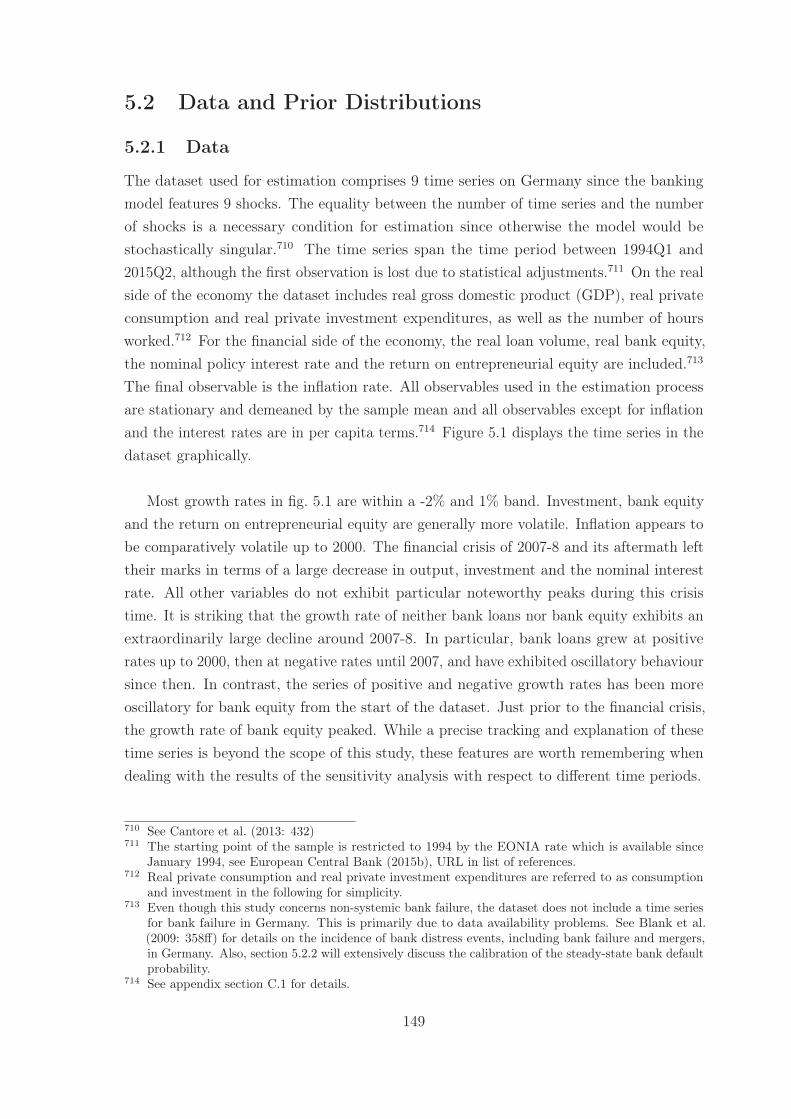
5.2 Data and Prior Distributions

5.2.1 Data

The dataset used for estimation comprises 9 time series on Germany since the bankingmodel features 9 shocks. The equality between the number of time series and the numberof shocks is a necessary condition for estimation since otherwise the model would bestochastically singular.710 The time series span the time period between 1994Q1 and2015Q2, although the first observation is lost due to statistical adjustments.711 On the realside of the economy the dataset includes real gross domestic product (GDP), real privateconsumption and real private investment expenditures, as well as the number of hoursworked.712 For the financial side of the economy, the real loan volume, real bank equity,the nominal policy interest rate and the return on entrepreneurial equity are included.713

The final observable is the inflation rate. All observables used in the estimation processare stationary and demeaned by the sample mean and all observables except for inflationand the interest rates are in per capita terms.714 Figure 5.1 displays the time series in thedataset graphically.

Most growth rates in fig. 5.1 are within a -2% and 1% band. Investment, bank equityand the return on entrepreneurial equity are generally more volatile. Inflation appears tobe comparatively volatile up to 2000. The financial crisis of 2007-8 and its aftermath lefttheir marks in terms of a large decrease in output, investment and the nominal interestrate. All other variables do not exhibit particular noteworthy peaks during this crisistime. It is striking that the growth rate of neither bank loans nor bank equity exhibits anextraordinarily large decline around 2007-8. In particular, bank loans grew at positiverates up to 2000, then at negative rates until 2007, and have exhibited oscillatory behavioursince then. In contrast, the series of positive and negative growth rates has been moreoscillatory for bank equity from the start of the dataset. Just prior to the financial crisis,the growth rate of bank equity peaked. While a precise tracking and explanation of thesetime series is beyond the scope of this study, these features are worth remembering whendealing with the results of the sensitivity analysis with respect to different time periods.

710 See Cantore et al. (2013: 432)711 The starting point of the sample is restricted to 1994 by the EONIA rate which is available since

January 1994, see European Central Bank (2015b), URL in list of references.712 Real private consumption and real private investment expenditures are referred to as consumption

and investment in the following for simplicity.713 Even though this study concerns non-systemic bank failure, the dataset does not include a time series

for bank failure in Germany. This is primarily due to data availability problems. See Blank et al.(2009: 358ff) for details on the incidence of bank distress events, including bank failure and mergers,in Germany. Also, section 5.2.2 will extensively discuss the calibration of the steady-state bank defaultprobability.

714 See appendix section C.1 for details.

149

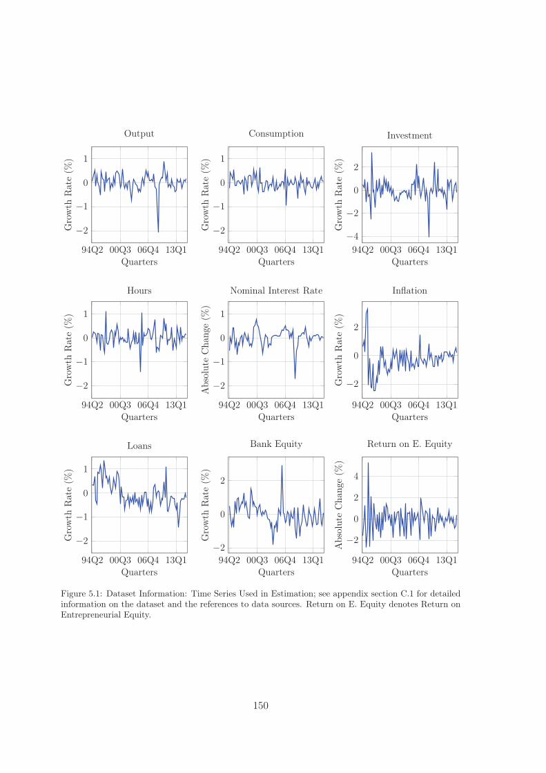
94Q2 00Q3 06Q4 13Q1

−2

−1

0

1

Quarters

Gro

wth

Rat

e(%

)

Output

94Q2 00Q3 06Q4 13Q1

−2

−1

0

1

Quarters

Gro

wth

Rat

e(%

)

Consumption

94Q2 00Q3 06Q4 13Q1−4

−2

0

2

Quarters

Gro

wth

Rat

e(%

)

Investment

94Q2 00Q3 06Q4 13Q1

−2

−1

0

1

Quarters

Gro

wth

Rat

e(%

)

Hours

94Q2 00Q3 06Q4 13Q1

−2

−1

0

1

Quarters

Abs

olut

eC

hang

e(%

)

Nominal Interest Rate

94Q2 00Q3 06Q4 13Q1

−2

0

2

Quarters

Gro

wth

Rat

e(%

)

Inflation

94Q2 00Q3 06Q4 13Q1

−2

−1

0

1

Quarters

Gro

wth

Rat

e(%

)

Loans

94Q2 00Q3 06Q4 13Q1−2

0

2

Quarters

Gro

wth

Rat

e(%

)

Bank Equity

94Q2 00Q3 06Q4 13Q1

−2

0

2

4

Quarters

Abs

olut

eC

hang

e(%

)

Return on E. Equity

Figure 5.1: Dataset Information: Time Series Used in Estimation; see appendix section C.1 for detailedinformation on the dataset and the references to data sources. Return on E. Equity denotes Return onEntrepreneurial Equity.

150

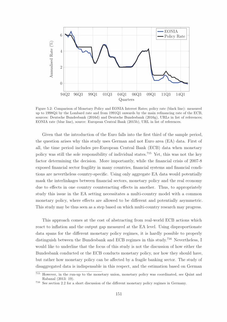
94Q2 96Q3 99Q1 01Q3 04Q1 06Q3 09Q1 11Q3 14Q1

0

2

4

6

Quarters

Ann

ualis

edR

ate

(%)

EONIAPolicy Rate

Figure 5.2: Comparison of Monetary Policy and EONIA Interest Rates; policy rate (black line): measuredup to 1998Q4 by the Lombard rate and from 1991Q1 onwards by the main refinancing rate of the ECB,sources: Deutsche Bundesbank (2016d) and Deutsche Bundesbank (2016g), URLs in list of references;EONIA rate (blue line), source: European Central Bank (2015b), URL in list of references.

Given that the introduction of the Euro falls into the first third of the sample period,the question arises why this study uses German and not Euro area (EA) data. First ofall, the time period includes pre-European Central Bank (ECB) data when monetarypolicy was still the sole responsibility of individual states.715 Yet, this was not the keyfactor determining the decision. More importantly, while the financial crisis of 2007-8exposed financial sector fragility in many countries, financial systems and financial condi-tions are nevertheless country-specific. Using only aggregate EA data would potentiallymask the interlinkages between financial sectors, monetary policy and the real economydue to effects in one country counteracting effects in another. Thus, to appropriatelystudy this issue in the EA setting necessitates a multi-country model with a commonmonetary policy, where effects are allowed to be different and potentially asymmetric.This study may be thus seen as a step based on which multi-country research may progress.

This approach comes at the cost of abstracting from real-world ECB actions whichreact to inflation and the output gap measured at the EA level. Using disproportionatedata spans for the different monetary policy regimes, it is hardly possible to properlydistinguish between the Bundesbank and ECB regimes in this study.716 Nevertheless, Iwould like to underline that the focus of this study is not the discussion of how either theBundesbank conducted or the ECB conducts monetary policy, nor how they should have,but rather how monetary policy can be affected by a fragile banking sector. The study ofdisaggregated data is indispensable in this respect, and the estimation based on German715 However, in the run-up to the monetary union, monetary policy was coordinated, see Quint and

Rabanal (2013: 19).716 See section 2.2 for a short discussion of the different monetary policy regimes in Germany.

151

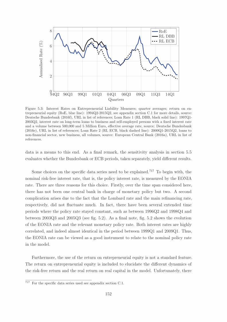
94Q2 96Q3 99Q1 01Q3 04Q1 06Q3 09Q1 11Q3 14Q10

2

4

6

8

Quarters

Ann

ualis

edR

ate

(%)

RoERL DBBRL ECB

Figure 5.3: Interest Rates on Entrepreneurial Liability Measures; quarter averages; return on en-trepreneurial equity (RoE, blue line): 1994Q2-2015Q2, see appendix section C.1 for more details, source:Deutsche Bundesbank (2016f), URL in list of references; Loan Rate 1 (RL DBB, black solid line): 1997Q1-2003Q2, interest rate on long-term loans to business and self-employed persons with a fixed interest rateand a volume between 500,000 and 5 Million Euro, effective average rate, source: Deutsche Bundesbank(2016e), URL in list of references; Loan Rate 2 (RL ECB, black dashed line): 2000Q1-2015Q2, loans tonon-financial sector, new business, all volumes, source: European Central Bank (2016a), URL in list ofreferences.

data is a means to this end. As a final remark, the sensitivity analysis in section 5.5evaluates whether the Bundesbank or ECB periods, taken separately, yield different results.

Some choices on the specific data series need to be explained.717 To begin with, thenominal risk-free interest rate, that is, the policy interest rate, is measured by the EONIArate. There are three reasons for this choice. Firstly, over the time span considered here,there has not been one central bank in charge of monetary policy but two. A secondcomplication arises due to the fact that the Lombard rate and the main refinancing rate,respectively, did not fluctuate much. In fact, there have been several extended timeperiods where the policy rate stayed constant, such as between 1996Q2 and 1998Q4 andbetween 2003Q3 and 2005Q3 (see fig. 5.2). As a final note, fig. 5.2 shows the evolutionof the EONIA rate and the relevant monetary policy rate. Both interest rates are highlycorrelated, and indeed almost identical in the period between 1999Q1 and 2009Q1. Thus,the EONIA rate can be viewed as a good instrument to relate to the nominal policy ratein the model.

Furthermore, the use of the return on entrepreneurial equity is not a standard feature.The return on entrepreneurial equity is included to elucidate the different dynamics ofthe risk-free return and the real return on real capital in the model. Unfortunately, there

717 For the specific data series used see appendix section C.1.

152

is no coherent data available on the macroeconomic concept of the real return on realcapital as used in the banking model. The use of the return on entrepreneurial equity as aproxy is justified by theoretical model-specific considerations and further data limitations:entrepreneurs equate the real return on real capital to the marginal financing cost ofbank loans. Ideally, I would thus want to use the bank loan rate as a measure. However,statistics on bank loan rates to businesses are available consistently only for relativelyshort sub-periods of the considered time span, as can be seen in fig. 5.3 (black dashedand solid lines). In contrast, the return on entrepreneurial equity is consistently availableover the complete time span (see fig. 5.3, blue line). Then again, the banking model doesnot feature entrepreneurial equity. Yet, the rationale of cost minimisation equally appliesto different forms of entrepreneurial financing. If entrepreneurial equity was availablein the banking model, the marginal financing costs of entrepreneurial equity and bankloans should be equal.718 Apart from this theoretical point of view, fig. 5.3 indicates thatreturns on different entrepreneurial liability measures evolved similarly. In conclusion,these considerations lead to the use of the return on entrepreneurial equity as a proxy forthe real return on real capital.

Finally, the GDP deflator is used to measure the inflation rate. Instead, many centralbanks such as the ECB and the Federal Reserve measure inflation in terms of a consumerprice index.719 Yet, the use of the GDP deflator for estimating monetary DSGE modelsis not uncommon.720 Moreover, the GDP deflator matches the model price index ontheoretical grounds, since there is only one price for consumption and investment goods.

5.2.2 Prior Distributions

There are 46 parameters in the banking model to be set. Some parameters are calibratedas is conventional practice in the literature. The 13 calibrated parameters are shown intable 5.1. There are several reasons for calibrating these parameters. Firstly, the datasetin its growth rate form is not informative on parameters which correspond to steady-stateratios. Also, some parameters are not identified in the model. Finally, one way to interpretthese calibrated parameters is to see them as very tight prior distributions.

First of all, the elasticity of substitution between retail goods ζ does not enter thelog-linear approximation to the model used for estimation. ζ is thus not identified by the

718 This assumes that all contracts last one period as always in the banking model. Furthermore, thisassumes that the information asymmetries for entrepreneurial equity are the same as for bank loans,thus resulting in equal required rates of return.

719 The ECB targets the Harmonised Index of Consumer Prices, the Federal Reserve targets the priceindex for personal consumption expenditure, see European Central Bank (2015a) and Board ofGovernors of the Federal Reserve System (2016b), URLs in list of references.

720 See for instance Christiano, Motto and Rostagno (2010), Smets and Wouters (2003) and Villa (2013)

153

model, and its value is calibrated to correspond to a 15% steady-state mark-up betweenwholesale and final retail goods prices.721 This value is within the range found in theliterature.722 ζ appears in the log-linear model because the log-linear approximation tothe aggregate demand relation depends on the steady-state values of its components, thatis, the steady-state consumption-to-output ratio, among others. These steady-state valuesin turn depend on the price mark-up. In contrast, taxes are non-distortionary up to afirst-order approximation, and thus the tax rate τ does not enter first-order dynamics.Hence, the tax rate does not need to be calibrated (or estimated).

The second set of calibrated parameters is determined by model-specific theoreticalconsiderations. Retailer’s marginal cost parameter c is set so that retailers make zeroprofits in the steady state. Workers’ steady-state equity to wealth ratio ω1 is a scalingparameter in the linear approximation to the model.723 It is thus set to match the divisionof bank equity and bank deposits determined by the agency problem between banks andequity holders in the steady state. Furthermore, the deposit insurance fee parameter νd isset such that the real deposit interest rate is equal to the real policy rate in the steadystate. As can be seen in table 5.1, these three parameters are not set to a specific value,but are functions of other estimated parameters and steady-state variable values. Theyare thus updated during the estimation exercise.

Thirdly, some calibrated parameters are used in virtually all DSGE models. Theseare mainly parameters pertaining to the real side of the economy. This includes thedepreciation rate δ, which is set to a quarterly rate of 2.5%, and the partial elasticity ofoutput with respect to labour α, set to 0.66. The latter value also corresponds to thelong-term average ratio of labour income to gross value added in Germany, which canbe related to the marginal product of labour on theoretical grounds.724 The steady-stategovernment consumption to output ratio ΥG/Y is set to 18.8%, that is its long-termaverage measured by national accounts.725

Finally, the remaining calibrated parameters relate to financial frictions. The firsttwo, ηE and ξE, determine roughly the allocation of entrepreneurial profit between en-

721 Note that the calibration refers to the steady state of the non-linear model, since the steady-statevalues of all endogenous variables in the log-linear model are zero, given that endogenous variables inthe log-linear approximation to the model are defined as log-deviations from the steady-state value inthe non-linear model.

722 See, for instance, Del Negro and Schorfheide (2008: 1200) for the US and Gerali et al. (2010: 122)and Quint and Rabanal (2013: 20) for the EA.

723 See eqs. (3.84) and (3.85) in chapter 3724 See Sachverständigenrat zur Begutachtung der Gesamtwirtschaftlichen Entwicklung (2014: 114)725 See Eurostat (2016), URL in list of references. This average value is obtained both for the time period

considered in the estimation exercise (1994Q2-2015Q2) and for the available period (1991Q1-2015Q3)for the time series.

154

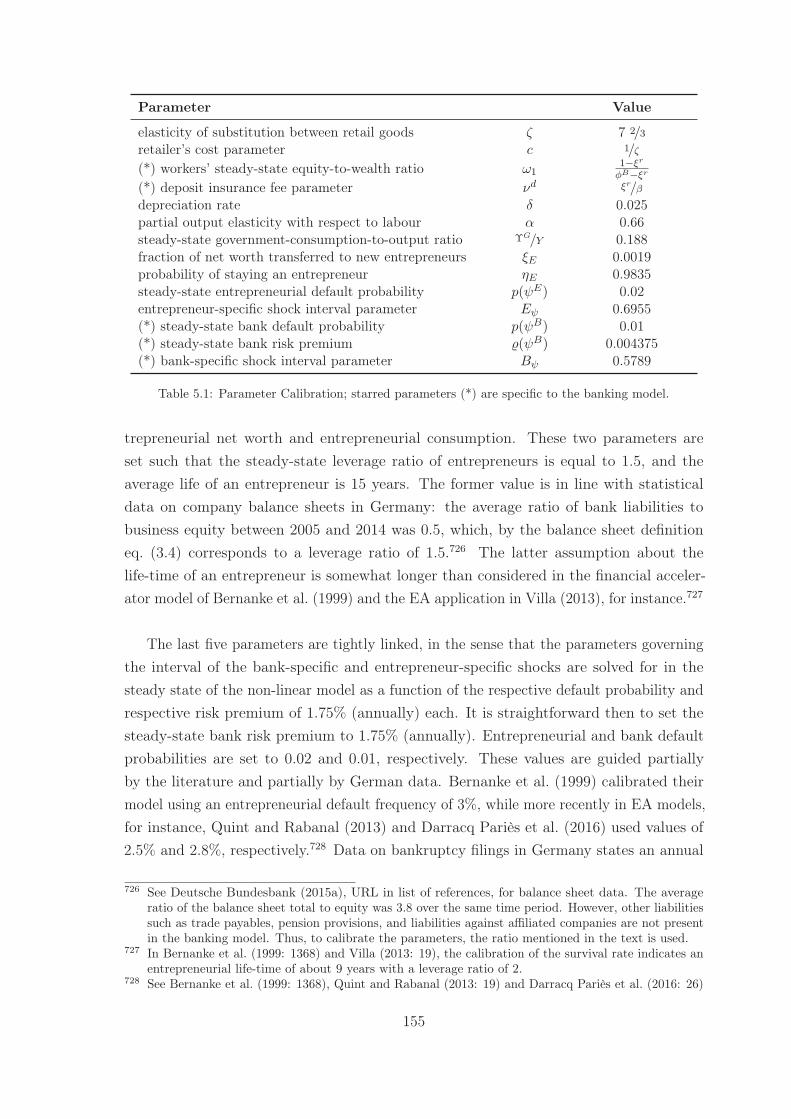
Parameter Value

elasticity of substitution between retail goods ζ 7 2/3retailer’s cost parameter c 1/ζ

(*) workers’ steady-state equity-to-wealth ratio ω11−ξr

φB−ξr

(*) deposit insurance fee parameter νd ξr/βdepreciation rate δ 0.025partial output elasticity with respect to labour α 0.66steady-state government-consumption-to-output ratio ΥG/Y 0.188fraction of net worth transferred to new entrepreneurs ξE 0.0019probability of staying an entrepreneur ηE 0.9835steady-state entrepreneurial default probability p(ψE) 0.02entrepreneur-specific shock interval parameter Eψ 0.6955(*) steady-state bank default probability p(ψB) 0.01(*) steady-state bank risk premium (ψB) 0.004375(*) bank-specific shock interval parameter Bψ 0.5789

Table 5.1: Parameter Calibration; starred parameters (*) are specific to the banking model.

trepreneurial net worth and entrepreneurial consumption. These two parameters areset such that the steady-state leverage ratio of entrepreneurs is equal to 1.5, and theaverage life of an entrepreneur is 15 years. The former value is in line with statisticaldata on company balance sheets in Germany: the average ratio of bank liabilities tobusiness equity between 2005 and 2014 was 0.5, which, by the balance sheet definitioneq. (3.4) corresponds to a leverage ratio of 1.5.726 The latter assumption about thelife-time of an entrepreneur is somewhat longer than considered in the financial acceler-ator model of Bernanke et al. (1999) and the EA application in Villa (2013), for instance.727

The last five parameters are tightly linked, in the sense that the parameters governingthe interval of the bank-specific and entrepreneur-specific shocks are solved for in thesteady state of the non-linear model as a function of the respective default probability andrespective risk premium of 1.75% (annually) each. It is straightforward then to set thesteady-state bank risk premium to 1.75% (annually). Entrepreneurial and bank defaultprobabilities are set to 0.02 and 0.01, respectively. These values are guided partiallyby the literature and partially by German data. Bernanke et al. (1999) calibrated theirmodel using an entrepreneurial default frequency of 3%, while more recently in EA models,for instance, Quint and Rabanal (2013) and Darracq Pariès et al. (2016) used values of2.5% and 2.8%, respectively.728 Data on bankruptcy filings in Germany states an annual

726 See Deutsche Bundesbank (2015a), URL in list of references, for balance sheet data. The averageratio of the balance sheet total to equity was 3.8 over the same time period. However, other liabilitiessuch as trade payables, pension provisions, and liabilities against affiliated companies are not presentin the banking model. Thus, to calibrate the parameters, the ratio mentioned in the text is used.

727 In Bernanke et al. (1999: 1368) and Villa (2013: 19), the calibration of the survival rate indicates anentrepreneurial life-time of about 9 years with a leverage ratio of 2.

728 See Bernanke et al. (1999: 1368), Quint and Rabanal (2013: 19) and Darracq Pariès et al. (2016: 26)

155

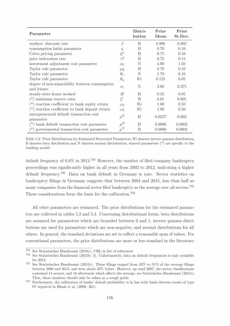
Parameter Distri-bution

PriorMean

PriorSt.Dev.

workers’ discount rate β B 0.996 0.002consumption habit parameter χ B 0.70 0.10Calvo pricing parameter ξp B 0.75 0.10price indexation rate γp B 0.75 0.15investment adjustment cost parameter φI N 4.00 1.50Taylor rule parameter ρR B 0.70 0.10Taylor rule parameter θπ N 1.70 0.10Taylor rule parameter θy IG 0.125 0.05degree of non-separability between consumptionand leisure σc N 3.00 0.375

steady-state hours worked H B 0.35 0.05(*) minimum reserve ratio ξr B 0.01 0.005(*) reaction coefficient to bank equity return ω2 IG 1.00 0.50(*) reaction coefficient to bank deposit return ω3 IG 1.00 0.50entrepreneurial default transaction costparameter μE B 0.0257 0.002

(*) bank default transaction cost parameter μB B 0.0006 0.0002(*) governmental transaction cost parameter μN B 0.0006 0.0002

Table 5.2: Prior Distributions for Estimated Structural Parameters; IG denotes inverse gamma distribution,B denotes beta distribution and N denotes normal distrubution; starred parameters (*) are specific to thebanking model.

default frequency of 0.8% in 2013.729 However, the number of filed company bankruptcyproceedings was significantly higher in all years from 2002 to 2012, indicating a higherdefault frequency.730 Data on bank default in Germany is rare. Sector statistics onbankruptcy filings in Germany suggests that between 2004 and 2015, less than half asmany companies from the financial sector filed bankruptcy as the average over all sectors.731

These considerations form the basis for the calibration.732

All other parameters are estimated. The prior distributions for the estimated parame-ters are collected in tables 5.2 and 5.3. Concerning distributional forms, beta distributionsare assumed for parameters which are bounded between 0 and 1, inverse gamma distri-butions are used for parameters which are non-negative, and normal distributions for allothers. In general, the standard deviations are set to reflect a reasonable span of values. Forconventional parameters, the prior distributions are more or less standard in the literature.

729 See Statistisches Bundesamt (2016c), URL in list of references730 See Statistisches Bundesamt (2015b: 3). Unfortunately, data on default frequencies is only available

for 2013.731 See Statistisches Bundesamt (2015c). These filings ranged from 43% to 51% of the average filings

between 2008 and 2015, and were about 20% before. However, up until 2007, the sector classificationscontained 14 sectors, and 18 afterwards which affects the average, see Statistisches Bundesamt (2015c).Thus, these numbers should only be taken as a rough guide.

732 Furthermore, the calibration of banks’ default probability is in line with bank distress events of typeIV reported in Blank et al. (2009: 361).

156

The prior mean for workers’ discount factor β is set to hit a 1.62% annual nominal interestrate. The prior distributions for workers’ habits χ, the Calvo pricing parameter ξp, thedegree of indexation γp and investment adjustment costs φI , as well as the monetary policyfunction parameters are standard and in line with Smets and Wouters (2003).733 The priordistribution of the degree of non-separability between consumption and leisure σc, centredaround 3, indicates a reasonable degree of non-separability.734 The other parameter inworkers’ utility function is the weight on labour ηl which is endogenously determined as afunction of steady-state hours worked H. The prior distribution for H is in turn relativelytightly centred around 0.35, in line with values used in the literature, indicating thatworkers spend 35% of their time endowment working.735

The remaining structural parameters are non-standard. The prior mean of the mini-mum reserve ratio is set at the value in effect in the EA at the time of writing.736 Theprior standard deviation allows for a higher value as was in effect previously.737 The priordistributions for the parameters in workers’ asset demand function cannot be taken fromthe related literature, since there is no clear consensus. From the theoretical considerationsin section 3.7, both reaction coefficients should be positive, thus leading to the inversegamma distribution. Mean and standard deviation are set identically for both coefficientsand are relatively uninformative. The former is guided by the deterministic model steadystate where both bank equity and bank deposits are substitutes, the latter due to a lack ofinformation.738 Assuming equal shares in wealth, that is, ω1 = 0.5, these prior distributionsimply that a 1% change in either return lead to a 2% change in volumes. Note that thestandard deviation also includes the case where a 1% change in a return leads to a 1%change in either volume variable, assuming equal shares in wealth. As the sensitivityanalysis in section 5.5 shows, the estimates of the other parameters are robust to a changein this prior distribution.

The various transaction cost parameters, μE, μB and μN are not straightforward either.

733 See Smets and Wouters (2003: 1140ff). Smets and Wouters (2003) is a standard reference for Bayesianestimation of DSGE models for the EA. Estimated large-scale models for Germany are rare, andthe chosen prior distributions are standard in the literature on Bayesian estimation, such that thereference to the EA can be justified. Furthermore, Gadatsch, Hauzenberger and Stähler (2015: 1,17ff), presenting a large-scale open economy model estimated on German (and other) data, use verysimilar prior distributions for χ, γp, φI and the Taylor rule parameters for the part of the modelrepresenting Germany. Since Gadatsch et al. (2015: 6) derive price stickiness using Rotemberg priceadjustment costs, the prior distribution of ξp is not directly comparable.

734 This value is a compromise of values used in the literature. Furlanetto and Seneca (2010: 14), forinstance, use a mean of 2, Kilponen, Vilmunen and Vähämaa (2013: 12) centre their prior distributionaround 5.

735 Furlanetto and Seneca (2010: 14), for example, use a value of 0.33.736 See European Central Bank (2016c), URL in list of references737 See European Central Bank (2016c), URL in list of references738 This approach is similar to Backus, Brainard, Smith and Tobin (1980: 273) in that it is left to the

estimation to determine whether the assets are substitutes or not.

157

These govern the amount of revenues lost in bankruptcy proceedings. There is a wide rangeof values used in the literature: for example, Bernanke et al. (1999) set this parameter to0.12, while Christiano et al. (2010) use a value of 0.94.739 In the banking model, both μE

and μB are tightly linked to the respective risk premium; thus, their prior means are setto the values which solve for entrepreneurial and bank risk premiums of 1.75% (annually)each. The targets for the risk premiums are in turn guided by values assumed in theliterature and the data. Alpanda and Aysun (2014) and Cúrdia and Woodford (2010)set the credit spread due to frictions between borrowers and financial intermediaries to2%, for instance.740 The spread between deposit interest and different loan rates rangesbetween 2.1% and 4.6% in Germany, calculated as the average between 2003 and 2015.741

Furthermore, as discussed in section 5.5, changing the prior distributions for μE and μB

increases the spread between these two risk premiums but does not impact the estimatesof most other parameters significantly. Thus, comparing the results of the benchmarkcalibration with the results of the sensitivity analysis will shed light on whether the dataprefers a more equal or a more disparate division of the total risk premium between thebank and entrepreneurial agency problem. As noted above, preliminary analyses showedthat the credit spread, that is the product of the two risk premiums, is very sensitive tothese transaction cost parameters. Therefore, the prior standard deviations for μE andμB are kept relatively tight. Furthermore, the mean and standard deviation of the priordistribution for the governmental transaction cost parameter μN use the same values as forμB. This implies that the government is as efficient in monitoring banks as equity-holdersare.

These values for the transaction cost parameters indicate that only 2.57% and 0.06%of revenues are lost in monitoring entrepreneurs and banks, respectively, during defaultexcluding governmental transaction costs. They are as such much lower than empiricalestimates of loss rates in bankruptcies. Davydenko and Franks (2008) report a medianrecovery rate, that is 1 minus the fraction of monitoring costs, of bank loans for firmsgoing into formal bankruptcy of 0.61 in Germany in his sample.742 However, this valueranges from 0.46 in the retail/wholesale sector to 0.91 in the services sector.743 On the

739 See Bernanke et al. (1999: 1368) and Christiano et al. (2010: 91)740 See Alpanda and Aysun (2014: 30) and Cúrdia and Woodford (2010: 13)741 Please refer to the discussion on the use of the return on entrepreneurial equity in the estimation for

a justification of the use of the loan rate in computing the credit spread (section 5.2.1). The averagespread is calculated from monthly data covering the years 2003 to 2015. The deposit rate is measuredby the effective interest rate on demand deposits, see Deutsche Bundesbank (2016a), URL in list ofreferences. The spread of 2.1% is calculated with respect to new business loans with maturity upto 1 year and a volume of more than 1 million Euro, see Deutsche Bundesbank (2016b), URL inlist of references. The spread of 4.6% is calculated with respect to revolving loans and overdrafts tonon-financial corporations, see Deutsche Bundesbank (2016c), URL in list of references.

742 See Davydenko and Franks (2008: 582)743 See Davydenko and Franks (2008: 582)

158

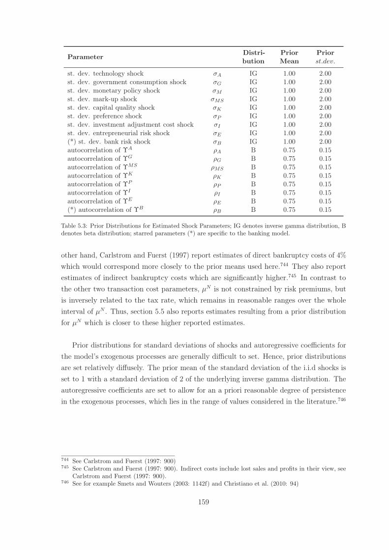
Parameter Distri-bution

PriorMean

Priorst.dev.

st. dev. technology shock σA IG 1.00 2.00st. dev. government consumption shock σG IG 1.00 2.00st. dev. monetary policy shock σM IG 1.00 2.00st. dev. mark-up shock σMS IG 1.00 2.00st. dev. capital quality shock σK IG 1.00 2.00st. dev. preference shock σP IG 1.00 2.00st. dev. investment adjustment cost shock σI IG 1.00 2.00st. dev. entrepreneurial risk shock σE IG 1.00 2.00(*) st. dev. bank risk shock σB IG 1.00 2.00autocorrelation of ΥA ρA B 0.75 0.15autocorrelation of ΥG ρG B 0.75 0.15autocorrelation of ΥMS ρMS B 0.75 0.15autocorrelation of ΥK ρK B 0.75 0.15autocorrelation of ΥP ρP B 0.75 0.15autocorrelation of ΥI ρI B 0.75 0.15autocorrelation of ΥE ρE B 0.75 0.15(*) autocorrelation of ΥB ρB B 0.75 0.15

Table 5.3: Prior Distributions for Estimated Shock Parameters; IG denotes inverse gamma distribution, Bdenotes beta distribution; starred parameters (*) are specific to the banking model.

other hand, Carlstrom and Fuerst (1997) report estimates of direct bankruptcy costs of 4%which would correspond more closely to the prior means used here.744 They also reportestimates of indirect bankruptcy costs which are significantly higher.745 In contrast tothe other two transaction cost parameters, μN is not constrained by risk premiums, butis inversely related to the tax rate, which remains in reasonable ranges over the wholeinterval of μN . Thus, section 5.5 also reports estimates resulting from a prior distributionfor μN which is closer to these higher reported estimates.

Prior distributions for standard deviations of shocks and autoregressive coefficients forthe model’s exogenous processes are generally difficult to set. Hence, prior distributionsare set relatively diffusely. The prior mean of the standard deviation of the i.i.d shocks isset to 1 with a standard deviation of 2 of the underlying inverse gamma distribution. Theautoregressive coefficients are set to allow for an a priori reasonable degree of persistencein the exogenous processes, which lies in the range of values considered in the literature.746

744 See Carlstrom and Fuerst (1997: 900)745 See Carlstrom and Fuerst (1997: 900). Indirect costs include lost sales and profits in their view, see

Carlstrom and Fuerst (1997: 900).746 See for example Smets and Wouters (2003: 1142f) and Christiano et al. (2010: 94)

159

5.3 Posterior Estimates of the Banking Model

The results of the posterior estimation are summarised in tables 5.4 and 5.5. As notedin section 5.1, the MH algorithm converges faster if the algorithm is initialised aroundthe posterior mode. Thus, the first two columns present the mean and standard error ofthe posterior mode. The last three columns of tables 5.4 and 5.5 present the results ofthe MH algorithm. These statistics are based on 200,000 draws of 5 chains. Convergencewas checked using the interval diagnostics developed by Brooks and Gelman (1998) asimplemented in Dynare.747 Furthermore, convergence was analysed using the potentialscale reduction factor, as well as CUSUM plots.748 All of these tests indicated convergenceof all chains after the burn-in period. Lastly, note that all parameters are statisticallysignificant from zero, as can be seen from the 90% highest posterior density (HPD) intervals.

Starting with the key friction in NK DSGE models, consider the estimates of theCalvo pricing parameter ξp and the price indexation parameter γp. The estimated meanof γp is within the usual range. Yet, the estimate of ξp is very low, which indicates lowprice stickiness.749 A value of 0.153 for ξp means that on average, a price is in effect forabout 1.2 quarters. Comparing with the discussion in section 3.3.1, this corresponds tothe lower bound of microeconomic data estimates for Germany. Furthermore, using theNK Phillips Curve (PC) representation described in section 4.3.3, it is clear that the lowestimate of ξp primarily impacts the relationship between inflation and retailers’ marginalcosts. Equations (5.3) and (5.4) show the NK PC functions for the banking model at theposterior mean (superscript po) and the prior mean (superscript pr), where ξp = 0.75,γp = 0.75 and β = 0.996:

πpot = 0.69IEt[π

pot+1] + 0.31πpo

t−1 + 3.25mcpot (5.3)

πprt = 0.57IEt[π

prt+1] + 0.43πpr

t−1 + 0.05mcprt (5.4)

The relationship between lagged and expected future inflation on the one hand andcurrent inflation on the other hand is not profoundly affected. The lower estimate ofthe indexation parameter leads to a lower coefficient on lagged inflation for the posteriormean parameter values. The somewhat higher coefficient for expected inflation is due tothe low estimate of the Calvo pricing parameter. In contrast, whereas a 1% deviation ofmarginal costs from the steady-state value increases inflation for the prior mean parametervalues by only 0.05%, it increases inflation for the posterior mean parameter values by

747 See Brooks and Gelman (1998) and Adjemian et al. (2011: 55f)748 For the potential scale reduction factor see Brooks and Gelman (1998: 437), for more details on the

use of CUSUM statistics as a convergence check see Yu and Mykland (1998). These computationswere conducted using the tool kit by Cesa-Bianchi (2012), URL in list of references.

749 For example, the estimate of γp is very similar to the corresponding parameter estimate in Smets andWouters (2003: 1143), while the estimate ξp is far lower than in Smets and Wouters (2003: 1143).

160

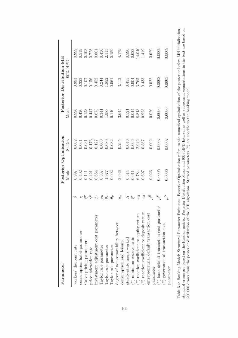
Par

amet

erPos

teri

orO

pti

mis

atio

nPos

teri

orD

istr

ibuti

onM

HM

ode

St.D

ev.

Mea

n90

%H

PD

wor

kers

’dis

coun

tra

teβ

0.99

70.

002

0.99

60.

993

0.99

9co

nsum

ptio

nha

bit

para

met

erχ

0.40

20.

061

0.42

00.

323

0.51

9C

alvo

pric

ing

para

met

erξp

0.14

10.

031

0.15

30.

107

0.19

3pr

ice

inde

xati

onra

teγp

0.42

10.

173

0.44

70.

156

0.72

8in

vest

men

tad

just

men

tco

stpa

ram

eter

φI

0.66

40.

127

0.67

30.

452

0.88

1Tay

lor

rule

para

met

erρR

0.33

70.

060

0.34

10.

244

0.43

6Tay

lor

rule

para

met

erθ π

1.97

70.

080

1.98

31.

852

2.11

5Tay

lor

rule

para

met

erθ y

0.09

20.

032

0.11

00.

061

0.15

9de

gree

ofno

n-se

para

bilit

ybe

twee

nco

nsum

ptio

nan

dle

isur

eσc

3.63

60.

295

3.64

53.

113

4.17

9

stea

dy-s

tate

hour

sw

orke

dH

0.51

40.

040

0.52

10.

455

0.59

0(*

)m

inim

umre

serv

era

tio

ξr0.

011

0.00

60.

014

0.00

40.

023

(*)

reac

tion

coeffi

cien

tto

equi

tyre

turn

ω2

6.78

42.

942

8.81

33.

765

14.0

10(*

)re

acti

onco

effici

ent

tode

posi

tre

turn

ω3

0.69

70.

387

0.92

50.

433

1.41

9en

trep

rene

uria

ldef

ault

tran

sact

ion

cost

para

met

erμE

0.02

60.

002

0.02

60.

022

0.02

9

(*)

bank

defa

ult

tran

sact

ion

cost

para

met

erμB

0.00

050.

0002

0.00

060.

0003

0.00

09(*

)go

vern

men

talt

rans

acti

onco

stpa

ram

eter

μN

0.00

060.

0002

0.00

060.

0003

0.00

09

Tab

le5.

4:B

anki

ngM

odel

:St

ruct

ural

Par

amet

erE

stim

ates

.Pos

teri

orO

ptim

isat

ion

refe

rsto

the

num

eric

alop

tim

isat

ion

ofth

epo

ster

ior

befo

reM

Hin

itia

lisat

ion,

stan

dard

erro

rsar

eba

sed

onth

eH

essi

anm

atri

x.Pos

teri

orD

istr

ibut

ion

Mea

nan

d90

%H

PD

Inte

rval

asw

ella

ssu

bseq

uent

com

puta

tion

sin

the

text

are

base

don

200,

000

draw

sfr

omth

epo

ster

ior

dist

ribu

tion

ofth

eM

Hal

gori

thm

.St

arre

dpa

ram

eter

s(*

)ar

esp

ecifi

cto

the

bank

ing

mod

el.

161

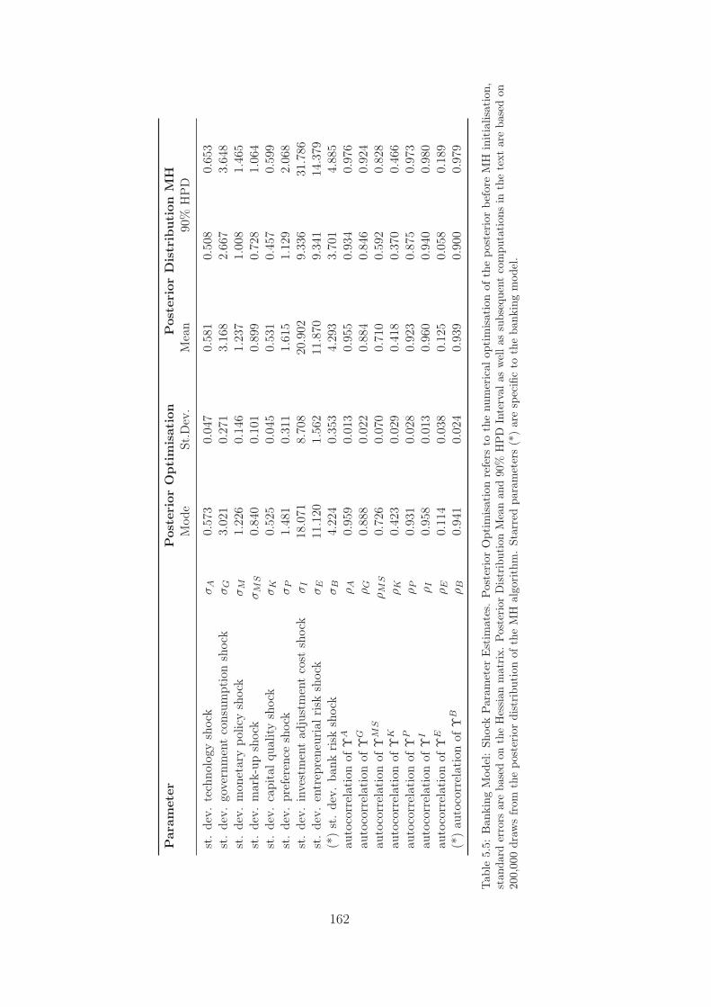
Par

amet

erPos

teri

orO

pti

mis

atio

nPos

teri

orD

istr

ibuti

onM

HM

ode

St.D

ev.

Mea

n90

%H

PD

st.

dev.

tech

nolo

gysh

ock

σA

0.57

30.

047

0.58

10.

508

0.65

3st

.de

v.go

vern

men

tco

nsum

ptio

nsh

ock

σG

3.02

10.

271

3.16

82.

667

3.64

8st

.de

v.m

onet

ary

polic

ysh

ock

σM

1.22

60.

146

1.23

71.

008

1.46

5st

.de

v.m

ark-

upsh

ock

σM

S0.

840

0.10

10.

899

0.72

81.

064

st.

dev.

capi

talq

ualit

ysh

ock

σK

0.52

50.

045

0.53

10.

457

0.59

9st

.de

v.pr

efer

ence

shoc

kσP

1.48

10.

311

1.61

51.

129

2.06

8st

.de

v.in

vest

men

tad

just

men

tco

stsh

ock

σI

18.0

718.

708

20.9

029.

336

31.7

86st

.de

v.en

trep

rene

uria

lris

ksh

ock

σE

11.1

201.

562

11.8

709.

341

14.3

79(*

)st

.de

v.ba

nkri

sksh

ock

σB

4.22

40.

353

4.29

33.

701

4.88

5au

toco

rrel

atio

nof

ΥA

ρA

0.95

90.

013

0.95

50.

934

0.97

6au

toco

rrel

atio

nof

ΥG

ρG

0.88

80.

022

0.88

40.

846

0.92

4au

toco

rrel

atio

nof

ΥM

SρM

S0.

726

0.07

00.

710

0.59

20.

828

auto

corr

elat

ion

ofΥ

KρK

0.42

30.

029

0.41

80.

370

0.46

6au

toco

rrel

atio

nof

ΥP

ρP

0.93

10.

028

0.92

30.

875

0.97

3au

toco

rrel

atio

nof

ΥI

ρI

0.95

80.

013

0.96

00.

940

0.98

0au

toco

rrel

atio

nof

ΥE

ρE

0.11

40.

038

0.12

50.

058

0.18

9(*

)au

toco

rrel

atio

nof

ΥB

ρB

0.94

10.

024

0.93

90.

900

0.97

9

Tab

le5.

5:B

anki

ngM

odel

:Sh

ock

Par

amet

erE

stim

ates

.Pos

teri

orO

ptim

isat

ion

refe

rsto

the

num

eric

alop

tim

isat

ion

ofth

epo

ster

ior

befo

reM

Hin

itia

lisat

ion,

stan

dard

erro

rsar

eba

sed

onth

eH

essi

anm

atri

x.Pos

teri

orD

istr

ibut

ion

Mea

nan

d90

%H

PD

Inte

rval

asw

ella

ssu

bseq

uent

com

puta

tion

sin

the

text

are

base

don

200,

000

draw

sfr

omth

epo

ster

ior

dist

ribu

tion

ofth

eM

Hal

gori

thm

.St

arre

dpa

ram

eter

s(*

)ar

esp

ecifi

cto

the

bank

ing

mod

el.

162

3.25%. Comparing the posterior mean estimates of the NK PC with the results from themeta-study by Schorfheide (2008), it is clear that the banking model coefficient for marginalcosts is at the upper bound of reported estimates.750 Consequently, these estimates implyinflation to be much more responsive to a change in marginal costs and, ceteris paribus,to be less smooth in the estimated banking model.

Furthermore, parameters governing the persistence of investment and consumption arealso estimated comparatively low. The posterior mean of the investment adjustment costparameter φI is estimated at 0.673, and the posterior mean of workers’ habit parameter χ is0.420. Usual estimates of these parameters lie in the ranges of 2-4 and 0.7-0.9 respectively.The immediate effect of these lower estimates is a reduced persistence of consumption andinvestment. So how might these results be explained? To begin with, these estimates couldbe attributed to low persistence in the data. Microeconomic estimates by, for instance,Cooper and Haltiwanger (2006) provide support for low investment adjustment costs.751

Model-based insight might be provided by the study by Christiano et al. (2005a) whoestimate various versions of a standard NK model with separable preferences. Their resultsshow that the estimate of the investment adjustment cost parameter is low when habitsare excluded, and the habit parameter is estimated low when the investment adjustmentcost parameter is set to a low value.752 Therefore, low estimates of one of these parametersmay be correlated with a low estimate of the other parameter.

Another explanation may be that a model with financial frictions already createsenough persistence, thus standard frictions such as habit persistence and investmentadjustment costs play less of a role.753 Comparing NK DSGE models with and withoutfinancial frictions, de Graeve (2008) found the habit parameter to be estimated lowerin the financial frictions model than in the model without financial frictions.754 In asimilar comparative exercise Villa (2013) reports a lower mean estimate of the investmentadjustment cost parameter in a model with financial frictions à la Bernanke et al. (1999)than in the standard Smets and Wouters (2003) model.755 Yet, both of these studies cannot

750 See Schorfheide (2008: 421ff)751 See Cooper and Haltiwanger (2006: 623). They note that their estimates are low in comparison to

the related literature; however, Cooper and Haltiwanger (2006: 624) argue that higher estimates inthe literature are due to measurement error introduced in the estimation process.

752 See Christiano et al. (2005a: 17). Note that their investment adjustment cost parameter κ is relatedto the investment adjustment cost parameter φI in the banking model by κ = 2φI .

753 See de Graeve (2008: 3424). Note that this reasoning is analogous to Justiniano and Preston (2010:105ff) who argue that an open-economy setting partly explains lower values for habit persistence andinvestment adjustment cost parameters because foreign variables can induce persistence in (home)consumption and investment.

754 See de Graeve (2008: 3421ff)755 See Villa (2013: 21). Due to the large size of the 95% probability intervals, these estimates are not

statistically different, see Villa (2013: 21).

163

entirely support this line of argument. In de Graeve (2008), the estimate of the investmentadjustment cost parameter is estimated high both in the model with and without financialfrictions, while the habit parameter is estimated similarly across models in Villa (2013).756

The difference in terms of the lower habit parameter estimate might be explained by thefact that Villa (2013) set the risk aversion parameter in the utility function to 1, whereasde Graeve (2008) estimates this parameter to be 2.15 in the financial frictions model.757

Consequently, these observations indicate that low estimates of χ and φI may beconnected to the form of workers’ utility function, and thus in the banking model to itsnon-separability between leisure and consumption. As noted in section 3.7, the separablecase corresponds to the limit of σc approaching 1. Yet, the posterior mean of the degree ofnon-separability of leisure and consumption is estimated at 3.645 in the banking model.It is statistically significantly different from the prior mean, indicating that the data isinformative on this parameter. Furthermore, the data does not move the parameter tomore separability between leisure and consumption. In fact, the posterior distribution liesfurther away from the separable case. Taken together with the low estimates of χ andφI , this is in line with the results in Guerrón-Quintana (2008) who finds lower estimatesof habit and investment adjustment costs with non-separable preferences as compared toseparable preferences.758

Turning to the remaining parameters of workers’ utility function, note that the posteriormean of the discount rate β is identical to the prior mean. Also, the prior-posterior plotshows that the prior and posterior distributions are the same, indicating that the datais not very informative on the level of the steady-state nominal interest rate.759 Sincethe data used in the estimation only included differenced time series, this result is notsurprising. In contrast, steady-state hours worked H are estimated relatively high, at0.521. This implies that workers spend more than half of their time endowment working.This results in a higher steady-state output level relative to the prior mean of 0.35, ceterisparibus. Also, since steady-state hours worked are directly related to the share of leisurein the utility function, the higher estimate has the effect of decreasing this share andincreasing the share of consumption in utility. Hence, this higher estimate implies thatworkers value leisure less, and consequently work more. From this point of view, the resultis in line with values for the share of consumption in non-separable utility functions.760

Consequently, while the estimate of H is too high when looking at data on hours worked,it is in line with estimates concerning the specific form of the utility function.

756 See de Graeve (2008: 3421) and Villa (2013: 21)757 See the utility function in Villa (2013: 8), and the estimation results in de Graeve (2008: 3421).758 See Guerrón-Quintana (2008: 3621)759 See fig. C.1 in appendix section C.2760 See for example Guerrón-Quintana (2008: 3621) and Backus, Kehoe and Kydland (1993: Table 3)

164

Focusing on the monetary policy rule, it can be seen that the Taylor rule coefficientsfor inflation and the output gap are consistent with previous estimates in the literature. Incontrast to earlier findings, however, interest rate persistence is estimated to be low. Thisfits the estimation results on sticky prices, habit persistence and investment adjustmentcosts. As described above, these estimates imply lower persistence in the behaviour ofthe respective endogenous variables. Hence, there appears a general pattern of lowerpersistence induced by these additional real frictions.

Turning to the structural parameters specific to the banking model, the data generallyappears to be informative, with two exceptions. Considering first the reaction coefficientsto bank equity and deposit returns in workers’ asset demand functions, it is evident thatworkers react differently to changes in the risky bank equity return and the safe bankdeposit return. Both parameters are statistically significant. Even though the 90% HPDintervals are rather wide, they do not overlap. Thus, bank equity and bank deposits cannotbe deemed perfect substitutes except for the deterministic steady state.761 Assuming equalshares in wealth, the point estimates indicate that the representative worker increaseshis bank equity holdings by 15.776% if both returns are expected to increase by 1%, andconsequently decreases his bank deposit holdings by the same percentage.762 Conversely,if both returns are expected to decrease by 1%, a worker decreases his equity holdings by15.776%. This is due to the reaction coefficient on the expected equity return ω2 beingestimated much higher than the reaction coefficient to the expected deposit return ω3. Thisfits the behaviour of a risk-averse worker, since if times are expected to be good, the chancesof the equity return to be less than the steady-state return are low. The worker thenexpands his equity-to-wealth share. In contrast, if expectations of the future short-termdevelopment of bank profits and thus returns are pessimistic, the probability of low bank re-turns and bank default is higher and the worker invests comparatively more in the safe asset.

The minimum reserve ratio ξr affects the change in the real deposit return due to achange in the real policy return. In the deterministic steady state the real deposit return isequal to the real risk-free return. Due to the fact that deposit insurance fees are governedby a fixed parameter, the real deposit return will change by (1 + ξr)% if the real policyrate changes by 1%. For small ξR this is a comparatively small effect. The posterior meanof ξr is higher than the prior mean which was set equal to the minimum reserve ratio in

761 Furthermore, these estimates are far away from the instability regions detected in section 4.4.762 The assumption of equal share of bank deposits and bank equity in workers’ wealth is not abstract,

since the estimation yielded a value of 0.568 for ω1. This appears unrealistic from the point of view ofobserved bank leverage ratios (see table 5.1 for the relationship between ω1 and banks’ leverage ratio inthe banking model). Yet, as the estimates and simulations are based on the log-linear approximations,and thus deal with deviations from the steady state, this should tend to understate, rather thanoverstate, the friction associated with risky bank equity since a given level change will translate into asmaller % change when bank equity is higher, ceteris paribus.

165

effect in the EA at the time of writing. However, since the minimum reserve ratio in theEA was 2% prior to 2012, the posterior estimate is still reasonable.763 The transaction costparameters μE, μB and μN do not appear to be updated by the information in the dataset.Prior and posterior means are almost identical and the prior-posterior plots show almostidentical distributions.764 These results suggest that the absolute size of monitoring costsdoes not affect model dynamics materially. The sensitivity analysis in section 5.5 furtheranalyses the impact of the chosen prior distributions for the estimation results concerningthese transaction cost parameters.

Finally, the estimates of the parameters governing the shock processes are largely inline with results in the literature in general. There are two estimates which stand out:the standard deviations of the investment cost and entrepreneurial risk shocks, σI andσE. The very low autocorrelation estimate of the entrepreneurial risk shock process ρE

may indicate that the data was not able to distinguish properly between big, weaklyautocorrelated shocks and small, highly autocorrelated shocks.765 The high estimate of thestandard deviation of the investment adjustment cost shock σI is probably related to thelow estimate of the investment adjustment cost parameter φI . A 20.902% shock intervalabove and below the mean estimate of φI is [0.532, 0.814], which is, as discussed above,still evidence of rather low investment adjustment costs. As a final note, the 90% HPDinterval for σI is very wide, implying that the mean estimate may not be a very precisedescription.

Concerning the remaining estimates of shock standard deviations, there are notabledifferences in terms of their size between shocks pertaining to the supply and demand sides.Demand side shocks, meaning government spending and preference shocks, are generallylarger than supply side shocks, meaning technology, capital quality, and mark-up shocks.This excludes the (supply side) investment adjustment cost shock, which was alreadydiscussed in the previous paragraph. The standard deviation of a government spendingshock is about six times the standard deviation of a technology or capital quality shock,and more than three times the standard deviation of a mark-up shock. Financial shocks,meaning the entrepreneurial and bank risk shocks, are yet more volatile than demand orsupply side shocks, except for the investment adjustment cost shock. Finally, the monetarypolicy shock is estimated to be more volatile than supply side shocks, but less volatilethan demand and financial shocks.766

763 See European Central Bank (2016c), URL in list of references764 See fig. C.1 in appendix section C.2765 Preliminary exercises yielded a posterior mode with the latter property, that is, small σE with high

ρE . However, the log-likelihood indicated that this mode was dominated by the mode used for theestimation reported in the text, even if only slightly.

766 The monetary policy shock is not grouped with the other shocks since monetary policy is the focus ofthis study.

166

Focusing on the estimated autocorrelation parameters, the patterns are not as clear-cut.Considering only the exogenous capital quality and mark-up processes would indicatea lower autocorrelation for supply side shock processes as compared to demand shockprocesses. However, the exogenous technology and investment adjustment cost processesare highly autocorrelated. The former may be explained by the fact that the data wasexpressed in per-capita and not in efficiency units. The latter, however, is relatively surpris-ing given the standard deviation of εI . Finally, exogenous financial shock processes are alsonot clearly more highly autocorrelated than other shock processes, as the autocorrelationof one exogenous process (ΥE) is estimated very low, whereas the other (ΥB) is estimatedcomparatively high.

To sum up, the posterior estimates of the banking model are plausible. As will be seenin chapter 6, the banking model is able to create long-lasting reactions of real variableseven though persistence parameters are estimated comparatively low. Whether or notdifferences in the estimated volatilities and autocorrelation parameters of the variousexogenous processes translate into a major impact of one kind of shock for the evolution ofthe endogenous variables will also be evaluated in chapter 6. Beforehand, this chapter willassess the empirical fit of the banking model with these estimates vis-à-vis the financialaccelerator model and discuss the sensitivity of these estimation results in sections 5.4and 5.5, respectively.

5.4 Evaluation of the Banking Model’s Empirical Per-

formance

5.4.1 Posterior Estimates of the Financial Accelerator Model

Before turning to the discussion about the empirical fit of the banking model, this sectionfirst presents the results of the estimation of the financial accelerator model. These esti-mates form the reference against which the performance of the banking model is evaluated.As detailed in chapter 4, the financial accelerator does not feature the financial friction be-tween workers and banks, as well as the portfolio choice problem of workers.767 Thus, thereis no model-equivalent to the time series of bank equity used in the estimation of the bank-ing model, and also, the bank risk shock is not present in the financial accelerator model.Hence, there are 8 shocks and 8 observables to estimate the financial accelerator model. Theposterior estimates for the financial accelerator model are summarised in tables 5.6 and 5.7.

The dataset is otherwise the same as the one used for the banking model.768 The calibra-

767 For details, see section 4.3.2.768 See section 5.2.1 and appendix section C.1

167

tion and prior distributions are the same as in the banking model for all parameters whichare also present in the financial accelerator model.769 The structure of tables 5.6 and 5.7 isequivalent to the one of tables 5.4 and 5.5. The posterior mean and 90% HPD intervals arebased on 200,000 draws from 5 chains of the MH algorithm. Convergence was checked bythe same means as for the banking model.770 All checks indicated convergence after burn-in.

If the overlap of 90% HPD intervals is taken as a measure, then the posterior estimatesin tables 5.6 and 5.7 are similar to the estimates of the banking model in tables 5.4 and 5.5,respectively.771 Furthermore, the posterior distributions for the banking and financialaccelerator models are generally close together, as can be seen from figs. C.1 and C.2in appendix section C.2. The result of close similarity of parameter estimates is in linewith previous results in the literature on comparing models with different sets of financialfrictions and without financial frictions.772

There are only a few cases where the estimate of the posterior mean of one model doesnot fall into the 90% HPD interval of the other model. These include workers’ consumptionhabit parameter χ and the standard deviation of the preference shock σP . In both casesthe estimate is lower in the banking model, indicating that lower habit persistence andsmaller shocks to the marginal utility of consumption are necessary for the banking modelto fit the data. Both a larger habit persistence parameter and larger preference shocksimply a more volatile path for consumption, ceteris paribus. Thus, either the introductionof the bank equity time series into the estimation process or the model layout work tomake the path for consumption more volatile, thus necessitating lower habit persistenceand smaller preference shocks.773

Thus, the estimates of the posterior distributions can be deemed roughly similar forthe banking and financial accelerator models. With a few exceptions, the additionalbank-specific friction does not as such impact parameter estimates. In order to asseswhether the banking model improves the financial accelerator model in terms of datafit, the next subsections consider three criteria, which are popular in the literature inturn: marginal likelihoods, steady-state ratios and second moments. While marginallikelihood comparisons are a truly Bayesian concept, steady-state ratios and second

769 See section 5.2.2, stars indicate parameters that do not apply to the financial accelerator model.770 See section 5.3 for details.771 See Villa (2013: 20) for this line of argument with respect to similarity between posterior estimates.772 See, for instance, de Graeve (2008) and Merola (2015) for studies using US data and Villa (2013) for

the EA.773 Since the estimates of the reduced-dataset banking model, which is estimated on the same dataset

except for the exclusion of the bank equity time series, are similar to the benchmark banking model,it appears to be the case that model dynamics are the main reason. See below for more details on thereduced-dataset banking model.

168

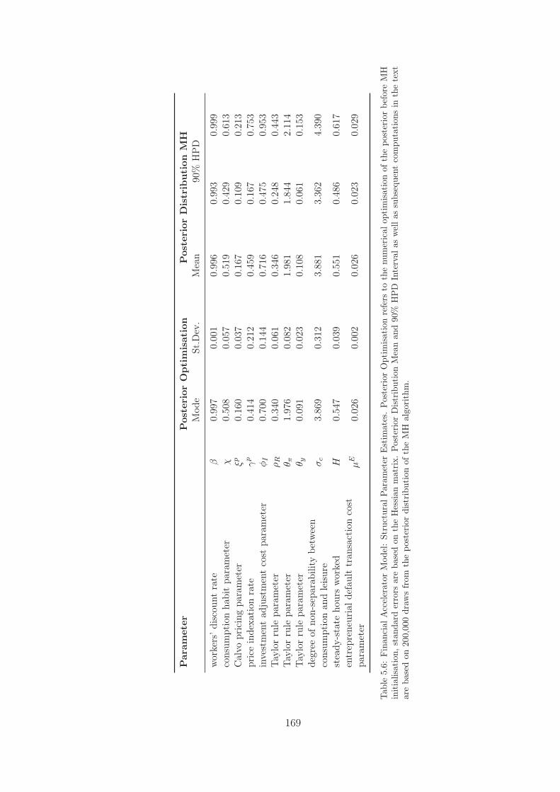
Par

amet

erPos

teri

orO

pti

mis

atio

nPos

teri

orD

istr

ibuti

onM

HM

ode

St.D

ev.

Mea

n90

%H

PD

wor

kers

’dis

coun

tra

teβ

0.99

70.

001

0.99

60.

993

0.99

9co

nsum

ptio

nha

bit

para

met

erχ

0.50

80.

057

0.51

90.

429

0.61

3C

alvo

pric

ing

para

met

erξp

0.16

00.

037

0.16

70.

109

0.21

3pr

ice

inde

xati

onra

teγp

0.41

40.

212

0.45

90.

167

0.75

3in

vest

men

tad

just

men

tco

stpa

ram

eter

φI

0.70

00.

144

0.71

60.

475

0.95

3Tay

lor

rule

para

met

erρR

0.34

00.

061

0.34

60.

248

0.44

3Tay

lor

rule

para

met

erθ π

1.97

60.

082

1.98

11.

844

2.11

4Tay

lor

rule

para

met

erθ y

0.09

10.

023

0.10

80.

061

0.15

3de

gree

ofno

n-se

para

bilit

ybe

twee

nco

nsum

ptio

nan

dle

isur

eσc

3.86

90.

312

3.88

13.

362

4.39

0

stea

dy-s

tate

hour

sw

orke

dH

0.54

70.

039

0.55

10.

486

0.61

7en

trep

rene

uria

ldef

ault

tran

sact

ion

cost

para

met

erμE

0.02

60.

002

0.02

60.

023

0.02

9

Tab

le5.

6:Fin

anci

alA

ccel

erat

orM

odel

:St

ruct

ural

Par

amet

erE

stim

ates

.Pos

teri

orO

ptim

isat

ion

refe

rsto

the

num

eric

alop

tim

isat

ion

ofth

epo

ster

ior

befo

reM

Hin

itia

lisat

ion,

stan

dard

erro

rsar

eba

sed

onth

eH

essi

anm

atri

x.Pos

teri

orD

istr

ibut

ion

Mea

nan

d90

%H

PD

Inte

rval

asw

ella

ssu

bseq

uent

com

puta

tion

sin

the

text

are

base

don

200,

000

draw

sfr

omth

epo

ster

ior

dist

ribu

tion

ofth

eM

Hal

gori

thm

.

169

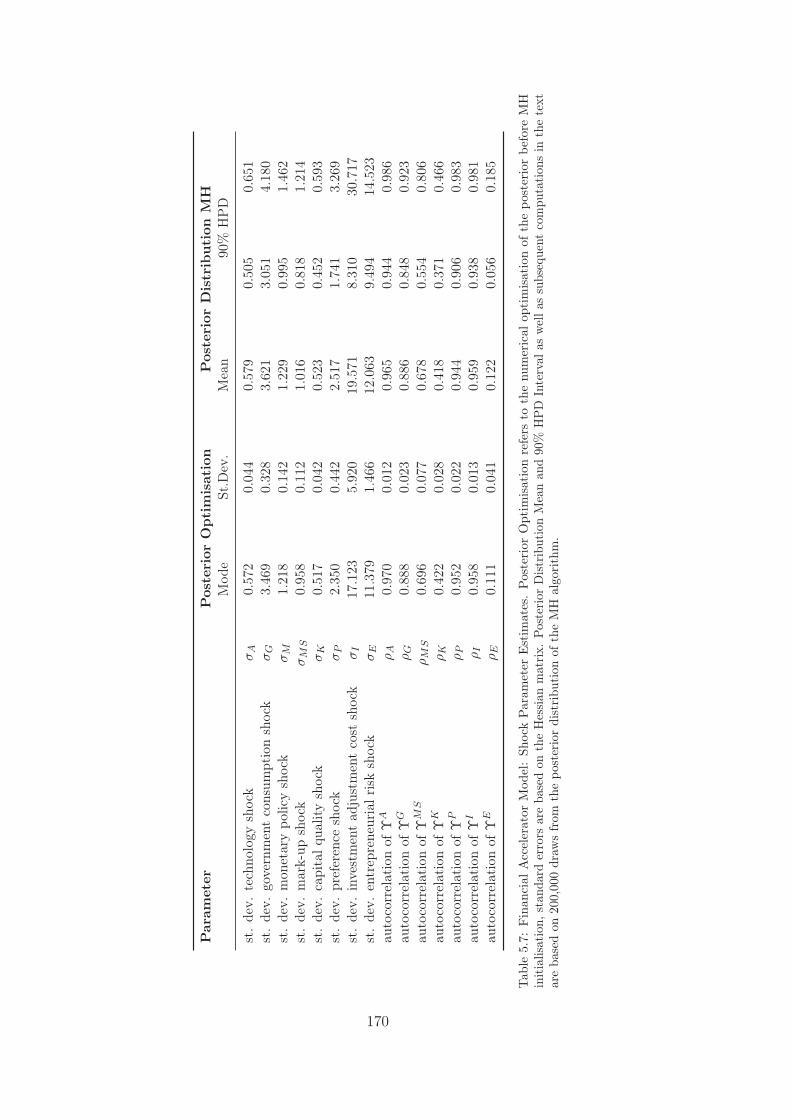
Par

amet

erPos

teri

orO

pti

mis

atio

nPos

teri

orD

istr

ibuti

onM

HM

ode

St.D

ev.

Mea

n90

%H

PD

st.

dev.

tech

nolo

gysh

ock

σA

0.57

20.

044

0.57

90.

505

0.65

1st

.de

v.go

vern

men

tco

nsum

ptio

nsh

ock

σG

3.46

90.

328

3.62

13.

051

4.18

0st

.de

v.m

onet

ary

polic

ysh

ock

σM

1.21

80.

142

1.22

90.

995

1.46

2st

.de

v.m

ark-

upsh

ock

σM

S0.

958

0.11

21.

016

0.81

81.

214

st.

dev.

capi

talq

ualit

ysh

ock

σK

0.51

70.

042

0.52

30.

452

0.59

3st

.de

v.pr

efer

ence

shoc

kσP

2.35

00.

442

2.51

71.

741

3.26

9st

.de

v.in

vest

men

tad

just

men

tco

stsh

ock

σI

17.1

235.

920

19.5

718.

310

30.7

17st

.de

v.en

trep

rene

uria

lris

ksh

ock

σE

11.3

791.

466

12.0

639.

494

14.5

23au

toco

rrel

atio

nof

ΥA

ρA

0.97

00.

012

0.96

50.

944

0.98

6au

toco

rrel

atio

nof

ΥG

ρG

0.88

80.

023

0.88

60.

848

0.92

3au

toco

rrel

atio

nof

ΥM

SρM

S0.

696

0.07

70.

678

0.55

40.

806

auto

corr

elat

ion

ofΥ

KρK

0.42

20.

028

0.41

80.

371

0.46

6au

toco

rrel

atio

nof

ΥP

ρP

0.95

20.

022

0.94

40.

906

0.98

3au

toco

rrel

atio

nof

ΥI

ρI

0.95

80.

013

0.95

90.

938

0.98

1au

toco

rrel

atio

nof

ΥE

ρE

0.11

10.

041

0.12

20.

056

0.18

5

Tab

le5.

7:Fin

anci

alA

ccel

erat

orM

odel

:Sh

ock

Par

amet

erE

stim

ates

.Pos

teri

orO

ptim

isat

ion

refe

rsto

the

num

eric

alop

tim

isat

ion

ofth

epo

ster

ior

befo

reM

Hin

itia

lisat

ion,

stan

dard

erro

rsar

eba

sed

onth

eH

essi

anm

atri

x.Pos

teri

orD

istr

ibut

ion

Mea

nan

d90

%H

PD

Inte

rval

asw

ella

ssu

bseq

uent

com

puta

tion

sin

the

text

are

base

don

200,

000

draw

sfr

omth

epo

ster

ior

dist

ribu

tion

ofth

eM

Hal

gori

thm

.

170

moment comparisons are more broadly used. There are many more possibilities to evaluatethe relative and absolute fit of models. The following discussion will focus on these threebecause of their wide use and expediency.

5.4.2 Banking vis-à-vis Financial Accelerator Model: Marginal

Likelihoods and Data Match

Dimension I: Marginal Likelihood One popular method to compare models from aBayesian perspective is the calculation of posterior odds ratios. The posterior odds ratioPO1,2 is defined as:774

PO1,2 =p(model1|data)p(model2|data) (5.5)

where p(model1|data) is the posterior model probability of model 1 given by:775

p(model1|data) = p(data|model1)p(model1)

p(data)(5.6)

This can be interpreted in a similar vein as the application of Bayes’ Theorem to parameterestimation, only this time to models. p(model1) is the prior probability of model 1 andcomprises the beliefs of the researcher concerning the validity of model 1.776 p(data) is themarginal likelihood of the data, as above. Finally, p(data|model1) is called the marginallikelihood (of model 1), which is a function of the prior distribution and likelihood usedin calculating the posterior distribution of the parameters.777 The marginal likelihoodcan be interpreted as an expression for the probability of the model given the data withrespect to other models.778 Similar to the computation of the posterior distribution ofparameters, the marginal likelihood is defined in terms of a high-dimensional integral andthus a numerical approximation is necessary.779 There exist various methods to compute anumerical approximation to the marginal likelihood, in the following the approximationusing the modified harmonic mean estimator is reported.780

The posterior odds ratio contrasts the marginal likelihood of model 1 with the marginallikelihood of model 2, to elucidate whether the data is in favour of one specific model.781

Combining eqs. (5.5) and (5.6) yields:

774 Koop (2003: 4), eq. 1.7, my notation.775 Koop (2003: 4), eq. 1.5, my notation.776 See Koop (2003: 4)777 See Koop (2003: 4). This term may also be called marginal data density, see for example Herbst and

Schorfheide (2016: 40f).778 See Geweke (1999: 14f)779 See Herbst and Schorfheide (2016: 93)780 See Geweke (1999: 42ff) and Herbst and Schorfheide (2016: 93ff)781 While posterior odds ratios are illustrative for comparing two models, numerous models can be

compared by calculating posterior model probabilities, see also Koop (2003: 4).

171

PO1,2 =p(data|model1)p(model1)

p(data|model2)p(model2)(5.7)

The special case of assuming equal prior probabilities, p(model1) = p(model2) is calledthe Bayes Factor.782 The comparison then reduces to comparing marginal likelihoods.For transparency, equal prior probabilities are assumed in the following. In this case, ifPO = 1, then the marginal likelihoods of both models are equal. In general, a value of PO

larger than 1 indicates a preference for model 1, whereas a value lower than 1 indicatesthat model 2 is preferred.

A crucial condition is that p(data) is the same used in the estimation of model 1and model 2 such that it cancels out in deriving eq. (5.7). For comparative purposes interms of marginal likelihoods this is intuitive: if the dataset used for estimating model 1were different from the dataset used in estimating model 2, then the researcher cannotdistinguish between the effects of different datasets or model implications for estimatingthe parameters. As noted above, the dataset used for estimating the financial acceleratormodel necessarily excluded the time series for bank equity.

To enable the comparison, a reduced-dataset version of the banking model is estimated,using the same dataset as for the financial accelerator model, and excluding the exogenousbank risk shock process ΥB. The assumptions about the calibrated parameters and theprior distributions are the same as for the complete banking model.783 The results fromthe posterior estimation are presented in appendix section C.3. In general, these estimatesare in line with the results of the complete banking model.784

The logarithm of the marginal likelihood is −804.91 for the banking model (reduceddataset) and −811.20 for the financial accelerator model. The Bayes Factor for thereduced-dataset banking model versus the financial accelerator model is then:

POBM,FAM =e−804.91

e−811.20≈ 5.39 ∗ 102 (5.8)

which is clearly greater than 1. Thus, the banking model (reduced dataset) is preferred tothe financial accelerator model according to this measure.

The size of the difference between the marginal likelihoods between those two modelsis difficult to assess. In terms of posterior probabilities, the comparison is rather futile.With only two models, the posterior probability for model 1 will be higher than 90% as

782 See Koop (2003: 5). Bayes Factors have to obey the principle of transitivity, see Robert (2001: 351).783 See section 5.2.2784 See appendix section C.3 for details.

172

soon as the log model likelihoods differ by 1 point.785 Comparing these Bayes Factorswith other reported numbers in the literature may also be only a rough guide, since thismeasure crucially depends on the dataset, model structure and parameter set. In thisrespect, it should be noted that the Bayes Factor is biased in favour of the model withfewer parameters.786

The scale created by Jeffreys (1961) is sometimes cited for interpreting Bayes Fac-tors.787 According to this scale, the Bayes Factor POBM,FAM of 5.39 ∗ 102 indicates thatthe evidence against the financial accelerator model is decisive.788 Yet, it has been pointedout that the bounds of the scale by Jeffreys (1961) are somewhat arbitrary.789 Kassand Raftery (1995), for instance, propose different bounds with stricter requirements forconsidering evidence against a model as decisive.790 Even on the stricter scale by Kass andRaftery (1995), POBM,FAM still presents decisive evidence against the financial acceleratormodel. The arbitrariness of the bounds can be resolved by following an explicit lossfunction approach.791 Yet, for the purposes of this study, the indication of aforementionedscales is sufficient.

Based on this result, the banking model estimated on the reduced dataset can be deemedsuperior in terms of data fit.792 Nevertheless, according to the Bayesian perspective, thispreference does not translate into an outright rejection of the financial accelerator model.Rather, the results of various models should be weighted by their posterior probabilityto reach some form of model average.793 As already discussed above, the restriction totwo models lends big support to the banking model in terms of posterior probabilities.794

Yet, there may be other models which fit the data better, but which are not includedhere. In fact, from a theoretical perspective, even if one model improves on another, itmay be a poor description of reality.795 In this study, no further model versions will beintroduced to alleviate this shortcoming since the maximisation of forecasting performanceor model fit is not the core research question. Rather, this discussion is intended to gauge

785 With two models, the posterior probability of model 1 is given by p(model1|data) = PO1,2/(1+PO1,2),see Koop (2003: 4), unnumbered equation, my notation.

786 See Rabanal and Rubio-Ramírez (2005: 1161)787 See, for instance, Rabanal and Rubio-Ramírez (2005: 1160)788 See Jeffreys (1961: 432). Note that the scale in Jeffreys (1961: 432) refers to the Bayes Factor notation

where the null hypothesis to be tested is the numerator, which is opposite to the notation used here.789 See Robert (2001: 228)790 See Kass and Raftery (1995: 777)791 See Robert (2001: 228)792 Model misspecification does not pose a problem for this comparison, since the Bayes Factor remains

a consistent method to choose among different models even if they are incorrectly specified, seeFernández-Villaverde and Rubio-Ramírez (2004: 159).

793 See Canova (2007: 339) and Koop (2003: 27)794 With equal prior probabilities, the posterior probabilities of the banking and financial accelerator

models are 99.76%, and 0.24%, respectively.795 See Canova (2007: 455)

173

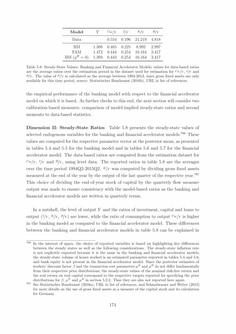
Model Y CW/Y I/Y K/Y B/Y

Data 0.554 0.196 21.219 4.818

BM 1.308 0.485 0.225 8.992 2.997FAM 1.472 0.444 0.254 10.164 3.417

BM ( B = 0) 1.393 0.443 0.254 10.164 3.417

Table 5.8: Steady-State Values: Banking and Financial Accelerator Models; values for data-based ratiosare the average ratios over the estimation period in the dataset used for estimation for CW/Y , I/Y andB/Y . The value of K/Y is calculated as the average between 1994-2013, since gross fixed assets are onlyavailable for this time period, source: Statistisches Bundesamt (2016b), URL in list of references.

the empirical performance of the banking model with respect to the financial acceleratormodel on which it is based. As further checks to this end, the next section will consider twocalibration-based measures: comparison of model-implied steady-state ratios and secondmoments to data-based statistics.

Dimension II: Steady-State Ratios Table 5.8 presents the steady-state values ofselected endogenous variables for the banking and financial accelerator models.796 Thesevalues are computed for the respective parameter vector at the posterior mean, as presentedin tables 5.4 and 5.5 for the banking model and in tables 5.6 and 5.7 for the financialaccelerator model. The data-based ratios are computed from the estimation dataset forCW/Y , I/Y and B/Y , using level data. The reported ratios in table 5.8 are the averagesover the time period 1994Q2-2015Q2. K/Y was computed by dividing gross fixed assetsmeasured at the end of the year by the output of the last quarter of the respective year.797

This choice of dividing the end-of-year stock of capital by the quarterly flow measureoutput was made to ensure consistency with the model-based ratios as the banking andfinancial accelerator models are written in quarterly terms.

In a nutshell, the level of output Y and the ratios of investment, capital and loans tooutput (I/Y , K/Y , B/Y ) are lower, while the ratio of consumption to output CW/Y is higherin the banking model as compared to the financial accelerator model. These differencesbetween the banking and financial accelerator models in table 5.8 can be explained in

796 In the interest of space, the choice of reported variables is based on highlighting key differencesbetween the steady states as well as the following considerations. The steady-state inflation rateis not explicitly reported because it is the same in the banking and financial accelerator models,the steady-state volume of hours worked is an estimated parameter reported in tables 5.4 and 5.6,and bank equity is not present in the financial accelerator model. Since the posterior estimates ofworkers’ discount factor β and the transaction cost parameters μE and μB do not differ fundamentallyfrom their respective prior distributions, the steady-state values of the nominal risk-free return andthe real return on real capital correspond to the respective targets reported for specifying the priordistributions for β, μE and μB in section 5.2.2. Thus they are also not reported here again.

797 See Statistisches Bundesamt (2016a), URL in list of references, and Schmalwasser and Weber (2012)for more details on the use of gross fixed assets as a measure of the capital stock and its calculationfor Germany.

174

terms of two factors: the steady-state real return on real capital and the steady-statevolume of hours worked. Due to the inclusion of the second financial friction betweenbanks and workers, the equilibrium spread between the real return on real capital andthe real risk-free return is larger in the banking model. This larger real return on realcapital implies a larger steady-state marginal product of capital, which in turn can onlybe accomplished through a lower capital stock per hour worked.798 A lower capital stock,ceteris paribus, then implies a lower output given the production function. Similarly, bythe production function, the lower estimate of the steady-state volume of hours worked inthe banking model works in the same direction.

Furthermore, consider the counterfactual experiment of setting the bank risk premiumto 0 in the banking model.799 This reduces the spread between the real return on realcapital and the real risk-free return to the entrepreneurial risk premium. Thus, thesteady-state real return on real capital in the banking model would be the same as inthe financial accelerator model. As can be seen in the last row of table 5.8, output isstill lower in the banking model due to the lower steady-state volume of hours worked.In contrast, the other ratios are now almost identical in the banking and the financialaccelerator models. Thus, the differences in the ratios noted above are principally due tothe higher real return on real capital in the banking model.

Lastly, note that the higher real return on real capital moves CW/Y and I/Y closer to thedata-implied ratios, while it conversely moves B/Y and K/Y further away. Since the financialaccelerator model’s implied capital-to-output ratio is already below the data-implied ratio,the latter observation is easily explained by the even lower capital stock in the bankingmodel. The lower capital stock in the banking model outweighs the effect of lower outputsuch that K/Y is lower than in the financial accelerator model. Since steady-state investmentis equal to the depreciated capital stock, and the depreciation rate is a parameter calibratedto the same value in both models, lower K/Y implies lower I/Y , which in fact is closer tothe data-implied ratio of I/Y . By the retail goods market clearing condition, this decreasein I/Y must be compensated by other aggregate demand components. The governmentspending to output ratio ΥG/Y is a calibrated value, monitoring costs only count as a small

798 Also, since the estimated steady-state volume of hours worked H is lower in the banking model thanin the financial accelerator model, and a lower H induces a lower marginal product of capital for agiven capital stock, the reduction in the capital stock to increase the marginal product of capital iseven larger than in the case of keeping the volume of hours worked constant.

799 This means setting the bank risk premium to 1 in the non-linear model, since Rk = E BRd. In thelog-linear approximation to the model the equation is given by rk = E + B + rd, thus B needs tobe set to 0. Additionally, another change is necessary since the transaction cost parameter associatedwith the loan market friction was estimated differently in the banking and financial accelerator models.In order to facilitate comparability, μE is set to 0.026, which is the value estimated for the financialaccelerator model. This change in parametrization does not affect the qualitative results discussed inthe main text.

175

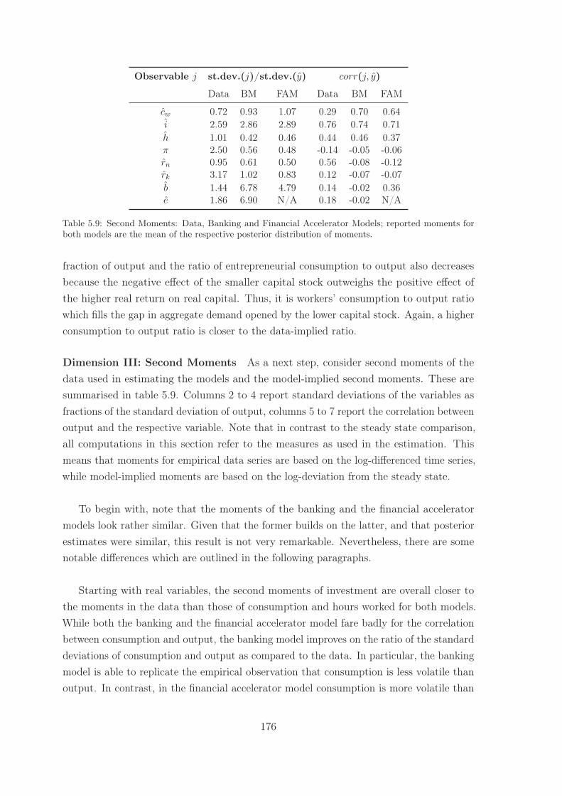
Observable j st.dev.(j)/st.dev.(y) corr(j, y)

Data BM FAM Data BM FAM

cw 0.72 0.93 1.07 0.29 0.70 0.64i 2.59 2.86 2.89 0.76 0.74 0.71h 1.01 0.42 0.46 0.44 0.46 0.37π 2.50 0.56 0.48 -0.14 -0.05 -0.06rn 0.95 0.61 0.50 0.56 -0.08 -0.12rk 3.17 1.02 0.83 0.12 -0.07 -0.07b 1.44 6.78 4.79 0.14 -0.02 0.36e 1.86 6.90 N/A 0.18 -0.02 N/A

Table 5.9: Second Moments: Data, Banking and Financial Accelerator Models; reported moments forboth models are the mean of the respective posterior distribution of moments.

fraction of output and the ratio of entrepreneurial consumption to output also decreasesbecause the negative effect of the smaller capital stock outweighs the positive effect ofthe higher real return on real capital. Thus, it is workers’ consumption to output ratiowhich fills the gap in aggregate demand opened by the lower capital stock. Again, a higherconsumption to output ratio is closer to the data-implied ratio.

Dimension III: Second Moments As a next step, consider second moments of thedata used in estimating the models and the model-implied second moments. These aresummarised in table 5.9. Columns 2 to 4 report standard deviations of the variables asfractions of the standard deviation of output, columns 5 to 7 report the correlation betweenoutput and the respective variable. Note that in contrast to the steady state comparison,all computations in this section refer to the measures as used in the estimation. Thismeans that moments for empirical data series are based on the log-differenced time series,while model-implied moments are based on the log-deviation from the steady state.

To begin with, note that the moments of the banking and the financial acceleratormodels look rather similar. Given that the former builds on the latter, and that posteriorestimates were similar, this result is not very remarkable. Nevertheless, there are somenotable differences which are outlined in the following paragraphs.

Starting with real variables, the second moments of investment are overall closer tothe moments in the data than those of consumption and hours worked for both models.While both the banking and the financial accelerator model fare badly for the correlationbetween consumption and output, the banking model improves on the ratio of the standarddeviations of consumption and output as compared to the data. In particular, the bankingmodel is able to replicate the empirical observation that consumption is less volatile thanoutput. In contrast, in the financial accelerator model consumption is more volatile than

176

output.800 Moreover, both models underestimate the volatility of hours worked. While thedata suggests that hours worked are as volatile as output, both models indicate that thestandard deviation of hours worked is only between 42% and 46% of the one of output.801

Yet, the model-implied correlation between hours worked and output of the bankingmodel is almost spot-on. The financial accelerator model slightly underestimates thiscorrelation. The model-implied second moments for investment are close to the empiricaldata. The banking model improves on the financial accelerator model marginally both interms of cross-correlation and in terms of the volatility of investment with respect to output.

Turning to the monetary and financial sides of the economy, both models’ performancegenerally declines. Both models cannot replicate the large volatility of inflation and thereal return on real capital as compared to output. Yet, the banking model improves on thefinancial accelerator model. Firstly, the model-implied standard deviations as fractions ofthe standard deviation of output are higher for inflation, the nominal interest rate and thereal return on real capital in the banking model, even though they are still considerablylower than the second moments for inflation and the real return on real capital seen inthe data. Turning to correlations, both the banking and the financial accelerator modelsestimate almost no correlation between these three variables and output. This can bedeemed roughly in line with the empirical data, which only shows a low positive correlationbetween the real return on real capital and output and a low negative one for inflationand output. Yet, the nominal return is clearly positively correlated with output, whichneither model is able to match.

In contrast to the underestimation of volatility for returns, the volatility of bankloans (and bank equity in the banking model) vis-à-vis output is overestimated both inthe banking and the financial accelerator models. The financial accelerator model faresbetter than the banking model in terms of volatility of bank loans, but worse in terms ofcorrelation between output and bank loans. This points to a general pattern: both modelsimply a larger volatility of financial quantities as opposed to returns than is observablein the empirical data. It may be that the model design is such that quantity and price

800 The result of higher consumption volatility in the financial accelerator model is in accordance with thediscussion of the higher estimates of the habit parameter and the standard deviation of the preferenceshock in the financial accelerator model (see above).

801 Wickens (2008: 407) argues that a comparatively low variability of hours worked with respect tooutput, coupled with a high correlation of wages with output can be taken as a sign that a modelis not able to replicate rather inflexible wages coupled with a more flexible employment process. Inthe banking model, for example, the correlation between output and wages is roughly 0.91. Wickens(2008: 408) suggests that model statistics can be aligned more closely with the respective data-basedstatistics by introducing wage stickiness and further exogenous shocks. Thus, model-implied volatilitystatistics for hours worked may be too low in the banking and financial accelerator models becausewages are completely flexible. Incorporating wage rigidities in the spirit of price rigidities may remedythis shortcoming.

177

effects are not clearly delimited. Given the reduced-form representation of bank equity,for instance, this result indicates that there is space for explicitly modelling price andquantity effects of financial volumes.

In conclusion, model-implied correlations of the banking and financial acceleratormodels are largely similar. This is in line with previous results described above. Yet, it canbe argued that the banking model improves on the financial accelerator model in terms ofempirical fit as measured by second moments. Since the additional friction in the bankingmodel impacts workers’ decision problem, the fact that the model is able to capture thelower volatility of consumption as compared to the financial accelerator model points toan advantage of the banking model in this respect. Both models perform well in terms ofinvestment moments. In fact, the banking model marginally improves the empirical fit inthis respect on the financial accelerator model.

Combining these results with the ones on marginal likelihoods and steady-state ratios,there are three main results. Firstly, the banking model with the estimated parametervector described in this chapter fits the data reasonably well. Secondly, the banking modelimproves on the financial accelerator model in terms of data fit in all three considereddimensions, although not monotonically for each variable. It should be noted that thisimprovement appears moderate. Thirdly, the underestimated volatility of returns andinflation, as well as the overestimated volatility of bank loans and bank equity, are clearshortcomings. The poor fit in these dimensions shows the compromises the estimationprocedure had to make in order to fit the data overall. Some weaknesses, such as thelow capital-to-output ratio, could be remedied by an appropriate recalibration of theparameters. For others, one of which is the underestimation of return and inflationvolatilities, it seems unlikely that such a path would yield much improved results.802 Beforeproceeding with further analysis, the sensitivity of the estimation results to the chosenprior distributions and time periods needs to be evaluated. The results are presented inthe subsequent section.

5.5 Sensitivity Analysis

Various sensitivity tests were conducted in order to examine whether the selection ofparameter calibration and prior distributions or the choice of time period have a significant

802 A higher capital-to-output ratio could potentially be achieved by decreasing the real return on realcapital. This decrease may, however, not improve the model fit in terms of volatilities, given that thereal return on real capital is lower in the financial accelerator model than in the banking model, andthe financial accelerator model fares worse in terms of the volatility of the real return on real capitalthan the banking model. Yet, this last conjecture is not clear-cut, as estimated volatilities depend onthe whole system.

178

impact on the posterior results as presented in the previous sections. The sensitivityanalysis proceeded along two dimensions: one is the sensitivity to the calibration ofparameters and prior distributions, the second dimension is in terms of the consideredtime periods. Since the focus of this research is the additional financial friction betweenbanks and workers, the prior sensitivity tests concentrate on the additional parameters ascompared to the financial accelerator model.

In terms of prior distributions, three sensitivity tests are reported in appendix sec-tion C.4: an asymmetric risk premiums (�E/B) prior, an equal friction size prior andan alternative asset demand parameters prior. In the first experiment, the assumptionabout the entrepreneurial risk premium being of equal size as the bank risk premiumis dropped. Instead, the prior distributions for μE and μB assume the credit spread tobe distributed asymmetrically, with the banking sector friction contributing 1.00625%quarterly, while the entrepreneurial risk premium is reduced to 1.0025% quarterly. Then,the transaction cost parameters μE and μB are of comparable size implying that costsincurred in entrepreneurial and bank default are of similar size. In contrast, the priormean for the governmental transaction cost parameter μN is centred at 0.2. This valuewas chosen to investigate whether the data is more in line with small monitoring costs, orwith the larger values for monitoring costs reported in the literature.803

The second prior sensitivity test instead assumes an equal size of financial frictions.Put in a nutshell, all parameters which can be attributed to either friction are set to thesame values for both the entrepreneurial liability friction and the bank liability friction.This firstly concerns the size of the risk premiums, but also the calibrated steady-statedefault probabilities of banks and entrepreneurs, for instance.804 The third prior sensitivitytest reduces the prior mean of the asset demand parameters ω2 and ω3 equally. Note thatbank equity and bank deposits are still assumed to be perfect substitutes in equilibrium,since this is a steady-state property of the banking model.

The results of all three sensitivity tests can be found in table C.6 in appendix sec-tion C.4.805 Consider first the sensitivity to an asymmetric �E/B prior and a same frictionsize prior. Except for the transaction cost parameters, the posterior estimates of thestructural parameters are very close to the benchmark banking model in tables 5.4 and 5.5

803 See the discussion in section 5.2.2804 See appendix section C.4 for details.805 The computational procedure was the same as for the benchmark banking model, details are also

reported in appendix section C.4.

179

for both sensitivity tests.806 For all structural parameters (except the transaction costparameters) the 90% HPD intervals overlap substantially and the posterior mean estimatesare reasonably similar. The posterior distributions for μE are in each case indistinguishablefrom the prior distribution. This implies that the data is not informative on this parameter,neither for the benchmark banking model nor for the two sensitivity tests. The posteriordistributions for μB show a slight reduction in the posterior mean as compared to therespective prior mean. This result indicates that transaction costs in case of bank defaulttend to be lower.

Yet, given that the differences are comparatively small and the prior and posteriordistributions overlap to a large degree, the actual significance of this result is limited.Hence, the findings from this sensitivity analysis should not be taken as evidence in favouror against an equal or asymmetric distribution of financial frictions. The data ratherappears not informative enough on these parameters. In contrast, the estimate of theposterior mean for μN in the asymmetric �E/B prior test is markedly different from its priormean. The posterior mean of 0.086 for μN also means that it is different from the estimatein the benchmark banking model. The simplistic assumptions about fiscal policy, however,prevent a meaningful interpretation of the findings on the governmental transaction costparameter. In the end, the dynamics of the model and the data appear to force the varioustransaction cost parameters to rather low values. The judgement of ‘rather low’ is madewith reference to the discussion in section 5.2.2.

Turning to the estimates for the exogenous processes, there are some differences be-tween the benchmark banking model and the sensitivity tests. In particular, the standarddeviation of the entrepreneurial risk shock σE is significantly larger with the asymmetric�E/B prior distribution than the benchmark prior distribution. This is probably a resultof the lower monitoring cost parameter μE and the lower entrepreneurial risk premium,as the estimate of σE with the equal friction size prior is similar to the benchmark priorestimates. Furthermore, the higher volatility of the government consumption process withthe asymmetric �E/B prior is probably related to the higher estimate of μN as comparedto the benchmark prior distribution. With higher monitoring costs the government budgetis more strongly affected by developments in the banking sector. In turn, government

806 The posterior estimates for ω2 could be argued to be a further case where posterior estimatessignificantly differ. The benchmark model’s mean estimate does not fall in the 90% HPD intervalin the asymmetric E/B prior distribution case, and is only marginally in the interval in the equalfriction size prior case. Yet, in both sensitivity tests, the 90% HPD interval for this parameter is muchsmaller than in the benchmark banking model. In fact, the intervals overlap almost perfectly withthe lower half of the 90% HPD interval of the benchmark model. Furthermore, both sensitivity testsproduced estimates for ω2 which are significantly above 1, and both sensitivity tests’ mean estimatesfall comfortably into the benchmark model’s 90% HPD interval for this parameter. Thus, the generalpattern of a large ω2 is robust to these sensitivity tests and thus, ω2 is not discussed extensively here.

180

consumption has to adjust to keep the budget in balance which can be taken as anexplanation for the higher volatility σG.

The third prior sensitivity test changed the prior distributions of the parameters inworkers’ asset demand equations. As the results in the last three columns of table C.6 show,the estimates of all parameters except for ω2 and ω3 are robust. There are no significantdifferences between the benchmark banking model and this alternative asset demand priorversion. In contrast, the posterior mean of the coefficient governing the reaction to thereal equity return, ω2, is much higher than in the benchmark banking model. This issurprising given that the assumed alternative asset demand prior distribution was centredat a lower mean value. Conversely, the reaction coefficient to the real deposit return, ω3,is significantly lower than in the benchmark version. As in the benchmark version, theestimated posterior distribution of ω3 for the alternative prior is almost identical to theprior distribution.807 It appears that it is the spread between the reaction coefficientswhich is informed by the data, not the reaction to the respective returns. This is likelysince bank equity is an observable in the estimation process and not a deposit or bankequity return. Thus, it seems probable that the estimation procedure targets a particularvolatility of bank equity. If, then, the model-implied correlation between the real equityand real deposit returns is high, a smaller reaction coefficient to one of them seeminglyimplies a stronger reaction coefficient to the other return.808

The results of the sensitivity analysis in terms of the sample period are reported in ta-bles C.7 and C.8 in appendix section C.4. There are two different cut-off points consideredin these exercises, that is in total 4 sets of posterior estimates are compared. The firstcut-off point is the transition from monetary policy being conducted by the Bundesbankto the monetary policy conduct of the ECB in 1999. These two sets of estimates arereferred to by the Bundesbank and ECB periods, respectively. The second exercise dividesthe sample into a pre-financial-crisis period, and a financial-crisis to post-financial-crisisperiod. These are accordingly referred to as the pre-crisis and crisis periods. The priordistributions and parameter calibration are the same as in the benchmark banking modelthis time.809 Similarly, the computational procedure is the same as before, and details canbe found in appendix section C.4.

Concerning this sensitivity analysis, the posterior estimates of the Bundesbank periodare very distinctive: the 90% HPD intervals do not overlap or overlap only marginally for10 out of the 16 structural, and 14 out of the 17 shock parameters with the respective

807 A graphical visualisation for the benchmark banking model can be found in fig. C.1.808 The model implies a close co-movement between the real bank equity return and the real deposit

return due to the incentive compatibility constraint of equity-holders.809 See section 5.2.2.

181

90% HPD intervals of the benchmark banking model estimates. The remaining similarlyestimated parameters are mainly the ones on which the data does not seem to be informa-tive (workers’ discount rate and the transaction cost parameters). These differences mightbe due to the underlying data. In particular, inflation and the return on entrepreneurialequity appear to be more volatile between the second quarter of 1994 and 2000.

A second explanation for this difference could be a markedly different behaviour ofmonetary policy during the Bundesbank period as compared to the ECB period. Aspointed out in chapter 2, even though both periods can be characterised by one policyrule, the weights attached to different sub-targets differed. This view is underscored firstlyby the different estimates of the monetary policy rule parameters, with the parametergoverning the response to the output gap being estimated relatively high. Secondly, ascan be seen from columns 5-7 of table C.7, the posterior estimates of the ECB sample arevery similar to the benchmark banking model. Only in three cases (σM , ρK and ξp) arethe respective posterior means not included in the other’s 90% HPD intervals. In thesecases, however, their 90% HPD intervals overlap. Following this line of argument, theseestimates indicate that the ECB period features more strongly in the estimates of thecomplete sample period than the Bundesbank period.

What is more, it may appear counter-intuitive that the estimated reaction to the outputgap is higher in the Bundesbank period. Yet, these results may be considered plausibleif the relevant monetary aggregate is highly correlated with the output gap. Since thereis no explicit money market in the banking model, this line of argument has to be takenwith caution. Furthermore, such a high estimate contradicts the findings of Hayo andHofmann (2006) who estimate a central bank Taylor rule, similar to the one used here,for Germany for both the Bundesbank and ECB periods separately.810 Not only is theoutput gap reaction coefficient of the Bundesbank period significantly below one, but it isalso estimated to be lower than the corresponding coefficient in the ECB period.811 WhileHayo and Hofmann (2006) suggest that this difference is due to the underlying structure ofthe economy rather than monetary policy conduct, this cannot be used as an explanationfor the estimation of the banking model using different datasets.812

Rather, the different estimates may be due to the short dataset used in this study: thesample of the Bundesbank period comprises only 20 observations, while the ECB periodcomprises 65 observations. Thus, the sample might be too small to properly estimate all33 parameters of the banking model. This is underscored by the fact that posterior mean

810 See Hayo and Hofmann (2006: 649ff). Hayo and Hofmann (2006) use data from 1979 to 1998 for theBundesbank period and from 1999 to 2003 for the ECB period.

811 See Hayo and Hofmann (2006: 651)812 See Hayo and Hofmann (2006: 655)

182

estimates of the Bundesbank period are for the most part comparatively close to the priormeans. Unfortunately, an extension of the Bundesbank sample by using pre-1994Q2 data isnot easily accomplished and would necessitate further assumptions and data adjustments.To sum up, there is an indication for the Bundesbank period yielding different parameterestimates. Yet, due to the small sample and the closeness to the prior, this finding has tobe qualified in terms of its strength.

Lastly, consider the estimates for the pre-crisis and crisis periods. Overall, theseestimates are in line with the benchmark banking model. There are, nevertheless, a fewdifferences worth commenting on. To start with, habit persistence is estimated higher inboth periods as compared to the benchmark sample. Yet, the 90% HPD intervals overlap.Secondly, this first finding may be connected to the estimate of the steady-state valueof hours worked, which is marginally lower in the pre-crisis period but markedly lowerin the crisis period. Given that the estimated means of habit persistence are 0.529 and0.551 for the pre-crisis and crisis periods, respectively, indicating a moderate degree ofhabit persistence, and the posterior means of the steady-state volume of hours workedis markedly higher than the prior mean, these results do not disagree with the findingsreported in section 5.3. Thirdly, the estimated mean of the Calvo pricing parameter ξp

is significantly higher for the crisis period than for the benchmark period, although it isstill low as compared to the prior mean. The posterior mean of the indexation parameterγp is also estimated higher for the crisis period. Yet, the 90% HPD intervals of γp inboth versions overlap to a large degree since they are estimated to be rather wide. Theseestimates then suggest a higher degree of price stickiness in the crisis period than in thepre-crisis period. This may reflect the lower degree of volatility of inflation at the endof the sample (and thus crisis) period.813 Finally, there are some differences concerningthe parameters of the exogenous shock processes.814 Differences in these parameters overdifferent sample periods are not too surprising. Furthermore, these differences are generallycomparatively minor, such that they can be most probably attributed to different datavolatilities.

Taken together, these findings suggest that parameter estimates are robust to excludingor only considering the period which followed the recent crisis. This is in line with theconclusion in European Central Bank (2010), stating that the interest rate pass-through

813 See fig. 5.1 in section 5.2.1.814 Incidentally, the investment adjustment cost shock process is estimated much less volatile and

autocorrelated in both the non-crisis and crisis periods. This is probably connected to the higherestimate of the investment adjustment cost parameter φI . These results underscore the explanationfor the investment adjustment cost process estimates given in section 5.3, Furthermore, the findings ofthis sensitivity tests do not contradict that the investment adjustment cost parameter φI is estimatedlow, since the posterior means are still considerably below the prior mean and the 90% HPD intervalsare rather wide and include the benchmark mean estimate in both sub-periods.

183

process did not break down in the EA in the wake of the financial crisis.815 While parameterestimates are not as such directly related to the interest rate pass-through, the conclusionin European Central Bank (2010) indicates that there were no fundamental changes in theunderlying structure.816 Furthermore, the elements of the transmission process itself weresimilar to the one in periods without financial instability.817 Unconventional monetarypolicies may have contributed to this steadiness.818 While unconventional monetary policiesare not explicitly dealt with in this study, they may thus serve as an explanation for thesimilar estimates of the pre-crisis and crisis periods.819

In sum, the sensitivity analysis showed that the estimation results of the benchmarkbanking model are generally robust to changes in the dataset and prior distributions.One exception to this finding is the estimation on the Bundesbank period, which yieldedconsiderably different posterior distributions. Furthermore, the analysis underscores theintuition in section 5.3 that the data is not very informative on some parameters, specificallythe transaction cost parameters. A manifold of other sensitivity tests could potentiallybe conducted. These include, for instance, the sensitivity to the calibration to standardparameters such as the depreciation rate. Yet, such exercises cannot be handled withinthe bounds of this study and are left to future research.

815 See European Central Bank (2010: 96)816 See European Central Bank (2010: 96)817 See European Central Bank (2010: 96)818 See Darracq Pariès et al. (2016: 39)819 See section 6.3.1 for a short discussion why unconventional monetary policies are excluded from this

study.

184

Chapter 6

Monetary Policy Transmission andPolicy Trade-offs in the Banking Model

The previous chapter presented the result of the estimation concerning the banking and thefinancial accelerator models. For, one it showed that the estimates of the two models are rel-atively similar. Yet, the previous chapter also demonstrated that introducing non-systemicbank failures into a New Keynesian (NK) dynamic stochastic general equilibrium (DSGE)model with financial accelerator improves the empirical fit. Building on the findings ofthe previous chapters, this chapter aims to answer the research questions of this thesis.To this end, two types of analysis are conducted: impulse response analysis and Taylorcurves. The first tracks the evolution of the model economy after being disturbed fromits steady state. The second sheds light on the policy trade-off between inflation andoutput gap stabilisation as monetary policy goals.820 Taken together, these analyses willhighlight the differences which arise when banks are allowed to fail in a macroeconomicmodel. Thus, this chapter provides an integrated assessment and discussion of the linksbetween non-systemic bank fragility and monetary policy.

This chapter is structured as follows. Firstly, the transmission of monetary policyimpulses is the focus of section 6.1. Section 6.2 discusses the trade-off between inflationand output gap stabilisation faced by the central bank in its conduct of monetary policyand how it is affected by the incidence of non-systemic bank default using Taylor curves.Finally, section 6.3 explores how introducing macroprudential instruments affects theprevious results on the transmission of monetary policy and the monetary policy objectivestrade-off.

820 In this chapter, stabilisation refers to the act of decreasing the volatility of the respective variable.The concept is thus different from the analysis of the stability of the model equilibrium conducted inchapter 4.

185

6.1 Monetary Policy Transmission with Non-Systemic

Bank Default

6.1.1 Reaction to a Monetary Policy Shock

The central bank conducts monetary policy in the banking model using a Taylor-typeinterest rate rule. The rule specifies that the central bank changes the nominal risk-freereturn only when it observes a deviation of inflation or the output gap from their respectivesteady-state values.821 Since the banking model features long-run monetary neutrality,changing the nominal risk-free return when the economy rests in the steady state willlead to short-run movements, but will not affect the steady state. Any such policy wouldengineer a departure from stable prices without any permanent effect on real variables. Asa consequence, the central bank merely reacts to developments in the economy to maintainprice stability. At the same time, it is rather complicated to study the transmissionof monetary policy when the nominal risk-free return merely changes as a result of adisplacement of the model economy from its steady state. In such a scenario, movementsin endogenous variables might be caused by factors other than monetary policy.822 Then,consequences of monetary policy actions are difficult to disentangle from other drivingfactors.

Therefore, this section makes use of the concept of monetary policy shocks.823 In thefinancial accelerator and banking models the monetary policy shock εM is an additivefactor in the Taylor rule.824 The shock changes the nominal risk-free return unexpectedly,and as a result displaces the economy from its steady state. Thus, this exogenous changein the nominal risk-free return highlights the effects of monetary policy on the evolution ofthe model economy. One interpretation of such a shock is that it represents a measurementerror on the part of the central bank.825 Another interpretation is that these shocks are

821 Remember that the Taylor rule in chapter 3 is written in terms of the nominal risk-free return,whereby returns and interest rates are linked to each other by the following relationship: return =1 + interest rate. Using the term interest rate would not change the findings with regard to contents.

822 See also Christiano et al. (1999: 68) on this issue.823 All computations were carried out with Matlab and the software platform Dynare. For coding (of

the model, of the estimation and analysis experiments in the previous and this chapters) the Dynaremanual (Adjemian et al. (2011)), the Matlab help section, and the resources made available duringthe Summer School ‘The Science and Art of DSGE Modelling’ (2014) at the Centre for InternationalMacroeconomic Studies, School of Economics at the University of Surrey were helpful and valuable.The tool developed by Schlömer (2016), URL in list of references, was used to convert pictures.

824 See eq. (4.35); note that this chapter deals with the log-linear approximation to the non-linear modelpresented in chapter 3.

825 This interpretation has been touched upon in chapter 2 when justifying the central bank target of 0%inflation in this model. As noted there, while measurement error has been used as a justification fortargeting a slightly positive inflation rate, there are good reasons for using the 0% inflation target inthe banking model even in the case of the interpretation of monetary policy shocks as measurementerrors.

186

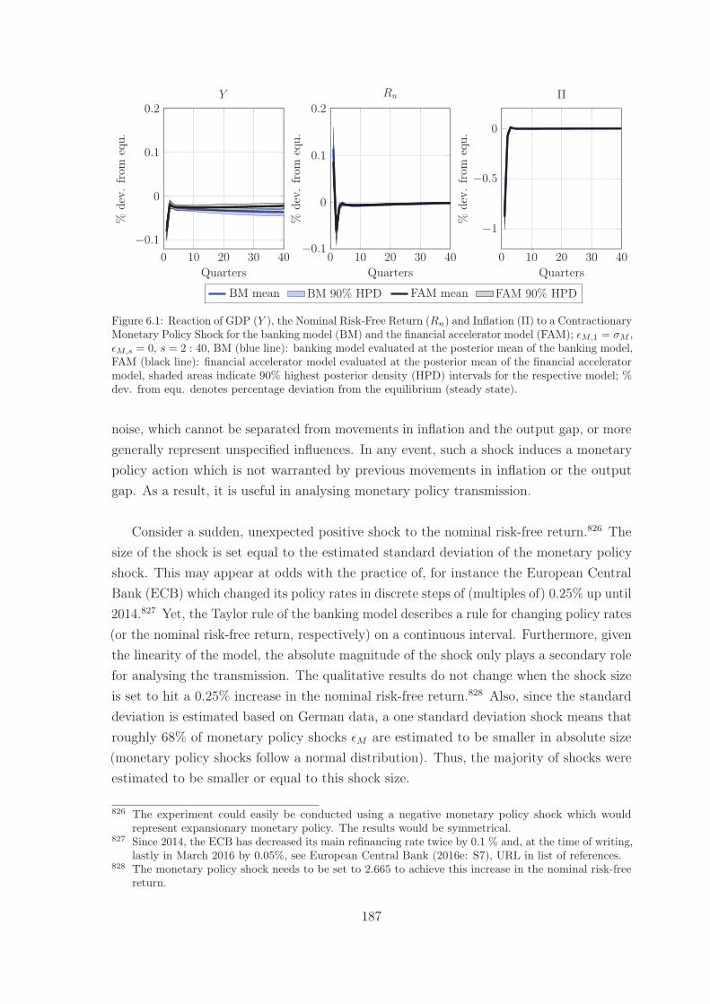
0 10 20 30 40

−0.1

0

0.1

0.2

Quarters

%de

v.fr

omeq

u.

Y

0 10 20 30 40−0.1

0

0.1

0.2

Quarters

%de

v.fr

omeq

u.

Rn

0 10 20 30 40

−1

−0.5

0

Quarters

%de

v.fr

omeq

u.

Π

BM mean BM 90% HPD FAM mean FAM 90% HPD

Figure 6.1: Reaction of GDP (Y ), the Nominal Risk-Free Return (Rn) and Inflation (Π) to a ContractionaryMonetary Policy Shock for the banking model (BM) and the financial accelerator model (FAM); εM,1 = σM ,εM,s = 0, s = 2 : 40, BM (blue line): banking model evaluated at the posterior mean of the banking model,FAM (black line): financial accelerator model evaluated at the posterior mean of the financial acceleratormodel, shaded areas indicate 90% highest posterior density (HPD) intervals for the respective model; %dev. from equ. denotes percentage deviation from the equilibrium (steady state).

noise, which cannot be separated from movements in inflation and the output gap, or moregenerally represent unspecified influences. In any event, such a shock induces a monetarypolicy action which is not warranted by previous movements in inflation or the outputgap. As a result, it is useful in analysing monetary policy transmission.

Consider a sudden, unexpected positive shock to the nominal risk-free return.826 Thesize of the shock is set equal to the estimated standard deviation of the monetary policyshock. This may appear at odds with the practice of, for instance the European CentralBank (ECB) which changed its policy rates in discrete steps of (multiples of) 0.25% up until2014.827 Yet, the Taylor rule of the banking model describes a rule for changing policy rates(or the nominal risk-free return, respectively) on a continuous interval. Furthermore, giventhe linearity of the model, the absolute magnitude of the shock only plays a secondary rolefor analysing the transmission. The qualitative results do not change when the shock sizeis set to hit a 0.25% increase in the nominal risk-free return.828 Also, since the standarddeviation is estimated based on German data, a one standard deviation shock means thatroughly 68% of monetary policy shocks εM are estimated to be smaller in absolute size(monetary policy shocks follow a normal distribution). Thus, the majority of shocks wereestimated to be smaller or equal to this shock size.

826 The experiment could easily be conducted using a negative monetary policy shock which wouldrepresent expansionary monetary policy. The results would be symmetrical.

827 Since 2014, the ECB has decreased its main refinancing rate twice by 0.1 % and, at the time of writing,lastly in March 2016 by 0.05%, see European Central Bank (2016e: S7), URL in list of references.

828 The monetary policy shock needs to be set to 2.665 to achieve this increase in the nominal risk-freereturn.

187

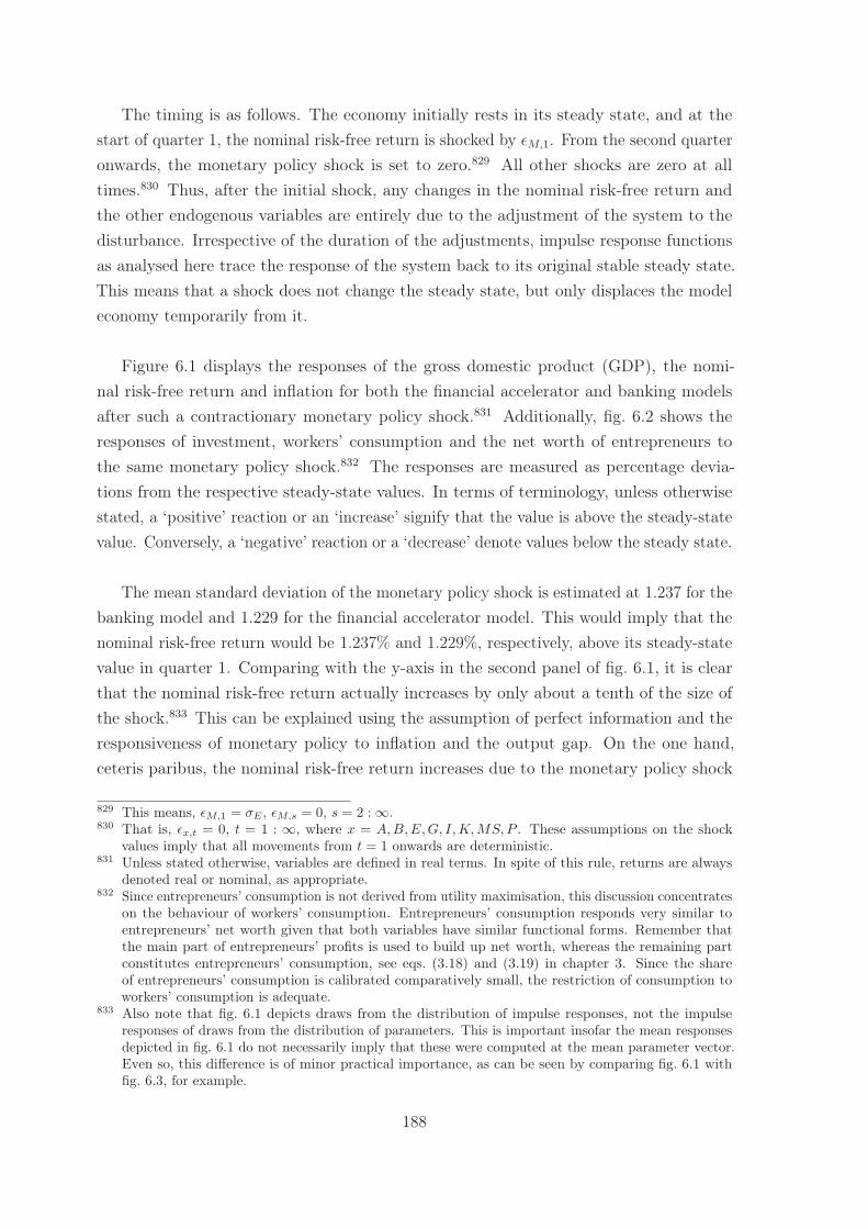
The timing is as follows. The economy initially rests in its steady state, and at thestart of quarter 1, the nominal risk-free return is shocked by εM,1. From the second quarteronwards, the monetary policy shock is set to zero.829 All other shocks are zero at alltimes.830 Thus, after the initial shock, any changes in the nominal risk-free return andthe other endogenous variables are entirely due to the adjustment of the system to thedisturbance. Irrespective of the duration of the adjustments, impulse response functionsas analysed here trace the response of the system back to its original stable steady state.This means that a shock does not change the steady state, but only displaces the modeleconomy temporarily from it.

Figure 6.1 displays the responses of the gross domestic product (GDP), the nomi-nal risk-free return and inflation for both the financial accelerator and banking modelsafter such a contractionary monetary policy shock.831 Additionally, fig. 6.2 shows theresponses of investment, workers’ consumption and the net worth of entrepreneurs tothe same monetary policy shock.832 The responses are measured as percentage devia-tions from the respective steady-state values. In terms of terminology, unless otherwisestated, a ‘positive’ reaction or an ‘increase’ signify that the value is above the steady-statevalue. Conversely, a ‘negative’ reaction or a ‘decrease’ denote values below the steady state.

The mean standard deviation of the monetary policy shock is estimated at 1.237 for thebanking model and 1.229 for the financial accelerator model. This would imply that thenominal risk-free return would be 1.237% and 1.229%, respectively, above its steady-statevalue in quarter 1. Comparing with the y-axis in the second panel of fig. 6.1, it is clearthat the nominal risk-free return actually increases by only about a tenth of the size ofthe shock.833 This can be explained using the assumption of perfect information and theresponsiveness of monetary policy to inflation and the output gap. On the one hand,ceteris paribus, the nominal risk-free return increases due to the monetary policy shock

829 This means, εM,1 = σE , εM,s = 0, s = 2 : ∞.830 That is, εx,t = 0, t = 1 : ∞, where x = A,B,E,G, I,K,MS, P . These assumptions on the shock

values imply that all movements from t = 1 onwards are deterministic.831 Unless stated otherwise, variables are defined in real terms. In spite of this rule, returns are always

denoted real or nominal, as appropriate.832 Since entrepreneurs’ consumption is not derived from utility maximisation, this discussion concentrates

on the behaviour of workers’ consumption. Entrepreneurs’ consumption responds very similar toentrepreneurs’ net worth given that both variables have similar functional forms. Remember thatthe main part of entrepreneurs’ profits is used to build up net worth, whereas the remaining partconstitutes entrepreneurs’ consumption, see eqs. (3.18) and (3.19) in chapter 3. Since the shareof entrepreneurs’ consumption is calibrated comparatively small, the restriction of consumption toworkers’ consumption is adequate.

833 Also note that fig. 6.1 depicts draws from the distribution of impulse responses, not the impulseresponses of draws from the distribution of parameters. This is important insofar the mean responsesdepicted in fig. 6.1 do not necessarily imply that these were computed at the mean parameter vector.Even so, this difference is of minor practical importance, as can be seen by comparing fig. 6.1 withfig. 6.3, for example.

188

by the size of the shock. On the other hand, ceteris paribus, the central bank reacts todecreases in the output gap and inflation by lowering the nominal risk-free return in linewith the Taylor rule coefficients.834 Hence, the monetary policy impulse disturbing thesystem is larger than the change in the nominal risk-free return.835 Note that this does notaffect the focus on the transmission of monetary policy. The fact that the nominal risk-freereturn in quarter 1 does not increase as much as the monetary policy shock merely signifiesthat the shock is moderated by the downturn induced by the contractionary monetarypolicy shock.

To build a point of reference, consider the impulse response functions of the financialaccelerator model.836 This is the reference model in which banks do not default.837 Theeffects of monetary policy in the financial accelerator model mainly work through theinterest rate and balance sheet channels.838 The interest rate channel works throughdecreasing investment demand by increasing the general level of interest rates. Thus,aggregate demand declines. At the same time, lower aggregate demand puts downwardpressure on prices through entrepreneurs’ marginal costs, in turn decreasing inflation.839

The balance sheet channel additionally affects monetary policy transmission through theeffect of interest rates on asset prices. Higher interest rates mean lower asset prices, in this

834 The contemporaneity assumption of the Taylor rule is not crucial for there to exist a difference betweenthe nominal risk-free return and the policy shock. Consider the counterfactual experiment where thecentral bank sets the nominal risk-free return as a function of the expected values of inflation and theoutput gap. All other equations are unchanged and the parameters are the same as before. Then, theresponses of GDP, inflation and the other endogenous variables would be amplified as compared tothe responses of the banking model in figs. 6.1 and 6.2. Secondly, the nominal risk-free return wouldactually decrease upon impact of the shock, due to the expected paths of inflation and the output gapto evolve much further below their steady-state values. Thus, the reaction of the nominal risk-freereturn does not equal the size of the monetary policy shock in this case either.

835 The crucial point here is that all agents are fully informed. Entrepreneurs and retailers observe theincidence of the shock, thus adjust their production and pricing choices even before the central bankhas set the nominal risk-free return. Private agents also know how the central bank will react to thesechoices which leads to the responses depicted in figs. 6.1 and 6.2. Perfect information and perfectforesight tend not to occur too often in reality. Yet, such a mechanism just described may be partiallyreflected in the use of central bank communications to explain the conduct of monetary policy interms of forward guidance.

836 Note that for clarity the scale of the y-axis is different for in the graphs of fig. 6.1 as compared to thegraphs in fig. 6.2. Also, the y-axis scales for inflation in fig. 6.1 and for entrepreneurial net worth infig. 6.2 are different from the y-axis scales of the other two plots in the respective figure.

837 See chapter 4 for more details.838 This reflects the modelling approach. The working capital channel of monetary policy, among others,

is not present in the banking or financial accelerator models. It could, however, be easily added byhaving part of the wage bill (paid by entrepreneurs) pre-financed, and thus creating additional loandemand for this purpose. Then, retail goods prices are also affected through the impact of the loanrate on entrepreneurs’ wage costs.

839 Since the steady-state inflation rate is zero, contractionary monetary policy leads to deflation in thiscase. However, there is no debt-deflation channel at work in this model, and the model is log-linearisedaround its steady state. This suggests that deflation does not lead to asymmetric effects as comparedto a positive inflation rate. In fact, an expansionary monetary policy shock looks like a mirror imageof the contractionary shock discussed in the text. More generally, in linear models, the shape of theimpulse response is independent of the shocks’ size and sign, see Canova (2007: 137).

189

case the price of physical capital. As the price of physical capital decreases, entrepreneursreceive lower cash flow from selling their depreciated capital stock at the end of the period.This immediately leads to a decrease in entrepreneurial net worth (fig. 6.2) and as a resultto a higher entrepreneurial default probability.840 In turn, this leads to tighter creditconditions, that is the external finance premium increases. As a result, entrepreneurs’capital demand decreases and consequently, investment and aggregate demand declinefurther.

Inflation shows a quantitatively stronger but more short-lived reaction than GDP. Theinitial effect on inflation is about 10 times stronger than the effect on GDP. At the sametime, inflation reverts to the close vicinity of its steady state within one year.841 Theshort-lived reaction of inflation is probably related to the low estimates of price stickinessparameters. Only about 17% of retailers cannot optimise their prices in any given period.Thus, the impact of current marginal costs on inflation is very strong.842 Then, inflationdoes not deviate from its steady state for a long period of time and the effects of exogenousshocks on inflation quickly phase out. The nominal risk-free return behaves similarly dueto the high reaction coefficient on inflation, θπ, in the Taylor rule. As a consequence ofthese two observations, it is clear that real returns do not deviate from their respectivesteady states for a long period of time either.

In contrast, variables such as consumption843 and investment only slowly return totheir respective steady-state values. They recover eventually since real returns are close totheir steady-state levels and shocks are zero, and as such there is no further motivationfor deviations from the steady state.844 Aggregate demand variables do not adjust at thesame speed as real returns because of the presence of real and financial frictions. Forconsumption, the presence of habits leads to a smooth path. Investment takes long torecover to its steady state due to investment adjustment costs which penalise volatility

840 Since this model consists of representative agents, the balance sheet channel leads to adverse effects onthe balance sheet of the representative entrepreneur. Empirical studies on the balance sheet channelusually assume that borrowers are heterogeneous in terms of their balance sheet strength, see Beck etal. (2014: 3). Size can be an indicator of the balance sheet channel in that smaller firms contracttheir borrowing more than others, see Beck et al. (2014: 3) and section 2.4. Yet, the Bernanke et al.(1999) approach relates financing conditions to net worth through the representative agent to modelthe balance sheet channel. Differences among entrepreneurs arise due to idiosyncratic shocks in themodel, see section 3.3.

841 After 3 quarters, the deviation of inflation from its steady-state value is less than 0.01%.842 See section 5.3 for a comparison of prior and posterior mean values for the coefficients of the NK

Phillips Curve and the weight of marginal costs in terms of its effects on current inflation for thebanking model. Since the estimates of the banking and financial accelerator models are similar, thediscussion there equally applies to the financial accelerator model.

843 Henceforth, the term ‘consumption’ is used to denote ‘workers’ consumption’. If explicit reference ismade to the retail goods demand of entrepreneurs, the term ‘entrepreneurs’ consumption’ is used.

844 Also, all variables eventually return to their steady state levels given the assumptions about thisexperiment, that is temporary shocks which do not change the steady state.

190

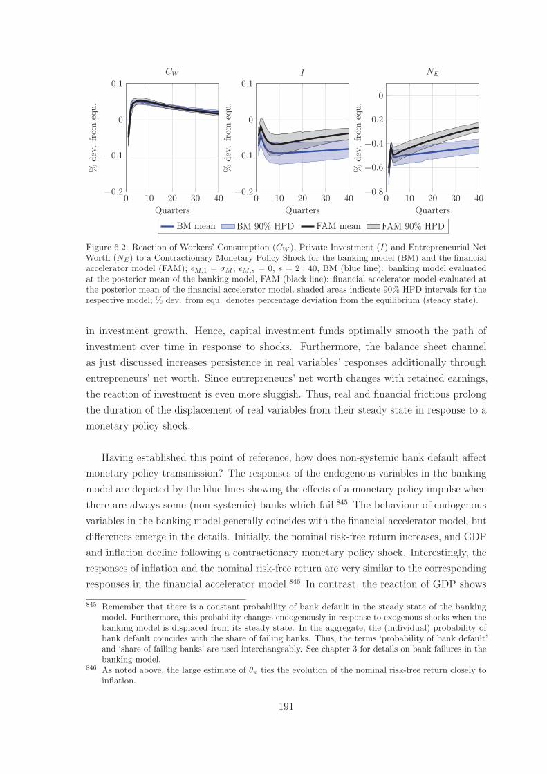
0 10 20 30 40−0.2

−0.1

0

0.1

Quarters

%de

v.fr

omeq

u.

CW

0 10 20 30 40−0.2

−0.1

0

0.1

Quarters

%de

v.fr

omeq

u.

I

0 10 20 30 40−0.8

−0.6

−0.4

−0.2

0

Quarters

%de

v.fr

omeq

u.

NE

BM mean BM 90% HPD FAM mean FAM 90% HPD

Figure 6.2: Reaction of Workers’ Consumption (CW ), Private Investment (I) and Entrepreneurial NetWorth (NE) to a Contractionary Monetary Policy Shock for the banking model (BM) and the financialaccelerator model (FAM); εM,1 = σM , εM,s = 0, s = 2 : 40, BM (blue line): banking model evaluatedat the posterior mean of the banking model, FAM (black line): financial accelerator model evaluated atthe posterior mean of the financial accelerator model, shaded areas indicate 90% HPD intervals for therespective model; % dev. from equ. denotes percentage deviation from the equilibrium (steady state).

in investment growth. Hence, capital investment funds optimally smooth the path ofinvestment over time in response to shocks. Furthermore, the balance sheet channelas just discussed increases persistence in real variables’ responses additionally throughentrepreneurs’ net worth. Since entrepreneurs’ net worth changes with retained earnings,the reaction of investment is even more sluggish. Thus, real and financial frictions prolongthe duration of the displacement of real variables from their steady state in response to amonetary policy shock.

Having established this point of reference, how does non-systemic bank default affectmonetary policy transmission? The responses of the endogenous variables in the bankingmodel are depicted by the blue lines showing the effects of a monetary policy impulse whenthere are always some (non-systemic) banks which fail.845 The behaviour of endogenousvariables in the banking model generally coincides with the financial accelerator model, butdifferences emerge in the details. Initially, the nominal risk-free return increases, and GDPand inflation decline following a contractionary monetary policy shock. Interestingly, theresponses of inflation and the nominal risk-free return are very similar to the correspondingresponses in the financial accelerator model.846 In contrast, the reaction of GDP shows

845 Remember that there is a constant probability of bank default in the steady state of the bankingmodel. Furthermore, this probability changes endogenously in response to exogenous shocks when thebanking model is displaced from its steady state. In the aggregate, the (individual) probability ofbank default coincides with the share of failing banks. Thus, the terms ‘probability of bank default’and ‘share of failing banks’ are used interchangeably. See chapter 3 for details on bank failures in thebanking model.

846 As noted above, the large estimate of θπ ties the evolution of the nominal risk-free return closely toinflation.

191

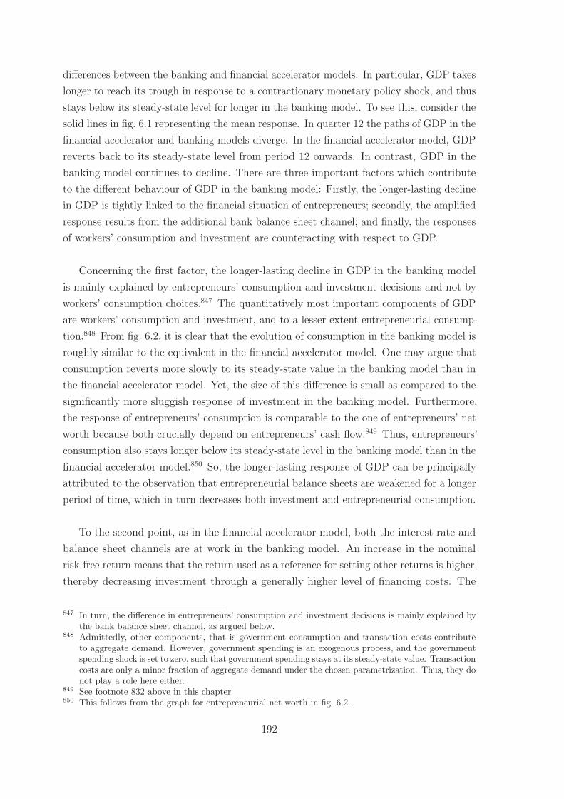
differences between the banking and financial accelerator models. In particular, GDP takeslonger to reach its trough in response to a contractionary monetary policy shock, and thusstays below its steady-state level for longer in the banking model. To see this, consider thesolid lines in fig. 6.1 representing the mean response. In quarter 12 the paths of GDP in thefinancial accelerator and banking models diverge. In the financial accelerator model, GDPreverts back to its steady-state level from period 12 onwards. In contrast, GDP in thebanking model continues to decline. There are three important factors which contributeto the different behaviour of GDP in the banking model: Firstly, the longer-lasting declinein GDP is tightly linked to the financial situation of entrepreneurs; secondly, the amplifiedresponse results from the additional bank balance sheet channel; and finally, the responsesof workers’ consumption and investment are counteracting with respect to GDP.

Concerning the first factor, the longer-lasting decline in GDP in the banking modelis mainly explained by entrepreneurs’ consumption and investment decisions and not byworkers’ consumption choices.847 The quantitatively most important components of GDPare workers’ consumption and investment, and to a lesser extent entrepreneurial consump-tion.848 From fig. 6.2, it is clear that the evolution of consumption in the banking model isroughly similar to the equivalent in the financial accelerator model. One may argue thatconsumption reverts more slowly to its steady-state value in the banking model than inthe financial accelerator model. Yet, the size of this difference is small as compared to thesignificantly more sluggish response of investment in the banking model. Furthermore,the response of entrepreneurs’ consumption is comparable to the one of entrepreneurs’ networth because both crucially depend on entrepreneurs’ cash flow.849 Thus, entrepreneurs’consumption also stays longer below its steady-state level in the banking model than in thefinancial accelerator model.850 So, the longer-lasting response of GDP can be principallyattributed to the observation that entrepreneurial balance sheets are weakened for a longerperiod of time, which in turn decreases both investment and entrepreneurial consumption.

To the second point, as in the financial accelerator model, both the interest rate andbalance sheet channels are at work in the banking model. An increase in the nominalrisk-free return means that the return used as a reference for setting other returns is higher,thereby decreasing investment through a generally higher level of financing costs. The

847 In turn, the difference in entrepreneurs’ consumption and investment decisions is mainly explained bythe bank balance sheet channel, as argued below.

848 Admittedly, other components, that is government consumption and transaction costs contributeto aggregate demand. However, government spending is an exogenous process, and the governmentspending shock is set to zero, such that government spending stays at its steady-state value. Transactioncosts are only a minor fraction of aggregate demand under the chosen parametrization. Thus, they donot play a role here either.

849 See footnote 832 above in this chapter850 This follows from the graph for entrepreneurial net worth in fig. 6.2.

192

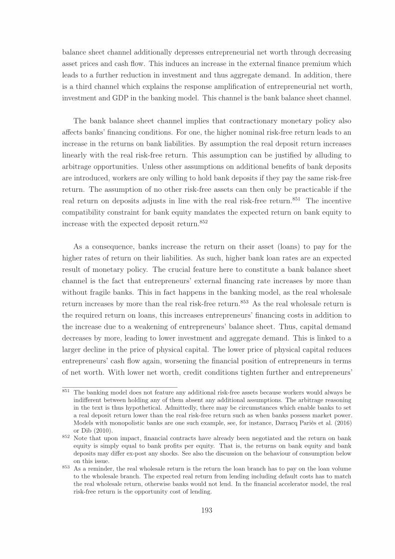
balance sheet channel additionally depresses entrepreneurial net worth through decreasingasset prices and cash flow. This induces an increase in the external finance premium whichleads to a further reduction in investment and thus aggregate demand. In addition, thereis a third channel which explains the response amplification of entrepreneurial net worth,investment and GDP in the banking model. This channel is the bank balance sheet channel.

The bank balance sheet channel implies that contractionary monetary policy alsoaffects banks’ financing conditions. For one, the higher nominal risk-free return leads to anincrease in the returns on bank liabilities. By assumption the real deposit return increaseslinearly with the real risk-free return. This assumption can be justified by alluding toarbitrage opportunities. Unless other assumptions on additional benefits of bank depositsare introduced, workers are only willing to hold bank deposits if they pay the same risk-freereturn. The assumption of no other risk-free assets can then only be practicable if thereal return on deposits adjusts in line with the real risk-free return.851 The incentivecompatibility constraint for bank equity mandates the expected return on bank equity toincrease with the expected deposit return.852

As a consequence, banks increase the return on their asset (loans) to pay for thehigher rates of return on their liabilities. As such, higher bank loan rates are an expectedresult of monetary policy. The crucial feature here to constitute a bank balance sheetchannel is the fact that entrepreneurs’ external financing rate increases by more thanwithout fragile banks. This in fact happens in the banking model, as the real wholesalereturn increases by more than the real risk-free return.853 As the real wholesale return isthe required return on loans, this increases entrepreneurs’ financing costs in addition tothe increase due to a weakening of entrepreneurs’ balance sheet. Thus, capital demanddecreases by more, leading to lower investment and aggregate demand. This is linked to alarger decline in the price of physical capital. The lower price of physical capital reducesentrepreneurs’ cash flow again, worsening the financial position of entrepreneurs in termsof net worth. With lower net worth, credit conditions tighten further and entrepreneurs’

851 The banking model does not feature any additional risk-free assets because workers would always beindifferent between holding any of them absent any additional assumptions. The arbitrage reasoningin the text is thus hypothetical. Admittedly, there may be circumstances which enable banks to seta real deposit return lower than the real risk-free return such as when banks possess market power.Models with monopolistic banks are one such example, see, for instance, Darracq Pariès et al. (2016)or Dib (2010).

852 Note that upon impact, financial contracts have already been negotiated and the return on bankequity is simply equal to bank profits per equity. That is, the returns on bank equity and bankdeposits may differ ex-post any shocks. See also the discussion on the behaviour of consumption belowon this issue.

853 As a reminder, the real wholesale return is the return the loan branch has to pay on the loan volumeto the wholesale branch. The expected real return from lending including default costs has to matchthe real wholesale return, otherwise banks would not lend. In the financial accelerator model, the realrisk-free return is the opportunity cost of lending.

193

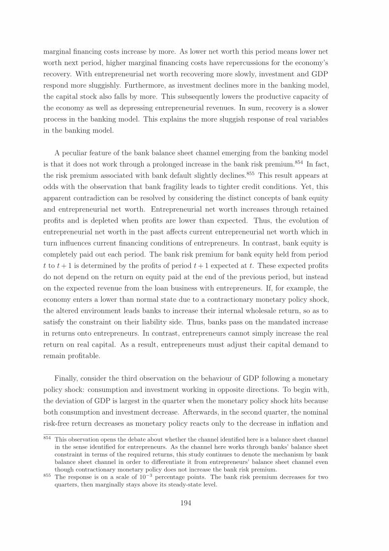
marginal financing costs increase by more. As lower net worth this period means lower networth next period, higher marginal financing costs have repercussions for the economy’srecovery. With entrepreneurial net worth recovering more slowly, investment and GDPrespond more sluggishly. Furthermore, as investment declines more in the banking model,the capital stock also falls by more. This subsequently lowers the productive capacity ofthe economy as well as depressing entrepreneurial revenues. In sum, recovery is a slowerprocess in the banking model. This explains the more sluggish response of real variablesin the banking model.

A peculiar feature of the bank balance sheet channel emerging from the banking modelis that it does not work through a prolonged increase in the bank risk premium.854 In fact,the risk premium associated with bank default slightly declines.855 This result appears atodds with the observation that bank fragility leads to tighter credit conditions. Yet, thisapparent contradiction can be resolved by considering the distinct concepts of bank equityand entrepreneurial net worth. Entrepreneurial net worth increases through retainedprofits and is depleted when profits are lower than expected. Thus, the evolution ofentrepreneurial net worth in the past affects current entrepreneurial net worth which inturn influences current financing conditions of entrepreneurs. In contrast, bank equity iscompletely paid out each period. The bank risk premium for bank equity held from periodt to t+ 1 is determined by the profits of period t+ 1 expected at t. These expected profitsdo not depend on the return on equity paid at the end of the previous period, but insteadon the expected revenue from the loan business with entrepreneurs. If, for example, theeconomy enters a lower than normal state due to a contractionary monetary policy shock,the altered environment leads banks to increase their internal wholesale return, so as tosatisfy the constraint on their liability side. Thus, banks pass on the mandated increasein returns onto entrepreneurs. In contrast, entrepreneurs cannot simply increase the realreturn on real capital. As a result, entrepreneurs must adjust their capital demand toremain profitable.

Finally, consider the third observation on the behaviour of GDP following a monetarypolicy shock: consumption and investment working in opposite directions. To begin with,the deviation of GDP is largest in the quarter when the monetary policy shock hits becauseboth consumption and investment decrease. Afterwards, in the second quarter, the nominalrisk-free return decreases as monetary policy reacts only to the decrease in inflation and

854 This observation opens the debate about whether the channel identified here is a balance sheet channelin the sense identified for entrepreneurs. As the channel here works through banks’ balance sheetconstraint in terms of the required returns, this study continues to denote the mechanism by bankbalance sheet channel in order to differentiate it from entrepreneurs’ balance sheet channel eventhough contractionary monetary policy does not increase the bank risk premium.

855 The response is on a scale of 10−3 percentage points. The bank risk premium decreases for twoquarters, then marginally stays above its steady-state level.

194

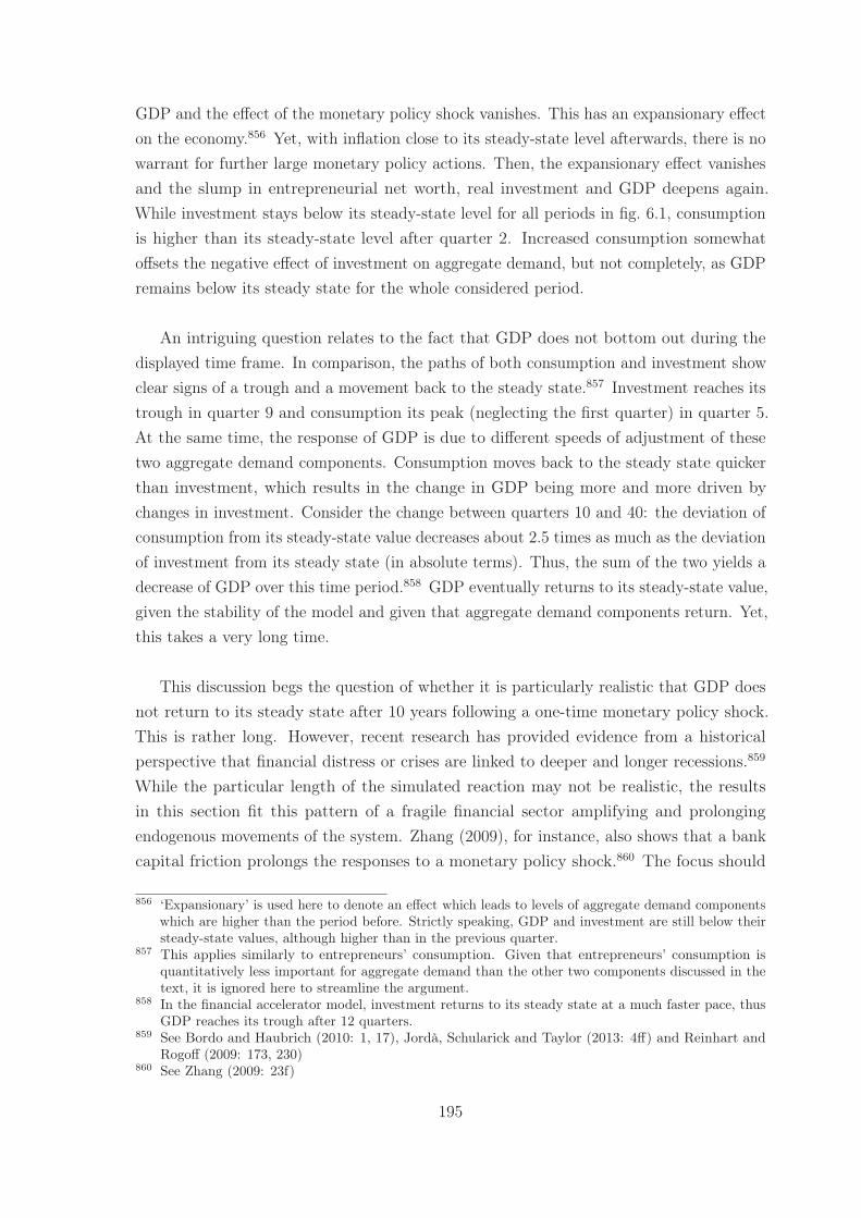
GDP and the effect of the monetary policy shock vanishes. This has an expansionary effecton the economy.856 Yet, with inflation close to its steady-state level afterwards, there is nowarrant for further large monetary policy actions. Then, the expansionary effect vanishesand the slump in entrepreneurial net worth, real investment and GDP deepens again.While investment stays below its steady-state level for all periods in fig. 6.1, consumptionis higher than its steady-state level after quarter 2. Increased consumption somewhatoffsets the negative effect of investment on aggregate demand, but not completely, as GDPremains below its steady state for the whole considered period.

An intriguing question relates to the fact that GDP does not bottom out during thedisplayed time frame. In comparison, the paths of both consumption and investment showclear signs of a trough and a movement back to the steady state.857 Investment reaches itstrough in quarter 9 and consumption its peak (neglecting the first quarter) in quarter 5.At the same time, the response of GDP is due to different speeds of adjustment of thesetwo aggregate demand components. Consumption moves back to the steady state quickerthan investment, which results in the change in GDP being more and more driven bychanges in investment. Consider the change between quarters 10 and 40: the deviation ofconsumption from its steady-state value decreases about 2.5 times as much as the deviationof investment from its steady state (in absolute terms). Thus, the sum of the two yields adecrease of GDP over this time period.858 GDP eventually returns to its steady-state value,given the stability of the model and given that aggregate demand components return. Yet,this takes a very long time.

This discussion begs the question of whether it is particularly realistic that GDP doesnot return to its steady state after 10 years following a one-time monetary policy shock.This is rather long. However, recent research has provided evidence from a historicalperspective that financial distress or crises are linked to deeper and longer recessions.859

While the particular length of the simulated reaction may not be realistic, the resultsin this section fit this pattern of a fragile financial sector amplifying and prolongingendogenous movements of the system. Zhang (2009), for instance, also shows that a bankcapital friction prolongs the responses to a monetary policy shock.860 The focus should

856 ‘Expansionary’ is used here to denote an effect which leads to levels of aggregate demand componentswhich are higher than the period before. Strictly speaking, GDP and investment are still below theirsteady-state values, although higher than in the previous quarter.

857 This applies similarly to entrepreneurs’ consumption. Given that entrepreneurs’ consumption isquantitatively less important for aggregate demand than the other two components discussed in thetext, it is ignored here to streamline the argument.

858 In the financial accelerator model, investment returns to its steady state at a much faster pace, thusGDP reaches its trough after 12 quarters.

859 See Bordo and Haubrich (2010: 1, 17), Jordà, Schularick and Taylor (2013: 4ff) and Reinhart andRogoff (2009: 173, 230)

860 See Zhang (2009: 23f)

195

thus be on the direction of the effects, while their absolute size and the resulting ab-solute time it takes for GDP to return to its steady state should be interpreted with caution.

The findings on the different responses in the financial accelerator and banking modelsare roughly in line with previous findings in the literature. The observation that thebank balance sheet channel affects the response of GDP while the one of inflation is notchanged significantly is in line with the econometric results of Ciccarelli et al. (2013).Based on a panel vector autoregression (VAR) using Euro area (EA) data, Ciccarelli et al.(2013) show that the response of GDP to a monetary policy shock varies over time andwas particularly strong during the financial crisis 2008-09.861 In contrast, the responseof inflation was comparatively uniform over time.862 Also, the amplification effect of thebank balance sheet channel generally agrees with findings from the DSGE-model-basedliterature.863 In the model by Markovic (2006), for instance, an additional bank-specificfinancial friction induces a stronger reaction of investment and GDP.864 Furthermore,the amplification effect of bank-based financial frictions has also been found in studieswith different assumptions about the nature of bank capital. Davis (2010), for example,show that a financial accelerator friction and a bank capital friction each amplify theresponse of GDP and investment to roughly the same extent, although the differences arequantitatively small.865

Usually, the impulse response function of consumption shows it to be decreasing for aprolonged period of time after a monetary policy shock.866 While the simulated response ofconsumption here is unusual, it is not unprecedented. In fact, the behaviour of consumptionpresented here is in line with the simulation results of Markovic (2006). The results inMarkovic (2006) suggest that consumption does not respond very differently comparing amodel with only an entrepreneurial balance sheet channel with a model which featuresan exogenous probability of bank default affecting the return on bank equity.867 Similarto fig. 6.2, consumption decreases upon impact of the contractionary monetary policy

861 See Ciccarelli et al. (2013: 21)862 See Ciccarelli et al. (2013: 21)863 The model-based literature has also found results which differ in terms of the additional effect of bank

default. Angeloni and Faia (2009: 15) and Meh and Moran (2004: 29), for example, find that bankdefault leads to a dampening effect on GDP. In Angeloni and Faia (2009) bank default occurs due tobank runs and they relate the dampening effect to relationship lending, see Angeloni and Faia (2009:2f, 15). Similarly, in Meh and Moran (2004: 11) bank default is due to insufficient diversification onthe part of banks. While the overall effect is dampened, their bank friction induces higher persistenceof investment in response to a contractionary monetary policy shock, which is in fact in line with theresults of this study, see Meh and Moran (2004: 30).

864 See Markovic (2006: 30)865 See Davis (2010: 25f, 56). Yet, Davis (2010) does not find a notable difference in terms of the duration

of deviations from the steady state or dissimilar effects on inflation and GDP.866 See, for instance, Gadatsch et al. (2015: 31)867 See Markovic (2006: 30)

196

shock, but subsequently shows a positive hump-shaped response in both cases in Markovic(2006).868 Furthermore, for a bank-based financial friction to affect mainly investment andto a lesser extent consumption has been shown in the literature, for example in Zhang(2009) where households also hold bank equity and bank deposits.869

So why does consumption show this pattern, and why does bank default not fun-damentally affect the path? The explanation lies partly in parameter estimates whichallow consumption to respond promptly to standard wealth and substitution effects. Thesubstitution effect outweighs the wealth effect initially, and vice versa over the long term.As real returns rise following the shock, workers save more and reduce their consumption.Subsequently, the central bank reduces the nominal risk-free return as it observes loweroutput and inflation. Thus, with higher wealth and the substitution effect inducing higherconsumption today, workers’ consumption rises. Real returns subsequently stay close totheir steady-state levels, but worker’s wealth has increased, such that the positive wealtheffect on consumption is still present but gradually phases out. Conversely, with higherhabit persistence and a higher share of consumption in the utility function, coupled witha stickier inflation response, a standard hump-shaped response of workers’ consumptioncould also arise in the banking model.

The other part of the explanation for the behaviour of consumption relates back tothe discussion about dynamic IS (DIS) curves and monetary policy in chapter 4. TheDIS curve is derived from workers’ optimisation problem and the economy’s resourceconstraint. The main difference of the DIS curves in the banking and financial acceleratormodels concerned the presence of the real portfolio return in the former and the realrisk-free return in the latter. Yet, this section showed that workers’ consumption does notevolve very differently in the banking and financial accelerator models. The reason for thissimilarity is that the real portfolio return in the banking model and the real risk-free returnin the financial accelerator model evolve similarly, although not identically. The incentivecompatibility constraint facing banks’ liability management states that the expected realbank equity return needs be equal to the expected real deposit return. Yet, even thoughworkers’ expect the remuneration on bank equity and bank deposits to be equal, thisalso means that the real bank equity return may differ ex-post shock realisations fromits ex-ante expectation and from the real deposit return. However, these differences aregenerally rather small, given that the effects of small shocks are analysed in vicinity ofthe steady state. While, for example, the real portfolio return does not increase as muchas the real deposit return in the banking model following a monetary policy shock, thedifference is not large enough to induce a substantially different consumption behaviour.

868 See Markovic (2006: 30)869 See Zhang (2009: 23)

197

The fact that the difference between the DIS curves in terms of returns does not yieldnoticeable differences may be taken as a weakness of the modelling approach. Alternatively,this observation may rather be interpreted as showing that the banking model does notcreate any synthetic arbitrage opportunities. In the financial accelerator model, workers’consumption/saving choice is directly anchored at the real risk-free rate. Chapter 4argued that this link is not as direct in the banking model because only part of workers’portfolio consists of the risk-free asset. However, the fact that bank equity has to paythe same return including default costs, the link between the real risk-free return andworkers’ consumption/saving choice is still intact. Thus, the real portfolio return does notdiffer systematically from the real risk-free rate ensuring that there are no free arbitrageopportunities.

This also means that workers cannot expect to earn a real return on their portfoliowhich is higher than the real risk-free return by investing in riskier bank equity. For one,absent further assumptions or restrictions, a higher return of either bank deposits or bankequity would make workers want to hold only one of the assets, that is the one whichis remunerated more highly. Moreover, the derivation of the bank risk premium ensuresthat equity-holders are exactly compensated for the risk of bank default and low bankprofits in expectations. There are no other differences between bank deposits and bankequity (other than the risk of default or low profits) which would warrant a further spreadbetween the two respective returns. Nevertheless, deriving the bank risk premium solely asa consequence of bank default can only be a partial explanation. The explanation of theequity premium in this study by default risk only should be seen as one aspect. Furtheraspects certainly play a role and have been used in the literature to motivate a spreadbetween bank equity and other bank liabilities.870 Instead of a mere weakness, the focuson one explanation for the bank risk premium is a benefit for discerning the impact ofnon-systemic bank default. It shows that even though the real portfolio return does notbehave very differently from the real risk-free return, small changes can have significanteffects for the decision-making process of banks, the financing costs of entrepreneurs andeventually aggregate demand.

It may be argued that the marginal effect on consumption is related to the specific formof the government budget. After all, the government in the banking model is confined to abalanced budget. Furthermore, the assumptions about taxes guarantee that private agents’optimality conditions are unaffected by changes in taxes in the log-linear approximation.However, the general results presented above hold for the case when workers’ tax rate

870 See, for example, the discussion in section 2.5.

198

changes with the budgetary position of the government.871 Adjusting the relevant equationsmeans that the labour market clearing condition is affected by changes in income taxesdue to changing governmental outlays.872 However, leisure and consumption decisions arestill separate from the portfolio choice decision. Thus, modelling endogenous taxes in thisway merely opens up another avenue through which financial frictions affect the economy:namely, the labour market.

Assume, for instance, that government expenditures increase. Since the governmentis confined to a balanced budget, this necessitates higher tax income. Therefore, the taxrate increases, ceteris paribus. Increased tax rates affect workers’ labour/consumptionchoice: per hour worked, they receive less wage income, ceteris paribus, which tends toreduce consumption. The additional channel is evidenced by the fact that the impact of amonetary policy shock on GDP is somewhat stronger in the financial accelerator modelwith endogenous taxes than in the benchmark financial accelerator model. Somewhatsurprisingly, the effect works in the opposite direction for the banking model: the impulseresponse function for GDP shifts upwards in parallel. This means, that in the short term,the deviation of GDP from its steady state is smaller in the banking model with endogenoustaxes than in the corresponding endogenous-tax financial accelerator model, but over thelong term it is larger in the endogenous-tax banking model, because the response of GDPis generally longer-lasting in the banking model. The asymmetric effect of endogenisingtaxes in these two models is due to different characterisations of the government budget.In the banking model, deposit insurance fees increase as a result of increased depositholdings, which counters the adverse effects of increased deposit insurance outlays in theshort term. Thus, tax rates counter-intuitively decrease in the banking model following amonetary policy shock, thus yielding a dampened response with respect to the exogenoustax banking model. The fundamental channel pointed to above, however, is the same asin the financial accelerator model, merely in the opposite direction.

If there is a link between the government budget, taxes and workers’ optimality condi-tions, why is this not already included in the benchmark banking model? Firstly, the resultthat the banking model yields a long-term amplified, and longer-lasting response of outputfollowing a monetary policy shock with respect to the financial accelerator model holdsirrespective of whether income taxes are exogenous or endogenous to the decision-makingof workers. So, endogenous taxes can be interpreted as a secondary factor in discerning theconsequences of bank default. Related, it may be argued that the treatment of workers’optimality conditions should be connected more generally, that is leisure and consumption

871 Since the benchmark banking model does not feature capital taxes at all, only labour income taxesare discussed.

872 Instead of the log-linear approximation to eq. (3.76), the equation used for this experiment iswt − pt = −uh,t − uc,t + τ/(1− τ)τt where τ is the steady-state income tax rate.

199

decisions should be linked to workers’ portfolio choice. In fact, in the banking model, theaggregate volume of workers’ saving is connected to the consumption decision. However,the crucial mechanism in the banking model concerns the composition of workers’ saving. Itis not clear in which way holding either bank deposits or bank equity should be connectedto the consumption/leisure decision other than through the return on workers’ portfolio.Another option to link the government’s budget to the portfolio choice problem wouldbe through taxes on capital income. Yet, this relates to the third reason why taxes arekept exogenous in the banking model: a more elaborate modelling of taxes necessitatesa more thorough treatment of the government’s budget, including the decision betweendebt and tax financing. Such a more thorough treatment would then also discern whetherabove mentioned behaviour of taxes (and tax rates) in the banking model holds for a morerealistic setting of government finances. Thus, an interesting avenue of future research isthe link between fiscal and monetary policies in economies with fragile banking sectors.

Finally, the question arises whether the disparate behaviour of the economy in thefinancial accelerator and banking models is due to the different size of the total creditspread. To this end, the following experiment was conducted: increase the monitoring costparameter μE in the financial accelerator model, such that the credit spread in the financialaccelerator model is roughly equal to the total credit spread in the banking model.873

The impulse responses of real variables to a contractionary monetary policy shock in thislarge-credit-spread financial accelerator model are amplified with respect to the benchmarkfinancial accelerator model. The largest deviation of GDP from its steady state is morethan twice the one of the benchmark financial accelerator model.874 Furthermore, GDPreaches its trough only after about 30 quarters. Thus, the deviation of GDP from itssteady state lasts longer in the large-credit-spread financial accelerator model, but not aslong as in the banking model. Furthermore, while the absolute deviation of GDP from itssteady state is comparable for the benchmark financial accelerator and banking models forthe first quarters, the absolute deviation is much larger in the large-credit-spread financialaccelerator model.

There are a few noteworthy conclusions to draw from this. Firstly, the share of thecredit spread due to the entrepreneurial risk premium impacts the size of the response ofreal variables to a monetary policy shock to a large extent. Conversely, this means that itis not so much the reaction of the credit spread which affects the strength of monetarytransmission, but rather the origin of this credit spread. As a corollary, the increase intransaction costs which is necessary to yield a certain increase in the credit spread is muchlarger for the friction between entrepreneurs and banks than for the friction between banks

873 More precisely, μE changes to 0.051, resulting in a steady state credit spread of 3.48%.874 Inflation and the nominal risk-free return do not respond materially differently.

200

and equity-holders. However, while the bank risk premium may not have a large impactin terms of the largest absolute deviation from the steady state, it does affect the time ittakes for the economy to return to its steady state. While the deviation of, for example,investment and entrepreneurs’ net worth from their respective steady states is larger in thelarge-credit-spread financial accelerator model than in the banking model, investment andentrepreneurs’ net worth return to their respective steady states at a faster speed in thelarge-credit-spread financial accelerator model. In fact, the deviation of entrepreneurs’ networth from its steady state is smaller in the large-credit-spread financial accelerator modelthan in the banking model from (roughly) quarter 24 onwards. Thus, this experimentfurther underscores the finding that the incidence of bank default prolongs the responsesof endogenous variables, which is in line with results in the literature cited above.

To summarise, the fundamental mechanisms at work in the financial accelerator modelare also present in the banking model. Additionally, non-systemic bank default gives riseto a bank balance sheet channel in the banking model. The bank balance sheet channelamplifies and prolongs the responses to a monetary policy shock of real variables pertainingto entrepreneurs’ decision-making. In contrast, the existence of bank default does notaffect workers’ consumption materially. A second conclusion relates to the discussion ofparameter estimates in chapter 5. Low (estimated) nominal (price) stickiness leads toa quick return of inflation to its steady-state value after a monetary policy shock. Incontrast, real variables exhibit sluggish behaviour despite the comparatively low estimatesof real friction parameters.875 Therefore, the results concerning the additional bank-specificfriction underscore the argument that financial frictions prolong endogenous developmentsof aggregate demand components.

What do these results imply for the conduct of monetary policy? For one, the way inwhich a monetary policy impulse is transmitted to inflation is not significantly affectedby the introduction of non-systemic bank default. Whether the model exhibits bankdefault or not, the path of inflation in response to monetary policy shocks does not change.Simultaneously, if the central bank engages in flexible inflation targeting so as to moderate(contractionary) effects on GDP, the incidence of bank default indicates that a givenmonetary impulse has quantitatively larger effects on real variables. Furthermore, thereare two reasons for considering bank default even if the inflation rate is the only objectivefor the central bank. First, to the extent that monetary policy affects inflation throughinfluencing aggregate demand, these results imply that the central bank has to inducea larger and longer-lasting decline in GDP for the same response of inflation to occur.The second reason is presented in section 6.2 concerning the central bank’s capabilities

875 These include, for example, the habit persistence parameter χ and the investment adjustment costparameter φI .

201

with respect to stabilising inflation (and the output gap). However, before analysing theconsequences for monetary policy from a different angle, the next section tries to illuminatethe underlying mechanism with two more experiments: the impact of steady-state fragilityand the importance of the roll-over nature of bank equity.

6.1.2 Monetary Policy Transmission, Banks’ Default Probability

and Equity Habits

This section assesses the impact of the severity of steady-state bank fragility and impedi-ments to instantaneous portfolio adjustments on the dynamic adjustments to a monetarypolicy shock. To this end, the experiment of an unexpected, one-off contractionary shockto the monetary policy rule is repeated with different assumptions about the steady-stateprobability of bank default and workers’ asset demand equations.876 Otherwise, the set-upand the assumptions concerning monetary policy shocks and other shocks are the same asin section 6.1.1.

Concerning the first experiment, two cases are considered: a high and a low fragilitystate. In the high fragility banking model the steady-state default probability p(ψ

B) is set

to 0.1. In the low fragility banking model p(ψB) is set to 1 ∗ 10−7. These alternative values

for p(ψB) are somewhat arbitrary. The objective was to choose a lower and a higher value

than the benchmark calibration. The high fragility value can be deemed a speculativeupper bound. For instance, considering the US between 1973 and 2015, the assets of failedbanks as a share of total assets reached a maximum of about 5.4% in 1989.877 Duringthe financial crisis of 2007-8 this ratio peaked at around 3.3% in 2008.878 On the otherhand, the low fragility value can be interpreted as the other extreme in which banks donot actually default. Note that in this case banks are still constrained by the incentivecompatibility constraint of equity-holders.

Figure 6.3 depicts the reactions of GDP, the nominal risk-free return and inflation toa contractionary monetary policy shock. The blue line depicts the reaction under thebenchmark parametrization. Note that in contrast to figs. 6.1 and 6.2, these lines tracethe reaction of the banking model at the posterior mean of the parameter vector. As the

876 Note that the banks’ probability of default is equal to the share of failing banks in a given period, seefootnote 845.

877 See Federal Deposit Insurance Corporation (2015), URL in list of references, and Board of Governorsof the Federal Reserve System (2015), URL in list of references, for data; own computations based onyearly aggregation. In the banking model all banks are alike. Thus, the assets of failed banks as ashare of total assets of the banking sector can be taken as a guide for the fraction of all banks failingin any given period in the banking model.

878 See Federal Deposit Insurance Corporation (2015), URL in list of references, and Board of Governorsof the Federal Reserve System (2015), URL in list of references, for data; own computations based onyearly aggregation.

202

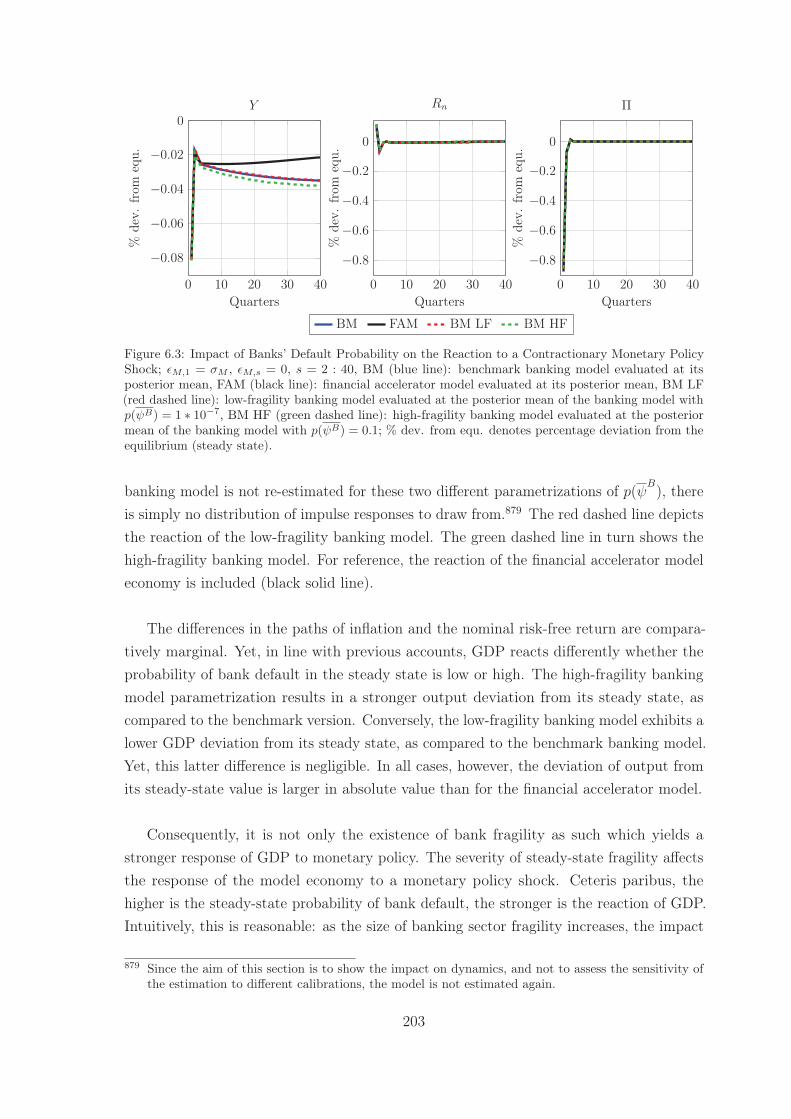
0 10 20 30 40

−0.08

−0.06

−0.04

−0.02

0

Quarters

%de

v.fr

omeq

u.

Y

0 10 20 30 40

−0.8

−0.6

−0.4

−0.2

0

Quarters

%de

v.fr

omeq

u.

Rn

0 10 20 30 40

−0.8

−0.6

−0.4

−0.2

0

Quarters

%de

v.fr

omeq

u.

Π

BM FAM BM LF BM HF

Figure 6.3: Impact of Banks’ Default Probability on the Reaction to a Contractionary Monetary PolicyShock; εM,1 = σM , εM,s = 0, s = 2 : 40, BM (blue line): benchmark banking model evaluated at itsposterior mean, FAM (black line): financial accelerator model evaluated at its posterior mean, BM LF(red dashed line): low-fragility banking model evaluated at the posterior mean of the banking model withp(ψB) = 1 ∗ 10−7, BM HF (green dashed line): high-fragility banking model evaluated at the posteriormean of the banking model with p(ψB) = 0.1; % dev. from equ. denotes percentage deviation from theequilibrium (steady state).

banking model is not re-estimated for these two different parametrizations of p(ψB), there

is simply no distribution of impulse responses to draw from.879 The red dashed line depictsthe reaction of the low-fragility banking model. The green dashed line in turn shows thehigh-fragility banking model. For reference, the reaction of the financial accelerator modeleconomy is included (black solid line).

The differences in the paths of inflation and the nominal risk-free return are compara-tively marginal. Yet, in line with previous accounts, GDP reacts differently whether theprobability of bank default in the steady state is low or high. The high-fragility bankingmodel parametrization results in a stronger output deviation from its steady state, ascompared to the benchmark version. Conversely, the low-fragility banking model exhibits alower GDP deviation from its steady state, as compared to the benchmark banking model.Yet, this latter difference is negligible. In all cases, however, the deviation of output fromits steady-state value is larger in absolute value than for the financial accelerator model.

Consequently, it is not only the existence of bank fragility as such which yields astronger response of GDP to monetary policy. The severity of steady-state fragility affectsthe response of the model economy to a monetary policy shock. Ceteris paribus, thehigher is the steady-state probability of bank default, the stronger is the reaction of GDP.Intuitively, this is reasonable: as the size of banking sector fragility increases, the impact

879 Since the aim of this section is to show the impact on dynamics, and not to assess the sensitivity ofthe estimation to different calibrations, the model is not estimated again.

203

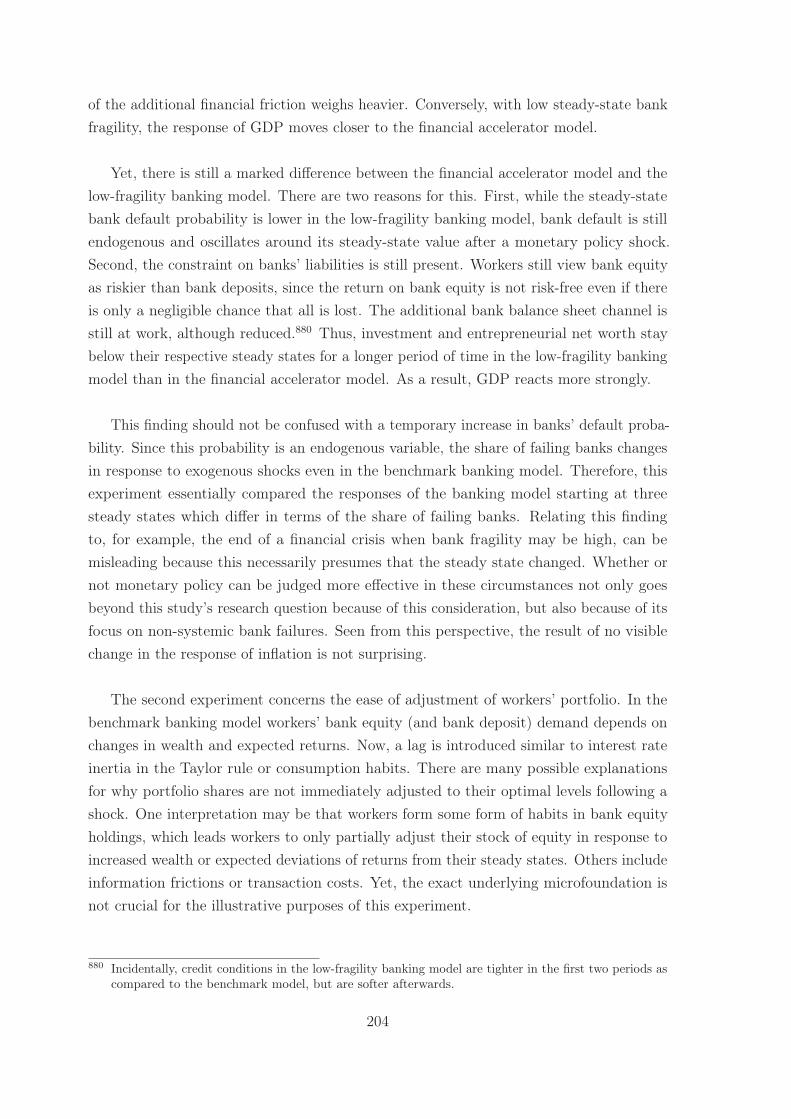
of the additional financial friction weighs heavier. Conversely, with low steady-state bankfragility, the response of GDP moves closer to the financial accelerator model.

Yet, there is still a marked difference between the financial accelerator model and thelow-fragility banking model. There are two reasons for this. First, while the steady-statebank default probability is lower in the low-fragility banking model, bank default is stillendogenous and oscillates around its steady-state value after a monetary policy shock.Second, the constraint on banks’ liabilities is still present. Workers still view bank equityas riskier than bank deposits, since the return on bank equity is not risk-free even if thereis only a negligible chance that all is lost. The additional bank balance sheet channel isstill at work, although reduced.880 Thus, investment and entrepreneurial net worth staybelow their respective steady states for a longer period of time in the low-fragility bankingmodel than in the financial accelerator model. As a result, GDP reacts more strongly.

This finding should not be confused with a temporary increase in banks’ default proba-bility. Since this probability is an endogenous variable, the share of failing banks changesin response to exogenous shocks even in the benchmark banking model. Therefore, thisexperiment essentially compared the responses of the banking model starting at threesteady states which differ in terms of the share of failing banks. Relating this findingto, for example, the end of a financial crisis when bank fragility may be high, can bemisleading because this necessarily presumes that the steady state changed. Whether ornot monetary policy can be judged more effective in these circumstances not only goesbeyond this study’s research question because of this consideration, but also because of itsfocus on non-systemic bank failures. Seen from this perspective, the result of no visiblechange in the response of inflation is not surprising.

The second experiment concerns the ease of adjustment of workers’ portfolio. In thebenchmark banking model workers’ bank equity (and bank deposit) demand depends onchanges in wealth and expected returns. Now, a lag is introduced similar to interest rateinertia in the Taylor rule or consumption habits. There are many possible explanationsfor why portfolio shares are not immediately adjusted to their optimal levels following ashock. One interpretation may be that workers form some form of habits in bank equityholdings, which leads workers to only partially adjust their stock of equity in response toincreased wealth or expected deviations of returns from their steady states. Others includeinformation frictions or transaction costs. Yet, the exact underlying microfoundation isnot crucial for the illustrative purposes of this experiment.

880 Incidentally, credit conditions in the low-fragility banking model are tighter in the first two periods ascompared to the benchmark model, but are softer afterwards.

204

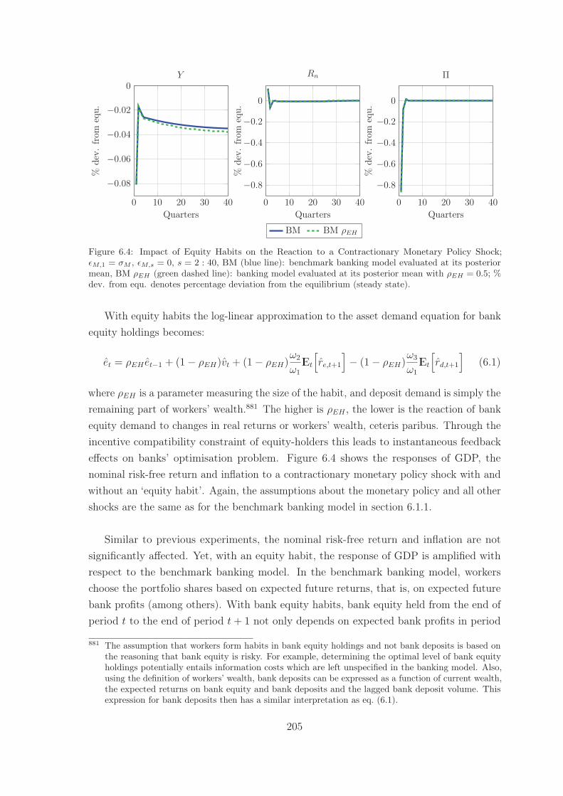
0 10 20 30 40

−0.08

−0.06

−0.04

−0.02

0

Quarters

%de

v.fr

omeq

u.

Y

0 10 20 30 40

−0.8

−0.6

−0.4

−0.2

0

Quarters

%de

v.fr

omeq

u.

Rn

0 10 20 30 40

−0.8

−0.6

−0.4

−0.2

0

Quarters

%de

v.fr

omeq

u.

Π

BM BM ρEH

Figure 6.4: Impact of Equity Habits on the Reaction to a Contractionary Monetary Policy Shock;εM,1 = σM , εM,s = 0, s = 2 : 40, BM (blue line): benchmark banking model evaluated at its posteriormean, BM ρEH (green dashed line): banking model evaluated at its posterior mean with ρEH = 0.5; %dev. from equ. denotes percentage deviation from the equilibrium (steady state).

With equity habits the log-linear approximation to the asset demand equation for bankequity holdings becomes:

et = ρEH et−1 + (1− ρEH)vt + (1− ρEH)ω2

ω1

IEt

[re,t+1

]− (1− ρEH)

ω3

ω1

IEt

[rd,t+1

](6.1)

where ρEH is a parameter measuring the size of the habit, and deposit demand is simply theremaining part of workers’ wealth.881 The higher is ρEH , the lower is the reaction of bankequity demand to changes in real returns or workers’ wealth, ceteris paribus. Through theincentive compatibility constraint of equity-holders this leads to instantaneous feedbackeffects on banks’ optimisation problem. Figure 6.4 shows the responses of GDP, thenominal risk-free return and inflation to a contractionary monetary policy shock with andwithout an ‘equity habit’. Again, the assumptions about the monetary policy and all othershocks are the same as for the benchmark banking model in section 6.1.1.

Similar to previous experiments, the nominal risk-free return and inflation are notsignificantly affected. Yet, with an equity habit, the response of GDP is amplified withrespect to the benchmark banking model. In the benchmark banking model, workerschoose the portfolio shares based on expected future returns, that is, on expected futurebank profits (among others). With bank equity habits, bank equity held from the end ofperiod t to the end of period t+ 1 not only depends on expected bank profits in period

881 The assumption that workers form habits in bank equity holdings and not bank deposits is based onthe reasoning that bank equity is risky. For example, determining the optimal level of bank equityholdings potentially entails information costs which are left unspecified in the banking model. Also,using the definition of workers’ wealth, bank deposits can be expressed as a function of current wealth,the expected returns on bank equity and bank deposits and the lagged bank deposit volume. Thisexpression for bank deposits then has a similar interpretation as eq. (6.1).

205

t+ 1, but also on bank profits of period t expected at the end of period t− 1. This leadsthe past to affect future (portfolio) decisions. Thus, the stronger effect on GDP is due toworkers’ sticky portfolios and the resulting adjustment lags.882

This simple experiment elucidates the consequences of frictions in portfolio adjustmentsand/or raising new bank equity.883 A similar result arises in Markovic (2006), wherethe introduction of equity adjustment costs to a model with bank default triggers anamplification of the output response.884 The finding of the banking model with equityhabits suggest that the consequences of bank default are less severe, for investment andGDP among others, if there are no impediments in adjusting portfolio shares. Furthermore,sluggish portfolio adjustment appears to make it more difficult for banks to service theirliability commitments as credit conditions tighten more in this case.885 This again relatesto the results of Kiley and Sim (2014). In their model, sudden increases in the costs ofissuing new equity lead to declines in investment and output.886 Overall, the frictionon banks’ liability side becomes more severe when there are further obstacles or costsassociated with an immediate adjustment to new conditions.

Summing up these two experiments, the more probable bank default is, that is thehigher is the share of failing banks in a given period, the higher is the impact of monetarypolicy on GDP. Yet, given the small differences between the benchmark case and the lowfragility banking model, the effects are rather small when the probability of bank default isalready small. This implies that merely reducing steady-state fragility does not remove thedynamic effects of bank default. Secondly, including habits in the adjustment of portfolioshares also amplifies the effect on GDP in the banking model. Supporting the findings insection 6.1.1, the path of inflation remains almost unchanged. The results of this sectionthen imply that consideration for the effects of monetary policy on aggregate demandis more important when banking sector fragility is high and when there are frictions inportfolio adjustments.

882 Note that the bank risk premium does not behave very differently when equity habits are present. Asfor the benchmark banking model, banks increase interest rates on the asset side in line with theirliability side leading to the stronger effect on entrepreneurs’ capital demand and eventually GDP.

883 This may also be related to instability - determinacy boundary findings for different asset demandfunction parameters. As shown in section 4.4.3, a higher equity share in workers’ wealth increased theinstability region (see fig. 4.3). Ceteris paribus, a higher equity share lowers the coefficients of workers’equity demand on the respective returns. Equity habits have the same effect on these coefficients.Thus, the larger instability region may be related to stronger responses of the models’ endogenousvariables to exogenous shocks.

884 See Markovic (2006: 30)885 Over the first few quarters following the shock, sometimes the model with, and sometimes the model

without bank equity habits induces tighter credit conditions. Over the medium to long term, it is themodel with equity habits which features tighter credit conditions than the model without.

886 See Kiley and Sim (2014: 186f)

206

6.1.3 Importance of Monetary Policy Shocks for the Model Econ-

omy

To gauge the importance of monetary policy shocks as well as of other shocks includedin the banking model, this section presents the results of the forecast error variancedecomposition (FEVD) analysis.887 There are two reasons for conducting this analysis.First, the estimates of the standard deviations of the various shocks in chapter 5 showedsignificant differences. Thus, the question is whether these differences resurface consideringthe importance for the dynamics of the model economy. Second, the previous sectionsanalysed the transmission of monetary policy shocks. Then, the question arises whethermonetary policy shocks are important in their own right, or whether the analysis wasmerely an illustrative device.

The FEVD is a means to quantify the relative impact of different exogenous shocks.In particular, an FEVD shows the fractions of the forecast error variance of a variable dueto individual shocks.888 On a technical note, the FEVD is calculated from the movingaverage representation of the model.889 The forecast error is then the difference betweenthe value at time t+ s and its expectation at time t, where s is the forecast horizon.890

In this experiment, a shock can be considered important if it contributes significantlyto the forecast error variance. This again is not definite as to what may be deemedsignificant. However, the objective of this section is to compare the shocks’ importancewith respect to each other. Thus, the exercise is inherently relational and as such, thissection aims to discern on whether there are many shocks which are equally important,or whether there is only a single very important shock, and which these are. Table 6.1displays the FEVD for the horizons 1, 8, 20 and 32. These forecast horizons roughlycorrespond to the business cycle, indicating the importance of various shocks in the shortterm (horizon 1), medium term (horizons 8 and 20) and the long term (horizon 32). TheFEVD is reported for variables which were matched to observables in the estimation process.

First consider the variables which form the core of DSGE models: GDP, inflation andthe real risk-free return. GDP is mainly driven by innovations in technology εA whichexplain more than half of the forecast error variance. The remaining forecast error varianceis explained by a bundle of other shocks which changes over time. The second largestcontributor only reaches between 10% and 15% of the forecast error variance at any horizon.

887 A historical decomposition of the error variance would be another means to this end. However, ahistorical decomposition would be more constrained in the sense that shock sequences are matched tothe estimation data, while the FEVD allows for a more general interpretation of the importance ofshocks in the banking model.

888 See Lütkepohl (2005: 64)889 See Fernández-Villaverde, Rubio-Ramírez and Schorfheide (2016: 123f)890 See Fernández-Villaverde et al. (2016: 123)

207

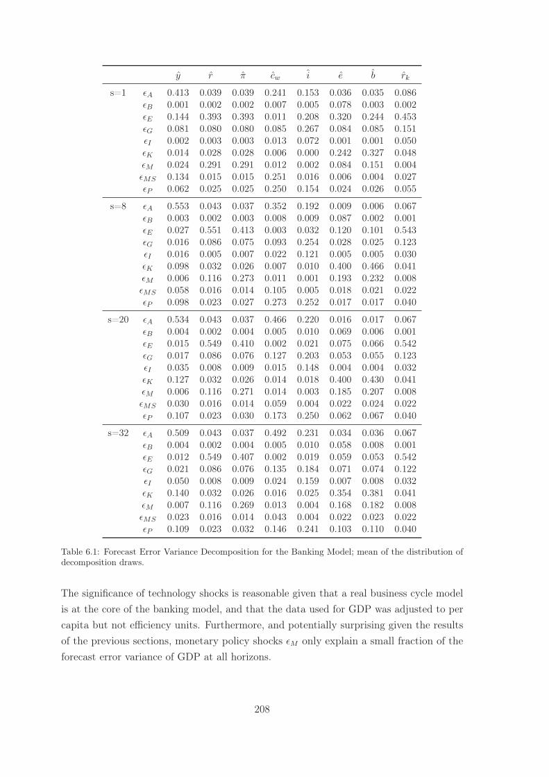
y r π cw i e b rk

s=1 εA 0.413 0.039 0.039 0.241 0.153 0.036 0.035 0.086εB 0.001 0.002 0.002 0.007 0.005 0.078 0.003 0.002εE 0.144 0.393 0.393 0.011 0.208 0.320 0.244 0.453εG 0.081 0.080 0.080 0.085 0.267 0.084 0.085 0.151εI 0.002 0.003 0.003 0.013 0.072 0.001 0.001 0.050εK 0.014 0.028 0.028 0.006 0.000 0.242 0.327 0.048εM 0.024 0.291 0.291 0.012 0.002 0.084 0.151 0.004εMS 0.134 0.015 0.015 0.251 0.016 0.006 0.004 0.027εP 0.062 0.025 0.025 0.250 0.154 0.024 0.026 0.055




Table 6.1: Forecast Error Variance Decomposition for the Banking Model; mean of the distribution ofdecomposition draws.

The significance of technology shocks is reasonable given that a real business cycle modelis at the core of the banking model, and that the data used for GDP was adjusted to percapita but not efficiency units. Furthermore, and potentially surprising given the resultsof the previous sections, monetary policy shocks εM only explain a small fraction of theforecast error variance of GDP at all horizons.

208

This is in stark contrast to inflation and the real risk-free return. In both cases, mone-tary policy shocks contribute about 30% to the forecast error variance in the short term.This share stays roughly constant over the medium and long term for inflation. In contrast,the corresponding share for the real risk-free return declines substantially over the mediumand long term. To put this observation into perspective, consider again the impulseresponse analysis of section 6.1.1. After a monetary policy shock, the impact on inflationand the real risk-free return dissipates quickly, while the effect on GDP is long-lasting.891

The FEVD suggests that monetary policy shocks contribute very little to the forecast errorvariance of GDP, but very much to the forecast error variance of inflation and the realreturn. Taking a closer look at the scales of fig. 6.1, however, might indicate the reasonfor this apparent conflict: while GDP decreases by only about 0.1% due to a one standarddeviation monetary policy shock, inflation decreases by 1%. Thus, a monetary policyshock has a larger impact on inflation than on output in percentage terms. There are othershocks which have a larger quantitative effect on GDP than the monetary policy shock, forinstance a technology shock.892 Thus, the apparently conflicting results can be reconciled.893

Surprisingly, the other and in fact major contributor to the forecast error varianceof both inflation and the real risk-free return is the entrepreneurial risk shock εE. Oneexplanation may be the estimated size of the standard deviation. The standard deviationof εE is estimated to be about 3 times larger than the one of government consumptionshocks, and roughly 10 times larger than the one of monetary policy shocks. Yet, thiscan hardly be the only reason. The standard deviation of the investment adjustment costshock εI was estimated twice the size of εE, and εI only marginally contributes to thevariance decomposition of any of these three endogenous variables. Again, the quantitativereaction to such a shock plays a role. Upon impact of εI , the percentage change in inflationis 0.12%. The entrepreneurial risk shock increases inflation by 0.90% upon impact.894 Thedifference in size is similar for the real risk-free return. Conversely, the low shares of εImay be connected to the low estimates of the adjustment cost parameter φI . Even thislarge shock interval implies only moderate investment adjustment costs, because φI iscomparatively low.895 Thus, while the estimated size of the shock may not provide a goodexplanation, the sizes and responses of the parameters and variables affected by the shockmay provide more intuition.

891 Note that while the response of the real risk-free return was not depicted, the corresponding short-livedreaction is a consequence of the responses of inflation and the nominal risk-free return, as noted insection 6.1.1.

892 See fig. D.1 in appendix section D.1 for a graphical comparison of the impulse response functions totechnology and monetary policy shocks.

893 Note that this does not moderate the importance of the results in section 6.1.1 since there the focusis on how monetary policy shocks are transmitted through the model economy.

894 In both cases inflation is below its steady state in subsequent quarters.895 See section 5.3

209

Furthermore, it is surprising that the mark-up shock εMS, which directly affects infla-tion, contributes only a small share to the forecast error variance of inflation at all horizons.This observation can be related to two factors. Firstly, prices are not very sticky in thebanking model. Thus, comparatively small mark-up shocks are sufficient to generate infla-tion volatility.896 Secondly, considering the impulse response function following a positiveone-standard deviation mark-up shock shows that inflation increases by 0.21%. In compar-ison with, for instance, monetary policy shocks this reaction is small in absolute terms.Thus, while mark-up shocks directly impact inflation, their quantitative impact is smallerthan the one of other shocks. Hence, mark-up shocks contribute less in terms of the FEVD.

Forecast errors in consumption are mainly explained by technology and a mixture ofmark-up, preference and government spending shocks at various horizons. The importanceof technology shocks can be related to the importance of technology shocks for GDPand thus national income. Preference shocks εP directly impact the marginal utilityof consumption and thus the optimal path of consumption over time. Mark-up shocksimpact consumption through their effect on inflation and thus real returns. It is inter-esting to note that the impact of such shocks on consumption is larger than the variable(inflation) through which the shock is transmitted. In the long term the governmentconsumption shock εG becomes more important concerning the forecast error varianceof consumption. Related, government consumption shocks also contribute most to theFEVD of investment in the short term, and stay a significant contributor over the completeforecast horizon.897 As a consequence, the large influence of government consumptionshocks for both consumption and investment can be interpreted as a sign of crowding out.898

Turning to financial variables, for both bank equity and bank loans, the capital qualityshock εK is the main shock explaining the forecast error variance.899 Monetary policyshocks are also an important contributor for bank loans and bank equity, especially inthe long term. Capital quality shocks are important because they affect the value ofcapital, thus the cash flow and net worth of entrepreneurs. The impact of monetarypolicy shocks on entrepreneurial net worth is clear from the preceding impulse responsefunction analysis. The importance for bank loans is thus a logical extension since bank

896 Note that this is the same but reversed argument of Smets and Wouters (2003). Smets and Wouters(2003: 1161f) find mark-up shocks to be very important for inflation. Smets and Wouters (2003: 1162)argue that given that their estimates imply very sticky prices, large mark-up shocks are necessary togenerate inflation volatility.

897 The entrepreneurial risk shock and the investment adjustment cost, preference and technology shocksare the main contributors to the forecast error variance of investment in addition to governmentconsumption shocks. Yet, their respective shares vary over time.

898 This is underscored by the impulse response function of a government spending shock: GDP increasesinitially, and both investment and consumption decrease.

899 That is, excluding the short term. In the short term, entrepreneurial risk shocks are the single mostimportant shock, see below.

210

loans fill the gap between the capital stock and entrepreneurial net worth. Remarkably,financial shocks are not the major contributor for bank equity and bank loans, especiallyin the long term. Of these two variables, the bank risk shock εB contributes more to theforecast error of bank equity.900 The entrepreneurial risk shock has a large impact onbank equity as well as bank loans in the short term, but its share decreases quickly over time.

In general, the bank risk shock accounts for only a minor fraction of the FEVD, whilethe entrepreneurial risk shock plays a much more prominent role. Why do bank riskshocks not contribute more to the FEVD? To answer this question, consider again theconsequences of entrepreneurial and bank risk shocks. Both work in a similar way: theyincrease the shock interval from which bank- and entrepreneur-specific shocks are drawn.Thus, for a given default threshold, more banks and entrepreneurs default, respectively.This increases monitoring costs and risk premiums. One possible indication for the resultsin this section might lie in the different magnitudes of monitoring costs. In case of default,the creditors of entrepreneurs pay 2.5% of the remaining assets, while banks’ creditorsonly pay 0.6%.901 This line of argument is at least partially supported by consideringthe banking model with the asymmetric �E/B prior distribution which yields more similarestimates of monitoring costs.902 The relative contribution of εB to the FEVD generallyincreases under the asymmetric �E/B prior distribution.903 εE continues to contribute morein the short term. In contrast, excluding for inflation and returns, εB generally contributesmore to the FEVD in the long term. At the same time, the impact of εE on the realrisk-free return, the real return on real capital and inflation remains many times largerthan the impact of εB in both banking model versions. Thus, monitoring costs do notexplain the asymmetry on their own.

The FEVD for the real return on real capital highlights a further aspect of the asym-metry. Here, the entrepreneurial risk shock contributes the largest share of all shocks bothin the short and the long term.904 An explanation for this significance might be the tightconnection of entrepreneurial risk shocks with entrepreneurial net worth. As outlined insection 6.1.1, the impact on entrepreneurial net worth was instrumental in explaining theresponse of investment and also aggregate demand to a monetary policy shock. Thus,as entrepreneurial risk shocks directly impact entrepreneurial net worth, the effects aretransmitted through the economy and time because entrepreneurial net worth comes from

900 Moreover, the bank risk shock is the single most important shock for the real return on equity,contributing 57% of the FEVD at horizon 1, and still 56% after 20 quarters.

901 These are the estimated values for μE and μB , respectively, see section 5.3.902 For details on this alternative prior distribution and estimation results, see appendix section C.4.903 The FEVD in table D.1 in appendix section D.2 compares the results of the benchmark and asymmetric

risk premiums prior distributions.904 Furthermore, the second largest contribution is from government consumption shocks, which is

probably connected to the crowding-out effect of government spending on investment noted above.

211

retained earnings of the last period. In contrast, bank equity is completely paid out everyperiod. The new bank equity collected only depends on the expected next period profits,and not on previously disbursed bank equity or current returns. Yet, the contemporaneousreturns on bank liabilities are mainly affected by bank risk shocks. In fact, the bank riskshock explains more than half of the forecast error variance of the real return on bankequity. The returns on bank liabilities impact consumption through workers’ optimisationproblem. Yet, the effects are comparatively small, as can be seen by the small contributionsof bank risk shocks to the FEVD. Hence, a major contributing factor to the asymmetrybetween shocks to entrepreneurs’ and banks’ balance sheets appears to be that bank equityis paid out in full every period while entrepreneurial net worth depends on retained earnings.

Differences in the relative contributions of various shocks over time are difficult to linkto specific estimates or characteristics. There are again several factors affecting the results,such as parameter estimates of a shock’s standard deviation and the autocorrelationcoefficient of the process which includes the respective shock, as well as the structure ofthe banking model. They all affect the moving average process from which the FEVDis derived. The results in table 6.1 indicate that some shocks have a strong impact overall considered horizons, while others are more important in the short or long term. Forinstance, the forecast error variance of output is mainly explained by innovations intechnology over the short, medium and long term. In contrast, monetary policy shocksaffect real returns strongly in the short term, but much less in the long term.

This last observation is crucial because it informs about the importance of predictablemonetary policy in the banking model. If monetary policy shocks are interpreted asmeasurement errors, then these have significant effects on real returns in the short run.However, while measurement errors become less important for real returns over time,they are one of the principal drivers in the forecast error variance of inflation both inthe short as well as in the long run. Thus, over both the short and long term, inflationexpectations err to a significant extent when monetary policy changes in unpredictableways. Importantly, inflation expectations in turn have a non-negligible impact on theactual price-setting behaviour of retailers.905 Then, these results corroborate the view thatmaking monetary policy predictable facilitates the anchoring of inflation expectations andforecasts. In contrast, long-term forecasts of real returns and aggregate demand mainly errdue to other supply and demand shocks. Consequently, these results mirror the conceptsof monetary non-neutrality in the short run and monetary neutrality in the long run.

Overall, shocks pertaining to either the demand or supply side (ΥA, ΥG, ΥI , ΥK , ΥMS,

905 See the discussion about posterior estimates in section 5.3. While the influence of marginal costs oncurrent inflation is the largest, the effect of expected inflation is non-negligible.

212

ΥP ) mainly contribute to the forecast error variance of real variables, while monetary andfinancial shocks mainly contribute to real returns and inflation. The financial volumes bankloans and bank equity are explained by all three kinds of shocks. The higher importance ofreal shocks vis-à-vis monetary policy shocks for real variables reflects a similar conclusion inthe macroeconomic literature.906 In particular, these results are in line with, for instance,Holtemöller and Schmidt (2008), who also find monetary policy shocks to be mainlyimportant for real returns.907 Nevertheless, an FEVD is highly dataset- and model-specific.As a counterexample using data on Germany in a structural VAR, de Graeve et al. (2008)find the monetary policy shock not to be very important, but rather their financial distressshock to be the single most important shock.908 In any event, scarce reports of this kind ofanalysis in the literature also prevent a thorough comparison with the existing literaturehere. Given model specificity, the potential reduced-form interpretation of these shocks andthe potential sensitivity to different sets of shocks, these results cannot be generalised.909

Rather, they should be regarded as supplementary information for the preceding andfollowing analyses in this chapter.

The results of the relative impact of entrepreneurial and bank risk shocks are in linewith the findings of Jimenéz et al. (2012) and Ciccarelli et al. (2013). Both studies indicatethat bank-specific characteristics are important only in crisis times while non-financialfirm-specific characteristics play a crucial role both in normal and crisis times.910 Whilethere are no explicit crisis and non-crisis times in this study, these findings are comparable.Consider again the banking model estimates with the asymmetric risk premiums priordistribution. Bank risk shocks become (somewhat) more important as real resource costsspent on monitoring banks rise. By arguing that the proportion of real resource costs risesduring crises, due to spillover effects for example, the connection between this FEVD andthe econometric results can be made. Thus, bank risk shocks do not have a large weightin the benchmark parametrization. Yet, their weight becomes larger as the cost associatedwith bank default increases.

906 See Woodford (2009: 272)907 See Holtemöller and Schmidt (2008: 15). Holtemöller and Schmidt (2008) build a small NK model

and estimate it using data on Germany over the period 1975-1998.908 See de Graeve et al. (2008: 217f). There are many possible explanations for the differences between

studies, such as time period, dataset and methodology.909 Also, other studies using different models or datasets find mixed results. Jermann and Quadrini

(2012), using Canadian data and a model without banks, for instance, find that financial shocks mainlyexplain GDP and investment. Similar to the results for the banking model, Jermann and Quadrini(2012: 268) also find the monetary policy shock to be mainly important for inflation, while mark-upshocks play a more marginal role. In contrast, also using Canadian data and a model without banks(but a different financial friction), Bailliu et al. (2015: 154) find a sizeable impact of their financialshock on the nominal risk-free return and inflation. In their model GDP and consumption are mainlyexplained by preference shocks, see Bailliu et al. (2015: 154).

910 Jimenéz et al. (2012: 2f) and Ciccarelli et al. (2013: 23f). Note that this also supports the findings insection 6.1.2 that higher steady-state bank default rates imply a stronger impact.

213

The relative significance of these two shocks links to the roles of the correspondingbalance sheet channels. As argued before, the decomposition of the credit spread withrespect to entrepreneurial and bank risk premiums matters for the size and duration ofthe reaction of GDP to a monetary policy shock. The findings so far suggest that themain mechanism revolves around the entrepreneurial balance sheet channel, while thebank balance sheet channel fulfils an amplifying role in the banking model. This is in linewith the results in Markovic (2006). In the model by Markovic (2006), the addition of thefinancial friction associated with entrepreneurs leads to a significant change in impulseresponses after a monetary policy shock. In contrast, the addition of bank-specific frictionsleads to a further amplification, but not fundamentally different behaviour.911 Similarly,the explanation of the transmission of monetary policy in the banking model revolvedaround the amplifying effects of the bank balance sheet channel on the entrepreneurialbalance sheet channel. Overall, the results of the FEVD support this description.

In conclusion, returning to the two questions posed at the beginning of this section,there are the following results: Firstly, the size of the estimated standard deviation ofa shock may not be a good guide for judging the importance of a shock in terms of theFEVD on its own. Rather, other factors play a role for the assessment in terms of theFEVD, such as the size of the impact of a shock on endogenous variables as measured, forinstance, by the impulse response function. Secondly, monetary policy shocks contributea significant share to the FEVD of inflation and the real risk-free return. Crucially, thissignificance of monetary policy shocks arises when taking the effects of other forms ofnoise, for instance on consumers’ preferences, into account. Thus, compared to other formsof distortions, monetary policy shocks matter to a significant extent for inflation forecasts.This implies that when conducting a rule-based policy in order to anchor private agents’expectations, the central bank has to be careful to act in accordance with the rule. Finally,this section also shed more light on the consequences of different modelling assumptionsabout net worth/equity. The fact that entrepreneurial net worth comes from retainedearnings induces a dependence on past developments which is in contrast to the roll-overnature of bank equity. Different shares in the FEVD for the bank risk shock vis-à-vis theentrepreneurial risk shock reflect this modelling structure and are in line with empiricalresults.

911 See Markovic (2006: 28ff)

214

6.2 The Trade-off between Inflation and Output Gap

Stabilisation with Non-Systemic Bank Default

The previous section on monetary policy transmission established the following key results:non-systemic bank default impacts the pass-through of monetary policy impulses, andthe bank balance sheet channel mainly affects the response of GDP, while the impact oninflation is marginal. For a central bank principally concerned with inflation stabilisationthis would imply that there are no major changes in terms of steering inflation. There aretwo qualifications which are added to this conclusion in this section. The first concernsthe single focus on inflation stabilisation: If the central bank only regards inflation asan objective, is the ‘achievable’ inflation volatility under a given monetary policy regimereally unaffected by non-systemic bank default? The second concerns the ranking ofmonetary policy objectives: If the central bank puts weight on output stabilisation inconducting monetary policy, what happens to the trade-off between inflation and outputgap stabilisation if non-systemic bank default is introduced? Answering these two questionsis the objective of this section. It will show that, and how the possibilities of the centralbank in terms of inflation (and output gap) stabilisation change in the banking model ascompared to the financial accelerator model.

The topic of this section relates to the vast literature on the design of optimal monetarypolicies. The question there is how monetary policy should optimally be conducted fora given model. Optimal monetary policy is generally analysed using welfare or ad-hocloss functions. The welfare function approach to optimal policy uses the utility functionof one or more of the (representative) agents of the model.912 Then, using a grid or anoptimisation routine, for instance, the optimal coefficients in the Taylor rule are computedwhich maximise the welfare function. The results may be used to quantify welfare improve-ments from changing the weights of the rule or introducing additional variables.913 Theprocedure is very similar for ad-hoc loss functions. The loss function is usually a functionof the variance of inflation and output (or output gap), where different weights may be at-tached to the objectives.914 Optimal coefficients are computed to minimise the loss function.

While the design of optimal monetary policy is certainly an important topic, this sectionwill take a more general approach. The question is not: what are the optimal coefficients.Rather, it is: irrespective of the particular weights of monetary policy objectives, which

912 See, for instance, Angeloni and Faia (2013)913 Additional variables may be introduced on the rationale of countering financial instability. See Quint

and Rabanal (2013: 28f) for an example of such an approach. Also, for instance, Christensen, Meh andMoran (2011) use welfare analysis to examine the welfare consequences of a separate macroprudentialpolicy rule.

914 See, for instance, Kannan, Rabanal and Scott (2012) and Woodford (2012)

215

trade-off between inflation and output gap variances does the central bank face. To thisend, this study follows Gambacorta and Signoretti (2014) in using Taylor curves. Taylorcurves show the possibilities frontier, or put differently, the efficient outcomes of monetarypolicy.915 For each possible combination of Taylor rule coefficients in a given grid, thetheoretical variances of inflation and the output gap are computed using the posteriormean of the shock parameters.916 Then, the results are plotted in the var(gap) - var(π)space.917 The lower envelope is the Taylor curve showing the lowest possible variance ofthe output gap that can be achieved for a given variance of inflation, or vice versa.918

It is important to note that these Taylor curves do not characterise the central banks’possibilities in the steady state, since in the deterministic steady state all endogenousvariables are constant. Rather, the Taylor curves show how the central banks’ choiceof reaction coefficients affects the variability of inflation and the output gap when themodel economy is displaced from its long-run deterministic steady state due to exogenousshocks. Furthermore, the approach is rather general, in that no assumption is made onthe desirability of inflation vis-à-vis output gap stabilisation. However, for a given setof weights on the two objectives, the data underlying the graphs can be used to find theparameter combination yielding the minimal loss.

A potential drawback of Taylor curves is that they do not allow any quantitativestatements on welfare improvements or losses. Yet, there are a number of reasons fornot dealing with optimal policy explicitly and thus abstracting from welfare analysis.Firstly, a discussion about optimal monetary policy naturally leads to questions aboutdiscretionary monetary policy or policy under commitment as well as time-consistency.919

These aspects command a thorough investigation of their own, which is out of the boundsof this study, and is left to future research.920 Secondly, given that both models are anabstract and certainly incomplete representation of reality, choosing a single combinationof coefficients does not appear to be the most fruitful exercise in the present context,even if the coefficient combination is based on welfare comparisons. As will be shownsubsequently, parametrization has a significant impact on the trade-off.

915 See Gambacorta and Signoretti (2014: 154)916 These variances are computed from the models’ decision and transition functions, see Adjemian et al.

(2011: 40).917 var denotes variance.918 See Gambacorta and Signoretti (2014: 154)919 The relevance of discretionary vis-à-vis rule-based monetary policy is explained in Woodford (2003:

19ff). Clarida et al. (1999: 1663, 1675ff), for instance, show in a simple NK model that commitmentcan improve on discretionary policy.

920 Essentially, this study assumes that the monetary policy commits to the specific Taylor rule. Also, thecentral bank has gained credibility for targeting price stability. Finally, time-inconsistency problemsare abstracted from by simply assuming that the central bank has to follow its Taylor rule once it haschosen the appropriate coefficients. Thus, this section deals with the question of how the choice ofTaylor rule coefficients affects the potential outcomes of monetary policy.

216

Thirdly, in the context of models with financial frictions the design of optimal monetarypolicy based on a welfare analysis may come with winners and losers.921 However, the onlyfully-specified utility function in the banking and financial accelerator models is the one ofthe representative worker. Admittedly, entrepreneurs consume as well. Yet, as Faia andMonacelli (2007) note, the risk-neutrality of entrepreneurs implies that the welfare measureis only affected by the mean entrepreneurial consumption level.922 Since this is constantat the steady state irrespective of the monetary policy rule, their utility measure does notimpact welfare rankings of different regimes.923 Hence, potential welfare conflicts betweenborrowers and savers cannot be dealt with adequately using the models considered in thisstudy. Lastly, from a practical perspective it can be argued that the monetary policystatute of the ECB mandates price stability, not welfare maximisation.924 Price stability di-rectly translates into the objective of low inflation variance. Thus, a welfare measure is notstrictly necessary to evaluate the central banks’ efficiency frontier from this point of view.925

The focus on output gap stabilisation in addition to inflation stabilisation can bejustified by two considerations. For one, flexible inflation targeting has been adopted ina number of countries. It is derived from the desire to moderate the short-run outputconsequences of monetary policy.926 A central bank which conducts flexible inflationtargeting is willing to be variable in its short-run inflation target by taking into ac-count the impact of its policy for the path of real variables.927 Also, it can be arguedthat output gap stabilisation is a means to inflation stability. The two-pillar strategyof the ECB, for instance, includes an analysis of the risks to price stability stemmingfrom developments in the real economy.928 Finally, from a theoretic perspective, a lossfunction with the variances of inflation and the output gap as instruments can be de-rived from maximizing the utility of the representative household in an NK model.929

This then translates into the two variables the central banks reacts to using the Taylor rule.

921 Quint and Rabanal (2013: 28ff), for instance, find asymmetric effects on borrowers and savers, and onperiphery and core households in a model on the EA.

922 See Faia and Monacelli (2007: 3244)923 See Faia and Monacelli (2007: 3244)924 See The Member States (2012: Article 127, 1, sentence 1)925 Note that a welfare approach also relates to the objective of price stability to the extent that agents’

utility depends on (the variance of) inflation.926 See Galí (2008: 95)927 See Galí (2008: 95)928 See European Central Bank (2016b, 2017), URLs in list of references929 See Woodford (2003: 392ff). For the cases of inflation indexation and consumption habit persistence,

the loss functions contain additional lags of inflation and the output gap, see Woodford (2003: 402ff).

217

Figure 6.5 shows the Taylor curves for the financial accelerator and banking models.930

The grids for the Taylor rule parameters θπ and θy are 1.25 - 5 and 0 - 2.5, respectively,with step size 0.25. The grid roughly corresponds to the one used by Gambacorta andSignoretti (2014).931 The lower bound for θπ is dictated by stability considerations: asshown in chapter 4, the models are unstable for θπ ≤ 1. Since the step-size is 0.25, thelower bound is given by the first step which leads to a stable and determinate equilibrium.Note that due to the nature of discrete steps, the Taylor curves presented in fig. 6.5 areactually not continuous, but provide a reasonable illustration of the underlying scatter plot.A remark on terminology: if the central bank is stated to achieve something, this meansthat it chooses the appropriate coefficients in the Taylor rule. The blue and green linesshow the Taylor curve for the banking model with all parameters (excluding the Taylorrule coefficients) set to the posterior mean of the banking model. The blue line shows thecomplete banking model, while the green line depicts the Taylor curve for the bankingmodel when the bank risk shock is excluded. The solid black line depicts the Taylor curveof the financial accelerator model where all parameters are also set to the posterior meanof the banking model. Thus, the parametrization in the left panel of fig. 6.5 is the sameacross all models. The second panel is explained below.

There are a couple of noteworthy points which can be taken from fig. 6.5. Firstly, thereexists a trade-off between inflation and output gap stabilisation for monetary policy in boththe financial accelerator and the banking models. This is evidenced by the negative slopeof all Taylor curves. For a central bank which is concerned with output gap stabilisationin addition to a stable path of prices, it will have to trade off a smaller inflation variancefor a lower output gap variance in a movement along the Taylor curve.

Furthermore, this trade-off is highly non-linear. When inflation variance is high, com-paratively large inflation variance improvements can be achieved by aiming for a slightlyhigher output gap variance. This trade-off moderates as the inflation variance decreases,and reverses when inflation variance is very low. However, the slope of the Taylor curve

930 Overall, the results of this section are qualitatively robust to considering lags of inflation and theoutput gap in the plotting of the Taylor curves, see footnote 929. The results concerning the positionof the financial accelerator with financial accelerator parametrization Taylor curve are, however,sensitive to the coefficient multiplying the lag of the output gap. Yet, it is not clear how large thiscoefficient, which Woodford (2003: 403f) derives for a comparatively simple NK DSGE model, is ineither the banking or financial accelerator models since the analytical form of this coefficient is notavailable here. For one, Woodford (2003: 404) states that, in general, the coefficient is smaller thanχ. However, for the banking (or financial accelerator) model it is unclear by how much. Overall, fora sufficiently small coefficient (≤ 0.5χ using var(gap), and ≤ 0.3χ using var(y)) the results of thissection hold for this modification. In any event, this study does not focus on optimal policy. Thus,this sensitivity concerning the lag of the output gap should be noted, but is of secondary nature forthe analysis here. The objective of this section is to show a central banks’ possibility frontier withrespect to inflation and output gap stabilisation and not to find the minimal loss.

931 See Gambacorta and Signoretti (2014: 154)

218

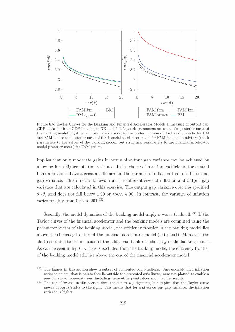
0 5 10 15 20

2.8

3

3.2

3.4

3.6

3.8

4

var(π)

var(gap)

FAM bm BMBM εB = 0

0 5 10 15 20

2.8

3

3.2

3.4

3.6

3.8

4

var(π)

var(gap)

FAM fam FAM bmFAM struct BM

Figure 6.5: Taylor Curves for the Banking and Financial Accelerator Models I; measure of output gap:GDP deviation from GDP in a simple NK model, left panel: parameters are set to the posterior mean ofthe banking model, right panel: parameters are set to the posterior mean of the banking model for BMand FAM bm, to the posterior mean of the financial accelerator model for FAM fam, and a mixture (shockparameters to the values of the banking model, but structural parameters to the financial acceleratormodel posterior mean) for FAM struct.

implies that only moderate gains in terms of output gap variance can be achieved byallowing for a higher inflation variance. In its choice of reaction coefficients the centralbank appears to have a greater influence on the variance of inflation than on the outputgap variance. This directly follows from the different sizes of inflation and output gapvariance that are calculated in this exercise. The output gap variance over the specifiedθπ-θy grid does not fall below 1.99 or above 4.00. In contrast, the variance of inflationvaries roughly from 0.33 to 201.932

Secondly, the model dynamics of the banking model imply a worse trade-off.933 If theTaylor curves of the financial accelerator and the banking models are computed using theparameter vector of the banking model, the efficiency frontier in the banking model liesabove the efficiency frontier of the financial accelerator model (left panel). Moreover, theshift is not due to the inclusion of the additional bank risk shock εB in the banking model.As can be seen in fig. 6.5, if εB is excluded from the banking model, the efficiency frontierof the banking model still lies above the one of the financial accelerator model.

932 The figures in this section show a subset of computed combinations. Unreasonably high inflationvariance points, that is points that lie outside the presented axis limits, were not plotted to enable asensible visual representation. Including these other points does not alter the results.

933 The use of ‘worse’ in this section does not denote a judgement, but implies that the Taylor curvemoves upwards/shifts to the right. This means that for a given output gap variance, the inflationvariance is higher.

219

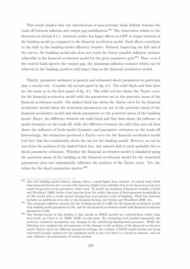
This result implies that the introduction of non-systemic bank default worsens thetrade-off between inflation and output gap stabilisation.934 The observation relates to thediscussion in section 6.1.1: monetary policy has larger effects on GDP at longer horizons inthe banking model as compared to the financial accelerator model. Such effects contributeto the shift in the banking model efficiency frontier. Related, inspecting the left end ofthe curves, the banking model also does not reach the lowest possible inflation varianceachievable in the financial accelerator model for the given parameter grid.935 Thus, even ifthe central bank ignores the output gap, the minimum inflation variance which can beachieved in the banking model is still larger than in the financial accelerator model.

Thirdly, parameter estimates in general and estimated shock parameters in particularplay a crucial role. Consider the second panel in fig. 6.5. The solid black and blue linesare the same as in the first panel of fig. 6.5. The solid red line shows the Taylor curvefor the financial accelerator model with the parameters set to the posterior mean of thefinancial accelerator model. The dashed black line shows the Taylor curve for the financialaccelerator model when the structural parameters are set to the posterior mean of thefinancial accelerator model and shock parameters to the posterior mean of the bankingmodel. Hence, the difference between the solid black and blue lines shows the influence ofmodel dynamics on the trade-off, while the difference between the solid blue and red linesshows the influence of both model dynamics and parameter estimates on the trade-off.Interestingly, the estimation produced a Taylor curve for the financial accelerator model(red line) that lies considerably above the one for the banking model. However, as can beseen from the position of the dashed black line, this upward shift is most probably due toshock parameter estimates. Whether the financial accelerator model is simulated usingthe posterior mean of the banking or the financial accelerator model for the structuralparameters does not substantially influence the position of the Taylor curve. Yet, thevalues for the shock parameters matter.936

934 Also, the banking model induces, among others, a much higher loan variance. A central bank whichtakes financial factors into account will experience higher loan volatility than in the financial acceleratormodel irrespective of the parameter values used. To justify the inclusion of financial variables, Cúrdiaand Woodford (2009) derive a loss function from the utility functions of heterogeneous households inan NK model with a credit spread arising from real resource costs of banking. Their loss functionincludes an additional term due to the financial friction, see Cúrdia and Woodford (2009: 31).

935 The minimum inflation variance for the banking model is 0.460, for the financial accelerator modelwith banking model parameters 0.331, and for the financial accelerator model with financial acceleratorparameters 0.404.

936 One interpretation of this finding is that shocks in DSGE models are reduced-form rather thanstructural, see Chari et al. (2009: 253ff) on this issue. By estimating both models separately, theposterior estimates incorporate any changes in the underlying fundamental processes. While thefollowing text explains the determinants of the changes in the position of the financial acceleratormodel Taylor curves for different parameter settings, the critique of DSGE model shocks not beingstructural actually underscores the argument made in the text that it is crucial to estimate, and notonly calibrate, the parameters of various models.

220

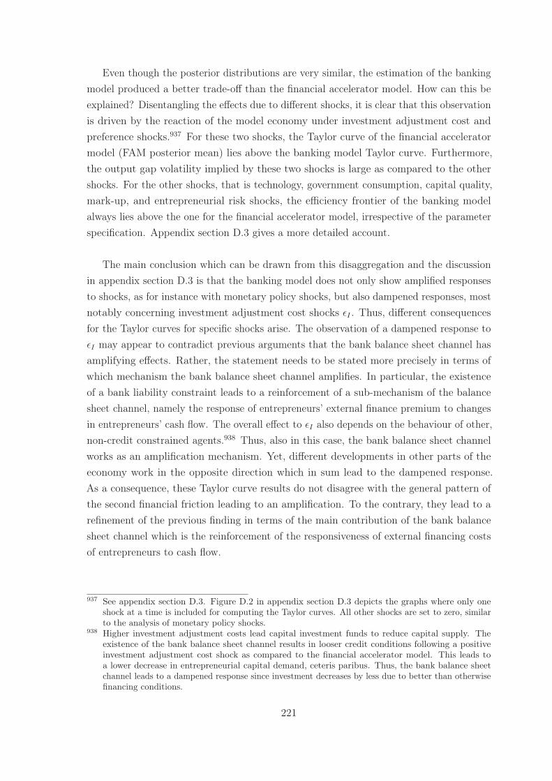
Even though the posterior distributions are very similar, the estimation of the bankingmodel produced a better trade-off than the financial accelerator model. How can this beexplained? Disentangling the effects due to different shocks, it is clear that this observationis driven by the reaction of the model economy under investment adjustment cost andpreference shocks.937 For these two shocks, the Taylor curve of the financial acceleratormodel (FAM posterior mean) lies above the banking model Taylor curve. Furthermore,the output gap volatility implied by these two shocks is large as compared to the othershocks. For the other shocks, that is technology, government consumption, capital quality,mark-up, and entrepreneurial risk shocks, the efficiency frontier of the banking modelalways lies above the one for the financial accelerator model, irrespective of the parameterspecification. Appendix section D.3 gives a more detailed account.

The main conclusion which can be drawn from this disaggregation and the discussionin appendix section D.3 is that the banking model does not only show amplified responsesto shocks, as for instance with monetary policy shocks, but also dampened responses, mostnotably concerning investment adjustment cost shocks εI . Thus, different consequencesfor the Taylor curves for specific shocks arise. The observation of a dampened response toεI may appear to contradict previous arguments that the bank balance sheet channel hasamplifying effects. Rather, the statement needs to be stated more precisely in terms ofwhich mechanism the bank balance sheet channel amplifies. In particular, the existenceof a bank liability constraint leads to a reinforcement of a sub-mechanism of the balancesheet channel, namely the response of entrepreneurs’ external finance premium to changesin entrepreneurs’ cash flow. The overall effect to εI also depends on the behaviour of other,non-credit constrained agents.938 Thus, also in this case, the bank balance sheet channelworks as an amplification mechanism. Yet, different developments in other parts of theeconomy work in the opposite direction which in sum lead to the dampened response.As a consequence, these Taylor curve results do not disagree with the general pattern ofthe second financial friction leading to an amplification. To the contrary, they lead to arefinement of the previous finding in terms of the main contribution of the bank balancesheet channel which is the reinforcement of the responsiveness of external financing costsof entrepreneurs to cash flow.

937 See appendix section D.3. Figure D.2 in appendix section D.3 depicts the graphs where only oneshock at a time is included for computing the Taylor curves. All other shocks are set to zero, similarto the analysis of monetary policy shocks.

938 Higher investment adjustment costs lead capital investment funds to reduce capital supply. Theexistence of the bank balance sheet channel results in looser credit conditions following a positiveinvestment adjustment cost shock as compared to the financial accelerator model. This leads toa lower decrease in entrepreneurial capital demand, ceteris paribus. Thus, the bank balance sheetchannel leads to a dampened response since investment decreases by less due to better than otherwisefinancing conditions.

221

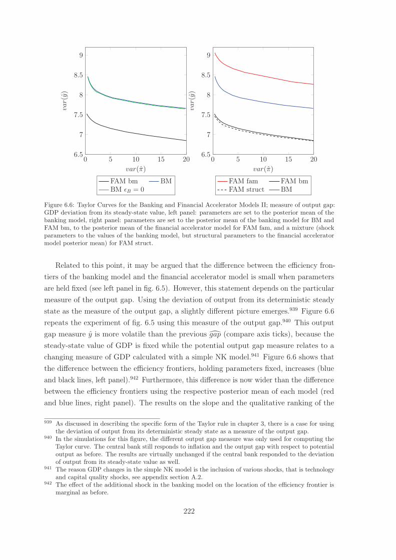
0 5 10 15 206.5

7

7.5

8

8.5

9

var(π)

var(y)

FAM bm BMBM εB = 0

0 5 10 15 206.5

7

7.5

8

8.5

9

var(π)

var(y)

FAM fam FAM bmFAM struct BM

Figure 6.6: Taylor Curves for the Banking and Financial Accelerator Models II; measure of output gap:GDP deviation from its steady-state value, left panel: parameters are set to the posterior mean of thebanking model, right panel: parameters are set to the posterior mean of the banking model for BM andFAM bm, to the posterior mean of the financial accelerator model for FAM fam, and a mixture (shockparameters to the values of the banking model, but structural parameters to the financial acceleratormodel posterior mean) for FAM struct.

Related to this point, it may be argued that the difference between the efficiency fron-tiers of the banking model and the financial accelerator model is small when parametersare held fixed (see left panel in fig. 6.5). However, this statement depends on the particularmeasure of the output gap. Using the deviation of output from its deterministic steadystate as the measure of the output gap, a slightly different picture emerges.939 Figure 6.6repeats the experiment of fig. 6.5 using this measure of the output gap.940 This outputgap measure y is more volatile than the previous gap (compare axis ticks), because thesteady-state value of GDP is fixed while the potential output gap measure relates to achanging measure of GDP calculated with a simple NK model.941 Figure 6.6 shows thatthe difference between the efficiency frontiers, holding parameters fixed, increases (blueand black lines, left panel).942 Furthermore, this difference is now wider than the differencebetween the efficiency frontiers using the respective posterior mean of each model (redand blue lines, right panel). The results on the slope and the qualitative ranking of the

939 As discussed in describing the specific form of the Taylor rule in chapter 3, there is a case for usingthe deviation of output from its deterministic steady state as a measure of the output gap.

940 In the simulations for this figure, the different output gap measure was only used for computing theTaylor curve. The central bank still responds to inflation and the output gap with respect to potentialoutput as before. The results are virtually unchanged if the central bank responded to the deviationof output from its steady-state value as well.

941 The reason GDP changes in the simple NK model is the inclusion of various shocks, that is technologyand capital quality shocks, see appendix section A.2.

942 The effect of the additional shock in the banking model on the location of the efficiency frontier ismarginal as before.

222

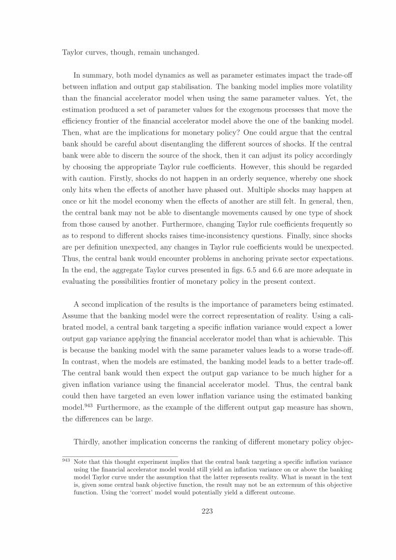
Taylor curves, though, remain unchanged.

In summary, both model dynamics as well as parameter estimates impact the trade-offbetween inflation and output gap stabilisation. The banking model implies more volatilitythan the financial accelerator model when using the same parameter values. Yet, theestimation produced a set of parameter values for the exogenous processes that move theefficiency frontier of the financial accelerator model above the one of the banking model.Then, what are the implications for monetary policy? One could argue that the centralbank should be careful about disentangling the different sources of shocks. If the centralbank were able to discern the source of the shock, then it can adjust its policy accordinglyby choosing the appropriate Taylor rule coefficients. However, this should be regardedwith caution. Firstly, shocks do not happen in an orderly sequence, whereby one shockonly hits when the effects of another have phased out. Multiple shocks may happen atonce or hit the model economy when the effects of another are still felt. In general, then,the central bank may not be able to disentangle movements caused by one type of shockfrom those caused by another. Furthermore, changing Taylor rule coefficients frequently soas to respond to different shocks raises time-inconsistency questions. Finally, since shocksare per definition unexpected, any changes in Taylor rule coefficients would be unexpected.Thus, the central bank would encounter problems in anchoring private sector expectations.In the end, the aggregate Taylor curves presented in figs. 6.5 and 6.6 are more adequate inevaluating the possibilities frontier of monetary policy in the present context.

A second implication of the results is the importance of parameters being estimated.Assume that the banking model were the correct representation of reality. Using a cali-brated model, a central bank targeting a specific inflation variance would expect a loweroutput gap variance applying the financial accelerator model than what is achievable. Thisis because the banking model with the same parameter values leads to a worse trade-off.In contrast, when the models are estimated, the banking model leads to a better trade-off.The central bank would then expect the output gap variance to be much higher for agiven inflation variance using the financial accelerator model. Thus, the central bankcould then have targeted an even lower inflation variance using the estimated bankingmodel.943 Furthermore, as the example of the different output gap measure has shown,the differences can be large.

Thirdly, another implication concerns the ranking of different monetary policy objec-

943 Note that this thought experiment implies that the central bank targeting a specific inflation varianceusing the financial accelerator model would still yield an inflation variance on or above the bankingmodel Taylor curve under the assumption that the latter represents reality. What is meant in the textis, given some central bank objective function, the result may not be an extremum of this objectivefunction. Using the ‘correct’ model would potentially yield a different outcome.

223

tives. While the choice of Taylor rule coefficients has substantial consequences for theresulting variability of inflation, the corresponding range of output gap variability valuesis tight. Therefore, the Taylor curves suggest that the capabilities of the central bank arecomparatively limited in pursuing the goal of output gap stabilisation. This observationlends support to inflation stabilisation as the primary objective of monetary policy. Atthe same time, the increasing slope at the far left hand of the Taylor curves also supportsthe mandate to support the general development of the real economy. When inflationvariability is very low, any further decreases tend to increase the volatility in the realeconomy at an increasing pace. Thus, there may be benefits to aiming to smooth thepath of the real economy in this case. Overall, these observations suggest that the centralbank’s capabilities yield a clear hierarchy of objectives: first inflation, and then outputgap stabilisation. Yet, this hierarchy should not be taken as definite without respect forother governmental policies’ efficiency frontiers as well as a precise objective function.

Finally, these results provide a rationale for targeting a non-zero inflation rate, eventhough this is not implemented here. Assume the central bank only puts weight oninflation stabilisation. Then, the financial accelerator model, independent of the particularparametrization, implies a lower minimum inflation variance than the banking model.944

According to this measure, the model with non-systemic bank default constrains the abilityto stabilise prices more than the financial accelerator model. Thus, these results providesupport for targeting 2% instead of 0% inflation.945 If non-systemic bank failures implyhigher inflation volatility, the argument for a buffer to the zero lower bound or deflationis reinforced. The argument can be made to pursue an even higher inflation target than2%. Yet, this does not necessarily follow from these results since the minimum inflationvariance is still comfortably within the 2% bound.

All in all, this analysis paints a mixed picture. Depending on parameter values, measureof the output gap and shock the Taylor curve of the banking model may show an improvedor a worse trade-off than the financial accelerator model. The results emphasise uncertainty:since the true representation of reality is not known, the outcome of any single modelcannot be taken for granted as representing possible outcomes of monetary policy. Asboth models are likely to be an abstract and incomplete representation of reality, it is notfeasible to judge which model provides a better foundation for policy decisions. However,applying the Bayesian paradigm of model averaging may be a promising avenue in this

944 See footnote 935 above in this chapter. For the banking model and the financial accelerator modelwith financial accelerator model parameters the corresponding values for the Taylor rule coefficientsare θπ = 5 and θy = 0, and for the financial accelerator model with banking model parameters theyare θπ = 5 and θy = 0.25.

945 This is despite the fact that factors proposed as justifications for a higher target rate of inflation arenot present in the banking model.

224

regard. As the results of this section suggest, when various models are used in conjunction,the target of the central bank will be more appropriately characterised by a range, not aspecific point in the var(π)-var(y) graph.

6.3 The Link between Non-Systemic Bank Default and

Monetary Policy with Macroprudential Policies

6.3.1 General Aspects of Macroprudential Policy

Previous results established that the incidence of non-systemic bank default has multipleadverse effects for the economy. For one, real resource costs are spent in monitoringdefaulting or badly-performing banks. Furthermore, extra outlays enter the governmentalbudget, potentially leading to tax increases or spending cuts. Finally, the investmentcycle, that is the response of investment to shocks, is generally amplified due to banks’impact on entrepreneurs marginal financing costs.946 In the banking model presentedin chapter 3, the deposit insurance scheme is the only governmental policy in place tocounter the negative effects of bank default (on workers’ budgets in this case).947 Thissection considers other instruments which may be implemented to offset the undesirableconsequences or preclude the incidence of bank default. In particular, the emphasis is onthe impact such policies have on the conduct of monetary policy.

The policies analysed in this chapter are illustrations of macroprudential policy. Es-pecially since the financial crisis of 2007-8, the term macroprudential policy has beenpopular. It denotes policy instruments directed at promoting systemic financial stability.948

More specifically, macroprudential policy aims at managing the adverse effects of excessivedeleveraging brought about by a shock which affects numerous financial intermediaries.949

This intention of avoiding deleveraging is the key differentiating feature with respect tomicroprudential policies. While microprudential policies also aim at enhancing financialstability, their primary focus is on decreasing a particular bank’s default probability.950

Furthermore, it can be argued that, when judging compliance, microprudential regulationis indifferent between a bank reducing its assets or increasing its capital base to decrease its

946 This list can be extended, but in the interest of space, the text is confined to the most importantconsiderations in this regard. As noted above, the response of investment in the banking model ismuted in the case of investment adjustment cost shocks with respect to the financial accelerator model,see footnote 938. See appendix section D.3 for more details.

947 Admittedly, there are also reserve requirements for bank deposits. Yet, their rationale can be basedon safeguarding the payments system. Furthermore, minimum reserves do not play an active role tocounter financial fragility in the banking model.

948 See Bailliu et al. (2015: 148)949 See Hanson, Kashyap and Stein (2011: 5)950 See Hanson et al. (2011: 4)

225

default probability.951 The case for macroprudential regulation rests on the reasoning thatmicroprudential regulation’s non-observance of how financial fragility is reduced becomescritical when many (or systemic) banks face problems running the risk of turning into abanking crisis.952 Thus, macroprudential policies have a systemic point of view.

Even though this thesis does not concern systemic bank failures or financial crises, theimpact of macroprudential, and not microprudential, policies will be studied here. Thereason is that the banking sector is characterised by a representative bank in the bankingmodel. Then, a microprudential policy would affect all banks equally, and thus the wholebanking sector, in the banking model instead of a single bank. Therefore, macroprudentialpolicy is the appropriate banking sector regulation to be studied here. This is not becausethe banking model features systemic bank failures, which it does not, but rather becausethe representative bank framework means that the banking sector as a whole is affectedby such government intervention.953

One objective of macroprudential policies is thus to prevent the build-up of so-calledfinancial imbalances which could potentially unravel in a financial crisis. Examples ofmacroprudential policies include loan-to-value ratios, capital adequacy ratios and theregulation of the shadow banking sector.954 Various arguments have been proposed forwarranting the introduction of such policies on economical grounds. For one, financial in-termediaries’ deleveraging or balance sheet shrinkage in a financial crisis creates social coststhrough fire sales and credit crunches.955 Also market imperfections such as externalitiesand moral hazard due to, among others, government guarantees provide a justification.956

Alpanda et al. (2014) argue that such financial market distortions make financial crisesmore probable, resulting in negative consequences for macroeconomic stability.957

In the case of the banking model the introduction of macroprudential policies can bejustified, for instance, by the existence of the deposit insurance scheme. On the one hand,deposit insurance may prevent bank runs and the accompanying adverse consequencesinvolving liquidity mismatch between bank assets and bank liabilities.958 On the other

951 See Hanson et al. (2011: 5)952 See Hanson et al. (2011: 5)953 One could pose the question of whether or not this means that micro- and macroprudential policies

coincide in the banking model. However, as emphasised before, this study does not aim for acomprehensive treatment of banking sector regulation. Rather, the purpose of this section is to showhow different policies can affect the interactions between financial fragility and monetary policy. Thus,the issue of micro- vs. macroprudential policies is not discussed further.

954 See, for instance, Hanson et al. (2011) and Beau, Clerc and Mojon (2011) for discussions of variousmacroprudential instruments.

955 See Hanson et al. (2011: 5)956 See Hanson et al. (2011: 5) and Alpanda, Cateau and Meh (2014: 7)957 See Alpanda et al. (2014: 7)958 See Diamond and Dybvig (1983: 403f, 415)

226

hand, it has been argued that deposit insurance schemes produce incentives for excessiverisk-taking.959 Macroprudential policies can then be used to moderate moral hazard onthe part of banks.960 Taking these considerations as a starting point, this study doesnot aim for an exhaustive treatment of macroprudential policies. Rather, the presence ofmacroprudential policies is taken as given. The following analyses are meant to exemplifythe consequences of macroprudential policies for monetary policy in a model with non-systemic bank default. The objective is to assess the overall impact of bank default bothwhen there is no explicit government policy aimed at reducing banking sector fragility andwhen there is such a policy in place. Further research can build on this, evaluating variouspolicies in terms of their efficiency and determining optimality.

Furthermore, debates about macroprudential policies are tightly linked to unconven-tional monetary policies as, for example, have been practised by various central banks sincethe financial crisis of 2007-8. The reason this study takes into account macroprudential butnot unconventional monetary policies is due to the justification of the latter as exceptionalmeasures to deal with exceptional circumstances.961 In contrast, this study focuses on howbanking sector fragility affects the monetary transmission mechanism in normal times andnot in crisis times. In the banking model, the monetary transmission mechanism is notcompletely unearthed by the existence of non-systemic bank default as has been shown inthe first two sections of this chapter. Rather, bank default creates another layer throughwhich monetary impulses are transmitted. The focus of this section is on whether and howadditional governmental measures aimed at countering financial fragility affect this layer.Therefore, the appropriate policy measures to study in this section are macroprudentialpolicies. The study of the relationships between unconventional and conventional policiesand financial fragility are left to research focusing on extreme events where the monetarypolicy transmission mechanism may be severely impeded.

To this end, this section concentrates on three possible policies: an endogenous depositinsurance factor, a macroprudential Taylor rule (MTR), and a macroprudential creditspread rule (MCS). One way to interpret these three policies is to view them in terms ofincreasing depth of governmental regulation. The endogenous deposit insurance factormerely adjusts the existing deposit insurance scheme to take financial risks into account.The MTR extends the mandate of the central bank to adjust the nominal risk-free returnin response to financial imbalances. The MCS works independently of monetary policyand allows the government to affect the credit spread directly. In this third regime, thecentral bank sets the nominal risk-free return in response to inflation and output gap

959 See Hanson et al. (2011: 4)960 See Hanson et al. (2011: 4)961 See Borio and Disyatat (2009: 26). The authors base their conclusion on the various problems

associated with unconventional monetary policies, see Borio and Disyatat (2009: 25f).

227

deviations as in the benchmark banking model.962

As noted above, the deposit insurance scheme in the banking model shields deposit-holders from the (direct) negative consequences of bank default. However, this policyhas the side-effect of distorting workers’ view of bank deposits as being default-risk-freeeven though the government budget, and by extension taxpayers, eventually incur thecosts of bank default. The question is now to which extent the results change if depositinsurance fees depend on the fragility of the banking sector, and not only on the volume ofdeposits.963 This modification is grounded in the objective of shielding the governmentalbudget in case of increased bank fragility to some extent. The crucial simplification thatall banks pay the same share of deposit insurance fees still holds. However, this share nowchanges with banking sector fragility.

An MTR commands the central bank to ‘lean against the wind’ in its conduct ofmonetary policy.964 This means that the central bank uses its interest rate policy to reactto financial imbalances. As financial imbalances build up in the economy, the central bankincreases the nominal risk-free return to counteract these pressures. Such a policy is acontentious issue. Proponents argue that it may help in preventing economic instability,while opponents reply with legitimacy and feasibility problems of such a policy.965 Forinstance, from a welfare-theoretic view such a macroprudential Taylor rule can be justified.In analysing optimal monetary policy, Cúrdia and Woodford (2009) derive a loss functionwhich includes a financial indicator variable from the welfare of households in a reduced-form NK framework.966 The financial variable in the loss function is then warranted bythe welfare distortions arising from frictions in the financial intermediation process.967

Thus, a justification for such a policy in the banking model can be established on the basisof the existence of financial frictions.

Nonetheless, an MTR may be contested on the grounds that the central bank targetsmultiple objectives with one instrument. This may lead to compromised results concerningall objectives. Badarau and Popescu (2015), for instance, find that a macroprudentialpolicy rule reacting to loan growth has the potential to improve financial stability.968

However, such a policy does not improve on the standard Taylor rule in terms of price

962 The exact formulations of these three policies will be explained in section 6.3.2.963 As noted in chapter 3, the calculation of deposit insurance fees is legally mandated to include risk

considerations in Germany, see footnote 459 in chapter 3. All banks are the same in the bankingmodel. Hence, risk considerations were disregarded in benchmark banking model for simplicity, asbanks do not differ in terms of their asset risk profile.

964 See Beau et al. (2011: 8)965 See Beau et al. (2011: 7f)966 See Cúrdia and Woodford (2009: 28ff)967 See Woodford (2012: 15)968 See Badarau and Popescu (2015: 370f)

228

stability and actually inhibits economic growth.969 This reasoning leads to the thirdmacroprudential policy considered here. As a separate macroprudential instrument, theMCS is introduced. Thus, as a short-cut to modelling a thorough quantity-based macro-prudential policy, here, the government is able to affect the spread between loan anddeposit rates directly in response to financial imbalances, without specifying preciselyhow.970 This modelling strategy follows Kannan et al. (2012) and Bailliu et al. (2015).971

Admittedly, the MCS is ad-hoc. Yet, it can be argued that it is a simple implementationof quantity-based macroprudential policies. In Iacoviello (2015), for example, the creditspread depends positively on the size of the capital adequacy requirement.972 Effects offinancial imbalances on the credit spread may work through additional requirements oncapital holdings or provisions but these mechanisms are not specified.973

There are many more possible macroprudential policies which could be analysed. How-ever, this would easily go beyond the agenda of this study. The choice of instruments isalso governed by considerations about model specificities. For instance, there is no oppor-tunity to evaluate regulation aimed at the shadow banking sector, since there is simply nocorresponding sector in the banking model. Moreover, quantity-based instruments suchas capital adequacy ratios are not explicitly analysed.974 Capital adequacy ratios targetbanks’ liability management. They introduce a (binding) constraint, beyond which bankscannot borrow. However, agents in the banking model can principally borrow as much asthey want. The mechanism stopping agents from borrowing infinitely is increasing interestrates. Lenders, whether they be banks or equity-holders, are only willing to supply fundsif they are remunerated adequately. Thus, modelling macroprudential policy using theshort-cut via the credit spread rule is more in line with the logic of the banking model.975

969 See Badarau and Popescu (2015: 370f)970 See Kannan et al. (2012: 13f) and Bailliu et al. (2015: 152f)971 See Kannan et al. (2012: 8, 13f) and Bailliu et al. (2015: 152f)972 See Iacoviello (2015: 5f). In fact, there is a great degree of similarity concerning the relationships

between the credit spread and the capital requirement in Iacoviello (2015) on the one hand, andbetween the credit spread and the macroprudential instrument presented below on the other hand.

973 See Kannan et al. (2012: 12ff)974 See for instance Van den Heuvel (2008), Aguiar and Drumond (2007) and Iacoviello (2015) for examples

of (binding) bank capital constraints. Loan-to-value ratios are another example of quantity-basedinstruments. They regulate the asset side of banks’ balance sheet. Thus, loan-to-value ratios shouldbe regarded as an instrument to reduce entrepreneurs’ riskiness. Since there is no risk-taking channelpresent in the banking model, such an analysis would probably contribute little to the question of theeffects of bank default on monetary policy here.

975 Related, including some form of bank capital adequacy constraint to reduce banks’ reliance on externalfinancing would entail a substantial change in the banking model layout. A bank equity adequacyconstraint essentially leads to a model where workers are willing to hold any amount of equity anddeposits commanded by governmental regulation. Instead, the rationale in deriving the bankingmodel was to explicitly consider the demand side. A plausible adjustment would then have to be theintroduction of internal bank net worth from retained earnings to comply with the kind of policiesintroduced in many countries. Such more fundamental changes to the banking model are left to futureresearch since these changes would certainly alter the benchmark model behaviour as well, and aresupplementary to the principal agenda of this research.

229

Given that any model is an abstraction from reality, this approach is deemed to be morepurposeful in the present context.

It is important to note that these macroprudential policies affect the evolution of thebanking model economy when displaced from its stable steady state. Macroprudentialpolicies as discussed in this study do not change the non-stochastic steady state of thebanking model. This is in line with the focus on business cycle developments. Thus,macroprudential policies will not be judged depending on whether they reduce bankingsector fragility in the steady state. As a consequence of the log-linearisation and the focuson non-systemic bank failures, the development of a financial crisis is not traced here, andthus, macroprudential policies can also not be assessed in terms of preventing financialcrises. Rather, macroprudential policies will be evaluated concerning how they affect theadjustments of the model economy back to its steady state when the model economy isdisplaced from its steady state by exogenous disturbances. This is in accordance withthe central concern of this thesis with monetary policy. The primary question is not, canmacroprudential policies enhance financial stability.976 Rather, the question is, assumingthat there are macroprudential policies in place, what is the impact of non-systemic bankdefault on the conduct of monetary policy?

The next section will present the adjustments to the banking model for each policyregime separately. Subsequently, the impact of these instruments on monetary policywill be evaluated using the two tools discussed above: impulse response analysis to amonetary policy shock and Taylor curves. The results suggest that the introductionof macroprudential policies affects the conduct of monetary policy with fragile banks.However, the results differ between the policy regimes as well as concerning the appropriatemeasurement of financial imbalances.

6.3.2 Macroprudential Policy Regimes in the Banking Model

Endogenous Deposit Insurance Factor Deposit insurance fees in the benchmarkbanking model are a simple function of the deposit volume. This relationship is given byeq. (3.43), reprinted here:

DIt = νdDt−1 (6.2)

The first macroprudential instrument introduces a risk factor in computing deposit in-surance fees. To this end, assume the fragility of the banking sector to be measured bybanks’ default probability. The justification for this choice is straightforward: bank defaultresults in extra outlays in the government budget. The bank default probability is directly

976 Appendix section D.5 discusses the consequences of the different macroprudential regimes with respectto measures of financial stability.

230

related to these additional outlays and easy to measure. Deposit insurance fees are thengoverned by the following equation:

DIet = νdet Dt−1 (6.3)

where νdet is the deposit insurance factor applied to the deposit base, given by:

νdet = ωmppp

(ψ

B

t

)ωmpe

(6.4)

The superscript e denotes the version of the model with endogenous bank deposit insurancefactor. ωmpp and ωmpe are parameters to be determined. In contrast to the benchmarkbanking model, νde

t is not a parameter, but an endogenous variable which depends onbanking sector fragility. Note that the benchmark banking model of chapter 3 correspondsto the case of ωmpe = 0. What is more, νd

t is simply substituted by νdet and eq. (6.4)

is added to the system of equations.977 All other relationships are unchanged. For thecomparative purposes of this analysis, it is beneficial to have the same steady state forboth the benchmark as well as the modified banking model (in terms of the non-linearmodel). Thus, the calibration of ωmpp and ωmpe is such that the real risk-free return isequal to the real deposit return and to the real effective deposit return in the steady state.Since the analysis will be conducted using the log-linear approximation of the model, onlythe calibration of ωmpe is relevant.978

As before, assume that the real effective deposit return is equal to the real risk-freereturn. This means that under all circumstances banks are able to adjust the deposit returnRd,t in such a way that banks’ real effective deposit return Red is equal to the real risk-freereturn. Then, deviations in the deposit insurance factor are completely passed throughto the real deposit return. In contrast, workers may receive a return on their depositswhich differs from the real risk-free return depending on νde

t .979 This may be justifiedby unspecified features of workers’ deposit demand, such as transaction services, whichmake workers hold deposits even though their return is lower than the real risk-free return.More simply, there are no other explicit assets workers can hold in the banking model.Thus, workers cannot hold the hypothetical asset connected to the real risk-free return.980

977 Thus, the real effective deposit return banks pay on their deposits is given by Red,t = Rd,t−ξrRt+νdetinstead of eq. (3.45a) in chapter 3, and the real return on bank deposits workers receive is given byRd,t = (1 + ξr)Rt − νdet instead of eq. (3.45b).

978 The derivation in terms of the non-linear model is illustrative for showing the differences between thebenchmark and endogenous deposit insurance scheme.

979 This is true to a certain extent in the banking model with exogenous insurance factor as well. There,the log-linear approximation yields a (1 + ξr)% change of the real deposit return for a 1% change inthe real risk-free return. In terms of pass-through, this is equivalent to overshooting. For small ξr,this effect is negligible.

980 This assumption is discussed further below.

231

Furthermore, the opposite assumption, that is for the real deposit return to equal the realrisk-free return with banks’ effective real deposit return varying around the real risk-freereturn does not change the results fundamentally. Thus, the implicit assumption is thatbanks are price-setters on the deposit market and workers are price-takers.981

Finally, workers’ perception of bank deposits being default risk-free does not changebecause consumption and portfolio decisions are separate. Hence, bank deposits are stillcheaper than bank equity from the point of view of banks, as outlined in section 4.2.Yet, ceteris paribus, an increasing deposit insurance factor induces banks to shift theirliability structure towards more bank equity, thus reducing their default probability. Thisis because, if default banks’ probability rises, then banks have to pay higher depositinsurance fees on their deposit base in order to alleviate the governmental budget fromthe increased probability of having to pay out bank deposits. Banks simply pass on thisincrease onto deposit-holders by reducing the deposit return. The lower deposit returndeposit-holders receive ensures that the effective deposit return banks pay on deposits,which takes into account minimum reserves interest income and deposit insurance fees,still equals the real risk-free return. With the decrease in the real deposit return, therequired return on equity also decreases, thus making bank equity less expensive from theperspective of banks.

Macroprudential Taylor Rule The second macroprudential policy concerns the Taylorrule. An MTR combines monetary policy with macroprudential policy. For example,Angeloni and Faia (2013) and Gambacorta and Signoretti (2014) use an MTR policy ofthis form to study the effects of macroprudential policies.982 The core of the Taylor ruleremains: the nominal risk-free return is adjusted in response to deviations of the outputgap and inflation from their respective steady-state levels. In addition, the central bankreacts to financial imbalances. Thus, the MTR has the following general form:

rn,t = ρRrn,t−1 + (1− ρR)θππt + (1− ρR)θygapt + (1− ρR)θmmtr,t + εM,t (6.5)

where mtr,t is an additional variable indicating the presence of financial imbalances. θm

is a parameter measuring the responsivity of the nominal risk-free return to financialimbalances. If financial imbalances build up, that is mtr,t is positive, the central bankobserves increasing risks to macroeconomic stability. Hence, the central bank respondswith contractionary monetary policy. In contrast, when financial sector developments areweak, the central bank will ease monetary policy in order to promote a recovery.

981 In the long term, banks do not have market power in the banking model so as to set a real depositreturn different from the real risk-free return. As noted above, the parameters ωmpp and ωmpe are setappropriately to achieve this result.

982 See Angeloni and Faia (2013: 316ff) and Gambacorta and Signoretti (2014: 154ff)

232

The question is how to measure financial imbalances, thus how to define mtr,t. Here,three different indicator variables are used which show different aspects of financial sectordevelopments. These are lagged loan growth, the real price of physical capital and theloan-to-GDP ratio. The choice of loan growth and asset prices is frequently observed in theliterature.983 Concerning the timing, Kannan et al. (2012) report that contemporaneousloan growth leads to very high values for the reaction coefficients in the Taylor rule whensolving for optimal policy.984 They argue that these large coefficients imply that the centralbank achieves low volatility by simply promising large reactions.985 Thus, lagged loangrowth is used here.986 Finally, the loan-to-GDP ratio is included to analyse whethermacroprudential instruments lead to different effects if they are only triggered when loangrowth exceeds GDP growth.

Macroprudential Credit Spread Rule Strictly speaking, the credit spread is definedas the difference between loan and deposit rates. In the banking model loan rates are ofsecondary nature; the key relationships arising from the optimisation problems deal withthe real return on real capital, the real wholesale return and the real deposit return. Thus,the appropriate point to introduce this macroprudential rule is the arbitrage conditionof banks in granting loans (eq. (3.16)). The arbitrage condition posits that the expectedreal return on real capital equals the expected real wholesale return times the expectedentrepreneurial risk premium.987 Following Kannan et al. (2012) and Bailliu et al. (2015),the macroprudential instrument enters multiplicatively in this arbitrage condition.988 Thismeans that the deviation of the instrument from its steady-state value enters additively inthe log-linear approximation as given by:

IEt

[rk,t+1

]= IEt

[�Et+1 + rw,t+1 + τMmcs,t+1

](6.6)

where mcs,t+1 is the indicator variable. This is similar to mtr,t in the MTR discussed above.τM is a parameter governing the degree to which the credit spread changes with financialimbalances. For comparability, the indicator variables included in the MCS equationare the same as for the MTR: lagged loan growth, the price of physical capital and theloan-to-GDP ratio.

983 For instance, Arango and Valencia (2015), Angeloni and Faia (2013) and Gambacorta and Signoretti(2014) use asset prices, Bailliu et al. (2015), Kannan et al. (2012), Ozkan and Unsal (2013), and Quintand Rabanal (2013) use credit growth, and Quint and Rabanal (2013) also use the loan-to-GDP ratioas the indicator variable (among others).

984 See Kannan et al. (2012: 12f)985 See Kannan et al. (2012: 12)986 Experiments with contemporaneous loan growth as the instrumental variable produced results very

similar to lagged loan growth.987 Remember the arbitrage condition governing banks’ liability management, which shows that the

expected real wholesale return is the product of the expected values of the bank risk premium andthe real deposit return. Thus, this condition relates both financial frictions.

988 See Kannan et al. (2012: 8) and Bailliu et al. (2015: 152)

233

The MCS policy affects the economy as follows. Following a build-up of financialimbalances, for instance ‘excessive’ credit growth, the MCS is triggered, exogenouslyincreasing the credit spread. Because of this, entrepreneurs’ marginal financing costincreases, decreasing entrepreneurs’ capital demand. Thus, loan demand decreases and the‘excessive’ credit growth is reigned in. To be clear, this policy will also affect non-financialvolumes by decreasing investment and thus GDP, ceteris paribus.

Combined Policy Finally, the following simulations also consider the case when MTRand MCS policies are used in conjunction. This means that both additional elements, mtr,t

and mcs,t in the Taylor rule and the credit spread, respectively, are used and respond tothe same indicator variable. Theoretically, one could combine different indicator variablesin each policy rule. Yet, as will be shown further below, this combination already yieldsa number of interesting scenarios which is sufficient for the illustrative purposes of thissection.

Parametrization Some final notes about parametrization and method are necessary.The parameter governing the responsiveness of deposit insurance fees to banks’ defaultprobability ωmpe is set to 1 for simplicity.989 This means that the deposit insurance factorchanges one for one with a change in banks’ default probability. It is also a procyclicalpolicy: when bank default occurs more frequently, banks pay higher insurance fees tocompensate for higher governmental outlays. The reaction coefficient of the indicatorvariable in the MTR θm is set to 0.25, and the parameter governing the impact of theindicator variable in the MCS rule τM is set to 0.15.990 These values are guided by thefollowing considerations. The value for θm can be justified as being the first step of thedistribution which was used for θy in computing Taylor curves.991 The value for τM isa compromise between the values used by Bailliu et al. (2015) (0.05) and by Kannan etal. (2012) (0.3).992 The sensitivity of the results with respect to this parametrization isdiscussed in appendix section D.4.

The different policies are evaluated with impulse response functions and Taylor curves.The assumptions for the responses to a monetary policy shock are the same as in sec-tion 6.1.1.993 The parameter grid for θy and θπ for calculating Taylor curves is the sameas in section 6.2. Similarly, the lines depicted for the Taylor curves with macroprudentialpolicies in section 6.3.4 are not actually continuous and the graphs only show a subsetof the point that were calculated as in section 6.2. Note that the cut-off point in the989 All other parameters are set to the posterior mean of the benchmark banking model for the simulations.990 Again, all other parameters are set to the posterior mean of the benchmark banking model.991 The grid for θy ranges from 0 to 2.5.992 See Bailliu et al. (2015: 156) and Kannan et al. (2012: 16)993 This means εM,1 = σM , εm,s = 0, s = 2 : ∞, εx,t = 0, t = 1 : ∞, where x = A,B,E,G, I,K,MS, P .

For details, see section 6.1.1.

234

Taylor curve graphs in section 6.3.4 is set to 10 for the variance of inflation to discernsome differences more clearly. This is also sufficient for this exercise since the qualitativeresults do not change when higher inflation variance points are included.994

6.3.3 Macroprudential Policies and Monetary Policy Transmis-

sion

The first experiment tracks the transmission of a monetary policy shock for each macropru-dential policy regime separately. Consider first the endogenous deposit insurance factor.Figure 6.7 depicts the responses of GDP, the nominal risk-free return and inflation to acontractionary monetary policy shock.995 The blue line depicts the benchmark bankingmodel without macroprudential policy, while the green dashed line shows the bankingmodel with endogenous deposit insurance factor. It is clear that the effects of a contrac-tionary monetary policy shock are only marginally different.996 The responses of inflationand the nominal risk-free return in the endogenous deposit insurance factor bankingmodel are indistinguishable from the responses in the benchmark model. However, theendogenous deposit insurance factor leads to a marginally lower impact on GDP while thetime it takes for GDP to return to its steady state is not fundamentally affected. A largerdifference between the benchmark banking model and the endogenous deposit insurancefactor version can be achieved by increasing ωmpe.997 Section 6.3.4 and appendix sectionD.4 will discuss why an increase in ωmpe may not be a good strategy.

This similarity between the banking model with and without the endogenous depositinsurance factor can be explained by the following considerations. The fundamentalmechanism transmitting the contractionary monetary policy impulse is still the increasein real returns. It is the determination of the real deposit return which the endogenousinsurance factor affects. As the real deposit return changes, so does the required returnon bank equity, in turn affecting the bank risk premium as well as the required returnon lending, that is the real wholesale return. Entrepreneurs’ marginal financing cost,investment and aggregate demand are affected through these two latter factors.

As mentioned in section 6.1.1, banks’ financing situation does not deteriorate monoton-

994 Besides, based on a loss function with inflation and the output gap as arguments, the maximuminflation variance depicted in the graphs in section 6.3.4 would be in line with central bank preferencesregarding output gap variance about three times more important than inflation variance.

995 Note that the y-axis scales in fig. 6.7 appear to be rather wide because they are aligned with therespective panels in fig. 6.8 for immediate comparability.

996 The results are virtually unchanged if the endogenous deposit insurance depends on the lagged bankdefault probability.

997 That is, up to a certain point. Put differently, higher positive values for ωmpe can lead to a deviationof output from its steady state which is larger than in the benchmark banking model. See section 6.3.4and appendix section D.4 for more details.

235

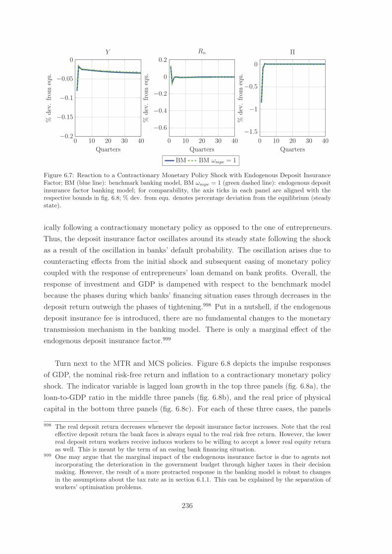
0 10 20 30 40

−0.6

−0.4

−0.2

0

0.2

Quarters%

dev.

from

equ.

Rn

0 10 20 30 40−0.2

−0.15

−0.1

−0.05

0

Quarters

%de

v.fr

omeq

u.Y

0 10 20 30 40

−1.5

−1

−0.5

0

Quarters

%de

v.fr

omeq

u.

Π

BM BM ωmpe = 1

Figure 6.7: Reaction to a Contractionary Monetary Policy Shock with Endogenous Deposit InsuranceFactor; BM (blue line): benchmark banking model, BM ωmpe = 1 (green dashed line): endogenous depositinsurance factor banking model; for comparability, the axis ticks in each panel are aligned with therespective bounds in fig. 6.8; % dev. from equ. denotes percentage deviation from the equilibrium (steadystate).

ically following a contractionary monetary policy as opposed to the one of entrepreneurs.Thus, the deposit insurance factor oscillates around its steady state following the shockas a result of the oscillation in banks’ default probability. The oscillation arises due tocounteracting effects from the initial shock and subsequent easing of monetary policycoupled with the response of entrepreneurs’ loan demand on bank profits. Overall, theresponse of investment and GDP is dampened with respect to the benchmark modelbecause the phases during which banks’ financing situation eases through decreases in thedeposit return outweigh the phases of tightening.998 Put in a nutshell, if the endogenousdeposit insurance fee is introduced, there are no fundamental changes to the monetarytransmission mechanism in the banking model. There is only a marginal effect of theendogenous deposit insurance factor.999

Turn next to the MTR and MCS policies. Figure 6.8 depicts the impulse responsesof GDP, the nominal risk-free return and inflation to a contractionary monetary policyshock. The indicator variable is lagged loan growth in the top three panels (fig. 6.8a), theloan-to-GDP ratio in the middle three panels (fig. 6.8b), and the real price of physicalcapital in the bottom three panels (fig. 6.8c). For each of these three cases, the panels

998 The real deposit return decreases whenever the deposit insurance factor increases. Note that the realeffective deposit return the bank faces is always equal to the real risk free return. However, the lowerreal deposit return workers receive induces workers to be willing to accept a lower real equity returnas well. This is meant by the term of an easing bank financing situation.

999 One may argue that the marginal impact of the endogenous insurance factor is due to agents notincorporating the deterioration in the government budget through higher taxes in their decisionmaking. However, the result of a more protracted response in the banking model is robust to changesin the assumptions about the tax rate as in section 6.1.1. This can be explained by the separation ofworkers’ optimisation problems.

236

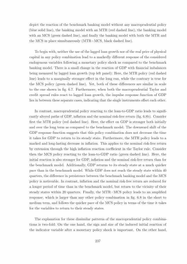
depict the reaction of the benchmark banking model without any macroprudential policy(blue solid line), the banking model with an MTR (red dashed line), the banking modelwith an MCS (green dashed line), and finally the banking model with both the MTR andthe MCS in place simultaneously (MTR+MCS, black dashed line).

To begin with, neither the use of the lagged loan growth nor of the real price of physicalcapital in any policy combination lead to a markedly different response of the consideredendogenous variables following a monetary policy shock as compared to the benchmarkbanking model. There is a small change in the reaction of GDP with financial imbalancesbeing measured by lagged loan growth (top left panel): Here, the MTR policy (red dashedline) leads to a marginally stronger effect in the long run, while the contrary is true forthe MCS policy (green dashed line). Yet, both of these differences are similar in scaleto the one shown in fig. 6.7. Furthermore, when both the macroprudential Taylor andcredit spread rules react to lagged loan growth, the impulse response function of GDPlies in between these separate cases, indicating that the single instruments offset each other.

In contrast, macroprudential policy reacting to the loan-to-GDP ratio leads to signifi-cantly altered paths of GDP, inflation and the nominal risk-free return (fig. 6.8b). Considerfirst the MTR policy (red dashed line). Here, the effect on GDP is stronger both initiallyand over the long term as compared to the benchmark model. The downward shift of theGDP response function suggests that this policy combination does not decrease the timeit takes for GDP to return to its steady state. Furthermore, the MTR policy leads to amarked and long-lasting decrease in inflation. This applies to the nominal risk-free returnby extension through the high inflation reaction coefficient in the Taylor rule. Considerthen the MCS policy reacting to the loan-to-GDP ratio (green dashed line). Here, theinitial reaction is also stronger for GDP, inflation and the nominal risk-free return than forthe benchmark model. Additionally, GDP returns to its steady state at a much quickerpace than in the benchmark model. While GDP does not reach the steady state within 40quarters, the difference in persistence between the benchmark banking model and the MCSpolicy is noticeable. In contrast, inflation and the nominal risk-free return are reduced fora longer period of time than in the benchmark model, but return to the vicinity of theirsteady states within 20 quarters. Finally, the MTR+MCS policy leads to an amplifiedresponse, which is larger than any other policy combination in fig. 6.8 in the short tomedium term, and follows the quicker pace of the MCS policy in terms of the time it takesfor the variables to return to their steady states.

The explanation for these dissimilar patterns of the macroprudential policy combina-tions is two-fold: On the one hand, the sign and size of the induced initial reaction ofthe indicator variable after a monetary policy shock is important. On the other hand,

237

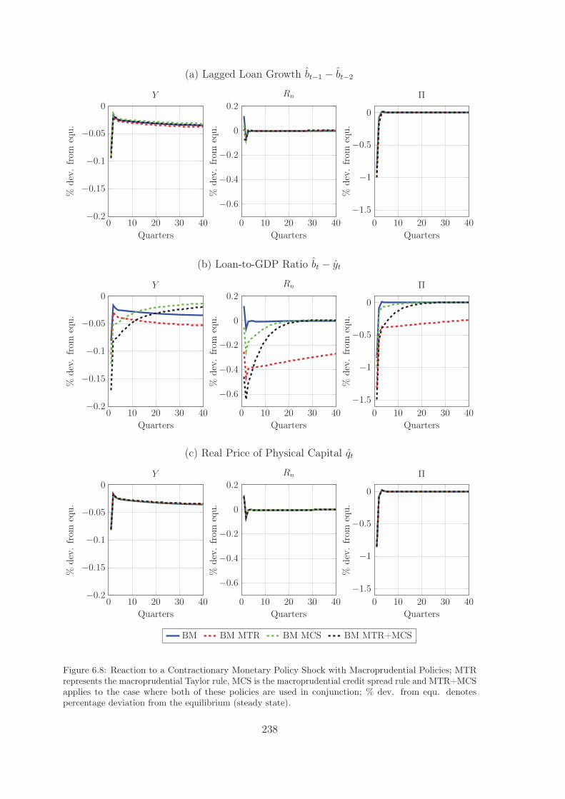
(a) Lagged Loan Growth bt−1 − bt−2

0 10 20 30 40−0.2

−0.15

−0.1

−0.05

0

Quarters

%de

v.fr

omeq

u.

Y

0 10 20 30 40

−0.6

−0.4

−0.2

0

0.2

Quarters

%de

v.fr

omeq

u.

Rn

0 10 20 30 40

−1.5

−1

−0.5

0

Quarters

%de

v.fr

omeq

u.

Π

(b) Loan-to-GDP Ratio bt − yt

0 10 20 30 40−0.2

−0.15

−0.1

−0.05

0

Quarters

%de

v.fr

omeq

u.

Y

0 10 20 30 40

−0.6

−0.4

−0.2

0

0.2

Quarters

%de

v.fr

omeq

u.

Rn

0 10 20 30 40

−1.5

−1

−0.5

0

Quarters

%de

v.fr

omeq

u.

Π

(c) Real Price of Physical Capital qt

0 10 20 30 40−0.2

−0.15

−0.1

−0.05

0

Quarters

%de

v.fr

omeq

u.

Y

0 10 20 30 40

−0.6

−0.4

−0.2

0

0.2

Quarters

%de

v.fr

omeq

u.

Rn

0 10 20 30 40

−1.5

−1

−0.5

0

Quarters

%de

v.fr

omeq

u.

Π

BM BM MTR BM MCS BM MTR+MCS

Figure 6.8: Reaction to a Contractionary Monetary Policy Shock with Macroprudential Policies; MTRrepresents the macroprudential Taylor rule, MCS is the macroprudential credit spread rule and MTR+MCSapplies to the case where both of these policies are used in conjunction; % dev. from equ. denotespercentage deviation from the equilibrium (steady state).

238

the duration for which the indicator variable is displaced from its steady state plays acrucial role. Take the MTR policy with the real price of capital as an example of the firstpoint: Following a contractionary monetary policy shock the real price of physical capitaldecreases. With a macroprudential Taylor rule in place, this leads to downward pressure onthe nominal risk-free return. Thus, the introduction of the additional variable in the Taylorrule moderates the contractionary impact of the monetary policy shock on the nominalrisk-free return, and by extension on the economy.1000 In contrast, lagged loan growth andthe loan-to-GDP ratio both increase following a monetary policy shock (see below). Thus,using the MTR policy with either of these latter two indicator variables produces a furthercontractionary effect. Moreover, the real price of physical capital reacts quantitatively lessthan lagged loan growth and the loan-to-GDP ratio. Thus, the quantitative impact ofusing the real price of physical capital as the indicator variable is smaller as compared tothe other two variables.1001

Concerning the time it takes for the indicator variables to return to their steady statesafter the initial shock, the comparison of lagged loan growth and the loan-to-GDP ratiois informative. Following a contractionary monetary policy shock, entrepreneurial loandemand increases immediately because net worth falls considerably. Due to the sluggishreturn of entrepreneurial net worth (see section 6.1.1), the loan volume also only slowlyreturns to its steady state. That means, lagged loan growth shows a stark increase inthe second quarter following a contractionary monetary policy shock, and subsequentlyshows marginally negative growth rates. In contrast, the loan-to-GDP ratio is signifi-cantly higher than its steady-state value from the period of the shock, and only slowlyreverts to its steady state.1002 Thus, the use of lagged loan growth can be interpretedas a strong one-off effect. To the contrary, the contractionary effect of the loan-to-GDPratio on the nominal risk-free return and the credit spread is long-lasting. This explainswhy the responses of GDP, inflation and the nominal risk-free return are significantlydifferent from the benchmark model when the loan-to-GDP ratio is used as an indicatorvariable, while the responses are only marginally different in the case of lagged loan growth.

However, the differences between the indicator variables do not explain the asymmetriceffects of the MTR and MCS policies. Turn next to the specificities behind the MTRpolicy. As noted above, contrary to the easing effect of the real price of physical capital,

1000 The differences are too small to be discernible in fig. 6.8c.1001 For the same reasons, the response under the MCS policy is also marginal for the real price of physical

capital q. For the MTR policy with q to yield a similar absolute quantitative impact on the nominalrisk-free return as lagged loan growth in fig. 6.8a, the coefficient θm for q would need to be 0.5 insteadof 0.25. Since qt has a dampening effect, the large amplifying effects of the loan-to-GDP ratio bt − ytas an indicator variable cannot be replicated.

1002 The effect of increasing bank loans and decreasing GDP reinforce each other with respect to theincrease in the loan-to-GDP ratio.

239

the peak in lagged loan growth in the second quarter works as a further contractionaryelement in the Taylor rule. Thus, with monetary policy reacting to lagged loan growth, thenominal risk-free return would turn out higher, ceteris paribus. Private agents are informedabout the central banks’ policy function and thus expect the additional contractionarymonetary policy. This explains why the economy is more strongly affected with the MTRpolicy as compared to the benchmark banking model.

In contrast to the one-off contractionary effect of lagged loan growth, the use of theloan-to-GDP ratio as the indicator variable has a long-lasting contractionary effect. Thus,the GDP decreases more strongly in the latter case. The long-lasting effect of contrac-tionary monetary policy is also reflected in the prolonged decrease in inflation. In contrastto the one-off monetary policy shock which reduces inflation for only a short time, thecontractionary pressure of the loan-to-GDP ratio lasts for a long period of time and inducesretailers to smooth their price-setting decision. Thus, inflation only slowly returns to itssteady state. In turn, both the long-lasting macroprudential trigger as well as long-lastinglow inflation lead to a prolonged decrease in the nominal risk-free return according to theTaylor rule.1003

The MCS policy yields results which can be deemed the opposite of the MTR policy.This is due to the fact that the MCS does not increase the general level of interest rates,but instead affects the credit spread. Furthermore, the credit spread under the MCSpolicy does not rise due to higher default probabilities but exogenously from the pointof view of entrepreneurs and banks.1004 Consider only a contractionary MCS policy dueto increases in the loan-to-GDP ratio or lagged loan growth.1005 With respect to thebenchmark banking model, loan demand still increases due to the decrease in entrepreneurs’net worth. Thus, increasing and costlier loans lead to a further fall in investment andGDP initially. Yet, subsequently, entrepreneurs’ net worth and investment, and also GDPrecover more quickly than in the benchmark banking model. The MCS policy thus induceslower capital demand due to higher marginal financing costs in the first quarters afterthe shock. This allows entrepreneurs to repair their net worth base and thus reduce theirreliance on expensive bank debt more quickly. For the one-off impact of lagged loangrowth these differences are marginal. However, for the loan-to-GDP ratio the effects ofmacroprudential policy are sizeable. In this latter case, the effect is large enough such thatinvestment and net worth return to their respective steady states at a faster pace than

1003 This reasoning is analogous to the discussion about why the monetary policy shock is larger in absolutesize than the resulting change in the nominal risk-free return in section 6.1.1.

1004 Lagged loan growth does not enter the computation of any risk premium. The loan-to-GDP ratio isnot exogenous to the computation of risk premiums. Thus, there may also be indirect effects in thiscase.

1005 Given the linearity of the model, the responses are symmetric for the easing effect of the price ofphysical capital.

240

in the benchmark banking model with the corresponding consequences for the path of GDP.

Furthermore, the different paths of the MTR and MCS policies are in fact explainedby these different dynamics and not, for example, by the impact of parametrization. Forinstance, for lagged loan growth, both macroprudential instruments imply a contractionaryimpulse by increasing the nominal risk-free return (MTR policy) or the credit spread(MCS policy), respectively. Yet, with the MTR policy the response of GDP is amplifiedwith respect to the benchmark model, while it is dampened with the MCS policy. Themain impact of different parametrizations is on the size of the deviation of endogenousvariables from their steady state in response of a monetary policy shock. Furthermore, thesensitivity analysis reported in appendix section D.4 shows that the qualitative results infig. 6.8 hold for different parameter values.

The way in which the individual MTR and MCS policies move the economy is crucialfor understanding the behaviour under the MTR+MCS policy case. This concerns whetherthe MTR and MCS policies individually work in the same or opposite directions. Forlagged loan growth, the MTR and MCS policies individually move the economy in oppositereactions in response to a monetary policy shock. Thus, the individual policies offseteach other. In contrast, the MTR+MCS policy with the loan-to-GDP ratio leads to aresponse which is stronger (initially) than under any single policy instrument since bothindividual policies work in the same direction. The response is stronger for MTR+MCSthan the individual policies, because both individual policies amplify the responses ofthe endogenous variables as compared to the benchmark model. Subsequently, the lowerpersistence of the MCS policy outweighs the reaction under the MTR policy. However,when both policies are implemented simultaneously, the response of all three variables isstronger and longer-lasting than when only the MCS policy is in place. Thus, the additionof an MTR to an existing MCS rule has a further contractionary effect, but does notdetermine by itself the duration of the response.

A related corollary of the analysis of the MCS policy with the loan-to-GDP ratioraises another topic: if the government tightens credit conditions in the short and mediumrun following a contractionary monetary policy shock, the speed of recovery concerningentrepreneurial net worth, investment and GDP is much higher. Thus, while the balancesheet position of entrepreneurs worsens with respect to the benchmark banking model inthe short run, it also means that balance sheets are repaired more quickly. This creates anew trade-off for financial stability if speed of recovery and small impact on entrepreneurialbalance sheets are taken as objectives: macroprudential policy may shorten the time ofbalance sheet repair, but at the cost of depressing the situation immediately after a shock.

241

Yet, this last result has to be regarded with caution given the reduced-form andad-hoc implementation of the macroprudential policies. The ability of the government ora macroprudential authority to actually affect the credit spread may be rather limited.Further, and more importantly, such a manipulation (other than a direct regulation ofthe size of the credit spread) will most probably involve costs of some form for one ofthe agents. These have been neglected in the interest of clarity, but play a crucial role indetermining the efficiency and desirability of any policy. Thus, these results suggest thatresearch in this area should be clear on the specific implementation, costs and benefits ofsuch a policy. Furthermore, the specific implementation of a macroprudential policy doesnot only impact the evaluation in terms of financial stability. Crucially, this section showsthat the specificities of the macroprudential policy affect the assessment of the effects onthe conduct of monetary policy.

One important factor which is only touched upon here are adjustment lags. Adjustmentlags concern two kinds of lags. They may be on the part of the policy institution whichonly gradually responds to developments as they are incorporated into the decision-makingprocess. The use of lagged loan growth can be interpreted as an example of such a lag. Onthe other hand, private agents may be slow in adjusting to new regulatory stimulus. Therational expectations and perfect foresight assumptions of the banking model preclude theincorporation of this latter kind of lag. Furthermore, these two assumptions also preventthe former kind of lags to have any significant effect on the results.1006 Since private agentsknow the structure of the model and the monetary policy function, agents’ expectationsalready incorporate the impact of lagged loan growth on the risk-free return in the future.Thus, decision-making lags concerning policy do not have a major impact.

What is more, adjustment lags may not be considered important because they changethe transmission of monetary policy shocks. Rather, adjustment lags need to be consideredbecause macroprudential policy reacting with a lag may hit the economy when it is alreadyrecovering and the macroprudential impulse is not ‘necessary’ any more. This question,however, commands a different analysis and focus from the one pursued here. Such ananalysis can be primarily interpreted as concerning the response of macroprudential policyto financial shocks. The question is then whether macroprudential policy is able to respondadequately to such (adverse) developments in the financial sector. In contrast, the rationalefor studying the impact of macroprudential policies in this thesis is based on the questionwhether the impact of financial fragility on monetary policy is altered when the governmentadditionally aims to foster financial stability. Financial fragility and macroprudential

1006 As noted above, results are not qualitatively different when contemporaneous loan growth is usedinstead of lagged loan growth. In fact, using contemporaneous loan growth shows that the change inthe response of GDP after a monetary policy shock is in the same direction but somewhat strongerthan for lagged loan growth.

242

policies can then be interpreted as established features of the banking model economy.While this does not alleviate the need for the correct timing of macroprudential policy,the fact that this kind of policy is taken into account by private agents immediately canbe deemed a reasonable starting point. Future research in this direction can then gofurther and discern the optimal timing, communication and measurement strategies ofmacroprudential policies.

To conclude, the results suggest that macroprudential policies which imply a small one-off effect on either the nominal risk-free return or the credit spread affect the transmissionof monetary policy only marginally. In contrast, if macroprudential policy is triggeredover a prolonged period of time, then the responses of GDP, inflation and the nominalrisk-free return change significantly. Moreover, the choice of indicator variable is crucial indetermining whether macroprudential policy induces a contractionary or an expansionary,short-term or long-lasting effect on the economy. For a more comprehensive assessment ofthe consequences for monetary policy, the next section will turn to the trade-off betweeninflation and output gap stabilisation and to the question whether previous results areaffected by the introduction of macroprudential policies.

6.3.4 Macroprudential Policies and the Inflation-Output Gap Sta-

bilisation Trade-off

The dynamics of the benchmark banking model led to a deterioration of the inflation-outputgap variances trade-off, while the posterior estimation produced a set of parameters thatyielded an improvement of the banking model with respect to the financial acceleratormodel when both models were evaluated using the respective posterior mean.1007 So, howdo different macroprudential policies affect this result?

To this end, fig. 6.9 displays Taylor curves for the various macroprudential policies.1008

Panels 1 to 3 show the macroprudential policy combinations already considered in fig. 6.8for each of the three indicator variables.1009 Again, the benchmark banking model (blueline) is included as a reference. The fourth, bottom right panel shows the Taylor curve forthe endogenous deposit insurance factor version without bank risk shocks.1010

1007 See section 6.21008 In computing the graphs the output gap definition of the deviation of GDP from its counterpart in a

simple NK model is used, as in fig. 6.5.1009 The Taylor curves in fig. 6.9 were also computed using different values for τM (0.05 to 0.3 in 0.05

steps) and θm (0.5 to 2.5 in 0.5 steps). The results of this section generally hold with these differentparameter values. See appendix section D.4 for more details.

1010 Note that in fig. 6.9 the legend on the left-hand side applies to panels 1-3 concerning the indicatorvariables lagged loan growth, loan-to-GDP ratio and real price of physical capital, and the legend onthe right-hand side applies to the endogenous deposit insurance factor.

243

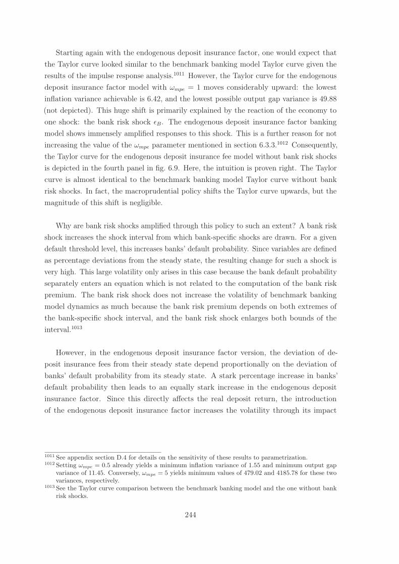
Starting again with the endogenous deposit insurance factor, one would expect thatthe Taylor curve looked similar to the benchmark banking model Taylor curve given theresults of the impulse response analysis.1011 However, the Taylor curve for the endogenousdeposit insurance factor model with ωmpe = 1 moves considerably upward: the lowestinflation variance achievable is 6.42, and the lowest possible output gap variance is 49.88(not depicted). This huge shift is primarily explained by the reaction of the economy toone shock: the bank risk shock εB. The endogenous deposit insurance factor bankingmodel shows immensely amplified responses to this shock. This is a further reason for notincreasing the value of the ωmpe parameter mentioned in section 6.3.3.1012 Consequently,the Taylor curve for the endogenous deposit insurance fee model without bank risk shocksis depicted in the fourth panel in fig. 6.9. Here, the intuition is proven right. The Taylorcurve is almost identical to the benchmark banking model Taylor curve without bankrisk shocks. In fact, the macroprudential policy shifts the Taylor curve upwards, but themagnitude of this shift is negligible.

Why are bank risk shocks amplified through this policy to such an extent? A bank riskshock increases the shock interval from which bank-specific shocks are drawn. For a givendefault threshold level, this increases banks’ default probability. Since variables are definedas percentage deviations from the steady state, the resulting change for such a shock isvery high. This large volatility only arises in this case because the bank default probabilityseparately enters an equation which is not related to the computation of the bank riskpremium. The bank risk shock does not increase the volatility of benchmark bankingmodel dynamics as much because the bank risk premium depends on both extremes ofthe bank-specific shock interval, and the bank risk shock enlarges both bounds of theinterval.1013

However, in the endogenous deposit insurance factor version, the deviation of de-posit insurance fees from their steady state depend proportionally on the deviation ofbanks’ default probability from its steady state. A stark percentage increase in banks’default probability then leads to an equally stark increase in the endogenous depositinsurance factor. Since this directly affects the real deposit return, the introductionof the endogenous deposit insurance factor increases the volatility through its impact

1011 See appendix section D.4 for details on the sensitivity of these results to parametrization.1012 Setting ωmpe = 0.5 already yields a minimum inflation variance of 1.55 and minimum output gap

variance of 11.45. Conversely, ωmpe = 5 yields minimum values of 479.02 and 4185.78 for these twovariances, respectively.

1013 See the Taylor curve comparison between the benchmark banking model and the one without bankrisk shocks.

244

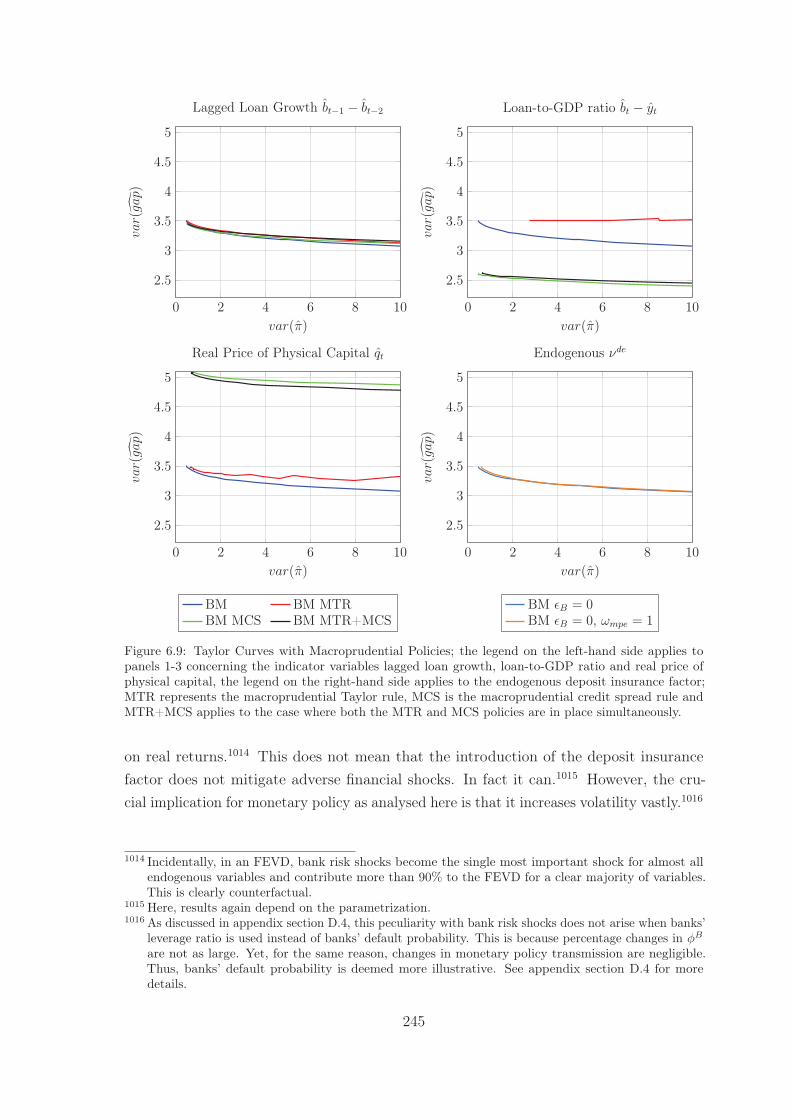
0 2 4 6 8 10

2.5

3

3.5

4

4.5

5

var(π)

var(gap)

Lagged Loan Growth bt−1 − bt−2

0 2 4 6 8 10

2.5

3

3.5

4

4.5

5

var(π)

var(gap)

Loan-to-GDP ratio bt − yt

0 2 4 6 8 10

2.5

3

3.5

4

4.5

5

var(π)

var(gap)

Real Price of Physical Capital qt

BM BM MTRBM MCS BM MTR+MCS

0 2 4 6 8 10

2.5

3

3.5

4

4.5

5

var(π)

var(gap)

Endogenous νde

BM εB = 0BM εB = 0, ωmpe = 1

Figure 6.9: Taylor Curves with Macroprudential Policies; the legend on the left-hand side applies topanels 1-3 concerning the indicator variables lagged loan growth, loan-to-GDP ratio and real price ofphysical capital, the legend on the right-hand side applies to the endogenous deposit insurance factor;MTR represents the macroprudential Taylor rule, MCS is the macroprudential credit spread rule andMTR+MCS applies to the case where both the MTR and MCS policies are in place simultaneously.

on real returns.1014 This does not mean that the introduction of the deposit insurancefactor does not mitigate adverse financial shocks. In fact it can.1015 However, the cru-cial implication for monetary policy as analysed here is that it increases volatility vastly.1016

1014 Incidentally, in an FEVD, bank risk shocks become the single most important shock for almost allendogenous variables and contribute more than 90% to the FEVD for a clear majority of variables.This is clearly counterfactual.

1015 Here, results again depend on the parametrization.1016 As discussed in appendix section D.4, this peculiarity with bank risk shocks does not arise when banks’

leverage ratio is used instead of banks’ default probability. This is because percentage changes in φBare not as large. Yet, for the same reason, changes in monetary policy transmission are negligible.Thus, banks’ default probability is deemed more illustrative. See appendix section D.4 for moredetails.

245

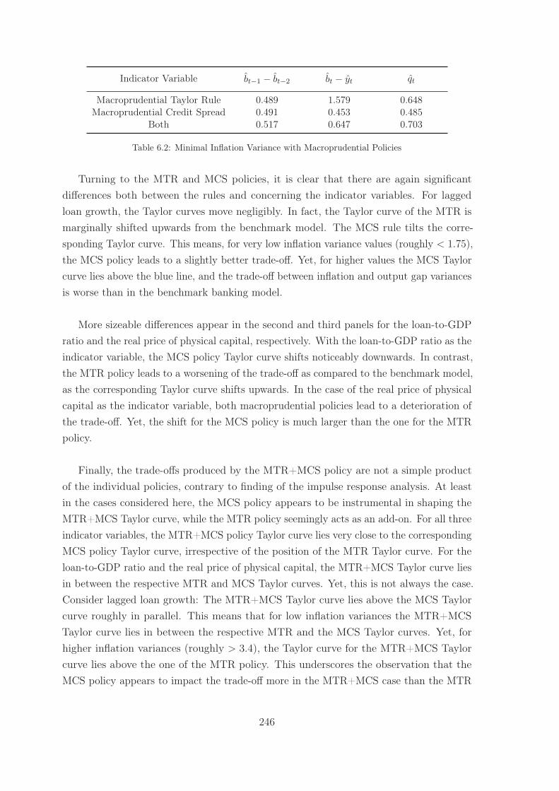
Indicator Variable bt−1 − bt−2 bt − yt qt

Macroprudential Taylor Rule 0.489 1.579 0.648Macroprudential Credit Spread 0.491 0.453 0.485

Both 0.517 0.647 0.703

Table 6.2: Minimal Inflation Variance with Macroprudential Policies

Turning to the MTR and MCS policies, it is clear that there are again significantdifferences both between the rules and concerning the indicator variables. For laggedloan growth, the Taylor curves move negligibly. In fact, the Taylor curve of the MTR ismarginally shifted upwards from the benchmark model. The MCS rule tilts the corre-sponding Taylor curve. This means, for very low inflation variance values (roughly < 1.75),the MCS policy leads to a slightly better trade-off. Yet, for higher values the MCS Taylorcurve lies above the blue line, and the trade-off between inflation and output gap variancesis worse than in the benchmark banking model.

More sizeable differences appear in the second and third panels for the loan-to-GDPratio and the real price of physical capital, respectively. With the loan-to-GDP ratio as theindicator variable, the MCS policy Taylor curve shifts noticeably downwards. In contrast,the MTR policy leads to a worsening of the trade-off as compared to the benchmark model,as the corresponding Taylor curve shifts upwards. In the case of the real price of physicalcapital as the indicator variable, both macroprudential policies lead to a deterioration ofthe trade-off. Yet, the shift for the MCS policy is much larger than the one for the MTRpolicy.

Finally, the trade-offs produced by the MTR+MCS policy are not a simple productof the individual policies, contrary to finding of the impulse response analysis. At leastin the cases considered here, the MCS policy appears to be instrumental in shaping theMTR+MCS Taylor curve, while the MTR policy seemingly acts as an add-on. For all threeindicator variables, the MTR+MCS policy Taylor curve lies very close to the correspondingMCS policy Taylor curve, irrespective of the position of the MTR Taylor curve. For theloan-to-GDP ratio and the real price of physical capital, the MTR+MCS Taylor curve liesin between the respective MTR and MCS Taylor curves. Yet, this is not always the case.Consider lagged loan growth: The MTR+MCS Taylor curve lies above the MCS Taylorcurve roughly in parallel. This means that for low inflation variances the MTR+MCSTaylor curve lies in between the respective MTR and the MCS Taylor curves. Yet, forhigher inflation variances (roughly > 3.4), the Taylor curve for the MTR+MCS Taylorcurve lies above the one of the MTR policy. This underscores the observation that theMCS policy appears to impact the trade-off more in the MTR+MCS case than the MTR

246

policy. Put differently, with an MCS policy in place, adding an MTR policy does notworsen the trade-off as much as when there is no MCS policy. Yet, the real price of physicalcapital also points to another feature: if both the MTR and the MCS policies individuallyimply a deterioration of the trade-off, then the combination in terms of the MTR+MCSpolicy does not need to fare even worse. In this case, adding the MTR policy to the MCSpolicy dampens fluctuations in response to shocks to some extent, such that the Taylorcurve shifts back downwards.

To view the results from a different angle, consider again the respective minimum infla-tion variance which is achievable in each policy case. These are summarised in table 6.2.1017

The minimum inflation variance in the benchmark banking model is 0.460. It is clear thatall policy and indicator variable combinations lead to an increase in the minimum inflationvariance, except for one. This exception is the MCS policy with the loan-to-GDP ratio asindicator variable. Here, the minimum inflation variance is 0.453. Thus, this combinationof macroprudential policy and indicator variable provides the opportunity of a marginallylower inflation variance in addition to significantly improving the inflation-output gapvariances trade-off.1018 In contrast, the MTR policy with the loan-to-GDP ratio leads to asignificantly higher minimum inflation variance. Taken together, these Taylor curve resultssuggest that the MCS policy with the loan-to-GDP ratio provides the best trade-off forthe central bank of the macroprudential policies introduced here. However, the mixedresults concerning all other combinations suggest that general patterns for one kind ofpolicy or indicator variable are difficult to establish.

Nevertheless, there are some noteworthy points. To start with, the tilt-shift in theMCS Taylor curve using lagged loan growth as the indicator variable offers an importantinsight for optimal policy analysis: Depending on the loss function, there may or maynot be a preference for the MCS as compared to the benchmark model. In this example,the Taylor curves for the banking model with and without the MCS policy cut eachother at an inflation variance of around 1.75. The corresponding value for the outputgap variance is roughly 3.31. Thus, as long as the central bank values inflation varianceabout twice as highly as output gap variance (in a corresponding loss function), thenthe MCS policy improves the policy trade-off. However, as the output gap variancebecomes more and more important, the MCS policy produces a worse trade-off. Asa consequence, a sensitivity analysis is imperative for optimal policy with ad-hoc loss

1017 The response coefficients in the Taylor rules for the values in table 6.2 are the following. The reactioncoefficient to inflation θπ is at its upper bound, that is θπ = 5, for all combinations. The reactioncoefficient to the output gap θy is also at its lower bound, but varies between 0 and 0.5 for differentcombinations of indicator variable and macroprudential policy.

1018 Comparing the curves in fig. 6.9 it is clear that this policy also yields the smallest output gap varianceof the model versions considered here.

247

functions. Kannan et al. (2012), for instance, compute optimal Taylor rule coefficientsfor a variety of central bank preferences in terms of the weight on output gap deviations.They also find some instances where the ranking of the various macroprudential poli-cies changes when preferences change.1019 Concerning optimal policy analysis based onwelfare functions, this remark may not seem as relevant on first sight. However, whilewelfare functions derive a model-based objective function, the underlying assumptionsabout the utility of one or more agents are still crucial, potentially affecting policy rankings.

Moreover, previous results in the literature indicate that the type of shock impactsthe usefulness of a macroprudential policy regime.1020 However, this observation can onlybe partially supported in this study. In particular, the assessment of the position ofshock-specific Taylor curves depends on the indicator variable. For the loan-to-GDP ratio,the results of the all-shock Taylor curve generally carry over to the single-shock Taylorcurves.1021 This implies that the MTR Taylor curve shifts upward and the MCS andMTR+MCS Taylor curves downwards with respect to the benchmark banking model.1022

This is also true for the real price of physical capital MCS and MTR+MCS policies, wherethe single-shock Taylor curves generally shift upwards.1023 In contrast, for lagged loangrowth, and the real price of physical capital MTR policy, the single-shock Taylor curveswander around the respective benchmark banking model Taylor curve. For either of thesepolicy combinations, there are some shocks which show no shift at all, a tilt in the Taylorcurve, or shifts up- or downwards. Given the closeness of the all-shock Taylor curves withthese latter macroprudential policies to the benchmark banking model Taylor curve, theseresults are not surprising.

Nonetheless, the absolute magnitude of shifts in single-shock Taylor curves point to asubordinate role of shock-specific differences. The Taylor curve movements induced by thevarious macroprudential policies are generally moderate when only one shock is considered.While different shocks induce different volatilities of inflation and the output gap, theintroduction of a macroprudential policy generally does not have a major impact on the

1019 See Kannan et al. (2012: 26f)1020 See Angelini et al. (2012: 25f), Bailliu et al. (2015: 161) and Kannan et al. (2012: 35)1021 This means that for each single-shock macroprudential Taylor curve the reference is to the banking

model Taylor curve computed for the same shock.1022 There are two exceptions: Government consumption shocks with either the MCS or the MTR+MCS

policy lead to an upward shift of the Taylor curve. Under the MTR policy, the Taylor curve withmark-up shocks tilts marginally. This tilt is also evident for government consumption and financialshocks for the MTR policy. However, the tilt is such that the MTR policy improves the trade-off athigh inflation variance values, and worsens it for low such values. Thus, it may be argued that forinflation-concerned central banks the relevant part of the Taylor curve tilts in the same direction asthe all-shocks Taylor curve shifts.

1023 Here, it is the entrepreneurial risk shock which breaks the pattern in showing a downward shift of theMCS and MTR+MCS policies. Also, preference shocks shift the MCS policy Taylor curve downwards.

248

position of the single-shock Taylor curves.1024 However, different indicator variables andthe parameters governing the rigour of the macroprudential policy reaction emerge as moredecisive in explaining different magnitudes. This supports the argument in section 6.2whereby it may be problematic for the central bank to adjust its rule-based conduct inresponse to specific shocks. The results of this section further show that the effects ofmacroprudential policies on policy trade-offs do not warrant a focus on specific shockssince the particular implementation of macroprudential policy exerts a larger influence.

More to the objective of macroprudential policies, their introduction can improve theinflation-output gap variances trade-off when faced with financial shocks. As discussed inappendix section D.3, the Taylor curve of the banking model showed a different slope ascompared to the financial accelerator model for the case of entrepreneurial risk shocks.With an MCS policy reacting to the loan-to-GDP ratio, this change in slope is reversed.1025

In fact, the Taylor curve lies to the left of the respective financial accelerator model Taylorcurve when only entrepreneurial risk shocks are considered. What is more, the MCS andMTR+MCS policies always show a (partial) improvement in terms of the Taylor curvewith entrepreneurial risk shocks, yet the results are mixed for bank risk shocks and theMTR policy.1026 This implies that macroprudential policy can mitigate the adverse effectsof financial shocks for macroeconomic stability. Yet again, the particular implementationis important.

The result that macroprudential policies can in general improve the inflation-outputgap variances trade-off supports related findings in the literature. Bailliu et al. (2015) findthat welfare improves when macroprudential Taylor or credit spread rules are used.1027

They find that different regimes increase agents’ welfare to different extents and thatthe size of the welfare gains depends on the type of shock.1028 Yet, in contrast to thesefindings, this study shows that not all macroprudential policy implementations lead to an

1024 There are again some exceptions. These are capital quality shocks when the loan-to-GDP ratio is used,and investment adjustment cost shocks with the price of physical capital. The fact that these policycombinations induce large shifts in the Taylor curves does not weaken the argument that the type ofshock is generally of lesser importance. Given the wide differences seen in the analysis of a monetarypolicy shock, it would be rather surprising to have no significant shifts in Taylor curves. However,as compared to the other two factors, these exceptions do not increase the weight of shock-specificanalyses.

1025 For bank risk shocks, the Taylor curve is comparatively flat in the var(gap)-var(π) space for thebenchmark banking model. With the MCS policy reacting to the loan-to-GDP ratio, the Taylor curvesimply shifts downwards without a noticeable change in slope.

1026 ‘Partial’ means that at least a tilt improving the output gap variance for small inflation variances isvisible.

1027 See Bailliu et al. (2015: 161)1028 See Bailliu et al. (2015: 161)

249

improvement of the policy objectives trade-off.1029 Furthermore, this study corroboratesexisting research that the usefulness of indicator variables varies. Gambacorta and Sig-noretti (2014), for example, find that the usefulness as an indicator variable varies for assetprices and credit growth. However, somewhat opposite to the findings here, Gambacortaand Signoretti (2014) find that a macroprudential Taylor rule reacting to asset pricesleads to a marked shift in the Taylor curve while the use of credit growth only leads toa marginal shift.1030 The term ‘somewhat’ is justified since Gambacorta and Signoretti(2014) consider technology shocks and mark-up shocks separately.1031 If there are onlyeither technology or mark-up shocks in the banking model, then an MTR policy witheither variable leads to a (marginal) leftward or no shift of the Taylor curve. Thus, thefinding concerning credit growth is confirmed, while the extent of the shift for asset pricesis not matched in the banking model. As discussed further below, the performance ofasset prices in the banking model may be connected to the empirical properties of the model.

So far the issue of whether financial stability is actually enhanced with any of thesemacroprudential policies has not been considered. This is due to the focus on monetarypolicy. Thus, the issue of how, and to what extent, macroprudential policies may enhancefinancial stability is of secondary importance. Appendix section D.5 provides more detailson how the considered macroprudential policies perform in terms of enhancing financialstability. A clear-cut answer to whether financial stability improves is challenging in thepresent context due to some difficulties. Given that three different indicator variables areused, should each policy be evaluated with respect to the variance of its indicator variable?Or should each combination be evaluated with respect to a common measure, such as thevariance of asset prices or loans? Finally, how should improvements in one dimension buta deterioration in another be evaluated, for instance if the variability of loans increases butthe variance of asset prices decreases? These are not theoretical questions. As detailed inappendix section D.5, there is not a single policy and indicator variable combination whichachieves a monotonic improvement in all dimensions.1032 For example, the MCS policywith the real price of physical capital decreases the variance of the real price of physicalcapital, but increases the variance of the loan-to-GDP ratio. So, is this an improvement interms of financial stability? Given that there are other combinations of macroprudentialpolicies and indicator variables leading to an improvement in at least one dimension, which

1029 There are various modelling differences which may explain these differences, not least the lower numberof shocks in Bailliu et al. (2015). Also, Bailliu et al. (2015) only consider credit growth. In thisrespect, the fact that the MCS policy improves the trade-off for low inflation values can be consideredin line with Bailliu et al. (2015) since they perform an optimal policy analysis. Furthermore, thewelfare gains are generally small in Bailliu et al. (2015) which resembles the closeness of the Taylorcurves in fig. 6.9.

1030 See Gambacorta and Signoretti (2014: 157)1031 See Gambacorta and Signoretti (2014: 156ff)1032 This excludes the case of a countercyclical deposit insurance factor. The reasons for not considering

this policy in more detail here are presented in appendix section D.5.

250

of them is preferable? From a financial stability perspective, these questions cannot beanswered properly within the bounds of this study, not least given the ad-hoc modellingapproach, and are thus left to future research.

Besides, the results on macroprudential policies in this chapter have to be qualifiedin at least three ways. Firstly, in this simple implementation of a macroprudential creditspread rule, the credit spread rises exogenously from private agents’ point of view. Witha more elaborate microfoundation, second-order or indirect effects may counteract orreinforce observed responses. Secondly, these results have to be viewed in the light of thesecond moment comparisons in chapter 5. The volatility of bank loans in the bankingmodel is significantly above the one implied by the data. Conversely, the volatility ofreal returns and inflation in the banking model is much lower than in the data. Thismight be an explanation for the small impact of macroprudential rules with the real priceof physical capital, and the stark differences when the loan-to-GDP ratio is used as theindicator variable. Thirdly, the results on individual shock processes have to be takenwith caution. To the extent that the shocks introduced in the banking model do not trulyrepresent structural shocks, the introduction of a macroprudential regime may change theinterpretation or the fundamental process.1033 Particularly the entrepreneurial and bankrisk shocks may be criticised for not representing structural disturbances holding up tothe Lucas critique.

Moreover, the introduction of the endogenous deposit insurance factor highlights theimportance of another assumption of the banking model. The assumption that neitherbanks nor workers have access to some other form of liability or asset plays a crucial rolein the banking model. There is no possibility for workers to save other than through banks.This allows banks to manipulate the real deposit return. More complex effects are to beexpected if there is the possibility to buy government bonds, for example. In this case, it isdisputable whether banks would be able to charge a real deposit return lower than the realrisk-free return.1034 This is in turn connected to issues of market power and competition inthe markets for banks’ liabilities as well as for other savings instruments.1035 The discussionabout the ability of banks to raise funds becomes crucial in this regard. Such constraintsmay work through effects emphasised by the bank lending channel literature, wherebythe overall volume of bank liabilities changes. In contrast, they may also work throughrestraining banks’ remuneration policies as modelled in this study. As a consequence of the

1033 See Chari et al. (2009: 253ff) on the issue of non-structural shocks in DSGE models.1034 This relates to the discussion of negative deposit rates which has been spurred by the financial crisis

and subsequent exceptionally long period of low policy rates.1035 The empirical evidence on competition in the banking sector suggests that monopolistic competition

can account for a differential between deposit and other risk-free returns. However, this still presupposesthat households cannot or do not want to hold other assets, due to simple participation exclusions orother benefits they receive from holding bank deposits.

251

reduced form representation of banks’ balance sheet, non-insured forms of bank debt aswell as other forms of bank capital cannot be studied in the banking model. This enabledthe banking model to highlight one possible mechanism through which credit conditionstighten due to bank-specific constraints. Further and ongoing research can build on thisand extend the analysis to more elaborate balance sheet compositions.

Finally, the results of this chapter point to the need to study coordination issues ofmonetary and macroprudential policies. Admittedly, the question of whether macropruden-tial and monetary policies are coordinated or not has not been explicitly dealt with in thisdiscussion. It is simply not pertinent to the focus of this study because the objective wasnot to discern the optimal policy mix. Yet, given that in the banking model not a singlecombination of macroprudential policy and indicator variable results in similar effects formonetary policy transmission and the monetary policy objectives trade-off, it is crucialthat spill-over effects to the conduct of monetary policy due to the design of macropruden-tial policy are taken into account. Recent research is already developing in this direction.1036

In a nutshell, irrespective of the potential of macroprudential policies to affect financialstability, such policies have an impact on the capabilities of the central bank in terms ofmanaging macroeconomic stability. Especially policy implementations which trigger along-lasting and sizeable macroprudential impulse affect the conduct of monetary policysignificantly. The results imply that the effects of macroprudential policies should notonly be considered as impacting the transmission of monetary policy, but also in termsof monetary policy goals. Moreover, the results suggest that these effects should beincorporated explicitly into the evaluation process so as to be able to communicate thechanges effectively and thus make the changes for monetary policy predictable.

Whether or not spill-over effects change the actual implementation is a different ques-tion. Therefore, these conclusions should not be interpreted as arguing for macroprudentialpolicies to be decided upon their impact on monetary policy. Any such statement ne-cessitates a thorough evaluation of the objectives of macroprudential as well as othergovernmental policies themselves. Rather, these conclusions point to the significance ofinterrelationships between different governmental policies. In line with the comments onfiscal policies, monetary policy transmission and policy trade-off depend on the specificconceptualisation of other governmental policies just as on the other features which formthe monetary policy transmission mechanism. Thus, an interesting avenue of futureresearch is the determination and quantitative significance of these spill-over effects andconnections.

1036 See Angelini et al. (2012), for example.

252

Chapter 7

Conclusion

This study was designed to determine the consequences of non-systemic bank failure forthe conduct of monetary policy. The objective was to evaluate how failures of non-systemicbanks affect the transmission of monetary policy and the potential to achieve differentmonetary policy objectives. These two elements were to be assessed for the case that thereexists no additional governmental policy targeting financial stability, as well as in thecase such a policy exists. Finally, a corollary research question was to judge the relativeimportance of the financial friction arising from default of non-financial firms versus theone arising from bank default.

To this end, a standard New Keynesian dynamic stochastic general equilibrium modelwith financial accelerator was extended to incorporate non-systemic bank default. Thebanking model presented in this thesis incorporates the endogenous determination ofnon-systemic bank default and of bank leverage through workers’ portfolio choice problem.A financial accelerator model without the additional bank friction is used as a referenceto discern the effects of non-systemic bank failures. Both the banking and financialaccelerator models were log-linearised around their respective deterministic steady states.These log-linear approximations were used for both estimation and simulation. First, thelog-linear approximations were estimated on German data using Bayesian techniques. Thenext and final step consisted in simulating the banking and financial accelerator modelsfor monetary policy analysis purposes. The main instruments used in chapter 6 to presentthe simulation results were impulse response functions and Taylor curves.

Succinctly, the findings of this thesis can be summarised as follows. Firstly, theincidence of non-systemic bank default affects the transmission of monetary policy. Inparticular, the introduction of the friction on banks’ liability side leading to bank defaultgives rise to an additional bank balance sheet channel. Incidentally, the bank balance sheetchannel does not fundamentally affect inflation. Rather, the bank balance sheet channelhas a non-trivial impact on the response of aggregate demand in that monetary policy

253

shocks affect GDP more lastingly than when banks do not default. This study maintainedthat the main mechanism of the bank balance sheet channel lies in the passing-throughbehaviour of banks: banks facing tighter financing conditions as a consequence of con-tractionary monetary policy pass these tighter conditions on to entrepreneurs. Therefore,this bank balance sheet channel works on top of the balance sheet channel based onentrepreneurs’ balance sheets. This implies that the bank balance sheet channel has afundamentally compounding nature. Furthermore, the findings suggest that the amplifyingand propagating effects of this bank balance sheet channel are the stronger, the higher isthe steady-state level of bank fragility and if there are impediments to the instantaneousadjustment of workers’ portfolio shares (that is by extension bank leverage).

Secondly, non-systemic bank default affects the capabilities of the central bank toachieve different monetary policy objectives. If a central bank aims to minimise inflationvolatility, the introduction of bank default yields a worse outcome than when banks do notdefault. Irrespective of the parametrization, when a central bank only cares about inflation,the resulting minimum inflation variance monetary policy can achieve is always higher inthe banking model. Moreover, taking output gap stabilisation as an additional (secondary)monetary policy objective into account, banking model dynamics also imply a deterio-ration of the central bank’s trade-off between inflation and output gap variance stabilisation.

Thirdly and related, the results concerning the monetary policy trade-off depend onthe parametrization. As noted, banking model dynamics imply a worse trade-off betweeninflation and output gap variance stabilisation than the dynamics of the financial accelera-tor model. Yet, the estimation produced a set of parameter estimates that shows a bettertrade-off for the banking model than the financial accelerator model when each models’own parameter estimates are used in the simulations. The results suggest that carefulattention should be paid to the parametrization of the model and that the improvementin terms of empirical fit may be connected to an improved trade-off between monetarypolicy objectives.1037

Thus, this thesis highlights the necessity of sensitivity and robustness analyses. For one,results for the trade-off between monetary policy objectives differ in terms of whether thesame parametrization is used or each model is simulated using its own estimated posteriorparameter vector. Therefore, uncertainty about models and parameters implies that policytargets are more robustly denominated in terms of ranges instead of specific point values.Another implication concerns research on optimal policy analyses. The possibility thatTaylor curves may tilt due to additional policies shows that care should be taken when

1037 The comparison of empirical fit concluded that the banking model improved upon the financialaccelerator model.

254

specifying loss functions. Sensitivity analyses should be conducted to discern whetherpolicies really improve the trade-off over a wide range of inflation variances, or only for aspecific interval.

What do the results imply for the conduct of monetary policy? The findings suggest ahierarchy of monetary policy objectives based on the capabilities of the central bank toimpact them: first inflation, then output gap stabilisation. So, taking monetary policydisturbances in isolation for analysing monetary policy transmission, this study foundthat the effectiveness of interest rate policy with respect to the primary objective of pricestability is not affected. Yet, allowing for disturbances in other parts of the model economy,the central banks’ capability to minimise inflation variability is impeded with non-systemicbank failures. This suggests a generally more aggressive stance of the central bank whenbanks can fail.

Even though the central bank is not as influential when it comes to output gap sta-bilisation, the effects on GDP should not be disregarded. A stronger impact on GDP isimportant for preparing monetary policy decisions in terms of data-gathering and analysingthe economic outlook. Also, private sector expectations about the future economic de-velopment change with the incidence of bank failures, which is important for monetarypolicy conduct to the extent that the central bank wishes to anchor inflation expectations.In this regard, this study corroborated the need for credible and predictable monetarypolicy for anchoring inflation expectations as long-term forecasts of inflation are criticallyinfluenced by unpredictable changes in monetary policy.

Furthermore, to the extent that the central bank conducts some form of inflationtargeting, the incidence of bank failures may mean that a central bank reacts moremoderately so as to avoid more severe consequences for GDP. Incidentally, this is theopposite of the conclusion about higher inflation volatility above. Thus, if output gapstabilisation is an additional goal of monetary policy, the incidence of bank default raisesconflicting implications for monetary policy. This has consequences for the optimal designof monetary policy and the weighting of different monetary policy objectives. Furthermore,an issue which has only been touched marginally here, but becomes especially importantfor optimal policy design, is that other governmental policies targeted at smoothing thebusiness cycle may (have to) adjust in response to the incidence of bank failure. Therefore,there may be spill-over effects between different economic policies which have not beendiscussed here.

The issue of policy spill-overs has been highlighted by the discussion about macro-prudential policy. Concerning monetary policy transmission, the findings are clear-cut.

255

Overall, the transmission to inflation is not fundamentally affected, thus interest rate policyremains effective in this respect. However, the nature of the macroprudential trigger affectsmonetary policy transmission to GDP. The stronger the impact of monetary policy on thefinancial imbalances which in turn trigger macroprudential policy, the stronger is the effectof monetary policy on GDP. Macroprudential triggers working in the same direction asthe monetary policy impulse, that is both either contractionary or expansionary, amplifythe response of GDP; macroprudential triggers working in the opposite direction of themonetary policy impulse moderate the response of GDP. Finally, one-off macroprudentialtriggers have a smaller effect on GDP than macroprudential triggers that are in effect for aprolonged period of time. With respect to the trade-off between inflation and output gapstabilisation, the results are not as clear-cut. In particular, depending on how financialimbalances are measured and with which macroprudential instrument the governmentresponds to them, macroprudential policies can lead to an improvement in terms of thetrade-off between policy objectives as well as to a deterioration, noting that the differencescan be large.

Thus, both the impulse response and the Taylor curve analyses indicate that thereare potentially large consequences of introducing macroprudential policies. Therefore,different governmental policies should not be dealt with separately or modelled in isolation.Rather, the results suggest that the specific implementation of policy changes shouldbe communicated to the central bank on the one hand and to the private sector on theother hand since information and transparency help in discerning potential spill-overs. Asargued above, the analyses of the transmission of impulses as well as of the central banks’capabilities to stabilise inflation and the output gap are important for the monetary policydecision-making process. Furthermore, different policies have non-trivial effects for privatesector expectations and thus again for central banks’ aim to anchor (inflation) expectations.

Nevertheless, this study gives some indication that it is not only transparency betweendifferent governmental policies which would be warranted, but also coordination. Somemacroprudential policy combinations yielded comparatively large effects in terms of impulseresponse functions and Taylor curves. This suggests that the decision about implementinga specific macroprudential policy may not only depend on its effects on financial stability.Rather, potentially adverse non-negligible consequences for the conduct and effectivenessof monetary policy may provide a rationale for considering policy spill-over effects duringthe conceptualisation and implementation stages, and also for coordinating differentgovernmental policies. However, the particular implementations in this thesis are tooad-hoc to make any definite recommendations about any policy (combination). Thus,this study provides a clear imperative for further research on the interactions betweenmonetary and macroprudential policies.

256

Moreover, the findings of this thesis suggest that the central financial friction impactingthe economy is the one on the loan market.1038 Unforeseen shocks to entrepreneurs’riskiness have a large impact on private sector expectations of nominal and real variables,while similar shocks on banks’ riskiness mainly impact the return on bank equity. Thisdifference is partly due to different sizes of monitoring costs associated with these frictions.More important appears to be that in the banking model entrepreneurial net worth isinternal, that is accumulated from retained earnings, while bank equity is external androlled over every period. The findings suggest that the bank balance sheet channel inthis form does not play a large role as an endogenous propagating mechanism by itself,but rather as an amplification and propagation mechanism to the entrepreneurial balancesheet channel. Future research can evaluate whether reputation effects, impedimentsto instantaneous portfolio adjustments or even simply a concept of bank capital whichincludes accumulated earnings increase the amplification mechanism of the bank balancesheet channel. In these cases, expected bank equity returns may not only depend on thefuture, but also on past events.

The results from the analysis of macroprudential policies highlight two issues whichhave been dealt with only marginally. Firstly, this concerns the interactions and rela-tionships between different governmental policies. These links could not be discernedcomprehensively in this thesis. Secondly, the specific implementation of macroprudentialpolicies was comparatively ad-hoc. The results highlight that care should be taken whendesigning policy, but are silent on which policy is preferred when banks can fail. Onecould introduce further ad-hoc objective functions to choose one policy. However, to fulfilthe requirements about sensitivity analyses pointed to above would require a much morethorough treatment of macroprudential policies themselves. The same limitation appliesto interactions between fiscal and monetary policies, for example. While both of theseissues are important, they are not dealt with extensively because they are secondary tothe main focus of this study. What is more, the focus on one additional bank-specificfriction (bank failure), coupled with the restrictions on the range of financial assets in themodel, constrains the description of possible effects and analysis of potential policy links.Furthermore, caution has to be applied when interpreting the findings of this study in thatonly one specific form of information asymmetries and one specific type of representingthis market imperfection are used in this thesis.

Overall, the results of this thesis confirm and extend previous findings on bank-relatedfrictions in the literature. This study contributes to the literature on the interactionsbetween monetary policy and financial intermediation by assessing the consequences for

1038 This is in addition to the obvious necessity of indirect financial intermediation to exist for financialintermediaries’ financial position to have any significance.

257

monetary policy transmission and policy-related trade-offs. Moreover, this study con-tributes to the literatures on bank liability management and portfolio choice as it hasshown how non-systemic bank default affects the mechanisms determining loans and creditconditions. Similar to related research, a friction connected to banks’ liability side leads toan amplification of monetary policy impulses. Also, the finding of a higher significance ofthe entrepreneurial balance sheet channel vis-à-vis the bank balance sheet channel agreeswith previous findings that banks’ balance sheets appear particularly important duringcrisis times. Furthermore, this study extends existing research by evaluating trade-offsbetween different monetary policy objectives in terms of its position and its sensitivityto parametrization. Moreover, the disparate patterns found for macroprudential policiesonly partially agree with results in the related literature. This suggests that more specificresearch is needed to study the interaction between monetary and macroprudential policiesin an environment with non-systemic bank failures. Finally, this thesis is furthermoreuseful for evaluating the effects of monetary policy for dissimilar financial systems in theEuro area by providing estimates based on German data.

These contributions have already highlighted some potential future research avenues.Concerning the model itself, incorporating additional financial assets and liabilities intomacroeconomic models appears to be a promising way forward. Introducing internal bankequity, which is accumulated from retained earnings, may expand the set of potentialscenarios to provide context-specific analyses. On the other hand, including other formsof household saving will open up the opportunity to study aggregate flows from banks’balance sheet and the ensuing consequences when bank health deteriorates as well as topicssuch as banking sector competition, both within and across sectors. To this latter point,heterogeneous agent modelling approaches can further disaggregate the effects by studyingdifferent banking business models, for example. To the other end, opening up the economyto examine cross-border flows and links will help in providing a more comprehensive pictureof the monetary transmission mechanism in the Euro area. All in all, while this studyprovides another piece, many remain scattered in the larger puzzle of monetary policy andfinancial sector interactions.

258

Appendix

A Appendices to Chapter 3

A.1 Aggregate Output with Price Dispersion

As noted above, price dispersion affects retailers’ output. The derivation here followsChristiano et al. (2011); however, the use of price dispersion as a measure of welfare lossdates back at least to Yun (1996).1039 Output of a single retailer is given by the formula:

Yt(nnr) = (1− c)Y Wt (nnr) (A.1)

which must equal the demand for this retailer’s output (eq. (3.27)):

(1− c)Y Wt (nnr) =

(Pt(nnr)

Pt

)−ζ

Yt (A.2)

where Y Wt (nnr) is the amount of the wholesale good used by the retailer to produce its

output Yt(nnr).1040 Furthermore, aggregate output over all retailers equals aggregatedemand for all retailers’ varieties:

(1− c)

∫ 1

0

Y Wt (nnr)dnnr =

∫ 1

0

(Pt(nnr)

Pt

)−ζ

dnnrYt (A.3)

Note that∫ 1

0Y Wt (nnr)dnnr = Y W

t , and that∫ 1

0

(Pt(nnr)

Pt

)−ζ

dnnr measures the decrease inoutput because of price dispersion Op

t .1041 Then, eq. (A.3) can be written as:

(1− c)Y Wt = Op

tYt (A.4)

1039 See Christiano et al. (2011: 294f) and Yun (1996: 355)1040 This differs from Christiano et al. (2011) in that retailers here do not demand factor inputs but a

wholesale good. In the derivation of Christiano et al. (2011) factor inputs enter directly, here it is thewholesale good that is used as the input. The result of either approach is the same concerning thedefinition of aggregate output with price dispersion.

1041 See Christiano et al. (2011: 295)

259

and thus:Yt =

(1− c)Y Wt

Opt

(A.5)

which is eq. (3.20) presented in the text.

A.2 The New Keynesian Flexible-Price Model and the Output

Gap

For the computation of the output gap, a small-scale New Keynesian (NK) model withflexible prices is used to calculate potential output. It features some real frictions such asconsumption habits, investment adjustment costs and monopolistic competition so as toalign the small-scale model with the banking model. Yet, prices are completely flexiblein this small-scale NK model and there are no financial frictions. This means that thearbitrage condition between the real return satisfying workers’ intertemporal consumptiondecision RFP

t+1 must be equal to the real return on real capital RFPk,t+1: RFP

t+1 = RFPk,t+1. The

superscript FP denotes the flexible-price model. There is also only a subset of shocks inthe small-scale NK model: technology and capital quality shocks. One could add othershocks also used in the banking model. However, since the discussion will focus on thedifferences of the banking model with a model without the additional banking frictions,and both models use the same flexible-price NK model for calculating potential output,this is not regarded as a major point.

There are workers, entrepreneurs, retailers, capital investment funds and the govern-ment.1042 Workers consume, work and save.1043 Entrepreneurs buy the capital stock, andcombine it with labour to produce the wholesale good. They then sell the wholesale goodto retailers who charge a mark-up, but can adjust prices freely. The final retail good isbought by workers, capital investment funds and the government.

Thus, the following equations carry over to the flexible price economy: eqs. (3.63)and (3.64) (without the exogenous preference process), eqs. (3.76) and (3.78), eqs. (3.1)to (3.3), eqs. (3.39) and (3.94) (without the exogenous investment adjustment cost process)and eq. (3.37). The assumptions for the exogenous processes of technology and capitalquality are the same as in the banking model.

What is more, the following adjustments need to be made. Instead of being equalto to the expected real portfolio return, the expected real stochastic discount factor

1042 Strictly speaking, such a small NK model does not necessitate so many different types of agents. Theyare kept separate here for comparability with the derivations of the banking model.

1043 Since there are no financial frictions, workers’ savings are remunerated at the real risk-free rate. Thesavings instrument is not explicitly modelled and there is no portfolio choice.

260

equals the expected real risk-free return in the small-scale NK model: ΛFPt+1 = RFP

t+1. Asnoted above, this real risk-free return is equal to the real return on real capital absentany financial frictions. Given that there is no price dispersion, output is simply givenby Y FP

t = (1 − c)Y W,FPt . Furthermore, since retailers can adjust prices instantly, the

mark-up is constant and equal to ζ/(ζ−1). Finally, output is equal to aggregate demand:Y FPt = CFP

W,t +GFPt + IFP

t . In total, these are 15 equations in 15 unknowns.

The only variable of this equation system which is of direct relevance for the bankingand financial accelerator models is aggregate output. The output gap entering the banking(and financial accelerator) model Taylor rule is given by GAPt = Yt/Y FP

t .

261

B Appendices to Chapter 4

B.1 Default Probabilities and Leverage

The default probability of banks is crucially determined by the default threshold ψB

t .For a given uniform distribution, the default probability rises with the default threshold.The default threshold itself is determined by the ratio of deposit costs to loan revenue,as defined in eq. (3.48a), which is reprinted here for convenience in its non-stochasticsteady-state representation:

ψB=

RedD

RwB(B.1)

Define banks’ leverage ratio φB as B/e. Using the fact that:

D

B=

1

1− ξr

(1− 1

φB

)(B.2)

the default threshold becomes:

ψB=

Red

(1− ξr)Rw

(1− 1

φB

)(B.3)

Thus, the default threshold, and hence the default probability, is a function of the (con-stant) reserve requirement, the leverage ratio of the banking sector, and the ratio of theeffective deposit return to the wholesale return.

Ceteris paribus, in particular assuming a constant bank risk premium, the first derivativeof the default probability p with respect to the leverage ratio is thus:1044

∂p

∂φB=

∂p

∂ψB

∂ψB

∂φB=

Red

2BψRw(1− ξr)

1

(φB)2≥ 0 (B.4)

which is strictly positive.1045 An increase in the leverage ratio leads, ceteris paribus,to a higher share of banks defaulting in a given period. The same result holds for therelationship between entrepreneurial leverage and default probability. A higher leverageincreases the threshold shock which, given a distribution interval, increases the defaultprobability.

1044 Strictly speaking, the bank risk premium relates the real wholesale return to the real deposit returnand not the real effective deposit return. However, for small ξr and νd, differences are small. Also, thereal deposit return is equal to the real effective deposit return in the steady state under the chosenparametrization.

1045Bψ governs the interval size of the uniform distribution of the bank-specific shock and is proportionalto the variance of the distribution, see section 3.9.

262

B.2 Details on Aggregate Retail Goods Demand

Aggregate demand in the banking model is defined as the sum of workers’, governmentaland entrepreneurs’ consumption demand, investment and transaction costs. Governmentalconsumption is simply an exogenous first-order autoregressive process and investment canbe characterised together with a path for the capital stock by eqs. (3.37) and (3.39). Asargued in the text, the main difficulty of reducing the complexity arises due to the definitionsof transaction costs and entrepreneurial consumption. Transaction costs and entrepreneur’sconsumption can be expressed as functions of bank-specific and entrepreneur-specific shockprobability functions, the return on and price of physical capital and the stock of physicalcapital. In the financial accelerator model the relevant non-linear equations are:

CE,t = (1− ηE)(1− ξE)(1− ΓE(ψ

E

t ))Rk,tQt−1Kt−1

= ze,tRk,tQt−1Kt−1 (B.5)

MoCFt = μEGE(ψ

E

t )Rk,tQt−1Kt−1

= zFm,tRk,tQt−1Kt−1 (B.6)

Thus, the log-linear approximations are:

ce,t = ze,t + rk,t + qt−1 + kt−1 (B.7)

mocFt = zFm,t + rk,t + qt−1 + kt−1 (B.8)

In the banking model the corresponding non-linear equations are:

CE,t = (1− ηE)(1− ξE)(1− ΓE(ψ

E

t ))Rk,tQt−1Kt−1

= ze,tRk,tQt−1Kt−1 (B.9)

MoCBt =

(μEGE(ψ

E

t ) +(μNGN(ψ

B

t ) + μBGB(ψB

t ))(

ΓE − μEGE(ψE

t )))

Rk,tQt−1Kt−1

= zBm,tRk,tQt−1Kt−1 (B.10)

Then, the log-linear approximations are:

ce,t = ze,t + rk,t + qt−1 + kt−1 (B.11)

mocBt = zBm,t + rk,t + qt−1 + kt−1 (B.12)

263

or more elaborately the log-linear approximation to aggregate monitoring costs mocBt

is:1046

mocBt =μEGEGE

t + (μNGN + μBGB)(ΓEΓEt − μEGEGE

t )

μEGE + (μNGN + μBGB)(ΓE − μEGE)

+(μNGNGN

t + μBGBGBt )(Γ

E − μEGE + ΓEΓEt − μEGEGE

t )

μEGE + (μNGN + μBGB)(ΓE − μEGE)

+ rk,t + qt−1 + kt−1 (B.13)

B.3 The Log-linear Approximation to Retailers’ Marginal Costs

Marginal costs of retailers in log-linear form are given by:

mct = pWt − pt (B.14)

The log-linear approximations to the labour supply and demand conditions are:

wt − pt =yt − (XF/Y )xF

t − χ(yt−1 − (XF/Y )xF

t−1

)(CW/Y )(1− χ)

+H

1−Hht (B.15)

wt − pWt = υat + (α− 1)ht + (1− α)kt−1 (B.16)

where consumption had been substituted for:

cw,t =1

CW/Yyt −

XF/YCW/Y

xFt (B.17)

Combining eqs. (B.15) and (B.16) to eliminate the nominal wage and rearranging for thedifference between wholesale and final retail goods prices leads to the equation eq. (4.18)in the text for marginal costs:

mct =

(1

(CW/Y )(1− χ)+

(1

(1−H)α− 1

))yt − χ

(CW/Y )(1− χ)yt−1

− 1

(CW/Y )(1− χ)

XF

Y(xF

t − χxFt−1)−

1

α(1−H)(υa

t + (1− α)kt−1) (B.18)

1046 Note that the dependence of ΓE , GE , GB , GN on the respective shock has been dropped for simplicity.

264

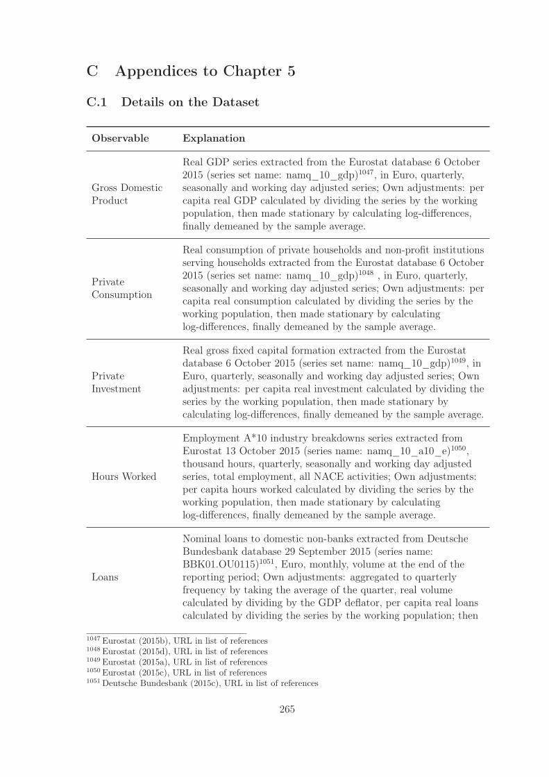
C Appendices to Chapter 5

C.1 Details on the Dataset

Observable Explanation

Gross DomesticProduct

Real GDP series extracted from the Eurostat database 6 October2015 (series set name: namq_10_gdp)1047, in Euro, quarterly,seasonally and working day adjusted series; Own adjustments: percapita real GDP calculated by dividing the series by the workingpopulation, then made stationary by calculating log-differences,finally demeaned by the sample average.

PrivateConsumption

Real consumption of private households and non-profit institutionsserving households extracted from the Eurostat database 6 October2015 (series set name: namq_10_gdp)1048 , in Euro, quarterly,seasonally and working day adjusted series; Own adjustments: percapita real consumption calculated by dividing the series by theworking population, then made stationary by calculatinglog-differences, finally demeaned by the sample average.

PrivateInvestment

Real gross fixed capital formation extracted from the Eurostatdatabase 6 October 2015 (series set name: namq_10_gdp)1049, inEuro, quarterly, seasonally and working day adjusted series; Ownadjustments: per capita real investment calculated by dividing theseries by the working population, then made stationary bycalculating log-differences, finally demeaned by the sample average.

Hours Worked

Employment A*10 industry breakdowns series extracted fromEurostat 13 October 2015 (series name: namq_10_a10_e)1050,thousand hours, quarterly, seasonally and working day adjustedseries, total employment, all NACE activities; Own adjustments:per capita hours worked calculated by dividing the series by theworking population, then made stationary by calculatinglog-differences, finally demeaned by the sample average.

Loans

Nominal loans to domestic non-banks extracted from DeutscheBundesbank database 29 September 2015 (series name:BBK01.OU0115)1051, Euro, monthly, volume at the end of thereporting period; Own adjustments: aggregated to quarterlyfrequency by taking the average of the quarter, real volumecalculated by dividing by the GDP deflator, per capita real loanscalculated by dividing the series by the working population; then

1047 Eurostat (2015b), URL in list of references1048 Eurostat (2015d), URL in list of references1049 Eurostat (2015a), URL in list of references1050 Eurostat (2015c), URL in list of references1051 Deutsche Bundesbank (2015c), URL in list of references

265

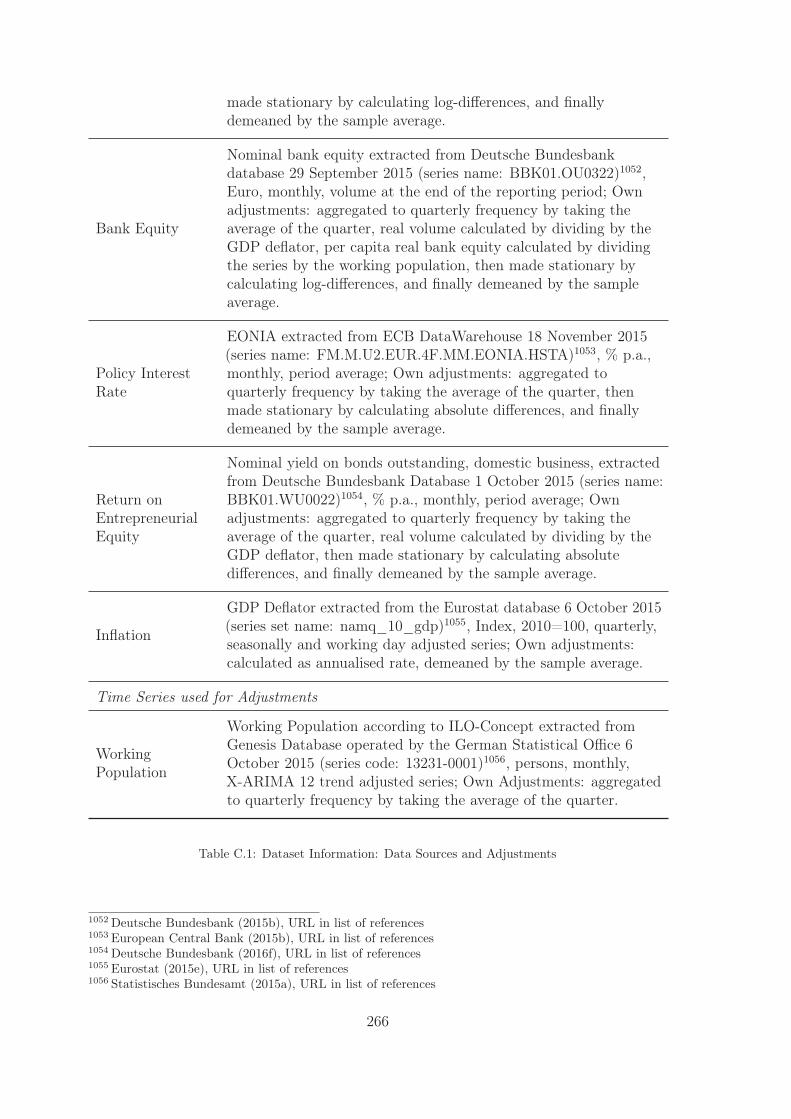
made stationary by calculating log-differences, and finallydemeaned by the sample average.

Bank Equity

Nominal bank equity extracted from Deutsche Bundesbankdatabase 29 September 2015 (series name: BBK01.OU0322)1052,Euro, monthly, volume at the end of the reporting period; Ownadjustments: aggregated to quarterly frequency by taking theaverage of the quarter, real volume calculated by dividing by theGDP deflator, per capita real bank equity calculated by dividingthe series by the working population, then made stationary bycalculating log-differences, and finally demeaned by the sampleaverage.

Policy InterestRate

EONIA extracted from ECB DataWarehouse 18 November 2015(series name: FM.M.U2.EUR.4F.MM.EONIA.HSTA)1053, % p.a.,monthly, period average; Own adjustments: aggregated toquarterly frequency by taking the average of the quarter, thenmade stationary by calculating absolute differences, and finallydemeaned by the sample average.

Return onEntrepreneurialEquity

Nominal yield on bonds outstanding, domestic business, extractedfrom Deutsche Bundesbank Database 1 October 2015 (series name:BBK01.WU0022)1054, % p.a., monthly, period average; Ownadjustments: aggregated to quarterly frequency by taking theaverage of the quarter, real volume calculated by dividing by theGDP deflator, then made stationary by calculating absolutedifferences, and finally demeaned by the sample average.

Inflation

GDP Deflator extracted from the Eurostat database 6 October 2015(series set name: namq_10_gdp)1055, Index, 2010=100, quarterly,seasonally and working day adjusted series; Own adjustments:calculated as annualised rate, demeaned by the sample average.

Time Series used for Adjustments

WorkingPopulation

Working Population according to ILO-Concept extracted fromGenesis Database operated by the German Statistical Office 6October 2015 (series code: 13231-0001)1056, persons, monthly,X-ARIMA 12 trend adjusted series; Own Adjustments: aggregatedto quarterly frequency by taking the average of the quarter.

Table C.1: Dataset Information: Data Sources and Adjustments

1052 Deutsche Bundesbank (2015b), URL in list of references1053 European Central Bank (2015b), URL in list of references1054 Deutsche Bundesbank (2016f), URL in list of references1055 Eurostat (2015e), URL in list of references1056 Statistisches Bundesamt (2015a), URL in list of references

266

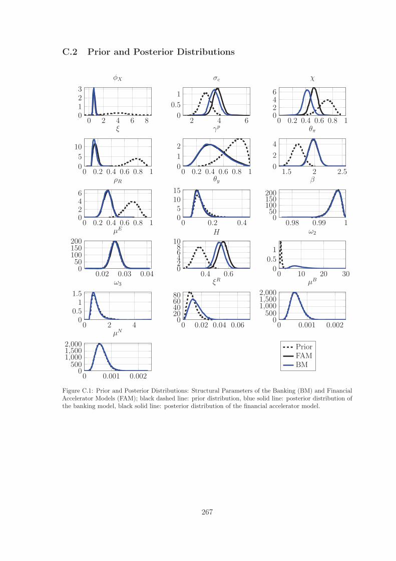
C.2 Prior and Posterior Distributions

0 0.2 0.4 0.6 0.8 10

1

2

γp2 4 6

0

0.5

1

σc

0 2 4 6 80123

φX

0 0.2 0.4 0.6 0.8 10

5

10

ξ

0 0.2 0.4 0.6 0.8 10246

ρR

0 0.2 0.4051015

θy

0.98 0.99 1050100150200

β1.5 2 2.5

0

2

4

θπ0 0.2 0.4 0.6 0.8 1

0246

χ

0 10 20 300

0.51

ω2

0.4 0.60246810

H

0.02 0.03 0.04050100150200

μE

0 2 40

0.51

1.5

ω3

0 0.02 0.04 0.06020406080

ξR

0 0.001 0.0020

5001,0001,5002,000

μB

0 0.001 0.0020

5001,0001,5002,000

μN

PriorFAMBM

Figure C.1: Prior and Posterior Distributions: Structural Parameters of the Banking (BM) and FinancialAccelerator Models (FAM); black dashed line: prior distribution, blue solid line: posterior distribution ofthe banking model, black solid line: posterior distribution of the financial accelerator model.

267

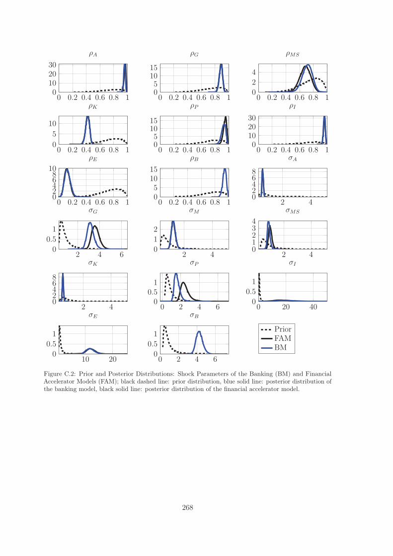
0 0.2 0.4 0.6 0.8 1051015

ρP0 0.2 0.4 0.6 0.8 1

051015

ρG

0 0.2 0.4 0.6 0.8 10102030

ρA

0 0.2 0.4 0.6 0.8 10

5

10

ρK

0 0.2 0.4 0.6 0.8 10246810

ρE

0 0.2 0.4 0.6 0.8 1051015

ρB0 0.2 0.4 0.6 0.8 1

0102030

ρI0 0.2 0.4 0.6 0.8 1

0

2

4

ρMS

0 20 400

0.5

1

σI

2 401234

σMS

2 402468

σA

2 40

1

2

σM

2 4 60

0.5

1

σG

2 402468

σK

0 2 4 60

0.51

σP

10 200

0.5

1

σE

0 2 4 60

0.5

1

σB

PriorFAMBM

Figure C.2: Prior and Posterior Distributions: Shock Parameters of the Banking (BM) and FinancialAccelerator Models (FAM); black dashed line: prior distribution, blue solid line: posterior distribution ofthe banking model, black solid line: posterior distribution of the financial accelerator model.

268

C.3 Posterior Estimates of the Banking Model (Reduced Dataset)

As noted in the text, the calibration and prior distributions for the reduced-dataset bankingmodel are the same as for the complete banking model, presented in tables 5.1 to 5.3. σB

and ρB are not included as estimated parameters since the exogenous bank risk shockprocess ΥB is not included in the reduced-dataset banking model to align the numberof shocks to the number of observable time series. The dataset is the same as for thefinancial accelerator model. The results presented in table C.2 are similarly based on200,000 draws of 5 chains. Convergence was checked again by the same means as for thecomplete banking model.1057 All tests indicated convergence after the burn-in period.

As can be seen by comparing the entries in table C.2 with the corresponding entriesin tables 5.4 and 5.5, the results are overwhelmingly similar. Estimated posterior meansgenerally differ to only a low degree and 90% highest posterior density (HPD) intervalsoverlap significantly. There are two exceptions to this observation: the posterior estimatesof ω2 and ω3. The respective 90% HPD intervals overlap only marginally for ω2. Also,the estimated posterior mean of ω2 in the complete banking model does not fall in the90% HPD interval of the reduced-dataset banking model and vice versa. The 90% HPDintervals overlap more widely for ω3 and it is only the posterior mean of the completebanking model which does not fall into the 90% HPD interval of the reduced-datasetbanking model. Given that bank equity is not included in the dataset used for estimatingthe reduced-dataset banking model, it appears to be the case that this time series isinformative on these two parameters. In contrast, the estimates of the other parametersare robust to the smaller dataset.

1057 See section 5.3

269

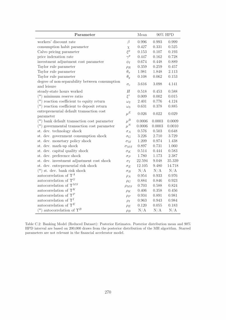
Parameter Mean 90% HPD

workers’ discount rate β 0.996 0.993 0.999consumption habit parameter χ 0.427 0.331 0.525Calvo pricing parameter ξp 0.153 0.107 0.193price indexation rate γp 0.447 0.162 0.728investment adjustment cost parameter φI 0.674 0.448 0.889Taylor rule parameter ρR 0.359 0.259 0.457Taylor rule parameter θπ 1.981 1.848 2.113Taylor rule parameter θy 0.108 0.062 0.153degree of non-separability between consumptionand leisure σc 3.616 3.098 4.141

steady-state hours worked H 0.518 0.453 0.588(*) minimum reserve ratio ξr 0.009 0.002 0.015(*) reaction coefficient to equity return ω2 2.401 0.776 4.124(*) reaction coefficient to deposit return ω3 0.631 0.378 0.885entrepreneurial default transaction costparameter μE 0.026 0.022 0.029

(*) bank default transaction cost parameter μB 0.0006 0.0003 0.0009(*) governmental transaction cost parameter μN 0.0006 0.0003 0.0010st. dev. technology shock σA 0.576 0.503 0.648st. dev. government consumption shock σG 3.226 2.710 3.729st. dev. monetary policy shock σM 1.209 0.974 1.438st. dev. mark-up shock σMS 0.897 0.731 1.060st. dev. capital quality shock σK 0.514 0.444 0.583st. dev. preference shock σP 1.780 1.173 2.387st. dev. investment adjustment cost shock σI 22.594 9.048 35.339st. dev. entrepreneurial risk shock σE 12.105 9.480 14.718(*) st. dev. bank risk shock σB N/A N/A N/Aautocorrelation of ΥA ρA 0.954 0.933 0.976autocorrelation of ΥG ρG 0.884 0.846 0.923autocorrelation of ΥMS ρMS 0.703 0.588 0.824autocorrelation of ΥK ρK 0.406 0.358 0.456autocorrelation of ΥP ρP 0.934 0.891 0.981autocorrelation of ΥI ρI 0.963 0.943 0.984autocorrelation of ΥE ρE 0.120 0.055 0.183(*) autocorrelation of ΥB ρB N/A N/A N/A

Table C.2: Banking Model (Reduced Dataset): Posterior Estimates. Posterior distribution mean and 90%HPD interval are based on 200,000 draws from the posterior distribution of the MH algorithm. Starredparameters are not relevant in the financial accelerator model.

270

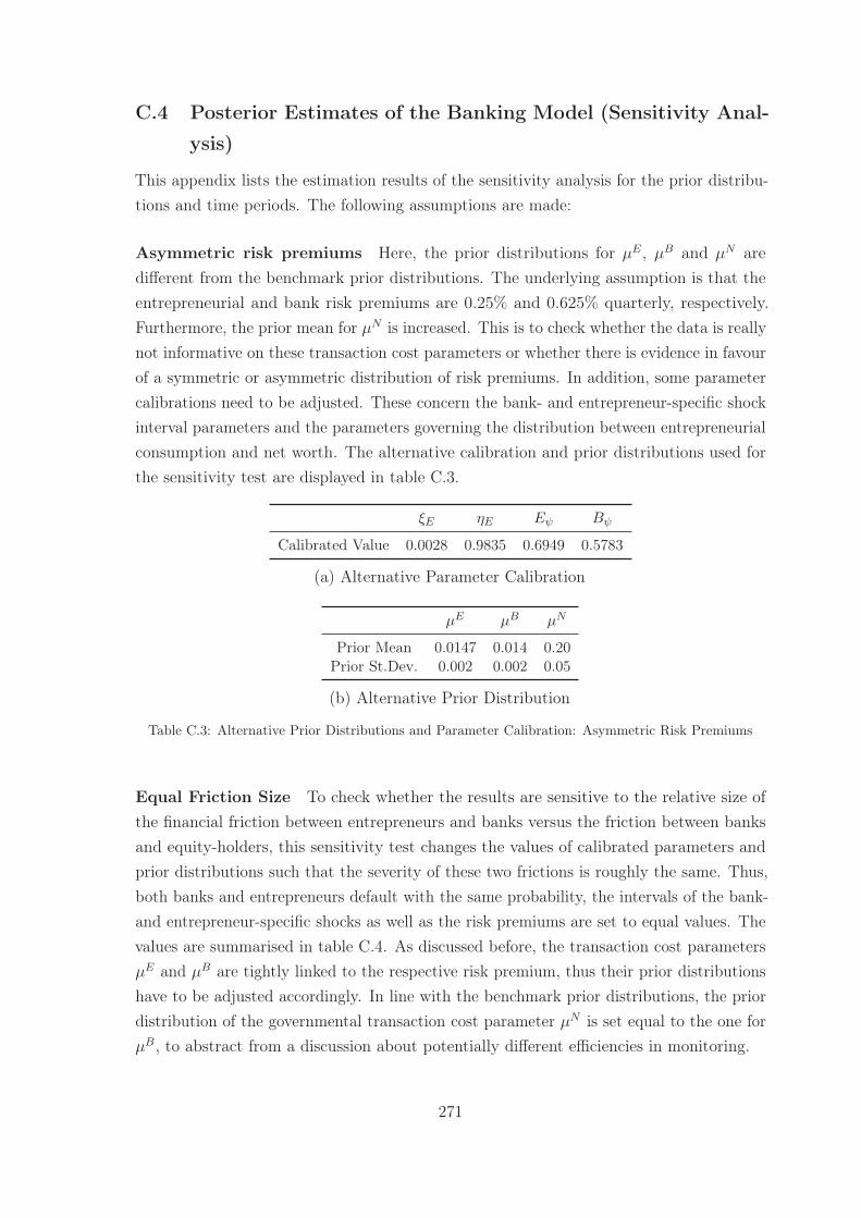
C.4 Posterior Estimates of the Banking Model (Sensitivity Anal-

ysis)

This appendix lists the estimation results of the sensitivity analysis for the prior distribu-tions and time periods. The following assumptions are made:

Asymmetric risk premiums Here, the prior distributions for μE, μB and μN aredifferent from the benchmark prior distributions. The underlying assumption is that theentrepreneurial and bank risk premiums are 0.25% and 0.625% quarterly, respectively.Furthermore, the prior mean for μN is increased. This is to check whether the data is reallynot informative on these transaction cost parameters or whether there is evidence in favourof a symmetric or asymmetric distribution of risk premiums. In addition, some parametercalibrations need to be adjusted. These concern the bank- and entrepreneur-specific shockinterval parameters and the parameters governing the distribution between entrepreneurialconsumption and net worth. The alternative calibration and prior distributions used forthe sensitivity test are displayed in table C.3.

ξE ηE Eψ Bψ

Calibrated Value 0.0028 0.9835 0.6949 0.5783

(a) Alternative Parameter Calibration

μE μB μN

Prior Mean 0.0147 0.014 0.20Prior St.Dev. 0.002 0.002 0.05

(b) Alternative Prior Distribution

Table C.3: Alternative Prior Distributions and Parameter Calibration: Asymmetric Risk Premiums

Equal Friction Size To check whether the results are sensitive to the relative size ofthe financial friction between entrepreneurs and banks versus the friction between banksand equity-holders, this sensitivity test changes the values of calibrated parameters andprior distributions such that the severity of these two frictions is roughly the same. Thus,both banks and entrepreneurs default with the same probability, the intervals of the bank-and entrepreneur-specific shocks as well as the risk premiums are set to equal values. Thevalues are summarised in table C.4. As discussed before, the transaction cost parametersμE and μB are tightly linked to the respective risk premium, thus their prior distributionshave to be adjusted accordingly. In line with the benchmark prior distributions, the priordistribution of the governmental transaction cost parameter μN is set equal to the one forμB, to abstract from a discussion about potentially different efficiencies in monitoring.

271

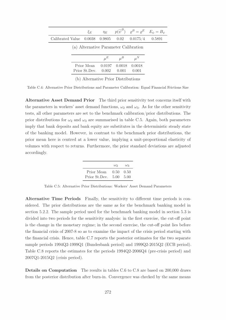
ξE ηE p(ψB) B = E Eψ = Bψ

Calibrated Value 0.0038 0.9805 0.02 0.0175/4 0.5891

(a) Alternative Parameter Calibration

μE μB μN

Prior Mean 0.0197 0.0018 0.0018Prior St.Dev. 0.002 0.001 0.001

(b) Alternative Prior Distributions

Table C.4: Alternative Prior Distributions and Parameter Calibration: Equal Financial Frictions Size

Alternative Asset Demand Prior The third prior sensitivity test concerns itself withthe parameters in workers’ asset demand functions, ω2 and ω3. As for the other sensitivitytests, all other parameters are set to the benchmark calibration/prior distributions. Theprior distributions for ω2 and ω3 are summarised in table C.5. Again, both parametersimply that bank deposits and bank equity are substitutes in the deterministic steady stateof the banking model. However, in contrast to the benchmark prior distributions, theprior mean here is centred at a lower value, implying a unit-proportional elasticity ofvolumes with respect to returns. Furthermore, the prior standard deviations are adjustedaccordingly.

ω2 ω3

Prior Mean 0.50 0.50Prior St.Dev. 5.00 5.00

Table C.5: Alternative Prior Distributions: Workers’ Asset Demand Parameters

Alternative Time Periods Finally, the sensitivity to different time periods is con-sidered. The prior distributions are the same as for the benchmark banking model insection 5.2.2. The sample period used for the benchmark banking model in section 5.3 isdivided into two periods for the sensitivity analysis: in the first exercise, the cut-off pointis the change in the monetary regime; in the second exercise, the cut-off point lies beforethe financial crisis of 2007-8 so as to examine the impact of the crisis period starting withthe financial crisis. Hence, table C.7 reports the posterior estimates for the two separatesample periods 1994Q2-1999Q1 (Bundesbank period) and 1999Q2-2015Q2 (ECB period).Table C.8 reports the estimates for the periods 1994Q2-2006Q4 (pre-crisis period) and2007Q1-2015Q2 (crisis period).

Details on Computation The results in tables C.6 to C.8 are based on 200,000 drawsfrom the posterior distribution after burn-in. Convergence was checked by the same means

272

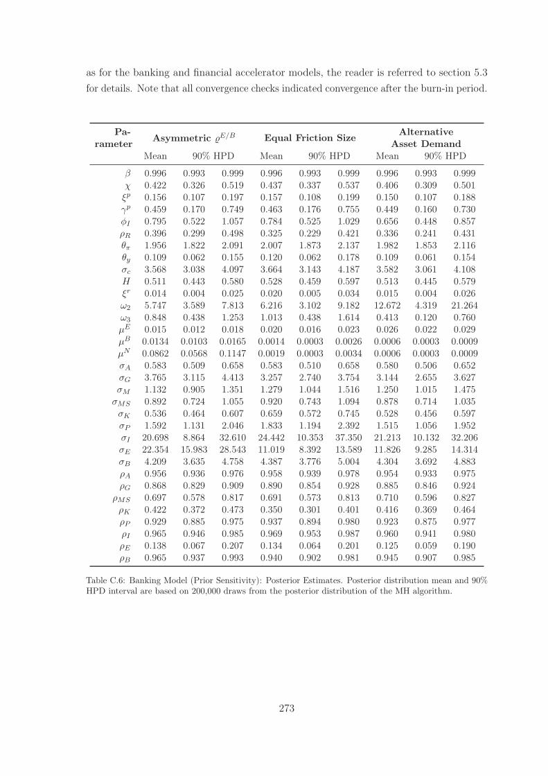
as for the banking and financial accelerator models, the reader is referred to section 5.3for details. Note that all convergence checks indicated convergence after the burn-in period.

Pa-Asymmetric E/B Equal Friction Size Alternative

rameter Asset DemandMean 90% HPD Mean 90% HPD Mean 90% HPD

β 0.996 0.993 0.999 0.996 0.993 0.999 0.996 0.993 0.999χ 0.422 0.326 0.519 0.437 0.337 0.537 0.406 0.309 0.501ξp 0.156 0.107 0.197 0.157 0.108 0.199 0.150 0.107 0.188γp 0.459 0.170 0.749 0.463 0.176 0.755 0.449 0.160 0.730φI 0.795 0.522 1.057 0.784 0.525 1.029 0.656 0.448 0.857ρR 0.396 0.299 0.498 0.325 0.229 0.421 0.336 0.241 0.431θπ 1.956 1.822 2.091 2.007 1.873 2.137 1.982 1.853 2.116θy 0.109 0.062 0.155 0.120 0.062 0.178 0.109 0.061 0.154σc 3.568 3.038 4.097 3.664 3.143 4.187 3.582 3.061 4.108H 0.511 0.443 0.580 0.528 0.459 0.597 0.513 0.445 0.579ξr 0.014 0.004 0.025 0.020 0.005 0.034 0.015 0.004 0.026ω2 5.747 3.589 7.813 6.216 3.102 9.182 12.672 4.319 21.264ω3 0.848 0.438 1.253 1.013 0.438 1.614 0.413 0.120 0.760μE 0.015 0.012 0.018 0.020 0.016 0.023 0.026 0.022 0.029μB 0.0134 0.0103 0.0165 0.0014 0.0003 0.0026 0.0006 0.0003 0.0009μN 0.0862 0.0568 0.1147 0.0019 0.0003 0.0034 0.0006 0.0003 0.0009σA 0.583 0.509 0.658 0.583 0.510 0.658 0.580 0.506 0.652σG 3.765 3.115 4.413 3.257 2.740 3.754 3.144 2.655 3.627σM 1.132 0.905 1.351 1.279 1.044 1.516 1.250 1.015 1.475σMS 0.892 0.724 1.055 0.920 0.743 1.094 0.878 0.714 1.035σK 0.536 0.464 0.607 0.659 0.572 0.745 0.528 0.456 0.597σP 1.592 1.131 2.046 1.833 1.194 2.392 1.515 1.056 1.952σI 20.698 8.864 32.610 24.442 10.353 37.350 21.213 10.132 32.206σE 22.354 15.983 28.543 11.019 8.392 13.589 11.826 9.285 14.314σB 4.209 3.635 4.758 4.387 3.776 5.004 4.304 3.692 4.883ρA 0.956 0.936 0.976 0.958 0.939 0.978 0.954 0.933 0.975ρG 0.868 0.829 0.909 0.890 0.854 0.928 0.885 0.846 0.924

ρMS 0.697 0.578 0.817 0.691 0.573 0.813 0.710 0.596 0.827ρK 0.422 0.372 0.473 0.350 0.301 0.401 0.416 0.369 0.464ρP 0.929 0.885 0.975 0.937 0.894 0.980 0.923 0.875 0.977ρI 0.965 0.946 0.985 0.969 0.953 0.987 0.960 0.941 0.980ρE 0.138 0.067 0.207 0.134 0.064 0.201 0.125 0.059 0.190ρB 0.965 0.937 0.993 0.940 0.902 0.981 0.945 0.907 0.985

Table C.6: Banking Model (Prior Sensitivity): Posterior Estimates. Posterior distribution mean and 90%HPD interval are based on 200,000 draws from the posterior distribution of the MH algorithm.

273

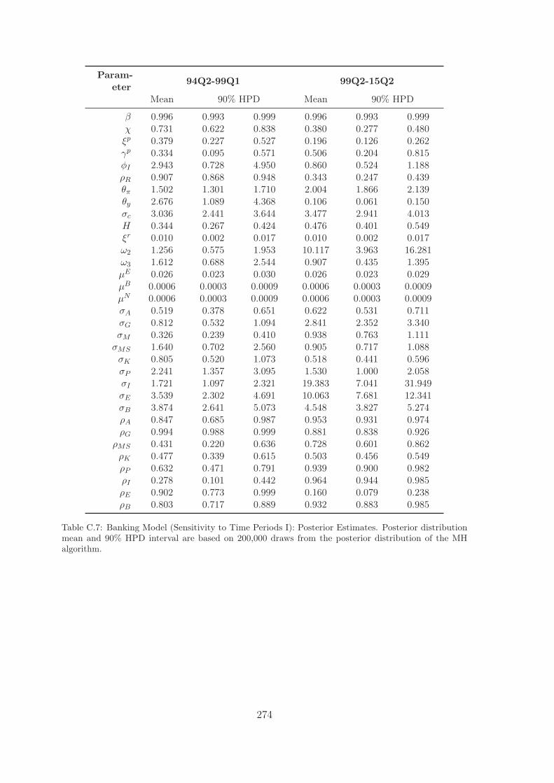
Param-eter 94Q2-99Q1 99Q2-15Q2

Mean 90% HPD Mean 90% HPD

β 0.996 0.993 0.999 0.996 0.993 0.999χ 0.731 0.622 0.838 0.380 0.277 0.480ξp 0.379 0.227 0.527 0.196 0.126 0.262γp 0.334 0.095 0.571 0.506 0.204 0.815φI 2.943 0.728 4.950 0.860 0.524 1.188ρR 0.907 0.868 0.948 0.343 0.247 0.439θπ 1.502 1.301 1.710 2.004 1.866 2.139θy 2.676 1.089 4.368 0.106 0.061 0.150σc 3.036 2.441 3.644 3.477 2.941 4.013H 0.344 0.267 0.424 0.476 0.401 0.549ξr 0.010 0.002 0.017 0.010 0.002 0.017ω2 1.256 0.575 1.953 10.117 3.963 16.281ω3 1.612 0.688 2.544 0.907 0.435 1.395μE 0.026 0.023 0.030 0.026 0.023 0.029μB 0.0006 0.0003 0.0009 0.0006 0.0003 0.0009μN 0.0006 0.0003 0.0009 0.0006 0.0003 0.0009σA 0.519 0.378 0.651 0.622 0.531 0.711σG 0.812 0.532 1.094 2.841 2.352 3.340σM 0.326 0.239 0.410 0.938 0.763 1.111σMS 1.640 0.702 2.560 0.905 0.717 1.088σK 0.805 0.520 1.073 0.518 0.441 0.596σP 2.241 1.357 3.095 1.530 1.000 2.058σI 1.721 1.097 2.321 19.383 7.041 31.949σE 3.539 2.302 4.691 10.063 7.681 12.341σB 3.874 2.641 5.073 4.548 3.827 5.274ρA 0.847 0.685 0.987 0.953 0.931 0.974ρG 0.994 0.988 0.999 0.881 0.838 0.926

ρMS 0.431 0.220 0.636 0.728 0.601 0.862ρK 0.477 0.339 0.615 0.503 0.456 0.549ρP 0.632 0.471 0.791 0.939 0.900 0.982ρI 0.278 0.101 0.442 0.964 0.944 0.985ρE 0.902 0.773 0.999 0.160 0.079 0.238ρB 0.803 0.717 0.889 0.932 0.883 0.985

Table C.7: Banking Model (Sensitivity to Time Periods I): Posterior Estimates. Posterior distributionmean and 90% HPD interval are based on 200,000 draws from the posterior distribution of the MHalgorithm.

274

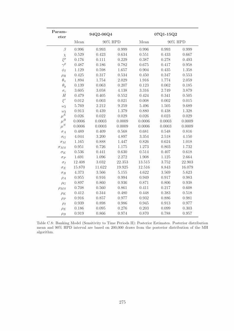
Param-eter 94Q2-06Q4 07Q1-15Q2

Mean 90% HPD Mean 90% HPD

β 0.996 0.993 0.999 0.996 0.993 0.999χ 0.529 0.423 0.634 0.551 0.433 0.667ξp 0.176 0.111 0.229 0.387 0.278 0.493γp 0.487 0.186 0.782 0.675 0.417 0.958φI 1.129 0.598 1.657 0.904 0.435 1.358ρR 0.425 0.317 0.534 0.450 0.347 0.553θπ 1.894 1.754 2.029 1.916 1.774 2.059θy 0.139 0.063 0.207 0.123 0.062 0.185σc 3.605 3.058 4.138 3.316 2.749 3.879H 0.479 0.405 0.552 0.424 0.341 0.505ξr 0.012 0.003 0.021 0.008 0.002 0.015ω2 5.769 2.212 9.259 5.496 1.505 9.689ω3 0.913 0.439 1.379 0.880 0.438 1.328μE 0.026 0.022 0.029 0.026 0.023 0.029μB 0.0006 0.0003 0.0009 0.0006 0.0003 0.0009μN 0.0006 0.0003 0.0009 0.0006 0.0003 0.0009σA 0.489 0.409 0.568 0.681 0.548 0.816σG 4.044 3.200 4.897 3.354 2.518 4.150σM 1.165 0.888 1.447 0.826 0.624 1.018σMS 0.951 0.726 1.175 1.273 0.803 1.732σK 0.536 0.441 0.630 0.514 0.407 0.618σP 1.691 1.096 2.272 1.908 1.125 2.664σI 12.408 3.032 22.353 13.515 3.752 22.903σE 15.870 11.622 19.925 12.516 8.843 16.079σB 4.373 3.566 5.155 4.622 3.569 5.623ρA 0.955 0.916 0.994 0.949 0.917 0.983ρG 0.897 0.860 0.936 0.871 0.806 0.938

ρMS 0.708 0.560 0.861 0.411 0.217 0.608ρK 0.412 0.344 0.480 0.448 0.383 0.518ρP 0.916 0.857 0.977 0.932 0.886 0.981ρI 0.939 0.898 0.986 0.945 0.913 0.977ρE 0.186 0.095 0.276 0.203 0.099 0.303ρB 0.919 0.866 0.974 0.870 0.788 0.957

Table C.8: Banking Model (Sensitivity to Time Periods II): Posterior Estimates. Posterior distributionmean and 90% HPD interval are based on 200,000 draws from the posterior distribution of the MHalgorithm.

275

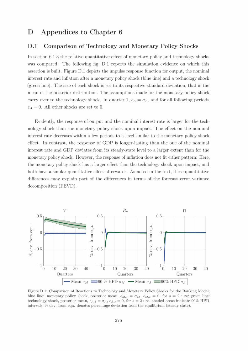
D Appendices to Chapter 6

D.1 Comparison of Technology and Monetary Policy Shocks

In section 6.1.3 the relative quantitative effect of monetary policy and technology shockswas compared. The following fig. D.1 reports the simulation evidence on which thisassertion is built. Figure D.1 depicts the impulse response function for output, the nominalinterest rate and inflation after a monetary policy shock (blue line) and a technology shock(green line). The size of each shock is set to its respective standard deviation, that is themean of the posterior distribution. The assumptions made for the monetary policy shockcarry over to the technology shock. In quarter 1, εA = σA, and for all following periodsεA = 0. All other shocks are set to 0.

Evidently, the response of output and the nominal interest rate is larger for the tech-nology shock than the monetary policy shock upon impact. The effect on the nominalinterest rate decreases within a few periods to a level similar to the monetary policy shockeffect. In contrast, the response of GDP is longer-lasting than the one of the nominalinterest rate and GDP deviates from its steady-state level to a larger extent than for themonetary policy shock. However, the response of inflation does not fit either pattern: Here,the monetary policy shock has a larger effect than the technology shock upon impact, andboth have a similar quantitative effect afterwards. As noted in the text, these quantitativedifferences may explain part of the differences in terms of the forecast error variancedecomposition (FEVD).

0 10 20 30 40−1

−0.5

0

0.5

Quarters

%de

v.fr

omeq

u.

Y

0 10 20 30 40−1

−0.5

0

0.5

Quarters

%de

v.fr

omeq

u.

Rn

0 10 20 30 40−1

−0.5

0

0.5

Quarters

%de

v.fr

omeq

u.

Π

Mean σM 90 % HPD σM Mean σA 90% HPD σA

Figure D.1: Comparison of Reactions to Technology and Monetary Policy Shocks for the Banking Model;blue line: monetary policy shock, posterior mean, εM,1 = σM , εM,s = 0, for s = 2 : ∞; green line:technology shock, posterior mean, εA,1 = σA, εA,s = 0, for s = 2 : ∞, shaded areas indicate 90% HPDintervals; % dev. from equ. denotes percentage deviation from the equilibrium (steady state).

276

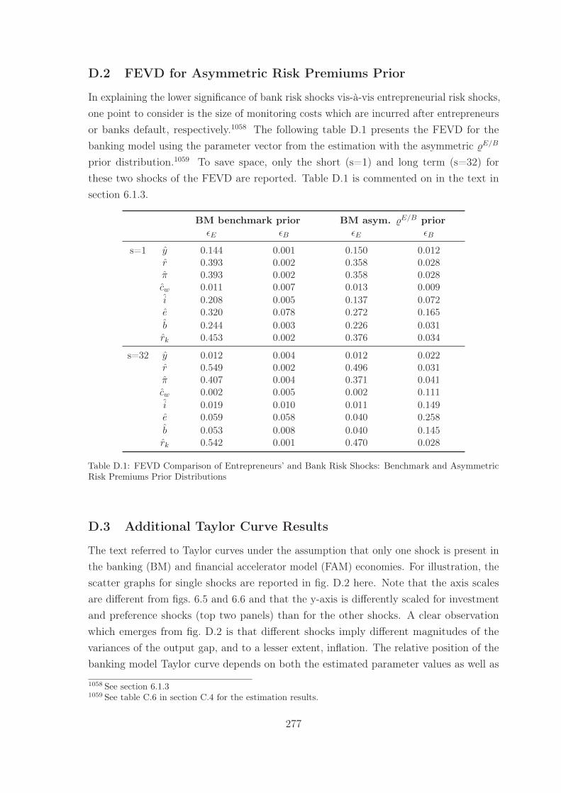
D.2 FEVD for Asymmetric Risk Premiums Prior

In explaining the lower significance of bank risk shocks vis-à-vis entrepreneurial risk shocks,one point to consider is the size of monitoring costs which are incurred after entrepreneursor banks default, respectively.1058 The following table D.1 presents the FEVD for thebanking model using the parameter vector from the estimation with the asymmetric �E/B

prior distribution.1059 To save space, only the short (s=1) and long term (s=32) forthese two shocks of the FEVD are reported. Table D.1 is commented on in the text insection 6.1.3.

BM benchmark prior BM asym. E/B priorεE εB εE εB

s=1 y 0.144 0.001 0.150 0.012r 0.393 0.002 0.358 0.028π 0.393 0.002 0.358 0.028cw 0.011 0.007 0.013 0.009i 0.208 0.005 0.137 0.072e 0.320 0.078 0.272 0.165b 0.244 0.003 0.226 0.031rk 0.453 0.002 0.376 0.034

s=32 y 0.012 0.004 0.012 0.022r 0.549 0.002 0.496 0.031π 0.407 0.004 0.371 0.041cw 0.002 0.005 0.002 0.111i 0.019 0.010 0.011 0.149e 0.059 0.058 0.040 0.258b 0.053 0.008 0.040 0.145rk 0.542 0.001 0.470 0.028

Table D.1: FEVD Comparison of Entrepreneurs’ and Bank Risk Shocks: Benchmark and AsymmetricRisk Premiums Prior Distributions

D.3 Additional Taylor Curve Results

The text referred to Taylor curves under the assumption that only one shock is present inthe banking (BM) and financial accelerator model (FAM) economies. For illustration, thescatter graphs for single shocks are reported in fig. D.2 here. Note that the axis scalesare different from figs. 6.5 and 6.6 and that the y-axis is differently scaled for investmentand preference shocks (top two panels) than for the other shocks. A clear observationwhich emerges from fig. D.2 is that different shocks imply different magnitudes of thevariances of the output gap, and to a lesser extent, inflation. The relative position of thebanking model Taylor curve depends on both the estimated parameter values as well as

1058 See section 6.1.31059 See table C.6 in section C.4 for the estimation results.

277

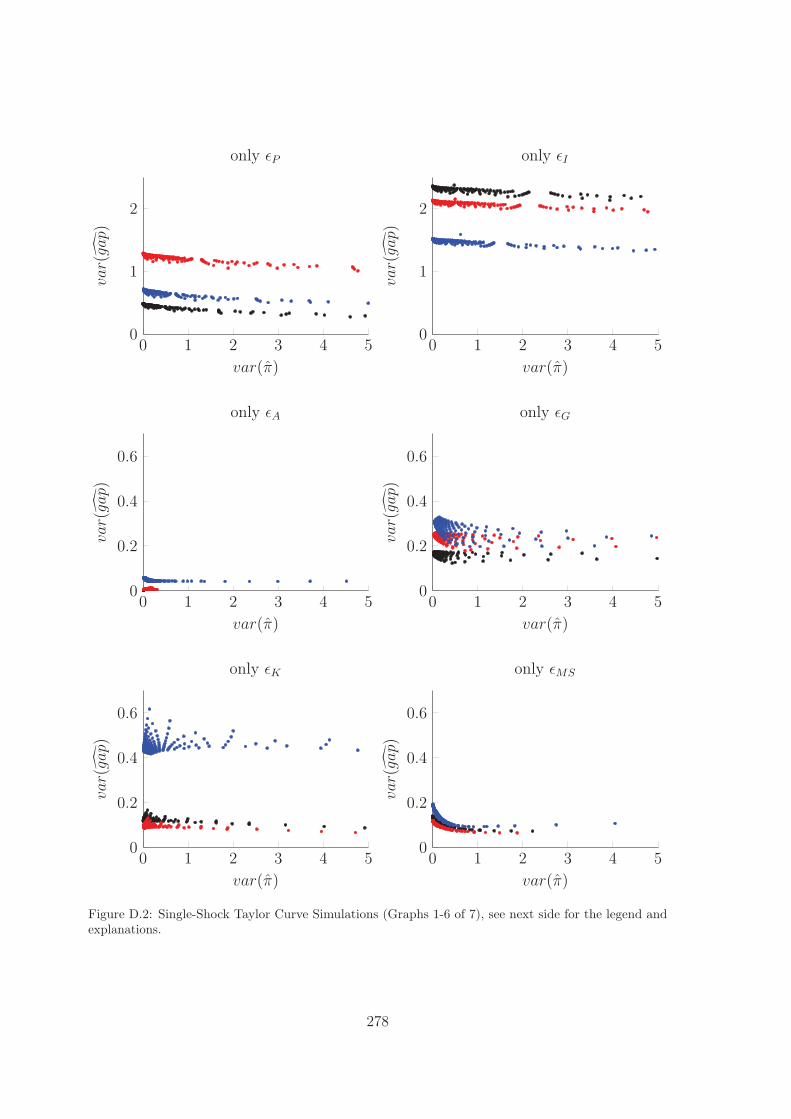
0 1 2 3 4 50

0.2

0.4

0.6

var(π)

var(gap)

only εA

0 1 2 3 4 50

1

2

var(π)

var(gap)

only εP

0 1 2 3 4 50

1

2

var(π)

var(gap)

only εI

0 1 2 3 4 50

0.2

0.4

0.6

var(π)

var(gap)

only εG

0 1 2 3 4 50

0.2

0.4

0.6

var(π)

var(gap)

only εMS

0 1 2 3 4 50

0.2

0.4

0.6

var(π)

var(gap)

only εK

Figure D.2: Single-Shock Taylor Curve Simulations (Graphs 1-6 of 7), see next side for the legend andexplanations.

278

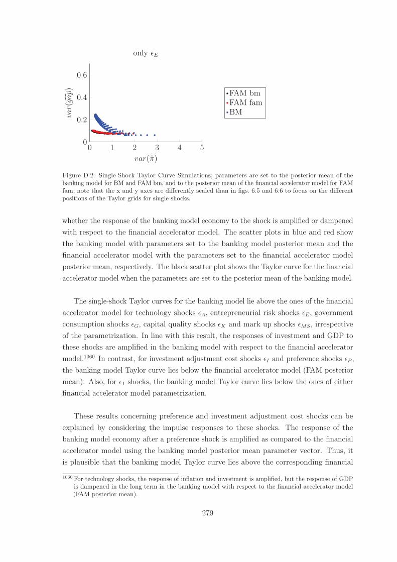
0 1 2 3 4 50

0.2

0.4

0.6

var(π)

var(gap)

only εE

FAM bmFAM famBM

Figure D.2: Single-Shock Taylor Curve Simulations; parameters are set to the posterior mean of thebanking model for BM and FAM bm, and to the posterior mean of the financial accelerator model for FAMfam, note that the x and y axes are differently scaled than in figs. 6.5 and 6.6 to focus on the differentpositions of the Taylor grids for single shocks.

whether the response of the banking model economy to the shock is amplified or dampenedwith respect to the financial accelerator model. The scatter plots in blue and red showthe banking model with parameters set to the banking model posterior mean and thefinancial accelerator model with the parameters set to the financial accelerator modelposterior mean, respectively. The black scatter plot shows the Taylor curve for the financialaccelerator model when the parameters are set to the posterior mean of the banking model.

The single-shock Taylor curves for the banking model lie above the ones of the financialaccelerator model for technology shocks εA, entrepreneurial risk shocks εE, governmentconsumption shocks εG, capital quality shocks εK and mark up shocks εMS, irrespectiveof the parametrization. In line with this result, the responses of investment and GDP tothese shocks are amplified in the banking model with respect to the financial acceleratormodel.1060 In contrast, for investment adjustment cost shocks εI and preference shocks εP ,the banking model Taylor curve lies below the financial accelerator model (FAM posteriormean). Also, for εI shocks, the banking model Taylor curve lies below the ones of eitherfinancial accelerator model parametrization.

These results concerning preference and investment adjustment cost shocks can beexplained by considering the impulse responses to these shocks. The response of thebanking model economy after a preference shock is amplified as compared to the financialaccelerator model using the banking model posterior mean parameter vector. Thus, itis plausible that the banking model Taylor curve lies above the corresponding financial

1060 For technology shocks, the response of inflation and investment is amplified, but the response of GDPis dampened in the long term in the banking model with respect to the financial accelerator model(FAM posterior mean).

279

accelerator Taylor curve evaluated at the posterior mean of the banking model (FAM bm,black dots). However, the preference shock process is estimated to be stronger initiallyand more strongly autocorrelated for the financial accelerator model than the bankingmodel. This leads to the response of GDP, investment and net worth to be weaker in thebanking model than in the financial accelerator model evaluated at the posterior mean ofthe financial accelerator model. Therefore, the banking model Taylor curve lies below thefinancial accelerator model (FAM posterior mean).

Considering investment adjustment cost shocks the explanation is different. The effi-ciency frontier of the banking model lies below the one of the financial accelerator modelirrespective of the parameter values. The impulse response functions show that the reactionto an investment adjustment cost shock is dampened in the banking model, with GDP andinvestment declining to a smaller extent in the banking model. The reason why investmentadjustment cost shocks are muted in the banking model is similar to the mechanism whichamplifies monetary policy shocks. The immediate impact of an adjustment cost shockis to reduce investment and increase the price of physical capital by making investmentmore costly. Due to the friction associated with banks’ liability management, the priceof capital increases by more, thus increasing entrepreneurial net worth by more in thebanking model.1061 This in turn reduces the external finance premium of entrepreneurs,alleviating the negative initial impact on investment as entrepreneurs’ capital demanddoes not fall as much as in the financial accelerator model. Thus, a dampened impulseresponse is in line with the banking model Taylor curve showing a better trade-off thanthe financial accelerator model. Furthermore, the investment adjustment cost process isestimated to be marginally stronger in the banking model. This explains why the Taylorcurve of the financial accelerator model with the banking model parameters (black dots)lies above the one of the financial accelerator model with financial accelerator parameters(red dots).

To sum up the previous discussion, for investment adjustment cost shocks differentmodel dynamics in the banking and financial accelerator models are the primary cause. Incontrast, for preference shocks stronger shock estimates for the financial accelerator modelimply more volatility, even though the dynamics of the financial accelerator model are lessvolatile than the ones of the banking model. This gives rise to the different positions ofthe single-shock Taylor curves. There is one further notable feature about shock-specificTaylor curves: The slope of the efficiency frontier of the banking model is significantlyaltered for the case of entrepreneurial risk shocks only.

1061 This is in contrast to a monetary policy shock which led to a decrease in the price of physical capitaland thus entrepreneurs’ net worth, reinforcing the negative effect on investment.

280

In the aggregate Taylor curves in fig. 6.5 (as well as the other single shock Taylor curvesin fig. D.2), the trade-off generally involves small increases in the output gap variancefor comparatively large decreases in the inflation variance. In contrast, for the financial-shocks-only banking model, the slope of the Taylor curve changes significantly with respectto the financial accelerator model. The same reduction in terms of inflation variance isrelated to a marked increase in output gap variance. Particularly interesting is the factthat increasing θy, that is the Taylor rule coefficient governing the response to the outputgap, does not monotonically decrease output gap variance in the financial-shocks-onlybanking model. In fact, the output gap variance monotonically increases with θy. Incontrast, this pattern does not arise when all shocks are present and only to a smallerextent in the financial accelerator model for the case of only entrepreneurial risk shocks.Hence, the additional financial friction induces a generally positive correlation betweenthe reaction of the central bank to the output gap and the variance of the output gapin the case of financial shocks. By reacting to deviations in the output gap, the centralbank moves away from its efficiency frontier. Yet, overall, it should be kept in mind thatthe implied variances of the output gap and inflation due to financial shocks are smallcompared to, for example, preference or investment adjustment cost shocks.

D.4 Sensitivity Analysis for Macroprudential Parameters

Various sensitivity analyses were conducted in order to test the robustness of the results insection 6.3. The impulse response analysis of section 6.3.3 and the Taylor curve analysis ofsection 6.3.4 were repeated for varying values of ωmpe, θm and τM . Also, banks’ leverageratio was used for computing deposit insurance fees instead of banks’ default probability.The following paragraphs report the results.

Concerning the endogenous deposit insurance factor, the results are generally robustto varying ωmpe. A countercyclical parametrization of the deposit insurance factor, that isusing a negative value for ωmpe, yields the opposite reaction to a monetary policy shockthan the procyclical policy: the change in the inflation response is still negligible, butthe deviation of GDP from its steady state is larger than in the benchmark bankingmodel. Larger absolute values of ωmpe lead to the respective effect being stronger, thatis the GDP response being further amplified with a countercyclical policy, and moredampened with a procyclical policy. However, values above 2 produce counter-intuitivebehaviour. Firstly, values for ωmpe above 2.9 but below 4.3 yield unstable equilibria.1062

Secondly, in contrast to the dampening effect of ωmpe = 2, setting ωmpe equal to 5 leads toa strong amplification with respect to the benchmark banking model. Thirdly, as ωmpe

increases further, the response of GDP is still amplified with respect to the benchmark

1062 This range concerns values on a 0.1 scale.

281

banking model, but ever more dampened with respect to the response with ωmpe = 5.This behaviour presents another reason for why increasing the responsivity of depositinsurance fees in order to moderate the effects of monetary policy shocks may not be viable.

Concerning the policy trade-off, both the countercyclical and the procyclical parametriza-tion lead to upward shifts in the all-shock Taylor curves. The shift is the stronger, thehigher is the absolute value of ωmpe. The results are different when bank risk shocksare excluded. For positive values of ωmpe, the Taylor curve shifts rightwards, with themaximum shift for ωmpe = 5. For values below 5, the higher is ωmpe, the stronger is therightward shift; for values above 5, the higher is ωmpe, the closer is the Taylor curve to thebenchmark position. This mirrors the behaviour of the impulse response functions. Fornegative values of ωmpe, the position of the Taylor curve tilts negligibly towards higheroutput gap variances at low inflation variances. The larger is the absolute value of theparameter, the larger is the tilt of the εB = 0 Taylor curve.

In conclusion, increasing ωmpe increases the absolute effects both in terms of the impulseresponse function and the policy trade-off, excluding the cases of ωmpe ≥ 5. Furthermore,a procyclical deposit insurance factor leads to a dampened response to monetary policyshocks and a worsening of the policy trade-off both with and without bank risk shocks.The countercyclical parametrization yields amplified responses to a monetary policy shockand a deterioration in the policy trade-off for the all-shock case, but a small tilt in theno-bank risk shocks Taylor curve. Yet, overall the differences are marginal. Thus, theevaluation of the particular implementation depends on how the transmission of monetarypolicy is judged and whether transmission or policy trade-offs weigh larger.

Also, the results are qualitatively unchanged when banks’ leverage ratio is used. Yet,the changes in the impulse response functions with respect to the benchmark bankingmodel are much smaller than with banks’ default probability. This is due to banks’ leverageratio changing to a much smaller extent than banks’ default probability. Also, the Taylorcurve anomaly in response to bank risk shocks does not arise for the same reason. TheTaylor curves for the countercyclical parametrization show a marginal downward shift ofthe Taylor curves, while the procyclical parametrization shows a slight upward shift. Theshifts are the stronger, the higher is the absolute value of ωmpe.

Turn next to the macroprudential Taylor rule (MTR) and macroprudential creditspread rule (MCS) policies. The sensitivity analysis used a value range for θm of 0.5 to 2.5in 0.5 steps. This is in line with the grid used for θy in computing Taylor curves, althoughmore coarse. The range for τM is 0.05 to 0.3, where the respective boundaries are given by

282

the values used in Bailliu et al. (2015) (0.05) and Kannan et al. (2012) (0.3).1063 For theMTR+MCS policy, θm was set to 0.25 when looping over τM , while τM was held constantat 0.15 when changing θm.

Regarding the Taylor curve analysis, the results presented in the text also hold forthese different parameter values. Furthermore, changes in Taylor curves become larger inabsolute size as the parameter values increase. The results concerning impulse responseanalysis also generally show that increasing parameter values lead to a stronger effect of themacroprudential policy. If a policy with θm = 0.5 leads to a dampened response of GDPfollowing a monetary policy shock, that is the deviation of GDP from its steady-state valueis smaller in absolute terms than in the benchmark model, then the same macroprudentialpolicy with θm = 1.0, ..., 2.5 leads to an even more dampened response of GDP, that islower absolute deviation from its steady state. Conversely, if macroprudential policy withθm = 0.5 leads to an amplified response of GDP compared to the benchmark case, that is alarger absolute deviation from the steady state, then increasing θm amplifies the responseof GDP even further, that is it increases the absolute deviation from the steady state.This similarly applies to τM .

There is one notable exception to this pattern. This concerns the impulse responseanalysis for the combination of MTR policy (with and without the MCS policy in place)with the loan-to-GDP ratio. For θm = 0.5 above pattern still holds. However, as θm

increases further, the responses of endogenous variables become counterfactual. In fact,real GDP, the nominal policy return and inflation increase long-lastingly with respect totheir steady-state values. This is not in line with the monetary transmission mechanismas considered here.

The explanation for this behaviour of the model with high θm is linked to the relationshipof bank loans, financing costs and the monetary policy rule. Normally, a monetary policyshock induces higher loan demand due to decreasing entrepreneurial net worth. However,as the central bank promises to react very aggressively to changes in the loan-to-GDP ratio,a relatively small increase in loans aggravates the financing situation of entrepreneurs evenfurther, as higher policy rates imply higher marginal financing costs. Anticipating thisaggressive stance of the central bank, entrepreneurs actually reduce their loan demand.This can only be achieved by an increase in entrepreneurial net worth since the capitalstock in the shock period is fixed at the value before the shock. This, in turn, impliesthat the real return on and the price of physical capital increase. Thus, the monetarytransmission mechanism is turned upside down in this case. The observation that everhigher values of θm decrease the quantitative impact arises for the same reasoning: absolute

1063 See Kannan et al. (2012: 16) and Bailliu et al. (2015: 156)

283

changes in the loan-to-GDP ratio yield an ever more aggressive reaction of the centralbank. Since agents anticipate this reaction, the responses of endogenous variables turn outto be less strong. The fact that this peculiarity only arises in this specific case with theloan-to-GDP ratio is due to the size and long duration of the reaction of loans: Accordingto the Taylor rule, as θm increases, the central bank eventually reacts more strongly todeviations in the loan-to-GDP ratio than to deviations in inflation. Thus, the link betweenthe MTR policy with the economy leads to the counterfactual reaction to a monetarypolicy shock.

D.5 Macroprudential Policies and Financial Stability

The main text only touched upon the issue of whether and how macroprudential policiescan enhance financial stability in the banking model. This appendix summarises thesimulation results on this topic. The implications are discussed in the main text. There aretwo ways to evaluate whether macroprudential policies enhance financial stability. Firstly,macroprudential policies may counter the accumulation of financial imbalances in terms ofreducing volatility. Secondly, macroprudential policies may increase the resilience of thebanking model economy to financial shocks.

Financial imbalances are incorporated into the specific macroprudential policies anal-ysed in the banking model. To measure such financial imbalances, three variables areused: lagged loan growth, the loan-to-GDP ratio and the price of physical capital. Thesethree variables are also used here to evaluate whether macroprudential policies enhancefinancial stability. To this end, the computations for the Taylor curves were modified toshow the trade-off between the variance of inflation and the respective financial variable.Using this measure, a macroprudential policy improves on the banking model in termsof financial stability if the same inflation variance is related to a lower variance of thefinancial variable.1064 To save space, the results of this experiment are summarised intable D.2.

Column 1 of table D.2 shows the measure of financial (in)stability. Column 2 showsthe indicator variable for the MTR and MCS policies, respectively. The following columns3 to 5 report the movement of the macroprudential ‘financial Taylor curve’ with respectto the location of the corresponding ‘financial Taylor curve’ of the benchmark bankingmodel. Finally, columns 6 and 7 report the movement in the ‘financial Taylor curve’ of thebanking model with endogenous deposit insurance factor for two parametrizations. Notethat in these latter two columns, the financial Taylor curves were computed without bank

1064 The reference to inflation is deemed important here because it rules out extreme cases when financialvolatilities decrease, but only when inflation variance is unreasonably high. Given the large range ofinflation variances in the benchmark experiment, this possibility is not hypothetical.

284

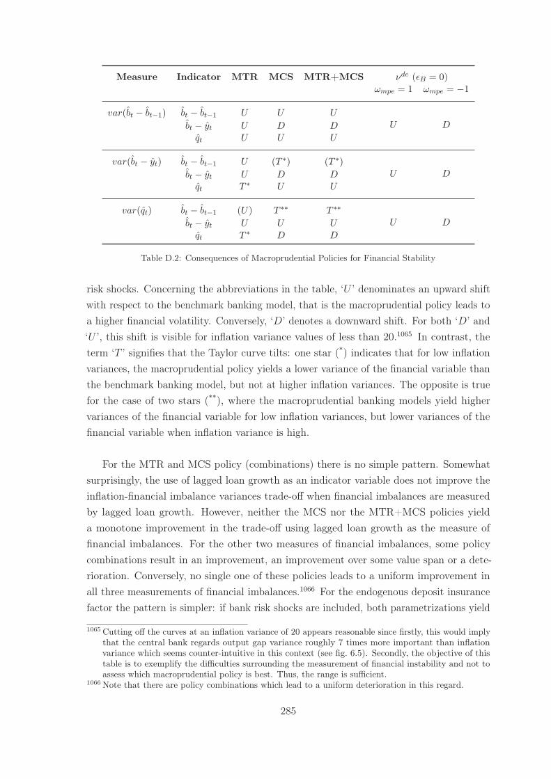
Measure Indicator MTR MCS MTR+MCS νde (εB = 0)ωmpe = 1 ωmpe = −1

var(bt − bt−1) bt − bt−1 U U UU Dbt − yt U D D

qt U U U

var(bt − yt) bt − bt−1 U (T ∗) (T ∗)U Dbt − yt U D D

qt T ∗ U U

var(qt) bt − bt−1 (U) T ∗∗ T ∗∗

U Dbt − yt U U Uqt T ∗ D D

Table D.2: Consequences of Macroprudential Policies for Financial Stability

risk shocks. Concerning the abbreviations in the table, ‘U ’ denominates an upward shiftwith respect to the benchmark banking model, that is the macroprudential policy leads toa higher financial volatility. Conversely, ‘D’ denotes a downward shift. For both ‘D’ and‘U ’, this shift is visible for inflation variance values of less than 20.1065 In contrast, theterm ‘T ’ signifies that the Taylor curve tilts: one star (*) indicates that for low inflationvariances, the macroprudential policy yields a lower variance of the financial variable thanthe benchmark banking model, but not at higher inflation variances. The opposite is truefor the case of two stars (**), where the macroprudential banking models yield highervariances of the financial variable for low inflation variances, but lower variances of thefinancial variable when inflation variance is high.

For the MTR and MCS policy (combinations) there is no simple pattern. Somewhatsurprisingly, the use of lagged loan growth as an indicator variable does not improve theinflation-financial imbalance variances trade-off when financial imbalances are measuredby lagged loan growth. However, neither the MCS nor the MTR+MCS policies yielda monotone improvement in the trade-off using lagged loan growth as the measure offinancial imbalances. For the other two measures of financial imbalances, some policycombinations result in an improvement, an improvement over some value span or a dete-rioration. Conversely, no single one of these policies leads to a uniform improvement inall three measurements of financial imbalances.1066 For the endogenous deposit insurancefactor the pattern is simpler: if bank risk shocks are included, both parametrizations yield

1065 Cutting off the curves at an inflation variance of 20 appears reasonable since firstly, this would implythat the central bank regards output gap variance roughly 7 times more important than inflationvariance which seems counter-intuitive in this context (see fig. 6.5). Secondly, the objective of thistable is to exemplify the difficulties surrounding the measurement of financial instability and not toassess which macroprudential policy is best. Thus, the range is sufficient.

1066 Note that there are policy combinations which lead to a uniform deterioration in this regard.

285

a deterioration in the trade-off. This is the reason they are not reported in table D.2. Ifbank risk shocks are excluded, a procyclical policy leads to a uniform deterioration, whilea countercyclical policy leads to a uniform improvement.

Concerning the resilience to financial shocks, there is a wide variety of effects. Mir-roring the results in table D.2, some policy combinations lead to amplifying and othersto dampening effects with respect to the benchmark banking model.1067 Also, the effectsmay be different for the responses of GDP and inflation.1068 Finally, macroprudentialpolicies may increase the duration for which GDP is displaced from its steady state.1069

The endogenous deposit insurance factor generally leads to an amplified response, exceptfor the procyclical policy in response to entrepreneurial risk shocks.

Thus, the endogenous deposit insurance factor presents mixed results in terms ofenhancing financial stability. Yet, the endogenous deposit insurance factor may instead bejudged based on its impact on the government budget. Upon impact of the monetary policyshock, either parametrization leads to an increase in the budget deficit, ceteris paribus.1070

However, after a few quarters, banks’ default probability is close to its steady state value,and so is the endogenous deposit insurance factor and the government budget deficit. Afurther curiosity arises in the benchmark banking model with endogenous taxes. In thiscase, the government runs a budget surplus a few quarters after the shock when the depositinsurance factor is exogenous while the budget is balanced in the case of the endogenousdeposit insurance factor. If a balanced budget is taken as a goal, then this policy can helpachieve it. However, since there are budget surpluses in the benchmark banking model,the endogenous deposit insurance factor may be judged to have a negative impact on thegovernment budget. Either way, above criticisms about the limited characterisation of thegovernment budget in the banking model apply here as well. This reduces the informativevalue of this experiment.

1067 An example of the former is the MCS policy with the price of physical capital in response to bankrisk shocks. Either policy with the price of physical capital in response to entrepreneurial risk shocksis an example of the latter.

1068 This occurs for example in response to financial shocks when the MTR policy reacts to the loan-to-GDPratio.

1069 This is the case with the MCS policy responding to lagged loan growth after bank risk shocks.1070 Since the government is confined to a balanced budget, this deficit is covered by tax increases.

286

References

Abbate, A., and Thaler, D. (2014). Monetary Policy Effects on Bank Risk Taking. EUI WorkingPapers , ECO 2014/07 .

Adjemian, S., Bastani, H., Juillard, M., Karamé, F., Mihoubi, G. P., Pfeifer, J., . . . Villemot, S.(2011). Dynare: Reference Manual, 4th ed. Dynare Working Papers , 1 .

Admati, A. R., and Hellwig, M. (2013). The bankers’ new clothes: What’s wrong with bankingand what to do about it. Princeton, N.J. and Oxford: Princeton University Press.

Agénor, P.-R., Alper, K. and Pereira da Silva, L. (2009). Capital Requirements And BusinessCycles With Credit Market Imperfections. The World Bank Policy Research Paper , 5151 .

Agénor, P. R., Alper, K. and Pereira da Silva, L. (2011). Capital Regulation, Monetary Policyand Financial Stability. Banco Central do Brasil Working Paper Series , 237 .

Aguiar, Á., and Drumond, I. (2007). Business Cycle and Bank Capital: Monetary PolicyTransmission under the Basel Accords. FEP Working Papers , 242 .

Al-Eyd, A., and Berkmen, S. P. (2013). Fragmentation and Monetary Policy in the Euro Area.IMF Working Paper , 13/208 .

Algan, Y., Allais, O., Den Haan, W. J. and Rendahl, P. (2014). Solving and Simulating Modelswith Heterogeneous Agents and Aggregate Uncertainty. In: K. Schmedders and K. L. Judd(Eds.), Handbook of computational economics (pp. 277–324).

Alpanda, S., and Aysun, U. (2014). International transmission of financial shocks in an estimatedDSGE model. Journal of International Money and Finance, 47 , 21–55.

Alpanda, S., Cateau, G. and Meh, C. (2014). A policy model to analyze macroprudentialregulations and monetary policy. BIS Working Papers , 461 .

Amman, H. M., Kendrick, D. A. and Rust, J. (Eds.). (2006). Handbook of computationaleconomics (Vol. 2). Amsterdam and New York: Elsevier.

An, S., and Schorfheide, F. (2007). Bayesian Analysis of DSGE Models. Econometric Reviews ,26 (2-4), 113–172.

Angelini, P., Neri, S. and Panetta, F. (2012). Monetary and macroprudential policies. EuropeanCentral Bank Working Paper Series , 1449 .

Angeloni, I., and Faia, E. (2009). A Tale of Two Policies: Prudential Regulation and MonetaryPolicy with Fragile Banks. Kiel Working Papers , 1569 .

Angeloni, I., and Faia, E. (2013). Capital regulation and monetary policy with fragile banks.Journal of Monetary Economics , 60 (3), 311–324.

Arango, C. A., and Valencia, O. M. (2015). Macro-Prudential Policy under Moral Hazard andFinancial Fragility. Borradores de Economía, 878 , Banco de la Repúbica Colombia.

Arestis, P., and Sawyer, M. C. (Eds.). (2006). A handbook of alternative monetary economics.Cheltenham: Elgar.

Arnold, I., Kool, C. and Raabe, K. (2011). Industry Effects of Bank Lending in Germany. TjallingC. Koopmans Research Institute Discussion Paper Series , 11-21 .

Aruoba, S. B., Fernández-Villaverde, J. and Rubio-Ramírez, J. F. (2006). Comparing solutionmethods for dynamic equilibrium economies. Journal of Economic Dynamics and Control ,30 (12), 2477–2508.

Bachmann, R., Born, B., Elstner, S. and Grimme, C. (2013). Time-Varying Business Volatility,

XVII

Price Setting, and the Real Effects of Monetary Policy. NBER Working Paper Series ,19180 .

Backus, D. K., Brainard, W. C., Smith, G. and Tobin, J. (1980). A Model of U.S. Financial andNonfinancial Economic Behavior. Journal of Money, Credit and Banking , 12 (2, Part 2:Financial Market Behaviorm Capital Formation, and Economic Performance), 259–293.

Backus, D. K., Kehoe, P. J. and Kydland, F. E. (1993). International Business Cycles: Theoryand Evidence. NBER Working Paper Series , 4493 .

Badarau, C., and Popescu, A. (2015). Monetary policy and financial stability: What role for theinterest rate? International Economics and Economic Policy , 12 (3), 359–374.

Bailliu, J., Meh, C. and Zhang, Y. (2015). Macroprudential rules and monetary policy whenfinancial frictions matter. Economic Modelling , 50 , 148–161.

Barro, R. J., and Sala-i Martin, X. (2004). Economic growth (2nd ed.). Cambridge, MA: MITPress.

Basu, S., and Kimball, M. S. (2002). Long-Run Labor Supply and the Elasticity of IntertemporalSubstitution for Consumption. Manuscript .

Beau, D., Clerc, L. and Mojon, B. (2011). Macro-prudential policy and the conduct of monetarypolicy. Banque de France Occasional Papers , 8 .

Beck, T., Colciago, A. and Pfajfar, D. (2014). The role of financial intermediaries in monetarypolicy transmission. Journal of Economic Dynamics and Control , 43 , 1–11.

Belke, A., Eppendorfer, C. and Heine, J. M. (2002). Finanzmarktstrukturen und geldpolitischerTransmissionsprozess in der EWU. Wirtschaftsdienst , 82 (7), 435–444.

Benes, J., Kumhof, M. and Laxton, D. (2014). Financial Crises in DSGE Models: A PrototypeModel. IMF Working Paper , WP/14/57 .

Bernanke, B. S., and Blinder, A. S. (1988). Credit, Money, and Aggregate Demand. The AmericanEconomic Review , 78 (2, Papers and Proceedings of the One-Hundredth Annual Meeting ofthe American Economic Association), 435–439.

Bernanke, B. S., and Gertler, M. (1995). Inside the Black Box: The Credit Channel of MonetaryPolicy. Journal of Economic Perspectives , 9 (4), 27–48.

Bernanke, B. S., Gertler, M. and Gilchrist, S. (1999). The Financial Accelerator in a QuantitativeBusiness Cycle Framework. In: J. B. Taylor and M. Woodford (Eds.), Handbook ofMacroeconomics (pp. 1341–1393).

Bianchi, J. (2014). Discussion of "The Risk Channel of Monetary Policy". International Journalof Central Banking , 10 (2), 161–168.

Bikker, J. A., and Haaf, K. (2002). Competition, concentration and their relationship: Anempirical analysis of the banking industry. Journal of Banking & Finance, 26 (11), 2191–2214.

Blanchard, O. J., and Kahn, C. M. (1980). The Solution of Linear Difference Models underRational Expectations. Econometrica, 48 (5), 1305–1311.

Blank, S., Buch, C. M. and Neugebauer, K. (2009). Shocks at large banks and banking sectordistress: The Banking Granular Residual. Journal of Financial Stability , 5 (4), 353–373.

Board of Governors of the Federal Reserve System. (2015). Total assets, all commercialbanks, seasonally adjusted: Time series: H8/H8/B1151NCBAM. On the pages of theBoard of Governors of the Federal Reserve System. Retrieved 29/05/2015, from http://

www.federalreserve.gov/econresdata/statisticsdata.htm

Board of Governors of the Federal Reserve System. (2016a). Press Release, Monetary PolicyReleases, June 15, 2016. On the pages of the Board of Governors of the Federal Reserve Sys-tem. Retrieved 22/07/2016, from http://www.federalreserve.gov/newsevents/press/

monetary/20160615a.htm

Board of Governors of the Federal Reserve System. (2016b). Statement on Longer-Run Goals andMonetary Policy Strategy. On the pages of the Board of Governors of the Federal Reserve Sys-tem. Retrieved 31/03/2016, from https://www.federalreserve.gov/monetarypolicy/

XVIII

default.htm

Boivin, J., Kiley, M. T. and Mishkin, F. S. (2011). How Has the Monetary TransmissionMechanism Evolved Over Time? In: B. M. Friedman and M. Woodford (Eds.), Handbookof monetary economics (Vol. 3A, pp. 369–422).

Bordo, M. D., and Haubrich, J. G. (2010). Credit crises, money and contractions: An historicalview. Journal of Monetary Economics , 57 (1), 1–18.

Borio, C., and Disyatat, P. (2009). Unconventional monetary policies: an appraisal. BIS WorkingPapers , 292 .

Borio, C., and Zhu, H. (2012). Capital regulation, risk-taking and monetary policy: A missinglink in the transmission mechanism? Journal of Financial Stability , 8 (4), 236–251.

Brooks, S. P., and Gelman, A. (1998). General Methods for Monitoring Convergence of IterativeSimulations. Journal of Computational and Graphical Statistics , 7 (4), 434–455.

Brunnermeier, M. K., Eisenbach, T. M. and Sannikov, Y. (2012). Macroeconomics with FinancialFrictions: A Survey. NBER Working Paper Series , 18102 .

Brzoza-Brzezina, M., Kolasa, M. and Makarski, K. (2013). The anatomy of standard DSGEmodels with financial frictions. Journal of Economic Dynamics and Control , 37 (1), 32–51.

Buch, C. M., Eickmeier, S. and Prieto, E. (2014). In search for yield? Survey-based evidence onbank risk taking. Journal of Economic Dynamics and Control , 43 , 12–30.

Buchheim, C. (2007). Die Geschichte der Deutschen Bundesbank in der geldpolitischen Verant-wortung. Zeitschrift für das gesamte Kreditwesen, 60 (19), 1020–1024.

Caiani, A., Godin, A., Caverzasi, E., Gallegati, M., Kinsella, S. and Stiglitz, J. E. (2016). Agentbased-stock flow consistent macroeconomics: Towards a benchmark model. Journal ofEconomic Dynamics and Control , 69 , 375–408.

Caiani, A., Godin, A. and Lucarelli, S. (2014). Innovation and finance: A stock flow consistentanalysis of great surges of development. Journal of Evolutionary Economics , 24 (2), 421–448.

Caldara, D., Fernández-Villaverde, J., Rubio-Ramírez, J. F. and Yao, W. (2012). ComputingDSGE models with recursive preferences and stochastic volatility. Review of EconomicDynamics, 15 (2), 188–206.

Calvo, G. A. (1983). Staggered Prices in a Utility-Maximizing Framework. Journal of MonetaryEconomics , 12 (3), 383–398.

Campbell, J. R., Evans, C. L., Fisher, J. D. M. and Justiniano, A. (2012). Macroeconomic Effectsof Federal Reserve Forward Guidance: with Comments and Discussion. Brookings Paperson Economic Activity , Spring 2012 , 1–80.

Campbell, J. Y., and Cochrane, J. H. (1999). By Force of Habit: A Consumption–BasedExplanation of Aggregate Stock Market Behavior. Journal of Political Economy , 107 (2),205–251.

Canova, F. (2007). Methods for applied macroeconomic research. Princeton, N.J.: PrincetonUniversity Press.

Canova, F., and Sala, L. (2009). Back to square one: Identification issues in DSGE models.Journal of Monetary Economics , 56 (4), 431–449.

Cantore, C., Gabriel, V. J., Levine, P., Pearlman, J. and Yang, B. (2013). The science andart of DSGE modelling: I - construction and Bayesian estimation. In: N. Hashimzadeand M. A. Thornton (Eds.), Handbook of research methods and applications in empiricalmacroeconomics (pp. 411–440).

Carlstrom, C. T., and Fuerst, T. S. (1997). Agency Costs, Net Worth, and Business Fluctuations:A Computable General Equilibrium Analysis. American Economic Review , 87 (5), 893–910.

Carlstrom, C. T., and Fuerst, T. S. (2005). Investment and interest rate policy: a discrete timeanalysis. Journal of Economic Theory , 123 (1), 4–20.

Cesa-Bianchi, A. (2012). A toolbox for the analysis of DSGE models estimated with Bayesian tech-niques: Software Toolbox. On the pages of Ambrogio Cesa-Bianchi. Retrieved 11/02/2016,from https://sites.google.com/site/ambropo/MatlabCodes

XIX

Chari, V. V., Kehoe, P. J. and McGrattan, E. R. (2009). New Keynesian Models: Not Yet Usefulfor Policy Analysis. American Economic Journal: Macroeconomics , 1 (1), 242–266.

Chen, N.-K. (2001). Bank net worth, asset prices and economic activity. Journal of MonetaryEconomics , 48 (2), 415–436.

Chib, S., and Greenberg, E. (1995). Understanding the Metropolis-Hastings Algorithm. TheAmerican Statistician, 49 (4), 327–335.

Christensen, I., Meh, C. and Moran, K. (2011). Bank Leverage Regulation and MacroeconomicDynamics. Bank of Canada Working Paper , 2011-32 .

Christiano, L., Eichenbaum, M. and Evans, C. L. (1999). Monetary Policy Shocks: What havewe learned and to what end? In: J. B. Taylor and M. Woodford (Eds.), Handbook ofMacroeconomics (pp. 65–148).

Christiano, L., Eichenbaum, M. and Evans, C. L. (2005a). Nominal Rigidities and the DynamicEffects of a Shock to Monetary Policy. Journal of Political Economy , 113 (1), 1–45.

Christiano, L., Eichenbaum, M. and Evans, C. L. (2005b). Nominal Rigidities and the DynamicEffects of a Shock to Monetary Policy. NBER Working Paper Series , 8403 .

Christiano, L., Motto, R. and Rostagno, M. (2003). The Great Depression and the Friedman-Schwartz Hypothesis. Journal of Money, Credit and Banking , 35 (6, Part 2: RecentDevelopments in Monetary Economics), 1119–1197.

Christiano, L., Motto, R. and Rostagno, M. (2010). Financial factors in economic fluctuations.European Central Bank Working Paper Series , 1192 .

Christiano, L., Trabandt, M. and Walentin, K. (2011). DSGE Models for Monetary PolicyAnalysis. In: B. M. Friedman and M. Woodford (Eds.), Handbook of monetary economics(pp. 285–367).

Ciccarelli, M., Maddaloni, A. and Peydró, J.-L. (2010). Trusting the bankers: a new look at thecredit channel of monetary policy. European Central Bank Working Paper Series , 1228 .

Ciccarelli, M., Maddaloni, A. and Peydró, J.-L. (2013). Heterogeneous transmission mechanism:monetary policy and financial fragility in the euro area. European Central Bank WorkingPaper Series , 1527 .

Claessens, S., and Laeven, L. (2004). What Drives Bank Competition? Some InternationalEvidence. Journal of Money, Credit and Banking , 36 (3, Part 2: Bank Concentration andCompetition: An Evolution in the Making A Conference Sponsored by the Federal ReserveBank of Cleveland May 21-23, 2003), 563–583.

Clarida, R., Gali, J. and Gertler, M. (1999). The Science of Monetary Policy: A New KeynesianPerspective. Journal of Economic Literature, 37 (4), 1661–1707.

Clarida, R., and Gertler, M. (1997). How the Bundesbank Conducts Monetary Policy. In:C. Romer and D. Romer (Eds.), Reducing inflation: Motivation and strategy (pp. 363–412).

Clerc, L., Derviz, A., Mendicino, C., Moyen, S., Nikolov, K., Stracca, L., . . . Vardoulakis, A. P.(2014). Capital regulation in a macroeconomic model with three layers of default. Banquede France Document de Travail , 533 .

Cochrane, J. H. (2005). Asset pricing (Rev. ed.). Princeton, N.J.: Princeton University Press.Cochrane, J. H. (2011). Determinacy and Identification with Taylor Rules. Journal of Political

Economy , 119 (3), 565–615.Coeurdacier, N., and Rey, H. (2013). Home Bias in Open Economy Financial Macroeconomics.

Journal of Economic Literature, 51 (1), 63–115.Coeurdacier, N., Rey, H. and Winant, P. (2011). The Risky Steady State. American Economic

Review , 101 (3), 398–401.Collard, F., Dellas, H., Diba, B. and Loisel, O. (2012). Optimal Monetary and Prudential Policies.

Banque de France Document de Travail , 413 .Constantinides, G. M. (1982). Intertemporal Asset Pricing with Heterogeneous Consumers and

Without Demand Aggregation. The Journal of Business , 55 (2), 253–267.Cooper, R. W., and Haltiwanger, J. C. (2006). On the Nature of Capital Adjustment Costs. The

XX

Review of Economic Studies , 73 (3), 611–633.Cottarelli, C., and Kourelis, A. (1994). Financial Structure, Bank Lending Rates, an the

Transmission Mechanism of Monetary Policy. IMF Working Paper , WP/94/39 .Covas, F., and Fujita, S. (2010). Procyclicality of Capital Requirements in a General Equilibrium

Model of Liquidity Dependence. International Journal of Central Banking , 6 (4), 137–173.Cúrdia, V., and Woodford, M. (2009). Credit frictions and optimal monetary policy. BIS Working

Papers , 278 .Cúrdia, V., and Woodford, M. (2010). Credit Spreads and Monetary Policy. Journal of Money,

Credit and Banking , 42 , 3–35.Darracq Pariès, M., Jacquinot, P. and Papadopoulou, N. (2016). Parsing financial fragmentation

in the euro area: a multi-country DSGE perspective. European Central Bank WorkingPaper Series , 1891 .

Davis, S. (2010). The Adverse Feedback Loop and the Effects of Risk in Both the Real andFinancial Sectors. Federal Reserve Bank of Dallas Globalization and Monetary PolicyInstitute Working Paper , 66 .

Davydenko, S. A., and Franks, J. R. (2008). Do Bankruptcy Codes Matter? A Study of Defaultsin France, Germany, and the U.K. The Journal of Finance, 63 (2), 565–608.

Dawid, H., Harting, P., van der Hoog, S. and Neugart, M. (2016). A Heterogeneous AgentMacroeconomic Model for Policy Evaluation: Improving Transparency and Reproducibility.Working Papers in Economics and Management , 06-2016 (Submitted), Faculty of BusinessAdministration and Economics, Bielefeld University.

Deaton, A. (1992). Understanding consumption. Oxford: Clarendon Press.de Bondt, G. J., Mojon, B. and Valla, N. (2005). Term structure and the sluggishness of retail

bank interest rates in euro area countries. European Central Bank Working Paper Series ,518 .

de Graeve, F. (2008). The external finance premium and the macroeconomy: US post-WWIIevidence. Journal of Economic Dynamics and Control , 32 (11), 3415–3440.

de Graeve, F., Kick, T. and Koetter, M. (2008). Monetary policy and financial (in)stability: Anintegrated micro–macro approach. Journal of Financial Stability , 4 (3), 205–231.

de Grauwe, P. (2010). The scientific foundation of dynamic stochastic general equilibrium (DSGE)models. Public Choice, 144 (3-4), 413–443.

de Groot, O. (2014). The Risk Channel of Monetary Policy. International Journal of CentralBanking , 10 (2), 115–160.

Deissenberg, C., van der Hoog, S. and Dawid, H. (2008). EURACE: A massively parallelagent-based model of the European economy. Applied Mathematics and Computation,204 (2), 541–552.

Del Negro, M., and Schorfheide, F. (2008). Forming priors for DSGE models (and how it affectsthe assessment of nominal rigidities). Journal of Monetary Economics , 55 (7), 1191–1208.

Dell‘Ariccia, G., Laeven, L. and Marquez, R. (2014). Real interest rates, leverage, and bankrisk-taking. Journal of Economic Theory , 149 , 65–99.

Dell‘Ariccia, G., Laeven, L. and Suarez, G. (2013). Bank Leverage and Monetary Policy’s Risk-Taking Channel: Evidence from the United States. IMF Working Paper , WP/13/143 .

Den Haan, W. J., Judd, K. L. and Juillard, M. (2010). Computational suite of models withheterogeneous agents: Incomplete markets and aggregate uncertainty. Journal of EconomicDynamics and Control , 34 (1), 1–3.

de Santis, R. A., and Surico, P. (2013). Bank lending and monetary transmission in the euroarea. Economic Policy , 28 (75), 423–457.

Deutsche Bundesbank. (1995). Die Geldpolitik der Bundesbank. Frankfurt am Main: Selbstverlagder Deutschen Bundesbank.

Deutsche Bundesbank. (2006). Die Deutsche Bundesbank: Aufgabenfelder, rechtlicher Rahmen,Geschichte. Frankfurt am Main: Selbstverlag der Deutschen Bundesbank.

XXI

Deutsche Bundesbank. (2015a). Hochgerechnete Angaben aus Jahresabschlüssen deutscherUnternehmen von 1997 bis 2015 (Excel Datei). On the pages of the Deutsche Bun-desbank. Retrieved 24/01/2017, from http://www.bundesbank.de/Navigation/DE/

Publikationen/Statistiken/Statistische_Sonderveroeffentlichungen/Statso_5/

statistische_sonderveroeffentlichungen_5.html

Deutsche Bundesbank. (2015b). Kapital, insgesamt, Alle Bankengruppen: TimeSeries BBK01.OU0322. On the pages of the Deutsche Bundesbank. Re-trieved 06/10/2015, from http://www.bundesbank.de/Navigation/DE/Statistiken/

Zeitreihen_Datenbanken/zeitreihen_datenbank.html

Deutsche Bundesbank. (2015c). Kredite an inländische Nichtbanken, insgesamt,mit Wertpapieren und Ausgleichsforderungen, Alle Bankengruppen: Time Se-ries BBK01.OU0115. On the pages of the Deutsche Bundesbank. Re-trieved 06/10/2015, from http://www.bundesbank.de/Navigation/DE/Statistiken/


Deutsche Bundesbank. (2016a). Effektivzinssätze Banken, Einlagen privater Haushalte, täglichfällig, Neugeschäft: Time Series BBK01.SUD101. On the pages of the Deutsche Bundesbank.Retrieved 02/05/2016, from http://www.bundesbank.de/Navigation/DE/Statistiken/


Deutsche Bundesbank. (2016b). Effektivzinssätze Banken, Kredite an nichtfinanzielle Kap-italgesellschaften über 1 Mio EUR, variabel oder anfängliche Zinsbindung bis 1 Jahr,Neugeschäft: Time Series BBK01.SUD127. On the pages of the Deutsche Bundesbank.Retrieved 02/05/2016, from http://www.bundesbank.de/Navigation/DE/Statistiken/


Deutsche Bundesbank. (2016c). Effektivzinssätze Banken, Revolvierende Kredite undÜberziehungskredite an nichtfinanzielle Kapitalgesellschaften, Neugeschäft: Time Se-ries BBK01.SUD123. On the pages of the Deutsche Bundesbank. Re-trieved 02/05/2016, from http://www.bundesbank.de/Navigation/DE/Statistiken/


Deutsche Bundesbank. (2016d). Lombardsatz der Deutschen Bundesbank, Stand am Monat-sende: Time Series BBK01.SU0113. On the pages of the Deutsche Bundesbank.Retrieved 11/02/2016, from http://www.bundesbank.de/Navigation/DE/Statistiken/


Deutsche Bundesbank. (2016e). Sollzinsen Banken, langfristige Festzinskredite an Un-ternehmen und Selbständige von 500.000 bis unter 5 Mio EUR, Durchschnittssatz:Time Series BBK01.SU0507. On the pages of the Deutsche Bundesbank. Re-trieved 05/02/2016, from http://www.bundesbank.de/Navigation/DE/Statistiken/


Deutsche Bundesbank. (2016f). Umlaufsrenditen inländischer Inhaberschuldverschreibungen,Anleihen von Unternehmen (Nicht-MFIs): Time Series BBK01.WU0022. On the pagesof the Deutsche Bundesbank. Retrieved 05/02/2016, from http://www.bundesbank.de/

Navigation/DE/Statistiken/Zeitreihen_Datenbanken/zeitreihen_datenbank.html

Deutsche Bundesbank. (2016g). Zinssatz der EZB für Hauptrefinanzierungsgeschäfte, Stand amMonatsende: Time Series BBK01.SU0202. On the pages of the Deutsche Bundesbank.Retrieved 11/02/2016, from http://www.bundesbank.de/Navigation/DE/Statistiken/


Deutscher Bundestag. (2015). Einlagensicherungsgesetz: EinSiG, vom 28. Mai 2015 (BGBl. I S.786), das durch Artikel 8 des Gesetzes vom 2. November 2015 (BGBl. I S. 1864) geändertworden ist.

Devereux, M. B., and Sutherland, A. (2011). Country portfolios in open economy macro models.Journal of the European Economic Association, 9 (2), 337–369.

Diamond, D. W., and Dybvig, P. H. (1983). Bank Runs, Deposit Insurance, and Liquidity. The

XXII

Journal of Political Economy , 91 (3), 401–419.Dib, A. (2010). Capital Requirement and Financial Frictions in Banking: Macroeconomic

Implications. Bank of Canada Working Paper , 2010-26 .Disyatat, P. (2011). The Bank Lending Channel Revisited. Journal of Money, Credit and

Banking , 43 (4), 711–734.Dixit, A. K., and Stiglitz, J. E. (1977). Monopolistic Competition and Optimum Product

Diversity. The American Economic Review , 67 (3), 297–308.Dixon, P. B., and Jorgenson, D. W. (Eds.). (2013). Handbook of CGE modeling. Amsterdam and

London: North Holland.Dosi, G., Fagiolo, G., Napoletano, M., Roventini, A. and Treibich, T. (2015). Fiscal and monetary

policies in complex evolving economies. Journal of Economic Dynamics and Control , 52 ,166–189.

Dow, S. C. (2006). Endogenous money: structuralist. In: P. Arestis and M. C. Sawyer (Eds.), Ahandbook of alternative monetary economics (pp. 35–51).

Draghi, M. (2016). Delivering a symmetric mandate with asymmetric tools: monetary policy ina context of low interest rates. Speech, Ceremony to mark the 200th anniversary of theOesterreichische Nationalbank, Vienna, 2 June 2016. On the pages of the European CentralBank. Retrieved 14/06/2016, from https://www.ecb.europa.eu/press/key/date/2016/

html/sp160602.en.html

Dupor, B. (2001). Investment and Interest Rate Policy. Journal of Economic Theory , 98 (1),85–113.

Ehrmann, M., Gambacorta, L., Martínez-Pagés, J., Sevestre, P. and Worms, A. (2001). Financialsystems and the role of banks in monetary policy transmission in the euro area. EuropeanCentral Bank Working Paper Series , 105 .

Eickmeier, S., Hofman, B. and Worms, A. (2009). Macroeconomic Fluctuations and BankLending: Evidence for Germany and the Euro Area. German Economic Review , 10 (2),193–223.

European Central Bank. (2002). The single monetary policy in the euro area: General doc-umentation on Eurosystem monetary policy instruments and procedures. Frankfurt amMain.

European Central Bank. (2003). Manual on MFI interest rate statistics: Regulation ECB 2001/18.Frankfurt am Main.

European Central Bank. (2010). Monetary policy transmission in the euro area, a decade afterthe introduction of the euro. ECB Monthly Bulletin, May , 85–98.

European Central Bank. (2015a). Definition of price stability. On the pages of the EuropeanCentral Bank. Retrieved 30/07/2015, from https://www.ecb.europa.eu/mopo/strategy/

pricestab/html/index.en.html

European Central Bank. (2015b). Eonia rate, Historical close, average of observations throughperiod: Time Series FM.M.U2.EUR.4F.MM.EONIA.HSTA. On the pages of the EuropeanCentral Bank. Retrieved 18/11/2015, from http://sdw.ecb.europa.eu/home.do

European Central Bank. (2016a). Bank interest rates, loans to corporations (new business),Germany: Time Series MIR.M.DE.B.A2A.A.R.A.2240.EUR.N. On the pages of theEuropean Central Bank. Retrieved 05/02/2016, from http://sdw.ecb.europa.eu/home

.do

European Central Bank. (2016b). Economic analysis. On the pages of the European CentralBank. Retrieved 10/08/2016, from https://www.ecb.europa.eu/mopo/strategy/ecana/

html/index.en.html

European Central Bank. (2016c). How to calculate the minimum reserve requirements. Onthe pages of the European Central Bank. Retrieved 15/02/2016, from https://www.ecb

.europa.eu/mopo/implement/mr/html/calc.en.html

European Central Bank. (2016d). Monetary analysis. On the pages of the European Central

XXIII

Bank. Retrieved 10/08/2016, from https://www.ecb.europa.eu/mopo/strategy/monan/

html/index.en.html

European Central Bank. (2016e). Statistics Bulletin: Euro Area Statistics Online. On the pagesof the European Central Bank. Retrieved 29/08/2016, from http://sdw.ecb.europa.eu/

reports.do?node=1000005

European Central Bank. (2017). Strategy. On the pages of the European Central Bank. Retrieved17/03/2017, from https://www.ecb.europa.eu/mopo/strategy/html/index.en.html

Eurostat. (2015a). Bruttoanlageinvestitionen, Verkettete Volumen (2010), Millionen Euro,Saisonbereinigte und arbeitstäglich bereinigte Daten: Time Series namq_10_gdp. On thepages of the European Commission. Retrieved 06/10/2015, from http://ec.europa.eu/

eurostat/data/database

Eurostat. (2015b). Bruttoinlandsprodukt zu Marktpreisen, Verkettete Volumen (2010), MillionenEuro, Saisonbereinigte und arbeitstäglich bereinigte Daten: Time Series namq_10_gdp. Onthe pages of the European Commission. Retrieved 06/10/2015, from http://ec.europa.eu/


Eurostat. (2015c). Erwerbstätigkeit insgesamt, Inlandskonzept, Tausend Arbeitsstunden, Saison-bereinigte und arbeitstäglich bereinigte Daten: Time Series namq_10_a10_e. On thepages of the European Commission. Retrieved 13/10/2015, from http://ec.europa.eu/


Eurostat. (2015d). Konsumausgaben der privaten Haushalte und POoE, Verkettete Volumen(2010), Millionen Euro, Saisonbereinigte und arbeitstäglich bereinigte Daten: Time Seriesnamq_10_gdp. On the pages of the European Commission. Retrieved 06/10/2015, fromhttp://ec.europa.eu/eurostat/data/database

Eurostat. (2015e). Preisindex (impliziter Deflator), Bruttoinlandsprodukt zu Marktpreisen,2010=100, Euro, Saisonbereinigte und arbeitstäglich bereinigte Daten: Time Seriesnamq_10_gdp. On the pages of the European Commission. Retrieved 06/10/2015, fromhttp://ec.europa.eu/eurostat/data/database

Eurostat. (2016). Konsumausgaben des Staates, Prozent des Bruttoinlandsprodukts, Saisonbere-inigte und arbeitstäglich bereinigte Daten: Time Series namq_10_gdp. On the pages ofthe European Commission. Retrieved 05/02/2016, from http://ec.europa.eu/eurostat/

data/database

Evans, M. D., and Hnatkovska, V. (2012). A method for solving general equilibrium modelswith incomplete markets and many financial assets. Journal of Economic Dynamics andControl , 36 (12), 1909–1930.

Fagiolo, G., and Roventini, A. (2012). Macroeconomic Policy in DSGE and Agent-Based Models.Revue de l’OFCE , 124 (5), 67–116.

Fagiolo, G., and Roventini, A. (2016). Macroeconomic Policy in DSGE and Agent-Based ModelsRedux: New Developments and Challenges Ahead. Manuscript. On the pages of SSRN.Retrieved 02/05/2016, from http://ssrn.com/abstract=2763735

Faia, E., and Monacelli, T. (2007). Optimal interest rate rules, asset prices, and credit frictions.Journal of Economic Dynamics and Control , 31 (10), 3228–3254.

Farmer, R., and Khramov, V. (2013). Solving and Estimating Indeterminate DSGE Models. IMFWorking Paper , WP/13/200 .

Favero, C., Giavazzi, F. and Flabbi, L. (1999). The Transmission Mechanism of Monetary Policyin Europe: Evidence from Banks’ Balance Sheets. NBER Working Paper Series , 7231 .

Federal Deposit Insurance Corporation. (2015). Failures and Assistance Transactions, HistoricalStatistics on Banking, US and Other Areas: Insurance Fund ALL, Charter Type ALL,Transaction Type All Failures. On the pages of the Federal Deposit Insurance Corporation.Retrieved 29/05/2015, from https://www.fdic.gov/bank/statistical/

Fernández-Villaverde, J. (2010). The econometrics of DSGE models. SERIEs, 1 (1-2), 3–49.Fernández-Villaverde, J., Guerrón-Quintana, P. and Rubio-Ramírez, J. F. (2010). The New

XXIV

Macroeconometrics: A Bayesian Approach. In: A. O’Hagan and M. West (Eds.), TheOxford handbook of Applied Bayesian analysis (pp. 366–399).

Fernández-Villaverde, J., Guerrón-Quintana, P. and Rubio-Ramírez, J. F. (2015). Estimatingdynamic equilibrium models with stochastic volatility. Journal of Econometrics , 185 (1),216–229.

Fernández-Villaverde, J., Posch, O. and Rubio-Ramírez, J. F. (2013). Solving the New KeynesianModel in Continuous Time. Manuscript , paper presented at the EEA-ESEM Congress,26-30 August 2013, Gothenburg.

Fernández-Villaverde, J., and Rubio-Ramírez, J. F. (2004). Comparing dynamic equilibriummodels to data: A Bayesian approach. Journal of Econometrics , 123 (1), 153–187.

Fernández-Villaverde, J., Rubio-Ramírez, J. F. and Schorfheide, F. (2016). Solution andEstimation Methods for DSGE Models. NBER Working Paper Series , 21862 .

Francke, H.-H., and Ketzel, E. (Eds.). (1995). Konzepte und Erfahrungen der Geldpolitik (Vol. 13).Berlin: Duncker & Humblot.

Freixas, X., and Rochet, J.-C. (2008). Microeconomics of banking (2nd ed.). Cambridge, MA:MIT Press.

Friedman, B. M. (1978). Crowding Out or Crowding In? Economic Consequences of FinancingGovernment Deficits. Brookings Papers on Economic Activity , 1978 (3), 593–641.

Friedman, B. M., and Woodford, M. (Eds.). (2011). Handbook of monetary economics (3rd ed.).San Diego, CA: North-Holland.

Friedman, M., and Schwartz, A. J. (1963). A Monetary history of the United States, 1867-1960(Vol. 12). Princeton, N.J.: Princeton University Press.

Furlanetto, F., and Seneca, M. (2010). Investment-specific technology shocks and consumption.Central Bank of Iceland Working Paper , 49 .

Gabriel, V. J., Levine, P., Pearlman, J. and Yang, B. (2010). An Estimated DSGE Model of theIndian Economy. University of Surrey Discussion Papers in Economics , 12/10 .

Gadatsch, N. A., Hauzenberger, K. and Stähler, N. (2015). German and the rest of euro areafiscal policy during the crisis. Deutsche Bundesbank Discussion Paper , 05/2015 .

Galí, J. (2008). Monetary policy, inflation, and the business cycle: An introduction to the newKeynesian framework. Princeton, N.J.: Princeton University Press.

Gambacorta, L., and Signoretti, F. M. (2014). Should monetary policy lean against the wind?Journal of Economic Dynamics and Control , 43 , 146–174.

Gandolfo, G. (2010). Economic dynamics: Study edition (4th ed.). Heidelberg, New York:Springer Verlag.

Gerali, A., Neri, S., Sessa, L. and Signoretti, F. M. (2010). Credit and Banking in a DSGE Modelof the Euro Area. Journal of Money, Credit and Banking , 42 (6 Supplement), 107–141.

Gerke, R., Jonsson, M., Kliem, M., Kolasa, M., Lafourcade, P., Locarno, A., . . . McAdam,P. (2013). Assessing macro-financial linkages: A model comparison exercise. EconomicModelling , 31 , 253–264.

Gertler, M., and Karadi, P. (2011). A model of unconventional monetary policy. Journal ofMonetary Economics , 58 (1), 17–34.

Gertler, M., Kiyotaki, N. and Queralto, A. (2012). Financial crises, bank risk exposure andgovernment financial policy. Journal of Monetary Economics , 59 , S17–S34.

Gertler, M., and Rogoff, K. S. (Eds.). (2006). NBER Macroeconomics Annual 2005 (Vol. 20).Cambridge, MA: MIT Press.

Geweke, J. (1999). Using simulation methods for bayesian econometric models: Inference,development, and communication. Econometric Reviews , 18 (1), 1–73.

Godley, W. (1996). Money, Finance and National Income Determination: An Integrated Approach.Working Paper , 167 , The Levy Economics Institute of Bard College.

Godley, W., and Lavoie, M. (2012). Monetary economics: An integrated approach to credit,money, income, production and wealth (2nd ed.). Houndmills, Basingstoke and New York:

XXV

Palgrave Macmillan.Goodfriend, M. (2004). Monetary Policy in the New Neoclassical Synthesis: A Primer. Federal

Reserve Bank of Richmond Economic Quarterly , 90 (3), 21–45.Goodfriend, M., and King, R. G. (1997). The New Neoclassical Synthesis and the Role of

Monetary Policy. NBER Macroeconomics Annual , 12 , 231–283.Gornicka, L., and van Wijnbergen, S. (2013). Financial Frictions and the Credit Transmission

Channel: Capital Requirements and Bank Capital. Duisenberg school of finance - TinbergenInstitute Discussion Paper , TI 13-013/VI/DSF 50 .

Greene, W. H. (2012). Econometric analysis (7th international ed.). Boston and Columbus [a.o.]:Pearson.

Guerrón-Quintana, P. A. (2008). Refinements on macroeconomic modeling: The role of non-separability and heterogeneous labor supply. Journal of Economic Dynamics and Control ,32 (11), 3613–3630.

Guerrón-Quintana, P. A., and Nason, J. M. (2013). Bayesian estimation of DSGE models. In:N. Hashimzade and M. A. Thornton (Eds.), Handbook of research methods and applicationsin empirical macroeconomics (pp. 486–512).

Guvenen, F. (2011). Macroeconomics with Heterogeneity: A Practical Guide. Federal ReserveBank of Richmond Economic Quarterly , 97 (3), 255–326.

Hackethal, A. (2004). German Banks and Banking Structure. In: J. P. Krahnen and R. H. Schmidt(Eds.), The German financial system (pp. 69–105).

Hall, A. R. (2013). Generalized Method of Moments. In: N. Hashimzade and M. A. Thornton(Eds.), Handbook of research methods and applications in empirical macroeconomics (pp.313–333).

Hall, R. E. (1988). Intertemporal Substitution in Consumption. Journal of Political Economy ,96 (2), 339–357.

Hannsgen, G. (2006). The transmission mechanism of monetary policy: a critical review. In:P. Arestis and M. C. Sawyer (Eds.), A handbook of alternative monetary economics (pp.205–223).

Hanson, S. G., Kashyap, A. K. and Stein, J. C. (2011). A Macroprudential Approach to FinancialRegulation. Journal of Economic Perspectives , 25 (1), 3–28.

Hashimzade, N., and Thornton, M. A. (Eds.). (2013). Handbook of research methods andapplications in empirical macroeconomics. Cheltenham: Edward Elgar Publishing Limited.

Hayo, B., and Hofmann, B. (2006). Comparing monetary policy reaction functions: ECB versusBundesbank. Empirical Economics , 31 (3), 645–662.

Heer, B., and Maussner, A. (2005). Dynamic general equilibrium modelling: Computationalmethods and applications. Berlin: Springer.

Herbst, E. P., and Schorfheide, F. (2016). Bayesian estimation of DSGE models. Princeton, N.J.:Princeton University Press.

Holden, T., and Paetz, M. (2012). Efficient simulation of DSGE Models with inequality constraints.University of Surrey Discussion Papers in Economics , DP 16/12 .

Hollander, H., and Liu, G. (2016). The equity price channel in a New-Keynesian DSGE modelwith financial frictions and banking. Economic Modelling , 52 , 375–389.

Holmstrom, B., and Tirole, J. (1997). Financial Intermediation, Loanable Funds, and the RealSector. The Quarterly Journal of Economics , 112 (3), 663–691.

Holtemöller, O., and Schmidt, T. (2008). Identifying sources of business cycle fluctuations inGermany 1975-1998. Ruhr economic papers , 68 , RWI Essen.

Howells, P. (2006). The endogeneity of money: empirical evidence. In: P. Arestis andM. C. Sawyer (Eds.), A handbook of alternative monetary economics (pp. 52–68).

Hülsewig, O. (2003). Bank behavior, interest rate targeting and monetary policy transmission.Würzburg economic papers , 43 .

Iacoviello, M. (2005). House Prices, Borrowing Constraints, and Monetary Policy in the Business

XXVI

Cycle. The American Economic Review , 95 (3), 739–764.Iacoviello, M. (2015). Financial business cycles. Review of Economic Dynamics , 18 (1), 140–163.Ivashina, V., and Scharfstein, D. S. (2010). Bank lending during the financial crisis of 2008.

Journal of Financial Economics , 97 (3), 319–338.Jeffreys, H. (1961). Theory of Probability (3rd ed.). Oxford: Clarendon Press.Jermann, U., and Quadrini, V. (2012). Macroeconomic Effects of Financial Shocks. American

Economic Review , 102 (1), 238–271.Jimenéz, G., Ongena, S., Peydró, J.-L. and Saurina, J. (2012). Credit Supply versus Demand:

Bank and Firm Balance-Sheet Channels in Good and Crisis Times. CentER DiscussionPaper , 2012-005 , Tilburg University: Finance.

Jiménez, G., Ongena, S., Peydró, J.-L. and Saurina, J. (2014). Hazardous Times for MonetaryPolicy: What Do Twenty-Three Million Bank Loans Say About the Effects of MonetaryPolicy on Credit Risk-Taking? Econometrica, 82 (2), 463–505.

Jordà, Ò., Schularick, M. and Taylor, A. M. (2013). When Credit Bites Back. Journal of Money,Credit and Banking , 45 (s2), 3–28.

Justiniano, A., and Preston, B. (2010). Monetary policy and uncertainty in an empirical smallopen-economy model. Journal of Applied Econometrics , 25 (1), 93–128.

Kakes, J., and Sturm, J.-E. (2002). Monetary policy and bank lending: Evidence from Germanbanking groups. Journal of Banking and Finance, 26 (11), 2077–2092.

Kannan, P., Rabanal, P. and Scott, A. M. (2012). Monetary and Macroprudential Policy Rulesin a Model with House Price Booms. The B.E. Journal of Macroeconomics , 12 (1), Article16, 1–42.

Kashyap, A. K., and Stein, J. C. (1994). Monetary policy. In: N. G. Mankiw (Ed.), Monetarypolicy (pp. 221–261).

Kashyap, A. K., and Stein, J. C. (2000). What Do a Million Observations on Banks Say Aboutthe Transmission of Monetary Policy? The American Economic Review , 90 (3), 407–428.

Kass, R. E., and Raftery, A. E. (1995). Bayes Factors. Journal of the American StatisticalAssociation, 90 (430), 773–795.

Kiley, M. T. (2010). Habit Persistence, Nonseparability between Consumption and Leisure,or Rule-of Thumb Consumers: Which Accounts for the Predictability of ConsumptionGrowth? Review of Economics & Statistics , 92 (3), 679–683.

Kiley, M. T., and Sim, J. W. (2012). Intermediary Leverage, Macroeconomic Dynamics, andMacroprudential Policy Version 3.0. Manuscript , paper presented at the “Day Ahead”conference on financial markets and institutions, 3 January 2013, San Diego, CA.

Kiley, M. T., and Sim, J. W. (2014). Bank capital and the macroeconomy: Policy considerations.Journal of Economic Dynamics and Control , 43 , 175–198.

Kilponen, J., Vilmunen, J. and Vähämaa, O. (2013). Estimating intertemporal elasticity ofsubstitution in a sticky price model. Bank of Finland Research Discussion Papers , 9-2013 .

King, R. G. (2000). The New IS-LM Model: Language, Logic, and Limits. Federal Reserve Bankof Richmond Economic Quarterly , 86 (3), 45–103.

King, R. G., Plosser, C. I. and Rebelo, S. T. (1988). Production, Growth and Business Cycles: I.The Basic Neoclassical Model. Journal of Monetary Economics , 21 (2-3), 195–232.

Kishan, R. P., and Opiela, T. P. (2006). Bank capital and loan asymmetry in the transmission ofmonetary policy. Journal of Banking & Finance, 30 (1), 259–285.

Kiyotaki, N., and Moore, J. (1997). Credit Cycles. Journal of Political Economy , 105 (2),211–248.

Kollmann, R. (2013). Global Banks, Financial Shocks, and International Business Cycles:Evidence from an Estimated Model. Journal of Money, Credit and Banking , 45 (s2).

Kollmann, R., Maliar, S., Malin, B. A. and Pichler, P. (2011). Comparison of solutions to themulti-country Real Business Cycle model. Journal of Economic Dynamics and Control ,35 (2), 186–202.

XXVII

Koop, G. (2003). Bayesian econometrics. Chichester and Hoboken, N.J.: J. Wiley.Kopecky, K. J., and van Hoose, D. D. (2012). Imperfect Competition in Bank Retail Markets,

Deposit and Loan Rate Dynamics, and Incomplete Pass Through. Journal of Money, Creditand Banking , 44 (6), 1185–1205.

Krahnen, J. P., and Schmidt, R. H. (Eds.). (2004). The German financial system. Oxford: OxfordUniversity Press.

Krusell, P., and Smith, A. A., Jr. (1998). Income and Wealth Heterogeneity in the Macroeconomy.Journal of Political Economy , 106 (5), 867–896.

Küppers, M. (2001). Curtailing the black box: German banking groups in the transmission ofmonetary policy. European Economic Review , 45 (10), 1907–1930.

Kydland, F. E., and Prescott, E. C. (1982). Time to Build and Aggregate Fluctuations.Econometrica, 50 (6), 1345–1370.

Laeven, L., and Valencia, F. (2013). Systemic Banking Crises Database. IMF Economic Review ,61 (2), 225–270.

Lindner, F. (2013). Does Saving Increase the Supply of Credit? A Critique of Loanable FundsTheory. IMK Working Paper , 120 (September).

Loisel, O. (2014). Discussion of "Monetary and Macroprudential Policy in an Estimated DSGEModel of the Euro Area". International Journal of Central Banking , 10 (2), 237–247.

Lubik, T. A., and Schorfheide, F. (2004). Testing for Indeterminacy: An Application to U.S.Monetary Policy. The American Economic Review , 94 (1), 190–217.

Lubik, T. A., and Schorfheide, F. (2006). A Bayesian Look at the New Open EconomyMacroeconomics. In: M. Gertler and K. S. Rogoff (Eds.), NBER Macroeconomics Annual2005 (Vol. 20, pp. 5–382).

Lucas, R. E. (1976). Econometric policy evaluation: A critique. Carnegie-Rochester ConferenceSeries on Public Policy , 1 , 19–46.

Lütkepohl, H. (2005). New introduction to multiple time series analysis. Berlin, New York:Springer.

Maddaloni, A., and Peydró, J.-L. (2011). Bank Risk-taking, Securitization, Supervision, and LowInterest Rates: Evidence from the Euro-area and the U.S. Lending Standards. Review ofFinancial Studies , 24 (6), 2121–2165.

Mankiw, N. G. (Ed.). (1994). Monetary policy. Chicago: University of Chicago Press.Markovic, B. (2006). Bank capital channels in the monetary transmission mechanism. Bank of

England Working Paper , 313 .Matsuyama, K. (1984). A Learning Effect Model of Investment: an Alternative Interpretation of

Tobin’s Q. Manuscript , Northwestern University .McCarthy, J., and Peach, R. W. (2002). Monetary Policy Transmission to Residential Investment.

FRBNY Economic Policy Review , 8 (1), 139–158.McGarrity, S. (2007). Programming Patterns: Maximizing Code Performance by Optimizing

Memory Access. On the pages of MathWorks. Retrieved 13/04/2015, from http://www

.mathworks.com/company/newsletters/articles/programming-patterns-maximizing

-code-performance-by-optimizing-memory-access.html?s_tid=gn_loc_drop

Meh, C., and Moran, K. (2004). Bank Capital, Agency Costs, and Monetary Policy. Bank ofCanada Working Paper , 2004-6 .

Meh, C., and Moran, K. (2010). The role of bank capital in the propagation of shocks. Journalof Economic Dynamics and Control , 34 (3), 555–576.

Mehra, R., and Prescott, E. C. (1985). The Equity Premium: A Puzzle. Journal of MonetaryEconomics , 15 (2), 145–161.

Meisenzahl, R. R. (2014). Verifying the state of financing constraints: Evidence from U.S. businesscredit contracts. Journal of Economic Dynamics and Control , 43 , 58–77.

Merola, R. (2015). The role of financial frictions during the crisis: An estimated DSGE model.Economic Modelling , 48 , 70–82.

XXVIII

Mishkin, F. S. (1995). Symposium on the Monetary Transmission Mechanism. Journal ofEconomic Perspectives , 9 (4), 3–10.

Modigliani, F., and Miller, M. H. (1958). The Cost of Capital, Corporation Finance and theTheory of Investment. American Economic Review , 48 (3), 261–297.

Mojon, B. (2000). Financial structure and the interest rate channel of ECB monetary policy.European Central Bank Working Paper Series , 40 .

Mueller-Spahn, S. (2008). The Pass-Through From Market Interest Rates to Retail Bank Ratesin Germany. Centre for Finance and Credit Markets Working Paper , 08/05 .

Nakamura, E., and Steinsson, J. (2008). Five Facts about Prices: A Reevaluation of Menu CostModels. The Quarterly Journal of Economics , 123 (4), 1415–1464.

Nuño, G., and Thomas, C. (2012). Bank leverage cycles. Banco de Espana Documentos deTrabajo, 1222 .

O’Hagan, A., and West, M. (Eds.). (2010). The Oxford handbook of Applied Bayesian analysis.Oxford and New York: Oxford University Press.

Ozkan, G., and Unsal, D. F. (2013). On the use of monetary and macroprudential policiesfor financial stability in emerging markets. The University of York Discussion Papers inEconomics , 13/14 .

Parra-Alvarez, J. C. (2013). A comparison of numerical methods for the solution of continuous-timeDSGE models. CREATES Research Paper , 2013-39 .

Poirier, D. J. (1995). Intermediate statistics and econometrics: A comparative approach. Cam-bridge, MA: MIT Press.

Puri, M., Rocholl, J. and Steffen, S. (2011). Global retail lending in the aftermath of the USfinancial crisis: Distinguishing between supply and demand effects. Journal of FinancialEconomics , 100 (3), 556–578.

Quint, D., and Rabanal, P. (2013). Monetary and Macroprudential Policy in an Estimated DSGEModel of the Euro Area. IMF Working Paper , WP/13/209 .

Rabanal, P., and Rubio-Ramírez, J. F. (2005). Comparing New Keynesian models of the businesscycle: A Bayesian approach. Journal of Monetary Economics , 52 (6), 1151–1166.

Rabitsch, K., Stepanchuk, S. and Tsyrennikov, V. (2014). International Portfolios: A Comparisonof Solution Methods. Department of Economics Working Paper , 159 , Vienna University ofEconomics and Business.

Reinhart, C. M., and Rogoff, K. S. (2009). This time is different: Eight centuries of financialfolly. Princeton, N.J.: Princeton University Press.

Repullo, R., and Suarez, J. (2008). The Procyclical Effects of Basel II. Manuscript , paperpresented at the 9th Jacques Polak Annual Research Conference, 13–14 November 2008,Washington, DC.

Robert, C. P. (2001). The Bayesian choice: From decision-theoretic foundations to computationalimplementation (2nd ed.). New York: Springer.

Roger, S., and Vlcek, J. (2011). Macroeconomic Costs of Higher Bank Capital and LiquidityRequirements. IMF Working Paper , WP/11/103 .

Rohde, A. (1995). Geldmarkt und Geldmarktsteuerung in der Bundesrepublik Deutschland.In: H.-H. Francke and E. Ketzel (Eds.), Konzepte und Erfahrungen der Geldpolitik (pp.243–266).

Romer, C., and Romer, D. (Eds.). (1997). Reducing inflation: Motivation and strategy. Chicagoand London: University of Chicago Press.

Romer, D. (2000). Keynesian Macroeconomics without the LM Curve. Journal of EconomicPerspectives , 14 (2), 149–169.

Romer, D. (2012). Advanced macroeconomics (4th ed.). New York: McGraw-Hill/Irwin.Ruge-Murcia, F. J. (2007). Methods to estimate dynamic stochastic general equilibrium models.

Journal of Economic Dynamics and Control , 31 (8), 2599–2636.Ruge-Murcia, F. J. (2013). Generalized Method of Moments estimation of DSGE models. In:

XXIX

N. Hashimzade and M. A. Thornton (Eds.), Handbook of research methods and applicationsin empirical macroeconomics (pp. 464–485).

Sachverständigenrat zur Begutachtung der Gesamtwirtschaftlichen Entwicklung (Ed.). (2014).Mehr Vertrauen in Marktprozesse: Jahresgutachten 2014/15. Wiesbaden: StatistischesBundesamt.

Schlömer, N. (2016). Matlab script: matlab2tikz/matlab2tikz. On the pages of MathWorks.Retrieved 03/02/2016, from http://www.mathworks.com/matlabcentral/fileexchange/

22022-matlab2tikz

Schlüter, T., Busch, R., Hartmann-Wendels, T. and Sievers, S. (2012). Determinants of theinterest rate pass-through of banks - Evidence from German loan products. Manuscript. Onthe pages of SSRN. Retrieved 18/12/2012, from http://ssrn.com/abstract=2161958

Schmalwasser, O., and Weber, N. (2012). Revision der Anlagevermögensrechnung für denZeitraum 1991 bis 2011. WISTA- Wirtschaft und Statistik , November , 933–946.

Schmedders, K., and Judd, K. L. (Eds.). (2014). Handbook of computational economics (Vol. 3).Oxford: North-Holland.

Schmidt, R. H., and Tyrell, M. (2004). What Constitutes a Financial System in General and theGerman Financial System in Particular? In: J. P. Krahnen and R. H. Schmidt (Eds.),The German financial system (pp. 19–67).

Schmidt, S., and Wieland, V. (2013). The New Keynesian Approach to Dynamic GeneralEquilibrium Modeling: Models, Methods and Macroeconomic Policy Evaluation. In:P. B. Dixon and D. W. Jorgenson (Eds.), Handbook of CGE modeling (Vol. 1, pp. 1439–1512).

Schorfheide, F. (2008). DSGE Model-Based Estimation of the New Keynesian Phillips Curve.Federal Reserve Bank of Richmond Economic Quarterly , 94 (4), 397–433.

Serletis, A. (2007). The demand for money: Theoretical and empirical approaches (2nd ed.). NewYork: Springer.

Smets, F., and Wouters, R. (2003). An Estimated Dynamic Stochastic General EquilibriumModel of the Euro Area. Journal of the European Economic Association, 1 (5), 1123–1175.

Statistisches Bundesamt. (2015a). Erwerbslose, Erwerbstätige, Erwerbspersonen, Erwerbslosen-quote: Deutschland, Monate, Original- und bereinigte Daten, Erwerbslosenstatistik nachdem ILO-Konzept: Time Series 13231-0001. On the pages of the Statistisches Bundesamt.Retrieved 06/10/2015, from https://www-genesis.destatis.de/genesis/online

Statistisches Bundesamt. (2015b). Unternehmen und Arbeitsstätten: Insolvenzverfahren: Dezem-ber und Jahr, 2015. Fachserie 2 , Reihe 4.1 .

Statistisches Bundesamt. (2015c). Unternehmen und Arbeitsstätten: Insolvenzverfahren: Dezem-ber und Jahr, verschiedene Ausgaben, 2004-2015. Fachserie 2 , Reihe 4.1 .

Statistisches Bundesamt. (2016a). 17,2 Billionen Euro Anlagevermögen in Deutsch-land. On the pages of the Statistisches Bundesamt. Retrieved 08/04/2016,from https://www.destatis.de/DE/ZahlenFakten/GesamtwirtschaftUmwelt/VGR/

Vermoegensrechnung/AnlagevermoegenKapitalstock2014.html

Statistisches Bundesamt. (2016b). Bruttoanlagevermögen, (preisbereinigt): Deutschland, Jahre,Wirtschaftsbereiche, Anlagearten: Time Series 81000-0116. On the pages of the StatistischesBundesamt. Retrieved 08/04/16, from https://www-genesis.destatis.de/genesis/

online

Statistisches Bundesamt. (2016c). Insolvenzen und Insolvenzhäufigkeiten von Un-ternehmen. On the pages of the Statistisches Bundesamt. Retrieved 15/02/2016,from https://www.destatis.de/DE/ZahlenFakten/GesamtwirtschaftUmwelt/

UnternehmenHandwerk/Insolvenzen/Tabellen/WirtschaftszweigeWZ2008.html

Svensson, L. E. (1999). Inflation targeting as a monetary policy rule. Journal of MonetaryEconomics , 43 (3), 607–654.

Svensson, L. E. (2000). The First Year of the Eurosystem: Inflation Targeting or Not? American

XXX

Economic Review , 90 (2), 95–99.Svensson, L. E. (2011). Inflation Targeting. In: B. M. Friedman and M. Woodford (Eds.),

Handbook of monetary economics (Vol. 3B, pp. 1237–1302).Taylor, J. B., and Woodford, M. (Eds.). (1999). Handbook of Macroeconomics (Vol. 1C).

Amsterdam and Oxford: Elsevier.Tesfatsion, L. (2006). Chapter 16 Agent-Based Computational Economics: A Constructive

Approach to Economic Theory. In: H. M. Amman, D. A. Kendrick and J. Rust (Eds.),Handbook of computational economics (Vol. 2, pp. 831–880).

The Member States. (2012). Consolidated Version of the Treaty on the Functioning of theEuropean Union. Official Journal of the European Union, C326 (26/10/2012), 47–390.

Tille, C., and van Wincoop, E. (2010). International capital flows. Journal of InternationalEconomics , 80 (2), 157–175.

Tobin, J. (1958). Liquidity Preference as Behavior Towards Risk. Review of Economic Studies ,25 (2), 65–86.

Tobin, J. (1969). A General Equilibrium Approach To Monetary Theory. Journal of Money,Credit and Banking , 1 (2), 15–29.

Tobin, J. (1982). Money and Finance in the Macroeconomic Process. Journal of Money, Creditand Banking , 14 (2), 171–204.

Townsend, R. M. (1979). Optimal Contracts and Competitive Markets with Costly StateVerification. Journal of Economic Theory , 21 (2), 265–293.

Van den Heuvel, S. J. (2008). The welfare cost of bank capital requirements. Journal of MonetaryEconomics , 55 (2), 298–320.

van der Kwaak, C., and van Wijnbergen, S. (2014). Financial fragility, sovereign default risk andthe limits to commercial bank bail-outs. Journal of Economic Dynamics and Control , 43 ,218–240.

Vermeulen, P., Dias, D. A., Dossche, M., Gautier, E., Hernando, I., Sabbatini, R. and Stahl, H.(2012). Price Setting in the Euro Area: Some Stylized Facts from Individual ProducerPrice Data. Journal of Money, Credit and Banking , 44 (8), 1631–1650.

Villa, S. (2013). Financial frictions in the euro area: a Bayesian assessment. European CentralBank Working Paper Series , 1521 .

Wäckerle, M. (2013). On the bottom-up foundations of the banking-macro nexus. EconomicsDiscussion Paper , 2013-5 .

Walsh, C. E. (2003). Monetary theory and policy (2nd ed.). Cambridge, MA: MIT Press.Weill, L. (2013). Bank competition in the EU: How has it evolved? Journal of International

Financial Markets, Institutions and Money , 26 , 100–112.Werner, R. (2005). New paradigm in macroeconomics: Solving the riddle of Japanese macroeco-

nomic performance. Houndmills, Basingstoke and New York: Palgrave Macmillan.Weth, M. A. (2002). The pass-through from market interest rates to bank lending rates in

Germany. Deutsche Bundesbank Discussion Paper , 11/02 .Wickens, M. R. (2008). Macroeconomic theory: A dynamic general equilibrium approach. Princeton,

N.J.: Princeton University Press.Woodford, M. (2003). Interest and prices: Foundations of a theory of monetary policy. Princeton,

N.J and Woodstock: Princeton University Press.Woodford, M. (2009). Convergence in Macroeconomics: Elements of the New Synthesis. American

Economic Journal: Macroeconomics , 1 (1), 267–279.Woodford, M. (2012). Inflation Targeting and Financial Stability. NBER Working Paper Series ,

17967 .Worms, A. (2003). Interbank Relationships and the Credit Channel in Germany. Empirica,

30 (2), 179–198.Worms, A. (2004). Monetary Policy Transmission and the Financial System in Germany. In:

J. P. Krahnen and R. H. Schmidt (Eds.), The German financial system (pp. 163–196).

XXXI

Yu, B., and Mykland, P. (1998). Looking at Markov samplers through cusum path plots: asimple diagnostic idea. Statistics and Computing , 8 (3), 275–286.

Yun, T. (1996). Nominal price rigidity, money supply endogeneity, and business cycles. Journalof Monetary Economics , 37 (2), 345–370.

Zhang, L. (2009). Bank capital regulation, the lending channel and business cycles. DeutscheBundesbank Discussion Paper, Series 1: Economic Studies , 33/2009 .

XXXII

financial intermediation in a new keynesian dsge model

Documents