dynamic meteorology - imd pune
TRANSCRIPT
Lecture Notes
on
Dynamic Meteorology
For
Integrated Meteorological Training Course
By
Dr. Somenath Dutta
Scientist E
India Meteorological Department
Meteorological Training Institute
Pashan,Pune-8
97
Course content
• Equation of Motion: Frames of reference, Vector equation of motion in inertial & non-inertial
frame (No derivation). Local tangential coordinate system. Equation of motion (in component
form), explanation (without derivation) of all the terms. Pressure as a vertical co-ordinate & its
usefulness. Horizontal equation of motion with pressure as a vertical co-ordinate. Atmospheric
forces: Real & apparent forces, body & surface forces: Coriolis force, Pressure gradient force,
Centrifugal force, Gravity and Gravitation.
• Geostrophic approximation: Definition and properties of geostrophic wind. Vectorial expression
for geostrophic wind. Schematic diagram to show how geostrophic balance can be achieved.
Ageostrophic wind: Definition, vectorial expression and its property.
• Hydrostatic approximation: Hydrostatic equation. What is hydrostatic approximation? Discussion
on the validity of this approximation. Using above approximation, definition of atmospheric
pressure at any point. Definition of geopotential and geopotential height of a point and
corresponding units. Hypsometric equation (no derivation) and its use in computing thickness of a
layer of atmosphere
• Balanced flow: Introduction to natural co-ordinate system. Horizontal equation of motion in natural
co-ordinate. Gradient balance and gradient wind. Physically possible different gradient flow.
Examples. Limits for gradient flow. Special cases of gradient balance:- geostrophic balance,
inertial balance, and cyclostrophic balance. Examples.
• Vertical variation of wind: Concept of vertical wind shear. Schematic explanation for horizontal
temperature gradient leading to vertical shear of geostrophic wind. Thermal wind: Definition,
Thermal wind equation and properties of thermal wind. Application of the concept of thermal wind:
cold and warm advection associated with veering/backing of geostrophic wind, Jet stream,
cold/warm core lows/high. Concept of barotropic and baroclinic atmosphere.
• Kinematics of wind and pressure field: Definition of Streamlines and trajectory, relation between
them, streamline patterns for pure translations, pure divergence, pure rotations and deformations.
Definition and mathematical expression for center of Lows/ highs, equation for trough/ ridge and
Col.
• Conservation of mass: Equation of continuity, Dines compensation principle, Concept of the
level of non-divergence. Moisture continuity equation.
• Divergence & vorticity: Definition of Divergence and vorticity & their mathematical expression.
Illustration by typical cases on synoptic charts.
• Introduction to PBL: Definition of PBL, Importance of PBL, Convective turbulence & mechanical
turbulence, depth of PBL, Static stability, Richardson number. Different sub layers in PBL.
• Practical Dynamic Met. : Computation of horizontal divergence & vorticity at a point on the
streamline using curvature method. Computation of the above and vertical velocity using finite
difference grid, Computation of precipitable water content, Computation of geostrophic wind,
thermal wind, thermal advection, moisture flux and vertical wind.
98
Chapter-1
Equation of Motion
To discuss about equation of motion, one first should know about reference frame,
because equation of motion is always written/talked about, with respect to some frame of
reference.
Thus, we start this subject from the concept of reference frame.
Reference frame:
It is defined as a system consisting of some fixed points and lines, which are just
sufficient to locate a point in space uniquely.
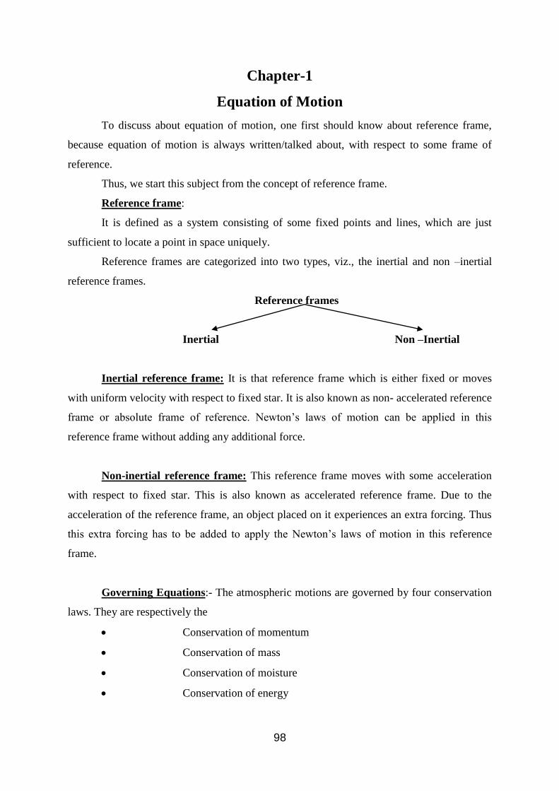
Reference frames are categorized into two types, viz., the inertial and non –inertial
reference frames.
Reference frames
Inertial Non –Inertial
Inertial reference frame: It is that reference frame which is either fixed or moves
with uniform velocity with respect to fixed star. It is also known as non- accelerated reference
frame or absolute frame of reference. Newton’s laws of motion can be applied in this
reference frame without adding any additional force.
Non-inertial reference frame: This reference frame moves with some acceleration
with respect to fixed star. This is also known as accelerated reference frame. Due to the
acceleration of the reference frame, an object placed on it experiences an extra forcing. Thus
this extra forcing has to be added to apply the Newton’s laws of motion in this reference
frame.
Governing Equations:- The atmospheric motions are governed by four conservation
laws. They are respectively the
• Conservation of momentum
• Conservation of mass
• Conservation of moisture
• Conservation of energy
99
The above conservation laws are expressed by six differential equations. These six
differential equations and the equation of state are known as governing equations.
Now we shall derive the governing equation:
Equation of motion:
This is simply the mathematical statement of the Newtons 2nd law of motion.
According to this law we have, Acceleration = Vector sum of forces per unit mass.
Now if aV
is the velocity vector in inertial frame of reference, then
equation motion in inertial frame can be written as :
dt
Vd aa = Vector sum of real forces, where the symbol dt
d a represents the time
derivative in an inertial frame of reference.
For the atmospheric motions, the real forces are the pressure gradient force,
gravitational force and the fractional (Viscous) force.
In this context, it is worth to mention that the forces may also be categorized into
different categories.
Again this categorization may also be done in different ways. One categorization of
forces is based on their existence in different reference frame and other one is based on the
direction of their line of action.
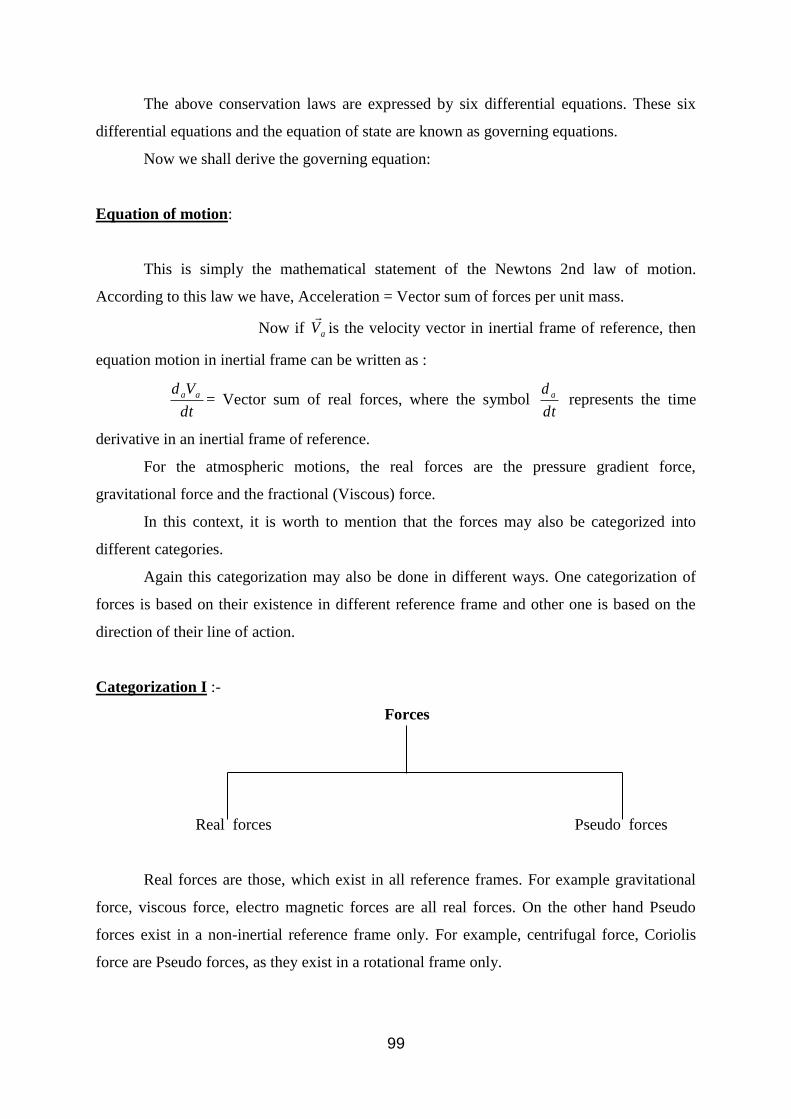
Categorization I :-
Forces
Real forces Pseudo forces
Real forces are those, which exist in all reference frames. For example gravitational
force, viscous force, electro magnetic forces are all real forces. On the other hand Pseudo
forces exist in a non-inertial reference frame only. For example, centrifugal force, Coriolis
force are Pseudo forces, as they exist in a rotational frame only.
100
Categorization-II:
Forces
Body force Surface force
Surface forces are those, the line of action of which is normal to the surface of the
object and depend on the area of the surface across which it act but not on the mass of the
object. Pressure gradient force, Viscous force are examples of surface force. On the other
hand body force acts at the centre of mass of the object and depends on mass of the object but
not on the surface area of the object. Examples of such forces are Coriolis force,
Gravitational force, Centrifugal force.
Illustration about pressure gradient force:-
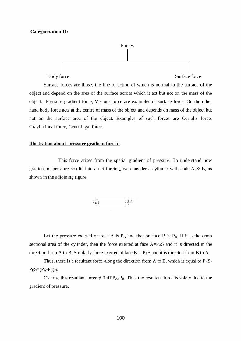
This force arises from the spatial gradient of pressure. To understand how
gradient of pressure results into a net forcing, we consider a cylinder with ends A & B, as
shown in the adjoining figure.
Let the pressure exerted on face A is PA and that on face B is PB, if S is the cross
sectional area of the cylinder, then the force exerted at face A=PAS and it is directed in the
direction from A to B. Similarly force exerted at face B is PBS and it is directed from B to A.
Thus, there is a resultant force along the direction from A to B, which is equal to PAS-
PBS=(PA-PB)S.
Clearly, this resultant force ≠ 0 iff PA≠PB. Thus the resultant force is solely due to the
gradient of pressure.
101
This illustrates how the gradient of pressure results into a forcing. This force is known
as pressure gradient force. It can be shown that the expression for pressure gradient force at
an arbitrary point ( ) ),,(000 000
1),,( zyxPzyx −=
.
Clearly PGF ≠ 0 if and only if 0p
. As gradient of any scalar is directed from its low
value to its high value, hence pressure gradient is directed from low to high-pressure area and
due to the presence of a minus sign, it follows that PGF force is directed from high to low
pressure. This force is always normal to the isobars.
Viscous force:- We know that in a sheared fluid flow, there is a relative motion at the
interface between two adjacent fluid layers. This relative motion causes a drag on the motion
of a fluid layer exerted by other one. This drag is proportional to the shear of the fluid
velocity. This is known as viscous stress.
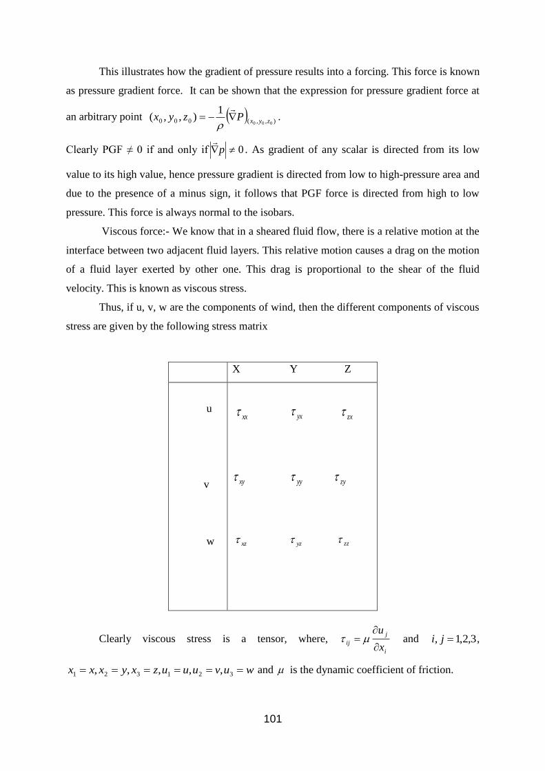
Thus, if u, v, w are the components of wind, then the different components of viscous
stress are given by the following stress matrix
Clearly viscous stress is a tensor, where, i
j
ijx
u
= and 3,2,1, =ji ,
wuvuuuzxyxxx ====== 321321 ,,,,, and is the dynamic coefficient of friction.
X Y Z
u
v
w
xx yx zx
xy yy zy
xz yz zz

102
It can be shown that the net viscous force along the positive x-direction, y direction and z-
direction are respectively u2 , v2 and w2 . Thus the frictional fore (Viscous force) in
vector form is given by, wkvjuiF 222 ˆˆˆ ++=
.
Equation of motion in a rotating reference frame:
It can be shown that, for an arbitrary vector B
, time rate of change of B
with
respect to absolute reference frame (Ox,Oy,Oz) = Time rate of change of B
with respect to
rotating reference frame (Ox,Oy,Oz)+ Time rate of change of B
due to rotation of the
reference frame (Ox,Oy,Oz) with respect to (Ox,Oy,Oz). Again it can be shown that the
rate of change of B
due to rotation of the reference frame (Ox,Oy,Oz) with respect to
(Ox,Oy,Oz) is .B
Hence, Bdt
Bd
dt
Bd a
+= .
To obtain the equation of motion in rotating reference frame, in the above expression
we substitute B
by r
to obtain aV
and then by aV
.
So, =aV
rVrdt
rd
dt
rd a
+=+=
And )()(2)()( rVdt
VdrVrV
dt
d
dt
Vd aa
++=+++=
To find out ( )r
the adjoining figure may be referred to, where a meridional
cross section of earth passing through an object at latitude has been shown. In this figure
radius of the -latitude circle is cosrR
= . Now,
RxRrr
==−= 00 90sin)90sin( . Since the vectors Rr
,, are coplanar,
hence any vector normal to the plane containing
and r
, will be so to the plane containing
and R
also.
Hence, Rxrx
= . Hence, ( ) RRxx
2−= .
103
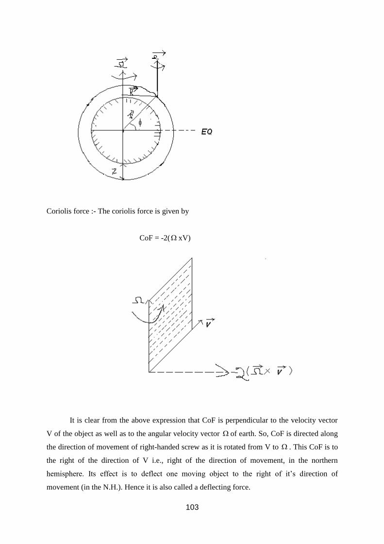
Coriolis force :- The coriolis force is given by
CoF = -2( xV)
It is clear from the above expression that CoF is perpendicular to the velocity vector
V of the object as well as to the angular velocity vector of earth. So, CoF is directed along
the direction of movement of right-handed screw as it is rotated from V to . This CoF is to
the right of the direction of V i.e., right of the direction of movement, in the northern
hemisphere. Its effect is to deflect one moving object to the right of it’s direction of
movement (in the N.H.). Hence it is also called a deflecting force.
104
As this force is perpendicular to the direction of movement, hence this force does not
do any work. One important thing to be noted that CoF comes in to play for a moving object
and in a rotational frame of reference ( x V≠ 0 iff ≠ O & V≠ O).
It is the rotation of the reference frame only, which is responsible for deflecting a
moving object to illustrate it following example may be referred.
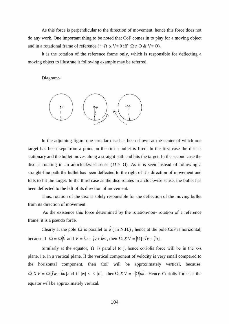
Diagram:-
In the adjoining figure one circular disc has been shown at the center of which one
target has been kept from a point on the rim a bullet is fired. In the first case the disc is
stationary and the bullet moves along a straight path and hits the target. In the second case the
disc is rotating in an anticlockwise sense ( O). As it is seen instead of following a
straight-line path the bullet has been deflected to the right of it’s direction of movement and
fells to hit the target. In the third case as the disc rotates in a clockwise sense, the bullet has
been deflected to the left of its direction of movement.
Thus, rotation of the disc is solely responsible for the deflection of the moving bullet
from its direction of movement.
As the existence this force determined by the rotation/non- rotation of a reference
frame, it is a pseudo force.
Clearly at the pole
is parallel to k ( in N.H.) , hence at the pole CoF is horizontal,
because if k=
and wkvjuiV ˆˆˆ ++=
, then ]ˆˆ[ ujviVX +−=
.
Similarly at the equator, is parallel to ĵ, hence coriolis force will be in the x-z
plane, i.e. in a vertical plane. If the vertical component of velocity is very small compared to
the horizontal component, then CoF will be approximately vertical, because,
]ˆˆ[ ukwiVX −=
and if |w| < < |u|, then kuVX ˆ−=
. Hence Coriolis force at the
equator will be approximately vertical.
105
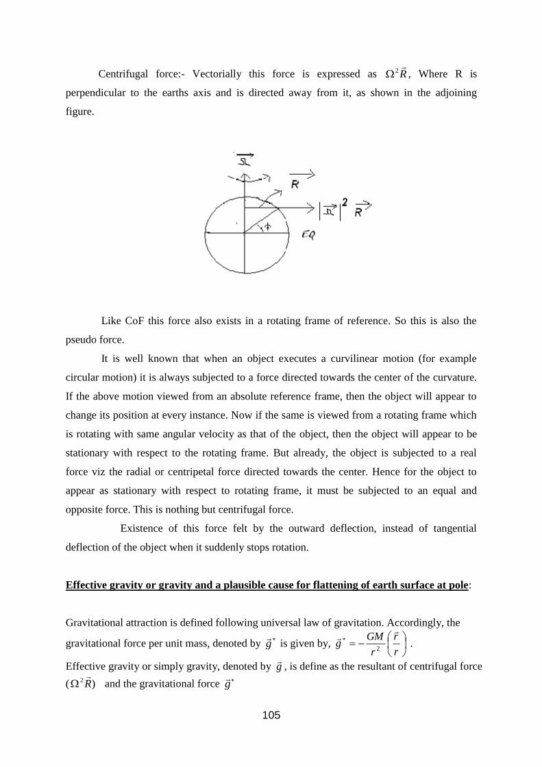
Centrifugal force:- Vectorially this force is expressed as R
2 , Where R is
perpendicular to the earths axis and is directed away from it, as shown in the adjoining
figure.
Like CoF this force also exists in a rotating frame of reference. So this is also the
pseudo force.
It is well known that when an object executes a curvilinear motion (for example
circular motion) it is always subjected to a force directed towards the center of the curvature.
If the above motion viewed from an absolute reference frame, then the object will appear to
change its position at every instance. Now if the same is viewed from a rotating frame which
is rotating with same angular velocity as that of the object, then the object will appear to be
stationary with respect to the rotating frame. But already, the object is subjected to a real
force viz the radial or centripetal force directed towards the center. Hence for the object to
appear as stationary with respect to rotating frame, it must be subjected to an equal and
opposite force. This is nothing but centrifugal force.
Existence of this force felt by the outward deflection, instead of tangential
deflection of the object when it suddenly stops rotation.
Effective gravity or gravity and a plausible cause for flattening of earth surface at pole:
Gravitational attraction is defined following universal law of gravitation. Accordingly, the
gravitational force per unit mass, denoted by *g
is given by,
−=
r
r
r
GMg
2
* .
Effective gravity or simply gravity, denoted by g
, is define as the resultant of centrifugal force
( )2 R
and the gravitational force g
106
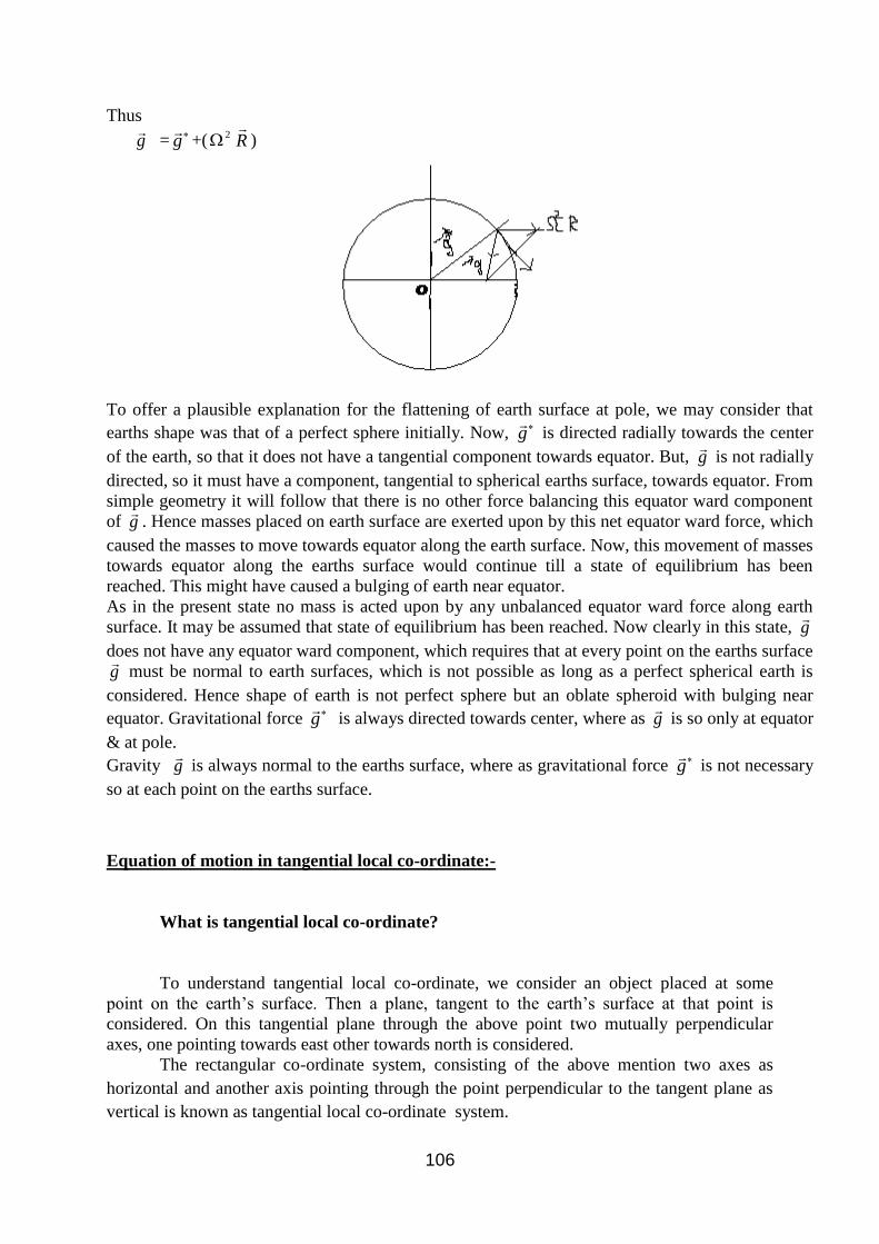
Thus
g
= g
+( 2 R
)
To offer a plausible explanation for the flattening of earth surface at pole, we may consider that
earths shape was that of a perfect sphere initially. Now, g
is directed radially towards the center
of the earth, so that it does not have a tangential component towards equator. But, g
is not radially
directed, so it must have a component, tangential to spherical earths surface, towards equator. From
simple geometry it will follow that there is no other force balancing this equator ward component
of g
. Hence masses placed on earth surface are exerted upon by this net equator ward force, which
caused the masses to move towards equator along the earth surface. Now, this movement of masses
towards equator along the earths surface would continue till a state of equilibrium has been
reached. This might have caused a bulging of earth near equator.
As in the present state no mass is acted upon by any unbalanced equator ward force along earth
surface. It may be assumed that state of equilibrium has been reached. Now clearly in this state, g
does not have any equator ward component, which requires that at every point on the earths surface
g
must be normal to earth surfaces, which is not possible as long as a perfect spherical earth is
considered. Hence shape of earth is not perfect sphere but an oblate spheroid with bulging near
equator. Gravitational force g
is always directed towards center, where as g
is so only at equator
& at pole.
Gravity g
is always normal to the earths surface, where as gravitational force g
is not necessary
so at each point on the earths surface.
Equation of motion in tangential local co-ordinate:-
What is tangential local co-ordinate?
To understand tangential local co-ordinate, we consider an object placed at some
point on the earth’s surface. Then a plane, tangent to the earth’s surface at that point is
considered. On this tangential plane through the above point two mutually perpendicular
axes, one pointing towards east other towards north is considered.
The rectangular co-ordinate system, consisting of the above mention two axes as
horizontal and another axis pointing through the point perpendicular to the tangent plane as
vertical is known as tangential local co-ordinate system.
107
The unit vectors kandji ˆˆ,ˆ are considered pointing towards east, north and local
vertical.
With respect to the above cartesian frame of reference, we have,
wkvjuiV ˆˆˆ ++=
z
kyx
i
+
+
ˆ jˆ
kgg ˆ−=
and ( )wkvjuiF 222 ˆˆˆ ++=
.
The Coriolis force in this co-ordinate system, at latitude ‘ ’ is given by
COF = ( ) ( ) ( ) cosˆsinˆsincosˆ2 ukujvwi −+−− .
Hence the component wise form of the equation of motion in tangential local co-
ordinate system can be written as :
dt
du= -
x
p
+2 (vSin -wCos ) + 2u
dt
dv= -
y
p
- 2 + uSin 2v
dt
dw= -
z
p
-g+2 + cosu 2w
Total change, In-situ change and advectional change:-
Let us consider an arbitrary function ),,,( tzyxf of space ),,( zyx and time ).(t Now a
change x in x, y in y , z in z and t in t, result in the following changes of f respectively:
tt
fandz
z
fy
y
fx
x
f
,,
Hence a total change in ),,,( tzyxf due to simultaneous changes in tzyx ,,, in
zyx ,, and t is given by
108
tt
fz
z
fy
y
fx
x
ff
+
+
+
=
= frtt
f+
.
Hence fVt
ff
t
r
t
f
t
f
dt
dfLtLt
tt
+
=+
==
→→
..00
Thus the total rate of change of ‘f’ with respect to‘t’ consists of two parts, viz., t
f
and fV
. . t
f
is known as in-situ rate of change, because this change does not involve any
change in location, where as fV
. is the charge in f due to change in x,y & z i.e. due to
change in position . This change is due to transport of f by wind.
Transport of any physical quantity by horizontal wind is known as advection and that
by vertical wind is known as convection. Advection is said to be positive at a point if at that
point
- fV
. > 0, i.e. if V
is directed to that point from higher value of f .
The derivative t
is called Eulerian derivative, where as
dt
d is called Lagrangian
derivative. Thus the complete form of the equation of motion in tangential local co-ordinate
system can be written as ,
uwCosvSinx
p
z
uw
y
uv
x
uu
t
u 2)(2 +−+
−=
+
+
+
vx
vu
t
v+
+
z
vw
y
v
+
= vuSin
y
p 22 +−
.
−=
+
+
+
z
ww
y
wv
x
wu
t
wwuCos
z
p 22 ++
.
109
Change of vertical co-ordinate:
Till now we have dealt the governing equations, taking ‘Z’ as vertical co-ordinate. Here we
shall see, what are the other parameters, which can be used as vertical co-ordinate.
An arbitrary quantity, say, ‘ξ’ may be used as a vertical co-ordinate if ‘ξ’ is a monotonic
(increasing or decreasing) function of ‘Z’, i.e.; if ξ either steadily increases or decreases with ‘Z’.
Mathematically Z
is either positive throughout in the vertical or negative in the
vertical.
Considering the above condition, it can be seen that gZ
p−=
< 0. Hence p is a
monotonic decreasing function of Z; therefore pressure ‘p’ can be used as a vertical co-
ordinate.
Similarly it can be seen that ,0
z
so potential temperature ‘ ’ being a monotonic
decreasing function of Z, may be used as a vertical co-ordinate.
Now we shall discuss the horizontal momentum equation in ‘p’ co-ordinate system. In
this system horizontal planes are constant ‘p’ surfaces, i.e., isobaric surfaces.
It can be shown that the gradient of a scalar ),,( zyx with respect to an arbitrary
vertical co-ordinate ),,( zyx can be expressed as :
= z
+ (z
)
Z.
Now we are in a position to have the expression for horizontal pressure gradient force
in different vertical coordinate. We know horizontal pressure gradient force in Z- co-ordinate
system is - pz
1.
In the above expression, we put p= and p= and then we have
p p = z
p + Zz
pp
- Zgp pz −=
1
Hence the horizontal pressure gradient force in p-co-ordinate can be expressed as, - )(gzp
.
-----------------------------------------------------------------------------------------------------------------
110
Chapter - 2
Geostrophic approximation
To understand geostrophic approximation, first we should understand some basic
concepts of atmospheric scale analysis.
Before discussing about scale analysis, we should first understand what is order of
magnitude of a physical parameter and what scale of atmospheric motion is.
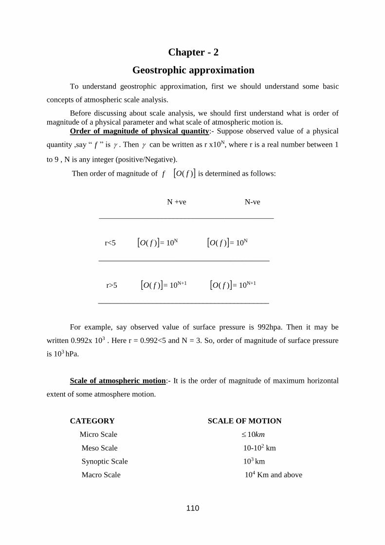
Order of magnitude of physical quantity:- Suppose observed value of a physical
quantity ,say “ f ” is . Then can be written as r x10N, where r is a real number between 1
to 9 , N is any integer (positive/Negative).
Then order of magnitude of f )( fO is determined as follows:
N +ve N-ve
_____________________________________________
r<5 )( fO = 10N )( fO = 10N
____________________________________________
r>5 )( fO = 10N+1 )( fO = 10N+1
____________________________________________
For example, say observed value of surface pressure is 992hpa. Then it may be
written 0.992x 10³ . Here r = 0.992<5 and N = 3. So, order of magnitude of surface pressure
is 103 hPa.
Scale of atmospheric motion:- It is the order of magnitude of maximum horizontal
extent of some atmosphere motion.
CATEGORY SCALE OF MOTION
Micro Scale km10
Meso Scale 10-102 km
Synoptic Scale 103 km
Macro Scale 104 Km and above
111
Scale analysis:- Atmospheric motion is governed by some conservation laws which
when are expressed as partial differential equations known as governing equations.
Each governing equation deals with tendency of some physical parameter
and possible mechanisms for that tendency.
In the governing equation terms other than the tendency term, represent
certain mechanism responsible for tendency. Now it is not necessary that all mechanisms will
contribute equally towards the change of the some parameter, rather this contribution
crucially depends on the scale of the motion under consideration.
Scale analysis is a convenient technique to estimate quantitatively the
contribution of individual mechanism and then after comparison certain terms with
comparatively less significant are ignored.
The following steps are to be performed to carry out scale analysis of any
governing equation:-
• To determine typical order of magnitude of field variables for a particular
type of motion at the given latitudinal belt.
• Using the above to find out the typical order of magnitude of individual
term of the governing equation.
• To retain those terms with highest order of magnitude, discarding others.
Performing scale analysis of equation of horizontal motion for mid-latitude synoptic
scale system it can be shown that the order of magnitude of the terms representing
pressure gradient force and Coriolis force is 10-3ms-2 and the order of magnitude of all
other terms are 10-4ms-2 or less.
So, following the principle of scale analysis, these two terms may be retained
discarding the other terms. Hence the above two equations for horizontal motion are
simplified to
0 fvx
p+
−
1
0 fuy
p−
−
1
The above two approximate equations are known as geostrophic approximation. The
values of u,v having dimension of wind, obtained from the equations:
01
=+
fv
x
p
112
01
=−
fu
y
p
are known as geostrophic wind, which is vectorially expressed as
pxf
kV Hg =
ˆ
Similarly, Geostrophic wind in p-coordinate is given as ( )zXkf
gV pg =
ˆ
It may be noted that geostrophic wind can be obtained from the spatial distribution of
the pressure field.
From the foregoing discussion it follows that geostrophic wind is horizontal,
frictionless flow, results from a complete balance between PGF & CoF. This wind is
proportional to the magnitude of pressure gradient and it is parallel to the isobars keeping low
pressure to its left in the northern hemisphere (opposite in southern hemisphere).
Thus scale analysis of horizontal equation of motion leads to geostrophic
approximation.
Ageostrophic flow:
Let (u,v) are the horizontal components of observed (actual) wind at a point and
(ug,vg) are the geostrophic approximation of the above, obtained from the horizontal
distribution of pressure, as
ug = -
y
p
1 & vg=
x
p
f
−
1.
Ageostrophic wind at that point is defined as the difference between actual wind and
geostrophic approximation. Of actual wind at that point. If the horizontal components of
ageostrophic wind are denoted by Ua & Va respectively, then
Ua = U-Ug & Va = V-Vg .
Horizontal equation of motion, neglecting the frictional effect, may be written as
VfkXpdt
dv +−=
1
113
Again gVfkXp
+−
10
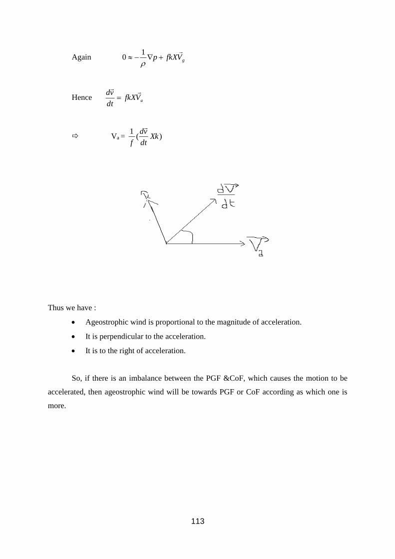
Hence aVfkXdt
vd
=
Va = )(1
Xkdt
vd
f
Thus we have :
• Ageostrophic wind is proportional to the magnitude of acceleration.
• It is perpendicular to the acceleration.
• It is to the right of acceleration.
So, if there is an imbalance between the PGF &CoF, which causes the motion to be
accelerated, then ageostrophic wind will be towards PGF or CoF according as which one is
more.
114
Chapter-3
Hydrostatic approximation
Hydrostatic balance refers to the balance between the vertical component of pressure
gradient force and the gravity. In the last chapter we have seen that by performing scale
analysis, for synoptic scale mid latitude system, the horizontal momentum equation
simplified to Geostrophic approximation. Similarly the vertical momentum equation after
scale analysis for synoptic scale system simplified to hydrostatic approximation. According
to this approximation, the vertical component of pressure gradient force and the gravity are
approximately in balance for synoptic or larger scale system. Mathematically it can be
expressed as:
0 gz
p−
1, Which is known as hydrostatic approximation.
This approximation is valid till there is no net vertical acceleration. In case of smaller
scale motion, viz., thunder storm, tornado etc, vertical component of pressure gradient force
may exceed gravity significantly, resulting into net vertical acceleration. For such situations,
hydrostatic approximation is not valid.
Some corollaries from hydrostatic approximation :
Definition of atmospheric pressure:
From the hydrostatic approximation we have,
gz
p−
Now integrating the above equation from an arbitrary pressure level, say ‘p’, to the
top of the atmosphere, we obtain
dzgdzz
p
zp
−
0
=> P
z
dzg
115
Hypsometric equation:
If the hydrostatic approximation is integrated between two pressure levels, say Z=ZL
&Z=ZU, with pressure, say P=PL & P=PU, we obtain
Zu – ZL )(ln pdTg
R
g
p L
U
U
L
P
P
P
P
=
−
Thickness= (ZU-ZL) = ),ln(U
L
P
PT
g
R
Where <T> is the mean temperature of air in the layer between Z=ZL & Z=Zu, given
by
<T> =
L
U
L
U
P
P
P
P
pd
pdT
)(ln
)(ln
This is known as hypsometric equation. This method of computation of thickness
is referred to as Isothermal method of computation of thickness.
116
Chapter-4
Balanced flow
Here we shall introduce another one co-ordinate system, which moves along with flow. This
co-ordinate system is known as Natural co-ordinate system.
We have seen earlier that any co-ordinate system is defined by the unit vectors along the co-
ordinate axis.
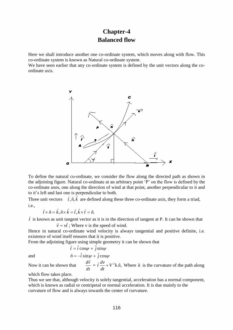
To define the natural co-ordinate, we consider the flow along the directed path as shown in
the adjoining figure. Natural co-ordinate at an arbitrary point ‘P’ on the flow is defined by the
co-ordinate axes, one along the direction of wind at that point, another perpendicular to it and
to it’s left and last one is perpendicular to both.
Three unit vectors knt ˆ,ˆ,ˆ are defined along these three co-ordinate axis, they form a triad,
i.e.,
.ˆˆˆ,ˆˆˆ,ˆˆˆ ntktknknt ===
t is known as unit tangent vector as it is in the direction of tangent at P. It can be shown that
tvv ˆ=
; Where v is the speed of wind.
Hence in natural co-ordinate wind velocity is always tangential and positive definite, i.e.
existence of wind itself ensures that it is positive.
From the adjoining figure using simple geometry it can be shown that
sinˆcosˆˆ jit +=
and cosˆsinˆˆ jin +−=
Now it can be shown that dt
vd
= ,ˆ.ˆ 2 nkVdt
dvt + Where k is the curvature of the path along
which flow takes place.
Thus we see that, although velocity is solely tangential, acceleration has a normal component,
which is known as radial or centripetal or normal acceleration. It is due mainly to the
curvature of flow and is always towards the center of curvature.
117
Hence tangential acceleration =dt
dv , and normal acceleration =
R
VkV
22 = , where ‘R’ is the
radius of curvature.
As the coriolis force is always normal to the direction of flow and to the right of the flow,
hence it follows that the horizontal component of coriolis force can be given by nfv ˆ− .
it can also be shown that, )ˆˆ(11
n
pn
s
ptpH
+
−=−
Hence, the equation of motion for horizontal flow in natural co-ordinate can be written as
)ˆˆ(ˆ)ˆˆ(1
ˆ2
FnnFtnfvn
pn
s
ptn
R
Vt
dt
dvs ++−
+
−=+
Component wise sFs
p
dt
dv+
−=
1
nFfvn
p
R
V+−
−=
12
These are equation of motion in natural co-ordinate.
Gradient flow:
While discussing the geostrophic flow it was assumed that isobars are straight lines. But in
reality isobars are curved lines.
Gradient flow is horizontal frictionless and isobaric flow i.e., parallel to isobars.
Since the flow is isobaric hence, .0=
s
p so, v = constant. And,
012
=+
+ fv
n
p
R
V
Thus gradient flow results from a three-way balance among the centrifugal force, coriolis
force and pressure gradient force. This balances known as gradient balance.
Resultant between coriolis force and pressure gradient force gives rise to the necessary
centripetal force required to maintain a curved flow, which is again equal and opposite to
centrifugal force.
If the flow is straight, then ,→R hence we have 01
=+
fv
n
p
, the geostrophic
balance.
Thus geostrophic balance is a special case of gradient balance for straight flow.
Wind obtained from gradient balance is known as gradient wind.
In the above gradient wind equation, n
pR
& may have different sign. Hence we shall
discuss all possible gradient flow for different combinations of sign of them.
118
Now from the gradient wind equation, V can be obtained as,
2
422
n
pRRffR
V
−−
=
Case I: n
pR
& both positive. Then the quantity inside the square root of expression for V is
less than 22Rf and hence the square root of the quantity is less than fR . Hence both the
positive and negative roots give negative root, which is not physically possible. Hence such
gradient flow with n
pR
& positive does not exist.
Case II: R positive and n
p
negative
Let hencen
pC ,
−= C>0
Now, 2
422
RCRffR
V
+−
=
Clearly the quantity inside the square root is greater than 22Rf . Hence the positive root only
physically possible.
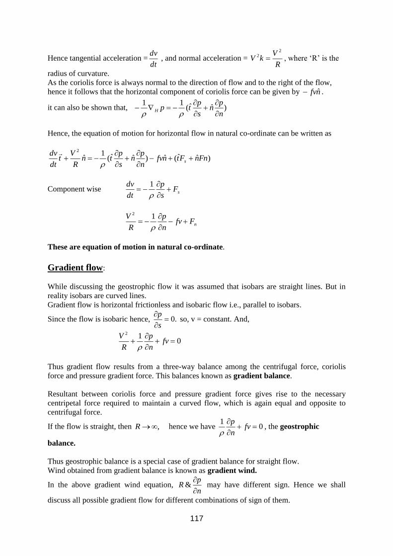
Possible gradient flow and the balance of force have been shown in the adjoining figure.
Clearly it is a cyclonic flow around a low. This flow is known as regular low. In this case
PGF acts towards the center of curvature, where as CFFCoF & both are away from center
of curvature. Hence in this case
fVn
p
R
V−
−=
12
fVC
−=
119
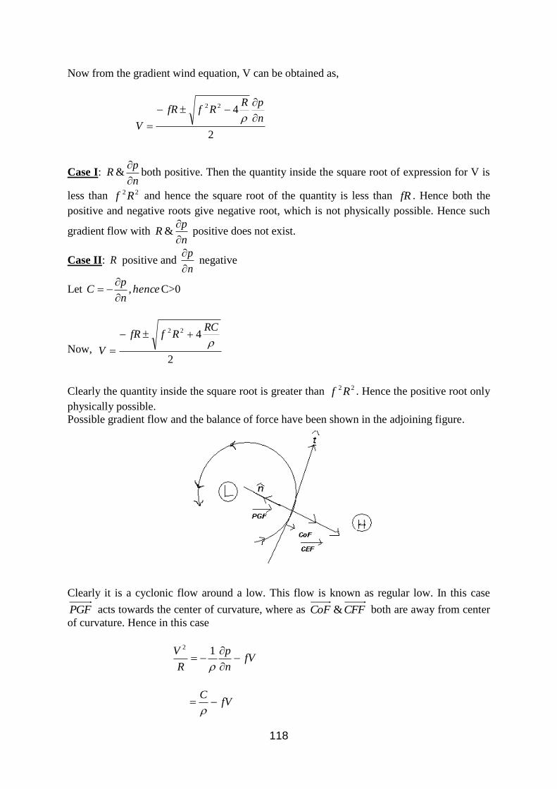
Case III : R negative and 0
n
p
Put S= -R>0,
Hence, 2
422
n
pSSffS
V
+
=
Clearly the square root is more than fS and hence only positive root is physically
possible. Possible gradient flow has been shown in the adjoining figure. It is an anticyclonic
flow around a low, known as anomalous low.
Here both CoFPGF & are towards the centre of curvature. Where as CFF is
away from the center of curvature.
Hence in this case the magnitude of CFF is the addition of that of CoFPGF & ,
where as in case of a regular low, magnitude of CFF is obtained by subtracting that of CoF
from that of .PGF
Hence for a given magnitude of radius of curvature and pressure gradient, gradient
wind is stronger in an anomalous low than in a regular low.
Case IV: Both n
pR
& are negative.
Let 0&0
−=−=
n
pCRS
Hence, 2
422
SCSffS
V
−
=
120
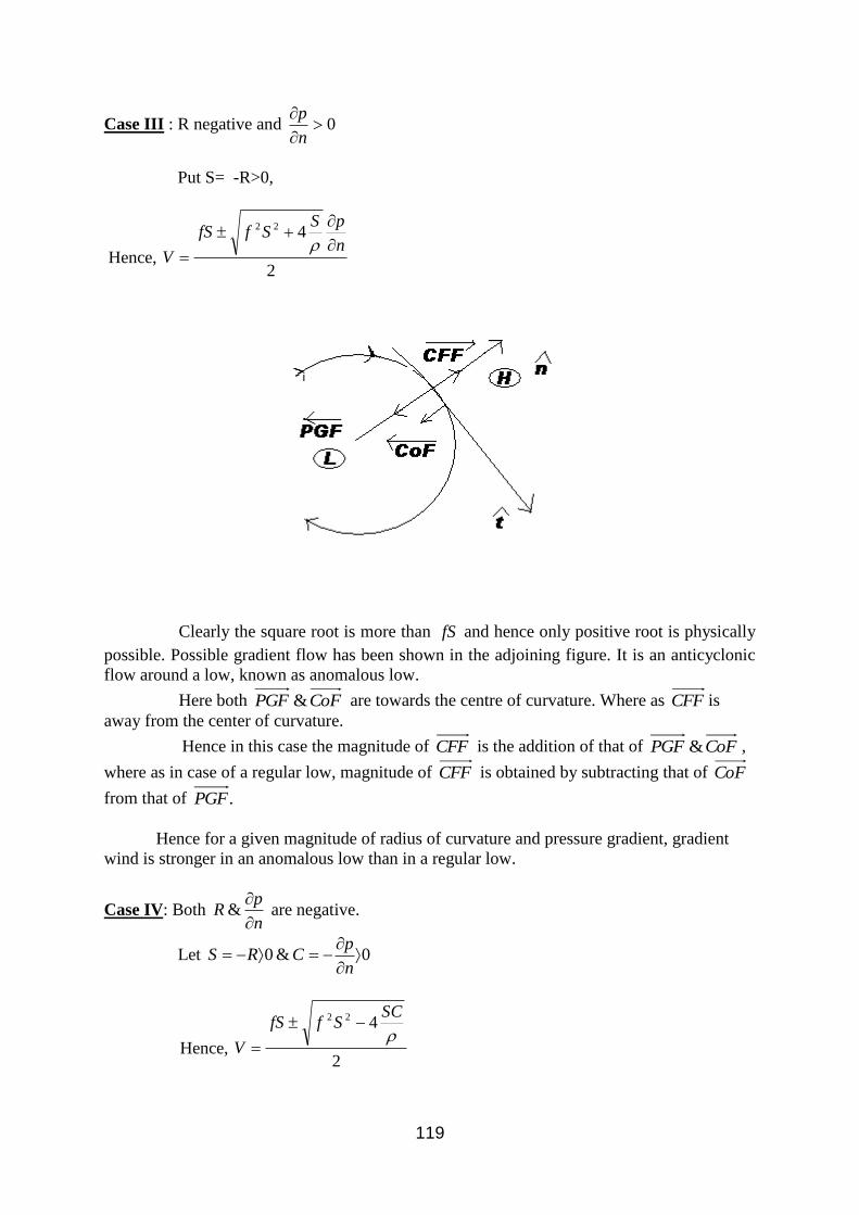
As, the square root is less than fS , hence both roots give physically possible solutions. For
the positive root 22
fRfSV −= and the corresponding flow is known as anomalous high and
for the negative root, ,22
fRfSV −= the corresponding flow is regular high. However in both
cases flow is an anticyclonic flow around a high, which is shown in the adjoining figure.
We can see that PGF is very less for such flow.
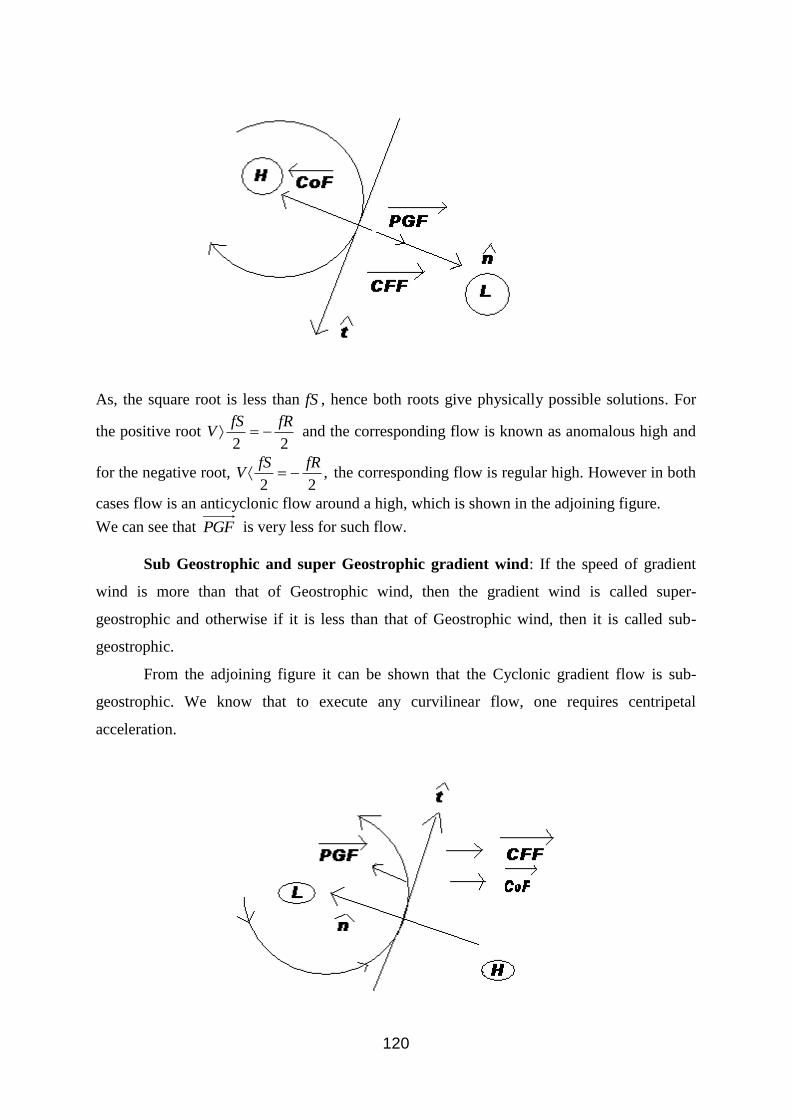
Sub Geostrophic and super Geostrophic gradient wind: If the speed of gradient
wind is more than that of Geostrophic wind, then the gradient wind is called super-
geostrophic and otherwise if it is less than that of Geostrophic wind, then it is called sub-
geostrophic.
From the adjoining figure it can be shown that the Cyclonic gradient flow is sub-
geostrophic. We know that to execute any curvilinear flow, one requires centripetal
acceleration.
121
One thing should be clear here, that the imbalance between the CoFPGF & only has
given rise to the centripetal acceleration. The net resultant between these two forces is
towards the direction of unit normal vector n . Accordingly the ageostrophic wind is normal
to n and to its left i.e.; opposite to the direction of horizontal wind. Hence the gradient wind,
which is a resultant of geostrophic & ageostrophic wind, must be lesser than the geostrophic
wind. Hence cyclonic gradient wind subgeostrophic.
Following similar argument one can offer a physical explanation for anticyclonic gradient
wind to be super geostrophic.
It can be shown that gradient wind for anticyclonic flow is more than Geostrophic wind but
less than four times the Geostrophic wind, i.e., ggrg VVV 2 .
Some special types of gradient balance/flow:
When we consider straight flow, →R and gradient wind equation transforms into,
fVn
p−
−=
10 , which is Geostrophic flow. In case of jet stream, curvature of the flow may not be
significant enough for presence of centrifugal force.
When Coriolis force is very week, then gradient balance becomes the balance between the
pressure gradient and centrifugal force, i.e.,
n
p
R
V
−=
12
. This balance is known as cyclostrophic balance. Cyclones, anticyclones etc are
suitable examples of cyclostrophic flow.
When pressure gradient is very weak, then the gradient balance becomes the balance between
the coriolis force and centrifugal force, i.e., fVR
V−=
2
. This balance is known as inertial balance. It
can be shown that inertial flow is always anticyclonic. Inertial waves (easterly waves) at low
latitudes are suitable examples for inertial flow.
122
Chapter-5
Vertical variation of wind
Vertical shear of geostrophic wind refers to rate of change of geostrophic wind vector with
height, mathematically it is expressed as z
Vg
. Now we shall first try to understand how horizontal
temperature gradient can lead to vertical shear of geostrophic wind.
We know that in isobaric co-ordinate, the equations for geostrophic wind are given by
p
gy
z
f
gu
−= and
p
gx
z
f
gv
= , i.e., zk
f
gV pg =
ˆ ….(1)
Thus, geostrophic wind at any isobaric level is directly proportional to the slope of that level.
Now let us consider two isobaric surfaces, which are having same slope initially. Now
consider the layer between these two isobaric surfaces. Now we create horizontal temperature
gradient in this layer by heating one part of the layer and cooling other part. This will cause a
difference in the slopes of these two isobaric surfaces. This in tern will cause a difference in
the geostrophic wind at these two levels, i.e., will cause a vertical shear of geostrophic wind.
Thus horizontal temperature can lead to vertical shear of geostrophic wind.
Now we are in a position to give the definition of thermal wind. Thermal wind is
defined as the vectorial difference between upper level geostrophic wind and lower level
geostrophic wind. From the above discussion it follows that for thermal wind to exist there
must be a horizontal temperature gradient. Thus we see that thermal wind owes to a thermal
effect Viz., horizontal temperature gradient.
Equation of thermal wind : Let glV
and guV
are respectively the lower level and upper level
geostropic wind at pressure levels lP and
uP .Then, glV
and guV
are given by
lpgl zkf
gV =
ˆ and upgu zk
f
gV =
ˆ , where ),( yxzl
and ),( yxzuare geopotential height
at different points at the above two levels. Then thermal wind TV
, in the layer between
pressure levels lP and uP is given by
)(ˆlupglguT zzk
f
gVVV −=−=
….(2)
Again from Hypsometric equation we know that
=− Tk
p
p
g
Rzz p
u
llu
ˆln ….(3), where, <T> is given by,
=
u
l
u
l
p
p
p
p
pd
pTd
T
)(ln
)(ln
….(4)
123
Hence using (3) in (2) we have,
= Tk
p
p
f
RV p
u
lT
ˆln ….(5)
Properties of thermal wind:
i. Thermal wind is not a real wind, it’s a concept only.
ii. It refers to a layer not a level.
iii. It exists as long as there exists horizontal temperature gradient.
iv. It is parallel to mean isotherms in a layer, keeping colder side to the left (In
northern hemisphere)
v. It is also parallel to mean thickness lines of the layer, keeping lower thickness to
the left (in Northern hemisphere)
Concept of barotropic and baroclinic atmosphere:
An atmosphere is said to be barotropic if the density is a function of pressure only.
Hence, )(pf= . This functional relation along with the equation of state RTp = gives
).(phT =
Thus, pphT =
)(
pIIT
isotherms are parallel to isobars, i.e., there is no change in T along
isobars, i.e., horizontal temperature gradient on an isobaric surface is zero for a barotropic
atmosphere. Thus in a barotropic atmosphere, the geostrophic wind does not change with
height and thermal wind is zero.
Otherwise if density is not a function of pressure only, then it is called a baroclinic
atmosphere. So, thermal wind exists only in a baroclinic atmosphere.
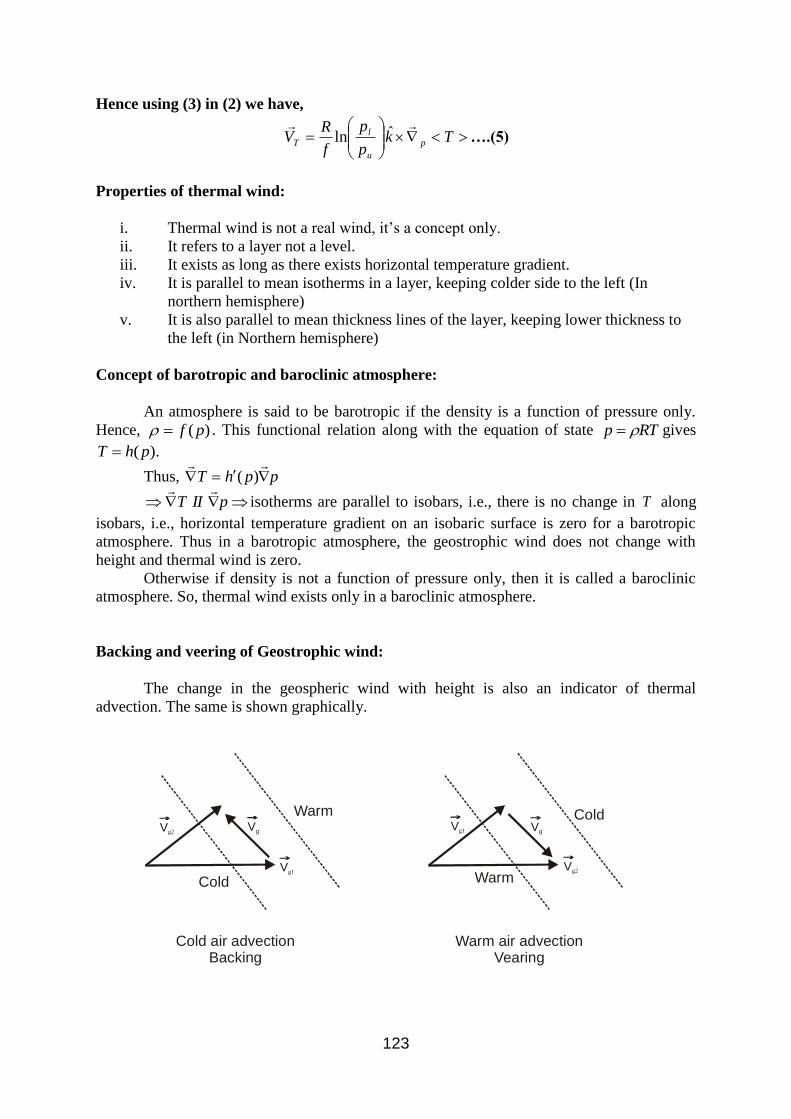
Backing and veering of Geostrophic wind:
The change in the geospheric wind with height is also an indicator of thermal
advection. The same is shown graphically.
Vg2
Vg1
Vg
Cold
ColdWarm
Warm
Cold air advectionBacking
Warm air advectionVearing
Vg2
Vg1 Vg
124
Backing refers to anti-clockwise turn of geostrophic wind with height, where as
veering refers to clockwise turn of geostrophic wind with height. The above two figures
explain warm (cold) air advection associated with veering (backing).
Application of the thermal wind concept:
i. Using thermal wind concept one can show that cold (warm) core low ( high)
intensifies with height.
ii. Using thermal wind concept one can, explain the existence of sub tropical
westerly jet in winter and tropical easterly jet in southwest monsoon season
over India.
iii. Using thermal wind concept one can explain warm (cold) air advection
associated with veering (backing).
125
Chapter-6
Kinematics of wind and pressure field
Streamline: Stream lines are curves, the tangent to each point of which is represented by
horizontal wind vector at that point. Thus if at an arbitrary point ( )yx, , ),( yxu and ( )yxv , are
horizontal components of wind, then we have,
),(
),(
yxu
yxv
dx
dy= . This is the differential equation of stream line. Stream lines give the picture of
instantaneous motion.
Trajectory: It is the actual path traced by an air parcel during a finite interval of time. Thus if
),,( tyxs is the displacement at time ‘t’ and V(x,y,t) is the speed, then ),,( tyxVdt
ds= . It gives
the picture of total motion during an interval of time.
Relation between streamlines and trajectories: It is expressed by an equation, known as,
Blaton’s equation, which is given by
)( STVt
−=
; where,
= Angle of turning of wind
=V Wind speed
=T Curvature of trajectory
=S Curvature of streamline.
Under steady state condition, left hand side of above equation vanishes and hence stream line
and trajectory coincides.
Stream line pattern for different wind field: It can be shown that horizontal motion
consists of pure translation, pure divergence, pure rotation and pure deformation.
Equation of stream lines for pure translation is given by: cmxy += ; ),(
)(
00
0,0
yxu
yxvm = ,
( )00 , yx is the centre and c is a parameter. Thus for pure translational motion stream lines are
family of parallel straight lines with slope ‘m’.
126
For pure divergence, stream lines are family of straight lines passing through centre (origin),
given by the equation: kxy = ; k being a parameter.
For pure rotational motion equation of stream lines is given by:
222 ayx =+ ; ‘a’ being a parameter. Thus for pure rotational motion, stream lines are family
of concentric circles. Similarly it can be shown that for pure deformation, stream line patterns
are either family of hyperbola ( )tconyx tan22 =− with same foci or family of rectangular
hyperbola ( )tconxy tan= .
Centre of low, high, trough of low pressure , ridge of high pressure and COL
An arbitrary point, ( )00 , yx is said to be a centre of low pressure/ high pressure if the pressure
field ( )yxp , has a local minima/ maxima at this point, i.e., if
Conditions for low pressure centre Conditions for high pressure centre
( )
0
00 ,
=
yxx
p
( )
0
00 ,
=
yxx
p
( )
0
00 ,
=
yxy
p
( )
0
00 ,
=
yxy
p
( )
0
00 ,
2
2
yxx
p and
( )
0
00 ,
2
2
yxy
p
( )
0
00 ,
2
2
yxx
p and
( )
0
00 ,
2
2
yxy
p
Conditions stated at first two rows states that the centre of high/low is a stationary point and
condition stated in last row implies that around a centre of low (or high), the isobars turn in
anti clock wise ( or clock wise) direction.
Before defining trough of low pressure or ridge of high pressure, we should first understand
about axis of symmetry. An arbitrary axis, say y-axis, is said to be an axis of symmetry for a
quantity, ‘S’, if each point on this axis is either a local minima or a local maxima for ‘S’, i.e.,
if either 0=
x
S and 0
2
2
x
S or 0=
x
S and 0
2
2
x
S.
127
Trough of low pressure is a line of symmetry, each point of which is a local minima for the
pressure field ( )yxp , i.e., at each point on the trough 0=
x
p and 0
2
2
x
p.
Similarly, ridge of high pressure is a line of symmetry, each point of which is a local maxima
for the pressure field ( )yxp , i.e., at each point on the ridge 0=
x
p and 0
2
2
x
p.
From the above, it follows that around a trough/ridge, isobars (isolines) turn in anti clock
wise (or clock wise) direction.
Centre of COL is the point of intersection between one trough and ridge. If the trough is
oriented along y-axis and ridge is oriented along x-axis, then at the COL, we have
0=
x
p and 0
2
2
x
p, 0=
y
p and 0
2
2
y
p.
128
Chapter-7
Divergence & vorticity
Before discussing about conservation laws for mass and water vapour, one must first
under stand about the concept of divergence. So in the next section, we shall discuss about
divergence.
Divergence: Divergence of an arbitrary vector field B
is its measure of outflow. It is
defined as B
. . In Meteorology, by the term divergence, we mean divergence of wind vector,
.V
Thus in meteorology divergence is mathematically expressed as V
. . If the value of this
quantity is positive then we say that divergence is taking place and if the value of this
quantity is negative then we say that convergence is taking place We may talk of 2
dimensional as well as 3 dimensional divergence, which are occasionally denoted as
y
v
x
uV
+
=
.2 and
z
w
y
v
x
uV
+
+
=
.3 . It can be shown that 2 dimensional divergence is
equal to fractional rate of change of area, i.e., the time rate at which a unit area is expanding
or contracting. It can be mathematically expressed asdt
dA
Ay
v
x
uV
1.2 =
+
=
, A being the
area. Similarly, it can be shown that 3 dimensional divergence is equal to fractional rate of
change of volume, i.e., the time rate at which a unit volume is expanding or contracting. It
can be mathematically expressed asdt
d
z
w
y
v
x
uV
1.3 =
+
+
=
, being the volume.
Physically one can visualize that expansion/contraction of an area or volume is possible only
by outflow (divergence)/inflow(convergence) of air.
In natural co-ordinate, 2-dimentional divergence (conventionally called as horizontal
divergence) is given by nVs
VV +
=
.2 , V is the wind speed and n is the orthogonal
curvature of the stream line. Orthogonal curvature of the stream line is nothing but the
curvature of a curve which is orthogonal to the stream line. A curve, C1 is said to be
orthogonal to another curve, say, C2 at a point, if the tangents at this point to both the curves
are perpendicular to each other.
From the above expression of horizontal divergence, it follows that down wind
increase/decrease of wind speed gives rise to divergence/convergence. It also follows that a
positive(cyclonic)/negative (anti-cyclonic) orthogonal curvature gives rise to
divergence/convergence.
129
VORTICITY:
Vorticity is a micro scale measure of rotation. It is a vector quantity. Direction of
this vector quantity is determined by the direction of movement of a fluid, when it is being
rotated in a plane. Observation shows that when a fluid is being rotated in a plane, then there
is a tendency of fluid movement in a direction normal to the plane of rotation (towards
outward normal if rotated anti clockwise or towards inward normal if rotated clockwise).
Thus due to rotation in the XY plane (Horizontal plane) fluid tends to move in the k
direction (i.e. vertical), due to rotation in the YZ plane (meridional vertical plane)fluid tends
to move in the i direction (East West) and due to rotation in ZX plane (zonal vertical plane)
fluid tends to move in the j direction (N-S).
Thus vorticity has three components. Mathematically it is expressed as
kjiV ˆˆˆ ++= where, y
u
x
v
x
w
z
u
z
v
y
w
−
=
−
=
−
= ;; .
In Meteorology, we are concerned about weather, which is due mainly to vertical
motion and also only the rotation in the horizontal plane can give rise to vertical motion. So,
in Meteorology, by the term vorticity, only the k component of the vorticity vector is
understood. Hence, throughout our study only k component is implied by vorticity.
Thus, hence forth, vorticity =y
u
x
v
−
= . It is known as relative vorticity. It is
solely due to motion of an object. But rotation of earth itself gives rise to some vorticity, even
to a stationary object. Vorticity, which is solely due to rotation of earth, is known as planetary
vorticity. It can be shown that, planetary vorticity at a latitude = f= 2Sin. Planetary
vorticity and relative vorticity, combined together, is known as absolute vorticity and is
denoted by fa += .
In natural co-ordinate, relative vorticity is expressed as
n
VV s
−= , where,
s is the stream line curvature and n
V
is across the streamline
wind shear. First term on right hand side of the above expression is known as curvature
vorticity and the second term (including sign) is known as shear vorticity. From first term it
follows that at an arbitrary point, vorticity will be cyclonic/anti-cyclonic if the curvature of
the stream line at that point is cyclonic / anti-cyclonic. Similarly from the second term, it
follows that if wind speed decreases/increases to the left across the stream line, then there
will be cyclonic/ anti cyclonic vorticity.
Due to effect of Coriolis force, the out flowing (inflowing) stream lines ( which are
straight lines) in a divergent/convergent field, are deflected to the right and acquire anti-
cyclonic curvature/cyclonic curvature. That’s why divergence is associated with anticyclonic
vorticity and convergence is associated with cyclonic vorticity.
It can be shown that for synoptic and larger scale motion, change in vorticity is
mainly due to large scale divergence/convergence.
130
Chapter – 8
Conservation of mass
Atmospheric motion is governed by some conservation laws, viz., the conservation of
momentum, conservation of mass, conservation of energy and conservation of moisture.
Conservation of momentum has already been discussed in the equation of motion.
Now, we shall discuss the conservation of mass, which says that mass remains
conserved. In this context of establishing the laws of conservation, it is worth to mention that
conservation laws can be established following two dynamical approaches,viz, Eulerian
approach and Lagrangian approach.
In both approach an air parcel is considered. In the former approach air parcel is
considered stationary while fluid is allowed to pass through it and in the later approach the
motion of the parcel along with flow in considered.
Mathematical equation expressing the law of conservation of mass is known as mass
continuity equation.
Following either of the above mentioned approach, we can arrive at following two
forms of mass continuity equation, viz., the mass divergence form
).( 0
0 vt
−=
, which states that in-situ/local change in mass at a point is
solely due to mass convergence/divergence at that point and the velocity divergence form
vdt
d o .
1
0
−=
, which states that total change of mass at a point is solely due to
convergence/divergence of wind.
Continuity equation in pressure co-ordinate is given by
0=
+
+
py
v
x
u , where
dt
dp= , the vertical velocity in pressure co-ordinate and its unit is
hPa/Sec. It can be shown that wg − , where w is the vertical velocity in m/Sec. Thus one
can see that is positive for sinking motion and negative for rising motion.
Is ‘P’ as a vertical co-ordinate is superior than ‘Z’? If so then how?
131
Pressure as a vertical co-ordinate is superior than Z, due to following reasons:
• Density ‘ ‘ does not appear explicitly in the governing equations in p-coordinate.
• The above is beneficial due to the fact that ‘ ’ is not an observed field, rather it is a
derived field. Use of it explicitly requires extra computations.
• As ‘ ’ is not appearing explicitly, rarefication and compression are eliminated
resulting into completely removal of sound wave-a meteorological noise.
Moisture Continuity Equation:
If q is the specific humidity of water vapour in air and if is the density of air, then density
of water vapour is q . Thus applying mass continuity equation to water vapour mass, we get
qvq
vtt
q
qvq
t
q−−=
+
−=
.
1).(
111).(
)(
Hence, using mass continuity equation, viz., ).( vt
−=
, we obtain
00. ==+
dt
dqqv
t
q . This is known as moisture continuity equation.
Dines compensation principle: If the mass conservation law is applied to an air column,
then one can find that convergence throughout entire column or divergence throughout entire
column, would lead to a net increase or net decrease of mass in the column, both of which
contradict law of conservation of mass. Thus only convergence or divergence throughout an
air column is not possible. Convergence in some layers must be compensated by divergence
in some other layers. This is known as Dines compensation principle.
This principle leads us to a level, theoretically at which there shouldn’t be any divergence or
convergence. This is known as level of non-divergence. For all operational purpose, 500hPa
level is considered to be the level of non divergence. If the observed divergence at this level
is more than its climatological normal value, then it’s an indication of enhancement of low-
level convergence. This is an important forecasting tool.
Application of continuity equation: Mass continuity equation in isobaric co-ordinate can be
used to find out vertical velocity at any level. Integrating this equation between two adjacent
pressure levels, say, LP and UP , we obtain,
PDPP LU += )()( ; Where
UL PPP −= ,
y
v
x
uD
+
= ,
Refers to mean of the values at two levels and
)(),( UL PP are vertical velocities in hPa/Sec at two levels.
132
Chapter-9
Planetary Boundary Layer (PBL)
A Brief essay on PBL:
PBL is the lower most portion of the atmosphere, adjacent to the earth’s surface,
where maximum interaction between the Earth surface and the atmosphere takes place and
thereby maximum exchange of Physical properties like momentum, heat, moisture etc., are
taking place.
Exchange of physical properties in the PBL is done by turbulent motion, which is a
characteristic feature of PBL. Turbulent motion may be convectively generated or it may be
mechanically generated.
If the lapse rate near the surface is super adiabatic, then PBL becomes positively
Buoyant, which is favorable for convective motion. In such case PBL is characterized by
convective turbulence. Generally over tropical oceanic region with high sea surface
temperature this convective turbulence occurs. If the lapse rate near the surface is sub
adiabatic then the PBL is negatively buoyant and it is not favourable for convective
turbulence. But in such case, if there is vertical shear of horizontal wind, then Vortex
(cyclonic or anti cyclonic) sets in, in the vertical planes in PBL. This vortex motion causes
turbulence in the PBL, known as mechanical turbulence.
If the PBL is positively buoyant as well as, if vertical shear of the horizontal wind
exists, then both convective and Mechanical turbulence exits in the PBL.
Now, we consider a typical situation, when PBL is stably stratified and there exists
vertical shear of mean horizontal wind. In such situation convective turbulence is
suppressed but mechanical turbulence is enhanced. In this situation it is difficult to say
whether their combined effect is to suppress turbulence or to sustain turbulence. This
situation is tackled using a non-dimentional number, which is defined as the ratio between,
static stability and square of vertical shear of horizontal wind, i.e.,
Richardson number = fR = 22
+
z
v
z
u
dz
dg
Empirically it has been found that, fR
must be less than 0.25 to sustain the turbulence. Thus fR should be less than ¼ to maintain
turbulence in a stably stratified PBL by wind shear.
133
The depth of the PBL is determined by the maximum vertical extent to which the
turbulent motion exists in PBL. On average it varies from few cms to few kms. In case of
thunderstorms PBL may extend up to tropopause.
Generally at a place on a day depth of PBL is maximum at noon and in a season it is
maximum during summer.
Division of the PBL into different sub layers:
The PBL may be sub divided into three different sections, viz viscous sub layer, the
surface layer and the Ekmann layer or entrainment layer or the transition layer.
Viscous layer is defined as the layer near the ground, where the transfer of physical
quantities by molecular motions becomes important. In this layer frictional force is
comparable with PGF.
The surface layer extends from z = 0z (roughness length) to
szz = with sz , the top of
the surface layer, usually varying from 10 m to 100 m. In this layer sub grid scale fluxes of
momentum (eddy stress) and frictional forces are comparable with PGF.
The last layer is the Ekmann layer is defined to occur from sz to
iz , which ranges
from 100 m or so to several kilometers or more. Above the surface layer, the mean wind
changes direction with height and approaches to free stream velocity at the height z as the sub
grid scale fluxes decrease in magnitude. In this layer both the COF and Eddy stress are
comparable with PGF.