Copyright Warning & Restrictions

The copyright law of the United States (Title 17, United States Code) governs the making of photocopies or other

reproductions of copyrighted material.

Under certain conditions specified in the law, libraries and archives are authorized to furnish a photocopy or other

reproduction. One of these specified conditions is that the photocopy or reproduction is not to be “used for any

purpose other than private study, scholarship, or research.” If a, user makes a request for, or later uses, a photocopy or reproduction for purposes in excess of “fair use” that user

may be liable for copyright infringement,

This institution reserves the right to refuse to accept a copying order if, in its judgment, fulfillment of the order

would involve violation of copyright law.

Please Note: The author retains the copyright while the New Jersey Institute of Technology reserves the right to

distribute this thesis or dissertation

Printing note: If you do not wish to print this page, then select “Pages from: first page # to: last page #” on the print dialog screen

The Van Houten library has removed some of the personal information and all signatures from the approval page and biographical sketches of theses and dissertations in order to protect the identity of NJIT graduates and faculty.

ABSTRACT

Dynamic Analysis of the Generalized Slider Crank

by

Sahidur Rahman

A numerical technique is used to analyze the kinematics of the generalized

slider crank mechanism and an analytical technique to derive dynamic force equations

for that mechanism has been formulated. The numerical technique used for displace-

ment analysis is based on a combination of Newton-Raphson and Davidon-Fletcher-

Powell optimization algorithm using dual-number coordinate-transformation matrices.

Velocity analysis is performed by using a dual number method. Finally, dynamic force

analysis is accomplished on the basis of the dual-Euler equation and D'Alembert's

principle. The approach is developed in such a manner that a digital computer can

detect when a solution is possible and then solve the whole problem.

In addition, kinematic displacements of slider and dynamic forces and torques

at each of the joints have been graphed against input crank angles for different offsets.

In all the graphs, possible cases have been compared with the ideal case, when the

mechanism has zero offsets.

DYNAMIC ANALYSIS OF THE GENERALIZED SLIDER CRANK

by

Sahidur Rahman

A Thesis

Submitted to the Faculty of the Graduate Division of the

New Jersey Institute of Technology

in Partial Fulfilment of the Requirements for the Degree of

Master of Science

Department of Mechanical Engineering

May 1991

APPROVAL PAGE

Dynamic Analysis of the Generalized Slider Crank

by

Sahidur Rahman

Dr. Ian S. Fischer, Thesis Adviser

Assistant Professor of Mechanical Engineering, NJIT

Dr. Rajesh Dave, Committee Member

Assistant Professor of Mechanical Engineering, NJIT

Dr. Anthony Rosato, Committee Member

Assistant Professor of Mechanical Engineering, NJIT

BIOGRAPHICAL SKETCH

Author: Sahidur Rahman

Degree: Master of Science in Mechanical Engineering

Date: May, 1991

Undergraduate and Graduate Education:

Master of Science in Mechanical Engineering,

New Jersey Institute of Technology, Newark, NJ, 1991

Bachelor of Engineering in Mechanical Engineering,

Regional Engineering College, Durgapur, India, 1984

Major: Mechanical Engineering

iv

ACKNOWLEDGEMENT

The author wishes to express his sincere gratitude to his adviser, Dr. Ian S.

Fischer for his guidance, advice, and moral support throughout this research.

Thanks also to Dr. Raj Dave and Dr. Anthony Rosato for serving as members

of the committee.

The author expresses deep appreciation for the support by National Science

Foundation under grant number MSM-8811101.

And finally a special thank to his parents for their consistent encouragement.

Copyright © 1991 by Sahidur Rahman

ALL RIGHTS RESERVED

TABLE OF CONTENTS

Page

1.INTRODUCTION 10

1.1 Background and Motivation 10

1.2 Outline of Thesis 11

2. ANALYSIS AND FORMULATION OF THE METHOD 12

2.1 Basic Definitions 12

2.2 Notations 14

2.3 Creation of link joint parameter table 15

2.4 Transformation Matrices 16

2.5 Partial Derivatives of the Transformation Matrices 20

2.6 Displacement Analysis 22

2.6.1 Dual-number formulation of Numerical Method 22

2.6.2 Plane Geometry Method for Initial Estimates of the Joint Variables 28

2.7 Velocity Analysis 28

2.8 Dynamic Force and Torque Analysis 33

3. ILLUSTRATIVE EXAMPLES, RESULTS AND CONCLUSIONS 54

3.1 Example 54

3.2 Discussion of Results 55

3.3 Conclusion 57

BIBLIOGRAPHY 59

APPENDICIES 61

vii

LIST OF TABLES

Table Page

1. Link joint parameters 15

viii

LIST OF FIGURES

Figure Page

1.Planar (ideal) slider crank with no offset 12

2. Planar slider crank with offset a4 only 13

3. Generalized slider crank with all offsets 13

4. Planar slider crank when crank angle is zero 25

ix

1 0

INTRODUCTION

1.1 Background and Motivation

In recent years mechanisms with multi-degree-of-freedom systems have commanded

a great deal of research activity. The rapid advancements of the robot manipulator for

industry is fueling the interest of many researchers. In 1964 Uicker, Denavit and

Hartenberg developed an iterative technique for displacement analysis of spatial

mechanisms using 4 x4 transformation matrices (1). Later in 1967 Uicker did the

dynamic force analysis of spatial linkages (2). Dual-number element coordinate trans-

formation matrices were introduced by researchers such as Yang to study spatial

mechanisms. In 1964 Yang and Freudenstein applied dual-number quaternion algebra

to the analysis of spatial mechanisms (3). Based on dual vectors and screw calculus,

Yang formulated inertia force equations for RCCC mechanisms (R stands for revolute

joint and C stands for cylindrical joint) in 1971 (4). One year later Bagci did dynamic

force and torque analysis of the planar 4R mechanism and spatial RCCC mechanism

using dual vectors and 3 x3 screw matrix (5). Pennock and Yang in 1983 developed the

technique for dynamic analysis of a multi-rigid-body open chain system based on

Newtonian mechanics with a composite 3 x3 dual number, 6 x 1 Plucker coordinate

method (6). In 1984 Fischer and Freudenstein did the complete derivation of internal

force and torque components of a statically loaded cardan joint with manufacturing

tolerances (7). As an extension of the earlier work, Chen and Freudenstein in 1986

developed a dynamic analysis of a universal joint with manufacturing tolerances (8).

Fischer and Paul successfully extended the concept of Uicker-Denavit-Hartenberg in

1989 for kinematic displacement analysis of a double cardon joint driveline using 3 x3

dual number transformation matrices (9). In 1990 Fischer investigated displacement

errors in Cardan joints caused by coupler-link joint-axes offset (10). To model robot

11

manipulators mathematically, Lagrange-Euler and Newton-Euler formulations using

4 x4 transformation matrices have been used widely. The method described here

serves a meaningful alternative to the existing procedures.

Sandor and Erdman did the displacement, velocity and acceleration analysis of

a similar type of mechanism using 4 x 4 transformation matrix (11). The solution is

based on Newton-Raphson iterative procedure commonly used for the solution of

nonlinear equations. The present work owes much to pioneering work of Uicker,

Denavit, Hartenberg and Yang on spatial mechanisms.

1.2 Outline of Thesis

Chapter 2 explains how displacement analysis is done numerically and the method of

deriving expressions for joint velocities, accelerations and dynamic forces acting at each

of the joints. Chapter 3 illustrates a physical example, discusses about the results and

draws conclusions.

12

ANALYSIS AND FORMULATION OF THE METHOD

2.1 Basic Definitions:

Joint axis: A joint axis is established at the connection of two links. It is defined as the

axis about which one link can either rotate or translate or both relative to the other.

Link axis and link length: Link length is defined as the shortest distance

measured along the common normal between two joint axes of the link and the common

normal is the link axis.

Link twist angle: Link twist angle is defined as the angle between two joint axis

of the link.

Generalized slider crank: The generalized slider crank is actually a spatial

mechanism with multi-degree-of-freedom joints, whereas the conventional slider crank

universally used in reciprocating engins and compressors is a planar mechanism with

single-degree-of-freedom joints. In a planar slider crank, the joint between frame and

Figure 1 Planar(ideal) slider crank with no offset

crank is revolute and has one degree of freedom; i.e. rotation only. In generalized slider

crank it is a cylindrical joint which has two degrees of freedom, one of translation and

Figure 2 Planar slider crank with offset a4 only

Figure 3 Generalized slider crank with all offsets

14

the other of rotation. In a planar slider crank, the joints between the crank and the

connecting rod and between connecting rod and slider are both revolute joints. In

generalized case both are ball (spherical) joints which have three rotational degrees of

freedom about each one of three mutually perpendicular axes. For both the cases, the

joint between slider and frame is prismatic i.e. joint having only one translational degree

of freedom.

Rotation matrix: A rotation matrix can be defined as a transformation matrix

which operates on a position vector in a three-dimensional euclidean space and maps

its coordinates expressed in a rotated coordinate system (body-attached frame) to a

reference coordinate system.

2.2 Notations:

Joint axis, link axis and the axis perpendicular to both of them in a right-handed

coordinate system are respectively denoted by k, i and j. Rotations about these axes are

respectively denoted by 0, a and n.Basic 3x3 rotation matrices (13) are denoted by [X(a)],

[Y )] and [ Z ( ) ]. They respectively represent rotations about i,j and k axes and

can be written as:

1 0 00 ca —sa0 sa ca

[X (a )] =

cy 0 sl[Y(i)]= 0 1 0

—sri 0 cry

c0 —s0 0[ Z = sO c0 0

0 0 1

when dual-number operations are done a, ?I and 0 are respectively replaced by

t\, //and 4:

15

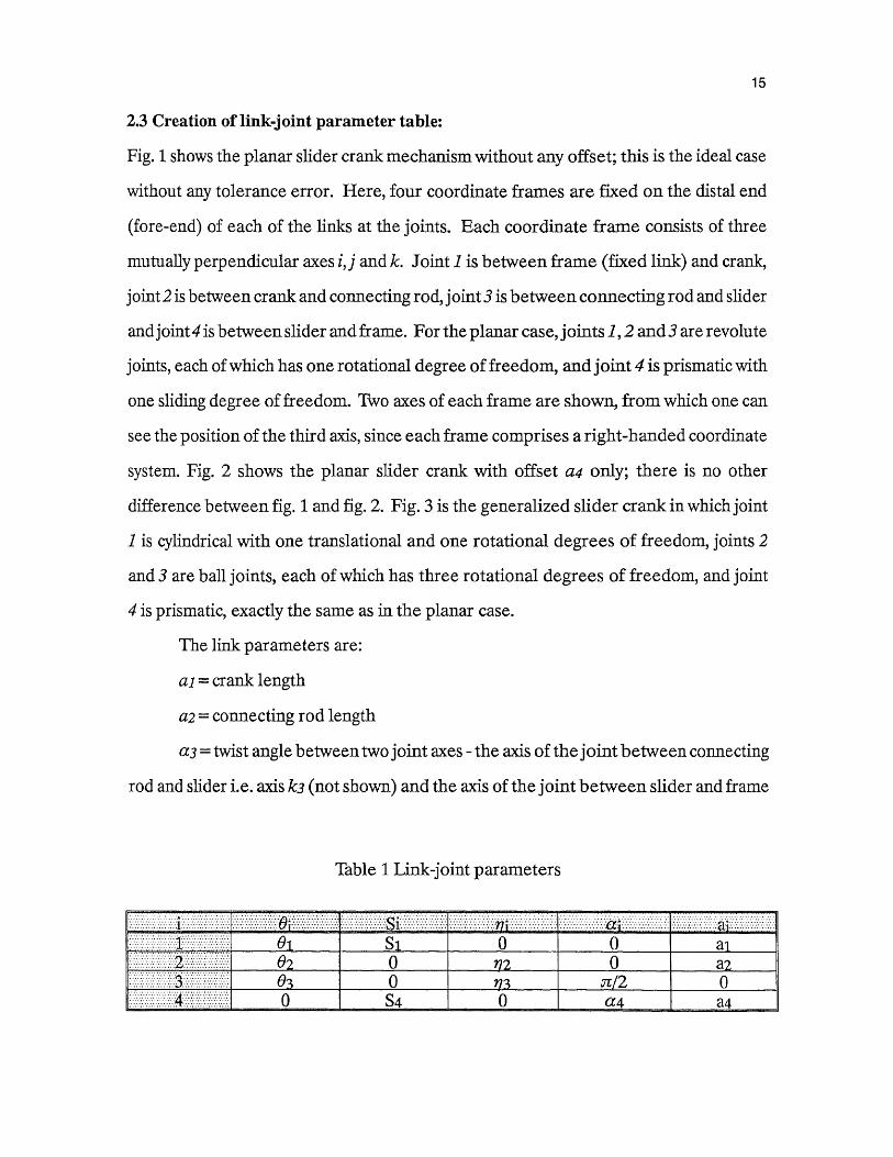
2.3 Creation of link-joint parameter table:

Fig. 1 shows the planar slider crank mechanism without any offset; this is the ideal case

without any tolerance error. Here, four coordinate frames are fixed on the distal end

(fore-end) of each of the links at the joints. Each coordinate frame consists of three

mutually perpendicular axes i, j and k. Joint 1 is between frame (fixed link) and crank,

joint 2 is between crank and connecting rod, joint 3 is between connecting rod and slider

and joint 4 is between slider and frame. For the planar case, joints 1,2 and 3 are revolute

joints, each of which has one rotational degree of freedom, and joint 4 is prismatic with

one sliding degree of freedom. Two axes of each frame are shown, from which one can

see the position of the third axis, since each frame comprises a right-handed coordinate

system. Fig. 2 shows the planar slider crank with offset a4 only; there is no other

difference between fig. 1 and fig. 2. Fig. 3 is the generalized slider crank in which joint

1 is cylindrical with one translational and one rotational degrees of freedom, joints 2

and 3 are ball joints, each of which has three rotational degrees of freedom, and joint

4 is prismatic, exactly the same as in the planar case.

The link parameters are:

al = crank length

a2= connecting rod length

a3 = twist angle between two joint axes - the axis of the joint between connecting

rod and slider i.e. axis k3 (not shown) and the axis of the joint between slider and frame

Table 1 Link-joint parameters

.. • . 1. • •

- •• 1 . .••••• • . i]:-.I: : : : • 01 Si 0 0 al

02 0 172 0 a2. ......: ..S .. . 03 0 n3 r/2 0:.:::::::::::::::::: .. 1- . 0 S4 0 a4 a4

16

i.e. axis k4; the angle is measured counterclockwise according to right-hand rule and is

equal to 90 degrees.

a4 = offset distance between two joint axes, one is the axis of the joint between

frame and crank i.e. axis ki and the another is the axis of the joint between the slider

and the frame i.e. axis k4. Axes ki and k4 are mutually perpendicular axes and the

distance a4 is measured from k4 to ki.

a4 = twist angle between two joint axes lc/ and k4; the angle is measured

counterclockwise according to right-hand rule. For the ideal(planar) slider crank this

angle is 270 degrees.

The joint variables are:

Oj, 02 and 03 = angular displacements about joint axes at joints 1, 2 and 3

respectively.

= angular displacement about the axis j2, perpendicular to the joint axis as

well as the link axis at joint 2 .

773 = angular displacement about the axis j3, perpendicular to the joint axis as

well as the link axis at joint 3 i.e. axis j3 .

SY = displacement of the crank along the axis of joint 1 i.e. axis

S4 = slider displacement which is measured about the axis k4.

The link joint parameter table is shown in table 1. This table describes the

complete geometry of the mechanism.

2.4 Transformation Matrices:

Once the coordinate systems are rigidly fixed to each link of the mechanism and the

link joint parameter table is formed, coordinate-transformation matrices are specified.

Coordinate-transformation matrices contain information about the links and the

displacements (both sliding and rotation) between coordinate frames in the form of

dual angles. The derivations of dual-number element coordinate transformation

17

matrices, describing the links connecting joints 1 and 2, 2 and 3, 3 and 4 and 4 and 1,

are as follows.

The cosine and sine will be abbreviated by c ands respectively in the remainder

of this work. The dual-number operator (3, 4), also called Clifford's screw operator, is

denoted by e (82 = 0, E# 0). The dual-number operator is used to express rotation and

displacement about the same axis in combined way. It has the following properties:

6= 0 + eS [0 and S are respectively rotation and displacement of any link about

the same axis], then trigonometric functions of dual-angle can be obtained by using

Taylor expansion. So, s(P= se + ES —d 0

(se ) ,c0‘= ce + eS d ( c0 ), etc. All identitiesde

for ordinary trigonometry hold true for dual angle.

One can trace the path from joint 1 to joint 2 by taking the rotation through

angle 0i and sliding through distance Si about and along the kl axis, followed by a link

twist angle rotation through zero degrees with a translation through the link length ai

about and along the i2 axis. Therefore, the transformation matrix, specifying the

location of coordinate frame {2} with respect to frame { 1}, can be written as

c611 –s61.1 0 1 0 02M- [ Z ) [ x( rti)]= cifii 0 0 cal –sal

0 0 1 0 sal

c01 – cS1sO1 –s01 –eSic01 0sül + eSicei c01 –eS1se1 0

0 0 1

1 0 00 cal – ealsai

0 sal + ealcal ca l – eaisai

Since 61 = 01 + ESi and ai = 0 + Ecti as there is no link twist ( al = 0 ), the above

expression can be simplified as [ In short MM is replaced by .11 .7/1 ],

–sei 0-sei c01 0 +e

0 0 1

aisei

S1c01

0 al 0 (1)

18

The path from joint 2 to joint 3 can be traced by taking a rotation through angle

02 and a translation through zero distance about and along the k2 axis (not shown),

followed by a rotation through angle 7/2 with no translation about the j2 axis, followed

by no rotation and a translation through link length a2 distance along the i3 axis.

Therefore, the derivation of the transformation matrix, specifying the location of

coordinate frame {3} with respect to frame {2}, is as follows:

Z (6/2) [ Y(C/2)] [ -74 la2)]

--ce\2 —s0.1/42 0-

= 04. 05\-s„2 c, 2 00 0 1

sij1 00 cii2

1 00 ca20 sa2

0—satca2

0 012— E.E2Sn2 o S272+ EE2C7I2

0 0 1 01 —sn2—EE2C212 0 cr12-6E2s172

c02 — ES2s02 — s02 eS2c02

s02 + eS2c02 c02—ES2s02

0

0

1 0 00 ca2 — ea2sa2 — sa2 — Ea2ca2

0 sa2 + Ea2ca2 ca2 — Ea2sa2

Since S2 = 0, E2 = 0, a2 = 0, and so 62 = 02 ES2 = 02, 7/2 = 772 + EE2 = 772 and,

a2 = a2 + ea2 = ea2. The above expression can be compressed as [ In short, IL, is

replaced by 12

CO2072 SO2— c92sn2

SO2012 c02 sO2s/2

—S272 0 072

0 a2c02sn2 a2s02

0 a2s02in2 —a2c02

0 a2c112, 0+E

(2)

The path from joint 3 to joint 4 can be traced by taking a rotation through angle

03 and a translation through zero distance about and along the k3 axis (not shown),

followed by a rotation through angle 7/3 with no translation about the j3 axis, followed

by a 90-degree rotation with no translation about the i4 axis. Therefore, the derivation

of the transformation matrix, specifying the location of coordinate frame {4} with

respect to frame {3}, is as follows:

19

Since S3= 0, E3 = 0, a3 = 0 and so θ3 = θ3 + εS3 = θ3, η3 = η3 + εE3 = η3

and α3 = α3 + εa3 = π/2 (as the link-twist angle = 90 degrees), the above expression can

be compressed as [ in short, 34L if is replaced by L3],

The path from joint 4 to joint 1 can be traced by sliding through distance S4 with

no rotation along the k4 axis, followed by a rotation through angle α4 and a translation

through distance a4 about and along the i 1 axis. Therefore, the transformation matrix,

specifying the location of coordinate frame {1} with respect to frame {4}, is written as

follows:

20

Since 64 = 0 + eS4, as there is no rotation (04 = 0 ), and i;c4 = a4 + ea4, the above

expression can be compressed as [ In short, ta is replaced by M4 ],

M4 =1 0 00 ca4 —sa4

0 sa4 ca4 +6

0 -S4Ca4 S4sa4

S4 -a4sa4 —a4ca4

0 a4ca4 —a4sa4 (4)

2.5 Partial Derivatives of the Transformation Matrices:

Noting that this problem is to be adapted to computer operation, linear operator

matrices will be introduced to perform differentiations of the transformation matrices.

Taking the partial derivatives of the transformation matrices with respect to the variable

quantity contained in the matrix is accomplished by premultiplying by an operator

matrix. The derivation of partial differential operator of each of the four transforma-

tion matrices follows.

The first transformation matrix contains only input parameters (input crank

angle and axial displacement) and crank length, which are all known quantities.

Therefore this matrix need not be differentiated.

The second transformation matrix contains two unknown variables 02 and 272.

Upon taking the partial derivative of this matrix (equation 2) with respect to variable

02 , the result is,

oft _002 -

-S02072 -CO2 -S02S712

CO2C112 -SO2 CO25772

0 0 0+

0 —a2s02sn2 a2c02

0 a2c02sn2 a2s02

0 0 0OLO2 f2

where partial differential operator QL02 can be obtained in a number of ways; the

easiest is perhaps by inspection. Hence operator QL02 can be written as follows:

O [0 —1 0-

L02 01 0 0

0 0 (2a)

The partial derivative of matrix equation (2) with respect to variable r72 is,

21

—c02s7/2 0 c02cij2 0 a2c02072 0-

—s02s712 0 s02c112 + E 0 a2s02cy2 0

—c172 0 —5772 0 —a2s7/2 0

hence partial differential operator QL772 can be written as,

6L2= OL n 2 -C2

0 0 c02

0 0 502

—c02 —502 0

The partial derivative of matrix equation (3) with respect to variable 03 is,

1;303 —

—s03C173 —SO3Sq3 c03Ce3C13 CO3S173 sO3

0 0 0= 6L 03 f3

hence the partial differential operator QL93 can be written as,

0 —1 01 0 00 0 0

The partial derivative of matrix equation (3) with respect to variable 173 is,

—0O35173 CO3073 0—503s7/3 s03013 0-a73 -s773 0

= 643 -t3

hence the partial differential operator QL773 can be written as,

642

61193

(2b)

(3a)

rdLn 3 =0 0 c03

0 0 503

—c03 —503 0 (3b)

The partial derivative of matrix equation (4) with respect to variable S4 is,

0 —ca4 sa4

1 0 00 0 0

= QMS4 M46144

S4 = E

hence the partial differential operator QMS4 can be written as,

0 —E 0QMS4 = 8 0 0

0 0 0 (4a)

22

2.6 Displacement Analysis:

The relationship between transformation matrices which describes the four links of the

mechanism and the joints connecting them is given by the Condition of Loop Closure.

Because the links are connected end to end to form a closed loop, transforming from

the frame to crank to the connecting rod to the slider brings one back to the coordinate

system fixed on the frame as if no transformation at all has occured. Hence this can

be written mathematically as:

2 iM IlM 3-L2:34"1/4

(5)which is a nonlinear matrix equation, where I is dual identity matrix

1 0 0 0 0 00 1 0 +E 0 0 00 0 1 0 0 0

[

2.6.1 Dual-number formulation of Numerical Method:

The numerical method being used to determine the displacements is based on the

algorithm (12) introduced by Hall, Root & Sandgren (1977). This algorithm is the

combination of Davidon-Fletcher-Powell optimization routine with the Newton-Raph-

son method as applied to kinematics by Uicker, Denavit and Hartenberg (1964). This

procedure was developed for the use with 4 x 4 homogeneous transformation matrices,

and was adopted to 3 x3 dual-number matrices by Fischer and Paul(1988). Details of

the Newton-Raphson method are as follows.

A first order expansion of the loop closure equation is

[ [ L2 + QL0 L2 6°2 QL77 L2 612 { L3 + QL0 L3 (5e3 QL, L3 6113

[ M4 + Qms metos4] = (7)where 02,172, 03, 173 and S4 are guesses of displacement variables; 662, ow, 66+3, 6/3 and

OS4 are errors between guesses and exact values of the displacement variables; QLO,

QLn and QMS are partial differential operators such that (as shown before)

I =(6)

23

0 —1 0-

1 0 00 0 0 (8)

0 0 ce0 0 sO

—c0 —s0 0 (9)

-o E 0

QMS = 0 00 0 0 (10)

Expanding equation (7), and putting it into a form which is computationally

advantageous, the following equation is obtained. Performance of the multiplication

yields a very lengthy equation. However, keeping with the idea of the iteration process,

all higher order terms of the form (602603, etc) are neglected.

H2602+11' 26712+H3603+H' 343 +H' ' 4„A c," 4 = 1,?T' -A

where

_ A A-TH2 = M1Q Lem (12)

H'2 = M1QuiM1 (13)7,

H3 = WiL2V.LoWiL2) - (14)

H' 3 = 4 -1-L2)Q L?"-L2) T(15)

H"4 (M1L2L3)Qms (MiL2L3) (16)

In general,

Hi = (TIT2 Ti—DQx(TiT2 T

(17)

and

B = M1L2L3M4 (18)

Equation (11) is condensed to

Q.Lo =

QL71

F = B —I (19)

F21 F22 F23

F31 F32 F33

B12 B22- 1 B32

B13 B23 - 1 (19a)

24

Equations (11) through (19) are all 3 x3 dual-number matrix equations. So this

equation can be written in a matrix form as follows:

F11 F12 F13 Bil - 1 B21 B31 1

where

F11 = H2,11 6°2 + 117 2,11 ön2 H3,11603 H'3,11 6/3 + H' '4,11 6 '54

F12 = H2,12 6°2 4- H'2,12 6112+ H3,12603 111 3,12 613 + 4,12 664

F13 = H2,13 602 + H1 2,13 (3172 + H3,13603 + H'3,13 6/3 + -H7 ' 4,13 6614

F21 = H2,21 6°2 + 1:11 2,21 6772 + 1/3,21603 1/13,21 67/3 1/"4,21 os4

F22 = H2,22 6°2 + H'2,22 a1i 2 + H3,22603 + If 3,22 6173 + 11"4,22 66'4" " " " " "F23 7---- H2,23 602 + H'2,23 6272 + B-3 ,23(303 + H'3,23 677-,•) + HH 4,23 6 '54

F31 = H2,31 6°2 4- H7 2,31 67/2 + H3,3103 + 1/73,31 on3+ 11"4,31 6s4

F32 = H2,32 602 + H1 2,32 6172+ H3,32603 + H'3,32 6773 H"4,32 6'54

F33 = H2,33 602 H'2,33 42 + H3,33603 + .H73 ,33 43 + HH 4,33 6S4 (19b)

So from equation (19a) nine dual equations can be written from this matrix

equation, out of which only three are independent. Using the three terms in the upper

triangle of each matrix and separating them into a set of real equations and a set of dual

equations:

Fp12=Bp21Fp i3 =Bp3iFp23--Bp32 (20)

and

25

where the symbols p and d represent primary and dual components respectively.

Equation set (20) does not include the constraint that the each diagonal element must

be equal to unity at closure. This constraint is included through modification of the

current set of equations as discussed in Sandor and Erdman (1984). So, this set can be

modified as,

Figure 4 Planar slider crank when crank angle is zero

26

The left-hand sides of equations (21) & (22) contain the linear combination of

respective elements of the H matrices and the error terms are contained in the left hand

side of equation (11). Hence, combining equations (21) & (22) as partitions of a single

matrix of real-number equations, the resulting equation is

where

and

Rearranging equation (23) to solve for the error terms, the Newton-Raphson

iteration technique can be achieved. But the matrixA, which is 6 x5, cannot be inverted

in usual method in order to do so, unless manipulations are performed as follows.

27

Hence the modified form of equation (23) is as follows:

A (A TA) -1ATv (23a)

which is exactly same as A = A —1V.

The guesses of displacement variables are revised by adding the error terms, A,

to the guesses and the new set of joint variables is used in the next iteration to compute

a new set of error terms. The iterative process is continued until the absolute values

of all error terms are less than or equal to the desired accuracy limits. At this point the

displacements are determined only for the first position of the input link. To solve for

the displacements for a new position of the input link displacement, angle 0/ is

increased by a small amount and the previously calculated displacements are used as

initial estimates for the next position. This process is continued for a complete rotation

of the input link, the crank.

Another input variable, i.e. length Si, the axial displacement of the crank, can

be introduced in two following ways:

(1) it is constant throughout the complete rotation of the crank, i.e. the crank is

axially displaced to a certain distance and is then rotated.

(2) the crank is constantly moving to and fro in simple harmonic motion along

its own joint axis (the joint connecting the frame and the crank, i.e. joint 1). A new

parameter a is introduced which can mathematically be defined as follows:

a — number of cycles the crank slides through along its own joint axis number of complete rotations of the crank

Hence relating the axial displacement of the crank to the rotation, translation

Si can be written as

S i = Ssisin(aOi) (28)

where symbol Ss/ is the amplitude of the sliding cyclic motion of the crank.

(27)

28

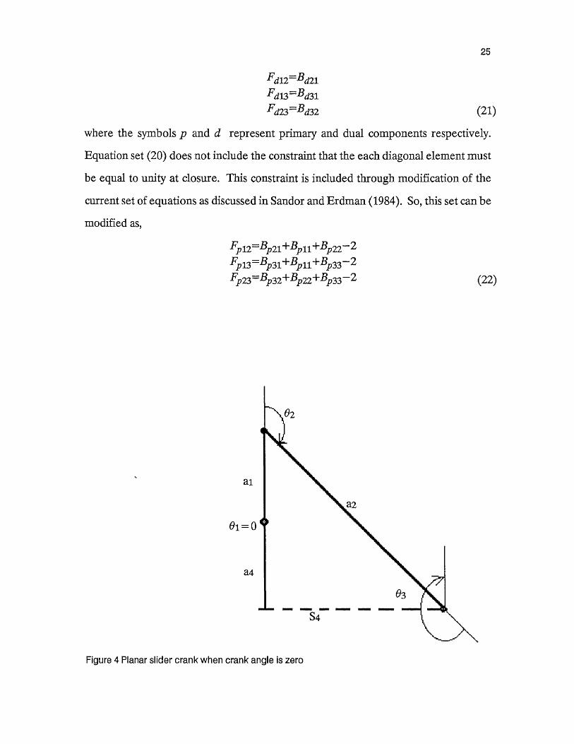
2.6.2 Plane Geometry Method for Initial Estimations of the Joint Variables:

Initial estimations of the joint variables 02, ?72, 03, 173, S4 have been done by following

simple plane geometry method. Fig. 4 shows planar slider crank with offset a4 only

when input crank angle is zero. From geometry the following formulas for the joint

variables can be written.

2 2 1S4 = [ a2 —( a1+a4 ) ]

02 = — tan-1iS+4[ aa14

03 27r — 62

712 = 0 and 773 = 0

2.7 Velocity Analysis:

The dual velocity of link 1 (i.e., the crank) relative to link 4 (i.e., the frame) with respect

to point 1 in terms of the unit vectors of system {/ } is represented by the vector

11 ,1V 14 —

(29)

where symbols eh and 1 denote the rotational and translational velocities about kJ_ axis

at joint 1 respectively. There is no other velocity about the other two axes at this joint.

Similarly the vector equations for other links can be written as

2T72V21 =

(30)

where symbols in and 02 denote rotational velocities about the j2 and k2 axes at joint 2

respectively.

3 V3V 32 =

0

X13(93 (31)

29

where symbols 7.13 and 03 denote rotational velocities about the j3 and k3 axes at joint 3

respectively.

04v4

v 43 — 0

(32)

where symbol S4 denotes actually the slider velocity about the k4 axis.

The dual velocity of point 2 on the crank relative to the frame in terms of the

unit vectors of system {2}, i.e. 2Vi4 , can be derived by premultiplying equation (29)

by the transpose of equation (1):

2V2 2 7i ,r 1v1v 14 = r 14

c01 —ES1sO1 se1+ES1091 0c01 —ES1sO1 Ea

eaisei 1

0ea101

(33)

The dual velocity of point 2 on the connecting rod relative to the frame in terms

of the unit vectors of the system {2} is determined by adding the equations (33) and

(30):

02T72

v 24 = 21-72v 14 ' 2172

v 21 = EaAel+ di

011262 (34)

The dual velocity of point 3 on the connecting rod relative to the frame in terms

of the unit vectors of the system {3} is determined by using this equation and the

transpose of equation (2):

3T73 3 2T72v 24 = v 24 ( 31= (i4T

CO2072 S02072 —Sn2 0—s02+ea2c02s772 c02+6a2s02s772 ta2o72 1712+ EOlai

e1-1-192-1-81}c91772+Ea2s02 s92s12—Ea2c02 072

1+ 2)s712+ ihs° 2012+ e(I9 iaise 2012— S

2c0 2+ 8 [0 i(aice 2+ a2c7 + 2a207 2+ 2a2s0 2sn

(O1+b2)072 -Eihs°2s/72±E(O1a1s92sn2— i12a2c02+Sfic172)

The matrix equation for dual velocity of point 3 on the connecting rod relative

to the frame in terms of unit vector of system {3} can also be formulated by using the

backward path of the loop. The procedure is as follows:

From equations (31) and (32) respectively,

031-73

V2323 = — v 32 —

(3 la)

4T74 4174v 34 — V43 —

(32a)

3/73 3 T 4v4 3v3v 24 = 4J-' 34 ' 23

30

(35)

00

c03013 ce3s273 s03 -s03cr13 s03sn3 —c03

—sn3 Cn3 0

—6'4903

—1.73+ 84c03

—03

0 0+ _ 413

—a (36)

[ This has been obtained using equations (3), (31a) and (32a)]

Equating the two expressions (35) & (36) yields

—(01+02)sn2+ii2s02c772+E(91aiS02012— S'1S712)

i72CO2+ 8[0 i(ctic0 2+ a2c712) +62a2c172+/72a2s02s772]

(0 1 + 0 2)cri 2+ i7 2s0 2sn 2+ e (0 lais0 2s77 2— i ha2c0 2+ ' 19272)

— 8 S 4S03

4c0 3

—03 (37)

This matrix equation actually contains six linear equations ( 3 primary and 3

dual) with five unknowns. The next step is to rewrite equation (37) as a system of linear

equations as follows:

(61+192)D72+172s02072 = 0 (37a)

61a1s02c172— SIR/2 = — 003

ii2c02= -473

81 (a1c02+a2c772)+02a2c772+iha2s02s12 = 4c03

01+62)012+i12se2s112= —03

61cl1s02s112 — i12a2c62+ S 1072 = 0

31

(37b)

(37c)

(37d)

(37e)

(37f)

Now separating the unknowns to form a column matrix and a coefficient matrix,

the product of these two matrices must be equal to some column matrix as shown below:

—si12 0 sO2c172 0 0

0 0 0 0 s03

0 0 c021 0a2c772 0 a2s02sr12 0 —c03

072 1 sO2sn2 0 0

0 0 —a2c02 0 0

615112—Olais02c12+Sfisii2

0—1+ 1 (a1092+ a2c772)

—019772

(.91aiser-S'ic172 (38)

The coefficient matrix is 6 x 5 and the column matrix of the unknowns is 5 x 1,

therefore it is a system of six equations with five unknowns. Since rank of the coefficient

matrix equals 5, the number of columns, a unique solution can be obtained. The final

solutions for all the unknowns are as follows:

6)2, =SiCO3Sn2C112—ai(01§02c03+t)ic02.03072) —aAs03

a2s03

. a 1(61c02s034-61s02c03c712)—Sic03sn203 — a2s03

112 = a2s02s03

cO2s772[61a1(s02c03c272+c02s03)--;s1sn2c63]773 = a2s02s03

—sq2[a1(O1c 0203 + is02c03012) Slis772c 03]

(39)

(40)

(41)

(42)

S'1sn2-61a1s02c772

Sf4 = SO3 (43)

32

All these equations involve the sliding velocity of the crank along its own joint

axis (the joint connecting frame and crank, i.e. joint 1), which is given by either

=0 [ when S1 = constant ]

or

aSsicos(a6901 [ when S1 is sinusoidal]

(28a)

[ equation (28a) is obtained by differentiating equation (28) with respect to time when

Si is variable ]

For dynamic analysis, equations (33) and (35) which respectively formulate the

dual velocities of point 2 on the crank relative to the stationary frame in terms of the

unit vectors of the system {2} and of point 3 on the connecting rod relative to the

stationary frame in terms of the unit vectors of the system {3}, will be used. In addition

to that, the dual velocity of point 4 on the slider relative frame in terms of the unit

vectors of the system {4}, i.e. 4V-4 ,is also needed. The derivation of that velocity

vector is obtained by adding equations (31) & (35)

3-1-73 3 1-73 i_3 /z3V 34 = r 24 ' r 32

(44)

using equations (3) & (44) 4144 = ;L 3V34

i12s02072— (el+ 62)sn2+ E(biaise2c772— Sgisii2)

2C612+ 3 + EV9 lc 1092+ ii2a2s 2s212+ (01+ 62)a2c1121

}

(614-62)cq24-ii2s02.9172+ 63 + E (Sficrh+a iPis02s7/2—ii2a2c02)

33

c03cy3(rj25.02o72— 62)s172)+s03o730.72c02+1)3)7sn3((01+ 02)02+)72502sy2+03)+8[c03cy3(01ais02q2— ks172)+s0303(01.aic02+ina2s02sy2+

(01+ 02)a2p72)—s13(S ion+ a101s025,12— ina2c02)]

c63s71302502a72— (01+ 62)s172) +s03s13(172c02+ ii3)+ 03((01+ 62)072+ins02s172+03)+E[CO3M3(01a1S642072 — S'IS712)+s03s173(01aic02+7.72a2s02m2+

(01+ 02)a2cn2)+ cii3(&102+ a1O1s72302 — ina2092)]

S0302S'02012 — 01+ 62)SW) CO302CO2+ i]3) -F E[S03(elalS0202 — Sf15112)— c03(01aic02+ ina2s02512+ (01+ 02)a2c272)1

2.8 Dynamic Force and Torque Analysis:

STEP (1) Formulation of inertia binors:

Assumhig that the links are symmetrical about their respective lengths, the location of

centers of mass of link 1 in terms of frame {2}, of link 2 in terms of frame {3} and of

link 3 in terms of {4} can be represented by the vector forms as follows:

g12 -*Gi = 0 3,71-* g2

= 1.0 4-*G3 = 0

0 0 0

where symbols g1, g2 and g3 are respectively the distances along the lengths of links 1,

2 and 3 from their distal joints to their centers of mass. If symbols mi, m2 and m3

represent their respective masses, then the inertia matrices of link 1 in terms of frame

{2}, of link 2 in terms of frame {3}, of link 3 in terms of frame {4} can be written as

[2 rix...) = m1

00 00 0 —g10 gi 0

352] = m2[00 00 0 —g2

0 g2 01/1

00 0

0 0 — g3

0 g3 0

(45)

Assuming that the principal axes of each link are oriented the same as the frame

fixed upon it, the mass moments of inertia for each link can be written as

34

r2 j1 m1Ky o 0

0 Kiy 0

0 0 KZ

[3 1 = m24 0 0

0 K2 02Y0 0

L4 J3]J3] = m3

Kix 0 0

0 4 00 0 Kiz

where symbols Kax, Kay and Kaz represent the radii of gyration of link a in terms of frame

{a+ 1} fixed on that link (a = 1, 2 and 3).

The general form of the inertia binor of link a in terms of frame {B} is written

as

[B s ai Tma[1]

[Bcoai[BJaII T I rsa]

This is a 6 x 6 matrix where symbol ma is the mass of link a, [BJa] is the mass moment

of inertia as described above and [1] is identity matrix,

I

1 0 00 1 00 0 1

and matrix [BSa] is the first moment of mass matrix of link 'a' in terms of frame {B},

which can be generalized as

[BSa] = ma

0 —gz gy

gz 0 —gx_gy gx

Therefore the inertia binors of link 1 in terms of frame {2}, of link 2 in terms of

frame {3}, of link 3 in terms of frame {4} can be formulated as follows:

35

0 0 010 0 g1 I0 —g1 0

1 0 00 1 0

0 0 1r2

9°11 = M1

0 0 00 00 4 0 0 0 —g10 0 4 0 g1 0

0 0 0 1 0 0

0 0 g2 0 1 0

0 —g2 0 0 0 1

[39°2] m2 •••••••••.r......■

Kix 0 0 I 0 0 00 K 0 I 0 0 —g20 0 0 g2 0

0 0 0 1 0 00 0 g3 0 1 00 —g3 0 I 0 0 1

[403] = m3

K 0 0 I 0 0 0

0 4 0 I 0 0 —g3

0 0 .K3z I 0 g3 0

STEP (2) Formulation of dual momentum vectors:

In this step, some of the velocity vector equations are used to formulate the

momenta of the moving links. In order to do that we can either use the velocity

equations formulated through the forward path only or some velocity equation ob-

tained through the backward path and some through the forward path. In either case,

(46)

(47)

(48)

36

the same numerical results are obtained, but mixed path equations set is much simpler

than only the forward path equations set.

First the forward path equations are used to formulate the momenta. Equations

(33), (35) and (45) can respectively be written in the form of 6 x 1 column matrices by

separating primary and dual components as shown below (equations (33), (35) and (45)

are obtained from the forward path only):

Vixp

Viyp

Vixd

Vlyd

2;2v 14 0

a101

Vizd (33a)

3;3V2424

V2yp

V2zp

V2xd

V2yd

V2zd

2s° 2072 — (6' 1+ e)2)si 2ii2c02

(01+ (92)012±ii2s°2912eha is02c772—S'is112

°1a1c°2+i12a2Se23/12+ (B'1 + 92)a2c712S'ic772-1-aiOisO2s172—ii2a2c02 (35a)

CO3c/3[17202072—(01+02)sn2]+s03073(i12c02+i73)—s13[(01+02)072+i7Zse2s172-1- 613]

ce3s13 [ii2s02cn2 (01 + 62)s12] +s039773 (172092+i73)

+073[(01+02)c12+i72s02m2+ 03]

s03[ii2s02cr7 h h2 — (- 1±-2)s172] — c030.72c02+173)

c03cr73(01a1s02c12—&1si12)+s03o73[ai 01c02-Ea2ihs02s272

+ (01 + 02)a2c172]— a181s82s12— a2ii2c02)

c03s713(a101s02o72—Sf1sii2)+s03sn3[a101c02+a2i72s025172

+(01+02)a2c172]+cri3 (S'ioi2+apis02s172—a2i72c02)

s03(ale1s02c12-4172)--. c03[41092+a217202sn2

+ (01 + 02)aph]

V.3x.p

v3yp44;4 _ V3zp

34 — yaw

V3yd

V3zd

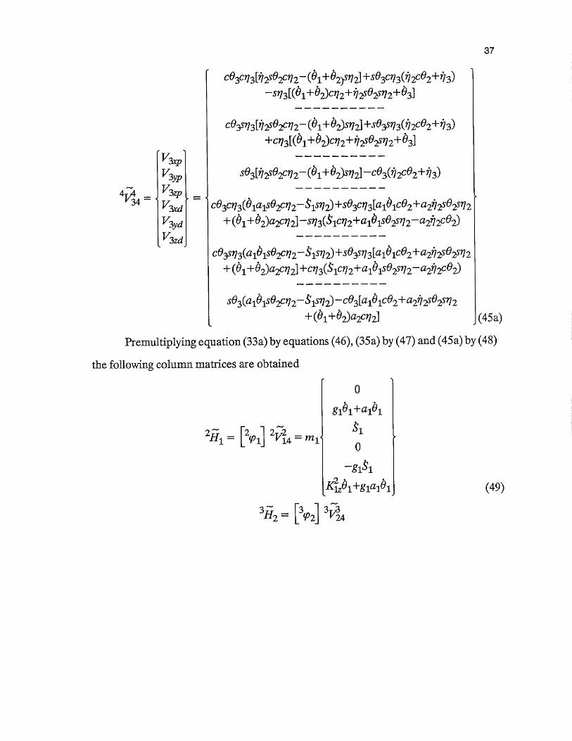
37

(45 a)

Premultiplying equation (33a) by equations (46), (35a) by (47) and (45a) by (48)

the following column matrices are obtained

0

[2 4,,, 7-2-I-4 1 = 1 14 = 1

0

—g1S'1+giai(9 (49)

81ctisO2o72—Sv1sw

g2(6.+02)cq2+g2572s02s1724-Olaic02+ina2s02sn2+(61+O2)6/2072

—g2ince2 + :Sicn2 + a101s02sn 2 — ina2c02

Kixii2S02Ct/2 —K2x(61+62)Sn2

Ki3112CO2 —g2Sq1C/72 —g2a101s02s772+g21i2a2c02

Kiz(01+02)cii2+Kizips02s272+g2haic02+g2ipa2s02s712+g2(O1+02)a2c7/2 J (50)

4113 = [4c03] 4-r7,314

c03o73(a1Ois92o72—S'1sn2)+s03o73[cn61c02+a2ps02sn2

+(O1+02)a2cro]—s173(1012+a101se2sw—a2i72c02)

g3[S03[1.72S02012— (01+02*2] —c03(1)2c02+173)]+CO35173

(a101S02012 — :515112)+S03.5113[a101CO2+a2112S025112+

(01+ e2)C1207 2] +073011C7/2±a101S026112 — a2i12CO2)

—g3 [c0357/3 2.02c1) 2 — (01+ 02)sn2] +s03s113 (1)2c02 + 7)3) +ci73[(01+ 02)072+ ips025772+ 63]] +s03(a101502012 — , 11s112)

—c03[(2101c02+a2i2sO2sn2+(61+O2)a2072]

Ki[CO3073 [12s02c712— (01+ .02)s172] +s03073 (ii2c02+ 2.73)—s73[(O1+O2)072+172s025772+O3]i

Kiy [ce3sy3[272s02c272—(01+02)3172]+s03s773(112c02+173)+

073[(O1+t92)cra+i]2s02s712+ (93]] —g3[s03(a101s02o72 — :S1s12)

—c03[a1e1c02+a2i7202s712+(61+02)a2072]]

38

(51)

Kiz[se3[17202o72—(61+02)s? 2]—c03(1)2c02+i13)]+

g3[c03s713(a161s02072—S1s772)+se3sn3[a101c02+a2i2se2sn2+

(191+ 02)a2072] +073(Sc1on+a10u025/72—a2i12c02)]

39

Formulations for the dual momentum of link 1, i.e. the crank in terms of frame

{2}, of link 2, i.e. the connecting rod, in terms frame {3} and of link 3, i.e. the slider, in

terms of frame {4}, can respectively be obtained by modifying equations (49), (50) and

(51) to 3 x 1 dual-number matrix equations as shown belowIN.

110x

Hiz

Hup + EHixd 0Hiyp + eiljyd _ m1 61(a1 +g1)--eg13 1Ilizp + E.Hizd

S'i+E(Kizei±giaiPi) (49a)

H,N2x Hap + ETI2xd3 Tj-'-

A-L2 = 11,-,2y = H2yp + CH2yd

H2z H2zp + 811.2zd

alO1sO2cr7 2 — S'151/ 2 ± E[Kix172502C7/ 2 — idx(01 + 02).57/2]

[(g2o72+a2c/72)(01+ 02)+ (g2+ a2)(ii2s02s)2)+ 01(21092]

E[(Kiy + g2a2)/7 2c 0 2 — g2S ic? g 2a hse hstn]

IS'1072+a181s92.sin—(a2+g2)inc02]+e[(K 012 -Fg2c12c712)(61+ 62)+ -1-g2a2Y/202M2-1- aig2P10921

m2

(50a)

4Lr' \.1.13 = Hay

H3z

Hip H d

H3yp CH3yd

H3zp

CO3073(C1101S02012,— SIS112) +s03013[a181c02+a2ips02s712+ (61+62)

a2c172] —s7/3(:51072+a161se2sra —a2n2c02)+E[Kix[CO3013[1.121020]2 —

(61+02)37121 -FS03013(112CO2+2.73) —S11301+62)012+1725'02s72+031]]

g3[s03[2.72s02072— (61+ e2),M2,] — c03(inc02+ + [ce3713(alfhs02012— :Sisn +seyn 3 [ai6ic02+ a2ips02m2+ (O1+62)a2c172]+ c03(:Sio1J2

+aiehs02s772—a2inc02)]+E{Kiy[CO35113[12S020/2— (61+62)5112]

+s6135773(i2c02+i73)+013[(01+02)012+i2S025112+63]] —g3[s03

(a161se2c772—SID72)—c03[a161c02+a2i72302s712+ (01+ 62)a20/ 2]1]

—g3[CO35713[rj2,S02012— (01 + k)S112]+S031113(i12CO2+1.13)+ 013

[(e1+ 02)012+2712S025712+03]]+[s03(a101S02012, — :S15172) — 0O3[a161ce2

+ a2,i72,902577 2 + (01+ th)a2cr] 2] 1 +E[Kiz[Se3[21202012 — (61+ 6'2)sn2]—c03(172c02+i/3)] -Fg3[c035773(a161s02c772 — Slisn2) +s935773[a161c02+

a27.72s02s172+ (61+ 62)a2012] + 073(S10/ 2 + aleise2sin—a2ince2)]] (51a)

Dual momentum equations (49a), (50a) and (51a) are purely forward path

equations, since all the velocity equations ( 33a, 35a and 45a) used to derive these

equations are forward path velocity equations. Out of these three momentum equa-

tions, two equations (50a) and (51a) are very large consisting of many sine and cosine

functions and their derivatives, which may cause inaccurate results. In order to have

more concise equations and better accuracy, two backward path velocity equations are

used to derive two momentum equations as the alternative to equations (50a) and (51a).

Now, the backward path velocity equations (36) and (32a) can be written in the

form of 6x 1 column matrices by the same method as before, and going through exactly

the same procedure, simpler and concise equations are obtained which can be used as

replacements for the above-mentioned large equations.

1713

40

41

V2-173v2yp

= T7V2zp31.7

'1 234

2xd

V2yd

V2zd

vim,

v3yp

4v4 V3zpr 34 — V3rd

V3yd

V3zd

0

-03—&003

S44CO30 (36a)

0

(32b)

Premultiplying equation (36a) by equation (47) and (32b) by (48) the following

column matrices are obtained.

3 T_T— 3,„ 3;32 — L y-2 j 24 —

—S003—g2 03 S'4c03

g2 7)3

0

— 3—4 03 + g2S4c03 (52)

4fi3 [ 41)31 4 E7434 = m3

00

0

g3&40

(53)

Now, alternative expressions for (50a) and (51a) using the backward path are

respectively

{

— :S4s03

= m2 (--g2e)3 + :54c03) — 84:03g3i73 + e(g2:S4c03 — K3)3)

{ H2xp + e H2xd

= H2yp + EH2y d

H2zp + EH2zd (52a)

Hix •EHixd

2,-n 1 — r_rA A lyI H Ayp i- EH:1yd •• =

H up+ EH izd 1 + EHiz

0

gia 1.)(54)

H2xp + eH2xd

H. 2yp E H 2y dH2zp + EH2zd

42

4 /.\H3 = 1-43x

-11,3yH3z

Harp + eH d

H3yp + EH3yd

H3zp EH3zd

0

Eg3S4 (53a)

In the next steps and in the computer program either equations set { (33 a), (35a),

(45a), (49a), (50a) and (51a) } or set { (33a), (36a), (32b), (49a), (52a) and (53a) } can

be used. The first set consists of purely forward path equations and the second set

consists of mixed path equations; equations (33a) and (49a) are forward path equations

and rest of the equations in the second set are backward path equations. Both the sets

were tested by the program for a number of cases and resulted in same outcome. Finally

the second set is used in the program to have better accuracy.

STEP (3) Time derivatives of dual momentum Equations:

Differentiating forward path equations (49a), (50a) and (51a) with respect to

time the following equations are obtained respectively:

rH

2x

31-1 \ 2 = Hi\ 2y

2z

alOis02072+ail4IP2c02c112— ai.1912.12s°2s112-31s12 :91/12012+ e[Kijii2S612C112+ 1.1262C°2C712-ib°25112)-4(1+62)sj2

x(61 + 62Y/120121

[( —g2i723272—a2ii2s172)(61+62)+ ($2012+ a20/2) (61 ± 62) (g2 Ea2)02s02s7/ 2+17262c02s7/2+ibt92cn2) +a161c02 — ail9102s02.1 +

m2 8 [ +g2a2)(1i2c°2— i1202s02) —g2(31 712— :517.12s712)

g2a i(elis02s7/2+ 0102c0211/ 2+ 01i72s02012)]

[31cn 2 &ii/2s7/ 2 + ai(Ois02s7/ 2+ 616°2092s/ 2 + 1)11.72s02012)

— (a2+g2)0712092— i7262s02)1+ e[(-4z1712s712—g2a2i72s112)(01+ 02) +

Acil 2 +g2a2c/2) (el + 62) ± (-1C3z +g2a2) (5i2s02s17 2 + 1.7264202sn 2+ibt92072) + a ig2(61c02- 2s02)]

43

(55)

H3x

•4fi-

3 = H3y

H3z

where

1-13xp+eliaxd= FT FT3yp +E 3y d

H3zp +E-113zd

(56)

liayp 7m3[( — bas'03c713 -413c03913)(ailais02012—:Sis272)+c03o73(aiOis92072+api02c02072—ai6Y72s612s712-31s212—S1112012)+ (03c03o73 — ii3s03sn 3)

[a161c62+ a2i72,s02sri2+ (0 1+02)a2c172]+s03a13[aiOic02— a 10102s02

+a2F12s023772+a2i7Ac82s712+a2402o72—(i91+1)2)a2i12sn2+(e1+62)a2072]

—173073(&1012+aiOise23112 — a2.12092) —s213(Sic7/2-31/12912+apisO2s7/2+a10102c02sn2+ai0iii2s02c772—a2ij2c02+ai0-i- 232 L °2)] (56a)

/13xd ni3[44( —1)303013 ii3c03s7/3M2s 02a/ 2 (0142)3172] +693a/ Aii2s02c772

+ 11202c02012-402s112 — 01+02Y/2012— (61+ 62* 21 + 03ce3c113il3s°3,5113) (11202+ i13) +s°3073W2c°2 2e2s°2+

—1130/3[(014-02)072+112s021772+ 031 —sn3[(01+ 02)072

(61 02)17257/2+;i2s82s712+i72°2092s/72± 1.72s02072+ 63] (56b)

H3yp = M3 rg3 [63C°3 [112S02C/ 2 (19 1 ± 192)311 "4- '5°3 2s0201 2 4- il2P2C°2C12

--i12

.9925172 — ( 1+62)512-11201 2(61+e2)1 +63s03(1?2c02+ ii3) — c03

0202 412° 2s° 2+ )3)i -F' [(11 3013c0 3— 63seas713) (aAs0 20 7 :9 is712)+ cOas13(a16 1s0 2072+ ale 10 20 9 207 2— a piii202sn273is12—Siii2072)+(o3co3973+ii3s03cri3)[aiOic02+a2ihs02s172+(01+02)a2c272]+s03sn3

[aiOic02—a16162s02+aA2s02912+a2i7202c02sT12+a2ilis°2c 712+

(61+ 2)a2c12— (0 1+ 0 Da2ii 2si 2] —173s713(S' lc?? 2+ ai0 is0 2 -- a2 2c0) +

cn 3(S 1012— SV121112+a10102c02sn2+ai0iii2s02q2+apis02s172

--a2j2092±a2e2f12s02)]]

44

(56c)

H3yd M3 [4[0 30 9 30 350 3S11

25° 2°1 (i9 1+ 2)S7 2] ± 3S11 3[3i 2S e 2Cr1 2+ il 26 2C° 2°1 e 2S 1 2(6 1 + (42)sn2 — 01+02)1720721+ (63c035773 + ilaSe3C/73) (112CO2 + 3) +SeaS113(i)3+ )2Ce2 —1126)23°2) +073[(61+ 62)072— 01+ 642)7.72S7/ 2

ii25°25172+ ii2192Ce2S/ 2+692072 + 6/3] "13377301+ e2)072+ 202,57/ 2+ 6311— g3[s0 3[a it9ie 2c0 2cn 2+ aiO is0 2c7 2— aiO 2s0 2— 3 isn2— SV1207

+ 03c03(a is02cn 2 — S'iS172) 3.St93 [a 16 lc° 2+ a2,112s0 2sn 2 4- 01+ 2)a2c17— c03[4 02 — ai61.0 2s0 2+ a2ij 2s0 2+ a2 262c0 2s, 2+

a2i722502o72+ (61 + 02)a2012. i92)a2i725112]]] (56d)

ii3zp = M3 [ —g3[(ii3c03c173 — 63s0 3317 3)[ii 2s0 207 2— (t) 1+ 2)sn 2] + c0 asil 3 25192°12 +

112°2Ce2C17 2 iiiS°2S 2/2 (81+ 62)i/20h— (81+ 62)51721 + (O3C°3-57/3 + 1.703013)

(ii2C°2+i13) +,03.57/30i2CO2—ii223°21-ii3) +07301+ 62)072— 01+ oDi/2.5172

+i12se2s772+i7202c0257/2+602072+031-47395773[(e1+e2)072+i12s02s7/2-1- 6311+163c03(aiOis 02072— S'is12)+s03(aAse2,012+ai°162c°2012

— cliPiiI2s°2s712-41s12— 'Y'12072) +_ 3s03[aibic02+a2i7 2s02s772+

(1)1+62)a2c772] — C 03 [a16 ice 2— alPiP2s02 + a2,ij 2s02sn 2 + a27.72(92c02sli 2 + a2/72is0207 2 +

(el + 62)a2C/12 — + 192)c/2112M i] (56e)

45

H3zd M3[4{03CO3{ii2S02072 — (111+02)S121+

se3N2S02072+ 1.7262c02C12-6°2s127 (01+02),5772 —(01+°2Y120721+°3s°302692+i/3)-0302c02--. ii2e2s02+ii3)]+g3[(173c03c/3 —

03s03D73)(aiOis02012— :515112)+cOas113(aPis02c112+a10102c02072—

aPiii2s02s172—Sisn2—S)Liip72)+(03c035713+ii3s03a73)[aiOic02+a2 72s02s712+

(01+02)a2cy12]+s03sh[a101c02—a10102s02+a2r125025712+

a21)33"'02072+a21)2P2c02sn2+(01+02)a2072—(61+ 62)a2ihsn21 —

i73s/3(S'icn2+aiOist92s7/2 —ail2c02)±013(319772 — SV/2s/72+aidis02s772+a10102c02s12 +aiOlihs02072—aiii2c02+a2/7202s02)]] (56f)

Now, backward path equations (52a) and (53a) are differentiated with respect

to time. The following equations are replacements for equations (55) and (56) respec-

tively.

H2xp+e11thH2yp+EH2yd

H2zp + EH2zd

—3003-34c0303

(34c03 —S4s0303 —g263) — (6403

g2273 + s(g23403 — g2S4s0303 — 463 ) (57)

•H.3rp +8H3rd

FT3yp +E 3y d

EH3zd{ 0= m3 Eg334

---- S4H3z (58)

In the program either forward path equations set { (54), (55) and (56) } or mixed

path equations set { (54), (57) and (58) } can be used. To have better results the second

set is used.

46

STEP (4) Formulation of the Dual-Euler equations:

In this step, equations for the inertia forces of link 1 (i.e. the crank) relative to

frame {2}, for link 2 (i.e. the connecting rod) relative to frame {3} and for link 3 (i.e.

the slider) relative to frame {4} are derived. The derivations are shown as follows:

Htv + ViyHiz

2 y

Expanding both sides,

(Hilp — VIzpHlyp -I- VlypHlzp)+ e(HIxd— VIzpHlyd— VIzdHlyp+VlypHlzd+VlydHlzp)

flap+ EfIxdflyp+ efiydfizp+efizd

(Thyp—VixpHizp +Vizpillxp)± E(Hlyd— VixpHlzd — VIxdfilzp+

VI2pHlxd+V1zdflIAP)

(Hizp—ViypHixp+VhpHiyp)+eWizd—ViypHixd—ViydHlip+Vixpnlyd+VIxdiflyp)

H2x—V2/12y+V2/12z

3 J2 = "2y — V2xH2z + V2zH2x

H2z — V2yH2x -FV2/12y

(59)

Expanding both sides,

(1/2xp — V2zpH2yp + V2ypH2zp)+ e(Had— V2zpH2yd — V2zdthyp+V2ypH2zd -1-. V2ydH2zp)

{f2xp+Ef2xdf2yp+ef2ydf2zp + Ef2zd

(Thyp — V2xpH2zp -FV2zpH2xp)+E(Thyd— V2rpH2zd—V2xdH2zp+V2zp112xd+V2zdil2xp)

(H2zp—V2ypH2xp-I-V2xpR2yp)+ E(H2zd— V2ypH2xd — V2ydH2xpV2apH2yd+V2xdH2yp) (60)

H3x— V3z11-3y -FV3y113z

y VITH3z V3zil3x

H3z — V3),H3x4-V3r1I3y

Expanding both sides,

(H3xp — V3zpH3yp -i-V3ypH3zp) E(Thxd— V3zpH3yd — V3zdff3yp+V3ypH3zd+V3ydif3zp)

47

4" =

(61)

(62)

(63)

(64)

falp+Efaxdf3yp+Ef3ydf3zp+Ef3zd

(Thyp — V3xpH3zp+ V3zpH3xp)± E(Thyd— V3xpH3zd — V3xdH3zp+V3zpH3rd -I- V3zdflaxp)

(Tip—V3ypH3xp+V3xpH3yp)+E(Thzd—V3ypH3xd—V3ydr-13xp+V3xpH3yd -i- V3xdfl3yp)

STEP (5) Application of D'Alembert's principles:

The force equations for links 1, 2 and 3 are respectively as follows:2 "\ 1 'N 2 iN 2

114. Fl + -F2 + f1 — °

3 r " 2 r" 3 , 3 /N.2 A 3

-

f2 = n

3w "\ 4r1.‘ar_i A' 3 J. 4

-

j3 =--

Dual forces acting on each joint can be written in vector form as follows:

1F ik elTik

2F2i 62T2i2 iNF = 2F 2j + 2T2i

2F2k E2T2k

where torques 2T2i = 2T2j = 2T2k = 0, since an intermediate ball joint cannot support

(65)

(66)

torque.

48

3F3i E3T3i3F3j E3T3i3F3k 83713k (67)

3 LI;A 3 =

where torques 3T3i = 3T3j = 3T3k = 0, since an intermediate ball joint cannot support

torque.

4'A 4 =

4F4i e4T4i4F4i E4T4i4F4k E

4T4k (68)

Expanding equations (62), (63), (64) and separating primary and dual parts, the

following equations are obtained:

= 0 (62a)

(171-c0i- 1FliSis01 + 1FijSic01+ 1Tys01+fird) = 0 (62b)1Flis 0 4. 0 2F2i thyp = 0

1Tlls 0 1 LI „ass rryL/ m 1 / v • ijoCla 01 --r u, ill • ik mhyd) = 0

(62c)

(62d)

1Fik+2F2k+fizp = 0 (62e)

(1.Fliais01-1Fijaic01+ 1T1k+fizd) = 0 (62f)

2F2ic02c772+ 2F2is02c172-2F2ks772+3F3i +f2.xp = 0 (63a)

fad = 0 (63b)

— 2F2is02+2F2c02+ 3F3i +f2yp = 0 (63c)

(2F2ja2c02s7/24-2F2p2s92s11 2 + 2F2k a2C 2 +f2yd) ° (63d)

2F22-CO2s772+ 2F2is02.5772 -1- 2F2k0j2+3F3k -f-f2zp = 0 (63e)

(2F2ia2s62-2F2P2c02+fad) = 0 (63f)

j_4r,3 r _L.3 r A 3 r' ILA/ 3143 1 1 3is„3„...773— 3k5713 -, A, 4i -1 f3xp = 0 (64a)

(474i+f3xd) 0

3F3ic03sq3+ 3F3iseasn3+ 3F3kcn3+ 4F4i+f3yp = 0

(474j±f3yd) 0

3F3is03-3F3f03+4F4k+f3zp = 0

(474k+f3zd) 0

49

(64b)

(64c)

(64d)

(64e)

(64f)

There are eighteen equations out of which one does not give any solution

(equation (63b)), since it is of the form 0 = 0; confirmation of this was done by

evaluating it in the computer program. The known force and torque are respectively

/FR and 1 T1k which are the crank inputs. Axial force 1F1k acts on the crank at joint 1

and equals mass of the crank times its axial acceleration, and torque iTik is applied

constantly. Force 1F1k can be written mathematically as either

1Fik = 0 [ when S1 = constant ]

or

1Fik =

where symbol m1 = mass of the crank and

= aSsi [cos(a01)01—asin(a01)01 (28b)

[ equation (28b) is obtained by differentiating equation (28a) with respect to time when

Si is sinusoidal ]

STEP (6) Solution of the dynamic equations:

There are sixteen unknowns, including both forces and torques and seventeen

equations. Although one equation is redundant, all seventeen equations have been

used to avoid sine or cosine functions in the denominator as much as possible, because

small sine or cosine terms in the denominator sometimes results in inaccurate division.

The details of the solution procedure are as follows:

50

From equation (62e),2F2 lc _ (1Fik+fizp) (69a)

Multiplying equation (63c) by parameter a2, adding equation (63f) and then

keeping the known terms on the right hand side,

fZd3F31 (f2 ..{_f,-, )

(69b)

Multiplying equation (63e) by parameter a2, subtracting that from equation

(63d) and then keeping the known terms on the right hand side,

3F f2yda2 2zp (69c)

From equation (64b),4

T4i (69d)

From equation (64d),4,r

4j = f3yd (69e)

From equation (64f),4114k —f3zd (69f)

Multiplying equation (62c) by parameter al, adding that to equation (62f) and

then keeping the known terms on the right hand side,

From equation (63f),

flzd Tlk 2F2i = —hypa1

2, r.2; a2 c02 — f2zd2F2i = ay02

(69g)

(69h)

The denominator of the right hand side of this equation involves the sine

function. This, in fact, resulted in some abnormal outcomes when values of angle 02

were very close to zero, while running the program. So, the results obtained from this

51

equation need to be modified. The modification is done by a numerical method as

follows.

Multiplying equation (62f) by the term set, multiplying equation (62a) by the

term aic0i, adding both the results and then keeping the known terms on the right hand

side,

Sei1F1i = —(2F2ii-fixp)ce1—(1T1k-i-fizd)

al

Multiplying equation (62f) by the term cei, multiplying (62a) by the term cus01,

subtracting one from another and then keeping the known terms on the right hand side,

cOi= — (2F2i+fixp)Sei (1Tik-Ffizd)

al

Both the equations (69i) and (69j) contain the previously-found value of force2F2i from equation (69h). Moreover the value for 2F2i may not be correct because of

the reason described before. If that value is incorrect, equation (62a) involving with

the terms 1F1i, 1F/i and 2F2i will not be satisfied by the values obtained from equations

(69h), (69i) and (69j). The computer program is written in such a way that it checks

whether equation (62a) is satisfied by those values or not. If that equation is satisfied,

the program goes to the next equation for the next unknown. If not satisfied, then a

better value of the force 2F2i is found from the following equation (69k), using

previously found values of the terms 1FE and 1Fij from the eqations (69i) and (69j)

respectively. The program then goes to equations (69i) and (69j) respectively to

improve the values of the terms 111 and 1F/j, using the better value of the term 2F2i

obtained from equation (69k). This modification operation is continued until equation

(62a) is approximately satisfied (since it is a numerical technique, it is not expected to

satisfy exactly). Equation (69k) is obtained from (62a).

2F2i = — 1Flic 0 — 1-Flis 01 —fixp (69k)

From equation (63a),

(69i)

(69j)

52

(691)

(69m)

(69n)

(69o)

3F3i = — 2F2ic02072- 2F2is02c772+2F20772—f2,q,

From equation (64e),

4 r 3F 4-9 3F Ae9 f31„ 3 — 3r, 3 32p

From equation (64c),

4r = r3 _1_3r —a, a. 3r,4j — fi 3 A 3p) q 3 3ki, // 3 I 3yp )

From equation (64a),

4 r 3 r3ic _L3 r a 3 r,— u 3c/ 3 T 3is L., 3c/ 3 3ks/3+f3xp)

Multiplying equation (62b) by the term s01, multiplying equation (62d) by the

term c0/, adding them together and then keeping the known terms on the right hand

side,

c1ixdS (1r,/ ' lisJ LY 1 ' lka rrj iyd)CV (69p)

Multiplying equation (62b) by the term c01, multiplying equation (62d) by the

term sOi, adding them together and then keeping the known terms on the right hand

side,

= — ijo i—fixdc01+(iFikai+fiyd)sOi (69q)

Equations (69a) through (69q) involve acceleration terms which are obtained

by differentiating equations (38) through (42) with respect to time. Hence the five

acceleration equations are as follows:

a2s03[303s/720/2 — :5183s0P72072+&iihc03c2772 —,Y72093s2172— a 1(6 ise 2c 03 + 0102c02c03 0103s0203 + d1c02s 0307 2: 01°23025'93C/72

+010302c93c172-0iii2c02.03s12)—a2Ois03 —a20103c03]—a203c03[Y03s12c712—a1(O1s02c03+01c02s03c712)—a20103]

(a2s03) 2

(38a)62

(43 —

a2s03[a1(el1c02s03-6102s02s03+6103c02c03+61092c03c172+6162c02c03o72-616302s03o72—

0112s02093,m2)—. Sice3sn2+S183s03s172—S1i72ce3012]—a203093[a1(e1c02,503+01s02CO3012)-41c°31172]

(a2s03)2

53

(39a)

a2S02s03[ — i12012[ai(Oic026,03+Ois92093o72)7St1sr12c03]—sn2[a1(6190203-.-0102se2s03+ 003ce2c03+61s02c03012

+0102c02c030727 60103se2s03072-01172s02c03s772)

— S'15112c03 — Sf1ii2c712c03+&10P72s03]]+a25212,[a1(01c02s03+ 01s02CO3c/72)—Sisn2c03](b2c02s03+03s92c03)

(a2s02s03)2

a2s02s03[(-62s02m2 +112092c772)[O1a1(s02c03cn2+c02s03)—S1si72c03]+c02s172[61a1(s02c93c772+ +01a10

(02c02c03a72-03s02s03o72—i12s02c03s17 2+03c02c03-02s02s03)— .S1s1i2c03 —V72072c03 +Sl1O3 s17 2s03]]—a2092s772

[01a1(s02093c772+c02s03)—S f1si72c03](02c02s03+03s02093)

(a2s0203)2

Se3rS1s172+sl1i12c772 -- a1(O1s02012+6102c02c712—eiii2s92s112)]—(Sisn2-01ais02q2)03c03

(40a)

(41a)

(s03)2

(42a)

54

ILLUSTRATIVE EXAMPLES, RESULTS AND CONCLUSIONS

3.1 Example

In order to run the program and check the feasibility of the method a number of physical

examples are considered, one of which has been illustrated here. The known link-joint

parameters, dimensions, other known parameters and some basic formulas used in the

computer program are as follows:

Crank length a1= 12 inches,

Connecting rod length a2 = 50 inches,

Offset a4= 0, 10, 20, 30 inches,

Offset a4 = 232, 270, 310 degrees,

Axial displacement of the crank Si= 0, 3, 6, 9 inches,

Rotation of crank 01= from 0 to 360 degrees,

The cross-section of crank is a circle of radius 71= 1.5 inches,

The cross-section of connecting rod is a circle of radius 7-2 =1 inch,

The slider is a cube of each side r3 3 inches,

Specific gravity of the material ( mild steel is used for all the links ) d= 0.28,

Acceleration due to gravity g =386.4 inches per square second,

Crank RPM = 50,

Rotational acceleration of the crank 61 is taken to be zero assuming that it is rotating

at constant RPM,

Torque acting in the crank 1Tik = 100 pound-inch,

Parameter a = 0, since the axial displacement of the crank is considered to be constant.

Parameter a will have some positive value if sinusoidal axial displacement of crank is

considered.

Location of center of the crank g1=

55

Location of center of mass of the connectin roda2

g g2 = 2'

Location of center of mass of the slider g3 = 0,

aria id Mass of the crank mi =

rian 2d Mass of the connecting rod m2 —

Mass of the slider m3 =

Radii of gyration are formulated as written below:

Kix v2 ,

1a

+4 3Kly = Kiz =

r2K2x = vT,

1ri ail 2

K2y = K2z = + 3 ,

Kay K3y = K3z = v6

3.2 Discussions of results:

The results obtained as computer output are the slider displacements, dynamic forces

and torques acting at each of the four joints for each position of the crank from 0 through

360 degrees. The program was first tested for the planar case and the results found to

be same as that obtained by the complex algebra method, a widely used procedure for

analyzing planar mechanisms. This verifies the feasibility of the method. Then the

program was run for different spatial cases. All the results have been graphed against

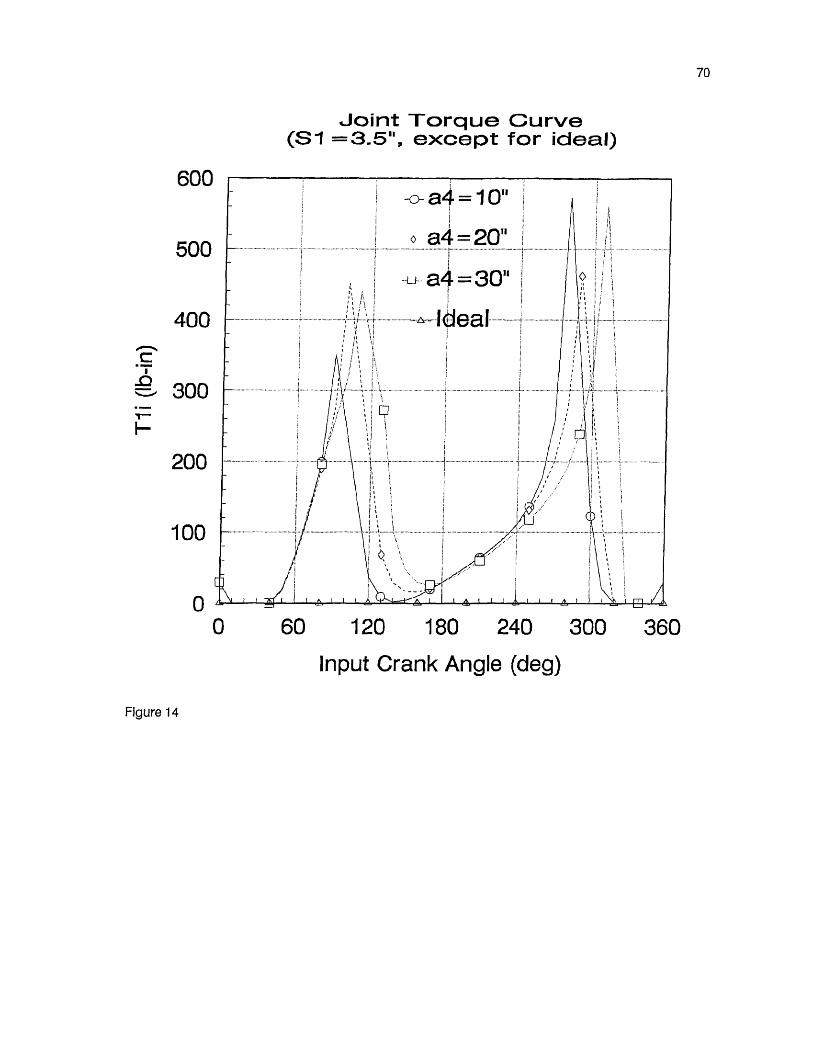
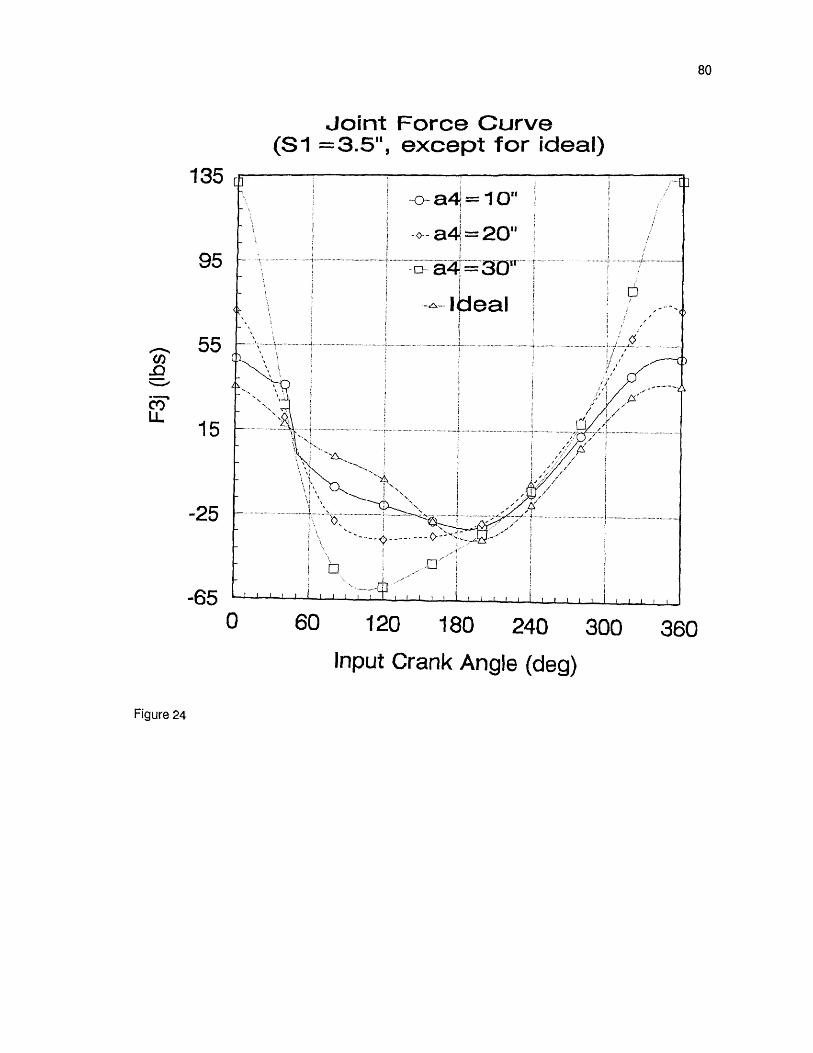
input crank angle as shown in figs. 5-38. In figs. 5, 8, 11, 14, 16, 18, 21, 24, 27, 30, 33,

56

36, slider displacements, different joint forces and torques are shown for variable offset

distance a4 (varying from 10" to 30"), constant crank axial offset Si (= 3.5") and ideal

offset angle a4 ( = 270 degrees, i.e. the crank shaft is perpendicular to the cylinder). In

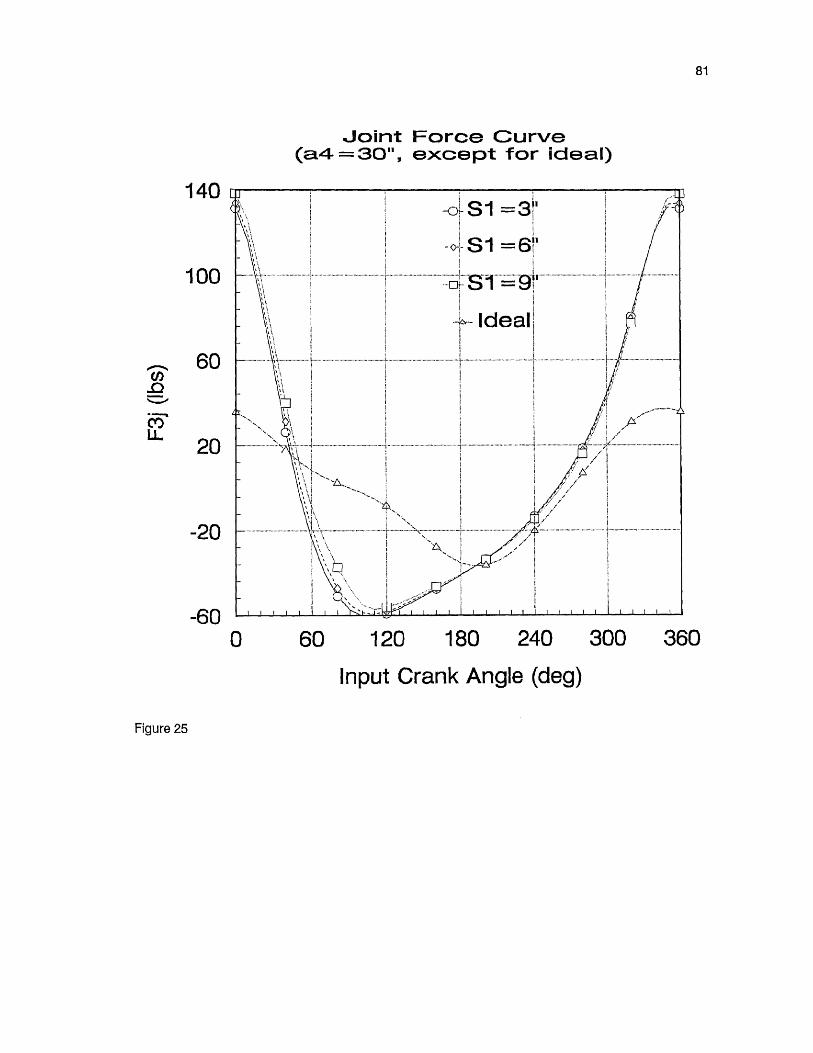
figs. 6, 9, 12, 15, 17, 19, 22, 25, 28, 31, 34, 37, slider displacements, different joint forces

and torques are shown for variable crank axial offset S (varing from 3" to 9"), constant

offset distance a4 ( = 30") and ideal offset angle a4 ( = 270 degree). In figs. 7, 10, 13, 20,

23, 26, 29, 32, 35, 38, slider displacements, different joint forces and no torques are

shown for variable offset angle a4 (varing from 232 degrees to 310 degrees), constant

offset distance ci4 ( = 20") and no crank axial offset (ideal). In each of the graphs

different spatial cases have been compared with the ideal case.

Although all the dynamic equations ( (68a) through (68g) and (68i) through

(68q) ) are free from sine or cosine terms in the denominator, the expressions for

acceleration ( equation (38a) through (42a) ) are not free from sine terms which

become very very close to zero at some particular positions of the crank, i.e. near 100

degrees and 300 degrees. Using the computer program it has been observed that near

those particular values for input crank angle, the joint angle 02 goes very close to zero

degrees and thus the calculated values of the acceleration terms, at those particular

positions, go abnormally high on account of roundoff errors in the computer calcula-

tions, which is clearly inaccurate. Therefore, in order to draw graphs, those particular

values have been discarded, otherwise those points would have taken most of the space

and the valid details of the graph would have been diminished.

All the torque components at joint 4, i.e. 4T4i, 47"41, and 4T4k and the force

components along joint axis (k) at joint 2, i.e. 2F2k are found to be zero throughout one

complete revolution of the crank at any offset. Interestingly, by manual manipulation

of the equation those components are also found to be zero. Another force component

along the j-axis of joint 2 , i.e. 2F21 is constant (-8.33 lbs) throughout one complete

57

rotation of the crank at any offset. By manual manipulation that force component is

found to be negative of the ratio of input torque ( 100 lb-in ) and the crank length (12

inches ). Two torque components at joint 1, i.e. 171 and lTii reduce to zero, when there

is no crank axial offset Si. By manual manipulation it is found that

171 = — and inj =

For the particular link lengths as mentioned before, when offset a4 is zero, the

program fails to converge if the term Si is greater than 1.5 inches. When offset is

increased to 10 inches or greater, the program fails to converge if the term Si is greater

than 3.5 inches and when offset a4 is 30 inches, the program converges as long as the

term Si is less than or equal to 9 inches. From this observation it can be inferred that

in order for the mechanism to work, with the increase of crank axial shift, offset a4

should be increased. In the case of mechanism failure, it will either lose closure, i.e.

one link or more will get detached from another at the joint or the slider will go to the

opposite side. When offset a4 is 20 inches and crank axial displacement Si is zero, the

program converges as long as offset a4 is between 232 and 310 degrees.

3.3 Conclusions

Slider displacement curves are almost semi-sinusoidal type of graphs which seem to be

quite reasonable. When crank is placed at higher level than the plane on which slider

is moving by providing positive offset distance a4, the stroke of the engine is reduced.

So in that case, while consuming less power the same RPM of the engine can be

obtained. But with the increase of offset distance a4, joint forces and torques also

increase. So proper design is necessary for the safe operation of the engine, considering

that factor. In most of the joint force and torque graphs (except for 3F3i with no spike,3F3k with one spike and 4F4k with one spike) two spikes are seen, one near 100 degrees

and other near 300 degrees. Hence it is very obvious that with the increase of offset

the chance of fatigue failure of the links at high speed is very large. In the presence of

58

offset distance Si, two extra torque components 1 Tii and 1Tij are acting at joint 1. So

extra precaution should be taken by designer, so that engine does not fail, and the

manufacturer should pay special attention to minimize this tolerance error.

Since the present work investigates dynamic forces and torques at each joint of

a slider crank with all kinds of manufacturing tolerances, the results provide informa-

tion needed for the sizing and dynamic balancing of a high speed slider crank in the

design stage. This analysis can be used to determine the effect and significance of the

inertia forces acting on each link due to its own mass and mass moment of inertia. It

is expected that this investigation will enable designers to have better insight into the

designing and testing of high speed spatial mechanisms and robot manipulators.

The main disadvantage of this method is that if we can not make good initial

estimates for joint displacements, ( which is normally done by using the direct formulas

for kinematic displacements, derived either by using plane geometry rules as shown

before in section 2.4.2 or by using the complex algebra method or by the dual-number

method, considering that there is no offset at all, i.e. the planar case ) the method will

not converge. Usually the process converges in 3 to 6 iterations if estimates are within

20 degrees, which is quite possible by using the direct formula for the planar case.

Another great disadvantage is that matrix A may become singular. Fortunately it never

happened while running the program. Since this method is well adapted for digital

computation, any complex system can be analyzed using this analytical tool. The main

advantages of this method are its generality and that all calculations can be performed

on digital computer. Other advantages are that this method is concise, flexible,

economical and its analytical approach is independent of visualization.

59

BIBLIOGRAPHY

1. Uicker, J. J., Denavit, J., and Hartenberg, R. S., "An Iterative Method for the

Displacement Analysis of Spatial Mechanisms," ASME Journal Of Applied Mechanics,

Vol. 31, June 1964, pp. 309-314.

2.Uicker, J. J., "Dynamic Force Analysis of Spatial Linkages,"ASMETournal OfApplied

Mechanics, Vol. 34, June 1967, pp. 418-424.

3.Yang. A. T., and Freudenstein. F., "Application of Dual-Number Quaternion Algebra

to the Analysis of Spatial Mechanisms,"ASME Journal Of Applied Mechanics, Vol. 31,

June 1964, pp. 300-308.

4. Yang. A. T., "Inertia Force Analysis of Spatial Mechanisms," ASME Journal Of

Engineering For Industry, Vol. 93, February 1971, pp. 27-33.

5. Bagci, C., "Dynamic Force and Torque Analysis of Mechanisms Using Dual Vectors

and 3 x3 Screw Matrix," ASME Journal Of Engineering For Industry, May 1972, pp.

738-745.

6. Pennock, G. R., and Yang, A. T., "Dynamic Analysis of a Multi-Rigid-Body Open-

Chain System," ASME Journal Of Mechanisms, Transmissions, And Automation In

Design, Vol. 105, March 1983, pp. 28-34.

7. Fischer, I. S., and Freudenstein, F., "Internal Force and Moment Transmission in a

Cardan Joint With Manufacturing Tolerances," ASME Journal Of Mechanisms, Trans-

missions, And Automation In Design, Vol. 106, December 1984, pp. 301-311.

8. Chen, C. K., and Freudenstein, F., 'Dynamic Analysis of a Universal Joint With

Manufacturing Tolerances," ASME Journal Of Mechanisms, Transmissions, And Auto-

mation In Design, Vol. 108, December 1986, pp. 524-532.

9. Fischer, I. S., and Paul, R. N., "Kinematic Displacement Analysis of a Double-Car-

dan-Joint Driveline,"Advancesln DesignAutomation,_ASME, DE-Vol. 10-2, September

1987, pp. 187-196.

60

10. Fischer, I. S., "Displacement Errors in Cardan Joints Caused by Coupler-Link

Joint-Axes Offset," 1st National Applied Mechanics And Robotics Conference, Cincin-

nati, Ohio, Vol. 2, November 1989, pp. 89 AMR-9A-2-5.

11. Sandor, G. N., and Erdman, A. G., Advanced Mechanism Design: Analysis and

Synthesis, Prentice Hall Inc., Englewood Cliffs, NJ, 1984, p. 611.

12.Hall, A. S., Root, R. R., and Sandgren, E., "ADependable Method for Solving Matrix

Loop Equations for the General Three-Dimensional Mechanism," ASME Journal Of

Engineering For Industry, August 1977, pp. 547-550.

13.Fu, K. S., Gonzalez, R. C., and Lee, C. S. G., Roboics: Control, Sensing, Vision, and

Intelligence, McGraw-Hill Book Company, 1987, pp. 12-50.

61

Figure 5

62

Figure 6

Figure 7

64

Figure 8

65

Figure 9

66

Figure 10

67

Figure 1 1

68

Figure 12

69

Figure 13

70

Figure 14

71

Figure 15

72

Figure 16

73

=figure 17

74

Figure 18

75

Figure 19

76

Figure 20

77

Figure 21

78

Figure 22

Figure 23

80

Figure 24

81

Figure 25

82

Figure 26

83

Figure 27

84

Figure 28

85

Figure 29

86

Figure 30

87

Figure 31

88

Figure 32

89

Figure33

90

Figure 34

91

Figure 35

Figure 36

93

Figure 37

94

Figure 38