droplet behavior in dense, low velocity aerosols
TRANSCRIPT

Marquette Universitye-Publications@Marquette
Master's Theses (2009 -) Dissertations, Theses, and Professional Projects
Droplet Behavior in Dense, Low Velocity AerosolsAlexander PolleyMarquette University
Recommended CitationPolley, Alexander, "Droplet Behavior in Dense, Low Velocity Aerosols" (2011). Master's Theses (2009 -). Paper 121.http://epublications.marquette.edu/theses_open/121

DROPLET BEHAVIOR IN DENSE, LOW VELOCITY AEROSOLS
By
Alexander F. Polley, B.S.
A Thesis submitted to the Faculty of the Graduate School,Marquette University,
in Partial Fulfillment of the Requirements forthe Degree of Master of Science
Milwaukee, Wisconsin
January 2012

ABSTRACTDROPLET BEHAVIOR IN DENSE, LOW VELOCITY AEROSOLS
Alexander F. Polley, B.S.
Marquette University, 2012
Rapid compression machines (RCM) are laboratory devices used to measure gas-phasefuel reactivity at conditions relevant to combustion engines. Test mixtures are generallyprepared by rapidly compressing a gas phase fuel+oxidizer+diluent mixture to highpressure and temperature (e.g., 10-50 bar, 650-1000 K). It is extremely challenging toutilize diesel-relevant liquid fuels in these devices due to their involatility. One proposedmethod involves the delivery of an aerosol of suspended fuel droplets (≈ 0.1 mLfuel/Lgasat stoichiometric fuel loading) to the machine. The compression stroke of the RCMsubsequently heats the gas phase of the aerosol thereby achieving vaporization of the fuel.The properties of the aerosol delivered to the RCM such as the droplet size distribution(DSD) are critical to ensuring successful execution of the experiments. For instance, thefuel droplets must be smaller than a critical threshold (e.g., d0 ≈ 6 - 10µm) to ensuretimely fuel evaporation and gas-phase mixing; in addition, the droplets must resistgravitational forces that could cause them to fall out of suspension. Low aerosol velocitiesare required in order to minimize fluid motion and thus heat loss from the compressedreacting gases during the RCM experiment. An aerosol model has been developed in thisthesis project in order to understand the aerosol dynamics during the generation andmachine delivery processes. Issues such as droplet impingement, coagulation, evaporationand settling can be investigated with the model, and thus the configuration (i.e., intakevalve geometry, mixing chamber design, etc.) and operational characteristics (i.e., gas flowrates, fuel loading, etc.) of the aerosol RCM can be understood/improved/optimized. Thesystem model is validated against gravimetric measurements using a mock up of aproposed delivery system. ‘Operating maps’ are generated for n-dodecane andn-hexadecane in oxygen + diluent mixtures covering a range of fuel loadings and deliveryflow rates.

i
ACKNOWLEDGMENTS
Alexander F. Polley, B.S.
I would like to thank Dr. S. Scott Goldsborough for his guidance as my thesis projectadvisor. I have really appreciated his consistent availability, suggestions and explanationswhen I faced difficulties along the way. I learned a lot and really enjoyed our relationship.I would also like to thank Dr. John Borg and Dr. Jon Koch for being members of mythesis committee.
I am grateful for the financial support of the National Science Foundation (GrantCBET-0968080)and Argonne National Laboratory (Grant 49463DR155) for materialsnecessary to carry out experiments and to Marquette University for providing me with aTeaching Assistantship during my first year of graduate school.
Thank you to Dr. Dimitri Kyritsis and Dr. Chia-fon Lee at the University ofIllinois - Urbana Champaign for the use of their laboratory equipment and time.
Mike Johnson for his time while transitioning the project and continued input overthe past two years.
Colin Banyon for his collaboration on the project and collection of experimentaldata.
Daniel Sherwin for his assistance with the lasers and optical equipment formeasuring droplet size distributions.
Tom Silman, Dave Gibas and Ray Hamilton for their assistance and input with thedesign and fabrication of components.
Annette Wolak for all of the guidance and help during my time at Marquette.
Finally, a special thanks to my wife Nicole for her loving support and to my Mom,Dad and Grandma for all of their contributions to my education over the years.

ii
TABLE OF CONTENTS
ACKNOWLEDGMENTS i
LIST OF TABLES v
LIST OF FIGURES vi
LIST OF PRINCIPAL SYMBOLS xi
1 INTRODUCTION 1
1.1 Study of Aerosols . . . . . . . . . . . . . . . . . . . . . . . . . . . . . . 1
1.2 Engine-Relevant Chemical Kinetics . . . . . . . . . . . . . . . . . . . . 8
1.2.1 Flow Reactors . . . . . . . . . . . . . . . . . . . . . . . . . . . 9
1.2.2 Shock Tubes . . . . . . . . . . . . . . . . . . . . . . . . . . . . 11
1.2.3 Rapid Compression Machines . . . . . . . . . . . . . . . . . . 13
1.2.4 Equipment Comparison . . . . . . . . . . . . . . . . . . . . . . 14
1.3 Fuel Loading in STs and RCMs . . . . . . . . . . . . . . . . . . . . . . 15
1.3.1 Partial Pressure Method . . . . . . . . . . . . . . . . . . . . . 16
1.3.2 Aerosol Method . . . . . . . . . . . . . . . . . . . . . . . . . . 17
1.4 Aerosol Loading in an RCM . . . . . . . . . . . . . . . . . . . . . . . . 19
1.4.1 Configuration . . . . . . . . . . . . . . . . . . . . . . . . . . . 19
1.4.2 Initial Aerosol Loss Results . . . . . . . . . . . . . . . . . . . 20
1.5 Overview of Computer Model . . . . . . . . . . . . . . . . . . . . . . . . 21
1.6 Outline of Thesis . . . . . . . . . . . . . . . . . . . . . . . . . . . . . . . 21
2 LITERATURE SURVEY & THEORY 23
2.1 Droplet Populations . . . . . . . . . . . . . . . . . . . . . . . . . . . . . 24
2.2 Droplet Motion . . . . . . . . . . . . . . . . . . . . . . . . . . . . . . . . 25
2.3 Mechanisms in Aerosol Dynamics Models . . . . . . . . . . . . . . . . . 28
2.3.1 Coagulation . . . . . . . . . . . . . . . . . . . . . . . . . . . . 28
2.3.2 Evaporation . . . . . . . . . . . . . . . . . . . . . . . . . . . . 31

iii
2.3.3 Removal . . . . . . . . . . . . . . . . . . . . . . . . . . . . . . 31
2.4 Methods of Solving the GDE . . . . . . . . . . . . . . . . . . . . . . . . 35
2.4.1 Continuous . . . . . . . . . . . . . . . . . . . . . . . . . . . . . 36
2.4.2 Modal . . . . . . . . . . . . . . . . . . . . . . . . . . . . . . . 36
2.4.3 Sectional . . . . . . . . . . . . . . . . . . . . . . . . . . . . . . 37
2.4.4 Piecewise . . . . . . . . . . . . . . . . . . . . . . . . . . . . . . 38
3 AEROSOL MODEL IMPLEMENTATION 40
3.1 Main Model . . . . . . . . . . . . . . . . . . . . . . . . . . . . . . . . . 41
3.2 Energy Balance . . . . . . . . . . . . . . . . . . . . . . . . . . . . . . . 43
3.3 Evaporation . . . . . . . . . . . . . . . . . . . . . . . . . . . . . . . . . 46
3.4 Coagulation . . . . . . . . . . . . . . . . . . . . . . . . . . . . . . . . . . 48
3.5 Removal Models . . . . . . . . . . . . . . . . . . . . . . . . . . . . . . . 50
3.6 Time Step Control . . . . . . . . . . . . . . . . . . . . . . . . . . . . . . 56
4 RESULTS AND DISCUSSION 59
4.1 Aerosol System Experiments . . . . . . . . . . . . . . . . . . . . . . . . 59
4.2 Droplet Size Distributions . . . . . . . . . . . . . . . . . . . . . . . . . . 63
4.3 Model Validation and System Modifications . . . . . . . . . . . . . . . . 64
4.4 Model Utilization . . . . . . . . . . . . . . . . . . . . . . . . . . . . . . 72
4.4.1 Effect of Mechanisms . . . . . . . . . . . . . . . . . . . . . . . 73
4.4.2 Evolution of DSD . . . . . . . . . . . . . . . . . . . . . . . . . 74
4.4.3 Aerosol Behavior . . . . . . . . . . . . . . . . . . . . . . . . . 75
4.4.4 Operating Maps . . . . . . . . . . . . . . . . . . . . . . . . . . 77
4.5 Fuel Delivery System Improvements . . . . . . . . . . . . . . . . . . . . 86
4.6 Areas for Model Improvement . . . . . . . . . . . . . . . . . . . . . . . 87
5 SUMMARY 88
BIBLIOGRAPHY 90
A THERMOPHYSICAL PROPERTY MODELS 97

iv
B ALGORITHM VALIDATION 101
C TUBE BEND DEPOSITION 110
D UNCERTAINTY 119
E SHADOWGRAPHY AND PDA RESULTS 121

v
LIST OF TABLES
3.1 Coefficients for use with Eq. (3.9) . . . . . . . . . . . . . . . . . . . . . . . . 45
3.2 Coefficients for use with Eq. (3.32) . . . . . . . . . . . . . . . . . . . . . . . 49
3.3 Coefficients for use with Eq. (3.53) . . . . . . . . . . . . . . . . . . . . . . . 56
4.1 Operating conditions for initial aerosol system experiments . . . . . . . . . 62
4.2 Operating conditions for modified aerosol system experiments . . . . . . . . 65
4.3 Operating conditions for simulated aerosol systems. . . . . . . . . . . . . . . 78
C.1 Parameters for Weibull distribution fits to deposition efficiency curves of Tsaiand Pui. . . . . . . . . . . . . . . . . . . . . . . . . . . . . . . . . . . . . . . 111
D.1 Measurements of aerosol losses in the mixing chamber and delivery tube forsimilar systems. . . . . . . . . . . . . . . . . . . . . . . . . . . . . . . . . . . 119

vi
LIST OF FIGURES
1.1 Examples of the mechanisms accounted for in the GDE. . . . . . . . . . . . 2
1.2 Diagrams of a (a) well stirred and (b) laminar flow reactor. . . . . . . . . . 9
1.3 Experimental mole fractions for oxidation of n-hexadecane at 1 atm in a wellstirred reactor. . . . . . . . . . . . . . . . . . . . . . . . . . . . . . . . . . . 11
1.4 A diagram of a typical ST. . . . . . . . . . . . . . . . . . . . . . . . . . . . 11
1.5 Experimental pressure and OH* traces for a ST experiment of n-decane. . . 12
1.6 A schematic of an RCM. . . . . . . . . . . . . . . . . . . . . . . . . . . . . . 13
1.7 RCM experiment pressure traces for n-decane in air at five compressed mix-ture temperatures. The unlabeled line is the pressure trace for a non-reactingmixture. . . . . . . . . . . . . . . . . . . . . . . . . . . . . . . . . . . . . . . 14
1.8 Ignition delay time as a function of inverse temperature from RCM (•, ◦)and ST (N,4,+) studies of n-decane/air mixtures at compressed pressuresof 13-14 bar. . . . . . . . . . . . . . . . . . . . . . . . . . . . . . . . . . . . . 15
1.9 Overhead view of the first generation aerosol ST at Stanford University. Thetop image shows the aerosol loading, and the bottom image shows the va-porization of the aerosol by the initial shock wave. . . . . . . . . . . . . . . 17
1.10 A diagram showing the second generation aerosol ST at Stanford University.The aerosol is mixed in a large tank and introduced through a gate valve inthe ST end wall. . . . . . . . . . . . . . . . . . . . . . . . . . . . . . . . . . 18
1.11 A diagram of the aerosol ST at Texas A&M University. The aerosol is loadednear the diaphragm and is drawn towards the end wall. . . . . . . . . . . . 19
1.12 Diagram of the aerosol RCM mock up at Marquette University . . . . . . . 20
2.1 The same DSD shown as (a) particle and (b) volume fraction distributions. 24
2.2 Brownian and gravitational coagulation rates of a 1 µm particle with particlesranging from 0.1 - 10 µm. . . . . . . . . . . . . . . . . . . . . . . . . . . . . 30
2.3 Examples of interception and impaction . . . . . . . . . . . . . . . . . . . . 32
3.1 Schematic of aerosol fueling system as depicted in the model. Inputs, outputsand example control volumes of the aerosol model are indicated. The plotshows an example sectional droplet distribution. . . . . . . . . . . . . . . . 41
3.2 Energy fluxes in a control volume. . . . . . . . . . . . . . . . . . . . . . . . 43

vii
3.3 (a) Flow field for the cyclone and (a) particle traces for the box designs ofthe mixing chamber. The flow in the box is non-uniform while the flow inthe cylinder is controlled. . . . . . . . . . . . . . . . . . . . . . . . . . . . . 51
4.1 Diagram of the aerosol RCM mock up at Marquette University . . . . . . . 59
4.2 (a) The location of the hose barb and poppet valve and (b) loss results frominitial configuration of the fuel delivery system. Experiments are conductedat T = 298 K, P = 1 bar, ml = 1.31 g/min and ReRC ≈ 517. . . . . . . . . 61
4.3 Comparison of the DSDs produced by the two types of Aeroneb OnQ nebu-lizers and the Pelas AGF 2.0. The legend value in parentheses was used fornormalization. . . . . . . . . . . . . . . . . . . . . . . . . . . . . . . . . . . . 63
4.4 Internal geometries of (a) the initial valve housing [#1], and the second gen-eration housings with entry on the (b) side [#2] and (c) base [#3] of thehousing cylinder. The boss on the inlet to the housing accepts the valvestem and the red arrows show the direction of aerosol flow. . . . . . . . . . 64
4.5 Measured and modeled losses in aerosol system components for Cases 4 &5. Conditions for the system are T = 297, P = 1 bar, ml ≈ 1.3 g/min andReRC ≈ 520. . . . . . . . . . . . . . . . . . . . . . . . . . . . . . . . . . . . 66
4.6 Measured and modeled losses in aerosol system components using valve hous-ing #3. Conditions for the system are T = 297, P = 1 bar, ml = 1.38 g/minand ReRC = 879. . . . . . . . . . . . . . . . . . . . . . . . . . . . . . . . . . 67
4.7 Measured and modeled losses in aerosol system components using valve hous-ing #5. Conditions for the system are T = 298, P = 1 bar, ml = 1.33 g/minand ReRC = 516. . . . . . . . . . . . . . . . . . . . . . . . . . . . . . . . . . 68
4.8 Delivery system with cyclone mixing chamber. The delivery tube is not toscale. . . . . . . . . . . . . . . . . . . . . . . . . . . . . . . . . . . . . . . . . 69
4.9 Measured and modeled losses in aerosol system components using valve hous-ing #5 and the 0.152 m diameter cyclone mixing chamber. Conditions forthe system are T = 297, P = 1 bar. For ReRC = 543, ml = 0.94 g/min andfor ReRC = 1094, ml = 1.09 g/min. . . . . . . . . . . . . . . . . . . . . . . 70
4.10 Modeled losses in aerosol system components for a full and half sweep of themixing chamber using valve housing #5 and the 0.152 m diameter cyclonemixing chamber. Conditions for the system are T = 297, P = 1 bar, ReRC= 543 and ml = 0.94 g/min . . . . . . . . . . . . . . . . . . . . . . . . . . . 70
4.11 Measured and modeled losses in aerosol system components using valve hous-ing #5 and the 0.205 m diameter cyclone mixing chamber. Conditions forthe system are T = 298, P = 1 bar, ml = 2.38 g/min and ReRC = 825. . . 71

viii
4.12 Percent loss in delivery systems components for n-dodecane in air with (a)φ = 1.0 and (b) φ = 2.0 at T = 350 K, P = 1 bar and ReRC = 800. . . . . 73
4.13 Initial and final volume fraction DSDs of n-dodecane in air for φ = 1.0 andφ = 2.0 at T = 350 K, P = 1 bar and ReRC = 800. . . . . . . . . . . . . . . 74
4.14 Relative humidity, mass loss, mass evaporation and aerosol temperature alongthe delivery system for (a) water and (b) n-dodecane at T = 298 K and P= 1 bar. The time in the mixing chamber (MC), delivery tube (DT) andreaction chamber (RC) is marked. The time in the valve housing is 0.01 s. . 76
4.15 Relative humidity, mass loss, mass evaporation and aerosol temperature alongthe delivery system for n-dodecane at T = 350 K and P = 1 bar. The timein the mixing chamber (MC), delivery tube (DT) and reaction chamber (RC)is marked. The time in the valve housing is 0.01 s. . . . . . . . . . . . . . . 77
4.16 Operating map of System 1: Air + C12H26, OnQ nebulizer, T = 300 K, P =1 bar. The range of conditions for the experiments with water is indicated. 78
4.17 Operating map of System 2: Air + C12H26, OnQ nebulizer, T = 350 K, P =1 bar. . . . . . . . . . . . . . . . . . . . . . . . . . . . . . . . . . . . . . . . 80
4.18 Operating map of System 3: 32 % Ar / 47 % N2 / 21 % O2 + C12H26, OnQnebulizer, T = 350 K, P = 1 bar. . . . . . . . . . . . . . . . . . . . . . . . . 81
4.19 Operating map of System 4: 36 % Ar / 53 % N2 / 11 % O2 + C12H26, OnQnebulizer, T = 350 K, P = 1 bar. . . . . . . . . . . . . . . . . . . . . . . . . 82
4.20 Operating map of System 5: Air + C12H26, AGF 2.0 nebulizer, T = 350 K,P = 1 bar. . . . . . . . . . . . . . . . . . . . . . . . . . . . . . . . . . . . . 83
4.21 Operating map of System 6: Air + C16H34, AGF 2.0 nebulizer, T = 350 K,P = 1 bar. . . . . . . . . . . . . . . . . . . . . . . . . . . . . . . . . . . . . 83
4.22 Operating map of System 7: Air + C12H26, OnQ nebulizer, T = 350 K, P =0.5 bar. . . . . . . . . . . . . . . . . . . . . . . . . . . . . . . . . . . . . . . 84
4.23 Operating map of System 8: Air + C16H34, OnQ nebulizer, T = 350 K, P =0.5 bar. . . . . . . . . . . . . . . . . . . . . . . . . . . . . . . . . . . . . . . 85
B.1 Comparison of the analytical solution for particle concentration as a functionof time with the numerical solution using different bin sizes . . . . . . . . . 102
B.2 Comparison of the analytical solution for particle diameter as a function oftime with the numerical solution using different bin sizes . . . . . . . . . . . 102
B.3 Non-dimensional surface area plotted as a function of time for an isolatedwater droplet with d0 = 2 µm, T = 293 K and P = 1 bar. . . . . . . . . . . 103

ix
B.4 Non-dimensional surface area plotted as a function of time for a monodispersewater droplet population with d0 = 2 µm, N0=1×10¹³ particles/kgg, Pv,0 =0, T = 293 K and P = 1 bar. . . . . . . . . . . . . . . . . . . . . . . . . . . 104
B.5 Non-dimensional surface areas plotted as a function of time for a bidispersedroplet population with (a) d0,1 = 2 µm, N0,1 = 1×10¹³ particles/kgg and(b) d0,2 = 10 µm, N0,2 = 1×10⁹ particles/kgg at Pv,0 = 0, T = 293 K and P= 1 bar. . . . . . . . . . . . . . . . . . . . . . . . . . . . . . . . . . . . . . . 105
B.6 The relative humidty during the initial evaporation of n-dodecane in themixing chamber using different values for the evaporation coefficient. . . . . 106
B.7 Diameter under which 98% of the mass is present and aerosol losses as afunction of number of discretizations for the (a) stirred vessel, (b) straighttube, (c) curved tube and (d) cyclone removal sub-models. . . . . . . . . . . 107
B.8 Diameter under which 98% of the mass is present and aerosol losses as afunction of number of discretizations for the (a) mixing chamber, (b) straightdelivery tube, (c) curved delivery tube, (d) valve housing and (e) reactionchamber using coagulation, evaporation and removal sub-models. . . . . . . 108
C.1 Weibull distribution fits (lines) to the deposition efficiency curves (points)from Tsai and Pui. . . . . . . . . . . . . . . . . . . . . . . . . . . . . . . . . 111
C.2 Shape parameter correlations of (a) f1(De) and (b) f2(Ro). . . . . . . . . . 112
C.3 Scale parameter correlations of (a) g1(Ro) and (b) g2(Re). . . . . . . . . . . 113
C.4 A comparison of deposition efficiency curves calculated (lines) using Eqs.(C.2), (C.5) and (C.8) with results (points) from Tsai and Pui. . . . . . . . 114
C.5 Side and cross-section views of the deposition observed in a 90 degree tubebend at Ro = 7.38 and Dn = 484. The dashed line indicates the boundarywhere deposition occurs. . . . . . . . . . . . . . . . . . . . . . . . . . . . . . 114
C.6 Comparison between measured and modeled aerosol losses in a tube bend atT = 297 K, P = 1 bar and low flow OnQ DSD. The model only accounts forlosses due to the flow and significantly underpredicts losses. . . . . . . . . . 115
C.7 Comparison between measured and modeled aerosol losses in a tube bend atT = 297 K, P = 1 bar and low flow OnQ DSD. The model accounts for lossesdue to the flow and gravity. . . . . . . . . . . . . . . . . . . . . . . . . . . . 116
C.8 Comparison between measured and modeled aerosol losses in a tube bend atT = 297 K, P = 1 bar and high flow OnQ DSD. The model accounts forlosses due to the flow and gravity. . . . . . . . . . . . . . . . . . . . . . . . . 117

x
C.9 Comparison between measured and modeled aerosol losses in a tube bend atT = 297 K, P = 1 bar and low flow OnQ DSD. The model accounts for lossesdue to the flow and gravity and sub-models were adjusted by the factor listedin the legend. . . . . . . . . . . . . . . . . . . . . . . . . . . . . . . . . . . . 117
E.1 Diagram of a Shadowgraphy measurement setup. . . . . . . . . . . . . . . . 121
E.2 Droplet measurements from a) 0 - 20 µm and b) 5 - 20 µm comparing Shad-owgraphy and PDA measurements against the results of Kuhli et al. . . . . 122
E.3 Diagram of PDA measurement setup. . . . . . . . . . . . . . . . . . . . . . 123

xi
LIST OF PRINCIPAL SYMBOLS
A areaAv Avogadro’s numberC Cunningham correction factorCp heat capacityD diffusion coefficientDn Dean numberE molar growth rate of a particle (kmol/s)K coagulation coefficient (m3/s)Kn Knudsen numberL percent mass lossLchar characteristic lengthM molar massN particle concentration (particles / kgg)P pressureQ volumetric flow, concentration of liquid molecules (kmolmolecules/ kgg)R net concentration flux of liquid molecules (kmolmolecules/ s-kgg)Ro curve ratioRu universal gas constantRe Reynold’s numberSc Schmidt numberSt Stokes’s numberT temperature (K)U velocityU average velocityUTS terminal settling velocityV volumeX total number of DSD sectional binsd diameterg gravitational accelerationh enthalpy, heighthconv convection coefficientk thermal conductivitykb Boltzmann’s constantm massm mass flow raten molesqj concentration of particles with size nj (kmolmolecules / kgg-kmolparticles)q energy flux into the control volumer radiust timex distance
Greek Symbols

xii
∆t time stepχ fraction loss of particlesε collision efficiency of two dropletsφ equivalence ratioλ mean free pathν viscosityθ, φ angleρ densityσ diameter of a general particleτ particle relaxation time, ignition delay timeω accentric factor
Subscripts
∞ far field1, 2 general particles with 1 being larger than 20 t = 0B BrownianG gravitationalLF laminar flowb tube bendc criticalcs cross section of tubedi discdt delivery tubee exitevap evaporationg gas phasein inleti, j, k DSD sectional bin numbersl liquid phasemc mixing chamberp particlerc reaction chambersat saturationstem stemsys systemtu straight tubev vapor phasevh valve housingw wall
Superscripts
∗ dimensionless

1
Chapter 1
INTRODUCTION
This thesis describes the development and application of a model utilized to predict the
behavior of dense, low velocity aerosols in a laboratory scale aerosol flow system. The
primary purpose of the system is to deliver involatile, transportation-relevant fuels to a
rapid compression machine (RCM). Experiments are performed with RCMs to understand
the combustion kinetics of fuels. The data and chemical kinetic models developed from
them have many important applications in the study and development of combustion
engines. Aerosol fueling of RCMs and the associated ‘wet compression’ process has been
proposed as a means of extending the utility of RCMs beyond gasoline-relevant
components and surrogate blends to the regime of diesel type fuels.
The chapter begins with an introduction to the study of aerosol dynamics,
especially concerning the modeling of aerosol transport, followed by a review of
experimental equipment used to gather chemical kinetic data for engine-relevant fuels.
Fuel loading of a few apparatuses is then discussed. The focus of this study is then
presented and the chapter concludes with an overview of the thesis.
1.1 Study of Aerosols
An aerosol is defined as a solid or liquid that is suspended in a gas. Examples of liquid
particle aerosols are clouds, fog, spray paint and medical inhalers. Examples of solid
particle aerosols include smoke, smog, engine exhaust, and airborne dust. Aerosols can
stay in suspension anywhere from a few seconds to a year depending on the physical
properties of the particle and gas. Aerosol particles range from 0.001 to over 100 µm with

2
Figure 1.1: Examples of the mechanisms accounted for in the GDE.
mass concentrations between 0.001 to 100 g/m3 [1].
The General Dynamics Equation (GDE) is used to model the transport of aerosol
particles within the gas phase and incorporates five mechanisms that lead to changes in
the aerosol particle distribution:
∂n(dp, t)
∂t= C(dp, t) +G(dp, t) +N(dp, t) + S(dp, t) +R(dp, t) (1.1)
Here dp is the particle diameter and t is time. Figure 1.1 presents sketches of these
mechanisms where each is described next.
Coagulation , C(dp, t), occurs when two particles collide and become one. This happens
as a result of particle motion caused by gravitational settling, velocity gradients, or
electrostatic forces, as well as Brownian motion [2]. Brownian motion is the random
motion of small particles in a gas due to the gas particles striking the suspended
particles. This effect decreases as the suspended particles increase in size and are no
longer affected by the gas particle momentum [1].

3
Growth , G(dp, t), includes both condensation and evaporation of suspended particles.
When the environment around a suspended particle becomes super-saturated (i.e.
P∞ > Psat), the vapor phase will condense onto suspended particles and increase
their size. The opposite is true when the environment is under-saturated. The
suspended particles will decrease in size as some of the liquid phase evaporates [2].
Nucleation , N(dp, t), will also happen when the gas phase of an aerosol is
super-saturated. New suspended particles can be formed as the gas and liquid
phases arrive at equilibrium.
Sources , S(dp, t), account for all particle generation (e.g., from an atomizer) with the
exception of nucleation.
Removal , R(dp, t), occurs when particles fall out of suspension. This is a result of
impaction, diffusion or gravitational settling onto surfaces. Diffusion is the dominant
phenomenon causing removal for particles under 1 µm while impaction and settling
have more influence for larger particles [1].
There are many fields that are concerned with the study of aerosol behavior. The
remainder of this section will introduce aerosol behavior, physical properties of aerosols
and major aerosol mechanisms studied in some of these fields. The section concludes with
an overview of fuel aerosols, which are under investigation towards developing
experimental equipment that is capable of acquiring chemical kinetic data for involatile,
transport-relevant fuels.
Atmospheric Sciences
Aerosols in the atmosphere such as smog and clouds play a central role in the world’s
climate system. These aerosols are a contributing factor in determining how much and
what type of radiation reaches and leaves the earth [2]. Therefore, it is very important to
have appropriate models that can facilitate the accurate prediction of climate behavior.
Primary aerosol dynamics are fairly well understood and the current focus in this field is
on incorporating aerosol models efficiently into computational fluid dynamics (CFD)

4
packages.
The study of atmospheric aerosols includes the mechanisms of coagulation, growth,
nucleation and removal. Models for coagulation, growth and nucleation are well studied
and have been extensively verified. They are universal to studies where these mechanisms
contribute to aerosol dynamics. Growth and nucleation can occur due to phase changes as
well as chemical changes in the aerosol. Removal of aerosol particles occurs when rain
drops fall and collect particles that are suspended in the air. This removal mechanism
does not have much application outside of the field of atmospheric sciences.
The aerosols studied in atmospheric sciences are composed of dust, sea salt, water
and various types of pollution. The aerosols are classified as smog (0.001 - 2 µm, <0.005
g/m3), clouds/fog (2 - 70 µm, 0.005 - 0.05 g/m3) or mist (70 - 200 µm, 0.01 - 0.1 g/m3) [1].
Combustion Systems
There is an ever increasing demand to reduce particulate emissions of combustion systems
due to detrimental effects on the environment and human health. As a result, soot
formation in flames is a major concern in combustion system design and has become a
focus of many studies. One of the major components of kinetic models for soot formation
is the soot particle dynamics.
The major mechanisms of particle dynamics involved in soot formation are
nucleation, coagulation and growth. The products of gas phase reactions can nucleate as
they become larger molecules with lower saturation pressures. These molecules will
coagulate as they collide with each other and will also grow as a result of chemical
reactions that occur at the surface of the droplet. Sub-models for the mechanisms in soot
formation models have been taken largely from atmospheric aerosol studies [3].
Soot is a result of the incomplete oxidation of the carbon and hydrogen atoms
originally contained in the fuel. Soot particles in diesel and gasoline engine exhaust range
from 20 to 500 nm and are at concentrations of 105 to 1010 particles/cm3 [4].

5
Drug Delivery
Certain medications are most effective when delivered directly to a person’s lungs where
the medication can enter the bloodstream or be absorbed within a specific section of the
lung. To achieve this, liquid solutions containing pharmaceutical compounds are atomized
into small particles and delivered through a patient’s airway. During drug delivery, the
aerosol passes through the mouth/nasal cavity, trachea, lung bifurcation, smaller branches
and alveoli. The changes in direction along this path result in the deposition of larger
aerosol particles along the early sections of the airway. Many studies have investigated the
process in order to understand and predict how aerosol medications should be delivered.
Aerosol modeling in drug delivery focuses almost exclusively on removal
mechanisms for aerosol particles. Early studies involved modeling and collecting data in
simple setups using straight or bent tubes to model the airway. More recent studies
simulate complex geometries with rough surfaces and use CFD packages to develop airway
models that can very accurately predict deposition in human lungs. The methodologies
used are applicable to all aerosols, however, the implementation can be very time
consuming. Results from these studies have had little applicability outside of the field.
The composition of drug aerosols are also specific to the field. Aerosol particles are
composed of active pharmaceutical ingredients dissolved in a combination of water,
glycerin, propylene glycol or ethanol. The aerosol particles are commonly generated using
ultrasonic, jet, micro-pump and vapor condensation nebulizers. These devices generate
particles below 10 µm with concentrations on the scale of 104 - 108 particles/cm3 before
dilution with air [5].
Material Processing
Chemical vapor deposition (CVD) is a method of material processing which is used to
coat a substrate with a thin film of material. The process starts with a precursor gas or
gases being introduced inside of a chamber containing the substrate. The gases undergo a
chemical reaction that produces a solid particle which is deposited on the substrate. For
some CVD processes, this reaction occurs at the substrate surface [6]. In other processes,

6
solid particles form away from the substrate producing an aerosol inside the chamber. The
particle size of the aerosol can be predicted to determine the impact on film quality [7].
Important mechanisms involved with CVD modeling are nucleation, growth and
coagulation. In this field, nucleation and growth models involve a chemical change as the
gas phase reacts to produce a solid that is deposited. Models developed and utilized in
this field sometimes have applicability to combustion studies investigating particulate
matter formation or engine exhaust behavior.
Some examples of materials that can be applied using CVD are silicon, tungsten,
and silicon dioxide for semiconductors and indium gallium nitride (InGaN) for LEDs [6].
A study by Sharifi and Achenie [7] investigated the thin film production of zinc sulfide
using CVD. The deposited particles were determined to have an average diameter of 2.35
nm with a concentration of roughly 7x10¹¹ particles/cm3. This is a very large particle
density compared with other fields, but the overall mass density is much lower due to the
small particle size.
Aerosol Sampling
Aerosols are present in many systems and often need to be monitored for a variety of
reasons including safety, regulation compliance and process design. Ideally, this data
would be collected without interfering with the aerosol, but this is usually not possible. At
nuclear power plants and nuclear waste disposal facilities the radioactivity of aerosols
needs to be monitored in accordance with Environmental Protection Agency (EPA)
regulations. As a result, aerosol samples are collected in one location and analyzed at
another. This requires transport of the aerosol through a series of pipes which results in
some aerosol particle loss. In order to infer the actual aerosol properties from the sampled
and measured ones, the effect of transport system deposition needs to be understood [8].
Similar to drug delivery, aerosol sampling models have focused primarily on
particle removal. Models for pipes and bends are created using results from CFD
calculations that investigate a range of flow conditions. While these models are primarily
applicable to specific geometries, they are often non-dimensionalized and thus can have a
wide range of applicability to engineered systems where suspended particles have various

7
size, composition and density.
Indoor Air Quality
Since the majority of the work force spends significant amounts time inside of buildings,
effects of indoor air quality is becoming a big concern. Studies indicate that the quality of
the air has a direct effect on the health of building occupants [9]. The chemical
compositions as well as the physical properties of particles suspended in the air both
contribute to the overall impact. Specifically, ultrafine particles (i.e. < 100 nm) with
low-solubility have been shown to have adverse effects on a person’s health. Aerosols
generated within a building can be different sizes and be generated in multiple areas.
These aerosols interact and are eventually inhaled. It is important to know the properties
of the inhaled aerosol and if building modifications can have any influence [10].
Air quality models incorporate all general mechanisms of the GDE. Numerical
studies often use common coagulation, growth and nucleation models and even
incorporate sources for aerosols generated within buildings. Removal models include losses
to ventilation ducts as well as to room objects, walls and floors. Studies can investigate
building-scale to room-scale scenarios depending on the objectives.
Aerosol particles that have been studied are composed of solids such as
polystyrene latex, titanium dioxide, aluminum, polytetrafluoroethylene (PTFE), and
granite. Particle sizes range on the order of 1 nm to 10 µm while concentrations have a
maximum of 106 particles/cm3 [10].
Involatile Fuels
Understanding the reaction kinetics of a fuel during combustion is very important towards
the development of modern combustion systems that can meet efficiency and emission
targets. In order to collect data and develop models for the combustion chemistry, fuels
must be reacted under tightly controlled conditions. One requirement for such tests is
that the fuel must be fully vaporized prior to the onset of chemical reaction processes.
This poses a problem for fuels with extremely low vapor pressures such as those
representative of diesel. One method that has been proposed to overcome this problem is

8
to prepare the liquid phase fuels as an aerosol which can be evaporated inside test
equipment due to ‘wet compression’ (i.e, the volumetric compression heating of the gas
phase) before combustion begins.
Loading a fuel aerosol with an appropriate droplet size distribution (DSD) and
overall fuel concentration is a major challenge. In order for the fuel to completely
evaporate and mix with the oxidizer and diluent gas, droplets must be smaller than a
specific size based on the fuel and equipment [11, 12, 13]. In order to achieve this loading
specification, the effect of the aerosol generation and delivery systems on the DSD must
be known.
The model developed in this study is used to predict changes in DSD along an
aerosol delivery system. The model can also track fuel fall out as well as the DSD and
equivalence ratio (φ) that remains suspended in the reaction chamber. It incorporates
sub-models for coagulation, growth and removal and draws upon findings in the fields
mentioned in this section. Sub-models for coagulation and growth are applicable, and
removal sub-models come from work investigating geometries that are similar to the
delivery system for a representative experimental apparatus which is discussed in the next
section.
In order to study engine-relevant combustion chemistry, the gas phase of an
aerosol will contain varying levels of oxygen concentration ranging from 1 - 21 % O2. This
means that an aerosol with a stoichiometric ratio of dodecane plus air, for example, needs
to have a concentration on the order of 106 particles/cm3 at standard temperature and
pressure when the droplet diameter is 4 µm [12]. Smaller droplet sizes will require higher
concentrations. The properties of the fuel and the conditions to be studied dictate the
density and maximum allowable droplet size of a fuel aerosol.
1.2 Engine-Relevant Chemical Kinetics
Research focusing on the combustion chemistry and the underlying fuel/oxidizer/diluent
kinetics has led to major reductions in emissions of harmful compounds (e.g., NOx, SOx)
and particulate matter in combustion systems over the past 50 years. These efforts involve

9
(a) (b)
Figure 1.2: Diagrams of a (a) well stirred [15] and (b) laminar flow reactor [16].
developing an understanding of chemical pathways by proposing reaction models (i.e.
kinetic mechanisms) and testing the validity of these models against fundamental
experimental data as well as data from operating engines. Work is ongoing to refine
models and to create new models that can account for more complex chemistries.
The major fuels in transportation-relevant combustion systems are derived from
petroleum (e.g., gasoline, diesel and jet fuel) and combustion generally occurs with peak
temperatures ranging from 1400 - 2800 K. As combustion systems evolve, systems will
utilize fuels with different molecular structures (e.g., butanol and biodiesel) and will
operate utilizing new combustion regimes (e.g., HCCI, DCDI, etc.) at temperatures lower
than traditional systems. These new systems will require continued work towards
developing an understanding of the combustion process in order to design systems that
meet performance and emission targets.
The remainder of this section will introduce some experimental equipment that is
used in fundamental studies of the chemical kinetics of fuels undergoing combustion.
Unless otherwise cited, the overview is a summary of work by Griffith & Mohamed [14].
1.2.1 Flow Reactors
Flow reactors can be classified as laminar flow (LFR), turbulent flow (TFR) or well stirred
(WSR) reactors. Examples of equipment setups can be seen in Figure 1.2. In these

10
systems fuel, oxidizer and diluent gas are premixed and preheated before entering the
reactor. In the case of the LFRs and TFRs, the test mixtures flow continuously through a
cylindrical configuration and measurements are made at different locations along the
reactor length. In the WSR, the test mixtures are introduced into a spherical vessel and
are mixed by either the test mixture jet or a mechanical stirrer with measurements made
at the reactor exit. Residence times are controlled by modifying the flow rate of the test
mixture.
Flow reactors are generally operated at pressures from 0.1 - 1 MPa and
equivalence ratios from 0.25 - 4.0. Temperatures in flow systems are well controlled in
order to isolate the effect of temperature on chemical kinetics. The temperature range of
experiments generally range from 600 - 1200 K and can either be held constant or, in the
case of LFRs and TFRs, can be gradually increased as the test mixture proceeds along a
tube. Test mixtures need to be dilute (e.g., 1% O2) in order to minimize the heat released
during reaction so that chemically-induced thermal gradients do not exist in the test
mixture. Generally the concentration of oxygen in the mixtures must be kept below three
percent by mass. The residence time of the test mixture ranges from 10 to 3000 ms.
In flow reactors, the concentrations of reaction intermediates are recorded during
an experiment. Concentrations can be measured by either direct sampling of the test
mixture or by spectroscopic methods. When using direct sampling, the probe must be
designed to not interfere with the reaction and must ensure that reactions are stopped
after the gas enters the probe. After sampling, the species are delivered to analytical
equipment, such as a mass spectrometer, where the concentrations are measured.
Spectroscopic methods, such as laser induced fluorescence, have the benefit of not
interfering with a test mixture during measurement.
An example of experimental data for n-hexadecane oxidation in a WSR can be
seen in Figure 1.3 [17]. Measurements of mole concentrations for different chemical species
are plotted against the reactor temperature. These results can be used to validate kinetic
models for the oxidation of the fuel.

11
Figure 1.3: Experimental mole fractions for oxidation of n-hexadecane at 1 atm in a wellstirred reactor [17].
Figure 1.4: A diagram of a typical ST [18].
1.2.2 Shock Tubes
Shock tubes (ST) use a rapidly traveling pressure wave to compression heat a test mixture
to high temperature and pressure. The pressure wave can be generated through a number
of ways including via the fracturing of a diaphragm separating the test mixture from a
higher pressure driver gas. A diagram of a typical shock tube can be seen in Figure 1.4. A
vacuum pump is used to evacuate the low pressure section of the tube followed by the
loading of the test mixture. Optical access at the end wall of the shock tube allows for
measurements to be taken. Any direct sampling equipment would also be located near the
end wall (e.g., see ref [19]).
After the diaphragm bursts during an ST experiment, an initial shock wave travels

12
Figure 1.5: Experimental pressure and OH* traces for a ST experiment of n-decane [20].
down the tube ahead of the driver gas, heating and raising the pressure of the contents of
the test section. The shock wave is reflected off the end wall and further raises the
temperature and pressure of the test gas. Generally, the test mixture is held at the
elevated temperature and pressure for 1 to 2 ms before experimental conditions
deteriorate as the driver gas reaches the end wall. Pressures and temperatures after the
reflected shock passes through the test section range from 0.1 to 10 MPa and 900 to 2500
K, respectively. Similar to flow systems, the concentration of fuel needs to be kept low in
order to control the homogeneity of the test gas. Equivalence ratios of ST experiments
generally vary from 0.25 to 2.0. Higher equivalence ratios can lead to soot deposits on the
reaction chamber walls which generally must be cleaned between tests.
Measurements of the concentration of species in ST experiments are collected in
the same manner as flow systems. The measurements are taken at the end wall of the ST
where the reaction conditions remain stable the longest. The pressure is also measured
along the test section to follow the progress of the shock wave and determine the shock
strength. Pressure measurements near the end wall are used to characterize the
auto-ignition delay time of a fuel. An example of experimental results from a study of
n-decane can be seen in Figure 1.5 [20]. The plot shows both the pressure and OH*

13
Figure 1.6: A schematic of an RCM [21].
concentration as a function of time. In the sidewall pressure trace, the first jump in
pressure represents the passing of the initial shock wave. The next jump in pressure
represents the reflected shock wave, while the final increase in pressure signifies
autoignition of n-decane. The OH* concentration trace shows one large increase which
also due to autoignition of n-decane. The pressure and OH* trace are used to determine
the ignition delay time, τ , at the specified condition. The ignition delay time is a
cumulative measure of the fuel mixture reactivity and is often measured during studies
because it is not as complicated as measuring species concentrations.
1.2.3 Rapid Compression Machines
The reaction section of a Rapid Compression Machine (RCM) is similar to the piston and
cylinder configuration that is present in IC engines. The piston in an RCM is designed to
travel at speeds between 5 and 15 m/s and locks into position at the end of the
compression stroke. A diagram of an RCM is presented in Figure 1.6. The reaction
chamber is typically loaded using the same method as described for the ST. To initiate an
experiment, the driver piston is locked in place (e.g., via hydraulic fluid) while high
pressure is built up behind it. The driver piston is then released causing the reaction
piston to compress the contents of the reactor chamber. A hydraulic locking chamber, or
something similar, is used to hold the reaction piston at the peak of the compression
stroke, providing a constant volume for the duration of the experiment.

14
Figure 1.7: RCM experiment pressure traces for n-decane in air at five compressed mixturetemperatures. The unlabeled line is the pressure trace for a non-reacting mixture [22].
Typical compression ratios in an RCM range from 10 to 15:1. The pressure and
temperature achieved by the test mixture after compression can cover 0.5 to 5 MPa and
500 to 1100 K, respectively. RCMs are capable of sustaining significant heat release during
the experiment due to their design operation and therefore test mixtures can contain 5 to
21% O2 with equivalence ratios from 0.25 to 2.0. However, RCMs must also be designed
to control the temperature and uniformity of the test mixture before a reaction initiates.
Another distinction of the RCM is that measurement times can be as long as ≈150 ms.
Data collection in RCMs is similar to that in STs with sampling probes and
optical access located near the end wall. An example of results from experiments using
n-decane and air mixtures can be seen in Figure 1.7 [22]. The plot shows the pressure
trace near the end wall of the RCM for five different compressed mixture temperatures.
At the experiment conditions, n-decane has a two-stage ignition as shown by the two
pressure increases after then end of compression. The ignition delay times can be
calculated based on the pressure traces.
1.2.4 Equipment Comparison
Various types of experimental equipment are needed to cover the entire range of
conditions that are of interest in the study of engines. While there is overlap between the
equipment, each apparatus also has conditions where it is the only effective test method.

15
Figure 1.8: Ignition delay time as a function of inverse temperature from RCM (•, ◦) andST (N,4,+) studies of n-decane/air mixtures at compressed pressures of 13-14 bar [22].
For instance, flow systems can investigate fuel reacting over large timescales. STs can
measure fuel behavior at high temperature and pressure. RCMs are useful for low
temperature combustion at oxygen concentrations that are equivalent to the atmosphere.
Data from many experiments is collected and can be plotted to gain a complete
understanding of fuel behavior. An example of a plot of ignition delay of n-decane as a
function of inverse temperature created using data from various studies can be seen in
Figure 1.8. The RCM results from Kumar [22] are compared with ST results from other
studies. The plot shows that the RCM was able to investigate lower temperature regions
than ST studies at similar pressures. This is important to gain a full understanding of
fuel’s decomposition and oxidation behavior.
1.3 Fuel Loading in STs and RCMs
The fuel loading of STs and RCMs was briefly discussed in the previous section. This
section will expand on the discussion by introducing the methods of partial pressure and
aerosol fuel loading of the experimental equipment.

16
1.3.1 Partial Pressure Method
Fuel loading into single shot equipment investigating gas phase chemistry has historically
been achieved by using the method of partial pressures. In this method, a mixing tank is
first evacuated and then the fuel is added. The fuel can be added by direct injection of a
desired amount of fuel, which will then evaporate inside the mixing tank, or the fuel can
be loaded as a vapor and the amount can be controlled by monitoring the pressure of the
tank. Once the desired amount of fuel is loaded, the diluent gas and oxidizer are added to
the tank sequentially. The mixture may be mechanically mixed first and can be stirred for
3 hours or more to ensure homogeneity.
The reaction chamber of the experimental apparatus is first evacuated and then
opened to the mixing chamber. The gas mixture fills the reaction chamber as a results of
the pressure difference and is then isolated from the mixing chamber. The experiment can
then be initiated after the gas is in thermal equilibrium with the walls of the reaction
chamber.
The partial pressure method is useful for fuels that have a sufficient vapor pressure
to provide the desired amount of fuel for an experiment. If the fuel has too low a vapor
pressure, the temperature of the mixing tank and experiment apparatus may be increased
in order to increase the vapor pressure of the fuel. This method will work for some fuels,
but must be be done carefully for the following reasons.
For a single component fuel the first issue of concern is to ensure that there are no
cool locations within the apparatus to which the higher temperature vapor may be
exposed. If these are present, the fuel may condense and ‘contaminate’ experimental
results. The other area of concern is the stability of the fuel. At elevated temperatures the
fuel may begin to decompose and change chemically. This too will cause any experimental
measurements to be invalid.
For multi-component fuels, an experimenter needs to be concerned with distillation
of the fuel. To ensure this does not happen, all fuel needs to be vaporized. If any is not,
the portions with higher boiling temperatures will stay in the liquid phase and the gas
phase will have a different composition than the fuel that is to be tested. Cool locations

17
Figure 1.9: Overhead view of the first generation aerosol ST at Stanford University. Thetop image shows the aerosol loading, and the bottom image shows the vaporization of theaerosol by the initial shock wave [26].
will also result in the less volatile components to condense first resulting in liquid
‘contamination’ and a gas phase with a different composition.
1.3.2 Aerosol Method
One method proposed to overcome the problems associated with the partial pressure
method for high boiling point fuels is aerosol loading. In this method, the fuel is
introduced into the test section of the ST or RCM as small suspended liquid droplets. The
droplets are evaporated in the test equipment during the initial compression heating
process before chemical reactions take place.
In a shock tube, evaporation occurs between the arrival of the initial shock wave
and arrival of the reflected shock wave. The initial compression initiates evaporation by
increasing the temperature of the gas and thus liquid phase and by breaking up droplets
into smaller fragments, thereby increasing the surface area of the liquid phase. Facilities
are currently in use at Stanford University [23, 24] and Texas A&M University [25] where
aerosol shock tubes are utilized.
A schematic of the initial aerosol ST developed at Stanford University is presented
in Figure 1.9. The top image shows the aerosol as it is loaded into the ST. The bottom
image shows how the aerosol is vaporized as the initial shock wave moves toward the end
wall of the ST. This system was designed to employ ultrasonic nebulizers (Ocean Mist R©)

18
Figure 1.10: A diagram showing the second generation aerosol ST at Stanford University.The aerosol is mixed in a large tank and introduced through a gate valve in the ST endwall [27].
[26] to generate droplets that are carried along the delivery tube by the gas phase oxidizer
and diluent and into the endwall of the ST. The aerosol is delivered to the ST test
chamber through multiple poppet vales that are closed after loading to seal the test
chamber. With this arrangement, the larger droplets are expected to fall out of suspension
during the delivery leaving only droplets smaller than 20 µm suspended in the aerosol [26].
Stanford’s second generation aerosol ST, shown in Figure 1.10, utilizes a 22 L
mixing tank with a plenum to mix and suspend the droplets in the test gas. Better spacial
uniformity of the aerosol was a primary motivation for the modified design. The aerosol is
generated through the use of ultrasonic nebulizers in the mixing tank and then the sliding
valve at the endwall of the ST is opened. A valve to the dump tank is opened and the
aerosol flows through the test chamber due to the pressure difference between the ST and
the dump tank. Once the aerosol is loaded, the valve at the endwall and the valve to the
dump tank are closed. A second sliding valve connecting the driver and driven section is
then opened and the experiment is initiated.
The aerosol ST at Texas A&M University operates in a fashion similar to the first
generation Stanford aerosol ST and can be seen in Figure 1.11. It, however, utilizes an
AGF 2.0 Aerosol Generator (Palas Technology) to provide an aerosol with droplets
smaller than 0.8 µm. The aerosol is introduced to the ST through a delivery tube far away
from the endwall. A small opening at the endwall is connected to a pump that provides

19
Figure 1.11: A diagram of the aerosol ST at Texas A&M University. The aerosol is loadednear the diaphragm and is drawn towards the end wall [25].
the difference in pressure for the aersol to flow through the ST. Once the aerosol is loaded,
both openings are closed and the system rests for ≈ 60 seconds before the experiment is
initiated in order for the fluid dynamics, and particularly turbulence to decay.
The aerosol loading method has proven successful in shock tubes and application
of the method to RCMs is now a focus of current studies [11, 12, 13, 28, 29]. The design
and development of an adequate aerosol system for an RCM is the focus of this report.
1.4 Aerosol Loading in an RCM
The development of an aerosol system that could be coupled to an RCM is a focus in the
Combustion Lab at Marquette University. A preliminary generation and delivery system
was designed and tested and will be discussed in the following sections. The inadequate
performance of this system was a motivation for the current work.
1.4.1 Configuration
A schematic of the preliminary aerosol system can be seen in Figure 1.12. The system is
composed of a mixing chamber, delivery tube, valve housing, reaction chamber and an exit
manifold. Droplets are generated at the top of the mixing chamber through a medical
grade ultrasonic mesh-type nebulizer and are diluted with gas to the desired concentration.
The aerosol then travels through the other components of the system before exiting.
One important behavior of the aerosol that must be considered during a particular

20
Figure 1.12: Diagram of the aerosol RCM mock up at Marquette University
test is the fall out of fuel droplets along the delivery system. This is important because
any fall out alters the fuel to air ratio that is delivered to the reaction chamber, which is a
key parameter that must be controlled in RCM experiments. It is also important to
characterize the fall out within the reaction chamber because wall contamination of liquid
fuel could affect the RCM experiment results.
1.4.2 Initial Aerosol Loss Results
Experiments were carried out to measure the aerosol loss for various delivery system
arrangements. In the initial system design, close to 10 % of the aerosol mass was lost in
the components the make up the reaction chamber (i.e. the valve housing, reaction
cylinder and exit manifold). This extent of contamination in an RCM would not be
acceptable for an experiment. Redesign of the valve housing reduced the fallout in the
reaction chamber components to ≈ 5 %, but this is still substantial.
Other factors influencing aerosol droplet losses are constriction and interference of
the aerosol flow in the valve housing. For example, the percent lost in the aerosol system
increases by ≈ 2.0 % when a hose barb is used to attach the delivery tube to the valve
housing where the flow area is reduced by 42 %; losses further increase ≈ 4 % when a
poppet valve is added.
Minor changes made to the delivery system configuration to reduce flow restriction
have a substantial effect on performance, however, changes to the DSD of the aerosol is
unknown because adequate measurement devices are not available in the lab. Because of

21
these features it was determined that a fundamental understanding of aerosol behavior
within the delivery system is needed where effects of system configurations and
operational parameters (e.g., fuel loading, flow rate, etc.) can be assessed. A model which
is capable of capturing the droplet dynamics could be used towards this, with the
simulation results employed towards improving the system design. The model could also
be used to explore system and operating conditions that might be difficult to test outside
of an operational aerosol RCM.
1.5 Overview of Computer Model
A wide variety of aerosol models presented in the literature have been assembled for
specific applications. None is quite applicable towards the goals of this study; though drug
delivery models are close, they are cumbersome to utilize. Atmospheric models provide a
good base from which to start as the coagulation and growth components of these models
are universal to all aerosols. Removal mechanisms, on the other hand, are very specific to
the problem or configuration being studied. Aerosol models developed by Anand, et al. [8]
and von der Weiden, et al. [30], for instance, incorporate removal mechanisms as an
aerosol flows through sampling systems composed of tubes. However, these models do not
include the effects of coagulation and evaporation. These two factors are expected to play
a large role in the delivery system where the temperature is elevated and the particle
concentration is high.
In order to study and eventually design the delivery system for an aerosol RCM, a
new model is developed here that integrates existing sub-models capable of accounting for
the physical phenomenon that occur within the fuel delivery system.
1.6 Outline of Thesis
The outline of this thesis follows. In Chapter 2 the description of droplet populations and
theory pertaining to droplet motion will first be discussed. The theory behind modeling
the aerosol dynamics in a fuel delivery system is next presented. Discussion focuses on the
development of applicable mechanisms and algorithms.

22
Chapter 3 reviews the methodology of the model study. Specific equations and
how they are utilized within the aerosol model are discussed.
Chapter 4 presents model results and compares these with experimental
measurements to demonstrate validity. The procedures of the experiments to measure the
aerosol loses in the preliminary delivery system are presented. Additional simulation
results are presented which explore effects of various operational parameters on the system
performance. Behavior is investigated covering a range of temperatures, pressures, aerosol
generators and bath gases, as well as fuel loading and flow rates. Modifications that could
improve the system and model performance are suggested.
The report concludes with a summary in Chapter 5.

23
Chapter 2
LITERATURE SURVEY & THEORY
To create a model which adequately describes how the fuel DSD evolves within the aerosol
fueling system the primary mechanisms affecting single droplets and droplet pairs must be
taken into account. These mechanisms, which were introduced in Chapter 1, have been
studied in depth in the literature. Of the five mechanisms reviewed, only three are
important in the fuel delivery system and need to be included in the model: coagulation,
evaporation and removal. Sources and nucleation are not included in the current model.
In modeling the system, the aerosol generated by a nebulizer is specified as an initial input
and there are no other sources in the system. Therefore, it is not necessary to include a
source mechanism.
The mechanism for nucleation is not included because it is expected that the vapor
phase of the fuel will not become over-saturated so that this mechanism will not have a
significant effect. Over-saturation of the vapor phase in the system would only be
expected if the initial bath gas were over-saturated, or there was a substantial drop in
temperature within the system after the vapor phase becomes saturated. Both of these
conditions are not expected in the operation of the fuel delivery system.
This chapter begins with a discussion of how aerosol populations are handled in a
model followed by a review of droplet motion. Next, relevant mechanisms are presented
and the chapter concludes with a presentation of the methodology used to incorporate the
mechanisms into a system model that is capable of tracking the evolution of a droplet size
distribution.

24
(a) (b)
Figure 2.1: The same DSD shown as (a) particle and (b) volume fraction distributions.
2.1 Droplet Populations
In the study of aerosol dynamics, the most important factors are the size and quantity of
the droplets present. The size of the droplets can be identified by molecules, mass, volume
or diameter with concentrations expressed per m3 or per kg of gas. These two factors are
represented by the droplet size distribution (DSD). Two representations of a DSD can be
seen in Figure 2.1.
Figure 2.1a shows the particle fraction distribution as a function of droplet
diameter, while Figure 2.1b represents the volume fraction distribution of the same
aerosol. The difference in appearance is due to the fact that the volume of a particle is
related to its diameter cubed. For example, one 10 µm droplet has a volume equal to one
thousand 1 µm droplets.
Because of the various ways to represent an aerosol population, averaging of the
particle diameter for droplet populations often presents some confusion. An aerosol
distribution can be represented by count, length, area or volume as a function of droplet
diameter and can be averaged by these four properties as well. This results in 16 different
methods of specifying the average particle diameter.
In addition, the average may be taken as the Stokes or aerodynamic diameter. The
Stoke’s diameter is defined as the diameter of the sphere that has the same density and
settling velocity as the aerosol particle. Whereas the aerodynamic diameter is defined is
the diameter of the unit density sphere (ρp = 1 g/cm3) that has the same settling velocity
of the particle [1].

25
The method used in a particular model or analysis depends on the type of study
and what parameter is important. For example, when studying the health effects of an
aerosol, the count average is often used because the number of inhaled particles is
important. On the other hand, for the present study of fuel aerosols, the volume average
is more applicable because the need to vaporize all of the particles is important, in
particular the largest ones which require the greatest evaporation time during the piston
compression process.
When studying aerosols it is critical to understand how droplet populations are
presented. See Chapter 4 in Hinds [1] for a complete discussion of particle size
distributions and statistics.
2.2 Droplet Motion
One important area to cover before discussing mechanisms affecting the DSD of an aerosol
population is droplet motion in aerosols. This plays a major role in the removal
mechanisms that will be presented later. This section is a highlight of important
information regarding particle motion as presented by Hinds [1].
As an object moves through a gas, a drag force is generated that resists the motion
of the object. This phenomenon was first investigated by Newton when studying the
motion of cannonballs in air. The particle Reynolds number of a cannonball is about 1000,
and at this condition, viscous forces of the air are negligible compared to the inertial
forces of the cannonball.
Aerosol particles, on the other hand, are generally very small and move slowly.
They exist in conditions where the particle Reynolds number, Rep is less than 1 and
inertial forces of the particle are negligible compared to the viscous forces of the air. This
region is referred to as the Stokes region. Solving the Navier-Stokes equations under these
conditions results in Stokes law where the drag force on a particle can be described as
FD =πρgd
2pU
2pCD
8(2.1)
where CD is the drag coefficient, ρg is the density the gas and Up is the relative particle

26
velocity. The drag coefficient for spherical particles is equal to 24/Rep in the Stokes region.
Setting the drag force equal to the force of gravity and solving for velocity
determines the terminal settling velocity of a particle
UTS =ρpd
2pg
18µg(2.2)
where g is gravitational acceleration and µg is the dynamic viscosity of the gas.
The equation needs to be corrected for particles that are smaller than 1 µm
because the assumption that the relative velocity of the gas at the particle surface is zero
does not hold. This can be done by using the Cunningham correction factor which reduces
the drag force and increases the settling velocity by
FD =πρgd
2pU
2pCD
8CUTS =
ρpd2pgC
18µg(2.3)
An expression of the Cunningham correction factor in various gases [31] is
C =
1 + αKn, if Kn < 0.4
1 +[α+ (1.647− α)e−γ/Kn
]Kn, if 0.4 ≤ Kn ≤ 20
1 + 1.647 Kn, if Kn > 20
(2.4)
The values for α and γ are determined from fits to experimental data. In the current work
air and N2 have α and γ values of 0.78 and 1.207, respectively, while Ar has values of 0.85
and 1.227. The Knudsen number is
Kn =2λgdp
(2.5)
with the mean free path of the gas calculated by
λg =µg
0.491ρg c(2.6)

27
and the mean velocity of the gas molecules defined as
c =
√8RuT
πMg(2.7)
The relaxation time of a particle is the time it takes for a particle to adjust its
velocity to new conditions. It is commonly used in conjunction with the terminal settling
velocity. It is generally assumed that an aerosol particle is traveling at its terminal
settling velocity since the relaxation time of a 1 µm particle is on the order of 10−6 s. In
the Stokes region the relaxation time is defined as
τ =ρpd
2pC
18µg(2.8)
The stopping distance of a particle is then defined as
S = Upτ (2.9)
This is the distance that a particle traveling at velocity Up will need in order to stop and
is an important factor in describing the curvilinear motion of aerosol particles.
Curvilinear motion is the motion of a particle on a curved path. It is characterized
by the Stokes number, St, which is the ratio of the stopping distance to a characteristic
length, S/Lchar. The significance of the Stokes number is that it represents how closely
particles will follow the stream lines in curvilinear flow. For example, when stream lines
curve to avoid an obstacle, particles with high Stokes numbers are more likely to collide
with the obstacle while particles with lower Stokes number will most likely follow the
stream lines and avoid the obstacle.
The motion of particles determines how they interact in an aerosol. These
interactions will be the focus of the following section.

28
2.3 Mechanisms in Aerosol Dynamics Models
The mechanisms that result in changes to an aerosol population have been studied and
refined for many years. Coagulation and evaporation models apply generally to most
aerosol systems, whereas removal models are specific to the geometries that are
encountered by an aerosol. This section introduces the theory behind these mechanisms.
2.3.1 Coagulation
As described earlier, coagulation occurs when two particles come into contact and join to
form one larger particle. This affects a DSD by decreasing the droplet concentration
(particles/m3) and increasing the droplet size. The equation for coagulation is
C(dp, t) =1
2
∫ dp
0K(dp − σ, σ)n(dp − σ, t)n(σ, t)dσ − n(dp, t)
∫ ∞0
K(σ, dp)n(σ, t)dσ (2.10)
where K is the sum kernel for the coagulation coefficient, n(dp, t) is the particle
distribution function and σ is the diameter of a general particle. The first term on the
right hand side of the equation represents particles that are size dp after coagulation, while
the second term represents coagulation of particles that are size dp with other particles.
The physical phenomena that cause aerosol particles to combine include Brownian
motion, gravitational settling, turbulent inertia, as well as laminar and turbulent shear.
Brownian motion may also be referred to as thermal coagulation, while the other
mechanisms are referred to as kinematic coagulation. Other forces that affect the
coagulation of aerosol particles include inter-particle, hydrostatic, thermal and
electrostatic [1, 2, 32]. Each of the physical processes will be discussed in the following
section, while discussions of the forces can be found in the cited references.
As mentioned earlier, Brownian motion (i.e. particle diffusion) is the random
motion of solid or liquid particles caused by collisions with gas molecules. When particles
are small, the force of a striking gas molecule is enough to alter the trajectory of
suspended particles. As particles increase in size, the effect of the striking gas molecule

29
diminishes. The particle diffusion coefficient is defined as
Dp =kbTgC
3πµgdp(2.11)
where kb is Boltzmann’s constant and Tg is the gas temperature.
When multiple particles are in an enclosed space, particle diffusion will cause some
of the particles to collide with each other. Collisions occur when the distance between the
center of the particles is equal to or less than the sum of the particles radii. Brownian
coagulation is the major coagulation mechanism for particles smaller than 1 µm, but still
contributes to overall coagulation rates above 1 µm [32]. The equation for the Brownian
coagulation coefficient between two particles is
KB(r1, r2) = 4π (Dp,1 +Dp,2) (r1 + r2) (2.12)
Gravitational coagulation occurs due to the difference in terminal settling velocity
of different sized drops. Larger drops fall faster than smaller ones and these will combine
as they come into contact. This mechanism can be neglected for particles below 1 µm but
becomes important as particles become larger [2]. The equation for the gravitational
coagulation coefficient is
KG(r1, r2) = επ(r1 + r2)2(UTS,1 − UTS,2) (2.13)
where particle 2 has the a smaller radius and ε is the collision efficiency of the droplets
which depends on the particle diameters.
A similar form of coagulation occurs in laminar flow. Adjacent particles in the flow
move at different speeds. Faster particles are brought into contact with the slower
particles and combine when they contact. This generally only effects particles below 1 µm
which are able to follow stream lines. The equation for the coagulation coefficient due to
laminar shear is
KLF (r1, r2) =4
3Γ(r1 + r2)3 (2.14)

30
Figure 2.2: Brownian and gravitational coagulation rates of a 1 µm particle with particlesranging from 0.1 - 10 µm [32].
where Γ is the velocity gradient perpendicular to the direction of flow. Laminar
coagulation is usually not significant because large velocity gradients (e.g., 60 s−1) are
necessary in order to be of the same magnitude as Brownian coagulation [2].
Particles can also be brought into contact with one another in turbulent flow,
however this phenomenon is much more complex and is only partially understood [32].
Turbulent coagulation can be segregated into shear and inertial components. A discussion
of the kernels can be found in the literature but will not be presented here because the
proposed delivery system and model to be used for it are expected to operate within the
laminar flow regime.
A comparison of the Brownian and gravitational coagulation mechanisms for a 1
µm particle interacting with various sized particles is presented in Figure 2.2. The plot
illustrates that for particles smaller than about 1 µm, Brownian motion is the dominant
force. However, as the particle size increases, gravitational coagulation becomes an
important factor.

31
2.3.2 Evaporation
The evaporation of aerosol droplets is controlled by the rate of diffusion of the vapor
throughout the surrounding gas [2, 33]. Often, the rate of heat diffusion to the droplet to
supply the vaporization enthalpy, as discussed in the next chapter, is assumed to be
infinite, and thus ignored in many models. In the continuum regime, the steady flow of
vapor from the surface of a droplet is defined by Maxwell’s equation:
G(dp, t) = −4πrpDv(ρv,sat − ρv,∞) (2.15)
where mp is the particle mass, Dv is the vapor diffusion coefficient into the bath gas, ρv,sat
is the assumed vapor concentration at the droplet surface and ρv,∞ is the vapor
concentration at the far field.
This equation is not valid as the particle diameter approaches the mean free path
of the diffusing vapor [2]. Evaporation then lies in the transition regime and a correction
factor can be applied to Maxwell’s equation. Various correction factors have been proposed
by multiple investigators though all approaches provide similar results. One commonly
used factor was proposed by Fuchs and Sutugin [34] and is presented in Chapter 3.
The theory discussed above has been developed for droplets with little relative
motion compared to the gas phase. This ideal case is not applicable for larger aerosol
droplets (e.g., ≈ 5 µm) where the settling velocity introduces relative motion between the
droplet and gas phase. In this case, evaporation is enhanced by the gas motion past the
droplet and Davies [33] proposed another correction to Maxwell’s equation to account for
this. Davies’ formulation is also presented in Chapter 3.
2.3.3 Removal
An aerosol in the fuel delivery system under investigation will be transported through a
mixing vessel where the fuel droplets are entrained with the oxidizer and diluent gas,
circular tubes that can be vertical, horizontal or curved which transport the aerosol from
the mixing chamber to the reactor as well as the cylinder and disc geometries of a

32
Figure 2.3: Examples of interception and impaction
poppet-type valve. All of these types of geometries have been studied in the literature for
the flow conditions expected to be utilized in the aerosol delivery system. Removal of
particles is primarily due to impaction and interception on surfaces, as well as gravitational
settling. Impaction occurs when the trajectory of a particle drives the particle into a
surface, while interception is when a particle deposits onto a surface because its trajectory
is less than the particle radius from the surface. This distinction can be seen in Figure 2.3.
Mixing Chamber
Aerosol losses in a mixing chamber are a result of particles depositing on the walls of the
chamber and particles settling out due to gravitational forces. Particle deposition onto
walls can occur due to diffusion, turbulence or body forces such as centripetal force. For
vessels in a laminar flow regime, gravitational sedimentation is the major driving force
behind the removal of particles.
Corner and Pendlebury [35] first studied aerosol losses in a rectangular box due to
turbulent diffusion and gravitational sedimentation. Crump and Seinfeld [36] expanded on
this study and developed an equation to determine the aerosol loss in a vessel of any
shape for mono-disperse aerosols. Park et al. [37] used the modal method to account for
the increased aerosol losses of a polydisperse aerosol compared to a monodisperse aerosol
with the same mean diameter.
In a cyclone-type chamber, the rotating flow will also contribute to particle
removal. Large particles having more inertia drift into the wall of the chamber and are
removed from suspension. This mechanism has been studied by by Fuchs [38] and

33
Friedlander [32].
Straight Tubes
Similar to mixing chambers, removal of aerosol particles in a straight tube is due to
turbulent diffusion of particles onto the walls and gravitational settling.
Aerosol loss by sedimentation in straight tubes was reported by Thomas [39] and
Fuchs [38]. Heyder and Gebhart [40] expanded on this work to develop a model that could
be used for straight tubes on an incline. Turbulent deposition in a tube was investigated
by Friedlander and Johstone [41] as well as Davies [42].
The simultaneous modeling of these two effects, sedimentation and turbulent
diffusion, was presented by Anand and McFarland [43]. In their study a method of
determining the optimal diameter of a tube for a particular particle size and volumetric
flow was also developed. When the tube diameter is below the optimal, turbulent diffusion
results in large aerosol losses. When the tube diameter is larger than optimal, particles are
not kept in suspension as well and particles sediment out due to gravitational forces.
Tube Bends
Particle loss in tube bends has been studied by many groups. These studies have focused
on the velocity profile of the flow in the bend and exclude effects of gravity. Early studies
by Landahl and Herrmann [44], Hacker et al. [45] and Yeh [46] assumed parabolic,
potential and laminar plug flows respectively, through a two dimensional channel bend.
Cheng and Wang [47] studied this phenomenon using a two dimensional forced vortex flow
in a pipe with circular cross-section. None of these studies included the secondary fluid
motion that develops as the gas moves through a bend, and thus the authors’ formulations
tend to overpredict experimental results.
Crane and Evans [48] were the first to include the effects of secondary flow using
the numerical technique of Rowe [49]. However, their results did not differ markedly from
the previous studies. Cheng and Wang [50] took another look at the problem using the
developed laminar flow field of a bend proposed by Mori and Nakayama [51]. Their results
showed a much better fit to data that had been collected by Johnston et al. [52] for a

34
Reynolds number of ≈1000.
Tsai and Pui [53] further investigated the deposition for developing flow using a
three-dimensional, fully elliptic finite difference program developed at the University of
Minnesota. They obtained results similar to Cheng and Wang [50] and showed that
deposition is not consistent throughout the bend.
Important non-dimensional parameters used in tube bend models include the
curvature ratio
Ro =rbrtu
(2.16)
the Dean number
Dn =Re√Ro
(2.17)
and the Stokes number where the characteristic distance is the radius of the tube, rtu. In
Eq. (2.16), rb is the centerline radius of a curved tube, and in Eq. (2.17), Re is the
Reynolds number
Re =ULcharνg
(2.18)
with νg the kinematic viscosity, U the mean axial velocity and Lchar a characteristic
length, generally taken as the tube diameter.
Valve
The valve in the valve housing provides two obstructions where aerosol particles may be
lost. The first obstruction is the cylinder of the valve stem and the second is the disc at
the end of the valve. Both of these geometries have been studied in the literature.
In the aerosol system, the flow is at an angle to the cylinder; however, no models
were found in the literature for this configuration. Models have been developed for the
deposition of aerosol particles in cross-flow with a cylinder and are presented in multiple
texts [1, 32, 38].
The theory was originally developed to understand the collection efficiency of
filters, which are made up of numerous fibers having the general shape of cylinders. Wessel
and Righi [54] expanded on this early work and developed generalized correlations for the

35
impaction of aerosol particles on cylinders using finite difference methods which solve the
equations of motion. Their results were in good agreement with experimental data.
As discussed earlier, the Stokes number is an important non-dimensional
parameter when an obstruction is present in an aerosol flow. For cylinders, a critical
Stokes number of 0.125 exists below which particles will not be removed [38]. The
characteristic distance used for the Stokes number is the cylinder radius.
Ranz and Wong [55] were the first to propose a theoretical relationship based on
potential flow for the deposition efficiency of a disc perpendicular to an aerosol flow. Both
Gregory and Stedman [56] and May and Clifford [57] conducted experiments to measure
the deposition efficiencies. The model proposed by Ranz and Wong [55] followed the same
trend as the experimental data, but overpredicted the deposition efficiency for a particular
Stokes number.
Vincent and Humphries [58] modified the equation of Ranz and Wong [55] after
studying the flow field visualizations captured by May and Clifford [57]. Their
modification produced similar results, with deposition efficiencies only slightly lower than
Ranz and Wong [55]. Vincent and Humphries [58] proposed that the discrepancy from
experimental results might be due to the effect of gravity, which is not taken into account
in the model. The experiment by May and Clifford [57] measured deposition of upward
flow onto a disc, where gravity could reduce collection efficiency.
Petkovic [59] extended the model of Ranz and Wong [55] to include the effect of
gravity on the deposition of a upward or downward flowing aerosol on a disc. However,
deposition efficiency curves were not presented to compare the theory to the experimental
data.
A validated model for the deposition of horizontally flowing aerosol particles onto
a disc as is used in the fuel delivery system was not found in the literature .
2.4 Methods of Solving the GDE
The general dynamics equation is non-linear and therefore, numerical methods must be
used to obtain a solution. Methods historically employed can be classified by how the

36
droplet distribution is approximated. Ones that have been proposed and developed in the
literature include continuous, sectional, modal and piecewise. A description of each
approach and its development, as well as the advantages and disadvantages are discussed
in the following sub-sections.
2.4.1 Continuous
The continuous method utilizes a continuous size spectrum for the DSD function while
solving for mechanisms using finite element methods. Suck and Brock [60] developed a
model using a J-space transformation that looked at the effect of Brownian coagulation on
atmospheric aerosols. Tsang and Brock [61] investigated effects of condensation and
evaporation on a DSD. Their model utilized separate techniques to solve for condensation
and evaporation which were later coupled by Tsang and Brock [62] so that both
coagulation and evaporation could alter the DSD within a particular simulation. Tsang
and Brock [63] also developed a model combining their previous work that solved for
coagulation, condensation and evaporation.
Continuous methods can be constructed to produce solutions to any desired level
of accuracy and are useful when studying individual mechanisms. However, the
computational demands of these accurate solutions are very large [64] and therefore, the
continuous method is not used in present day aerosol studies.
2.4.2 Modal
The modal method was first introduced by K. T. Whitby [65] to study aerosol growth
rates in the atmosphere. A detailed description of the method and derivation of important
equations was presented by E. R. Whitby and McMurry [66].
The modal method treats the aerosol DSD as a combination of distinct aerosol
populations each with its own parameterized distribution function. Each function is
referred to as a mode and generally up to three modes can be used in simulations. The
major assumption of the modal method is that the initial and final DSDs can be
represented by the same parameterized distribution function. The most common
distribution function is the log normal distribution, but others are used as well [67]. The

37
inputs and outputs of a modal model that define the DSD are parameters that describe
the modes of the aerosol population.
The modal method is a computationally efficient approach for tracking aerosol
dynamics and is most appropriate for large scale applications where accuracy is not
critical [64]. The method is fairly accurate for dilute aerosols, but is challenged when
aerosol particle densities are large because it overpredicts coagulation rates due to the
fixed distribution function [68]. The need for the aerosol DSD to be represented by a
distribution function also limits use of the method as it is not able to accurately track
droplet populations that deviate from the specified function. Some efforts have been made
to correct this problem and improve the accuracy of the modal method, however these
have not been adequately validated for a range of conditions [67].
2.4.3 Sectional
The sectional method was first rigorously derived by Gelbard, et al. [69] for a single
component aerosol undergoing coagulation. The derivation was expanded by Gelbard and
Seinfeld [70] for multi-component aerosols undergoing coagulation, intra-particle chemical
reaction, gas to particle conversion as well as particle source and removal mechanisms.
The sectional method approximates the aerosol DSD by dividing it into different
size classes, or sections, where aerosol particles are assumed to be the same size. The
sections are classified by a property of the aerosol that is conserved during coagulation
(e.g., mass). The number of sections used is an important factor in all sectional models; as
the number of sections in a model increases, the results become closer to the solution
when a continuous distribution is used.
When a sufficient number of ‘bins’ is used in a model, the sectional method
conserves particle count and total mass when handling the mechanisms of coagulation and
removal. However, this is not the case for growth mechanisms. This is because the
particles grow in amounts that can be smaller than the bin spacing. One- and two-degrees
of freedom (DOF) methods have been developed to handle the growth mechanism.
According to Makiharju [71], the 1 DOF method is more commonly used in aerosol
modeling and is relatively easy to comprehend and implement. With this method, one

38
parameter is tracked and conserved during a simulation, most commonly the mass of
aerosol particles. This method provides accurate results as long as a sufficient number of
bins is used to control numerical diffusion. However, this requirement increases the
computational demand of the model.
A 2 DOF model follows and conserves two parameters of the aerosol particles
[71, 72]. The two parameters are generally the mass and number of the aerosol particles.
The method provides results that are comparable to the 1 DOF method with greater
efficiency. However, this method is not as straight forward as the one DOF method and
requires filtering and other special handling of bins to overcome non-physical results that
can be generated by the model.
The sectional method allows a model developer to tailor the trade off between
accuracy and speed based on the application. The methodology is well suited to track
rapidly changing DSDs [69] as there is no need to conform to a particular DSD profile, but
the computational demands are larger than modal methods [68]. When the section sizes
are appropriate, the sectional method is an accurate means of tracking the dynamics of an
aerosol DSD. It is the most common method used in aerosol models [73].
2.4.4 Piecewise
The piecewise method is a hybrid of the modal and sectional methods. In this approach,
the aerosol DSD is divided into sections, and the distribution in each of the sections is
represented by an analytical function. Log normal distributions are utilized by von Salzen
[73] to represent the aerosol population in each section while Sandu [74] uses polynomial
representations of varying degree.
The piecewise method is relatively new and has not seen much utilization or
validation in aerosol dynamics models. Both studies [73, 74] demonstrate that accurate
results can be obtained more efficiently when compared to sectional and modal methods.
However, both sets of researchers also acknowledge that more thorough investigations
looking into the generally applicability of the method needs to be completed before the
piecewise method can be widely adopted.

39
Based on the motivation and objectives of the current study, a sectional method
was selected as the framework for solving the GDE and the evolution of the fuel aerosol
within the aerosol fueling system.

40
Chapter 3
AEROSOL MODEL IMPLEMENTATION
A model was developed to determine the aerosol delivery efficiency of a system designed
to prepare and introduce fuel aerosols into a reaction chamber of an RCM. As mentioned
earlier, the aerosol delivery system is composed of a mixing chamber, valve housing and a
reaction chamber with a delivery tube connecting the mixing chamber and valve housing,
a schematic of which is shown in Figure 1.12 . Aerosols are desired which have initial
mixture equivalence ratios from 0.25 to 2 at 5 - 21% O2 and are delivered with reaction
chamber Reynolds numbers between 500 and 800, which has been found to prevent bulk
scale aerosol stratification [28].
At these delivery conditions the mechanisms directly and indirectly accounting for
aerosol loss are evaporation, coagulation, deposition and sedimentation. Evaporation and
coagulation models apply to all sections of the delivery system. Deposition and
sedimentation mechanisms are contained within removal sub-models. All of the models
employed will be discussed later in the chapter.
One goal of the aerosol model is to be able to determine how various fuel and gas
combinations behave in a delivery system. Specifically, what fuel concentrations can be
reliably delivered and the locations where the fuel is removed from suspension. To do this
utilizing high fidelity CFD modeling can be very time consuming and this does not allow
for a variety of fuels, gases, operating conditions or system configurations to be tested
easily. Therefore a model using the bulk properties of the aerosol was developed.
Based on the review of methods used to predict aerosol behavior in Chapter 2, the
1 DOF sectional method was selected for the basis of the model. This method provides
fairly accurate results and is proven to be dependable. One downside is that the DSD

41
Figure 3.1: Schematic of aerosol fueling system as depicted in the model. Inputs, outputsand example control volumes of the aerosol model are indicated. The plot shows an examplesectional droplet distribution.
needs to be divided into many sections in order to limit diffusion. A discussion of the bin
sizing used in the aerosol model can be found in Appendix B.
Similar to the DSD, the aerosol system needs to be divided into multiple control
volumes in order to capture the effects of the interacting mechanisms. A diagram showing
the inputs into the model, where each sub-model is used, and the outputs of the model
can be seen in Figure 3.1. A discussion of how the system components are discretized can
also be found in Appendix B.
The model assumes 1D, laminar flow and also assumes bulk homogeneity within
each discretized control volume. This means that the droplet distribution, flow rate and
properties, as well as gas and liquid temperatures are uniform throughout a cross section,
of the reaction chamber, for example. Energy addition to the system is taken into account
by employing a constant wall temperature and a model for bulk heat transfer.
In describing the sub-models, liquid refers to fuel droplets, vapor refers to fuel in
the vapor phase, and gas refers to the bath gas initially introduced (e.g, air).
3.1 Main Model
Inputs into the model include a droplet distribution, evaporation coefficient (discussed in
Appendix B), properties of the bath gas and fuel, ambient conditions, geometries of the

42
system components, the size in kmol of the smallest particle, equivalence ratio of the
aerosol created in the mixing chamber (φin) and the Reynolds number of the reaction
chamber (ReRC).
The thermophysical properties of the gas and fuel are determined initially and
then updated after every time step. The thermophysical models used for these properties
are reviewed in Appendix A. Most models are chosen based on the recommendations from
Poling, et al. [75].
The mass flow rate of the liquid from the aerosol generator and the bath gas are
specified from the desired ReRC and φin as well as the associated temperature pressure,
etc. and are used throughout the model to determine the progression of the aerosol
through the system. Discretized volumes of the system components are calculated and
used to determine retention times. The initial mass of fuel per kg of bath gas is calculated
and is used to determine the percent loss in each of the system components.
The model handles each component of the delivery system in a similar manner.
The evaporation sub-model generally limits the time step, and the sub-models are
implemented in the following order: evaporation, energy balance, coagulation and
removal. When the coagulation sub-model limits the time step, the implementation is:
coagulation, energy balance and removal. The sub-models and time step control are
discussed in the remainder of this chapter.
The mass of the aerosol liquid phase is calculated as
ml =
X∑j=1
njNjMp, (3.1)
where X is the total number of DSD sectional bins, nj is the molar particle size of bin j,
Nj is the particle concentration in bin j and Mp is the molar mass of the particle. The
mass of the vapor phase is initially calculated using the ideal gas law
mv =P∞VMp
RuT(3.2)
where V is the discretized volume size and Ru is the universal gas constant. Thereafter it

43
Figure 3.2: Energy fluxes in a control volume.
is calculated in the evaporation sub-model, discussed in Section 3.3.
The loss in a component of the fuel system is determined by
L =(ml +mv)in − (ml +mv)e
(ml +mv)0. (3.3)
where subscripts in, e, and 0 represent the inlet, exit and t = 0 values. The overall loss in
the system is defined as
Lsys = Lmc + Ldt + Lvh + Lrc. (3.4)
3.2 Energy Balance
During each time step, the energy flows are taken into account using the bulk properties
of the aerosol components (i.e., the liquid and vapor phases of the “fuel” as well as the
diluent gas). The mass of the vapor phase is tracked in the aerosol model and the mass of
the liquid is calculated using the DSD. The gas phase (i.e. oxidizer and diluent) does not
change mass during a simulation and the pressure increase due to vaporization is not
included due to the small contribution to total pressure.
A schematic of the energy flows in a discretized control volume can be seen in
Figure 3.2. While the aerosol passes through the control volume, energy is added via
convection from the walls and transfered from the gas to liquid phase. Energy also moves
to the vapor phase as the liquid evaporates. The temperature of the aerosol in the control
volume is assumed to be homogeneous and the exit temperature is determined by solving

44
the following energy balance
[mlhl(T ) + mvhv(T ) + mghg(T )]e
= qw + [mlhl(T ) + mvhv(T ) + mghg(T )]in
(3.5)
where qw is the energy flux from the wall into the control volume, m is the mass flux and
h is the enthalpy. It is assumed here that the rate of heat transfer from the gas to liquid
phase to supply the required vaporization enthalpy is infinitely fast so that the gas and
liquid phases can be assumed to be in thermal equilibrium. The approximation used is
appropriate because the Lewis numbers of the liquids of interest are relatively high and
the relative time scale on which evaporation occurs is fairly small. The Lewis number
represents the ratio of thermal diffusivity to the mass diffusivity and the values are
approximately 1 for water and 4 for large hydrocarbons (i.e. 12 - 18 carbon atoms). Thus,
heat and mass transfer occur on roughly the same time scale for water which, for the initial
evaporating in the mixing chamber, is on the order of 10−5 s; for hydrocarbons of interest
heat transfer is ≈ 4 times faster than the diffusion flow of fuel vapor from the droplets.
These time scales are very small in comparison to the retention time of the aerosol in the
fuel delivery system which is on the order of 10 s. Therefore, during nearly all of the time
in the system, the gas and liquid phases are expected to be nearly the same temperature.
This homogeneous temperature approximation could be improved by incorporating
a diffusion limited rate equation for the heat transport while tracking the liquid and gas
phase temperatures through the delivery system. Accounting for liquid phase thermal
diffusion though would also increase the complexity of the model.
The energy flux from the wall during a time step is determined by assuming a
constant wall temperature and employing Newton’s law of cooling
qw = hconvAw(Tw − T ) (3.6)
where Aw is the surface area of the wall in the control volume. The convection coefficient

45
Table 3.1: Coefficients for use with Eq. (3.9)
z 0 1 2 3 4
Gz 0.749 0.544 0.463 0.415 0.383
λz 7.313 44.61 113.9 215.2 348.6
is calculated by
hconv =NukgLchar
(3.7)
where kg is the thermal conductivity of the gas and Nu is the local or average Nusselt
number.
Inside the mixing chamber, the Nusselt number is determined using the model for
a cyclone proposed by Szekely and Carr [76]
Nu = 0.042Re0.8 (3.8)
In straight tubes, the Nusselt number is calculated from the internal developing flow
model using the first five components of the infinite series [77]
Nu =Σ∞z=0Gze
−λzx+
2Σ∞z=0Gz/λze−λzx+
(3.9)
where Gz and λz are the eigenvalues of the solution where these are listed in Table 3.1,
and
x+ =2x∗
RePr(3.10)
with x∗ being the axial distance along a length of tube non-dimensionalized by the total
length of the tube (i.e. x/xtu).
In tube bends, the Nusselt number is determined using the a fully developed flow
model given by Kalb and Seader [78]
Nu = 0.836Dn0.5Pr0.1 for Dn ≥ 80, 0.7 < Pr < 5 (3.11)
where Dn is the Dean number as calculated in Eq. (2.17).

46
In the previous equations the Reynolds number is calculated using Eq. (2.18) and
the Prandtl number is calculated as
Pr =Cpµgkg
(3.12)
where Cp is the specific heat capacity. The average velocity in the mixing chamber is
calculated from
U =mg
ρgx2(3.13)
where x is the cyclone radius or the smallest dimension of the box. In all other
components, the average velocity in each section is
U =mg
ρgAcs(3.14)
where Acs is the cross sectional area of a component section.
3.3 Evaporation
In using the sectional method to track the aerosol dynamics, the biggest challenge is the
incorporation of an evaporation model. This is because droplet sizes decrease on a
continuum, and discretizing the continuum (i.e. droplet volume) leads to an acceleration
of the process. The algorithm utilized for the evaporation sub-model is the 1 DOF method
described by Moffat [72] where
dQjdt
= Rj
(1 +
nj−1
nj − nj−1
)− Rj+1njnj+1 − nj
(3.15)
where Qj is the total concentration of liquid molecules in bin j. The net flux of the
concentration of liquid molecules into a bin is
Rj =qjnj
∫ nj+1
nj
E(n)dn (3.16)

47
where E(n) is the molar evaporation rate and the molecule concentration of particles with
size nj is
qj =njNj
nj − nj−1(3.17)
Any particle growth model, or in this case shrinkage, may be incorporated into the
algorithm. The one used for the aerosol model is given by Davies [33]
E(n) =2πdpDvMpf(α)f(Re, Sc)(P∞ − Psat)
RuT(3.18)
where
dp =
(nMp6
πρp
)1/3
(3.19)
A positive value of E represents particle growth (i.e. condensation) and a negative value is
particle shrinkage (i.e. evaporation). As stated earlier, a spatially homogeneous vapor
pressure is assumed for the far field, while the vapor just above the surface of the droplet
surface is assumed to be at the saturated condition. The gradient between the two
concentrations drives the evaporation process.
In Eq. (3.18), f(α) is the correction as the particle size approaches the mean free
path of the vapor, λv. The correction used in the aerosol model was proposed by Fuchs
and Sutugin [34]
f(α) =0.75α(1 + Kn)
Kn2 + Kn + 0.283Knα+ 0.75α(3.20)
with the accommodation coefficient, α, set to 1 in the aerosol model. The Knudsen number
is defined in Eq. (2.5), however the mean free path of the vapor is defined differently as
λv =3Dv
c(3.21)
where the mean speed of the vapor molecules, c, is
c =
(8kbTAv
πMv
)1/2
(3.22)
with Av representing Avogadro’s number.

48
The other correction function in Eq. (3.18) is due to relative motion between
particles and is presented by Davies [33]
f(Rep, Sc) = 1 + 0.276Re1/2p Sc1/3 (3.23)
where the Schmidt number, Sc, is νg/Dv.
The new DSD and total mass of the vapor phase are calculated as
Nj =qj(nj − nj−1) +
dQjdt ∆t
nj(3.24)
and
mv,e = mv,in +
X∑j=1
njMp(Nj,in −Nj,e). (3.25)
The new vapor pressure of the far field is determined using the ideal gas equation
of state, Eq (3.2).
3.4 Coagulation
The coagulation algorithm in the aerosol model is modified from Makiharju [71] and is
presented by Pirjola et al. [79] where the rate of droplet change is given by
dNi
dt=
i∑j=1
i∑k=1
Kj,k
1 + δj,kNj(t)Nk(t)
(nj + nk)− ni−1
ni − ni−1δnj+nk, ]ni−1,ni ]
+i∑
j=1
i∑k=1
Kj,k
1 + δj,kNj(t)Nk(t)
ni−1 − (ni + nk)
ni+1 − niδnj+nk, ]ni−1,ni ]
−Ni(t)X∑j=1
Ki,jNj(t)
(3.26)
with Kj,k the combined coagulation coefficient between particles in bin j and k and
Kronecker’s deltas are
δj,k =
0, if j 6= k
1, if j = k
(3.27)

49
Table 3.2: Coefficients for use with Eq. (3.32)
1 2 3 4 5
Ak -0.17812145 -0.020380564 - - -
Bk 0.027554519 -0.002650077 - - -
Ck 1.1986361 - - - -
Dk 0.204316 -0.0179707 - - -
Ek - 8.84424 -18.3794 13.9340 -3.25641
Fk 0.0207133 - - - -
Gk 0.195231 - - - -
Hk 2.843 - - - -
and
δnj+nk, ]ni,ni+1 ] =
0, if nj + nk /∈ ]ni, ni+1 ]]
1, if nj + nk ∈ ]ni, ni+1 ]]
(3.28)
Any coagulation kernel may be used in this algorithm. The kernel selected for the
aerosol model is presented by Sajo [80, 81] with the Cunningham coefficient added
according to Hinds [1] and the collision efficiency, ε, included according to Williams [82],
Ki,j = γi,jρg
[2kbT
3µg
(Ciri
+Cjrj
)(ri + rj) +
2εgρpπ
9µg(ri + rj)
2|Cir2i − Cjr2
j |]
(3.29)
with the first and second terms in the bracket representing Brownian and gravitational
coagulation, respectively and
ε = 1 +1 + p2
2(1 + p)3− 3
2(1 + p)(3.30)
where
p =min(ri, rj)
max(ri, rj)(3.31)
The correction factor for the sum coagulation kernel for Brownian and gravitational

50
coagulation is
γi,j =
∑k Ake
−kβi,j +∑
k Bkβki,j + C1, if βi,j ≤ 5.5∑
kDk [ln(βi,j)]k +
∑k Ekβ
−k/3i,j +
∑k Fkβ
k/3i,j +G1, if 5.5 < βi,j ≤ 2000
1 +H1β−2/3i,j , if βi,j > 2000
(3.32)
where the coefficients are listed in Table 3.2 and βi,j is a dimensionless quantity indicating
the relative importance of diffusion versus gravitational settling and is calculated by
βi,j =4πρpg(ri + rj)
∣∣∣Cir2i − Cjr2
j
∣∣∣3kbT
(Ciri
+Cjrj
) (3.33)
The new DSD is calculated by
Ni,e = Ni,in +dNi
dt∆t (3.34)
3.5 Removal Models
Sub-models for removal are described in this section. Sub-models for the valve stem and
seat are implemented after the last step of the valve housing, while other removal models
are used in each control volume within the system. For each sub-model the exiting droplet
concentration in a bin is
Ni,e = (1− χi)Ni,in (3.35)
where χ is the particle fraction loss in a component, or a particular section of a
component. Since the removal of particles is dependent on droplet size, each bin will have
a different value for χ.
Mixing Chamber Removal Model
The removal modeling of the mixing chamber is handled differently for the box and
cyclone mixing chambers because the configurations and thus internal flow dynamics are
different. The box-type mixing chamber introduces the bath gas at the bottom and the

51
(a) (b)
Figure 3.3: (a) Flow field for the cyclone [83] and (a) particle traces for the box [28] designsof the mixing chamber. The flow in the box is non-uniform while the flow in the cylinder iscontrolled.
liquid droplets at the top with the aerosol exit at the top. The cyclone mixing chamber,
on the other hand, introduces both the bath gas and the droplets at the top of the vessel
while aerosol exits at the bottom. Simulations of the fluid dynamics within the box and
cyclone, seen in Figure 3.3, illustrate the non-uniform behavior in the box configuration.
The sub-model for the cyclone will be discussed first, followed by the sub-model for the
box mixing chamber.
The cyclone mixing chamber deposition sub-model uses two models from the
literature. Droplet loss due to gravitational settling and diffusion is calculated using the
model developed by Crump and Seinfeld [36]. The removal rate in a stirred tank is defined
as
χmc =ysin(π/y)(keD
y−1p )1/yAmc,w
πAmc,bohmc+UTShmc
coth
(πUts
2ysin(π/y)(keDy−1p )1/y
)(3.36)
where Abo is the area of the bottom of the mixing chamber, y is a constant constrained to
a value between 2 and 3, with the value set to 2.7 in the present simulations, and the
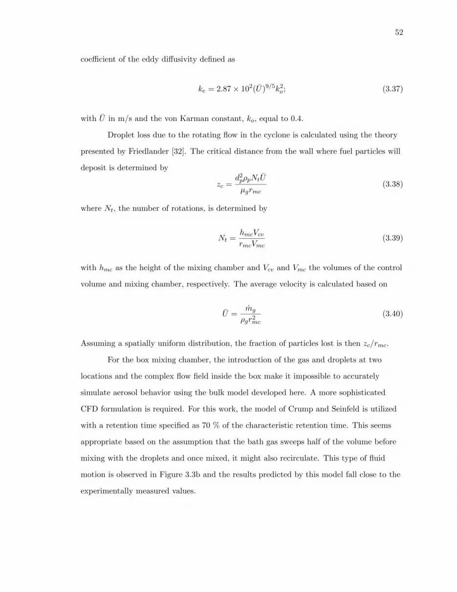
52
coefficient of the eddy diffusivity defined as
ke = 2.87× 10²(U)9/5k2o ; (3.37)
with U in m/s and the von Karman constant, ko, equal to 0.4.
Droplet loss due to the rotating flow in the cyclone is calculated using the theory
presented by Friedlander [32]. The critical distance from the wall where fuel particles will
deposit is determined by
zc =d2pρpNtU
µgrmc(3.38)
where Nt, the number of rotations, is determined by
Nt =hmcVcvrmcVmc
(3.39)
with hmc as the height of the mixing chamber and Vcv and Vmc the volumes of the control
volume and mixing chamber, respectively. The average velocity is calculated based on
U =mg
ρgr2mc
(3.40)
Assuming a spatially uniform distribution, the fraction of particles lost is then zc/rmc.
For the box mixing chamber, the introduction of the gas and droplets at two
locations and the complex flow field inside the box make it impossible to accurately
simulate aerosol behavior using the bulk model developed here. A more sophisticated
CFD formulation is required. For this work, the model of Crump and Seinfeld is utilized
with a retention time specified as 70 % of the characteristic retention time. This seems
appropriate based on the assumption that the bath gas sweeps half of the volume before
mixing with the droplets and once mixed, it might also recirculate. This type of fluid
motion is observed in Figure 3.3b and the results predicted by this model fall close to the
experimentally measured values.

53
Straight Tube Removal Model
The straight tube removal sub-model used in the aerosol model was developed by Anand
et al. [8, 43]. This sub-model is used for straight tubes within the fueling system as well
as the reaction chamber. The particle fraction loss in the tube is
χtu = 100
(1− e
−πdtuUefxtu
Q
)(3.41)
where Q is the volumetric flow, xtu is the length of the tube segment and the effective
velocity is
Uef =Udfθcπ
+Udf2
+UTSsin(φtu)cos(θc)
π(3.42)
with φtu as the angle of the tube from vertical and the settling velocity, which is
dependent on droplet size, calculated from Eq. (2.2). The critical angle in a tube cross
section defined as
θc =
0, if UTSsin(φtu) = 0
asin(
UdfUTSsin(φtu)
), if UTSsin(φtu) > Udf
π/2, if UTSsin(φtu) ≤ Udf
(3.43)
The velocity caused by diffusion is defined as
Udf = U+U√f/2 (3.44)
when
U+ =
6.9× 10⁻⁴τ2
+, if τ+ ≤ 15
0.16/τ0.086+
, if τ+ > 15
(3.45)
and
τ+ =τUfRe
dtu(3.46)

54
The friction factor is given by the Blasius equation
f =0.316
4Re0.25 (3.47)
where the Reynolds number is based on the tube diameter.
Bend Removal Model
The deposition sub-model developed by Tsai and Pui [53] was initially incorporated into
the model in order to determine the removal of aerosol particles, assuming laminar flow.
However, this sub-model significantly underpredicts experimentally measured aerosol loss
within the system mock up, as well as a simple tube bend. In an attempt to reconcile
these discrepancies an empirical correlation was developed based on the Tsai and Pui
model, and validated by experimental gravimetric measurements. The bend removal
model can be written as
χb =θb90χb,LF + 3.75χtu (3.48)
Here χb,LF represents a correlation to the Tsai and Pui model which is dependent on
droplet Stokes number, and χtu is a gravitational settling component. A detailed
discussion of this is included in Appendix C where the gravitational validation
measurements are reviewed. The sub-model assumes uniform deposition throughout the
bend and was developed over a range of Dean numbers with Ro = 7.38. The bend is
assumed to be positioned such that the inlet is above a horizontal outlet with the bend
angle, θb, measured in degrees.
This combined sub-model is not expected to be completely accurate when used in
the aerosol model to predict losses. For example, in the aerosol system the bend angles
will be less than 90 degrees and some bends are positioned such that the inlet is below a
horizontal outlet. However, the loss in the valve housing in most configurations only
contributes a small amount to the total loss (i.e. 4 - 12 %) so innacuracies of this
sub-model do not have a great affect on the loss predictions. Though this is not ideal, it
allows for a determination of aerosol behavior in the delivery system over a range of

55
conditions.
Valve Seat Removal Model
The model for the loss of particles onto the valve seat is taken from Ranz & Wong [55].
Loss onto the surface, which is modeled as a disc obstructing the flow, is determined by
χdi =AdiAcs
[S2 − S1
S2eS1t∗c − S1eS2t∗c
]2
(3.49)
with Adi as the projected area of the disc, Acs as the cross-section of the aerosol flow (i.e.
the tube cross section) and
S1,2 = − 1
4 St±
√(1
4 St
)2
+1
2 St(3.50)
and the dimensionless time of surface impact is
t∗c =atan
(4qSt
8St−1
)q
(3.51)
with
q =
√1
St−(
1
4St
)2
(3.52)
The characteristic length for the determination of the Stokes number in the previous
equations is the diameter of the disc.
Valve Stem Removal Model
The model proposed by Wessel and Righi [54] is used to calculate the loss of aerosol
particles due to the stem of the valve. The deposition efficiency onto this cylindrical

56
Table 3.3: Coefficients for use with Eq. (3.53)
A B C D E F
0.01978749 0.5136545 -0.0482858 1.54424 -0.538013 0.2020116
obstruction is
χstemAstem/Acs
=
0, if Ste < 0.125
Aln(8 Ste) +B(Ste − 0.125) + C(Ste − 0.125)2, if 0.125 < Ste ≤ 0.5
[1 +D(Ste − 0.125)−1 + E(Ste − 0.125)−2
+F (Ste − 0.125)−3]−1, if 0.5 < Ste
(3.53)
where the coefficients are listed in Table 3.3 and
Ste = Stψ (3.54)
with
ψ =3[√
cRe1/3p − atan(
√cRe
1/3p
]c3/2Rep
(3.55)
where c = 0.158 and Rep is the Reynolds number with the particle diameter as the
characteristic length and U as the average gas velocity.
3.6 Time Step Control
Within the aerosol model the time step must be controlled in order to prevent numerical
diffusion as droplets are moved between bins due to evaporation and coagulation, and
control the accuracy of the application of the removal sub-models. The size of time steps
in the aerosol model, and therefore the bulk transport within the system components, is
modulated by the evaporation and coagulation sub-models. This is conducted in order to
prevent bins from having a negative value for the particle count and to improve the
resolution of the model.
The evaporation sub-model is used to set the time step when the pressure of the
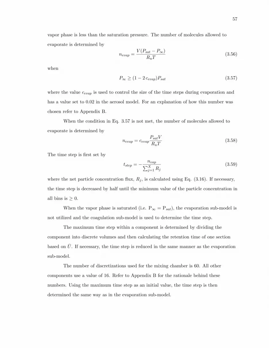
57
vapor phase is less than the saturation pressure. The number of molecules allowed to
evaporate is determined by
nevap =V (Psat − P∞)
RuT(3.56)
when
P∞ ≥ (1− 2 cevap)Psat (3.57)
where the value cevap is used to control the size of the time steps during evaporation and
has a value set to 0.02 in the aerosol model. For an explanation of how this number was
chosen refer to Appendix B.
When the condition in Eq. 3.57 is not met, the number of molecules allowed to
evaporate is determined by
nevap = cevapPsatV
RuT(3.58)
The time step is first set by
tstep = − nvap∑Xj=1Rj
(3.59)
where the net particle concentration flux, Rj , is calculated using Eq. (3.16). If necessary,
the time step is decreased by half until the minimum value of the particle concentration in
all bins is ≥ 0.
When the vapor phase is saturated (i.e. P∞ = Psat), the evaporation sub-model is
not utilized and the coagulation sub-model is used to determine the time step.
The maximum time step within a component is determined by dividing the
component into discrete volumes and then calculating the retention time of one section
based on U . If necessary, the time step is reduced in the same manner as the evaporation
sub-model.
The number of discretizations used for the mixing chamber is 60. All other
components use a value of 16. Refer to Appendix B for the rationale behind these
numbers. Using the maximum time step as an initial value, the time step is then
determined the same way as in the evaporation sub-model.

58
In both sub-models, the cumulative volume swept by the aerosol is determined by
Vtot,e = Vtot,in +mg∆t
ρg. (3.60)
where Vtot,in is the volume swept before entering the control volume. If the cumulative
volume swept is greater than the total volume of the component, the time step is reset so
that the cumulative volume swept is equal to the total volume of the component.
The next chapter presents validation results for the model based on experimental
data acquired from a mock-up of an aerosol RCM.

59
Chapter 4
RESULTS AND DISCUSSION
In this chapter, the aerosol model described in the Chapter 3 is first validated using an
aerosol RCM mock up with water as the ‘fuel’ and the model is then utilized to gain
insight into the behavior of the system. Of particular interest is how the aerosol evolves as
it is transported through the system components, which mechanisms are most important
during typical operation and how the operating conditions, including the fuel and diluent
conditions, impact the system performance. System performance is assessed here based on
aerosol loss and peak droplet diameter in the reaction chamber. The chapter concludes
with a discussion of potential improvements to the delivery system and aerosol model.
4.1 Aerosol System Experiments
Experiments have been conducted to investigate the behavior of an aerosol in an RCM
mock up within the Energy Lab at Marquette University. The intent is to understand how
various configurations and operating parameters affect system performance. The goal is to
Figure 4.1: Diagram of the aerosol RCM mock up at Marquette University

60
design a system that can achieve low levels of droplet fallout and bulk scale droplet
stratification at operating conditions where stoichiometric fuel loading is possible at
atmospheric oxygen concentrations. The RCM mock up was designed, built, and modified
by John Bustamante, Mike Denk, Mike Johnson, Alex Polley and Colin Banyon under the
direction of Dr. S. Scott Goldsborough. As discussed in previous chapters, the delivery
system consists of a mixing chamber, delivery tube, valve housing, reaction chamber and
exit manifold. A schematic was presented earlier in Figure 1.12 and is shown again in
Figure 4.1. A description of the initial configuration and experiment results follows. As
mentioned in Chapter 1, the poor performance seen in the results was a motivation for the
current work.
The droplets for the aerosol are generated with tap water using an array of
Aeroneb OnQ nebulizers (usually four) that are assembled onto a detachable tray with a
covered trough that seats onto the top of the mixing chamber. The initial rectangular
mixing chamber measures 0.178 m × 0.152 m × 0.203 m and is fabricated from 6.4 mm
thick acrylic plastic. Air from the building’s compressed air line is introduced at the side
of the mixing chamber. The gas flow is metered using orifices from O’Keefe Controls
Company. The air pressure before and after the orifice is measured using MGA-100-A-9V
digital gages from SSI Technologies, Inc.
After the mixing chamber, the aerosol is transported through a delivery tube that
connects to the valve housing. The tubing is Kuri Tec Clearbraid which has an internal
diameter (ID) of 12.7 mm and length of 1.65 m.
The initial valve housing (#1) is machined from aluminum and contains a 12.7
mm ID tube which leads to a horizontal cylinder (i.e., the reaction chamber) that is 0.051
m in diameter by 0.038 m long. Inside the valve housing, the path of the tube comes to a
right angle after which the aerosol is introduced to the cylinder. At the open end of the
valve housing cylinder a 0.064 m diameter by 0.013 m deep counter bore is employed to
accept the reaction chamber. This is illustrated in Figure 4.2a.
The reaction chamber is simulated by a cylindrical glass tube with inside diameter
of 0.051 m and length of 0.305 m. After the reaction chamber, the aerosol flows through
an exit manifold that has the same configuration as the inlet valve housing (#1) and

61
(a) (b)
Figure 4.2: (a) The location of the hose barb and poppet valve and (b) loss results frominitial configuration of the fuel delivery system. Experiments are conducted at T = 298 K,P = 1 bar, ml = 1.31 g/min and ReRC ≈ 517.
allows the aerosol to exit the delivery system.
Experiments are conducted at T ≈ 297 K and P = 1 bar. To begin an experiment,
the mixing chamber, delivery tube, valve housing, reaction chamber and exit manifold are
weighed using a Mettler Toledo SB16001 scale and then assembled. About 200 mL of
water is added to a 600 mL beaker and covered to prevent evaporation loss. The beaker,
nebulizer tray and both covers are weighed together before the experiment.
The pressure behind the orifice is measured and the mass flow rate of the gas is
calculated using the ideal gas, choked flow expression,
m = AoCdPtu
√γ
RTtu
(2
γ + 1
) γ+12(γ−1)
(4.1)
where Ao is the area of the orifice opening, Ptu the pressure of the gas behind the orifice,
Ttu the temperature of the gas behind the orifice, γ the specific heat ratio and 0.9 is used
as the discharge coefficient, Cd [84].
The water is poured from the beaker into the nebulizer tray and both components
are covered to prevent evaporation loss. The nebulizers are powered on to initiate the
experiment. The nebulizers run for ≈ 30 minutes and are then powered off. Adequate flow
is required in order to achieve resolution with the Mettler scale. The air flow is allowed to
continue until the aerosol clears the system.

62
Table 4.1: Operating conditions for initial aerosol system experiments
Case 1 2 3
Mixing Chamber Design box box box
Delivery Tube ID (mm) 12.7 12.7 12.7
Delivery Tube Length (m),Position
1.65,Horizontal
1.65,Horizontal
1.65,Horizontal
Valve Housing Design #1 #1 #1
Barb no yes yes
Valve no no yes
Water Delivered byNebulizers (g/min)
1.31 1.31 1.31
Flow Rate (L/min) 18.8 18.9 18.7
Temperature (K) 298 298 298
Pressure (bar) 1 1 1
Aerosol Concentration(mL/L)
0.070 0.069 0.070
Total Aerosol Loss (%) 18.58±1.92 20.56±1.92 24.37±1.92
The air flow is shut off, the system dismantled and each component weighed again.
The difference between the final and initial mass is divided by the duration of the run to
determine the rate of aerosol loss in the components. Likewise, the difference between the
initial and final mass of the nebulizer tray and beaker is divided by the experiment
duration to determine the aerosol delivery rate.
Results using the initial system configuration with operating parameters listed in
Table 4.1 are presented in Figure 4.2b. The indicated uncertainty is discussed in Appendix
D. These tests are conducted to investigate the influence of restrictions within the system.
Case 1 uses no poppet valve and no barb to connect the delivery tube. Case 2 has the
barb but no valve, and Case 3 has the connecting barb and the poppet valve. As can be
seen in Figure 4.2b, when more restrictions are placed in the path of the aerosol, the losses
in the system are increased. This is due to two factors. First, the restrictions may changes
in the flow of the aerosol which results in increased deposition of particles that do not
adjust to the flow before impacting a wall. Second, restrictions can also provide more
opportunity for impaction since more surface area may be presented to the aerosol.
Modifications to these components and system configuration were undertaken in

63
Figure 4.3: Comparison of the DSDs produced by the two types of Aeroneb OnQ nebulizersand the Pelas AGF 2.0. The legend value in parentheses was used for normalization.
an attempt to reduce the system losses. Experimental and simulation results of the
modifications are presented later in this chapter. The next few subsections discuss some
modeling details and validation of the system model.
4.2 Droplet Size Distributions
The DSDs used for the simulations are taken from the literature and discretized into
sectional distributions with bin spacings of 0.1 µm. In the case of the AGF 2.0 discussed
below, the bins under a diameter of 1 µm have spacings of 0.01 µm. Representative
volume fractions for these nebulizers are shown in Figure 4.3.
Kuhli et al. [85] measured the production from a low flow, Aeroneb OnQ nebulizer
(VMD = 4.09 µm) using three different methods including optical particle counting,
cascade impaction and laser diffraction. The droplet diameters from this distribution are
shifted (i.e. increased) in order to model a high flow Aeroneb OnQ nebulizer (VMD =
6.35 µm).
Rotovera et al. [25] measured the output from a Pelas Technology AGF 2.0
Aerosol Generator using laser diffraction. This generator is used in the aerosol shock tube
of Texas A&M University. This device employs compressed air to create the droplets and
the maximum aerosol concentration is 0.01 mL liquid per L of gas (i.e. φdodecane ≈ 0.04 in
air at 297 K) thus diluted conditions (O2 < 21 %) must be utilized in the ignition tests.

64
(a) (b) (c)
Figure 4.4: Internal geometries of (a) the initial valve housing [#1], and the second gener-ation housings with entry on the (b) side [#2] and (c) base [#3] of the housing cylinder.The boss on the inlet to the housing accepts the valve stem and the red arrows show thedirection of aerosol flow.
While high liquid concentrations are not physically achievable with this device (liquid
volume ratio < 0.01 mLliq/Lgas) , it is useful to compare its performance to the Aeroneb
nebulizers since much smaller droplets are generated and this may be useful for
investigating larger hydrocarbon and oxygenated hydrocarbon fuels.
Shadowgraphy and phase doppler anemometry (PDA) techniques were attempted
for this thesis as a means of experimentally quantifying the DSD changes experienced
through the delivery system and further validating the aerosol model. However, these
measurements were not successful. A discussion of these is presented in Appendix E.
Primary validation of the aerosol model is achieved through the gravimetric measurements.
4.3 Model Validation and System Modifications
A series of system modifications was undertaken in an attempt to decrease substantial
aerosol losses in the system. The modifications as well as measured and predicted losses
are discussed in this section. The data for the cyclone mixing chambers was collected by
Colin Banyon. Refer to Table 4.2 for the operating conditions used for these experiments.
Aerosol losses in the initial valve housing (#1) of the system were high considering
the small amount of residence time in the component. In order to reduce losses, the valve
housing was redesigned so that the aerosol is introduced into the cylinder along a wider
bend and larger cross-section; a 19.1 mm ID tube with 35◦ curve of radius of 76.2 mm is

65
Tab
le4.2
:O
per
atin
gco
nd
itio
ns
for
mod
ified
aero
sol
syst
emex
per
imen
ts
Case
45
67
89
10
Mix
ing
Ch
amb
erD
esig
nB
oxB
oxB
oxB
oxC
ycl
one
Cycl
one
Cycl
one
Del
iver
yT
ub
eID
(mm
)12.7
12.7
12.7
25.4
25.4
25.4
25.4
Del
iver
yT
ub
eL
ength
(m),
Posi
tion
1.6
5,
Hor
izon
tal
1.65
,H
oriz
onta
l1.
65,
Hor
izon
tal
1, Hor
izon
tal
0.8,
Ver
tica
l;0.
2,55◦
ben
d
0.8,
Ver
tica
l;0.
2,55◦
ben
d
0.8,
Ver
tica
l;0.
2,55◦
ben
d
Valv
eH
ou
sin
gD
esig
n#
3#
3#
3#
5#
5#
5#
5
Hos
eB
arb
use
dto
con
nec
tD
Tan
dV
Hn
on
on
on
on
on
on
o
Valv
ep
rese
nt
inV
Hn
oye
sn
on
oye
sn
on
o
Wate
rF
low
Rate
from
Neb
uli
zers
(g/m
in)
1.3
21.
341.
381.
330.
941.
092.
38
Gas
Flo
wR
ate
(L/m
in)
18.8
19.1
32.1
18.8
19.8
40.0
30.1
Syst
emT
emp
erat
ure
(K)
297
297
297
298
297
297
298
Syst
emP
ress
ure
(bar)
11
11
11
1
Aer
osol
Con
centr
atio
n(m
L/L
)0.0
70
0.07
00.
043
0.07
10.
047
0.02
70.
079
Tot
al
Syst
emA
eros
ol
Loss
(%)
14.1
0±
1.92
15.7
0±1.
927.
27±
1.44
(w/o
RC
)13
.64±
1.92
7.77±
1.92
2.77±
1.92
15.0
4±1.
92

66
Figure 4.5: Measured and modeled losses in aerosol system components for Cases 4 & 5.Conditions for the system are T = 297, P = 1 bar, ml ≈ 1.3 g/min and ReRC ≈ 520.
used. Two variations of the housing were made where the aerosol is introduced to either
the side (#2) or base (#3) of the cylinder. The second generation housings were machined
from aluminum (#2) or made from ABS plastic (#3) in a rapid prototyping machine,
respectively. The internal geometries of the initial and redesigned valve housings are
depicted in Figure 4.4.
The aerosol model predicts that the loss in the second generation valve housing
will be reduced to 1.04 % when no valve is present and 1.42 % when a valve is present.
Unfortunately however, the model is not able to indicate whether there is a difference
between the performance of the side or base entry. Model predictions match fairly well
with experiment measurements of aerosol loss for Case 4 & 5 and the comparison is
presented in Figure 4.5.
In the initial configuration particles flow into a sharp angle where the aerosol must
change direction quickly which allows inertia to carry the larger particles into the wall. By
adding the curve, directional changes in the flow field are not as drastic and larger
particles have more time to adjust and not deposit on the walls.
The difference between the measured and modeled delivery tube loss is likely a
result of the tube position in the experiment. When performing the experiments, the
position of the tube was not held constant or recorded. On the other hand, the position of
the tube was assumed to be horizontal for the simulations. In the experiment without the
valve, the configuration of the tube was likely positioned close to horizontal for the entire

67
Figure 4.6: Measured and modeled losses in aerosol system components using valve housing#3. Conditions for the system are T = 297, P = 1 bar, ml = 1.38 g/min and ReRC = 879.
length of the tube. In the case of the experiment with the valve, the tube may have
curved once or twice on the way to the reaction chamber, increasing the loss; though, this
was not carefully controlled or documented in the experiments.
At a higher flow rate (i.e. ReRC = 879) the model predicts that the losses will be
reduced in each component as shown in Figure 4.6. This is the case for the experimental
measurements of the mixing chamber and valve housing for Case 6, but not for the
delivery tube. The loss in the reaction chamber was not measured. The discrepancy in the
delivery tube can once again be attributed to the configuration of the delivery tube in the
system. In this instance, a portion of the delivery tube may have been positioned
vertically, which works to reduce deposition losses. In the figure, it can also be seen that
modeled value for the valve housing overpredicts the measured losses. This discrepancy
might be due to the fact that the flow through the tube is in the transition regime
between laminar and turbulent flow (i.e. Retu = 3516) and the model for removal in the
tube bend was not developed for this regime where droplet penetration is generally higher.
The next modification to the system changed the 12.7 mm ID delivery tube to a
25.4 mm ID Tygon tube with a length of 1 m. Two more valve housings with a side (#4)
and base (#5) entry to the cylinder were fabricated from ABS using the rapid prototyping
machine where the internal passages were increased from 19.1 to 25.4 mm. The model
predicts that the loss in the valve housing and delivery tube will remain about the same.
These predictions are compared to the experiment losses for Case 7 in Figure 4.7.

68
Figure 4.7: Measured and modeled losses in aerosol system components using valve housing#5. Conditions for the system are T = 298, P = 1 bar, ml = 1.33 g/min and ReRC = 516.
The measured loss decrease seen in the valve housing for Case 7 relative to Case 4
occurs for two reasons. First, the velocity of the flow in the tube is reduced due to the
larger diameter. This decreases the stopping distance of the particles. Second, the
diameter of the tube is increased. These changes reduce the Stokes number of particles
and a particles with lower Stokes number is less likely to be removed from an aerosol. Due
to the quasi-empirical sub-model for the bend though, these mechanisms are not
completely captured in the model.
Once again, the difference in predicted and measured losses in the delivery tube
seen in the data is likely due to the tube position. The 25.4 mm ID tube that was utilized
had a gentle arc that could not be straightened. As a result the tube had both inclined
and declined portions along its length which result in less deposition than would be
expected with a horizontal tube. Predicted losses in the delivery tube remain the same
because the effects of increasing the diameter and decreasing the length oppose each other.
The larger diameter decreases the flow though the tube. This means the aerosol remains in
the tube longer and particles are more likely to settle out. On the other hand, shortening
the tube decreases the retention time and less particles are lost for the same reason.
Another modification made to the fuel delivery system was to change the mixing
chamber from the box geometry to a cyclone with a 0.152 m diameter × 0.254 m high
cylinder and a cone with a half angle of Θ = 35◦. The bottom of the mixing chamber
opens to the 1 m x 25.4 mm ID delivery tube which is approximately positioned such that

69
Figure 4.8: Delivery system with cyclone mixing chamber. The delivery tube is not to scale.
a 0.8 m vertical section is followed by a 55 degree curve at a radius of 0.2 m before
meeting with the valve housing. A schematic of the system is presented in Figure 4.8. The
new configuration was designed to have well controlled mixing of droplets and gas.
Results from the model and experiment are shown in Figure 4.9. The model
predicts that the losses in the mixing chamber will be about the same as the box mixing
chamber and losses in the delivery tube will be smaller at similar conditions. The
measured results are in agreement with the delivery tube, but the mixing chamber losses
are less than half of the predicted values. The model does however predict the correct
trend where losses decrease as the Reynolds number of the reaction chamber increases.
The discrepancy in the magnitude of the loss could possibly be attributed to the aerosol
not sweeping the entire volume of the mixing chamber. This might happen if the aerosol
only flows along the outside of the cylinder with a dead zone in the center of the cylinder.
The possibility of incomplete sweeping of the mixing chamber was investigated for
Case 8 to determine the effect on the losses of the other components of the system. The
model results in Figure 4.10 show that the level of losses in the mixing chamber has a

70
Figure 4.9: Measured and modeled losses in aerosol system components using valve housing#5 and the 0.152 m diameter cyclone mixing chamber. Conditions for the system are T =297, P = 1 bar. For ReRC = 543, ml = 0.94 g/min and for ReRC = 1094, ml = 1.09 g/min.
Figure 4.10: Modeled losses in aerosol system components for a full and half sweep of themixing chamber using valve housing #5 and the 0.152 m diameter cyclone mixing chamber.Conditions for the system are T = 297, P = 1 bar, ReRC = 543 and ml = 0.94 g/min

71
Figure 4.11: Measured and modeled losses in aerosol system components using valve housing#5 and the 0.205 m diameter cyclone mixing chamber. Conditions for the system are T =298, P = 1 bar, ml = 2.38 g/min and ReRC = 825.
minimal effect on the losses of components down system from the mixing chamber. The
same pair of simulations was conducted for lower gas flow, higher liquid flow aerosols with
similar results. A more rigorous model is necessary to ascertain the reason for the
discrepancy, but the full and half sweep simulations show that even with uncertainty in
the mixing chamber losses, losses in the other components can be reasonably predicted
using the model.
For the delivery tube, losses are decreased because the majority of the tube is
vertical, therefore there is no surface for settling droplets to collect until the tube bend.
The final change to the delivery system was to increase the cyclone diameter to
0.205 m and was designed to accommodate up to 10 nebulizers in order to prepare fuel
rich (i.e. φ > 1.0) aerosols of high concentration. For this geometry though, the model
predicts that the loss in the mixing chamber will increase significantly. The simulations
also indicate that the loss in the delivery tube is expected to decrease while the loss in the
reaction chamber should increase, at least for the typical conditions expected to be
utilized. The model results are compared to experimental measurements in Figure 4.11.
In the experiment data and the model for Case 10, it should be noted that the
DSD from the nebulizers is thought to be slightly larger. This is probably due to problems
with the nebulizer manufacturer where adequate control could not be achieved with the
nebulizers provided to the laboratory. The overall output for these nebulizers is
approximately 0.60 g/min compared to 0.33 g/min for the lower VMD nebulizers.

72
The trend in the model and experiments can be explained as follows. The volume
of the 0.205 m diameter cyclone is ≈ 1.7 times larger than the other mixing chambers and
therefore the retention time is increased leading to larger losses. The larger droplet sizes
also contribute to the increase in mixing chamber loss because they have larger settling
velocities. The increased deposition in the reaction chamber is due to the larger initial
droplets and the fact that fewer droplet are removed in the delivery tube than previous
configurations.
It can be seen in the validation experiments that the aerosol model provides
reasonably accurate predictions of the expected losses in most fuel delivery system
components as the system configuration and operating conditions are changed. Another
method of validation not pursued in this study would be to measure the temperature at
the mixing chamber inlet and outlet. Comparing these measurements to model results
would help to confirm the evaporation and heat transfer models used.
Comparisons of experiment and model results show that the mechanisms in the
mixing chamber cannot be completely captured by the bulk model, however, the level of
losses in the mixing chamber do not significantly impact the level of losses in other system
components. In the next section the model is used to understand the important
mechanisms that effect the aerosol, follow the aerosol behavior inside the system, and
investigating conditions that could not be tested using the experimental setup.
4.4 Model Utilization
In this section, the model is used to understand the behavior of the aerosol in the delivery
system and predict how the system should behave over a range of parameters. The effect
of mechanisms, conditions along the system, operating maps of the aerosol system and
potential system improvements are presented next.
Unless otherwise stated, the simulated aerosol system is composed of:
1. Cyclone mixing chamber (.205 m ID, 35◦ tapered cone)
2. Delivery tube (25.4 mm ID) with a 50.8 mm vertical section followed by a 55◦ bend

73
(a) (b)
Figure 4.12: Percent loss in delivery systems components for n-dodecane in air with (a) φ= 1.0 and (b) φ = 2.0 at T = 350 K, P = 1 bar and ReRC = 800.
with a 76.2 mm radius
3. 2nd generation valve housing (#5) with a 25.4 mm ID inlet and poppet valve (6.1
mm OD stem, 31 mm OD seat)
4. Reaction chamber (51 mm ID, 0.305 m length)
4.4.1 Effect of Mechanisms
Simulations of n-dodecane in air (21 % O2, 79 % N2) are conducted with sub-models for
coagulation and evaporation sequentially turned on and off in order to ascertain the effect
on aerosol loss. The simulation conditions and results for these tests are presented in
Figure 4.12. A reaction chamber Reynolds number of 800 is used (40.1 LPM gas) with T
= 350 K and P = 1 bar. Fuel loadings of φ = 1 and 2 are investigated.
At low fuel concentrations (i.e. φ = 1), it can be seen that evaporation has a
major effect on the losses in an aerosol system because a large portion of the liquid mass
is vaporized. More droplets completely evaporate, lowering the particle concentration, and
the remaining droplets are reduced in size. On the other hand, because of the low
concentration conditions present coagulation has a minimal effect. Results when the
sub-model for Brownian coagulation is turned off are nearly identical to the results for all
models turned on, which is expected since Brownian coagulation is only significant for
particles below 1 µm. Results when the sub-model for gravitational coagulation is turned

74
Figure 4.13: Initial and final volume fraction DSDs of n-dodecane in air for φ = 1.0 and φ= 2.0 at T = 350 K, P = 1 bar and ReRC = 800.
off show a small effect on system losses. In this scenario, the coagulation creates larger
droplets which are more likely to fall out of suspension and increase losses in the aerosol
system.
At higher liquid concentrations (i.e. φ = 2), fuel droplets are more plentiful and
this creates an environment where droplets collide more frequently, increasing the impact
of gravitational coagulation. At the same time, the proportion of liquid converted to the
vapor phase is reduced and this lessens the effect of evaporation.
4.4.2 Evolution of DSD
The behavior of the aerosol DSD is also of interest since the droplets will need to be
evaporated during the compression stroke of the RCM’s pistons. In particular it is the
largest droplets that will require the longest time to evaporate, so these must be as small
as possible. The volume fraction DSD at the exit of each component in the delivery
system is therefore tracked for each of the conditions used in Section 4.4.1. In both cases,
it is found that the DSD is modified substantially only during the time that the aerosol is
retained in the mixing chamber. Thereafter, the DSD remains constant until it exits the
system.
A plot showing the initial and final DSDs is provided in Figure 4.13. The volume
fraction contained in the smaller droplets is first reduced as the droplets vaporize. Once

75
the gas phase is saturated, the smaller particles coagulate to form larger particles. This
moves mass to the larger particles as is shown in the plot. Only a slight difference is
present between the final DSDs for the two equivalence ratios and in particularly the peak
droplet size is unaffected by the fuel concentration of these conditions. As a percentage,
more mass exists in the gas phase for the lower equivalence ratio. This mass comes mainly
from the smaller droplets as they evaporate more quickly. The end result is a lower
percentage of small particles and greater percentage of large particles when compared to
the higher equivalence ratio.
4.4.3 Aerosol Behavior
The aerosol model is next used to track key parameters of the aerosol as it is transported
through the delivery system; these include the relative humidity (RH), mass percent
evaporated (MPE), mass percent lost (MPL) and aerosol temperature. The parameters
are defined as
RH = 100× P∞Psat
(4.2)
MPE = 100× mv
ml,0(4.3)
MPL = 100×ml,0 −ml −mv
ml,0(4.4)
For the investigation Case 1 is simulated with a flow rate of 18.8 LPM at T = 298
K, P = 1 bar (ReRC = 516) for the inlet gas. A liquid concentration at 0.070 mL/L with
water and n-dodecane as the liquids. Results from these simulations are shown in Figure
4.14. Here it can be seen that initial evaporation occurs very quickly (≈ 100 ms) with a
corresponding drop in temperature. As the aerosol moves through the system its
temperature, MPE and MPL slowly increase. When the aerosol reaches the delivery tube
a sharp rise in temperature occurs due to the increased heat transfer as the aerosol is
more exposed to the system boundaries. The MPE increases due to the increased
temperature while the MPL increases due to the more constricting geometry. The same
trends continue through the valve housing. As the aerosol moves into the reaction
chamber, the temperature and MPE begin to stabilize as contact with the system
76
(a) (b)
Figure 4.14: Relative humidity, mass loss, mass evaporation and aerosol temperature alongthe delivery system for (a) water and (b) n-dodecane at T = 298 K and P = 1 bar. The timein the mixing chamber (MC), delivery tube (DT) and reaction chamber (RC) is marked.The time in the valve housing is 0.01 s.
boundaries is decreased. A slight increase in the MPL occurs as the aerosol moves through
the reaction chamber and exits the system.
The RH for each liquid reaches 100 % after the initial evaporation and remains at
this level through-out the system. The unsteadiness in the water is attributed to the fact
that parameters in the model are optimized for n-dodecane. Using smaller evaporation
steps would result in an improved trace for the RH of water, as discussed in Appendix B
The difference in MPE is due to the difference in saturation pressures of the two
liquids. Water has a saturation pressure of about 0.03 bar at 297 K while Psat is 0.00014
bar for n-dodecane. While the vapor pressure of n-dodecane is 0.5 % of the value for
water, the MPE of n-dodecane is 5 % of the value for water. This factor of 10 is because
of the difference in molar mass between the two liquids: 18.02 and 170.3 g/mol for water
and n-dodecane, respectively.
The MPL for the water and n-dodecane are similar, with the values for
n-dodecane being smaller that values for water. This result is due to the differing densities
of the two liquids. The density of n-dodecane is 75 % of the value for water. This means
that a particle of n-dodecane will have a smaller terminal settling velocity and a lower
Stokes number that an equal sized particle of water.
The difference in the scale of the temperature traces for the two liquids is due to
77
Figure 4.15: Relative humidity, mass loss, mass evaporation and aerosol temperature alongthe delivery system for n-dodecane at T = 350 K and P = 1 bar. The time in the mixingchamber (MC), delivery tube (DT) and reaction chamber (RC) is marked. The time in thevalve housing is 0.01 s.
the different vaporization enthalpies. Water has hfg ≈ 2,440 kJ/kg while that for
n-dodecane is ≈ 350 kJ/kg, so that the bath gas experiences a larger temperature drop
with water.
A simulation was also run for n-dodecane in the cyclone fuel delivery system
described in Section 4.3 with T = 350 K, P = 1 bar, φ = 1.0 and ReRC = 800. The
results are shown in Figure 4.15 and differ from the simulation at lower temperature.
When the aerosol reaches the reaction chamber 44.5% of the mass is in the vapor phase.
This is more than water at 298 K and the reason is because of the difference in molar
mass, as discussed previously. With such a large percent of mass in the vapor phase, the
remaining aerosol droplets are smaller than at low temperature and thus they are not lost
as easily in the delivery system.
4.4.4 Operating Maps
The aerosol model was used to generate operating maps for the eight different aerosol
systems listed in Table 4.3. Simulations were run for overall fuel loading equivalence ratios
up to 2.0 with reaction chamber Reynolds numbers between 200 and 1200 as these are the
conditions under which RCM experiments are expected to be performed. Equivalence

78
Table 4.3: Operating conditions for simulated aerosol systems.
System 1 2 3 4 5 6 7 8
Nebulizer OnQ OnQ OnQ OnQ AGF 2.0 AGF 2.0 OnQ OnQ
Gas Air Air32% Ar,47% N2,21% O2
36% Ar,53% N2,11% O2
Air Air Air Air
Fuel C12H26 C12H26 C12H26 C12H26 C12H26 C16H34 C12H26 C16H34
T0 (K) 300 350 350 350 350 350 350 350
P0 (bar) 1 1 1 1 1 1 0.5 0.5
Figure 4.16: Operating map of System 1: Air + C12H26, OnQ nebulizer, T = 300 K, P =1 bar. The range of conditions for the experiments with water is indicated.
ratios and Reynolds numbers were incremented by values of 0.25 and 100, respectively.
The overall system loss and the droplet diameter under which 98% of the ‘fuel’
mass is contained, d98, in the reaction chamber are predicted for each of the operating
conditions. These values indicate the potential for performing an experiment in an aerosol
RCM. High losses are not acceptable because they will lead to uncertainty of fuel loading,
more frequent cleaning of equipment, and contamination of experment results. Small
droplets (i.e. < 4 µm for n-dodecane) are desired to ensure complete evaporation and
mixing during the compression of the RCM piston.
The predicted performance of System 1 is shown in Figure 4.16 where the
stratification limit for the OnQ nebulizer, determined by Johnson [28], is indicated. For
lower Reynolds numbers, the loss in the aerosol system is almost entirely dependent on

79
the overall fuel loading. As the flow rate increases, loss in the aerosol system decreases as
expected. However, the predicted losses for the highest flow rate are still unacceptable for
RCM experiments. The reduction in losses is mainly due to the decreased retention time
in the delivery system. Reducing the time that the aerosol is contained in the delivery
system limits the number of droplets that settle out of suspension.
Figure 4.16 also indicates the initial d98 value, d98,0, for the OnQ nebulizer of 11.7
µm. This value will decrease as droplets evaporate and the larger particles fall out of
suspension. At the same time, particles will also coagulate and increase the d98 value. The
d98,0 line indicated on the graph shows where these mechanisms are balanced. Above the
line, coagulation is more of a factor, and below the line, evaporation and removal are
larger factors.
In Figure 4.16 the mechanisms are balanced at an equivalence ratio of ≈ 0.5.
When the fuel loading is above 0.5, coagulation is the dominant mechanism affecting the
DSD. It is also important to note the spacing between the d98 contour lines. For slower
flows, droplet size increase is more pronounced as the fuel loading increases. This is once
again due to the increased retention time in the aerosol system, which allows more time
for the mechanisms to affect the DSD.
Another important feature of the plot in Figure 4.16 is that the vast majority of
fuel is in the liquid phase for the ’low’ temperature system. At 300 K, the gas phase has a
saturated equivalence ratio of 0.016. The large amount of fuel in the liquid phase results
in the performance behavior discussed above. With little evaporation, small droplets do
not disappear and large droplets do not decrease in size.
The behavior of the other systems listed in Table 4.3 are discussed next. For
System 2, the temperature is increased to 350 K. The operating map presented in Figure
4.17 shows that the increased temperature leads to significant decreases in aerosol losses.
Also shown is that the d98 values are lower than System 1 for equivalent operating
conditions. In this system more of the fuel evaporates because the higher temperature
increases the vapor pressure of the fuel. Thus, when the global equivalence ratio is below
≈ 0.5 all of the fuel is in the gas phase.

80
Figure 4.17: Operating map of System 2: Air + C12H26, OnQ nebulizer, T = 350 K, P =1 bar.
The increased evaporation is the main reason for both of the changes seen in the
operating map of System 2. Evaporation causes smaller droplets to completely vaporize
thereby reducing the aerosol droplet count density and also causes larger droplets to
decrease in size. Smaller particles are less affected by gravity and remain in suspension.
Smaller particles in aerosols with lower droplet count densities are also less likely to
coagulate and therefore the d98 values are not as large.
In both systems, the d98 value increases with increased fuel loading and, as stated
earlier, losses decrease as the flow rate increases. However, when the equivalence ratio is
near the level where the fuel is completely in the gas phase, the dependence on flow rate is
not as strong. This is when the droplets are smallest and do not settle out of the aerosol.
In System 3, the gas is composed 32 % Ar, 47 % N2 and 21 % O2 by volume. This
represents a test gas that is prepared using 21 % O2 and 79 % of a 60/40 blend of N2/Ar.
Argon is commonly used in RCM experiments due to its low heat capacity which allows
for increased compression temperatures to be achieved relative to using air at the same
compression ratio. Argon mixtures extend the temperature regime where an RCM can
operate. However, the larger molar mass of argon affects its transport properties and this
would impact performance of the aerosol fueling system.
The operating map for System 3 is shown in Figure 4.18. Here it is seen that the

81
Figure 4.18: Operating map of System 3: 32 % Ar / 47 % N2 / 21 % O2 + C12H26, OnQnebulizer, T = 350 K, P = 1 bar.
map is almost identical to the map of System 2 with the d98 and loss values slightly larger
for the individual operating conditions. This indicates that there is not a significant
change in behavior of aerosol particles between the air and the Ar/N2/O2 gas mixture,
even though the Ar mixture has a higher molar density which can reduce evaporation
rates and increase rates of heat transfer, as well as wall friction.
System 4 is configured using a gas mixture that represents a gas composed of 36 %
Ar, 53 % N2 and 11 % O2. Dilute mixtures are often used in STs and RCMs in order to
minimize extreme pressures after ignition takes place as well as decrease the chemical
reactivity in order to prevent reaction during the piston compression. The operating map
for this system is shown in Figure 4.19, and indicates different behavior from the previous
system. In this case, the mass of fuel needed to obtain a particular equivalence ratio is less
than the previous systems because of the reduced O2 concentration. At the same time, the
mass of fuel that enters the gas phase is the same as in the previous system. This leads to
a gas phase with a higher achievable equivalence ratio and a liquid phase that generally
has smaller droplets.
In Figure 4.19, it can be seen that once the system operates above the
stratification limit, increasing the fuel loading only has a small effect on the d98 value and
the flow rate has virtually no effect. The contour for the d98,0 value is no longer present on

82
Figure 4.19: Operating map of System 4: 36 % Ar / 53 % N2 / 11 % O2 + C12H26, OnQnebulizer, T = 350 K, P = 1 bar.
the plot indicating that the large extent of evaporation in this system reduces the droplet
sizes below this value.
System 5 used the same parameters as System 2 with the AGF 2.0 droplet
distribution, as opposed to the OnQ droplet distribution. The results in Figure 4.20 show
that a significant improvement in performance can be made by using smaller droplets.
While the trend of the aerosol loss contour lines is similar to previous systems, the amount
of loss is at the level where it will have almost no effect on an actual RCM experiment.
The stratification limit for the AGF 2.0 nebulizer has not been investigated unfortunately
and is expected to be significantly below the range presented on the operating map.
Comparing the operating maps for System 2 and 5 indicates that the droplet size
does not impact the amount of fuel that evaporates in the fueling system. This means
that the time scale for evaporation is much smaller than that for transport of the aerosol
through the delivery system. The plots also show that coagulation has only a limited
effect on the smaller droplets. In System 2, the range of d98 values is smaller for the high
flow rates. This is because the retention time in the system is decreased and there is less
time for particles to coagulate. In System 5, this trend is not present and the d98 value is
independent of the flow rate.
System 6 uses the same conditions as System 5, however the fuel is n-hexadecane,

83
Figure 4.20: Operating map of System 5: Air + C12H26, AGF 2.0 nebulizer, T = 350 K, P= 1 bar.
Figure 4.21: Operating map of System 6: Air + C16H34, AGF 2.0 nebulizer, T = 350 K, P= 1 bar.

84
Figure 4.22: Operating map of System 7: Air + C12H26, OnQ nebulizer, T = 350 K, P =0.5 bar.
as opposed to n-dodecane. n-Hexadecane is a larger fuel molecule (i.e. 16 carbons as
opposed to 12) and is more representative of biodiesel than n-dodecane. The operating
map for this system is shown in Figure 4.21.
Compared to the previous system, the equivalence ratio of the vapor phase is much
smaller because the vapor pressure for n-hexadecane is much lower than n-dodecane.
Also, once the equivalence ratio is above 0.25, the aerosol loss is predicted to be dependent
only on the flow rate. This change in behavior can also be attributed to the saturation
pressure since the other thermophysical properties of the two fuels are very similar.
The parameters for System 7 are similar to System 2, however the system pressure
is reduced from 1 bar to 0.5 bar. This condition will reduce the peak compressed
temperature during the experiment as well as reduce the chemical reactivity and alter the
fuel’s evaporation characteristics. The results from the simulation with this system are
shown in Figure 4.22. As it can be seen, the equivalence ratio supported by the gas phase
is once again increased because the lower amount of O2 in the bath gas.
The losses decrease significantly compared to System 4 where the O2 level is about
the same. The reduction in loss seen here is a result of the increased flow. In order to
maintain the same Reynolds number at 0.5 bar, the flow rate must be doubled because the
kinematic viscosity of the gas is doubled. Increased flow rate results in less residence time

85
Figure 4.23: Operating map of System 8: Air + C16H34, OnQ nebulizer, T = 350 K, P =0.5 bar.
which improves the system performance.
The plot shows that an aerosol in this system is not retained long enough to be
affected by coagulation. On the other hand, the simulation results for this case indicate
that the Reynolds number based on the bulk scale characteristics might not be the best
value for comparison between all systems. The changing pressure has a direct impact on
the Reynolds number, but does not significantly alter the Stokes number of the droplets,
which is a more important parameter affecting the individual droplet behavior.
In the final System, n-hexadecane is used as the fuel under the same parameters as
in System 7. The results are shown in Figure 4.23 and are once again much different than
the system using n-dodecane. The reduced effect of evaporation due to the low saturation
pressure of the fuel leads to a system where losses are only dependent on the gas flow rate.
However, once the flow rate is above the stratification limit, the effect of the flow rate on
the losses is greatly reduced and the range of d98 values is very small. Both of these
results can be attributed to the reduced retention time.
It can be seen that the trends for losses in the reaction chamber follow closely with
the trends in the overall loss in the aerosol system. For the OnQ nebulizer droplet
distribution, the losses in the reaction chamber generally account for 21 % of the over all
system loss. The most significant contribution to the aerosol loss comes from the mixing

86
chamber, which on average, makes up about 65 % of the overall system loss, while the
curved portion of the delivery tube contributes the remaining losses. On the other hand,
for the AGF 2.0 nebulizer, the reaction and mixing chambers contribute roughly 13 and
80 % of the overall loss, respectively.
4.5 Fuel Delivery System Improvements
Based on the results from simulations conducted in the previous section, it appears that
the most effective way to improve the system performance is to generate aerosols with
very small droplets. Unfortunately, current technologies capable of generating small
droplets are not able to achieve high enough fueling loads. Even though this is the case,
the simulations do provide insight into the droplet distributions that are needed in order
to deliver an appropriate droplet size to the reaction chamber. At 350 K and above a
reaction chamber Reynolds number of 500, the delivered distributions had a d98 that was
no larger than 7 % of the original value and the majority of operating conditions had d98
values that were lower than the initial value. Therefore, a delivered droplet distribution
should have a d98 that is equal to the desired delivered value.
Simulations and experiments also showed that systems with larger droplets (i.e. >
1 µm) performed best when the retention time is the smallest, because the effects of
coagulation and removal are reduced. Therefore, each component in the system needs to
be properly sized. This is most important for the mixing chamber, where the majority of
system losses occur. Properly sized for this component means that once the aerosol is
homogeneous it should enter the delivery tube.
Another design feature that could be modified to further reduce losses in the
system would be to remove the curved portion of the system (i.e. delivery tube and valve
housing). This would require the use of a different type of valve (e.g. ball, gate, or
butterfly) that would need to be designed for the high temperature and pressure
environment experienced in an RCM. The poppet valve was originally used because of its
simplicity and low cost. Removing the curve also means that the mixing chamber outlet
would need to be on the side similar to the box-type mixing chamber.

87
4.6 Areas for Model Improvement
The major area for improvement in the aerosol model lies in the bend removal sub-model.
A semi-empirical fit of the data was used and is only shown to correlate to experimental
results at one geometry of the tube bend. Therefore, the model is not able to test the
effect of changing the geometry of a bend in the system.
Another area for improvement is the mixing chamber removal sub-model. The
bulk model presented is not able to predict the magnitude of aerosol loss. It assumes that
all particles move through the system at the same rate and this is not the case. Larger
particles move to the exit of the mixing chamber more quickly that the smaller molecules
because of increased settling velocity. In order to more accurately predict the losses, a
more refined method that can track particle location is necessary.
Finally, multiple assumptions were made in the model in order to simplify the
calculations and allow for exploration of the system performance over a range of operating
conditions and various system setups. Therefore, it would be useful to validate the
assumptions by comparing model results to other studies of the aerosol system. CFD
simulations or measurement of droplet distributions along the aerosol system are two
potential methods that could be used for additional, more rigorous validation of the
system model.

88
Chapter 5
SUMMARY
The main goal of this thesis was to develop a model that could be used to understand the
behavior of dense aerosols in a fuel delivery system under laminar flow conditions, as well
as predict system performance over a range of operating conditions. This study is
applicable the development of an aerosol RCM that can be used to measure the chemical
kinetics of low-volatility fuels such as biodiesel.
The model predictions for aerosol losses in a fuel delivery system mock-up matched
fairly well with measured results from experiments. The experiments were conducted with
an aerosol of water in air at T = 297 K, P = 1 bar and at system flow rates of 19 and 33
liters per minute. The loss in the mixing chamber could not be consistently predicted,
however, the trends in performance were captured reasonably well. It was shown that the
magnitude of the predicted mixing chamber loss did not have a large effect on the level of
losses in other components and, therefore, the model could be used to predict losses in the
reaction chamber. Any loss in the reaction chamber can affect the RCM experiment
results and it is important to know what levels of loss are expected.
The model was used to gain an understanding of important mechanisms and to
predict system performance of fuel aerosols in various fueling systems and operating
conditions. The study showed that the generated and delivered DSDs do not differ
greatly, and for most operating conditions, the delivered DSD has a smaller d98 value than
the the generated DSD. This is an important result to consider for the design of the
delivery system. Initially, it was suspected that smaller droplets would lead to increased
coagulation due to the high particles densities, but this was not shown to be a problem.
The study also showed that gravity is the most important force influencing the

89
behavior of the aerosols in the system. It is responsible for large droplets settling out of
suspension and coagulating with smaller, slower settling droplets before depositing on
system components. Therefore, it both causes and enhances the loss in the system.
The simulations show that one technique to reduce the effect of gravity is to
increase the flow rate through the delivery system. This decreases the time over which
gravity can impact an aerosol. Another way to reduce the effect of gravity is to perform
experiments with smaller aerosol droplets. However, generating droplets that are small
enough in a high enough concentration aerosol is a major challenge that would need to be
overcome in order to successfully perform an actual RCM experiment. Finally, another
method, though probably not as practical, would be to reduce the gravitational force itself
and conduct experiments in microgravity conditions.

90
BIBLIOGRAPHY
[1] W.C. Hinds. Aerosol Technology. John Wiley & Sons, New York, 1999.
[2] J. H. Seinfeld and S. N. Pandis. Atmospheric Chemistry and Physics : From AirPollution to Climate Change. John Wiley & Sons, New York, 2006.
[3] M. Frenklach. Reaction mechanism of soot formation in flames. Phys. Chem. Chem.Phys., 4:2028–2037, 2002.
[4] S. J. Harris and M. M. Maricq. Signature size distributions for diesel and gasolineengine exhaust particulate matter. Journal of Aerosol Science, 32(6):749 – 764, 2001.
[5] A. J. Hickey. Pharmaceutical Inhalation Aerosol Technology. Marcel Dekker, NewYork, 2004.
[6] J.-H Park and T. S. Sudarshan. Chemical Vapor Deposition. ASM International,Materials Park, OH, 2001.
[7] Y. Sharifi and L. Achenie. Particle dynamics in a chemical vapor deposition reactor:A multiscale approach. Industrial & Engineering Chemistry Research,48(13):5969–5974, 2009.
[8] N. K. Anand, A. R. McFarland, K. D. Kim, and F. S. Wong. Optimization of aerosolpenetration through transport lines. Aerosol Science and Technology, 16(2):105 – 112,1992.
[9] A. P. Jones. Indoor air quality and health. Atmospheric Environment, 33(28):4535 –4564, 1999.
[10] A. D. Maynard and A. T. Zimmer. Development and validation of a simple numericalmodel for estimating workplace aerosol size distribution evolution throughcoagulation, settling, and diffusion. Aerosol Science and Technology, 37(10):804 –817, 2003.
[11] M.V. Johnson, G.S. Zhu, S.K. Aggarwal, and S.S. Goldsborough. Dropletevaporation characteristics due to wet compression under RCM conditions.International Journal of Heat and Mass Transfer, 53(5-6):1100 – 1111, 2010.
[12] S.S. Goldsborough, M.V. Johnson, G.S. Zhu, and S.K. Aggarwal. Gas-phasesaturation and evaporative cooling effects during wet compression of a fuel aerosolunder RCM conditions. Combustion and Flame, 158(1):57 – 68, 2011.
[13] S.S. Goldsborough, M.V. Johnson, G.S. Zhu, and S.K. Aggarwal. Fuel and diluentproperty effects during wet compression of a fuel aerosol under RCM conditions.Fuel, In-press.
[14] J. F. Griffiths and C. Mohamed. Experimental and numerical studies of oxidationchemistry and spontaneous ignition phenomena. In M. J. Piling, editor,Comprehensive Chemical Kinetics, Volume 35: Low-Temperature Combustion andAutoignition. Elsevier Science, Amsterdam, 1997.

91
[15] P. Dagaut, M. Cathonnet, J. P. Rouan, R. Foulatier, A. Quilgars, J. C. Boettner,F. Gaillard, and H. James. A jet-stirred reactor for kinetic studies of homogeneousgas-phase reactions at pressures up to ten atmospheres (-1 mpa). Journal of PhysicsE: Scientific Instruments, 19(3):207 – 209, 1986.
[16] Princeton University. PFCRL research.http://www.princeton.edu/~combust/research/reactor.jpg, November 2007.Last checked 4 April 2011.
[17] A. Ristori, P. Dagaut, and M. Cathonnet. The oxidation of n-hexadecane:experimental and detailed kinetic modeling. Combustion and Flame, 125(3):1128 –1137, 2001.
[18] G. Friedrichs. Shock tube / frequency modulation spectroscopy.http://www1.phc.uni-kiel.de/cms/index.php/de/research-m-gfr/
147-shock-tube-investigations-of-high-temperature-react-kin.html,January 2006. Last checked 16 April 2011.
[19] R. S. Tranter, K. Brezinsky, and D. Fulle. Design of a high-pressure single pulseshock tube for chemical kinetic investigations. Review of Scientific Instruments,72:3046 – 3054, 2001.
[20] H. S.Shen, J. Steinberg, J. Vanderover, and M. A. Oehlschlaeger. A shock tube studyof the ignition of n-heptane, n-decane, n-dodecane, and n-tetradecane at elevatedpressures. Energy & Fuels, 23(5):2482–2489, 2009.
[21] University of Connecticut. Rapid compression machine.http://combdiaglab.engr.uconn.edu/facilities/rapid-compression-machine.Last checked 4 April 2011.
[22] K. Kumar. Global Combustion Responses of Practical Hydrocarbon Fuels: n-heptane,iso-octane, n-decane, n-dodecane and ethylene. PhD thesis, Case Western ReserveUniversity, 2007.
[23] D.F. Davidson, D.R. Haylett, and R.K. Hanson. Development of an aerosol shocktube for kinetic studies of low-vapor-pressure fuels. Combustion and Flame,155(1-2):108 – 117, 2008.
[24] D. R. Haylett, D. F. Davidson, and R. K. Hanson. A second-generation aerosol shocktube for combustion research. In 48th AIAA Aerospace Sciences Meeting Includingthe New Horizons Forum and Aerospace Exposition, 2010.
[25] B. Rotavera, N. Polley, E. L. Peterson, K. Scheu, M. Crofton, and G. Bourque.Ignition and combustion of heavy hydrocarbons using and aerosol shock-tubeapproach. In Proceedings of ASME Turbo Expo 2010, pages 699 – 707, 2010.
[26] T. C. Hanson. The Development of a Facility and Diagnostics for StudyingShock-Induced Behavior in Micron-Sized Aerosols. PhD thesis, Stanford University,2005.
[27] R. K. Hanson, M. E. MacDonald, and D. F. Davidson. Shock tube studies of RPseries fuel surrogates and RP fuel thermal stability. http:

92
//melchior.usc.edu/fuelsummit/macccr2009/MACCCR_Hanson_RP_Fuels.pdf,September 2009. Last checked 5 April 2011.
[28] M. V. Johnson. Ignition studies of bio-based fuels for advanced combustion engines.Master’s thesis, Marquette University, 2009.
[29] C. Allen, G. Mittal, C.-J. Sung, E. Toulson, and T. Lee. An aerosol rapidcompression machine for studying energetic-nanoparticle-enhanced combustion ofliquid fuels. Proceedings of the Combustion Institute, 33(2):3367 – 3374, 2011.
[30] S.-L. von der Weiden, F. Drewnick, and S. Borrmann. Particle loss calculator - a newsoftware tool for the assessment of the performance of aerosol inlet systems.Atmospheric Measurement Technique Discussions, 2:1099 – 1141, 2009.
[31] D. J. Rader. Momentum slip correction factor for small particles in nine commongases. Journal of Aerosol Science, 21(2):161 – 168, 1990.
[32] S. K. Friedlander. Smoke, Dust and Haze Fundamentals of Aerosol Dynamics. OxfordUniversity Press, New York, 2000.
[33] C. N. Davies. Evaporation of airborne droplets. In D. T. Shaw, editor, Fundamentalsof Aerosol Science. Wiley-Interscience, New York, 1978.
[34] N. A. Fuchs and A. G. Sutugin. High dispersed aerosols. In G. M. Hidy and J. R.Brock, editors, Topics in Current Aerosol Research (Part 2). Pergamon Press, NewYork, 1971.
[35] J. Corner and E. D. Pendlebury. The coagulation and deposition of a stirred aerosol.Proceedings of the Physical Society. Section B, 64(8):645–654, 1951.
[36] J. G. Crump and J. H. Seinfeld. Turbulent deposition and gravitationalsedimentation of an aerosol in a vessel of arbitrary shape. Journal of Aerosol Science,12(5):405 – 415, 1981.
[37] S. H. Park, H. O. Kim, Y. T. Han, S. B. Kwon, and K. W. Lee. Wall loss rate ofpolydispersed aerosols. Aerosol Science and Technology, 35(3):710 – 717, 2001.
[38] N. A. Fuchs. The Mechanics of Aerosols. Pergamon Press, Oxford, England, 1964.
[39] J. W. Thomas. Gravity settling of particles in a horizontal tube. Journal of the AirPollution Control Association, 8:32 – 34, 1958.
[40] J. Heyder and J. Gebhart. Gravitational deposition of particles from laminar aerosolflow through inclined circular tubes. Journal of Aerosol Science, 8(4):289 – 295, 1977.
[41] S. K. Friedlander and H. F. Johnstone. Deposition of suspended particles fromturbulent gas streams. Industrial & Engineering Chemistry, 49(7):1151–1156, 1957.
[42] C. N. Davies. Deposition from moving aerosols. In Aerosol Science. Academic Press,New York, 1966.
[43] N. K. Anand and A. R. McFarland. Particle deposition in aerosol sampling linescause by turbulent diffusion and gravitational settling. American Industrial HygieneAssociation Journal, 50(6):307 – 312, 1989.

93
[44] H. D. Landahl and R. G. Herrmann. Sampling of liquid aerosols by wires, cylinders,and slides, and the efficiency of impaction of the droplets. Journal of Colloid Science,4:103 – 136, 1949.
[45] P. T. Hacker, R. J. Brun, and B. Boyd. Impingement of droplets in 90 degree elbowswith potential flow. Technical Report NACA-TN-2999, National Advisory Committeefor Aeronautics, 1953.
[46] H.C. Yeh. Use of a heat transfer analogy for a mathematical model of respiratorytract deposition. Bulletin of Mathematical Biology, 36:105–116, 1974.
[47] Y.S. Cheng and C.S. Wang. Inertial deposition of particles in a bend. Journal ofAerosol Science, 6(2):139 – 145, 1975.
[48] R.I. Crane and R.L. Evans. Inertial deposition of particles in a bent pipe. Journal ofAerosol Science, 8(3):161 – 170, 1977.
[49] M. Rowe. Measurements and computations of flow in pipe bends. Journal of FluidMechanics, 43(04):771–783, 1970.
[50] Y.S. Cheng and C.S. Wang. Motion of particles in bends of circular pipes.Atmospheric Environment (1967), 15(3):301 – 306, 1981.
[51] Y. Mori and W. Nakayama. Study of forced convective heat transfer in curved pipes(1st report, laminar region). International Journal of Heat and Mass Transfer, 8:67 –82, 1965.
[52] J. R. Johnston, K. D. Isles, and D. C. Muir. Inertial deposition of particles in humanbranching airways. In Inhaled Particles and Vapours 1975: 4: SymposiumProceedings, pages 61 – 73, 1977.
[53] C. Tsai and D. Y. H. Pui. Numerical study of particle deposition in bends of acircular cross-section-laminar flow regime. Aerosol Science and Technology, 12(4):813– 831, 1990.
[54] R. A. Wessel and J. Righi. Generalized correlations for inertial impaction of particleson a circular cylinder. Aerosol Science and Technology, 9(1):29 – 60, 1988.
[55] W. E. Ranz and J. B. Wong. Impaction of dust and smoke particles on surface andbody collectors. Industrial & Engineering Chemistry, 44(6):1371–1381, 1952.
[56] P. H. Gregory and O. J. Stedman. Deposition of air-borne lycopodium spores onplane surfaces. Annals of Applied Biology, 40(4):651–674, 1953.
[57] K. R. May and R. Clifford. The impaction of aerosol particles on cylinders, spheres,ribbons and discs. The Annals of Occupational Hygiene, 10:83 – 95, 1967.
[58] J.H. Vincent and W. Humphries. The collection of airborne dusts by bluff bodies.Chemical Engineering Science, 33(8):1147 – 1155, 1978.
[59] B. Petkovic. Deposition of droplets onto solid objects in aerosol flow. Master’s thesis,The University of British Columbia, Vancouver, 2010.

94
[60] S.H. Suck and J.R. Brock. Evolution of atmospheric aerosol particle size distributionsvia Brownian coagulation numerical simulation. Journal of Aerosol Science, 10(6):581– 590, 1979.
[61] T.H. Tsang and J.R. Brock. Simulation of condensation aerosol growth bycondensation and evaporation. Aerosol Science and Technology, 2(3):311 – 320, 1983.
[62] T.H. Tsang and J.R. Brock. On Ostwald ripening. Aerosol Science and Technology,3(3):283 – 292, 1984.
[63] T.H. Tsang and J.R. Brock. Dynamics of Ostwald ripening with coalescence foraerosols with continuum diffusive growth laws. Aerosol Science and Technology,5(3):385 – 388, 1986.
[64] Y. Zhang, C. Seigneur, J. H. Seinfeld, M. Z. Jacobson, and F. S. Binkowski.Simulation of aerosol dynamics: A comparative review of algorithms used in airquality models. Aerosol Science and Technology, 31(6):487 – 514, 1999.
[65] K. T. Whitby. Determination of aerosol growth rates in the atmosphere using lumpedaerosol dynamics. Journal of Aerosol Science, 12:174 – 178, 1981.
[66] E. R. Whitby and P. H. McMurry. Modal aerosol dynamics modeling. AerosolScience and Technology, 27(6):673 – 688, 1997.
[67] R. A. Hamilton, J. S. Curtis, and D. Ramkrishna. Beyond log-normal distributions:Hermite spectra for solving population balances. AIChE Journal, 49(9):2328–2343,2003.
[68] C. Seigneur, A. B. Hudischewskyj, J. H. Seinfeld, K. T. Whitby, E. R. Whitby, J. R.Brock, and H. M. Barnes. Simulation of aerosol dynamics: A comparative review ofmathematical models. Aerosol Science and Technology, 5(2):205 – 222, 1986.
[69] F. Gelbard, Y. Tambour, and J. H. Seinfeld. Sectional representations for simulatingaerosol dynamics. Journal of Colloid and Interface Science, 76(2):541 – 556, 1980.
[70] F. Gelbard and J. H. Seinfeld. Simulation of multicomponent aerosol dynamics.Journal of Colloid and Interface Science, 78(2):485 – 501, 1980.
[71] S. A. Makiharju. Aerosol dynamics in a turbulent jet. Master’s thesis, The OhioState University, 2005.
[72] H. K. Moffat. CADS cantera aerosol dynamics simulator. Technical ReportSAND2007-4216, Sandia National Laboratories, July 2007.
[73] K. von Salzen. Piecewise log-normal approximation of size distributions for aerosolmodeling. Atmospheric Chemistry and Physics, 6(5):1351 – 1372, 2006.
[74] A. Sandu. Piecewise polynomial solutions of aerosol dynamic equation. AerosolScience and Technology, 40(4):261 – 273, 2006.
[75] B. E. Poling, J. M. Prausnitz, and J. P. O’Connell. The Properties of Gases andLiquids. McGraw-Hill, New York, 2001.

95
[76] J. Szekely and R. Carr. Heat transfer in a cyclone. Chemical Engineering Science,21(12):1119 – 1132, 1966.
[77] W. M. Kays, M. E. Crawford, and B. Weigand. Convective Heat and Mass Transfer.McGraw Hill, New York, 2004.
[78] C. E. Kalb and J. D. Seader. Fully developed viscous-flow heat transfer in curvedcircular tubes with uniform wall temperature. AIChE Journal, 20(2):340–346, 1974.
[79] L. Pirjola, M. Kulmala, M. Wilck, A. Bischoff, F. Stratmann, and E. Otto.Formation of sulphuric acid aerosols and cloud condensation nuclei: An expression forsignificant nucleation and model comparison. Journal of Aerosol Science, 30(8):1079– 1094, 1999.
[80] E. Sajo. Evaluation of the exact coagulation kernel under simultaneous brownianmotion and gravitational settling. Aerosol Science and Technology, 42(2):134 – 139,2008.
[81] E. Sajo. Update and erratum on the numerical evaluation of the exact coagulationkernel under simultaneous brownian motion and gravitational settling. AerosolScience and Technology, 44(10):916, 2010.
[82] M. M. R. Williams. A unified theory of aerosol coagulation. Journal of Physics D:Applied Physics, 21:875 – 886, 1988.
[83] C. Banyon. CFD simulation of cyclone mixing chamber. Unpublished work,November 2011.
[84] R. W. Fox, A. T. McDonald, and P. J. Pritchard. Introduction to Fluid Mechanics.John Wiley & Sons, New York, 2006.
[85] M. Kuhli, M. Weiss, and H. Steckel. A sampling and dilution system for dropletaerosols from medical nebulisers developed for use with an optical particle counter.Journal of Aerosol Science, 40(6):523 – 533, 2009.
[86] K. Lucas. Berechnungsmethoden fur stoffeigenschaften. In VDI-Warmeatlas. VereinDeutscher Ingenieure, Dusseldorf, 1984.
[87] T. H. Chung, M. Ajlan, L. L. Lee, and K. E. Starling. Generalized multiparametercorrelation for nonpolar and polar fluid transport properties. Industrial &Engineering Chemistry Research, 27(4):671–679, 1988.
[88] A. Burcat. Prof. burcat’s thermodynamic data.http://garfield.chem.elte.hu/Burcat/burcat.html, March 2006. Last checked10 April 2011.
[89] E. N. Fuller, P. D. Schettler, and J. C. Giddings. New method for prediction ofbinary gas-phase diffusion coefficients. Industrial & Engineering Chemistry,58(5):18–27, 1966.
[90] C. Antoine. Tensions des vapeurs; nouvelle relation entre les tensions et lestemperatures. Comptes Rendus, 107:681 – 684, 778 – 780, 836 – 837, 1888.

96
[91] H. G. Rackett. Equation of state for saturated liquids. Journal of Chemical &Engineering Data, 15(4):514–517, 1970.
[92] V. Ruzicka and A. S. Domalski. Estimation of the heat capacities of organic liquidsas a function of temperature using group additivity. I. hydrocarbon compounds.Journal of Physical and Chemical Reference Data, 22(3):597–618, 1993.
[93] K. Wark. Advanced Thermodynamics for Engineers. McGraw-Hill Companies, UnitedStates, 1994.
[94] W. M. Haynes, editor. CRC Handbook of Chemistry and Physics. CRC Press; 91stedition, Cleveland, 2010.
[95] C. Gutfinger, D. Pnueli, L. Moldavsky, K. Shuster, and M. Fichman. Particle motionin simple shear flow with gravity. Aerosol Science and Technology, 37(10):841–845,2010.
[96] S. Ghaemi, P. Rahimi, and D. S. Nobes. Measurement of droplet centricity andvelocity in the spray field of an effervescent atomizer. In 14th Int Symp onApplications of Laser Techniques to Fluid Mechanics, 2008.
[97] LaVision. Laser doppler velocimetryphase doppler interferometry.http://www.lavision.de/en/techniques/ldv_pdi.php. Last checked 15 Oct 2011.
[98] R. Kapulla and S. B. Najera. Operation conditions of a phase doppler anemometer:droplet size measurements with laser beam power, photomultiplier voltage, signalgain and signal-to-noise ratio as parameters. Measurement Science and Technology,17(1):221–227, 2006.

97
Appendix A
THERMOPHYSICAL PROPERTY MODELS
All models with the exception of gas enthalpies are used as recommended by Poling, et al.
[75].
Gas Density
The Ideal Gas equation of state was used to calculate the density of gases in the model.
ρg =PMg
RuT(A.1)
Gas Viscosity
The model used to calculate the dynamic viscosity of a gas suggested by Lucas [86] is
µg =1
ζ
[0.807T 0.618
r − 0.357e−0.449Tr + 0.340e−4.058Tr + 0.018]
(A.2)
ζ = 3.79× 10¹⁰
(Tc
M3gP
4c
)1/6
(A.3)
Tr =T
Tc(A.4)
Kinematic viscosity is defined as
νg =µgρg
(A.5)

98
Gas Conductivity
The thermal conductivity of a gas is calculated using the method of Chung, et al. [87]
where
k =3.75× 10⁻³ψRuµg
Mg(A.6)
ψ = 1 + α
(0.215 + 0.28288α− 1.061β + 0.26665Z
0.6366 + βZ + 1.061αβ
)(A.7)
α =CvRu− 3
2(A.8)
β = 0.7862− 0.7109ω + 1.3168ω2 (A.9)
Z = 2.0 + 10.5T 2r ; (A.10)
Cv = Cp −Ru (A.11)
Gas Enthalpy and Specific Heat
The enthalpy and specific heat of individual gases are calculated from the polynomial fit
with the coefficients coming from the Burcat database [88]. The values for mixtures are
computed using a simple molar weighting.
Vapor Diffusivity
The model used to calculate the diffusion coefficient was developed by Fuller, et al. [89].
Dv =0.0143T 1.75
PM0.5AB(Σ
1/3A + Σ
1/3B )2
(A.12)
MAB =2
1/MA + 1/MB(A.13)
where ΣA is the summation of atomic diffusion volumes for species A. Representative
diffusion volumes for H2O, n-dodecane, n-hexadecane, Air, N2 and Ar are 13.1, 250.9,
332.9, 19.7, 18.5 and 16.2, respectively [75].

99
Vapor Saturation Pressure
The saturation pressure is calculated using the following equation proposed by Antoine
[90]
log10(psat) = 5
(A− B
T + C − 273.15
)(A.14)
where the values for A, B and C are tabulated in Poling, et al. [75]. The values for water
are A = 5.11564, B = 1687.5370 and C = 230.17. The values for n-dodecane are A =
4.12285, B = 1639.27 and C = 181.84. The values for n-hexadecane are A = 4.15357, B =
1830.51 and C = 154.45. The value for Psat is given in Pascals.
Liquid Density
The density of a liquid is calculated using the equation proposed by Rackett [91]
ρp =ρRp
(0.29056− 0.08775ω)φ(A.15)
where ω is the accentric factor and
φ =
(1− T
Tc
)2/7
−(
1− TR
Tc
)2/7
(A.16)
where ρRp is the density at reference temperature TR.
Liquid Enthalpy
The enthalpy for liquids, with the exception of water, is determined using the method of
Ruzicka and Domalski [92]. The heat capacity is integrated from 298 K to the liquid
temperature and added to the heat of formation at 298 K to determine the enthalpy value.
The heat capacity is calculated by
CpR
=
[A+B
T
100+D
(T
100
)2]
(A.17)
where R is the gas constant and A, B and D are parameters obtained using group
additivity. The values for n-dodecane are A = 35.6624, B = -1.22961 and C = 1.45768

100
respectively.
The enthalpy for liquid phase water is calculated using the polynomial fit from the
Burcat database [88].
Thermophysical Property Model Parameters
A matrix of the parameter values used in the various thermophysical property models is
created for each gas mixture and fuel. The matrices are loaded into the main aerosol code
in order to compute the properties during the system simulations. Parameter values are
gathered from various sources [1, 75, 88, 93, 94].

101
Appendix B
ALGORITHM VALIDATION
This appendix reviews the validation of various sub-models used in the aerosol fuel
delivery model, coefficients for evaporation, and time steps selection for use in the aerosol
model. The methods utilized to account for coagulation and evaporation are compared to
analytical solutions for monodisperse and bidisperse droplet populations to evaluate issues
of numerical diffusion. Next, the value for an appropriate evaporation coefficient is
determined using simulations of initial liquid evaporation in the mixing chamber. Finally,
the minimum number of coagulation time steps needed in the delivery system components
is evaluated.
The analytical solutions used for model validation are derived by Hinds [1] and in
some cases an adjustment made by Seinfeld and Pandis [2] is used to modify the solution.
Coagulation
Equation (3.26) is used to model a monodisperse aerosol population with d0 = 2 µm and
N0 = 2×10¹³ particles/m3 undergoing coagulation with a constant coefficient of
5.90×10⁻¹⁶ m3/s. The total number of particles is allowed to decrease by one percent
during each time step and the model is run for a simulated time of 30 s. Simulations use
bin spacings of 0.1, 0.5 and 2.0 µm with the largest bin having a size of 40 µm.
The analytical solution for particle concentration as a function of time is
represented as
N(t) =N0
1 + 0.5N0Kt(B.1)
Results of this comparison can be seen in Figure B.1 where water is used as the dispersed

102
Figure B.1: Comparison of the analytical solution for particle concentration as a functionof time with the numerical solution using different bin sizes
Figure B.2: Comparison of the analytical solution for particle diameter as a function oftime with the numerical solution using different bin sizes
phase and air is the gase phase at T = 300 K and P = 1 bar. The numerical and
analytical solutions are nearly identical for the monodisperse aerosol where there is no
effect of the bin size on the numerical solution.
A comparison between the analytical and numerical solution is also made using a
bidisperse aerosol with an initial population of d0,1 = 2 µm, d0,2 = 10 µm and N0,1 = N0,2
= 1×10¹³ particles/m3. All other variables are the same as the monodisperse simulation.
The analytical solution for a droplet diameter as a function of time is
d(t) = d0(1 + 0.5N0Kt)1/3 (B.2)
The analytical solution is compared to the diameter of average mass for the numerical

103
Figure B.3: Non-dimensional surface area plotted as a function of time for an isolated waterdroplet with d0 = 2 µm, T = 293 K and P = 1 bar.
solution which is calculated by
dm =
(Σnd3
N
)1/3
(B.3)
Results of this comparison are shown in Figure B.2 and once again it can be seen that
these are nearly identical.
These simulations indicate that the coagulation algorithm can be used at these
conditions without generating any numerical diffusion. One problem that may arise
however is if there are not enough bins to capture the majority of the droplets generated.
For example, a sectional model has bins that range from 1 arbitrary units (au) to 10 au. If
two particles with 6 au coagulate then there is no bin for a 12 au particle to be placed in
these simulations. This mass will be lost from the system thereby creating diffusion.
Evaporation
Equation (3.15), with Eq. (3.18) as the rate equation, is used to model evaporation of a
single water droplet with d0 = 2 µm, T = 300 K and P = 1 bar where the gas phase is air.
Heat transfer is not incorporated into these simulations, but the temperature is assumed
to remain constant. The particle is allowed to evaporate so that it moves one bin per time
step. The total computed evaporation time is 1.25 ms and simulations are conducted
using bin sizes of 0.1, 0.5, and 2.0 µm. The sectional method using a range of bin sizes is

104
Figure B.4: Non-dimensional surface area plotted as a function of time for a monodispersewater droplet population with d0 = 2 µm, N0=1×10¹³ particles/kgg, Pv,0 = 0, T = 293 Kand P = 1 bar.
compared to the analytical equation and the results are presented in Figure B.3. In this
figure the non-dimensional surface area is plotted as a function of time. Typical d2-law
behavior is expected for this isolated droplet.
Bin spacings of 0.1 and 0.5 µm provide results that closely match the analytical
rate equation. Deviation from the rate equation for the 2.0 µm spacing is due to droplets
moving through the bins too quickly because there is not enough resolution. For example,
with bin spacing of 0.1 µm, the 2.0 µm droplet needs to move through 19 bins before
evaporation. On the other hand, with bin spacing of 2 µm, the droplet moves through no
bins before evaporation. Droplets either exist or they do not, and this causes droplets to
evaporate faster than the analytical model would predict otherwise.
A monodisperse aerosol population with d0 = 2 µm, N0=1×10¹³ particles/kgg and
Pv,0 = 0 is also simulated. In this case the aerosol is confined so that the vapor pressure
provided by the evaporating liquid eventually saturates the gas phase. The time step is set
so that 10% of the difference between the saturation pressure and vapor pressure was
allowed to evaporate each step. In the sectional model, the surface area of the droplet
population is calculated as the summation of the surface area of each individual droplet.
The results of simulations with differing bin sizes are compared to the analytical equation
in Figure B.4. The effect of gas phase saturation is clearly visible as the evaporation

105
(a) (b)
Figure B.5: Non-dimensional surface areas plotted as a function of time for a bidispersedroplet population with (a) d0,1 = 2 µm, N0,1 = 1×10¹³ particles/kgg and (b) d0,2 = 10µm, N0,2 = 1×10⁹ particles/kgg at Pv,0 = 0, T = 293 K and P = 1 bar.
process eventually terminates at t ≈ 1.5 ms.
Once again, it can be seen that as the bin size increases the deviation from the
analytical equation increases. This is due to numerical diffusion. Using the analytical
equation, all particles are the same size and decrease in size until the vapor has saturated
the gas phase. In the numerical solution, particles move between bins in order to decrease
in size and can only move to bins with pre-determined sizes. A portion of the particles
move to a smaller bin each time step. This leads to some droplets completely evaporating,
thereby lowering the total number of particles. The final populations for the analytical and
numerical solution contain the same mass of liquid, however the numerical model has less
particles which results in decreased surface area. This deviation can be seen in Figure B.4.
An analogous simulation is also run for a bidisperse water aerosol with d0,1 = 2
µm, d0,2 = 10 µm, N0,1 = 1×10¹³ particles/kgg and N0,2 = 1×10⁹ particles/kgg at T =
300 K and P = 1 bar. Results are presented in Figure B.5 and indicate the same trends as
the monodisperse aerosol. While the plots for the small and large droplets appear the
same, the scale of the small droplet plot is much larger than the scale for the large droplet
plot. For the d0 = 2 µm drops, the difference between the analytical solution and the 2 µm
per bin simulation is 11 % while the difference is only 0.8 % for the larger droplets. This
illustrates that that large droplets are less affected by numerical diffusion because they are
farther away from the smallest bin and only lose a few droplets during the simulation.

106
Figure B.6: The relative humidty during the initial evaporation of n-dodecane in the mixingchamber using different values for the evaporation coefficient.
Bin Size Selection
Based on the results of these simulations a bin spacing of 0.1 µm is selected to be used in
the aerosol model. Some deviation from the analytical solution is present, but decreasing
the bin size further increases the computational cost of the model.
Evaporation Coefficient
The evaporation coefficient is used to determine the number of molecules that evaporate
during a particular time step. In Eqs. (3.57) and (3.58) the value used in the aerosol
model is determined by conducting simulations of n-dodecane in air at T = 350 K, P = 1
bar and φ = 2. The coefficient is initially set at 0.2 and decreased until the vapor pressure
does not over-shoot the saturation pressure. The realtive humidity is monitored to
determine when this occurs. The results are shown in Figure B.6.
Using a value of 0.2 for the evaporation coefficient results in the oversaturation of
the vapor phase. This is because as liquid molecules evaporate, the temperature of the
droplet decreases and the saturation pressure is lowered. Smaller steps need to be taken in
order to ensure that the vapor pressure does not exceed the saturation pressure. As the
evaporation coefficient is decreased, the amount of saturation pressure over shoot also
decreases. Based on the results seen in Figure B.6 an evaporation coefficient of 0.02 is
utilized in the aerosol model.

107
(a) (b)
(c) (d)
Figure B.7: Diameter under which 98% of the mass is present and aerosol losses as a functionof number of discretizations for the (a) stirred vessel, (b) straight tube, (c) curved tube and(d) cyclone removal sub-models.
Coagulation Time Steps
The minimum number of time steps needed in each component of the delivery system is
determined based on simulations using n-decane in air with Rerc = 200, φ = 2, T = 300 K
and P = 1 bar. These conditions are used because the aerosol will be retained the longest
in the delivery system and will have the highest concentration of droplets. For higher flow
rates, greater gas temperatures and lower fuel loadings (i.e. φ ≈ 0.5 ) the modification to
the DSD due to coagulation will be less. Results using the OnQ nebulizer distribution are
discussed in this section.
The number of discretized sections in each component is initially set to one and
the simulation of the delivery process is run. The actual number of divisions is set in the
model. The number of divisions is then doubled and another simulation is run. This
process is continued until there is either no significant change in the results, or the results
are shown not to stabilize. The percent aerosol loss, and the droplet diameter under which
98% of the ‘fuel’ mass is contained, d98, are the metrics that are monitored.
The removal sub-models are first tested without coagulation or evaporation to

108
(a) (b)
(c) (d)
(e)
Figure B.8: Diameter under which 98% of the mass is present and aerosol losses as afunction of number of discretizations for the (a) mixing chamber, (b) straight delivery tube,(c) curved delivery tube, (d) valve housing and (e) reaction chamber using coagulation,evaporation and removal sub-models.
ensure that removal sub-models are stable. Components are tested individually using the
OnQ nebulizer distribution for the initial incoming DSD. Plots from this series of
simulations can be seen in Figure B.7. The removal sub-model for the mixing chamber
provides stable results after about 10 time steps, or discretizations. The sub-models for
aerosol loss in a straight tube and for the cyclone flow give results that are stable using
only one time step. Finally, the aerosol loss for the tube bend removal sub-model shows
that about 16 steps are needed before the value is stable.
After investigating the sub-models individually, the simulations are run with the
coagulation and evaporation models in order to determine the minimum number of bins
required to adequately resolve the aerosol dynamics. The components are tested in the

109
order that the aerosol moves through the system. Results from the simulations are shown
in Figure B.8.
The maximum diameter and aerosol loss within the mixing chamber stabilize after
about 60 time steps, or discretizations, while all of the other sub-models need 16 steps
before the aerosol loss stabilizes. These values are used in the aerosol model as the
minimum duscretizations in each component.

110
Appendix C
TUBE BEND DEPOSITION
Due to discrepancies seen with many tube bend models (e.g. [48, 50, 53]) a correlation
was developed using the Tsai and Pui [53] model where this was modified from the
original form, and then validated with experimental gravitational measurements.
The results of simulations from Tsai and Pui [53] are fit using the Weibull
distribution. This is necessary because the formulations provided in their paper are not
sufficient for utilization over a wide range of conditions.
The Weibull distribution is selected based on the shape of the derivatives of the
Tsai and Pui [53] deposition efficiency curves, which indicate similar behavior as the
probability distribution functions (PDFs) of the Weibull distribution. The PDF of a
Weibull distribution is
f(x) =c
b
(xb
)c−1e−(x/b)c (C.1)
when x, the independent variable, is greater than zero. The scale and shape parameters
are b and c, respectively. The cumulative distribution function (CDF) is the integral of the
PDF and is used to represent the deposition efficiency curves from the paper
χb,LF = 1− e−(St/b)c (C.2)
where the Stokes number is the independent variable.
Six relevant curves are used from the paper and are manually fit so that the
smaller Stokes numbers had the best fit. This is done to keep the relative error of the fit
to a minimum. The droplets expected in the aerosol system have Stokes numbers below
0.1. The parameters for the curve fits are presented in Table C.1 and the CDFs are

111
Table C.1: Parameters for Weibull distribution fits to deposition efficiency curves of Tsaiand Pui [53].
Re De Ro b c
170 38 20 0.85 3.6
1000 419 5.7 0.38 2.8
1874 419 20 0.58 2.7
101 38 7 0.62 3.4
373 141 7 0.49 3.1
2299 869 7 0.38 2.8
(a) (b)
(c)
Figure C.1: Weibull distribution fits (lines) to the deposition efficiency curves (points) fromTsai and Pui [53].

112
(a) (b)
Figure C.2: Shape parameter correlations of (a) f1(De) and (b) f2(Ro).
compared to the deposition efficiency curves in Figure C.1.
The shape and scale parameters are then correlated to either the flow Reynolds
number, Dean number and/or the curve ratio in order to interpolate the results. The
shape parameter is first correlated to the Dean number using an exponential fit
f1(De) = −0.1067ln(De) + 1.1015 (C.3)
Next, shape parameter is divided by f1(De) and correlated to the curve ratio using a
linear fit
b
f1(De)= f2(Ro) = 0.0222Ro + 0.5944 (C.4)
Using the two previous equations, the shape factor can be calculated by
bcalc = f1(De)f2(Ro) (C.5)
Plots illustrating the correlations are presented in Figure C.2.
A similar process is used to correlate the scale parameter. In this case, however,
the correlations both utilize linear fits and are
g1(Ro) = 0.0106Ro + 2.9493 (C.6)
c
g1(Ro)= g2(Re) = −1.0772× 10⁻⁴Re + 1.1056 (C.7)

113
(a) (b)
Figure C.3: Scale parameter correlations of (a) g1(Ro) and (b) g2(Re).
with the scale parameter calculated as
ccalc = g1(Ro)g2(Re) (C.8)
Plots showing the correlations to the scale parameter are presented in Figure C.3.
The calculated and published [53] deposition efficiency curves are compared in
Figure C.4. Overall, the curves compare well with a small overprediction when the Stokes
number is above ≈ 0.4. This is acceptable for this study because nearly all of the liquid
mass is in droplets with Stokes numbers below this value.
Experiments are conducted to validate the new correlations where ≈ 90-degree
bend is utilized with Ro = 7.38. This radius is most applicable to the expected system
configuration. The experiments were setup the same way as experiments conducted to
measure the aerosol loss in the delivery system discussed in Chapter 4. In this case, the
outlet of the cyclone mixing chamber is connected to a vertical piece of 0.43 m x 23.8 mm
ID aluminum tube followed by a piece of 25.4 mm ID Tygon tubing which is fit into a jig
made from a 2 x 12 piece of wood. The jig has a channel cut with turn radius of 94 mm
and straight sections of 25.7 mm before and after the turn. The tube is pressed into the
jig using a C-clamp to prevent the tube from pinching. The aerosol (air + water) enters
the curve vertically flowing with gravity and exits the bend horizontally. This can be seen
in Figure C.5.
A range of Dean numbers is investigated during these validation tests with the

114
(a) (b)
(c)
Figure C.4: A comparison of deposition efficiency curves calculated (lines) using Eqs. (C.2),(C.5) and (C.8) with results (points) from Tsai and Pui [53].
Figure C.5: Side and cross-section views of the deposition observed in a 90 degree tubebend at Ro = 7.38 and Dn = 484. The dashed line indicates the boundary where depositionoccurs.

115
Figure C.6: Comparison between measured and modeled aerosol losses in a tube bend atT = 297 K, P = 1 bar and low flow OnQ DSD. The model only accounts for losses due tothe flow and significantly underpredicts losses.
measurements shown in Figure C.6 along with predicted deposition loss using the new
correlation. The DSD for the low flow OnQ nebulizer is used in the calculations. The
trend in the experimental results indicates that as the gas flow rate is reduced and the
Dean number decreases the aerosol loss in the bend increases. This, however, is opposite
of the trend seen in the model results. The figure also indicates that the correlated model
significantly underpredicts the aerosol loss in the bend. This could be due to the fact that
the model developed by Tsai and Pui [53] and others (e.g. [48, 50]) only account for losses
due to the flow field.
The deposition pattern observed in the tube bend highlighted in Figure C.5
suggests that gravity also significantly influences the aerosol loss and indicates that this
must be taken into account when modeling the bend loss. The importance of this effect
was also demonstrated by Gutfinger et al. [95]. When viewing the tube from the side after
conducting the experiment, as shown in Figure C.5, a distinct zone of deposition and one
of no deposition are visible. When viewing the tube cross-section, the deposition of the
water distinctly stops where the perimeter of the tube begins to curve towards the top. If
the deposition were due to the flow alone, it is expected that no distinct deposition zone
would form because the different sizes of aerosol particles would have different deposition
patterns. The overlapping of these patterns should results in gradual transitions between

116
Figure C.7: Comparison between measured and modeled aerosol losses in a tube bend atT = 297 K, P = 1 bar and low flow OnQ DSD. The model accounts for losses due to theflow and gravity.
the deposition and deposition free portions of the tube wall. It is also expected that some
droplets would deposit on the inside edge (i.e. the top of the cross-section) of the bend,
however this is not observed during the experiments.
To account for gravity, the sub-model for straight tube deposition presented in
Section 3.5 is combined with the modified sub-model of Tsai and Pui [53]. The angle of
the tube is based on the line tangent to each control volume of the tube bend. Results
from the combined sub-models are shown in Figure C.7. The new model still
underpredicts the experiment results, but the values are closer and follow the same trend.
One reason that the model predictions do not match the experiment results is that
the droplet distribution of the low flow OnQ nebulizer may not be correct. In order to test
this hypothesis, simulations were run with the combined model using the high flow OnQ
nebulizer distribution and the results are shown in Figure C.8. Once again, the loss in the
bend is still underpredicted.
The difference between the models and experiment results could be due to effects
of gravity on the flow field and the coagulation as larger drops move outward toward the
walls. Both of these mechanisms would require extensive work in order to develop and
validate an appropriate model. In an attempt to match the experiment results, the models
for gravity (i.e. Anand et al. [8, 43]) and flow (i.e. Tsai and Pui [53]) were multiplied by a

117
Figure C.8: Comparison between measured and modeled aerosol losses in a tube bend atT = 297 K, P = 1 bar and high flow OnQ DSD. The model accounts for losses due to theflow and gravity.
Figure C.9: Comparison between measured and modeled aerosol losses in a tube bend atT = 297 K, P = 1 bar and low flow OnQ DSD. The model accounts for losses due to theflow and gravity and sub-models were adjusted by the factor listed in the legend.

118
factor of 3.75 and 10 respectively. The factors were applied one at a time and were
determined by matching the results from the experiment with a Dean number of 876.
Results from the adjusted models are shown in Figure C.9. It can be seen that when the
sub-model that accounts for gravity is multiplied by a factor of 3.5, the experiment results
are predicted fairly well. Therefore, the sub-model for bend removal in the aerosol model is
χb =θb90χb,LF + 3.75χtu (C.9)
The sub-model assumes uniform deposition throughout the bend. It was developed over a
range of Dean numbers with Ro = 7.38 and the bend is positioned such that the inlet is
above a horizontal outlet. The bend angle, θb is measured in degrees.

119
Appendix D
UNCERTAINTY
The uncertainty associated with experimental gravimetric measurements is determined
using the data in Table D.1 [83]. Measurements are conducted using the system with the
0.152 m diameter cyclone discussed in Section 4.3 at 297 K and 1 bar with 3 nebulizers
and inlet manifold #5. Losses from the mixing chamber and delivery tube were analyzed
because these components were the same for each test. It is assumed that the error
associated with losses in the inlet manifold and reaction chamber are of similar
magnitude. The losses in these components were not analyzed because the valve position
in the inlet manifold was different in each test. Standard statistical analysis produced an
absolute error of 0.48 % at a 95 % confidence level for the cyclone and delivery tube loss
measurements.
The error associated with the aerosol losses is also calculated by propagating the
measurement uncertainty of the instruments. The resolution of the scale, pressure gage,
timer and thermometer are 0.1 g, 0.1 psi, 1 s and 0.1 C, respectively. Using EES, the
absolute error associated with aerosol loss measurements is calculated to be 0.36 % in each
component. This value matches well with the statistical analysis of the repeated
Table D.1: Measurements of aerosol losses in the mixing chamber and delivery tube forsimilar systems.
Test 1 2 3 4 5 6 7
Air Flow Rate (L/min) 19.8 17.3 16.6 16.6 17.9 20.0 20.0
Water Flow Rate (g/min) 0.94 0.95 0.97 0.97 0.97 0.98 1.09
Loss in Cyclone (%) 2.12 2.46 2.05 2.75 1.72 3.07 3.07
Loss in Delivery Tube (%) 2.12 2.46 2.74 3.09 2.06 3.41 2.15

120
experiments and shows that 75 % of the random error is associated with the measurement
equipment.
Uncertainties for the individual components are summed to calculate the
uncertainty of total measured aerosol loss in a system. Therefore, the absolute uncertainty
of the total loss is equal to 1.92 %.

121
Appendix E
SHADOWGRAPHY AND PDA RESULTS
Showdowgraphy and phase doppler anemometry (PDA) are two techniques for measuring
fine DSDs of liquid droplets suspended is a gas phase or gas bubbles suspended in a liquid
phase. The intent of the measurements performed for this thesis was to provide and
additional means of validation for the numerical model.
The setup to take shadowgraphy measurements is shown in Figure E.1. The
droplets pass between a backlight source and an image capturing device. The image
captured is the shadow that is created by the droplets as they pass in front of the light
source. An algorithm is then used to determine the size of the droplets based on the image
collected.
Measurements for the current study were carried out using the SizingMaster
Shadow package from LaVision. The equipment used was:
• Navitar 12 x zoom
Figure E.1: Diagram of a Shadowgraphy measurement setup [96].

122
(a) (b)
Figure E.2: Droplet measurements from a) 0 - 20 µm and b) 5 - 20 µm comparing shad-owgraphy and PDA measurements against the results of Kuhli et al. [85].
• Mitutoyo 5 x zoom lens
• LaVision Diffuser
• Calibration disk
• Imager pro X CCD camera
• New Wave Research Solo PIV model: Solo II-15 Hz
• Ekspla NL 303D/SH/TH/FH
• Ekspla PS 5012E Power Supply
• Berkeley Nucleonics Corporation Model 565 Pulse/Delay Generator
Two laser sources were used, SoloPIV and Ekspla, with no difference in results.
Images were collected using DaVis 7.2 software and processed using the SizingMaster
Shadow software package. For a full description of measurement setup and image
processing see the product manual for the SizingMaster Shadow software package.
Measurements were taken of the droplets created by an Aeroneb OnQ nebulizer
and compared with the results from Kuhli et al. [85]. For shadowgraphy measurements,
many variables were adjusted during image processing to try to improve the measurement
of droplets below 5 µm. The best results can be seen in Figure E.2. Figure E.2a shows the
distribution of droplets from 0 - 20 µm while Figure E.2b shows only the droplets between
5 - 20 µm. As can be seen here, the droplets smaller than 5 µm were not measured
accurately by the shadowgraphy system. Upon further review of the product manual, it
was found that the shadowgraphy technique is intended for droplets larger than 5 µm.

123
Figure E.3: Diagram of a PDA measurement setup [97].
A typical PDA setup is shown in Figure E.3. A laser is split into two beams which
intersect to form an interference pattern. As a droplet travels through the pattern, the
scattered light is collected by photodetectors and the size of the droplet is computed [97].
Probe volumes are very small and measure one droplet at a time as opposed to
shadowgraphy, where images capture a larger area containing multiple droplets.
PDA measurements were taken at the Multiphase Flow Research Lab at the
University of Illinois Urbana-Champaign using the OnQ low VMD nebulizer. As shown in
Figure E.2, measurements did not match the published data, and due to limited access to
the equipment, there was not an opportunity to optimize the measurement parameters. It
has been shown that the operating conditions of the equipment (e.g. beam power,
photomultiplier voltage, etc.) must be carefully chosen in order to accurately measure
small droplets [98], and this may be a reason for the discrepancy between the published
and measured DSDs.
In order to investigate the range of particles of interest in this study (0.1 - 20 um),
an optimized PDA system, or another method such as laser diffraction would need to be
used.