do technology shocks affect output and profitability over the business cycles in greece (1960-2008)?

International Conference on Policy Modeling, Berlin, Germany, July 2-4, 2008

1

Do Technology Shocks affect Output and Profitability

over the Business Cycle in Greece (1960-2008)?

Panayotis Michaelides* a , John Milios a and Angelos Vouldis b

a National Technical University of Athens, Greece

b University of Athens, Greece

Abstract: The purpose of this paper is to answer some fundamental economic questions concerning the interpretation of the cyclical behavior of macroeconomic time series in the Greek economy. For instance, how do technology shocks and changes in labor productivity affect the behavior of variables, such as real output and profitability over time? First, we assess the co-movements between the cyclical components of each series observed and our reference series (real G.D.P. and Profit Rate) by the magnitude of the correlation coefficient for up to and including eight (8) leads and lags. Then, we conduct bivariate Granger causality tests between real output and technological change as well as between profitability and labor productivity (or technological change). The main findings of the paper can be summarized as follows: The cyclical components of real output and the measure of technological change (T.F.P.) clearly move in the same direction in the Greek economy. Also, there is, generally, a strong correlation between real output or profitability and technological change or labor productivity in both leads and lags for the majority of cases. Moreover, the timing pattern of technological change indicates that the peak correlations of variables appear at relatively moderate lags. This could mean that the technology shocks are not transmitted in the economy very quickly. Also, we provide evidence supporting the fact that technological change and labor productivity have predictive power for profitability growth in the Granger-causal sense. As regards technological change (and labor productivity) for the Greek economy, there is a clear bidirectional causality in the Granger sense between technology shocks (and labor productivity) and profitability. The causality test results can be interpreted as indicating an ambivalent relationship in the flow of cause and effect.

* Lecturer in Economics (407/80); email: [email protected]; fax: +302107721618 (Contact Author).


2

1. Introduction

As is well known, business cycle theory has attracted attention among economists since the very beginning of economics as a science. Early theoreticians regarded business cycles and crises chiefly as self sustained phenomena inherent in the capitalist economic system, where each crisis fuelled the phases of recovery and boom. However, the so-called “Keynesian revolution” shifted the focus of economic theory from crises and economic fluctuations to the fight against unemployment and later on to the neoclassical models of economic growth.

Without exaggeration one could argue that during the sixties there was a feeling of generalized euphoria that economic crises and business cycles could be cured. However, the poor economic performance of the seventies shifted the attention on business cycle theory, and the effectiveness of economic policy to deal with similar phenomena was questioned during the eighties. The nineties could be characterized as a period of renewed interest in business cycles theory focusing on the role of productivity and technological change for the propagation of shocks in a (neo)Schumpeterian spirit (Kaskarelis 1993).

In this paper, we assess the relevance of this approach in the context of the Greek economy in the period 1960-2008 when data are available. This investigation is of great importance since Greece, despite its high growth rates in the last decades, it has long been viewed as one of the laggards within the European Union (EU). In fact, it ranked last among EU members in R&D expenditures (EC 2003) and very low in terms of growth in productivity change (O’Mahony 2002).

We begin by analyzing the stylized facts of the macroeconomic fundamentals over the business cycle in Greece in the time period 1960-2008. The analysis of empirical facts is very important because it has often been used as a basis for the testing and formulation of theoretical models of the business cycles as well as a way of judging them. We adopt a definition according to which business cycles are regarded as “deviation” cycles, i.e. fluctuations around a trend. The type of trend has serious implications for the business cycle theory because it determines the propagation of shocks. The trend can be deterministic or stochastic. In order to investigate the stationarity properties of each time series examined, it is essential to test the existence of unit roots in the time series. In our study, we use the augmented Dickey-Fuller (ADF) test. ADF test results suggest that most series are stationary in their first differences. Given that the macroeconomic series contain a trend, linear, exponential or quadratic de-trending is highly recommended. Apart from the above mentioned de-trending methods, we also apply the Hodrick-Prescott filter and the Baxter-King filter. Moreover, we use spectral analysis to extract periodograms which indicate, approximately, the lengths of the business cycles based on the available data and then we test whether the various de-trended macroeconomic time series tend to follow a cyclical pattern or their evolution in time is white noise.

Next, we focus on the main purpose of this paper which is to answer some fundamental economic questions regarding the interpretation of the cyclical behavior of underlying economic variables in the Greek economy. For instance, how do technology shocks and changes in labor productivity affect the behavior of variables, such as real output and profitability over time? Our analysis of the cyclical behavior of the time series is based on data for Greece for the period 1960-2008 published by the European Union (EU). Our methodology resembles, in general terms, to the one used by Kydland and Prescott (1990). However, the methodological framework used is not identical to the corresponding frameworks of any of the studies to be cited herein.

One of the principal statistical tools we use is the cross correlation between the de-trended components of the variables. We assess the co-movements between the


3

cyclical components of each series observed and our reference series by the magnitude of the correlation coefficient for up to and including eight (8) leads and lags. Then, we attempt to detect the predictability of variables for the Greek economy. For this reason, we conduct bivariate Granger causality tests between real output and technological change as well as between profitability and labor productivity (or technological change) changing the selection of lags.

The rest of the paper is organized as follows: section 2 discusses some previous studies on the Greek including recent business cycles research; section 3 sets out the methodological framework; section 4 presents and discusses the empirical results; finally, section 5 concludes the paper. 2. Previous Studies on the Greek Economy

2.1 General Studies There is a scarcity of works which attempt to asses the performance of the Greek economy from the post-World War II period until recently. Here, the significant contributions will be presented briefly, along with some comments emphasizing on some crucial issues.

In an early study, Mouzelis (1977) argued that the 1960s coincided with a period when investment, chiefly in the manufacturing sector (chemicals, metallurgy, etc), took place, for the first time to a considerable degree. This was, according to the author, an important step towards the ‘industrialization’ of the Greek economy (Mouzelis 1977, p. 91, pp. 276-7). Also, he stressed that during the pre-1974 period of rapid growth the wage share fell significantly in contrast to the capital profits share (Mouzelis 1977, p. 280).

Ioakimoglou and Milios (1993), proposed the following periodization for Greece’s economic performance: (a) 1960-1973 (“the golden era of Greek capitalism”) characterized by economic boom and increasing profit rate supported by the repression of the labor movement (b) 1974-79 (“the first period of crisis”) during which high inflation rates and decreasing rates of investment persisted and a radical change in the political and social relation of forces benefited the working class (c) 1980-85 (“the aggravation of the crisis”) marked by the government change and the application of ‘left-Keynesian economics’ destined to fail due to the negative response of both the workers and the employers and, finally, (d) 1986-91 (‘some recovery of profits’) during which an increase in the marginal rate of profit on fixed capital is observed but not enough to ensure a steady increase in the profit rate. For an extension of this analysis see Ioakimoglou and Milios (2005).

Alogoskoufis (1995) separated the performance of the Greek economy of the post - 1960 period in two distinct phases, and regarded the year 1974 (i.e. the end of the military dictatorship) as the turning point. In the pre–1974 period, the Greek economy was characterized by high growth rates in terms of GDP, labor productivity and TFP. On the contrary, the post–1974 period exhibited a dramatic slowdown in most indices and the economy remained in a state of stagflation. Writing in 1995, he pointed to some signs of economic recovery but evaluated them as insufficient to lead to a return to a “high growth, non-inflationary path” (Alogoskoufis 1995, p. 183).

More specifically, the author specified the change in economic policy regime that took place in 1974, as the most significant determinant of this radical turnaround. The abolishment of restrictions regarding political and civil freedoms in an economic environment characterized by a “corporatist and centralized economic management”, i.e. the acquisition of significant power by the labor unions and the popular demand for


4

redistribution policies, created a hostile business environment, non-conducive to investment and growth. The entry in the European Community (EC) which took place in 1981 did not have the positive effects of trade liberalization predicted by economic theory due to the misallocation of EC transfers to Greece “which helped hide the root causes of the problems […] allowing domestic consumption to keep rising, despite the growth slowdown” (ibid, p. 157).

Alogoskoufis mentioned that growth can decomposed into a component caused by investment and a second component attributed to the productivity of capital. His econometric analysis led him to assume constant returns to scale as a persistent feature of the Greek economy (not influenced by the regime shift) and as a result traced the main determinant of output growth rate in the gross investment rate. Next, he found that after 1974 new investment became (on average) less productive. This situation, combined with the fall of average investment (% of GDP) after 1974, accounted almost fully for the slowdown of the economy after 1974.

Tsakalotos (1998) focused on the internal and external constraints facing social-democratic parties in power which aimed at extending democracy and “promote coordination and cooperation between economic agents and groups”. The author examined the gradual transformation of the Socialist Party’s (PASOK) economic policies until its second return to the government in 1993 and concluded that internal and not exogenous factors lie behind it. His main argument was that “the Greek context was not propitious for introducing measures for extending democracy to the economic sphere” (Tsakalotos 1998, p. 115). Among the features hindering economic performance he mentioned the prevalence of “strong state and clientelistic relationships between politicians/political parties and the electorate” (ibid, p. 129) and the weakness of civil society in the Greek social formation. Furthermore, he commented on the institutional reforms initiated in 1981 and noted the lack of a coherently implemented supply-side policy in PASOK’s first term (ibid, p. 117). Finally, concerning the post –1993 developments he considered as an interesting aspect the fact that the stabilization policies followed did not appear to have had any adverse effect on the performance of the economy.

Bosworth and Kollintzas (2001) discerned two distinct phases in the growth patterns of the Greek economy and placed the year 1973 as their demarcation date. They accounted for external shocks occurring in all European countries and compared Greece’s performance against the average of the rest of the EU countries. However, this extension of the analysis does not alter significantly their main conclusions. The authors decomposed the growth of labor productivity into the contribution of added investment and the residuals as TFP. The decrease in both capital accumulation and TFP rates are found to contribute significantly to the growth slowdown. Regarding TFP they found a large downward break in the early 1980s and this led them to argue that the break in performance occurred in the early 1980s and not in 1973 (Bosworth and Kollintzas 2001, pp. 157, 160).

This periodization is consistent, in general terms, with Christodoulakis et al. (1996) who reached the same conclusion focusing on the reduction in industry protection following Greece’s entry in the E.U. and the impact of uncertainties about the future political situation on investment as the underlying cause for their choice of the inflexion point. This periodization is also consistent with the findings by Michaelides et al. (2005) who focused in their study on investment activity and stressed its low levels during the first half of the 1980s.

Bosworth and Kollintzas (2001) attempted to trace the causes for the fall-off in TFP growth. They argued that this was the result of a large number of negative developments such as “the worsening macroeconomic situation and a highly inefficient


5

structure of the labor market” alongside the unsuccessful trade policy after E.U. accession (ibid, p. 168 ff.). In the first place, the authors focused on the strengthening of labor’s bargaining situation and the centralized management of the economy as causes behind the deteriorating performance of the Greek economy in the post–1973 period. Also, as regards the labor market structures, they pointed to the “rapid expansion of life-time government jobs in the 1980s […] as well as the increase in the public/private relative wages in the 1980s” (ibid, pp. 175-6) as examples of growth-hindering processes.

Deterioration of macroeconomic environment resulting in steadily increasing budget deficits and double-digit inflation is regarded as another contributing factor to the slowdown. Furthermore, Bosworth and Kollintzas (2001) did not attribute to the EC accession the deteriorating performance, a thesis which is consistent with Alogoskoufis (1995) and opposed to the conclusions reached by Giannitsis (1993). However, with regard to EC accession, they emphasized the lack of any sectors of clear comparative advantage in industry that could be utilized in the integrated economic environment as opposed to Alogoskoufis’s (1995) stress on the negative impact that EC transfers had due to the postponements they caused to the restructuring of the economy.

Tavlas and Zonzilos (2001) used econometric tests, namely the Zivot-Andrews test, to locate the point of structural break. They pinpointed the early 1980s as the inflexion year which led to the low-growth regime (ibid, p. 205). An important conclusion of their analysis is that a second structural break seems to have taken place in the Greek economy in 1994. The authors attributed this change to the stable macroeconomic environment created thereafter and the implementation of structural reforms (ibid, p. 209).

Skouras (2001) focused on the macroeconomic policy of the Socialist Governments (PASOK) through 1980s and 1990s. He located the underpinning theoretical framework of the policies followed in the 1980s to the (neo–)Marxist “dependency theories” of the 1960s and the “centre–periphery schema” as the main theoretical tool in order to explain the nature and historical development of the Greek social formation.1 He commented on the institutional reforms planned or implemented until 1985 and in a similar vein with Tsakalotos (1998), noted that “the management of their implementation was dismal” (Skouras 2001, pp. 174-5). Skouras argued that PASOK’s “biggest strategic mistake” was its ignorance of investment policies. His general view is that “economic policy was marked by a series of attempts to keep up aggregate demand and jump-start the economy. This was done by boosting private and then public consumption while ignoring investment. Thus, it may be argued that PASOK subscribed in practice to “naïve Keynesianism” (ibid, p. 172)2.

The shift in policy was noticeable after the second return to power in 1993 labeled by the same author, as “the phase of embracement” due to the decisive orientation towards the EU. The drafting of the Convergence Programme determined to a large extent the macroeconomic policy followed. Skouras commented that “PASOK significantly improved its performance in managing the economy during this phase” (ibid, p. 178). Reduction of the budget deficit to GDP ratio and macroeconomic stability (low inflation and interest rates) are considered as the main achievements of the macroeconomic policy. Consistent with Tsakalotos (1998), Skouras (2001) observed that in the second half of the 1990s, “macroeconomic stability was not achieved at the cost of a stagnant economy” (ibid, p. 179). As a result, a steady increase in profitability due to the fall in interest rates but also due to restructuring and a revival of private investment are pinpointed as distinguishing characteristics of this phase. The rise in unemployment in 1 For a critique to these approaches see Milios (1988). 2 Kollintzas and Vassilatos (1996) argued that increases in the shares of government consumption have led to the worsening of the performance of the Greek economy.


6

the same period is attributed to the “attendant restrictive monetary policy” which was dictated by the need to converge towards the Maastricht treaty targets.

Other authors focus on the macroeconomic policies followed in the 1980s after the government change that took place in 1981. For instance, Giannitsis (2005, p. 73 ff.) noted that it is difficult to find reliable economic analyses which support the economic policies of that period but argued that the criteria for its evaluation should not be strictly economic.

OECD (2002) characterized the performance of the Greek economy since the early 1990s as ‘remarkable’, stressing the prevalence of high growth rates both in output and productivity. The effective macroeconomic policies along with the liberalisation of product and financial markets were marked as the main drivers behind this growth pattern.

Finally, a more recent OECD survey (2007) reported that Greece’s growth rate since 1997 has exceeded 4.5%, ranking second after Ireland among OECD countries. The reasons for this impressive performance are (a) financial market liberalisation, (b) EMU membership, (c) growing activity in export markets in south-eastern Europe and (d) the fiscal stimulus given by the Olympic games in 2004 (see also Belegri-Roboli and Michaelides, 2007; 2008). Regarding the factors which affect productivity growth, the study suggested the need for reforms in education and the abolishment of market regulations which hinder competition (OECD 2007, pp. 9-10).

It seems that there is an agreement, in general terms, among the various authors that the recent economic history of Greece since 1960 can be separated into three distinct periods: (i) The period extending from 1960 until some point in the middle 1970s where the Greek economy experienced rapid growth (ii) A “halt” lasting until about the early or middle 1990s when most economic indexes showed a marked deceleration (iii) From that point on until today the Greek economy is experiencing a period of steady growth.

Of course, in this broad periodization, the specific years of transition (turning points) cannot be specified with great accuracy. This is due to three reasons: Firstly, because the transition usually takes place in a gradual way; secondly, because there is disagreement among the authors regarding their demarcation; and, finally, because econometric estimations are contingent on measurement errors and other disturbances and should not be treated as firm precise measures, given the fact that there is always some uncertainty in their estimation.

Conclusively, all authors agree that the Greek economy entered a protracted period of a recession in the mid-1970s which interrupted the steady growth initiated by the wave of industrialization in the 1960s. The macroeconomic policies of the 1980s are related to this slowdown and most authors stress the absence of long-term planning. A common point of the analyses is the concentration of the macroeconomic policies on the demand side and more specifically on consumption, neglecting both investments and the supply side of the economy. Also, they noted an important change in the policy regime occurring in the 1990s which led to an acceleration of growth while restoring economic stability.

2.2 Studies on Business Cycles So far, empirical research focusing on business cycles in Greece has been very limited. Most authors use Real Business Cycles (RBC) model to test for the existence of output fluctuations. Apergis and Panethimitakis (2007) examined the stylized facts of the Greek economy over the period 1960-2003. The authors investigated the behavior of basic


7

macroeconomic variables with respect to the business cycle. They found that consumption fluctuates procyclically as do real wages. The later fact pointed to shocks that shift the demand curve for labor. The same conclusions were reached when allowance was made for policy regime changes. The authors’ conclusion was that real shocks drive the economy, implying that demand policies are ineffective. Kollintzas and Vassilatos (1996) built a RBC model for Greece and investigated its ability to account for the stylized facts of post-war Greece. They concluded that the model does quite well in this respect. The model was also used to investigate the effects of fiscal policy and transfers from abroad. The authors arrived to the conclusion that an increase in government consumption has an adverse effect on output and the productivity of factors of production while tending to increase foreign asset-holdings. On the other hand, an increase in the GDP share of government investment is conducive to output growth and higher productivity while lowering foreign-asset holdings. These predictions of the model led the authors to argue that the increases in the shares of government consumption, foreign transfers and domestic transfers in the post-1973 period have acted to reduce the performance of the Greek economy. Christodoulakis et al. (1993) compared the cyclical behavior of the Greek economy to that of other EC economies. In their study quarterly and annual data since 1960 were used and a RBC model was chosen as the methodological framework of their analysis. The authors argued that similarities exist in the propagation mechanism for business cycles in Greece relative to the other EC countries. The policy implication of this work is that the integration of the Greek economy within the EC under a set of uniform institutions and policies should not be a problem as far as the business cycle is concerned. Kaskarelis (1993) focused on the effects of monetary policy in output. The examination of several Greek macroeconomic time series suggested that monetary policy was able to explain, to a large extent, output fluctuations.

In a similar vein, Karasawoglou and Katrakilidis (1993) investigated empirically the causal relationship between money growth, budget deficits and inflation in Greece over the business cycle employing a tri-variate error-correction Granger model. The results provided evidence that deficits are inflationary when monetized. Much recent effort has been put to investigate the question of the synchronicity of the business cycles in the EU area. This question has gained in importance in the context of the Economic and Monetary Union (EMU) where monetary policy has been delegated to the European Central Bank (ECB) and fiscal policy is restricted by the Stability and Growth Pact. The literature on the subject is becoming increasingly extensive and the results reached are interesting. More precisely, in relatively few studies where Greece is included explicitly it seems that a lack of synchronicity of the national business cycle with that of the Eurozone emerges as the main conclusion. For instance, see Montoya and Hann (2007) who pointed to the existence of a ‘national border’ effect. In a similar vein, Gallegati et al. (2004) found weak links among Mediterranean countries, including Greece, and the European continental area. Similar results are reached by Leon (2007) who used spectral analysis to analyse quantitatively the stochastic shocks of Greece and the Eurozone for the period 1980-2005 and concluded that the synchronization of the cycles in terms of correlation and their transmission mechanism becomes weaker over time. His results are very consistent with the findings by Gouveia and Correia (2008) and Camacho et al. (2006).


8

3. Methodological Framework

3.1 Defining Business Cycles The business cycle component is regarded as the movement in the time series that exhibits periodicity within a certain range of time duration. This approach is often called the “classical business cycles” approach and is based on Burns and Mitchell (1946) and the National Bureau of Economic Research (NBER). This approach argues that business cycles are characterized by the “turning point” in the level of the time series which indicates, roughly speaking, the beginning of an expansionary period at the end of a recession. Another popular approach to the subject regards business cycles as fluctuations around a trend; the so-called “deviation cycles” (Lucas 1997). The estimation of this trend for each time series is of great importance because it is necessary for the extraction of the cyclical component. In this study we adopt both these approaches. 3.2 Testing for Stationarity in the Time Series First, we examine the stationarity characteristics of each time series. As we know there are several ways to test for the existence of a unit root. In this paper we use the Augmented Dickey – Fuller popular methodology (ADF) (Dickey and Fuller, 1979).3 If the results suggest that the time series are stationary in their first differences then, various de-trending methods are highly suggested.

The ADF test is based on the following regression (Kaskarelis 1993):

t

m

iititt YYbta ε+Δγ+ρ++=ΔΥ ∑

=−−

11 (1)

where Δ is the first difference operator, t is time and ε t is the error term. (a) If b≠0 and ρ=-1 implies a trend stationary (TS) model. (b) If b=0 and -1<ρ<0 implies an ARMA Box/Jenkins class of models. (c) If b=0 and ρ=0 implies a difference stationary (DS) model where Y variable is integrated of degree one I(1). If we assume that the cyclical component is stationary, the secular component has a unit root and Y follows a random walk process. Furthermore, if α≠0 Y follows a random walk process with a drift. The lag dependent polynomial is inserted in order to deal with the potential serial correlation of the residuals. 3.3 De-trending the Times Series The trend is important for the propagation of shocks (Nelson and Plosser 1982). A time series tx with a linear deterministic trend is as follows:

t tx a bt ε= + + (2) where a and b are parameters, t is time and ε t is white noise.

3 Alternatively, the test of Zivot and Andrews (1992) could have been used or some other panel unit root tests such as the IPS test (Im et al. 1997), the MW test (Maddala and Wu 1999), or the Choi test (Choi, 2001).


9

A time series tx with an exponential deterministic trend is as follows: log t tx a bt ε= + + (3) where a , b are parameters, t is time and tε is white noise. A time series tx with a quadratic deterministic trend is as follows:

2t tx a bt ct ε= + + + (4)

where a , b, c are parameters, t is time and tε is white noise. In these cases, linear, exponential or quadratic de-trending, respectively, is highly recommended and the estimated residuals constitute the de-trended data series. Besides these methods we also use the following alternative approaches: (a) The Hodrick-Prescott Filter This method decomposes a series into a trend (i.e. permanent component) and a stationary (i.e. cyclical) component. The parameter used for annual data is equal to λ=100 (Hodrick and Prescott 1997, Kydland and Prescott 1990, Canova 1998).

A large number of studies has used the HP filter de-trending method for different purposes (e.g. Danthine and Girardin 1989, Blackburn and Ravn 1992, Backus and Kehoe 1992, Fiorito and Kollintzas 1994, Belegri-Roboli and Michaelides 2007). The Hodrick and Prescott Filter is able to extract the same trend from all time-series which is considered a significant advantage since many real business cycle models indicate that all variables will have the same trend.4

The linear, two-sided HP-filter approach is a widely used method by which the long-term trend of a series is obtained using only actual data. The trend is obtained by minimizing the fluctuations of the actual data around it, i.e. by minimizing the following function:

( ) ( ) ( ) ( ) ( ) ( )22

ln ln * ln * 1 ln * ln * ln * 1y t y t y t y t y t y tλ ⎡ ⎤− − + − − − −⎡ ⎤ ⎡ ⎤ ⎡ ⎤⎣ ⎦ ⎣ ⎦ ⎣ ⎦⎣ ⎦∑ ∑ (5) where y* is the long-term trend of the variable y and the coefficient λ>0 determines the smoothness of the long-term trend.

(b) The Baxter-King Filter

Another popular method for extracting the business cycle component of macroeconomic time series is the Baxter-King Filter (Baxter and King 1999). It is based on the idea to construct an band-pass linear-filter that extracts a frequency range [ ]min max,ω ω dictated by economic reasoning. Here, this range corresponds to the

4 However, there are shortcomings as well in this approach. For overviews of the HP filtering method shortcomings see Harvey and Jaeger (1993), King and Rebelo (1993), Cogley and Nason (1995) and Billmeier (2004).


10

minimum and maximum frequency of the business cycle. The algorithm consists in constructing two low-pass filters, the first passing through the frequency range [ ]max0,ω

(denoted as ( )a L , where L is the lag operator) and the second through the range

[ ]min0,ω (denoted as ( )a L ). Subtracting these two filters, the ideal frequency response is obtained and the detrended time series is calculated:

( ) [ ] ( )BPy t a a y t= − (6) Two of the main advantages of this approach are: first, it leaves the properties of the extracted component unaffected and, second, it does not change the timing of the “turning points”. There is widespread agreement that a business cycle lasts between 8 and 32 quarters and the length of the (moving) average is 12 quarters (Baxter and King 1999)5. Consequently, these are the values that we use in the de-trending methods described above. A large number of studies have used this method (see e.g. Stock and Watson 1999, Wynne and Koo 2000, Agresti and Mojon 2001, Benetti 2001, Massmann and Mitchell 2004).

3.4 Testing for Cycles As we know, white noise does not permit any temporal dependence and so its autocovariance function is trivially equal to zero for the various lags. The sample autocorrelation function measures how a time series is correlated with its own past history. Its graphical illustration is the correlogram. In order to test for autocorrelation we use the Ljung and Box (1978) test (Q-stat) which practically tests the null hypothesis of white noise for a maximum lag length k. The alternative hypothesis is that at least one of theses autocorrelations is nonzero, so that the series is not white noise. In case the null hypothesis is rejected then the underlying time series is clearly not white noise and can be considered a cycle. In case we are dealing with a trending time series, then we study and test not the raw series but its deviations from trend, i.e. the residuals from which sample autocorrelations can be computed. 3.5 Measuring the Period of the Cycles Here we investigate the periodicities of business cycles assuming that the actual fluctuations of the data are chiefly of a periodic character. We are supposing that the presence of periodic elements in the given fluctuations is possible. It is the object of this section to isolate those elements and indicate the approximate length of the cycle. The length of the period in an economic series may, in general, be variable. Therefore, we understand by the term “period” the average length of the cycles and the periodogram can assist in finding these average lengths. Consequently, the period can be measured by constructing a graphical illustration of the value R in the time frequency and checking for the highest pick:

5It is widely argued nowadays that a business cycle lasts between two (2) and eight (8) years. This is due to the seminal works of Burns and Mitchell (1946). Burns and Mitchell (1946) found that business cycles in the United States lasted a minimum of 17 months and a maximum of 101 months when measured peak to peak, or a minimum of 29 months and a maximum of 99 months when measured though to though. For a critique to this approach see Agresti and Mojon (2001).


11

R i = 22ii ba + , ∑

=

π=αn

tti itX

n 1)/2cos(2 , )/2sin(2

1itX

nb

n

tti π= ∑

=

, 1,2,...i m= , / 2m n= (7)

where ia , ib are the coefficients of the Fourier-transformed function tX (Rudin 1976). 3.6 Testing for Correlation The econometric approach we are using here is the correlation between the de-trended components of the macroeconomic time series. More precisely, we investigate the co-movements between the cyclical part of the time series observed (TFP, Labor Productivity) and the reference time series (GDP and Profit Rate) by means of the correlation coefficient r(i) for up to eight (8) lags, i.e. i ∈ {±1, ±2, …, ±8}. If r(0) is positive, zero or negative, the time series is pro-cyclical, a-cyclical or counter-cyclical respectively. If )0(r is maximal for negative, zero or positive i, we say that the series is leading the cycle by i periods, synchronous, or lagging the cycle by i periods. 3.7 Testing for Granger Causality In this section we re dealing with questions of causality in business cycle theory, deriving theoretical arguments from Schumpeter’s and Marx’s works. In the Schumpeterian tradition, the standard interpretation of his analysis is that long waves are caused by the clustering of innovations. Schumpeter conceptualized business cycles as disturbances in the equilibrium and a return to a new equilibrium point. The adjustment of the economic system after the introduction of innovations cannot take place smoothly and cyclical fluctuations are bound to arise. TFP is used as a proxy for technological innovation.

On the other hand, in the Marxist tradition, a matter of great importance is the explanation of the course of the average rate of profit. Typically, a crisis results in a fall in the profit rate and expresses a reduced ability of the capitalist class to exploit labor. Marx, with his law of the tendential fall in the rate of profit, showed that technological innovation aimed at increasing labor productivity, and induced through competition, could - under certain presuppositions - cause a downward movement in the rate of profit, independently of the acute fluctuations connected with crises. Some Marxists, however, combine both processes and see crises as an outcome of the Marxian “law of the tendential fall”. Speaking in general, in both cases, the rate of profit seems to be driven by labor productivity which is used as a proxy for technological innovation. See further Milios et al. (2002).

In this context, we investigate whether technological innovation has predictive power for profitability and output growth, respectively, in the Granger-causal sense. Thus, we conduct bivariate (Granger) causality tests between:

(a) real output (GDP) and technological change (TFP) (b) profitability (Profit Rate) and technological change (TFP) (c) profitability (Profit Rate) and technological innovation (Labor Productivity).

Apparently, (a) and (b) build on the Schumpeterian tradition, whereas (c) builds on

the Marxist tradition. The concept of causality, introduced by Granger (1969) has been widely used in economics. In general, we say that a variable X causes another variable Y if past changes in X help to explain current change in Y with past changes in Y. Thus,


12

the empirical investigation of (Granger) causality is based on the following general autoregressive model (Karasawoglou and Katrakilidis 1993):

(8)

where Δ is the first difference operator, ΔY and ΔX are stationary time series and tε is the white noise error term with zero mean and constant variance.

The null hypothesis that X does not Granger-cause Y is rejected if the coefficient ia2 is statistically significant. Various lag-lengths are tested in order to identify the

optimal value. The most frequently used testable hypotheses are expressed as follows: (a) Y

Granger-causes X, (b) X Granger-causes Y (c) Y and Granger cause each other, and (d) neither variable Granger–causes the other. 4. Empirical Analysis

We applied the aforementioned econometric techniques in order to investigate empirically the cyclical behavior of macroeconomic time series in the Greek economy. More specifically, we focused on investigating the effects of technological change (as quantified by TFP and labor productivity respectively) on real output and profitability. The data used come from the AMECO database (Eurostat). First, the stationarity properties of the various macroeconomic variables were checked. Table 1 shows the results of the Augmented Dickey-Fuller test regarding labor (L), real output (Y), consumption (C), stock of fixed capital (K), total factor productivity (TFP), real wages (W), labor productivity ( /Y L ) and the profit rate (Π), defined as

Π= Y WK− . Except for the profit rate, all other macroeconomic variables are found to be

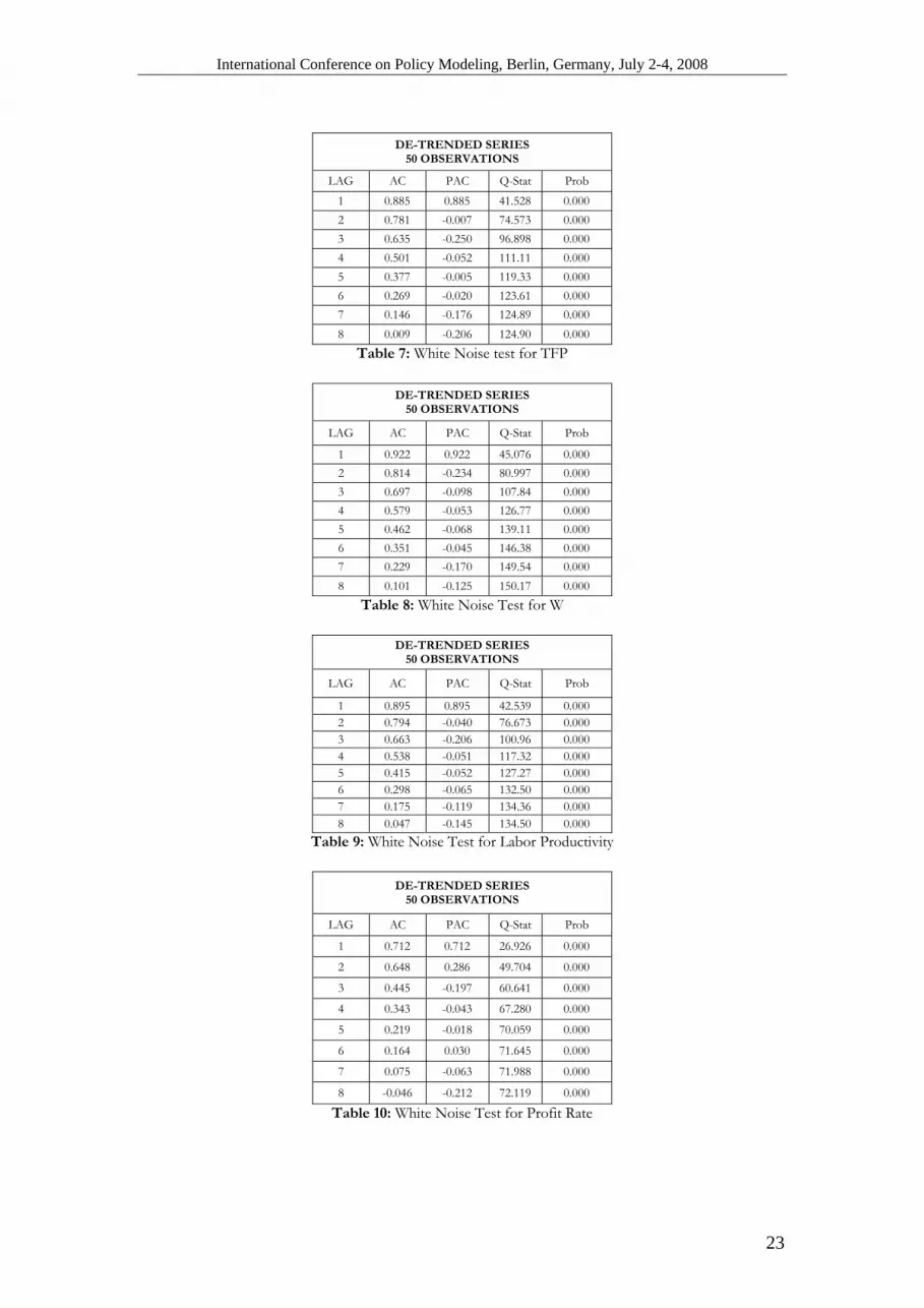
non-stationary6. Then the stationarity of their first differences was tested. In Table 2 the results are presented. The first differences of most macroeconomic variables are found to be stationary, as it was expected, except for consumption and labor productivity. The next step was to de-trend the macroeconomic variables. The five kinds of de-trending approaches, presented in section 3.3, were used and the time graphs of the residuals are depicted in Fig. 1. Also, the results from the analysis based on the correlograms for the various macroeconomic variables are shown in Tables 3-8. The results of the Ljung/Box test indicate a rejection of the null hypothesis of white noise for all the de-trended macroeconomic variables under examination. In other words, the existence of cyclical regularities is a valid hypothesis from a statistical viewpoint.

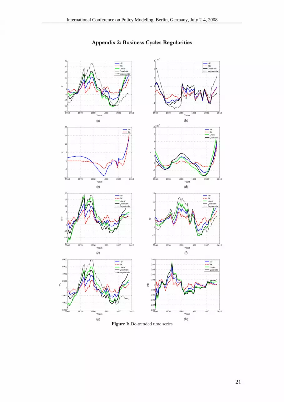
The distinct phases of development of the Greek economy can be discerned in the graphs. For instance, the cyclical component of the gross domestic product shows a clear upward trend from the start of the 1960s until 1973 (Fig. 1a) with the years 1962 and 1967 providing exceptions to this continuous rise, finding which is consistent with Ioakimoglou and Milios (1993, 2005). The effect of the 1973 oil price shock is clear in the de-trended series, irrespectively of the filter used. After that, the de-trended GDP recovers its previous levels by the end of 1970s. From 1980 onwards the continuous fall of GDP from its trend is obvious. The slow GDP growth during the 1980s relative to Greece’s own post-war performance has been noted by many authors (e.g. Stournaras

6 The absence of a trend for the profit rate for the Greek manufacturing sector has been documented by Lianos (1992) for the period 1960-1983.

0 1 21 0

m n

t i t i i t i ti i

a a Y a X ε− −= =

ΔΥ = + Δ + Δ +∑ ∑


13

1992) and has been attributed by some authors to the policies followed after the electoral victory of PASOK in 1981 which neglected investment (Skouras 2001, Michaelides et al. 2005).

On the other hand, other studies attempt to locate the cause of this slowdown to structural characteristics of the Greek society. More specifically, it has been noted that the period of acceleration (1960-1973) intensified to a socially unacceptable degree the extent of income inequalities (Mouzelis 1977). After the restoration of democracy in 1974 there was public demand for redistribution policies and the labor unions acquired power that could no longer be mitigated by the authoritarian mechanisms of the previous regime. The policies followed after 1981, characterized by efforts to redistribute income, were to a large extent an expression of this underlying social transformation (Papademos 2001). The implementation of such policies and the institutional arrangements devised by the new government has been criticized by the majority of authors (e.g. Skouras 2001, Tsakalotos 1998). In a similar vein, it has been noted that the slowdown of the Greek economy which started from the mid-1970s could be attributed to “external” determinations of the economic system (Dumenil 1978) and more precisely to the strengthening of the bargaining power of the trade unions (Ioakimoglou and Milios 1993). Fig. 1a shows that the slump of the 1980s persists until the first half of the 1990s. Since 1996 the economy has entered a protracted period of upward movement for the detrended GDP. The reversal is caused to a large extent by a restoration of sufficient rates of accumulation of capital. In the period from 1996-2004 Greece is found to be first among the EU countries in the rate of increase of investment in mechanical equipment (Ioakimoglou and Milios 2005). On the other hand, the cyclical component of the employed workforce is depicted in Fig. 1b. From the beginning of the period under survey, since the early 1970s, it is moving downwards and remains approximately stable in the post-1973 period. The 1980s mark clearly a distinct period in its evolution as all de-trending methods point to a sharp increase in 1981 and a stay in high levels lasting throughout the whole decade. However, the year 1990 is found to be a clear inflexion point where the de-trended employed workforce decreases to a large extent. The years 1997 and 2001 which are very close to the elections that took place in Greece constitute two years of negative shock for the cyclical employment. Since then it seems that an upward trend prevails (see Ioakimoglou and Milios 2005). Interestingly, all filtering methods agree to a considerable degree to the evolution of the cyclical behavior adding to the reliability of the conclusions that can be reached from the statistical analysis. The de-trended Consumption (Fig. 1c) is characterized by a more stable behavior. It seems to have reached a minimum at the end of the 1980s and since then, except from a negative shock in 1999 it is rising. Regarding the cyclical component of the capital stock, it seems that a low point was reached at 1967 and then continuous positive rates of growth led to the attainment of a maximum value in 1980 (Fig. 1d). Then, a steady decreasing movement lasted until the end of the 1990s. The collapse of the private sector investment occurring in the 1980s has been attributed by Skouras (2001, p. 172) to PASOK’s victory in the elections of 1981 and a hostile environment towards the private sector. Since then a rising trend appears to dominate the de-trended capital stock. The residual component of TFP quantifies the cyclical evolution of technological innovation (Fig. 1e). As it was expected from previous studies presented earlier, the period 1960-1973 was characterized by rapid growth in the industrialization of the Greek economy and this development is shown clearly in the de-trended TFP evolution. Mouzelis (1977, p. 277) attributed the qualitative leap of Greece’s industry to the attraction of foreign investment in dynamic sectors of manufacturing such as chemicals and metallurgy. After the oil price shock in 1973, a period of stagnation ensued that


14

lasted until the late 1970s. A sharp decline around 1980 is captured by all filtering techniques and could be attributed to a collapse of investment which took placer after 1981 (Skouras 2001) and an ensuing stagnation of technological change. A negative deviation of TFP from its trend persisted in the 1980s while the recovery of positive growth rates is clear since the second half of the 1990s. The cyclical component of wages (Fig. 1f) is constantly rising during the period 1960-1973 interrupted temporarily by the oil price shock of 1973. From the late 1970s until the first half of the 1980s the de-trended wages reached historically high levels. The stabilization program undertaken during the years 1985-87 had an adverse effect on cyclical wages as all de-trending techniques indicate. A downward trend lasted throughout the first half of the 1990s reaching a trough in around 1995. Since then an increase in the cyclical component of wages has been sustained7. Labor productivity ( /Y L ) increased steadily in the time period 1960-1973 (Fig. 1g). The shock of 1973 put an end to this rise and during the rest of the 1970s it remained approximately stable. The beginning of the 1980s showed a very steep deterioration which prevailed for the rest of the decade although with slower rates. A low end was reached in the mid-1990s and an upward movement characterizes its evolution since then. From a mere visual inspection of the graphs in Fig. 1g and Fig. 1e it is obvious that the time patterns of labor productivity and TFP are very closely linked with each other. This observation is consistent with the noted improvement in the investment performance in Greece (see e.g. Ioakimoglou and Milios 2005) and the resulting renewal of the production technology. Finally, as regards the de-trended profit rate (Fig. 1h), it reached historically high levels in 19738 and then it was adversely affected by the negative macroeconomic environment of the 1970s. A quick downward movement occurred in the beginning of the 1980s and the cyclical profit rate remained at low levels until the 1990s. This period of continuous negative deviation of profitability from the trend has been attributed by Giannitsis (1993) to the reduction in the degree of protection which took place over the 1974-86 time span. The author’s main argument is that the liberalisation of trade worsened the competitive position of the Greek industries and led to a profit squeeze for domestic industries9. However, in contrast to Giannitsis (1993), Bosworth and Kollintzas (2001, p. 171 ff.) argued that it is not clear whether a large trade shock attributed to the EU accession process can be considered as having a significant influence on the development of the Greek economy for the post-1973 period. The interpretation of the negative deviation of the profit rate from its trend due to the underlying social conditions as was put forward in the examination of the GDP evolution is an alternative. As is the case with most other macroeconomic indices, clear upward movements appear in the beginning both of the 1990s and the 2000s. The cyclical profit rate does not show any clear trend since the first years of the 2000s. The periodograms reveal the periodicity of the cycles and are shown in Figs. 2-9. The de-trended real GDP seems to follow a short-term cycle (2 years), two mid-term cycles (5 and 9 years) and two long-term ones (12 and 16 years respectively) (Fig. 3). In fact, the long wave (16 years) which is the dominant and most acute as can be seen in Fig. 3 coincides with the periodization of the Greek economy analysed earlier (i.e. 1960 - mid 1970s, mid 1970s - early 1990s, early 1990s - 2008) and confirms the empirical

7 For an examination of the long-term trends of labor’s share in income see Milios and Ioakimoglou (2005). For the period 1960-1973 it is also discussed in Mouzelis (1977). 8 For an extensive analysis of the determinants of profitability from a Marxian perspective see Milios et al. (2002, pp. 145-189). 9 Stournaras et al. (2005) analysed the lack of competitiveness of Greek exports for the period 1980-2004.


15

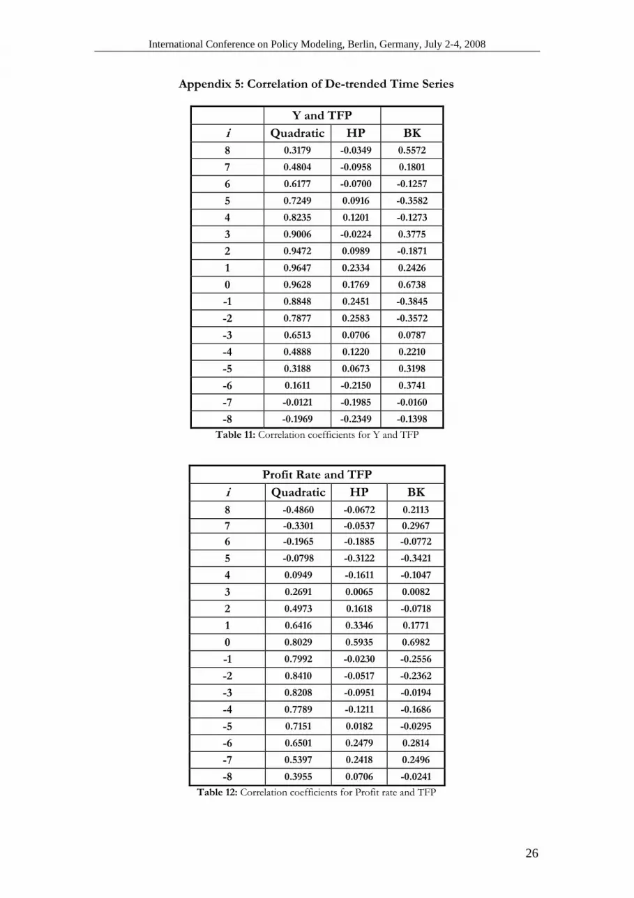
findings by most of the relevant studies. The spectral content of the cyclical component of TFP (Fig. 6) exhibits local maxima at the frequencies of 3, 6, 10 and 15 years. Again, this is consistent with our analysis of the distinct phases of the Greek economy. Accordingly, the de-trended labor productivity is characterized by the same frequency peaks (Fig. 8) giving credit to the previous observation that the cyclical movements of TFP and labor productivity seem to be synchronized to a great extent. Finally, the cycle of the profit rate is characterized by periodicities of 3, 7 and 10 and 15 years. In fact, its second most significant period (15 years) is also consistent with the aforementioned periodization. Finally, an interesting observation is that most macroeconomic time series exhibit, roughly speaking, a similar pattern characterized by periodicities exhibiting a short term cycle (approximately 3 years), a mid-term cycle (approximately 10 years) and a long term cycle (approximately 16 years). These results can be interpreted by economic theory as indications for the existence of various types of cycles with different lengths (i.e. periods) that are also synchronized within the total economy, in the sense that they affect almost equally all the macroeconomic variables under survey. Tables 11-13 show the correlation coefficients between the various variables under discussion. It can be seen that in all cases peaks occur at moderate lags (and leads) implying a slow transmission process of technological shocks throughout the Greek economy. Table 14 presents the results of Granger causality tests between, on the one hand, real output and profit rate, respectively, and TFP (Schumpeterian approach), and profit rate and labor productivity (Marxist approach), on the other. As can be seen, the profit rate seems to cause (in the Granger sense) and be affected simultaneously by both the TFP (Schumpeterian approach) and labor productivity (Marxian approach). In other words, an ambivalent relationship in the flow of cause and effect seems to emerge from the econometric analysis between TFP and labor productivity, respectively, and profit rate. The fact that this ambivalent relationship characterizes both TFP and labor productivity was expected taking into account the theoretical content of both variables as well as the definition of the Granger causality test and the synchronous evolution of these two variables.

Conclusively, our findings regarding the cyclical patterns of the macroeconomic variables under discussion are consistent with those of previous studies. Also, our results give credit to certain aspects of both the Schumpeterian and Marxist theories of economic crises, respectively, adopted here.

5. Conclusion

This paper attempted to answer some fundamental economic questions concerning the interpretation of the cyclical behavior of macroeconomic time series in the Greek economy. For instance, how do technology shocks and changes in labor productivity affect the behavior of variables, such as real output and profitability over time? The main findings of the paper can be summarized as follows: The cyclical components of real output and the measure of technological change (T.F.P.) clearly move in the same direction in the Greek economy. Also, there is, generally, a strong correlation between real output or profitability and technological change or labor productivity in both leads and lags for the majority of cases. Moreover, the timing pattern of technological change indicates that the peak correlations of variables appear at relatively moderate lags. This could mean that the technology shocks are not transmitted in the economy very quickly. Also, we provide robust evidence supporting the fact that technological change and labor productivity have independently, (causal) explanatory power for profitability growth in the Granger-causal sense at various lags which gives credit to certain aspects of both the


16

Schumpeterian and Marxist theories of economic crises, respectively, adopted here. As regards technological change (and labor productivity) for the Greek economy, there is a clear bidirectional causality in the Granger sense between technology shocks (and labor productivity) and profitability which can be interpreted as indicating an ambivalent relationship in the flow of cause and effect. Finally, our findings regarding the cyclical patterns of the macroeconomic variables under survey and the periodization of the phases of development of the Greek economy are consistent, in general terms, with the findings of other researchers.

References

Agresti, A-M. and B. Mojon (2001), Some Stylized Facts on the Euro Area Business Cycle, ECB Working Paper 95. Alogoskoufis, G., Giavazzi, F., and Laroque, G., (1995), The Two Faces of Janus: Institutions, Policy Regimes and Macroeconomic Performance in Greece, Economic Policy, Vol. 10, pp. 147-192 Apergis, N., and Panethimitakis, A., (2007), Stylized Facts of Greek Business Cycles: New Evidence from Aggregate and Across Regimes Data, SSRN Working Paper Series, January. Artis, M., (2003), Analysis of European and UK business cycles and shocks, EMU Study for HM Treasury. Backus, D.K., and P.J. Kehoe (1992), International evidence on the historical properties on business cycles, American Economic Review, 82(4), pp. 864-888. Baxter, M. and R.G. King (1999), Measuring Business Cycles: Approximate Band-pass Filters for Economic Time Series, Review of Economic and Statistics, 81(4), 575-593. Belegri-Roboli, A. and Michaelides, P., (2006), Measuring Technological Change in Greece, Journal of Technology Transfer, Vol. 31, pp. 663-671. Belegri-Roboli, A. and Michaelides, P., (2008), Potential Output and Output Gap in Greece by sector of Economic Activity, Journal of Policy Modeling (accepted subject to revisions). Belegri-Roboli, A. and Michaelides, P., (2007), Estimating Labour and Output Gap: Evidence from the Athens Olympic Region in Greece, Applied Economics, Vol. 39, Issue 19, pp. 2519 - 2528. Beneti, L. (2001), Band-Pass Filtering Cointegration and Business Cycle Analysis, Bank of England, Working Paper 142. Billmeier, A. (2004) Ghostbusting: which output gap measure really matters?, IMF Working paper WP/04/146. Blackburn, K., and M. Ravn (1992), Business Cycles in the United Kingdom: Facts and Frictions, Economica, 59, pp. 382-401. Bosworth, B. and Kollintzas, T. (2001), “Economic Growth in Greece: Past Performance and Future Prospects” in R. Bryant, N. Garganas and G. Tavlas (eds.), Greece’s Economic Performance and Prospects, Athens: Bank of Greece and the Brookings Institution, pp. 189-237 Böwer, U., and Guillemineau, C. (2006), Determinants of Business Cycle Synchronisation Across Euro Area Countries, ECB, Working Paper No. 587. Burns, A.F., and W.C. Mitchell (1946), Measuring Business Cycles, New York: National Bureau of Economic Research.


17

Camacho, M., Perez-Quiros, G., and Saiz, L. (2006), Are European Business Cycles Close Enough to be just One?, Journal of Economic Dynamics and Control Vol. 30, pp. 1687-1706. Canova, F. (1998), Detrending and Business Cycle Facts, Journal of Monetary Economics 41, pp. 475-512. Chauvet, M., and Xu, G. (2006), International Business Cycles: G7 and OECD Countries”, Economic Review of Federal Reserve Bank of Atlanta, issue Q 1, pp. 43-54. Choi, I. (2001), Unit Root Tests for Panel Data, Journal of International Money and Finance, 20, pp. 249-272. Christodoulakis, N., Dimelis, S., and Kollintzas, T., (1993), Comparisons of Business Cycles in Greece and the EC: Idiosyncracies and Regularities, Centre for Economic Policy Research Discussion Paper 809. Cogley, T., and Nason, J.M. (1995), .Effects of the Hodrick-Prescott Filter on Trend and Difference Stationary Time Series: Implications for Business Cycles Research, Journal of Economic Dynamics and Control, 19, 253-278. Danthine, J.P., and M. Girardin (1989), .Business Cycles in Switzerland. A Comparative Study, European Economic Review, 33, pp. 31-50. Dickey, D.A. and Fuller, W. A. (1979), Distribution of the Estimates for Autoregressive Time Series With a Unit Root, Journal of the American Statistical Association, 74, pp. 427-431. Dumenil, G., (1978), Le concept de loi economique dans le Capital, Maspero: Paris Engle, R.F., and C.W.J. Granger (1987), Co-integration and Error Correction: Representation, Estimation, and Testing, Econometrica, 55, 251-276. European Commission, 2003, European Innovation Scoreboard 2003, Issue No. 20, November. Fiorito, R., and T. Kollintzas (1994), Stylized Facts of Business Cycles in the G7 from a Real Business Cycle Perspective, European Economic Review, 38, pp. 235-269. Furceri, D., and Karras, G. (2008) Business cycle volatility and country size: evidence for a sample of OECD countries, Economics Bulletin, Vol. 5, No. 3, pp. 1-7. Gallegati, M., Gallegati, M., and Polasek, W. (2004), Business Cycles’ Characteristics of the Mediterranean Area Countries, Proceedings of the Middle East Economic Association. Garganas, N. and Tavlas, G. (2001), Monetary Regimes and Inflation Performance: The Case of Greece, in R. Bryant, N. Garganas and G. Tavlas (eds.), Greece’s Economic Performance and Prospects, Athens: Bank of Greece and the Brookings Institution, pp. 43-102 Giannitsis, T. (1993), World Market Integration: Trade Effects and Implications for Industrial and Technological Change in the Case of Greece, in Psomiades, H., and Thomadakis, S., (eds.) Greece, the New Europe and the Changing International Order. New York: Pella for the Center for Byzantine and Modern Greek Studies. Queen’s College, City University of New York, pp. 217-256. Giannitsis, T. (2005), Greece and the Future: Pragmatism and Illusions, Athens: Polis Publications (in Greek). Gouveia, S., and Correia, L., (2008), Business cycle synchronisation in the Euro Area: the case of small countries, International Economics and Economic Policy, Springer Publications, April 4. Granger, C. W.J. (1969), Investigating Causal Relations by Econometric Models and Cross-Spectral Methods, Econometrica 37, July, pp. 424-438. Harvey, A.C., and Jaeger, A. (1993), Detrending Stylized Facts and the Business Cycle, Journal of Applied Econometrics, 8, 231-247. Hodrick, R.J., and Prescott, E.C. (1997), .Postwar U.S. Business Cycles: An Empirical Investigation, Journal of Money, Credit, and Banking, 29, 1-16.


18

Im, K.S., Pesaran, M.H., and Shin, Y. (1997), Testing for Unit Roots in Heterogeneous Panel, Department of Applied Econometrics, University of Cambridge. Inklaar, R., and de Haan, J. (2001), Is there really a European business cycle? A comment, Oxford Economic Papers, Vol. 53, pp. 215-220. Ioakimoglou, E. and Milios, J. (1993), Capital Accumulation and Over-Accumulation Crisis: The Case of Greece (1960-1989), Review of Radical Political Economics, Vol. 25, No. 2, pp. 81-107. Ioakimoglou, E. and Milios, J. (2005), Capital Accumulation and Profitability in Greece (1964-2004), Proceedings of the INEK Conference on Sustainable Development, Nicosia, July, 23-24. Karasawoglou, A., and Katrakilidis, K. (1993), The Accommodation Hypothesis in Greece. A Tri-Variate Granger-Causality Approach, SPOUDAI, Vol. 43, No 1, pp. 3-18. Karras, G., Lee Jin Man and Stokes, H. (2006), Why are postwar cycles smoother? Impulses or propagation?, Journal of Economics and Business, Vol. 58, pp. 392-406. Kaskarelis, I. (1993), Investigating the Features of Greek Business Cycles, SPOUDAI, Vol. 43, No 1, pp. 19-32. King, R. G. and Rebelo, S. (1993), Low frequency filtering and real business cycles, Journal of Economic Dynamics and Control, 17, pp. 361–368. Kollintzas, T. and Vassilatos, V. (1996), A Stochastic Dynamic General Equilibrium Model for Greece, Centre for Economic Policy Research, Discussion Paper No. 1518. Kose, A., Otrok, C. and Prasad, E. (2008), Global Business Cycles: Convergence or Decoupling?, Insititute for the Study of Labor, Discussion Paper No. 3442. Kydland, F.E., and E.C. Prescott (1990), Business Cycles: Real Facts and a Monetary Myth, Federal Reserve Bank of Minneapolis Quarterly Review, 14, pp. 3-18. Leon, C. (2007), The European and the Greek Business Cycles: Are they synchronized?, MRPA Paper, No. 1312, November. Lianos, T. (1992), The Rate of Surplus Value, the Organic Composition of Capital and the Rate of Profit in Greek Manufacturing, Review of Radical Political Economics, Vol. 24, No. 1, pp. 136-145. Ljung. G. and Box, G.E.P. (1978), On a measure of lack of fit in time series models, Biometrika 65, pp. 297–303. Lucas Jr, R.E. (1977), Understanding Business Cycles, in Karl Brunner, K. and Meltzer. A. (eds.), Stabilization of the Domestic and International Economy, Amsterdam: North Holland. Maddala, G.S. and S. Wu. (1999), A Comparative Study of Unit Root Tests with Panel Data and a New Simple Test, Oxford Bulletin of Economics and Statistics, 61, pp. 631-652. Maddison, A. (1995), Monitoring the World Economy, 1820-1992, Paris: OECD Development Studies. Massmann, M., and Mitchell, J. (2004), Reconsidering the evidence: are Eurozone business cycles converging?, Journal of Business Cycle Measurement and Analysis, Vol. 1, pp. 275-307. Michaelides, P., Roboli, A., Economakis, G. and Milios, J. (2005), The Determinants of Investment Activity in Greece (1960-1999), Journal of Transport and Shipping (former Aegean Working Papers), Issue 3, 2005, pp. 23-45. Milios, J. (1988), The Greek Capital Formation: From Expansionism to Capitalist Development, Athens: Exantas Publications (in Greek). Milios, J., Dimoulis, D., and Economakis, G. (2002), Karl Marx and the Classics, Ashgate.


19

Montoya, L. and de Haan, J. (2007), Regional Business Cycle synchronization in Europe ?, BEER Paper, No 10, March. Mouzelis, N. (1977), Modern Greek Society: Facets of Underdevelopment, Athens: Exantas Publications (in Greek). Nelson, C.R., and Plosser, C.I. (1982), Trends and Random Walks in Macroeconomics Time Series: Some Evidence and Implications,. Journal of Monetary Economics, 10, pp. 139-167. OECD (2002), Economic Survey of Greece: 2002. OECD (2007), Economic Survey of Greece: 2007. O’ Mahony, M. (1992), Productivity in the EU, 1979-’99, The Public Enquiry Unit, HM Treasury. Papademos, L. (2001), The Greek Economy: Performance and Policy Challenges, in R. Bryant, N. Garganas and G. Tavlas (eds.), Greece’s Economic Performance and Prospects, Athens: Bank of Greece and the Brookings Institution, pp. xxxiii-xxxix. Rudin, W. (1976), Principles of Mathematical Analysis, McGraw-Hill International Edition. Skouras, T. (2001), The Greek Experiment with the Third Way, in Arestis, P. and Sawyer, M. (eds.), The Economics of the Third Way, Cheltenham: Edwar Elgar, pp. 170-182. Stock, J.H. and M.W. Watson (1999a), Business Cycle Fluctuations in U.S. Macroeconomic Time Series, ch. 1 in J.B. Taylor and Woodford, M. (eds.), Handbook of Macroeconomics, 1, pp. 3-64. Stock, J. and Watson, M. (2003), Has the Business Cycle Changed? Evidence and Explanations, Proceedings, Federal Reserve Bank of Kansas City, pp. 9-56. Stournaras, Y. (1992), Greece on the Road to Economic and Monetary Union. Problems and Prospects, in Gibson, H. and Tsakalotos, E. (eds.), Economic Integration and Financial Liberalization: Prospects for Southern Europe, Macmillan/St.Antony’s. Stournaras,Y., Bakinezou, D., Pantazidis, S., Papadogonas, T., and Papazoglou, C. (2005), Aspects of the Economic and Financial Integration of Greece into the European Union, Bank of Greece, Research Department, July. Tavlas, G. and Zonzilos, N. (2001), Comment on Bosworth and Kollintzas, in R. Bryant, N. Garganas and G. Tavlas (eds.), Greece’s Economic Performance and Prospects, Athens: Bank of Greece and the Brookings Institution, pp. 202-210. Tsakalotos, E. (1998), The Political Economy of Social Democratic Economic Policies: The PASOK Experiment in Greece, Oxford Review of Economic Policy, Vol. 14, No. 1, pp. 114-138. Wynne, M., and Koo, J. (2000), Business Cycles under Monetary Union: A Comparison of the EU and US," Economica, 67, pp. 347-374.


20

Appendix 1: ADF Statistics

Table 1: Original Variables

COUNTRY VARIABLE LAGS Τ-STAT PROBABILITY STATIONARY NON

STATIONARY

GREECE L 0-10 2.197469 0.9999 NO YES

Y 0-10 2.068819 0.9999 NO YES

C 0-10 1.176580 0.9976 NO YES

K 1-10 1.126858 0.9972 NO YES

TFP 0-10 -2.237329 0.1962 NO YES

W 1-10 0.326710 0.9774 NO YES

Y/L 0-10 -0.983346 0.7522 NO YES

PROFIT RATE 0-10 -3.227509 0.0243 YES NO

Table 2: First Differenced Variables

COUNTRY VARIABLE LAGS Τ-STAT PROBABILITY STATIONARY NON

STATIONARY

GREECE ΔL 0-10 2.197469 0.0330 YES NO

ΔY 0-10 2.068819 0.0441 YES NO

ΔC 0-10 1.312691 0.1957 NO YES

ΔK 1-10 17.10366 0.0000 YES NO

ΔTFP 0-10 -2.237329 0.0300 YES NO

ΔW 1-10 2.406293 0.0203 YES NO

ΔY/L 0-10 -0.983346 0.3305 NO YES

ΔPR 0-10 -3.227509 0.0023 YES NO


21

Appendix 2: Business Cycles Regularities

1960 1970 1980 1990 2000 2010-20

-15

-10

-5

0

5

10

15

20

25Y

Years

HPBKLinearQuadraticExponential

(a)

1960 1970 1980 1990 2000 2010-2

-1

0

1

2

3

4x 105

L

Years

HPBKQuadraticexponential

(b)

1960 1970 1980 1990 2000 2010-10

-5

0

5

10

15

20

C

Years

HPBK

(c)

1960 1970 1980 1990 2000 2010-4

-2

0

2

4

6

8

10x 105

K

Years

HPBKLinearQuadratic

(d)

1960 1970 1980 1990 2000 2010-20

-15

-10

-5

0

5

10

15

20

TFP

Years


(e)

1960 1970 1980 1990 2000 2010-15

-10

-5

0

5

10

15

W

Years


(f)

1960 1970 1980 1990 2000 2010-6000

-4000

-2000

0

2000

4000

6000

8000

Y/L

Years


(g)

1960 1970 1980 1990 2000 2010-0.05

-0.04

-0.03

-0.02

-0.01

0

0.01

0.02

0.03

0.04

0.05

PR

Years

HPBKLinearQuadratic

(h)

Figure 1: De-trended time series


22

Appendix 3: Correlograms and White Noise Tests

50 OBSERVATIONS

LAG AC PAC Q-Stat Prob

1 0.796 0.796 33.643 0.000 2 0.605 -0.080 53.461 0.000 3 0.440 -0.045 64.172 0.000 4 0.340 0.067 70.716 0.000 5 0.227 -0.109 73.701 0.000 6 0.096 -0.133 74.246 0.000 7 -0.012 -0.034 74.254 0.000

8 -0.085 -0.026 74.699 0.000

Table 3: White Noise test for L

DE-TRENDED SERIES 50 OBSERVATIONS


1 0.902 0.902 43.182 0.000 2 0.813 -0.004 78.986 0.000 3 0.691 -0.223 105.41 0.000 4 0.570 -0.088 123.75 0.000 5 0.448 -0.052 135.34 0.000 6 0.335 -0.032 141.97 0.000 7 0.210 -0.153 144.63 0.000 8 0.075 -0.185 144.98 0.000

Table 4: White Noise test for Y



1 0.911 0.911 43.988 0.000 2 0.822 -0.038 80.630 0.000 3 0.721 -0.127 109.39 0.000 4 0.611 -0.110 130.50 0.000 5 0.498 -0.085 144.84 0.000 6 0.388 -0.050 153.76 0.000 7 0.261 -0.180 157.88 0.000 8 0.157 0.035 159.41 0.000

Table 5: White Noise test for C


LAG AC PAC Q-Stat Prob 1 0.915 0.915 44.471 0.000 2 0.823 -0.096 81.129 0.000 3 0.724 -0.085 110.12 0.000 4 0.617 -0.107 131.62 0.000 5 0.506 -0.083 146.44 0.000 6 0.398 -0.058 155.79 0.000 7 0.293 -0.050 160.99 0.000 8 0.193 -0.057 163.29 0.000

Table 6: White Noise test for K


23

DE-TRENDED SERIES

50 OBSERVATIONS


1 0.885 0.885 41.528 0.000 2 0.781 -0.007 74.573 0.000 3 0.635 -0.250 96.898 0.000 4 0.501 -0.052 111.11 0.000 5 0.377 -0.005 119.33 0.000 6 0.269 -0.020 123.61 0.000 7 0.146 -0.176 124.89 0.000 8 0.009 -0.206 124.90 0.000

Table 7: White Noise test for TFP



1 0.922 0.922 45.076 0.000 2 0.814 -0.234 80.997 0.000 3 0.697 -0.098 107.84 0.000 4 0.579 -0.053 126.77 0.000 5 0.462 -0.068 139.11 0.000 6 0.351 -0.045 146.38 0.000 7 0.229 -0.170 149.54 0.000 8 0.101 -0.125 150.17 0.000

Table 8: White Noise Test for W



1 0.895 0.895 42.539 0.000 2 0.794 -0.040 76.673 0.000 3 0.663 -0.206 100.96 0.000 4 0.538 -0.051 117.32 0.000 5 0.415 -0.052 127.27 0.000 6 0.298 -0.065 132.50 0.000 7 0.175 -0.119 134.36 0.000 8 0.047 -0.145 134.50 0.000

Table 9: White Noise Test for Labor Productivity



1 0.712 0.712 26.926 0.000

2 0.648 0.286 49.704 0.000

3 0.445 -0.197 60.641 0.000

4 0.343 -0.043 67.280 0.000

5 0.219 -0.018 70.059 0.000

6 0.164 0.030 71.645 0.000

7 0.075 -0.063 71.988 0.000

8 -0.046 -0.212 72.119 0.000

Table 10: White Noise Test for Profit Rate


24

Appendix 4: Periodograms for Time Series

5 10 15 20 250

0.2

0.4

0.6

0.8

1

1.2

1.4

1.6

1.8

2x 106

Spe

ctra

l den

sity

- L

Years Figure 2: Periodogram for L

5 10 15 20 250.2

0.4

0.6

0.8

1

1.2

1.4

1.6

1.8

2x 106

Spe

ctra

l den

sity

- I

Years Figure 3: Periodogram for Y

5 10 15 20 250

0.5

1

1.5

2

2.5

3x 106

Spe

ctra

l den

sity

- C

Years Figure 4: Periodogram for C

5 10 15 20 250

1

2

3

4

5

6x 105

Spe

ctra

l den

sity

- K

Years Figure 5: Periodogram for K


25

5 10 15 20 250

2

4

6

8

10

12

14x 106

Spe

ctra

l den

sity

- TF

PYears

Figure 6: Periodogram for TFP

5 10 15 20 250

0.5

1

1.5

2

2.5

3x 106

Spe

ctra

l den

sity

- W

Years Figure 7: Periodogram for W

5 10 15 20 250

0.5

1

1.5

2

2.5

3

3.5

4

4.5

5x 10-3

Spe

ctra

l den

sity

- Y

/L

Years Figure 8: Periodogram for labor productivity

5 10 15 20 250

0.5

1

1.5

2

2.5

3

3.5x 10-3

Spe

ctra

l den

sity

- P

R

Years Figure 9: Periodogram for profit rate


26

Appendix 5: Correlation of De-trended Time Series

Y and TFP

i Quadratic HP BK 8 0.3179 -0.0349 0.5572

7 0.4804 -0.0958 0.1801

6 0.6177 -0.0700 -0.1257

5 0.7249 0.0916 -0.3582

4 0.8235 0.1201 -0.1273

3 0.9006 -0.0224 0.3775

2 0.9472 0.0989 -0.1871

1 0.9647 0.2334 0.2426

0 0.9628 0.1769 0.6738

-1 0.8848 0.2451 -0.3845

-2 0.7877 0.2583 -0.3572

-3 0.6513 0.0706 0.0787

-4 0.4888 0.1220 0.2210

-5 0.3188 0.0673 0.3198

-6 0.1611 -0.2150 0.3741

-7 -0.0121 -0.1985 -0.0160

-8 -0.1969 -0.2349 -0.1398

Table 11: Correlation coefficients for Y and TFP

Profit Rate and TFP

i Quadratic HP BK 8 -0.4860 -0.0672 0.2113

7 -0.3301 -0.0537 0.2967

6 -0.1965 -0.1885 -0.0772

5 -0.0798 -0.3122 -0.3421

4 0.0949 -0.1611 -0.1047

3 0.2691 0.0065 0.0082

2 0.4973 0.1618 -0.0718

1 0.6416 0.3346 0.1771

0 0.8029 0.5935 0.6982

-1 0.7992 -0.0230 -0.2556

-2 0.8410 -0.0517 -0.2362

-3 0.8208 -0.0951 -0.0194

-4 0.7789 -0.1211 -0.1686

-5 0.7151 0.0182 -0.0295

-6 0.6501 0.2479 0.2814

-7 0.5397 0.2418 0.2496

-8 0.3955 0.0706 -0.0241

Table 12: Correlation coefficients for Profit rate and TFP


27

Profit Rate and Labor Productivity

i Quadratic HP BK 8 -0.6157 -0.1747 0.1616

7 -0.4741 -0.1866 0.2398

6 -0.3509 -0.3122 -0.0917

5 -0.2393 -0.3774 -0.3178

4 -0.0718 -0.2135 -0.0895

3 0.0981 -0.0346 -0.0353

2 0.3375 0.1144 -0.0738

1 0.4934 0.3274 0.1497

0 0.6816 0.5262 0.6708

-1 0.7082 0.0334 -0.2306

-2 0.7634 -0.0289 -0.2356

-3 0.7779 -0.0409 -0.0277

-4 0.7729 -0.0616 -0.1389

-5 0.7454 0.0613 -0.0039

-6 0.7064 0.2260 0.2472

-7 0.6308 0.2136 0.2261

-8 0.5175 0.0306 -0.0838

Table 133: Correlation coefficients for Profit rate and Labor Productivity

Appendix 6: Granger Causality Test

PAIRWISE GRANGER CAUSALITY TESTS SAMPLE 50

Hypothesis to be Tested LAGS OBS F-STATISTIC PROBABILITY TFP does not Granger Cause Y 2.68126 0.06244 Y does not Granger Cause TFP

13 37 0.52560 0.86213

Labor Productivity does not Granger Cause PROFIT RATE 2.83408 0.09906 PROFIT RATE does not Granger Cause Labor Productivity

1 49

5.99925 0.01818 TFP does not Granger Cause PROFIT RATE 2.88107 0.09638 PPROFIT RATE does not Granger Cause TFP

1 49 9.38100 0.00366

Table 14: Granger causality test results

do technology shocks affect output and profitability over the business cycles in greece (1960-2008)?

Documents