REVIEW

Distance software: design and analysis of distance

sampling surveys for estimating population size

Len Thomas*,1, Stephen T. Buckland2, Eric A. Rexstad1, Jeff L. Laake3,

Samantha Strindberg4, Sharon L. Hedley2, Jon R.B. Bishop1, Tiago A. Marques1

and Kenneth P. Burnham5

1Research Unit for Wildlife Population Assessment, Centre for Research into Ecological and Environmental Modelling,

University of St. Andrews, St. Andrews KY16 9LZ, UK; 2Centre for Research into Ecological and Environmental

Modelling, University of St. Andrews, St. Andrews KY16 9LZ, UK; 3National Marine Mammal Laboratory, Alaska

Fisheries Science Center, National Marine Fisheries Service, 7600 Sand Point Way NE F ⁄AKC3, Seattle, WA

98115 6349, USA; 4Wildlife Conservation Society, 2300 Southern Boulevard, Bronx, NY 10460, USA; and 5Colorado

Cooperative Fish and Wildlife Research Unit, Department of Fish, Wildlife and Conservation Biology, Colorado State

University, Fort Collins, CO 80523, USA

Summary

1. Distance sampling is a widely used technique for estimating the size or density of biological

populations.Many distance sampling designs andmost analyses use the softwareDistance.

2. We briefly review distance sampling and its assumptions, outline the history, structure and

capabilities of Distance, and provide hints on its use.

3. Good survey design is a crucial prerequisite for obtaining reliable results. Distance has a survey

design engine, with a built-in geographic information system, that allows properties of different pro-

posed designs to be examined via simulation, and survey plans to be generated.

4. A first step in analysis of distance sampling data is modelling the probability of detection.

Distance contains three increasingly sophisticated analysis engines for this: conventional distance

sampling, which models detection probability as a function of distance from the transect and

assumes all objects at zero distance are detected; multiple-covariate distance sampling, which allows

covariates in addition to distance; and mark–recapture distance sampling, which relaxes the

assumption of certain detection at zero distance.

5. All three engines allow estimation of density or abundance, stratified if required, with associated

measures of precision calculated either analytically or via the bootstrap.

6. Advanced analysis topics covered include the use of multipliers to allow analysis of indirect

surveys (such as dung or nest surveys), the density surface modelling analysis engine for spatial and

habitatmodelling, and information about accessing the analysis engines directly from other software.

7. Synthesis and applications. Distance sampling is a key method for producing abundance and

density estimates in challenging field conditions. The theory underlying the methods continues to

expand to cope with realistic estimation situations. In step with theoretical developments, state-

of-the-art software that implements these methods is described that makes the methods accessible

to practising ecologists.

Key-words: distance sampling, line transect sampling, point transect sampling, population

abundance, population density, sighting surveys, survey design, wildlife surveys

Introduction

Distance sampling comprises a set of methods in which

distances from a line or point to detections are recorded,

from which the density and ⁄or abundance of objects is

*Correspondence author. E-mail: len@mcs.st-and.ac.uk

Re-use of this article is permitted in accordance with the Terms

and Conditions set out at http://www3.interscience.wiley.com/

authorresources/onlineopen.html

Journal of Applied Ecology 2010, 47, 5–14 doi: 10.1111/j.1365-2664.2009.01737.x

� 2009 The Authors. Journal compilation � 2009 British Ecological Society

estimated. Objects are usually animals or animal groups

(termed clusters), but may be plants or inanimate objects.

Detections are usually of animals or clusters, but may be

of cues (such as whale blows or bird songbursts) or sign

(such as dung or nests). Conventional distance sampling

(CDS) methods are described by Buckland et al. (2001),

and various extensions are considered in Buckland et al.

(2004). An extensive distance sampling reference list, covering

both methodological developments and practical application

of the methods, is available at http://www.ruwpa.st-and.

ac.uk/distancesamplingreferences/.

Most distance sampling surveys are analysed, and many are

designed, using the software Distance (http://www.ruwpa.

st-and.ac.uk/distance/). In this paper, we describe version 6 of

the software and its capabilities, and give guidance on how to

use it to design and analyse surveys.

What is distance sampling?

TYPES OF DISTANCE SAMPLING

Themost widely used form of distance sampling is line transect

sampling. A survey region is sampled by placing a number of

lines at random in the region or, more commonly, a series of

systematically spaced parallel lines with a random start point.

An observer travels along each line, recording any animals

detected within a distance w of the line. In the standard

method, we assume all animals on the line are detected, but

detection probability decreases with increasing distance from

the line. Hence, not all animals in the strip of half-widthw need

to be detected. In addition, the distance of each detected ani-

mal from the line is recorded. We use the distribution of these

distances to estimate the proportion of animals in the strip that

is detected, which allows us to estimate animal density and

abundance. If animals occur in well-defined clusters (e.g. flocks

or herds), then detections refer to clusters rather than to indi-

vidual animals.

A second common form, particularly for surveys of breeding

songbirds, is point transect sampling, where the design is based

on randomly placed points rather than lines.

Several other variations exist. In indirect surveys, animal

signs are surveyed by one of the above methods, and sign den-

sity is converted to animal density using estimates of sign pro-

duction and decay rates (Marques et al. 2001). In cue count

surveys (nearly) instantaneous cues are surveyed, e.g. whale

blows (Hiby 1985) or bird songbursts (Buckland 2006), and

the resulting estimate of number of cues per unit time per unit

area is converted to estimated animal density using an estimate

of the cue rate per animal. In trapping webs or trapping line

transects (Lukacs, Franklin & Anderson 2004), a network of

traps is placed around the point or line, and if an animal enters

a trap, its recorded distance is the distance of that trap from

the point or line. In trapping or lure point transect sampling, a

single trap or lure is placed at each point of the design, and the

probability of detecting a given animal is estimated by con-

ducting separate trials on animals with known location (Buck-

land et al. 2006).

ASSUMPTIONS

Webriefly summarize the key assumptions of the basicmethod

(for a more detailed discussion, see Buckland et al. 2001:29–

37). Many of the recent advances of distance sampling allow

one or more of these assumptions to be relaxed. There are just

three key assumptions.

1. Objects on the line or point are detected with cer-

tainty. Most surveys are conducted with a single observer, or

a single observation ‘platform’ consisting of multiple observers

but with data pooled across them. In cases where it is impor-

tant to relax assumption 1, double-observer or double-plat-

form surveys may be conducted (Laake & Borchers 2004). In

these, observers either search independently of each other or

there may be ‘one-way’ independence, with one observer being

unaware of detections made by the other, but not vice versa.

Such methods are quite often used for marine mammal sur-

veys. The mark–recapture distance sampling (MRDS) engine

ofDistance can be used to analyse such double-observer data.

2. Objects do not move. Conceptually, distance sampling is a

‘snapshot’ method: we would like to freeze animals in position

while we conduct the survey. In practice, non-responsive

movement in line transect surveys is not problematic provided

it is slow relative to the speed of the observer. Non-responsive

movement is more problematic for point transect surveys,

leading to overestimation of density (Buckland et al.

2001:173). Responsive movement before detection is problem-

atic because animals are assumed to be located independently

of the position of the line or point (see below); implications are

addressed by Fewster et al. (2008).

3. Measurements are exact. Untrained observers tend to be

poor at estimating distances by eye or ear (Alldredge, Simons

& Pollock 2007). Wherever possible, training and technology

(e.g. laser rangefinders) should be used to ensure adequate

accuracy. Provided distance measurements are approximately

unbiased, bias in line transect estimates tends to be small in the

presence of measurement errors, but larger for estimates from

point transect surveys (Buckland et al. 2001:264–265). In some

line transect surveys, particularly shipboard surveys, direct ani-

mal-observer distance r is recorded together with sighting angle

h from the transect line and perpendicular distance is then

calculated as r sin h. In this case, it is important to obtain

accurate angles, particularly for small angles, and an angle

board can be used to help achieve this. In addition to exact

distances, if animals occur in clusters, we assume cluster sizes

are accurately recorded, at least for those close to the line or

point.We also assume species are notmisidentified.

Other assumptions are made, but they are seldom of great

practical significance. We assume animal locations are

independent of the positions of the lines or points, which we

ensure if we have an adequate sample of lines or points, and

randomize their location. This assumption becomes critical if,

for example, transects are placed along roads or tracks. We

6 L. Thomas et al.

� 2009 The Authors. Journal compilation � 2009 British Ecological Society, Journal of Applied Ecology, 47, 5–14

also assume detections are independent events, but our analysis

methods are very robust to failures of this assumption (except

in the case of double-platform designs, where independence

between duplicate detections of the same animal at zero dis-

tance is required).

DESIGN-BASED AND MODEL-BASED ESTIMATION

In the case of strip transect sampling, where all animals within

the strip of half-widthw are assumed to be detected, estimation

of abundancewithin the survey region can be achieved using an

entirely design-based framework. To do this successfully, it is

critical to place the strips at random throughout the survey

region, to ensure that we count representative strips. We can

then assume the density in the strips is an unbiased estimate of

density in thewider survey region;nomodel isneeded.Standard

distance sampling also uses design-based inference to extrapo-

late from the sampled plots (strips for line transect sampling or

circles for point transect sampling) to the survey region.

However, we do not know the true number of animals in the

plots. We therefore fit a detection model, which allows us to

estimate this number. Standard distance sampling is thus a

hybrid, blending model-based (within the plots) and design-

based (extrapolation from the plots) inference (Fewster &

Buckland2004).Wecouldadopta fullymodel-basedapproach.

The simplest would be to assume that animals are uniformly

and independently distributed throughout the survey region.

This leads to the same abundance estimate as for the hybrid

approach, but estimates of precision would change. This strat-

egy is not usually adoptedbecause the estimates of precision are

not robust to the failure of the model assumptions made about

the spatial distribution of animals. However, there is increasing

interest in modelling how animal density varies spatially, and

fully model-based approaches that make more reasonable

assumptions are an active area of research (e.g. Hedley &

Buckland 2004; Johnson, Laake&VerHoef 2009). It is possible

tofit relatively simple spatialmodels inDistance6 (seebelow).

Historical development

The Distance software evolved from two earlier software

developments. The first was the program TRANSECT

(Laake, Burnham & Anderson 1979) for fitting Fourier series

and other models to line transect distance data. The methods

on which the software was based were developed in a series of

publications, culminating in the first monograph on distance

sampling (Burnham, Anderson & Laake 1980). The second

development was of an algorithm for maximum likelihood fit-

ting of models to line or point transect distance data, based on

a parametric key function multiplied by series adjustments

(Buckland 1992). Code implementing this algorithm was

merged with TRANSECT to create Distance (Laake et al.

1993), which provided analysis of line and point transect data.

The methods were comprehensively documented in a second

monograph (Buckland et al. 1993). Distance versions 1.0–2.2

were DOS-based applications that were controlled using a

command language to invoke various program options

appropriate for the sampling used, and analysis options

desired. Version 3.0 was a Microsoft Windows console appli-

cation, but retained the command language structure.

With funds from British research funding councils, a pro-

gramming team developed a version of Distance with fully

integrated, Windows-based graphical user interface. This ver-

sion, Distance 3.5, became generally available in 1998. Subse-

quent versions saw the addition of more features: Distance 4

(in 2002) the multiple-covariate distance sampling (MCDS)

and automated survey design engines, Distance 5 (in 2005) the

MRDS engine and Distance 6 (in 2009) the density surface

modelling (DSM) engine. The basic methods in Distance 6 are

described in a third monograph (Buckland et al. 2001), which

is essentially an updated version of the second one; the more

advanced methods are described in an edited volume (Buck-

land et al. 2004), and in additional references given below.

Users downloadingDistance are asked to register their email

address and country. Distance versions 3.5, 4 and 5 together

have been registered by over 19 000 users from 135 countries.

Program structure and overview

From the users’ perspective, Distance consists of a graphical

interface that allows users to enter, import and view data,

design surveys and run analyses. Users begin by creating aDis-

tance project, which contains information about a single study.

Wizards are available to help in setting up a project and enter-

ing data, or importing it from delimited text files. Data are

organized into nested layers: global (for data that relates to the

whole study area), stratum (data relating to individual survey

strata), sample (data relating to individual survey lines or

points) and observation (data relating to single observations).

More complex nested structures are possible. Geographical

data, in the form of ESRI shapefiles, can also be associated

with each layer. Having entered or imported data, users under-

take one of two tasks: design of a new survey or analysis of

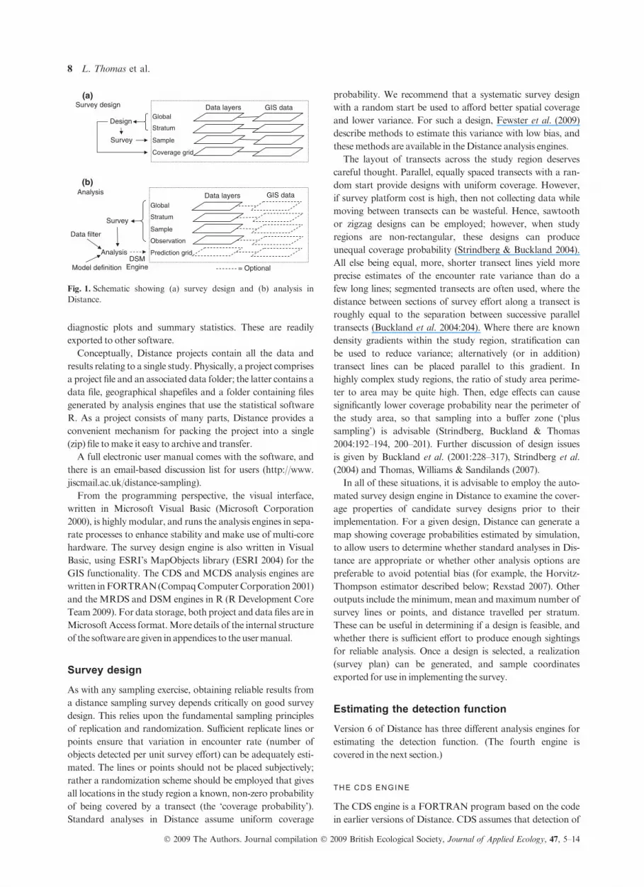
already-collected survey data (Fig. 1).

A design is an algorithm for laying out samples within the

study area; multiple designs can be created using the design

engine in Distance, and their properties examined by simula-

tion. A single realization of a design is called in Distance a

survey, and this consists of the position of a set of sample lines

or points together with the survey methods (e.g. collection of

perpendicular distances to clusters of animals). Line or point

positions can be readily exported from Distance and used for

navigation in the field. Results can also be viewed within

Distance in the form of simple maps and text output contain-

ing summary statistics.

Analysis inDistance involves combining three elements: (i) a

survey, which specifies which data layers to use and the survey

methods used; (ii) a data filter, which allows subsets of the data

to be selected, truncation distances to be chosen and other pre-

processing; and (iii) a model definition, which specifies how the

data should be analysed. These are then run using one of the

four analysis engines available in Distance: CDS, MCDS,

MRDS andDSM. Each has different capabilities, as explained

below. Results are available within Distance in the form of

Distance software for density estimation 7

� 2009 The Authors. Journal compilation � 2009 British Ecological Society, Journal of Applied Ecology, 47, 5–14

diagnostic plots and summary statistics. These are readily

exported to other software.

Conceptually, Distance projects contain all the data and

results relating to a single study. Physically, a project comprises

a project file and an associated data folder; the latter contains a

data file, geographical shapefiles and a folder containing files

generated by analysis engines that use the statistical software

R. As a project consists of many parts, Distance provides a

convenient mechanism for packing the project into a single

(zip) file tomake it easy to archive and transfer.

A full electronic user manual comes with the software, and

there is an email-based discussion list for users (http://www.

jiscmail.ac.uk/distance-sampling).

From the programming perspective, the visual interface,

written in Microsoft Visual Basic (Microsoft Corporation

2000), is highly modular, and runs the analysis engines in sepa-

rate processes to enhance stability and make use of multi-core

hardware. The survey design engine is also written in Visual

Basic, using ESRI’s MapObjects library (ESRI 2004) for the

GIS functionality. The CDS and MCDS analysis engines are

written inFORTRAN(CompaqComputerCorporation 2001)

and the MRDS and DSM engines in R (R Development Core

Team 2009). For data storage, both project and data files are in

Microsoft Access format.More details of the internal structure

of the softwareare given in appendices to theusermanual.

Survey design

As with any sampling exercise, obtaining reliable results from

a distance sampling survey depends critically on good survey

design. This relies upon the fundamental sampling principles

of replication and randomization. Sufficient replicate lines or

points ensure that variation in encounter rate (number of

objects detected per unit survey effort) can be adequately esti-

mated. The lines or points should not be placed subjectively;

rather a randomization scheme should be employed that gives

all locations in the study region a known, non-zero probability

of being covered by a transect (the ‘coverage probability’).

Standard analyses in Distance assume uniform coverage

probability. We recommend that a systematic survey design

with a random start be used to afford better spatial coverage

and lower variance. For such a design, Fewster et al. (2009)

describe methods to estimate this variance with low bias, and

thesemethods are available in theDistance analysis engines.

The layout of transects across the study region deserves

careful thought. Parallel, equally spaced transects with a ran-

dom start provide designs with uniform coverage. However,

if survey platform cost is high, then not collecting data while

moving between transects can be wasteful. Hence, sawtooth

or zigzag designs can be employed; however, when study

regions are non-rectangular, these designs can produce

unequal coverage probability (Strindberg & Buckland 2004).

All else being equal, more, shorter transect lines yield more

precise estimates of the encounter rate variance than do a

few long lines; segmented transects are often used, where the

distance between sections of survey effort along a transect is

roughly equal to the separation between successive parallel

transects (Buckland et al. 2004:204). Where there are known

density gradients within the study region, stratification can

be used to reduce variance; alternatively (or in addition)

transect lines can be placed parallel to this gradient. In

highly complex study regions, the ratio of study area perime-

ter to area may be quite high. Then, edge effects can cause

significantly lower coverage probability near the perimeter of

the study area, so that sampling into a buffer zone (‘plus

sampling’) is advisable (Strindberg, Buckland & Thomas

2004:192–194, 200–201). Further discussion of design issues

is given by Buckland et al. (2001:228–317), Strindberg et al.

(2004) and Thomas, Williams & Sandilands (2007).

In all of these situations, it is advisable to employ the auto-

mated survey design engine in Distance to examine the cover-

age properties of candidate survey designs prior to their

implementation. For a given design, Distance can generate a

map showing coverage probabilities estimated by simulation,

to allow users to determine whether standard analyses in Dis-

tance are appropriate or whether other analysis options are

preferable to avoid potential bias (for example, the Horvitz-

Thompson estimator described below; Rexstad 2007). Other

outputs include the minimum, mean andmaximum number of

survey lines or points, and distance travelled per stratum.

These can be useful in determining if a design is feasible, and

whether there is sufficient effort to produce enough sightings

for reliable analysis. Once a design is selected, a realization

(survey plan) can be generated, and sample coordinates

exported for use in implementing the survey.

Estimating the detection function

Version 6 of Distance has three different analysis engines for

estimating the detection function. (The fourth engine is

covered in the next section.)

THE CDS ENGINE

The CDS engine is a FORTRAN program based on the code

in earlier versions of Distance. CDS assumes that detection of

(a)

(b)

Model definition

Survey

Analysis

Stratum

Data layers Global

GIS data

Sample

Observation

Analysis

Data filter

Prediction grid

= OptionalDSM

Engine

Stratum

Global Data layers

Sample

GIS data

Survey

Design

Survey design

Coverage grid

Fig. 1. Schematic showing (a) survey design and (b) analysis in

Distance.

8 L. Thomas et al.

� 2009 The Authors. Journal compilation � 2009 British Ecological Society, Journal of Applied Ecology, 47, 5–14

an animal on the line or point is certain. The same detection

function is assumed to apply for all animals; this seems unreal-

istic, but the ‘pooling robustness’ property of CDS estimators

ensures that moderate amounts of unmodelled heterogeneity

cause little bias (Buckland et al. 2004:389–392). The CDS

engine implements the flexible semi-parametric detection func-

tion modelling framework proposed by Buckland (1992),

where a parametric key function is paired with zero or more

series adjustment terms. Four key functions are available: uni-

form, half-normal, hazard-rate and negative exponential.

Adjustments can be cosine terms, orHermite or simple polyno-

mials. Selection of the appropriate combination can be done

using standard model selection techniques (see Analysis hints,

below).

THE MCDS ENGINE

The MCDS engine is an extension of the CDS FORTRAN

program that allows inclusion of covariates other than distance

from the line or point in the detection function (Marques &

Buckland 2003, 2004). This is useful in four circumstances

(Marques et al. 2007): first, when we wish to estimate density

for a subset of the data (e.g. a stratum), but there are too few

observations to fit a separate detection function to each subset;

secondly, when pooling robustness does not hold (e.g. too

much heterogeneity in detection probability); thirdly, because

it can reduce the variance of the density estimate; and fourthly,

if the covariate distribution is of interest in its own right. Only

two key functions are allowed: the half-normal and the

hazard-rate. Both of these have a scale parameter, which is

modelled as a function of the covariates. The covariates may

relate to the individual detections (e.g. cluster size or animal

behaviour), the observer (e.g. observer ID) or the environment

(e.g. habitat or weather), and can be either continuous covari-

ates or qualitative factors.

THE MRDS ENGINE

TheMRDS engine is anR package for use primarily with dou-

ble-platform line transect data, where the assumption of cer-

tain detection on the line can be relaxed (Laake & Borchers

2004). Double-platformmethods arewidely used in both aerial

and shipboard surveys ofmarinemammals (e.g. Borchers et al.

2006), but are potentially useful in many situations where

objects at zero distance are difficult to detect. Users wishing

to run this engine need to have R installed in addition to

Distance. As with the MCDS engine, covariates can be incor-

porated into the detection function model; however, inclusion

of adjustment functions is not supported at present. Every

attempt should be made to include all covariates that have a

large effect on detectability, because unlike CDS and MCDS,

estimation is not robust to the effects of unmodelled heteroge-

neity at zero distance when detection on the line is not certain.

Single platform surveys can also be analysed using the

MRDS engine, but this is only really useful when calling the

engine from R (where the CDS and MCDS engines are not

readily available).

Other data analysis issues

ESTIMATING ABUNDANCE

Consider first the case that detections are of single animals.

Estimated abundance (N) may be formulated in terms of a

Horvitz-Thompson estimator, but with the inclusion probabil-

ities estimated (Borchers &Burnham 2004):

N ¼Xn

i¼1

1

Pi

eqn 1

where Pi is the estimated inclusion probability for animal

i and n is the number of observations. Pi has two compo-

nents: first the probability that animal i falls within the

sampled plots (the ‘coverage probability’ previously intro-

duced) and secondly an estimate of its probability of

detection, given that it is within the plots.

When animals occur in clusters, we can estimate abundance

as ):

N ¼Xn

i¼1

si

Pi

eqn 2

where si is the size of cluster i, i = 1, ..., n. Alternatively,

we can multiply estimated cluster abundance by an esti-

mate EðsÞ of mean cluster size in the population:

N ¼ EðsÞXn

i¼1

1

Pi

eqn 3

If the CDS engine is selected, the detection function is

assumed to be the same for all detections, so that eqn 1 sim-

plifies to N ¼ n�P. For clustered populations, the CDS

engine uses a simplification of eqn 3. The default method for

estimating mean cluster size is the regression method of

Buckland et al. (2001:73–75) in which log cluster size is

regressed on estimated probability of detection. This is

designed to remove any effect of ‘size bias’, which occurs

when larger clusters are easier to detect than small ones at

large distances, so the simple mean of observed cluster sizes

is a positively biased estimate of population mean cluster

size. It also corrects for bias that arises when cluster size

tends to be underestimated at large distances, so mean

observed cluster size is a negatively biased estimate of popu-

lation mean cluster size.

The MCDS and MRDS engines allow the detection func-

tion (but not coverage probability) to vary, so that eqn 1

applies when detections are of single animals. Equation 2 is

used for clustered populations.

ESTIMATING PRECIS ION

For most analyses, the default method for estimating precision

is an analytical one. However, a nonparametric bootstrap is

available. The default option for the bootstrap is to resample

lines or points. In some circumstances, the user may wish to

resample strata, for example in point transect sampling, where

Distance software for density estimation 9

� 2009 The Authors. Journal compilation � 2009 British Ecological Society, Journal of Applied Ecology, 47, 5–14

a grid of points is placed at each of a number of random loca-

tions (called ‘cluster sampling’), where the grid is the appropri-

ate unit to resample. This is achieved by defining each grid of

points as a stratum, and resampling strata. The user can also

opt to resample individual detections, although this is not rec-

ommended. Multi-level bootstrapping is also allowed but is

not recommended as resampling by line or point gives a better

representation of the variability induced by the sampling pro-

cess (Davison&Hinkley 1997:100–102).

For the CDS engine, the analytical variance of a density

or abundance estimate is estimated by the delta method

(Buckland et al. 2001:52), and comprises three components,

corresponding to estimation of encounter rate, the detection

function and mean cluster size in the population (for clus-

tered populations). For details of how the three components

are obtained and combined, see Buckland et al. (2001:76–

79). However, the formulae for estimating encounter rate

variance given by Buckland et al. (2001:78–79) are not the

default option in Distance version 6, following work by Few-

ster et al. (2009) showing an alternative estimator gives more

robust estimates of variance when there are strong spatial

trends through the survey region. By default, the estimators

assume lines or points were laid down at random. This leads

to overestimates of variance where systematic designs are

used. For systematic parallel designs, estimators based on

post-stratification (Fewster et al. 2009) are available, and

these produce more reliable (and usually lower) estimates for

that design.

For the MCDS and MRDS engines, detection probability

is allowed to depend on covariates other than distance, and a

different, more integrated approach to variance estimation is

required. For the MCDS engine, see Marques & Buckland

(2003, 2004:38–43) and Marques et al. (2007); for the MRDS

engine, see Borchers et al. (2006).

STRATIF ICATION ( INCLUDING POST-STRATIF ICATION)

Geographical stratification can be used to improve precision of

estimates by subdividing the study region into blocks that are

likely to be similar in animal density. Stratification can also be

used when there is management interest in estimating density

in sub-sections of the study region. The overall estimate of den-

sity is obtained as the mean of the stratum-specific estimates,

weighted by the respective areas of the strata.

If the same study area is surveyed repeatedly, then survey-

level strata could be defined. If a study area is surveyed by say

two ships, an analysis with ships as strata can be performed.

In this latter case, the overall estimate of density would be

the mean of stratum-specific density estimates, weighted by

the effort carried out by each ship.

In some cases, strata can be defined using criteria not avail-

able during survey design. For example, it may be of scientific

interest to produce sex-specific estimates of density in the study

area if the animals can be identified by gender. However, if the

genders mix freely within the study area, the survey cannot be

designed to account for sex-specific estimation. This type of

stratification is called post-stratification, and can be accom-

plished using Distance. The overall density would then be esti-

mated as the sum of the stratum-specific estimates.

A current limitation of Distance is that it can only handle

one level of stratification.

ANALYSIS HINTS

There are typically three phases in analysing data in Distance:

exploratory data analysis, followed by model selection, and

then final analysis and inference.We focus here on CDS analy-

ses; suggestions for MCDS analyses were given by Marques

et al. (2007).

Exploratory data analysis

Initially, exploratory data analysis is carried out to aid under-

standing of the data and identify any problems. This phase

should be started while the data are being collected, as this

allows any problems with data collection to be identified and

rectified. If exact distances are recorded (rather than grouped

or interval distance data), it is useful to plot histograms of the

distances withmany cutpoints.

In Fig. 2, we show examples of problematic line transect

data sets. Figure 2a shows an example of ‘spiked’ data. For

such data, different models will give very different estimates of

density, so it is important to understand what has caused the

spike, and to modify field procedures accordingly. A common

cause in shipboard surveys is inaccurate estimation of sighting

angles for detections ahead of the vessel. With inadequate

training and ⁄or aids, observers often record most detections

within perhaps 10� of the line as 0�, leading to rounding of

many perpendicular distances to zero.

Spiked datamight also arise if animals are attracted towards

the observer. It is important that detections are made before

any responsivemovement occurs.

Spiked data may arise even when there has been no failure

of an assumption. For example, in surveys of breeding

songbirds, singing males may be much more detectable than

(non-singing and cryptic) females. In that case, the spike

arises because females are only detectable close to the line.

The simplest solution in this case is to additionally record

whether the bird was singing. An analysis can then be

conducted for singing birds, allowing estimation of the

number of territories. If females are certain to be detected

when on the line, then a separate analysis of females could be

conducted, if sample size is adequate, or sex could be included

as a covariate in an MCDS analysis. Similar issues apply for

point transect surveys.

Figure 2b gives clear evidence that at least one assumption

has failed. Aerial survey data can look like this, because it may

be difficult for observers to see the line, so that animals close to

the line are missed. Solutions include aircraft with bubble win-

dows, allowing the line to be seen, or offsetting the line, with

markers onwindow andwing strut, which, when aligned, allow

the observer to record accurately which side of the line an ani-

mal is on. Animals closer to the path of the aircraft than the

line are not included in the analysis.

10 L. Thomas et al.

� 2009 The Authors. Journal compilation � 2009 British Ecological Society, Journal of Applied Ecology, 47, 5–14

Another possible cause of this pattern of observed distances

is animal movement away from the line before detection. In

this case, attempts should be made to detect animals sooner,

e.g. by searching ahead instead of to the side in aerial surveys,

or by searching with binoculars in shipboard surveys. For

surveys of terrestrial mammals, nocturnal surveys using a

thermal imager can be effective.

Figure 2c shows considerable variability in the frequency

counts. In this case, high frequency counts correspond to inter-

vals containing distances that are a multiple of 10. This is

caused by rounding of estimated distances. Better observer

training, together with aids to estimation (e.g. laser rangefind-

ers for terrestrial surveys or reticles for shipboard surveys), can

usually minimize this problem. Given sufficient data, rounding

does not usually compromise estimation unless there is exces-

sive rounding to distance zero (see above). However, judicious

choice of cutpoints is needed for testing v2goodness-of-fit, sothat most rounded distances remain in their correct distance

interval.

Figure 2d is similar to Fig. 2c, except that the large frequen-

cies do not occur at any obvious values to which distances

might be rounded. Data like these indicate over-dispersion,

andmay occur for example if animals occur in clusters, but are

recorded as individuals. This can occur when it is not easy to

locate the centre of a cluster of animals (a common problem

with primates), or to detect all animals in a cluster; in such cir-

cumstances, a recommended field protocol is to record each

detected animal separately. This violates the independence

assumption, but estimation is remarkably robust to even gross

violations of this assumption. However, model selection is

more problematic, because the usual tools such as Akaike

Information Criterion (AIC) and goodness-of-fit statistics are

invalidated by the failure of independence. It may be better to

analyse clusters for model selection, then having selected a

model, fit it to data for individuals for estimating abundance.

The same problem arises when analysing cue count data, as

multiple cues from the same animal may all be at similar dis-

tances, especially when cue counting is conducted from points,

rather than along lines (Buckland 2006).

In Fig. 3a, we show a quantile–quantile (q–q) plot corre-

sponding to the fit of a half-normal detection function model

to distances from the line for a line transect survey. If themodel

is good, we expect to see approximately a straight line. This

plot shows no systematic curvature, but has ‘steps’ – a clear

indication that distances have been rounded. When distances

are analysed as exact (as distinct from grouped), Distance gen-

erates q–q plots; these can be useful for diagnosing problems

with the data (as here) or poormodel fit (next section).

Model selection

The second phase of analysis is model selection. Included in

this phase is selection of a suitable truncation distance w for

the distance data. We truncate because otherwise extra adjust-

ment terms may be needed to fit a long tail to the detection

function. This reduces precision for little gain, as data a long

way from the line or point contribute little to the abundance

estimate (Buckland et al. 2001:103–108, 151–153). We typi-

cally truncate around 5% of distances for line transect sam-

pling, andmore for point transect sampling (for which a higher

proportion of detections corresponds to the tail of the detec-

tion function, Buckland et al. 2001:151). If grouped distance

Distance from line (m)

snoitcetedfo

rebmu

N0(a) (b)

(d)(c)

403

0201

0

Distance from line (m)

Num

ber

of d

etec

tions

0 10 20 30 40 0 10 20 30 40

5202

5101

50

Distance from line (m)

snoitcetedfo

rebmu

N

2101

86

42

0

Distance from line (m)

snoitcetedfo

rebmu

N

0 5 10 15 20 0 10 20 30 40

0403

0201

0

Fig. 2. Examples of problematic line transect data sets: (a) spike at zero, (b) too few detections near zero, (c) rounding to favoured distances, (d)

overdispersed data.

Distance software for density estimation 11

� 2009 The Authors. Journal compilation � 2009 British Ecological Society, Journal of Applied Ecology, 47, 5–14

data are collected, choice of w is restricted to the cutpoints

defining the intervals.

Having selected w, cutpoints should be set for the distance

data. If data are recorded in intervals, the cutpoints will be

predetermined. If data are recorded as ‘exact’, but in fact are

subject to substantial rounding, theremay bemerit in assigning

the distances to intervals for analysis, where cutpoints are

defined well away from favoured rounding distances, so that

few observations will be recorded in the wrong interval. This is

achieved by setting cutpoints in the data filter of Distance.

More usually, we will wish to analyse the data as exact (even if

there is rounding, provided it is not severe), but set cutpoints

for presenting histograms and conducting v2 goodness-of-fit

tests. This is achieved by setting cutpoints in the diagnostics

section of the detection functionmodel definition.

When selecting a suitable model, it is worth bearing in mind

that it is only an approximation to the true detection function.

There is little point in throwing every possible model at the

data – this risks over-fitting. If the data are of high quality,

many possible model and adjustment combinations will give

very similar estimates. In our experience, the following combi-

nations often perform well and there is rarely any need to try

others: uniform key with cosine adjustments; half-normal key

with cosine adjustments; half-normal key with Hermite poly-

nomial adjustments; hazard-rate key with simple polynomial

adjustments. We would never recommend using the negative

exponential key, which is present inDistance largely for histor-

ical reasons.

Having fitted several models, visual assessment of model fit

can be performed by examining histograms. For example, the

hazard-rate model can fit implausible shapes for some data

sets, especially for spiked data and for some point transect data

sets. There may therefore be reasons to reject that model even

if it fits the data well, for example because the estimated proba-

bility of detection falls off more quickly with distance than is

consistent with how the observer searches. For those models

that give a reasonable fit, compare the goodness-of-fit mea-

sures. Distance provides v2 goodness-of-fit tests. If exact dis-tances are recorded, it also gives test statistics for the

Kolmogorov–Smirnov and Cramer-von Mises tests and a q–q

plot (Buckland et al. 2004:385–389). Figure 3b is an example

of where the model (the half-normal in this case) provides a

poor fit to the data, as can be seen by the departure from a

straight line. These data have too few observations close to the

line relative to mid-distances to be well modelled by a half-nor-

mal; a model with a flatter ‘shoulder’ to the detection function

is needed.

The AIC provides a relative measure of fit. The model with

the smallest AIC provides, in some sense, the best fit to the

data. AIC values are only comparable if they are applied to

exactly the same data – in Distance, this means that runs made

using the same survey and data filter are comparable. For such

sets, Distance provides the DAIC values, which are AIC values

with the AIC of the best-fitting model subtracted. Thus

DAIC = 0 for the best model. Other model selection criteria

are also available.

Final analysis and inference

The third phase of analysis is to select the best model, and

extract summary analyses and plots for reporting. If choice of

model is uncertain and influential, an analysis in which more

than one model is selected can be run, and the option to esti-

mate the variance by bootstrap selected. For each bootstrap

resample, the best model will be selected (using AIC by

default), so that different models may be selected for the analy-

sis of different resamples. Resulting variances and confidence

intervals then reflect model uncertainty. An example is given

byWilliams&Thomas (2009).

More advanced analysis options

MULTIPL IERS

Multipliers provide a simple means of extending standard dis-

tance sampling methods. They may be added in Distance via

the project set-up wizard, or later in the multipliers section of

themodel definition.

Indirect surveys of animal sign are often conducted, e.g.

dung surveys of deer or elephants, or nest surveys of apes. Sign

density is converted to animal density by dividing by an esti-

mate of the sign production rate per animal, and an estimate of

the mean time to decay of the sign. These estimates can be

added as multipliers, with the divide operator option (hence

they are actually ‘dividers’), together with estimates of their

0·0 0·2 0·4 0·6 0·8 1·0

1·0

0·8

0·6

0·4

0·2

0·0

Empirical distribution function

0·0 0·2 0·4 0·6 0·8 1·0Empirical distribution function

noitcnufnoitub irtsi d

e vitalumuc

d ettiF

(b)

1·0

0·8

0·6

0·4

0·2

0·0

noitc nufnoitub irtsi d

e vitalumuc

d ettiF

(a)

Fig. 3. Quantile–quantile (q–q) plots corresponding to fits of a half-

normal model to line transect data. (a) The model fit seems satisfac-

tory, although there is clear evidence of rounding in the observations.

(b) These data show evidence of too few detections close to the line,

relative to what would be expected under the half-normal model.

12 L. Thomas et al.

� 2009 The Authors. Journal compilation � 2009 British Ecological Society, Journal of Applied Ecology, 47, 5–14

standard errors. If the degrees of freedom associated with the

estimated standard error are known, theymay also be added.

Cues are instantaneous, or at least very short-lived, signs,

such as a whale blow or a songburst. Point transect methods

may be used to estimate the number of cues per unit area per

unit time, and this may be converted to estimated animal den-

sity by entering a divider equal to the estimated number of cues

per unit of time per animal. For whale cue count surveys

(Buckland et al. 2001:191–197), only a sector of the full circle

is surveyed; the fraction of the circle surveyed may be entered

as an additional divider, but in this case as it is a known con-

stant no standard error would be entered.

For trapping and lure point transect sampling (Buckland

et al. 2006), the detection function is estimated by setting up

trials with animals at known locations. We record whether or

not each trial results in detection of the animal, and use logistic

regression to estimate the detection function (in general, with

probability of detection at the point allowed to be less than

unity). This allows the effective area covered around each point

to be estimated, and counts of animals from the main survey

can be converted to estimated animal density by dividing by

the effective area, by setting up the appropriate multiplier in

Distance. Similarly, if too few detections aremade in a distance

sampling survey to allow reliable estimation of the detection

function, but an estimate is available from another survey that

is considered appropriate, counts can be converted to estimates

of animal density in the sameway.

THE DSM ENGINE

If transects are not positioned according to a random design,

design-based extrapolation of densities to the wider region

may be unreliable. Even if a randomized design is used, we

may wish to model animal density as a function of spatially

indexed environmental covariates – so called ‘spatial model-

ling’ or ‘habitat modelling’. This is also useful for estimating

abundance in small regions of the study area, for which there

is inadequate sampling effort to produce a stand-alone esti-

mate.

The DSM analysis engine implements the ‘count method’ of

Hedley & Buckland (2004), in which the segment counts (seg-

ments having been defined outside Distance) are modelled as a

function of covariates such as habitat type, altitude or bottom

depth, distance from human access, land-use type, latitude and

longitude. This is commonly done using generalized additive

models (GAM) (Wood 2006) with overdispersed Poisson error

structure and a log link, with effective area of the segment

(defined as actual area multiplied by the estimated proportion

of animals counted in the segment) serving as an offset. Other

modelling strategies for DSM are also available in Distance.

The counts within each segment can be converted to estimates

of abundancewithin each segment, and the area of the segment

(out to truncation distance w) is the offset. Alternatively, esti-

mated density can be used as the response variable, no offset,

and the area of the segment used as a weight.

To use this engine, Distance requires that transect lines are

divided into segments and that covariates to be included in the

model are attached to each segment. Once a density surface

model has been built, density or abundance can be estimated

over any area of interest within the study area by predicting

over a grid of points to which the same covariates are attached.

To build this grid, Distance requires that the global data layer

be associated with a shapefile.

ACCESSING ANALYSIS ENGINES FROM OTHER

SOFTWARE

Sometimes analyses are required that are too complex to

carry out within Distance. In this case, the graphical user

interface of Distance can be circumvented. For the CDS and

MCDS engines, data and descriptions of the models are

passed to the FORTRAN program via a data file and a

command file. Results of an analysis are placed into a statis-

tics (‘stats’) file, which can be read by software written by a

researcher to extract useful parameter estimates for further

analysis. Bootstrapping, for example, can be accomplished

by resampling the data, and rewriting the data file presented

to MCDS. This process is somewhat streamlined for

researchers familiar with R, using the MRDS engine. With

this approach, data are read into R only once, and the re-

sampling and accumulation of parameter estimates are all

conducted within R without the use of intermediate text files.

Likewise, the DSM engine can be accessed directly from

within R. The command languages of all four engines are

documented in an appendix to the Users’ Guide (CDS and

MCDS) and R help files (MRDS and DSM).

Future plans

Theoretical developments in distance sampling continue to

occur, and we endeavour to incorporate these into Distance.

The most recent enhancements include the DSM engine and

the improved estimator of encounter rate variance of Fewster

et al. (2009). In future, we hope to incorporate a simulation

engine into Distance, so practitioners can more readily exam-

ine the behaviour of distance sampling estimators for their par-

ticular situation. Other enhancements we hope to make

include: advances in estimating the effects of treatments (in the

sense of designed experiments) that are relevant to many

impact assessment studies (Buckland et al. 2009); assessment

of time trends in abundance or density from repeated surveys

(Thomas, Burnham & Buckland 2004); and unequal coverage

estimators (Rexstad 2007).

There are some challenges associated with modelling density

surfaces, including variance estimation associated with the two

stages of the modelling process, autocorrelation in the counts,

potential for unreasonable extrapolation of the density surface,

and ‘bleeding’ of abundance estimates to areas spatially proxi-

mate but separated by adverse topography. Subsequent ver-

sions of Distance may incorporate the refinements developed

by Wood, Bravington & Hedley (2008), which makes substan-

tial progress in tackling the latter two issues.

The field of distance sampling is dynamic and growing. Con-

sequently, we anticipate that the software will also continue to

Distance software for density estimation 13

� 2009 The Authors. Journal compilation � 2009 British Ecological Society, Journal of Applied Ecology, 47, 5–14

evolve, to address more complex ecological applications and

make use of further statistical developments.

Acknowledgements

We are grateful to the organizations that have funded the development of Dis-

tance, an up-to-date list of whom can be found on the software web pages. The

creation and maintenance of the software is a large, collaborative project; in

addition to the authors of this paper, contributions have been made by David

Anderson, David Borchers, Louise Burt, Julian Derry, Rachel Fewster, Fer-

nandaMarques, David Miller and John Pollard. We thank Stuart Newson, an

anonymous reviewer and E.J. Milner-Gulland for their helpful comments on

an earlier draft.

References

Alldredge, M.W., Simons, T.R. & Pollock, K.H. (2007) A field evaluation of

distance measurement error in auditory avian point count surveys. Journal

ofWildlifeManagement, 71, 2759–2766.

Borchers, D.L. & Burnham, K.P. (2004) General formulation for distance sam-

pling. Advanced Distance Sampling (eds S.T. Buckland, D.R. Anderson,

K.P. Burnham, J.L. Laake, D.L. Borchers & L. Thomas), pp. 6–30. Oxford

University Press, Oxford.

Borchers, D.L., Laake, J.L., Southwell, C. & Paxton, C.G.M. (2006) Accom-

modating unmodeled heterogeneity in double-observer distance sampling

surveys.Biometrics, 62, 372–378.

Buckland, S.T. (1992) Fitting density functions using polynomials.Applied Sta-

tistics, 41, 63.

Buckland, S.T. (2006) Point transect surveys for songbirds: robust methodolo-

gies.The Auk, 123, 345–357.

Buckland, S.T., Anderson, D.R., Burnham,K.P. & Laake, J.L. (1993)Distance

Sampling: Estimating Abundance of Biological Populations. Chapman &

Hall, London.

Buckland, S.T., Anderson, D.R., Burnham, K.P., Laake, J.L., Borchers, D.L.

& Thomas, L. (2001) Introduction to Distance Sampling. Oxford University

Press, Oxford.

Buckland, S.T., Anderson, D.R., Burnham K.P., Laake, J.L., Borchers, D.L.

& Thomas L (eds) (2004) Advanced Distance Sampling. Oxford University

Press, Oxford.

Buckland, S.T., Summers, R.W., Borchers, D.L. & Thomas, L. (2006) Point

transect sampling with traps or lures. Journal of Applied Ecology, 43, 377–

384.

Buckland, S.T., Russell, R.E., Dickson, B.G., Saab, V.A., Gorman, D.G. &

Block, W.M. 2009. Analysing designed experiments in distance sampling.

Journal of Agricultural, Biological and Environmental Statistics, DOI:

10.1198/jabes.2009.08030.

Burnham, K.P., Anderson, D.R. & Laake, J.L. (1980) Estimation of density

from line transect sampling of biological populations. Ecological Mono-

graphs, 72, 1–202.

Compaq Computer Corporation (2001) Compaq Visual Fortran. Version 6.6.

CompaqComputer Corporation, Houston, Texas,USA.

Davison, A.C. & Hinkley, D.V. (1997) Bootstrap Methods and Their Applica-

tion. CambridgeUniversity Press, Cambridge, UK.

ESRI, Inc. (2004)MapObjects 2.3. Environmental Systems Research, Institute

Inc., Redlands, CA, USA.

Fewster, R.M. & Buckland, S.T. (2004) Assessment of distance sampling esti-

mators. Advanced Distance Sampling (eds S.T. Buckland, D.R. Anderson,

K.P. Burnham, J.L. Laake, D.L. Borchers & L. Thomas), pp. 281–306.

OxfordUniversity Press, Oxford.

Fewster, R.M., Southwell, C., Borchers, D.L., Buckland, S.T. & Pople, A.R.

(2008) The influence of animal mobility on the assumption of uniform dis-

tances in aerial line transect surveys.Wildlife Research, 35, 275–288.

Fewster, R.M., Buckland, S.T., Burnham, K.P., Borchers, D.L., Jupp, P.E.,

Laake, J.L. & Thomas, L. (2009) Estimating the encounter rate variance in

distance sampling.Biometrics, 65, 225–236.

Hedley, S.L. & Buckland, S.T. (2004) Spatial models for line transect sampling.

Journal of Agricultural, Biological and Environmental Statistics, 9, 181–199.

Hiby, A.R. (1985) An approach to estimating population densities of great

whales from sighting surveys. IMA Journal of Mathematics Applied in Medi-

cine and Biology, 2, 201–220.

Johnson, D., Laake, J. & VerHoef, J. (2009) Amodel-based approach formak-

ing ecological inference from distance sampling data. Biometrics, DOI:

10.1111/j.1541-0420.2009.01265.x.

Laake, J.L. & Borchers, D.L. (2004) Methods for incomplete detection at dis-

tance zero.AdvancedDistance Sampling (eds S.T. Buckland,D.R. Anderson,

K.P. Burnham, J.L. Laake, D.L. Borchers & L. Thomas), pp. 108–189.

OxfordUniversity Press, Oxford.

Laake, J.L., Burnham, K.P. & Anderson, D.R. (1979) User’s Manual for Pro-

gramTRANSECT. Utah State University Press, Logan, UT.

Laake, J.L., Buckland, S.T., Anderson, D.R. & Burnham, K.P. (1993) DIS-

TANCE User’s Guide V2.0. Colorado Cooperative Fish and Wildlife

ResearchUnit, Colorado State University, Fort Collins, CO, 72 pp.

Lukacs, P.M., Franklin, A.B. & Anderson, D.R. (2004) Passive approaches to

detection in distance sampling. Advanced Distance Sampling (eds S.T. Buck-

land, D.R. Anderson, K.P. Burnham, J.L. Laake, D.L. Borchers & L. Tho-

mas), pp. 260–280. OxfordUniversity Press, Oxford.

Marques, F.F.C. & Buckland, S.T. (2003) Incorporating covariates into stan-

dard line transect analyses.Biometrics, 59, 924–935.

Marques, F.F.C. & Buckland, S.T. (2004) Covariate models for the detection

function. Advanced Distance Sampling (eds S.T. Buckland, D.R. Anderson,

K.P. Burnham, J.L. Laake, D.L. Borchers & L. Thomas), pp. 31–47. Oxford

University Press, Oxford.

Marques, F.F.C., Buckland, S.T., Goffin, D., Dixon, C.E., Borchers, D.L.,

Mayle, B.A. & Peace, A.J. (2001) Estimating deer abundance from line tran-

sect surveys of dung: sika deer in southern Scotland. Journal of Applied Ecol-

ogy, 38, 349–363.

Marques, T.A., Thomas, L., Fancy, S.G. & Buckland, S.T. (2007) Improving

estimates of bird density using multiple covariate distance sampling. The

Auk, 127, 1229–1243.

Microsoft Corporation (2000) Visual Basic 6. Microsoft Corporation, Red-

mond,Washington,USA.

RDevelopment Core Team (2009)R: ALanguage and Environment for Statisti-

cal Computing. R Foundation for Statistical Computing, Vienna. ISBN

3-900051-07-0. http://www.R-project.org.

Rexstad, E. (2007) Non-Uniform Coverage Estimators for Distance Sampling.

Technical Report 2007-1. Centre for Research into Ecological and Environ-

mentalModelling, St.AndrewsUniversity. http://hdl.handle.net/10023/628/.

Strindberg, S. & Buckland, S.T. (2004) Zigzag survey designs in line transect

sampling. Journal of Agricultural, Biological and Environmental Statistics, 9,

443–461.

Strindberg, S., Buckland, S.T. & Thomas, L. (2004) Design of distance sam-

pling surveys and Geographic Information Systems. Advanced Distance

Sampling (eds S.T. Buckland, D.R. Anderson, K.P. Burnham, J.L. Laake,

D.L. Borchers & L. Thomas), pp. 190–228. Oxford University Press,

Oxford.

Thomas, L., Burnham,K.P.& Buckland, S.T. (2004) Temporal inferences from

distance sampling surveys. Advanced Distance Sampling (eds S.T. Buckland,

D.R. Anderson, K.P. Burnham, J.L. Laake, D.L. Borchers & L. Thomas),

pp. 71–107. OxfordUniversity Press, Oxford.

Thomas, L., Williams, R. & Sandilands, D. (2007) Designing line transect sur-

veys for complex survey regions. Journal of Cetacean Research and Manage-

ment, 9, 1–13.

Williams, R. & Thomas, L. (2009) Cost-effective abundance estimation of rare

marine animals: small-boat surveys for killer whales in British Columbia,

Canada.Biological Conservation, 142, 1542–1547.

Wood, S.N. (2006)Generalized AdditiveModels: An Introduction with R. Chap-

man&Hall, BocaRaton, FL.

Wood, S.N., Bravington, M.V. & Hedley, S.L. (2008) Soap film smoothing.

Journal of the Royal Statistical Society B, 70, 931–955.

Received 29 July 2009; accepted 21October 2009

Handling Editor: E.J.Milner-Gulland

14 L. Thomas et al.

� 2009 The Authors. Journal compilation � 2009 British Ecological Society, Journal of Applied Ecology, 47, 5–14