short distance properties from large distance behavior
TRANSCRIPT

arX
iv:h
ep-t
h/97
0207
2v1
9 F
eb 1
997
DTP 96/65
Short Distance Properties from Large Distance Behaviour
Paul Mansfield and Marcos SampaioDepartment of Mathematical Sciences
University of DurhamSouth Road
Durham, DH1 3LE, England
and Jiannis PachosCenter for Theoretical Physics
Massachusetts Institute of TechnologyCambridge, MA 02139-4307, USA.
[email protected], [email protected],
Abstract
For slowly varying fields the vacuum functional of a quantum field theory may be
expanded in terms of local functionals. This expansion satisfies its own form of the
Schrodinger equation from which the expansion coefficents can be found. For scalar
field theory in 1+1 dimensions we show that this approach correctly reproduces
the short-distance properties as contained in the counter-terms. We also describe
an approximate simplification that occurs for the Sine-Gordon and Sinh-Gordon
vacuum functionals.

1 Introduction
Whilst asymptotic freedom has lead to an accurate determination of the Lagrangian of the
Standard Model of particle physics from high energy experiments there are few analyticaltools enabling us to calculate with that Lagrangian at low energies where the semi-classical
approximation is no longer valid. For example, the eigenvalue problem for the Hamilto-nian of Yang-Mills theory cannot be solved in a semi-classical expansion because the
renormalisation group implies that the energy eigenvalues depend non-perturbatively onthe coupling. Consequently the computation of the hadron spectrum can only be done
numerically. In ordinary quantum mechanics there are many ways to tackle this problemwhich are not widely used in a field theory context, but which, if suitably generalised
might allow non-perturbative methods to be developed for field theory. The oldest ofthese is the Schrodinger representation, (see [1]-[22] for applications to field theory, and
[23]-[29] for applications to the Wheeler-de Witt equation).
In the Schrodinger representation the vacuum, |E0〉, of a scalar quantum field theory
is represented by the functional 〈ϕ|E0〉 = exp W [ϕ], where 〈ϕ| is an eigenbra of the fieldoperator φ(x) at fixed time, belonging to eigenvalue ϕ(x). In general W is non-local, but
if ϕ(x) varies slowly on the scale of the inverse of the mass of the lightest particle, m−10 ,
it can be expanded in terms of local functionals, [30], for example in 1+1 dimensions
W =∫
dx∑
Bj0..jnϕ(x)j0ϕ′(x)j1 ..ϕ(n)(x)jn. (1)
The coefficents Bj0..jnare constant, assuming translation invariance, and finite as the ultra-
violet cut-off is removed, [2]. Particle structure is characterised by length scales smaller
than m−10 , so this simplification in W [ϕ] does not appear useful, however, a knowlege of
this local expansion is sufficent to reconstruct W for arbitrary ϕ,[31]. This is because if
W [ϕ] is evaluated for a scaled field, ϕs(x) ≡ ϕ(x/√
s), it extends to an analytic functionof s with cuts restricted to the negative real axis, so that Cauchy’s theorem can be used
to relate the large-s behaviour (when ϕs is slowly varying) to the s = 1 value:
W [ϕ] = limλ→∞
1
2πi
∫
|s|=∞
ds
s − 1eλ(s−1)W [ϕs]. (2)
The exponential term removes the contribution of the cut as λ → ∞. The vacuum
functional satisfies the Schrodinger equation from which the coefficents Bj0..jncan be found
in principle, however care must be exercised because this equation depends explicitly
on short-distance effects via the cut-off, whereas the local expansion is only valid forfields characterised by large length-scales, so we cannot simply substitute (1) into the
Schrodinger equation and expect to be able to satisfactorily take the limit in which thecut-off is removed. However, we can again exploit Cauchy’s theorem to construct a version
of the Schrodinger equation that acts directly on the local expansion by considering the
effect of a scale-transformation on the cut-off, as well as on the field,[30]. The Hamiltonianwith a scaled cut-off acting on the vacuum functional evaluated for the scaled field again
extends to an analytic function with cuts on the negative real axis. This enables thelimit in which the short-distance cut-off is taken to zero to be expressed in terms of large-
distance behaviour described by the local expansion for W [ϕ]. This leads to an infinite
1

set of algebraic equations for the coefficents Bj0..jn. By truncating the expansion the
Schrodinger equation offers the possibility of solution beyond perturbation theory in the
couplings, however, before this is attempted it is essential to show that this formulation iscapable of reproducing the results that can be obtained using the standard approach of the
semi-classical expansion and Feynman diagram perturbation theory. In particular, since
the method consists of building states out of their large distance properties it is importantto show that it gets right the short-distance behaviour as contained in the counter-terms
of the Hamiltonian. The purpose of this paper is to demonstrate that this short-distancebehaviour is correctly reproduced by our approach to the Schrodinger equation in which
we build the vacuum state from its large-distance behaviour, and that, at least to loworders, the resulting local expansion coincides with the Feynman diagram calculation of
the vacuum functional.
2 Semi-classical analysis of local expansion
The classical Hamiltonian of ϕ4 theory is∫
dx(12(π2 + ϕ′2 + m2ϕ2) + g
4!ϕ4) in 1+1 di-
mensions. In the Schrodinger representation the canonical momentum is represented by
functional differentiation π = −ihδ/δϕ(x), so the kinetic term leads to the product of twofunctional derivatives at the same point which we regulate by introducing a momentum
cut-off p2 < 1/ǫ. The couplings must consequently be renormalised so that the Hamilto-nian has a finite action on the vacuum. Writing the vacuum functional as exp (W [ϕ]/h)
gives the Schrodinger equation as limǫ↓0 Fǫ[ϕ] = 0 where
Fǫ[ϕ] = − h
2∆ǫW +
∫
dx
1
2
−(
δW
δϕ
)2
+ ϕ′2 + M2(ǫ)ϕ2
+g
4!ϕ4 − E(ǫ)
(3)
and
∆ǫ =∫
dx dy∫
p2<1/ǫ
dp
2πeip(x−y) δ2
δϕ(x)δϕ(y)=∫
p2<1/ǫdp 2π
δ2
δϕ(−p)δϕ(p), (4)
where ϕ(p) =∫
dxϕ(x) exp(−ipx). In perturbation theory the only divergent diagrams
with external legs are tadpoles, and these can be removed by normal ordering the Hamil-tonian. This enables the ǫ-dependence of the parameters to be calculated exactly as
M2(ǫ) = M2 + hδM2 − hg
4
∫
p2<1/ǫ
dp
2π
1√p2 + M2
, (5)
E(ǫ) = δE +h
2
∫
p2<1/ǫ
dp
2π
(
√
p2 + M2 +M2(ǫ) − M2
2√
p2 + M2
)
+gh2
32
(
∫ dp
2π
1√p2 + M2
)2
(6)
where M2, δM2, δE and E remain finite when the cut-off is removed. The ambiguity in the
choice of counterterms represented by δM2 and δE is resolved, as usual, by renormalisationconditions. We shall soon see that there is a natural way to do this in the present context.
If Fǫ[ϕ] is evaluated for a ϕ whose Fourier transform is non-zero only for momenta lessthan m0 it will reduce to a sum of local functionals of ϕ,
Fǫ[ϕ] =∫
dx∑
fj0..jn(ǫ)ϕ(x)j0ϕ′(x)j1..ϕ(n)(x)jn (7)
2

The expansion functions, ϕj0ϕ′j1ϕ′′j2 .., are related by partial integration so we can specifya linearly independent basis by insisting that the power of the highest derivative be at
least two, and we will assume parity and ϕ → −ϕ invariance, restricting both the totalnumber of ϕ and the total number of derivatives in the expansion functions appearing
in (1) and (7) to be even. It is important to note that (7) is not the same expression
that would be obtained by acting with ∆ǫ on the local expansion (1), because the formercorrectly includes differentiation with respect to the Fourier modes of ϕ with momenta in
the range m20 < p2 < 1/ǫ absent from the second. Now if we scale the cut-off (∆sǫW )[ϕs]
extends to an analytic function in the complex s-plane with singularities only on the
negative real axis, [30],the same is true of M2(sǫ) and E(sǫ), and consequently of thecoefficents of the linearly independent expansion functions, fj0..jn
in (7), so the contour
integral
Ij0..jn(λ) =
1
2πi
∫
|s|=∞
ds
seλs
√πλsfj0..jn
(sǫ) (8)
can be calculated by collapsing the contour to a small circle about the origin and a contouralong the cut on the negative real axis. The contribution from the circle about the origin
is controlled by the small ǫ behaviour of fj0..jn(ǫ). As ǫ → 0 this vanishes due to the
Schrodinger equation, and in perturbation theory the Feynman diagram expansion gives
an asymptotic expansion of fj0..jn(ǫ) in positive powers of
√ǫ. The inclusion of
√πλs in
(8) ensures that the contribution from the origin will be of order 1/λ rather than 1/√
λ.
For large |s| the scaled field ϕs is slowly varying and the scaled cut-off 1/(sǫ) is less thanm0 so (∆sǫW )[ϕs] can now be calculated by acting with ∆sǫ directly on the local expansion
of W , (1). Furthermore as the real part of λ tends to infinity the contribution from thecut tends to zero due to the exp(λs) factor, (the contribution from that part of the cut
for which |s| is large is again given by the local expansion and seen to be suppressed asλ → ∞). Thus the Schrodinger equation leads to an infinite set of algebraic equations
limλ→∞ Ij0j1..jn(λ) = 0 where
I0 = −E(λ) − h
√λ√π
(
B2 +B0,2λ
3+
B0,0,2λ2
10+ ..
)
I2 =M2(λ)
2− 2B2
2 − h
√λ√π
(
6B4 +B2,2λ
3+
B2,0,2λ2
10+ ..
)
I4 =g
4!− 8B2B4 − h
√λ√π
(
15B6 +B4,2λ
3+
B4,0,2λ2
4+ ..
)
I0,2 =1
2− 4B2B0,2 − h
√λ√π
(
B2,2 + 2B0,4λ +4B2,0,2λ
3+ ..
)
(9)
and
E(λ) =1
2πi
∫
|s|=∞
ds
seλs
√πλsE(s) =
∞∑
0
hnE(λ)hn
(10)
M2(λ) =1
2πi
∫
|s|=∞
ds
seλs
√πλsM2(s) = M2 + hM2(λ)h (11)
3

As the product sǫ now plays the role of cut-off, rather than ǫ alone, we have taken ǫto be finite and equal to unity. We will now choose renormalisation conditions. Note
that the counter-terms only enter I0 and I2. If these are fixed then the above equationsdetermine the coefficents Bj0,.,jn
and the energy eigenvalue, E , which are themselves finite
as the cut-off is removed. Alternatively we could instead choose the values of two of these
quantities, B2 and E for example, and then think of the equations I0 = 0 and I2 = 0as determining the counter-terms. So we will take B2 = −M/2, which is its classical
value, and E = 0 as our renormalisation conditions. The advantage of imposing therenormalisation conditions on E and B2 is that we are free to solve (9) for the remaining
Bj0,..,jnwithout first computing the λ-dependence of the counter-terms which in a more
general context can only be done in perturbation theory.
The equations (9) may be solved in the usual semi-classical approach in which weexpand the coefficents as B =
∑
hnBhn
, by first ignoring the terms proportional to h.
Although the resulting equations are quadratic in the Bj0..jnthey are readily solved by
starting with the coefficents of local functions of the lowest dimension and number of ϕ,
giving at tree-level
Wtree =∫
dx
(
−1
2ϕ2 − 1
4ϕ′2 +
1
16ϕ′′2 − 1
32ϕ′′′2 +
5
256ϕ′′′′2 − 1
96gϕ4 +
1
64gϕ2ϕ′2
− 1
128gϕ2ϕ′′2 +
1
256gϕ′4 +
5
1024gϕ2ϕ′′′2 − 3
256gϕϕ′′3 − 31
1024gϕ′2ϕ′′2
− 7
2048gϕ2ϕ′′′′2 +
41
1024gϕϕ′′ϕ′′′2 +
75
2048gϕ′2ϕ′′′2 − 93
4096gϕ′′4 + ..
)
(12)
where we have chosen our mass-scale so that M = 1. Particular tree-level coefficents thatwill be of use are
B10,0,..,0,jn=2 = −1
2
(
1/2n
)
(13)
and the coefficients B14 , B
12,2, B
12,0,2, . . . , B
12,0...0,jn=2. To simplify the following formulae
we re-name some of the coefficents. Firstly let B12 ≡ b0/2, B1
0,0,..,0,jn=2 ≡ bn, n = 1, 2, ..
and B14 ≡ c0/6, B1
2,2, B12,0,2, . . . , B
12,0...0,jn=2 ≡ cn then the tree-level contribution to the
equations I4 = 0, I2,2 = 0, I2,0,2 = 0, . . . , I2,0...0,2 = 0 can be written as
b0c1 + b1c0 = 0
b0c2 + b1c1 + b2c0 = 0
b0c3 + b1c2 + b2c1 + b3c0 = 0
etc (14)
which, in turn, may be expressed as the vanishing of each coefficent of z in
( ∞∑
n=0
bnzn
)( ∞∑
m=0
cmzm
)
− b0c0 = 0, (15)
We can solve for the cn in (15) to give
4

B12,0,..,0,jn=2 = − g
16
∣
∣
∣
∣
∣
∣
∣
∣
∣
∣
∣
∣
B10,2 B1
0,0,2 .. B10,0,..,jn−1=2 B1
0,0,..,jn=2
−1 B10,2 .. B1
0,0,..,jn−2=2 B10,0,..,jn−1=2
0 −1 .. B10,0,..,jn−3=2 B1
0,0,..,jn−2=2
.. .. .. .. ..0 0 .. −1 B1
0,2
∣
∣
∣
∣
∣
∣
∣
∣
∣
∣
∣
∣
(16)
We can find in a similar fashion the coefficients B16 ≡ f0/15, B1
4,0...0,jn=2 ≡ fn, n = 1...They are determined by the tree level equations I6 = 0, I4,2 = 0, I4,0,2 = 0, etc. Redefining
B12 ≡ 1
3b0, B1
4 = 18c0 allows us to write those equations as
( ∞∑
n=0
cnzn
)2
+ 2
( ∞∑
m=0
bmzm
)( ∞∑
l=0
flzl
)
− (c0)2 − 2b0f0 = 0 (17)
where each coefficent of z must separately vanish. If we set (∑∞
m=0 bmzm)−1 =∑∞
m=0 βmzm
as well as (∑∞
n=0 cnzn)2 =∑∞
n=0 γnzn we can formally write, after substituting back the
original values of b0, c0 and f0 ,
fn =1
2
(
(c0)2 + 2b0f0
)
βn − 1
2
n∑
k=0
βkγn−k = −1
2
(
1
27648βn +
n∑
k=0
βkγn−k
)
, (18)
n ≥ 1 . Using the formulae for inversion and product of power series from the mathemat-ical literature [32], we can calculate all the B1
4,0...0,jn=2
The order-h corrections are obtained by substituting the tree-level results into the
previously ignored order-h term in the Schrodinger equation and treating this as a per-turbation to the classical equation. We want to use this to show that our large-distance
expansion correctly gives the short-distance behaviour as contained in the divergent massand energy subtractions E(λ) and M2(λ), which occur only in I0 and I2. We first study
I2. Using (16) we get the O(h) expression
I h2 (λ) =
M2(λ)h
2+ 2Bh
2 − g
√λ√π
(
1
16− λ
192+
λ2
1280− 5λ3
43008+ ..
)
(19)
This vanishes when λ → ∞, but we get a good approximation if we truncate the seriesand take λ as large as the truncation will allow, i.e. small enough for the first neglected
term to be insignificant. Since I(λ) is of order 1/λ for large λ the accuracy of thisapproximation is greatly improved if we perform a further contour integration, amounting
to a re-summation of the series in λ. Observe that substituting λ = 1/√
s in I(λ) gives a
function that is analytic in s with a cut on the negative real axis that we wish to evaluateas s tends to zero from real positive values, so we define
I(λ) =1
2πi
∫
|s|=∞
ds
seλ2s
√πλ2s I(s−1/2) (20)
for which limλ→∞ I(λ) = 0. Thus
I h0 (λ) =
δM2 + M2(λ)h
2+ 2Bh
2 − gS(λ) (21)
5

where
S(λ) =
√λ√π
(
1
16Γ(3/4)− λ
√2Γ(3/4)
96π+
λ2
960Γ(3/4)− λ3
√2Γ(3/4)
5376π+ ..
)
(22)
The terms in S(λ) now decrease more rapidly than the corresponding terms in I(λ).Since I(1/
√s) behaves asymptotically as
√s for small s this re-summation has the effect
of eliminating the leading term so that I(λ) is now of order 1/λ2. Further re-summationsare only efficacious given a sufficent number of terms in the truncated series for the extra
gamma-functions in the coefficents to be noticeable.
−M2(λ)h/2g
S(λ)
S(λ) − M2(λ)h/2g
-0.1
-0.05
0
0.05
0.1
0 2 4 6 8 10 12 14lambda
Figure 1: The mass subtraction
In fig. (1) we plot, the series S(λ) truncated to 13 terms, −M2(λ)h/(2g), their sum,
and the limit of this sum as λ → ∞, (which we obtain exactly in the next section as−1/(8π) ≃ −0.0398). Clearly neither S(λ) nor −M2(λ)h/(2g) are constant for large
λ but their sum is, to a good approximation for λ > 2. This shows that our large-distance expansion correctly reproduces the short-distance effects encoded in M2(ǫ)h. The
departure from this constant value for λ > 11 is due to the error involved in truncatingS(λ) to 13 terms. If we denote by Sn the series truncated to n terms minus M2(λ)h/(2g)
then in fig. (2) we have shown Sn for n = 4, 5, 8, 9, 12, 13.Each truncation provides a good approximation to S(λ) up to a value of λ which is
large enough for the highest order term to be a significant fraction of the whole. Takingthis to be one per cent gives an estimate of S(∞) with an error that ranges from three
per cent (five terms) to half a per cent (13 terms).
6

S13S9S5
S12S8S4-0.0414
-0.0412
-0.041
-0.0408
-0.0406
-0.0404
-0.0402
-0.04
-0.0398
-0.0396
0 2 4 6 8 10 12lambda
Figure 2: Truncating S(λ)
To check that our large distance expansion correctly reproduces the energy subtraction
we need the O(h) part of W [ϕ] that is quadratic in ϕ. We obtain this from the equationsI0,2 = 0, I0,0,2 = 0, .., having imposed the renormalisation condition B2 = −M/2. We
use the re-summation described earlier, truncate the series in λ so that they include
contributions from coefficents of functionals of ϕ of dimension less than 26, and take λ sothat the last incuded term is one per cent of the value of the truncated series. We also
use Stieltje’s trick of halving the contribution of the last included term to improve theaccuracy of the approximation [33]. This gives the estimate
W h2 =
g
1000
∫
dx
(
6.64ϕ′2 − 6.02ϕ′′2 + 5.40ϕ′′′2 − 4.91ϕ′′′′2 + 4.54ϕ(5)2
−4.24ϕ(6)2 + 4.01ϕ(7)2 − 3.79ϕ(8)2 + 3.58ϕ(9)2 − 3.34ϕ(10)2 + ..
)
(23)
7

In the next section we obtain W h2 exactly. Rounding the exact results to three signif-
icant figures gives
W h2 =
g
1000
∫
dx
(
6.63ϕ′2 − 5.97ϕ′′2 + 5.33ϕ′′′2 − 4.84ϕ′′′′2 + 4.45ϕ(5)2
−4.14ϕ(6)2 + 3.89ϕ(7)2 − 3.68ϕ(8)2 + 3.50ϕ(9)2 − 3.34ϕ(10)2 + ..
)
(24)
which shows that our approximate results are good to a few per cent.
A
B
C
-0.008
-0.006
-0.004
-0.002
0
0.002
0.004
0.006
0.008
0.01
0.012
0 2 4 6 8 10lambda
Energy Subtraction
Figure 3: The energy subtraction
Figure (3) shows the effect of substituting this estimate into the O(h2) contribution
to I0. The top curve, A, is the estimate of the re-summation of the series in λ, whilst thebottom curve, B, is the O(h2) contribution to the re-summation of E(λ) evaluated using
(6) with δM2 = g/(4π). Neither of these curves appears to tend to a constant for large λwhereas their sum, represented by the middle curve, C, provides a good approximation to
a constant value for λ larger than four until λ is sufficently large that the approximationof the infinite series by just ten terms breaks down. The straight line in the figure is the
value 0.0052 which would be obtained by truncating the series at fifty terms using theexpression for W h
2 we find in the next section.
Having seen that our large distance expansion successfully reproduces the short-distance effects contained in the counter-terms of the Hamiltonian we turn to the one-loop
evaluation of the Bj0,..,jncoefficents corresponding to higher numbers of fields. Begin with
the coefficents of local functions containing four fields. Rounding the tree-level result to
8

three significant figures gives
W 14 =
g
1000
∫
dx
(
−10.4ϕ4 + 15.6ϕ2ϕ′2 + 3.91ϕ′4
−7.81ϕ2ϕ′′2 − 30.3ϕ′2ϕ′′2 − 11.7ϕϕ′′3 + 4.88ϕ2ϕ′′′2 − 22.7ϕ′′4
+36.6ϕ′2ϕ′′′2 + 40.0ϕϕ′′ϕ′′′2 − 3.42ϕ2ϕ′′′′2 + ..
)
(25)
Estimating the O(h) contribution in the same way that we estimated W h2 gives
W h4 =
g2
10000
∫
dx
(
4.02ϕ4 − 20.0ϕ2ϕ′2 − 7.96ϕ′4
17.4ϕ2ϕ′′2 + 83.8ϕ′2ϕ′′2 + 37.6ϕϕ′′3 − 15.6ϕ2ϕ′′′2 + 87.7ϕ′′4
−129ϕ′2ϕ′′′2 + −164ϕϕ′′ϕ′′′2 + 14.0ϕ2ϕ′′′′2 + ..
)
(26)
There are two things to note. Firstly there is a proliferation of local functionals of the
same dimension and number of ϕ as these increase. So, for example, there is a uniquelocal functional with just two ϕ for any dimension, but there are two hundred and seven
with twelve ϕ and dimension twelve. Secondly the ratio of the O(h) corrections to anytwo coefficents of functionals containing the same number of ϕ and the same dimension
is approximately the same as the ratio of the tree-level values. For example the ratioof the O(h) coefficents of ϕ2ϕ′′2 and ϕ′4 is −17.4/7.96 ≃ −2.19.. whereas the ratio of
the corresponding tree-level values is exactly −2. Given that our estimate is probablyonly good to a few per cent it is not clear at this stage whether the one-loop ratios are
exactly equal to the tree-level ratios, but we will investigate this with greater accuracy inthe next section. We will now compare these results with those obtained by solving the
Schrodinger equation without first expanding in terms of local functions.
3 Direct Semi-Classical Solution
It is straightforward to solve the Schrodinger equation limǫ↓0 Fǫ[ϕ] = 0 without resortingto the local expansion, at least for low orders of an expansion in ϕ and h,[1]. This turns
out to be remarkably efficent compared to the Feynman diagram expansion which wedescribe in the next section. Expand W [ϕ] as
W [ϕ] =∞∑
n=1
∫
dp1..dp2nϕ(p1)..ϕ(p2n)Γ2n(p1, .., p2n)δ(p1 + .. + p2n) (27)
where the Γ are unknown functions. Then we can write ∆ǫW [ϕ] =∑
∆Γ2n where ∆Γ2n
is∫
q2<1/ǫ2πdq
∫
dp3..dp2n2n(2n − 1)ϕ(p3)..ϕ(p2n)Γ2n(q,−q, p3.., p2n)δ(p3 + .. + p2n) (28)
and∫
dx
(
δW
δϕ
)2
=∑
n,m
Γ2n ◦ Γ2m (29)
9

where Γ2n ◦ Γ2m is
8nmπ∫
dp2..dp2ndk2..dk2m ϕ(p2)..ϕ(p2n)ϕ(k2)..ϕ(k2m)Γ2n(−(p2 + .. + p2n), p2, .., p2n)
×Γ2m(−(k2 + .. + k2m), k2, .., k2m) δ(p2 + .. + p2n + k2 + ..k2m) (30)
Expanding the Γ in powers of h as Γ2n =∑
hmΓhm
2n and ignoring order-h terms in the
Schrodinger equation gives the tree-level result
Γ12 ◦ Γ1
2 + 2Γ12 ◦ Γ1
4 + 2Γ12 ◦ Γ1
6 + Γ14 ◦ Γ1
4 + .. =∫
dx(
ϕ′2 + M2ϕ2 +g
12ϕ4)
(31)
The term quadratic in ϕ is
Γ12 ◦ Γ1
2 =∫
dp8π(Γ12(p,−p))2ϕ(p)ϕ(−p) =
∫ dp
2π(p2 + M2)ϕ(p)ϕ(−p) (32)
so if we take the negative root for normalisability of the vacuum functional we get
Γ12 = −
√p2 + M2
4π≡ −ω(p)
4π. (33)
Using
Γ12 ◦ Γ2n = −
∫
dp1..dp2nϕ(p1)..ϕ(p2n)
(
2n∑
1
ω(pi)
)
Γ2n(p1, .., p2n)δ(p1 + .. + p2n) (34)
in
Γ12 ◦ Γ1
4 =g
4!
∫
dxϕ4. (35)
gives, for p1 + .. + p4 = 0, [1],
Γ14(p1, .., p4) = − g
(2π)3(4!)(ω(p1) + .. + ω(p4)). (36)
The terms of higher order in ϕ, for which there are no contributions from the potential
give∑
n+m=const Γ12n ◦ Γ1
2m = 0 which can be solved recursively as
Γ12r(p1, ..p2r) =
4π∑2r
1 ω(pi)
r−1∑
n=2
n(r + 1 − n)S{
Γ12n(−(p2 + .. + p2n), p2, .., p2n)
×Γ12(r+1−n)(−(p2n+2 + .. + p2(r+1−n)), p2n+2, .., p2(r+1−n))
}
(37)
where S symmetrises the momenta. Expanding Γ12 and Γ1
4 in positive powers of the
momenta reproduces (12) as it should since no re-summation is involved in either approachto the tree-level result.
The order-h contribution to the Schrodinger equation is
∑
n,m
Γ12n ◦ Γh
2m +∑
n
∆Γ12n +
∫
dx(
2E h − (M2)hϕ2)
= 0. (38)
10

The term quadratic in ϕ gives the limit as ǫ → 0 of
δM2 + M2(ǫ)h
4π− 2ω(p)Γh
2(p,−p) +g
32π2
∫ 1/√
ǫ
−1/√
ǫ
dq
ω(q) + ω(p)= 0 (39)
which can be solved for p 6= 0 as, [1],
Γh2(p,−p) =
g
32π2
∫ ∞
0dq
(
1
ω(q)(ω(q) + ω(p))
)
− δM2
8πω(p)(40)
=g
32π2psinh−1
(
p
M
)
− δM2
8πω(p)(41)
and for p = 0 we get Γh2 = g/(32π2M)−δM2/(8πM). The renormalisation condition that
fixes B2 at its classical value requires that Γh2(0, 0) = 0, which determines δM2 = g/(4π).
Setting p = 0 in (39) and taking the limit ǫ → 0 is meant to yield the same as taking the
limit λ → ∞ of I h0 (λ) in (21) when we identify Γ2(0, 0) = B2/(2π). This gives the value
−g/(8π) quoted earlier that agrees well with the large λ behaviour of S(λ) − M2(λ)h/2.
More particularly S(λ) should be obtained from the large ǫ expansion of
H(ǫ) =1
16π
∫
q2<1/ǫ
dq
ω(q) + ω(p)(42)
by applying the two contour integral re-summations, giving
− λ
4π
∫
|s|=∞ds s−3/4eλ2s
∫
|s|=∞ds s−1/2es/
√sH(s) (43)
which does in fact coincide with (22). Since the large λ behaviour corresponds to small ǫ
we can use (41) to investigate this. Thus for small ǫ
∫ 1/√
ǫ
0dq
(
1
ω(q)(ω(q) + M)
)
=√
M−1 + ǫ−√
ǫ ≈√
M −√
ǫ+ǫ
2√
M− ǫ2
8√
M3 + .. (44)
which leads to the power law corrections to the large-λ behaviour described earlier. Ex-
panding (41) in positive powers of p2 leads to the exact results for the W h2 quoted earlier
∫ dp
2πΓh
2(p,−p)ϕ(p)ϕ(−p) =
−g
π
∫
dx
(
ϕ′2
48+
3ϕ′′2
160+
15ϕ′′′2
896+
35ϕ′′′′2
2304+
315ϕ(5)2
22528
+693ϕ(6)2
53248+
1001ϕ(7)2
81920+
6435ϕ(8)2
557056+
109395ϕ(9)2
9961472+
230945ϕ(10)2
22020096+ ..
)
(45)
The O(h) contribution to the part of W [ϕ] that is quartic in ϕ is obtained from
2Γ12 ◦ Γh
4 + 2Γ14 ◦ Γh
2 + ∆Γ16 = 0 (46)
11
which leads to
Γh4(p1, .., p4) =
g2
(2π)34!π∑4
1 ω(pi)S
{
∫ ∞
0
dq
2ω(q) +∑4
1 ω(pi)
(
− 1
ω(q)(ω(q) + ω(p1))
+3
(ω(q) + ω(p1) + ω(p2) + ω(q + p1 + p2))(ω(q) + ω(p3) + ω(p4) + ω(−q + p3 + p4))
)
+1
2ω(p1)∑4
1 ω(pi)
}
(47)
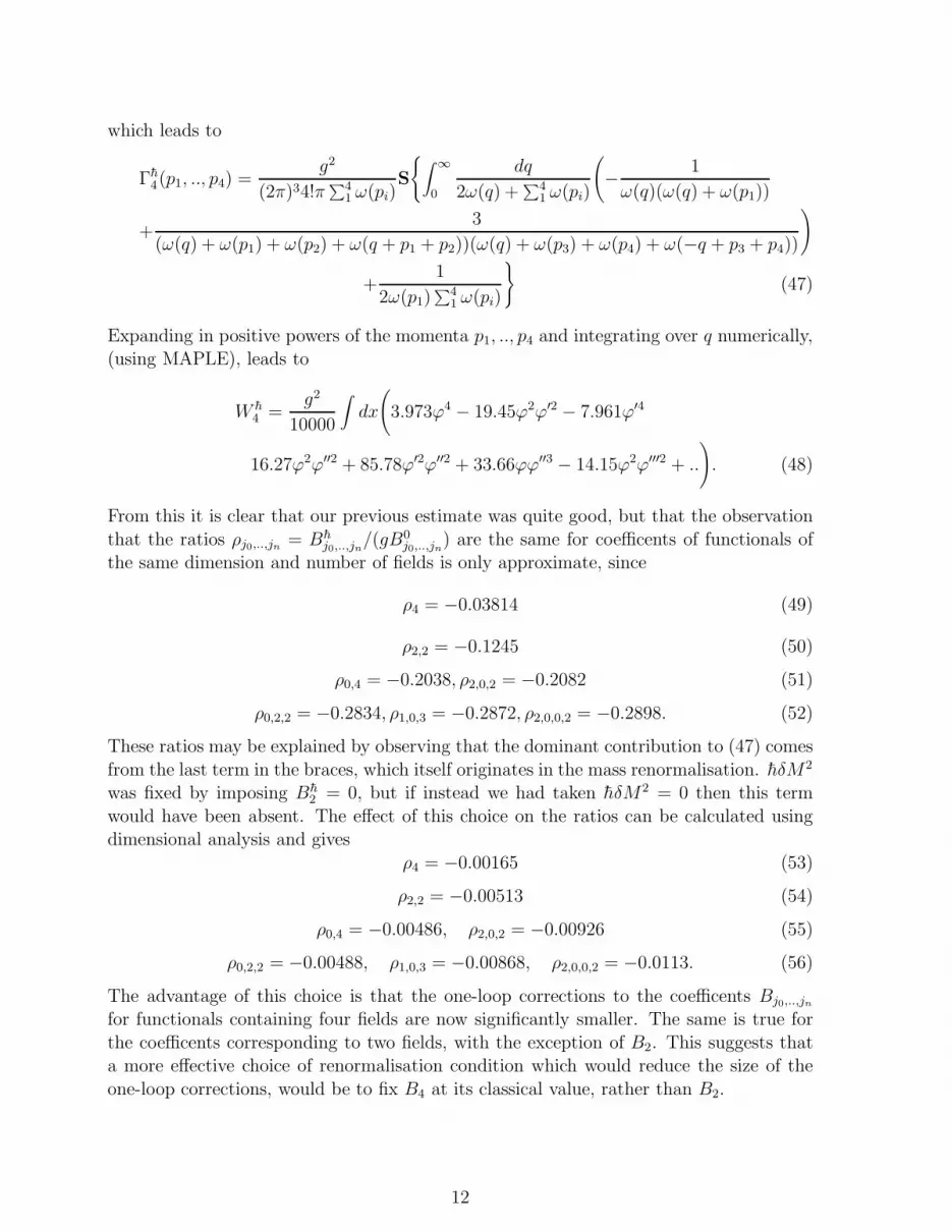
Expanding in positive powers of the momenta p1, .., p4 and integrating over q numerically,(using MAPLE), leads to
W h4 =
g2
10000
∫
dx
(
3.973ϕ4 − 19.45ϕ2ϕ′2 − 7.961ϕ′4
16.27ϕ2ϕ′′2 + 85.78ϕ′2ϕ′′2 + 33.66ϕϕ′′3 − 14.15ϕ2ϕ′′′2 + ..
)
. (48)
From this it is clear that our previous estimate was quite good, but that the observation
that the ratios ρj0,..,jn= Bh
j0,..,jn/(gB0
j0,..,jn) are the same for coefficents of functionals of
the same dimension and number of fields is only approximate, since
ρ4 = −0.03814 (49)
ρ2,2 = −0.1245 (50)
ρ0,4 = −0.2038, ρ2,0,2 = −0.2082 (51)
ρ0,2,2 = −0.2834, ρ1,0,3 = −0.2872, ρ2,0,0,2 = −0.2898. (52)
These ratios may be explained by observing that the dominant contribution to (47) comes
from the last term in the braces, which itself originates in the mass renormalisation. hδM2
was fixed by imposing Bh2 = 0, but if instead we had taken hδM2 = 0 then this term
would have been absent. The effect of this choice on the ratios can be calculated usingdimensional analysis and gives
ρ4 = −0.00165 (53)
ρ2,2 = −0.00513 (54)
ρ0,4 = −0.00486, ρ2,0,2 = −0.00926 (55)
ρ0,2,2 = −0.00488, ρ1,0,3 = −0.00868, ρ2,0,0,2 = −0.0113. (56)
The advantage of this choice is that the one-loop corrections to the coefficents Bj0,..,jn
for functionals containing four fields are now significantly smaller. The same is true for
the coefficents corresponding to two fields, with the exception of B2. This suggests thata more effective choice of renormalisation condition which would reduce the size of the
one-loop corrections, would be to fix B4 at its classical value, rather than B2.
12

4 Sinh-Gordon Model
From the standpoint of perturbation theory ϕ4-theory is ‘close’ to a theory that is quite
special, namely the Sinh-Gordon theory which has an infinite number of conserved quanti-ties that imply the absence of particle production, it is interesting to calculate the vacuum
functional for this case. The potential of the Sinh-Gordon theory may be taken to be [34]
V =M2 + hδM2
β2cosh(βϕ) exp
(
−β2
4π
∫ 1/√
ǫ
0
dp
ω(p)
)
=
(M2 + hδM2)
(
1
β2+
ϕ2
2+
β2ϕ4
4!+
β4ϕ6
6!+ ..
)(
1 − β2
4π
∫ 1/√
ǫ
0
dp
ω(p)+ ..
)
(57)
Apart from the replacement g → M2β2 the Sinh-Gordon potential leads to the sameexpressions for the tree-level values of Γ1
2, Γ14 and the one-loop result Γh
2 . The tree-level
Γ16 is modified by the ϕ6 term in the potential
Γ16 → Γ1
6 −β4M2
6!(2π)5∑6
1 ω(pi)(58)
this, together with the δM2ϕ4 term in V modifies the one-loop value Γh4
Γh4 → Γh
4 −β4M2
(2π)44!∑4
1 ω(pi)
(
∫ ∞
0dq
(
1
2ω(q) +∑4
1 ω(pi)− 1
2ω(q)
)
+1
2
)
(59)
so that for the sinh-Gordon model
W h4 =
β4
π
∫
dx
(
ϕ4
384+
5π − 22
1280ϕ2ϕ′2 − 2275π − 8952
860160ϕ′4 +
651π − 2768
172032ϕ2ϕ′′2
−1041705π − 4243072
41287680ϕ′2ϕ′′2 − 689535π − 2920448
82575360ϕϕ′′3
+13905π − 58624
3932160ϕ2ϕ′′′2 + ..
)
≃ β4
10000
∫
dx
(
8.2893ϕ4 − 15.647ϕ2ϕ′2 − 6.6791ϕ′4
+13.3743ϕ2ϕ′′2 + 74.818ϕ′2ϕ′′2 + 29.0731ϕϕ′′3 − 12.0941ϕ2ϕ′′′2 + ..
)
. (60)
The ratios of the one-loop coefficents to their tree-level values for this model are
ρ4 = −0.07958 (61)
ρ2,2 = −0.1001 (62)
ρ0,4 = −0.1710, ρ2,0,2 = −0.1712 (63)
ρ0,2,2 = −0.2471, ρ1,0,3 = −0.2481, ρ2,0,0,2 = −0.2477. (64)
Note that again the ratios are approximately the same for coefficents of functionals of the
same number of fields and dimension, however this cannot be explained away as simply
13

the effect of mass or coupling renormalisation. If we had taken δM2 = 0 we would haveobtained
ρ4 = −0.1194 (65)
ρ2,2 = −0.06035 (66)
ρ0,4 = −0.05162, ρ2,0,2 = −0.05183 (67)
ρ0,2,2 = −0.04820, ρ1,0,3 = −0.04915, ρ2,0,2 = −0.04875. (68)
which are approximately constant for coefficents of functionals of the same number of fieldsand dimension. These coefficents would, with a change of sign, apply to the Sine-Gordon
model as well.
5 Feynman Diagram Expansion
We will now describe how the results of the previous section are obtained within the moreconventional approach to field theory based on Feynman diagrams. There are several
ways to represent the vacuum functional as a functional integral, the most convenient for
our purposes is the representation, [2],
Ψ[ϕ] =∫
Dφe−SE [φ]+∫
dx ϕφ (69)
where φ vanishes on the surface t = 0, which is the boundary of the Euclidean space-time
t < 0 in which the field φ lives. Therefore, W [ϕ] is a sum of connected Euclidean FeynmanDiagrams in which ϕ is the source for φ on this boundary, the only major difference from
the usual Feynman diagrams encountered in free space is that the propagator vanisheswhen either of its arguments lies on the boundary. Such a propagator can be obtained
using the method of images as
G(x,y) = G0(x,y) − G0(x,y) = G0(x,y) − G0(x,y) (70)
where x = (t, x), x = (−t, x), similarly for y and y, and G0(x,y) is the free spacepropagator. Developing the Feynman diagram expansion yields the tree level diagrams
up to ϕ6 which are shown in figure (4).
(a) (b) (c)
1 2 3 46
p p p p p p p p p p1 2 3 4 5
Figure 4: Tree Diagrams up to ϕ6
The Feynman rules in the coordinate space for the diagram (b), for instance, yield
gsf
∫
dx1..dx4d2v ϕ(x1)..ϕ(x4)
∂G(x1,v)
∂t1
∂G(x2,v)
∂t2
∂G(x3,v)
∂t3
∂G(x4,v)
∂t4(71)
14

where sf is the symmetry factor associated to the diagram, the times t1, .., t4 are all setto zero, and the time-like component of v is integrated over negative values only. When
a propagator ends on the boundary it is equal to twice the free space propagator, so thatin momentum space this is proportional to
∫
dp1..dp4 dq1..dq4ϕ(p1)..ϕ(p4)δ(p1 + .. + p4) δ(q1 + .. + q4)∏
j=1..4
qj
p2j + q2
j + M2(72)
The momenta q1, .., q4 are the time-like components which, when integrated over, give rise
to δ-functions that impose the vanishing of t1, .., t4 in the configuration space represen-
tation (71). In the momentum-space representation these integrals are readily performedas contour integrals leading to our previous expression (36) for Γ1
4. Diagram (a) gives
2
(2π)2
∫
dpdq ϕ(p)ϕ(−p)q2
p2 + q2 + M2(73)
The integral over q is divergent. Formally we can write it as
∫
dp
2πϕ(p)ϕ(−p)
(
δ(0) −√
p22 + M2
)
(74)
The origin of δ(0) is in the construction of the original path integral representation of W ,[30]. Rather than the functional integral (69), we should start with
Ψ[ϕ] = 〈ϕ|0〉 = 〈D|ei∫
πϕ dx|0〉 (75)
(where the state 〈D| satisfies 〈D| ϕ = 0) . As operators π =˙φ , but in the passage from
(75) to the functional integral π is represented by φ plus terms coming from the time
derivative acting on the T -ordering because the functional integral represents T -orderedproducts. This leads to terms like
∫
dxϕ2δ(0), because this is local it may be cancelled by
an equal but opposite counterterm, which amounts to simply discarding the divergence.Alternatively, and perhaps more satisfactorily, we can deal with this divergence by placing
the source terms πϕ not at t = 0 but at small, distinct times ti and finally taking thelimit ti → 0 . This leads to an extra factor of the form eiqǫ in (73) which regularizes
the divergence and enables the integral to be done by closing the q-contour in the upperhalf-plane, yielding a finite result in limit as ǫ → 0, so that we end up with our earlier
expression (33).
When neither end of a propagator is on the boundary, t = 0, the image charge breaksenergy conservation leading to more complicated expressions. However for the tree-level
diagram (c) these may be combined into an expression proportional to
∫
(
6∏
1
dpidqi ϕ(qi) pi
p2i + q2
i + M2
)
δ(p1 + .. + p6) δ(q1 + .. + q6)
(p1 + p2 + p3)2 + (q1 + q2 + q3)2 + M2(76)
which, after integration over the qi gives the same as (37).The diagrams represented in figure (5) enable us to calculate the O(h) correction for
the coefficients of 2 and 4 fields .
15

(a) (b) (c) (d) (e)
z
1 2x
X
x
p p
q
X
p p pp1 2 3 4
k
l
p pp
k1 2
4p3
Figure 5: Two and four field one loop diagrams
From fig.5(a) above we can work out the first order correction to B2 as
sf g∫
dx1dx2d2z ϕ(x1)ϕ(x2)
∂G(x, z)
∂t1G(z, z)
∂G(y, z)
∂t2(77)
This is divergent due to the factor G(z, z). Since the propagator does not touch the
boundary, it has an energy non-conserving contribution from the image represented bythe exponential in
G(z, z) =∫
dp dq
(2π)2
(1 − e2iqt)
(p2 + q2 + M2). (78)
where t is the time-like coordinate of z. We regulate the integral by restricting the
space-like component of momentum, p2 < 1/ǫ, just as we did for the Laplacian in theHamiltonian. The divergence is then cancelled by the counter-term represented by fig.5(b),
which is due to the order-h terms in M2(ǫ), (5). Taken together these diagrams give Γh2
as in (41).
The first order correction Γh4 is given by the sum of diagrams 5(c), 5(d) and 5(e). As
before, diagram (e) is the counterterm diagram associated to the bubble appearing in (d).
In momentum space 5(c) gives
g2s(c)f
8π4
∫
dk dp1..dp4 ϕ(p1)..ϕ(p4) δ(p1 + .. + p4)∑4
1 ω(pi) + ω(k) + ω(l)∑4
1 ω(pi)(ω(p3) + ω(p4) + ω(k) + ω(l))(ω(p1) + ω(p2) + ω(k) + ω(l)).
1
(∑4
1 ω(pi) + 2ω(k))(∑4
1 ω(pi) + 2ω(l)), (79)
where l = p3 + p4 + k. whereas, for the sum of the other two diagrams, (with δM2 = 0),we have
− 4g2s(d)f
π4
∫
dk dp1..dp4ϕ(p1)..ϕ(p4) δ(p1 + .. + p4)
ω(k)(ω(p4) + ω(k))∑4
1 ω(pi)(∑4
1 ω(pi) + 2ω(k))(80)
The symmetry factors s(c)f and s
(d)f are respectively equal to 1/16 and 1/12. If we expand
in powers of the momenta p1, .., p4 the loop integration over k can be done to reproducethe results for W h
4 given by (48).
The extra ϕ6 term in the potential of the Sinh-Gordon model generates the diagramfig. (6). Its analytic expression after subtracting the counterterm reads
β4 sf1
(2π)3
∫
dk dp1..dp4ϕ(p1)..ϕ(p4)δ(p1 + .. + p4)
ω(k)(2ω(k) +∑4
1 ω(pi)). (81)
16

where sf for this diagram is 1/96. This gives the modifications to the ϕ4 results describedearlier.
X
p p pp
k
(a) (b)
1 2 3 4
Figure 6: 6 point interaction for the Sinh-Gordon Model
6 Reconstructing the Vacuum Functional
√p2 + 1
S12
C
p0 20151050
0
20
15
10
5
0
Figure 7: Tree-level vacuum functional: Γ12(p,−p)
We will now use the above results for the ϕ2 part of W [ϕ] to illustrate how the vacuumfunctional can be reconstructed from its large distance expansion. The tree-level contri-
bution has been treated in detail in [30]. Applying formula (2) to∫
dpϕ(p)ϕ(−p)Γ2(p,−p)amounts to the expression
Γ2(p,−p) = limλ→∞
1
2πi
∫
|s|=∞
ds
s − 1eλ(s−1)
√sΓ2(p/
√s,−p/
√s) (82)
17

Since |s| is large on the contour we can use the local expansion Γ2(p,−p) =∑∞
0 anp2n.Shifting s we get
limλ→∞
1
2πi
∫
|s|=∞
ds
seλs
√s + 1
∞∑
0
anp2n
(s + 1)n≡ lim
λ→∞S(p, λ) (83)
Expanding the (s + 1) factors in powers of 1/s enables the integral to be done, yielding apower series in λ. For example, at tree-level
1
2πi
∫
|s|=∞
ds
s − 1eλ(s−1)
√
p2 + s =∞∑
0
(−)n+1λn−1/2(1 + p2)n
n!(2n − 1)√
π. (84)
This series converges for all positive λ. We get an approximation by truncating the
expansion by including terms up to and including λN−1/2, say. This requires a knowledgeof the local expansion only up to terms in (ϕ(N)(x))2. To demonstrate this approximation
we have plotted in fig. (7) the series (84) truncated at N = 12, S12. The value of λ
is chosen so that the last term included is one per cent of the value of the series. Wehave also plotted
√p2 + 1, and the expansion of
√p2 + 1 in powers of p2, C truncated to
fourteen terms. The full series fails to converge for p2 > 1, and this is reflected in thefact that the truncated series ceases to be a good approximation for p2 > 1. However,
S12, which is a resummation of this series is a very good approximation for a much largerrange of momenta.
S12
R12
arcsinh(p)/p
C
p0 6543210
0
1
0.8
0.6
0.4
0.2
0
Figure 8: One-loop vacuum functional: Γh2(p,−p)
The one-loop correction, Γh2 , may be treated in the same way. In fig. (8) we have
plotted arcsinh(p)/p. The small p expansion, C is again only good for p2 < 1. Our
18

approximation that re-sums this series, S12 provides a good approximation only over aslightly larger range. The accuracy of this approximation is greatly improved by further
re-summations, just as we did for the Laplacian. Let us define the re-summation operatoracting on a function of λ and p to be
R · S(λ, p) ≡ 1
2πi
∫
|s|=∞
ds
seλsS(s−1/2, p). (85)
Then the curve R12 shown in fig. (8) results from applying R twice to S12, and provides
a good approximation to arcsinh(p)/p for values of p up to about p = 5. Since theeffect of applying Rp to a term in S12 that is proportional to λn is simply to divide it by
Γ(n/2 + 1)Γ(n/4 + 1)..Γ(n/2p + 1) further applications would have no significant effectwhen we take just twelve terms in the expansion.
7 Conclusions
The purpose of this paper has been to test an approach to quantum field theory in
which states are constructed in the Schrodinger representation from their large-distancebehaviour. The vacuum functional is expanded as a series of local functionals. Truncat-
ing this series at some convenient order leads to an approximation scheme. For scalarϕ4 theory in 1+1-dimensions we compared the results obtained by solving the form of
the Schrodinger equation that applies in this approach with those obtained from a semi-classical expansion, and from the Feynman diagram expansion of the wave-functional. We
have found that the expansion coeficents agree to within a few per cent when we truncatethese series at about ten terms. Also we found that the known counterterms that contain
information about short-distance effects are correctly reproduced by our large-distanceexpansion to a similar accuracy.
We also found a curious simplification that occurs in the vacuum functional of the
Sinh-Gordon and Sine-Gordon models. The ratios of coefficents of the one-loop correctionsto the coefficents of local functionals containing four fields to their tree-level values are
approximately the same for functionals of the same dimension.
8 Acknowledgements
M. Sampaio acknowledges a grant from CNPq - Conselho Nacional de DesenvolvimentoCientıfico e Tecnologico - Brasil, and J. Pachos acknowledges a studentship from the
University of Durham.
References
[1] Hatfield, B. Quantum Field Theory of Particle and Strings, Addison Wesley, 1992,ISBN 0-201-11-11982X.
[2] Symanzik, K. Nucl. Phys. B190[FS3] (1983) 1.
19

[3] Symanzik, K. Schrodinger Representation in Renormalizable Quantum Field Theory,Les Houches 1982, Proceedings, Recent Advances In Field Theory and Statistical
Mechanics.
[4] Luscher, M. , Schrodinger Representation in Quantum Field Theory, Nucl. Phys.B254 ( 1985) 52-57.
[5] Chan, H.S., Nucl. Phys. B278(1986)721.
[6] Luscher, M. , Narayanan, R. , Weisz, P. and Wolff,U. , Nucl. Phys. B384 (1992) 168.
[7] K. Jansen, C. Liu, M. Luscher, H. Simma, S Sint, R. Sommer, P. Weisz, U. Wolff,
Phys. Lett. B372 (1996) 275.
[8] S. Sint, Nucl. Phys. B451 (1995) 416.
[9] S. Sint, R. Sommer, Nucl. Phys.B465 (1996) 71.
[10] Jackiw, R. ,Analysis on Infinite Dimensional Manifolds: Schrodinger Representation
for Quantized Fields, Brazil Summer School 1989:78-143.
[11] McAvity, D.M. and Osborn, H. Nucl. Phys. B394 (1993) 728.
[12] Yee, J. H., Schrodinger Picture Representation of Quantum Field Theory, Mt. Sorak
Symposium 1991:210-271.
[13] Floreanini, R.,Applications of Schrodinger Picture in Quantum Field Theory, LucVinet (Montreal U.), MIT-CTP-1517, Sept. 1987.
[14] C. Kiefer, Phys. Rev. D 45 (1992) 2044.
[15] C. Kiefer and Andreas Wipf, Ann. Phys. 236 (1994)241.
[16] Feynman, R. P., Nucl. Phys. B188(1981) 479.
[17] Greensite, J., Nucl.Phys. B158 (1979) 469, Nucl.Phys. B166 (1980) 113.
[18] Kawamura, M., Maeda, K., Sakamoto, M., KOBE-TH-96-02 hep-th/9607176.
[19] P. Mansfield, Nucl. Phys. B418 (1994) 113.
[20] G.V. Dunne, R. Jackiw, C.A. Trugenberger , Chern-Simons Theory in the
Schrodinger Representation, Ann.Phys.194:197,1989.
[21] A.V. Ramallo, Two Dimensional Chiral Gauge Theories in the Schrodinger Repre-
sentation, Int.J.Mod.Phys.A5:153,1990.
[22] K. Heck, Some Considerations on the Problem of Renormalization of Quantum Field
Theory in the Schrodinger Representation. In German, Heidelberg Univ. - HD-THEP
82-04 .
[23] T. Horiguchi, KIFR-94-01, KIFR-94-03, KIFR-95-02, KIFR-96-01, KIFR-96-03.
20

[24] T. Horiguchi, Nuovo. Cim. 111B (1996) 49,85,293.
[25] T.Horiguchi, K. Maeda, M. Sakamoto, Phys.Lett. B344 (1994) 105.
[26] Kowalski-Glikman, J., Meissner, K.A., Phys.Lett. B376 (1996) 48.
[27] Kowalski-Glikman, J. gr-qc/9511014.
[28] Blaut, A.,Kowalski-Glikman, J. gr-qc/9607004.
[29] Maeda, K., Sakamoto, M., Phys.Rev. D54 (1996) 1500.
[30] Mansfield, P., Phys. Lett. B358 (1995) 287.
[31] Mansfield, P., Phys. Lett. B365 (1996) 207.
[32] Jeffrey, A., Handbook of Mathematical Formulas and Integrals, Academic Press.
(1995).
[33] Copson, E., Asymptotic Series, Cambridge University Press, 1965.
[34] Coleman, S., Phys. Rev. D11 (1975) 2088.
21