development of autonomous surface vessels
TRANSCRIPT
DEVELOPMENT OF AUTONOMOUS SURFACE VESSELS
FOR HYDROGRAPHIC SURVEY APPLICATIONSBY
DAMIAN MANDA
BS, University of Colorado, 2010
THESIS
Submitted to the University of New Hampshire
in Partial Fulfillment of the Requirements for the Degree of
Master of Science
in
Ocean Engineering, Ocean Mapping
September, 2016

All rights reserved
INFORMATION TO ALL USERSThe quality of this reproduction is dependent upon the quality of the copy submitted.
In the unlikely event that the author did not send a complete manuscriptand there are missing pages, these will be noted. Also, if material had to be removed,
a note will indicate the deletion.
All rights reserved.
This work is protected against unauthorized copying under Title 17, United States CodeMicroform Edition © ProQuest LLC.
ProQuest LLC.789 East Eisenhower Parkway
P.O. Box 1346Ann Arbor, MI 48106 - 1346
ProQuest 10161845
Published by ProQuest LLC (2016). Copyright of the Dissertation is held by the Author.
ProQuest Number: 10161845
This thesis has been examined and approved in partial fulfillment of the requirements for the degree ofMaster of Science in Ocean Engineering by:
Thesis Director, Dr. May-Win Thein,Associate Professor of Mechanical Engineeringand Ocean Engineering
Andy Armstrong,Co-Director, Joint Hydrographic CenterAffiliate Professor of Ocean Engineeringand Marine Sciences and Earth Sciences
Dr. Martin Renken,Lead Engineer, Naval Undersea Warfare Center
on 5/12/2016.
Original approval signatures are on file with the University of New Hampshire Graduate School.
ii
ACKNOWLEDGEMENTSThe author would like to thank the Naval Engineering Education Consortium for financial sup-
port of this research project over the past 2 years. The NOAA Office of Coast Survey has provided
general funding for Mr. Manda’s degree and the ability to pursue the program at the University of
New Hampshire. The NOAA Office of Unmanned Systems provided the EMILY vehicle for use
in field testing. The NOAA Hydrographic Systems and Technologies Branch (HSTB) provided
resources for the purchase of a sonar system for installation on the EMILY vehicle to be used in
testing the path planning. Without this support, many aspects of this research would not have been
possible.
The author would also like to thank the crew of NOAA Ship Thomas Jefferson and Teledyne
Oceanscience for providing time and resources to allow experimentation on multiple Z-Boat plat-
forms. In addition to the assistance provided by the thesis committee, UNH Center for Coastal
and Ocean Mapping research scientist Val Schmidt and research project engineer Andy McLeod
were integral to successful Z-Boat deployments at UNH and provided valuable feedback for the
research at many opportunities.
The constant support, feedback and guidance of thesis director Dr. May-Win Thein facilitated
the completion of this ambitious research. The opportunity as her student to attend conferences,
mentor undergraduates and collaborate with others in the field were greatly appreciated and led
to additional insight into the academic process and ocean engineering field outside the classroom
environment.
iii
TABLE OF CONTENTS
ACKNOWLEDGEMENTS iii
LIST OF TABLES vii
LIST OF FIGURES viii
LIST OF SYMBOLS xii
ABSTRACT xiii
INTRODUCTION 1
1 VESSEL HARDWARE AND ELECTRONICS 5
1.1 Vessels . . . . . . . . . . . . . . . . . . . . . . . . . . . . . . . . . . . . . . . . . 5
1.1.1 Hydronalix Hurricane EMILY . . . . . . . . . . . . . . . . . . . . . . . . 5
1.1.2 Teledyne OceanScience Z-Boat 1800 . . . . . . . . . . . . . . . . . . . . 7
1.1.3 UNH Developed ASVs . . . . . . . . . . . . . . . . . . . . . . . . . . . . 9
1.2 Full Retrofit System . . . . . . . . . . . . . . . . . . . . . . . . . . . . . . . . . . 11
1.2.1 Processing and Autonomy Execution . . . . . . . . . . . . . . . . . . . . 11
1.2.2 Wireless Communication . . . . . . . . . . . . . . . . . . . . . . . . . . . 13
1.2.3 Positioning and Depth Measurement . . . . . . . . . . . . . . . . . . . . . 16
1.2.4 Power . . . . . . . . . . . . . . . . . . . . . . . . . . . . . . . . . . . . . 17
1.2.5 System Integration . . . . . . . . . . . . . . . . . . . . . . . . . . . . . . 19
1.3 Reduced System for Commercial Survey ASVs . . . . . . . . . . . . . . . . . . . 23
1.4 Direct Autonomy Installation . . . . . . . . . . . . . . . . . . . . . . . . . . . . . 24
iv
2 AUTONOMY SOFTWARE AND OPERATION 26
2.1 IvP Helm . . . . . . . . . . . . . . . . . . . . . . . . . . . . . . . . . . . . . . . 28
2.2 Implementation of MOOS-IvP for This Project . . . . . . . . . . . . . . . . . . . 28
2.3 Custom MOOSApps . . . . . . . . . . . . . . . . . . . . . . . . . . . . . . . . . 31
3 AUTOMATED SWATH SURVEY PATH PLANNING 39
3.1 Introduction . . . . . . . . . . . . . . . . . . . . . . . . . . . . . . . . . . . . . . 39
3.2 Adaptive Line Planning . . . . . . . . . . . . . . . . . . . . . . . . . . . . . . . . 40
3.2.1 Swath History Recording . . . . . . . . . . . . . . . . . . . . . . . . . . . 40
3.2.2 Planning Subsequent Paths . . . . . . . . . . . . . . . . . . . . . . . . . . 42
3.2.3 Completion Metric and Holiday Detection . . . . . . . . . . . . . . . . . . 46
3.3 Auxiliary Functionality . . . . . . . . . . . . . . . . . . . . . . . . . . . . . . . . 48
3.4 Simulation Results . . . . . . . . . . . . . . . . . . . . . . . . . . . . . . . . . . 50
3.4.1 Custom Simulation Program . . . . . . . . . . . . . . . . . . . . . . . . . 50
3.4.2 MOOS-IvP Implementation and Simulation . . . . . . . . . . . . . . . . . 52
3.5 Field Testing Results . . . . . . . . . . . . . . . . . . . . . . . . . . . . . . . . . 60
3.5.1 Single Beam Sonar Tests . . . . . . . . . . . . . . . . . . . . . . . . . . . 60
3.5.2 Multibeam Sonar Tests . . . . . . . . . . . . . . . . . . . . . . . . . . . . 61
4 CONTROL SYSTEM 67
4.1 Introduction to Control System Types . . . . . . . . . . . . . . . . . . . . . . . . 67
4.1.1 PID Control . . . . . . . . . . . . . . . . . . . . . . . . . . . . . . . . . . 67
4.1.2 Model Reference Adaptive Heading Control . . . . . . . . . . . . . . . . . 68
4.2 Implementation of MRAC . . . . . . . . . . . . . . . . . . . . . . . . . . . . . . 69
4.2.1 Course Change Controller . . . . . . . . . . . . . . . . . . . . . . . . . . 70
4.2.2 Course Keep Controller . . . . . . . . . . . . . . . . . . . . . . . . . . . 78
4.2.3 Hybrid Heading Control System . . . . . . . . . . . . . . . . . . . . . . . 85
4.3 Speed Control . . . . . . . . . . . . . . . . . . . . . . . . . . . . . . . . . . . . . 85
v
4.3.1 Initial Setting Stage . . . . . . . . . . . . . . . . . . . . . . . . . . . . . . 86
4.3.2 Coarse Adjustment . . . . . . . . . . . . . . . . . . . . . . . . . . . . . . 87
4.3.3 Fine Adjustments . . . . . . . . . . . . . . . . . . . . . . . . . . . . . . . 88
4.4 Control System Simulation Testing . . . . . . . . . . . . . . . . . . . . . . . . . . 89
4.4.1 Heading Control Tests . . . . . . . . . . . . . . . . . . . . . . . . . . . . 90
4.4.2 Speed Control Tests . . . . . . . . . . . . . . . . . . . . . . . . . . . . . 98
4.5 Field Tests . . . . . . . . . . . . . . . . . . . . . . . . . . . . . . . . . . . . . . . 100
4.5.1 Rate-of-Turn Characterization . . . . . . . . . . . . . . . . . . . . . . . . 101
4.5.2 Course Change Controller Field Test . . . . . . . . . . . . . . . . . . . . . 104
CONCLUSION AND FUTURE WORK 106
LIST OF REFERENCES 108
vi

LIST OF TABLES
1.1 Specification and uses of voltage regulators . . . . . . . . . . . . . . . . . . . . . 18
1.2 Autonomy hardware system component current and power draws. . . . . . . . . . 19
1.3 Autonomy hardware system components and costs. . . . . . . . . . . . . . . . . . 20
3.1 Comparison of survey methodologies in different regions . . . . . . . . . . . . . . 59
4.1 Thrust to speed relationships of systems used in this thesis . . . . . . . . . . . . . 86
4.2 Measured vessel response characteristics . . . . . . . . . . . . . . . . . . . . . . . 102
vii
LIST OF FIGURES
1.1 Profile view of Hurricane EMILY vessel. . . . . . . . . . . . . . . . . . . . . . . . 6
1.2 Overhead view of Hurricane EMILY vessel with covers removed, showing loca-
tion of components. Autonomy control box fits in compartment above batteries,
secured with the straps shown. . . . . . . . . . . . . . . . . . . . . . . . . . . . . 7
1.3 Profile view of Z-Boat 1800-RP. . . . . . . . . . . . . . . . . . . . . . . . . . . . 8
1.4 Custom multibeam demo Z-Boat for Teledyne OceanScience. . . . . . . . . . . . . 8
1.5 Undergraduate ASV2, including mast for antennas. . . . . . . . . . . . . . . . . . 9
1.6 Undergraduate ASV3, in storage configuration with propulsion and sonar systems
retracted. . . . . . . . . . . . . . . . . . . . . . . . . . . . . . . . . . . . . . . . 10
1.7 Undergraduate ASV3, underway for sonar data collection with the author aboard. . 10
1.8 Autonomy processing computer and microcontroller . . . . . . . . . . . . . . . . 12
1.9 Range performance of long distance Wi-Fi system . . . . . . . . . . . . . . . . . . 14
1.10 Wireless data transfer and control hardware. . . . . . . . . . . . . . . . . . . . . . 15
1.11 Position and depth sensing equipment . . . . . . . . . . . . . . . . . . . . . . . . 17
1.12 Block diagram of vessel autonomy system . . . . . . . . . . . . . . . . . . . . . . 20
1.13 Schematic of EMILY control signal isolation board . . . . . . . . . . . . . . . . . 21
1.14 Complete autonomy retrofit hardware system for EMILY, marking components not
previously pictured. . . . . . . . . . . . . . . . . . . . . . . . . . . . . . . . . . . 22
1.15 Exterior of the EMILY hardware box. . . . . . . . . . . . . . . . . . . . . . . . . 22
1.16 System diagram for Z-Boat module. . . . . . . . . . . . . . . . . . . . . . . . . . 23
1.17 Simplified autonomy module for Z-Boat . . . . . . . . . . . . . . . . . . . . . . . 24
2.1 Graphical interface for monitoring MOOS missions, shown with waypoint behavior. 27
viii
2.2 Basic behavior structure used for field testing, including details of survey behavior
described in Chapter 3. . . . . . . . . . . . . . . . . . . . . . . . . . . . . . . . . 29
2.3 MOOS application diagram for core autonomy system . . . . . . . . . . . . . . . 30
2.4 Flow of information in automatic configuration and communication between ASV
and shore station. . . . . . . . . . . . . . . . . . . . . . . . . . . . . . . . . . . . 31
2.5 Effect of simulated waves on speed and heading, waves from 000. . . . . . . . . . 37
2.6 Effect of simulated noise on measured heading while ASV is navigating on a head-
ing of 090. . . . . . . . . . . . . . . . . . . . . . . . . . . . . . . . . . . . . . . 38
3.1 Results of automatic path planning designed by Bourgeois [1], using piecewise
linear planning. . . . . . . . . . . . . . . . . . . . . . . . . . . . . . . . . . . . . 40
3.2 Illustration of the selection of swath minima points from full raw data record,
which are then used as a basis for planning the next path. . . . . . . . . . . . . . . 41
3.3 Illustration of the generation of an offset line for initial input into the refinements
of the path planning algorithm. This shows a straight initial line for data collection,
but the same process is used for subsequent segmented lines. No additional overlap
is added in this example. . . . . . . . . . . . . . . . . . . . . . . . . . . . . . . . 43
3.4 Example of path refinement from a simulated path, with removal of intersecting
segments (green) and areas with sharp bends . . . . . . . . . . . . . . . . . . . . . 45
3.5 Diagram of path clipping and extension process, showing before (left) and after
(right) . . . . . . . . . . . . . . . . . . . . . . . . . . . . . . . . . . . . . . . . . 46
3.6 Half stepping behavior demonstrated, with next line planned along edge of previ-
ous swath coverage. . . . . . . . . . . . . . . . . . . . . . . . . . . . . . . . . . . 47
3.7 Example of a planned turn between subsequent survey lines showing the turn point
extended from the end of the first line and alignment line extending from the be-
ginning of the second line. . . . . . . . . . . . . . . . . . . . . . . . . . . . . . . 49
3.8 Custom simulation with generated terrain. Survey paths shown in white, coverage
in transparent blue. . . . . . . . . . . . . . . . . . . . . . . . . . . . . . . . . . . 51
ix

3.9 Custom simulator with generated terrain, with vessel path in white and detected
holidays marked with stars. Bathymetry is shown as a rainbow colored background
where blues represent deeper depths and reds shallower. . . . . . . . . . . . . . . . 51
3.10 Custom simulation using actual terrain. Data coverage is shown in transparent blue
and holidays marked with stars. . . . . . . . . . . . . . . . . . . . . . . . . . . . . 52
3.11 MOOS behavior and application flow diagram showing states during the survey
portion of a path planning mission. . . . . . . . . . . . . . . . . . . . . . . . . . . 53
3.12 MOOS behavior and application flow diagram showing states during path planning
algorithm and simulation execution. . . . . . . . . . . . . . . . . . . . . . . . . . 54
3.13 Simulation results from MOOS-IvP simulation showing survey behavior. A red
box denotes the specified operation region and the white lines show survey paths.
Human data collection paths shown in light grey. Bathymetry is shown as a rain-
bow colored background where blues represent deeper depths and reds shallower. . 56
3.14 Surveyed polygon in H12450 from NOAA Ship Rainier launch near Chirikof Is-
land, showing automated planning in white and human lines in black. . . . . . . . 57
3.15 Surveyed polygon in H12758 from NOAA Ship Fairweather launch in the Shuma-
gin Islands, showing automated planning in white and human lines in black. . . . . 58
3.16 Surveyed polygon in H12472 from NOAA Ship Rainier launch in the Shumagin
Islands, showing automated planning in white and human lines in black. . . . . . . 59
3.17 Automated survey path planning test at Naval Station Newport. . . . . . . . . . . . 61
3.18 MOOS-IvP pMarineViewer monitoring view of automated survey in progress. Op-
eration region shown in red, current survey line in white and vessel track in yellow. 62
3.19 Automatically planned multibeam survey, showing survey region in red and vessel
track in white. . . . . . . . . . . . . . . . . . . . . . . . . . . . . . . . . . . . . . 63
3.20 Data density information from multibeam sonar survey near Solomons, MD. . . . . 65
3.21 Chart representations of the area shown with survey data to illustrate changes since
prior survey. . . . . . . . . . . . . . . . . . . . . . . . . . . . . . . . . . . . . . . 65
x

4.1 Course changing maneuver showing rudder and heading response. From Van
Amerongen [2] . . . . . . . . . . . . . . . . . . . . . . . . . . . . . . . . . . . . 70
4.2 Effect of ζ on overshoot and settling, with example heading change of 90. . . . . 72
4.3 Course change controller block diagram. . . . . . . . . . . . . . . . . . . . . . . . 75
4.4 Course change controller series model for modification of reference input. . . . . . 76
4.5 Course keep controller block diagram. . . . . . . . . . . . . . . . . . . . . . . . . 79
4.6 Effect of ωn with varying damping ratios during a heading change of 90. . . . . . 82
4.7 Power spectra of various trials with different vessels, exhibiting characteristics of
the vessels, environment and measurement noise. . . . . . . . . . . . . . . . . . . 83
4.8 Relationship between τs and Ks and speed of the vessel, showing minimum limit
of U = 0.5m/s. For this example L = 2.5, K∗s = 1.56, τ∗s = 0.8. . . . . . . . . . . 85
4.9 Averaging speed controller state diagram. . . . . . . . . . . . . . . . . . . . . . . 89
4.10 Course change controller maneuver with ζ = 0.6,1.0,1.4 . . . . . . . . . . . . . . 91
4.11 Adaptive parameters for course change controller maneuver with ζ = 1.0. . . . . . 92
4.12 Effect of different magnitudes of adaptive gains . . . . . . . . . . . . . . . . . . . 93
4.13 Adaptation of course keep controller with ωn = 2.4 and different values of ζ . . . . 94
4.14 Controlled heading response for turns ωn = 2.4 and different values of ζ . . . . . . 95
4.15 Adaptation of Ki with rudder offset of 5 . . . . . . . . . . . . . . . . . . . . . . . 96
4.16 Simulated noise and low pass filtered rate of turn . . . . . . . . . . . . . . . . . . 97
4.17 Full conditions simulation, including waves, rudder offset and sensor noise . . . . 97
4.18 Speed control comparison with waves and vessel turns but no currents in simulation 99
4.19 Speed control comparison with waves, currents, and vessel turns in simulation . . . 100
4.20 Z-Boat rate-of-turn effects from rudder and thrust settings . . . . . . . . . . . . . . 102
4.21 ASV3 rate-of-turn response to rudder angle and thrust . . . . . . . . . . . . . . . . 103
4.22 Course change controller field test, showing heading and PID feedback gains dur-
ing a 90 turn. . . . . . . . . . . . . . . . . . . . . . . . . . . . . . . . . . . . . . 105
xi

LIST OF SYMBOLS
τm — Time constant of modeled heading system (s)
τs — Time constant of vessel for reaching steady-state rate of turn (s)
Kpm — Proportionality constant of modeled heading system (unitless)
Ks — Proportionality constant of vessel between rate of turn and rudder angle (unitless)
δ — Rudder angle ()
ψm — Heading of the modeled system ()
ψr — Desired heading when making a turn (deg)
ψp — Heading of the vessel (measured) (deg)
ψ — Heading rate-of-turn (ROT), how quickly the vessel is turning
ζ — Damping ratio, a factor governing overshoot in a system response (unitless)
ωn — Natural frequency of a system (rad/s)
L — Length of a vessel (m)
U — Speed of a vessel (m/s)
I — The identity matrix.
xii

ABSTRACTDEVELOPMENT OF AUTONOMOUS SURFACE VESSELS FOR HYDROGRAPHIC
SURVEY APPLICATIONS
by
Damian Manda
University of New Hampshire, September 2016
Autonomously navigating surface vessels have a variety of potential applications for ocean
mapping. The use of small vessels for coastal mapping is investigated through development of
hardware and software that form a complete system for survey operations. The hardware is se-
lected to minimize cost while providing flexibility for installation on different platforms. MOOS-
IvP open-source autonomy software enables independent operation of the vessel and provides for
human monitoring. Custom applications allow the sensors and actuators of the hardware platforms
to interface with MOOS-IvP.
An autonomy behavior is developed that replicates current human driven survey acquisition, in
which the boat plans paths automatically to achieve full survey coverage with a swath sonar system.
With initial input of a survey boundary and depths from the onboard sonar system, subsequent
paths are planned to be offset based on the collected data. This behavior is tested in simulation and
field experiments.
A model reference adaptive control system for the heading of the vessel is investigated for im-
proved reliability of vessel operation in a variety of conditions and over the full range of operation
speeds. Simulations tests verify the adaptation of two types of controllers. A new method for speed
control to increase endurance and decrease engine wear is also proposed and simulated.
Together, these developments form an easily configurable system that provides automated hy-
drographic survey capability to a vessel with minimal human involvement for optimal performance.
xiii
INTRODUCTIONMarine vessels were one of the first applications of both unmanned systems and automated
control. Their operation in less constrained environments than on land, but with simpler design
requirements than aerial vehicles led to early experiments. Some of the first took place in the
1860’s with developments of rudimentary torpedoes [3] and steam based ship steering systems [4].
The development of the North-seeking electronic gyrocompass in 1908 and spreading application
of powered steering mechanisms spurred advancement in the development of control systems, and
Sperry patented the first widely used automated controller in 1911 [4]. Minorsky improved the
operation of these controllers, developing an early form of the Proportional, Integral, Derivative
(PID) controllers used in many applications today [5].
Subsequent advances were driven by military applications, including target drones and minesweep-
ing vessels [6]. All of these vessels were unmanned and could follow commands either from a
plan or remote control, but did not have decision based behavior capabilities. Throughout this
period, automated heading control for long transits became widespread and was available on most
commercial and research vessels, where the headings were selected by the officers of the watch.
Modern large ship autopilots remain very similar in capability to these early models, being able to
follow tracks and headings but not assimilate other information and react to a changing environ-
ment. Dynamic positioning systems installed on vessels with the need to accurately station keep
improve the positioning capability beyond heading, but still follow human directed plans.
The first truly autonomous surface vessels (ASVs) emerged in the late 1980s and early 1990s
with the introduction of GPS positioning. The Owl vessels designed for the US Navy by companies
that later became Navtec Inc. are often cited as the first operationally deployed ASV [3], [6]. These
vessels were jet ski to small Rigid Hull Inflatable type boats with onboard sensing and navigation
systems and have been mimicked by many other efforts leading into the present day. However,
1
the situational awareness, ability to complete complex missions and operational robustness only
marginally improved until the early 2010s [3]. Recent work in autonomous land vehicles and air-
craft allow them to operate for long periods of time in complex situations without human guidance,
but marine vehicles have not received as much attention. This is potentially because of the same
reasons that made early development more simple, the operation space is less constrained than in
land navigation, but must remain on a single vertical surface. In addition, most interactions are un-
structured and human mariners often negotiate passing arrangements contrary to the international
standard Collision Regulations (COLREGS).
Until the early 2010s, most unmanned systems outside the Navy were isolated research efforts.
In recent years, a number of commercial ASV manufacturers have begun producing models for
applications in the oil and gas industry, environmental monitoring and seafloor mapping. Exam-
ples of these include the up to 7 m, diesel powered C-Worker produced by ASV Global [7] and
the smaller, battery powered Teledyne Oceanscience Z-Boat 1800 [8]. Other vessels target long
duration deployment, such as the Liquid Robotics Wave Glider [9] and the Saildrone [10]. These
vessels can be delivered as a ready-to-run package with integrated sensing systems, path following
autonomy and operator interfaces. The Saildrone and Wave Glider are designed to operate for
indefinite periods of time, and therefore contain redundant, fault tolerant systems for long duration
autonomy.
In addition to vessel advancements, the ecosystem necessary to fit autonomous vessels into
marine operations have been subject to recent developments. Many research efforts have targeted
vessels enacting COLREGS compliant maneuvers, using a variety of methods including multi-
objective optimization [11], velocity obstacles [12], 4D space models [13] and fuzzy logic [14].
The infrastructure necessary to support navigation of many vessels is being investigated through
projects like the Sea Traffic Management validation study by the European Union and Swedish
Maritime Administration [15]. Large companies such as Rolls Royce are also beginning to expand
on their visions of where these projects could evolve in the future, with centralized control of an
autonomous vessel fleet [16].
2
For hydrographic surveying, autonomous underwater vehicles (AUVs) were introduced in the
1990s and became more feasible for routine surveys in the following decade. AUVs take advan-
tage of submergence to survey closer to the seafloor and are more decoupled from surface condi-
tions than traditional marine vessels, but still have major limitations in positioning and operational
endurance and are typically very expensive as a result of the additional engineering burden for
submerged vehicles. Many of these costs and concerns can be greatly reduced through the use of
small autonomous surface vessels. Global Navigation Satellite System (GNSS) reception allows
for cheaper navigation systems, hull sealing only needs to withstand wave action, and absolute
reliability in operation is not paramount since the vessel can still be recovered if it malfunctions
or is depleted of power. Air breathing gasoline or diesel engines or generators facilitate improved
operating time and batteries can be much more easily swapped than with a pressure sealed hull.
For these reasons, increased interest in the use of ASVs for survey operations has led to a need
software that allows flexible configuration and deployment in the field. In addition to the general
maritime ecosystem and situational advancements, hydrography requires specialized navigation
and path planning in order to map the seafloor to desired levels of coverage. Previous work on path
planning mostly focuses on either filling areas with parallel lines, which can be fixed spacing such
as in Hodo et al [17] or divided into regions based on depth such as in Galceran and Carreras [18].
These methods involve prior knowledge of the depths and obstacles within the survey region to
function correctly. Methods targeting previously uncharacterized areas have been developed for
single beam surveys by Wilson and Williams [19] and swath sonar surveys by Bourgeois [1].
These approaches enable the vessel to automatically respond to detected depths while surveying,
allowing less human preparation time for deployment and more flexible use. This type of path
planning was used as the basis for this research.
This research creates a system that is capable of converting any surface vessel for use in au-
tonomous operations, and is customized for a number of small vessels. An autonomy system is
implemented that allows basic operation in a variety of behaviors. A hydrographic survey path
planning algorithm is implemented that achieves full coverage in previously unsurveyed regions.
3

In order to accurately follow the paths, an adaptive control system is developed that improves
performance in wave and current conditions over traditional PID control.
4
CHAPTER 1
VESSEL HARDWARE AND ELECTRONICSThe hardware underlying the autonomous control system consists of primarily commercially
available components that interact to make navigation decisions and drive the control surfaces
of the ASV. Variants of this hardware are currently being used by multiple parallel development
efforts at the University of New Hampshire for implementation on different research ASVs, as
well as on NOAA’s commercially produced ASVs. This rapid duplication and integration is made
possible by the low-cost, mass-produced availability and the flexibility of the hardware system for
interfacing with a variety of devices. Two major versions are implemented for this research. One is
a full system capable of interfacing with low level hardware and providing monitoring and manual
control capabilities, while the other is designed to add autonomy to vessels with existing remote
control survey infrastructure.
1.1 Vessels
Two models of small commercially produced ASVs were specifically targeted for the autonomy
retrofit in this research. In addition to these installations, versions of the hardware system were in-
stalled on two boats as part of undergraduate senior projects. These vessels were used to test some
autonomy and control algorithms for this research, and demonstrate the simultaneous operation of
multiple vessels.
1.1.1 Hydronalix Hurricane EMILY
The Hurricane EMILY vessel is based on the Hydronalix EMILY surf rescue boat, a remote con-
trolled life buoy that can be deployed at beaches and rivers. The Hurricane version is designed
5
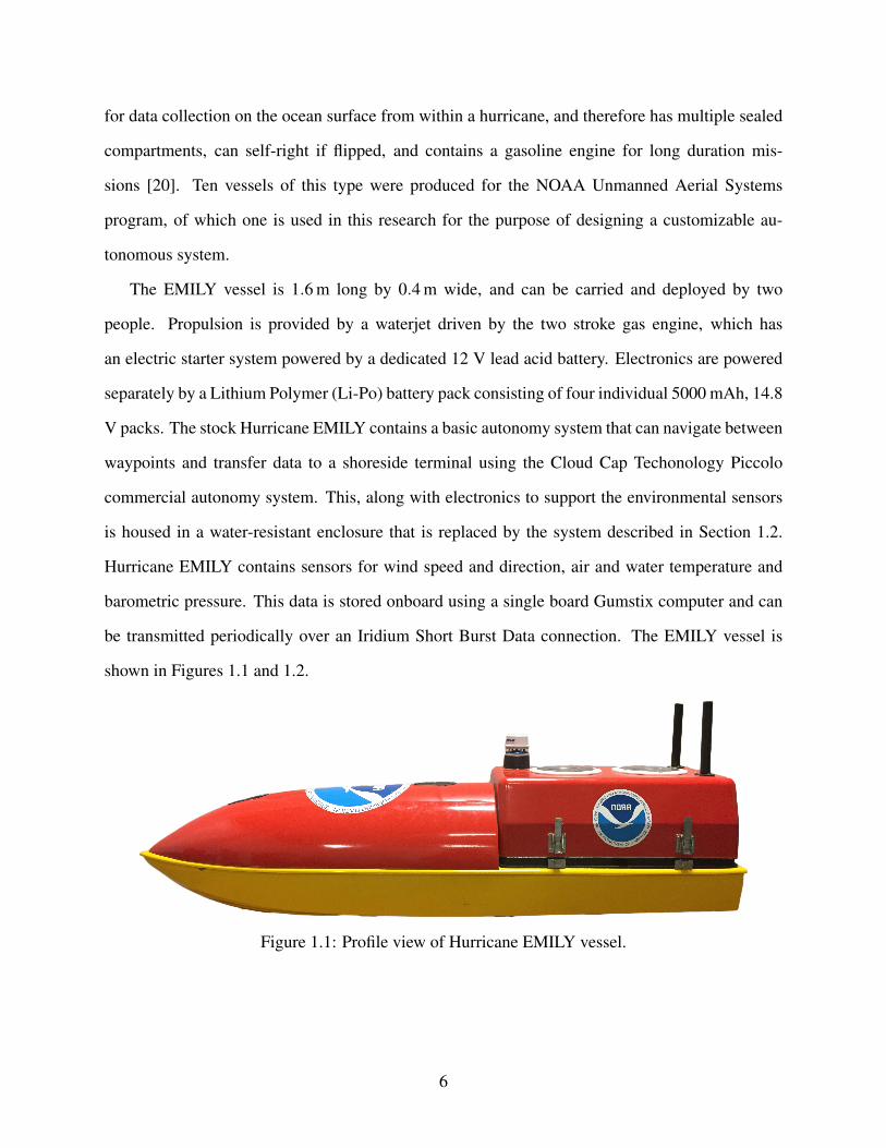
for data collection on the ocean surface from within a hurricane, and therefore has multiple sealed
compartments, can self-right if flipped, and contains a gasoline engine for long duration mis-
sions [20]. Ten vessels of this type were produced for the NOAA Unmanned Aerial Systems
program, of which one is used in this research for the purpose of designing a customizable au-
tonomous system.
The EMILY vessel is 1.6 m long by 0.4 m wide, and can be carried and deployed by two
people. Propulsion is provided by a waterjet driven by the two stroke gas engine, which has
an electric starter system powered by a dedicated 12 V lead acid battery. Electronics are powered
separately by a Lithium Polymer (Li-Po) battery pack consisting of four individual 5000 mAh, 14.8
V packs. The stock Hurricane EMILY contains a basic autonomy system that can navigate between
waypoints and transfer data to a shoreside terminal using the Cloud Cap Techonology Piccolo
commercial autonomy system. This, along with electronics to support the environmental sensors
is housed in a water-resistant enclosure that is replaced by the system described in Section 1.2.
Hurricane EMILY contains sensors for wind speed and direction, air and water temperature and
barometric pressure. This data is stored onboard using a single board Gumstix computer and can
be transmitted periodically over an Iridium Short Burst Data connection. The EMILY vessel is
shown in Figures 1.1 and 1.2.
Figure 1.1: Profile view of Hurricane EMILY vessel.
6
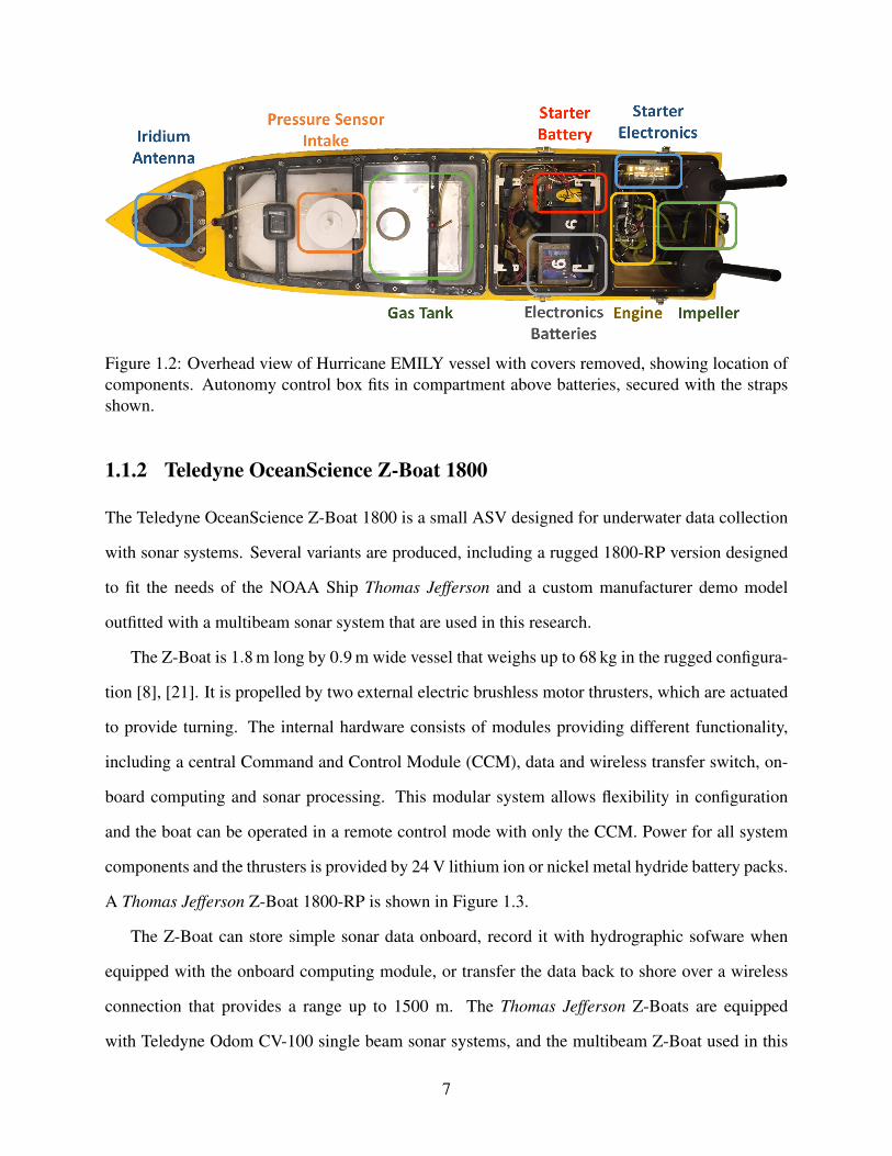
Figure 1.2: Overhead view of Hurricane EMILY vessel with covers removed, showing location ofcomponents. Autonomy control box fits in compartment above batteries, secured with the strapsshown.
1.1.2 Teledyne OceanScience Z-Boat 1800
The Teledyne OceanScience Z-Boat 1800 is a small ASV designed for underwater data collection
with sonar systems. Several variants are produced, including a rugged 1800-RP version designed
to fit the needs of the NOAA Ship Thomas Jefferson and a custom manufacturer demo model
outfitted with a multibeam sonar system that are used in this research.
The Z-Boat is 1.8 m long by 0.9 m wide vessel that weighs up to 68 kg in the rugged configura-
tion [8], [21]. It is propelled by two external electric brushless motor thrusters, which are actuated
to provide turning. The internal hardware consists of modules providing different functionality,
including a central Command and Control Module (CCM), data and wireless transfer switch, on-
board computing and sonar processing. This modular system allows flexibility in configuration
and the boat can be operated in a remote control mode with only the CCM. Power for all system
components and the thrusters is provided by 24 V lithium ion or nickel metal hydride battery packs.
A Thomas Jefferson Z-Boat 1800-RP is shown in Figure 1.3.
The Z-Boat can store simple sonar data onboard, record it with hydrographic sofware when
equipped with the onboard computing module, or transfer the data back to shore over a wireless
connection that provides a range up to 1500 m. The Thomas Jefferson Z-Boats are equipped
with Teledyne Odom CV-100 single beam sonar systems, and the multibeam Z-Boat used in this
7
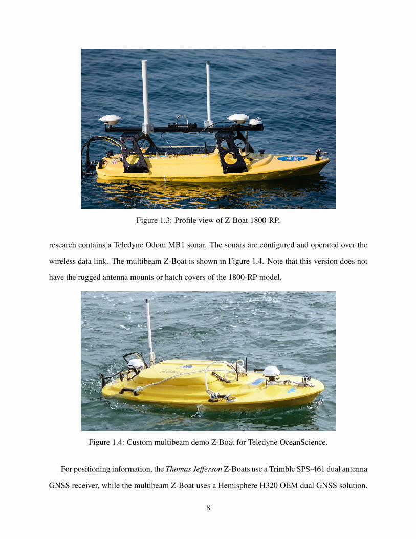
Figure 1.3: Profile view of Z-Boat 1800-RP.
research contains a Teledyne Odom MB1 sonar. The sonars are configured and operated over the
wireless data link. The multibeam Z-Boat is shown in Figure 1.4. Note that this version does not
have the rugged antenna mounts or hatch covers of the 1800-RP model.
Figure 1.4: Custom multibeam demo Z-Boat for Teledyne OceanScience.
For positioning information, the Thomas Jefferson Z-Boats use a Trimble SPS-461 dual antenna
GNSS receiver, while the multibeam Z-Boat uses a Hemisphere H320 OEM dual GNSS solution.
8
Both systems are capable of improving positioning with RTK correctors, which can be transferred
over Wi-Fi or cell connections.
1.1.3 UNH Developed ASVs
During development of the retrofit hardware of Section 1.2, three vessels were constructed or
modified for autonomous operation by undergraduate senior project teams. The first vessel was
completely constructed at UNH. This vessel did not operate successfully, but allowed initial exper-
imentation with some of the hardware later used in this research.
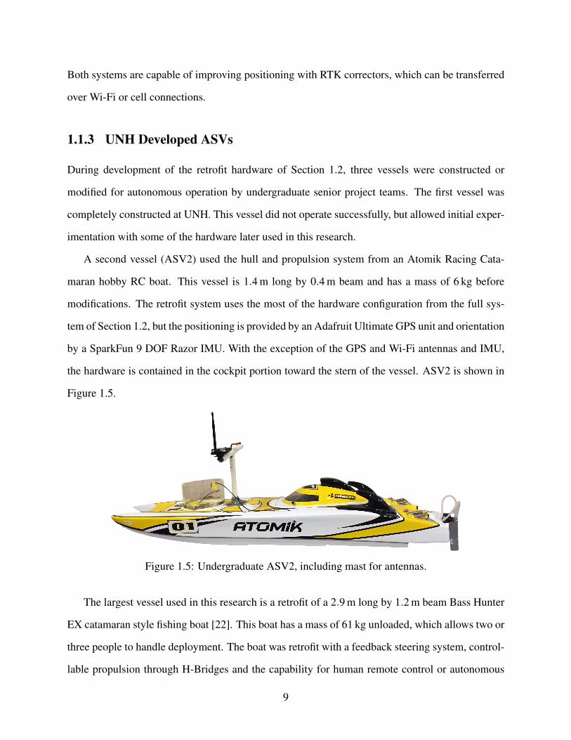
A second vessel (ASV2) used the hull and propulsion system from an Atomik Racing Cata-
maran hobby RC boat. This vessel is 1.4 m long by 0.4 m beam and has a mass of 6 kg before
modifications. The retrofit system uses the most of the hardware configuration from the full sys-
tem of Section 1.2, but the positioning is provided by an Adafruit Ultimate GPS unit and orientation
by a SparkFun 9 DOF Razor IMU. With the exception of the GPS and Wi-Fi antennas and IMU,
the hardware is contained in the cockpit portion toward the stern of the vessel. ASV2 is shown in
Figure 1.5.
Figure 1.5: Undergraduate ASV2, including mast for antennas.
The largest vessel used in this research is a retrofit of a 2.9 m long by 1.2 m beam Bass Hunter
EX catamaran style fishing boat [22]. This boat has a mass of 61 kg unloaded, which allows two or
three people to handle deployment. The boat was retrofit with a feedback steering system, control-
lable propulsion through H-Bridges and the capability for human remote control or autonomous
9
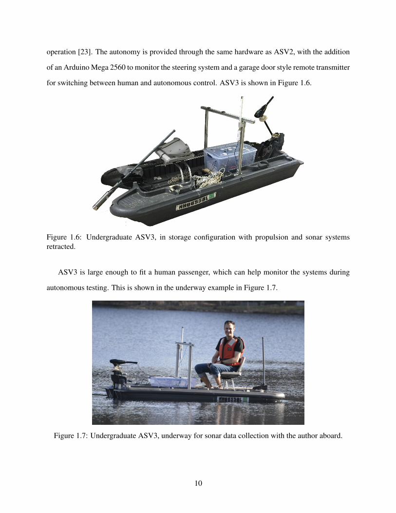
operation [23]. The autonomy is provided through the same hardware as ASV2, with the addition
of an Arduino Mega 2560 to monitor the steering system and a garage door style remote transmitter
for switching between human and autonomous control. ASV3 is shown in Figure 1.6.
Figure 1.6: Undergraduate ASV3, in storage configuration with propulsion and sonar systemsretracted.
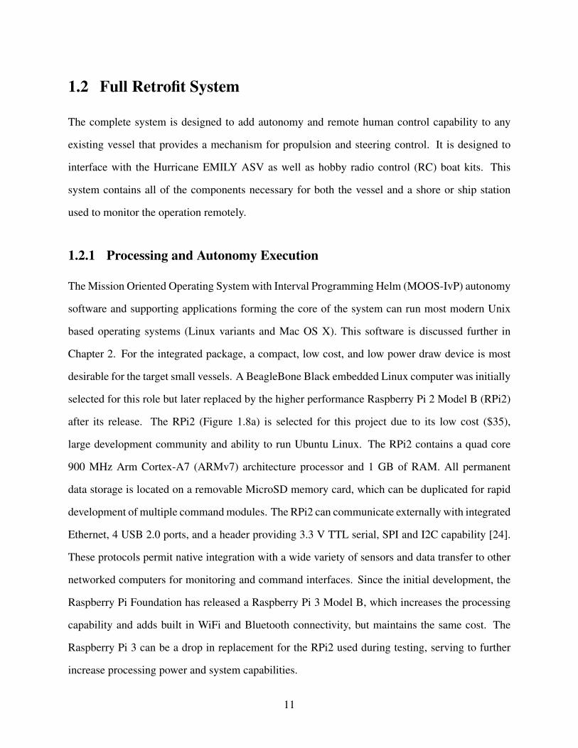
ASV3 is large enough to fit a human passenger, which can help monitor the systems during
autonomous testing. This is shown in the underway example in Figure 1.7.
Figure 1.7: Undergraduate ASV3, underway for sonar data collection with the author aboard.
10
1.2 Full Retrofit System
The complete system is designed to add autonomy and remote human control capability to any
existing vessel that provides a mechanism for propulsion and steering control. It is designed to
interface with the Hurricane EMILY ASV as well as hobby radio control (RC) boat kits. This
system contains all of the components necessary for both the vessel and a shore or ship station
used to monitor the operation remotely.
1.2.1 Processing and Autonomy Execution
The Mission Oriented Operating System with Interval Programming Helm (MOOS-IvP) autonomy
software and supporting applications forming the core of the system can run most modern Unix
based operating systems (Linux variants and Mac OS X). This software is discussed further in
Chapter 2. For the integrated package, a compact, low cost, and low power draw device is most
desirable for the target small vessels. A BeagleBone Black embedded Linux computer was initially
selected for this role but later replaced by the higher performance Raspberry Pi 2 Model B (RPi2)
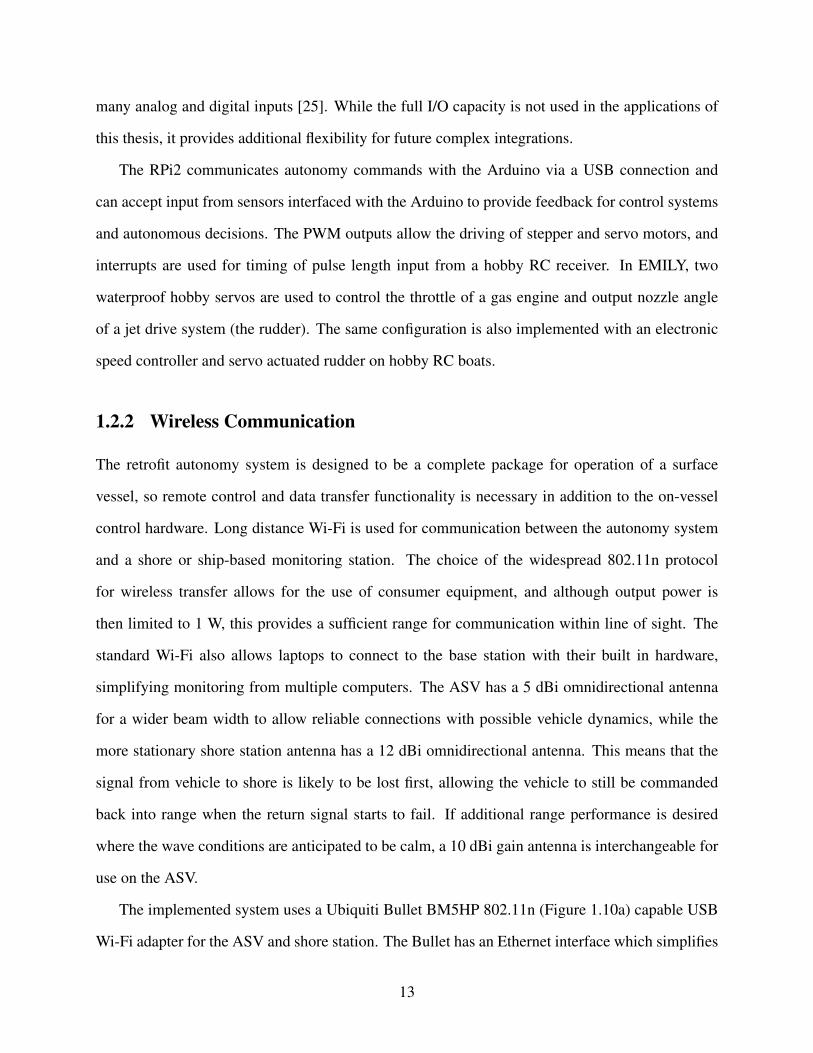
after its release. The RPi2 (Figure 1.8a) is selected for this project due to its low cost ($35),
large development community and ability to run Ubuntu Linux. The RPi2 contains a quad core
900 MHz Arm Cortex-A7 (ARMv7) architecture processor and 1 GB of RAM. All permanent
data storage is located on a removable MicroSD memory card, which can be duplicated for rapid
development of multiple command modules. The RPi2 can communicate externally with integrated
Ethernet, 4 USB 2.0 ports, and a header providing 3.3 V TTL serial, SPI and I2C capability [24].
These protocols permit native integration with a wide variety of sensors and data transfer to other
networked computers for monitoring and command interfaces. Since the initial development, the
Raspberry Pi Foundation has released a Raspberry Pi 3 Model B, which increases the processing
capability and adds built in WiFi and Bluetooth connectivity, but maintains the same cost. The
Raspberry Pi 3 can be a drop in replacement for the RPi2 used during testing, serving to further
increase processing power and system capabilities.
11
Multiple versions of Linux designed for ARM computers are available for the RPi2. For this
project, Ubuntu 14.04 is chosen, which uses the 3.18 Linux kernel for the current RPi2 version.
This was the latest long term service release at the time of initial development, and therefore
provided best compatibility with third party programs and drivers. Selection of a mainstream
Linux distribution simplifies compatibility with applications and drivers and increases the ease of
transitioning the developed autonomy system to other platforms that support Ubuntu or Debian
Linux based operating systems. The switch from initial development on the BeagleBone Black
benefited from this ability to use the same operating system on both devices.
(a) Raspberry Pi 2 (b) Arduino Mega 2560
Figure 1.8: Autonomy processing computer and microcontroller
A separate microcontroller is chosen to interact with the physical systems on the boat and in-
terpret human remote control input. Since a dedicated microcontroller is more suitable for timing
sensitive tasks, such as Pulse Width Modulation (PWM) output and pulse length detection, this
choice enables robust operation without interference from processor intensive autonomy determi-
nations. The Arduino Mega 2560 (Figure 1.8b) was selected as the microprocessor platform due to
existing usage within the University of New Hampshire, the large community of Arduino develop-
ers, an operating voltage of 5 V for broad compatibility, and the capability to natively handle more
serial data streams and interrupts than other Arduino platforms. The Mega 2560 uses an Atmel
ATmega2560 processor running at 16 MHz and has 4 serial UARTs, up to 15 PWM outputs, and 6
hardware interrupts. It also supports communication with other devices via SPI and I2C as well as
12
many analog and digital inputs [25]. While the full I/O capacity is not used in the applications of
this thesis, it provides additional flexibility for future complex integrations.
The RPi2 communicates autonomy commands with the Arduino via a USB connection and
can accept input from sensors interfaced with the Arduino to provide feedback for control systems
and autonomous decisions. The PWM outputs allow the driving of stepper and servo motors, and
interrupts are used for timing of pulse length input from a hobby RC receiver. In EMILY, two
waterproof hobby servos are used to control the throttle of a gas engine and output nozzle angle
of a jet drive system (the rudder). The same configuration is also implemented with an electronic
speed controller and servo actuated rudder on hobby RC boats.
1.2.2 Wireless Communication
The retrofit autonomy system is designed to be a complete package for operation of a surface
vessel, so remote control and data transfer functionality is necessary in addition to the on-vessel
control hardware. Long distance Wi-Fi is used for communication between the autonomy system
and a shore or ship-based monitoring station. The choice of the widespread 802.11n protocol
for wireless transfer allows for the use of consumer equipment, and although output power is
then limited to 1 W, this provides a sufficient range for communication within line of sight. The
standard Wi-Fi also allows laptops to connect to the base station with their built in hardware,
simplifying monitoring from multiple computers. The ASV has a 5 dBi omnidirectional antenna
for a wider beam width to allow reliable connections with possible vehicle dynamics, while the
more stationary shore station antenna has a 12 dBi omnidirectional antenna. This means that the
signal from vehicle to shore is likely to be lost first, allowing the vehicle to still be commanded
back into range when the return signal starts to fail. If additional range performance is desired
where the wave conditions are anticipated to be calm, a 10 dBi gain antenna is interchangeable for
use on the ASV.
The implemented system uses a Ubiquiti Bullet BM5HP 802.11n (Figure 1.10a) capable USB
Wi-Fi adapter for the ASV and shore station. The Bullet has an Ethernet interface which simplifies
13
connection to the RPi2 and is found to provide a more reliable connection than USB based alter-
natives due to the Bullet itself managing the connection versus the operating system driver. This
also allows other Ethernet capable devices, such as sonar systems, to pass data directly over the
connection to shore. The shore station can be any available Mac or Linux computer using another
Bullet configured as an access point. The autonomy system can also connect to infrastructure Wi-
Fi networks for testing in the office or research environment. Wi-Fi radios operating at 5 GHz are
chosen to reduce the possibility for interference with the 2.4 GHz human control radios described
later in this chapter.
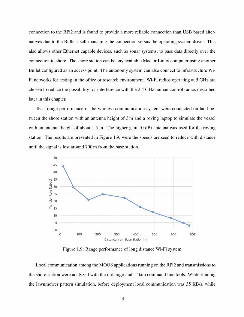
Tests range performance of the wireless communication system were conducted on land be-
tween the shore station with an antenna height of 3 m and a roving laptop to simulate the vessel
with an antenna height of about 1.5 m. The higher gain 10 dBi antenna was used for the roving
station. The results are presented in Figure 1.9, were the speeds are seen to reduce with distance
until the signal is lost around 700 m from the base station.
Figure 1.9: Range performance of long distance Wi-Fi system
Local communication among the MOOS applications running on the RPi2 and transmissions to
the shore station were analyzed with the nethogs and iftop command line tools. While running
the lawnmower pattern simulation, before deployment local communication was 35 KB/s, while
14
adding the shoreside monitoring passed 2 KB/s over the Wi-Fi. When deployed, the local traffic
increased to 50 KB/s and with shoreside to 4 KB/s. This traffic is much lower than maximum single
stream 802.11n throughput of 9 MB/s at full signal strength [26] and allows for data transmission
from other equipment and reduced-signal, long-distance monitoring. Even the lowest speed mode
of 802.11n far exceeds these data rates at about 900 KB/s. At the furthest data point where a
reliable signal existed in Figure 1.9 at a distance of 684 m, the data rate is 2.98 Mbps or 373 KB/s,
which would permit the monitoring data to be passed.
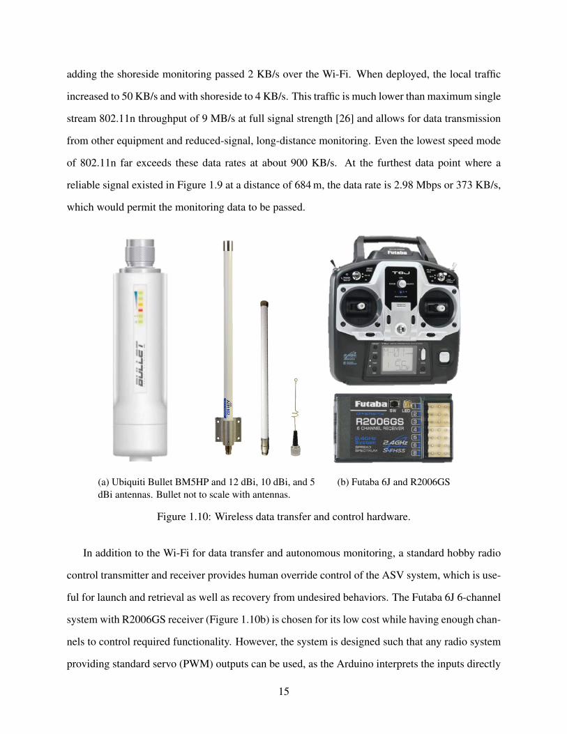
(a) Ubiquiti Bullet BM5HP and 12 dBi, 10 dBi, and 5dBi antennas. Bullet not to scale with antennas.
(b) Futaba 6J and R2006GS
Figure 1.10: Wireless data transfer and control hardware.
In addition to the Wi-Fi for data transfer and autonomous monitoring, a standard hobby radio
control transmitter and receiver provides human override control of the ASV system, which is use-
ful for launch and retrieval as well as recovery from undesired behaviors. The Futaba 6J 6-channel
system with R2006GS receiver (Figure 1.10b) is chosen for its low cost while having enough chan-
nels to control required functionality. However, the system is designed such that any radio system
providing standard servo (PWM) outputs can be used, as the Arduino interprets the inputs directly
15
from the receiver outputs for each channel. For the EMILY system, the RC controller provides
throttle, rudder, and motor starting commands as well as a switch to select human or autonomous
control. The same Arduino program has been successfully used with other hobby RC systems
supplied with boats converted to ASVs. The range of most hobby RC controllers is sufficient to
control the ASV within a distance where observation with the naked eye is reasonable, and thus
does not require additional amplifiers or high gain antennas, which contributes to the simplicity
and compact design of this self-contained hardware system.
1.2.3 Positioning and Depth Measurement
For the purpose of developing a complete hardware package that is usable for single beam sonar
survey applications and for installation on the development ASV, a dedicated inertial navigation
system (INS) is integrated. The CHRobotics GP9 GPS-Aided INS (Figure 1.11a) is selected for
this purpose due to acceptable accuracy and ease of integration while at very low costs compared
to similar systems. The GP9 is a Microelectromechanical system (MEMS) based inertial unit
with temperature calibration, barometric compensation of heights, and an internal Kalman Filter
to compensate for accelerometer and gyroscope drift using the GPS. It interfaces natively with the
RPi2 using a 3.3V TTL serial connection, and the binary data format is decoded in the autonomy
software. The power requirements are low enough that the GP9 can be directly powered from the
RPi2 as well, simplifying installation. With a GPS signal, the GP9 has specified accuracies of 1
in roll, pitch, and heading and 2.5 m positioning accuracy at a 95% confidence interval [27], [28].
These accuracies are sufficient for International Hydrographic Organization (IHO) Order 1b
uncertainty standards [29] when using single beam sonar, since beamwidths on a small system
would be larger than the roll and pitch accuracies. The IHO is the worldwide governing body of
ocean mapping and NOAA survey practices adhere to their standards. If the use of a multibeam
sonar is desired on an ASV with this system, better positioning and orientation would be required
but could still be achieved with a compact, low power MEMS system such as the SBG Ekinox,
Applanix POS MV Surfmaster, or possibly even the SBG Ellipse-D in shallow water [30]. These
16
systems, however, are at least an order of magnitude more expensive than the GP9.
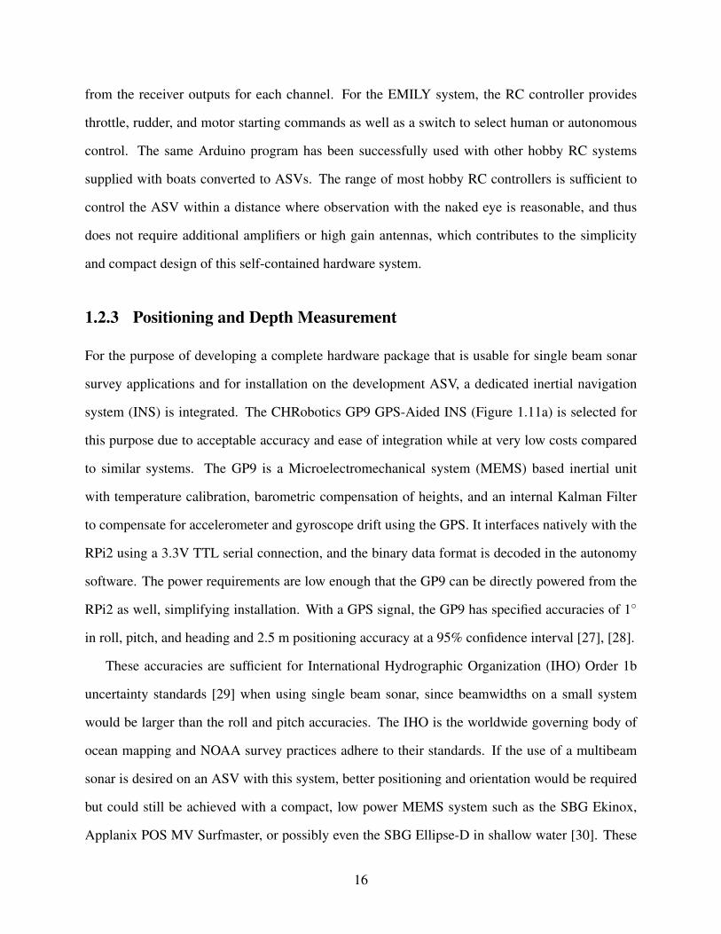
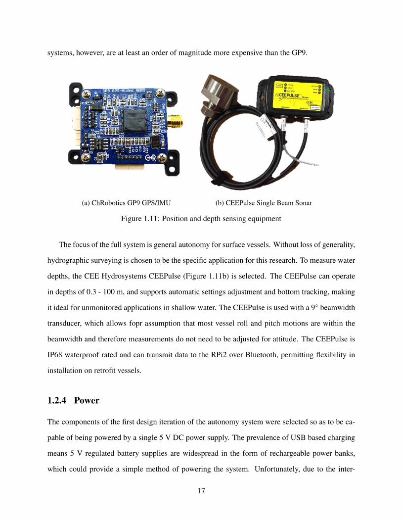
(a) ChRobotics GP9 GPS/IMU (b) CEEPulse Single Beam Sonar
Figure 1.11: Position and depth sensing equipment
The focus of the full system is general autonomy for surface vessels. Without loss of generality,
hydrographic surveying is chosen to be the specific application for this research. To measure water
depths, the CEE Hydrosystems CEEPulse (Figure 1.11b) is selected. The CEEPulse can operate
in depths of 0.3 - 100 m, and supports automatic settings adjustment and bottom tracking, making
it ideal for unmonitored applications in shallow water. The CEEPulse is used with a 9 beamwidth
transducer, which allows fopr assumption that most vessel roll and pitch motions are within the
beamwidth and therefore measurements do not need to be adjusted for attitude. The CEEPulse is
IP68 waterproof rated and can transmit data to the RPi2 over Bluetooth, permitting flexibility in
installation on retrofit vessels.
1.2.4 Power
The components of the first design iteration of the autonomy system were selected so as to be ca-
pable of being powered by a single 5 V DC power supply. The prevalence of USB based charging
means 5 V regulated battery supplies are widespread in the form of rechargeable power banks,
which could provide a simple method of powering the system. Unfortunately, due to the inter-
17
mittent current draw of servos, electrical interference in the EMILY system, and the change to
Bullet Wi-Fi, a multi-voltage operation system is used instead. However, the goal of simplicity in
integration is still achieved, as the final system requires only a single 9-24 V DC input. This falls
within the range of standard 12 V marine batteries, as well as the 11.1-18.5 V Lithium Polymer
(LiPo) batteries common in hobby RC boats. The EMILY boat has a 14.8 V battery pack that can
also be used to power the autonomy system. A reduced system (later discussed in Section 1.3) is
still capable of operating from a single 5 V battery pack.
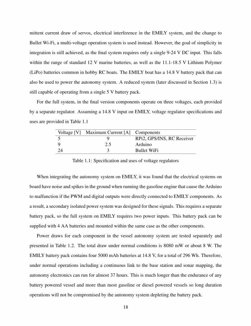
For the full system, in the final version components operate on three voltages, each provided
by a separate regulator. Assuming a 14.8 V input on EMILY, voltage regulator specifications and
uses are provided in Table 1.1
Voltage [V] Maximum Current [A] Components5 9 RPi2, GPS/INS, RC Receiver9 2.5 Arduino24 3 Bullet WiFi
Table 1.1: Specification and uses of voltage regulators
When integrating the autonomy system on EMILY, it was found that the electrical systems on
board have noise and spikes in the ground when running the gasoline engine that cause the Arduino
to malfunction if the PWM and digital outputs were directly connected to EMILY components. As
a result, a secondary isolated power system was designed for these signals. This requires a separate
battery pack, so the full system on EMILY requires two power inputs. This battery pack can be
supplied with 4 AA batteries and mounted within the same case as the other components.
Power draws for each component in the vessel autonomy system are tested separately and
presented in Table 1.2. The total draw under normal conditions is 8080 mW or about 8 W. The
EMILY battery pack contains four 5000 mAh batteries at 14.8 V, for a total of 296 Wh. Therefore,
under normal operations including a continuous link to the base station and sonar mapping, the
autonomy electronics can run for almost 37 hours. This is much longer than the endurance of any
battery powered vessel and more than most gasoline or diesel powered vessels so long duration
operations will not be compromised by the autonomy system depleting the battery pack.
18
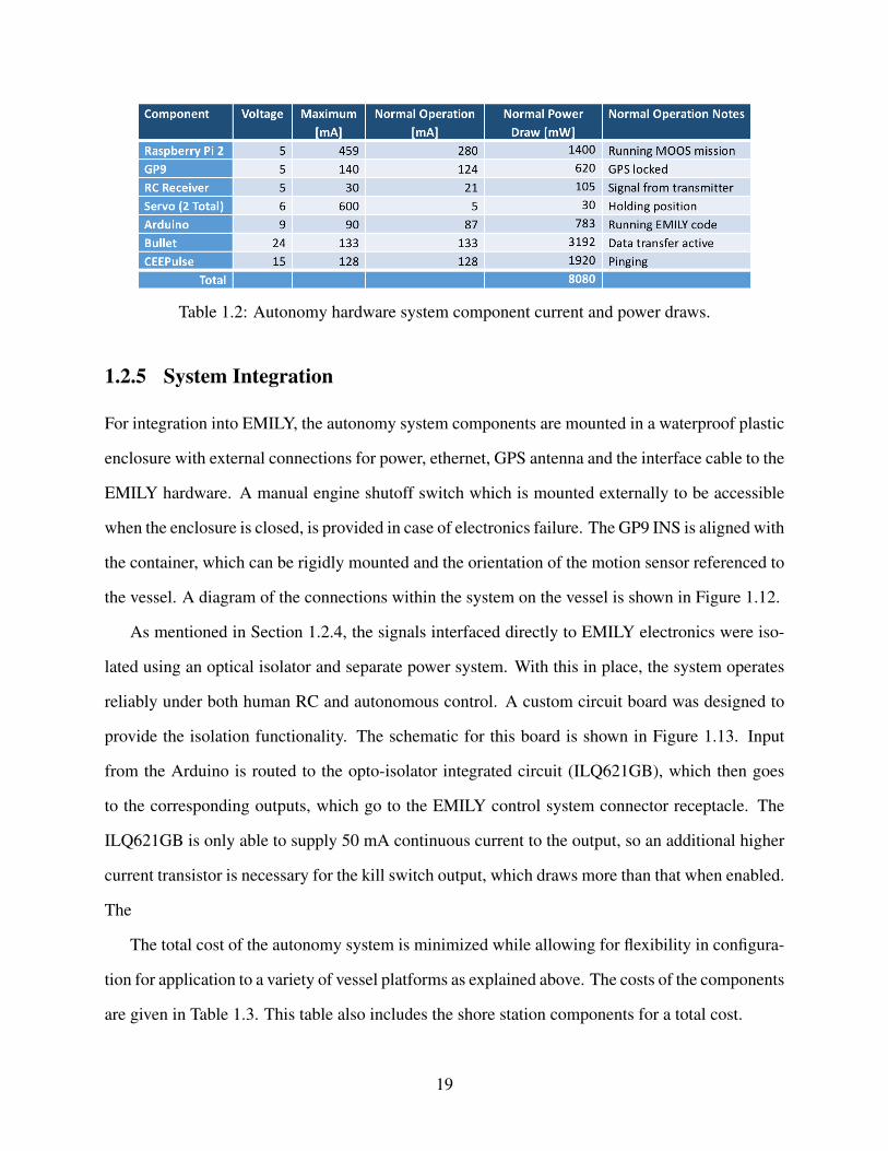
Table 1.2: Autonomy hardware system component current and power draws.
1.2.5 System Integration
For integration into EMILY, the autonomy system components are mounted in a waterproof plastic
enclosure with external connections for power, ethernet, GPS antenna and the interface cable to the
EMILY hardware. A manual engine shutoff switch which is mounted externally to be accessible
when the enclosure is closed, is provided in case of electronics failure. The GP9 INS is aligned with
the container, which can be rigidly mounted and the orientation of the motion sensor referenced to
the vessel. A diagram of the connections within the system on the vessel is shown in Figure 1.12.
As mentioned in Section 1.2.4, the signals interfaced directly to EMILY electronics were iso-
lated using an optical isolator and separate power system. With this in place, the system operates
reliably under both human RC and autonomous control. A custom circuit board was designed to
provide the isolation functionality. The schematic for this board is shown in Figure 1.13. Input
from the Arduino is routed to the opto-isolator integrated circuit (ILQ621GB), which then goes
to the corresponding outputs, which go to the EMILY control system connector receptacle. The
ILQ621GB is only able to supply 50 mA continuous current to the output, so an additional higher
current transistor is necessary for the kill switch output, which draws more than that when enabled.
The
The total cost of the autonomy system is minimized while allowing for flexibility in configura-
tion for application to a variety of vessel platforms as explained above. The costs of the components
are given in Table 1.3. This table also includes the shore station components for a total cost.
19
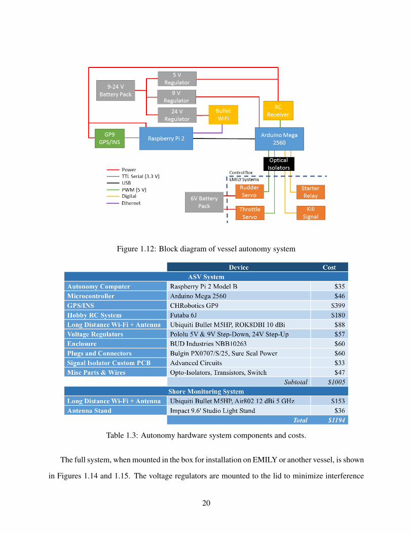
Figure 1.12: Block diagram of vessel autonomy system
Table 1.3: Autonomy hardware system components and costs.
The full system, when mounted in the box for installation on EMILY or another vessel, is shown
in Figures 1.14 and 1.15. The voltage regulators are mounted to the lid to minimize interference
20
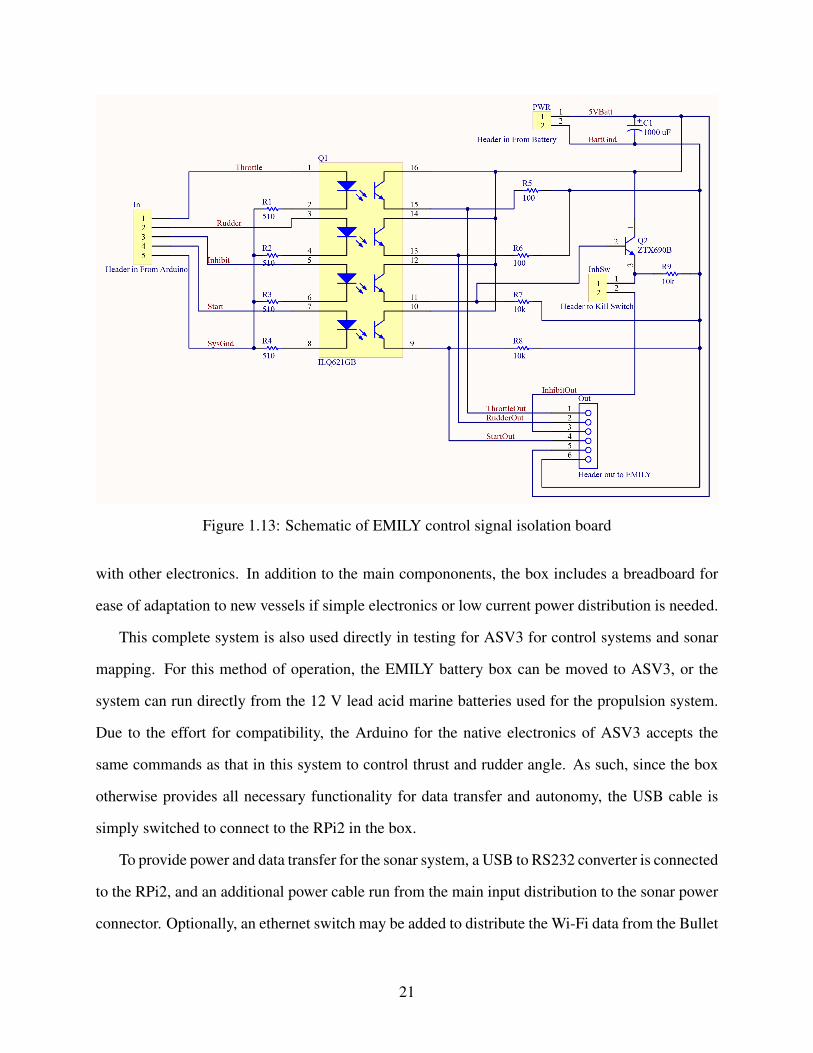
Figure 1.13: Schematic of EMILY control signal isolation board
with other electronics. In addition to the main compononents, the box includes a breadboard for
ease of adaptation to new vessels if simple electronics or low current power distribution is needed.
This complete system is also used directly in testing for ASV3 for control systems and sonar
mapping. For this method of operation, the EMILY battery box can be moved to ASV3, or the
system can run directly from the 12 V lead acid marine batteries used for the propulsion system.
Due to the effort for compatibility, the Arduino for the native electronics of ASV3 accepts the
same commands as that in this system to control thrust and rudder angle. As such, since the box
otherwise provides all necessary functionality for data transfer and autonomy, the USB cable is
simply switched to connect to the RPi2 in the box.
To provide power and data transfer for the sonar system, a USB to RS232 converter is connected
to the RPi2, and an additional power cable run from the main input distribution to the sonar power
connector. Optionally, an ethernet switch may be added to distribute the Wi-Fi data from the Bullet
21
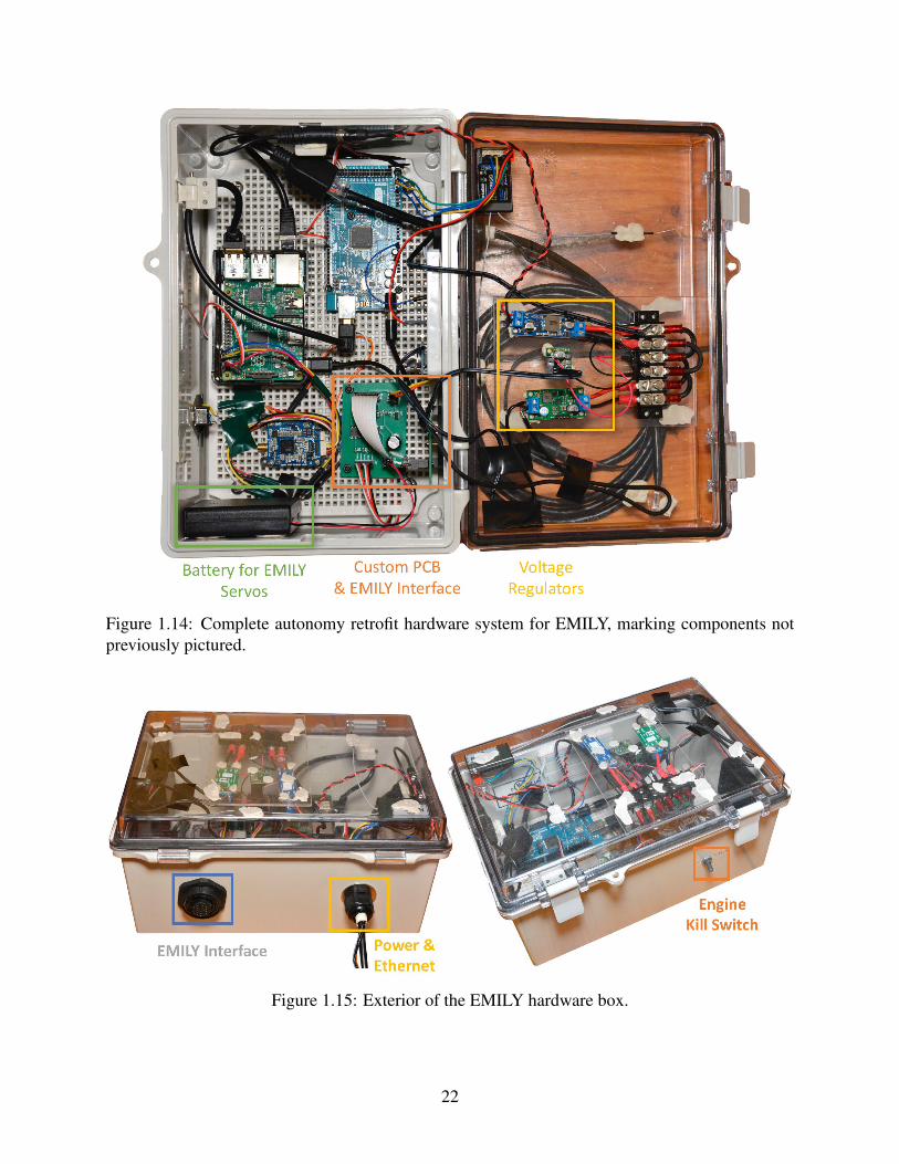
Figure 1.14: Complete autonomy retrofit hardware system for EMILY, marking components notpreviously pictured.
Figure 1.15: Exterior of the EMILY hardware box.
22
to multiple onboard computers, and draws power from the 5 V regulator. This additional wiring is
fed through the penetration in the box where the EMILY control system connector is mounted for
operation on EMILY.
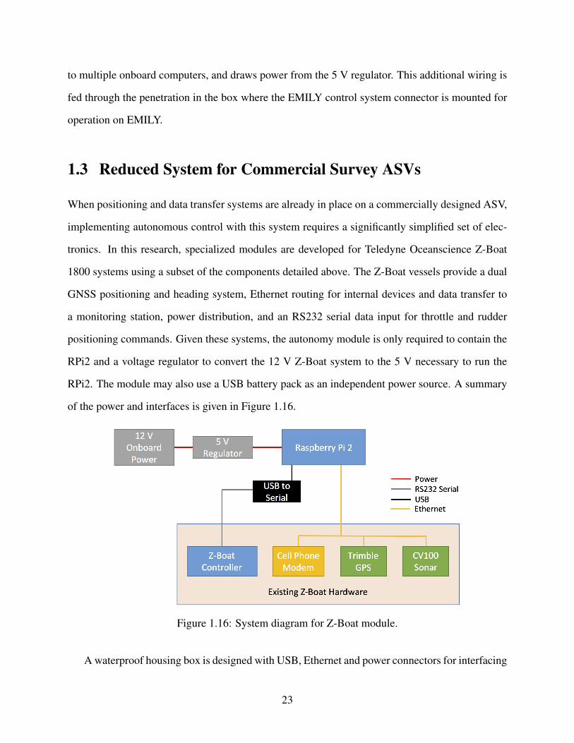
1.3 Reduced System for Commercial Survey ASVs
When positioning and data transfer systems are already in place on a commercially designed ASV,
implementing autonomous control with this system requires a significantly simplified set of elec-
tronics. In this research, specialized modules are developed for Teledyne Oceanscience Z-Boat
1800 systems using a subset of the components detailed above. The Z-Boat vessels provide a dual
GNSS positioning and heading system, Ethernet routing for internal devices and data transfer to
a monitoring station, power distribution, and an RS232 serial data input for throttle and rudder
positioning commands. Given these systems, the autonomy module is only required to contain the
RPi2 and a voltage regulator to convert the 12 V Z-Boat system to the 5 V necessary to run the
RPi2. The module may also use a USB battery pack as an independent power source. A summary
of the power and interfaces is given in Figure 1.16.
Figure 1.16: System diagram for Z-Boat module.
A waterproof housing box is designed with USB, Ethernet and power connectors for interfacing
23
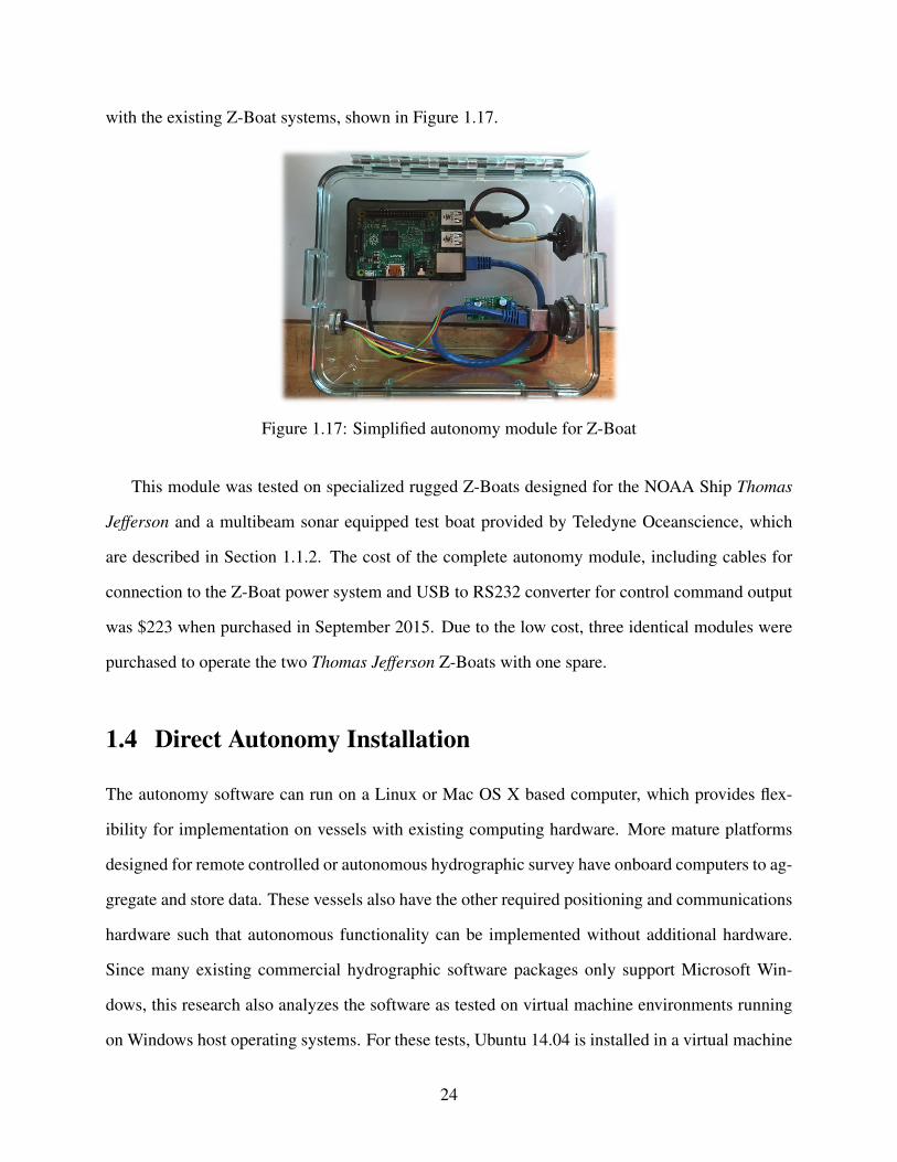
with the existing Z-Boat systems, shown in Figure 1.17.
Figure 1.17: Simplified autonomy module for Z-Boat
This module was tested on specialized rugged Z-Boats designed for the NOAA Ship Thomas
Jefferson and a multibeam sonar equipped test boat provided by Teledyne Oceanscience, which
are described in Section 1.1.2. The cost of the complete autonomy module, including cables for
connection to the Z-Boat power system and USB to RS232 converter for control command output
was $223 when purchased in September 2015. Due to the low cost, three identical modules were
purchased to operate the two Thomas Jefferson Z-Boats with one spare.
1.4 Direct Autonomy Installation
The autonomy software can run on a Linux or Mac OS X based computer, which provides flex-
ibility for implementation on vessels with existing computing hardware. More mature platforms
designed for remote controlled or autonomous hydrographic survey have onboard computers to ag-
gregate and store data. These vessels also have the other required positioning and communications
hardware such that autonomous functionality can be implemented without additional hardware.
Since many existing commercial hydrographic software packages only support Microsoft Win-
dows, this research also analyzes the software as tested on virtual machine environments running
on Windows host operating systems. For these tests, Ubuntu 14.04 is installed in a virtual machine
24

hosted with Oracle VirtualBox VM software. By leveraging existing hardware, the cost and com-
plexity of implementation can be further reduced and the processing power will often be higher
than on the default embedded computer for the full system described in Section 1.2. The common
operating system between the RPi2 and virtual machine facilitate rapid simultaneous development
with corresponding software package availability and device configuration.
25
CHAPTER 2
AUTONOMY SOFTWARE AND OPERATIONThe MOOS-IvP open source autonomy framework, which is maintained by MIT and Oxford
forms the basis for the autonomy system [31]. The software compiles and runs on most Linux
distributions and Mac OS X, including embedded ARM based systems such as the RPi2 in this
application. MOOS (Mission Oriented Operating Suite) utilizes a centralized message-passing
architecture (MOOSDB) which coordinates communication between multiple applications known
as MOOSApps. MOOSApps can publish and subscribe to data streams without knowledge of any
other running applications. In an autonomous vehicle, these postings consist of information about
the status of subsystems, the position of the vehicle, and the environment in which it is operating.
MOOS uses TCP connections to transfer information, so the core MOOS process can be on
the same computer as the applications or a different one across a network. MOOS also includes
applications that add functionality for sharing information between MOOS databases, so that each
maintains up-to-date copies of certain information when networked, while allowing multiple in-
dependent instances to run. This can facilitate interaction between different vehicles in a swarm,
or in this case it is used for the monitoring station to interact with the vehicle without affecting
autonomous operations if it is out of range.
The MOOS-IvP package comes with applications for common tasks and behaviors in marine
autonomy and can be extended to interface with platform specific systems. The applications can be
configured on the command line or with options provided in a human-readable structured text file
defining the mission. The provided pAntler utility automatically launches and configures MOOS-
Apps based on the mission file. Together, the MOOSDB and communicating MOOSApps form
what is termed a MOOS community. MOOS-IvP provides simulation capabilities which allow
testing of applications and behavior configurations with simulated vessel movements. Simulations
26
can be accelerated to multiples of real-time operation speed for rapid testing of full missions or
reaction to long term processes.
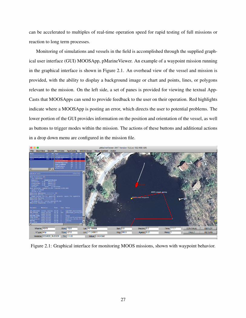
Monitoring of simulations and vessels in the field is accomplished through the supplied graph-
ical user interface (GUI) MOOSApp, pMarineViewer. An example of a waypoint mission running
in the graphical interface is shown in Figure 2.1. An overhead view of the vessel and mission is
provided, with the ability to display a background image or chart and points, lines, or polygons
relevant to the mission. On the left side, a set of panes is provided for viewing the textual App-
Casts that MOOSApps can send to provide feedback to the user on their operation. Red highlights
indicate where a MOOSApp is posting an error, which directs the user to potential problems. The
lower portion of the GUI provides information on the position and orientation of the vessel, as well
as buttons to trigger modes within the mission. The actions of these buttons and additional actions
in a drop down menu are configured in the mission file.
Figure 2.1: Graphical interface for monitoring MOOS missions, shown with waypoint behavior.
27
2.1 IvP Helm
A key MOOS application is the IvP (Interval Programming) helm, which defines the actual behav-
iors for autonomy and commands the heading and speed of the ASV. The MIT repository includes
existing behaviors for waypoint navigation, collision avoidance, track and trail, and station keep-
ing, along with simple constant heading and speed behaviors. The behaviors are configured in a
text file (separate from the mission file) that sets the initial configuration options, which in turn
contribute to how a heading and speed are determined for the behavior. Behaviors may also be
updated from other MOOS applications. For example the waypoint navigation behavior is able to
receive a new set of waypoints from a separate path planning MOOS application.
The IvP Helm includes the ability to build a hierarchical behavior structure, and facilities are
exposed for development of custom behaviors. Behaviors define functions over the domains of
speed and heading (and depth for underwater vessels), where the peaks of these represent optimal
settings for the vessel. Multiple behaviors can be active simultaneously, and a weighted sum of
their functions used to determine the path of the vessel. This is used for reactionary behaviors
that are always active, but sometimes not contributing to the desired motion of the vessel, such as
collision avoidance which modifies behavior only when other vessels are detected.
2.2 Implementation of MOOS-IvP for This Project
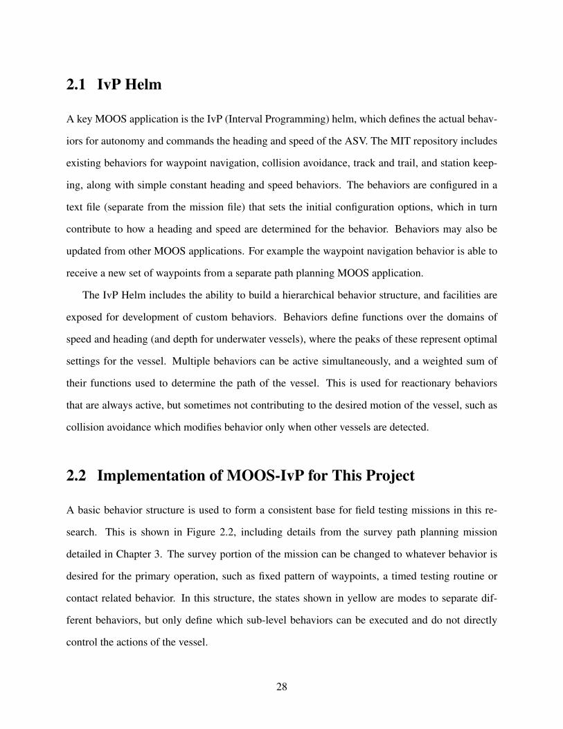
A basic behavior structure is used to form a consistent base for field testing missions in this re-
search. This is shown in Figure 2.2, including details from the survey path planning mission
detailed in Chapter 3. The survey portion of the mission can be changed to whatever behavior is
desired for the primary operation, such as fixed pattern of waypoints, a timed testing routine or
contact related behavior. In this structure, the states shown in yellow are modes to separate dif-
ferent behaviors, but only define which sub-level behaviors can be executed and do not directly
control the actions of the vessel.
28
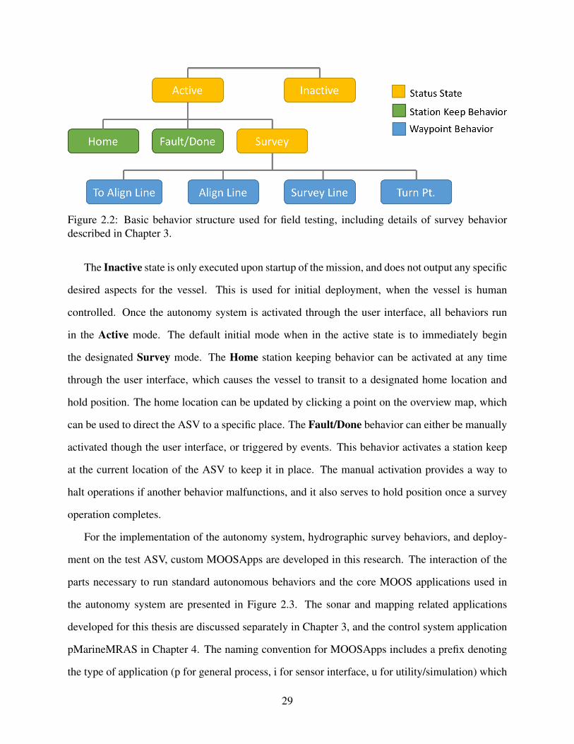
Figure 2.2: Basic behavior structure used for field testing, including details of survey behaviordescribed in Chapter 3.
The Inactive state is only executed upon startup of the mission, and does not output any specific
desired aspects for the vessel. This is used for initial deployment, when the vessel is human
controlled. Once the autonomy system is activated through the user interface, all behaviors run
in the Active mode. The default initial mode when in the active state is to immediately begin
the designated Survey mode. The Home station keeping behavior can be activated at any time
through the user interface, which causes the vessel to transit to a designated home location and
hold position. The home location can be updated by clicking a point on the overview map, which
can be used to direct the ASV to a specific place. The Fault/Done behavior can either be manually
activated though the user interface, or triggered by events. This behavior activates a station keep
at the current location of the ASV to keep it in place. The manual activation provides a way to
halt operations if another behavior malfunctions, and it also serves to hold position once a survey
operation completes.
For the implementation of the autonomy system, hydrographic survey behaviors, and deploy-
ment on the test ASV, custom MOOSApps are developed in this research. The interaction of the
parts necessary to run standard autonomous behaviors and the core MOOS applications used in
the autonomy system are presented in Figure 2.3. The sonar and mapping related applications
developed for this thesis are discussed separately in Chapter 3, and the control system application
pMarineMRAS in Chapter 4. The naming convention for MOOSApps includes a prefix denoting
the type of application (p for general process, i for sensor interface, u for utility/simulation) which
29
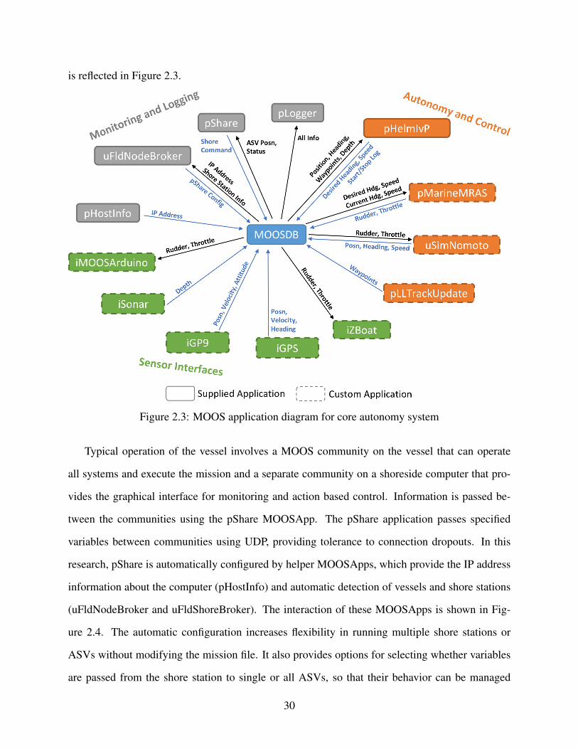
is reflected in Figure 2.3.
Figure 2.3: MOOS application diagram for core autonomy system
Typical operation of the vessel involves a MOOS community on the vessel that can operate
all systems and execute the mission and a separate community on a shoreside computer that pro-
vides the graphical interface for monitoring and action based control. Information is passed be-
tween the communities using the pShare MOOSApp. The pShare application passes specified
variables between communities using UDP, providing tolerance to connection dropouts. In this
research, pShare is automatically configured by helper MOOSApps, which provide the IP address
information about the computer (pHostInfo) and automatic detection of vessels and shore stations
(uFldNodeBroker and uFldShoreBroker). The interaction of these MOOSApps is shown in Fig-
ure 2.4. The automatic configuration increases flexibility in running multiple shore stations or
ASVs without modifying the mission file. It also provides options for selecting whether variables
are passed from the shore station to single or all ASVs, so that their behavior can be managed
30
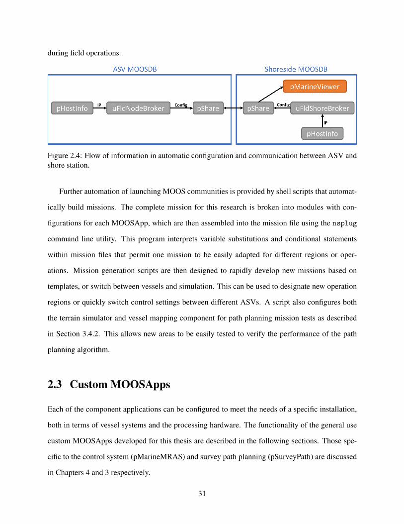
during field operations.
Figure 2.4: Flow of information in automatic configuration and communication between ASV andshore station.
Further automation of launching MOOS communities is provided by shell scripts that automat-
ically build missions. The complete mission for this research is broken into modules with con-
figurations for each MOOSApp, which are then assembled into the mission file using the nsplug
command line utility. This program interprets variable substitutions and conditional statements
within mission files that permit one mission to be easily adapted for different regions or oper-
ations. Mission generation scripts are then designed to rapidly develop new missions based on
templates, or switch between vessels and simulation. This can be used to designate new operation
regions or quickly switch control settings between different ASVs. A script also configures both
the terrain simulator and vessel mapping component for path planning mission tests as described
in Section 3.4.2. This allows new areas to be easily tested to verify the performance of the path
planning algorithm.
2.3 Custom MOOSApps
Each of the component applications can be configured to meet the needs of a specific installation,
both in terms of vessel systems and the processing hardware. The functionality of the general use
custom MOOSApps developed for this thesis are described in the following sections. Those spe-
cific to the control system (pMarineMRAS) and survey path planning (pSurveyPath) are discussed
in Chapters 4 and 3 respectively.
31
iGP9
The GP9 interface driver (iGP9) configures the GP9 GPS/INS and outputs the required data on
startup. It then parses the data stream and posts the information to MOOS variables. The GP9 is
already equipped with filters for real-time orientation data while in motion, so no additional filters
are applied. An existing driver for the Robotic Operating System (ROS) for a similar device by
the same manufacturer was ported to the MOOS environment to form the basis for this driver. As
a result, a ROS version of this driver is also available. The GP9 interface provides location, roll,
pitch, and heading.
iGPS
The GPS interface driver (iGPS) parses NMEA 0183 data that is commonly output by GPS devices.
It is capable of connecting to both serial data streams and network data. The network data allows
passing of positioning information from Hypack data collection software, which is commonly
used on autonomous vessels with onboard computers. Hypack provides drivers for most standard
equipment used in hydrographic surveying and can be set to output data from the interfaced sensors
in the standardized NMEA format. This eliminates the need to write custom MOOS drivers for
every proprietary data format, although it requires Hypack to be running for the autonomy system
to function.
iSonar
The sonar interface driver (iSonar) accepts and interprets NMEA data strings from sonar systems.
It can be configured for either network or serial port data input. This allows it to interface with
any sonar that has an option to output data in this format (such as the CEEPULSE 100 used for the
testing system). Hypack surveying software can also output depth data in NMEA format, so any
sonar supported by Hypack can be used to measure nadir depths.
32
iZBoat
The Teledyne Oceanscience Z-Boat interface, iZBoat, sends commands to the Z-Boat Command
and Control Module (CCM) to control the throttle and rudder angle of the propellers. As the CCM
handles the low level control of the servos and motors, this interface driver sends only ASCII
commands over a RS232 serial connection. In addition to the throttle and rudder, commands are
sent to initiate and terminate autonomous mode. These commands are automatically sent when
the system is initialized, and may also be triggered manually for operations that switch between
human remote control and autonomous operation.
pLLTrackUpdate
The pLLTrackUpdate program accepts posts of new waypoints to update a track. The IvP helm
handles waypoint coordinates in a local x-y grid system with an origin defined for the specific
MOOS mission. This MOOSApp translates coordinates in Latitude/Longitude or Universal Trans-
verse Mercator (UTM) to the local coordinate system and posts an updated track which can modify
the mission during execution. It is designed to work in conjunction with a python script which
reads Hypack planned line files (which are natively in UTM coordinates) and posts them to the
appropriate variables for conversion by pLLTrackUpdate.
uSimNomoto
The simulator provided with the distribution MOOS-IvP program (uSimMarine) provides basic
functionality, but contains a simplified method of determining heading and cannot simulate the
effects of waves or noise in sensor readings. A modified version (uSimNomoto) is created to
address some of the shortcomings. For determining the heading of a vessel from turns caused by a
rudder, the linear Nomoto model is used. This model also forms the basis for the adaptive control
system in this research and is further discussed in Section 4.2.2.
33
Wave Simulator
In order to test against some factors present in the environment, a wave simulator was developed.
The simulator generates random waves of a specified significant height (H1/3) and period (T ).
This is achieved by filtering Gaussian white noise with a second order band-pass filter to isolate
the required spectrum. This method is used in similar simulations by Van Amerongen [2] and
Velagic [32]. While the frequency response of the band-pass filter does not exactly match that of
observed waves, it is sufficient for testing of response to environmental conditions.
Before applying the bandpass filter, an Infinite Impulse Response (IIR) filter implementing
a second order Butterworth low pass transfer function is first applied to the Gaussian noise, to
further reduce the effects of high frequency components that would be unusual in waves. The
cutoff frequency for the low pass filter is based on the desired dominant wave period T as given in
Equation 2.1.
fc =3T
(2.1)
The filter is implemented with the standard Butterworth second order transfer function
H(s) =1(
sωc
)2+√
2sωc
+1(2.2)
where ωc = 2π fc. This is implemented digitally with a bi-linear transform, resulting in the nor-
malized discrete time transfer function
H(z) =1+2z−1 + z−2(
c2 +√
2c+1)+(−2(c2−1))z−1 +
(c2−√
2c+1)
z−2(2.3)
where c is a frequency warping factor given by
c = cot(
ωcTs
2
)(2.4)
34

where Ts is the sample time specified by the MOOSApp iteration rate [33].
The center frequency ω0 of the bandpass filter is based on the Bretshneither family, with
ω0 =
(4B5
) 14
(2.5)
where B is defined from the Modified Pierson-Moskowitz family as
B =691T 4 (2.6)
where T is again the dominant period of the waves [34]. This frequency is shifted to get an
encounter frequency based on the motion of the ship. This is given in Equation 2.7, where U is the
speed of the ship, γ is the angle between the heading of the ship and the direction of travel of the
waves and g is the acceleration due to gravity [32].
ωe = ω0−ω2
0Ug
cosγ (2.7)
The encounter frequency is used as the center of a second order bandpass filter defined in the
Laplace domain in Equation 2.8, where HRMS is the root-mean-square height of the waves, defined
from significant wave height as HRMS ≈ H1/3/1.4.
H(s) =2ζ ωeHRMS
s2 +2ζ ωes+ω2e
(2.8)
The transfer function is transformed to the Z domain as given in Equation 2.9. This is applied
in the MOOSApp as an IIR difference equation, the components of which are broken out in 2.9 for
clarity.
35
H(z) = Gb1 +b2z−1
1+a2z−1 +a3z−2
G =− 2ζ ωeH√1−ζ 2
b1 =−√
1−ζ 2
b2 = e−ζ ωeTs sin(√
1−ζ 2ωeTs + arccosζ
)a2 =−2e−ζ ωeTs cos
(√1−ζ 2ωeTs
)a3 = e−ζ ωeTs
(2.9)
The damping ratio ζ is determined to give a constant bandwidth, which transfers the same power
from the Gaussian noise signal, allowing the amplitude of the result to be consistently scaled for
the correct significant wave height. It is defined in Equation 2.10, where the numerical factor of
0.017 is found to give approximate RMS results to the desired wave height.
ζ =0.017π
ωe(2.10)
The simulated waves affect the speed and rate of turn of the vessel. The speed is most affected
when the waves come from directly ahead or behind the vessel and the heading when they are at a
45 degree angle to the bow or stern. This means that when the waves are on the beam, they have
their minimal effects on both speed and heading, as most of the energy would be translated into roll
and sway in the vessel. In addition, the effect on vessels by waves of the same amplitude should
be inversely proportional to the size of the vessel. These effects are achieved by multiplying the
wave amplitude by factors given in Equation 2.11, where Awave is the wave amplitude output from
the bandpass filter. These scaled amplitudes are added to the speed and rate-of-turn otherwise
determined by the vessel model. The scaling factors approximate the responses observed in the
small ASVs of this research, and may not be directly applicable to larger vessels.
36
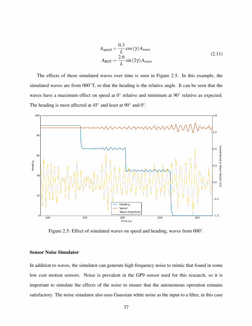
Aspeed =0.3L
cos(γ)Awave
AROT =2.6L
sin(2γ)Awave
(2.11)
The effects of these simulated waves over time is seen in Figure 2.5. In this example, the
simulated waves are from 000T, so that the heading is the relative angle. It can be seen that the
waves have a maximum effect on speed at 0 relative and minimum at 90 relative as expected.
The heading is most affected at 45 and least at 90 and 0.
Figure 2.5: Effect of simulated waves on speed and heading, waves from 000.
Sensor Noise Simulator
In addition to waves, the simulator can generate high frequency noise to mimic that found in some
low cost motion sensors. Noise is prevalent in the GP9 sensor used for this research, so it is
important to simulate the effects of the noise to ensure that the autonomous operation remains
satisfactory. The noise simulator also uses Gaussian white noise as the input to a filter, in this case
37
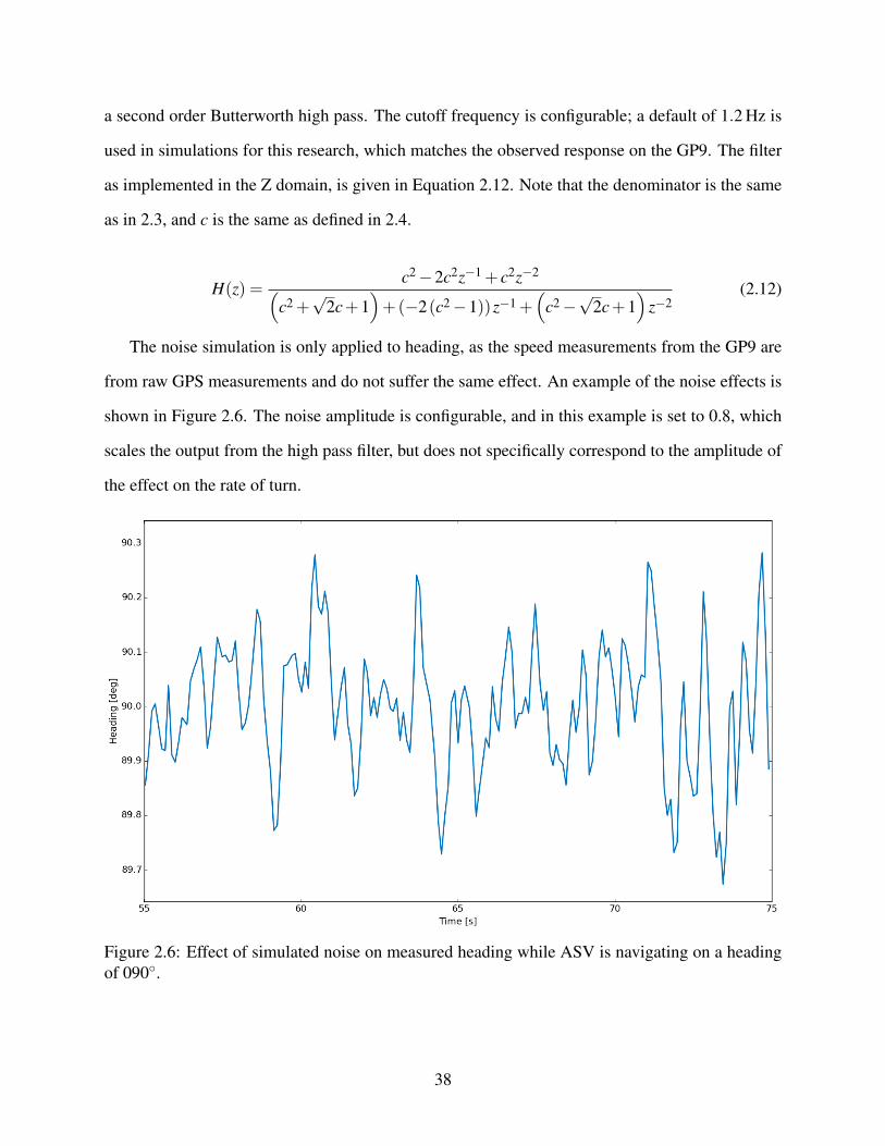
a second order Butterworth high pass. The cutoff frequency is configurable; a default of 1.2 Hz is
used in simulations for this research, which matches the observed response on the GP9. The filter
as implemented in the Z domain, is given in Equation 2.12. Note that the denominator is the same
as in 2.3, and c is the same as defined in 2.4.
H(z) =c2−2c2z−1 + c2z−2(
c2 +√
2c+1)+(−2(c2−1))z−1 +
(c2−√
2c+1)
z−2(2.12)
The noise simulation is only applied to heading, as the speed measurements from the GP9 are
from raw GPS measurements and do not suffer the same effect. An example of the noise effects is
shown in Figure 2.6. The noise amplitude is configurable, and in this example is set to 0.8, which
scales the output from the high pass filter, but does not specifically correspond to the amplitude of
the effect on the rate of turn.
Figure 2.6: Effect of simulated noise on measured heading while ASV is navigating on a headingof 090.
38
CHAPTER 3
AUTOMATED SWATH SURVEY PATH PLANNING
3.1 Introduction
Most current hydrographic surveys employ multibeam sonar systems for depth measurement,
which provide a fixed swath angle viewing of the seafloor with a number of data points returned
along the swath profile. Most multibeam hydrographic surveys require complete coverage, defined
as “100% bathymetric bottom coverage with multibeam sonars” [35]. The fixed angle of the sonar
causes the width of the swath across the seafloor to vary with depth. Therefore, in order to achieve
complete bottom coverage, neighboring survey lines must be spaced more closely in shallow water
than in deep water. AUVs avoid the problem of having to anticipate varying swath widths over a
survey area, as they can be instructed to maintain a constant altitude above the seafloor.
Maintaining a constant altitude above the seafloor is not an option for ASVs, as their height
above the bottom is determined by the full water depth. However, in most existing applications,
survey planning for ASVs inherits fixed or preplanned line spacing from the AUV paradigm [36].
In more complex schemes, an area can be subdivided by depth ranges and different line spacings
planned for each range [18] [37]. In order to achieve complete coverage, these parallel lines are
still required to be spaced according to minimum depths in the region, leading to inefficient extra
overlap elsewhere. Any preplanned adjustments for depth also require knowledge of the area, but
usually the purpose for conducting a survey is due to uncertainty in the existing data. This chapter
presents a method for comprehensive coverage path planning that does not require prior knowl-
edge of the bathymetry in the survey area and that adjusts survey lines dynamically based on the
data acquired during the survey. This method mimics that of how human-driven data is currently
collected during NOAA surveys, where a coxswain steers a survey launch to match and overlap
39
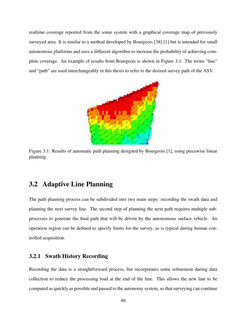
realtime coverage reported from the sonar system with a graphical coverage map of previously
surveyed area. It is similar to a method developed by Bourgeois [38] [1] but is intended for small
autonomous platforms and uses a different algorithm to increase the probability of achieving com-
plete coverage. An example of results from Bourgeois is shown in Figure 3.1. The terms “line”
and “path” are used interchangeably in this thesis to refer to the desired survey path of the ASV.
Figure 3.1: Results of automatic path planning designed by Bourgeois [1], using piecewise linearplanning.
3.2 Adaptive Line Planning
The path planning process can be subdivided into two main steps: recording the swath data and
planning the next survey line. The second step of planning the next path requires multiple sub-
processes to generate the final path that will be driven by the autonomous surface vehicle. An
operation region can be defined to specify limits for the survey, as is typical during human con-
trolled acquisition.
3.2.1 Swath History Recording
Recording the data is a straightforward process, but incorporates some refinement during data
collection to reduce the processing load at the end of the line. This allows the new line to be
computed as quickly as possible and passed to the autonomy system, so that surveying can continue
40
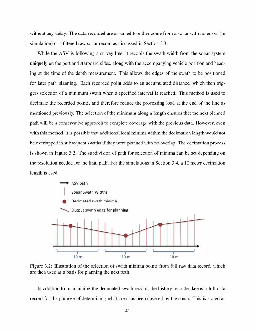
without any delay. The data recorded are assumed to either come from a sonar with no errors (in
simulation) or a filtered raw sonar record as discussed in Section 3.3.
While the ASV is following a survey line, it records the swath width from the sonar system
uniquely on the port and starboard sides, along with the accompanying vehicle position and head-
ing at the time of the depth measurement. This allows the edges of the swath to be positioned
for later path planning. Each recorded point adds to an accumulated distance, which then trig-
gers selection of a minimum swath when a specified interval is reached. This method is used to
decimate the recorded points, and therefore reduce the processing load at the end of the line as
mentioned previously. The selection of the minimum along a length ensures that the next planned
path will be a conservative approach to complete coverage with the previous data. However, even
with this method, it is possible that additional local minima within the decimation length would not
be overlapped in subsequent swaths if they were planned with no overlap. The decimation process
is shown in Figure 3.2. The subdivision of path for selection of minima can be set depending on
the resolution needed for the final path. For the simulations in Section 3.4, a 10 meter decimation
length is used.
Figure 3.2: Illustration of the selection of swath minima points from full raw data record, whichare then used as a basis for planning the next path.
In addition to maintaining the decimated swath record, the history recorder keeps a full data
record for the purpose of determining what area has been covered by the sonar. This is stored as
41
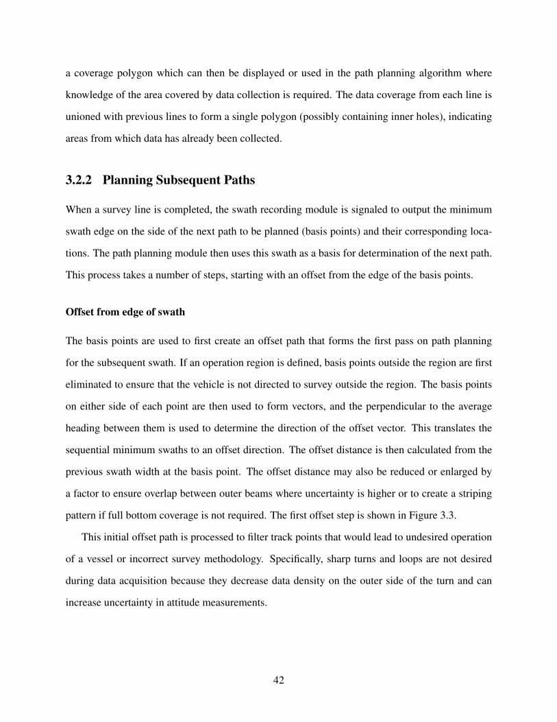
a coverage polygon which can then be displayed or used in the path planning algorithm where
knowledge of the area covered by data collection is required. The data coverage from each line is
unioned with previous lines to form a single polygon (possibly containing inner holes), indicating
areas from which data has already been collected.
3.2.2 Planning Subsequent Paths
When a survey line is completed, the swath recording module is signaled to output the minimum
swath edge on the side of the next path to be planned (basis points) and their corresponding loca-
tions. The path planning module then uses this swath as a basis for determination of the next path.
This process takes a number of steps, starting with an offset from the edge of the basis points.
Offset from edge of swath
The basis points are used to first create an offset path that forms the first pass on path planning
for the subsequent swath. If an operation region is defined, basis points outside the region are first
eliminated to ensure that the vehicle is not directed to survey outside the region. The basis points
on either side of each point are then used to form vectors, and the perpendicular to the average
heading between them is used to determine the direction of the offset vector. This translates the
sequential minimum swaths to an offset direction. The offset distance is then calculated from the
previous swath width at the basis point. The offset distance may also be reduced or enlarged by
a factor to ensure overlap between outer beams where uncertainty is higher or to create a striping
pattern if full bottom coverage is not required. The first offset step is shown in Figure 3.3.
This initial offset path is processed to filter track points that would lead to undesired operation
of a vessel or incorrect survey methodology. Specifically, sharp turns and loops are not desired
during data acquisition because they decrease data density on the outer side of the turn and can
increase uncertainty in attitude measurements.
42
Figure 3.3: Illustration of the generation of an offset line for initial input into the refinements of thepath planning algorithm. This shows a straight initial line for data collection, but the same processis used for subsequent segmented lines. No additional overlap is added in this example.
Removal of self intersects
The first step to refine the path is to remove areas where the path crosses over itself, which would
not only cause unnecessary turns, but also duplicate coverage in some areas. These crossings can
occur where the ASV executes a turn with a radius less than twice the width of the sonar swath
at that point. Each segment is tested against following segments to see if it intersects them. If
there are intersections, the portion of the path between the first and last intersect is removed. This
process is repeated along the path until all self intersections are removed.
Removal of sharp bends
The processing algorithm next eliminates bends in the path that exceed a defined angle. Large
angle turns are avoided because they cause increased spacing between sonar detections along the
outside of the turn and force the ASV to turn in a smaller space than its physically possible turning
radius, which could lead to undesired operation from the line following control system. For the
simulation and testing discussed in Section 3.4, the maximum bend angle is 60. To eliminate
bends, the path is checked along the direction of travel. When an angle between segments is larger
43
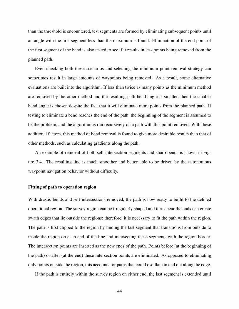
than the threshold is encountered, test segments are formed by eliminating subsequent points until
an angle with the first segment less than the maximum is found. Elimination of the end point of
the first segment of the bend is also tested to see if it results in less points being removed from the
planned path.
Even checking both these scenarios and selecting the minimum point removal strategy can
sometimes result in large amounts of waypoints being removed. As a result, some alternative
evaluations are built into the algorithm. If less than twice as many points as the minimum method
are removed by the other method and the resulting path bend angle is smaller, then the smaller
bend angle is chosen despite the fact that it will eliminate more points from the planned path. If
testing to eliminate a bend reaches the end of the path, the beginning of the segment is assumed to
be the problem, and the algorithm is run recursively on a path with this point removed. With these
additional factors, this method of bend removal is found to give more desirable results than that of
other methods, such as calculating gradients along the path.
An example of removal of both self intersection segments and sharp bends is shown in Fig-
ure 3.4. The resulting line is much smoother and better able to be driven by the autonomous
waypoint navigation behavior without difficulty.
Fitting of path to operation region
With drastic bends and self intersections removed, the path is now ready to be fit to the defined
operational region. The survey region can be irregularly shaped and turns near the ends can create
swath edges that lie outside the regions; therefore, it is necessary to fit the path within the region.
The path is first clipped to the region by finding the last segment that transitions from outside to
inside the region on each end of the line and intersecting these segments with the region border.
The intersection points are inserted as the new ends of the path. Points before (at the beginning of
the path) or after (at the end) these intersection points are eliminated. As opposed to eliminating
only points outside the region, this accounts for paths that could oscillate in and out along the edge.
If the path is entirely within the survey region on either end, the last segment is extended until
44
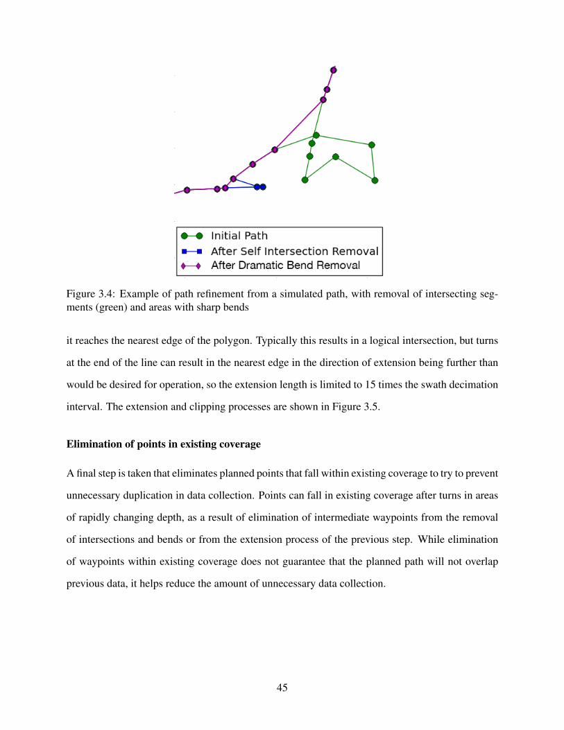
Figure 3.4: Example of path refinement from a simulated path, with removal of intersecting seg-ments (green) and areas with sharp bends
it reaches the nearest edge of the polygon. Typically this results in a logical intersection, but turns
at the end of the line can result in the nearest edge in the direction of extension being further than
would be desired for operation, so the extension length is limited to 15 times the swath decimation
interval. The extension and clipping processes are shown in Figure 3.5.
Elimination of points in existing coverage
A final step is taken that eliminates planned points that fall within existing coverage to try to prevent
unnecessary duplication in data collection. Points can fall in existing coverage after turns in areas
of rapidly changing depth, as a result of elimination of intermediate waypoints from the removal
of intersections and bends or from the extension process of the previous step. While elimination
of waypoints within existing coverage does not guarantee that the planned path will not overlap
previous data, it helps reduce the amount of unnecessary data collection.
45
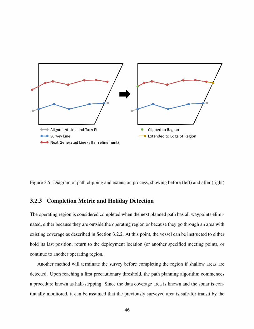
Figure 3.5: Diagram of path clipping and extension process, showing before (left) and after (right)
3.2.3 Completion Metric and Holiday Detection
The operating region is considered completed when the next planned path has all waypoints elimi-
nated, either because they are outside the operating region or because they go through an area with
existing coverage as described in Section 3.2.2. At this point, the vessel can be instructed to either
hold its last position, return to the deployment location (or another specified meeting point), or
continue to another operating region.
Another method will terminate the survey before completing the region if shallow areas are
detected. Upon reaching a first precautionary threshold, the path planning algorithm commences
a procedure known as half-stepping. Since the data coverage area is known and the sonar is con-
tinually monitored, it can be assumed that the previously surveyed area is safe for transit by the
46
ASV. Therefore, upon detection of a shoal, it will divert in the direction of the prior survey line
and follow the edge of the previous swath, as shown in Figure 3.6. This is the same procedure
currently followed by human coxswains. While half-stepping, if the depths increase, such as for
an isolated shoal, the ASV resumes normal path planning operation. If the shoal is part of a natural
rise toward shore and a shallower halt threshold is reached, the next path will be planned on top of
the previous path for these locations. If all other areas in the operation region are completed but a
shoal remains, or the shoal stretches along the entire line, the region is determined to be complete.
Figure 3.6: Half stepping behavior demonstrated, with next line planned along edge of previousswath coverage.
Within the operating region that has just been completed, the coverage record kept by the
swath recorder can be used to identify where there are gaps in the data such that it would not
meet complete coverage requirements. These gaps are known as holidays and are required to be
filled before a survey area is deemed complete. The holidays can then be targeted for completion,
which is currently achieved by planning a path among them after completion of the first pass of the
region. The current algorithm only addresses holidays as point locations, but larger ones could be
addressed as a separate set of operation regions.
47
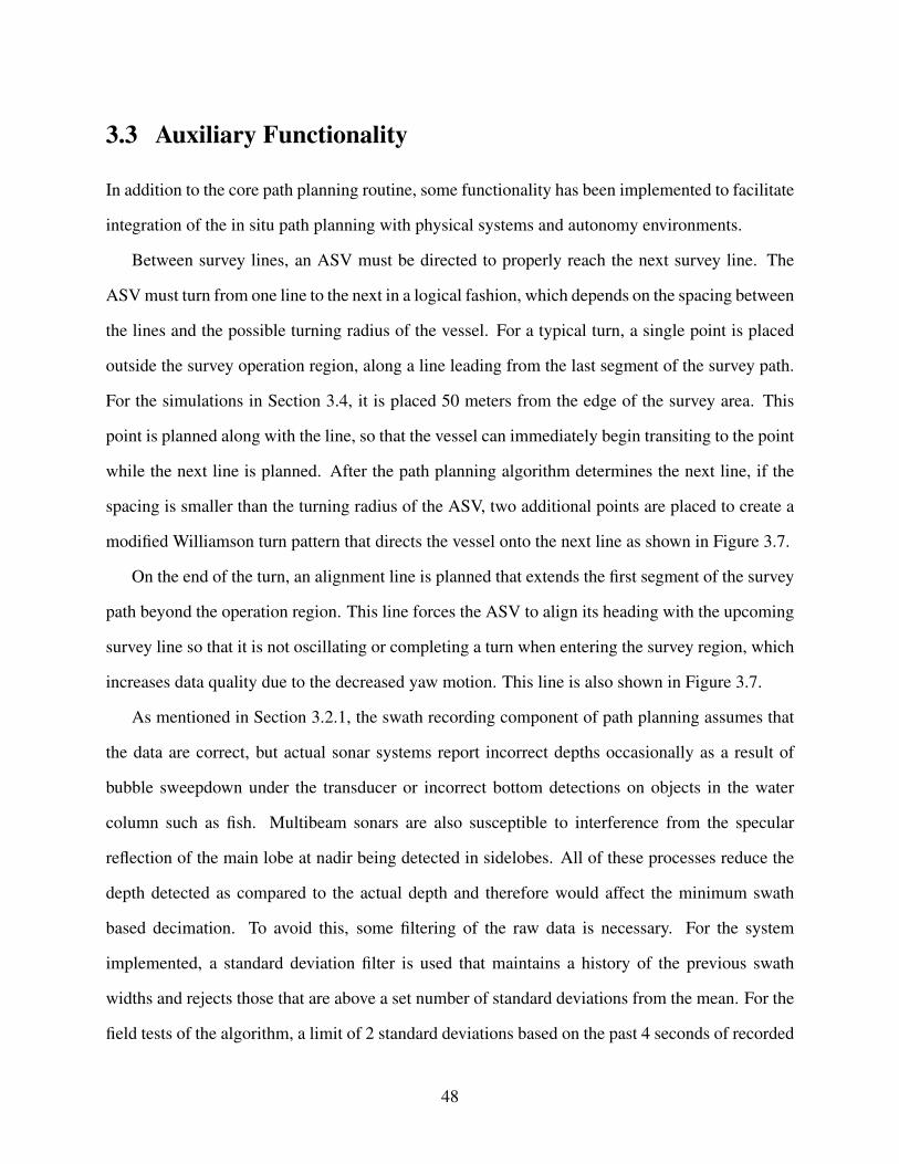
3.3 Auxiliary Functionality
In addition to the core path planning routine, some functionality has been implemented to facilitate
integration of the in situ path planning with physical systems and autonomy environments.
Between survey lines, an ASV must be directed to properly reach the next survey line. The
ASV must turn from one line to the next in a logical fashion, which depends on the spacing between
the lines and the possible turning radius of the vessel. For a typical turn, a single point is placed
outside the survey operation region, along a line leading from the last segment of the survey path.
For the simulations in Section 3.4, it is placed 50 meters from the edge of the survey area. This
point is planned along with the line, so that the vessel can immediately begin transiting to the point
while the next line is planned. After the path planning algorithm determines the next line, if the
spacing is smaller than the turning radius of the ASV, two additional points are placed to create a
modified Williamson turn pattern that directs the vessel onto the next line as shown in Figure 3.7.
On the end of the turn, an alignment line is planned that extends the first segment of the survey
path beyond the operation region. This line forces the ASV to align its heading with the upcoming
survey line so that it is not oscillating or completing a turn when entering the survey region, which
increases data quality due to the decreased yaw motion. This line is also shown in Figure 3.7.
As mentioned in Section 3.2.1, the swath recording component of path planning assumes that
the data are correct, but actual sonar systems report incorrect depths occasionally as a result of
bubble sweepdown under the transducer or incorrect bottom detections on objects in the water
column such as fish. Multibeam sonars are also susceptible to interference from the specular
reflection of the main lobe at nadir being detected in sidelobes. All of these processes reduce the
depth detected as compared to the actual depth and therefore would affect the minimum swath
based decimation. To avoid this, some filtering of the raw data is necessary. For the system
implemented, a standard deviation filter is used that maintains a history of the previous swath
widths and rejects those that are above a set number of standard deviations from the mean. For the
field tests of the algorithm, a limit of 2 standard deviations based on the past 4 seconds of recorded
48
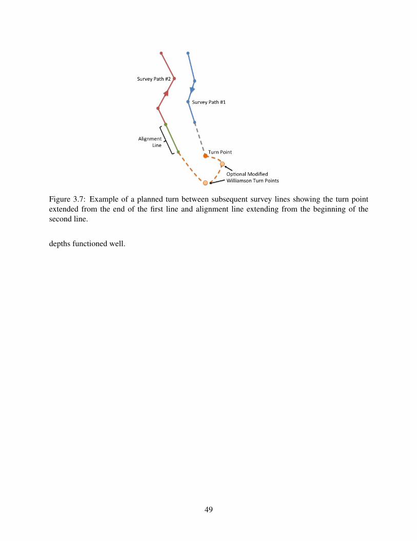
Figure 3.7: Example of a planned turn between subsequent survey lines showing the turn pointextended from the end of the first line and alignment line extending from the beginning of thesecond line.
depths functioned well.
49

3.4 Simulation Results
The path planning algorithm is developed and tested using a custom simulation program created
for this purpose. After the algorithm was determined to perform suitably, it was integrated into the
MOOS-IvP autonomy environment for deployment on ASVs and further testing in simulation.
3.4.1 Custom Simulation Program
A custom vessel movement simulator is programmed in Python to support development of the
path planning algorithm. The program developed for this research simulates a vessel following a
trackline made up of waypoints and gives sonar depth and swath width values from either generated
depth patterns or data imported from previous surveys. It implements the full sonar swath recording
and path planning algorithm from Section 3.2.
An example of a simulation run on a generated pattern of an “X” shaped depression with a
hole in the middle is shown in Figure 3.8. The survey lines are initially planned at an angle to the
edge of the operation region in this example, showing how the lines will be extended and clipped
as needed. The distance between lines increases in the deeper areas (blue) causing them to bend
around the spot. The calculated coverage using this simulator shows gaps at the edges of the survey
area, but this is because the turning points are not included when driving the simulated vessel. In
an actual survey using the turning points and alignment lines, these planned paths would achieve
full coverage of the assigned region. This issue is also discussed in more detail by Bourgeois in [1].
Additional examples with generated terrain are shown in Figure 3.9, where the differences in
spacing between lines with depth are clear. Figure 3.9a shows a sharp bend elimination limit of 60
in effect, where the ridge slowly creates a sharper bend after the first line until the limit is reached,
at which point they stay constant. As a result, small holidays are created in the areas around bends,
but these are detected and could easily be addressed with a line before completion of the region,
which is preferable over attempting to make turns that are not physically possible with the vessel.
The simulation developed for this research can also be run with previously collected and grid-
50
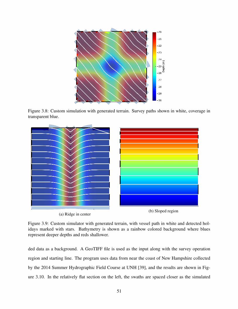
Figure 3.8: Custom simulation with generated terrain. Survey paths shown in white, coverage intransparent blue.
(a) Ridge in center(b) Sloped region
Figure 3.9: Custom simulator with generated terrain, with vessel path in white and detected hol-idays marked with stars. Bathymetry is shown as a rainbow colored background where bluesrepresent deeper depths and reds shallower.
ded data as a background. A GeoTIFF file is used as the input along with the survey operation
region and starting line. The program uses data from near the coast of New Hampshire collected
by the 2014 Summer Hydrographic Field Course at UNH [39], and the results are shown in Fig-
ure 3.10. In the relatively flat section on the left, the swaths are spaced closer as the simulated
51
vessel moves inshore, and the survey lines remain fairly parallel. In the more complex terrain of
the right section, the paths become bent where the depths change and some holidays are left where
dramatic bends were removed from the planned paths. These are marked with stars and can be
addressed by additional data acquisition.
Figure 3.10: Custom simulation using actual terrain. Data coverage is shown in transparent blueand holidays marked with stars.
3.4.2 MOOS-IvP Implementation and Simulation
The implementation of these core and some auxiliary behaviors discussed in Section 3.3 is shown
in Figure 3.11. The complete MOOS mission is structured as discussed in Section 2.2, this shows
the execution during the survey portion. A starting line is first surveyed along an edge of the region,
which can be selected automatically as the first side of the polygon or defined in the mission. When
this line or any subsequent one completes, swaths continue to be recorded until both sides are
outside the region, or the turn point is reached. This ensures that full coverage is achieved within
the region as long as the turn points are sufficiently offset.
When recording ceases, the processing for the next line is initiated in a separate thread, while
the vessel transits to the turn point if it has not yet reached it. At the turn point, if processing
is complete, the next survey line and its associated alignment line and turn point are posted to
update the associated IvP behaviors. If processing is incomplete, or was initiated by reaching the
52
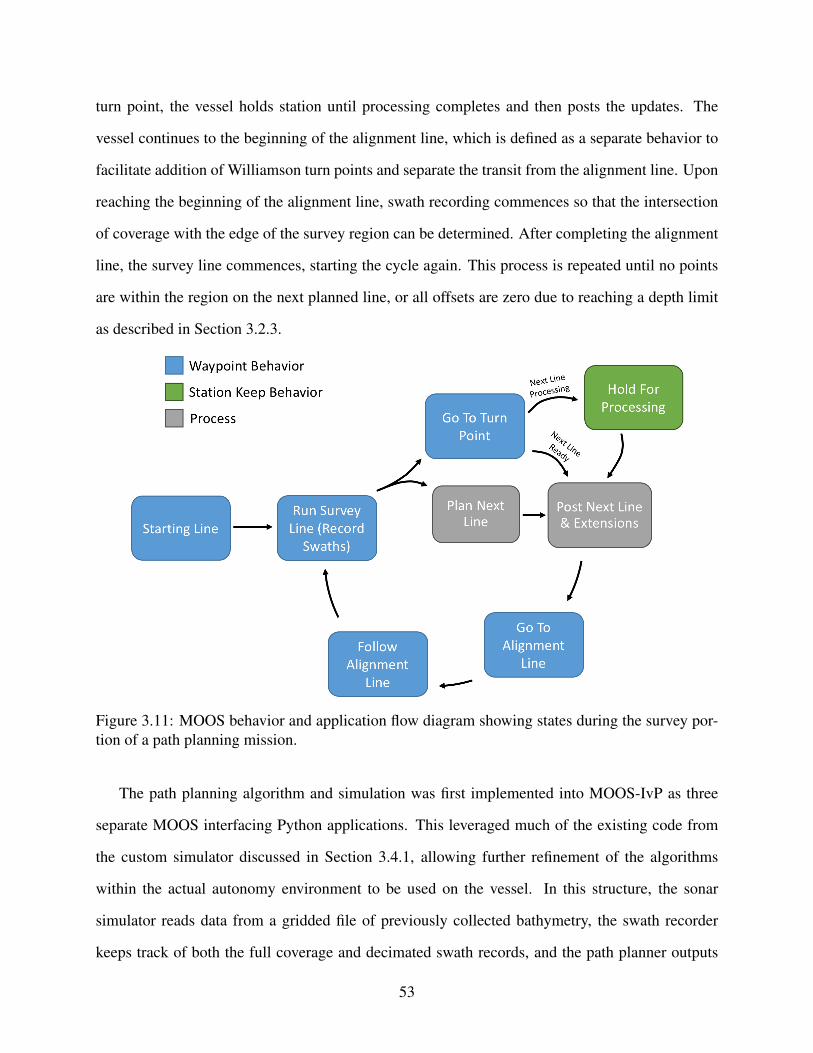
turn point, the vessel holds station until processing completes and then posts the updates. The
vessel continues to the beginning of the alignment line, which is defined as a separate behavior to
facilitate addition of Williamson turn points and separate the transit from the alignment line. Upon
reaching the beginning of the alignment line, swath recording commences so that the intersection
of coverage with the edge of the survey region can be determined. After completing the alignment
line, the survey line commences, starting the cycle again. This process is repeated until no points
are within the region on the next planned line, or all offsets are zero due to reaching a depth limit
as described in Section 3.2.3.
Figure 3.11: MOOS behavior and application flow diagram showing states during the survey por-tion of a path planning mission.
The path planning algorithm and simulation was first implemented into MOOS-IvP as three
separate MOOS interfacing Python applications. This leveraged much of the existing code from
the custom simulator discussed in Section 3.4.1, allowing further refinement of the algorithms
within the actual autonomy environment to be used on the vessel. In this structure, the sonar
simulator reads data from a gridded file of previously collected bathymetry, the swath recorder
keeps track of both the full coverage and decimated swath records, and the path planner outputs
53
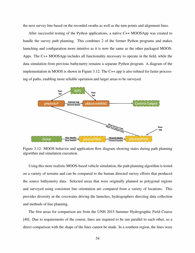
the next survey line based on the recorded swaths as well as the turn points and alignment lines.
After successful testing of the Python applications, a native C++ MOOSApp was created to
handle the survey path planning. This combines 2 of the former Python programs and makes
launching and configuration more intuitive as it is now the same as the other packaged MOOS-
Apps. The C++ MOOSApp includes all functionality necessary to operate in the field, while the
data simulation from previous bathymetry remains a separate Python program. A diagram of the
implementation in MOOS is shown in Figure 3.12. The C++ app is also refined for faster process-
ing of paths, enabling more reliable operation and larger areas to be surveyed.
Figure 3.12: MOOS behavior and application flow diagram showing states during path planningalgorithm and simulation execution.
Using this more realistic MOOS-based vehicle simulation, the path planning algorithm is tested
on a variety of terrains and can be compared to the human directed survey efforts that produced
the source bathymetry data. Selected areas that were originally planned as polygonal regions
and surveyed using consistent line orientation are compared from a variety of locations. This
provides diversity in the coxswains driving the launches, hydrographers directing data collection
and methods of line planning.
The first areas for comparison are from the UNH 2015 Summer Hydrographic Field Course
[40]. Due to requirements of the course, lines are required to be run parallel to each other, so a
direct comparison with the shape of the lines cannot be made. In a southern region, the lines were
54
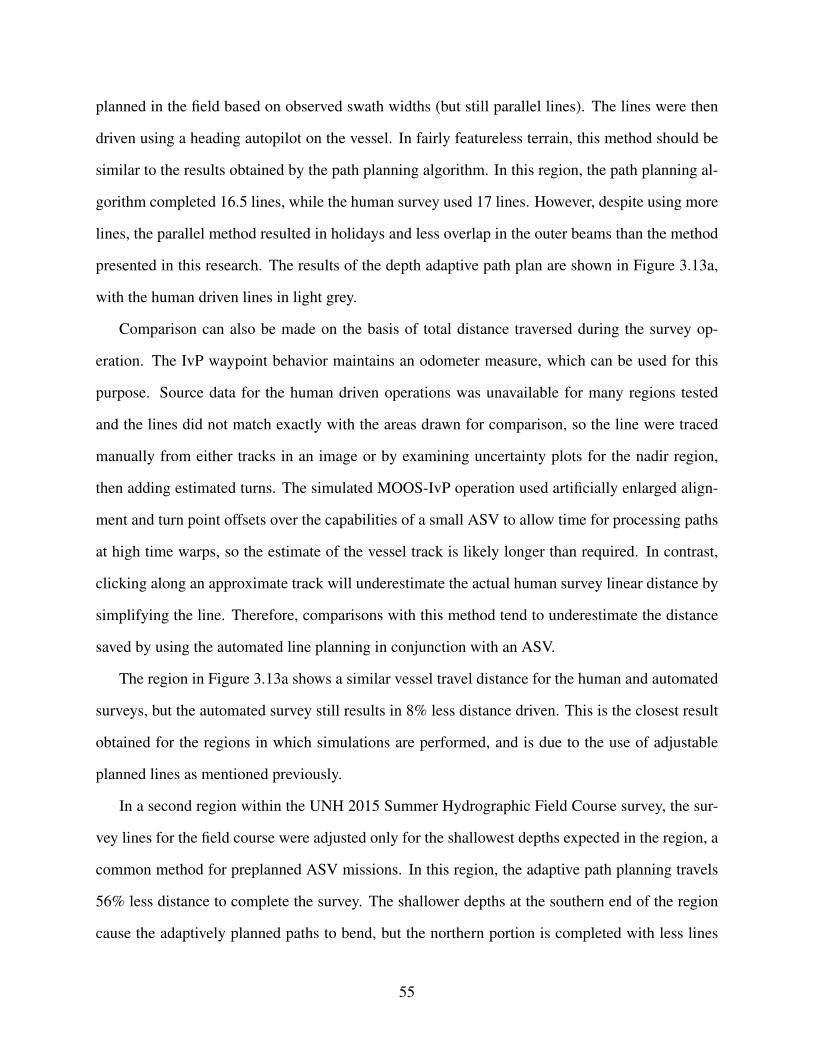
planned in the field based on observed swath widths (but still parallel lines). The lines were then
driven using a heading autopilot on the vessel. In fairly featureless terrain, this method should be
similar to the results obtained by the path planning algorithm. In this region, the path planning al-
gorithm completed 16.5 lines, while the human survey used 17 lines. However, despite using more
lines, the parallel method resulted in holidays and less overlap in the outer beams than the method
presented in this research. The results of the depth adaptive path plan are shown in Figure 3.13a,
with the human driven lines in light grey.
Comparison can also be made on the basis of total distance traversed during the survey op-
eration. The IvP waypoint behavior maintains an odometer measure, which can be used for this
purpose. Source data for the human driven operations was unavailable for many regions tested
and the lines did not match exactly with the areas drawn for comparison, so the line were traced
manually from either tracks in an image or by examining uncertainty plots for the nadir region,
then adding estimated turns. The simulated MOOS-IvP operation used artificially enlarged align-
ment and turn point offsets over the capabilities of a small ASV to allow time for processing paths
at high time warps, so the estimate of the vessel track is likely longer than required. In contrast,
clicking along an approximate track will underestimate the actual human survey linear distance by
simplifying the line. Therefore, comparisons with this method tend to underestimate the distance
saved by using the automated line planning in conjunction with an ASV.
The region in Figure 3.13a shows a similar vessel travel distance for the human and automated
surveys, but the automated survey still results in 8% less distance driven. This is the closest result
obtained for the regions in which simulations are performed, and is due to the use of adjustable
planned lines as mentioned previously.
In a second region within the UNH 2015 Summer Hydrographic Field Course survey, the sur-
vey lines for the field course were adjusted only for the shallowest depths expected in the region, a
common method for preplanned ASV missions. In this region, the adaptive path planning travels
56% less distance to complete the survey. The shallower depths at the southern end of the region
cause the adaptively planned paths to bend, but the northern portion is completed with less lines
55
(a) Southern Region (b) Northern Region
Figure 3.13: Simulation results from MOOS-IvP simulation showing survey behavior. A red boxdenotes the specified operation region and the white lines show survey paths. Human data collec-tion paths shown in light grey. Bathymetry is shown as a rainbow colored background where bluesrepresent deeper depths and reds shallower.
and only small holidays are left in the regions with tight turns. Assuming a survey speed of 7 kts,
the depth adaptively planned survey requires almost 2 hours less underway time than the static
spacing version, a dramatic time and fuel savings. The survey planning results for this region are
shown in Figure 3.13b.
Surveys conducted by NOAA Ships Fairweather and Rainier are used to compare the path
planning algorithm to human surveys conducted under an adaptive methodology, where the coxswain
visually matches the current swath with the edge of previous coverage. Three regions are investi-
gated that contain a variety of terrain. A fairly flat area with a few ridges near Chirikof Island, AK
is shown in Figure 3.14. The general patterns of each data collection method are similar, but even
here, the automated survey is able to reduce acquisition travel distance by 20%. The reduction is
mostly due to the ability to more closely follow the desired path, reducing unnecessary overlap
between swaths. While the environmental conditions may have dictated closer spacing at the time,
it is also likely that less overlap was required in the human survey.
Surveys conducted near the Shumagin islands are also compared between human and auto-
56
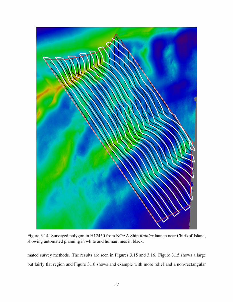
Figure 3.14: Surveyed polygon in H12450 from NOAA Ship Rainier launch near Chirikof Island,showing automated planning in white and human lines in black.
mated survey methods. The results are seen in Figures 3.15 and 3.16. Figure 3.15 shows a large
but fairly flat region and Figure 3.16 shows and example with more relief and a non-rectangular
57
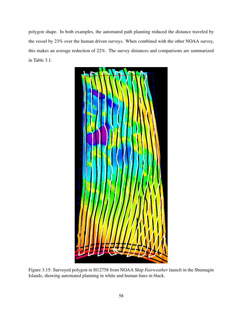
polygon shape. In both examples, the automated path planning reduced the distance traveled by
the vessel by 23% over the human driven surveys. When combined with the other NOAA survey,
this makes an average reduction of 22%. The survey distances and comparisons are summarized
in Table 3.1.
Figure 3.15: Surveyed polygon in H12758 from NOAA Ship Fairweather launch in the ShumaginIslands, showing automated planning in white and human lines in black.
58
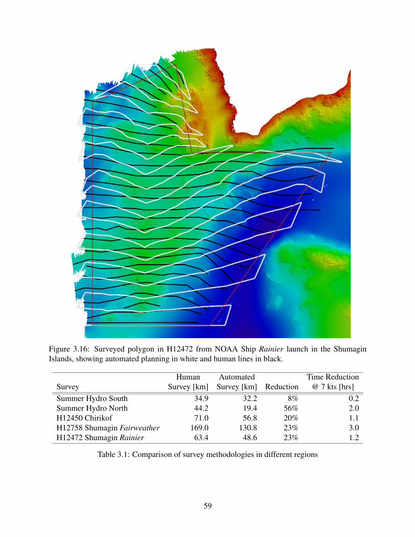
Figure 3.16: Surveyed polygon in H12472 from NOAA Ship Rainier launch in the ShumaginIslands, showing automated planning in white and human lines in black.
SurveyHuman
Survey [km]Automated
Survey [km] ReductionTime Reduction
@ 7 kts [hrs]Summer Hydro South 34.9 32.2 8% 0.2Summer Hydro North 44.2 19.4 56% 2.0H12450 Chirikof 71.0 56.8 20% 1.1H12758 Shumagin Fairweather 169.0 130.8 23% 3.0H12472 Shumagin Rainier 63.4 48.6 23% 1.2
Table 3.1: Comparison of survey methodologies in different regions
59
3.5 Field Testing Results
The path planning algorithm was able to be tested in the field during development on different Z-
Boat vessels, with both single beam and multibeam mapping systems installed. Unfortunately, due
to limited platform availability and hardware difficulties with the UNH ASVs, the final versions of
the behavior are not able to be tested beyond simulations.
3.5.1 Single Beam Sonar Tests
While the algorithm is intended to be used with a swath sonar like a multibeam, it can also be
tested with a single beam using the simulated swath angle option in pSonarFilter. While the vessel
will not achieve full coverage with this scheme, it can be used to show the path a swath mapping
vessel would take and visually verify the behavior versus what would be expected for a human
operator. The first field tests were conducted on Z-Boats in conjunction with the NOAA Ship
Thomas Jefferson at the Naval Station Newport in Newport, RI. These Z-Boats have a Teledyne
Odom CV100 single beam sonar system installed, and through the module described in Section 1.3,
depth data is passed to MOOS and the boat controlled to follow the planned paths.
At the time, the Z-Boats were new to the Thomas Jefferson, so operations were limited to the
area around the piers where the ship docked to reduce risk from malfunctions. This area is dredged,
and therefore very flat, so evenly spaced, straight paths could be expected. A rectangular operation
region was designated for the survey within the area between two piers. The results of this survey
from 28 August 2015 are shown in Figure 3.17.
This shows the depth map created from the single beam sonar data. As expected, a mostly
linear path is followed. The survey had to be manually terminated before the final boundary was
reached due to the presence of a barge in the designated region. To better visualize the autonomy
system, a screenshot of the shoreside MOOS-IvP pMarineViewer monitoring window is shown in
Figure 3.18 for a time toward the end of the survey mission.
Figure 3.18 shows the turn point and alignment line that are placed outside the survey region for the
60
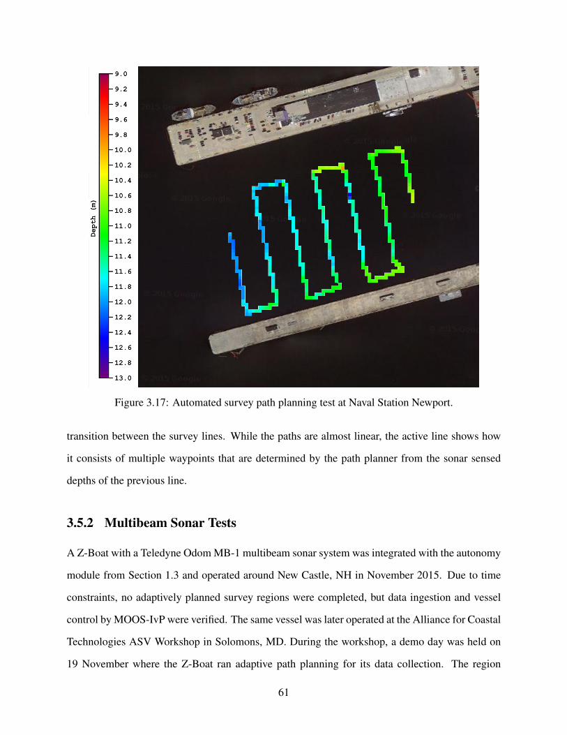
Figure 3.17: Automated survey path planning test at Naval Station Newport.
transition between the survey lines. While the paths are almost linear, the active line shows how
it consists of multiple waypoints that are determined by the path planner from the sonar sensed
depths of the previous line.
3.5.2 Multibeam Sonar Tests
A Z-Boat with a Teledyne Odom MB-1 multibeam sonar system was integrated with the autonomy
module from Section 1.3 and operated around New Castle, NH in November 2015. Due to time
constraints, no adaptively planned survey regions were completed, but data ingestion and vessel
control by MOOS-IvP were verified. The same vessel was later operated at the Alliance for Coastal
Technologies ASV Workshop in Solomons, MD. During the workshop, a demo day was held on
19 November where the Z-Boat ran adaptive path planning for its data collection. The region
61
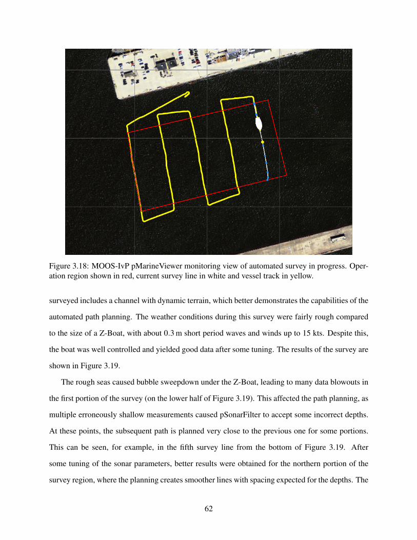
Figure 3.18: MOOS-IvP pMarineViewer monitoring view of automated survey in progress. Oper-ation region shown in red, current survey line in white and vessel track in yellow.
surveyed includes a channel with dynamic terrain, which better demonstrates the capabilities of the
automated path planning. The weather conditions during this survey were fairly rough compared
to the size of a Z-Boat, with about 0.3 m short period waves and winds up to 15 kts. Despite this,
the boat was well controlled and yielded good data after some tuning. The results of the survey are
shown in Figure 3.19.
The rough seas caused bubble sweepdown under the Z-Boat, leading to many data blowouts in
the first portion of the survey (on the lower half of Figure 3.19). This affected the path planning, as
multiple erroneously shallow measurements caused pSonarFilter to accept some incorrect depths.
At these points, the subsequent path is planned very close to the previous one for some portions.
This can be seen, for example, in the fifth survey line from the bottom of Figure 3.19. After
some tuning of the sonar parameters, better results were obtained for the northern portion of the
survey region, where the planning creates smoother lines with spacing expected for the depths. The
62
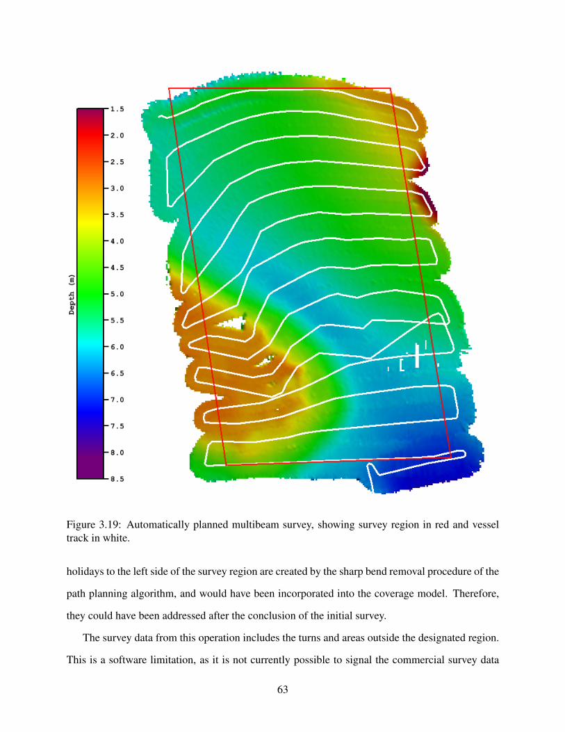
Figure 3.19: Automatically planned multibeam survey, showing survey region in red and vesseltrack in white.
holidays to the left side of the survey region are created by the sharp bend removal procedure of the
path planning algorithm, and would have been incorporated into the coverage model. Therefore,
they could have been addressed after the conclusion of the initial survey.
The survey data from this operation includes the turns and areas outside the designated region.
This is a software limitation, as it is not currently possible to signal the commercial survey data
63
collection software (Hypack) to start and stop logging over a network or serial connection. In
addition, the only output available at the time of survey provided the nadir (directly beneath the
boat) depth, so the swath width had to be estimated. Discussions with Hypack representatives
have yielded a method for transferring swath coverage and the possibility of future integration of
automatic logging within a region and support for external logging commands.
NOAA full coverage requirements specify that each depth point in the final gridded product
must have at least 5 individual soundings (sonar measurements) contributing to the calculated
depth for greater than 95% of the grid cells [35]. In all areas where there are not holidays created
by either blowouts or the path planning bend angle limit, the data density meets this criteria, as
shown in Figure 3.20a. In addition, a scaled representation showing more detail on the range
of data density is shown in Figure 3.20b. From this version, it is possible to see the amount of
swath overlap, since these areas have slightly increased data density. The path planning algorithm
adequately creates overlap throughout the survey, and is particularly effective at having minimal
overlap in the northern portion where there is good quality input sonar data. Since it achieves the
5 sounding per node requirement with this small overlap, it is likely this survey is more efficient
than a human driven one in the same area.
This survey reinforces the need for resurveying shallow, high traffic areas. In this busy port,
a shoal was found that is not currently represented on NOAA nautical charts. On the raster chart
(RNC), from which the survey was planned, the survey limits are deeper than the 6 ft contour on
the eastern side. However, survey data revealed that both the channel and land in this area does
not match the chart. The land outline is updated on the Electronic Navigation Chart (ENC), but
the depths and contours are not, so they go through land at this location. The survey is shown in
the context of these charts in Figure 3.21. It can also be seen that despite the shoal and land jutting
into the surveyed area, the main channel has widened since the previous survey.
[Maybe include figure of the old survey from ACT paper]
Field tests of the path planning algorithm and associated MOOS-IvP behavioral structure show
that its operation is robust to real world conditions and largely fault tolerant to intermittently er-
64
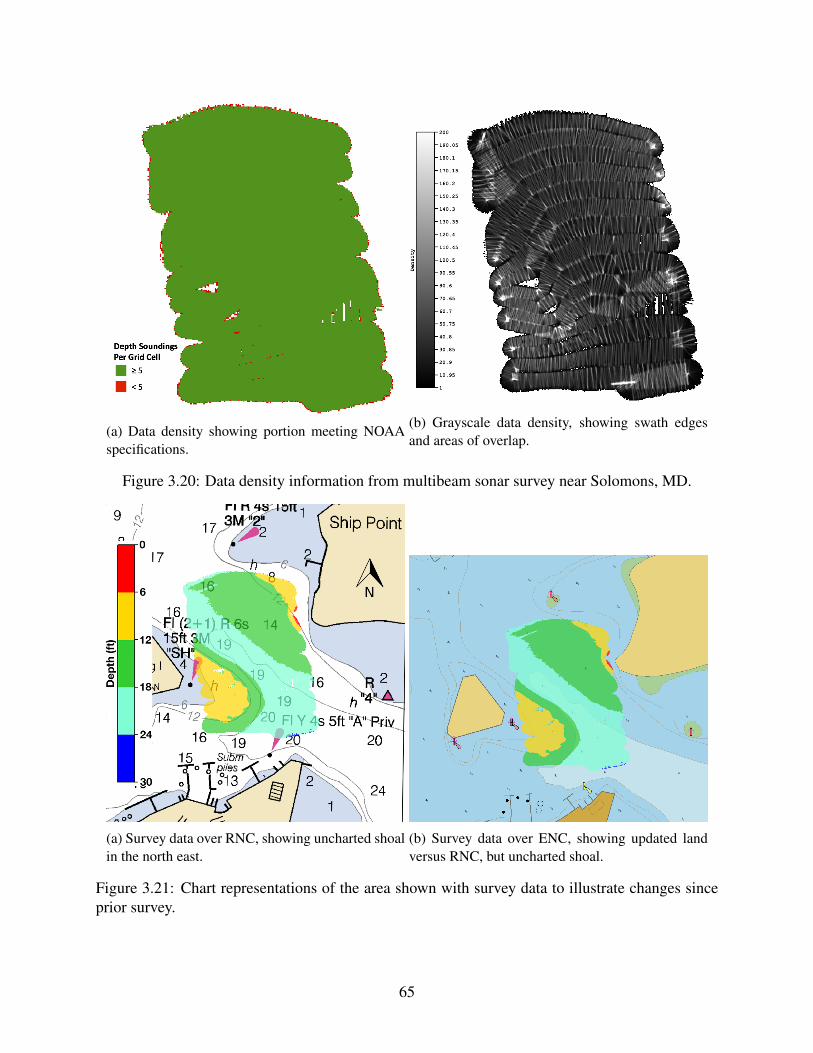
(a) Data density showing portion meeting NOAAspecifications.
(b) Grayscale data density, showing swath edgesand areas of overlap.
Figure 3.20: Data density information from multibeam sonar survey near Solomons, MD.
(a) Survey data over RNC, showing uncharted shoalin the north east.
(b) Survey data over ENC, showing updated landversus RNC, but uncharted shoal.
Figure 3.21: Chart representations of the area shown with survey data to illustrate changes sinceprior survey.
65

roneous data from the sonar system. Even when individual lines have mistaken trajectories due to
poor data quality, future lines are able to recover and the survey completes satisfactorily. Addi-
tional reductions in data quality could compromise the performance, but under these conditions the
sonar data would not be acceptable for charting either. With adequate quality data, the automated
survey system can complete a designated polygonal region to meet NOAA specifications.
66
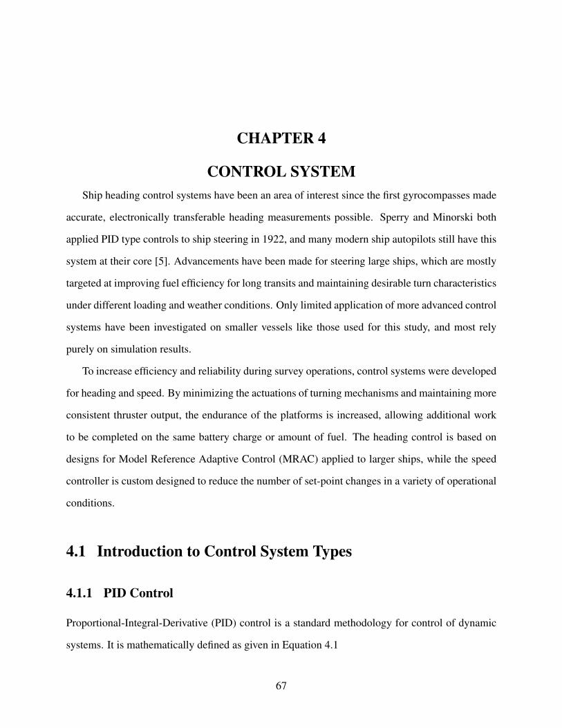
CHAPTER 4
CONTROL SYSTEMShip heading control systems have been an area of interest since the first gyrocompasses made
accurate, electronically transferable heading measurements possible. Sperry and Minorski both
applied PID type controls to ship steering in 1922, and many modern ship autopilots still have this
system at their core [5]. Advancements have been made for steering large ships, which are mostly
targeted at improving fuel efficiency for long transits and maintaining desirable turn characteristics
under different loading and weather conditions. Only limited application of more advanced control
systems have been investigated on smaller vessels like those used for this study, and most rely
purely on simulation results.
To increase efficiency and reliability during survey operations, control systems were developed
for heading and speed. By minimizing the actuations of turning mechanisms and maintaining more
consistent thruster output, the endurance of the platforms is increased, allowing additional work
to be completed on the same battery charge or amount of fuel. The heading control is based on
designs for Model Reference Adaptive Control (MRAC) applied to larger ships, while the speed
controller is custom designed to reduce the number of set-point changes in a variety of operational
conditions.
4.1 Introduction to Control System Types
4.1.1 PID Control
Proportional-Integral-Derivative (PID) control is a standard methodology for control of dynamic
systems. It is mathematically defined as given in Equation 4.1
67
c(t) = Kpe(t)+Ki
∫ t
0e(τ)dτ−Kd
de(t)dt
(4.1)
where c(t) is the control output signal, and e(t) is the error between the system under control and
the desired behavior. The proportional term (Kp) sets the output based on the currently known
error, and the differential (Kd) and integral (Ki) terms provide anticipatory and historical error
compensation, respectively. In physical terms for a vessel, the proportional feedback sets the
initial non-zero desired rudder when a heading change is requested. As the vessel begins to turn,
the differential feedback allows damping by reducing the desired rudder in proportion to the rate
of turn. Finally, integral feedback compensates over time for static disturbances, such as rotational
push from wind or an offset in the rudder positioning. Together, all the terms of the PID controller
gives a defined characteristic to the response of the heading control and is able to compensate for
both static and dynamic disturbances.
However, if the behavior of the vessel itself changes as a result of speed, thrust, or mass changes
due to loading and fuel consumption, the PID controller gains will have to be changed to achieve
the same response characteristic and avoid unwanted oscillation, course overshoot, or sluggish
adjustment. With a simple addition to the PID controller and thorough testing under various con-
ditions, gain schedules can be designed to compensate for some of these effects. However, this
requires testing to be completed, which becomes increasingly difficult and time consuming with
vessels that undergo many modifications, as is common on survey vessels with different sonar sys-
tems and other payloads. Therefore, an automatically adapting approach using model reference
adaptive control is introduced.
4.1.2 Model Reference Adaptive Heading Control
Model reference adaptive control (MRAC) uses a mathematically defined model to approximate
the behavior of the system under control, which in this case is the heading of the ship. The model
is initialized with parameters close to those expected for the system and is continually fed mea-
68
surements of the inputs to the physical system, so that the model operates in parallel to the physical
system. The differences between the model and the measured response of the system are used to
adjust the model, which over time, should closely match the behavior of the physical system as
long as the major dynamics are captured by the model [41]. The adjustment laws are derived to
ensure stability in the system over time. The adaptation can be applied to either parameters of a
model of the system or the feedback gains of the controller.
4.2 Implementation of MRAC
For this autonomy system, MRAC is implemented for heading control of the vessel. Two ver-
sions of a heading controller are implemented, which can be operated separately or as a hybrid
combination. These two controllers are adapted from versions originally developed by Job Van
Amerongen [2], [42]. Van Amerongen applied MRAC to larger ships (42 m to 168 m), for which
two modes of operation were desirable. Throughout this section, the term rudder angle applies
to both the physical rudder on systems with separate propulsion and rudder (common on larger
vessels) as well as the angle of the thrusters or thrust nozzle on platforms where the thrusters are
actuated (common on the smaller platforms of this study). The characteristics of each should be
similar, with actuated thrusters likely performing closer to the simplified models due to less re-
liance on lift over the rudder for turning. Thrusters give a constant force at the angle to which they
are turned, while rudders stall at high angles and do not provide a linear relationship between angle
and force.
The controllers are implemented as part of the same MOOSApp, pMarineMRAS, which facil-
itates passing information when running in hybrid mode and simplifies deployment and configura-
tion for users. The acronym MRAS in the application name refers to Model Reference Adaptive
Systems, taking into account the multiple methods. The pMarineMRAS application subscribes to
the desired heading and speed from the IvP Helm and uses measured heading and speed to provide
feedback and control the vessel.
69
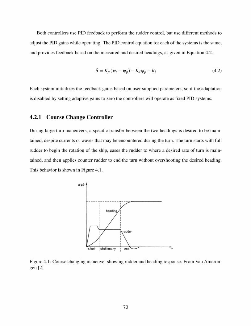
Both controllers use PID feedback to perform the rudder control, but use different methods to
adjust the PID gains while operating. The PID control equation for each of the systems is the same,
and provides feedback based on the measured and desired headings, as given in Equation 4.2.
δ = Kp (ψr−ψp)−Kdψp +Ki (4.2)
Each system initializes the feedback gains based on user supplied parameters, so if the adaptation
is disabled by setting adaptive gains to zero the controllers will operate as fixed PID systems.
4.2.1 Course Change Controller
During large turn maneuvers, a specific transfer between the two headings is desired to be main-
tained, despite currents or waves that may be encountered during the turn. The turn starts with full
rudder to begin the rotation of the ship, eases the rudder to where a desired rate of turn is main-
tained, and then applies counter rudder to end the turn without overshooting the desired heading.
This behavior is shown in Figure 4.1.
Figure 4.1: Course changing maneuver showing rudder and heading response. From Van Ameron-gen [2]
70
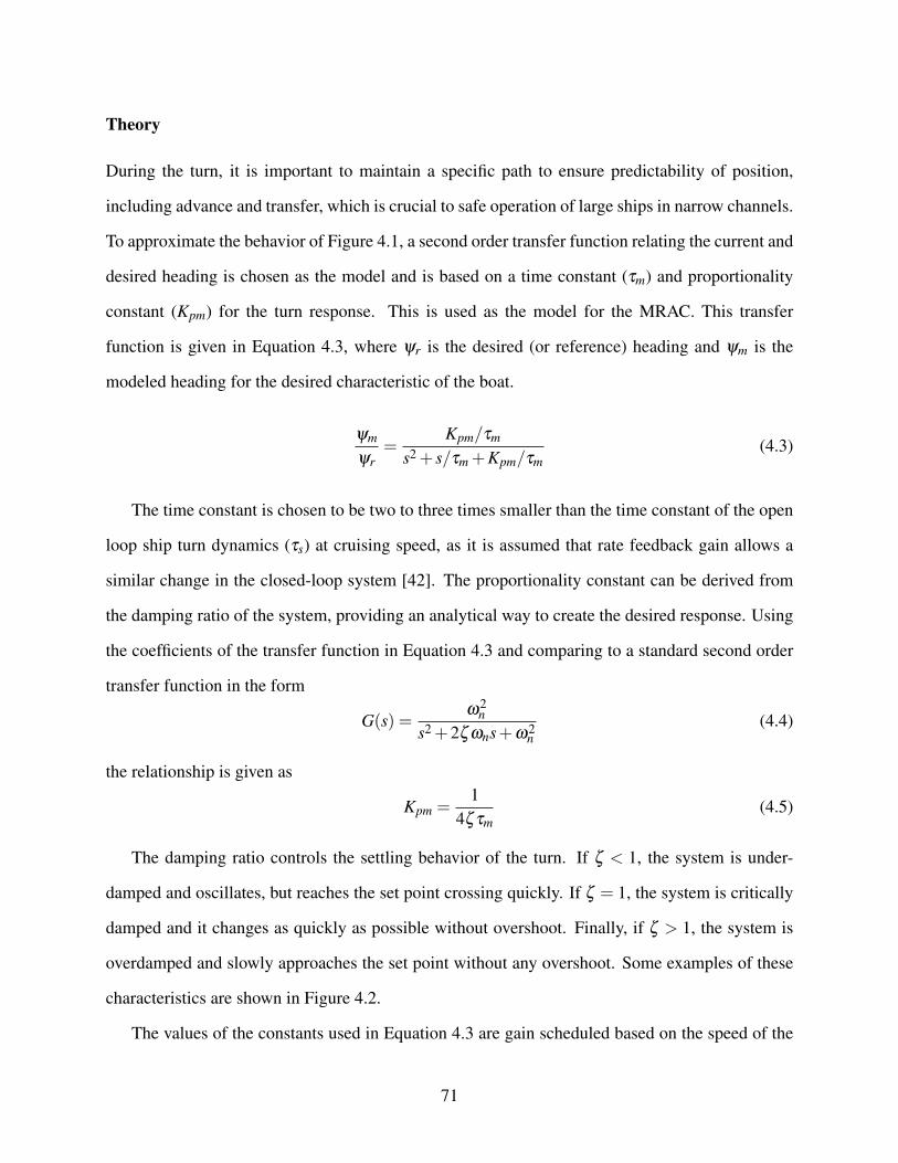
Theory
During the turn, it is important to maintain a specific path to ensure predictability of position,
including advance and transfer, which is crucial to safe operation of large ships in narrow channels.
To approximate the behavior of Figure 4.1, a second order transfer function relating the current and
desired heading is chosen as the model and is based on a time constant (τm) and proportionality
constant (Kpm) for the turn response. This is used as the model for the MRAC. This transfer
function is given in Equation 4.3, where ψr is the desired (or reference) heading and ψm is the
modeled heading for the desired characteristic of the boat.
ψm
ψr=
Kpm/τm
s2 + s/τm +Kpm/τm(4.3)
The time constant is chosen to be two to three times smaller than the time constant of the open
loop ship turn dynamics (τs) at cruising speed, as it is assumed that rate feedback gain allows a
similar change in the closed-loop system [42]. The proportionality constant can be derived from
the damping ratio of the system, providing an analytical way to create the desired response. Using
the coefficients of the transfer function in Equation 4.3 and comparing to a standard second order
transfer function in the form
G(s) =ω2
ns2 +2ζ ωns+ω2
n(4.4)
the relationship is given as
Kpm =1
4ζ τm(4.5)
The damping ratio controls the settling behavior of the turn. If ζ < 1, the system is under-
damped and oscillates, but reaches the set point crossing quickly. If ζ = 1, the system is critically
damped and it changes as quickly as possible without overshoot. Finally, if ζ > 1, the system is
overdamped and slowly approaches the set point without any overshoot. Some examples of these
characteristics are shown in Figure 4.2.
The values of the constants used in Equation 4.3 are gain scheduled based on the speed of the
71
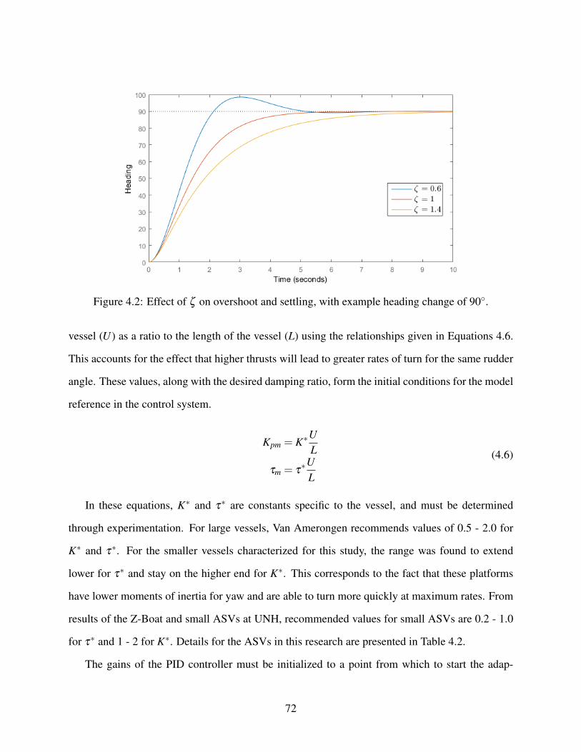
Figure 4.2: Effect of ζ on overshoot and settling, with example heading change of 90.
vessel (U) as a ratio to the length of the vessel (L) using the relationships given in Equations 4.6.
This accounts for the effect that higher thrusts will lead to greater rates of turn for the same rudder
angle. These values, along with the desired damping ratio, form the initial conditions for the model
reference in the control system.
Kpm = K∗UL
τm = τ∗U
L
(4.6)
In these equations, K∗ and τ∗ are constants specific to the vessel, and must be determined
through experimentation. For large vessels, Van Amerongen recommends values of 0.5 - 2.0 for
K∗ and τ∗. For the smaller vessels characterized for this study, the range was found to extend
lower for τ∗ and stay on the higher end for K∗. This corresponds to the fact that these platforms
have lower moments of inertia for yaw and are able to turn more quickly at maximum rates. From
results of the Z-Boat and small ASVs at UNH, recommended values for small ASVs are 0.2 - 1.0
for τ∗ and 1 - 2 for K∗. Details for the ASVs in this research are presented in Table 4.2.
The gains of the PID controller must be initialized to a point from which to start the adap-
72
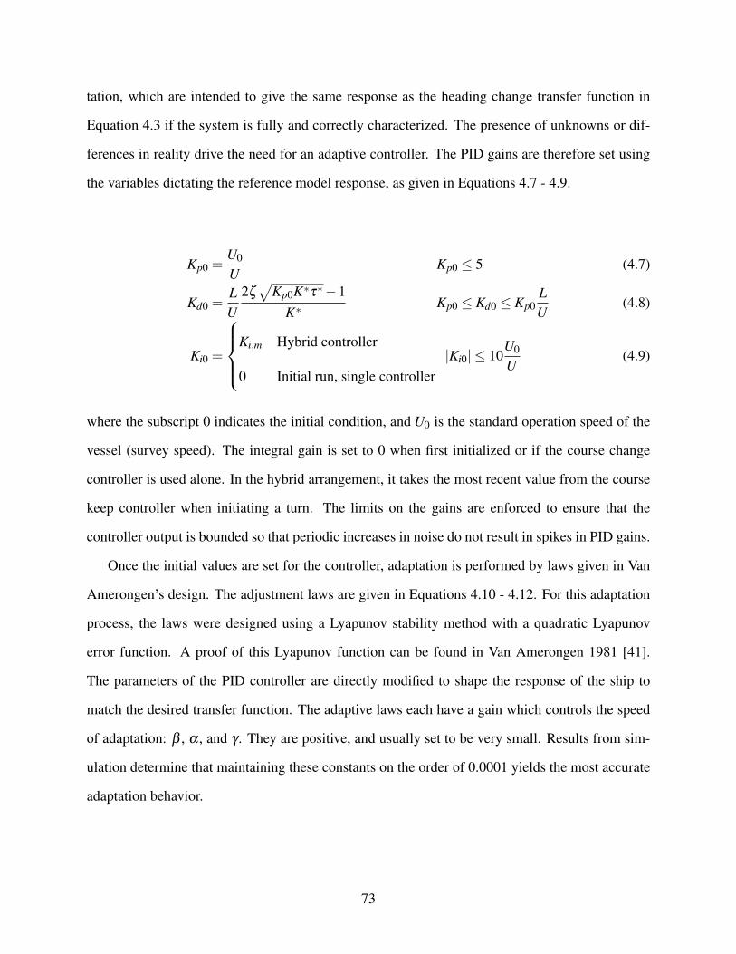
tation, which are intended to give the same response as the heading change transfer function in
Equation 4.3 if the system is fully and correctly characterized. The presence of unknowns or dif-
ferences in reality drive the need for an adaptive controller. The PID gains are therefore set using
the variables dictating the reference model response, as given in Equations 4.7 - 4.9.
Kp0 =U0
UKp0 ≤ 5 (4.7)
Kd0 =LU
2ζ√
Kp0K∗τ∗−1K∗
Kp0 ≤ Kd0 ≤ Kp0LU
(4.8)
Ki0 =
Ki,m Hybrid controller
0 Initial run, single controller|Ki0| ≤ 10
U0
U(4.9)
where the subscript 0 indicates the initial condition, and U0 is the standard operation speed of the
vessel (survey speed). The integral gain is set to 0 when first initialized or if the course change
controller is used alone. In the hybrid arrangement, it takes the most recent value from the course
keep controller when initiating a turn. The limits on the gains are enforced to ensure that the
controller output is bounded so that periodic increases in noise do not result in spikes in PID gains.
Once the initial values are set for the controller, adaptation is performed by laws given in Van
Amerongen’s design. The adjustment laws are given in Equations 4.10 - 4.12. For this adaptation
process, the laws were designed using a Lyapunov stability method with a quadratic Lyapunov
error function. A proof of this Lyapunov function can be found in Van Amerongen 1981 [41].
The parameters of the PID controller are directly modified to shape the response of the ship to
match the desired transfer function. The adaptive laws each have a gain which controls the speed
of adaptation: β , α , and γ . They are positive, and usually set to be very small. Results from sim-
ulation determine that maintaining these constants on the order of 0.0001 yields the most accurate
adaptation behavior.
73
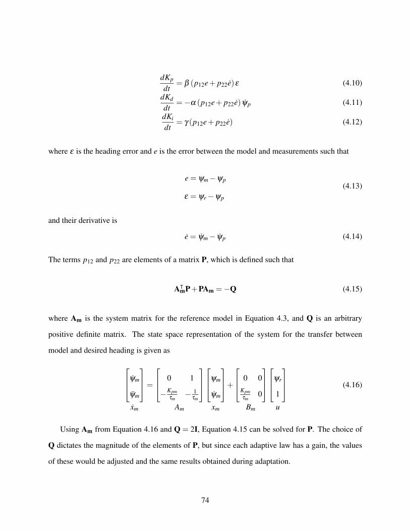
dKp
dt= β (p12e+ p22e)ε (4.10)
dKd
dt=−α (p12e+ p22e) ψp (4.11)
dKi
dt= γ (p12e+ p22e) (4.12)
where ε is the heading error and e is the error between the model and measurements such that
e = ψm−ψp
ε = ψr−ψp
(4.13)
and their derivative is
e = ψm− ψp (4.14)
The terms p12 and p22 are elements of a matrix P, which is defined such that
AᵀmP+PAm =−Q (4.15)
where Am is the system matrix for the reference model in Equation 4.3, and Q is an arbitrary
positive definite matrix. The state space representation of the system for the transfer between
model and desired heading is given as
ψm
ψm
xm
=
0 1
−Kpmτm− 1
τm
Am
ψm
ψm
xm
+
0 0Kpmτm
0
Bm
ψr
1
u
(4.16)
Using Am from Equation 4.16 and Q = 2I, Equation 4.15 can be solved for P. The choice of
Q dictates the magnitude of the elements of P, but since each adaptive law has a gain, the values
of these would be adjusted and the same results obtained during adaptation.
74
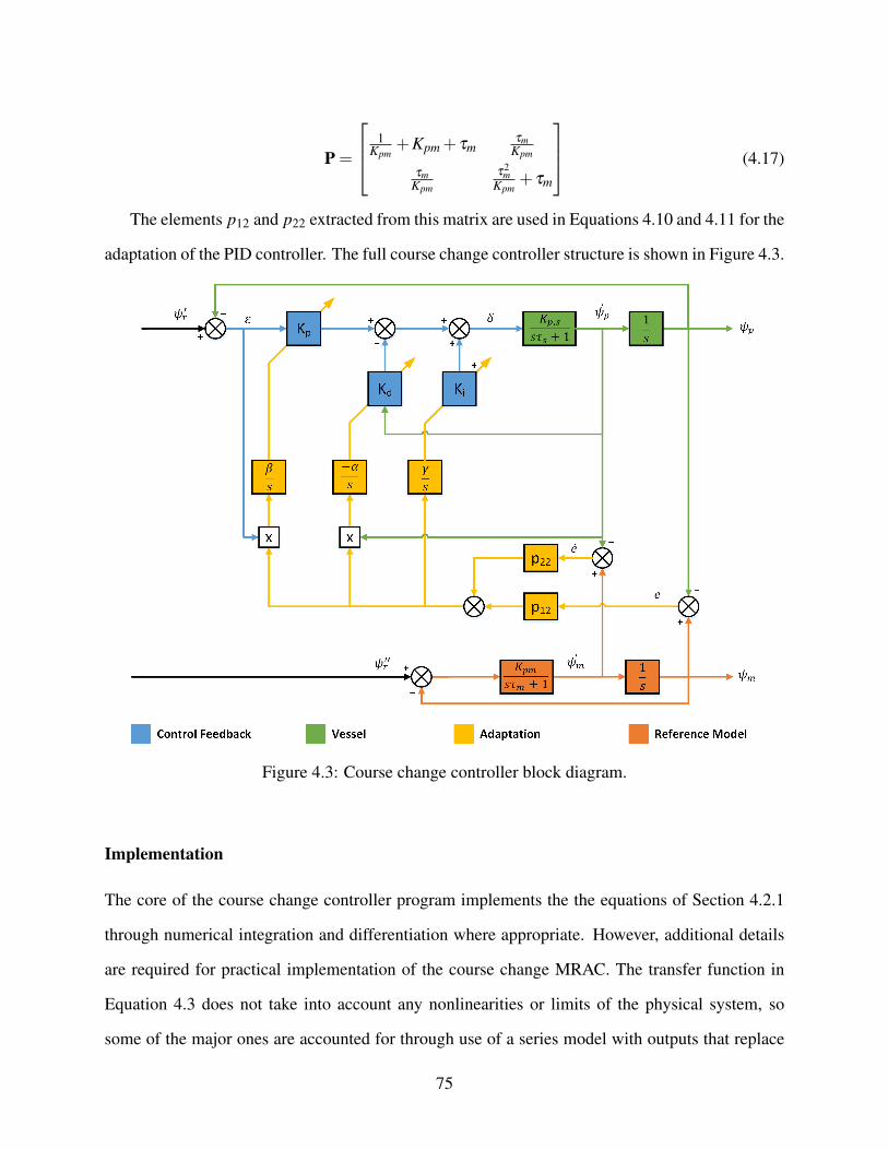
P =
1Kpm
+Kpm + τmτm
Kpm
τmKpm
τ2m
Kpm+ τm
(4.17)
The elements p12 and p22 extracted from this matrix are used in Equations 4.10 and 4.11 for the
adaptation of the PID controller. The full course change controller structure is shown in Figure 4.3.
Figure 4.3: Course change controller block diagram.
Implementation
The core of the course change controller program implements the the equations of Section 4.2.1
through numerical integration and differentiation where appropriate. However, additional details
are required for practical implementation of the course change MRAC. The transfer function in
Equation 4.3 does not take into account any nonlinearities or limits of the physical system, so
some of the major ones are accounted for through use of a series model with outputs that replace
75
the desired heading input ψr in Figure 4.3 for both the PID controller and MRAC model. The
series model enforces absolute limits on rate of turn (ROT) and the angle of the rudder. The series
model is shown in Figure 4.4.
Figure 4.4: Course change controller series model for modification of reference input.
The rate of turn limiter sets a configurable maximum on the rate of turn, which should corre-
spond to what is possible for the vessel, or a lower value if there is a desire to limit the rate of turn.
The output from the ROT limiter (ψ ′r) is used as the input to the PID controller. The ROT limited
signal is then passed through a stage which accounts for the physical limits of rudder movement,
using a ratio ( f ) between an unrestricted desired rudder angle out of the PID controller (δ ) and the
maximum rudder (δmax), to give a continuous response at larger desired rudder angles. The ratio is
capped to a maximum of 1, as there is no need to modify the reference heading when the desired
rudder angle is physically possible. This relationship is summarized in Equation 4.18.
f =δmax
|δ |, f ≤ 1 (4.18)
In addition to this limit on the rate of turn from physically unreasonable rudder values, the desired
rudder output of the control system to MOOS is also limited to ±δmax.
Since the adaptation in this controller is based on a defined transfer curve between the starting
and desired heading for a turn, it provides no benefit to continue the adaptation after the turn, as
the model will always converge the desired heading, while the vessel will be affected by waves
and other disturbances which cause changes in heading. This leads to Kd growing without bound,
76
which can be seen from Equation 4.11. When the model has converged to the desired heading and
the vessel heading approaches the desired heading, e is small and e =−ψp, since the model ROT
is zero. This results in the adaptation of Kp becoming proportional to the square of the measured
ROT ψp, so Kd always increases while driving straight lines such that
dKd
dt≈−α p22 (−ψp) ψp
= ατm
(1+
τm
Kpm
)ψ
2p
(4.19)
To counteract this effect, the effect of the adaptation laws for both Kp and Kd are reduced over
time by multiplying the adaptive gains β and α by a factor that decreases over time such that
α = α0ξ
1+T
β = β0ξ
1+T
(4.20)
where T is the time since the start of the turn, and ξ defines the rate of decrease of adaptation.
For the rapidly turning Z-Boat, values of ξ in the range 0.9 - 1.1 are found to be most suitable.
The speed of reduction can also be controlled during operation by the magnitude of the heading
difference and the expected time for the vessel to complete the turn. In this case, ξ is set during
the initiation of a turn.
The final control parameter determines when the change in desired heading is large enough to
begin the adaptation process. Unlike larger ships under human command, where heading orders
are given fairly infrequently, the IvP Helm in these autonomous vessels continuously updates the
desired heading. A threshold is set at 10 for a heading change indicating a new course where
adaptation is to be initiated, as opposed to using the existing PID gains. A higher setting of up to
45 degrees would be relevant for the operation of small boats in complex scenarios or rough seas.
When the threshold is reached between two subsequent iterations of the course change controller,
the PID control gains are reset according to Equations 4.7, 4.8, and 4.9. This causes the adaptation
process to be triggered when the IvP Helm jumps discretely between decisions, such as during a
77
turn between two lines of a lawnmower pattern or the activation of a new behavior, and standard
PID action is to be maintained for the small adjustments required when following a line or driving
to a waypoint.
4.2.2 Course Keep Controller
When maintaining a constant heading, as would occur on long transit legs, rudder action should be
minimized, since oscillation around a desired heading adds length to the path and decreases speed,
both of which lead to decreased efficiency. Since many of the vessels automated in this study use
battery packs that provide relatively limited operating durations, any increase in path following
efficiency means that more area can be surveyed with the same battery charge. To control the
vessel most accurately, a model for how the vessel responds to changes in rudder is required so
that the response can be tuned.
Theory
A simple linear model first presented by Nomoto [43] is used to represent the rate of turn of the
vessel. The model is defined as
τsψm + ψm = Ks (δ −Ki,m) (4.21)
This model defines the maximum rate of turn as ψmax = Ksδ , which will be approached expo-
nentially with time constant τs. This is easily observed from the equivalent time domain model
ψm (t) = Ksδ(
1− et
τs
)(4.22)
As with the course change controller, the parameters of the model are gain-scheduled with
respect to speed as given in Equation 4.23. This relies on the assumption that greater turn rates
occur at higher speeds (a phenomenon observed in the experimental results with the small ASVs
78
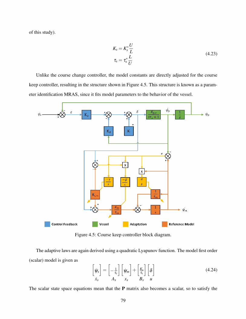
of this study).
Ks = K∗sUL
τs = τ∗s
LU
(4.23)
Unlike the course change controller, the model constants are directly adjusted for the course
keep controller, resulting in the structure shown in Figure 4.5. This structure is known as a param-
eter identification MRAS, since it fits model parameters to the behavior of the vessel.
Figure 4.5: Course keep controller block diagram.
The adaptive laws are again derived using a quadratic Lyapunov function. The model first order
(scalar) model is given as [ψs
]xs
=
[− 1
τs
]As
[ψm
]xs
+
[Ksτs
]Bs
[δ
]u
(4.24)
The scalar state space equations mean that the P matrix also becomes a scalar, so to satisfy the
79
Lyapunov condition that AsP+PAs =−Q, one obtains
P =Qτs
2, Q > 0 (4.25)
All of the constants in Equation 4.25 are positive, so P will always be a positive constant. There-
fore, P can be consolidated into the adaptive gains, resulting in the following adaptive laws:
ddt
(K∗sτ∗s
)=−βe(δ −Ki,s) (4.26)
ddt
(1τ∗s
)= αeψs (4.27)
ddt
(Ki,s) =−γe (4.28)
where
e = ψs− ψp (4.29)
and the adaptive gains are again small (on the order of 0.0001). The initial values for K∗s and
τ∗s are user defined and should be estimated from characterization trials of the vessel. Unless the
rudder is known to be physically offset from the hull axis when set to zero angle, Ki,s is initialized
to 0. While the adaptation system is designed to adjust these time-varying parameters, the initial
operation will not be correct unless the parameters are chosen to be near the known characteristics
of the vessel. Incorrect initialization can lead to instability in the PID control of the vessel, in
which case the adaptation will likely fail.
While the adaptation law in Equation 4.28 provides for direct calculation of the integral gain
for the PID controller, the other laws determine the open loop dynamics of the vessel, which can
then be used to create desired behavior when under control. Using the PID control Equation 4.2
and approximating the vessel response with the model parameters, the controlled rate of turn is
sψp =δKs
sτs +1=
Ks (Kp (ψr−ψp)− sKdψp +Ki)
sτs +1(4.30)
80
where sψp is the rate of turn of the vessel. If Ki is properly compensating for long term effects of
wind, current, or rudder inaccuracy, it will not affect individual turns, so it can be assumed to not
affect the transfer function. Using this and solving for the transfer between desired and controlled
ship heading gives the following transfer function:
ψp
ψr=
KpKs/τs
s2 + s(1+KdKs)/τs +KpKs/τs(4.31)
This determines the response of the ship when it is given a new heading input, which can be
modeled as a step input since it changes instantaneously. Through comparison to the standard
format second order transfer function given in Equation 4.4, the parameters can be determined
with respect to natural frequency and damping ratio. Since the natural frequency and damping
ratio dictate the shape of the response to inputs, these can be used to calculate values for the PID
control gains, which will cause the vessel to respond accordingly. Solving for the PID gains gives
Kp =ω2
n τs
KsKp ≤ 2.5 (4.32)
Kd =2ζ√
KpKsτs−1Ks
0≤ Kd ≤ Kp0LU
(4.33)
Ki = Ki,s (4.34)
Note that Equation 4.33 is the same as Equation 4.8, since they both dictate responses based on
the characteristics of the system. The physical interpretation of the damping ratio ζ is straight-
forward and has the same effects described in Section 4.2.1. As long as the other parameters are
determined, it is independent of the vessel itself and only determines the overshoot characteristic
of the response. The natural frequency is related to how quickly the vessel can yaw but is specific
to the vessel and difficult to measure directly. It dictates the speed of response, with higher ωn
corresponding to a quicker turn. However, just as with the τm of the course change controller, it is
possible to specify a value which is too fast to be physically achieved by the vessel. As such, some
experimentation is required during implementation of the controller on a new vessel. Van Ameron-
81
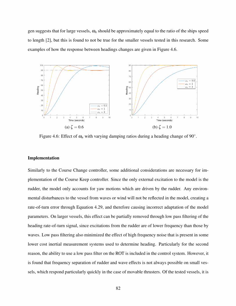
gen suggests that for large vessels, ωn should be approximately equal to the ratio of the ships speed
to length [2], but this is found to not be true for the smaller vessels tested in this research. Some
examples of how the response between headings changes are given in Figure 4.6.
(a) ζ = 0.6 (b) ζ = 1.0
Figure 4.6: Effect of ωn with varying damping ratios during a heading change of 90.
Implementation
Similarly to the Course Change controller, some additional considerations are necessary for im-
plementation of the Course Keep controller. Since the only external excitation to the model is the
rudder, the model only accounts for yaw motions which are driven by the rudder. Any environ-
mental disturbances to the vessel from waves or wind will not be reflected in the model, creating a
rate-of-turn error through Equation 4.29, and therefore causing incorrect adaptation of the model
parameters. On larger vessels, this effect can be partially removed through low pass filtering of the
heading rate-of-turn signal, since excitations from the rudder are of lower frequency than those by
waves. Low pass filtering also minimized the effect of high frequency noise that is present in some
lower cost inertial measurement systems used to determine heading. Particularly for the second
reason, the ability to use a low pass filter on the ROT is included in the control system. However, it
is found that frequency separation of rudder and wave effects is not always possible on small ves-
sels, which respond particularly quickly in the case of movable thrusters. Of the tested vessels, it is
82
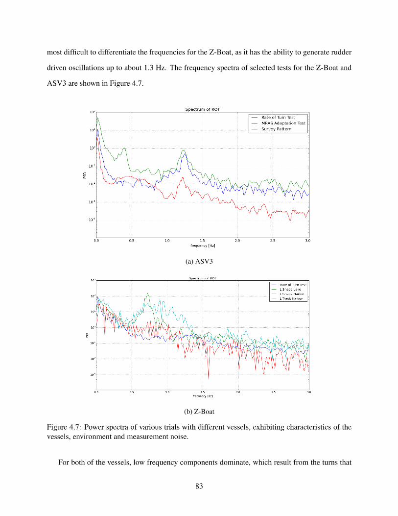
most difficult to differentiate the frequencies for the Z-Boat, as it has the ability to generate rudder
driven oscillations up to about 1.3 Hz. The frequency spectra of selected tests for the Z-Boat and
ASV3 are shown in Figure 4.7.
(a) ASV3
(b) Z-Boat
Figure 4.7: Power spectra of various trials with different vessels, exhibiting characteristics of thevessels, environment and measurement noise.
For both of the vessels, low frequency components dominate, which result from the turns that
83
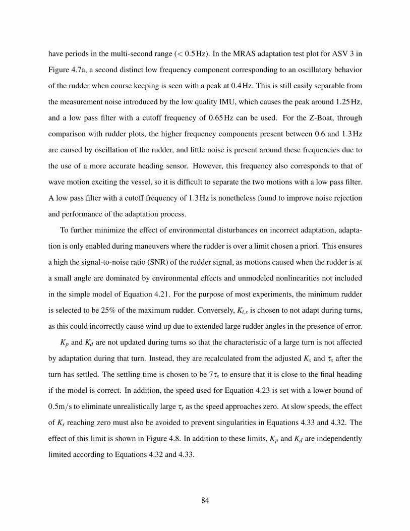
have periods in the multi-second range (< 0.5Hz). In the MRAS adaptation test plot for ASV 3 in
Figure 4.7a, a second distinct low frequency component corresponding to an oscillatory behavior
of the rudder when course keeping is seen with a peak at 0.4Hz. This is still easily separable from
the measurement noise introduced by the low quality IMU, which causes the peak around 1.25Hz,
and a low pass filter with a cutoff frequency of 0.65Hz can be used. For the Z-Boat, through
comparison with rudder plots, the higher frequency components present between 0.6 and 1.3Hz
are caused by oscillation of the rudder, and little noise is present around these frequencies due to
the use of a more accurate heading sensor. However, this frequency also corresponds to that of
wave motion exciting the vessel, so it is difficult to separate the two motions with a low pass filter.
A low pass filter with a cutoff frequency of 1.3Hz is nonetheless found to improve noise rejection
and performance of the adaptation process.
To further minimize the effect of environmental disturbances on incorrect adaptation, adapta-
tion is only enabled during maneuvers where the rudder is over a limit chosen a priori. This ensures
a high the signal-to-noise ratio (SNR) of the rudder signal, as motions caused when the rudder is at
a small angle are dominated by environmental effects and unmodeled nonlinearities not included
in the simple model of Equation 4.21. For the purpose of most experiments, the minimum rudder
is selected to be 25% of the maximum rudder. Conversely, Ki,s is chosen to not adapt during turns,
as this could incorrectly cause wind up due to extended large rudder angles in the presence of error.
Kp and Kd are not updated during turns so that the characteristic of a large turn is not affected
by adaptation during that turn. Instead, they are recalculated from the adjusted Ks and τs after the
turn has settled. The settling time is chosen to be 7τs to ensure that it is close to the final heading
if the model is correct. In addition, the speed used for Equation 4.23 is set with a lower bound of
0.5m/s to eliminate unrealistically large τs as the speed approaches zero. At slow speeds, the effect
of Ks reaching zero must also be avoided to prevent singularities in Equations 4.33 and 4.32. The
effect of this limit is shown in Figure 4.8. In addition to these limits, Kp and Kd are independently
limited according to Equations 4.32 and 4.33.
84
Figure 4.8: Relationship between τs and Ks and speed of the vessel, showing minimum limit ofU = 0.5m/s. For this example L = 2.5, K∗s = 1.56, τ∗s = 0.8.
4.2.3 Hybrid Heading Control System
In addition to being able to run each control system separately, the course keep and course change
control systems may be combined into a hybrid system. Under this mode of operation, the course
change controller is used to enact large turns, which are defined as course changes of more than
20. While conducting the turn, the course keep controller is run in parallel, but the output is
ignored so that it can adapt while the SNR is high. The course keep controller is allowed to steady
the heading (with decreasing adaptive gains) until the same settling time as defined above (7τs) is
reached. The course keep controller is then selected for output, as the course change controller
would otherwise result in a static PID controller as the adaptive gains approach zero.
4.3 Speed Control
The MRAC combined with PID approach works well for heading control where continual response
to conditions with respect to the desired direction is necessary for reliable operation of a vessel.
In many circumstances, it is not as critical to maintain an exact speed, and doing so can lead to
detrimental performance in other metrics such as power consumption. For example, while sur-
veying an approximate speed may be maintained while the effects of waves and currents modify
85
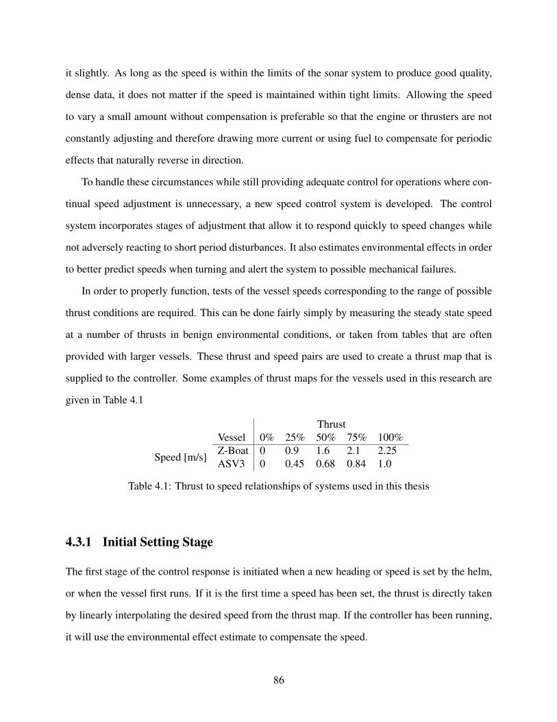
it slightly. As long as the speed is within the limits of the sonar system to produce good quality,
dense data, it does not matter if the speed is maintained within tight limits. Allowing the speed
to vary a small amount without compensation is preferable so that the engine or thrusters are not
constantly adjusting and therefore drawing more current or using fuel to compensate for periodic
effects that naturally reverse in direction.
To handle these circumstances while still providing adequate control for operations where con-
tinual speed adjustment is unnecessary, a new speed control system is developed. The control
system incorporates stages of adjustment that allow it to respond quickly to speed changes while
not adversely reacting to short period disturbances. It also estimates environmental effects in order
to better predict speeds when turning and alert the system to possible mechanical failures.
In order to properly function, tests of the vessel speeds corresponding to the range of possible
thrust conditions are required. This can be done fairly simply by measuring the steady state speed
at a number of thrusts in benign environmental conditions, or taken from tables that are often
provided with larger vessels. These thrust and speed pairs are used to create a thrust map that is
supplied to the controller. Some examples of thrust maps for the vessels used in this research are
given in Table 4.1
ThrustVessel 0% 25% 50% 75% 100%
Speed [m/s]Z-Boat 0 0.9 1.6 2.1 2.25ASV3 0 0.45 0.68 0.84 1.0
Table 4.1: Thrust to speed relationships of systems used in this thesis
4.3.1 Initial Setting Stage
The first stage of the control response is initiated when a new heading or speed is set by the helm,
or when the vessel first runs. If it is the first time a speed has been set, the thrust is directly taken
by linearly interpolating the desired speed from the thrust map. If the controller has been running,
it will use the environmental effect estimate to compensate the speed.
86
The environmental effects are estimated from two different methods depending on available
data. If the vessel has previously traveled within a threshold of the desired heading (10 by default),
the average offset from the expected speed based on the thrust map is used. This accounts for
effects that depend on the relative heading between the vessel and the disturbance, such as wind or
waves.
If the vessel does not have any history of previous runs near the desired heading but has been
operating on other headings, an estimate is made of the average effect of disturbances. This can
again be done with two methods. If the positioning system provides a course over ground mea-
surement in addition to heading, the average vector difference between the expected speed (from
the thrust map or speed through the water measurement if available) at the heading, and speed over
ground on the course over ground is used to find an average disturbance vector. The effect of this
at the new heading is used to compensate the initial speed setting.
A final method is used if no course over ground signal is available. During operation, the
speed difference from the thrust map value at the current heading is averaged into angular sector
bins distributed at equal intervals around the compass, by default every 10. The direction and
magnitude of the disturbance are taken to be the heading bin with the maximum difference from
expected speeds. In practice, this tends to give similar results, as the vector is oriented in the
direction of greatest effect.
4.3.2 Coarse Adjustment
After the initial setting, the control system waits until the speed has reaches steady state to make
any more adjustments. This is in contrast to a PID controller that continually adjusts based on the
differences between desired and actual speeds. The first adjustment is based on an average speed
over a short period of time selected as an averaging period (Tavg). For most small vessels a value
of approximately Tavg = 3s performs well. A longer period is applicable to larger vessels since
settling times are longer and they may have a throttle that takes time to adjust the actual engine
output.
87
The time for the first adjustment is determined by when the average slope of the speed over a
length of time is below a threshold. The time range for the slope is determined from a setting for
how quickly an operator wishes the vessel to respond, and is set as 2Tavg by default. This threshold
can be configured to account for sea state, as movement of the vessel in waves causes the speed
to fluctuate even when it has been fully accelerated by the thrusters. For the Z-Boat, values of
0.05 m/s2 for calm seas and 0.10 m/s2 for 1-2 ft seas performed well.
In addition to ensuring the speed has reached a steady value, the controller does not make an
adjustment until the heading is steady after a turn, which is defined as being within a configurable
threshold for Tavg. A threshold of 10 works well for small vessels, and this may be set smaller for
larger vessels which are less affected by environmental disturbances.
The amount of adjustment is based on the difference between the average speed for the last Tavg
seconds and the desired speed. If the difference is within a configurable tolerance (0.1 m/s used
for testing), no adjustment is made. Otherwise, this difference is added to the initial speed setting
and fed back into the thrust map to determine an offset thrust.
4.3.3 Fine Adjustments
Subsequent adjustments are spaced out by at least a time specified for the long adjustment period
(Tlong). Tlong defaults to 5Tavg, or can be set longer if frequent adjustments are not desired and
a higher speed tolerance is acceptable. For further speed changes to take place, the heading and
speed must also be steady as defined in Section 4.3.2.
Since the adjustments at this stage are intended to be small, it is assumed the vessel will settle
within Tavg, so the average speed from the last Tlong−Tavg seconds is used for the difference from
desired speed. Again, if this is within the set tolerance, no adjustment is made, otherwise the speed
offset is again put into the thrust map to determine a new thrust. The thrust map is still used for
these later adjustments because it is assumed that even if the exact value of the thrust to speed
mapping is not correct (hence the need for adjustment), the slope of the measured relationship is
close to the actual response of the vessel, so small changes will approximate the same change in
88
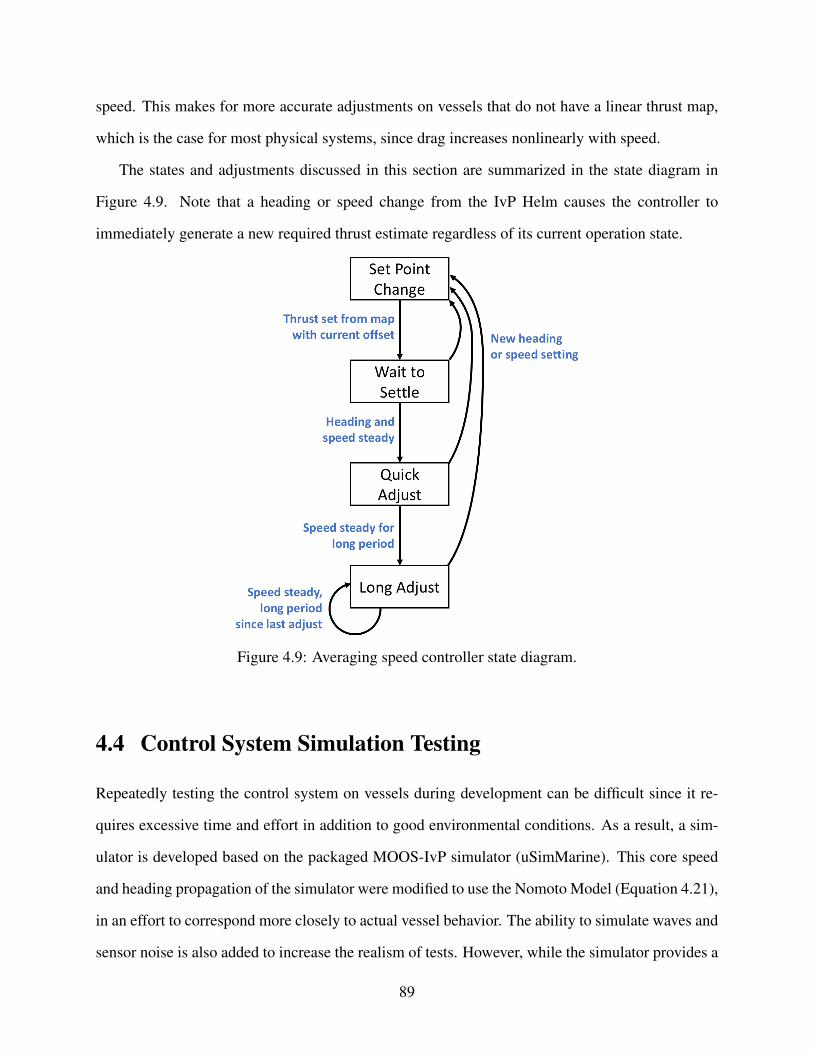
speed. This makes for more accurate adjustments on vessels that do not have a linear thrust map,
which is the case for most physical systems, since drag increases nonlinearly with speed.
The states and adjustments discussed in this section are summarized in the state diagram in
Figure 4.9. Note that a heading or speed change from the IvP Helm causes the controller to
immediately generate a new required thrust estimate regardless of its current operation state.
Figure 4.9: Averaging speed controller state diagram.
4.4 Control System Simulation Testing
Repeatedly testing the control system on vessels during development can be difficult since it re-
quires excessive time and effort in addition to good environmental conditions. As a result, a sim-
ulator is developed based on the packaged MOOS-IvP simulator (uSimMarine). This core speed
and heading propagation of the simulator were modified to use the Nomoto Model (Equation 4.21),
in an effort to correspond more closely to actual vessel behavior. The ability to simulate waves and
sensor noise is also added to increase the realism of tests. However, while the simulator provides a
89
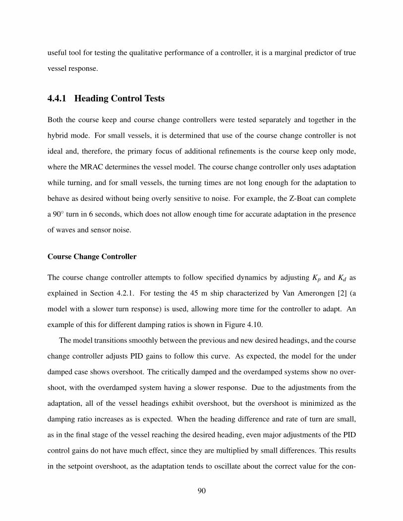
useful tool for testing the qualitative performance of a controller, it is a marginal predictor of true
vessel response.
4.4.1 Heading Control Tests
Both the course keep and course change controllers were tested separately and together in the
hybrid mode. For small vessels, it is determined that use of the course change controller is not
ideal and, therefore, the primary focus of additional refinements is the course keep only mode,
where the MRAC determines the vessel model. The course change controller only uses adaptation
while turning, and for small vessels, the turning times are not long enough for the adaptation to
behave as desired without being overly sensitive to noise. For example, the Z-Boat can complete
a 90 turn in 6 seconds, which does not allow enough time for accurate adaptation in the presence
of waves and sensor noise.
Course Change Controller
The course change controller attempts to follow specified dynamics by adjusting Kp and Kd as
explained in Section 4.2.1. For testing the 45 m ship characterized by Van Amerongen [2] (a
model with a slower turn response) is used, allowing more time for the controller to adapt. An
example of this for different damping ratios is shown in Figure 4.10.
The model transitions smoothly between the previous and new desired headings, and the course
change controller adjusts PID gains to follow this curve. As expected, the model for the under
damped case shows overshoot. The critically damped and the overdamped systems show no over-
shoot, with the overdamped system having a slower response. Due to the adjustments from the
adaptation, all of the vessel headings exhibit overshoot, but the overshoot is minimized as the
damping ratio increases as is expected. When the heading difference and rate of turn are small,
as in the final stage of the vessel reaching the desired heading, even major adjustments of the PID
control gains do not have much effect, since they are multiplied by small differences. This results
in the setpoint overshoot, as the adaptation tends to oscillate about the correct value for the con-
90
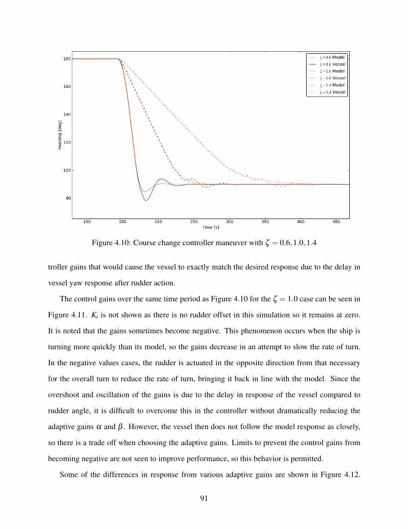
Figure 4.10: Course change controller maneuver with ζ = 0.6,1.0,1.4
troller gains that would cause the vessel to exactly match the desired response due to the delay in
vessel yaw response after rudder action.
The control gains over the same time period as Figure 4.10 for the ζ = 1.0 case can be seen in
Figure 4.11. Ki is not shown as there is no rudder offset in this simulation so it remains at zero.
It is noted that the gains sometimes become negative. This phenomenon occurs when the ship is
turning more quickly than its model, so the gains decrease in an attempt to slow the rate of turn.
In the negative values cases, the rudder is actuated in the opposite direction from that necessary
for the overall turn to reduce the rate of turn, bringing it back in line with the model. Since the
overshoot and oscillation of the gains is due to the delay in response of the vessel compared to
rudder angle, it is difficult to overcome this in the controller without dramatically reducing the
adaptive gains α and β . However, the vessel then does not follow the model response as closely,
so there is a trade off when choosing the adaptive gains. Limits to prevent the control gains from
becoming negative are not seen to improve performance, so this behavior is permitted.
Some of the differences in response from various adaptive gains are shown in Figure 4.12.
91
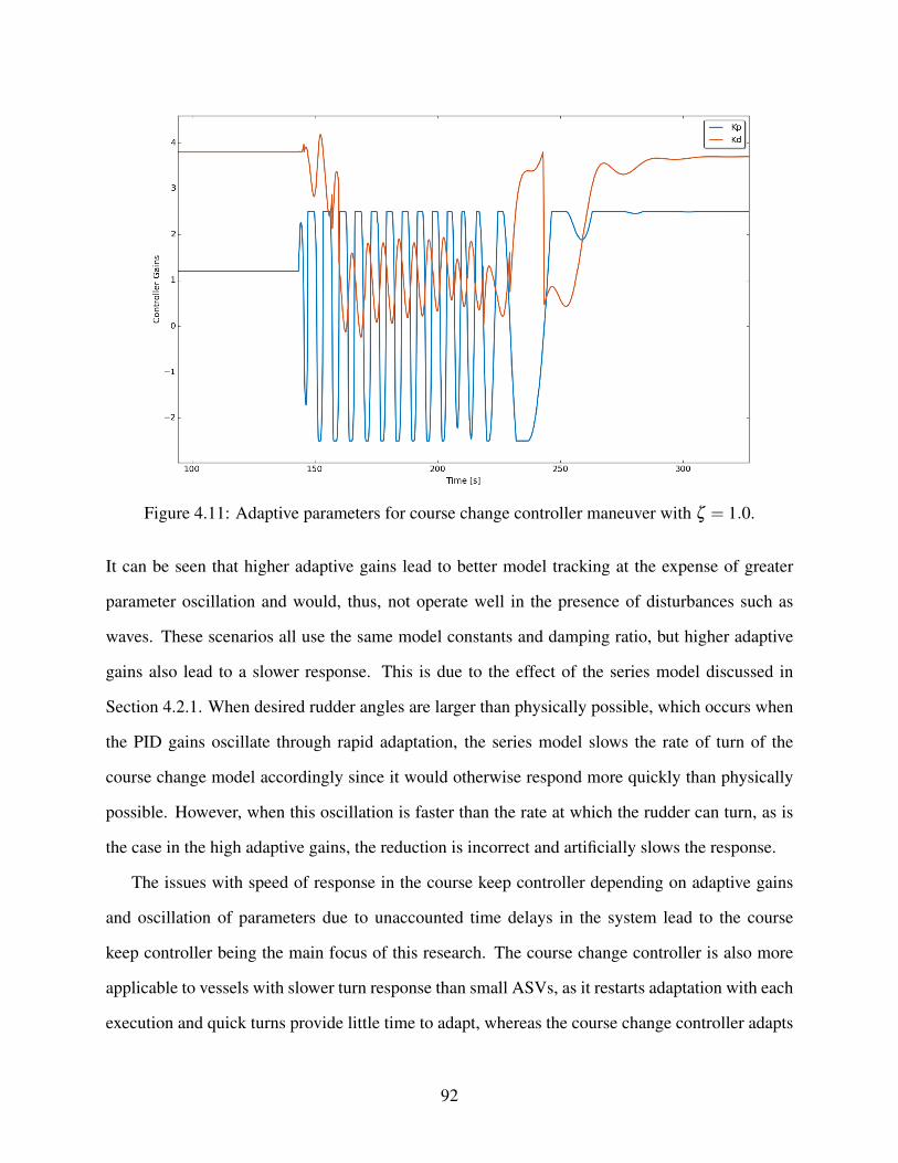
Figure 4.11: Adaptive parameters for course change controller maneuver with ζ = 1.0.
It can be seen that higher adaptive gains lead to better model tracking at the expense of greater
parameter oscillation and would, thus, not operate well in the presence of disturbances such as
waves. These scenarios all use the same model constants and damping ratio, but higher adaptive
gains also lead to a slower response. This is due to the effect of the series model discussed in
Section 4.2.1. When desired rudder angles are larger than physically possible, which occurs when
the PID gains oscillate through rapid adaptation, the series model slows the rate of turn of the
course change model accordingly since it would otherwise respond more quickly than physically
possible. However, when this oscillation is faster than the rate at which the rudder can turn, as is
the case in the high adaptive gains, the reduction is incorrect and artificially slows the response.
The issues with speed of response in the course keep controller depending on adaptive gains
and oscillation of parameters due to unaccounted time delays in the system lead to the course
keep controller being the main focus of this research. The course change controller is also more
applicable to vessels with slower turn response than small ASVs, as it restarts adaptation with each
execution and quick turns provide little time to adapt, whereas the course change controller adapts
92
Figure 4.12: Effect of different magnitudes of adaptive gains
progressively over time.
Course Keep Controller
The course keep controller provides better overall control of small vessels since it characterizes
the response and is able to use this to create both turns and straight areas that fit desired response
characteristics. Many characteristics of the response can be tested under different conditions with
the simulator and some examples are given here.
The adaptation behavior of the controller can be tested by starting it with known incorrect
values of K∗ and τ∗. Since the controller only adapts during turns and other large rudder angle
maneuvers, the simulated vessel is instructed to run in an L shaped pattern with periodic turns
greater than 80 degrees. An of adaptation is shown in Figure 4.13.
As expected from Equation 4.33, the final values for Kd when the controller has adapted are
different for the different values of ζ . However, Kp does not have any dependence on ζ , so all
of the parameters end near the same value. The spikes to large values of Kp and Kd near the
beginning of the plot are caused by the low speed while the vessel is first accelerating and exceeds
93
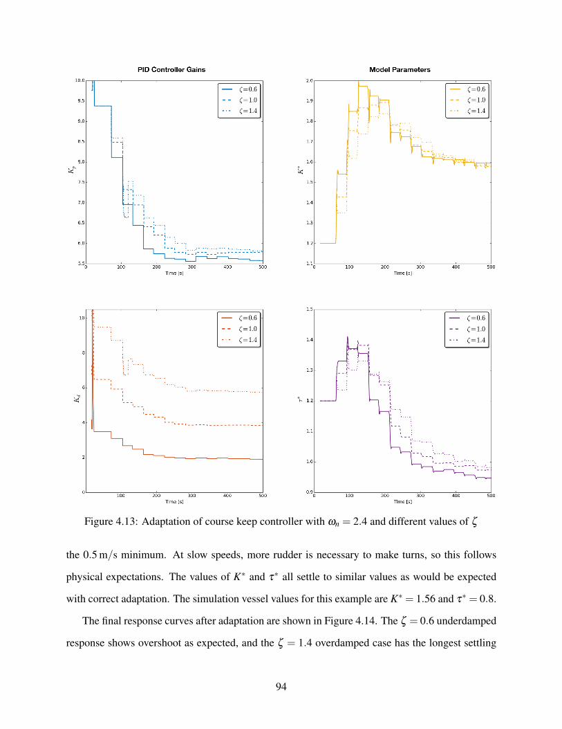
Figure 4.13: Adaptation of course keep controller with ωn = 2.4 and different values of ζ
the 0.5 m/s minimum. At slow speeds, more rudder is necessary to make turns, so this follows
physical expectations. The values of K∗ and τ∗ all settle to similar values as would be expected
with correct adaptation. The simulation vessel values for this example are K∗ = 1.56 and τ∗ = 0.8.
The final response curves after adaptation are shown in Figure 4.14. The ζ = 0.6 underdamped
response shows overshoot as expected, and the ζ = 1.4 overdamped case has the longest settling
94
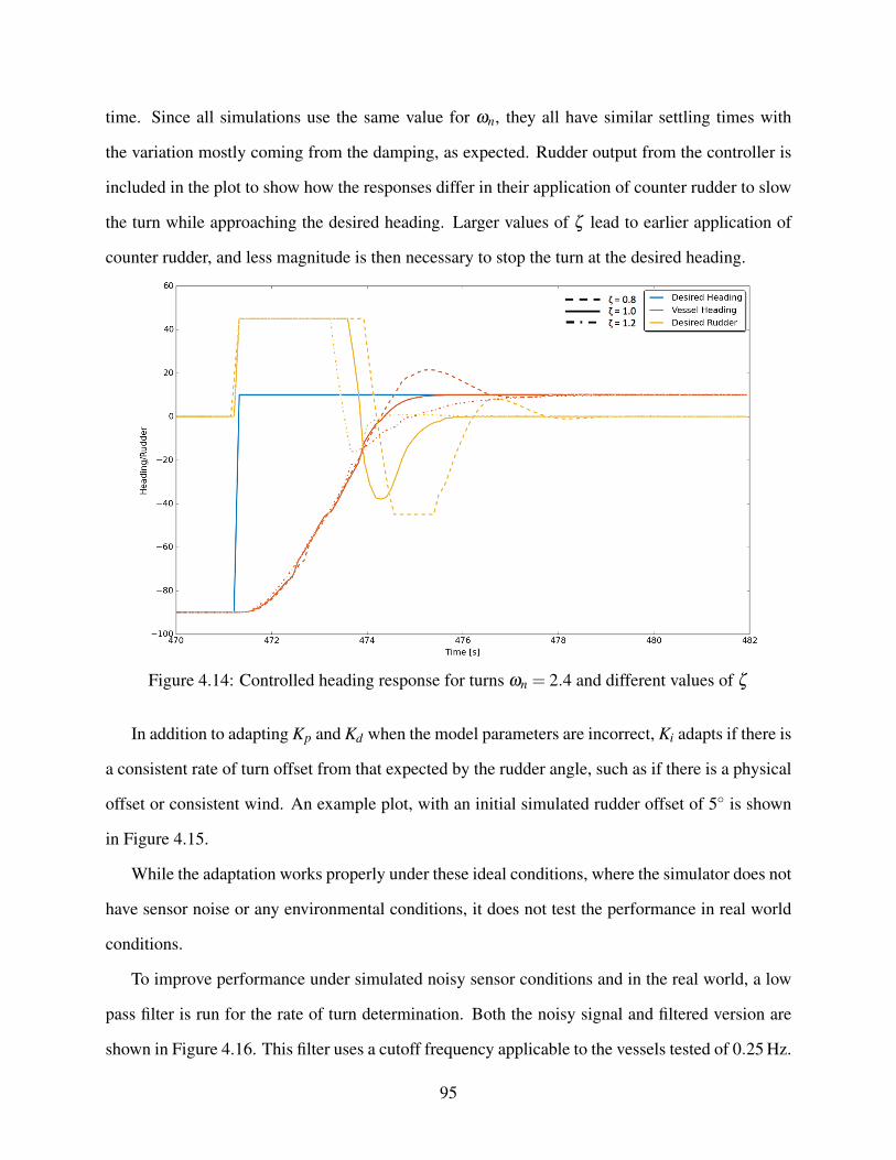
time. Since all simulations use the same value for ωn, they all have similar settling times with
the variation mostly coming from the damping, as expected. Rudder output from the controller is
included in the plot to show how the responses differ in their application of counter rudder to slow
the turn while approaching the desired heading. Larger values of ζ lead to earlier application of
counter rudder, and less magnitude is then necessary to stop the turn at the desired heading.
Figure 4.14: Controlled heading response for turns ωn = 2.4 and different values of ζ
In addition to adapting Kp and Kd when the model parameters are incorrect, Ki adapts if there is
a consistent rate of turn offset from that expected by the rudder angle, such as if there is a physical
offset or consistent wind. An example plot, with an initial simulated rudder offset of 5 is shown
in Figure 4.15.
While the adaptation works properly under these ideal conditions, where the simulator does not
have sensor noise or any environmental conditions, it does not test the performance in real world
conditions.
To improve performance under simulated noisy sensor conditions and in the real world, a low
pass filter is run for the rate of turn determination. Both the noisy signal and filtered version are
shown in Figure 4.16. This filter uses a cutoff frequency applicable to the vessels tested of 0.25 Hz.
95
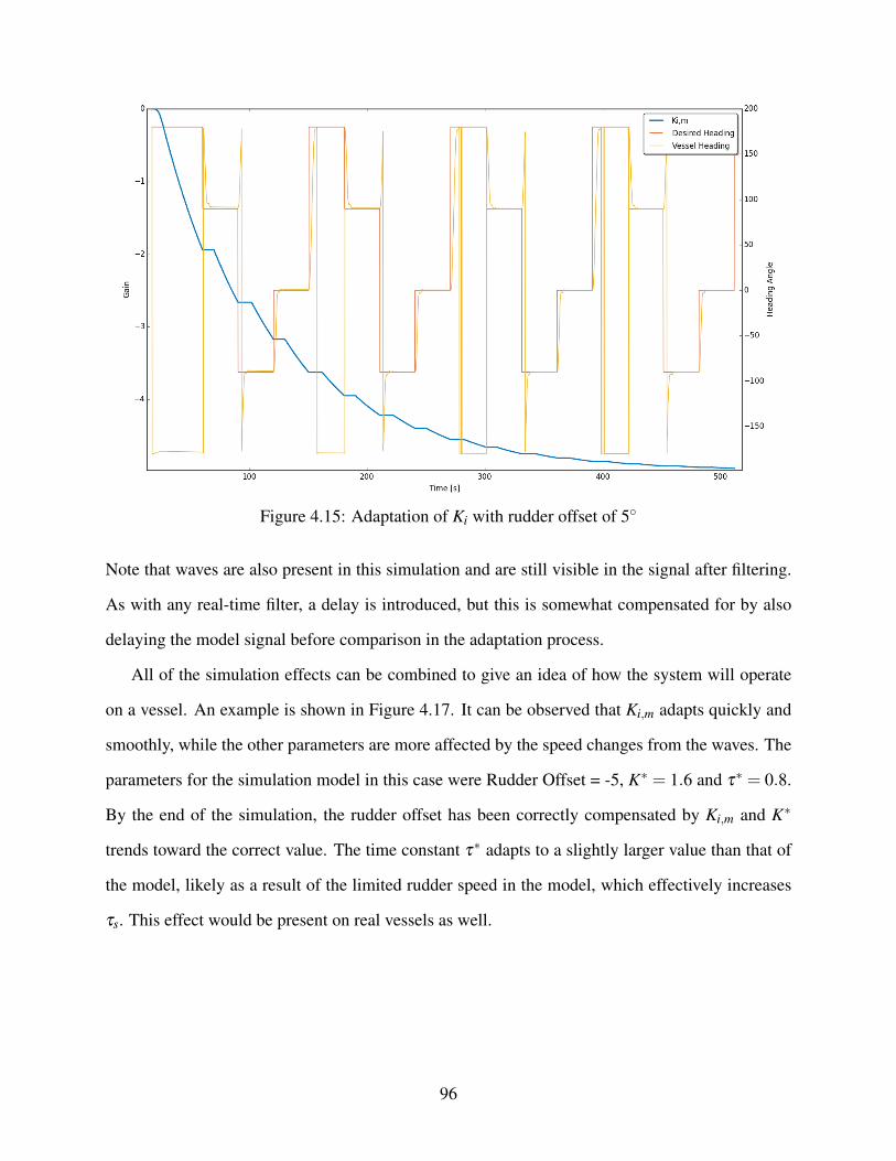
Figure 4.15: Adaptation of Ki with rudder offset of 5
Note that waves are also present in this simulation and are still visible in the signal after filtering.
As with any real-time filter, a delay is introduced, but this is somewhat compensated for by also
delaying the model signal before comparison in the adaptation process.
All of the simulation effects can be combined to give an idea of how the system will operate
on a vessel. An example is shown in Figure 4.17. It can be observed that Ki,m adapts quickly and
smoothly, while the other parameters are more affected by the speed changes from the waves. The
parameters for the simulation model in this case were Rudder Offset = -5, K∗ = 1.6 and τ∗ = 0.8.
By the end of the simulation, the rudder offset has been correctly compensated by Ki,m and K∗
trends toward the correct value. The time constant τ∗ adapts to a slightly larger value than that of
the model, likely as a result of the limited rudder speed in the model, which effectively increases
τs. This effect would be present on real vessels as well.
96
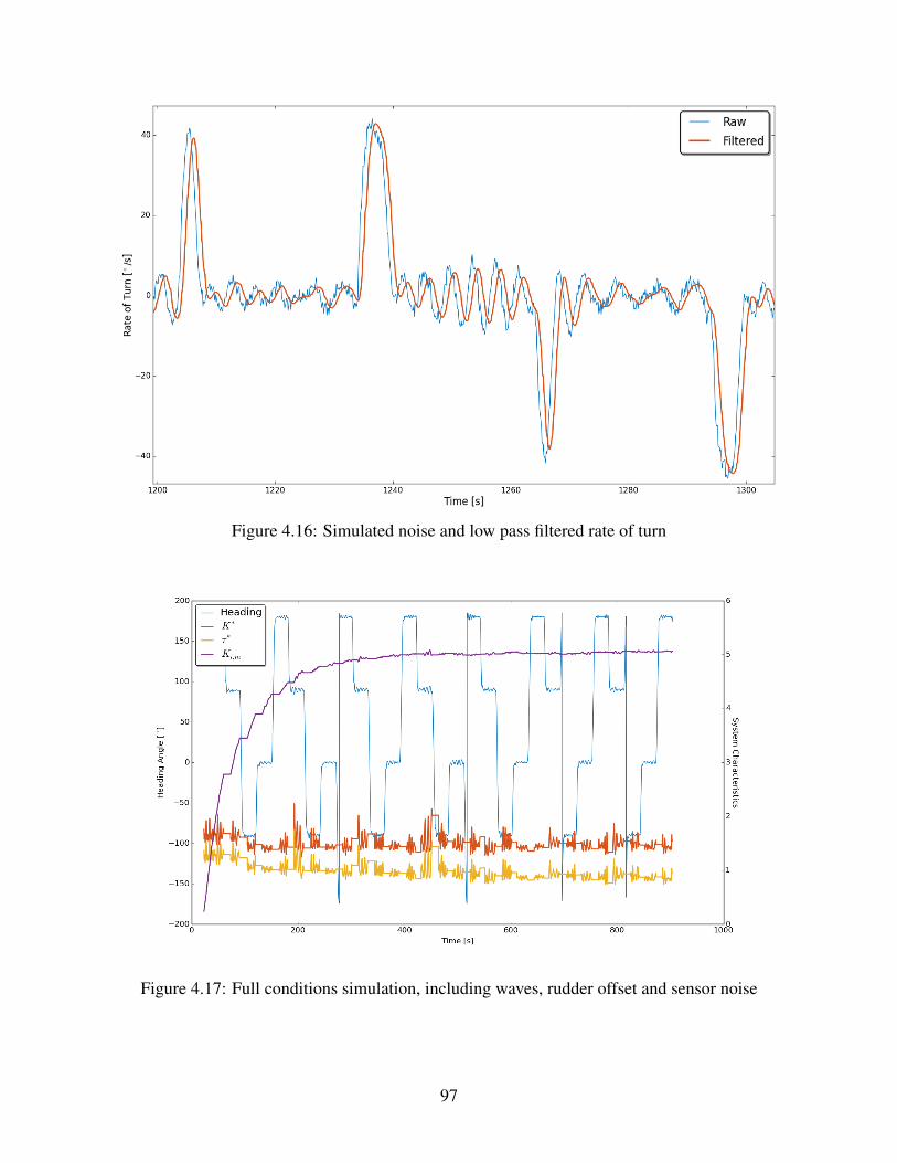
Figure 4.16: Simulated noise and low pass filtered rate of turn
Figure 4.17: Full conditions simulation, including waves, rudder offset and sensor noise
97

4.4.2 Speed Control Tests
The speed control system is also tested using the same simulation architecture. When compared
to a standard PID controller, it creates many fewer setpoint adjustments and also does not react
to transient effects. A comparison with a PID controller is shown in Figure 4.18. In this sce-
nario, speed changes result from turns and cause the PID controller to respond, but the survey
controller anticipates the speed after the turn and does not run faster than necessary through the
turn. This eliminates the spikes in thrust seen in the PID controller example, increasing battery life.
In addition, the controller developed in this research does not respond unnecessarily to temporary
fluctuations due to waves, while still maintaining a speed within 0.2 m/s2
98
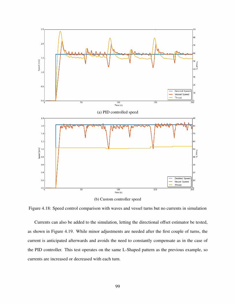
(a) PID controlled speed
(b) Custom controller speed
Figure 4.18: Speed control comparison with waves and vessel turns but no currents in simulation
Currents can also be added to the simulation, letting the directional offset estimator be tested,
as shown in Figure 4.19. While minor adjustments are needed after the first couple of turns, the
current is anticipated afterwards and avoids the need to constantly compensate as in the case of
the PID controller. This test operates on the same L-Shaped pattern as the previous example, so
currents are increased or decreased with each turn.
99

(a) PID controlled speed
(b) Custom controller speed
Figure 4.19: Speed control comparison with waves, currents, and vessel turns in simulation
4.5 Field Tests
Due to limited ASV availability and hardware issues with vessels at UNH, only limited field tests
were performed. A Z-Boat from NOAA Ship Thomas Jefferson was available for some initial con-
trol system tests and operations on UNH ASV3 were attempted but unsuccessful due to hardware
failures in the propulsion system and rough environmental conditions. The Z-Boats transitioned to
100
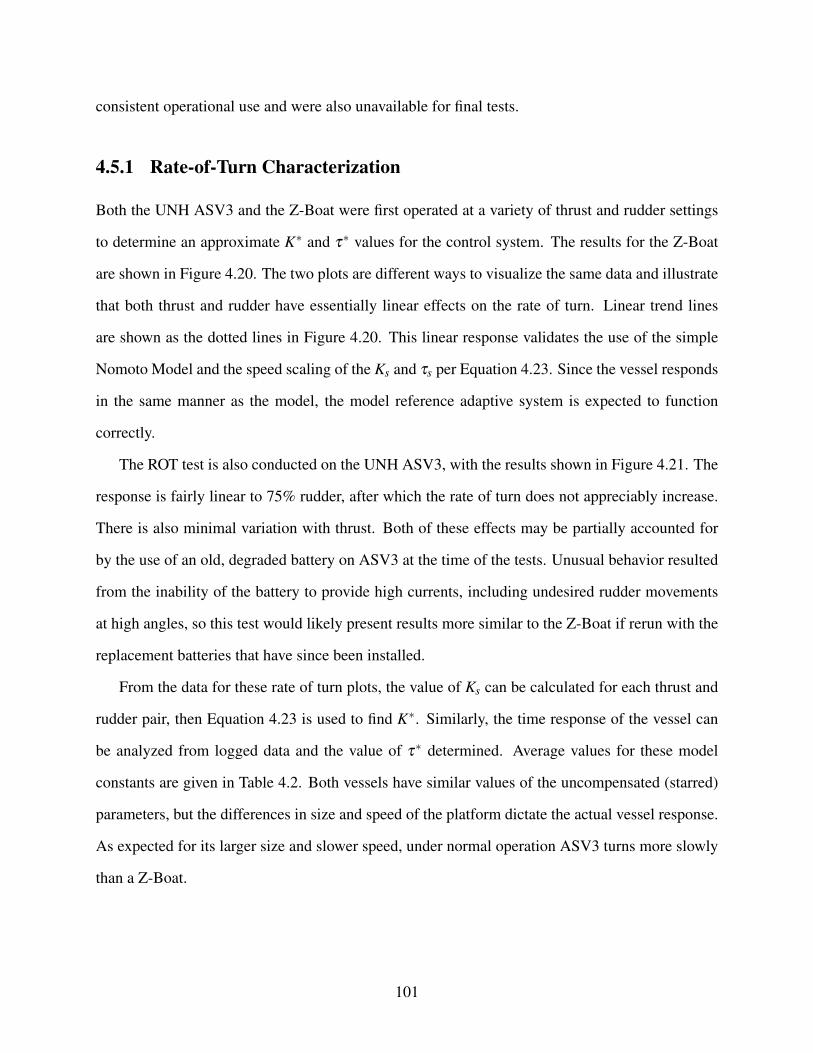
consistent operational use and were also unavailable for final tests.
4.5.1 Rate-of-Turn Characterization
Both the UNH ASV3 and the Z-Boat were first operated at a variety of thrust and rudder settings
to determine an approximate K∗ and τ∗ values for the control system. The results for the Z-Boat
are shown in Figure 4.20. The two plots are different ways to visualize the same data and illustrate
that both thrust and rudder have essentially linear effects on the rate of turn. Linear trend lines
are shown as the dotted lines in Figure 4.20. This linear response validates the use of the simple
Nomoto Model and the speed scaling of the Ks and τs per Equation 4.23. Since the vessel responds
in the same manner as the model, the model reference adaptive system is expected to function
correctly.
The ROT test is also conducted on the UNH ASV3, with the results shown in Figure 4.21. The
response is fairly linear to 75% rudder, after which the rate of turn does not appreciably increase.
There is also minimal variation with thrust. Both of these effects may be partially accounted for
by the use of an old, degraded battery on ASV3 at the time of the tests. Unusual behavior resulted
from the inability of the battery to provide high currents, including undesired rudder movements
at high angles, so this test would likely present results more similar to the Z-Boat if rerun with the
replacement batteries that have since been installed.
From the data for these rate of turn plots, the value of Ks can be calculated for each thrust and
rudder pair, then Equation 4.23 is used to find K∗. Similarly, the time response of the vessel can
be analyzed from logged data and the value of τ∗ determined. Average values for these model
constants are given in Table 4.2. Both vessels have similar values of the uncompensated (starred)
parameters, but the differences in size and speed of the platform dictate the actual vessel response.
As expected for its larger size and slower speed, under normal operation ASV3 turns more slowly
than a Z-Boat.
101
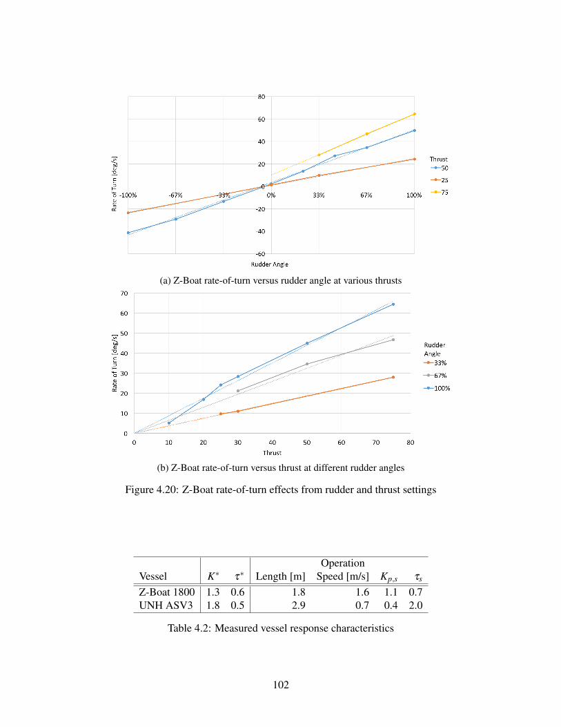
(a) Z-Boat rate-of-turn versus rudder angle at various thrusts
(b) Z-Boat rate-of-turn versus thrust at different rudder angles
Figure 4.20: Z-Boat rate-of-turn effects from rudder and thrust settings
Vessel K∗ τ∗ Length [m]Operation
Speed [m/s] Kp,s τs
Z-Boat 1800 1.3 0.6 1.8 1.6 1.1 0.7UNH ASV3 1.8 0.5 2.9 0.7 0.4 2.0
Table 4.2: Measured vessel response characteristics
102
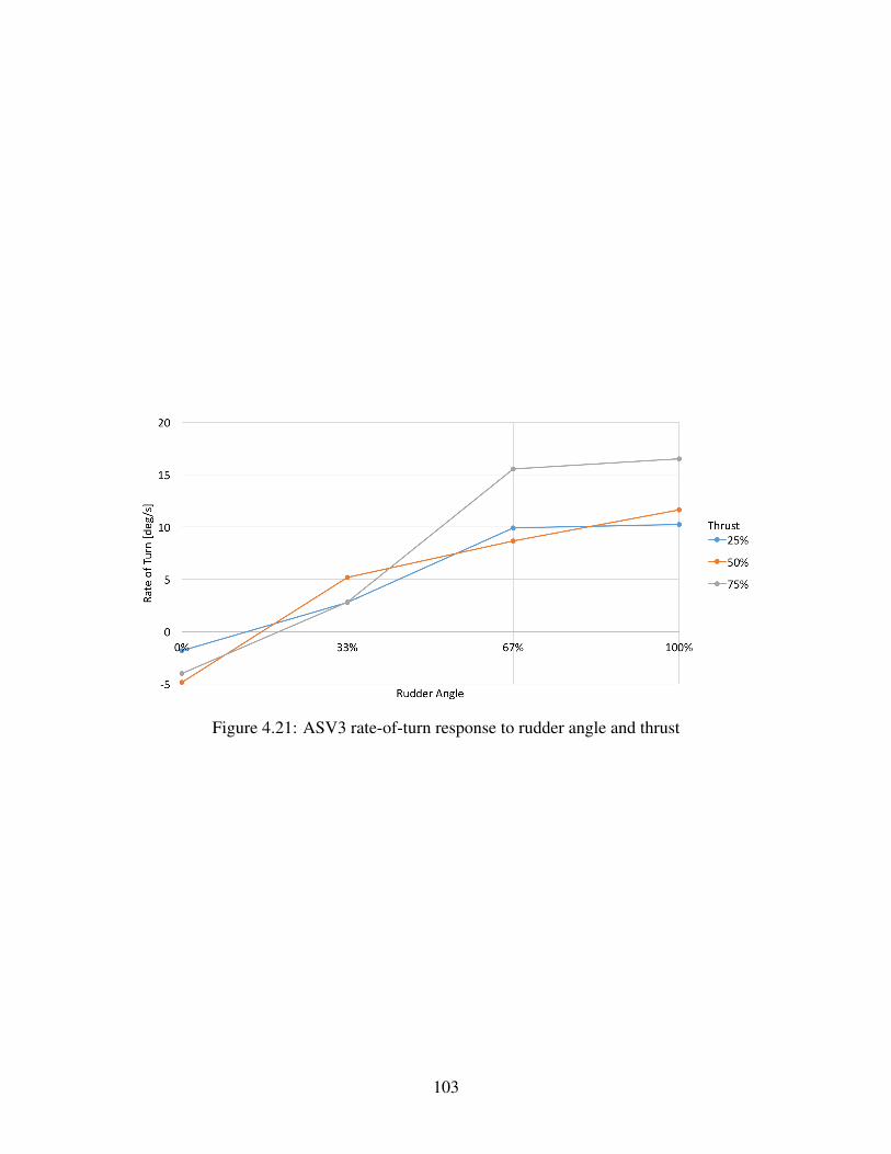
Figure 4.21: ASV3 rate-of-turn response to rudder angle and thrust
103

4.5.2 Course Change Controller Field Test
A preliminary version of the course change controller was tested remotely on a Z-Boat in Norfolk,
VA on January 20, 2016. The result for a single turn is shown in Figure 4.22. In this instance,
the response of the vessel is not as fast as the MRAS model, so the value of Kp increases as the
turn progresses, but does not adapt quickly enough for the vessel to more closely follow the model.
Decreasing adaptive gains, as specified in Equation 4.20, with ξ = 0.9 were used in this test. As a
result, the PID gains are seen to change less rapidly over time.
During this field test, the course keep controller is also tested through the use of the hybrid
arrangement. However, mathematical errors in the controller implementation at the time of testing
prevented the vessel from fully behaving as desired. Despite this, the results of early tests on Z-
Boats led to the sole use of the course keep controller to achieve the best performance. Due to the
hardware limitations mentioned previously, tests on the final controller were not possible.
104
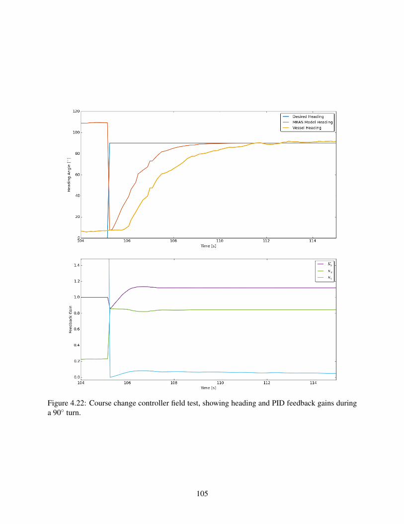
Figure 4.22: Course change controller field test, showing heading and PID feedback gains duringa 90 turn.
105
CONCLUSION AND FUTURE WORK
Summary of Research
A complete package for autonomous marine operations, focused on executing hydrographic sur-
veys, is developed in this research. A hardware and electronics system, capable of being packaged
for integration on vessels of opportunity provides flexibility for deployment. This system provides
full autonomous functionality and the ability for a human operator to monitor or manually con-
trol the vessel when desired, and can be entirely constructed for under $1200. Core autonomy
functionality is provided by the open source MOOS-IvP framework, with additional applications
supporting integration on multiple platforms.
A new approach to autonomous hydrographic survey line planning is developed that provides
full bottom coverage when used in conjunction with a swath sonar system. This system was field
tested on multiple Z-Boat platforms with positive results. Simulations show expected performance
on a variety of terrains when compared to human surveys of the same areas.
The Model Reference Adaptive Control system is able to determine model parameters for a
simplified vessel, which show promising application for the control of small ASVs in simulation
and field tests. A second controller performs controlled turns for larger vessels, and can be used
in conjunction with the model identification controller for reduced rudder actuation while course
keeping. Specialized speed control for applications where constant adjustment is unneeded in-
creases power efficiency while still maintaining speeds within a designated threshold
Together, these components form an autonomy and data acquisition system that can be easily
deployed in the field for rapid survey operations in shallow water with small ASVs. The modular
nature of the system permits installation on a range of vessels and much of the research is also
applicable to large ships and high integrity sensors.
106

Future Work
The control system and survey path planning aspects of this research present opportunities for
improvement. The path planning algorithm could be extended to automatically partition larger ir-
regular polygons, which would further simplify the human planning element. The behavior when
isolated shallow areas are located could be improved to deal with them in a more systematic man-
ner, instead of halting progress on the survey in that area. More work could be done on optimal
path refinement and processing of the sonar data, particularly in regions with greatly varying depths
that lead to significant repeated bends in survey lines.
The control system could be extended with a fuzzy logic intelligence or neural network, as
other research has investigated in relation to MRAC. Frequency analysis of the heading history
could provide diagnostics and removal of unwanted oscillation. The speed based gain scheduling
of system parameters could be improved, as this does not appear to always be a linear effect. In
addition, the speed control could be better applied to fault detection through analysis of long term
speed trends and comparison with expected behavior. More field testing is required for refinement
of the controllers, as well as testing on a wider range of vessel sizes and types.
In order for any component of the autonomy system to be more accessible to an unfamiliar
user, an improved graphical interface and configuration tools will need to be developed. Some
work has begun in this effort, including work toward universal mission planning file structures and
visual mission planning tools.
107
LIST OF REFERENCES[1] B. S. Bourgeois, D. L. Brandon Jr et al., “Efficient hydrographic survey planning using an
environmentally adaptive approach,” DTIC Document, Tech. Rep., 2006.
[2] J. Van Amerongen, “Adaptive Steering of Ships,” Ph.D. dissertation, Delft University of Tech-nology, 1982.
[3] A. Motwani, “A Survey of Uninhabited Surface Vehicles,” Tech. Rep., 2012.
[4] G. Roberts, R. Sutton et al., “Intelligent ship autopilotsA historical perspective,” Mechatron-ics, vol. 13, pp. 1091–1103, 2003.
[5] S. Bennett, “Nicolas Minorsky and the Automatic Steering of Ships,” IEEE Control SystemsMagazine, vol. 4, no. 4, pp. 10–15, 1984.
[6] V. Bertram, “Unmanned Surface Vehicles A Survey,” Skibsteknisk Selskab, Copenhagen,Denmark, pp. 1–14, 2008. [Online]. Available: http://www.skibstekniskselskab.dk/public/dokumenter/Skibsteknisk/Downloadmateriale/2008/10marts08/USVsurvey DTU.pdf
[7] ASV Global. C-worker 6. ASV Global. [Online]. Available: http://asvglobal.com/product/c-worker-6/
[8] Teledyne Oceanscience. Z-boat 1800-rp. Teledyne Oceanscience. [Online]. Available:http://oceanscience.com/Products/Z-Boat/Z-Boat-RP.aspx
[9] J. Manley and S. Willcox, “The Wave Glider: A persistent platform for ocean science,” inOCEANS 2010 IEEE - Sydney. IEEE, May 2010, pp. 1–5.
[10] C. Meinig, N. Lawrence-Slavas et al., “The use of saildrones to examine spring conditions inthe bering sea: Vehicle specification and mission performance,” in OCEANS’15 MTS/IEEEWashington. IEEE, 2015, pp. 1–6.
[11] K. Woerner, “COLREGS-Compliant Autonomous Collision Avoidance Using Multi-Objective Optimization with Interval Programming by,” Ph.D. dissertation, MassachusetsInstitute of Technology, 2014.
[12] Y. Kuwata, M. T. Wolf et al., “Safe Maritime Autonomous Navigation With COLREGS ,Using Velocity Obstacles,” IEEE Journal of Oceanic Engineering, vol. 39, no. 1, pp. 110–119, 2014.
[13] P. Svec, B. C. Shah et al., “Dynamics-aware target following for an autonomous surfacevehicle operating under COLREGs in civilian traffic,” IEEE International Conference onIntelligent Robots and Systems, pp. 3871–3878, 2013.
108
[14] L. P. Perera, J. P. Carvalho, and C. Guedes Soares, “Autonomous guidance and navigationbased on the COLREGs rules and regulations of collision avoidance .” Advanced Ship Designfor Pollution Prevention, no. 1999, pp. 205–216, 2010.
[15] U. Siwe. (2016) Sea Traffic Management. The Swedish Maritime Administration. [Online].Available: http://www.stmvalidation.eu
[16] Rolls-Royce. (2016) Rolls-Royce reveals future shore control centre. Rolls-Royce. [Online]. Available: http://www.rolls-royce.com/media/press-releases/yr-2016/pr-2016-03-22-rr-reveals-future-shore-control-centre.aspx
[17] D. W. Hodo, D. M. Bevly et al., “Optimal path planning with obstacle avoidance for au-tonomous surveying,” in IECON 2010-36th Annual Conference on IEEE Industrial Electron-ics Society. IEEE, 2010, pp. 1577–1583.
[18] E. Galceran and M. Carreras, “Efficient seabed coverage path planning for asvs and auvs,” inIntelligent Robots and Systems (IROS), 2012 IEEE/RSJ International Conference on. IEEE,2012, pp. 88–93.
[19] T. Wilson and S. B. Williams, “Adaptive Path Planning for Depth ConstrainedBathymetric Mapping with an Autonomous Surface Vessel,” 2016. [Online]. Available:http://arxiv.org/abs/1603.06324
[20] Hydronalix EMILY. Hurricane tracker. Hydronalix. [Online]. Available: http://emilyrobot.com/hurricane-tracker
[21] M. Head, S. Smith, and D. Manda, “Into the Blue (Tint): Unmanned Survey Boats Com-plement Multibeam, Lidar, and Satellite Derived Bathymetry on the NOAA Ship ThomasJefferson,” in Canadian Hydrographic Conference - Halifax, NS. Canadian HydrographicConference, May 2016.
[22] Bass Hunter. EX. Bass Hunter. [Online]. Available: http://www.basshunter.com/index.php?option=com content&view=article&id=11
[23] J. Perrella, T. Panella et al., “Autonomous surface vehicle senior research project.”
[24] Raspberry Pi Foundation. Raspberry Pi 2 Model B. [Online]. Available: https://www.raspberrypi.org/products/raspberry-pi-2-model-b/
[25] Arduino. Arduino mega 2560. [Online]. Available: http://arduino.cc/en/Main/ArduinoBoardMega2560
[26] K. Parsons. MCS Index for 802.11n and 802.11ac Chart. [Online]. Available: http://www.wlanpros.com/mcs-index-802-11n-802-11ac-chart
[27] CHRobotics LLC. GP9 GPS-Aided AHRS Datasheet, Revision 1.3. [Online]. Available:http://www.chrobotics.com/docs/GP9Datasheet.pdf
[28] C. Chamberlain, personal communication.
109
[29] International Hydrographic Bureau, IHO Standards for Hydrographic Surveys, 5th Edition,International Hydrographic Organization. [Online]. Available: http://www.iho.int/iho pubs/standard/S-44 5E.pdf
[30] SBG Systems, “Hydrographic Test Result: Ellipse, Ekinox,” SBG Systems, Tech. Rep., 2015.[Online]. Available: http://www.sbg-systems.com/docs/Ellipse Ekinox Test Hydrography.pdf
[31] M. Benjamin, H. Schmidt, and P. Newman. (2015, May) An Overview of MOOS-IvP and a Users Guide to the IvP Helm - Release 15.5. MIT. [Online]. Available:http://oceanai.mit.edu/ivpman/pmwiki/pmwiki.php
[32] J. Velagic, Z. Vukic, and E. Omerdic, “Adaptive fuzzy ship autopilot for track-keeping,”Control Engineering Practice, vol. 11, no. 4, pp. 433–443, 2003.
[33] B. T. Boulter, “Digital Filter Design Writing Difference Equations For Digital Filters,” 2000.[Online]. Available: http://www.apicsllc.com/apics/Sr 3/Sr 3.htm
[34] T. Perez and T. Fossen, “Modelling and Simulation of Environmental Disturbances,” Bol,Croatia, 2007. [Online]. Available: http://www.marinecontrol.org/pdf/Tutorial/CAMS M5 disturbances.pdf
[35] National Oceanic and Atmospheric Administration, NOS Hydrographic Surveys Specifica-tions and Deliverables, May 2015.
[36] Spatial Integrated Systems, Inc, “Demonstration of autonomous maritime navigation (amn)in support of noaa surveying missions,” Spatial Integrated Systems, Inc, Technical Report,March 2012.
[37] C. Fang and S. Anstee, “Coverage path planning for harbour seabed surveys using an au-tonomous underwater vehicle,” in OCEANS 2010 IEEE-Sydney. IEEE, 2010, pp. 1–8.
[38] B. S. Bourgeois, P. J. Alleman et al., “Autonomous bathymetry survey system,” OceanicEngineering, IEEE Journal of, vol. 24, no. 4, pp. 414–423, 1999.
[39] K. Wylie and T. Ketter, “Summer hydrographic field course 2014,” University of New Hamp-shire, Descriptive Report, July 2014.
[40] D. Manda, O. Irish et al., “Summer hydrographic field course 2015,” University of NewHampshire, Descriptive Report, July 2015.
[41] J. Van Amerongen, “MRAS: Model Reference Adaptive Systems,” Journal A, vol. 22, no. 4,pp. 192–198, 1981.
[42] ——, “Adaptive steering of ships: A model reference approach,” Automatica, vol. 20, no. 1,pp. 3–14, jan 1984. [Online]. Available: http://www.sciencedirect.com/science/article/pii/0005109884900608
[43] K. Nomoto, T. Taguchi et al., “On the steering qualities of ships,” Int. Shipbuilding Progress,vol. 4, 1957.
110