Development of a Transit Cost Allocation Formula MICHAEL G. FERRERI, Simpson and Curtin, Transportation Engineers, Philadelphia

The operating cost accounts of the Metropolitan Dade County Transit Authority are analyzed to develop a cost allocation formula of general application to any bus operating company. Standard cost account items were allocated among four major elements that affect expenses: vehicle costs, vehicle-miles, peak vehicle needs, and passenger revenue. Further study determined the relative loss in accuracy flowing from the elimination of two of these variables. In total, three formulas are devised and evaluated. The first uses all four allocators, the second eliminates peak vehicle needs, and the third uses only vehicle-miles and vehicle-hours.

The "four-variable" analysis resulted in the following cost allocation formula: C = 0.1459 M + 3.0017 H + 0.0578 R + 2521.69 v. C is average daily cost of route operation, Mis average daily vehicle-hours of service on route, H is average daily vehicle-miles of service on route, R is average daily passenger revenue on route, and V is peak vehicle needs on route. Comparison of operating costs by routes as calculated by the formula with route costs resulting from two- and three­variable formulas showed a maximum route mean square error of 10.8 percent for crosstown routes. The maximum deviation for the entire MTA system was only 6.3 percent. The conclu­sion to be drawn from this analysis is that for long-range planning projections, a simplified operating cost formula using only vehicle-miles and vehicle-hours is more than adequate and probably desirable because of the need to estimate only miles and hours of service on each route. On the other hand, for short-range service improvements and fiscal planning, a more accurate allocation formula such as the four-variable method is more appropriate.

•TO allocate community financial resources among transportation facility improve­ments, it is necessary to estimate the use of the elements of a proposed transportation network related to the expenditures required to achieve that use. The development of area-wide transportation plans with specific new facilities requires estimates of the num­ber of trips that will use each facility-transit and highways-for the design year.

Transportation studies have developed data that provide an understanding of present transit use, travel patterns, characteristics of riders, and the related socioeconomic characteristics that affect transit use. These data are being employed in modal split­traffic assignment processes to develop future estimates of transit facility use for any set of system circumstances. ·

The other side of the revenue and traffic analyses for area transportation studies, the cost of travel, has been very carefully tabulated in terms of capital improvements recommended for the transportation facilities master plan. When considering im­proved transit service and possible rapid transit developments, previous studies have

Paper sponsored by Committee on Passenger Transportation Economics and presented at the 48th Annual Meeting.

2

made meticulous estimates of the cost of capital facilities while completely overlooking the expense involved in operating the surface transit system.

Transit systems cun-ently spend only 5 to 10 cents of their revenue dollar on capital costs. The other 90 to 95 percent of annual costs go toward the day-to-day operation of the system. Transit companies that operate fixed rapid transit facilities sometimes devote as much as one-third of their operating expenses to the amortization of these capital facilities; the great bulk of expense still goes to operating the system.

The mass transit analysis conducted for the Miami Urban Area Transportation Study (MUATS) devoted planning attention and prepared cost estimates for the 10 percent item, capital costs. This paper, however, fully develops the companion analysis necessary for the proper calculation of the 90 percent item, the cost of operating any of the transit system alternativesto betested. Revenues and operating costs of the Metropolitan Dade County Transit Authority (MTA) a.re analyzed by subaccounts to develop a cost allocation model for application to routes of test transit networks.

MTA PATRONAGE AND SERVICE

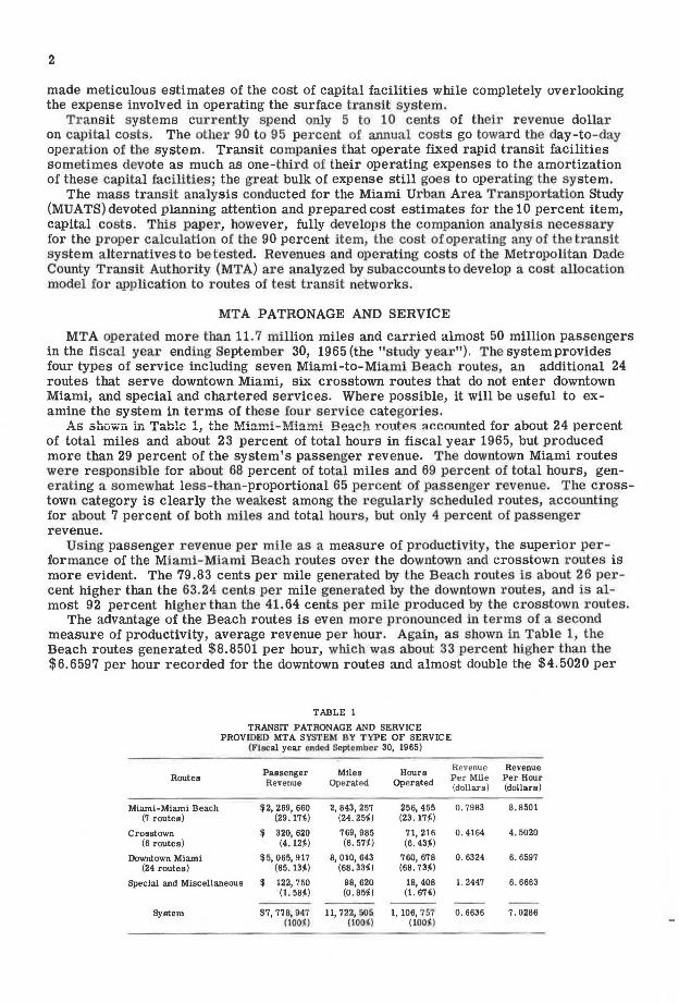
MTA operated more than 11. 7 million miles and carried almost 50 million passengers in the fiscal year ending September 30, 1965 (the "study year"). The system provides four types of service including seven Miami-to-Miami Beach routes, an additional 24 routes that serve downtown Miami, six crosstown routes that do not enter downtown Miami, and special and chartered services. Where possible, it will be useful to ex­amine the system in terms of these four service categories.

As shown in Tablo 1, the !',1:i:tmi-!'.l!iami Bearh route,;i ar.r.ounted for about 24 percent of total miles and about 23 percent of total hours in fiscal year 1965, but produced more than 29 percent of the system's passenger revenue. The downtown Miami routes were responsible for about 68 percent of total miles and 69 percent of total hours, gen­e1·ating a somewhat less-than-proportional 65 percent of passenger revenue. The cross­town category is clearly the weakest among the regularly scheduled routes, accounting for about 7 percent of both miles and total hours, but only 4 percent of passenger revenue.

Using passenger revenue per mile as a measure of p1·oductivity, the superior per­formance of the Miami-Miami Beach 1·outes over the downtown and crosstown routes is more evident. The 79.83 cents per mile generated by the Beach routes is about 26 per­cent higher than the 63.24 cents per mile generated by the downtown routes, and is al­most 92 percent higher than the 41.64 cents per mile produced by the crosstown routes.

The advantage of the Beach routes is even more pronounced in terms of a second measure of productivity, average revenue per hour. Again, as shown in Table 1, the Beach routes generated $8.8501 per hour, which was about 33 percent higher than the $6.6597 per hour recorded for the downtown routes and almost double the $4.5020 per

TABLE 1

TRANSIT PATRONAGE AND SERVICE PROVIDBD MTA SYSTEM BY TYPE OF SERVICE

(Fiscal year ended Septamber 30, 1965)

Passenger Miles Hours Revenue Revenue

Routes Per Mile Per Hour Revenue Operated Operated (dollars) (dollars)

Miami-Miami Beach $2, 269, 660 2, 843, 257 256, 455 0 . 7983 8. 8501 (7 routes) (29 . 17i) (24. 25i) (23.17i)

Crosstown $ 320, 620 769, 985 71, 216 o. 4164 4. 5020 (6 routes} (4.12i} (6. 57i} (6.43i)

Downtown Miami $5,065,917 8, 010, 643 760, 678 0. 6324 6. 6597 (24 routes) (65. 13i} (68. 33:£) (68. 73i)

Special and Miscellaneous $ 122, 750 98, 620 18, 408 1. 2447 6. 6683 (1. 58i} (0. 85\&) (1.67%)

System $7,77 8,917 11, 722, 505 1, 106, 757 0. 6636 7 . 0286 oooiJ (IOOt,) (looi1

3

hour produced by the crosstown routes. These results are a reflection of higher aver­age speeds on the Beach routes and relatively slow operation on the crosstown routes .

It is interesting to note that although the special and miscellaneous bus services are very productive in terms of revenue per mile ($1.2447), they are no more productive than the downtown routes in terms of revenue per hour ($6.6683). This results from the fact that long layovers at chartered outings, the Orange Bowl, Hialeah, etc., inflate the hours in this category.

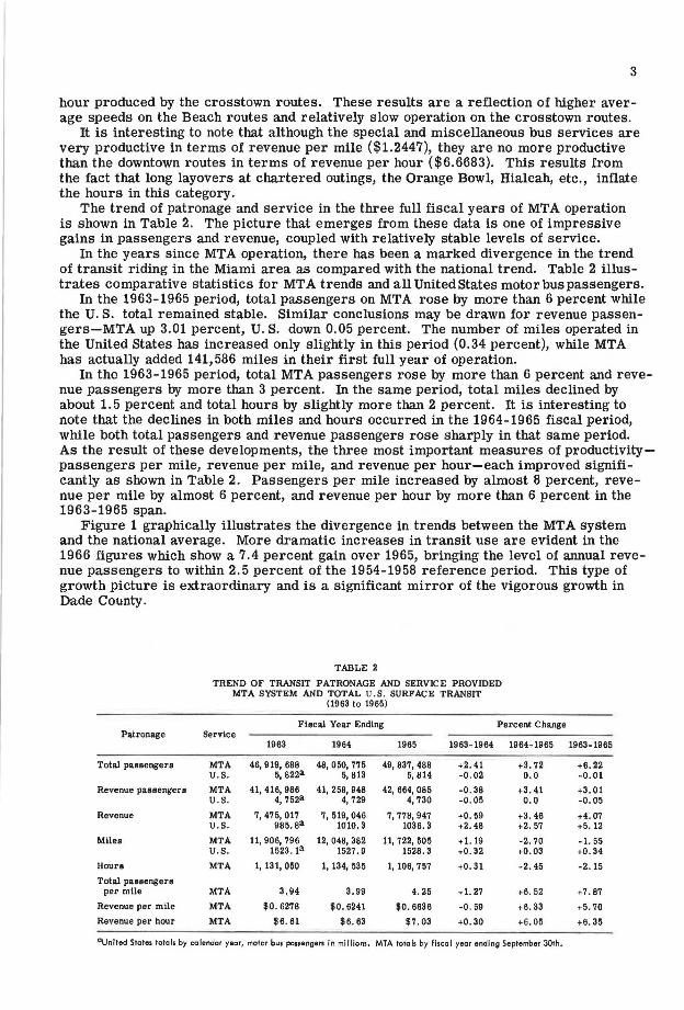
The trend of patronage and service in the three full fiscal years of MTA operation is shown in Table 2. The picture that emerges from these data is one of impressive gains in passengers and revenue, coupled with relatively stable levels of service.

In the years since MTA operation, there has been a marked divergence in the trend of transit riding in the Miami area as compared with the national trend. Table 2 illus­trates comparative statistics for MT A trends and all United States motor bus passengers.

In the 1963-1965 period, total passengers on MTA rose by more than 6 percent while the U.S. total remained stable. Similar conclusions may be drawn for revenue passen­gers-MTA up 3.01 percent, U.S. down 0.05 percent. The number of miles operated in the United States has increased only slightly in this period (0.34 percent), while MTA has actually added 141,586 miles in their first full year of operation.

In the 1963-1965 period, total MTA passengers rose by more than 6 percent and reve­nue passengers by more than 3 percent. In the same period, total miles declined by about 1. 5 percent and total hours by slightly more than 2 percent. It is interesting to note that the declines in both miles and hours occurred in the 1964-1965 fiscal period, while both total passengers and revenue passengers rose sharply in that same period. As the result of these developments, the three most important measures of productivity­passengers per mile, revenue per mile, and revenue per hour-each improved signifi­cantly as shown in Table 2. Passengers per mile increased by almost 8 percent, reve­nue per mile by almost 6 percent, and revenue per hour by more than 6 percent in the 1963-1965 span.

Figure 1 graphically illustrates the divergence in trends between the MT A system and the national average. More dramatic increases in transit use are evident in the 1966 figures which show a 7.4 percent gain over 1965, bringing the level of annual reve­nue passengers to within 2. 5 percent of the 1954-1958 reference period. This type of growth picture is extraordinary and is a significant mirror of the vigorous growth in Dade County.

TABLE 2

TREND OF TRANSIT PATRONAGE AND SERVICE PROVIDED MTA SYSTEM AND TOTAL U.S. SURFACE TRANSIT

(1963 to 1965)

Fiscal Year Ending Percent Change Patronage Service

1963 1964 1965 1963-1964 1964-1965 1963-1965

Total passengers MTA 46,919, 688 48, 050, 775 49, 837, 488 +2. 41 +3. 72 +6. 22 U.S. 5, e22a 5, 813 5,814 -0.02 0.0 -0. 01

Revenue passengers MTA 41, 416, 986 41, 258, 948 42, 664, 085 -0. 38 +3.41 +3, 01 U.S. 4, 752a 4,729 4, 730 -0 . 05 0 . 0 -0 , 05

Revenue MTA 7, 475, 017 7,519,046 7,778,947 +0. 59 +3.46 +4.07 U.S. 985. ea 1010. 3 1036. 3 +2. 48 +2. 57 +5, 12

Miles MTA 11, 906, 796 12, 048, 382 11, 722, 505 +1. 19 -2, 70 -1. 55 U.S. 1523 , 1a 1527. 9 1528. 3 +0.32 +0.03 +0. 34

Hours MTA 1, 131, 050 1, 134, 535 1, 106, 757 +0 . 31 -2. 45 -2. 15

Total passengers per mile MTA 3.94 3.99 4. 25 +1. 27 +6. 52 +7. 87

Revenue per mile MTA $0 . 6278 $0. 6241 $0. 6636 -0. 59 +6. 33 +5. 70

Revenue per hour MTA $6. 61 $6. 63 $7. 03 +0 . 30 +6. 05 +6. 35

0 United States totals by calendar year, motor bus passengers in millions. MTA totals by fiscal year ending September 30tli.

4

15 --i ;a N I

! .. ~ -- •

15 .__ ____________ _,

1151 1111 IHI IN.I INJ 1114 1115 llH U U ll IEIEHE PASSEIIHI

Figure 1. Trend of transit traffic, Metropoli-' km Dade County Transit Authorlty W.TA).

OPERATING COST ACCOUNTS

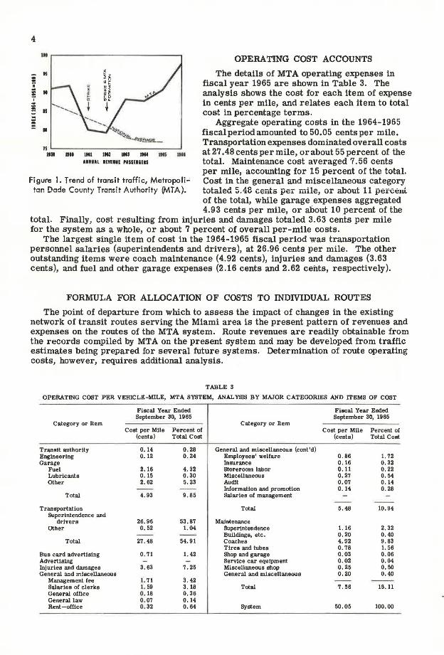
The details of MT A operating expenses in fiscal year 1965 are shown in Table 3. The analysis shows the cost for each item of expense in cents per mile, and relates each item to total cost in percentage terms .

Aggregate operating costs in the 1964-1965 fiscalperiodamounted to 50.05 cents per mile. Transportation expenses dominated overall costs at 27 .48 cents per mile, or about 55 percent of the total. Maintenance cost averaged 7. 56 cents per mile, accounting for 15 percent of the total. Cost in the general and miscellaneous category totaled 5.48 cents pe:r mile, o:r about 11 percent of the total, while garage expenses aggregated 4.93 cents per mile, or about 10 percent of the

total. Finally, cost resulting from injuries and damages totaled 3.63 cents per mile for the system as a whole, or about 7 percent of overall per-mile costs.

The largest single item of cost in the 1964-1965 fiscal period was transportation personnel salaries (superintendents and drivers), at 26.96 cents per mile. The other outstanding items were coach maintenance (4.92 cents), injuries and damages (3.63 cents), and fuel and other garage expenses (2.16 cents and 2.62 cents, respectively).

FORMULA FOR ALLOCATION OF COSTS TO INDIVIDUAL ROUTES

The point of departure from which to assess the impact of changes in the existing network of transit routes serving the Miami area is the present pattern of revenues and expenses on the routes of the MTA system. Route revenues are readily obtainable from the records compiled by MT A on the present system and may be developed from traffic estimates being prepared for several future systems. Determination of route operating costs, however, requires additional analysis.

TABLE 3

OPERATING COST PER VEHICLE-MILE, MTA SYSTEM, ANALYSIS BY MAJOR CATEGORIES AND ITEMS OF COST

Fiscal Year Ended Fiscal Year Ended September 30, 1965 September 30, 1965

Category or Item Category or Item Cost per Mile Percent of Cost per Mile Percent of

(cents) Total Cost (cents) Total Cost

Transit authority 0.14 0 . 28 General and miscellaneous (cont'd) Engineering 0.12 0.24 Employees' welfare 0.86 1. 72 Garage Insurance 0.16 0.32

Fuel 2.16 4.32 storeroom labor 0.11 0 . 22 Lubricants 0 . 15 0.30 Miscellaneous 0.27 0 . 54 Other 2. 62 5. 23 Audit 0.07 0.14

Information and promotion 0 . 14 0. 28 T otal 4. 93 9.85 Salaries of management

Transportation Total 5.48 10. 94 Superintendence and

drivers 26. 96 53,87 Maintenance Other 0. 52 1.04 Superintendence 1. 16 2. 32

Buildings, etc. 0 . 20 0.40 Total 27.48 54. 91 Coaches 4. 92 9. 83

Tires and tubes 0 . 78 1. 56 Bus card advertloing o. 71 1. 42 Shop and garage 0 . 03 0.06 Advertlolng Service car equipment 0.02 0. 04 Injuries and damages 3. 63 7. 25 Miscellaneous shop 0.25 o. 50 General and miscellaneous General and miscellaneous 0.20 0 . 40

Management fee 1. 71 3.42 Salaries of clerks I . 59 3. 18 Total 7. 56 15. 11 General office 0. 18 0.36 General law 0. 07 0.14 Rent-office 0. 32 0.64 System 50 . 05 100. 00

5

This study analyzes the detailed operating expense accounts of MTA leading to a classification of each expense item within one of several categories as the basis for allocation to individual lines. A consideration of the nature of various operating costs has resulted in the identification of four major elements that have been used to allo­cate particular expense items. These four elements are vehicle-hours, vehicle-miles, peak vehicle needs, and passenger revenue.

This four-variable formula is calibrated in this paper and compared to the MT A formula that has been developed by the transit authority using three of these four elements: vehicle-hours, vehicle-miles, and passenger revenue. One additional two­variable formula is developed using only vehicle-hours and vehicle-miles. The premise behind this comparative investigation is that for planning purposes, the simpler the formula, the easier the application, if a sufficient degree of accuracy can be maintained.

Vehicle-Hours

The wages of drivers and transportation superintendents represent by far the largest single element of cost in the MTA system, having accounted for about 54 percent of the total cost per mile in fiscal 1965. Employees engaged in operating vehicles are paid on an hourly basis. Allocation of this wage expense would be most properly made on the basis of hours of service on each of the lines. This is best estimated by the aggregate vehicle-hours operated on each line, and this is the basis that has been used to allocate the wages of transportation personnel.

Another important classification has been allocated on a vehicle-hour basis; that is, employees' welfare expense. Whereas costs in this category are attributable to all classes of employees, the bulk of the amount is directly assignable to the largest group of workers; namely, the operating force. Thus, these nonpayroll labor costs have been allocated in the same fashion as the main portion of direct wages and are assigned to individual routes on the basis of vehicle-hours.

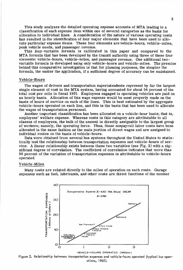
Data were obtained from several bus systems throughout the United States to statis­tically test the relationship between transportation expenses and vehicle-hours of ser­vice . A linear relationship exists between these two variables (see Fig. 2) with a sig­nificant degree of correlation. The coefficient of correlation indicates that more than 96 percent of the variation of transportation expenses is attributable to vehicle-hours operated.

Vehicle-Miles

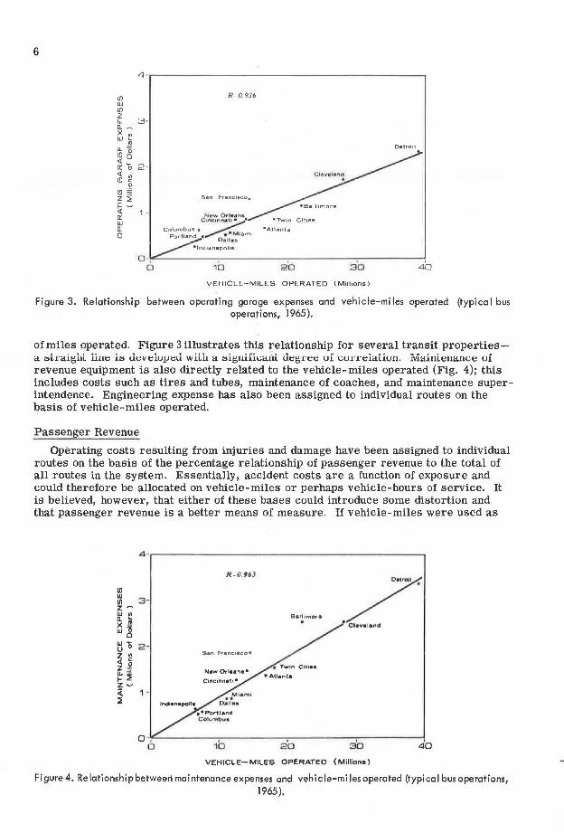
Many costs are related directly to the miles of operation on each route. Garage expenses such as fuel, lubricants, and other costs are direct functions of the number

40-.--------------------- ----,

(/) llJ (/) Z 30-l/J~

~ I'! llJ ~

0 Z Cl Q o 20· ~ " t- g ~~ Q. ::!; (/) ~ z 10· <( a:: t-

Tra n,portation E:rpense ,'$) • 4,4]3 1Veh. Hours) -566,369

R • 0.984

N•w Orle•ne • Atlanta

C lnc1nna1I Columbu• •r-,,, t• m1

lt>d~~ D• tlaa

o -~. ------,------ -,-------,-, ----' a 1 e 3

VEHICLE-HOURS OPERATED (Millions)

Figure 2. Relationship between transportation expenses and vehicle-hours operated (typical bus oper­ations, 1965).

6

4-.---------------------------, U) UJ U) 2 UJ 3 -a. ~ X m UJ " ~

~o <( 0 a: o 2 · <( m (9 C

0 (9 ~ Z:;;i

~ ~ 1 -0: UJ a. 0

R= 0 936

Detroit

San Francisco.

0 -...:C------------------------' 0 10 80 30 40

VEHICLE-MILES OPERATED (Millions)

Figure 3. Relationship between operating garage expenses and vehicle-miles operated (typical bus operations, 1965).

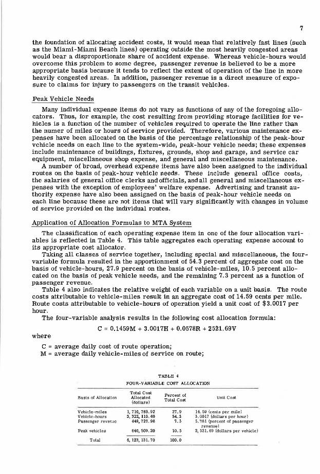
of miles operated. Figure 3 illustrates this relationship for several transit properties­a stl·aight line is deveioped with a significant deg1°ee oI coneiatiou. iviaiult:mauct:: uI revenue equipment is also directly related to the vehicle-miles operated (Fig. 4); this includes costs such as tires and tubes, maintenance of coaches, and maintenance super­intendence. Engineering expense has also been assigned to individual routes on the }?asis of vehicle-miles operated.

Passenger Revenue

Operating costs resulting from injuries and damage have been assigned to individual routes on the basis of the percentage relationship of passenger revenue to the total of all routes in the system. Essentially, accident costs are a function of exposure and could therefore be allocated on vehicle-miles or perhaps vehicle-hours of service. It is believed, however, that either of these bases could introduce some distortion and that passenger revenue is a better means of measure. If vehicle-miles were used as

4-.------ ----- - ---------------, R=0. 963

San Fr• ncieco •

Baltimore .

0 -·~,--------,-- -----,-------,------4, o 1b 20 30 4 •

VEHICLE-MILES OPERATED (Millions)

Figure 4. Relationship between maintenance expenses and vehicle-miles operated (typical bus operations, 1965).

7

the foundation of allocating accident costs, it would mean that relatively fast lines (such as the Miami-Miami Beach lines) operating outside the most heavily congested areas would bear a disproportionate share of accident expense. Whereas vehicle-hours would overcome this problem to some degree, passenger revenue is believed to be a more appropriate basis because it tends to reflect the extent of operation of the line in more heavily congested areas. In addition, passenger revenue is a direct measure of expo­sure to claims for injury to passengers on the transit vehicles.

Peak Vehicle Needs

Many individual expense items do not vary as functions of any of the foregoing allo­cators. Thus, for example, the cost resulting from providing storage facilities for ve­hicles is a function of the number of vehicles required to operate the line rather than the numer of miles or hours of service provided. Therefore, various maintenance ex­penses have been allocated on the basis of the percentage relationship of the peak-hour vehicle needs on each line to the system-wide, peak-hour vehicle needs; these expenses include maintenance of buildings, fixtures, grounds, shop and garage, and ser vice car equipment, miscellaneous shop expense, and general and miscellaneous maintenance.

A number of broad, overhead expense items have also been assigned to the individual routes on the basis of peak-hour vehicle needs. These include general office costs, the salaries of general office clerks and officials, and all general and miscellaneous ex­penses with the exception of employees' welfare expense. Advertising and transit au­thority expense have also been assigned on the basis of peak-hour vehicle needs on each line because these are not items that will vary significantly with changes in volume of service provided on the individual routes.

Application of Allocation Formulas to MTA System

The classification of each operating expense item in one of the four allocation vari­ables is reflected in Table 4. This table aggregates each operating expense account to its appropriate cost allocator.

Taking all classes of service together, including special and miscellaneous, the four­variable formula resulted in the apportionment of 54 .3 percent of aggregate cost on the basis of vehicle-hours, 27.9 percent on the basis of vehicle-miles, 10.5 percent allo­cated on the basis of peak vehicle needs, and the remaining 7. 3 percent as a function of passenger revenue.

Table 4 also indicates the relative weight of each variable on a unit basis. The route costs attributable to vehicle-miles result in an aggregate cost of 14.59 cents per mile. Route costs attributable to vehicle-hours of operation yield a unit cost of $3.0017 per hour .

The four-variable analysis results in the following cost allocation formula:

C = 0.1459M + 3.0017H + 0.0578R + 2521.69V where

C = average daily cost of route operation; M = average daily vehicle-miles of service on route;

Basis of Allocation

Vehicle-mlles Vehicle-hours Passenger revenue

Peak vehicles

Total

TABLE 4

FOUR-VARIABLE COST ALLOCATION

Total Cost Allocated (dollars)

1, 710,783. 92 3, 322, 110. 60

449,727 . 98

640, 509. 20

6, 123,13 1. 70

Percent of Total Cost

27 . 9 54. 3 7. 3

10. 5

100. 0

Unit Cost

14. 59 (cents per mile) 3. 0017 (dollars per hour) 5. 781 (percent of passenger

revenue) 2,521.69 (dollars per vehicle)

8

H = average dailyvehicle-hours of service on route; R = average daily passenger revenue on route; and V = peak vehicle needs on route.

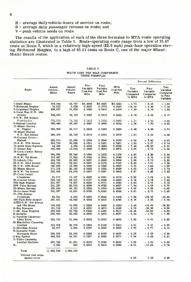
The results of the application of each of the three formulas to MT A route-operating statistics are illustrated in Table 5. Route-operating costs range from a low of 35.47 cents on Route 2, which is a relatively high-speed (22.6 mph) peak-hour operation serv-ing Richmond Heights, to a high of 65.11 cents on Route C, one of the major Miami-Miami Beach routes.

TABLE 5

ROUTE COST PER MILE COMPARISON THREE FORMULAS

Pe!"cent Difference

Annual Annual Two Four MTA Two

Route Vehicle- Vehicle- Variable Variable Cost Per Two Four Variable Cost Per Cost Per Variable Variable Miles Hours Mile Mile Mlle

Compared Compared Compared

toMTA to MTA to Four Variable

1-South Miami 336,044 24, 757 $0.4600 $0. 4527 $0. 4521 + 1. 75 + 0.13 + 1. 61 2-Richmond Heights 54, 810 3,028 0. 4047 o. 3776 0. 3547 + 14. 10 + 6. 46 + 7. 18 3-Grapeland Heights 209,837 21, 629 0. 5483 0. 5410 o. 5419 + 1. 19 - 0.16 + 1. 35 4-Coral Way-N. W. 12th

Avenue 342, 834 34, 195 0. 5383 0. 5374 0. 5242 + 0. 78 + 2. 52 + 0.17 5-N. W. 2nd Avenue-

11, ... ..... ,,. 1,, ... ..4- __ ,.,.,c nn.e ' ...... , ......... 1-s, ... ,u U, ,J'S,L,J U. GOlO u. 5':t05 - l. ~j + i.4~ - ~- tib 6-Hialeah Limited 629, 488 56, 587 o. 5087 o. 4938 0. 5018 + 1.38 - 1. 59 + 2. 93 11-Mlami Shores,

W. Flagler 669, 202 62,717 0. 5202 0. 5459 0. 5226 - 0. 46 + 4.46 - 4. 71 12-Miami Shores,

N. E. 2nd Avenue 299, 150 29, 150 0. 5314 o. 5351 o. 5379 - 1. 21 - 0. 52 - 0. 69 14-Coconut Grove-

Hialeah 630,311 61, 929 0. 5338 o. 5542 o. 5339 - 0.00 + 3. 80 - 0.07 15-N. W. 27th Avenue 392, 700 38,098 0. 5301 0. 5261 0. 5231 + 1.34 + 0.57 + 0. 76 16-South Dixie Express 64, 388 4,232 0. 4362 0. 4826 0. 4059 + 7.46 +18. 90 - 9. 61 17 -Dinner Key 145, 689 13, 944 0. 5262 0. 4936 0. 4973 + 5. 81 - 0. 74 + 6,60 18-Civlc Center-Mercy

Hospital 286,388 26,540 0. 5360 0. 5252 0. 5132 + 4.83 + 2.28 + 2.44 19-N, W. 7th street 174, 487 17, 284 0. 5362 0 . 5341 0. 5349 + 0.24 - 0 . 15 + 0 . 39 21-Llberty City 424, 780 50,063 0. 5927 0. 6062 o. 6298 - 5.89 - 3. 75 - 2. 23 23-N. W, 22nd Avenue 342,781 32, 641 o. 5247 o. 5170 o. 5103 + 2.82 + 1. 31 + 1. 49 24-N. W. 46th street 169, 265 18, 380 o. 5648 0. 5589 o. 5693 - o. 79 - 1. 83 + 1.06 25-Miami Shores 311, 135 29, 185 0. 5205 o. 5065 o. 4996 + 4.02 + 1. 38 + 2. 76 26-N.W. 7th Avenue 335, 365 34, 054 0. 5437 0. 5267 0. 5662 - 3.97 - 6. 68 + 3. 22 27-Civlc Center

Crosstown 90, 911 11, 187 0. 6083 0. 5991 0. 5912 + 2. 89 - 1. 34 + 1. 54 28-Coconut Grove 264, 166 24, 181 0. 5137 0. 4968 o. 4884 + 5. 18 + 1. 72 + 3.40 29E-East Hialeah 201, 437 16, 987 0.4920 0. 4771 0. 4644 + 5.94 + 2. 73 + 3.12 29W-Palm Springs 241, 027 20,955 o. 4999 0. 4728 0. 4657 + 7.34 + 1. 52 + 5. 73 30-Miami Springe 425, 524 40, 192 0. 5224 0. 5266 0. 5045 + 3. 55 + 4. 38 - 0.80 34-Le Jeune Road 210,227 16,831 0. 4792 0. 4545 0. 4364 + 9.81 + 4.15 + 5.43 37 -17th Avenue

Crosstown 92, 561 9,253 0. 5390 o. 6345 0. 5102 + 7.60 +24. 36 -15. 05 100-Park Ride-Airport 247, 431 18, 323 o. 4612 o. 4212 o. 4343 + 6.19 - 3. 02 + 9. 50 A(XX)-S. W. 3rd Avenue

and 13th street 106, 862 10, 323 o. 5288 0. 6469 0. 5564 - 5. 44 +15. 85 -18. 26 B-Key Biscayne 131,318 8,515 0.4335 0. 4075 0.4549 - 4.70 -10. 42 + 6.38 C-Mt. Sinai Hospital 336, 825 32,760 0. 5308 o. 5469 0. 6511 -18. 48 -10. 00 - 2.94 K-Surfside 539, 686 45, 850 0. 4939 0. 4873 0. 4957 - o. 36 - 1. 70 + 1. 35 L-Venetlan Causeway-

Little River 580, 705 51, 584 o. 5055 o. 4910 0. 4894 + 3. 29 + o. 51 + 2.95 M-MacArthur Causeway

Limited 315, 354 29,576 0. 5204 0. 5156 0. 5451 - 4. 51 - 5. 41 + 0.93 O-Merld!an Avenue 62, 377 6,604 o. 5567 0. 5245 0. 5205 + 6.95 + 0.77 + 6.14 R-Biecayne Point-

Normandy Shore 259, 099 24,313 0. 5206 0. 5033 o. 4933 + 5. 53 + 2.03 + 3. 44 S-Bay Harbor 466,005 44, 531 o. 5257 o. 5268 o. 5571 - 5. 64 - 5. 44 - 0. 21 T-Tuttle Causeway

Limited-Surfside 497, 720 41, 631 0. 4912 o. 4769 o. 4859 + 1.09 - 1. 85 + 3.00 X- 5,459 663 o. 6034 0. 5814 0. 6595 - 8. 51 - 11. 84 + 3.78

Total 11, 629, 344 1, 089, 012

Percent root mean square error 5. 93 7.26 5.48

9

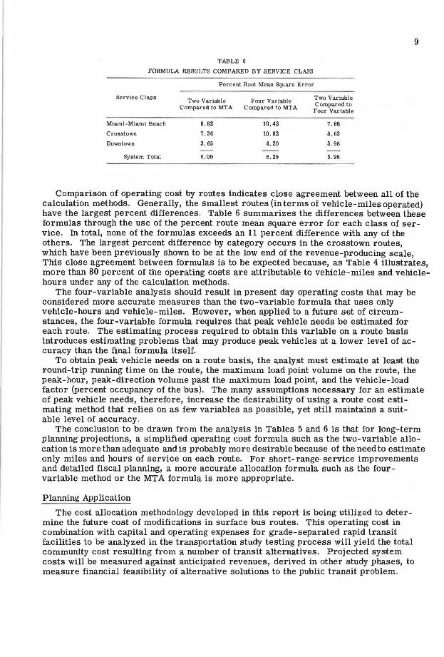
TABLE 6

FORMULA RESULTS COMPARED BY SERVICE CLASS

Percent Root Mean Square Error

Service Class Two Variable Four Variable Two Variable

Compared to MTA Compared to MTA Compared to Four Variable

Miami-Miami Beach 8. 82 10. 42 7. 88

Crosstown 7. 36 10. 82 8 . 63

Downtown 3. 65 4. 20 3 . 98

System Total 6. 00 6. 29 5. 98

Comparison of operating cost by routes indicates close agreement between all of the calculation methods. Generally, the smallest routes (in terms of vehicle-miles operated) have the largest percent differences . Table 6 summarizes the differences between these formulas through the use of the percent route mean square error for each class of ser­vice. In total, none of the formulas exceeds an 11 percent difference with any of the others. The largest percent difference by category occurs in the crosstown routes, which have been previously shown to be at the low end of the revenue-producing scale, This close agreement between formulas is to be expected because, as Table 4 illustrates, more than 80 percent of the operating costs are attributable to vehicle-miles and vehicle­hours under any of the calculation methods.

The four-variable analysis should result in present day operating costs that may be considered more accurate measures than the two-variable formula that uses only vehicle-hours and vehicle-miles. However, when applied to a future set of circum­stances, the four-variable formula requires that peak vehicle needs be estimated for each route. The estimating process required to obtain this variable on a route basis introduces estimating problems that may produce peak vehicles at a lower level of ac­curacy than the final formula itself.

To obtain peak vehicle needs on a route basis, the analyst must estimate at least the round-trip running time on the route, the maximum load point volume on the route, the peak-hour, peak-direction volume past the maximum load point, and the vehicle-load factor (percent occupancy of the bus). The many assumptions necessary for an estimate of peak vehicle needs, therefore, increase the desirability of using a route cost esti­mating method that relies on as few variables as possible, yet still maintains a suit­able level of accuracy.

The conclusion to be drawn from the analysis in Tables 5 and 6 is that for long-term planning projections, a simplified operating cost formula such as the two-variable allo­cation is more than adequate and is probably more desirable because of the need to estimate only miles and hours of service on each route. For short-range- service improvements and detailed fiscal planning, a more accurate allocation formula such as the four­variable method or the MTA formula is more appropriate.

Planning Application

The cost allocation methodology developed in this report is being utilized to deter­mine the future cost of modifications in surface bus routes. This operating cost in combination with capital and operating expenses for grade- separated rapid transit facilities to be analyzed in the transportation study testing process will yield the total community cost resulting from a number of transit alternatives. Projected system costs will be measured against anticipated revenues, derived in other study phases, to measure financial feasibility of alternative solutions to the public transit problem.