transit analysis package: an idl graphical user interface for exoplanet transit photometry

Hindawi Publishing CorporationAdvances in AstronomyVolume 2012, Article ID 697967, 8 pagesdoi:10.1155/2012/697967

Research Article

Transit Analysis Package: An IDL Graphical User Interface forExoplanet Transit Photometry

J. Zachary Gazak,1 John A. Johnson,2, 3 John Tonry,1 Diana Dragomir,4 Jason Eastman,5

Andrew W. Mann,1 and Eric Agol6

1 Institute for Astronomy, University of Hawaii, 2680 Woodlawn Dr, Honolulu, HI 96822, USA2 Department of Astrophysics, California Institute of Technology, MC 249-17, Pasadena, CA 91125, USA3 NASA Exoplanet Science Institute (NExScI), CIT Mail Code 100-22, 770 South Wilson Avenue, Pasadena, CA 94720, USA4 Department of Physics & Astronomy, The University of British Columbia, Vancouver, BC, Canada V6T1Z15 The Ohio State University, Columbus, OH 43210, USA6 Department of Astronomy, University of Washington, Box 351580, Seattle, WA 98195, USA

Correspondence should be addressed to J. Zachary Gazak, [email protected]

Received 26 September 2011; Accepted 19 February 2012

Academic Editor: Cesare Barbieri

Copyright © 2012 J. Zachary Gazak et al. This is an open access article distributed under the Creative Commons AttributionLicense, which permits unrestricted use, distribution, and reproduction in any medium, provided the original work is properlycited.

We present an IDL graphical user-interface-driven software package designed for the analysis of exoplanet transit light curves.The Transit Analysis Package (TAP) software uses Markov Chain Monte Carlo (MCMC) techniques to fit light curves using theanalytic model of Mandal and Agol (2002). The package incorporates a wavelet-based likelihood function developed by Carter andWinn (2009), which allows the MCMC to assess parameter uncertainties more robustly than classic χ2 methods by parameterizinguncorrelated “white” and correlated “red” noise. The software is able to simultaneously analyze multiple transits observed indifferent conditions (instrument, filter, weather, etc.). The graphical interface allows for the simple execution and interpretationof Bayesian MCMC analysis tailored to a user’s specific data set and has been thoroughly tested on ground-based and Keplerphotometry. This paper describes the software release and provides applications to new and existing data. Reanalysis of ground-based observations of TrES-1b, WASP-4b, and WASP-10b (Winn et al., 2007, 2009; Johnson et al., 2009; resp.) and space-basedKepler 4b–8b (Kipping and Bakos 2010) show good agreement between TAP and those publications. We also present new multi-filter light curves of WASP-10b and we find excellent agreement with previously published values for a smaller radius.

1. Introduction

The thriving field of exoplanet science began when Dopplertechniques reached the precision required to detect theradial velocity (RV) variations of stars due to their orbitalinteractions with planets [1, 2]. The first detection of anexoplanet orbiting a main sequence star was followed closelyby dozens more (51 Pegasi b; [3], see also, [4, 5]). To date,this technique has supplied the vast majority of knowledge—both detection and characterization—of exoplanets and theirenvironments. Five years later the first photometric observa-tion of an exoplanet transiting the stellar disk of its parentstar provided a new, rich source of information on exoplanetsystems (HD 209458; [6–8]). Transit measurements provide

the true masses and radii of the planet and present manyopportunities for diverse followup science [9, 10]. UnlikeDoppler RV exoplanet signatures, transits affect observationsonly during the actual event so survey missions capable ofconstantly monitoring stars are needed to detect exoplanetsby their transits. Today, such dedicated wide field transitsurvey missions have begun to keep pace with Doppler RVsurveys and are ushering in a new era of exoplanetary science.

The bulk of this forward momentum has been providedby NASA’s Kepler mission, which provides photometry ofunprecedented precision (down to a few parts in 105) ofover 150,000 stars in a 10◦ × 10◦ field. The first Keplerpublic data release referenced 1235 planet candidates, andcontinuing data releases promise planets and candidates

2 Advances in Astronomy

in even greater numbers [11]. Kepler’s continuous highprecision monitoring allows for the detection of planets overa large range of orbital periods while avoiding many biasesthat plague ground-based surveys [12, 13].

A planet passing between its host star and an observerblocks a region of the stellar disk, imprinting a signatureon the observed stellar flux. As the planet first encounters,crosses, and finally passes beyond the stellar disk, theresulting shadow encodes the geometry of the encounter intoa dip in the observed stellar light curve. With sufficient obser-vational cadence and photometric precision, researchers maygain access to fundamental planet parameters by forwardmodeling the light curves. The resulting transit light curvemodel provides salient details regarding the geometry of anexoplanet system with no need to spatially resolve the event.

The unique shape of an exoplanet transit is well studied,with analytic descriptions of the signal (and covariancesamong parameters) documented throughout the literature[14–17]. Even so, different fitting methods can lead to varia-tions in derived quantities, and quantification of confidencein derived parameters depends critically on the treatmentof noise, stellar limb darkening, and observational cadence.Many authors in the field of exoplanet transit photometryhave access to private MCMC software codes that yieldreliable results easily comparable to other studies. Yet publicanalysis packages providing for uniform application oftransit models to the analysis of observed light curves are rare(one alternate package is JKTEBOP, see [18]) and the Keplerpublic data releases bring with them an ever-growing needfor such software.

To satisfy this need we present the Transit AnalysisPackage (TAP): a graphical user interface developed forthe Interactive Data Language (IDL) to allow easy accessto state-of-the-art analysis of photometric exoplanet transitlight curves (Figure 1). TAP models the shape of a transitwith the analytic light curve of [15]. Best-fit “median”parameter values and statistical distributions are extractedusing Markov Chain Monte Carlo analysis techniques (see,e.g., [19–21]). Instead of the classic χ2, TAP uses the wavelet-based likelihood function of [17], which parameterizes bothuncorrelated and correlated photometric noise allowing foraccurate uncertainties. For long integration observations (asis the case with most Kepler light curves) the software can beset to calculate transit models on a finer temporal scale. TAPthen integrates that model to the cadence of the observeddata to match distortions due to long integrations [22]. Thesetechniques represent over a decade of work by the exoplanet(and greater astronomy) community. The software presentedin this paper unifies this knowledge and experience intoan easily obtainable tool. TAP has been developed for thesimultaneous analysis of multiple light curves of varyingcadence, filter (limb darkening), and noise (observational)conditions with no need to phase fold and rebin data. InSection 2 we briefly review the analysis tools coded into TAP.In Section 3 we present and discuss TAP analysis results fromground- (TrES-1b, WASP-4b, and WASP-10b) and space-based (Kepler-4b through 8b) observations, including a newobservation of WASP-10b. We summarize the public releaseof TAP in Section 4.

Figure 1: The Transit Analysis Package (TAP) Graphical UserInterface while executing a Markov Chain Monte Carlo analysis onthree light curves of WASP-10b (Section 3.1). The main backgroundwidget freezes during MCMC calculation as a new smaller widget isspawned in the foreground. The MCMC widget provides updateson the status of the analysis process while plotting every tenth xnmodel state with a blue analytic model and red curve representingthe model and red noise. The top and bottom progress barsrepresent the current chain and overall completeness, respectively.During MCMC execution, the window in the main widget cyclesthrough the currently explored probability density distributions fordifferent parameters so that a user may monitor the progress of theanalysis.

2. Analysis Techniques

2.1. Transit Analysis Package. The TAP software package usesEXOFAST [23], an improved implementation of the [15]analytic transit model because, among transit parameteri-zations, it is commonly used, physically realistic, and com-putationally efficient. This analytic function takes as inputthe following parameters: planet orbit period P, radius ratioRp/Rs, scaled semimajor axis a/Rs, orbital inclination withrespect to observer i, orbital eccentricity e, and argumentof periastron ω, the time of transit center Tmid, and twoparameters (μ1, μ2) specifying a quadratic limb-darkeninglaw describing the occulted stellar disk [15, 24, 25]. A usercan choose to draw directly from μ1 and μ2 or handlethe correlation between those parameters by selecting fromdistributions of 2μ1 + μ2 and μ1 − 2μ2 [19]. Limb-darkeningparameters which are allowed to evolve as free parametersare restricted only so that the limb darkening is positive andmonotonically decreasing towards the disk center (μ1 > 0and 0 < μ1 + μ2 < 1; [16]). TAP includes three parametersfor the fitting of a quadratic trend in the light curve.

Within the Bayesian statistical framework we assume theexistence of a probability distribution of model parameters,x, with respect to an observed data set, d. That probabilitydensity function, p(x | d), is accessed by considering both

Advances in Astronomy 3

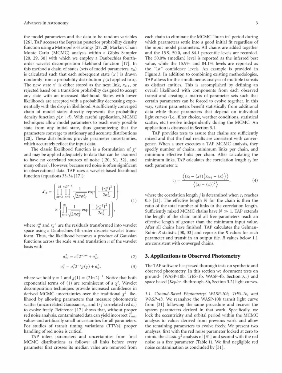
the model parameters and the data to be random variables[26]. TAP accesses the Bayesian posterior probability densityfunction using a Metropolis-Hastings [27, 28] Markov ChainMonte Carlo (MCMC) analysis within a Gibbs Sampler[20, 29, 30] with which we employ a Daubechies fourth-order wavelet decomposition likelihood function [17]. Inthis method a chain of states (sets of model parameters, xn)is calculated such that each subsequent state (x′) is drawnrandomly from a probability distribution f (x) applied to xi.The new state x′ is either stored as the next link, xi+1, orrejected based on a transition probability designed to acceptany state with an increased likelihood. States with lowerlikelihoods are accepted with a probability decreasing expo-nentially with the drop in likelihood. A sufficiently convergedchain of model states directly represents the probabilitydensity function p(x | d). With careful application, MCMCtechniques allow model parameters to reach every possiblestate from any initial state, thus guaranteeing that theparameters converge to stationary and accurate distributions[20]. These distributions provide parameter uncertainties,which accurately reflect the input data.

The classic likelihood function is a formulation of χ2

and may be applied adequately to data that can be assumedto have no correlated sources of noise ([20, 31, 32], andmany others). However, because red noise is often significantin observational data, TAP uses a wavelet-based likelihoodfunction (equations 33-34 [17]):

Lx =⎧⎪⎨

⎪⎩

M∏

m=2

n02m−1∏

n=1

1√

2πσ2W

exp

[

−(rmn)2

2σ2W

]⎫⎪⎬

⎪⎭

×⎧⎪⎨

⎪⎩

n0∏

n=1

1√

2πσ2S

exp

[

−(r−1n

)2

2σ2S

]⎫⎪⎬

⎪⎭,

(1)

where rmn and r−1n are the residuals transformed into wavelet

space using a Daubechies 4th-order discrete wavelet trans-form. Thus, the likelihood becomes a product of Gaussianfunctions across the scale m and translation n of the waveletbasis with

σ2W = σ2

r 2−γm + σ2w, (2)

σ2S = σ2

r 2−γg(γ)

+ σ2w, (3)

where we hold γ = 1 and g(1) = (2 ln 2)−1. Notice that bothexponential terms of (1) are reminiscent of a χ2. Waveletdecomposition techniques provide increased confidence inderived MCMC uncertainties over the traditional χ2 like-lihood by allowing parameters that measure photometricscatter (uncorrelated Gaussian σw, and 1/ f correlated red σr)to evolve freely. Reference [17] shows that, without properred noise analysis, contaminated data can yield incorrectTmid

values and artificially small uncertainties for all parameters.For studies of transit timing variations (TTVs), properhandling of red noise is critical.

TAP infers parameters and uncertainties from finalMCMC distributions as follows: all links before everyparameter first crosses its median value are removed from

each chain to eliminate the MCMC “burn in” period duringwhich parameters settle into a good initial fit regardless ofthe input model parameters. All chains are added togetherand the 15.9, 50.0, and 84.1 percentile levels are recorded.The 50.0% (median) level is reported as the inferred bestvalue, while the 15.9% and 84.1% levels are reported asthe “1σ” confidence levels. An example is provided inFigure 3. In addition to combining existing methodologies,TAP allows for the simultaneous analysis of multiple transitsas distinct entities. This is accomplished by defining anoverall likelihood with components from each observedtransit and creating a matrix of parameter sets such thatcertain parameters can be forced to evolve together. In thisway, system parameters benefit statistically from additionaldata while those parameters that depend on individuallight curves (i.e., filter choice, weather conditions, statisticalscatter, etc.) evolve independently during the MCMC. Anapplication is discussed in Section 3.1.

TAP provides tests to assure that chains are sufficientlymixed and that the final results are consistent with conver-gence. When a user executes a TAP MCMC analysis, theyspecify number of chains, minimum links per chain, andminimum effective links per chain. After calculating theminimum links, TAP calculates the correlation length cj foreach parameter x:

cj =⟨

(xi − 〈x〉)(

xi+ j − 〈x〉)⟩

⟨

(xi − 〈x〉)2⟩ , (4)

where the correlation length j is determined when cj reaches0.5 [21]. The effective length N for the chain is then theratio of the total number of links to the correlation length.Sufficiently mixed MCMC chains have N � 1. TAP extendsthe length of the chain until all free parameters reach aneffective length of greater than the minimum input value.After all chains have finished, TAP calculates the Gelman-Rubin R statistic [30, 33] and reports the R values for eachparameter and transit in an output file. R values below 1.1are consistent with converged chains.

3. Applications to Observed Photometry

The TAP software has passed thorough tests on synthetic andobserved photometry. In this section we document tests onground- (WASP-10b, TrES-1b, WASP-4b, Section 3.1) andspace based (Kepler-4b through-8b, Section 3.2) light curves.

3.1. Ground-Based Photometry: WASP-10b, TrES-1b, andWASP-4b. We reanalyze the WASP-10b transit light curvefrom [31] following the same procedure and recover thesystem parameters derived in that work. Specifically, welock the eccentricity and orbital period within the MCMCanalysis to values derived from previous work and allowthe remaining parameters to evolve freely. We present twoanalyses, first with the red noise parameter locked at zero tomimic the classic χ2 analysis of [31] and second with the rednoise as a free parameter (Table 1). We find negligible rednoise contamination as concluded by [31].


Table 1: Analysis of Johnson et al., [34] WASP-10b light curve.

ParameterValue

Johnson et al. [34] TAP: no red noise TAP

Period [days] 3.0927616 · · · · · ·Inclination [deg] 88.49+0.22

−0.17 88.44+0.25−0.21 88.50+0.34

−0.25

a/Rs 11.65+0.09−0.13 11.60± 0.14 11.64± 0.16

Rp/Rs 0.1592+0.0005−0.0012 0.1593± 0.0012 0.1588+0.0014

−0.0017

Tmid [HJD since 2454664.0] 0.037295± 0.000082 0.03731± 0.0000660.037312±0.000087

A comparison between the analysis originally published by [17] and our TAP analysis. The results indicate that TAP reproduces the derived parameters andthat the light curve contains no significant red noise contamination. For all analyses, orbital period (P = 3.0927616 days) and eccentricity parameters (e =0.051, ω = 2.67 radians) were locked to values derived by [17] using RV data from [10].

We observed an additional transit of WASP-10b inthree bands (Barr V, R, and I) on UT August 22 2010 inclear but nonphotometric weather using the OrthogonalParallel Transfer Imaging Camera (OPTIC) mounted on theUniversity of Hawaii 2.2 m telescope on Mauna Kea. OPTIC’sunique Orthogonal Transfer Array CCD (OTA, see [34–36])provides submillimag precision through a technique calledPSF shaping where the light from the bright star beingocculted is spread out over a small box on the CCD duringexposure. Shaped-PSFs allow for longer exposure times onbright stars and improve the duty cycle by drawing out theexposure before incurring the 30-second readout. Betweeneach exposure the OPTIC filter wheel was advanced so thatthe transit light curve is fully covered by observations inV, R, and I bands. The light curves for each band wereproduced using basic aperture photometry techniques witha square aperture to account for the shaped PSFs. A relativelylarge aperture was chosen relative to the PSFs to account forvariable PSF scatter due to changing atmospheric conditions.Four background apertures located on each side of the PSFwere medianed and subtracted. Unlike [31] light curve rednoise contamination is evident (Figure 2).

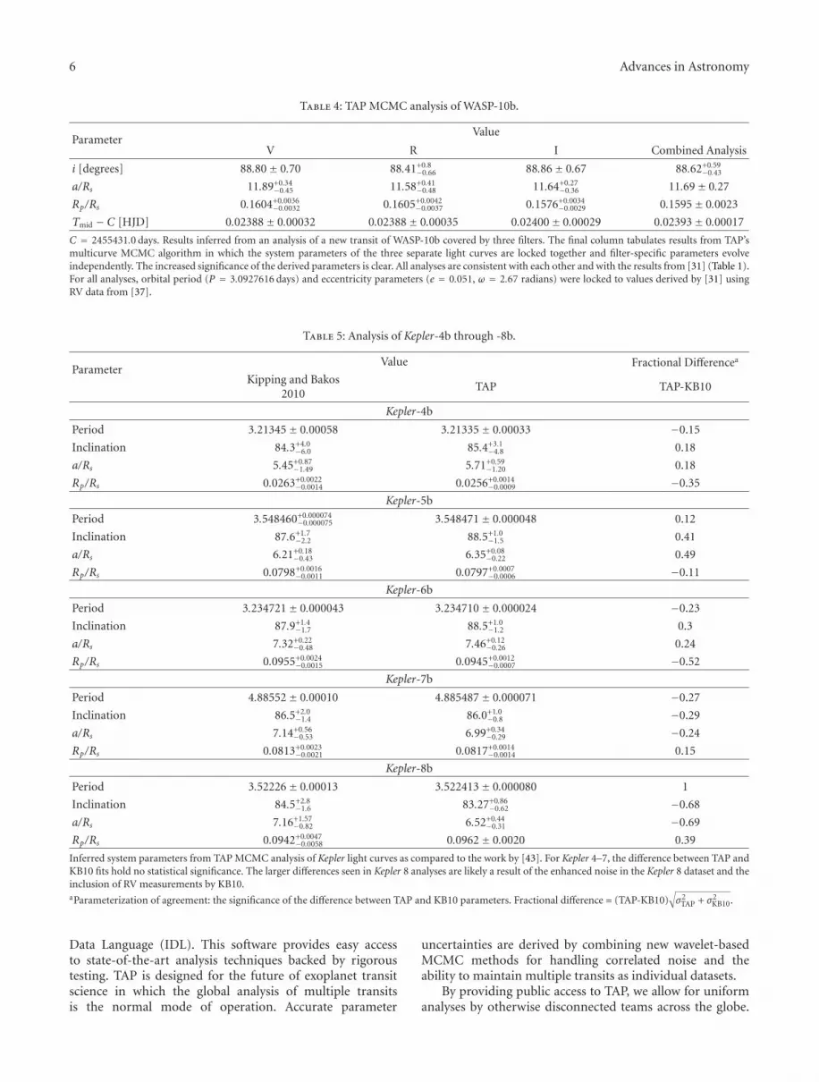
We conduct two analyses—one in which all transits areconsidered independent observations and a second in whichwe use the full power of TAP by locking system and orbitparameters into a single set (Section 2). For this combinedanalysis, parameters describing limb darkening, noise, anda quadratic trend to account for out-of-transit variationsremain independent per light curve. The results of theseanalyses are reported in Table 4. Each individual transit andthe combined set yield parameters consistent with [31].The TAP simultaneous analysis method shows improvedprecision in the derived system parameters while providinglimb-darkening coefficients in three photometric bands froma single observation. A final analysis was conducted bylocking the parameter for red noise at zero to mimic theclassic χ2, which derived parameters consistent but with errorbars scaled down by a factor of 0.7—an overestimation of thesignificance of the contaminated data.

In [31], a high precision (∼0.5 millimag) transit ofWASP-10b allowed for a robust MCMC fit in which onlyperiod and eccentricity parameters required constraint. Theresults of that work disagreed significantly with the discovery

0 1 2Hours from midtransit

0.96

0.98

1

1.02

Rel

ativ

e fl

ux

+ c

onst

ant

WASP-10 V

WASP-10 R

WASP-10 I

−1−2−3

Figure 2: A transit of WASP-10b collected in three filters usingOPTIC on UH 2.2m telescope via a filter flipping technique(Section 3.1). Blue curves represent the model light curve while redcurves are modified with the derived red noise.

parameters of [37], in particular for transit depth, yieldinga 16% smaller planetary radius (a 2.5σ change). Since then,two additional papers [38, 39] have supported the conclu-sions of the discovery paper—that WASP-10b is inflatedbeyond the theoretical predictions of radii of irradiatedJovian planets [40]. Our data agree with the smaller radiusmeasurement of [31], using the same instrument but withthree different filters. In our analysis, like that of [31],the limb-darkening parameters are allowed to vary freely,a robust method allowed by our high precision curves.Reference [37] locks these parameters at theoretical values,while the treatment of limb darkening in [38, 39] is unclear.We stress the importance of additional followup observationsto clarify these discrepancies and urge authors to provide thelight curves that they collect. This allows for reanalysis byother teams and is a boon to the community as a whole.


10 11 12 13

a/Rs

Rel

ativ

e fr

equ

ency

VR

I

Figure 3: Parameter extraction from Bayesian posterior probabilitydistribution. The solid black histogram displays a Bayesian posteriorprobability density distribution for the parameter a/Rs of thecombined analysis of three light curves of WASP-10b (Section 3.1).The solid vertical line marks the median (50.0 percentile), while thedashed vertical lines represent the ±1σ inferred statistics describedin Section 2. The additional histograms represent the posteriordistributions for independent analyses of each curve (V: dashedgreen, R: dash-dotted red, I: dotted gray).

Table 2: Analysis of 3 [41] TrES-1b light curves.

ParameterValue

[41] TAP

Period [days] 3.0300737 · · ·Inclination [deg] >88.4 (95% conf.) 89.01± 0.61

a/Rs 10.45± 0.15 10.46+0.13−0.23

Rp/Rs 0.13686± 0.00082 0.1375± 0.0012

Tmid [HJD since2453895.0]

0.84297± 0.00018 0.84298± 0.00019


0.87341± 0.00014 0.87341± 0.00018


0.90372± 0.00019 0.90371± 0.00020

A comparison between TAP and the analysis originally published by [41].Eccentricity and argument of periastron (e,ω) are locked at zero to mimicthe analysis in that work.

We reanalyze the three TrES-1b transit light curves of[41] and two WASP-4b transits of [42]. In both cases, allsystem parameters except Tmid are locked to a single set.The transit midtime Tmid, along with observation-specificparameters including noise and a linear airmass trend, wasallowed to evolve independently per transit observation.For both systems TAP reproduces the previously publishedsystem parameters. We report the results as a comparison tothe published values of [41] in Table 2 and [42] Table 3.

3.2. Space-Based Photometry: Kepler-4b through-8b. Ideally,multiple transits of an exoplanet are analyzed as a set. Thisestablishes a measurement of orbital period and increasesconfidence in derived parameters. In general, the transitmidtime of each observation is measured and the data is

Table 3: Analysis of 2 [42] WASP-4b light curves.

ParameterValue

[42] TAP

Period [days] 1.33823214 · · ·Inclination [deg] 88.56+0.98

−0.46 88.97± 0.65

a/Rs 5.473+0.015−0.051 5.476+0.023

−0.030

Rp/Rs 0.15375+0.00077−0.00055 0.15398± 0.00055

Tmid [BJD since2454697.0]

0.797489± 0.000055 0.797484±0.000054

Tmid [BJD since2454748.0]

0.650490± 0.000072 0.650490±0.000047

A comparison between TAP and the analysis originally published by [42].Eccentricity and argument of periastron (e,ω) are locked at zero to mimicthe analysis in that work.

phase folded into a single light curve for analysis. Theweaknesses of this technique are numerous, including aloss of per-transit midtime error, troublesome handling ofdifferent observing conditions, and the loss of ability tocharacterize the noise of each individual observation. In theera of Kepler and beyond, multiple transits are the normand often ground based followup provides additional dataof wildly differing quality.

TAP is designed for exactly such analyses, and reproduc-ing published system parameters for Kepler targets is an idealtest of these new methods. Data for Kepler-4b through-8bwere acquired through the MAST Kepler data archive. Wenormalized the Kepler flux around each transit event to anout-of-transit value of unity using a 5th-order polynomial fitto account for stellar flux variations over each transit epoch.During analysis TAP was set to calculate models with a factorof ten finer temporal cadence before rebinning that modelback to the observed 29.4-minute cadence. Eccentricityparameters were locked to assume circular orbits.

To compare with the results of [43] we use an argumentof fractional difference,

XTAP − XKB10√

σ2TAP + σ2

KB10

, (5)

where X are the parameter values and σ their 1-σ uncer-tainties. Thus, a fractional difference with absolute valueless than unity represents statistical agreement. The inferredsystem parameters (Table 5) show such agreement with thecomplementary method “A.c” of [43] for Kepler 4b–7b,where the authors assume circular orbits and allow limb-darkening parameters to evolve freely. In contrast to ouranalysis, [43] also takes into account RV measurements. Forthe case of Kepler-8b, the difference between TAP and KB10fits of orbital period is significant. This difference is likelyattributed to the increased noise in the Kepler 8 dataset andthe inclusion of radial velocity measurements by [43].

4. Summary

In this paper we present a graphical user interface-drivenexoplanet transit analysis package written in the Interactive


Table 4: TAP MCMC analysis of WASP-10b.

ParameterValue

V R I Combined Analysis

i [degrees] 88.80± 0.70 88.41+0.8−0.66 88.86± 0.67 88.62+0.59

−0.43

a/Rs 11.89+0.34−0.45 11.58+0.41

−0.48 11.64+0.27−0.36 11.69± 0.27

Rp/Rs 0.1604+0.0036−0.0032 0.1605+0.0042

−0.0037 0.1576+0.0034−0.0029 0.1595± 0.0023

Tmid − C [HJD] 0.02388± 0.00032 0.02388± 0.00035 0.02400± 0.00029 0.02393± 0.00017

C = 2455431.0 days. Results inferred from an analysis of a new transit of WASP-10b covered by three filters. The final column tabulates results from TAP’smulticurve MCMC algorithm in which the system parameters of the three separate light curves are locked together and filter-specific parameters evolveindependently. The increased significance of the derived parameters is clear. All analyses are consistent with each other and with the results from [31] (Table 1).For all analyses, orbital period (P = 3.0927616 days) and eccentricity parameters (e = 0.051, ω = 2.67 radians) were locked to values derived by [31] usingRV data from [37].

Table 5: Analysis of Kepler-4b through -8b.

ParameterValue Fractional Differencea

Kipping and Bakos2010

TAP TAP-KB10

Kepler-4b

Period 3.21345± 0.00058 3.21335± 0.00033 −0.15

Inclination 84.3+4.0−6.0 85.4+3.1

−4.8 0.18

a/Rs 5.45+0.87−1.49 5.71+0.59

−1.20 0.18

Rp/Rs 0.0263+0.0022−0.0014 0.0256+0.0014

−0.0009 −0.35

Kepler-5b

Period 3.548460+0.000074−0.000075 3.548471± 0.000048 0.12

Inclination 87.6+1.7−2.2 88.5+1.0

−1.5 0.41

a/Rs 6.21+0.18−0.43 6.35+0.08

−0.22 0.49

Rp/Rs 0.0798+0.0016−0.0011 0.0797+0.0007

−0.0006 −0.11

Kepler-6b

Period 3.234721± 0.000043 3.234710± 0.000024 −0.23

Inclination 87.9+1.4−1.7 88.5+1.0

−1.2 0.3

a/Rs 7.32+0.22−0.48 7.46+0.12

−0.26 0.24

Rp/Rs 0.0955+0.0024−0.0015 0.0945+0.0012

−0.0007 −0.52

Kepler-7b

Period 4.88552± 0.00010 4.885487± 0.000071 −0.27

Inclination 86.5+2.0−1.4 86.0+1.0

−0.8 −0.29

a/Rs 7.14+0.56−0.53 6.99+0.34

−0.29 −0.24

Rp/Rs 0.0813+0.0023−0.0021 0.0817+0.0014

−0.0014 0.15

Kepler-8b

Period 3.52226± 0.00013 3.522413± 0.000080 1

Inclination 84.5+2.8−1.6 83.27+0.86

−0.62 −0.68

a/Rs 7.16+1.57−0.82 6.52+0.44

−0.31 −0.69

Rp/Rs 0.0942+0.0047−0.0058 0.0962± 0.0020 0.39

Inferred system parameters from TAP MCMC analysis of Kepler light curves as compared to the work by [43]. For Kepler 4–7, the difference between TAP andKB10 fits hold no statistical significance. The larger differences seen in Kepler 8 analyses are likely a result of the enhanced noise in the Kepler 8 dataset and theinclusion of RV measurements by KB10.aParameterization of agreement: the significance of the difference between TAP and KB10 parameters. Fractional difference = (TAP-KB10)

√

σ2TAP + σ2

KB10.

Data Language (IDL). This software provides easy accessto state-of-the-art analysis techniques backed by rigoroustesting. TAP is designed for the future of exoplanet transitscience in which the global analysis of multiple transitsis the normal mode of operation. Accurate parameter

uncertainties are derived by combining new wavelet-basedMCMC methods for handling correlated noise and theability to maintain multiple transits as individual datasets.

By providing public access to TAP, we allow for uniformanalyses by otherwise disconnected teams across the globe.


Any method and implementation is prone to systematicerrors, and the increasing sophistication of transit analysistechniques provides an increasing possibility for codingerrors and severe systematics. By using the same tools, theeffects of systematics are marginalized and results fromseparate teams can be simply and meaningfully compared.Utilizing MCMC software, which accounts for correlatednoise, greatly increases the accuracy of derived parameteruncertainties, a critical component in transit science whereinaccurate error bars can lead to false claims of planet phaseamplitudes, secondary eclipse depths, and transit timing andshape variations.

TAP is one culmination of groundbreaking work bynumerous teams over the last ten years of exoplanettransit science. Our goal—to provide these state-of-the-arttechniques freely to all—arises from the needs of manyresearchers. These include professional astronomers, gradu-ate and undergraduate students, and amateur astronomers.With no need to conduct intensive software design cam-paigns, these individuals and teams may focus on interpret-ing the rich information available in their data. As Kepler andground based campaigns continue to collect light curves ofhundreds and soon thousands of exoplanet transits, the needfor such public software has never been greater.

TAP is publicly available at http://ifa.hawaii.edu/users/zgazak/IfA/TAP.html along with an example video and FAQfile.

Acknowledgments

The authors gratefully acknowledge discussions with JoshCarter relating to the new wavelet-based likelihood methodsand David Kipping and Gaspar Bakos for respondingthoughtfully to questions regarding their independent analy-sis of Kepler-4b through -8b. They thank the individuals whoprovided helpful insight and comments regarding early ver-sions of TAP, including especially John Rayner, Karen Collins,and Kaspar von Braun. J. A. Johnson was supported by theNSF Grant AST-0702821. A. W. Mann was supported by NSFgrant AST-0908419. For this work the authors made use ofthe UH 2.2 m telescope atop Mauna Kea. The authors wish toextend special thanks to those of Hawaiian ancestry on whosesacred mountain of Mauna Kea they are privileged to beguests. Without their generous hospitality, the observationspresented herein would not have been possible.

References

[1] B. Campbell and G. A. H. Walker, “Precision radial velocitieswith an absorption cell,” Publications of the AstronomicalSociety of the Pacific, vol. 91, pp. 540–545, 1979.

[2] R. P. Butler, G. W. Marcy, E. Williams, C. McCarthy, P.Dosanjh, and S. S. Vogt, “Attaining doppler precision of 3 ms-1 1,2,” Publications of the Astronomical Society of the Pacific,vol. 108, no. 724, pp. 500–509, 1996.

[3] M. Mayor and D. Queloz, “A jupiter-mass companion to asolar-type star,” Nature, vol. 378, no. 6555, pp. 355–359, 1995.

[4] G. W. Marcy and R. P. Butler, “A planetary companion to 70virginis,” The Astrophysical Journal Letters, vol. 464, no. 2, pp.L147–L151, 1996.

[5] G. W. Marcy, R. P. Butler, E. Williams et al., “The planetaround 51 pegasi,” The Astrophysical Journal Letters, vol. 481,no. 2, pp. 926–935, 1997.

[6] G. W. Henry, G. Marcy, R. P. Butler, and S. S. Vogt, “HD209458,” IAU Circulars, vol. 7307, p. 1, 1999.

[7] G. W. Henry, G. W. Marcy, R. P. Butler, and S. S. Vogt, “Atransiting ”51 peg-like” planet,” The Astrophysical Journal, vol.529, no. 1, pp. L41–L44, 2000.

[8] D. Charbonneau, T. M. Brown, D. W. Latham, and M. Mayor,“Detection of planetary transits across a sun-like star,” TheAstrophysical Journal, vol. 529, no. 1, pp. L45–L48, 2000.

[9] D. Charbonneau, T. M. Brown, A. Burrows, and G. Laughlin,“When extrasolar planets transit their parent stars,” Protostarsand Planets V, pp. 701–716, 2007.

[10] J. N. Winn, Exoplanet Transits and Occultations, 2010.[11] W. J. Borucki, D. Koch, G. Basri et al., “Kepler planet-detection

mission: introduction and first results,” Science, vol. 327, no.5968, pp. 977–980, 2010.

[12] B. Scott Gaudi, “On the size distribution of close-in extrasolargiant planets,” The Astrophysical Journal, vol. 628, no. 1, pp.L73–L76, 2005.

[13] B. S. Gaudi, S. Seager, and G. Mallen-Ornelas, “On theperiod distribution of close-in extrasolar giant planets,” TheAstrophysical Journal, vol. 623, no. 1 I, pp. 472–481, 2005.

[14] S. Seager and G. Mallen-Ornelas, “Extrasolar planet transitlight curves and a method to select the best planet candidatesfor mass follow-up,” Bulletin of the American AstronomicalSociety, vol. 34, p. 1138, 2002.

[15] K. Mandel and E. Agol, “Analytic light curves for planetarytransit searches,” The Astrophysical Journal Letters, vol. 580, no.2, pp. L171–L175, 2002.

[16] J. A. Carter, J. C. Yee, J. Eastman, B. S. Gaudi, and J.N. Winn, “Analytic approximations for transit light-curveobservables, uncertainties, and covariances,” The AstrophysicalJournal Letters, vol. 689, no. 1, pp. 499–512, 2008.

[17] J. A. Carter and J. N. Winn, “Parameter estimation from time-series data with correlated errors: a wavelet-based methodand its application to transit light curves,” The AstrophysicalJournal Letters, vol. 704, no. 1, pp. 51–67, 2009.

[18] J. Southworth, “Homogeneous studies of transiting extrasolarplanets—I. Light-curve analyses,” Monthly Notices of the RoyalAstronomical Society, vol. 386, no. 3, pp. 1644–1666, 2008.

[19] M. J. Holman, J. N. Winn, D. W. Latham et al., “Thetransit light curve project. I. Four consecutive transits of theexoplanet XO-1b,” The Astrophysical Journal, vol. 652, no. 2 I,pp. 1715–1723, 2006.

[20] E. B. Ford, “Quantifying the uncertainty in the orbits ofextrasolar planets,” Astronomical Journal, vol. 129, no. 3, pp.1706–1717, 2005.

[21] M. Tegmark, M. A. Strauss, M. R. Blanton et al., “Cosmolog-ical parameters from sdss and wmap,” Physical Review D, vol.69, no. 10, Article ID 103501, 2004.

[22] D. M. Kipping, “Morphological light-curve distortions dueto finite integration time,” Monthly Notices of the RoyalAstronomical Society, vol. 408, no. 3, pp. 1758–1769, 2010.

[23] J. Eastman, E. Agol, and S. Gaudi, “The TAP software packageuses EXOFAST,” in prep., 2011.

[24] A. Claret, “A new non-linear limb-darkening law for ltestellar atmosphere models III sloan filters: calculations for−5.0≤ log[m/h]≤+1, 2000 K≤Teff ≤ 50000 K at several sur-face gravities,” Astronomy & Astrophysics, vol. 428, no. 3, pp.1001–1005, 2004.


[25] A. Claret, “A new non-linear limb-darkening law for LTEstellar atmosphere models: calculations for−5.0 = log[M/H]=+1, 2000 K = Teff = 50000 K at several surface gravities,”Astronomy & Astrophysics, vol. 363, pp. 1081–1190, 2000.

[26] T. Bayes and Price, “An essay towards solving a problem in thedoctrine of chances,” Philosophical Transactions of the RoyalSociety of London, vol. 53, pp. 370–418, 1763.

[27] N. Metropolis, A. W. Rosenbluth, M. N. Rosenbluth, A. H.Teller, and E. Teller, “Equation of state calculations by fastcomputing machines,” Journal of Chemical Physics, vol. 21, no.6, pp. 1087–1092, 1953.

[28] W. K. Hastings, “Monte carlo sampling methods using markovchains and their applications,” Biometrika, vol. 57, no. 1, pp.97–109, 1970.

[29] S. Geman and D. Geman, “Stochastic relaxation, gibbsdistributions, and the bayesian restoration of images,” IEEETransactions on Pattern Analysis and Machine Intelligence, vol.6, no. 6, pp. 721–741, 1984.

[30] E. B. Ford, “Improving the efficiency of markov chain montecarlo for analyzing the orbits of extrasolar planets,” TheAstrophysical Journal, vol. 642, no. 1 I, pp. 505–522, 2006.

[31] J. A. Johnson, J. N. Winn, N. E. Cabrera, and J. A. Carter,“A smaller radius for the transiting exoplanet wasp-10b,” TheAstrophysical Journal Letters, vol. 692, no. 2, pp. L100–L104,2009.

[32] J. N. Winn, M. J. Holman, G. Torres et al., “The transit lightcurve project. ix. evidence for a smaller radius of the exoplanetXO-3b,” The Astrophysical Journal Letters, vol. 683, no. 2, pp.1076–1084, 2008.

[33] A. Gelman and D. Rubin, “Inference from iterative simulationusing multiple sequences,” Statistical Sciences, vol. 7, no. 4, pp.457–511, 1992.

[34] J. A. Johnson, J. N. Winn, and N. E. Cabrera, “Submillimagphotometry of transiting exoplanets with an orthogonaltransfer array,” Bulletin of the American Astronomical Society,vol. 41, p. 192, 2009.

[35] J. L. Tonry, S. B. Howell, M. E. Everett, S. A. Rodney, M.Willman, and C. Vanoutryve, “A search for variable stars andplanetary occultations in ngc 2301. I. Techniques,” Publicationsof the Astronomical Society of the Pacific, vol. 117, no. 829, pp.281–289, 2005.

[36] S. B. Howell and J. L. Tonry, “OPTIC—THE CCD camera forplanet hunting,” Bulletin of the American Astronomical Society,vol. 35, p. 1235, 2003.

[37] D. J. Christian, N. P. Gibson, E. K. Simpson et al., “Wasp-10b:a 3mj, gas-giant planet transiting a late-type k star,” MonthlyNotices of the Royal Astronomical Society, vol. 392, no. 4, pp.1585–1590, 2009.

[38] J. A. Dittmann, L. M. Close, L. J. Scuderi, and M. D.Morris, “Transit observations of the wasp-10 system,” TheAstrophysical Journal Letters, vol. 717, no. 1, pp. 235–238, 2010.

[39] T. Krejcova, J. Budaj, and V. Krushevska, “Photometricobservations of transiting extrasolar planet wasp—10 b,”Contributions of the Astronomical Observatory Skalnate Pleso,vol. 40, no. 2, pp. 77–82, 2010.

[40] N. Miller, J. J. Fortney, and B. Jackson, “Inflating and deflatinghot jupiters: coupled tidal and thermal evolution of knowntransiting planets,” The Astrophysical Journal Letters, vol. 702,no. 2, pp. 1413–1427, 2009.

[41] J. N. Winn, M. J. Holman, and A. Roussanova, “The transitlight curve project. iii. tres transits of tres-1,” The AstrophysicalJournal, vol. 657, no. 2 I, pp. 1098–1106, 2007.

[42] J. N. Winn, M. J. Holman, J. A. Carter, G. Torres, D. J.Osip, and T. Beatty, “The transit light curve project. XI.Submillimagnitude photometry of two transits of the bloatedplanet WASP-4b,” The Astrophysical Journal, vol. 137, pp.3826–3833, 2009.

[43] D. Kipping and G. Bakos, “An independent analysis of kepler-4b through kepler-8b,” The Astrophysical Journal Letters, vol.730, no. 1, article no. 50, 2011.

Submit your manuscripts athttp://www.hindawi.com

Hindawi Publishing Corporationhttp://www.hindawi.com Volume 2014

High Energy PhysicsAdvances in

The Scientific World JournalHindawi Publishing Corporation http://www.hindawi.com Volume 2014


FluidsJournal of

Atomic and Molecular Physics

Journal of



Advances in Condensed Matter Physics

OpticsInternational Journal of



AstronomyAdvances in

International Journal of


Superconductivity


Statistical MechanicsInternational Journal of


GravityJournal of


AstrophysicsJournal of


Physics Research International


Solid State PhysicsJournal of

Computational Methods in Physics

Journal of



Soft MatterJournal of

Hindawi Publishing Corporationhttp://www.hindawi.com

AerodynamicsJournal of

Volume 2014


PhotonicsJournal of


Journal of

Biophysics


ThermodynamicsJournal of

transit analysis package: an idl graphical user interface for exoplanet transit photometry

Documents