development of a predictive model for spoilage of cooked cured meat products and its validation...

M:F

ood

Mic

robi

olog

y&

Safe

ty

JFS M: Food Microbiology and Safety

Development of a Predictive Model forSpoilage of Cooked Cured Meat Productsand Its Validation Under Constant andDynamic Temperature Storage ConditionsM. MATARAGAS, E.H. DROSINOS, A. VAIDANIS, AND I. METAXOPOULOS

ABSTRACT: In the present study, the spoilage flora of a sliced cooked cured meat product was studied to determine thespecific spoilage organism (SSO). The physicochemical changes of the product during its storage in a temperaturerange of 0 to 12 ◦C were also studied. Among the primary models used to model the temperature effect on SSOgrowth, the modified Gompertz described better the experimental data than modified logistic and Baranyi. Thederived growth kinetic parameters, such as maximum specific growth rate (μmax) and lag phase duration (LPD),were modeled by using the square root and Arrhenius equation (secondary models). The latter described better thedata of μmax and LPD; therefore, this model was chosen for correlating temperature with kinetic parameters. Theselection of the best model (primary or secondary) was based on some statistical indices (the root mean square errorof residuals of the model, the coefficient of multiple determination, the F-test, the goodness of fit, the bias, andaccuracy factor). The validation of the developed model was carried out under constant and dynamic temperaturestorage conditions. To validate its usefulness to similar products, another sliced cooked cured meat product storedunder constant temperature conditions was also used. The log shelf life model was used for shelf life predictionsbased on the evident (visual defects) or the incipient spoilage (attainment of a certain spoilage level by SSO and/orchemical spoilage index). The possibility for shelf life predictions constitutes a valuable information source for thequality assurance systems of meat industries.

Keywords: lactic acid bacteria, meat products, modeling, spoilage, validation

Introduction

The development and application of mathematic equations thatdescribe the growth kinetics of microorganisms have gained in-

creasing attention as a means of predicting the growth of pathogenicand spoilage organisms, determining in this way the remaining shelflife of the products (Dalgaard 1995a, 1995b; Wijtzes and others 1995;Malakar and others 1999; Koutsoumanis and Nychas 2000; Shimoniand Labuza 2000; Castillejo-Rodrıguez and others 2002). Thus, pre-dictive microbiology is rendered a reliable and economic tool forrapid shelf life determinations. The majority of predictive modelsthat have been developed use experimental data from trials con-ducted in laboratory media. These kinds of models in some casesoverestimate the microbial growth in comparison with the one thathappens in food since interaction between the microorganisms,structure, and composition of the product are not taken into con-sideration (Pin and Baranyi 1998; Pin and others 1999).

Meat spoilage is caused mainly by microorganisms and includesdiscoloration, changes in texture, slime formation, development ofoff-odors and off-flavors as a result of microbial growth. However,within a certain range of environmental conditions, often only onemember from the total microflora is responsible for spoilage (spe-cific spoilage organism—SSO). The spoilage is caused when a certainspoilage level is reached by the SSO and/or the microbial metabolic

MS 20060017 Submitted 1/11/2006, Accepted 4/14/2006. The authors are withAgricultural Univ. of Athens, Dept. of Food Science and Technology, Labora-tory of Food Quality Control and Hygiene, Iera Odos 75, GR-118 55, Athens,Greece. Direct inquiries to author Drosinos (E-mail: [email protected]).

product (Chemical Spoilage Index—CSI) (Huis in’t Veld 1996; Gramand Dalgaard 2002).

The main factor that influences the microbial spoilage is the tem-perature, which is related to the maximum specific growth rate andthe lag phase duration (LPD) of microorganisms. Primary modelsdescribe the changes in the microbial population over time, whereassecondary models describe the effect of environmental factors onthe growth kinetic parameters (Whiting 1995).

The objective of the present study was to develop a predictivespoilage model capable of giving reliable and fast shelf life predic-tions. For this reason, a sliced cooked cured meat product was usedbecause in this way possible effects of microbial competitiveness,food structure, and food composition on the growth of SSO, whichmay lead to prediction errors, are included in the model since thegrowth data of SSO are obtained from trials in naturally contami-nated meat product. Furthermore, the model was validated underdynamic temperature storage conditions, which very often are en-countered in chill chains, and also to another meat product of thesame category to evaluate its applicability to other similar products.

Materials and Methods

An overview of the experimental setupThe procedure applied by Koutsoumanis and Nychas (2000) to

develop a predictive model for rapid fish shelf life predictions wasalso followed in the present study. The identification of the SSOand its spoilage level was determined by studying the growth of dif-ferent types of microorganisms in 2 independent series (different

C© 2006 Institute of Food Technologists Vol. 71, Nr. 6, 2006—JOURNAL OF FOOD SCIENCE M157doi: 10.1111/j.1750-3841.2006.00058.xFurther reproduction without permission is prohibited

M:Food

Microbiology

&Safety

Modeling of spoilage of cooked meat products . . .

batches of product) of storage trials (Table 1). Microbiological andphysicochemical analysis with naturally contaminated meat prod-ucts was conducted. The vacuum-packaged samples were stored at4 different controlled temperatures (0, 4, 8, and 12 ◦C ± 0.2 ◦C) (HighPrecision Incubator, MIR153, Sanyo Electric Co., Ora-Gun, Gunma,Japan) and the temperature was monitored by using temperatureloggers (Comark EVt2 Data Loggers, Stevenage, U.K.). Independentexperiments were also conducted for the validation of the devel-oped model under constant (7 and 10 ◦C) and dynamic temperatureconditions (2 different temperature profiles). Furthermore, anothermeat product of the same category (Table 1) was chosen for modelvalidation purposes and the samples were stored at the followingconstant temperatures: 0, 4, 8, and 12 ◦C. The temperature historyof the stored products was recorded as before. The end of the shelflife of the products was evaluated based on the following criteria:visual defects such as discoloration, detachment of packaging ma-terial (CO2 formation), drip loss, slime formation, sour off-flavors,and pH decrease (evident spoilage), and the achievement of a cer-tain spoilage level determined by the level of SSO population and/orthe concentration of CSI (D-lactate) produced by the SSO (incipi-ent spoilage). The predictive spoilage model is applicable within theexperimental limits determined by the product characteristics (pH,6.26 to 6.48; aw, 0.977 to 0.983; NaCl, 2.0%, and initial microbial loadof SSO, 0.5 to 1.5 log colony forming units [CFU]/g) and temperaturestorage conditions (0 to 12 ◦C).

Meat productsThe meat products used in the experiment were sliced cooked

cured meat products (“pik-nik” used for the development andvalidation of the model will be referred as SCCMP1 in the text;“pork shoulder” used for the validation of the model will be re-ferred as SCCMP2 in the text) and their final composition is dis-played in Table 1. The packaging materials used were 2 differentpolyamide/polyethylene-type foils, MULTILAM PA/PE 90 μm (up-per foil) and MULTIFOL GA PA/PE 170 μm (bottom foil) with lowoxygen permeability (50 cm3/m2/day at 23 ◦C for MULTILAM and13 cm3/m2/day at 23 ◦C for MULTIFOL GA). Each package contained2 slices of the product. The weight of each slice was 25 g having thefollowing dimensions (H × L × W): 10 cm × 10 cm × 0.5 mm.

Microbiological analysisA 25-g unit of sample, taken randomly from the 2 slices, was

weighed and aseptically transferred into a sterile stomacher bag(Seward, London, U.K.). Then 225 mL of sterile saline peptone(0.1% [wt/v] peptone and 0.85% [wt/v] NaCl) (Merck, Darmstadt,Germany) were added and the sample was homogenized in a stom-acher (Lab Blender 400, Seward, London, U.K.) for 2 min at nor-mal speed at room temperature. Serial decimal dilutions in sterile 1

4

Table 1 --- Final composition of the used sliced cookedcured meat products

% Composition

SCCMP (model SCCMPComponent development/validation) (model validation)

Pork meat 45 60Pork fat 21 –Water 25 32NaCl 2 1.8Curing salts 0.5 0.35Starch 5 5Spices 1.5 0.85Initial pH value 6.26–6.48 6.33–6.64Initial aw value 0.977–0.983 0.982–0.988

SCCMP, sliced cooked cured meat product.

strength Ringer’s solution (Merck, Darmstadt, Germany) were pre-pared from this 10−1 dilution and 1 or 0.1 mL samples from 3 appro-priate dilutions were poured (enterobacteria) or plated in triplicateon total count and selective agars.

Total viable counts (TVC) were determined on Plate Count Agar(PCA, Merck, Darmstadt, Germany), incubated at 30 ◦C for 72 h;lactic acid bacteria (LAB) on de Man, Rogosa, Sharpe agar (MRSagar, Merck, Darmstadt, Germany), incubated at 30 ◦C for 72 h un-der anaerobic conditions (Gas-Pack System, BBL, Becton Dickinson,Franklin Lakes, N.J., U.S.A.); pseudomonads on Cetrimide-Fucidin-Cephaloridine medium (CFC, Pseudomonas agar base, Oxoid, Bas-ingstoke, U.K.), incubated at 25 ◦C for 48 h; yeasts on Yeast ex-tract Glucose Chloramphenicol agar (YGC agar, Merck, Darmstadt,Germany), incubated at 25 ◦C for 5 d; Brochothrix thermosphactaon Streptomycin Thallous Acetate Actidione agar (STAA agar base,Biolife, Milano, Italy), incubated at 25 ◦C for 48 h; and enterobac-teria in crystal-Violet neutral-Red Bile D(+)-glucose agar (VRBDagar, Merck, Darmstadt, Germany), overlaid with 5 mL of the samemedium and the plates were incubated at 37 ◦C for 24 h.

The plates were examined visually for typical colonies and mor-phological characteristics that were associated with each growthmedium. The selectivity of the growth media was also checked bycarrying out rapid tests (for example, Gram and catalase reaction)on about 10% of the colonies grown on countable plates, accordingto Harrigan and McCance (1976).

Physicochemical analysisThe pH was measured according to the British method for meat

and meat products (ISO 3100, British Standard Institution[1975] formeat and meat products) by using a digital pH-meter (WTW, pH526, Weilheim, Germany). The water activity (aw) was measuredwith a calibrated electric hygrometer, Rotronic HygroLab (Rotronic,Bassersdorf, Switzerland). For the determination of lactate and ac-etate, the samples were prepared according to Skandamis and oth-ers (2000) and analyzed in high performance liquid chromatography(HPLC) (Waters 600E System Controller, Millipore, Bedford, Mass.,U.S.A.). HPLC analysis was performed under the following condi-tions: HPLC organic acid analysis column, HyperREZ XP organicacid column, 100 × 7.7 mm (ThermoHypersil-Keystone, Cheshire,UK); Sample, 20 μL; eluent, 5mM sulfuric acid (Merck); flow rate, 0.7mL/min, temperature, 57 ◦C (Column heater, Jones Chromatogra-phy, Model 7971, Pontypridd, U.K.); detection, UV at 210 nm (UV Wa-ters 486 Tunable Absorbance Detector, Millipore, Mass., U.S.A.). D-and L-lactate were assayed enzymatically by the methods describedby Gawehn (1984) and Noll (1984), respectively, and the sampleswere prepared according to Drosinos and Board (1995). The enzy-matic kit of D- and L-lactate of Boehringer Mannheim (BoehringerMannheim GmbH, Mannheim, Germany) was supplied by Roche(Nutley, N.J., U.S.A.). The analytical method and calculations wereperformed in accordance with suppliers’ instructions.

Primary modelsThe following most commonly used primary models were fitted

to the data sets (all the data from the 2 replicates were modeled)from SSO growth in order to determine the growth kinetic parame-ters, such as maximum specific growth rate (μmax), LPD, initial andmaximum population (N 0 and N max, respectively):

a. modified Gompertz function (Gibson and others 1987):

Nt = A + C × exp{− exp[−B × (t − M )]}

where Nt , the cell number (log CFU/g) at any time t; A, the lowerasymptotic line of the growth curve as t decreases to zero (initial

M158 JOURNAL OF FOOD SCIENCE—Vol. 71, Nr. 6, 2006 URLs and E-mail addresses are active links at www.ift.org

M:F

ood

Mic

robi

olog

y&

Safe

ty


population level, N 0) (log CFU/g); C, the difference between theupper asymptotic line of the growth curve (maximum popula-tion level, N max) minus the lower asymptotic line (for example,N max − N 0) (log CFU/g); B, the relative maximum growth rate(d−1) at time M ; and M , the time at which the growth rate is max-imum (d). Then, μmax (d−1) and LPD (d) can be calculated by theequations:

μmax = BCe

where

e = 2.7182

LPD = M − 1B

Nmax = A + C

b. modified logistic function (Gibson and others 1987):

Nt = A + C1 + exp[−B × (t − M )]

where Nt , A, B, M, and C have the same meaning as given for themodified Gompertz equation. The μmax and LPD parameters arecalculated as follows:

μmax = BC4

LPD = M − 2B

c. Baranyi function (Baranyi and Roberts 1994):

Nt = N0 + μmax × At + ln[

1 + exp(μmax × At) − 1exp(Nmax − N0)

]where Nt , the bacterial population at any time t (ln CFU/g); N max

and N 0, the maximum and initial population level, respectively(ln CFU/g); μmax, the maximum specific growth rate (d−1); andAt , an adjustment function as defined by Baranyi and Roberts(1994), considered to account for the physiological state of thecells. Its role is to define the LPD. At parameter is calculated by theequation:

At = t + 1μmax

× ln{exp (−μmax × t)

+ exp (−h0) − exp [(−μmax × t) − h0]}

where h0 is simply a transformation of the initial conditions.The modified Gompertz and modified logistic equations were

fitted to the growth data by nonlinear regression with a Marquardtalgorithm using the StatGraphics Plus 2.1 computer-based program(Statistical Graphics Corp., Herndon, Va., U.S.A.), whereas for fittingpurposes with the Baranyi function the DMFit program was used(Institute of Food Research, Norwich, UK).

The statistical indices used to compare the models were the fol-lowing (Ross 1996; Giannuzzi and others 1998; te Giffel and Zwieter-ing 1999):

a. The root mean square error of the residuals of the model(RrMSE model). This is the standard deviation of the residuals. The

lower the RrMSE model the better the adequacy of the model to de-scribe the data. It is calculated by the equation:

RrMSEmodel =√

RSSDF

=

√√√√√√n∑

i=1

(xo

i − xfi

)2

n − s

where RSS, the residual sum of squares; DF , the degrees of freedom;n, the number of data points; s, the number of parameters of themodel; xi

o, the observed values; and xif, the fitted values.

b. The coefficient of multiple determination (R2). The R2 is thefraction of the square of the deviations of the observed values abouttheir mean explained by the equation fitted to the experimental data.R2 values close to 1 shows that the curve comes closer to the data. Itis calculated by the equation:

R2 = 1 −

n∑i=1

(observedi − predictedi

)2

n∑i=1

(observedi − mean

)2

where n, the total number of data points; mean, the average valuefrom all observed values, for example, mean = ∑n

i=1 observedi/.n.c. The F-test. The adequacy of the primary models to describe the

experimental data was also evaluated by the comparison of residualmean square errors between model (rMSE model) and data (rMSE data).The rMSE data was calculated according to Zwietering and others(1994). The rMSE model is derived from the equation:

rMSEmodel = (RrMSEmodel)2

The F-value (f ) was used to decide if the deviation of the model wassignificantly larger than the experimental error:

f = rMSEmodel

rMSEdata

Then, f is tested against F table value (95% confidence). If f is smallerthan F table value (F DFmodel

DFdata) then the F-test is accepted and this indi-

cates that the model describes the observed data well. The DF model

and DF data are the degrees of freedom of the model (number ofdata points minus number of parameters) and data (number of datapoints minus number of time points), respectively.

Secondary modelsTwo equations for the modeling of the growth parameters (μmax

and LPD) were used: the square root (Ratkowsky and others 1982)and Arrhenius functions, which have been widely used for describ-ing the effect of temperature on μmax and LPD of SSOs (Giannuzziand others 1998; Koutsoumanis and Nychas 2000; Cayre and others2003):

a. Square root equation:

√μmax = aμ × (T − Tmin)√

1LPD

= aLPD × (T − Tmin)

where aμ and aLPD, the slope of the regression line for μmax and LPD,respectively [(d−1)−1/2 ◦C−1]; and T min, the theoretical minimumtemperature value for cell growth (◦C).

URLs and E-mail addresses are active links at www.ift.org Vol. 71, Nr. 6, 2006—JOURNAL OF FOOD SCIENCE M159

M:Food

Microbiology

&Safety


b. Arrhenius equation:

ln μmax = ln Aμ −(

Ea

RT

)ln

(1

LPD

)= ln ALPD −

(Ea

RT

)where Aμ and ALPD are pre-exponential factors to enable the modelto fit the data of μmax and LPD, respectively (d−1); Ea, the activa-tion energy for bacterial growth (kJ/mol); R, the gas constant (8.314J/mol × K); and T , the absolute temperature (K). The equations werefitted to the experimental data using StatGraphics Plus 2.1. The sta-tistical indices used to evaluate the adequacy of the models to de-scribe the data were (Ross 1996):

a. The bias factor (Bf ). The Bf estimates the mean differencebetween the observed and predicted values. It assesses whetherthe model is “fail-safe” or “fail-dangerous.” When Bf is above one(Bf > 1) for LPD is “fail-dangerous”, but for μmax the model is “fail-dangerous” when Bf is below one (Bf < 1). If Bf is equal to onethen there is on average a perfect agreement between predicted andobserved values. The Bf is expressed as:

B f = 10[∑n

i=1 log(predictedi /observedi )/n]

where n, the number of data points; predicted values are the μmax

(d−1) and LPD (d) that were predicted from the model; observedvalues are the μmax (d−1) and LPD (d) that were experimentallyobserved.

b. The accuracy factor (Af ). Because Bf provides no indication ofthe accuracy of the model, Af is also used. Af shows how accurate themodel is, meaning how close the predicted values are to observedvalues. It takes values above one and the larger the value the lessaccurate is the model, and if Af is equal to one then there is a per-fect agreement between predicted and observed values. Af can becalculated by the equation:

A f = 10[∑n

i=1 |log(predictedi/observedi )|/n]

where n, predicted and observed values as before.c. The coefficient of multiple determination (R2). The R2 has the

same meaning as given before.d. The goodness of fit (GoF). The GoF is the root mean square error

of the model (RMSEmodel) and is analogous to the Af. It is calculatedby using the equation of RrMSEmodel, as previously described, withthe exception that the denominator (DF) is equal with n (number ofdata points) instead of n – s.

Validation of the modelThe modified Gompertz equation was used to predict the growth

of SSO at constant temperature storage conditions whereas the dy-namic model developed by Baranyi and others (1995) for predict-ing growth of Brochothrix thermosphacta at changing temperaturewas used to predict the growth of SSO under fluctuating tempera-ture storage conditions. The validation of the predictive model wasevaluated by the graphical comparison of predictive and observedvalues, and by using the bias and accuracy factors.

Shelf life predictionsWhen the temperature range of concern is relatively narrow (0 to

12 ◦C) then the shelf life of a product can be determined by using thelog shelf life model (Labuza and Fu 1993). In this case, the regressionline between the parameter of concern, for example, end of shelf life(time needed for the appearance of visual defects or time needed

by SSO or CSI to reach their maximum level) and temperature isstraight. The log shelf life equation is expressed as:

ts = t0 × exp (−b × T )

where ts, the shelf life (d) at any temperature T within the examinedrange; t 0, the shelf life (d) at 0 ◦C; and b, the slope of the regressionline of plot ln ts = f(T).

Alternatively, the following shelf life equation can be used whenthe end of shelf life is considered the time needed by the SSO toincrease from its initial to spoilage level (Ratkowsky 2004):

SL = LPD + tg × log (Nmax/N0)log (2)

where SL, the shelf life of the product (d); N max and N 0, the maximumand initial population level, respectively (CFU/g); LPD, the durationof lag phase (d); and tg , the generation time (d).

Results and Discussion

Identification of SSO and its spoilage levelThe microorganisms examined were those that usually dominate

and spoil meat and its products based on storage conditions (for ex-ample, gas atmosphere and temperature) and product composition(for example, pH and salt content). The results from the microbio-logical analysis of SCCMP1 and SCCMP2 showed that LAB were byfar the most prevalent spoilage microorganisms among the others(3 to 4 logs difference in final population). Initial populations werebelow the detection limit (101 CFU/g for Enterobacteriaceae and 102

CFU/g for the rest of microorganisms). The growth of LAB followedthe growth of TVC with a final population of 8.3 to 8.9 and 8.4 to9.0 log CFU/g, respectively. Brochothrix thermosphacta and yeastsgrew to a final population of 4.3 to 5.1 and 3.8 to 4.3 log CFU/g,respectively, but the low permeability of package material to oxy-gen, the presence of nitrites (150 mg/kg), and the decrease of pH byLAB limited their growth at much lower population levels than thatof LAB. Finally, the growth of Enterobacteriaceae and Pseudomonasspp. did not exceed the level of 3 log CFU/g (2.4 to 2.7 and 2.8 to 3.0log CFU/g, respectively). Thus, LAB were the predominant microor-ganisms of the 2 examined meat products. The presence of curingsalts, the vacuum packaging, and the low temperatures form an en-vironment that favors the growth of psychrotrophic LAB, such asLeuconostoc spp. and Lactobacillus spp. (von Holy and others 1991).Furthermore, the high initial pH and aw value in combination withthe low salt content of the products do not constitute hurdles toinhibit the microbial growth of spoilage microorganisms. LAB nat-urally dominate the microflora of many foods, including raw meatsand meat products that are chill-stored under vacuum, causing theirspoilage (Borch and others 1996).

The physicochemical analysis of the 2 products showed that theinitial pH and aw value ranged between 6.3 to 6.6 and 0.98 to 0.99,respectively. During the storage, pH decreased to a final value of5.0 to 5.5 whereas aw remained almost constant. The results ob-tained from the HPLC analysis of the organic acids showed thatthe initial and final lactate concentration was 150 to 220 mg/100gand 400 to 550 mg/100g, respectively. The acetate concentrationalso increased during storage (100 to 150 mg/100 g increase) butits production rate was slower compared to that of lactate. The2 isomers of lactate (L- and D-lactate) were distinguished enzy-matically. The L-lactate decreased from the initial concentration of130 to 250 mg/100g to 90 to 200 mg/100g whereas D-lactate wasinitially not detectable but increased to a final concentration of


M:F

ood

Mic

robi

olog

y&

Safe

ty


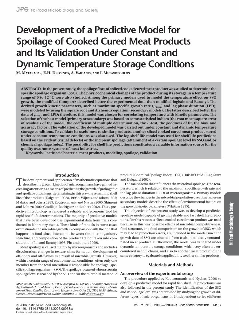
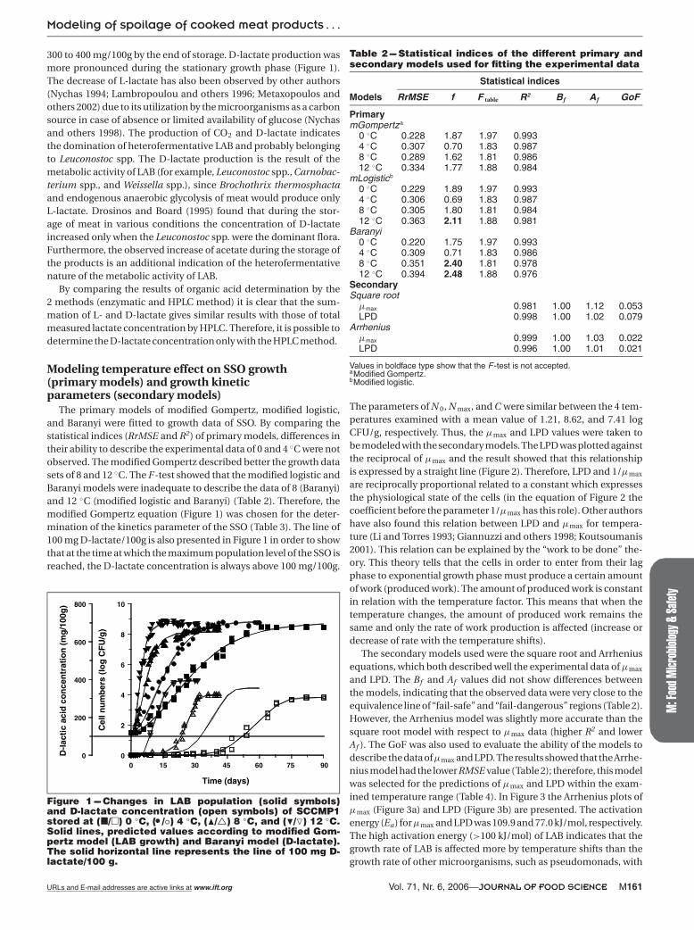
300 to 400 mg/100g by the end of storage. D-lactate production wasmore pronounced during the stationary growth phase (Figure 1).The decrease of L-lactate has also been observed by other authors(Nychas 1994; Lambropoulou and others 1996; Metaxopoulos andothers 2002) due to its utilization by the microorganisms as a carbonsource in case of absence or limited availability of glucose (Nychasand others 1998). The production of CO2 and D-lactate indicatesthe domination of heterofermentative LAB and probably belongingto Leuconostoc spp. The D-lactate production is the result of themetabolic activity of LAB (for example, Leuconostoc spp., Carnobac-terium spp., and Weissella spp.), since Brochothrix thermosphactaand endogenous anaerobic glycolysis of meat would produce onlyL-lactate. Drosinos and Board (1995) found that during the stor-age of meat in various conditions the concentration of D-lactateincreased only when the Leuconostoc spp. were the dominant flora.Furthermore, the observed increase of acetate during the storage ofthe products is an additional indication of the heterofermentativenature of the metabolic activity of LAB.

By comparing the results of organic acid determination by the2 methods (enzymatic and HPLC method) it is clear that the sum-mation of L- and D-lactate gives similar results with those of totalmeasured lactate concentration by HPLC. Therefore, it is possible todetermine the D-lactate concentration only with the HPLC method.

Modeling temperature effect on SSO growth(primary models) and growth kineticparameters (secondary models)

The primary models of modified Gompertz, modified logistic,and Baranyi were fitted to growth data of SSO. By comparing thestatistical indices (RrMSE and R2) of primary models, differences intheir ability to describe the experimental data of 0 and 4 ◦C were notobserved. The modified Gompertz described better the growth datasets of 8 and 12 ◦C. The F-test showed that the modified logistic andBaranyi models were inadequate to describe the data of 8 (Baranyi)and 12 ◦C (modified logistic and Baranyi) (Table 2). Therefore, themodified Gompertz equation (Figure 1) was chosen for the deter-mination of the kinetics parameter of the SSO (Table 3). The line of100 mg D-lactate/100g is also presented in Figure 1 in order to showthat at the time at which the maximum population level of the SSO isreached, the D-lactate concentration is always above 100 mg/100g.

0 15 30 45 60 75 90

Time (days)

0

2

4

6

8

10

Cell n

um

bers

(lo

g C

FU

/g)

0

200

400

600

800

D-l

acti

c a

cid

co

ncen

trati

on

(m

g/1

00g

)

Figure 1 --- Changes in LAB population (solid symbols)and D-lactate concentration (open symbols) of SCCMP1stored at (�/�) 0 ◦C, ( �/◦) 4 ◦C, (�/�) 8 ◦C, and (�/�) 12 ◦C.Solid lines, predicted values according to modified Gom-pertz model (LAB growth) and Baranyi model (D-lactate).The solid horizontal line represents the line of 100 mg D-lactate/100 g.

Table 2 --- Statistical indices of the different primary andsecondary models used for fitting the experimental data

Statistical indices

Models RrMSE f F table R2 Bf Af GoF

PrimarymGompertza

0 ◦C 0.228 1.87 1.97 0.9934 ◦C 0.307 0.70 1.83 0.9878 ◦C 0.289 1.62 1.81 0.98612 ◦C 0.334 1.77 1.88 0.984

mLogisticb

0 ◦C 0.229 1.89 1.97 0.9934 ◦C 0.306 0.69 1.83 0.9878 ◦C 0.305 1.80 1.81 0.98412 ◦C 0.363 2.11 1.88 0.981

Baranyi0 ◦C 0.220 1.75 1.97 0.9934 ◦C 0.309 0.71 1.83 0.9868 ◦C 0.351 2.40 1.81 0.97812 ◦C 0.394 2.48 1.88 0.976

SecondarySquare root

μmax 0.981 1.00 1.12 0.053LPD 0.998 1.00 1.02 0.079

Arrheniusμmax 0.999 1.00 1.03 0.022LPD 0.996 1.00 1.01 0.021

Values in boldface type show that the F -test is not accepted.aModified Gompertz.bModified logistic.

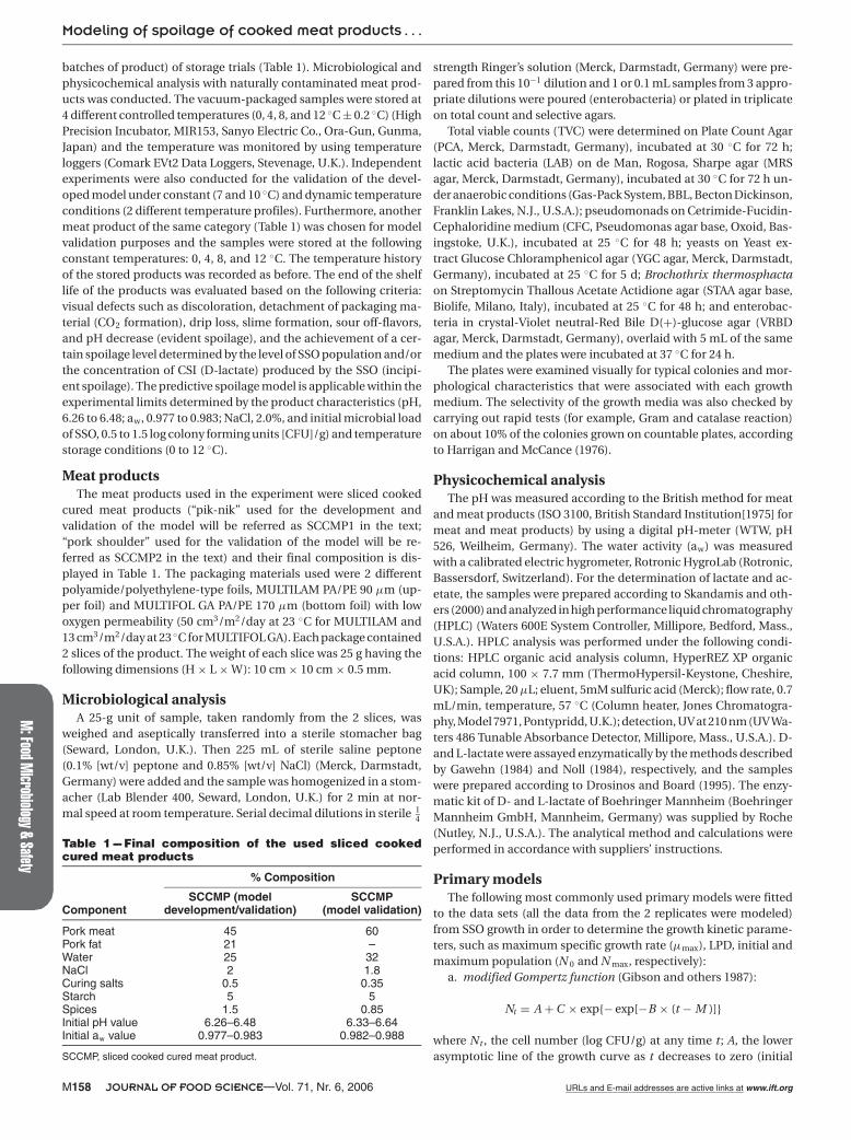
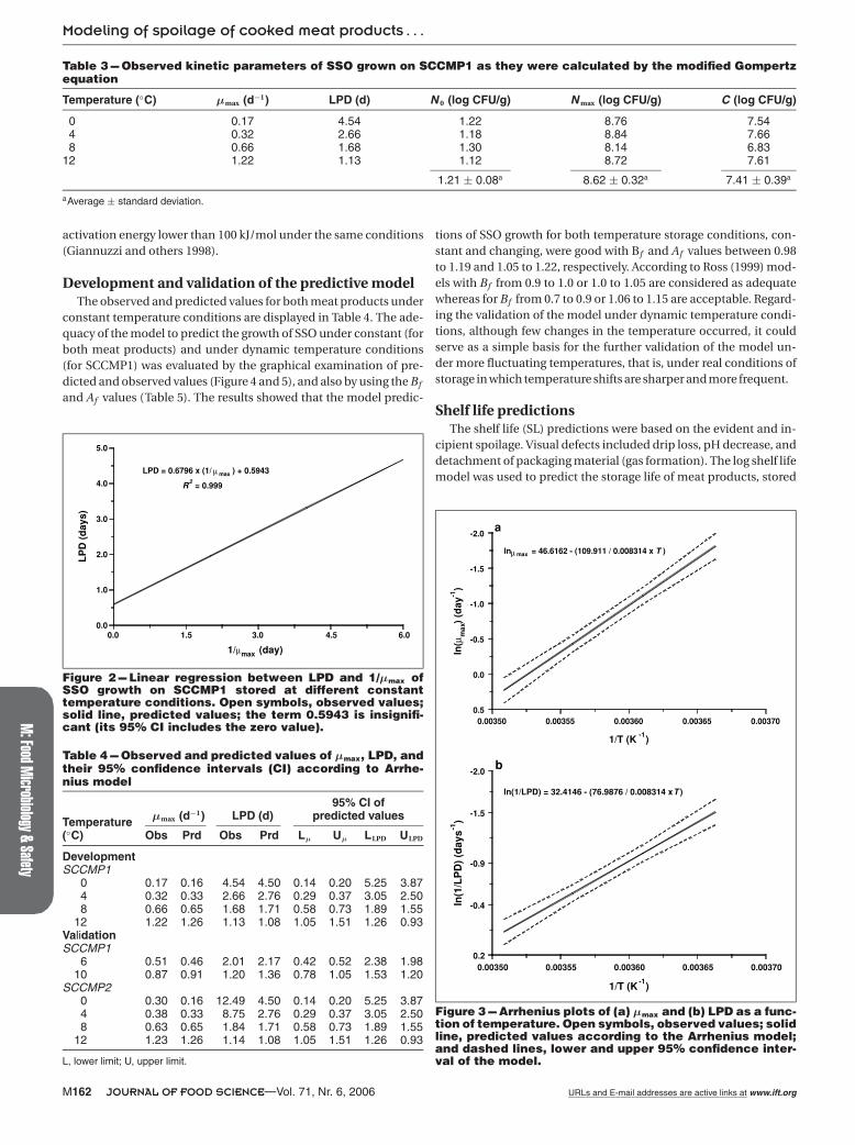
The parameters of N 0, N max, and C were similar between the 4 tem-peratures examined with a mean value of 1.21, 8.62, and 7.41 logCFU/g, respectively. Thus, the μmax and LPD values were taken tobe modeled with the secondary models. The LPD was plotted againstthe reciprocal of μmax and the result showed that this relationshipis expressed by a straight line (Figure 2). Therefore, LPD and 1/μmax

are reciprocally proportional related to a constant which expressesthe physiological state of the cells (in the equation of Figure 2 thecoefficient before the parameter 1/μmax has this role). Other authorshave also found this relation between LPD and μmax for tempera-ture (Li and Torres 1993; Giannuzzi and others 1998; Koutsoumanis2001). This relation can be explained by the “work to be done” the-ory. This theory tells that the cells in order to enter from their lagphase to exponential growth phase must produce a certain amountof work (produced work). The amount of produced work is constantin relation with the temperature factor. This means that when thetemperature changes, the amount of produced work remains thesame and only the rate of work production is affected (increase ordecrease of rate with the temperature shifts).

The secondary models used were the square root and Arrheniusequations, which both described well the experimental data of μmax

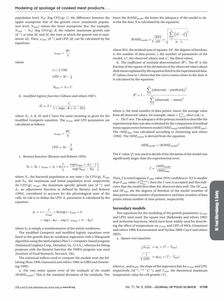
and LPD. The Bf and Af values did not show differences betweenthe models, indicating that the observed data were very close to theequivalence line of “fail-safe” and “fail-dangerous” regions (Table 2).However, the Arrhenius model was slightly more accurate than thesquare root model with respect to μmax data (higher R2 and lowerAf ). The GoF was also used to evaluate the ability of the models todescribe the data ofμmax and LPD. The results showed that the Arrhe-nius model had the lower RMSE value (Table 2); therefore, this modelwas selected for the predictions of μmax and LPD within the exam-ined temperature range (Table 4). In Figure 3 the Arrhenius plots ofμmax (Figure 3a) and LPD (Figure 3b) are presented. The activationenergy (Ea) forμmax and LPD was 109.9 and 77.0 kJ/mol, respectively.The high activation energy (>100 kJ/mol) of LAB indicates that thegrowth rate of LAB is affected more by temperature shifts than thegrowth rate of other microorganisms, such as pseudomonads, with


M:Food

Microbiology

&Safety


Table 3 --- Observed kinetic parameters of SSO grown on SCCMP1 as they were calculated by the modified Gompertzequation

Temperature (◦C) μmax (d−1) LPD (d) N 0 (log CFU/g) N max (log CFU/g) C (log CFU/g)

0 0.17 4.54 1.22 8.76 7.544 0.32 2.66 1.18 8.84 7.668 0.66 1.68 1.30 8.14 6.83

12 1.22 1.13 1.12 8.72 7.61

1.21 ± 0.08a 8.62 ± 0.32a 7.41 ± 0.39a

aAverage ± standard deviation.

activation energy lower than 100 kJ/mol under the same conditions(Giannuzzi and others 1998).

Development and validation of the predictive modelThe observed and predicted values for both meat products under

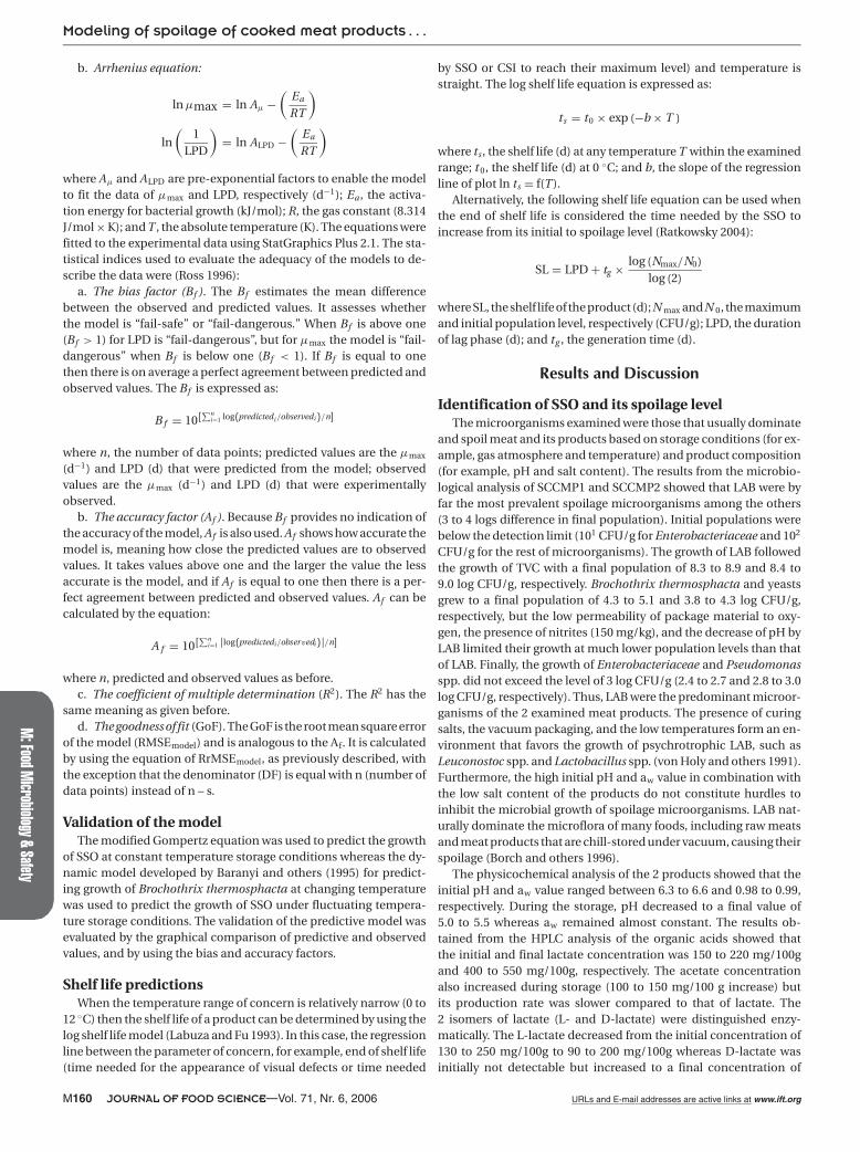
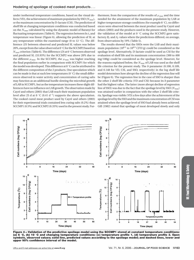
constant temperature conditions are displayed in Table 4. The ade-quacy of the model to predict the growth of SSO under constant (forboth meat products) and under dynamic temperature conditions(for SCCMP1) was evaluated by the graphical examination of pre-dicted and observed values (Figure 4 and 5), and also by using the Bf

and Af values (Table 5). The results showed that the model predic-

0.0 1.5 3.0 4.5 6.0

1/μmax (day)

0.0

1.0

2.0

3.0

4.0

5.0

LP

D (

da

ys

)

LPD = 0.6796 x (1/ μ max ) + 0.5943

R2 = 0.999

Figure 2 --- Linear regression between LPD and 1/μmax ofSSO growth on SCCMP1 stored at different constanttemperature conditions. Open symbols, observed values;solid line, predicted values; the term 0.5943 is insignifi-cant (its 95% CI includes the zero value).

Table 4 --- Observed and predicted values of μmax, LPD, andtheir 95% confidence intervals (CI) according to Arrhe-nius model

95% CI ofμmax (d−1) LPD (d) predicted values

Temperature(◦C) Obs Prd Obs Prd Lμ Uμ LLPD ULPD

DevelopmentSCCMP1

0 0.17 0.16 4.54 4.50 0.14 0.20 5.25 3.874 0.32 0.33 2.66 2.76 0.29 0.37 3.05 2.508 0.66 0.65 1.68 1.71 0.58 0.73 1.89 1.55

12 1.22 1.26 1.13 1.08 1.05 1.51 1.26 0.93ValidationSCCMP1

6 0.51 0.46 2.01 2.17 0.42 0.52 2.38 1.9810 0.87 0.91 1.20 1.36 0.78 1.05 1.53 1.20

SCCMP20 0.30 0.16 12.49 4.50 0.14 0.20 5.25 3.874 0.38 0.33 8.75 2.76 0.29 0.37 3.05 2.508 0.63 0.65 1.84 1.71 0.58 0.73 1.89 1.55

12 1.23 1.26 1.14 1.08 1.05 1.51 1.26 0.93

L, lower limit; U, upper limit.

tions of SSO growth for both temperature storage conditions, con-stant and changing, were good with Bf and Af values between 0.98to 1.19 and 1.05 to 1.22, respectively. According to Ross (1999) mod-els with Bf from 0.9 to 1.0 or 1.0 to 1.05 are considered as adequatewhereas for Bf from 0.7 to 0.9 or 1.06 to 1.15 are acceptable. Regard-ing the validation of the model under dynamic temperature condi-tions, although few changes in the temperature occurred, it couldserve as a simple basis for the further validation of the model un-der more fluctuating temperatures, that is, under real conditions ofstorage in which temperature shifts are sharper and more frequent.

Shelf life predictionsThe shelf life (SL) predictions were based on the evident and in-

cipient spoilage. Visual defects included drip loss, pH decrease, anddetachment of packaging material (gas formation). The log shelf lifemodel was used to predict the storage life of meat products, stored

0.00350 0.00355 0.00360 0.00365 0.00370

1/T (K-1

)

0.5

0.0

-0.5

-1.0

-1.5

-2.0

ln(μ

ma

x) (

day

-1)

a

lnμ max = 46.6162 - (109.911 / 0.008314 x T )

0.00350 0.00355 0.00360 0.00365 0.00370

1/T (K-1

)

0.2

-0.4

-0.9

-1.5

-2.0

ln(1

/LP

D)

(da

ys

-1)

b

ln(1/LPD) = 32.4146 - (76.9876 / 0.008314 x T )

Figure 3 --- Arrhenius plots of (a) μmax and (b) LPD as a func-tion of temperature. Open symbols, observed values; solidline, predicted values according to the Arrhenius model;and dashed lines, lower and upper 95% confidence inter-val of the model.


M:F

ood

Mic

robi

olog

y&

Safe

ty


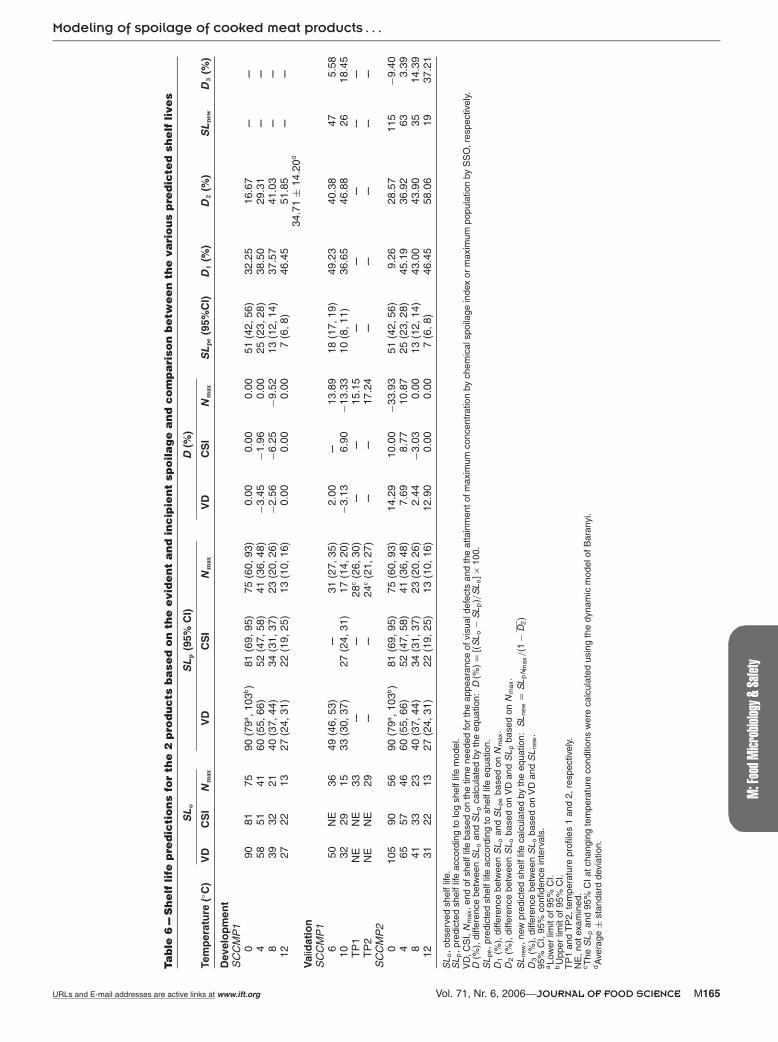
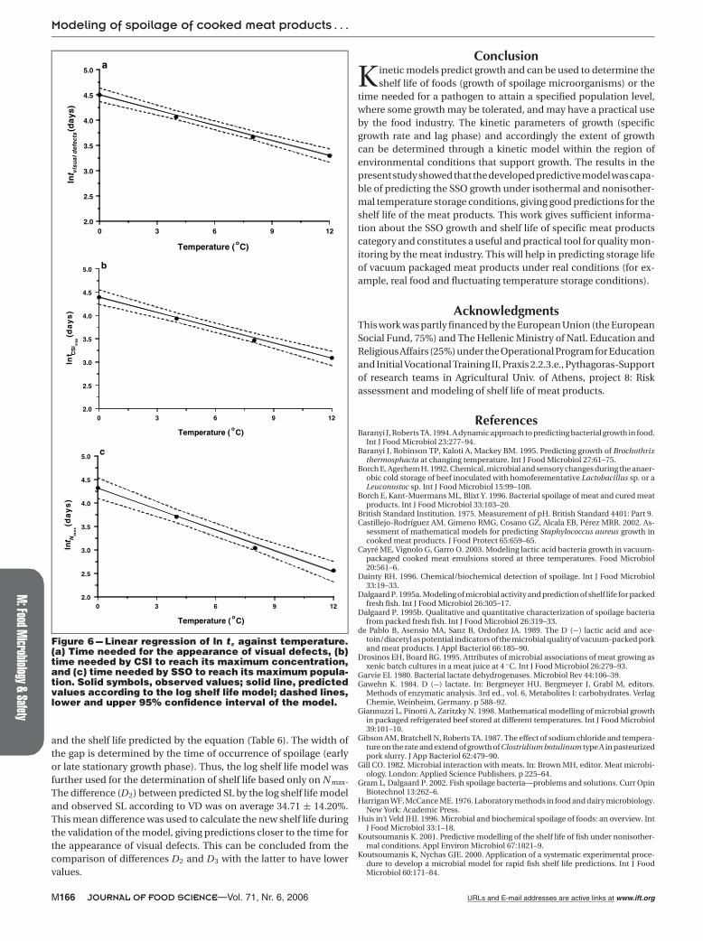
under isothermal temperature conditions, based on the visual de-fects (VD), the achievement of maximum population by SSO (N max),or the maximum concentration by D-lactate (CSI). The prediction ofshelf life at changing temperature conditions was conducted basedon the N max calculated by using the dynamic model of Baranyi forfluctuating temperatures (Table 6). The regression between ln ts andtemperature was linear (Figure 6), allowing the prediction of SL atany temperature within the examined range (0 to 12 ◦C). The dif-ference (D) between observed and predicted SL values was below20%, except from the value observed at 0 ◦C for the SCCMP2 based onN max criterion (Table 6). The difference (D) at 0 ◦C between observedand predicted SL (33.93%) for the SCCMP2 was above 20% due tothe different μmax. In the SCCMP2, the μmax was higher reachingthe final population earlier in comparison with SCCMP1 for whichthe model was developed. This difference at 0 ◦C can be attributed tothe different composition of the 2 products. One speculation whichcan be made is that at such low temperatures (0 ◦C) the small differ-ences observed in water activity and concentration of curing saltsmay function as an additional hurdle slowing the microbial growthof LAB in SCCMP1, but as the temperature increases these slight dif-ferences have no influence on LAB growth. The observation made byCayre and others (2003) that LAB reach their maximum populationlevel after 25 d at 0 ◦C (0.41 d−1) supports the above speculation.The cooked cured meat product used by Cayre and others (2003)for their experimental trials contained less curing salts (0.2%) thanSCCMP1 (0.5%) and SCCMP2 (0.35%) used in the present study. Fur-

0 8 16 24 32 40

Time (days)

0

2

4

6

8

10

Ce

ll n

um

be

rs (

log

CF

U/g

)

b

0 9 18 27 36 45 54

Time (days)

0

2

4

6

8

10

Ce

ll n

um

be

rs (

log

CF

U/g

)

0

3

6

9

12

15

Te

mp

era

ture

(o C

)

d

Temperature profile

0 8 16 24 32 40

Time (days)

0

2

4

6

8

10

Ce

ll n

um

be

rs (

log

CF

U/g

)

a

0 10 20 30 40 50 60

Time (days)

0

2

4

6

8

10

Ce

ll n

um

be

rs (

log

CF

U/g

)

0

3

6

9

12

15

Te

mp

era

ture

(oC

)

c

Temperature profile

Figure 4 --- Validation of the predictive spoilage model using the SCCMP1 stored at constant temperature conditions:(a) 6 ◦C, (b) 10 ◦C and changing temperature conditions: (c) temperature profile 1, (d) temperature profile 2. Opensymbols, observed values; solid line, predicted values according to the spoilage model; and dashed lines, lower andupper 95% confidence interval of the model.

thermore, from the comparison of the results of μmax and the timeneeded for the attainment of the maximum population by LAB athigher temperature storage conditions (for example 8 ◦C), no differ-ences were observed between the meat product used by Cayre andothers (2003) and the products used in the present study. However,the validation of the model at 0 ◦C using the SCCMP2 gave satis-factory Bf and Af values where the predictions differed, on average,from observations by 19% (Table 5).

The results showed that the SSOs were the LAB and their maxi-mum population (108.3 to 108.9 CFU/g) could be considered as thespoilage level. Alternatively, D-lactate could be used as CSI for theevaluation of shelf life and its maximum concentration (300 to 400mg/100g) could be considered as the spoilage level. However, forthe reasons explained below, the N max of LAB was used as the shelflife criterion for the present study. The b parameter (0.100, 0.109,and 0.148 for VD, CSI, and SSO, respectively) in the log shelf lifemodel determines how abrupt the decline of the regression line willbe (Figure 6). The regression line in the case of SSO is sharper thanthe other 2 shelf life criteria (VD and CSI) because its b parameterhad the highest value. The latter (more abrupt decline of regressionline of SSO) was due to the fact that the spoilage level by SSO (N max)was attained earlier in comparison with the other 2 shelf life crite-ria. Spoilage was visible (VD) a few days after the achievement of thespoilage level by the SSO and the maximum concentration of CSI wasattained when the spoilage level of SSO had already been achieved.Gill (1982) stated that spoilage of meat developed slowly and only


M:Food

Microbiology

&Safety


0 15 30 45 60 75

Time (days)

0

2

4

6

8

10

Ce

ll n

um

be

rs (

log

CF

U/g

)

b

0 5 10 15 20 25 30 35

Time (days)

0

2

4

6

8

10

Ce

ll n

um

be

rs (

log

CF

U/g

)

d

0 20 40 60 80 100 120

Time (days)

0

2

4

6

8

10C

ell

nu

mb

ers

(lo

g C

FU

/g)

a

0 8 15 23 30 38 45

Time (days)

0

2

4

6

8

10

Ce

ll n

um

be

rs (

log

CF

U/g

)

c

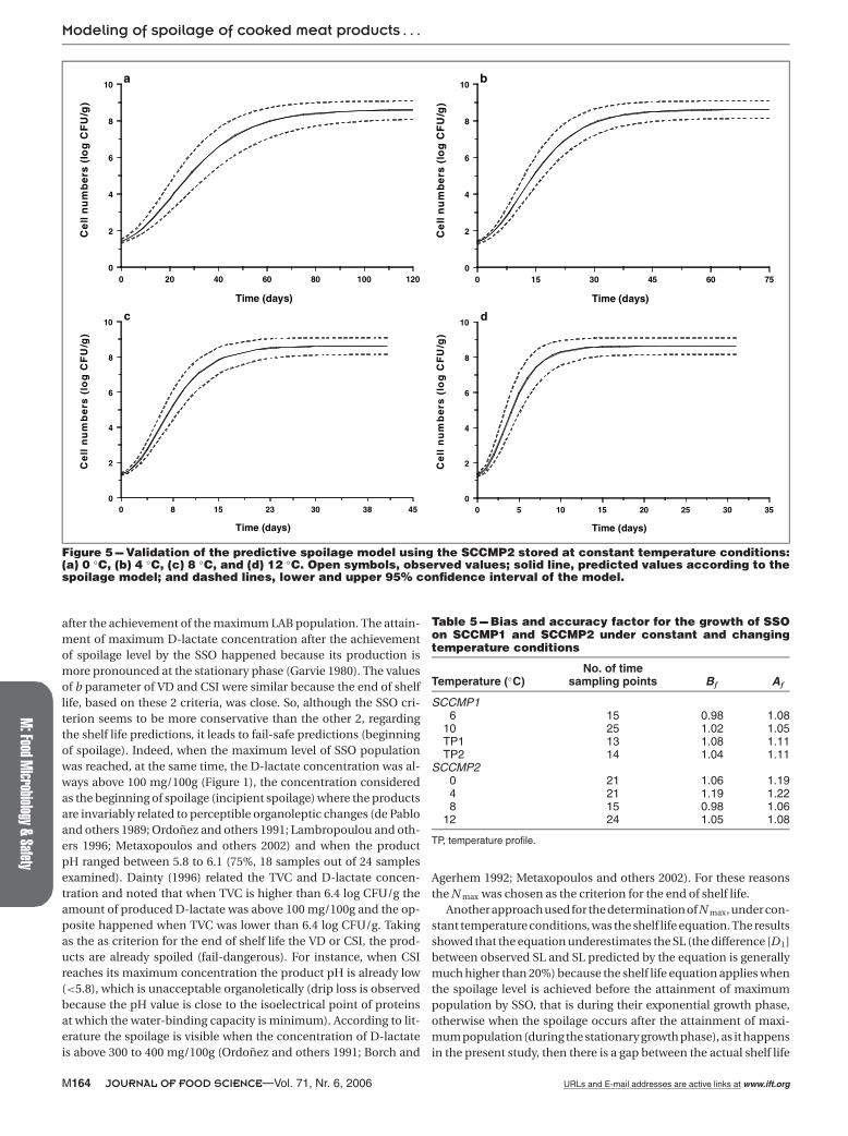
Figure 5 --- Validation of the predictive spoilage model using the SCCMP2 stored at constant temperature conditions:(a) 0 ◦C, (b) 4 ◦C, (c) 8 ◦C, and (d) 12 ◦C. Open symbols, observed values; solid line, predicted values according to thespoilage model; and dashed lines, lower and upper 95% confidence interval of the model.

after the achievement of the maximum LAB population. The attain-ment of maximum D-lactate concentration after the achievementof spoilage level by the SSO happened because its production ismore pronounced at the stationary phase (Garvie 1980). The valuesof b parameter of VD and CSI were similar because the end of shelflife, based on these 2 criteria, was close. So, although the SSO cri-terion seems to be more conservative than the other 2, regardingthe shelf life predictions, it leads to fail-safe predictions (beginningof spoilage). Indeed, when the maximum level of SSO populationwas reached, at the same time, the D-lactate concentration was al-ways above 100 mg/100g (Figure 1), the concentration consideredas the beginning of spoilage (incipient spoilage) where the productsare invariably related to perceptible organoleptic changes (de Pabloand others 1989; Ordonez and others 1991; Lambropoulou and oth-ers 1996; Metaxopoulos and others 2002) and when the productpH ranged between 5.8 to 6.1 (75%, 18 samples out of 24 samplesexamined). Dainty (1996) related the TVC and D-lactate concen-tration and noted that when TVC is higher than 6.4 log CFU/g theamount of produced D-lactate was above 100 mg/100g and the op-posite happened when TVC was lower than 6.4 log CFU/g. Takingas the as criterion for the end of shelf life the VD or CSI, the prod-ucts are already spoiled (fail-dangerous). For instance, when CSIreaches its maximum concentration the product pH is already low(<5.8), which is unacceptable organoletically (drip loss is observedbecause the pH value is close to the isoelectrical point of proteinsat which the water-binding capacity is minimum). According to lit-erature the spoilage is visible when the concentration of D-lactateis above 300 to 400 mg/100g (Ordonez and others 1991; Borch and

Table 5 --- Bias and accuracy factor for the growth of SSOon SCCMP1 and SCCMP2 under constant and changingtemperature conditions

No. of timeTemperature (◦C) sampling points Bf Af

SCCMP16 15 0.98 1.08

10 25 1.02 1.05TP1 13 1.08 1.11TP2 14 1.04 1.11

SCCMP20 21 1.06 1.194 21 1.19 1.228 15 0.98 1.06

12 24 1.05 1.08

TP, temperature profile.

Agerhem 1992; Metaxopoulos and others 2002). For these reasonsthe N max was chosen as the criterion for the end of shelf life.

Another approach used for the determination of N max, under con-stant temperature conditions, was the shelf life equation. The resultsshowed that the equation underestimates the SL (the difference [D1]between observed SL and SL predicted by the equation is generallymuch higher than 20%) because the shelf life equation applies whenthe spoilage level is achieved before the attainment of maximumpopulation by SSO, that is during their exponential growth phase,otherwise when the spoilage occurs after the attainment of maxi-mum population (during the stationary growth phase), as it happensin the present study, then there is a gap between the actual shelf life


M:F

ood

Mic

robi

olog

y&

Safe

ty


Tab

le6

---S

he

lfli

fep

red

icti

on

sfo

rth

e2

pro

du

cts

ba

sed

on

the

evi

de

nt

an

din

cip

ien

tsp

oil

ag

ea

nd

co

mp

ari

son

be

twe

en

the

vari

ou

sp

red

icte

dsh

elf

live

s

SL

oS

Lp

(95

%C

I)D

(%)

Te

mp

era

ture

(◦ C)

VD

CS

IN

max

VD

CS

IN

max

VD

CS

IN

max

SL

pe

(95

%C

I)D

1(%

)D

2(%

)S

Ln

ewD

3(%

)

Dev

elo

pm

en

tS

CC

MP

10

90

81

75

90

(79

a,

10

3b)

81

(69

,9

5)

75

(60

,9

3)

0.0

00

.00

0.0

05

1(4

2,5

6)

32

.25

16

.67

------

45

85

14

16

0(5

5,6

6)

52

(47

,5

8)

41

(36

,4

8)

−3.4

5−1

.96

0.0

02

5(2

3,2

8)

38

.50

29

.31

------

83

93

22

14

0(3

7,4

4)

34

(31

,3

7)

23

(20

,2

6)

−2.5

6−6

.25

−9.5

21

3(1

2,1

4)

37

.57

41

.03

------

12

27

22

13

27

(24

,3

1)

22

(19

,2

5)

13

(10

,1

6)

0.0

00

.00

0.0

07

(6,

8)

46

.45

51

.85

------

34

.71

±1

4.2

0d

Va

lida

tio

nS

CC

MP

16

50

NE

36

49

(46

,5

3)

---3

1(2

7,3

5)

2.0

0---

13

.89

18

(17

,1

9)

49

.23

40

.38

47

5.5

81

03

22

91

53

3(3

0,3

7)

27

(24

,3

1)

17

(14

,2

0)

−3.1

36

.90

−13

.33

10

(8,

11

)3

6.6

54

6.8

82

61

8.4

5T

P1

NE

NE

33

------

28

c(2

6,3

0)

------

15

.15

------

------

---T

P2

NE

NE

29

------

24

c(2

1,2

7)

------

17

.24

------

------

---S

CC

MP

20

10

59

05

69

0(7

9a,

10

3b)

81

(69

,9

5)

75

(60

,9

3)

14

.29

10

.00

−33

.93

51

(42

,5

6)

9.2

62

8.5

71

15

−9.4

04

65

57

46

60

(55

,6

6)

52

(47

,5

8)

41

(36

,4

8)

7.6

98

.77

10

.87

25

(23

,2

8)

45

.19

36

.92

63

3.3

98

41

33

23

40

(37

,4

4)

34

(31

,3

7)

23

(20

,2

6)

2.4

4−3

.03

0.0

01

3(1

2,1

4)

43

.00

43

.90

35

14

.39

12

31

22

13

27

(24

,3

1)

22

(19

,2

5)

13

(10

,1

6)

12

.90

0.0

00

.00

7(6

,8

)4

6.4

55

8.0

61

93

7.2

1

SL

o,

ob

se

rve

dsh

elf

life.

SL

p,

pre

dic

ted

sh

elf

life

acco

rdin

gto

log

sh

elf

life

mo

de

l.V

D,

CS

I,N

max,

en

do

fsh

elf

life

ba

se

do

nth

etim

en

ee

de

dfo

rth

ea

pp

ea

ran

ce

of

vis

ua

ld

efe

cts

an

dth

ea

tta

inm

en

to

fm

axim

um

co

nce

ntr

atio

nby

ch

em

ica

lsp

oila

ge

ind

ex

or

ma

xim

um

po

pu

latio

nby

SS

O,

resp

ective

ly.

D(%

),d

iffe

ren

ce

be

twe

en

SL

oa

nd

SL

pca

lcu

late

dby

the

eq

ua

tio

n:

D(%

)=

[(S

Lo

−S

Lp)/

SL

o]×

10

0.

SL

pe,

pre

dic

ted

sh

elf

life

acco

rdin

gto

sh

elf

life

eq

ua

tio

n.

D1

(%),

diffe

ren

ce

be

twe

en

SL

oa

nd

SL

pe

ba

se

do

nN

max.

D2

(%),

diffe

ren

ce

be

twe

en

SL

ob

ase

do

nV

Da

nd

SL

pb

ase

do

nN

max.

SL

new

,n

ew

pre

dic

ted

sh

elf

life

ca

lcu

late

dby

the

eq

ua

tio

n:

SL

new

=S

Lp

Nm

ax/(1

−D

2)

D3

(%),

diffe

ren

ce

be

twe

en

SL

ob

ase

do

nV

Da

nd

SL

new

.9

5%

CI,

95

%co

nfid

en

ce

inte

rva

ls.

aL

ow

er

limit

of9

5%

CI.

bU

pp

er

limit

of9

5%

CI.

TP

1a

nd

TP

2,te

mp

era

ture

pro

file

s1

an

d2

,re

sp

ective

ly.

NE

,n

otexa

min

ed

.cT

he

SL

pa

nd

95

%C

Ia

tch

an

gin

gte

mp

era

ture

co

nd

itio

ns

we

reca

lcu

late

du

sin

gth

ed

yn

am

icm

od

elo

fB

ara

nyi.

dA

vera

ge

±sta

nd

ard

devia

tio

n.


M:Food

Microbiology

&Safety


0 3 6 9 12

Temperature (oC)

2.0

2.5

3.0

3.5

4.0

4.5

5.0

lnt C

SI m

ax (

da

ys

)

b

0 3 6 9 12

Temperature (oC)

2.0

2.5

3.0

3.5

4.0

4.5

5.0

lnt N

ma

x (d

ay

s)

c

0 3 6 9 12

Temperature (oC)

2.0

2.5

3.0

3.5

4.0

4.5

5.0ln

t vis

ua

l d

efe

cts (

da

ys

)a

Figure 6 --- Linear regression of ln ts against temperature.(a) Time needed for the appearance of visual defects, (b)time needed by CSI to reach its maximum concentration,and (c) time needed by SSO to reach its maximum popula-tion. Solid symbols, observed values; solid line, predictedvalues according to the log shelf life model; dashed lines,lower and upper 95% confidence interval of the model.

and the shelf life predicted by the equation (Table 6). The width ofthe gap is determined by the time of occurrence of spoilage (earlyor late stationary growth phase). Thus, the log shelf life model wasfurther used for the determination of shelf life based only on N max.The difference (D2) between predicted SL by the log shelf life modeland observed SL according to VD was on average 34.71 ± 14.20%.This mean difference was used to calculate the new shelf life duringthe validation of the model, giving predictions closer to the time forthe appearance of visual defects. This can be concluded from thecomparison of differences D2 and D3 with the latter to have lowervalues.

Conclusion

Kinetic models predict growth and can be used to determine theshelf life of foods (growth of spoilage microorganisms) or the

time needed for a pathogen to attain a specified population level,where some growth may be tolerated, and may have a practical useby the food industry. The kinetic parameters of growth (specificgrowth rate and lag phase) and accordingly the extent of growthcan be determined through a kinetic model within the region ofenvironmental conditions that support growth. The results in thepresent study showed that the developed predictive model was capa-ble of predicting the SSO growth under isothermal and nonisother-mal temperature storage conditions, giving good predictions for theshelf life of the meat products. This work gives sufficient informa-tion about the SSO growth and shelf life of specific meat productscategory and constitutes a useful and practical tool for quality mon-itoring by the meat industry. This will help in predicting storage lifeof vacuum packaged meat products under real conditions (for ex-ample, real food and fluctuating temperature storage conditions).

AcknowledgmentsThis work was partly financed by the European Union (the EuropeanSocial Fund, 75%) and The Hellenic Ministry of Natl. Education andReligious Affairs (25%) under the Operational Program for Educationand Initial Vocational Training II, Praxis 2.2.3.e., Pythagoras-Supportof research teams in Agricultural Univ. of Athens, project 8: Riskassessment and modeling of shelf life of meat products.

ReferencesBaranyi J, Roberts TA. 1994. A dynamic approach to predicting bacterial growth in food.

Int J Food Microbiol 23:277–94.Baranyi J, Robinson TP, Kaloti A, Mackey BM. 1995. Predicting growth of Brochothrix

thermosphacta at changing temperature. Int J Food Microbiol 27:61–75.Borch E, Agerhem H. 1992. Chemical, microbial and sensory changes during the anaer-

obic cold storage of beef inoculated with homoferementative Lactobacillus sp. or aLeuconostoc sp. Int J Food Microbiol 15:99–108.

Borch E, Kant-Muermans ML, Blixt Y. 1996. Bacterial spoilage of meat and cured meatproducts. Int J Food Microbiol 33:103–20.

British Standard Institution. 1975. Measurement of pH. British Standard 4401: Part 9.Castillejo-Rodrıguez AM, Gimeno RMG, Cosano GZ, Alcala EB, Perez MRR. 2002. As-

sessment of mathematical models for predicting Staphylococcus aureus growth incooked meat products. J Food Protect 65:659–65.

Cayre ME, Vignolo G, Garro O. 2003. Modeling lactic acid bacteria growth in vacuum-packaged cooked meat emulsions stored at three temperatures. Food Microbiol20:561–6.

Dainty RH. 1996. Chemical/biochemical detection of spoilage. Int J Food Microbiol33:19–33.

Dalgaard P. 1995a. Modeling of microbial activity and prediction of shelf life for packedfresh fish. Int J Food Microbiol 26:305–17.

Dalgaard P. 1995b. Qualitative and quantitative characterization of spoilage bacteriafrom packed fresh fish. Int J Food Microbiol 26:319–33.

de Pablo B, Asensio MA, Sanz B, Ordonez JA. 1989. The D (−) lactic acid and ace-toin/diacetyl as potential indicators of the microbial quality of vacuum-packed porkand meat products. J Appl Bacteriol 66:185–90.

Drosinos EH, Board RG. 1995. Attributes of microbial associations of meat growing asxenic batch cultures in a meat juice at 4 ◦C. Int J Food Microbiol 26:279–93.

Garvie EI. 1980. Bacterial lactate dehydrogenases. Microbiol Rev 44:106–39.Gawehn K. 1984. D (−) lactate. In: Bergmeyer HU, Bergmeyer J, Grabl M, editors.

Methods of enzymatic analysis. 3rd ed., vol. 6, Metabolites I: carbohydrates. VerlagChemie, Weinheim, Germany. p 588–92.

Giannuzzi L, Pinotti A, Zaritzky N. 1998. Mathematical modelling of microbial growthin packaged refrigerated beef stored at different temperatures. Int J Food Microbiol39:101–10.

Gibson AM, Bratchell N, Roberts TA. 1987. The effect of sodium chloride and tempera-ture on the rate and extend of growth of Clostridium botulinum type A in pasteurizedpork slurry. J App Bacteriol 62:479–90.

Gill CO. 1982. Microbial interaction with meats. In: Brown MH, editor. Meat microbi-ology. London: Applied Science Publishers. p 225–64.

Gram L, Dalgaard P. 2002. Fish spoilage bacteria—problems and solutions. Curr OpinBiotechnol 13:262–6.

Harrigan WF, McCance ME. 1976. Laboratory methods in food and dairy microbiology.New York: Academic Press.

Huis in’t Veld JHJ. 1996. Microbial and biochemical spoilage of foods: an overview. IntJ Food Microbiol 33:1–18.

Koutsoumanis K. 2001. Predictive modelling of the shelf life of fish under nonisother-mal conditions. Appl Environ Microbiol 67:1821–9.

Koutsoumanis K, Nychas GJE. 2000. Application of a systematic experimental proce-dure to develop a microbial model for rapid fish shelf life predictions. Int J FoodMicrobiol 60:171–84.


M:F

ood

Mic

robi

olog

y&

Safe

ty


Labuza TP, Fu B. 1993. Growth kinetics for shelf-life prediction: theory and practice. JInd Microbiol 12:309–23.

Lambropoulou KA, Drosinos EH, Nychas GJE. 1996. The effect of glucose supplemen-tation on the spoilage microflora and chemical composition of minced beef storedaerobically or under a modified atmosphere at 4 ◦C. Int J Food Microbiol 30:281–91.

Li KY, Torres JA. 1993. Microbial growth estimation in liquid media exposed to tem-perature fluctuations. J Food Sci 58:644–8.

Malakar PK, Martens DE, Zwietering MH, Beal C, van’t Riet K. 1999. Modelling the inter-action between Lactobacillus curvatus and Enterobacter cloacae. II. Mixed culturesand shelf life predictions. Int J Food Microbiol 51:67–79.

Metaxopoulos J, Mataragas M, Drosinos EH. 2002. Microbial interaction in cookedcured meat products under vacuum or modified atmosphere at 4 ◦C. J Appl Microbiol93:363–73.

Noll F. 1984. L (−) lactate. In: Bergmeyer HU, Bergmeyer J, Grabl M, editors. Methodsof enzymatic analysis. 3rd ed., vol. 6, Metabolites I: carbohydrates. Verlag Chemie,Weinheim, Germany. p 582–8.

Nychas GJE. 1994. Modified atmosphere packaging of meats. In: Singh RP, OliveiraFAR, editors. Minimal processing of foods and process optimization: an interface.Boca Raton: CRC Press. p 417–35.

Nychas GJE, Drosinos EH, Board RG. 1998. Chemical changes in stored meat. In: DaviesA, Board RG, editors. The microbiology of meat and poultry. London: Blackie Aca-demic & Professional. p 288–326.

Ordonez JA, de Pablo B, Perez de Castro B, Asensio MA, Sanz B. 1991. Selected chem-ical and microbiological changes in refrigerated pork stored in carbon dioxide andoxygen enriched atmospheres. J Agric Food Chem 39:668–72.

Pin C, Baranyi J. 1998. Predictive models as means to quantify the interactions ofspoilage organisms. Int J Food Microbiol 41:59–72.

Pin C, Sutherland JP, Baranyi J. 1999. Validating predictive models of food spoilageorganisms. J Appl Microbiol 87:491–9.

Ratkowsky DA. 2004. Model fitting and uncertainty. In: McKellar RC, Lu X, editors.Modeling microbial responses in food. Boca Raton: CRC Press. p 151–95.

Ratkowsky DA, Olley J, McMeekin TA, Ball A. 1982. Relationship between temperatureand growth rate of bacterial cultures. J Bacteriol 149:1–5.

Ross T. 1996. Indices for performance evaluation of predictive models in food micro-biology. J App Bacteriol 81:501–8.

Ross T. 1999. Predictive food microbiology models in the meat industry. In: Meat andlivestock. Sydney: Australia. p 196.

Shimoni E, Labuza PT. 2000. Modeling pathogen growth in meat products: futurechallenges. Trends Food Sci Technol 11:394–402.

Skandamis P, Tsigarida E, Nychas GJE. 2000. Ecophysiological attributes of Salmonellatyphimurium in liquid culture and within gelatin gel or without the addition oforegano essential oil. World J Microbiol Biotechnol 16:31–5.

te Giffel MC, Zwietering MH. 1999. Validation of predictive models describing thegrowth of Listeria monocytogenes. Int J Food Microbiol 46:135–49.

von Holy A, Cloete TE, Dykes GA. 1991. Quantification and characterization of micro-bial populations associated with spoiled, vacuum-packed Vienna sausages. FoodMicrobiol 8:95–104.

Whiting RC. 1995. Microbial modeling in foods. Crit Rev Food Sci Nutr 35:467–94.Wijtzes T, de Wit JC, Huis in’t Veld JHJ, van’t Riet K, Zwietering MH. 1995. Modelling

bacterial growth of Lactobacillus curvatus as a function of acidity and temperature.Appl Environ Microbiol 61:2533–9.

Zwietering MH, Cuppers HG, de Wit JC, van’t Riet K. 1994. Evaluation of data transfor-mations and validation of a model for the effect of temperature on bacterial growth.Appl Environ Microbiol 60:195–203.


development of a predictive model for spoilage of cooked cured meat products and its validation...

Documents