detecting crosstalk errors in quantum information processors

Detecting crosstalk errors in quantum information processorsMohan Sarovar, Timothy Proctor, Kenneth Rudinger, Kevin Young, Erik Nielsen, and Robin Blume-Kohout

Quantum Performance Laboratory, Sandia National Laboratories, Albuquerque, NM 87185 and Livermore, CA 94550

Crosstalk occurs in most quantum com-puting systems with more than one qubit.It can cause a variety of correlated andnonlocal crosstalk errors that can be es-pecially harmful to fault-tolerant quan-tum error correction, which generally re-lies on errors being local and relativelypredictable. Mitigating crosstalk errorsrequires understanding, modeling, and de-tecting them. In this paper, we introducea comprehensive framework for crosstalkerrors and a protocol for detecting andlocalizing them. We give a rigorous def-inition of crosstalk errors that capturesa wide range of disparate physical phe-nomena that have been called “crosstalk”,and a concrete model for crosstalk-freequantum processors. Errors that violatethis model are crosstalk errors. Next,we give an equivalent but purely oper-ational (model-independent) definition ofcrosstalk errors. Using this definition, weconstruct a protocol for detecting a largeclass of crosstalk errors in a multi-qubitprocessor by finding conditional dependen-cies between observed experimental prob-abilities. It is highly efficient, in the sensethat the number of unique experiments re-quired scales at most cubically, and veryoften quadratically, with the number ofqubits. We demonstrate the protocol usingsimulations of 2-qubit and 6-qubit proces-sors.

1 Introduction

Quantum computing has grown from a theoreticalconcept into a nascent technology. Cloud-accessiblequantum information processors (QIPs) with 20+

qubits exist today, and ones with around 100 qubitsmay appear in the next few years [45]. Fundamen-

Mohan Sarovar: [email protected]

tal operations – gates, state preparation and measure-ments (SPAM) – are approaching the demanding er-ror rates required by the theory of fault-tolerance ona number of physical platforms, including supercon-ducting qubits and trapped ions [29]. However, as ex-perimentalists and engineers have begun to build sys-tems of 10-20 qubits, it is becoming clear that emer-gent failure modes may be an even bigger problemthan errors in elementary operations. The most obvi-ous failure mode that emerges at scale is crosstalk.

“Crosstalk” describes a wide range of physicalphenomena that vary significantly across physicalplatforms used for quantum computing. We will fo-cus, instead, on the visible effects of crosstalk on thequantum logical behavior of a physical system that isused and treated like a quantum computer. We referto these hardware-agnostic effects as crosstalk errors– deviations from the ideal behavior of quantum gatesand circuits, which can be formalized and captured inan architecture-independent way. Crosstalk errors vi-olate either of two key assumptions that go into anywell-behaved model of QIP dynamics: spatial local-ity, and independence of operations. Gates and otheroperations are supposed to act non-trivially only in aspecific “target” region of the QIP, and their action onthat region is supposed to be independent of the con-text in which they are applied. These assumptionsenable tractable models for quantum computing, andcrosstalk errors violate them. Here, we give a rigor-ous definition of crosstalk errors that captures the ef-fects of crosstalk, while avoiding the need to engagedeeply with the physical phenomena themselves.

We begin in Sec. 2 and Sec. 3 by defining what itmeans for a quantum processor to be “crosstalk-free”at the quantum logic level. In Sec. 4, we constructan explicit error model for Markovian crosstalk-freebehavior. Markovian dynamics that are not consis-tent with that model constitute crosstalk errors. Thenin Sec. 5 we discuss the difficulty of detecting ar-bitrary unknown crosstalk errors and define a classof low-weight crosstalk errors that can be efficientlydetected. In Sec. 6 and Sec. 7, we take an opera-tional approach and show how to detect low-weight

Accepted in Quantum 2020-09-07, click title to verify. Published under CC-BY 4.0. 1

arX

iv:1

908.

0985

5v3

[qu

ant-

ph]

10

Sep

2020

https://quantum-journal.org/?s=Detecting%20crosstalk%20errors%20in%20quantum%20information%20processors&reason=title-click

mailto:[email protected]

crosstalk errors using only correlations between ex-perimental variables – the settings and the outcomesof experiments. The protocol we develop specifies aset of at most O(n3), and often O(n2), experimentsfor detecting crosstalk on an n-qubit QIP. The analy-sis of the data from these experiments uses techniquesadapted from causal inference on probabilistic graph-ical models [27, 52].

Much recent work has been published on de-tecting, quantifying, and modeling crosstalk andcrosstalk errors in quantum computing devices [6, 42,18, 44, 51, 39, 16, 23, 49, 50, 48, 17, 2, 19, 21, 11,35]. Variants of Ramsey sequences have been used todetect and quantify coherent coupling between qubits[2]. This technique is very hardware-specific andtypically limited to detecting crosstalk in the formof unwanted Hamiltonian couplings of known form.Several groups have also demonstrated mitigation ofcrosstalk in readout lines by detailed characteriza-tion and compensation [23, 49, 11, 35] (see alsoSupplementary Information in Refs. [6, 42, 16, 19,21]). A very different approach, which is platform-independent and model-free like the work we presenthere, is the simultaneous randomized benchmark-ing (SRB) technique for detecting and quantifyingcrosstalk between pairs of qubits [18, 51]. Thecrosstalk detection protocol we present here is simi-lar in motivation to SRB, and is meant to be used as alight-weight diagnostic for the presence of crosstalk.It is specifically designed to be run efficiently onmany-qubit QIPs and identify the crosstalk struc-ture (i.e., which qubits have crosstalk errors betweenthem), whereas we are not aware of an applicationof SRB that reveals crosstalk structure in a many-qubit QIP as efficiently. Moreover, our protocol is de-signed to detect a wide range of crosstalk errors and ismore flexible in terms of the experiments that are per-formed, allowing it to be tailored towards detectionof certain types of crosstalk errors. However, SRBhas at least one clear advantage over our protocol; itmeasures the quantitative rate of certain crosstalk er-rors, whereas our protocol is just designed to detectand localize them, and has limited quantitative abil-ity. Finally, we note that in a previous paper [50] wegave a protocol for detecting context dependence, in-cluding crosstalk, that can be seen as a precursor tothe protocol given here.

2 Crosstalk and crosstalk errors

Before we embark on defining things precisely, abrief discussion of exactly what we are definingis apropos. In particular, the distinction between“crosstalk” and “crosstalk errors” needs further ex-planation.

Crosstalk is an imprecise but widely used term thatappears primarily in electrical engineering and com-munication theory, and generally refers to “unwantedcoupling between signal paths” [38]. In experimen-tal quantum computing, the word has been adaptedto describe a range of physical phenomena in whichsome subsystem of an experimental device – a qubit,field, control line, resonator, photodetector, etc. – un-intentionally affects another subsystem.

A specific quantum computing device will gener-ally display more than one such effect. For example, atransmon-based quantum processor might experience

• Residual coherent couplings between transmonsthat should be uncoupled,

• Traditional electromagnetic (EM) crosstalk be-tween microwave lines,

• Stray on-chip EM fields due to imperfect mi-crowave hygiene,

• Coupling between readout resonators attachedto distinct qubits,

• 60Hz line noise that influences all the qubits.

Any and all of these phenomena could legitimatelybe termed crosstalk. All of them are architecture-specific; a trapped-ion processor would have its ownendemic crosstalk effects, some analogous to theseand some not.

Our goal is to understand and address crosstalk ina platform-independent way that facilitates compar-isons between quantum processors without referenceto the underlying physics. This is clearly inconsistentwith the established use of the term crosstalk to de-scribe specific physics phenomena. There is no rea-sonable direct comparison between an unwanted 2-transmon coupling (measured in MHz) and the inten-sity of a control laser spillover in a trapped-ion setup(measured in W/m2). But we can legitimately com-pare their effects at the quantum logic level of abstrac-tion, where each device is required to behave like aquantum computer, performing quantum logic gatesand quantum circuits.


We introduce the new term “crosstalk errors” forthis purpose. It means any observable effect at thequantum logic level (qubits, gates, quantum circuits,and their associated probabilities) that stems uniquelyfrom some form of physical crosstalk. Some formsof physical crosstalk may result in purely local er-rors – e.g., independent bit flips – at the quantumlogic level; these are not crosstalk errors (despite theirsource) because they could have been produced bylocal noise. Similarly, if physical crosstalk exists buthas no effect at the quantum logic level (perhaps be-cause of intentional mitigation) then we say that thesystem is “crosstalk-free”.

3 Definition of crosstalk errors

Crosstalk errors are undesired dynamics that violateeither (or both) of two principles: locality and in-dependence. In an ideal QIP, each qubit is com-pletely isolated from the rest of the universe, andevolves independently of it, except when an operationis applied. Operations, including gates and measure-ments, couple qubits to other systems, such as exter-nal control fields and/or other qubits. This couplingis supposed to be precise and limited in scope.

Unfortunately, real QIPs are not ideal. They expe-rience all manner of noise and errors. Of course, notall errors constitute crosstalk errors. Errors can causedeviations from ideal behavior yet still respect local-ity and independence. Unwanted dynamics that doviolate locality or independence constitute crosstalkerrors. We now make this precise by defining localityand independence.Locality of operations: A QIP has local operations ifand only if the physical implementation of any quan-tum circuit does not create correlation between anyqubits, or disjoint subsets of qubits, unless that cir-cuit contains multiqubit operations that intentionallycouple them.

If a processor obeys locality, then it makes senseto talk about the action of operations on their targetqubits, and we can go further and define indepen-dence. If locality is violated, then operations do notnecessarily have well-defined actions on their targets,and independence may not be well-defined.Independence of local operations: When an oper-ation (gate, measurement, etc) appears in a quantumcircuit acting on target qubits q at time t, the dynam-ical evolution of q at time t does not depend on whatother operations (acting on disjoint qubits) appear inthe circuit at the same time t.

Defintion 1: A QIP’s behavior is crosstalk-free ifits behavior, when implementing arbitrary circuits,satisfies locality and independence.

4 An explicit error model for crosstalk-free processors

The definitions in the previous section are abstract.They neither rely upon nor define a concrete modelfor crosstalk errors or for crosstalk-free processors.In this section, we specialize to Markovian proces-sors and construct an explicit model for crosstalk-free Markovian processors. By assuming Markovian-ity we are able to rule out many conceivable failuresand define a model in which only finitely many thingscan go wrong. By defining crosstalk-free within thisframework, we get a division of Markovian errorsinto crosstalk-free or local, independent errors, andeverything else (i.e., crosstalk errors).

4.1 Defining crosstalk-free for Markovian QIPs

We place Markovianity in context within a hierarchyof models for quantum hardware, based on increas-ing levels of modularity (see Fig. 1): stable quantumcircuit, Markovian quantum circuit, and Markovian,crosstalk-free quantum circuit. We define each layerin this hierarchy in the following.

4.1.1 Stable QIPs

We call a QIP stable if every circuit’s outcome prob-ability distribution (over n-bit strings) is independentof external contexts [58]. Contexts on which theseprobabilities might depend include the time at whichthe circuit is run, the identity of the circuit that wasrun before it, or even the phase of the moon. Sta-bility is the weakest notion of modularity: a stableQIP is modular only in the sense that its output dis-tribution is independent of any external contexts, sothat each circuit run on the QIP forms a “module”.If a QIP is not stable, then modeling or probing itsbehavior becomes much more difficult. Importantlyfor this work, protocols for detecting crosstalk willlikely be corrupted by this instability, and any resultswill be unreliable or inconclusive. Fortunately, ex-plicit stability tests for QIPs can often be applied di-rectly to data from other characterization protocolswith only minimal modifications to the experimentdesign. For instance, by repeating a characterization


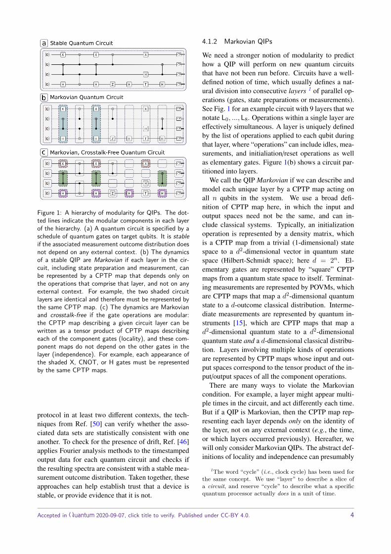
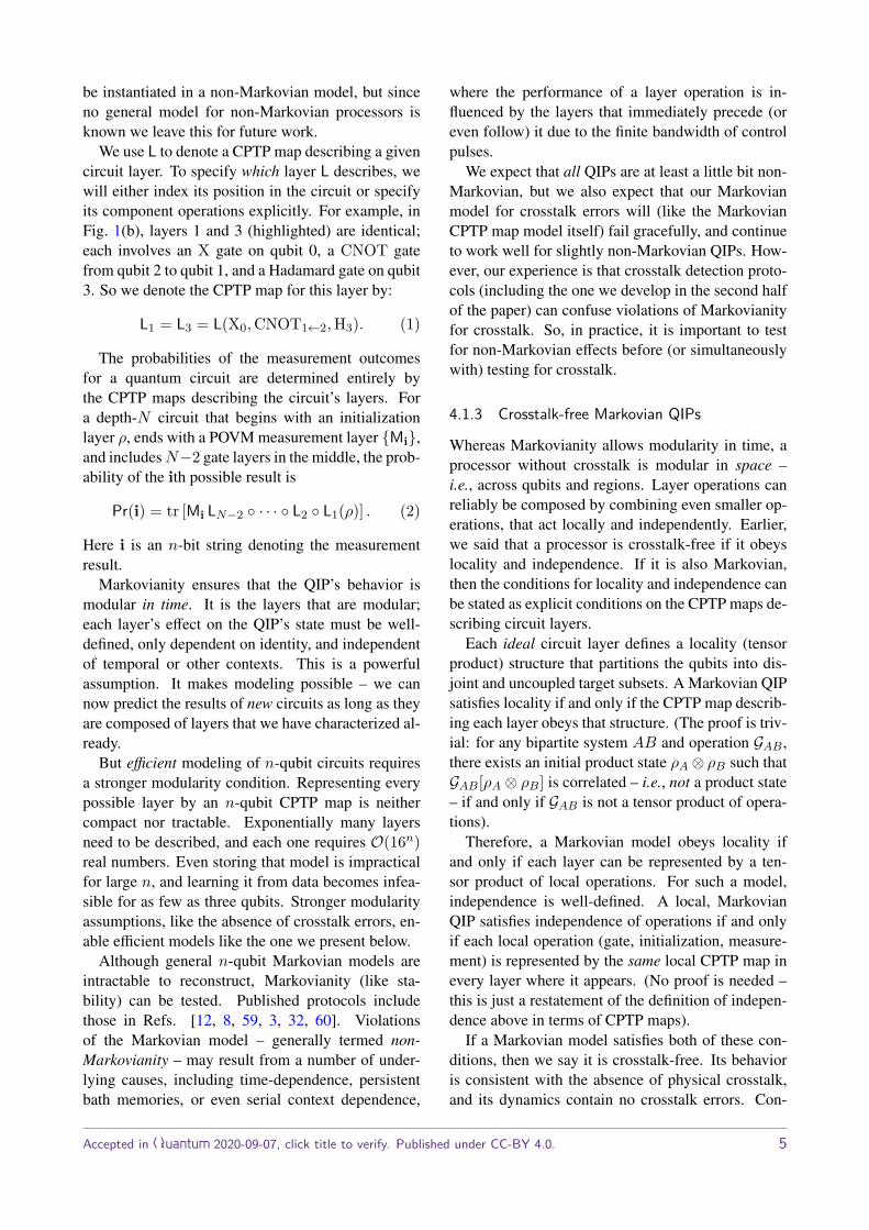
Figure 1: A hierarchy of modularity for QIPs. The dot-ted lines indicate the modular components in each layerof the hierarchy. (a) A quantum circuit is specified by aschedule of quantum gates on target qubits. It is stableif the associated measurement outcome distribution doesnot depend on any external context. (b) The dynamicsof a stable QIP are Markovian if each layer in the cir-cuit, including state preparation and measurement, canbe represented by a CPTP map that depends only onthe operations that comprise that layer, and not on anyexternal context. For example, the two shaded circuitlayers are identical and therefore must be represented bythe same CPTP map. (c) The dynamics are Markovianand crosstalk-free if the gate operations are modular:the CPTP map describing a given circuit layer can bewritten as a tensor product of CPTP maps describingeach of the component gates (locality), and these com-ponent maps do not depend on the other gates in thelayer (independence). For example, each appearance ofthe shaded X, CNOT, or H gates must be representedby the same CPTP maps.

protocol in at least two different contexts, the tech-niques from Ref. [50] can verify whether the asso-ciated data sets are statistically consistent with oneanother. To check for the presence of drift, Ref. [46]applies Fourier analysis methods to the timestampedoutput data for each quantum circuit and checks ifthe resulting spectra are consistent with a stable mea-surement outcome distribution. Taken together, theseapproaches can help establish trust that a device isstable, or provide evidence that it is not.

4.1.2 Markovian QIPs

We need a stronger notion of modularity to predicthow a QIP will perform on new quantum circuitsthat have not been run before. Circuits have a well-defined notion of time, which usually defines a nat-ural division into consecutive layers 1 of parallel op-erations (gates, state preparations or measurements).See Fig. 1 for an example circuit with 9 layers that wenotate L0, ..., L8. Operations within a single layer areeffectively simultaneous. A layer is uniquely definedby the list of operations applied to each qubit duringthat layer, where “operations” can include idles, mea-surements, and initialiation/reset operations as wellas elementary gates. Figure 1(b) shows a circuit par-titioned into layers.

We call the QIP Markovian if we can describe andmodel each unique layer by a CPTP map acting onall n qubits in the system. We use a broad defi-nition of CPTP map here, in which the input andoutput spaces need not be the same, and can in-clude classical systems. Typically, an initializationoperation is represented by a density matrix, whichis a CPTP map from a trivial (1-dimensional) statespace to a d2-dimensional vector in quantum statespace (Hilbert-Schmidt space); here d = 2n. El-ementary gates are represented by “square” CPTPmaps from a quantum state space to itself. Terminat-ing measurements are represented by POVMs, whichare CPTP maps that map a d2-dimensional quantumstate to a d-outcome classical distribution. Interme-diate measurements are represented by quantum in-struments [15], which are CPTP maps that map ad2-dimensional quantum state to a d2-dimensionalquantum state and a d-dimensional classical distribu-tion. Layers involving multiple kinds of operationsare represented by CPTP maps whose input and out-put spaces correspond to the tensor product of the in-put/output spaces of all the component operations.

There are many ways to violate the Markoviancondition. For example, a layer might appear multi-ple times in the circuit, and act differently each time.But if a QIP is Markovian, then the CPTP map rep-resenting each layer depends only on the identity ofthe layer, not on any external context (e.g., the time,or which layers occurred previously). Hereafter, wewill only consider Markovian QIPs. The abstract def-initions of locality and independence can presumably

1The word “cycle” (i.e., clock cycle) has been used forthe same concept. We use “layer” to describe a slice ofa circuit, and reserve “cycle” to describe what a specificquantum processor actually does in a unit of time.


be instantiated in a non-Markovian model, but sinceno general model for non-Markovian processors isknown we leave this for future work.

We use L to denote a CPTP map describing a givencircuit layer. To specify which layer L describes, wewill either index its position in the circuit or specifyits component operations explicitly. For example, inFig. 1(b), layers 1 and 3 (highlighted) are identical;each involves an X gate on qubit 0, a CNOT gatefrom qubit 2 to qubit 1, and a Hadamard gate on qubit3. So we denote the CPTP map for this layer by:

L1 = L3 = L(X0,CNOT1←2,H3). (1)

The probabilities of the measurement outcomesfor a quantum circuit are determined entirely bythe CPTP maps describing the circuit’s layers. Fora depth-N circuit that begins with an initializationlayer ρ, ends with a POVM measurement layer Mi,and includesN−2 gate layers in the middle, the prob-ability of the ith possible result is

Pr(i) = tr [Mi LN−2 · · · L2 L1(ρ)] . (2)

Here i is an n-bit string denoting the measurementresult.

Markovianity ensures that the QIP’s behavior ismodular in time. It is the layers that are modular;each layer’s effect on the QIP’s state must be well-defined, only dependent on identity, and independentof temporal or other contexts. This is a powerfulassumption. It makes modeling possible – we cannow predict the results of new circuits as long as theyare composed of layers that we have characterized al-ready.

But efficient modeling of n-qubit circuits requiresa stronger modularity condition. Representing everypossible layer by an n-qubit CPTP map is neithercompact nor tractable. Exponentially many layersneed to be described, and each one requires O(16n)real numbers. Even storing that model is impracticalfor large n, and learning it from data becomes infea-sible for as few as three qubits. Stronger modularityassumptions, like the absence of crosstalk errors, en-able efficient models like the one we present below.

Although general n-qubit Markovian models areintractable to reconstruct, Markovianity (like sta-bility) can be tested. Published protocols includethose in Refs. [12, 8, 59, 3, 32, 60]. Violationsof the Markovian model – generally termed non-Markovianity – may result from a number of under-lying causes, including time-dependence, persistentbath memories, or even serial context dependence,

where the performance of a layer operation is in-fluenced by the layers that immediately precede (oreven follow) it due to the finite bandwidth of controlpulses.

We expect that all QIPs are at least a little bit non-Markovian, but we also expect that our Markovianmodel for crosstalk errors will (like the MarkovianCPTP map model itself) fail gracefully, and continueto work well for slightly non-Markovian QIPs. How-ever, our experience is that crosstalk detection proto-cols (including the one we develop in the second halfof the paper) can confuse violations of Markovianityfor crosstalk. So, in practice, it is important to testfor non-Markovian effects before (or simultaneouslywith) testing for crosstalk.

4.1.3 Crosstalk-free Markovian QIPs

Whereas Markovianity allows modularity in time, aprocessor without crosstalk is modular in space –i.e., across qubits and regions. Layer operations canreliably be composed by combining even smaller op-erations, that act locally and independently. Earlier,we said that a processor is crosstalk-free if it obeyslocality and independence. If it is also Markovian,then the conditions for locality and independence canbe stated as explicit conditions on the CPTP maps de-scribing circuit layers.

Each ideal circuit layer defines a locality (tensorproduct) structure that partitions the qubits into dis-joint and uncoupled target subsets. A Markovian QIPsatisfies locality if and only if the CPTP map describ-ing each layer obeys that structure. (The proof is triv-ial: for any bipartite system AB and operation GAB ,there exists an initial product state ρA ⊗ ρB such thatGAB[ρA ⊗ ρB] is correlated – i.e., not a product state– if and only if GAB is not a tensor product of opera-tions).

Therefore, a Markovian model obeys locality ifand only if each layer can be represented by a ten-sor product of local operations. For such a model,independence is well-defined. A local, MarkovianQIP satisfies independence of operations if and onlyif each local operation (gate, initialization, measure-ment) is represented by the same local CPTP map inevery layer where it appears. (No proof is needed –this is just a restatement of the definition of indepen-dence above in terms of CPTP maps).

If a Markovian model satisfies both of these con-ditions, then we say it is crosstalk-free. Its behavioris consistent with the absence of physical crosstalk,and its dynamics contain no crosstalk errors. Con-


versely, any violation of these conditions constitutesa crosstalk error.

If a QIP satisfies Condition 1 (locality), then eachlayer’s CPTP map is a tensor product over the targetsubsets implied by that layer. The CPTP map for thelayer described above, in the example of Markovian-ity, would be

L(X0,CNOT1←2,H3) =G(X0)⊗ G(CNOT1←2)⊗ G(H3), (3)

where G, indexed by the gate operation and qubit tar-get, represents a component CPTP map for that gate.

To satisfy Condition 2 (independence), a gate thatappears in multiple layers must act identically in eachof them. For example, in Fig. 1, layers 1, 3, 5, and7 all contain a Hadamard gate acting on the fourthqubit. So the CPTP map describing layer 5 then musttake the form

L5 = L(H3) = G(I0)⊗G(I1)⊗G(I2)⊗G(H3), (4)

where G(H3) is the same local map that appearedin the other layers (although this map does not haveto be the same as the same gate on another qubit,e.g., G(H4)).

Initialization and measurement operations mustobey the same structure. For the four-qubit QIPshown in Fig. 1, this means that:

ρ = ρ0 ⊗ ρ1 ⊗ ρ2 ⊗ ρ3 (5)Mi = M0,i0 ⊗M1,i1 ⊗M2,i2 ⊗M3,i3 , (6)

whereMj,ij is the POVM effect operator for outcomeij on qubit j. If the initial state is correlated, or theoutput bit on one qubit depends on another qubit’sstate, then the QIP is not crosstalk-free.

4.2 Discussion of the crosstalk-free QIP model

In classical systems, crosstalk usually refers to a sig-nal in one channel influencing the signal on anotherchannel. For example, inductive coupling betweenadjacent copper telephone wires may cause a con-versation on one line to be heard on another. Anal-ogous effects occur in QIPs – laser beams have fi-nite width and may illuminate neighboring ions, su-perconducting transmission line resonators may ca-pacitively couple to each other, or qubits themselvesmay interact directly. These interactions can be mod-eled by coupling Hamiltonians. So it is temptingto say that “crosstalk” is nothing more than a cou-pling Hamiltonian, and the complex abstraction thatwe have introduced is unnecessary.

But this misses three key points. First, thoseHamiltonians appear in low-level device modeling,and are specific to particular physical implementa-tions. Second, like all low-level device Hamiltoni-ans, they fluctuate in time and with the state of theenvironment. Third, the systems that they couple areoften ancillary ones – control wires, ambient fields,etc – that would not normally appear in an effectivedescription of the processor and its qubits. Defining,detecting, and modeling crosstalk at this low level ispossible – and even desirable for device physicists –but not portable across many devices.

We have presented a high-level, hardware-agnosticeffective model. This approach is common. It ispresent when qubits are described as 2-dimensionalHilbert spaces, when elementary gates are describedby CPTP maps, and when errors are modeled as de-polarization or T1 processes. Our model, like all ofthose techniques, trades the conceptual simplicity ofHamiltonian dynamics on very large system-specificHilbert spaces for the practical tractability of an ef-fective model on n qubits. The CPTP map formalismstrikes a good balance between rigorous, low-leveldevice models and cross-platform, high-level abstrac-tion – but as a picture of the underlying physics, itis coarse-grained and can sometimes be counterintu-itive.

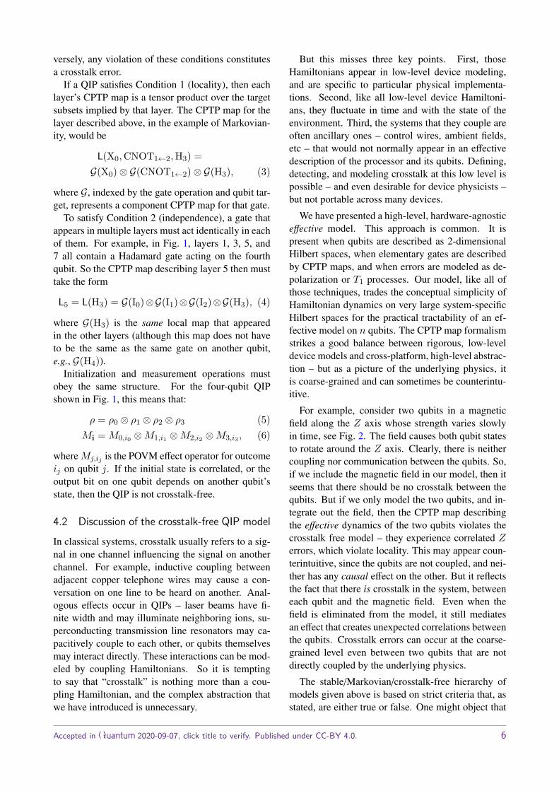
For example, consider two qubits in a magneticfield along the Z axis whose strength varies slowlyin time, see Fig. 2. The field causes both qubit statesto rotate around the Z axis. Clearly, there is neithercoupling nor communication between the qubits. So,if we include the magnetic field in our model, then itseems that there should be no crosstalk between thequbits. But if we only model the two qubits, and in-tegrate out the field, then the CPTP map describingthe effective dynamics of the two qubits violates thecrosstalk free model – they experience correlated Zerrors, which violate locality. This may appear coun-terintuitive, since the qubits are not coupled, and nei-ther has any causal effect on the other. But it reflectsthe fact that there is crosstalk in the system, betweeneach qubit and the magnetic field. Even when thefield is eliminated from the model, it still mediatesan effect that creates unexpected correlations betweenthe qubits. Crosstalk errors can occur at the coarse-grained level even between two qubits that are notdirectly coupled by the underlying physics.

The stable/Markovian/crosstalk-free hierarchy ofmodels given above is based on strict criteria that, asstated, are either true or false. One might object that


q1 q2

~B<latexit sha1_base64="Opz2ZFiUD4WWbXfVkk/Ol00y2Co=">AAAEBnicjVPLbtQwFHUbHiW8WliysRghsRpNChIsq8ICFohSzXQqjYfKcW4yVhwnsp3CyPKeLVv4B3aILb/BJ/AXOJkRmmY6iCs5vrrnHN9H7LgSXJvB4NfWdnDl6rXrOzfCm7du37m7u3fvRJe1YjBipSjVaUw1CC5hZLgRcFopoEUsYBznLxp8fA5K81IOzbyCaUEzyVPOqPGhMTkHZg/d2W5v0B+0htedaOn00NKOzva2f5OkZHUB0jBBtZ5Eg8pMLVWGMwEuJLWGirKcZjDxrqQF6Klt63X4kY8kOC2VX9LgNrqqsLTQel7EnllQM9NdrAlehk1qkz6fWi6r2oBki0RpLbApcdM8TrgCZsTcO5Qp7mvFbEYVZcaPKAzJS/DNKHjjD35bgaKmVJYY5axfG9DhP1GVO6uozDfhvo7M2fYbEgkfWFkUVCaWxIq6STS1BKSuFTStWiIgNURQmQmwvcgRxbOZ8b9QGdeR52A2yBv2ili1p3XlNNYL+V8J7kV4Nd9FPnys/Fz/t+DLc/LE3yVnLWmkcRx18cQP6r3faJaB6oJGVS2qUzxsMAWr6DE4S8rl0JuraI9hnfW66LJ8xIWhfxxR9ymsOyf7/ehJf//d097B4fKZ7KAH6CF6jCL0DB2gV+gIjRBDOfqMvqCvwafgW/A9+LGgbm8tNffRBQt+/gG3J2Vm</latexit>

H2( ~B)<latexit sha1_base64="awVg8ObAd9yQ+KnoTldS0+OzyiM=">AAAEC3icjVPNjtMwEPY2/CzhbxeOXCIqpOVSNV0kOK4WDssBsaza3ZXqUjnOJLXiOJHtLFSWH4ErV3gHbogrD8Ej8BY4aYW66RYxkuPRfN/nGU88UcmZ0v3+r62Od+36jZvbt/zbd+7eu7+z++BUFZWkMKIFL+R5RBRwJmCkmeZwXkogecThLMpe1vjZBUjFCjHU8xImOUkFSxgl2oXw0XSwhy+AmkP7dLrT7ff6jQXrTrh0umhpx9Pdzm8cF7TKQWjKiVLjsF/qiSFSM8rB+rhSUBKakRTGzhUkBzUxTdE2eOIicZAU0i2hgya6qjAkV2qeR46ZEz1TbawOXoWNK528mBgmykqDoItEScUDXQR1B4KYSaCaz51DqGSu1oDOiCRUuz75Pn4F7jIS3riD35YgiS6kwVpa49YGdPhPVGbWSCKyTbirI7Wm+fpYwAda5DkRscGRJHYcTgwGoSoJ9VUN5pBozIlIOZhuaLFk6Uy7fyi1bckz0BvkNXtFLJvT2nISqYX8ryTohsFqvst8+Fi6vv5vwVfnZLF7S9YYXEujKGzjsWvUe7eRNAXZBrUsG1QlwbDGJKyiJ2ANLpZNr5+iOYF11uu8zXIR6/tuOML2KKw7p4NeuN8bvHvWPThcjsk2eoQeoz0UoufoAB2hYzRCFJXoM/qCvnqfvG/ed+/HgtrZWmoeokvm/fwDuupmwg==</latexit>

H1( ~B)<latexit sha1_base64="z+sBakssvJl1r0nyvEm4r09mEm8=">AAAEC3icjVPNbtQwEHYbfkr4a+HIxWKFVC6rTYsEx6pwKAdEqXbbSutl5TiTrLWOE9lOYWX5EbhyhXfghrjyEDwCb4GTXaFttosYyfFovu/zjCeeuBRcm17v18ZmcO36jZtbt8Lbd+7eu7+98+BUF5ViMGCFKNR5TDUILmFguBFwXiqgeSzgLJ6+rPGzC1CaF7JvZiWMcppJnnJGjQ+Ro3G0Sy6A2UP3dLzd6XV7jeFVJ1o4HbSw4/HO5m+SFKzKQRomqNbDqFeakaXKcCbAhaTSUFI2pRkMvStpDnpkm6IdfuIjCU4L5Zc0uIkuKyzNtZ7lsWfm1Ex0G6uDV2HDyqQvRpbLsjIg2TxRWglsClx3ACdcATNi5h3KFPe1YjahijLj+xSG5BX4yyh44w9+W4KiplCWGOWsX2vQ/j9RNXVWUTldh/s6Mmebb0gkfGBFnlOZWBIr6obRyBKQulJQX9USAakhgspMgO1EjiieTYz/h8q4lnwKZo28Zi+JVXNaW05jPZf/leBOhJfzXebDx9L39X8LvjonT/xbctaSWhrHURtPfKPe+41mGag2aFTZoDrF/RpTsIyegLOkWDS9for2BFZZr/M2y0dcGPrhiNqjsOqc7nWj/e7eu2edg8PFmGyhR+gx2kUReo4O0BE6RgPEUIk+oy/oa/Ap+BZ8D37MqZsbC81DdMmCn38At0VmwQ==</latexit>

q1 q2

a bEe↵12<latexit sha1_base64="fCDy+LR9FCEAS8hT7TB74eQy+D8=">AAAEG3icjVPLjtMwFPW0PIbw6sAONhYVEquq6SDBcsRDggViGLUzI9Wlcpyb1KrjRLYDVJYlfoQtW/gHdogtCz6Bv8BJK9RJpwhLjq7uOcf3kXujQnBt+v1fO632hYuXLu9eCa5eu37jZmfv1rHOS8VgxHKRq9OIahBcwshwI+C0UECzSMBJNH9a4SfvQGmey6FZFDDJaCp5whk13jXt3CEZNTNGhX3upjYcuLeWqAxDkrhpp9vv9euDN41wZXTR6hxO91q/SZyzMgNpmKBaj8N+YSaWKsOZABeQUkNB2ZymMPampBnoia2LcPi+98Q4yZW/0uDau66wNNN6kUWeWaWsm1jlPA8blyZ5PLFcFqUByZaBklJgk+OqIzjmCpgRC29QprjPFbMZVZQZ37cgIM/AF6PglX/4dQGKmlxZYpSz/m5Bh/9E1dxZReV8G+7zSJ2tvwGR8J7lWUZlbEmkqBuHE0tA6lJBVaolAhJDBJWpANsNHVE8nRni/7lxDfkczBZ5xV4Tq/q1ppxGein/K8HdEK/HO8uHD4Xv6/8mfH5MHvtZctbWUxpFYROPfaP8xMY0TUE1QaOKGtUJHlaYgnX0CJwl+arp1SjaI9hkvcyaLO9xQeCXI2yuwqZxPOiF+73Bm4fdgyerNdlFd9E99ACF6BE6QC/QIRohhj6iz+gL+tr+1P7W/t7+saS2dlaa2+jMaf/8A+kvbZA=</latexit>

Figure 2: Two qubits influenced by the same fluctuatingmagnetic field ( ~B). (a) If the field’s state is modeledand tracked, then there is no crosstalk between the twoqubits the correlations between their states and errorsare fully explained by the field and its coupling to them.(b) But if we do not track the field, focusing on the twoqubits only then there is crosstalk between the qubits,in the form of correlated stochastic errors mediated bythe (untracked) magnetic field.

these conditions are practically useless – no processoris perfectly Markovian or crosstalk-free, and couldnot be proven so even if it were. While this objec-tion is strictly speaking true, it dismisses the utility ofidealized models. No operation is perfectly unitary,yet unitary dynamics is both well-defined and highlyuseful as an ideal. In the same way, what matters isnot whether a QIP is perfectly crosstalk-free, but howclose it is to the ideal. The definitions given above laythe groundwork for metrics that quantify that close-ness, and thus for measuring how much crosstalk ispresent.

Similarly, perfect Markovianity is not required. Ina real and slightly non-Markovian QIP, we can con-fidently detect crosstalk as long as the violations ofMarkovianity (or stability) are small compared to theviolations of the crosstalk-free conditions. An exper-iment to detect crosstalk has a certain duration and acertain statistical power. If it detects crosstalk, thatconclusion is reliable as long as the QIP’s instabilityand non-Markovianity do not rise above the experi-ment’s level of sensitivity over its duration.

Finally, note that the CPTP maps describing ex-perimental operations are only unique up to a gaugefreedom [7, 47, 37]. In multiqubit QIPs, this gaugefreedom is non-local. Gauge transformations – whichsimply change the description of the QIP, and haveno observable consequences – can change the tensorproduct structure of operations, transforming a CPTPmap that respects a tensor product structure to onethat does not, and vice versa. This raises the questionof whether the “crosstalk-freeness” of a model is realand experimentally testable, since it appears to be notgauge-invariant.

Fortunately, there is a simple resolution: a stable,

Markovian QIP is crosstalk-free if there exists somegauge in which Conditions 1-2 hold. This is directlyanalogous to the definition of a perfectly error-freegate set. An ideal target set of operations can be writ-ten down in many gauges. In all but one of them, theCPTP maps appear to be different from the original“ideal” ones. But this is the nature of gauge theo-ries. What matters are the observable probabilitiespredicted from the theory. Those are identical in allgauges. So if there exists any gauge in which a gateset coincides with its ideal target, then no experiment(with this gate set) will ever detect any error. Sim-ilarly, if there exists any gauge in which a set of n-qubit operations is crosstalk-free, then no experiment(with this gate set) will detect evidence of crosstalk.A processor is crosstalk-free if and only if it admitssome crosstalk-free model.

4.3 Examples

We now consider some examples of crosstalk phe-nomena, and the crosstalk errors they induce. All theexamples in this section involve a QIP with just twoqubits, which we label A and B. The examples can begeneralized easily to more qubits.

1. Pulse spillover: Quantum gates should actonly on their target qubits, but control pulses mayspill over onto neighboring qubits and affect them.This is the most widely discussed form of crosstalk,e.g., [57, 44, 43, 10, 34]. For example, consider twoqubits that experience no errors when both are idle.But whenever an Xπ gate is applied to qubit A, thecontrol field spills over onto qubit B and induces asmall X rotation. Each layer still respects the tensorproduct structure of the two qubits, so locality is notviolated. However, the effect of the idle operation onqubit B depends on whether an idle or anXπ gate wasapplied to qubit A at the same time, so this scenarioviolates independence.

2. Always-on Hamiltonian: Suppose thatwhen both qubits are idle, they experience an un-wanted XX Hamiltonian. Thus, if A is in the |+〉(respectively, |−〉) state, B undergoes a slow rota-tion around the +X (respectively, −X) axis. Eachqubit is influenced by the state of the other. Thisexample violates locality, because the map describ-ing the global idle is an entangling unitary opera-tion, which is not a tensor product of two single-qubitCPTP maps.

3. Correlated stochastic errors fromcommon causes: Correlated dynamics caused bya common influence can violate locality. For example


(see Fig. 2), suppose both qubits interact with a com-mon magnetic field along the quantization axis, andthat field undergoes white-noise fluctuations. Thisproduces correlated (weight-2) dephasing or ZZ er-rors while the qubits are idle. This is not a tensorproduct map, and violates locality. Note that a con-stant field would only cause local unitary rotations,which respect the tensor product structure and doesnote result in crosstalk errors.

4. Detection crosstalk: Measurements of aqubit’s state may be influenced by the state of neigh-boring qubits. As an example, consider measuringtrapped-ion qubits A and B simultaneously using res-onance fluorescence. If light scattered from qubit Bspills over onto the detector for qubit A, then the re-sult of measuring qubit A will depend on the stateof qubit B. We refer to this type of crosstalk erroras detection (or readout) crosstalk, because it specif-ically affects measurement results. This example vi-olates locality – the POVM describing the measure-ment does not respect the QIP’s tensor product struc-ture, because the marginal effects corresponding to“0” and “1” on qubit A act nontrivially on qubit B.

5. Correlated state preparation: Corre-lated errors in the controls used to prepare the qubitscan create correlated, or even entangled, initial states.This violates locality. For example, consider initial-izing qubits A and B to the |0〉 state using a commoncontrol field. Occasionally, some noise in the com-mon control field may increase the state preparationerror for both qubits. For any single trial, the result-ing state would be a product state, but when averagedover many initializations the density matrix describ-ing the initial state can no longer be factorized, solocality is violated.

This list of examples is not exhaustive, but we hopeit helps to connect common notions of crosstalk to theconditions that define the crosstalk-free model.

4.4 Useful terminology for crosstalk errors

Any violation of the crosstalk-free model results incrosstalk errors, but there are many ways to violatethe model. Some of them are quite distinct from oth-ers, both in the physical phenomena that typicallyproduce them, and in their consequences and behav-ior. It is useful to identify the most common cat-egories and give them names, if only to facilitateanswering the question “What kind of crosstalk doyou see?” We suggest some useful categories here,based on our experience examining data and model-ing noise.

First, we observe a fundamental difference be-tween errors that violate locality, and those that onlyviolate independence. Any violation of locality canbe traced to at least one specific layer operationthat creates unexpected correlations. We call thesecrosstalk errors absolute. In contrast, violations ofindependence cannot be isolated to a specific layeroperation. Some local operation just behaves dif-ferently in different layers, and no one layer definesthe correct behavior of that operation. We call thesecrosstalk errors relative.

In addition to these terms, which are relatively rig-orous, we have found the following less-precise cate-gories to be useful. These categories are not intendedto be exhaustive, and may not prove over time to bethe most useful classification. For example, the “cor-related state preparation” example given in the previ-ous section does not fall into any of these categories(it could define another category, but it is not clearthat it is sufficiently common or important). Otherviolations of the crosstalk-free model can be inventedthat fall into none of these three categories, or bridgethem. Furthermore, we do not yet have specific pro-tocols for rigorously distinguishing these categories.Nonetheless, we have found them useful, and so wepropose them to the research community.

Idle crosstalk is any violation of locality when allqubits are idle. The unique layer in which no nontriv-ial operations are performed corresponds to a CPTPmap that we call the global idle, and if the global idleis not a tensor product of 1-qubit CPTP maps, thenwe say there is idle crosstalk. Any error occurringduring the global idle that produces correlation be-tween qubits (an error of weight 2 or higher) is anidle crosstalk error. Examples 2 and 3 in the pre-vious section are examples of idle crosstalk errors.The same physical phenomena (always-on Hamilto-nians, correlated decoherence, etc.) can also causehigh-weight errors during nontrivial gates, but theireffects are usually strongest and easiest to detect dur-ing the global idle.

Operation crosstalk refers to violations of inde-pendence caused by particular elementary operations.A QIP displays operation crosstalk if the act of per-forming an operation on qubits in region A changesthe dynamics of qubits in a disjoint region B. Itis not always possible to unambiguously ascribe acrosstalk error to an operation (i.e., to define opera-tion crosstalk orthogonally to idle crosstalk), but wehave found it useful to have terminology for crosstalkerrors that change as (non-idle) operations are ap-


plied to a QIP. Operation crosstalk is a special caseof relative crosstalk, corresponding to cases wherethe change in region B’s dynamics can confidentlybe blamed on a particular operation.

Detection crosstalk refers to violations of local-ity in the outcomes or results of measurement opera-tions. If the result of a measurement on one qubit de-pends on the pre-measurement state of another qubit,that is detection crosstalk. We avoid the term “mea-surement crosstalk” because it is ambiguous; it couldalso refer to errors on spectator qubits that are causedby measuring a target qubit in the middle of a circuit,which would be an instance of operation crosstalk in-stead of detection crosstalk. Example 4 in the previ-ous section is an instance of detection crosstalk.

5 Crosstalk errors are too diverse todetect without assumptions

Having given a definition of crosstalk errors, wewould like to be able to test a QIP to detect theirpresence, and for further characterization purposes,reveal the structure of crosstalk in the QIP (i.e., mapout which qubits are most impacted by the crosstalkerrors so as to focus the next level of detailed charac-terization on this subset).

5.1 Detecting arbitrary crosstalk errors is hard

Comprehensive characterization of crosstalk errorsis extraordinarily demanding. Even just detectingany possible crosstalk error is hard (it requires re-sources that scale super-polynomially with the num-ber of qubits). Let us demonstrate this. To begin,we need to define and exclude “weak” errors thatcan be arbitrarily hard to detect. We say that an ex-periment E detects crosstalk in a stable, Markovianmodel M if performing E on a QIP described by Mhas a high probability of producing data that rulesout every crosstalk-free model with high confidence.Crosstalk in a model M is “strong” if it can be de-tected by an experiment using a small number of lay-ers, and “weak” if all the experiments that detect itrequire a large number of layers. (These concepts areeasy to state quantitatively, but it is tedious and notnecessary here).

Even detecting strong crosstalk errors is hard be-cause crosstalk models M are combinatorially di-verse. Each given one can be detected easily by atailored experiment, but no small set of experimentscan detect them all efficiently. To illustrate this, we

consider two examples, one for relative crosstalk andone for absolute crosstalk.

To see that arbitrary relative crosstalk is hard todetect, consider a QIP that allows any parallel com-bination of either an Xπ rotation or I (the identity)on each qubit. Index these possible layers by n-bitstrings, where “0” and “1” on the kth bit indicate (re-spectively) that I or Xπ should be performed on thekth qubit. Let s be a randomly selected n-bit string,and suppose that every layer except the one indexedby s acts perfectly, while applying the one indexedby s depolarizes all qubits. While each layer respectslocality, this model has strong violation of indepen-dence because on each qubit there is a gate that causesan error if (and only if) the other n−1 qubits are con-trolled in a particular way.

This crosstalk error is hard to detect because itonly occurs if a particular layer (out of exponentiallymany possible layers) is performed – but it constitutesstrong crosstalk because it is easy to demonstrate byusing that layer.

A second example illustrates an analogous prob-lem for absolute crosstalk. Consider the “idle layer”,where no gates are performed on the qubits. It shouldact as the n-qubit identity channel. Again, let s be arandomly selected n-bit string, and let the idle layeract as the unitary that applies a phase −1 to |s〉 andacts trivially on its complement. This unitary can eas-ily correlate qubits, so it violates locality. It is strong,because if s is known, then the correlation can be de-tected using just a few very short circuits. But it isalso, of course, a Grover oracle for the unknown s.Detecting that it is not the identity is known to be ashard as finding s, which requiresO(

√2n) uses of the

layer [5].This sort of crosstalk is hard to detect because it is

very weak on almost all input states. It only mani-fests as a significant effect if the input state has highoverlap with |s〉. So there is a bit of a catch-22: thiscrosstalk is strong because it could have a dramaticimpact on a particular input state, but hard to detectbecause it has almost no effect on most input states.

Detecting arbitrary strong crosstalk errors is im-possible to do efficiently, because it requires testingan exponential number of configurations. Going fur-ther, and characterizing those errors (even partially)is strictly harder. Designing a protocol to detectcrosstalk errors and learn something about them re-quires specifying something more about the kind oferrors to be detected, and accepting that other kindsof errors may not be detected.


5.2 Low-weight crosstalk errors

We expect characterizing crosstalk in QIPs to requiredevice-specific protocols, informed both by theoreti-cal models of a specific QIP’s behavior and the spe-cific tasks or applications that it will run. But genericprotocols are also important. They provide cross-platform benchmarks, and may detect unexpected er-rors that tailored protocols miss because of their de-sign. In the next section, we present a candidate pro-tocol of this type, whose purpose is to (1) detect asignificant (but not universal) class of crosstalk er-rors, and (2) localize those errors, by characterizingwhich qubits they affect (but not how they act onthose qubits). Since no efficient protocol can be com-pletely generic, some sort of assumptions are neces-sary to limit the diversity of crosstalk errors.

Our protocol targets low-weight crosstalk errors –ones that result from interactions of just a few sub-systems that are supposed to be independent. In aprocessor that is crosstalk-free, distinct subsystemsnever interact or develop correlations (note that by“distinct” we mean “not intentionally” coupled – twoqubits undergoing a 2-qubit gate form a single sub-system for this purpose). So if the weight of acrosstalk error is (informally) defined as the numberof distinct subsystems that it couples together, thenall the errors in a crosstalk-free QIP have weight 1.

In contrast, the two examples in the previous sub-section illustrated high-weight crosstalk errors. Eachexample constructs an input/output function that de-pends on all of its inputs. In the first example, thatfunction was the map from layer specifications (rep-resented as n-bit strings) to CPTP maps. In the sec-ond example, that function was the CPTP map for asingle layer, which applied a phase that depended in-extricably on every qubit of the input state. Functionsor maps that depend on all their inputs in arbitraryways are (demonstrably) too diverse, allowing evenstrong crosstalk to be hidden from efficient detection.

Defining “weight” precisely for an absolutecrosstalk error, which appears in a specific layer x,is straightforward. That layer’s action is representedby a CPTP map L(x). Its ideal error-free action canbe represented by a CPTP map L0(x), and so the errorin that layer is represented by E(x) = L0(x)−1L(x).The layer’s ideal behavior defines a decompositioninto distinct subsystems r1 ⊗ r2 ⊗ ... that should notinteract. An error map has weight k if it can be writ-ten as a convex combination of maps that act trivially(as the identity) on all but k of those subsystems, andcannot be written this way for any smaller k.

Typical error maps are not exactly weight-k forany finite k – e.g., a tensor product of local weak er-ror channels has terms of every weight – but can beapproximated very well by low-weight channels, be-cause the magnitude of the weight-k terms declinesexponentially with k above some value. Henceforthwe will take this for granted, and by “low-weight er-ror map”, we will mean “error map that can be ap-proximated to high precision by a sum of low-weightterms.”

Quantifying the weight of relative crosstalk er-rors is slightly more technical. To do so, we con-sider a larger state space describing a register of nqubits Q =

⊗Qi and a register of n classical digits

C =⊗Ci. Each Ci specifies what operation is to be

performed on the corresponding Qi. Every possiblelayer is represented by a distinct state of C, and anentire stable Markovian model can be represented bya single operationM acting on C ⊗Q, of the form

M =∑

possible layer specs x|x〉〈x|C ⊗ L(x)Q. (7)

This is simply a conditional operation, which appliesCPTP map L(x) to the qubits, conditional on the clas-sical control register being in state x.

Now, as above, we can writeM =M0EM so that

EM =∑x

|x〉〈x|C ⊗ E(x)Q (8)

is the entire model’s error operation, and perform thesame decomposition into weight-k terms. Now theith subsystem is not just Qi but Ci ⊗ Qi, and a rel-ative crosstalk error that causes Qi to evolve differ-ently conditional on another qubit’s control line Cj isrepresented by a weight-2 term in EM 2.

Many natural and expected forms of crosstalk havelow weight. Note that low weight does not mean thata single qubit is not perturbed by many other qubitsor control lines – it just means that it is perturbedindependently by them. So low-weight crosstalkencompasses many simultaneous few-body interac-tions. Moreover, low-weight crosstalk errors are notvery diverse. Simple counting shows that there are

2We note that it is arguably more elegant to representerror maps including EM by their logarithms or genera-tors, and apply the same weight decomposition to them.The logarithm of a tensor product E1 ⊗ E2 is a sum ofweight-1 terms, log(E1)⊗I+I⊗log(E2). So the error gener-ator of a crosstalk-free model is exactly weight-1, whereasthe error map itself is only approximately weight-1. How-ever, this representation is less common and requires moremachinery that seems unjustified for our purposes here.


onlyO(n)k errors of weight at most k on n qubits, sowe can hope to detect any low-weight crosstalk errorwithout devoting exponential resources to the task.

We do not expect that all crosstalk errors will havelow weight, but we expect that high-weight errorswill stem directly from specific features of the QIP(especially its control architecture, where classicalcorrelations can flourish and induce highly complexdependencies), and are best addressed by tailored,device-specific protocols. Because low-weight errorsare plausible in almost any architecture, a genericprotocol to detect and localize them is desirable.

6 An operational protocol for detect-ing crosstalk errors

We now return to the abstract definitions of localityand independence presented in Sec. 3 to build a pro-tocol for detecting crosstalk errors, based on the factthat violations of these conditions can be observeddirectly from operational phenomena.

In Sec. 6.1 we present the model-free and opera-tional definition of crosstalk-free QIPs that forms thebasis of the protocol. In Sec. 6.2-6.4 we develop theingredients of the protocol, including an efficient setof experiments to be performed and tractable dataanalysis based on statistical tools originally devel-oped for inference on probabilistic graphical models.In Sec. 6.5 we discuss in detail the assumptions be-hind our protocol and its limitations, especially thecrosstalk errors it can and cannot detect. Finally, inSec. 6.6 we present some guidance on how to choosethe parameters that define our crosstalk detection pro-tocol based on the physics of the QIP under test.

6.1 Model-free framework and definitions

Consider a QIP comprising n qubits. Let r be apartition of the n qubits into M < n disjoint sub-sets, ri ⊂ 0, ..., n − 1, which we call regions,and let n(ri) be the number of qubits in region ri.We assume no model, only that for each region riwe (1) apply operations that ideally should only af-fect qubits in ri and should not affect qubits in anyother region, and (2) make measurements whose re-sults should only depend on the state of qubits inri. We will define crosstalk errors in terms of thesettings that denote the operations applied to a re-gion, and the results of measurements on qubits ina region. An experiment is defined by a tuple Ω ≡(Sr0 ,Sr1 , ...,SrM−1 ,Rr0 ,Rr1 , ...,RrM−1), where Sri

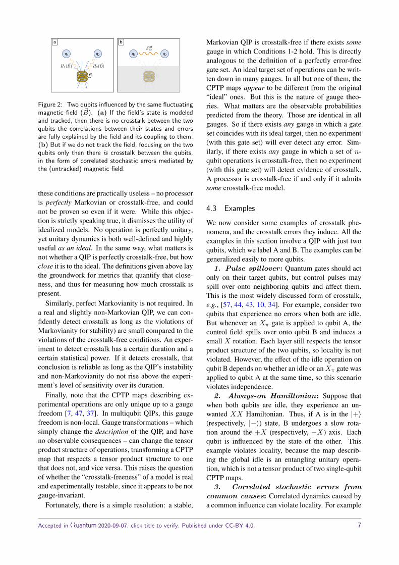
Figure 3: Illustration of the type of circuits used in ourprotocol. A 4-qubit QIP is partitioned into three regions,labeled r0, r1, r2, and the goal is to detect crosstalk er-rors between these regions. To do so, we perform cir-cuits that only apply coupling operations between qubitswithin a region, never between regions (across the redlines in the figure). The random variable outcome frommeasuring the qubits in region ri is denoted Rri

. Inthis example Rr0 and Rr2 are 1-bit-valued while Rr1 is2-bit-valued.

are the settings assigned to the qubits in region riand Rri are the measurement results from the qubitsin region ri. We treat each member of this tuple asa random variable drawn from some sample space,Sri ∈ Sri ,Rri ∈ Rri . It is clear that the results arerandom variables; they are the results of measure-ments on quantum systems, which are always randomvariables. We also treat the settings as random vari-ables, but for a different reason. In a large QIP, it isnot feasible to perform an exhaustive set of experi-ments that enumerates all the possible experimentalsettings. So, in practice, observed data constitute asample over all the possible settings. As we shall see,a random sampling over settings often yields goodresults. The random variable Rri takes values thatare bit strings of length n(ri), obtained by measuringall qubits in region ri in some basis. More compli-cated scenarios, e.g., involving detection of leakage,are possible but we restrict ourselves to the simplestcase here. Fig. 3 illustrates these definitions.

The settings Sri are random variables that describe(i) what state is prepared natively on the qubits in ri,(ii) what gates are applied to the qubits in ri, and (iii)what basis the qubits in ri are measured in. So Srilabels a quantum circuit for that region (defined hereas the state preparation, applied gates and measure-ment basis choice for a region). We note that mostquantum computing architectures have only one qubitstate that is natively prepared (e.g., the ground state)and only one measurement basis (e.g., the Z basis).Therefore the only setting that can be varied is thegates applied to the qubits in between state prepara-tion and measurement. Hence in most quantum com-puting architectures, the settings will be synonymouswith “gates applied to qubits in ri”.


Definition 2: We say that a region ri is free ofcrosstalk errors to/from other regions if conditionaldistributions over the measurement results on this re-gion satisfy:

P (Rri |Sri ,T) = P (Rri |Sri), withT ⊆ Ω \ Rri ,Sri (9)

This means that the distribution of measurement re-sults on region ri depends only on the settings forri; conditioned on those settings, it is independent ofall the other random variables in Ω. Any violation ofthese conditions is a witness to some kind of crosstalkerror.

It is preferable to define the crosstalk-free con-dition in terms of conditional independence as op-posed to marginal independence – i.e., P (Rri ,Srj ) =P (Rri)P (Srj ) – because it is more robust to con-founding by hidden (or intentional) correlations insettings, which can become an issue when detectingcrosstalk errors in large QIPs. Appendix A discussesthis further.

This model-free definition of crosstalk errors isequivalent to our model-based definition of crosstalkerrors (Definition 1) stated in Sec. 3; see AppendixB for proof. The two definitions capture the samenotions of locality and independence of quantumoperations – the model-based definition does so interms of conditions on models of quantum operations(i.e., CPTP maps), while the model-free definitiondoes so in terms of conditions on operational randomvariables that arise naturally in a QIP.

Example. Here is an example to illustrate the nota-tion introduced above. We wish to detect crosstalk er-rors induced by single qubit operations on a QIP with3 qubits, partitioned into two regions r0 = 0 andr1 = r0 = 1, 2. The following elementary single-qubit operations can be performed: initialization in|0〉; initialization in |+〉; idle gate (i.e., do nothingfor one clock cycle); Xπ/2 gate; Zπ/2 gate; and mea-surement in the computational basis. Circuits can beperformed that comprise (1) parallel initialization ofall 3 qubits, (2) a sequence of k layers built from arbi-trary single-qubit gates on each qubit in parallel, and(3) measurement of all qubits in the computationalbasis. Then the sample space of settings on region r0– which includes only qubit 0 – is

Sr0 = Sp × Sg= Prep|0〉,Prep|+〉 × GI , GX , GZk

where we have distinguished prep settings (Sp) andgate settings (Sg). Only one measurement layer is

allowed and the only measurement basis accessibleis the computational basis, so there are no measure-ment settings. The space of settings for region r1is isomorphic to two copies of the settings for r0:Sr1 = Sr0 × Sr0 . The spaces of possible results foreach of the two regions are simply Rr0 = 0, 1 andRr1 = 0, 12. In this example, each experiment islabeled by the following tuple of nine random vari-ables,

(Sr0 ,Sr1 ,Rr0 ,Rr1)= ((P0, G0), ((P1, G1), (P2, G2)), R0, (R1, R2)),

(10)

where Pi ∈ Sp, Gi ∈ Sg and Ri ∈ 0, 1 label (re-spectively) the preparation, sequence of gates, andmeasurements results for qubit i.

The model-free definition given by Eq. (9)leads directly to practical tests for crosstalk, be-cause if we draw a circuit at random from thedistribution defined by P (Sr0 ,Sr1 , ...,SrM−1) andperform it on the QIP, the result is a samplefrom the joint probability distribution P (Ω) ≡P (Sr0 ,Sr1 , ...,SrM−1 ,Rr0 ,Rr1 , ...,RrM−1). Thesesamples can be used to statistically test the condi-tions implied by Eq. (9). This is, in fact, a generalprocedure for detecting crosstalk errors. There is al-ways some partitioning of the QIP into regions, somecircuit family that can be executed, and some datasample size that will detect any crosstalk error usingthis method. However, as discussed in Sec. 5, de-tecting any possible crosstalk error requires exponen-tial resources, and thus is not a scalable goal. There-fore, our aim is to use this model-independent def-inition to formulate an efficient protocol that targetslow-weight crosstalk errors.

Developing this protocol requires three ingredi-ents: (i) defining a set of region partitions for aQIP, (ii) defining a set of experiments to performon the QIP, and (iii) defining an analysis techniqueon the data produced by these experiments to detectcrosstalk using Definition 2. The following subsec-tions tackle each of these ingredients.

6.2 Defining regions

Our crosstalk detection protocol looks for correla-tions between regions of a QIP that should be uncou-pled. This requires partitioning the QIP into disjointregions. No single partition into regions will suffice– for example, we might need to test whether the2-qubit region 1, 2 has crosstalk with the 2-qubit


region 3, 4, but also whether 2, 3 has crosstalkwith 4, 5. So we need multiple partitions, and foreach one, we will define a set of circuits that respectit.

We cannot test every possible partition – the to-tal number of ways to partition n qubits is Bn, thenth Bell number, which scales super-exponentially inn. However, testing all possible partitions is unnec-essary. Crosstalk errors are associated with individ-ual layers of elementary operations. In almost everyQIP architecture, each elementary operation targetsonly 1 or 2 qubits. So, since we focus on low-weightcrosstalk errors, it is sufficient to consider partitionsinto disjoint one- and two-qubit regions. These allowus to ask (and detect) whether correlations emergebetween any two such regions, in circuits that nevercouple them intentionally.

Let us first set some terminology. We refer to a re-gion containing exactly k qubits as a k-region, and apartition of the entire QIP into regions that each con-tain k or fewer qubits as a k-partition. We say thata region is allowed if it is possible to define circuitsthat couple all the qubits within that region, withoutinvolving any other qubits. So a 2-region is allowedonly if the QIP has a 2-qubit gate directly betweenthose qubits. We say that a region is in a given par-tition if it is one of the regions making up the par-tition – e.g., region 1, 2 is in the 6-qubit partition1, 2, 3, 4, 5, 6. Further, a tuple of regions isin a given partition if each region in the tuple is in thepartition – e.g., the pair 1, 2, 5, 6 is also in theabove partition.

There is exactly one unique 1-partition of an n-qubit QIP. So if we wish to detect crosstalk errors as-sociated with single-qubit gates, this is the only par-tition we need to use.

However, we must also detect crosstalk errorsassociated with 2-qubit gates, which requires 2-partitions. The number of possible 2-partitions scalesexponentially with n; the number of ways to parti-tion n elements into distinct sets of size k (assumingk divides n) is #(n, k) = n!

(k!)n/2(n/k)! , and hence

#(n, 2) ≈ (√n/e)n, via the Stirling approximation.

This assumes that two-qubit operations are possiblebetween any two qubits in the QIP, however even inthe more realistic case of limited connectivity, thenumber of 2-regions grows exponentially in n. Soit is impractical to even test all 2-partitions exhaus-tively. Fortunately, since we are focused on detectinglow-weight crosstalk errors, it suffices to detect pair-wise crosstalk between 2-regions (see Sec. 6.5 for a

discussion of the resulting limitations), and doing thisonly requires that we guarantee that every pair of 2-regions is in at least one 2-partition of the QIP that istested.

Since there are at most n(n − 1)/2 allowed 2-regions, there are O(n4) pairs of 2-regions. There-fore, it is easy to define a set of O(n4) 2-partitionsthat contain every such pair (e.g., for each of theO(n4) possible pairs of 2-regions, define a partitionby starting with those two 2-regions and then arbitrar-ily partitioning the remaining qubits into 2-regions).This requires only poly(n) resources, but is clearlywasteful. If we are satisfied with a high probabilityguarantee, a randomized partitioning strategy is moreefficient.

Theorem 1 Given an n-qubit QIP, let ri, 0 < i <

R = n(n−1)2 , be a labeling of all 2-regions in the

QIP, and let P be a set of independent and uniformlysampled random 2-partitions of the QIP. For any0 < ε < 1, the probability that any pair of distinct 2-regions is in at least one 2-partition is bounded belowby (1− ε) if |P| ≥ n2(2 log(R)− log(ε)).

Proof: We will follow the logic of the proof of Theo-rem 3.1 in Ref. [36]. Let p be a lower bound on theprobability that any 2-partition of the QIP containsa pair of 2-regions (we will see below this bound isthe same for any pair). Then, the probability that thispair of 2-regions is not in |P| random 2-partitions is atmost (1−p)|P|. By applying the union bound, we seethat the probability that any one of the R(R − 1)/2possible pairs of 2-regions in the QIP is not in anypartition in P is at most R(R−1)

2 (1−p)|P|. We wouldlike this probability to be at most ε,

R(R− 1)2 (1− p)|P| ≤ ε

⇒ |P| ≥log

(εR2

)log(1− p)

⇒ |P| ≥ p−1(2 log(R)− log(ε)),

where we have used the fact that −p > log(1 − p).It remains to compute the lower bound p in terms ofthe system parameters. The probability that any pairof 2-regions is in a 2-partition is given by the ratio#(n−4,2)

#(n,2) since there are #(n − 4, 2) possible par-titions of the remaining n − 4 qubits once the fourqubits in the pair of 2-regions have been removed.Computing this ratio, we get 1

(n−1)(n−3) , and hence alower bound on this probability is p > 1

n2 . Substitut-ing this into the above bound on |P| gives the desiredresult.


Either of these approaches – the brute-force arrayofO(n4) partitions, or theO(n2 log(n)) randomizedstrategy – defines a list of poly(n) partitions of theQIP that will detect pairwise crosstalk between anypair of 2-regions with high probability.

We note that in QIPs with local connectivity re-strictions, e.g., a planar array of qubits where inten-tional coupling operations are only possible betweennearest neighbors qubits, p−1 = O(n), and thereforethe scaling of the randomized strategy is improved toO(n log(n)). Similarly, the scaling of the brute-forcepartitioning improves to O(n2) under local connec-tivity.

6.3 Lightweight experiment design

Given a partition of a QIP into regions, we must de-fine a set of circuits to run on the QIP that consti-tute the crosstalk detection experiment. We only con-sider circuits that do not (intentionally) couple re-gions, which means that for each region there is awell-defined subcircuit comprising all operations ap-plied to it. We also assume, for the sake of simplic-ity, that the QIP has unique initialization and mea-surement operations (in |0〉⊗n and the 〈0| , 〈1|⊗nbasis). Thus, the settings for a region correspond pre-cisely to the gates in the subcircuit on that region.

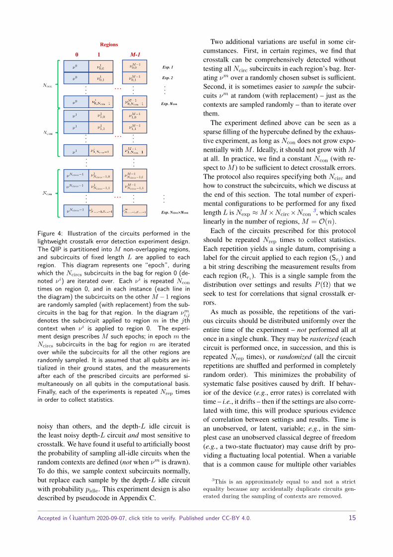
Each possible circuit on the QIP is composed ofthe parallel application of multiple subcircuits, oneon each region. The simplest approach is to choosea collection of Ncirc subcircuits for each region, andthen perform all combinations of those subcircuits.We refer to this collection of subcircuits as the “bag”of circuits applied to a region. (We postpone thequestion of what subcircuits to place in the bag to theend of this subsection). We call this the exhaustive ex-periment, in which each subcircuit on region ri getsperformed in an exhaustive variety of different con-texts – i.e., in parallel with all Ncirc circuits on otherregions – and so violations of independence are easyto detect in the data. Unfortunately, this experimentdefines a hypercube containingNM

circ distinct circuits,which grows too rapidly with M (the number of re-gions) to be feasible.

However, we observe that in the exhaustive experi-ment, each subcircuit on every region ri is performedin exponentially many distinct contexts (defined bythe settings on the other regions rj , ri). This isarduous and overkill; since crosstalk errors are notlikely to only be present in one or few of this expo-nential number of contexts (this is discussed furtherin Sec. 6.5), we can subsample from this exhaustive

experiment. So we will choose a sparse subset of theexperiments in the hypercube defining the exhaustiveexperiment, with the goal of defining a small set ofexperiments that allow low-weight crosstalk errors tobe detected.

6.3.1 An explicit construction

The sparse sampling of the hypercube should main-tain two important properties of the exhaustive ex-periment. First, each subcircuit in the bag for eachregion ri must appear in multiple contexts (but notexponentially many). Second, that set of contexts inwhich each subcircuit gets performed must vary oneach of the other regions. These properties ensurethat – whatever subcircuits we select for each region’sbag – the data will reveal whether the local results ofthose subcircuits are significantly influenced by thesettings (choice of subcircuit) on any other region.

The construction we outline now ensures that theseproperties are preserved, even with much fewer ex-periments. It is defined by three adjustable integerparameters:

• L is the length or depth of all the subcircuits.Subcircuits on different regions are applied inparallel, so they must all be the same length, soL must be chosen and fixed.

• Ncirc is the number of circuits in the bag for eachregion. This number can be chosen to be a con-stant (independent of n), as we argue below.

• Ncon is the number of random contexts in whicheach subcircuit will be tested.

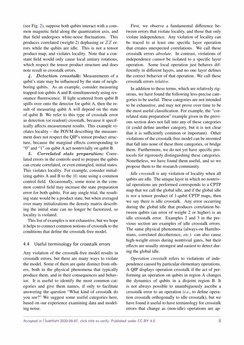
First, we choose a bag of Ncirc depth-L subcircuitsfor each of the M regions (see below for their con-struction). Now, for each region m ∈ [0 . . .M − 1]and each of the subcircuits νm in that region’s bag,we define Ncon different circuits that perform νm indifferent contexts, by choosing a subcircuit for eachof the other regions at random from the correspond-ing bag, and performing all those subcircuits (includ-ing νm) in parallel. This circuit selection procedureis illustrated in Fig. 4.

This design ensures that (1) for each region, ap-proximately Ncirc different subcircuits are studied indetail, (2) each of these subcircuits is performed inNcon different contexts, and (3) those contexts varyindependently across all the other regions.

We have found that a small refinement improvesthe protocol in practice. Often, the idle gate is less


Regions

0 1 M-1

. . .

Exp. 2

Exp. 1

. . .

1<latexit sha1_base64="qSvHhJwQAZWT5ZnoMusg7f6J+8E=">AAAEBnicjVPLjtMwFPU0PIbwmoElm4gIiVWVABIsR8ACFohh1E5Hqjsjx7lJrThOZDtAZXnPli38AzvElt/gE/gLnLRCnXSKuJLjq3vO8X3ETmrOlI6iXzsD79LlK1d3r/nXb9y8dXtv/86xqhpJYUwrXsmThCjgTMBYM83hpJZAyoTDJCletPjkPUjFKjHSixpmJckFyxgl2oUmWDSnJrZne2E0jDoLNp145YRoZYdn+4PfOK1oU4LQlBOlpnFU65khUjPKwfq4UVATWpAcps4VpAQ1M129NnjgImmQVdItoYMuuq4wpFRqUSaOWRI9V32sDV6ETRudPZsZJupGg6DLRFnDA10FbfNByiRQzRfOIVQyV2tA50QSqt2IfB+/BNeMhDfu4Lc1SKIrabCW1ri1BR39E5WFNZKIYhvu6sit6b4+FvCBVmVJRGpwIomdxjODQahGQtuqwRwyjTkROQcTxhZLls81dr9X2568AL1F3rLXxLI7rS8niVrK/0qCMA7W853nw8fazfV/C744J0vdXbLG4FaaJHEfT92gTt1G8hxkH9Sy7lCVBaMWk7COHoE1uFoNvb2K5gg2Wa/LPstFrO+7xxH3n8Kmc/xoGD8eRu+ehAfPV89kF91D99FDFKOn6AC9QodojCgq0Gf0BX31PnnfvO/ejyV1sLPS3EXnzPv5B4PzZVY=</latexit>



M11,1

<latexit sha1_base64="O50i3zt9S/dA33xy7EEEDnH1OoE=">AAAEEHicjVPNjtMwEPY2/CzhZ7tw5BJRIXGAKgEkOK6AAxxWu6za3ZXqbuU4k9Sq40S2A1SWX4IrV3gHbmivvAGPwFvgpBXqplvESHZG832fZzzxxCVnSofhr62Od+XqtevbN/ybt27f2enu3j1WRSUpDGnBC3kaEwWcCRhqpjmclhJIHnM4iWeva/zkA0jFCjHQ8xLGOckESxkl2oUm3R0sqjOz/ySyExM9dnu3F/bDxoJ1J1o6PbS0w8lu5zdOClrlIDTlRKlRFJZ6bIjUjHKwPq4UlITOSAYj5wqSgxqbpnIbPHSRJEgL6ZbQQRNdVRiSKzXPY8fMiZ6qNlYHL8NGlU5fjg0TZaVB0EWitOKBLoK6DUHCJFDN584hVDJXa0CnRBKqXbN8H78BdxkJ++7ggxIk0YU0WEtr3NqADv6Jypk1kojZJtzVkVnT7D4W8JEWeU5EYnAsiR1FY4NBqEpCfVWDOaQacyIyDqYXWSxZNtXY/WhtW/IZ6A3ymr0ils1pbTmJ1UL+VxL0omA130U+fCpdX/+34MtzssS9JWsMrqVxHLXxxDXqzH1IloFsg1qWDarSYFBjElbRI7AGF8um10/RHME6613eZrmI9X03HFF7FNad46f96Fk/fP+8t/dqOSbb6D56gB6hCL1Ae+gtOkRDRFGFvqCv6Jv32fvu/fDOF9TO1lJzD10w7+cfImVoNg==</latexit>

. . .

0<latexit sha1_base64="AoO9REyCigQuUN/EEand4ksb5kk=">AAAEBnicjVPLjtMwFPU0PIbwmoElm4gIiVWVABIsR8ACFohh1E5Hqjsjx7lJrThOZDtAZXnPli38AzvElt/gE/gLnLRCnXSKuJLjq3vO8X3ETmrOlI6iXzsD79LlK1d3r/nXb9y8dXtv/86xqhpJYUwrXsmThCjgTMBYM83hpJZAyoTDJCletPjkPUjFKjHSixpmJckFyxgl2oUmWDSnJrJne2E0jDoLNp145YRoZYdn+4PfOK1oU4LQlBOlpnFU65khUjPKwfq4UVATWpAcps4VpAQ1M129NnjgImmQVdItoYMuuq4wpFRqUSaOWRI9V32sDV6ETRudPZsZJupGg6DLRFnDA10FbfNByiRQzRfOIVQyV2tA50QSqt2IfB+/BNeMhDfu4Lc1SKIrabCW1ri1BR39E5WFNZKIYhvu6sit6b4+FvCBVmVJRGpwIomdxjODQahGQtuqwRwyjTkROQcTxhZLls81dr9X2568AL1F3rLXxLI7rS8niVrK/0qCMA7W853nw8fazfV/C744J0vdXbLG4FaaJHEfT92gTt1G8hxkH9Sy7lCVBaMWk7COHoE1uFoNvb2K5gg2Wa/LPstFrO+7xxH3n8Kmc/xoGD8eRu+ehAfPV89kF91D99FDFKOn6AC9QodojCgq0Gf0BX31PnnfvO/ejyV1sLPS3EXnzPv5B4BWZVU=</latexit>



10,1

<latexit sha1_base64="gXmOoXsBhEFpysTNfazxgv78K1Y=">AAAEDHicjVPNbtQwEHY3/JTw18KRS8QKiQNaJYAExwo4wAFRqt220jqtHGeSteI4wXaAleVX4MoV3oEb4so78Ai8BU52hbbZLmIkO6P5vs8znniSmjOlw/DX1sC7cPHS5e0r/tVr12/c3Nm9daiqRlKY0IpX8jghCjgTMNFMcziuJZAy4XCUFM9b/Og9SMUqMdbzGuKS5IJljBLtQjEWzYmJ7KkJH7h9ZxiOws6CdSdaOkO0tP3T3cFvnFa0KUFoyolS0yisdWyI1IxysD5uFNSEFiSHqXMFKUHFpqvaBvdcJA2ySroldNBFVxWGlErNy8QxS6Jnqo+1wfOwaaOzp7Fhom40CLpIlDU80FXQtiBImQSq+dw5hErmag3ojEhCtWuU7+MX4C4j4bU7+E0NkuhKGqylNW5tQMf/RGVhjSSi2IS7OnJrut3HAj7QqiyJSA1OJLHTKDYYhGoktFc1mEOmMSci52CGkcWS5TON3U/WticvQG+Qt+wVsexO68tJohbyv5JgGAWr+c7y4WPt+vq/BZ+fk6XuLVljcCtNkqiPp65RJ+5D8hxkH9Sy7lCVBeMWk7CKHoA1uFo2vX2K5gDWWa/KPstFrO+74Yj6o7DuHD4cRY9G4dvHw71nyzHZRnfQXXQfRegJ2kMv0T6aIIreoc/oC/rqffK+ed+9HwvqYGupuY3OmPfzD1ctZ3Y=</latexit>

Exp. Ncircs×"#$%

Exp. "#$%

Ncircs1<latexit sha1_base64="IogXehKBsSNI2ayquLGgfYne/yk=">AAAEFnicjVPNjtMwEPZu+FnCXxfEiYtFhcSFqlmQ4LgCDnAAllW7u1LdrRxnklp1nMh2gMrye3DlCu/ADXHlyiPwFjhphbrpFjGS49F83+cZTzxxKbg2/f6vre3gwsVLl3euhFevXb9xs7N760gXlWIwZIUo1ElMNQguYWi4EXBSKqB5LOA4nj2v8eP3oDQv5MDMSxjnNJM85YwaH5p07hBZndo3E0tUjhlXTLuHkZt0uv1evzG87kRLp4uWdjDZ3f5NkoJVOUjDBNV6FPVLM7ZUGc4EuJBUGkrKZjSDkXclzUGPbVO/w/d9JMFpofySBjfRVYWludbzPPbMnJqpbmN18DxsVJn06dhyWVYGJFskSiuBTYHrZuCEK2BGzL1DmeK+VsymVFFmfMvCkLwAfxkFr/3Bb0tQ1BTKEqOc9WsDOvgnqmbOKipnm3BfR+Zs8w2JhA+syHMqE0tiRd0oGlsCUlcK6qtaIiA1RFCZCbDdyBHFs6kh/ncb15LPwGyQ1+wVsWpOa8tprBfyvxLcjfBqvrN8+Fj6vv5vwefn5Il/S85aUkvjOGrjiW/Uqd9oloFqg0aVDapTPKgxBavoIThLimXT66doD2Gd9Spvs3zEhaEfjqg9CuvO0V4vetTbe/e4u/9sOSY76C66hx6gCD1B++glOkBDxJBFn9EX9DX4FHwLvgc/FtTtraXmNjpjwc8/oxRrVg==</latexit>



11,1

<latexit sha1_base64="zHiFzS3Z7Zq3mF/pm9185LWRiog=">AAAECnicjVPNjtMwEPY2/CzhbxeOXCIqJA6oqhckOK4WDnBALKt2d6W6WznOJLXqOJHtLFSW34ArV3gHbogrL8Ej8BY4aYW66RYxkuPRfN/nGU88cSm4Nv3+r61OcOXqtevbN8Kbt27fubuze+9YF5ViMGSFKNRpTDUILmFouBFwWiqgeSzgJJ69rPGTc1CaF3Jg5iWMc5pJnnJGjQ+NiKzO8MTiJ9hNdrr9Xr+xaN3BS6eLlnY42e38JknBqhykYYJqPcL90owtVYYzAS4klYaSshnNYORdSXPQY9vU7KJHPpJEaaH8kiZqoqsKS3Ot53nsmTk1U93G6uBl2Kgy6Yux5bKsDEi2SJRWIjJFVDcgSrgCZsTcO5Qp7muN2JQqyoxvUxiSV+Avo+CtP/hdCYqaQllilLN+bUAH/0TVzFlF5WwT7uvInG2+IZHwgRV5TmViSayoG+GxJSB1paC+qiUCUkMElZkA28WOKJ5NDfG/2LiWfAZmg7xmr4hVc1pbTmO9kP+VRF0crea7yIePpe/r/xZ8eU6e+LfkrCW1NI5xG098o878RrMMVBs0qmxQnUaDGlOwih6Bs6RYNr1+ivYI1llv8jbLR1wY+uHA7VFYd473evhpb+/9s+7+wXJMttED9BA9Rhg9R/voNTpEQ8RQgT6jL+hr8Cn4FnwPfiyona2l5j66YMHPP4PBZm0=</latexit>

10,0

<latexit sha1_base64="7fJwoUAWhY46DT1/wNwiIolmRgA=">AAAECnicjVPNjtMwEPZu+FnC3y4cuURUSBxQlSxIcFwBBzggllW7u1LdrRxnklp17Mh2gMryG3DlCu/ADXHlJXgE3gInrVA33SJGcjya7/s844knrTjTJo5/bW0Hly5fubpzLbx+4+at27t7d461rBWFIZVcqtOUaOBMwNAww+G0UkDKlMNJOnvR4CfvQWkmxcDMKxiXpBAsZ5QYHxphUZ8lExs/it1ktxf349aidSdZOj20tMPJ3vZvnElalyAM5UTrURJXZmyJMoxycCGuNVSEzkgBI+8KUoIe27ZmFz3wkSzKpfJLmKiNriosKbWel6lnlsRMdRdrghdho9rkz8aWiao2IOgiUV7zyMioaUCUMQXU8Ll3CFXM1xrRKVGEGt+mMMQvwV9GwRt/8NsKFDFSWWyUs35tQAf/RNXMWUXEbBPu6yicbb8hFvCByrIkIrM4VcSNkrHFIHStoLmqxRxygzkRBQfbSxxWrJga7H+xcR35DMwGecNeEav2tK6cpHoh/yuJekm0mu88Hz5Wvq//W/DFOVnm35KzFjfSNE26eOYbdeY3UhSguqBRVYvqPBo0mIJV9AicxXLZ9OYp2iNYZ70uuywfcWHohyPpjsK6c7zfTx7399896R08X47JDrqH7qOHKEFP0QF6hQ7REFEk0Wf0BX0NPgXfgu/BjwV1e2upuYvOWfDzD3yFZms=</latexit>

11,0

<latexit sha1_base64="uk2F9UDA/vdWTZg098Pyo40kl8I=">AAAECnicjVPNjtMwEPZu+FnC3y4cuURUSBxQlSxIcFwBBzggllW7u1LdrRxnklp17Mh2gMryG3DlCu/ADXHlJXgE3gInrVA33SJGcjya7/s844knrTjTJo5/bW0Hly5fubpzLbx+4+at27t7d461rBWFIZVcqtOUaOBMwNAww+G0UkDKlMNJOnvR4CfvQWkmxcDMKxiXpBAsZ5QYHxphUZ8lE5s8it1ktxf349aidSdZOj20tMPJ3vZvnElalyAM5UTrURJXZmyJMoxycCGuNVSEzkgBI+8KUoIe27ZmFz3wkSzKpfJLmKiNriosKbWel6lnlsRMdRdrghdho9rkz8aWiao2IOgiUV7zyMioaUCUMQXU8Ll3CFXM1xrRKVGEGt+mMMQvwV9GwRt/8NsKFDFSWWyUs35tQAf/RNXMWUXEbBPu6yicbb8hFvCByrIkIrM4VcSNkrHFIHStoLmqxRxygzkRBQfbSxxWrJga7H+xcR35DMwGecNeEav2tK6cpHoh/yuJekm0mu88Hz5Wvq//W/DFOVnm35KzFjfSNE26eOYbdeY3UhSguqBRVYvqPBo0mIJV9AicxXLZ9OYp2iNYZ70uuywfcWHohyPpjsK6c7zfTx7399896R08X47JDrqH7qOHKEFP0QF6hQ7REFEk0Wf0BX0NPgXfgu/BjwV1e2upuYvOWfDzD4AkZmw=</latexit>

1Ncircs1,0

<latexit sha1_base64="t2rx3CG/MifnJnok6LDDVqv9T5w=">AAAEGnicjVPLjtMwFPU0PIbw6sAKsbGokFhAlQxIsBwBC1gAw6idGanuVI5zk1pNnMh2gMqy+BG2bOEf2CG2bPgE/gInrVAnnSKu5PjqnnN8H7GjMuNKB8GvrY537vyFi9uX/MtXrl673t25caiKSjIYsiIr5HFEFWRcwFBzncFxKYHmUQZH0exZjR+9A6l4IQZ6XsI4p6ngCWdUu9Cke4uI6iScmNcTQ2SOGZdM2Qfh/cBOur2gHzSG151w6fTQ0vYnO53fJC5YlYPQLKNKjcKg1GNDpeYsA+uTSkFJ2YymMHKuoDmosWl6sPiui8Q4KaRbQuMmuqowNFdqnkeOmVM9VW2sDp6FjSqdPBkbLspKg2CLREmVYV3geiA45hKYzubOoUxyVytmUyop025svk+eg2tGwit38JsSJNWFNERLa9zagA7+icqZNZKK2Sbc1ZFa03x9IuA9K/KcitiQSFI7CseGgFCVhLpVQzJINMmoSDMwvdASydOpJu6Xa9uSz0BvkNfsFbFsTmvLaaQW8r8S3Avxar7TfPhQurn+b8Fn5+Sxu0vWGFJLoyhs47Eb1InbaJqCbINalg2qEjyoMQmr6AFYQ4rl0OuraA5gnfUyb7NcxPq+exxh+ymsO4e7/fBhf/fto97e0+Uz2Ua30R10D4XoMdpDL9A+GiKGPqLP6Av66n3yvnnfvR8LamdrqbmJTpn38w+x72xq</latexit>

1Ncircs1,1

<latexit sha1_base64="rP9Uab4iWIYZj+AStWM+SwZVX7E=">AAAEGnicjVPLjtMwFPW0PIbw6sAKsbGokFhA1QxIsBwBC1gAw6idGanuVI5zk1p1nMh2gMqy+BG2bOEf2CG2bPgE/gInrVAnnSKu5PjqnnN8H7GjQnBt+v1fW632ufMXLm5fCi5fuXrtemfnxqHOS8VgyHKRq+OIahBcwtBwI+C4UECzSMBRNHtW4UfvQGmey4GZFzDOaCp5whk1PjTp3CKyPAkn9vXEEpVhxhXT7kF4P3STTrff69eG151w6XTR0vYnO63fJM5ZmYE0TFCtR2G/MGNLleFMgAtIqaGgbEZTGHlX0gz02NY9OHzXR2Kc5MovaXAdXVVYmmk9zyLPzKiZ6iZWBc/CRqVJnowtl0VpQLJFoqQU2OS4GgiOuQJmxNw7lCnua8VsShVlxo8tCMhz8M0oeOUPflOAoiZXlhjlrF8b0ME/UTVzVlE524T7OlJn629AJLxneZZRGVsSKepG4dgSkLpUULVqiYDEEEFlKsB2Q0cUT6eG+F9uXEM+A7NBXrFXxKo+rSmnkV7I/0pwN8Sr+U7z4UPh5/q/BZ+dk8f+LjlrSSWNorCJx35QJ36jaQqqCRpV1KhO8KDCFKyiB+AsyZdDr66iPYB11susyfIRFwT+cYTNp7DuHO72woe93bePuntPl89kG91Gd9A9FKLHaA+9QPtoiBj6iD6jL+hr+1P7W/t7+8eC2tpaam6iU9b++Qe1jGxr</latexit>

M10,0

<latexit sha1_base64="IKJLp+qOoDz4hbDFH/ftBTF9AZc=">AAAEEHicjVPNjtMwEPY2/CzhZ7tw5BJRIXGAKtlFguMKOMBhxbJqd1equ5XjTFKrjhPZDlBZfgmuXOEduCGuvAGPwFvgpBXqplvESI5H832fZzzxxCVnSofhr62Od+XqtevbN/ybt27f2enu3j1RRSUpDGnBC3kWEwWcCRhqpjmclRJIHnM4jWcva/z0PUjFCjHQ8xLGOckESxkl2oUm3R0sqnNz+CSyExM+Du2k2wv7YWPBuhMtnR5a2tFkt/MbJwWtchCacqLUKApLPTZEakY5WB9XCkpCZySDkXMFyUGNTVO5DR66SBKkhXRL6KCJrioMyZWa57Fj5kRPVRurg5dho0qnz8eGibLSIOgiUVrxQBdB3YYgYRKo5nPnECqZqzWgUyIJ1a5Zvo9fgbuMhEN38NsSJNGFNFhLa9zagA7+icqZNZKI2Sbc1ZFZ03x9LOADLfKciMTgWBI7isYGg1CVhPqqBnNINeZEZBxML7JYsmyqsfvR2rbkM9Ab5DV7RSyb09pyEquF/K8k6EXBar6LfPhYur7+b8GX52SJe0vWGFxL4zhq44lr1LnbSJaBbINalg2q0mBQYxJW0WOwBhfLptdP0RzDOutN3ma5iPV9NxxRexTWnZO9frTf33v3tHfwYjkm2+g+eoAeoQg9QwfoNTpCQ0RRhT6jL+ir98n75n33fiyona2l5h66YN7PPxvNaDY=</latexit>

M10,1

<latexit sha1_base64="OXn3Id0n6wxEv5XwqMQHQIMBNtg=">AAAEEHicjVPNjtMwEPY2/CzhZ7tw5BJRIXGAKtlFguMKOMBhxbJqd1equ5XjTFKrjhPZDlBZfgmuXOEduCGuvAGPwFvgpBXqplvESHZG832fZzzxxCVnSofhr62Od+XqtevbN/ybt27f2enu3j1RRSUpDGnBC3kWEwWcCRhqpjmclRJIHnM4jWcva/z0PUjFCjHQ8xLGOckESxkl2oUm3R0sqnNz+CSyExM+dnu3F/bDxoJ1J1o6PbS0o8lu5zdOClrlIDTlRKlRFJZ6bIjUjHKwPq4UlITOSAYj5wqSgxqbpnIbPHSRJEgL6ZbQQRNdVRiSKzXPY8fMiZ6qNlYHL8NGlU6fjw0TZaVB0EWitOKBLoK6DUHCJFDN584hVDJXa0CnRBKqXbN8H78CdxkJh+7gtyVIogtpsJbWuLUBHfwTlTNrJBGzTbirI7Om2X0s4AMt8pyIxOBYEjuKxgaDUJWE+qoGc0g15kRkHEwvsliybKqx+9HatuQz0BvkNXtFLJvT2nISq4X8ryToRcFqvot8+Fi6vv5vwZfnZIl7S9YYXEvjOGrjiWvUufuQLAPZBrUsG1SlwaDGJKyix2ANLpZNr5+iOYZ11pu8zXIR6/tuOKL2KKw7J3v9aL+/9+5p7+DFcky20X30AD1CEXqGDtBrdISGiKIKfUZf0Ffvk/fN++79WFA7W0vNPXTBvJ9/AB9qaDc=</latexit>

M11,0

<latexit sha1_base64="zn2+8vqRvidV2i6G28oT6nv1BYs=">AAAEEHicjVPNjtMwEPY2/CzhZ7tw5BJRIXGAKtlFguMKOMBhxbJqd1equ5XjTFKrjhPZDlBZfgmuXOEduCGuvAGPwFvgpBXqplvESI5H832fZzzxxCVnSofhr62Od+XqtevbN/ybt27f2enu3j1RRSUpDGnBC3kWEwWcCRhqpjmclRJIHnM4jWcva/z0PUjFCjHQ8xLGOckESxkl2oUm3R0sqnNz+CSyExM9Du2k2wv7YWPBuhMtnR5a2tFkt/MbJwWtchCacqLUKApLPTZEakY5WB9XCkpCZySDkXMFyUGNTVO5DR66SBKkhXRL6KCJrioMyZWa57Fj5kRPVRurg5dho0qnz8eGibLSIOgiUVrxQBdB3YYgYRKo5nPnECqZqzWgUyIJ1a5Zvo9fgbuMhEN38NsSJNGFNFhLa9zagA7+icqZNZKI2Sbc1ZFZ03x9LOADLfKciMTgWBI7isYGg1CVhPqqBnNINeZEZBxML7JYsmyqsfvR2rbkM9Ab5DV7RSyb09pyEquF/K8k6EXBar6LfPhYur7+b8GX52SJe0vWGFxL4zhq44lr1LnbSJaBbINalg2q0mBQYxJW0WOwBhfLptdP0RzDOutN3ma5iPV9NxxRexTWnZO9frTf33v3tHfwYjkm2+g+eoAeoQg9QwfoNTpCQ0RRhT6jL+ir98n75n33fiyona2l5h66YN7PPx9saDc=</latexit>

M1Ncircs1,1

<latexit sha1_base64="mXIMWayg/536JYLRqW3swZm6nYM=">AAAEHnicjVPLbhMxFHU7PMrwSmGJkCwiJBY0yhQkWFbAAhaFUiVtpTiNPJ47Eysez8j2AJHlFT/Cli38AzvEFj6Bv8CTRCidNIgreXx1zzm+j7HjUnBtut1fG5vBhYuXLm9dCa9eu37jZmv71pEuKsWgzwpRqJOYahBcQt9wI+CkVEDzWMBxPHle48fvQGleyJ6ZljDMaSZ5yhk1PjRq3SWyOrX7O5Eb2dcjS1SOGVdMu53ooY+12t1Od2Z41YkWThst7GC0vfmbJAWrcpCGCar1IOqWZmipMpwJcCGpNJSUTWgGA+9KmoMe2lkfDt/3kQSnhfJLGjyLLisszbWe5rFn5tSMdROrg+dhg8qkT4eWy7IyINk8UVoJbApcDwUnXAEzYuodyhT3tWI2pooy40cXhuQF+GYU7PuD35SgqCmUJUY569catPdPVE2cVVRO1uG+jszZ2TckEt6zIs+pTCyJFXWDaGgJSF0pqFu1REBqiKAyE2DbkSOKZ2ND/G83riGfgFkjr9lLYjU7rSmnsZ7L/0pwO8LL+c7y4UPp5/q/BZ+fkyf+LjlrSS2N46iJJ35Qp36jWQaqCRpVzlCd4l6NKVhGD8FZUiyGXl9FewirrFd5k+UjLgz944iaT2HVOdrtRI86u28ft/eeLZ7JFrqD7qEHKEJP0B56iQ5QHzH0EX1GX9DX4FPwLfge/JhTNzcWmtvojAU//wCxUG4F</latexit>

M1Ncircs1,0

<latexit sha1_base64="x0EvqCFTBa7dxIsRzpTQ0cB8F4c=">AAAEHnicjVNNb9MwGPYWPkb46uCIkCIqJA6sSgYSHCfgAIfBmNptUt1VjvMmteo4ke0AleUTf4QrV/gP3BBX+An8C5y0Ql26Il7J8av3eR6/H7HjkjOlw/DXxqZ34eKly1tX/KvXrt+42dm+daSKSlIY0IIX8iQmCjgTMNBMczgpJZA85nAcT5/X+PE7kIoVoq9nJYxykgmWMkq0C407d7GoTs3+TmTH5vXYYJkHlEmq7E70MLTjTjfshY0Fq060cLpoYQfj7c3fOClolYPQlBOlhlFY6pEhUjPKwfq4UlASOiUZDJ0rSA5qZJo+bHDfRZIgLaRbQgdNdFlhSK7ULI8dMyd6otpYHTwPG1Y6fToyTJSVBkHnidKKB7oI6qEECZNANZ85h1DJXK0BnRBJqHaj8338AlwzEvbdwW9KkEQX0mAtrXFrDdr/Jyqn1kgiputwV0dmTfP1sYD3tMhzIhKDY0nsMBoZDEJVEupWDeaQasyJyDiYbmSxZNlEY/fbtW3Jp6DXyGv2klg2p7XlJFZz+V9J0I2C5Xxn+fChdHP934LPz8kSd5esMbiWxnHUxhM3qFO3kSwD2Qa1LBtUpUG/xiQso4dgDS4WQ6+vojmEVdarvM1yEev77nFE7aew6hzt9qJHvd23j7t7zxbPZAvdQffQAxShJ2gPvUQHaIAo+og+oy/oq/fJ++Z9937MqZsbC81tdMa8n38ArbNuBA==</latexit>

Figure 4: Illustration of the circuits performed in thelightweight crosstalk error detection experiment design.The QIP is partitioned into M non-overlapping regions,and subcircuits of fixed length L are applied to eachregion. This diagram represents one “epoch”, duringwhich the Ncircs subcircuits in the bag for region 0 (de-noted νi) are iterated over. Each νi is repeated Ncontimes on region 0, and in each instance (each line inthe diagram) the subcircuits on the other M −1 regionsare randomly sampled (with replacement) from the sub-circuits in the bag for that region. In the diagram νm

i,j

denotes the subcircuit applied to region m in the jthcontext when νi is applied to region 0. The experi-ment design prescribes M such epochs; in epoch m theNcircs subcircuits in the bag for region m are iteratedover while the subcircuits for all the other regions arerandomly sampled. It is assumed that all qubits are ini-tialized in their ground states, and the measurementsafter each of the prescribed circuits are performed si-multaneously on all qubits in the computational basis.Finally, each of the experiments is repeated Nrep timesin order to collect statistics.

noisy than others, and the depth-L idle circuit isthe least noisy depth-L circuit and most sensitive tocrosstalk. We have found it useful to artificially boostthe probability of sampling all-idle circuits when therandom contexts are defined (not when νm is drawn).To do this, we sample context subcircuits normally,but replace each sample by the depth-L idle circuitwith probability pidle. This experiment design is alsodescribed by pseudocode in Appendix C.

Two additional variations are useful in some cir-cumstances. First, in certain regimes, we find thatcrosstalk can be comprehensively detected withouttesting all Ncirc subcircuits in each region’s bag. Iter-ating νm over a randomly chosen subset is sufficient.Second, it is sometimes easier to sample the subcir-cuits νm at random (with replacement) – just as thecontexts are sampled randomly – than to iterate overthem.

The experiment defined above can be seen as asparse filling of the hypercube defined by the exhaus-tive experiment, as long as Ncon does not grow expo-nentially with M . Ideally, it should not grow with Mat all. In practice, we find a constant Ncon (with re-spect to M ) to be sufficient to detect crosstalk errors.The protocol also requires specifying both Ncirc andhow to construct the subcircuits, which we discuss atthe end of this section. The total number of experi-mental configurations to be performed for any fixedlength L isNexp ≈M×Ncirc×Ncon

3, which scaleslinearly in the number of regions, M = O(n).

Each of the circuits prescribed for this protocolshould be repeated Nrep times to collect statistics.Each repetition yields a single datum, comprising alabel for the circuit applied to each region (Sri) anda bit string describing the measurement results fromeach region (Rri). This is a single sample from thedistribution over settings and results P (Ω) that weseek to test for correlations that signal crosstalk er-rors.

As much as possible, the repetitions of the vari-ous circuits should be distributed uniformly over theentire time of the experiment – not performed all atonce in a single chunk. They may be rasterized (eachcircuit is performed once, in succession, and this isrepeated Nrep times), or randomized (all the circuitrepetitions are shuffled and performed in completelyrandom order). This minimizes the probability ofsystematic false positives caused by drift. If behav-ior of the device (e.g., error rates) is correlated withtime – i.e., it drifts – then if the settings are also corre-lated with time, this will produce spurious evidenceof correlation between settings and results. Time isan unobserved, or latent, variable; e.g., in the sim-plest case an unobserved classical degree of freedom(e.g., a two-state fluctuator) may cause drift by pro-viding a fluctuating local potential. When a variablethat is a common cause for multiple other variables

3This is an approximately equal to and not a strictequality because any accidentally duplicate circuits gen-erated during the sampling of contexts are removed.


is not observed, it can create a fictitious conditionaldependence between these variables [24]. Random-ization and rasterization reduce or destroy correla-tions between the settings and time, reducing the riskof conflation; see also related discussion about con-flation in Sec. 6.4.2. Finally, we note that rasteriz-ing also facilitates concurrent drift detection with thesame data [46].

We saw above that the number of distinct experi-ments required to detect crosstalk errors for one par-tition of the QIP is O(n). This is multiplied by thenumber of partitions to get the overall cost of detect-ing crosstalk errors for the QIP. As discussed above,the number of required partitions for a QIP scales asO(n2 log(n)) in the worst case. Therefore the num-ber of distinct experiments required for crosstalk de-tection with our protocol scales asO(n3 log(n)) (thisreduces to O(n2 log(n)) if qubits are only coupledlocally).

6.3.2 Choosing the subcircuits for each region’sbag

Exactly what subcircuits to choose or define for eachregion is a critical component. We have left it openfor now for a simple reason: there are many reason-able, yet very different, possible choices. For the sakeof concreteness, we specify particular circuits here.But we also expect that new, creative, and perhapsobjectively better choices can be usefully explored.

The subcircuits run on each region have two pur-poses: to manifest crosstalk, and to detect crosstalk.It may be that only certain circuits, when run on ri,cause or amplify errors on rj . And it may also be thatcertain circuits on rj are more sensitive to these ef-fects. Our goal is to detect whatever crosstalk errorsexist. Therefore, in principle, the subcircuits chosenfor each region’s bag should be those that (1) causethe greatest effects on other regions, and (2) are themost sensitive to effects caused by other regions.

Given a specific physical model of crosstalk, itis possible to design subcircuits with these proper-ties. Or, given a parameterized model of the sorts ofcrosstalk that might occur, it is possible to design arather larger set of subcircuits that collectively am-plify all the effects appearing in that model. (This ishow the circuits for gate set tomography (GST) arechosen).

An entirely different approach is to switch fromtrying to detect all low-weight crosstalk errors to fo-cusing on the crosstalk errors that impact a specificapplication. This motivates choosing subcircuits that

are representative of the subroutines that appear inspecific algorithms, and would emphasize detectionof crosstalk errors that impact execution of those par-ticular algorithms. There is no obvious general wayto doing this since most algorithms will couple manyqubits and not respect the region boundaries definedfor crosstalk detection. However, if there are certainsubcircuits, or circuit motifs, that occur repeatedly inan algorithm or application, these can be used to de-fine regions and subcircuits for crosstalk detection. Itshould be noted though that this approach will not de-tect crosstalk errors that might occur only when thesecircuit motifs are all put together into an applicationcircuit. Detecting such errors requires an application-or architecture-specific test.

But we have intentionally assumed no specificmodel and no specific application. In the absence ofany other guidance, random circuits – like those usedin randomized benchmarking – are a sensible choice.These have certain known drawbacks; they are lesssensitive than periodic circuits (e.g., those used inGST or robust phase estimation) to some forms ofnoise because they twirl it [14, 20, 7]. But randomcircuits are both common and hard to fool – their sen-sitivity to noise is not always high, but it is reliable.Therefore, we propose that the bag for each region beconstructed by choosing Ncirc subcircuits uniformlyat random from an ensemble of random sequencesof the processor’s elementary gates. The simulationspresented in Sec. 7 use this construction.

6.4 Analyzing data to detect crosstalk errors

The experiment described in Sec. 6.3 generatesdata, which can be analyzed to detect and quantifycrosstalk errors in a QIP. In this section we explainhow to do this.

Running the circuits described above gener-ates samples from a joint probability distribu-tion of settings and results over the M regions,P (Sr0 , Sr1 , ...,SrM−1 ,Rr0 ,Rr1 , ...,RrM−1). Testingthis joint distribution for violations of the condi-tions in Eq. (9) enables detecting whether where arecrosstalk errors between any of the regions in the QIP.But we can go further, by determining the structure ofthe crosstalk errors – i.e., which pairs of regions ex-perience crosstalk errors. This can be achieved usingtechniques from causal inference that discover con-ditional dependence relationships between the 2Mvariables in this distribution. Specifically, we showhow to adapt techniques developed to learn causalstructure in Bayesian networks [41, 27], to detect the


structure of crosstalk errors.

A Bayesian network is a directed graph where eachnode represents a random variable and the edges rep-resent joint probabilistic relationships between thevariables. It is a concise representation of the jointdistribution over the variables, with an edge indicat-ing a conditional dependence between the variables– an edge from node i to node j indicates that vari-able j is dependent on variable i, when conditionedon the other variables in the graph. This is notated(i 6y j) | A, where A is a set representing all othernodes/variables in the graph.

Identifying causal network structure from data isan active and rapidly evolving area of research in thefield of causal inference, and there are many algo-rithms available to do such causal network discovery[55]. These algorithms fall into two broad classes.The first, termed search-and-score methods, enumer-ate or search through graph structures (each of whichcorresponds to a particular form of the joint distribu-tion over the variables) and evaluates the how welleach fits the data according to a score (which is oftenits likelihood 4). The second class of algorithms, re-ferred to as constraint-based methods, operate by re-constructing a graph that is consistent with the condi-tional dependencies seen in the data by performing aseries of hypothesis tests. Search-and-score methodsare typically very computationally expensive, espe-cially for datasets with a large number of variables, sowe focus on constraint-based algorithms in this work.

Any constraint-based algorithm for causal networkstructure discovery can be split into two parts: (i) astatistical test that tests for conditional independence(CI) of some sets of random variables, given samplesand at a level of statistical significance, and (ii) a net-work discovery algorithm that repeatedly applies thisCI test to determine the edges in the network. Thekeys to developing a “good” network learning algo-rithm are to formulate a CI test that is efficient andpowerful, and to formulate a network discovery al-gorithm that is efficient, in the sense of needing toapplying as few CI tests as possible. Given the ma-ture body of research in this field, we seek to ap-ply a previously developed network discovery algo-

rithm to reveal the conditional dependence structurebetween the random variables we have in the contextof crosstalk error detection. In the following subsec-tions we present specific choices for the CI test andnetwork discovery algorithm.

We emphasize that although we are using tools tra-ditionally used in causal inference, we are not makingclaims about causality. Specifically, an edge betweennodes Sri and Rrj (or Rri and Rrj ) for i , j doesnot imply a direct causal relationship between the re-gions ri and rj , just that there is some crosstalk errorbetween these regions. This is an important caveat.Even in the context of classical physics, it is wellknown that statistical causal discovery algorithms areonly heuristics for revealing causal relationships (es-pecially in the presence of latent, or unobserved, vari-ables) [54, 27, 55]. In quantum theory, even defin-ing causality and a definite causal order between ran-dom variables is thorny [9, 61]. So we emphasizethat we are simply using causal inference tools toefficiently assess conditional independence relation-ships that form the basis of our model-free definitionof crosstalk errors.

6.4.1 Statistical tests for conditional indepen-dence

There are many statistical tests for conditional inde-pendence. In the protocol described in Sec. 6.3 therandom variables of interest represent experimentalsettings and measurement outcomes. Both are drawnfrom a finite set. Therefore, all random variables in adata set resulting from such experiments will be cate-gorical. For such variables, a well-motivated test forconditional independence is the log-likelihood ratiotest, or G2 test [4].

To describe the test statistic associated with thistest, let us first describe the data. The dataset consistsof samples from K random variables X = XkK−1

k=0some of which represent experimental settings (Sri)and some of which represent measurement outcomes(the Rri). We assume that each Xk takes values froma finite set Xk of size |Xk|. Then the G2 test statis-tic that tests for the conditional dependence betweenvariable Xi and Xj , conditioned on the variables inthe set A ⊂ X is defined as [4]

4In practice one uses an information criterion as op-posed to just the likelihood in order to avoid overfittingthe data.


G2(i, j | A) = 2∑

xi,xj ,xA

nijA(xi, xj , xA) log nijA(xi, xj , xA)nA(xA)niA(xi, xA)njA(xj , xA) , (11)

where nijA(xi, xj , xA) is the frequency of the ran-dom variables (Xi,Xj ,XA) taking on the values(xi, xj , xA) in the dataset, and similarly for the otherquantities. Note that XA is a composite random vari-able since one may want to condition on several vari-ables, i.e., |A| > 1. Under the null hypothesis, where(Xi y Xj) | A, this test statistic is asymptoticallydistributed as chi-squared with degrees of freedomdf = (|Xi| − 1)(|Xj | − 1)(|XA|). This test statis-tic is a scaled version of the empirical estimate of theconditional mutual information between variables Xiand Xj , given A. Thus this quantity also has a conve-nient information theoretic interpretation [4].

Finally, we note that in the simplest case where theconditioning set is null, A = ∅, this statistical test isoften referred to as a homogeneity or independencetest (with df = (|Xi| − 1)(|Xj | − 1)) since it testswhether the distribution of variable i is the same (ho-mogeneous) regardless of the value of the variable j.

6.4.2 Network discovery algorithms

The second part of a constraint-based causal networkstructure learning algorithm applies a CI test on datato reconstruct a network consistent with the data. ThePC algorithm by Spirtes and Glymour [53] is a popu-lar network discovery algorithm that has been widelyimplemented and tested. Appendix D has a detaileddescription of the algorithm, but here we outline itsbasic steps. The PC algorithm starts with a com-plete undirected graph with edges between all nodes(each of which represents a variable in the dataset).Then each edge is tested for conditional indepen-dence, given some conditioning set A comprisingneighbors of the nodes connected by the edge, forconditioning sets of increasing size (starting from anempty set). The resulting undirected graph is calledthe skeleton, and the last step applies certain edge ori-entation rules in order to estimate a directed acyclicgraph (DAG) representing the causal relations in thedata.

For crosstalk error detection, we will omit the last,edge orientation, step of the PC algorithm and will fo-cus on the graph skeleton. We do this because we arenot interested in identifying causal relationships (for

reasons mentioned at the beginning of the section)and simply wish to detect conditional dependence re-lationships that signal violation of the crosstalk-freemodel.

In the worst case, the runtime of the PC algorithmgrows exponentially with the number of variables.However, graph sparsity greatly reduces computa-tional cost, and the algorithm has been demonstratedon data with hundreds and thousands of variables[30]. Furthermore, detecting crosstalk errors is sim-pler than general causal network learning, becausewe can enforce some sparsity by encoding physicallymotivated information into the graph from the start.For example, the edge between any two experimentalsettings can be removed if they are randomized ac-cording to the experiment design outlined in Sec. 6.3.

The PC algorithm performs multiple hypothesistests to determine conditional independence relation-ships between random variables. In such multiple hy-pothesis testing scenarios one typically applies a sig-nificance adjustment, such as the Bonferroni correc-tion, to control the number of false positives (type-Ierrors). These corrections are not done in the stan-dard PC algorithm, because controlling the family-wise error rate is complicated by the structure ofthe PC algorithm: one does not know how manyhypothesis tests will be performed a priori. How-ever, we note that there have been recent attemptsto incorporate statistical methods for controlling thefalse discovery rate by modifying the PC algorithm[31, 56]. Implementing this more complex algorithmmay increase the reliability and statistical rigor ofthe crosstalk error detection protocol. Alternatively,α-significance weak control of the family-wise errorrate 5 can be maintained by setting the input signifi-cance of the standard algorithm to α/K where K isthe number of edges in the initial graph.

5Weak control of the family-wise error rate with a sig-nificance level of α means that the probability of rejectingone or more null hypothesis is at most α when all thenull hypotheses are true. It is more common to demandstrong control of the family-wise error rate at significanceα, meaning that the probability of rejecting one or moretrue null hypothesis is at most α regardless of which ofthe hypotheses are true.


6.4.3 Quantifying crosstalk errors

Applying the PC algorithm to a dataset reporting theexperimental settings and measurement outcomes forregions will reconstruct a graph whose edges can beused to detect crosstalk errors at a specified signifi-cance level. However, we can also use this analysisto statistically quantify the amount of crosstalk erroracross any edge that represents crosstalk.

Let the edge that represents crosstalk in a re-constructed graph be between variables X and Y,i.e., X → Y. Recall that X takes values in the setx0, ...x|X|−1 and Y takes values in y0, ...y|Y|−1.We compute the following total variation distance(TVD) estimates

dX→Yij

=y|Y|−1∑z=y0

∣∣∣∣∣ nxy(xi, z)∑y|Y|−1z=y0 nxy(xi, z)

− nxy(xj , z)∑y|Y|−1z=y0 nxy(xj , z)

∣∣∣∣∣,for 0 ≤ i, j ≤ |X| − 1. This quantity is a measureof the difference between the distribution of Y whenX = xi and when X = xj . We quantify the amountof crosstalk error across the edge X→ Y as the max-imum over all i, j, since this represents the maximumdeviation in the distribution of Y when X is varied:

CX→Y = maxi,j

dX→Yij . (12)

Often, we also calculate the median over these TVDsto understand how much of an outlier the maximumis.

One has to be a little careful with this definitionwhen Y is a result random variable and X is a settingrandom variable. To see this, suppose X = S1 andY = R2. Then, the most sensible thing is to comparethe distributions of R2 generated by the same settingS2, as S1 is varied. This requires that S2 take on avalue s when S1 = i and S2 = j in the above defi-nition. In this case, we calculate the above TVD forevery such common setting S2 for a pair S1 = i andS2 = j, and maximize over these. If no such com-mon settings exist (which can happen for example, inthe experiment specified in Sec. 6.3 since it is a ran-domized design), then we fail to compute a TVD forthat edge.

6.5 Discussion and limitations

The crosstalk error detection protocol developed inthe previous subsections is efficient in terms of ex-periment number and has tractable post-processing

complexity for QIPs with hundreds of qubits [30].However, we have made several assumptions and re-strictions in order to obtain this efficiency. Our as-sumptions stem from the fact that we are targetinglow-weight crosstalk errors, see Sec. 5. This greatlyrestricts the set of realistic crosstalk errors, and weconcentrate on detecting these. Here we discuss theimplications of our assumptions, and the associatedlimitations of the protocol.

Given a circuit layer in an n-qubit Markovian QIPthat has crosstalk errors (or a family of layers for rel-ative crosstalk), the question of whether our protocolwill detect it or not is dictated by the following fac-tors:

1. The partition of the QIP into regions, since theprotocol detects crosstalk errors across regions.

2. Whether the particular layer(s) that exhibitthe crosstalk error is (are) sampled in thelightweight experiment design.

3. Whether the detection procedure, using a net-work discovery algorithm and pairwise condi-tional independence tests is sufficient to detectthe error.

4. Statistical power; do we collect enough samplesto determine the signal from noise?

In the following, we will discuss each of these in turn.Factor 1: We partition a QIP into regions based on

the elementary operations in the device and this im-plies a poly(n) number of necessary partitions. Sucha partitioning ignores regions of larger size that arecomposed of k > 2 qubits. Operations on such re-gions will be composed out of one- and two-qubit op-erations, and therefore any crosstalk error would stillbe generated by the elementary operations. The as-sumption behind ignoring partitions with such “com-posite” regions is that any crosstalk error present be-tween such regions will also be present between someset of regions composed of k ≤ 2 qubits.

More fundamentally, a crosstalk error that existsbetween a region with k − 1 qubits and another withone qubit, and does not exist when the k−1-qubit re-gion is sub-partitioned in any way, must be a weight-k crosstalk error. Given this, by choosing regions ofsize at most 2 as suggested above, we are acceptingthat we have no guarantee of detecting crosstalk er-rors of weight 4 or higher.

Factor 2: Since the lightweight experiment de-sign is based on random sampling, L, Ncirc and


Ncon dictate the probability that any particular layerwill be present in the crosstalk detection experiment.There are an exponential number of possible layers –if there are g elementary gates that can be appliedto each region in an M -region QIP, this results ingM possible layers that can be executed in this QIP.Therefore, in order to guarantee that any possiblelayer is included in the experiment with high prob-ability, L or Ncirc are required to scale exponentiallyin M . Our lightweight experiment does not providethis guarantee. However, such a guarantee of includ-ing every possible layer should be unnecessary forrealistic quantum computing architectures, where ifcrosstalk is present in one layer it is also present inmany others since the source of the crosstalk is oneor several of the operations within a layer, and theseare present in exponentially many layers. It is easyto imagine adversarial crosstalk error models that donot fit this bill – e.g., there are crosstalk errors onqubit 1 if and only if there is an Xπ gate is appliedon all the other qubits. Our protocol would almostcertainly not detect this crosstalk error because ofthe low probability of sampling this particular layer.However, this is an adversarial error model that ishigh-weight (since the operation on qubit 1 is con-ditioned on the classical register recording the oper-ation applied to all the other qubits). We sacrificedetecting such crosstalk errors in order to derive anefficient protocol.

Factor 3: Using the PC algorithm to identifycrosstalk structure in a QIP implies some subtle as-sumptions about the crosstalk errors. To clarify these,we first note that the PC algorithm is known to failto detect causal network structure when the proba-bility distribution being sampled from is not faith-ful to the underlying causal graph [54, 26, 55]. Inour context, faithfulness means that if there existscrosstalk between regions ri and rj , then there ex-ist at least some random variables in ri that exhibitdependence to some random variables rj , vice versa,or both. The classic example [28, 26] where the faith-fulness assumption is violated and the PC algorithmfails is with three random variables X1,X2,X3, thatare pairwise independent; e.g., if X1,X2,X3 are bi-nary, and X3 = X1 ⊕ X2. This means that Xi y Xj ,for any i, j, but (Xi 6y Xj) | Xk (for i , j , k).So each pair Xi and Xj are conditionally dependent,but marginally independent. The PC algorithm’s firststep tests each pair of variables for marginal indepen-dence [54]. This step would indicate that all pairsare marginally independent, and therefore all edges

would be removed and the algorithm would termi-nate. Therefore the PC algorithm evaluated on sam-ples from this distribution (even in the infinite sam-ple size limit) would yield a graph with three nodesand no edges, despite the fact that these variablesare clearly dependent. An analogue of this examplein the context of crosstalk detection in QIPs is thefollowing: suppose one is trying to detect crosstalkcaused by single qubit gates in an n-qubit QIP. Theregions are composed of single qubits, and supposethat the crosstalk errors are such that with the circuitsthat are tested, one ends up preparing an entangledstate of the n qubits with any two-local marginal den-sity matrix that is completely mixed (e.g., multipartydata hiding states [22]). Then the results of measur-ing any qubit will be uncorrelated with the resultsfrom any other qubit (if all other measurement resultsare ignored) and the PC algorithm would not indicateany crosstalk between regions. The basic problem isthat the marginal/local states do not produce distribu-tions over measurement outcomes that are faithful tothe underlying dependence (and correlation) betweenlocal subsystems. Testing the dependence (or corre-lation) between a large number of subsystems wouldreveal strong dependence. But the PC algorithm or-ders its tests by increasing number of variables (in-creasing size of conditioning set) for efficiency, anddeclares two variables to be independent as soon asit fails to detect a dependence. Therefore, it wouldnever perform the necessary tests to reveal the depen-dence, which is also the root cause of the failure in thepairwise independent, three variable example givenabove.

Fortunately, producing unfaithful distributionsover the random variables in the crosstalk error detec-tion setting appears to be extremely artificial. Everycase where we have been able to manufacture suchdistributions requires either (i) high-weight crosstalkerrors acting non-trivially on several regions, (ii) ex-tremely large crosstalk errors (e.g., errors causing π

2 -rotations), or (iii) fine-tuned crosstalk that cancels oradds up in precise ways. Moreover, we have not en-countered this issue in any of the physically-relevantcrosstalk error models that we have simulated. There-fore, we note it as an issue to be aware of when usingthe PC algorithm, but something that does not seemto practically affect the performance of the crosstalkdetection protocol developed here. Moreover, wenote that the PC algorithm is not the only option forthe graph discovery portion of the protocol; it is pos-sible to apply other approaches to detect the condi-


tional dependency relationships between the opera-tional variables [55], although we have not exploredthese.

Factor 4: If the experiment design and data anal-ysis technique are sufficient to detect the faultylayer, the statistical power of each of the hypothe-sis tests underlying the network discovery algorithmincreases with Nrep (i.e., the distribution of the teststatistic narrow with sample size). However, as men-tioned above, since the overall analysis involves an apriori unknown number of hypothesis tests, it is dif-ficult to estimate the detection accuracy of the wholeprocedure as a function of sample size. Hence, wesimply advice as large an Nrep as possible to mini-mize statistical error.

6.6 Guidance for selecting protocol parameters

This protocol has several user-adjustable parameters.Their values can be chosen, but not arbitrarily – theycontrol the reliability and power of the experiment.Here, we provide some heuristic guidance on how tochoose them.

1. Nrep is the number of repetitions of each exper-iment. Increasing Nrep reduces statistical noise,at the cost of requiring more time to take data.We suggest that this should be as large as possi-ble, and no less than 1000.

2. L is the the length or depth of the circuits, andtwo useful rules of thumb suggest whatL shouldbe. The first is that longer circuits (all else beingequal) can exhibit increased crosstalk effects andtherefore permit more sensitive detection. How-ever, once L becomes greater than 1/ε, whereε is the rate of stochastic errors or decoherence,generic noise tends to swamp the effect sought.Therefore, L should be as large as feasible, butno greater than O(1/ε).

3. Ncirc is the number of circuits in each region’sbag, which in turn are randomly selected fromthe population of all depth-L subcircuits on eachregion. This parameter can be chosen to be aconstant, independent of M , of order 10 − 30.At a minimum, it needs to be large enough toguarantee that all possible elementary gates thatcan be performed in a region appear in at leastone of the subcircuits chosen for that region.

4. Ncon is the number of random contexts in whicheach subcircuit is intentionally performed. Em-pirically, we find that it should be O(Ncircs) –

but the best value for this parameter depends onthe relative strength of crosstalk errors and lo-cal errors, which we refer to as signal-to-noiseratio. When crosstalk errors are comparableto local errors (low signal-to-noise), we requireNcon ∼ Ncircs/2. But if crosstalk errors domi-nate (high signal-to-noise), we find that Ncon ∼Ncircs/4 is sufficient.

5. pidle is the probability of sampling the length Lidle circuit on any of the M − 1 regions whenconstructing a context. The recommended valueof pidle depends on whether the idle operationhas a significantly lower local error rate thanother operations. If it does, then we recommendchoosing pidle ∼ 1/M , so that there is probabil-ity ∼ (M − 1)/M ≈ 1 for large M that the idlecircuit is among the contexts provided. Other-wise, pidle should be smaller – but even in thiscase, we find that pidle > 0 is often advanta-geous, although we do not have a good rule ofthumb for how the optimal value varies with theidle error rate.

As mentioned, the guidance for these parameters isbased on empirical studies (except for the guidancefor L, which is fairly standard in quantum bench-marking). It might be possible to develop more rigor-ous estimates for these parameters based on an anal-ysis of the statistical convergence of the PC algo-rithm. However, the complexity of the PC algorithmmakes analysis of its convergence difficult [25, 56],and hence we leave this as an avenue for potentialfuture work.

is fairly standard, the guidance for Ncon and pdileis

7 Simulations

In this section we illustrate the crosstalk error detec-tion and quantification procedure developed above bysimulation. The analysis of simulated data is per-formed using crosstalk error detection routines in thepyGSTi package [1] that implement the PC algorithmas described above.

7.1 Two-qubit simulations

We first simulate several kinds of crosstalk error ona two-qubit system, with qubits (which form the re-gions in this case) labeled 0 and 1. The settings foreach qubit enumerate the subcircuits applied (which


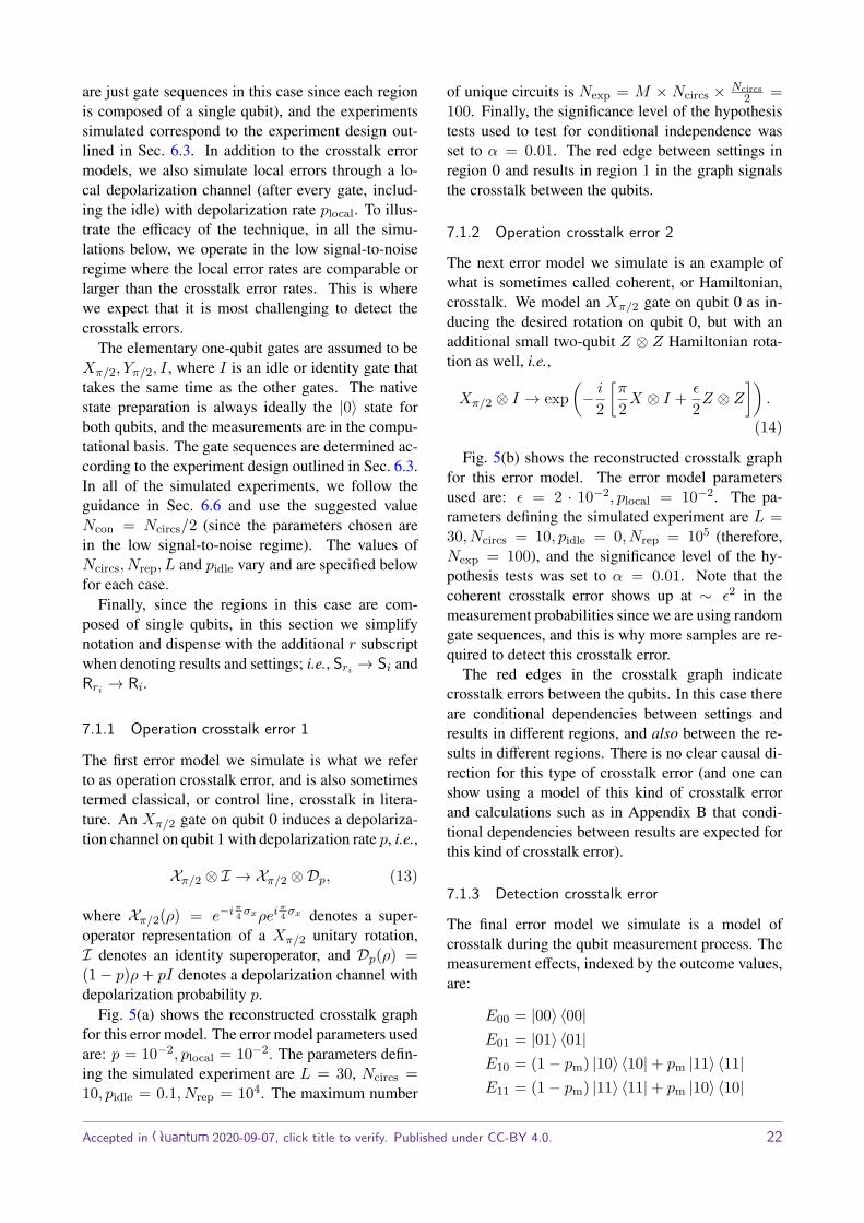
are just gate sequences in this case since each regionis composed of a single qubit), and the experimentssimulated correspond to the experiment design out-lined in Sec. 6.3. In addition to the crosstalk errormodels, we also simulate local errors through a lo-cal depolarization channel (after every gate, includ-ing the idle) with depolarization rate plocal. To illus-trate the efficacy of the technique, in all the simu-lations below, we operate in the low signal-to-noiseregime where the local error rates are comparable orlarger than the crosstalk error rates. This is wherewe expect that it is most challenging to detect thecrosstalk errors.

The elementary one-qubit gates are assumed to beXπ/2, Yπ/2, I , where I is an idle or identity gate thattakes the same time as the other gates. The nativestate preparation is always ideally the |0〉 state forboth qubits, and the measurements are in the compu-tational basis. The gate sequences are determined ac-cording to the experiment design outlined in Sec. 6.3.In all of the simulated experiments, we follow theguidance in Sec. 6.6 and use the suggested valueNcon = Ncircs/2 (since the parameters chosen arein the low signal-to-noise regime). The values ofNcircs, Nrep, L and pidle vary and are specified belowfor each case.

Finally, since the regions in this case are com-posed of single qubits, in this section we simplifynotation and dispense with the additional r subscriptwhen denoting results and settings; i.e., Sri → Si andRri → Ri.

7.1.1 Operation crosstalk error 1

The first error model we simulate is what we referto as operation crosstalk error, and is also sometimestermed classical, or control line, crosstalk in litera-ture. An Xπ/2 gate on qubit 0 induces a depolariza-tion channel on qubit 1 with depolarization rate p, i.e.,

Xπ/2 ⊗ I → Xπ/2 ⊗Dp, (13)

where Xπ/2(ρ) = e−iπ4 σxρei

π4 σx denotes a super-

operator representation of a Xπ/2 unitary rotation,I denotes an identity superoperator, and Dp(ρ) =(1− p)ρ+ pI denotes a depolarization channel withdepolarization probability p.

Fig. 5(a) shows the reconstructed crosstalk graphfor this error model. The error model parameters usedare: p = 10−2, plocal = 10−2. The parameters defin-ing the simulated experiment are L = 30, Ncircs =10, pidle = 0.1, Nrep = 104. The maximum number

of unique circuits is Nexp = M × Ncircs × Ncircs2 =

100. Finally, the significance level of the hypothesistests used to test for conditional independence wasset to α = 0.01. The red edge between settings inregion 0 and results in region 1 in the graph signalsthe crosstalk between the qubits.

7.1.2 Operation crosstalk error 2

The next error model we simulate is an example ofwhat is sometimes called coherent, or Hamiltonian,crosstalk. We model an Xπ/2 gate on qubit 0 as in-ducing the desired rotation on qubit 0, but with anadditional small two-qubit Z ⊗ Z Hamiltonian rota-tion as well, i.e.,

Xπ/2 ⊗ I → exp(− i2

[π

2X ⊗ I + ε

2Z ⊗ Z])

.

(14)

Fig. 5(b) shows the reconstructed crosstalk graphfor this error model. The error model parametersused are: ε = 2 · 10−2, plocal = 10−2. The pa-rameters defining the simulated experiment are L =30, Ncircs = 10, pidle = 0, Nrep = 105 (therefore,Nexp = 100), and the significance level of the hy-pothesis tests was set to α = 0.01. Note that thecoherent crosstalk error shows up at ∼ ε2 in themeasurement probabilities since we are using randomgate sequences, and this is why more samples are re-quired to detect this crosstalk error.

The red edges in the crosstalk graph indicatecrosstalk errors between the qubits. In this case thereare conditional dependencies between settings andresults in different regions, and also between the re-sults in different regions. There is no clear causal di-rection for this type of crosstalk error (and one canshow using a model of this kind of crosstalk errorand calculations such as in Appendix B that condi-tional dependencies between results are expected forthis kind of crosstalk error).

7.1.3 Detection crosstalk error

The final error model we simulate is a model ofcrosstalk during the qubit measurement process. Themeasurement effects, indexed by the outcome values,are:

E00 = |00〉〈00|E01 = |01〉〈01|E10 = (1− pm) |10〉〈10|+ pm |11〉〈11|E11 = (1− pm) |11〉〈11|+ pm |10〉〈10|


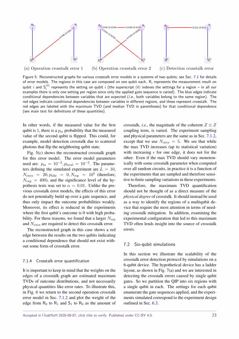
(a) Operation crosstalk error 1 (b) Operation crosstalk error 2 (c) Detection crosstalk error

Figure 5: Reconstructed graphs for various crosstalk error models in a systems of two qubits; see Sec. 7.1 for detailsof error models. The regions in this case are composed on one qubit each. Ri represents the measurement result onqubit i and S(0)

i represents the setting on qubit i (the superscript (0) indexes the settings for a region – in all ourexamples there is only one setting per region since only the applied gate sequence is varied). The blue edges indicateconditional dependencies between variables that are expected (i.e., both variables belong to the same region). Thered edges indicate conditional dependencies between variables in different regions, and these represent crosstalk. Thered edges are labeled with the maximum TVD (and median TVD in parentheses) for that conditional dependence(see main text for definitions of these quantities).

In other words, if the measured value for the firstqubit is 1, there is a pm probability that the measuredvalue of the second qubit is flipped. This could, forexample, model detection crosstalk due to scatteredphotons that flip the neighboring qubit state.

Fig. 5(c) shows the reconstructed crosstalk graphfor this error model. The error model parametersused are: pm = 10−2, plocal = 10−2. The parame-ters defining the simulated experiment are L = 10,Ncircs = 20, pidle = 0, Nrep = 105 (therefore,Nexp = 400), and the significance level of the hy-pothesis tests was set to α = 0.01. Unlike the pre-vious crosstalk error models, the effects of this errordo not potentially build up over a gate sequence, andthus only impact the outcome probabilities weakly.Moreover, its effect is reduced in the experimentswhere the first qubit’s outcome is 0 with high proba-bility. For these reasons, we found that a larger Nrepand Ncircs are required to detect this crosstalk error.

The reconstructed graph in this case shows a rededge between the results on the two qubits indicatinga conditional dependence that should not exist with-out some form of crosstalk error.

7.1.4 Crosstalk error quantification

It is important to keep in mind that the weights on theedges of a crosstalk graph are estimated maximumTVDs of outcome distributions, and not necessarilyphysical quantities like error rates. To illustrate this,in Fig. 6 we return to the second operation crosstalkerror model in Sec. 7.1.2 and plot the weight of theedge from R0 to R1 and S1 to R0 as the amount of

crosstalk, i.e., the magnitude of the coherent Z ⊗ Zcoupling term, is varied. The experiment samplingand physical parameters are the same as in Sec. 7.1.2,except that we use Ncircs = 5. We see that whilethe max TVD increases (up to statistical variation)with increasing ε for one edge, it does not for theother. Even if the max TVD should vary monoton-ically with some crosstalk parameter when computedover all random circuits, in practice it is a function ofthe experiments that are sampled and therefore sensi-tive to finite sampling variations in these experiments.

Therefore, the maximum TVD quantificationshould not be thought of as a direct measure of thephysical degree of crosstalk. It should instead be usedas a way to identify the regions of a multiqubit de-vice that require the most attention in terms of need-ing crosstalk mitigation. In addition, examining theexperimental configuration that led to this maximumTVD often lends insight into the source of crosstalkerrors.

7.2 Six-qubit simulations

In this section we illustrate the scalability of thecrosstalk error detection protocol by simulations on a6-qubit device. The hypothetical device has a ladderlayout, as shown in Fig. 7(a) and we are interested indetecting the crosstalk errors caused by single qubitgates. So we partition the QIP into six regions witha single qubit in each. The settings for each qubitenumerate the gate sequences applied, and the experi-ments simulated correspond to the experiment designoutlined in Sec. 6.3.


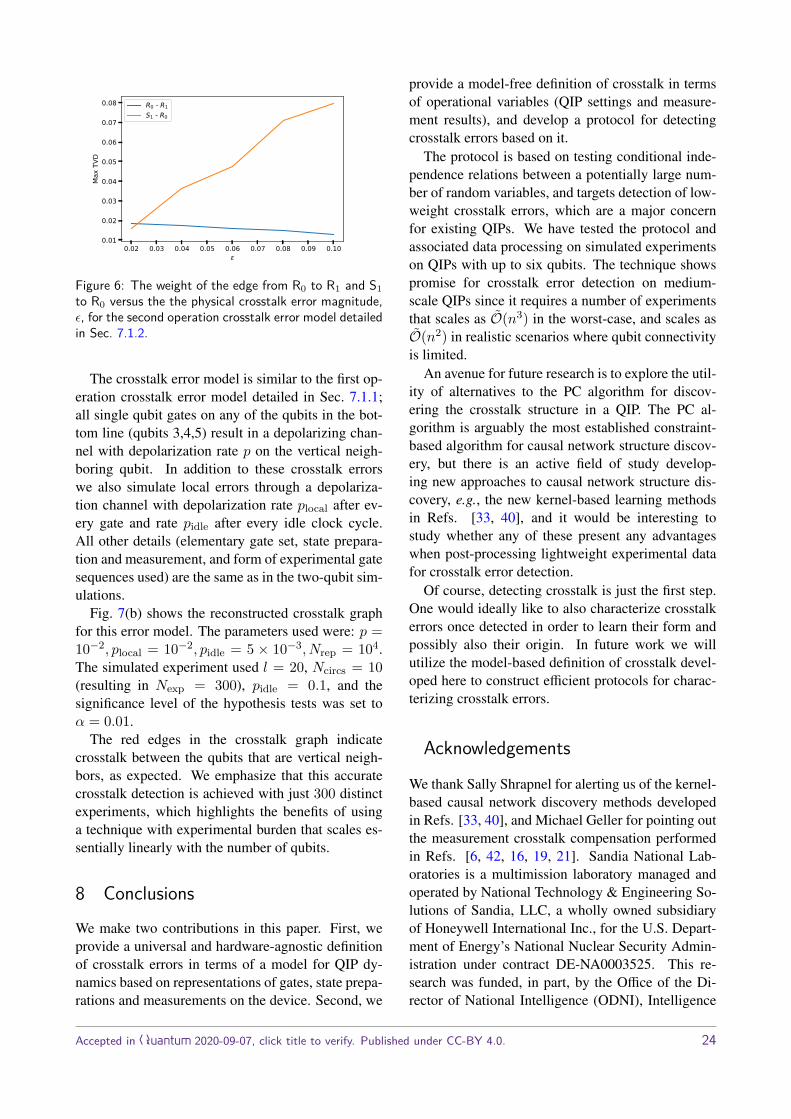
0.02 0.03 0.04 0.05 0.06 0.07 0.08 0.09 0.100.01

0.02

0.03

0.04

0.05

0.06

0.07

0.08M

ax T

VDR0 - R1S1 - R0

Figure 6: The weight of the edge from R0 to R1 and S1to R0 versus the the physical crosstalk error magnitude,ε, for the second operation crosstalk error model detailedin Sec. 7.1.2.

The crosstalk error model is similar to the first op-eration crosstalk error model detailed in Sec. 7.1.1;all single qubit gates on any of the qubits in the bot-tom line (qubits 3,4,5) result in a depolarizing chan-nel with depolarization rate p on the vertical neigh-boring qubit. In addition to these crosstalk errorswe also simulate local errors through a depolariza-tion channel with depolarization rate plocal after ev-ery gate and rate pidle after every idle clock cycle.All other details (elementary gate set, state prepara-tion and measurement, and form of experimental gatesequences used) are the same as in the two-qubit sim-ulations.

Fig. 7(b) shows the reconstructed crosstalk graphfor this error model. The parameters used were: p =10−2, plocal = 10−2, pidle = 5 × 10−3, Nrep = 104.The simulated experiment used l = 20, Ncircs = 10(resulting in Nexp = 300), pidle = 0.1, and thesignificance level of the hypothesis tests was set toα = 0.01.

The red edges in the crosstalk graph indicatecrosstalk between the qubits that are vertical neigh-bors, as expected. We emphasize that this accuratecrosstalk detection is achieved with just 300 distinctexperiments, which highlights the benefits of usinga technique with experimental burden that scales es-sentially linearly with the number of qubits.

8 Conclusions

We make two contributions in this paper. First, weprovide a universal and hardware-agnostic definitionof crosstalk errors in terms of a model for QIP dy-namics based on representations of gates, state prepa-rations and measurements on the device. Second, we

provide a model-free definition of crosstalk in termsof operational variables (QIP settings and measure-ment results), and develop a protocol for detectingcrosstalk errors based on it.

The protocol is based on testing conditional inde-pendence relations between a potentially large num-ber of random variables, and targets detection of low-weight crosstalk errors, which are a major concernfor existing QIPs. We have tested the protocol andassociated data processing on simulated experimentson QIPs with up to six qubits. The technique showspromise for crosstalk error detection on medium-scale QIPs since it requires a number of experimentsthat scales as O(n3) in the worst-case, and scales asO(n2) in realistic scenarios where qubit connectivityis limited.

An avenue for future research is to explore the util-ity of alternatives to the PC algorithm for discov-ering the crosstalk structure in a QIP. The PC al-gorithm is arguably the most established constraint-based algorithm for causal network structure discov-ery, but there is an active field of study develop-ing new approaches to causal network structure dis-covery, e.g., the new kernel-based learning methodsin Refs. [33, 40], and it would be interesting tostudy whether any of these present any advantageswhen post-processing lightweight experimental datafor crosstalk error detection.

Of course, detecting crosstalk is just the first step.One would ideally like to also characterize crosstalkerrors once detected in order to learn their form andpossibly also their origin. In future work we willutilize the model-based definition of crosstalk devel-oped here to construct efficient protocols for charac-terizing crosstalk errors.

Acknowledgements

We thank Sally Shrapnel for alerting us of the kernel-based causal network discovery methods developedin Refs. [33, 40], and Michael Geller for pointing outthe measurement crosstalk compensation performedin Refs. [6, 42, 16, 19, 21]. Sandia National Lab-oratories is a multimission laboratory managed andoperated by National Technology & Engineering So-lutions of Sandia, LLC, a wholly owned subsidiaryof Honeywell International Inc., for the U.S. Depart-ment of Energy’s National Nuclear Security Admin-istration under contract DE-NA0003525. This re-search was funded, in part, by the Office of the Di-rector of National Intelligence (ODNI), Intelligence


0 1 2

5 4 3(a) 6 qubit QIP layout (b) Reconstructed crosstalk graph

Figure 7: Reconstructed graphs for 6 qubit QIP with operation crosstalk errors along vertical lines; see Sec. 7.2 fordetails of error models. The regions in this case are composed on one qubit each. Ri represents the measurementresults on qubit i and S(0)

i represents the setting on qubit i (the superscript (0) indexes the settings for a region –in all our examples there is only one setting per region since only the gate sequence applied is varied). The blueedges indicate conditional dependencies between variables that are expected (i.e., both variables belong to the sameregion). The red edges indicate conditional dependencies between variables in different regions, and this representcrosstalk. The red edges are labeled with the maximum TVD (and median TVD in parentheses) for that conditionaldependence (see main text for definitions of these quantities).

Advanced Research Projects Activity (IARPA) andby the U.S. Department of Energy, Office of Science,Office of Advanced Scientific Computing ResearchQuantum Testbed Program. This paper describes ob-jective technical results and analysis. Any subjec-tive views or opinions that might be expressed in thepaper do not necessarily represent the views of theU.S. Department of Energy, IARPA, the ODNI, orthe United States Government.

References[1] PyGSTi. A python implementation of Gate Set

Tomography. URL: http://www.pygsti.info/.

[2] IBM Qiskit/ibmq-device-information/tenerife,2019. URL: https://github.com/Qiskit/ibmq-device-information/tree/master/backends/tenerife/V1.

[3] Carole Addis, Francesco Ciccarello, MicheleCascio, G Massimo Palma, and Sabrina Man-iscalco. Dynamical decoupling efficiency ver-sus quantum non-markovianity. New Journal ofPhysics, 17(12):123004, 2015. doi:10.1088/1367-2630/17/12/123004.

[4] D Bacciu, T A Etchells, P J G Lisboa, andJ Whittaker. Efficient identification of inde-pendence networks using mutual information.Computational Statistics, 28:621, 2013. doi:10.1007/s00180-012-0320-6.

[5] Robert Beals, Harry Buhrman, Richard Cleve,Michele Mosca, and Ronald de Wolf. Quan-

tum lower bounds by polynomials. Journalof the ACM, 48(4):778–797, July 2001. doi:10.1145/502090.502097.

[6] R. C. Bialczak, M. Ansmann, M. Hofheinz,E. Lucero, M. Neeley, A. D. O’Connell,D. Sank, H. Wang, J. Wenner, M. Steffen, A. N.Cleland, and J. M. Martinis. Quantum processtomography of a universal entangling gate im-plemented with Josephson phase qubits. NaturePhysics, 6(6):409–413, 2010. doi:10.1038/nphys1639.

[7] Robin Blume-Kohout, John King Gamble, ErikNielsen, Kenneth Rudinger, Jonathan Mizrahi,Kevin Fortier, and Peter Maunz. Demonstra-tion of qubit operations below a rigorous faulttolerance threshold with gate set tomography.Nature Communications, 8:1, 2017. doi:10.1038/ncomms14485.

[8] Heinz-Peter Breuer, Elsi-Mari Laine, and JyrkiPiilo. Measure for the degree of non-markovianbehavior of quantum processes in open systems.Phys. Rev. Lett., 103:210401, 2009. doi:10.1103/PhysRevLett.103.210401.

[9] Caslav Brukner. Quantum causality. NaturePhysics, 10(4):259–263, 2014. doi:10.1038/nphys2930.

[10] Donovan Buterakos, Robert E. Throckmorton,and S. Das Sarma. Crosstalk error correc-tion through dynamical decoupling of single-qubit gates in capacitively coupled singlet-triplet semiconductor spin qubits. Physical Re-


http://www.pygsti.info/

http://www.pygsti.info/

https://github.com/Qiskit/ibmq-device-information/tree/master/backends/tenerife/V1



http://dx.doi.org/10.1088/1367-2630/17/12/123004

http://dx.doi.org/10.1088/1367-2630/17/12/123004

http://dx.doi.org/10.1007/s00180-012-0320-6

http://dx.doi.org/10.1007/s00180-012-0320-6

http://dx.doi.org/10.1145/502090.502097

http://dx.doi.org/10.1145/502090.502097

http://dx.doi.org/10.1038/nphys1639


http://dx.doi.org/10.1038/ncomms14485


http://dx.doi.org/10.1103/PhysRevLett.103.210401




view B, 97(4):045431, January 2018. doi:10.1103/PhysRevB.97.045431.

[11] Yanzhu Chen, Maziar Farahzad, Shinjae Yoo,and Tzu-Chieh Wei. Detector tomography onIBM quantum computers and mitigation of animperfect measurement. Physical Review A,100(5):052315, November 2019. Publisher:American Physical Society. doi:10.1103/PhysRevA.100.052315.

[12] W. A. Coish and Daniel Loss. Hyperfine inter-action in a quantum dot: Non-markovian elec-tron spin dynamics. Phys. Rev. B, 70:195340,2004. doi:10.1103/PhysRevB.70.195340.

[13] Diego Colombo and Marloes H Maathuis.Order-Independent Constraint-Based CausalStructure Learning. J. Machine Learn-ing Research, 15:3921, 2014. URL:http://jmlr.org/papers/volume15/colombo14a/colombo14a.pdf.

[14] Christoph Dankert, Richard Cleve, JosephEmerson, and Etera Livine. Exact and ap-proximate unitary 2-designs and their appli-cation to fidelity estimation. Physical Re-view A, 80(1):012304, 2009. doi:10.1103/PhysRevA.80.012304.

[15] E. B. Davies and J. T. Lewis. An operationalapproach to quantum probability. Communica-tions in Mathematical Physics, 17(3):239–260,1970. doi:10.1007/BF01647093.

[16] S. Debnath, N. M. Linke, C. Figgatt, K. A.Landsman, K. Wright, and C. Monroe.Demonstration of a small programmable quan-tum computer with atomic qubits. Nature,536(7614):63–66, August 2016. doi:10.1038/nature18648.

[17] Alexander Erhard, Joel J. Wallman, LukasPostler, Michael Meth, Roman Stricker, Este-ban A. Martinez, Philipp Schindler, ThomasMonz, Joseph Emerson, and Rainer Blatt.Characterizing large-scale quantum computersvia cycle benchmarking. Nature Communi-cations, 10(1):5347, 2019. doi:10.1038/s41467-019-13068-7.

[18] Jay M. Gambetta, A D Corcoles, S T Merkel,B R Johnson, John A Smolin, Jerry MChow, Colm A Ryan, Chad Rigetti, S Poletto,Thomas A Ohki, Mark B Ketchen, and M Stef-fen. Characterization of Addressability by Si-multaneous Randomized Benchmarking. Phys-

ical Review Letters, 109(24):240504–5, 2012.doi:10.1103/PhysRevLett.109.240504.

[19] Ming Gong, Ming-Cheng Chen, Yarui Zheng,Shiyu Wang, Chen Zha, Hui Deng, ZhiguangYan, Hao Rong, Yulin Wu, Shaowei Li,Fusheng Chen, Youwei Zhao, Futian Liang,Jin Lin, Yu Xu, Cheng Guo, Lihua Sun, An-thony D. Castellano, Haohua Wang, ChengzhiPeng, Chao-Yang Lu, Xiaobo Zhu, and Jian-Wei Pan. Genuine 12-Qubit Entanglement on aSuperconducting Quantum Processor. PhysicalReview Letters, 122(11):110501, 2019. doi:10.1103/PhysRevLett.122.110501.

[20] D. Gross, K. Audenaert, and J. Eisert. Evenlydistributed unitaries: On the structure ofunitary designs. Journal of MathematicalPhysics, 48(5):052104, 2007. doi:10.1063/1.2716992.

[21] Vojtech Havlicek, Antonio D. Corcoles, Kris-tan Temme, Aram W. Harrow, Abhinav Kan-dala, Jerry M. Chow, and Jay M. Gambetta. Su-pervised learning with quantum-enhanced fea-ture spaces. Nature, 567(7747):209–212, 2019.doi:10.1038/s41586-019-0980-2.

[22] Patrick Hayden, Debbie Leung, and GraemeSmith. Multiparty data hiding of quantum in-formation. Physical Review A, 71(6):062339,2005. doi:10.1103/PhysRevA.71.062339.

[23] Johannes Heinsoo, Christian Kraglund Ander-sen, Ants Remm, Sebastian Krinner, TheodoreWalter, Yves Salathe, Simone Gasparinetti,Jean-Claude Besse, Anton Potocnik, AndreasWallraff, and Christopher Eichler. Rapid High-fidelity Multiplexed Readout of Superconduct-ing Qubits. Physical Review Applied, 10(3),2018. doi:10.1103/PhysRevApplied.10.034040.

[24] Miguel A Hernan, David Clayton, and NielsKeiding. The Simpson’s paradox unrav-eled. International Journal of Epidemiology,40(3):780–785, 2011. doi:10.1093/ije/dyr041.

[25] Markus Kalisch and Peter Bhlmann. Es-timating High-Dimensional Directed AcyclicGraphs with the PC-Algorithm. Journal ofMachine Learning Research, 8(Mar):613–636,January 2007. URL: http://www.jmlr.org/papers/v8/kalisch07a.html.


http://dx.doi.org/10.1103/PhysRevB.97.045431


http://dx.doi.org/10.1103/PhysRevA.100.052315



http://jmlr.org/papers/volume15/colombo14a/colombo14a.pdf

http://jmlr.org/papers/volume15/colombo14a/colombo14a.pdf



http://dx.doi.org/10.1007/BF01647093

http://dx.doi.org/10.1038/nature18648


http://dx.doi.org/10.1038/s41467-019-13068-7

http://dx.doi.org/10.1038/s41467-019-13068-7




http://dx.doi.org/10.1063/1.2716992

http://dx.doi.org/10.1063/1.2716992

http://dx.doi.org/10.1038/s41586-019-0980-2


http://dx.doi.org/10.1103/PhysRevApplied.10.034040

http://dx.doi.org/10.1103/PhysRevApplied.10.034040

http://dx.doi.org/10.1093/ije/dyr041

http://dx.doi.org/10.1093/ije/dyr041

http://www.jmlr.org/papers/v8/kalisch07a.html

http://www.jmlr.org/papers/v8/kalisch07a.html

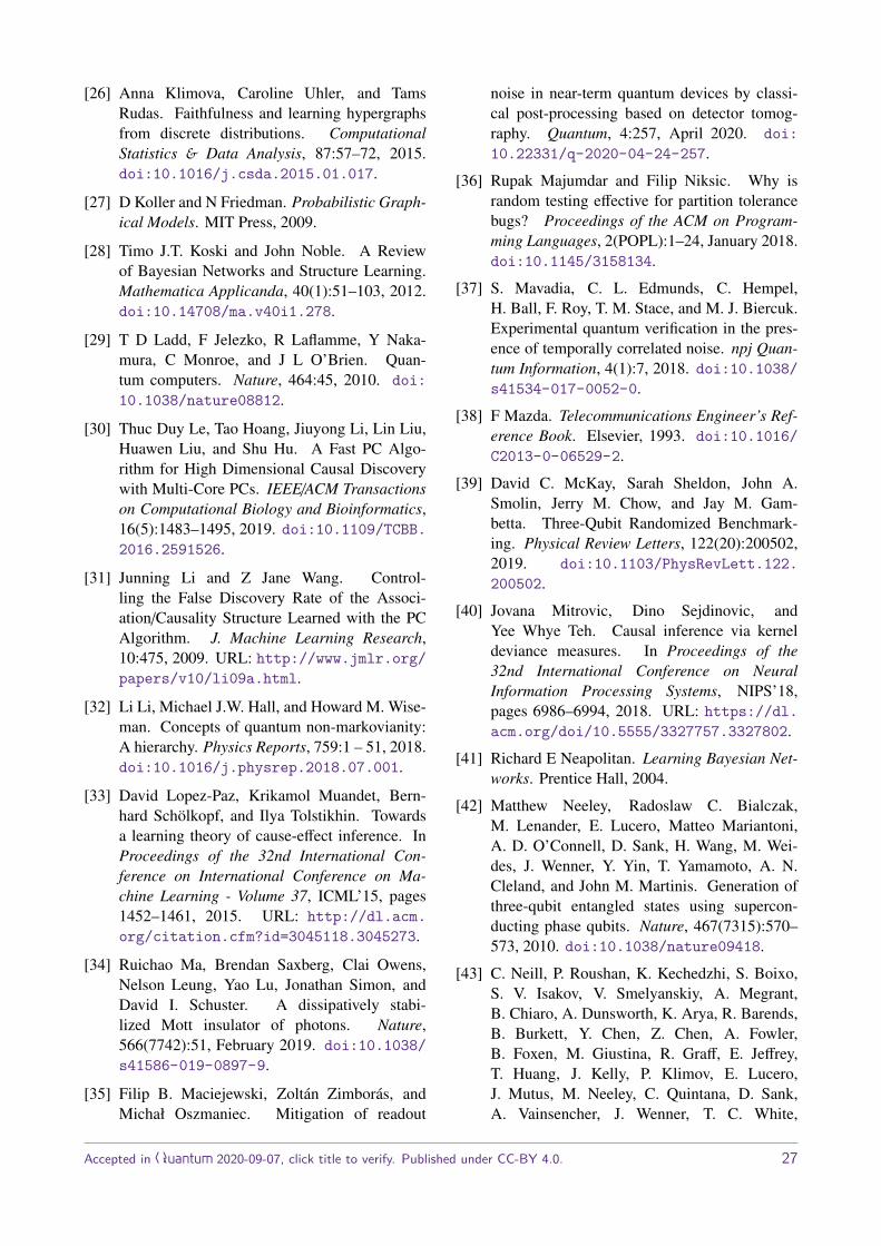
[26] Anna Klimova, Caroline Uhler, and TamsRudas. Faithfulness and learning hypergraphsfrom discrete distributions. ComputationalStatistics & Data Analysis, 87:57–72, 2015.doi:10.1016/j.csda.2015.01.017.

[27] D Koller and N Friedman. Probabilistic Graph-ical Models. MIT Press, 2009.

[28] Timo J.T. Koski and John Noble. A Reviewof Bayesian Networks and Structure Learning.Mathematica Applicanda, 40(1):51–103, 2012.doi:10.14708/ma.v40i1.278.

[29] T D Ladd, F Jelezko, R Laflamme, Y Naka-mura, C Monroe, and J L O’Brien. Quan-tum computers. Nature, 464:45, 2010. doi:10.1038/nature08812.

[30] Thuc Duy Le, Tao Hoang, Jiuyong Li, Lin Liu,Huawen Liu, and Shu Hu. A Fast PC Algo-rithm for High Dimensional Causal Discoverywith Multi-Core PCs. IEEE/ACM Transactionson Computational Biology and Bioinformatics,16(5):1483–1495, 2019. doi:10.1109/TCBB.2016.2591526.

[31] Junning Li and Z Jane Wang. Control-ling the False Discovery Rate of the Associ-ation/Causality Structure Learned with the PCAlgorithm. J. Machine Learning Research,10:475, 2009. URL: http://www.jmlr.org/papers/v10/li09a.html.

[32] Li Li, Michael J.W. Hall, and Howard M. Wise-man. Concepts of quantum non-markovianity:A hierarchy. Physics Reports, 759:1 – 51, 2018.doi:10.1016/j.physrep.2018.07.001.

[33] David Lopez-Paz, Krikamol Muandet, Bern-hard Scholkopf, and Ilya Tolstikhin. Towardsa learning theory of cause-effect inference. InProceedings of the 32nd International Con-ference on International Conference on Ma-chine Learning - Volume 37, ICML’15, pages1452–1461, 2015. URL: http://dl.acm.org/citation.cfm?id=3045118.3045273.

[34] Ruichao Ma, Brendan Saxberg, Clai Owens,Nelson Leung, Yao Lu, Jonathan Simon, andDavid I. Schuster. A dissipatively stabi-lized Mott insulator of photons. Nature,566(7742):51, February 2019. doi:10.1038/s41586-019-0897-9.

[35] Filip B. Maciejewski, Zoltan Zimboras, andMichał Oszmaniec. Mitigation of readout

noise in near-term quantum devices by classi-cal post-processing based on detector tomog-raphy. Quantum, 4:257, April 2020. doi:10.22331/q-2020-04-24-257.

[36] Rupak Majumdar and Filip Niksic. Why israndom testing effective for partition tolerancebugs? Proceedings of the ACM on Program-ming Languages, 2(POPL):1–24, January 2018.doi:10.1145/3158134.

[37] S. Mavadia, C. L. Edmunds, C. Hempel,H. Ball, F. Roy, T. M. Stace, and M. J. Biercuk.Experimental quantum verification in the pres-ence of temporally correlated noise. npj Quan-tum Information, 4(1):7, 2018. doi:10.1038/s41534-017-0052-0.

[38] F Mazda. Telecommunications Engineer’s Ref-erence Book. Elsevier, 1993. doi:10.1016/C2013-0-06529-2.

[39] David C. McKay, Sarah Sheldon, John A.Smolin, Jerry M. Chow, and Jay M. Gam-betta. Three-Qubit Randomized Benchmark-ing. Physical Review Letters, 122(20):200502,2019. doi:10.1103/PhysRevLett.122.200502.

[40] Jovana Mitrovic, Dino Sejdinovic, andYee Whye Teh. Causal inference via kerneldeviance measures. In Proceedings of the32nd International Conference on NeuralInformation Processing Systems, NIPS’18,pages 6986–6994, 2018. URL: https://dl.acm.org/doi/10.5555/3327757.3327802.

[41] Richard E Neapolitan. Learning Bayesian Net-works. Prentice Hall, 2004.

[42] Matthew Neeley, Radoslaw C. Bialczak,M. Lenander, E. Lucero, Matteo Mariantoni,A. D. O’Connell, D. Sank, H. Wang, M. Wei-des, J. Wenner, Y. Yin, T. Yamamoto, A. N.Cleland, and John M. Martinis. Generation ofthree-qubit entangled states using supercon-ducting phase qubits. Nature, 467(7315):570–573, 2010. doi:10.1038/nature09418.

[43] C. Neill, P. Roushan, K. Kechedzhi, S. Boixo,S. V. Isakov, V. Smelyanskiy, A. Megrant,B. Chiaro, A. Dunsworth, K. Arya, R. Barends,B. Burkett, Y. Chen, Z. Chen, A. Fowler,B. Foxen, M. Giustina, R. Graff, E. Jeffrey,T. Huang, J. Kelly, P. Klimov, E. Lucero,J. Mutus, M. Neeley, C. Quintana, D. Sank,A. Vainsencher, J. Wenner, T. C. White,


http://dx.doi.org/10.1016/j.csda.2015.01.017

http://dx.doi.org/10.14708/ma.v40i1.278



http://dx.doi.org/10.1109/TCBB.2016.2591526

http://dx.doi.org/10.1109/TCBB.2016.2591526

http://www.jmlr.org/papers/v10/li09a.html

http://www.jmlr.org/papers/v10/li09a.html

http://dx.doi.org/10.1016/j.physrep.2018.07.001

http://dl.acm.org/citation.cfm?id=3045118.3045273

http://dl.acm.org/citation.cfm?id=3045118.3045273

http://dx.doi.org/10.1038/s41586-019-0897-9

http://dx.doi.org/10.1038/s41586-019-0897-9

http://dx.doi.org/10.22331/q-2020-04-24-257

http://dx.doi.org/10.22331/q-2020-04-24-257

http://dx.doi.org/10.1145/3158134

http://dx.doi.org/10.1038/s41534-017-0052-0

http://dx.doi.org/10.1038/s41534-017-0052-0

http://dx.doi.org/10.1016/C2013-0-06529-2

http://dx.doi.org/10.1016/C2013-0-06529-2



https://dl.acm.org/doi/10.5555/3327757.3327802

https://dl.acm.org/doi/10.5555/3327757.3327802


H. Neven, and J. M. Martinis. A blueprintfor demonstrating quantum supremacy with su-perconducting qubits. Science, 360(6385):195–199, April 2018. doi:10.1126/science.aao4309.

[44] C. Piltz, T. Sriarunothai, A.F. Varon, andC. Wunderlich. A trapped-ion-based quan-tum byte with 10−5 next-neighbour cross-talk.Nature Communications, 5(1):4679, December2014. doi:10.1038/ncomms5679.

[45] John Preskill. Quantum Computing in the NISQera and beyond. Quantum, 2:79, 2018. doi:10.22331/q-2018-08-06-79.

[46] Timothy Proctor, Melissa Revelle, Erik Nielsen,Kenneth Rudinger, Daniel Lobser, Peter Maunz,Robin Blume-Kohout, and Kevin Young. De-tecting, tracking, and eliminating drift in quan-tum information processors. July 2019. arXiv:1907.13608. URL: http://arxiv.org/abs/1907.13608.

[47] Timothy Proctor, Kenneth Rudinger, KevinYoung, Mohan Sarovar, and Robin Blume-Kohout. What Randomized BenchmarkingActually Measures. Physical Review Letters,119(13), 2017. doi:10.1103/PhysRevLett.119.130502.

[48] Timothy J. Proctor, Arnaud Carignan-Dugas,Kenneth Rudinger, Erik Nielsen, Robin Blume-Kohout, and Kevin Young. Direct RandomizedBenchmarking for Multiqubit Devices. Physi-cal Review Letters, 123(3):030503, 2019. doi:10.1103/PhysRevLett.123.030503.

[49] Matthew Reagor, Christopher B. Osborn, Niko-las Tezak, Alexa Staley, Guenevere Prawiroat-modjo, Michael Scheer, Nasser Alidoust,Eyob A. Sete, Nicolas Didier, Marcus P. daSilva, Ezer Acala, Joel Angeles, Andrew Best-wick, Maxwell Block, Benjamin Bloom, AdamBradley, Catvu Bui, Shane Caldwell, LaurenCapelluto, Rick Chilcott, Jeff Cordova, GenyaCrossman, Michael Curtis, Saniya Deshpande,Tristan El Bouayadi, Daniel Girshovich, Sab-rina Hong, Alex Hudson, Peter Karalekas, KatKuang, Michael Lenihan, Riccardo Manenti,Thomas Manning, Jayss Marshall, Yuvraj Mo-han, William O’Brien, Johannes Otterbach,Alexander Papageorge, Jean-Philip Paquette,Michael Pelstring, Anthony Polloreno, VijayRawat, Colm A. Ryan, Russ Renzas, Nick Ru-bin, Damon Russel, Michael Rust, Diego Scara-

belli, Michael Selvanayagam, Rodney Sin-clair, Robert Smith, Mark Suska, Ting-WaiTo, Mehrnoosh Vahidpour, Nagesh Vodrahalli,Tyler Whyland, Kamal Yadav, William Zeng,and Chad T. Rigetti. Demonstration of univer-sal parametric entangling gates on a multi-qubitlattice. Science Advances, 4(2):eaao3603, 2018.doi:10.1126/sciadv.aao3603.

[50] Kenneth Rudinger, Timothy Proctor, DylanLangharst, Mohan Sarovar, Kevin Young,and Robin Blume-Kohout. Probing Context-Dependent Errors in Quantum Processors.Physical Review X, 9(2):021045, 2019. doi:10.1103/PhysRevX.9.021045.

[51] Sarah Sheldon, Easwar Magesan, Jerry MChow, and Jay M. Gambetta. Procedure forsystematically tuning up cross-talk in the cross-resonance gate. Phys. Rev. A, 93(6):060302,2016. doi:10.1103/PhysRevA.93.060302.

[52] Peter Spirtes. Introduction to Causal Infer-ence. Journal of Machine Learning Research,11:1643, 2010. URL: http://www.jmlr.org/papers/v11/spirtes10a.html.

[53] Peter Spirtes and Clark Glymour. An Algorithmfor Fast Recovery of Sparse Causal Graphs. So-cial Science Computer Review, 9(1):67, 1991.doi:10.1177/089443939100900106.

[54] Peter Spirtes, Clark N. Glymour, and RichardScheines. Causation, prediction, and search.MIT Press, Cambridge, Mass, 2nd ed edition,2000.

[55] Peter Spirtes and Kun Zhang. Causal discoveryand inference: concepts and recent methodolog-ical advances. Applied Informatics, 3:3, 2016.doi:10.1186/s40535-016-0018-x.

[56] Eric V. Strobl, Peter L. Spirtes, and ShyamVisweswaran. Estimating and Controlling theFalse Discovery Rate of the PC Algorithm Us-ing Edge-specific P-Values. ACM Transactionson Intelligent Systems and Technology, 10(5):1–37, 2019. doi:10.1145/3351342.

[57] L. M. K. Vandersypen and I. L. Chuang.NMR techniques for quantum control andcomputation. Reviews of Modern Physics,76(4):1037–1069, January 2005. doi:10.1103/RevModPhys.76.1037.

[58] Andrzej Veitia, Marcus P. da Silva, RobinBlume-Kohout, and Steven J. van Enk. Macro-scopic instructions vs microscopic operations.


http://dx.doi.org/10.1126/science.aao4309

http://dx.doi.org/10.1126/science.aao4309


http://dx.doi.org/10.22331/q-2018-08-06-79

http://dx.doi.org/10.22331/q-2018-08-06-79

http://arxiv.org/abs/1907.13608






http://dx.doi.org/10.1126/sciadv.aao3603

http://dx.doi.org/10.1103/PhysRevX.9.021045

http://dx.doi.org/10.1103/PhysRevX.9.021045


http://www.jmlr.org/papers/v11/spirtes10a.html

http://www.jmlr.org/papers/v11/spirtes10a.html

http://dx.doi.org/10.1177/089443939100900106

http://dx.doi.org/10.1186/s40535-016-0018-x

http://dx.doi.org/10.1145/3351342

http://dx.doi.org/10.1103/RevModPhys.76.1037

http://dx.doi.org/10.1103/RevModPhys.76.1037

2017. arXiv: 1708.08173. URL: http://arxiv.org/abs/1708.08173.

[59] Joel J Wallman and Steven T Flammia. Ran-domized benchmarking with confidence. NewJournal of Physics, 16(10):103032, 2014. doi:10.1088/1367-2630/16/10/103032.

[60] Adam Winick, Joel J. Wallman, andJoseph Emerson. Phenomenologicalmeasure of quantum non-markovianity.2019. arXiv:1901.00267. URL:http://arxiv.org/abs/1901.00267.

[61] Christopher J Wood and Robert W Spekkens.The lesson of causal discovery algorithms forquantum correlations: causal explanations ofBell-inequality violations require fine-tuning.New Journal of Physics, 17(3):033002, 2015.doi:10.1088/1367-2630/17/3/033002.




http://dx.doi.org/10.1088/1367-2630/16/10/103032

http://dx.doi.org/10.1088/1367-2630/16/10/103032


http://dx.doi.org/10.1088/1367-2630/17/3/033002

A Conditional versus marginal independenceOur definition of crosstalk errors is based conditional independence of random variables. As mentioned inthe main text, this is motivated by the central role played by conditional independence in defining causality ingraphical models. In this Appendix we explain why we prefer to use the notion of conditional independenceover marginal independence, which might seem simpler to work with. To do this, we refer to Fig. 8, whichrepresents the random variables involved in a two qubit example: S1,S2,R1,R2. Fig. 8(a) represents the truedependence relationships between the variables. The arrow between S1 and S2 could be due to poor experimentdesign, whereby the settings on qubit 2 are not selected independently of those on qubit 1.

Excepting statistical issues (i.e., given the underlying probability distribution over these random variables),the dependency relationships given by the graph in Fig. 8(a) would be reconstructed by examining conditionaldependence relations. In contrast, if we only assess marginal independence between R1 and S2, the fact thatboth random variables have a common cause (S1) would create a fictitious dependence between these variables(see Fig. 8(b)). This is of course well known in statistics as the confounding of statistical association by anunobserved common cause [24].

Now, a marginal independence test would be sufficient if the experiment design was suitably randomizedsuch that S1 and S2 are independent. However, for quantum computing platforms with many qubits a suitablyrandomized experiment design may be difficult to guarantee, and evaluation of association between randomvariables in distinct regions based on conditional independence testing is more reliable.

S1 S2

R1 R2

S2

R1

(a) (b)

Figure 8: An example illustrating the difference between conditional and marginal independence between randomvariables. (a) shows the true causal relationships between the settings (S1, S2) and results (R1,R2) in a two qubitexperiment. (b) shows the causal relationship inferred if a marginal independence test is performed on just variablesR1 and S2.

B Equivalence of two definitions of crosstalkIn the main text we presented two definitions of crosstalk-free QIPs, at two different layers of abstraction.The first, Definition 1, was stated in terms of properties of quantum operations (locality and independence)assuming a Markovian QIP, and the second, Definition 2, was stated operationally in terms of conditionalindependence between of classical random variables associated with experiments. In this Appendix we provethat these two definitions are in fact, equivalent; i.e., A QIP is crosstalk-free according to Definition 1 ⇐⇒ AQIP is crosstalk-free according to Definition 2.

B.1 Conditional independence in terms of quantum operations

Before we prove this equivalence we need to define the probabilities that arise in assessing conditional inde-pendence in terms of the quantum operations that form a model for the QIP.

We restrict ourselves to a QIP composed of two qubits for simplicity, and because it suffices to demonstratethe points we wish to make. In this case there are four random variables in the problem: Ri ∈ rki Kk=1, i = 1, 2,the measurement results on the two qubits, and Si ∈ rliLl=1, i = 1, 2, the settings on the two qubits. Thesettings will enumerate over some set of single-qubit gate sequences on each qubit.


Consider the conditional independence statement P (Ri|Si,Sj ,Rj) = P (Ri|Si) for i, j ∈ 1, 2, i , j, whichcaptures the crosstalk-free condition between regions 1 and 2. What is this condition equivalent to in terms ofphysical states, operations and measurements? To address this question, we note that for any experiment, theBorn rule dictates

P (ri1, rj2|s

k1, s

l2) =

(E(ri1, r

j2)∣∣M(sk1, sl2)

∣∣ρ0), (15)

where∣∣E(ri1, r

j2))

is a POVM indexed by the measurement results,M(sk1, sl2) is a general two qubit CPTP mapindexed by the settings, and

∣∣ρ0)

is the initial state of the two qubits. Note that we are using Hilbert-Schmidtrepresentations of all of these quantities for notational simplicity. In fact, this is the only relation we can writedown without making further assumptions about crosstalk, factorizability of operations, etc. To obtain otherprobabilities we need to apply the usual conditioning and marginalization rules, e.g.,

P (ri1|sk1, sl2) =∑n

(E(ri1, rn2 )

∣∣M(sk1, sl2)∣∣ρ0)

P (ri1|sk1) =∑n

P (ri1|sk1, sn2 )P (sn2 |sk1)

=∑n

∑m

(E(ri1, rm2 )

∣∣M(sk1, sn2 )∣∣ρ0)P (sn2 |sk1). (16)

Using such relations we can write the crosstalk-free condition as

P (R1|S1, S2,R2) = P (R1|S1)⇒ P (ri1|sk1, sl2, r

j2) = P (ri1|sk1) ∀i, j, k, l

⇒ P (ri1, rj2|sk1, sl2)

P (rj2|sk1, sl2)=∑n,m

P (ri1, rn2 |sk1, sm2 )P (sm2 |sk1) ∀i, j, k, l

⇒ P (ri1, rj2|s

k1, s

l2) =

(∑z

P (rz1, rj2|s

k1, s

l2))(∑

n,m

P (ri1, rn2 |sk1, sm2 )P (sm2 |sk1))

∀i, j, k, l

(17)

⇒(E(ri1, r

j2)∣∣M(sk1, sl2)

∣∣ρ0)

=(∑

z

(E(rz1, r

j2)∣∣M(sk1, sl2)

∣∣ρ0))(∑

n,m

(E(ri1, rn2 )

∣∣M(sk1, sm2 )∣∣ρ0)P (sm2 |sk1)

)∀i, j, k, l

We can write a similar explicit equation for the condition P (R2|S1, S2,R1) = P (R2|S2).

B.2 Definition 1 ⇒ Definition 2

A crosstalk-free Markovian QIP according to model-based definition, see Sec. 4, has state preparations, gateoperations, and measurements that satisfy:

∣∣ρ0)

=∣∣ρ1

0)⊗∣∣ρ2

0)

M(S1, S2) =M1(S1)⊗M2(S2)∣∣E(R1,R2))

=∣∣E(R1)

)⊗∣∣E(R2

)) (18)

We proceed to show that given such a model for operations, the QIP is also crosstalk-free under Definition2; i.e., P (Ri|Si,Sj ,Rj) = P (Ri|Si), for i, j ∈ 1, 2, i , j. To do so, we substitute the factorized forms in


Eq. (18) into the explicit form of the condition P (R1|S1,S2,R2) = P (R1|S1) given in Eq. (17):

P (ri1, rj2|s

k1, s

l2) ?=

(∑z

P (rz1, rj2|s

k1, s

l2))(∑

n,m

P (ri1, rn2 |sk1, sm2 )P (sm2 |sk1))

∀i, j, k, l

⇒(E(ri1)

∣∣M1(sk1)∣∣ρ1

0)(E(rj2)

∣∣M2(sl2)∣∣ρ2

0) ?=

(∑z

(E(rz1)

∣∣M1(sk1)∣∣ρ1

0)(E(rj2)

∣∣M2(sl2)∣∣ρ2

0))·(∑

n,m

(E(ri1)

∣∣M1(sk1)∣∣ρ1

0)(E(rn2 )

∣∣M2(sm2 )∣∣ρ2

0)P (sm2 |sk1)

)∀i, j, k, l

⇒(E(ri1)

∣∣M1(sk1)∣∣ρ1

0)(E(rj2)

∣∣M2(sl2)∣∣ρ2

0) ?=

(E(rj2)

∣∣M2(sl2)∣∣ρ2

0)(E(ri1)

∣∣M1(sk1)∣∣ρ1

0), (19)

which is obviously true. To arrive at the last line we have used the properties∑z

(E(rz)

∣∣M(sk)∣∣ρ0)

= 1 forany k, ρ0, and

∑m P (sm2 |sk1) = 1. We can verify that the equality P (R2|S2, S1,R1) = P (R2|S2) also holds

for quantum operations that satisfy Eq. (18). This concludes the proof that the model-based definition of acrosstalk-free QIP implies our model-free definition of a crosstalk-free QIP.

B.3 Definition 2 ⇒ Definition 1

To prove this direction, we will actually prove its contrapositive, namely,

(¬locality) or (¬independence)⇒ violation of Definition 2. (20)

We proceed by showing that quantum operations that do not satisfy locality or independence lead to violationsof the explicit form of P (R1|S1, S2,R2) = P (R1|S1) stated in Eq. (17). The proofs straightforwardly generalizeto the violation of P (R2|S2, S1,R1) = P (R2|S2).

B.3.1 Locality

A Markovian QIP that does not satisfy the locality principle has state preparations, gate operations, or measure-ments (or all of these) that do not factorize as in Eq. (18).

First consider the case where the initial state does not factorize, but all other operations do. Then, expandingEq. (17), we get:

P (ri1, rj2|s

k1, s

l2) ?=

(∑z

P (rz1, rj2|s

k1, s

l2))(∑

n,m

P (ri1, rn2 |sk1, sm2 )P (sm2 |sk1))

∀i, j, k, l

⇒(E(ri1)

∣∣⊗ (E(rj2)∣∣M1(sk1)⊗M2(sl2)

∣∣ρ0) ?=

(∑z

(E(rz1)

∣∣⊗ (E(rj2)∣∣M1(sk1)⊗M2(sl2)

∣∣ρ0))·(∑

n,m

(E(ri1)

∣∣⊗ (E(rn2 )∣∣M1(sk1)⊗M2(sm2 )

∣∣ρ0)P (sm2 |sk1)

)∀i, j, k, l

⇒(E(ri1)

∣∣⊗ (E(rj2)∣∣M1(sk1)⊗M2(sl2)

∣∣ρ0) ?=

((E(rj2)

∣∣∣∣ρ2(k, l))) (

E(ri1)∣∣∣∣ρ1(k)

)∀i, j, k, l, (21)

where we have defined∣∣ρ1(k)

)≡ tr2

(M1(sk1)⊗

∑m P (sm2 |sk1)M2(sm2 )

∣∣ρ0))

and∣∣ρ2(k, l)

)≡

tr1(M1(sk1)⊗M2(sl2)

∣∣ρ0))

. This last equality cannot be true in general since it is expressing a joint dis-

tribution over ri1, rj2 on the left hand side with a product of marginal distributions over these two variables


on the right hand side. To see this more clearly, note that the equality must hold for all i, j, k, l, so supposeM1(sk1) =M2(sl2) = 1, ∀k, l. In this case, the condition simplifies to:(

E(ri1)∣∣⊗ (E(rj2)

∣∣∣∣ρ0) ?=

((E(rj2)

∣∣∣∣ρ2)) (

E(ri1)∣∣∣∣ρ1

)∀i, j, (22)

where∣∣ρ1(2)

)= tr2(1)

(∣∣ρ0))

. This equality cannot be true for any state ρ0 that is not separable and thereforewe conclude that conditional independence condition is violated in the case where the initial state does notfactorize.

Next, consider the case where the gate operations do not factorize:

∃a :M(sa1, sl2) ,M1(sa1)M2(sl2), ∀l, (23)

i.e., that the operation induced when the setting on the first qubit is a is an entangling (non-factorizable) oper-ation between the two qubits (regardless of what the setting is on qubit 1). We assume that the initial state andall measurement POVM elements factorize.

Then, returning to the condition in Eq. (17), and considering the case k = a,

P (ri1, rj2|s

a1, s

l2) ?=

(∑z

P (rz1, rj2|s

a1, s

l2))(∑

n,m

P (ri1, rn2 |sk1, sm2 )P (sm2 |sk1))

∀i, j, l

⇒(E(ri1)

∣∣⊗ (E(rj2)∣∣M(sa1, sl2)

∣∣ρ10)⊗∣∣ρ2

0) ?=

(∑z

(E(rz1)

∣∣⊗ (E(rj2)∣∣M(sa1, sl2)

∣∣ρ10)⊗∣∣ρ2

0))·(∑

n,m

(E(ri1)

∣∣⊗ (E(rn2 )∣∣M(sa1, sm2 )

∣∣ρ10)⊗∣∣ρ2

0)P (sm2 |sk1)

)∀i, j, l (24)

Now, suppose this equality holds. Then we can perform a weighted sum over L on both sides to get(E(ri1)

∣∣⊗ (E(rj2)∣∣M(sa1)

∣∣ρ10)⊗∣∣ρ2

0)

=(E(ri1)

∣∣∣∣ρ1(a))(E(rj2)

∣∣∣∣ρ2(a)), ∀i, j,

where

M(sa1) ≡∑l

P (sl2|sa1)M(sa1, sl2), and

∣∣ρ1(2)(a))≡ tr2(1)

(M(sa1)

∣∣ρ10)⊗∣∣ρ2

0))

Again, we have an expression with a joint distribution over ri1, rj2 on the left hand side and a product of marginals

over the same variables on the right hand side. This cannot be true ifM(sa1, sl2) does not factorize for all L,and therefore we conclude the original assumption of Eq. (24) holding is false. Therefore, we have shown thatthe model-free crosstalk-free condition is violated when gate operations violate locality and do not factorize.

Finally, the proof that violation of locality in measurements – i.e.,∣∣E(R1,R2

),∣∣E(R1)

)⊗∣∣E(R2)

)– results

in a violation of the model-free crosstalk-free conditions follows straightforwardly from the correspondingproof for non-factorizable initial states since state preparation and measurement are dual operations.

B.3.2 Independence

Now we proceed to show that even if locality is respected by a QIP, violations of independence in the model-based framework result in violations of the model-free definition of a crosstalk-free QIP. For simplicity we haveassumed that the only settings correspond to gate operations, and we only have one choice for state preparationand measurement basis. Therefore violation of independence within a model that respects locality can onlymanifest in one way:

∃a, b : M(sa1, sb2) = E1(sb2)M1(sa1)⊗M2(sb2). (25)


In other words, for some combination of settings, the operation done on the first qubit depends on the settingof the second qubit. Here, E1() is some CPTP map on qubit 1.

Let us determine if this violation of independence results in a violation of the model-free condition inEq. (17), by assuming all other operations respect locality and independence, and considering the casek = a, l = b:

P (ri1, rj2|s

a1, s

b2) ?=

(∑z

P (rz1, rj2|s

a1, s

b2))(∑

n,m

P (ri1, rn2 |sa1, sm2 )P (sm2 |sa1))

∀i, j

⇒(E(ri1)

∣∣E1(sb2)M1(sa1)∣∣ρ1

0)(E(rj2)

∣∣M2(sb2)∣∣ρ2

0) ?=

(∑z

(E(rz1)

∣∣E1(sb2)M1(sa1)∣∣ρ1

0)(E(rj2)

∣∣M2(sb2)∣∣ρ2

0))·(∑

n

[(E(ri1)

∣∣E1(sb2)M1(sa1)∣∣ρ1

0)(E(rn2 )

∣∣M2(sb2)∣∣ρ2

0)P (sb2|sa1)

+∑m,b

(E(ri1)

∣∣M1(sa1)∣∣ρ1

0)(E(rn2 )

∣∣M2(sm2 )∣∣ρ2

0)P (sm2 |sa1)

])∀i, j

⇒(E(ri1)

∣∣E1(sb2)M1(sa1)∣∣ρ1

0)(E(rj2)

∣∣M2(sb2)∣∣ρ2

0) ?=

(E(rj2)

∣∣M2(sb2)∣∣ρ2

0)·[(

E(ri1)∣∣E1(sb2)M1(sa1)

∣∣ρ10)P (sb2|sa1) +

(E(ri1)

∣∣M1(sa1)∣∣ρ1

0) (

1− P (sb2|sa1)) ]

∀i, j,

where we have used the completeness property of the POVM elements to perform the sums over z and n inthe last line. The equality on the last line holds if

(E(rj2)

∣∣M2(sb2)∣∣ρ2

0)

= 0, so consider the cases where thisquantity is non-zero (it cannot be zero for all j), and divide through both sides by this non-zero value. So for jsuch that

(E(rj2)

∣∣M2(sb2)∣∣ρ2

0), 0, the condition we are evaluating becomes:

(E(ri1)

∣∣E1(sb2)M1(sa1)∣∣ρ1

0) (

1− P (sb2|sa1)) ?=

(E(ri1)

∣∣M1(sa1)∣∣ρ1

0) (

1− P (sb2|sa1))

∀i

⇒(E(ri1)

∣∣E1(sb2)M1(sa1)∣∣ρ1

0) ?=

(E(ri1)

∣∣M1(sa1)∣∣ρ1

0)

∀i, (26)

where we have assumed 1 − P (sb2|sa1) , 0. Under what conditions is this last equality true when E1(sb2) , 1?The only other way for this equality to hold is if

(E(ri1)

∣∣E1(sb2) =(E(ri1)

∣∣, ∀i; i.e., all the error maps acttrivially on the measurement effects. Note that we could have written the violation of independence as apremultiplication error map (i.e.,M(sa1, sb2) = M1(sa1)E1(sb2) ⊗M2(sb2)), in which case the equality wouldhold if the initial state is invariant under the error map. However, note that these CPTP maps represent the actionof gate sequences, and the error map E1(sb2) is the effective error on qubit 1 when some sequenceM2(sb2) isperformed on qubit 2, after the desired sequence on qubit 1,M1(sa1) has been factored out. These sequencesare composed of elementary gates, some subset of which violate the independence condition, which leads thewhole map to violate the independence condition. However, for a sufficiently rich set of sequences if onesequence violates independence, then it is likely that others do as well (in other words, there are a set of (a, b)satisfying Eq. (25). And the probability that the measurement effects are invariant under all the effective errormaps E1(sb2) is extremely unlikely. Therefore we conclude that for a sufficiently rich set of settings, violationof independence results in violation of model-free definition of a crosstalk-free QIP.

B.4 Definition 1 ⇐⇒ Definition 2

The above subsections prove the two directions of implication required to establish equivalence between themodel-based definition (Definition 1) and the model-free definition (Definition 2) of crosstalk-free QIPs.


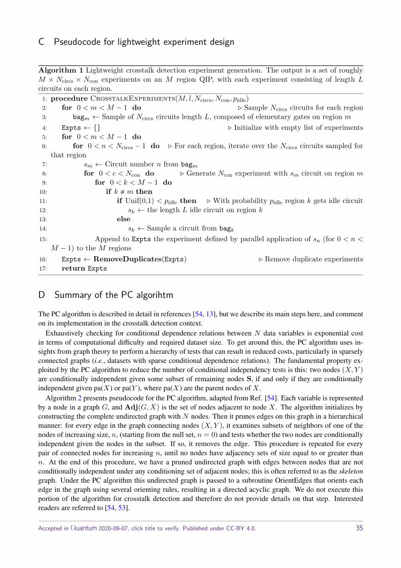
C Pseudocode for lightweight experiment design

Algorithm 1 Lightweight crosstalk detection experiment generation. The output is a set of roughlyM × Ncircs × Ncon experiments on an M region QIP, with each experiment consisting of length Lcircuits on each region.

1: procedure CrosstalkExperiments(M, l,Ncircs, Ncon, pidle)2: for 0 < m < M − 1 do . Sample Ncircs circuits for each region3: bagm ← Sample of Ncircs circuits length L, composed of elementary gates on region m

4: Expts ← . Initialize with empty list of experiments5: for 0 < m < M − 1 do6: for 0 < n < Ncircs − 1 do . For each region, iterate over the Ncircs circuits sampled for

that region7: sm ← Circuit number n from bagm8: for 0 < c < Ncon do . Generate Ncon experiment with sm circuit on region m9: for 0 < k < M − 1 do

10: if k , m then11: if Unif(0,1) < pidle then . With probability pidle region k gets idle circuit12: sk ← the length L idle circuit on region k13: else14: sk ← Sample a circuit from bagk15: Append to Expts the experiment defined by parallel application of sn (for 0 < n <

M − 1) to the M regions16: Expts ← RemoveDuplicates(Expts) . Remove duplicate experiments17: return Expts

D Summary of the PC algorihtm

The PC algorithm is described in detail in references [54, 13], but we describe its main steps here, and commenton its implementation in the crosstalk detection context.

Exhaustively checking for conditional dependence relations between N data variables is exponential costin terms of computational difficulty and required dataset size. To get around this, the PC algorithm uses in-sights from graph theory to perform a hierarchy of tests that can result in reduced costs, particularly in sparselyconnected graphs (i.e., datasets with sparse conditional dependence relations). The fundamental property ex-ploited by the PC algorithm to reduce the number of conditional independency tests is this: two nodes (X,Y )are conditionally independent given some subset of remaining nodes S, if and only if they are conditionallyindependent given pa(X) or pa(Y ), where pa(X) are the parent nodes of X .

Algorithm 2 presents pseudocode for the PC algorithm, adapted from Ref. [54]. Each variable is representedby a node in a graph G, and Adj(G,X) is the set of nodes adjacent to node X . The algorithm initializes byconstructing the complete undirected graph with N nodes. Then it prunes edges on this graph in a hierarchicalmanner: for every edge in the graph connecting nodes (X,Y ), it examines subsets of neighbors of one of thenodes of increasing size, n, (starting from the null set, n = 0) and tests whether the two nodes are conditionallyindependent given the nodes in the subset. If so, it removes the edge. This procedure is repeated for everypair of connected nodes for increasing n, until no nodes have adjacency sets of size equal to or greater thann. At the end of this procedure, we have a pruned undirected graph with edges between nodes that are notconditionally independent under any conditioning set of adjacent nodes; this is often referred to as the skeletongraph. Under the PC algorithm this undirected graph is passed to a subroutine OrientEdges that orients eachedge in the graph using several orienting rules, resulting in a directed acyclic graph. We do not execute thisportion of the algorithm for crosstalk detection and therefore do not provide details on that step. Interestedreaders are referred to [54, 53].


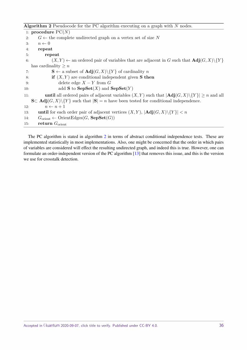
Algorithm 2 Pseudocode for the PC algorithm executing on a graph with N nodes.1: procedure PC(N)2: G← the complete undirected graph on a vertex set of size N3: n← 04: repeat5: repeat6: (X,Y )← an ordered pair of variables that are adjacent in G such that Adj(G,X)\Y

has cardinality ≥ n7: S ← a subset of Adj(G,X)\Y of cardinality n8: if (X,Y ) are conditional independent given S then9: delete edge X − Y from G

10: add S to SepSet(X) and SepSet(Y )11: until all ordered pairs of adjacent variables (X,Y ) such that |Adj(G,X)\Y | ≥ n and all

S⊂ Adj(G,X)\Y such that |S| = n have been tested for conditional independence.12: n← n+ 113: until for each order pair of adjacent vertices (X,Y ), |Adj(G,X)\Y | < n14: Gorient ← OrientEdges(G, SepSet(G))15: return Gorient

The PC algorithm is stated in algorithm 2 in terms of abstract conditional independence tests. These areimplemented statistically in most implementations. Also, one might be concerned that the order in which pairsof variables are considered will effect the resulting undirected graph, and indeed this is true. However, one canformulate an order-independent version of the PC algorithm [13] that removes this issue, and this is the versionwe use for crosstalk detection.


detecting crosstalk errors in quantum information processors

Documents