detecting actin fibers in cell images using minimal spanning

Detecting Actin Fibers in Cell Images using Minimal Spanning n e e s

Andrew E. Johnson and Ra61 E. Vald6s-P6rez

September 2 1, 1993 CMU-RI-TR-93- 18

The Robotics Institute Carnegie Mellon University

Pittsburgh, Pennsylvania 152 13-3890

0 1993 Camegie Mellon University

This research was partially supported by the W.M. Keck Foundation for advanced training in computational biology at Camegie Mellon University, the University of Pittsburgh, and the Pittsburgh Supercomputing Center. The views and conclusions contained in this document are those of the authors and should not be interpreted as representing the official policies, either expressed or implied, of the funding agencies or the U S . govern- ment.

Abstract

The quantitati,:e descriplion of cell structures in light microscope images is an important task in biological reseurch. The inclusion of digital image processing techniques ancljuorescenf markers into light microscope imaging has recently made this task feasible. In this papec we present a method for detection of filuinenraty strucfures in cell images that have been highlighted withjuorescent markers. The method has three stages. First, pixels belonging to fiber contours are extracted from the image. Then these pixels are grouped together based on proximity by a minimal spanning tree. Finuilj the fiber contours are determined as sub-trees of the minimal spanning tree. Once the pixels belonging to individual fibers contours have been determined, quantitative statistics describing fhe j’ibers in the cell can be calculated.

Keywords: Light Microscopy, Actin Fibers, Minimal Spanning Trees, Bio- logical Imaging, Filamentary Structure.

1 Introduction

In recent years, biological imaging using light microscopes has been augmented with a powerful new tool, the computer. The traditional approach to light microscope imaging involved a biologist setting up a microscope by hand, taking a picture of a cell, and then analyzing the picture after i t was developed. These steps have been improved by a more imme- diate approach in which the microscope is set up under computer control and the pictures are taken by video cameras and stored as digital data in computer memory. This new method frees the biologist from the time consuming task of setting up the microscope and allows the experiment to be immediately reviewed by accessing the images stored in computer memory. Furthermore, storing the images in digital form allows them to be manipulated in many ways. This manipulation could take the form of sharpening the image, extracting features from the cell and other image processing techniques [l]. The computer has become a tool for the biologist that partially automates the analysis of light microscope images.

For a typical biological experiment using a light microscope, the results obtained are qualitative (e.g. there are more fibers at the center of the cell than at the edges) than quantitative because getting quantitative results about cell structures is usually a tedious and labo- rious process. However, quantitative results are more useful for scientific discovery because they allow more precise comparison of results between experiments. An advantage of using a computer to store and manipulate images of cells is that the computer can be programmed to generate statistics about cell structures which can be used as quantitative results for experiments (e.g. there are 4.5 fibers per square micrometer at position (20,ZO) in the cell). The computer can perform this tedious task much faster than humans. Such automation of measurement allows the biologist to spend more time analyzing results and less time getting them.

Cells and cell structures are generally colorless and transparent in their natural state. The traditional method of improving contrast in cells and highlighting cell structures is through staining. Unfortunately, staining usually kills the cell, so dynamic processes in the cell can- not be measured. Recently a new method for highlighting cell structures using fluorescent markers instead of stains has been developed. Fluorescent markers have transformed light microscope imaging because they do not kill cells and can be attached to many different cell structures [ I ] . Fluorescent markers are molecules that bond to cell structure, but are not thought to inhibit the processes of the cell. When radiated with light of a particular wavelength the markers absorb photons and then emit photons of a different wavelength. The emitted photons are recorded in a video image that only shows the places in the cell where the molecules have attached. Different markers (with different emitted photon wavelengths) attach to different elements in the cell and multiple markers can be used at one time, so many cell processes can be analyzed simultaneously. This lets biologists study the dynamic interaction of cell elements.

1.1 The Biological Problem Actin is a protein common in muscle cells of animals which is biologically significant

because it is related to cell structure and mobility and because it interacts with other cell Structures in complex ways. Single monomers of Actin form into long chains called fibers and sets of these fibers wrap around each other to form fiber bundles. These fibers and fiber bundles are large enough to be imaged by a light microscope. Measuring properties of fibers in cells like length, width, curvature, orientation, density, movement and coherence is difficult and time consuming because there are many fibers in the cell and the fibers intersect and branch. Dynamic measurement of these properties of Actin fiber is important for under- standing how cells move and are formed. If the pmcess of measuring Actin fiber properties is automated, biological research into the purpose of Actin will be accelerated. Fortunately, there exist fluorescent markers for Actin which can be used to segment the parts of a cell image that contain Actin from the rest of the image and facilitate the measurement of fiber properties.

Figure 1: Image of cell with Actin fibers highlight& by fluorescent markers

1.2 Motivation of Approach The problem at hand is to measure the properties of Actin fibers in an image of a cell

where the fibers have been highlighted with fluorescent markers. If the fibers could be mod- eled easily and were spatially distinct from each other the pmblem would be straightforward. In reality Actin appears as a network of overlapping, intersecting and branching

fibers, so extracting individual fibers from the image is not straightforward. An effective method for finding fibers in a cell and calculating their statistics will need a way of representing fibers and extracting individual fibers from the network of fibers,

Many of the statistics that convey relevant information about a fiber are based on how the fiber changes position along its length (Le. many of the statistics are based on the contour of the fiber). For this reason, the contour of the fiber was chosen as the way to represent fibers in the image. A contour is a list of pixels, given as (row,column) positions in the image, that follow the course of the fiber. Because the width of fibers is fairly constant along their length, the edge of a fiber follows the contour of the fiber. Hence, pixels in the image that can be associated with fiber contours are found by finding strong edges in the image of the cell. The fiber contour pixels are thus determined, but these pixels still need to be grouped together into fibers.

As Figure 1 shows, each fiber in the cell image is separated from other fibers except at intersection of fibers. It follows that a pixel belonging to a specific fiber will be closer to pixels in the same fiber than pixels belonging to other fibers Our method that groups fiber contour pixels into fibers exploits this proximity of pixels to group fiber pixels together and then deals with the problems of intersection and branching of fibers. A minimal spanning tree of a set of points is the tree that connects these points such that the sum of the inter-point distances in the tree is a minimum. Given the close proximity of pixels belonging to the same fiber and the greater distance between pixels from different fibers, a natural way to group the fiber contour pixels is with a minimal spanning tree. Minimal spanning trees group points according to a global perspective and associates things that are close together more readily than things h t are far apart.

Minimal spanning tree grouping has several advantages over other contour finding methods. First, the grouping of the fiber contour pixels is done without requiring any domain knowledge about the expected shape of fiber contours. Second, the minimal spanning tree grouping is invariant under similarity transforms @e., scaling, skewing, rotation, translation). Finally, efficient algorithms for finding the minimal spanning tree of a set of points exist and are well understood. An efficient algorithm is needed because the set of points to be grouped can be large in image processing applications.

Once the fiber contour pixels are grouped into a minimal spanning tree, ambiguities at intersections and branches in the tree must be resolved to determine the final set of fiber contours in the image. This is done by first identifying sets of fiber contour pixels that can be associated unambiguously within the minimal spanning tree. Three or more of thesc sets meet at intersections in the tree. At each intersection, the sets that lie along roughly the same line and are close together are matched and their pixel sets are merged. In this way the small sets of pixels can be merged into larger sets to form complete fiber contours.

1.2.1 Previous Work

The human vision system uses clustering techniques based on minimizing inter-point distances [Z]. This is essentially the way that minimal spanning tree algorithms group discrete sets of points into groups. Minimal spanning trees are also used to group spark profiles

in physics spark-chamber photography [3]. Cosmologists have used minimal spanning trees to detect filamentary structure in the universe [4].

There have been previous attempts to solve the problem of finding Actin fibers in cell images. One technique followed the contours of the fibers in the image with a tracking routine [ 5 ] . Thc routine depended heavily on the domain knowledge that fibers are roughly linear, and relied on having rather good clean images of the cell. It found most well-defined fibers but had trouble tracking fibers at intersections and under low contrast. Another possible method could use a Hough transform to find fibers in the image based on a model of the fibers. Implementation of this would be complex because it would be difficult to find an appropriate model for fibers and any reasonable model of fibers would have to have a large number of parameters. Hough space has the same number of dimensions as the number of parameters in the fiber model, so a large number of parameters would make the search for local maxima in Hough space to find the fibers extremely time consuming.

2 Extracting Fiber Contours

An initial step in image analysis is to determine what constitutes information and what constitutes noise in the image. In the case of finding cell fibers, the pixels that show fibers are information and everything else is noise. The contour of a fiber (i.e., the curve that describes how the fiber is positioned in the image) contains all of the information needed to calculate most of the statistics of the fiber. Therefore, to achieve our goal of calculating the statistics of the fibers, we need only determine a set of pixels in the image that describe the contours of the fibers. All input images were 8-bit gray scale images.

2.1 Edge Detection Actin fibers are highlighted by fluorescent dyes. This simplifies the segmentation prob-

Icm because fiber intensities are greater than their surroundings. Unfortunately, simple thresholding will not result in a representative set of fiber pixels. Cells are thicker toward the middle than at the edges, so more dye accumulates around the center of the cell. This implies an overall increase in intensity near its center. Picking a threshold that includes the fibers on the perimeter of the cell results in the fibers in the middle of the cell being blurred together. Picking a threshold that decreases the blumng of the fibers in the middle of the cell results in the fibers on the perimeter not being detected. Therefore, selecting one threshold for the entire image is problematic because this method does not convey all of the information about the shape of the cell fibers.

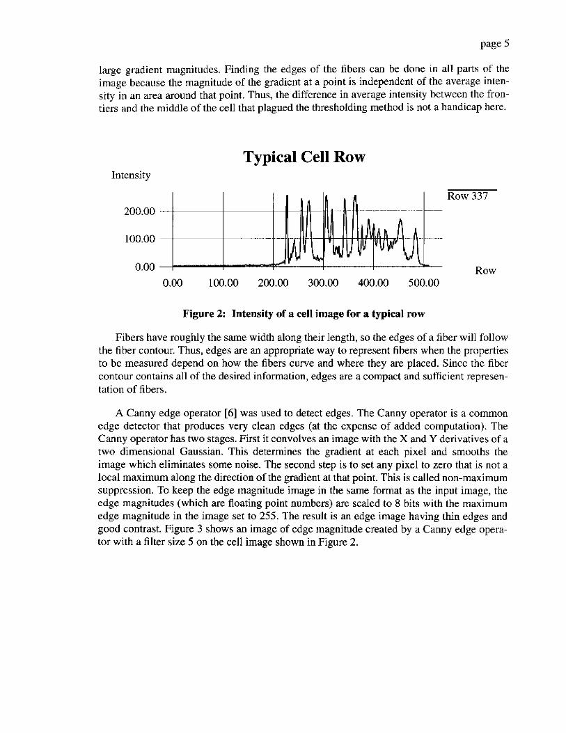
When the image of the cell is regarded as a surface with intensity as the third dimension, the fibers appear as long “hills” in the surface that spring from the background of the image. Figure 2 shows this hill-like nature of fibers by showing the intensity of a single row of a cell image. The sides of these hills can be found with an edge detector. An edge in the image corresponds to a rapid change of intensity in a small image area. These rapid changes are found by finding large values of the gradient of intensity because sharp edges will yield

large gradient mdgnitudes. Finding the edges of the fibers can be done in all parts of the image because the milgnitude of the gradient at a p i n t is independent of the average intensity in an area around that point. Thus, the difference in average intensity between the fron- tiers and the middle of the cell that plagued the thresholding method is not a handicap here.

Intensity

200.00

100.00

0.00

Typical Cell Row

Row 337

Row 0.00 100.00 200.00 300.00 400.00 500.00

Figure 2: Intensity of a cell image for a typical row

Fibers have roughly the same width along their length, so the edges of a fiber will follow the fiber contour. Thus, edges are an appropriate way to represent fibers when the properties to be measured depend on how the fibers curve and where they are placed. Since the fiber contour contains all of the desired information, edges are a compact and sufficient representation of fibers.

A Canny edge operator [6] was used to detect edges. The Canny operator is a common edge detector that produces very clean edges (at the expense of added computation). The Canny operator has two stages. First it convolves an image with the X and Y derivatives of a two dimensional Gaussian. This determines the gradient at each pixel and smooths the image which eliminates some noise. The second step is to set any pixel to zero that is not a local maximum along the direction of the gradient at that point. This is called non-maximum suppression. To keep the edge magnitude image in the same format as the input image, the edge magnitudes (which are floating point numbers) are scaled to 8 bits with the maximum edge magnitude in the image set to 255. The result is an edge image having thin edges and good contrast. Figure 3 shows an image of edge magnitude created by a Canny edge operator with a filter size 5 on the cell image shown in Figure 2.

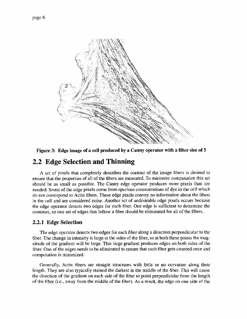
Figure 3: Edge image of a cell produced by a Canny operator with a filter size of 5

2.2 Edge Selection and Thinning A set of pixels that completely describes the contour of the image fibers is desired to

ensure that the properties of all of the fibers are measured. To minimize computation this set should be as small as possible. The Canny edge operator produces more pixels than are needed. Some of the edge pixels come from spurious concentrations of dye in the cell which do not correspond to Actin fibers. These edge pixels convey no information about the fibers in the cell and are considered noise. Another set of undesirable edge pixels occurs because the edge operator detects two edges for each fiber. One edge is sufficient to determine the contours, so one set of edges that follow a fiber should be eliminated for all of the fibers.

2.2.1 Edge Selection

The edge operator detects two edges for each fiber along a direction perpendicular to the fiber. The change in intensity is large at the sides of the fiber, so at both these points the magnitude of the gradient will be large. This large gradient produces edges on both sides of the fiber. One of the edges needs to be eliminated to ensure that each fiber gets counted once and computation is minimized.

Generally, Actin fibers are straight structures with little or no curvature along their length. They are also typically stained the darkest in the middle of the fiber. This will cause the direction of the gradient on each side of the fiber to point perpendicular from the length of the fiber &e., away from the middle of the fiber). As a result, the edge on one side of the

fiber will have gradient directions that are roughly the same along the entire edge, and the gradient on the other side of the fiber will have directions that are rotated roughly 180 degrees. Therefore, the edges on either side of the fiber are naturally segmented based on the gradient direction. For a given fiber, one can keep only the edge pixels with directions in one half plane determined by the direction of the fiber, and the others are thrown away. Hence, one edge of the fiber is kept and the other is eliminated

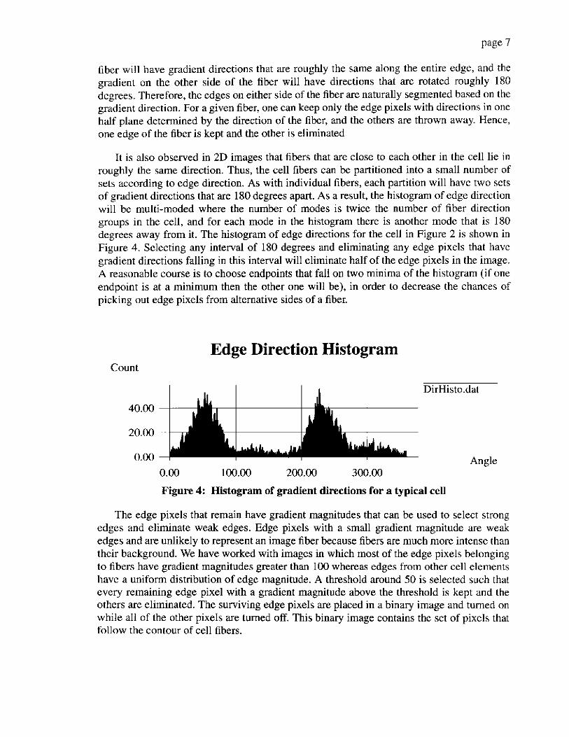
It is also observed in 2D images that fibers that are close to each other in the cell lie in roughly the same direction. Thus, the cell fibers can be partitioned into a small number of sets according to edge direction. As with individual fibers, each partition will have two scts of gradient directions that are 180 degrees apart. As a result, the histogram of edge direction will be multi-moded where the number of modes is twice the number of fiber direction groups in the cell, and for each mode in the histogram there is another mode that is 180 degrees away from it. The histogram of edge directions for the cell in Figure 2 is shown in Figure 4. Selecting any interval of 180 degrees and eliminating any edge pixels that have gradient directions falling in this interval will eliminate half of the edge pixels in the image. A reasonable course is to choose endpoints that fall on two minima of the histogram (if one endpoint is at a minimum then the other one will be), in order to decrease the chances of picking out edge pixels from alternative sides of a fiber.

Edge Direction Histogram Count

I i DirHisto.dat

40.00 I ' 0.00 -

0.00 100.00 200.00 300.00

Figure 4: Histogram of gradient directions for a typical cell

The edge pixels that remain have gradient magnitudes that can be used to select strong edges and eliminate weak edges. Edge pixels with a small gradient magnitude are weak edges and are unlikely to represent an image fiber because fibers are much more intense than their background. We have worked with images in which most of the edge pixels belonging to fibers have gradient magnitudes greater than 100 whereas edges from other cell elements have a uniform distribution of edge magnitude. A threshold around 50 is selected such that every remaining edge pixel with a gradient magnitude above the threshold is kept and the others are eliminated. The surviving edge pixels are placed in a binary image and turned on while all of the other pixels are turned off. This binary image contains the set of pixels that follow the contour of cell fibers.

2.2.2 Thinning

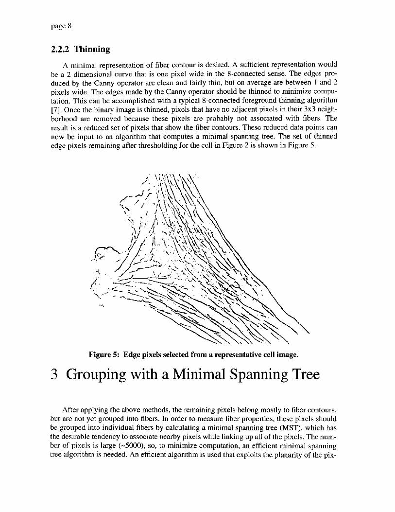
A minimal representation of fiber contour is desired. A sufficient representation would be a 2 dimensional curve that is one pixel wide in the 8-connected sense. The edges produced by the Canny operator are clean and fairly thin, but on average are between 1 and 2 pixels wide. The edges made by the Canny operator should be thinned to minimize computation. This can be accomplished with a typical 8-connected foreground thinning algorithm [ 7 ] . Once the binary image is thinned, pixels that have no adjacent pixels in their 3x3 neigh- borhood are removed because these pixels are probably not associated with fibers. The result is a reduced set of pixels that show the fiber contours. These reduced data points can now be input to an algorithm that computes a minimal spanning tree. The set of thinned edge pixels remaining after thresholding for the cell in Figure 2 is shown in Figure 5.

Figure 5: Edge pixels selected from a representative cell image.

3 Grouping with a Minimal Spanning Tree

After applying the above methods, the remaining pixels belong mostly to fiber contours, but are not yet grouped into fibers. In order to measure fiber properties, these pixels should be grouped into individual fibers by calculating a minimal spanning tree (MST), which has the desirable tendency to awxiate nearby pixels while linking up all of the pixels. The number of pixels is large (-5000), so, to minimize computation, an efficient minimal spanning tree algorithm is needed. An efficient algorithm is used that exploits the planarity of the pix-

els to create the minimal spanning tree in O(Nlog(N)) time where N is the number of image pixels [SI. This algorithm is explained next.

3.1 The Voronoi Diagram Minimal spanning tree algorithms are typically greedy algorithms, in the sense that at

each decision point, a partially-built tree is expanded irrevocably by adding an extra edge. Clearly, reducing the number of candidate edge extensions at each point will decrease the run time, and possibly even the computational complexity.

It turns out that when the graph vertices are embedded on the plane, as occurs naturally in the case of image pixels, the candidate edge extensions can be reduced drastically: one need only consider edges from a graph known as the Delaunay Triangulation, which is a dual of the better-known Voronoi Diagram, and which is a subgraph of the complete graph connecting all image points. Some minimal spanning tree will be a subgraph of the Delaunay Triangulation, so only the edges in the latter graph need to be considered.

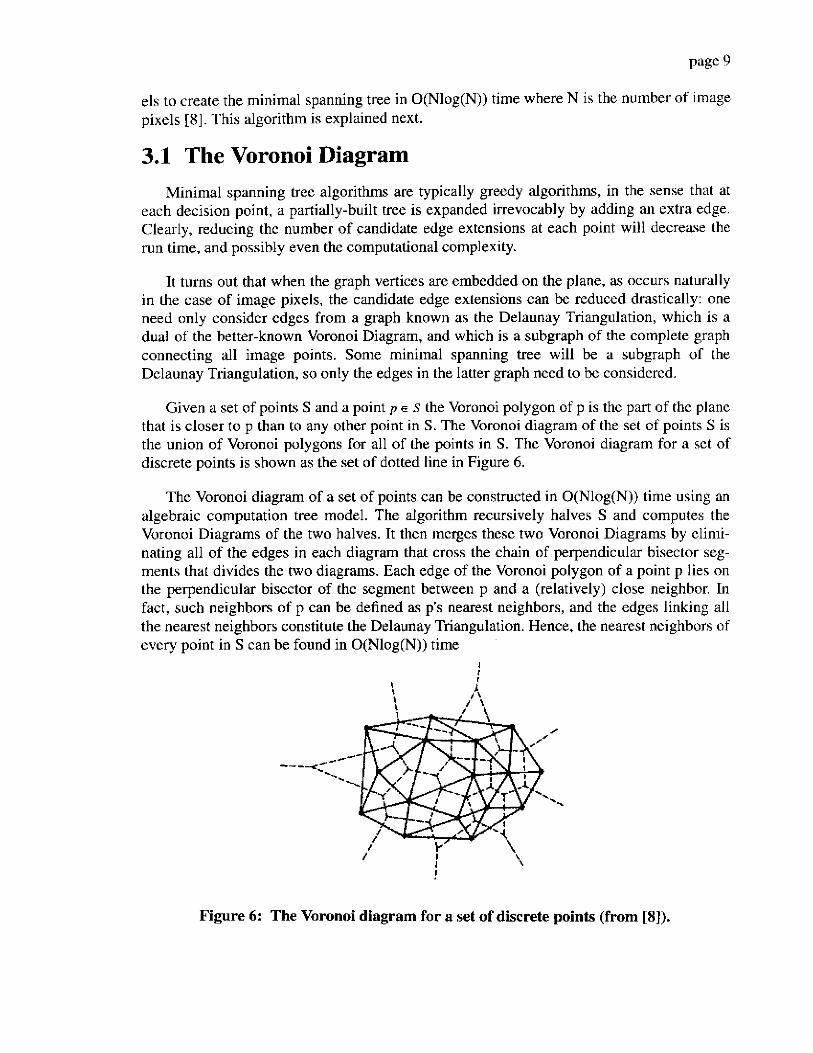
Given a set of point? S and a point p E s the Voronoi polygon of p is the part of the plane that is closer to p than to any other point in S. The Voronoi diagram of the set of points S is the union of Voronoi polygons for all of the points in S. The Voronoi diagram for a set of discrete points is shown as the set of dotted line in Figure 6.

The Voronoi diagram of a set of points can be constructed in O(Nlog(N)) time using an algebraic computation tree model. The algorithm recursively halves S and computes the Voronoi Diagrams of the two halves. It then merges these two Voronoi Diagrams by eliminating all of the edges in each diagram that cross the chain of perpendicular bisector seg- ments that divides the two diagrams. Each edge of the Voronoi polygon of a point p lies on the perpendicular bisector of the segment between p and a (relatively) close neighbor. In fact, such neighbors of p can be defined as p's nearest neighbors, and the edges linking all the nearest neighbors constitute the Delaundy Triangulation. Hence, the nearest neighbors of every point in S can be found in O(Nlog(N)) time

!

Figure 6: The Voronoi diagram for a set of discrete points (from [SI).

Given the Cartesian locations of all fiber pixels in an image, the nearest neighbors of all the pixels are determined and then used to calculate a minimal tree that spans all the fiber pixels. The nearest neighbors of a point in Figure 6 are the set of points connected to the point by a solid line. We have used Fortune’s implementation of his algorithm for computing Voronoi Diagrams [9].

3.2 The Euclidean Minimal Spanning Tree Algorithm The Delaunay Triangulation is exploited to find a minimal spanning tree that connects

all of the contour points in the image. MST algorithms tend to link nearby points, and the closest point to a point p is one of its nearest (Delaunay) neighbors, so an efficient Euclidean minimal spanning tree algorithm only examines the Delaunay edges of a planar graph. An MST algorithm that is given nearest neighbor information can operate in linear time [SI. It is based on merging minimal spanning sub-trees through nearest neighbors until only one tree remains.

I.

2.

Create an empty queue of trees F. For every selected edge pixel P.

1,

2. stage(T) := 0

3. Push T onto F

Create a tree T from P of one point and no edges

3. STAGE-NUM := 1

4. While F contains more than one tree

1. T=pop(F) 2. If stage(T) = STAGE-NUM then

I. Clean up trees in F by eliminating all unselected edges except those that are the shortest edges bridging different trees.

2. STAGE-NUM = STAGE-NUM+I 3. 4.

E:= shortest edge connecting T to any other tree T’:= tree in F that is connected to T by E

5 . T”= the tree created by merging T and T’ which contains all of the edges and points of T and T’

6. Delete T’ from F 7. stage(T”) := min(stage(T).stage(T’))+l 8. Push T” onto the back of F

This algorithm is faster than more general MST algorithms that do not exploit planarity [IO], but is more complicated and uses more memory. Vertex data structures that contain information about position, nearest neighbors and tree membership must be created for all pixels in the fiber contour image. Edge data structures must be created to describe all con- nections between pixels in the planar graph. Tree data structures that list all of the vertices and edges in the tree must be created as well. New trees are constantly being created from the merging of smaller sub-trees and added to a queue. Old trees are deleted when they are merged into larger trees. After every stage the queue is cleaned up which requires pruning

many of the edges in the trees within the queue. Because the number of trees is so large, sophisticated memory management is required to store all of the trees in memoly and main- tain the queue.

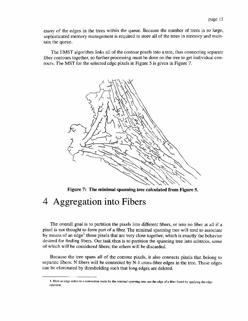
The EMST algorithm links all of the contour pixels into a tree, thus connecting separate fiber contours together, so further processing must be done on the tree to get individual contours. The MST for the selected edge pixels in Figure 5 is given in Figure 7.

Figure 7: The minimal spanning tree calculated from Figure 5.

4 Aggregation into Fibers

The overall goal is to partition the pixels into different fibers, or into no fiber at all if a pixel is not thought to form part of a fiber. The minimal spanning tree will tend to associate by means of an edge' those pixels that are very close together, which is exactly the behavior desired for finding fibers. Our task then is to partition the spanning tree into subtrecs, some of which will be considered fibers; the others will be discarded.

Because the tree spans all of the contour pixels, it also connects pixels that belong to separate fibers: N fibers will be connected by N-1 cross-fiber edges in the tree. These edges can be eliminated by thresholding such that long edges are deleted.

I. Here illl edge refem to a cnnncction mode by h e minimal spanning tree, no1 rhe e d p of a h k r found by applying rhe edge "pcMtOr.

However, extracting the subtrees corresponding to fibers i, not straightforward for the following reason. There is ambiguity at pixels in the tree that have degree greater than two regarding which way a fiber from one direction should extend, if at all. Our general approach will be to make the easy decisions first; for example, if two pixels connected by an edge both have degree 2 (and the edge length is below threshold for deletion), then decide that the pixels are part of the same fiber. After making these easy associations, pieces of fibers will be built up, which can then be linked at intersections based on whether they are similar. A representative grouping of fiber contour pixels by a MST is given in Figure 8 which shows the problem areas in extracting fibers from the minimal spanning tree.

Figure 8: Difficulties arising from the grouping by the MST

4.1 Protofibers In the minimal spanning tree there exist sets of pixels than are associated sequentially

without branches. These sets of pixels lie between leaves, intersections and branches in the tree. Because these sets are the building blocks of the final fiber contours, they will be called prorojbers. The length of a protofiber is the number of pixels that it contains. The tree is segmented into protofibers so that these can be merged into correct fiber contours. The protofibers derived from the minimal spanning tree in Figure 8 are shown in Figure 9.

Figure 9: Examples of protofibers.

4.2 Removing Undesirable Protofibers Some of the resulting protofibers are made of one long link (Le., two connected pixels

that are far apart) in the MST that spans a gap between two dense protofibers. These protofibers are created in the tree because the tree must link all of the pixels together and doing so

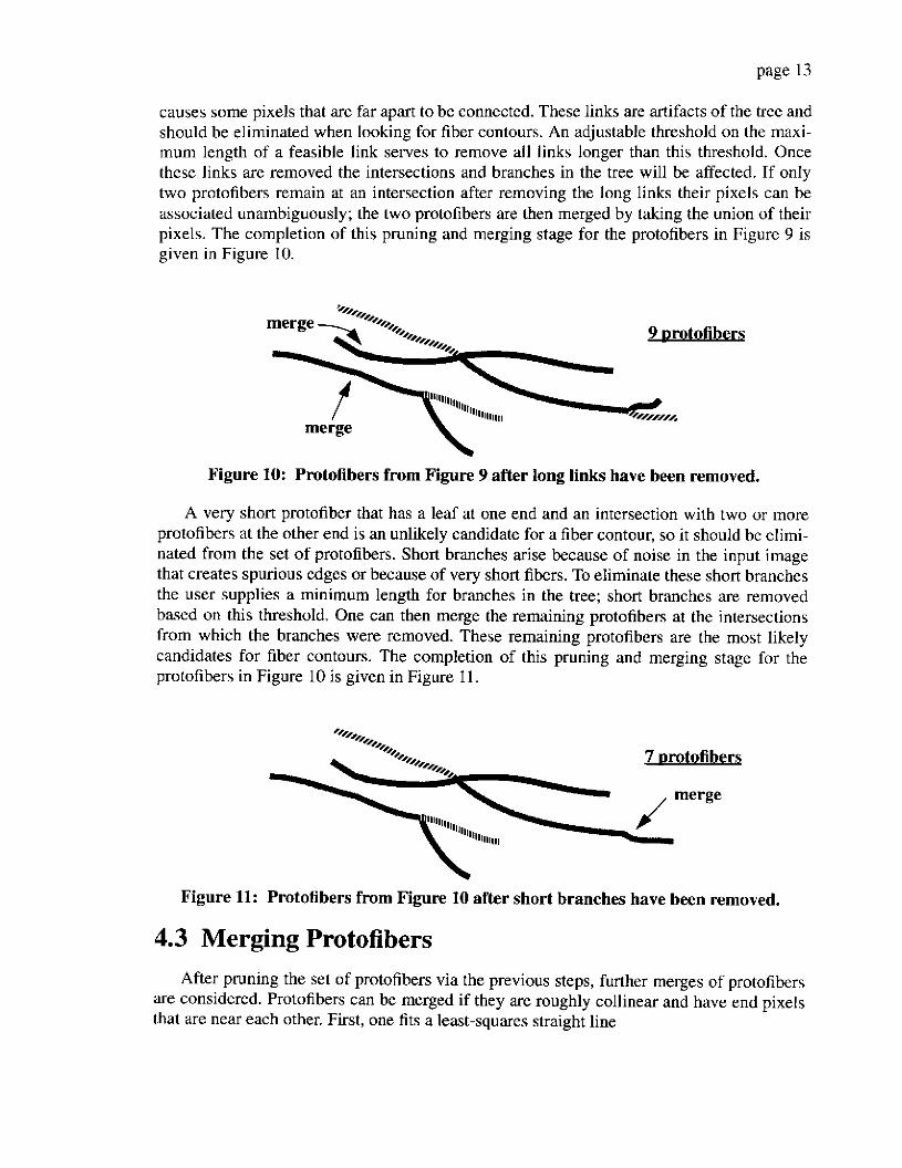
causes some pixels that are far apart to be connected. These links are artifacts of the tree and should be eliminated when looking for fiber contours. An adjustable threshold on the maximum length of a feasible link serves to remove all links longer than this threshold. Once these links are removed the intersections and branches in the tree will be affected. If only two protofibers remain at an intersection after removing the long links their pixels can be associated unambiguously; the two protofibers are then merged by taking the union of their pixels. The completion of this pruning and merging stage for the protofibers in Figure 9 is given in Figure 10.

Figure 10: Protofibers from Figure 9 after long links have been removed.

A very short protofiber that has a leaf at one end and an intersection with two or more protofibers at the other end is an unlikely candidate for a fiber contour, so it should be eliminated from the set of protofibers. Short branches arise because of noise in the input image that creates spurious edges or because of very short fibers. To eliminate these short branches the user supplies a minimum length for branches in the tree; short branches a n removed based on this threshold. One can then merge the remaining protofibers at the intersections from which the branches were removed. These remaining protofibers are the most likely candidates for fiber contours. The completion of this pruning and merging stage for the protofibers in Figure 10 is given in Figure 11.

Figure 11: Protofibers from Figure 10 after short branches have been removed.

4.3 Merging Protofibers After pruning the set of protofibers via the previous steps, further merges of protofibers

are considered. Protofibers can be merged if they are roughly collinear and have end pixels that are near each other. First, one fits a least-squares straight line

a x + b y + c = 0 V-1)

to all of the pixels in each protofiber. The angle a that each protofiber makes with respect to the horizontal image axis is calculated via the expression

(EQ2) h

Next, each intersection of protofibers is tested for possible merging. All of the protofibers within a user defined radius of an intersection are found by searching along the protofibers that make the intersection. If a neighboring protofiber is not part of the intersection it is still considered for merging.

U a = a tan( - ) .

All pairs of protofibers (i j) near the intersection are then matched. The match cost of a pair is defined as:

IcLi-a.I I hij +6 C ( i , j ) = W

%lax max

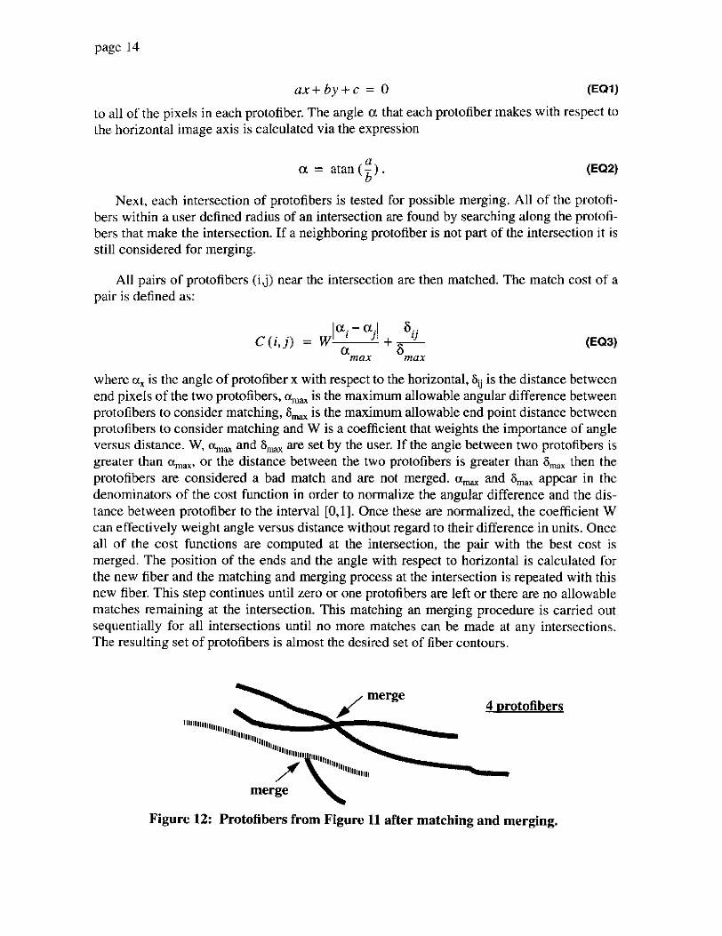
where c(, i s the angle of protofiber x with respect to the horizontal, &ij is the distance between end pixels of the two protofibers, %m is the maximum allowable angular difference between protofibers to consider matching, 6- is the maximum allowable end point distance between protofibers to consider matching and W is a coefficient that weights the importance of angle versus distance. W, a,,,= and S,, are set by the user. If the angle between two protofibers is greater than or the distance between the two protofibers is greater than S,, then the protofibers are considered a bad match and are not merged. amax and S,,, appear in the denominators of the cost function in order to normalize the angular difference and the distance between protofiber to the interval [0,1]. Once these are normalized, the coefficient W can effectively weight angle versus distance without regard to their difference in units. Once all of the cost functions are computed at the intersection, the pair with the best cost is merged. The position of the ends and the angle with respect to horizontal is calculated for the new fiber and the matching and merging process at the intersection is repeated with this new fiber. This step continues until zero or one protofibers are left or there are no allowable matches remaining at the intersection. This matching an merging procedure is carried out sequentially for all intersections until no more matches can be made at any intersections. The resulting set of protofibers is almost the desired set of fiber contours.

\ merge

Figure 12: Protofibers from Figure 11 after matching and merging.

The contours that are too short to be useful are then discarded, which yields the final set of fiber contours. From these pixel groupings, any desired fiber statistics can be calculated. Figure 12 shows the final set of fibers extracted from the minimal spanning tree in Figure 8.

5 Testing

It is unclear what is a “correct” extraction of fibers, due to the inevitablc ambiguity introduced by a 2D projection of what in reality are 3D fibers. In a sense the current work is an attempt to define what is correct. These circumstances make it problematic to evaluate the performance of the approach. Moreover, it is very tedious to extract fibers manually, and two biologists might well disagree on the results. For these reasons it is currently only prac- tical to test the program on real data by qualitative inspection. However, we can use synthetic data with known fibers to obtain one measure of perfomlance.

5.1 Synthetic Data A representative set of synthetic data for testing should show all the characteristics of

fibers in real images including the characteristics that make fibers difficult to detect. A representative set of fibers should contain:

- Intersecting fibers

Branchings into multiple fibers

Short “noisy” fibers

Fibers with thickness greater than one pixel

Fibers that are roughly linear

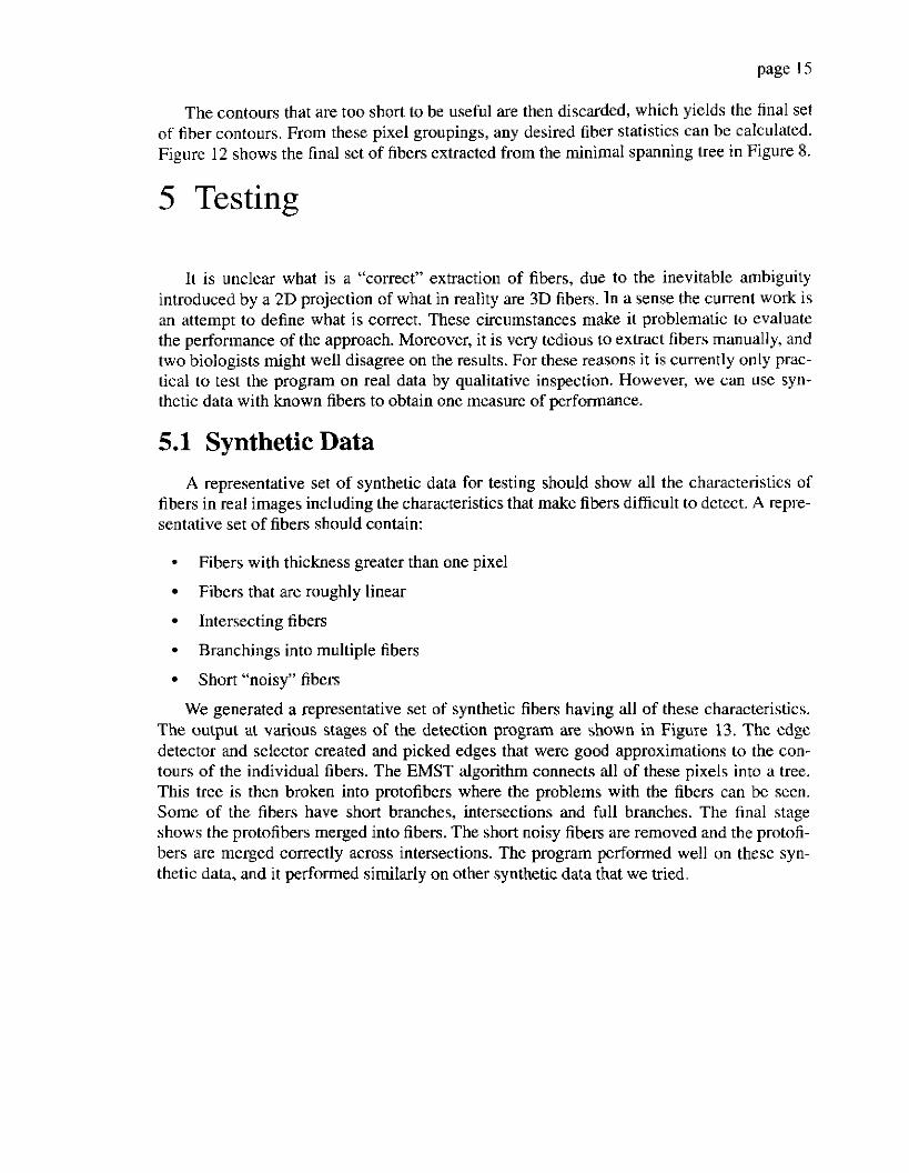
We generated a representative set of synthetic fibers having all of these characteristics. The output at various stages of the detection program are shown in Figure 13. The edge detector and selector created and picked edges that were good approximations to the contours of the individual fibers. The EMST algorithm connects all of these pixels into a tree. This tree is then broken into protofibers where the problems with the fibers can be seen. Some of the fibers have short branches, intersections and full branches. The final stage shows the protofibers merged into fibers. The short noisy fibers are removed and the protofibers are merged correctly across intersections. The program performed well on these synthetic data, and it performed similarly on other synthetic data that we tried.

4< 1 i / J

Figure 13:

I irput Image 2 Edges 3 Thinned edges 4 Triangulation 5 MST 6 Protornets 7 Fibers

The stages of the fiber detection sgstem on a set of synthetic fibers.

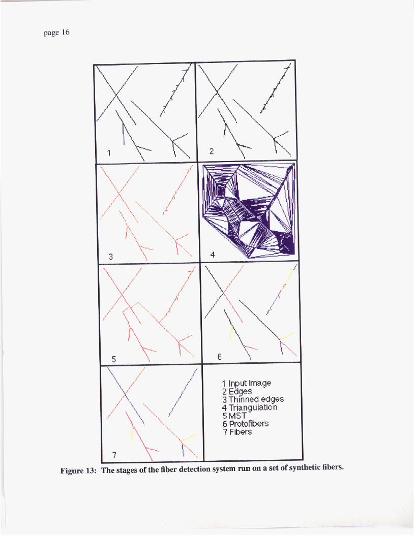
5.2 RealData The results of the matching and merging of protofibers for the real image in figure 1 are

given in Figure 14. The system in general did a better job of matching protofibers when fibers had fewer intersections and branches. Fibers with strong contrast with the background were easier to detect and show up correctly in the final set of fibers. It seems that the system had trouble matching fibers that had varying intensities along their length and that inter- sected wide fibers. From OUT tests we expect that the system will give accurate measure ments of the position, curvature, density and d a t i o n of the fibers in the cell whereas it will not be as good at measuring length and connectivity

\

F i p t 14 Fiber contours detected in a repmentab 've cell image

6 Conclusions and Future Work

Detection of Actin fibers highlighted by fluorescent markers in cell images is difficult because the image of the fibers is a 2D projection of 3D structures which intersect and branch throughout the cell. We have shown that the contour of a fiber can be approximated by one edge of the fiber. The pixels making this contour can be grouped with a minimal spanning tree, and the fiber contours can be extracted from this tree by pruning and matching of protofibers at intersections. These methods were shown to work adequately on a lim- ited set of synthetic and real data. The minimal spanning tree approach to grouping pixels is useful because it groups pixels based on a global perspective and does not rely on uncertain local predictions of where fibers might extend, as was done by Nedelof et al. [5].

Actin fibers are three dimensional structures, so this approach could be improved by extending the methods to three dimensions; work on recovery of 3D Actin fibers is in progress. Another issue to deal with is the breaking of fiber bundles into individual fibers. The matching algorithm used to eliminate ambiguity at intersections does not consider the break-up of fiber bundles. We expect that the current methods could be applied successfully to detect other filamentary structures in cell images.

Acknowledgments We thank D. Lansing Taylor for his help defining the biological problem, George Baxter

for his technical support and Martial Hebert for his insights into the image analysis. This work was supported in part by a grant from the W.M. Keck Foundation for advanced training in computational biology at Camegie Mellon University, the University of Pittsburgh, and the Pittsburgh Supercomputing Center.

References D.L. Taylor, M. Nederlof, E Lanni and A.S. Waggoner. The New Ksion uJ Light Microscopy. American Scientist, Vol. 80, July-August 1992.

M. Minsky and S . Papert. Percepfrons. M.I.T. Press, Cambridge MA, 1969.

C.T. Zahn. Graph-Theoretical Methods for Detecting and Describing Gestalt Clus- ters. IEEE Transactions of Computers, Vol. C-20, No.1, January 1971.

S.P. Bhavsar and E.N. Ling. Are the Filaments Real? The Astrophysical Journal, Vol. 331, 15 August 1988.

M.A. Nederlof, A. Witkin and D.L. Taylor. Knowledge Driven Image Analysis of Cell Structures. SPIE Proceedings from Three-Dimensional Bioimaging Systems and Lasers in the Neurosciences. 1991.

J.F. Canny. Finding Edges and Lines in Images. M.I.T. AI Laboratory Technical Report 720, June 1983.

D.M. Ballard and C.M. Brown. Computer &ion. Prentice Hall, Englewood Cliffs NJ, 1982.

F.P. Preparata and M.I. Shamos. Computation Geometry: An Introduction. Springer- Verlag, New York, 1985.

S.J. Fortune. A Sweepline Algorithm for Voronoi Diagrams. Algorithmica, Vol. 2, pages 153-174, 1987.

R.E. Tarjan. Data Structures and Network Algorithms. SIAM Press, Philadelphia, 1983.

detecting actin fibers in cell images using minimal spanning

Documents