arX

iv:c

ond-

mat

/060

6338

v4 [

cond

-mat

.dis

-nn]

27

Sep

2006

Optimal Path and Minimal Spanning Trees in Random Weighted

Networks

Contents

I. Introduction 6

II. Algorithms 9

A. Construction of the Networks 9

B. Dijkstra’s algorithm 10

C. Ultrametric Optimization 10

D. Bombing Optimization 11

E. The Minimum Spanning Tree (MST) 13

F. The Incipient Infinite Cluster (IIC) 14

III. Optimal path in strong disorder and percolation on the Cayley tree. 15

A. Distribution of the maximal weight on the optimal path 16

B. Distribution of the cluster chemical length at percolation threshold 21

C. Distribution of the cluster sizes at percolation threshold 22

IV. Scaling of the length of the optimal path in Strong Disorder 24

V. Scaling of the length of the optimal path in Weak Disorder 27

VI. Crossover from Weak to Strong Disorder 29

A. Exponential Disorder 29

B. General Disorder: Criterion for SD, WD crossovers 36

VII. Scaling of optimal-path-lengths distribution with finite disorder in complex networks42

VIII. Scale-Free Networks Emerging from Weighted Random Graphs 49

IX. Partition of the minimum spanning tree into superhighways and roads 54

X. Summary 63

1

Acknowledgments 64

References 64

2

Optimal Path and Minimal Spanning Trees in Random Weighted

Networks

Lidia A. Braunstein,1, 2 Zhenhua Wu,2 Yiping Chen,2 Sergey V.

Buldyrev,2, 3 Tomer Kalisky,4 Sameet Sreenivasan,2 Reuven Cohen,5, 4

Eduardo Lopez,2, 6 Shlomo Havlin,4, 2 and H. Eugene Stanley2

1Departamento de Fısica, Facultad de Ciencias Exactas y Naturales,

Universidad Nacional de Mar del Plata,

Funes 3350, 7600 Mar del Plata, Argentina∗

2Center for Polymer Studies, Boston University,

Boston, Massachusetts 02215, USA

3Department of Physics Yeshiva University,

500 West 185th Street Room 1112,NY, 10033, USA

4Minerva Center and Department of Physics,

Bar-Ilan University, 52900 Ramat-Gan, Israel

5 Dept. of Electrical and Computer Engineering,

Boston University, Boston, Massachusetts 02215, USA

6Theoretical Division, Los Alamos National Laboratory,

Mail Stop B258, Los Alamos, NM 87545 USA

3

Abstract

We review results on the scaling of the optimal path length ℓopt in random networks with

weighted links or nodes. We refer to such networks as “weighted” or “disordered” networks. The

optimal path is the path with minimum sum of the weights. In strong disorder, where the maximal

weight along the path dominates the sum, we find that ℓopt increases dramatically compared to

the known small world result for the minimum distance ℓmin ∼ log N , where N is the number of

nodes. For Erdos-Renyi (ER) networks ℓopt ∼ N1/3, while for scale free (SF) networks, with degree

distribution P (k) ∼ k−λ, we find that ℓopt scales as N (λ−3)/(λ−1) for 3 < λ < 4 and as N1/3 for

λ ≥ 4. Thus, for these networks, the small-world nature is destroyed. For 2 < λ < 3 in contrary,

our numerical results suggest that ℓopt scales as lnλ−1 N , representing still a small world. We also

find numerically that for weak disorder ℓopt ∼ ln N for ER models as well as for SF networks. We

also review the transition between the strong and weak disorder regimes in the scaling properties

of ℓopt for ER and SF networks and for a general distribution of weights τ , P (τ). For a weight

distribution of the form P (τ) = 1/(aτ) with (τmin < τ < τmax) and a = ln τmax/τmin, we find that

there is a crossover network size N∗ = N∗(a) at which the transition occurs. For N ≪ N∗ the

scaling behavior of ℓopt is in the strong disorder regime, while for N ≫ N∗ the scaling behavior is in

the weak disorder regime. The value of N∗ can be determined from the expression ℓ∞(N∗) = apc,

where ℓ∞ is the optimal path length in the limit of strong disorder, A ≡ apc → ∞ and pc is the

percolation threshold of the network. We suggest that for any P (τ) the distribution of optimal

path lengths has a universal form which is controlled by the scaling parameter Z = ℓ∞/A where

A ≡ pcτc/∫ τc0 τP (τ)dτ plays the role of the disorder strength and τc is defined by

∫ τc0 P (τ)dτ = pc.

In case P (τ) ∼ 1/(aτ), the equation for A is reduced to A = apc. The relation for A is derived

analytically and supported by numerical simulations for Erdos-Renyi and scale-free graphs. We also

determine which form of P (τ) can lead to strong disorder A → ∞. We then study the minimum

spanning tree (MST), which is the subset of links of the network connecting all nodes of the network

such that it minimizes the sum of their weights. We show that the minimum spanning tree (MST)

in the strong disorder limit is composed of percolation clusters, which we regard as ”super-nodes”,

interconnected by a scale-free tree. The MST is also considered to be the skeleton of the network

where the main transport occurs. We furthermore show that the MST can be partitioned into two

distinct components, having significantly different transport properties, characterized by centrality

— number of times a node (or link) is used by transport paths. One component the superhighways,

4

for which the nodes (or links) with high centrality dominate, corresponds to the largest cluster at

the percolation threshold (incipient infinite percolation cluster) which is a subset of the MST. The

other component, roads, includes the remaining nodes, low centrality nodes dominate. We find

also that the distribution of the centrality for the incipient infinite percolation cluster satisfies a

power law, with an exponent smaller than that for the entire MST. We demonstrate the significance

identifying the superhighways by showing that one can improve significantly the global transport

by improving a very small fraction of the network, the superhighways.

PACS numbers: 89.75.Hc,89.20.Ff

Keywords: minimum spanning tree, percolation, scale-free, optimization

∗Electronic address: lbrauns@mdp.edu.ar

5

I. INTRODUCTION

Recently much attention has been focused on the topic of complex networks which char-

acterize many biological, social, and communication systems [1, 2, 3]. The networks are

represented by nodes associated to individuals, organizations, or computers and by links

representing their interactions. The classical model for random networks is the Erdos-Renyi

(ER) model [4, 5, 6]. An important quantity characterizing networks is the average distance

(minimal hopping) ℓmin between two nodes in the network of total N nodes. For the Erdos-

Renyi network ℓmin scales as ln N [6], which leads to the concept of “small worlds” or “six

degrees of separation”. For scale-free (SF) [1] networks ℓmin scales as ln ln N , this leads to

the concept of ultra small worlds [2, 8].

In most studies, all links in the network are regarded as identical and thus a crucial

parameter for information flow including efficient routing, searching, and transport is ℓmin. In

practice, however, the weights (e.g., the quality or cost) of links are usually not equal [9, 10].

Thus the length of the optimal path ℓopt, minimizing the sum of weights, is usually longer

than ℓmin. For example, the cost could be the time required to transit the link. There are

often many traffic routes from site A to site B with a set of transit time τi, associated

with each link along the path. The fastest (optimal) path is the one for which∑

i τi is a

minimum, and often the optimal path has more links than the shortest path. In many cases,

the selection of the path is controlled by most of the weights (e.g., total cost) contributing

to the sum. This case corresponds to weak disorder (WD). However, in other cases, for

example when the distribution of disorder is very broad a single weight dominates the sum.

This situation—in which one link controls the selection of the path—is called the strong

disorder limit (SD).

For a recent quantitative criterion for SD and WD, see Ref [73] and Section VI(B) in this

article.

The strong disorder is relevant e.g. for computer and traffic networks, since the slowest

link in communication networks determines the connection speed. An example for SD is

when a transmission at a constant high rate is needed (e.g., in broadcasting video records

over the Internet). In this case the narrowest band link in the path between the transmitter

and receiver controls the rate of transmission. This limit is also called the “ultrametric”

limit and we refer to the optimal path in this limit as the min-max path.

6

The SD limit is also related to the minimal spanning tree which includes all optimal paths

between all pairs of sites in the network. The disorder on a network is usually implemented

from a distribution P (τ) ∼ 1/(aτ), where 1 < τ < ea [22, 24, 30, 32]. We assign to each

link of the network a random number r, uniformly distributed between 0 and 1. The cost

associated with link i is then τi ≡ exp(ari) where a is the parameter which controls the

broadness of the distribution of link costs. The parameter a represents the strength of

disorder. The limit a → ∞ is the strong disorder limit, since for this case clearly only one

link dominates the cost of the path. The strong disorder limit (SD) can be implemented in a

disordered media by assigning to each link a potential barrier ǫi so that τi is the time to cross

this barrier in a thermal activation process. Thus τi = eǫi/KT , where K is the Boltzmann

constant and T is absolute temperature. The optimal path corresponds to the minimum

(∑

i τi) over all possible paths. We can define disorder strength a = 1/KT . When a → ∞,

only the largest τi dominates the sum. Thus, T → 0 (very low temperature) corresponds to

the strong disorder limit.

There are distinct scaling relationships between the length of the average optimal path

ℓopt and the network size (number of nodes) N depending on whether the network is strongly

or weakly disordered [30, 32]. It was shown using percolation arguments (See Section IV)

that for strong disorder [32], ℓopt ∼ Nνopt , where νopt = 1/3 for Erdos-Renyi (ER) random

networks [4] and for scale-free (SF) [1] networks with λ > 4, where λ is the exponent

characterizing the power law decay of the degree distribution. For SF networks with 3 <

λ < 4, νopt = (λ − 3)/(λ − 1). For 2 < λ < 3, percolation arguments do not work, but

the numerical results suggest ℓopt ∼ lnλ−1 N , which is again much larger than the ultra

small result for the shortest path ℓmin ∼ ln lnN found for 2 < λ < 3 in Ref.[7]. When the

weights are taken from a uniform distribution we are in the weak disorder limit. In this case

ℓopt ∼ ln N for both ER and SF for all the values of λ [32]. For 2 < λ < 3, this result is

significantly different from the ultra small world result found for unweighed networks.

Porto et al . [30] considered the optimal path transition from weak to strong disorder for

2-D and 3-D lattices, and found a crossover in the scaling properties of the optimal path

that depends on the disorder strength a, as well as the lattice size L (see also [23]). Similar

to regular lattices, there exists for any finite a, a crossover network size N∗(a) such that for

N ≪ N∗(a), the scaling properties of the optimal path are in the strong disorder regime

while for N ≫ N∗(a), the network is in the weak disorder regime. The function N∗(a)

7

was evaluated. Moreover, a general criterion to determine which form of P (τ) can lead to

strong disorder, and a general condition when strong or weak disorder occurs was found

analytically [73]. The derivation was supported by extensive simulations.

The study of the distribution of the length of the optimal paths in a network was re-

ported in Ref [44]. It was found that the distribution has the scaling form P (ℓopt, N, a) ∼1

ℓ∞G(

ℓopt

ℓ∞, 1

pc

ℓ∞a

)

, where ℓ∞ is ℓopt for a → ∞ and pc is the percolation threshold. It was

also shown that a single parameter Z ≡ 1pc

ℓ∞a

determines the functional form of the distri-

bution. Importantly, it was found [73] that for all P (τ) that possess a strong-weak disorder

crossover, the distributions P (ℓopt) of the optimal path lengths display the same universal

behavior.

Another interesting question is about a possible origin of scale-free degree distribution

with λ = 2.5 in some real world networks. Kalisky et al., [77] introduced a simple process that

generates random scale-free networks with λ = 2.5 from weighted Erdos-Renyi graphs [5].

They found that the minimum spanning tree (MST) on an Erdos-Renyi graph is composed

of percolation clusters, which we regard as “super nodes”, interconnected by a scale-free tree

with λ = 2.5.

Known as the tree with the minimum weight among all possible spanning tree, the MST

is also the union of all “strong disorder” optimal paths between any two nodes [11, 14, 24,

30, 32, 68]. As the global optimal tree, the MST plays a major role for transport process,

which is widely used in different fields, such as the design and operation of communication

networks, the travelling salesman problem, the protein interaction problem, optimal traffic

flow, and economic networks [16, 17, 18, 19, 20, 21, 79]. One important question in network

transport is how to identify the nodes or links that are more important than others. A

relevant quantity that characterizes transport in networks is the betweenness centrality, C,

which is the number of times a node (or link) used by all optimal paths between all pairs of

nodes [55, 56, 57]. For simplicity we call the “betweenness centrality” here “centrality” and

we use the notation “nodes” but similar results have been obtained for links. The centrality,

C, quantifies the “importance” of a node for transport in the network. Moreover, identifying

the nodes with high C enables us to improve their transport capacity and thus improve the

global transport in the network. The probability density function (pdf) of C was studied

on the MST for both SF [61] and ER [4, 5] networks and found to satisfy a power law,

PMST(C) ∼ C−δMST, with δMST close to 2 [57, 58]. However, Ref [83] found that a sub-

8

network of the MST [59], the infinite incipient percolation cluster (IIC) has a significantly

higher average C than the entire MST — i.e., the set of nodes inside the IIC are typically

used by transport paths more often than other nodes in the MST (See Section IX). In this

sense the IIC can be viewed as a set of superhighways (SHW) in the MST. The nodes on

the MST which are not in the IIC are called roads, due to their analogy with roads which

are not superhighways (usually used by local residents). Wu et al. [60] demonstrate the

impact of this finding by showing that improving the capacity of the superhighways (IIC)

is significantly a better strategy to enhance global transport compared to improving the

same number of links of the highest C in the MST, although they have higher C [64]. This

counterintuitive result shows the advantage of identifying the IIC subsystem, which is very

small and of oder zero compared to the full network [63].

II. ALGORITHMS

A. Construction of the Networks

To construct an ER network of size N with average node degree 〈k〉, we start with 〈k〉N/2

edges and randomly pick a pair of nodes from the total possible N(N −1)/2 pairs to connect

with an edge. The only condition we impose is that there cannot be multiple edges between

two nodes. When 〈k〉 > 1 almost all nodes of the network will be connected with high

probability.

To generate scale-free (SF) graphs of size N , we employ the Molloy-Reed algorithm [12] :

initially the degree of each node is chosen according to a scale-free distribution, where each

node is given a number of open links or ”stubs” according to its degree. Then, stubs from

all nodes of the network are interconnected randomly to each other with two constraints

that there are no multiple edges between two nodes and that there are no looped edges with

identical ends. The exact form of the degree distribution is usually taken to be

P (k) = ck−λ k = m, · · ·K (1)

where m and K are the minimal and maximal degrees, and c ≈ (λ−1)mλ−1 is a normalization

constant . For real networks with finite size, the highest degree K depends on network size

N : K ≈ mN1/(λ−1), thus creating a ”natural” cutoff for the highest possible degree . When

m > 1 there is a high probability that the network is fully connected.

9

B. Dijkstra’s algorithm

The Dijkstra’s algorithm [13] is used in general to find the optimal path, when the weights

are drawn from an arbitrary distribution. The search for the optimal path follows a procedure

akin to “burning” where the “fire” starts from our chosen origin. At the beginning, all nodes

are given a distance ∞ except the origin which is given a distance 0. At each step we choose

the next unburned node which is nearest to the origin, and “burn” it, while updating the

optimal distance to all its neighbors. The optimal distance of a neighbor is updated only if

reaching it from the current burning node gives a total path length that is shorter than its

current distance.

C. Ultrametric Optimization

Next we describe a numerical method for computing ℓopt between any two nodes in strong

disorder [14, 22]. In this case the sum of the weights must be completely dominated by the

largest weight. Sometimes this condition is referred as ultrametric. We can satisfy this

condition assigning weights to all the links τi = exp(ari) choosing a to be so large, that

any two links will have different binary orders of magnitude. For example, if we can select

0 ≤ ri < 1 from a uniform distribution, using a 48-bit random number generator, there

will be no two identical values of ri in a system of any size that we study. In this case

∆ri ≥ 2−48 and we can select a ≥ 248 ln 2 to guarantee the strong disorder limit. To find

the optimal paths under the ultrametric condition, we start from one node (the origin—see

Fig. 1) and visit all the other nodes connected to the origin using a burning algorithm. If

a node at distance ℓ0 (from the origin) is being visited for the first time, this node will be

assigned a list S0 of weights τ0i, i = 1 · · · ℓ0 of the links by which we reach that node sorted

in descending order. Since τ0i = exp(ar0i), we can use a list of random numbers r0i instead.

S0 = {r01, r02, r03, ...r0l0}, (2)

with r0j > r0j+1 for all j. If we reach a node for a second time by another path of length ℓ1,

we define for this path a new list S1,

S1 = {r11, r12, r13, . . . r1l1}, (3)

and compare it with S0 previously defined for this node.

10

Different sequences can have weights in common because some paths have links in common

because of the loops, so it is not enough to identify the sequence by its maximum weight;

in this case it must also be compared with the second maximum, the third maximum, etc.

We define Sp < Sq if there exists a value m, 1 ≤ m ≤ min(ℓp, ℓq) such that

rpj = rqj for 1 ≤ j < m and

rpj < rqj for j = m, (4)

or if ℓq > ℓp and rpj = rqj for all j ≤ ℓp. If S1 < S0, we replace S0 by S1. The procedure

continues until all paths have been explored and compared. At this point, S0 = Sopt,

where Sopt is the sequence of weights for the optimal path of length ℓopt. A schematic

representation of this ultrametric algorithm is presented in Fig. 1. This algorithm is slow

and memory consuming since we have to keep track of a sequence of values and the rank.

Using this method, we obtain systems of sizes up to 212 nodes, typically 105 realizations of

disorder.

D. Bombing Optimization

This algorithm allows to compute ℓopt (and other relevant quantities) between any two

nodes in strong disorder limit and was introduced by Cieplak et. al. [24]. Basically the

algorithm does the following

1. Sort the edges by descending weight.

2. If the removal of the highest weight edge will not disconnect A from B – remove it.

3. Go back to step 2 until all edges have been processed.

Since the edge weights are random, so is the ordering. Therefore, in fact, one does not need

even to select edge weights and “bombing” algorithm can be simplified by removing randomly

chosen edges one at a time, provided that their removal does not break the connectivity

between the two nodes. The bottleneck of this algorithm is checking the connectivity after

each removal. To speed it up, we first compute the minimal path between nodes A and B

using Dijkstra’s algorithm. Then we must check the connectivity only if the removed bond

belongs to this path. In this case, we attempt to compute a new minimal path between A

11

76

4

3

8

10

7

4

3

10

8 6

10

6 7

4

3

8

(10,8)

76

4

3

8

(8,7)

7

4

3

8

(8)

(8,7)(8,7)

76

4

3

8

(8)

76

4

3

8

10

(8,7)

(8) (10,8)

(8,7,6)(8,7,6) (8,7,4,3)(8)

(8,7,4) (8,7,4)

(8) (8)

(a) (b) (c) (d)

(g)(f)(e)

A

C B

D

E

FIG. 1: In (a) we show schematically a network consisting of five nodes (A, B, C, D, and E). The

links between them are shown in dashed lines. The origin (A) is marked in gray. All links were

assigned random weights, shown beside the links. In (b) one node (C) has been visited for the

first time (marked in black) and assigned the sequence (8) of length ℓ = 1. The path is marked

by a solid arrow. Notice that there is no other path going from the origin (A) to this node (C)

so ℓopt = 1 for that path. In (c) another node (B) is visited for the first time (marked in black)

and assigned the sequence (10, 8) of length 2. The sequence has the information of all the weights

of that path arranged in decreasing order. In (d) another node (D) is visited for the first time

and assigned the sequence (8, 7) of length 2. In (e), node (B) visited in (c) with sequence (10, 8)

is visited again with sequence (8, 7, 6). The last sequence is smaller than the previous sequence

(10, 8) so that node (B) is reassigned the sequence (8, 7, 6) of length 3 [See Eq. (4)]. The new path

is shown as a solid line. In (f) a new node (E) is assigned with sequence (8, 7, 4). In (g) node (B)

is reached for the third time and reassigned the sequence (8, 7, 4, 3) of length 4. The optimal path

for this configuration from A to B is denoted by the solid arrows in (g) (After [52]).

and B on the subset of remaining bonds. If our attempt fails, it means that the removal of

this bond would destroy the connectivity between A and B. Therefore, we restore this bond

and exclude it from the list of bonds subject to random removal. With this improvement

we could reach systems of sizes up to 216 nodes and 105 realizations of weight disorder.

12

E. The Minimum Spanning Tree (MST)

The MST on a weighted graph is a tree that reaches all nodes of the graph and for

which the sum of the weights of all the links or nodes (total weight) is minimal. Also,

in the “strong disorder” limit, each path between two sites on the MST is the optimal

path [14, 24], meaning that along this path the maximum barrier (weight) is the smallest

possible [14, 32, 47]. Standard algorithms for finding the MST are Prim’s algorithm[13]

which resembles invasion percolation [25] and Kruskal’s algorithm [13]. First we explain the

Prim’s algorithm.

(a) Create a tree containing a single vertex, chosen arbitrarily from the graph.

(b) Create a set containing all the edges in the graph.

(c) Remove from the set an edge with minimum weight that connects a vertex in the tree

with a vertex not in the tree.

(d) Add that edge to the tree.

(e) Repeat steps (c-d) until every edge in the set connects two vertices in the tree.

Note that two nodes in the tree cannot be connected again by a link, thus forbidding loops

to be formed. Prim’s algorithm essentially starts by choosing a random node in the network,

and then growing outward to the ”cheapest” link which is adjacent to the starting node.

Each link which is ”invaded” is added to the growing cluster (tree), and the process is iterated

until every site has been reached. Bonds can only be invaded if they do not produce a loop,

so that the tree structure is maintained [20]. This process resembles invasion percolation

with trapping studied in the physics literature [11, 31]. A direct consequence of the invasion

process is that a path between two sites A and B on the MST is the path whose maximum

weight is minimal, i.e., the minimal-barrier path. This is because if there were another

path with a smaller barrier (i.e. maximal weight link) connecting A and B, the invasion

process would have chosen that path to be on the MST instead. The minimal-barrier path

is important in cases where the ”bottleneck” link is important. For example, in streaming

video broadcast on the Internet, it is important that each link along the path to the client

will have enough capacity to support the transmission rate, and even one link with not

enough bandwidth can become a bottleneck and block the transmission. In this case we will

13

choose the minimal-barrier path rather than the optimal path. An equivalent algorithm for

generating the MST is the Kruskal’s algorithm:

(a) Create a forest F (a set of trees), where each vertex in the graph is a separate tree.

(b) Create a set S containing all the edges in the graph.

(c) While S is nonempty: ” Remove an edge with minimum weight from S. ” If that edge

connects two different trees, then add it to the forest, combining two trees into a single

tree. ” Otherwise discard that edge. Note that an edge cannot connect a tree to itself,

thus forbidding loops to be formed.

Kruskal’s algorithm resembles the percolation process because we add links to the forest

according to increasing order of weights. The forest is actually the set of percolation clusters

growing as the occupation probability is increasing. It was noted by Dobrin et al. [14] that

the geometry of the MST depends only on the unique ordering of the links of the network

according to their weights. It does not matter if the weights are nearly the same or wildly

different, it is only their ordering that matters. Given a network with weights on the links,

any transformation which preserves the ordering of the weights (e.g., the link which has

the fiftieth largest energy is the same before and after the transformation) leaves the MST

geometry unaltered. This property is termed ”universality” of the MST. Thus, given a

network with weights, represented by a random variable distributed uniformly, a monotonic

transformation of the weights will leave the MST unchanged.

Another equivalent algorithm to find the MST is the “bombing optimization algorithm”

[32]. Similar to the one explained in Section IID, we start with the full network and remove

links in order of descending weights. If the removal of a link disconnects the graph, we

restore the link [42]; otherwise the link is removed. The algorithm ends and the MST is

obtained when no more links can be removed without disconnecting the graph.

F. The Incipient Infinite Cluster (IIC)

To find the IIC of ER and SF in uncorrelated weighted networks [66], we start with the

fully connected network and remove links in descending order of their weights. After each

removal of a link, we calculate the weighted average degree κ ≡ 〈k2〉/〈k〉, which decreases

14

with link removals. When κ < 2, we stop the process [26]. The meaning of this criterion

is explained in the next section, where its connection with the percolation threshold pc is

established. The largest remaining component is the IIC. For the two dimensional (2D)

square lattice we cut the links (bonds) in descending order of their weights until we reach

the percolation threshold pc (= 0.5). At that point the largest remaining component is the

IIC [25].

III. OPTIMAL PATH IN STRONG DISORDER AND PERCOLATION ON THE

CAYLEY TREE.

In this section we review classical analytical methods for exploring random networks

based on percolation theory on a Cayley tree [25, 72], or branching processes [27]. To obtain

the optimal path in the strong disorder limit, we present the following theoretical argument.

It has been shown [22, 24] that the optimal path for a → ∞ between two nodes A and

B on the network can be obtained by the bombing algorithm described in Section IID.

This algorithm is based on randomly removing links. Since randomly removing links is a

percolation process, the optimal path must be on the percolation backbone connecting A and

B. We can explore the network starting with node A by Dijkstra’s algorithm, sequentially

creating burning shells of chemical distance n from the node A. Alternatively we can think

of the n-th shell as of n-th generation of descendants of a parent A in a branching process.

The random network consisting of a large number of nodes N → ∞ and small average degree

〈k〉 ≪ N , has a tree-like local structure with no loops, since the probability that a node

we randomly chose by an outgoing link has been already visited is less than 〈k〉n/N , which

remains negligible for n < ln N/ ln〈k〉.As we remove links by the bombing algorithm, the average degree of remaining nodes

decreases, and the role of loops decreases. Thus finite loops play no role in determining the

properties of the optimal path. In fact, connecting the nodes A and B by an optimal path is

equivalent to connecting each of them to a very distant shell on a corresponding Cayley tree.

As the fraction q = 1 − p of remaining links decreases, we reach the percolation threshold

at which removal of a next link destroys the connectivity with a very high probability. Note

that if we select weights of the links τi = exp(ari), where ri is uniformly distributed on [0, 1],

the fraction of remaining bonds, p, is equal to ri of the next link we will remove.

15

A. Distribution of the maximal weight on the optimal path

In order to further develop this analogy, we will show that the distribution of the maxi-

mal random number rmax along the optimal path [84] can be expressed in terms of the order

parameter P∞(p) in the percolation problem on the Cayley tree, where P∞(p) is the proba-

bility that a randomly chosen site on the Cayley tree has infinite number of generations of

descendants or, in other words, belongs to the infinite cluster.

If the original graph has a degree distribution P (k), the probability that we reach a node

with a degree k by following a randomly chosen link on the graph, is equal to kP (k)/〈k〉,where 〈k〉 is the average degree. This is because the probability of reaching a given node by

following a randomly chosen link is proportional to the number of links, k, of that node and

〈k〉 comes from normalization. Also, if we arrive at a node with degree k, the total number

of outgoing branches is k − 1 . Therefore, from the point of view of the Cayley tree, the

probability pk−1 to arrive at a node with k − 1 outgoing branches by following a randomly

chosen link is

pk−1 = kP (k)/〈k〉. (5)

In the asymptotic limit, N → ∞, when the optimal path between the two nodes is very long,

the probability distribution for the maximal weight link can be obtained from the following

analysis. Let us assume that the probability of not reaching n− th generation starting from

a randomly chosen link of the Cayley tree whose links exist with a probability p, is Qn.

Suppose this link leads to a node whose outgoing degree is 2. Then the probability that

starting from this link, we will not reach n generations of its descendants is the sum of three

terms:

1. The probability that both outgoing links do not exist is equal to (1 − p)2

2. The probability that both outgoing links exist, but they do not have n−1 generations

of descendants is equal to p2Q2n−1

3. The probability that only one of the two outgoing links exist but it does not have n−1

generations of descendants is equal to 2(1 − p)pQn−1

Therefore, in this case

Qn = (1 − p)2 + p2Q2n−1 + 2(1 − p)pQn−1, (6)

16

which on simplification becomes

Qn = ((1 − p) + pQn−1)2. (7)

Following this argument for the case when our link leads to a node with m outgoing links,

the probability that starting from this node, we can not reach n generations, is

Qn = ((1 − p) + pQn−1)m. (8)

In the case of a Cayley tree with a variable degree, we must incorporate a factor pk−1 given

by Eq.(5) which accounts for the probability that the node under consideration has k − 1

outgoing edges and sum up over all possible values of k. Thus for a conducting link on

the Cayley tree, the probability that it does not have descendants in generation n can be

obtained by applying a recursion relation

Ql =∞∑

k=1

P (k)k((1 − p) + pQl−1)k−1/〈k〉 (9)

for l = 1, 2, ..., n with the initial condition Q0 = 0, which indicates that a given link is always

present in generation zero of its descendants.

For a random graph, a randomly chosen node has k outgoing edges with the original

probability P (k). Thus it has a slightly different probability Qn(p) of not having descendants

in its nth generation:

Qn =∞∑

k=0

P (k)((1 − p) + pQn−1)k. (10)

It is convenient to introduce the generating function of the original degree distribution

G(x) ≡∞∑

k=1

P (k)xk (11)

and the generating function of the degree distribution of the Cayley tree

G(x) ≡∞∑

k=1

kP (k)

〈k〉 xk−1, (12)

where x is an arbitrary complex variable. Using the normalization conditions for the

probabilities∑∞

k=0 P (k) = 1, it easy to see that G(1) = 1. Taking into account that

〈k〉 =∑∞

k=0 kP (k) we have 〈k〉 = dG/dx|x=1 = G′(1) and hence G(x) and G(x) are connected

by a relation

G(x) = G′(x)/G′(1). (13)

17

For any degree distribution P (k) → 0, as k → ∞ and thus both functions are analytic

functions of x and have a convergence radius R ≥ 1. Since P (k) > 0, these functions and

all their derivatives are monotonically increasing functions on an interval [0, 1). For the

ER networks, the degree distribution is Poisson given by: P (k) = 〈k〉k exp−〈k〉 /k!, hence

G(x) = G(x) = exp[〈k〉(x − 1)]. For scale free distribution, P (k) ∼ k−λ, hence G(x) is

proportional to Riemann ζ-function, ζλ(x).

If we denote by fn(p), the probability that starting at a randomly chosen conducting link

we can reach, or survive up to, the n-th generation, then

fn = 1 − Qn(p) (14)

and by fn(p), the probability that a randomly chosen node has at least n generation of

descendants,

fn = 1 − Qn(p) (15)

then

fn = 1 − G(1 − pfn−1) (16)

and

fn = 1 − G(1 − pfn−1). (17)

The sequence of iterations (16) is visualized (See Fig. 2) as a process of solving the equation

x = 1 − G(1 − px) (18)

by an iteration method. Obviously, this equation has at least one root x0 = 1. But if

the derivative of the right hand side, [1 − G(1 − px)]′|x=0 = pG′(1) > 1, we will have

another root 0 < x1 ≤ 1. This root has a physical meaning of a probability P∞(p) that a

randomly selected conducting link is connected to infinity (See also [26]). For p > 1/G′(1),

the iterations will converge to this root, while for p ≤ 1/G′(1), the iterations will converge

to P∞(p) = 0. Thus

pc ≡1

G′(1)=

〈k〉〈k2〉 − 〈k〉 =

1

κ − 1(19)

has a meaning of the percolation threshold above which there is a finite probability to reach

the infinity. Using this equation we can derive the condition κ < 2 to stop bombing in the

process of obtaining IIC. Indeed κ < 2 indicates that equation (18) has only one trivial

solution x0 = 0 even for p = 1. This means that all the clusters in this network are finite. If

18

0 0.2 0.4 0.6 0.8 1

fn−1

0

0.2

0.4

0.6

0.8

1

f n

p=pc

p>pc

P∞(p)

FIG. 2: The iterative process of solving equation (18). The thin straight line y = x represents

the left hand side. The bold curve represents the right hand side (r.h.s) for p = pc, at which the

r.h.s. is tangential to y = x at the origin. The dashed curve represents r.h.s. for p > pc. Both

cases are computed for the Poisson degree distribution with 〈k〉 = 2, so r.h.s of Eq. (18) is given

by 1 − exp(−2px). The arrows represent iterations starting from f0 = 1 (the starting link belongs

to generation 0). It is clear that the convergence of the iterations is very fast (exponential) for

p 6= pc, while it is very slow (power law) for p = pc.

κ > 2, pc < 1 accordingly P∞(1) > 0, i.e. the infinite cluster does exist. The condition κ = 2

corresponds to pc = 1 which means that any further link removal will produce a network

in which P∞(1) = 0 ,i.e. the network with only finite clusters, while at p = 1, the infinite

cluster is incipient.

The probability that a randomly chosen node is connected to infinity can be determined

as

P∞(p) = 1 − G(1 − pP∞(p)), (20)

where P∞(p) is a non-trivial solution of Eq. (18). For some degree distributions including

Poisson distribution, P∞(1) < 1. This indicates that a randomly chosen node on the original

network may not belong to the giant component of the network. In fact, the optimal path

between nodes A and B exists if both belong to the giant component. Provided that A and

B both belong to the giant component, the probability that they are still connected when

19

0 0.2 0.4 0.6 0.8 1rmax

0

1

2

3

4

P(r

ma

x )

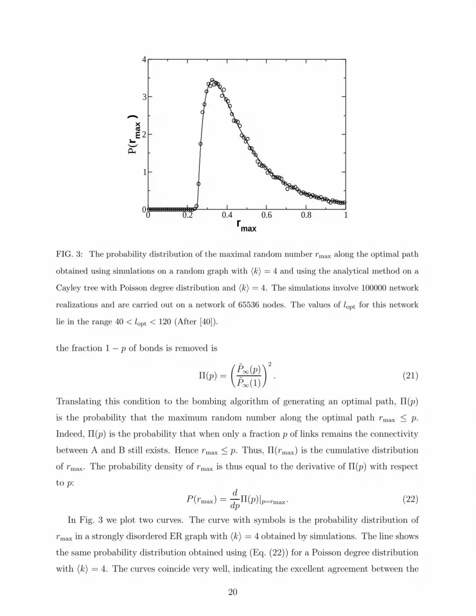
FIG. 3: The probability distribution of the maximal random number rmax along the optimal path

obtained using simulations on a random graph with 〈k〉 = 4 and using the analytical method on a

Cayley tree with Poisson degree distribution and 〈k〉 = 4. The simulations involve 100000 network

realizations and are carried out on a network of 65536 nodes. The values of lopt for this network

lie in the range 40 < lopt < 120 (After [40]).

the fraction 1 − p of bonds is removed is

Π(p) =

(

P∞(p)

P∞(1)

)2

. (21)

Translating this condition to the bombing algorithm of generating an optimal path, Π(p)

is the probability that the maximum random number along the optimal path rmax ≤ p.

Indeed, Π(p) is the probability that when only a fraction p of links remains the connectivity

between A and B still exists. Hence rmax ≤ p. Thus, Π(rmax) is the cumulative distribution

of rmax. The probability density of rmax is thus equal to the derivative of Π(p) with respect

to p:

P (rmax) =d

dpΠ(p)|p=rmax. (22)

In Fig. 3 we plot two curves. The curve with symbols is the probability distribution of

rmax in a strongly disordered ER graph with 〈k〉 = 4 obtained by simulations. The line shows

the same probability distribution obtained using (Eq. (22)) for a Poisson degree distribution

with 〈k〉 = 4. The curves coincide very well, indicating the excellent agreement between the

20

theoretical analysis and simulations.

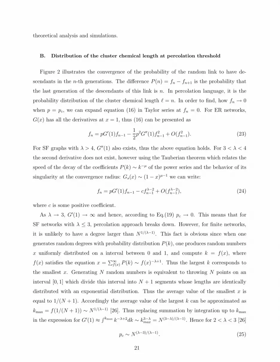
B. Distribution of the cluster chemical length at percolation threshold

Figure 2 illustrates the convergence of the probability of the random link to have de-

scendants in the n-th generations. The difference P (n) = fn − fn+1 is the probability that

the last generation of the descendants of this link is n. In percolation language, it is the

probability distribution of the cluster chemical length ℓ = n. In order to find, how fn → 0

when p = pc, we can expand equation (16) in Taylor series at fn = 0. For ER networks,

G(x) has all the derivatives at x = 1, thus (16) can be presented as

fn = pG′(1)fn−1 −1

2p2G′′(1)f 2

n−1 + O(f 2n−1). (23)

For SF graphs with λ > 4, G′′(1) also exists, thus the above equation holds. For 3 < λ < 4

the second derivative does not exist, however using the Tauberian theorem which relates the

speed of the decay of the coefficients P (k) ∼ k−µ of the power series and the behavior of its

singularity at the convergence radius: Gs(x) ∼ (1 − x)µ−1 we can write:

fn = pG′(1)fn−1 − cfλ−2n−1 + O(fλ−2

n−1 ), (24)

where c is some positive coefficient.

As λ → 3, G′(1) → ∞ and hence, according to Eq.(19) pc → 0. This means that for

SF networks with λ ≤ 3, percolation approach breaks down. However, for finite networks,

it is unlikely to have a degree larger than N1/(λ−1). This fact is obvious since when one

generates random degrees with probability distribution P (k), one produces random numbers

x uniformly distributed on a interval between 0 and 1, and compute k = f(x), where

f(x) satisfies the equation x =∑∞

f(x) P (k) ∼ f(x)−λ+1. Thus the largest k corresponds to

the smallest x. Generating N random numbers is equivalent to throwing N points on an

interval [0, 1] which divide this interval into N + 1 segments whose lengths are identically

distributed with an exponential distribution. Thus the average value of the smallest x is

equal to 1/(N + 1). Accordingly the average value of the largest k can be approximated as

kmax = f(1/(N + 1)) ∼ N1/(λ−1) [26]. Thus replacing summation by integration up to kmax

in the expression for G′(1) ≈ ∫ kmax k−λ+2dk ∼ k3−λmax = N (3−λ)/(λ−1). Hence for 2 < λ < 3 [26]

pc ∼ N (λ−3)/(λ−1). (25)

21

When p < pc, fn ∼ (p/pc)n, i.e. the convergence is exponential. When p = pc, we will

seek the solution of the above recursion relations in a power law form: fn ∼ n−θ. Expanding

them in powers of n−1, and equating the leading powers, we have θ + 1 = θ(λ − 2), from

which we obtain

fn ∼ n−1/(λ−3), (26)

or

P (ℓ) = fℓ − fℓ+1 ∼ ℓ−τℓ , (27)

where [8, 46]

τℓ =

2, λ > 4 ER

1(λ−3)

+ 1, 3 < λ ≤ 4. (28)

The probability that a randomly selected node has exactly ℓ generations of descendants is

equal to

P (ℓ) = fℓ − fℓ+1 = G(1 − pfℓ) − G(1 − pfℓ−1) ∼ 〈k〉p(fℓ − fℓ−1). (29)

Thus it is characterized by the same τℓ as P (ℓ).

Taylor expansions (23) and (24) can be used to derive the behavior of P∞(p) as p → pc by

letting fn = fn−1 = P∞(p) and solving the resulting equations with a leading term accuracy:

P∞(p) = (p − pc)β, (30)

where [26]

β =

1, λ > 4 ER

λ − 3, 3 < λ ≤ 4. (31)

C. Distribution of the cluster sizes at percolation threshold

Using the generating functions [8, 46, 53], one can also find the distribution of the clusters

sizes, P (s), connected to a randomly selected link. For simplicity, let us again consider a

link (conducting with probability p) leading to a node of a degree k = 3, so it has only two

outgoing links. The probability that this link is connected to a cluster consisting of s nodes

obeys the following relations

P (s) = p∑

k+l=s−1

P (k)P (l) (32)

22

for s > 0 and P (0) = 1− p. Introducing the generating function of the cluster size distribu-

tion H(x) =∑∞

0 P (s)xs, we have: H(x) = 1 − p + xpH2(x). In a general Cayley tree with

an arbitrary degree distribution we have:

H(x) = 1 − p + xpG(H(x)). (33)

This equation defines the behavior of H(x) for x → 1, and thus via the Tauberian theorem

defines the asymptotic behavior of its coefficients P (s). Note that H(1) is the cumulative

probability of all finite clusters. Thus (1−H(1)) = pP∞(p) is the probability that a randomly

selected link conducting with probability p is connected to the infinity and Eq.(33) becomes

equivalent to Eq. (18) for P∞(p).

Introducing δx = 1 − x and δH = 1 − H(x) and expanding G(x) around x = 1 at

percolation threshold p = 1/G′(1), we have δHδx + pδx = cxδλ−2H + O(δλ−2

H ) which yields

δH ∼ δ1/(λ−2)x . Using the Tauberian theorem we conclude [8, 46]:

P (s) ∼ s−τs, (34)

where

τs =

3/2, λ > 4 ER

1λ−2

+ 1, 3 < λ ≤ 4. (35)

Analogous considerations suggest that the probabilities P (s) that a randomly selected node

belongs to the cluster of size s produce the generating function H(x) = G(H(x)). Since for

λ > 3, G′′(1) < ∞, the singularity of H(x) for x → 1 is of the same order as the singularity

of H(x) and thus its coefficients, P (s), also decay as s−τs.

Following [72], we will show that the distribution of all the disconnected clusters in a

network scales as Pall(s) = P (s)/s ∼ s−τs+1. Indeed, let us select a random node in this

network. The number of nodes belonging to the clusters of size s is NsPall(s)/∑∞

1 sPall(s) =

NsPall(s)/〈s〉. Thus, P (s) = sPall(s)/〈s〉.If we have a network of N nodes, the size of the largest cluster S is determined by the

relation∑∞

s=S Pall(s) ∼ 1/N , which becomes clear if we describe a concrete realization of the

cluster sizes by throwing N/〈s〉 random points representing clusters under the curve Pall(s).

The average area corresponding to each of these points is 1/N and the area corresponding to

the rightmost point representing the largest cluster is∑∞

s=S Pall(s) ∼ S−τs. Thus the largest

cluster (which coincides with IIC) in the network of N nodes scales as

S ∼ N1/τs . (36)

23

For ER graphs, the relation S ∼ N2/3 has been derived in a classical work [4].

IV. SCALING OF THE LENGTH OF THE OPTIMAL PATH IN STRONG DIS-

ORDER

The relations obtained in the previous subsections allow us to determine the scaling

of the average optimal path length in a network of N nodes. When during bombing, we

reach percolation threshold, we have targeted only a tiny fraction of links (or nodes) on the

optimal path, with rmax > pc which we have to restore, because their removal would destroy

the connectivity. The majority of the links on the optimal path remains intact. All of them

belong to the remaining percolation clusters which at percolation threshold has a tree like

structure with no loops. At this point, the optimal path coincides with the shortest path,

which is uniquely determined. We will describe this situation in detail in SectionVI. With

high probability, the optimal path between any two nodes A and B goes through the largest

cluster at the percolation threshold. Thus its length must scale as the chemical length of

the largest percolation cluster [32]. Assuming a power law relation between the cluster size

s and its chemical dimension ℓ, s = ℓdℓ , and using the fact that both of the quantities have

power law distributions P (ℓ)dℓ = P (s)ds, we have ℓ−τℓ = ℓ−dℓτs+dℓ−1. Thus [9]

dℓ = (τl − 1)/(τs − 1). (37)

Therefore, S ∼ ℓdℓopt and using (36) we have ℓopt ∼ S1/dℓ ∼ Nνopt , where

νopt = 1/(dℓτs). (38)

Using Eqs. (35) and (28) for τs and τℓ respectively, we have

νopt =

1/3, λ > 4, ER

(λ − 3)/(λ − 1), 3 < λ ≤ 4. (39)

Note that λ = 4 corresponds to the special case when G′′(1) diverges, in this case the

Tauberian theorem predicts logarithmic corrections, and hence we expect ℓopt ∼ N1/3/ lnN

for λ = 4.

We review above the exact results for the Cayley tree, from which using heuristic argu-

ments we have derived the scaling relation between the average length of the optimal path

24

100

101

102

103

104

105

N

100

101

102

l op

t(a)

0 0.1 0.2 0.3 0.4 0.5

1/N1/3

0.3

0.4

0.5

0.6

νo

pt(

N)

(b)

1/3

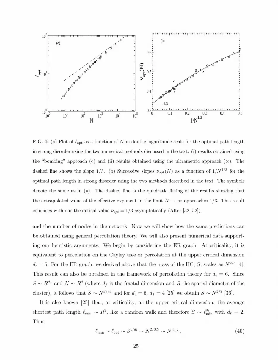
FIG. 4: (a) Plot of ℓopt as a function of N in double logarithmic scale for the optimal path length

in strong disorder using the two numerical methods discussed in the text: (i) results obtained using

the “bombing” approach (◦) and (ii) results obtained using the ultrametric approach (×). The

dashed line shows the slope 1/3. (b) Successive slopes νopt(N) as a function of 1/N1/3 for the

optimal path length in strong disorder using the two methods described in the text. The symbols

denote the same as in (a). The dashed line is the quadratic fitting of the results showing that

the extrapolated value of the effective exponent in the limit N → ∞ approaches 1/3. This result

coincides with our theoretical value νopt = 1/3 asymptotically (After [32, 52]).

and the number of nodes in the network. Now we will show how the same predictions can

be obtained using general percolation theory. We will also present numerical data support-

ing our heuristic arguments. We begin by considering the ER graph. At criticality, it is

equivalent to percolation on the Cayley tree or percolation at the upper critical dimension

dc = 6. For the ER graph, we derived above that the mass of the IIC, S, scales as N2/3 [4].

This result can also be obtained in the framework of percolation theory for dc = 6. Since

S ∼ Rdf and N ∼ Rd (where df is the fractal dimension and R the spatial diameter of the

cluster), it follows that S ∼ Ndf /d and for dc = 6, df = 4 [25] we obtain S ∼ N2/3 [36].

It is also known [25] that, at criticality, at the upper critical dimension, the average

shortest path length ℓmin ∼ R2, like a random walk and therefore S ∼ ℓdℓmin with dℓ = 2.

Thus

ℓmin ∼ ℓopt ∼ S1/dℓ ∼ N2/3dℓ ∼ Nνopt , (40)

25

where νopt = 2/3dℓ = 1/3.

For SF networks, we can also use the percolation results at criticality. It was found [8, 46]

(see Sec. III) that dℓ = 2 for λ > 4, dℓ = (λ− 2)/(λ− 3) for 3 < λ < 4, S ∼ N2/3 for λ > 4,

and S ∼ N (λ−2)/(λ−1) for 3 < λ ≤ 4. Hence, we conclude that

ℓmin ∼ ℓopt ∼{

N1/3 λ > 4

N (λ−3)/(λ−1) 3 < λ ≤ 4. (41)

Thus νopt = 1/3 for ER and SF with λ > 4, and νopt = (λ−3)/(λ−1) for SF with 3 < λ < 4.

Since for SF networks with λ > 4 the scaling behavior of ℓopt is the same as for ER graphs

and for λ < 4 the scaling is different, we can regard SF networks as a generalization of ER

graphs.

Next we describe the details of the numerical simulations and show that the results agree

with the above theoretical predictions. We perform numerical simulations in the strong

disorder limit by the method described in Section IID for ER and SF networks. We also

perform additional simulations for the case of strong disorder on ER networks using the

ultrametric optimization algorithm (see Section IIC) and find results identical to the results

obtained by randomly removing links. In Fig. 4(a) we show a double logarithmic plot of

ℓopt as a function of N for ER graphs. To evaluate the asymptotic value for νopt we use

for both approaches successive slopes, defined as the successive slopes [22] of the values on

Fig. 4. One can see from Fig. 4(b) that their value approaches 1/3 when N ≫ 1, supporting

Eq. (40).

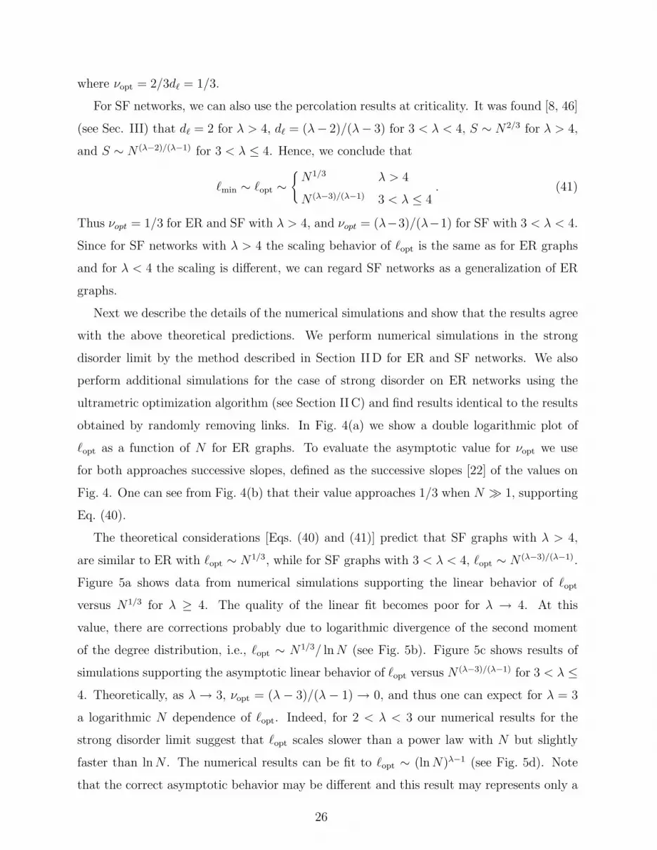
The theoretical considerations [Eqs. (40) and (41)] predict that SF graphs with λ > 4,

are similar to ER with ℓopt ∼ N1/3, while for SF graphs with 3 < λ < 4, ℓopt ∼ N (λ−3)/(λ−1).

Figure 5a shows data from numerical simulations supporting the linear behavior of ℓopt

versus N1/3 for λ ≥ 4. The quality of the linear fit becomes poor for λ → 4. At this

value, there are corrections probably due to logarithmic divergence of the second moment

of the degree distribution, i.e., ℓopt ∼ N1/3/ ln N (see Fig. 5b). Figure 5c shows results of

simulations supporting the asymptotic linear behavior of ℓopt versus N (λ−3)/(λ−1) for 3 < λ ≤4. Theoretically, as λ → 3, νopt = (λ − 3)/(λ − 1) → 0, and thus one can expect for λ = 3

a logarithmic N dependence of ℓopt. Indeed, for 2 < λ < 3 our numerical results for the

strong disorder limit suggest that ℓopt scales slower than a power law with N but slightly

faster than ln N . The numerical results can be fit to ℓopt ∼ (ln N)λ−1 (see Fig. 5d). Note

that the correct asymptotic behavior may be different and this result may represents only a

26

0 10 20 30

N1/3

0

20

40

60

80

100l op

tλ=5.004.754.504.254.00

(a)

0 10 20 30

N1/3

0

200

400

600

l optln

N

(b)

0 10 20 30

N(λ-3)/(λ-1)

0

10

20

30

40

50

60

lopt

λ=4.003.753.503.25

(c)

0 50 100

lnλ-1

N

0

10

20

30

lopt

λ=3.002.752.50

(d)

FIG. 5: Results of numerical simulations. (a) The dependence of ℓopt on N1/3 for λ ≥ 4. (b)

The dependence of ℓopt/ ln N on N1/3 for λ = 4. (c) The dependence of ℓopt on N (λ−3)/(λ−1) for

3 < λ < 4. (d) The dependence of ℓopt on ln N for λ ≤ 3 (After [32, 52]).

crossover regime. The exact nature of the percolation cluster at λ < 3 is not clear yet, since

in this regime the transition does not occur at a finite (non zero) critical threshold [26]. We

obtain similar results for SF networks where the weights are associated with nodes instead

of links.

V. SCALING OF THE LENGTH OF THE OPTIMAL PATH IN WEAK DISOR-

DER

When a = 1/kT → 0, all the τi essentially contribute to the total cost. Thus T → ∞(very high temperatures) corresponds to weak disorder limit. We expect that the optimal

27

path length in the weak disorder case will not be considerably different from the shortest

path, as found also for regular lattices [28] and random graphs [29]. Thus we expect that

the scaling for the shortest path will also be valid for the optimal path in weak disorder, but

with a different prefactor depending on the details of the graph and on the type of disorder.

We simulate weak disorder by selecting 0 ≤ τi < 1 from a uniform distribution. To compute

ℓopt we use the Dijkstra algorithm (See Section IIB)[13]. The scaling of the length of the

optimal path in WD for ER, is shown in Fig. 6(a). Here we plot ℓopt as a function of ln N

for 〈k〉 = 4. The weak disorder does not change the scaling behavior of ℓopt on ER compared

to ℓmin, only the prefactor.

2 4 6 8 10

Ln N0

2

4

6

8

10

l op

t

(a)

2 3 4 5 6 7 8 9

ln N0

5

10

15

20

l opt

(b)

FIG. 6: Results of numerical simulations. (a) The linear dependence of ℓopt on ln N for ER graphs

in the weak disorder case for < k >= 4. The dashed line is used as a guide to show the linear

dependence. (b) The dependence of ℓopt on ln N for SF graphs in the weak disorder case for various

values of λ. The different curves represent different values of λ from 2.5 (bottom) to 5 (top) (After

[47, 48]).

For SF networks, the behavior of the optimal path in the weak disorder limit is shown

in Fig. 6(b) for different degree distribution exponents λ. Here we plot ℓopt as a function

of ln N . All the curves seem to have linear asymptotes. This result is analogous to the

behavior of the shortest path ℓmin ∼ ln N for 3 < λ < 4 and ER. Note, however, that for

2 < λ < 3, ℓmin scale as ln ln N [7]. Thus, ℓopt is significantly larger and scales as ln N

(Fig. 3b). Thus, weak disorder does not change the universality class of the length of the

optimal path except in the case of “ultra-small” worlds 2 < λ < 3, where ℓopt ∼ exp(ℓmin),

and the networks become small worlds.

28

VI. CROSSOVER FROM WEAK TO STRONG DISORDER

A. Exponential Disorder

Consider the case of finite a (T > 0). In this case we expect a crossover in the length

of the optimal path (or the system size N) from strong disorder behavior to weak disorder

depending on the value of a. In order to study this crossover we have to use an implemen-

tation of disorder that can be tuned to realize narrow distributions of link weights (WD) as

well as broad distributions of link weights (SD). The procedure that we adopt to implement

the disorder is as follows [22, 24, 30, 32] (See Sec. IV A). Assign to each link i of the network

a random number ri, uniformly distributed between 0 and 1. For the analogy with the ther-

mally activated process described in Sec. IV the ri play the role of the energy barriers. The

transit time or cost associated with link i is then τi ≡ exp(ari), where a controls the strength

of disorder i.e., the broadness of the distribution of link weights. The limit a → ∞ is the

strong disorder limit, where a single link dominates the cost of the path. For d-dimensional

lattices of size L, the crossover is found [24, 30] to behave as

ℓopt ∼

Ldopt , L ≪ aν ;

L, L ≫ aν .(42)

where ν is the percolation correlation exponent [67, 68]. For d = 2, dopt ≈ 1.22 and for d = 3,

dopt ≈ 1.44 [24, 30]. Here we show [47] that for any network of size N and any finite a, there

exists a crossover network size N∗(a) such that for N ≪ N∗(a) the scaling properties of the

optimal path are in the strong disorder regime, while for N ≫ N∗(a) the typical optimal

paths are in the weak disorder regime. We evaluate below the function N∗(a).

In general, the average optimal path length ℓopt(a) in a weighted network depends on a

as well as on N . In the following we use instead of N the min-max path length ℓ∞ which is

related to N as ℓ∞ ≡ ℓopt(∞) ∼ Nνopt [Eqs.(40) and (41)] and hence N can be expressed in

terms of ℓ∞,

N ∼ ℓ1/νopt∞ . (43)

Thus, for finite a, ℓopt(a) depends on both a and ℓ∞. We expect a crossover length ℓ∗(a),

which corresponds to the crossover network size N∗(a), such that (i) for ℓ∞ ≪ ℓ∗(a), the

scaling properties of ℓopt(a) are of the strong disorder regime, and (ii) for ℓ∞ ≫ ℓ∗(a), the

29

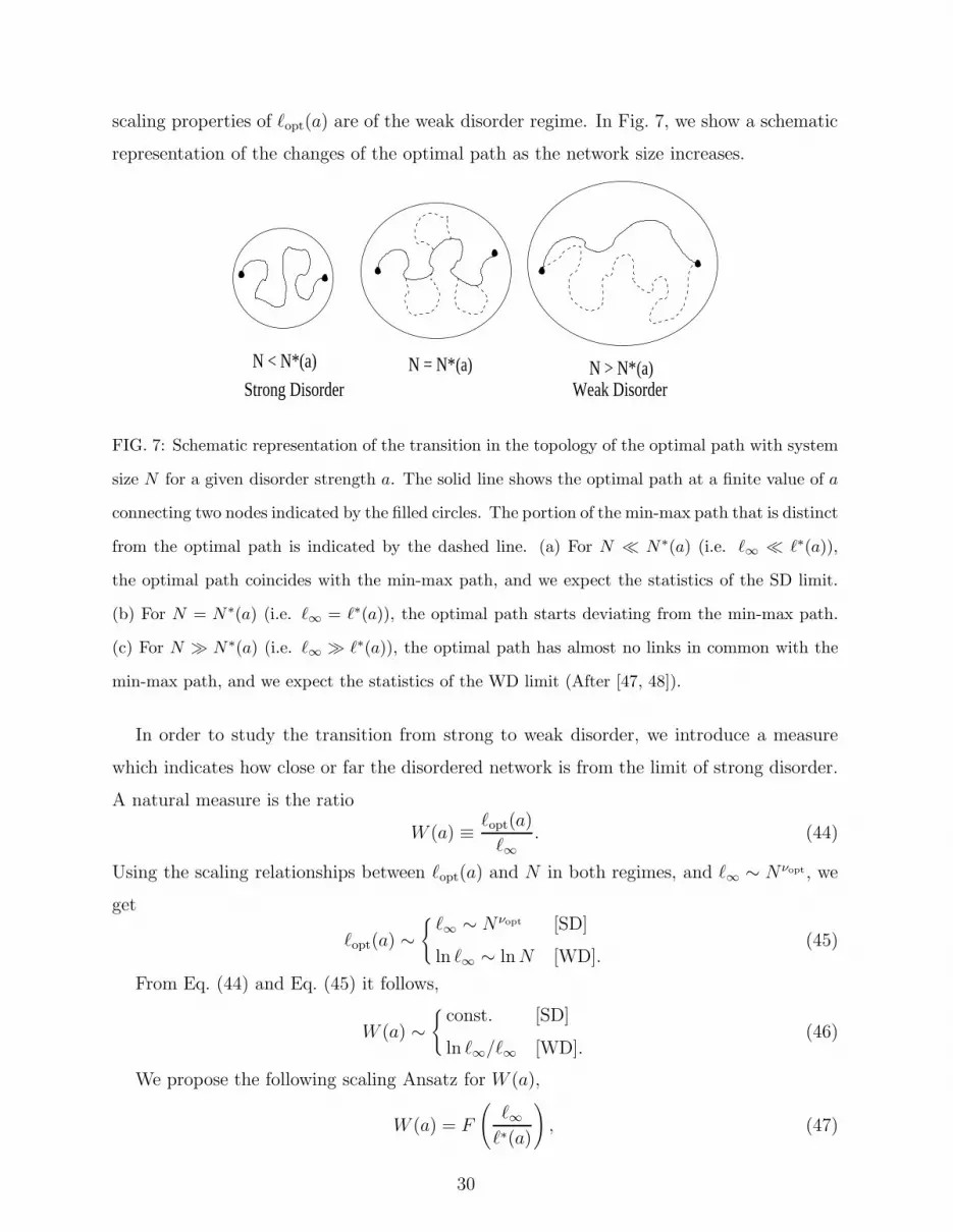
scaling properties of ℓopt(a) are of the weak disorder regime. In Fig. 7, we show a schematic

representation of the changes of the optimal path as the network size increases.

Strong DisorderN = N* N > N*

Weak Disorder

N < N*(a) (a) (a)

FIG. 7: Schematic representation of the transition in the topology of the optimal path with system

size N for a given disorder strength a. The solid line shows the optimal path at a finite value of a

connecting two nodes indicated by the filled circles. The portion of the min-max path that is distinct

from the optimal path is indicated by the dashed line. (a) For N ≪ N∗(a) (i.e. ℓ∞ ≪ ℓ∗(a)),

the optimal path coincides with the min-max path, and we expect the statistics of the SD limit.

(b) For N = N∗(a) (i.e. ℓ∞ = ℓ∗(a)), the optimal path starts deviating from the min-max path.

(c) For N ≫ N∗(a) (i.e. ℓ∞ ≫ ℓ∗(a)), the optimal path has almost no links in common with the

min-max path, and we expect the statistics of the WD limit (After [47, 48]).

In order to study the transition from strong to weak disorder, we introduce a measure

which indicates how close or far the disordered network is from the limit of strong disorder.

A natural measure is the ratio

W (a) ≡ ℓopt(a)

ℓ∞. (44)

Using the scaling relationships between ℓopt(a) and N in both regimes, and ℓ∞ ∼ Nνopt, we

get

ℓopt(a) ∼{

ℓ∞ ∼ Nνopt [SD]

ln ℓ∞ ∼ ln N [WD].(45)

From Eq. (44) and Eq. (45) it follows,

W (a) ∼{

const. [SD]

ln ℓ∞/ℓ∞ [WD].(46)

We propose the following scaling Ansatz for W (a),

W (a) = F

(

ℓ∞ℓ∗(a)

)

, (47)

30

where

F (u) ∼{

const. u ≪ 1

ln(u)/u u ≫ 1, (48)

with

u ≡ ℓ∞ℓ∗(a)

. (49)

We now develop analytic arguments [47] to obtain the dependence of the crossover length

ℓ∗ on the disorder strength a. These arguments will also give a clearer picture about the

nature of the transition of the optimal path with disorder strength.

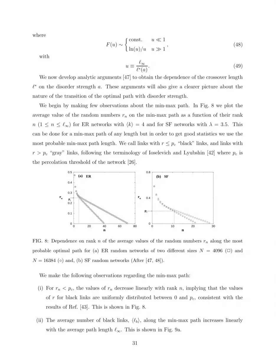
We begin by making few observations about the min-max path. In Fig. 8 we plot the

average value of the random numbers rn on the min-max path as a function of their rank

n (1 ≤ n ≤ ℓ∞) for ER networks with 〈k〉 = 4 and for SF networks with λ = 3.5. This

can be done for a min-max path of any length but in order to get good statistics we use the

most probable min-max path length. We call links with r ≤ pc “black” links, and links with

r > pc “gray” links, following the terminology of Ioselevich and Lyubshin [42] where pc is

the percolation threshold of the network [26].

0 20 40 60 80n

0

0.1

0.2

0.3

0.4

0.5

rn

(a)

pc

ER

0 10 20 30n

0

0.4

0.8

rn

(b)

pc

SF

FIG. 8: Dependence on rank n of the average values of the random numbers rn along the most

probable optimal path for (a) ER random networks of two different sizes N = 4096 (2) and

N = 16384 (◦) and, (b) SF random networks (After [47, 48]).

We make the following observations regarding the min-max path:

(i) For rn < pc, the values of rn decrease linearly with rank n, implying that the values

of r for black links are uniformly distributed between 0 and pc, consistent with the

results of Ref. [43]. This is shown in Fig. 8.

(ii) The average number of black links, 〈ℓb〉, along the min-max path increases linearly

with the average path length ℓ∞. This is shown in Fig. 9a.

31

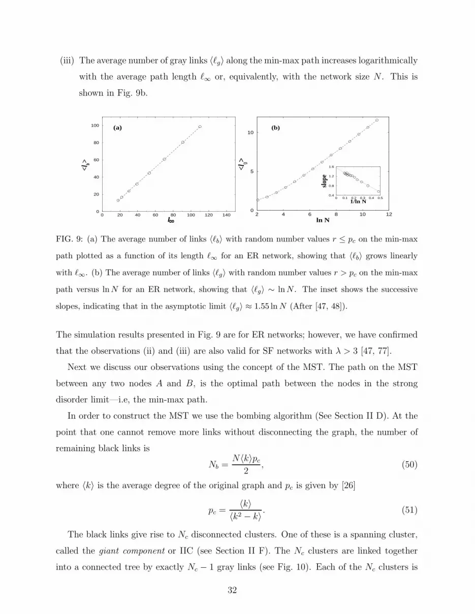
(iii) The average number of gray links 〈ℓg〉 along the min-max path increases logarithmically

with the average path length ℓ∞ or, equivalently, with the network size N . This is

shown in Fig. 9b.

0 20 40 60 80 100 120 140l

0

20

40

60

80

100

<lb>

8

(a)

2 4 6 8 10 12ln N

0

5

10

<lg>

0 0.1 0.2 0.3 0.4 0.51/ln N

0.4

0.8

1.2

1.6

slope

(b)

FIG. 9: (a) The average number of links 〈ℓb〉 with random number values r ≤ pc on the min-max

path plotted as a function of its length ℓ∞ for an ER network, showing that 〈ℓb〉 grows linearly

with ℓ∞. (b) The average number of links 〈ℓg〉 with random number values r > pc on the min-max

path versus ln N for an ER network, showing that 〈ℓg〉 ∼ ln N . The inset shows the successive

slopes, indicating that in the asymptotic limit 〈ℓg〉 ≈ 1.55 ln N (After [47, 48]).

The simulation results presented in Fig. 9 are for ER networks; however, we have confirmed

that the observations (ii) and (iii) are also valid for SF networks with λ > 3 [47, 77].

Next we discuss our observations using the concept of the MST. The path on the MST

between any two nodes A and B, is the optimal path between the nodes in the strong

disorder limit—i.e, the min-max path.

In order to construct the MST we use the bombing algorithm (See Section II D). At the

point that one cannot remove more links without disconnecting the graph, the number of

remaining black links is

Nb =N〈k〉pc

2, (50)

where 〈k〉 is the average degree of the original graph and pc is given by [26]

pc =〈k〉

〈k2 − k〉 . (51)

The black links give rise to Nc disconnected clusters. One of these is a spanning cluster,

called the giant component or IIC (see Section II F). The Nc clusters are linked together

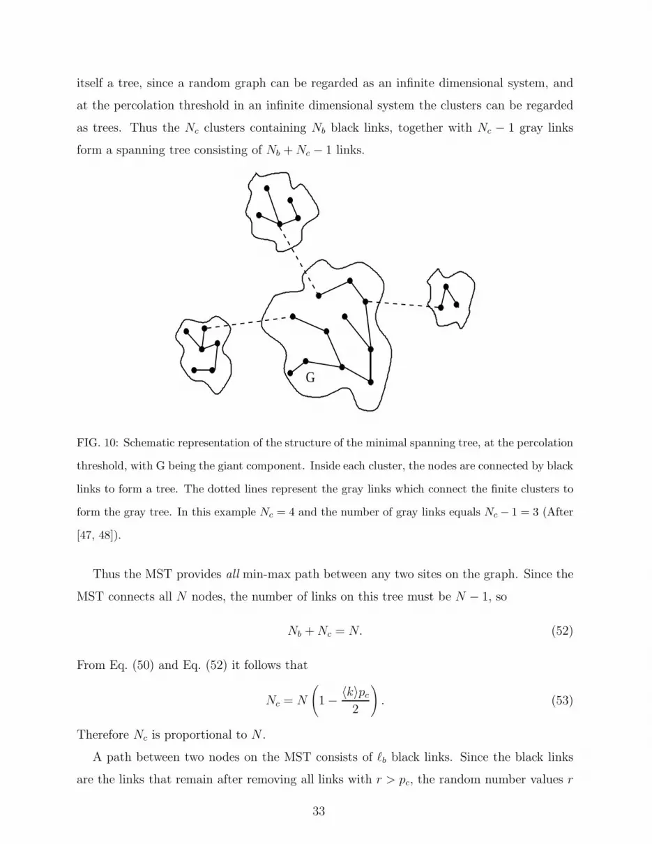
into a connected tree by exactly Nc − 1 gray links (see Fig. 10). Each of the Nc clusters is

32

itself a tree, since a random graph can be regarded as an infinite dimensional system, and

at the percolation threshold in an infinite dimensional system the clusters can be regarded

as trees. Thus the Nc clusters containing Nb black links, together with Nc − 1 gray links

form a spanning tree consisting of Nb + Nc − 1 links.

G

FIG. 10: Schematic representation of the structure of the minimal spanning tree, at the percolation

threshold, with G being the giant component. Inside each cluster, the nodes are connected by black

links to form a tree. The dotted lines represent the gray links which connect the finite clusters to

form the gray tree. In this example Nc = 4 and the number of gray links equals Nc − 1 = 3 (After

[47, 48]).

Thus the MST provides all min-max path between any two sites on the graph. Since the

MST connects all N nodes, the number of links on this tree must be N − 1, so

Nb + Nc = N. (52)

From Eq. (50) and Eq. (52) it follows that

Nc = N

(

1 − 〈k〉pc

2

)

. (53)

Therefore Nc is proportional to N .

A path between two nodes on the MST consists of ℓb black links. Since the black links

are the links that remain after removing all links with r > pc, the random number values r

33

on the black links are uniformly distributed between 0 and pc in agreement with observation

(i) and Ref. [43].

Since there are Nc clusters which include clusters of nodes connected by black links as

well as isolated nodes, the MST can be described as an effective tree of Nc “super” nodes,

each representing a cluster, and Nc − 1 gray links. We call this tree the “gray tree” (see

Fig. 10). This tree is in fact a scale free tree [45, 77] with degree exponent λg = 2.5 for ER

networks and for scale for networks with λ ≥ 4, and λg = (2λ − 3)/(λ − 2) for SF networks

with 3 < λ < 4. If we take two nodes A and B on the original network, they will most likely

lie on two distinct effective nodes of the gray tree. The number of gray links encountered

on the min-max path connecting these two nodes will therefore equal the number of links

separating the effective nodes on the gray tree. Hence the average number of gray links

〈ℓg〉 encountered on the min-max path between an arbitrary pair of nodes on the network is

simply the average diameter of the gray tree. Our simulation results (see Fig. 9b) indicate

that

〈ℓg〉 ∼ ln N. (54)

Since 〈ℓg〉 ∼ ln ℓ∞ ≪ ℓ∞, the average number of black links 〈ℓb〉 on the min-max path

scales as ℓ∞ in the limit of large ℓ∞ in agreement with observation (2) as shown in Fig. 9a.

Next we discuss the implications of our findings for the crossover from strong to weak

disorder. From observations (i) and (ii), it follows that for the portion of the path belonging

to the giant component, the distribution of random values r is uniform. Hence we can

approximate the sum of weights by [44],

ℓb∑

k=1

exp(ark) ≈ℓb

pc

∫ pc

0exp ar dr =

ℓb

apc

(exp(apc) − 1) ≡ exp(ar∗), (55)

where r∗ ≈ pc + (1/a) ln(〈ℓb〉/apc). Since 〈ℓb〉 ≈ ℓ∞,

r∗ ≈ pc +1

aln

(

ℓ∞apc

)

. (56)

Thus restoring a short-cut link between two nodes on the optimal path with pc < r < r∗

may drastically reduce the length of the optimal path. When apc ≫ ℓ∞, r∗ < pc and such

a link does not exists, if ℓ∞ > apc, the probability that such a link exist becomes positive.

Hence when the min-max path is of length ℓ∞ ≈ apc, the optimal path starts deviating from

the min-max path. The length of the min-max path at which the deviation first occurs is

34

precisely the crossover length ℓ∗(a), and therefore ℓ∗(a) ∼ apc. In the case of a network with

an arbitrary degree distribution we can write using Eq. (51), ℓ∗(a) ∼ a 〈k〉〈k2−k〉 .

Note that in the case of SF networks, as λ → 3+, pc approaches zero and consequently

ℓ∗(a) → 0. This suggests that for any finite value of disorder strength a, a SF network with

λ ≤ 3 is in the weak disorder regime. We perform numerical simulations and show that the

results agree with our theoretical predictions. For the details of our simulation methods see

Section II.

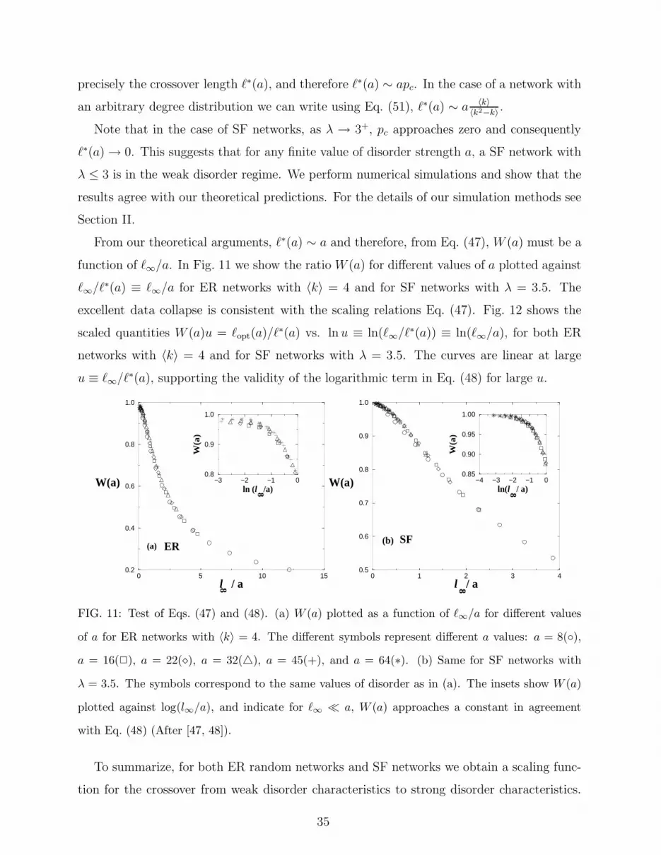
From our theoretical arguments, ℓ∗(a) ∼ a and therefore, from Eq. (47), W (a) must be a

function of ℓ∞/a. In Fig. 11 we show the ratio W (a) for different values of a plotted against

ℓ∞/ℓ∗(a) ≡ ℓ∞/a for ER networks with 〈k〉 = 4 and for SF networks with λ = 3.5. The

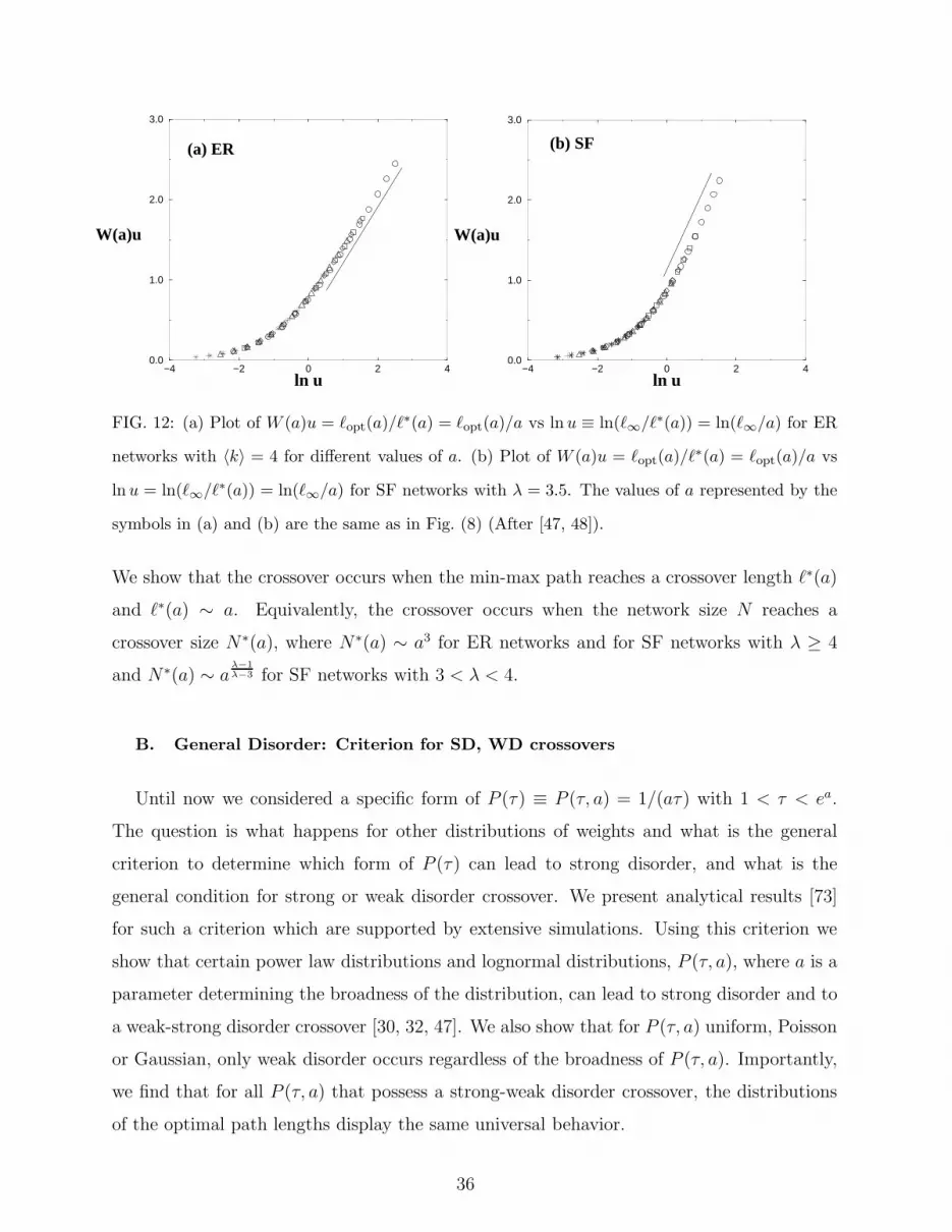
excellent data collapse is consistent with the scaling relations Eq. (47). Fig. 12 shows the

scaled quantities W (a)u = ℓopt(a)/ℓ∗(a) vs. ln u ≡ ln(ℓ∞/ℓ∗(a)) ≡ ln(ℓ∞/a), for both ER

networks with 〈k〉 = 4 and for SF networks with λ = 3.5. The curves are linear at large

u ≡ ℓ∞/ℓ∗(a), supporting the validity of the logarithmic term in Eq. (48) for large u.

0 5 10 15l / a

0.2

0.4

0.6

0.8

1.0

W(a) −3 −2 −1 0ln (l /a)

0.8

0.9

1.0

W(a

)

8

8

(a) ER

0 1 2 3 4l / a

0.5

0.6

0.7

0.8

0.9

1.0

W(a) −4 −3 −2 −1 0ln(l / a)

0.85

0.90

0.95

1.00

W(a

)

8

8

(b) SF

FIG. 11: Test of Eqs. (47) and (48). (a) W (a) plotted as a function of ℓ∞/a for different values

of a for ER networks with 〈k〉 = 4. The different symbols represent different a values: a = 8(◦),

a = 16(2), a = 22(⋄), a = 32(△), a = 45(+), and a = 64(∗). (b) Same for SF networks with

λ = 3.5. The symbols correspond to the same values of disorder as in (a). The insets show W (a)

plotted against log(l∞/a), and indicate for ℓ∞ ≪ a, W (a) approaches a constant in agreement

with Eq. (48) (After [47, 48]).

To summarize, for both ER random networks and SF networks we obtain a scaling func-

tion for the crossover from weak disorder characteristics to strong disorder characteristics.

35

−4 −2 0 2 4ln u

0.0

1.0

2.0

3.0

W(a)u

(a) ER

−4 −2 0 2 4ln u

0.0

1.0

2.0

3.0

W(a)u

(b) SF

FIG. 12: (a) Plot of W (a)u = ℓopt(a)/ℓ∗(a) = ℓopt(a)/a vs ln u ≡ ln(ℓ∞/ℓ∗(a)) = ln(ℓ∞/a) for ER

networks with 〈k〉 = 4 for different values of a. (b) Plot of W (a)u = ℓopt(a)/ℓ∗(a) = ℓopt(a)/a vs

ln u = ln(ℓ∞/ℓ∗(a)) = ln(ℓ∞/a) for SF networks with λ = 3.5. The values of a represented by the

symbols in (a) and (b) are the same as in Fig. (8) (After [47, 48]).

We show that the crossover occurs when the min-max path reaches a crossover length ℓ∗(a)

and ℓ∗(a) ∼ a. Equivalently, the crossover occurs when the network size N reaches a

crossover size N∗(a), where N∗(a) ∼ a3 for ER networks and for SF networks with λ ≥ 4

and N∗(a) ∼ aλ−1λ−3 for SF networks with 3 < λ < 4.

B. General Disorder: Criterion for SD, WD crossovers

Until now we considered a specific form of P (τ) ≡ P (τ, a) = 1/(aτ) with 1 < τ < ea.

The question is what happens for other distributions of weights and what is the general

criterion to determine which form of P (τ) can lead to strong disorder, and what is the

general condition for strong or weak disorder crossover. We present analytical results [73]

for such a criterion which are supported by extensive simulations. Using this criterion we

show that certain power law distributions and lognormal distributions, P (τ, a), where a is a

parameter determining the broadness of the distribution, can lead to strong disorder and to

a weak-strong disorder crossover [30, 32, 47]. We also show that for P (τ, a) uniform, Poisson

or Gaussian, only weak disorder occurs regardless of the broadness of P (τ, a). Importantly,

we find that for all P (τ, a) that possess a strong-weak disorder crossover, the distributions

of the optimal path lengths display the same universal behavior.

36

If we express τ in terms of a random variable r uniformly distributed in [0, 1), we can use

the same gray and black link formalism as in the previous section. This can be achieved by

defining r(τ) by a relation:

r(τ) =∫ τ

0P (τ ′, a)dτ ′. (57)

Solving this equation with respect to τ gives us τ(r, a) = f(r, a), where f(r, a) satisfies the

relation

r =∫ f(r,a)

0P (τ ′, a)dτ ′. (58)

For a strong disorder regime, the sum of the weights of the black links on the IIC must be

smaller than the smallest weight of the removed link τc = f(pc, a):

ℓb∑

i=1

τi =ℓb∑

i=1

f(ri, a) < τc, (59)

where ri are independent random variables uniformly distributed on [0, pc]. As we shown

above, ℓb ≈ ℓ∞ so in the following we will replace ℓb by the average path length in the

strong disorder limit, ℓ∞. The transition to weak disorder begins when the probability that

this sum is greater than τc becomes substantial. The investigation of this condition belongs

to the realm of pure mathematics and can be answered explicitly for any functional form

f(r, a). This condition is satisfied when the mathematical expectation of the sum is greater

than τc.ℓ∞pc

∫ pc

0f(r, a)dr > τc. (60)

Thus the crossover to weak disorder happens if

ℓ∞ > A ≡ f(pc, a)pc∫ pc0 f(r, a)dr

=τcpc

∫ τc0 τP (τ, a)dτ

, (61)

where A plays the role of the disorder strength and τc satisfies the equation pc =∫ τc0 P (τ, a)dτ . In order for the strong disorder to exist for any network size N , the disorder

strength must diverge together with the parameter a of the weight distribution a → ∞. In

order to determine if a network exhibits a strong disorder behavior it is useful to introduce

a scaling variable

Z ≡ ℓ∞/A, (62)

so that if Z ≫ 1 the network is in the weak disorder regime and if Z ≪ 1, the network is in

the strong disorder regime.

37

Note that if f ′/f > A0 on the entire interval [0, 1], then A > A0pc. Thus another sufficient

condition for a strong disorder to exist is

f ′/f > ℓ∞/pc. (63)

For the exponential disorder function τ = exp(ar), we have f ′/f = a and thus Eq.(63)

coincides with the condition of strong disorder apc > ℓ∞ derived in the previous Section.

In the following, we will show how the above condition is related to the strong to weak

crossover condition for the optimal path on lattices [23, 24, 30]. For the optimal path in the

strong disorder limit connecting the opposite sides of the lattice of linear size L, the largest

random number r1 follows a distribution characterized by a width which scales as L−1/ν ,

where ν is the percolation connectivity length exponent [25, 50, 72, 78]. The transition to

weak disorder starts when the optimal path may prefer to go through a slightly larger value

r2, taken from the same distribution and thus r2 − r1 ∼ pcL−1/ν . The condition for this to

happen is [f(r2) − f(r1)]/f(r1) < 1, which is equivalent to

f ′/f < L1/ν/pc. (64)

Now we will show that this condition is equivalent to (63). Percolation on Erdos-Renyi

(ER) networks is equivalent to percolation on a lattice at the upper critical dimension

dc = 6 [25, 46]. For d = 6, L ∼ N1/6, and ν = 1/2. Thus indeed L1/ν ∼ N1/(dcν) ∼ ℓ∞ [32].

Following similar arguments for a scale-free network with degree distribution P (k) ∼ k−λ

and 3 < λ < 4, we can replace L−1/ν by N−(λ−3)/(λ−1) since dc = 2(λ−1)/(λ−3) [46]. Thus,

due to Eq. (38) L1/ν ∼ ℓ∞ and we can introduce the analogous scaling parameter Z for

lattices:

Z =L1/ν

pcf ′/f. (65)

Next we calculate A for several specific weight distributions P (τ) [73]. We begin with the

well-studied exponential disorder function f(x) = ear, where r is a random number between

0 and 1 [24, 67]. From Eq. (58) follows that P (τ, a) = 1/(aτ), where τ ∈ [1, ea]. Using

Eq. (61) we have

A = apcτc/(τc − 1) ∼ apc; (66)

For fixed A, but different a and pc, we expect to obtain the same optimal path behavior.

Indeed, this has been shown to be valid [44, 67, 68, 73].

38

Next we study A for the disorder function f(r, a) = ra, with r between 0 and 1 where

a > 0 [69]. For this case the disorder distribution is a power law P (τ, a) = a−1τ 1/a−1.

Following Eq. (61) we obtain

A = a + 1 ∼ a. (67)

Note that here a plays a similar role as a in Eq. (66), but now A is independent of pc, which

means that networks with different pc, such as ER networks with different average degree

< k >= 1/pc, yield the same optimal path behavior.

For the power law distribution with negative exponent f(r) = (1− r)−a (a > 0), we have

P (τ, a) = a−1τ−1−1/a and

A =(a − 1)pc(1 − pc)

−a

(1 − pc)1−a − 1∼ apc

1 − pc. (68)

We further generalize the power law distribution with the disorder function f(r, a) = ra

by introducing the parameter 0 ≤ ∆ ≤ 1 which is defined as the lower bound of the uniformly

distributed random number r, i.e., 1−∆ ≤ r ≤ 1 [69]. Under this condition, the distribution

becomes

P (τ, a) =τ 1/a−1

|a|∆ τ ∈ [(1 − ∆)a, 1]. (69)

Again using Eq. (61), we obtain

A =apc∆

pc∆ + 1 − ∆. (70)

Table I shows the results of similar analysis for the lognormal, Gaussian, uniform and

exponential distributions P (τ, a). From Table I, we see that for exponential function, power

law and lognormal distributions, A is proportional to a and thus can become large. However

for uniform, Gaussian and exponential distributions, A is limited to a value of order 1, so

Z ≫ 1 for large N and the optimal path is always in the weak disorder regime. Note that

for these distributions, A is independent of a.

In general, one can prove that A → ∞ for a given distribution P (τ, a) as a → ∞ if there

exist a normalization function c(a) and a cutoff function τ(a) such that for ∀ǫ > 0, ∀E > 0,

∃M > 0 such that for a > M and τ ∈ [τ(a), τ(a)E], |τP (τ, a)c(a)− 1| < ǫ. We will call such

functions P (τ, a) “quasi-1/τ” distributions because they behave as 1/τ in a wide range of τ .

Obviously that exponential, power-law and lognormal distributions are quasi-1/τ functions,

so for them, for large enough a we can observe a strong disorder.

39

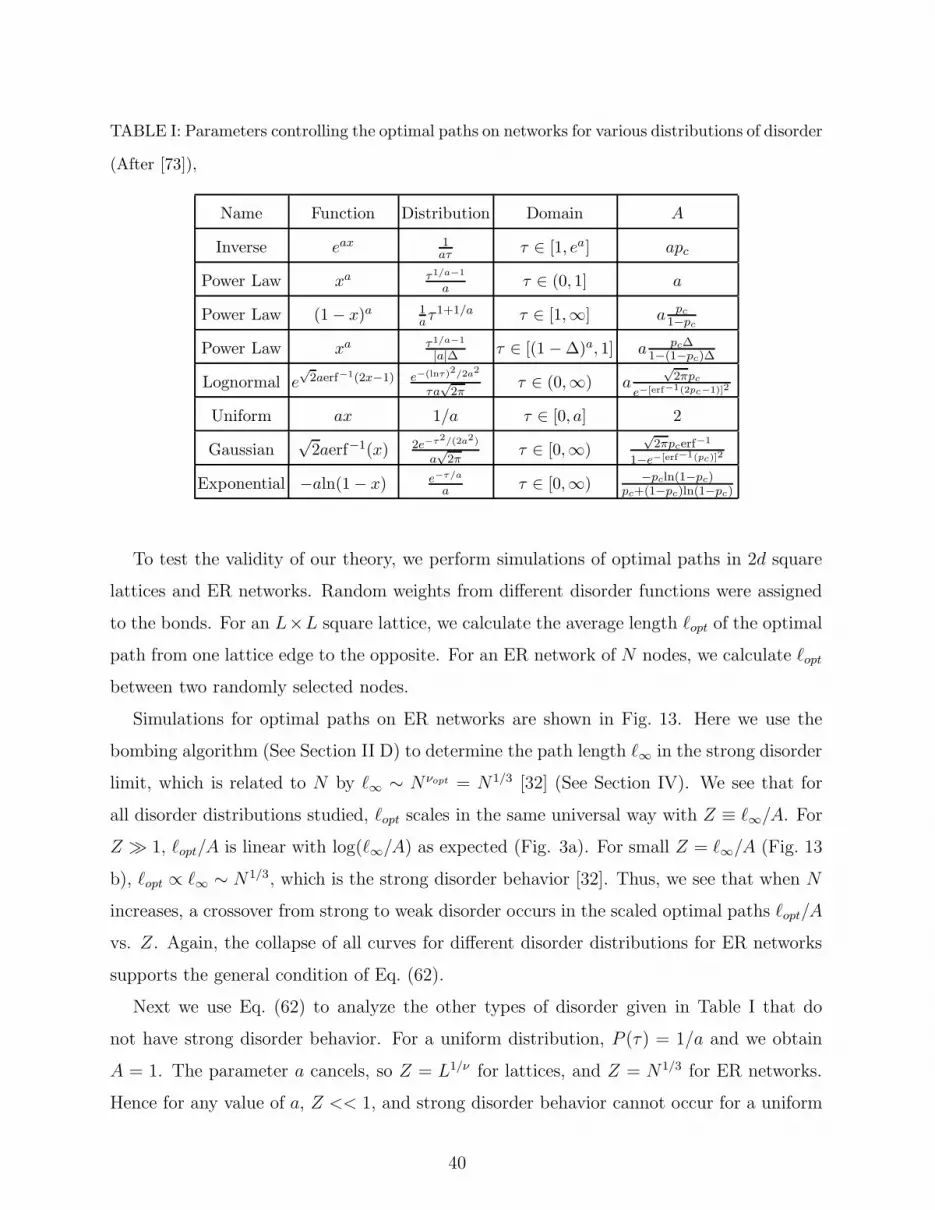
TABLE I: Parameters controlling the optimal paths on networks for various distributions of disorder

(After [73]),

Name Function Distribution Domain A

Inverse eax 1aτ τ ∈ [1, ea] apc

Power Law xa τ1/a−1

a τ ∈ (0, 1] a

Power Law (1 − x)a 1aτ1+1/a τ ∈ [1,∞] a pc

1−pc

Power Law xa τ1/a−1

|a|∆ τ ∈ [(1 − ∆)a, 1] a pc∆1−(1−pc)∆

Lognormal e√

2aerf−1(2x−1) e−(lnτ)2/2a2

τa√

2πτ ∈ (0,∞) a

√2πpc

e−[erf−1(2pc−1)]2

Uniform ax 1/a τ ∈ [0, a] 2

Gaussian√

2aerf−1(x) 2e−τ2/(2a2)

a√

2πτ ∈ [0,∞)

√2πpcerf−1

1−e−[erf−1(pc)]2

Exponential −aln(1 − x) e−τ/a

a τ ∈ [0,∞) −pcln(1−pc)pc+(1−pc)ln(1−pc)

To test the validity of our theory, we perform simulations of optimal paths in 2d square

lattices and ER networks. Random weights from different disorder functions were assigned

to the bonds. For an L×L square lattice, we calculate the average length ℓopt of the optimal

path from one lattice edge to the opposite. For an ER network of N nodes, we calculate ℓopt

between two randomly selected nodes.

Simulations for optimal paths on ER networks are shown in Fig. 13. Here we use the

bombing algorithm (See Section II D) to determine the path length ℓ∞ in the strong disorder

limit, which is related to N by ℓ∞ ∼ Nνopt = N1/3 [32] (See Section IV). We see that for

all disorder distributions studied, ℓopt scales in the same universal way with Z ≡ ℓ∞/A. For

Z ≫ 1, ℓopt/A is linear with log(ℓ∞/A) as expected (Fig. 3a). For small Z = ℓ∞/A (Fig. 13

b), ℓopt ∝ ℓ∞ ∼ N1/3, which is the strong disorder behavior [32]. Thus, we see that when N

increases, a crossover from strong to weak disorder occurs in the scaled optimal paths ℓopt/A

vs. Z. Again, the collapse of all curves for different disorder distributions for ER networks

supports the general condition of Eq. (62).

Next we use Eq. (62) to analyze the other types of disorder given in Table I that do

not have strong disorder behavior. For a uniform distribution, P (τ) = 1/a and we obtain

A = 1. The parameter a cancels, so Z = L1/ν for lattices, and Z = N1/3 for ER networks.

Hence for any value of a, Z << 1, and strong disorder behavior cannot occur for a uniform

40

1 10Z

0

1

2

3

4

5

6

l opt /

A

PL a=10 ∆=1PL a=20 ∆=1PL a=30 ∆=1PL a=30 ∆=0.6PL a=30 ∆=0.8LN σ=5LN σ=10LN σ=20

(a)

Weak

1 10Z

1

10

l opt /

A

(b)

1

Strong

FIG. 13: The function ℓopt/A for ER networks after scaling, where (a) is a linear-log plot and (b)

is a log-log plot. Distributions used are power law xa with 10 ≤ a ≤ 30 where 0 ≤ x < 1, xa

with a = 30 and the range of ∆ < x ≤ 1 with ∆ = 0.6 or 0.8, and lognormal distribution with

10 ≤ a ≤ 30. The straight line in (a) indicates weak disorder and the straight line in (b) indicates

strong disorder (After [73]).

distribution.

10 20 30 40l 8

6

8

10

l opt

Gaussian σ=10Gaussian σ=20Gaussian σ=30Gaussian σ=40

FIG. 14: The optimal path for Gaussian distribution of weights for ER networks. Note that these

curves would collapse after scaling to the curves in Fig. 13 in the weak disorder tail of large Z−1

(After [73]).

Next we analyze the Gaussian distribution. We assume that all the weights τj are positive

and thus we consider only the positive regime of the distribution. Using Eq. (61) we obtain

A =

√2πpcerf

−1

1 − e−[erf−1(pc)]2. (71)

41

The disorder is controlled solely by pc which is related only to the type of network, and A

cannot take on large values. Thus, also for the Gaussian P (τ, a), all optimal paths are in the

weak disorder regime. Similar considerations lead to the same conclusion for the exponential

distribution where A = −pcln(1−pc)pc+(1−pc)ln(1−pc)

. Simulation results for the Gaussian distribution

shown in Fig. 14 display only weak disorder (i.e. no weak-strong disorder crossover), thus

supporting the above conclusions.

To summarize, in this section we presented a criterion for the inverse disorder strength

Z on the optimal path in weighted networks for general distributions P (τ, a). We show an

analytical expression, Eq. (61), which fully characterizes the behavior of the optimal path.

Simulation of several distributions support these analytical predictions. It is plausible that

the criterion of Eq. (61) is valid also for other physical properties in weighted networks —

such as conductivity and flow in random resistor networks — due to a recently-found close

relation between the optimal path and flow [67, 68].

VII. SCALING OF OPTIMAL-PATH-LENGTHS DISTRIBUTION WITH FINITE

DISORDER IN COMPLEX NETWORKS

In this chapter we present further support [44] for the general analytical results pre-

sented in section VIB. The question is how the different optimal paths in a network are

distributed? The distribution of the optimal path lengths is especially important in commu-

nication networks, in which the overall network performance depends on the different path

lengths between all nodes of the network, and not only the average. Ref. [47] studied the

probability distribution P (ℓopt) of optimal path lengths in an ER network in the SD limit.

The scaled curve for P (ℓopt) for different network sizes is shown in Fig. 15 in a log-log plot.

We find that similarly to the behavior of self avoiding walks [74] there are two regimes in

this distribution, the first one being a power law P (ℓopt) ∼ (ℓopt)g which is evident from the

figure, with g ≈ 2. The second regime is an exponential P (ℓopt) ∼ e−Cℓδ

opt where C is a

constant and δ is around 2. This leads us to the conjecture that the distribution may have

a Maxwellian functional form:

P (ℓopt) =4ℓ2

opte−(ℓopt/lo)2

√πl3o

, (72)

42

Where ℓo =√

π〈ℓopt〉/2 is the most probable value of ℓopt. The solid line in the figure is the

plot of this function and as seen it agrees with our numerical results.

The exponents g and δ can be obtained from the following heuristic arguments. The

right tail of the distribution P (ℓopt) is determined by the distribution of the IIC size in

the network of N nodes. At percolation threshold (Sec. VI), N nodes are divided into N/2

clusters, obeying the power law distribution. However, the sum of all the cluster sizes is equal

to N , thus the distribution of the largest cluster sizes must have a finite size exponential

cutoff P (S) ∼ exp(−CS), as for the distribution of the segments of an interval divided by

random partitions. Since S ∼ ℓdℓopt, we have δ = dℓ.

To find the left tail distribution, we use the concept of MST. The chemical diameter of

the MST is ℓopt while its mass is N ∼ ℓ1/νoptopt . Due to self-similarity of the MST the number

of nodes n(ℓ) within a chemical distance ℓ also scales as n(ℓ) ∼ ℓ1/νopt . Thus the probability

density of the of the optimal path for small values of ℓ scales as dn(ℓ)/dℓ = ℓ1/νopt−1. Hence

g = 1/νopt−1. We expect that our conjecture is valid also for SF networks. Using Eqs. (37)

and (38) we have:

δ = dℓ =

2, λ > 4, ER

(λ − 2)/(λ − 3), 3 < λ ≤ 4, (73)

and

g =

2, λ > 4, ER

2/(λ − 3), 3 < λ ≤ 4. (74)

A recent work has studied the distribution form of shortest path lengths on minimum

spanning trees [40], which corresponds to optimal paths on networks with large variation in

link weights (a → ∞).

Using the scaling derived in Sect. VI, more precisely:

ℓ(a) ∼ ℓ∞F

(

ℓ∞apc

)

, (75)

where pc is the percolation threshold and ℓ∞ ∼ Nνopt is the optimal path length for strong

disorder (a → ∞). For Erdos-Renyi (ER) graphs νopt = 1/3. We generalize these results

and suggest that the distribution of the optimal path lengths has the following scaling form:

P (ℓopt, N, a) ∼ 1

ℓ∞G

(

ℓopt

ℓ∞,

1

pc

ℓ∞a

)

. (76)

43

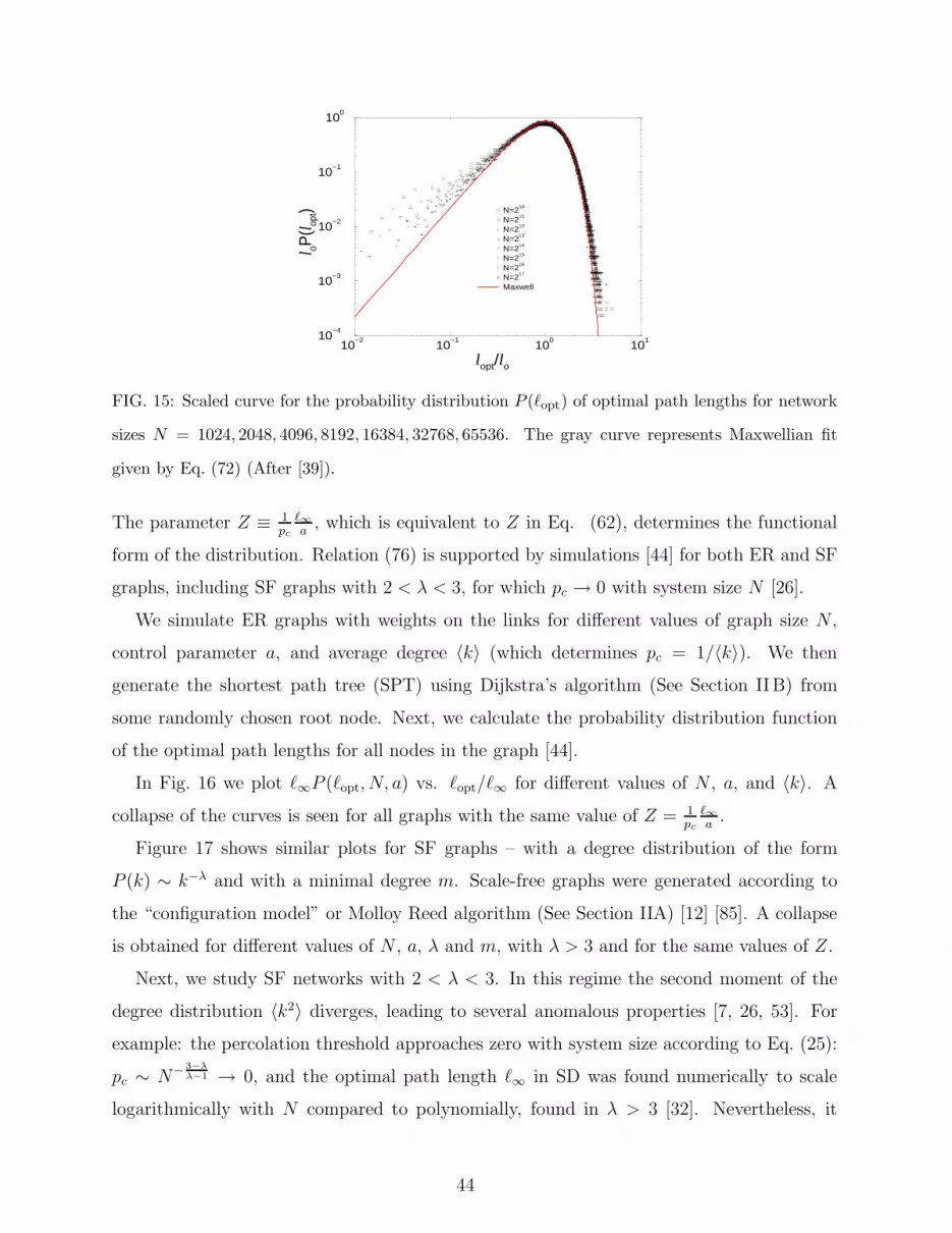
10−2

10−1

100

101

lopt/lo

10−4

10−3

10−2

10−1

100

l oP(l op

t) N=210

N=211

N=212

N=213

N=214

N=215

N=216

N=217

Maxwell

FIG. 15: Scaled curve for the probability distribution P (ℓopt) of optimal path lengths for network

sizes N = 1024, 2048, 4096, 8192, 16384, 32768, 65536. The gray curve represents Maxwellian fit

given by Eq. (72) (After [39]).

The parameter Z ≡ 1pc

ℓ∞a

, which is equivalent to Z in Eq. (62), determines the functional

form of the distribution. Relation (76) is supported by simulations [44] for both ER and SF

graphs, including SF graphs with 2 < λ < 3, for which pc → 0 with system size N [26].

We simulate ER graphs with weights on the links for different values of graph size N ,

control parameter a, and average degree 〈k〉 (which determines pc = 1/〈k〉). We then

generate the shortest path tree (SPT) using Dijkstra’s algorithm (See Section IIB) from

some randomly chosen root node. Next, we calculate the probability distribution function

of the optimal path lengths for all nodes in the graph [44].

In Fig. 16 we plot ℓ∞P (ℓopt, N, a) vs. ℓopt/ℓ∞ for different values of N , a, and 〈k〉. A

collapse of the curves is seen for all graphs with the same value of Z = 1pc

ℓ∞a

.

Figure 17 shows similar plots for SF graphs – with a degree distribution of the form

P (k) ∼ k−λ and with a minimal degree m. Scale-free graphs were generated according to

the “configuration model” or Molloy Reed algorithm (See Section IIA) [12] [85]. A collapse

is obtained for different values of N , a, λ and m, with λ > 3 and for the same values of Z.

Next, we study SF networks with 2 < λ < 3. In this regime the second moment of the

degree distribution 〈k2〉 diverges, leading to several anomalous properties [7, 26, 53]. For

example: the percolation threshold approaches zero with system size according to Eq. (25):

pc ∼ N− 3−λλ−1 → 0, and the optimal path length ℓ∞ in SD was found numerically to scale

logarithmically with N compared to polynomially, found in λ > 3 [32]. Nevertheless, it

44

20 40 60 800

0.01

0.02

0.03

0.04

0.05

l

P(l)

(a)

0 0.5 1 1.50

0.5

1

1.5

2

l/l∞

l ∞*P

(l)

(b)

0 50 1000

0.01

0.02

0.03

l

P(l)

(c)

0 1 20

0.2

0.4

0.6

0.8

1

1.2

l/l∞

l ∞*P

(l)

(d)

FIG. 16: Optimal path lengths distribution, P (ℓopt), for ER networks with (a,b) Z ≡ 1pc

ℓ∞a = 10

and (c,d) Z = 3. (a) and (c) represent the unscaled distributions for Z = 10 and Z = 3 respectively,

while (b) and (d) are the scaled distribution. Different symbols represent networks with different

characteristics such as size N = 2000, 4000, 8000 (which determines ℓ∞ ∼ N1/3), average degree

〈k〉 = 3, 5, 8 (which determines pc = 1/〈k〉), and disorder strength a = ℓ∞/(pcZ) Results were

averaged over 1500 realizations (After [44]).

seems from Fig. 18 that the optimal paths probability distribution for SF networks with

2 < λ < 3 exhibits similar collapse for different values of N and a for the same Z (although

its functional form is different compared to the λ > 3 case) [44].

We present evidence that the optimal path is related to percolation [47]. The numerical

results suggest that for a finite disorder parameter a, the optimal path (on average) follows

the percolation cluster in the network (i.e., links with weight below pc) up to a typical

“characteristic length” ξ = apc, before deviating and making a “shortcut” (i.e. crossing

45

0 50 1000

0.01

0.02

0.03

0.04

0.05

0.06

l

P(l)

(a)

0 0.5 1 1.50

0.5

1

1.5

l/l∞

l ∞*P

(l)

(b)

0 50 100 1500

0.01

0.02

0.03

l

P(l)

(c)

0 1 20

0.2

0.4

0.6

0.8

1

l/l∞

l ∞*P

(l)

(d)

FIG. 17: Optimal path lengths distribution, P (l), for SF networks with (a,b) Z ≡ 1pc

ℓ∞a = 10 and

(c,d) Z = 2. (a) and (c) represent the unscaled distributions for Z = 10 and Z = 2 respectively,

while (b) and (d) are the scaled distribution. Different symbols represent networks with different

characteristics such as size N = 4000, 8000 (which determines ℓ∞ ∼ Nνopt), λ = 3.5, 5 and m =

2 (which determine pc), and disorder strength a = ℓ∞/(pcZ). Results were averaged over 250

realizations (After [44]).

a link with weight above pc). For length scales below ξ the optimal path behaves as in

strong disorder and its length is relatively long. The shortcuts have an effect of shortening

the optimal path length from a polynomial to logarithmic form according to the universal

function F (u) (Eq. (75)). Thus, the optimal path for finite a can be viewed as consisting

of “blobs” of size ξ in which strong disorder persists. These blobs are interconnected by

shortcuts, which result in the total path being in weak disorder.

We next present direct simulations supporting this argument [44]. We calculate the

46

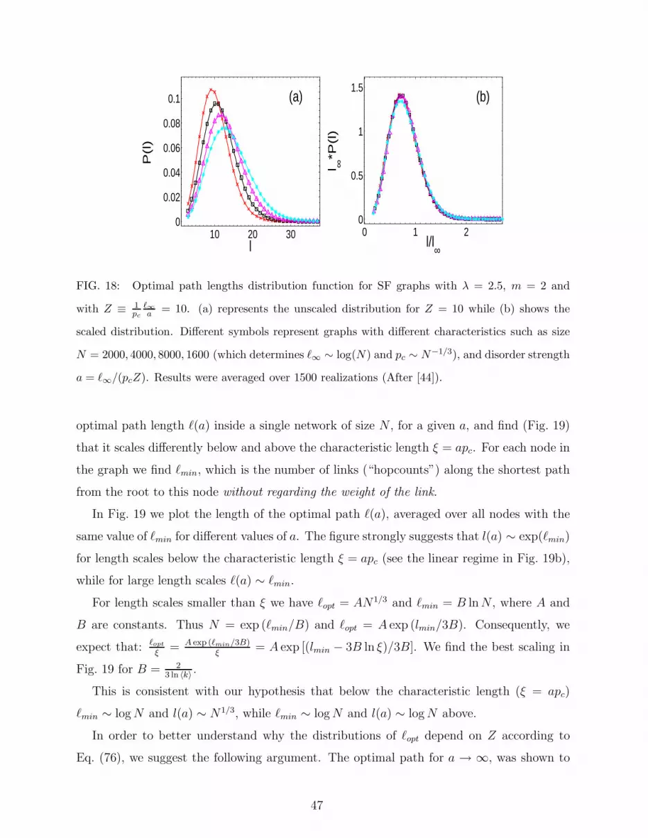
10 20 300

0.02

0.04

0.06

0.08

0.1

l

P(l)

(a)

0 1 20

0.5

1

1.5

l/l∞

l ∞*P

(l)

(b)

FIG. 18: Optimal path lengths distribution function for SF graphs with λ = 2.5, m = 2 and

with Z ≡ 1pc

ℓ∞a = 10. (a) represents the unscaled distribution for Z = 10 while (b) shows the

scaled distribution. Different symbols represent graphs with different characteristics such as size

N = 2000, 4000, 8000, 1600 (which determines ℓ∞ ∼ log(N) and pc ∼ N−1/3), and disorder strength

a = ℓ∞/(pcZ). Results were averaged over 1500 realizations (After [44]).

optimal path length ℓ(a) inside a single network of size N , for a given a, and find (Fig. 19)

that it scales differently below and above the characteristic length ξ = apc. For each node in

the graph we find ℓmin, which is the number of links (“hopcounts”) along the shortest path

from the root to this node without regarding the weight of the link.

In Fig. 19 we plot the length of the optimal path ℓ(a), averaged over all nodes with the

same value of ℓmin for different values of a. The figure strongly suggests that l(a) ∼ exp(ℓmin)

for length scales below the characteristic length ξ = apc (see the linear regime in Fig. 19b),

while for large length scales ℓ(a) ∼ ℓmin.

For length scales smaller than ξ we have ℓopt = AN1/3 and ℓmin = B ln N , where A and

B are constants. Thus N = exp (ℓmin/B) and ℓopt = A exp (lmin/3B). Consequently, we

expect that: ℓopt

ξ= A exp (ℓmin/3B)

ξ= A exp [(lmin − 3B ln ξ)/3B]. We find the best scaling in

Fig. 19 for B = 23 ln 〈k〉 .

This is consistent with our hypothesis that below the characteristic length (ξ = apc)

ℓmin ∼ log N and l(a) ∼ N1/3, while ℓmin ∼ log N and l(a) ∼ log N above.

In order to better understand why the distributions of ℓopt depend on Z according to

Eq. (76), we suggest the following argument. The optimal path for a → ∞, was shown to

47

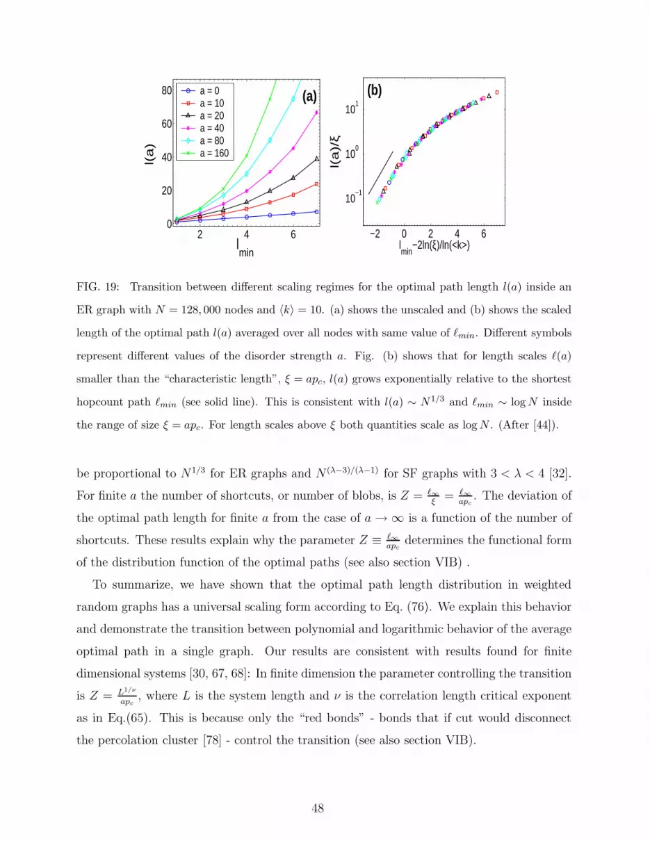
2 4 60

20

40

60

80

lmin

l(a

)

a = 0a = 10a = 20a = 40a = 80a = 160

(a)

−2 0 2 4 6

10−1

100

101

lmin

−2ln(ξ)/ln(<k>)

l(a

)/ξ

(b)

FIG. 19: Transition between different scaling regimes for the optimal path length l(a) inside an

ER graph with N = 128, 000 nodes and 〈k〉 = 10. (a) shows the unscaled and (b) shows the scaled

length of the optimal path l(a) averaged over all nodes with same value of ℓmin. Different symbols

represent different values of the disorder strength a. Fig. (b) shows that for length scales ℓ(a)

smaller than the “characteristic length”, ξ = apc, l(a) grows exponentially relative to the shortest

hopcount path ℓmin (see solid line). This is consistent with l(a) ∼ N1/3 and ℓmin ∼ log N inside

the range of size ξ = apc. For length scales above ξ both quantities scale as log N . (After [44]).

be proportional to N1/3 for ER graphs and N (λ−3)/(λ−1) for SF graphs with 3 < λ < 4 [32].

For finite a the number of shortcuts, or number of blobs, is Z = ℓ∞ξ

= ℓ∞apc

. The deviation of

the optimal path length for finite a from the case of a → ∞ is a function of the number of

shortcuts. These results explain why the parameter Z ≡ ℓ∞apc

determines the functional form

of the distribution function of the optimal paths (see also section VIB) .

To summarize, we have shown that the optimal path length distribution in weighted

random graphs has a universal scaling form according to Eq. (76). We explain this behavior

and demonstrate the transition between polynomial and logarithmic behavior of the average

optimal path in a single graph. Our results are consistent with results found for finite

dimensional systems [30, 67, 68]: In finite dimension the parameter controlling the transition

is Z = L1/ν

apc, where L is the system length and ν is the correlation length critical exponent

as in Eq.(65). This is because only the “red bonds” - bonds that if cut would disconnect

the percolation cluster [78] - control the transition (see also section VIB).

48

VIII. SCALE-FREE NETWORKS EMERGING FROM WEIGHTED RANDOM

GRAPHS

In this section we introduce a simple process that generates random scale-free networks

with λ = 2.5 from weighted Erdos-Renyi graphs [77]. We further show that the minimum

spanning tree (MST) on an Erdos-Renyi graph is related to this network, and is composed

of percolation clusters, which we regard as “super nodes”, interconnected by a scale-free

tree. We will see that due to optimization this scale-free tree is dominated by links having

high weights — significantly higher than the percolation threshold pc. Hence, the MST

naturally distinguishes between links below and above the percolation threshold, leading to

a scale-free “supernode network”. Our results may explain the origin of scale-free degree

distribution in some real world networks.

Consider an Erdos-Renyi (ER) graph with N nodes and an average degree 〈k〉, thus

having a total of N〈k〉/2 links. To each link we assign a weight chosen randomly and

uniformly from the range [0, 1]. We define black links to be those links with weights below a

threshold pc = 1/〈k〉. Two nodes belong to the same cluster if they are connected by black

links [Fig. 20(a)].

From Section VI follows that the number of clusters of s nodes scales as a power law,

ns ∼ s−τ , with τ = 2.5 for ER networks. Next, we merge all nodes inside each cluster into

a single “supernode”. We define a new “supernode network” [Fig. 20(b)] of Nsn supernodes

[47]. The links between two supernodes [see Figs. 20(a) and 20(b)] have weights larger than

pc. The degree distribution P (k) of the supernode network can be obtained as follows. Every

node in a supernode has the same (finite) probability to be connected to a node outside the

supernode. Thus, we assume that the degree k of each supernode is proportional to the

cluster size s, which obeys ns ∼ s−2.5. Hence P (k) ∼ k−λ, with λ = 2.5, as supported by

simulations shown in Fig. 21. Furthermore, we also see that if the threshold for obtaining

the clusters which are merged into supernodes is changed slightly, the degree distribution

still remains scale free with λ = 2.5, but with an exponential cutoff. This is an indication

of the fact that there are still supernodes of high degree which are connected to many other

(small) supernodes by links with weights significantly higher than pc; if this was not the

case, a small change in the threshold would cause many clusters to merge and destroy the

power law in the supernode network degree distribution.

49

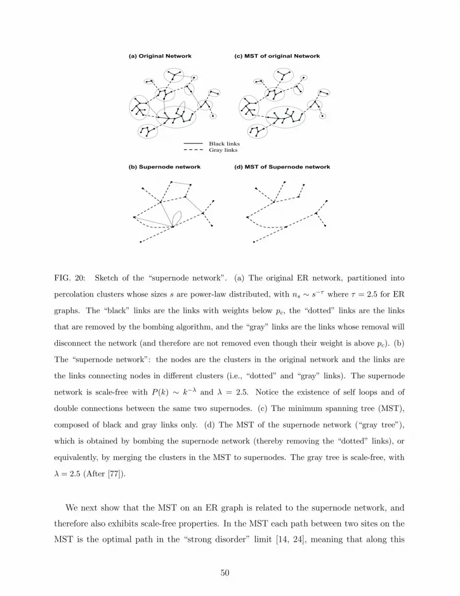
FIG. 20: Sketch of the “supernode network”. (a) The original ER network, partitioned into

percolation clusters whose sizes s are power-law distributed, with ns ∼ s−τ where τ = 2.5 for ER

graphs. The “black” links are the links with weights below pc, the “dotted” links are the links

that are removed by the bombing algorithm, and the “gray” links are the links whose removal will

disconnect the network (and therefore are not removed even though their weight is above pc). (b)

The “supernode network”: the nodes are the clusters in the original network and the links are

the links connecting nodes in different clusters (i.e., “dotted” and “gray” links). The supernode

network is scale-free with P (k) ∼ k−λ and λ = 2.5. Notice the existence of self loops and of

double connections between the same two supernodes. (c) The minimum spanning tree (MST),

composed of black and gray links only. (d) The MST of the supernode network (“gray tree”),

which is obtained by bombing the supernode network (thereby removing the “dotted” links), or

equivalently, by merging the clusters in the MST to supernodes. The gray tree is scale-free, with

λ = 2.5 (After [77]).

We next show that the MST on an ER graph is related to the supernode network, and

therefore also exhibits scale-free properties. In the MST each path between two sites on the

MST is the optimal path in the “strong disorder” limit [14, 24], meaning that along this

50

100

101

102

103

10−3

10−2

10−1

100

101

102

103

k

P(k

)

2.5

FIG. 21: The degree distribution of the supernode network of Fig. 1(b), where the supernodes

are the percolation clusters, and the links are the links with weights larger than pc (©). The

distribution exhibits a scale-free tail with λ ≈ 2.5. If we choose a threshold less than pc, we obtain

the same power law degree distribution with an exponential cutoff. The different symbols represent

slightly different threshold values: pc − 0.03 (2) and pc − 0.05 (△). The original ER network has

N = 50, 000 and 〈k〉 = 5. Note that for k ≈ 〈k〉 the degree distribution has a maximum (After

[77]).

path the maximum barrier (weight) is the smallest possible [14, 32, 47].

Here we use the bombing algorithm (See Section IID ). If the removal of a link disconnects

the graph, we restore the link and mark it “gray” ; otherwise the link [shown dotted in

Fig. 20(a)] is removed. The links that are not bombed are marked as “black”. In the

bombing algorithm, only links that close a loop can be removed. Because below criticality

loops are negligible [1, 4] for ER networks (d → ∞), bombing does not modify the percolation

clusters — where the links are black and have weights below pc. Thus, bombing modifies

only links outside the clusters, so actually it is only the links of the supernode network that

are bombed. Hence the MST resulting from bombing is composed of percolation clusters

(composed of black links) and connected by gray links [Fig. 20(c)].

From the MST of Fig. 20(c) we now generate a new tree, the MST of the supernode

network, which we call the “gray tree”, whose nodes are the supernodes and whose links

are the gray links connecting them [see Fig. 20(d)]. Note that bombing the original ER

network to obtain the MST of Fig. 20(c) is equivalent to bombing the supernode network

51

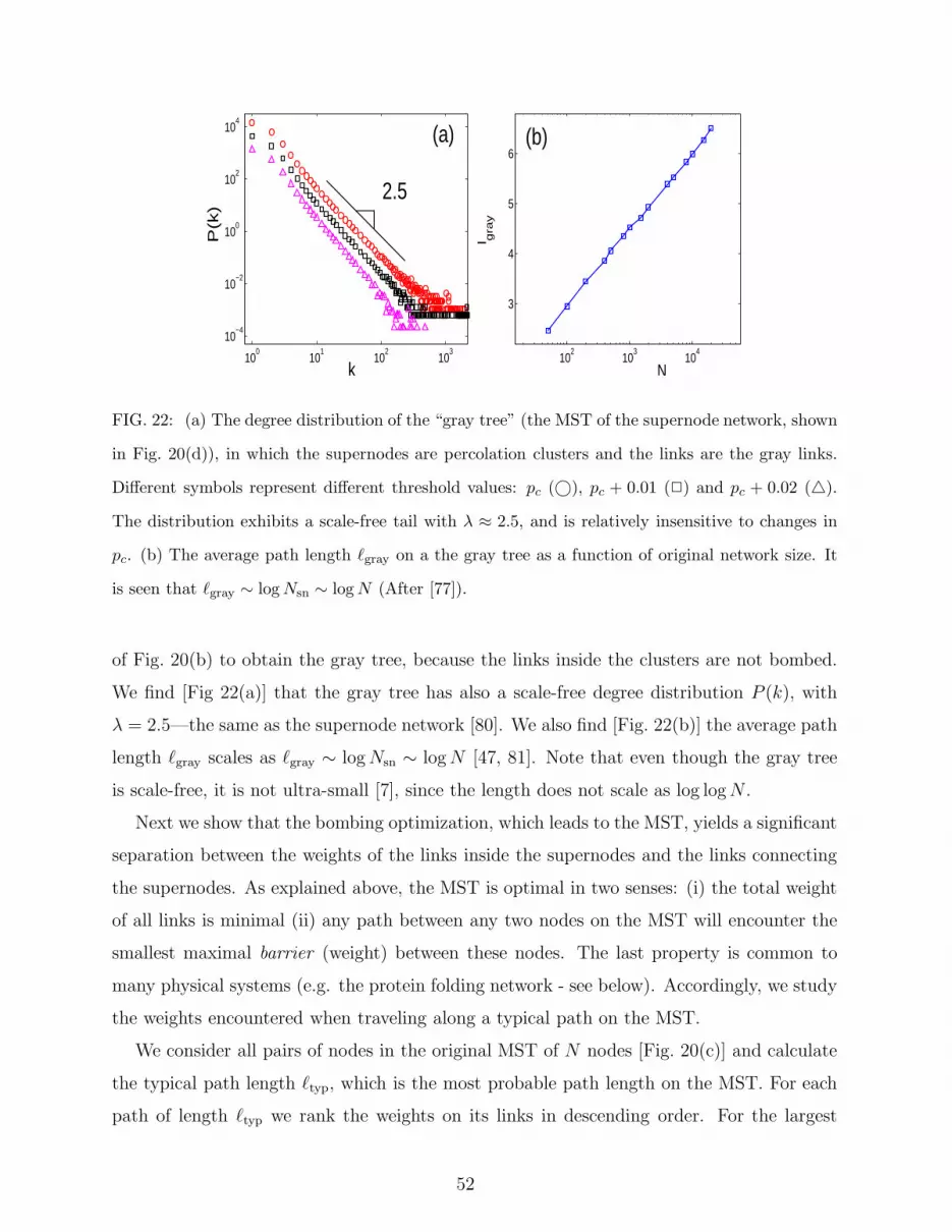
100

101

102

103

10−4

10−2

100

102

104

k

P(k

)

(a)

2.5

102

103

104

3

4

5

6

N

l gra

y

(b)

FIG. 22: (a) The degree distribution of the “gray tree” (the MST of the supernode network, shown

in Fig. 20(d)), in which the supernodes are percolation clusters and the links are the gray links.

Different symbols represent different threshold values: pc (©), pc + 0.01 (2) and pc + 0.02 (△).

The distribution exhibits a scale-free tail with λ ≈ 2.5, and is relatively insensitive to changes in

pc. (b) The average path length ℓgray on a the gray tree as a function of original network size. It

is seen that ℓgray ∼ log Nsn ∼ log N (After [77]).

of Fig. 20(b) to obtain the gray tree, because the links inside the clusters are not bombed.

We find [Fig 22(a)] that the gray tree has also a scale-free degree distribution P (k), with

λ = 2.5—the same as the supernode network [80]. We also find [Fig. 22(b)] the average path

length ℓgray scales as ℓgray ∼ log Nsn ∼ log N [47, 81]. Note that even though the gray tree

is scale-free, it is not ultra-small [7], since the length does not scale as log log N .

Next we show that the bombing optimization, which leads to the MST, yields a significant

separation between the weights of the links inside the supernodes and the links connecting

the supernodes. As explained above, the MST is optimal in two senses: (i) the total weight

of all links is minimal (ii) any path between any two nodes on the MST will encounter the

smallest maximal barrier (weight) between these nodes. The last property is common to

many physical systems (e.g. the protein folding network - see below). Accordingly, we study

the weights encountered when traveling along a typical path on the MST.

We consider all pairs of nodes in the original MST of N nodes [Fig. 20(c)] and calculate

the typical path length ℓtyp, which is the most probable path length on the MST. For each

path of length ℓtyp we rank the weights on its links in descending order. For the largest

52

weights (“rank 1 links”), we calculate the average weight wr=1 over all paths. Similarly, for

the next largest weights (“rank 2 links”) we find the average wr=2 over all paths, and so

on up to r = ℓtyp. Fig. 23(a) shows wr as a function of rank r for three different network

sizes N = 2000, 8000, and 32000. It can be seen that weights below pc (black links inside

the supernodes) are uniformly distributed and approach one another as N increases. As

opposed to this, weights above pc (“gray links”) are not uniformly distributed, due to the

bombing algorithm, and are independent of N . Actually, weights above pc encountered along

the optimal path (such as the largest weights w1, w2 and w3) are significantly higher than

those below pc. Fig. 23(b) shows that the links with the highest weights on the MST can

be associated with gray links from very small clusters [Figs. 20(a) and 20(c)] (similar results

have been obtained along the optimal path).

As mentioned earlier, this property is present also in the original supernode network and

hence the change in the threshold used to obtain the supernodes does not destroy the power

law degree distribution but only introduces an exponential cutoff. We thereby obtain a scale-

free supernode network with λ = 2.5, which is not very sensitive to the precise value of the

threshold used for defining the supernodes. For example, the scale-free degree distribution

shown in Fig. 22(a) for a threshold of pc+0.01 corresponds to having only four largest weights

on the optimal paths [see Fig. 23(a)]. However, even for pc + 0.02 the degree distribution is

well approximated by a scale-free distribution with λ = 2.5 [see Fig. 22(a)]. This means that

mainly very small clusters, connected with high-weight links to large clusters, dominate the

scale-free distribution P (k) of the MST of the supernode network (gray tree). Hence, the

bombing optimization process on an ER graph causes a significant separation between links

below and above pc to emerge spontaneously in the system, and by merging nodes connected

with links of low weights, a scale-free network can arise.

The process described above may be related to the evolution of some real world networks.

Consider a homogeneous network with many components whose average degree 〈k〉 is well

defined. Suppose that the links between the components have different weights, and that

some optimization process separates the network into nodes which are well connected (i.e.,

connected by links with low weights) and nodes connected by links having much higher

weights. If the well-connected components merge into a single node, this results in a new

heterogeneous supernode network with scale free degree distribution.

An example of a real world network whose evolution may be related to this model is the

53

protein folding network, which was found to be scale-free with λ ≈ 2.3 [54]. The nodes

are the possible physical configurations of the system and the links between them describe

the possible transitions between the different configurations. We assume that this network

is optimal because the system chooses the path with the smallest energy barrier from all

possible trajectories in phase space. It is possible that the scale-free distribution evolves

through a similar procedure as described above for random graphs: adjacent configurations

with close energies (nodes in the same cluster) cannot be distinguished and are regarded as

a single supernode, while configurations (clusters) with high barriers between them belong

to different supernodes.

A second example is computer networks. Strongly interacting computers (such as com-

puters belonging to researchers from the same company or research institution) are likely

to converge into a single domain, and thus domains with various sizes and connectivities

are formed. This network might be also optimal, because packets destined to an external

domain are presumably routed through the router which has the best connection to the

target domain.

To summarize, we have seen that any weighted random network hides an inherent scale-

free “supernode network” [82]. We showed that the minimum spanning tree, generated by

the bombing algorithm, is composed of percolation clusters connected by a scale-free tree

of “gray” links. Most of the gray links connect small clusters to large ones, thus having

weights well above the percolation threshold that do not change with the original size of the

network. Thus the optimization in the process of building the MST distinguishes between

links with weights below and above the threshold, leading to a spontaneous emergence of

a scale-free “supernode network”. We raise the possibility that in some naturally optimal

real-world networks, nodes connected well merge into one single node, and thus a scale-free

network emerges.

IX. PARTITION OF THE MINIMUM SPANNING TREE INTO SUPERHIGH-

WAYS AND ROADS

The centrality, C, quantifies the “importance” of a node for transport in the network.

Moreover, identifying the nodes with high C enables, as shown below, to improve their

transport capacity and thus improve the global transport in the network. Several definitions

54

0 10 20

0.15

0.2

0.25

0.3

0.35

rank

wr

pc

pc+0.01

(a)

100

101

102

10−3

10−2

10−1

s

wg

ray −

pc

(b)

FIG. 23: (a) The average weights wr along the optimal path of an ER graph with 〈k〉 = 5,

sorted according to their rank. Different symbols represent different system sizes: N = 2000 (©),

N = 8000 (2) and N = 32000 (△). Below pc = 0.2, the weights are uniformly distributed, while

weights above pc are significantly higher and independent of N . (b) Cluster size vs. the minimal

gray link emerging from each cluster, for ER graphs with 〈k〉 = 5 and N = 10000. Small clusters

are associated with higher weights because they have a small number of exits and thus cannot be

optimized (After [77]).

of centrality exists. Here we deal with the “betweeness centrality” which is defined as the

relative number of shortest path in the network passing through a node (or a link). The

probability density function (pdf) of C was studied on the MST for both scale-free (SF) [61]

and Erdos-Renyi (ER) [4, 5] networks and found to satisfy a power law,

PMST(C) ∼ C−δMST (77)

with δMST close to 2 [57, 58]. An important question is weather there are substructure of

the MST which are more central and play a major role on the transport. Reference [60]

shows that a sub-network of the MST, the infinite incipient percolation cluster (IIC) has a

significantly higher average C than the entire MST [59] — i.e., the set of nodes inside the

IIC are typically used by transport paths more often than other nodes in the MST [60].

— In this sense the IIC can be viewed as a set of superhighways (SHW) in the MST. The

nodes on the MST which are not in the IIC are called roads, due to their analogy with roads

of less traffic (usually used by local residents). We demonstrate the impact of this finding

by showing that improving the capacity of the superhighways (IIC) is significantly a better

55

strategy to enhance global transport compared to improving the same number of links with

the highest C in the MST, although they have higher C [60]. This counterintuitive result

shows the advantage of identifying the IIC subsystem, which is very small compared to the

full network [63]. These results are based on extensive numerical studies for centrality of the

IIC, and comparison with the centrality of the entire MST [55, 60], as described below. ER

and SF network of size N are generated by the methods explained in section IIA. Multiple

connections between two nodes and self-loops in a single node are disallowed. To construct

a weighted network, a weight wi is assigned to each link from a uniform distribution between

0 and 1. The MST is obtained from the weighted network using Prim’s algorithm [41] (see

Section II E). Once the MST is built, one can compute the value of C of each node by

counting the number of paths between all possible pairs passing through that node and

normalize C by the total number of pairs in the MST, N(N − 1)/2, which ensures that

C is between 0 and 1 [62]. The IIC of ER and SF networks is simulated as explained in

Section II F.

To quantitatively study the centrality of the nodes in the IIC, we calculate the pdf,

PIIC(C) of C. Figure 24 shows that for all three cases studied, ER, SF and square lattice

networks, PIIC(C) for nodes satisfies a power law

PIIC(C) ∼ C−δIIC , (78)

where

δIIC ≈

1.2 [ER, SF]

1.25 [square lattice]. (79)

Moreover, from Fig. 24, it is seen that δIIC < δMST, implying a larger probability to find a

larger value of C in the IIC compared to the entire MST. The values for δMST are consistent

with those found in Ref. [58]. Similar results for the centrality of the links were obtained.

The results thus show that the IIC is like a network of superhighways inside the MST. When

we analyze centrality of the entire MST, the effect of the high C of the IIC is not seen since

the IIC is only a tiny fraction of the MST. Some results are summarized in Table II.

The values of δMST and δIIC can be understood from the following scaling arguments, based

self-similarity properties of the MST and the IIC. Similar arguments are used in [25, 72] to

express exponent τs describing the cluster size distribution at percolation threshold on a

lattice in terms of the cluster fractal dimension and the dimension of the lattice. Indeed,

56

the majority of nodes are connected through the superhighway links, whose centrality is

proportional to N2. The number of these links for the entire network scales as ℓ∞(N) ∼N1/νopt [32, 68]. Thus small regions of the MST of chemical diameter ℓ consists of n1/νopt

nodes. These regions have length ℓ∞(n) ∼ n1/νopt . These roads connect the nodes in this

region with the rest of the nodes of the MST, and thus their centrality is at least nN . The

total number of such links in all the regions of size n is m(n) = ℓ∞(n)N/n ∼ nνopt−1. This

is the number of links with centrality larger than nN . Thus number of links with centrality

exactly nN is m(n) − m(n + 1) ∼ nνopt−2 = n−δMST . Using Eq. (38) we have:

δMST =

5/3, λ > 4, ER

(λ + 1)/(λ − 1), 3 < λ ≤ 4. (80)

Similar arguments lead to the centrality distribution of the nodes on the IIC. The small

regions of chemical diameter ℓ have centrality larger or equal to Nn(ℓ). The number of links

in the IIC belonging to these regions is s(ℓ) = ℓdℓ [8]. The total number of such regions is

S/s(ℓ), thus the total number of the links of the IIC with centrality larger than Nn(ℓ) is

m[n(ℓ)] = ℓ/s(ℓ) ∼ ℓ1−dℓ = n(1−dℓ) νopt. Accordingly

δIIC = 1 + (dℓ − 1)νopt =

4/3, λ > 4, ER

λ/(λ − 1), 3 < λ ≤ 4. (81)

The values predicted by Eqs. (80) and (81) are in good agreement with the simulation

results presented in Table II.

To further demonstrate the significance of the IIC, we compute the average 〈C〉 for each

realization of the network over all nodes. Fig. 27, shows the histograms of 〈C〉 for both the

IIC and for the other nodes on the MST. We see that the nodes on the IIC have significantly

larger 〈C〉 compared to the other nodes of the MST.

ER SF (λ = 4.5) SF (λ = 3.5) square lattice

δIIC 1.2 1.2 1.2 1.25

δMST 1.6 1.7 1.7 1.32

νopt 1/3 1/3 0.2 0.61

〈u〉 0.29 0.20 0.13 0.64

TABLE II: Results for the IIC and the MST (After [60]).

57

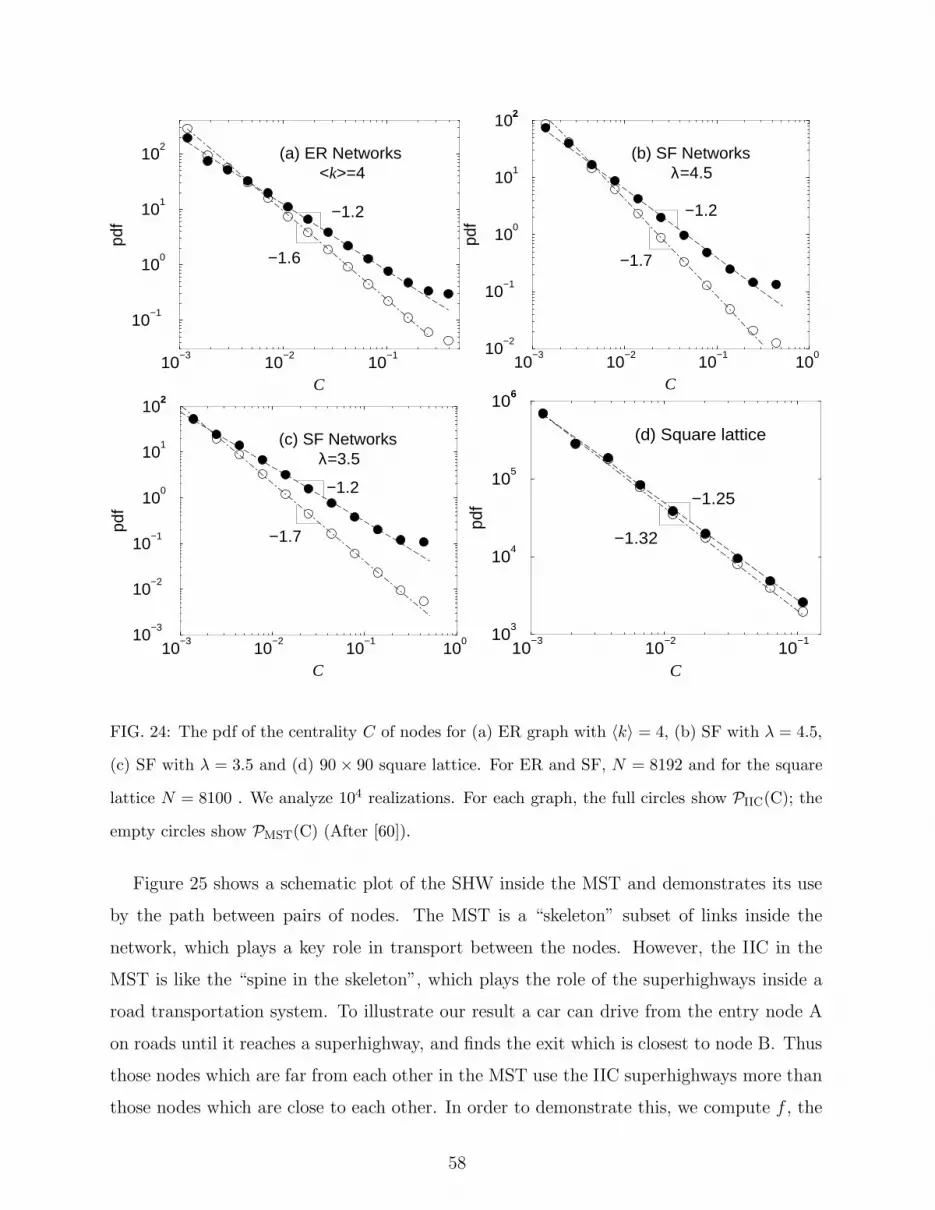
10−3

10−2

10−1

100

C

10−2

10−1

100

101

102

pdf

(b) SF Networks

−1.2

−1.7

λ=4.5

10−3

10−2

10−1

C

103

104

105

106

pdf

(d) Square lattice

−1.32

−1.25

10−3

10−2

10−1

C

10−1

100

101

102

pdf

(a) ER Networks

−1.2

−1.6

<k>=4

10−3

10−2

10−1

100

C

10−3

10−2

10−1

100

101

102

pdf

(c) SF Networks

−1.2

−1.7

λ=3.5

62

2

FIG. 24: The pdf of the centrality C of nodes for (a) ER graph with 〈k〉 = 4, (b) SF with λ = 4.5,

(c) SF with λ = 3.5 and (d) 90 × 90 square lattice. For ER and SF, N = 8192 and for the square

lattice N = 8100 . We analyze 104 realizations. For each graph, the full circles show PIIC(C); the

empty circles show PMST(C) (After [60]).

Figure 25 shows a schematic plot of the SHW inside the MST and demonstrates its use

by the path between pairs of nodes. The MST is a “skeleton” subset of links inside the

network, which plays a key role in transport between the nodes. However, the IIC in the

MST is like the “spine in the skeleton”, which plays the role of the superhighways inside a

road transportation system. To illustrate our result a car can drive from the entry node A

on roads until it reaches a superhighway, and finds the exit which is closest to node B. Thus

those nodes which are far from each other in the MST use the IIC superhighways more than

those nodes which are close to each other. In order to demonstrate this, we compute f , the

58

��������������������������������������������������������������������������������������������������������������������������������������������������������������������������������������������������������������������������������������������������������������������������������������������������������������������������������������������������������������������������������������������������������������������������������������������������������������������������������������������������������������

��������������������������������������������������������������������������������������������������������������������������������������������������������������������������������������������������������������������������������������������������������������������������������������������������������������������������������������������������������������������������������������������������������������������������������������������������������������������������������������������������������������A

B

C

MST

roadssmall percolationclusters

(Superhighways)IIC

FIG. 25: Schematic graph of the network of connected superhighways (heavy lines) inside the MST

(shaded). A, B and C are examples of possible entry and exit nodes, which connect to the network

of superhighways by “roads” (thin lines). The middle size lines indicate other percolation clusters

with much smaller size compared to the IIC (After [60]).

average fraction of pairs of nodes using by the shortest paths the IIC, as a function of ℓMST,

the distance between a pair of nodes on the MST (Fig. 26). We see that f increases and

approaches one as ℓMST grows. We also show that f scales as ℓMST/Nνopt for different system

sizes, where νopt is the percolation connectedness exponent [32, 68].

The next question is how much the IIC is used in transport on the MST? We define the

IIC superhighway usage,

u ≡ ℓIIC

ℓMST, (82)

where ℓIIC is the number of links in a given path of length ℓMST belonging to the IIC

superhighways. The average usage 〈u〉 quantifies what fraction of nodes/links of the IIC is

used by the transport between all pairs of nodes. In Fig. 28(a), we show 〈u〉 as a function of

the system size N . Our results suggest that 〈u〉 approaches a constant value and becomes

independent of N for large N . This is surprising since the average value of the ratio between

the number of nodes on the IIC and on the MST, 〈NIIC/NMST〉, approaches zero as N →∞ [63], showing that although the IIC contains only a tiny fraction of the nodes in the

entire network, its usage for the transport in the entire network is constant. We find that

〈u〉 ≈ 0.3 for ER networks, 〈u〉 ≈ 0.2 for SF networks with λ = 4.5, and 〈u〉 ≈ 0.64 for

the square lattice. The reason why 〈u〉 is not close to 1.0 is that in addition to the IIC,

59

0 10 20 30 40lMST/N

υopt

0

0.2

0.4

0.6

0.8

1

< f

>

(c) SF Networksλ=3.5

0 5 10 15lMST/N

υopt

0

0.2

0.4

0.6

0.8

1

< f

>

(a) ER Networks<k>=4

0 5 10 15 20lMST/N

υopt

0

0.2

0.4

0.6

0.8

1

< f

>

(b) SF Networksλ=4.5

0 1 2 3 4lMST/N

υopt

0.4

0.6

0.8

1

< f

>

(d) LxL square lattice

FIG. 26: The average fraction, 〈f〉, of pairs using the SHW, as a function of ℓMST, the distance

between the pair on the MST. (a) ER graph with 〈k〉 = 4, (b) SF with λ = 4.5, (c) SF with λ = 3.5

and (d) square lattice. For ER and SF: (©)N = 1024 and (2)N = 2048 with 104 realizations. For

square lattice: (©)N = 1024 and (2)N = 2500 with 103 realizations. The x axis is rescaled by

Nνopt , where νopt = 1/3 for ER and for SF with λ > 4, and νopt = (λ − 3)/λ − 1) for SF networks

with 3 < λ < 4 [32]. For the L×L square lattice, ℓMST ∼ Ldopt with dopt = 1.22 and since L2 = N ,

νopt = dopt/2 ≈ 0.61 [24, 30] (After [60]).

the optimal path passes also through other percolation clusters, such as the second largest

and the third largest percolation clusters. In Fig. 28, we also show for ER networks, the

average usage of the two largest and the three largest percolation clusters for a path on the

MST and we see that the average usage increases significantly and is also independent of N .

However, the number of clusters used by a path on MST is relatively small and proportional

to ln N [47], suggesting that the path on the MST uses only few percolation clusters and few

jumps between them (of order ln N) when traveling from an entry node to an exit node on

the network. When N → ∞ the average usage of all percolation clusters should approach 1.

Can we use the above results to improve the transport in networks? It is clear that by

60

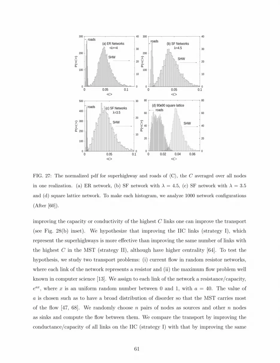
0 0.05 0.1<C>

0

100

200

300

P(<

C>

)

0

10

20

30

40roads

SHW

(a) ER Networks<k>=4

0 0.05 0.1<C>

0

100

200

300

400

500

P(<

C>

)

0

10

20

30

(c) SF Networksroads

SHW

λ=3.5

0 0.02 0.04 0.06<C>

0

20

40

60

80

P(<

C>

)

0

20

40

60

80

(d) 90x90 square latticeroads

SHW

0 0.05 0.1<C>

0

100

200

300

P(<

C>

)

0

10

20

30

40

(b) SF Networksroads

SHW

λ=4.5

FIG. 27: The normalized pdf for superhighway and roads of 〈C〉, the C averaged over all nodes

in one realization. (a) ER network, (b) SF network with λ = 4.5, (c) SF network with λ = 3.5

and (d) square lattice network. To make each histogram, we analyze 1000 network configurations

(After [60]).

improving the capacity or conductivity of the highest C links one can improve the transport

(see Fig. 28(b) inset). We hypothesize that improving the IIC links (strategy I), which

represent the superhighways is more effective than improving the same number of links with

the highest C in the MST (strategy II), although have higher centrality [64]. To test the

hypothesis, we study two transport problems: (i) current flow in random resistor networks,

where each link of the network represents a resistor and (ii) the maximum flow problem well

known in computer science [13]. We assign to each link of the network a resistance/capacity,

eax, where x is an uniform random number between 0 and 1, with a = 40. The value of

a is chosen such as to have a broad distribution of disorder so that the MST carries most

of the flow [47, 68]. We randomly choose n pairs of nodes as sources and other n nodes

as sinks and compute the flow between them. We compare the transport by improving the

conductance/capacity of all links on the IIC (strategy I) with that by improving the same

61

0 5000 10000 15000number of nodes N

0.0

0.2

0.4

0.6

0.8A

vera

ge u

sage

<u>

(a)

100

101

102

factor of improving

1

10

<FsI/F

sII>

100

101

102

103

factor of improving

100

102

<FsI/F

0>

(b)

FIG. 28: (a) The average usage 〈u〉 ≡ 〈ℓIIC/ℓMST〉 for different networks, as a function of the

number of nodes N . © (ER with 〈k〉 = 4), 2 (SF with λ = 4.5), 3 (SF with λ = 3.5), △ (L × L

square lattice). The symbols (�) and (�) represent the average usage for ER with 〈k〉 = 4 when the

two largest percolation clusters and the three largest percolation clusters are taken into account,

respectively. (b) The ratio between the flow using strategy I, FsI, and that using strategy II, FsII,

as a function of the factor of improving conductivity/capacity. The inset is the ratio between the

flow using strategy I and the flow in the original network, F0. The data are all for ER networks

with N = 2048, 〈k〉 = 4 and n = 50(©), n = 250(3) and n = 500(2). The unfilled symbols are

for current flow and the filled symbols are for maximum flow (After [60]).

number of links with the highest C in the MST (strategy II). Since the two sets are not

the same and therefore higher centrality links will be improved in II [64], it is tempting to

suggest that the better strategy to improve the global flow is strategy II. However, here we

demonstrate using ER networks as an example that counterintuitively strategy I is better.

We also find similar advantage of strategy I compared to strategy II for SF networks with

λ = 3.5.

In Fig. 28(b), we compute the ratio between the flow using strategy I (FsI) and the flow

using strategy II (FsII) as a function of the factor of improving conductivity/capacity of the

links. The figure clearly shows that strategy I is better than strategy II. Since the number

of links in the IIC is relatively very small comparing to the number of links in the whole

network [63], it could proven to be a very efficient strategy.

62

In summary, we find that the centrality of the IIC for transport in networks is significantly

larger than the centrality of the other nodes in the MST. Thus the IIC is a key component

for transport in the MST. We demonstrate that improving the capacity/conductance of the

links in the IIC is useful strategy to improve transport.

X. SUMMARY

We reviewed recent studies on the scaling of the average optimal path length ℓopt in a

disordered network. There are two scaling regimes of ℓopt corresponding to the regimes of

weak and strong disorder. For ER networks and SF networks with λ > 4, ℓopt ∼ ln N in

the weak disorder regime while ℓopt ∼ N1/3 in the strong disorder regime. For SF networks

with 3 < λ < 4, ℓopt ∼ lnN in the weak disorder regime while ℓopt ∼ Nλ−3λ−1 in the strong

disorder regime. For SF networks with 2 < λ < 3, ℓopt ∼ ln N in the weak disorder regime

while ℓopt ∼ lnλ−1 N in the strong disorder regime. The scaling behavior of ℓopt in the

strong disorder regime for ER and SF networks with λ > 3 is obtained analytically using

percolation theory [33]. For exponential disorder, for both ER random networks and SF

networks we obtain a scaling function for the crossover from weak disorder characteristics to

strong disorder characteristics. We show that the crossover occurs when the min-max path

reaches a crossover length ℓ∗(a) and ℓ∗(a) ∼ a. Equivalently, the crossover occurs when the

network size N reaches a crossover size N∗(a), where N∗(a) ∼ a3 for ER networks and for

SF networks with λ ≥ 4 and N∗(a) ∼ aλ−1λ−3 for SF networks with 3 < λ < 4.

We also have shown that the optimal path length distribution in weighted random graphs

has a universal scaling form according to Eq. (76). We explain this behavior and demonstrate

the transition between polynomial to logarithmic behavior of the average optimal path in a

single graph.

Our results are consistent with results found for finite dimensional systems [30, 68, 71, 76]:

In finite dimension the parameter controlling the transition is L1/ν

apc, where L is the system

length and ν is the correlation length critical exponent. This is because only the “red bonds”

- bonds that if cut would disconnect the percolation cluster [78] - control the transition.

We also show that any weighted random network hides an inherent scale-free “supernode

network” [82]. We showed that the minimum spanning tree, generated by the bombing

algorithm, is composed of percolation clusters connected by a scale-free tree of “gray” links.

63

Most of the gray links connect small clusters to large ones, thus having weights well above the

percolation threshold that do not change with the size of the network. Thus the optimization

in the process of building the MST distinguishes between links with weights below and above

the threshold, leading to a spontaneous emergence of a scale-free “supernode network” with

λ = 2.5. We raise the possibility that in some naturally optimal real-world networks, nodes

connected well merge into one single node, and thus a scale-free network emerges.

The centrality in networks for transport on the MST is studied. We found that the

centrality of the nodes in the IIC is significantly larger than the centrality of the other nodes

in the MST. The analytical estimation for the exponents of the centrality distribution for

both the MST and the IIC are provided. Thus the IIC is a key component for transport in the

MST. As a result of this finding, we demonstrated that improving the capacity/conductance

of the links in the IIC is a useful strategy to improve transport which is a better strategy

compare to improving the same number of links with the highest centrality in the MST.

This is probably due to the global nature of transport which prefer global improvement of

the superhighways rather than local improvement of high centrality links.

Acknowledgments

We thank ONR, Israel Science Foundation, European NEST project DYSONET, FONCyt

(PICT-O 2004/370) and Israeli Center for Complexity Science for financial support.

[1] R. Albert and A.-L. Barabasi, Rev. Mod. Phys. 74, 47 (2002).

[2] J. F. F. Mendes, S. N. Dorogovtsev, and A. F. Ioffe, Evolution of Networks: From Biological

Nets to the Internet and the WWW (Oxford University Press, Oxford, 2003).

[3] R. Pastor-Satorras and A. Vespignani, Evolution and Structure of the Internet: A Statistical

Physics Approach (Cambridge University Press, in press).

[4] P. Erdos and A. Renyi, Publicationes Mathematicae 6, 290 (1959).

[5] P. Erdos and A. Renyi, Publications of the Mathematical Inst. of the Hungarian Acad. of

Sciences 5, 17 (1960).

[6] B. Bollobas, Random Graphs (Academic, London, 1985).

64

[7] R. Cohen and S. Havlin, Phys. Rev. Lett. 90, 058701 (2003).

[8] R. Cohen, S. Havlin and D. ben-Avraham, in Handbook of Graphs and Networks, edited by S.

Bornholdt and H. G. Shuster (Willey-VCH, New York, 2002), Ch. 4.

[9] A. Barrat, et al., PNAS, 101, 3747 (2004).

[10] S. Boccaletti, V. Latora, Y. Moreno, M. Chavez , D.-U. Hwang, Physics Reports 424, 175

(2006)

[11] A.-L. Barabasi, Phys. Rev. Lett. 76, 3750 (1996).

[12] M. Molloy and B. Reed, Random Structures and Algorithms 6 161 (1995); Combin. Probab.

Comput. 7, 295 (1998).

[13] T. H. Cormen, C. E. Leiserson, and R. L. Rivest, Introduction to Algorithms (MIT Press,

Cambridge MA, 1990).

[14] R. Dobrin and P. M. Duxbury, Phys. Rev. Lett. 86, 5076 (2001).

[15] In the literature of computer science it is called “Shortest Path Tree”

[16] M. Khan, G. Pandurangan, and B. Bhargava, Tech. Rep. CSD TR 03-013, Dept. of Computer

Science, Purdue University (2003).

[17] S. Skiena, Implementing Discrete Mathematics: Combinatorics and Graph Theory With Math-

ematica (Addison-Wesley, NY, 1990).

[18] M. L. Fredman and R. E. Tarjan, J. ACM 34, 596 (1987).

[19] J. B. Kruskal, Proc. Amer. Math. Soc. 7, 48 (1956).

[20] G. Bonanno, G. Caldarelli, F. Lillo, and R. N. Mantegna, Phys. Rev. E 68, 046130 (2003).

[21] J.-P. Onnela, et al., Phys. Rev. E 68, 056110 (2003).

[22] L. A. Braunstein, S. V. Buldyrev, S. Havlin, and H. E. Stanley, Phys. Rev. E 65, 056128

(2001).

[23] S. V. Buldyrev, S. Havlin, H. E. Stanley Phys. Rev. E 73, 036128 (2006).

[24] M. Cieplak, A. Maritan, and J. R. Banavar, Phys. Rev. Lett. 72 2320 (1994); 76, 3754 (1996).

[25] A. Bunde and S. Havlin, eds., Fractals and Disordered Systems (Springer, New York, 1996).

[26] R. Cohen, K. Erez, D. ben-Avraham and S. Havlin, Phys. Rev. Lett. 85, 4626 (2000).

[27] T. E. Harris, The Theory of Branching Processes (Dover Publication Inc., New York, 1989);

[28] I. Smailer, J. Machta and S. Redner, Phys. Rev. E 47, 262 (1993).

[29] P. van der Hofstad, G. Hooghienstra, and P. van Mieghem, Prob. Eng. Inf. Sciences 15, 225

(2001).

65

[30] M. Porto, N. Schwartz, S. Havlin, and A. Bunde, Phys. Rev. E 60, R2448 (1999).

[31] M. Porto, S. Havlin, S. Schwarzer, A. Bunde Phys. Rev. Lett. 79, 4060 (1997)

[32] L. A. Braunstein, S. V. Buldyrev, R. Cohen, S. Havlin and H. E. Stanley, Phys. Rev. Lett.

91, 168701 (2003) .

[33] The results for SF networks with 2 < λ < 3 have been obtained numerically and a theoretical

explanation for these results is still pending.

[34] A.-L. Barabasi, Linked: The New Science of Networks (Perseus Publishing, Cambridge MA,

2002).

[35] M. Buchanan, Nexus: Small Worlds and the Groundbreaking Theory of Networks (W. W.

Norton, New York, 2002).

[36] D. J. Watts, Six Degrees: The Science of a Connected Age (W. W. Norton, New York, 2003).

[37] S. N. Dorogovtsev and J. F. F. Mendes, Evolution of Networks: From Biological Nets to the

Internet and WWW (Oxford University Press, Oxford, 2003).

[38] R. Pastor-Satorras and A. Vespignani, Structure and Evolution of the Internet: A Statistical

Physics Approach (Cambridge University Press, 2004).

[39] S. V. Buldyrev, L. A. Braunstein, R. Cohen, S. Havlin, and H. E. Stanley, Physica A 330,

246 (2003).

[40] L. A. Braunstein S. V. Buldyrev, S. Sreenivasan, R. Cohen, S. Havlin, and H. E. Stanley,

Lecture Notes in Physics: Proceedings of the 23rd CNLS Conference, “Complex Networks,”

Santa Fe 2003, edited by E. Ben-Naim, H. Frauenfelder, and Z. Toroczkai (Springer, Berlin,

2004).

[41] R. K. Ahuja, T. L. Magnanti, and J. B. Orlin, Network Flows: Theory, Algorithms and

Applications (Prentice-Hall, Inc. Englewood Cliffs, 1993).

[42] A. S. Ioselevich and D. S. Lyubshin, JETP 79, 286 (2004).

[43] G. J. Szabo, M. Alava and J. Kertesz, Physica A 330, 31 (2003).

[44] T. Kalisky, L. A. Braunstein, S. V. Buldyrev, S. Havlin and H. E. Stanley, Phys. Rev. E 72,

025102(R) (2005).

[45] This is a consequence of the fact that for the original network the clusters at percolation have

sizes s distributed as P (s) ∼ s−τ [46], (with τ = 2.5 for ER networks and for SF networks

with λ ≥ 4, and τ = (2λ − 3)/(λ − 2) for SF networks with 3 < λ < 4) and each node within

this cluster has a non-zero probability of connecting to a node outside the cluster.

66

[46] R. Cohen D. ben-Avraham, and S. Havlin, Phys. Rev. E 66, 036113 (2002).

[47] S. Sreenivasan, T. Kalisky, L. A. Braunstein, S. V. Buldyrev, S. Havlin and H. E. Stanley,

Phys. Rev. E 70, 046133 (2004).

[48] S. Sreenivasan, Tomer Kalisky, L. A. Braunstein, S. V. Buldyrev, S. Havlin and H. E. Stanley,

Transition between Strong and Weak Disorder Regimes on the Optimal Path, Physica A 346,

174-182 (2005).

[49] P. Grassberger and Y. C. Zhang, Physica A 224, 169 (1996).

[50] T. Kalisky and R. Cohen, Phys. Rev. E, in press (RC) (2006).

[51] E. Perlsman and S. Havlin, to be published. (2004)

[52] S. Havlin, L. A. Braunstein, S. V. Buldyrev, R. Cohen, T. Kalisky, S. Sreenivasan and H. E.

Stanley, Optimal paths in Random Networks with Disorder: A Mini Review, Physica A 346,

82-92 (2005).

[53] D. S. Callaway and M. E. J. Newman and S. H. Strogatz and D. J. Watts, Phys. Rev. Lett.,

85, 5468-5471 (2000).

[54] A. C. F. Rao, J. Mol. Biol. 342, 299 (2004).

[55] M. E. J. Newman, Phys. Rev. E 64, 016131 (2001); 64 016132 (2001).

[56] K.-I. Goh, B. Kahng, and D. Kim, Phys. Rev. Lett. 87,278701 (2001).

[57] D.-H. Kim, J. D. Noh, and H. Jeong, Phys. Rev. E 70, 046126 (2004).

[58] K.-I. Goh, J. D. Noh, B. Kahng, and D. Kim, Phys. Rev. E 72, 017102 (2005).

[59] The IIC contains loops in lattices in dimension d below 6. However, for networks (d = ∞), in

the IIC loops can be neglegted and in this case for large N and therefore the IIC must be a

subset of the MST. In our simulations, we found that more than 99% links of IIC belong to

MST. For lattices, we only choose the part of the IIC that belongs to the MST.

[60] Z. Wu , L. A. Braunstein, S. Havlin and H. E. Stanley, Phys. Rev. Lett. 96, 148702 (2006).

[61] A.-L. Barabasi and R. Albert, Science 286, 509 (1999).

[62] This C measurement is equivalent to counting the number of times a node (link) is used by

the set of optimal paths linking all pairs of nodes, in the limit of strong disorder.

[63] The ratio 〈NIIC/NMST〉 approaches zero for large NMST ≡ N due to the fractal nature of the

IIC. Indeed, NIIC ∼ N2/3 both for ER [4] and for SF with λ > 4 [8]. For SF with λ = 3.5,

NIIC ∼ N0.6 [8] and for the L × L square lattice NIIC ∼ L91/48 ∼ N91/96 [25].

[64] The overlap between the two groups is about 30% for ER networks of size N = 8192

67

[65] This criterion can be regarded as the definition of strong disorder

[66] By uncorrelated we mean that the weights are not correlated with the topology, such as the

degree of nodes,

[67] Y. M. Strelniker et al., Phys. Rev. E 69, 065105(R) (2004).

[68] Z. Wu et al., Phys. Rev. E 71, 045101(R) (2005).

[69] A. Hansen and J. Kertesz, Phys. Rev. Lett. 93, 040601 (2004).

[70] This is actually the bombing algorithm that determines the optimal path in strong disor-

der [24].

[71] E. Perlsman and S. Havlin Eur. Phys. J. B 43, 517 (2005)

[72] D. Stauffer and A. Aharony, Introduction to Percolation Theory (Taylor & Francis, London,

1994).

[73] Y. Chen et. al, Phys. Rev. Lett. 96, 68702, (2006).

[74] P.G. de Gennes, Scaling Concepts in Polymer Physics,(Cornell Univ. Press, Ithaca,1979).

[75] M. Barthelemy and L. A. Nunes Amaral, Phys. Rev. Lett. 82, 3180, (1999).

[76] Y. M. Strelniker and S. Havlin and R. Berkovits and A. Frydman, Phys. Rev. E, 72, 016121

(2005).

[77] T. Kalisky, S. Sreenivasan, L. A. Braunstein, S. Havlin and H. E. Stanley, Phys. Rev. E, 73

025103(R), (2006).

[78] A. Coniglio, J. Phys. A., 15, 3829-3844, (1982).

[79] P.J. Macdonald and E. Almaas and A.L. Barabasi, Europhys. Lett. 72 (2), 308 (2005).

[80] MSTs on scale-free networks were found to retain the original network’s degree distribution

[43, 57, 79].

[81] MST’s on scale-free networks with λ = 2.5 were found to retain the original network’s degree

distribution.

[82] Similar results can also be obtained for graphs embedded in two or three dimensions, with

different power law exponents.

[83] Z. Wu, L. A. Braunstein, S. Havlin and H. E. Stanley, “Minimum Spannig Tree: highways

and small roads ”, Phys. Rev. Lett. 96, 148702 (2006).

[84] The maximal random number, is the first random number in the bombing process that we

cannot remove without breaking the connection between a pair of nodes. In other words it is

the value that dominate the sum of the costs in the SD limit (See Ref [32, 40])

68

[85] Note that the minimal degree is m = 2 thus ensuring that there exists an infinite cluster for

any λ, and thus 0 < pc < 1. For the case of m = 1 there is almost surely no infinite cluster

for λ > λc ≈ 4 (or for a slightly different model, λc = 3.47875), resulting in an effective

percolation threshold pc = 〈k〉〈k(k−1)〉 > 1.

69