designer guide - sap help portal
TRANSCRIPT

PUBLIC
SAP Data ServicesDocument Version: 4.2 Support Package 8 (14.2.8.0) – 2017-05-03
Designer Guide
Content
1 Introduction. . . . . . . . . . . . . . . . . . . . . . . . . . . . . . . . . . . . . . . . . . . . . . . . . . . . . . . . . . . . . . . . . .161.1 Welcome to SAP Data Services. . . . . . . . . . . . . . . . . . . . . . . . . . . . . . . . . . . . . . . . . . . . . . . . . . . . . 16
Welcome. . . . . . . . . . . . . . . . . . . . . . . . . . . . . . . . . . . . . . . . . . . . . . . . . . . . . . . . . . . . . . . . . . 16Documentation set for SAP Data Services. . . . . . . . . . . . . . . . . . . . . . . . . . . . . . . . . . . . . . . . . . . 16Accessing documentation from the Web. . . . . . . . . . . . . . . . . . . . . . . . . . . . . . . . . . . . . . . . . . . . 18SAP information resources. . . . . . . . . . . . . . . . . . . . . . . . . . . . . . . . . . . . . . . . . . . . . . . . . . . . . 18
1.2 Overview of this guide. . . . . . . . . . . . . . . . . . . . . . . . . . . . . . . . . . . . . . . . . . . . . . . . . . . . . . . . . . . 19About this guide. . . . . . . . . . . . . . . . . . . . . . . . . . . . . . . . . . . . . . . . . . . . . . . . . . . . . . . . . . . . . 19Who should read this guide. . . . . . . . . . . . . . . . . . . . . . . . . . . . . . . . . . . . . . . . . . . . . . . . . . . . . 20
2 Logging into the Designer. . . . . . . . . . . . . . . . . . . . . . . . . . . . . . . . . . . . . . . . . . . . . . . . . . . . . . . 212.1 Version restrictions. . . . . . . . . . . . . . . . . . . . . . . . . . . . . . . . . . . . . . . . . . . . . . . . . . . . . . . . . . . . . 212.2 Resetting users. . . . . . . . . . . . . . . . . . . . . . . . . . . . . . . . . . . . . . . . . . . . . . . . . . . . . . . . . . . . . . . . 22
3 Designer User Interface. . . . . . . . . . . . . . . . . . . . . . . . . . . . . . . . . . . . . . . . . . . . . . . . . . . . . . . . .233.1 Objects. . . . . . . . . . . . . . . . . . . . . . . . . . . . . . . . . . . . . . . . . . . . . . . . . . . . . . . . . . . . . . . . . . . . . .23
Reusable objects. . . . . . . . . . . . . . . . . . . . . . . . . . . . . . . . . . . . . . . . . . . . . . . . . . . . . . . . . . . . 23Single-use objects. . . . . . . . . . . . . . . . . . . . . . . . . . . . . . . . . . . . . . . . . . . . . . . . . . . . . . . . . . . 24Object hierarchy. . . . . . . . . . . . . . . . . . . . . . . . . . . . . . . . . . . . . . . . . . . . . . . . . . . . . . . . . . . . .24
3.2 Menu bar. . . . . . . . . . . . . . . . . . . . . . . . . . . . . . . . . . . . . . . . . . . . . . . . . . . . . . . . . . . . . . . . . . . . 25Project menu. . . . . . . . . . . . . . . . . . . . . . . . . . . . . . . . . . . . . . . . . . . . . . . . . . . . . . . . . . . . . . . 26Edit menu. . . . . . . . . . . . . . . . . . . . . . . . . . . . . . . . . . . . . . . . . . . . . . . . . . . . . . . . . . . . . . . . . 26View menu. . . . . . . . . . . . . . . . . . . . . . . . . . . . . . . . . . . . . . . . . . . . . . . . . . . . . . . . . . . . . . . . . 27Tools menu. . . . . . . . . . . . . . . . . . . . . . . . . . . . . . . . . . . . . . . . . . . . . . . . . . . . . . . . . . . . . . . . 27Debug menu. . . . . . . . . . . . . . . . . . . . . . . . . . . . . . . . . . . . . . . . . . . . . . . . . . . . . . . . . . . . . . . 29Validation menu. . . . . . . . . . . . . . . . . . . . . . . . . . . . . . . . . . . . . . . . . . . . . . . . . . . . . . . . . . . . . 29Window menu. . . . . . . . . . . . . . . . . . . . . . . . . . . . . . . . . . . . . . . . . . . . . . . . . . . . . . . . . . . . . . 30Help menu. . . . . . . . . . . . . . . . . . . . . . . . . . . . . . . . . . . . . . . . . . . . . . . . . . . . . . . . . . . . . . . . . 30
3.3 Toolbar. . . . . . . . . . . . . . . . . . . . . . . . . . . . . . . . . . . . . . . . . . . . . . . . . . . . . . . . . . . . . . . . . . . . . . 313.4 Project area . . . . . . . . . . . . . . . . . . . . . . . . . . . . . . . . . . . . . . . . . . . . . . . . . . . . . . . . . . . . . . . . . . 323.5 Tool palette. . . . . . . . . . . . . . . . . . . . . . . . . . . . . . . . . . . . . . . . . . . . . . . . . . . . . . . . . . . . . . . . . . .333.6 Designer keyboard accessibility. . . . . . . . . . . . . . . . . . . . . . . . . . . . . . . . . . . . . . . . . . . . . . . . . . . . 343.7 Workspace. . . . . . . . . . . . . . . . . . . . . . . . . . . . . . . . . . . . . . . . . . . . . . . . . . . . . . . . . . . . . . . . . . . 35
Moving objects in the workspace area. . . . . . . . . . . . . . . . . . . . . . . . . . . . . . . . . . . . . . . . . . . . . 35Connecting objects. . . . . . . . . . . . . . . . . . . . . . . . . . . . . . . . . . . . . . . . . . . . . . . . . . . . . . . . . . .36Disconnecting objects. . . . . . . . . . . . . . . . . . . . . . . . . . . . . . . . . . . . . . . . . . . . . . . . . . . . . . . . .36Describing objects. . . . . . . . . . . . . . . . . . . . . . . . . . . . . . . . . . . . . . . . . . . . . . . . . . . . . . . . . . . 36
2 P U B L I CDesigner Guide
Content
Scaling the workspace. . . . . . . . . . . . . . . . . . . . . . . . . . . . . . . . . . . . . . . . . . . . . . . . . . . . . . . . 37Arranging workspace windows. . . . . . . . . . . . . . . . . . . . . . . . . . . . . . . . . . . . . . . . . . . . . . . . . . .37Closing workspace windows. . . . . . . . . . . . . . . . . . . . . . . . . . . . . . . . . . . . . . . . . . . . . . . . . . . . 37
3.8 Local object library. . . . . . . . . . . . . . . . . . . . . . . . . . . . . . . . . . . . . . . . . . . . . . . . . . . . . . . . . . . . . 38Opening the object library. . . . . . . . . . . . . . . . . . . . . . . . . . . . . . . . . . . . . . . . . . . . . . . . . . . . . . 38Displaying the name of each tab as well as its icon. . . . . . . . . . . . . . . . . . . . . . . . . . . . . . . . . . . . . 39Sorting columns in the object library. . . . . . . . . . . . . . . . . . . . . . . . . . . . . . . . . . . . . . . . . . . . . . 39
3.9 Object editors. . . . . . . . . . . . . . . . . . . . . . . . . . . . . . . . . . . . . . . . . . . . . . . . . . . . . . . . . . . . . . . . . 393.10 Working with objects. . . . . . . . . . . . . . . . . . . . . . . . . . . . . . . . . . . . . . . . . . . . . . . . . . . . . . . . . . . . 40
Working with new reusable objects. . . . . . . . . . . . . . . . . . . . . . . . . . . . . . . . . . . . . . . . . . . . . . . 40Adding an existing object. . . . . . . . . . . . . . . . . . . . . . . . . . . . . . . . . . . . . . . . . . . . . . . . . . . . . . . 41Opening an object's definition. . . . . . . . . . . . . . . . . . . . . . . . . . . . . . . . . . . . . . . . . . . . . . . . . . . 41Changing object names. . . . . . . . . . . . . . . . . . . . . . . . . . . . . . . . . . . . . . . . . . . . . . . . . . . . . . . .42Adding, changing, and viewing object properties. . . . . . . . . . . . . . . . . . . . . . . . . . . . . . . . . . . . . . 42Creating descriptions. . . . . . . . . . . . . . . . . . . . . . . . . . . . . . . . . . . . . . . . . . . . . . . . . . . . . . . . . 44Creating annotations. . . . . . . . . . . . . . . . . . . . . . . . . . . . . . . . . . . . . . . . . . . . . . . . . . . . . . . . . 46Copying objects. . . . . . . . . . . . . . . . . . . . . . . . . . . . . . . . . . . . . . . . . . . . . . . . . . . . . . . . . . . . . 46Saving and deleting objects. . . . . . . . . . . . . . . . . . . . . . . . . . . . . . . . . . . . . . . . . . . . . . . . . . . . . 47Searching for objects. . . . . . . . . . . . . . . . . . . . . . . . . . . . . . . . . . . . . . . . . . . . . . . . . . . . . . . . . 49
3.11 General and environment options. . . . . . . . . . . . . . . . . . . . . . . . . . . . . . . . . . . . . . . . . . . . . . . . . . . 50Designer — Environment. . . . . . . . . . . . . . . . . . . . . . . . . . . . . . . . . . . . . . . . . . . . . . . . . . . . . . . 51Designer — General. . . . . . . . . . . . . . . . . . . . . . . . . . . . . . . . . . . . . . . . . . . . . . . . . . . . . . . . . . 52Designer — Graphics. . . . . . . . . . . . . . . . . . . . . . . . . . . . . . . . . . . . . . . . . . . . . . . . . . . . . . . . . .53Designer — Attribute values. . . . . . . . . . . . . . . . . . . . . . . . . . . . . . . . . . . . . . . . . . . . . . . . . . . . 54Designer — Central Repository Connections. . . . . . . . . . . . . . . . . . . . . . . . . . . . . . . . . . . . . . . . . 54Designer — Language. . . . . . . . . . . . . . . . . . . . . . . . . . . . . . . . . . . . . . . . . . . . . . . . . . . . . . . . . 55Designer — SSL. . . . . . . . . . . . . . . . . . . . . . . . . . . . . . . . . . . . . . . . . . . . . . . . . . . . . . . . . . . . . 55Data — General. . . . . . . . . . . . . . . . . . . . . . . . . . . . . . . . . . . . . . . . . . . . . . . . . . . . . . . . . . . . . 56Job Server — Environment. . . . . . . . . . . . . . . . . . . . . . . . . . . . . . . . . . . . . . . . . . . . . . . . . . . . . 56Job Server — General. . . . . . . . . . . . . . . . . . . . . . . . . . . . . . . . . . . . . . . . . . . . . . . . . . . . . . . . . 56
4 Projects and Jobs. . . . . . . . . . . . . . . . . . . . . . . . . . . . . . . . . . . . . . . . . . . . . . . . . . . . . . . . . . . . . 584.1 Projects. . . . . . . . . . . . . . . . . . . . . . . . . . . . . . . . . . . . . . . . . . . . . . . . . . . . . . . . . . . . . . . . . . . . . 58
Objects that make up a project. . . . . . . . . . . . . . . . . . . . . . . . . . . . . . . . . . . . . . . . . . . . . . . . . . 58Creating a new project. . . . . . . . . . . . . . . . . . . . . . . . . . . . . . . . . . . . . . . . . . . . . . . . . . . . . . . . 59Opening an existing project. . . . . . . . . . . . . . . . . . . . . . . . . . . . . . . . . . . . . . . . . . . . . . . . . . . . . 59Saving all changes to a project. . . . . . . . . . . . . . . . . . . . . . . . . . . . . . . . . . . . . . . . . . . . . . . . . . .60
4.2 Jobs. . . . . . . . . . . . . . . . . . . . . . . . . . . . . . . . . . . . . . . . . . . . . . . . . . . . . . . . . . . . . . . . . . . . . . . .60Creating a job in the project area. . . . . . . . . . . . . . . . . . . . . . . . . . . . . . . . . . . . . . . . . . . . . . . . . 61Creating a job in the object library. . . . . . . . . . . . . . . . . . . . . . . . . . . . . . . . . . . . . . . . . . . . . . . . .61Naming conventions for objects in jobs. . . . . . . . . . . . . . . . . . . . . . . . . . . . . . . . . . . . . . . . . . . . . 61
Designer GuideContent P U B L I C 3
5 Datastores. . . . . . . . . . . . . . . . . . . . . . . . . . . . . . . . . . . . . . . . . . . . . . . . . . . . . . . . . . . . . . . . . . 635.1 What are datastores?. . . . . . . . . . . . . . . . . . . . . . . . . . . . . . . . . . . . . . . . . . . . . . . . . . . . . . . . . . . .635.2 Database datastores. . . . . . . . . . . . . . . . . . . . . . . . . . . . . . . . . . . . . . . . . . . . . . . . . . . . . . . . . . . . 64
Mainframe interface. . . . . . . . . . . . . . . . . . . . . . . . . . . . . . . . . . . . . . . . . . . . . . . . . . . . . . . . . . 64Defining a database datastore. . . . . . . . . . . . . . . . . . . . . . . . . . . . . . . . . . . . . . . . . . . . . . . . . . . 67Creating a Microsoft SQL Server datastore with SSL encryption. . . . . . . . . . . . . . . . . . . . . . . . . . . 69Creating an SAP HANA datastore with SSL encryption. . . . . . . . . . . . . . . . . . . . . . . . . . . . . . . . . .70Creating HP Vertica datastore with SSL encryption. . . . . . . . . . . . . . . . . . . . . . . . . . . . . . . . . . . . 70Configuring ODBC data sources on UNIX. . . . . . . . . . . . . . . . . . . . . . . . . . . . . . . . . . . . . . . . . . . 72Browsing metadata through a database datastore. . . . . . . . . . . . . . . . . . . . . . . . . . . . . . . . . . . . . 72Importing metadata through a database datastore. . . . . . . . . . . . . . . . . . . . . . . . . . . . . . . . . . . . 75Memory datastores. . . . . . . . . . . . . . . . . . . . . . . . . . . . . . . . . . . . . . . . . . . . . . . . . . . . . . . . . . 80Persistent cache datastores. . . . . . . . . . . . . . . . . . . . . . . . . . . . . . . . . . . . . . . . . . . . . . . . . . . . 83Linked datastores. . . . . . . . . . . . . . . . . . . . . . . . . . . . . . . . . . . . . . . . . . . . . . . . . . . . . . . . . . . .85Changing a datastore definition. . . . . . . . . . . . . . . . . . . . . . . . . . . . . . . . . . . . . . . . . . . . . . . . . . 87
5.3 Adapter datastores. . . . . . . . . . . . . . . . . . . . . . . . . . . . . . . . . . . . . . . . . . . . . . . . . . . . . . . . . . . . . 885.4 Web service datastores. . . . . . . . . . . . . . . . . . . . . . . . . . . . . . . . . . . . . . . . . . . . . . . . . . . . . . . . . . 88
Defining a web service datastore. . . . . . . . . . . . . . . . . . . . . . . . . . . . . . . . . . . . . . . . . . . . . . . . . 89Changing a web service datastore's configuration. . . . . . . . . . . . . . . . . . . . . . . . . . . . . . . . . . . . . 89Deleting a web service datastore and associated metadata objects. . . . . . . . . . . . . . . . . . . . . . . . . 89Browsing WSDL and WADL metadata through a web service datastore. . . . . . . . . . . . . . . . . . . . . . 90Importing metadata through a web service datastore. . . . . . . . . . . . . . . . . . . . . . . . . . . . . . . . . . . 91
5.5 Creating and managing multiple datastore configurations. . . . . . . . . . . . . . . . . . . . . . . . . . . . . . . . . . 91Definitions. . . . . . . . . . . . . . . . . . . . . . . . . . . . . . . . . . . . . . . . . . . . . . . . . . . . . . . . . . . . . . . . . 92Why use multiple datastore configurations?. . . . . . . . . . . . . . . . . . . . . . . . . . . . . . . . . . . . . . . . . 92Creating a new configuration. . . . . . . . . . . . . . . . . . . . . . . . . . . . . . . . . . . . . . . . . . . . . . . . . . . . 93Adding a datastore alias. . . . . . . . . . . . . . . . . . . . . . . . . . . . . . . . . . . . . . . . . . . . . . . . . . . . . . . 94Functions to identify the configuration. . . . . . . . . . . . . . . . . . . . . . . . . . . . . . . . . . . . . . . . . . . . . 95Portability solutions. . . . . . . . . . . . . . . . . . . . . . . . . . . . . . . . . . . . . . . . . . . . . . . . . . . . . . . . . . 96Job portability tips. . . . . . . . . . . . . . . . . . . . . . . . . . . . . . . . . . . . . . . . . . . . . . . . . . . . . . . . . . . 99Renaming table and function owner. . . . . . . . . . . . . . . . . . . . . . . . . . . . . . . . . . . . . . . . . . . . . . 101Defining a system configuration. . . . . . . . . . . . . . . . . . . . . . . . . . . . . . . . . . . . . . . . . . . . . . . . . 104
6 File formats. . . . . . . . . . . . . . . . . . . . . . . . . . . . . . . . . . . . . . . . . . . . . . . . . . . . . . . . . . . . . . . . . 1076.1 Understanding file formats. . . . . . . . . . . . . . . . . . . . . . . . . . . . . . . . . . . . . . . . . . . . . . . . . . . . . . . 1076.2 File format editor. . . . . . . . . . . . . . . . . . . . . . . . . . . . . . . . . . . . . . . . . . . . . . . . . . . . . . . . . . . . . . 1076.3 Create file formats. . . . . . . . . . . . . . . . . . . . . . . . . . . . . . . . . . . . . . . . . . . . . . . . . . . . . . . . . . . . . 109
Creating a new flat file format. . . . . . . . . . . . . . . . . . . . . . . . . . . . . . . . . . . . . . . . . . . . . . . . . . . 110Modeling a file format on a sample file. . . . . . . . . . . . . . . . . . . . . . . . . . . . . . . . . . . . . . . . . . . . . 112Replicate and rename file formats. . . . . . . . . . . . . . . . . . . . . . . . . . . . . . . . . . . . . . . . . . . . . . . . 114Creating a file format from an existing flat table schema. . . . . . . . . . . . . . . . . . . . . . . . . . . . . . . . 115Creating a specific source or target file. . . . . . . . . . . . . . . . . . . . . . . . . . . . . . . . . . . . . . . . . . . . 115
4 P U B L I CDesigner Guide
Content
6.4 Editing file formats. . . . . . . . . . . . . . . . . . . . . . . . . . . . . . . . . . . . . . . . . . . . . . . . . . . . . . . . . . . . . 116Editing a source or target file. . . . . . . . . . . . . . . . . . . . . . . . . . . . . . . . . . . . . . . . . . . . . . . . . . . 116Changing multiple column properties. . . . . . . . . . . . . . . . . . . . . . . . . . . . . . . . . . . . . . . . . . . . . 117
6.5 File format features. . . . . . . . . . . . . . . . . . . . . . . . . . . . . . . . . . . . . . . . . . . . . . . . . . . . . . . . . . . . .117Reading multiple files at one time. . . . . . . . . . . . . . . . . . . . . . . . . . . . . . . . . . . . . . . . . . . . . . . . 117Identifying source file names. . . . . . . . . . . . . . . . . . . . . . . . . . . . . . . . . . . . . . . . . . . . . . . . . . . 118Number formats. . . . . . . . . . . . . . . . . . . . . . . . . . . . . . . . . . . . . . . . . . . . . . . . . . . . . . . . . . . . 118Ignoring rows with specified markers. . . . . . . . . . . . . . . . . . . . . . . . . . . . . . . . . . . . . . . . . . . . . .119Date formats at the field level. . . . . . . . . . . . . . . . . . . . . . . . . . . . . . . . . . . . . . . . . . . . . . . . . . . 120Parallel process threads. . . . . . . . . . . . . . . . . . . . . . . . . . . . . . . . . . . . . . . . . . . . . . . . . . . . . . 120Error handling for flat-file sources. . . . . . . . . . . . . . . . . . . . . . . . . . . . . . . . . . . . . . . . . . . . . . . .120
6.6 File transfer protocols. . . . . . . . . . . . . . . . . . . . . . . . . . . . . . . . . . . . . . . . . . . . . . . . . . . . . . . . . . .124Custom file transfers. . . . . . . . . . . . . . . . . . . . . . . . . . . . . . . . . . . . . . . . . . . . . . . . . . . . . . . . . 124
6.7 Working with COBOL copybook file formats. . . . . . . . . . . . . . . . . . . . . . . . . . . . . . . . . . . . . . . . . . . 129Creating a new COBOL copybook file format. . . . . . . . . . . . . . . . . . . . . . . . . . . . . . . . . . . . . . . . 129Creating a new COBOL copybook file format and a data file. . . . . . . . . . . . . . . . . . . . . . . . . . . . . .130Creating rules to identify which records represent which schemas. . . . . . . . . . . . . . . . . . . . . . . . 130Identifying the field that contains the length of the schema's record. . . . . . . . . . . . . . . . . . . . . . . . 131
6.8 Creating Microsoft Excel workbook file formats on UNIX platforms. . . . . . . . . . . . . . . . . . . . . . . . . . . 131Creating a Microsoft Excel workbook file format on UNIX. . . . . . . . . . . . . . . . . . . . . . . . . . . . . . . 132
6.9 Creating Web log file formats. . . . . . . . . . . . . . . . . . . . . . . . . . . . . . . . . . . . . . . . . . . . . . . . . . . . . 132Word_ext function. . . . . . . . . . . . . . . . . . . . . . . . . . . . . . . . . . . . . . . . . . . . . . . . . . . . . . . . . . .133Concat_date_time function. . . . . . . . . . . . . . . . . . . . . . . . . . . . . . . . . . . . . . . . . . . . . . . . . . . . 134WL_GetKeyValue function. . . . . . . . . . . . . . . . . . . . . . . . . . . . . . . . . . . . . . . . . . . . . . . . . . . . . 134
6.10 Unstructured file formats. . . . . . . . . . . . . . . . . . . . . . . . . . . . . . . . . . . . . . . . . . . . . . . . . . . . . . . . 135
7 File location objects. . . . . . . . . . . . . . . . . . . . . . . . . . . . . . . . . . . . . . . . . . . . . . . . . . . . . . . . . . . 1377.1 Manage local and remote data files. . . . . . . . . . . . . . . . . . . . . . . . . . . . . . . . . . . . . . . . . . . . . . . . . 1377.2 Creating a new file location object. . . . . . . . . . . . . . . . . . . . . . . . . . . . . . . . . . . . . . . . . . . . . . . . . . 1407.3 Editing an existing file location object. . . . . . . . . . . . . . . . . . . . . . . . . . . . . . . . . . . . . . . . . . . . . . . . 1417.4 Create multiple configurations of a file location object. . . . . . . . . . . . . . . . . . . . . . . . . . . . . . . . . . . . 141
Creating multiple file location object configurations. . . . . . . . . . . . . . . . . . . . . . . . . . . . . . . . . . . 1427.5 Associate file location objects to file formats. . . . . . . . . . . . . . . . . . . . . . . . . . . . . . . . . . . . . . . . . . .142
Associating flat file format with file location object. . . . . . . . . . . . . . . . . . . . . . . . . . . . . . . . . . . . 143Associating XML, DTD, or JSON schema files . . . . . . . . . . . . . . . . . . . . . . . . . . . . . . . . . . . . . . . 144Associating COBOL copybooks with a file location object. . . . . . . . . . . . . . . . . . . . . . . . . . . . . . . 145Associating Excel workbooks with a file location object . . . . . . . . . . . . . . . . . . . . . . . . . . . . . . . . 146
7.6 Adding a file location object to data flow. . . . . . . . . . . . . . . . . . . . . . . . . . . . . . . . . . . . . . . . . . . . . . 1477.7 Using scripts to move files from or to a remote server. . . . . . . . . . . . . . . . . . . . . . . . . . . . . . . . . . . . 147
Moving files to and from Azure containers. . . . . . . . . . . . . . . . . . . . . . . . . . . . . . . . . . . . . . . . . . 148
8 Data flows. . . . . . . . . . . . . . . . . . . . . . . . . . . . . . . . . . . . . . . . . . . . . . . . . . . . . . . . . . . . . . . . . . 150
Designer GuideContent P U B L I C 5
8.1 What is a data flow?. . . . . . . . . . . . . . . . . . . . . . . . . . . . . . . . . . . . . . . . . . . . . . . . . . . . . . . . . . . . 150Naming data flows. . . . . . . . . . . . . . . . . . . . . . . . . . . . . . . . . . . . . . . . . . . . . . . . . . . . . . . . . . 150Data flow example. . . . . . . . . . . . . . . . . . . . . . . . . . . . . . . . . . . . . . . . . . . . . . . . . . . . . . . . . . .150Steps in a data flow. . . . . . . . . . . . . . . . . . . . . . . . . . . . . . . . . . . . . . . . . . . . . . . . . . . . . . . . . . 151Data flows as steps in work flows. . . . . . . . . . . . . . . . . . . . . . . . . . . . . . . . . . . . . . . . . . . . . . . . .151Intermediate data sets in a data flow. . . . . . . . . . . . . . . . . . . . . . . . . . . . . . . . . . . . . . . . . . . . . . 152Operation codes. . . . . . . . . . . . . . . . . . . . . . . . . . . . . . . . . . . . . . . . . . . . . . . . . . . . . . . . . . . . 152Passing parameters to data flows. . . . . . . . . . . . . . . . . . . . . . . . . . . . . . . . . . . . . . . . . . . . . . . . 153
8.2 Creating and defining data flows. . . . . . . . . . . . . . . . . . . . . . . . . . . . . . . . . . . . . . . . . . . . . . . . . . . 153Defining a new data flow using the object library. . . . . . . . . . . . . . . . . . . . . . . . . . . . . . . . . . . . . .154Defining a new data flow using the tool palette. . . . . . . . . . . . . . . . . . . . . . . . . . . . . . . . . . . . . . . 154Changing properties of a data flow. . . . . . . . . . . . . . . . . . . . . . . . . . . . . . . . . . . . . . . . . . . . . . . 154
8.3 Source and target objects. . . . . . . . . . . . . . . . . . . . . . . . . . . . . . . . . . . . . . . . . . . . . . . . . . . . . . . . 155Source objects. . . . . . . . . . . . . . . . . . . . . . . . . . . . . . . . . . . . . . . . . . . . . . . . . . . . . . . . . . . . . 156Target objects. . . . . . . . . . . . . . . . . . . . . . . . . . . . . . . . . . . . . . . . . . . . . . . . . . . . . . . . . . . . . 156Adding source or target objects to data flows. . . . . . . . . . . . . . . . . . . . . . . . . . . . . . . . . . . . . . . .157Template tables. . . . . . . . . . . . . . . . . . . . . . . . . . . . . . . . . . . . . . . . . . . . . . . . . . . . . . . . . . . . 158Converting template tables to regular tables. . . . . . . . . . . . . . . . . . . . . . . . . . . . . . . . . . . . . . . . 159
8.4 Understanding column propagation. . . . . . . . . . . . . . . . . . . . . . . . . . . . . . . . . . . . . . . . . . . . . . . . .160Adding columns within a dataflow. . . . . . . . . . . . . . . . . . . . . . . . . . . . . . . . . . . . . . . . . . . . . . . . 161Propagating columns in a data flow containing a Merge transform. . . . . . . . . . . . . . . . . . . . . . . . . 162
8.5 Lookup tables and the lookup_ext function. . . . . . . . . . . . . . . . . . . . . . . . . . . . . . . . . . . . . . . . . . . . 163Accessing the lookup_ext editor. . . . . . . . . . . . . . . . . . . . . . . . . . . . . . . . . . . . . . . . . . . . . . . . . 163Example: Defining a simple lookup_ext function. . . . . . . . . . . . . . . . . . . . . . . . . . . . . . . . . . . . . . 164Example: Defining a complex lookup_ext function. . . . . . . . . . . . . . . . . . . . . . . . . . . . . . . . . . . . 166
8.6 Data flow execution. . . . . . . . . . . . . . . . . . . . . . . . . . . . . . . . . . . . . . . . . . . . . . . . . . . . . . . . . . . . 169Push down operations to the database server. . . . . . . . . . . . . . . . . . . . . . . . . . . . . . . . . . . . . . . 169Distributed data flow execution. . . . . . . . . . . . . . . . . . . . . . . . . . . . . . . . . . . . . . . . . . . . . . . . . 170Load balancing. . . . . . . . . . . . . . . . . . . . . . . . . . . . . . . . . . . . . . . . . . . . . . . . . . . . . . . . . . . . . 171Caches. . . . . . . . . . . . . . . . . . . . . . . . . . . . . . . . . . . . . . . . . . . . . . . . . . . . . . . . . . . . . . . . . . . 171
8.7 Audit Data Flow overview. . . . . . . . . . . . . . . . . . . . . . . . . . . . . . . . . . . . . . . . . . . . . . . . . . . . . . . . 172
9 Transforms. . . . . . . . . . . . . . . . . . . . . . . . . . . . . . . . . . . . . . . . . . . . . . . . . . . . . . . . . . . . . . . . . 1739.1 Adding a transform to a data flow. . . . . . . . . . . . . . . . . . . . . . . . . . . . . . . . . . . . . . . . . . . . . . . . . . 1759.2 Transform editors. . . . . . . . . . . . . . . . . . . . . . . . . . . . . . . . . . . . . . . . . . . . . . . . . . . . . . . . . . . . . 1769.3 Transform configurations. . . . . . . . . . . . . . . . . . . . . . . . . . . . . . . . . . . . . . . . . . . . . . . . . . . . . . . . 176
Creating a transform configuration. . . . . . . . . . . . . . . . . . . . . . . . . . . . . . . . . . . . . . . . . . . . . . . 177Adding a user-defined field. . . . . . . . . . . . . . . . . . . . . . . . . . . . . . . . . . . . . . . . . . . . . . . . . . . . .178
9.4 The Query transform. . . . . . . . . . . . . . . . . . . . . . . . . . . . . . . . . . . . . . . . . . . . . . . . . . . . . . . . . . . 178Adding a Query transform to a data flow. . . . . . . . . . . . . . . . . . . . . . . . . . . . . . . . . . . . . . . . . . . 179Query Editor. . . . . . . . . . . . . . . . . . . . . . . . . . . . . . . . . . . . . . . . . . . . . . . . . . . . . . . . . . . . . . . 179
9.5 Data Quality transforms. . . . . . . . . . . . . . . . . . . . . . . . . . . . . . . . . . . . . . . . . . . . . . . . . . . . . . . . . 181
6 P U B L I CDesigner Guide
Content
Adding a Data Quality transform to a data flow. . . . . . . . . . . . . . . . . . . . . . . . . . . . . . . . . . . . . . . 181Data Quality transform editors. . . . . . . . . . . . . . . . . . . . . . . . . . . . . . . . . . . . . . . . . . . . . . . . . . 183
9.6 Text Data Processing transforms. . . . . . . . . . . . . . . . . . . . . . . . . . . . . . . . . . . . . . . . . . . . . . . . . . .187Text Data Processing overview. . . . . . . . . . . . . . . . . . . . . . . . . . . . . . . . . . . . . . . . . . . . . . . . . . 187Entity Extraction transform overview. . . . . . . . . . . . . . . . . . . . . . . . . . . . . . . . . . . . . . . . . . . . . 188Using the Entity Extraction transform. . . . . . . . . . . . . . . . . . . . . . . . . . . . . . . . . . . . . . . . . . . . . 190Differences between text data processing and data cleanse transforms. . . . . . . . . . . . . . . . . . . . . 191Using multiple transforms. . . . . . . . . . . . . . . . . . . . . . . . . . . . . . . . . . . . . . . . . . . . . . . . . . . . . 191Examples for using the Entity Extraction transform. . . . . . . . . . . . . . . . . . . . . . . . . . . . . . . . . . . 192Adding a text data processing transform to a data flow. . . . . . . . . . . . . . . . . . . . . . . . . . . . . . . . . 193Entity Extraction transform editor. . . . . . . . . . . . . . . . . . . . . . . . . . . . . . . . . . . . . . . . . . . . . . . .194Using filtering options. . . . . . . . . . . . . . . . . . . . . . . . . . . . . . . . . . . . . . . . . . . . . . . . . . . . . . . . 195
10 Work flows. . . . . . . . . . . . . . . . . . . . . . . . . . . . . . . . . . . . . . . . . . . . . . . . . . . . . . . . . . . . . . . . . .19810.1 Steps in a work flow. . . . . . . . . . . . . . . . . . . . . . . . . . . . . . . . . . . . . . . . . . . . . . . . . . . . . . . . . . . . 19810.2 Order of execution in work flows. . . . . . . . . . . . . . . . . . . . . . . . . . . . . . . . . . . . . . . . . . . . . . . . . . . 19910.3 Example of a work flow. . . . . . . . . . . . . . . . . . . . . . . . . . . . . . . . . . . . . . . . . . . . . . . . . . . . . . . . . 20010.4 Creating work flows. . . . . . . . . . . . . . . . . . . . . . . . . . . . . . . . . . . . . . . . . . . . . . . . . . . . . . . . . . . . 200
Creating a new work flow using the object library. . . . . . . . . . . . . . . . . . . . . . . . . . . . . . . . . . . . .200Creating a new work flow using the tool palette. . . . . . . . . . . . . . . . . . . . . . . . . . . . . . . . . . . . . . 201Specifying that a job executes the work flow one time. . . . . . . . . . . . . . . . . . . . . . . . . . . . . . . . . .201What is a single work flow?. . . . . . . . . . . . . . . . . . . . . . . . . . . . . . . . . . . . . . . . . . . . . . . . . . . . .201What is a continuous work flow?. . . . . . . . . . . . . . . . . . . . . . . . . . . . . . . . . . . . . . . . . . . . . . . . 202
10.5 Conditionals. . . . . . . . . . . . . . . . . . . . . . . . . . . . . . . . . . . . . . . . . . . . . . . . . . . . . . . . . . . . . . . . . 203Defining a conditional. . . . . . . . . . . . . . . . . . . . . . . . . . . . . . . . . . . . . . . . . . . . . . . . . . . . . . . . 204
10.6 While loops. . . . . . . . . . . . . . . . . . . . . . . . . . . . . . . . . . . . . . . . . . . . . . . . . . . . . . . . . . . . . . . . . . 204Defining a while loop. . . . . . . . . . . . . . . . . . . . . . . . . . . . . . . . . . . . . . . . . . . . . . . . . . . . . . . . . 206Using a while loop with View Data. . . . . . . . . . . . . . . . . . . . . . . . . . . . . . . . . . . . . . . . . . . . . . . . 207
10.7 Try/catch blocks. . . . . . . . . . . . . . . . . . . . . . . . . . . . . . . . . . . . . . . . . . . . . . . . . . . . . . . . . . . . . . 207Defining a try/catch block. . . . . . . . . . . . . . . . . . . . . . . . . . . . . . . . . . . . . . . . . . . . . . . . . . . . . 208Categories of available exceptions. . . . . . . . . . . . . . . . . . . . . . . . . . . . . . . . . . . . . . . . . . . . . . . 209Example: Catching details of an error. . . . . . . . . . . . . . . . . . . . . . . . . . . . . . . . . . . . . . . . . . . . . 210
10.8 Scripts. . . . . . . . . . . . . . . . . . . . . . . . . . . . . . . . . . . . . . . . . . . . . . . . . . . . . . . . . . . . . . . . . . . . . 210Creating a script. . . . . . . . . . . . . . . . . . . . . . . . . . . . . . . . . . . . . . . . . . . . . . . . . . . . . . . . . . . . 211Debugging scripts using the print function. . . . . . . . . . . . . . . . . . . . . . . . . . . . . . . . . . . . . . . . . . 211
11 Nested Data. . . . . . . . . . . . . . . . . . . . . . . . . . . . . . . . . . . . . . . . . . . . . . . . . . . . . . . . . . . . . . . . .21311.1 Representing hierarchical data. . . . . . . . . . . . . . . . . . . . . . . . . . . . . . . . . . . . . . . . . . . . . . . . . . . . 21311.2 Formatting XML documents. . . . . . . . . . . . . . . . . . . . . . . . . . . . . . . . . . . . . . . . . . . . . . . . . . . . . . 215
XML Schema specification. . . . . . . . . . . . . . . . . . . . . . . . . . . . . . . . . . . . . . . . . . . . . . . . . . . . . 216About importing XML schemas. . . . . . . . . . . . . . . . . . . . . . . . . . . . . . . . . . . . . . . . . . . . . . . . . .217Importing abstract types. . . . . . . . . . . . . . . . . . . . . . . . . . . . . . . . . . . . . . . . . . . . . . . . . . . . . . 219
Designer GuideContent P U B L I C 7
Importing substitution groups. . . . . . . . . . . . . . . . . . . . . . . . . . . . . . . . . . . . . . . . . . . . . . . . . . 220Limiting the number of substitution groups to import. . . . . . . . . . . . . . . . . . . . . . . . . . . . . . . . . .220Specifying source options for XML files. . . . . . . . . . . . . . . . . . . . . . . . . . . . . . . . . . . . . . . . . . . . 221Mapping optional schemas. . . . . . . . . . . . . . . . . . . . . . . . . . . . . . . . . . . . . . . . . . . . . . . . . . . . 222Using Document Type Definitions (DTDs). . . . . . . . . . . . . . . . . . . . . . . . . . . . . . . . . . . . . . . . . . 223Generating DTDs and XML Schemas from an NRDM schema. . . . . . . . . . . . . . . . . . . . . . . . . . . . 225
11.3 Operations on nested data. . . . . . . . . . . . . . . . . . . . . . . . . . . . . . . . . . . . . . . . . . . . . . . . . . . . . . . 226Overview of nested data and the Query transform. . . . . . . . . . . . . . . . . . . . . . . . . . . . . . . . . . . . 226FROM clause construction. . . . . . . . . . . . . . . . . . . . . . . . . . . . . . . . . . . . . . . . . . . . . . . . . . . . .227Nesting columns. . . . . . . . . . . . . . . . . . . . . . . . . . . . . . . . . . . . . . . . . . . . . . . . . . . . . . . . . . . 230Using correlated columns in nested data. . . . . . . . . . . . . . . . . . . . . . . . . . . . . . . . . . . . . . . . . . . 231Distinct rows and nested data. . . . . . . . . . . . . . . . . . . . . . . . . . . . . . . . . . . . . . . . . . . . . . . . . . 232Grouping values across nested schemas. . . . . . . . . . . . . . . . . . . . . . . . . . . . . . . . . . . . . . . . . . .232Unnesting nested data. . . . . . . . . . . . . . . . . . . . . . . . . . . . . . . . . . . . . . . . . . . . . . . . . . . . . . . 233Transforming lower levels of nested data. . . . . . . . . . . . . . . . . . . . . . . . . . . . . . . . . . . . . . . . . . 236
11.4 XML extraction and parsing for columns. . . . . . . . . . . . . . . . . . . . . . . . . . . . . . . . . . . . . . . . . . . . . 236Sample scenarios. . . . . . . . . . . . . . . . . . . . . . . . . . . . . . . . . . . . . . . . . . . . . . . . . . . . . . . . . . . 237
11.5 JSON extraction. . . . . . . . . . . . . . . . . . . . . . . . . . . . . . . . . . . . . . . . . . . . . . . . . . . . . . . . . . . . . . 242Extracting data from JSON string using extract_from_json function. . . . . . . . . . . . . . . . . . . . . . . 243
12 Real-time Jobs. . . . . . . . . . . . . . . . . . . . . . . . . . . . . . . . . . . . . . . . . . . . . . . . . . . . . . . . . . . . . . 24412.1 Request-response message processing. . . . . . . . . . . . . . . . . . . . . . . . . . . . . . . . . . . . . . . . . . . . . .24412.2 What is a real-time job?. . . . . . . . . . . . . . . . . . . . . . . . . . . . . . . . . . . . . . . . . . . . . . . . . . . . . . . . . 245
Real-time versus batch. . . . . . . . . . . . . . . . . . . . . . . . . . . . . . . . . . . . . . . . . . . . . . . . . . . . . . . 245Messages. . . . . . . . . . . . . . . . . . . . . . . . . . . . . . . . . . . . . . . . . . . . . . . . . . . . . . . . . . . . . . . . 246Real-time job examples. . . . . . . . . . . . . . . . . . . . . . . . . . . . . . . . . . . . . . . . . . . . . . . . . . . . . . . 247
12.3 Creating real-time jobs. . . . . . . . . . . . . . . . . . . . . . . . . . . . . . . . . . . . . . . . . . . . . . . . . . . . . . . . . .249Real-time job models. . . . . . . . . . . . . . . . . . . . . . . . . . . . . . . . . . . . . . . . . . . . . . . . . . . . . . . . 249Using real-time job models. . . . . . . . . . . . . . . . . . . . . . . . . . . . . . . . . . . . . . . . . . . . . . . . . . . . 250Creating a real-time job with a single data flow. . . . . . . . . . . . . . . . . . . . . . . . . . . . . . . . . . . . . . .252
12.4 Real-time source and target objects. . . . . . . . . . . . . . . . . . . . . . . . . . . . . . . . . . . . . . . . . . . . . . . . 253Viewing an XML message source or target schema. . . . . . . . . . . . . . . . . . . . . . . . . . . . . . . . . . . 254Secondary sources and targets. . . . . . . . . . . . . . . . . . . . . . . . . . . . . . . . . . . . . . . . . . . . . . . . . 254Transactional loading of tables. . . . . . . . . . . . . . . . . . . . . . . . . . . . . . . . . . . . . . . . . . . . . . . . . .255Design tips for data flows in real-time jobs. . . . . . . . . . . . . . . . . . . . . . . . . . . . . . . . . . . . . . . . . 256
12.5 Testing real-time jobs. . . . . . . . . . . . . . . . . . . . . . . . . . . . . . . . . . . . . . . . . . . . . . . . . . . . . . . . . . 256Executing a real-time job in test mode. . . . . . . . . . . . . . . . . . . . . . . . . . . . . . . . . . . . . . . . . . . . 256Using View Data. . . . . . . . . . . . . . . . . . . . . . . . . . . . . . . . . . . . . . . . . . . . . . . . . . . . . . . . . . . . 257Using an XML file target. . . . . . . . . . . . . . . . . . . . . . . . . . . . . . . . . . . . . . . . . . . . . . . . . . . . . . .257
12.6 Building blocks for real-time jobs. . . . . . . . . . . . . . . . . . . . . . . . . . . . . . . . . . . . . . . . . . . . . . . . . . 258Supplementing message data. . . . . . . . . . . . . . . . . . . . . . . . . . . . . . . . . . . . . . . . . . . . . . . . . . 258Branching data flow based on a data cache value. . . . . . . . . . . . . . . . . . . . . . . . . . . . . . . . . . . . . 261
8 P U B L I CDesigner Guide
Content
Calling application functions. . . . . . . . . . . . . . . . . . . . . . . . . . . . . . . . . . . . . . . . . . . . . . . . . . . 26212.7 Designing real-time applications. . . . . . . . . . . . . . . . . . . . . . . . . . . . . . . . . . . . . . . . . . . . . . . . . . . 262
Reducing queries requiring back-office application access. . . . . . . . . . . . . . . . . . . . . . . . . . . . . . 262Messages from real-time jobs to adapter instances. . . . . . . . . . . . . . . . . . . . . . . . . . . . . . . . . . . 263Real-time service invoked by an adapter instance. . . . . . . . . . . . . . . . . . . . . . . . . . . . . . . . . . . . 263
13 Embedded Data Flows. . . . . . . . . . . . . . . . . . . . . . . . . . . . . . . . . . . . . . . . . . . . . . . . . . . . . . . . . 26413.1 Overview of embedded data flows. . . . . . . . . . . . . . . . . . . . . . . . . . . . . . . . . . . . . . . . . . . . . . . . . . 26413.2 Embedded data flow examples. . . . . . . . . . . . . . . . . . . . . . . . . . . . . . . . . . . . . . . . . . . . . . . . . . . . 26413.3 Creating embedded data flows. . . . . . . . . . . . . . . . . . . . . . . . . . . . . . . . . . . . . . . . . . . . . . . . . . . . 265
Using the Make Embedded Data Flow option. . . . . . . . . . . . . . . . . . . . . . . . . . . . . . . . . . . . . . . . 266Creating embedded data flows from existing flows. . . . . . . . . . . . . . . . . . . . . . . . . . . . . . . . . . . .267Using embedded data flows. . . . . . . . . . . . . . . . . . . . . . . . . . . . . . . . . . . . . . . . . . . . . . . . . . . .268Separately testing an embedded data flow. . . . . . . . . . . . . . . . . . . . . . . . . . . . . . . . . . . . . . . . . 270Troubleshooting embedded data flows. . . . . . . . . . . . . . . . . . . . . . . . . . . . . . . . . . . . . . . . . . . . 270
14 Variables and Parameters. . . . . . . . . . . . . . . . . . . . . . . . . . . . . . . . . . . . . . . . . . . . . . . . . . . . . . 27214.1 Variables and Parameters window. . . . . . . . . . . . . . . . . . . . . . . . . . . . . . . . . . . . . . . . . . . . . . . . . .273
Variable and parameter types. . . . . . . . . . . . . . . . . . . . . . . . . . . . . . . . . . . . . . . . . . . . . . . . . . 274Definitions and Calls tabs. . . . . . . . . . . . . . . . . . . . . . . . . . . . . . . . . . . . . . . . . . . . . . . . . . . . . 275
14.2 Viewing variables and parameters. . . . . . . . . . . . . . . . . . . . . . . . . . . . . . . . . . . . . . . . . . . . . . . . . . 27614.3 Accessing View Where Used from variables and parameters window. . . . . . . . . . . . . . . . . . . . . . . . . 27714.4 Use local variables and parameters. . . . . . . . . . . . . . . . . . . . . . . . . . . . . . . . . . . . . . . . . . . . . . . . . 278
Parameters. . . . . . . . . . . . . . . . . . . . . . . . . . . . . . . . . . . . . . . . . . . . . . . . . . . . . . . . . . . . . . . 278Pass values into data flows. . . . . . . . . . . . . . . . . . . . . . . . . . . . . . . . . . . . . . . . . . . . . . . . . . . . 279Defining a local variable. . . . . . . . . . . . . . . . . . . . . . . . . . . . . . . . . . . . . . . . . . . . . . . . . . . . . . . 279Replicating a local variable. . . . . . . . . . . . . . . . . . . . . . . . . . . . . . . . . . . . . . . . . . . . . . . . . . . . 280Defining parameters. . . . . . . . . . . . . . . . . . . . . . . . . . . . . . . . . . . . . . . . . . . . . . . . . . . . . . . . . 280
14.5 Use global variables . . . . . . . . . . . . . . . . . . . . . . . . . . . . . . . . . . . . . . . . . . . . . . . . . . . . . . . . . . . 282Defining a global variable. . . . . . . . . . . . . . . . . . . . . . . . . . . . . . . . . . . . . . . . . . . . . . . . . . . . . .282Replicating a global variable. . . . . . . . . . . . . . . . . . . . . . . . . . . . . . . . . . . . . . . . . . . . . . . . . . . .282Viewing global variables from the Properties dialog. . . . . . . . . . . . . . . . . . . . . . . . . . . . . . . . . . . 283Values for global variables. . . . . . . . . . . . . . . . . . . . . . . . . . . . . . . . . . . . . . . . . . . . . . . . . . . . . 283
14.6 Local and global variable rules. . . . . . . . . . . . . . . . . . . . . . . . . . . . . . . . . . . . . . . . . . . . . . . . . . . . .28714.7 Environment variables. . . . . . . . . . . . . . . . . . . . . . . . . . . . . . . . . . . . . . . . . . . . . . . . . . . . . . . . . . 28814.8 Set file names at run-time using variables. . . . . . . . . . . . . . . . . . . . . . . . . . . . . . . . . . . . . . . . . . . . 288
Using a variable in a flat file name. . . . . . . . . . . . . . . . . . . . . . . . . . . . . . . . . . . . . . . . . . . . . . . .28914.9 Substitution parameters. . . . . . . . . . . . . . . . . . . . . . . . . . . . . . . . . . . . . . . . . . . . . . . . . . . . . . . . 290
Overview of substitution parameters. . . . . . . . . . . . . . . . . . . . . . . . . . . . . . . . . . . . . . . . . . . . . 290Tasks in the Substitution Parameter Editor. . . . . . . . . . . . . . . . . . . . . . . . . . . . . . . . . . . . . . . . . 291Substitution parameter configurations and system configurations. . . . . . . . . . . . . . . . . . . . . . . . 296Associating substitution parameter configurations with system configurations. . . . . . . . . . . . . . . 296
Designer GuideContent P U B L I C 9
Overriding a substitution parameter in the Administrator. . . . . . . . . . . . . . . . . . . . . . . . . . . . . . . 297Executing a job with substitution parameters . . . . . . . . . . . . . . . . . . . . . . . . . . . . . . . . . . . . . . . 298Exporting and importing substitution parameters. . . . . . . . . . . . . . . . . . . . . . . . . . . . . . . . . . . . 299
15 Executing Jobs. . . . . . . . . . . . . . . . . . . . . . . . . . . . . . . . . . . . . . . . . . . . . . . . . . . . . . . . . . . . . . 30015.1 Overview of job execution. . . . . . . . . . . . . . . . . . . . . . . . . . . . . . . . . . . . . . . . . . . . . . . . . . . . . . . 30015.2 Preparing for job execution. . . . . . . . . . . . . . . . . . . . . . . . . . . . . . . . . . . . . . . . . . . . . . . . . . . . . . 300
Validating jobs and job components. . . . . . . . . . . . . . . . . . . . . . . . . . . . . . . . . . . . . . . . . . . . . . 300Ensuring that the Job Server is running. . . . . . . . . . . . . . . . . . . . . . . . . . . . . . . . . . . . . . . . . . . . 301Setting job execution options. . . . . . . . . . . . . . . . . . . . . . . . . . . . . . . . . . . . . . . . . . . . . . . . . . .302
15.3 Executing jobs as immediate tasks. . . . . . . . . . . . . . . . . . . . . . . . . . . . . . . . . . . . . . . . . . . . . . . . . 302Executing a job as an immediate task. . . . . . . . . . . . . . . . . . . . . . . . . . . . . . . . . . . . . . . . . . . . . 303Monitor tab . . . . . . . . . . . . . . . . . . . . . . . . . . . . . . . . . . . . . . . . . . . . . . . . . . . . . . . . . . . . . . . 303Log tab . . . . . . . . . . . . . . . . . . . . . . . . . . . . . . . . . . . . . . . . . . . . . . . . . . . . . . . . . . . . . . . . . . 304
15.4 Debugging execution errors. . . . . . . . . . . . . . . . . . . . . . . . . . . . . . . . . . . . . . . . . . . . . . . . . . . . . . 304Using logs. . . . . . . . . . . . . . . . . . . . . . . . . . . . . . . . . . . . . . . . . . . . . . . . . . . . . . . . . . . . . . . . 305Examining target data. . . . . . . . . . . . . . . . . . . . . . . . . . . . . . . . . . . . . . . . . . . . . . . . . . . . . . . . 307Creating a debug package. . . . . . . . . . . . . . . . . . . . . . . . . . . . . . . . . . . . . . . . . . . . . . . . . . . . . 307
15.5 Changing Job Server options. . . . . . . . . . . . . . . . . . . . . . . . . . . . . . . . . . . . . . . . . . . . . . . . . . . . . 307Changing option values for an individual Job Server. . . . . . . . . . . . . . . . . . . . . . . . . . . . . . . . . . .309Using mapped drive names in a path. . . . . . . . . . . . . . . . . . . . . . . . . . . . . . . . . . . . . . . . . . . . . . 311
16 Data assessment. . . . . . . . . . . . . . . . . . . . . . . . . . . . . . . . . . . . . . . . . . . . . . . . . . . . . . . . . . . . . 31216.1 Using the Data Profiler. . . . . . . . . . . . . . . . . . . . . . . . . . . . . . . . . . . . . . . . . . . . . . . . . . . . . . . . . . 313
Data sources that you can profile. . . . . . . . . . . . . . . . . . . . . . . . . . . . . . . . . . . . . . . . . . . . . . . . 313Connecting to the profiler server. . . . . . . . . . . . . . . . . . . . . . . . . . . . . . . . . . . . . . . . . . . . . . . . 314Profiler statistics. . . . . . . . . . . . . . . . . . . . . . . . . . . . . . . . . . . . . . . . . . . . . . . . . . . . . . . . . . . . 315Executing a profiler task. . . . . . . . . . . . . . . . . . . . . . . . . . . . . . . . . . . . . . . . . . . . . . . . . . . . . . .317Monitoring profiler tasks using the Designer. . . . . . . . . . . . . . . . . . . . . . . . . . . . . . . . . . . . . . . . 322Viewing the profiler results. . . . . . . . . . . . . . . . . . . . . . . . . . . . . . . . . . . . . . . . . . . . . . . . . . . . 323
16.2 Using View Data to determine data quality. . . . . . . . . . . . . . . . . . . . . . . . . . . . . . . . . . . . . . . . . . . . 328Data tab. . . . . . . . . . . . . . . . . . . . . . . . . . . . . . . . . . . . . . . . . . . . . . . . . . . . . . . . . . . . . . . . . .328Profile tab. . . . . . . . . . . . . . . . . . . . . . . . . . . . . . . . . . . . . . . . . . . . . . . . . . . . . . . . . . . . . . . . 329Relationship Profile or Column Profile tab. . . . . . . . . . . . . . . . . . . . . . . . . . . . . . . . . . . . . . . . . . 330
16.3 Using the Validation transform. . . . . . . . . . . . . . . . . . . . . . . . . . . . . . . . . . . . . . . . . . . . . . . . . . . . 330Analyzing the column profile. . . . . . . . . . . . . . . . . . . . . . . . . . . . . . . . . . . . . . . . . . . . . . . . . . . 330Defining a validation rule based on a column profile. . . . . . . . . . . . . . . . . . . . . . . . . . . . . . . . . . . 332
16.4 Using Auditing . . . . . . . . . . . . . . . . . . . . . . . . . . . . . . . . . . . . . . . . . . . . . . . . . . . . . . . . . . . . . . . 332Auditing objects in a data flow. . . . . . . . . . . . . . . . . . . . . . . . . . . . . . . . . . . . . . . . . . . . . . . . . . 333Accessing the Audit window. . . . . . . . . . . . . . . . . . . . . . . . . . . . . . . . . . . . . . . . . . . . . . . . . . . .337Defining audit points, rules, and action on failure. . . . . . . . . . . . . . . . . . . . . . . . . . . . . . . . . . . . . 337Guidelines to choose audit points . . . . . . . . . . . . . . . . . . . . . . . . . . . . . . . . . . . . . . . . . . . . . . . 340
10 P U B L I CDesigner Guide
Content
Auditing embedded data flows. . . . . . . . . . . . . . . . . . . . . . . . . . . . . . . . . . . . . . . . . . . . . . . . . . 341Resolving invalid audit labels. . . . . . . . . . . . . . . . . . . . . . . . . . . . . . . . . . . . . . . . . . . . . . . . . . . 343Viewing audit results . . . . . . . . . . . . . . . . . . . . . . . . . . . . . . . . . . . . . . . . . . . . . . . . . . . . . . . . 343
17 Data Quality. . . . . . . . . . . . . . . . . . . . . . . . . . . . . . . . . . . . . . . . . . . . . . . . . . . . . . . . . . . . . . . . 34617.1 Overview of data quality. . . . . . . . . . . . . . . . . . . . . . . . . . . . . . . . . . . . . . . . . . . . . . . . . . . . . . . . . 34617.2 Data Cleanse. . . . . . . . . . . . . . . . . . . . . . . . . . . . . . . . . . . . . . . . . . . . . . . . . . . . . . . . . . . . . . . . .346
About cleansing data. . . . . . . . . . . . . . . . . . . . . . . . . . . . . . . . . . . . . . . . . . . . . . . . . . . . . . . . 346Cleansing package lifecycle: develop, deploy and maintain. . . . . . . . . . . . . . . . . . . . . . . . . . . . . . 348Configuring the Data Cleanse transform. . . . . . . . . . . . . . . . . . . . . . . . . . . . . . . . . . . . . . . . . . . 352Ranking and prioritizing parsing engines. . . . . . . . . . . . . . . . . . . . . . . . . . . . . . . . . . . . . . . . . . . 353About parsing data. . . . . . . . . . . . . . . . . . . . . . . . . . . . . . . . . . . . . . . . . . . . . . . . . . . . . . . . . . 353About standardizing data. . . . . . . . . . . . . . . . . . . . . . . . . . . . . . . . . . . . . . . . . . . . . . . . . . . . . 366About assigning gender descriptions and prenames. . . . . . . . . . . . . . . . . . . . . . . . . . . . . . . . . . 366Prepare records for matching. . . . . . . . . . . . . . . . . . . . . . . . . . . . . . . . . . . . . . . . . . . . . . . . . . 367Region-specific data. . . . . . . . . . . . . . . . . . . . . . . . . . . . . . . . . . . . . . . . . . . . . . . . . . . . . . . . . 368
17.3 Geocoding. . . . . . . . . . . . . . . . . . . . . . . . . . . . . . . . . . . . . . . . . . . . . . . . . . . . . . . . . . . . . . . . . . 376Address geocoding . . . . . . . . . . . . . . . . . . . . . . . . . . . . . . . . . . . . . . . . . . . . . . . . . . . . . . . . . 376Reverse geocoding. . . . . . . . . . . . . . . . . . . . . . . . . . . . . . . . . . . . . . . . . . . . . . . . . . . . . . . . . . 381POI textual search . . . . . . . . . . . . . . . . . . . . . . . . . . . . . . . . . . . . . . . . . . . . . . . . . . . . . . . . . . 391Understanding your output. . . . . . . . . . . . . . . . . . . . . . . . . . . . . . . . . . . . . . . . . . . . . . . . . . . . 395Standardize Geocoder output data. . . . . . . . . . . . . . . . . . . . . . . . . . . . . . . . . . . . . . . . . . . . . . .396Working with other transforms. . . . . . . . . . . . . . . . . . . . . . . . . . . . . . . . . . . . . . . . . . . . . . . . . .397
17.4 Match. . . . . . . . . . . . . . . . . . . . . . . . . . . . . . . . . . . . . . . . . . . . . . . . . . . . . . . . . . . . . . . . . . . . . .398Match and consolidation using Data Services and Information Steward. . . . . . . . . . . . . . . . . . . . . 398Matching strategies. . . . . . . . . . . . . . . . . . . . . . . . . . . . . . . . . . . . . . . . . . . . . . . . . . . . . . . . . 399Match components. . . . . . . . . . . . . . . . . . . . . . . . . . . . . . . . . . . . . . . . . . . . . . . . . . . . . . . . . 400Match Wizard. . . . . . . . . . . . . . . . . . . . . . . . . . . . . . . . . . . . . . . . . . . . . . . . . . . . . . . . . . . . . . 401Transforms for match data flows. . . . . . . . . . . . . . . . . . . . . . . . . . . . . . . . . . . . . . . . . . . . . . . . 408Working in the Match and Associate editors. . . . . . . . . . . . . . . . . . . . . . . . . . . . . . . . . . . . . . . . 409Physical and logical sources. . . . . . . . . . . . . . . . . . . . . . . . . . . . . . . . . . . . . . . . . . . . . . . . . . . .410Match preparation. . . . . . . . . . . . . . . . . . . . . . . . . . . . . . . . . . . . . . . . . . . . . . . . . . . . . . . . . . 414Match criteria. . . . . . . . . . . . . . . . . . . . . . . . . . . . . . . . . . . . . . . . . . . . . . . . . . . . . . . . . . . . . .434Post-match processing. . . . . . . . . . . . . . . . . . . . . . . . . . . . . . . . . . . . . . . . . . . . . . . . . . . . . . . 451Association matching. . . . . . . . . . . . . . . . . . . . . . . . . . . . . . . . . . . . . . . . . . . . . . . . . . . . . . . . 467Unicode matching. . . . . . . . . . . . . . . . . . . . . . . . . . . . . . . . . . . . . . . . . . . . . . . . . . . . . . . . . . 468Phonetic match criteria. . . . . . . . . . . . . . . . . . . . . . . . . . . . . . . . . . . . . . . . . . . . . . . . . . . . . . . 470Set up for match reports. . . . . . . . . . . . . . . . . . . . . . . . . . . . . . . . . . . . . . . . . . . . . . . . . . . . . . 473
17.5 Address Cleanse. . . . . . . . . . . . . . . . . . . . . . . . . . . . . . . . . . . . . . . . . . . . . . . . . . . . . . . . . . . . . . 475How address cleanse works. . . . . . . . . . . . . . . . . . . . . . . . . . . . . . . . . . . . . . . . . . . . . . . . . . . . 475Address cleanse reports. . . . . . . . . . . . . . . . . . . . . . . . . . . . . . . . . . . . . . . . . . . . . . . . . . . . . . 477Preparing your input data. . . . . . . . . . . . . . . . . . . . . . . . . . . . . . . . . . . . . . . . . . . . . . . . . . . . . 478
Designer GuideContent P U B L I C 11
Determining which transform(s) to use. . . . . . . . . . . . . . . . . . . . . . . . . . . . . . . . . . . . . . . . . . . .479Identifying the country of destination. . . . . . . . . . . . . . . . . . . . . . . . . . . . . . . . . . . . . . . . . . . . . 482Set up the reference files. . . . . . . . . . . . . . . . . . . . . . . . . . . . . . . . . . . . . . . . . . . . . . . . . . . . . .483Defining the standardization options. . . . . . . . . . . . . . . . . . . . . . . . . . . . . . . . . . . . . . . . . . . . . 485Process Japanese addresses. . . . . . . . . . . . . . . . . . . . . . . . . . . . . . . . . . . . . . . . . . . . . . . . . . .486Process Chinese addresses. . . . . . . . . . . . . . . . . . . . . . . . . . . . . . . . . . . . . . . . . . . . . . . . . . . . 495Supported countries (Global Address Cleanse). . . . . . . . . . . . . . . . . . . . . . . . . . . . . . . . . . . . . . 500New Zealand certification. . . . . . . . . . . . . . . . . . . . . . . . . . . . . . . . . . . . . . . . . . . . . . . . . . . . . 502Global Address Cleanse Suggestion List option. . . . . . . . . . . . . . . . . . . . . . . . . . . . . . . . . . . . . . 505Global Suggestion List transform. . . . . . . . . . . . . . . . . . . . . . . . . . . . . . . . . . . . . . . . . . . . . . . . 505
17.6 Beyond the basic address cleansing. . . . . . . . . . . . . . . . . . . . . . . . . . . . . . . . . . . . . . . . . . . . . . . . 506USPS DPV®. . . . . . . . . . . . . . . . . . . . . . . . . . . . . . . . . . . . . . . . . . . . . . . . . . . . . . . . . . . . . . . 506LACSLink . . . . . . . . . . . . . . . . . . . . . . . . . . . . . . . . . . . . . . . . . . . . . . . . . . . . . . . . . . . . . . . . 516SuiteLink™ . . . . . . . . . . . . . . . . . . . . . . . . . . . . . . . . . . . . . . . . . . . . . . . . . . . . . . . . . . . . . . . . 525USPS DSF2® . . . . . . . . . . . . . . . . . . . . . . . . . . . . . . . . . . . . . . . . . . . . . . . . . . . . . . . . . . . . . . 528NCOALink® overview. . . . . . . . . . . . . . . . . . . . . . . . . . . . . . . . . . . . . . . . . . . . . . . . . . . . . . . . . 537USPS eLOT®. . . . . . . . . . . . . . . . . . . . . . . . . . . . . . . . . . . . . . . . . . . . . . . . . . . . . . . . . . . . . . .553Early Warning System (EWS). . . . . . . . . . . . . . . . . . . . . . . . . . . . . . . . . . . . . . . . . . . . . . . . . . .553USPS RDI® . . . . . . . . . . . . . . . . . . . . . . . . . . . . . . . . . . . . . . . . . . . . . . . . . . . . . . . . . . . . . . . .555GeoCensus ( USA Regulatory Address Cleanse ). . . . . . . . . . . . . . . . . . . . . . . . . . . . . . . . . . . . . 557Z4Change (USA Regulatory Address Cleanse). . . . . . . . . . . . . . . . . . . . . . . . . . . . . . . . . . . . . . . 561Suggestion lists overview. . . . . . . . . . . . . . . . . . . . . . . . . . . . . . . . . . . . . . . . . . . . . . . . . . . . . 562Multiple data source statistics reporting. . . . . . . . . . . . . . . . . . . . . . . . . . . . . . . . . . . . . . . . . . . 565
17.7 Data quality statistics repository tables. . . . . . . . . . . . . . . . . . . . . . . . . . . . . . . . . . . . . . . . . . . . . . 57017.8 Data Quality support for native data types. . . . . . . . . . . . . . . . . . . . . . . . . . . . . . . . . . . . . . . . . . . . 570
Data Quality data type definitions. . . . . . . . . . . . . . . . . . . . . . . . . . . . . . . . . . . . . . . . . . . . . . . .57017.9 Data Quality support for NULL values. . . . . . . . . . . . . . . . . . . . . . . . . . . . . . . . . . . . . . . . . . . . . . . .571
18 Design and Debug. . . . . . . . . . . . . . . . . . . . . . . . . . . . . . . . . . . . . . . . . . . . . . . . . . . . . . . . . . . . 57218.1 Using View Where Used. . . . . . . . . . . . . . . . . . . . . . . . . . . . . . . . . . . . . . . . . . . . . . . . . . . . . . . . . 572
Accessing View Where Used from the object library. . . . . . . . . . . . . . . . . . . . . . . . . . . . . . . . . . . 573Accessing View Where Used from the workspace. . . . . . . . . . . . . . . . . . . . . . . . . . . . . . . . . . . . .575Limitations. . . . . . . . . . . . . . . . . . . . . . . . . . . . . . . . . . . . . . . . . . . . . . . . . . . . . . . . . . . . . . . .576
18.2 Using View Data. . . . . . . . . . . . . . . . . . . . . . . . . . . . . . . . . . . . . . . . . . . . . . . . . . . . . . . . . . . . . . .576Accessing View Data. . . . . . . . . . . . . . . . . . . . . . . . . . . . . . . . . . . . . . . . . . . . . . . . . . . . . . . . . 577Viewing data in the workspace. . . . . . . . . . . . . . . . . . . . . . . . . . . . . . . . . . . . . . . . . . . . . . . . . . 578View Data Properties. . . . . . . . . . . . . . . . . . . . . . . . . . . . . . . . . . . . . . . . . . . . . . . . . . . . . . . . 580View Data tool bar options. . . . . . . . . . . . . . . . . . . . . . . . . . . . . . . . . . . . . . . . . . . . . . . . . . . . . 583View Data tabs. . . . . . . . . . . . . . . . . . . . . . . . . . . . . . . . . . . . . . . . . . . . . . . . . . . . . . . . . . . . . 584
18.3 Using the Design-Time Data Viewer. . . . . . . . . . . . . . . . . . . . . . . . . . . . . . . . . . . . . . . . . . . . . . . . .588Viewing Design-Time Data. . . . . . . . . . . . . . . . . . . . . . . . . . . . . . . . . . . . . . . . . . . . . . . . . . . . .588Configuring the Design-Time Data Viewer. . . . . . . . . . . . . . . . . . . . . . . . . . . . . . . . . . . . . . . . . . 589
12 P U B L I CDesigner Guide
Content
Specifying variables for expressions. . . . . . . . . . . . . . . . . . . . . . . . . . . . . . . . . . . . . . . . . . . . . .58918.4 Using the interactive debugger. . . . . . . . . . . . . . . . . . . . . . . . . . . . . . . . . . . . . . . . . . . . . . . . . . . . 589
Before starting the interactive debugger. . . . . . . . . . . . . . . . . . . . . . . . . . . . . . . . . . . . . . . . . . .590Starting and stopping the interactive debugger. . . . . . . . . . . . . . . . . . . . . . . . . . . . . . . . . . . . . . 593Panes. . . . . . . . . . . . . . . . . . . . . . . . . . . . . . . . . . . . . . . . . . . . . . . . . . . . . . . . . . . . . . . . . . . 594Debug menu options and tool bar. . . . . . . . . . . . . . . . . . . . . . . . . . . . . . . . . . . . . . . . . . . . . . . .599Viewing data passed by transforms. . . . . . . . . . . . . . . . . . . . . . . . . . . . . . . . . . . . . . . . . . . . . . 601Push-down optimizer. . . . . . . . . . . . . . . . . . . . . . . . . . . . . . . . . . . . . . . . . . . . . . . . . . . . . . . . 602Limitations. . . . . . . . . . . . . . . . . . . . . . . . . . . . . . . . . . . . . . . . . . . . . . . . . . . . . . . . . . . . . . . 602
18.5 Comparing Objects. . . . . . . . . . . . . . . . . . . . . . . . . . . . . . . . . . . . . . . . . . . . . . . . . . . . . . . . . . . . 603Comparing two different objects. . . . . . . . . . . . . . . . . . . . . . . . . . . . . . . . . . . . . . . . . . . . . . . . 603Comparing two versions of the same object. . . . . . . . . . . . . . . . . . . . . . . . . . . . . . . . . . . . . . . . 603Overview of the Difference Viewer window. . . . . . . . . . . . . . . . . . . . . . . . . . . . . . . . . . . . . . . . . 604Navigating through differences. . . . . . . . . . . . . . . . . . . . . . . . . . . . . . . . . . . . . . . . . . . . . . . . . 608
18.6 Calculating column mappings. . . . . . . . . . . . . . . . . . . . . . . . . . . . . . . . . . . . . . . . . . . . . . . . . . . . .608Automatically calculating column mappings. . . . . . . . . . . . . . . . . . . . . . . . . . . . . . . . . . . . . . . . 608Manually calculating column mappings. . . . . . . . . . . . . . . . . . . . . . . . . . . . . . . . . . . . . . . . . . . 609
18.7 Bypassing specific work flows and data flows. . . . . . . . . . . . . . . . . . . . . . . . . . . . . . . . . . . . . . . . . .609Bypassing a single data flow or work flow. . . . . . . . . . . . . . . . . . . . . . . . . . . . . . . . . . . . . . . . . . 610Bypassing multiple data flows or work flows. . . . . . . . . . . . . . . . . . . . . . . . . . . . . . . . . . . . . . . . 610Disabling bypass. . . . . . . . . . . . . . . . . . . . . . . . . . . . . . . . . . . . . . . . . . . . . . . . . . . . . . . . . . . .610
19 Recovery Mechanisms. . . . . . . . . . . . . . . . . . . . . . . . . . . . . . . . . . . . . . . . . . . . . . . . . . . . . . . . . 61219.1 Recovering from unsuccessful job execution. . . . . . . . . . . . . . . . . . . . . . . . . . . . . . . . . . . . . . . . . . 61219.2 Automatically recovering jobs. . . . . . . . . . . . . . . . . . . . . . . . . . . . . . . . . . . . . . . . . . . . . . . . . . . . . 613
Enabling automated recovery. . . . . . . . . . . . . . . . . . . . . . . . . . . . . . . . . . . . . . . . . . . . . . . . . . .613Marking recovery units. . . . . . . . . . . . . . . . . . . . . . . . . . . . . . . . . . . . . . . . . . . . . . . . . . . . . . . 613Running in recovery mode. . . . . . . . . . . . . . . . . . . . . . . . . . . . . . . . . . . . . . . . . . . . . . . . . . . . . 614Ensuring proper execution path. . . . . . . . . . . . . . . . . . . . . . . . . . . . . . . . . . . . . . . . . . . . . . . . . 615Using try/catch blocks with automatic recovery. . . . . . . . . . . . . . . . . . . . . . . . . . . . . . . . . . . . . 616Ensuring that data is not duplicated in targets. . . . . . . . . . . . . . . . . . . . . . . . . . . . . . . . . . . . . . . 617Using preload SQL to allow re-executable data flows . . . . . . . . . . . . . . . . . . . . . . . . . . . . . . . . . . 618
19.3 Manually recovering jobs using status tables. . . . . . . . . . . . . . . . . . . . . . . . . . . . . . . . . . . . . . . . . . 62019.4 Processing data with problems. . . . . . . . . . . . . . . . . . . . . . . . . . . . . . . . . . . . . . . . . . . . . . . . . . . . 620
Using overflow files. . . . . . . . . . . . . . . . . . . . . . . . . . . . . . . . . . . . . . . . . . . . . . . . . . . . . . . . . . 621Filtering missing or bad values . . . . . . . . . . . . . . . . . . . . . . . . . . . . . . . . . . . . . . . . . . . . . . . . . . 621Handling facts with missing dimensions. . . . . . . . . . . . . . . . . . . . . . . . . . . . . . . . . . . . . . . . . . . 622
19.5 Exchanging metadata. . . . . . . . . . . . . . . . . . . . . . . . . . . . . . . . . . . . . . . . . . . . . . . . . . . . . . . . . . 622Metadata exchange. . . . . . . . . . . . . . . . . . . . . . . . . . . . . . . . . . . . . . . . . . . . . . . . . . . . . . . . . 623
19.6 Loading Big Data file with recovery option. . . . . . . . . . . . . . . . . . . . . . . . . . . . . . . . . . . . . . . . . . . . 624Turning on the recovery option for Big Data loading. . . . . . . . . . . . . . . . . . . . . . . . . . . . . . . . . . . 625Limitations. . . . . . . . . . . . . . . . . . . . . . . . . . . . . . . . . . . . . . . . . . . . . . . . . . . . . . . . . . . . . . . .625
Designer GuideContent P U B L I C 13
20 Changed Data capture. . . . . . . . . . . . . . . . . . . . . . . . . . . . . . . . . . . . . . . . . . . . . . . . . . . . . . . . .62820.1 Full refresh. . . . . . . . . . . . . . . . . . . . . . . . . . . . . . . . . . . . . . . . . . . . . . . . . . . . . . . . . . . . . . . . . . 62820.2 Capture only changes. . . . . . . . . . . . . . . . . . . . . . . . . . . . . . . . . . . . . . . . . . . . . . . . . . . . . . . . . . 62820.3 Source-based and target-based CDC. . . . . . . . . . . . . . . . . . . . . . . . . . . . . . . . . . . . . . . . . . . . . . . 628
Source-based CDC. . . . . . . . . . . . . . . . . . . . . . . . . . . . . . . . . . . . . . . . . . . . . . . . . . . . . . . . . . 629Target-based CDC. . . . . . . . . . . . . . . . . . . . . . . . . . . . . . . . . . . . . . . . . . . . . . . . . . . . . . . . . . 630
20.4 Use CDC with Oracle sources. . . . . . . . . . . . . . . . . . . . . . . . . . . . . . . . . . . . . . . . . . . . . . . . . . . . . 630Overview of CDC for Oracle databases. . . . . . . . . . . . . . . . . . . . . . . . . . . . . . . . . . . . . . . . . . . . 630Set up Oracle CDC. . . . . . . . . . . . . . . . . . . . . . . . . . . . . . . . . . . . . . . . . . . . . . . . . . . . . . . . . . 634Creating a CDC datastore for Oracle. . . . . . . . . . . . . . . . . . . . . . . . . . . . . . . . . . . . . . . . . . . . . .635Import CDC data into tables . . . . . . . . . . . . . . . . . . . . . . . . . . . . . . . . . . . . . . . . . . . . . . . . . . . 635Viewing an imported CDC table. . . . . . . . . . . . . . . . . . . . . . . . . . . . . . . . . . . . . . . . . . . . . . . . . 638Configuring an Oracle CDC source table. . . . . . . . . . . . . . . . . . . . . . . . . . . . . . . . . . . . . . . . . . . 640Creating a data flow with an Oracle CDC source. . . . . . . . . . . . . . . . . . . . . . . . . . . . . . . . . . . . . . 641Maintaining CDC tables and subscriptions. . . . . . . . . . . . . . . . . . . . . . . . . . . . . . . . . . . . . . . . . 642Limitations. . . . . . . . . . . . . . . . . . . . . . . . . . . . . . . . . . . . . . . . . . . . . . . . . . . . . . . . . . . . . . . .643
20.5 Use CDC with Attunity mainframe sources. . . . . . . . . . . . . . . . . . . . . . . . . . . . . . . . . . . . . . . . . . . .643Setting up Attunity CDC. . . . . . . . . . . . . . . . . . . . . . . . . . . . . . . . . . . . . . . . . . . . . . . . . . . . . . 644Setting up the software for CDC on mainframe sources. . . . . . . . . . . . . . . . . . . . . . . . . . . . . . . . 645Importing mainframe CDC data. . . . . . . . . . . . . . . . . . . . . . . . . . . . . . . . . . . . . . . . . . . . . . . . . 646Configuring a mainframe CDC source. . . . . . . . . . . . . . . . . . . . . . . . . . . . . . . . . . . . . . . . . . . . . 647Using mainframe check-points. . . . . . . . . . . . . . . . . . . . . . . . . . . . . . . . . . . . . . . . . . . . . . . . . 648Limitations. . . . . . . . . . . . . . . . . . . . . . . . . . . . . . . . . . . . . . . . . . . . . . . . . . . . . . . . . . . . . . . .649
20.6 Use CDC with SAP Replication Server. . . . . . . . . . . . . . . . . . . . . . . . . . . . . . . . . . . . . . . . . . . . . . . 649Overview for using a continuous work flow and functions . . . . . . . . . . . . . . . . . . . . . . . . . . . . . . .650Overview for using the SAP PowerDesigner modeling method. . . . . . . . . . . . . . . . . . . . . . . . . . . .655
20.7 Use CDC with Microsoft SQL Server databases. . . . . . . . . . . . . . . . . . . . . . . . . . . . . . . . . . . . . . . . 665Limitations. . . . . . . . . . . . . . . . . . . . . . . . . . . . . . . . . . . . . . . . . . . . . . . . . . . . . . . . . . . . . . . .666Data Services columns. . . . . . . . . . . . . . . . . . . . . . . . . . . . . . . . . . . . . . . . . . . . . . . . . . . . . . . 666Changed-data capture (CDC) method. . . . . . . . . . . . . . . . . . . . . . . . . . . . . . . . . . . . . . . . . . . . 667Change Tracking method. . . . . . . . . . . . . . . . . . . . . . . . . . . . . . . . . . . . . . . . . . . . . . . . . . . . . 669Replication Server method. . . . . . . . . . . . . . . . . . . . . . . . . . . . . . . . . . . . . . . . . . . . . . . . . . . . . 671
20.8 Use CDC with timestamp-based sources. . . . . . . . . . . . . . . . . . . . . . . . . . . . . . . . . . . . . . . . . . . . . 678Processing timestamps. . . . . . . . . . . . . . . . . . . . . . . . . . . . . . . . . . . . . . . . . . . . . . . . . . . . . . .679Overlaps. . . . . . . . . . . . . . . . . . . . . . . . . . . . . . . . . . . . . . . . . . . . . . . . . . . . . . . . . . . . . . . . . 681Types of timestamps. . . . . . . . . . . . . . . . . . . . . . . . . . . . . . . . . . . . . . . . . . . . . . . . . . . . . . . . 685Timestamp-based CDC examples. . . . . . . . . . . . . . . . . . . . . . . . . . . . . . . . . . . . . . . . . . . . . . . 687Additional job design tips. . . . . . . . . . . . . . . . . . . . . . . . . . . . . . . . . . . . . . . . . . . . . . . . . . . . . . 691
20.9 Use CDC for targets. . . . . . . . . . . . . . . . . . . . . . . . . . . . . . . . . . . . . . . . . . . . . . . . . . . . . . . . . . . . 693
21 Monitoring Jobs. . . . . . . . . . . . . . . . . . . . . . . . . . . . . . . . . . . . . . . . . . . . . . . . . . . . . . . . . . . . . 69421.1 Administrator. . . . . . . . . . . . . . . . . . . . . . . . . . . . . . . . . . . . . . . . . . . . . . . . . . . . . . . . . . . . . . . . 694
14 P U B L I CDesigner Guide
Content
22 Multi-user Development. . . . . . . . . . . . . . . . . . . . . . . . . . . . . . . . . . . . . . . . . . . . . . . . . . . . . . . 69522.1 Central versus local repository. . . . . . . . . . . . . . . . . . . . . . . . . . . . . . . . . . . . . . . . . . . . . . . . . . . . 69522.2 Multiple users. . . . . . . . . . . . . . . . . . . . . . . . . . . . . . . . . . . . . . . . . . . . . . . . . . . . . . . . . . . . . . . . 69622.3 Security and the central repository. . . . . . . . . . . . . . . . . . . . . . . . . . . . . . . . . . . . . . . . . . . . . . . . . 69822.4 Multi-user Environment Setup. . . . . . . . . . . . . . . . . . . . . . . . . . . . . . . . . . . . . . . . . . . . . . . . . . . . 699
Creating a nonsecure central repository. . . . . . . . . . . . . . . . . . . . . . . . . . . . . . . . . . . . . . . . . . . 699Defining a connection to a nonsecure central repository. . . . . . . . . . . . . . . . . . . . . . . . . . . . . . . 700Activating a central repository. . . . . . . . . . . . . . . . . . . . . . . . . . . . . . . . . . . . . . . . . . . . . . . . . . 701
22.5 Implementing Central Repository Security. . . . . . . . . . . . . . . . . . . . . . . . . . . . . . . . . . . . . . . . . . . . 702Overview. . . . . . . . . . . . . . . . . . . . . . . . . . . . . . . . . . . . . . . . . . . . . . . . . . . . . . . . . . . . . . . . . 703Creating a secure central repository. . . . . . . . . . . . . . . . . . . . . . . . . . . . . . . . . . . . . . . . . . . . . .704Adding a multi-user administrator (optional). . . . . . . . . . . . . . . . . . . . . . . . . . . . . . . . . . . . . . . . 705Setting up groups and users. . . . . . . . . . . . . . . . . . . . . . . . . . . . . . . . . . . . . . . . . . . . . . . . . . . 705Defining a connection to a secure central repository. . . . . . . . . . . . . . . . . . . . . . . . . . . . . . . . . . 705Working with objects in a secure central repository. . . . . . . . . . . . . . . . . . . . . . . . . . . . . . . . . . . 706
22.6 Working in a Multi-user Environment. . . . . . . . . . . . . . . . . . . . . . . . . . . . . . . . . . . . . . . . . . . . . . . . 707Filtering. . . . . . . . . . . . . . . . . . . . . . . . . . . . . . . . . . . . . . . . . . . . . . . . . . . . . . . . . . . . . . . . . . 707Adding objects to the central repository. . . . . . . . . . . . . . . . . . . . . . . . . . . . . . . . . . . . . . . . . . . 708Checking out objects. . . . . . . . . . . . . . . . . . . . . . . . . . . . . . . . . . . . . . . . . . . . . . . . . . . . . . . . 709Undoing check out. . . . . . . . . . . . . . . . . . . . . . . . . . . . . . . . . . . . . . . . . . . . . . . . . . . . . . . . . . .712Checking in objects. . . . . . . . . . . . . . . . . . . . . . . . . . . . . . . . . . . . . . . . . . . . . . . . . . . . . . . . . . 713Labeling objects. . . . . . . . . . . . . . . . . . . . . . . . . . . . . . . . . . . . . . . . . . . . . . . . . . . . . . . . . . . . 715Getting objects. . . . . . . . . . . . . . . . . . . . . . . . . . . . . . . . . . . . . . . . . . . . . . . . . . . . . . . . . . . . . 717Comparing objects. . . . . . . . . . . . . . . . . . . . . . . . . . . . . . . . . . . . . . . . . . . . . . . . . . . . . . . . . . 718Viewing object history. . . . . . . . . . . . . . . . . . . . . . . . . . . . . . . . . . . . . . . . . . . . . . . . . . . . . . . . 718Deleting objects. . . . . . . . . . . . . . . . . . . . . . . . . . . . . . . . . . . . . . . . . . . . . . . . . . . . . . . . . . . . 720
22.7 Migrating Multi-user Jobs. . . . . . . . . . . . . . . . . . . . . . . . . . . . . . . . . . . . . . . . . . . . . . . . . . . . . . . . 720Application phase management. . . . . . . . . . . . . . . . . . . . . . . . . . . . . . . . . . . . . . . . . . . . . . . . . 720Copying contents between central repositories. . . . . . . . . . . . . . . . . . . . . . . . . . . . . . . . . . . . . . 722Central repository migration. . . . . . . . . . . . . . . . . . . . . . . . . . . . . . . . . . . . . . . . . . . . . . . . . . . 723
Designer GuideContent P U B L I C 15
1 Introduction
1.1 Welcome to SAP Data Services
1.1.1 Welcome
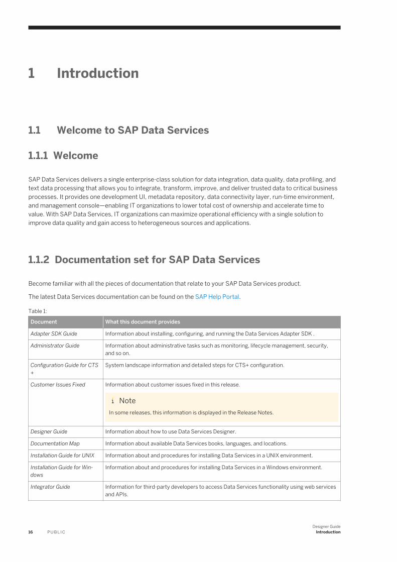
SAP Data Services delivers a single enterprise-class solution for data integration, data quality, data profiling, and text data processing that allows you to integrate, transform, improve, and deliver trusted data to critical business processes. It provides one development UI, metadata repository, data connectivity layer, run-time environment, and management console—enabling IT organizations to lower total cost of ownership and accelerate time to value. With SAP Data Services, IT organizations can maximize operational efficiency with a single solution to improve data quality and gain access to heterogeneous sources and applications.
1.1.2 Documentation set for SAP Data Services
Become familiar with all the pieces of documentation that relate to your SAP Data Services product.
The latest Data Services documentation can be found on the SAP Help Portal.
Table 1:
Document What this document provides
Adapter SDK Guide Information about installing, configuring, and running the Data Services Adapter SDK .
Administrator Guide Information about administrative tasks such as monitoring, lifecycle management, security, and so on.
Configuration Guide for CTS+
System landscape information and detailed steps for CTS+ configuration.
Customer Issues Fixed Information about customer issues fixed in this release.
NoteIn some releases, this information is displayed in the Release Notes.
Designer Guide Information about how to use Data Services Designer.
Documentation Map Information about available Data Services books, languages, and locations.
Installation Guide for UNIX Information about and procedures for installing Data Services in a UNIX environment.
Installation Guide for Windows
Information about and procedures for installing Data Services in a Windows environment.
Integrator Guide Information for third-party developers to access Data Services functionality using web services and APIs.
16 P U B L I CDesigner Guide
Introduction
Document What this document provides
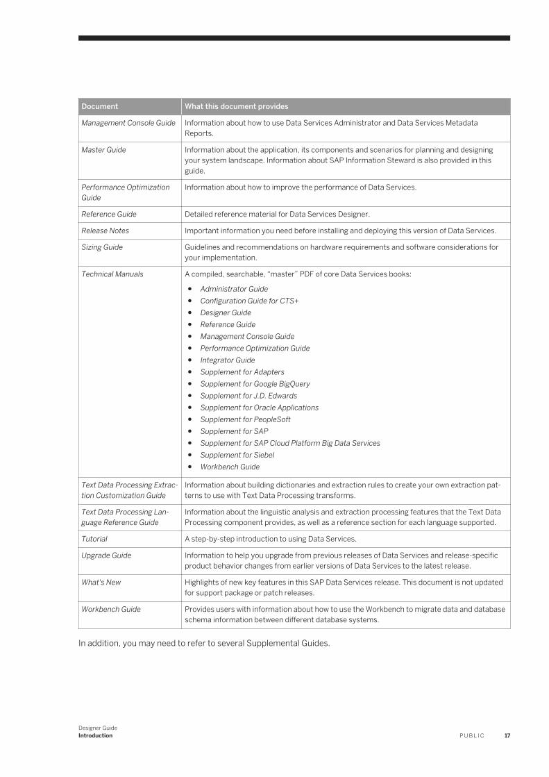
Management Console Guide Information about how to use Data Services Administrator and Data Services Metadata Reports.
Master Guide Information about the application, its components and scenarios for planning and designing your system landscape. Information about SAP Information Steward is also provided in this guide.
Performance Optimization Guide
Information about how to improve the performance of Data Services.
Reference Guide Detailed reference material for Data Services Designer.
Release Notes Important information you need before installing and deploying this version of Data Services.
Sizing Guide Guidelines and recommendations on hardware requirements and software considerations for your implementation.
Technical Manuals A compiled, searchable, “master” PDF of core Data Services books:
● Administrator Guide● Configuration Guide for CTS+● Designer Guide ● Reference Guide● Management Console Guide● Performance Optimization Guide● Integrator Guide● Supplement for Adapters● Supplement for Google BigQuery● Supplement for J.D. Edwards● Supplement for Oracle Applications● Supplement for PeopleSoft ● Supplement for SAP ● Supplement for SAP Cloud Platform Big Data Services● Supplement for Siebel● Workbench Guide
Text Data Processing Extraction Customization Guide
Information about building dictionaries and extraction rules to create your own extraction patterns to use with Text Data Processing transforms.
Text Data Processing Language Reference Guide
Information about the linguistic analysis and extraction processing features that the Text Data Processing component provides, as well as a reference section for each language supported.
Tutorial A step-by-step introduction to using Data Services.
Upgrade Guide Information to help you upgrade from previous releases of Data Services and release-specific product behavior changes from earlier versions of Data Services to the latest release.
What's New Highlights of new key features in this SAP Data Services release. This document is not updated for support package or patch releases.
Workbench Guide Provides users with information about how to use the Workbench to migrate data and database schema information between different database systems.
In addition, you may need to refer to several Supplemental Guides.
Designer GuideIntroduction P U B L I C 17
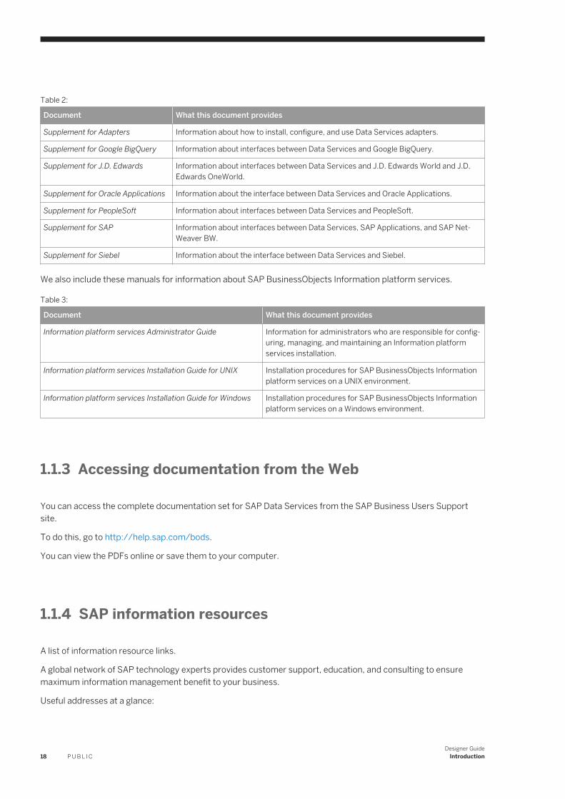
Table 2:
Document What this document provides
Supplement for Adapters Information about how to install, configure, and use Data Services adapters.
Supplement for Google BigQuery Information about interfaces between Data Services and Google BigQuery.
Supplement for J.D. Edwards Information about interfaces between Data Services and J.D. Edwards World and J.D. Edwards OneWorld.
Supplement for Oracle Applications Information about the interface between Data Services and Oracle Applications.
Supplement for PeopleSoft Information about interfaces between Data Services and PeopleSoft.
Supplement for SAP Information about interfaces between Data Services, SAP Applications, and SAP NetWeaver BW.
Supplement for Siebel Information about the interface between Data Services and Siebel.
We also include these manuals for information about SAP BusinessObjects Information platform services.
Table 3:
Document What this document provides
Information platform services Administrator Guide Information for administrators who are responsible for configuring, managing, and maintaining an Information platform services installation.
Information platform services Installation Guide for UNIX Installation procedures for SAP BusinessObjects Information platform services on a UNIX environment.
Information platform services Installation Guide for Windows Installation procedures for SAP BusinessObjects Information platform services on a Windows environment.
1.1.3 Accessing documentation from the Web
You can access the complete documentation set for SAP Data Services from the SAP Business Users Support site.
To do this, go to http://help.sap.com/bods.
You can view the PDFs online or save them to your computer.
1.1.4 SAP information resources
A list of information resource links.
A global network of SAP technology experts provides customer support, education, and consulting to ensure maximum information management benefit to your business.
Useful addresses at a glance:
18 P U B L I CDesigner Guide
Introduction
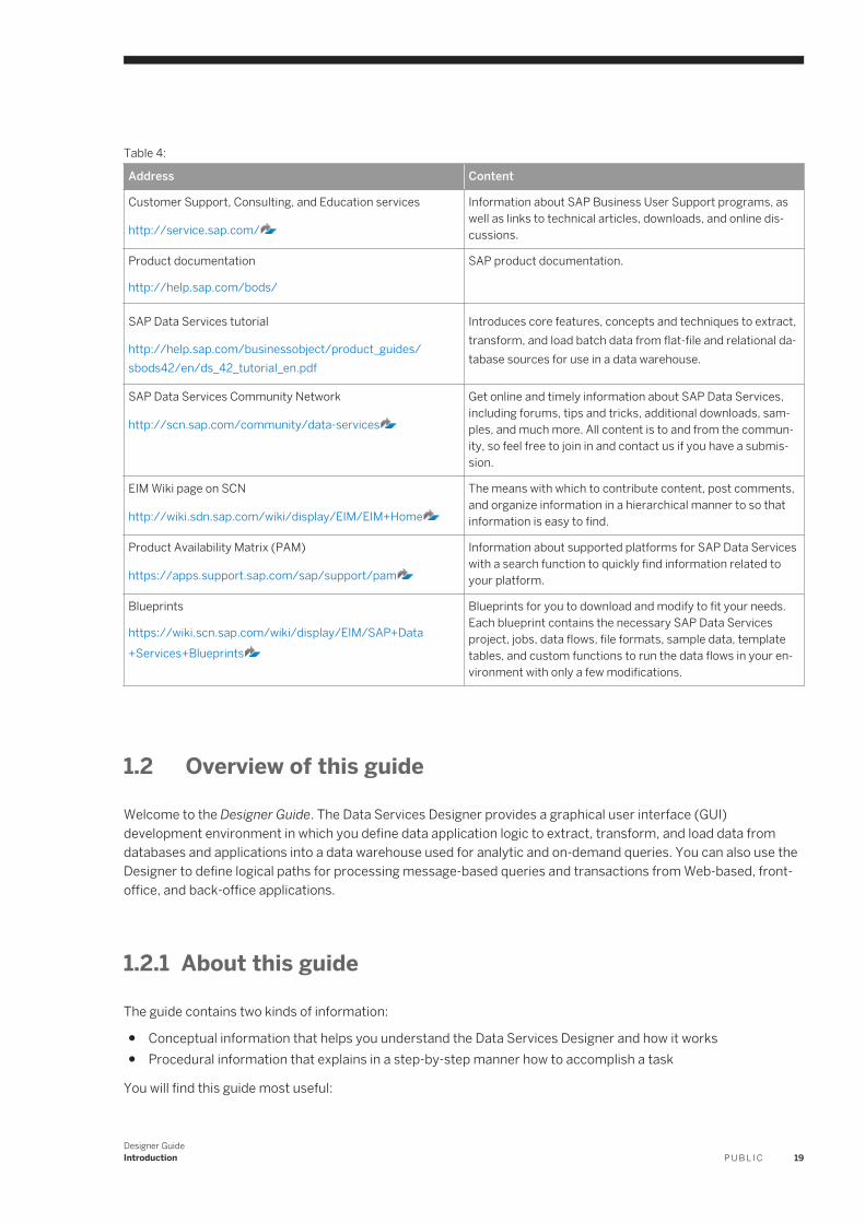
Table 4:
Address Content
Customer Support, Consulting, and Education services
http://service.sap.com/
Information about SAP Business User Support programs, as well as links to technical articles, downloads, and online discussions.
Product documentation
http://help.sap.com/bods/
SAP product documentation.
SAP Data Services tutorial
http://help.sap.com/businessobject/product_guides/sbods42/en/ds_42_tutorial_en.pdf
Introduces core features, concepts and techniques to extract, transform, and load batch data from flat-file and relational database sources for use in a data warehouse.
SAP Data Services Community Network
http://scn.sap.com/community/data-services
Get online and timely information about SAP Data Services, including forums, tips and tricks, additional downloads, samples, and much more. All content is to and from the community, so feel free to join in and contact us if you have a submission.
EIM Wiki page on SCN
http://wiki.sdn.sap.com/wiki/display/EIM/EIM+Home
The means with which to contribute content, post comments, and organize information in a hierarchical manner to so that information is easy to find.
Product Availability Matrix (PAM)
https://apps.support.sap.com/sap/support/pam
Information about supported platforms for SAP Data Services with a search function to quickly find information related to your platform.
Blueprints
https://wiki.scn.sap.com/wiki/display/EIM/SAP+Data+Services+Blueprints
Blueprints for you to download and modify to fit your needs. Each blueprint contains the necessary SAP Data Services project, jobs, data flows, file formats, sample data, template tables, and custom functions to run the data flows in your environment with only a few modifications.
1.2 Overview of this guide
Welcome to the Designer Guide. The Data Services Designer provides a graphical user interface (GUI) development environment in which you define data application logic to extract, transform, and load data from databases and applications into a data warehouse used for analytic and on-demand queries. You can also use the Designer to define logical paths for processing message-based queries and transactions from Web-based, front-office, and back-office applications.
1.2.1 About this guide
The guide contains two kinds of information:
● Conceptual information that helps you understand the Data Services Designer and how it works● Procedural information that explains in a step-by-step manner how to accomplish a task
You will find this guide most useful:
Designer GuideIntroduction P U B L I C 19
● While you are learning about the product● While you are performing tasks in the design and early testing phase of your data-movement projects● As a general source of information during any phase of your projects
1.2.2 Who should read this guide
This and other Data Services product documentation assumes the following:
● You are an application developer, consultant, or database administrator working on data extraction, data warehousing, data integration, or data quality.
● You understand your source data systems, RDBMS, business intelligence, and messaging concepts.● You understand your organization's data needs.● You are familiar with SQL (Structured Query Language).● If you are interested in using this product to design real-time processing, you should be familiar with:
○ DTD and XML Schema formats for XML files○ Publishing Web Services (WSDL, REST, HTTP, and SOAP protocols, etc.)
● You are familiar Data Services installation environments—Microsoft Windows or UNIX.
20 P U B L I CDesigner Guide
Introduction
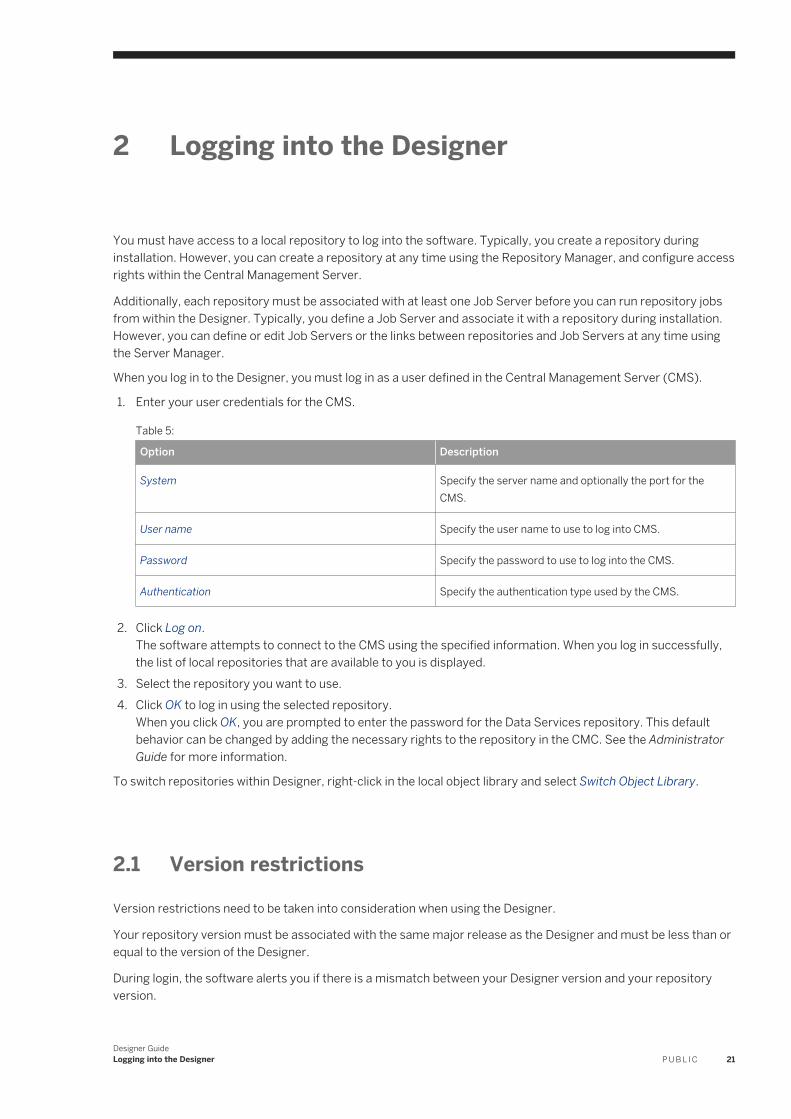
2 Logging into the Designer
You must have access to a local repository to log into the software. Typically, you create a repository during installation. However, you can create a repository at any time using the Repository Manager, and configure access rights within the Central Management Server.
Additionally, each repository must be associated with at least one Job Server before you can run repository jobs from within the Designer. Typically, you define a Job Server and associate it with a repository during installation. However, you can define or edit Job Servers or the links between repositories and Job Servers at any time using the Server Manager.
When you log in to the Designer, you must log in as a user defined in the Central Management Server (CMS).
1. Enter your user credentials for the CMS.
Table 5:
Option Description
System Specify the server name and optionally the port for the CMS.
User name Specify the user name to use to log into CMS.
Password Specify the password to use to log into the CMS.
Authentication Specify the authentication type used by the CMS.
2. Click Log on.The software attempts to connect to the CMS using the specified information. When you log in successfully, the list of local repositories that are available to you is displayed.
3. Select the repository you want to use.4. Click OK to log in using the selected repository.
When you click OK, you are prompted to enter the password for the Data Services repository. This default behavior can be changed by adding the necessary rights to the repository in the CMC. See the Administrator Guide for more information.
To switch repositories within Designer, right-click in the local object library and select Switch Object Library.
2.1 Version restrictions
Version restrictions need to be taken into consideration when using the Designer.
Your repository version must be associated with the same major release as the Designer and must be less than or equal to the version of the Designer.
During login, the software alerts you if there is a mismatch between your Designer version and your repository version.
Designer GuideLogging into the Designer P U B L I C 21
After you log in, you can view the software and repository versions by selecting Help About Data Services .
Some features in the current release of the Designer might not be supported if you are not logged in to the latest version of the repository.
2.2 Resetting users
If more than one person attempts to log in to a single repository, you may have to reset or log off a user to continue.
The Reset Users window lists users and the time they logged in to the repository.
From this window, you have several options. You can:
● Reset Users to clear the users in the repository and set yourself as the currently logged in user.● Continue to log in to the system regardless of who else might be connected.● Exit to terminate the login attempt and close the session.
NoteOnly use Reset Users or Continue if you know that you are the only user connected to the repository. Subsequent changes could corrupt the repository.
22 P U B L I CDesigner Guide
Logging into the Designer
3 Designer User Interface
This section provides basic information about the Designer's graphical user interface.
3.1 Objects
All "entities" you define, edit, or work with in Designer are called objects.
The local object library shows objects such as source and target metadata, system functions, projects, and jobs.
Objects are hierarchical and consist of:
● Options, which control the operation of objects. For example, in a datastore, the name of the database to which you connect is an option for the datastore object.
● Properties, which document the object. For example, the name of the object and the date it was created are properties. Properties describe an object, but do not affect its operation.
The software has two types of objects:
● Reusable● Single-use
The object type affects how you define and retrieve the object.
3.1.1 Reusable objects
You can reuse and replicate most objects defined in the software.
After you define and save a reusable object, the software stores the definition in the local repository. You can then reuse the definition as often as necessary by creating calls to the definition. Access reusable objects through the local object library.
A reusable object has a single definition; all calls to the object refer to that definition. If you change the definition of the object in one place, you are changing the object in all other places in which it appears.
A data flow, for example, is a reusable object. Multiple jobs, like a weekly load job and a daily load job, can call the same data flow. If the data flow changes, both jobs use the new version of the data flow.
The object library contains object definitions. When you drag and drop an object from the object library, you are really creating a new reference (or call) to the existing object definition.
Related Information
Working with new reusable objects [page 40]
Designer GuideDesigner User Interface P U B L I C 23

3.1.2 Single-use objects
Single-use objects appear only as components of other objects and operate only in the context in which they were created.
You would define a single-use object within the context of a single job or data flow (for example, scripts and specific transform definitions).
3.1.3 Object hierarchy
Object relationships are hierarchical.
The following figure shows the relationships between major object types:
24 P U B L I CDesigner Guide
Designer User Interface
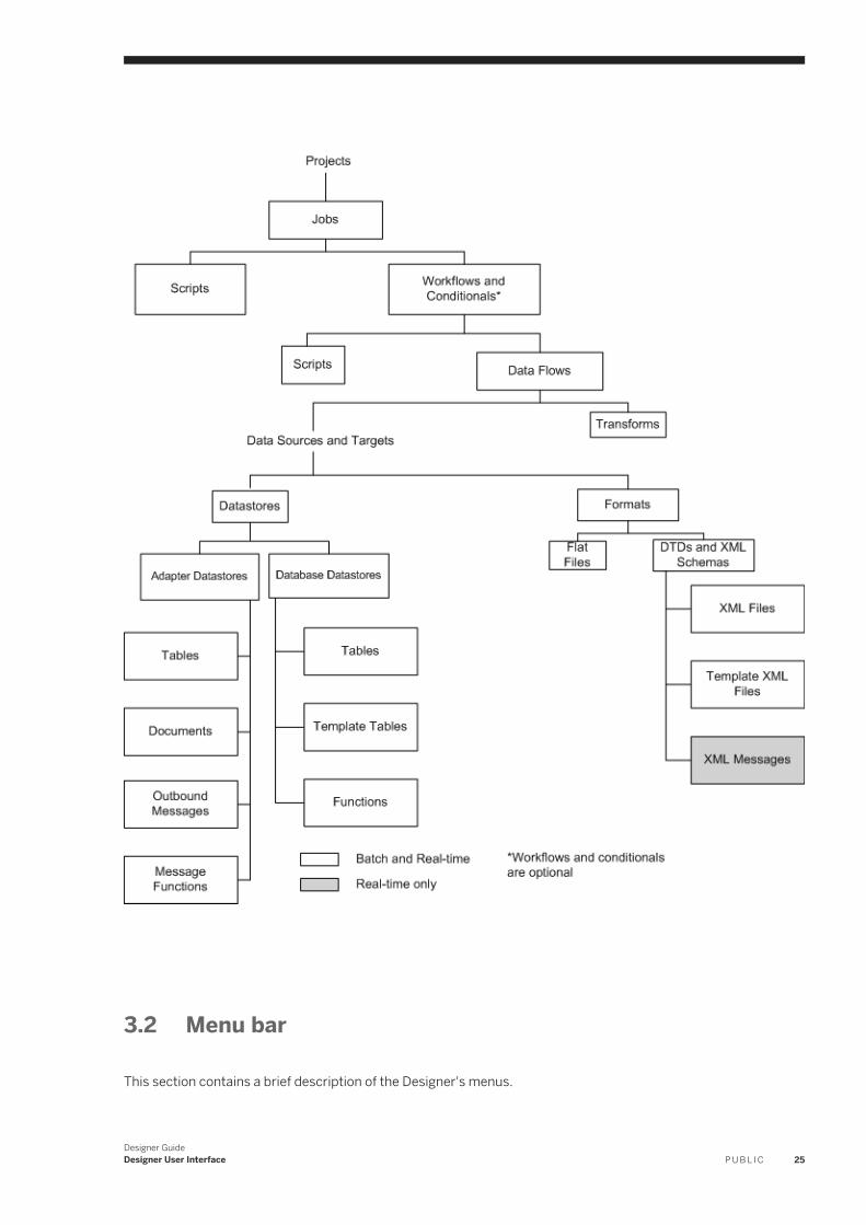
3.2 Menu bar
This section contains a brief description of the Designer's menus.
Designer GuideDesigner User Interface P U B L I C 25
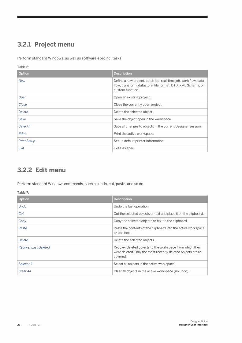
3.2.1 Project menu
Perform standard Windows, as well as software-specific, tasks.
Table 6:
Option Description
New Define a new project, batch job, real-time job, work flow, data flow, transform, datastore, file format, DTD, XML Schema, or custom function.
Open Open an existing project.
Close Close the currently open project.
Delete Delete the selected object.
Save Save the object open in the workspace.
Save All Save all changes to objects in the current Designer session.
Print Print the active workspace.
Print Setup Set up default printer information.
Exit Exit Designer.
3.2.2 Edit menu
Perform standard Windows commands, such as undo, cut, paste, and so on.
Table 7:
Option Description
Undo Undo the last operation.
Cut Cut the selected objects or text and place it on the clipboard.
Copy Copy the selected objects or text to the clipboard.
Paste Paste the contents of the clipboard into the active workspace or text box.
Delete Delete the selected objects.
Recover Last Deleted Recover deleted objects to the workspace from which they were deleted. Only the most recently deleted objects are recovered.
Select All Select all objects in the active workspace.
Clear All Clear all objects in the active workspace (no undo).
26 P U B L I CDesigner Guide
Designer User Interface
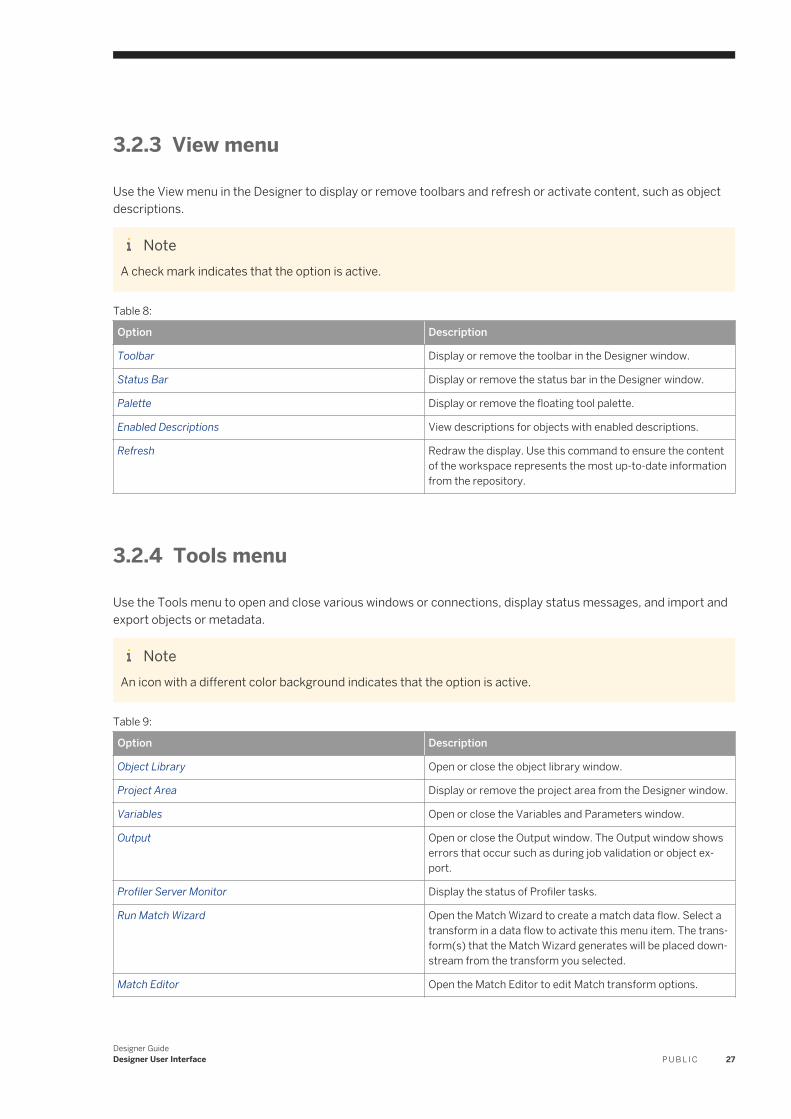
3.2.3 View menu
Use the View menu in the Designer to display or remove toolbars and refresh or activate content, such as object descriptions.
NoteA check mark indicates that the option is active.
Table 8:
Option Description
Toolbar Display or remove the toolbar in the Designer window.
Status Bar Display or remove the status bar in the Designer window.
Palette Display or remove the floating tool palette.
Enabled Descriptions View descriptions for objects with enabled descriptions.
Refresh Redraw the display. Use this command to ensure the content of the workspace represents the most up-to-date information from the repository.
3.2.4 Tools menu
Use the Tools menu to open and close various windows or connections, display status messages, and import and export objects or metadata.
NoteAn icon with a different color background indicates that the option is active.
Table 9:
Option Description
Object Library Open or close the object library window.
Project Area Display or remove the project area from the Designer window.
Variables Open or close the Variables and Parameters window.
Output Open or close the Output window. The Output window shows errors that occur such as during job validation or object export.
Profiler Server Monitor Display the status of Profiler tasks.
Run Match Wizard Open the Match Wizard to create a match data flow. Select a transform in a data flow to activate this menu item. The transform(s) that the Match Wizard generates will be placed downstream from the transform you selected.
Match Editor Open the Match Editor to edit Match transform options.
Designer GuideDesigner User Interface P U B L I C 27
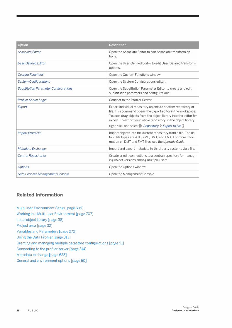
Option Description
Associate Editor Open the Associate Editor to edit Associate transform options.
User-Defined Editor Open the User-Defined Editor to edit User-Defined transform options.
Custom Functions Open the Custom Functions window.
System Configurations Open the System Configurations editor.
Substitution Parameter Configurations Open the Substitution Parameter Editor to create and edit substitution paramters and configurations.
Profiler Server Login Connect to the Profiler Server.
Export Export individual repository objects to another repository or file. This command opens the Export editor in the workspace. You can drag objects from the object library into the editor for export. To export your whole repository, in the object library
right-click and select Repository Export to file .
Import From File Import objects into the current repository from a file. The default file types are ATL, XML, DMT, and FMT. For more information on DMT and FMT files, see the Upgrade Guide.
Metadata Exchange Import and export metadata to third-party systems via a file.
Central Repositories Create or edit connections to a central repository for managing object versions among multiple users.
Options Open the Options window.
Data Services Management Console Open the Management Console.
Related Information
Multi-user Environment Setup [page 699]Working in a Multi-user Environment [page 707]Local object library [page 38]Project area [page 32]Variables and Parameters [page 272]Using the Data Profiler [page 313]Creating and managing multiple datastore configurations [page 91]Connecting to the profiler server [page 314]Metadata exchange [page 623]General and environment options [page 50]
28 P U B L I CDesigner Guide
Designer User Interface
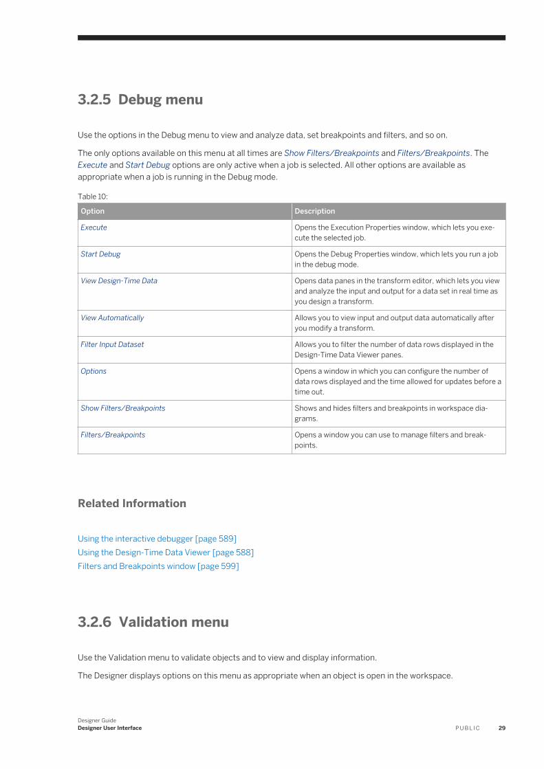
3.2.5 Debug menu
Use the options in the Debug menu to view and analyze data, set breakpoints and filters, and so on.
The only options available on this menu at all times are Show Filters/Breakpoints and Filters/Breakpoints. The Execute and Start Debug options are only active when a job is selected. All other options are available as appropriate when a job is running in the Debug mode.
Table 10:
Option Description
Execute Opens the Execution Properties window, which lets you execute the selected job.
Start Debug Opens the Debug Properties window, which lets you run a job in the debug mode.
View Design-Time Data Opens data panes in the transform editor, which lets you view and analyze the input and output for a data set in real time as you design a transform.
View Automatically Allows you to view input and output data automatically after you modify a transform.
Filter Input Dataset Allows you to filter the number of data rows displayed in the Design-Time Data Viewer panes.
Options Opens a window in which you can configure the number of data rows displayed and the time allowed for updates before a time out.
Show Filters/Breakpoints Shows and hides filters and breakpoints in workspace diagrams.
Filters/Breakpoints Opens a window you can use to manage filters and breakpoints.
Related Information
Using the interactive debugger [page 589]Using the Design-Time Data Viewer [page 588]Filters and Breakpoints window [page 599]
3.2.6 Validation menu
Use the Validation menu to validate objects and to view and display information.
The Designer displays options on this menu as appropriate when an object is open in the workspace.
Designer GuideDesigner User Interface P U B L I C 29
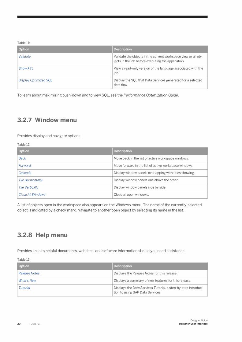
Table 11:
Option Description
Validate Validate the objects in the current workspace view or all objects in the job before executing the application.
Show ATL View a read-only version of the language associated with the job.
Display Optimized SQL Display the SQL that Data Services generated for a selected data flow.
To learn about maximizing push-down and to view SQL, see the Performance Optimization Guide.
3.2.7 Window menu
Provides display and navigate options.
Table 12:
Option Description
Back Move back in the list of active workspace windows.
Forward Move forward in the list of active workspace windows.
Cascade Display window panels overlapping with titles showing.
Tile Horizontally Display window panels one above the other.
Tile Vertically Display window panels side by side.
Close All Windows Close all open windows.
A list of objects open in the workspace also appears on the Windows menu. The name of the currently-selected object is indicated by a check mark. Navigate to another open object by selecting its name in the list.
3.2.8 Help menu
Provides links to helpful documents, websites, and software information should you need assistance.
Table 13:
Option Description
Release Notes Displays the Release Notes for this release.
What's New Displays a summary of new features for this release.
Tutorial Displays the Data Services Tutorial, a step-by-step introduction to using SAP Data Services.
30 P U B L I CDesigner Guide
Designer User Interface
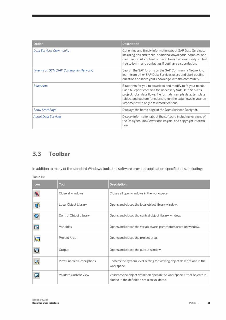
Option Description
Data Services Community Get online and timely information about SAP Data Services, including tips and tricks, additional downloads, samples, and much more. All content is to and from the community, so feel free to join in and contact us if you have a submission.
Forums on SCN (SAP Community Network) Search the SAP forums on the SAP Community Network to learn from other SAP Data Services users and start posting questions or share your knowledge with the community.
Blueprints Blueprints for you to download and modify to fit your needs. Each blueprint contains the necessary SAP Data Services project, jobs, data flows, file formats, sample data, template tables, and custom functions to run the data flows in your environment with only a few modifications.
Show Start Page Displays the home page of the Data Services Designer.
About Data Services Display information about the software including versions of the Designer, Job Server and engine, and copyright information.
3.3 Toolbar
In addition to many of the standard Windows tools, the software provides application-specific tools, including:
Table 14:
Icon Tool Description
Close all windows Closes all open windows in the workspace.
Local Object Library Opens and closes the local object library window.
Central Object Library Opens and closes the central object library window.
Variables Opens and closes the variables and parameters creation window.
Project Area Opens and closes the project area.
Output Opens and closes the output window.
View Enabled Descriptions Enables the system level setting for viewing object descriptions in the workspace.
Validate Current View Validates the object definition open in the workspace. Other objects included in the definition are also validated.
Designer GuideDesigner User Interface P U B L I C 31
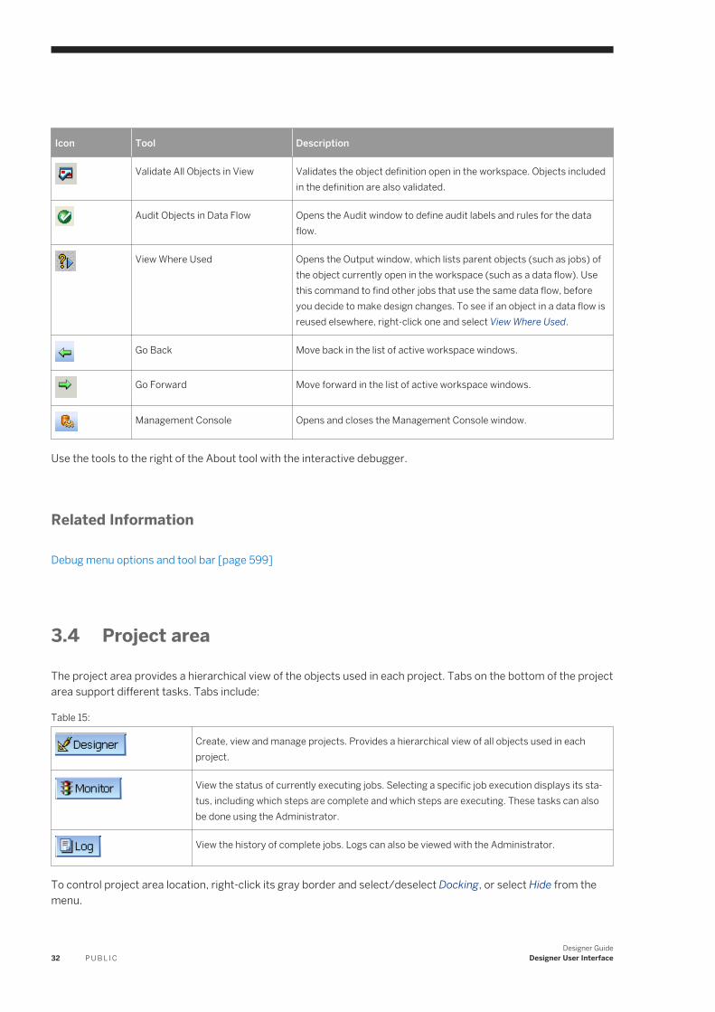
Icon Tool Description
Validate All Objects in View Validates the object definition open in the workspace. Objects included in the definition are also validated.
Audit Objects in Data Flow Opens the Audit window to define audit labels and rules for the data flow.
View Where Used Opens the Output window, which lists parent objects (such as jobs) of the object currently open in the workspace (such as a data flow). Use this command to find other jobs that use the same data flow, before you decide to make design changes. To see if an object in a data flow is reused elsewhere, right-click one and select View Where Used.
Go Back Move back in the list of active workspace windows.
Go Forward Move forward in the list of active workspace windows.
Management Console Opens and closes the Management Console window.
Use the tools to the right of the About tool with the interactive debugger.
Related Information
Debug menu options and tool bar [page 599]
3.4 Project area
The project area provides a hierarchical view of the objects used in each project. Tabs on the bottom of the project area support different tasks. Tabs include:
Table 15:
Create, view and manage projects. Provides a hierarchical view of all objects used in each project.
View the status of currently executing jobs. Selecting a specific job execution displays its status, including which steps are complete and which steps are executing. These tasks can also be done using the Administrator.
View the history of complete jobs. Logs can also be viewed with the Administrator.
To control project area location, right-click its gray border and select/deselect Docking, or select Hide from the menu.
32 P U B L I CDesigner Guide
Designer User Interface
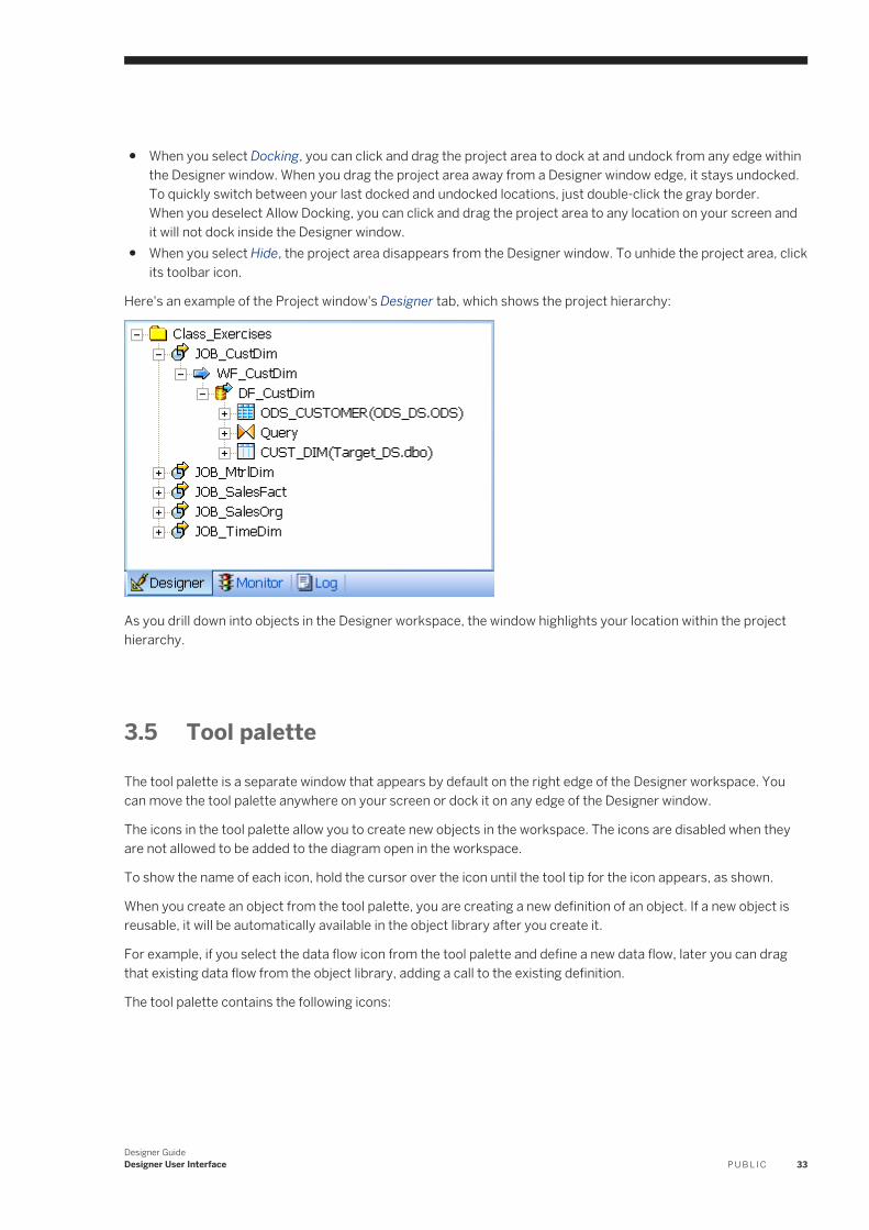
● When you select Docking, you can click and drag the project area to dock at and undock from any edge within the Designer window. When you drag the project area away from a Designer window edge, it stays undocked. To quickly switch between your last docked and undocked locations, just double-click the gray border.When you deselect Allow Docking, you can click and drag the project area to any location on your screen and it will not dock inside the Designer window.
● When you select Hide, the project area disappears from the Designer window. To unhide the project area, click its toolbar icon.
Here's an example of the Project window's Designer tab, which shows the project hierarchy:
As you drill down into objects in the Designer workspace, the window highlights your location within the project hierarchy.
3.5 Tool palette
The tool palette is a separate window that appears by default on the right edge of the Designer workspace. You can move the tool palette anywhere on your screen or dock it on any edge of the Designer window.
The icons in the tool palette allow you to create new objects in the workspace. The icons are disabled when they are not allowed to be added to the diagram open in the workspace.
To show the name of each icon, hold the cursor over the icon until the tool tip for the icon appears, as shown.
When you create an object from the tool palette, you are creating a new definition of an object. If a new object is reusable, it will be automatically available in the object library after you create it.
For example, if you select the data flow icon from the tool palette and define a new data flow, later you can drag that existing data flow from the object library, adding a call to the existing definition.
The tool palette contains the following icons:
Designer GuideDesigner User Interface P U B L I C 33
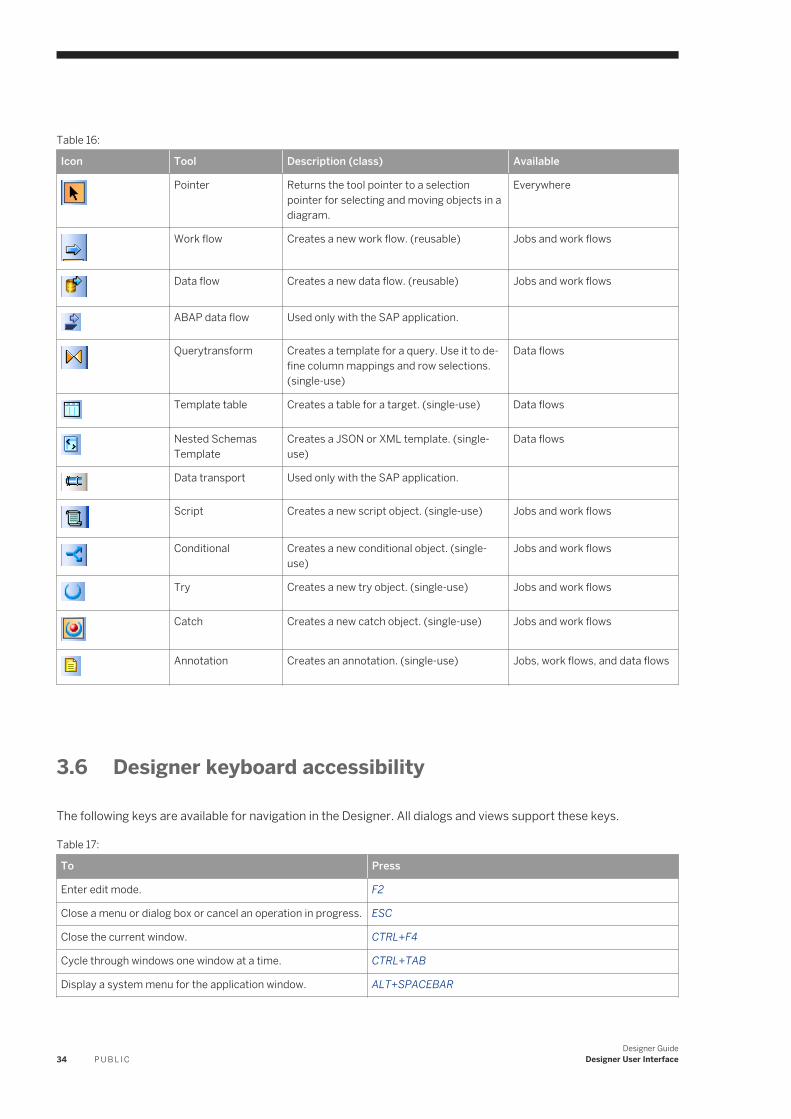
Table 16:
Icon Tool Description (class) Available
Pointer Returns the tool pointer to a selection pointer for selecting and moving objects in a diagram.
Everywhere
Work flow Creates a new work flow. (reusable) Jobs and work flows
Data flow Creates a new data flow. (reusable) Jobs and work flows
ABAP data flow Used only with the SAP application.
Querytransform Creates a template for a query. Use it to define column mappings and row selections. (single-use)
Data flows
Template table Creates a table for a target. (single-use) Data flows
Nested Schemas Template
Creates a JSON or XML template. (single-use)
Data flows
Data transport Used only with the SAP application.
Script Creates a new script object. (single-use) Jobs and work flows
Conditional Creates a new conditional object. (single-use)
Jobs and work flows
Try Creates a new try object. (single-use) Jobs and work flows
Catch Creates a new catch object. (single-use) Jobs and work flows
Annotation Creates an annotation. (single-use) Jobs, work flows, and data flows
3.6 Designer keyboard accessibility
The following keys are available for navigation in the Designer. All dialogs and views support these keys.
Table 17:
To Press
Enter edit mode. F2
Close a menu or dialog box or cancel an operation in progress. ESC
Close the current window. CTRL+F4
Cycle through windows one window at a time. CTRL+TAB
Display a system menu for the application window. ALT+SPACEBAR
34 P U B L I CDesigner Guide
Designer User Interface
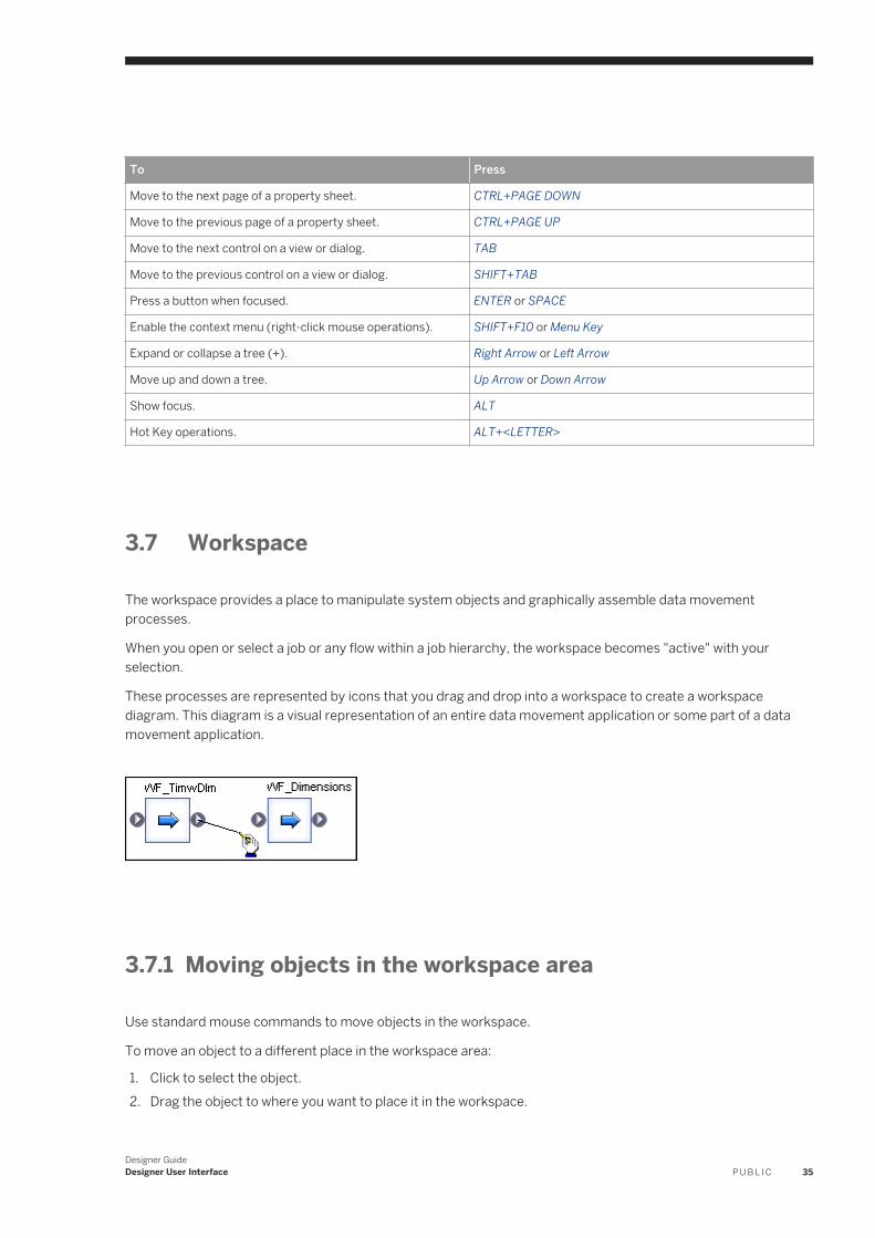
To Press
Move to the next page of a property sheet. CTRL+PAGE DOWN
Move to the previous page of a property sheet. CTRL+PAGE UP
Move to the next control on a view or dialog. TAB
Move to the previous control on a view or dialog. SHIFT+TAB
Press a button when focused. ENTER or SPACE
Enable the context menu (right-click mouse operations). SHIFT+F10 or Menu Key
Expand or collapse a tree (+). Right Arrow or Left Arrow
Move up and down a tree. Up Arrow or Down Arrow
Show focus. ALT
Hot Key operations. ALT+<LETTER>
3.7 Workspace
The workspace provides a place to manipulate system objects and graphically assemble data movement processes.
When you open or select a job or any flow within a job hierarchy, the workspace becomes "active" with your selection.
These processes are represented by icons that you drag and drop into a workspace to create a workspace diagram. This diagram is a visual representation of an entire data movement application or some part of a data movement application.
3.7.1 Moving objects in the workspace area
Use standard mouse commands to move objects in the workspace.
To move an object to a different place in the workspace area:
1. Click to select the object.2. Drag the object to where you want to place it in the workspace.
Designer GuideDesigner User Interface P U B L I C 35
3.7.2 Connecting objects
You specify the flow of data through jobs and work flows by connecting objects in the workspace from left to right in the order you want the data to be moved.
To connect objects:
1. Place the objects you want to connect in the workspace.2. Click and drag from the triangle on the right edge of an object to the triangle on the left edge of the next object
in the flow.
3.7.3 Disconnecting objects
You can disconnect objects in the workspace.
To disconnect objects:
1. Click the connecting line.2. Press the Delete key.
3.7.4 Describing objects
You can use descriptions to add comments about objects.
You can use annotations to explain a job, work flow, or data flow. You can view object descriptions and annotations in the workspace. Together, descriptions and annotations allow you to document an SAP Data Services application. For example, you can describe the incremental behavior of individual jobs with numerous annotations and label each object with a basic description.
ExampleThis job loads current categories and expenses and produces tables for analysis.
Related Information
Creating descriptions [page 44]Creating annotations [page 46]
36 P U B L I CDesigner Guide
Designer User Interface
3.7.5 Scaling the workspace
By scaling the workspace, you can change the focus of a job, work flow, or data flow.
For example, you might want to increase the scale to examine a particular part of a work flow, or you might want to reduce the scale so that you can examine the entire work flow without scrolling.
There are several ways to scale the workspace:
● In the drop-down list on the tool bar, select a predefined scale or enter a custom value (for example, 100%).● Right-click in the workspace and select a desired scale.● Select Scale to Fit. The Designer calculates the scale that fits the entire project in the current view area.● Select Scale to Whole to show the entire workspace area in the current view area.
3.7.6 Arranging workspace windows
The Window menu allows you to arrange multiple open workspace windows.
You can arrange the windows in the following ways:
● cascade● tile horizontally● tile vertically
3.7.7 Closing workspace windows
When you drill into an object in the project area or workspace, a view of the object's definition opens in the workspace area. These views use system resources and should be closed when not in use.
The view is marked by a tab at the bottom of the workspace area, and as you open more objects in the workspace, more tabs appear. (You can show/hide these tabs from the Tools Options menu. Go to DesignerGeneral options and select/deselect Show tabs in workspace.)
NoteThese views use system resources. If you have a large number of open views, you might notice a decline in performance.
Close the views individually by clicking the close box in the top right corner of the workspace. Close all open views by selecting Window Close All Windows or clicking the Close All Windows icon on the toolbar.
Related Information
General and environment options [page 50]
Designer GuideDesigner User Interface P U B L I C 37
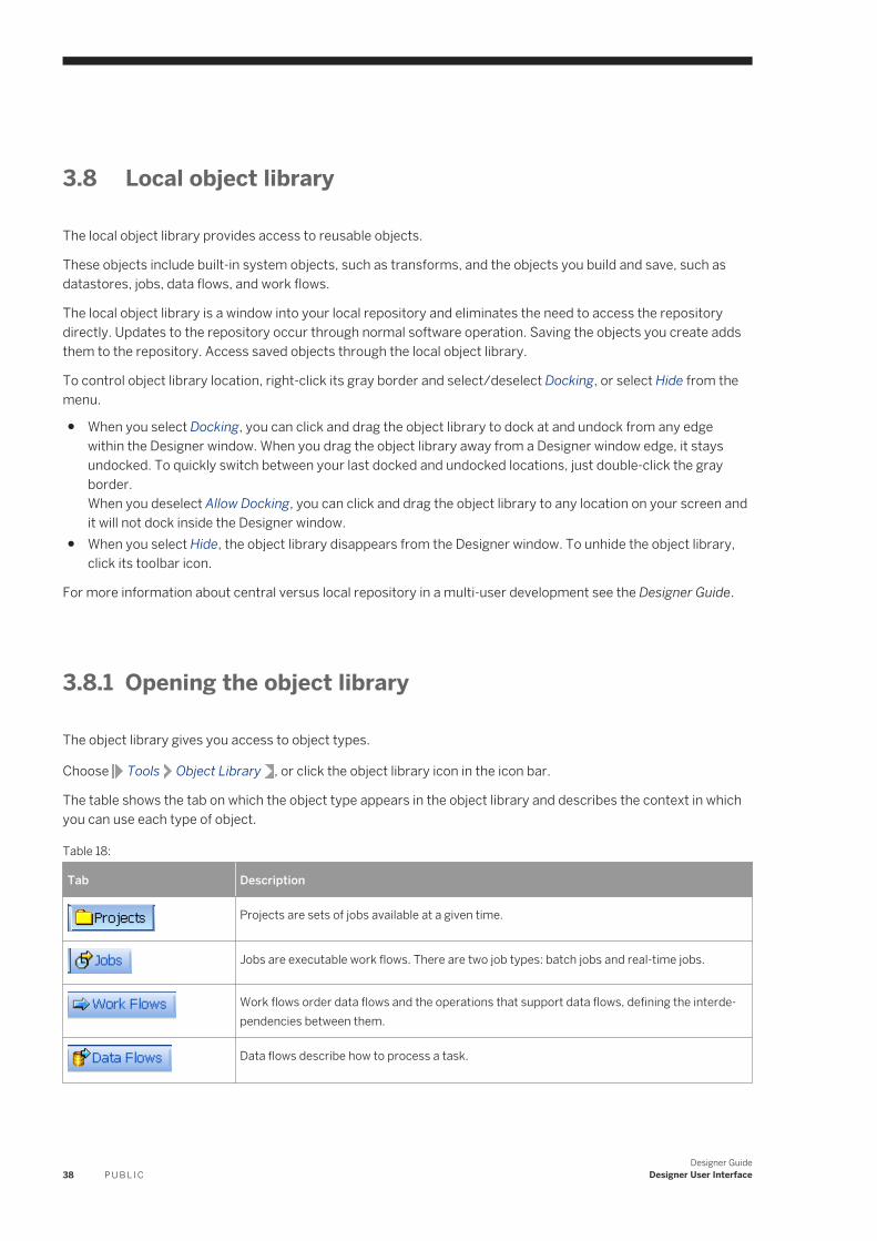
3.8 Local object library
The local object library provides access to reusable objects.
These objects include built-in system objects, such as transforms, and the objects you build and save, such as datastores, jobs, data flows, and work flows.
The local object library is a window into your local repository and eliminates the need to access the repository directly. Updates to the repository occur through normal software operation. Saving the objects you create adds them to the repository. Access saved objects through the local object library.
To control object library location, right-click its gray border and select/deselect Docking, or select Hide from the menu.
● When you select Docking, you can click and drag the object library to dock at and undock from any edge within the Designer window. When you drag the object library away from a Designer window edge, it stays undocked. To quickly switch between your last docked and undocked locations, just double-click the gray border.When you deselect Allow Docking, you can click and drag the object library to any location on your screen and it will not dock inside the Designer window.
● When you select Hide, the object library disappears from the Designer window. To unhide the object library, click its toolbar icon.
For more information about central versus local repository in a multi-user development see the Designer Guide.
3.8.1 Opening the object library
The object library gives you access to object types.
Choose Tools Object Library , or click the object library icon in the icon bar.
The table shows the tab on which the object type appears in the object library and describes the context in which you can use each type of object.
Table 18:
Tab Description
Projects are sets of jobs available at a given time.
Jobs are executable work flows. There are two job types: batch jobs and real-time jobs.
Work flows order data flows and the operations that support data flows, defining the interdependencies between them.
Data flows describe how to process a task.
38 P U B L I CDesigner Guide
Designer User Interface
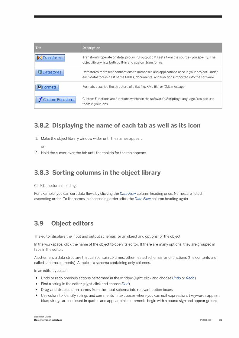
Tab Description
Transforms operate on data, producing output data sets from the sources you specify. The object library lists both built-in and custom transforms.
Datastores represent connections to databases and applications used in your project. Under each datastore is a list of the tables, documents, and functions imported into the software.
Formats describe the structure of a flat file, XML file, or XML message.
Custom Functions are functions written in the software's Scripting Language. You can use them in your jobs.
3.8.2 Displaying the name of each tab as well as its icon
1. Make the object library window wider until the names appear.
or2. Hold the cursor over the tab until the tool tip for the tab appears.
3.8.3 Sorting columns in the object library
Click the column heading.
For example, you can sort data flows by clicking the Data Flow column heading once. Names are listed in ascending order. To list names in descending order, click the Data Flow column heading again.
3.9 Object editors
The editor displays the input and output schemas for an object and options for the object.
In the workspace, click the name of the object to open its editor. If there are many options, they are grouped in tabs in the editor.
A schema is a data structure that can contain columns, other nested schemas, and functions (the contents are called schema elements). A table is a schema containing only columns.
In an editor, you can:
● Undo or redo previous actions performed in the window (right-click and choose Undo or Redo)● Find a string in the editor (right-click and choose Find)● Drag-and-drop column names from the input schema into relevant option boxes● Use colors to identify strings and comments in text boxes where you can edit expressions (keywords appear
blue; strings are enclosed in quotes and appear pink; comments begin with a pound sign and appear green)
Designer GuideDesigner User Interface P U B L I C 39
NoteYou cannot add comments to a mapping clause in a Query transform. If you do, the job will not run and you cannot successfully export it. Use the object description or workspace annotation feature instead. For example, the following syntax would not be supported on the Mapping tab:
table.column # comment
Related Information
Query Editor [page 179]Data Quality transform editors [page 183]
3.10 Working with objects
Information about common tasks you complete when working with objects in the Designer.
With these tasks, you use various parts of the Designer—the toolbar, tool palette, workspace, and local object library.
3.10.1 Working with new reusable objects
You can create reusable objects from the object library or by using the tool palette.
After you create an object, you can work with the object, editing its definition and adding calls to other objects.
Related Information
Reusable objects [page 23]
3.10.1.1 Creating a reusable object in the object library
You can create a reusable object in the object library, as opposed to creating it using the tools pallette.
1. Open the object library by choosing Tools Object Library .2. Click the tab corresponding to the object type.3. Right-click anywhere except on existing objects and choose New.
40 P U B L I CDesigner Guide
Designer User Interface
4. Right-click the new object and select Properties. Enter options such as name and description to define the object.
3.10.1.2 Creating a reusable object using the tool palette
You can reuse and replicate most objects defined in the software through the tools pallette.
1. In the tool palette, left-click the icon for the object you want to create.2. Move the cursor to the workspace and left-click again.
The object icon appears in the workspace where you have clicked.
3.10.2 Adding an existing object
Add an existing object or create a new call to an existing object.
1. Open the object library by choosing Tools Object Library .2. Click the tab corresponding to any object type.3. Select an object.4. Drag the object to the workspace.
NoteObjects dragged into the workspace must obey the hierarchy logic. For example, you can drag a data flow into a job, but you cannot drag a work flow into a data flow.
Related Information
Object hierarchy [page 24]
3.10.3 Opening an object's definition
The options that describe the operation of an object, which are viewable in the workspace when you open the object.
You can open an object's definition in one of two ways:
1. From the workspace, click the object name. The software opens a blank workspace in which you define the object.
2. From the project area, click the object.
Designer GuideDesigner User Interface P U B L I C 41
You define an object using other objects. For example, if you click the name of a batch data flow, a new workspace opens for you to assemble sources, targets, and transforms that make up the actual flow.
3.10.4 Changing object names
You can change the name of an object from the workspace or the object library.
You can also create a copy of an existing object.
NoteYou cannot change the names of built-in objects.
1. To change the name of an object in the workspacea. Click to select the object in the workspace.b. Right-click and choose Rename.c. Edit the text in the name text box.d. Click outside the text box or press Enter to save the new name.
2. To change the name of an object in the object librarya. Select the object in the object library.b. Right-click and choose Properties.c. Edit the text in the first text box.d. Click OK.
3. To copy an objecta. Select the object in the object library.b. Right-click and choose Replicate.c. The software makes a copy of the top-level object (but not of objects that it calls) and gives it a new name,
which you can edit.
3.10.5 Adding, changing, and viewing object properties
You can add, view, and, in some cases, change an object's properties through its property page.
1. Select the object in the object library.2. Right-click and choose Properties. The General tab of the Properties window opens.3. Complete the property sheets. The property sheets vary by object type, but General, Attributes and Class
Attributes are the most common and are described in the following sections.4. When finished, click OK to save changes you made to the object properties and to close the window.
Alternatively, click Apply to save changes without closing the window.
42 P U B L I CDesigner Guide
Designer User Interface
3.10.5.1 General tab
Allows you to change the object name as well as enter or edit the object description.
The General tab contains two main object properties: name and description.
You can add object descriptions to single-use objects as well as to reusable objects. Note that you can toggle object descriptions on and off by right-clicking any object in the workspace and selecting/clearing View Enabled Descriptions.
Depending on the object, other properties may appear on the General tab. Examples include:
● Execute only once● Recover as a unit● Degree of parallelism● Use database links ● Cache type ● Bypass
Related Information
Linked datastores [page 85]Recovery Mechanisms [page 612]Creating and defining data flows [page 153]
3.10.5.2 Attributes tab
Allows you to assign values to the attributes of the current object.
To assign a value to an attribute, select the attribute and enter the value in the Value box at the bottom of the window.
Some attribute values are set by the software and cannot be edited. When you select an attribute with a system-defined value, the Value field is unavailable.
3.10.5.3 Class Attributes tab
Shows the attributes available for the type of object selected.
For example, all data flow objects have the same class attributes.
To create a new attribute for a class of objects, right-click in the attribute list and select Add. The new attribute is now available for all of the objects of this class.
To delete an attribute, select it then right-click and choose Delete. You cannot delete the class attributes predefined by Data Services.
Designer GuideDesigner User Interface P U B L I C 43
3.10.6 Creating descriptions
Use descriptions to document objects.
You can see descriptions on workspace diagrams. Therefore, descriptions are a convenient way to add comments to workspace objects.
A description is associated with a particular object. When you import or export that repository object (for example, when migrating between development, test, and production environments), you also import or export its description.
The Designer determines when to show object descriptions based on a system-level setting and an object-level setting. Both settings must be activated to view the description for a particular object.
The system-level setting is unique to your setup. The system-level setting is disabled by default. To activate that system-level setting, select ViewEnabled Descriptions, or click the View Enabled Descriptions button on the toolbar.
The object-level setting is saved with the object in the repository. The object-level setting is also disabled by default unless you add or edit a description from the workspace. To activate the object-level setting, right-click the object and select Enable object description.
An ellipses after the text in a description indicates that there is more text. To see all the text, resize the description by clicking and dragging it. When you move an object, its description moves as well. To see which object is associated with which selected description, view the object's name in the status bar.
3.10.6.1 Adding a description to an object
1. In the project area or object library, right-click an object and select Properties.2. Enter your comments in the Description text box.3. Click OK.
The description for the object displays in the object library.
3.10.6.2 Displaying a description in the workspace
1. In the project area, select an existing object (such as a job) that contains an object to which you have added a description (such as a work flow).
2. From the View menu, select Enabled Descriptions.
Alternately, you can select the View Enabled Descriptions button on the toolbar.3. Right-click the work flow and select Enable Object Description.
The description displays in the workspace under the object.
44 P U B L I CDesigner Guide
Designer User Interface
3.10.6.3 Adding a description to an object from the workspace
1. From the View menu, select Enabled Descriptions.2. In the workspace, right-click an object and select Properties.3. In the Properties window, enter text in the Description box.4. Click OK.
The description displays automatically in the workspace (and the object's Enable Object Description option is selected).
3.10.6.4 Hiding an object's description
1. In the workspace diagram, right-click an object.
Alternately, you can select multiple objects by:
○ Pressing and holding the Control key while selecting objects in the workspace diagram, then right-clicking one of the selected objects.
○ Dragging a selection box around all the objects you want to select, then right-clicking one of the selected objects.
2. In the pop-up menu, deselect Enable Object Description.
The description for the object selected is hidden, even if the View Enabled Descriptions option is checked, because the object-level switch overrides the system-level switch.
3.10.6.5 Editing object descriptions
1. In the workspace, double-click an object description.2. Enter, cut, copy, or paste text into the description.3. In the Project menu, select Save.
Alternately, you can right-click any object and select Properties to open the object's Properties window and add or edit its description.
NoteIf you attempt to edit the description of a reusable object, the software alerts you that the description will be updated for every occurrence of the object, across all jobs. You can select the Don't show this warning next time check box to avoid this alert. However, after deactivating the alert, you can only reactivate the alert by calling Technical Support.
Designer GuideDesigner User Interface P U B L I C 45
3.10.7 Creating annotations
Annotations describe a flow, part of a flow, or a diagram in a workspace.
An annotation is associated with the job, work flow, or data flow where it appears. When you import or export that job, work flow, or data flow, you import or export associated annotations.
3.10.7.1 Annotating a workspace diagram
1. Open the workspace diagram you want to annotate.
You can use annotations to describe any workspace such as a job, work flow, data flow, catch, conditional, or while loop.
2. In the tool palette, click the annotation icon.3. Click a location in the workspace to place the annotation.
An annotation appears on the diagram.
You can add, edit, and delete text directly on the annotation. In addition, you can resize and move the annotation by clicking and dragging. You can add any number of annotations to a diagram.
3.10.7.2 Deleting an annotation
1. Right-click an annotation.2. Select Delete.
Alternately, you can select an annotation and press the Delete key.
3.10.8 Copying objects
Objects can be cut or copied and then pasted on the workspace where valid.
Multiple objects can be copied and pasted either within the same or other data flows, work flows, or jobs. Additionally, calls to data flows and works flows can be cut or copied and then pasted to valid objects in the workspace.
References to global variables, local variables, parameters, and substitution parameters are copied; however, you must be define each within its new context.
NoteThe paste operation duplicates the selected objects in a flow, but still calls the original objects. In other words, the paste operation uses the original object in another location. The replicate operation creates a new object in the object library.
46 P U B L I CDesigner Guide
Designer User Interface
To cut or copy and then paste objects:
1. In the workspace, select the objects you want to cut or copy.You can select multiple objects using Ctrl-click, Shift-click, or Ctrl+A.
2. Right-click and then select either Cut or Copy.3. Click within the same flow or select a different flow. Right-click and select Paste.
Where necessary to avoid a naming conflict, a new name is automatically generated.
NoteThe objects are pasted in the selected location if you right-click and select Paste.
The objects are pasted in the upper left-hand corner of the workspace if you paste using any of the following methods:○ cIick the Paste icon.
○ click Edit Paste .○ use the Ctrl+V keyboard short-cut.
If you use a method that pastes the objects to the upper left-hand corner, subsequent pasted objects are layered on top of each other.
3.10.9 Saving and deleting objects
Saving an object in the software means storing the language that describes the object to the repository.
You can save reusable objects; single-use objects are saved only as part of the definition of the reusable object that calls them.
You can choose to save changes to the reusable object currently open in the workspace. When you save the object, the object properties, the definitions of any single-use objects it calls, and any calls to other reusable objects are recorded in the repository. The content of the included reusable objects is not saved; only the call is saved.
The software stores the description even if the object is not complete or contains an error (does not validate).
3.10.9.1 Saving changes to a single reusable object
1. Open the project in which your object is included.
2. Choose Project Save .This command saves all objects open in the workspace.
Repeat these steps for other individual objects you want to save.
Designer GuideDesigner User Interface P U B L I C 47
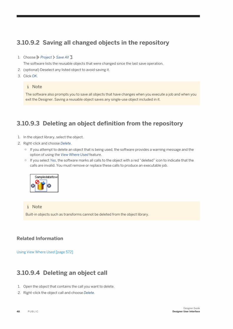
3.10.9.2 Saving all changed objects in the repository
1. Choose Project Save All .The software lists the reusable objects that were changed since the last save operation.
2. (optional) Deselect any listed object to avoid saving it.3. Click OK.
NoteThe software also prompts you to save all objects that have changes when you execute a job and when you exit the Designer. Saving a reusable object saves any single-use object included in it.
3.10.9.3 Deleting an object definition from the repository
1. In the object library, select the object.2. Right-click and choose Delete.
○ If you attempt to delete an object that is being used, the software provides a warning message and the option of using the View Where Used feature.
○ If you select Yes, the software marks all calls to the object with a red “deleted” icon to indicate that the calls are invalid. You must remove or replace these calls to produce an executable job.
NoteBuilt-in objects such as transforms cannot be deleted from the object library.
Related Information
Using View Where Used [page 572]
3.10.9.4 Deleting an object call
1. Open the object that contains the call you want to delete.2. Right-click the object call and choose Delete.
48 P U B L I CDesigner Guide
Designer User Interface
If you delete a reusable object from the workspace or from the project area, only the object call is deleted. The object definition remains in the object library.
3.10.10 Searching for objects
From within the object library, you can search for objects defined in a repository or objects available through a datastore.
1. Right-click in the object library and choose Search.The Search window appears.
2. Enter the appropriate values for the search.Options available in the Search window are described in detail following this procedure.
3. Click Search.The objects matching your entries are listed in the window. A status line at the bottom of the Search window shows where the search was conducted (Local or Central), the total number of items found, and the amount of time it took to complete the search.
From the search results window the following options are available from the context menu:
○ Open an item○ Import external tables as repository metadata○ Save as to export the search results to a CSV file○ View Where Used to show parent objects in the Output Window○ Locate in library to select the object in the local or central library○ Properties to view the attributes
You can also drag objects from the search results window and drop them in the desired location.
The Search window provides the following options:
Table 19:
Option Description
Look in Where to search.
Choose a repository or a specific datastore.
When you designate a datastore, you can also choose to search the imported data (Internal Data) or the entire datastore (External Data) You can also choose to search the Local Repository or the Central Repository.
Object type The type of object to find.
When searching the repository, choose from Tables, Files, Data flows, Work flows, Jobs, Hierarchies, IDOCs, and Domains.
When searching a datastore or application, choose from object types available through that datastore.
Designer GuideDesigner User Interface P U B L I C 49
Option Description
Name Searches for a text string in the name of the object.
If you are searching in the repository, the name is not case sensitive. If you are searching in a datastore and the name is case sensitive in that datastore, enter the name as it appears in the database or application and use double quotation marks (") around the name to preserve the case.
You can designate whether the information to be located Contains the specified name or Equals the specified name using the drop-down box next to the Name field.
Description Searches for a text string in the description of the object.
Objects imported into the repository have a description from their source. By default, objects you create in the Designer have no description unless you add one.
The search returns objects whose description attribute contains the value entered.
Search all Searches for a text string in every part of the object.
For jobs, it searches in the job itself and every job element. (Contains is the only search option for this option.)
The Search window also includes an Advanced button where, you can choose to search for objects based on their attribute values. You can search by attribute values only when searching in the repository.
The Advanced button provides the following options:
Table 20:
Option Description
Attribute The object attribute in which to search.
Value The attribute value to find.
Match The type of search performed.
Select Contains to search for any attribute that contains the value specified. Select Equals to search for any attribute that contains only the value specified.
Related Information
Using View Where Used [page 572]
3.11 General and environment optionsDisplays option groups for Designer, Data, and Job Server options.
To open the Options window, select Tools Options .
50 P U B L I CDesigner Guide
Designer User Interface
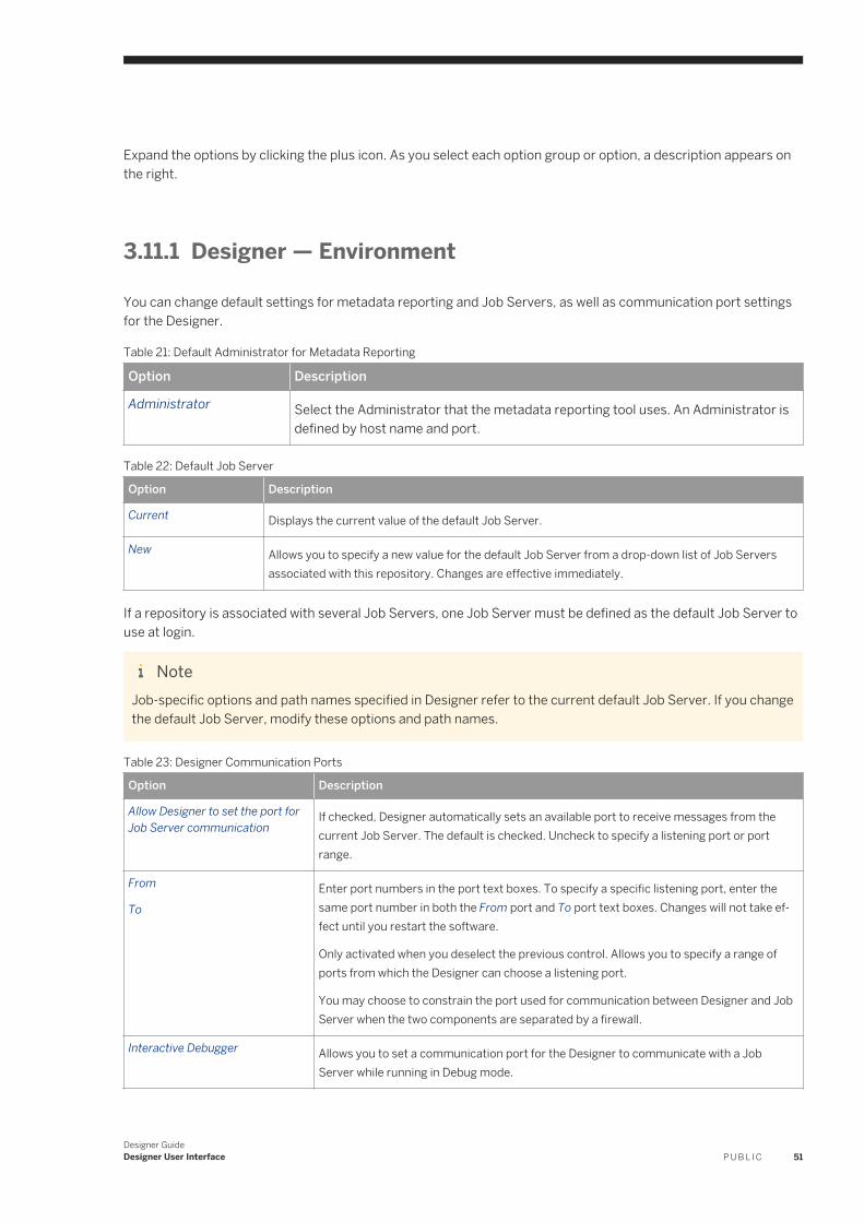
Expand the options by clicking the plus icon. As you select each option group or option, a description appears on the right.
3.11.1 Designer — Environment
You can change default settings for metadata reporting and Job Servers, as well as communication port settings for the Designer.
Table 21: Default Administrator for Metadata Reporting
Option Description
Administrator Select the Administrator that the metadata reporting tool uses. An Administrator is defined by host name and port.
Table 22: Default Job Server
Option Description
Current Displays the current value of the default Job Server.
New Allows you to specify a new value for the default Job Server from a drop-down list of Job Servers associated with this repository. Changes are effective immediately.
If a repository is associated with several Job Servers, one Job Server must be defined as the default Job Server to use at login.
NoteJob-specific options and path names specified in Designer refer to the current default Job Server. If you change the default Job Server, modify these options and path names.
Table 23: Designer Communication Ports
Option Description
Allow Designer to set the port for Job Server communication
If checked, Designer automatically sets an available port to receive messages from the current Job Server. The default is checked. Uncheck to specify a listening port or port range.
From
ToEnter port numbers in the port text boxes. To specify a specific listening port, enter the same port number in both the From port and To port text boxes. Changes will not take effect until you restart the software.
Only activated when you deselect the previous control. Allows you to specify a range of ports from which the Designer can choose a listening port.
You may choose to constrain the port used for communication between Designer and Job Server when the two components are separated by a firewall.
Interactive Debugger Allows you to set a communication port for the Designer to communicate with a Job Server while running in Debug mode.
Designer GuideDesigner User Interface P U B L I C 51
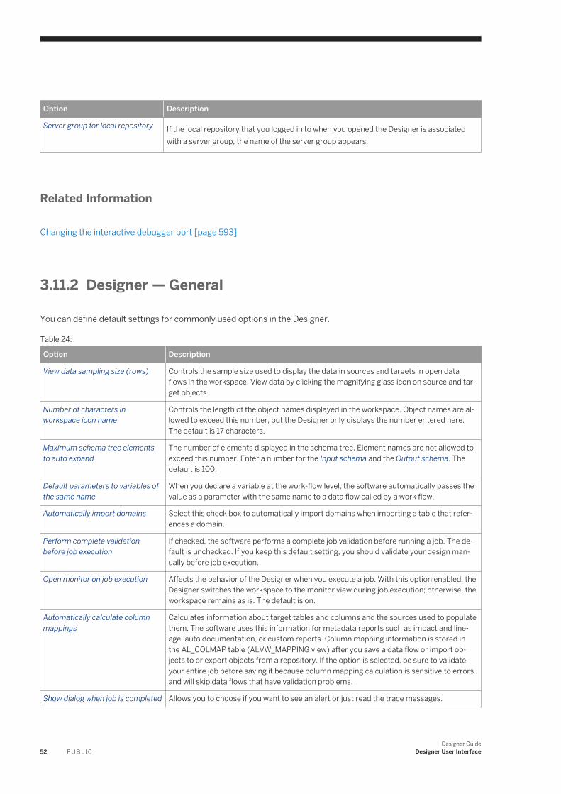
Option Description
Server group for local repository If the local repository that you logged in to when you opened the Designer is associated with a server group, the name of the server group appears.
Related Information
Changing the interactive debugger port [page 593]
3.11.2 Designer — General
You can define default settings for commonly used options in the Designer.
Table 24:
Option Description
View data sampling size (rows) Controls the sample size used to display the data in sources and targets in open data flows in the workspace. View data by clicking the magnifying glass icon on source and target objects.
Number of characters in workspace icon name
Controls the length of the object names displayed in the workspace. Object names are allowed to exceed this number, but the Designer only displays the number entered here. The default is 17 characters.
Maximum schema tree elements to auto expand
The number of elements displayed in the schema tree. Element names are not allowed to exceed this number. Enter a number for the Input schema and the Output schema. The default is 100.
Default parameters to variables of the same name
When you declare a variable at the work-flow level, the software automatically passes the value as a parameter with the same name to a data flow called by a work flow.
Automatically import domains Select this check box to automatically import domains when importing a table that references a domain.
Perform complete validation before job execution
If checked, the software performs a complete job validation before running a job. The default is unchecked. If you keep this default setting, you should validate your design manually before job execution.
Open monitor on job execution Affects the behavior of the Designer when you execute a job. With this option enabled, the Designer switches the workspace to the monitor view during job execution; otherwise, the workspace remains as is. The default is on.
Automatically calculate column mappings
Calculates information about target tables and columns and the sources used to populate them. The software uses this information for metadata reports such as impact and lineage, auto documentation, or custom reports. Column mapping information is stored in the AL_COLMAP table (ALVW_MAPPING view) after you save a data flow or import objects to or export objects from a repository. If the option is selected, be sure to validate your entire job before saving it because column mapping calculation is sensitive to errors and will skip data flows that have validation problems.
Show dialog when job is completed Allows you to choose if you want to see an alert or just read the trace messages.
52 P U B L I CDesigner Guide
Designer User Interface
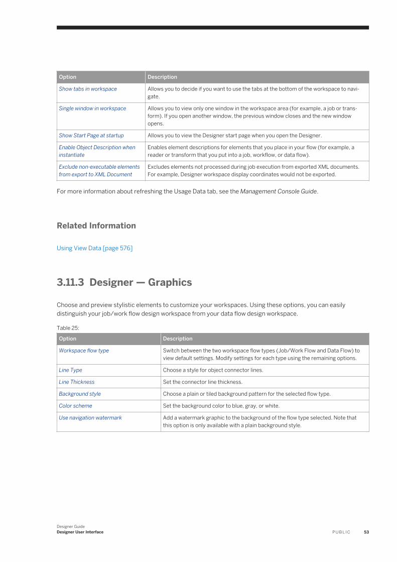
Option Description
Show tabs in workspace Allows you to decide if you want to use the tabs at the bottom of the workspace to navigate.
Single window in workspace Allows you to view only one window in the workspace area (for example, a job or transform). If you open another window, the previous window closes and the new window opens.
Show Start Page at startup Allows you to view the Designer start page when you open the Designer.
Enable Object Description when instantiate
Enables element descriptions for elements that you place in your flow (for example, a reader or transform that you put into a job, workflow, or data flow).
Exclude non-executable elements from export to XML Document
Excludes elements not processed during job execution from exported XML documents. For example, Designer workspace display coordinates would not be exported.
For more information about refreshing the Usage Data tab, see the Management Console Guide.
Related Information
Using View Data [page 576]
3.11.3 Designer — Graphics
Choose and preview stylistic elements to customize your workspaces. Using these options, you can easily distinguish your job/work flow design workspace from your data flow design workspace.
Table 25:
Option Description
Workspace flow type Switch between the two workspace flow types (Job/Work Flow and Data Flow) to view default settings. Modify settings for each type using the remaining options.
Line Type Choose a style for object connector lines.
Line Thickness Set the connector line thickness.
Background style Choose a plain or tiled background pattern for the selected flow type.
Color scheme Set the background color to blue, gray, or white.
Use navigation watermark Add a watermark graphic to the background of the flow type selected. Note that this option is only available with a plain background style.
Designer GuideDesigner User Interface P U B L I C 53
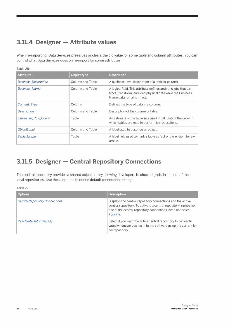
3.11.4 Designer — Attribute values
When re-importing, Data Services preserves or clears the old value for some table and column attributes. You can control what Data Services does on re-import for some attributes.
Table 26:
Attribute Object type Description
Business_Description Column and Table A business-level description of a table or column.
Business_Name Column and Table A logical field. This attribute defines and runs jobs that extract, transform, and load physical data while the Business Name data remains intact.
Content_Type Column Defines the type of data in a column.
Description Column and Table Description of the column or table.
Estimated_Row_Count Table An estimate of the table size used in calculating the order in which tables are read to perform join operations.
ObjectLabel Column and Table A label used to describe an object.
Table_Usage Table A label field used to mark a table as fact or dimension, for example.
3.11.5 Designer — Central Repository Connections
The central repository provides a shared object library allowing developers to check objects in and out of their local repositories. Use these options to define default connection settings.
Table 27:
Options Description
Central Repository Connections Displays the central repository connections and the active central repository. To activate a central repository, right-click one of the central repository connections listed and select Activate.
Reactivate automatically Select if you want the active central repository to be reactivated whenever you log in to the software using the current local repository.
54 P U B L I CDesigner Guide
Designer User Interface
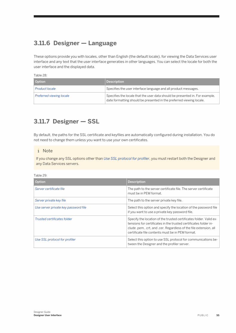
3.11.6 Designer — Language
These options provide you with locales, other than English (the default locale), for viewing the Data Services user interface and any text that the user interface generaties in other languages. You can select the locale for both the user interface and the displayed data.
Table 28:
Option Description
Product locale Specifies the user interface language and all product messages.
Preferred viewing locale Specifies the locale that the user data should be presented in. For example, date formatting should be presented in the preferred viewing locale.
3.11.7 Designer — SSL
By default, the paths for the SSL certificate and keyfiles are automatically configured during installation. You do not need to change them unless you want to use your own certificates.
NoteIf you change any SSL options other than Use SSL protocol for profiler, you must restart both the Designer and any Data Services servers.
Table 29:
Option Description
Server certificate file The path to the server certificate file. The server certificate must be in PEM format.
Server private key file The path to the server private key file.
Use server private key password file Select this option and specify the location of the password file if you want to use a private key password file.
Trusted certificates folder Specify the location of the trusted certificates folder. Valid extensions for certificates in the trusted certificates folder include .pem, .crt, and .cer. Regardless of the file extension, all certificate file contents must be in PEM format.
Use SSL protocol for profiler Select this option to use SSL protocol for communications between the Designer and the profiler server.
Designer GuideDesigner User Interface P U B L I C 55
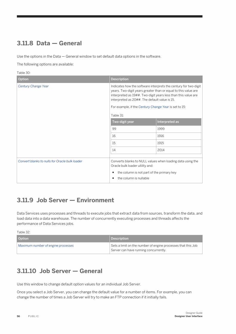
3.11.8 Data — General
Use the options in the Data — General window to set default data options in the software.
The following options are available:
Table 30:
Option Description
Century Change Year Indicates how the software interprets the century for two-digit years. Two-digit years greater than or equal to this value are interpreted as 19##. Two-digit years less than this value are interpreted as 20##. The default value is 15.
For example, if the Century Change Year is set to 15:
Table 31:
Two-digit year Interpreted as
99 1999
16 1916
15 1915
14 2014
Convert blanks to nulls for Oracle bulk loader Converts blanks to NULL values when loading data using the Oracle bulk loader utility and:
● the column is not part of the primary key● the column is nullable
3.11.9 Job Server — Environment
Data Services uses processes and threads to execute jobs that extract data from sources, transform the data, and load data into a data warehouse. The number of concurrently executing processes and threads affects the performance of Data Services jobs.
Table 32:
Option Description
Maximum number of engine processes Sets a limit on the number of engine processes that this Job Server can have running concurrently.
3.11.10 Job Server — General
Use this window to change default option values for an individual Job Server.
Once you select a Job Server, you can change the default value for a number of items. For example, you can change the number of times a Job Server will try to make an FTP connection if it initially fails.
56 P U B L I CDesigner Guide
Designer User Interface

Related Information
Changing option values for an individual Job Server [page 309]
Designer GuideDesigner User Interface P U B L I C 57
4 Projects and Jobs
Project and job objects represent the top two levels of organization for the application flows you create using the Designer.
4.1 Projects
A project is a reusable object that allows you to group jobs.
A project is the highest level of organization offered by the software. Opening a project makes one group of objects easily accessible in the user interface.
You can use a project to group jobs that have schedules that depend on one another or that you want to monitor together.
Projects have common characteristics:
● Projects are listed in the object library.● Only one project can be open at a time.● Projects cannot be shared among multiple users.
4.1.1 Objects that make up a project
The objects in a project appear hierarchically in the project area.
If a plus sign (+) appears next to an object, expand it to view the lower-level objects contained in the object. The software shows you the contents as both names in the project area hierarchy and icons in the workspace.
In the following example, the Job_KeyGen job contains two data flows, and the DF_EmpMap data flow contains multiple objects.
58 P U B L I CDesigner Guide
Projects and Jobs
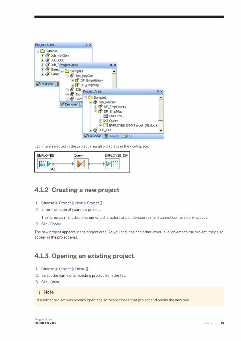
Each item selected in the project area also displays in the workspace:
4.1.2 Creating a new project
1. Choose Project New Project .2. Enter the name of your new project.
The name can include alphanumeric characters and underscores (_). It cannot contain blank spaces.3. Click Create.
The new project appears in the project area. As you add jobs and other lower-level objects to the project, they also appear in the project area.
4.1.3 Opening an existing project
1. Choose Project Open .2. Select the name of an existing project from the list.3. Click Open.
NoteIf another project was already open, the software closes that project and opens the new one.
Designer GuideProjects and Jobs P U B L I C 59
4.1.4 Saving all changes to a project
1. Choose Project Save All .
The software lists the jobs, work flows, and data flows that you edited since the last save.2. (ptional) Deselect any listed object to avoid saving it.3. Click OK.
NoteThe software also prompts you to save all objects that have changes when you execute a job and when you exit the Designer. Saving a reusable object saves any single-use object included in it.
4.2 Jobs
A job is the only object you can execute.
You can manually execute and test jobs in development. In production, you can schedule batch jobs and set up real-time jobs as services that execute a process when the software receives a message request.
A job is made up of steps you want executed together. Each step is represented by an object icon that you place in the workspace to create a job diagram. A job diagram is made up of two or more objects connected together. You can include any of the following objects in a job definition:
● Data flows○ Sources○ Targets○ Transforms
● Work flows○ Scripts○ Conditionals○ While Loops○ Try/catch blocks
If a job becomes complex, organize its content into individual work flows, then create a single job that calls those work flows.
Real-time jobs use the same components as batch jobs. You can add work flows and data flows to both batch and real-time jobs. When you drag a work flow or data flow icon into a job, you are telling the software to validate these objects according the requirements of the job type (either batch or real-time).
There are some restrictions regarding the use of some software features with real-time jobs.
Related Information
60 P U B L I CDesigner Guide
Projects and Jobs
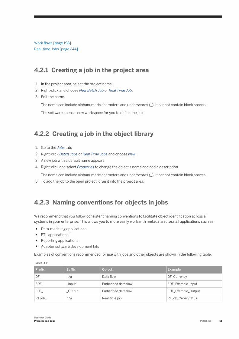
Work flows [page 198]Real-time Jobs [page 244]
4.2.1 Creating a job in the project area
1. In the project area, select the project name.2. Right-click and choose New Batch Job or Real Time Job.3. Edit the name.
The name can include alphanumeric characters and underscores (_). It cannot contain blank spaces.
The software opens a new workspace for you to define the job.
4.2.2 Creating a job in the object library
1. Go to the Jobs tab.2. Right-click Batch Jobs or Real Time Jobs and choose New.3. A new job with a default name appears.4. Right-click and select Properties to change the object's name and add a description.
The name can include alphanumeric characters and underscores (_). It cannot contain blank spaces.5. To add the job to the open project, drag it into the project area.
4.2.3 Naming conventions for objects in jobs
We recommend that you follow consistent naming conventions to facilitate object identification across all systems in your enterprise. This allows you to more easily work with metadata across all applications such as:
● Data-modeling applications● ETL applications● Reporting applications● Adapter software development kits
Examples of conventions recommended for use with jobs and other objects are shown in the following table.
Table 33:
Prefix Suffix Object Example
DF_ n/a Data flow DF_Currency
EDF_ _Input Embedded data flow EDF_Example_Input
EDF_ _Output Embedded data flow EDF_Example_Output
RTJob_ n/a Real-time job RTJob_OrderStatus
Designer GuideProjects and Jobs P U B L I C 61

Prefix Suffix Object Example
WF_ n/a Work flow WF_SalesOrg
JOB_ n/a Job JOB_SalesOrg
n/a _DS Datastore ORA_DS
DC_ n/a Datastore configuration DC_DB2_production
SC_ n/a System configuration SC_ORA_test
n/a _Memory_DS Memory datastore Catalog_Memory_DS
PROC_ n/a Stored procedure PROC_SalesStatus
Although the Designer is a graphical user interface with icons representing objects in its windows, other interfaces might require you to identify object types by the text alone. By using a prefix or suffix, you can more easily identify your object's type.
In addition to prefixes and suffixes, you might want to provide standardized names for objects that identify a specific action across all object types. For example: DF_OrderStatus, RTJob_OrderStatus.
In addition to prefixes and suffixes, naming conventions can also include path name identifiers. For example, the stored procedure naming convention can look like either of the following:
<datastore>.<owner>.<PROC_Name>
<datastore>.<owner>.<package>.<PROC_Name>
62 P U B L I CDesigner Guide
Projects and Jobs
5 Datastores
Describes different types of datastores, provides details about the Attunity Connector datastore, and instructions for configuring datastores.
5.1 What are datastores?
Datastores represent connection configurations between the software and databases or applications.
These configurations can be direct or through adapters. Datastore configurations allow the software to access metadata from a database or application and read from or write to that database or application while the software executes a job.
SAP Data Services datastores can connect to:
● Databases and mainframe file systems.● Applications that have pre-packaged or user-written adapters.● J.D. Edwards One World and J.D. Edwards World, Oracle Applications, PeopleSoft, SAP Applications, SAP
Data Quality Management, microservices for location data, SAP NetWeaver BW, Siebel Applications, and Google BigQuery. For more information, see the appropriate supplement guide.
● Remote servers using FTP, SFTP, and SCP.
NoteThe software reads and writes data stored in flat files through flat file formats. The software reads and writes data stored in XML documents through DTDs and XML Schemas.
The specific information that a datastore object can access depends on the connection configuration. When your database or application changes, make corresponding changes in the datastore information in the software. The software does not automatically detect the new information.
NoteObjects deleted from a datastore connection are identified in the project area and workspace by a red "deleted"
icon. This visual flag allows you to find and update data flows affected by datastore changes.
You can create multiple configurations for a datastore. This allows you to plan ahead for the different environments your datastore may be used in and limits the work involved with migrating jobs. For example, you can add a set of configurations (DEV, TEST, and PROD) to the same datastore name. These connection settings stay with the datastore during export or import. You can group any set of datastore configurations into a system configuration. When running or scheduling a job, select a system configuration, and thus, the set of datastore configurations for your current environment.
Designer GuideDatastores P U B L I C 63
Related Information
Database datastores [page 64]Adapter datastores [page 88]File formats [page 107]Formatting XML documents [page 215]Creating and managing multiple datastore configurations [page 91]
5.2 Database datastores
Allows Data Services to read from and write to supported database types.
Database datastores can represent single or multiple connections with:
● Legacy systems using Attunity Connect● IBM DB2, HP Vertica, Informix, Microsoft SQL Server, Oracle, SQL Anywhere, SAP ASE, Sybase IQ, MySQL,
Netezza, SAP HANA, SAP Data Federator, SQL Anywhere and Teradata databases (using native connections)● Other databases (through ODBC)● A repository, using a memory datastore or persistent cache datastore
You can create a connection to most of the data sources using the server name instead of the DSN (Data Source Name) or TNS (Transparent Network Substrate) name. Server name connections (also known as DSN-less and TNS-less connections) eliminate the need to configure the same DSN or TNS entries on every machine in a distributed environment.
For information about DSN-less and TNS-less connections, see the Administrator Guide.
5.2.1 Mainframe interface
The software provides the Attunity Connector datastore that accesses mainframe data sources through Attunity Connect.
The data sources that Attunity Connect accesses are in the following list. For a complete list of sources, refer to the Attunity documentation.
● Adabas● DB2 UDB for OS/390 and DB2 UDB for OS/400● IMS/DB● VSAM● Flat files on OS/390 and flat files on OS/400
64 P U B L I CDesigner Guide
Datastores
5.2.1.1 Prerequisites for an Attunity datastore
Attunity Connector accesses mainframe data using software that you must manually install on the mainframe server and the local client (Job Server) computer. The software connects to Attunity Connector using its ODBC interface.
It is not necessary to purchase a separate ODBC driver manager for UNIX and Windows platforms.
Servers
Install and configure the Attunity Connect product on the server (for example, an zSeries computer).
Clients
To access mainframe data using Attunity Connector, install the Attunity Connect product. The ODBC driver is required. Attunity also offers an optional tool called Attunity Studio, which you can use for configuration and administration.
Configure ODBC data sources on the client (SAP Data Services Job Server).
When you install a Job Server on UNIX, the installer will prompt you to provide an installation directory path for Attunity connector software. In addition, you do not need to install a driver manager, because the software loads ODBC drivers directly on UNIX platforms.
For more information about how to install and configure these products, refer to their documentation.
5.2.1.2 Creating and configuring an Attunity datastore
To use the Attunity Connector datastore option, upgrade your repository to SAP Data Services version 6.5.1 or later.
To create and configure an Attunity Connector datastore:
1. In the Datastores tab of the object library, right-click and select New.2. Enter a name for the datastore.3. In the Datastore type box, select Database.4. In the Database type box, select Attunity Connector.5. Type the Attunity data source name, location of the Attunity daemon (Host location), the Attunity daemon
port number, and a unique Attunity server workspace name.6. To change any of the default options (such as Rows per Commit or Language), click the Advanced button.7. Click OK.
You can now use the new datastore connection to import metadata tables into the current repository.
Designer GuideDatastores P U B L I C 65
5.2.1.3 Specifying multiple data sources in one Attunity datastore
The Attunity Connector datastore allows access to multiple Attunity data sources on the same Attunity Daemon location.
If you have several types of data on the same computer, for example a DB2 database and VSAM, you might want to access both types of data using a single connection. For example, you can use a single connection to join tables (and push the join operation down to a remote server), which reduces the amount of data transmitted through your network.
To specify multiple sources in the Datastore Editor:
1. Separate data source names with semicolons in the Attunity data source box using the following format:
AttunityDataSourceName;AttunityDataSourceName
For example, if you have a DB2 data source named DSN4 and a VSAM data source named Navdemo, enter the following values into the Data source box:
DSN4;Navdemo
2. If you list multiple data source names for one Attunity Connector datastore, ensure that you meet the following requirements:○ All Attunity data sources must be accessible by the same user name and password.○ All Attunity data sources must use the same workspace. When you setup access to the data sources in
Attunity Studio, use the same workspace name for each data source.
5.2.1.4 Data Services naming convention for Attunity tables
Data Services' format for accessing Attunity tables is unique to Data Services.
Because a single datastore can access multiple software systems that do not share the same namespace, the name of the Attunity data source must be specified when referring to a table. With an Attunity Connector, precede the table name with the data source and owner names separated by a colon. The format is as follows:
AttunityDataSource:OwnerName.TableName
When using the Designer to create your jobs with imported Attunity tables, Data Services automatically generates the correct SQL for this format. However, when you author SQL, be sure to use this format. You can author SQL in the following constructs:
● SQL function● SQL transform● Pushdown_sql function● Pre-load commands in table loader● Post-load commands in table loader
66 P U B L I CDesigner Guide
Datastores
NoteFor tables in Data Services, the maximum length of the owner name for most repository types is 256 (MySQL is 64 and MS SQL server is 128). In the case of Attunity tables, the maximum length of the Attunity data source name and actual owner name is 63 (the colon accounts for 1 character).
5.2.1.5 Limitations for Attunity datastore
All Data Services features are available when using an Attunity Connector datastore except for a few.
● Bulk loading● Imported functions (imports metadata for tables only)● Template tables (creating tables)● The datetime data type supports up to 2 sub-seconds only● Data Services cannot load timestamp data into a timestamp column in a table because Attunity truncates
varchar data to 8 characters, which is not enough to correctly represent a timestamp value.● When running a job on UNIX, the job could fail with following error:
[D000] Cannot open file /usr1/attun/navroot/def/sys System error 13: The file access permissions do not allow the specified action.; (OPEN)
This error occurs because of insufficient file permissions to some of the files in the Attunity installation directory. To avoid this error, change the file permissions for all files in the Attunity directory to 777 by executing the following command from the Attunity installation directory:
$ chmod -R 777 *
5.2.2 Defining a database datastore
Define at least one database datastore for each database or mainframe file system with which you are exchanging data.
Before defining a database datastore, you must get appropriate access privileges to the database or file system that the datastore describes.
For example, to allow the software to use parameterized SQL when reading or writing to DB2 databases, authorize the user (of the datastore/database) to create, execute, and drop stored procedures. If a user is not authorized to create, execute, and drop stored procedures, jobs will still run. However, the jobs will produce a warning message and will run less efficiently.
1. In the Datastores tab of the object library, right-click and select New.2. Enter the name of the new datastore in the Datastore name field.
The name can contain any alphabetical or numeric characters or underscores (_). It cannot contain spaces.3. In the Datastore type list, select Database.
Designer GuideDatastores P U B L I C 67
The software displays options relevant to that type. For more information about these options and for information about database types not discussed here, see "Database datastores" in the Reference Guide.
The following table contains information about special situations related to database types:
Table 34:
Database type Information
Oracle The Oracle database type supports TNS-less connections. To use a TNS-less connection, deselect Use TNS name and enter the host name, SID, and port.
Data Federator When using this database type, you must specify the catalog name and the schema name in the URL. If you do not, you may see all of the tables from each catalog.1. Select ODBC Admin and then the System DSN tab.2. Highlight Data Federator and then click Configure.3. In the URL option, enter the catalog name and the
schema name. For example: jdbc:leselect://localhost/<catalogname>;schema=<schemaname>
Additionally, if you choose DSN-less connections (you de-select the option Use data source name), the following information applies:○ Applicable only for the following database types: DB2, Informix, MySQL, Netezza, or SAP HANA. To view
the the most current list of supported databases for DSN-less connections, see the Release Notes.○ Enter information in the following options: Database Server Name, Database Name (for DB2 and MySQL),
Port information, User Name and Password.○ If you select Informix and you want to use DSN-less connections when Data Services is on a different
computer than the Informix server, you must identify the Informix host as follows:1. Go to your Informix client installation folder (for example: C:\Program Files\IBM\Informix
\Client-SDK\bin Run setnet32.exe).2. In the Server Information tab, enter the name of the IBM Informix server, the host name, and other
required information.3. Make the IBM Informix server the default server.
○ For DSN-less connections to an Informix database, the Designer can obtain the Informix host name for the Informix server name you provided.
4. Select Enable automatic data transfer to enable the Data_Transfer transform to use transfer tables in this datastore to push down subsequent database operations. This check box displays for all databases except Attunity Connector, Data Federator, Memory, and Persistent Cache.
5. To add more information, click Advanced.Click the cell under each configuration option and enter or select a value.
6. If you want the software to convert a data type in your source that it would not normally support, select Import unsupported data types as VARCHAR of size and enter the number of characters that you will allow. For more information about data types, see the Reference Guide.
7. Click OK to save the database datastore.
68 P U B L I CDesigner Guide
Datastores
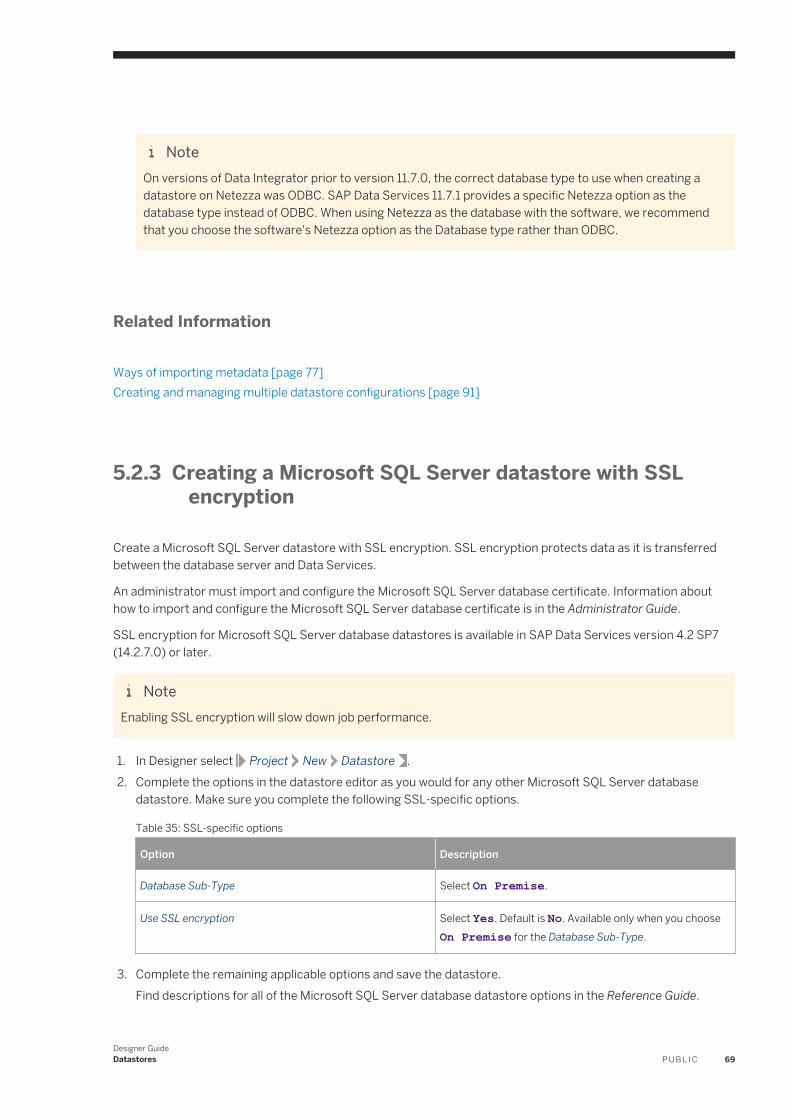
NoteOn versions of Data Integrator prior to version 11.7.0, the correct database type to use when creating a datastore on Netezza was ODBC. SAP Data Services 11.7.1 provides a specific Netezza option as the database type instead of ODBC. When using Netezza as the database with the software, we recommend that you choose the software's Netezza option as the Database type rather than ODBC.
Related Information
Ways of importing metadata [page 77]Creating and managing multiple datastore configurations [page 91]
5.2.3 Creating a Microsoft SQL Server datastore with SSL encryption
Create a Microsoft SQL Server datastore with SSL encryption. SSL encryption protects data as it is transferred between the database server and Data Services.
An administrator must import and configure the Microsoft SQL Server database certificate. Information about how to import and configure the Microsoft SQL Server database certificate is in the Administrator Guide.
SSL encryption for Microsoft SQL Server database datastores is available in SAP Data Services version 4.2 SP7 (14.2.7.0) or later.
NoteEnabling SSL encryption will slow down job performance.
1. In Designer select Project New Datastore .2. Complete the options in the datastore editor as you would for any other Microsoft SQL Server database
datastore. Make sure you complete the following SSL-specific options.
Table 35: SSL-specific options
Option Description
Database Sub-Type Select On Premise.
Use SSL encryption Select Yes. Default is No. Available only when you choose On Premise for the Database Sub-Type.
3. Complete the remaining applicable options and save the datastore.Find descriptions for all of the Microsoft SQL Server database datastore options in the Reference Guide.
Designer GuideDatastores P U B L I C 69
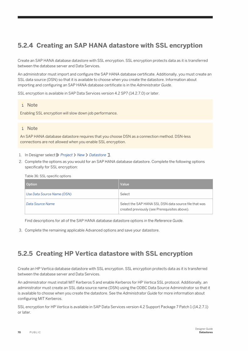
5.2.4 Creating an SAP HANA datastore with SSL encryption
Create an SAP HANA database datastore with SSL encryption. SSL encryption protects data as it is transferred between the database server and Data Services.
An administrator must import and configure the SAP HANA database certificate. Additionally, you must create an SSL data source (DSN) so that it is available to choose when you create the datastore. Information about importing and configuring an SAP HANA database certificate is in the Administrator Guide.
SSL encryption is available in SAP Data Services version 4.2 SP7 (14.2.7.0) or later.
NoteEnabling SSL encryption will slow down job performance.
NoteAn SAP HANA database datastore requires that you choose DSN as a connection method. DSN-less connections are not allowed when you enable SSL encryption.
1. In Designer select Project New Datastore .2. Complete the options as you would for an SAP HANA database datastore. Complete the following options
specifically for SSL encryption:
Table 36: SSL-specific options
Option Value
Use Data Source Name (DSN) Select
Data Source Name Select the SAP HANA SSL DSN data source file that was created previously (see Prerequisites above).
Find descriptions for all of the SAP HANA database datastore options in the Reference Guide.
3. Complete the remaining applicable Advanced options and save your datastore.
5.2.5 Creating HP Vertica datastore with SSL encryption
Create an HP Vertica database datastore with SSL encryption. SSL encryption protects data as it is transferred between the database server and Data Services.
An administrator must install MIT Kerberos 5 and enable Kerberos for HP Vertica SSL protocol. Additionally, an administrator must create an SSL data source name (DSN) using the ODBC Data Source Administrator so that it is available to choose when you create the datastore. See the Administrator Guide for more information about configuring MIT Kerberos.
SSL encryption for HP Vertica is available in SAP Data Services version 4.2 Support Package 7 Patch 1 (14.2.7.1) or later.
70 P U B L I CDesigner Guide
Datastores
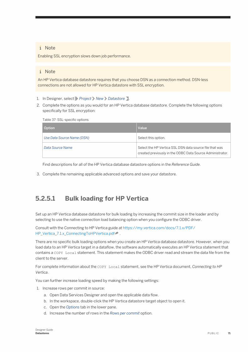
NoteEnabling SSL encryption slows down job performance.
NoteAn HP Vertica database datastore requires that you choose DSN as a connection method. DSN-less connections are not allowed for HP Vertica datastore with SSL encryption.
1. In Designer, select Project New Datastore .2. Complete the options as you would for an HP Vertica database datastore. Complete the following options
specifically for SSL encryption:
Table 37: SSL-specific options
Option Value
Use Data Source Name (DSN) Select this option.
Data Source Name Select the HP Vertica SSL DSN data source file that was created previously in the ODBC Data Source Administrator.
Find descriptions for all of the HP Vertica database datastore options in the Reference Guide.
3. Complete the remaining applicable advanced options and save your datastore.
5.2.5.1 Bulk loading for HP Vertica
Set up an HP Vertica database datastore for bulk loading by increasing the commit size in the loader and by selecting to use the native connection load balancing option when you configure the ODBC driver.
Consult with the Connecting to HP Vertica guide at https://my.vertica.com/docs/7.1.x/PDF/HP_Vertica_7.1.x_ConnectingToHPVertica.pdf .
There are no specific bulk loading options when you create an HP Vertica database datastore. However, when you load data to an HP Vertica target in a dataflow, the software automatically executes an HP Vertica statement that contains a COPY Local statement. This statement makes the ODBC driver read and stream the data file from the client to the server.
For complete information about the COPY Local statement, see the HP Vertica document, Connecting to HP Vertica.
You can further increase loading speed by making the following settings:
1. Increase rows per commit in source:a. Open Data Services Designer and open the applicable data flow.b. In the workspace, double-click the HP Vertica datastore target object to open it.c. Open the Options tab in the lower pane.d. Increase the number of rows in the Rows per commit option.
Designer GuideDatastores P U B L I C 71
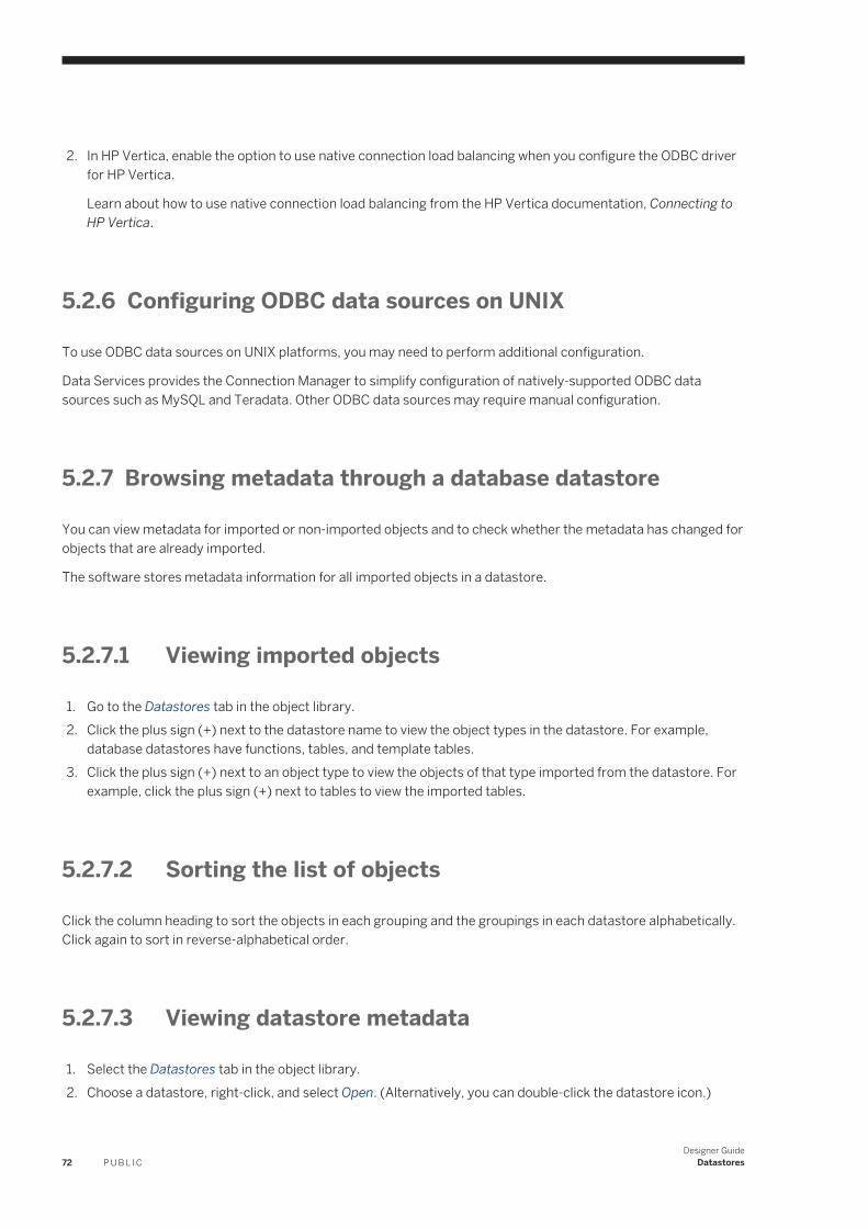
2. In HP Vertica, enable the option to use native connection load balancing when you configure the ODBC driver for HP Vertica.
Learn about how to use native connection load balancing from the HP Vertica documentation, Connecting to HP Vertica.
5.2.6 Configuring ODBC data sources on UNIX
To use ODBC data sources on UNIX platforms, you may need to perform additional configuration.
Data Services provides the Connection Manager to simplify configuration of natively-supported ODBC data sources such as MySQL and Teradata. Other ODBC data sources may require manual configuration.
5.2.7 Browsing metadata through a database datastore
You can view metadata for imported or non-imported objects and to check whether the metadata has changed for objects that are already imported.
The software stores metadata information for all imported objects in a datastore.
5.2.7.1 Viewing imported objects
1. Go to the Datastores tab in the object library.2. Click the plus sign (+) next to the datastore name to view the object types in the datastore. For example,
database datastores have functions, tables, and template tables.3. Click the plus sign (+) next to an object type to view the objects of that type imported from the datastore. For
example, click the plus sign (+) next to tables to view the imported tables.
5.2.7.2 Sorting the list of objects
Click the column heading to sort the objects in each grouping and the groupings in each datastore alphabetically. Click again to sort in reverse-alphabetical order.
5.2.7.3 Viewing datastore metadata
1. Select the Datastores tab in the object library.2. Choose a datastore, right-click, and select Open. (Alternatively, you can double-click the datastore icon.)
72 P U B L I CDesigner Guide
Datastores
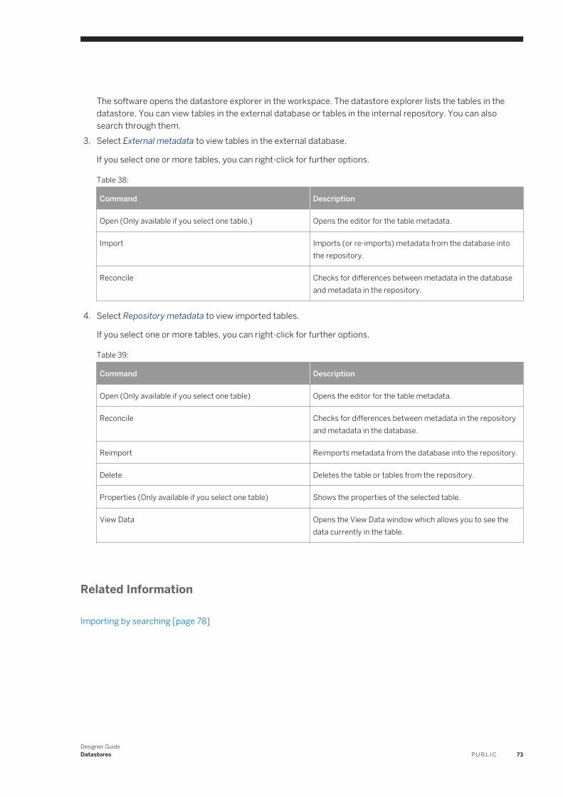
The software opens the datastore explorer in the workspace. The datastore explorer lists the tables in the datastore. You can view tables in the external database or tables in the internal repository. You can also search through them.
3. Select External metadata to view tables in the external database.
If you select one or more tables, you can right-click for further options.
Table 38:
Command Description
Open (Only available if you select one table.) Opens the editor for the table metadata.
Import Imports (or re-imports) metadata from the database into the repository.
Reconcile Checks for differences between metadata in the database and metadata in the repository.
4. Select Repository metadata to view imported tables.
If you select one or more tables, you can right-click for further options.
Table 39:
Command Description
Open (Only available if you select one table) Opens the editor for the table metadata.
Reconcile Checks for differences between metadata in the repository and metadata in the database.
Reimport Reimports metadata from the database into the repository.
Delete Deletes the table or tables from the repository.
Properties (Only available if you select one table) Shows the properties of the selected table.
View Data Opens the View Data window which allows you to see the data currently in the table.
Related Information
Importing by searching [page 78]
Designer GuideDatastores P U B L I C 73
5.2.7.4 Determining if a schema has changed since it was imported
1. In the browser window showing the list of repository tables, select External Metadata.2. Choose the table or tables you want to check for changes.3. Right-click and choose Reconcile.
The Changed column displays YES to indicate that the database tables differ from the metadata imported into the software. To use the most recent metadata from the software, reimport the table.
The Imported column displays YES to indicate that the table has been imported into the repository.
5.2.7.5 Browsing the metadata for an external table
1. In the browser window showing the list of external tables, select the table you want to view.2. Right-click and choose Open.
A table editor appears in the workspace and displays the schema and attributes of the table.
5.2.7.6 Viewing the metadata for an imported table
1. Select the table name in the list of imported tables.2. Right-click and select Open.
A table editor appears in the workspace and displays the schema and attributes of the table.
5.2.7.7 Viewing secondary index information for tables
Secondary index information can help you understand the schema of an imported table.
1. From the datastores tab in the Designer, right-click a table to open the shortcut menu.2. From the shortcut menu, click Properties to open the Properties window.3. In the Properties window, click the Indexes tab. The left portion of the window displays the Index list.4. Click an index to see the contents.
74 P U B L I CDesigner Guide
Datastores
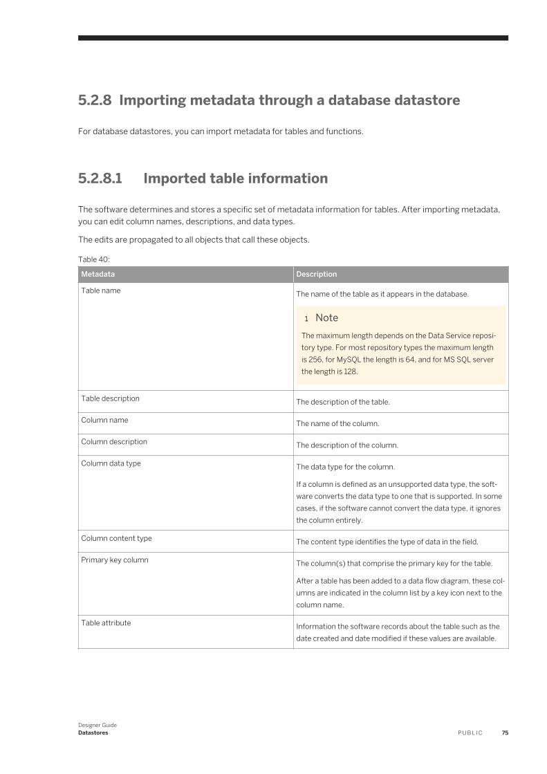
5.2.8 Importing metadata through a database datastore
For database datastores, you can import metadata for tables and functions.
5.2.8.1 Imported table information
The software determines and stores a specific set of metadata information for tables. After importing metadata, you can edit column names, descriptions, and data types.
The edits are propagated to all objects that call these objects.
Table 40:
Metadata Description
Table name The name of the table as it appears in the database.
NoteThe maximum length depends on the Data Service repository type. For most repository types the maximum length is 256, for MySQL the length is 64, and for MS SQL server the length is 128.
Table description The description of the table.
Column name The name of the column.
Column description The description of the column.
Column data type The data type for the column.
If a column is defined as an unsupported data type, the software converts the data type to one that is supported. In some cases, if the software cannot convert the data type, it ignores the column entirely.
Column content type The content type identifies the type of data in the field.
Primary key column The column(s) that comprise the primary key for the table.
After a table has been added to a data flow diagram, these columns are indicated in the column list by a key icon next to the column name.
Table attribute Information the software records about the table such as the date created and date modified if these values are available.
Designer GuideDatastores P U B L I C 75
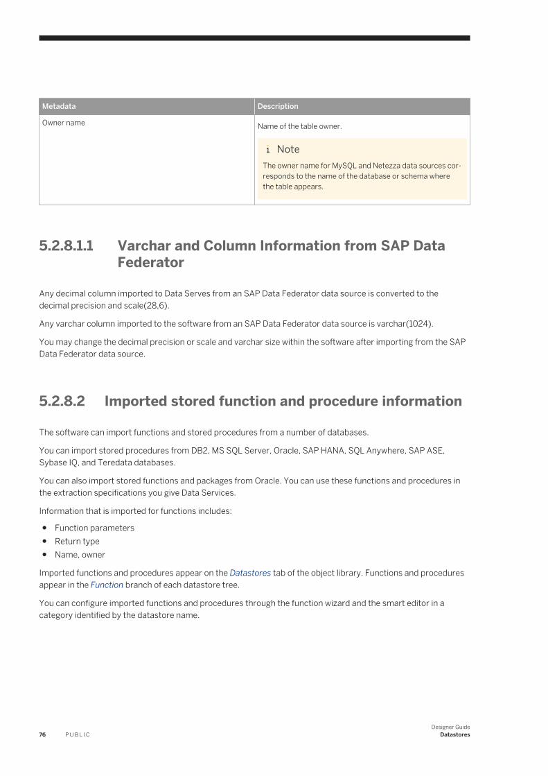
Metadata Description
Owner name Name of the table owner.
NoteThe owner name for MySQL and Netezza data sources corresponds to the name of the database or schema where the table appears.
5.2.8.1.1 Varchar and Column Information from SAP Data Federator
Any decimal column imported to Data Serves from an SAP Data Federator data source is converted to the decimal precision and scale(28,6).
Any varchar column imported to the software from an SAP Data Federator data source is varchar(1024).
You may change the decimal precision or scale and varchar size within the software after importing from the SAP Data Federator data source.
5.2.8.2 Imported stored function and procedure information
The software can import functions and stored procedures from a number of databases.
You can import stored procedures from DB2, MS SQL Server, Oracle, SAP HANA, SQL Anywhere, SAP ASE, Sybase IQ, and Teredata databases.
You can also import stored functions and packages from Oracle. You can use these functions and procedures in the extraction specifications you give Data Services.
Information that is imported for functions includes:
● Function parameters● Return type● Name, owner
Imported functions and procedures appear on the Datastores tab of the object library. Functions and procedures appear in the Function branch of each datastore tree.
You can configure imported functions and procedures through the function wizard and the smart editor in a category identified by the datastore name.
76 P U B L I CDesigner Guide
Datastores
5.2.8.3 Ways of importing metadata
Discusses methods you can use to import metadata.
5.2.8.3.1 Importing by browsing
NoteFunctions cannot be imported by browsing.
1. Open the object library.2. Go to the Datastores tab.3. Select the datastore you want to use.4. Right-click and choose Open.
The items available to import through the datastore appear in the workspace.
In some environments, the tables are organized and displayed as a tree structure. If this is true, there is a plus sign (+) to the left of the name. Click the plus sign to navigate the structure.
The workspace contains columns that indicate whether the table has already been imported into the software (Imported) and if the table schema has changed since it was imported (Changed). To verify whether the repository contains the most recent metadata for an object, right-click the object and choose Reconcile.
5. Select the items for which you want to import metadata.
For example, to import a table, you must select a table rather than a folder that contains tables.6. Right-click and choose Import.7. In the object library, go to the Datastores tab to display the list of imported objects.
5.2.8.3.2 Importing by name
1. Open the object library.2. Click the Datastores tab.3. Select the datastore you want to use.4. Right-click and choose Import By Name.5. In the Import By Name window, choose the type of item you want to import from the Type list.
If you are importing a stored procedure, select Function.6. To import tables:
a. Enter a table name in the Name box to specify a particular table, or select the All check box, if available, to specify all tables.If the name is case-sensitive in the database (and not all uppercase), enter the name as it appears in the database and use double quotation marks (") around the name to preserve the case.
Designer GuideDatastores P U B L I C 77
b. Enter an owner name in the Owner box to limit the specified tables to a particular owner. If you leave the owner name blank, you specify matching tables regardless of owner (that is, any table with the specified table name).
7. To import functions and procedures:○ In the Name box, enter the name of the function or stored procedure.
If the name is case-sensitive in the database (and not all uppercase), enter the name as it appears in the database and use double quotation marks (") around the name to preserve the case. Otherwise, the software will convert names into all upper-case characters.You can also enter the name of a package. An Oracle package is an encapsulated collection of related program objects (e.g., procedures, functions, variables, constants, cursors, and exceptions) stored together in the database. The software allows you to import procedures or functions created within packages and use them as top-level procedures or functions.If you enter a package name, the software imports all stored procedures and stored functions defined within the Oracle package. You cannot import an individual function or procedure defined within a package.
○ Enter an owner name in the Owner box to limit the specified functions to a particular owner. If you leave the owner name blank, you specify matching functions regardless of owner (that is, any function with the specified name).
○ If you are importing an Oracle function or stored procedure and any of the following conditions apply, clear the Callable from SQL expression check box. A stored procedure cannot be pushed down to a database inside another SQL statement when the stored procedure contains a DDL statement, ends the current transaction with COMMIT or ROLLBACK, or issues any ALTER SESSION or ALTER SYSTEM commands.
8. Click OK.
5.2.8.3.3 Importing by searching
NoteFunctions cannot be imported by searching.
1. Open the object library.2. Click the Datastores tab.3. Select the name of the datastore you want to use.4. Right-click and select Search.
The Search window appears.5. Enter the entire item name or some part of it in the Name text box.
If the name is case-sensitive in the database (and not all uppercase), enter the name as it appears in the database and use double quotation marks (") around the name to preserve the case.
6. Select Contains or Equals from the drop-down list to the right depending on whether you provide a complete or partial search value.
Equals qualifies only the full search string. That is, you need to search for owner.table_name rather than simply table_name.
78 P U B L I CDesigner Guide
Datastores
7. (Optional) Enter a description in the Description text box.8. Select the object type in the Type box.9. Select the datastore in which you want to search from the Look In box.10. Select External from the drop-down box to the right of the Look In box.
External indicates that the software searches for the item in the entire database defined by the datastore.
Internal indicates that the software searches only the items that have been imported.11. Go to the Advanced tab to search using the software's attribute values.
The advanced options only apply to searches of imported items.12. Click Search.
The software lists the tables matching your search criteria.13. To import a table from the returned list, select the table, right-click, and choose Import.
5.2.8.4 Reimporting objects
If you have already imported an object such as a datastore, function, or table, you can reimport it, which updates the object's metadata from your database (reimporting overwrites any changes you might have made to the object in the software).
To reimport objects in previous versions of the software, you opened the datastore, viewed the repository metadata, and selected the objects to reimport. In this version of the software, you can reimport objects using the object library at various levels:
● Individual objects — Reimports the metadata for an individual object such as a table or function● Category node level — Reimports the definitions of all objects of that type in that datastore, for example all
tables in the datastore● Datastore level — Reimports the entire datastore and all its dependent objects including tables, functions,
IDOCs, and hierarchies
5.2.8.4.1 Reimporting objects from the object library
1. In the object library, click the Datastores tab.2. Right-click an individual object and click Reimport, or right-click a category node or datastore name and click
Reimport All.
You can also select multiple individual objects using Ctrl-click or Shift-click.3. Click Yes to reimport the metadata.4. If you selected multiple objects to reimport (for example with Reimport All), the software requests
confirmation for each object unless you check the box Don't ask me again for the remaining objects.
You can skip objects to reimport by clicking No for that object.
If you are unsure whether to reimport (and thereby overwrite) the object, click View Where Used to display where the object is currently being used in your jobs.
Designer GuideDatastores P U B L I C 79
5.2.9 Memory datastores
A memory datastore is a container for memory tables.
The software allows you to create a database datastore using Memory as the Database type. Memory datastores are designed to enhance processing performance of data flows executing in real-time jobs. Data (typically small amounts in a real-time job) is stored in memory to provide immediate access instead of going to the original source data.
A datastore normally provides a connection to a database, application, or adapter. By contrast, a memory datastore contains memory table schemas saved in the repository.
Memory tables are schemas that allow you to cache intermediate data. Memory tables can cache data from relational database tables and hierarchical data files such as XML messages and SAP IDocs (both of which contain nested schemas).
Memory tables can be used to:
● Move data between data flows in real-time jobs. By caching intermediate data, the performance of real-time jobs with multiple data flows is far better than it would be if files or regular tables were used to store intermediate data. For best performance, only use memory tables when processing small quantities of data.
● Store table data in memory for the duration of a job. By storing table data in memory, the LOOKUP_EXT function and other transforms and functions that do not require database operations can access data without having to read it from a remote database.
The lifetime of memory table data is the duration of the job. The data in memory tables cannot be shared between different real-time jobs. Support for the use of memory tables in batch jobs is not available.
5.2.9.1 Defining a memory datastore
1. From the Project menu, select New Datastore .2. In the Name box, enter the name of the new datastore.
Be sure to use the naming convention "Memory_DS". Datastore names are appended to table names when table icons appear in the workspace. Memory tables are represented in the workspace with regular table icons. Therefore, label a memory datastore to distinguish its memory tables from regular database tables in the workspace.
3. In the Datastore type box keep the default Database.4. In the Database Type box select Memory.
No additional attributes are required for the memory datastore.5. Click OK.
5.2.9.2 Creating a memory table
1. From the tool palette, click the template table icon.
80 P U B L I CDesigner Guide
Datastores
2. Click inside a data flow to place the template table.
The Create Table window opens.3. From the Create Table window, select the memory datastore.4. Enter a table name.5. If you want a system-generated row ID column in the table, click the Create Row ID check box.6. Click OK.
The memory table appears in the workspace as a template table icon.7. Connect the memory table to the data flow as a target.8. From the Project menu select Save.
In the workspace, the memory table's icon changes to a target table icon and the table appears in the object library under the memory datastore's list of tables.
Related Information
Create Row ID option [page 82]
5.2.9.3 Using a memory table as a source or target
1. In the object library, click the Datastores tab.2. Expand the memory datastore that contains the memory table you want to use.3. Expand Tables.
A list of tables appears.4. Select the memory table you want to use as a source or target, and drag it into an open data flow.5. Connect the memory table as a source or target in the data flow.
If you are using a memory table as a target, open the memory table's target table editor to set table options.6. Save the job.
Related Information
Memory table target options [page 82]
Designer GuideDatastores P U B L I C 81
5.2.9.4 Update Schema option
You might want to quickly update a memory target table's schema if the preceding schema changes.
To do this, use the Update Schema option. Otherwise, you would have to add a new memory table to update a schema.
1. Right-click the memory target table's icon in the work space.2. Select Update Schema.
The schema of the preceding object is used to update the memory target table's schema. The current memory table is updated in your repository. All occurrences of the current memory table are updated with the new schema.
5.2.9.5 Memory table target options
The Delete data from table before loading option is available for memory table targets. The default is on (the box is selected). To set this option, open the memory target table editor. If you deselect this option, new data will append to the existing table data.
5.2.9.6 Create Row ID option
If the Create Row ID is checked in the Create Memory Table window, the software generates an integer column called DI_Row_ID in which the first row inserted gets a value of 1, the second row inserted gets a value of 2, etc. This new column allows you to use a LOOKUP_EXT expression as an iterator in a script.
NoteThe same functionality is available for other datastore types using the SQL function.
Use the DI_Row_ID column to iterate through a table using a lookup_ext function in a script. For example:
$NumOfRows = total_rows (memory_DS..table1) $I = 1;$count=0while ($count < $NumOfRows)begin $data = lookup_ext([memory_DS..table1, 'NO_CACHE','MAX'],[A],[O],[DI_Row_ID,'=',$I]); $1 = $I + 1; if ($data != NULL) begin $count = $count + 1; endend
In the preceding script, table1 is a memory table. The table's name is preceded by its datastore name (memory_DS), a dot, a blank space (where a table owner would be for a regular table), then a second dot. There are no owners for memory datastores, so tables are identified by just the datastore name and the table name as shown.
82 P U B L I CDesigner Guide
Datastores
Select the LOOKUP_EXT function arguments (line 7) from the function editor when you define a LOOKUP_EXT function.
The TOTAL_ROWS(DatastoreName.Owner.TableName) function returns the number of rows in a particular table in a datastore. This function can be used with any type of datastore. If used with a memory datastore, use the following syntax: TOTAL_ROWS( <DatastoreName..TableName> )
The software also provides a built-in function that you can use to explicitly expunge data from a memory table. This provides finer control than the active job has over your data and memory usage. The TRUNCATE_TABLE( <DatastoreName..TableName> ) function can only be used with memory tables.
5.2.9.7 Troubleshooting memory tables
● One possible error, particularly when using memory tables, is that the software runs out of virtual memory space. The software exits if it runs out of memory while executing any operation.
● A validation and run time error occurs if the schema of a memory table does not match the schema of the preceding object in the data flow.To correct this error, use the Update Schema option or create a new memory table to match the schema of the preceding object in the data flow.
● Two log files contain information specific to memory tables: trace_memory_reader log and trace_memory_loader log.
5.2.10 Persistent cache datastores
A persistent cache datastore is a container for cache tables.
The software also allows you to create a database datastore using Persistent cache as the Database type. Persistent cache datastores provide the following benefits for data flows that process large volumes of data.
● You can store a large amount of data in persistent cache which the software quickly loads into memory to provide immediate access during a job. For example, you can access a lookup table or comparison table locally (instead of reading from a remote database).
● You can create cache tables that multiple data flows can share (unlike a memory table which cannot be shared between different real-time jobs). For example, if a large lookup table used in a lookup_ext function rarely changes, you can create a cache once and subsequent jobs can use this cache instead of creating it each time.
A datastore normally provides a connection to a database, application, or adapter. By contrast, a persistent cache datastore contains cache table schemas saved in the repository.
Persistent cache tables allow you to cache large amounts of data. Persistent cache tables can cache data from relational database tables and files.
NoteYou cannot cache data from hierarchical data files such as XML messages and SAP IDocs (both of which contain nested schemas). You cannot perform incremental inserts, deletes, or updates on a persistent cache table.
Designer GuideDatastores P U B L I C 83
You create a persistent cache table by loading data into the persistent cache target table using one data flow. You can then subsequently read from the cache table in another data flow. When you load data into a persistent cache table, the software always truncates and recreates the table.
5.2.10.1 Creating persistent cache datastores
You can create persistent cache datastores using the Datastore Editor window.
1. From the Project menu, select New Datastore .2. In the Name box, enter the name of the new datastore.
Be sure to use a naming convention such as "Persist_DS". Datastore names are appended to table names when table icons appear in the workspace. Persistent cache tables are represented in the workspace with regular table icons. Therefore, label a persistent cache datastore to distinguish its persistent cache tables from regular database tables in the workspace.
3. In the Datastore type box, keep the default Database.4. In the Database Type box, select Persistent cache.5. In the Cache directory box, you can either type or browse to a directory where you want to store the persistent
cache.6. Click OK.
5.2.10.2 Creating persistent cache tables
When you create a persistent cache table, you do not have to specify the table's schema or import the table's metadata.
Instead, the software creates the schema for each persistent cache table automatically based on the preceding schema. The first time you save the job, the software defines the persistent cache table's schema and saves the table. Subsequently, the table appears with a table icon in the workspace and in the object library under the persistent cache datastore.
You create a persistent cache table in one of the following ways:
● As a target template table in a data flow● As part of the Data_Transfer transform during the job execution
5.2.10.2.1 Creating a persistent cache table as a target in a data flow
1. Use one of the following methods to open the Create Template window:
○ From the tool palette:
1. Click the template table icon.
84 P U B L I CDesigner Guide
Datastores
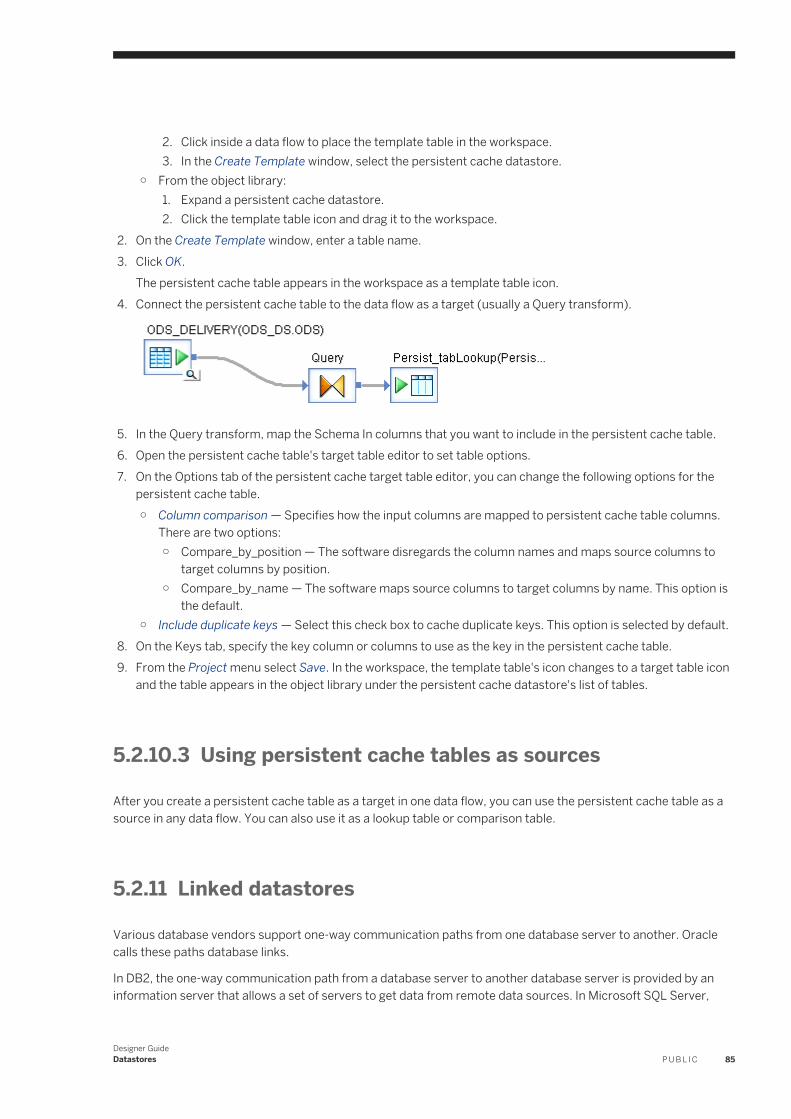
2. Click inside a data flow to place the template table in the workspace.3. In the Create Template window, select the persistent cache datastore.
○ From the object library:1. Expand a persistent cache datastore.2. Click the template table icon and drag it to the workspace.
2. On the Create Template window, enter a table name.3. Click OK.
The persistent cache table appears in the workspace as a template table icon.4. Connect the persistent cache table to the data flow as a target (usually a Query transform).
5. In the Query transform, map the Schema In columns that you want to include in the persistent cache table.6. Open the persistent cache table's target table editor to set table options.7. On the Options tab of the persistent cache target table editor, you can change the following options for the
persistent cache table.○ Column comparison — Specifies how the input columns are mapped to persistent cache table columns.
There are two options:○ Compare_by_position — The software disregards the column names and maps source columns to
target columns by position.○ Compare_by_name — The software maps source columns to target columns by name. This option is
the default.○ Include duplicate keys — Select this check box to cache duplicate keys. This option is selected by default.
8. On the Keys tab, specify the key column or columns to use as the key in the persistent cache table.9. From the Project menu select Save. In the workspace, the template table's icon changes to a target table icon
and the table appears in the object library under the persistent cache datastore's list of tables.
5.2.10.3 Using persistent cache tables as sources
After you create a persistent cache table as a target in one data flow, you can use the persistent cache table as a source in any data flow. You can also use it as a lookup table or comparison table.
5.2.11 Linked datastores
Various database vendors support one-way communication paths from one database server to another. Oracle calls these paths database links.
In DB2, the one-way communication path from a database server to another database server is provided by an information server that allows a set of servers to get data from remote data sources. In Microsoft SQL Server,
Designer GuideDatastores P U B L I C 85
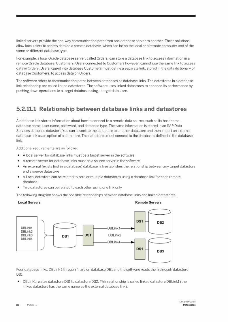
linked servers provide the one-way communication path from one database server to another. These solutions allow local users to access data on a remote database, which can be on the local or a remote computer and of the same or different database type.
For example, a local Oracle database server, called Orders, can store a database link to access information in a remote Oracle database, Customers. Users connected to Customers however, cannot use the same link to access data in Orders. Users logged into database Customers must define a separate link, stored in the data dictionary of database Customers, to access data on Orders.
The software refers to communication paths between databases as database links. The datastores in a database link relationship are called linked datastores. The software uses linked datastores to enhance its performance by pushing down operations to a target database using a target datastore.
5.2.11.1 Relationship between database links and datastores
A database link stores information about how to connect to a remote data source, such as its host name, database name, user name, password, and database type. The same information is stored in an SAP Data Services database datastore.You can associate the datastore to another datastore and then import an external database link as an option of a datastore. The datastores must connect to the databases defined in the database link.
Additional requirements are as follows:
● A local server for database links must be a target server in the software● A remote server for database links must be a source server in the software● An external (exists first in a database) database link establishes the relationship between any target datastore
and a source datastore● A Local datastore can be related to zero or multiple datastores using a database link for each remote
database● Two datastores can be related to each other using one link only
The following diagram shows the possible relationships between database links and linked datastores:
Four database links, DBLink 1 through 4, are on database DB1 and the software reads them through datastore DS1.
● DBLink1 relates datastore DS1 to datastore DS2. This relationship is called linked datastore DBLink1 (the linked datastore has the same name as the external database link).
86 P U B L I CDesigner Guide
Datastores
● DBLink2 is not mapped to any datastore in the software because it relates DS1 with DS2, which are also related by DBLink1. Although it is not a regular case, you can create multiple external database links that connect to the same remote source. However, the software allows only one database link between a target datastore and a source datastore pair. For example, if you select DBLink1 to link target datastore DS1 with source datastore DS2, you cannot import DBLink2 to do the same.
● DBLink3 is not mapped to any datastore in the software because there is no datastore defined for the remote data source to which the external database link refers.
● DBLink4 relates DS1 with DS3.
5.2.12 Changing a datastore definition
Like all objects, datastores are defined by both options and properties.
Options control the operation of objects. For example, the name of the database to connect to is a datastore option.
Properties document the object. For example, the name of the datastore and the date on which it was created are datastore properties. Properties are merely descriptive of the object and do not affect its operation.
5.2.12.1 Changing datastore options
1. Go to the Datastores tab in the object library.2. Right-click the datastore name and choose Edit.
The Datastore Editor appears (the title bar for this dialog displays Edit Datastore). You can do the following tasks:
○ Change the connection information for the current datastore configuration.○ Click Advanced and change properties for the current configuration.○ Click Edit to add, edit, or delete additional configurations. The Configurations for Datastore dialog opens
when you select Edit in the Datastore Editor. After you add a new configuration to an existing datastore, you can use the fields in the grid to change connection values and properties for the new configuration.
3. Click OK.
The options take effect immediately.
5.2.12.2 Changing datastore properties
1. Go to the datastore tab in the object library.2. Right-click the datastore name and select Properties.
The Properties window opens.3. Change the datastore properties.4. Click OK.
Designer GuideDatastores P U B L I C 87
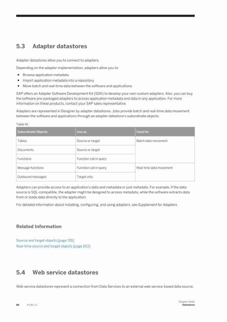
5.3 Adapter datastores
Adapter datastores allow you to connect to adapters.
Depending on the adapter implementation, adapters allow you to:
● Browse application metadata● Import application metadata into a repository● Move batch and real-time data between the software and applications
SAP offers an Adapter Software Development Kit (SDK) to develop your own custom adapters. Also, you can buy the software pre-packaged adapters to access application metadata and data in any application. For more information on these products, contact your SAP sales representative.
Adapters are represented in Designer by adapter datastores. Jobs provide batch and real-time data movement between the software and applications through an adapter datastore's subordinate objects:
Table 41:
Subordinate Objects Use as Used for
Tables Source or target Batch data movement
Documents Source or target
Functions Function call in query
Message functions Function call in query Real-time data movement
Outbound messages Target only
Adapters can provide access to an application's data and metadata or just metadata. For example, if the data source is SQL-compatible, the adapter might be designed to access metadata, while the software extracts data from or loads data directly to the application.
For detailed information about installing, configuring, and using adapters, see Supplement for Adapters.
Related Information
Source and target objects [page 155]Real-time source and target objects [page 253]
5.4 Web service datastores
Web service datastores represent a connection from Data Services to an external web service-based data source.
88 P U B L I CDesigner Guide
Datastores
5.4.1 Defining a web service datastore
You need to define at least one datastore for each web service with which you are exchanging data.
To define a datastore, you must have the appropriate access privileges to the web services that the datastore describes.
1. In the Datastores tab of the object library, right-click and select New.2. Enter the name of the new datastore in the Datastore name field.
The name can contain any alphabetical or numeric characters or underscores (_). It cannot contain spaces.3. Select the Datastore type.
Choose a web service option. When you select a Datastore Type, Data Services displays other options relevant to that type.
4. Specify the Web Service URL.The URL must accept connections and return the WSDL. For REST web services, you can either enter a URL or the path to the local WADL file. See "Web services technologies" in the Integrator Guide for more information about WSDL and WADL files.
5. Click OK.The datastore configuration is saved in your metadata repository and the new datastore appears in the object library.
5.4.2 Changing a web service datastore's configuration
1. Right-click the datastore you want to browse and select Edit to open the Datastore Editor window.2. Edit configuration information.3. Click OK.
The edited datastore configuration is saved in your metadata repository.
5.4.3 Deleting a web service datastore and associated metadata objects
1. Right-click the datastore you want to delete and select Delete.2. Click OK in the confirmation window.
Data Services removes the datastore and all metadata objects contained within that datastore from the metadata repository. If these objects exist in established data flows, they appear with a deleted icon.
Designer GuideDatastores P U B L I C 89
5.4.4 Browsing WSDL and WADL metadata through a web service datastore
Data Services stores metadata information for all imported objects in a datastore. You can use Data Services to view metadata for imported or non-imported objects and to check whether the metadata has changed for objects already imported.
See "Web services technologies" in the Integrator Guide for more information about WSDL and WADL files.
5.4.4.1 Viewing imported objects
1. Go to the Datastores tab in the object library.2. Click the plus sign (+) next to the datastore name to view the object types in the datastore. Web service
datastores have functions.3. Click the plus sign (+) next to an object type to view the objects of that type imported from the datastore.
5.4.4.2 Sorting the list of objects
Click the column heading to sort the objects in each grouping and the groupings in each datastore alphabetically. Click again to sort in reverse-alphabetical order.
5.4.4.3 Viewing WSDL and WADL metadata
1. Select the Datastores tab in the object library.2. Choose a datastore, right-click, and select Open. (Alternatively, you can double-click the datastore icon.)
Data Services opens the datastore explorer in the workspace. The datastore explorer lists the web service ports and operations in the datastore. You can view ports and operations in the external web service or in the internal repository. You can also search through them.
3. Select External metadata to view web service ports and operations from the external WSDL or WADL file. See "Web services technologies" in the Integrator Guide for more information about WSDL and WADL files.If you select one or more operations, you can right-click for further options.
Table 42:
Command Description
Import Imports (or re-imports) operations from the database into the repository.
4. Select Repository metadata to view imported web service operations.If you select one or more operations, you can right-click for further options.
90 P U B L I CDesigner Guide
Datastores
Table 43:
Command Description
Delete Deletes the operation or operations from the repository.
Properties Shows the properties of the selected web service operation.
5.4.5 Importing metadata through a web service datastore
For web service datastores, you can import metadata for web service operations.
5.4.5.1 Importing web service operations
1. Right-click the datastore you want to browse, then select Open.2. Find the web service operation you want to import from the browsable list.3. Right-click the operation and select Import.
The operation is imported into the web service datastore's function container.
5.5 Creating and managing multiple datastore configurations
Creating multiple configurations for a single datastore allows you to consolidate separate datastore connections for similar sources or targets into one source or target datastore with multiple configurations.
Then, you can select a set of configurations that includes the sources and targets you want by selecting a system configuration when you execute or schedule the job. The ability to create multiple datastore configurations provides greater ease-of-use for job portability scenarios, such as:
● OEM (different databases for design and distribution)● Migration (different connections for DEV, TEST, and PROD)● Multi-instance (databases with different versions or locales)● Multi-user (databases for central and local repositories)
Related Information
Portability solutions [page 96]
Designer GuideDatastores P U B L I C 91
5.5.1 Definitions
There are terms you should be familiar with when creating and managing multiple datastore configurations
Table 44:
Term Definition
Datastore configuration Allows you to provide multiple metadata sources or targets for datastores. Each configuration is a property of a datastore that refers to a set of configurable options (such as database connection name, database type, user name, password, and locale) and their values.
Default datastore configuration The datastore configuration that the software uses for browsing and importing database objects (tables and functions) and executing jobs if no system configuration is specified. If a datastore has more than one configuration, select a default configuration, as needed. If a datastore has only one configuration, the software uses it as the default configuration.
Current datastore configuration The datastore configuration that the software uses to execute a job. If you define a system configuration, the software will execute the job using the system configuration. Specify a current configuration for each system configuration. If you do not create a system configuration, or the system configuration does not specify a configuration for a datastore, the software uses the default datastore configuration as the current configuration at job execution time.
Database objects The tables and functions that are imported from a datastore. Database objects usually have owners. Some database objects do not have owners. For example, database objects in an ODBC datastore connecting to an Access database do not have owners.
Owner name Owner name of a database object (for example, a table) in an underlying database. Also known as database owner name or physical owner name.
Alias A logical owner name. Create an alias for objects that are in different database environments if you have different owner names in those environments. You can create an alias from the datastore editor for any datastore configuration.
Dependent objects Dependent objects are the jobs, work flows, data flows, and custom functions in which a database object is used. Dependent object information is generated by the where-used utility.
5.5.2 Why use multiple datastore configurations?
By creating multiple datastore configurations, you can decrease end-to-end development time in a multi-source, 24x7, enterprise data warehouse environment because you can easily port jobs among different database types, versions, and instances.
For example, porting can be as simple as:
1. Creating a new configuration within an existing source or target datastore.2. Adding a datastore alias then map configurations with different object owner names to it.3. Defining a system configuration then adding datastore configurations required for a particular environment.
Select a system configuration when you execute a job.
92 P U B L I CDesigner Guide
Datastores
5.5.3 Creating a new configuration
You can create multiple configurations for all datastore types except memory datastores.
Use the Datastore Editor to create and edit datastore configurations.
5.5.3.1 Creating a new datastore configuration
1. From the Datastores tab of the object library, right-click any existing datastore and select Edit.2. Click Advanced to view existing configuration information.
Each datastore must have at least one configuration. If only one configuration exists, it is the default configuration.
3. Click Edit to open the Configurations for Datastore window.
4. Click the Create New Configuration icon on the toolbar.
The Create New Configuration window opens.5. In the Create New Configuration window:
a. Enter a unique, logical configuration Name.b. Select a Database type from the drop-down menu.c. Select a Database version from the drop-down menu.d. In the Values for table targets and SQL transforms section, the software pre-selects the Use values from
value based on the existing database type and version. The Designer automatically uses the existing SQL transform and target values for the same database type and version.
Further, if the database you want to associate with a new configuration in a later version than that associated with other existing configurations, the Designer automatically populates the Use values from with the earlier version.
However, if the database type and version are not already specified in an existing configuration, or if the database version is older than your existing configuration, you can choose to use the values from another existing configuration or the default for the database type and version.
e. Select or clear the Restore values if they already exist option.
When you delete datastore configurations, the software saves all associated target values and SQL transforms. If you create a new datastore configuration with the same database type and version as the one previously deleted, the Restore values if they already exist option allows you to access and take advantage of the saved value settings.)
○ If you keep this option (selected as default) the software uses customized target and SQL transform values from previously deleted datastore configurations.
○ If you deselect Restore values if they already exist, the software does not attempt to restore target and SQL transform values, allowing you to provide new values.
f. Click OK to save the new configuration.
If your datastore contains pre-existing data flows with SQL transforms or target objects, the software must add any new database type and version values to these transform and target objects. Under these circumstances, when you add a new datastore configuration, the software displays the Added New Values
Designer GuideDatastores P U B L I C 93
- Modified Objects window which provides detailed information about affected data flows and modified objects. These same results also display in the Output window of the Designer.
For each datastore, the software requires that one configuration be designated as the default configuration. The software uses the default configuration to import metadata and also preserves the default configuration during export and multi-user operations. Your first datastore configuration is automatically designated as the default; however after adding one or more additional datastore configurations, you can use the datastore editor to flag a different configuration as the default.
When you export a repository, the software preserves all configurations in all datastores including related SQL transform text and target table editor settings. If the datastore you are exporting already exists in the target repository, the software overrides configurations in the target with source configurations. The software exports system configurations separate from other job related objects.
5.5.4 Adding a datastore alias
You can create multiple aliases for a datastore then map datastore configurations to each alias in the datastore editor.
5.5.4.1 Creating an alias
1. From within the datastore editor, click Advanced, then click Aliases (Click here to create).
The Create New Alias window opens.2. Under Alias Name in Designer, use only alphanumeric characters and the underscore symbol (_) to enter an
alias name.3. Click OK.
The Create New Alias window closes and your new alias appears underneath the Aliases category
When you define a datastore alias, the software substitutes your specified datastore configuration alias for the real owner name when you import metadata for database objects. You can also rename tables and functions after you import them.
Related Information
Renaming table and function owner [page 101]
94 P U B L I CDesigner Guide
Datastores
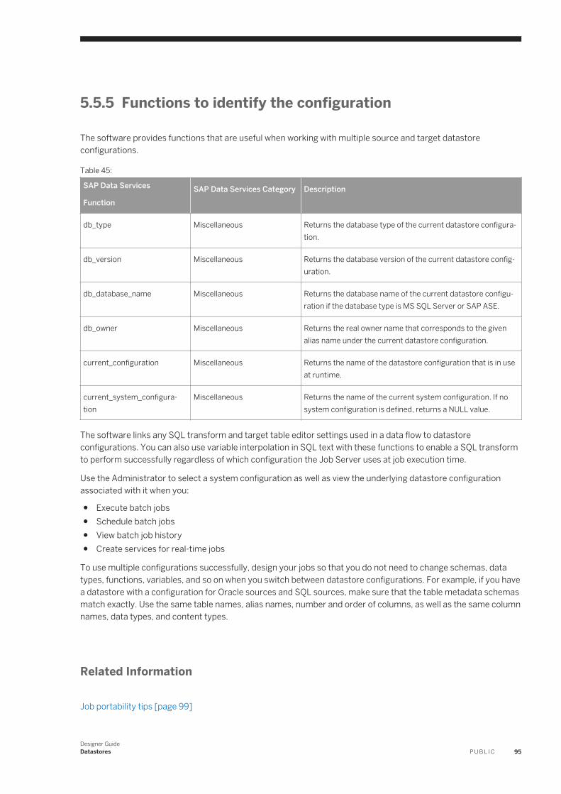
5.5.5 Functions to identify the configuration
The software provides functions that are useful when working with multiple source and target datastore configurations.
Table 45:
SAP Data Services
FunctionSAP Data Services Category Description
db_type Miscellaneous Returns the database type of the current datastore configuration.
db_version Miscellaneous Returns the database version of the current datastore configuration.
db_database_name Miscellaneous Returns the database name of the current datastore configuration if the database type is MS SQL Server or SAP ASE.
db_owner Miscellaneous Returns the real owner name that corresponds to the given alias name under the current datastore configuration.
current_configuration Miscellaneous Returns the name of the datastore configuration that is in use at runtime.
current_system_configuration
Miscellaneous Returns the name of the current system configuration. If no system configuration is defined, returns a NULL value.
The software links any SQL transform and target table editor settings used in a data flow to datastore configurations. You can also use variable interpolation in SQL text with these functions to enable a SQL transform to perform successfully regardless of which configuration the Job Server uses at job execution time.
Use the Administrator to select a system configuration as well as view the underlying datastore configuration associated with it when you:
● Execute batch jobs● Schedule batch jobs● View batch job history● Create services for real-time jobs
To use multiple configurations successfully, design your jobs so that you do not need to change schemas, data types, functions, variables, and so on when you switch between datastore configurations. For example, if you have a datastore with a configuration for Oracle sources and SQL sources, make sure that the table metadata schemas match exactly. Use the same table names, alias names, number and order of columns, as well as the same column names, data types, and content types.
Related Information
Job portability tips [page 99]
Designer GuideDatastores P U B L I C 95
5.5.6 Portability solutions
Set multiple source or target configurations for a single datastore if you want to quickly change connections to a different source or target database.
The software provides several different solutions for porting jobs.
Related Information
Multi-user Development [page 695]Working in a Multi-user Environment [page 707]
5.5.6.1 Migration between environments
Moving repository metadata to another environment (for example, from development to test or from test to production) uses different source and target databases.
The process typically includes the following characteristics:
● The environments use the same database type but may have unique database versions or locales.● Database objects (tables and functions) can belong to different owners.● Each environment has a unique database connection name, user name, password, other connection
properties, and owner mapping.● You use a typical repository migration procedure. Either you export jobs to an ATL file then import the ATL file
to another repository, or you export jobs directly from one repository to another repository.
Because the software overwrites datastore configurations during export, you should add configurations for the target environment (for example, add configurations for the test environment when migrating from development to test) to the source repository (for example, add to the development repository before migrating to the test environment). The Export utility saves additional configurations in the target environment, which means that you do not have to edit datastores before running ported jobs in the target environment.
This solution offers the following advantages:
● Minimal production down time: You can start jobs as soon as you export them.● Minimal security issues: Testers and operators in production do not need permission to modify repository
objects.
96 P U B L I CDesigner Guide
Datastores
5.5.6.2 Loading multiple instances
The migration scenario for loading multiple instances of a data source to a target data warehouse is the same as a migration scenario except that you are using only one repository.
5.5.6.2.1 Loading multiple instances of a data source to a target data warehouse
1. Create a datastore that connects to a particular instance.2. Define the first datastore configuration. This datastore configuration contains all configurable properties such
as database type, database connection name, user name, password, database version, and locale information.
When you define a configuration for an Adapter datastore, make sure that the relevant Job Server is running so the Designer can find all available adapter instances for the datastore.
3. Define a set of alias-to-owner mappings within the datastore configuration. When you use an alias for a configuration, the software imports all objects using the metadata alias rather than using real owner names. This allows you to use database objects for jobs that are transparent to other database instances.
4. Use the database object owner renaming tool to rename owners of any existing database objects.5. Import database objects and develop jobs using those objects, then run the jobs.6. To support executing jobs under different instances, add datastore configurations for each additional
instance.7. Map owner names from the new database instance configurations to the aliases that you defined in an earlier
step.8. Run the jobs in all database instances.
Related Information
Renaming table and function owner [page 101]
5.5.6.3 OEM deployment
You can design jobs for one database type and deploy those jobs to other database types as an OEM partner.
The deployment typically has the following characteristics:
● The instances require various source database types and versions.● Since a datastore can only access one instance at a time, you may need to trigger functions at run-time to
match different instances. If this is the case, the software requires different SQL text for functions (such as lookup_ext and sql) and transforms (such as the SQL transform). The software also requires different settings for the target table (configurable in the target table editor).
Designer GuideDatastores P U B L I C 97
● The instances may use different locales.● Database tables across different databases belong to different owners.● Each instance has a unique database connection name, user name, password, other connection properties,
and owner mappings.● You export jobs to ATL files for deployment.
5.5.6.3.1 Deploying jobs to other database types as an OEM partner
1. Develop jobs for a particular database type following the steps described in the Loading multiple instances [page 97] scenario.
To support a new instance under a new database type, the software copies target table and SQL transform database properties from the previous configuration to each additional configuration when you save it.
If you selected a bulk loader method for one or more target tables within your job's data flows, and new configurations apply to different database types, open your targets and manually set the bulk loader option (assuming you still want to use the bulk loader method with the new database type). The software does not copy bulk loader options for targets from one database type to another.
When the software saves a new configuration it also generates a report that provides a list of targets automatically set for bulk loading. Reference this report to make manual changes as needed.
2. If the SQL text in any SQL transform is not applicable for the new database type, modify the SQL text for the new database type.
If the SQL text contains any hard-coded owner names or database names, consider replacing these names with variables to supply owner names or database names for multiple database types. This way, you will not have to modify the SQL text for each environment.
3. Because the software does not support unique SQL text for each database type or version of the sql(), lookup_ext(), and pushdown_sql() functions, use the db_type() and similar functions to get the database type and version of the current datastore configuration and provide the correct SQL text for that database type and version using the variable substitution (interpolation) technique.
5.5.6.4 Multi-user development
When using the central repository management system, multiple developers, each with their own local repository, can check in and check out jobs.
The development environment typically has the following characteristics:
● It has a central repository and a number of local repositories.● Multiple development environments get merged (via central repository operations such as check in and check
out) at times. When this occurs, real owner names (used initially to import objects) must be later mapped to a set of aliases shared among all users.
● The software preserves object history (versions and labels).● The instances share the same database type but may have different versions and locales.
98 P U B L I CDesigner Guide
Datastores
● Database objects may belong to different owners.● Each instance has a unique database connection name, user name, password, other connection properties,
and owner mapping.
In the multi-user development scenario you must define aliases so that the software can properly preserve the history for all objects in the shared environment.
5.5.6.4.1 Porting jobs in a multi-user environment
When porting jobs in a multi-user environment, consider these points:
● Rename table owners and function owners to consolidate object database object owner names into aliases.○ Renaming occurs in local repositories. To rename the database objects stored in the central repository,
check out the datastore to a local repository and apply the renaming tool in the local repository.○ If the objects to be renamed have dependent objects, the software will ask you to check out the
dependent objects.○ If all the dependent objects can be checked out, renaming will create a new object that has the alias and
delete the original object that has the original owner name.○ If all the dependent objects cannot be checked out (data flows are checked out by another user), the
software displays a message, which gives you the option to proceed or cancel the operation. If you cannot check out some of the dependent objects, the renaming tool only affects the flows that you can check out. After renaming, the original object will co-exist with the new object. The number of flows affected by the renaming process will affect the Usage and Where-Used information in the Designer for both the original object and the new object.
● You are responsible for checking in all the dependent objects that were checked out during the owner renaming process. Checking in the new objects does not automatically check in the dependent objects that were checked out.○ The software does not delete original objects from the central repository when you check in the new
objects.○ Use caution because checking in datastores and checking them out as multi-user operations can override
datastore configurations.○ Maintain the datastore configurations of all users by not overriding the configurations they created.
Instead, add a configuration and make it your default configuration while working in your own environment.○ When your group completes the development phase, It is recommended that the last developer
delete the configurations that apply to the development environments and add the configurations that apply to the test or production environments.
5.5.7 Job portability tips
● The software assumes that the metadata of a table or function is the same across different database types and versions specified in different configurations in the same datastore. For instance, if you import a table when the default configuration of the datastore is Oracle, then later use the table in a job to extract from DB2, your job will run.
● Import metadata for a database object using the default configuration and use that same metadata with all configurations defined in the same datastore.
Designer GuideDatastores P U B L I C 99
● The software supports options in some database types or versions that it does not support in others For example, the software supports parallel reading on Oracle hash-partitioned tables, not on DB2 or other database hash-partitioned tables. If you import an Oracle hash-partitioned table and set your data flow to run in parallel, the software will read from each partition in parallel. However, when you run your job using sources from a DB2 environment, parallel reading will not occur.
● The following features support job portability:○ Enhanced SQL transform
With the enhanced SQL transform, you can enter different SQL text for different database types/versions and use variable substitution in the SQL text to allow the software to read the correct text for its associated datastore configuration.
○ Enhanced target table editorUsing enhanced target table editor options, you can configure database table targets for different database types/versions to match their datastore configurations.
○ Enhanced datastore editorUsing the enhanced datastore editor, when you create a new datastore configuration you can choose to copy the database properties (including the datastore and table target options as well as the SQL transform text) from an existing configuration or use the current values.
● When you design a job that will be run from different database types or versions, name database tables, functions, and stored procedures the same for all sources. If you create configurations for both case-insensitive databases and case-sensitive databases in the same datastore, It is recommended that you name the tables, functions, and stored procedures using all upper-case characters.
● Table schemas should match across the databases in a datastore. This means the number of columns, the column names, and column positions should be exactly the same. The column data types should be the same or compatible. For example, if you have a VARCHAR column in an Oracle source, use a VARCHAR column in the Microsoft SQL Server source too. If you have a DATE column in an Oracle source, use a DATETIME column in the Microsoft SQL Server source. Define primary and foreign keys the same way.
● Stored procedure schemas should match. When you import a stored procedure from one datastore configuration and try to use it for another datastore configuration, the software assumes that the signature of the stored procedure is exactly the same for the two databases. For example, if a stored procedure is a stored function (only Oracle supports stored functions), then you have to use it as a function with all other configurations in a datastore (in other words, all databases must be Oracle). If your stored procedure has three parameters in one database, it should have exactly three parameters in the other databases. Further, the names, positions, data types, and in/out types of the parameters must match exactly.
Related Information
Advanced Development Guide: Multi-user Development [page 695]Advanced Development Guide: Multi-user Environment Setup [page 699]
100 P U B L I CDesigner Guide
Datastores
5.5.8 Renaming table and function owner
Use owner renaming to assign a single metadata alias instead of the real owner name for database objects in the datastore.
You can rename the owner of imported tables, template tables, or functions. Consolidating metadata under a single alias name allows you to access accurate and consistent dependency information at any time while also allowing you to more easily switch between configurations when you move jobs to different environments.
When using objects stored in a central repository, a shared alias makes it easy to track objects checked in by multiple users. If all users of local repositories use the same alias, the software can track dependencies for objects that your team checks in and out of the central repository.
When you rename an owner, the instances of a table or function in a data flow are affected, not the datastore from which they were imported.
1. From the Datastore tab of the local object library, expand a table, template table, or function category.2. Right-click the table or function and select Rename Owner.3. Enter a New Owner Name then click Rename.
When you enter a New Owner Name, the software uses it as a metadata alias for the table or function.
NoteIf the object you are renaming already exists in the datastore, the software determines if that the two objects have the same schema. If they are the same, then the software proceeds. If they are different, then the software displays a message to that effect. You may need to choose a different object name.
The software supports both case-sensitive and case-insensitive owner renaming.
● If the objects you want to rename are from a case-sensitive database, the owner renaming mechanism preserves case sensitivity.
● If the objects you want to rename are from a datastore that contains both case-sensitive and case-insensitive databases, the software will base the case-sensitivity of new owner names on the case sensitivity of the default configuration. To ensure that all objects are portable across all configurations in this scenario, enter all owner names and object names using uppercase characters.
During the owner renaming process:
● The software updates the dependent objects (jobs, work flows, and data flows that use the renamed object) to use the new owner name.
● The object library shows the entry of the object with the new owner name. Displayed Usage and Where-Used information reflect the number of updated dependent objects.
● If the software successfully updates all the dependent objects, it deletes the metadata for the object with the original owner name from the object library and the repository.
Designer GuideDatastores P U B L I C 101
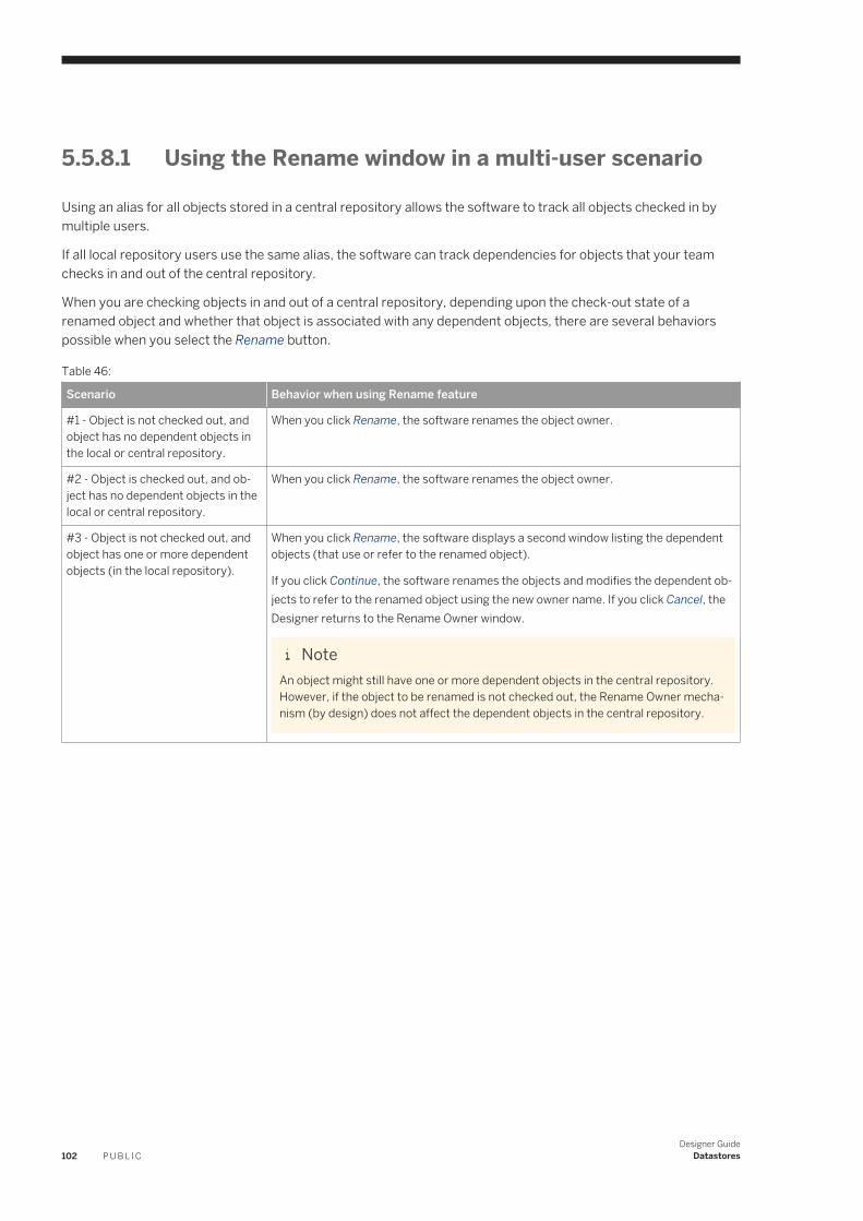
5.5.8.1 Using the Rename window in a multi-user scenario
Using an alias for all objects stored in a central repository allows the software to track all objects checked in by multiple users.
If all local repository users use the same alias, the software can track dependencies for objects that your team checks in and out of the central repository.
When you are checking objects in and out of a central repository, depending upon the check-out state of a renamed object and whether that object is associated with any dependent objects, there are several behaviors possible when you select the Rename button.
Table 46:
Scenario Behavior when using Rename feature
#1 - Object is not checked out, and object has no dependent objects in the local or central repository.
When you click Rename, the software renames the object owner.
#2 - Object is checked out, and object has no dependent objects in the local or central repository.
When you click Rename, the software renames the object owner.
#3 - Object is not checked out, and object has one or more dependent objects (in the local repository).
When you click Rename, the software displays a second window listing the dependent objects (that use or refer to the renamed object).
If you click Continue, the software renames the objects and modifies the dependent objects to refer to the renamed object using the new owner name. If you click Cancel, the Designer returns to the Rename Owner window.
NoteAn object might still have one or more dependent objects in the central repository. However, if the object to be renamed is not checked out, the Rename Owner mechanism (by design) does not affect the dependent objects in the central repository.
102 P U B L I CDesigner Guide
Datastores
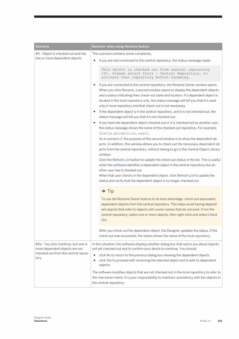
Scenario Behavior when using Rename feature
#4 - Object is checked out and has one or more dependent objects.
This scenario contains some complexity.
● If you are not connected to the central repository, the status message reads:
This object is checked out from central repository <X>. Please select Tools | Central Repository… to activate that repository before renaming.
● If you are connected to the central repository, the Rename Owner window opens.When you click Rename, a second window opens to display the dependent objects and a status indicating their check-out state and location. If a dependent object is located in the local repository only, the status message will tell you that it's used only in local repository and that check-out is not necessary.
● If the dependent object is in the central repository, and it is not checked out, the status message will tell you that it's not checked out.
● If you have the dependent object checked out or it is checked out by another user, the status message shows the name of the checked out repository. For example, Oracle.production.user1.As in scenario 2, the purpose of this second window is to show the dependent objects. In addition, this window allows you to check out the necessary dependent objects from the central repository, without having to go to the Central Object Library window.Click the Refresh List button to update the check out status in the list. This is useful when the software identifies a dependent object in the central repository but another user has it checked out.When that user checks in the dependent object, click Refresh List to update the status and verify that the dependent object is no longer checked out.
TipTo use the Rename Owner feature to its best advantage, check out associated dependent objects from the central repository. This helps avoid having dependent objects that refer to objects with owner names that do not exist. From the central repository, select one or more objects, then right-click and select Check Out.
After you check out the dependent object, the Designer updates the status. If the check out was successful, the status shows the name of the local repository.
#4a - You click Continue, but one or more dependent objects are not checked out from the central repository.
In this situation, the software displays another dialog box that warns you about objects not yet checked out and to confirm your desire to continue. You should:
● click No to return to the previous dialog box showing the dependent objects.● click Yes to proceed with renaming the selected object and to edit its dependent
objects.
The software modifies objects that are not checked out in the local repository to refer to the new owner name. It is your responsibility to maintain consistency with the objects in the central repository.
Designer GuideDatastores P U B L I C 103
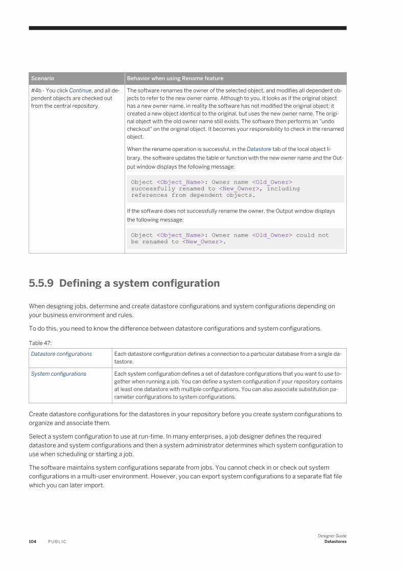
Scenario Behavior when using Rename feature
#4b - You click Continue, and all dependent objects are checked out from the central repository.
The software renames the owner of the selected object, and modifies all dependent objects to refer to the new owner name. Although to you, it looks as if the original object has a new owner name, in reality the software has not modified the original object; it created a new object identical to the original, but uses the new owner name. The original object with the old owner name still exists. The software then performs an "undo checkout" on the original object. It becomes your responsibility to check in the renamed object.
When the rename operation is successful, in the Datastore tab of the local object library, the software updates the table or function with the new owner name and the Output window displays the following message:
Object <Object_Name>: Owner name <Old_Owner> successfully renamed to <New_Owner>, including references from dependent objects.
If the software does not successfully rename the owner, the Output window displays the following message:
Object <Object_Name>: Owner name <Old_Owner> could not be renamed to <New_Owner>.
5.5.9 Defining a system configuration
When designing jobs, determine and create datastore configurations and system configurations depending on your business environment and rules.
To do this, you need to know the difference between datastore configurations and system configurations.
Table 47:
Datastore configurations Each datastore configuration defines a connection to a particular database from a single datastore.
System configurations Each system configuration defines a set of datastore configurations that you want to use together when running a job. You can define a system configuration if your repository contains at least one datastore with multiple configurations. You can also associate substitution parameter configurations to system configurations.
Create datastore configurations for the datastores in your repository before you create system configurations to organize and associate them.
Select a system configuration to use at run-time. In many enterprises, a job designer defines the required datastore and system configurations and then a system administrator determines which system configuration to use when scheduling or starting a job.
The software maintains system configurations separate from jobs. You cannot check in or check out system configurations in a multi-user environment. However, you can export system configurations to a separate flat file which you can later import.
104 P U B L I CDesigner Guide
Datastores
Related Information
Creating a new configuration [page 93]
5.5.9.1 Creating a system configuration
1. From the Designer menu bar, select Tools System Configurations .
The Edit System Configurations window displays.2. To add a new system configuration, do one of the following:
○ Click the Create New Configuration icon to add a configuration that references the default configuration of the substitution parameters and each datastore connection.
○ Select an existing configuration and click the Duplicate Configuration icon to create a copy of the selected configuration.You can use the copy as a template and edit the substitution parameter or datastore configuration selections to suit your needs.
3. If desired, rename the new system configuration.a. Select the system configuration you want to rename.b. Click the Rename Configuration icon to enable the edit mode for the configuration name field.c. Type a new, unique name and click outside the name field to accept your choice.
It is recommended that you follow a consistent naming convention and use the prefix SC_ in each system configuration name so that you can easily identify this file as a system configuration. This practice is particularly helpful when you export the system configuration.
4. From the list, select a substitution parameter configuration to associate with the system configuration.5. For each datastore, select the datastore configuration you want to use when you run a job using the system
configuration.If you do not map a datastore configuration to a system configuration, the Job Server uses the default datastore configuration at run-time.
6. Click OK to save your system configuration settings.
Related Information
Associating substitution parameter configurations with system configurations [page 296]
5.5.9.2 Exporting a system configuration
1. In the object library, select the Datastores tab and right-click a datastore.
2. Select Repository Export System Configurations .
Designer GuideDatastores P U B L I C 105

It is recommended that you add the SC_ prefix to each exported system configuration .atl file to easily identify that file as a system configuration.
3. Click OK.
106 P U B L I CDesigner Guide
Datastores
6 File formats
A set of properties describing the metadata structure of a flat file (ASCII).
File formats describe the metadata structure of a specific file. A file format template is a generic description that can be used for multiple data files.
This section discusses file formats, how to use the file format editor, and how to create a file format in the software.
6.1 Understanding file formats
The software can use data stored in files for data sources and targets.
A file format defines a connection to a file. Therefore, you use a file format to connect to source or target data when the data is stored in a file rather than a database table. The object library stores file format templates that you use to define specific file formats as sources and targets in data flows.
To work with file formats, perform the following tasks:
● Create a file format template that defines the structure for a file.● Create a specific source or target file format in a data flow. The source or target file format is based on a
template and specifies connection information such as the file name.
File format objects can describe files of the following types:
● Delimited: Characters such as commas or tabs separate each field.● Fixed width: You specify the column width.● SAP transport: Use to define data transport objects in SAP application data flows.● Unstructured text: Use to read one or more files of unstructured text from a directory.● Unstructured binary: Use to read one or more binary documents from a directory.
6.2 File format editor
Use the file format editor to set properties for file format templates and source and target file formats.
Available properties vary by the mode of the file format editor:
Table 48:
Mode Description
New mode Create a new file format template
Designer GuideFile formats P U B L I C 107
Mode Description
Edit mode Edit an existing file format template
Source mode Edit the file format of a particular source file
Target mode Edit the file format of a particular target file
The file format editor has three work areas:
Table 49:
Work area Location Description
Properties-values The left side of the file format editor window.
Edit the values for file format properties. Expand and collapse the property groups by clicking the leading plus or minus.
Column attributes The upper right side of the file format editor window.
Edit and define the columns or fields in the file. Field-specific formats override the default format set in the Properties-Values area.
Data preview The lower right side of the file format editor window.
View how the settings affect sample data, when applicable.
The file format editor contains "splitter" bars to allow resizing of the window and all the work areas. You can expand the file format editor to the full screen size.
The properties and appearance of the work areas vary with the format of the file.
108 P U B L I CDesigner Guide
File formats
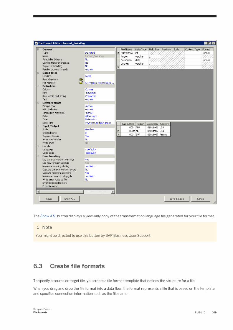
The Show ATL button displays a view-only copy of the transformation language file generated for your file format.
NoteYou might be directed to use this button by SAP Business User Support.
6.3 Create file formats
To specify a source or target file, you create a file format template that defines the structure for a file.
When you drag and drop the file format into a data flow, the format represents a file that is based on the template and specifies connection information such as the file name.
Designer GuideFile formats P U B L I C 109
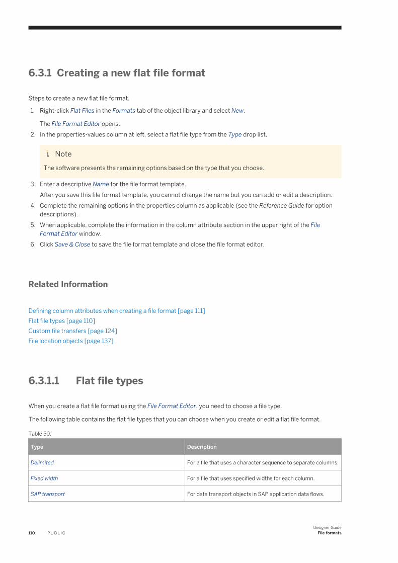
6.3.1 Creating a new flat file format
Steps to create a new flat file format.
1. Right-click Flat Files in the Formats tab of the object library and select New.
The File Format Editor opens.2. In the properties-values column at left, select a flat file type from the Type drop list.
NoteThe software presents the remaining options based on the type that you choose.
3. Enter a descriptive Name for the file format template.After you save this file format template, you cannot change the name but you can add or edit a description.
4. Complete the remaining options in the properties column as applicable (see the Reference Guide for option descriptions).
5. When applicable, complete the information in the column attribute section in the upper right of the File Format Editor window.
6. Click Save & Close to save the file format template and close the file format editor.
Related Information
Defining column attributes when creating a file format [page 111]Flat file types [page 110]Custom file transfers [page 124]File location objects [page 137]
6.3.1.1 Flat file types
When you create a flat file format using the File Format Editor, you need to choose a file type.
The following table contains the flat file types that you can choose when you create or edit a flat file format.
Table 50:
Type Description
Delimited For a file that uses a character sequence to separate columns.
Fixed width For a file that uses specified widths for each column.
SAP transport For data transport objects in SAP application data flows.
110 P U B L I CDesigner Guide
File formats
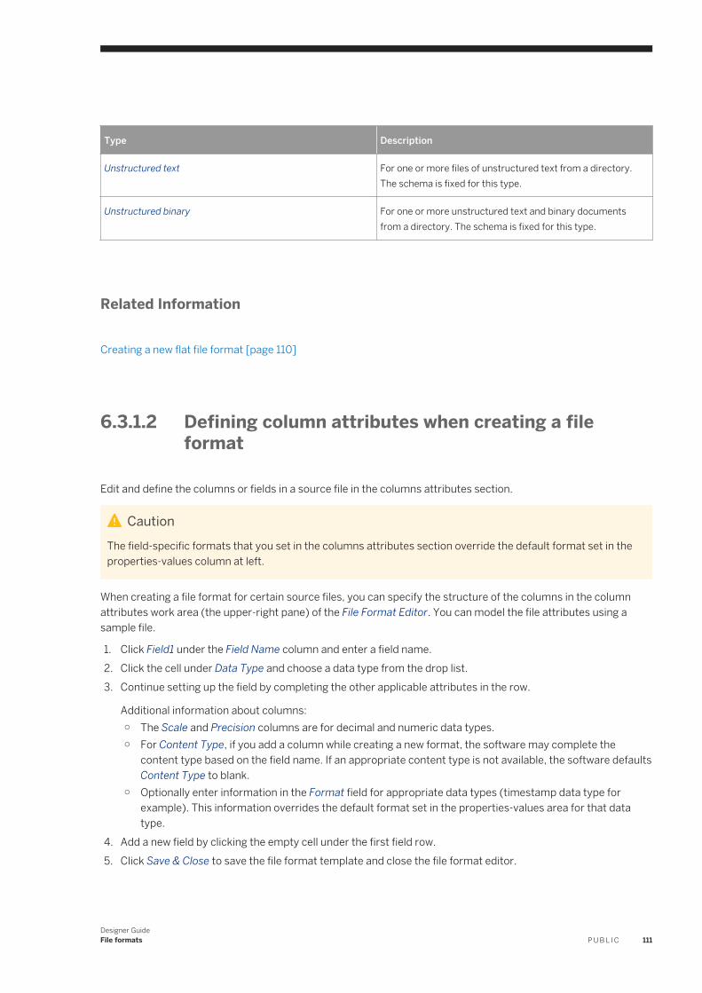
Type Description
Unstructured text For one or more files of unstructured text from a directory. The schema is fixed for this type.
Unstructured binary For one or more unstructured text and binary documents from a directory. The schema is fixed for this type.
Related Information
Creating a new flat file format [page 110]
6.3.1.2 Defining column attributes when creating a file format
Edit and define the columns or fields in a source file in the columns attributes section.
CautionThe field-specific formats that you set in the columns attributes section override the default format set in the properties-values column at left.
When creating a file format for certain source files, you can specify the structure of the columns in the column attributes work area (the upper-right pane) of the File Format Editor. You can model the file attributes using a sample file.
1. Click Field1 under the Field Name column and enter a field name.2. Click the cell under Data Type and choose a data type from the drop list.3. Continue setting up the field by completing the other applicable attributes in the row.
Additional information about columns:○ The Scale and Precision columns are for decimal and numeric data types.○ For Content Type, if you add a column while creating a new format, the software may complete the
content type based on the field name. If an appropriate content type is not available, the software defaults Content Type to blank.
○ Optionally enter information in the Format field for appropriate data types (timestamp data type for example). This information overrides the default format set in the properties-values area for that data type.
4. Add a new field by clicking the empty cell under the first field row.5. Click Save & Close to save the file format template and close the file format editor.
Designer GuideFile formats P U B L I C 111
NoteYou do not need to specify columns for files used as targets. If you do specify columns and they do not match the output schema from the preceding transform, the software writes to the target file using the transform's output schema.
NoteFor a decimal or real data type, if you only specify a source column format and the column names and data types in the target schema do not match those in the source schema, the software cannot use the source column format specified. Instead, it defaults to the format used by the code page on the computer where the Job Server is installed.
Related Information
Creating a new flat file format [page 110]
6.3.1.3 Using a custom transfer program
A custom transfer program refers to a specific third-party file transfer protocol program that you use to read and load flat files. This option applies to fixed width or delimited flat files.
For other flat file types, and for nested schemas, you can set up a file transfer protocol definition by creating a file location object instead of using the custom transfer program settings.
If you select Yes for the Custom Transfer Program option, you must complete the options in the Custom Transfer section later in the properties-values section.
1. Set Custom Transfer Program option to Yes.2. Expand the Custom Transfer section and enter the custom transfer program name and arguments.
Related Information
Creating a new flat file format [page 110]File transfer protocols [page 124]File location objects [page 137]
6.3.2 Modeling a file format on a sample file
1. From the Formats tab in the local object library, create a new flat file format template or edit an existing flat file format template.
112 P U B L I CDesigner Guide
File formats
2. Under Data File(s):○ If the sample file is on the same computer as Data Services Designer, set Location to Local. Browse to set
the Root directory and File(s) to specify the sample file.
NoteDuring design, you can specify a file located on the computer where the Designer runs or on the computer where the Job Server runs. Indicate the file location in the Location property. During execution, you must specify a file located on the Job Server computer that will execute the job.
○ If the sample file is on the same computer as the current Job Server, set Location to Job Server. Enter the Root directory and File(s) to specify the sample file. When you select Job Server, the Browse icon is disabled, so you must type the path to the file. You can type an absolute path or a relative path, but the Job Server must be able to access it. For example, a path on UNIX might be /usr/data/abc.txt. A path on Windows might be C:\DATA\abc.txt.
NoteIn the Windows operating system, files are not case-sensitive; however, file names are case sensitive in the UNIX environment. (For example, abc.txt and aBc.txt would be two different files in the same UNIX directory.)
To reduce the risk of typing errors, you can telnet (establish a connection to the Telnet protocol) to the Job Server (UNIX or Windows) computer and find the full path name of the file you want to use. Then, copy and paste the path name from the Telnet application directly into the Root directory text box in the file format editor. You cannot use the Windows Explorer to determine the exact file location on Windows.
3. If the file type is delimited, set the appropriate column delimiter for the sample file. You can choose from the drop-down list or specify Unicode delimiters by directly typing the Unicode character code in the form of /XXXX, where XXXX is a decimal Unicode character code. For example, /44 is the Unicode character for the comma (,) character.
4. Under Input/Output, set Skip row header to Yes if you want to use the first row in the file to designate field names.
The file format editor will show the column names in the Data Preview area and create the metadata structure automatically.
5. Optional. Edit the metadata structure as needed in the column attributes area in the upper right portion of the File Format Editor.
For both delimited and fixed-width files, you can edit the metadata structure in the Column Attributes work area:
a. Right-click to insert or delete fields.b. Rename fields.c. Set data types.d. Enter field lengths for the Blob and VarChar data type.e. Enter scale and precision information for Numeric and Decimal data types.f. Enter Format field information for appropriate data types, if desired. This format information overrides
the default format set in the Properties-Values area for that data type.g. Enter the Content Type information. You do not need to specify columns for files used as targets. If you
have added a column while creating a new format, the content type may auto-fill based on the field name. If an appropriate content type cannot be automatically filled, then it will default to blank.
Designer GuideFile formats P U B L I C 113
For fixed-width files, you can also edit the metadata structure in the Data Preview area:
a. Click to select and highlight columns.b. Right-click to insert or delete fields.
NoteThe Data Preview area cannot display blob data.
6. Click Save & Close to save the file format template and close the file format editor.
6.3.3 Replicate and rename file formats
After you create one file format schema, you can quickly create another file format object with the same schema by replicating the existing file format and renaming it.
6.3.3.1 Replicating a file format to create a file format
Steps to create a file format using the Replicate option.
1. In the Formats tab of the object library, right-click an existing file format and choose Replicate from the drop menu.
The File Format Editor opens, displaying the schema of the copied file format.2. Type a new, unique name in the Name option.
NoteYou must enter a new name for the replicated file. The software does not allow you to save the replicated file with the same name as the original (or any other existing file format object). Also, this is your only opportunity to modify the Name property value. Once saved, you cannot modify the name again.
3. Edit other properties as applicable.
Look for properties available when the file format editor is in source mode or target mode.4. To save and view your new file format schema, click Save.
To terminate the replication process (even after you have changed the name and clicked Save), click Cancel or press Esc
on your keyboard.5. Click Save & Close.
Related Information
File formats [page 107]
114 P U B L I CDesigner Guide
File formats
6.3.4 Creating a file format from an existing flat table schema
Steps to use an existing flat file schema in a data flow to quickly create a new flat file format instead of creating a file format from scratch.
Before you follow the steps below, open the applicable data flow that has the object that contains the schema to copy.
1. Click the name of the object.
The object editor opens showing the schema (for example, Schema In located in the upper left of the editor).2. Right-click the schema name and select Create File format from the drop menu.
The File Format Editor opens showing the current schema settings.3. Enter a name for the new schema in the Name option.4. Set applicable properties for the new schema as applicable and click Save & Close.
The software saves the new file format template in the repository. You can access it from the Formats tab of the object library under the Flat Files folder.
6.3.5 Creating a specific source or target file
Steps to use a file format template as a source or target in a data flow.
Create a data flow in the work space and decide which flat file you will use as a source or target.
1. Click a flat file format name under the Flat Files folder in the Formats tab of the local object library.2. Drag the file format template to the data flow workspace.
A popup menu appears.3. Select Make Source to define a source file format, or select Make Target to define a target file format.
The source or target flat file appears in your work space.4. Click the name of the file format object in the workspace to open the editor.
The object editor opens. The available properties vary based on whether you chose Make Source or Make Target.
5. Complete the File name(s) and Location properties under Data File(s).
NoteYou can use variables as file names.
6. Connect the file format object to the applicable object in the data flow.
Related Information
Set file names at run-time using variables [page 288]
Designer GuideFile formats P U B L I C 115
6.4 Editing file formats
You can modify existing file format templates to match changes in the format or structure of a file.
You cannot change the name of a file format template.
For example, if you have a date field in a source or target file that is formatted as mm/dd/yy and the data for this field changes to the format dd-mm-yy due to changes in the program that generates the source file, you can edit the corresponding file format template and change the date format information.
For specific source or target file formats, you can edit properties that uniquely define that source or target such as the file name and location.
CautionIf the template is used in other jobs (usage is greater than 0), changes that you make to the template are also made in the files that use the template.
To edit a file format template, do the following:
1. In the object library Formats tab, double-click an existing flat file format (or right-click and choose Edit).
The file format editor opens with the existing format values.2. Edit the values as needed.
Look for properties available when the file format editor is in source mode or target mode.3. Click Save.
6.4.1 Editing a source or target file
1. From the workspace, click the name of a source or target file.
The file format editor opens: Either the Source File Editor or the Target File Editor opens, displaying the properties for the selected source or target file.
2. Edit the desired properties.
There are some properties that are common for source and target modes. However, there are specific options that are just for source mode or just for target mode. Find complete option descriptions in the Reference Guide.
RestrictionAny changes you make to values in source or target modes in a data flow override those on the original file format.
To change properties that are not available in source or target mode, you must edit the file's file format template.
3. Click Save.
116 P U B L I CDesigner Guide
File formats
6.4.2 Changing multiple column properties
Steps to set the same column properties, such as data type and content type, for multiple columns of a file format in the column attribute area of the File Format Editor.
Use these steps when you are creating a new file format or editing an existing one.
NoteFor clarification, we refer to each field as a separate column. For example, the field First_Name and Last_Name are two columns. We are not referring to the actual columns (Field Name, Data Type, and so on) in the column attribute area.
1. Right-click the name of an existing file format under the Flat Files folder in the Formats tab of the object library and select Edit.The File Format Editor opens.
2. In the column attributes area (upper right pane) select the multiple columns that you want to change.
○ To choose consecutive columns, select the first column, press the Shift key and select the last column.
○ To choose non-consecutive columns, press the Control key and click each applicable column.
3. Right click and choose Properties.The Multiple Columns Properties window opens. The Name option shows the name of each column that you selected, and it cannot be changed.
4. Change the applicable options, Data Type or Content Type for example, and click OK.The values that you set in the Multiple Columns Properties dialog appear as the values in the column attribute area of the File Format Editor.
Related Information
File formats [page 107]
6.5 File format features
The software offers several capabilities for processing files.
6.5.1 Reading multiple files at one time
The software can read multiple files with the same format from a single directory using a single source object.
1. Open the editor for your source file format2. Under Data File(s) in the file format editor, set the Location of the source files to Local or Job Server.
Designer GuideFile formats P U B L I C 117
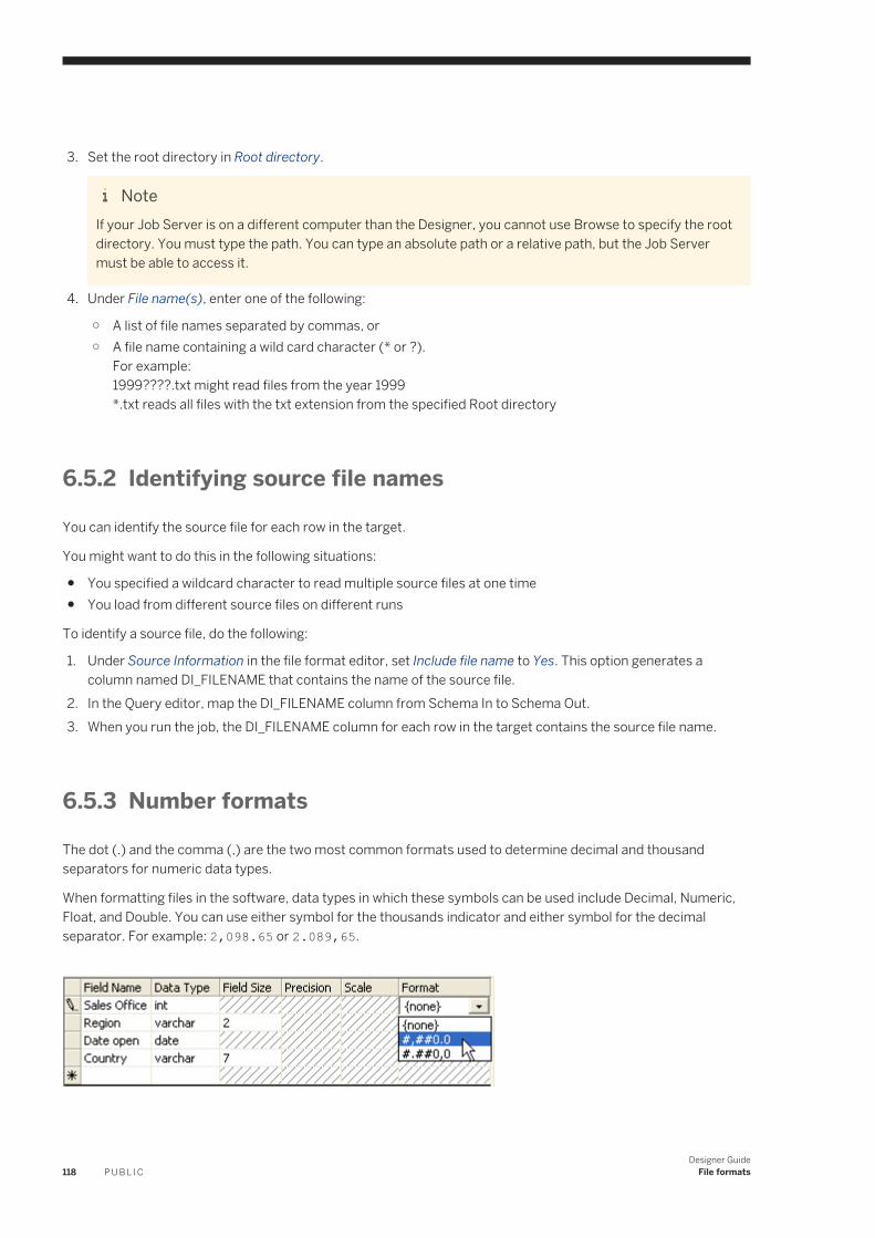
3. Set the root directory in Root directory.
NoteIf your Job Server is on a different computer than the Designer, you cannot use Browse to specify the root directory. You must type the path. You can type an absolute path or a relative path, but the Job Server must be able to access it.
4. Under File name(s), enter one of the following:
○ A list of file names separated by commas, or○ A file name containing a wild card character (* or ?).
For example:1999????.txt might read files from the year 1999*.txt reads all files with the txt extension from the specified Root directory
6.5.2 Identifying source file names
You can identify the source file for each row in the target.
You might want to do this in the following situations:
● You specified a wildcard character to read multiple source files at one time● You load from different source files on different runs
To identify a source file, do the following:
1. Under Source Information in the file format editor, set Include file name to Yes. This option generates a column named DI_FILENAME that contains the name of the source file.
2. In the Query editor, map the DI_FILENAME column from Schema In to Schema Out.3. When you run the job, the DI_FILENAME column for each row in the target contains the source file name.
6.5.3 Number formats
The dot (.) and the comma (,) are the two most common formats used to determine decimal and thousand separators for numeric data types.
When formatting files in the software, data types in which these symbols can be used include Decimal, Numeric, Float, and Double. You can use either symbol for the thousands indicator and either symbol for the decimal separator. For example: 2,098.65 or 2.089,65.
118 P U B L I CDesigner Guide
File formats
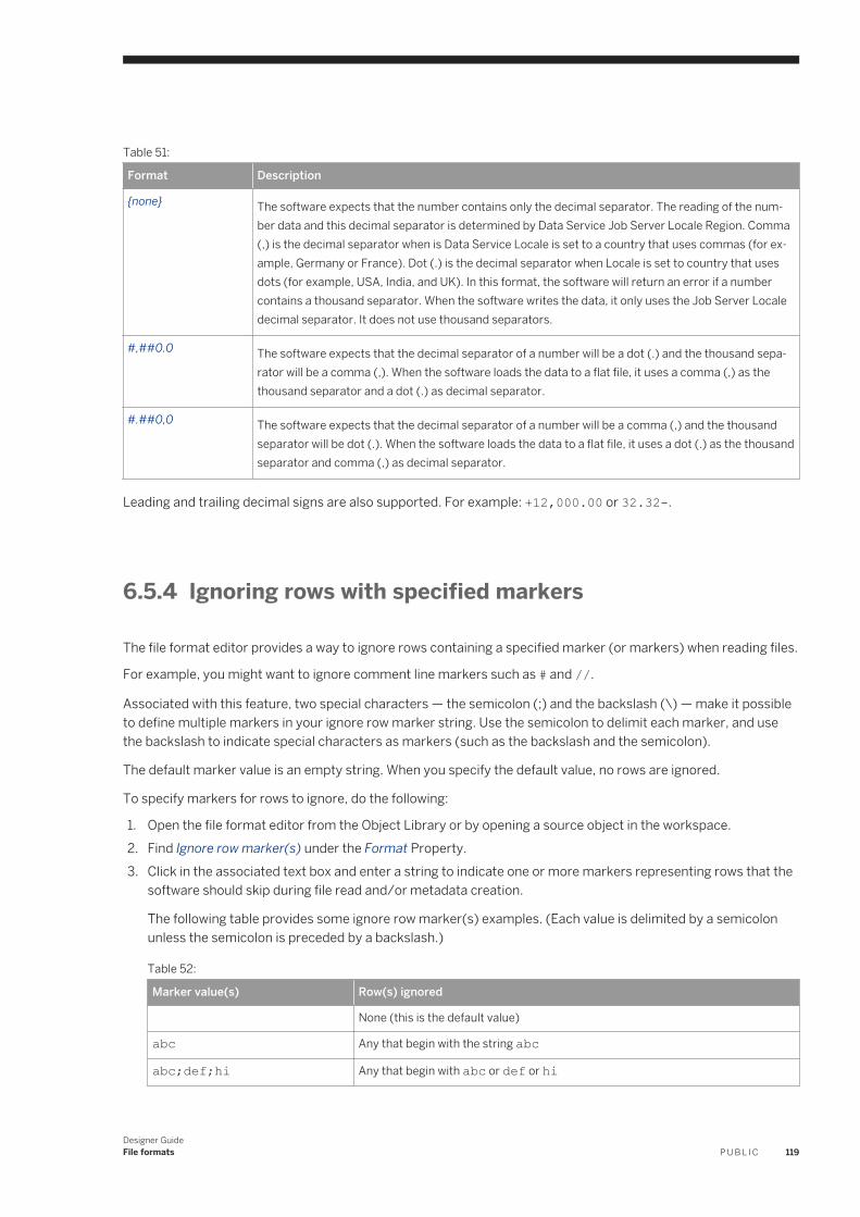
Table 51:
Format Description
{none} The software expects that the number contains only the decimal separator. The reading of the number data and this decimal separator is determined by Data Service Job Server Locale Region. Comma (,) is the decimal separator when is Data Service Locale is set to a country that uses commas (for example, Germany or France). Dot (.) is the decimal separator when Locale is set to country that uses dots (for example, USA, India, and UK). In this format, the software will return an error if a number contains a thousand separator. When the software writes the data, it only uses the Job Server Locale decimal separator. It does not use thousand separators.
#,##0.0 The software expects that the decimal separator of a number will be a dot (.) and the thousand separator will be a comma (,). When the software loads the data to a flat file, it uses a comma (,) as the thousand separator and a dot (.) as decimal separator.
#.##0,0 The software expects that the decimal separator of a number will be a comma (,) and the thousand separator will be dot (.). When the software loads the data to a flat file, it uses a dot (.) as the thousand separator and comma (,) as decimal separator.
Leading and trailing decimal signs are also supported. For example: +12,000.00 or 32.32-.
6.5.4 Ignoring rows with specified markers
The file format editor provides a way to ignore rows containing a specified marker (or markers) when reading files.
For example, you might want to ignore comment line markers such as # and //.
Associated with this feature, two special characters — the semicolon (;) and the backslash (\) — make it possible to define multiple markers in your ignore row marker string. Use the semicolon to delimit each marker, and use the backslash to indicate special characters as markers (such as the backslash and the semicolon).
The default marker value is an empty string. When you specify the default value, no rows are ignored.
To specify markers for rows to ignore, do the following:
1. Open the file format editor from the Object Library or by opening a source object in the workspace.2. Find Ignore row marker(s) under the Format Property.3. Click in the associated text box and enter a string to indicate one or more markers representing rows that the
software should skip during file read and/or metadata creation.
The following table provides some ignore row marker(s) examples. (Each value is delimited by a semicolon unless the semicolon is preceded by a backslash.)
Table 52:
Marker value(s) Row(s) ignored
None (this is the default value)
abc Any that begin with the string abc
abc;def;hi Any that begin with abc or def or hi
Designer GuideFile formats P U B L I C 119
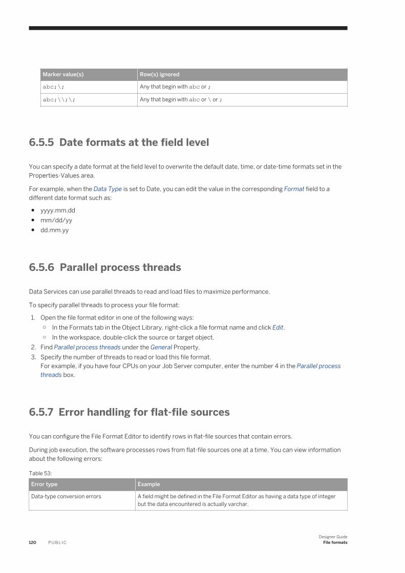
Marker value(s) Row(s) ignored
abc;\; Any that begin with abc or ;
abc;\\;\; Any that begin with abc or \ or ;
6.5.5 Date formats at the field level
You can specify a date format at the field level to overwrite the default date, time, or date-time formats set in the Properties-Values area.
For example, when the Data Type is set to Date, you can edit the value in the corresponding Format field to a different date format such as:
● yyyy.mm.dd● mm/dd/yy● dd.mm.yy
6.5.6 Parallel process threads
Data Services can use parallel threads to read and load files to maximize performance.
To specify parallel threads to process your file format:
1. Open the file format editor in one of the following ways:○ In the Formats tab in the Object Library, right-click a file format name and click Edit.○ In the workspace, double-click the source or target object.
2. Find Parallel process threads under the General Property.3. Specify the number of threads to read or load this file format.
For example, if you have four CPUs on your Job Server computer, enter the number 4 in the Parallel process threads box.
6.5.7 Error handling for flat-file sources
You can configure the File Format Editor to identify rows in flat-file sources that contain errors.
During job execution, the software processes rows from flat-file sources one at a time. You can view information about the following errors:
Table 53:
Error type Example
Data-type conversion errors A field might be defined in the File Format Editor as having a data type of integer but the data encountered is actually varchar.
120 P U B L I CDesigner Guide
File formats
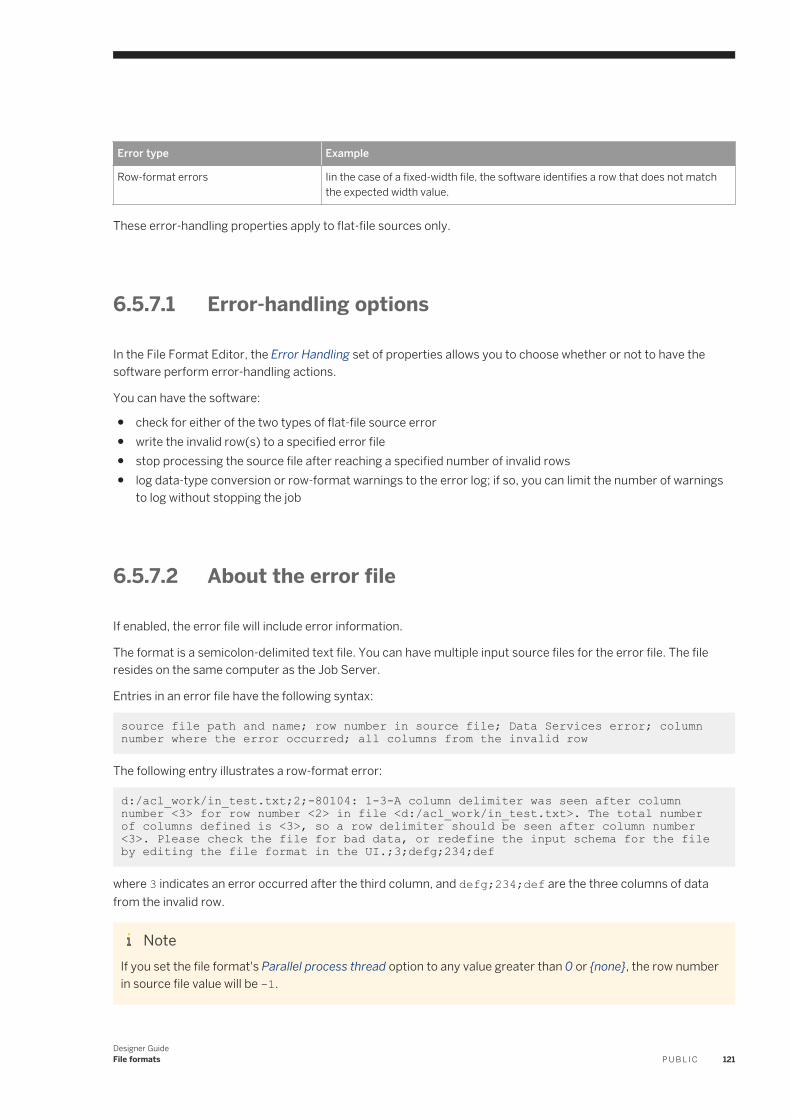
Error type Example
Row-format errors Iin the case of a fixed-width file, the software identifies a row that does not match the expected width value.
These error-handling properties apply to flat-file sources only.
6.5.7.1 Error-handling options
In the File Format Editor, the Error Handling set of properties allows you to choose whether or not to have the software perform error-handling actions.
You can have the software:
● check for either of the two types of flat-file source error● write the invalid row(s) to a specified error file● stop processing the source file after reaching a specified number of invalid rows● log data-type conversion or row-format warnings to the error log; if so, you can limit the number of warnings
to log without stopping the job
6.5.7.2 About the error file
If enabled, the error file will include error information.
The format is a semicolon-delimited text file. You can have multiple input source files for the error file. The file resides on the same computer as the Job Server.
Entries in an error file have the following syntax:
source file path and name; row number in source file; Data Services error; column number where the error occurred; all columns from the invalid row
The following entry illustrates a row-format error:
d:/acl_work/in_test.txt;2;-80104: 1-3-A column delimiter was seen after column number <3> for row number <2> in file <d:/acl_work/in_test.txt>. The total number of columns defined is <3>, so a row delimiter should be seen after column number <3>. Please check the file for bad data, or redefine the input schema for the file by editing the file format in the UI.;3;defg;234;def
where 3 indicates an error occurred after the third column, and defg;234;def are the three columns of data from the invalid row.
NoteIf you set the file format's Parallel process thread option to any value greater than 0 or {none}, the row number in source file value will be -1.
Designer GuideFile formats P U B L I C 121
6.5.7.3 Configuring the File Format Editor for error handling
6.5.7.3.1 Capturing data-type conversion or row-format errors
1. In the object library, click the Formats tab.2. Expand Flat Files, right-click a format, and click Edit.3. The File Format Editor opens.4. To capture data-type conversion errors, under the Error Handling properties for Capture data conversion
errors, click Yes.5. To capture errors in row formats, for Capture row format errors click Yes.6. Click Save or Save & Close.
6.5.7.3.2 Writing invalid rows to an error file
1. In the object library, click the Formats tab.2. Expand Flat Files, right-click a format, and click Edit.
The File Format Editor opens.3. Under the Error Handling properties, click Yes for either or both of the Capture data conversion errors or
Capture row format errors properties.4. For Write error rows to file, click Yes.
Two more fields appear: Error file root directory and Error file name.5. Type an Error file root directory in which to store the error file.
If you type a directory path here, then enter only the file name in the Error file name property.6. Type an Error file name.
If you leave Error file root directory blank, then type a full path and file name here.7. Click Save or Save & Close.
For added flexibility when naming the error file, you can enter a variable that is set to a particular file with full path name. Use variables to specify file names that you cannot otherwise enter such as those that contain multibyte characters
6.5.7.3.3 Limiting the number of invalid rows processed before stopping the job
1. In the object library, click the Formats tab.2. Expand Flat Files, right-click a format, and click Edit.
The File Format Editor opens.
122 P U B L I CDesigner Guide
File formats
3. Under the Error Handling properties, click Yes for either or both the Capture data conversion errors or Capture row format errors properties.
4. For Maximum errors to stop job, type a number.
NoteThis property was previously known as Bad rows limit.
5. Click Save or Save & Close.
6.5.7.3.4 Logging data-type conversion warnings in the error log
1. In the object library, click the Formats tab.2. Expand Flat Files, right-click a format, and click Edit.
The File Format Editor opens.3. Under the Error Handling properties, for Log data conversion warnings, click Yes.4. Click Save or Save & Close.
6.5.7.3.5 Logging row-format warnings in the error log
1. In the object library, click the Formats tab.2. Expand Flat Files, right-click a format, and click Edit.
The File Format Editor opens.3. Under the Error Handling properties, for Log row format warnings, click Yes.4. Click Save or Save & Close.
6.5.7.3.6 Limiting the number of warning messages to log
If you choose to log either data-type or row-format warnings, you can limit the total number of warnings to log without interfering with job execution.
1. In the object library, click the Formats tab.2. Expand Flat Files, right-click a format, and click Edit.
The File Format Editor opens.3. Under the Error Handling properties, for Log row format warnings or Log data conversion warnings (or
both),click Yes.4. For Maximum warnings to log, type a number.5. Click Save or Save & Close.
Designer GuideFile formats P U B L I C 123
6.6 File transfer protocols
Describes two methods to set up file transfer protocols in a file format.
To use custom settings for file transfer protocol, you can choose to set up a custom transfer program, or you can create a file location object. Both methods need to be set up with a specific file format in the File Format Editor. The following table describes the file transfer protocol methods.
Table 54:
File transfer method Description
Custom transfer program For fixed and delimited width file types only. Reads and loads files using the custom transfer program settings in the Custom Transfer group of options in the File Format Editor.
File location object For a variety of file types. Contains file protocol information for transfer protocols such as FTP, SFTP, or SCP, and includes local and remote server information. Create a file location object and associate it to a file format in the File Format Editor.
Related Information
Custom file transfers [page 124]File location objects [page 137]
6.6.1 Custom file transfers
The software can read and load files using a third-party file transfer program for flat files.
Set up a custom file transfer program when you create or edit a file format for a fixed or delimited flat file. You can use third-party (custom) transfer programs to:
● Incorporate company-standard file-transfer applications as part of the software job execution● Provide high flexibility and security for files transferred across a firewall
The custom transfer program option allows you to specify:
● A custom transfer program (invoked during job execution)● Additional arguments, based on what is available in your program, such as:
○ Connection data○ Encryption/decryption mechanisms○ Compression mechanisms
124 P U B L I CDesigner Guide
File formats
Related Information
Using a custom transfer program [page 112]
6.6.1.1 Custom transfer system variables for flat files
By using variables as custom transfer program arguments, you can collect connection information entered in the software and use that data at run-time with your custom transfer program.
NoteIf you have detailed information like a remote and local server to add to the custom transfer variables, consider creating a file location object instead. The File location dialog provides options to enter server locations.
When you set custom transfer options for external file sources and targets, some transfer information, like the name of the remote server that the file is being transferred to or from, may need to be entered literally as a transfer program argument. You can enter other information using the following system variables:
Table 55:
Data entered for: Is substituted for this variable if it is defined in the Arguments field
User name $AW_USER
Password $AW_PASSWORD
Local directory $AW_LOCAL_DIR
File(s) $AW_FILE_NAME
The following custom transfer options use a Windows command file (Myftp.cmd) with five arguments. Arguments 1 through 4 are system variables:
● User and Password variables are for the external server● The Local Directory variable is for the location where the transferred files will be stored in the software● The File Name variable is for the names of the files to be transferred
Argument 5 provides the literal external server name.
NoteIf you do not specify a standard output file (such as ftp.out in the example below), the software writes the standard output into the job's trace log.
@echo off set USER=%1set PASSWORD=%2set LOCAL_DIR=%3set FILE_NAME=%4set LITERAL_HOST_NAME=%5set INP_FILE=ftp.inpecho %USER%>%INP_FILE%echo %PASSWORD%>>%INP_FILE%echo lcd %LOCAL_DIR%>>%INP_FILE%
Designer GuideFile formats P U B L I C 125
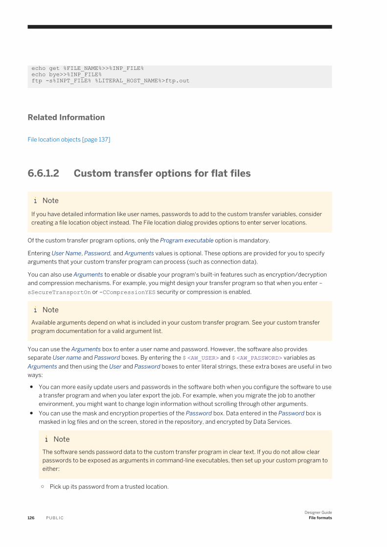
echo get %FILE_NAME%>>%INP_FILE%echo bye>>%INP_FILE% ftp -s%INPT_FILE% %LITERAL_HOST_NAME%>ftp.out
Related Information
File location objects [page 137]
6.6.1.2 Custom transfer options for flat files
NoteIf you have detailed information like user names, passwords to add to the custom transfer variables, consider creating a file location object instead. The File location dialog provides options to enter server locations.
Of the custom transfer program options, only the Program executable option is mandatory.
Entering User Name, Password, and Arguments values is optional. These options are provided for you to specify arguments that your custom transfer program can process (such as connection data).
You can also use Arguments to enable or disable your program's built-in features such as encryption/decryption and compression mechanisms. For example, you might design your transfer program so that when you enter -sSecureTransportOn or -CCompressionYES security or compression is enabled.
NoteAvailable arguments depend on what is included in your custom transfer program. See your custom transfer program documentation for a valid argument list.
You can use the Arguments box to enter a user name and password. However, the software also provides separate User name and Password boxes. By entering the $ <AW_USER> and $ <AW_PASSWORD> variables as Arguments and then using the User and Password boxes to enter literal strings, these extra boxes are useful in two ways:
● You can more easily update users and passwords in the software both when you configure the software to use a transfer program and when you later export the job. For example, when you migrate the job to another environment, you might want to change login information without scrolling through other arguments.
● You can use the mask and encryption properties of the Password box. Data entered in the Password box is masked in log files and on the screen, stored in the repository, and encrypted by Data Services.
NoteThe software sends password data to the custom transfer program in clear text. If you do not allow clear passwords to be exposed as arguments in command-line executables, then set up your custom program to either:
○ Pick up its password from a trusted location.
126 P U B L I CDesigner Guide
File formats
○ Inherit security privileges from the calling program (in this case, the software).
Related Information
File location objects [page 137]
6.6.1.3 Custom transfer options
The custom transfer option allows you to use a third-party program to transfer flat file sources and targets.
You can configure your custom transfer program in the File Format Editor window. Like other file format settings, you can override custom transfer program settings if they are changed for a source or target in a particular data flow. You can also edit the custom transfer option when exporting a file format.
Related Information
Configuring a custom transfer program in the file format editor [page 127]File transfer protocols [page 124]
6.6.1.3.1 Configuring a custom transfer program in the file format editor
1. Select the Formats tab in the object library.2. Right-click Flat Files in the tab and select New.
The File Format Editor opens.3. Select either the Delimited or the Fixed width file type.
NoteWhile the custom transfer program option is not supported by SAP application file types, you can use it as a data transport method for an SAP ABAP data flow.
4. Enter a format name.5. Select Yes for the Custom transfer program option.6. Expand Custom Transfer and enter the custom transfer program name and arguments.7. Complete the other boxes in the file format editor window.
In the Data File(s) section, specify the location of the file in the software.
To specify system variables for Root directory and File(s) in the Arguments box:
Designer GuideFile formats P U B L I C 127
○ Associate the system variable $ <AW_LOCAL_DIR> with the local directory argument of your custom transfer program.
○ Associate the system variable $ <AW_FILE_NAME> with the file name argument of your custom transfer program.
For example, enter: -l$AW_LOCAL_DIR\$AW_FILE_NAME
When the program runs, the Root directory and File(s) settings are substituted for these variables and read by the custom transfer program.
NoteThe flag -l used in the example above is a custom program flag. Arguments you can use as custom program arguments in the software depend upon what your custom transfer program expects.
8. Click Save.
6.6.1.4 Design tips
Use these design tips when using custom transfer options.
● Variables are not supported in file names when invoking a custom transfer program for the file.● You can only edit custom transfer options in the File Format Editor (or Datastore Editor in the case of SAP
application) window before they are exported. You cannot edit updates to file sources and targets at the data flow level when exported. After they are imported, you can adjust custom transfer option settings at the data flow level. They override file format level settings.
When designing a custom transfer program to work with the software, keep in mind that:
● The software expects the called transfer program to return 0 on success and non-zero on failure.● The software provides trace information before and after the custom transfer program executes. The full
transfer program and its arguments with masked password (if any) is written in the trace log. When "Completed Custom transfer" appears in the trace log, the custom transfer program has ended.
● If the custom transfer program finishes successfully (the return code = 0), the software checks the following:○ For an ABAP data flow, if the transport file does not exist in the local directory, it throws an error and the
software stops.○ For a file source, if the file or files to be read by the software do not exist in the local directory, the
software writes a warning message into the trace log.● If the custom transfer program throws an error or its execution fails (return code is not 0), then the software
produces an error with return code and stdout/stderr output.● If the custom transfer program succeeds but produces standard output, the software issues a warning, logs
the first 1,000 bytes of the output produced, and continues processing.● The custom transfer program designer must provide valid option arguments to ensure that files are
transferred to and from the local directory (specified in the software). This might require that the remote file and directory name be specified as arguments and then sent to the Designer interface using system variables.
128 P U B L I CDesigner Guide
File formats
6.7 Working with COBOL copybook file formats
A COBOL copybook file format describes the structure defined in a COBOL copybook file (usually denoted with a .cpy extension).
When creating a COBOL copybook format, you can:
● Create just the format, then configure the source after you add the format to a data flow, or● Create the format and associate it with a data file at the same time.
This section also describes how to:
● Create rules to identify which records represent which schemas using a field ID option.● Identify the field that contains the length of the schema's record using a record length field option.
Related Information
File location objects [page 137]
6.7.1 Creating a new COBOL copybook file format
1. In the local object library, click the Formats tab, right-click COBOL copybooks, and click New.
The Import COBOL copybook window opens.2. Name the format by typing a name in the Format name field.3. On the Format tab for File name, specify the COBOL copybook file format to import, which usually has the
extension .cpy.
During design, you can specify a file in one of the following ways:
○ For a file located on the computer where the Designer runs, you can use the Browse button.○ For a file located on the computer where the Job Server runs, you must type the path to the file. You can
type an absolute path or a relative path, but the Job Server must be able to access it.4. Click OK.
The software adds the COBOL copybook to the object library.5. The COBOL Copybook schema name(s) dialog box displays. If desired, select or double-click a schema name
to rename it.6. Click OK.
When you later add the format to a data flow, you can use the options in the source editor to define the source.
Designer GuideFile formats P U B L I C 129
6.7.2 Creating a new COBOL copybook file format and a data file
1. In the local object library, click the Formats tab, right-click COBOL copybooks, and click New.
The Import COBOL copybook window opens.2. Name the format by typing a name in the Format name field.3. On the Format tab for File name, specify to the COBOL copybook file format to import, which usually has the
extension .cpy.
During design, you can specify a file in one of the following ways:
○ For a file located on the computer where the Designer runs, you can use the Browse button.○ For a file located on the computer where the Job Server runs, you must type the path to the file. You can
type an absolute path or a relative path, but the Job Server must be able to access it.4. Click the Data File tab.5. For Directory, type or browse to the directory that contains the COBOL copybook data file to import.
If you include a directory path here, then enter only the file name in the Name field.6. Specify the COBOL copybook data file Name.
If you leave Directory blank, then type a full path and file name here.
During design, you can specify a file in one of the following ways:
○ For a file located on the computer where the Designer runs, you can use the Browse button.○ For a file located on the computer where the Job Server runs, you must type the path to the file. You can
type an absolute path or a relative path, but the Job Server must be able to access it.7. If the data file is not on the same computer as the Job Server, click the Data Access tab. Select FTP or Custom
and enter the criteria for accessing the data file.8. Click OK.9. The COBOL Copybook schema name(s) dialog box displays. If desired, select or double-click a schema name
to rename it.10. Click OK.
The Field ID tab allows you to create rules for indentifying which records represent which schemas.
6.7.3 Creating rules to identify which records represent which schemas
1. In the local object library, click the Formats tab, right-click COBOL copybooks, and click Edit.
The Edit COBOL Copybook window opens.2. In the top pane, select a field to represent the schema.3. Click the Field ID tab.4. On the Field ID tab, select the check box Use field <schema name.field name> as ID.5. Click Insert below to add an editable value to the Values list.
130 P U B L I CDesigner Guide
File formats
6. Type a value for the field.7. Continue (adding) inserting values as necessary.8. Select additional fields and insert values as necessary.9. Click OK.
6.7.4 Identifying the field that contains the length of the schema's record
1. In the local object library, click the Formats tab, right-click COBOL copybooks, and click Edit.
The Edit COBOL Copybook window opens.2. Click the Record Length Field tab.3. For the schema to edit, click in its Record Length Field column to enable a drop-down menu.4. Select the field (one per schema) that contains the record's length.
The offset value automatically changes to the default of 4; however, you can change it to any other numeric value. The offset is the value that results in the total record length when added to the value in the Record length field.
5. Click OK.
6.8 Creating Microsoft Excel workbook file formats on UNIX platforms
Describes how to use a Microsoft Excel workbook as a source with a Job Server on a UNIX platform.
To create Microsoft Excel workbook file formats on Windows, refer to the Reference Guide.
To access the workbook, you must create and configure an adapter instance in the Administrator. The following procedure provides an overview of the configuration process. For details about creating adapters, refer to the Management Console Guide.
Also consider the following requirements:
● To import the workbook, it must be available on a Windows file system. You can later change the location of the actual file to use for processing in the Excel workbook file format source editor. See the Reference Guide.
● To reimport or view data in the Designer, the file must be available on Windows.● Entries in the error log file might be represented numerically for the date and time fields.
Additionally, Data Services writes the records with errors to the output (in Windows, these records are ignored).
Related Information
Designer GuideFile formats P U B L I C 131
File location objects [page 137]
6.8.1 Creating a Microsoft Excel workbook file format on UNIX
1. Using the Server Manager (<LINK_DIR>/bin/svrcfgInstallation Guide for UNIX), ensure the UNIX Job Server can support adapters. See the .
2. Ensure a repository associated with the Job Server is registered in the Central Management Console (CMC). To register a repository in the CMC, see the Administrator Guide.
3. In the Administrator, add an adapter to access Excel workbooks. See the Management Console Guide.You can only configure one Excel adapter per Job Server. Use the following options:○ On the Status tab, click the job server adapter at right to configure.○ ), ensure theOn the Adapter Configuration tab of Adapter Instances page, click Add.○ On the Adapter Configuration tab, enter the Adapter instance name. Type BOExcelAdapter (required
and case sensitive).You may leave all other options at their default values except when processing files larger than 1 MB. In that case, change the Additional Java Launcher Options value to -Xms64m -Xmx512 or -Xms128m -Xmx1024m (the default is -Xms64m -Xmx256m). Note that Java memory management can prevent processing very large files (or many smaller files).
NoteStarting with Data Services 4.2 SP5, the Excel adapter uses a SAX event-based mechanism to parse the Excel files. If you want to revert it to the way it was processed in version 4.2 SP4 or earlier, set the following flag to false and restart the Job Server. The flag is specified at the Java launcher options for the BOExcelAdapter configuration settings in Management Console.
DuseSAXEventModelForXlsx=false
If the DuseSAXEventModelForXlsx flag is not specified, it defaults to true and uses the SAX event model.
When processing large Excel files, it is recommended to increase the Java heap size in the Java Launcher Options. For example:
-Xms256m –Xmx4096m
4. From the Administrator Adapter Adapter Instance Status tab, start the adapter.5. In the Designer on the Formats tab of the object library, create the file format by importing the Excel
workbook. For details, see the Reference Guide.
6.9 Creating Web log file formats
Web logs are flat files generated by Web servers and are used for business intelligence.
Web logs typically track details of Web site hits such as:
132 P U B L I CDesigner Guide
File formats
● Client domain names or IP addresses● User names● Timestamps● Requested action (might include search string)● Bytes transferred● Referred address● Cookie ID
Web logs use a common file format and an extended common file format.
Common Web log format:
151.99.190.27 - - [01/Jan/1997:13:06:51 -0600] "GET /~bacuslab HTTP/1.0" 301 -4
Extended common Web log format:
saturn5.cun.com - - [25/JUN/1998:11:19:58 -0500] "GET /wew/js/mouseover.html HTTP/1.0" 200 1936"http://av.yahoo.com/bin/query?p=mouse+over+javascript+source+code&hc=0" "Mozilla/4.02 [en] (x11; U; SunOS 5.6 sun4m)"
The software supports both common and extended common Web log formats as sources. The file format editor also supports the following:
● Dash as NULL indicator● Time zone in date-time, e.g. 01/Jan/1997:13:06:51 –0600
The software includes several functions for processing Web log data:
● Word_ext function● Concat_data_time function● WL_GetKeyValue function
Related Information
Word_ext function [page 133]Concat_date_time function [page 134]WL_GetKeyValue function [page 134]
6.9.1 Word_ext function
The word_ext is a string function that extends the word function by returning the word identified by its position in a delimited string.
This function is useful for parsing URLs or file names.
Designer GuideFile formats P U B L I C 133
Format
word_ext(string, word_number, separator(s))
A negative word number means count from right to left
Examples
word_ext('www.bodi.com', 2, '.') returns 'bodi'.
word_ext('www.cs.wisc.edu', -2, '.') returns 'wisc'.
word_ext('www.cs.wisc.edu', 5, '.') returns NULL.
word_ext('aaa+=bbb+=ccc+zz=dd', 4, '+=') returns 'zz'. If 2 separators are specified (+=), the function looks for either one.
word_ext(',,,,,aaa,,,,bb,,,c ', 2, '.') returns 'bb'. This function skips consecutive delimiters.
6.9.2 Concat_date_time function
The concat_date_time is a date function that returns a datetime from separate date and time inputs.
Format
concat_date_time(date, time)
Example
concat_date_time(MS40."date",MS40."time")
6.9.3 WL_GetKeyValue function
The WL_GetKeyValue is a custom function (written in the Scripting Language) that returns the value of a given keyword.
It is useful for parsing search strings.
134 P U B L I CDesigner Guide
File formats
Format
WL_GetKeyValue(string, keyword)
Example
A search in Google for bodi B2B is recorded in a Web log as:
GET "http://www.google.com/search?hl=en&lr=&safe=off&q=bodi+B2B&btnG=Google+Search" WL_GetKeyValue('http://www.google.com/search?hl=en&lr=&safe=off&q=bodi+B2B&btnG=Google+Search','q') returns 'bodi+B2B'.
6.10 Unstructured file formats
Unstructured file formats are a type of flat file format.
To read files that contain unstructured content, create a file format as a source that reads one or more files from a directory. At runtime, the source object in the data flow produces one row per file and contains a reference to each file to access its content. In the data flow, you can use a Text Data Processing transform such as Entity Extraction to process unstructured text or employ another transform to manipulate the data.
The unstructured file format types include:
Table 56:
Unstructured file format types Description
Unstructured text Use this format to process a directory of text-based files including
● Text● HTML● XML
Data Services stores each file's content using the long data type.
Designer GuideFile formats P U B L I C 135
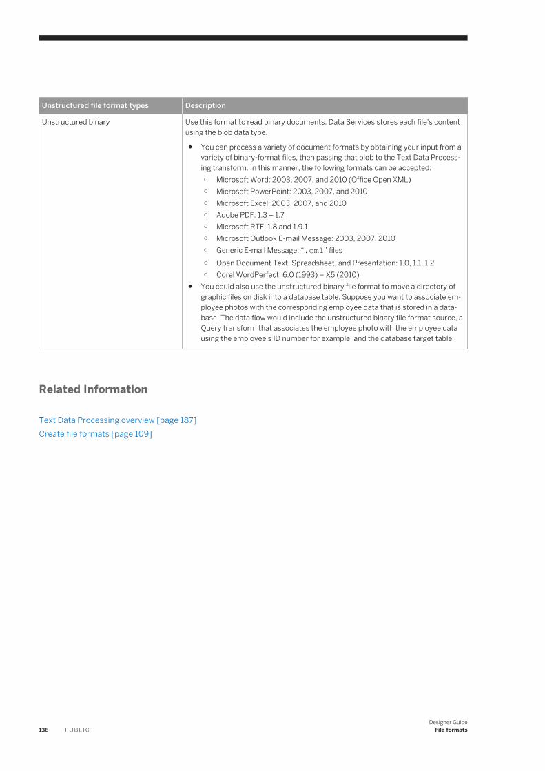
Unstructured file format types Description
Unstructured binary Use this format to read binary documents. Data Services stores each file's content using the blob data type.
● You can process a variety of document formats by obtaining your input from a variety of binary-format files, then passing that blob to the Text Data Processing transform. In this manner, the following formats can be accepted:○ Microsoft Word: 2003, 2007, and 2010 (Office Open XML)○ Microsoft PowerPoint: 2003, 2007, and 2010○ Microsoft Excel: 2003, 2007, and 2010○ Adobe PDF: 1.3 – 1.7○ Microsoft RTF: 1.8 and 1.9.1○ Microsoft Outlook E-mail Message: 2003, 2007, 2010○ Generic E-mail Message: “.eml” files○ Open Document Text, Spreadsheet, and Presentation: 1.0, 1.1, 1.2○ Corel WordPerfect: 6.0 (1993) – X5 (2010)
● You could also use the unstructured binary file format to move a directory of graphic files on disk into a database table. Suppose you want to associate employee photos with the corresponding employee data that is stored in a database. The data flow would include the unstructured binary file format source, a Query transform that associates the employee photo with the employee data using the employee's ID number for example, and the database target table.
Related Information
Text Data Processing overview [page 187]Create file formats [page 109]
136 P U B L I CDesigner Guide
File formats
7 File location objects
File location objects are first-class reusable objects that define properties for a specific file transfer protocol.
Applicable file transfer protocols are Local, AWS S3, SCP, FTP, and SFTP. In addition to entering the file transfer protocol specifics, you define a local and remote server for which you (or the user) have access permission. The software stores file location objects under File Locations in the Format tab of the Data Services Designer object library.
After you have created a file location object, you can associate it to a format object when you create a new or edit an existing object. To use the file location object transfer protocol information in a data flow, you must associate a file location object with a source or target in a data flow.
Applicable format objects include flat files, nested schema files (XML/DTD, JSON), COBOL copybooks, and Excel workbooks.
NoteExcel workbooks and COBOL copybooks paired with a file location object can only be used as sources in a data flow.
When you use the file location object in a data flow as a source or target, the software uses the remote and local server information and the file transfer protocols from the file location object to move a copy of the data from the remote server to the local server to use as a source in a data flow, and to load generated output data from the data flow into the local server and then to the remote server.
The software provides options to control what happens to any existing data when the software transfers the data into a file (either remote or local files). The software can append, overwrite, delete, or save data in the local or remote servers based on the format object type, the protocol type, and the use type (source or target). The software can also create a data file in the local or remote server if one does not exist.
Related Information
Creating a new file location object [page 140]Manage local and remote data files [page 137]
7.1 Manage local and remote data files
Set up a file location object to append, overwrite, save, or delete data in local or remote data files as applicable, and to create a data file if one does not exist.
Even though, in some cases the options save or delete existing data, we call these options append options. Append options are located in various editor dialogs based on whether you are working with a source or target, and whether you are working with a flat file, nested schema, COBOL copybook or Excel workbook.
Designer GuideFile location objects P U B L I C 137
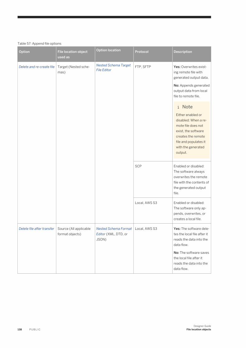
Table 57: Append file options
Option File location object used as
Option location Protocol Description
Delete and re-create file Target (Nested schemas)
Nested Schema Target File Editor
FTP, SFTP Yes: Overwrites existing remote file with generated output data.
No: Appends generated output data from local file to remote file.
NoteEither enabled or disabled: When a remote file does not exist, the software creates the remote file and populates it with the generated output.
SCP Enabled or disabled: The software always overwrites the remote file with the contents of the generated output file.
Local, AWS S3 Enabled or disabled: The software only appends, overwrites, or creates a local file.
Delete file after transfer Source (All applicable format objects)
Nested Schema Format Editor (XML, DTD, or JSON)
Local, AWS S3 Yes: The software deletes the local file after it reads the data into the data flow.
No: The software saves the local file after it reads the data into the data flow.
138 P U B L I CDesigner Guide
File location objects
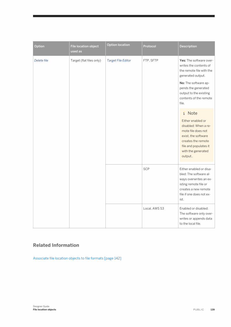
Option File location object used as
Option location Protocol Description
Delete file Target (flat files only) Target File Editor FTP, SFTP Yes: The software overwrites the contents of the remote file with the generated output.
No: The software appends the generated output to the existing contents of the remote file.
NoteEither enabled or disabled: When a remote file does not exist, the software creates the remote file and populates it with the generated output..
SCP Either enabled or disabled: The software always overwrites an existing remote file or creates a new remote file if one does not exist.
Local, AWS S3 Enabled or disabled: The software only overwrites or appends data to the local file.
Related Information
Associate file location objects to file formats [page 142]
Designer GuideFile location objects P U B L I C 139
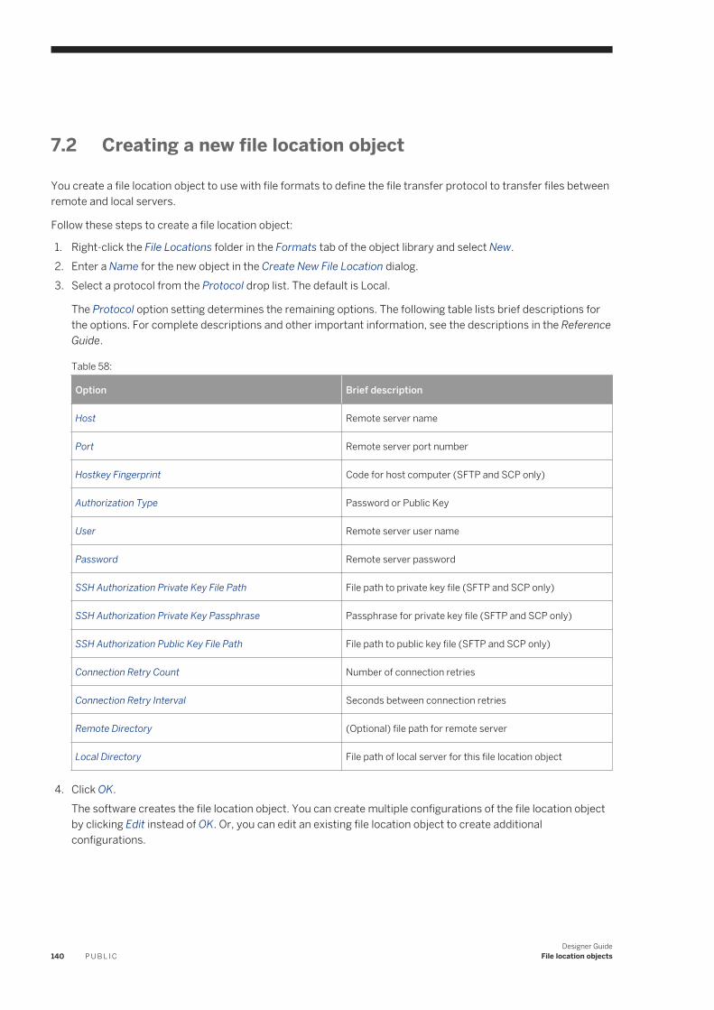
7.2 Creating a new file location object
You create a file location object to use with file formats to define the file transfer protocol to transfer files between remote and local servers.
Follow these steps to create a file location object:
1. Right-click the File Locations folder in the Formats tab of the object library and select New.2. Enter a Name for the new object in the Create New File Location dialog.3. Select a protocol from the Protocol drop list. The default is Local.
The Protocol option setting determines the remaining options. The following table lists brief descriptions for the options. For complete descriptions and other important information, see the descriptions in the Reference Guide.
Table 58:
Option Brief description
Host Remote server name
Port Remote server port number
Hostkey Fingerprint Code for host computer (SFTP and SCP only)
Authorization Type Password or Public Key
User Remote server user name
Password Remote server password
SSH Authorization Private Key File Path File path to private key file (SFTP and SCP only)
SSH Authorization Private Key Passphrase Passphrase for private key file (SFTP and SCP only)
SSH Authorization Public Key File Path File path to public key file (SFTP and SCP only)
Connection Retry Count Number of connection retries
Connection Retry Interval Seconds between connection retries
Remote Directory (Optional) file path for remote server
Local Directory File path of local server for this file location object
4. Click OK.The software creates the file location object. You can create multiple configurations of the file location object by clicking Edit instead of OK. Or, you can edit an existing file location object to create additional configurations.
140 P U B L I CDesigner Guide
File location objects
Related Information
Associate file location objects to file formats [page 142]Create multiple configurations of a file location object [page 141]
7.3 Editing an existing file location object
Edit a file location object to change settings or to add additional configurations.
1. Right-click the name of the File Locations object to edit in the Formats tab of the object library and select Edit.
The Edit File Location <filename> dialog box opens.
2. Edit the applicable options and click OK.
You name the file location object when you create it. You cannot change the name of the file location object when you edit it.
Related Information
Creating multiple file location object configurations [page 142]
7.4 Create multiple configurations of a file location object
Create multiple file location object configurations for each type of file transfer protocol you use.
Each file location object has at least one configuration. If only one configuration exists, it is the default configuration. When you create multiple configurations in one file location object, you can change the default configuration to any of the other configurations in the object.
Using multiple configurations is convenient. For example, when you use different protocols based on your environment, you can create one file location object that contains configurations for your test and production environments. In your test environment you use a local protocol because testing is performed in-house. When you migrate to production, you use SFTP to securely transfer your files between a remote and local server. Switch protocols by editing the file location object that you have used in your job to use a different default configuration.
Designer GuideFile location objects P U B L I C 141
7.4.1 Creating multiple file location object configurations
Steps to create additional file location configurations in a single file loction object, and select a default configuration.
1. Right-click an existing file location object name under File locations in the Format tab in object library and click Edit.
The Edit File Location <filename> dialog box opens.
2. Click Edit....
The Configurations for File Location <filename> dialog box opens.
3. Click the create new configuration icon ( ).
The Create New Configuration dialog opens.4. Enter a unique name for the configuration and click OK.
A new configurations column appears with the new name as the heading.5. Select Yes for Default configuration if this configuration is your default.
NoteIf you have multiple configuration in the file location object, the software automatically switches Default configuration for the other configurations to No.
6. Select a protocol from the Protocol drop menu.
The remaining options that appear after the Protocols option are based on the protocol type you choose. However, if you have multiple configurations (more than one column of settings), there may be options listed that don't apply to the protocol you are defining. Options that don't apply to a configuration appear with “N/A” in the column.
7. Complete the other applicable options and click OK.
For option descriptions, see the Reference Guide.
7.5 Associate file location objects to file formats
To use the file transfer protocol information that you entered into a file location object, you associate the file location object with a specific file source or target in a data flow.
You can also include a file location object when you create or edit a new format.
NoteSome formats are not applicable for file location objects. In those cases, the file location object options don't apply. See the following table for format types.
The following table provides an overview of how to associate a specific file location object with a specific format type.
142 P U B L I CDesigner Guide
File location objects
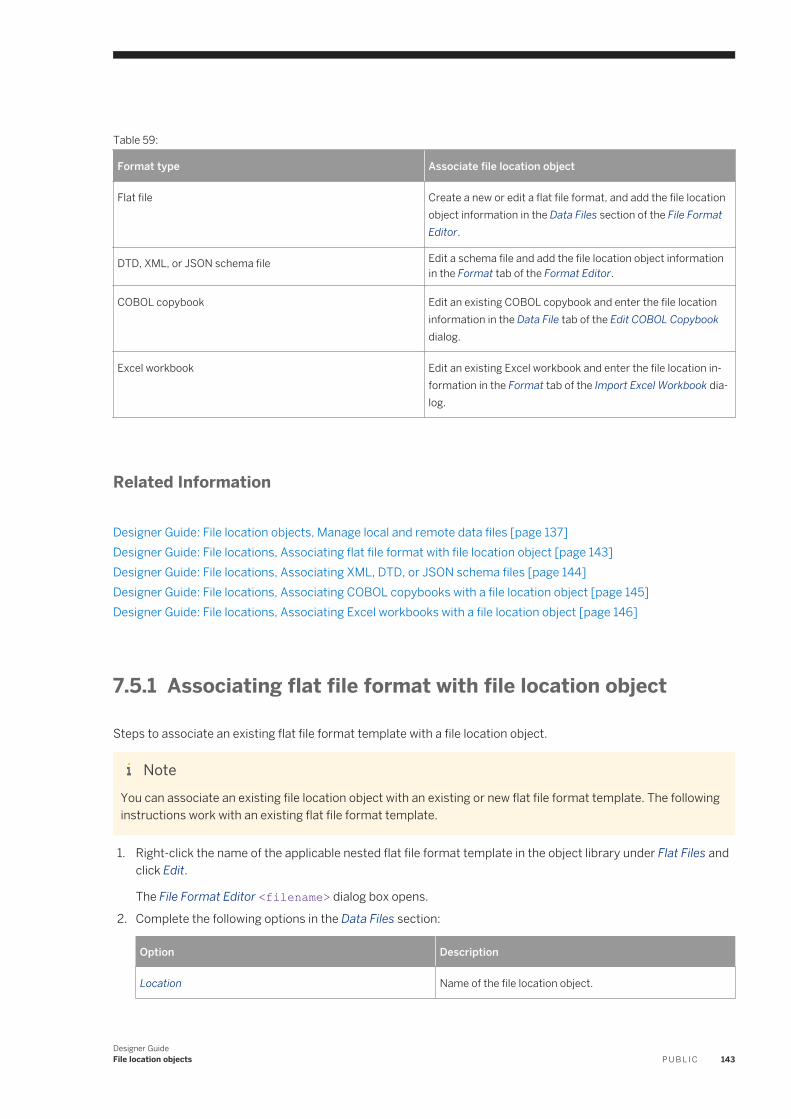
Table 59:
Format type Associate file location object
Flat file Create a new or edit a flat file format, and add the file location object information in the Data Files section of the File Format Editor.
DTD, XML, or JSON schema file Edit a schema file and add the file location object information in the Format tab of the Format Editor.
COBOL copybook Edit an existing COBOL copybook and enter the file location information in the Data File tab of the Edit COBOL Copybook dialog.
Excel workbook Edit an existing Excel workbook and enter the file location information in the Format tab of the Import Excel Workbook dialog.
Related Information
Designer Guide: File location objects, Manage local and remote data files [page 137]Designer Guide: File locations, Associating flat file format with file location object [page 143]Designer Guide: File locations, Associating XML, DTD, or JSON schema files [page 144]Designer Guide: File locations, Associating COBOL copybooks with a file location object [page 145]Designer Guide: File locations, Associating Excel workbooks with a file location object [page 146]
7.5.1 Associating flat file format with file location object
Steps to associate an existing flat file format template with a file location object.
NoteYou can associate an existing file location object with an existing or new flat file format template. The following instructions work with an existing flat file format template.
1. Right-click the name of the applicable nested flat file format template in the object library under Flat Files and click Edit.
The File Format Editor <filename> dialog box opens.
2. Complete the following options in the Data Files section:
Option Description
Location Name of the file location object.
Designer GuideFile location objects P U B L I C 143
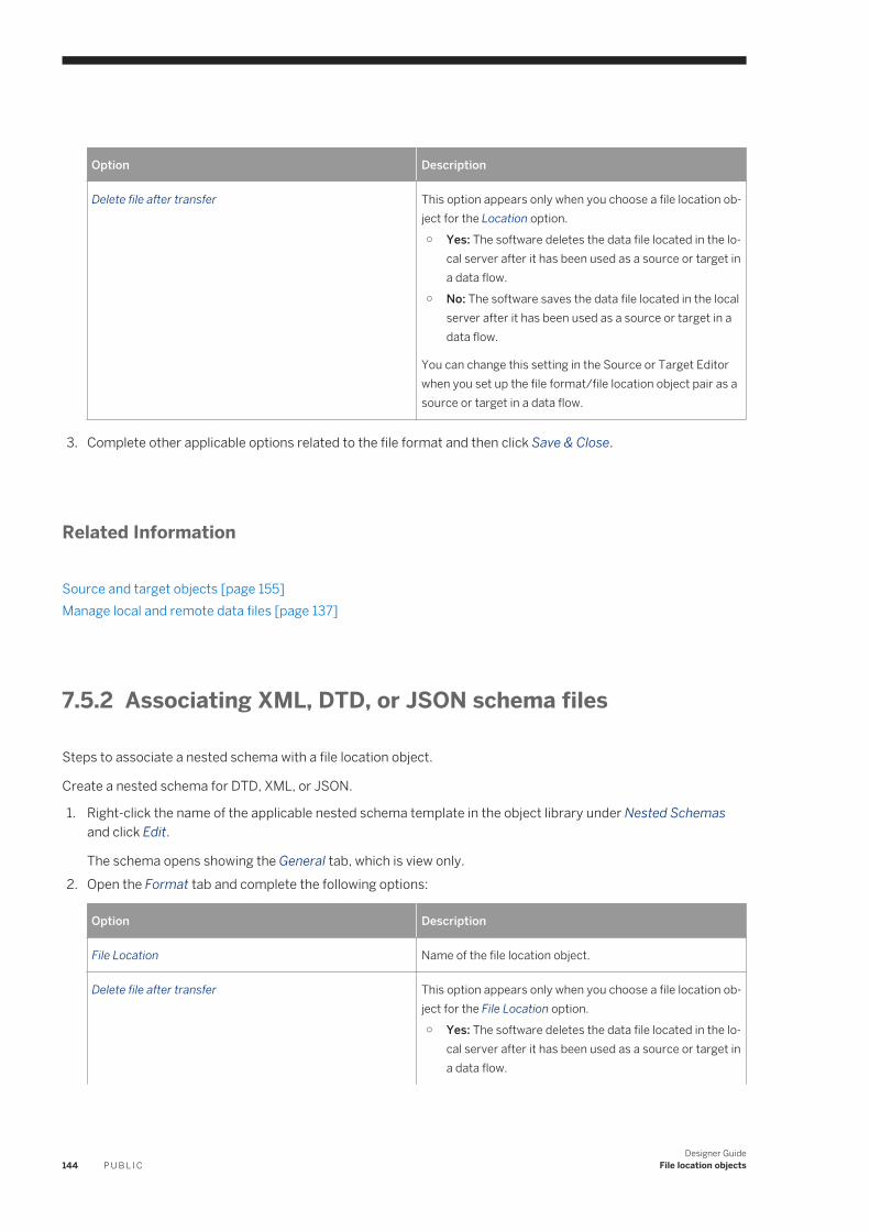
Option Description
Delete file after transfer This option appears only when you choose a file location object for the Location option.○ Yes: The software deletes the data file located in the lo
cal server after it has been used as a source or target in a data flow.
○ No: The software saves the data file located in the local server after it has been used as a source or target in a data flow.
You can change this setting in the Source or Target Editor when you set up the file format/file location object pair as a source or target in a data flow.
3. Complete other applicable options related to the file format and then click Save & Close.
Related Information
Source and target objects [page 155]Manage local and remote data files [page 137]
7.5.2 Associating XML, DTD, or JSON schema files
Steps to associate a nested schema with a file location object.
Create a nested schema for DTD, XML, or JSON.
1. Right-click the name of the applicable nested schema template in the object library under Nested Schemas and click Edit.
The schema opens showing the General tab, which is view only.2. Open the Format tab and complete the following options:
Option Description
File Location Name of the file location object.
Delete file after transfer This option appears only when you choose a file location object for the File Location option.○ Yes: The software deletes the data file located in the lo
cal server after it has been used as a source or target in a data flow.
144 P U B L I CDesigner Guide
File location objects
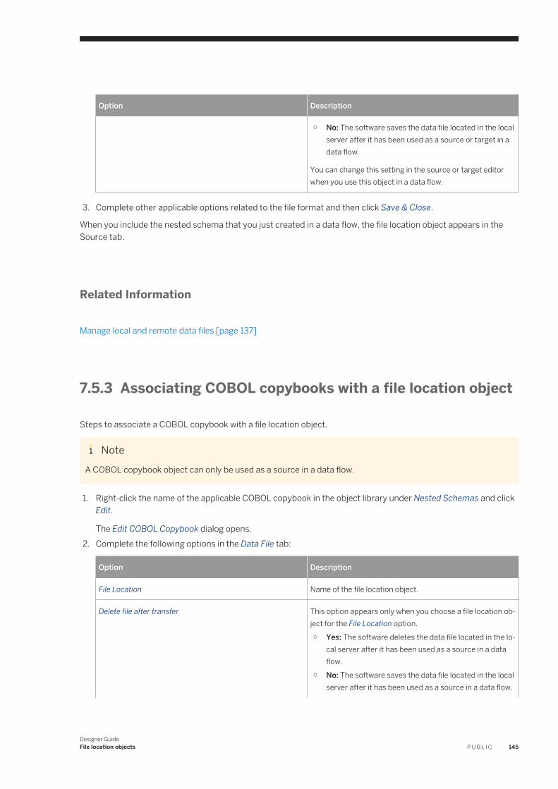
Option Description
○ No: The software saves the data file located in the local server after it has been used as a source or target in a data flow.
You can change this setting in the source or target editor when you use this object in a data flow.
3. Complete other applicable options related to the file format and then click Save & Close.
When you include the nested schema that you just created in a data flow, the file location object appears in the Source tab.
Related Information
Manage local and remote data files [page 137]
7.5.3 Associating COBOL copybooks with a file location object
Steps to associate a COBOL copybook with a file location object.
NoteA COBOL copybook object can only be used as a source in a data flow.
1. Right-click the name of the applicable COBOL copybook in the object library under Nested Schemas and click Edit.
The Edit COBOL Copybook dialog opens.2. Complete the following options in the Data File tab:
Option Description
File Location Name of the file location object.
Delete file after transfer This option appears only when you choose a file location object for the File Location option.○ Yes: The software deletes the data file located in the lo
cal server after it has been used as a source in a data flow.
○ No: The software saves the data file located in the local server after it has been used as a source in a data flow.
Designer GuideFile location objects P U B L I C 145
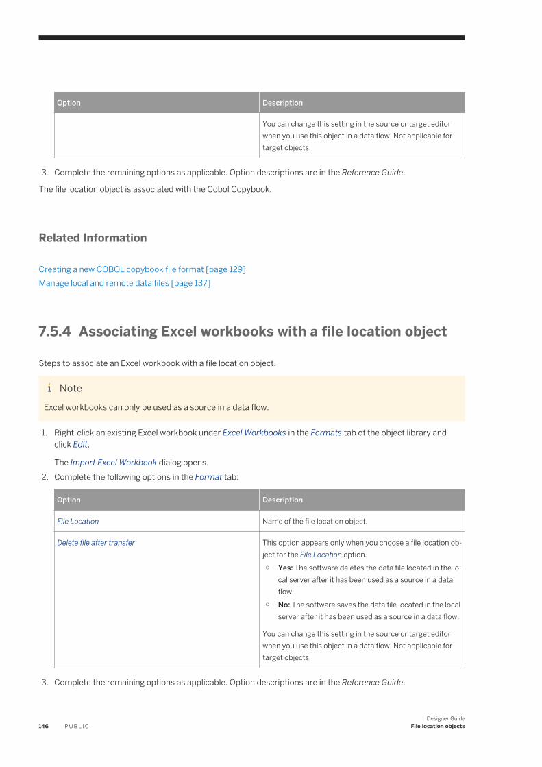
Option Description
You can change this setting in the source or target editor when you use this object in a data flow. Not applicable for target objects.
3. Complete the remaining options as applicable. Option descriptions are in the Reference Guide.
The file location object is associated with the Cobol Copybook.
Related Information
Creating a new COBOL copybook file format [page 129]Manage local and remote data files [page 137]
7.5.4 Associating Excel workbooks with a file location object
Steps to associate an Excel workbook with a file location object.
NoteExcel workbooks can only be used as a source in a data flow.
1. Right-click an existing Excel workbook under Excel Workbooks in the Formats tab of the object library and click Edit.
The Import Excel Workbook dialog opens.2. Complete the following options in the Format tab:
Option Description
File Location Name of the file location object.
Delete file after transfer This option appears only when you choose a file location object for the File Location option.○ Yes: The software deletes the data file located in the lo
cal server after it has been used as a source in a data flow.
○ No: The software saves the data file located in the local server after it has been used as a source in a data flow.
You can change this setting in the source or target editor when you use this object in a data flow. Not applicable for target objects.
3. Complete the remaining options as applicable. Option descriptions are in the Reference Guide.
146 P U B L I CDesigner Guide
File location objects
The file location object is associated with the Excel workbook.
Related Information
Creating a Microsoft Excel workbook file format on UNIX [page 132]
7.6 Adding a file location object to data flow
Steps to add a file location object to a data flow as a source or target.
You can perform these steps with a format object that does or does not have an associated file location object. If the format object does not have an associated file location object, or you want to edit the associated file location object, you can add or edit the association while performing the steps below.
1. Drag the applicable format object into a data flow on your workspace.2. Select Make Source or Make Target from the popup dialog as applicable.3. Click the name of the object that you just added. If it is a source, the Source File Editor opens. If it is a target,
the Target File Editor opens.
The options that appear vary based on the type of format object you chose (flat file, JSON, XML, for example).4. In the Source File Editor or Target File Editor, select an existing file location object from the Location drop
menu. You can also do this to change the existing association to a different file location object if applicable.5. Close the Source File Editor or Target File Editor window.6. Continue with the data flow setup as applicable.
Related Information
Creating and defining data flows [page 153]File location objects [page 137]Associate file location objects to file formats [page 142]Manage local and remote data files [page 137]
7.7 Using scripts to move files from or to a remote server
Examples of using file location object built-in functions in scripts in a work flow.
Use the two built-in functions, copy_from_remote_server and copy_to_remote_server in data flow scripts to identify a file location object and a format object instead of using a format with a file location object association. The scripts identify the file location object that contains your file transfer protocol settings, so the software uses
Designer GuideFile location objects P U B L I C 147
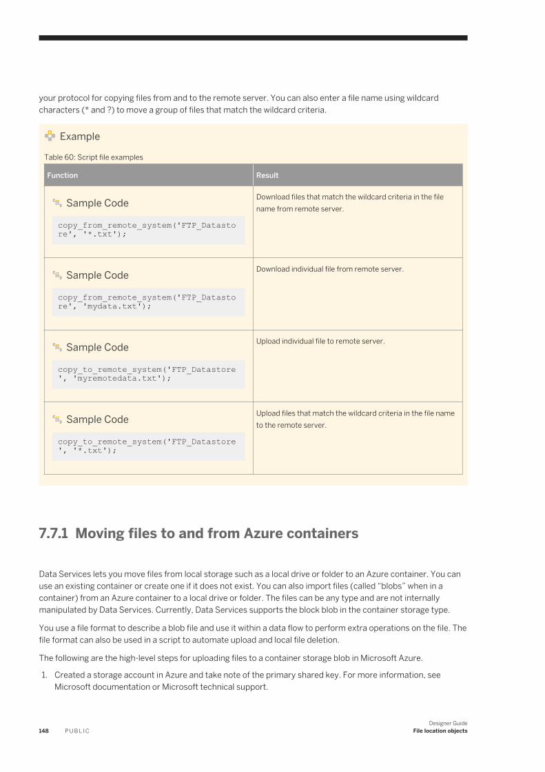
your protocol for copying files from and to the remote server. You can also enter a file name using wildcard characters (* and ?) to move a group of files that match the wildcard criteria.
Example
Table 60: Script file examples
Function Result
Sample Code
copy_from_remote_system('FTP_Datastore', '*.txt');
Download files that match the wildcard criteria in the file name from remote server.
Sample Code
copy_from_remote_system('FTP_Datastore', 'mydata.txt');
Download individual file from remote server.
Sample Code
copy_to_remote_system('FTP_Datastore', 'myremotedata.txt');
Upload individual file to remote server.
Sample Code
copy_to_remote_system('FTP_Datastore', '*.txt');
Upload files that match the wildcard criteria in the file name to the remote server.
7.7.1 Moving files to and from Azure containers
Data Services lets you move files from local storage such as a local drive or folder to an Azure container. You can use an existing container or create one if it does not exist. You can also import files (called “blobs” when in a container) from an Azure container to a local drive or folder. The files can be any type and are not internally manipulated by Data Services. Currently, Data Services supports the block blob in the container storage type.
You use a file format to describe a blob file and use it within a data flow to perform extra operations on the file. The file format can also be used in a script to automate upload and local file deletion.
The following are the high-level steps for uploading files to a container storage blob in Microsoft Azure.
1. Created a storage account in Azure and take note of the primary shared key. For more information, see Microsoft documentation or Microsoft technical support.
148 P U B L I CDesigner Guide
File location objects
2. Create a file location object with the Azure Cloud Storage protocol. For details about the file location object option settings in Azure, see the Reference Guide.
3. Create a job in Data Services Designer.4. Add a script containing the appropriate function to the job.
○ copy_to_remote_system○ copy_from_remote_system
Example
copy_to_remote_system('New_FileLocation', '*')
A script that contains this function copies all of the files from the local directory specified in the file location object to the container specified in the same object.
5. Save and run the job.
Designer GuideFile location objects P U B L I C 149
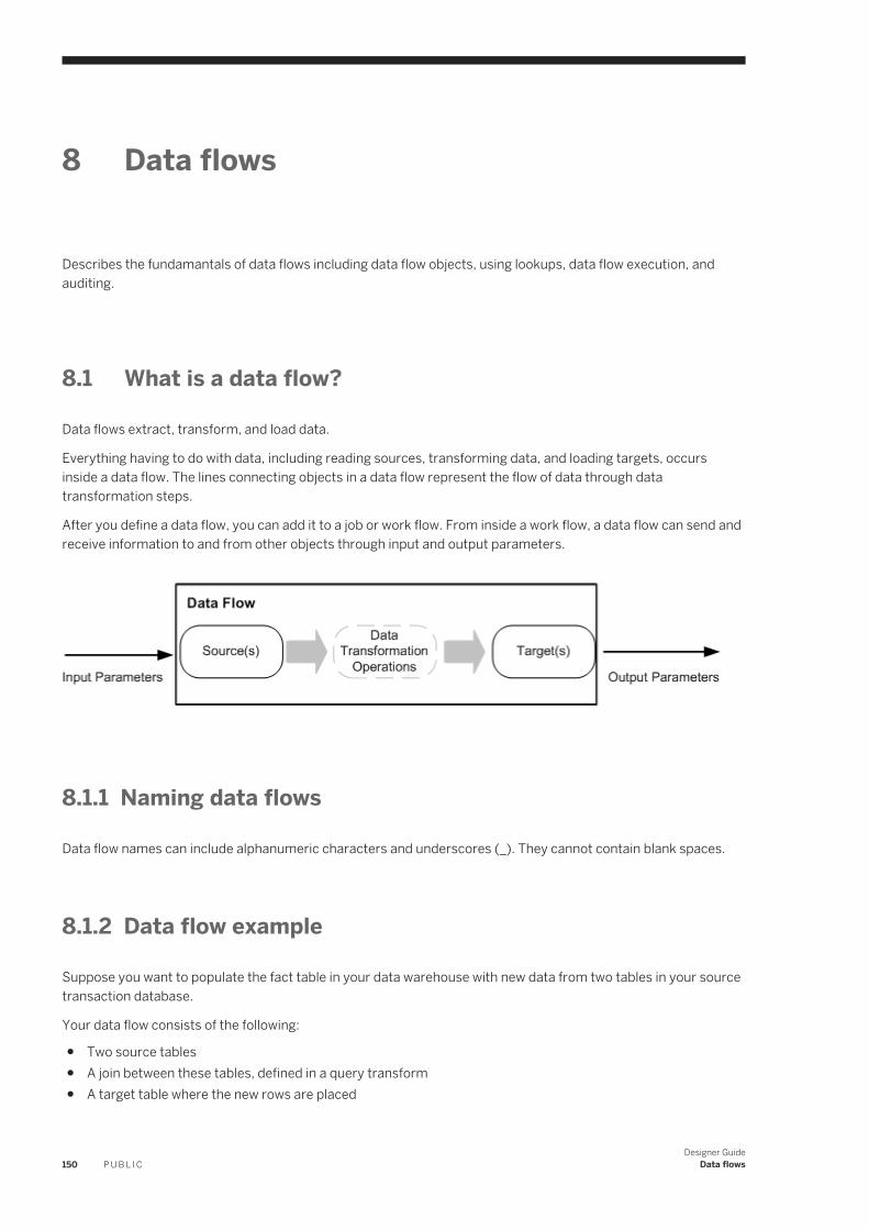
8 Data flows
Describes the fundamantals of data flows including data flow objects, using lookups, data flow execution, and auditing.
8.1 What is a data flow?
Data flows extract, transform, and load data.
Everything having to do with data, including reading sources, transforming data, and loading targets, occurs inside a data flow. The lines connecting objects in a data flow represent the flow of data through data transformation steps.
After you define a data flow, you can add it to a job or work flow. From inside a work flow, a data flow can send and receive information to and from other objects through input and output parameters.
8.1.1 Naming data flows
Data flow names can include alphanumeric characters and underscores (_). They cannot contain blank spaces.
8.1.2 Data flow example
Suppose you want to populate the fact table in your data warehouse with new data from two tables in your source transaction database.
Your data flow consists of the following:
● Two source tables● A join between these tables, defined in a query transform● A target table where the new rows are placed
150 P U B L I CDesigner Guide
Data flows
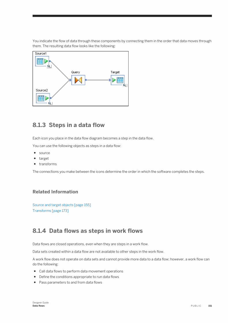
You indicate the flow of data through these components by connecting them in the order that data moves through them. The resulting data flow looks like the following:
8.1.3 Steps in a data flow
Each icon you place in the data flow diagram becomes a step in the data flow.
You can use the following objects as steps in a data flow:
● source● target● transforms
The connections you make between the icons determine the order in which the software completes the steps.
Related Information
Source and target objects [page 155]Transforms [page 173]
8.1.4 Data flows as steps in work flows
Data flows are closed operations, even when they are steps in a work flow.
Data sets created within a data flow are not available to other steps in the work flow.
A work flow does not operate on data sets and cannot provide more data to a data flow; however, a work flow can do the following:
● Call data flows to perform data movement operations● Define the conditions appropriate to run data flows● Pass parameters to and from data flows
Designer GuideData flows P U B L I C 151
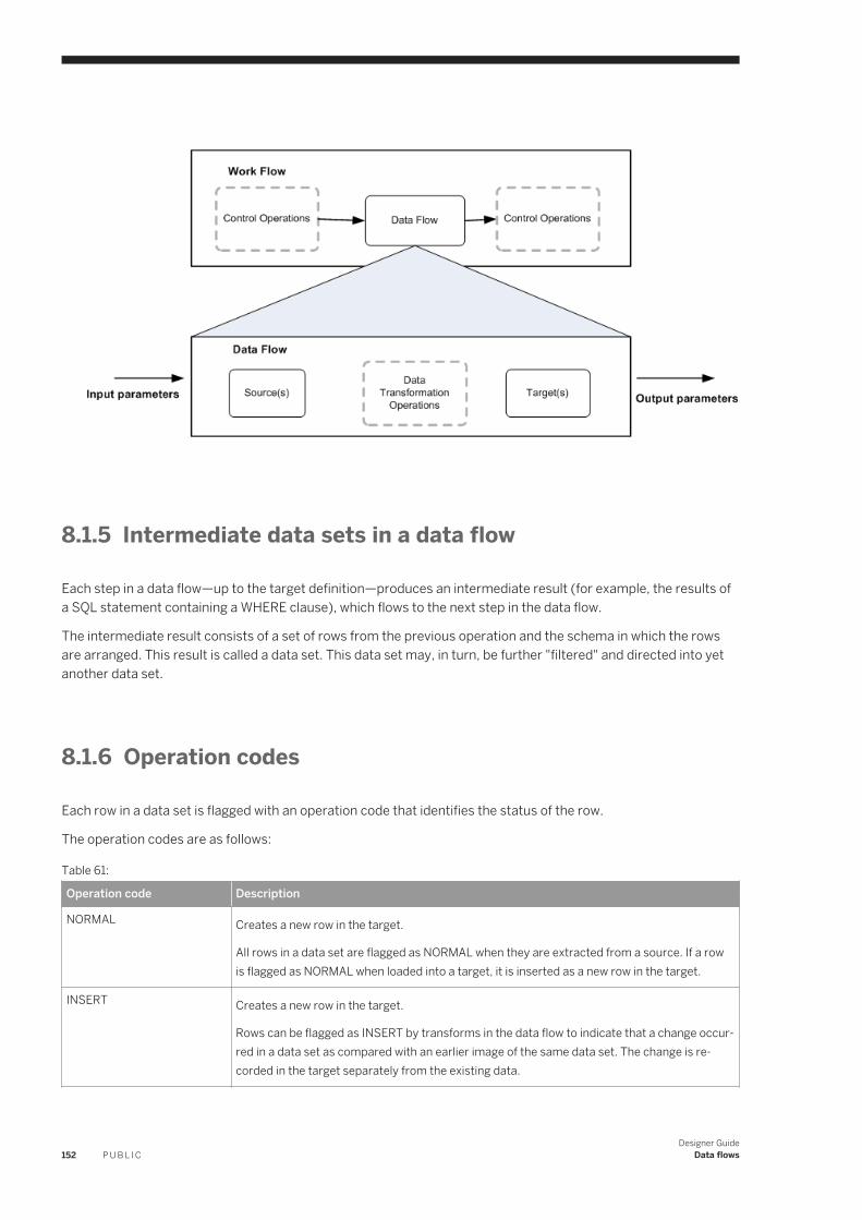
8.1.5 Intermediate data sets in a data flow
Each step in a data flow—up to the target definition—produces an intermediate result (for example, the results of a SQL statement containing a WHERE clause), which flows to the next step in the data flow.
The intermediate result consists of a set of rows from the previous operation and the schema in which the rows are arranged. This result is called a data set. This data set may, in turn, be further "filtered" and directed into yet another data set.
8.1.6 Operation codes
Each row in a data set is flagged with an operation code that identifies the status of the row.
The operation codes are as follows:
Table 61:
Operation code Description
NORMAL Creates a new row in the target.
All rows in a data set are flagged as NORMAL when they are extracted from a source. If a row is flagged as NORMAL when loaded into a target, it is inserted as a new row in the target.
INSERT Creates a new row in the target.
Rows can be flagged as INSERT by transforms in the data flow to indicate that a change occurred in a data set as compared with an earlier image of the same data set. The change is recorded in the target separately from the existing data.
152 P U B L I CDesigner Guide
Data flows
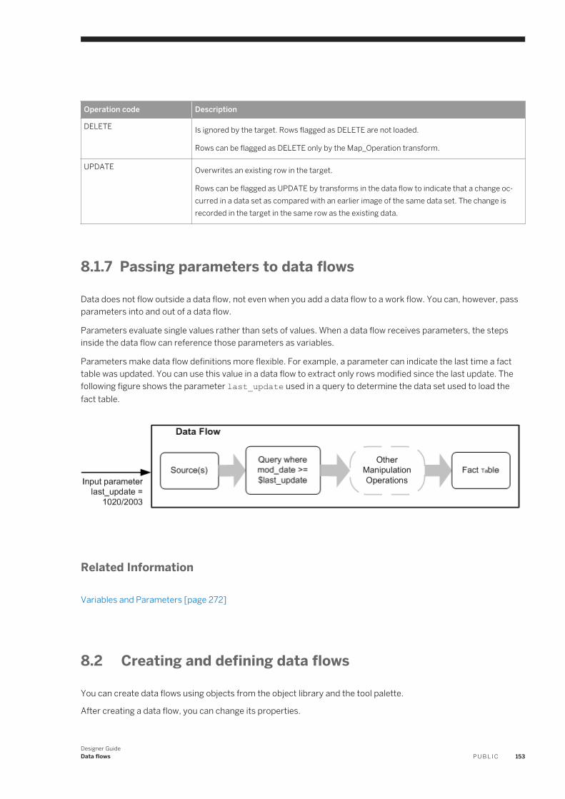
Operation code Description
DELETE Is ignored by the target. Rows flagged as DELETE are not loaded.
Rows can be flagged as DELETE only by the Map_Operation transform.
UPDATE Overwrites an existing row in the target.
Rows can be flagged as UPDATE by transforms in the data flow to indicate that a change occurred in a data set as compared with an earlier image of the same data set. The change is recorded in the target in the same row as the existing data.
8.1.7 Passing parameters to data flows
Data does not flow outside a data flow, not even when you add a data flow to a work flow. You can, however, pass parameters into and out of a data flow.
Parameters evaluate single values rather than sets of values. When a data flow receives parameters, the steps inside the data flow can reference those parameters as variables.
Parameters make data flow definitions more flexible. For example, a parameter can indicate the last time a fact table was updated. You can use this value in a data flow to extract only rows modified since the last update. The following figure shows the parameter last_update used in a query to determine the data set used to load the fact table.
Related Information
Variables and Parameters [page 272]
8.2 Creating and defining data flows
You can create data flows using objects from the object library and the tool palette.
After creating a data flow, you can change its properties.
Designer GuideData flows P U B L I C 153
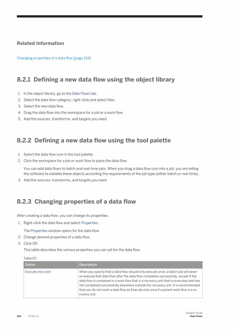
Related Information
Changing properties of a data flow [page 154]
8.2.1 Defining a new data flow using the object library
1. In the object library, go to the Data Flows tab.2. Select the data flow category, right-click and select New.3. Select the new data flow.4. Drag the data flow into the workspace for a job or a work flow.5. Add the sources, transforms, and targets you need.
8.2.2 Defining a new data flow using the tool palette
1. Select the data flow icon in the tool palette.2. Click the workspace for a job or work flow to place the data flow.
You can add data flows to batch and real-time jobs. When you drag a data flow icon into a job, you are telling the software to validate these objects according the requirements of the job type (either batch or real-time).
3. Add the sources, transforms, and targets you need.
8.2.3 Changing properties of a data flow
After creating a data flow, you can change its properties.
1. Right-click the data flow and select Properties.
The Properties window opens for the data flow.2. Change desired properties of a data flow.3. Click OK.
This table describes the various properties you can set for the data flow.
Table 62:
Option Description
Execute only once When you specify that a data flow should only execute once, a batch job will never re-execute that data flow after the data flow completes successfully, except if the data flow is contained in a work flow that is a recovery unit that re-executes and has not completed successfully elsewhere outside the recovery unit. It is recommended that you do not mark a data flow as Execute only once if a parent work flow is a recovery unit.
154 P U B L I CDesigner Guide
Data flows
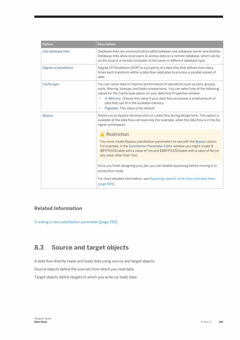
Option Description
Use database links Database links are communication paths between one database server and another. Database links allow local users to access data on a remote database, which can be on the local or a remote computer of the same or different database type.
Degree of parallelism Degree Of Parallelism (DOP) is a property of a data flow that defines how many times each transform within a data flow replicates to process a parallel subset of data.
Cache type You can cache data to improve performance of operations such as joins, groups, sorts, filtering, lookups, and table comparisons. You can select one of the following values for the Cache type option on your data flow Properties window:○ In-Memory: Choose this value if your data flow processes a small amount of
data that can fit in the available memory.○ Pageable: This value is the default.
Bypass Allows you to bypass the execution of a data flow during design time. This option is available at the data flow call level only (for example, when the data flow is in the Designer workspace).
RestrictionYou must create Bypass substitution parameters to use with the Bypass option. For example, in the Substitution Parameter Editor window you might create $$BYPASSEnable with a value of Yes and $$BYPASSDisable with a value of No (or any value other than Yes).
Once you finish designing your job, you can disable bypassing before moving it to production mode.
For more detailed information, see Bypassing specific work flows and data flows [page 609].
Related Information
Creating a new substitution parameter [page 294]
8.3 Source and target objects
A data flow directly reads and loads data using source and target objects.
Source objects define the sources from which you read data.
Target objects define targets to which you write (or load) data.
Designer GuideData flows P U B L I C 155
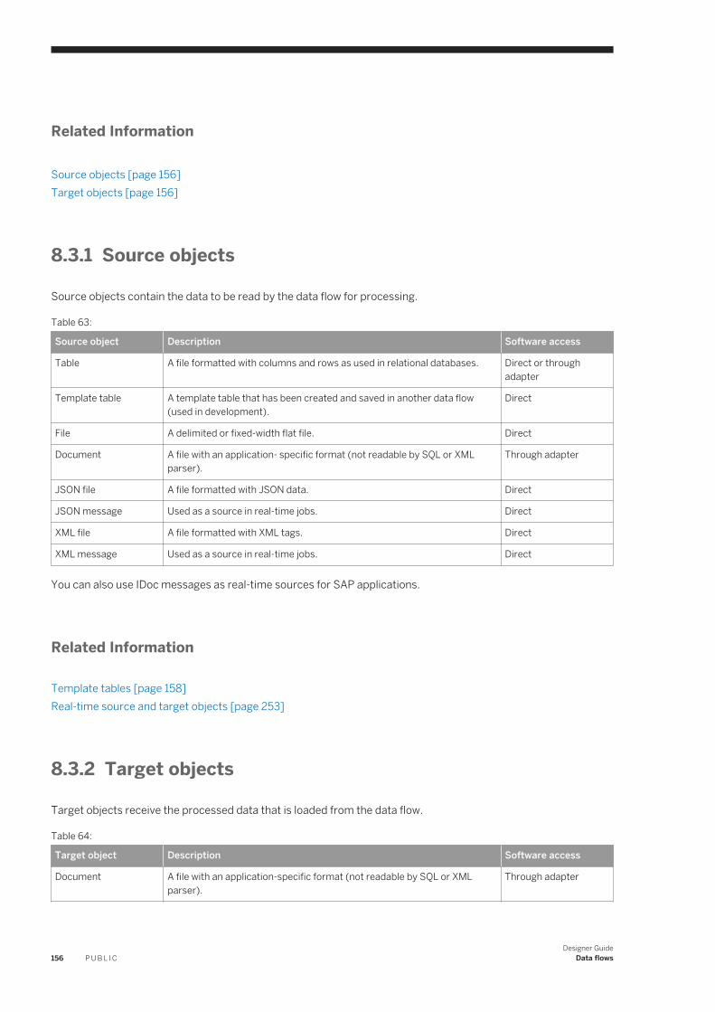
Related Information
Source objects [page 156]Target objects [page 156]
8.3.1 Source objects
Source objects contain the data to be read by the data flow for processing.
Table 63:
Source object Description Software access
Table A file formatted with columns and rows as used in relational databases. Direct or through adapter
Template table A template table that has been created and saved in another data flow (used in development).
Direct
File A delimited or fixed-width flat file. Direct
Document A file with an application- specific format (not readable by SQL or XML parser).
Through adapter
JSON file A file formatted with JSON data. Direct
JSON message Used as a source in real-time jobs. Direct
XML file A file formatted with XML tags. Direct
XML message Used as a source in real-time jobs. Direct
You can also use IDoc messages as real-time sources for SAP applications.
Related Information
Template tables [page 158]Real-time source and target objects [page 253]
8.3.2 Target objects
Target objects receive the processed data that is loaded from the data flow.
Table 64:
Target object Description Software access
Document A file with an application-specific format (not readable by SQL or XML parser).
Through adapter
156 P U B L I CDesigner Guide
Data flows
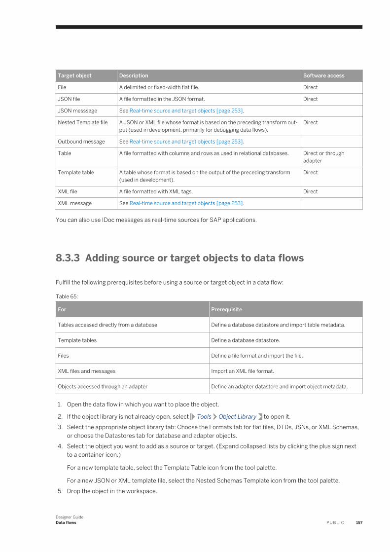
Target object Description Software access
File A delimited or fixed-width flat file. Direct
JSON file A file formatted in the JSON format. Direct
JSON messsage See Real-time source and target objects [page 253].
Nested Template file A JSON or XML file whose format is based on the preceding transform output (used in development, primarily for debugging data flows).
Direct
Outbound message See Real-time source and target objects [page 253].
Table A file formatted with columns and rows as used in relational databases. Direct or through adapter
Template table A table whose format is based on the output of the preceding transform (used in development).
Direct
XML file A file formatted with XML tags. Direct
XML message See Real-time source and target objects [page 253].
You can also use IDoc messages as real-time sources for SAP applications.
8.3.3 Adding source or target objects to data flows
Fulfill the following prerequisites before using a source or target object in a data flow:
Table 65:
For Prerequisite
Tables accessed directly from a database Define a database datastore and import table metadata.
Template tables Define a database datastore.
Files Define a file format and import the file.
XML files and messages Import an XML file format.
Objects accessed through an adapter Define an adapter datastore and import object metadata.
1. Open the data flow in which you want to place the object.
2. If the object library is not already open, select Tools Object Library to open it.3. Select the appropriate object library tab: Choose the Formats tab for flat files, DTDs, JSNs, or XML Schemas,
or choose the Datastores tab for database and adapter objects.4. Select the object you want to add as a source or target. (Expand collapsed lists by clicking the plus sign next
to a container icon.)
For a new template table, select the Template Table icon from the tool palette.
For a new JSON or XML template file, select the Nested Schemas Template icon from the tool palette.5. Drop the object in the workspace.
Designer GuideData flows P U B L I C 157
6. For objects that can be either sources or targets, when you release the cursor, a popup menu appears. Select the kind of object to make.
For new template tables and XML template files, when you release the cursor, a secondary window appears. Enter the requested information for the new template object. Names can include alphanumeric characters and underscores (_). Template tables cannot have the same name as an existing table within a datastore.
7. The source or target object appears in the workspace.8. Click the object name in the workspace
The software opens the editor for the object. Set the options you require for the object.
NoteEnsure that any files that reference flat file, DTD, JSON, or XML Schema formats are accessible from the Job Server where the job will be run and specify the file location relative to this computer.
Related Information
Database datastores [page 64]Template tables [page 158]File formats [page 107]Importing a DTD or XML Schema format [page 224]Adapter datastores [page 88]Adding a file location object to data flow [page 147]
8.3.4 Template tables
During the initial design of an application, you might find it convenient to use template tables to represent database tables.
With template tables, you do not have to initially create a new table in your DBMS and import the metadata into the software. Instead, the software automatically creates the table in the database with the schema defined by the data flow when you execute a job.
After creating a template table as a target in one data flow, you can use it as a source in other data flows. Though a template table can be used as a source table in multiple data flows, it can only be used as a target in one data flow.
Template tables are particularly useful in early application development when you are designing and testing a project. If you modify and save the data transformation operation in the data flow where the template table is a target, the schema of the template table automatically changes. Any updates to the schema are automatically made to any other instances of the template table. During the validation process, the software warns you of any errors such as those resulting from changing the schema.
158 P U B L I CDesigner Guide
Data flows
8.3.4.1 Creating a target template table
1. Use one of the following methods to open the Create Template window:
○ From the tool palette:
○ Click the template table icon. ○ Click inside a data flow to place the template table in the workspace.○ In the Create Template window, select a datastore.
○ From the object library:○ Expand a datastore.○ Click the template table icon and drag it to the workspace.
2. In the Create Template window, enter a table name.3. Click OK.
The table appears in the workspace as a template table icon.4. Connect the template table to the data flow as a target (usually a Query transform).5. In the Query transform, map the Schema In columns that you want to include in the target table.6. From the Project menu select Save.
In the workspace, the template table's icon changes to a target table icon and the table appears in the object library under the datastore's list of tables.
After you are satisfied with the design of your data flow, save it. When the job is executed, software uses the template table to create a new table in the database you specified when you created the template table. Once a template table is created in the database, you can convert the template table in the repository to a regular table.
8.3.5 Converting template tables to regular tables
You must convert template tables to regular tables to take advantage of some features such as bulk loading.
Other features, such as exporting an object, are available for template tables.
NoteOnce a template table is converted, you can no longer alter the schema.
8.3.5.1 Converting a template table into a regular table from the object library
1. Open the object library and go to the Datastores tab.2. Click the plus sign (+) next to the datastore that contains the template table you want to convert.
A list of objects appears.3. Click the plus sign (+) next to Template Tables.
Designer GuideData flows P U B L I C 159
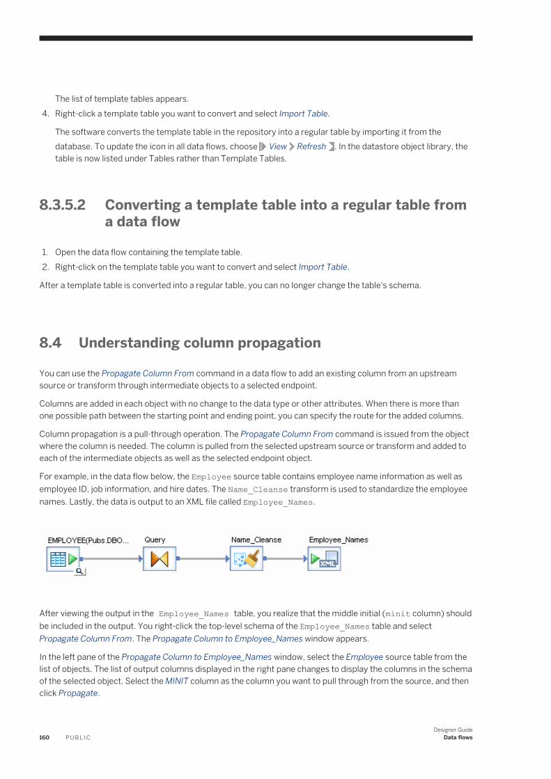
The list of template tables appears.4. Right-click a template table you want to convert and select Import Table.
The software converts the template table in the repository into a regular table by importing it from the database. To update the icon in all data flows, choose View Refresh . In the datastore object library, the table is now listed under Tables rather than Template Tables.
8.3.5.2 Converting a template table into a regular table from a data flow
1. Open the data flow containing the template table.2. Right-click on the template table you want to convert and select Import Table.
After a template table is converted into a regular table, you can no longer change the table's schema.
8.4 Understanding column propagation
You can use the Propagate Column From command in a data flow to add an existing column from an upstream source or transform through intermediate objects to a selected endpoint.
Columns are added in each object with no change to the data type or other attributes. When there is more than one possible path between the starting point and ending point, you can specify the route for the added columns.
Column propagation is a pull-through operation. The Propagate Column From command is issued from the object where the column is needed. The column is pulled from the selected upstream source or transform and added to each of the intermediate objects as well as the selected endpoint object.
For example, in the data flow below, the Employee source table contains employee name information as well as employee ID, job information, and hire dates. The Name_Cleanse transform is used to standardize the employee names. Lastly, the data is output to an XML file called Employee_Names.
After viewing the output in the Employee_Names table, you realize that the middle initial (minit column) should be included in the output. You right-click the top-level schema of the Employee_Names table and select Propagate Column From. The Propagate Column to Employee_Names window appears.
In the left pane of the Propagate Column to Employee_Names window, select the Employee source table from the list of objects. The list of output columns displayed in the right pane changes to display the columns in the schema of the selected object. Select the MINIT column as the column you want to pull through from the source, and then click Propagate.
160 P U B L I CDesigner Guide
Data flows
The minit column schema is carried through the Query and Name_Cleanse transforms to the Employee_Names table.
Characteristics of propagated columns are as follows:
● The Propagate Column From command can be issued from the top-level schema of either a transform or a target.
● Columns are added in each object with no change to the data type or other attributes. Once a column is added to the schema of an object, the column functions in exactly the same way as if it had been created manually.
● The propagated column is added at the end of the schema list in each object.● The output column name is auto-generated to avoid naming conflicts with existing columns. You can edit the
column name, if desired.● Only columns included in top-level schemas can be propagated. Columns in nested schemas cannot be
propagated.● A column can be propagated more than once. Any existing columns are shown in the right pane of the
Propagate Column to window in the Already Exists In field. Each additional column will have a unique name.● Multiple columns can be selected and propagated in the same operation.
NoteYou cannot propagate a column through a Hierarchy_Flattening transform or a Table_Comparison transform.
8.4.1 Adding columns within a dataflow
You can add a column from an upstream source or transform, through intermediate objects, to a selected endpoint using the propagate command.
Columns are added in each object with no change to the data type or other attributes.
To add columns within a data flow:
1. In the downstream object where you want to add the column (the endpoint), right-click the top-level schema and click Propagate Column From.The Propagate Column From can be issued from the top-level schema in a transform or target object.
2. In the left pane of the Propagate Column to window, select the upstream object that contains the column you want to map.The available columns in that object are displayed in the right pane along with a list of any existing mappings from that column.
3. In the right pane, select the column you wish to add and click either Propagate or Propagate and Close.One of the following occurs:○ If there is a single possible route, the selected column is added through the intermediate transforms to
the downstream object.○ If there is more than one possible path through intermediate objects, the Choose Route to dialog displays.
This may occur when your data flow contains a Query transform with multiple input objects. Select the path you prefer and click OK.
Designer GuideData flows P U B L I C 161
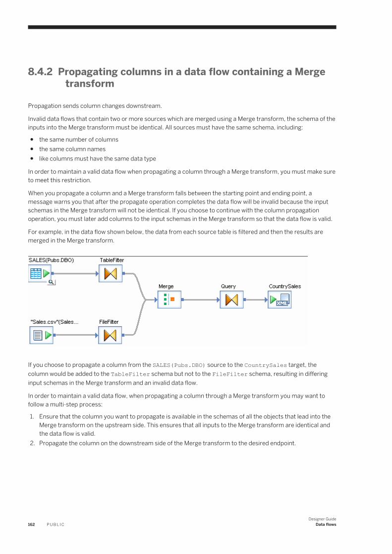
8.4.2 Propagating columns in a data flow containing a Merge transform
Propagation sends column changes downstream.
Invalid data flows that contain two or more sources which are merged using a Merge transform, the schema of the inputs into the Merge transform must be identical. All sources must have the same schema, including:
● the same number of columns● the same column names● like columns must have the same data type
In order to maintain a valid data flow when propagating a column through a Merge transform, you must make sure to meet this restriction.
When you propagate a column and a Merge transform falls between the starting point and ending point, a message warns you that after the propagate operation completes the data flow will be invalid because the input schemas in the Merge transform will not be identical. If you choose to continue with the column propagation operation, you must later add columns to the input schemas in the Merge transform so that the data flow is valid.
For example, in the data flow shown below, the data from each source table is filtered and then the results are merged in the Merge transform.
If you choose to propagate a column from the SALES(Pubs.DBO) source to the CountrySales target, the column would be added to the TableFilter schema but not to the FileFilter schema, resulting in differing input schemas in the Merge transform and an invalid data flow.
In order to maintain a valid data flow, when propagating a column through a Merge transform you may want to follow a multi-step process:
1. Ensure that the column you want to propagate is available in the schemas of all the objects that lead into the Merge transform on the upstream side. This ensures that all inputs to the Merge transform are identical and the data flow is valid.
2. Propagate the column on the downstream side of the Merge transform to the desired endpoint.
162 P U B L I CDesigner Guide
Data flows
8.5 Lookup tables and the lookup_ext function
Lookup tables contain data that other tables reference.
Typically, lookup tables can have the following kinds of columns:
● Lookup column—Use to match a row(s) based on the input values. You apply operators such as =, >, <, ~ to identify a match in a row. A lookup table can contain more than one lookup column.
● Output column—The column returned from the row that matches the lookup condition defined for the lookup column. A lookup table can contain more than one output column.
● Return policy column—Use to specify the data to return in the case where multiple rows match the lookup condition(s).
Use the lookup_ext function to retrieve data from a lookup table based on user-defined lookup conditions that match input data to the lookup table data. Not only can the lookup_ext function retrieve a value in a table or file based on the values in a different source table or file, but it also provides extended functionality that lets you do the following:
● Return multiple columns from a single lookup● Choose from more operators, including pattern matching, to specify a lookup condition● Specify a return policy for your lookup● Call lookup_ext in scripts and custom functions (which also lets you reuse the lookup(s) packaged inside
scripts)● Define custom SQL using the SQL_override parameter to populate the lookup cache, which is useful for
narrowing large quantities of data to only the sections relevant for your lookup(s)● Call lookup_ext using the function wizard in the query output mapping to return multiple columns in a Query
transform● Choose a caching strategy, for example decide to cache the whole lookup table in memory or dynamically
generate SQL for each input record● Use lookup_ext with memory datastore tables or persistent cache tables. The benefits of using persistent
cache over memory tables for lookup tables are:○ Multiple data flows can use the same lookup table that exists on persistent cache.○ The software does not need to construct the lookup table each time a data flow uses it.○ Persistent cache has no memory constraints because it is stored on disk and the software quickly pages it
into memory.● Use pageable cache (which is not available for the lookup and lookup_seq functions)● Use expressions in lookup tables and return the resulting values
For a description of the related functions lookup and lookup_seq, see the Reference Guide.
8.5.1 Accessing the lookup_ext editor
Lookup_ext has its own graphic editor.
There are two ways to invoke the editor:
● Add a new function call inside a Query transform—Use this option if you want the lookup table to return more than one column.
Designer GuideData flows P U B L I C 163
● From the Mapping tab in a query or script function.
8.5.1.1 Adding a new function call
1. In the Query transform Schema out pane, without selecting a specific output column right-click in the pane and select New Function Call.
2. Select the Function category Lookup Functions and the Function name lookup_ext.3. Click Next to invoke the editor.
In the Output section, you can add multiple columns to the output schema.
An advantage of using the new function call is that after you close the lookup_ext function window, you can reopen the graphical editor to make modifications (right-click the function name in the schema and select Modify Function Call).
8.5.1.2 Invoking the lookup_ext editor from the Mapping tab
1. Select the output column name.2. On the Mapping tab, click Functions.3. Select the Function category Lookup Functions and the Function name lookup_ext.4. Click Next to invoke the editor.
In the Output section, Variable replaces Output column name. You can define one output column that will populate the selected column in the output schema. When lookup_ext returns more than one output column, use variables to store the output values, or use lookup_ext as a new function call as previously described in this section.
With functions used in mappings, the graphical editor isn't available, but you can edit the text on the Mapping tab manually.
8.5.2 Example: Defining a simple lookup_ext function
This procedure describes the process for defining a simple lookup_ext function using a new function call. The associated example illustrates how to use a lookup table to retrieve department names for employees.
For details on all the available options for the lookup_ext function, see the Reference Guide.
1. In a data flow, open the Query editor.2. From the Schema in pane, drag the ID column to the Schema out pane.3. Select the ID column in the Schema out pane, right-click, and click New Function Call. Click Insert Below.4. Select the Function category Lookup Functions and the Function name lookup_ext and click Next.
The lookup_ext editor opens.5. In the Lookup_ext - Select Parameters window, select a lookup table:
a. Next to the Lookup table text box, click the drop-down arrow and double-click the datastore, file format, or current schema that includes the table.
164 P U B L I CDesigner Guide
Data flows
b. Select the lookup table and click OK.In the example, the lookup table is a file format called ID_lookup.txt that is in D:\Data.
6. For the Cache spec, the default of PRE_LOAD_CACHE is useful when the number of rows in the table is small or you expect to access a high percentage of the table values.NO_CACHE reads values from the lookup table for every row without caching values. Select DEMAND_LOAD_CACHE when the number of rows in the table is large and you expect to frequently access a low percentage of table values or when you use the table in multiple lookups and the compare conditions are highly selective, resulting in a small subset of data.
7. To provide more resources to execute the lookup_ext function, select Run as a separate process. This option creates a separate child data flow process for the lookup_ext function when the software executes the data flow.
8. Define one or more conditions. For each, add a lookup table column name (select from the drop-down list or drag from the Parameter pane), select the appropriate operator, and enter an expression by typing, dragging, pasting, or using the Smart Editor (click the icon in the right column).In the example, the condition is ID_DEPT = Employees.ID_DEPT.
9. Define the output. For each output column:a. Add a lookup table column name.b. Optionally change the default value from NULL.c. Specify the Output column name by typing, dragging, pasting, or using the Smart Editor (click the icon in
the right column).In the example, the output column is ID_DEPT_NAME.
10. If multiple matches are possible, specify the ordering and set a return policy (default is MAX) to select one match. To order the output, enter the column name(s) in the Order by list.
ExampleThe following example illustrates how to use the lookup table ID_lookup.txt to retrieve department names for employees.
The Employees table is as follows:
Table 66:
ID NAME ID_DEPT
SSN111111111 Employee1 10
SSN222222222 Employee2 10
TAXID333333333 Employee3 20
The lookup table ID_lookup.txt is as follows:
Table 67:
ID_DEPT ID_PATTERN ID_RETURN ID_DEPT_NAME
10 ms(SSN*) =substr(ID_Pattern,4,20) Payroll
20 ms(TAXID*) =substr(ID_Pattern,6,30) Accounting
The lookup_ext editor would be configured as follows.
Designer GuideData flows P U B L I C 165
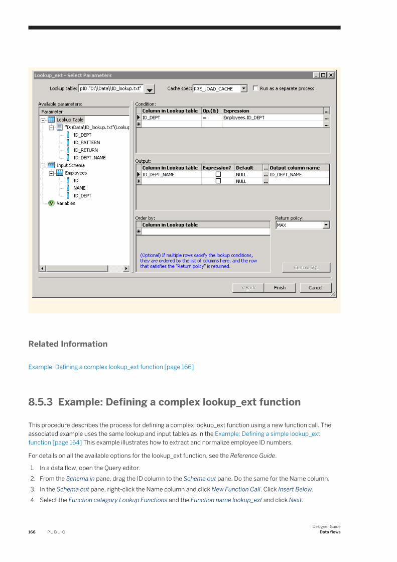
Related Information
Example: Defining a complex lookup_ext function [page 166]
8.5.3 Example: Defining a complex lookup_ext function
This procedure describes the process for defining a complex lookup_ext function using a new function call. The associated example uses the same lookup and input tables as in the Example: Defining a simple lookup_ext function [page 164] This example illustrates how to extract and normalize employee ID numbers.
For details on all the available options for the lookup_ext function, see the Reference Guide.
1. In a data flow, open the Query editor.2. From the Schema in pane, drag the ID column to the Schema out pane. Do the same for the Name column.3. In the Schema out pane, right-click the Name column and click New Function Call. Click Insert Below.4. Select the Function category Lookup Functions and the Function name lookup_ext and click Next.
166 P U B L I CDesigner Guide
Data flows

5. In the Lookup_ext - Select Parameters window, select a lookup table:In the example, the lookup table is in the file format ID_lookup.txt that is in D:\Data.
6. Define one or more conditions.In the example, the condition is ID_PATTERN ~ Employees.ID.
7. Define the output. For each output column:a. Add a lookup table column name.b. If you want the software to interpret the column in the lookup table as an expression and return the
calculated value, select the Expression check box.c. Optionally change the default value from NULL.d. Specify the Output column name(s) by typing, dragging, pasting, or using the Smart Editor (click the icon
in the right column).In the example, the output columns are ID_RETURN and ID_DEPT_NAME.
ExampleExtract and normalize employee ID numbers
In this example, you want to extract and normalize employee Social Security numbers and tax identification numbers that have different prefixes. You want to remove the prefixes, thereby normalizing the numbers. You also want to identify the department from where the number came. The data flow has one source table Employees, a query configured with lookup_ext, and a target table.
Configure the lookup_ext editor as in the following graphic.
Designer GuideData flows P U B L I C 167
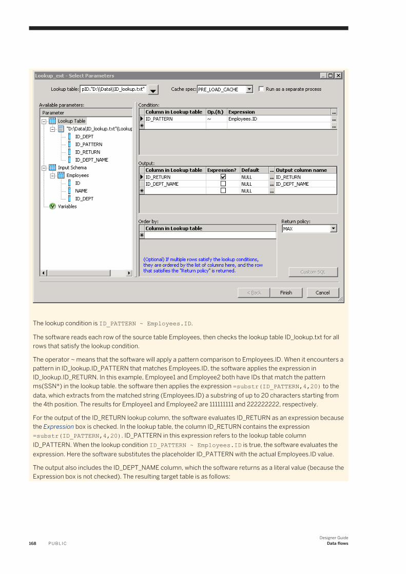
The lookup condition is ID_PATTERN ~ Employees.ID.
The software reads each row of the source table Employees, then checks the lookup table ID_lookup.txt for all rows that satisfy the lookup condition.
The operator ~ means that the software will apply a pattern comparison to Employees.ID. When it encounters a pattern in ID_lookup.ID_PATTERN that matches Employees.ID, the software applies the expression in ID_lookup.ID_RETURN. In this example, Employee1 and Employee2 both have IDs that match the pattern ms(SSN*) in the lookup table. the software then applies the expression =substr(ID_PATTERN,4,20) to the data, which extracts from the matched string (Employees.ID) a substring of up to 20 characters starting from the 4th position. The results for Employee1 and Employee2 are 111111111 and 222222222, respectively.
For the output of the ID_RETURN lookup column, the software evaluates ID_RETURN as an expression because the Expression box is checked. In the lookup table, the column ID_RETURN contains the expression =substr(ID_PATTERN,4,20). ID_PATTERN in this expression refers to the lookup table column ID_PATTERN. When the lookup condition ID_PATTERN ~ Employees.ID is true, the software evaluates the expression. Here the software substitutes the placeholder ID_PATTERN with the actual Employees.ID value.
The output also includes the ID_DEPT_NAME column, which the software returns as a literal value (because the Expression box is not checked). The resulting target table is as follows:
168 P U B L I CDesigner Guide
Data flows
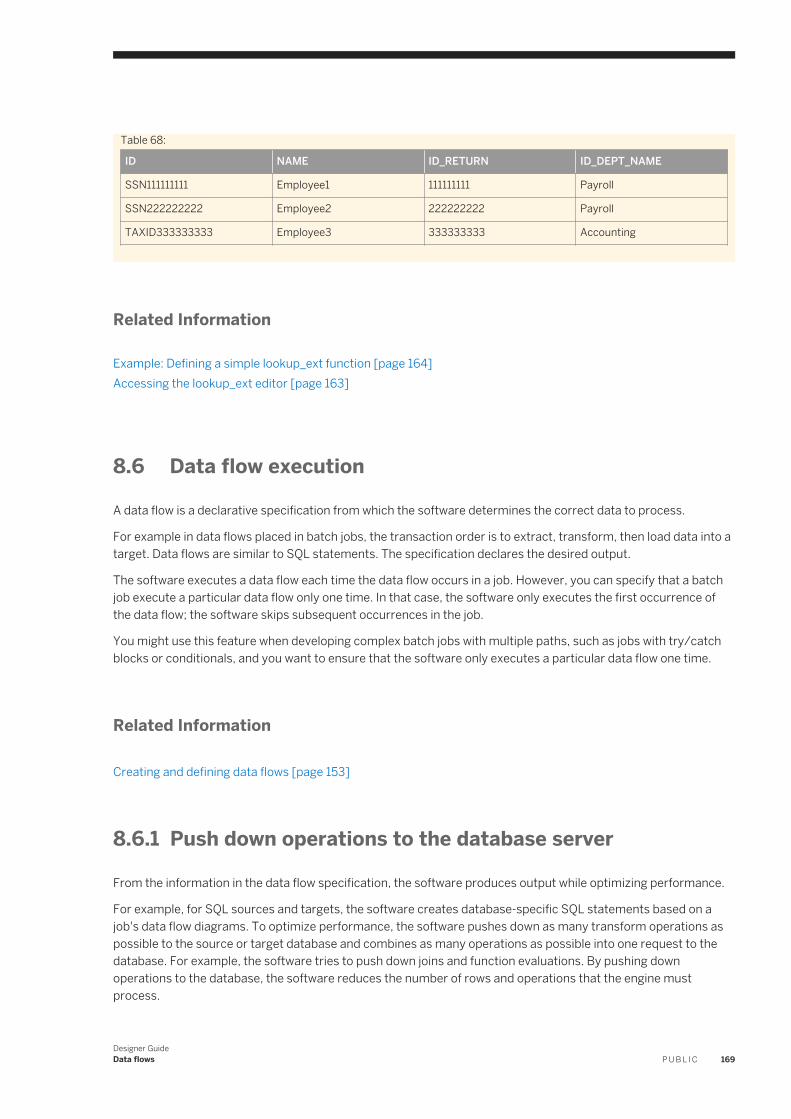
Table 68:
ID NAME ID_RETURN ID_DEPT_NAME
SSN111111111 Employee1 111111111 Payroll
SSN222222222 Employee2 222222222 Payroll
TAXID333333333 Employee3 333333333 Accounting
Related Information
Example: Defining a simple lookup_ext function [page 164]Accessing the lookup_ext editor [page 163]
8.6 Data flow execution
A data flow is a declarative specification from which the software determines the correct data to process.
For example in data flows placed in batch jobs, the transaction order is to extract, transform, then load data into a target. Data flows are similar to SQL statements. The specification declares the desired output.
The software executes a data flow each time the data flow occurs in a job. However, you can specify that a batch job execute a particular data flow only one time. In that case, the software only executes the first occurrence of the data flow; the software skips subsequent occurrences in the job.
You might use this feature when developing complex batch jobs with multiple paths, such as jobs with try/catch blocks or conditionals, and you want to ensure that the software only executes a particular data flow one time.
Related Information
Creating and defining data flows [page 153]
8.6.1 Push down operations to the database server
From the information in the data flow specification, the software produces output while optimizing performance.
For example, for SQL sources and targets, the software creates database-specific SQL statements based on a job's data flow diagrams. To optimize performance, the software pushes down as many transform operations as possible to the source or target database and combines as many operations as possible into one request to the database. For example, the software tries to push down joins and function evaluations. By pushing down operations to the database, the software reduces the number of rows and operations that the engine must process.
Designer GuideData flows P U B L I C 169
Data flow design influences the number of operations that the software can push to the source or target database. Before running a job, you can examine the SQL that the software generates and alter your design to produce the most efficient results.
You can use the Data_Transfer transform to push down resource-intensive operations anywhere within a data flow to the database. Resource-intensive operations include joins, GROUP BY, ORDER BY, and DISTINCT.
8.6.2 Distributed data flow execution
The software provides capabilities to distribute CPU-intensive and memory-intensive data processing work (such as join, grouping, table comparison and lookups) across multiple processes and computers.
This work distribution provides the following potential benefits:
● Better memory management by taking advantage of more CPU resources and physical memory● Better job performance and scalability by using concurrent sub data flow execution to take advantage of grid
computing
You can create sub data flows so that the software does not need to process the entire data flow in memory at one time. You can also distribute the sub data flows to different job servers within a server group to use additional memory and CPU resources.
Use the following features to split a data flow into multiple sub data flows:
● Run as a separate process option on resource-intensive operations that include the following:○ Hierarchy_Flattening transform○ Associate transform○ Country ID transform○ Global Address Cleanse transform○ Global Suggestion Lists transform○ Match Transform○ United States Regulatory Address Cleanse transform○ User-Defined transform○ Query operations that are CPU-intensive and memory-intensive:
○ Join○ GROUP BY○ ORDER BY○ DISTINCT
○ Table_Comparison transform○ Lookup_ext function○ Count_distinct function○ Search_replace function
If you select the Run as a separate process option for multiple operations in a data flow, the software splits the data flow into smaller sub data flows that use separate resources (memory and computer) from each other. When you specify multiple Run as a separate process options, the sub data flow processes run in parallel.
● Data_Transfer transformWith this transform, the software does not need to process the entire data flow on the Job Server computer. Instead, the Data_Transfer transform can push down the processing of a resource-intensive operation to the
170 P U B L I CDesigner Guide
Data flows
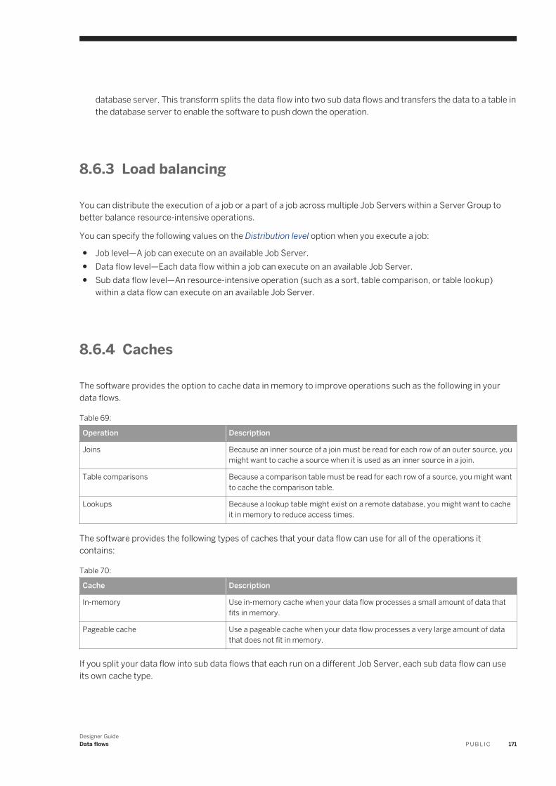
database server. This transform splits the data flow into two sub data flows and transfers the data to a table in the database server to enable the software to push down the operation.
8.6.3 Load balancing
You can distribute the execution of a job or a part of a job across multiple Job Servers within a Server Group to better balance resource-intensive operations.
You can specify the following values on the Distribution level option when you execute a job:
● Job level—A job can execute on an available Job Server.● Data flow level—Each data flow within a job can execute on an available Job Server.● Sub data flow level—An resource-intensive operation (such as a sort, table comparison, or table lookup)
within a data flow can execute on an available Job Server.
8.6.4 Caches
The software provides the option to cache data in memory to improve operations such as the following in your data flows.
Table 69:
Operation Description
Joins Because an inner source of a join must be read for each row of an outer source, you might want to cache a source when it is used as an inner source in a join.
Table comparisons Because a comparison table must be read for each row of a source, you might want to cache the comparison table.
Lookups Because a lookup table might exist on a remote database, you might want to cache it in memory to reduce access times.
The software provides the following types of caches that your data flow can use for all of the operations it contains:
Table 70:
Cache Description
In-memory Use in-memory cache when your data flow processes a small amount of data that fits in memory.
Pageable cache Use a pageable cache when your data flow processes a very large amount of data that does not fit in memory.
If you split your data flow into sub data flows that each run on a different Job Server, each sub data flow can use its own cache type.
Designer GuideData flows P U B L I C 171
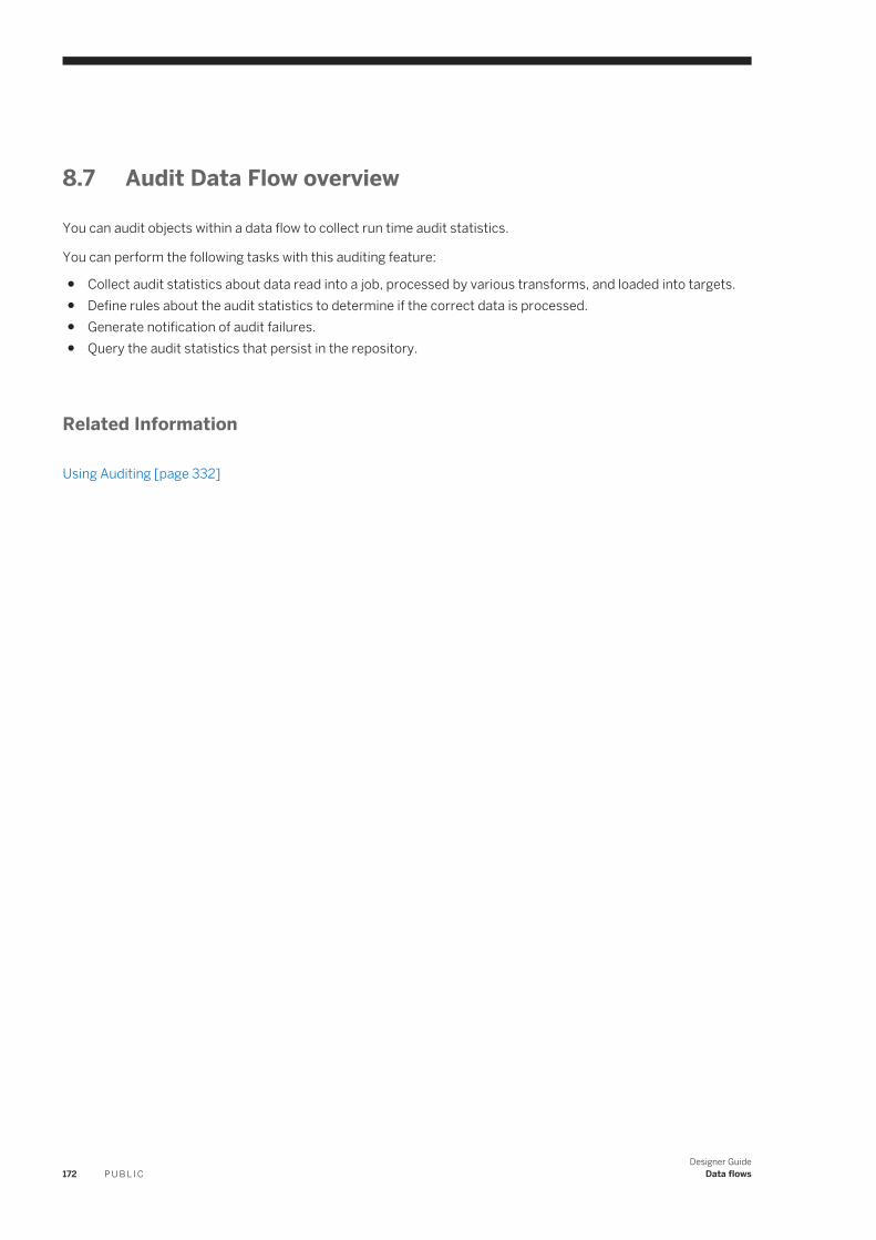
8.7 Audit Data Flow overview
You can audit objects within a data flow to collect run time audit statistics.
You can perform the following tasks with this auditing feature:
● Collect audit statistics about data read into a job, processed by various transforms, and loaded into targets.● Define rules about the audit statistics to determine if the correct data is processed.● Generate notification of audit failures.● Query the audit statistics that persist in the repository.
Related Information
Using Auditing [page 332]
172 P U B L I CDesigner Guide
Data flows
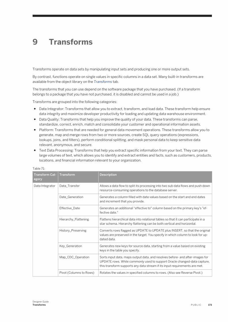
9 Transforms
Transforms operate on data sets by manipulating input sets and producing one or more output sets.
By contrast, functions operate on single values in specific columns in a data set. Many built-in transforms are available from the object library on the Transforms tab.
The transforms that you can use depend on the software package that you have purchased. (If a transform belongs to a package that you have not purchased, it is disabled and cannot be used in a job.)
Transforms are grouped into the following categories:
● Data Integrator: Transforms that allow you to extract, transform, and load data. These transform help ensure data integrity and maximize developer productivity for loading and updating data warehouse environment.
● Data Quality: Transforms that help you improve the quality of your data. These transforms can parse, standardize, correct, enrich, match and consolidate your customer and operational information assets.
● Platform: Transforms that are needed for general data movement operations. These transforms allow you to generate, map and merge rows from two or more sources, create SQL query operations (expressions, lookups, joins, and filters), perform conditional splitting, and mask personal data to keep sensitive data relevant, anonymous, and secure.
● Text Data Processing: Transforms that help you extract specific information from your text. They can parse large volumes of text, which allows you to identify and extract entities and facts, such as customers, products, locations, and financial information relevant to your organization.
Table 71:
Transform Category
Transform Description
Data Integrator Data_Transfer Allows a data flow to split its processing into two sub data flows and push down resource-consuming operations to the database server.
Date_Generation Generates a column filled with date values based on the start and end dates and increment that you provide.
Effective_Date Generates an additional "effective to" column based on the primary key's "effective date."
Hierarchy_Flattening Flattens hierarchical data into relational tables so that it can participate in a star schema. Hierarchy flattening can be both vertical and horizontal.
History_Preserving Converts rows flagged as UPDATE to UPDATE plus INSERT, so that the original values are preserved in the target. You specify in which column to look for updated data.
Key_Generation Generates new keys for source data, starting from a value based on existing keys in the table you specify.
Map_CDC_Operation Sorts input data, maps output data, and resolves before- and after-images for UPDATE rows. While commonly used to support Oracle changed-data capture, this transform supports any data stream if its input requirements are met.
Pivot (Columns to Rows) Rotates the values in specified columns to rows. (Also see Reverse Pivot.)
Designer GuideTransforms P U B L I C 173
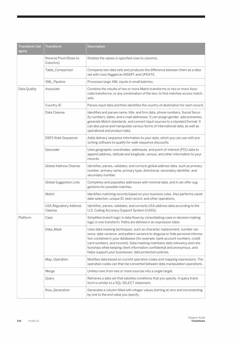
Transform Category
Transform Description
Reverse Pivot (Rows to Columns)
Rotates the values in specified rows to columns.
Table_Comparison Compares two data sets and produces the difference between them as a data set with rows flagged as INSERT and UPDATE.
XML_Pipeline Processes large XML inputs in small batches.
Data Quality Associate Combine the results of two or more Match transforms or two or more Associate transforms, or any combination of the two, to find matches across match sets.
Country ID Parses input data and then identifies the country of destination for each record.
Data Cleanse Identifies and parses name, title, and firm data, phone numbers, Social Security numbers, dates, and e-mail addresses. It can assign gender, add prenames, generate Match standards, and convert input sources to a standard format. It can also parse and manipulate various forms of international data, as well as operational and product data.
DSF2 Walk Sequencer Adds delivery sequence information to your data, which you can use with presorting software to qualify for walk-sequence discounts.
Geocoder Uses geographic coordinates, addresses, and point-of-interest (POI) data to append address, latitude and longitude, census, and other information to your records.
Global Address Cleanse Identifies, parses, validates, and corrects global address data, such as primary number, primary name, primary type, directional, secondary identifier, and secondary number.
Global Suggestion Lists Completes and populates addresses with minimal data, and it can offer suggestions for possible matches.
Match Identifies matching records based on your business rules. Also performs candidate selection, unique ID, best record, and other operations.
USA Regulatory Address Cleanse
Identifies, parses, validates, and corrects USA address data according to the U.S. Coding Accuracy Support System (CASS).
Platform Case Simplifies branch logic in data flows by consolidating case or decision making logic in one transform. Paths are defined in an expression table.
Data_Mask Uses data masking techniques, such as character replacement, number variance, date variance, and pattern variance to disguise or hide personal information contained in your databases (for example, bank account numbers, credit card numbers, and income). Data masking maintains data relevancy and relationships while keeping client information confidential and anonymous, and helps support your businesses’ data protection policies.
Map_Operation Modifies data based on current operation codes and mapping expressions. The operation codes can then be converted between data manipulation operations.
Merge Unifies rows from two or more sources into a single target.
Query Retrieves a data set that satisfies conditions that you specify. A query transform is similar to a SQL SELECT statement.
Row_Generation Generates a column filled with integer values starting at zero and incrementing by one to the end value you specify.
174 P U B L I CDesigner Guide
Transforms
Transform Category
Transform Description
SQL Performs the indicated SQL query operation.
User-Defined Does just about anything that you can write Python code to do. You can use the User-Defined transform to create new records and data sets, or populate a field with a specific value, just to name a few possibilities.
Validation Ensures that the data at any stage in the data flow meets your criteria. You can filter out or replace data that fails your criteria.
Text Data Processing
Entity_Extraction Extracts information (entities and facts) from any text, HTML, XML , or binary format content such as PDF.
9.1 Adding a transform to a data flow
You can use the Designer to add transforms to data flows.
1. Open a data flow object.2. Open the object library if it is not already open and click the Transforms tab.3. Select the transform or transform configuration that you want to add to the data flow.4. Drag the transform or transform configuration icon into the data flow workspace. If you selected a transform
that has available transform configurations, a drop-down menu prompts you to select a transform configuration.
5. Draw the data flow connections.
To connect a source to a transform, click the square on the right edge of the source and drag the cursor to the arrow on the left edge of the transform.
Continue connecting inputs and outputs as required for the transform.
○ The input for the transform might be the output from another transform or the output from a source; or, the transform may not require source data.
○ You can connect the output of the transform to the input of another transform or target.6. Double-click the name of the transform.
This opens the transform editor, which lets you complete the definition of the transform.7. Enter option values.
To specify a data column as a transform option, enter the column name as it appears in the input schema or drag the column name from the input schema into the option box.
Designer GuideTransforms P U B L I C 175
Related Information
Adding a Query transform to a data flow [page 179]Adding a Data Quality transform to a data flow [page 181]Adding a text data processing transform to a data flow [page 193]
9.2 Transform editors
After adding a transform to a data flow, you configure it using the transform's editor.
Transform editor layouts vary.
The most commonly used transform is the Query transform, which has two panes:
● An input schema area and/or output schema area● An options area (or parameters area) that lets you set all the values the transform requires
Data Quality transforms, such as Match and Data Cleanse, use a transform editor that lets you set options and map input and output fields.
The Entity Extraction transform editor lets you set extraction options and map input and output fields.
Related Information
Query Editor [page 179]Data Quality transform editors [page 183]Entity Extraction transform editor [page 194]
9.3 Transform configurations
A transform configuration is a transform with preconfigured best practice input fields, best practice output fields, and options that can be used in multiple data flows.
These are useful if you repeatedly use a transform with specific options and input and output fields.
Some transforms, such as Data Quality transforms, have read-only transform configurations that are provided when Data Services is installed. You can also create your own transform configuration, either by replicating an existing transform configuration or creating a new one. You cannot perform export or multi-user operations on read-only transform configurations.
In the Transform Configuration Editor window, you set up the default options, best practice input fields, and best practice output fields for your transform configuration. After you place an instance of the transform configuration in a data flow, you can override these preset defaults.
176 P U B L I CDesigner Guide
Transforms
If you edit a transform configuration, that change is inherited by every instance of the transform configuration used in data flows, unless a user has explicitly overridden the same option value in an instance.
Related Information
Creating a transform configuration [page 177]Adding a user-defined field [page 178]
9.3.1 Creating a transform configuration
You can create preconfigured best practice input fields, best practice output fields, and options that you want to use in multiple data flows.
1. In the Transforms tab of the Local Object Library, right-click a transform and select New to create a new transform configuration, or right-click an existing transform configuration and select Replicate.If New or Replicate is not available from the menu, then the selected transform type cannot have transform configurations.The Transform Configuration Editor window opens.
2. In Transform Configuration Name, enter the name of the transform configuration.3. In the Options tab, set the option values to determine how the transform will process your data. The available
options depend on the type of transform that you are creating a configuration for.
For the Associate, Match, and User-Defined transforms, options are not editable in the Options tab. You must set the options in the Associate Editor, Match Editor, or User-Defined Editor, which are accessed by clicking the Edit Options button.
If you change an option value from its default value, a green triangle appears next to the option name to indicate that you made an override.
4. To designate an option as "best practice," select the Best Practice checkbox next to the option's value. Designating an option as best practice indicates to other users who use the transform configuration which options are typically set for this type of transform.Use the filter to display all options or just those options that are designated as best practice options.
5. Click the Verify button to check whether the selected option values are valid.If there are any errors, they are displayed at the bottom of the window.
6. In the Input Best Practices tab, select the input fields that you want to designate as the best practice input fields for the transform configuration.The transform configurations provided with Data Services do not specify best practice input fields, so that it doesn't appear that one input schema is preferred over other input schemas. For example, you may map the fields in your data flow that contain address data whether the address data resides in discrete fields, multiline fields, or a combination of discrete and multiline fields.These input fields will be the only fields displayed when the Best Practice filter is selected in the Input tab of the transform editor when the transform configuration is used within a data flow.
7. For Associate, Match, and User-Defined transform configurations, you can create user-defined input fields. Click the Create button and enter the name of the input field.
Designer GuideTransforms P U B L I C 177
8. In the Output Best Practices tab, select the output fields that you want to designate as the best practice output fields for the transform configuration.These output fields will be the only fields displayed when the Best Practice filter is selected in the Output tab of the transform editor when the transform configuration is used within a data flow.
9. Click OK to save the transform configuration.The transform configuration is displayed in the Local Object Library under the base transform of the same type.
You can now use the transform configuration in data flows.
9.3.2 Adding a user-defined field
For some transforms, such as the Associate, Match, and User-Defined transforms, you can create user-defined input fields rather than fields that are recognized by the transform.
These transforms use user-defined fields because they do not have a predefined set of input fields.
You can add a user-defined field either to a single instance of a transform in a data flow or to a transform configuration so that it can be used in all instances.
In the User-Defined transform, you can also add user-defined output fields.
1. In the Transforms tab of the Local Object Library, right-click an existing Associate, Match, or User-Defined transform configuration and select Edit.The Transform Configuration Editor window opens.
2. In the Input Best Practices tab, click the Create button and enter the name of the input field.3. Click OK to save the transform configuration.
When you create a user-defined field in the transform configuration, it is displayed as an available field in each instance of the transform used in a data flow. You can also create user-defined fields within each transform instance.
Related Information
Data Quality transform editors [page 183]
9.4 The Query transform
Retrieves a data set that satisfies conditions that you specify. This transform is similar to a SQL SELECT statement.
The Query transform is by far the most commonly used transform.
The Query transform can perform the following operations:
178 P U B L I CDesigner Guide
Transforms
● Choose (filter) the data to extract from sources● Join data from multiple sources● Map columns from input to output schemas● Perform transformations and functions on the data● Perform data nesting and unnesting● Add new columns, nested schemas, and function results to the output schema● Assign primary keys to output columns
Related Information
Nested Data [page 213]
9.4.1 Adding a Query transform to a data flow
Use the Query transform icon to add a Query transform to a data flow.
1. Click the Query icon in the tool palette.2. Click anywhere in a data flow workspace.3. Connect the Query to inputs and outputs.
Note○ The inputs for a Query can include the output from another transform or the output from a source.○ The outputs from a Query can include input to another transform or input to a target.○ You can change the content type for the columns in your data by selecting a different type from the
output content type list.○ If you connect a target table to a Query with an empty output schema, the software automatically fills
the Query's output schema with the columns from the target table, without mappings.
9.4.2 Query Editor
The Query Editor is a graphical interface for performing query operations.
It contains the following areas: input schema area (upper left), output schema area (upper right), and a
parameters area (lower tabbed area). The icon indicates that the tab contains user-defined entries or that there is at least one join pair (FROM tab only).
The input and output schema areas can contain: Columns, Nested schemas, and Functions (output only).
The Schema In and Schema Out lists display the currently selected schema in each area. The currently selected output schema is called the current schema and determines the following items:
● The output elements that can be modified (added, mapped, or deleted)
Designer GuideTransforms P U B L I C 179
● The scope of the Select through Order by tabs in the parameters area
The current schema is highlighted while all other (non-current) output schemas are gray.
9.4.2.1 Changing the current output schema
You can make a schema, column, or functions "current" in the Output Schema area.
You can do the following:
● Select a schema from the Output list so that it is highlighted.● Right-click a schema, column, or function in the Output Schema area and select Make Current.● Double-click one of the non-current (grayed-out) elements in the Output Schema area.
9.4.2.2 Modifying the output schema contents
The output schema area displays the fields that the transform outputs, and which become the input fields for the downstream transform in the data flow.
You can modify the output schema in several ways:
● Drag and drop (or copy and paste) columns or nested schemas from the input schema area to the output schema area to create simple mappings.
● Use right-click menu options on output elements to:
○ Add new output columns and schemas.○ Use function calls to generate new output columns.○ Assign or reverse primary key settings on output columns. Primary key columns are flagged by a key icon.○ Unnest or re-nest schemas.
● Use the Mapping tab to provide complex column mappings. Drag and drop input schemas and columns into the output schema to enable the editor. Use the function wizard and the smart editor to build expressions. When the text editor is enabled, you can access these features using the buttons above the editor.
● Use the Select through Order By tabs to provide additional parameters for the current schema (similar to SQL SELECT statement clauses). You can drag and drop schemas and columns into these areas.
Table 72:
Tab name Description
Select Specifies whether to output only distinct rows (discarding any identical duplicate rows).
From Lists all input schemas. Allows you to specify join pairs and join conditions as well as enter join rank and cache for each input schema. The resulting SQL FROM clause is displayed.
180 P U B L I CDesigner Guide
Transforms
Tab name Description
Where Specifies conditions that determine which rows are output.
Enter the conditions in SQL syntax, like a WHERE clause in a SQL SELECT statement. For example:
<TABLE1.EMPNO> = <TABLE2.EMPNO> AND <TABLE1.EMPNO> > 1000 OR <TABLE2.EMPNO> < 9000
Use the Functions, Domains, and smart editor buttons for help building expressions.
Group By Specifies how the output rows are grouped (if required).
Order By Specifies how the output rows are sequenced (if required).
● Use the Find tab to locate input and output elements containing a specific word or term.
9.5 Data Quality transforms
Data Quality transforms are a set of transforms that help you improve the quality of your data.
The transforms can parse, standardize, correct, and append information to your customer and operational data.
Data Quality transforms include the following transforms:
● Associate● Country ID● Data Cleanse● DSF2 Walk Sequencer● Geocoder● Global Address Cleanse● Global Suggestion Lists● Match● USA Regulatory Address Cleanse
9.5.1 Adding a Data Quality transform to a data flow
Data Quality transforms cannot be directly connected to an upstream transform that contains or generates nested tables. This is common in real-time data flows, especially those that perform matching. To connect these transforms, you must insert either a Query transform or an XML Pipeline transform between the transform with the nested table and the Data Quality transform.
1. Open a data flow object.2. Open the object library if it is not already open.3. Go to the Transforms tab.
Designer GuideTransforms P U B L I C 181
4. Expand the Data Quality transform folder and select the transform or transform configuration that you want to add to the data flow.
5. Drag the transform or transform configuration icon into the data flow workspace. If you selected a transform that has available transform configurations, a drop-down menu prompts you to select a transform configuration.
6. Draw the data flow connections.
To connect a source or a transform to another transform, click the square on the right edge of the source or upstream transform and drag the cursor to the arrow on the left edge of the Data Quality transform.
○ The input for the transform might be the output from another transform or the output from a source; or, the transform may not require source data.
○ You can connect the output of the transform to the input of another transform or target.7. Double-click the name of the transform.
This opens the transform editor, which lets you complete the definition of the transform.8. In the input schema, select the input fields that you want to map and drag them to the appropriate field in the
Input tab.This maps the input field to a field name that is recognized by the transform so that the transform knows how to process it correctly. For example, an input field that is named "Organization" would be mapped to the Firm field. When content types are defined for the input, these columns are automatically mapped to the appropriate input fields. You can change the content type for the columns in your data by selecting a different type from the output content type list.
9. For the Associate, Match, and User-Defined transforms, you can add user-defined fields to the Input tab. You can do this in two ways:
○ Click the first empty row at the bottom of the table and press F2 on your keyboard. Enter the name of the field. Select the appropriate input field from the drop-down box to map the field.
○ Drag the appropriate input field to the first empty row at the bottom of the table.
To rename the user-defined field, click the name, press F2 on your keyboard, and enter the new name.10. In the Options tab, select the appropriate option values to determine how the transform will process your
data.○ Make sure that you map input fields before you set option values, because in some transforms, the
available options and option values depend on the mapped input fields.○ For the Associate, Match, and User-Defined transforms, options are not editable in the Options tab. You
must set the options in the Associate Editor, Match Editor, and User-Defined Editor. You can access these editors either by clicking the Edit Options button in the Options tab or by right-clicking the transform in the data flow.
If you change an option value from its default value, a green triangle appears next to the option name to indicate that you made an override.
11. In the Output tab, double-click the fields that you want to output from the transform. Data Quality transforms can generate fields in addition to the input fields that the transform processes, so you can output many fields.
Make sure that you set options before you map output fields.
The selected fields appear in the output schema. The output schema of this transform becomes the input schema of the next transform in the data flow.
12. If you want to pass data through the transform without processing it, drag fields directly from the input schema to the output schema.
182 P U B L I CDesigner Guide
Transforms
13. To rename or resize an output field, double-click the output field and edit the properties in the Column Properties window.
Related Information
Data Quality transform editors [page 183]
9.5.2 Data Quality transform editors
The Data Quality editors provide graphical interfaces for setting input and output fields and options.
The transform editor user interface contains the following areas: Input schema area (upper left), output schema area (upper right), and the parameters area (lower tabbed area).
Table 73: Transform editor areas
Area Description
Input schema Displays the input fields that are output from the upstream transform in the data flow.
Output schema Displays the fields that the transform outputs. The output fields become the input fields for the downstream transform in the data flow.
Parameters Contains three tabs:
● Input● Options● Output
The Associate, Match, and User-Defined transforms have additional editors to set various options specific to the transform type. For details, see Associate, Match, and User-Defined transform editors [page 185].
Embedded help
The software includes more information to help you understand the transform and the settings you make. The embedded help changes the topic based on the option you select, to provide information directly related to the option. You can also move to other topics by using hyperlinks when they are present in the open topic.
The embedded help appears to the right of the Data Services Designer workspace.
Designer GuideTransforms P U B L I C 183
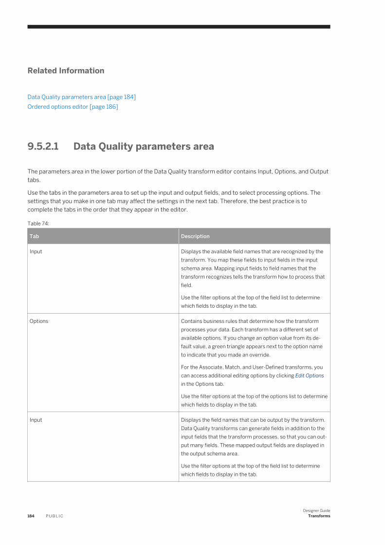
Related Information
Data Quality parameters area [page 184]Ordered options editor [page 186]
9.5.2.1 Data Quality parameters area
The parameters area in the lower portion of the Data Quality transform editor contains Input, Options, and Output tabs.
Use the tabs in the parameters area to set up the input and output fields, and to select processing options. The settings that you make in one tab may affect the settings in the next tab. Therefore, the best practice is to complete the tabs in the order that they appear in the editor.
Table 74:
Tab Description
Input Displays the available field names that are recognized by the transform. You map these fields to input fields in the input schema area. Mapping input fields to field names that the transform recognizes tells the transform how to process that field.
Use the filter options at the top of the field list to determine which fields to display in the tab.
Options Contains business rules that determine how the transform processes your data. Each transform has a different set of available options. If you change an option value from its default value, a green triangle appears next to the option name to indicate that you made an override.
For the Associate, Match, and User-Defined transforms, you can access additional editing options by clicking Edit Options in the Options tab.
Use the filter options at the top of the options list to determine which fields to display in the tab.
Input Displays the field names that can be output by the transform. Data Quality transforms can generate fields in addition to the input fields that the transform processes, so that you can output many fields. These mapped output fields are displayed in the output schema area.
Use the filter options at the top of the field list to determine which fields to display in the tab.
184 P U B L I CDesigner Guide
Transforms
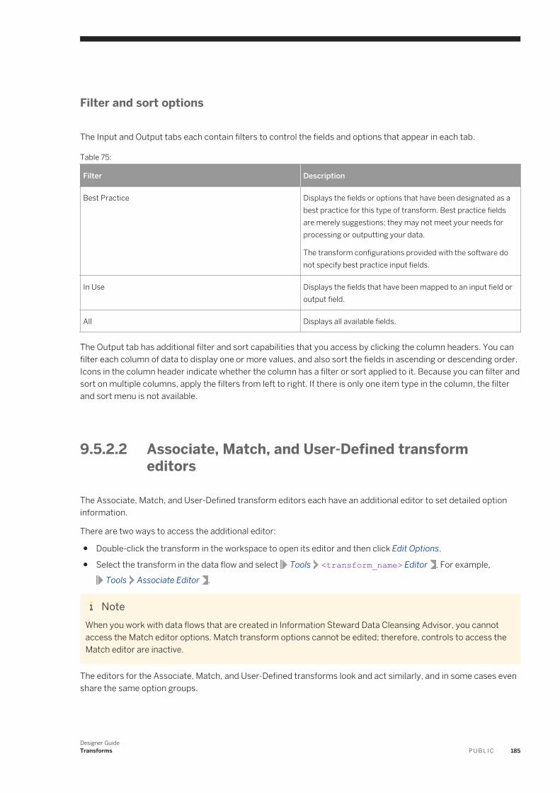
Filter and sort options
The Input and Output tabs each contain filters to control the fields and options that appear in each tab.
Table 75:
Filter Description
Best Practice Displays the fields or options that have been designated as a best practice for this type of transform. Best practice fields are merely suggestions; they may not meet your needs for processing or outputting your data.
The transform configurations provided with the software do not specify best practice input fields.
In Use Displays the fields that have been mapped to an input field or output field.
All Displays all available fields.
The Output tab has additional filter and sort capabilities that you access by clicking the column headers. You can filter each column of data to display one or more values, and also sort the fields in ascending or descending order. Icons in the column header indicate whether the column has a filter or sort applied to it. Because you can filter and sort on multiple columns, apply the filters from left to right. If there is only one item type in the column, the filter and sort menu is not available.
9.5.2.2 Associate, Match, and User-Defined transform editors
The Associate, Match, and User-Defined transform editors each have an additional editor to set detailed option information.
There are two ways to access the additional editor:
● Double-click the transform in the workspace to open its editor and then click Edit Options.
● Select the transform in the data flow and select Tools <transform_name> Editor . For example, Tools Associate Editor .
NoteWhen you work with data flows that are created in Information Steward Data Cleansing Advisor, you cannot access the Match editor options. Match transform options cannot be edited; therefore, controls to access the Match editor are inactive.
The editors for the Associate, Match, and User-Defined transforms look and act similarly, and in some cases even share the same option groups.
Designer GuideTransforms P U B L I C 185
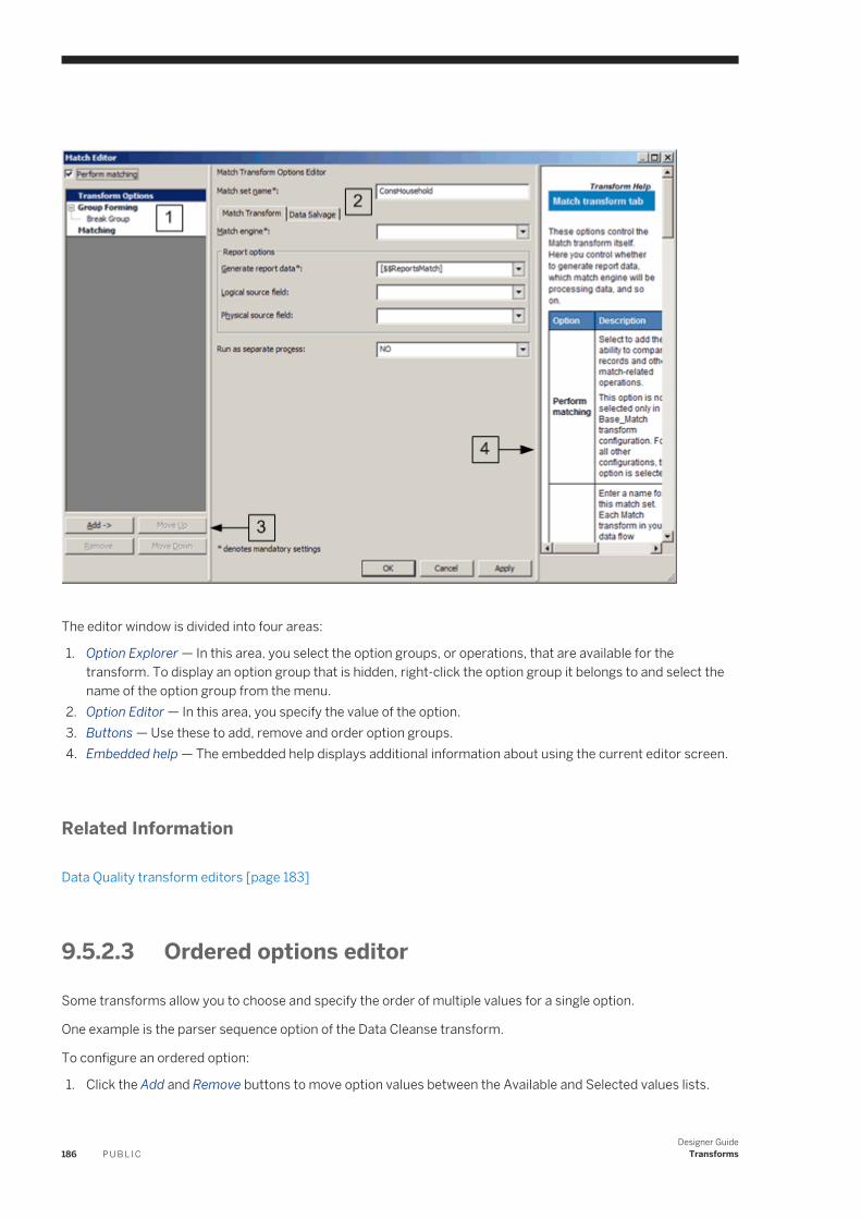
The editor window is divided into four areas:
1. Option Explorer — In this area, you select the option groups, or operations, that are available for the transform. To display an option group that is hidden, right-click the option group it belongs to and select the name of the option group from the menu.
2. Option Editor — In this area, you specify the value of the option.3. Buttons — Use these to add, remove and order option groups.4. Embedded help — The embedded help displays additional information about using the current editor screen.
Related Information
Data Quality transform editors [page 183]
9.5.2.3 Ordered options editor
Some transforms allow you to choose and specify the order of multiple values for a single option.
One example is the parser sequence option of the Data Cleanse transform.
To configure an ordered option:
1. Click the Add and Remove buttons to move option values between the Available and Selected values lists.
186 P U B L I CDesigner Guide
Transforms
NoteRemove all values. To clear the Selected values list and move all option values to the Available values list, click Remove All.
2. Select a value in the Available values list, and click the up and down arrow buttons to change the position of the value in the list.
3. Click OK to save your changes to the option configuration. The values are listed in the Designer and separated by pipe characters.
9.6 Text Data Processing transforms
Text Data Processing transforms help you extract specific information from your text.
They can parse large volumes of text, identifying and extracting entities and facts, such as customers, products, locations, and financial information relevant to your organization. The following sections provide an overview of this functionality and the Entity Extraction transform.
9.6.1 Text Data Processing overview
Text Data Processing can automatically identify the input text language and select language-specific dictionaries and rules for analysis to extract entities, including people, dates, places, organizations and so on, in the languages.
It also looks for patterns, activities, events, and relationships among entities and enables their extraction. Extracting such information from text tells you what the text is about — this information can be used within applications for information management, data integration, and data quality; business intelligence; query, analytics and reporting; search, navigation, document and content management; among other usage scenarios.
Text Data Processing goes beyond conventional character matching tools for information retrieval, which can only seek exact matches for specific strings. It understands semantics of words. In addition to known entity matching, it performs a complementary function of new entity discovery. To customize entity extraction, the software enables you to specify your own list of entities in a custom dictionary. These dictionaries enable you to store entities and manage name variations. Known entity names can be standardized using a dictionary.
Text Data Processing automates extraction of key information from text sources to reduce manual review and tagging. This in turn can reduce cost toward understanding important insights hidden in text. Access to relevant information from unstructured text can help streamline operations and reduce unnecessary costs.
In Data Services, text data processing refers to a set of transforms that extracts information from unstructured data and creates structured data that can be used by various business intelligence tools.
Designer GuideTransforms P U B L I C 187
9.6.2 Entity Extraction transform overview
Text data processing is accomplished in the software using the Entity Extraction transform.
The Entity Extraction transform extracts entities and facts from unstructured text.
Extraction involves processing and analyzing text identifying languages, finding entities of interest, assigning them to the appropriate type, and presenting this metadata in a standard format. By using dictionaries and rules, you can customize your extraction output to include entities defined in them. Extraction applications are as diverse as your information needs. Some examples of information that can be extracted using this transform include:
● Co-occurrence and associations of brand names, company names, people, supplies, and more.● Competitive and market intelligence such as competitors’ activities, merger and acquisition events, press
releases, contact information, and so on.● A person’s associations, activities, or role in a particular event.● Customer claim information, defect reports, or patient information such as adverse drug effects.● Various alphanumeric patterns such as ID numbers, contract dates, profits, and so on.
9.6.2.1 Entities and facts overview
Entities denote names of people, places, and things that can be extracted.
Entities are defined as a pairing of a name and its type. Type indicates the main category of an entity.
Here are some examples of entities:
● Paris is an entity with name "Paris" and type LOCALITY.● Mr. Joe Smith is an entity with name "Mr. Joe Smith" and type PERSON.
Entities can have subtypes. A subtype indicates further classification of an entity; it is a hierarchical specification of an entity type that enables the distinction between different semantic varieties of the same entity type. A subtype can be described as a sub-category of an entity.
Here are some examples of entities and subtypes:
● Boeing 747 is an entity of type VEHICLE with a subtype AIR.● Mercedes-Benz SL500 is an entity of type VEHICLE with a subtype LAND.● SAP is an entity of type ORGANIZATION with a subtype COMMERCIAL.
Facts denote a pattern that creates an expression to extract information such as sentiments, events, or relationships. Facts are extracted using custom extraction rules. Fact is an umbrella term covering extractions of more complex patterns including one or more entities, a relationship between one or more entities, or some sort of predicate about an entity. Facts provide context of how different entities are connected in the text. Entities by themselves only show that they are present in a document, but facts provide information on how these entities are related. Fact types identify the category of a fact; for example, sentiments and requests. A subfact is a key piece of information embedded within a fact. A subfact type can be described as a category associated with the subfact.
Here are some examples of facts and fact types:
● SAP acquired Business Objects in a friendly takeover. This is an event of type merger and acquisition (M&A).● Mr. Joe Smith is very upset with his airline bookings. This is a fact of type SENTIMENT.
188 P U B L I CDesigner Guide
Transforms
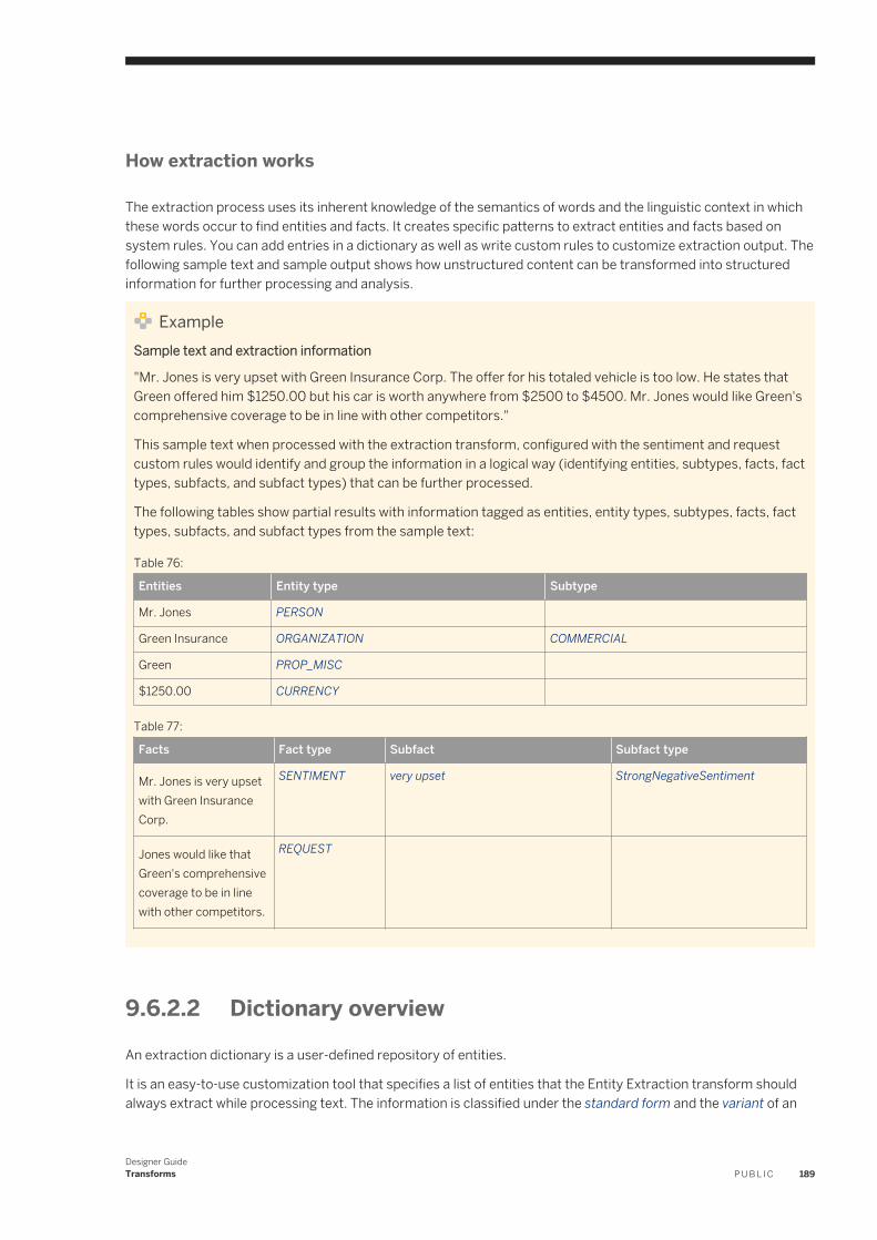
How extraction works
The extraction process uses its inherent knowledge of the semantics of words and the linguistic context in which these words occur to find entities and facts. It creates specific patterns to extract entities and facts based on system rules. You can add entries in a dictionary as well as write custom rules to customize extraction output. The following sample text and sample output shows how unstructured content can be transformed into structured information for further processing and analysis.
ExampleSample text and extraction information
"Mr. Jones is very upset with Green Insurance Corp. The offer for his totaled vehicle is too low. He states that Green offered him $1250.00 but his car is worth anywhere from $2500 to $4500. Mr. Jones would like Green's comprehensive coverage to be in line with other competitors."
This sample text when processed with the extraction transform, configured with the sentiment and request custom rules would identify and group the information in a logical way (identifying entities, subtypes, facts, fact types, subfacts, and subfact types) that can be further processed.
The following tables show partial results with information tagged as entities, entity types, subtypes, facts, fact types, subfacts, and subfact types from the sample text:
Table 76:
Entities Entity type Subtype
Mr. Jones PERSON
Green Insurance ORGANIZATION COMMERCIAL
Green PROP_MISC
$1250.00 CURRENCY
Table 77:
Facts Fact type Subfact Subfact type
Mr. Jones is very upset with Green Insurance Corp.
SENTIMENT very upset StrongNegativeSentiment
Jones would like that Green's comprehensive coverage to be in line with other competitors.
REQUEST
9.6.2.2 Dictionary overview
An extraction dictionary is a user-defined repository of entities.
It is an easy-to-use customization tool that specifies a list of entities that the Entity Extraction transform should always extract while processing text. The information is classified under the standard form and the variant of an
Designer GuideTransforms P U B L I C 189
entity. A standard form may have one or more variants embedded under it; variants are other commonly known names of an entity. For example, United Parcel Service of America is the standard form for that company, and United Parcel Service and UPS are both variants for the same company.
While each standard form must have a type, variants can optionally have their own type; for example, while United Parcel Service of America is associated with a standard form type ORGANIZATION, you might define a variant type ABBREV to include abbreviations. A dictionary structure can help standardize references to an entity.
For more information, see “Using Dictionaries” in the Text Data Processing Extraction Customization Guide.
9.6.2.3 Rule overview
An extraction rule defines custom patterns to extract entities, relationships, events, and other larger extractions that are together referred to as facts.
You write custom extraction rules to perform extraction that is customized to your specific needs.
For more information, see “Using Extraction Rules” in the Text Data Processing Extraction Customization Guide.
9.6.3 Using the Entity Extraction transform
Use the Entity Extraction transform to extract information from any text, HTML, XML, or certain binary-format (such as PDF) content and generate structured output.
You can use the output in several ways based on your work flow. You can use it as an input to another transform or write to multiple output sources such as a database table or a flat file. The output is generated in UTF-16 encoding. The following list provides some scenarios on when to use the transform alone or in combination with other Data Services transforms.
● Searching for specific information and relationships from a large amount of text related to a broad domain. For example, a company is interested in analyzing customer feedback received in free form text after a new product launch.
● Linking structured information from unstructured text together with existing structured information to make new connections. For example, a law enforcement department is trying to make connections between various crimes and people involved using their own database and information available in various reports in text format.
● Analyzing and reporting on product quality issues such as excessive repairs and returns for certain products. For example, you may have structured information about products, parts, customers, and suppliers in a database, while important information pertaining to problems may be in notes: fields of maintenance records, repair logs, product escalations, and support center logs. To identify the issues, you need to make connections between various forms of data.
190 P U B L I CDesigner Guide
Transforms
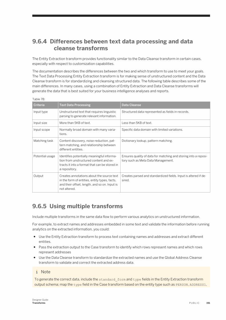
9.6.4 Differences between text data processing and data cleanse transforms
The Entity Extraction transform provides functionality similar to the Data Cleanse transform in certain cases, especially with respect to customization capabilities.
The documentation describes the differences between the two and which transform to use to meet your goals. The Text Data Processing Entity Extraction transform is for making sense of unstructured content and the Data Cleanse transform is for standardizing and cleansing structured data. The following table describes some of the main differences. In many cases, using a combination of Entity Extraction and Data Cleanse transforms will generate the data that is best suited for your business intelligence analyses and reports.
Table 78:
Criteria Text Data Processing Data Cleanse
Input type Unstructured text that requires linguistic parsing to generate relevant information.
Structured data represented as fields in records.
Input size More than 5KB of text. Less than 5KB of text.
Input scope Normally broad domain with many variations.
Specific data domain with limited variations.
Matching task Content discovery, noise reduction, pattern matching, and relationship between different entities.
Dictionary lookup, pattern matching.
Potential usage Identifies potentially meaningful information from unstructured content and extracts it into a format that can be stored in a repository.
Ensures quality of data for matching and storing into a repository such as Meta Data Management.
Output Creates annotations about the source text in the form of entities, entity types, facts, and their offset, length, and so on. Input is not altered.
Creates parsed and standardized fields. Input is altered if desired.
9.6.5 Using multiple transformsInclude multiple transforms in the same data flow to perform various analytics on unstructured information.
For example, to extract names and addresses embedded in some text and validate the information before running analytics on the extracted information, you could:
● Use the Entity Extraction transform to process text containing names and addresses and extract different entities.
● Pass the extraction output to the Case transform to identify which rows represent names and which rows represent addresses
● Use the Data Cleanse transform to standardize the extracted names and use the Global Address Cleanse transform to validate and correct the extracted address data.
NoteTo generate the correct data, include the standard_form and type fields in the Entity Extraction transform output schema; map the type field in the Case transform based on the entity type such as PERSON, ADDRESS1,
Designer GuideTransforms P U B L I C 191
etc. Next, map any PERSON entities from the Case transform to the Data Cleanse transform and map any ADDRESS1 entities to the Global Address Cleanse transform.
9.6.6 Examples for using the Entity Extraction transform
Describes some examples for employing the Entity Extraction transform.
The scenario is that a human resources department wants to analyze résumés received in a variety of formats. The formats include:
● A text file as an attachment to an email● A text résumé pasted into a field on the company's Web site● Updates to résumé content that the department wants to process in real time
ExampleText file email attachment
The human resources department frequently receives résumés as attachments to emails from candidates. They store these attachments in a separate directory on a server.
To analyze and process data from these text files:
1. Configure an Unstructured text file format that points to the directory of résumés.2. Build a data flow with the unstructured text file format as the source, an Entity Extraction transform, and a
target.3. Configure the transform to process and analyze the text.
ExampleText résumé pasted into a field on a Web site
The human resources department's online job application form includes a field into which applicants can paste their résumés. This field is captured in a database table column.
To analyze and process data from the database:
1. Configure a connection to the database via a datastore.2. Build a data flow with the database table as the source, an Entity Extraction transform, and a target.3. Configure the transform to process and analyze the text.
ExampleUpdated content to be processed in real time
Suppose the human resources department is seeking a particular qualification in an applicant. When the applicant updates her résumé in the company's Web-based form with the desired qualification, the HR manager wants to be immediately notified. Use a real-time job to enable this functionality.
To analyze and process the data in real time:
1. Add a real-time job including begin and end markers and a data flow. Connect the objects.
192 P U B L I CDesigner Guide
Transforms
2. Build the data flow with a message source, an Entity Extraction transform, and a message target.3. Configure the transform to process and analyze the text.
Related Information
Unstructured file formats [page 135]Database datastores [page 64]Real-time Jobs [page 244]
9.6.7 Adding a text data processing transform to a data flow
Adding this transform to your data flow allows you to extract information (entities and facts) from any text, HTML, XML, or binary format content such as PDF.
1. Open a data flow object.2. Open the local object library if it is not already open.3. Go to the Transforms tab.4. Expand the Text Data Processing transform folder and select the transform or transform configuration that
you want to add to the data flow.5. Drag the transform or transform configuration icon into the data flow workspace. If you selected a transform
that has available transform configurations, a drop-down menu prompts you to select a transform configuration.
6. Draw the data flow connections.
To connect a source or a transform to another transform, click the square on the right edge of the source or upstream transform and drag the cursor to the arrow on the left edge of the text data processing transform.
○ The input for the transform might be the output from another transform or the output from a source.○ You can connect the output of the transform to the input of another transform or target.
7. Double-click the name of the transform.
This opens the transform editor, which lets you complete the definition of the transform.8. In the input schema, select the input field that you want to map and drag it to the appropriate field in the Input
tab.This maps the input field to a field name that is recognized by the transform so that the transform knows how to process it correctly. For example,○ an input field that is named Content would be mapped to the TEXT input field.○ an input field that can uniquely identify the content would be mapped to the TEXT_ID input field.
9. In the Options tab, select the appropriate option values to determine how the transform will process your data.Make sure that you map input fields before you set option values.If you change an option value from its default value, a green triangle appears next to the option name to indicate that you made an override.
Designer GuideTransforms P U B L I C 193
10. In the Output tab, double-click the fields that you want to output from the transform. The transforms can generate fields in addition to the input fields that the transform processes, so you can output many fields.
Make sure that you set options before you map output fields.
The selected fields appear in the output schema. The output schema of this transform becomes the input schema of the next transform in the data flow.
11. If you want to pass data through the transform without processing it, drag fields directly from the input schema to the output schema.
12. To rename or resize an output field, double-click the output field and edit the properties in the Column Properties window.
Related Information
Entity Extraction transform editor [page 194]
9.6.8 Entity Extraction transform editor
The Entity Extraction transform options specify various parameters to process content using the transform.
Filtering options, under different extraction options, enable you to limit the entities and facts extracted to specific entities from a dictionary, the system files, entities/facts from rules, or a combination of them.
Extraction options are divided into the following categories:
● CommonThis option is set to specify that the Entity Extraction transform is to be run as a separate process.
● LanguagesUse this option to specify the language for the extraction process.○ Language—The default is 'Auto', directing the transform to attempt to identify the language. You may
select another language from a list.○ Default Language—You may select the language that should be assumed if the transform was not able to
identify the language.○ Filter by Entity Types is optional and you may select it when you select the language to limit your
extraction output.● Processing Options
Use these options to specify parameters to be used when processing the content.● Dictionaries
Use this option to specify different dictionaries to be used for processing the content. To use the Entity Types filtering option, you must specify the Dictionary File.
NoteText Data Processing includes the dictionary schema file extraction-dictionary.xsd. By default, this file is installed in the LINK_DIR/bin folder, where LINK_DIR is your Data Services installation directory. Refer to this schema to create your own dictionary files.
194 P U B L I CDesigner Guide
Transforms
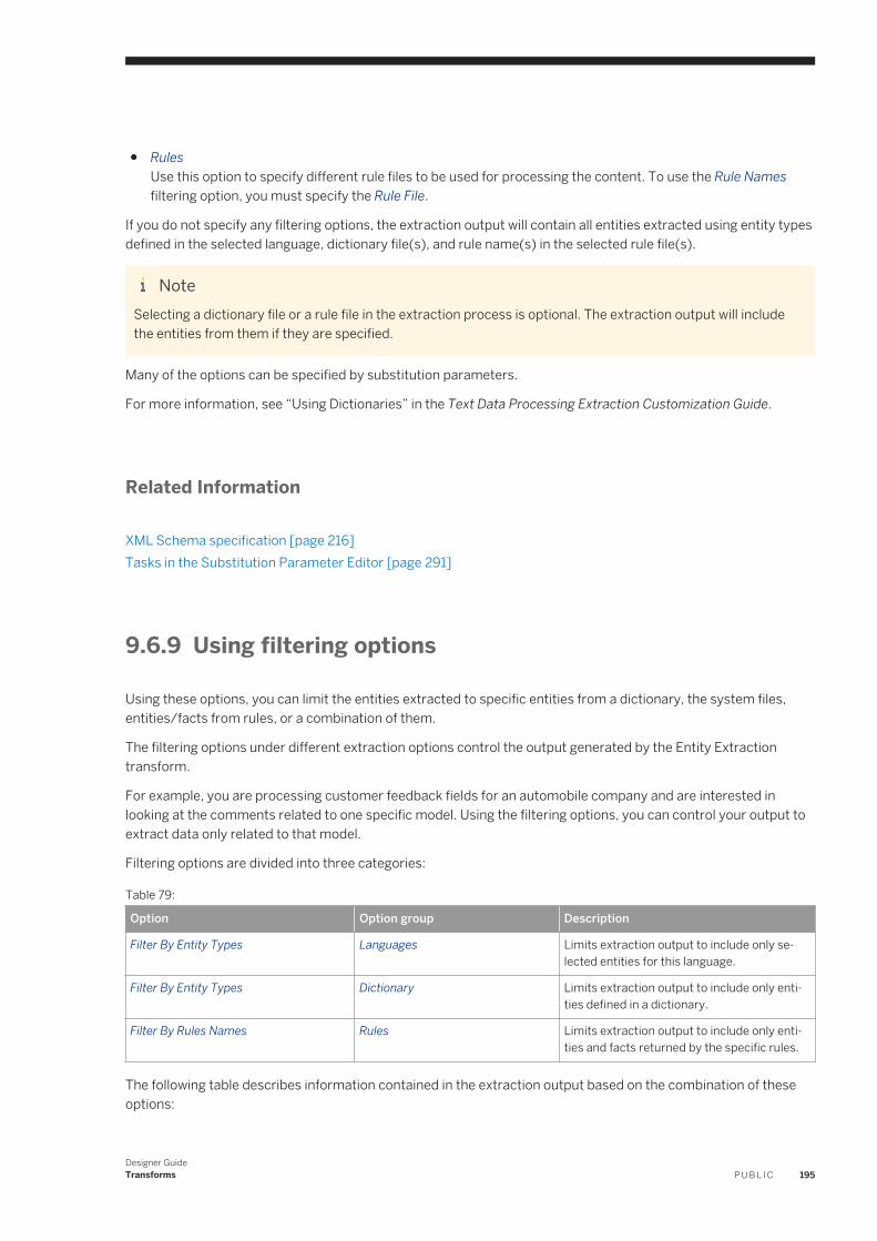
● Rules Use this option to specify different rule files to be used for processing the content. To use the Rule Names filtering option, you must specify the Rule File.
If you do not specify any filtering options, the extraction output will contain all entities extracted using entity types defined in the selected language, dictionary file(s), and rule name(s) in the selected rule file(s).
NoteSelecting a dictionary file or a rule file in the extraction process is optional. The extraction output will include the entities from them if they are specified.
Many of the options can be specified by substitution parameters.
For more information, see “Using Dictionaries” in the Text Data Processing Extraction Customization Guide.
Related Information
XML Schema specification [page 216]Tasks in the Substitution Parameter Editor [page 291]
9.6.9 Using filtering options
Using these options, you can limit the entities extracted to specific entities from a dictionary, the system files, entities/facts from rules, or a combination of them.
The filtering options under different extraction options control the output generated by the Entity Extraction transform.
For example, you are processing customer feedback fields for an automobile company and are interested in looking at the comments related to one specific model. Using the filtering options, you can control your output to extract data only related to that model.
Filtering options are divided into three categories:
Table 79:
Option Option group Description
Filter By Entity Types Languages Limits extraction output to include only selected entities for this language.
Filter By Entity Types Dictionary Limits extraction output to include only entities defined in a dictionary.
Filter By Rules Names Rules Limits extraction output to include only entities and facts returned by the specific rules.
The following table describes information contained in the extraction output based on the combination of these options:
Designer GuideTransforms P U B L I C 195
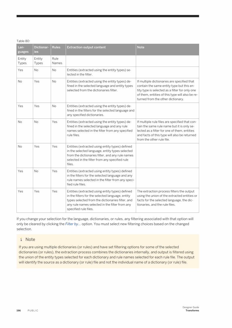
Table 80:
Languages
Dictionaries
Rules Extraction output content Note
Entity Types
Entity Types
Rule Names
Yes No No Entities (extracted using the entity types) selected in the filter.
No Yes No Entities (extracted using the entity types) defined in the selected language and entity types selected from the dictionaries filter.
If multiple dictionaries are specified that contain the same entity type but this entity type is selected as a filter for only one of them, entities of this type will also be returned from the other dictionary.
Yes Yes No Entities (extracted using the entity types) defined in the filters for the selected language and any specified dictionaries.
No No Yes Entities (extracted using the entity types) defined in the selected language and any rule names selected in the filter from any specified rule files.
If multiple rule files are specified that contain the same rule name but it is only selected as a filter for one of them, entities and facts of this type will also be returned from the other rule file.
No Yes Yes Entities (extracted using entity types) defined in the selected language, entity types selected from the dictionaries filter, and any rule names selected in the filter from any specified rule files.
Yes No Yes Entities (extracted using entity types) defined in the filters for the selected language and any rule names selected in the filter from any specified rule files.
Yes Yes Yes Entities (extracted using entity types) defined in the filters for the selected language, entity types selected from the dictionaries filter, and any rule names selected in the filter from any specified rule files.
The extraction process filters the output using the union of the extracted entities or facts for the selected language, the dictionaries, and the rule files.
If you change your selection for the language, dictionaries, or rules, any filtering associated with that option will only be cleared by clicking the Filter by... option. You must select new filtering choices based on the changed selection.
NoteIf you are using multiple dictionaries (or rules) and have set filtering options for some of the selected dictionaries (or rules), the extraction process combines the dictionaries internally, and output is filtered using the union of the entity types selected for each dictionary and rule names selected for each rule file. The output will identify the source as a dictionary (or rule) file and not the individual name of a dictionary (or rule) file.
196 P U B L I CDesigner Guide
Transforms

NoteIf you select the Dictionary Only option under the Processing Options group, with a valid dictionary file, the entity types defined for the language are not included in the extraction output, but any extracted rule file entities and facts are included.
Related Information
Entity Extraction transform editor [page 194]
Designer GuideTransforms P U B L I C 197
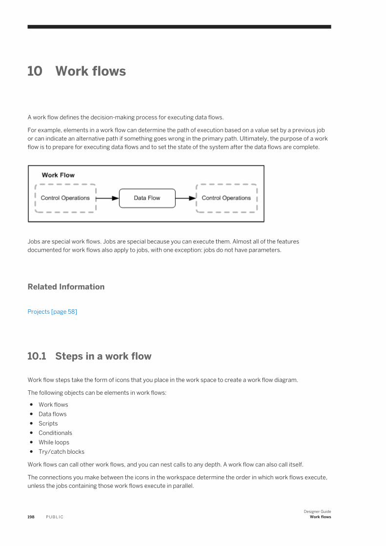
10 Work flows
A work flow defines the decision-making process for executing data flows.
For example, elements in a work flow can determine the path of execution based on a value set by a previous job or can indicate an alternative path if something goes wrong in the primary path. Ultimately, the purpose of a work flow is to prepare for executing data flows and to set the state of the system after the data flows are complete.
Jobs are special work flows. Jobs are special because you can execute them. Almost all of the features documented for work flows also apply to jobs, with one exception: jobs do not have parameters.
Related Information
Projects [page 58]
10.1 Steps in a work flow
Work flow steps take the form of icons that you place in the work space to create a work flow diagram.
The following objects can be elements in work flows:
● Work flows● Data flows● Scripts● Conditionals● While loops● Try/catch blocks
Work flows can call other work flows, and you can nest calls to any depth. A work flow can also call itself.
The connections you make between the icons in the workspace determine the order in which work flows execute, unless the jobs containing those work flows execute in parallel.
198 P U B L I CDesigner Guide
Work flows
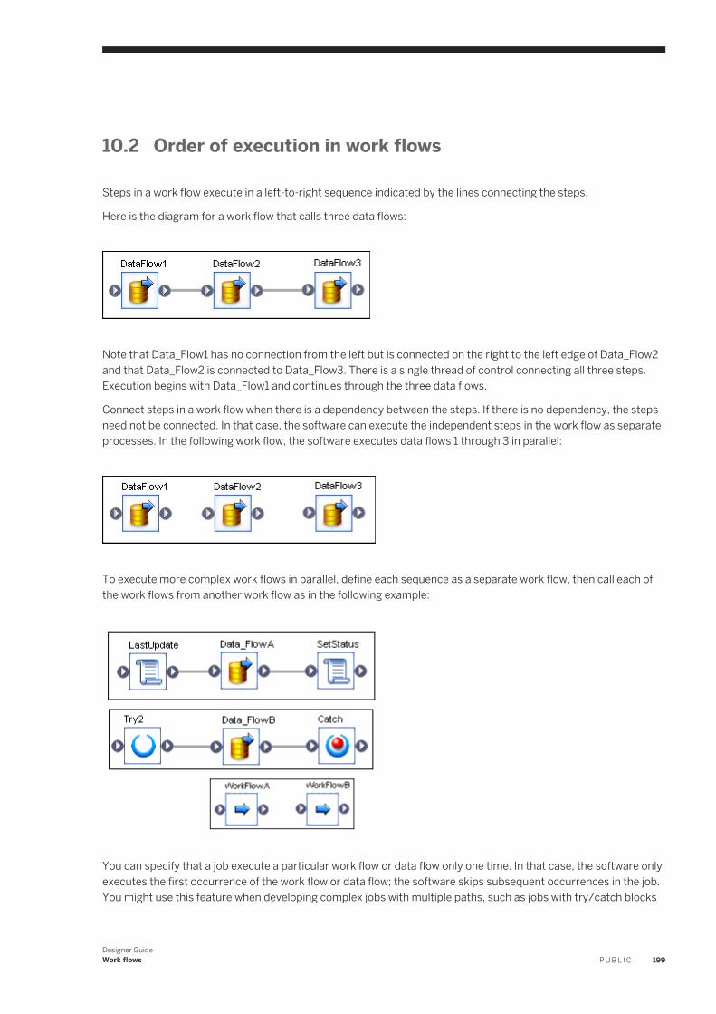
10.2 Order of execution in work flows
Steps in a work flow execute in a left-to-right sequence indicated by the lines connecting the steps.
Here is the diagram for a work flow that calls three data flows:
Note that Data_Flow1 has no connection from the left but is connected on the right to the left edge of Data_Flow2 and that Data_Flow2 is connected to Data_Flow3. There is a single thread of control connecting all three steps. Execution begins with Data_Flow1 and continues through the three data flows.
Connect steps in a work flow when there is a dependency between the steps. If there is no dependency, the steps need not be connected. In that case, the software can execute the independent steps in the work flow as separate processes. In the following work flow, the software executes data flows 1 through 3 in parallel:
To execute more complex work flows in parallel, define each sequence as a separate work flow, then call each of the work flows from another work flow as in the following example:
You can specify that a job execute a particular work flow or data flow only one time. In that case, the software only executes the first occurrence of the work flow or data flow; the software skips subsequent occurrences in the job. You might use this feature when developing complex jobs with multiple paths, such as jobs with try/catch blocks
Designer GuideWork flows P U B L I C 199
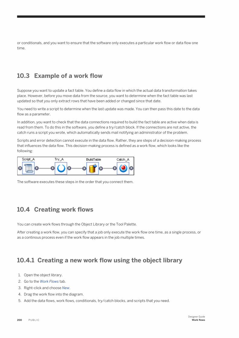
or conditionals, and you want to ensure that the software only executes a particular work flow or data flow one time.
10.3 Example of a work flow
Suppose you want to update a fact table. You define a data flow in which the actual data transformation takes place. However, before you move data from the source, you want to determine when the fact table was last updated so that you only extract rows that have been added or changed since that date.
You need to write a script to determine when the last update was made. You can then pass this date to the data flow as a parameter.
In addition, you want to check that the data connections required to build the fact table are active when data is read from them. To do this in the software, you define a try/catch block. If the connections are not active, the catch runs a script you wrote, which automatically sends mail notifying an administrator of the problem.
Scripts and error detection cannot execute in the data flow. Rather, they are steps of a decision-making process that influences the data flow. This decision-making process is defined as a work flow, which looks like the following:
The software executes these steps in the order that you connect them.
10.4 Creating work flows
You can create work flows through the Object Library or the Tool Palette.
After creating a work flow, you can specify that a job only execute the work flow one time, as a single process, or as a continous process even if the work flow appears in the job multiple times.
10.4.1 Creating a new work flow using the object library
1. Open the object library.2. Go to the Work Flows tab.3. Right-click and choose New.4. Drag the work flow into the diagram.5. Add the data flows, work flows, conditionals, try/catch blocks, and scripts that you need.
200 P U B L I CDesigner Guide
Work flows
10.4.2 Creating a new work flow using the tool palette
1. Select the work flow icon in the tool palette.2. Click where you want to place the work flow in the diagram.
If more than one instance of a work flow appears in a job, you can improve execution performance by running the work flow only one time.
10.4.3 Specifying that a job executes the work flow one time
When you specify that a work flow should only execute once, a job will never re-execute that work flow after the work flow completes successfully.
The exception is if the work flow is contained in a work flow that is a recovery unit that re-executes and has not completed successfully elsewhere outside the recovery unit.
It is recommended that you not mark a work flow as Execute only once if the work flow or a parent work flow is a recovery unit.
1. Right click on the work flow and select Properties.
The Properties window opens for the work flow.2. Select Regular from the Execution type dropdown list.3. Select the Execute only once check box.4. Click OK.
10.4.4 What is a single work flow?
A single work flow runs all of its child data flows in one operating system process.
If the data flows are designed to be run in parallel then they are run in different threads instead of different processes. The advantage of single process is that it is possible to share resources such as database connections across multiple data flows.
NoteSingle work flows have the following limitations:
● A single work flow cannot call or contain a continuous work flow.● A single work flow cannot use sub data flows. Therefore, the Data Transfer transform and "Run as a
separate process" options are invalid. The software will generate a runtime validation error.● A single work flow can be only executed by a continuous work flow. A single work flow cannot call another
single work flow.
Designer GuideWork flows P U B L I C 201
10.4.4.1 Specifying that a job executes as a single work flow
1. Right-click a work flow and select Properties2. Select Single from the Execution type dropdown list.3. Click OK.
10.4.5 What is a continuous work flow?
A continuous work flow runs all data flows in a loop but keeps them in the memory for the next iteration.
This eliminates the need to repeat some of the common steps of execution (for example, connecting to the repository, parsing/optimizing/compiling ATL, opening database connections.
NoteContinuous work flows have the following limitations:
● A continuous work flow cannot call or contain another continuous work flow. If a continuous work flow calls another continous work flow which never terminates, the work flow can never restart the child processes.
● A continuous work flow cannot use sub data flows. Therefore, the Data Transfer transform and "Run as a separate process" options are invalid. The software will generate a runtime validation error.
● A regular or single work flow cannot call or contain a continuous work flow.● A real-time job cannot call a continuous work flow.● The platform transform XML_Map cannot be used in a continuous work flow.● The Data Integrator transforms Data_Transfer and XML_Pipeline cannot be used in a continuous work flow.
10.4.5.1 Specifying that a job executes a continuous work flow
1. Right-click a work flow and select Properties2. Select Continuous from the Execution type dropdown list.3. Access the Continuous Options tab.4. Specify when you want the work flow to release resources:
○ To release resources after a number of runs, select Number of runs and enter the number of runs. The default is 100.
○ To release resources after a number of hours, select the After checkbox, select Number of hours, and enter the number of hours.
○ To release resources after a number of days, select the After checkbox, select Number of days, and enter the number of days.
○ To release resources when the result of a function is not equal to zero, select the After checkbox, select Result of the function is not equal to zero, and enter the function you want to use.
5. To stop the work flow when the result of a custom function is equal to zero, select When result of the function is equal to zero, and enter the custom function you want to use.
202 P U B L I CDesigner Guide
Work flows
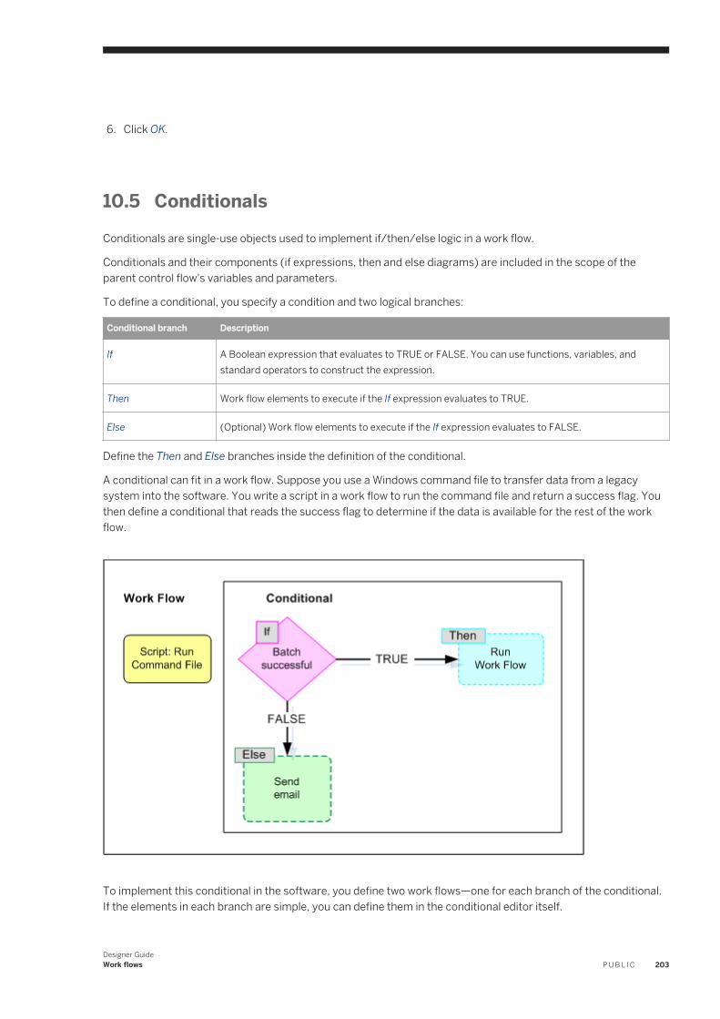
6. Click OK.
10.5 Conditionals
Conditionals are single-use objects used to implement if/then/else logic in a work flow.
Conditionals and their components (if expressions, then and else diagrams) are included in the scope of the parent control flow's variables and parameters.
To define a conditional, you specify a condition and two logical branches:
Conditional branch Description
If A Boolean expression that evaluates to TRUE or FALSE. You can use functions, variables, and standard operators to construct the expression.
Then Work flow elements to execute if the If expression evaluates to TRUE.
Else (Optional) Work flow elements to execute if the If expression evaluates to FALSE.
Define the Then and Else branches inside the definition of the conditional.
A conditional can fit in a work flow. Suppose you use a Windows command file to transfer data from a legacy system into the software. You write a script in a work flow to run the command file and return a success flag. You then define a conditional that reads the success flag to determine if the data is available for the rest of the work flow.
To implement this conditional in the software, you define two work flows—one for each branch of the conditional. If the elements in each branch are simple, you can define them in the conditional editor itself.
Designer GuideWork flows P U B L I C 203
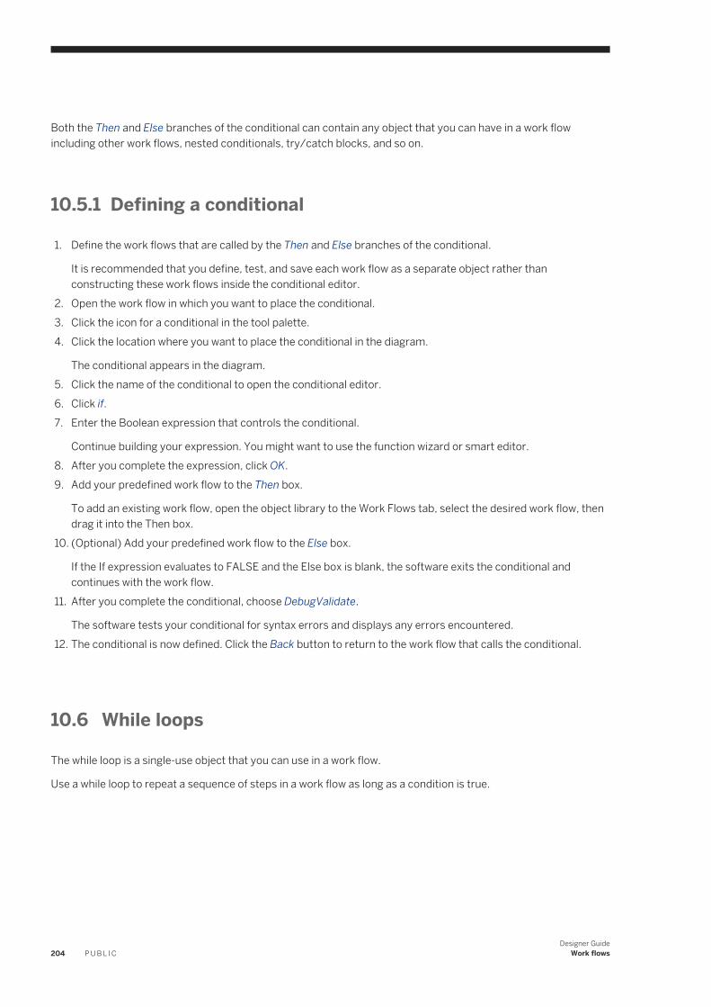
Both the Then and Else branches of the conditional can contain any object that you can have in a work flow including other work flows, nested conditionals, try/catch blocks, and so on.
10.5.1 Defining a conditional
1. Define the work flows that are called by the Then and Else branches of the conditional.
It is recommended that you define, test, and save each work flow as a separate object rather than constructing these work flows inside the conditional editor.
2. Open the work flow in which you want to place the conditional.3. Click the icon for a conditional in the tool palette.4. Click the location where you want to place the conditional in the diagram.
The conditional appears in the diagram.5. Click the name of the conditional to open the conditional editor.6. Click if.7. Enter the Boolean expression that controls the conditional.
Continue building your expression. You might want to use the function wizard or smart editor.8. After you complete the expression, click OK.9. Add your predefined work flow to the Then box.
To add an existing work flow, open the object library to the Work Flows tab, select the desired work flow, then drag it into the Then box.
10. (Optional) Add your predefined work flow to the Else box.
If the If expression evaluates to FALSE and the Else box is blank, the software exits the conditional and continues with the work flow.
11. After you complete the conditional, choose DebugValidate.
The software tests your conditional for syntax errors and displays any errors encountered.12. The conditional is now defined. Click the Back button to return to the work flow that calls the conditional.
10.6 While loops
The while loop is a single-use object that you can use in a work flow.
Use a while loop to repeat a sequence of steps in a work flow as long as a condition is true.
204 P U B L I CDesigner Guide
Work flows
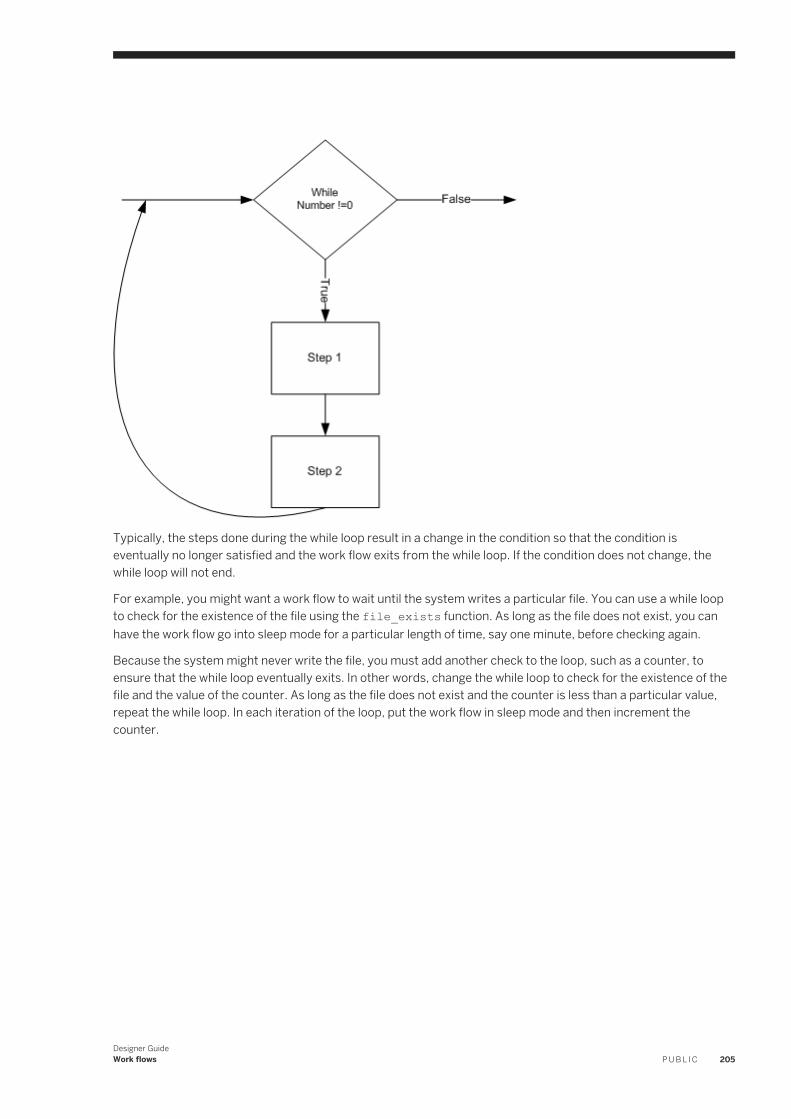
Typically, the steps done during the while loop result in a change in the condition so that the condition is eventually no longer satisfied and the work flow exits from the while loop. If the condition does not change, the while loop will not end.
For example, you might want a work flow to wait until the system writes a particular file. You can use a while loop to check for the existence of the file using the file_exists function. As long as the file does not exist, you can have the work flow go into sleep mode for a particular length of time, say one minute, before checking again.
Because the system might never write the file, you must add another check to the loop, such as a counter, to ensure that the while loop eventually exits. In other words, change the while loop to check for the existence of the file and the value of the counter. As long as the file does not exist and the counter is less than a particular value, repeat the while loop. In each iteration of the loop, put the work flow in sleep mode and then increment the counter.
Designer GuideWork flows P U B L I C 205
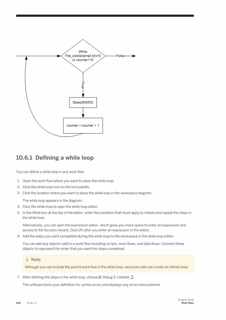
10.6.1 Defining a while loop
You can define a while loop in any work flow.
1. Open the work flow where you want to place the while loop.2. Click the while loop icon on the tool palette.3. Click the location where you want to place the while loop in the workspace diagram.
The while loop appears in the diagram.4. Click the while loop to open the while loop editor.5. In the While box at the top of the editor, enter the condition that must apply to initiate and repeat the steps in
the while loop.
Alternatively, you can oprn the expression editor, which gives you more space to enter an expression and access to the function wizard. Click OK after you enter an expression in the editor.
6. Add the steps you want completed during the while loop to the workspace in the while loop editor.
You can add any objects valid in a work flow including scripts, work flows, and data flows. Connect these objects to represent the order that you want the steps completed.
NoteAlthough you can include the parent work flow in the while loop, recursive calls can create an infinite loop.
7. After defining the steps in the while loop, choose Debug Validate .
The software tests your definition for syntax errors and displays any errors encountered.
206 P U B L I CDesigner Guide
Work flows
8. Close the while loop editor to return to the calling work flow.
10.6.2 Using a while loop with View Data
Depending on the design of your job, the software might not complete all iterations of a while loop if you run a job in view data mode.
When using View Data, a job stops when the software has retrieved the specified number of rows for all scannable objects.
The following might occur when using while loop when running a job in view data mode:
● If the while loop contains scannable objects and there are no scannable objects outside the while loop (for example, if the while loop is the last object in a job), then the job will complete after the scannable objects in the while loop are satisfied, possibly after the first iteration of the while loop.
● If there are scannable objects after the while loop, the while loop will complete normally. Scanned objects in the while loop will show results from the last iteration.
● If there are no scannable objects following the while loop but there are scannable objects completed in parallel to the while loop, the job will complete as soon as all scannable objects are satisfied. The while loop might complete any number of iterations.
10.7 Try/catch blocks
A try/catch block is a combination of one try object and one or more catch objects that allow you to specify alternative work flows if errors occur while the software is executing a job.
Try/catch blocks:
● "Catch" groups of exceptions "thrown" by the software, the DBMS, or the operating system.● Apply solutions that you provide for the exceptions groups or for specific errors within a group.● Continue execution.
Try and catch objects are single-use objects.
Here's the general method to implement exception handling:
1. Insert a try object before the steps for which you are handling errors.2. Insert a catch object in the work flow after the steps.3. In the catch object, do the following:
○ Select one or more groups of errors that you want to catch.○ Define the actions that a thrown exception executes. The actions can be a single script object, a data flow,
a work flow, or a combination of these objects.○ Optional. Use catch functions inside the catch block to identify details of the error.
If an exception is thrown during the execution of a try/catch block and if no catch object is looking for that exception, then the exception is handled by normal error logic.
The following work flow shows a try/catch block surrounding a data flow:
Designer GuideWork flows P U B L I C 207
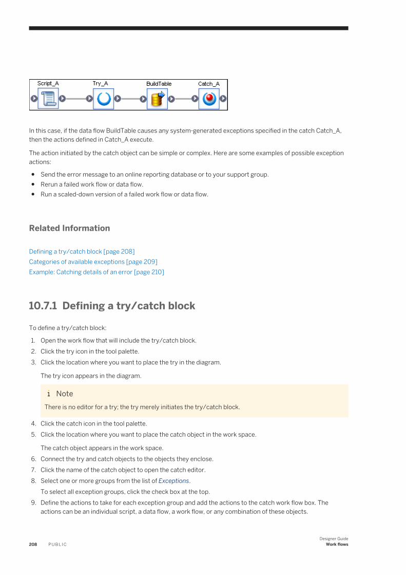
In this case, if the data flow BuildTable causes any system-generated exceptions specified in the catch Catch_A, then the actions defined in Catch_A execute.
The action initiated by the catch object can be simple or complex. Here are some examples of possible exception actions:
● Send the error message to an online reporting database or to your support group.● Rerun a failed work flow or data flow.● Run a scaled-down version of a failed work flow or data flow.
Related Information
Defining a try/catch block [page 208]Categories of available exceptions [page 209]Example: Catching details of an error [page 210]
10.7.1 Defining a try/catch block
To define a try/catch block:
1. Open the work flow that will include the try/catch block.2. Click the try icon in the tool palette.3. Click the location where you want to place the try in the diagram.
The try icon appears in the diagram.
NoteThere is no editor for a try; the try merely initiates the try/catch block.
4. Click the catch icon in the tool palette.5. Click the location where you want to place the catch object in the work space.
The catch object appears in the work space.6. Connect the try and catch objects to the objects they enclose.7. Click the name of the catch object to open the catch editor.8. Select one or more groups from the list of Exceptions.
To select all exception groups, click the check box at the top.9. Define the actions to take for each exception group and add the actions to the catch work flow box. The
actions can be an individual script, a data flow, a work flow, or any combination of these objects.
208 P U B L I CDesigner Guide
Work flows
a. It is recommended that you define, test, and save the actions as a separate object rather than constructing them inside the catch editor.
b. If you want to define actions for specific errors, use the following catch functions in a script that the work flow executes:○ error_context()○ error_message()○ error_number()○ error_timestamp()
c. To add an existing work flow to the catch work flow box, open the object library to the Work Flows tab, select the desired work flow, and drag it into the box.
10. After you have completed the catch, choose Validation Validate All Objects in View .
The software tests your definition for syntax errors and displays any errors encountered.11. Click the Back button to return to the work flow that calls the catch.12. If you want to catch multiple exception groups and assign different actions to each exception group, repeat
steps 4 through 11 for each catch in the work flow.
NoteIn a sequence of catch blocks, if one catch block catches an exception, the subsequent catch blocks will not be executed. For example, if your work flow has the following sequence and Catch1 catches an exception, then Catch2 and CatchAll will not execute.
Try > DataFlow1 > Catch1 > Catch2 > CatchAll
If any error in the exception group listed in the catch occurs during the execution of this try/catch block, the software executes the catch work flow.
Related Information
Categories of available exceptions [page 209]Example: Catching details of an error [page 210]
10.7.2 Categories of available exceptions
Categories of available exceptions include:
● Execution errors (1001)● Database access errors (1002)● Database connection errors (1003)● Flat file processing errors (1004)● File access errors (1005)● Repository access errors (1006)● SAP system errors (1007)
Designer GuideWork flows P U B L I C 209
● System resource exception (1008)● SAP BW execution errors (1009)● XML processing errors (1010)● COBOL copybook errors (1011)● Excel book errors (1012)● Data Quality transform errors (1013)
10.7.3 Example: Catching details of an error
This example illustrates how to use the error functions in a catch script. Suppose you want to catch database access errors and send the error details to your support group.
1. In the catch editor, select the exception group that you want to catch. In this example, select the checkbox in front of Database access errors (1002).
2. In the work flow area of the catch editor, create a script object with the following script:
mail_to('[email protected]', 'Data Service error number' || error_number(), 'Error message: ' || error_message(),20,20); print('DBMS Error: ' || error_message());
3. This sample catch script includes the mail_to function to do the following:○ Specify the email address of your support group.○ Send the error number that the error_number() function returns for the exception caught.○ Send the error message that the error_message() function returns for the exception caught.
4. The sample catch script includes a print command to print the error message for the database error.
10.8 Scripts
Scripts are single-use objects used to call functions and assign values to variables in a work flow.
For example, you can use the SQL function in a script to determine the most recent update time for a table and then assign that value to a variable. You can then assign the variable to a parameter that passes into a data flow and identifies the rows to extract from a source.
A script can contain the following statements:
● Function calls● If statements● While statements● Assignment statements● Operators
The basic rules for the syntax of the script are as follows:
● Each line ends with a semicolon (;).● Variable names start with a dollar sign ($).
210 P U B L I CDesigner Guide
Work flows
● String values are enclosed in single quotation marks (').● Comments start with a pound sign (#).● Function calls always specify parameters even if the function uses no parameters.
For example, the following script statement determines today's date and assigns the value to the variable $TODAY:
$TODAY = sysdate();
You cannot use variables unless you declare them in the work flow that calls the script.
10.8.1 Creating a script
1. Open the work flow.2. Click the script icon in the tool palette.3. Click the location where you want to place the script in the diagram.
The script icon appears in the diagram.4. Click the name of the script to open the script editor.5. Enter the script statements, each followed by a semicolon.
The following example shows a script that determines the start time from the output of a custom function.
AW_StartJob ('NORMAL','DELTA', $G_STIME,$GETIME); $GETIME =to_date(sql('ODS_DS','SELECT to_char(MAX(LAST_UPDATE) ,\'YYYY-MM-DDD HH24:MI:SS\')FROM EMPLOYEE'), 'YYYY_MMM_DDD_HH24:MI:SS');
Click the function button to include functions in your script.
6. After you complete the script, select Validation Validate .
The software tests your script for syntax errors and displays any errors encountered.7. Click the ... button and then save to name and save your script.
The script is saved by default in <LINK_DIR>/Data Services/ DataQuality/Samples.
10.8.2 Debugging scripts using the print function
The software has a debugging feature that allows you to print:
● The values of variables and parameters during execution● The execution path followed within a script
You can use the print function to write the values of parameters and variables in a work flow to the trace log. For example, this line in a script:
print('The value of parameter $<x>: [$<x>]');
Designer GuideWork flows P U B L I C 211
produces the following output in the trace log:
The following output is being printed via the Print function in <Session <job_name>. The value of parameter $<x>: <value>
212 P U B L I CDesigner Guide
Work flows
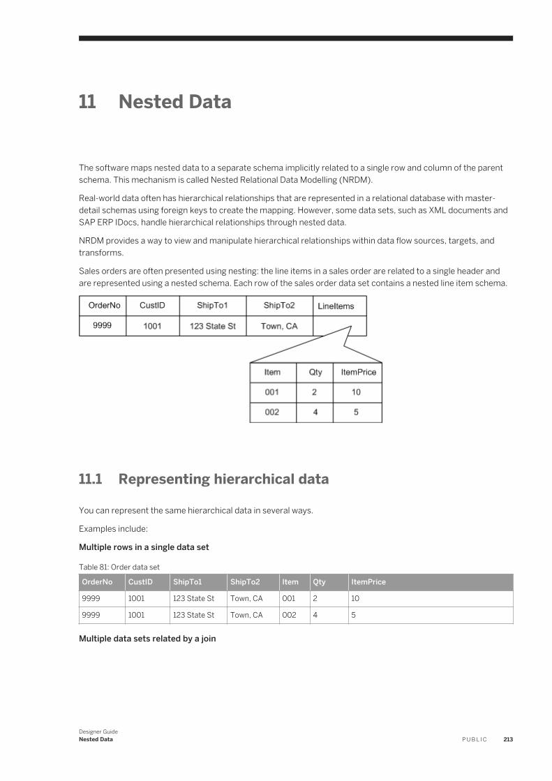
11 Nested Data
The software maps nested data to a separate schema implicitly related to a single row and column of the parent schema. This mechanism is called Nested Relational Data Modelling (NRDM).
Real-world data often has hierarchical relationships that are represented in a relational database with master-detail schemas using foreign keys to create the mapping. However, some data sets, such as XML documents and SAP ERP IDocs, handle hierarchical relationships through nested data.
NRDM provides a way to view and manipulate hierarchical relationships within data flow sources, targets, and transforms.
Sales orders are often presented using nesting: the line items in a sales order are related to a single header and are represented using a nested schema. Each row of the sales order data set contains a nested line item schema.
11.1 Representing hierarchical data
You can represent the same hierarchical data in several ways.
Examples include:
Multiple rows in a single data set
Table 81: Order data set
OrderNo CustID ShipTo1 ShipTo2 Item Qty ItemPrice
9999 1001 123 State St Town, CA 001 2 10
9999 1001 123 State St Town, CA 002 4 5
Multiple data sets related by a join
Designer GuideNested Data P U B L I C 213
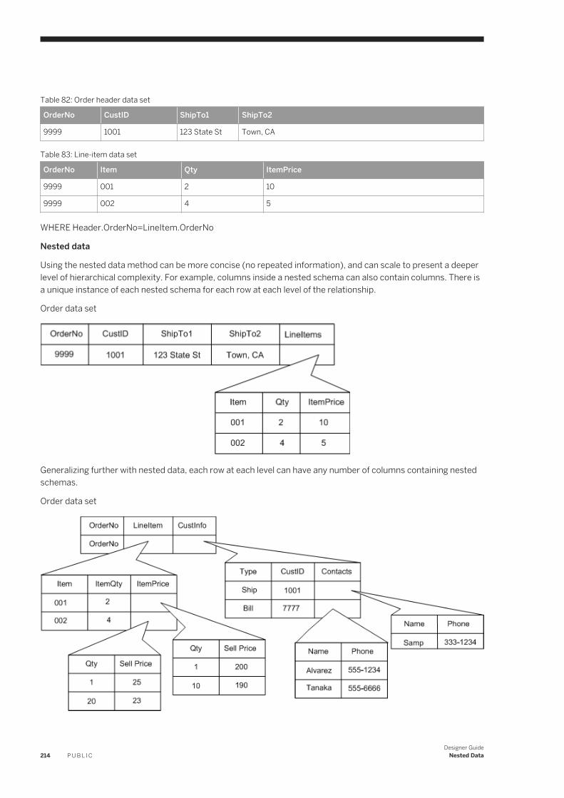
Table 82: Order header data set
OrderNo CustID ShipTo1 ShipTo2
9999 1001 123 State St Town, CA
Table 83: Line-item data set
OrderNo Item Qty ItemPrice
9999 001 2 10
9999 002 4 5
WHERE Header.OrderNo=LineItem.OrderNo
Nested data
Using the nested data method can be more concise (no repeated information), and can scale to present a deeper level of hierarchical complexity. For example, columns inside a nested schema can also contain columns. There is a unique instance of each nested schema for each row at each level of the relationship.
Order data set
Generalizing further with nested data, each row at each level can have any number of columns containing nested schemas.
Order data set
214 P U B L I CDesigner Guide
Nested Data
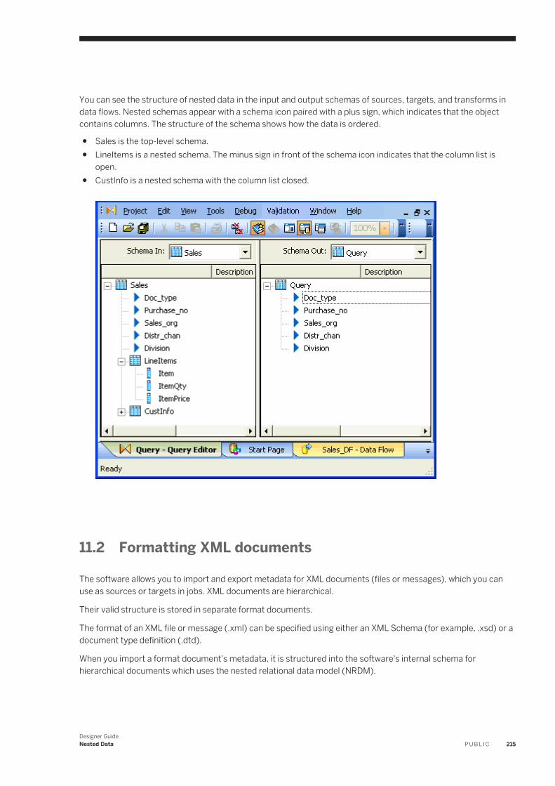
You can see the structure of nested data in the input and output schemas of sources, targets, and transforms in data flows. Nested schemas appear with a schema icon paired with a plus sign, which indicates that the object contains columns. The structure of the schema shows how the data is ordered.
● Sales is the top-level schema.● LineItems is a nested schema. The minus sign in front of the schema icon indicates that the column list is
open.● CustInfo is a nested schema with the column list closed.
11.2 Formatting XML documents
The software allows you to import and export metadata for XML documents (files or messages), which you can use as sources or targets in jobs. XML documents are hierarchical.
Their valid structure is stored in separate format documents.
The format of an XML file or message (.xml) can be specified using either an XML Schema (for example, .xsd) or a document type definition (.dtd).
When you import a format document's metadata, it is structured into the software's internal schema for hierarchical documents which uses the nested relational data model (NRDM).
Designer GuideNested Data P U B L I C 215
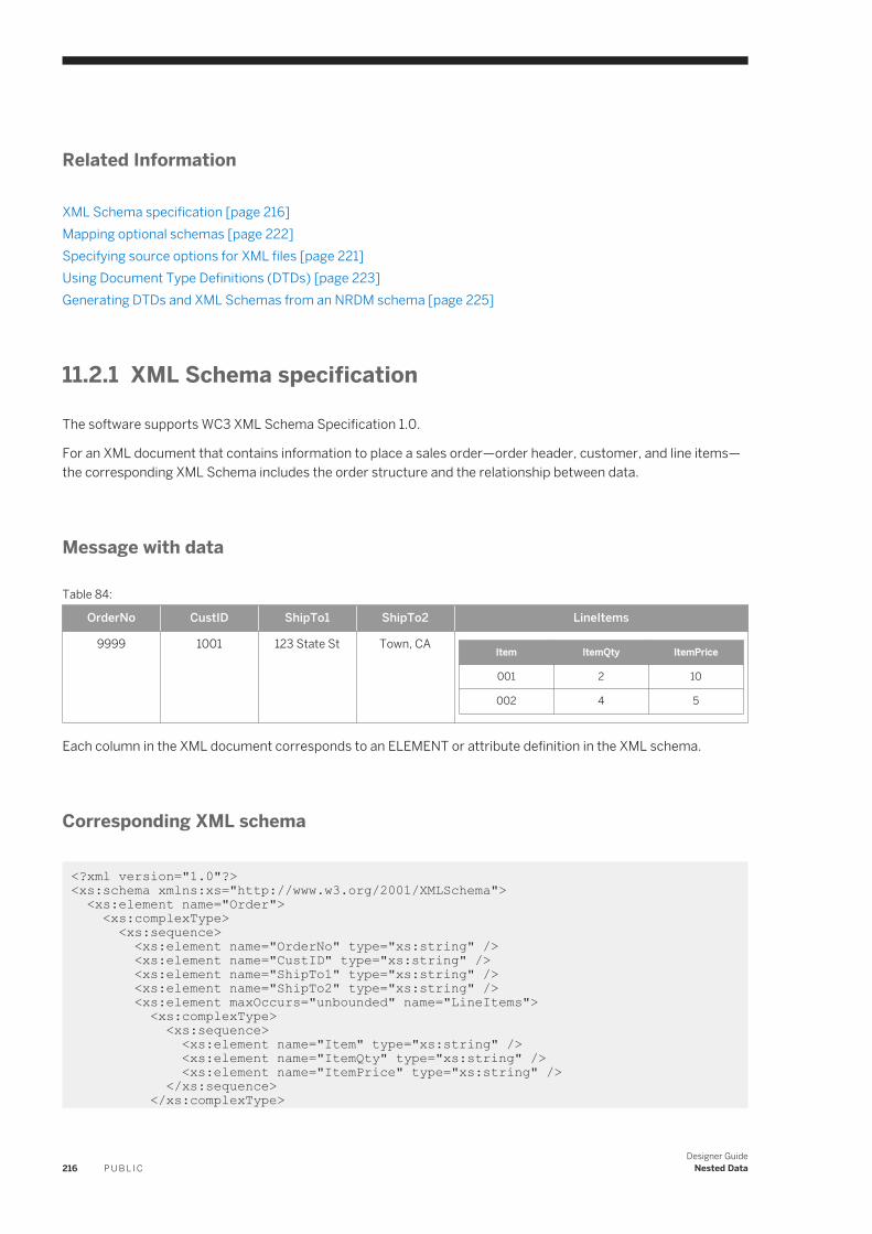
Related Information
XML Schema specification [page 216]Mapping optional schemas [page 222]Specifying source options for XML files [page 221]Using Document Type Definitions (DTDs) [page 223]Generating DTDs and XML Schemas from an NRDM schema [page 225]
11.2.1 XML Schema specification
The software supports WC3 XML Schema Specification 1.0.
For an XML document that contains information to place a sales order—order header, customer, and line items—the corresponding XML Schema includes the order structure and the relationship between data.
Message with data
Table 84:
OrderNo CustID ShipTo1 ShipTo2 LineItems
9999 1001 123 State St Town, CAItem ItemQty ItemPrice
001 2 10
002 4 5
Each column in the XML document corresponds to an ELEMENT or attribute definition in the XML schema.
Corresponding XML schema
<?xml version="1.0"?> <xs:schema xmlns:xs="http://www.w3.org/2001/XMLSchema"> <xs:element name="Order"> <xs:complexType> <xs:sequence> <xs:element name="OrderNo" type="xs:string" /> <xs:element name="CustID" type="xs:string" /> <xs:element name="ShipTo1" type="xs:string" /> <xs:element name="ShipTo2" type="xs:string" /> <xs:element maxOccurs="unbounded" name="LineItems"> <xs:complexType> <xs:sequence> <xs:element name="Item" type="xs:string" /> <xs:element name="ItemQty" type="xs:string" /> <xs:element name="ItemPrice" type="xs:string" /> </xs:sequence> </xs:complexType>
216 P U B L I CDesigner Guide
Nested Data
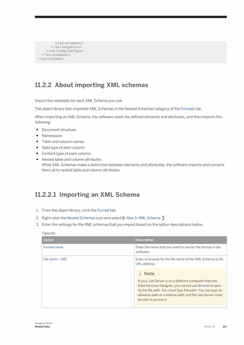
</xs:element> </xs:sequence> </xs:complexType> </xs:element> </xs:schema>
11.2.2 About importing XML schemas
Import the metadata for each XML Schema you use.
The object library lists imported XML Schemas in the Nested Schemas category of the Formats tab.
When importing an XML Schema, the software reads the defined elements and attributes, and then imports the following:
● Document structure● Namespace● Table and column names● Data type of each column● Content type of each column● Nested table and column attributes
While XML Schemas make a distinction between elements and attributes, the software imports and converts them all to nested table and column attributes.
11.2.2.1 Importing an XML Schema
1. From the object library, click the Format tab.
2. Right-click the Nested Schemas icon and select New XML Schema .3. Enter the settings for the XML schemas that you import based on the option descriptions below.
Table 85:
Option Description
Format name Enter the name that you want to use for the format in the software.
File name / URL Enter or browse for the file name of the XML Schema or its URL address.
NoteIf your Job Server is on a different computer than the Data Services Designer, you cannot use Browse to specify the file path. You must type the path. You can type an absolute path or a relative path, but the Job Server must be able to access it.
Designer GuideNested Data P U B L I C 217
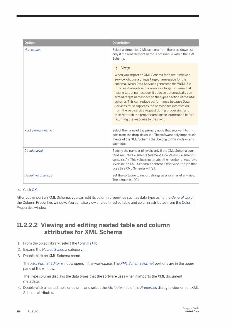
Option Description
Namespace Select an imported XML schema from the drop-down list only if the root element name is not unique within the XML Schema.
NoteWhen you import an XML Schema for a real-time web service job, use a unique target namespace for the schema. When Data Services generates the WSDL file for a real-time job with a source or target schema that has no target namespace, it adds an automatically generated target namespace to the types section of the XML schema. This can reduce performance because Data Services must suppress the namespace information from the web service request during processing, and then reattach the proper namespace information before returning the response to the client.
Root element name Select the name of the primary node that you want to import from the drop-down list. The software only imports elements of the XML Schema that belong to this node or any subnodes.
Circular level Specify the number of levels only if the XML Schema contains recursive elements (element A contains B, element B contains A). This value must match the number of recursive levels in the XML Schema's content. Otherwise, the job that uses this XML Schema will fail.
Default varchar size Set the software to import strings as a varchar of any size. The default is 1024.
4. Click OK.
After you import an XML Schema, you can edit its column properties such as data type using the General tab of the Column Properties window. You can also view and edit nested table and column attributes from the Column Properties window.
11.2.2.2 Viewing and editing nested table and column attributes for XML Schema
1. From the object library, select the Formats tab.2. Expand the Nested Schema category.3. Double-click an XML Schema name.
The XML Format Editor window opens in the workspace. The XML Schema Format portions are in the upper pane of the window.
The Type column displays the data types that the software uses when it imports the XML document metadata.
4. Double-click a nested table or column and select the Attributes tab of the Properties dialog to view or edit XML Schema attributes.
218 P U B L I CDesigner Guide
Nested Data
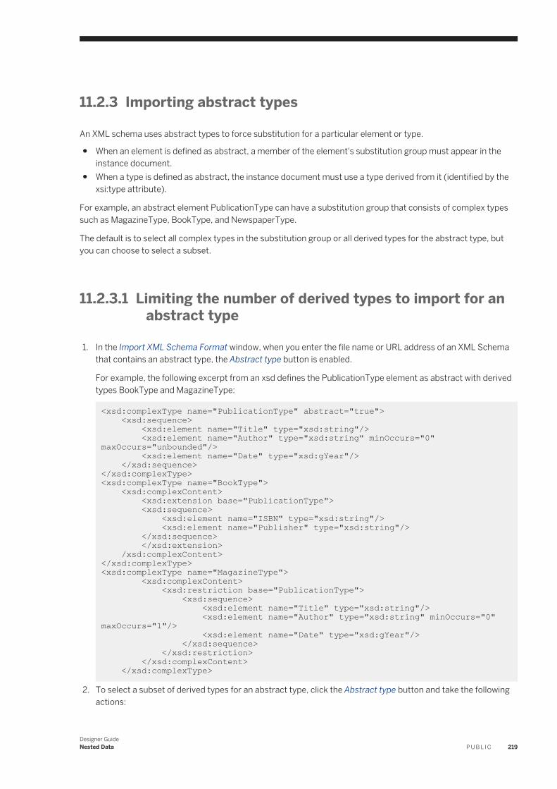
11.2.3 Importing abstract types
An XML schema uses abstract types to force substitution for a particular element or type.
● When an element is defined as abstract, a member of the element's substitution group must appear in the instance document.
● When a type is defined as abstract, the instance document must use a type derived from it (identified by the xsi:type attribute).
For example, an abstract element PublicationType can have a substitution group that consists of complex types such as MagazineType, BookType, and NewspaperType.
The default is to select all complex types in the substitution group or all derived types for the abstract type, but you can choose to select a subset.
11.2.3.1 Limiting the number of derived types to import for an abstract type
1. In the Import XML Schema Format window, when you enter the file name or URL address of an XML Schema that contains an abstract type, the Abstract type button is enabled.
For example, the following excerpt from an xsd defines the PublicationType element as abstract with derived types BookType and MagazineType:
<xsd:complexType name="PublicationType" abstract="true"> <xsd:sequence> <xsd:element name="Title" type="xsd:string"/> <xsd:element name="Author" type="xsd:string" minOccurs="0" maxOccurs="unbounded"/> <xsd:element name="Date" type="xsd:gYear"/> </xsd:sequence></xsd:complexType><xsd:complexType name="BookType"> <xsd:complexContent> <xsd:extension base="PublicationType"> <xsd:sequence> <xsd:element name="ISBN" type="xsd:string"/> <xsd:element name="Publisher" type="xsd:string"/> </xsd:sequence> </xsd:extension> /xsd:complexContent></xsd:complexType><xsd:complexType name="MagazineType"> <xsd:complexContent> <xsd:restriction base="PublicationType"> <xsd:sequence> <xsd:element name="Title" type="xsd:string"/> <xsd:element name="Author" type="xsd:string" minOccurs="0" maxOccurs="1"/> <xsd:element name="Date" type="xsd:gYear"/> </xsd:sequence> </xsd:restriction> </xsd:complexContent> </xsd:complexType>
2. To select a subset of derived types for an abstract type, click the Abstract type button and take the following actions:
Designer GuideNested Data P U B L I C 219
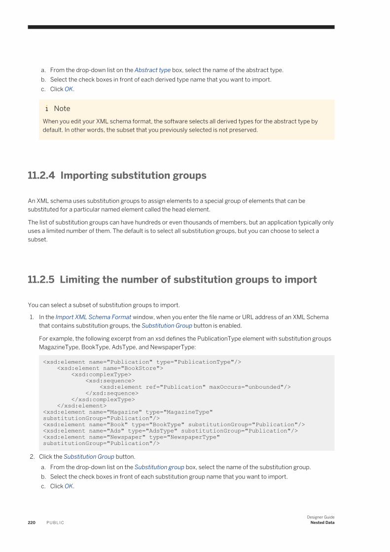
a. From the drop-down list on the Abstract type box, select the name of the abstract type.b. Select the check boxes in front of each derived type name that you want to import.c. Click OK.
NoteWhen you edit your XML schema format, the software selects all derived types for the abstract type by default. In other words, the subset that you previously selected is not preserved.
11.2.4 Importing substitution groups
An XML schema uses substitution groups to assign elements to a special group of elements that can be substituted for a particular named element called the head element.
The list of substitution groups can have hundreds or even thousands of members, but an application typically only uses a limited number of them. The default is to select all substitution groups, but you can choose to select a subset.
11.2.5 Limiting the number of substitution groups to import
You can select a subset of substitution groups to import.
1. In the Import XML Schema Format window, when you enter the file name or URL address of an XML Schema that contains substitution groups, the Substitution Group button is enabled.
For example, the following excerpt from an xsd defines the PublicationType element with substitution groups MagazineType, BookType, AdsType, and NewspaperType:
<xsd:element name="Publication" type="PublicationType"/> <xsd:element name="BookStore"> <xsd:complexType> <xsd:sequence> <xsd:element ref="Publication" maxOccurs="unbounded"/> </xsd:sequence> </xsd:complexType> </xsd:element><xsd:element name="Magazine" type="MagazineType" substitutionGroup="Publication"/><xsd:element name="Book" type="BookType" substitutionGroup="Publication"/><xsd:element name="Ads" type="AdsType" substitutionGroup="Publication"/><xsd:element name="Newspaper" type="NewspaperType" substitutionGroup="Publication"/>
2. Click the Substitution Group button.a. From the drop-down list on the Substitution group box, select the name of the substitution group.b. Select the check boxes in front of each substitution group name that you want to import.c. Click OK.
220 P U B L I CDesigner Guide
Nested Data
NoteWhen you edit your XML schema format, the software selects all elements for the substitution group by default. In other words, the subset that you previously selected is not preserved.
11.2.6 Specifying source options for XML files
Create a data flow with an XML file as source.
After you import metadata for XML documents (files or messages), you create a data flow to use the XML documents as sources or targets in jobs.
Follow these steps to create a data flow with a source XML file:
1. From the Nested Schema category in the Format tab of the object library, drag the XML Schema that defines your source XML file into your data flow.
2. Place a query in the data flow and connect the XML source to the input of the query.3. Double-click the XML source in the work space to open the XML Source File Editor.4. Specify the name of the source XML file in the XML file text box.
Related Information
Reading multiple XML files at one time [page 221]Identifying source file names [page 118]
11.2.6.1 Reading multiple XML files at one time
The software can read multiple files with the same format from a single directory using a single source object.
Set up a data flow as discussed in Specifying source options for XML files [page 221].
1. Double-click the source XML file in the applicable data flow to open the Nested Schemas Source File Editor window in the Workspace.
2. In the Source tab in the lower portion of the window, enter an applicable file name that includes a wild card character (* or ?) in the File option.
For example:
D:\orders\1999????.xml reads all .xml files that contain “1999” in the file name from the specified directory.
D:\orders\*.xml reads all files with the .xml extension from the specified directory.
Designer GuideNested Data P U B L I C 221
11.2.6.2 Identifying source file names
You might want to identify the source XML file for each row in your source output in the following situations:
● You specified a wildcard character to read multiple source files at one time.● You load from a different source file on different days.
11.2.6.2.1 Identifying the source XML file for each row in the target
Set up a data flow as discussed in Specifying source options for XML files [page 221].
1. Double-click the source XML file in the applicable data flow to open the Nested Schemas Source File Editor window in the Workspace.
2. In the Source tab in the lower portion of the window, select Include file name column.
This option generates a column named DI_FILENAME to contain the name of the source XML file.3. Open the Query transform in the data flow. In the Query editor, map the DI_FILENAME column from Schema
In to Schema Out.
When you run the job, the target DI_FILENAME column will contain the source XML file name for each row in the target.
11.2.7 Mapping optional schemas
You can quickly specify default mapping for optional schemas without having to manually construct an empty nested table for each optional schema in the Query transform. Also, when you import XML schemas (either through DTDs or XSD files), the software automatically marks nested tables as optional if the corresponding option was set in the DTD or XSD file. The software retains this option when you copy and paste schemas into your Query transforms.
This feature is especially helpful when you have very large XML schemas with many nested levels in your jobs. When you make a schema column optional and do not provide mapping for it, the software instantiates the empty nested table when you run the job.
While a schema element is marked as optional, you can still provide a mapping for the schema by appropriately programming the corresponding sub-query block with application logic that specifies how the software should produce the output. However, if you modify any part of the sub-query block, the resulting query block must be complete and conform to normal validation rules required for a nested query block. You must map any output schema not marked as optional to a valid nested query block. The software generates a NULL in the corresponding PROJECT list slot of the ATL for any optional schema without an associated, defined sub-query block.
222 P U B L I CDesigner Guide
Nested Data
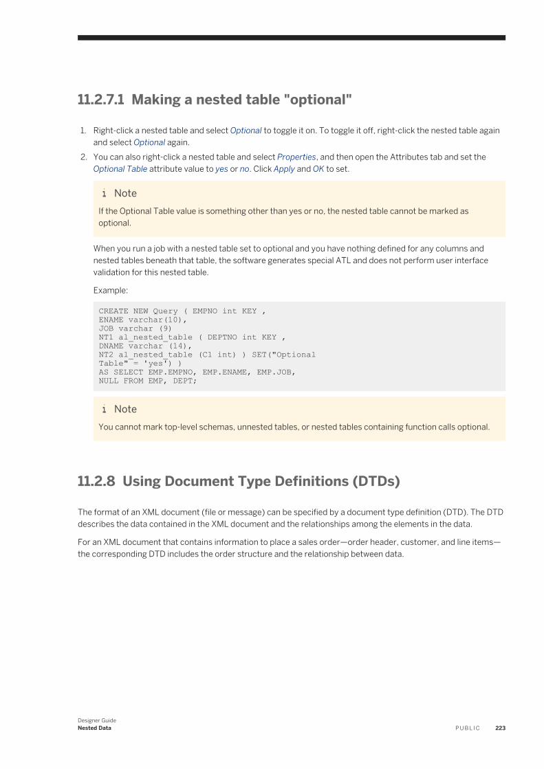
11.2.7.1 Making a nested table "optional"
1. Right-click a nested table and select Optional to toggle it on. To toggle it off, right-click the nested table again and select Optional again.
2. You can also right-click a nested table and select Properties, and then open the Attributes tab and set the Optional Table attribute value to yes or no. Click Apply and OK to set.
NoteIf the Optional Table value is something other than yes or no, the nested table cannot be marked as optional.
When you run a job with a nested table set to optional and you have nothing defined for any columns and nested tables beneath that table, the software generates special ATL and does not perform user interface validation for this nested table.
Example:
CREATE NEW Query ( EMPNO int KEY , ENAME varchar(10),JOB varchar (9)NT1 al_nested_table ( DEPTNO int KEY ,DNAME varchar (14),NT2 al_nested_table (C1 int) ) SET("OptionalTable" = 'yes') )AS SELECT EMP.EMPNO, EMP.ENAME, EMP.JOB, NULL FROM EMP, DEPT;
NoteYou cannot mark top-level schemas, unnested tables, or nested tables containing function calls optional.
11.2.8 Using Document Type Definitions (DTDs)
The format of an XML document (file or message) can be specified by a document type definition (DTD). The DTD describes the data contained in the XML document and the relationships among the elements in the data.
For an XML document that contains information to place a sales order—order header, customer, and line items—the corresponding DTD includes the order structure and the relationship between data.
Designer GuideNested Data P U B L I C 223
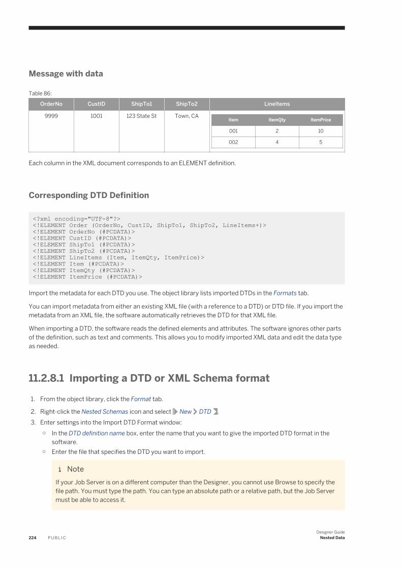
Message with data
Table 86:
OrderNo CustID ShipTo1 ShipTo2 LineItems
9999 1001 123 State St Town, CAItem ItemQty ItemPrice
001 2 10
002 4 5
Each column in the XML document corresponds to an ELEMENT definition.
Corresponding DTD Definition
<?xml encoding="UTF-8"?> <!ELEMENT Order (OrderNo, CustID, ShipTo1, ShipTo2, LineItems+)><!ELEMENT OrderNo (#PCDATA)><!ELEMENT CustID (#PCDATA)><!ELEMENT ShipTo1 (#PCDATA)><!ELEMENT ShipTo2 (#PCDATA)><!ELEMENT LineItems (Item, ItemQty, ItemPrice)><!ELEMENT Item (#PCDATA)><!ELEMENT ItemQty (#PCDATA)> <!ELEMENT ItemPrice (#PCDATA)>
Import the metadata for each DTD you use. The object library lists imported DTDs in the Formats tab.
You can import metadata from either an existing XML file (with a reference to a DTD) or DTD file. If you import the metadata from an XML file, the software automatically retrieves the DTD for that XML file.
When importing a DTD, the software reads the defined elements and attributes. The software ignores other parts of the definition, such as text and comments. This allows you to modify imported XML data and edit the data type as needed.
11.2.8.1 Importing a DTD or XML Schema format
1. From the object library, click the Format tab.
2. Right-click the Nested Schemas icon and select New DTD .3. Enter settings into the Import DTD Format window:
○ In the DTD definition name box, enter the name that you want to give the imported DTD format in the software.
○ Enter the file that specifies the DTD you want to import.
NoteIf your Job Server is on a different computer than the Designer, you cannot use Browse to specify the file path. You must type the path. You can type an absolute path or a relative path, but the Job Server must be able to access it.
224 P U B L I CDesigner Guide
Nested Data
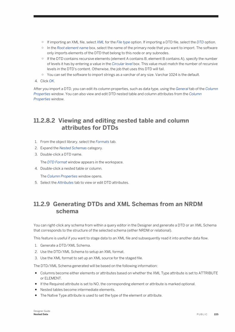
○ If importing an XML file, select XML for the File type option. If importing a DTD file, select the DTD option.○ In the Root element name box, select the name of the primary node that you want to import. The software
only imports elements of the DTD that belong to this node or any subnodes.○ If the DTD contains recursive elements (element A contains B, element B contains A), specify the number
of levels it has by entering a value in the Circular level box. This value must match the number of recursive levels in the DTD's content. Otherwise, the job that uses this DTD will fail.
○ You can set the software to import strings as a varchar of any size. Varchar 1024 is the default.4. Click OK.
After you import a DTD, you can edit its column properties, such as data type, using the General tab of the Column Properties window. You can also view and edit DTD nested table and column attributes from the Column Properties window.
11.2.8.2 Viewing and editing nested table and column attributes for DTDs
1. From the object library, select the Formats tab.2. Expand the Nested Schemas category.3. Double-click a DTD name.
The DTD Format window appears in the workspace.4. Double-click a nested table or column.
The Column Properties window opens.5. Select the Attributes tab to view or edit DTD attributes.
11.2.9 Generating DTDs and XML Schemas from an NRDM schema
You can right-click any schema from within a query editor in the Designer and generate a DTD or an XML Schema that corresponds to the structure of the selected schema (either NRDM or relational).
This feature is useful if you want to stage data to an XML file and subsequently read it into another data flow.
1. Generate a DTD/XML Schema.2. Use the DTD/XML Schema to setup an XML format.3. Use the XML format to set up an XML source for the staged file.
The DTD/XML Schema generated will be based on the following information:
● Columns become either elements or attributes based on whether the XML Type attribute is set to ATTRIBUTE or ELEMENT.
● If the Required attribute is set to NO, the corresponding element or attribute is marked optional.● Nested tables become intermediate elements.● The Native Type attribute is used to set the type of the element or attribute.
Designer GuideNested Data P U B L I C 225
● While generating XML Schemas, the MinOccurs and MaxOccurs values are set based on the Minimum Occurrence and Maximum Occurrence attributes of the corresponding nested table.
No other information is considered while generating the DTD or XML Schema.
11.3 Operations on nested data
This section discusses the operations that you can perform on nested data.
11.3.1 Overview of nested data and the Query transform
When working with nested data, the Query transform provides an interface to perform SELECT statements at each level of the relationship that you define in the output schema.
With relational data, a Query transform allows you to execute a SELECT statement. The mapping between input and output schemas defines the project list for the statement.
You use the Query transform to manipulate nested data. If you want to extract only part of the nested data, you can use the XML_Pipeline transform.
Without nested schemas, the Query transform assumes that the FROM clause in the SELECT statement contains the data sets that are connected as inputs to the query object. When working with nested data, you must explicitly define the FROM clause in a query. The software assists by setting the top-level inputs as the default FROM clause values for the top-level output schema.
The other SELECT statement elements defined by the query work the same with nested data as they do with flat data. However, because a SELECT statement can only include references to relational data sets, a query that includes nested data includes a SELECT statement to define operations for each parent and child schema in the output.
The Query Editor contains a tab for each clause of the query:
● SELECT provides an option to specify distinct rows to output (discarding any identical duplicate rows).● FROM lists all input schemas and allows you to specify join pairs and conditions.
The parameters you enter for the following tabs apply only to the current schema (displayed in the Schema Out text box at the top right of the Query Editor):
● WHERE● GROUP BY● ORDER BY
Related Information
Query Editor [page 179]
226 P U B L I CDesigner Guide
Nested Data
11.3.2 FROM clause construction
The FROM clause allows you to specify the tables and views to use in a join statement.
The FROM clause is located at the bottom of the FROM tab. It automatically populates with the information included in the Input Schema(s) section at the top, and the Join Pairs section in the middle of the tab. You can change the FROM clause by changing the selected schema in the Input Schema(s) area and the Join Pairs section.
Schemas selected in the Input Schema(s) section (and reflected in the FROM clause), including columns containing nested schemas, are available to be included in the output.
When you include more than one schema in the Input Schema(s) section (by selecting the From check box), you can specify join pairs and join conditions as well as enter join rank and cache for each input schema.
FROM clause descriptions and the behavior of the query are exactly the same with nested data as with relational data. The current schema allows you to distinguish multiple SELECT statements from each other within a single query. However, because the SELECT statements are dependent upon each other, and because the user interface makes it easy to construct arbitrary data sets, determining the appropriate FROM clauses for multiple levels of nesting can be complex.
A FROM clause can contain:
● Any top-level schema from the input● Any schema that is a column of a schema in the FROM clause of the parent schema● Any join conditions from the join pairs
The FROM clause forms a path that can start at any level of the output. The first schema in the path must always be a top-level schema from the input.
The data that a SELECT statement from a lower schema produces differs depending on whether or not a schema is included in the FROM clause at the top-level.
The next two examples use the sales order data set to illustrate scenarios where FROM clause values change the data resulting from the query.
Related Information
Modifying the output schema contents [page 180]
11.3.2.1 Example: FROM clause includes all top-level inputs
To include detailed customer information for all of the orders in the output, join the Order_Status_In schema at the top level with the Cust schema. Include both input schemas at the top level in the FROM clause to produce the appropriate data. When you select both input schemas in the Input schema(s) area of the FROM tab, they automatically appear in the FROM clause.
Designer GuideNested Data P U B L I C 227
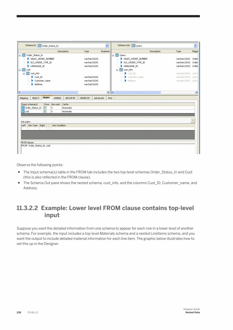
Observe the following points:
● The Input schema(s) table in the FROM tab includes the two top-level schemas Order_Status_In and Cust (this is also reflected in the FROM clause).
● The Schema Out pane shows the nested schema, cust_info, and the columns Cust_ID, Customer_name, and Address.
11.3.2.2 Example: Lower level FROM clause contains top-level input
Suppose you want the detailed information from one schema to appear for each row in a lower level of another schema. For example, the input includes a top-level Materials schema and a nested LineItems schema, and you want the output to include detailed material information for each line item. The graphic below illustrates how to set this up in the Designer.
228 P U B L I CDesigner Guide
Nested Data
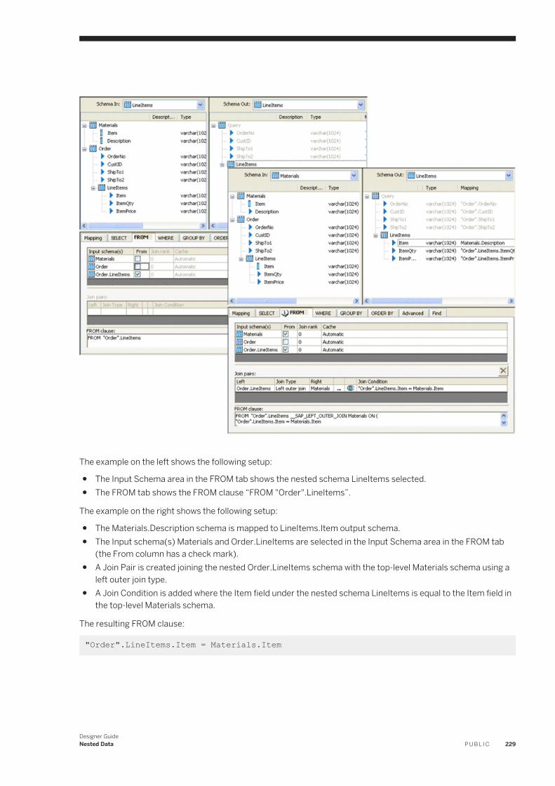
The example on the left shows the following setup:
● The Input Schema area in the FROM tab shows the nested schema LineItems selected.● The FROM tab shows the FROM clause “FROM "Order".LineItems”.
The example on the right shows the following setup:
● The Materials.Description schema is mapped to LineItems.Item output schema.● The Input schema(s) Materials and Order.LineItems are selected in the Input Schema area in the FROM tab
(the From column has a check mark).● A Join Pair is created joining the nested Order.LineItems schema with the top-level Materials schema using a
left outer join type.● A Join Condition is added where the Item field under the nested schema LineItems is equal to the Item field in
the top-level Materials schema.
The resulting FROM clause:
"Order".LineItems.Item = Materials.Item
Designer GuideNested Data P U B L I C 229
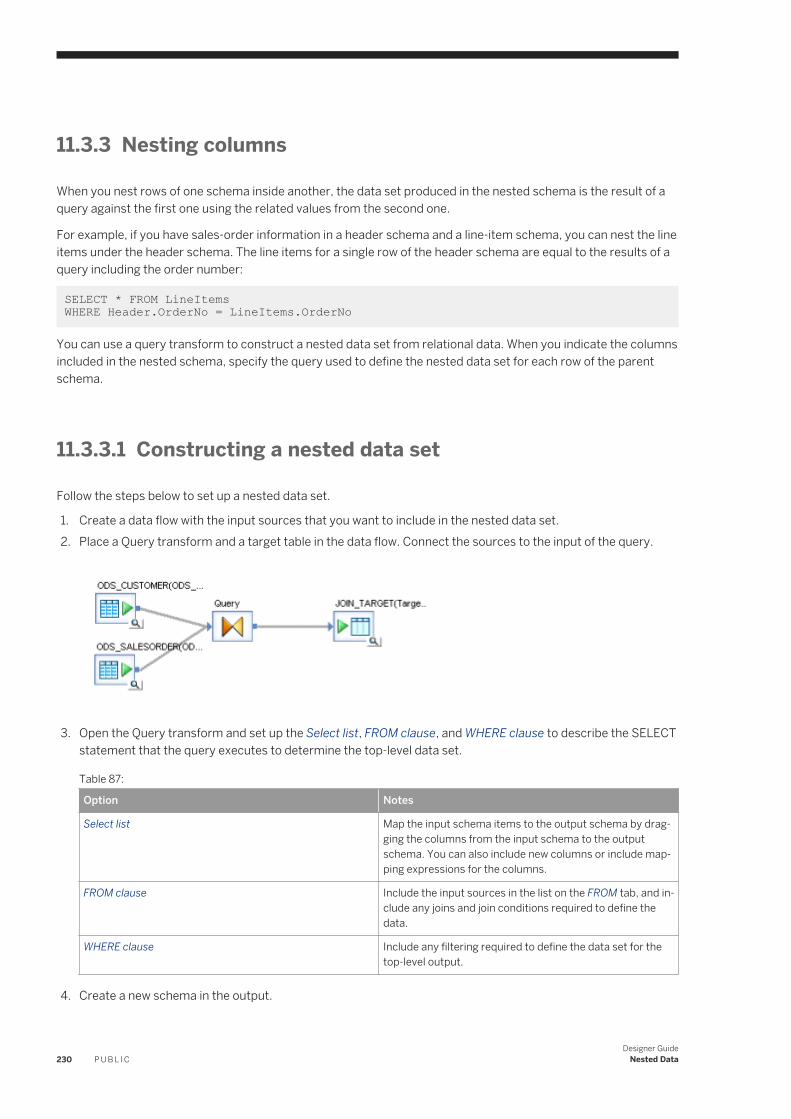
11.3.3 Nesting columns
When you nest rows of one schema inside another, the data set produced in the nested schema is the result of a query against the first one using the related values from the second one.
For example, if you have sales-order information in a header schema and a line-item schema, you can nest the line items under the header schema. The line items for a single row of the header schema are equal to the results of a query including the order number:
SELECT * FROM LineItems WHERE Header.OrderNo = LineItems.OrderNo
You can use a query transform to construct a nested data set from relational data. When you indicate the columns included in the nested schema, specify the query used to define the nested data set for each row of the parent schema.
11.3.3.1 Constructing a nested data set
Follow the steps below to set up a nested data set.
1. Create a data flow with the input sources that you want to include in the nested data set.2. Place a Query transform and a target table in the data flow. Connect the sources to the input of the query.
3. Open the Query transform and set up the Select list, FROM clause, and WHERE clause to describe the SELECT
statement that the query executes to determine the top-level data set.
Table 87:
Option Notes
Select list Map the input schema items to the output schema by dragging the columns from the input schema to the output schema. You can also include new columns or include mapping expressions for the columns.
FROM clause Include the input sources in the list on the FROM tab, and include any joins and join conditions required to define the data.
WHERE clause Include any filtering required to define the data set for the top-level output.
4. Create a new schema in the output.
230 P U B L I CDesigner Guide
Nested Data
Right-click in the Schema Out area of the Query Editor, choose New Output Schema, and name the new schema. A new schema icon appears in the output, nested under the top-level schema.
You can also drag an entire schema from the input to the output.5. Change the current output schema to the nested schema by right-clicking the nested schema and selecting
Make Current.
The Query Editor changes to display the new current schema.6. Indicate the FROM clause, Select list, and WHERE clause to describe the SELECT statement that the query
executes to determine the top-level data set.
Table 88:
Option Notes
FROM clause If you created a new output schema, you need to drag schemas from the input to populate the FROM clause. If you dragged an existing schema from the input to the top-level output, that schema is automatically mapped and listed in the From tab.
Select list Only columns are available that meet the requirements for the FROM clause.
WHERE clause Only columns are available that meet the requirements for the FROM clause.
7. If the output requires it, nest another schema at this level.
Repeat steps 4 through 6 in this current schema for as many nested schemas that you want to set up.8. If the output requires it, nest another schema under the top level.
Make the top-level schema the current schema.
Related Information
Query Editor [page 179]FROM clause construction [page 227]Modifying the output schema contents [page 180]
11.3.4 Using correlated columns in nested data
Correlation allows you to use columns from a higher-level schema to construct a nested schema.
In a nested-relational model, the columns in a nested schema are implicitly related to the columns in the parent row. To take advantage of this relationship, you can use columns from the parent schema in the construction of the nested schema. The higher-level column is a correlated column.
Including a correlated column in a nested schema can serve two purposes:
Designer GuideNested Data P U B L I C 231
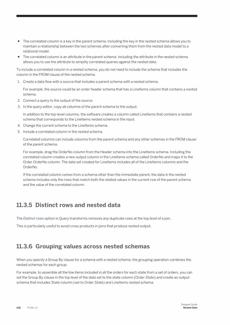
● The correlated column is a key in the parent schema. Including the key in the nested schema allows you to maintain a relationship between the two schemas after converting them from the nested data model to a relational model.
● The correlated column is an attribute in the parent schema. Including the attribute in the nested schema allows you to use the attribute to simplify correlated queries against the nested data.
To include a correlated column in a nested schema, you do not need to include the schema that includes the column in the FROM clause of the nested schema.
1. Create a data flow with a source that includes a parent schema with a nested schema.
For example, the source could be an order header schema that has a LineItems column that contains a nested schema.
2. Connect a query to the output of the source.3. In the query editor, copy all columns of the parent schema to the output.
In addition to the top-level columns, the software creates a column called LineItems that contains a nested schema that corresponds to the LineItems nested schema in the input.
4. Change the current schema to the LineItems schema.5. Include a correlated column in the nested schema.
Correlated columns can include columns from the parent schema and any other schemas in the FROM clause of the parent schema.
For example, drag the OrderNo column from the Header schema into the LineItems schema. Including the correlated column creates a new output column in the LineItems schema called OrderNo and maps it to the Order.OrderNo column. The data set created for LineItems includes all of the LineItems columns and the OrderNo.
If the correlated column comes from a schema other than the immediate parent, the data in the nested schema includes only the rows that match both the related values in the current row of the parent schema and the value of the correlated column.
11.3.5 Distinct rows and nested data
The Distinct rows option in Query transforms removes any duplicate rows at the top level of a join.
This is particularly useful to avoid cross products in joins that produce nested output.
11.3.6 Grouping values across nested schemas
When you specify a Group By clause for a schema with a nested schema, the grouping operation combines the nested schemas for each group.
For example, to assemble all the line items included in all the orders for each state from a set of orders, you can set the Group By clause in the top level of the data set to the state column (Order.State) and create an output schema that includes State column (set to Order.State) and LineItems nested schema.
232 P U B L I CDesigner Guide
Nested Data
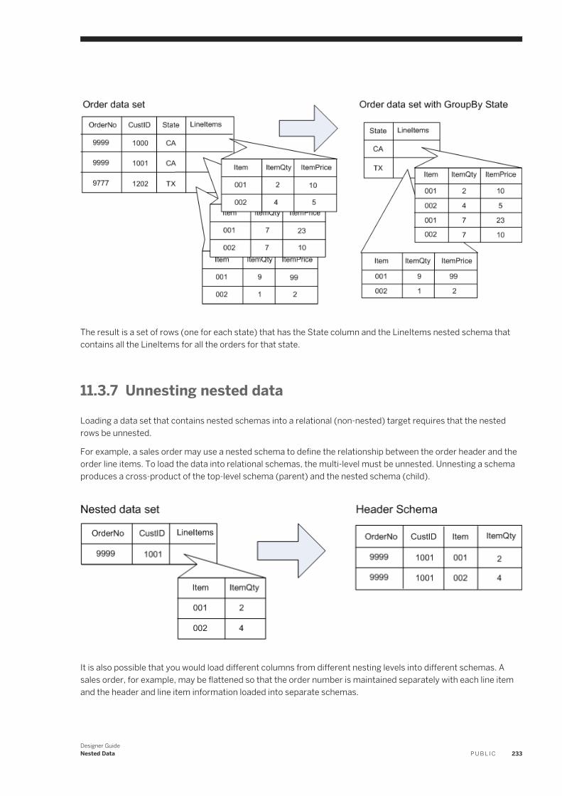
The result is a set of rows (one for each state) that has the State column and the LineItems nested schema that contains all the LineItems for all the orders for that state.
11.3.7 Unnesting nested data
Loading a data set that contains nested schemas into a relational (non-nested) target requires that the nested rows be unnested.
For example, a sales order may use a nested schema to define the relationship between the order header and the order line items. To load the data into relational schemas, the multi-level must be unnested. Unnesting a schema produces a cross-product of the top-level schema (parent) and the nested schema (child).
It is also possible that you would load different columns from different nesting levels into different schemas. A sales order, for example, may be flattened so that the order number is maintained separately with each line item and the header and line item information loaded into separate schemas.
Designer GuideNested Data P U B L I C 233
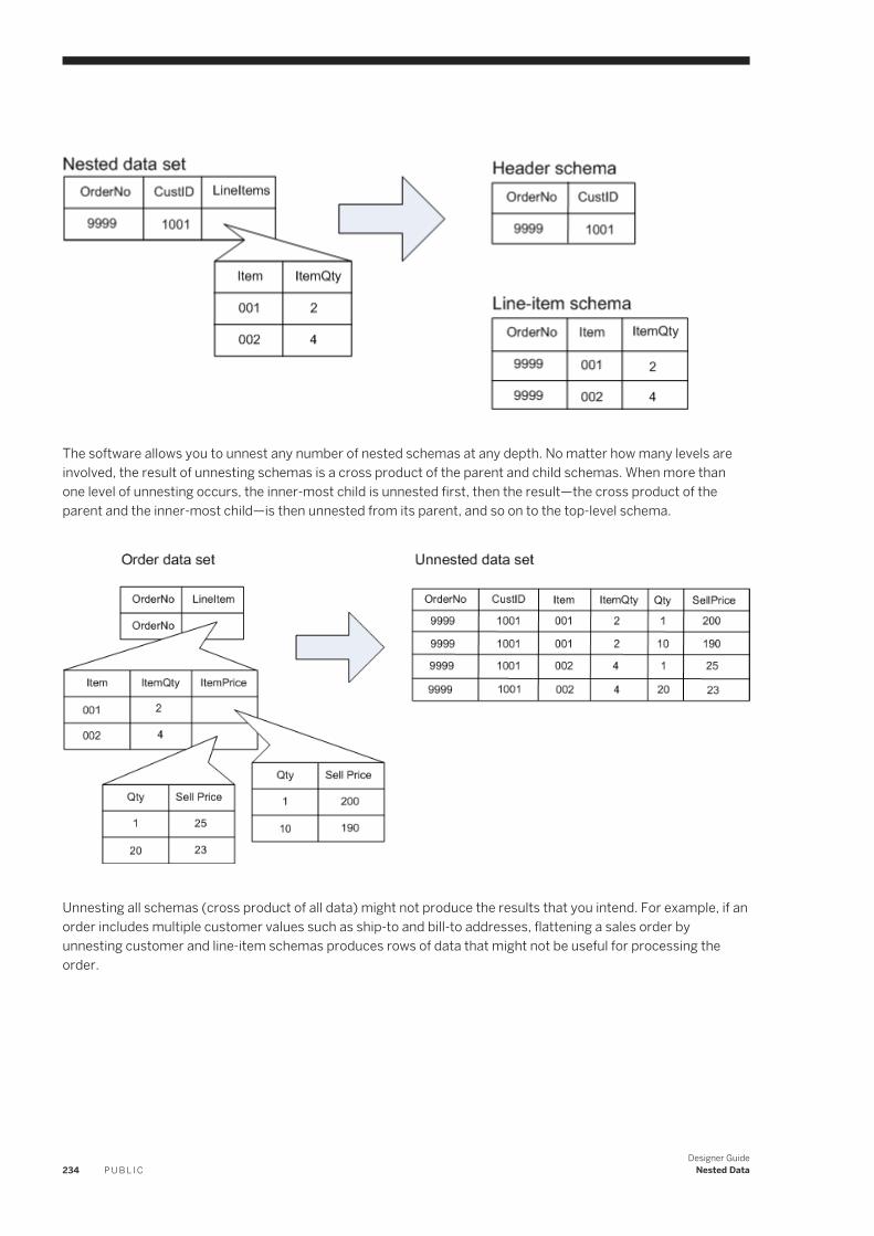
The software allows you to unnest any number of nested schemas at any depth. No matter how many levels are involved, the result of unnesting schemas is a cross product of the parent and child schemas. When more than one level of unnesting occurs, the inner-most child is unnested first, then the result—the cross product of the parent and the inner-most child—is then unnested from its parent, and so on to the top-level schema.
Unnesting all schemas (cross product of all data) might not produce the results that you intend. For example, if an order includes multiple customer values such as ship-to and bill-to addresses, flattening a sales order by unnesting customer and line-item schemas produces rows of data that might not be useful for processing the order.
234 P U B L I CDesigner Guide
Nested Data
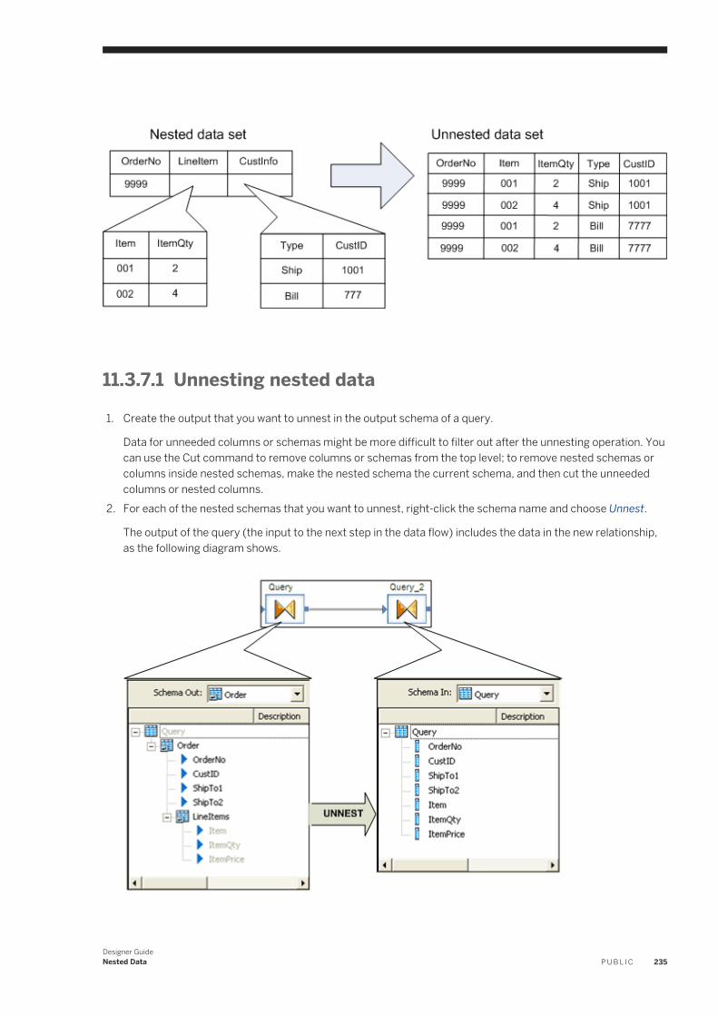
11.3.7.1 Unnesting nested data
1. Create the output that you want to unnest in the output schema of a query.
Data for unneeded columns or schemas might be more difficult to filter out after the unnesting operation. You can use the Cut command to remove columns or schemas from the top level; to remove nested schemas or columns inside nested schemas, make the nested schema the current schema, and then cut the unneeded columns or nested columns.
2. For each of the nested schemas that you want to unnest, right-click the schema name and choose Unnest.
The output of the query (the input to the next step in the data flow) includes the data in the new relationship, as the following diagram shows.
Designer GuideNested Data P U B L I C 235
11.3.8 Transforming lower levels of nested data
Nested data included in the input to transforms (with the exception of a Query or XML_Pipeline transform) passes through the transform without being included in the transform's operation. Only the columns at the first level of the input data set are available for subsequent transforms.
11.3.8.1 Transforming values in lower levels of nested schemas
1. Take one of the following actions to obtain the nested data:○ Use a Query transform to unnest the data.○ Use an XML_Pipeline transform to select portions of the nested data.○ Perform the transformation.
2. Nest the data again to reconstruct the nested relationships.
Related Information
Unnesting nested data [page 233]
11.4 XML extraction and parsing for columns
You can use the software to extract XML data stored in a source table or flat file column, transform it as NRDM data, and then load it to a target or flat file column.
In addition, you can extract XML message and file data, representing it as NRDM data during transformation, and then loading it to an XML message or file.
More and more database vendors allow you to store XML in one column. The field is usually a varchar, long, or clob. The software's XML handling capability also supports reading from and writing to such fields. The software provides four functions to support extracting from and loading to columns:
● extract_from_xml● load_to_xml● long_to_varchar● varchar_to_long
The extract_from_xml function gets the XML content stored in a single column and builds the corresponding NRDM structure so that the software can transform it. This function takes varchar data only.
To enable extracting and parsing for columns, data from long and clob columns must be converted to varchar before it can be transformed by the software.
● The software converts a clob data type input to varchar if you select the Import unsupported data types as VARCHAR of size option when you create a database datastore connection in the Datastore Editor.
236 P U B L I CDesigner Guide
Nested Data
● If your source uses a long data type, use the long_to_varchar function to convert data to varchar.
NoteThe software limits the size of the XML supported with these methods to 100K due to the current limitation of its varchar data type. There are plans to lift this restriction in the future.
The function load_to_xml generates XML from a given NRDM structure in the software, then loads the generated XML to a varchar column. If you want a job to convert the output to a long column, use the varchar_to_long function, which takes the output of the load_to_xml function as input.
11.4.1 Sample scenarios
The following scenarios describe how to use functions to extract XML data from a source column and load it into a target column.
Related Information
Extracting XML data from a column into the software [page 237]Loading XML data into a column of the data type long [page 239]Extract data quality XML strings using extract_from_xml function [page 240]
11.4.1.1 Extracting XML data from a column into the software
This scenario uses long_to_varchar and extract_from_xml functions to extract XML data from a column with data type long.
Perform the following prerequisite steps before beginning the main steps:
1. Import an Oracle table that contains a column named Content, the data type long, and which contains XML data for a purchase order.
2. Import the XML Schema PO.xsd, that provides the format for the XML data, into the repository.3. Create a project, a job, and a data flow for your design.4. Open the data flow and drop the source table with the column named content in the data flow.
To extract XML data from a column into the software, follow the prerequisite steps above, and then follow the steps below:
1. Create a query with an output column of data type varchar, and make sure that its size is big enough to hold the XML data.
2. Name this output column content.3. In the Map section of the query editor, open the Function Wizard, select the Conversion function type, then
select the long_to_varchar function and configure it by entering its parameters.
long_to_varchar(content, 4000)
Designer GuideNested Data P U B L I C 237
The second parameter in this function (4000 in the example above) is the maximum size of the XML data stored in the table column. Use this parameter with caution. If the size is not big enough to hold the maximum XML data for the column, the software will truncate the data and cause a runtime error. Conversely, do not enter a number that is too big, which would waste computer memory at runtime.
4. In the query editor, map the source table column to a new output column.5. Create a second query that uses the function extract_from_xml to extract the XML data.
To invoke the function extract_from_xml:a. Right-click the current context in the query.b. Choose New Function Call.c. When the Function Wizard opens, select Conversion and extract_from_xml.
NoteYou can only use the extract_from_xml function in a new function call. Otherwise, this function is not displayed in the function wizard.
6. Enter values for the input parameters and click Next.
Table 89: Input parameters
Parameter Description
XML column name Enter content, which is the output column in the previous query that holds the XML data.
DTD or XML Schema name Enter the name of the purchase order schema (in this case PO).
Enable validation Enter 1 if you want the software to validate the XML with the specified Schema. Enter 0 if you do not.
7. For the function, select a column or columns that you want to use on output.Imagine that this purchase order schema has five top-level elements: orderDate, shipTo, billTo, comment, and items. You can select any number of the top-level columns from an XML schema, which include either scalar or nested relational data model (NRDM) column data. The return type of the column is defined in the schema. If the function fails due to an error when trying to produce the XML output, the software returns NULL for scalar columns and empty nested tables for NRDM columns. The extract_from_xml function also adds two columns:○ AL_ERROR_NUM — returns error codes: 0 for success and a non-zero integer for failures○ AL_ERROR_MSG — returns an error message if AL_ERROR_NUM is not 0. Returns NULL if
AL_ERROR_NUM is 0Choose one or more of these columns as the appropriate output for the extract_from_xml function.
8. Click Finish.The software generates the function call in the current context and populates the output schema of the query with the output columns you specified.
With the data converted into the NRDM structure, you are ready to do appropriate transformation operations on it.
For example, if you want to load the NRDM structure to a target XML file, create an XML file target and connect the second query to it.
238 P U B L I CDesigner Guide
Nested Data
NoteIf you find that you want to modify the function call, right-click the function call in the second query and choose Modify Function Call.
In this example, to extract XML data from a column of data type long, we created two queries: the first query to convert the data using the long_to_varchar function and the second query to add the extract_from_xml function.
Alternatively, you can use just one query by entering the function expression long_to_varchar directly into the first parameter of the function extract_from_xml. The first parameter of the function extract_from_xml can take a column of data type varchar or an expression that returns data of type varchar.
If the data type of the source column is not long but varchar, do not include the function long_to_varchar in your data flow.
11.4.1.2 Loading XML data into a column of the data type long
This scenario uses the load_to_xml function and the varchar_to_long function to convert an NRDM structure to scalar data of the varchar type in an XML format and load it to a column of the data type long.
In this example, you want to convert an NRDM structure for a purchase order to XML data using the function load_to_xml, and then load the data to an Oracle table column called content, which is of the long data type. Because the function load_to_xml returns a value of varchar data type, you use the function varchar_to_long to convert the value of varchar data type to a value of the data type long.
1. Create a query and connect a previous query or source (that has the NRDM structure of a purchase order) to it. In this query, create an output column of the data type varchar called content. Make sure the size of the column is big enough to hold the XML data.
2. From the Mapping area open the function wizard, click the category Conversion Functions, and then select the function load_to_xml.
3. Click Next.4. Enter values for the input parameters.
The function load_to_xml has seven parameters.5. Click Finish.
In the mapping area of the Query window, notice the function expression:
load_to_xml(PO, 'PO', 1, '<?xml version="1.0" encoding = "UTF-8" ?>', NULL, 1, 4000)
In this example, this function converts the NRDM structure of purchase order PO to XML data and assigns the value to output column content.
6. Create another query with output columns matching the columns of the target table.a. Assume the column is called content and it is of the data type long.b. Open the function wizard from the mapping section of the query and select the Conversion Functions
categoryc. Use the function varchar_to_long to map the input column content to the output column content.
The function varchar_to_long takes only one input parameter.
Designer GuideNested Data P U B L I C 239
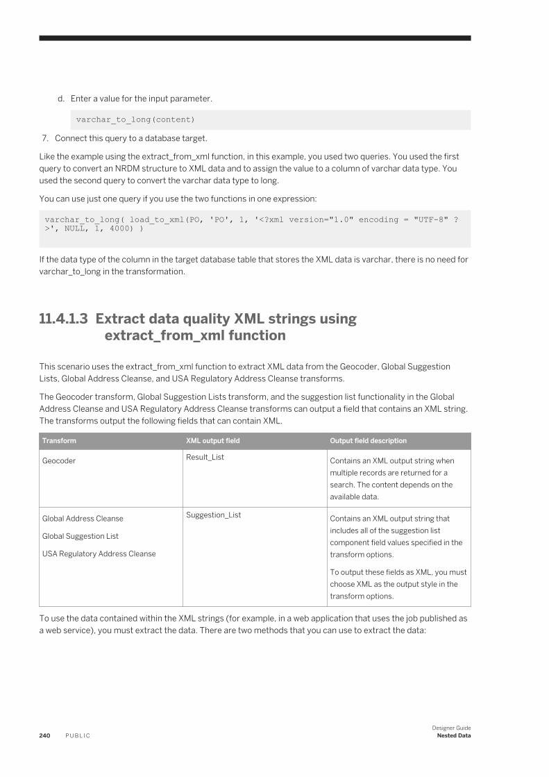
d. Enter a value for the input parameter.
varchar_to_long(content) 7. Connect this query to a database target.
Like the example using the extract_from_xml function, in this example, you used two queries. You used the first query to convert an NRDM structure to XML data and to assign the value to a column of varchar data type. You used the second query to convert the varchar data type to long.
You can use just one query if you use the two functions in one expression:
varchar_to_long( load_to_xml(PO, 'PO', 1, '<?xml version="1.0" encoding = "UTF-8" ?>', NULL, 1, 4000) )
If the data type of the column in the target database table that stores the XML data is varchar, there is no need for varchar_to_long in the transformation.
11.4.1.3 Extract data quality XML strings using extract_from_xml function
This scenario uses the extract_from_xml function to extract XML data from the Geocoder, Global Suggestion Lists, Global Address Cleanse, and USA Regulatory Address Cleanse transforms.
The Geocoder transform, Global Suggestion Lists transform, and the suggestion list functionality in the Global Address Cleanse and USA Regulatory Address Cleanse transforms can output a field that contains an XML string. The transforms output the following fields that can contain XML.
Transform XML output field Output field description
Geocoder Result_List Contains an XML output string when multiple records are returned for a search. The content depends on the available data.
Global Address Cleanse
Global Suggestion List
USA Regulatory Address Cleanse
Suggestion_List Contains an XML output string that includes all of the suggestion list component field values specified in the transform options.
To output these fields as XML, you must choose XML as the output style in the transform options.
To use the data contained within the XML strings (for example, in a web application that uses the job published as a web service), you must extract the data. There are two methods that you can use to extract the data:
240 P U B L I CDesigner Guide
Nested Data
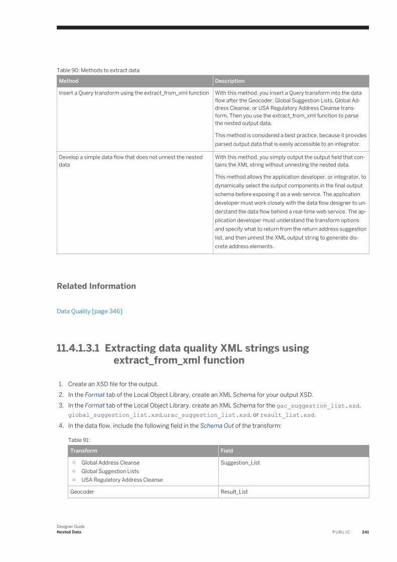
Table 90: Methods to extract data
Method Description
Insert a Query transform using the extract_from_xml function With this method, you insert a Query transform into the data flow after the Geocoder, Global Suggestion Lists, Global Address Cleanse, or USA Regulatory Address Cleanse transform. Then you use the extract_from_xml function to parse the nested output data.
This method is considered a best practice, because it provides parsed output data that is easily accessible to an integrator.
Develop a simple data flow that does not unnest the nested data
With this method, you simply output the output field that contains the XML string without unnesting the nested data.
This method allows the application developer, or integrator, to dynamically select the output components in the final output schema before exposing it as a web service. The application developer must work closely with the data flow designer to understand the data flow behind a real-time web service. The application developer must understand the transform options and specify what to return from the return address suggestion list, and then unnest the XML output string to generate discrete address elements.
Related Information
Data Quality [page 346]
11.4.1.3.1 Extracting data quality XML strings using extract_from_xml function
1. Create an XSD file for the output.2. In the Format tab of the Local Object Library, create an XML Schema for your output XSD.3. In the Format tab of the Local Object Library, create an XML Schema for the gac_suggestion_list.xsd,
global_suggestion_list.xsd,urac_suggestion_list.xsd, or result_list.xsd.
4. In the data flow, include the following field in the Schema Out of the transform:
Table 91:
Transform Field
○ Global Address Cleanse○ Global Suggestion Lists○ USA Regulatory Address Cleanse
Suggestion_List
Geocoder Result_List
Designer GuideNested Data P U B L I C 241
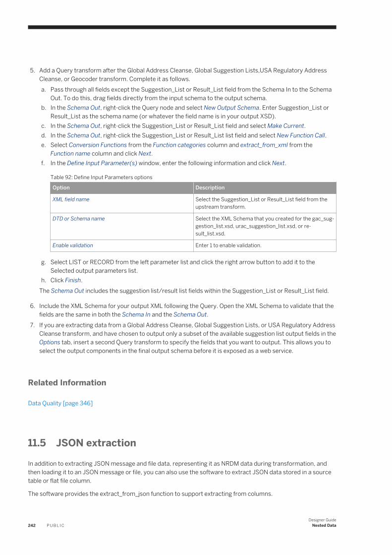
5. Add a Query transform after the Global Address Cleanse, Global Suggestion Lists,USA Regulatory Address Cleanse, or Geocoder transform. Complete it as follows.a. Pass through all fields except the Suggestion_List or Result_List field from the Schema In to the Schema
Out. To do this, drag fields directly from the input schema to the output schema.b. In the Schema Out, right-click the Query node and select New Output Schema. Enter Suggestion_List or
Result_List as the schema name (or whatever the field name is in your output XSD).c. In the Schema Out, right-click the Suggestion_List or Result_List field and select Make Current.d. In the Schema Out, right-click the Suggestion_List or Result_List list field and select New Function Call.e. Select Conversion Functions from the Function categories column and extract_from_xml from the
Function name column and click Next.f. In the Define Input Parameter(s) window, enter the following information and click Next.
Table 92: Define Input Parameters options
Option Description
XML field name Select the Suggestion_List or Result_List field from the upstream transform.
DTD or Schema name Select the XML Schema that you created for the gac_suggestion_list.xsd, urac_suggestion_list.xsd, or result_list.xsd.
Enable validation Enter 1 to enable validation.
g. Select LIST or RECORD from the left parameter list and click the right arrow button to add it to the Selected output parameters list.
h. Click Finish.The Schema Out includes the suggestion list/result list fields within the Suggestion_List or Result_List field.
6. Include the XML Schema for your output XML following the Query. Open the XML Schema to validate that the fields are the same in both the Schema In and the Schema Out.
7. If you are extracting data from a Global Address Cleanse, Global Suggestion Lists, or USA Regulatory Address Cleanse transform, and have chosen to output only a subset of the available suggestion list output fields in the Options tab, insert a second Query transform to specify the fields that you want to output. This allows you to select the output components in the final output schema before it is exposed as a web service.
Related Information
Data Quality [page 346]
11.5 JSON extraction
In addition to extracting JSON message and file data, representing it as NRDM data during transformation, and then loading it to an JSON message or file, you can also use the software to extract JSON data stored in a source table or flat file column.
The software provides the extract_from_json function to support extracting from columns.
242 P U B L I CDesigner Guide
Nested Data
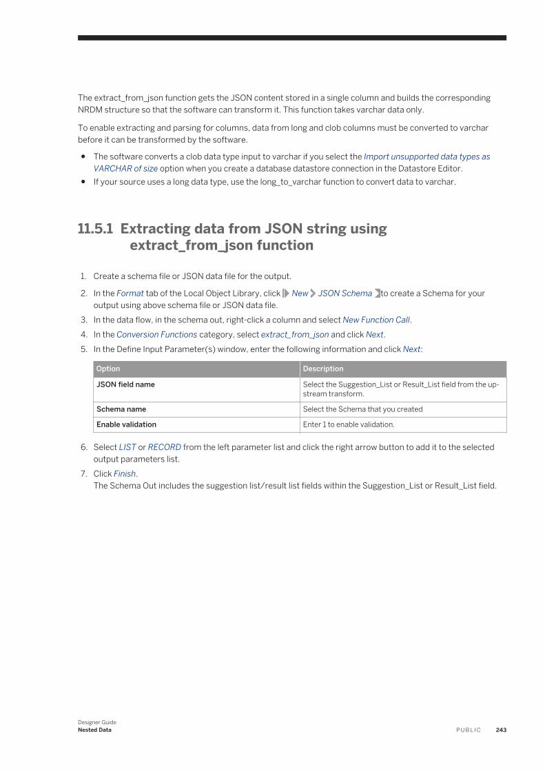
The extract_from_json function gets the JSON content stored in a single column and builds the corresponding NRDM structure so that the software can transform it. This function takes varchar data only.
To enable extracting and parsing for columns, data from long and clob columns must be converted to varchar before it can be transformed by the software.
● The software converts a clob data type input to varchar if you select the Import unsupported data types as VARCHAR of size option when you create a database datastore connection in the Datastore Editor.
● If your source uses a long data type, use the long_to_varchar function to convert data to varchar.
11.5.1 Extracting data from JSON string using extract_from_json function
1. Create a schema file or JSON data file for the output.
2. In the Format tab of the Local Object Library, click New JSON Schema to create a Schema for your output using above schema file or JSON data file.
3. In the data flow, in the schema out, right-click a column and select New Function Call.4. In the Conversion Functions category, select extract_from_json and click Next.5. In the Define Input Parameter(s) window, enter the following information and click Next:
Option Description
JSON field name Select the Suggestion_List or Result_List field from the upstream transform.
Schema name Select the Schema that you created
Enable validation Enter 1 to enable validation.
6. Select LIST or RECORD from the left parameter list and click the right arrow button to add it to the selected output parameters list.
7. Click Finish.The Schema Out includes the suggestion list/result list fields within the Suggestion_List or Result_List field.
Designer GuideNested Data P U B L I C 243
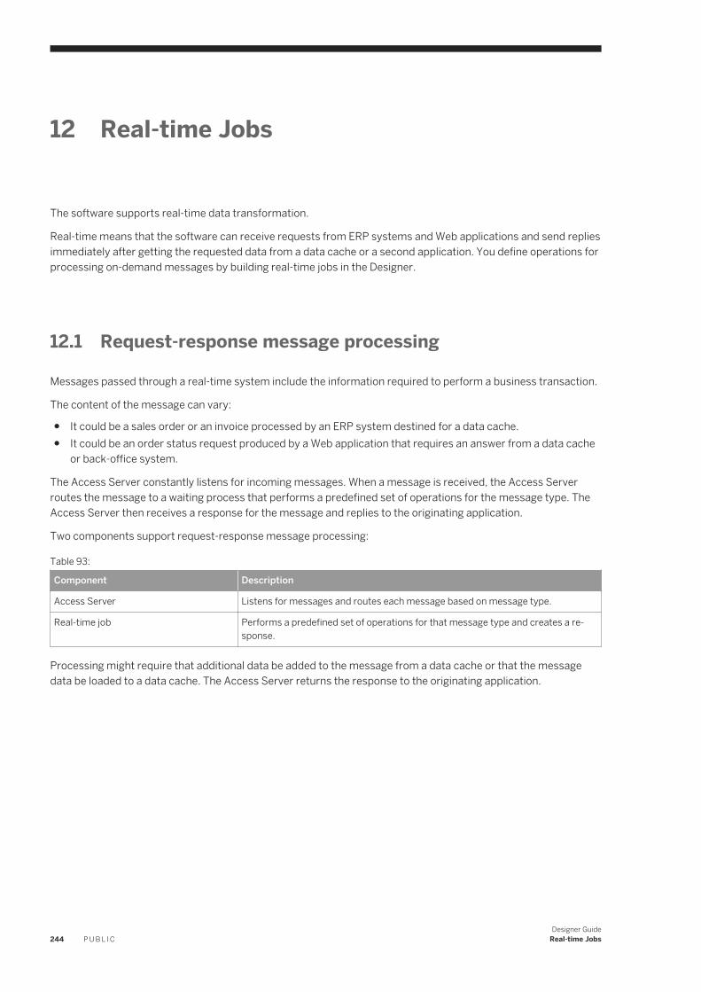
12 Real-time Jobs
The software supports real-time data transformation.
Real-time means that the software can receive requests from ERP systems and Web applications and send replies immediately after getting the requested data from a data cache or a second application. You define operations for processing on-demand messages by building real-time jobs in the Designer.
12.1 Request-response message processing
Messages passed through a real-time system include the information required to perform a business transaction.
The content of the message can vary:
● It could be a sales order or an invoice processed by an ERP system destined for a data cache.● It could be an order status request produced by a Web application that requires an answer from a data cache
or back-office system.
The Access Server constantly listens for incoming messages. When a message is received, the Access Server routes the message to a waiting process that performs a predefined set of operations for the message type. The Access Server then receives a response for the message and replies to the originating application.
Two components support request-response message processing:
Table 93:
Component Description
Access Server Listens for messages and routes each message based on message type.
Real-time job Performs a predefined set of operations for that message type and creates a response.
Processing might require that additional data be added to the message from a data cache or that the message data be loaded to a data cache. The Access Server returns the response to the originating application.
244 P U B L I CDesigner Guide
Real-time Jobs
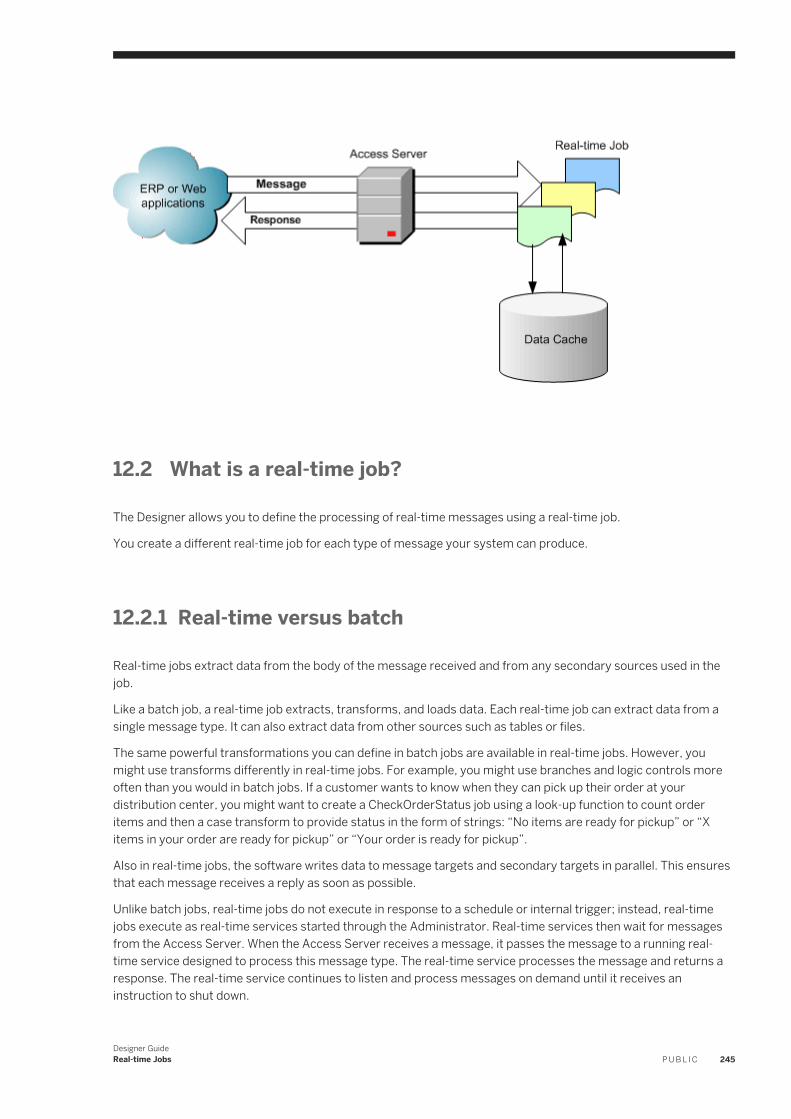
12.2 What is a real-time job?
The Designer allows you to define the processing of real-time messages using a real-time job.
You create a different real-time job for each type of message your system can produce.
12.2.1 Real-time versus batch
Real-time jobs extract data from the body of the message received and from any secondary sources used in the job.
Like a batch job, a real-time job extracts, transforms, and loads data. Each real-time job can extract data from a single message type. It can also extract data from other sources such as tables or files.
The same powerful transformations you can define in batch jobs are available in real-time jobs. However, you might use transforms differently in real-time jobs. For example, you might use branches and logic controls more often than you would in batch jobs. If a customer wants to know when they can pick up their order at your distribution center, you might want to create a CheckOrderStatus job using a look-up function to count order items and then a case transform to provide status in the form of strings: “No items are ready for pickup” or “X items in your order are ready for pickup” or “Your order is ready for pickup”.
Also in real-time jobs, the software writes data to message targets and secondary targets in parallel. This ensures that each message receives a reply as soon as possible.
Unlike batch jobs, real-time jobs do not execute in response to a schedule or internal trigger; instead, real-time jobs execute as real-time services started through the Administrator. Real-time services then wait for messages from the Access Server. When the Access Server receives a message, it passes the message to a running real-time service designed to process this message type. The real-time service processes the message and returns a response. The real-time service continues to listen and process messages on demand until it receives an instruction to shut down.
Designer GuideReal-time Jobs P U B L I C 245
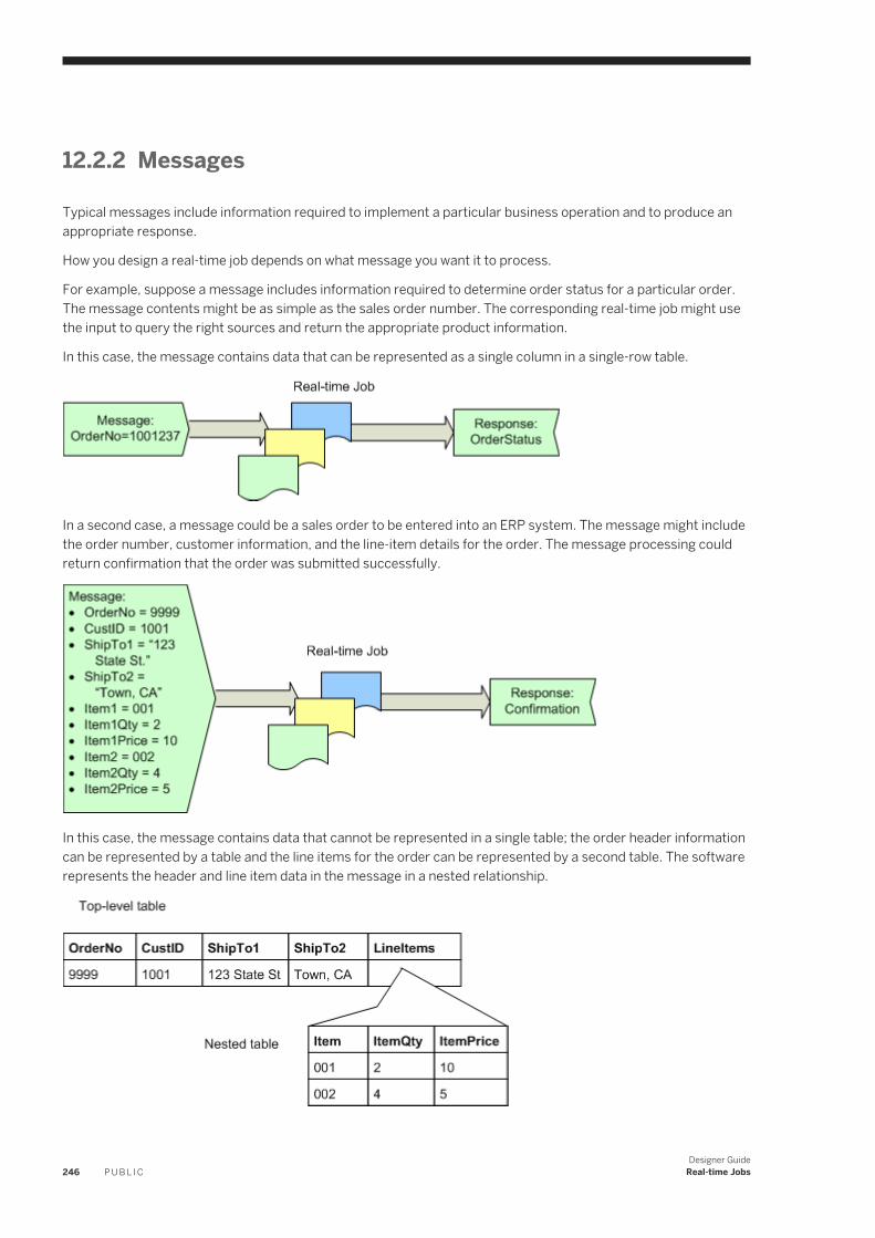
12.2.2 Messages
Typical messages include information required to implement a particular business operation and to produce an appropriate response.
How you design a real-time job depends on what message you want it to process.
For example, suppose a message includes information required to determine order status for a particular order. The message contents might be as simple as the sales order number. The corresponding real-time job might use the input to query the right sources and return the appropriate product information.
In this case, the message contains data that can be represented as a single column in a single-row table.
In a second case, a message could be a sales order to be entered into an ERP system. The message might include the order number, customer information, and the line-item details for the order. The message processing could return confirmation that the order was submitted successfully.
In this case, the message contains data that cannot be represented in a single table; the order header information can be represented by a table and the line items for the order can be represented by a second table. The software represents the header and line item data in the message in a nested relationship.
246 P U B L I CDesigner Guide
Real-time Jobs
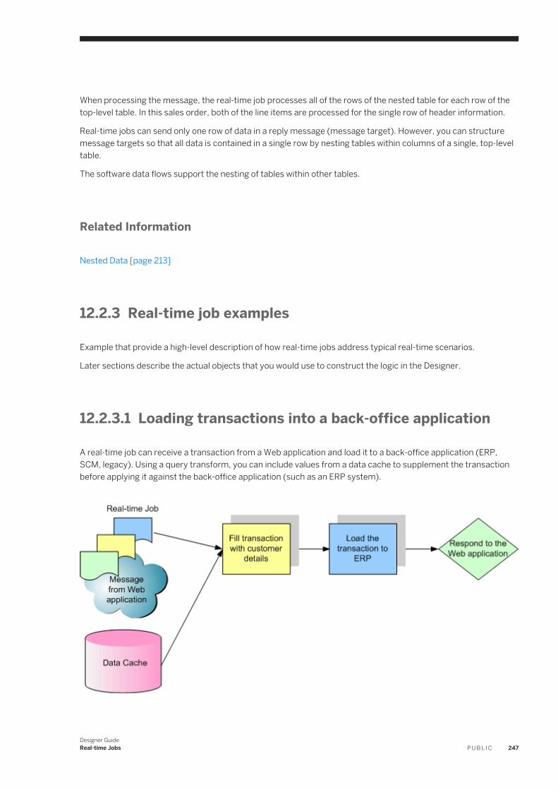
When processing the message, the real-time job processes all of the rows of the nested table for each row of the top-level table. In this sales order, both of the line items are processed for the single row of header information.
Real-time jobs can send only one row of data in a reply message (message target). However, you can structure message targets so that all data is contained in a single row by nesting tables within columns of a single, top-level table.
The software data flows support the nesting of tables within other tables.
Related Information
Nested Data [page 213]
12.2.3 Real-time job examples
Example that provide a high-level description of how real-time jobs address typical real-time scenarios.
Later sections describe the actual objects that you would use to construct the logic in the Designer.
12.2.3.1 Loading transactions into a back-office application
A real-time job can receive a transaction from a Web application and load it to a back-office application (ERP, SCM, legacy). Using a query transform, you can include values from a data cache to supplement the transaction before applying it against the back-office application (such as an ERP system).
Designer GuideReal-time Jobs P U B L I C 247
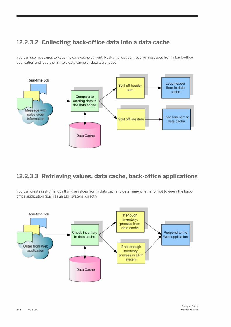
12.2.3.2 Collecting back-office data into a data cache
You can use messages to keep the data cache current. Real-time jobs can receive messages from a back-office application and load them into a data cache or data warehouse.
12.2.3.3 Retrieving values, data cache, back-office applications
You can create real-time jobs that use values from a data cache to determine whether or not to query the back-office application (such as an ERP system) directly.
248 P U B L I CDesigner Guide
Real-time Jobs
12.3 Creating real-time jobs
You can create real-time jobs using the same objects as batch jobs (data flows, work flows, conditionals, scripts, while loops, etc.).
However, object usage must adhere to a valid real-time job model.
12.3.1 Real-time job models
In contrast to batch jobs, which typically move large amounts of data at scheduled times, a real-time job, once started as a real-time service, listens for a request.
When a real-time job receives a request (typically to access small number of records), the software processes the request, returns a reply, and continues listening. This listen-process-listen logic forms a processing loop.
A real-time job is divided into three processing components: initialization, a real-time processing loop, and clean-up.
● The initialization component (optional) can be a script, work flow, data flow, or a combination of objects. It runs only when a real-time service starts.
● The real-time processing loop is a container for the job's single process logic. You can specify any number of work flows and data flows inside it.
● The clean-up component (optional) can be a script, work flow, data flow, or a combination of objects. It runs only when a real-time service is shut down.
In a real-time processing loop, a single message source must be included in the first step and a single message target must be included in the last step.
The following models support this rule:
● Single data flow model● Multiple data flow model● Request/Acknowledge data flow model
Related Information
Single data flow model [page 249]Multiple data flow model [page 250]
12.3.1.1 Single data flow model
With the single data flow model, you create a real-time job using a single data flow in its real-time processing loop. This single data flow must include a single message source and a single message target.
Designer GuideReal-time Jobs P U B L I C 249
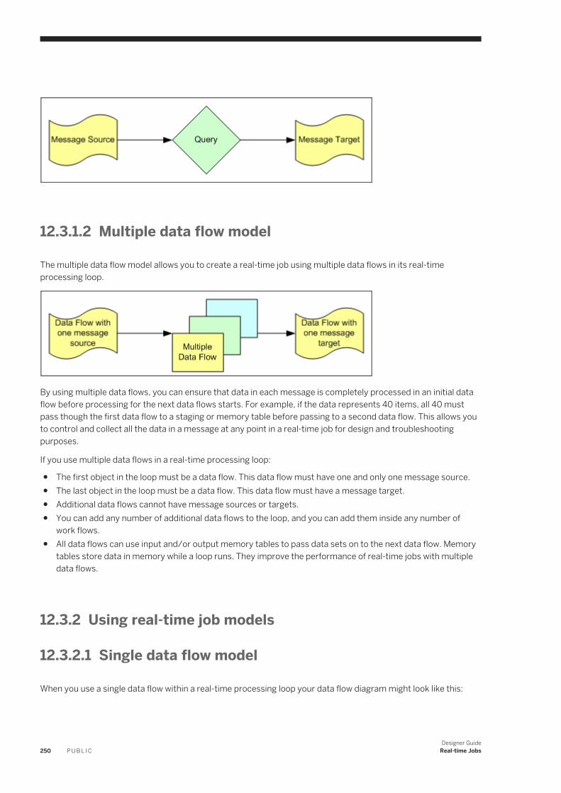
12.3.1.2 Multiple data flow model
The multiple data flow model allows you to create a real-time job using multiple data flows in its real-time processing loop.
By using multiple data flows, you can ensure that data in each message is completely processed in an initial data flow before processing for the next data flows starts. For example, if the data represents 40 items, all 40 must pass though the first data flow to a staging or memory table before passing to a second data flow. This allows you to control and collect all the data in a message at any point in a real-time job for design and troubleshooting purposes.
If you use multiple data flows in a real-time processing loop:
● The first object in the loop must be a data flow. This data flow must have one and only one message source.● The last object in the loop must be a data flow. This data flow must have a message target.● Additional data flows cannot have message sources or targets.● You can add any number of additional data flows to the loop, and you can add them inside any number of
work flows.● All data flows can use input and/or output memory tables to pass data sets on to the next data flow. Memory
tables store data in memory while a loop runs. They improve the performance of real-time jobs with multiple data flows.
12.3.2 Using real-time job models
12.3.2.1 Single data flow model
When you use a single data flow within a real-time processing loop your data flow diagram might look like this:
250 P U B L I CDesigner Guide
Real-time Jobs
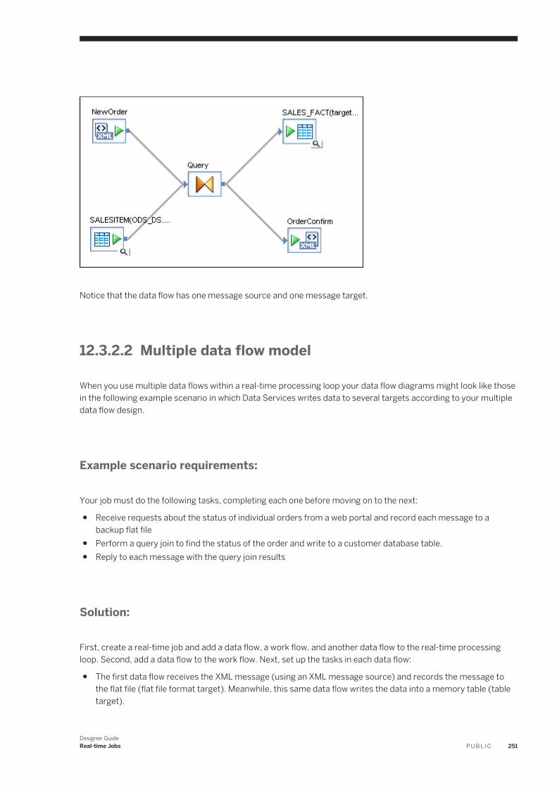
Notice that the data flow has one message source and one message target.
12.3.2.2 Multiple data flow model
When you use multiple data flows within a real-time processing loop your data flow diagrams might look like those in the following example scenario in which Data Services writes data to several targets according to your multiple data flow design.
Example scenario requirements:
Your job must do the following tasks, completing each one before moving on to the next:
● Receive requests about the status of individual orders from a web portal and record each message to a backup flat file
● Perform a query join to find the status of the order and write to a customer database table.● Reply to each message with the query join results
Solution:
First, create a real-time job and add a data flow, a work flow, and another data flow to the real-time processing loop. Second, add a data flow to the work flow. Next, set up the tasks in each data flow:
● The first data flow receives the XML message (using an XML message source) and records the message to the flat file (flat file format target). Meanwhile, this same data flow writes the data into a memory table (table target).
Designer GuideReal-time Jobs P U B L I C 251
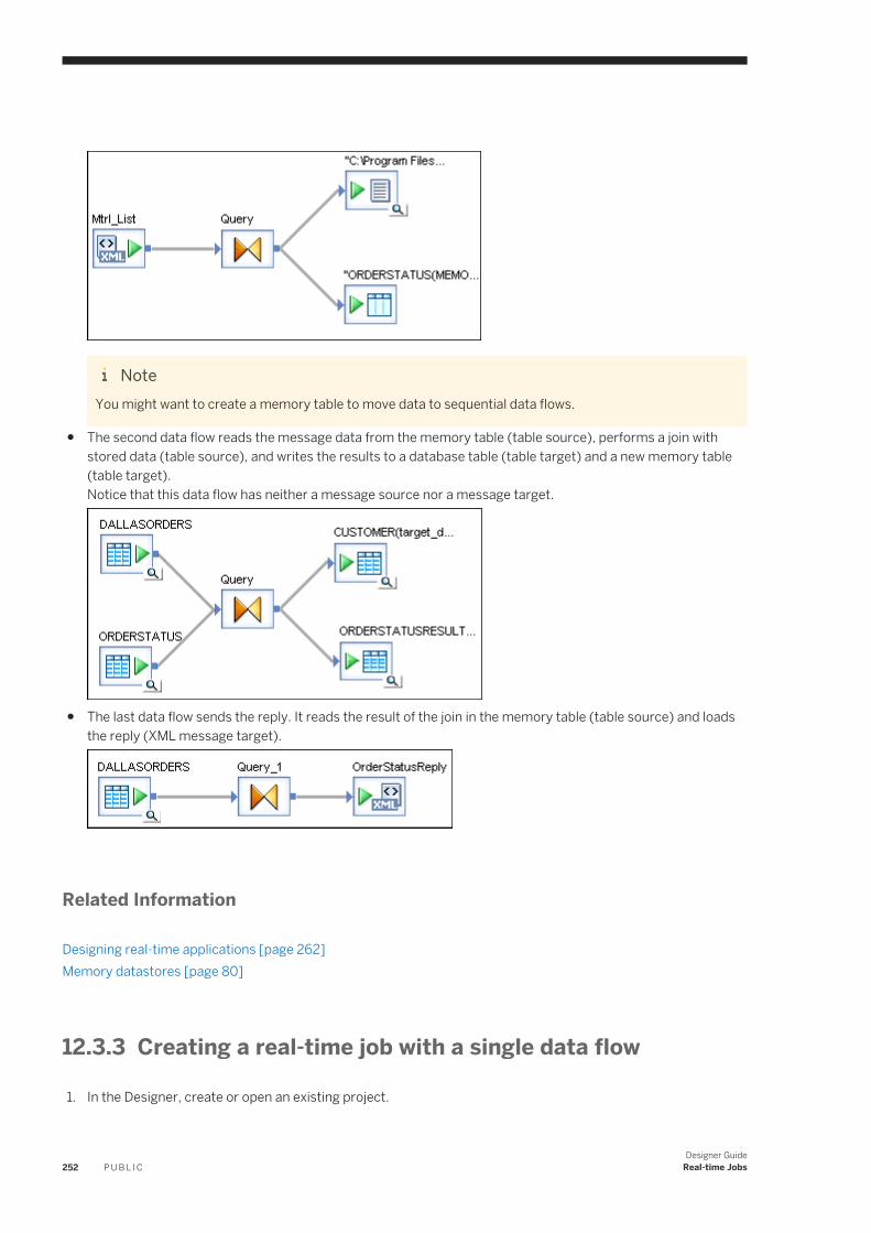
NoteYou might want to create a memory table to move data to sequential data flows.
● The second data flow reads the message data from the memory table (table source), performs a join with stored data (table source), and writes the results to a database table (table target) and a new memory table (table target).Notice that this data flow has neither a message source nor a message target.
● The last data flow sends the reply. It reads the result of the join in the memory table (table source) and loads the reply (XML message target).
Related Information
Designing real-time applications [page 262]Memory datastores [page 80]
12.3.3 Creating a real-time job with a single data flow
1. In the Designer, create or open an existing project.
252 P U B L I CDesigner Guide
Real-time Jobs
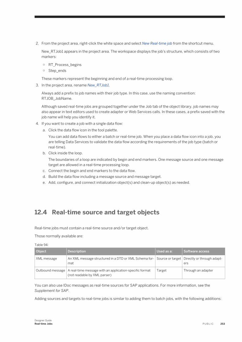
2. From the project area, right-click the white space and select New Real-time job from the shortcut menu.
New_RTJob1 appears in the project area. The workspace displays the job's structure, which consists of two markers:
○ RT_Process_begins○ Step_ends
These markers represent the beginning and end of a real-time processing loop.3. In the project area, rename New_RTJob1.
Always add a prefix to job names with their job type. In this case, use the naming convention: RTJOB_JobName.
Although saved real-time jobs are grouped together under the Job tab of the object library, job names may also appear in text editors used to create adapter or Web Services calls. In these cases, a prefix saved with the job name will help you identify it.
4. If you want to create a job with a single data flow:a. Click the data flow icon in the tool palette.
You can add data flows to either a batch or real-time job. When you place a data flow icon into a job, you are telling Data Services to validate the data flow according the requirements of the job type (batch or real-time).
b. Click inside the loop.The boundaries of a loop are indicated by begin and end markers. One message source and one message target are allowed in a real-time processing loop.
c. Connect the begin and end markers to the data flow.d. Build the data flow including a message source and message target.e. Add, configure, and connect initialization object(s) and clean-up object(s) as needed.
12.4 Real-time source and target objects
Real-time jobs must contain a real-time source and/or target object.
Those normally available are:
Table 94:
Object Description Used as a: Software access
XML message An XML message structured in a DTD or XML Schema format
Source or target Directly or through adapters
Outbound message A real-time message with an application-specific format (not readable by XML parser)
Target Through an adapter
You can also use IDoc messages as real-time sources for SAP applications. For more information, see the Supplement for SAP.
Adding sources and targets to real-time jobs is similar to adding them to batch jobs, with the following additions:
Designer GuideReal-time Jobs P U B L I C 253
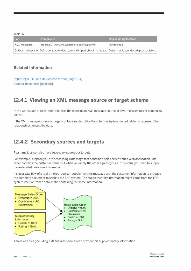
Table 95:
For Prerequisite Object library location
XML messages Import a DTD or XML Schema to define a format Formats tab
Outbound message Define an adapter datastore and import object metadata. Datastores tab, under adapter datastore
Related Information
Importing a DTD or XML Schema format [page 224]Adapter datastores [page 88]
12.4.1 Viewing an XML message source or target schema
In the workspace of a real-time job, click the name of an XML message source or XML message target to open its editor.
If the XML message source or target contains nested data, the schema displays nested tables to represent the relationships among the data.
12.4.2 Secondary sources and targets
Real-time jobs can also have secondary sources or targets.
For example, suppose you are processing a message that contains a sales order from a Web application. The order contains the customer name, but when you apply the order against your ERP system, you need to supply more detailed customer information.
Inside a data flow of a real-time job, you can supplement the message with the customer information to produce the complete document to send to the ERP system. The supplementary information might come from the ERP system itself or from a data cache containing the same information.
Tables and files (including XML files) as sources can provide this supplementary information.
254 P U B L I CDesigner Guide
Real-time Jobs
The software reads data from secondary sources according to the way you design the data flow. The software loads data to secondary targets in parallel with a target message.
Add secondary sources and targets to data flows in real-time jobs as you would to data flows in batch jobs.
Related Information
Source and target objects [page 155]Adding source or target objects to data flows [page 157]
12.4.3 Transactional loading of tables
Target tables in real-time jobs support transactional loading, in which the data resulting from the processing of a single data flow can be loaded into multiple tables as a single transaction.
No part of the transaction applies if any part fails.
NoteTarget tables in batch jobs also support transactional loading. However, use caution when you consider enabling this option for a batch job because it requires the use of memory, which can reduce performance when moving large amounts of data.
You can specify the order in which tables in the transaction are included using the target table editor. This feature supports a scenario in which you have a set of tables with foreign keys that depend on one with primary keys.
You can use transactional loading only when all the targets in a data flow are in the same datastore. If the data flow loads tables in more than one datastore, targets in each datastore load independently. While multiple targets in one datastore may be included in one transaction, the targets in another datastores must be included in another transaction.
You can specify the same transaction order or distinct transaction orders for all targets to be included in the same transaction. If you specify the same transaction order for all targets in the same datastore, the tables are still included in the same transaction but are loaded together. Loading is committed after all tables in the transaction finish loading.
If you specify distinct transaction orders for all targets in the same datastore, the transaction orders indicate the loading orders of the tables. The table with the smallest transaction order is loaded first, and so on, until the table with the largest transaction order is loaded last. No two tables are loaded at the same time. Loading is committed when the last table finishes loading.
Designer GuideReal-time Jobs P U B L I C 255
12.4.4 Design tips for data flows in real-time jobs
When designing data flows in real-time jobs, there are rules that need to be followed.
● If you include a table in a join with a real-time source, the software includes the data set from the real-time source as the outer loop of the join. If more than one supplementary source is included in the join, you can control which table is included in the next outer-most loop of the join using the join ranks for the tables.
● In real-time jobs, do not cache data from secondary sources unless the data is static. The data will be read when the real-time job starts and will not be updated while the job is running.
● If no rows are passed to the XML target, the real-time job returns an empty response to the Access Server. For example, if a request comes in for a product number that does not exist, your job might be designed in such a way that no data passes to the reply message. You might want to provide appropriate instructions to your user (exception handling in your job) to account for this type of scenario.
● If more than one row passes to the XML target, the target reads the first row and discards the other rows. To avoid this issue, use your knowledge of the software's Nested Relational Data Model (NRDM) and structure your message source and target formats so that one "row" equals one message. With NRDM, you can structure any amount of data into a single "row" because columns in tables can contain other tables.
● Recovery mechanisms are not supported in real-time jobs.
Related Information
Nested Data [page 213]
12.5 Testing real-time jobs
12.5.1 Executing a real-time job in test mode
You can test real-time job designs without configuring the job as a service associated with an Access Server.
In test mode, you can execute a real-time job using a sample source message from a file to determine if the software produces the expected target message.
12.5.1.1 Specifying a sample XML message and target test file
1. In the XML message source and target editors, enter a file name in the XML test file box.
Enter the full path name for the source file that contains your sample data. Use paths for both test files relative to the computer that runs the Job Server for the current repository.
2. Execute the job.
Test mode is always enabled for real-time jobs. The software reads data from the source test file and loads it into the target test file.
256 P U B L I CDesigner Guide
Real-time Jobs
12.5.2 Using View Data
Use the View Data feature to capture a sample of your output data to ensure that your design is working.
This allows you to see that your design returns the results you expect.
Related Information
Design and Debug [page 572]
12.5.3 Using an XML file target
Use an XML file target to capture the message produced by a data flow while allowing the message to be returned to the Access Server.
Just like an XML message, you define an XML file by importing a DTD or XML Schema for the file, then dragging the format into the data flow definition. Unlike XML messages, you can include XML files as sources or targets in batch and real-time jobs.
12.5.3.1 Using a file to capture output from steps in a real-time job
1. In the Formats tab of the object library, drag the DTD or XML Schema into a data flow of a real-time job.
A menu prompts you for the function of the file.2. Choose Make XML File Target.
The XML file target appears in the workspace.3. In the file editor, specify the location to which the software writes data.
Enter a file name relative to the computer running the Job Server.4. Connect the output of the step in the data flow that you want to capture to the input of the file.
Designer GuideReal-time Jobs P U B L I C 257
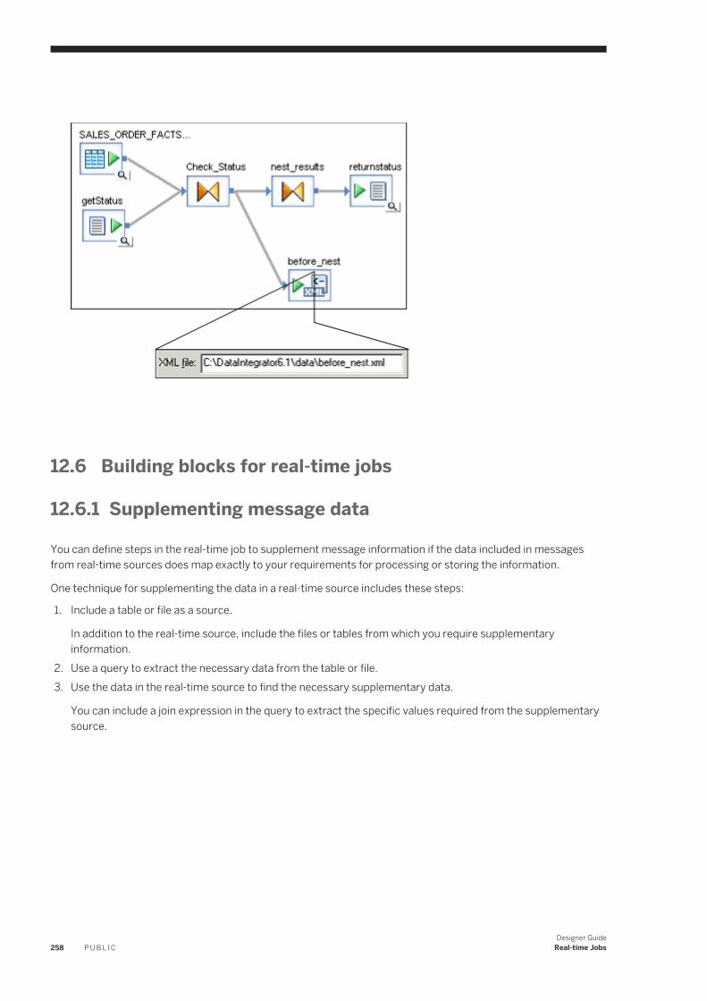
12.6 Building blocks for real-time jobs
12.6.1 Supplementing message data
You can define steps in the real-time job to supplement message information if the data included in messages from real-time sources does map exactly to your requirements for processing or storing the information.
One technique for supplementing the data in a real-time source includes these steps:
1. Include a table or file as a source.
In addition to the real-time source, include the files or tables from which you require supplementary information.
2. Use a query to extract the necessary data from the table or file.3. Use the data in the real-time source to find the necessary supplementary data.
You can include a join expression in the query to extract the specific values required from the supplementary source.
258 P U B L I CDesigner Guide
Real-time Jobs
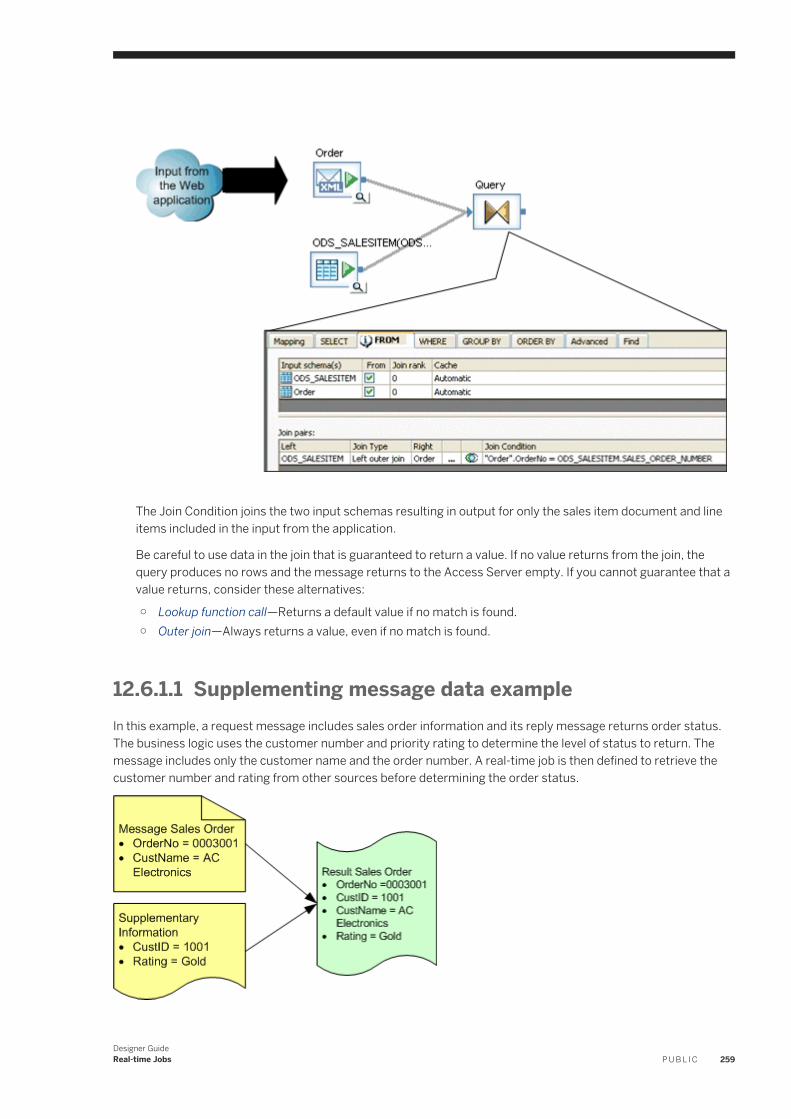
The Join Condition joins the two input schemas resulting in output for only the sales item document and line items included in the input from the application.
Be careful to use data in the join that is guaranteed to return a value. If no value returns from the join, the query produces no rows and the message returns to the Access Server empty. If you cannot guarantee that a value returns, consider these alternatives:
○ Lookup function call—Returns a default value if no match is found.○ Outer join—Always returns a value, even if no match is found.
12.6.1.1 Supplementing message data exampleIn this example, a request message includes sales order information and its reply message returns order status. The business logic uses the customer number and priority rating to determine the level of status to return. The message includes only the customer name and the order number. A real-time job is then defined to retrieve the customer number and rating from other sources before determining the order status.
Designer GuideReal-time Jobs P U B L I C 259
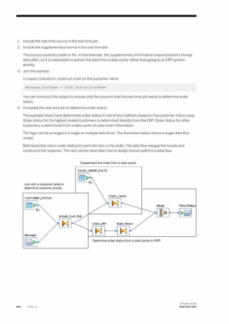
1. Include the real-time source in the real-time job.2. Include the supplementary source in the real-time job.
This source could be a table or file. In this example, the supplementary information required doesn't change very often, so it is reasonable to extract the data from a data cache rather than going to an ERP system directly.
3. Join the sources.
In a query transform, construct a join on the customer name:
Message.CustName = Cust_Status.CustName
You can construct the output to include only the columns that the real-time job needs to determine order status.
4. Complete the real-time job to determine order status.
The example shown here determines order status in one of two methods based on the customer status value. Order status for the highest ranked customers is determined directly from the ERP. Order status for other customers is determined from a data cache of sales order information.
The logic can be arranged in a single or multiple data flows. The illustration below shows a single data flow model.
Both branches return order status for each line item in the order. The data flow merges the results and constructs the response. The next section describes how to design branch paths in a data flow.
260 P U B L I CDesigner Guide
Real-time Jobs
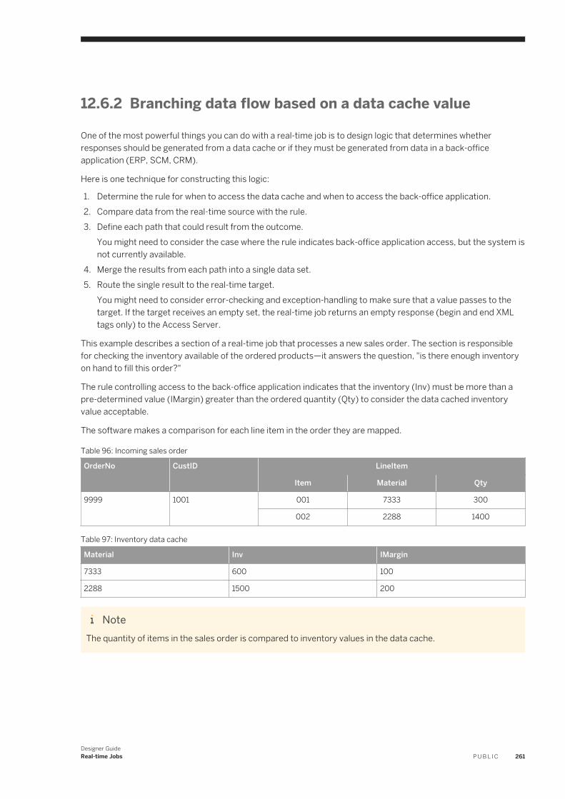
12.6.2 Branching data flow based on a data cache value
One of the most powerful things you can do with a real-time job is to design logic that determines whether responses should be generated from a data cache or if they must be generated from data in a back-office application (ERP, SCM, CRM).
Here is one technique for constructing this logic:
1. Determine the rule for when to access the data cache and when to access the back-office application.2. Compare data from the real-time source with the rule.3. Define each path that could result from the outcome.
You might need to consider the case where the rule indicates back-office application access, but the system is not currently available.
4. Merge the results from each path into a single data set.5. Route the single result to the real-time target.
You might need to consider error-checking and exception-handling to make sure that a value passes to the target. If the target receives an empty set, the real-time job returns an empty response (begin and end XML tags only) to the Access Server.
This example describes a section of a real-time job that processes a new sales order. The section is responsible for checking the inventory available of the ordered products—it answers the question, "is there enough inventory on hand to fill this order?"
The rule controlling access to the back-office application indicates that the inventory (Inv) must be more than a pre-determined value (IMargin) greater than the ordered quantity (Qty) to consider the data cached inventory value acceptable.
The software makes a comparison for each line item in the order they are mapped.
Table 96: Incoming sales order
OrderNo CustID LineItem
Item Material Qty
9999 1001 001 7333 300
002 2288 1400
Table 97: Inventory data cache
Material Inv IMargin
7333 600 100
2288 1500 200
NoteThe quantity of items in the sales order is compared to inventory values in the data cache.
Designer GuideReal-time Jobs P U B L I C 261
12.6.3 Calling application functions
A real-time job can use application functions to operate on data.
You can include tables as input or output parameters to the function.
Application functions require input values for some parameters and some can be left unspecified. You must determine the requirements of the function to prepare the appropriate inputs.
To make up the input, you can specify the top-level table, top-level columns, and any tables nested one-level down relative to the tables listed in the FROM clause of the context calling the function. If the application function includes a structure as an input parameter, you must specify the individual columns that make up the structure.
A data flow may contain several steps that call a function, retrieve results, then shape the results into the columns and tables required for a response.
12.7 Designing real-time applications
You can design real-time applications that meet your internal and external information and resource needs.
The software provides a reliable and low-impact connection between a Web application and back-office applications such as an enterprise resource planning (ERP) system. Because each implementation of an ERP system is different and because the software includes versatile decision support logic, you may decide to design a system.
12.7.1 Reducing queries requiring back-office application access
A collection of recommendations and considerations that can help reduce the time you spend experimenting in your development cycles.
The information you allow your customers to access through your Web application can impact the performance that your customers see on the Web. You can maximize performance through your Web application design decisions. In particular, you can structure your application to reduce the number of queries that require direct back-office (ERP, SCM, Legacy) application access.
For example, if your ERP system supports a complicated pricing structure that includes dependencies such as customer priority, product availability, or order quantity, you might not be able to depend on values from a data cache for pricing information. The alternative might be to request pricing information directly from the ERP system. ERP system access is likely to be much slower than direct database access, reducing the performance your customer experiences with your Web application.
To reduce the impact of queries requiring direct ERP system access, modify your Web application. Using the pricing example, design the application to avoid displaying price information along with standard product information and instead show pricing only after the customer has chosen a specific product and quantity. These techniques are evident in the way airline reservations systems provide pricing information—a quote for a specific flight—contrasted with other retail Web sites that show pricing for every item displayed as part of product catalogs.
262 P U B L I CDesigner Guide
Real-time Jobs
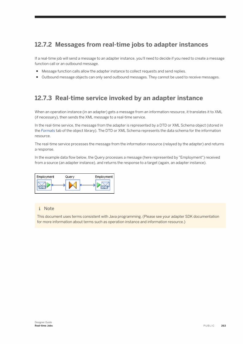
12.7.2 Messages from real-time jobs to adapter instances
If a real-time job will send a message to an adapter instance, you'll need to decide if you need to create a message function call or an outbound message.
● Message function calls allow the adapter instance to collect requests and send replies.● Outbound message objects can only send outbound messages. They cannot be used to receive messages.
12.7.3 Real-time service invoked by an adapter instance
When an operation instance (in an adapter) gets a message from an information resource, it translates it to XML (if necessary), then sends the XML message to a real-time service.
In the real-time service, the message from the adapter is represented by a DTD or XML Schema object (stored in the Formats tab of the object library). The DTD or XML Schema represents the data schema for the information resource.
The real-time service processes the message from the information resource (relayed by the adapter) and returns a response.
In the example data flow below, the Query processes a message (here represented by "Employment") received from a source (an adapter instance), and returns the response to a target (again, an adapter instance).
NoteThis document uses terms consistent with Java programming. (Please see your adapter SDK documentation for more information about terms such as operation instance and information resource.)
Designer GuideReal-time Jobs P U B L I C 263
13 Embedded Data Flows
An embedded data flow is a data flow that is called from inside another data flow.
The software provides easy-to-use options to create embedded data flows.
13.1 Overview of embedded data flows
Data passes into or out of the embedded data flow from the parent flow through a single source or target.
An embedded data flow can contain any number of sources or targets, but only one input or one output can pass data to or from the parent data flow.
You can create the following types of embedded data flows:
Table 98:
Type Use when you want to...
One input Add an embedded data flow at the end of a data flow.
One output Add an embedded data flow at the beginning of a data flow.
No input or output Replicate an existing data flow.
An embedded data flow is a design aid that has no effect on job execution. When the software executes the parent data flow, it expands any embedded data flows, optimizes the parent data flow, and then executes it.
Use embedded data flows to:
● Simplify data flow display. Group sections of a data flow in embedded data flows to allow clearer layout and documentation.
● Reuse data flow logic. Save logical sections of a data flow so you can use the exact logic in other data flows, or provide an easy way to replicate the logic and modify it for other flows.
● Debug data flow logic. Replicate sections of a data flow as embedded data flows so you can execute them independently.
13.2 Embedded data flow examples
Examples of when and how to use embedded data flows.
In this example, a data flow uses a single source to load three different target systems. The Case transform sends each row from the source to different transforms that process it to get a unique target output.
264 P U B L I CDesigner Guide
Embedded Data Flows
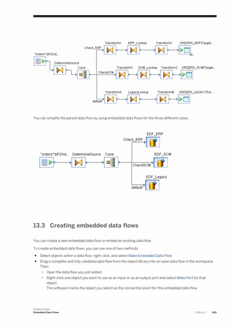
You can simplify the parent data flow by using embedded data flows for the three different cases.
13.3 Creating embedded data flows
You can create a new embedded data flow or embed an existing data flow.
To create embedded data flows, you can use one of two methods:
● Select objects within a data flow, right-click, and select Make Embedded Data Flow.● Drag a complete and fully validated data flow from the object library into an open data flow in the workspace.
Then:○ Open the data flow you just added.○ Right-click one object you want to use as an input or as an output port and select Make Port for that
object.The software marks the object you select as the connection point for this embedded data flow.
Designer GuideEmbedded Data Flows P U B L I C 265
NoteYou can specify only one port, which means that the embedded data flow can appear only at the beginning or at the end of the parent data flow.
Data Services ignores some physical files that are required for sources and targets with assigned ports.
○ When you use an embedded data flow, data will flow directly from the caller to the transform(s) next to the port source.
○ When you use a data flow directly, Data Services uses the physical files in sources and targets, but ignores the ports.
13.3.1 Using the Make Embedded Data Flow option
Use this option to create a new embedded data flow.
1. Select objects from an open data flow using one of the following methods:
○ Click the white space and drag the rectangle around the objects.○ CTRL-click each object.
Ensure that the set of objects you select are:○ All connected to each other.○ Connected to other objects according to the type of embedded data flow you want to create such as one
input, one output, or no input or output.2. Right-click and select Make Embedded Data Flow.
The Create Embedded Data Flow window opens, with the embedded data flow connected to the parent by one input object.
3. Name the embedded data flow using the convention EDF_ <EDFName> for example EDF_ERP.
If you deselect the Replace objects in original data flow box, the software will not make a change in the original data flow. The software saves the new embedded data flow object to the repository and displays it in the object library under the Data Flows tab.
You can use an embedded data flow created without replacement as a stand-alone data flow for troubleshooting.
If Replace objects in original data flow is selected, the original data flow becomes a parent data flow, which has a call to the new embedded data flow.
4. Click OK.
266 P U B L I CDesigner Guide
Embedded Data Flows
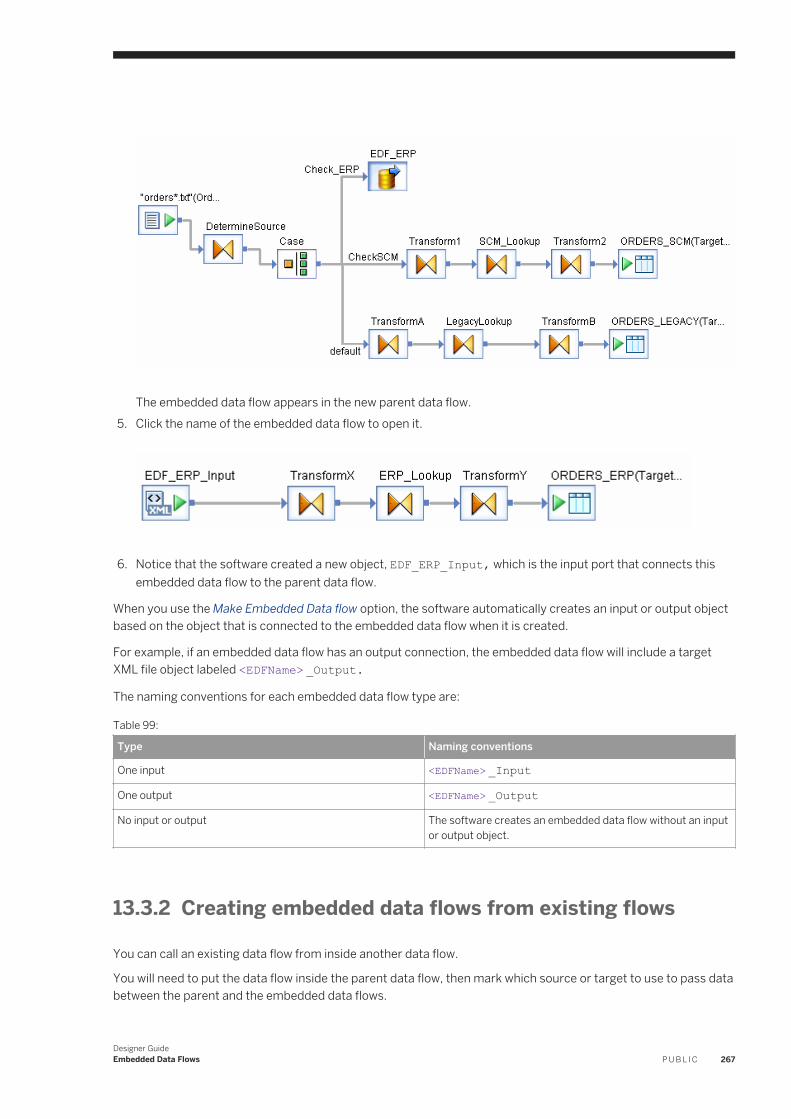
The embedded data flow appears in the new parent data flow.
5. Click the name of the embedded data flow to open it.
6. Notice that the software created a new object, EDF_ERP_Input, which is the input port that connects this
embedded data flow to the parent data flow.
When you use the Make Embedded Data flow option, the software automatically creates an input or output object based on the object that is connected to the embedded data flow when it is created.
For example, if an embedded data flow has an output connection, the embedded data flow will include a target XML file object labeled <EDFName> _Output.
The naming conventions for each embedded data flow type are:
Table 99:
Type Naming conventions
One input <EDFName> _Input
One output <EDFName> _Output
No input or output The software creates an embedded data flow without an input or output object.
13.3.2 Creating embedded data flows from existing flows
You can call an existing data flow from inside another data flow.
You will need to put the data flow inside the parent data flow, then mark which source or target to use to pass data between the parent and the embedded data flows.
Designer GuideEmbedded Data Flows P U B L I C 267
1. Drag an existing valid data flow from the object library into a data flow that is open in the workspace.2. Consider renaming the flow using the EDF_ <EDFName> naming convention.
The embedded data flow appears without any arrowheads (ports) in the workspace.3. Open the embedded data flow.4. Right-click a source or target object (file or table) and select Make Port.
NoteEnsure that you specify only one input or output port.
Like a normal data flow, different types of embedded data flow ports are indicated by directional markings on the embedded data flow icon.
13.3.3 Using embedded data flows
When you create and configure an embedded data flow using the Make Embedded Data Flow option, the software creates new input or output XML file and saves the schema in the repository as an XML Schema.
You can reuse an embedded data flow by dragging it from the Data Flow tab of the object library into other data flows. To save mapping time, you might want to use the Update Schema option or the Match Schema option.
The following example scenario uses both options:
● Create data flow 1.● Select objects in data flow 1, and create embedded data flow 1 so that parent data flow 1 calls embedded data
flow 1.● Create data flow 2 and data flow 3 and add embedded data flow 1 to both of them.● Go back to data flow 1. Change the schema of the object preceding embedded data flow 1 and use the Update
Schema option with embedded data flow 1. It updates the schema of embedded data flow 1 in the repository.● Now the schemas in data flow 2 and data flow 3 that are feeding into embedded data flow 1 will be different
from the schema the embedded data flow expects.● Use the Match Schema option for embedded data flow 1 in both data flow 2 and data flow 3 to resolve the
mismatches at runtime. The Match Schema option only affects settings in the current data flow.
The following sections describe the use of the Update Schema and Match Schema options in more detail.
13.3.3.1 Updating Schemas
The software provides an option to update an input schema of an embedded data flow.
This option updates the schema of an embedded data flow's input object with the schema of the preceding object in the parent data flow. All occurrences of the embedded data flow update when you use this option.
1. Open the embedded data flow's parent data flow.2. Right-click the embedded data flow object and select Update Schema.
268 P U B L I CDesigner Guide
Embedded Data Flows
13.3.3.2 Matching data between parent and embedded data flow
The schema of an embedded data flow's input object can match the schema of the preceding object in the parent data flow by name or position. A match by position is the default.
13.3.3.2.1 Specifying how schemas should be matched
1. Open the embedded data flow's parent data flow.2. Right-click the embedded data flow object and select Match SchemaBy Name or Match SchemaBy Position.
The Match Schema option only affects settings for the current data flow.
Data Services also allows the schema of the preceding object in the parent data flow to have more or fewer columns than the embedded data flow. The embedded data flow ignores additional columns and reads missing columns as NULL.
Columns in both schemas must have identical or convertible data types. See the section on "Type conversion" in the Reference Guide for more information.
13.3.3.3 Deleting embedded data flow objects
You can delete embedded data flow ports, or remove entire embedded data flows.
13.3.3.3.1 Removing a port
Right-click the input or output object within the embedded data flow and deselect Make Port. Data Services removes the connection to the parent object.
NoteYou cannot remove a port simply by deleting the connection in the parent flow.
13.3.3.3.2 Removing an embedded data flow
Select it from the open parent data flow and choose Delete from the right-click menu or edit menu.
If you delete embedded data flows from the object library, the embedded data flow icon appears with a red circle-slash flag in the parent data flow.
Designer GuideEmbedded Data Flows P U B L I C 269
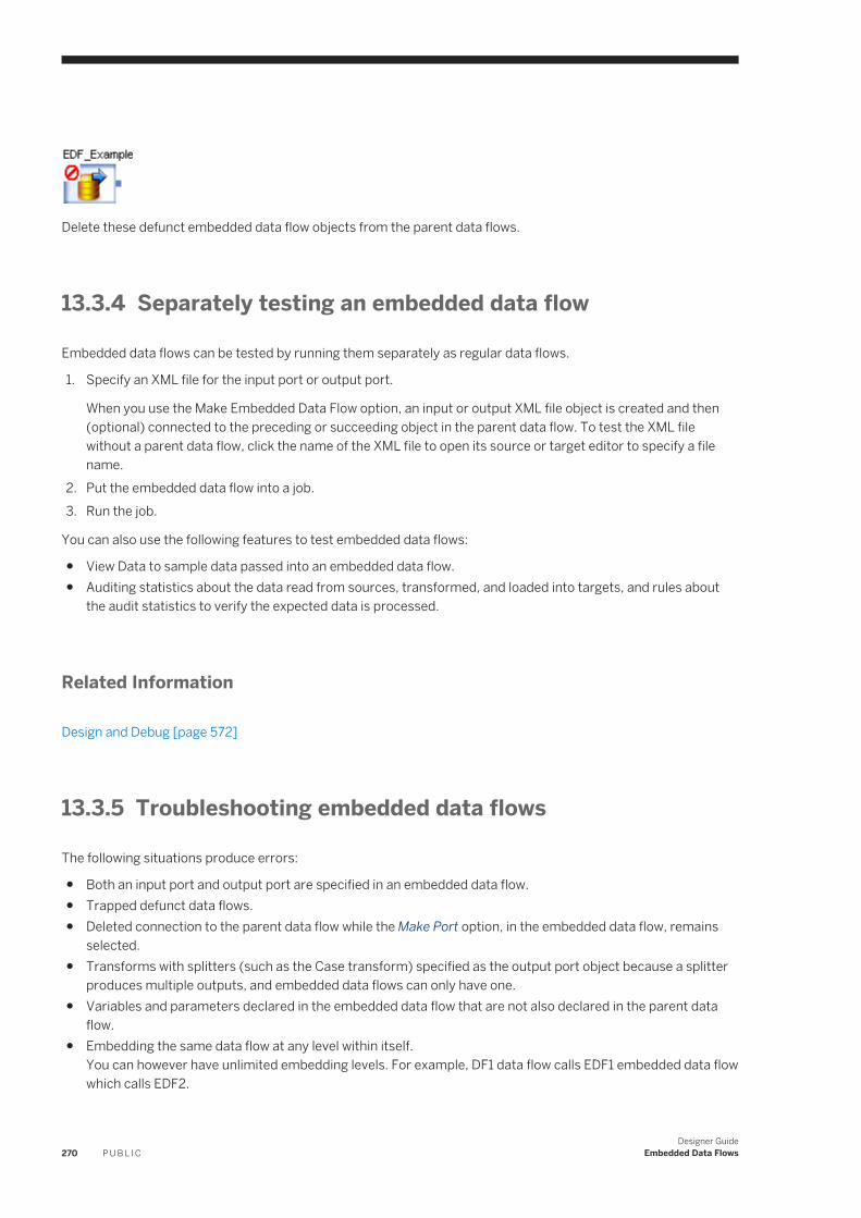
Delete these defunct embedded data flow objects from the parent data flows.
13.3.4 Separately testing an embedded data flow
Embedded data flows can be tested by running them separately as regular data flows.
1. Specify an XML file for the input port or output port.
When you use the Make Embedded Data Flow option, an input or output XML file object is created and then (optional) connected to the preceding or succeeding object in the parent data flow. To test the XML file without a parent data flow, click the name of the XML file to open its source or target editor to specify a file name.
2. Put the embedded data flow into a job.3. Run the job.
You can also use the following features to test embedded data flows:
● View Data to sample data passed into an embedded data flow.● Auditing statistics about the data read from sources, transformed, and loaded into targets, and rules about
the audit statistics to verify the expected data is processed.
Related Information
Design and Debug [page 572]
13.3.5 Troubleshooting embedded data flows
The following situations produce errors:
● Both an input port and output port are specified in an embedded data flow.● Trapped defunct data flows.● Deleted connection to the parent data flow while the Make Port option, in the embedded data flow, remains
selected.● Transforms with splitters (such as the Case transform) specified as the output port object because a splitter
produces multiple outputs, and embedded data flows can only have one.● Variables and parameters declared in the embedded data flow that are not also declared in the parent data
flow.● Embedding the same data flow at any level within itself.
You can however have unlimited embedding levels. For example, DF1 data flow calls EDF1 embedded data flow which calls EDF2.
270 P U B L I CDesigner Guide
Embedded Data Flows

Related Information
Removing an embedded data flow [page 269]Removing a port [page 269]
Designer GuideEmbedded Data Flows P U B L I C 271
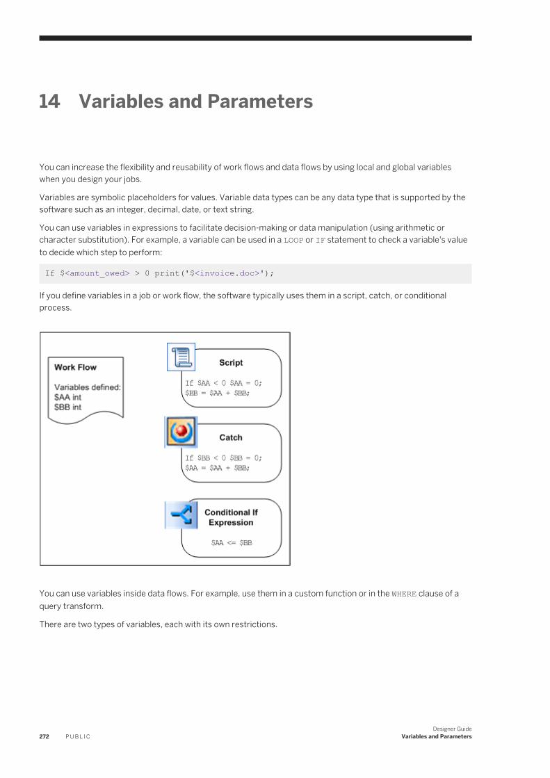
14 Variables and Parameters
You can increase the flexibility and reusability of work flows and data flows by using local and global variables when you design your jobs.
Variables are symbolic placeholders for values. Variable data types can be any data type that is supported by the software such as an integer, decimal, date, or text string.
You can use variables in expressions to facilitate decision-making or data manipulation (using arithmetic or character substitution). For example, a variable can be used in a LOOP or IF statement to check a variable's value to decide which step to perform:
If $<amount_owed> > 0 print('$<invoice.doc>');
If you define variables in a job or work flow, the software typically uses them in a script, catch, or conditional process.
You can use variables inside data flows. For example, use them in a custom function or in the WHERE clause of a query transform.
There are two types of variables, each with its own restrictions.
272 P U B L I CDesigner Guide
Variables and Parameters
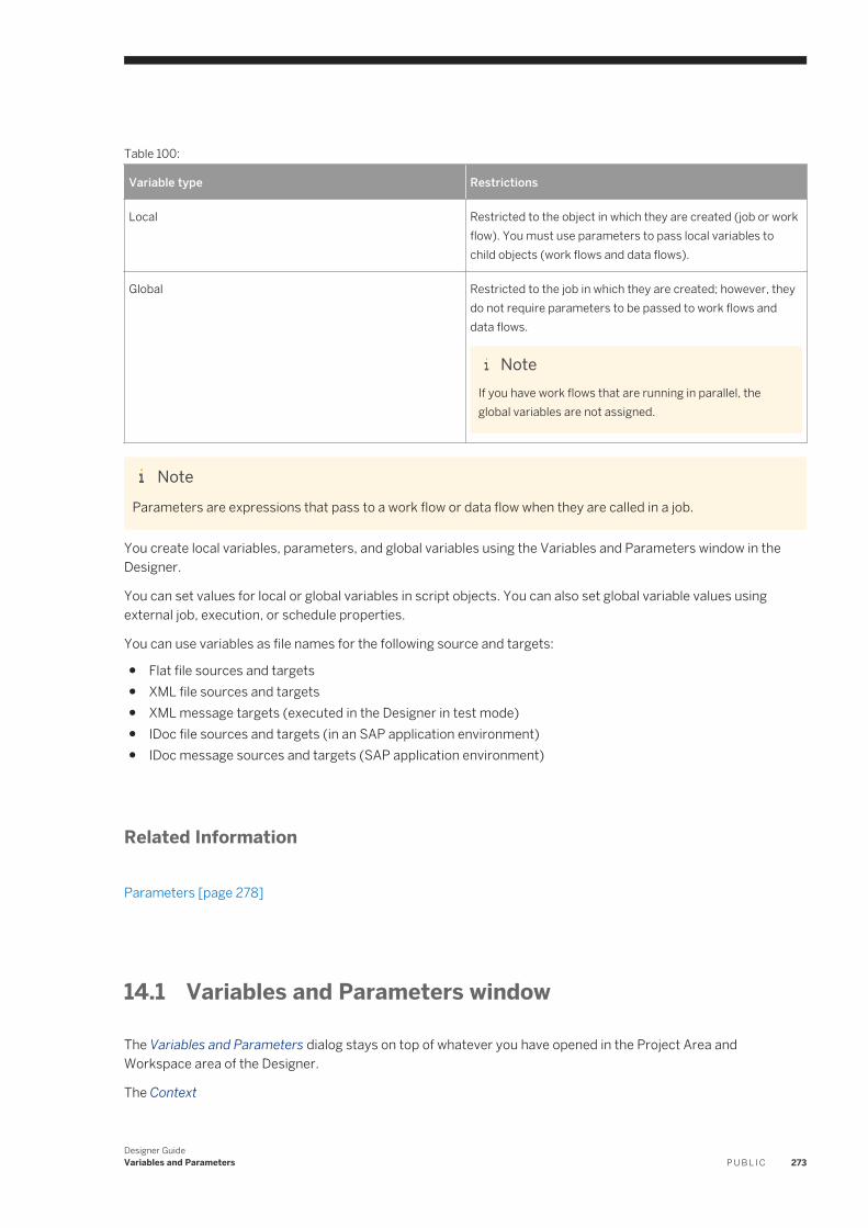
Table 100:
Variable type Restrictions
Local Restricted to the object in which they are created (job or work flow). You must use parameters to pass local variables to child objects (work flows and data flows).
Global Restricted to the job in which they are created; however, they do not require parameters to be passed to work flows and data flows.
NoteIf you have work flows that are running in parallel, the global variables are not assigned.
NoteParameters are expressions that pass to a work flow or data flow when they are called in a job.
You create local variables, parameters, and global variables using the Variables and Parameters window in the Designer.
You can set values for local or global variables in script objects. You can also set global variable values using external job, execution, or schedule properties.
You can use variables as file names for the following source and targets:
● Flat file sources and targets● XML file sources and targets● XML message targets (executed in the Designer in test mode)● IDoc file sources and targets (in an SAP application environment)● IDoc message sources and targets (SAP application environment)
Related Information
Parameters [page 278]
14.1 Variables and Parameters window
The Variables and Parameters dialog stays on top of whatever you have opened in the Project Area and Workspace area of the Designer.
The Context
Designer GuideVariables and Parameters P U B L I C 273
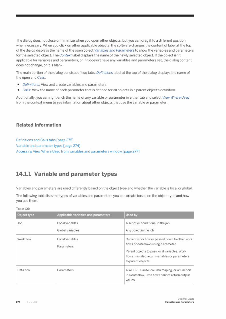
The dialog does not close or minimize when you open other objects, but you can drag it to a different position when necessary. When you click on other applicable objects, the software changes the content of label at the top of the dialog displays the name of the open object.Variables and Parameters to show the variables and parameters for the selected object. The Context label displays the name of the newly selected object. If the object isn't applicable for variables and parameters, or if it doesn't have any variables and parameters set, the dialog content does not change, or it is blank.
The main portion of the dialog consists of two tabs: Definitions label at the top of the dialog displays the name of the open and Calls.
● Definitions: View and create variables and parameters.● Calls: View the name of each parameter that is defined for all objects in a parent object's definition.
Additionally, you can right-click the name of any variable or parameter in either tab and select View Where Used from the context menu to see information about other objects that use the variable or parameter.
Related Information
Definitions and Calls tabs [page 275]Variable and parameter types [page 274]Accessing View Where Used from variables and parameters window [page 277]
14.1.1 Variable and parameter types
Variables and parameters are used differently based on the object type and whether the variable is local or global.
The following table lists the types of variables and parameters you can create based on the object type and how you use them.
Table 101:
Object type Applicable variables and parameters Used by
Job Local variables
Global variables
A script or conditional in the job
Any object in the job
Work flow Local variables
Parameters
Current work flow or passed down to other work flows or data flows using a arameter.
Parent objects to pass local variables. Work flows may also return variables or parameters to parent objects.
Data flow Parameters A WHERE clause, column maping, or a function in a data flow. Data flows cannot return output values.
274 P U B L I CDesigner Guide
Variables and Parameters
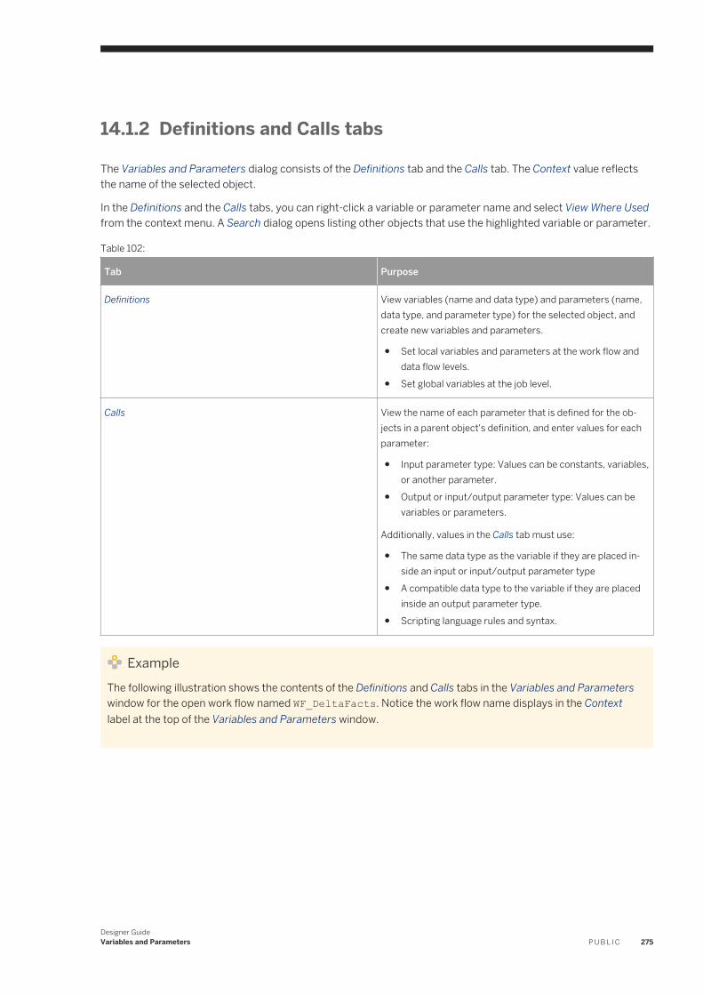
14.1.2 Definitions and Calls tabs
The Variables and Parameters dialog consists of the Definitions tab and the Calls tab. The Context value reflects the name of the selected object.
In the Definitions and the Calls tabs, you can right-click a variable or parameter name and select View Where Used from the context menu. A Search dialog opens listing other objects that use the highlighted variable or parameter.
Table 102:
Tab Purpose
Definitions View variables (name and data type) and parameters (name, data type, and parameter type) for the selected object, and create new variables and parameters.
● Set local variables and parameters at the work flow and data flow levels.
● Set global variables at the job level.
Calls View the name of each parameter that is defined for the objects in a parent object's definition, and enter values for each parameter:
● Input parameter type: Values can be constants, variables, or another parameter.
● Output or input/output parameter type: Values can be variables or parameters.
Additionally, values in the Calls tab must use:
● The same data type as the variable if they are placed inside an input or input/output parameter type
● A compatible data type to the variable if they are placed inside an output parameter type.
● Scripting language rules and syntax.
ExampleThe following illustration shows the contents of the Definitions and Calls tabs in the Variables and Parameters window for the open work flow named WF_DeltaFacts. Notice the work flow name displays in the Context label at the top of the Variables and Parameters window.
Designer GuideVariables and Parameters P U B L I C 275
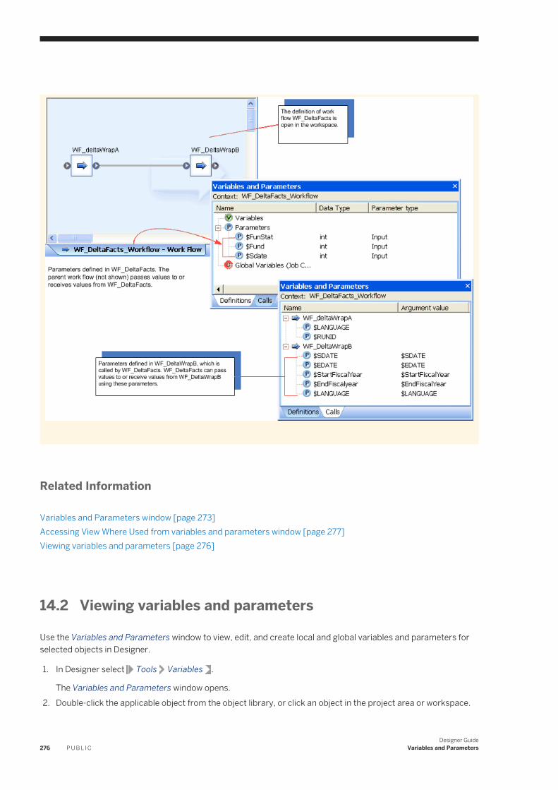
Related Information
Variables and Parameters window [page 273]Accessing View Where Used from variables and parameters window [page 277]Viewing variables and parameters [page 276]
14.2 Viewing variables and parameters
Use the Variables and Parameters window to view, edit, and create local and global variables and parameters for selected objects in Designer.
1. In Designer select Tools Variables .
The Variables and Parameters window opens.2. Double-click the applicable object from the object library, or click an object in the project area or workspace.
276 P U B L I CDesigner Guide
Variables and Parameters
The Context label in the Variables and Parameters window shows the name of the object you selected, or the object you are viewing in the workspace. If there is no object selected, or the object isn't applicable for variables and parameters, the window content either does not change, or it is blank.
3. If applicable, open a different object.
The Variables and Parameters content changes to reflect the variables and parameters for the newly-opened object.
Related Information
Variables and Parameters window [page 273]Variable and parameter types [page 274]Definitions and Calls tabs [page 275]
14.3 Accessing View Where Used from variables and parameters window
Use View Where Used for objects in the Variables and Parameters dialog.
1. Open a job, work flow, or data flow from the object library.
2. Select Tools Variables .
The Variables and Parameters dialog opens.3. In either the Definitions or Calls tab, right-click the name of the applicable variable, and select View Where
Used from the context menu.
A Search dialog opens showing a list of all objects that use the variable.
NoteYou do not have to change any settings in the Search dialog. The software automatically populates search criteria to find the “view where used” information for the selected variable.
Without closing either the Search dialog or the Variables and Parameters dialog, you can select a different object from the object library and perform the same steps to obtain information for a different variable.
Related Information
Variables and Parameters window [page 273]Viewing variables and parameters [page 276]
Designer GuideVariables and Parameters P U B L I C 277
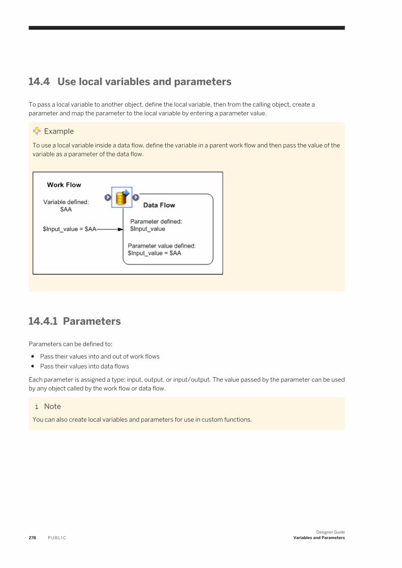
14.4 Use local variables and parameters
To pass a local variable to another object, define the local variable, then from the calling object, create a parameter and map the parameter to the local variable by entering a parameter value.
ExampleTo use a local variable inside a data flow, define the variable in a parent work flow and then pass the value of the variable as a parameter of the data flow.
14.4.1 Parameters
Parameters can be defined to:
● Pass their values into and out of work flows● Pass their values into data flows
Each parameter is assigned a type: input, output, or input/output. The value passed by the parameter can be used by any object called by the work flow or data flow.
NoteYou can also create local variables and parameters for use in custom functions.
278 P U B L I CDesigner Guide
Variables and Parameters
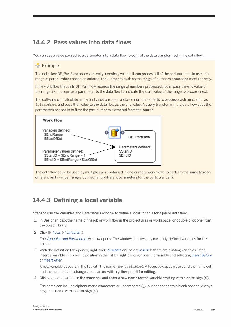
14.4.2 Pass values into data flows
You can use a value passed as a parameter into a data flow to control the data transformed in the data flow.
ExampleThe data flow DF_PartFlow processes daily inventory values. It can process all of the part numbers in use or a range of part numbers based on external requirements such as the range of numbers processed most recently.
If the work flow that calls DF_PartFlow records the range of numbers processed, it can pass the end value of the range $EndRange as a parameter to the data flow to indicate the start value of the range to process next.
The software can calculate a new end value based on a stored number of parts to process each time, such as $SizeOfSet, and pass that value to the data flow as the end value. A query transform in the data flow uses the parameters passed in to filter the part numbers extracted from the source.
The data flow could be used by multiple calls contained in one or more work flows to perform the same task on different part number ranges by specifying different parameters for the particular calls.
14.4.3 Defining a local variable
Steps to use the Variables and Parameters window to define a local variable for a job or data flow.
1. In Designer, click the name of the job or work flow in the project area or workspace, or double-click one from the object library.
2. Click Tools Variables .The Variables and Parameters window opens. The window displays any currently-defined variables for this object.
3. With the Definition tab opened, right-click Variables and select Insert. If there are existing variables listed, insert a variable in a specific position in the list by right-clicking a specific variable and selecting Insert Before or Insert After.A new variable appears in the list with the name $NewVariable0. A focus box appears around the name cell and the cursor shape changes to an arrow with a yellow pencil for editing.
4. Click $NewVariable0 in the name cell and enter a new name for the variable starting with a dollar sign ($).
The name can include alphanumeric characters or underscores (_), but cannot contain blank spaces. Always begin the name with a dollar sign ($).
Designer GuideVariables and Parameters P U B L I C 279
5. Click the data type cell for the new variable and select the appropriate data type from the drop list.6. Optional. If there are more than one variable created, specify the order of the new variable in the list using the
context menu (right-click) and select Move Up or Move Down options.7. When you are finished creating and editing variables, click the “x” in the upper right corner of the Variables
and Parameters window to close it.
14.4.4 Replicating a local variable
Steps to copy an existing variable to create a new variable.
1. In Designer, click the name of the job or work flow in the project area or workspace, or double-click one from the object library.
2. Click Tools Variables .The Variables and Parameters window appears. The window displays any currently-defined variables for this object.
3. With the Definition tab opened, right-click the name of the Variable to copy and select Replicate.A properties window opens and displays a new variable with the same properties as the replicated variable, and a name that you can change (for example, $Copy_1_NewVariable1).
4. Type a new name for the variable, and make any other changes to the Data type as applicable.
The name can include alphanumeric characters or underscores (_), but cannot contain blank spaces. Always begin the name with a dollar sign ($).
5. Click OK.
The new variable appears in the list of variables in the Definition tab.6. Optional. Right-click the name of the variable in the list and select Move Up or Move Down to move the
variable to a new location in the list.7. When you are finished creating and editing variables, click the “x” in the upper right corner of the Variables
and Parameters window to close it.
14.4.5 Defining parameters
There are two steps for setting up a parameter for a work flow or data flow:
● Add the parameter definition to the flow.● Set the value of the parameter in the flow call.
14.4.5.1 Adding a parameter to a work flow or data flow
1. Click the name of the work flow or data flow.
2. Click Tools Variables .The Variables and Parameters window appears.
280 P U B L I CDesigner Guide
Variables and Parameters
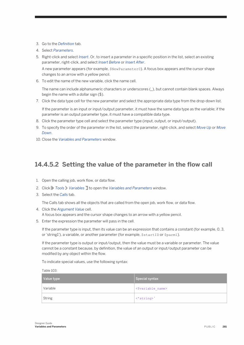
3. Go to the Definition tab.4. Select Parameters.5. Right-click and select Insert. Or, to insert a parameter in a specific position in the list, select an existing
parameter, right-click, and select Insert Before or Insert After.A new parameter appears (for example, $NewParameter0). A focus box appears and the cursor shape changes to an arrow with a yellow pencil.
6. To edit the name of the new variable, click the name cell.
The name can include alphanumeric characters or underscores (_), but cannot contain blank spaces. Always begin the name with a dollar sign ($).
7. Click the data type cell for the new parameter and select the appropriate data type from the drop-down list.
If the parameter is an input or input/output parameter, it must have the same data type as the variable; if the parameter is an output parameter type, it must have a compatible data type.
8. Click the parameter type cell and select the parameter type (input, output, or input/output).9. To specify the order of the parameter in the list, select the parameter, right-click, and select Move Up or Move
Down.10. Close the Variables and Parameters window.
14.4.5.2 Setting the value of the parameter in the flow call
1. Open the calling job, work flow, or data flow.
2. Click Tools Variables to open the Variables and Parameters window.3. Select the Calls tab.
The Calls tab shows all the objects that are called from the open job, work flow, or data flow.4. Click the Argument Value cell.
A focus box appears and the cursor shape changes to an arrow with a yellow pencil.5. Enter the expression the parameter will pass in the cell.
If the parameter type is input, then its value can be an expression that contains a constant (for example, 0, 3, or 'string1'), a variable, or another parameter (for example, $startID or $parm1).
If the parameter type is output or input/output, then the value must be a variable or parameter. The value cannot be a constant because, by definition, the value of an output or input/output parameter can be modified by any object within the flow.
To indicate special values, use the following syntax:
Table 103:
Value type Special syntax
Variable <$variable_name>
String <'string> '
Designer GuideVariables and Parameters P U B L I C 281
14.5 Use global variables
Global variables are global within a job only. There is no need to set parameters when you use global variables.
When you assign a name to a global variable, that name is exclusive to the job, and you cannot use the same global variable or global variable name in any other job.
Global variables provides you with maximum flexibility at runtime. For example, during production you can change values for default global variables at runtime from a job's schedule or SOAP call without having to open a job in the Designer.
You can set values for global variables in script objects, or you can use external job, execution, or schedule properties.
14.5.1 Defining a global variable
Steps to use the Variables and Parameters window to define a global variable for a job.
1. In Designer, click the name of the job in the project area or workspace, or double-click one from the object library.
2. Click Tools Variables .The Variables and Parameters window appears. The window displays any currently-defined variables for this object.
3. With the Definition tab opened, right-click Global Variables and select Insert. If there are existing variables listed, insert a variable in a specific position in the list by right-clicking a specific variable and selecting Insert Before or Insert After.A new variable appears in the list with the name $NewJobGlobalVariable0. A focus box appears around the name cell and the cursor shape changes to an arrow with a yellow pencil for editing.
4. Click $NewJobGlobalVariable0 in the Name cel. and enter a new name for the variable starting with a dollar sign ($).
The name can include alphanumeric characters or underscores (_), but cannot contain blank spaces. Always begin the name with a dollar sign ($).
5. Click the data type cell for the new variable and select the appropriate data type from the drop list.6. Optional. If there are more than one variable created, specify the order of the new variable in the list using the
context menu (right-click) and select Move Up or Move Down options.7. When you are finished creating and editing variables, click the “x” in the upper right corner of the Variables
and Parameters window to close it.
14.5.2 Replicating a global variable
Steps to copy an existing global variable to create a new global variable.
1. In Designer, click the name of the job in the project area or workspace, or double-click a job name from the object library.
282 P U B L I CDesigner Guide
Variables and Parameters
2. Click Tools Variables .The Variables and Parameters window appears. The window displays any currently-defined variables for this object.
3. With the Definition tab opened, right-click the name of the global variable to copy and select Replicate.A properties window opens and displays a new variable with the same properties as the replicated variable, and a name that you can change (for example, $Copy_1_NewJobGlobalVariable1).
4. Edit the name of the new global variable, and make any other changes to the Data type as applicable.
The name can include alphanumeric characters or underscores (_), but cannot contain blank spaces. Always begin the name with a dollar sign ($).
5. Click OK.
The new global variable appears in the list of global variables in the Definition tab.6. Optional. Right-click the name of the global variable in the list and select Move Up or Move Down to move the
variable to a new location in the list.7. When you are finished creating and editing global variables, click the “x” in the upper right corner of the
Variables and Parameters window to close it.
14.5.3 Viewing global variables from the Properties dialog
While you can view global variables for a job using the Variables and Parameters window, you can also view global variables from the Properties dialog of a selected job.
Global variables, defined in a job, are visible to those objects relative to that job. A global variable defined in one job is not available for modification or viewing from another job.
To view global variables from a job's Properties dialog:
1. In the object library, select the Jobs tab.2. Right-click the applicable job and select Properties.3. Click the Global Variable tab.4. Optional. Use the Filter box to filter the list of global variables based on specific characteristics.
14.5.4 Values for global variables
In addition to setting a global variable value inside a job using an initialization script, you can set and maintain global variable values outside a job as well.
Values set outside a job are processed the same way as those set inside a job (for example, in an initialization script). Both methods have their advantages.
When you have both internal and external values set for a global variable in a job, the software automatically chooses the value that you set inside the job as the value to use.
There are some advantages to setting values outside a job. For example, you can open the properties dialog of a job to view global substitution values instead of opening up the job.
Designer GuideVariables and Parameters P U B L I C 283
You set global variable values outside a job in the following ways:
● As a job property● As an execution or schedule property
NoteYou don't have to assign a value to a global variable. However, the software reads a global variable without a value as NULL.
When you set values for global variables outside a job, you can view the values in the Properties and the Execution Properties dialogs in Designer and in the Execution Options and Schedule pages of the Administrator. Additionally, you can easily edit the values when you test or schedule the job.
NoteYou cannot pass global variables as command line arguments for real-time jobs.
14.5.4.1 Automatic ranking of global variable values in a job
When you set values for global variables, and you enter different values for the same global variable using different methods, the software uses automatic ranking to select the value to use for a job run.
The software selects the highest ranking value for use in the job. A value entered as a job property has the lowest rank. A value defined inside a job has the highest rank.
14.5.4.1.1 Execution property versus job property
If you set a global variable value using a job property, and you set a different global variable (for the same global variable) using an execution property, the execution property value overrides the job property value and becomes the default value for the current job run.
NoteYou cannot save execution property global variable values.
ExampleAssume that a job named JOB_Test1 has three global variables declared:
● $YEAR● $MONTH● $DAY
You set the variable “$YEAR” as a job property with a value of “2003”.
For the initial job run, you set variables values for $MONTH and $DAY as execution properties as follows:
284 P U B L I CDesigner Guide
Variables and Parameters
● $MONTH = JANUARY'● $DAY = 31
The software executes a list of statements which includes default values for JOB_Test1:
$YEAR=2003; $MONTH='JANUARY'; $DAY=31;
For the second job run, you set variables $YEAR = “2002” and $MONTH = “JANUARY” as execution properties but you don't set a value for $DAY. The software executes the following list of statements:
$YEAR=2002; $MONTH='JANUARY';
Because you do not set a value for $DAY during execution for the second job, the software reads it as NULL, and the $YEAR value is 2002 and not 2003, because you set it as an execution property to “2002” for the second run.
14.5.4.1.2 Job property versus schedule property
If you set a global variable value for both a job property and a schedule property, the schedule property value overrides the job property value and becomes the external default value for the current job run.
The software saves the schedule property value in the repository. However, these values are only associated with a job schedule, not the job itself. Consequently, you must view and edit these values from within the Administrator.
14.5.4.1.3 Inside job versus external property
The value is determined at the time the software attempts to apply the external value.
A global variable value defined inside a job always overrides any external values. However, the override does not occur until the software attempts to apply the external values to the job being processed with the internal value. Up until that point, the software processes execution, schedule, or job property values as default values.
ExampleSuppose you have a job called JOB_Test2 that has three work flows, each containing a data flow. The second data flow is inside a work flow that is preceded by a script in which $MONTH is defined as 'MAY'. The first and third data flows have the same global variable with no value defined. The execution property $MONTH = 'APRIL' is the global variable value.
In this scenario, 'APRIL' becomes the default value for the job. 'APRIL' remains the value for the global variable until it encounters the other value for the same variable in the second work flow. Since the value in the script is inside the job, 'MAY' overrides 'APRIL' for the variable $MONTH. The software continues the processing the job with this new value.
Designer GuideVariables and Parameters P U B L I C 285
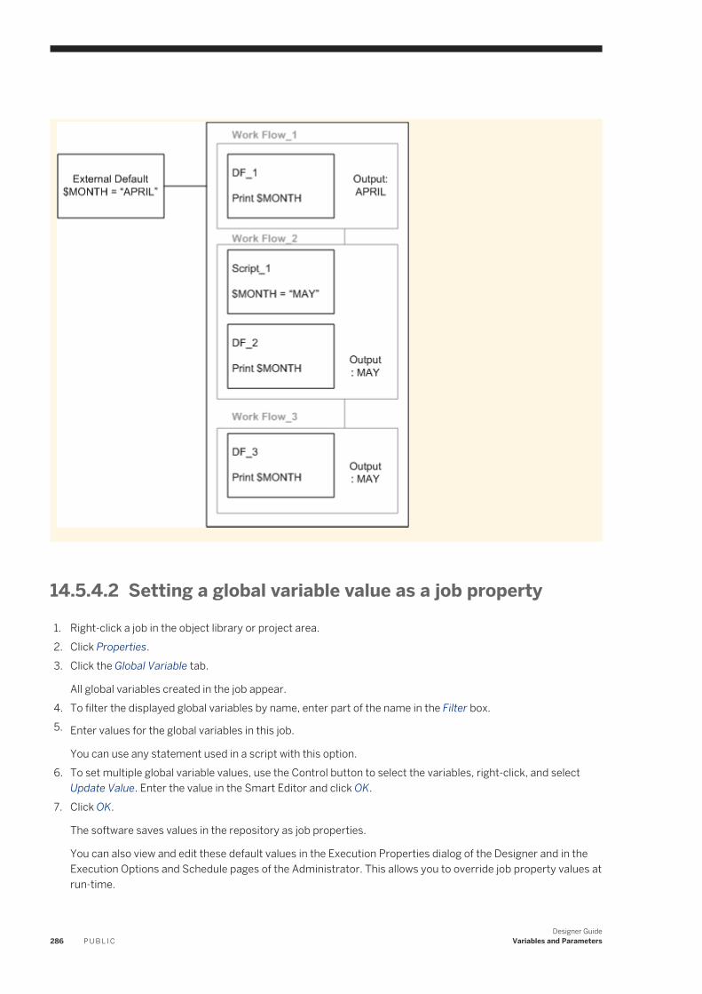
14.5.4.2 Setting a global variable value as a job property
1. Right-click a job in the object library or project area.2. Click Properties.3. Click the Global Variable tab.
All global variables created in the job appear.4. To filter the displayed global variables by name, enter part of the name in the Filter box.5. Enter values for the global variables in this job.
You can use any statement used in a script with this option.6. To set multiple global variable values, use the Control button to select the variables, right-click, and select
Update Value. Enter the value in the Smart Editor and click OK.7. Click OK.
The software saves values in the repository as job properties.
You can also view and edit these default values in the Execution Properties dialog of the Designer and in the Execution Options and Schedule pages of the Administrator. This allows you to override job property values at run-time.
286 P U B L I CDesigner Guide
Variables and Parameters
14.5.4.3 Setting a global variable value as an execution property
1. Execute a job from the Designer, or execute or schedule a batch job from the Administrator.
NoteFor testing purposes, you can execute real-time jobs from the Designer in test mode. Make sure to set the execution properties for a real-time job.
2. View the global variables in the job and their default values (if available).3. Edit values for global variables as desired.4. If you are using the Designer, click OK. If you are using the Administrator, click Execute or Schedule.
The job runs using the values you enter. Values entered as execution properties are not saved. Values entered as schedule properties are saved but can only be accessed from within the Administrator.
14.6 Local and global variable rules
There are rules to follow when you set values for local and global variables.
The following table describes specific rules to follow when you set local and global variables.
Table 104:
Rule for Description
Naming ● Local and global variables must have unique names within their job context.
● Any name modification to a global variable can only be performed at the job level.
Replicating job and work flows ● When you replicate all objects, the local and global variables defined in that job context are also replicated.
● When you replicate a data flow or work flow, all parameters and local and global variables are also replicated. However, you must validate these local and global variables within the job context in which they were created.
NoteIf you attempt to validate a data flow or work flow containing global variables without a job, Data Services reports an error.
Designer GuideVariables and Parameters P U B L I C 287
Rule for Description
Importing and exporting ● When you export a job object, you also export all local and global variables defined for that job.
● When you export a lower-level object (such as a data flow) without the parent job, the global variable is not exported. Only the call to that global variable is exported.
NoteIf you use this object in another job without defining the global variable in the new job, a validation error will occur.
14.7 Environment variables
You can use system-environment variables inside jobs, work flows, or data flows. The get_env, set_env, and is_set_env functions provide access to underlying operating system variables that behave as the operating system allows.
You can temporarily set the value of an environment variable inside a job, work flow or data flow. Once set, the value is visible to all objects in that job.
Use the get_env, set_env, and is_set_env functions to set, retrieve, and test the values of environment variables.
14.8 Set file names at run-time using variables
You can set file names at runtime by specifying a variable as the file name.
Variables can be used as file names for these sources and targets:
● Flat files● XML files and messages● IDoc files and messages (in an SAP environment)
Variables can be also be used as file names for the lookup_ext function (for a flat file used as a lookup table parameter).
288 P U B L I CDesigner Guide
Variables and Parameters
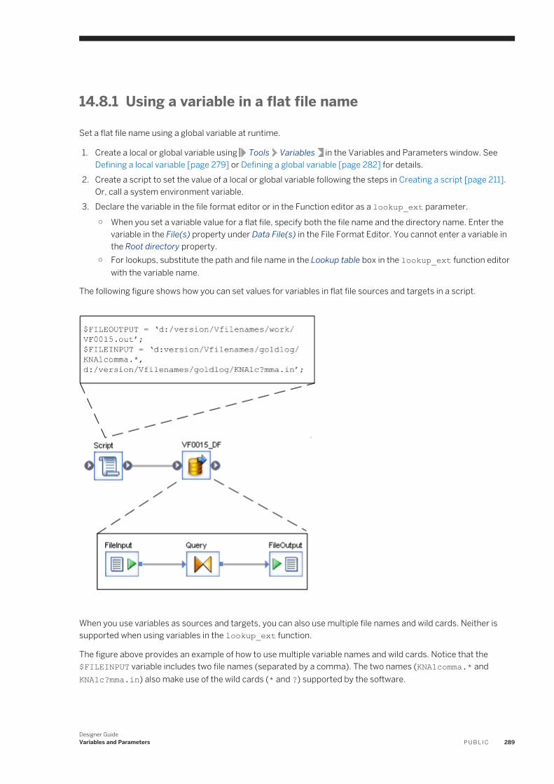
14.8.1 Using a variable in a flat file name
Set a flat file name using a global variable at runtime.
1. Create a local or global variable using Tools Variables in the Variables and Parameters window. See Defining a local variable [page 279] or Defining a global variable [page 282] for details.
2. Create a script to set the value of a local or global variable following the steps in Creating a script [page 211]. Or, call a system environment variable.
3. Declare the variable in the file format editor or in the Function editor as a lookup_ext parameter.
○ When you set a variable value for a flat file, specify both the file name and the directory name. Enter the variable in the File(s) property under Data File(s) in the File Format Editor. You cannot enter a variable in the Root directory property.
○ For lookups, substitute the path and file name in the Lookup table box in the lookup_ext function editor with the variable name.
The following figure shows how you can set values for variables in flat file sources and targets in a script.
When you use variables as sources and targets, you can also use multiple file names and wild cards. Neither is supported when using variables in the lookup_ext function.
The figure above provides an example of how to use multiple variable names and wild cards. Notice that the $FILEINPUT variable includes two file names (separated by a comma). The two names (KNA1comma.* and KNA1c?mma.in) also make use of the wild cards (* and ?) supported by the software.
Designer GuideVariables and Parameters P U B L I C 289
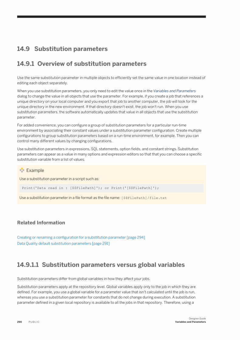
14.9 Substitution parameters
14.9.1 Overview of substitution parameters
Use the same substitution parameter in multiple objects to efficiently set the same value in one location instead of editing each object separately.
When you use substitution parameters, you only need to edit the value once in the Variables and Parameters dialog to change the value in all objects that use the parameter. For example, if you create a job that references a unique directory on your local computer and you export that job to another computer, the job will look for the unique directory in the new environment. If that directory doesn't exist, the job won't run. When you use substitution parameters, the software automatically updates that value in all objects that use the substitution parameter.
For added convenience, you can configure a group of substitution parameters for a particular run-time environment by associating their constant values under a substitution parameter configuration. Create multiple configurations to group substitution parameters based on a run-time environment, for example. Then you can control many different values by changing configurations.
Use substitution parameters in expressions, SQL statements, option fields, and constant strings. Substitution parameters can appear as a value in many options and expression editors so that that you can choose a specific substitution variable from a list of values.
ExampleUse a substitution parameter in a script such as:
Print('Data read in : [$$FilePath]'); or Print('[$$FilePath]');
Use a substitution parameter in a file format as the file name: [$$FilePath]/file.txt
Related Information
Creating or renaming a configuration for a substitution parameter [page 294]Data Quality default substitution parameters [page 291]
14.9.1.1 Substitution parameters versus global variables
Substitution parameters differ from global variables in how they affect your jobs.
Substitution parameters apply at the repository level. Global variables apply only to the job in which they are defined. For example, you use a global variable for a parameter value that isn't calculated until the job is run, whereas you use a substitution parameter for constants that do not change during execution. A substitution parameter defined in a given local repository is available to all the jobs in that repository. Therefore, using a
290 P U B L I CDesigner Guide
Variables and Parameters
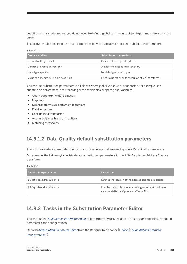
substitution parameter means you do not need to define a global variable in each job to parameterize a constant value.
The following table describes the main differences between global variables and substitution parameters.
Table 105:
Global variables Substitution parameters
Defined at the job level Defined at the repository level
Cannot be shared across jobs Available to all jobs in a repository
Data-type specific No data type (all strings)
Value can change during job execution Fixed value set prior to execution of job (constants)
You can use substitution parameters in all places where global variables are supported, for example, use substitution parameters in the following areas, which also support global variables:
● Query transform WHERE clauses● Mappings● SQL transform SQL statement identifiers● Flat-file options● User-defined transforms● Address cleanse transform options● Matching thresholds
14.9.1.2 Data Quality default substitution parameters
The software installs some default substitution parameters that are used by some Data Quality transforms.
For example, the following table lists default substitution parameters for the USA Regulatory Address Cleanse transform.
Table 106:
Substitution parameter Description
$$RefFilesAddressCleanse Defines the location of the address cleanse directories.
$$ReportsAddressCleanse Enables data collection for creating reports with address cleanse statistics. Options are Yes or No.
14.9.2 Tasks in the Substitution Parameter Editor
You can use the Substitution Parameter Editor to perform many tasks related to creating and editing substitution parameters and configurations.
Open the Substitution Parameter Editor from the Designer by selecting Tools Substitution Parameter Configurations .
Designer GuideVariables and Parameters P U B L I C 291
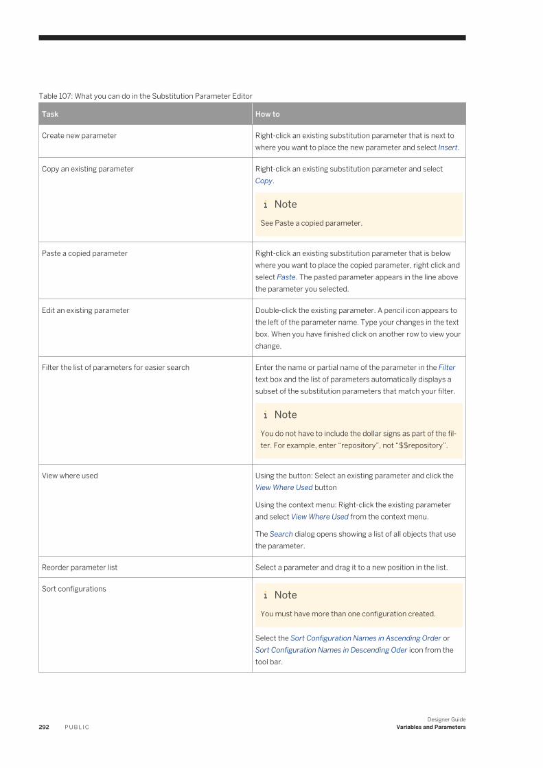
Table 107: What you can do in the Substitution Parameter Editor
Task How to
Create new parameter Right-click an existing substitution parameter that is next to where you want to place the new parameter and select Insert.
Copy an existing parameter Right-click an existing substitution parameter and select Copy.
NoteSee Paste a copied parameter.
Paste a copied parameter Right-click an existing substitution parameter that is below where you want to place the copied parameter, right click and select Paste. The pasted parameter appears in the line above the parameter you selected.
Edit an existing parameter Double-click the existing parameter. A pencil icon appears to the left of the parameter name. Type your changes in the text box. When you have finished click on another row to view your change.
Filter the list of parameters for easier search Enter the name or partial name of the parameter in the Filter text box and the list of parameters automatically displays a subset of the substitution parameters that match your filter.
NoteYou do not have to include the dollar signs as part of the filter. For example, enter “repository”, not “$$repository”.
View where used Using the button: Select an existing parameter and click the View Where Used button
Using the context menu: Right-click the existing parameter and select View Where Used from the context menu.
The Search dialog opens showing a list of all objects that use the parameter.
Reorder parameter list Select a parameter and drag it to a new position in the list.
Sort configurations NoteYou must have more than one configuration created.
Select the Sort Configuration Names in Ascending Order or Sort Configuration Names in Descending Oder icon from the tool bar.
292 P U B L I CDesigner Guide
Variables and Parameters
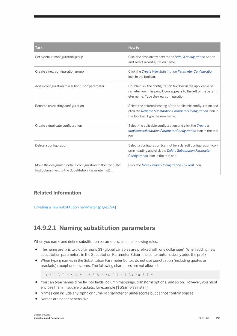
Task How to
Set a default configuration group Click the drop arrow next to the Default configuration option and select a configuration name.
Create a new configuration group Click the Create New Substitution Parameter Configuration icon in the tool bar.
Add a configuration to a substitution parameter Double-click the configuration text box in the applicable parameter row. The pencil icon appears to the left of the parameter name. Type the new configuration.
Rename an existing configuration Select the column heading of the applicable configuration and click the Rename Substitution Parameter Configuration icon in the tool bar. Type the new name.
Create a duplicate configuration Select the aplicable configuration and click the Create a duplicate substitution Parameter Configuration icon in the tool bar.
Delete a configuration Select a configuration (cannot be a default configuration) column heading and click the Delete Substitution Parameter Configuration icon in the tool bar.
Move the designated default configuration to the front (the first column next to the Substitution Parameter list).
Click the Move Default Configuration To Front icon.
Related Information
Creating a new substitution parameter [page 294]
14.9.2.1 Naming substitution parameters
When you name and define substitution parameters, use the following rules:
● The name prefix is two dollar signs $$ (global variables are prefixed with one dollar sign). When adding new substitution parameters in the Substitution Parameter Editor, the editor automatically adds the prefix.
● When typing names in the Substitution Parameter Editor, do not use punctuation (including quotes or brackets) except underscores. The following characters are not allowed:
,: / ' \ " = < > + | - * % ; \t [ ] ( ) \r \n $ ] +
● You can type names directly into fields, column mappings, transform options, and so on. However, you must enclose them in square brackets, for example [$$SamplesInstall].
● Names can include any alpha or numeric character or underscores but cannot contain spaces.● Names are not case sensitive.
Designer GuideVariables and Parameters P U B L I C 293
● The maximum length for most repository types is 256 (MySQL is 64 and MS SQL server is 128).● Names must be unique within the repository.
14.9.2.2 Creating a new substitution parameter
How to add a substitution parameter to a configuration.
You create substitution paramters to save time by entering the value once and saving it to a substitution parameter configuration. You set a constant value for the substitution parameter so that when you use the parameter in several objects, you only have to enter the constant value once, when you create it.
1. In the Designer, select Tools Substitution Parameter Configurations .
The Substitution Parameter Editor opens. The first column, named Substitution Parameter, lists the substitution parameters available in the repository. The second column contains the constant value for the parameter. By default the column heading is Configuration1.
2. Double-click a blank row. A pencil icon appears to the left of the row. Type a name. (You may have to scroll to the bottom of the Substitution Parameters column for a blank row.)
The software automatically adds a double dollar-sign prefix ($$) to the name when you navigate away from the cell.
3. Double-click in the next cell under the applicable configuration column and type the constant value that the parameter represents in that configuration. The software applies the constant value to the parameter when you run the job.
Related Information
Creating or renaming a configuration for a substitution parameter [page 294]Exporting and importing substitution parameters [page 299]
14.9.2.3 Creating or renaming a configuration for a substitution parameter
How to create a new configuration group or rename an existing configuration group.
You may want to create a second configuration group so that you can assign more than one constant value to a substitution parameter. For example, if your directory files for testing a job are located in a different location than the directories you use in production, you could assign two different constant values for the parameter. The software automatically names the first configuration group Configuration1, and subsequent configuration groups Configuration_1, Configuration_n+1, and so on.
1. To change the name of a configuration group, select the applicable configuration column heading to highlight it and click the Rename Substitution Parameter Configuration icon in the tool bar.
2. Type the new name in the highlighted column heading.
294 P U B L I CDesigner Guide
Variables and Parameters
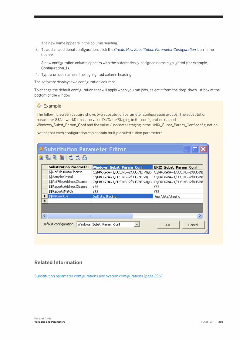
The new name appears in the column heading.3. To add an additional configuration, click the Create New Substitution Parameter Configuration icon in the
toolbar.
A new configuration column appears with the automatically-assigned name highlighted (for example, Configuration_1).
4. Type a unique name in the highlighted column heading.
The software displays two configuration columns.
To change the default configuration that will apply when you run jobs, select it from the drop-down list box at the bottom of the window.
ExampleThe following screen capture shows two substitution parameter configuration groups. The substitution parameter $$NetworkDir has the value D:/Data/Staging in the configuration named Windows_Subst_Param_Conf and the value /usr/data/staging in the UNIX_Subst_Param_Conf configuration.
Notice that each configuration can contain multiple substitution parameters.
Related Information
Substitution parameter configurations and system configurations [page 296]
Designer GuideVariables and Parameters P U B L I C 295
14.9.3 Substitution parameter configurations and system configurations
A system configuration groups together a set of datastore configurations and a substitution parameter configuration.
A substitution parameter configuration can be associated with one or more system configurations. For example, you might create one system configuration for your local system and a different system configuration for your remote system. Depending on your environment, both system configurations might point to the same substitution parameter configuration or each system configuration might require a different substitution parameter configuration.
At job execution time, you can set the system configuration and the job will execute with the values for the associated substitution parameter configuration.
Related Information
What are datastores? [page 63]Overview of substitution parameters [page 290]
14.9.4 Associating substitution parameter configurations with system configurations
How to associate a substitution parameter configuration with a system configuration.
To associate a substitution parameter configuration with a system configuration:
1. In the Designer, open the System Configuration Editor by selecting Tools System Configurations .
The editor contains at least two columns: The first column contains existing datastores, and the column is headed with the name Substitution Parameter. The second and subsequent columns are headed with the name of an existing system configuration. For example, if you have one system configuration, there is one column headed with the name of your system configuration.
2. In the row for the applicable datastore object, select the down arrow in the cell that is under the applicable system configuration column.
A list of existing substitution parameter configurations appears.3. Select a substitution parameter configuration from the drop list.4. If you want to create a new system configuration, click the Create New Configuration icon in the tool bar. A
new column appears. Type the name of the new system configuration in the column heading.5. When you are finished, click OK.
ExampleThe following example shows two system configurations, SC_Americas and SC_Europe. There are two substitution parameter configurations, one for each region: Americas_Subst_Parm_Conf and
296 P U B L I CDesigner Guide
Variables and Parameters
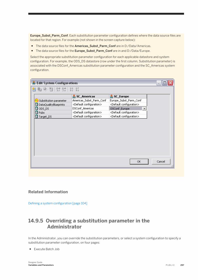
Europe_Subst_Parm_Conf. Each substitution parameter configuration defines where the data source files are located for that region. For example (not shown in the screen capture below):
● The data source files for the Americas_Subst_Parm_Conf are in D:/Data/Americas.● The data source files for the Europe_Subst_Parm_Conf are in and D:/Data/Europe.
Select the appropriate substitution parameter configuration for each applicable datastore and system configuration. For example, the ODS_DS datastore (row under the first column, Substitution parameter) is associated with the DSConf_Americas substitution parameter configuration and the SC_Americas system configuration.
Related Information
Defining a system configuration [page 104]
14.9.5 Overriding a substitution parameter in the Administrator
In the Administrator, you can override the substitution parameters, or select a system configuration to specify a substitution parameter configuration, on four pages:
● Execute Batch Job
Designer GuideVariables and Parameters P U B L I C 297
● Schedule Batch Job● Export Execution Command● Real-Time Service Configuration
For example, the Execute Batch Job page displays the name of the selected system configuration, the substitution parameter configuration, and the name of each substitution parameter and its value.
To override a substitution parameter:
1. Select the appropriate system configuration.2. Under Substitution Parameters, click Add Overridden Parameter, which displays the available substitution
parameters.3. From the drop-down list, select the substitution parameter to override.4. In the second column, type the override value. Enter the value as a string without quotes (in contrast with
Global Variables).5. Execute the job.
14.9.6 Executing a job with substitution parameters
To see the details of how substitution parameters are being used in the job during execution in the Designer trace log:
1. Right-click the job name and click Properties.2. Click the Trace tab.3. For the Trace Assemblers option, set the value to Yes.4. Click OK.
When you execute a job from the Designer, the Execution Properties window displays. You have the following options:
● On the Execution Options tab from the System configuration drop-down menu, optionally select the system configuration with which you want to run the job. If you do not select a system configuration, the software applies the default substitution parameter configuration as defined in the Substitution Parameter Editor.You can click Browse to view the Select System Configuration window in order to see the substitution parameter configuration associated with each system configuration. The Select System Configuration is read-only. If you want to change a system configuration, click Tools System Configurations .
● You can override the value of specific substitution parameters at run time. Click the Substitution Parameter tab, select a substitution parameter from the Name column, and enter a value by double-clicking in the Value cell.To override substitution parameter values when you start a job via a Web service, see the Integrator Guide.
Related Information
Associating substitution parameter configurations with system configurations [page 296]Overriding a substitution parameter in the Administrator [page 297]
298 P U B L I CDesigner Guide
Variables and Parameters
14.9.7 Exporting and importing substitution parameters
Substitution parameters are stored in a local repository along with their configured values. The software does not include substitution parameters as part of a regular export.You can, however, export substitution parameters and configurations to other repositories by exporting them to a file and then importing the file to another repository.
14.9.7.1 Exporting substitution parameters
1. Right-click in the local object library and select Repository Export Substitution Parameter Configurations .
2. Select the check box in the Export column for the substitution parameter configurations to export.3. Save the file.
The software saves it as a text file with an .atl extension.
14.9.7.2 Importing substitution parameters
The substitution parameters must have first been exported to an ATL file.
Be aware of the following behaviors when importing substitution parameters:
● The software adds any new substitution parameters and configurations to the destination local repository.● If the repository has a substitution parameter with the same name as in the exported file, importing will
overwrite the parameter's value. Similarly, if the repository has a substitution parameter configuration with the same name as the exported configuration, importing will overwrite all the parameter values for that configuration.
1. In the Designer, right-click in the object library and select Repository Import from file .2. Browse to the file to import.3. Click OK.
Related Information
Exporting substitution parameters [page 299]
Designer GuideVariables and Parameters P U B L I C 299
15 Executing Jobs
This section contains an overview of the software job execution, steps to execute jobs, debug errors, and change job server options.
15.1 Overview of job execution
You can run jobs in three different ways. Depending on your needs, you can configure:
Table 108:
Job Description
Immediate jobs The software initiates both batch and real-time jobs and runs them immediately from within the Designer. For these jobs, both the Designer and designated Job Server (where the job executes, usually many times on the same machine) must be running. You will most likely run immediate jobs only during the development cycle.
Scheduled jobs Batch jobs are scheduled. To schedule a job, use the Administrator or use a third-party scheduler.
When jobs are scheduled by third-party software:
● The job initiates outside of the software.● The job operates on a batch job (or shell script for UNIX) that has been exported
from the software.
When a job is invoked by a third-party scheduler:
● The corresponding Job Server must be running.● The Designer does not need to be running.
Services Real-time jobs are set up as services that continuously listen for requests from an Access Server and process requests on-demand as they are received. Use the Administrator to create a service from a real-time job.
15.2 Preparing for job execution
15.2.1 Validating jobs and job components
You can also explicitly validate jobs and their components as you create them by:
300 P U B L I CDesigner Guide
Executing Jobs
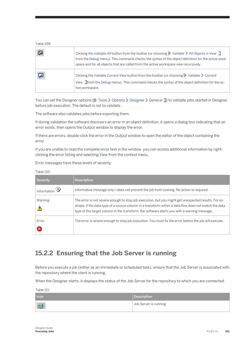
Table 109:
Clicking the Validate All button from the toolbar (or choosing Validate All Objects in View from the Debug menu). This command checks the syntax of the object definition for the active workspace and for all objects that are called from the active workspace view recursively.
Clicking the Validate Current View button from the toolbar (or choosing Validate Current
View from the Debug menu). This command checks the syntax of the object definition for the active workspace.
You can set the Designer options ( Tools Options Designer General ) to validate jobs started in Designer before job execution. The default is not to validate.
The software also validates jobs before exporting them.
If during validation the software discovers an error in an object definition, it opens a dialog box indicating that an error exists, then opens the Output window to display the error.
If there are errors, double-click the error in the Output window to open the editor of the object containing the error.
If you are unable to read the complete error text in the window, you can access additional information by right-clicking the error listing and selecting View from the context menu.
Error messages have these levels of severity:
Table 110:
Severity Description
Information Informative message only—does not prevent the job from running. No action is required.
Warning The error is not severe enough to stop job execution, but you might get unexpected results. For example, if the data type of a source column in a transform within a data flow does not match the data type of the target column in the transform, the software alerts you with a warning message.
Error The error is severe enough to stop job execution. You must fix the error before the job will execute.
15.2.2 Ensuring that the Job Server is running
Before you execute a job (either as an immediate or scheduled task), ensure that the Job Server is associated with the repository where the client is running.
When the Designer starts, it displays the status of the Job Server for the repository to which you are connected.
Table 111:
Icon Description
Job Server is running
Designer GuideExecuting Jobs P U B L I C 301
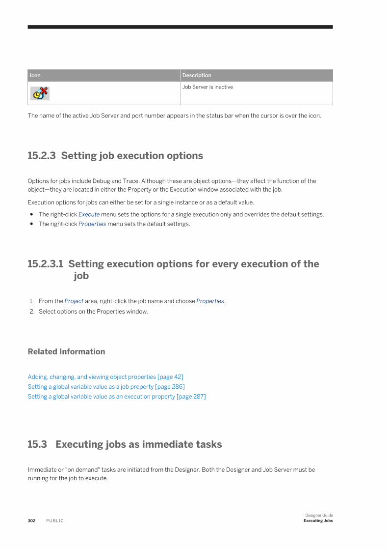
Icon Description
Job Server is inactive
The name of the active Job Server and port number appears in the status bar when the cursor is over the icon.
15.2.3 Setting job execution options
Options for jobs include Debug and Trace. Although these are object options—they affect the function of the object—they are located in either the Property or the Execution window associated with the job.
Execution options for jobs can either be set for a single instance or as a default value.
● The right-click Execute menu sets the options for a single execution only and overrides the default settings.● The right-click Properties menu sets the default settings.
15.2.3.1 Setting execution options for every execution of the job
1. From the Project area, right-click the job name and choose Properties.2. Select options on the Properties window.
Related Information
Adding, changing, and viewing object properties [page 42]Setting a global variable value as a job property [page 286]Setting a global variable value as an execution property [page 287]
15.3 Executing jobs as immediate tasks
Immediate or "on demand" tasks are initiated from the Designer. Both the Designer and Job Server must be running for the job to execute.
302 P U B L I CDesigner Guide
Executing Jobs
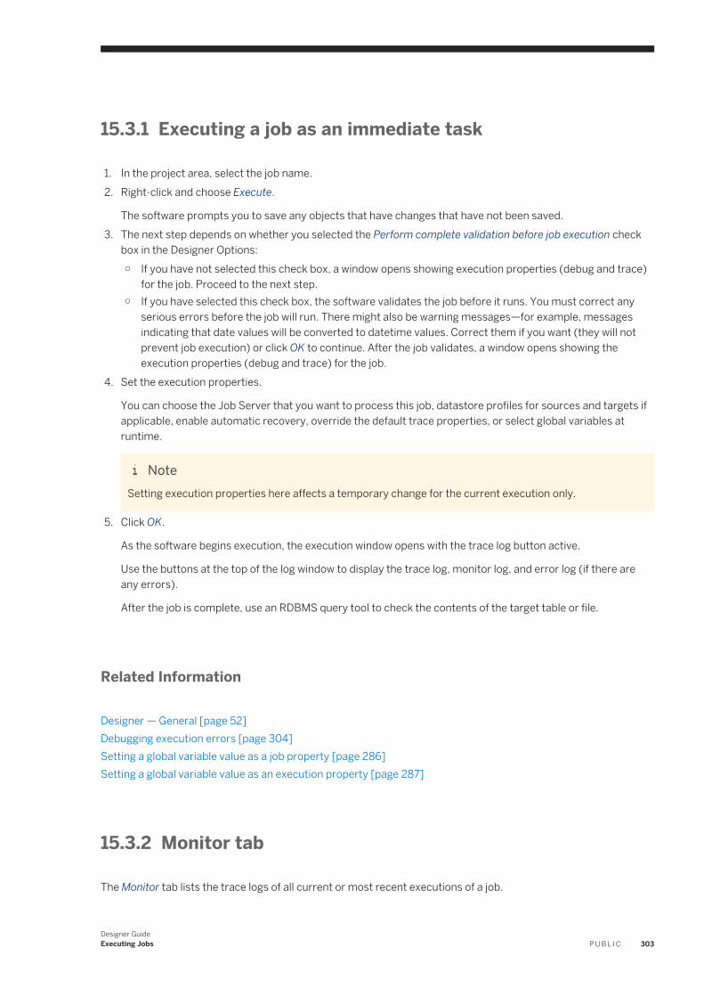
15.3.1 Executing a job as an immediate task
1. In the project area, select the job name.2. Right-click and choose Execute.
The software prompts you to save any objects that have changes that have not been saved.3. The next step depends on whether you selected the Perform complete validation before job execution check
box in the Designer Options:○ If you have not selected this check box, a window opens showing execution properties (debug and trace)
for the job. Proceed to the next step.○ If you have selected this check box, the software validates the job before it runs. You must correct any
serious errors before the job will run. There might also be warning messages—for example, messages indicating that date values will be converted to datetime values. Correct them if you want (they will not prevent job execution) or click OK to continue. After the job validates, a window opens showing the execution properties (debug and trace) for the job.
4. Set the execution properties.
You can choose the Job Server that you want to process this job, datastore profiles for sources and targets if applicable, enable automatic recovery, override the default trace properties, or select global variables at runtime.
NoteSetting execution properties here affects a temporary change for the current execution only.
5. Click OK.
As the software begins execution, the execution window opens with the trace log button active.
Use the buttons at the top of the log window to display the trace log, monitor log, and error log (if there are any errors).
After the job is complete, use an RDBMS query tool to check the contents of the target table or file.
Related Information
Designer — General [page 52]Debugging execution errors [page 304]Setting a global variable value as a job property [page 286]Setting a global variable value as an execution property [page 287]
15.3.2 Monitor tab
The Monitor tab lists the trace logs of all current or most recent executions of a job.
Designer GuideExecuting Jobs P U B L I C 303
The traffic-light icons in the Monitor tab have the following meanings:
● A green light indicates that the job is runningYou can right-click and select Kill Job to stop a job that is still running.
● A red light indicates that the job has stoppedYou can right-click and select Properties to add a description for a specific trace log. This description is saved with the log which can be accessed later from the Log tab.
● A red cross indicates that the job encountered an error
15.3.3 Log tab
You can also select the Log tab to view a job's trace log history.
Click a trace log to open it in the workspace.
Use the trace, monitor, and error log icons (left to right at the top of the job execution window in the workspace) to view each type of available log for the date and time that the job was run.
15.4 Debugging execution errors
The following table lists tools that can help you understand execution errors:
Table 112:
Tool Definition
Debug package Creates a job debug package that includes the ATL and trace, monitor, and log files. This will help you and SAP customer support troubleshoot execution-related issues.
Error log Displays the name of the object being executed when an error occurred and the text of the resulting error message. If the job ran against SAP data, some of the ABAP errors are also available in the error log.
Monitor log Displays each step of each data flow in the job, the number of rows streamed through each step, and the duration of each step.
Target data Always examine your target data to see if your job produced the results you expected.
Trace log Itemizes the steps executed in the job and the time execution began and ended.
Related Information
Using logs [page 305]
304 P U B L I CDesigner Guide
Executing Jobs
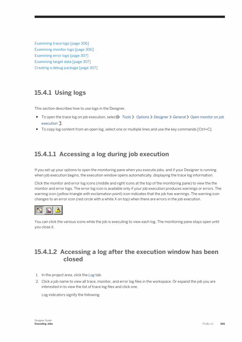
Examining trace logs [page 306]Examining monitor logs [page 306]Examining error logs [page 307]Examining target data [page 307]Creating a debug package [page 307]
15.4.1 Using logs
This section describes how to use logs in the Designer.
● To open the trace log on job execution, select Tools Options Designer General Open monitor on job execution .
● To copy log content from an open log, select one or multiple lines and use the key commands [Ctrl+C].
15.4.1.1 Accessing a log during job execution
If you set up your options to open the monitoring pane when you execute jobs, and if your Designer is running when job execution begins, the execution window opens automatically, displaying the trace log information.
Click the monitor and error log icons (middle and right icons at the top of the monitoring pane) to view the the monitor and error logs. The error log icon is available only if your job execution produces warnings or errors. The warning icon (yellow triangle with exclamation point) icon indicates that the job has warnings. The warning icon changes to an error icon (red circle with a white X on top) when there are errors in the job execution.
You can click the various icons while the job is executing to view each log. The monitoring pane stays open until you close it.
15.4.1.2 Accessing a log after the execution window has been closed
1. In the project area, click the Log tab.2. Click a job name to view all trace, monitor, and error log files in the workspace. Or expand the job you are
interested in to view the list of trace log files and click one.
Log indicators signify the following:
Designer GuideExecuting Jobs P U B L I C 305
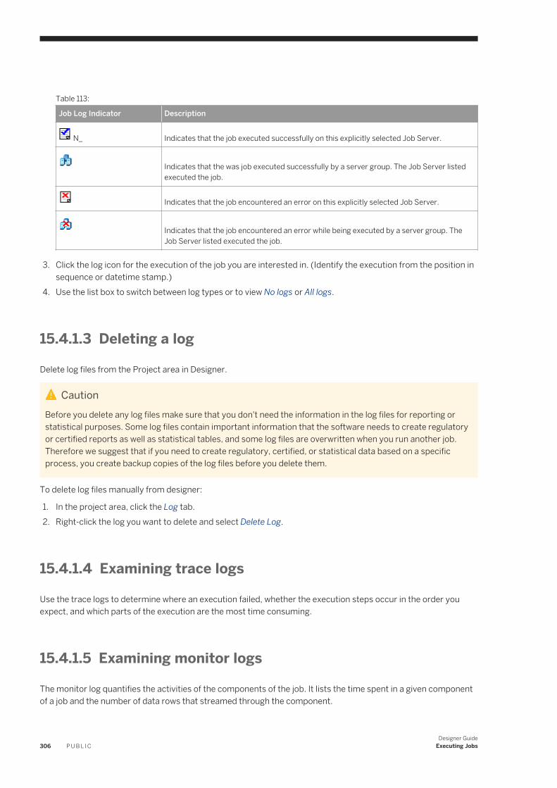
Table 113:
Job Log Indicator Description
N_ Indicates that the job executed successfully on this explicitly selected Job Server.
Indicates that the was job executed successfully by a server group. The Job Server listed executed the job.
Indicates that the job encountered an error on this explicitly selected Job Server.
Indicates that the job encountered an error while being executed by a server group. The Job Server listed executed the job.
3. Click the log icon for the execution of the job you are interested in. (Identify the execution from the position in sequence or datetime stamp.)
4. Use the list box to switch between log types or to view No logs or All logs.
15.4.1.3 Deleting a log
Delete log files from the Project area in Designer.
CautionBefore you delete any log files make sure that you don't need the information in the log files for reporting or statistical purposes. Some log files contain important information that the software needs to create regulatory or certified reports as well as statistical tables, and some log files are overwritten when you run another job. Therefore we suggest that if you need to create regulatory, certified, or statistical data based on a specific process, you create backup copies of the log files before you delete them.
To delete log files manually from designer:
1. In the project area, click the Log tab.2. Right-click the log you want to delete and select Delete Log.
15.4.1.4 Examining trace logs
Use the trace logs to determine where an execution failed, whether the execution steps occur in the order you expect, and which parts of the execution are the most time consuming.
15.4.1.5 Examining monitor logs
The monitor log quantifies the activities of the components of the job. It lists the time spent in a given component of a job and the number of data rows that streamed through the component.
306 P U B L I CDesigner Guide
Executing Jobs
15.4.1.6 Examining error logs
The software produces an error log for every job execution. Use the error logs to determine how an execution failed. If the execution completed without error, the error log is blank.
15.4.2 Examining target data
The best measure of the success of a job is the state of the target data. Always examine your data to make sure the data movement operation produced the results you expect. Be sure that:
● Data was not converted to incompatible types or truncated.● Data was not duplicated in the target.● Data was not lost between updates of the target.● Generated keys have been properly incremented.● Updated values were handled properly.
15.4.3 Creating a debug package
Create a job debug package that includes the ATL and trace, monitor, and log files.
You can create a job debug package that includes the ATL and trace, monitor, and log files. Send the generated .zip or .tar file to SAP customer support to help you troubleshoot execution-related issues. You can generate the debug package as you execute the job either from the Execution Properties window of the Designer or in the Execution Options page of the Management Console Administrator.
1. In the Designer project area, right-click the job name and choose Execute.
The software prompts you to save any objects that have changes that have not been saved.2. In the Execution Properties window, select the Trace tab.3. Select Create Debug Package, and change the value to Yes.4. Click OK.
The software generates the zip or tar debug package file in the following location: <DS_COMMON_DIR>\log\<Job_Server_Name>\<repository name> on the machine where the Job Server is installed.
You can download the debug package from the Management Console Administrator. For more information, see the SAP Data Services Management Console Guide.
15.5 Changing Job Server options
Familiarize yourself with the more technical aspects of how the software handles data (using the Reference Guide) and some of its interfaces like those for adapters and SAP application.
Designer GuideExecuting Jobs P U B L I C 307
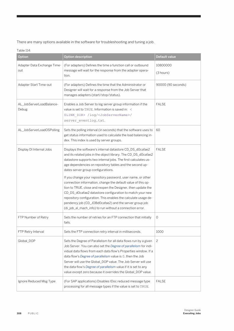
There are many options available in the software for troubleshooting and tuning a job.
Table 114:
Option Option description Default value
Adapter Data Exchange Time-out
(For adapters) Defines the time a function call or outbound message will wait for the response from the adapter operation.
10800000
(3 hours)
Adapter Start Time-out (For adapters) Defines the time that the Administrator or Designer will wait for a response from the Job Server that manages adapters (start/stop/status).
90000 (90 seconds)
AL_JobServerLoadBalanceDebug
Enables a Job Server to log server group information if the value is set to TRUE. Information is saved in: <$LINK_DIR> /log/<JobServerName>/server_eventlog.txt.
FALSE
AL_JobServerLoadOSPolling Sets the polling interval (in seconds) that the software uses to get status information used to calculate the load balancing index. This index is used by server groups.
60
Display DI Internal Jobs Displays the software's internal datastore CD_DS_d0cafae2 and its related jobs in the object library. The CD_DS_d0cafae2 datastore supports two internal jobs. The first calculates usage dependencies on repository tables and the second updates server group configurations.
If you change your repository password, user name, or other connection information, change the default value of this option to TRUE, close and reopen the Designer, then update the CD_DS_d0cafae2 datastore configuration to match your new repository configuration. This enables the calculate usage dependency job (CD_JOBd0cafae2) and the server group job (di_job_al_mach_info) to run without a connection error.
FALSE
FTP Number of Retry Sets the number of retries for an FTP connection that initially fails.
0
FTP Retry Interval Sets the FTP connection retry interval in milliseconds. 1000
Global_DOP Sets the Degree of Parallelism for all data flows run by a given Job Server. You can also set the Degree of parallelism for individual data flows from each data flow's Properties window. If a data flow's Degree of parallelism value is 0, then the Job Server will use the Global_DOP value. The Job Server will use the data flow's Degree of parallelism value if it is set to any value except zero because it overrides the Global_DOP value.
2
Ignore Reduced Msg Type (For SAP applications) Disables IDoc reduced message type processing for all message types if the value is set to TRUE.
FALSE
308 P U B L I CDesigner Guide
Executing Jobs
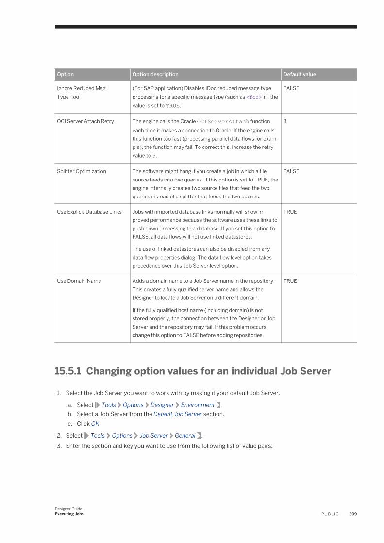
Option Option description Default value
Ignore Reduced Msg Type_foo
(For SAP application) Disables IDoc reduced message type processing for a specific message type (such as <foo> ) if the value is set to TRUE.
FALSE
OCI Server Attach Retry The engine calls the Oracle OCIServerAttach function each time it makes a connection to Oracle. If the engine calls this function too fast (processing parallel data flows for example), the function may fail. To correct this, increase the retry value to 5.
3
Splitter Optimization The software might hang if you create a job in which a file source feeds into two queries. If this option is set to TRUE, the engine internally creates two source files that feed the two queries instead of a splitter that feeds the two queries.
FALSE
Use Explicit Database Links Jobs with imported database links normally will show improved performance because the software uses these links to push down processing to a database. If you set this option to FALSE, all data flows will not use linked datastores.
The use of linked datastores can also be disabled from any data flow properties dialog. The data flow level option takes precedence over this Job Server level option.
TRUE
Use Domain Name Adds a domain name to a Job Server name in the repository. This creates a fully qualified server name and allows the Designer to locate a Job Server on a different domain.
If the fully qualified host name (including domain) is not stored properly, the connection between the Designer or Job Server and the repository may fail. If this problem occurs, change this option to FALSE before adding repositories.
TRUE
15.5.1 Changing option values for an individual Job Server
1. Select the Job Server you want to work with by making it your default Job Server.
a. Select Tools Options Designer Environment .b. Select a Job Server from the Default Job Server section.c. Click OK.
2. Select Tools Options Job Server General .3. Enter the section and key you want to use from the following list of value pairs:
Designer GuideExecuting Jobs P U B L I C 309
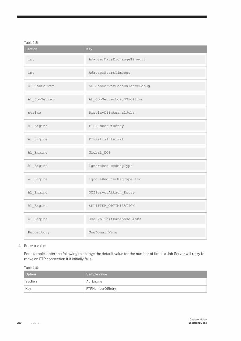
Table 115:
Section Key
int AdapterDataExchangeTimeout
int AdapterStartTimeout
AL_JobServer AL_JobServerLoadBalanceDebug
AL_JobServer AL_JobServerLoadOSPolling
string DisplayDIInternalJobs
AL_Engine FTPNumberOfRetry
AL_Engine FTPRetryInterval
AL_Engine Global_DOP
AL_Engine IgnoreReducedMsgType
AL_Engine IgnoreReducedMsgType_foo
AL_Engine OCIServerAttach_Retry
AL_Engine SPLITTER_OPTIMIZATION
AL_Engine UseExplicitDatabaseLinks
Repository UseDomainName
4. Enter a value.
For example, enter the following to change the default value for the number of times a Job Server will retry to make an FTP connection if it initially fails:
Table 116:
Option Sample value
Section AL_Engine
Key FTPNumberOfRetry
310 P U B L I CDesigner Guide
Executing Jobs
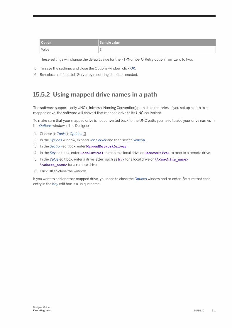
Option Sample value
Value 2
These settings will change the default value for the FTPNumberOfRetry option from zero to two.
5. To save the settings and close the Options window, click OK.6. Re-select a default Job Server by repeating step 1, as needed.
15.5.2 Using mapped drive names in a path
The software supports only UNC (Universal Naming Convention) paths to directories. If you set up a path to a mapped drive, the software will convert that mapped drive to its UNC equivalent.
To make sure that your mapped drive is not converted back to the UNC path, you need to add your drive names in the Options window in the Designer.
1. Choose Tools Options .2. In the Options window, expand Job Server and then select General.3. In the Section edit box, enter MappedNetworkDrives.
4. In the Key edit box, enter LocalDrive1 to map to a local drive or RemoteDrive1 to map to a remote drive.
5. In the Value edit box, enter a drive letter, such as M:\ for a local drive or \\<machine_name>\<share_name> for a remote drive.
6. Click OK to close the window.
If you want to add another mapped drive, you need to close the Options window and re-enter. Be sure that each entry in the Key edit box is a unique name.
Designer GuideExecuting Jobs P U B L I C 311
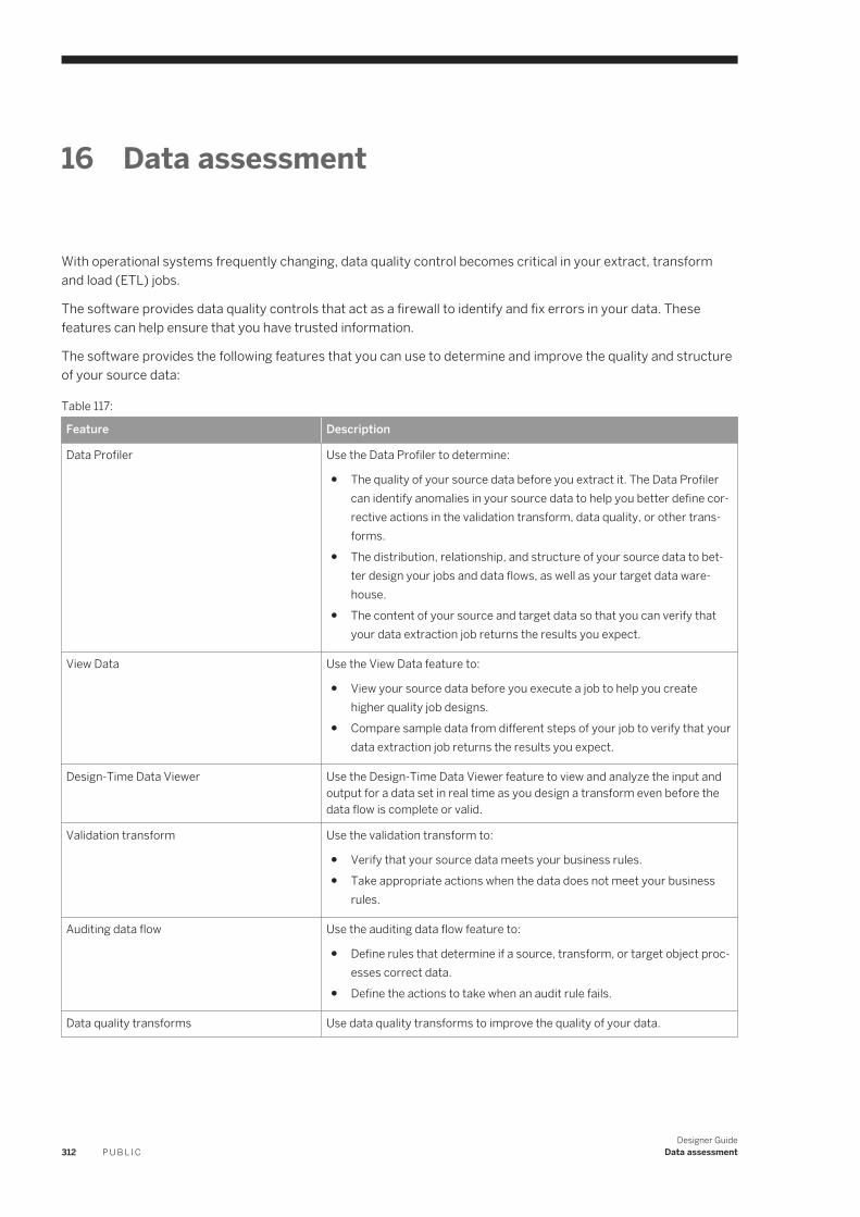
16 Data assessment
With operational systems frequently changing, data quality control becomes critical in your extract, transform and load (ETL) jobs.
The software provides data quality controls that act as a firewall to identify and fix errors in your data. These features can help ensure that you have trusted information.
The software provides the following features that you can use to determine and improve the quality and structure of your source data:
Table 117:
Feature Description
Data Profiler Use the Data Profiler to determine:
● The quality of your source data before you extract it. The Data Profiler can identify anomalies in your source data to help you better define corrective actions in the validation transform, data quality, or other transforms.
● The distribution, relationship, and structure of your source data to better design your jobs and data flows, as well as your target data warehouse.
● The content of your source and target data so that you can verify that your data extraction job returns the results you expect.
View Data Use the View Data feature to:
● View your source data before you execute a job to help you create higher quality job designs.
● Compare sample data from different steps of your job to verify that your data extraction job returns the results you expect.
Design-Time Data Viewer Use the Design-Time Data Viewer feature to view and analyze the input and output for a data set in real time as you design a transform even before the data flow is complete or valid.
Validation transform Use the validation transform to:
● Verify that your source data meets your business rules.● Take appropriate actions when the data does not meet your business
rules.
Auditing data flow Use the auditing data flow feature to:
● Define rules that determine if a source, transform, or target object processes correct data.
● Define the actions to take when an audit rule fails.
Data quality transforms Use data quality transforms to improve the quality of your data.
312 P U B L I CDesigner Guide
Data assessment
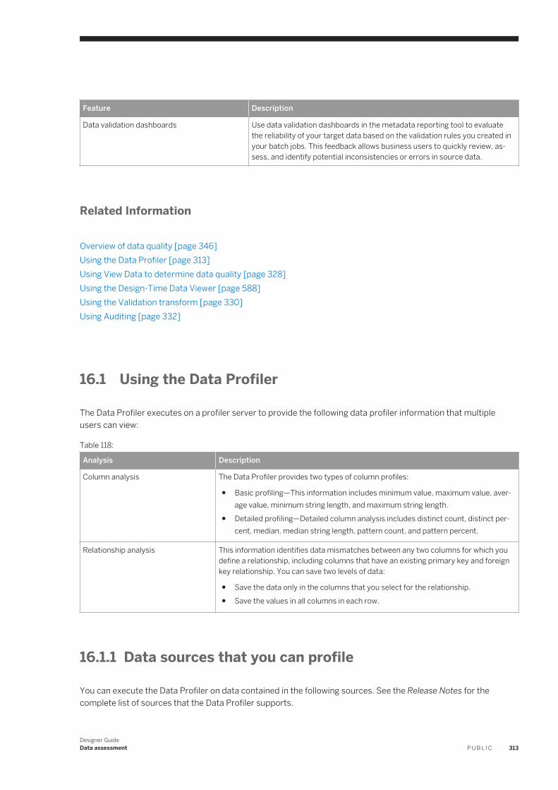
Feature Description
Data validation dashboards Use data validation dashboards in the metadata reporting tool to evaluate the reliability of your target data based on the validation rules you created in your batch jobs. This feedback allows business users to quickly review, assess, and identify potential inconsistencies or errors in source data.
Related Information
Overview of data quality [page 346]Using the Data Profiler [page 313]Using View Data to determine data quality [page 328]Using the Design-Time Data Viewer [page 588]Using the Validation transform [page 330]Using Auditing [page 332]
16.1 Using the Data Profiler
The Data Profiler executes on a profiler server to provide the following data profiler information that multiple users can view:
Table 118:
Analysis Description
Column analysis The Data Profiler provides two types of column profiles:
● Basic profiling—This information includes minimum value, maximum value, average value, minimum string length, and maximum string length.
● Detailed profiling—Detailed column analysis includes distinct count, distinct percent, median, median string length, pattern count, and pattern percent.
Relationship analysis This information identifies data mismatches between any two columns for which you define a relationship, including columns that have an existing primary key and foreign key relationship. You can save two levels of data:
● Save the data only in the columns that you select for the relationship.● Save the values in all columns in each row.
16.1.1 Data sources that you can profile
You can execute the Data Profiler on data contained in the following sources. See the Release Notes for the complete list of sources that the Data Profiler supports.
Designer GuideData assessment P U B L I C 313
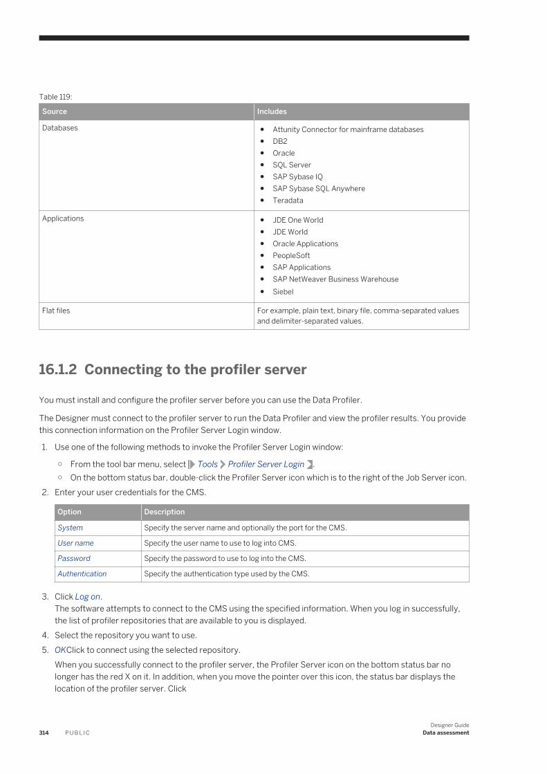
Table 119:
Source Includes
Databases ● Attunity Connector for mainframe databases● DB2● Oracle● SQL Server● SAP Sybase IQ● SAP Sybase SQL Anywhere● Teradata
Applications ● JDE One World● JDE World● Oracle Applications● PeopleSoft● SAP Applications● SAP NetWeaver Business Warehouse ● Siebel
Flat files For example, plain text, binary file, comma-separated values and delimiter-separated values.
16.1.2 Connecting to the profiler server
You must install and configure the profiler server before you can use the Data Profiler.
The Designer must connect to the profiler server to run the Data Profiler and view the profiler results. You provide this connection information on the Profiler Server Login window.
1. Use one of the following methods to invoke the Profiler Server Login window:
○ From the tool bar menu, select Tools Profiler Server Login .○ On the bottom status bar, double-click the Profiler Server icon which is to the right of the Job Server icon.
2. Enter your user credentials for the CMS.
Option Description
System Specify the server name and optionally the port for the CMS.
User name Specify the user name to use to log into CMS.
Password Specify the password to use to log into the CMS.
Authentication Specify the authentication type used by the CMS.
3. Click Log on.The software attempts to connect to the CMS using the specified information. When you log in successfully, the list of profiler repositories that are available to you is displayed.
4. Select the repository you want to use.5. OKClick to connect using the selected repository.
When you successfully connect to the profiler server, the Profiler Server icon on the bottom status bar no longer has the red X on it. In addition, when you move the pointer over this icon, the status bar displays the location of the profiler server. Click
314 P U B L I CDesigner Guide
Data assessment
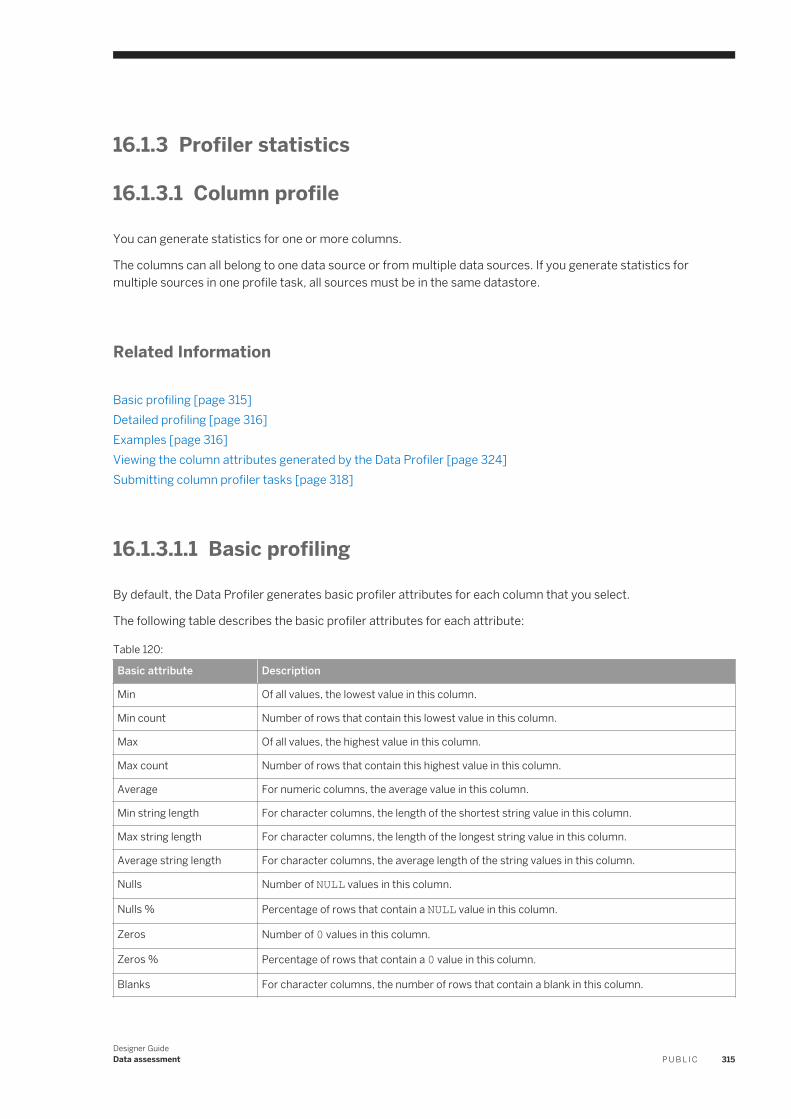
16.1.3 Profiler statistics
16.1.3.1 Column profile
You can generate statistics for one or more columns.
The columns can all belong to one data source or from multiple data sources. If you generate statistics for multiple sources in one profile task, all sources must be in the same datastore.
Related Information
Basic profiling [page 315]Detailed profiling [page 316]Examples [page 316]Viewing the column attributes generated by the Data Profiler [page 324]Submitting column profiler tasks [page 318]
16.1.3.1.1 Basic profiling
By default, the Data Profiler generates basic profiler attributes for each column that you select.
The following table describes the basic profiler attributes for each attribute:
Table 120:
Basic attribute Description
Min Of all values, the lowest value in this column.
Min count Number of rows that contain this lowest value in this column.
Max Of all values, the highest value in this column.
Max count Number of rows that contain this highest value in this column.
Average For numeric columns, the average value in this column.
Min string length For character columns, the length of the shortest string value in this column.
Max string length For character columns, the length of the longest string value in this column.
Average string length For character columns, the average length of the string values in this column.
Nulls Number of NULL values in this column.
Nulls % Percentage of rows that contain a NULL value in this column.
Zeros Number of 0 values in this column.
Zeros % Percentage of rows that contain a 0 value in this column.
Blanks For character columns, the number of rows that contain a blank in this column.
Designer GuideData assessment P U B L I C 315
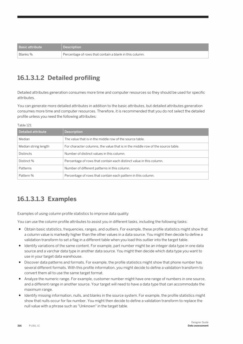
Basic attribute Description
Blanks % Percentage of rows that contain a blank in this column.
16.1.3.1.2 Detailed profiling
Detailed attributes generation consumes more time and computer resources so they should be used for specific attributes.
You can generate more detailed attributes in addition to the basic attributes, but detailed attributes generation consumes more time and computer resources. Therefore, it is recommended that you do not select the detailed profile unless you need the following attributes:
Table 121:
Detailed attribute Description
Median The value that is in the middle row of the source table.
Median string length For character columns, the value that is in the middle row of the source table.
Distincts Number of distinct values in this column.
Distinct % Percentage of rows that contain each distinct value in this column.
Patterns Number of different patterns in this column.
Pattern % Percentage of rows that contain each pattern in this column.
16.1.3.1.3 Examples
Examples of using column profile statistics to improve data quality
You can use the column profile attributes to assist you in different tasks, including the following tasks:
● Obtain basic statistics, frequencies, ranges, and outliers. For example, these profile statistics might show that a column value is markedly higher than the other values in a data source. You might then decide to define a validation transform to set a flag in a different table when you load this outlier into the target table.
● Identify variations of the same content. For example, part number might be an integer data type in one data source and a varchar data type in another data source. You might then decide which data type you want to use in your target data warehouse.
● Discover data patterns and formats. For example, the profile statistics might show that phone number has several different formats. With this profile information, you might decide to define a validation transform to convert them all to use the same target format.
● Analyze the numeric range. For example, customer number might have one range of numbers in one source, and a different range in another source. Your target will need to have a data type that can accommodate the maximum range.
● Identify missing information, nulls, and blanks in the source system. For example, the profile statistics might show that nulls occur for fax number. You might then decide to define a validation transform to replace the null value with a phrase such as "Unknown" in the target table.
316 P U B L I CDesigner Guide
Data assessment
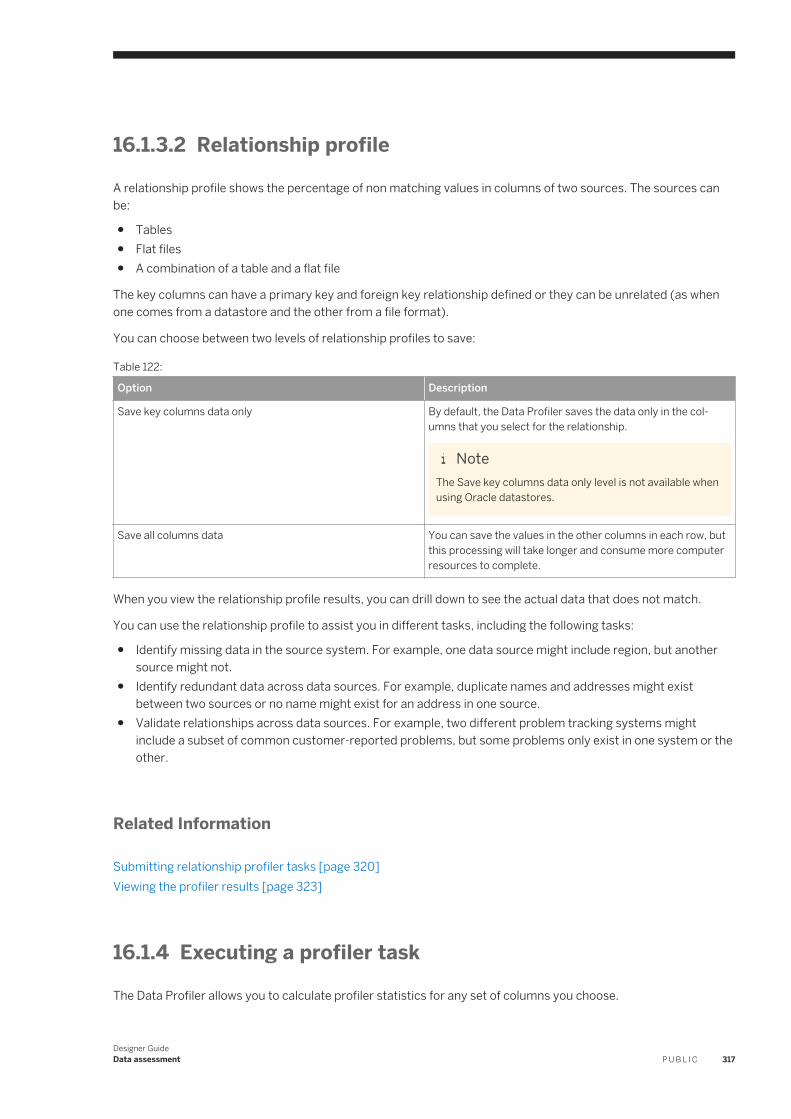
16.1.3.2 Relationship profile
A relationship profile shows the percentage of non matching values in columns of two sources. The sources can be:
● Tables● Flat files● A combination of a table and a flat file
The key columns can have a primary key and foreign key relationship defined or they can be unrelated (as when one comes from a datastore and the other from a file format).
You can choose between two levels of relationship profiles to save:
Table 122:
Option Description
Save key columns data only By default, the Data Profiler saves the data only in the columns that you select for the relationship.
NoteThe Save key columns data only level is not available when using Oracle datastores.
Save all columns data You can save the values in the other columns in each row, but this processing will take longer and consume more computer resources to complete.
When you view the relationship profile results, you can drill down to see the actual data that does not match.
You can use the relationship profile to assist you in different tasks, including the following tasks:
● Identify missing data in the source system. For example, one data source might include region, but another source might not.
● Identify redundant data across data sources. For example, duplicate names and addresses might exist between two sources or no name might exist for an address in one source.
● Validate relationships across data sources. For example, two different problem tracking systems might include a subset of common customer-reported problems, but some problems only exist in one system or the other.
Related Information
Submitting relationship profiler tasks [page 320]Viewing the profiler results [page 323]
16.1.4 Executing a profiler task
The Data Profiler allows you to calculate profiler statistics for any set of columns you choose.
Designer GuideData assessment P U B L I C 317
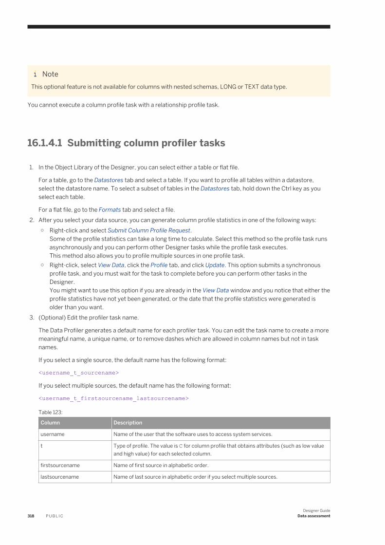
NoteThis optional feature is not available for columns with nested schemas, LONG or TEXT data type.
You cannot execute a column profile task with a relationship profile task.
16.1.4.1 Submitting column profiler tasks
1. In the Object Library of the Designer, you can select either a table or flat file.
For a table, go to the Datastores tab and select a table. If you want to profile all tables within a datastore, select the datastore name. To select a subset of tables in the Datastores tab, hold down the Ctrl key as you select each table.
For a flat file, go to the Formats tab and select a file.2. After you select your data source, you can generate column profile statistics in one of the following ways:
○ Right-click and select Submit Column Profile Request.Some of the profile statistics can take a long time to calculate. Select this method so the profile task runs asynchronously and you can perform other Designer tasks while the profile task executes.This method also allows you to profile multiple sources in one profile task.
○ Right-click, select View Data, click the Profile tab, and click Update. This option submits a synchronous profile task, and you must wait for the task to complete before you can perform other tasks in the Designer.You might want to use this option if you are already in the View Data window and you notice that either the profile statistics have not yet been generated, or the date that the profile statistics were generated is older than you want.
3. (Optional) Edit the profiler task name.
The Data Profiler generates a default name for each profiler task. You can edit the task name to create a more meaningful name, a unique name, or to remove dashes which are allowed in column names but not in task names.
If you select a single source, the default name has the following format:
<username_t_sourcename>
If you select multiple sources, the default name has the following format:
<username_t_firstsourcename_lastsourcename>
Table 123:
Column Description
username Name of the user that the software uses to access system services.
t Type of profile. The value is C for column profile that obtains attributes (such as low value and high value) for each selected column.
firstsourcename Name of first source in alphabetic order.
lastsourcename Name of last source in alphabetic order if you select multiple sources.
318 P U B L I CDesigner Guide
Data assessment
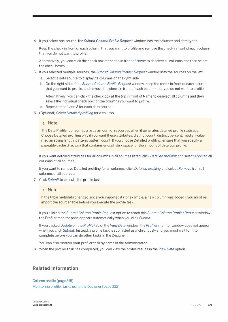
4. If you select one source, the Submit Column Profile Request window lists the columns and data types.
Keep the check in front of each column that you want to profile and remove the check in front of each column that you do not want to profile.
Alternatively, you can click the check box at the top in front of Name to deselect all columns and then select the check boxes.
5. If you selected multiple sources, the Submit Column Profiler Request window lists the sources on the left.a. Select a data source to display its columns on the right side.b. On the right side of the Submit Column Profile Request window, keep the check in front of each column
that you want to profile, and remove the check in front of each column that you do not want to profile.
Alternatively, you can click the check box at the top in front of Name to deselect all columns and then select the individual check box for the columns you want to profile.
c. Repeat steps 1 and 2 for each data source.6. (Optional) Select Detailed profiling for a column.
NoteThe Data Profiler consumes a large amount of resources when it generates detailed profile statistics. Choose Detailed profiling only if you want these attributes: distinct count, distinct percent, median value, median string length, pattern, pattern count. If you choose Detailed profiling, ensure that you specify a pageable cache directory that contains enough disk space for the amount of data you profile.
If you want detailed attributes for all columns in all sources listed, click Detailed profiling and select Apply to all columns of all sources.
If you want to remove Detailed profiling for all columns, click Detailed profiling and select Remove from all columns of all sources.
7. Click Submit to execute the profile task.
NoteIf the table metadata changed since you imported it (for example, a new column was added), you must re-import the source table before you execute the profile task.
If you clicked the Submit Column Profile Request option to reach this Submit Column Profiler Request window, the Profiler monitor pane appears automatically when you click Submit.
If you clicked Update on the Profile tab of the View Data window, the Profiler monitor window does not appear when you click Submit. Instead, a profile task is submitted asynchronously and you must wait for it to complete before you can do other tasks in the Designer .
You can also monitor your profiler task by name in the Administrator.8. When the profiler task has completed, you can view the profile results in the View Data option.
Related Information
Column profile [page 315]Monitoring profiler tasks using the Designer [page 322]
Designer GuideData assessment P U B L I C 319
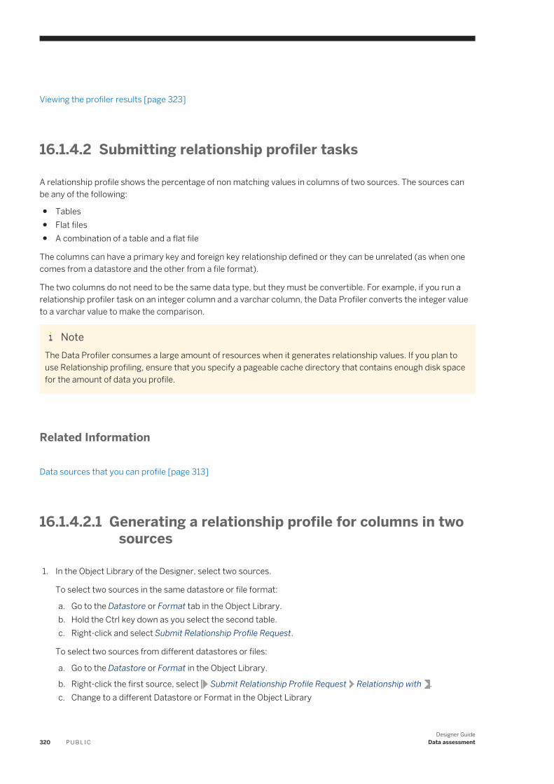
Viewing the profiler results [page 323]
16.1.4.2 Submitting relationship profiler tasks
A relationship profile shows the percentage of non matching values in columns of two sources. The sources can be any of the following:
● Tables● Flat files● A combination of a table and a flat file
The columns can have a primary key and foreign key relationship defined or they can be unrelated (as when one comes from a datastore and the other from a file format).
The two columns do not need to be the same data type, but they must be convertible. For example, if you run a relationship profiler task on an integer column and a varchar column, the Data Profiler converts the integer value to a varchar value to make the comparison.
NoteThe Data Profiler consumes a large amount of resources when it generates relationship values. If you plan to use Relationship profiling, ensure that you specify a pageable cache directory that contains enough disk space for the amount of data you profile.
Related Information
Data sources that you can profile [page 313]
16.1.4.2.1 Generating a relationship profile for columns in two sources
1. In the Object Library of the Designer, select two sources.
To select two sources in the same datastore or file format:
a. Go to the Datastore or Format tab in the Object Library.b. Hold the Ctrl key down as you select the second table.c. Right-click and select Submit Relationship Profile Request.
To select two sources from different datastores or files:
a. Go to the Datastore or Format in the Object Library.
b. Right-click the first source, select Submit Relationship Profile Request Relationship with .c. Change to a different Datastore or Format in the Object Library
320 P U B L I CDesigner Guide
Data assessment
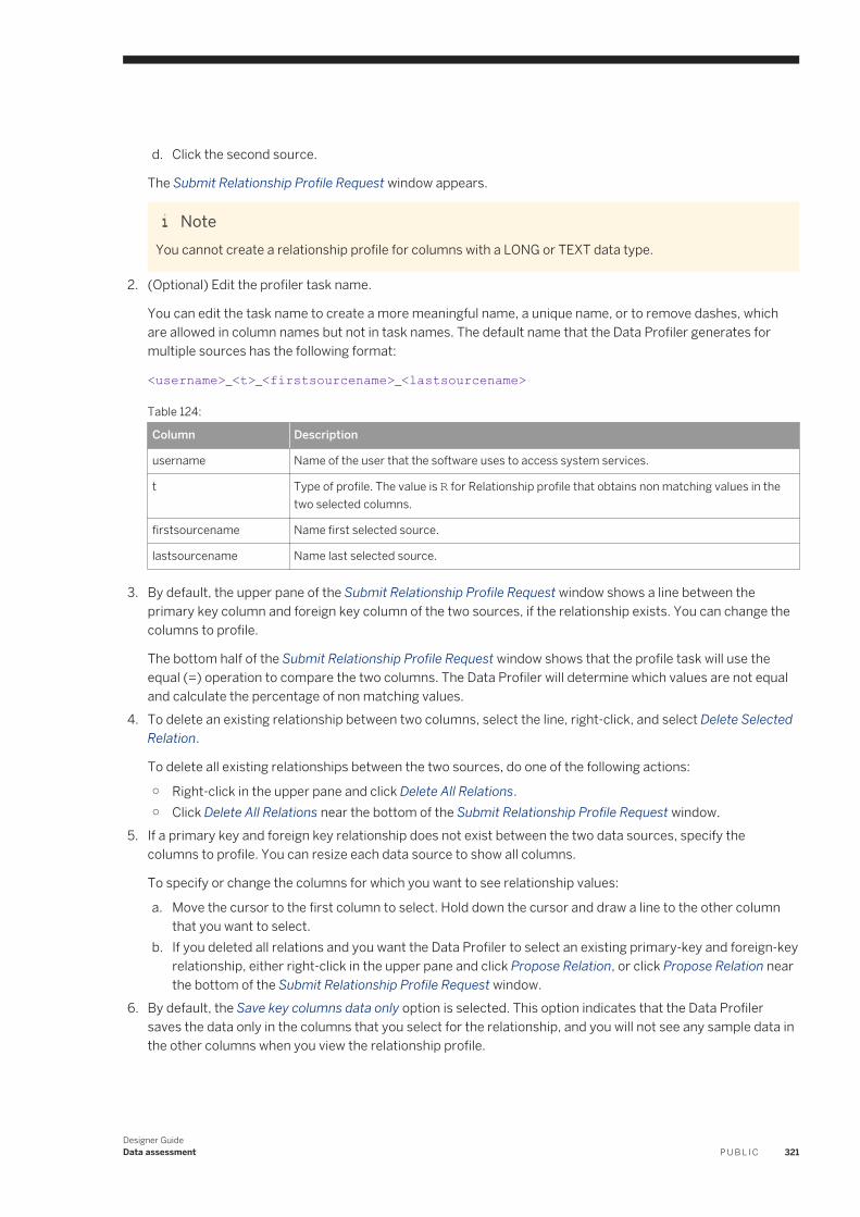
d. Click the second source.
The Submit Relationship Profile Request window appears.
NoteYou cannot create a relationship profile for columns with a LONG or TEXT data type.
2. (Optional) Edit the profiler task name.
You can edit the task name to create a more meaningful name, a unique name, or to remove dashes, which are allowed in column names but not in task names. The default name that the Data Profiler generates for multiple sources has the following format:
<username>_<t>_<firstsourcename>_<lastsourcename>
Table 124:
Column Description
username Name of the user that the software uses to access system services.
t Type of profile. The value is R for Relationship profile that obtains non matching values in the two selected columns.
firstsourcename Name first selected source.
lastsourcename Name last selected source.
3. By default, the upper pane of the Submit Relationship Profile Request window shows a line between the primary key column and foreign key column of the two sources, if the relationship exists. You can change the columns to profile.
The bottom half of the Submit Relationship Profile Request window shows that the profile task will use the equal (=) operation to compare the two columns. The Data Profiler will determine which values are not equal and calculate the percentage of non matching values.
4. To delete an existing relationship between two columns, select the line, right-click, and select Delete Selected Relation.
To delete all existing relationships between the two sources, do one of the following actions:
○ Right-click in the upper pane and click Delete All Relations.○ Click Delete All Relations near the bottom of the Submit Relationship Profile Request window.
5. If a primary key and foreign key relationship does not exist between the two data sources, specify the columns to profile. You can resize each data source to show all columns.
To specify or change the columns for which you want to see relationship values:
a. Move the cursor to the first column to select. Hold down the cursor and draw a line to the other column that you want to select.
b. If you deleted all relations and you want the Data Profiler to select an existing primary-key and foreign-key relationship, either right-click in the upper pane and click Propose Relation, or click Propose Relation near the bottom of the Submit Relationship Profile Request window.
6. By default, the Save key columns data only option is selected. This option indicates that the Data Profiler saves the data only in the columns that you select for the relationship, and you will not see any sample data in the other columns when you view the relationship profile.
Designer GuideData assessment P U B L I C 321
If you want to see values in the other columns in the relationship profile, select the Save all columns data option.
7. Click Submit to execute the profiler task.
NoteIf the table metadata changed since you imported it (for example, a new column was added), you must re-import the source table before you execute the profile task.
8. The Profiler monitor pane appears automatically when you click Submit.
You can also monitor your profiler task by name in the Administrator.9. When the profiler task has completed, you can view the profile results in the View Data option when you right
click on a table in the Object Library.
Related Information
Viewing the relationship profile data generated by the Data Profiler [page 326]Monitoring profiler tasks using the Designer [page 322]Viewing the profiler results [page 323]
16.1.5 Monitoring profiler tasks using the Designer
The Profiler monitor window appears automatically when you submit a profiler task if you clicked the menu bar to view the Profiler monitor window. You can dock this profiler monitor pane in the Designer or keep it separate.
The Profiler monitor pane displays the currently running task and all of the profiler tasks that have executed within a configured number of days.
● Click the Refresh● Click the Information icon to view the sources that the selected task is profiling. If the task failed, the
Information window also displays an error message.
The Profiler monitor shows the following columns: The icons in the upper-left corner of the Profiler monitor display the following information:
322 P U B L I CDesigner Guide
Data assessment
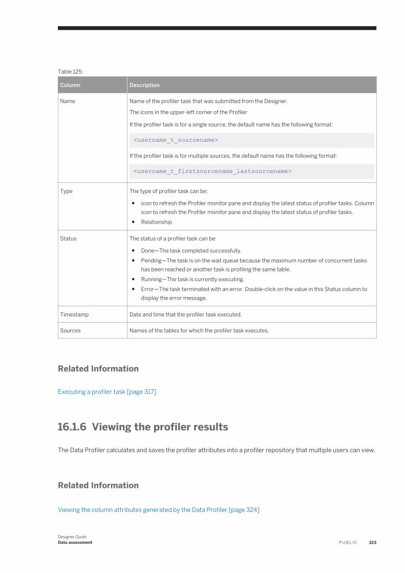
Table 125:
Column Description
Name Name of the profiler task that was submitted from the Designer.
The icons in the upper-left corner of the Profiler
If the profiler task is for a single source, the default name has the following format:
<username_t_sourcename>
If the profiler task is for multiple sources, the default name has the following format:
<username_t_firstsourcename_lastsourcename>
Type The type of profiler task can be:
● icon to refresh the Profiler monitor pane and display the latest status of profiler tasks. Column icon to refresh the Profiler monitor pane and display the latest status of profiler tasks.
● Relationship
Status The status of a profiler task can be:
● Done—The task completed successfully.● Pending—The task is on the wait queue because the maximum number of concurrent tasks
has been reached or another task is profiling the same table.● Running—The task is currently executing.● Error—The task terminated with an error. Double-click on the value in this Status column to
display the error message.
Timestamp Date and time that the profiler task executed.
Sources Names of the tables for which the profiler task executes.
Related Information
Executing a profiler task [page 317]
16.1.6 Viewing the profiler results
The Data Profiler calculates and saves the profiler attributes into a profiler repository that multiple users can view.
Related Information
Viewing the column attributes generated by the Data Profiler [page 324]
Designer GuideData assessment P U B L I C 323
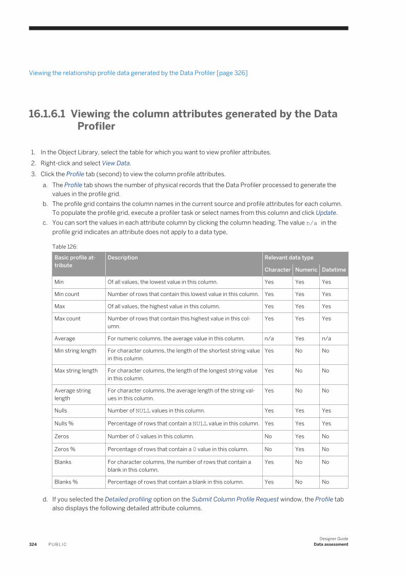
Viewing the relationship profile data generated by the Data Profiler [page 326]
16.1.6.1 Viewing the column attributes generated by the Data Profiler
1. In the Object Library, select the table for which you want to view profiler attributes.2. Right-click and select View Data.3. Click the Profile tab (second) to view the column profile attributes.
a. The Profile tab shows the number of physical records that the Data Profiler processed to generate the values in the profile grid.
b. The profile grid contains the column names in the current source and profile attributes for each column. To populate the profile grid, execute a profiler task or select names from this column and click Update.
c. You can sort the values in each attribute column by clicking the column heading. The value n/a in the profile grid indicates an attribute does not apply to a data type,
Table 126:
Basic profile attribute
Description Relevant data type
Character Numeric Datetime
Min Of all values, the lowest value in this column. Yes Yes Yes
Min count Number of rows that contain this lowest value in this column. Yes Yes Yes
Max Of all values, the highest value in this column. Yes Yes Yes
Max count Number of rows that contain this highest value in this column.
Yes Yes Yes
Average For numeric columns, the average value in this column. n/a Yes n/a
Min string length For character columns, the length of the shortest string value in this column.
Yes No No
Max string length For character columns, the length of the longest string value in this column.
Yes No No
Average string length
For character columns, the average length of the string values in this column.
Yes No No
Nulls Number of NULL values in this column. Yes Yes Yes
Nulls % Percentage of rows that contain a NULL value in this column. Yes Yes Yes
Zeros Number of 0 values in this column. No Yes No
Zeros % Percentage of rows that contain a 0 value in this column. No Yes No
Blanks For character columns, the number of rows that contain a blank in this column.
Yes No No
Blanks % Percentage of rows that contain a blank in this column. Yes No No
d. If you selected the Detailed profiling option on the Submit Column Profile Request window, the Profile tab also displays the following detailed attribute columns.
324 P U B L I CDesigner Guide
Data assessment
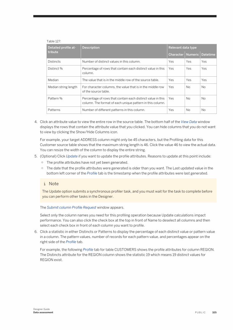
Table 127:
Detailed profile attribute
Description Relevant data type
Character Numeric Datetime
Distincts Number of distinct values in this column. Yes Yes Yes
Distinct % Percentage of rows that contain each distinct value in this column.
Yes Yes Yes
Median The value that is in the middle row of the source table. Yes Yes Yes
Median string length For character columns, the value that is in the middle row of the source table.
Yes No No
Pattern % Percentage of rows that contain each distinct value in this column. The format of each unique pattern in this column.
Yes No No
Patterns Number of different patterns in this column. Yes No No
4. Click an attribute value to view the entire row in the source table. The bottom half of the View Data window displays the rows that contain the attribute value that you clicked. You can hide columns that you do not want to view by clicking the Show/Hide Columns icon.
For example, your target ADDRESS column might only be 45 characters, but the Profiling data for this Customer source table shows that the maximum string length is 46. Click the value 46 to view the actual data. You can resize the width of the column to display the entire string.
5. (Optional) Click Update if you want to update the profile attributes. Reasons to update at this point include:○ The profile attributes have not yet been generated.○ The date that the profile attributes were generated is older than you want. The Last updated value in the
bottom left corner of the Profile tab is the timestamp when the profile attributes were last generated.
NoteThe Update option submits a synchronous profiler task, and you must wait for the task to complete before you can perform other tasks in the Designer.
The Submit column Profile Request window appears.
Select only the column names you need for this profiling operation because Update calculations impact performance. You can also click the check box at the top in front of Name to deselect all columns and then select each check box in front of each column you want to profile.
6. Click a statistic in either Distincts or Patterns to display the percentage of each distinct value or pattern value in a column. The pattern values, number of records for each pattern value, and percentages appear on the right side of the Profile tab.
For example, the following Profile tab for table CUSTOMERS shows the profile attributes for column REGION. The Distincts attribute for the REGION column shows the statistic 19 which means 19 distinct values for REGION exist.
Designer GuideData assessment P U B L I C 325
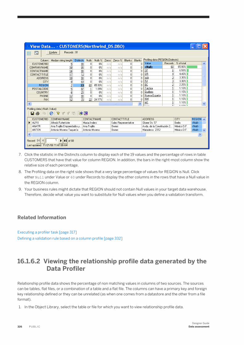
7. Click the statistic in the Distincts column to display each of the 19 values and the percentage of rows in table CUSTOMERS that have that value for column REGION. In addition, the bars in the right-most column show the relative size of each percentage.
8. The Profiling data on the right side shows that a very large percentage of values for REGION is Null. Click either Null under Value or 60 under Records to display the other columns in the rows that have a Null value in the REGION column.
9. Your business rules might dictate that REGION should not contain Null values in your target data warehouse. Therefore, decide what value you want to substitute for Null values when you define a validation transform.
Related Information
Executing a profiler task [page 317]Defining a validation rule based on a column profile [page 332]
16.1.6.2 Viewing the relationship profile data generated by the Data Profiler
Relationship profile data shows the percentage of non matching values in columns of two sources. The sources can be tables, flat files, or a combination of a table and a flat file. The columns can have a primary key and foreign key relationship defined or they can be unrelated (as when one comes from a datastore and the other from a file format).
1. In the Object Library, select the table or file for which you want to view relationship profile data.
326 P U B L I CDesigner Guide
Data assessment
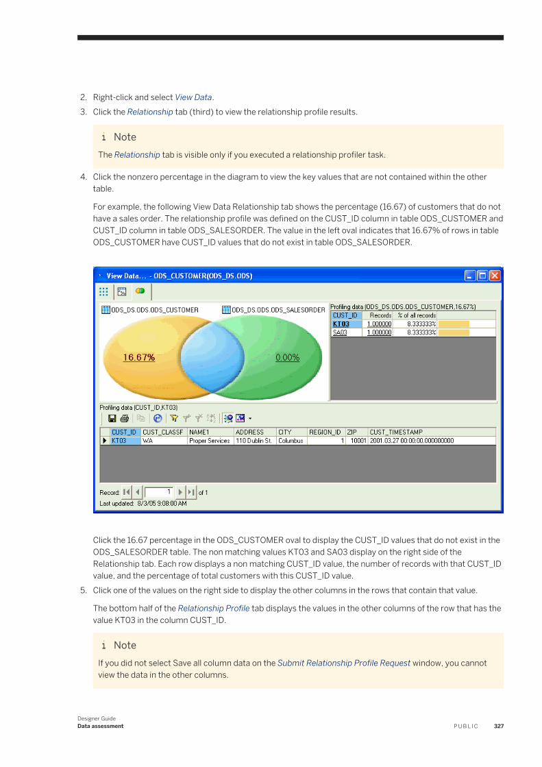
2. Right-click and select View Data.3. Click the Relationship tab (third) to view the relationship profile results.
NoteThe Relationship tab is visible only if you executed a relationship profiler task.
4. Click the nonzero percentage in the diagram to view the key values that are not contained within the other table.
For example, the following View Data Relationship tab shows the percentage (16.67) of customers that do not have a sales order. The relationship profile was defined on the CUST_ID column in table ODS_CUSTOMER and CUST_ID column in table ODS_SALESORDER. The value in the left oval indicates that 16.67% of rows in table ODS_CUSTOMER have CUST_ID values that do not exist in table ODS_SALESORDER.
Click the 16.67 percentage in the ODS_CUSTOMER oval to display the CUST_ID values that do not exist in the ODS_SALESORDER table. The non matching values KT03 and SA03 display on the right side of the Relationship tab. Each row displays a non matching CUST_ID value, the number of records with that CUST_ID value, and the percentage of total customers with this CUST_ID value.
5. Click one of the values on the right side to display the other columns in the rows that contain that value.
The bottom half of the Relationship Profile tab displays the values in the other columns of the row that has the value KT03 in the column CUST_ID.
NoteIf you did not select Save all column data on the Submit Relationship Profile Request window, you cannot view the data in the other columns.
Designer GuideData assessment P U B L I C 327
Related Information
Submitting relationship profiler tasks [page 320]
16.2 Using View Data to determine data quality
Use View Data to help you determine the quality of your source and target data. View Data provides the capability to:
● View sample source data before you execute a job to create higher quality job designs.● Compare sample data from different steps of your job to verify that your data extraction job returns the
results you expect.
NoteTo use View Data on a file, the file must be accessible from the Designer.
Related Information
Defining a validation rule based on a column profile [page 332]Using View Data [page 576]
16.2.1 Data tab
The Data tab is always available and displays the data contents of sample rows. You can display a subset of columns in each row and define filters to display a subset of rows.
For example, your business rules might dictate that all phone and fax numbers be in one format for each country. The following Data tab shows a subset of rows for the customers that are in France.
328 P U B L I CDesigner Guide
Data assessment
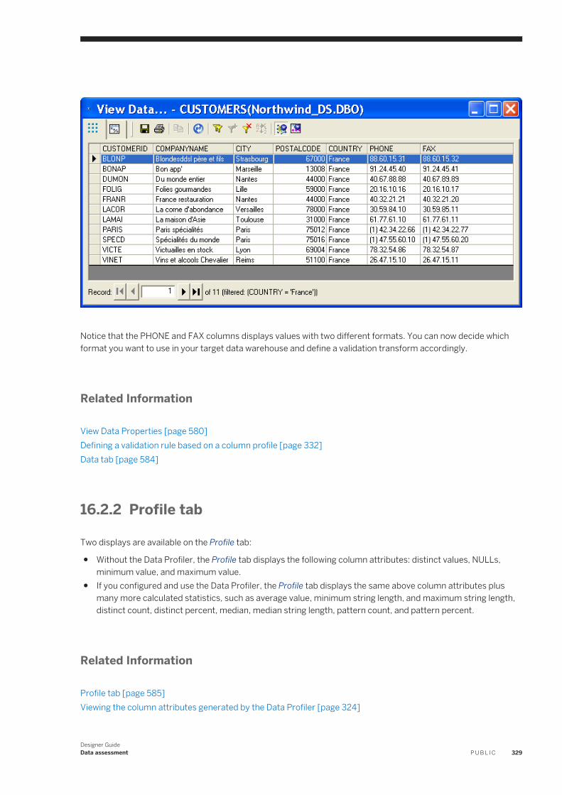
Notice that the PHONE and FAX columns displays values with two different formats. You can now decide which format you want to use in your target data warehouse and define a validation transform accordingly.
Related Information
View Data Properties [page 580]Defining a validation rule based on a column profile [page 332]Data tab [page 584]
16.2.2 Profile tab
Two displays are available on the Profile tab:
● Without the Data Profiler, the Profile tab displays the following column attributes: distinct values, NULLs, minimum value, and maximum value.
● If you configured and use the Data Profiler, the Profile tab displays the same above column attributes plus many more calculated statistics, such as average value, minimum string length, and maximum string length, distinct count, distinct percent, median, median string length, pattern count, and pattern percent.
Related Information
Profile tab [page 585]Viewing the column attributes generated by the Data Profiler [page 324]
Designer GuideData assessment P U B L I C 329
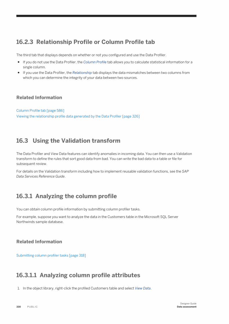
16.2.3 Relationship Profile or Column Profile tab
The third tab that displays depends on whether or not you configured and use the Data Profiler.
● If you do not use the Data Profiler, the Column Profile tab allows you to calculate statistical information for a single column.
● If you use the Data Profiler, the Relationship tab displays the data mismatches between two columns from which you can determine the integrity of your data between two sources.
Related Information
Column Profile tab [page 586]Viewing the relationship profile data generated by the Data Profiler [page 326]
16.3 Using the Validation transform
The Data Profiler and View Data features can identify anomalies in incoming data. You can then use a Validation transform to define the rules that sort good data from bad. You can write the bad data to a table or file for subsequent review.
For details on the Validation transform including how to implement reusable validation functions, see the SAP Data Services Reference Guide.
16.3.1 Analyzing the column profile
You can obtain column profile information by submitting column profiler tasks.
For example, suppose you want to analyze the data in the Customers table in the Microsoft SQL Server Northwinds sample database.
Related Information
Submitting column profiler tasks [page 318]
16.3.1.1 Analyzing column profile attributes
1. In the object library, right-click the profiled Customers table and select View Data.
330 P U B L I CDesigner Guide
Data assessment
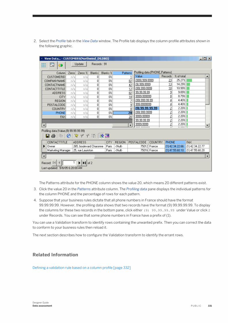
2. Select the Profile tab in the View Data window. The Profile tab displays the column-profile attributes shown in the following graphic.
The Patterns attribute for the PHONE column shows the value 20, which means 20 different patterns exist.3. Click the value 20 in the Patterns attribute column. The Profiling data pane displays the individual patterns for
the column PHONE and the percentage of rows for each pattern.4. Suppose that your business rules dictate that all phone numbers in France should have the format
99.99.99.99. However, the profiling data shows that two records have the format (9) 99.99.99.99. To display the columns for these two records in the bottom pane, click either (9) 99.99.99.99 under Value or click 2 under Records. You can see that some phone numbers in France have a prefix of (1).
You can use a Validation transform to identify rows containing the unwanted prefix. Then you can correct the data to conform to your busness rules then reload it.
The next section describes how to configure the Validation transform to identify the errant rows.
Related Information
Defining a validation rule based on a column profile [page 332]
Designer GuideData assessment P U B L I C 331
16.3.2 Defining a validation rule based on a column profile
This section takes the Data Profiler results and defines the Validation transform according to the sample business rules. Based on the preceding example of the phone prefix (1) for phone numbers in France, the following procedure describes how to define a data flow and validation rule that identifies that pattern. You can then review the failed data, make corrections, and reload the data.
16.3.2.1 Defining the validation rule that identifies a pattern
This procedure describes how to define a data flow and validation rule that identifies rows containing the (1) prefix described in the previous section.
1. Create a data flow with the Customers table as a source, add a Validation transform and a target, and connect the objects.
2. Open the Validation transform by clicking its name.3. In the transform editor, click Add.
The Rule Editor dialog box displays.4. Type a Name and optionally a Description for the rule.5. Verify the Enabled check box is selected.6. For Action on Fail, select Send to Fail.7. Select the Column Validation radio button.
a. Select the Column CUSTOMERS.PHONE from the drop-down list.b. For Condition, from the drop-down list select Match pattern.c. For the value, type the expression '99.99.99.99'.
8. Click OK.The rule appears in the Rules list.
After running the job, the incorrectly formatted rows appear in the Fail output. You can now review the failed data, make corrections as necessary upstream, and reload the data.
Related Information
Analyzing the column profile [page 330]
16.4 Using Auditing
Auditing provides a way to ensure that a data flow loads correct data into the warehouse. Use auditing to perform the following tasks:
● Define audit points to collect run time statistics about the data that flows out of objects. Auditing stores these statistics in the repository.
332 P U B L I CDesigner Guide
Data assessment
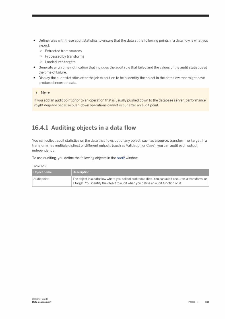
● Define rules with these audit statistics to ensure that the data at the following points in a data flow is what you expect:○ Extracted from sources○ Processed by transforms○ Loaded into targets
● Generate a run time notification that includes the audit rule that failed and the values of the audit statistics at the time of failure.
● Display the audit statistics after the job execution to help identify the object in the data flow that might have produced incorrect data.
NoteIf you add an audit point prior to an operation that is usually pushed down to the database server, performance might degrade because push-down operations cannot occur after an audit point.
16.4.1 Auditing objects in a data flow
You can collect audit statistics on the data that flows out of any object, such as a source, transform, or target. If a transform has multiple distinct or different outputs (such as Validation or Case), you can audit each output independently.
To use auditing, you define the following objects in the Audit window:
Table 128:
Object name Description
Audit point The object in a data flow where you collect audit statistics. You can audit a source, a transform, or a target. You identify the object to audit when you define an audit function on it.
Designer GuideData assessment P U B L I C 333
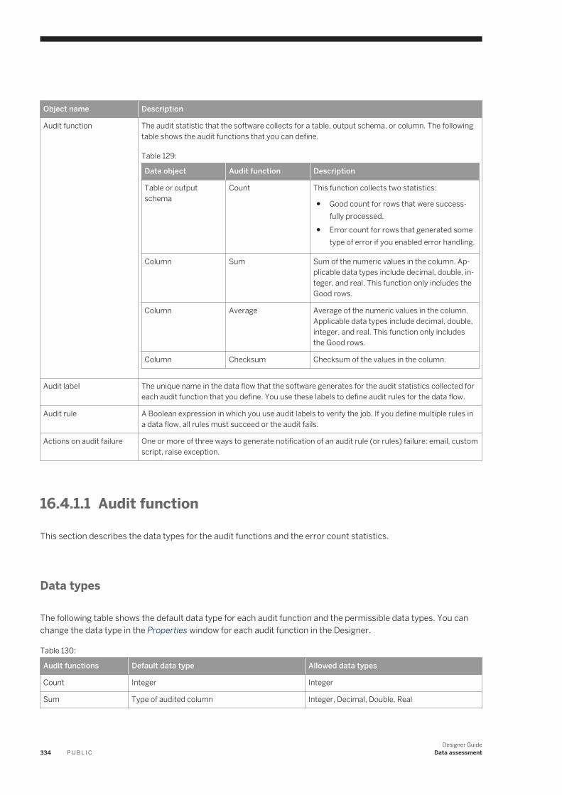
Object name Description
Audit function The audit statistic that the software collects for a table, output schema, or column. The following table shows the audit functions that you can define.
Table 129:
Data object Audit function Description
Table or output schema
Count This function collects two statistics:
● Good count for rows that were successfully processed.
● Error count for rows that generated some type of error if you enabled error handling.
Column Sum Sum of the numeric values in the column. Applicable data types include decimal, double, integer, and real. This function only includes the Good rows.
Column Average Average of the numeric values in the column. Applicable data types include decimal, double, integer, and real. This function only includes the Good rows.
Column Checksum Checksum of the values in the column.
Audit label The unique name in the data flow that the software generates for the audit statistics collected for each audit function that you define. You use these labels to define audit rules for the data flow.
Audit rule A Boolean expression in which you use audit labels to verify the job. If you define multiple rules in a data flow, all rules must succeed or the audit fails.
Actions on audit failure One or more of three ways to generate notification of an audit rule (or rules) failure: email, custom script, raise exception.
16.4.1.1 Audit function
This section describes the data types for the audit functions and the error count statistics.
Data types
The following table shows the default data type for each audit function and the permissible data types. You can change the data type in the Properties window for each audit function in the Designer.
Table 130:
Audit functions Default data type Allowed data types
Count Integer Integer
Sum Type of audited column Integer, Decimal, Double, Real
334 P U B L I CDesigner Guide
Data assessment
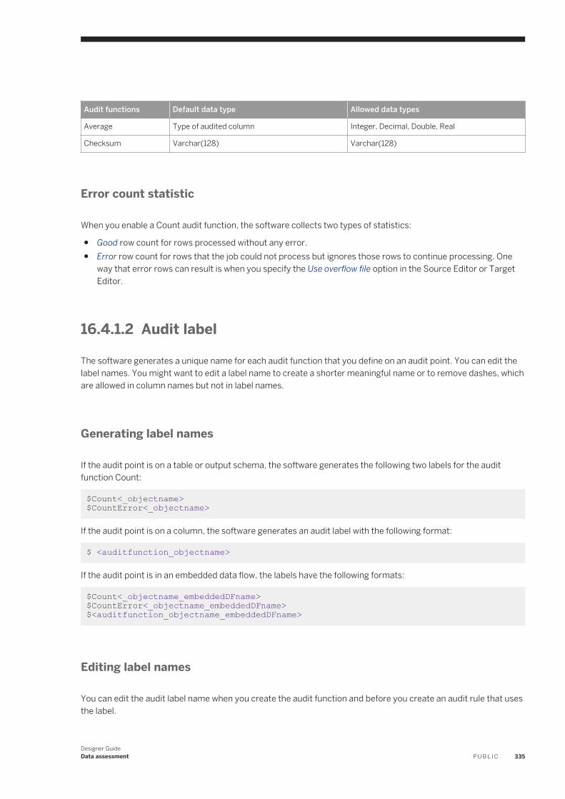
Audit functions Default data type Allowed data types
Average Type of audited column Integer, Decimal, Double, Real
Checksum Varchar(128) Varchar(128)
Error count statistic
When you enable a Count audit function, the software collects two types of statistics:
● Good row count for rows processed without any error.● Error row count for rows that the job could not process but ignores those rows to continue processing. One
way that error rows can result is when you specify the Use overflow file option in the Source Editor or Target Editor.
16.4.1.2 Audit label
The software generates a unique name for each audit function that you define on an audit point. You can edit the label names. You might want to edit a label name to create a shorter meaningful name or to remove dashes, which are allowed in column names but not in label names.
Generating label names
If the audit point is on a table or output schema, the software generates the following two labels for the audit function Count:
$Count<_objectname> $CountError<_objectname>
If the audit point is on a column, the software generates an audit label with the following format:
$ <auditfunction_objectname>
If the audit point is in an embedded data flow, the labels have the following formats:
$Count<_objectname_embeddedDFname> $CountError<_objectname_embeddedDFname> $<auditfunction_objectname_embeddedDFname>
Editing label names
You can edit the audit label name when you create the audit function and before you create an audit rule that uses the label.
Designer GuideData assessment P U B L I C 335
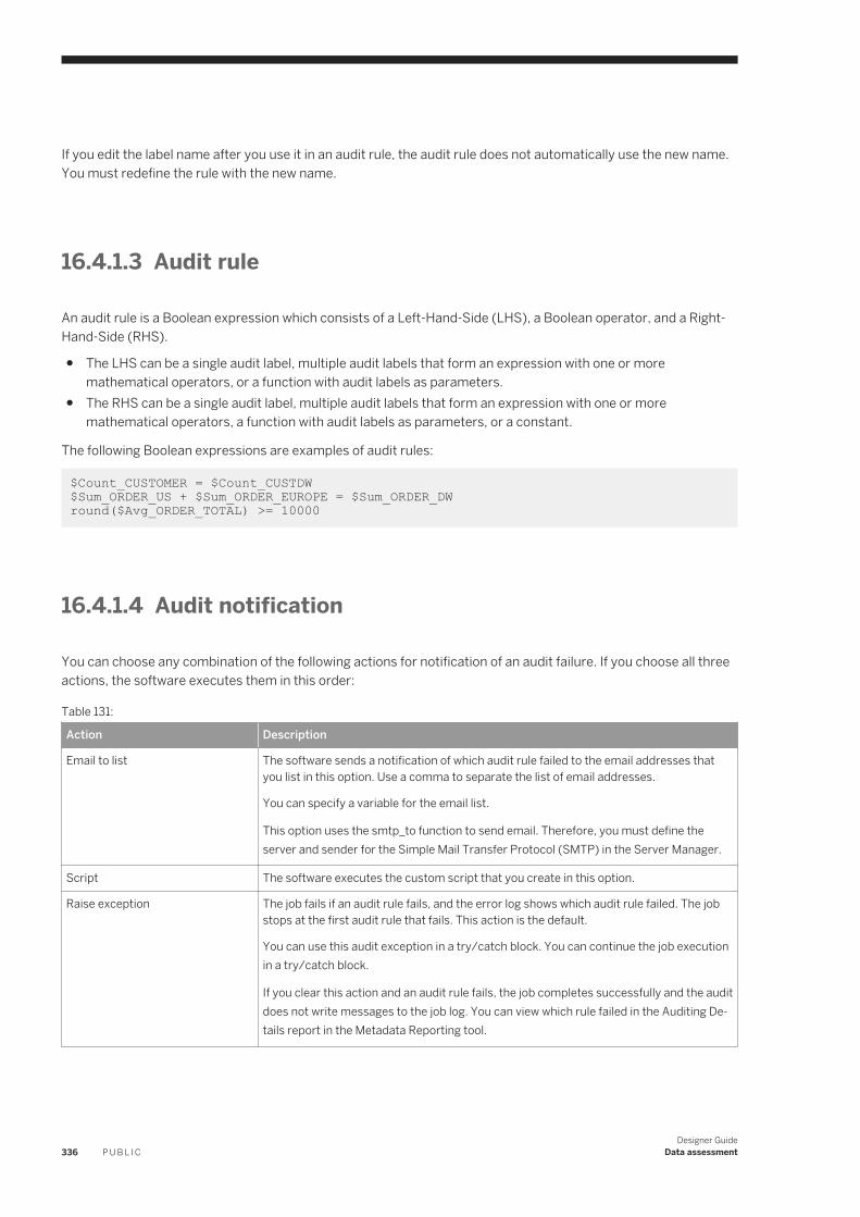
If you edit the label name after you use it in an audit rule, the audit rule does not automatically use the new name. You must redefine the rule with the new name.
16.4.1.3 Audit rule
An audit rule is a Boolean expression which consists of a Left-Hand-Side (LHS), a Boolean operator, and a Right-Hand-Side (RHS).
● The LHS can be a single audit label, multiple audit labels that form an expression with one or more mathematical operators, or a function with audit labels as parameters.
● The RHS can be a single audit label, multiple audit labels that form an expression with one or more mathematical operators, a function with audit labels as parameters, or a constant.
The following Boolean expressions are examples of audit rules:
$Count_CUSTOMER = $Count_CUSTDW $Sum_ORDER_US + $Sum_ORDER_EUROPE = $Sum_ORDER_DWround($Avg_ORDER_TOTAL) >= 10000
16.4.1.4 Audit notification
You can choose any combination of the following actions for notification of an audit failure. If you choose all three actions, the software executes them in this order:
Table 131:
Action Description
Email to list The software sends a notification of which audit rule failed to the email addresses that you list in this option. Use a comma to separate the list of email addresses.
You can specify a variable for the email list.
This option uses the smtp_to function to send email. Therefore, you must define the server and sender for the Simple Mail Transfer Protocol (SMTP) in the Server Manager.
Script The software executes the custom script that you create in this option.
Raise exception The job fails if an audit rule fails, and the error log shows which audit rule failed. The job stops at the first audit rule that fails. This action is the default.
You can use this audit exception in a try/catch block. You can continue the job execution in a try/catch block.
If you clear this action and an audit rule fails, the job completes successfully and the audit does not write messages to the job log. You can view which rule failed in the Auditing Details report in the Metadata Reporting tool.
336 P U B L I CDesigner Guide
Data assessment
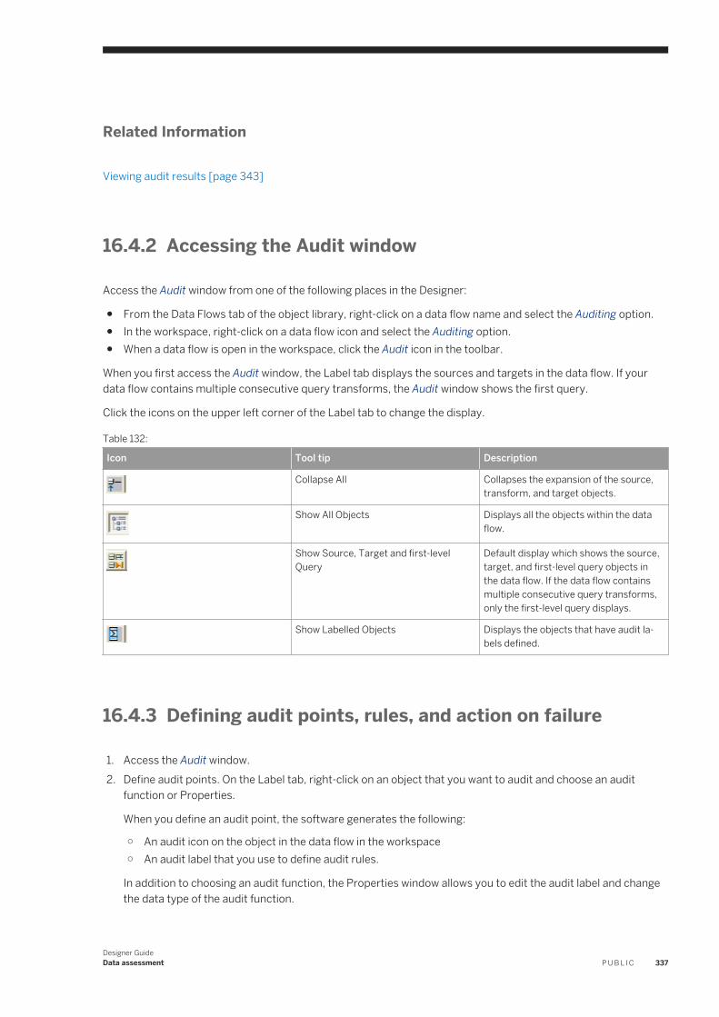
Related Information
Viewing audit results [page 343]
16.4.2 Accessing the Audit window
Access the Audit window from one of the following places in the Designer:
● From the Data Flows tab of the object library, right-click on a data flow name and select the Auditing option.● In the workspace, right-click on a data flow icon and select the Auditing option.● When a data flow is open in the workspace, click the Audit icon in the toolbar.
When you first access the Audit window, the Label tab displays the sources and targets in the data flow. If your data flow contains multiple consecutive query transforms, the Audit window shows the first query.
Click the icons on the upper left corner of the Label tab to change the display.
Table 132:
Icon Tool tip Description
Collapse All Collapses the expansion of the source, transform, and target objects.
Show All Objects Displays all the objects within the data flow.
Show Source, Target and first-level Query
Default display which shows the source, target, and first-level query objects in the data flow. If the data flow contains multiple consecutive query transforms, only the first-level query displays.
Show Labelled Objects Displays the objects that have audit labels defined.
16.4.3 Defining audit points, rules, and action on failure
1. Access the Audit window.2. Define audit points. On the Label tab, right-click on an object that you want to audit and choose an audit
function or Properties.
When you define an audit point, the software generates the following:
○ An audit icon on the object in the data flow in the workspace○ An audit label that you use to define audit rules.
In addition to choosing an audit function, the Properties window allows you to edit the audit label and change the data type of the audit function.
Designer GuideData assessment P U B L I C 337
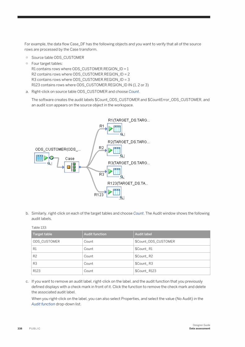
For example, the data flow Case_DF has the following objects and you want to verify that all of the source rows are processed by the Case transform.
○ Source table ODS_CUSTOMER○ Four target tables:
R1 contains rows where ODS_CUSTOMER.REGION_ID = 1R2 contains rows where ODS_CUSTOMER.REGION_ID = 2R3 contains rows where ODS_CUSTOMER.REGION_ID = 3R123 contains rows where ODS_CUSTOMER.REGION_ID IN (1, 2 or 3)
a. Right-click on source table ODS_CUSTOMER and choose Count.
The software creates the audit labels $Count_ODS_CUSTOMER and $CountError_ODS_CUSTOMER, and an audit icon appears on the source object in the workspace.
b. Similarly, right-click on each of the target tables and choose Count. The Audit window shows the following
audit labels.
Table 133:
Target table Audit function Audit label
ODS_CUSTOMER Count $Count_ODS_CUSTOMER
R1 Count $Count_ R1
R2 Count $Count_ R2
R3 Count $Count_ R3
R123 Count $Count_ R123
c. If you want to remove an audit label, right-click on the label, and the audit function that you previously defined displays with a check mark in front of it. Click the function to remove the check mark and delete the associated audit label.When you right-click on the label, you can also select Properties, and select the value (No Audit) in the Audit function drop-down list.
338 P U B L I CDesigner Guide
Data assessment
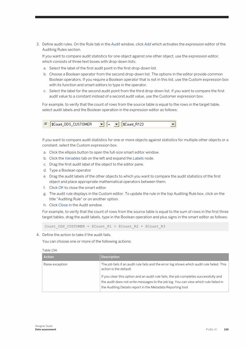
3. Define audit rules. On the Rule tab in the Audit window, click Add which activates the expression editor of the Auditing Rules section.If you want to compare audit statistics for one object against one other object, use the expression editor, which consists of three text boxes with drop-down lists:a. Select the label of the first audit point in the first drop-down list.b. Choose a Boolean operator from the second drop-down list. The options in the editor provide common
Boolean operators. If you require a Boolean operator that is not in this list, use the Custom expression box with its function and smart editors to type in the operator.
c. Select the label for the second audit point from the third drop-down list. If you want to compare the first audit value to a constant instead of a second audit value, use the Customer expression box.
For example, to verify that the count of rows from the source table is equal to the rows in the target table, select audit labels and the Boolean operation in the expression editor as follows:
If you want to compare audit statistics for one or more objects against statistics for multiple other objects or a constant, select the Custom expression box.
a. Click the ellipsis button to open the full-size smart editor window.b. Click the Variables tab on the left and expand the Labels node.c. Drag the first audit label of the object to the editor pane.d. Type a Boolean operatore. Drag the audit labels of the other objects to which you want to compare the audit statistics of the first
object and place appropriate mathematical operators between them.f. Click OK to close the smart editor.g. The audit rule displays in the Custom editor. To update the rule in the top Auditing Rule box, click on the
title "Auditing Rule" or on another option.h. Click Close in the Audit window.
For example, to verify that the count of rows from the source table is equal to the sum of rows in the first three target tables, drag the audit labels, type in the Boolean operation and plus signs in the smart editor as follows:
Count_ODS_CUSTOMER = $Count_R1 + $Count_R2 + $Count_R3
4. Define the action to take if the audit fails.You can choose one or more of the following actions:
Table 134:
Action Description
Raise exception The job fails if an audit rule fails and the error log shows which audit rule failed. This action is the default.
If you clear this option and an audit rule fails, the job completes successfully and the audit does not write messages to the job log. You can view which rule failed in the Auditing Details report in the Metadata Reporting tool.
Designer GuideData assessment P U B L I C 339
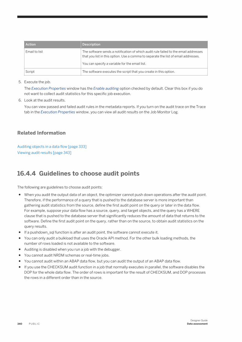
Action Description
Email to list The software sends a notification of which audit rule failed to the email addresses that you list in this option. Use a comma to separate the list of email addresses.
You can specify a variable for the email list.
Script The software executes the script that you create in this option.
5. Execute the job.The Execution Properties window has the Enable auditing option checked by default. Clear this box if you do not want to collect audit statistics for this specific job execution.
6. Look at the audit results.You can view passed and failed audit rules in the metadata reports. If you turn on the audit trace on the Trace tab in the Execution Properties window, you can view all audit results on the Job Monitor Log.
Related Information
Auditing objects in a data flow [page 333]Viewing audit results [page 343]
16.4.4 Guidelines to choose audit points
The following are guidelines to choose audit points:
● When you audit the output data of an object, the optimizer cannot push down operations after the audit point. Therefore, if the performance of a query that is pushed to the database server is more important than gathering audit statistics from the source, define the first audit point on the query or later in the data flow.For example, suppose your data flow has a source, query, and target objects, and the query has a WHERE clause that is pushed to the database server that significantly reduces the amount of data that returns to the software. Define the first audit point on the query, rather than on the source, to obtain audit statistics on the query results.
● If a pushdown_sql function is after an audit point, the software cannot execute it.● You can only audit a bulkload that uses the Oracle API method. For the other bulk loading methods, the
number of rows loaded is not available to the software.● Auditing is disabled when you run a job with the debugger.● You cannot audit NRDM schemas or real-time jobs.● You cannot audit within an ABAP data flow, but you can audit the output of an ABAP data flow.● If you use the CHECKSUM audit function in a job that normally executes in parallel, the software disables the
DOP for the whole data flow. The order of rows is important for the result of CHECKSUM, and DOP processes the rows in a different order than in the source.
340 P U B L I CDesigner Guide
Data assessment
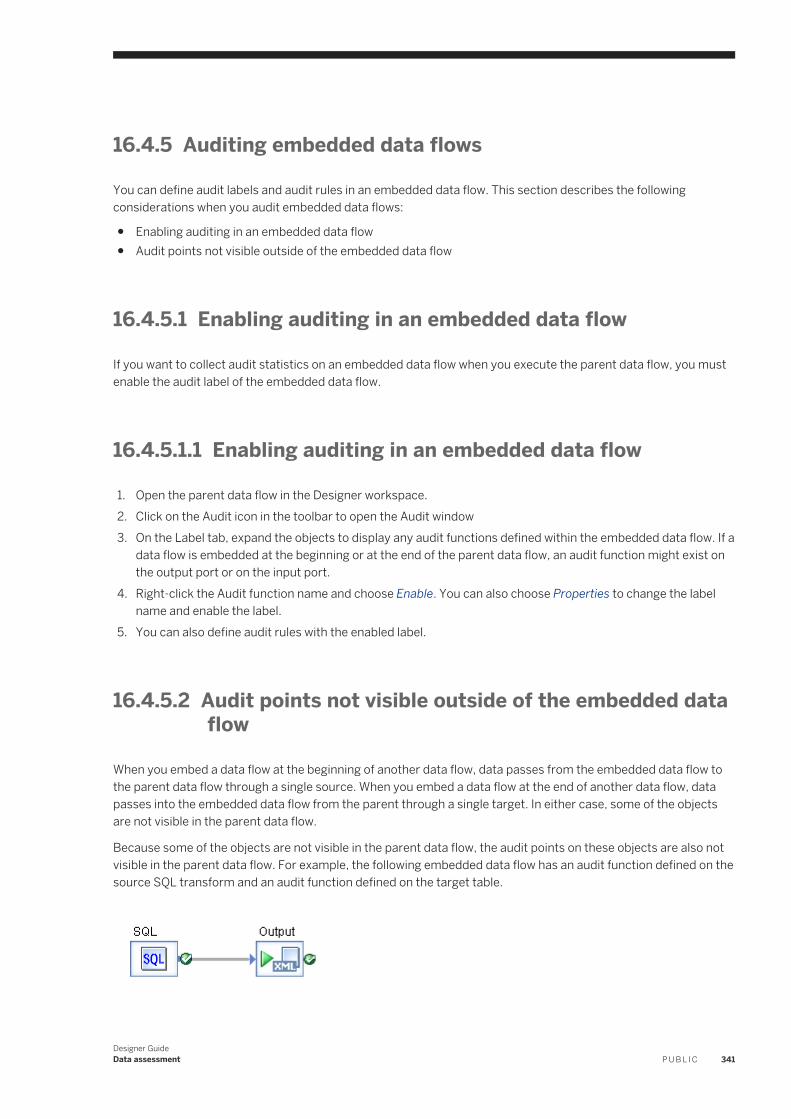
16.4.5 Auditing embedded data flows
You can define audit labels and audit rules in an embedded data flow. This section describes the following considerations when you audit embedded data flows:
● Enabling auditing in an embedded data flow● Audit points not visible outside of the embedded data flow
16.4.5.1 Enabling auditing in an embedded data flow
If you want to collect audit statistics on an embedded data flow when you execute the parent data flow, you must enable the audit label of the embedded data flow.
16.4.5.1.1 Enabling auditing in an embedded data flow
1. Open the parent data flow in the Designer workspace.2. Click on the Audit icon in the toolbar to open the Audit window3. On the Label tab, expand the objects to display any audit functions defined within the embedded data flow. If a
data flow is embedded at the beginning or at the end of the parent data flow, an audit function might exist on the output port or on the input port.
4. Right-click the Audit function name and choose Enable. You can also choose Properties to change the label name and enable the label.
5. You can also define audit rules with the enabled label.
16.4.5.2 Audit points not visible outside of the embedded data flow
When you embed a data flow at the beginning of another data flow, data passes from the embedded data flow to the parent data flow through a single source. When you embed a data flow at the end of another data flow, data passes into the embedded data flow from the parent through a single target. In either case, some of the objects are not visible in the parent data flow.
Because some of the objects are not visible in the parent data flow, the audit points on these objects are also not visible in the parent data flow. For example, the following embedded data flow has an audit function defined on the source SQL transform and an audit function defined on the target table.
Designer GuideData assessment P U B L I C 341
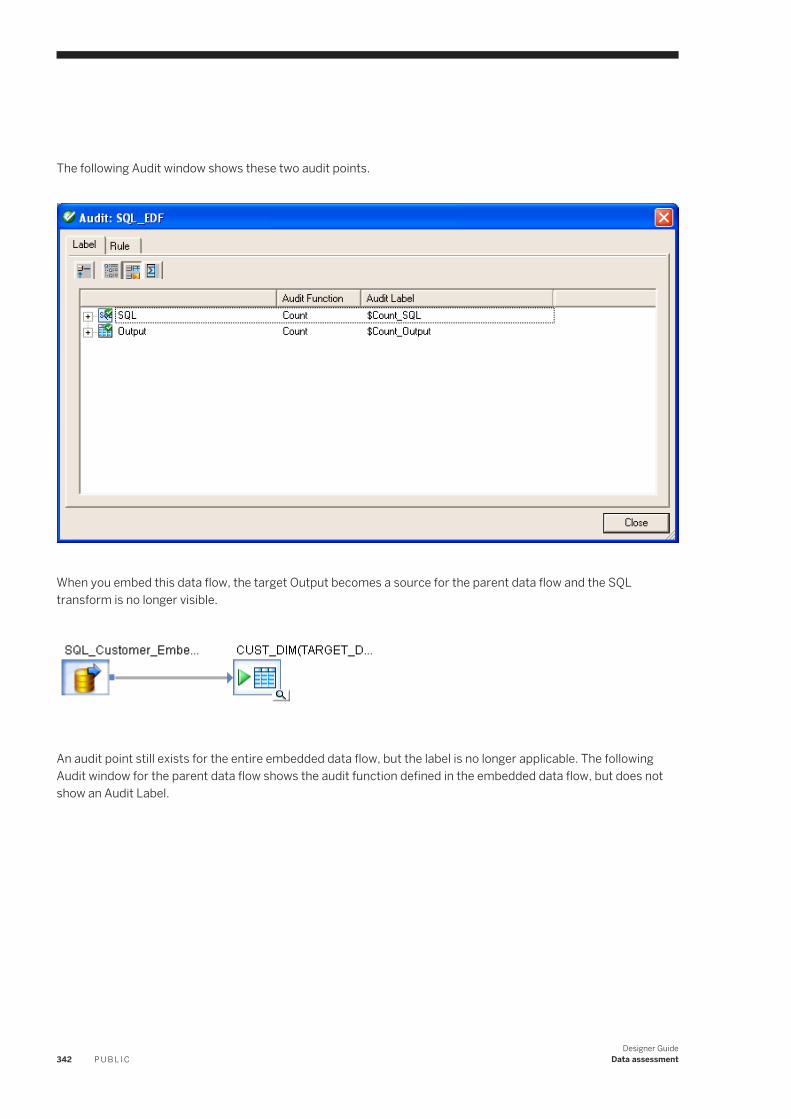
The following Audit window shows these two audit points.
When you embed this data flow, the target Output becomes a source for the parent data flow and the SQL transform is no longer visible.
An audit point still exists for the entire embedded data flow, but the label is no longer applicable. The following Audit window for the parent data flow shows the audit function defined in the embedded data flow, but does not show an Audit Label.
342 P U B L I CDesigner Guide
Data assessment
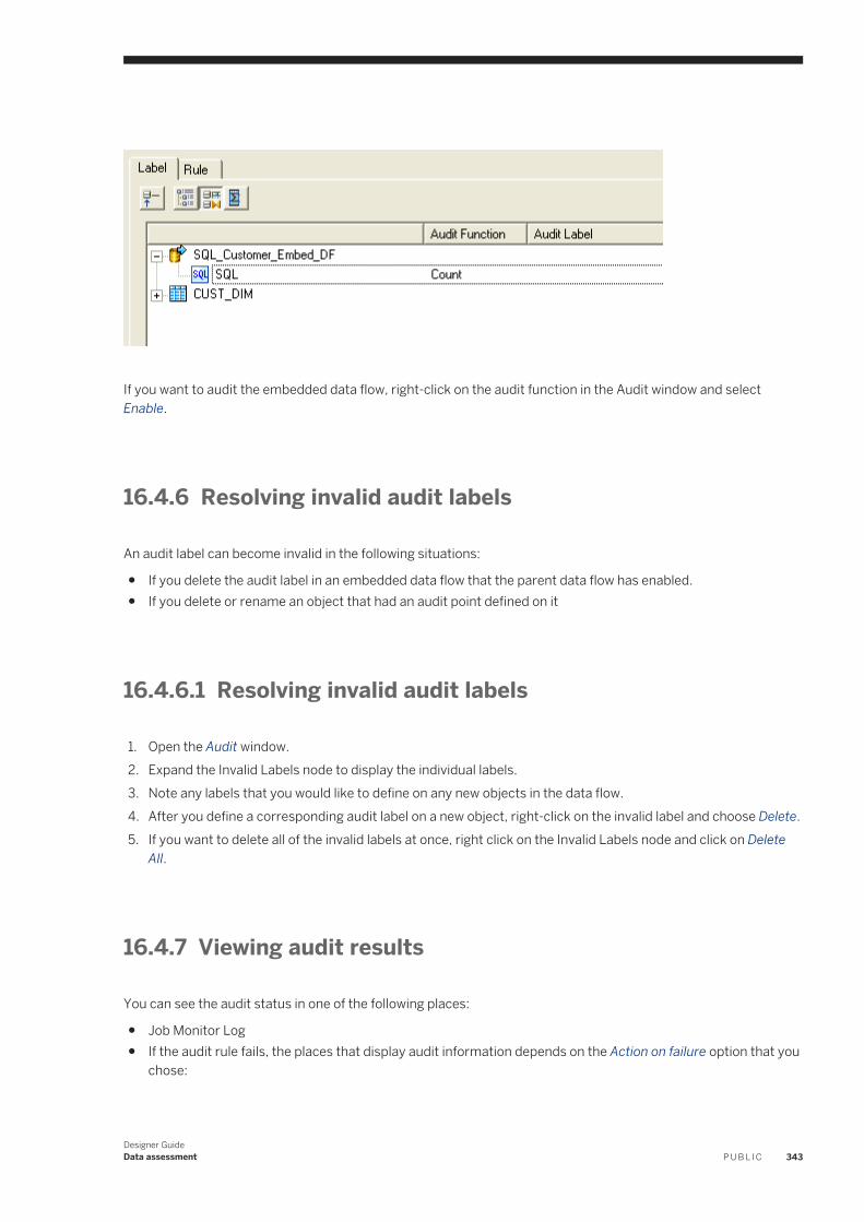
If you want to audit the embedded data flow, right-click on the audit function in the Audit window and select Enable.
16.4.6 Resolving invalid audit labels
An audit label can become invalid in the following situations:
● If you delete the audit label in an embedded data flow that the parent data flow has enabled.● If you delete or rename an object that had an audit point defined on it
16.4.6.1 Resolving invalid audit labels
1. Open the Audit window.2. Expand the Invalid Labels node to display the individual labels.3. Note any labels that you would like to define on any new objects in the data flow.4. After you define a corresponding audit label on a new object, right-click on the invalid label and choose Delete.5. If you want to delete all of the invalid labels at once, right click on the Invalid Labels node and click on Delete
All.
16.4.7 Viewing audit results
You can see the audit status in one of the following places:
● Job Monitor Log● If the audit rule fails, the places that display audit information depends on the Action on failure option that you
chose:
Designer GuideData assessment P U B L I C 343
Table 135:
Action on failure Places where you can view audit information
Raise exception Job Error Log, Metadata Reports
Email to list Email message, Metadata Reports
Script Wherever the custom script sends the audit messages, Metadata Reports
Related Information
Job Monitor Log [page 344]Job Error Log [page 344]Metadata Reports [page 345]
16.4.7.1 Job Monitor Log
If you set Audit Trace to Yes on the Trace tab in the Execution Properties window, audit messages appear in the Job Monitor Log. You can see messages for audit rules that passed and failed.
The following sample audit success messages appear in the Job Monitor Log when Audit Trace is set to Yes:
Audit Label $Count_R2 = 4. Data flow <Case_DF>. Audit Label $CountError_R2 = 0. Data flow <Case_DF>.Audit Label $Count_R3 = 3. Data flow <Case_DF>.Audit Label $CountError_R3 = 0. Data flow <Case_DF>.Audit Label $Count_R123 = 12. Data flow <Case_DF>.Audit Label $CountError_R123 = 0. Data flow <Case_DF>.Audit Label $Count_R1 = 5. Data flow <Case_DF>.Audit Label $CountError_R1 = 0. Data flow <Case_DF>.Audit Label $Count_ODS_CUSTOMER = 12. Data flow <Case_DF>.Audit Label $CountError_ODS_CUSTOMER = 0. Data flow <Case_DF>.Audit Rule passed ($Count_ODS_CUSTOMER = (($CountR1 + $CountR2 + $Count_R3)): LHS=12, RHS=12. Data flow <Case_DF>.Audit Rule passed ($Count_ODS_CUSTOMER = $CountR123): LHS=12, RHS=12. Data flow <Case_DF>.
16.4.7.2 Job Error Log
When you choose the Raise exception option and an audit rule fails, the Job Error Log shows the rule that failed. The following sample message appears in the Job Error Log:
Audit rule failed <($Count_ODS_CUSTOMER = $CountR1)> for <Data flow Case_DF>.
344 P U B L I CDesigner Guide
Data assessment
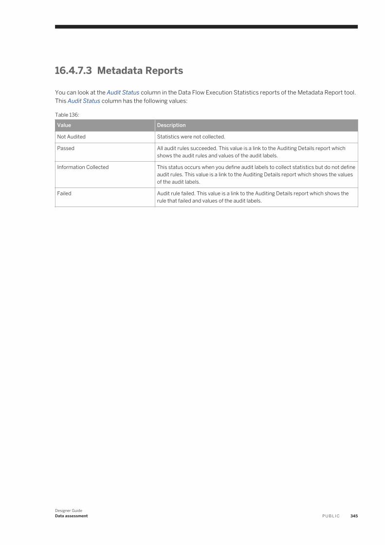
16.4.7.3 Metadata Reports
You can look at the Audit Status column in the Data Flow Execution Statistics reports of the Metadata Report tool. This Audit Status column has the following values:
Table 136:
Value Description
Not Audited Statistics were not collected.
Passed All audit rules succeeded. This value is a link to the Auditing Details report which shows the audit rules and values of the audit labels.
Information Collected This status occurs when you define audit labels to collect statistics but do not define audit rules. This value is a link to the Auditing Details report which shows the values of the audit labels.
Failed Audit rule failed. This value is a link to the Auditing Details report which shows the rule that failed and values of the audit labels.
Designer GuideData assessment P U B L I C 345
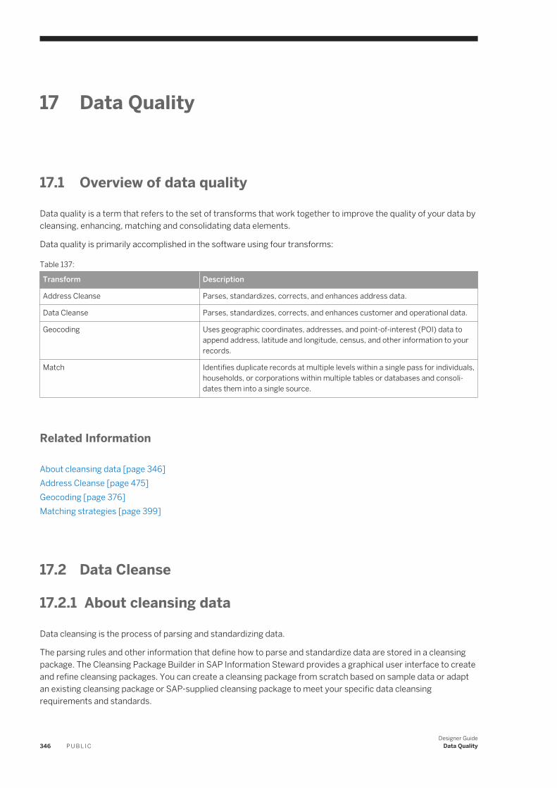
17 Data Quality
17.1 Overview of data quality
Data quality is a term that refers to the set of transforms that work together to improve the quality of your data by cleansing, enhancing, matching and consolidating data elements.
Data quality is primarily accomplished in the software using four transforms:
Table 137:
Transform Description
Address Cleanse Parses, standardizes, corrects, and enhances address data.
Data Cleanse Parses, standardizes, corrects, and enhances customer and operational data.
Geocoding Uses geographic coordinates, addresses, and point-of-interest (POI) data to append address, latitude and longitude, census, and other information to your records.
Match Identifies duplicate records at multiple levels within a single pass for individuals, households, or corporations within multiple tables or databases and consolidates them into a single source.
Related Information
About cleansing data [page 346]Address Cleanse [page 475]Geocoding [page 376]Matching strategies [page 399]
17.2 Data Cleanse
17.2.1 About cleansing data
Data cleansing is the process of parsing and standardizing data.
The parsing rules and other information that define how to parse and standardize data are stored in a cleansing package. The Cleansing Package Builder in SAP Information Steward provides a graphical user interface to create and refine cleansing packages. You can create a cleansing package from scratch based on sample data or adapt an existing cleansing package or SAP-supplied cleansing package to meet your specific data cleansing requirements and standards.
346 P U B L I CDesigner Guide
Data Quality
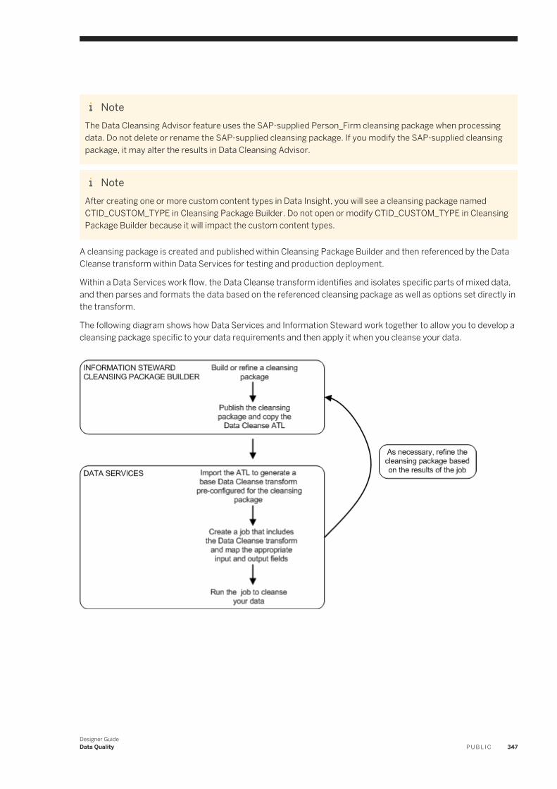
NoteThe Data Cleansing Advisor feature uses the SAP-supplied Person_Firm cleansing package when processing data. Do not delete or rename the SAP-supplied cleansing package. If you modify the SAP-supplied cleansing package, it may alter the results in Data Cleansing Advisor.
NoteAfter creating one or more custom content types in Data Insight, you will see a cleansing package named CTID_CUSTOM_TYPE in Cleansing Package Builder. Do not open or modify CTID_CUSTOM_TYPE in Cleansing Package Builder because it will impact the custom content types.
A cleansing package is created and published within Cleansing Package Builder and then referenced by the Data Cleanse transform within Data Services for testing and production deployment.
Within a Data Services work flow, the Data Cleanse transform identifies and isolates specific parts of mixed data, and then parses and formats the data based on the referenced cleansing package as well as options set directly in the transform.
The following diagram shows how Data Services and Information Steward work together to allow you to develop a cleansing package specific to your data requirements and then apply it when you cleanse your data.
Designer GuideData Quality P U B L I C 347

17.2.2 Cleansing package lifecycle: develop, deploy and maintain
The process of developing, deploying, and maintaining a cleansing package is the result of action and communication between the Data Services administrator, Data Services tester, and Cleansing Package Builder data steward. The exact roles, responsibilities, and titles vary by organization, but often include the following:
Table 138:
Role Responsibility
Cleansing Package Builder data steward
Uses Cleansing Package Builder and has domain knowledge to develop and refine a cleansing package for a specific data domain.
Data Services tester Uses the Data Services transform in a Data Services test environment to cleanse data. Sends results to the Cleansing Package Builder data steward for verification and refinement.
Data Services administrator Uses the Data Cleanse transform in a Data Services production environment to cleanse data based on the rules and standards defined in the selected cleansing package.
There are typically three iterative phases in a cleansing package workflow: Create and test (develop), deploy, and maintain.
348 P U B L I CDesigner Guide
Data Quality
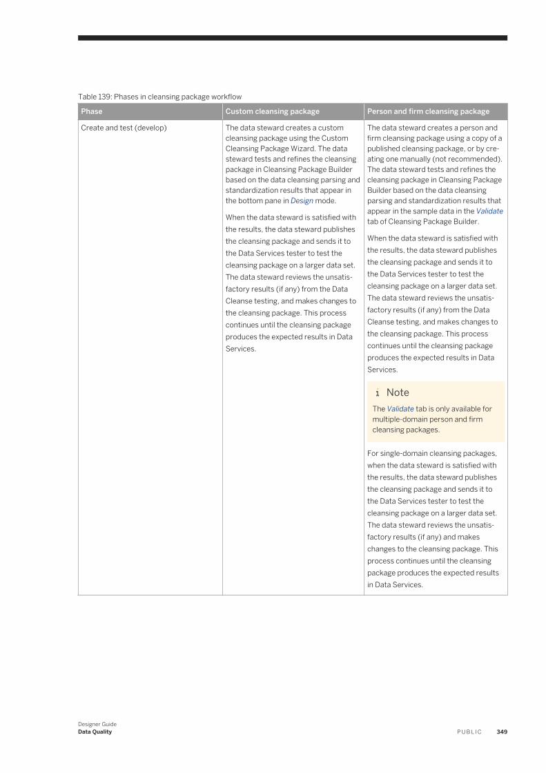
Table 139: Phases in cleansing package workflow
Phase Custom cleansing package Person and firm cleansing package
Create and test (develop) The data steward creates a custom cleansing package using the Custom Cleansing Package Wizard. The data steward tests and refines the cleansing package in Cleansing Package Builder based on the data cleansing parsing and standardization results that appear in the bottom pane in Design mode.
When the data steward is satisfied with the results, the data steward publishes the cleansing package and sends it to the Data Services tester to test the cleansing package on a larger data set. The data steward reviews the unsatisfactory results (if any) from the Data Cleanse testing, and makes changes to the cleansing package. This process continues until the cleansing package produces the expected results in Data Services.
The data steward creates a person and firm cleansing package using a copy of a published cleansing package, or by creating one manually (not recommended). The data steward tests and refines the cleansing package in Cleansing Package Builder based on the data cleansing parsing and standardization results that appear in the sample data in the Validate tab of Cleansing Package Builder.
When the data steward is satisfied with the results, the data steward publishes the cleansing package and sends it to the Data Services tester to test the cleansing package on a larger data set. The data steward reviews the unsatisfactory results (if any) from the Data Cleanse testing, and makes changes to the cleansing package. This process continues until the cleansing package produces the expected results in Data Services.
NoteThe Validate tab is only available for multiple-domain person and firm cleansing packages.
For single-domain cleansing packages, when the data steward is satisfied with the results, the data steward publishes the cleansing package and sends it to the Data Services tester to test the cleansing package on a larger data set. The data steward reviews the unsatisfactory results (if any) and makes changes to the cleansing package. This process continues until the cleansing package produces the expected results in Data Services.
Designer GuideData Quality P U B L I C 349
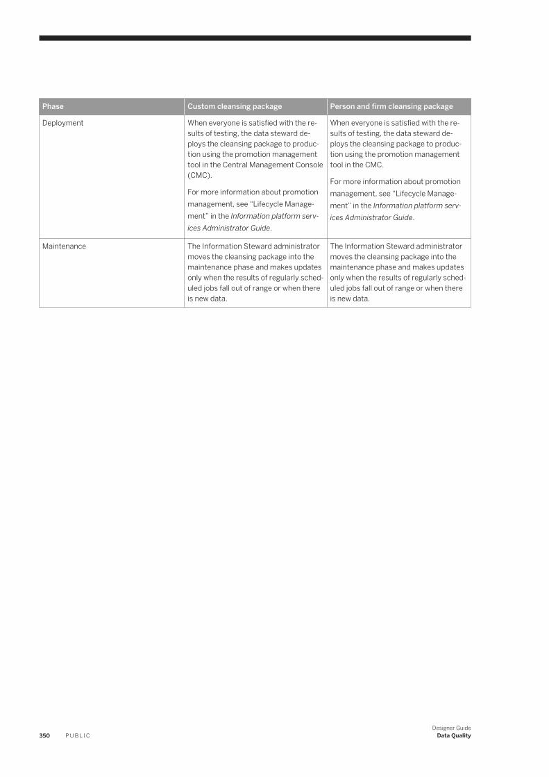
Phase Custom cleansing package Person and firm cleansing package
Deployment When everyone is satisfied with the results of testing, the data steward deploys the cleansing package to production using the promotion management tool in the Central Management Console (CMC).
For more information about promotion management, see “Lifecycle Management” in the Information platform services Administrator Guide.
When everyone is satisfied with the results of testing, the data steward deploys the cleansing package to production using the promotion management tool in the CMC.
For more information about promotion management, see “Lifecycle Management” in the Information platform services Administrator Guide.
Maintenance The Information Steward administrator moves the cleansing package into the maintenance phase and makes updates only when the results of regularly scheduled jobs fall out of range or when there is new data.
The Information Steward administrator moves the cleansing package into the maintenance phase and makes updates only when the results of regularly scheduled jobs fall out of range or when there is new data.
350 P U B L I CDesigner Guide
Data Quality
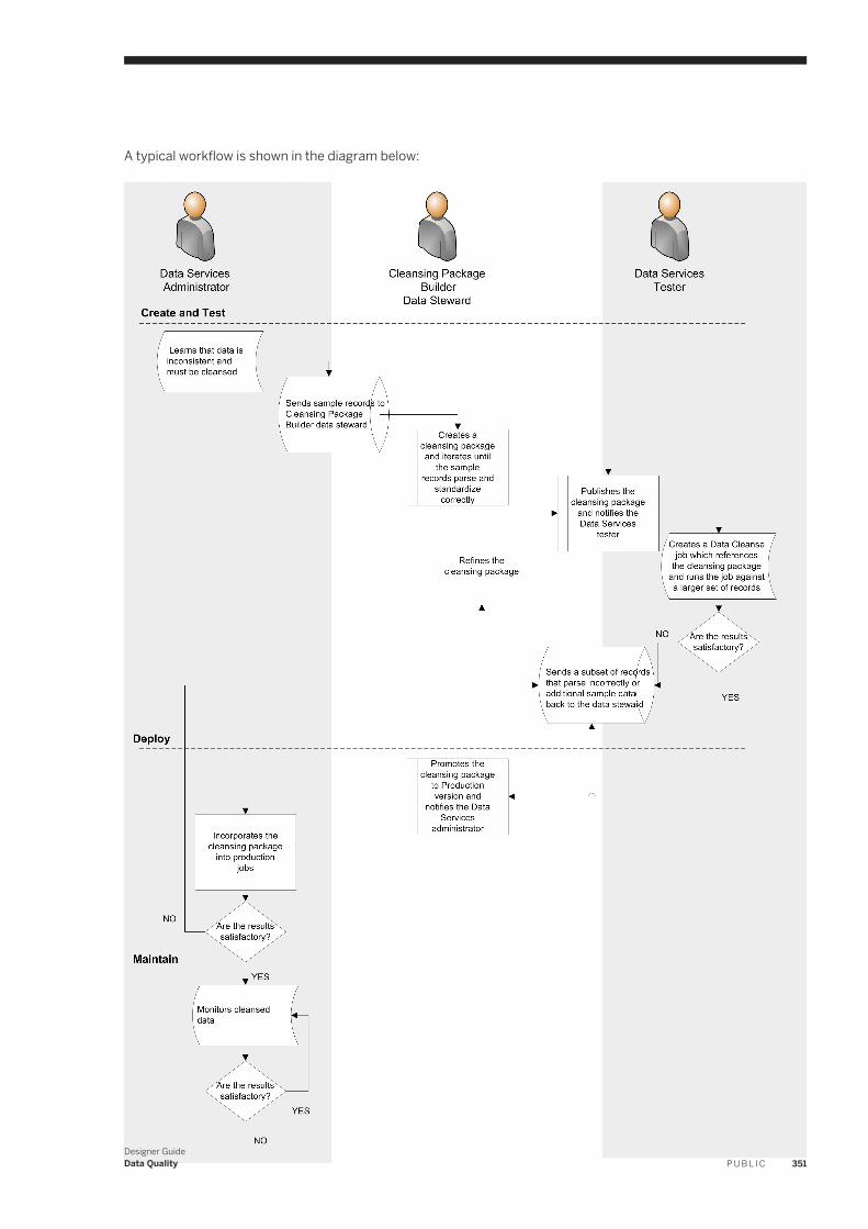
A typical workflow is shown in the diagram below:
Designer GuideData Quality P U B L I C 351
For more information about the process of moving a cleansing package from development to production to maintenance, see the Information Steward Administrator Guide.
For more information about how to use the promotion management tool in the Central Management Console (CMC) to move cleansing packages (referred to as promoting “Objects” or “InfoObjects”), see the Business Intelligence platform Administrator Guide.
17.2.3 Configuring the Data Cleanse transform
Prerequisites for configuring the Data Cleanse transform include:
● Access to the necessary cleansing package.● Access to the ATL file transferred from Cleansing Package Builder.● Input field and attribute (output field) mapping information for user-defined pattern matching rules defined in
the Reference Data tab of Cleansing Package Builder.
To configure the Data Cleanse transform:
1. Import the ATL file transferred from Cleansing Package Builder.Importing the ATL file brings the required information and automatically sets the following options:○ Cleansing Package○ Filter Output Fields○ Input Word Breaker○ Parser Configuration
NoteYou can install and use SAP-supplied person and firm cleansing package without modifications directly in Data Services. To do so, skip step 1 and manually set any required options in the Data Cleanse transform.
2. In the input schema, select the input fields that you want to map and drag them to the appropriate fields in the Input tab.○ Name and firm data can be mapped either to discrete fields or multiline fields.○ Custom data must be mapped to multiline fields.○ Phone, date, email, Social Security number, and user-defined pattern data can be mapped either to
discrete fields or multiline fields. The corresponding parser must be enabled.3. In the Options tab, select the appropriate option values to determine how Data Cleanse will process your data.
If you change an option value from its default value, a green triangle appears next to the option name to indicate that the value has been changed.
The ATL file that you imported in step 1 sets certain options based on information in the cleansing package.4. In the Output tab, select the fields that you want to output from the transform. In Cleansing Package Builder,
output fields are referred to as attributes.Ensure that you map any attributes (output fields) defined in user-defined patterns in Cleansing Package Builder reference data.
352 P U B L I CDesigner Guide
Data Quality
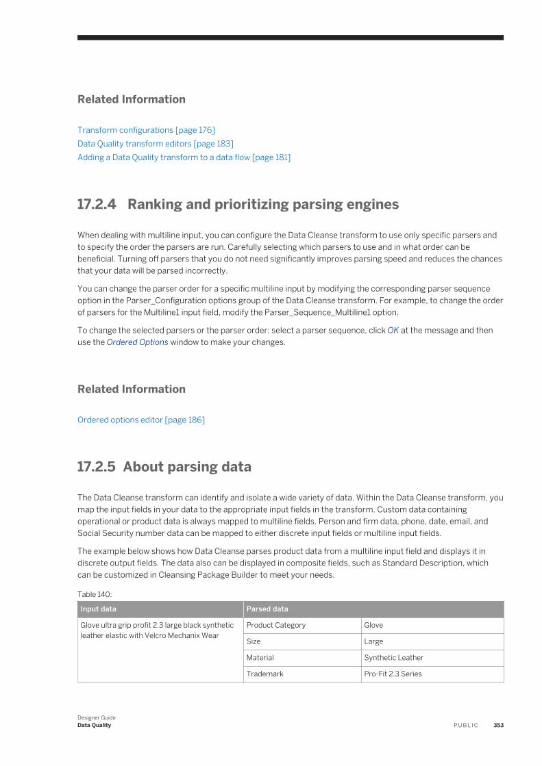
Related Information
Transform configurations [page 176]Data Quality transform editors [page 183]Adding a Data Quality transform to a data flow [page 181]
17.2.4 Ranking and prioritizing parsing engines
When dealing with multiline input, you can configure the Data Cleanse transform to use only specific parsers and to specify the order the parsers are run. Carefully selecting which parsers to use and in what order can be beneficial. Turning off parsers that you do not need significantly improves parsing speed and reduces the chances that your data will be parsed incorrectly.
You can change the parser order for a specific multiline input by modifying the corresponding parser sequence option in the Parser_Configuration options group of the Data Cleanse transform. For example, to change the order of parsers for the Multiline1 input field, modify the Parser_Sequence_Multiline1 option.
To change the selected parsers or the parser order: select a parser sequence, click OK at the message and then use the Ordered Options window to make your changes.
Related Information
Ordered options editor [page 186]
17.2.5 About parsing data
The Data Cleanse transform can identify and isolate a wide variety of data. Within the Data Cleanse transform, you map the input fields in your data to the appropriate input fields in the transform. Custom data containing operational or product data is always mapped to multiline fields. Person and firm data, phone, date, email, and Social Security number data can be mapped to either discrete input fields or multiline input fields.
The example below shows how Data Cleanse parses product data from a multiline input field and displays it in discrete output fields. The data also can be displayed in composite fields, such as Standard Description, which can be customized in Cleansing Package Builder to meet your needs.
Table 140:
Input data Parsed data
Glove ultra grip profit 2.3 large black synthetic leather elastic with Velcro Mechanix Wear
Product Category Glove
Size Large
Material Synthetic Leather
Trademark Pro-Fit 2.3 Series
Designer GuideData Quality P U B L I C 353
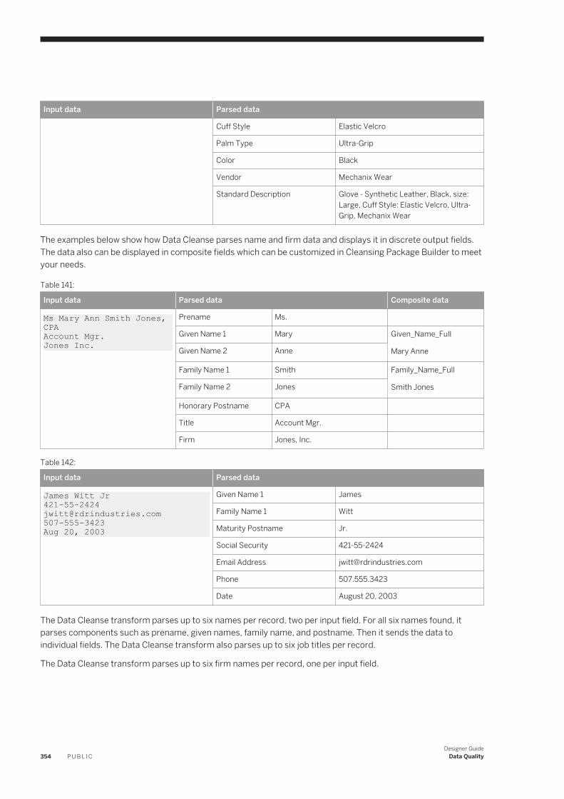
Input data Parsed data
Cuff Style Elastic Velcro
Palm Type Ultra-Grip
Color Black
Vendor Mechanix Wear
Standard Description Glove - Synthetic Leather, Black, size: Large, Cuff Style: Elastic Velcro, Ultra-Grip, Mechanix Wear
The examples below show how Data Cleanse parses name and firm data and displays it in discrete output fields. The data also can be displayed in composite fields which can be customized in Cleansing Package Builder to meet your needs.
Table 141:
Input data Parsed data Composite data
Ms Mary Ann Smith Jones, CPAAccount Mgr.Jones Inc.
Prename Ms.
Given Name 1 Mary Given_Name_Full
Mary AnneGiven Name 2 Anne
Family Name 1 Smith Family_Name_Full
Smith JonesFamily Name 2 Jones
Honorary Postname CPA
Title Account Mgr.
Firm Jones, Inc.
Table 142:
Input data Parsed data
James Witt [email protected] 20, 2003
Given Name 1 James
Family Name 1 Witt
Maturity Postname Jr.
Social Security 421-55-2424
Email Address [email protected]
Phone 507.555.3423
Date August 20, 2003
The Data Cleanse transform parses up to six names per record, two per input field. For all six names found, it parses components such as prename, given names, family name, and postname. Then it sends the data to individual fields. The Data Cleanse transform also parses up to six job titles per record.
The Data Cleanse transform parses up to six firm names per record, one per input field.
354 P U B L I CDesigner Guide
Data Quality
17.2.5.1 About parsing phone numbers
Data Cleanse parses both North American Numbering Plan (NANP) and international phone numbers.
Phone numbering systems differ around the world. When Data Cleanse parses a phone number, it outputs the individual components of the number into the appropriate output fields.
The most efficient parsing happens when the phone number has a valid country code that appears before the phone number. If the country code is not present, or it is not first in the string, Data Cleanse uses other resources to attempt to parse the phone number.
Data Cleanse parses phone numbers by first searching internationally. It uses ISO2 country codes, when available, along with the patterns defined in the cleansing package for each country to identify the country code. If it encounters a country that participates in the NANP, it automatically stops trying to parse the number as international and attempts to parse the phone number as North American, comparing the phone number to commonly used patterns such as (234) 567-8901, 234-567-8901, and 2345678901.
Currently, the participating countries in the NANP include:
● AS - American Samoa● AI - Anquilla● AG - Antiqua and Barbuda● BS- The Bahamas● BB - Barbados● BM - Bermuda● VG - British Virgin Islands● CA - Canada● KY - Cayman islands● DM - Dominica● DO - Dominican Republic● GD - Grenada● GU - Guam● JM - Jamaica● MS - Montserrat● MP - Northern Mariana Islands● PR - Puerto Rico● KN - Saint Kitts and Nevis● LC - Saint Lucia● VC - Saint Vincent and the Grenadines● SX - Saint Maarten● TT - Trinidad and Tobago● TC - Turks and Calcos Islands● US - United States● VI - United States Virgin Islands
Data Cleanse gives you the option for formatting North American numbers on output (such as your choice of delimiters). However, Data Cleanse outputs international numbers as they were input, without any formatting. Also, Data Cleanse does not cross-compare to the address to see whether the country and city codes in the phone number match the address.
Designer GuideData Quality P U B L I C 355
Related Information
About one-to-one mapping [page 364]
17.2.5.1.1 How Data Cleanse parses phone numbers
Set up international phone parsing in the Data Cleanse transform.
You can set up international phone parsing in the Data Cleanse transform at three levels: Record, job file, and global. Data Cleanse attempts to parse phone data in order as explained in the following table. If the transform cannot parse phone data using one of the three levels, it attempts to parse the phone data as a North American phone number. If Data Cleanse encounters a country code that is in the North American Numbering Plan (NANP) at any level, it skips any remaining levels and automatically attempts to parse the number as a North American phone number.
NoteThe country has to be specified in the cleansing package before Data Cleanse attempts to parse using the three levels listed in the following table.
356 P U B L I CDesigner Guide
Data Quality
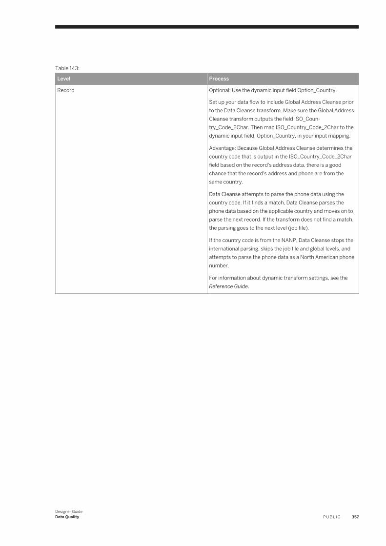
Table 143:
Level Process
Record Optional: Use the dynamic input field Option_Country.
Set up your data flow to include Global Address Cleanse prior to the Data Cleanse transform. Make sure the Global Address Cleanse transform outputs the field ISO_Country_Code_2Char. Then map ISO_Country_Code_2Char to the dynamic input field, Option_Country, in your input mapping.
Advantage: Because Global Address Cleanse determines the country code that is output in the ISO_Country_Code_2Char field based on the record's address data, there is a good chance that the record's address and phone are from the same country.
Data Cleanse attempts to parse the phone data using the country code. If it finds a match, Data Cleanse parses the phone data based on the applicable country and moves on to parse the next record. If the transform does not find a match, the parsing goes to the next level (job file).
If the country code is from the NANP, Data Cleanse stops the international parsing, skips the job file and global levels, and attempts to parse the phone data as a North American phone number.
For information about dynamic transform settings, see the Reference Guide.
Designer GuideData Quality P U B L I C 357
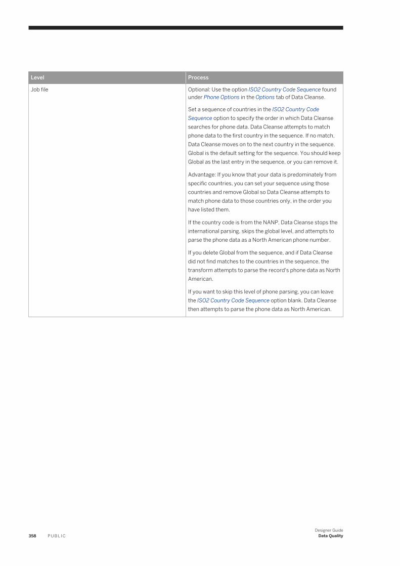
Level Process
Job file Optional: Use the option ISO2 Country Code Sequence found under Phone Options in the Options tab of Data Cleanse.
Set a sequence of countries in the ISO2 Country Code Sequence option to specify the order in which Data Cleanse searches for phone data. Data Cleanse attempts to match phone data to the first country in the sequence. If no match, Data Cleanse moves on to the next country in the sequence. Global is the default setting for the sequence. You should keep Global as the last entry in the sequence, or you can remove it.
Advantage: If you know that your data is predominately from specific countries, you can set your sequence using those countries and remove Global so Data Cleanse attempts to match phone data to those countries only, in the order you have listed them.
If the country code is from the NANP, Data Cleanse stops the international parsing, skips the global level, and attempts to parse the phone data as a North American phone number.
If you delete Global from the sequence, and if Data Cleanse did not find matches to the countries in the sequence, the transform attempts to parse the record's phone data as North American.
If you want to skip this level of phone parsing, you can leave the ISO2 Country Code Sequence option blank. Data Cleanse then attempts to parse the phone data as North American.
358 P U B L I CDesigner Guide
Data Quality
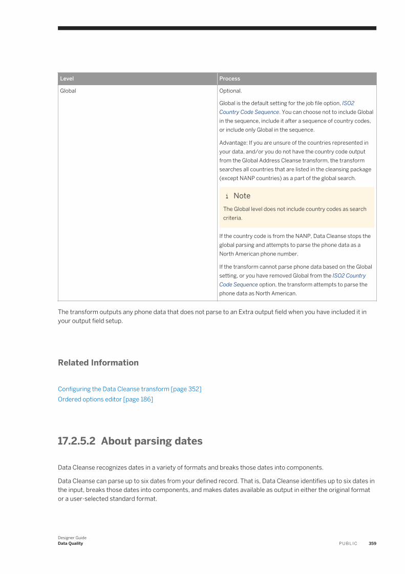
Level Process
Global Optional.
Global is the default setting for the job file option, ISO2 Country Code Sequence. You can choose not to include Global in the sequence, include it after a sequence of country codes, or include only Global in the sequence.
Advantage: If you are unsure of the countries represented in your data, and/or you do not have the country code output from the Global Address Cleanse transform, the transform searches all countries that are listed in the cleansing package (except NANP countries) as a part of the global search.
NoteThe Global level does not include country codes as search criteria.
If the country code is from the NANP, Data Cleanse stops the global parsing and attempts to parse the phone data as a North American phone number.
If the transform cannot parse phone data based on the Global setting, or you have removed Global from the ISO2 Country Code Sequence option, the transform attempts to parse the phone data as North American.
The transform outputs any phone data that does not parse to an Extra output field when you have included it in your output field setup.
Related Information
Configuring the Data Cleanse transform [page 352]Ordered options editor [page 186]
17.2.5.2 About parsing dates
Data Cleanse recognizes dates in a variety of formats and breaks those dates into components.
Data Cleanse can parse up to six dates from your defined record. That is, Data Cleanse identifies up to six dates in the input, breaks those dates into components, and makes dates available as output in either the original format or a user-selected standard format.
Designer GuideData Quality P U B L I C 359
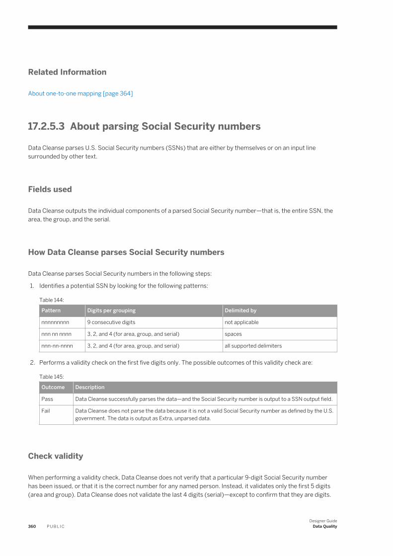
Related Information
About one-to-one mapping [page 364]
17.2.5.3 About parsing Social Security numbers
Data Cleanse parses U.S. Social Security numbers (SSNs) that are either by themselves or on an input line surrounded by other text.
Fields used
Data Cleanse outputs the individual components of a parsed Social Security number—that is, the entire SSN, the area, the group, and the serial.
How Data Cleanse parses Social Security numbers
Data Cleanse parses Social Security numbers in the following steps:
1. Identifies a potential SSN by looking for the following patterns:
Table 144:
Pattern Digits per grouping Delimited by
nnnnnnnnn 9 consecutive digits not applicable
nnn nn nnnn 3, 2, and 4 (for area, group, and serial) spaces
nnn-nn-nnnn 3, 2, and 4 (for area, group, and serial) all supported delimiters
2. Performs a validity check on the first five digits only. The possible outcomes of this validity check are:
Table 145:
Outcome Description
Pass Data Cleanse successfully parses the data—and the Social Security number is output to a SSN output field.
Fail Data Cleanse does not parse the data because it is not a valid Social Security number as defined by the U.S. government. The data is output as Extra, unparsed data.
Check validity
When performing a validity check, Data Cleanse does not verify that a particular 9-digit Social Security number has been issued, or that it is the correct number for any named person. Instead, it validates only the first 5 digits (area and group). Data Cleanse does not validate the last 4 digits (serial)—except to confirm that they are digits.
360 P U B L I CDesigner Guide
Data Quality
SSA data
Data Cleanse validates the first five digits based on a table from the Social Security Administration (http://www.socialsecurity.gov/employer/ssns/HGJune2411_final.txt ). The rules and data that guide this check are available at http://www.ssa.gov/history/ssn/geocard.html . The Social Security number information that Data Cleanse references is included in the cleansing package.
NoteThe Social Security administration no longer updates the table. The last time it was updated was in July, 2011. Therefore, Social Security validation performed in Data Cleanse is based on data through July, 2011. For more information about the Social Security Administration's Social Security number assignment process, see http://www.ssa.gov/employer/randomizationfaqs.html .
Outputs valid SSNs
Data Cleanse outputs only Social Security numbers that pass its validation. If an apparent SSN fails validation, Data Cleanse does not pass on the number as a parsed, but invalid, Social Security number.
17.2.5.4 About parsing email addresses
When Data Cleanse parses input data that it determines is an email address, it places the components of that data into specific fields for output. Below is an example of a simple email address:
By identifying the various data components (user name, host, and so on) by their relationships to each other, Data Cleanse can assign the data to specific attributes (output fields).
Output fields Data Cleanse uses
Data Cleanse outputs the individual components of a parsed email address—that is, the email user name, complete domain name, top domain, second domain, third domain, fourth domain, fifth domain, and host name.
What Data Cleanse does
Data Cleanse can take the following actions:
● Parse an email address located either in a discrete field or combined with other data in a multiline field.● Break down the domain name into sub-elements.
Designer GuideData Quality P U B L I C 361
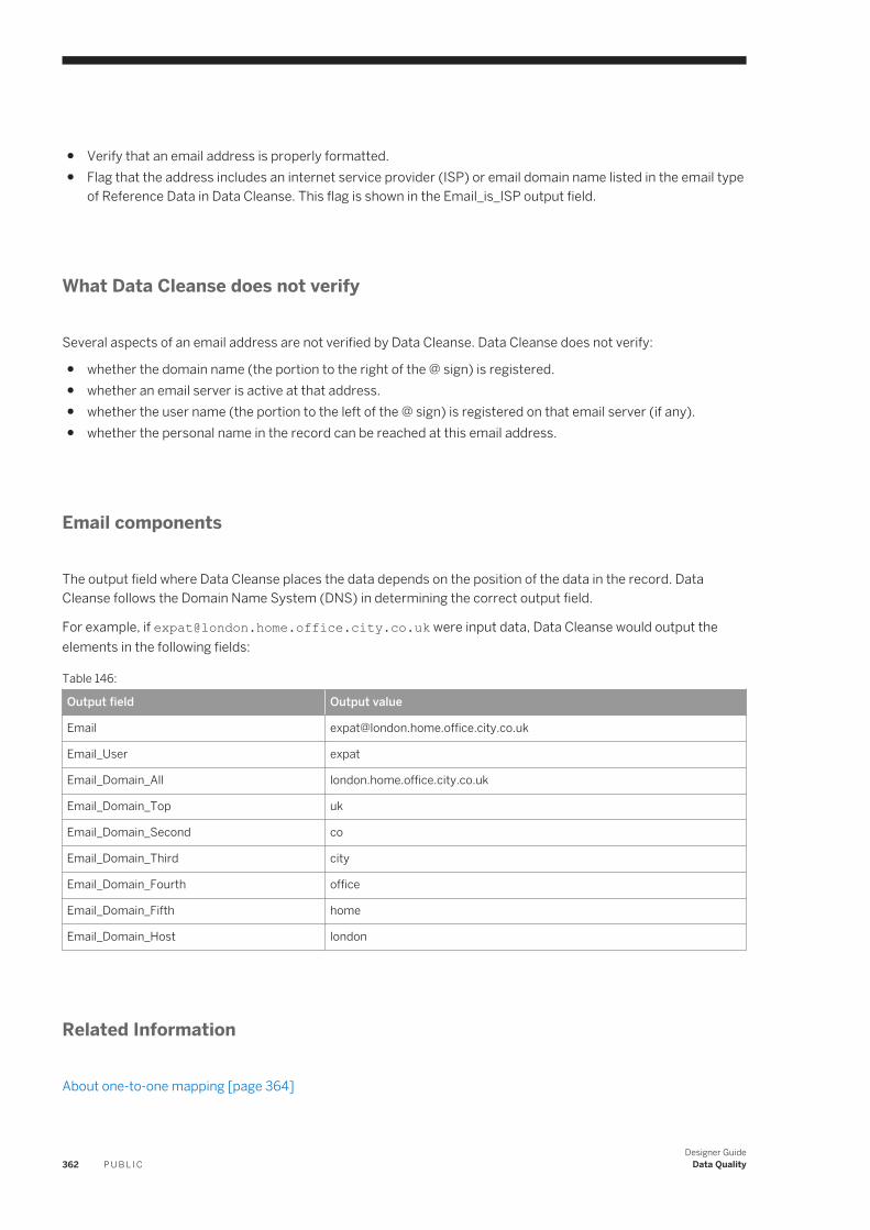
● Verify that an email address is properly formatted.● Flag that the address includes an internet service provider (ISP) or email domain name listed in the email type
of Reference Data in Data Cleanse. This flag is shown in the Email_is_ISP output field.
What Data Cleanse does not verify
Several aspects of an email address are not verified by Data Cleanse. Data Cleanse does not verify:
● whether the domain name (the portion to the right of the @ sign) is registered.● whether an email server is active at that address.● whether the user name (the portion to the left of the @ sign) is registered on that email server (if any).● whether the personal name in the record can be reached at this email address.
Email components
The output field where Data Cleanse places the data depends on the position of the data in the record. Data Cleanse follows the Domain Name System (DNS) in determining the correct output field.
For example, if [email protected] were input data, Data Cleanse would output the elements in the following fields:
Table 146:
Output field Output value
Email [email protected]
Email_User expat
Email_Domain_All london.home.office.city.co.uk
Email_Domain_Top uk
Email_Domain_Second co
Email_Domain_Third city
Email_Domain_Fourth office
Email_Domain_Fifth home
Email_Domain_Host london
Related Information
About one-to-one mapping [page 364]
362 P U B L I CDesigner Guide
Data Quality
17.2.5.5 About parsing user-defined patterns
Data Cleanse can parse patterns found in a wide variety of data such as:
● account numbers● part numbers● purchase orders● invoice numbers● VINs (vehicle identification numbers)● driver license numbers
In other words, Data Cleanse can parse any alphanumeric sequence for which you can define a pattern.
The user-defined pattern matching (UDPM) parser looks for the pattern across each entire field.
Patterns are defined using regular expressions in the Reference Data tab of Cleansing Package Builder. Check with the cleansing package owner to determine any required mappings for input fields and output fields (attributes).
17.2.5.6 About parsing street addresses
Data Cleanse does not identify and parse individual address components. To parse data that contains address information, process it using a Global Address Cleanse or U.S. Regulatory Address Cleanse transform prior to Data Cleanse. If address data is processed by the Data Cleanse transform, it is usually output to the Extra fields.
Related Information
How address cleanse works [page 475]
17.2.5.7 About parsing firm names
Data Cleanse can parse firm data.
Data Cleanse accepts these firm names alone in a field or together with other data.
An exception to how Data Cleanse recombines contiguous word pieces is made for words that end with an S, such as Applebee's or Macy's. An input string of Macy's is broken into three individual tokens: MACY, ', S. Because the last token is an S, Data Cleanse first combines the tokens and looks up the term including the apostrophe (MACY'S). If the term is not found, Data Cleanse looks up the term without the apostrophe (MACYS). If that is not successful, Data Cleanse automatically keeps the tokens together (MACY'S) and adds the FIRM_MISCELLANEOUS classification to the term. Since words ending with S are automatically kept together, it is not necessary to add all possessive firm names to the dictionary.
Designer GuideData Quality P U B L I C 363
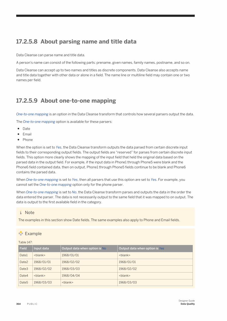
17.2.5.8 About parsing name and title data
Data Cleanse can parse name and title data.
A person's name can consist of the following parts: prename, given names, family names, postname, and so on.
Data Cleanse can accept up to two names and titles as discrete components. Data Cleanse also accepts name and title data together with other data or alone in a field. The name line or multiline field may contain one or two names per field.
17.2.5.9 About one-to-one mapping
One-to-one mapping is an option in the Data Cleanse transform that controls how several parsers output the data.
The One-to-one mapping option is available for these parsers:
● Date● Email● Phone
When the option is set to Yes, the Data Cleanse transform outputs the data parsed from certain discrete input fields to their corresponding output fields. The output fields are “reserved” for parses from certain discrete input fields. This option more clearly shows the mapping of the input field that held the original data based on the parsed data in the output field. For example, if the input data in Phone1 through Phone5 were blank and the Phone6 field contained data, then on output, Phone1 through Phone5 fields continue to be blank and Phone6 contains the parsed data.
When One-to-one mapping is set to Yes, then all parsers that use this option are set to Yes. For example, you cannot set the One-to-one mapping option only for the phone parser.
When One-to-one mapping is set to No, the Data Cleanse transform parses and outputs the data in the order the data entered the parser. The data is not necessarily output to the same field that it was mapped to on output. The data is output to the first available field in the category.
NoteThe examples in this section show Date fields. The same examples also apply to Phone and Email fields.
Example
Table 147:
Field Input data Output data when option is No Output data when option is Yes
Date1 <blank> 1968/01/01 <blank>
Date2 1968/01/01 1968/02/02 1968/01/01
Date3 1968/02/02 1968/03/03 1968/02/02
Date4 <blank> 1968/04/04 <blank>
Date5 1968/03/03 <blank> 1968/03/03
364 P U B L I CDesigner Guide
Data Quality
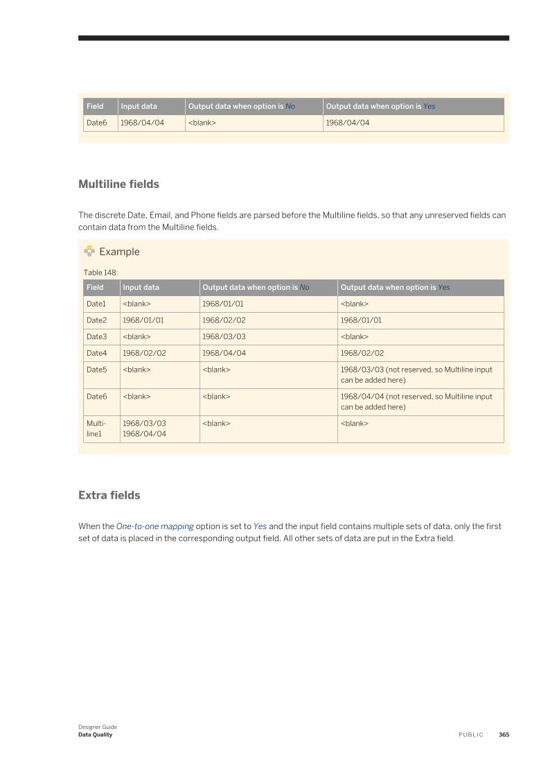
Field Input data Output data when option is No Output data when option is Yes
Date6 1968/04/04 <blank> 1968/04/04
Multiline fields
The discrete Date, Email, and Phone fields are parsed before the Multiline fields, so that any unreserved fields can contain data from the Multiline fields.
Example
Table 148:
Field Input data Output data when option is No Output data when option is Yes
Date1 <blank> 1968/01/01 <blank>
Date2 1968/01/01 1968/02/02 1968/01/01
Date3 <blank> 1968/03/03 <blank>
Date4 1968/02/02 1968/04/04 1968/02/02
Date5 <blank> <blank> 1968/03/03 (not reserved, so Multiline input can be added here)
Date6 <blank> <blank> 1968/04/04 (not reserved, so Multiline input can be added here)
Multiline1
1968/03/03 1968/04/04
<blank> <blank>
Extra fields
When the One-to-one mapping option is set to Yes and the input field contains multiple sets of data, only the first set of data is placed in the corresponding output field. All other sets of data are put in the Extra field.
Designer GuideData Quality P U B L I C 365
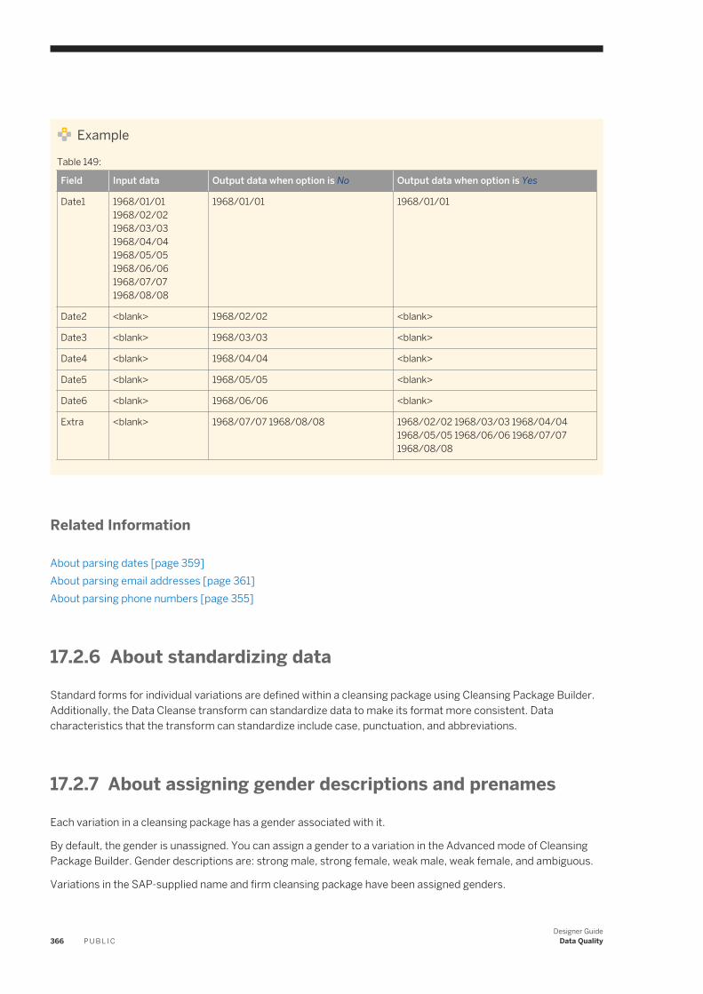
Example
Table 149:
Field Input data Output data when option is No Output data when option is Yes
Date1 1968/01/01 1968/02/02 1968/03/03 1968/04/04 1968/05/05 1968/06/06 1968/07/07 1968/08/08
1968/01/01 1968/01/01
Date2 <blank> 1968/02/02 <blank>
Date3 <blank> 1968/03/03 <blank>
Date4 <blank> 1968/04/04 <blank>
Date5 <blank> 1968/05/05 <blank>
Date6 <blank> 1968/06/06 <blank>
Extra <blank> 1968/07/07 1968/08/08 1968/02/02 1968/03/03 1968/04/04 1968/05/05 1968/06/06 1968/07/07 1968/08/08
Related Information
About parsing dates [page 359]About parsing email addresses [page 361]About parsing phone numbers [page 355]
17.2.6 About standardizing data
Standard forms for individual variations are defined within a cleansing package using Cleansing Package Builder. Additionally, the Data Cleanse transform can standardize data to make its format more consistent. Data characteristics that the transform can standardize include case, punctuation, and abbreviations.
17.2.7 About assigning gender descriptions and prenames
Each variation in a cleansing package has a gender associated with it.
By default, the gender is unassigned. You can assign a gender to a variation in the Advanced mode of Cleansing Package Builder. Gender descriptions are: strong male, strong female, weak male, weak female, and ambiguous.
Variations in the SAP-supplied name and firm cleansing package have been assigned genders.
366 P U B L I CDesigner Guide
Data Quality
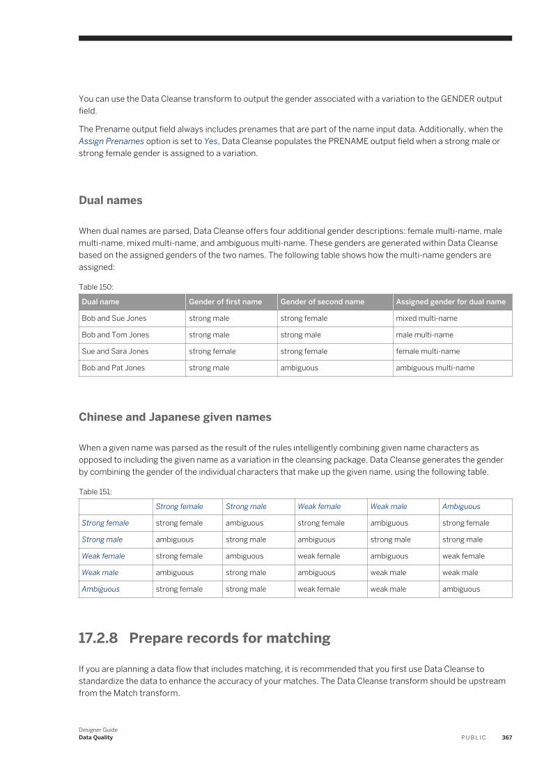
You can use the Data Cleanse transform to output the gender associated with a variation to the GENDER output field.
The Prename output field always includes prenames that are part of the name input data. Additionally, when the Assign Prenames option is set to Yes, Data Cleanse populates the PRENAME output field when a strong male or strong female gender is assigned to a variation.
Dual names
When dual names are parsed, Data Cleanse offers four additional gender descriptions: female multi-name, male multi-name, mixed multi-name, and ambiguous multi-name. These genders are generated within Data Cleanse based on the assigned genders of the two names. The following table shows how the multi-name genders are assigned:
Table 150:
Dual name Gender of first name Gender of second name Assigned gender for dual name
Bob and Sue Jones strong male strong female mixed multi-name
Bob and Tom Jones strong male strong male male multi-name
Sue and Sara Jones strong female strong female female multi-name
Bob and Pat Jones strong male ambiguous ambiguous multi-name
Chinese and Japanese given names
When a given name was parsed as the result of the rules intelligently combining given name characters as opposed to including the given name as a variation in the cleansing package, Data Cleanse generates the gender by combining the gender of the individual characters that make up the given name, using the following table.
Table 151:
Strong female Strong male Weak female Weak male Ambiguous
Strong female strong female ambiguous strong female ambiguous strong female
Strong male ambiguous strong male ambiguous strong male strong male
Weak female strong female ambiguous weak female ambiguous weak female
Weak male ambiguous strong male ambiguous weak male weak male
Ambiguous strong female strong male weak female weak male ambiguous
17.2.8 Prepare records for matching
If you are planning a data flow that includes matching, it is recommended that you first use Data Cleanse to standardize the data to enhance the accuracy of your matches. The Data Cleanse transform should be upstream from the Match transform.
Designer GuideData Quality P U B L I C 367
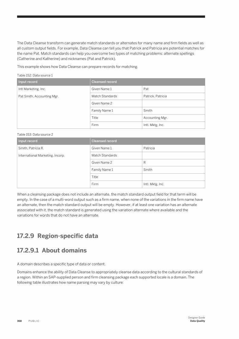
The Data Cleanse transform can generate match standards or alternates for many name and firm fields as well as all custom output fields. For example, Data Cleanse can tell you that Patrick and Patricia are potential matches for the name Pat. Match standards can help you overcome two types of matching problems: alternate spellings (Catherine and Katherine) and nicknames (Pat and Patrick).
This example shows how Data Cleanse can prepare records for matching.
Table 152: Data source 1
Input record Cleansed record
Intl Marketing, Inc.
Pat Smith, Accounting Mgr.
Given Name 1 Pat
Match Standards Patrick, Patricia
Given Name 2
Family Name 1 Smith
Title Accounting Mgr.
Firm Intl. Mktg, Inc.
Table 153: Data source 2
Input record Cleansed record
Smith, Patricia R.
International Marketing, Incorp.
Given Name 1 Patricia
Match Standards
Given Name 2 R
Family Name 1 Smith
Title
Firm Intl. Mktg, Inc.
When a cleansing package does not include an alternate, the match standard output field for that term will be empty. In the case of a multi-word output such as a firm name, when none of the variations in the firm name have an alternate, then the match standard output will be empty. However, if at least one variation has an alternate associated with it, the match standard is generated using the variation alternate where available and the variations for words that do not have an alternate.
17.2.9 Region-specific data
17.2.9.1 About domains
A domain describes a specific type of data or content.
Domains enhance the ability of Data Cleanse to appropriately cleanse data according to the cultural standards of a region. Within an SAP-supplied person and firm cleansing package each supported locale is a domain. The following table illustrates how name parsing may vary by culture:
368 P U B L I CDesigner Guide
Data Quality
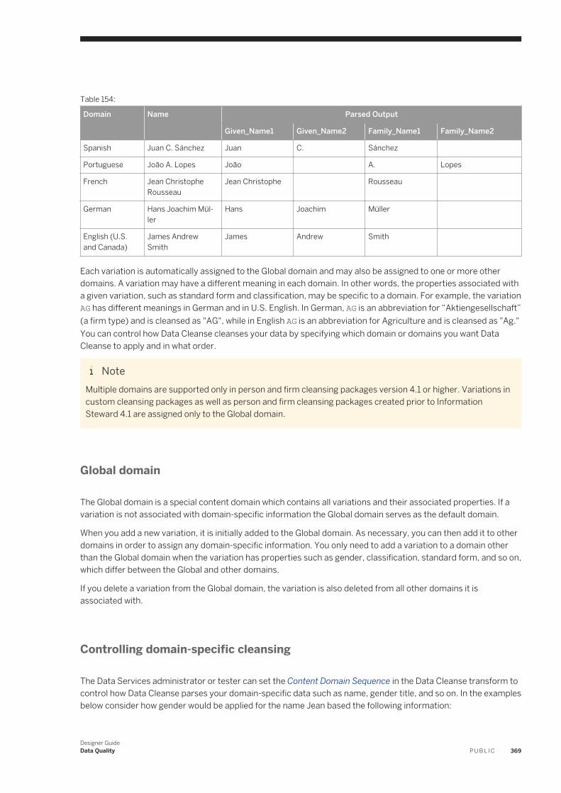
Table 154:
Domain Name Parsed Output
Given_Name1 Given_Name2 Family_Name1 Family_Name2
Spanish Juan C. Sánchez Juan C. Sánchez
Portuguese João A. Lopes João A. Lopes
French Jean Christophe Rousseau
Jean Christophe Rousseau
German Hans Joachim Müller
Hans Joachim Müller
English (U.S. and Canada)
James Andrew Smith
James Andrew Smith
Each variation is automatically assigned to the Global domain and may also be assigned to one or more other domains. A variation may have a different meaning in each domain. In other words, the properties associated with a given variation, such as standard form and classification, may be specific to a domain. For example, the variation AG has different meanings in German and in U.S. English. In German, AG is an abbreviation for “Aktiengesellschaft” (a firm type) and is cleansed as "AG", while in English AG is an abbreviation for Agriculture and is cleansed as "Ag." You can control how Data Cleanse cleanses your data by specifying which domain or domains you want Data Cleanse to apply and in what order.
NoteMultiple domains are supported only in person and firm cleansing packages version 4.1 or higher. Variations in custom cleansing packages as well as person and firm cleansing packages created prior to Information Steward 4.1 are assigned only to the Global domain.
Global domain
The Global domain is a special content domain which contains all variations and their associated properties. If a variation is not associated with domain-specific information the Global domain serves as the default domain.
When you add a new variation, it is initially added to the Global domain. As necessary, you can then add it to other domains in order to assign any domain-specific information. You only need to add a variation to a domain other than the Global domain when the variation has properties such as gender, classification, standard form, and so on, which differ between the Global and other domains.
If you delete a variation from the Global domain, the variation is also deleted from all other domains it is associated with.
Controlling domain-specific cleansing
The Data Services administrator or tester can set the Content Domain Sequence in the Data Cleanse transform to control how Data Cleanse parses your domain-specific data such as name, gender title, and so on. In the examples below consider how gender would be applied for the name Jean based the following information:
Designer GuideData Quality P U B L I C 369
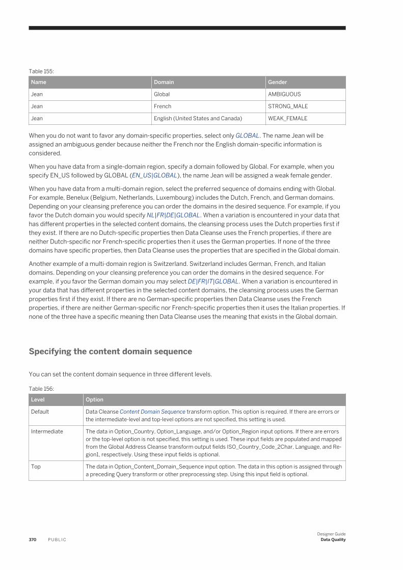
Table 155:
Name Domain Gender
Jean Global AMBIGUOUS
Jean French STRONG_MALE
Jean English (United States and Canada) WEAK_FEMALE
When you do not want to favor any domain-specific properties, select only GLOBAL. The name Jean will be assigned an ambiguous gender because neither the French nor the English domain-specific information is considered.
When you have data from a single-domain region, specify a domain followed by Global. For example, when you specify EN_US followed by GLOBAL (EN_US|GLOBAL), the name Jean will be assigned a weak female gender.
When you have data from a multi-domain region, select the preferred sequence of domains ending with Global. For example, Benelux (Belgium, Netherlands, Luxembourg) includes the Dutch, French, and German domains. Depending on your cleansing preference you can order the domains in the desired sequence. For example, if you favor the Dutch domain you would specify NL|FR|DE|GLOBAL. When a variation is encountered in your data that has different properties in the selected content domains, the cleansing process uses the Dutch properties first if they exist. If there are no Dutch-specific properties then Data Cleanse uses the French properties, if there are neither Dutch-specific nor French-specific properties then it uses the German properties. If none of the three domains have specific properties, then Data Cleanse uses the properties that are specified in the Global domain.
Another example of a multi-domain region is Switzerland. Switzerland includes German, French, and Italian domains. Depending on your cleansing preference you can order the domains in the desired sequence. For example, if you favor the German domain you may select DE|FR|IT|GLOBAL. When a variation is encountered in your data that has different properties in the selected content domains, the cleansing process uses the German properties first if they exist. If there are no German-specific properties then Data Cleanse uses the French properties, if there are neither German-specific nor French-specific properties then it uses the Italian properties. If none of the three have a specific meaning then Data Cleanse uses the meaning that exists in the Global domain.
Specifying the content domain sequence
You can set the content domain sequence in three different levels.
Table 156:
Level Option
Default Data Cleanse Content Domain Sequence transform option. This option is required. If there are errors or the intermediate-level and top-level options are not specified, this setting is used.
Intermediate The data in Option_Country, Option_Language, and/or Option_Region input options. If there are errors or the top-level option is not specified, this setting is used. These input fields are populated and mapped from the Global Address Cleanse transform output fields ISO_Country_Code_2Char, Language, and Region1, respectively. Using these input fields is optional.
Top The data in Option_Content_Domain_Sequence input option. The data in this option is assigned through a preceding Query transform or other preprocessing step. Using this input field is optional.
370 P U B L I CDesigner Guide
Data Quality
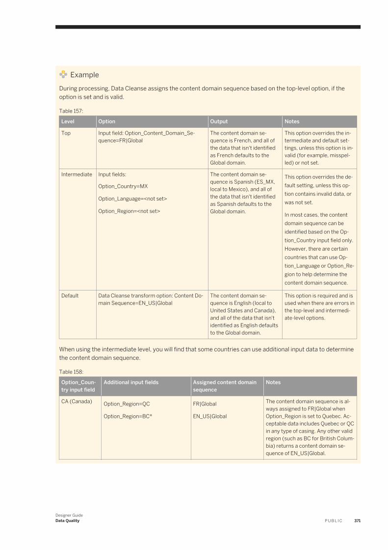
ExampleDuring processing, Data Cleanse assigns the content domain sequence based on the top-level option, if the option is set and is valid.
Table 157:
Level Option Output Notes
Top Input field: Option_Content_Domain_Sequence=FR|Global
The content domain sequence is French, and all of the data that isn't identified as French defaults to the Global domain.
This option overrides the intermediate and default settings, unless this option is invalid (for example, misspelled) or not set.
Intermediate Input fields:
Option_Country=MX
Option_Language=<not set>
Option_Region=<not set>
The content domain sequence is Spanish (ES_MX, local to Mexico), and all of the data that isn't identified as Spanish defaults to the Global domain.
This option overrides the default setting, unless this option contains invalid data, or was not set.
In most cases, the content domain sequence can be identified based on the Option_Country input field only. However, there are certain countries that can use Option_Language or Option_Region to help determine the content domain sequence.
Default Data Cleanse transform option: Content Domain Sequence=EN_US|Global
The content domain sequence is English (local to United States and Canada), and all of the data that isn't identified as English defaults to the Global domain.
This option is required and is used when there are errors in the top-level and intermediate-level options.
When using the intermediate level, you will find that some countries can use additional input data to determine the content domain sequence.
Table 158:
Option_Country input field
Additional input fields Assigned content domain sequence
Notes
CA (Canada) Option_Region=QC
Option_Region=BC*
FR|Global
EN_US|Global
The content domain sequence is always assigned to FR|Global when Option_Region is set to Quebec. Acceptable data includes Quebec or QC in any type of casing. Any other valid region (such as BC for British Columbia) returns a content domain sequence of EN_US|Global.
Designer GuideData Quality P U B L I C 371
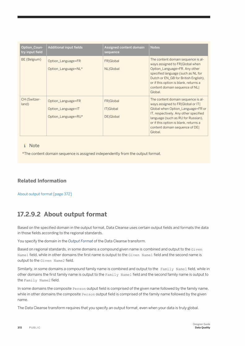
Option_Country input field
Additional input fields Assigned content domain sequence
Notes
BE (Belgium) Option_Language=FR
Option_Language=NL*
FR|Global
NL|Global
The content domain sequence is always assigned to FR|Global when Option_Language=FR. Any other specified language (such as NL for Dutch or EN_GB for British English), or if this option is blank, returns a content domain sequence of NL|Global.
CH (Switzerland)
Option_Language=FR
Option_Language=IT
Option_Language=RU*
FR|Global
IT|Global
DE|Global
The content domain sequence is always assigned to FR|Global or IT|Global when Option_Language=FR or IT, respectively. Any other specified language (such as RU for Russian), or if this option is blank, returns a content domain sequence of DE|Global.
Note*The content domain sequence is assigned independently from the output format.
Related Information
About output format [page 372]
17.2.9.2 About output format
Based on the specified domain in the output format, Data Cleanse uses certain output fields and formats the data in those fields according to the regional standards.
You specify the domain in the Output Format of the Data Cleanse transform.
Based on regional standards, in some domains a compound given name is combined and output to the Given Name1 field, while in other domains the first name is output to the Given Name1 field and the second name is output to the Given Name2 field.
Similarly, in some domains a compound family name is combined and output to the Family Name1 field, while in other domains the first family name is output to the Family Name1 field and the second family name is output to the Family Name2 field.
In some domains the composite Person output field is comprised of the given name followed by the family name, while in other domains the composite Person output field is comprised of the family name followed by the given name.
The Data Cleanse transform requires that you specify an output format, even when your data is truly global.
372 P U B L I CDesigner Guide
Data Quality
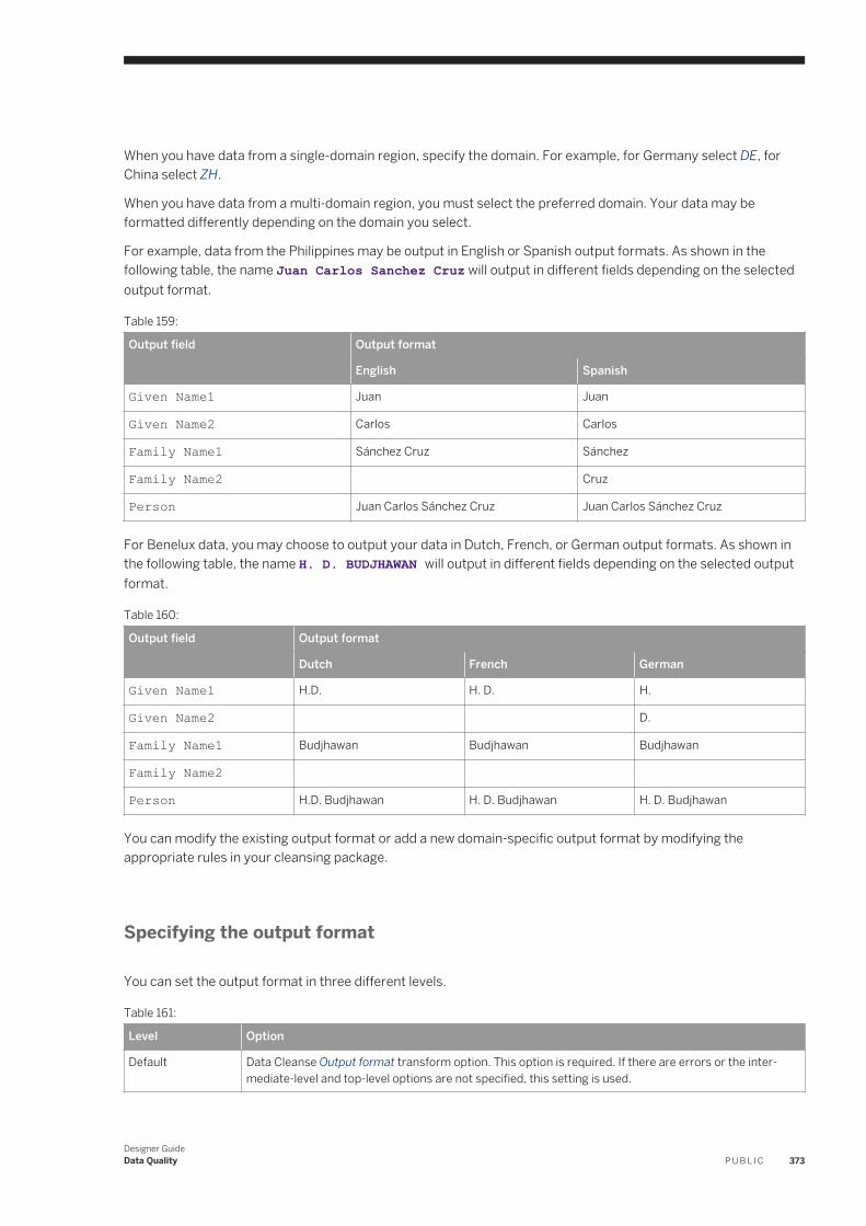
When you have data from a single-domain region, specify the domain. For example, for Germany select DE, for China select ZH.
When you have data from a multi-domain region, you must select the preferred domain. Your data may be formatted differently depending on the domain you select.
For example, data from the Philippines may be output in English or Spanish output formats. As shown in the following table, the name Juan Carlos Sanchez Cruz will output in different fields depending on the selected output format.
Table 159:
Output field Output format
English Spanish
Given Name1 Juan Juan
Given Name2 Carlos Carlos
Family Name1 Sánchez Cruz Sánchez
Family Name2 Cruz
Person Juan Carlos Sánchez Cruz Juan Carlos Sánchez Cruz
For Benelux data, you may choose to output your data in Dutch, French, or German output formats. As shown in the following table, the name H. D. BUDJHAWAN will output in different fields depending on the selected output format.
Table 160:
Output field Output format
Dutch French German
Given Name1 H.D. H. D. H.
Given Name2 D.
Family Name1 Budjhawan Budjhawan Budjhawan
Family Name2
Person H.D. Budjhawan H. D. Budjhawan H. D. Budjhawan
You can modify the existing output format or add a new domain-specific output format by modifying the appropriate rules in your cleansing package.
Specifying the output format
You can set the output format in three different levels.
Table 161:
Level Option
Default Data Cleanse Output format transform option. This option is required. If there are errors or the intermediate-level and top-level options are not specified, this setting is used.
Designer GuideData Quality P U B L I C 373
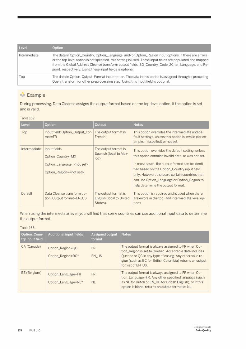
Level Option
Intermediate The data in Option_Country, Option_Language, and/or Option_Region input options. If there are errors or the top-level option is not specified, this setting is used. These input fields are populated and mapped from the Global Address Cleanse transform output fields ISO_Country_Code_2Char, Language, and Region1, respectively. Using these input fields is optional.
Top The data in Option_Output_Format input option. The data in this option is assigned through a preceding Query transform or other preprocessing step. Using this input field is optional.
ExampleDuring processing, Data Cleanse assigns the output format based on the top-level option, if the option is set and is valid.
Table 162:
Level Option Output Notes
Top Input field: Option_Output_Format=FR
The output format is French.
This option overrides the intermediate and default settings, unless this option is invalid (for example, misspelled) or not set.
Intermediate Input fields:
Option_Country=MX
Option_Language=<not set>
Option_Region=<not set>
The output format is Spanish (local to Mexico).
This option overrides the default setting, unless this option contains invalid data, or was not set.
In most cases, the output format can be identified based on the Option_Country input field only. However, there are certain countries that can use Option_Language or Option_Region to help determine the output format.
Default Data Cleanse transform option: Output format=EN_US
The output format is English (local to United States).
This option is required and is used when there are errors in the top- and intermediate-level options.
When using the intermediate level, you will find that some countries can use additional input data to determine the output format.
Table 163:
Option_Country input field
Additional input fields Assigned output format
Notes
CA (Canada) Option_Region=QC
Option_Region=BC*
FR
EN_US
The output format is always assigned to FR when Option_Region is set to Quebec. Acceptable data includes Quebec or QC in any type of casing. Any other valid region (such as BC for British Columbia) returns an output format of EN_US.
BE (Belgium) Option_Language=FR
Option_Language=NL*
FR
NL
The output format is always assigned to FR when Option_Language=FR. Any other specified language (such as NL for Dutch or EN_GB for British English), or if this option is blank, returns an output format of NL.
374 P U B L I CDesigner Guide
Data Quality
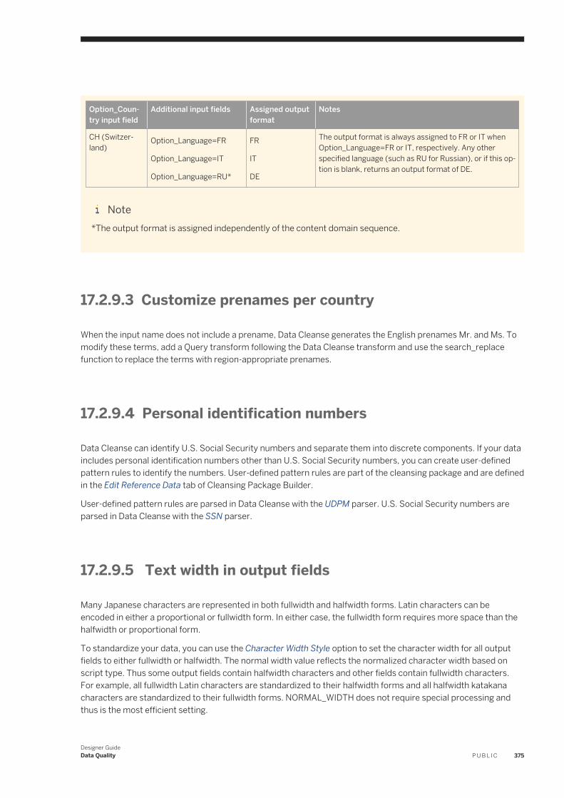
Option_Country input field
Additional input fields Assigned output format
Notes
CH (Switzerland)
Option_Language=FR
Option_Language=IT
Option_Language=RU*
FR
IT
DE
The output format is always assigned to FR or IT when Option_Language=FR or IT, respectively. Any other specified language (such as RU for Russian), or if this option is blank, returns an output format of DE.
Note*The output format is assigned independently of the content domain sequence.
17.2.9.3 Customize prenames per country
When the input name does not include a prename, Data Cleanse generates the English prenames Mr. and Ms. To modify these terms, add a Query transform following the Data Cleanse transform and use the search_replace function to replace the terms with region-appropriate prenames.
17.2.9.4 Personal identification numbers
Data Cleanse can identify U.S. Social Security numbers and separate them into discrete components. If your data includes personal identification numbers other than U.S. Social Security numbers, you can create user-defined pattern rules to identify the numbers. User-defined pattern rules are part of the cleansing package and are defined in the Edit Reference Data tab of Cleansing Package Builder.
User-defined pattern rules are parsed in Data Cleanse with the UDPM parser. U.S. Social Security numbers are parsed in Data Cleanse with the SSN parser.
17.2.9.5 Text width in output fields
Many Japanese characters are represented in both fullwidth and halfwidth forms. Latin characters can be encoded in either a proportional or fullwidth form. In either case, the fullwidth form requires more space than the halfwidth or proportional form.
To standardize your data, you can use the Character Width Style option to set the character width for all output fields to either fullwidth or halfwidth. The normal width value reflects the normalized character width based on script type. Thus some output fields contain halfwidth characters and other fields contain fullwidth characters. For example, all fullwidth Latin characters are standardized to their halfwidth forms and all halfwidth katakana characters are standardized to their fullwidth forms. NORMAL_WIDTH does not require special processing and thus is the most efficient setting.
Designer GuideData Quality P U B L I C 375
NoteBecause the output width is based on the normalized width for the character type, the output data may be larger than the input data. You may need to increase the column width in the target table.
For template tables, selecting the Use NVARCHAR for VARCHAR columns in supported databases box changes the VARCHAR column type to NVARCHAR and allows for increased data size.
17.3 Geocoding
An introduction to the Geocoder transform features.
The Geocoder transform uses geographic coordinates expressed as latitude and longitude, addresses, and point-of-interest (POI) data. With the Geocoder transform, you can append addresses, latitude and longitude, census data, and other information to your data.
Based on mapped input fields, the Geocoder transform has three modes of geocode processing:
● Address geocoding● Reverse geocoding● POI textual search
Typically, you use the Geocoder transform with the Global Address Cleanse or USA Regulatory Address Cleanse transform.
NoteWe are removing the GeoCensus functionality from the USA Regulatory Address Cleanse transform and including the features in the Geocoder transform. Ensure that you upgrade existing data flows that use GeoCensus features in the USA Regulatory Address Cleanse transform to the Geocoder transform. Find instructions for upgrading from GeoCensus to the Geocoder transform in the Upgrade Guide.
Related Information
GeoCensus ( USA Regulatory Address Cleanse ) [page 557]
17.3.1 Address geocoding
In address geocoding mode, the Geocoder transform assigns geographic data. Based on the completeness of the input address data, the Geocoder transform can return multiple levels of latitude and longitude data. Appending different levels of latitude and longitude information to your data may help your organization target certain population sizes and other regional geographical data.
376 P U B L I CDesigner Guide
Data Quality
Prepare records for geocoding
The Geocoder transform works best when it has standardized and corrected address data, so to obtain the most accurate information you may want to place an address cleanse transform before the Geocoder transform in the work flow.
17.3.1.1 Latitude and longitude levels
Primary Number level
If your input data has a complete address (including the primary number), the Geocoder transform returns latitude and longitude coordinates to the exact location based on the directory type (range-based or parcel-based) that you subscribe to.
In general, the Geocoder transform uses geocoding directories to calculate latitude and longitude values for a house by interpolating between the beginning and ending point of a line segment, where the line segment represents a range of houses. The latitude and longitude values may be slightly offset from the exact location from where the house actually exists. This is called the primary range interpolated (PRI) assignment level.
NoteIf you want to get an address-level assignment, the Primary_Number input field must be mapped and cannot be blank.
The Geocoder transform also supports parcel directories, which contain the most precise and accurate latitude and longitude values available for addresses, depending on the available country data. Parcel data is stored as points. Rather than getting you near the house, it takes you to the exact door. This is called the primary range exact (PRE) assignment level.
Postcode Centroid level
If an address has a postcode, you receive coordinates in the appropriate postcode area. The Geocoder transform has Postcode Full (PF), Postcode2 Partial (P2P) and Postcode1 (P1) assignment levels, depending on the available country data.
Locality Centroid level
If an address has a locality, you receive coordinates in the appropriate locality area. The Geocoder transform has Locality1 (L1), Locality2 (L2), Locality3 (L3) and Locality4 (L4) assignment levels, depending on the available country data.
Designer GuideData Quality P U B L I C 377
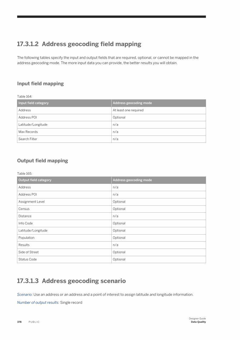
17.3.1.2 Address geocoding field mapping
The following tables specify the input and output fields that are required, optional, or cannot be mapped in the address geocoding mode. The more input data you can provide, the better results you will obtain.
Input field mapping
Table 164:
Input field category Address geocoding mode
Address At least one required
Address POI Optional
Latitude/Longitude n/a
Max Records n/a
Search Filter n/a
Output field mapping
Table 165:
Output field category Address geocoding mode
Address n/a
Address POI n/a
Assignment Level Optional
Census Optional
Distance n/a
Info Code Optional
Latitude/Longitude Optional
Population Optional
Results n/a
Side of Street Optional
Status Code Optional
17.3.1.3 Address geocoding scenario
Scenario: Use an address or an address and a point of interest to assign latitude and longitude information.
Number of output results: Single record
378 P U B L I CDesigner Guide
Data Quality
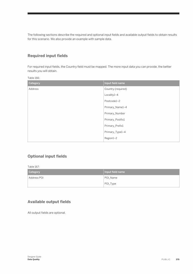
The following sections describe the required and optional input fields and available output fields to obtain results for this scenario. We also provide an example with sample data.
Required input fields
For required input fields, the Country field must be mapped. The more input data you can provide, the better results you will obtain.
Table 166:
Category Input field name
Address Country (required)
Locality1–4
Postcode1–2
Primary_Name1–4
Primary_Number
Primary_Postfix1
Primary_Prefix1
Primary_Type1–4
Region1–2
Optional input fields
Table 167:
Category Input field name
Address POI POI_Name
POI_Type
Available output fields
All output fields are optional.
Designer GuideData Quality P U B L I C 379
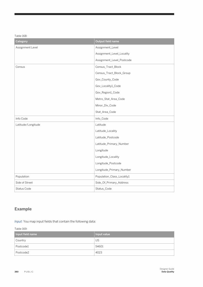
Table 168:
Category Output field name
Assignment Level Assignment_Level
Assignment_Level_Locality
Assignment_Level_Postcode
Census Census_Tract_Block
Census_Tract_Block_Group
Gov_County_Code
Gov_Locality1_Code
Gov_Region1_Code
Metro_Stat_Area_Code
Minor_Div_Code
Stat_Area_Code
Info Code Info_Code
Latitude/Longitude Latitude
Latitude_Locality
Latitude_Postcode
Latitude_Primary_Number
Longitude
Longitude_Locality
Longitude_Postcode
Longitude_Primary_Number
Population Population_Class_Locality1
Side of Street Side_Of_Primary_Address
Status Code Status_Code
Example
Input: You map input fields that contain the following data:
Table 169:
Input field name Input value
Country US
Postcode1 54601
Postcode2 4023
380 P U B L I CDesigner Guide
Data Quality
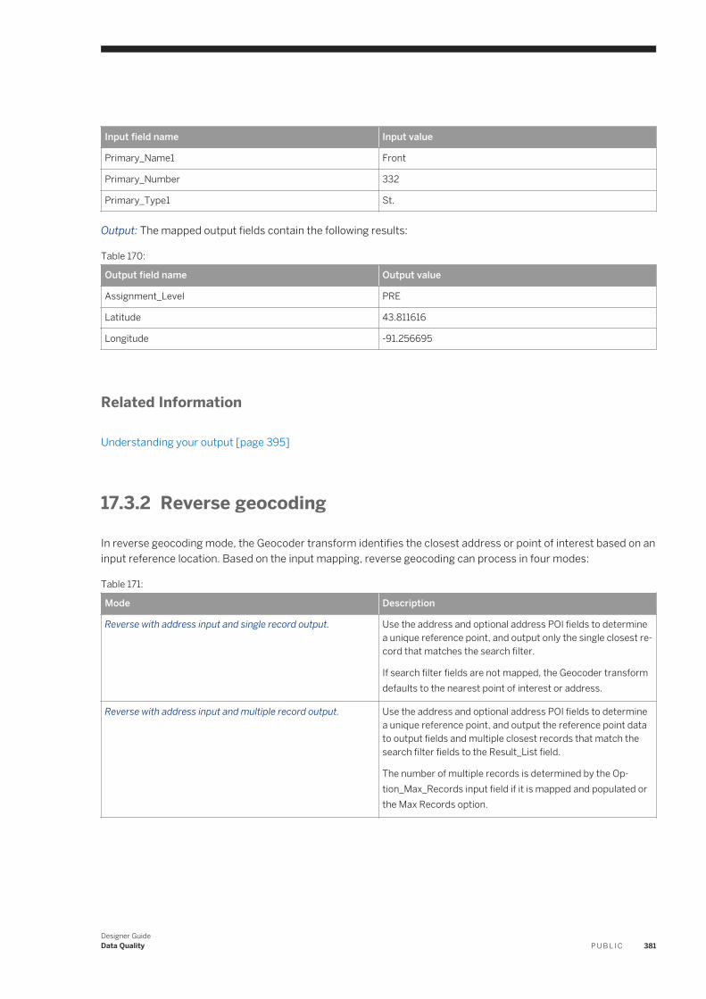
Input field name Input value
Primary_Name1 Front
Primary_Number 332
Primary_Type1 St.
Output: The mapped output fields contain the following results:
Table 170:
Output field name Output value
Assignment_Level PRE
Latitude 43.811616
Longitude -91.256695
Related Information
Understanding your output [page 395]
17.3.2 Reverse geocoding
In reverse geocoding mode, the Geocoder transform identifies the closest address or point of interest based on an input reference location. Based on the input mapping, reverse geocoding can process in four modes:
Table 171:
Mode Description
Reverse with address input and single record output. Use the address and optional address POI fields to determine a unique reference point, and output only the single closest record that matches the search filter.
If search filter fields are not mapped, the Geocoder transform defaults to the nearest point of interest or address.
Reverse with address input and multiple record output. Use the address and optional address POI fields to determine a unique reference point, and output the reference point data to output fields and multiple closest records that match the search filter fields to the Result_List field.
The number of multiple records is determined by the Option_Max_Records input field if it is mapped and populated or the Max Records option.
Designer GuideData Quality P U B L I C 381
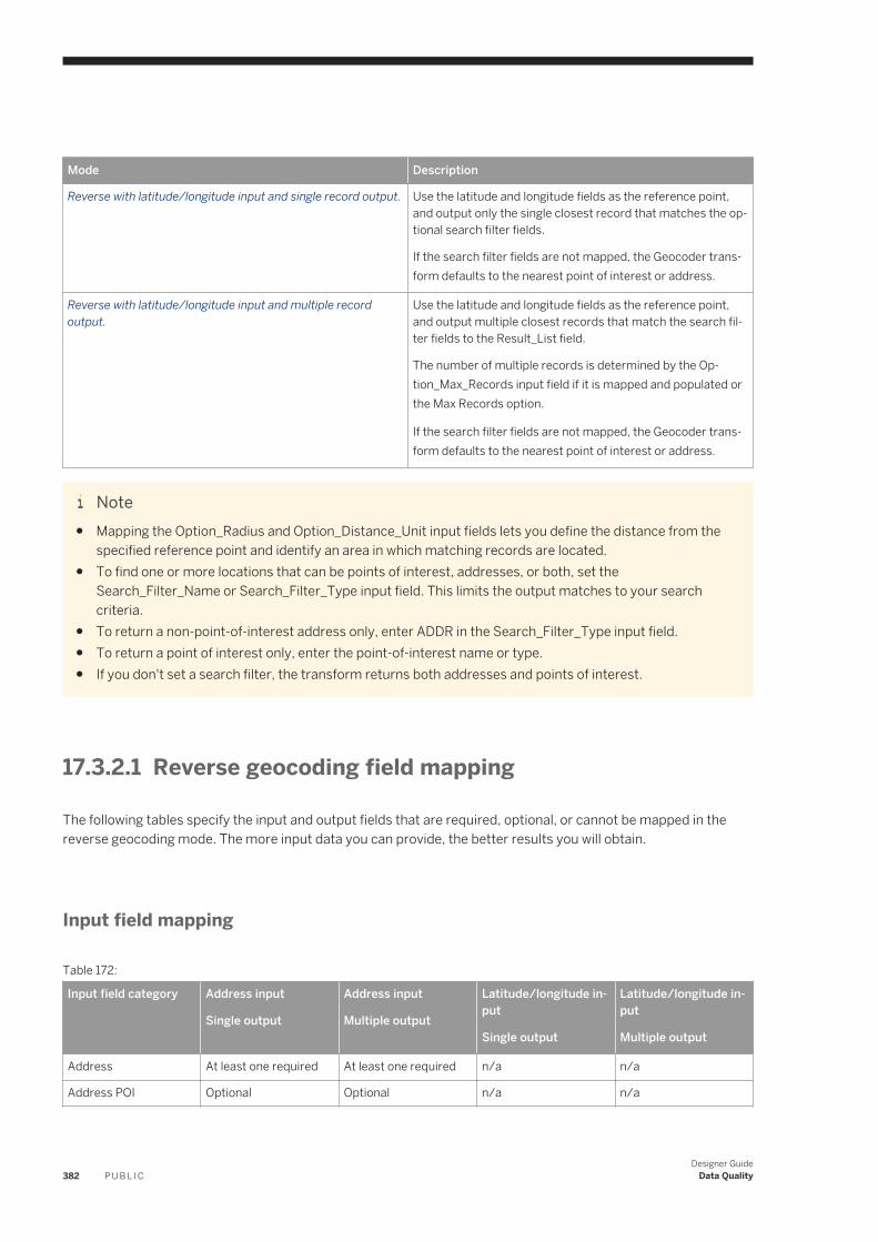
Mode Description
Reverse with latitude/longitude input and single record output. Use the latitude and longitude fields as the reference point, and output only the single closest record that matches the optional search filter fields.
If the search filter fields are not mapped, the Geocoder transform defaults to the nearest point of interest or address.
Reverse with latitude/longitude input and multiple record output.
Use the latitude and longitude fields as the reference point, and output multiple closest records that match the search filter fields to the Result_List field.
The number of multiple records is determined by the Option_Max_Records input field if it is mapped and populated or the Max Records option.
If the search filter fields are not mapped, the Geocoder transform defaults to the nearest point of interest or address.
Note● Mapping the Option_Radius and Option_Distance_Unit input fields lets you define the distance from the
specified reference point and identify an area in which matching records are located.● To find one or more locations that can be points of interest, addresses, or both, set the
Search_Filter_Name or Search_Filter_Type input field. This limits the output matches to your search criteria.
● To return a non-point-of-interest address only, enter ADDR in the Search_Filter_Type input field.● To return a point of interest only, enter the point-of-interest name or type.● If you don't set a search filter, the transform returns both addresses and points of interest.
17.3.2.1 Reverse geocoding field mapping
The following tables specify the input and output fields that are required, optional, or cannot be mapped in the reverse geocoding mode. The more input data you can provide, the better results you will obtain.
Input field mapping
Table 172:
Input field category Address input
Single output
Address input
Multiple output
Latitude/longitude input
Single output
Latitude/longitude input
Multiple output
Address At least one required At least one required n/a n/a
Address POI Optional Optional n/a n/a
382 P U B L I CDesigner Guide
Data Quality
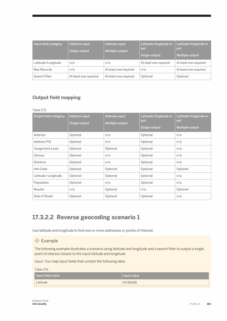
Input field category Address input
Single output
Address input
Multiple output
Latitude/longitude input
Single output
Latitude/longitude input
Multiple output
Latitude/Longitude n/a n/a At least one required At least one required
Max Records n/a At least one required n/a At least one required
Search Filter At least one required At least one required Optional Optional
Output field mapping
Table 173:
Output field category Address input
Single output
Address input
Multiple output
Latitude/longitude input
Single output
Latitude/longitude input
Multiple output
Address Optional n/a Optional n/a
Address POI Optional n/a Optional n/a
Assignment Level Optional Optional Optional n/a
Census Optional n/a Optional n/a
Distance Optional n/a Optional n/a
Info Code Optional Optional Optional Optional
Latitude/ Longitude Optional Optional Optional n/a
Population Optional n/a Optional n/a
Results n/a Optional n/a Optional
Side of Street Optional Optional Optional n/a
17.3.2.2 Reverse geocoding scenario 1
Use latitude and longitude to find one or more addresses or points of interest.
ExampleThe following example illustrates a scenario using latitude and longitude and a search filter to output a single point of interest closest to the input latitude and longitude.
Input: You map input fields that contain the following data:
Table 174:
Input field name Input value
Latitude 43.811616
Designer GuideData Quality P U B L I C 383
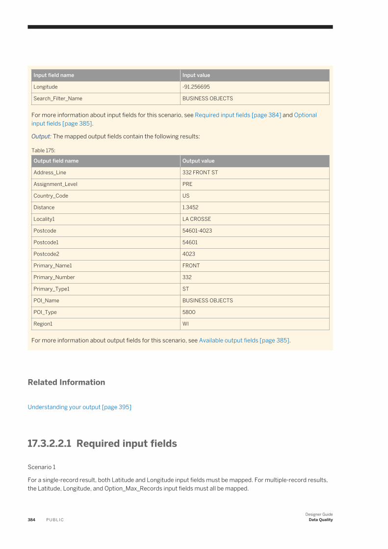
Input field name Input value
Longitude -91.256695
Search_Filter_Name BUSINESS OBJECTS
For more information about input fields for this scenario, see Required input fields [page 384] and Optional input fields [page 385].
Output: The mapped output fields contain the following results:
Table 175:
Output field name Output value
Address_Line 332 FRONT ST
Assignment_Level PRE
Country_Code US
Distance 1.3452
Locality1 LA CROSSE
Postcode 54601-4023
Postcode1 54601
Postcode2 4023
Primary_Name1 FRONT
Primary_Number 332
Primary_Type1 ST
POI_Name BUSINESS OBJECTS
POI_Type 5800
Region1 WI
For more information about output fields for this scenario, see Available output fields [page 385].
Related Information
Understanding your output [page 395]
17.3.2.2.1 Required input fields
Scenario 1
For a single-record result, both Latitude and Longitude input fields must be mapped. For multiple-record results, the Latitude, Longitude, and Option_Max_Records input fields must all be mapped.
384 P U B L I CDesigner Guide
Data Quality

Table 176:
Category Single-record results
Input field name
Multiple-record results
Input field name
Latitude/Longitude Latitude
Longitude
Latitude
Longitude
Max Records n/a Option_Max_Records
17.3.2.2.2 Optional input fields
Scenario 1
Table 177:
Category Single-record results
Input field name
Multiple-record results
Input field name
Search Filter Option Radius
Search_Filter_Name
Search_Filter_Type
Option_Radius
Search_Filter_Name
Search_Filter_Type
17.3.2.2.3 Available output fields
Scenario 1
All output fields are optional.
Designer GuideData Quality P U B L I C 385
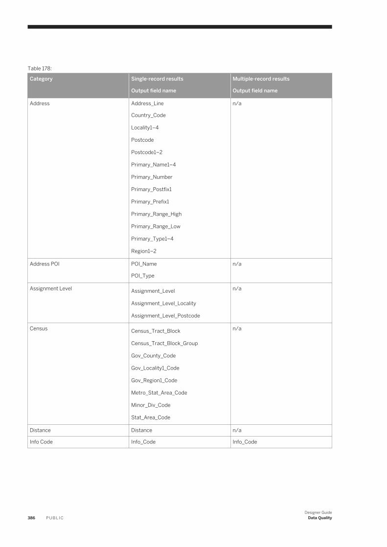
Table 178:
Category Single-record results
Output field name
Multiple-record results
Output field name
Address Address_Line
Country_Code
Locality1–4
Postcode
Postcode1–2
Primary_Name1–4
Primary_Number
Primary_Postfix1
Primary_Prefix1
Primary_Range_High
Primary_Range_Low
Primary_Type1–4
Region1–2
n/a
Address POI POI_Name
POI_Type
n/a
Assignment Level Assignment_Level
Assignment_Level_Locality
Assignment_Level_Postcode
n/a
Census Census_Tract_Block
Census_Tract_Block_Group
Gov_County_Code
Gov_Locality1_Code
Gov_Region1_Code
Metro_Stat_Area_Code
Minor_Div_Code
Stat_Area_Code
n/a
Distance Distance n/a
Info Code Info_Code Info_Code
386 P U B L I CDesigner Guide
Data Quality
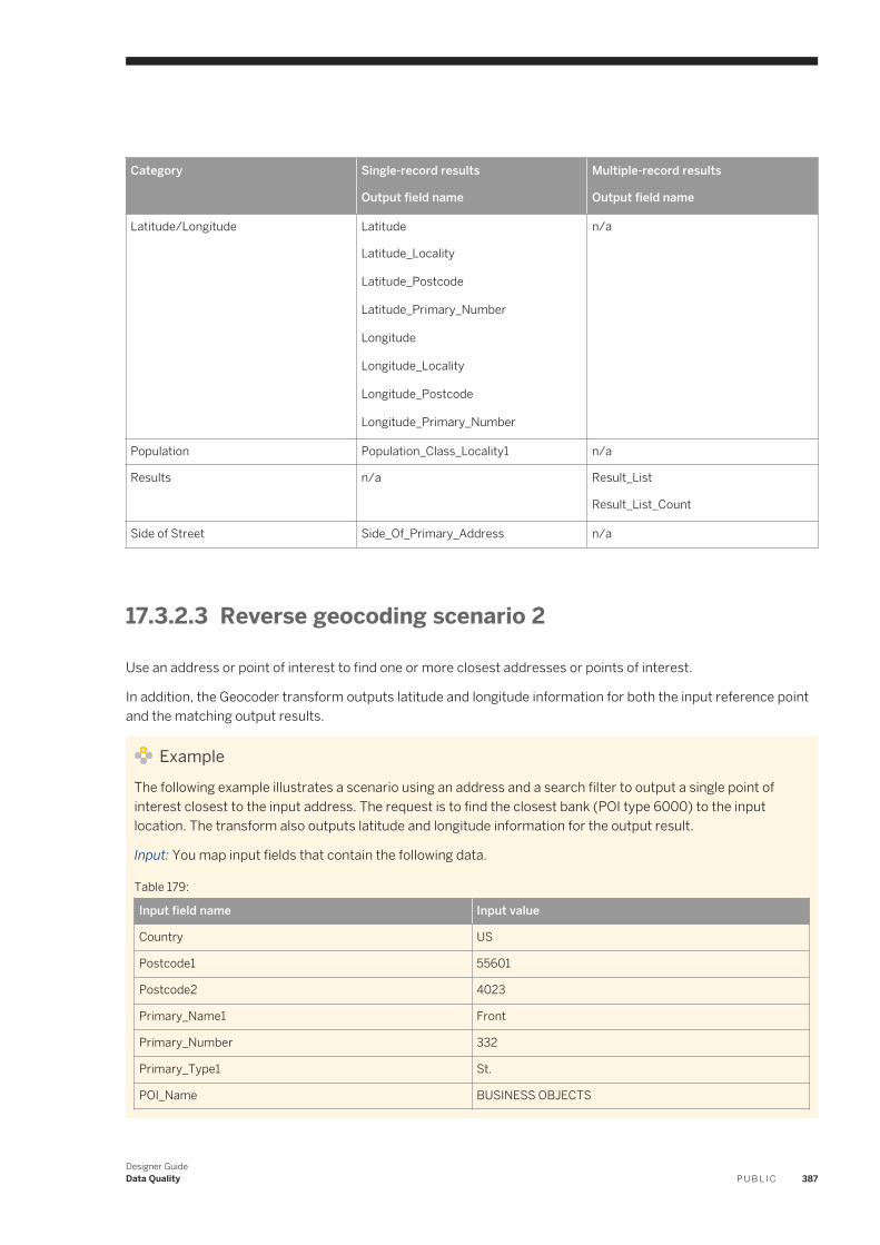
Category Single-record results
Output field name
Multiple-record results
Output field name
Latitude/Longitude Latitude
Latitude_Locality
Latitude_Postcode
Latitude_Primary_Number
Longitude
Longitude_Locality
Longitude_Postcode
Longitude_Primary_Number
n/a
Population Population_Class_Locality1 n/a
Results n/a Result_List
Result_List_Count
Side of Street Side_Of_Primary_Address n/a
17.3.2.3 Reverse geocoding scenario 2
Use an address or point of interest to find one or more closest addresses or points of interest.
In addition, the Geocoder transform outputs latitude and longitude information for both the input reference point and the matching output results.
ExampleThe following example illustrates a scenario using an address and a search filter to output a single point of interest closest to the input address. The request is to find the closest bank (POI type 6000) to the input location. The transform also outputs latitude and longitude information for the output result.
Input: You map input fields that contain the following data.
Table 179:
Input field name Input value
Country US
Postcode1 55601
Postcode2 4023
Primary_Name1 Front
Primary_Number 332
Primary_Type1 St.
POI_Name BUSINESS OBJECTS
Designer GuideData Quality P U B L I C 387
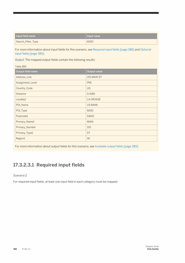
Input field name Input value
Search_Filter_Type 6000
For more information about input fields for this scenario, see Required input fields [page 388] and Optional input fields [page 389].
Output: The mapped output fields contain the following results:
Table 180:
Output field name Output value
Address_Line 201 MAIN ST
Assignment_Level PRE
Country_Code US
Distance 0.4180
Locality1 LA CROSSE
POI_Name US BANK
POI_Type 6000
Postcode1 54601
Primary_Name1 MAIN
Primary_Number 201
Primary_Type1 ST
Region1 WI
For more information about output fields for this scenario, see Available output fields [page 389].
17.3.2.3.1 Required input fields
Scenario 2
For required input fields, at least one input field in each category must be mapped.
388 P U B L I CDesigner Guide
Data Quality
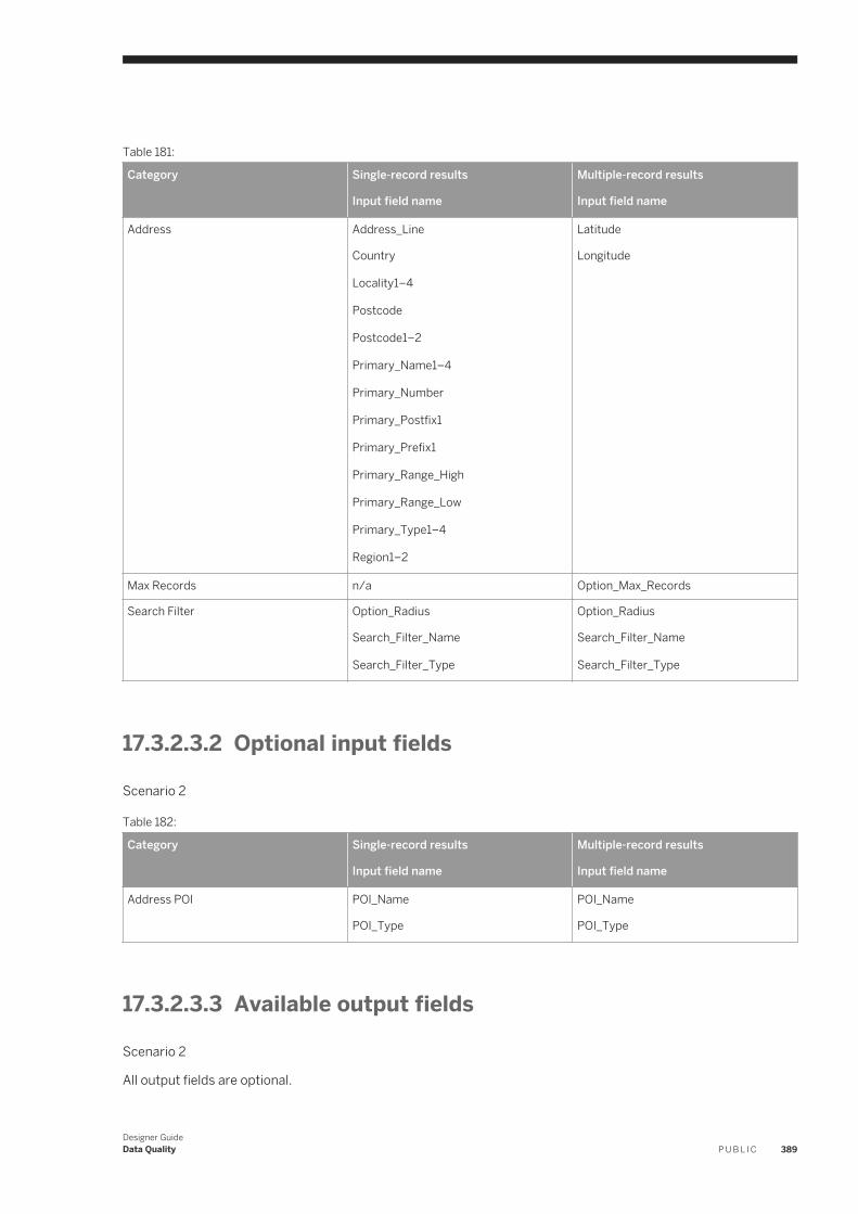
Table 181:
Category Single-record results
Input field name
Multiple-record results
Input field name
Address Address_Line
Country
Locality1–4
Postcode
Postcode1–2
Primary_Name1–4
Primary_Number
Primary_Postfix1
Primary_Prefix1
Primary_Range_High
Primary_Range_Low
Primary_Type1–4
Region1–2
Latitude
Longitude
Max Records n/a Option_Max_Records
Search Filter Option_Radius
Search_Filter_Name
Search_Filter_Type
Option_Radius
Search_Filter_Name
Search_Filter_Type
17.3.2.3.2 Optional input fields
Scenario 2
Table 182:
Category Single-record results
Input field name
Multiple-record results
Input field name
Address POI POI_Name
POI_Type
POI_Name
POI_Type
17.3.2.3.3 Available output fields
Scenario 2
All output fields are optional.
Designer GuideData Quality P U B L I C 389
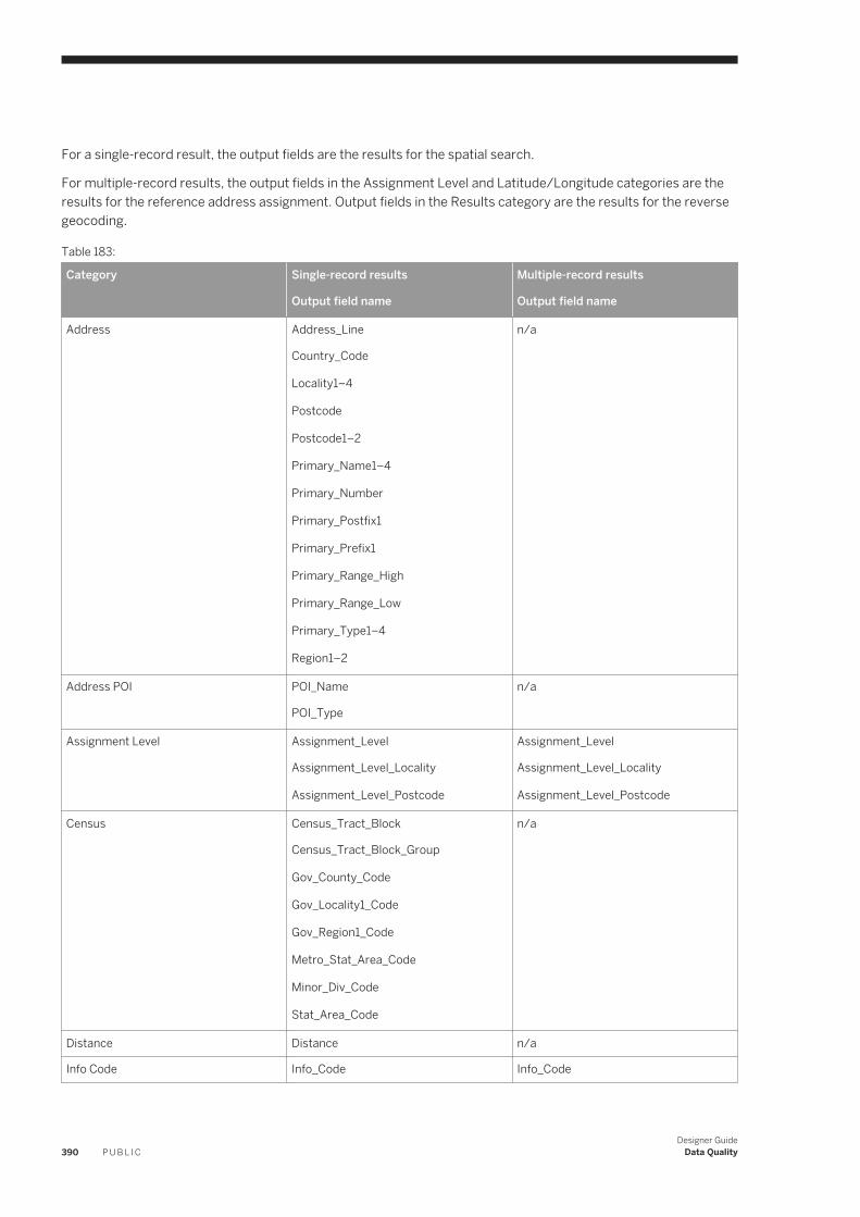
For a single-record result, the output fields are the results for the spatial search.
For multiple-record results, the output fields in the Assignment Level and Latitude/Longitude categories are the results for the reference address assignment. Output fields in the Results category are the results for the reverse geocoding.
Table 183:
Category Single-record results
Output field name
Multiple-record results
Output field name
Address Address_Line
Country_Code
Locality1–4
Postcode
Postcode1–2
Primary_Name1–4
Primary_Number
Primary_Postfix1
Primary_Prefix1
Primary_Range_High
Primary_Range_Low
Primary_Type1–4
Region1–2
n/a
Address POI POI_Name
POI_Type
n/a
Assignment Level Assignment_Level
Assignment_Level_Locality
Assignment_Level_Postcode
Assignment_Level
Assignment_Level_Locality
Assignment_Level_Postcode
Census Census_Tract_Block
Census_Tract_Block_Group
Gov_County_Code
Gov_Locality1_Code
Gov_Region1_Code
Metro_Stat_Area_Code
Minor_Div_Code
Stat_Area_Code
n/a
Distance Distance n/a
Info Code Info_Code Info_Code
390 P U B L I CDesigner Guide
Data Quality
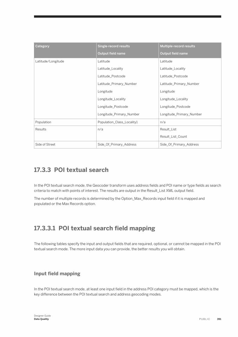
Category Single-record results
Output field name
Multiple-record results
Output field name
Latitude/Longitude Latitude
Latitude_Locality
Latitude_Postcode
Latitude_Primary_Number
Longitude
Longitude_Locality
Longitude_Postcode
Longitude_Primary_Number
Latitude
Latitude_Locality
Latitude_Postcode
Latitude_Primary_Number
Longitude
Longitude_Locality
Longitude_Postcode
Longitude_Primary_Number
Population Population_Class_Locality1 n/a
Results n/a Result_List
Result_List_Count
Side of Street Side_Of_Primary_Address Side_Of_Primary_Address
17.3.3 POI textual search
In the POI textual search mode, the Geocoder transform uses address fields and POI name or type fields as search criteria to match with points of interest. The results are output in the Result_List XML output field.
The number of multiple records is determined by the Option_Max_Records input field if it is mapped and populated or the Max Records option.
17.3.3.1 POI textual search field mapping
The following tables specify the input and output fields that are required, optional, or cannot be mapped in the POI textual search mode. The more input data you can provide, the better results you will obtain.
Input field mapping
In the POI textual search mode, at least one input field in the address POI category must be mapped, which is the key difference between the POI textual search and address geocoding modes.
Designer GuideData Quality P U B L I C 391
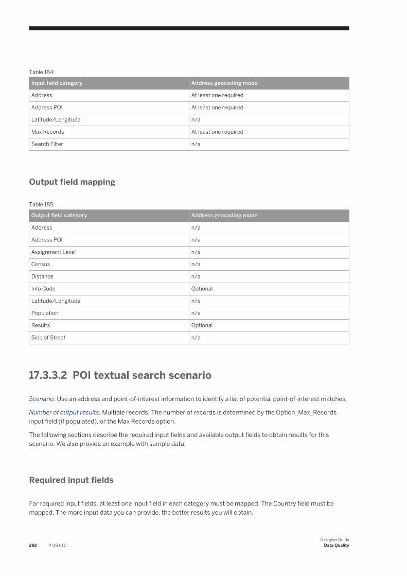
Table 184:
Input field category Address geocoding mode
Address At least one required
Address POI At least one required
Latitude/Longitude n/a
Max Records At least one required
Search Filter n/a
Output field mapping
Table 185:
Output field category Address geocoding mode
Address n/a
Address POI n/a
Assignment Level n/a
Census n/a
Distance n/a
Info Code Optional
Latitude/Longitude n/a
Population n/a
Results Optional
Side of Street n/a
17.3.3.2 POI textual search scenario
Scenario: Use an address and point-of-interest information to identify a list of potential point-of-interest matches.
Number of output results: Multiple records. The number of records is determined by the Option_Max_Records input field (if populated), or the Max Records option.
The following sections describe the required input fields and available output fields to obtain results for this scenario. We also provide an example with sample data.
Required input fields
For required input fields, at least one input field in each category must be mapped. The Country field must be mapped. The more input data you can provide, the better results you will obtain.
392 P U B L I CDesigner Guide
Data Quality
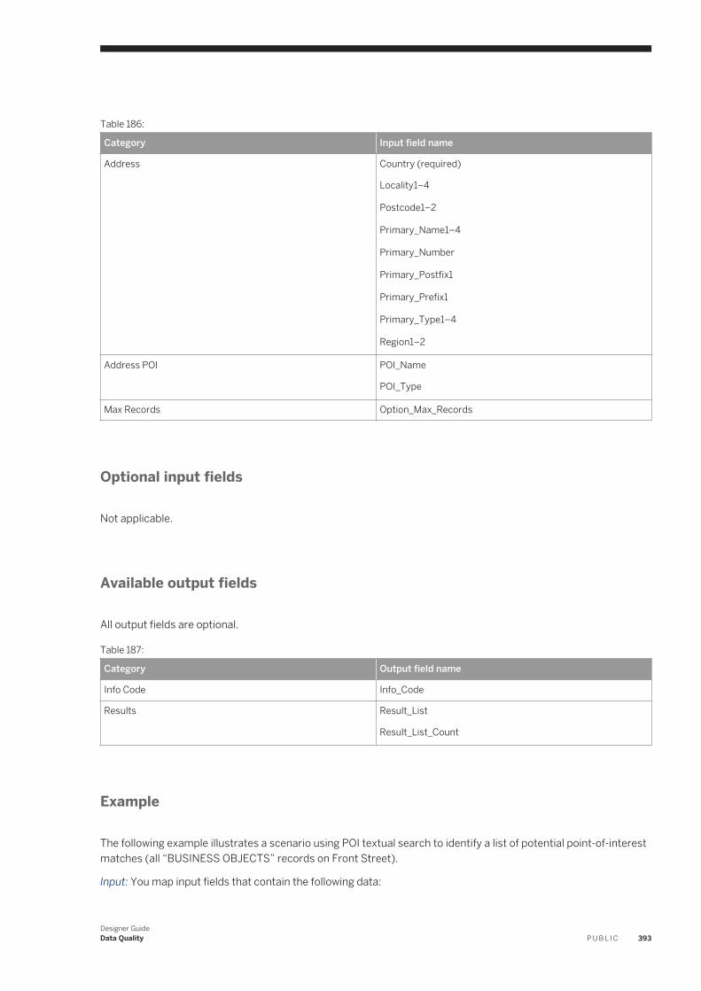
Table 186:
Category Input field name
Address Country (required)
Locality1–4
Postcode1–2
Primary_Name1–4
Primary_Number
Primary_Postfix1
Primary_Prefix1
Primary_Type1–4
Region1–2
Address POI POI_Name
POI_Type
Max Records Option_Max_Records
Optional input fields
Not applicable.
Available output fields
All output fields are optional.
Table 187:
Category Output field name
Info Code Info_Code
Results Result_List
Result_List_Count
Example
The following example illustrates a scenario using POI textual search to identify a list of potential point-of-interest matches (all “BUSINESS OBJECTS” records on Front Street).
Input: You map input fields that contain the following data:
Designer GuideData Quality P U B L I C 393
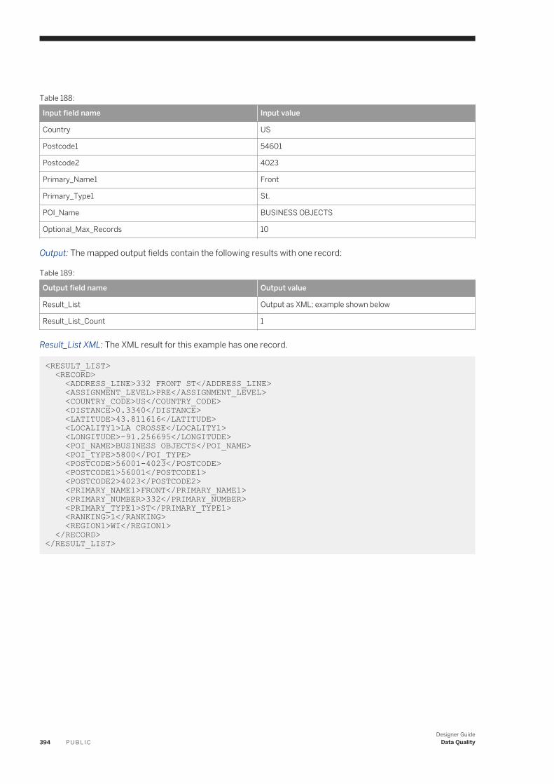
Table 188:
Input field name Input value
Country US
Postcode1 54601
Postcode2 4023
Primary_Name1 Front
Primary_Type1 St.
POI_Name BUSINESS OBJECTS
Optional_Max_Records 10
Output: The mapped output fields contain the following results with one record:
Table 189:
Output field name Output value
Result_List Output as XML; example shown below
Result_List_Count 1
Result_List XML: The XML result for this example has one record.
<RESULT_LIST> <RECORD> <ADDRESS_LINE>332 FRONT ST</ADDRESS_LINE> <ASSIGNMENT_LEVEL>PRE</ASSIGNMENT_LEVEL> <COUNTRY_CODE>US</COUNTRY_CODE> <DISTANCE>0.3340</DISTANCE> <LATITUDE>43.811616</LATITUDE> <LOCALITY1>LA CROSSE</LOCALITY1> <LONGITUDE>-91.256695</LONGITUDE> <POI_NAME>BUSINESS OBJECTS</POI_NAME> <POI_TYPE>5800</POI_TYPE> <POSTCODE>56001-4023</POSTCODE> <POSTCODE1>56001</POSTCODE1> <POSTCODE2>4023</POSTCODE2> <PRIMARY_NAME1>FRONT</PRIMARY_NAME1> <PRIMARY_NUMBER>332</PRIMARY_NUMBER> <PRIMARY_TYPE1>ST</PRIMARY_TYPE1> <RANKING>1</RANKING> <REGION1>WI</REGION1> </RECORD> </RESULT_LIST>
394 P U B L I CDesigner Guide
Data Quality
17.3.4 Understanding your output
Information about Geocoder output data including latitude and longitude, assignment level, and multi record output.
Latitude and longitude
Latitude and longitude data is represented by decimal degrees such as 12.12345, for example. The decimals indicate the number of degrees from the equator. Latitude represents locations north or south of the equator. Longitude represents locations east or west of the equator.
● Latitude: 0-90 degrees north or south of the equator○ Negative number indicates south of the equator○ Positive number indicates north of the equator
● Longitude: 0-180 degrees east or west of Greenwich Meridian in London, England○ Negative number indicates location within 180 degrees west of Greenwich○ Positive number indicates location within 180 degrees east of Greenwich
Assignment level
You can understand the accuracy of the assignment based on the Assignment_Level output field.
Table 190:
Output field Description
PRE First level of assignment. The finest depth of assignment available to the exact location.
PRI Second level of assignment. The finest depth of assignment available to the primary address range or house number.
P1
L1
Most general level of assignment. General assignment based on the postcode, P1, or the locality, L1. P1 or L1 is output depending on the value you choose in the Best Assignment Level option.
Multiple results
When your output consists of multiple records, the Result_List output field data is based the available data. The output format is an XML string.
Designer GuideData Quality P U B L I C 395
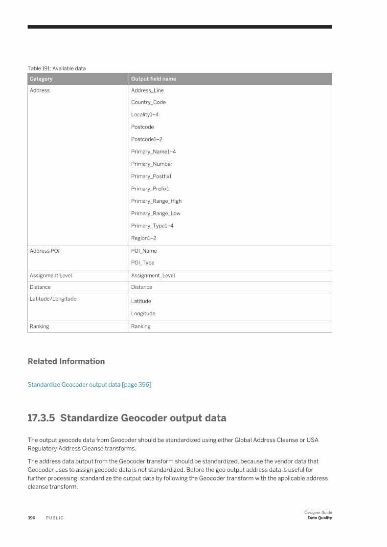
Table 191: Available data
Category Output field name
Address Address_Line
Country_Code
Locality1–4
Postcode
Postcode1–2
Primary_Name1–4
Primary_Number
Primary_Postfix1
Primary_Prefix1
Primary_Range_High
Primary_Range_Low
Primary_Type1–4
Region1–2
Address POI POI_Name
POI_Type
Assignment Level Assignment_Level
Distance Distance
Latitude/Longitude Latitude
Longitude
Ranking Ranking
Related Information
Standardize Geocoder output data [page 396]
17.3.5 Standardize Geocoder output data
The output geocode data from Geocoder should be standardized using either Global Address Cleanse or USA Regulatory Address Cleanse transforms.
The address data output from the Geocoder transform should be standardized, because the vendor data that Geocoder uses to assign geocode data is not standardized. Before the geo output address data is useful for further processing, standardize the output data by following the Geocoder transform with the applicable address cleanse transform.
396 P U B L I CDesigner Guide
Data Quality
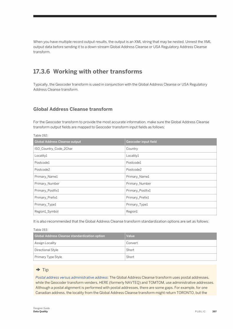
When you have multiple record output results, the output is an XML string that may be nested. Unnest the XML output data before sending it to a down-stream Global Address Cleanse or USA Regulatory Address Cleanse transform.
17.3.6 Working with other transforms
Typically, the Geocoder transform is used in conjunction with the Global Address Cleanse or USA Regulatory Address Cleanse transform.
Global Address Cleanse transform
For the Geocoder transform to provide the most accurate information, make sure the Global Address Cleanse transform output fields are mapped to Geocoder transform input fields as follows:
Table 192:
Global Address Cleanse output Geocoder input field
ISO_Country_Code_2Char Country
Locality1 Locality1
Postcode1 Postcode1
Postcode2 Postcode2
Primary_Name1 Primary_Name1
Primary_Number Primary_Number
Primary_Postfix1 Primary_Postfix1
Primary_Prefix1 Primary_Prefix1
Primary_Type1 Primary_Type1
Region1_Symbol Region1
It is also recommended that the Global Address Cleanse transform standardization options are set as follows:
Table 193:
Global Address Cleanse standardization option Value
Assign Locality Convert
Directional Style Short
Primary Type Style Short
TipPostal address versus administrative address: The Global Address Cleanse transform uses postal addresses, while the Geocoder transform venders, HERE (formerly NAVTEQ) and TOMTOM, use administrative addresses. Although a postal alignment is performed with postal addresses, there are some gaps. For example, for one Canadian address, the locality from the Global Address Cleanse transform might return TORONTO, but the
Designer GuideData Quality P U B L I C 397
Geocoder directory stores NORTH YORK. In this case, when the Locality1 field is mapped on input, it results in an Address Not Found error. As a workaround for this issue, you can remove the Locality1 input field mapping to get a better geocoding assignment.
17.4 Match
17.4.1 Match and consolidation using Data Services and Information Steward
When manual review is necessary, use SAP Data Services to automatically implement the overall matching and consolidation process. This process stages the match groups for manual review in SAP Information Steward.
To implement this process, consider the following factors:
● Do you stage only suspect match groups (groups that do not meet a match score or threshold that you define) for manual review? Or do you stage all the match results including unique records for match review and let data stewards manually move suspect records or unique records to the group they should belong? Note that the target group in this case could be a suspect group or “high confidence” group.
● Do you want to enable best record creation within Information Steward? Or do you want the Information Steward manual review to only modify suspect match groups as necessary and have Data Services handle the best record creation after the manual review is complete?
● If you want to enable best record creation within Information Steward, when do you perform the best record creation for high confidence match groups?○ Manually creating a best record for all match groups in a large data set might not be practical.○ On the other hand, if you have already consolidated high-confidence match groups within Data Services,
then you have already modified the original match group to include the best record values, and you cannot stage these modified match groups for manual review in Information Steward.
Consider the following approaches for match review:
● Engage data stewards and domain experts in manual review of suspect match groups only. They can modify the suspect match groups if necessary and create the best record for these match groups.1. The Data Services job performs automated matching, identifies suspect match groups, and populates
only suspect match groups in a staging database. In this scenario, “high confidence match groups” must be separated from “suspect match groups”. The best record can be created for the “high confidence match groups” and those match groups can be consolidated within Data Services.This process can be accomplished by routing the “high confidence match groups” to another Match transform that is configured to create best records out of already matched groups of records.
2. Data stewards and domain experts review the “suspect match groups” in Information Steward and make corrections as appropriate (for example unmatch or move a record). They can manually create the best record for these match groups.
● Engage data stewards and domain experts in manual review and correction of all match groups, but keep the best record creation and consolidation logic in Data Services.1. The Data Services job performs automated matching and populates all match results into the staging
database. A match result table in the staging database contains suspect match groups, “high confidence” match groups, and unique records.
398 P U B L I CDesigner Guide
Data Quality
2. Data stewards and domain experts review the suspect match groups in Information Steward and make corrections as appropriate. They can move the records between suspect match groups and “high confidence” match groups, or include a unique record in the appropriate match group.
3. After the match review is finished, all match groups are processed in another Data Services job which creates the best record and consolidates all match groups.This process could be accomplished by a Match transform that is configured to create best records out of already matched groups of records.
NoteYou can find examples of best record creation using Information Steward or Data Services by downloading the Data Quality Management Match blueprints. You can find more information about blueprints at https://wiki.scn.sap.com/wiki/display/EIM/SAP+Data+Services+Blueprints .
17.4.2 Matching strategies
Here are a few examples of strategies to help you think about how you want to approach the setup of your matching data flow.
Table 194:
Strategy Description
Simple match Use this strategy when your matching business rules consist of a single match criteria for identifying relationships in consumer, business, or product data.
Consumer Householding Use this strategy when your matching business rules consist of multiple levels of consumer relationships, such as residential matches, family matches, and individual matches.
Corporate Householding Use this strategy when your matching business rules consist of multiple levels of corporate relationships, such as corporate matches, subsidiary matches, and contact matches.
Multinational consumer match Use this match strategy when your data consists of multiple countries and your matching business rules are different for different countries
Identify a person multiple ways Use this strategy when your matching business rules consist of multiple match criteria for identifying relationships, and you want to find the overlap between all of those definitions.
Think about the answers to these questions before deciding on a match strategy:
● What does my data consist of? (Customer data, international data, and so on)● What fields do I want to compare? (last name, firm, and so on.)● What are the relative strengths and weaknesses of the data in those fields?
TipYou will get better results if you cleanse your data before matching. Also, data profiling can help you answer this question.
● What end result do I want when the match job is complete? (One record per family, per firm, and so on.)
Designer GuideData Quality P U B L I C 399
Related Information
Association matching [page 467]
17.4.3 Match components
The basic components of matching are:
● Match sets● Match levels● Match criteria
Match sets
A match set is represented by a Match transform on your workspace. Each match set can have its own break groups, match criteria, and prioritization.
A match set has three purposes:
● To allow only select data into a given set of match criteria for possible comparison (for example, exclude blank SSNs, international addresses, and so on).
● To allow for related match scenarios to be stacked to create a multi-level match set.● To allow for multiple match sets to be considered for association in an Associate match set.
Match levels
A match level is an indicator to what type of matching will occur, such as on individual, family, resident, firm, and so on. A match level refers not to a specific criteria, but to the broad category of matching.
You can have as many match levels as you want. However, the Match wizard restricts you to three levels during setup (more can be added later). You can define each match level in a match set in a way that is increasingly more strict. Multi-level matching feeds only the records that match from match level to match level (for example, resident, family, individual) for comparison.
Table 195:
Match component Description
Family The purpose of the family match type is to determine whether two people should be considered members of the same family, as reflected by their record data. The Match transform compares the last name and the address data. A match means that the two records represent members of the same family. The result of the match is one record per family.
400 P U B L I CDesigner Guide
Data Quality
Match component Description
Individual The purpose of the individual match type is to determine whether two records are for the same person, as reflected by their record data. The Match transform compares the first name, last name, and address data. A match means that the two records represent the same person. The result of the match is one record per individual.
Resident The purpose of the resident match type is to determine whether two records should be considered members of the same residence, as reflected by their record data. The Match transform compares the address data. A match means that the two records represent members of the same household. Contrast this match type with the family match type, which also compares last-name data. The result of the match is one record per residence.
Firm The purpose of the firm match type is to determine whether two records reflect the same firm. This match type involves comparisons of firm and address data. A match means that the two records represent the same firm. The result of the match is one record per firm.
Firm-Individual The purpose of the firm-individual match type is to determine whether two records are for the same person at the same firm, as reflected by their record data. With this match type, we compare the first name, last name, firm name, and address data. A match means that the two records reflect the same person at the same firm. The result of the match is one record per individual per firm.
Match criteria
Match criteria refers to the field you want to match on. You can use criteria options to specify business rules for matching on each of these fields. They allow you to control how close to exact the data needs to be for that data to be considered a match.
For example, you may require first names to be at least 85% similar, but also allow a first name initial to match a spelled out first name, and allow a first name to match a middle name.
● Family level match criteria may include family (last) name and address, or family (last) name and telephone number.
● Individual level match criteria may include full name and address, full name and SSN, or full name and e-mail address.
● Firm level match criteria may include firm name and address, firm name and Standard Industrial Classification (SIC) Code, or firm name and Data Universal Numbering System (DUNS) number.
17.4.4 Match Wizard
17.4.4.1 Match wizard
The Match wizard can quickly set up match data flows, without requiring you to manually create each individual transform it takes to complete the task.
Designer GuideData Quality P U B L I C 401
What the Match wizard does
The Match wizard:
● Builds all the necessary transforms to perform the match strategy you choose.● Applies default values to your match criteria based on the strategy you choose.● Places the resulting transforms on the workspace, connected to the upstream transform you choose.● Detects the appropriate upstream fields and maps to them automatically.
What the Match wizard does not do
The Match wizard provides you with a basic match setup that in some cases, will require customization to meet your business rules.
The Match wizard:
● Does not alter any data that flows through it. To correct non-standard entries or missing data, place one of the address cleansing transforms and a Data Cleanse transform upstream from the matching process.
● Does not connect the generated match transforms to any downstream transform, such as a Loader. You are responsible for connecting these transforms.
● Does not allow you to set rule-based or weighted scoring values for matching. The Match wizard incorporates a "best practices" standard that set these values for you. You may want to edit option values to conform to your business rules.
Related Information
Combination method [page 440]
17.4.4.2 Before you begin
Prepare a data flow for the Match wizard
To maximize its usefulness, be sure to include the following in your data flow before you launch the Match wizard:
● Include a Reader in your data flow. You may want to match on a particular input field that our data cleansing transforms do not handle.
● Include one of the address cleansing transforms and the Data Cleanse transform. The Match wizard works best if the data you're matching has already been cleansed and parsed into discrete fields upstream in the data flow.
● If you want to match on any address fields, be sure that you pass them through the Data Cleanse transform. Otherwise, they will not be available to the Match transform (and Match Wizard). This rule is also true if you have the Data Cleanse transform before an address cleanse transform.
402 P U B L I CDesigner Guide
Data Quality
17.4.4.3 Use the Match Wizard
17.4.4.3.1 Selecting match strategy
The Match wizard begins by prompting you to choose a match strategy, based on your business rule requirements. The path through the Match wizard depends on the strategy you select here. Use these descriptions to help you decide which strategy is best for you:
● Simple match. Use this strategy when your matching business rules consist of a single match criteria for identifying relationships in consumer, business, or product data.
● Consumer Householding. Use this strategy when your matching business rules consist of multiple levels of consumer relationships, such as residential matches, family matches, and individual matches.
● Corporate Householding. Use this strategy when your matching business rules consist of multiple levels of corporate relationships, such as corporate matches, subsidiary matches, and contact matches.
● Multinational consumer match. Use this match strategy when your data consists of multiple countries and your matching business rules are different for different countries.
NoteThe multinational consumer match strategy sets up a data flow that expects Latin1 data. If you want to use Unicode matching, you must edit your data flow after it has been created.
● Identify a person multiple ways. Use this strategy when your matching business rules consist of multiple match criteria for identifying relationships, and you want to find the overlap between all of those definitions.
Source statistics
If you want to generate source statistics for reports, make sure a field that houses the physical source value exists in all of the data sources.
To generate source statistics for your match reports, select the Generate statistics for your sources checkbox, and then select a field that contains your physical source value.
Related Information
Unicode matching [page 468]Association matching [page 467]
17.4.4.3.2 Identifying matching criteria
Criteria represent the data that you want to use to help determine matches. In this window, you will define these criteria for each match set that you are using.
Designer GuideData Quality P U B L I C 403
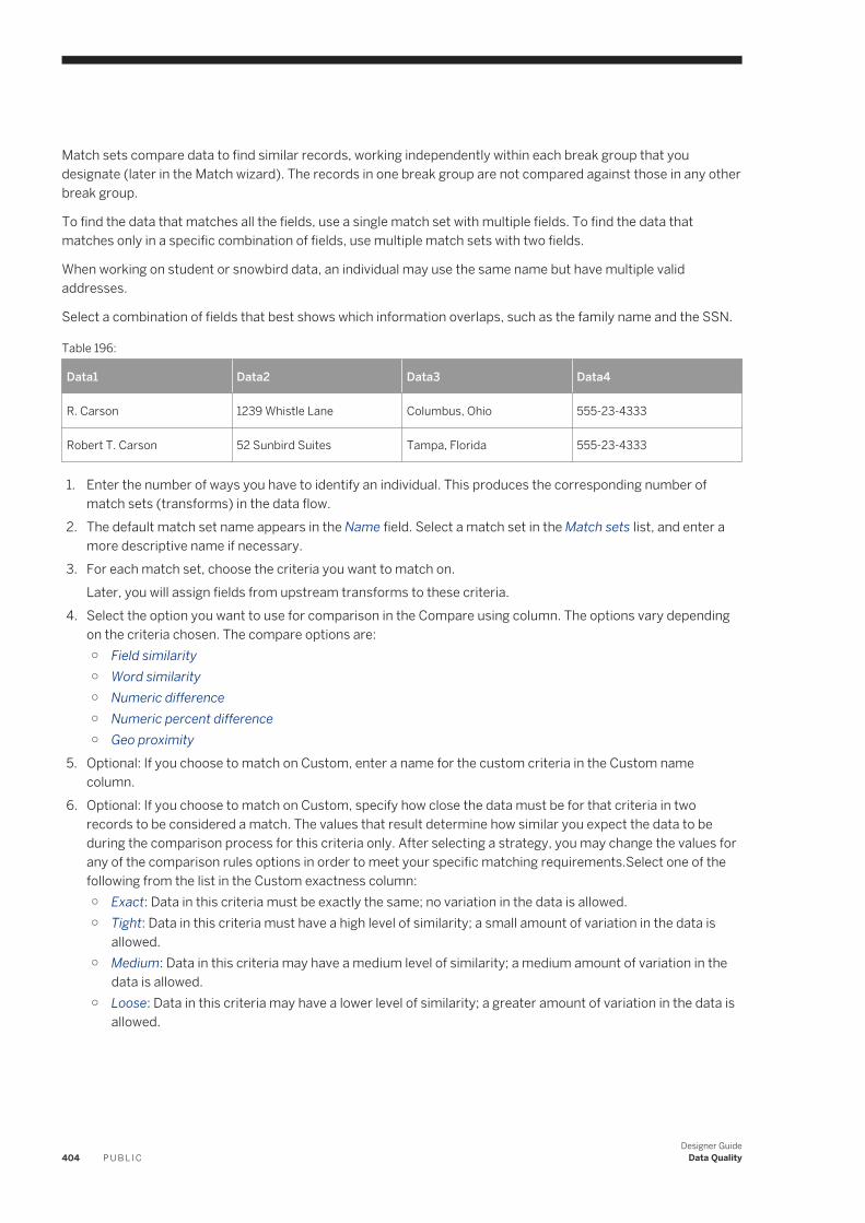
Match sets compare data to find similar records, working independently within each break group that you designate (later in the Match wizard). The records in one break group are not compared against those in any other break group.
To find the data that matches all the fields, use a single match set with multiple fields. To find the data that matches only in a specific combination of fields, use multiple match sets with two fields.
When working on student or snowbird data, an individual may use the same name but have multiple valid addresses.
Select a combination of fields that best shows which information overlaps, such as the family name and the SSN.
Table 196:
Data1 Data2 Data3 Data4
R. Carson 1239 Whistle Lane Columbus, Ohio 555-23-4333
Robert T. Carson 52 Sunbird Suites Tampa, Florida 555-23-4333
1. Enter the number of ways you have to identify an individual. This produces the corresponding number of match sets (transforms) in the data flow.
2. The default match set name appears in the Name field. Select a match set in the Match sets list, and enter a more descriptive name if necessary.
3. For each match set, choose the criteria you want to match on.Later, you will assign fields from upstream transforms to these criteria.
4. Select the option you want to use for comparison in the Compare using column. The options vary depending on the criteria chosen. The compare options are:○ Field similarity○ Word similarity○ Numeric difference○ Numeric percent difference○ Geo proximity
5. Optional: If you choose to match on Custom, enter a name for the custom criteria in the Custom name column.
6. Optional: If you choose to match on Custom, specify how close the data must be for that criteria in two records to be considered a match. The values that result determine how similar you expect the data to be during the comparison process for this criteria only. After selecting a strategy, you may change the values for any of the comparison rules options in order to meet your specific matching requirements.Select one of the following from the list in the Custom exactness column:○ Exact: Data in this criteria must be exactly the same; no variation in the data is allowed.○ Tight: Data in this criteria must have a high level of similarity; a small amount of variation in the data is
allowed.○ Medium: Data in this criteria may have a medium level of similarity; a medium amount of variation in the
data is allowed.○ Loose: Data in this criteria may have a lower level of similarity; a greater amount of variation in the data is
allowed.
404 P U B L I CDesigner Guide
Data Quality
17.4.4.3.3 Defining match levels
Match levels allow matching processes to be defined at distinct levels that are logically related. Match levels refer to the broad category of matching not the specific rules of matching. For instance, a residence-level match would match on only address elements, a family-level match would match on only Last Name, and the individual-level match would match on First Name.
Multi-level matching can contain up to three levels within a single match set defined in a way that is increasingly more strict. Multi-level matching feeds only the records that match from match level to match level (that is, resident, family, individual) for comparison.
To define match levels:
1. Click the top level match, and enter a name for the level, if you don't want to keep the default name. The default criteria is already selected. If you do not want to use the default criteria, click to remove the check mark from the box.The default criteria selection is a good place to start when choosing criteria. You can add criteria for each level to help make finer or more precise matches.
2. Select any additional criteria for this level.3. If you want to use criteria other than those offered, click Custom and then select the desired criteria.4. Continue until you have populated all the levels that you require.
17.4.4.3.4 Selecting countries
Select the countries whose postal standards may be required to effectively compare the incoming data. The left panel shows a list of all available countries. The right panel shows the countries you already selected.
1. Select the country name in the All Countries list.2. Click Add to move it into the Selected Countries list.3. Repeat steps 1 and 2 for each country that you want to include.
You can also select multiple countries and add them all by clicking the Add button.
The countries that you select are remembered for the next Match wizard session.
17.4.4.3.5 Grouping countries into tracks
Create tracks to group countries into logical combinations based on your business rules (for example Asia, Europe, South America). Each track creates up to six match sets (Match transforms).
1. Select the number of tracks that you want to create. The Tracks list reflects the number of tracks you choose and assigns a track number for each.
2. To create each track, select a track title, such as Track1.3. Select the countries that you want in that track.4. Click Add to move the selected countries to the selected track.
Use the COUNTRY UNKNOWN (__) listing for data where the country of origin has not been identified.
Designer GuideData Quality P U B L I C 405
Use the COUNTRY OTHER (--) listing for data whose country of origin has been identified, but the country does not exist in the list of selected countries.
5. From Match engines, select one of the following engines for each track:
NoteAll match transforms generated for the track will use the selected Match engine.
○ LATIN1 (Default)○ CHINESE○ JAPANESE○ KOREAN○ TAIWANESE○ OTHER_NON_LATIN1
The Next button is only enabled when all tracks have an entry and all countries are assigned to a track.
17.4.4.3.6 Selecting criteria fields
Select and deselect criteria fields for each match set and match level you create in your data flow. These selections determine which fields are compared for each record. Some criteria may be selected by default, based on the data input.
If there is only one field of the appropriate content type, you will not be able to change the field for that criteria within the Match Wizard.
To enable the Next button, you must select at least one non-match-standard field.
1. For each of the criteria fields you want to include, select an available field from the drop-down list, which contains fields from upstream source(s). The available fields are limited to the appropriate content types for that criteria. If no fields of the appropriate type are available, all upstream fields display in the menu.
2. Optional: Deselect any criteria fields you do not want to include.
17.4.4.3.7 Creating break keys
Use break keys to create manageable groups of data to compare. The match set compares the data in the records within each break group only, not across the groups. Making the correct selections can save valuable processing time by preventing widely divergent data from being compared.
Break keys are especially important when you deal with large amounts of data, because the size of the break groups can affect processing time. Even if your data is not extensive, break groups will help to speed up processing.
Create break keys that group similar data that would most likely contain matches. Keep in mind that records in one break group will not be compared against records in any other break group.
For example, when you match to find duplicate addresses, base the break key on the postcode, city, or state to create groups with the most likely matches. When you match to find duplicate individuals, base the break key on the postcode and a portion of the name as the most likely point of match.
406 P U B L I CDesigner Guide
Data Quality
To create break keys:
1. In the How many fields column, select the number of fields to include in the break key.2. For each break key, select the following:
○ the field(s) in the break key○ the starting point for each field○ the number of positions to read from each field
3. After you define the break keys, do one of the following:
○ Click Finish. This completes the match transform.○ If you are performing multi-national matching, click Next to go to the Matching Criteria page.
17.4.4.4 After setup
Although the Match wizard does a lot of the work, there are some things that you must do to have a runnable match job. There are also some things you want to do to refine your matching process.
Connect to downstream transforms
When the Match wizard is complete, it places the generated transforms on the workspace, connected to the upstream transform you selected to start the Match wizard. For your job to run, you must connect each port from the last transform to a downstream transform. To do this, click a port and drag to connect to the desired object.
View and edit the new match transform
To see what is incorporated in the transform(s) the Match Wizard produces, right-click the transform and choose Match Editor.
View and edit Associate transforms
To see what is incorporated in the Associate transform(s) the Match Wizard produces, right-click the transform and choose Associate Editor.
Multinational matching
For the Multinational consumer match strategy, the wizard builds a Match transform for each track that you create.
Designer GuideData Quality P U B L I C 407
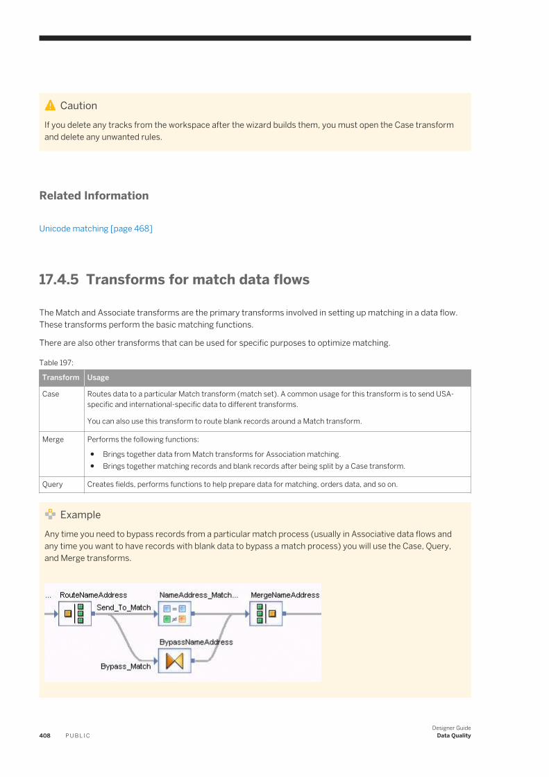
CautionIf you delete any tracks from the workspace after the wizard builds them, you must open the Case transform and delete any unwanted rules.
Related Information
Unicode matching [page 468]
17.4.5 Transforms for match data flows
The Match and Associate transforms are the primary transforms involved in setting up matching in a data flow. These transforms perform the basic matching functions.
There are also other transforms that can be used for specific purposes to optimize matching.
Table 197:
Transform Usage
Case Routes data to a particular Match transform (match set). A common usage for this transform is to send USA-specific and international-specific data to different transforms.
You can also use this transform to route blank records around a Match transform.
Merge Performs the following functions:
● Brings together data from Match transforms for Association matching.● Brings together matching records and blank records after being split by a Case transform.
Query Creates fields, performs functions to help prepare data for matching, orders data, and so on.
ExampleAny time you need to bypass records from a particular match process (usually in Associative data flows and any time you want to have records with blank data to bypass a match process) you will use the Case, Query, and Merge transforms.
408 P U B L I CDesigner Guide
Data Quality
● The Case transform has two routes: one route sends all records that meet the criteria to the Match transform, and one that sends all other records to the bypass match route.
● The Query transform adds the fields that the Match transform generates and that you output. (The output schema in the Match transform and the output schema in the Query transform must be identical for the routes to be merged.) The contents of the newly added fields in the Query transform may be populated with an empty string.
● The Merge transform merges the two routes into a single route.
17.4.5.1 Removing matching from the Match transform
You may want to place a transform that employs some of the functionality of a Match transform in your data flow, but does not include the actual matching features. For example, you may want to do candidate selection or prioritization in a data flow or a location in a data flow that doesn't do matching at all.
1. Right-click the Match transform in the object library, and choose New.2. In the Format name field, enter a meaningful name for your transform. It's helpful to indicate which type of
function this transform will be performing.3. Click OK.4. Drag and drop your new Match transform configuration onto the workspace and connect it to your data flow.5. Right-click the new transform, and choose Match Editor.6. Deselect the Perform matching option in the upper left corner of the Match editor.
Now you can add any available operation to this transform.
17.4.6 Working in the Match and Associate editors
Editors
The Match and Associate transform editors allow you to set up your input and output schemas. You can access these editors by double-clicking the appropriate transform icon on your workspace.
The Match and Associate editors allow you to configure your transform's options. You can access these editors by right-clicking the appropriate transform and choosing Match Editor (or Associate Editor).
Order of setup
TipThe order that you set up your Match transform is important!
First, it is best to map your input fields. If you don't, and you add an operation in the Match editor, you may not see a particular field you want to use for that operation.
Designer GuideData Quality P U B L I C 409
Secondly, you should configure your options in the Match editor before you map your output fields. Adding operations to the Match transform (such as Unique ID and Group Statistics) can provide you with useful Match transform-generated fields that you may want to use later in the data flow or add to your database.
RememberMake sure that you:
1. Map your input fields.2. Configure the options for the transform.3. Map your output fields.
17.4.7 Physical and logical sources
Tracking your input data sources and other sources is essential for producing informative match reports.
Whether based on an input source or based on some data element in the rows being read, tracking your input data sources and other sources throughout the data flow is essential for producing informative match reports. Depending on what you are tracking, you must create the appropriate fields in your data flow to ensure that the software generates the statistics you want, if you don't already have them in your database. There are two types of input sources as described in the following table.
Table 198:
Input source Description
Physical The filename or value attributed to the source of the input data.
Logical A group of records spanning multiple input sources or a subset of records from a single input source.
17.4.7.1 Logical input source
Track various sources of input data for reports, statistics, and compare tables.
If you want to count source statistics in the Match transform (for the Match Source Statistics Summary report, for example), you must create a field using a Query transform or a User-Defined transform, if you don't already have one in your input data sources.
This field tracks the various sources within a Reader for reporting purposes, and is used in the Group Statistics operation of the Match transform to generate the source statistics. It is also used in compare tables, so that you can specify which sources to compare.
410 P U B L I CDesigner Guide
Data Quality
17.4.7.2 Physical input source
You track your input data source by assigning the physical source a value in a field.
Then you use this field in the transforms where report statistics are generated.
To assign this value, add a Query transform after the source and add a column with a constant containing the name you want to assign to this source.
NoteIf your source is a flat file, you can use the Include file name option to automatically generate a column containing the file name.
17.4.7.3 Using sources
A source is the grouping of records on the basis of some data characteristic that you can identify. A source might be all records from one input file, or all records that contain a particular value in a particular field.
Sources are abstract and arbitrary—there is no physical boundary line between sources. Source membership can cut across input files or database records as well as distinguish among records within a file or database, based on how you define the source.
If you are willing to treat all your input records as normal, eligible records with equal priority, then you do not need to include sources in your job.
Typically, a match user expects some characteristic or combination of characteristics to be significant, either for selecting the best matching record, or for deciding which records to include or exclude from a mailing list, for example. Sources enable you to attach those characteristics to a record, by virtue of that record’s membership in its particular source.
Before getting to the details about how to set up and use sources, here are some of the many reasons you might want to include sources in your job:
● To give one set of records priority over others. For example, you might want to give the records of your house database or a suppression source priority over the records from an update file.
● To identify a set of records that match suppression sources, such as the DMA.● To set up a set of records that should not be counted toward multi-source status. For example, some mailers
use a seed source of potential buyers who report back to the mailer when they receive a mail piece so that the mailer can measure delivery. These are special-type records.
● To save processing time, by canceling the comparison within a set of records that you know contains no matching records. In this case, you must know that there are no matching records within the source, but there may be matches among sources. To save processing time, you could set up sources and cancel comparing within each source.
● To get separate report statistics for a set of records within an source, or to get report statistics for groups of sources.
● To protect a source from having its data overwritten by a best record or unique ID operation. You can choose to protect data based on membership in a source.
Designer GuideData Quality P U B L I C 411
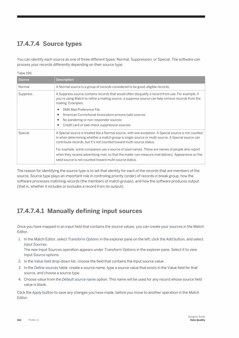
17.4.7.4 Source types
You can identify each source as one of three different types: Normal, Suppression, or Special. The software can process your records differently depending on their source type.
Table 199:
Source Description
Normal A Normal source is a group of records considered to be good, eligible records.
Suppress A Suppress source contains records that would often disqualify a record from use. For example, if you’re using Match to refine a mailing source, a suppress source can help remove records from the mailing. Examples:
● DMA Mail Preference File● American Correctional Association prisons/jails sources● No pandering or non-responder sources● Credit card or bad-check suppression sources
Special A Special source is treated like a Normal source, with one exception. A Special source is not counted in when determining whether a match group is single-source or multi-source. A Special source can contribute records, but it’s not counted toward multi-source status.
For example, some companies use a source of seed names. These are names of people who report when they receive advertising mail, so that the mailer can measure mail delivery. Appearance on the seed source is not counted toward multi-source status.
The reason for identifying the source type is to set that identity for each of the records that are members of the source. Source type plays an important role in controling priority (order) of records in break group, how the software processes matching records (the members of match groups), and how the software produces output (that is, whether it includes or excludes a record from its output).
17.4.7.4.1 Manually defining input sources
Once you have mapped in an input field that contains the source values, you can create your sources in the Match Editor.
1. In the Match Editor, select Transform Options in the explorer pane on the left, click the Add button, and select Input Sources.The new Input Sources operation appears under Transform Options in the explorer pane. Select it to view Input Source options.
2. In the Value field drop-down list, choose the field that contains the input source value.3. In the Define sources table, create a source name, type a source value that exists in the Value field for that
source, and choose a source type.4. Choose value from the Default source name option. This name will be used for any record whose source field
value is blank.
Click the Apply button to save any changes you have made, before you move to another operation in the Match Editor.
412 P U B L I CDesigner Guide
Data Quality
17.4.7.4.2 Automatically defining input sources
To avoid manually defining your input sources, you can choose to do it automatically by choosing the Auto generate sources option in the Input Sources operation.
1. In the Match Editor, select Transform Options in the explorer pane on the left, click the Add button, and select Input Sources.The new Input Sources operation appears under Transform Options in the explorer pane. Select it to view Input Source options.
2. In the Value field drop-down list, choose the field that contains the input source value.3. Choose value from the Default source name option. This name will be used for any record whose source field
value is blank.4. Select the Auto generate sources option.5. Choose a value in the Default type option
The default type will be assigned to to any source that does not already have the type defined in the Type field.6. Select a field from the drop-down list in the Type field option.
Auto generating sources will create a source for each unique value in the Value field. Any records that do not have a value field defined will be assigned to the default source name.
17.4.7.5 Source groups
The source group capability adds a higher level of source management. For example, suppose you rented several files from two brokers. You define five sources to be used in ranking the records. In addition, you would like to see your job’s statistics broken down by broker as well as by file. To do this, you can define groups of sources for each broker.
Source groups primarily affect reports. However, you can also use source groups to select multi-source records based on the number of source groups in which a name occurs.
Remember that you cannot use source groups in the same way you use sources. For example, you cannot give one source group priority over another.
17.4.7.5.1 Creating source groups
You must have input sources in an Input Source operation defined to be able to add this operation or define your source groups.
1. Select a Match transform in your data flow, and choose Tools Match Editor .2. In the Match Editor, select Transform Options in the explorer pane on the left, click the Add button, and select
Source Groups.The new Source Groups operation appears under Input Sources operation in the explorer pane. Select it to view Source Group options.
3. Confirm that the input sources you need are in the Sources column on the right.
Designer GuideData Quality P U B L I C 413
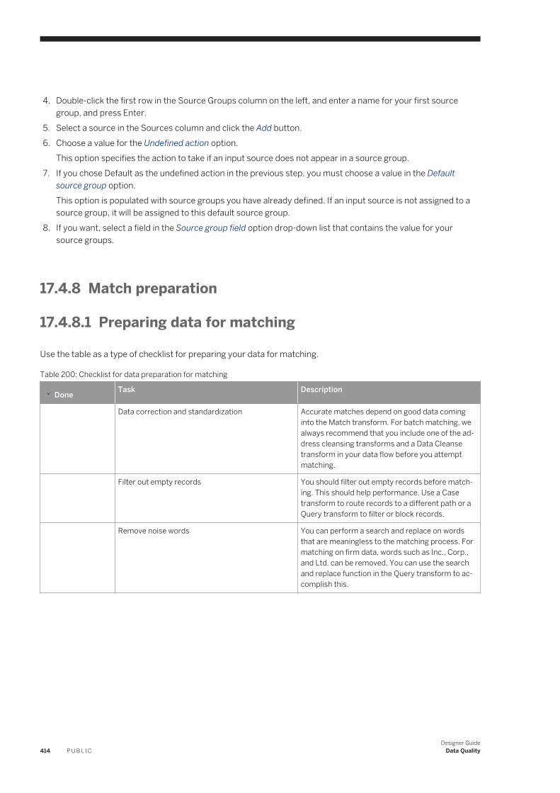
4. Double-click the first row in the Source Groups column on the left, and enter a name for your first source group, and press Enter.
5. Select a source in the Sources column and click the Add button.6. Choose a value for the Undefined action option.
This option specifies the action to take if an input source does not appear in a source group.7. If you chose Default as the undefined action in the previous step, you must choose a value in the Default
source group option.This option is populated with source groups you have already defined. If an input source is not assigned to a source group, it will be assigned to this default source group.
8. If you want, select a field in the Source group field option drop-down list that contains the value for your source groups.
17.4.8 Match preparation
17.4.8.1 Preparing data for matching
Use the table as a type of checklist for preparing your data for matching.
Table 200: Checklist for data preparation for matching
Done Task Description
Data correction and standardization Accurate matches depend on good data coming into the Match transform. For batch matching, we always recommend that you include one of the address cleansing transforms and a Data Cleanse transform in your data flow before you attempt matching.
Filter out empty records You should filter out empty records before matching. This should help performance. Use a Case transform to route records to a different path or a Query transform to filter or block records.
Remove noise words You can perform a search and replace on words that are meaningless to the matching process. For matching on firm data, words such as Inc., Corp., and Ltd. can be removed. You can use the search and replace function in the Query transform to accomplish this.
414 P U B L I CDesigner Guide
Data Quality
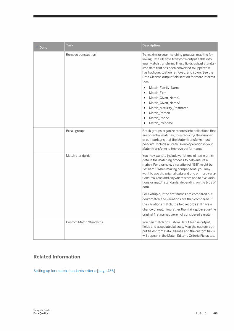
Done Task Description
Remove punctuation To maximize your matching process, map the following Data Cleanse transform output fields into your Match transform. These fields output standarized data that has been converted to uppercase, has had punctuation removed, and so on. See the Data Cleanse output field section for more information.
● Match_Family_Name● Match_Firm● Match_Given_Name1● Match_Given_Name2● Match_Maturity_Postname● Match_Person● Match_Phone● Match_Prename
Break groups Break groups organize records into collections that are potential matches, thus reducing the number of comparisons that the Match transform must perform. Include a Break Group operation in your Match transform to improve performance.
Match standards You may want to include variations of name or firm data in the matching process to help ensure a match. For example, a variation of “Bill” might be “William”. When making comparisons, you may want to use the original data and one or more variations. You can add anywhere from one to five variations or match standards, depending on the type of data.
For example, If the first names are compared but don't match, the variations are then compared. If the variations match, the two records still have a chance of matching rather than failing, because the original first names were not considered a match.
Custom Match Standards You can match on custom Data Cleanse output fields and associated aliases. Map the custom output fields from Data Cleanse and the custom fields will appear in the Match Editor's Criteria Fields tab.
Related Information
Setting up for match standards criteria [page 436]
Designer GuideData Quality P U B L I C 415
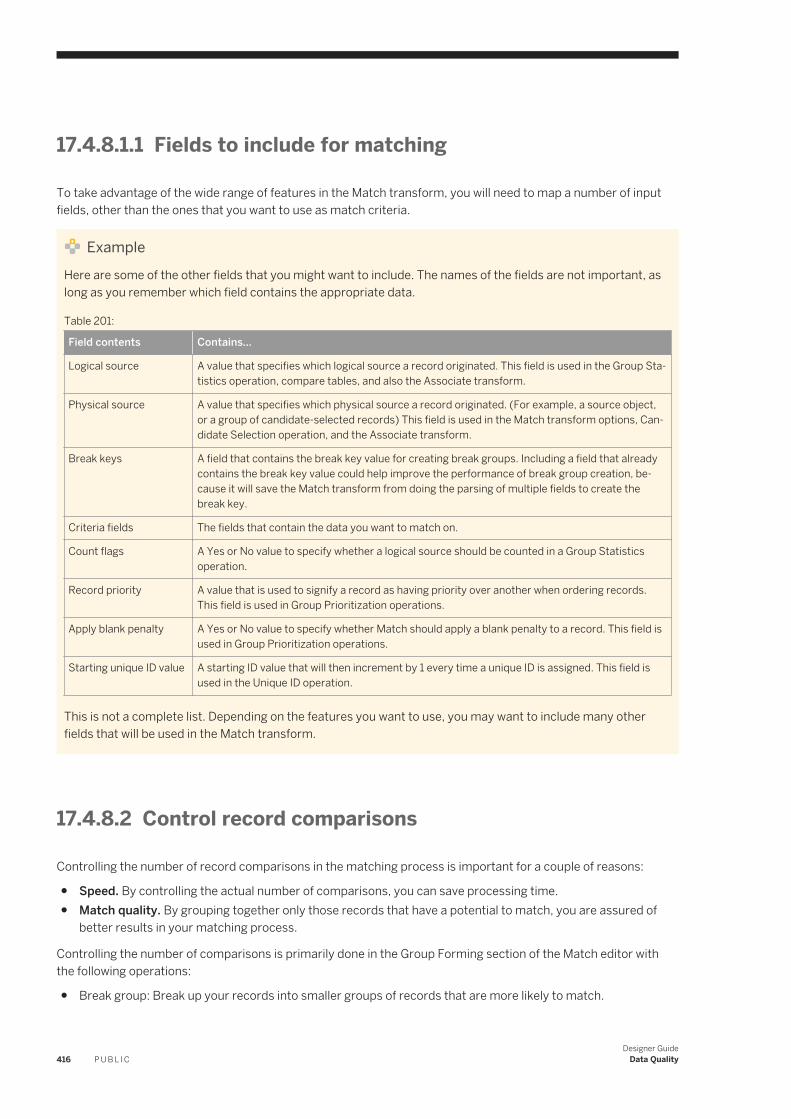
17.4.8.1.1 Fields to include for matching
To take advantage of the wide range of features in the Match transform, you will need to map a number of input fields, other than the ones that you want to use as match criteria.
ExampleHere are some of the other fields that you might want to include. The names of the fields are not important, as long as you remember which field contains the appropriate data.
Table 201:
Field contents Contains...
Logical source A value that specifies which logical source a record originated. This field is used in the Group Statistics operation, compare tables, and also the Associate transform.
Physical source A value that specifies which physical source a record originated. (For example, a source object, or a group of candidate-selected records) This field is used in the Match transform options, Candidate Selection operation, and the Associate transform.
Break keys A field that contains the break key value for creating break groups. Including a field that already contains the break key value could help improve the performance of break group creation, because it will save the Match transform from doing the parsing of multiple fields to create the break key.
Criteria fields The fields that contain the data you want to match on.
Count flags A Yes or No value to specify whether a logical source should be counted in a Group Statistics operation.
Record priority A value that is used to signify a record as having priority over another when ordering records. This field is used in Group Prioritization operations.
Apply blank penalty A Yes or No value to specify whether Match should apply a blank penalty to a record. This field is used in Group Prioritization operations.
Starting unique ID value A starting ID value that will then increment by 1 every time a unique ID is assigned. This field is used in the Unique ID operation.
This is not a complete list. Depending on the features you want to use, you may want to include many other fields that will be used in the Match transform.
17.4.8.2 Control record comparisons
Controlling the number of record comparisons in the matching process is important for a couple of reasons:
● Speed. By controlling the actual number of comparisons, you can save processing time.● Match quality. By grouping together only those records that have a potential to match, you are assured of
better results in your matching process.
Controlling the number of comparisons is primarily done in the Group Forming section of the Match editor with the following operations:
● Break group: Break up your records into smaller groups of records that are more likely to match.
416 P U B L I CDesigner Guide
Data Quality
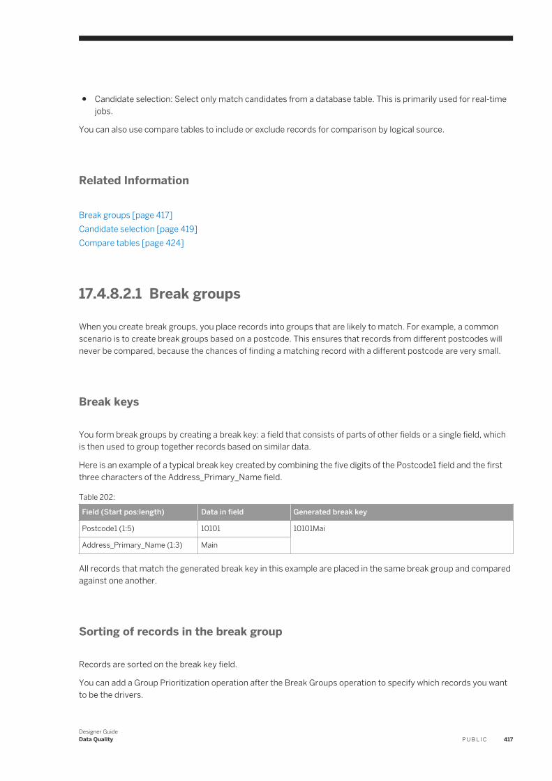
● Candidate selection: Select only match candidates from a database table. This is primarily used for real-time jobs.
You can also use compare tables to include or exclude records for comparison by logical source.
Related Information
Break groups [page 417]Candidate selection [page 419]Compare tables [page 424]
17.4.8.2.1 Break groups
When you create break groups, you place records into groups that are likely to match. For example, a common scenario is to create break groups based on a postcode. This ensures that records from different postcodes will never be compared, because the chances of finding a matching record with a different postcode are very small.
Break keys
You form break groups by creating a break key: a field that consists of parts of other fields or a single field, which is then used to group together records based on similar data.
Here is an example of a typical break key created by combining the five digits of the Postcode1 field and the first three characters of the Address_Primary_Name field.
Table 202:
Field (Start pos:length) Data in field Generated break key
Postcode1 (1:5) 10101 10101Mai
Address_Primary_Name (1:3) Main
All records that match the generated break key in this example are placed in the same break group and compared against one another.
Sorting of records in the break group
Records are sorted on the break key field.
You can add a Group Prioritization operation after the Break Groups operation to specify which records you want to be the drivers.
Designer GuideData Quality P U B L I C 417
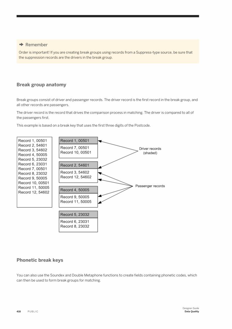
RememberOrder is important! If you are creating break groups using records from a Suppress-type source, be sure that the suppression records are the drivers in the break group.
Break group anatomy
Break groups consist of driver and passenger records. The driver record is the first record in the break group, and all other records are passengers.
The driver record is the record that drives the comparison process in matching. The driver is compared to all of the passengers first.
This example is based on a break key that uses the first three digits of the Postcode.
Phonetic break keys
You can also use the Soundex and Double Metaphone functions to create fields containing phonetic codes, which can then be used to form break groups for matching.
418 P U B L I CDesigner Guide
Data Quality
Related Information
Phonetic match criteria [page 470]
17.4.8.2.1.1 Creating break groups
We recommend that you standardize your data before you create your break keys. Data can be treated differently that is inconsistently cased, for example.
1. Add a Break Groups operation to the Group Forming option group.2. in the Break key table, add a row by clicking the Add button.3. Select a field in the field column that you want to use as a break key.
Postcode is a common break key to use.4. Choose the start position and length (number of characters) you want used in your break key.
You can use negative integers to signify that you want to start at the end of the actual string length, not the specified length of the field. For example, Field(-3,3) takes the last 3 characters of the string, whether the string has length of 10 or a length of 5.
5. Add more rows and fields as necessary.6. Order your rows by selecting a row and clicking the Move Up and Move Down buttons.
Ordering your rows ensures that the fields are used in the right order in the break key.
Your break key is now created.
17.4.8.2.2 Candidate selection
To speed processing in a match job, use the Candidate Selection operaton (Group forming option group) in the Match transform to append records from a relational database to an existing data collection before matching. When the records are appended, they are not logically grouped in any way. They are simply appended to the end of the data collection on a record-by-record basis until the collection reaches the specified size.
For example, suppose you have a new source of records that you want to compare against your data warehouse in a batch job. From this warehouse, you can select records that match the break keys of the new source. This helps narrow down the number of comparisons the Match transform has to make.
For example, here is a simplified illustration: Suppose your job is comparing a new source database—a smaller, regional file—with a large, national database that includes 15 records in each of 43,000 or so postcodes. Further assume that you want to form break groups based only on the postcode.
Designer GuideData Quality P U B L I C 419
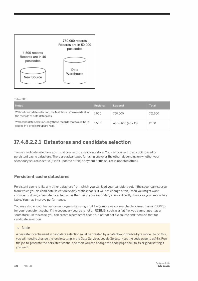
Table 203:
Notes Regional National Total
Without candidate selection, the Match transform reads all of the records of both databases.
1,500 750,000 751,500
With candidate selection, only those records that would be included in a break group are read.
1,500 About 600 (40 x 15) 2,100
17.4.8.2.2.1 Datastores and candidate selection To use candidate selection, you must connect to a valid datastore. You can connect to any SQL-based or persistent cache datastore. There are advantages for using one over the other, depending on whether your secondary source is static (it isn't updated often) or dynamic (the source is updated often).
Persistent cache datastores
Persistent cache is like any other datastore from which you can load your candidate set. If the secondary source from which you do candidate selection is fairly static (that is, it will not change often), then you might want consider building a persistent cache, rather than using your secondary source directly, to use as your secondary table. You may improve performance.
You may also encounter performance gains by using a flat file (a more easily searchable format than a RDBMS) for your persistent cache. If the secondary source is not an RDBMS, such as a flat file, you cannot use it as a "datastore". In this case, you can create a persistent cache out of that flat file source and then use that for candidate selection.
NoteA persistent cache used in candidate selection must be created by a data flow in double-byte mode. To do this, you will need to change the locale setting in the Data Services Locale Selector (set the code page to utf-8). Run the job to generate the persistent cache, and then you can change the code page back to its original setting if you want.
420 P U B L I CDesigner Guide
Data Quality
Cache size
Performance gains using persistent cache also depend on the size of the secondary source data. As the size of the data loaded in the persistent cache increases, the performance gains may decrease. Also note that if the original secondary source table is properly indexed and optimized for speed then there may be no benefit in creating a persistent cache (or even pre-load cache) out of it.
Related Information
Persistent cache datastores [page 83]
17.4.8.2.2.2 Auto-generation vs. custom SQL
There are cases where the Match transform can generate SQL for you, and there are times where you must create your own SQL. This is determined by the options you and how your secondary table (the table you are selecting match candidates from) is set up.
Use this table to help you determine whether you can use auto-generated SQL or if you must create your own.
NoteIn the following scenarios, “input data” refers to break key fields coming from a transform upstream from the Match transform (such as a Query transform) or a break key fields coming from the Break Group operation within the Match transform itself.
Table 204:
Scenario Auto-generate or Custom?
You have a single break key field in your input data, and you have the same field in your secondary table.
Auto-generate
You have multiple break key fields in your input data, and you have the same fields in your secondary table.
Auto-generate
You have multiple break key fields in your input data, and you have one break key field in your secondary table.
Auto-generate
You have a single break key field in your input data, and you have multiple break key fields in your secondary table.
Custom
You have multiple break key fields in your input data, but you have a different format or number of fields in your secondary table.
Custom
You want to select from multiple input sources. Custom
Designer GuideData Quality P U B L I C 421
17.4.8.2.2.3 Break keys and candidate selection
We recommend that you create a break key column in your secondary table (the table that contains the records you want to compare with the input data in your data flow) that matches the break key you create your break groups with in the Match transform. This makes setup of the Candidate Selection operation much easier. Also, each of these columns should be indexed.
We also recommend that you create and populate the database you are selecting from with a single break key field, rather than pulling substrings from database fields to create your break key. This can help improve the performance of candidate selection.
NoteRecords extracted by candidate selection are appended to the end of an existing break group (if you are using break groups). So, if you do not reorder the records using a Group Prioritization operation after the Candidate Selection operation, records from the original source will always be the driver records in the break groups. If you are using candidate selection on a Suppress source, you will need to reorder the records so that the records from the Suppress source are the drivers.
17.4.8.2.2.4 Setting up candidate selection
If you are using Candidate selection for a real-time job, be sure to deselect the Split records into break groups option in the Break Group operation of the Match transform.
To speed processing in a real-time match job, use the Candidate Selection operaton (Group forming option group) in the Match transform to append records from a relational database to an existing data collection before matching. When the records are appended, they are not logically grouped in any way. They are simply appended to the end of the data collection on a record-by-record basis until the collection reaches the specified size.
1. In the Candidate Selection operation, select a valid datastore from the Datastore drop-down list.2. In the Cache type drop-down list, choose from the following values:
Option Description
No_Cache Captures data at a point in time. The data doesn't change until the job restarts.
Pre-load Cache Use this option for static data.
3. Depending on how your input data and secondary table are structured, do one of the following:
○ Select Auto-generate SQL. Then select the Use break column from database option, if you have one, and choose a column from the Break key field drop-down list.
NoteIf you choose the Auto-generate SQL option, we recommend that you have a break key column in your secondary table and select the Use break column from database option. If you don't, the SQL that is created could be incorrect.
○ Select Create custom SQL, and either click the Launch SQL Editor button or type your SQL in the SQL edit box.
422 P U B L I CDesigner Guide
Data Quality
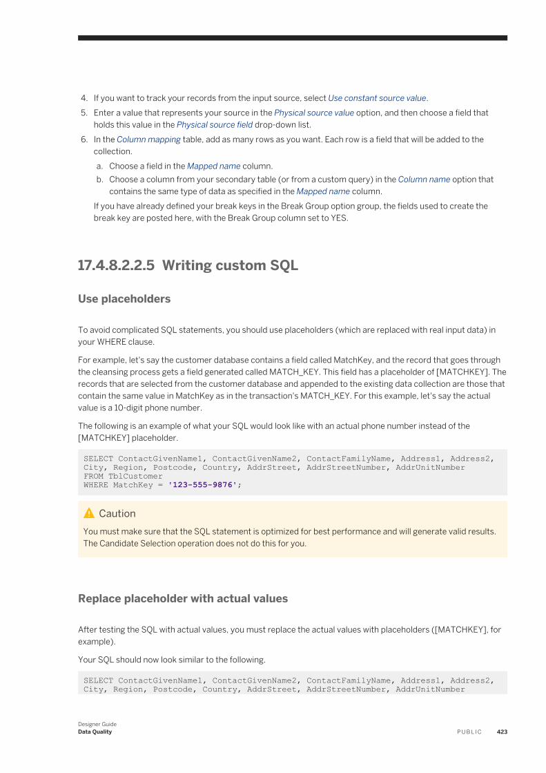
4. If you want to track your records from the input source, select Use constant source value.5. Enter a value that represents your source in the Physical source value option, and then choose a field that
holds this value in the Physical source field drop-down list.6. In the Column mapping table, add as many rows as you want. Each row is a field that will be added to the
collection.a. Choose a field in the Mapped name column.b. Choose a column from your secondary table (or from a custom query) in the Column name option that
contains the same type of data as specified in the Mapped name column.If you have already defined your break keys in the Break Group option group, the fields used to create the break key are posted here, with the Break Group column set to YES.
17.4.8.2.2.5 Writing custom SQL
Use placeholders
To avoid complicated SQL statements, you should use placeholders (which are replaced with real input data) in your WHERE clause.
For example, let's say the customer database contains a field called MatchKey, and the record that goes through the cleansing process gets a field generated called MATCH_KEY. This field has a placeholder of [MATCHKEY]. The records that are selected from the customer database and appended to the existing data collection are those that contain the same value in MatchKey as in the transaction's MATCH_KEY. For this example, let's say the actual value is a 10-digit phone number.
The following is an example of what your SQL would look like with an actual phone number instead of the [MATCHKEY] placeholder.
SELECT ContactGivenName1, ContactGivenName2, ContactFamilyName, Address1, Address2, City, Region, Postcode, Country, AddrStreet, AddrStreetNumber, AddrUnitNumber FROM TblCustomer WHERE MatchKey = '123-555-9876';
CautionYou must make sure that the SQL statement is optimized for best performance and will generate valid results. The Candidate Selection operation does not do this for you.
Replace placeholder with actual values
After testing the SQL with actual values, you must replace the actual values with placeholders ([MATCHKEY], for example).
Your SQL should now look similar to the following.
SELECT ContactGivenName1, ContactGivenName2, ContactFamilyName, Address1, Address2, City, Region, Postcode, Country, AddrStreet, AddrStreetNumber, AddrUnitNumber
Designer GuideData Quality P U B L I C 423
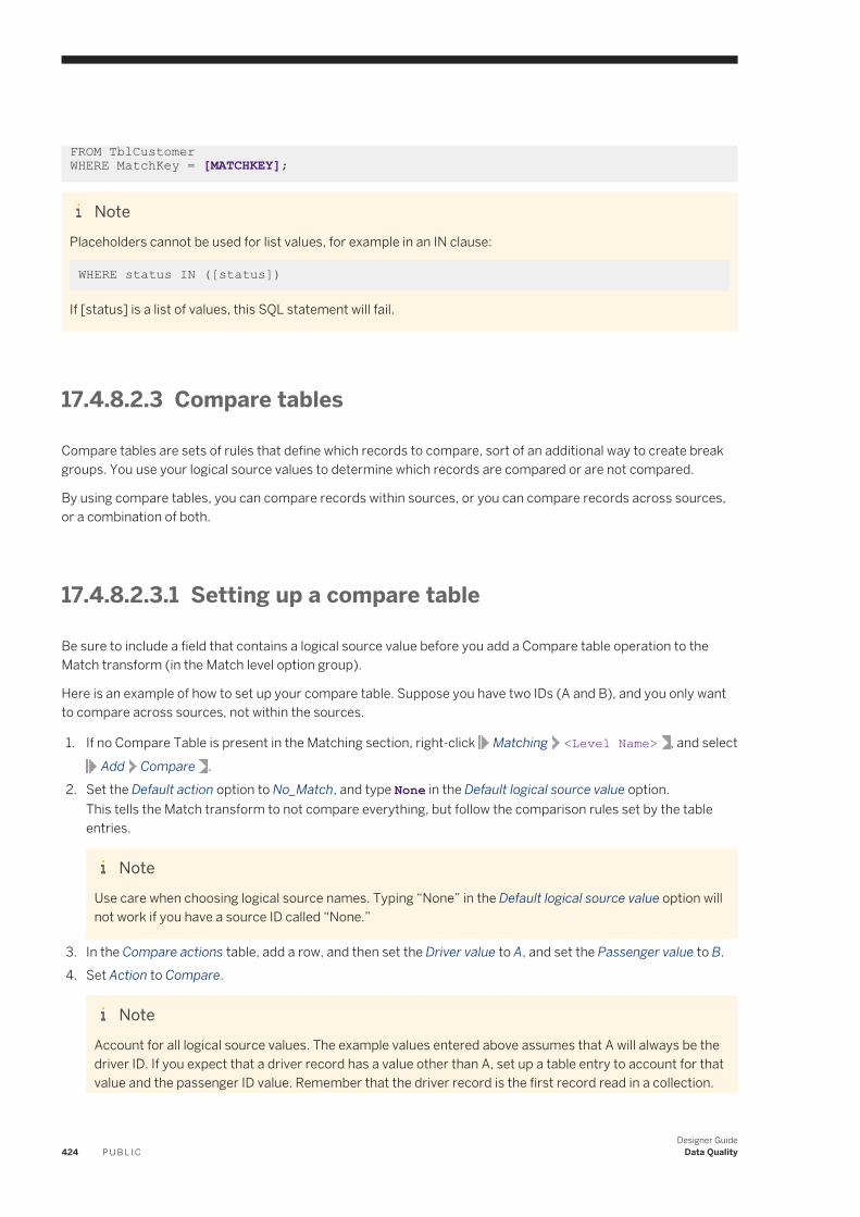
FROM TblCustomer WHERE MatchKey = [MATCHKEY];
NotePlaceholders cannot be used for list values, for example in an IN clause:
WHERE status IN ([status])
If [status] is a list of values, this SQL statement will fail.
17.4.8.2.3 Compare tables
Compare tables are sets of rules that define which records to compare, sort of an additional way to create break groups. You use your logical source values to determine which records are compared or are not compared.
By using compare tables, you can compare records within sources, or you can compare records across sources, or a combination of both.
17.4.8.2.3.1 Setting up a compare table
Be sure to include a field that contains a logical source value before you add a Compare table operation to the Match transform (in the Match level option group).
Here is an example of how to set up your compare table. Suppose you have two IDs (A and B), and you only want to compare across sources, not within the sources.
1. If no Compare Table is present in the Matching section, right-click Matching <Level Name> , and select Add Compare .
2. Set the Default action option to No_Match, and type None in the Default logical source value option.This tells the Match transform to not compare everything, but follow the comparison rules set by the table entries.
NoteUse care when choosing logical source names. Typing “None” in the Default logical source value option will not work if you have a source ID called “None.”
3. In the Compare actions table, add a row, and then set the Driver value to A, and set the Passenger value to B.4. Set Action to Compare.
NoteAccount for all logical source values. The example values entered above assumes that A will always be the driver ID. If you expect that a driver record has a value other than A, set up a table entry to account for that value and the passenger ID value. Remember that the driver record is the first record read in a collection.
424 P U B L I CDesigner Guide
Data Quality
If you leave the Driver value or Passenger value options blank in the compare table, then it will mean that you want to compare all sources. So a Driver value of A and a blank passenger record with an action of compare will make a record from A compare against all other passenger records.
Sometimes data in collections can be ordered (or not ordered, as the case may be) differently than your compare table is expecting. This can cause the matching process to miss duplicate records.
In the example, the way you set up your Compare action table row means that you are expecting that the driver record should have a driver value of A, but if the driver record comes in with a value of B, and the passenger comes in with a value of A, it won't be compared.
To account for situations where a driver record might have a value of B and the passenger a value of A, for example, include another row in the table that does the opposite. This will make sure that any record with a value of A or B is compared, no matter which is the Driver or Passenger.
NoteIn general, if you use a suppress source, you should compare within the other sources.This ensures that all of the matches of those sources are suppressed when any are found to duplicate a record on the suppress source, regardless of which record is the driver record.
17.4.8.3 Ordering and prioritizing records
You may have data sources, such as your own data warehouse, that you might trust more than records from another source, such as a rented source, for example. You may also prefer newer records over older records, or more complete records over those with blank fields. Whatever your preference, the way to express this preference in the matching process is using priorities.
There are other times where you might want to ensure that your records move to a given operation, such as matching or best record, for example, in a particular order. For example, you might want your match groups to be ordered so that the first record in is the newest record of the group. In this case, you would want to order your records based on a date field.
Whatever the reason, there are a two ways to order your records, either before or after the comparison process:
● Sorting records in break groups or match groups using a value in a field.● Using penalty scores. These can be defined per field, per record, or based on input source membership.
Match editor
You can define your priorities and order your records in the Group Prioritization operation, available in Group Forming and in the Post-match processing operations of each match level in the Match editor.
Designer GuideData Quality P U B L I C 425
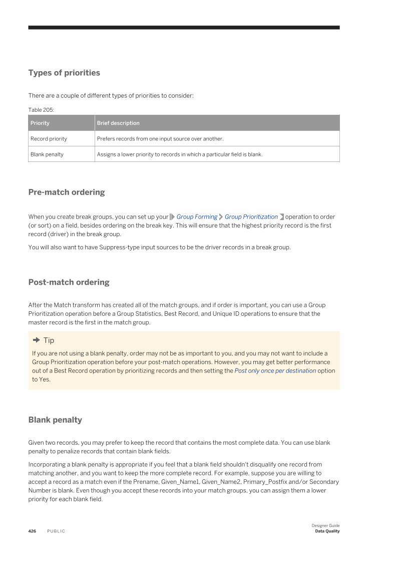
Types of priorities
There are a couple of different types of priorities to consider:
Table 205:
Priority Brief description
Record priority Prefers records from one input source over another.
Blank penalty Assigns a lower priority to records in which a particular field is blank.
Pre-match ordering
When you create break groups, you can set up your Group Forming Group Prioritization operation to order (or sort) on a field, besides ordering on the break key. This will ensure that the highest priority record is the first record (driver) in the break group.
You will also want to have Suppress-type input sources to be the driver records in a break group.
Post-match ordering
After the Match transform has created all of the match groups, and if order is important, you can use a Group Prioritization operation before a Group Statistics, Best Record, and Unique ID operations to ensure that the master record is the first in the match group.
TipIf you are not using a blank penalty, order may not be as important to you, and you may not want to include a Group Prioritization operation before your post-match operations. However, you may get better performance out of a Best Record operation by prioritizing records and then setting the Post only once per destination option to Yes.
Blank penalty
Given two records, you may prefer to keep the record that contains the most complete data. You can use blank penalty to penalize records that contain blank fields.
Incorporating a blank penalty is appropriate if you feel that a blank field shouldn't disqualify one record from matching another, and you want to keep the more complete record. For example, suppose you are willing to accept a record as a match even if the Prename, Given_Name1, Given_Name2, Primary_Postfix and/or Secondary Number is blank. Even though you accept these records into your match groups, you can assign them a lower priority for each blank field.
426 P U B L I CDesigner Guide
Data Quality
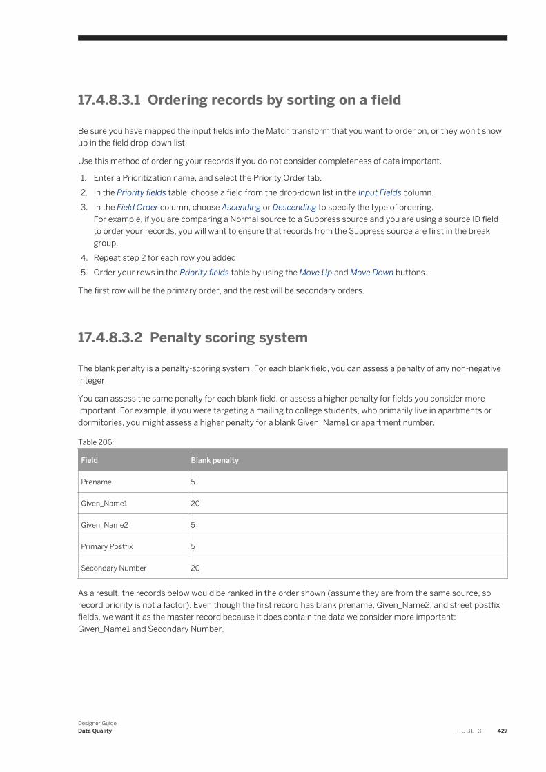
17.4.8.3.1 Ordering records by sorting on a field
Be sure you have mapped the input fields into the Match transform that you want to order on, or they won't show up in the field drop-down list.
Use this method of ordering your records if you do not consider completeness of data important.
1. Enter a Prioritization name, and select the Priority Order tab.2. In the Priority fields table, choose a field from the drop-down list in the Input Fields column.3. In the Field Order column, choose Ascending or Descending to specify the type of ordering.
For example, if you are comparing a Normal source to a Suppress source and you are using a source ID field to order your records, you will want to ensure that records from the Suppress source are first in the break group.
4. Repeat step 2 for each row you added.5. Order your rows in the Priority fields table by using the Move Up and Move Down buttons.
The first row will be the primary order, and the rest will be secondary orders.
17.4.8.3.2 Penalty scoring system
The blank penalty is a penalty-scoring system. For each blank field, you can assess a penalty of any non-negative integer.
You can assess the same penalty for each blank field, or assess a higher penalty for fields you consider more important. For example, if you were targeting a mailing to college students, who primarily live in apartments or dormitories, you might assess a higher penalty for a blank Given_Name1 or apartment number.
Table 206:
Field Blank penalty
Prename 5
Given_Name1 20
Given_Name2 5
Primary Postfix 5
Secondary Number 20
As a result, the records below would be ranked in the order shown (assume they are from the same source, so record priority is not a factor). Even though the first record has blank prename, Given_Name2, and street postfix fields, we want it as the master record because it does contain the data we consider more important: Given_Name1 and Secondary Number.
Designer GuideData Quality P U B L I C 427
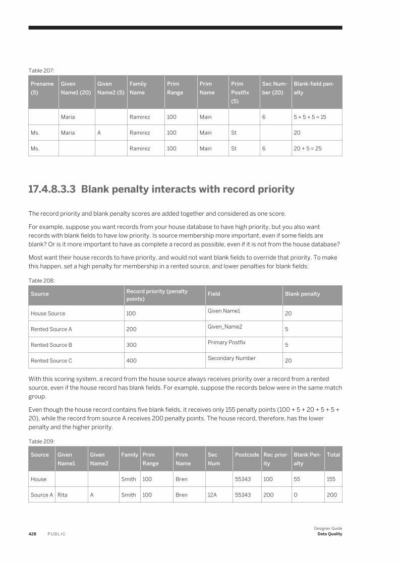
Table 207:
Prename (5)
Given Name1 (20)
Given Name2 (5)
Family Name
Prim Range
Prim Name
Prim Postfix (5)
Sec Number (20)
Blank-field penalty
Maria Ramirez 100 Main 6 5 + 5 + 5 = 15
Ms. Maria A Ramirez 100 Main St 20
Ms. Ramirez 100 Main St 6 20 + 5 = 25
17.4.8.3.3 Blank penalty interacts with record priority
The record priority and blank penalty scores are added together and considered as one score.
For example, suppose you want records from your house database to have high priority, but you also want records with blank fields to have low priority. Is source membership more important, even if some fields are blank? Or is it more important to have as complete a record as possible, even if it is not from the house database?
Most want their house records to have priority, and would not want blank fields to override that priority. To make this happen, set a high penalty for membership in a rented source, and lower penalties for blank fields:
Table 208:
Source Record priority (penalty points)
Field Blank penalty
House Source 100 Given Name1 20
Rented Source A 200 Given_Name2 5
Rented Source B 300 Primary Postfix 5
Rented Source C 400 Secondary Number 20
With this scoring system, a record from the house source always receives priority over a record from a rented source, even if the house record has blank fields. For example, suppose the records below were in the same match group.
Even though the house record contains five blank fields, it receives only 155 penalty points (100 + 5 + 20 + 5 + 5 + 20), while the record from source A receives 200 penalty points. The house record, therefore, has the lower penalty and the higher priority.
Table 209:
Source Given Name1
Given Name2
Family Prim Range
Prim Name
Sec Num
Postcode Rec priority
Blank Penalty
Total
House Smith 100 Bren 55343 100 55 155
Source A Rita A Smith 100 Bren 12A 55343 200 0 200
428 P U B L I CDesigner Guide
Data Quality
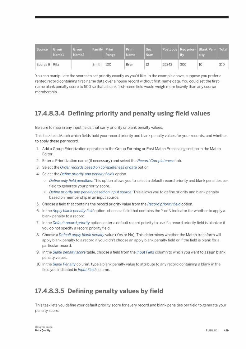
Source Given Name1
Given Name2
Family Prim Range
Prim Name
Sec Num
Postcode Rec priority
Blank Penalty
Total
Source B Rita Smith 100 Bren 12 55343 300 10 310
You can manipulate the scores to set priority exactly as you'd like. In the example above, suppose you prefer a rented record containing first-name data over a house record without first-name data. You could set the first-name blank penalty score to 500 so that a blank first-name field would weigh more heavily than any source membership.
17.4.8.3.4 Defining priority and penalty using field values
Be sure to map in any input fields that carry priority or blank penalty values.
This task tells Match which fields hold your record priority and blank penalty values for your records, and whether to apply these per record.
1. Add a Group Prioritization operation to the Group Forming or Post Match Processing section in the Match Editor.
2. Enter a Prioritization name (if necessary) and select the Record Completeness tab.3. Select the Order records based on completeness of data option.4. Select the Define priority and penalty fields option.
○ Define only field penalties: This option allows you to select a default record priority and blank penalties per field to generate your priority score.
○ Define priority and penalty based on input source: This allows you to define priority and blank penalty based on membership in an input source.
5. Choose a field that contains the record priority value from the Record priority field option.6. In the Apply blank penalty field option, choose a field that contains the Y or N indicator for whether to apply a
blank penalty to a record.7. In the Default record priority option, enter a default record priority to use if a record priority field is blank or if
you do not specify a record priority field.8. Choose a Default apply blank penalty value (Yes or No). This determines whether the Match transform will
apply blank penalty to a record if you didn't choose an apply blank penalty field or if the field is blank for a particular record.
9. In the Blank penalty score table, choose a field from the Input Field column to which you want to assign blank penalty values.
10. In the Blank Penalty column, type a blank penalty value to attribute to any record containing a blank in the field you indicated in Input Field column.
17.4.8.3.5 Defining penalty values by field
This task lets you define your default priority score for every record and blank penalties per field to generate your penalty score.
Designer GuideData Quality P U B L I C 429
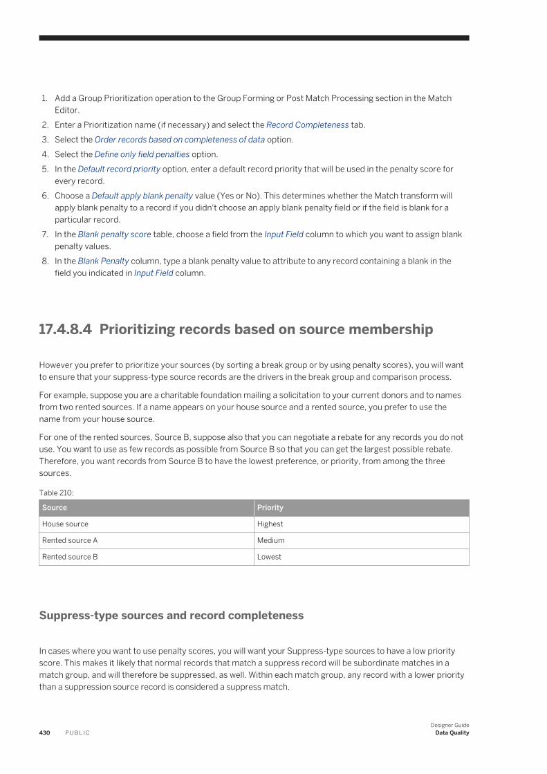
1. Add a Group Prioritization operation to the Group Forming or Post Match Processing section in the Match Editor.
2. Enter a Prioritization name (if necessary) and select the Record Completeness tab.3. Select the Order records based on completeness of data option.4. Select the Define only field penalties option.5. In the Default record priority option, enter a default record priority that will be used in the penalty score for
every record.6. Choose a Default apply blank penalty value (Yes or No). This determines whether the Match transform will
apply blank penalty to a record if you didn't choose an apply blank penalty field or if the field is blank for a particular record.
7. In the Blank penalty score table, choose a field from the Input Field column to which you want to assign blank penalty values.
8. In the Blank Penalty column, type a blank penalty value to attribute to any record containing a blank in the field you indicated in Input Field column.
17.4.8.4 Prioritizing records based on source membership
However you prefer to prioritize your sources (by sorting a break group or by using penalty scores), you will want to ensure that your suppress-type source records are the drivers in the break group and comparison process.
For example, suppose you are a charitable foundation mailing a solicitation to your current donors and to names from two rented sources. If a name appears on your house source and a rented source, you prefer to use the name from your house source.
For one of the rented sources, Source B, suppose also that you can negotiate a rebate for any records you do not use. You want to use as few records as possible from Source B so that you can get the largest possible rebate. Therefore, you want records from Source B to have the lowest preference, or priority, from among the three sources.
Table 210:
Source Priority
House source Highest
Rented source A Medium
Rented source B Lowest
Suppress-type sources and record completeness
In cases where you want to use penalty scores, you will want your Suppress-type sources to have a low priority score. This makes it likely that normal records that match a suppress record will be subordinate matches in a match group, and will therefore be suppressed, as well. Within each match group, any record with a lower priority than a suppression source record is considered a suppress match.
430 P U B L I CDesigner Guide
Data Quality
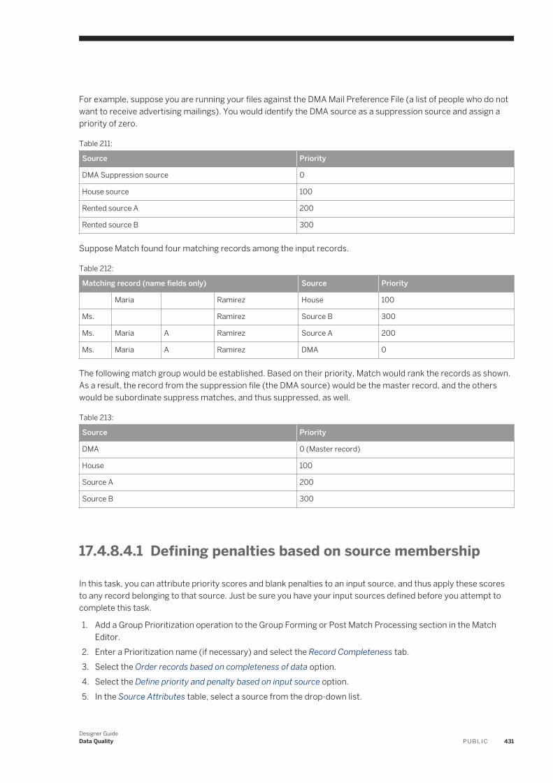
For example, suppose you are running your files against the DMA Mail Preference File (a list of people who do not want to receive advertising mailings). You would identify the DMA source as a suppression source and assign a priority of zero.
Table 211:
Source Priority
DMA Suppression source 0
House source 100
Rented source A 200
Rented source B 300
Suppose Match found four matching records among the input records.
Table 212:
Matching record (name fields only) Source Priority
Maria Ramirez House 100
Ms. Ramirez Source B 300
Ms. Maria A Ramirez Source A 200
Ms. Maria A Ramirez DMA 0
The following match group would be established. Based on their priority, Match would rank the records as shown. As a result, the record from the suppression file (the DMA source) would be the master record, and the others would be subordinate suppress matches, and thus suppressed, as well.
Table 213:
Source Priority
DMA 0 (Master record)
House 100
Source A 200
Source B 300
17.4.8.4.1 Defining penalties based on source membership
In this task, you can attribute priority scores and blank penalties to an input source, and thus apply these scores to any record belonging to that source. Just be sure you have your input sources defined before you attempt to complete this task.
1. Add a Group Prioritization operation to the Group Forming or Post Match Processing section in the Match Editor.
2. Enter a Prioritization name (if necessary) and select the Record Completeness tab.3. Select the Order records based on completeness of data option.4. Select the Define priority and penalty based on input source option.5. In the Source Attributes table, select a source from the drop-down list.
Designer GuideData Quality P U B L I C 431
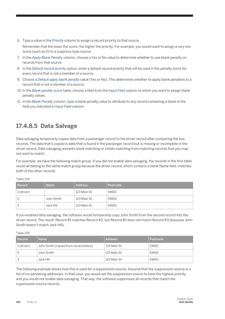
6. Type a value in the Priority column to assign a record priority to that source.Remember that the lower the score, the higher the priority. For example, you would want to assign a very low score (such as 0) to a suppress-type source.
7. In the Apply Blank Penalty column, choose a Yes or No value to determine whether to use blank penalty on records from that source.
8. In the Default record priority option, enter a default record priority that will be used in the penalty score for every record that is not a member of a source.
9. Choose a Default apply blank penalty value (Yes or No). This determines whether to apply blank penalties to a record that is not a member of a source.
10. In the Blank penalty score table, choose a field from the Input Field column to which you want to assign blank penalty values.
11. In the Blank Penalty column, type a blank penalty value to attribute to any record containing a blank in the field you indicated in Input Field column.
17.4.8.5 Data Salvage
Data salvaging temporarily copies data from a passenger record to the driver record after comparing the two records. The data that’s copied is data that is found in the passenger record but is missing or incomplete in the driver record. Data salvaging prevents blank matching or initials matching from matching records that you may not want to match.
For example, we have the following match group. If you did not enable data salvaging, the records in the first table would all belong to the same match group because the driver record, which contains a blank Name field, matches both of the other records.
Table 214:
Record Name Address Postcode
1 (driver) 123 Main St. 54601
2 John Smith 123 Main St. 54601
3 Jack Hill 123 Main St. 54601
If you enabled data salvaging, the software would temporarily copy John Smith from the second record into the driver record. The result: Record #1 matches Record #2, but Record #1 does not match Record #3 (because John Smith doesn’t match Jack Hill).
Table 215:
Record Name Address Postcode
1 (driver) John Smith (copied from record below) 123 Main St. 54601
2 John Smith 123 Main St. 54601
3 Jack Hill 123 Main St. 54601
The following example shows how this is used for a suppression source. Assume that the suppression source is a list of no-pandering addresses. In that case, you would set the suppression source to have the highest priority, and you would not enable data salvaging. That way, the software suppresses all records that match the suppression source records.
432 P U B L I CDesigner Guide
Data Quality
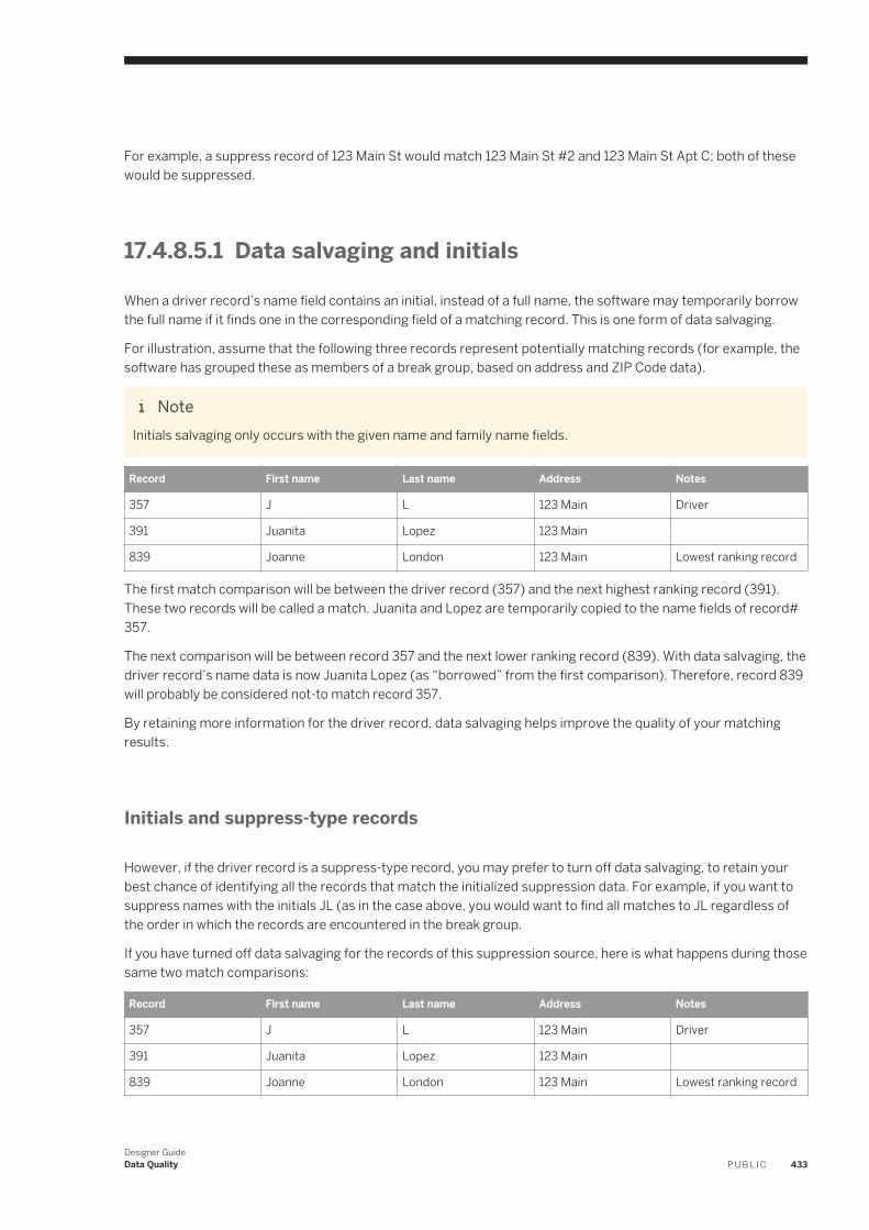
For example, a suppress record of 123 Main St would match 123 Main St #2 and 123 Main St Apt C; both of these would be suppressed.
17.4.8.5.1 Data salvaging and initials
When a driver record’s name field contains an initial, instead of a full name, the software may temporarily borrow the full name if it finds one in the corresponding field of a matching record. This is one form of data salvaging.
For illustration, assume that the following three records represent potentially matching records (for example, the software has grouped these as members of a break group, based on address and ZIP Code data).
NoteInitials salvaging only occurs with the given name and family name fields.
Record First name Last name Address Notes
357 J L 123 Main Driver
391 Juanita Lopez 123 Main
839 Joanne London 123 Main Lowest ranking record
The first match comparison will be between the driver record (357) and the next highest ranking record (391). These two records will be called a match. Juanita and Lopez are temporarily copied to the name fields of record# 357.
The next comparison will be between record 357 and the next lower ranking record (839). With data salvaging, the driver record’s name data is now Juanita Lopez (as “borrowed” from the first comparison). Therefore, record 839 will probably be considered not-to match record 357.
By retaining more information for the driver record, data salvaging helps improve the quality of your matching results.
Initials and suppress-type records
However, if the driver record is a suppress-type record, you may prefer to turn off data salvaging, to retain your best chance of identifying all the records that match the initialized suppression data. For example, if you want to suppress names with the initials JL (as in the case above, you would want to find all matches to JL regardless of the order in which the records are encountered in the break group.
If you have turned off data salvaging for the records of this suppression source, here is what happens during those same two match comparisons:
Record First name Last name Address Notes
357 J L 123 Main Driver
391 Juanita Lopez 123 Main
839 Joanne London 123 Main Lowest ranking record
Designer GuideData Quality P U B L I C 433
The first match comparison will be between the driver record (357) and the next- highest ranking record (391). These two records will be called a match, since the driver record’s JL and Juanita Lopez will be called a match.
The next comparison will be between the driver record (357) and the next lower ranking record (839). This time these two records will also be called a match, since the driver record’s JL will match Joanne London.
Since both records 391 and 839 matched the suppress-type driver record, they are both designated as suppress matches, and, therefore, neither will be included in your output.
17.4.8.5.2 Controlling data salvaging using a field
You can use a field to control whether data salvage is enabled. If the field's value is Y for a record, data salvaging is enabled. Be sure to map the field into the Match transform that you want to use beforehand.
1. Open the Match Editor for a Match transform.2. In the Transform Options window, click the Data Salvage tab.3. Select the Enable data salvage option, and choose a default value for those records.
The default value will be used in the cases where the field you choose is not populated for a particular record.4. Select the Specify data salvage by field option, and choose a field from the drop-down menu.
17.4.8.5.3 Controlling data salvaging by source
You can use membership in an input source to control whether data salvage is enabled or disabled for a particular record. Be sure to create your input sources beforehand.
1. Open the Match Editor for a Match transform.2. In the Transform Options window, click the Data Salvage tab.3. Select the Enable data salvage option, and choose a default value for those records.
The default value will be used if a record's input source is not specified in the following steps.4. Select the Specify data salvage by source option.5. In the table, choose a Source and then a Perform Data Salvage value for each source you want to use.
17.4.9 Match criteria
17.4.9.1 Overview of match criteria
Use match criteria in each match level to determine the threshold scores for matching and to define how to treat various types of data, such as numeric, blank, name data, and so on (your business rules).
You can do all of this in the Criteria option group of the Match Editor.
434 P U B L I CDesigner Guide
Data Quality
Match criteria
To the Match transform, match criteria represent the fields you want to compare. For example, if you wanted to match on the first ten characters of a given name and the first fifteen characters of the family name, you must create two criteria that specify these requirements.
Criteria provide a way to let the Match transform know what kind of data is in the input field and, therefore, what types of operations to perform on that data.
Pre-defined vs. custom criteria
There are two types of criteria:
● Pre-defined criteria are available for fields that are typically used for matching, such as name, address, and other data. By assigning a criteria to a field, the Match transform is able to identify what type of data is in the field, and allow it to perform internal operations to optimize the data for matching, without altering the actual input data.
● Data Cleanse custom (user-defined, non party-data) output fields are available as pre-defined criteria. Map the custom output fields from Data Cleanse and the custom fields appear in the Match Editor's Criteria Fields tab.Any other types of data (such as part numbers or other proprietary data), for which a pre-defined criteria does not exist, should be designated as a custom criteria. Certain functions can be performed on custom keys, such as abbreviation, substring, numeric matching, but the Match transform cannot perform some cross-field comparisons such as some name matching functions.
Match criteria pre-comparison options
The majority of your data standardization should take place in the address cleansing and Data Cleanse transforms. However, the Match transform can perform some preprocessing per criteria (and for matching purposes only; your actual data is not affected) to provide more accurate matches. The options to control this standardization are located in the Options and Multi Field Comparisons tabs of the Match editor. They include:
● Convert diacritical characters● Convert text to numbers● Convert to uppercase● Remove punctuation● Locale
For more information about these options, see the Match transform section of the Reference Guide.
17.4.9.1.1 Adding and ordering a match criteria
You can add as many criteria as you want to each match level in your Match transform.
Designer GuideData Quality P U B L I C 435
1. Select the appropriate match level or Match Criteria option group in the Option Explorer of the Match Editor, and right-click.
2. Choose Criteria.3. Enter a name for your criteria in the Criteria name box.
You can keep the default name for pre-defined criteria, but you should enter a meaningful criteria name if you chose a Custom criteria.
4. On the Criteria Fields tab, in the Available criteria list, choose the criteria that best represents the data that you want to match on. If you don't find what you are looking for, choose the Custom criteria.
5. In the Criteria field mapping table, choose an input field mapped name that contains the data you want to match on for this criteria.
6. Click the Options tab.7. Configure the Pre-comparison options and Comparison rules.
Be sure to set the Match score and No match score, because these are required.8. If you want to enable multiple field (cross-field) comparison, click the Multiple Fields Comparisons tab, and
select the Compare multiple fields option.a. Choose the type of multiple field comparison to perform:
○ All selected fields in other records: Compare each field to all fields selected in the table in all records.○ The same field in other records: Compare each field only to the same field in all records.
b. In the Additional fields to compare table, choose input fields that contain the data you want to include in the multiple field comparison for this criteria.
TipYou can use custom match criteria field names for multiple field comparison by typing in the Custom name column.
NoteIf you enable multiple field comparison, any appropriate match standard fields are removed from the Criteria field mapping table on the Criteria Fields tab . If you want to include them in the match process, add them in the Additional fields to compare table.
9. Configure the Pre-comparison options for multiple field comparison.10. To order your criteria in the Options Explorer of the Match Editor (or the Match Table), select a criteria and
click the Move Up or Move Down buttons as necessary.
17.4.9.1.2 Setting up for match standards criteria
Be sure you have created and mapped in match standard fields from the Data Cleanse transform.
1. In the Match transform, add a Person1_Given_Name1 match criteria by selecting it from the Person category.The editor automatically adds that criteria and its associated match standard criteria to the Criteria field mapping table.
2. Choose a field in the Input field mapped name column that best represents the data to be compared.
For Given_Name2 data (middle names), complete the above procedure, but use the following criteria:
436 P U B L I CDesigner Guide
Data Quality
● Person1_Given_Name2● Person1_Given_Name2_Match_Std1● Person1_Given_Name2_Match_Std2● Person1_Given_Name2_Match_Std3
You can also use match standards for prename, maturity postname, honorary postname, firm, and firm location fields.
17.4.9.2 Matching methods
There are a number of ways to set up and order your criteria to get the matching results you want. Each of these ways have advantages and disadvantages, so consider them carefully.
Table 216:
Match method Description
Rule-based Allows you to control which criteria determines a match. This method is easy to set up.
Weighted-scoring Allows you to assign importance, or weight, to any criteria. However, weighted-scoring evaluates every rule before determining a match, which might cause an increase in processing time.
Combination method
Same relative advantages and disadvantages as the other two methods.
17.4.9.2.1 Similarity score
The similarity score is the percentage that your data is alike.
This score is calculated internally by the application when records are compared. Whether the application considers the records a match depends on the Match and No match scores you define in the Criteria option group (as well as other factors, but for now let's focus on these scores).
ExampleThis is an example of how similarity scores are determined. Here are some things to note:
● The following comparison table is intended to serve as an example. This is not how the matching process works in the weighted scoring method, for example.
● Only the first comparison is considered a match, because the similarity score met or exceeded the match score. The last comparison is considered a no-match because the similarity score was less than the no-match score.
● When a single criteria cannot determine a match, as in the case of the second comparison in the following table, the process moves to the next criteria, if possible.
Designer GuideData Quality P U B L I C 437
Table 217:
Comparison No match Match Similarity score Matching?
Smith > Smith 72 95 100% Yes
Smith > Smitt 72 95 80% Depends on other criteria
Smith > Smythe 72 95 72% No
Smith > Jones 72 95 20% No
17.4.9.2.2 Rule-based method
With rule-based matching, you rely only on your match and no-match scores to determine matches within a criteria.
ExampleThis example shows how to set up this method in the Match transform.
Table 218:
Criteria Record A Record B No match Match Similarity score
Given Name1 Mary Mary 82 101 100
Family Name Smith Smitt 74 101 80
E-mail [email protected] [email protected] 79 80 91
By entering a value of 101 in the match score for every criteria except the last, the Given Name1 and Family Name criteria never determine a match, although they can determine a no match.
By setting the Match score and No match score options for the E-mail criteria with no gap, any comparison that reaches the last criteria must either be a match or a no match.
A match score of 101 ensures that the criteria does not cause the records to be a match, because two fields cannot be more than 100 percent alike.
RememberOrder is important! For performance reasons, you should have the criteria that is most likely to make the match or no-match decisions first in your order of criteria. This can help reduce the number of criteria comparisons.
438 P U B L I CDesigner Guide
Data Quality
17.4.9.2.3 Weighted-scoring method
In a rule-based matching method, the application gives all of the criteria the same amount of importance (or weight). That is, if any criteria fails to meet the specified match score, the application determines that the records do not match.
When you use the weighted scoring method, you are relying on the total contribution score for determining matches, as opposed to using match and no-match scores on their own.
Contribution values
Contribution values are your way of assigning weight to individual criteria. The higher the value, the more weight that criteria carries in determining matches. In general, criteria that might carry more weight than others include account numbers, Social Security numbers, customer numbers, Postcode1, and addresses.
NoteAll contribution values for all criteria that have them must total 100. You do not need to have a contribution value for all of your criteria.
You can define a criteria's contribution value in the Contribution to weighted score option in the Criteria option group.
Contribution and total contribution score
The Match transform generates the contribution score for each criteria by multiplying the contribution value you assign with the similarity score (the percentage alike). These individual contribution scores are then added to get the total contribution score.
Weighted match score
In the weighted scoring method, matches are determined only by comparing the total contribution score with the weighted match score. If the total contribution score is equal to or greater than the weighted match score, the records are considered a match. If the total weighted score is less than the weighted match score, the records are considered a no-match.
You can set the weighted match score in the Weighted match score option of the Level option group.
ExampleThe following table is an example of how to set up weighted scoring. Notice the various types of scores that we have discussed. Also notice the following:
Designer GuideData Quality P U B L I C 439
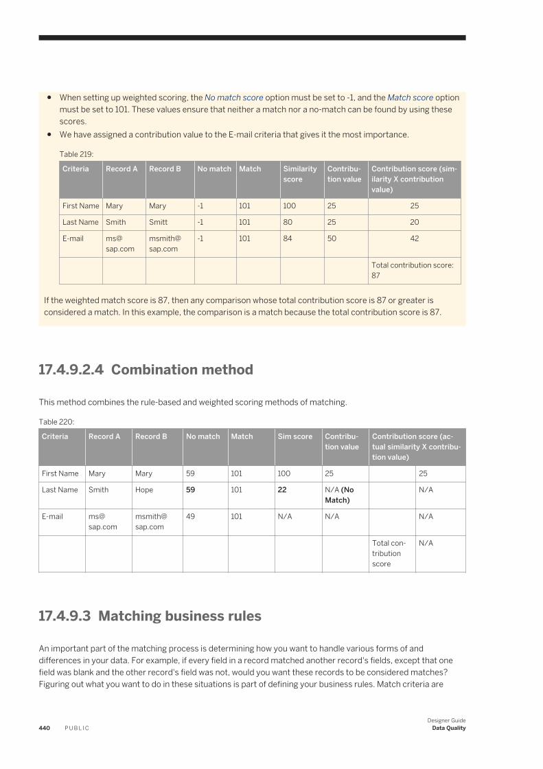
● When setting up weighted scoring, the No match score option must be set to -1, and the Match score option must be set to 101. These values ensure that neither a match nor a no-match can be found by using these scores.
● We have assigned a contribution value to the E-mail criteria that gives it the most importance.
Table 219:
Criteria Record A Record B No match Match Similarity score
Contribution value
Contribution score (similarity X contribution value)
First Name Mary Mary -1 101 100 25 25
Last Name Smith Smitt -1 101 80 25 20
E-mail ms@ sap.com
msmith@ sap.com
-1 101 84 50 42
Total contribution score: 87
If the weighted match score is 87, then any comparison whose total contribution score is 87 or greater is considered a match. In this example, the comparison is a match because the total contribution score is 87.
17.4.9.2.4 Combination method
This method combines the rule-based and weighted scoring methods of matching.
Table 220:
Criteria Record A Record B No match Match Sim score Contribution value
Contribution score (actual similarity X contribution value)
First Name Mary Mary 59 101 100 25 25
Last Name Smith Hope 59 101 22 N/A (No Match)
N/A
E-mail ms@ sap.com
msmith@ sap.com
49 101 N/A N/A N/A
Total contribution score
N/A
17.4.9.3 Matching business rules
An important part of the matching process is determining how you want to handle various forms of and differences in your data. For example, if every field in a record matched another record's fields, except that one field was blank and the other record's field was not, would you want these records to be considered matches? Figuring out what you want to do in these situations is part of defining your business rules. Match criteria are
440 P U B L I CDesigner Guide
Data Quality
where you define most of your business rules, while some name-based options are set in the Match Level option group.
17.4.9.3.1 Matching on strings, abbreviations, and initials
Part of defining your business rules is to make settings for matching strings, abbreviations, and initials.
For more information about setting scores for the following three options, see the Match criteria sections of the Reference Guide.
Table 221:
Option Description
Initials adjustment score Allows matching initials to whole words. For example, “International Health Providers” can be matched to “IHP”.
Abbreviation adjustment score Allows matching whole words to abbreviations. For example, “International Health Providers” can be matched to “Intl Health Providers”.
Substring adjustment score Allows matching longer strings to shorter strings. For example, the string “Mayfield Painting and Sand Blasting” can match “Mayfield painting”.
17.4.9.3.2 Extended abbrevation matching
Extended abbreviation matching offers functionality that handles situations not covered by the Initials adjustment score, Substring adjustment score, and Abbreviation adjustment score options. For example, you might encounter the following situations:
● Suppose you have localities in your data such as La Crosse and New York. However, you also have these same localities listed as LaCrosse and NewYork (without spaces). Under normal matching, you cannot designate these (La Crosse/LaCrosse and New York/NewYork) as matching 100%; the spaces prevent this. (These would normally be 94 and 93 percent matching.)
● Suppose you have Metropolitan Life and MetLife (an abbreviation and combination of Metropolitan Life) in your data. The Abbreviation adjustment score option cannot detect the combination of the two words.
If you are concerned about either of these cases in your data, you should use the Ext abbreviation adjustment score option.
How the adjustment score works
The score you set in the Ext abbreviation adjustment score option tunes your similarity score to consider these types of abbreviations and combinations in your data.
The adjustment score adds a penalty for the non-matched part of the words. The higher the number, the lower the penalty. A score of 100 means no penalty and score of 0 means maximum penalty.
Designer GuideData Quality P U B L I C 441
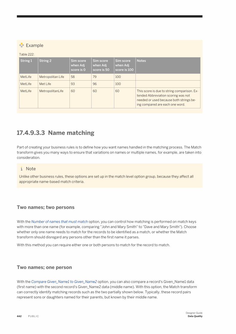
Example
Table 222:
String 1 String 2 Sim score when Adj score is 0
Sim score when Adj score is 50
Sim score when Adj score is 100
Notes
MetLife Metropolitan Life 58 79 100
MetLife Met Life 93 96 100
MetLife MetropolitanLife 60 60 60 This score is due to string comparison. Extended Abbreviation scoring was not needed or used because both strings being compared are each one word.
17.4.9.3.3 Name matching
Part of creating your business rules is to define how you want names handled in the matching process. The Match transform gives you many ways to ensure that variations on names or multiple names, for example, are taken into consideration.
NoteUnlike other business rules, these options are set up in the match level option group, because they affect all appropriate name-based match criteria.
Two names; two persons
With the Number of names that must match option, you can control how matching is performed on match keys with more than one name (for example, comparing "John and Mary Smith" to "Dave and Mary Smith"). Choose whether only one name needs to match for the records to be identified as a match, or whether the Match transform should disregard any persons other than the first name it parses.
With this method you can require either one or both persons to match for the record to match.
Two names; one person
With the Compare Given_Name1 to Given_Name2 option, you can also compare a record's Given_Name1 data (first name) with the second record's Given_Name2 data (middle name). With this option, the Match transform can correctly identify matching records such as the two partially shown below. Typically, these record pairs represent sons or daughters named for their parents, but known by their middle name.
442 P U B L I CDesigner Guide
Data Quality
Table 223:
Record # First name Middle name Last name Address
170 Leo Thomas Smith 225 Pushbutton Dr
198 Tom Smith 225 Pushbutton Dr
Hyphenated family names
With the Match on hyphenated family name option, you can control how matching is performed if a Family_Name (last name) field contains a hyphenated family name (for example, comparing "Smith-Jones" to "Jones"). Choose whether both criteria must have both names to match or just one name that must match for the records to be called a match.
17.4.9.3.3.1 Matching compound family names
The Approximate Substring score assists in setting up comparison of compound family names. The Approximate Substring score is assigned to the words that do not match to other words in a compared string. This option loosens some of the requirements of the Substring Adjustment score option in the following ways:
● First words do not have to match exactly.● The words that do match can use initials and abbreviations adjustments (For example, Rodriguez and RDZ).● Matching words have to be in the same order, but there can be non-matching words before or after the
matching words.● The Approximate Substring score is assigned the leftover words and spaces in the compared string.
The Approximate Substring option will increase the score for some matches found when using the Substring Matching Score.
ExampleWhen comparing CRUZ RODRIGUEZ and GARCIA CRUZ DE RDZ, the similarity scores are:
● Without setting any adjusments, the Similarity score is 48.● When you set the Substring adjustment score to 80 and the Abbreviation score to 80, the Similarity score
is 66.● When you set the Approximate substring adjustment score to 80 and the Abbreviation score to 80, the
Similarity score is 91.
17.4.9.3.4 Numeric data matching
Use the Numeric words match exactly option to choose whether data with a mixture of numbers and letters should match exactly. You can also specify how this data must match. This option applies most often to address data and custom data, such as a part number.
Designer GuideData Quality P U B L I C 443
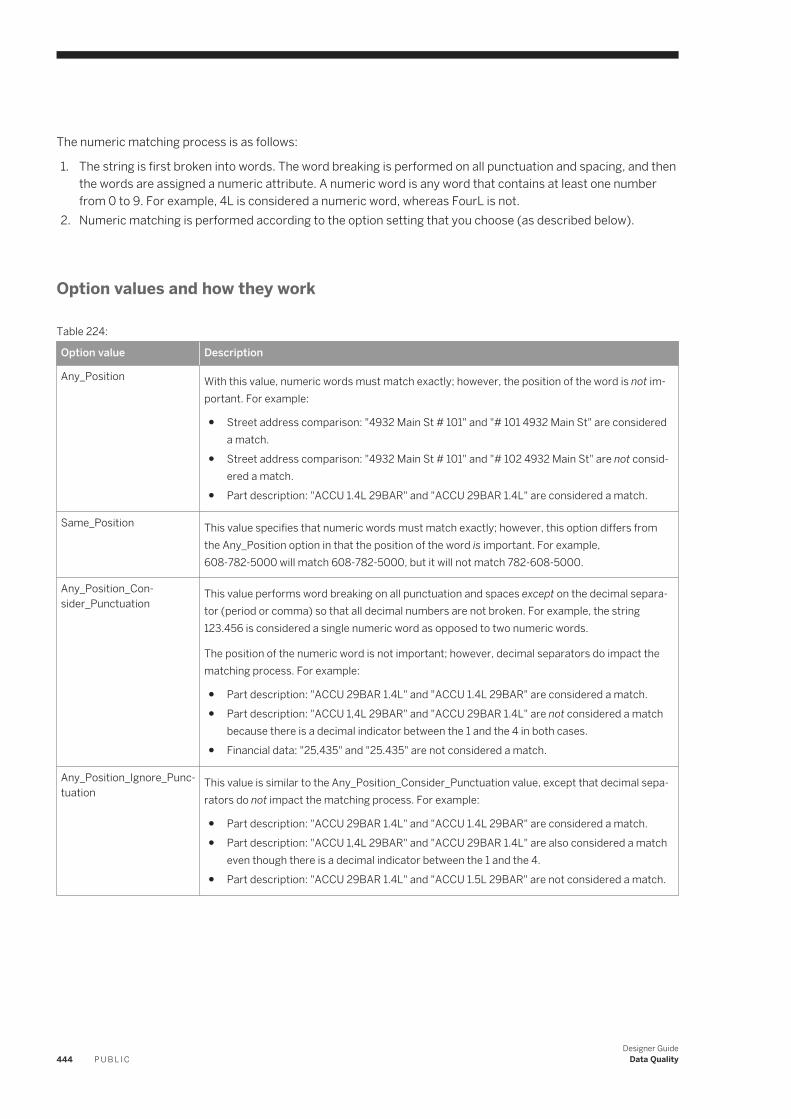
The numeric matching process is as follows:
1. The string is first broken into words. The word breaking is performed on all punctuation and spacing, and then the words are assigned a numeric attribute. A numeric word is any word that contains at least one number from 0 to 9. For example, 4L is considered a numeric word, whereas FourL is not.
2. Numeric matching is performed according to the option setting that you choose (as described below).
Option values and how they work
Table 224:
Option value Description
Any_Position With this value, numeric words must match exactly; however, the position of the word is not important. For example:
● Street address comparison: "4932 Main St # 101" and "# 101 4932 Main St" are considered a match.
● Street address comparison: "4932 Main St # 101" and "# 102 4932 Main St" are not considered a match.
● Part description: "ACCU 1.4L 29BAR" and "ACCU 29BAR 1.4L" are considered a match.
Same_Position This value specifies that numeric words must match exactly; however, this option differs from the Any_Position option in that the position of the word is important. For example, 608-782-5000 will match 608-782-5000, but it will not match 782-608-5000.
Any_Position_Consider_Punctuation
This value performs word breaking on all punctuation and spaces except on the decimal separator (period or comma) so that all decimal numbers are not broken. For example, the string 123.456 is considered a single numeric word as opposed to two numeric words.
The position of the numeric word is not important; however, decimal separators do impact the matching process. For example:
● Part description: "ACCU 29BAR 1.4L" and "ACCU 1.4L 29BAR" are considered a match.● Part description: "ACCU 1,4L 29BAR" and "ACCU 29BAR 1.4L" are not considered a match
because there is a decimal indicator between the 1 and the 4 in both cases.● Financial data: "25,435" and "25.435" are not considered a match.
Any_Position_Ignore_Punctuation
This value is similar to the Any_Position_Consider_Punctuation value, except that decimal separators do not impact the matching process. For example:
● Part description: "ACCU 29BAR 1.4L" and "ACCU 1.4L 29BAR" are considered a match.● Part description: "ACCU 1,4L 29BAR" and "ACCU 29BAR 1.4L" are also considered a match
even though there is a decimal indicator between the 1 and the 4.● Part description: "ACCU 29BAR 1.4L" and "ACCU 1.5L 29BAR" are not considered a match.
444 P U B L I CDesigner Guide
Data Quality
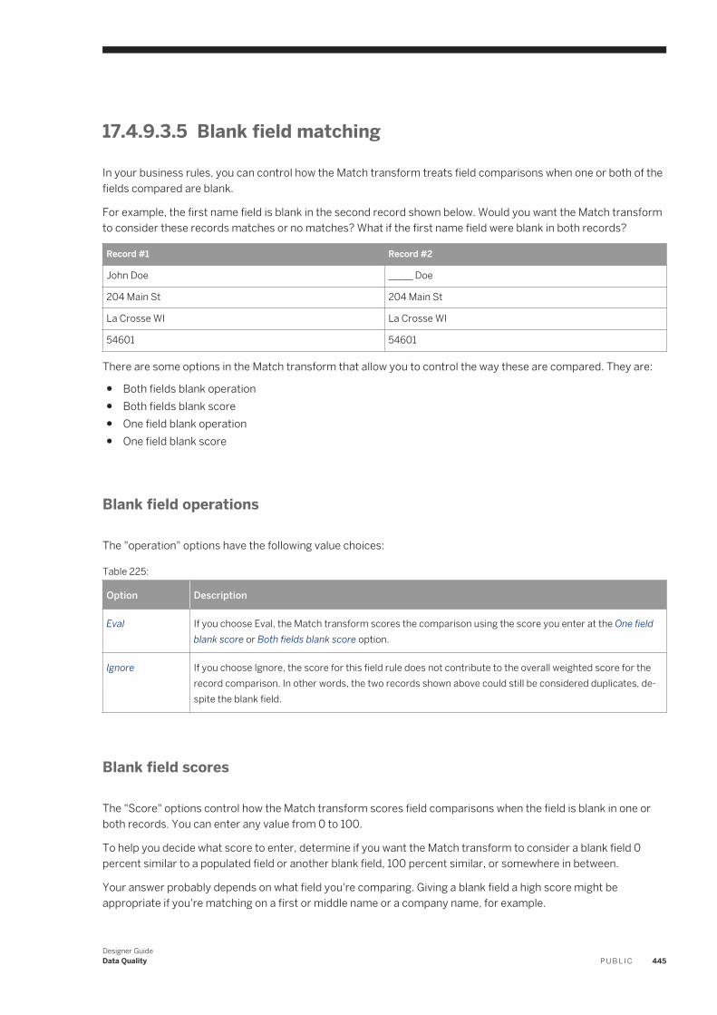
17.4.9.3.5 Blank field matching
In your business rules, you can control how the Match transform treats field comparisons when one or both of the fields compared are blank.
For example, the first name field is blank in the second record shown below. Would you want the Match transform to consider these records matches or no matches? What if the first name field were blank in both records?
Record #1 Record #2
John Doe _____ Doe
204 Main St 204 Main St
La Crosse WI La Crosse WI
54601 54601
There are some options in the Match transform that allow you to control the way these are compared. They are:
● Both fields blank operation● Both fields blank score● One field blank operation● One field blank score
Blank field operations
The "operation" options have the following value choices:
Table 225:
Option Description
Eval If you choose Eval, the Match transform scores the comparison using the score you enter at the One field blank score or Both fields blank score option.
Ignore If you choose Ignore, the score for this field rule does not contribute to the overall weighted score for the record comparison. In other words, the two records shown above could still be considered duplicates, despite the blank field.
Blank field scores
The "Score" options control how the Match transform scores field comparisons when the field is blank in one or both records. You can enter any value from 0 to 100.
To help you decide what score to enter, determine if you want the Match transform to consider a blank field 0 percent similar to a populated field or another blank field, 100 percent similar, or somewhere in between.
Your answer probably depends on what field you're comparing. Giving a blank field a high score might be appropriate if you're matching on a first or middle name or a company name, for example.
Designer GuideData Quality P U B L I C 445
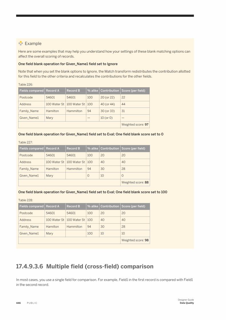
ExampleHere are some examples that may help you understand how your settings of these blank matching options can affect the overall scoring of records.
One field blank operation for Given_Name1 field set to Ignore
Note that when you set the blank options to Ignore, the Match transform redistributes the contribution allotted for this field to the other criteria and recalculates the contributions for the other fields.
Table 226:
Fields compared Record A Record B % alike Contribution Score (per field)
Postcode 54601 54601 100 20 (or 22) 22
Address 100 Water St 100 Water St 100 40 (or 44) 44
Family_Name Hamilton Hammilton 94 30 (or 33) 31
Given_Name1 Mary — 10 (or 0) —
Weighted score: 97
One field blank operation for Given_Name1 field set to Eval; One field blank score set to 0
Table 227:
Fields compared Record A Record B % alike Contribution Score (per field)
Postcode 54601 54601 100 20 20
Address 100 Water St 100 Water St 100 40 40
Family_Name Hamilton Hammilton 94 30 28
Given_Name1 Mary 0 10 0
Weighted score: 88
One field blank operation for Given_Name1 field set to Eval; One field blank score set to 100
Table 228:
Fields compared Record A Record B % alike Contribution Score (per field)
Postcode 54601 54601 100 20 20
Address 100 Water St 100 Water St 100 40 40
Family_Name Hamilton Hammilton 94 30 28
Given_Name1 Mary 100 10 10
Weighted score: 98
17.4.9.3.6 Multiple field (cross-field) comparison
In most cases, you use a single field for comparison. For example, Field1 in the first record is compared with Field1 in the second record.
446 P U B L I CDesigner Guide
Data Quality
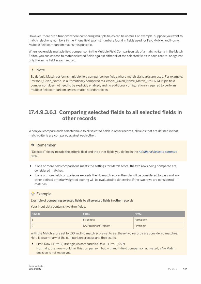
However, there are situations where comparing multiple fields can be useful. For example, suppose you want to match telephone numbers in the Phone field against numbers found in fields used for Fax, Mobile, and Home. Multiple field comparison makes this possible.
When you enable multiple field comparison in the Multiple Field Comparison tab of a match criteria in the Match Editor, you can choose to match selected fields against either all of the selected fields in each record, or against only the same field in each record.
NoteBy default, Match performs multiple field comparison on fields where match standards are used. For example, Person1_Given_Name1 is automatically compared to Person1_Given_Name_Match_Std1-6. Multiple field comparison does not need to be explicitly enabled, and no additional configuration is required to perform multiple field comparison against match standard fields.
17.4.9.3.6.1 Comparing selected fields to all selected fields in other records
When you compare each selected field to all selected fields in other records, all fields that are defined in that match criteria are compared against each other.
Remember“Selected” fields include the criteria field and the other fields you define in the Additional fields to compare table.
● If one or more field comparisons meets the settings for Match score, the two rows being compared are considered matches.
● If one or more field comparisons exceeds the No match score, the rule will be considered to pass and any other defined criteria/weighted scoring will be evaluated to determine if the two rows are considered matches.
ExampleExample of comparing selected fields to all selected fields in other records
Your input data contains two firm fields.
Row ID Firm1 Firm2
1 Firstlogic Postalsoft
2 SAP BusinessObjects Firstlogic
With the Match score set to 100 and No match score set to 99, these two records are considered matches. Here is a summary of the comparison process and the results.
● First, Row 1 Firm1 (Firstlogic) is compared to Row 2 Firm1 (SAP).Normally, the rows would fail this comparison, but with multi-field comparison activated, a No Match decision is not made yet.
Designer GuideData Quality P U B L I C 447
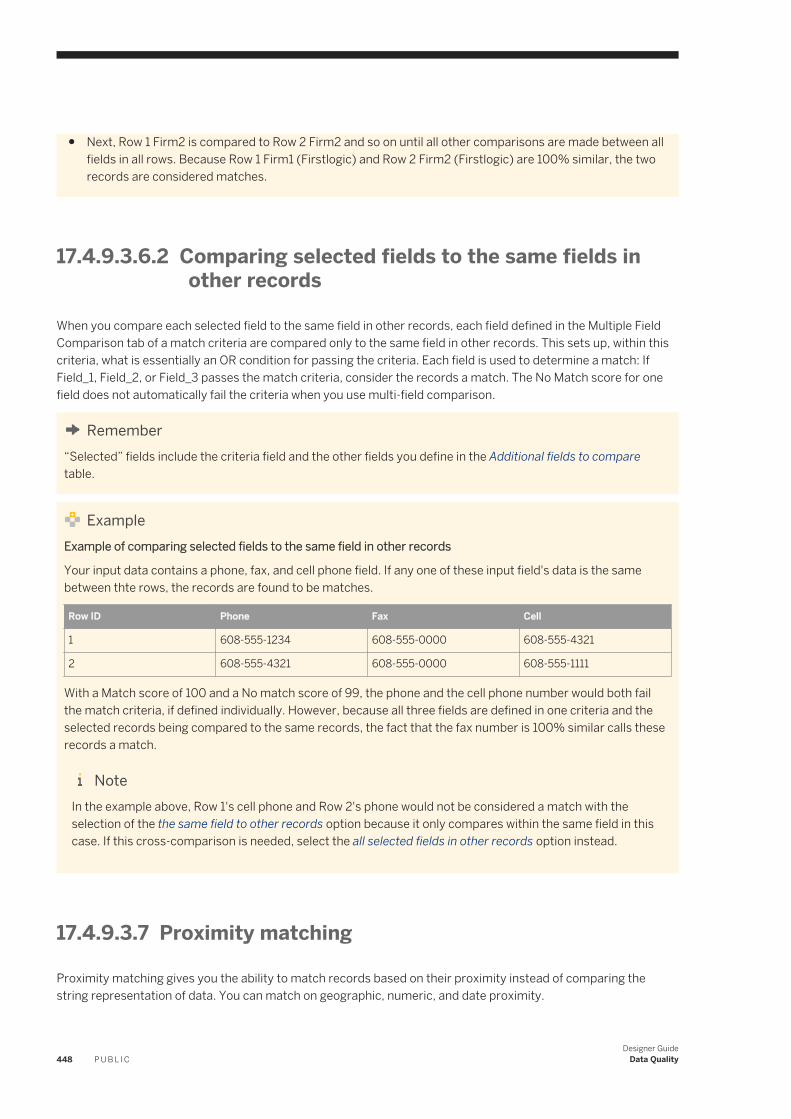
● Next, Row 1 Firm2 is compared to Row 2 Firm2 and so on until all other comparisons are made between all fields in all rows. Because Row 1 Firm1 (Firstlogic) and Row 2 Firm2 (Firstlogic) are 100% similar, the two records are considered matches.
17.4.9.3.6.2 Comparing selected fields to the same fields in other records
When you compare each selected field to the same field in other records, each field defined in the Multiple Field Comparison tab of a match criteria are compared only to the same field in other records. This sets up, within this criteria, what is essentially an OR condition for passing the criteria. Each field is used to determine a match: If Field_1, Field_2, or Field_3 passes the match criteria, consider the records a match. The No Match score for one field does not automatically fail the criteria when you use multi-field comparison.
Remember“Selected” fields include the criteria field and the other fields you define in the Additional fields to compare table.
ExampleExample of comparing selected fields to the same field in other records
Your input data contains a phone, fax, and cell phone field. If any one of these input field's data is the same between thte rows, the records are found to be matches.
Row ID Phone Fax Cell
1 608-555-1234 608-555-0000 608-555-4321
2 608-555-4321 608-555-0000 608-555-1111
With a Match score of 100 and a No match score of 99, the phone and the cell phone number would both fail the match criteria, if defined individually. However, because all three fields are defined in one criteria and the selected records being compared to the same records, the fact that the fax number is 100% similar calls these records a match.
NoteIn the example above, Row 1's cell phone and Row 2's phone would not be considered a match with the selection of the the same field to other records option because it only compares within the same field in this case. If this cross-comparison is needed, select the all selected fields in other records option instead.
17.4.9.3.7 Proximity matching
Proximity matching gives you the ability to match records based on their proximity instead of comparing the string representation of data. You can match on geographic, numeric, and date proximity.
448 P U B L I CDesigner Guide
Data Quality
Related Information
Matching on Geographic proximity [page 449]Matching on numeric or date proximity [page 450]
17.4.9.3.7.1 Matching on Geographic proximity
Geographic Proximity finds duplicate records based on geographic proximity, using latitude and longitude information. This is not driving distance, but Geographic distance. This option uses WGS 84 (GPS) coordinates.
The Geographic proximity option can:
● Search on objects within a radial range. This can help a company that wants to send a mailing out to customers within a certain distance from their business location.
● Search on the nearest location. This can help a consumer find a store location closest to their address.
17.4.9.3.7.2 Setting up Geographic Proximity matching - criteria fields
To select the fields for Geographic Proximity matching, follow these steps:
1. Access the Match Editor, add a new criteria.2. From Available Criteria, expand Geographic.3. Select LATITUDE_LONGITUDE.
This will make the two criteria fields available for mapping.4. Map the correct latitude and longitude fields. You must map both fields.
17.4.9.3.7.3 Setting up Geographic Proximity matching - criteria options
You must have the Latitude and Longitude fields mapped before you can use this option.
To perform geographic proximity matching, follow these steps:
1. From Compare data using, select Geo Proximity.This filters the options under Comparison Rules to show only applicable options.
2. Set the Distance unit option to one of the following:○ Miles○ Feet○ Kilometers○ Meters
Designer GuideData Quality P U B L I C 449
3. Enter the Max Distance you want to consider for the range.4. Set the Max Distance Score.
NoteA distance equal to Max distance will receive a score of Max distance score. Any distance less than the Max distance will receive a proportional score between Max distance score and 100. For example, a proximity of 10 miles will have higher score than a 40 miles.
NoteIf the data for Max Distance may change from row to row, you should dynamically input the data using the Option_Field_Algorithm_Geo_Proximity_<logical_name> _Max_Distance field.
17.4.9.3.7.4 Matching on numeric or date proximity
The Match Transform's numeric proximity options find duplicates based on numerical closeness of data. You can find duplicates based on numeric values and date values. The following options are available in the Match Criteria Editor Options tab for numeric and date matching:
Numeric difference
Finds duplicates based on the numeric difference for numeric or date values. For example, you can use this option to find duplicates based on date values in a specific range (for example, plus or minus 35 days), regardless of character-based similarity.
Numeric percent difference
Finds duplicates based on the percentage of numeric difference for numeric values. Here are two examples where this might be useful :
● Finance data domain : You can search financial data to find all monthly mortgage payments that are within 5 percent of a given value.
● Product data domain, you can search product data to find all the steel rods that are within 10% tolerance of a given diameter.
450 P U B L I CDesigner Guide
Data Quality
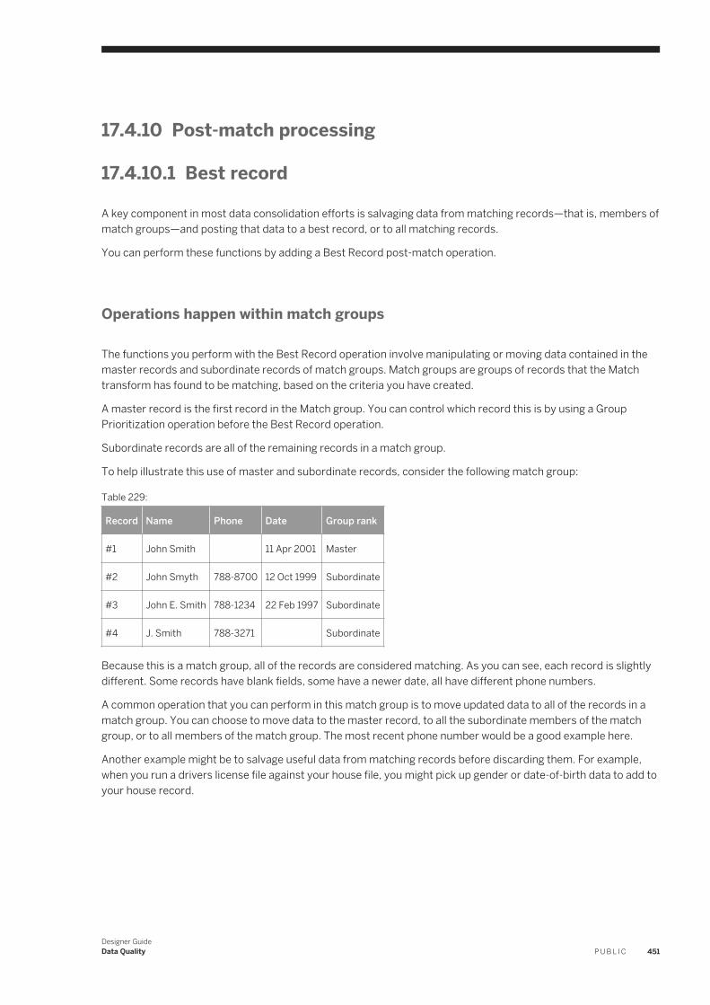
17.4.10 Post-match processing
17.4.10.1 Best record
A key component in most data consolidation efforts is salvaging data from matching records—that is, members of match groups—and posting that data to a best record, or to all matching records.
You can perform these functions by adding a Best Record post-match operation.
Operations happen within match groups
The functions you perform with the Best Record operation involve manipulating or moving data contained in the master records and subordinate records of match groups. Match groups are groups of records that the Match transform has found to be matching, based on the criteria you have created.
A master record is the first record in the Match group. You can control which record this is by using a Group Prioritization operation before the Best Record operation.
Subordinate records are all of the remaining records in a match group.
To help illustrate this use of master and subordinate records, consider the following match group:
Table 229:
Record Name Phone Date Group rank
#1 John Smith 11 Apr 2001 Master
#2 John Smyth 788-8700 12 Oct 1999 Subordinate
#3 John E. Smith 788-1234 22 Feb 1997 Subordinate
#4 J. Smith 788-3271 Subordinate
Because this is a match group, all of the records are considered matching. As you can see, each record is slightly different. Some records have blank fields, some have a newer date, all have different phone numbers.
A common operation that you can perform in this match group is to move updated data to all of the records in a match group. You can choose to move data to the master record, to all the subordinate members of the match group, or to all members of the match group. The most recent phone number would be a good example here.
Another example might be to salvage useful data from matching records before discarding them. For example, when you run a drivers license file against your house file, you might pick up gender or date-of-birth data to add to your house record.
Designer GuideData Quality P U B L I C 451
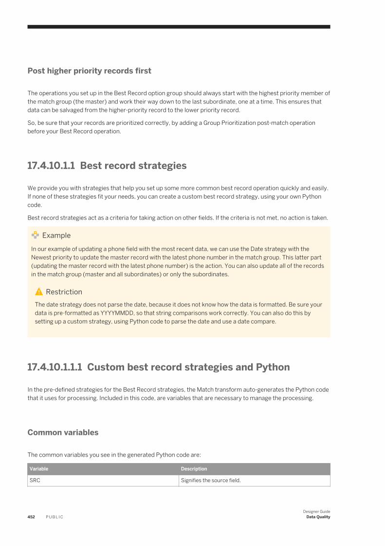
Post higher priority records first
The operations you set up in the Best Record option group should always start with the highest priority member of the match group (the master) and work their way down to the last subordinate, one at a time. This ensures that data can be salvaged from the higher-priority record to the lower priority record.
So, be sure that your records are prioritized correctly, by adding a Group Prioritization post-match operation before your Best Record operation.
17.4.10.1.1 Best record strategies
We provide you with strategies that help you set up some more common best record operation quickly and easily. If none of these strategies fit your needs, you can create a custom best record strategy, using your own Python code.
Best record strategies act as a criteria for taking action on other fields. If the criteria is not met, no action is taken.
ExampleIn our example of updating a phone field with the most recent data, we can use the Date strategy with the Newest priority to update the master record with the latest phone number in the match group. This latter part (updating the master record with the latest phone number) is the action. You can also update all of the records in the match group (master and all subordinates) or only the subordinates.
RestrictionThe date strategy does not parse the date, because it does not know how the data is formatted. Be sure your data is pre-formatted as YYYYMMDD, so that string comparisons work correctly. You can also do this by setting up a custom strategy, using Python code to parse the date and use a date compare.
17.4.10.1.1.1 Custom best record strategies and Python
In the pre-defined strategies for the Best Record strategies, the Match transform auto-generates the Python code that it uses for processing. Included in this code, are variables that are necessary to manage the processing.
Common variables
The common variables you see in the generated Python code are:
Variable Description
SRC Signifies the source field.
452 P U B L I CDesigner Guide
Data Quality
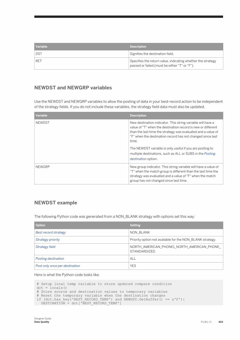
Variable Description
DST Signifies the destination field.
RET Specifies the return value, indicating whether the strategy passed or failed (must be either "T" or "F").
NEWDST and NEWGRP variables
Use the NEWDST and NEWGRP variables to allow the posting of data in your best-record action to be independent of the strategy fields. If you do not include these variables, the strategy field data must also be updated.
Variable Description
NEWDST New destination indicator. This string variable will have a value of "T" when the destination record is new or different than the last time the strategy was evaluated and a value of "F" when the destination record has not changed since last time.
The NEWDST variable is only useful if you are posting to multiple destinations, such as ALL or SUBS in the Posting destination option.
NEWGRP New group indicator. This string variable will have a value of "T" when the match group is different than the last time the strategy was evaluated and a value of "F" when the match group has not changed since last time.
NEWDST example
The following Python code was generated from a NON_BLANK strategy with options set this way:
Option Setting
Best record strategy NON_BLANK
Strategy priority Priority option not available for the NON_BLANK strategy.
Strategy field NORTH_AMERICAN_PHONE1_NORTH_AMERICAN_PHONE_STANDARDIZED.
Posting destination ALL
Post only once per destination YES
Here is what the Python code looks like.
# Setup local temp variable to store updated compare condition dct = locals()# Store source and destination values to temporary variables# Reset the temporary variable when the destination changesif (dct.has_key('BEST_RECORD_TEMP') and NEWDST.GetBuffer() == u'F'): DESTINATION = dct['BEST_RECORD_TEMP']
Designer GuideData Quality P U B L I C 453
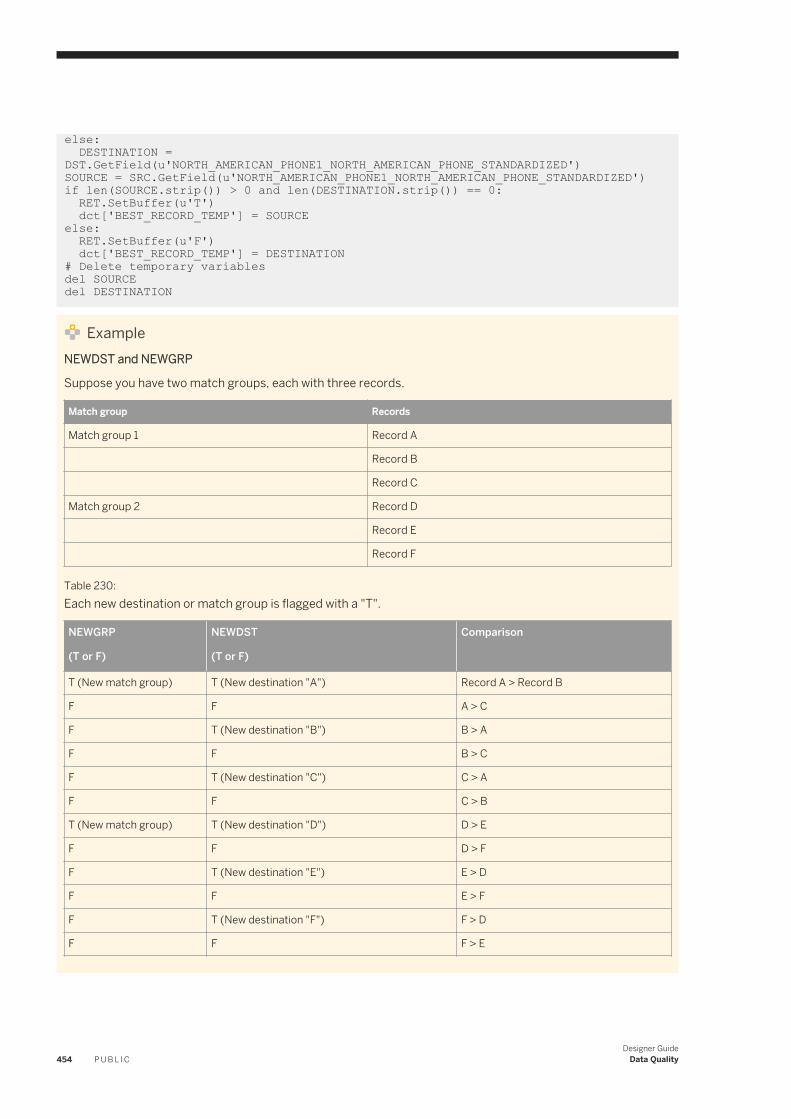
else: DESTINATION = DST.GetField(u'NORTH_AMERICAN_PHONE1_NORTH_AMERICAN_PHONE_STANDARDIZED')SOURCE = SRC.GetField(u'NORTH_AMERICAN_PHONE1_NORTH_AMERICAN_PHONE_STANDARDIZED')if len(SOURCE.strip()) > 0 and len(DESTINATION.strip()) == 0: RET.SetBuffer(u'T') dct['BEST_RECORD_TEMP'] = SOURCEelse: RET.SetBuffer(u'F') dct['BEST_RECORD_TEMP'] = DESTINATION# Delete temporary variablesdel SOURCEdel DESTINATION
ExampleNEWDST and NEWGRP
Suppose you have two match groups, each with three records.
Match group Records
Match group 1 Record A
Record B
Record C
Match group 2 Record D
Record E
Record F
Table 230:Each new destination or match group is flagged with a "T".
NEWGRP
(T or F)
NEWDST
(T or F)
Comparison
T (New match group) T (New destination "A") Record A > Record B
F F A > C
F T (New destination "B") B > A
F F B > C
F T (New destination "C") C > A
F F C > B
T (New match group) T (New destination "D") D > E
F F D > F
F T (New destination "E") E > D
F F E > F
F T (New destination "F") F > D
F F F > E
454 P U B L I CDesigner Guide
Data Quality
17.4.10.1.1.2 Creating a pre-defined best record strategy
Be sure to add a Best Record post-match operation to the appropriate match level in the Match Editor. Also, remember to map any pertinent input fields to make them available for this operation.
This procedure allows you to quickly generate the criteria for your best record action. The available strategies reflect common use cases.
1. Enter a name for this Best Record operation.2. Select a strategy from the Best record strategy option.3. Select a priority from the Strategy priority option.
The selection of values depends on the strategy you chose in the previous step.4. Select a field from the Strategy field drop-down menu.
The field you select here is the one that acts as a criteria for determining whether a best record action is taken.
ExampleThe strategy field you choose must contain data that matches the strategy you are creating. For example, if you are using a newest date strategy, be sure that the field you choose contains date data.
17.4.10.1.1.3 Creating a custom best record strategy
1. Add a best record operation to your Match transform.2. Enter a name for your best record operation.3. In the Best record strategy option, choose Custom.4. Choose a field from the Strategy field drop-down list.5. Click the View/Edit Python button to create your custom Python code to reflect your custom strategy.
The Python Editor window appears.
17.4.10.1.2 Best record actions
Best record actions are the functions you perform on data if a criteria of a strategy is met.
ExampleSuppose you want to update phone numbers of the master record. You would only want to do this if there is a subordinate record in the match group that has a newer date, which signifies a potentially new phone number for that person.
The action you set up would tell the Match transform to update the phone number field in the master record (action) if a newer date in the date field is found (strategy).
Designer GuideData Quality P U B L I C 455
17.4.10.1.2.1 Sources and destinations
When working with the best record operation, it is important to know the differences between sources and destinations in a best record action.
The source is the field from which you take data and the destination is where you post the data. A source or destination can be either a master or subordinate record in a match group.
ExampleIn our phone number example, the subordinate record has the newer date, so we take data from the phone field (the source) and post it to the master record (the destination).
17.4.10.1.2.2 Posting once or many times per destination
In the Best Record options, you can choose to post to a destination once or many times per action by setting the Post only once per destination option.
You may want your best record action to stop after the first time it posts data to the destination record, or you may want it to continue with the other match group records as well. Your choice depends on the nature of the data you’re posting and the records you’re posting to. The two examples that follow illustrate each case.
If you post only once to each destination record, then once data is posted for a particular record, the Match transform moves on to either perform the next best record action (if more than one is defined) or to the next record.
If you don’t limit the action in this way, all actions are performed each time the strategy returns True.
Regardless of this setting, the Match transform always works through the match group members in priority order. When posting to record #1 in the figure below, without limiting the posting to only once, here is what happens:
Table 231:
Match group Action
Record #1 (master)
Record #2 (subordinate)
First, the action is attempted using, as a source, that record from among the other match group records that has the highest priority (record #2).
Record #3 (subordinate)
Next, the action is attempted with the next highest priority record (record #3) as the source.
Record #4 (subordinate)
Finally, the action is attempted with the lowest priority record (record #4) as the source.
The results In the case above, record #4 was the last source for the action, and therefore could be a source of data for the output record. However, if you set your best record action to post only once per destination record, here is what happens:
456 P U B L I CDesigner Guide
Data Quality
Table 232:
Match group Action
Record #1 (master)
Record #2 (subordinate)
First, the action is attempted using, as a source, that record from among the other match group records that has the highest priority (record #2).
If this attempt is successful, the Match transform considers this best record action to be complete and moves to the next best record action (if there is one), or to the next output record.
If this attempt is not successful, the Match transform moves to the match group member with the next highest priority and attempts the posting operation.
Record #3 (subordinate)
Record #4 (subordinate)
In this case, record #2 was the source last used for the best record action, and so is the source of posted data in the output record.
17.4.10.1.2.3 Creating a best record action
The best record action is the posting of data from a source to a destination record, based on the criteria of your best record strategy.
1. Create a strategy, either pre-defined or custom.2. Select the record(s) to post to in the Posting destination option.3. Select whether you want to post only once or multiple times to a destination record in the Post only once per
destination option.4. In the Best record action fields table, choose your source field and destination field.
When you choose a source field, the Destination field column is automatically populated with the same field. You need to change the destination field if this is not the field you want to post your data to.
5. If you want to create a custom best record action, choose Yes in the Custom column.You can now access the Python editor to create custom Python code for your custom action.
17.4.10.1.3 Destination protection
The Best Record and Unique ID operations in the Match transform offer you the power to modify existing records in your data. There may be times when you would like to protect data in particular records or data in records from particular input sources from being overwritten.
The Destination Protection tab in these Match transform operations allow you the ability to protect data from being modified.
Designer GuideData Quality P U B L I C 457
17.4.10.1.3.1 Protecting destination records through fields
1. In the Destination Protection tab, select Enable destination protection.2. Select a value in the Default destination protection option drop-down list.
This value determines whether a destination is protected if the destination protection field does not have a valid value.
3. Select the Specify destination protection by field option, and choose a field from the Destination protection field drop-down list (or Unique ID protected field).The field you choose must have a Y or N value to specify the action.
Any record that has a value of Y in the destination protection field will be protected from being modified.
17.4.10.1.3.2 Protecting destination records based on input source membership
You must add an Input Source operation and define input sources before you can complete this task.
1. In the Destination Protection tab, select Enable destination protection.2. Select a value in the Default destination protection option drop-down list.
This value determines whether a destination (input source) is protected if you do not specifically define the source in the table.
3. Select the Specify destination protection by source option.4. Select an input source from the first row of the Source name column, and then choose a value from the
Destination protected (or Unique ID protected) column.Repeat for every input source you want to set protection for. Remember that if you do not specify for every source, the default value will be used.
17.4.10.2 Unique ID
A unique ID refers to a field within your data which contains a unique value that is associated with a record or group of records. You could use a unique ID, for example, in your company's internal database that receives updates at some predetermined interval, such as each week, month, or quarter. Unique ID applies to a data record in the same way that a national identification number might apply to a person; for example, a Social Security number (SSN) in the United States, or a National Insurance number (NINO) in the United Kingdom. It creates and tracks data relationships from run to run. With the Unique ID operation, you can set your own starting ID for new key generation, or have it dynamically assigned based on existing data. The Unique ID post-match processing operation also lets you begin where the highest unique ID from the previous run ended.
458 P U B L I CDesigner Guide
Data Quality
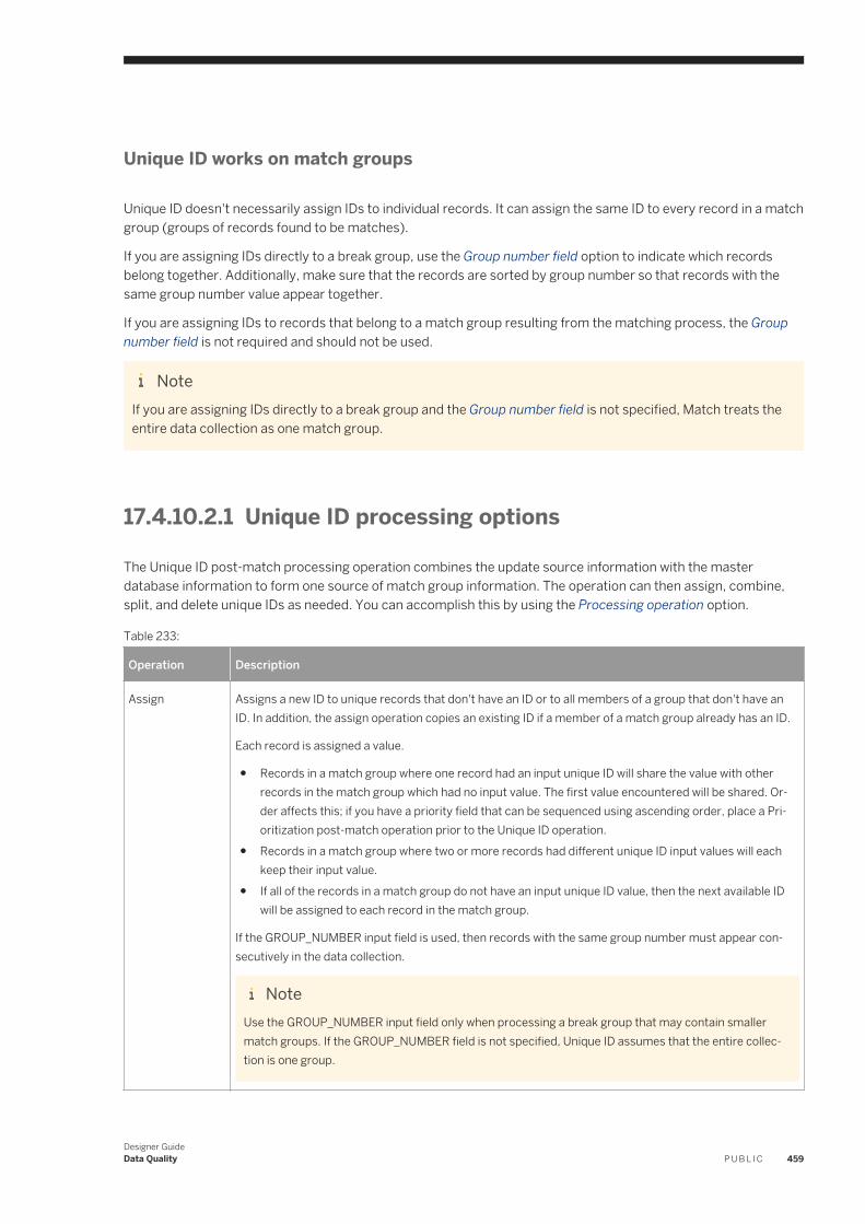
Unique ID works on match groups
Unique ID doesn't necessarily assign IDs to individual records. It can assign the same ID to every record in a match group (groups of records found to be matches).
If you are assigning IDs directly to a break group, use the Group number field option to indicate which records belong together. Additionally, make sure that the records are sorted by group number so that records with the same group number value appear together.
If you are assigning IDs to records that belong to a match group resulting from the matching process, the Group number field is not required and should not be used.
NoteIf you are assigning IDs directly to a break group and the Group number field is not specified, Match treats the entire data collection as one match group.
17.4.10.2.1 Unique ID processing options
The Unique ID post-match processing operation combines the update source information with the master database information to form one source of match group information. The operation can then assign, combine, split, and delete unique IDs as needed. You can accomplish this by using the Processing operation option.
Table 233:
Operation Description
Assign Assigns a new ID to unique records that don't have an ID or to all members of a group that don't have an ID. In addition, the assign operation copies an existing ID if a member of a match group already has an ID.
Each record is assigned a value.
● Records in a match group where one record had an input unique ID will share the value with other records in the match group which had no input value. The first value encountered will be shared. Order affects this; if you have a priority field that can be sequenced using ascending order, place a Prioritization post-match operation prior to the Unique ID operation.
● Records in a match group where two or more records had different unique ID input values will each keep their input value.
● If all of the records in a match group do not have an input unique ID value, then the next available ID will be assigned to each record in the match group.
If the GROUP_NUMBER input field is used, then records with the same group number must appear consecutively in the data collection.
NoteUse the GROUP_NUMBER input field only when processing a break group that may contain smaller match groups. If the GROUP_NUMBER field is not specified, Unique ID assumes that the entire collection is one group.
Designer GuideData Quality P U B L I C 459
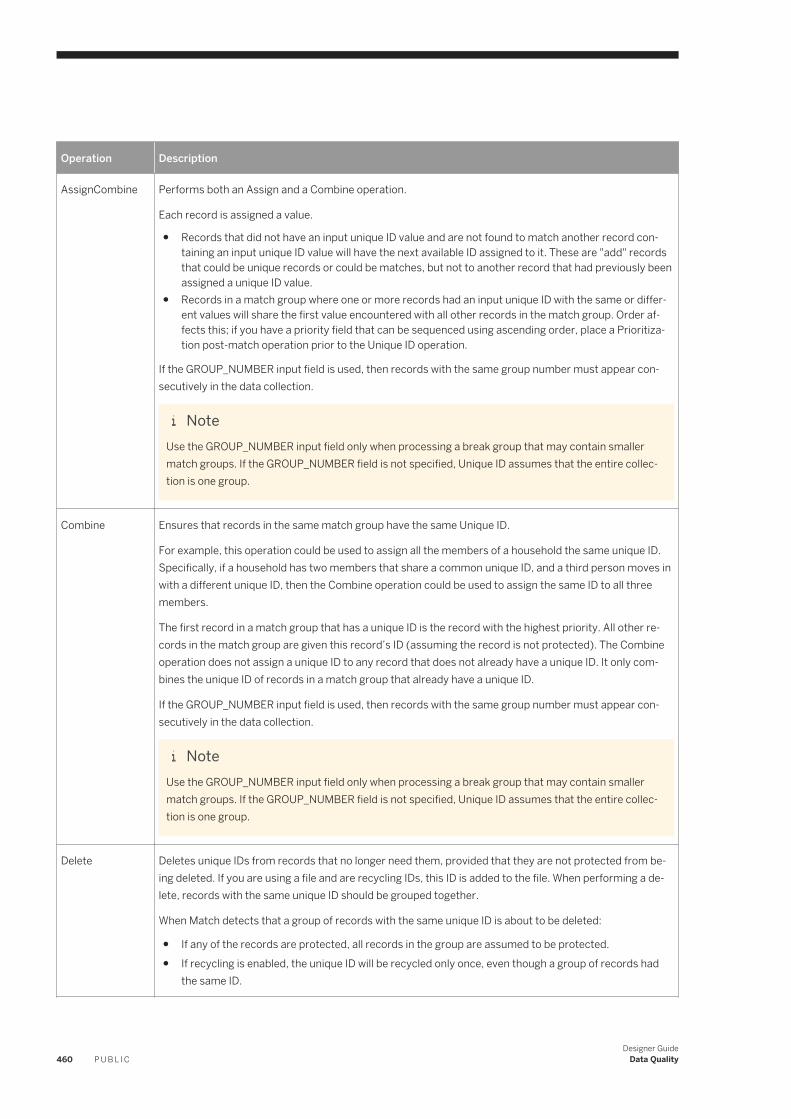
Operation Description
AssignCombine Performs both an Assign and a Combine operation.
Each record is assigned a value.
● Records that did not have an input unique ID value and are not found to match another record containing an input unique ID value will have the next available ID assigned to it. These are "add" records that could be unique records or could be matches, but not to another record that had previously been assigned a unique ID value.
● Records in a match group where one or more records had an input unique ID with the same or different values will share the first value encountered with all other records in the match group. Order affects this; if you have a priority field that can be sequenced using ascending order, place a Prioritization post-match operation prior to the Unique ID operation.
If the GROUP_NUMBER input field is used, then records with the same group number must appear consecutively in the data collection.
NoteUse the GROUP_NUMBER input field only when processing a break group that may contain smaller match groups. If the GROUP_NUMBER field is not specified, Unique ID assumes that the entire collection is one group.
Combine Ensures that records in the same match group have the same Unique ID.
For example, this operation could be used to assign all the members of a household the same unique ID. Specifically, if a household has two members that share a common unique ID, and a third person moves in with a different unique ID, then the Combine operation could be used to assign the same ID to all three members.
The first record in a match group that has a unique ID is the record with the highest priority. All other records in the match group are given this record’s ID (assuming the record is not protected). The Combine operation does not assign a unique ID to any record that does not already have a unique ID. It only combines the unique ID of records in a match group that already have a unique ID.
If the GROUP_NUMBER input field is used, then records with the same group number must appear consecutively in the data collection.
NoteUse the GROUP_NUMBER input field only when processing a break group that may contain smaller match groups. If the GROUP_NUMBER field is not specified, Unique ID assumes that the entire collection is one group.
Delete Deletes unique IDs from records that no longer need them, provided that they are not protected from being deleted. If you are using a file and are recycling IDs, this ID is added to the file. When performing a delete, records with the same unique ID should be grouped together.
When Match detects that a group of records with the same unique ID is about to be deleted:
● If any of the records are protected, all records in the group are assumed to be protected.● If recycling is enabled, the unique ID will be recycled only once, even though a group of records had
the same ID.
460 P U B L I CDesigner Guide
Data Quality
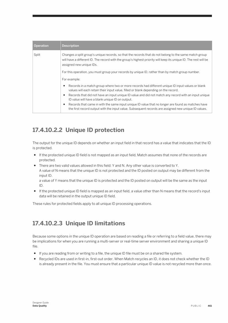
Operation Description
Split Changes a split group's unique records, so that the records that do not belong to the same match group will have a different ID. The record with the group's highest priority will keep its unique ID. The rest will be assigned new unique IDs.
For this operation, you must group your records by unique ID, rather than by match group number.
For example:
● Records in a match group where two or more records had different unique ID input values or blank values will each retain their input value, filled or blank depending on the record.
● Records that did not have an input unique ID value and did not match any record with an input unique ID value will have a blank unique ID on output.
● Records that came in with the same input unique ID value that no longer are found as matches have the first record output with the input value. Subsequent records are assigned new unique ID values.
17.4.10.2.2 Unique ID protection
The output for the unique ID depends on whether an input field in that record has a value that indicates that the ID is protected.
● If the protected unique ID field is not mapped as an input field, Match assumes that none of the records are protected.
● There are two valid values allowed in this field: Y and N. Any other value is converted to Y.A value of N means that the unique ID is not protected and the ID posted on output may be different from the input ID.a value of Y means that the unique ID is protected and the ID posted on output will be the same as the input ID.
● If the protected unique ID field is mapped as an input field, a value other than N means that the record's input data will be retained in the output unique ID field.
These rules for protected fields apply to all unique ID processing operations.
17.4.10.2.3 Unique ID limitations
Because some options in the unique ID operation are based on reading a file or referring to a field value, there may be implications for when you are running a multi-server or real-time server environment and sharing a unique ID file.
● If you are reading from or writing to a file, the unique ID file must be on a shared file system.● Recycled IDs are used in first-in, first-out order. When Match recycles an ID, it does not check whether the ID
is already present in the file. You must ensure that a particular unique ID value is not recycled more than once.
Designer GuideData Quality P U B L I C 461
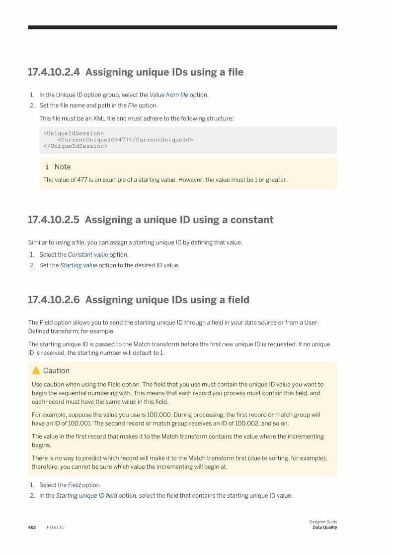
17.4.10.2.4 Assigning unique IDs using a file
1. In the Unique ID option group, select the Value from file option.2. Set the file name and path in the File option.
This file must be an XML file and must adhere to the following structure:
<UniqueIdSession> <CurrentUniqueId>477</CurrentUniqueId> </UniqueIdSession>
NoteThe value of 477 is an example of a starting value. However, the value must be 1 or greater.
17.4.10.2.5 Assigning a unique ID using a constant
Similar to using a file, you can assign a starting unique ID by defining that value.
1. Select the Constant value option.2. Set the Starting value option to the desired ID value.
17.4.10.2.6 Assigning unique IDs using a field
The Field option allows you to send the starting unique ID through a field in your data source or from a User-Defined transform, for example.
The starting unique ID is passed to the Match transform before the first new unique ID is requested. If no unique ID is received, the starting number will default to 1.
CautionUse caution when using the Field option. The field that you use must contain the unique ID value you want to begin the sequential numbering with. This means that each record you process must contain this field, and each record must have the same value in this field.
For example, suppose the value you use is 100,000. During processing, the first record or match group will have an ID of 100,001. The second record or match group receives an ID of 100,002, and so on.
The value in the first record that makes it to the Match transform contains the value where the incrementing begins.
There is no way to predict which record will make it to the Match transform first (due to sorting, for example); therefore, you cannot be sure which value the incrementing will begin at.
1. Select the Field option.2. In the Starting unique ID field option, select the field that contains the starting unique ID value.
462 P U B L I CDesigner Guide
Data Quality
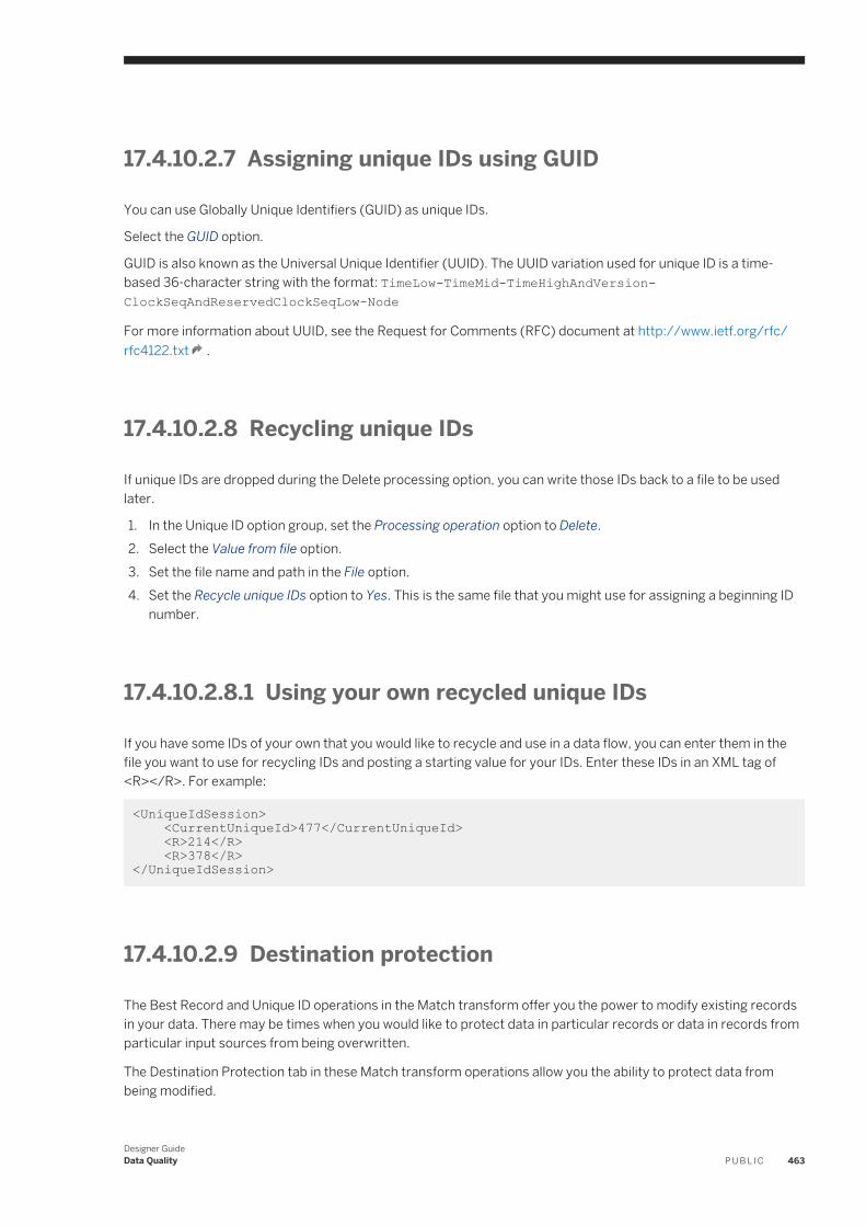
17.4.10.2.7 Assigning unique IDs using GUID
You can use Globally Unique Identifiers (GUID) as unique IDs.
Select the GUID option.
GUID is also known as the Universal Unique Identifier (UUID). The UUID variation used for unique ID is a time-based 36-character string with the format: TimeLow-TimeMid-TimeHighAndVersion-ClockSeqAndReservedClockSeqLow-Node
For more information about UUID, see the Request for Comments (RFC) document at http://www.ietf.org/rfc/rfc4122.txt .
17.4.10.2.8 Recycling unique IDs
If unique IDs are dropped during the Delete processing option, you can write those IDs back to a file to be used later.
1. In the Unique ID option group, set the Processing operation option to Delete.2. Select the Value from file option.3. Set the file name and path in the File option.4. Set the Recycle unique IDs option to Yes. This is the same file that you might use for assigning a beginning ID
number.
17.4.10.2.8.1 Using your own recycled unique IDs
If you have some IDs of your own that you would like to recycle and use in a data flow, you can enter them in the file you want to use for recycling IDs and posting a starting value for your IDs. Enter these IDs in an XML tag of <R></R>. For example:
<UniqueIdSession> <CurrentUniqueId>477</CurrentUniqueId> <R>214</R> <R>378</R></UniqueIdSession>
17.4.10.2.9 Destination protection
The Best Record and Unique ID operations in the Match transform offer you the power to modify existing records in your data. There may be times when you would like to protect data in particular records or data in records from particular input sources from being overwritten.
The Destination Protection tab in these Match transform operations allow you the ability to protect data from being modified.
Designer GuideData Quality P U B L I C 463
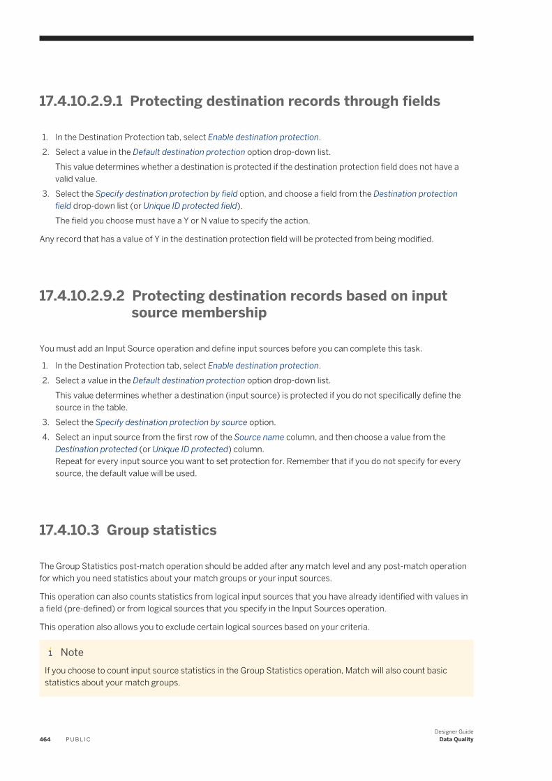
17.4.10.2.9.1 Protecting destination records through fields
1. In the Destination Protection tab, select Enable destination protection.2. Select a value in the Default destination protection option drop-down list.
This value determines whether a destination is protected if the destination protection field does not have a valid value.
3. Select the Specify destination protection by field option, and choose a field from the Destination protection field drop-down list (or Unique ID protected field).The field you choose must have a Y or N value to specify the action.
Any record that has a value of Y in the destination protection field will be protected from being modified.
17.4.10.2.9.2 Protecting destination records based on input source membership
You must add an Input Source operation and define input sources before you can complete this task.
1. In the Destination Protection tab, select Enable destination protection.2. Select a value in the Default destination protection option drop-down list.
This value determines whether a destination (input source) is protected if you do not specifically define the source in the table.
3. Select the Specify destination protection by source option.4. Select an input source from the first row of the Source name column, and then choose a value from the
Destination protected (or Unique ID protected) column.Repeat for every input source you want to set protection for. Remember that if you do not specify for every source, the default value will be used.
17.4.10.3 Group statistics
The Group Statistics post-match operation should be added after any match level and any post-match operation for which you need statistics about your match groups or your input sources.
This operation can also counts statistics from logical input sources that you have already identified with values in a field (pre-defined) or from logical sources that you specify in the Input Sources operation.
This operation also allows you to exclude certain logical sources based on your criteria.
NoteIf you choose to count input source statistics in the Group Statistics operation, Match will also count basic statistics about your match groups.
464 P U B L I CDesigner Guide
Data Quality
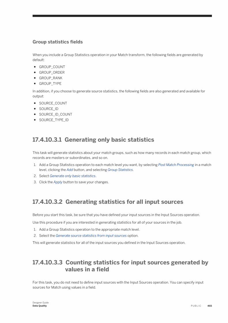
Group statistics fields
When you include a Group Statistics operation in your Match transform, the following fields are generated by default:
● GROUP_COUNT● GROUP_ORDER● GROUP_RANK● GROUP_TYPE
In addition, if you choose to generate source statistics, the following fields are also generated and available for output:
● SOURCE_COUNT● SOURCE_ID● SOURCE_ID_COUNT● SOURCE_TYPE_ID
17.4.10.3.1 Generating only basic statistics
This task will generate statistics about your match groups, such as how many records in each match group, which records are masters or subordinates, and so on.
1. Add a Group Statistics operation to each match level you want, by selecting Post Match Processing in a match level, clicking the Add button, and selecting Group Statistics.
2. Select Generate only basic statistics.3. Click the Apply button to save your changes.
17.4.10.3.2 Generating statistics for all input sources
Before you start this task, be sure that you have defined your input sources in the Input Sources operation.
Use this procedure if you are interested in generating statistics for all of your sources in the job.
1. Add a Group Statistics operation to the appropriate match level.2. Select the Generate source statistics from input sources option.
This will generate statistics for all of the input sources you defined in the Input Sources operation.
17.4.10.3.3 Counting statistics for input sources generated by values in a field
For this task, you do not need to define input sources with the Input Sources operation. You can specify input sources for Match using values in a field.
Designer GuideData Quality P U B L I C 465
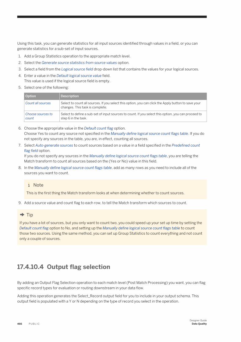
Using this task, you can generate statistics for all input sources identified through values in a field, or you can generate statistics for a sub-set of input sources.
1. Add a Group Statistics operation to the appropriate match level.2. Select the Generate source statistics from source values option.3. Select a field from the Logical source field drop-down list that contains the values for your logical sources.4. Enter a value in the Default logical source value field.
This value is used if the logical source field is empty.5. Select one of the following:
Option Description
Count all sources Select to count all sources. If you select this option, you can click the Apply button to save your changes. This task is complete.
Choose sources to count
Select to define a sub-set of input sources to count. If you select this option, you can proceed to step 6 in the task.
6. Choose the appropriate value in the Default count flag option.Choose Yes to count any source not specified in the Manually define logical source count flags table. If you do not specify any sources in the table, you are, in effect, counting all sources.
7. Select Auto-generate sources to count sources based on a value in a field specified in the Predefined count flag field option.If you do not specify any sources in the Manually define logical source count flags table, you are telling the Match transform to count all sources based on the (Yes or No) value in this field.
8. In the Manually define logical source count flags table, add as many rows as you need to include all of the sources you want to count.
NoteThis is the first thing the Match transform looks at when determining whether to count sources.
9. Add a source value and count flag to each row, to tell the Match transform which sources to count.
TipIf you have a lot of sources, but you only want to count two, you could speed up your set up time by setting the Default count flag option to No, and setting up the Manually define logical source count flags table to count those two sources. Using the same method, you can set up Group Statistics to count everything and not count only a couple of sources.
17.4.10.4 Output flag selection
By adding an Output Flag Selection operation to each match level (Post Match Processing) you want, you can flag specific record types for evaluation or routing downstream in your data flow.
Adding this operation generates the Select_Record output field for you to include in your output schema. This output field is populated with a Y or N depending on the type of record you select in the operation.
466 P U B L I CDesigner Guide
Data Quality
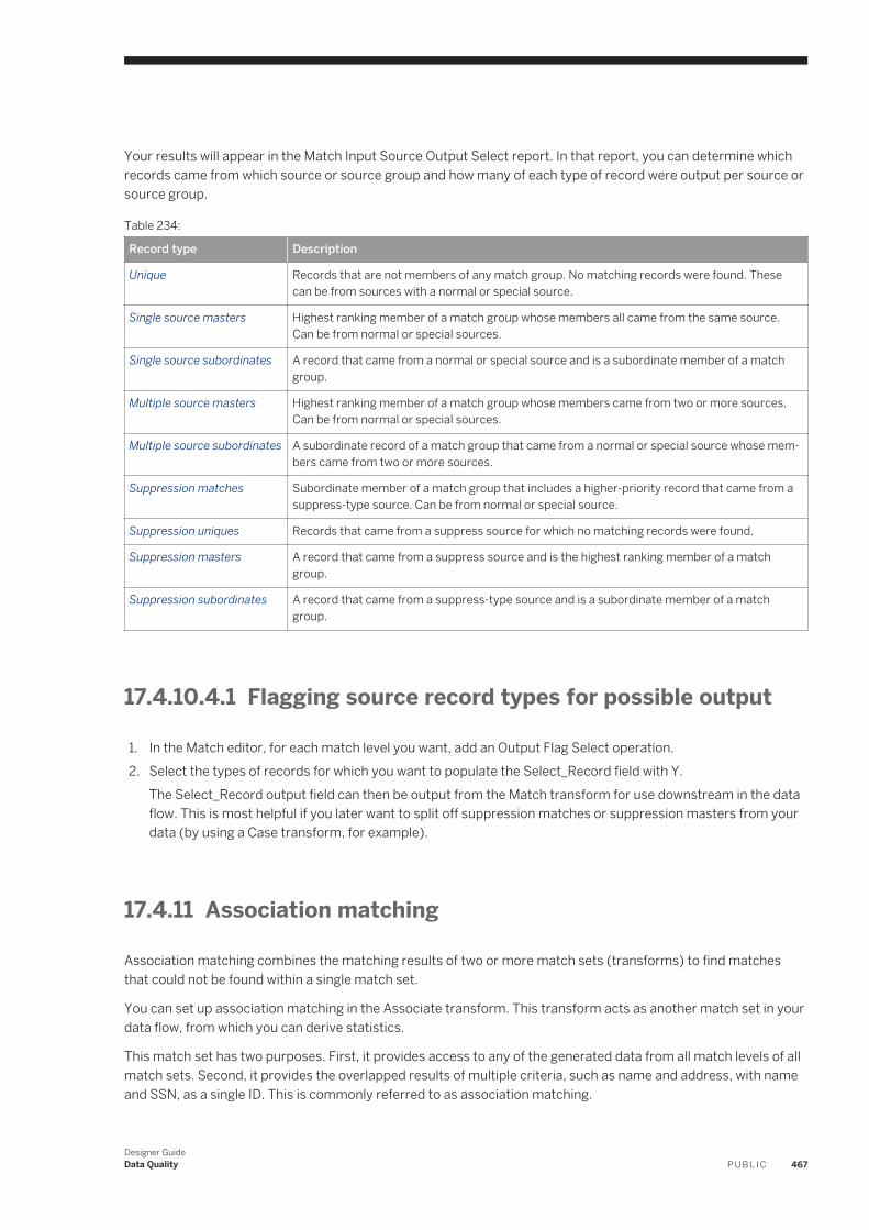
Your results will appear in the Match Input Source Output Select report. In that report, you can determine which records came from which source or source group and how many of each type of record were output per source or source group.
Table 234:
Record type Description
Unique Records that are not members of any match group. No matching records were found. These can be from sources with a normal or special source.
Single source masters Highest ranking member of a match group whose members all came from the same source. Can be from normal or special sources.
Single source subordinates A record that came from a normal or special source and is a subordinate member of a match group.
Multiple source masters Highest ranking member of a match group whose members came from two or more sources. Can be from normal or special sources.
Multiple source subordinates A subordinate record of a match group that came from a normal or special source whose members came from two or more sources.
Suppression matches Subordinate member of a match group that includes a higher-priority record that came from a suppress-type source. Can be from normal or special source.
Suppression uniques Records that came from a suppress source for which no matching records were found.
Suppression masters A record that came from a suppress source and is the highest ranking member of a match group.
Suppression subordinates A record that came from a suppress-type source and is a subordinate member of a match group.
17.4.10.4.1 Flagging source record types for possible output
1. In the Match editor, for each match level you want, add an Output Flag Select operation.2. Select the types of records for which you want to populate the Select_Record field with Y.
The Select_Record output field can then be output from the Match transform for use downstream in the data flow. This is most helpful if you later want to split off suppression matches or suppression masters from your data (by using a Case transform, for example).
17.4.11 Association matching
Association matching combines the matching results of two or more match sets (transforms) to find matches that could not be found within a single match set.
You can set up association matching in the Associate transform. This transform acts as another match set in your data flow, from which you can derive statistics.
This match set has two purposes. First, it provides access to any of the generated data from all match levels of all match sets. Second, it provides the overlapped results of multiple criteria, such as name and address, with name and SSN, as a single ID. This is commonly referred to as association matching.
Designer GuideData Quality P U B L I C 467
Group numbers
The Associate transform accepts a group number field, generated by the Match transforms, for each match result that will be combined. The transform can then output a new associated group number.
The Associate transform can operate either on all the input records or on one data collection at a time. The latter is needed for real-time support.
ExampleAssociation example
Say you work at a technical college and you want to send information to all of the students prior to the start of a new school year. You know that many of the students have a temporary local address and a permanent home address.
In this example, you can match on name, address, and postal code in one match set, and match on name and Social Security number (SSN), which is available to the technical college on every student, in another match set.
Then, the Associate transform combines the two match sets to build associated match groups. This lets you identify people who may have multiple addresses, thereby maximizing your one-to-one marketing and mailing efforts.
17.4.12 Unicode matching
Unicode matching lets you match Unicode data. You can process any non-Latin1 Unicode data, with special processing for Chinese, Japanese, Korean and Taiwanese (or CJKT) data.
Chinese, Japanese, Korean, and Taiwanese matching
Regardless of the country-specific language, the matching process for CJKT data is the same. For example, the Match transform:
● Considers half-width and full-width characters to be equal.● Considers native script numerals and Arabic numerals to be equal. It can interpret numbers that are written in
native script. This can be controlled with the Convert text to numbers option in the Criteria options group.● Includes variations for popular, personal, and firm name characters in the referential data.● Considers firm words, such as Corporation or Limited, to be equal to their variations (Corp. or Ltd.) during the
matching comparison process. To find the abbreviations, the transform uses native script variations of the English alphabets during firm name matching.
● Ignores commonly used optional markers for province, city, district, and so on, in address data comparison.● Intelligently handles variations in a building marker.
468 P U B L I CDesigner Guide
Data Quality
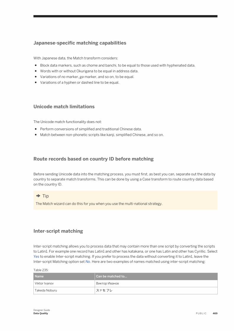
Japanese-specific matching capabilities
With Japanese data, the Match transform considers:
● Block data markers, such as chome and banchi, to be equal to those used with hyphenated data.● Words with or without Okurigana to be equal in address data.● Variations of no marker, ga marker, and so on, to be equal.● Variations of a hyphen or dashed line to be equal.
Unicode match limitations
The Unicode match functionality does not:
● Perform conversions of simplified and traditional Chinese data.● Match between non-phonetic scripts like kanji, simplified Chinese, and so on.
Route records based on country ID before matching
Before sending Unicode data into the matching process, you must first, as best you can, separate out the data by country to separate match transforms. This can be done by using a Case transform to route country data based on the country ID.
TipThe Match wizard can do this for you when you use the multi-national strategy.
Inter-script matching
Inter-script matching allows you to process data that may contain more than one script by converting the scripts to Latin1. For example one record has Latin1 and other has katakana, or one has Latin and other has Cyrillic. Select Yes to enable Inter-script matching. If you prefer to process the data without converting it to Latin1, leave the Inter-script Matching option set No. Here are two examples of names matched using inter-script matching:
Table 235:
Name Can be matched to...
Viktor Ivanov Виктор Иванов
Takeda Noburu スッセ フレ
Designer GuideData Quality P U B L I C 469
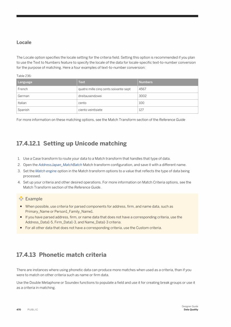
Locale
The Locale option specifies the locale setting for the criteria field. Setting this option is recommended if you plan to use the Text to Numbers feature to specify the locale of the data for locale-specific text-to-number conversion for the purpose of matching. Here a four examples of text-to-number conversion:
Table 236:
Language Text Numbers
French quatre mille cinq cents soixante-sept 4567
German dreitausendzwei 3002
Italian cento 100
Spanish ciento veintisiete 127
For more information on these matching options, see the Match Transform section of the Reference Guide
17.4.12.1 Setting up Unicode matching
1. Use a Case transform to route your data to a Match transform that handles that type of data.2. Open the AddressJapan_MatchBatch Match transform configuration, and save it with a different name.3. Set the Match engine option in the Match transform options to a value that reflects the type of data being
processed.4. Set up your criteria and other desired operations. For more information on Match Criteria options, see the
Match Transform section of the Reference Guide.
Example● When possible, use criteria for parsed components for address, firm, and name data, such as
Primary_Name or Person1_Family_Name1.● If you have parsed address, firm, or name data that does not have a corresponding criteria, use the
Address_Data1-5, Firm_Data1-3, and Name_Data1-3 criteria.● For all other data that does not have a corresponding criteria, use the Custom criteria.
17.4.13 Phonetic match criteria
There are instances where using phonetic data can produce more matches when used as a criteria, than if you were to match on other criteria such as name or firm data.
Use the Double Metaphone or Soundex functions to populate a field and use it for creating break groups or use it as a criteria in matching.
470 P U B L I CDesigner Guide
Data Quality
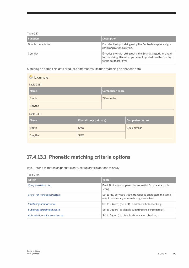
Table 237:
Function Description
Double metaphone Encodes the input string using the Double Metaphone algorithm and returns a string.
Soundex Encodes the input string using the Soundex algorithm and returns a string. Use when you want to push down the function to the database-level.
Matching on name field data produces different results than matching on phonetic data.
Example
Table 238:
Name Comparison score
Smith 72% similar
Smythe
Table 239:
Name Phonetic key (primary) Comparison score
Smith SMO 100% similar
Smythe SMO
17.4.13.1 Phonetic matching criteria options
If you intend to match on phonetic data, set up criteria options this way.
Table 240:
Option Value
Compare data using Field Similarity compares the entire field's data as a single string.
Check for transposed letters Set to No. Software treats transposed characters the same way it handles any non-matching characters.
Intials adjustment score Set to 0 (zero) (default) to disable initials checking.
Substring adjustment score Set to 0 (zero) to disable substring checking (default).
Abbreviation adjustment score Set to 0 (zero) to disable abbreviation checking.
Designer GuideData Quality P U B L I C 471
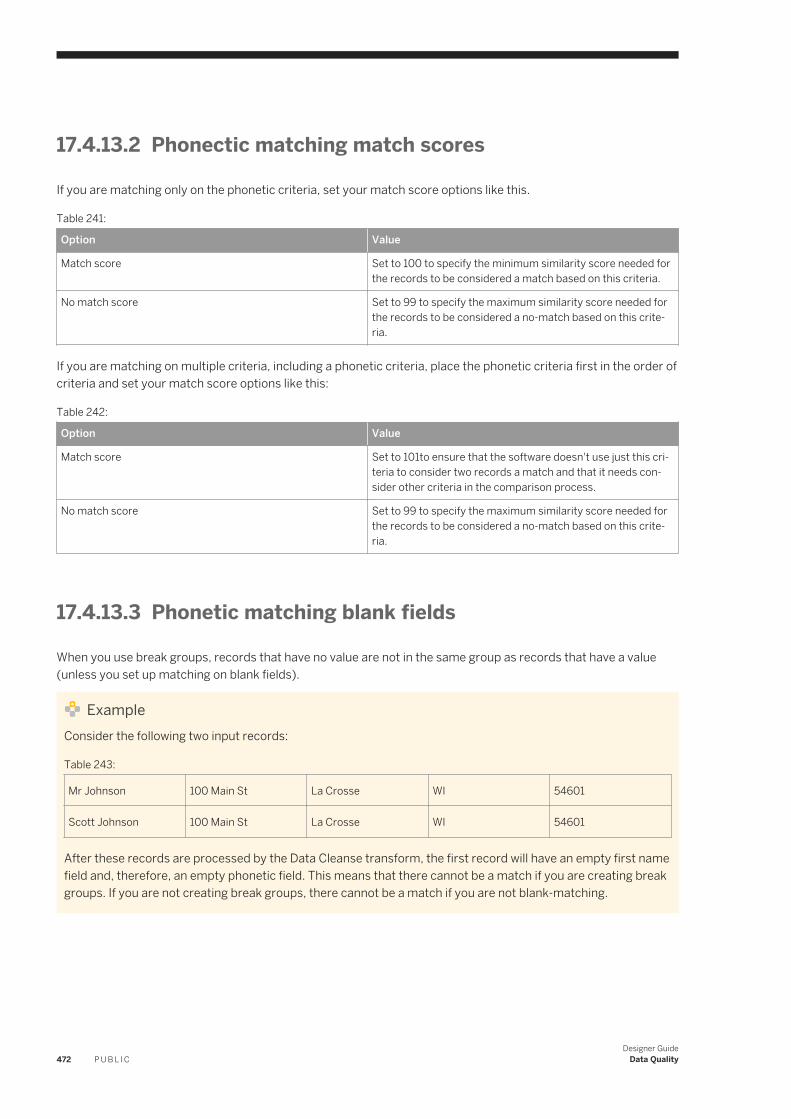
17.4.13.2 Phonectic matching match scores
If you are matching only on the phonetic criteria, set your match score options like this.
Table 241:
Option Value
Match score Set to 100 to specify the minimum similarity score needed for the records to be considered a match based on this criteria.
No match score Set to 99 to specify the maximum similarity score needed for the records to be considered a no-match based on this criteria.
If you are matching on multiple criteria, including a phonetic criteria, place the phonetic criteria first in the order of criteria and set your match score options like this:
Table 242:
Option Value
Match score Set to 101to ensure that the software doesn't use just this criteria to consider two records a match and that it needs consider other criteria in the comparison process.
No match score Set to 99 to specify the maximum similarity score needed for the records to be considered a no-match based on this criteria.
17.4.13.3 Phonetic matching blank fields
When you use break groups, records that have no value are not in the same group as records that have a value (unless you set up matching on blank fields).
ExampleConsider the following two input records:
Table 243:
Mr Johnson 100 Main St La Crosse WI 54601
Scott Johnson 100 Main St La Crosse WI 54601
After these records are processed by the Data Cleanse transform, the first record will have an empty first name field and, therefore, an empty phonetic field. This means that there cannot be a match if you are creating break groups. If you are not creating break groups, there cannot be a match if you are not blank-matching.
472 P U B L I CDesigner Guide
Data Quality
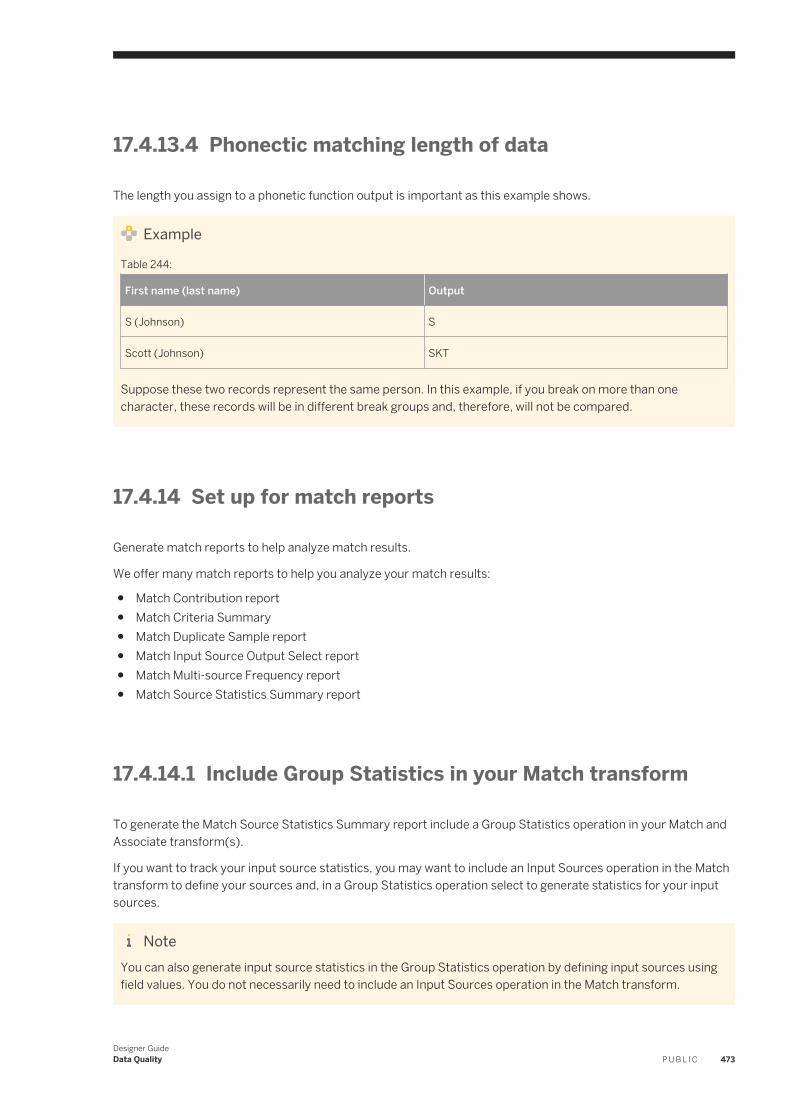
17.4.13.4 Phonectic matching length of data
The length you assign to a phonetic function output is important as this example shows.
Example
Table 244:
First name (last name) Output
S (Johnson) S
Scott (Johnson) SKT
Suppose these two records represent the same person. In this example, if you break on more than one character, these records will be in different break groups and, therefore, will not be compared.
17.4.14 Set up for match reports
Generate match reports to help analyze match results.
We offer many match reports to help you analyze your match results:
● Match Contribution report● Match Criteria Summary● Match Duplicate Sample report● Match Input Source Output Select report● Match Multi-source Frequency report● Match Source Statistics Summary report
17.4.14.1 Include Group Statistics in your Match transform
To generate the Match Source Statistics Summary report include a Group Statistics operation in your Match and Associate transform(s).
If you want to track your input source statistics, you may want to include an Input Sources operation in the Match transform to define your sources and, in a Group Statistics operation select to generate statistics for your input sources.
NoteYou can also generate input source statistics in the Group Statistics operation by defining input sources using field values. You do not necessarily need to include an Input Sources operation in the Match transform.
Designer GuideData Quality P U B L I C 473
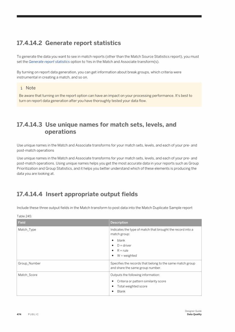
17.4.14.2 Generate report statistics
To generate the data you want to see in match reports (other than the Match Source Statistics report), you must set the Generate report statistics option to Yes in the Match and Associate transform(s).
By turning on report data generation, you can get information about break groups, which criteria were instrumental in creating a match, and so on.
NoteBe aware that turning on the report option can have an impact on your processing performance. It's best to turn on report data generation after you have thoroughly tested your data flow.
17.4.14.3 Use unique names for match sets, levels, and operations
Use unique names in the Match and Associate transforms for your match sets, levels, and each of your pre- and post-match operations
Use unique names in the Match and Associate transforms for your match sets, levels, and each of your pre- and post-match operations. Using unique names helps you get the most accurate data in your reports such as Group Prioritization and Group Statistics, and it helps you better understand which of these elements is producing the data you are looking at.
17.4.14.4 Insert appropriate output fields
Include these three output fields in the Match transform to post data into the Match Duplicate Sample report
Table 245:
Field Description
Match_Type Indicates the type of match that brought the record into a match group:
● blank● D = driver● R = rule● W = weighted
Group_Number Specifies the records that belong to the same match group and share the same group number.
Match_Score Outputs the following information:
● Criteria or pattern similarity score● Total weighted score● Blank
474 P U B L I CDesigner Guide
Data Quality
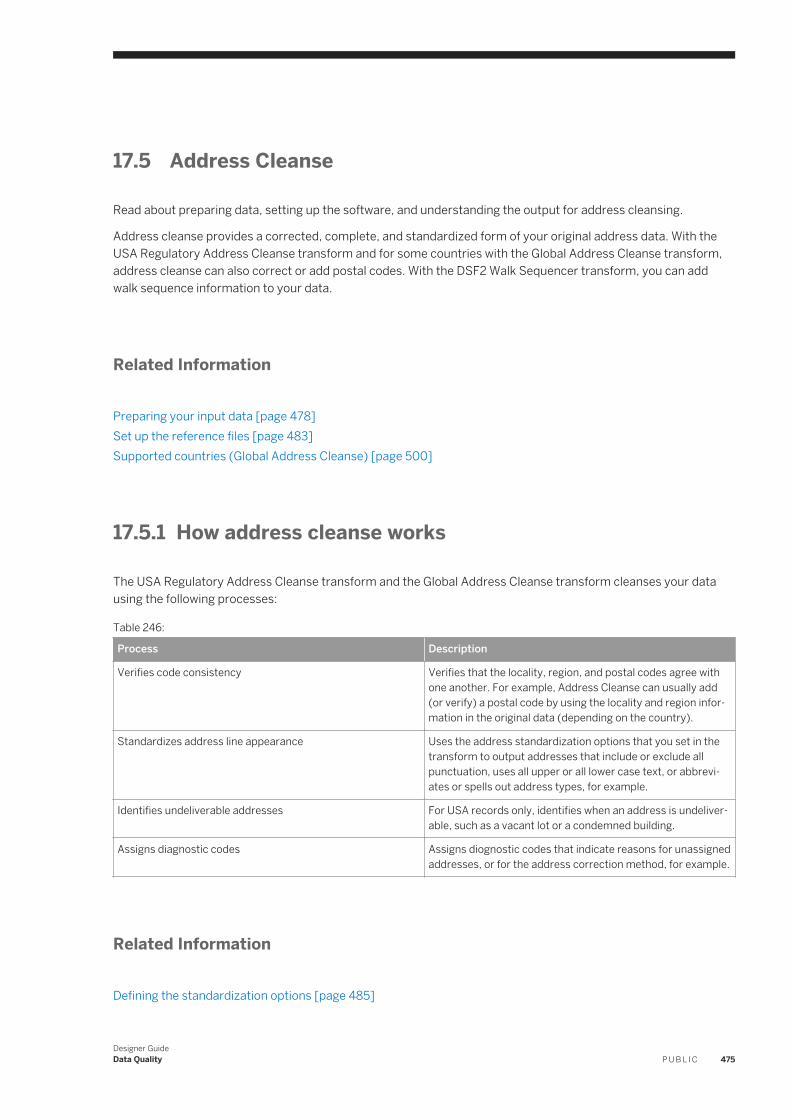
17.5 Address Cleanse
Read about preparing data, setting up the software, and understanding the output for address cleansing.
Address cleanse provides a corrected, complete, and standardized form of your original address data. With the USA Regulatory Address Cleanse transform and for some countries with the Global Address Cleanse transform, address cleanse can also correct or add postal codes. With the DSF2 Walk Sequencer transform, you can add walk sequence information to your data.
Related Information
Preparing your input data [page 478]Set up the reference files [page 483]Supported countries (Global Address Cleanse) [page 500]
17.5.1 How address cleanse works
The USA Regulatory Address Cleanse transform and the Global Address Cleanse transform cleanses your data using the following processes:
Table 246:
Process Description
Verifies code consistency Verifies that the locality, region, and postal codes agree with one another. For example, Address Cleanse can usually add (or verify) a postal code by using the locality and region information in the original data (depending on the country).
Standardizes address line appearance Uses the address standardization options that you set in the transform to output addresses that include or exclude all punctuation, uses all upper or all lower case text, or abbreviates or spells out address types, for example.
Identifies undeliverable addresses For USA records only, identifies when an address is undeliverable, such as a vacant lot or a condemned building.
Assigns diagnostic codes Assigns diognostic codes that indicate reasons for unassigned addresses, or for the address correction method, for example.
Related Information
Defining the standardization options [page 485]
Designer GuideData Quality P U B L I C 475
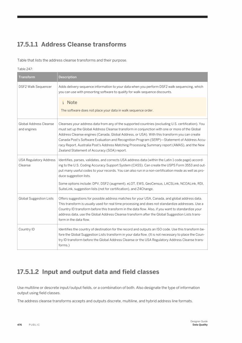
17.5.1.1 Address Cleanse transforms
Table that lists the address cleanse transforms and their purpose.
Table 247:
Transform Description
DSF2 Walk Sequencer Adds delivery sequence information to your data when you perform DSF2 walk sequencing, which you can use with presorting software to qualify for walk-sequence discounts.
NoteThe software does not place your data in walk sequence order.
Global Address Cleanse and engines
Cleanses your address data from any of the supported countries (excluding U.S. certification). You must set up the Global Address Cleanse transform in conjunction with one or more of the Global Address Cleanse engines (Canada, Global Address, or USA). With this transform you can create Canada Post's Software Evaluation and Recognition Program (SERP)—Statement of Address Accuracy Report, Australia Post's Address Matching Processing Summary report (AMAS), and the New Zealand Statement of Accuracy (SOA) report.
USA Regulatory Address Cleanse
Identifies, parses, validates, and corrects USA address data (within the Latin 1 code page) according to the U.S. Coding Accuracy Support System (CASS). Can create the USPS Form 3553 and output many useful codes to your records. You can also run in a non-certification mode as well as produce suggestion lists.
Some options include: DPV, DSF2 (augment), eLOT, EWS, GeoCensus, LACSLink, NCOALink, RDI, SuiteLink, suggestion lists (not for certification), and Z4Change.
Global Suggestion Lists Offers suggestions for possible address matches for your USA, Canada, and global address data. This transform is usually used for real time processing and does not standardize addresses. Use a Country ID transform before this transform in the data flow. Also, if you want to standardize your address data, use the Global Address Cleanse transform after the Global Suggestion Lists transform in the data flow.
Country ID Identifies the country of destination for the record and outputs an ISO code. Use this transform before the Global Suggestion Lists transform in your data flow. (It is not necessary to place the Country ID transform before the Global Address Cleanse or the USA Regulatory Address Cleanse transforms.)
17.5.1.2 Input and output data and field classes
Use multiline or descrete input/output fields, or a combination of both. Also designate the type of information output using field classes.
The address cleanse transforms accepts and outputs discrete, multiline, and hybrid address line formats.
476 P U B L I CDesigner Guide
Data Quality
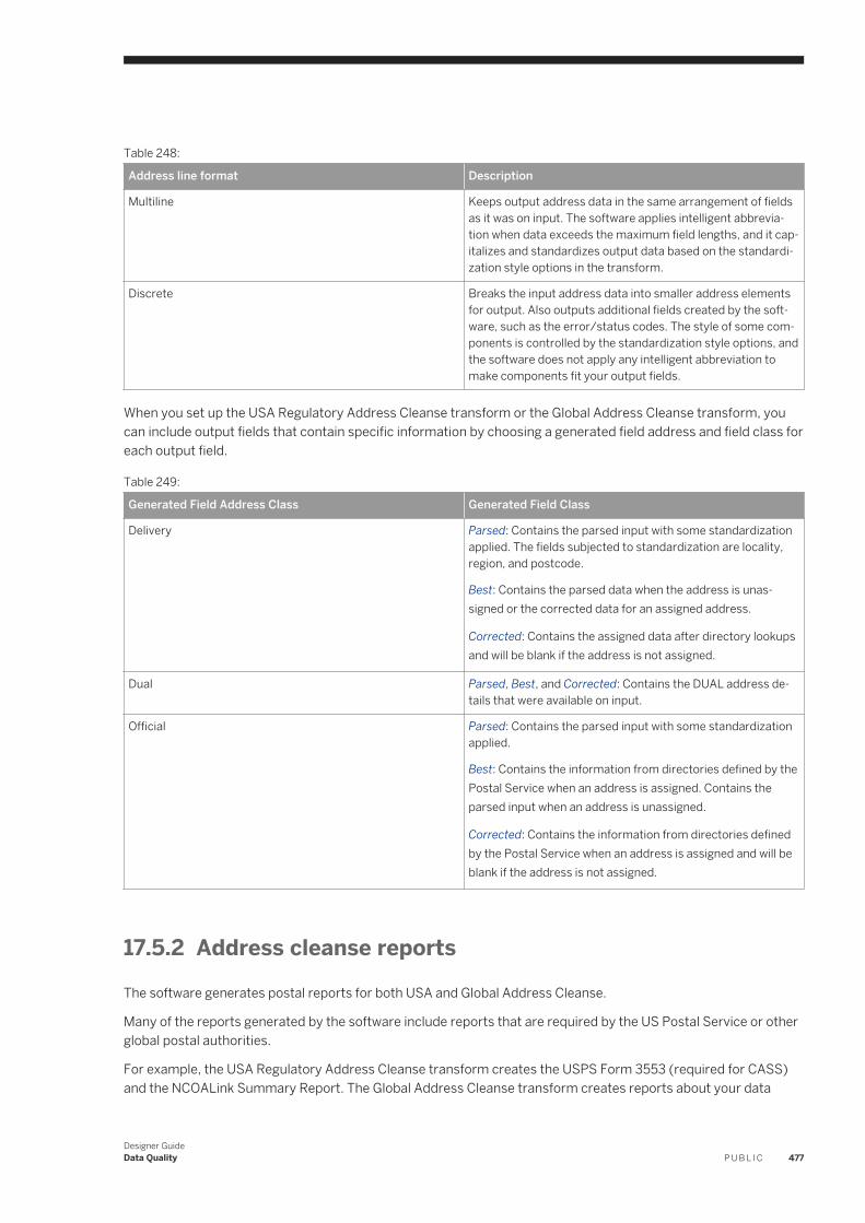
Table 248:
Address line format Description
Multiline Keeps output address data in the same arrangement of fields as it was on input. The software applies intelligent abbreviation when data exceeds the maximum field lengths, and it capitalizes and standardizes output data based on the standardization style options in the transform.
Discrete Breaks the input address data into smaller address elements for output. Also outputs additional fields created by the software, such as the error/status codes. The style of some components is controlled by the standardization style options, and the software does not apply any intelligent abbreviation to make components fit your output fields.
When you set up the USA Regulatory Address Cleanse transform or the Global Address Cleanse transform, you can include output fields that contain specific information by choosing a generated field address and field class for each output field.
Table 249:
Generated Field Address Class Generated Field Class
Delivery Parsed: Contains the parsed input with some standardization applied. The fields subjected to standardization are locality, region, and postcode.
Best: Contains the parsed data when the address is unassigned or the corrected data for an assigned address.
Corrected: Contains the assigned data after directory lookups and will be blank if the address is not assigned.
Dual Parsed, Best, and Corrected: Contains the DUAL address details that were available on input.
Official Parsed: Contains the parsed input with some standardization applied.
Best: Contains the information from directories defined by the Postal Service when an address is assigned. Contains the parsed input when an address is unassigned.
Corrected: Contains the information from directories defined by the Postal Service when an address is assigned and will be blank if the address is not assigned.
17.5.2 Address cleanse reports
The software generates postal reports for both USA and Global Address Cleanse.
Many of the reports generated by the software include reports that are required by the US Postal Service or other global postal authorities.
For example, the USA Regulatory Address Cleanse transform creates the USPS Form 3553 (required for CASS) and the NCOALink Summary Report. The Global Address Cleanse transform creates reports about your data
Designer GuideData Quality P U B L I C 477
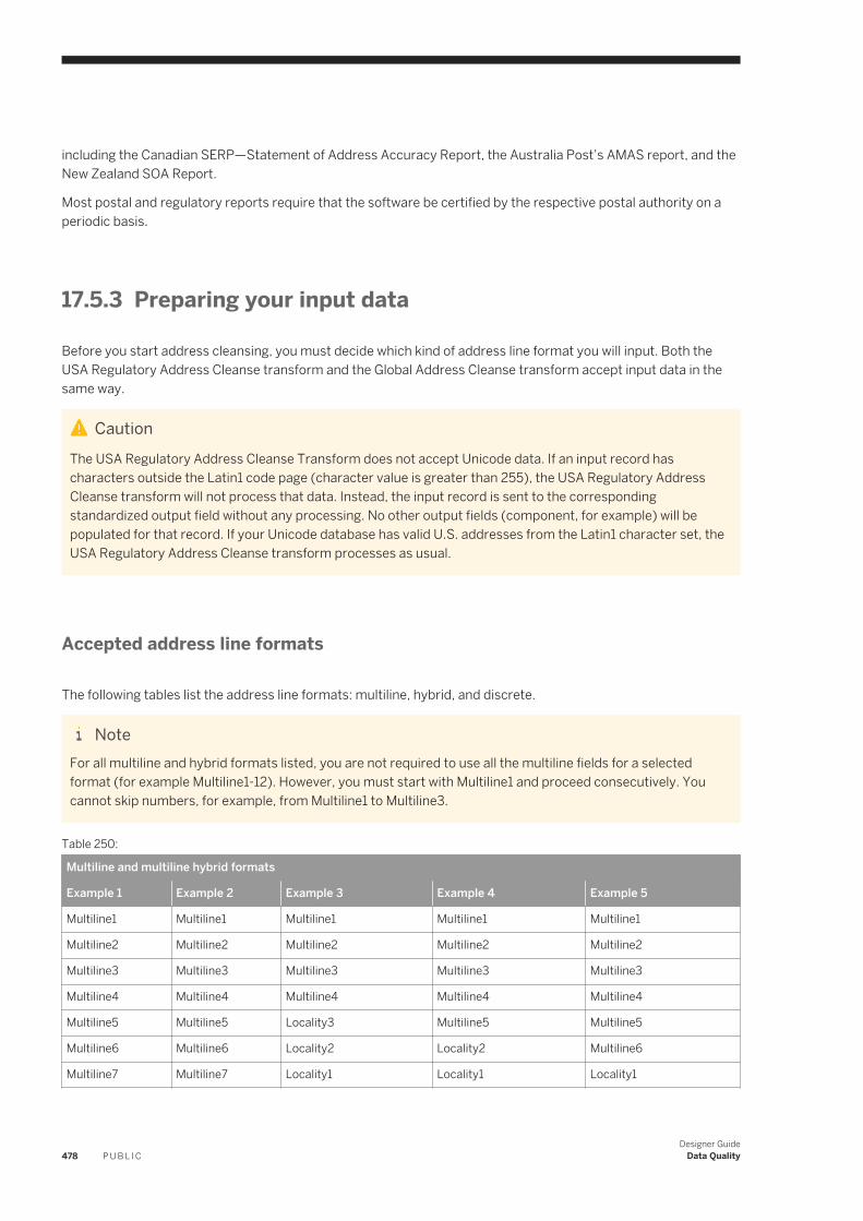
including the Canadian SERP—Statement of Address Accuracy Report, the Australia Post’s AMAS report, and the New Zealand SOA Report.
Most postal and regulatory reports require that the software be certified by the respective postal authority on a periodic basis.
17.5.3 Preparing your input data
Before you start address cleansing, you must decide which kind of address line format you will input. Both the USA Regulatory Address Cleanse transform and the Global Address Cleanse transform accept input data in the same way.
CautionThe USA Regulatory Address Cleanse Transform does not accept Unicode data. If an input record has characters outside the Latin1 code page (character value is greater than 255), the USA Regulatory Address Cleanse transform will not process that data. Instead, the input record is sent to the corresponding standardized output field without any processing. No other output fields (component, for example) will be populated for that record. If your Unicode database has valid U.S. addresses from the Latin1 character set, the USA Regulatory Address Cleanse transform processes as usual.
Accepted address line formats
The following tables list the address line formats: multiline, hybrid, and discrete.
NoteFor all multiline and hybrid formats listed, you are not required to use all the multiline fields for a selected format (for example Multiline1-12). However, you must start with Multiline1 and proceed consecutively. You cannot skip numbers, for example, from Multiline1 to Multiline3.
Table 250:
Multiline and multiline hybrid formats
Example 1 Example 2 Example 3 Example 4 Example 5
Multiline1 Multiline1 Multiline1 Multiline1 Multiline1
Multiline2 Multiline2 Multiline2 Multiline2 Multiline2
Multiline3 Multiline3 Multiline3 Multiline3 Multiline3
Multiline4 Multiline4 Multiline4 Multiline4 Multiline4
Multiline5 Multiline5 Locality3 Multiline5 Multiline5
Multiline6 Multiline6 Locality2 Locality2 Multiline6
Multiline7 Multiline7 Locality1 Locality1 Locality1
478 P U B L I CDesigner Guide
Data Quality
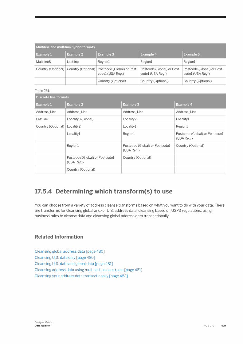
Multiline and multiline hybrid formats
Example 1 Example 2 Example 3 Example 4 Example 5
Multiline8 Lastline Region1 Region1 Region1
Country (Optional) Country (Optional) Postcode (Global) or Postcode1 (USA Reg.)
Postcode (Global) or Postcode1 (USA Reg.)
Postcode (Global) or Postcode1 (USA Reg.)
Country (Optional) Country (Optional) Country (Optional)
Table 251:
Discrete line formats
Example 1 Example 2 Example 3 Example 4
Address_Line Address_Line Address_Line Address_Line
Lastline Locality3 (Global) Locality2 Locality1
Country (Optional) Locality2 Locality1 Region1
Locality1 Region1 Postcode (Global) or Postcode1 (USA Reg.)
Region1 Postcode (Global) or Postcode1 (USA Reg.)
Country (Optional)
Postcode (Global) or Postcode1 (USA Reg.)
Country (Optional)
Country (Optional)
17.5.4 Determining which transform(s) to use
You can choose from a variety of address cleanse transforms based on what you want to do with your data. There are transforms for cleansing global and/or U.S. address data, cleansing based on USPS regulations, using business rules to cleanse data and cleansing global address data transactionally.
Related Information
Cleansing global address data [page 480]Cleansing U.S. data only [page 480]Cleansing U.S. data and global data [page 481]Cleansing address data using multiple business rules [page 481]Cleansing your address data transactionally [page 482]
Designer GuideData Quality P U B L I C 479
17.5.4.1 Cleansing global address data
To cleanse your address data for any of the software-supported countries (including Canada for SERP, Software Evaluation and Recognition Program, certification and Australia for AMAS, Address Matching Approval System, certification), use the Global Address Cleanse transform in your project with one or more of the following engines:
● Canada● Global Address● USA
TipCleansing U.S. data with the USA Regulatory Address Cleanse transform is usually faster than with the Global Address Cleanse transform and USA engine. This scenario is usually true even if you end up needing both transforms.
You can also use the Global Address Cleanse transform with the Canada, USA, Global Address engines in a real time data flow to create suggestion lists for those countries.
Start with a sample transform configuration
The software includes a variety of Global Address Cleanse sample transform configurations (which include at least one engine) that you can copy to use for a project.
Related Information
Supported countries (Global Address Cleanse) [page 500]Cleansing U.S. data and global data [page 481]
17.5.4.2 Cleansing U.S. data only
To cleanse U.S. address data, use the USA Regulatory Address Cleanse transform for the best results. With this transform, and with DPV, LACSLink, and SuiteLink enabled, you can produce a CASS-certified mailing and produce a USPS Form 3553. If you do not intend to process CASS-certified lists, you should still use the USA Regulatory Address Cleanse transform for processing your U.S. data. Using the USA Regulatory Address Cleanse transform on U.S. data is more efficient than using the Global Address Cleanse transform.
With the USA Regulatory Address Cleanse transform you can add additional information to your data such as DSF2, EWS, eLOT, NCOALink, and RDI. And you can process records one at a time by using suggestion lists.
480 P U B L I CDesigner Guide
Data Quality
Start with a sample transform configuration
The software includes a variety of USA Regulatory Address Cleanse sample transform configurations that can help you set up your projects.
Related Information
Introduction to suggestion lists [page 563]
17.5.4.3 Cleansing U.S. data and global data
What should you do when you have U.S. addresses that need to be certified and also addresses from other countries in your database? In this situation, you should use both the Global Address Cleanse transform and the USA Regulatory Address Cleanse transform in your data flow.
TipEven if you are not processing U.S. data for USPS certification, you may find that cleansing U.S. data with the USA Regulatory Address Cleanse transform is faster than with the Global Address Cleanse transform and USA engine.
17.5.4.4 Cleansing address data using multiple business rules
When you have two addresses intended for different purposes (for example, a billing address and a shipping address), you should use two of the same address cleanse transforms in a data flow.
One or two engines?
When you use two Global Address Cleanse transforms for data from the same country, they can share an engine. You do not need to have two engines of the same kind. If you use one engine or two, it does not affect the overall processing time of the data flow.
In this situation, however, you may need to use two separate engines (even if the data is from the same country). Depending on your business rules, you may have to define the settings in the engine differently for a billing address or for a shipping address. For example, in the Standardization Options group, the Output Country Language option can convert the data used in each record to the official country language or it can preserve the language used in each record. For example, you may want to convert the data for the shipping address but preserve the data for the billing address.
Designer GuideData Quality P U B L I C 481
17.5.4.5 Cleansing your address data transactionally
The Global Suggestion Lists transform, best used in transactional projects, is a way to complete and populate addresses with minimal data, or it can offer suggestions for possible matches. For example, the Marshall Islands and the Federated States of Micronesia were recently removed from the USA Address directory. Therefore, if you previously used the USA engine, you'll now have to use the Global Address engine. The Global Suggestion Lists transform can help identify that these countries are no longer in the USA Address directory.
This easy address-entry system is ideal in call center environments or any transactional environment where cleansing is necessary at the point of entry. It's also a beneficial research tool when you need to manage bad addresses from a previous batch process.
Place the Global Suggestion Lists transform after the Country ID transform and before a Global Address Cleanse transform that uses a Global Address, Canada, and/or USA engine.
Integrating functionality
Global Suggestion Lists functionality is designed to be integrated into your own custom applications via the Web Service. If you are a programmer looking for details about how to integrate this functionality, see "Integrate Global Suggestion Lists" in the Integrator Guide.
Start with a sample transform configuration
Data Quality includes a Global Suggestion Lists sample transform that can help you when setting up a project.
Related Information
Introduction to suggestion lists [page 563]
17.5.5 Identifying the country of destination
The Global Address Cleanse transform includes Country ID processing. Therefore, you do not need to place a Country ID transform before the Global Address Cleanse transform in your data flow.
In the Country ID Options option group of the Global Address Cleanse transform, you can define the country of destination or define whether you want to run Country ID processing.
482 P U B L I CDesigner Guide
Data Quality
Constant country
If all of your data is from one country, such as Australia, you do not need to run Country ID processing or input a discrete country field. You can tell the Global Address Cleanse transform the country and it will assume all records are from this country (which may save processing time).
Assign default
You'll want to run Country ID processing if you are using two or more of the engines and your input addresses contain country data (such as the two-character ISO code or a country name), or if you are using only one engine and your input source contains many addresses that cannot be processed by that engine. Addresses that cannot be processed are not sent to the engine. The transform will use the country you specify in this option group as a default.
Related Information
Setting a constant country [page 501]Setting a default country [page 500]
17.5.6 Set up the reference files
The USA Regulatory Address Cleanse transform and the Global Address Cleanse transform and engines rely on several directories (reference files) to cleanse your data.
When you use directories to standardize addresses and assign postal codes, you must use the most up-to-date directories, which requires you to periodically update your files with new directories. SAP keeps you informed about current directory dates, and alerts you when you need to download newer directories.
Related Information
Beyond the basic address cleansing [page 506]Supported countries (Global Address Cleanse) [page 500]Process Japanese addresses [page 486]Process Chinese addresses [page 495]New Zealand certification [page 502]
Designer GuideData Quality P U B L I C 483
17.5.6.1 Directories
To correct addresses and assign codes, the address cleanse transforms relies on address directories.
These directories contain specific types of information related to what processes you want performed on your addresses. For example, the United States Postal Service has directories with address information about every address in the United States and its territories. And the software uses many other directories issued by other postal authorities such as Canada, New Zealand, and Japan.
NoteAddress cleanse transforms support many countries, however, when you use the Global Address Cleanse transform, there may be some countries that are not supported by official directories.
Besides the basic address directories, there are many specialized directories. For example, the USA Regulatory Address Cleanse transform uses the following specialized directories:
● DPV®● DSF2®● Early Warning System (EWS)● eLOT®● GeoCensus● LACSLink®● NCOALink®● RDI™● SuiteLink™● Z4Change
These specialized directories help extend US address cleansing beyond the basic parsing and standardizing.
17.5.6.2 Directory file locations
Set directory file locations in the transform's Reference Files option group.
Your system administrator should have already installed the necessary files to the appropriate locations based on your company's needs.
CautionIncompatible or out-of-date directories can render the software unusable. The system administrator must install weekly, monthly or bimonthly directory updates for the USA Regulatory Address Cleanse Transform; monthly directory updates for the Australia and Canada engines; and quarterly directory updates for the Global Address engine to ensure that they are compatible with the current software.
484 P U B L I CDesigner Guide
Data Quality
17.5.6.3 Directory files substitution values
Use substitution values to set a constant value for your directory locations.
If you start with a sample transform, the Reference Files options are already completed with a substitution variable by default. For example, the variable $$RefFilesAddressCleanse points to the reference data folder of the software directory by default.
NoteYou can change that location by editing the substitution file associated with the data flow. This change is made for every data flow that uses that substitution file.
Related Information
Overview of substitution parameters [page 290]
17.5.6.4 Viewing directory expiration dates in the trace log
Steps to set up the trace log with directory expiration dates.
To include directory expiration information in the trace log, perform the following steps.
1. Right click on the applicable job icon in Designer and select Execute.2. In the Execution Properties window, open the Execution Options tab (it should already be open by default).3. Select Print all trace messages.
Related Information
Using logs [page 305]
17.5.7 Defining the standardization options
Standardization changes the way the data is presented after an assignment has been made. The type of change depends on the options that you define in the transform. These options include casing, punctuation, sequence, abbreviations, and much more. It helps ensure the integrity of your databases, makes mail more deliverable, and gives your communications with customers a more professional appearance.
For example, the following address was standardized for capitalization, punctuation, and postal phrase (route to RR).
Designer GuideData Quality P U B L I C 485
Table 252:
Input Output
Multiline1 = route 1 box 44a
Multiline2 = stodard wisc
Address_Line = RR 1 BOX 44A
Locality1 = STODDARD
Region1 = WI
Postcode1 = 54658
Global Address Cleanse transform
In the Global Address Cleanse transform, you set the standardization options in the Standardization Options option group.
You can standardize addresses for all countries and/or for individual countries (depending on your data). For example, you can have one set of French standardization options that standardize addresses within France only, and another set of Global standardization options that standardize all other addresses.
USA Regulatory Address Cleanse transform
If you use the USA Regulatory Address Cleanse transform, you set the standardization options on the Options tab in the Standardization Options section.
17.5.8 Process Japanese addresses
The Global Address Cleanse transform's Global Address engine parses Japanese addresses. The primary purpose of this transform and engine is to parse and normalize Japanese addresses for data matching and cleansing applications.
NoteThe Japan engine only supports kanji and katakana data. The engine does not support Latin data.
A significant portion of the address parsing capability relies on the Japanese address database. The software has data from the Ministry of Public Management, Home Affairs, Posts and Telecommunications (MPT) and additional data sources. The enhanced address database consists of a regularly updated government database that includes regional postal codes mapped to localities.
Related Information
486 P U B L I CDesigner Guide
Data Quality
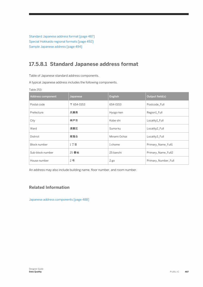
Standard Japanese address format [page 487]Special Hokkaido regional formats [page 492]Sample Japanese address [page 494]
17.5.8.1 Standard Japanese address format
Table of Japanese standard address components.
A typical Japanese address includes the following components.
Table 253:
Address component Japanese English Output field(s)
Postal code 〒 654-0153 654-0153 Postcode_Full
Prefecture 兵庫県 Hyogo-ken Region1_Full
City 神戸市 Kobe-shi Locality1_Full
Ward 須磨区 Suma-ku Locality2_Full
District 南落合 Minami Ochiai Locality3_Full
Block number 1 丁目 1 chome Primary_Name_Full1
Sub-block number 25 番地 25 banchi Primary_Name_Full2
House number 2 号 2 go Primary_Number_Full
An address may also include building name, floor number, and room number.
Related Information
Japanese address components [page 488]
Designer GuideData Quality P U B L I C 487
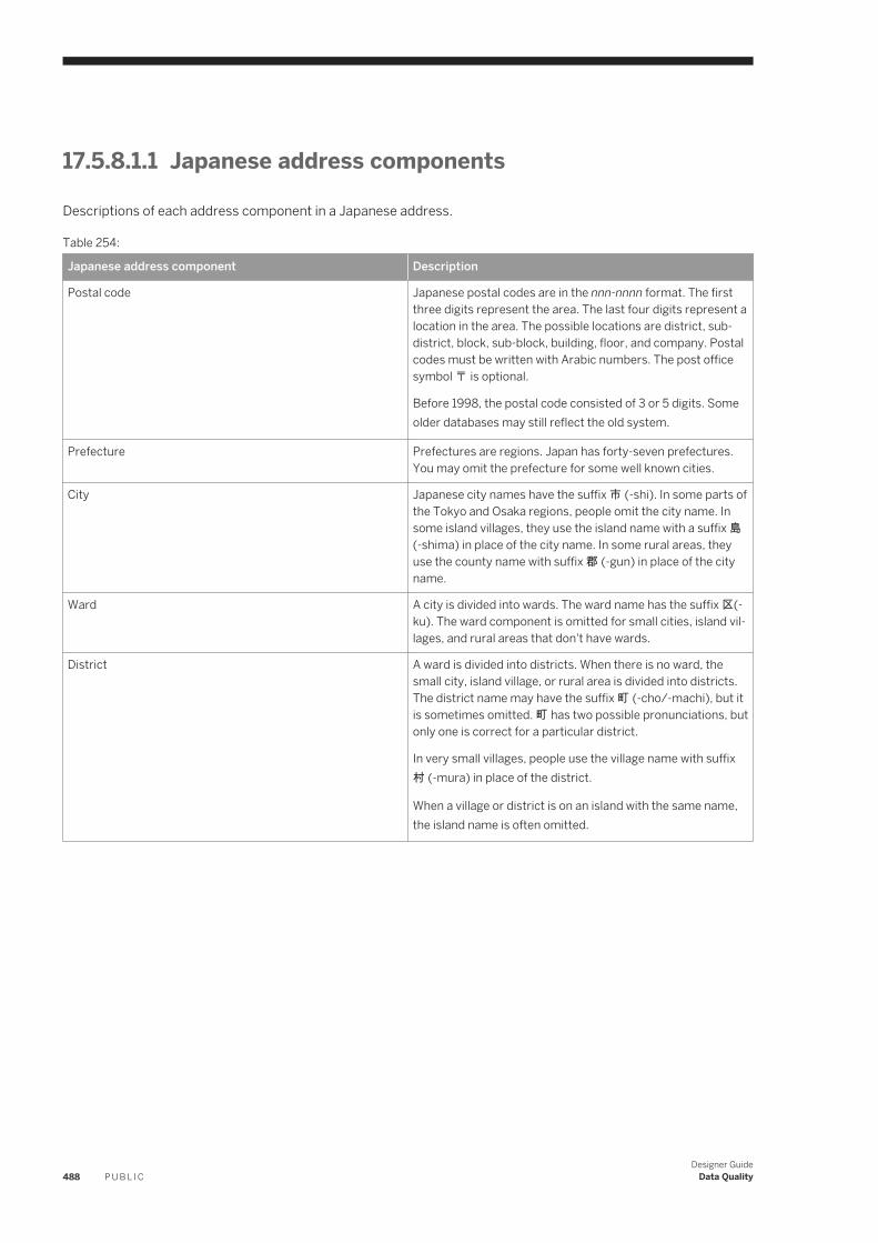
17.5.8.1.1 Japanese address components
Descriptions of each address component in a Japanese address.
Table 254:
Japanese address component Description
Postal code Japanese postal codes are in the nnn-nnnn format. The first three digits represent the area. The last four digits represent a location in the area. The possible locations are district, sub-district, block, sub-block, building, floor, and company. Postal codes must be written with Arabic numbers. The post office symbol 〒 is optional.
Before 1998, the postal code consisted of 3 or 5 digits. Some older databases may still reflect the old system.
Prefecture Prefectures are regions. Japan has forty-seven prefectures. You may omit the prefecture for some well known cities.
City Japanese city names have the suffix 市 (-shi). In some parts of the Tokyo and Osaka regions, people omit the city name. In some island villages, they use the island name with a suffix 島 (-shima) in place of the city name. In some rural areas, they use the county name with suffix 郡 (-gun) in place of the city name.
Ward A city is divided into wards. The ward name has the suffix 区(-ku). The ward component is omitted for small cities, island villages, and rural areas that don't have wards.
District A ward is divided into districts. When there is no ward, the small city, island village, or rural area is divided into districts. The district name may have the suffix 町 (-cho/-machi), but it is sometimes omitted. 町 has two possible pronunciations, but only one is correct for a particular district.
In very small villages, people use the village name with suffix 村 (-mura) in place of the district.
When a village or district is on an island with the same name, the island name is often omitted.
488 P U B L I CDesigner Guide
Data Quality
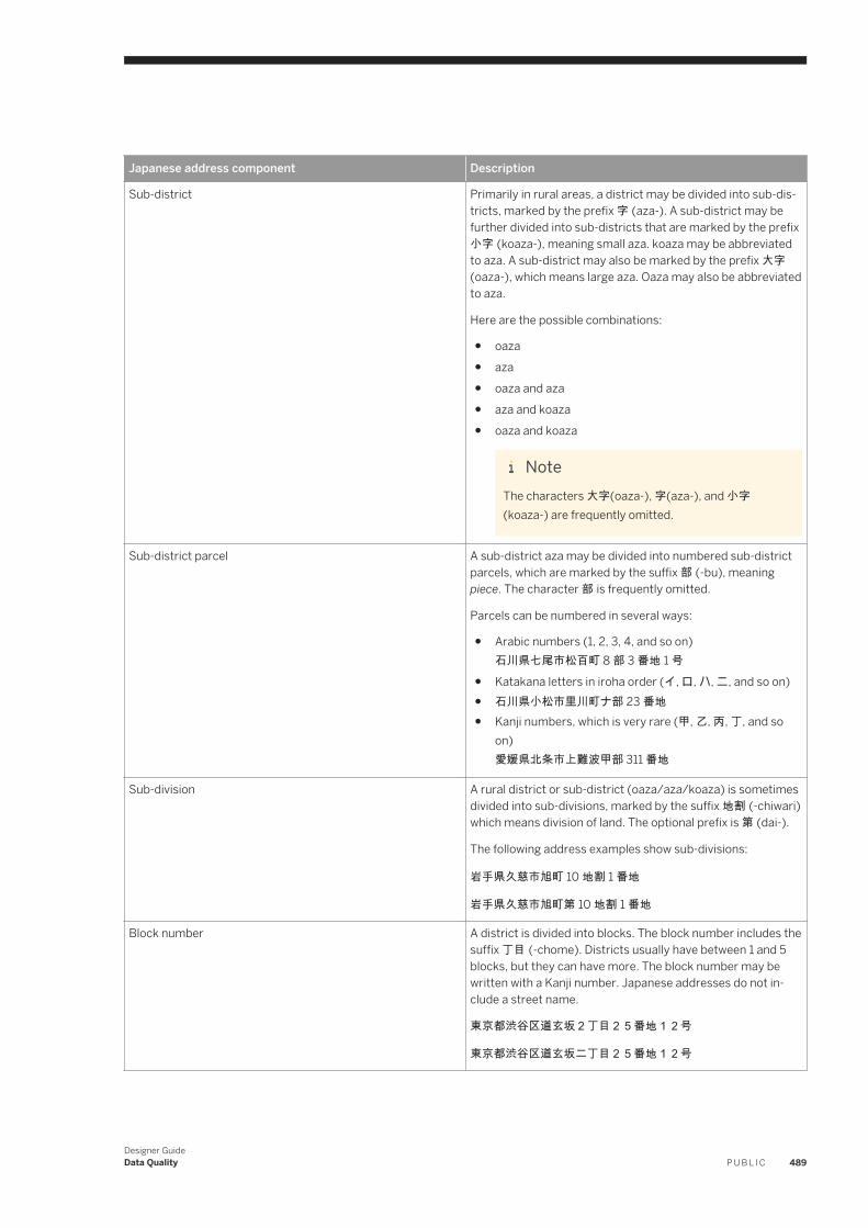
Japanese address component Description
Sub-district Primarily in rural areas, a district may be divided into sub-districts, marked by the prefix 字 (aza-). A sub-district may be further divided into sub-districts that are marked by the prefix 小字 (koaza-), meaning small aza. koaza may be abbreviated to aza. A sub-district may also be marked by the prefix 大字 (oaza-), which means large aza. Oaza may also be abbreviated to aza.
Here are the possible combinations:
● oaza● aza● oaza and aza● aza and koaza● oaza and koaza
NoteThe characters 大字(oaza-), 字(aza-), and 小字 (koaza-) are frequently omitted.
Sub-district parcel A sub-district aza may be divided into numbered sub-district parcels, which are marked by the suffix 部 (-bu), meaning piece. The character 部 is frequently omitted.
Parcels can be numbered in several ways:
● Arabic numbers (1, 2, 3, 4, and so on)石川県七尾市松百町 8 部 3 番地 1 号
● Katakana letters in iroha order (イ, ロ, ハ, ニ, and so on)● 石川県小松市里川町ナ部 23 番地● Kanji numbers, which is very rare (甲, 乙, 丙, 丁, and so
on)愛媛県北条市上難波甲部 311 番地
Sub-division A rural district or sub-district (oaza/aza/koaza) is sometimes divided into sub-divisions, marked by the suffix 地割 (-chiwari) which means division of land. The optional prefix is 第 (dai-).
The following address examples show sub-divisions:
岩手県久慈市旭町 10 地割 1 番地
岩手県久慈市旭町第 10 地割 1 番地
Block number A district is divided into blocks. The block number includes the suffix 丁目 (-chome). Districts usually have between 1 and 5 blocks, but they can have more. The block number may be written with a Kanji number. Japanese addresses do not include a street name.
東京都渋谷区道玄坂2丁目25番地12号
東京都渋谷区道玄坂二丁目25番地12号
Designer GuideData Quality P U B L I C 489
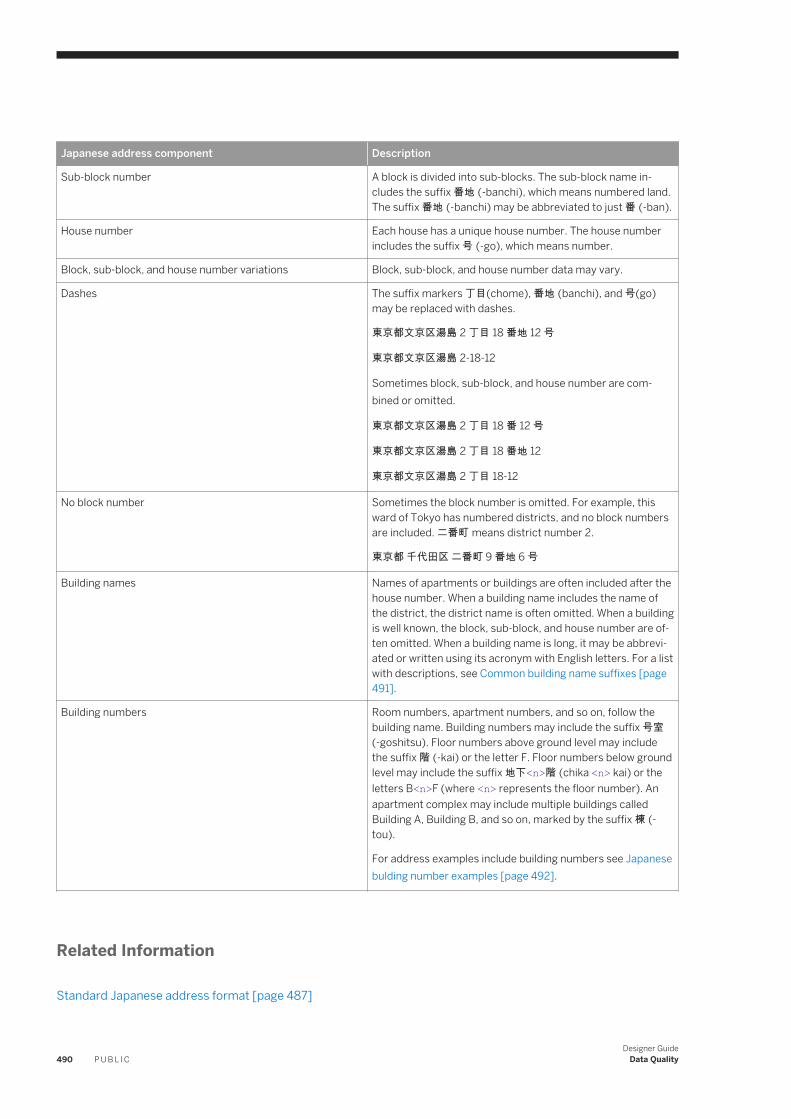
Japanese address component Description
Sub-block number A block is divided into sub-blocks. The sub-block name includes the suffix 番地 (-banchi), which means numbered land. The suffix 番地 (-banchi) may be abbreviated to just 番 (-ban).
House number Each house has a unique house number. The house number includes the suffix 号 (-go), which means number.
Block, sub-block, and house number variations Block, sub-block, and house number data may vary.
Dashes The suffix markers 丁目(chome), 番地 (banchi), and 号(go) may be replaced with dashes.
東京都文京区湯島 2 丁目 18 番地 12 号
東京都文京区湯島 2-18-12
Sometimes block, sub-block, and house number are combined or omitted.
東京都文京区湯島 2 丁目 18 番 12 号
東京都文京区湯島 2 丁目 18 番地 12
東京都文京区湯島 2 丁目 18-12
No block number Sometimes the block number is omitted. For example, this ward of Tokyo has numbered districts, and no block numbers are included. 二番町 means district number 2.
東京都 千代田区 二番町 9 番地 6 号
Building names Names of apartments or buildings are often included after the house number. When a building name includes the name of the district, the district name is often omitted. When a building is well known, the block, sub-block, and house number are often omitted. When a building name is long, it may be abbreviated or written using its acronym with English letters. For a list with descriptions, see Common building name suffixes [page 491].
Building numbers Room numbers, apartment numbers, and so on, follow the building name. Building numbers may include the suffix 号室 (-goshitsu). Floor numbers above ground level may include the suffix 階 (-kai) or the letter F. Floor numbers below ground level may include the suffix 地下<n>階 (chika <n> kai) or the letters B<n>F (where <n> represents the floor number). An apartment complex may include multiple buildings called Building A, Building B, and so on, marked by the suffix 棟 (-tou).
For address examples include building numbers see Japanese bulding number examples [page 492].
Related Information
Standard Japanese address format [page 487]
490 P U B L I CDesigner Guide
Data Quality
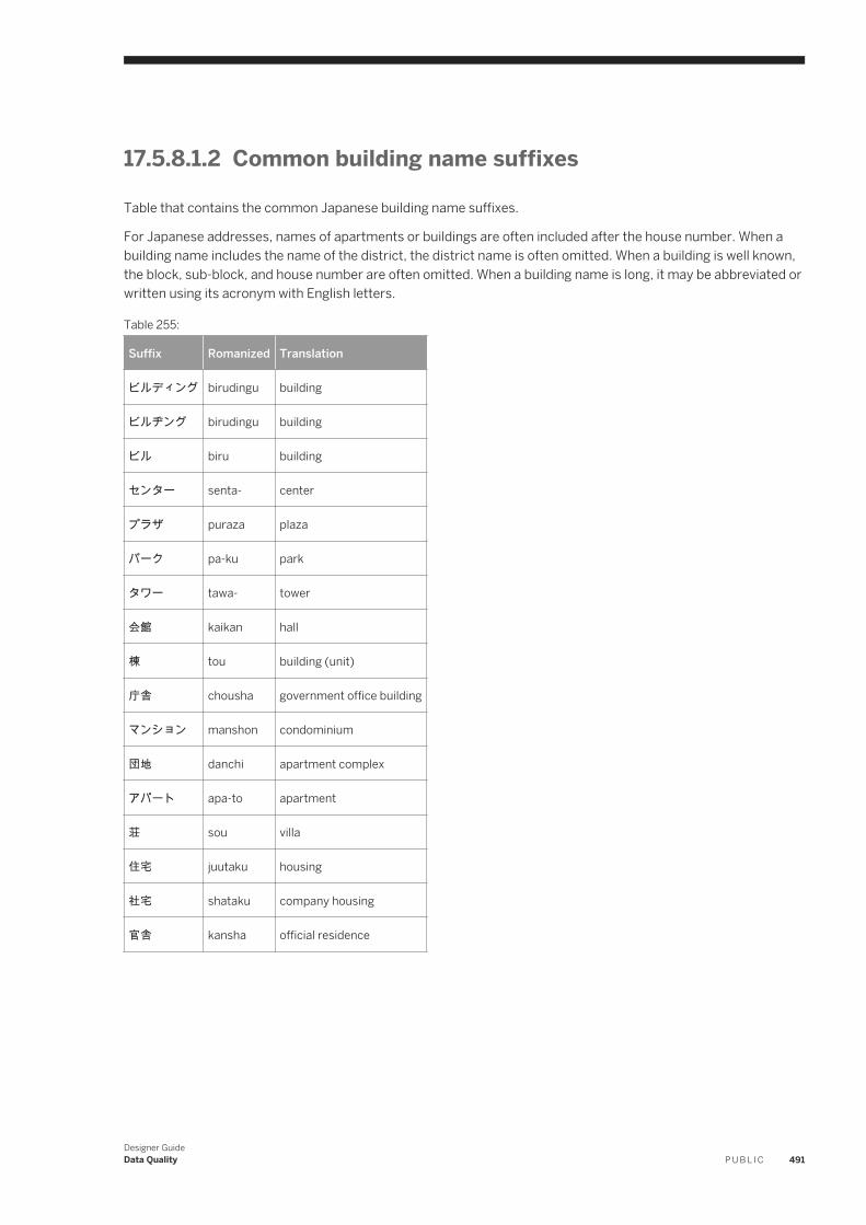
17.5.8.1.2 Common building name suffixes
Table that contains the common Japanese building name suffixes.
For Japanese addresses, names of apartments or buildings are often included after the house number. When a building name includes the name of the district, the district name is often omitted. When a building is well known, the block, sub-block, and house number are often omitted. When a building name is long, it may be abbreviated or written using its acronym with English letters.
Table 255:
Suffix Romanized Translation
ビルディング birudingu building
ビルヂング birudingu building
ビル biru building
センター senta- center
プラザ puraza plaza
パーク pa-ku park
タワー tawa- tower
会館 kaikan hall
棟 tou building (unit)
庁舎 chousha government office building
マンション manshon condominium
団地 danchi apartment complex
アパート apa-to apartment
荘 sou villa
住宅 juutaku housing
社宅 shataku company housing
官舎 kansha official residence
Designer GuideData Quality P U B L I C 491
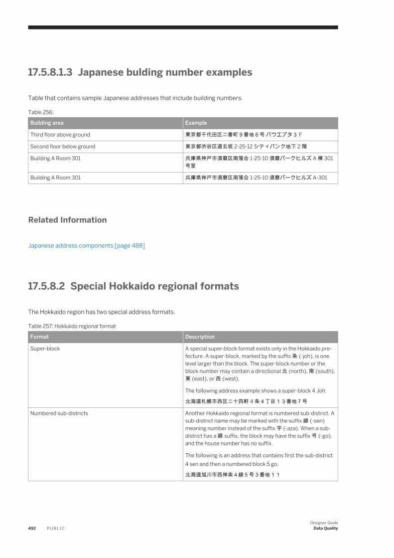
17.5.8.1.3 Japanese bulding number examples
Table that contains sample Japanese addresses that include building numbers.
Table 256:
Building area Example
Third floor above ground 東京都千代田区二番町9番地6号 バウエプタ3 F
Second floor below ground 東京都渋谷区道玄坂 2-25-12 シティバンク地下 2 階
Building A Room 301 兵庫県神戸市須磨区南落合 1-25-10 須磨パークヒルズ A 棟 301 号室
Building A Room 301 兵庫県神戸市須磨区南落合 1-25-10 須磨パークヒルズ A-301
Related Information
Japanese address components [page 488]
17.5.8.2 Special Hokkaido regional formats
The Hokkaido region has two special address formats.
Table 257: Hokkaido regional format
Format Description
Super-block A special super-block format exists only in the Hokkaido prefecture. A super-block, marked by the suffix 条 (-joh), is one level larger than the block. The super-block number or the block number may contain a directional 北 (north), 南 (south), 東 (east), or 西 (west).
The following address example shows a super-block 4 Joh.
北海道札幌市西区二十四軒 4 条4丁目13番地7号
Numbered sub-districts Another Hokkaido regional format is numbered sub-district. A sub-district name may be marked with the suffix 線 (-sen) meaning number instead of the suffix 字 (-aza). When a sub-district has a 線 suffix, the block may have the suffix 号 (-go), and the house number has no suffix.
The following is an address that contains first the sub-district 4 sen and then a numbered block 5 go.
北海道旭川市西神楽4線5号3番地11
492 P U B L I CDesigner Guide
Data Quality
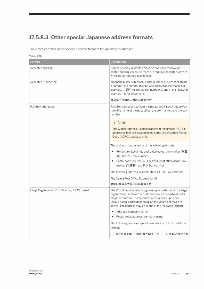
17.5.8.3 Other special Japanese address formats
Table that contains other special address formats for Japanese addresses.
Table 258:
Format Description
Accepted spelling Names of cities, districts and so on can have multiple accepted spellings because there are multiple accepted ways to write certain sounds in Japanese.
Accepted numbering When the block, sub-block, house number or district contains a number, the number may be written in Arabic or Kanji. For example, 二番町 means district number 2, and in the following example it is for Niban-cho.
東京都千代田区二番町九番地六号
P.O. Box addresses P.O. Box addresses contain the postal code, Locality1, prefecture, the name of the post office, the box marker, and the box number.
NoteThe Global Address Cleanse transform recognizes P.O. box addresses that are located in the Large Organization Postal Code (LOPC) database only.
The address may be in one of the following formats:
● Prefecture, Locality1, post office name, box marker (私書箱), and P.O. box number.
● Postal code, prefecture, Locality1, post office name, box marker (私書箱), and P.O. box number.
The following address example shows a P.O. Box address:
The Osaka Post Office Box marker #1
大阪府大阪市大阪支店私書箱 1 号
Large Organization Postal Code (LOPC) format The Postal Service may assign a unique postal code to a large organization, such as the customer service department of a major corporation. An organization may have up to two unique postal codes depending on the volume of mail it receives. The address may be in one of the following formats:
● Address, company name● Postal code, address, company name
The following is an example of an address in a LOPC address format.
100-8798 東京都千代田区霞が関1丁目 3 - 2 日本郵政 株式会社
Designer GuideData Quality P U B L I C 493
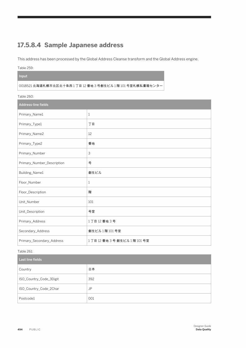
17.5.8.4 Sample Japanese address
This address has been processed by the Global Address Cleanse transform and the Global Address engine.
Table 259:
Input
0018521 北海道札幌市北区北十条西 1 丁目 12 番地 3 号創生ビル 1 階 101 号室札幌私書箱センター
Table 260:
Address-line fields
Primary_Name1 1
Primary_Type1 丁目
Primary_Name2 12
Primary_Type2 番地
Primary_Number 3
Primary_Number_Description 号
Building_Name1 創生ビル
Floor_Number 1
Floor_Description 階
Unit_Number 101
Unit_Description 号室
Primary_Address 1 丁目 12 番地 3 号
Secondary_Address 創生ビル 1 階 101 号室
Primary_Secondary_Address 1 丁目 12 番地 3 号 創生ビル 1 階 101 号室
Table 261:
Last line fields
Country 日本
ISO_Country_Code_3Digit 392
ISO_Country_Code_2Char JP
Postcode1 001
494 P U B L I CDesigner Guide
Data Quality
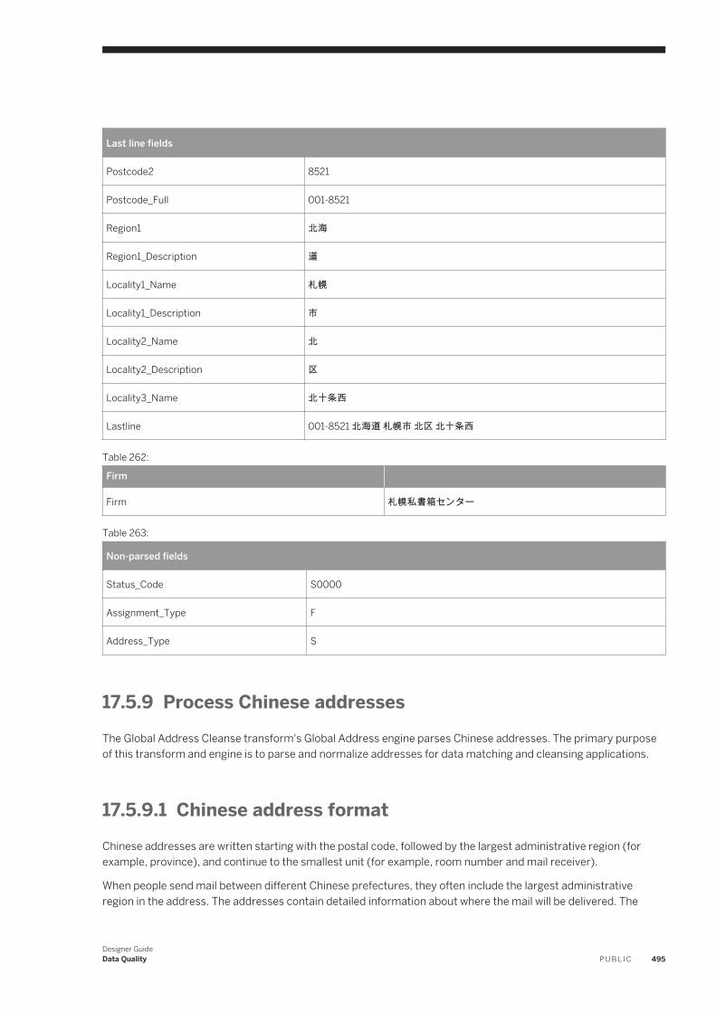
Last line fields
Postcode2 8521
Postcode_Full 001-8521
Region1 北海
Region1_Description 道
Locality1_Name 札幌
Locality1_Description 市
Locality2_Name 北
Locality2_Description 区
Locality3_Name 北十条西
Lastline 001-8521 北海道 札幌市 北区 北十条西
Table 262:
Firm
Firm 札幌私書箱センター
Table 263:
Non-parsed fields
Status_Code S0000
Assignment_Type F
Address_Type S
17.5.9 Process Chinese addressesThe Global Address Cleanse transform's Global Address engine parses Chinese addresses. The primary purpose of this transform and engine is to parse and normalize addresses for data matching and cleansing applications.
17.5.9.1 Chinese address formatChinese addresses are written starting with the postal code, followed by the largest administrative region (for example, province), and continue to the smallest unit (for example, room number and mail receiver).
When people send mail between different Chinese prefectures, they often include the largest administrative region in the address. The addresses contain detailed information about where the mail will be delivered. The
Designer GuideData Quality P U B L I C 495
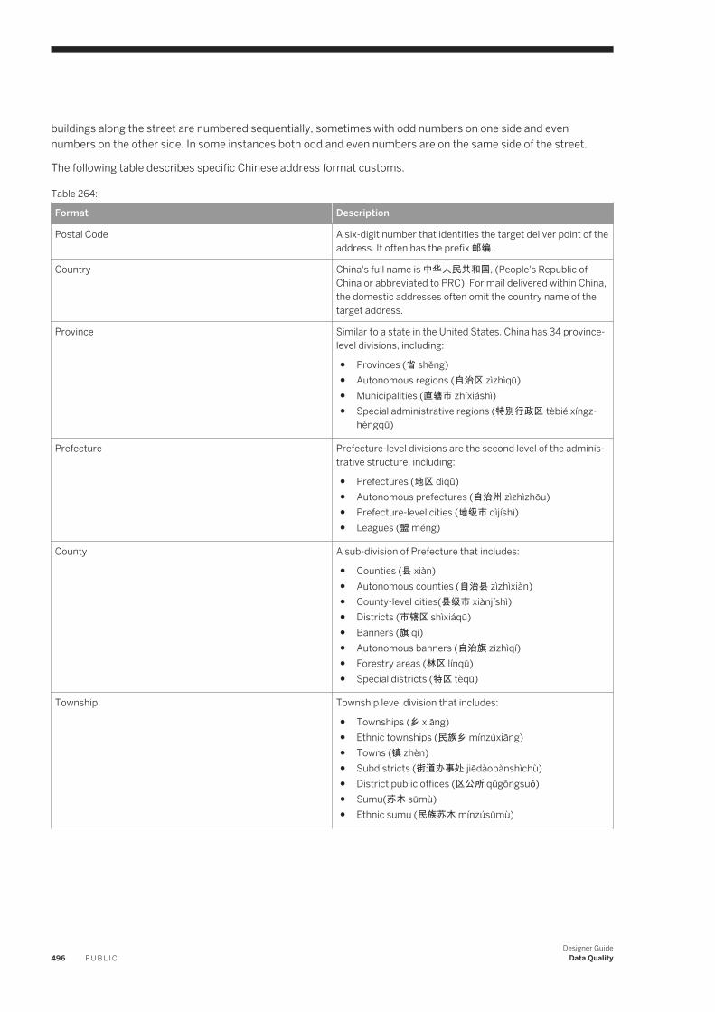
buildings along the street are numbered sequentially, sometimes with odd numbers on one side and even numbers on the other side. In some instances both odd and even numbers are on the same side of the street.
The following table describes specific Chinese address format customs.
Table 264:
Format Description
Postal Code A six-digit number that identifies the target deliver point of the address. It often has the prefix 邮编.
Country China's full name is 中华人民共和国, (People's Republic of China or abbreviated to PRC). For mail delivered within China, the domestic addresses often omit the country name of the target address.
Province Similar to a state in the United States. China has 34 province-level divisions, including:
● Provinces (省 shěng)● Autonomous regions (自治区 zìzhìqū)● Municipalities (直辖市 zhíxiáshì)● Special administrative regions (特别行政区 tèbié xíngz
hèngqū)
Prefecture Prefecture-level divisions are the second level of the administrative structure, including:
● Prefectures (地区 dìqū)● Autonomous prefectures (自治州 zìzhìzhōu)● Prefecture-level cities (地级市 dìjíshì)● Leagues (盟 méng)
County A sub-division of Prefecture that includes:
● Counties (县 xiàn)● Autonomous counties (自治县 zìzhìxiàn)● County-level cities(县级市 xiànjíshì)● Districts (市辖区 shìxiáqū)● Banners (旗 qí)● Autonomous banners (自治旗 zìzhìqí)● Forestry areas (林区 línqū)● Special districts (特区 tèqū)
Township Township level division that includes:
● Townships (乡 xiāng)● Ethnic townships (民族乡 mínzúxiāng)● Towns (镇 zhèn)● Subdistricts (街道办事处 jiēdàobànshìchù)● District public offices (区公所 qūgōngsuǒ)● Sumu(苏木 sūmù)● Ethnic sumu (民族苏木 mínzúsūmù)
496 P U B L I CDesigner Guide
Data Quality
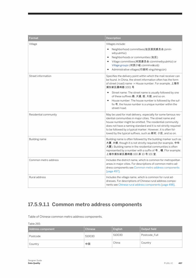
Format Description
Village Villages include:
● Neighborhood committees(社区居民委员会 jūmínwěiyuánhùi)
● Neighborhoods or communities (社区)● Village committees(村民委员会 cūnmínwěiyuánhùi) or
Village groups (村民小组 cūnmínxiǎozǔ)● Administrative villages(行政村 xíngzhèngcūn)
Street information Specifies the delivery point within which the mail receiver can be found. In China, the street information often has the form of street (road) name -> House number. For example, 上海市浦东新区晨晖路 1001 号
● Street name: The street name is usually followed by one of these suffixes 路, 大道, 街, 大街, and so on.
● House number: The house number is followed by the suffix 号, the house number is a unique number within the street/road.
Residential community May be used for mail delivery, especially for some famous residential communities in major cities. The street name and house number might be omitted. The residential community does not have a naming standard and it is not strictly required to be followed by a typical marker. However, it is often followed by the typical suffixes, such as 新村, 小区, and so on.
Building name Building name is often followed by the building marker such as 大厦, 大楼, though it is not strictly required (for example, 中华大厦). Building name in the residential communities is often represented by a number with a suffix of 号,幢. Ffor example: 上海市浦东新区晨晖路 100 弄 10 号 101 室.
Common metro address Includes the district name, which is common for metropolitan areas in major cities. For descriptions of common metro address components see Common metro address components [page 497].
Rural address Includes the village name, which is common for rural addresses. For descriptions of Chinese rural address components see Chinese rural address components [page 498].
17.5.9.1.1 Common metro address components
Table of Chinese common metro address components.
Table 265:
Address component Chinese English Output field
Postcode 510030 510030 Postcode_Full
Country 中国 China Country
Designer GuideData Quality P U B L I C 497
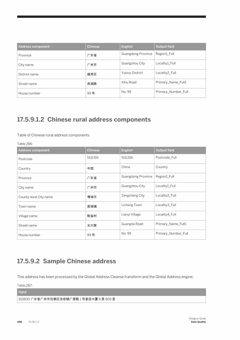
Address component Chinese English Output field
Province 广东省 Guangdong Province Region1_Full
City name 广州市 Guangzhou City Locality1_Full
District name 越秀区 Yuexiu District Locality2_Full
Street name 西湖路 Xihu Road Primary_Name_Full1
House number 99 号 No. 99 Primary_Number_Full
17.5.9.1.2 Chinese rural address components
Table of Chinese rural address components
Table 266:
Address component Chinese English Output field
Postcode 5111316 5111316 Postcode_Full
Country 中国 China Country
Province 广东省 Guangdong Province Region1_Full
City name 广州市 Guangzhou City Locality1_Full
County-level City name 增城市 Zengcheng City Locality2_Full
Town name 荔城镇 Licheng Town Locality3_Full
Village name 联益村 Lianyi Village Locality4_Full
Street name 光大路 Guangda Road Primary_Name_Full1
House number 99 号 No. 99 Primary_Number_Full
17.5.9.2 Sample Chinese address
This address has been processed by the Global Address Cleanse transform and the Global Address engine.
Table 267:
Input
510830 广东省广州市花都区赤坭镇广源路 1 号星辰大厦 8 层 809 室
498 P U B L I CDesigner Guide
Data Quality
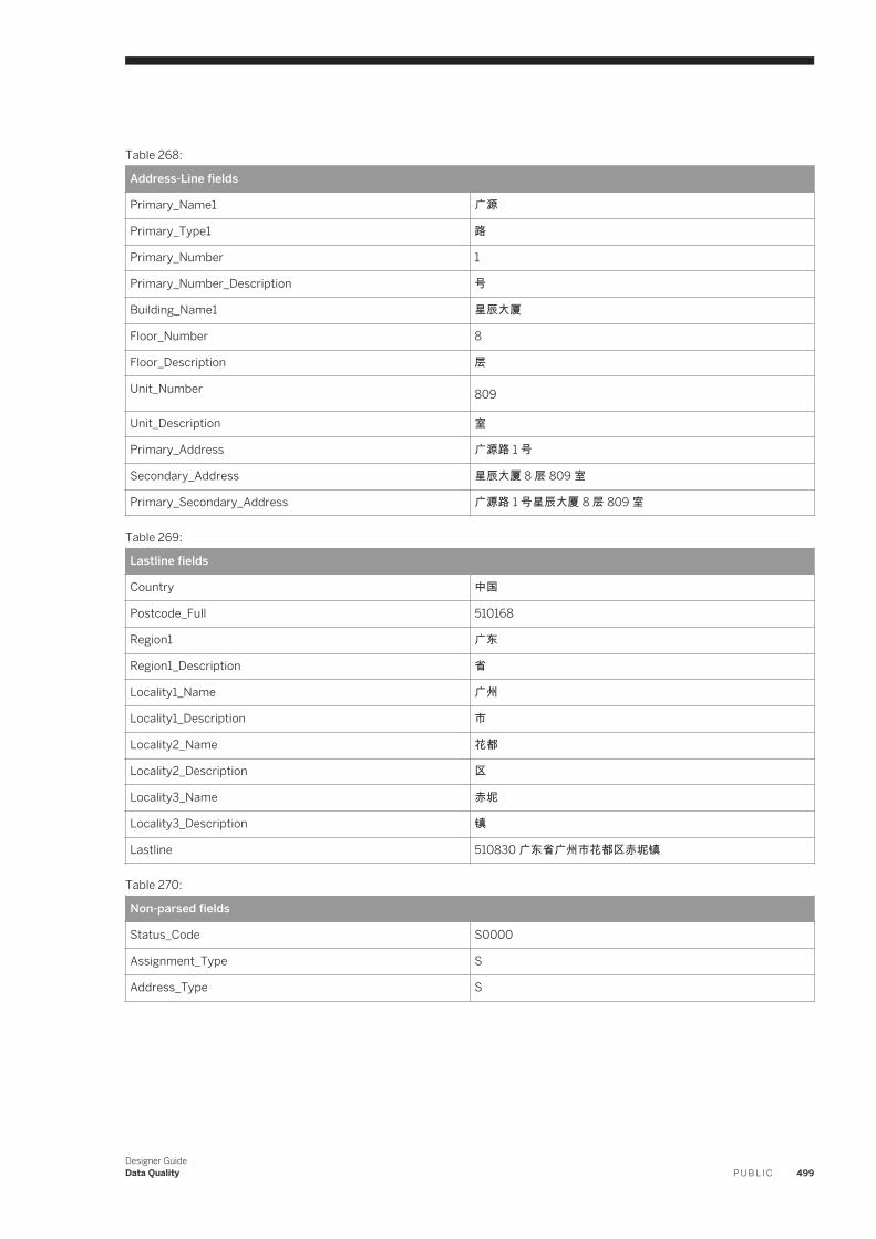
Table 268:
Address-Line fields
Primary_Name1 广源
Primary_Type1 路
Primary_Number 1
Primary_Number_Description 号
Building_Name1 星辰大厦
Floor_Number 8
Floor_Description 层
Unit_Number 809
Unit_Description 室
Primary_Address 广源路 1 号
Secondary_Address 星辰大厦 8 层 809 室
Primary_Secondary_Address 广源路 1 号星辰大厦 8 层 809 室
Table 269:
Lastline fields
Country 中国
Postcode_Full 510168
Region1 广东
Region1_Description 省
Locality1_Name 广州
Locality1_Description 市
Locality2_Name 花都
Locality2_Description 区
Locality3_Name 赤坭
Locality3_Description 镇
Lastline 510830 广东省广州市花都区赤坭镇
Table 270:
Non-parsed fields
Status_Code S0000
Assignment_Type S
Address_Type S
Designer GuideData Quality P U B L I C 499
17.5.10 Supported countries (Global Address Cleanse)
There are several countries supported by the Global Address Cleanse transform. The level of correction varies by country and by the engine that you use. Complete coverage of all addresses in a country is not guaranteed.
For the Global Address engine, country support depends on which sets of postal directories you have purchased.
For Japan, the assignment level is based on data provided by the Ministry of Public Management Home Affairs, Posts and Telecommunications (MPT).
During Country ID processing, the transform can identify many countries. However, the Global Address Cleanse transform's engines may not provide address correction for all of those countries.
Related Information
Changing the default output country name [page 500]
17.5.10.1 Changing the default output country name
When you use the USA engine to process addresses from American Samoa, Guam, Northern Mariana Islands, Palau, Puerto Rico, and the U.S. Virgin Islands, the output region is AS, GU, MP, PW, PR, or VI, respectively. The output country, however, is the United States (US).
If you do not want the output country as the United States when processing addresses with the USA engine, set the Use Postal Country Name option to No.
These steps show you how to set the Use Postal Country Name in the Global Address Cleanse transform.
1. Open the Global Address Cleanse transform.
2. On the Options tab, expand Standardization Options Country Options .3. For the Use Postal Country Name option, select No.
Related Information
Supported countries (Global Address Cleanse) [page 500]
17.5.10.2 Setting a default country
NoteRun Country ID processing only if you are:
500 P U B L I CDesigner Guide
Data Quality
● Using two or more of the engines and your input addresses contain country data (such as the two-character ISO code or a country name).
● Using only one engine, but your input data contains addresses from multiple countries.
1. Open the Global Address Cleanse transform.2. On the Options tab, expand Country ID Options, and then for the Country ID Mode option select Assign.
This value directs the transform to use Country ID to assign the country. If Country ID cannot assign the country, it will use the value in Country Name.
3. For the Country Name option, select the country that you want to use as a default country.
The transform will use this country only when Country ID cannot assign a country. If you do not want a default country, select None.
4. For the Script Code option, select the type of script code that represents your data.The LATN option provides script code for most types of data. However, if you are processing Japanese data, select KANA
Related Information
Identifying the country of destination [page 482]Setting a constant country [page 501]
17.5.10.3 Setting a constant country
1. Open the Global Address Cleanse transform.2. On the Options tab, expand Country ID Options, and then for the Country ID Mode option select Constant.
This value tells the transform to take the country information from the Country Name and Script Code options (instead of running Country ID processing).
3. For the Country Name option, select the country that represents all your input data.4. For the Script Code option, select the type of script code that represents your data.
The LATN option provides script code for most types of data. However, if you are processing Japanese data, select KANA
Related Information
Identifying the country of destination [page 482]Setting a default country [page 500]
Designer GuideData Quality P U B L I C 501
17.5.11 New Zealand certification
New Zealand certification enables you to process New Zealand addresses and qualify for mailing discounts with the New Zealand Post.
17.5.11.1 Enabling New Zealand certification
You need to purchase the New Zealand directory data and obtain a customer number from the New Zealand Post before you can use the New Zealand certification option.
To process New Zealand addresses that qualify for mailing discounts:
1. In the Global Address Cleanse Transform, enable Report and Analysis Generate Report Data .
2. In the Global Address Cleanse Transform, set Country Options Disable Certification to No.
NoteThe software does not produce the New Zealand Statement of Accuracy (SOA) report when this option is set to Yes.
3. In the Global Address Transform, complete all applicable options in the Global Address Report OptionsNew Zealand subgroup.
4. In the Global Address Cleanse Transform, set Engines Global Address to Yes.
After you run the job and produce the New Zealand Statement of Accuracy (SOA) report, you need to rename the New Zealand Statement of Accuracy (SOA) report and New Zealand Statement of Accuracy (SOA) Production Log before submitting your mailing. For more information on the required naming format, See New Zealand Statement of Accuracy Report [page 502].
17.5.11.2 New Zealand Statement of Accuracy Report
The New Zealand Statement of Accuracy (SOA) report includes statistical information about address cleansing for New Zealand.
17.5.11.3 New Zealand SOA Production Log
The Production Log is a pipe-delimited ASCII text file (with a header record).
The Production Log is identical to the New Zealand Statement of Accuracy (SOA) report except it is in a pipe-delimited ASCII text file (with a header record). The software creates the SOA Production Log by extracting data from the Sendrightaddraccuracy table within the repository. The software appends a new record to the Sendrightaddraccuracy table each time a file is processed with the DISABLE_CERTIFICATION option set to No. If the DISABLE_CERTIFICATION option is set to Yes, the software does not produce the SOA report and an entry will not be appended to the Sendrightaddraccuracy table.
502 P U B L I CDesigner Guide
Data Quality
Mailers must retain the production log file for at least 2 years.
The default location of the SOA production log is <INSTALL_DIR>\Data Services\DataQuality\certifications\CertificationLogs.
17.5.11.4 Mailing requirements
The SOA report and production log are only required when you submit the data processed for a mailing and want to receive postage discounts.
● Submit the SOA production log at least once a month.● Submit an SOA report for each file that is processed for mailing discounts.
Related Information
New Zealand certification [page 502]New Zealand Statement of Accuracy Report [page 502]New Zealand SOA Production Log [page 502]
17.5.11.5 Editing the New Zealand certification blueprint
Follow the steps below to edit the New Zealand certification blueprint:
1. Import the file nz_sendright_certification.atl located in the DataQuality\certifications folder where you installed the software.The default location is <INSTALL_DIR>\Data Services\DataQuality\certifications.
The import adds the following objects to the repository:○ The project DataQualityCertifications○ The job Job_DqBatchNewZealand_SOAProductionLog○ The data flow DF_DqBatchNewZealand_SOAProductionLog○ The datastore DataQualityCertifications○ The file format DqNewZealandSOAProductionLog
2. Edit the datastore DataQualityCertifications object by following the steps in Editing the datastore [page 504].
3. Keep the default location for the SOA Production log or change it to a different location by editing the substitution parameter configuration:
a. From the Designer, select Tools Substitution Parameter Configurations .b. Change the path location in Configuration1 for the substitution parameter $$CertificationLogPath to
the location of your choice.The default location for the SOA Production Log is <INSTALL_DIR>\Data Services\DataQuality\certifications\CertificationLogs.
Designer GuideData Quality P U B L I C 503
4. Run the job Job_DqBatchNewZealand_SOAProductionLog.The job produces an SOA Production Log called SOAPerc_SOAExpDate_SOAId.txt in the default location or the location you specified in the substitution parameter configuration.
5. Rename the SOAPerc_SOAExpDate_SOAId.txt file using data from the last record in the log file and the file naming format described in New Zealand Statement of Accuracy Report [page 502].
Related Information
New Zealand Statement of Accuracy Report [page 502]
17.5.11.6 Editing the datastore
After you download the blueprint .zip file to the appropriate folder, unzip it, and import the .atl file in the software, you must edit the DataQualityCertifications datastore.
To edit the datastore:
1. Select the Datastores tab of the Local Object Library, right-click DataQualityCertifications and select Edit.2. Click Advanced to expand the Edit Datastore DataQualityCertifications window.
NoteSkip step 3 if you have Microsoft SQL Server 2000 or 2005 as a datastore database type.
3. Click Edit.4. Find the column for your database type, change Default configuration to Yes, and click OK.
NoteIf you are using a version of Oracle other than Oracle 9i, perform the following substeps:
a. In the toolbar, click Create New Configuration.b. Enter your information, including the Oracle database version that you are using, and then click OK.c. Click Close on the Added New Values - Modified Objects window.d. In the new column that appears to the right of the previous columns, select Yes for the Default
configuration.e. Enter your information for the Database connection name, User name, and Password options.f. In DBO, enter your schema name.g. In Code Page, select cp1252 and then click OK.
5. At the Edit Datastore DataQualityCertifications window, enter your repository connection information in place of the CHANGE_THIS values. (You may have to change three or four options, depending on your repository type.)
6. Expand the Aliases group and enter your owner name in place of the CHANGE_THIS value. If you are using Microsoft SQL Server, set this value to DBO.
504 P U B L I CDesigner Guide
Data Quality
7. Click OK.If the window closes without any error message, then the database is successfully connected.
17.5.12 Global Address Cleanse Suggestion List option
The Global Address Cleanse transform's Suggestion List processing option is used in transactional projects to complete and populate addresses that have minimal data. Suggestion lists can offer suggestions for possible matches if an exact match is not found.
This option is beneficial in situations where you want to extract addresses not completely assigned by an automated process, and run through the system to find a list of possible matches. Based on the given input address, the Global Address Cleanse transform performs an error-tolerant search in the address directory and returns a list of possible matches. From the suggestion list returned, you can select the correct suggestion and update the database accordingly.
NoteNo certification with suggestion lists: If you use the Canada engine or Global Address engine for Australia and New Zealand, you cannot certify your mailing for SERP, AMAS, or New Zealand certification.
Start with a sample transform
If you want to use the suggestion lists feature, it is best to start with the sample transforms that is configured for it. The sample transform, GlobalSuggestions_AddressCleanse is configured to cleanse Latin-1 address data in any supported country using the Suggestion List feature.
Related Information
Extract data quality XML strings using extract_from_xml function [page 240]
17.5.13 Global Suggestion List transform
The Global Suggestion List transform allows you to query addresses with minimal data (allowing the use of wildcards), and it can offer a list of suggestions for possible matches.
It is a beneficial tool for a call center environment, where operators need to enter minimum input (number of keystrokes) to find the caller's delivery address. For example, if the operator is on the phone with a caller from the United Kingdom, the application prompts for the postcode and address range. Global Suggestion List is used to look up the address with quick-entry.
The Global Suggestion List transform requires the two-character ISO country code on input. Therefore, you may want to place a transform, such as the Country ID transform, that outputs the ISO_Country_Code_2Char field
Designer GuideData Quality P U B L I C 505
before the Global Suggestion Lists transform. The Global Suggestion List transform is available for use with the Canada, Global Address, and USA engines.
NoteNo certification with suggestion lists: If you use the Canada, Global Address, or USA engines for Australia and New Zealand, you cannot certify your mailing for SERP, CASS, AMAS, or New Zealand certification.
NoteThis option does not support processing of Japanese or Chinese address data.
Start with a sample transform
If you want to use the Global Suggestion List transform, it is best to start with one of the sample transforms that is configured for it. The following sample tranforms are available.
Table 271:
Sample transform Description
GlobalSuggestions A sample transform configured to generate a suggestion list for Latin-1 address data in any supported country.
UKSuggestions A sample transform configured to generate a suggestion list for partial address data in the United Kingdom.
17.6 Beyond the basic address cleansing
The USA Regulatory Address Cleanse transform offers many additional address cleanse features for U.S. addresses. These features extend address cleansing beyond the basic parsing and standardizing. To read about the USA Regulatory Address Cleanse transform and its options, see the Reference Guide.
17.6.1 USPS DPV®
Delivery Point Validation® is a USPS product developed to assist users in validating the accuracy of their address information. DPV compares Postcode2 information against the DPV directories to identify known addresses and potential problems with the address that may cause an address to become undeliverable.
DPV is available for U.S. data in the USA Regulatory Address Cleanse transform only.
NoteDPV processing is required for CASS certification. If you are not processing for CASS certification, you can choose to run your jobs in non-certified mode and still enable DPV.
506 P U B L I CDesigner Guide
Data Quality
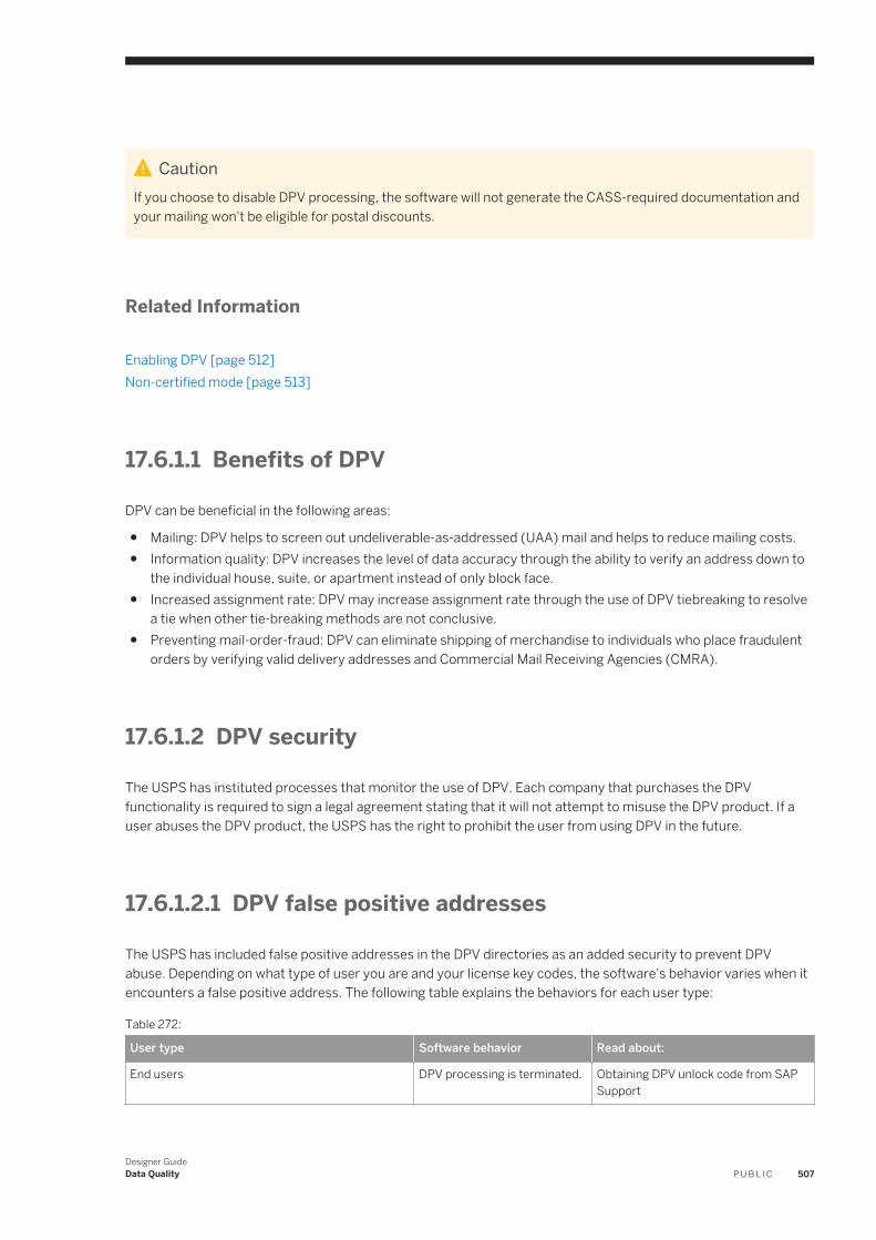
CautionIf you choose to disable DPV processing, the software will not generate the CASS-required documentation and your mailing won't be eligible for postal discounts.
Related Information
Enabling DPV [page 512]Non-certified mode [page 513]
17.6.1.1 Benefits of DPV
DPV can be beneficial in the following areas:
● Mailing: DPV helps to screen out undeliverable-as-addressed (UAA) mail and helps to reduce mailing costs.● Information quality: DPV increases the level of data accuracy through the ability to verify an address down to
the individual house, suite, or apartment instead of only block face.● Increased assignment rate: DPV may increase assignment rate through the use of DPV tiebreaking to resolve
a tie when other tie-breaking methods are not conclusive.● Preventing mail-order-fraud: DPV can eliminate shipping of merchandise to individuals who place fraudulent
orders by verifying valid delivery addresses and Commercial Mail Receiving Agencies (CMRA).
17.6.1.2 DPV security
The USPS has instituted processes that monitor the use of DPV. Each company that purchases the DPV functionality is required to sign a legal agreement stating that it will not attempt to misuse the DPV product. If a user abuses the DPV product, the USPS has the right to prohibit the user from using DPV in the future.
17.6.1.2.1 DPV false positive addresses
The USPS has included false positive addresses in the DPV directories as an added security to prevent DPV abuse. Depending on what type of user you are and your license key codes, the software's behavior varies when it encounters a false positive address. The following table explains the behaviors for each user type:
Table 272:
User type Software behavior Read about:
End users DPV processing is terminated. Obtaining DPV unlock code from SAP Support
Designer GuideData Quality P U B L I C 507
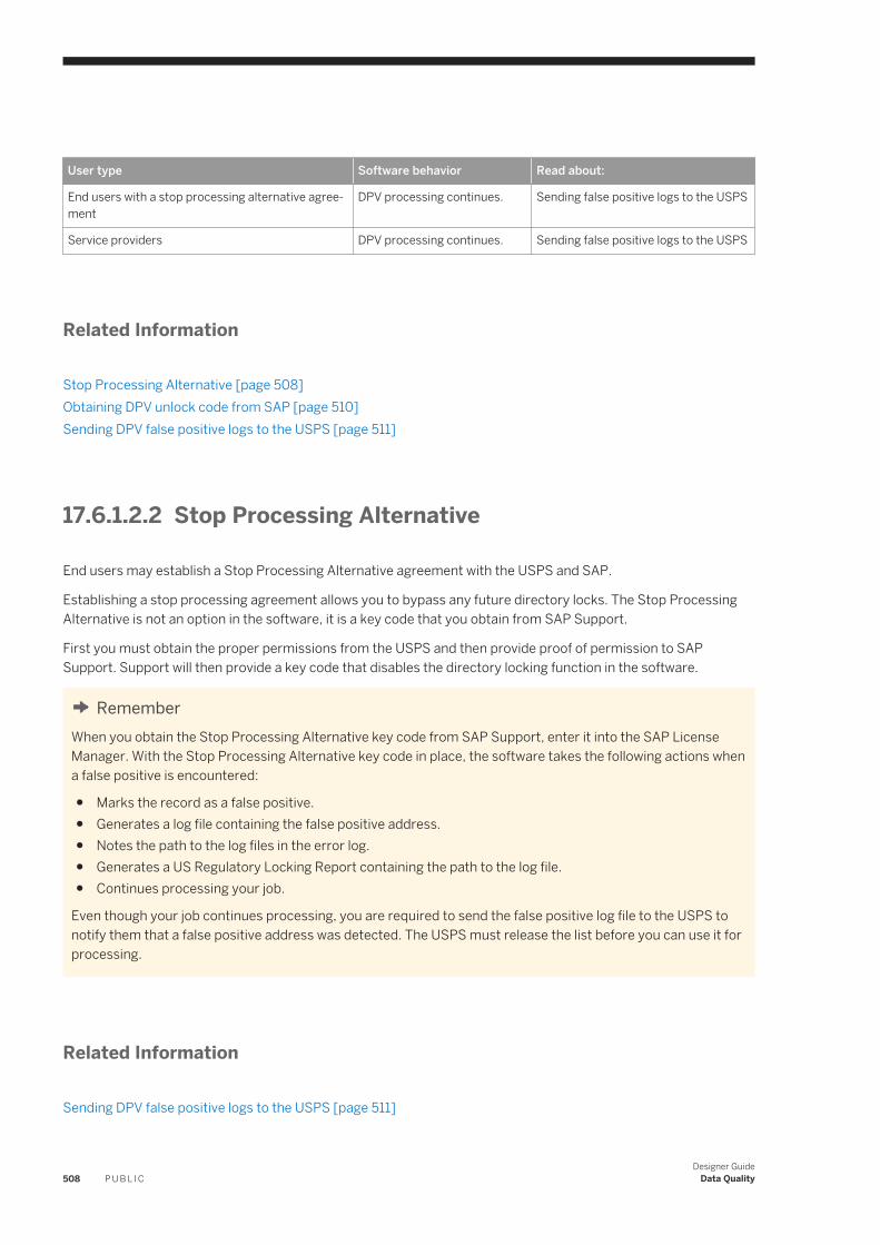
User type Software behavior Read about:
End users with a stop processing alternative agreement
DPV processing continues. Sending false positive logs to the USPS
Service providers DPV processing continues. Sending false positive logs to the USPS
Related Information
Stop Processing Alternative [page 508]Obtaining DPV unlock code from SAP [page 510]Sending DPV false positive logs to the USPS [page 511]
17.6.1.2.2 Stop Processing Alternative
End users may establish a Stop Processing Alternative agreement with the USPS and SAP.
Establishing a stop processing agreement allows you to bypass any future directory locks. The Stop Processing Alternative is not an option in the software, it is a key code that you obtain from SAP Support.
First you must obtain the proper permissions from the USPS and then provide proof of permission to SAP Support. Support will then provide a key code that disables the directory locking function in the software.
RememberWhen you obtain the Stop Processing Alternative key code from SAP Support, enter it into the SAP License Manager. With the Stop Processing Alternative key code in place, the software takes the following actions when a false positive is encountered:
● Marks the record as a false positive.● Generates a log file containing the false positive address.● Notes the path to the log files in the error log.● Generates a US Regulatory Locking Report containing the path to the log file.● Continues processing your job.
Even though your job continues processing, you are required to send the false positive log file to the USPS to notify them that a false positive address was detected. The USPS must release the list before you can use it for processing.
Related Information
Sending DPV false positive logs to the USPS [page 511]
508 P U B L I CDesigner Guide
Data Quality
17.6.1.2.3 DPV false positive logs
The software generates a false positive log file any time it encounters a false positive record, regardless of how your job is set up. The software creates a separate log file for each mailing list that contains a false positive. If multiple false positives exist within one mailing list, the software writes them all to the same log file.
17.6.1.2.3.1 DPV log file name and location
The software stores DPV log files in the directory specified in the USPS Log Path option in the Reference Files group.
NoteThe USPS log path that you enter must be writable. An error is issued if you have entered a path that is not writable.
Log file naming convention
The software automatically names DPV false positive logs with the following format: dpvl####.log
The #### portion of the naming format is a number between 0001 and 9999. For example, the first log file generated is dpvl0001.log, the next one is dpvl0002.log, and so on.
NoteWhen you have set the data flow degree of parallelism to greater than 1, or you have enabled the run as a separate process option, the software generates one log per thread or process. During a job run, if the software encounters only one false positive record, one log will be generated. However, if it encounters more than one false positive record and the records are processed on different threads or processes, then the software will generate one log for each thread that processes a false positive record.
17.6.1.2.4 DPV locking for end users
This locking behavior is applicable for end users or users who are DSF2 licensees that have DSF2 disabled in the job
When the software finds a false positive address, DPV processing is discontinued for the remainder of the data flow. The software also takes the following actions:
● Marks the record as a false positive address.● Issues a message in the error log stating that a DPV false positive address was encountered.● Includes the false positive address and lock code in the error log.
Designer GuideData Quality P U B L I C 509
● Continues processing your data flow without DPV processing.● Generates a lock code.● Generates a false positive log.● Generates a US Regulatory Locking Report that contains the false positive address and the lock code. (Report
generation must be enabled in the USA Regulatory Address Cleanse transform.)
To restore DPV functionality, users must obtain a DPV unlock code from SAP Support.
Related Information
Obtaining DPV unlock code from SAP [page 510]
17.6.1.2.5 Obtaining DPV unlock code from SAP
These steps are applicable for end users who do not have a Stop Processing Alternative agreement with the USPS. When you receive a processing message that DPV false positive addresses are present in your address list, use the SAP USPS Unlock Utility to obtain an unlock code.
1. Navigate to https://support.sap.com/keys-systems-installations/keys/usps-unlock-codes.html to open the USPS Unlock Codes page on the SAP Support Portal.
2. Click Retrieve USPS Unlock Code.3. Click Search and select an applicable Data Services system from the list.4. Enter the lock code found in the dpvx.txt file (location is specified in the DPV Path option in the Reference
Files group).5. Select DPV as the lock type.6. Select BOJ-EIM-DS as the component.7. Enter the locking address that is listed in the dpvx.txt file.
8. Attach the dpvl####.log file (location is specified in the USPS Log Path option in the Reference Files group).
9. Click Submit.The unlock code displays.
10. Copy the unlock code and paste it into the dpvw.txt file, replacing all contents of the file with the unlock code (location is specified in the DPV path option of the Reference Files group).
11. Remove the record that caused the lock from the database, and delete the dpvl####.log file before processing the list again.
TipKeep in mind that you can only use the unlock code once. If the software detects another false-positive (even if it is the same record), you must retrieve a new LACSLink unlock code.
If an unlock code could not be generated, a message is still created and is processed by a Technical Customer Assurance engineer (during regular business hours).
510 P U B L I CDesigner Guide
Data Quality
NoteIf you are an end user who has a Stop Processing Alternative agreement, follow the steps to send the false positive log to the USPS.
17.6.1.2.6 Sending DPV false positive logs to the USPS
Service providers should follow these steps after receiving a processing message that DPV false positive addresses are present in their address list. End users with a Stop Processing Alternative agreement should follow these steps after receiving a processing message that DPV false positive addresses are present in their address list.
1. Send an email to the USPS NCSC at [email protected], and include the following information:○ Type “DPV False Positive” as the subject line○ Attach the dpvl####.log file or files that were generated by the software (location is specified in the
USPS Log Path directory option in the Reference Files group)The USPS NCSC uses the information to determine whether the list can be returned to the mailer.
2. After the USPS NCSC has released the list that contained the locked or false positive record:○ Delete the corresponding log file or files○ Remove the record that caused the lock from the list and reprocess the file
If you are an end user who does not have a Stop Processing Alternative agreement, follow the steps to retrieve the DPV unlock code from SAP Support.
Related Information
Obtaining DPV unlock code from SAP [page 510]
17.6.1.3 DPV monthly directories
DPV directories are shipped monthly with the USPS directories in accordance with USPS guidelines.
The directories expire in 105 days. The date on the DPV directories must be the same date as the Address directory.
Do not rename any of the files. DPV will not run if the file names are changed. Here is a list of the DPV directories:
● dpva.dir● dpvb.dir ● dpvc.dir ● dpvd.dir● dpv_vacant.dir
Designer GuideData Quality P U B L I C 511
● dpv_no_stats.dir
17.6.1.4 Required information in the job setup
When you set up for DPV processing, the following options in the USPS License Information group are required:
● Customer Company Name ● Customer Company Address● Customer Company Locality● Customer Company Region ● Customer Company Postcode1● Customer Company Postcode2
17.6.1.5 Enabling DPV
NoteDPV is required for CASS.
In addition to the required customer company information that you enter into the USPS License Information group, set the following options to perform DPV processing:
1. Open the USA Regulatory Address Cleanse transform.2. Open the Options tab. Expand the Assignment Options group, and select Yes for the Enable DPV option.3. In the Reference Files group, enter the path for your DPV directories in the DPV Path option.
NoteDPV can run only when the location for all the DPV directories have been entered and none of the DPV directory files have been renamed.
4. Set a directory for the DPV log file in the USPS Path option. Use the substitution variable $$CertificationLogPath if you have it set up.
5. In the Report and Analysis group, select Yes for the Generate Report Data option.
17.6.1.6 DPV output fields
Several output fields are available for reporting DPV processing results:
● DPV_CMRA● DPV_Footnote● DPV_NoStats● DPV_Status
512 P U B L I CDesigner Guide
Data Quality
● DPV_Vacant
For full descriptions of these output fields, refer to the Reference Guide or view the Data Services Help information that appears when you open the Output tab of the USA Regulatory Address Cleanse transform.
17.6.1.7 Non-certified mode
You can set up your jobs with DPV disabled if you are not a CASS customer but you want a Postcode2 added to your addresses. The non-CASS option, Assign Postcode2 Not DPV Validated, enables the software to assign a Postcode2 when an address does not DPV-confirm.
CautionIf you choose to disable DPV processing, the software does not generate the CASS-required documentation and your mailing won't be eligible for postal discounts.
17.6.1.7.1 Enabling non-certified mode
To run your job in non certified mode, follow these setup steps:
1. In the Assignment Options group, set the Enable DPV option to No.2. In the Non Certified options group, set the Disable Certification to Yes.3. In the Non Certified options group, set the Assign Postcode2 Not DPV Validated to Yes.
CautionThe software blanks out all Postcode2 information in your data if you disable DPV processing and you disable the Assign Postcode2 Not DPV Validated option. This includes Postcode2 information provided in your input file.
17.6.1.8 DPV performance
Due to additional time required to perform DPV processing, you may see a change in processing time. Processing time may vary with the DPV feature based on operating system, system configuration, and other variables that may be unique to your operating environment.
You can decrease the time required for DPV processing by loading DPV directories into system memory before processing.
Designer GuideData Quality P U B L I C 513
17.6.1.8.1 Memory usage
You may need to install additional memory on your operating system for DPV processing. We recommend a minimum of 768 MB to process with DPV enabled.
To determine the amount of memory required to run with DPV enabled, check the size of the DPV directories (recently about 600 MB1) and add that to the amount of memory required to run the software.
The size of the DPV directories will vary depending on the amount of new data in each directory release.
Make sure that your computer has enough memory available before performing DPV processing.
To find the amount of disk space required to cache the directories, see the Supported Platforms document in the SAP Support portal. Find link information in the SAP Information resources table (see the link below).
17.6.1.8.2 Caching DPV directories
To better manage memory usage when you have enabled DPV processing, choose to cache the DPV directories.
To set up your job for DPV caching, follow these steps:
1. In the Transform Performance group, set the Cache DPV Directories option to Yes.2. In the same group, set the Insufficient Cache Memory Action to one of the following:
Table 273:
Option Description
Error Software issues an error and terminates the transform.
Continue Software attempts to continue initialization without caching.
17.6.1.8.3 Running multiple jobs with DPV
When running multiple DPV jobs and loading directories into memory, you should add a 10-second pause between jobs to allow time for the memory to be released. For more information about setting this properly, see your operating system manual.
If you don't add a 10-second pause between jobs, there may not be enough time for your system to release the memory used for caching the directories from the first job. The next job waiting to process may error out or access the directories from disk if there is not enough memory to cache directories. This may result in performance degradation.
1 The directory size is subject to change each time new DPV directories are installed.
514 P U B L I CDesigner Guide
Data Quality
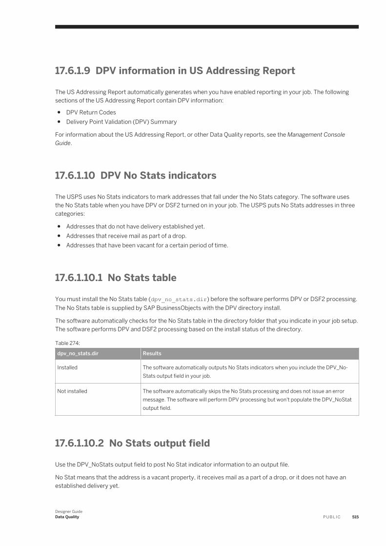
17.6.1.9 DPV information in US Addressing Report
The US Addressing Report automatically generates when you have enabled reporting in your job. The following sections of the US Addressing Report contain DPV information:
● DPV Return Codes● Delivery Point Validation (DPV) Summary
For information about the US Addressing Report, or other Data Quality reports, see the Management Console Guide.
17.6.1.10 DPV No Stats indicators
The USPS uses No Stats indicators to mark addresses that fall under the No Stats category. The software uses the No Stats table when you have DPV or DSF2 turned on in your job. The USPS puts No Stats addresses in three categories:
● Addresses that do not have delivery established yet.● Addresses that receive mail as part of a drop.● Addresses that have been vacant for a certain period of time.
17.6.1.10.1 No Stats table
You must install the No Stats table (dpv_no_stats.dir) before the software performs DPV or DSF2 processing. The No Stats table is supplied by SAP BusinessObjects with the DPV directory install.
The software automatically checks for the No Stats table in the directory folder that you indicate in your job setup. The software performs DPV and DSF2 processing based on the install status of the directory.
Table 274:
dpv_no_stats.dir Results
Installed The software automatically outputs No Stats indicators when you include the DPV_NoStats output field in your job.
Not installed The software automatically skips the No Stats processing and does not issue an error message. The software will perform DPV processing but won't populate the DPV_NoStat output field.
17.6.1.10.2 No Stats output field
Use the DPV_NoStats output field to post No Stat indicator information to an output file.
No Stat means that the address is a vacant property, it receives mail as a part of a drop, or it does not have an established delivery yet.
Designer GuideData Quality P U B L I C 515
Related Information
DPV output fields [page 512]
17.6.1.11 DPV Vacant indicators
The software provides vacant information in output fields and reports using DPV vacant counts. The USPS DPV vacant lookup table is supplied by SAP BusinessObjects with the DPV directory install.
The USPS uses DPV vacant indicators to mark addresses that fall under the vacant category. The software uses DPV vacant indicators when you have DPV or DSF2 enabled in your job.
TipThe USPS defines vacant as any delivery point that was active in the past, but is currently not occupied (usually over 90 days) and is not currently receiving mail delivery. The address could receive delivery again in the future. "Vacant" does not apply to seasonal addresses.
17.6.1.11.1 DPV address-attribute output field
Vacant indicators for the assigned address are available in the DPV_Vacant output field.
NoteThe US Addressing Report contains DPV Vacant counts in the DPV Summary section.
Related Information
DPV output fields [page 512]
17.6.2 LACSLink
LACSLink is a USPS product that is available for U.S. records with the USA Regulatory Address Cleanse transform only. LACSLink processing is required for CASS certification.
LACSLink updates addresses when the physical address does not move but the address has changed. For example, when the municipality changes rural route addresses to street-name addresses. Rural route conversions make it easier for police, fire, ambulance, and postal personnel to locate a rural address. LACSLink also converts addresses when streets are renamed or post office boxes renumbered.
516 P U B L I CDesigner Guide
Data Quality
LACSLink technology ensures that the data remains private and secure, and at the same time gives you easy access to the data. LACSLink is an integrated part of address processing; it is not an extra step. To obtain the new addresses, you must already have the old address data.
Related Information
How LACSLink works [page 520]Controlling memory usage for LACSLink processing [page 524]To disable LACSLink [page 522]LACSLink security [page 517]
17.6.2.1 Benefits of LACSLink
LACSLink processing is required for all CASS customers.
If you process your data without LACSLink enabled, you won't get the CASS-required reports or postal discounts.
17.6.2.2 LACSLink security
The USPS has instituted processes that monitor the use of LACSLink. Each company that purchases the LACSLink functionality is required to sign a legal agreement stating that it will not attempt to misuse the LACSLink product. If a user abuses the LACSLink product, the USPS has the right to prohibit the user from using LACSLink in the future.
17.6.2.2.1 LACSLink false positive addresses
The USPS has included false positive addresses in the LACSLink directories as an added security to prevent LACSLink abuse. Depending on what type of user you are and your license key codes, the software's behavior varies when it encounters a false positive address. The following table explains the behaviors for each user type:
Table 275:
User type Software behavior Read about:
End users LACSLink processing is terminated. Obtaining the LACSLink unlock code from SAP Support
End users with a Stop Processing Alternative agreement
LACSLink processing continues. Sending false positive logs to the USPS
Service providers LACSLink processing continues. Sending false positive logs to the USPS
Designer GuideData Quality P U B L I C 517
Related Information
Stop Processing Alternative [page 508]Obtaining LACSLink unlock code from SAP [page 519]Sending LACSLink false positive logs to the USPS [page 520]
17.6.2.2.2 LACSLink false positive logs
The software generates a false-positive log file any time it encounters a false positive record, regardless of how your job is set up. The software creates a separate log file for each mailing list that contains a false positive. If multiple false positives exist within one mailing list, the software writes them all to the same log file.
17.6.2.2.2.1 LACSLink log file location
The software stores LACSLink log files in the directory specified for the USPS Log Path in the Reference Files group.
NoteThe USPS log path that you enter must be writable. An error is issued if you have entered a path that is not writable.
The software names LACSLink false positive logs lacsl<###>.log, where <###> is a number between 001 and 999. For example, the first log file generated is lacsl001.log, the next one is lacsl002.log, and so on.
NoteWhen you have set the data flow degree of parallelism to greater than 1, the software generates one log per thread. During a job run, if the software encounters only one false positive record, one log will be generated. However, if it encounters more than one false positive record and the records are processed on different threads, then the software will generate one log for each thread that processes a false positive record.
17.6.2.2.3 LACSLink locking for end users
This locking behavior is applicable for end users or users who are DSF2 licensees that have DSF2 disabled in the job.
When the software finds a false positive address, LACSLink processing is discontinued for the remainder of the job processing. The software takes the following actions:
● Marks the record as a false positive address.● Issues a message in the error log that a LACSLink false positive address was encountered.
518 P U B L I CDesigner Guide
Data Quality
● Includes the false positive address and lock code in the error log.● Continues processing your data flow without LACSLink processing.● Generates a lock code.● Generates a false positive error log.● Generates a US Regulatory Locking Report that contains the false positive address and the lock code (Report
generation must be enabled in the USA Regulatory Address Cleanse transform.
To restore LACSLink functionality, users must obtain a LACSLink unlock code from SAP Support.
17.6.2.2.4 Obtaining LACSLink unlock code from SAP
These steps are applicable for end users who do not have a Stop Processing Alternative agreement with the USPS. When you receive a processing message that LACSLink false positive addresses are present in your address list, use the SAP USPS Unlock Utility to obtain an unlock code.
1. Navigate to https://support.sap.com/keys-systems-installations/keys/usps-unlock-codes.html to open the USPS Unlock Codes page on the SAP Support Portal.
2. Click Retrieve USPS Unlock Code.3. Click Search and select an applicable Data Services system from the list.4. Enter the lock code found in the lacsx.txt file (location is specified in the LACSLink Path option in the
Reference Files group).5. Select LACSLink as the lock type.6. Select BOJ-EIM-DS as the component.7. Enter the locking address that is listed in the lacsx.txt file.
8. Attach the lacsl####.log file (location specified in the USPS Log Path option in the Reference Files group).
9. Click Submit.The unlock code displays.
10. Copy the unlock code and paste it into the lacsw.txt file, replacing all contents of the file with the unlock code (location is specified in the LACSLink path option in the Reference Files group).
11. Remove the record that caused the lock from the database, and delete the lacsl####.log file before processing the list again.
TipKeep in mind that you can only use the unlock code once. If the software detects another false-positive (even if it is the same record), you must retrieve a new LACSLink unlock code.
If an unlock code could not be generated, a message is still created and is processed by a Technical Customer Assurance engineer (during regular business hours).
NoteIf you are an end user who has a Stop Processing Alternative agreement, follow the steps to send the false positive log to the USPS.
Designer GuideData Quality P U B L I C 519
17.6.2.2.5 Sending LACSLink false positive logs to the USPS
Service providers should follow these steps after receiving a processing message that LACSLink false positive addresses are present in their address list. End users with a Stop Processing Alternative agreement should follow these steps after receiving a processing message that LACSLink false positive addresses are present in their address list.
1. Send an email to the USPS at [email protected]. Include the following:○ Type “LACSLink False Positive” as the subject line○ Attach the lacsl###.log file or files that were generated by the software (location specified in the USPS
Log Files option in the Reference Files group).The USPS NCSC uses the information to determine whether or not the list can be returned to the mailer.
2. After the USPS NCSC has released the list that contained the locked or false positive record:○ Delete the corresponding log file or files○ Remove the record that caused the lock from the list and reprocess the file
If you are an end user who does not have a Stop Processing Alternative agreement, follow the steps to retrieve the LACSLink unlock code from SAP Support.
Related Information
Obtaining LACSLink unlock code from SAP [page 519]
17.6.2.3 How LACSLink works
LACSLink provides a new address when one is available. LACSLink follows these steps when processing an address:
1. The USA Regulatory Address Cleanse transform standardizes the input address.2. The transform looks for a matching address in the LACSLink data.3. If a match is found, the transform outputs the LACSLink-converted address and other LACSLink information.
Related Information
Controlling memory usage for LACSLink processing [page 524]LACSLink [page 516]
520 P U B L I CDesigner Guide
Data Quality
17.6.2.4 Conditions for address processing
The transform does not process all of your addresses with LACSLink when it is enabled. Here are the conditions under which your data is passed into LACSLink processing:
● The address is found in the address directory, and it is flagged as a LACS-convertible record within the address directory.
● The address is found in the address directory, and, even though a rural route or highway contract default assignment was made, the record wasn't flagged as LACS convertible.
● The address is not found in the address directory, but the record contains enough information to be sent into LACSLink.
For example, the following table shows an address that was found in the address directory as a LACS-convertible address.
Table 276:
Original address After LACSLink conversion
RR2 BOX 204
DU BOIS PA 15801
463 SHOWERS RD
DU BOIS PA 15801-66675
17.6.2.5 Sample transform configuration
LACSLink processing is enabled by default in the sample transform configuration because it is required for CASS certification. The sample transform configuration is named USARegulatory_AddressCleanse and is found under the USA_Regulatory_Address_Cleanse group in the Object Library.
17.6.2.6 LACSLink directory files
SAP ships the LACSLink directory files with the U.S. National Directory update. The LACSLink directory files require about 600 MB of additional hard drive space. The LACSLink directories include the following:
● lacsw.txt ● lacsx.txt ● lacsy.ll ● lacsz.ll
CautionThe LACSLink directories must reside on the hard drive in the same directory as the LACSLink supporting files. Do not rename any of the files. LACSLink will not run if the file names are changed.
Designer GuideData Quality P U B L I C 521
17.6.2.6.1 Directory expiration and updates
LACSLink directories expire in 105 days. LACSLink directories must have the same date as the other directories that you are using from the U.S. National Directories.
17.6.2.7 Enabling LACSLink
LACSLink is enabled by default in the USA Regulatory Address Cleanse transform. If you need to re-enable the option, follow these steps:
1. Open the USA Regulatory Address Cleanse transform and open the Options tab.2. Expand the Processing Options group3. select Yes in the Enable LACSLink option.4. Enter the LACSLink path for the LACSLink Path option In the Reference Files group. You can use the
substitution variable $$RefFilesAddressCleanse if you have it set up.5. Complete the required fields in the USPS License Information group.
17.6.2.7.1 Required information in the job setup
All users running LACSLink must include required information in the USPS License Information group. The required options include the following:
● Customer Company Name● Customer Company Address● Customer Company Locality● Customer Company Region● Customer Company Postcode1● Customer Company Postcode2● Customer Company Phone
17.6.2.7.2 To disable LACSLink
LACSLink is enabled by default in the USA Regulatory Address Cleanse transform configuration because it is required for CASS processing. Therefore, you must disable CASS certification in order to disable LACSLink.
1. In the USA Regulatory Address Cleanse transform configuration, open the Options tab.2. Open the Non Certified Options group.3. Select Yes for the Disable Certification option.4. Open the Assignment Option group.5. Select No for the Enable LACSLink option.
522 P U B L I CDesigner Guide
Data Quality
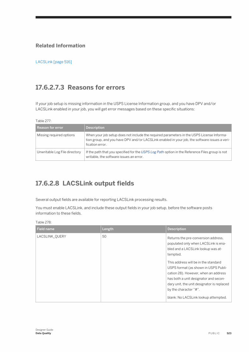
Related Information
LACSLink [page 516]
17.6.2.7.3 Reasons for errors
If your job setup is missing information in the USPS License Information group, and you have DPV and/or LACSLink enabled in your job, you will get error messages based on these specific situations:
Table 277:
Reason for error Description
Missing required options When your job setup does not include the required parameters in the USPS License Information group, and you have DPV and/or LACSLink enabled in your job, the software issues a verification error.
Unwritable Log File directory If the path that you specified for the USPS Log Path option in the Reference Files group is not writable, the software issues an error.
17.6.2.8 LACSLink output fields
Several output fields are available for reporting LACSLink processing results.
You must enable LACSLink, and include these output fields in your job setup, before the software posts information to these fields.
Table 278:
Field name Length Description
LACSLINK_QUERY 50 Returns the pre-conversion address, populated only when LACSLink is enabled and a LACSLink lookup was attempted.
This address will be in the standard USPS format (as shown in USPS Publication 28). However, when an address has both a unit designator and secondary unit, the unit designator is replaced by the character “#”.
blank: No LACSLink lookup attempted.
Designer GuideData Quality P U B L I C 523
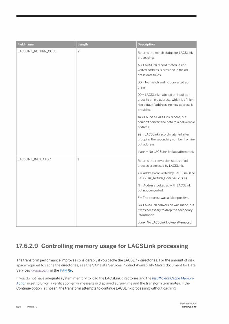
Field name Length Description
LACSLINK_RETURN_CODE 2 Returns the match status for LACSLink processing:
A = LACSLink record match. A converted address is provided in the address data fields.
00 = No match and no converted address.
09 = LACSLink matched an input address to an old address, which is a "high-rise default" address; no new address is provided.
14 = Found a LACSLink record, but couldn't convert the data to a deliverable address.
92 = LACSLink record matched after dropping the secondary number from input address.
blank = No LACSLink lookup attempted.
LACSLINK_INDICATOR 1 Returns the conversion status of addresses processed by LACSLink.
Y = Address converted by LACSLink (the LACSLink_Return_Code value is A).
N = Address looked up with LACSLink but not converted.
F = The address was a false-positive.
S = LACSLink conversion was made, but it was necessary to drop the secondary information.
blank: No LACSLink lookup attempted.
17.6.2.9 Controlling memory usage for LACSLink processing
The transform performance improves considerably if you cache the LACSLink directories. For the amount of disk space required to cache the directories, see the SAP Data Services Product Availablility Matrix document for Data Services <version> in the PAM .
If you do not have adequate system memory to load the LACSLink directories and the Insufficient Cache Memory Action is set to Error, a verification error message is displayed at run-time and the transform terminates. If the Continue option is chosen, the transform attempts to continue LACSLink processing without caching.
524 P U B L I CDesigner Guide
Data Quality
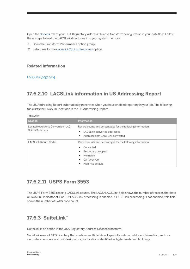
Open the Options tab of your USA Regulatory Address Cleanse transform configuration in your data flow. Follow these steps to load the LACSLink directories into your system memory:
1. Open the Transform Performance option group.2. Select Yes for the Cache LACSLink Directories option.
Related Information
LACSLink [page 516]
17.6.2.10 LACSLink information in US Addressing Report
The US Addressing Report automatically generates when you have enabled reporting in your job. The following table lists the LACSLink sections in the US Addressing Report:
Table 279:
Section Information
Locatable Address Conversion (LACSLink) Summary
Record counts and percentages for the following information:
● LACSLink converted addresses● Addresses not LACSLink converted
LACSLink Return Codes Record counts and percentages for the following information:
● Converted● Secondary dropped● No match● Can't convert● High-rise default
17.6.2.11 USPS Form 3553
The USPS Form 3553 reports LACSLink counts. The LACS/LACSLink field shows the number of records that have a LACSLink Indicator of Y or S, if LACSLink processing is enabled. If LACSLink processing is not enabled, this field shows the number of LACS code count.
17.6.3 SuiteLink™
SuiteLink is an option in the USA Regulatory Address Cleanse transform.
SuiteLink uses a USPS directory that contains multiple files of specially indexed address information, such as secondary numbers and unit designators, for locations identified as high-rise default buildings.
Designer GuideData Quality P U B L I C 525
With SuiteLink, you can build accurate and complete addresses by adding suite numbers to high-rise business addresses. With the secondary address information added to your addresses, more of your pieces are sorted by delivery sequence and delivered with accuracy and speed.
SuiteLink is required for CASS
SuiteLink is required when you process in CASS mode (and the Disable certification option is set to No). If you have disabled SuiteLink in your job setup, but you are in CASS mode, an error message is issued and processing does not continue.
17.6.3.1 Benefits of SuiteLink
Businesses that depend on website, mail, or in-store orders from customers will find that SuiteLink is a powerful money-saving tool. Also, businesses that have customers that reside in buildings which house several businesses will appreciate getting their marketing materials, bank statements, and orders delivered right to their door.
The addition of secondary number information to your addresses allows for the most efficient and cost-effective delivery sequencing and postage discounts.
NoteSuiteLink is required for those preparing CASS-compliant mailing lists.
17.6.3.2 How SuiteLink works
The software uses the data in the SuiteLink directories to add suite numbers to applicable addresses. The software matches a company name, a known high-rise address, and the CASS-certified postcode2 in your database to data in SuiteLink. When there is a match, the software creates a complete business address that includes the suite number.
ExampleAssign suite number
This example shows a record that is processed through SuiteLink, and the output record with the assigned suite number.
The input record contains:
● Firm name (in FIRM input field)● Known high-rise address● CASS-certified postcode2
The SuiteLink directory contains:
526 P U B L I CDesigner Guide
Data Quality
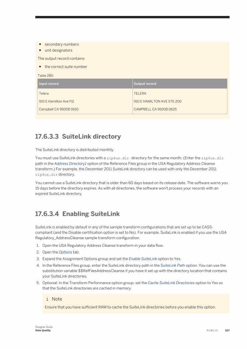
● secondary numbers● unit designators
The output record contains:
● the correct suite number
Table 280:
Input record Output record
Telera
910 E Hamilton Ave Fl2
Campbell CA 95008 0610
TELERA
910 E HAMILTON AVE STE 200
CAMPBELL CA 95008 0625
17.6.3.3 SuiteLink directory
The SuiteLink directory is distributed monthly.
You must use SuiteLink directories with a zip4us.dir directory for the same month. (Enter the zip4us.dir path in the Address Directory1 option of the Reference Files group in the USA Regulatory Address Cleanse transform.) For example, the December 2011 SuiteLink directory can be used with only the December 2011 zip4us.dir directory.
You cannot use a SuiteLink directory that is older than 60 days based on its release date. The software warns you 15 days before the directory expires. As with all directories, the software won't process your records with an expired SuiteLink directory.
17.6.3.4 Enabling SuiteLink
SuiteLink is enabled by default in any of the sample transform configurations that are set up to be CASS-compliant (and the Disable certification option is set to No). For example, SuiteLink is enabled if you use the USA Regulatory_AddressCleanse sample transform configuration.
1. Open the USA Regulatory Address Cleanse transform in your data flow.2. Open the Options tab.3. Expand the Assignment Options group and set the Enable SuiteLink option to Yes.4. In the Reference Files group, enter the SuiteLink directory path in the SuiteLink Path option. You can use the
substitution variable $$RefFilesAddressCleanse if you have it set up with the directory location that contains your SuiteLink directories.
5. Optional: In the Transform Performance option group, set the Cache SuiteLink Directories option to Yes so that the SuiteLink directories are cached in memory.
NoteEnsure that you have sufficient RAM to cache the SuiteLink directories before you enable this option.
Designer GuideData Quality P U B L I C 527
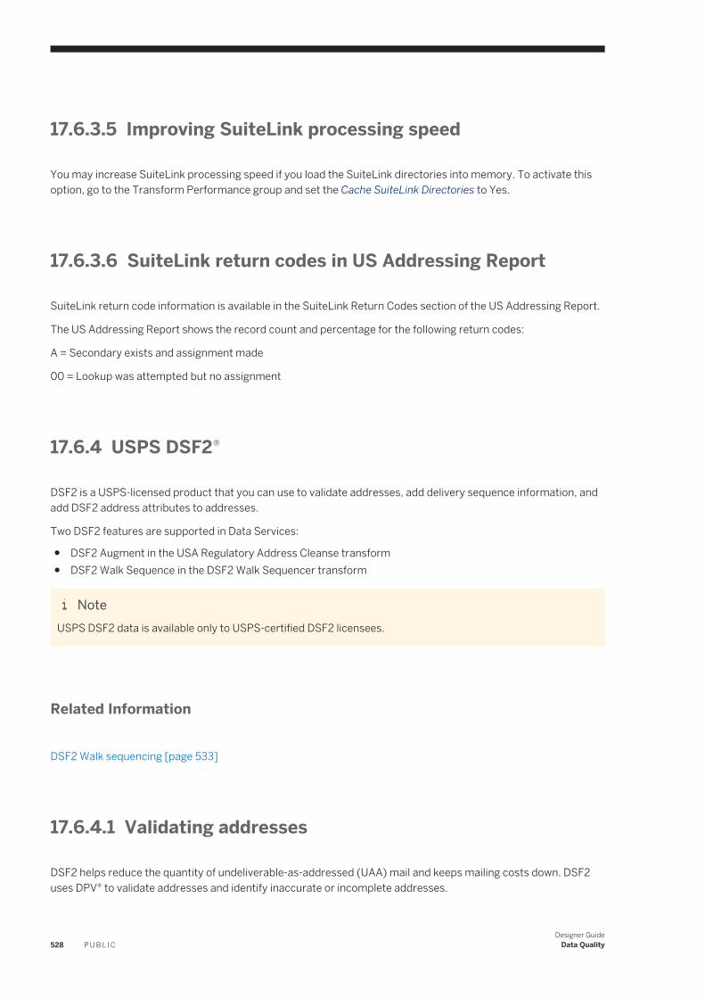
17.6.3.5 Improving SuiteLink processing speed
You may increase SuiteLink processing speed if you load the SuiteLink directories into memory. To activate this option, go to the Transform Performance group and set the Cache SuiteLink Directories to Yes.
17.6.3.6 SuiteLink return codes in US Addressing Report
SuiteLink return code information is available in the SuiteLink Return Codes section of the US Addressing Report.
The US Addressing Report shows the record count and percentage for the following return codes:
A = Secondary exists and assignment made
00 = Lookup was attempted but no assignment
17.6.4 USPS DSF2®
DSF2 is a USPS-licensed product that you can use to validate addresses, add delivery sequence information, and add DSF2 address attributes to addresses.
Two DSF2 features are supported in Data Services:
● DSF2 Augment in the USA Regulatory Address Cleanse transform● DSF2 Walk Sequence in the DSF2 Walk Sequencer transform
NoteUSPS DSF2 data is available only to USPS-certified DSF2 licensees.
Related Information
DSF2 Walk sequencing [page 533]
17.6.4.1 Validating addresses
DSF2 helps reduce the quantity of undeliverable-as-addressed (UAA) mail and keeps mailing costs down. DSF2 uses DPV® to validate addresses and identify inaccurate or incomplete addresses.
528 P U B L I CDesigner Guide
Data Quality
Related Information
DPV overview [page 506]
17.6.4.2 Adding address attributes
DSF2 adds address attributes (information about the addresses) to your data. Use the attribute information to create more targeted mailings.
17.6.4.3 Adding delivery sequence information
DSF2 adds delivery sequence information to your data, which you can use to qualify for walk-sequence discounts. This information is sometimes called walk sequencing or pseudo sequencing.
Related Information
Walk sequencing [page 533]Pseudo sequencing [page 533]
17.6.4.4 Benefits of DSF2
Those who want to target their mail to specific types of addresses and those who want to earn additional postal discounts will appreciate what DSF2 can do.
The DSF2 address-attribute data provides mailers with knowledge about the address above and beyond what is necessary to accurately format the addresses. Address-attribute data allows mailers to produce more targeted mailings.
For example, If you plan to send out a coupon for your lawn-care service business, you do not want to send it to apartment dwellers (they may not have a lawn). You want your coupon to go to residential addresses that are not centralized in an apartment building.
With the DSF2 information you can walk-sequence your mailings to achieve the best possible postal discounts by using the DSF2 Walk Sequencer transform.
17.6.4.5 Becoming a DSF2 licensee
Before you can perform DSF2 processing in the software, you must complete the USPS DSF2 certification procedures and become licensed by the USPS.
Designer GuideData Quality P U B L I C 529
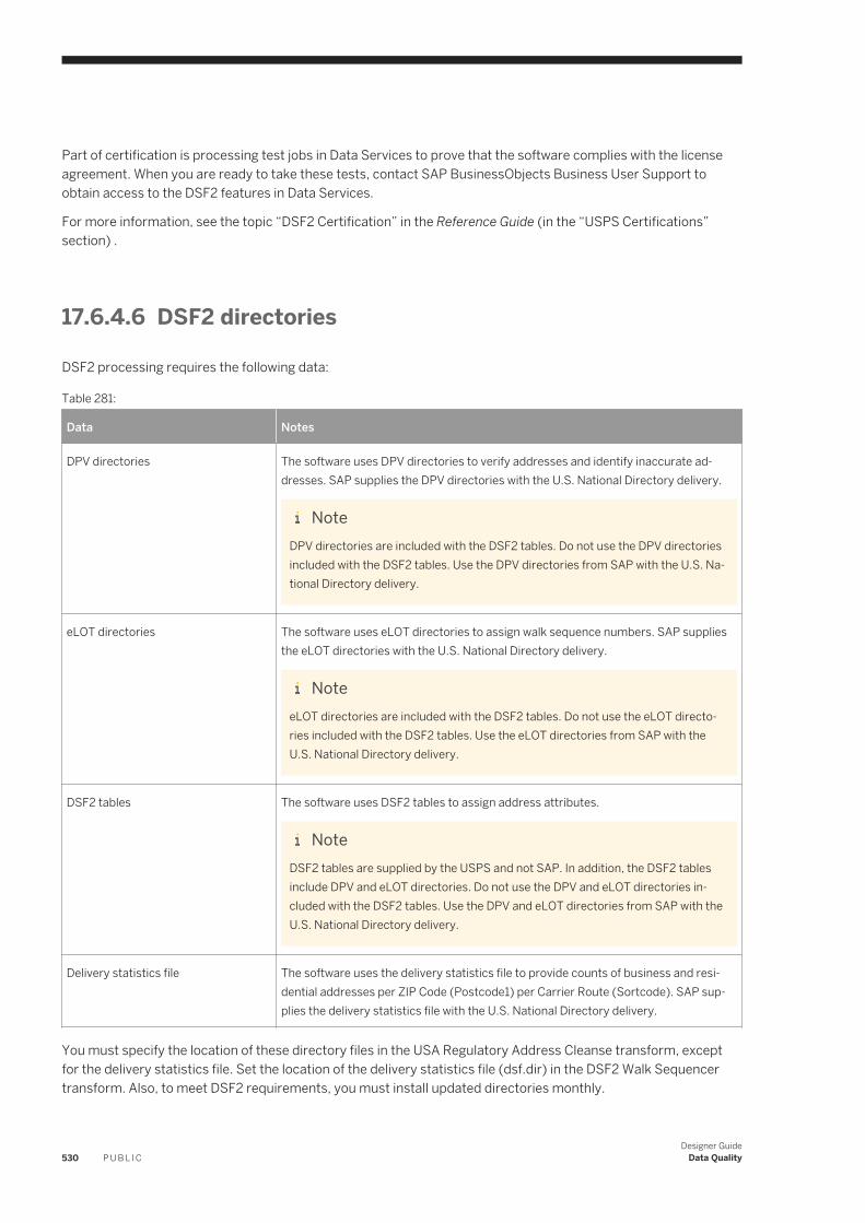
Part of certification is processing test jobs in Data Services to prove that the software complies with the license agreement. When you are ready to take these tests, contact SAP BusinessObjects Business User Support to obtain access to the DSF2 features in Data Services.
For more information, see the topic “DSF2 Certification” in the Reference Guide (in the “USPS Certifications” section) .
17.6.4.6 DSF2 directories
DSF2 processing requires the following data:
Table 281:
Data Notes
DPV directories The software uses DPV directories to verify addresses and identify inaccurate addresses. SAP supplies the DPV directories with the U.S. National Directory delivery.
NoteDPV directories are included with the DSF2 tables. Do not use the DPV directories included with the DSF2 tables. Use the DPV directories from SAP with the U.S. National Directory delivery.
eLOT directories The software uses eLOT directories to assign walk sequence numbers. SAP supplies the eLOT directories with the U.S. National Directory delivery.
NoteeLOT directories are included with the DSF2 tables. Do not use the eLOT directories included with the DSF2 tables. Use the eLOT directories from SAP with the U.S. National Directory delivery.
DSF2 tables The software uses DSF2 tables to assign address attributes.
NoteDSF2 tables are supplied by the USPS and not SAP. In addition, the DSF2 tables include DPV and eLOT directories. Do not use the DPV and eLOT directories included with the DSF2 tables. Use the DPV and eLOT directories from SAP with the U.S. National Directory delivery.
Delivery statistics file The software uses the delivery statistics file to provide counts of business and residential addresses per ZIP Code (Postcode1) per Carrier Route (Sortcode). SAP supplies the delivery statistics file with the U.S. National Directory delivery.
You must specify the location of these directory files in the USA Regulatory Address Cleanse transform, except for the delivery statistics file. Set the location of the delivery statistics file (dsf.dir) in the DSF2 Walk Sequencer transform. Also, to meet DSF2 requirements, you must install updated directories monthly.
530 P U B L I CDesigner Guide
Data Quality
17.6.4.7 DSF2 augment processing
Set up DSF2 augment processing in the USA Regulatory Address Cleanse transform.
DSF2 processing requires DPV information, therefore, enable DPV in your job setup.
If you plan to use the output information from the DSF2 augment processing for walk sequence processing, you must also enable eLOT.
NoteDSF2 augment is available only in batch mode. You cannot add augment information to your data in real time.
17.6.4.7.1 DSF2 Augment directory expiration
The DSF2 directories are distributed monthly. You must use the DSF2 directories with U.S. National directories that are labeled for the same month. For example, the May 2011 DSF2 directories can be used with only the May 2011 National directories.
The DSF2 Augment data expires in 60 days instead of the 105 day expiration for the U.S. National directories. Because directories must all have the same base date (MM/YYYY), DSF2 users who have Yes set for the Enable DSF2 Augment option must update all of the U.S. National directories and other directories they use (for example, LACSLink or DPV) at the same time as the DSF2 Augment directories. The software will remind users to update the directories with a warning message that appears 15 days before the directory expires.
RememberAs with all directories, the software will not process your records with expired DSF2 directories.
17.6.4.7.2 Identifying the DSF2 licensee
When you perform DSF2 processing, you must provide the following information: The DSF2-licensed company and the client for whom the company is processing this job.
You must complete the following options in the USPS License Information group for DSF2 processing:
● DSF2 Licensee ID● Licensee Name● List Owner NAICS Code● List ID● Customer Company Name● Customer Company Address● Customer Company Locality● Customer Company Region● Customer Company Postcode1
Designer GuideData Quality P U B L I C 531
● Customer Company Postcode2● List Received Date● List Return Date
NoteIf you are performing DSF2 and NCOALink processing in the same instance of the USA Regulatory Address Cleanse transform, then the information that you enter in the USPS License Information group must apply to both DSF2 and NCOALink processing. If, for example, the List ID is different for DSF2 and NCOALink, you will need to include two USA Regulatory Address Cleanse transforms: One for NCOALink and another for DSF2.
17.6.4.7.3 Enabling DSF2 Augment
Before you can process with DSF2, you must first become a certified licensee.
In addition to the required customer company information that you enter into the USPS License Information group, set the following options to perform DSF2 Augment processing:
1. In the USA Regulatory Address Cleanse transform, open the Options tab.2. Expand the Report and Analysis group and set the Generate Report Data option to Yes.3. Expand the Reference Files group and enter the path for the options DSF2 Augment Path, DPV Path, and eLOT
Directory, or use the $$RefFilesAddressCleanse substitution variable if you have it set up.4. Also in the Reference Files group, enter a path for the USPS Log Path option, or use the $
$CertificationLogPath substitution variable if you have it set up.5. Optional. Expand the Transform Performance group and set the Cache DPV Directories and Cache DSF2
Augment Directories to Yes.6. Expand the Assignment Options group and set the Enable DSF2 Augment, Enable DPV, and Enable eLOT to
Yes.7. Include the DSF2 address attributes output fields in your output file setup.
17.6.4.7.4 DSF2 output fields
When you perform DSF2 Augment processing in the software, address attributes are available in the following output fields for every address that was assigned. Be sure to include the fields containing information you'll need in your output file setup:
● DSF2_Business_Indicator● DSF2_Delivery_Type● DSF2_Drop_Count● DSF2_Drop_Indicator● DSF2_Educational_Ind● DSF2_LACS_Conversion_Ind● DSF2_Record_Type● DSF2_Seasonal_Indicator
532 P U B L I CDesigner Guide
Data Quality
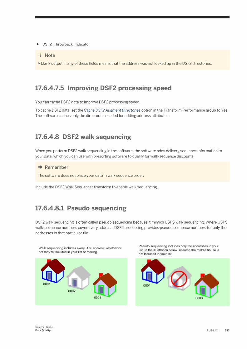
● DSF2_Throwback_Indicator
NoteA blank output in any of these fields means that the address was not looked up in the DSF2 directories.
17.6.4.7.5 Improving DSF2 processing speed
You can cache DSF2 data to improve DSF2 processing speed.
To cache DSF2 data, set the Cache DSF2 Augment Directories option in the Transform Performance group to Yes. The software caches only the directories needed for adding address attributes.
17.6.4.8 DSF2 walk sequencing
When you perform DSF2 walk sequencing in the software, the software adds delivery sequence information to your data, which you can use with presorting software to qualify for walk-sequence discounts.
RememberThe software does not place your data in walk sequence order.
Include the DSF2 Walk Sequencer transform to enable walk sequencing.
17.6.4.8.1 Pseudo sequencing
DSF2 walk sequencing is often called pseudo sequencing because it mimics USPS walk sequencing. Where USPS walk-sequence numbers cover every address, DSF2 processing provides pseudo sequence numbers for only the addresses in that particular file.
Designer GuideData Quality P U B L I C 533
The software uses DSF2 data to assign sequence numbers for all addresses that are DPV-confirmed delivery points (DPV_Status = Y). Other addresses present in your output file that are not valid DPV-confirmed delivery points (DPV_Status = S, N, or D) will receive "0000" as their sequence number. All other addresses will have a blank sequence number.
NoteWhen you walk-sequence your mail with the software, remember the following points:
● (Batch only.) DSF2 walk sequencing is available only in batch mode. You cannot assign sequence numbers in real time.
● Reprocess if you have made file changes. If your data changes in any way, you must re-assign sequence numbers. Sequence numbers are valid only for the data file as you process it at the time.
17.6.4.9 Break key creation
Break keys create manageable groups of data. They are created when there are two or more fields to compare.
The DSF2 Walk Sequencer transform automatically forms break groups before it adds walk sequence information to your data. The software creates break groups based on the Postcode1 and Sortcode_Route fields.
Set options for how you want the software to configure the fields in the Data Collection Config group. Keeping the default settings optimizes the data flow and allows the software to make the break key consistent throughout the data.
Table 282:
Option Default value
Replace NULL with space Yes
Right pad with spaces Yes
17.6.4.10 Enabling DSF2 walk sequencing
To enable DSF2 walk sequence, include the DSF2 Walk Sequencer transform in your data flow.
The input file for the DSF2 Walk Sequencer transform must have been pre-processed with CASS-certified software (such as the USA Regulatory Address Cleanse transform). To obtain an additional postage discount, include the DSF2_Business_Indicator output field information from CASS-certified software.
When you set up for DSF2 walk sequence processing, the following options in the USPS License Information group are required:
● Licensee Name● DSF2 Licensee ID● List ID
In addition to the required USPS License Information fields, make the following settings in the DSF2 Walk Sequencer transform:
534 P U B L I CDesigner Guide
Data Quality
1. Optional. Select Yes or No in the Common group, Run as Separate Process option. Select No if you are gathering DSF2 statistics. Select Yes to save processing time (if you don't need DSF2 statistics).
2. Enter the file path and file name (dsf.dir) to the Delivery Statistics directory in the DelStats Directory option in the Reference Files group. You may use the $$RefFilesAddressCleanse substitution parameter if you have it set up.
3. Enter the processing site location in the Site Location option of the Processing Options group. This is applicable only if you have more than one site location for DSF2 processing.
4. Make the following settings in the Data Collection Configuration group:
○ Select Yes or No in the Replace Null With Space option as desired.○ Select Yes or No for the Right Pad With Spaces option as desired.○ Select Yes or No for the Pre Sorted Data option (optional). We recommend that you keep the default
setting of No so that Data Services sorts your data based on the break key fields (instead of using another software program).
17.6.4.11 DSF2 walk sequence input fields
Here is a list of the DSF2 walk sequence input fields.
NoteThese fields must have been output from CASS-certified software processing before they can be used as input for the DSF2 Walk Sequencer transform:
● Postcode1● Postcode2● Sortcode_Route● LOT● LOT_Order● Delivery_Point● DPV_Status● DSF2_Business_Indicator (optional)
The software uses the information in these fields to determine the way the records should be ordered (walk sequenced) if they were used in a mailing list. The software doesn’t physically change the order of your database. The software assigns walk-sequence numbers to each record based on the information it gathers from these input fields.
NoteAll fields are required except for the DSF2_Business_Indicator field.
The optional DSF2_Business_Indicator field helps the software determine if the record qualifies for saturation discounts. Saturation discounts are determined by the percentage of residential addresses in each carrier route. See the USPS Domestic Mail Manual for details about all aspects of business mailing and sorting discounts.
Designer GuideData Quality P U B L I C 535
17.6.4.12 DSF2 walk-sequence output fields
The software outputs walk-sequence number information to the following fields:
● Active_Del_Discount● Residential_Sat_Discount● Sortcode_Route_Discount● Walk_Sequence_Discount● Walk_Sequence_Number
17.6.4.13 DSF2 reporting
There are reports and log files that the software generates for DSF2 augment and walk sequencing.
Find complete information about these reports and log files in the Management Console Guide.
Delivery Sequence Invoice Report
The USPS requires that you submit the Delivery Sequence Invoice report if you claim DSF2 walk-sequence discounts for this job.
US Addressing Report
● The US Addressing Report is generated by the USA Regulatory Address Cleanse transform.● The Second Generation Delivery Sequence File Summary and Address Delivery Types sections of the US
Addressing Report shows counts and percentages of addresses in your file that match the various DSF2 categories (if NCOALink is enabled). The information is listed for pre and post NCOALink processing.
DSF2 Augment Statistics Log File
The USPS requires that DSF2 licensees save information about their processing in the DSF2 log file. The USPS dictates the contents of the DSF2 log file and requires that you submit it to them monthly.
Log files are available to users with administrator or operator permissions.
536 P U B L I CDesigner Guide
Data Quality
17.6.4.13.1 DSF2 Augment Statistics Log FileThe DSF2 Augment Statistics Log File is stored in the repository. The software generates the log file to the repository where you can export them by using the Data Services Management Console (for Administrators or Operators only).
The naming format for the log file is as follows:
[DSF2_licensee_ID][mm][yy].dat
The USPS dictates the contents of the DSF2 log file and requires that you submit it to them monthly. For details, read the DSF2 Licensee Performance Requirements document, which is available on the USPS RIBBS website (http://ribbs.usps.gov/dsf2/documents/tech_guides ).
You must submit the DSF2 log file to the USPS by the third business day of each month by e-mail.
Log file retention and automatic deletion
You must submit the Augment Statistics Log File to the USPS every month. The software deletes log files on a periodic basis (default is 30 days), which can be controlled through Data Services Application Settings in the Central Management Console. To avoid losing monthly log information, set the History Retention Period to more than 31 days (we recommend a setting of 50 days).
In addition to sending monthly log files to the USPS, you are required to have the data available for the USPS to examine for several years after the job is processed. (Make sure you are aware of current USPS rules for data retention by checking your USPS licensing agreement.) To ensure that you retain all required reports and logs before the data is deleted from the repository, we recommend that you export the required reports and logs from the repository to a local folder on a monthly basis. This also prevents the repository contents from becoming so large that the export process “times out” due to the volume of statistics retained.
17.6.5 NCOALink® overviewThe USPS Move Update standard helps users and the USPS to reduce the number of records that are returned because the address is out of date. NCOALink is a part of this effort. Move Updating is the process of checking addresses against the National Change of Address (NCOA) database to make sure your data is updated with current addresses.
When you process your data using NCOALink, you update your records for individuals or businesses that have moved and have filed a Change of Address (COA) form with the USPS. Other programs that are a part of Move Update, and that are supported in the USA Regulatory Address Cleanse transform, include ANKLink®, and SuiteLink®.
The USPS requires that your lists comply with Move Update standards in order for it to qualify for the discounted postal rates available for First-Class presorted mailings. You can meet this requirement through the NCOALink process.
NoteMover ID is the name under which SAP Data Services is certified for NCOALink.
Designer GuideData Quality P U B L I C 537
Related Information
About ANKLink [page 542]SuiteLink™ [page 525]
17.6.5.1 The importance of move updating
The USPS requires move updating on all First Class presorted mailings. To help mailers meet this requirement, the USPS offers certain options, including NCOALink.
To keep accurate address information for your contacts, you must use a USPS method for receiving your contacts' new addresses. Not only is move updating good business, it is required for all First-Class mailers who claim presorted or automation rates. As the USPS expands move-updating requirements and more strictly enforces the existing regulations, move updating will become increasingly important.
Related Information
About ANKLink [page 542]
17.6.5.2 Benefits of NCOALink
By using NCOALink in the USA Regulatory Address Cleanse transform, you are updating the addresses in your lists with the latest move data. With NCOALink, you can:
● Improve mail deliverability.● Reduce the cost and time needed to forward mail.● Meet the USPS move-updating requirement for presorted First Class mail.● Prepare for the possible expansion of move-update requirements.
17.6.5.3 How NCOALink works
When processing addresses with NCOALink enabled, the software follows these steps:
1. The USA Regulatory Address Cleanse transform standardizes the input addresses. NCOALink requires parsed, standardized address data as input.
2. The software searches the NCOALink database for records that match your parsed, standardized records.3. If a match is found, the software receives the move information, including the new address, if one is available.4. The software looks up move records that come back from the NCOALink database to assign postal and other
codes.
538 P U B L I CDesigner Guide
Data Quality

5. Depending on your field class selection, the output file contains:○ The original input address. The complete and correct value found in the directories, standardized
according to any settings that you defined in the Standardization Options group in the Options tab. (CORRECT)
○ The address components that have been updated with move-updated address data. (MOVE-UPDATED)
NoteThe transform looks for the move-updated address information in the U.S. National Directories. When the move-updated address is not found in the U.S. National Directories, the software populates the Move Updated fields with information found in the Move Update Directories only. The Move Updated fields that are populated as a result of standardizing against the U.S. National Directories will not be updated.
○ The move-updated address data if it exists and if it matches in the U.S. National directories. Or the field contains the original address data if a move does not exist or if the move does not match in the U.S. National Directories. (BEST)
Based on the Apply Move to Standardized Fields option in the NCOALink group, standardized components can contain either original or move-updated addresses.
6. The software produces the reports and log files required for USPS compliance.
Example
Designer GuideData Quality P U B L I C 539
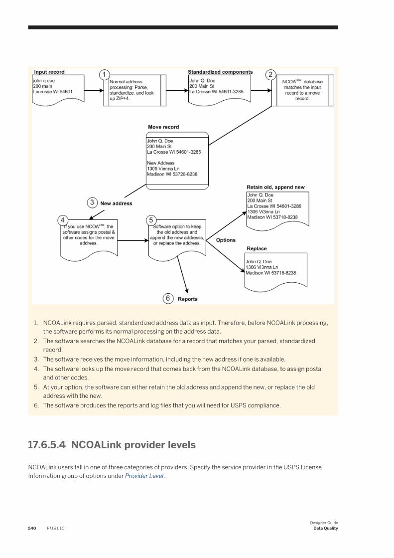
1. NCOALink requires parsed, standardized address data as input. Therefore, before NCOALink processing, the software performs its normal processing on the address data.
2. The software searches the NCOALink database for a record that matches your parsed, standardized record.
3. The software receives the move information, including the new address if one is available.4. The software looks up the move record that comes back from the NCOALink database, to assign postal
and other codes.5. At your option, the software can either retain the old address and append the new, or replace the old
address with the new.6. The software produces the reports and log files that you will need for USPS compliance.
17.6.5.4 NCOALink provider levels
NCOALink users fall in one of three categories of providers. Specify the service provider in the USPS License Information group of options under Provider Level.
540 P U B L I CDesigner Guide
Data Quality
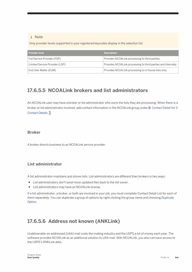
NoteOnly provider levels supported in your registered keycodes display in the selection list.
Provider level Description
Full Service Provider (FSP) Provides NCOALink processing to third parties.
Limited Service Provider (LSP) Provides NCOALink processing to third parties and internally.
End User Mailer (EUM) Provides NCOALInk processing to in-house lists only.
17.6.5.5 NCOALink brokers and list administrators
An NCOALink user may have a broker or list administrator who owns the lists they are processing. When there is a broker or list administrator involved, add contact information in the NCOALink group under Contact Detail listContact Details .
Broker
A broker directs business to an NCOALink service provider.
List administrator
A list administrator maintains and stores lists. List administrators are different than brokers in two ways:
● List administrators don't send move-updated files back to the list owner.● List administrators may have an NCOALink license.
If a list administrator, a broker, or both are involved in your job, you must complete Contact Detail List for each of them separately. You can duplicate a group of options by right-clicking the group name and choosing Duplicate Option.
17.6.5.6 Address not known (ANKLink)
Undeliverable-as-addressed (UAA) mail costs the mailing industry and the USPS a lot of money each year. The software provides NCOALink as an additional solution to UAA mail. With NCOALink, you also can have access to the USPS's ANKLink data.
Designer GuideData Quality P U B L I C 541
17.6.5.6.1 About ANKLink
NCOALink limited service providers and end users receive change of address data for the preceding 18 months. The ANKLink option enhances that information by providing additional data about moves that occurred in the previous months 19 through 48.
TipIf you are an NCOALink full service provider you already have access to the full 48 months of move data (including the new addresses).
NoteThe additional 30 months of data that comes with ANKLink indicates only that a move occurred and the date of the move; the new address is not provided.
The ANKLink data helps you make informed choices regarding a contact. If the data indicates that the contact has moved, you can choose to suppress that contact from the list or try to acquire the new address from an NCOALINK full service provider.
If you choose to purchase ANKLink to extend NCOALINK information, then the DVD you receive from the USPS will contain both the NCOALink 18-month full change of address information and the additional 30 month ANKLink information which indicates that a move has occurred.
If an ANKLink match exists, it is noted in the ANKLINK_RETURN_CODE output field and in the NCOALink Processing Summary report.
17.6.5.6.2 ANKLink data
ANKLink is a subset of NCOALink. You can request ANKLink data from the USPS National Customer Support Center (NCSC) by calling 1-800-589-5766 or by e-mail at [email protected]. ANKLink data is not available from SAP.
The software detects if you're using ANKLink data. Therefore, you do not have to specify whether you're using ANKLink in your job setup.
17.6.5.6.3 ANKLink support for NCOALink provider levels
The software supports three NCOALink provider levels defined by the USPS. Software options vary by provider level and are activated based on the software package that you purchased. The following table shows the provider levels and support:
542 P U B L I CDesigner Guide
Data Quality
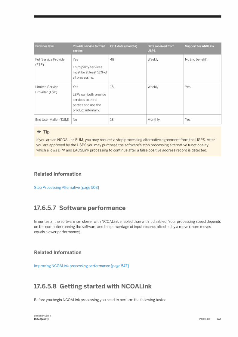
Provider level Provide service to third parties
COA data (months) Data received from USPS
Support for ANKLink
Full Service Provider (FSP)
Yes
Third party services must be at least 51% of all processing.
48 Weekly No (no benefit)
Limited Service Provider (LSP)
Yes
LSPs can both provide services to third parties and use the product internally.
18 Weekly Yes
End User Mailer (EUM) No 18 Monthly Yes
TipIf you are an NCOALink EUM, you may request a stop processing alternative agreement from the USPS. After you are approved by the USPS you may purchase the software's stop processing alternative functionality which allows DPV and LACSLink processing to continue after a false positive address record is detected.
Related Information
Stop Processing Alternative [page 508]
17.6.5.7 Software performance
In our tests, the software ran slower with NCOALink enabled than with it disabled. Your processing speed depends on the computer running the software and the percentage of input records affected by a move (more moves equals slower performance).
Related Information
Improving NCOALink processing performance [page 547]
17.6.5.8 Getting started with NCOALink
Before you begin NCOALink processing you need to perform the following tasks:
Designer GuideData Quality P U B L I C 543
● Complete the USPS certification process to become an NCOALink service provider or end user. For information about certification, see the NCOALink Certification section following the link below.
● Understand the available output strategies and performance optimization options.● Configure your job.
17.6.5.9 What to expect from the USPS and SAP
NCOALink, and the license requirements that go with it, has created a new dimension in the relationship among mailers (you), the USPS, and vendors. It's important to be clear about what to expect from everyone.
17.6.5.9.1 Move updating is a business decision for you to make
NCOALink offers an option to replace a person's old address with their new address. You as a service provider must decide whether you accept move updates related to family moves, or only individual moves. The USPS recommends that you make these choices only after careful thought about your customer relationships. Consider the following examples:
● If you are mailing checks, account statements, or other correspondence for which you have a fiduciary responsibility, then move updating is a serious undertaking. The USPS recommends that you verify each move by sending a double postcard, or other easy-reply piece, before changing a financial record to the new address.
● If your business relationship is with one spouse and not the other, then move updating must be handled carefully with respect to divorce or separation. Again, it may make sense for you to take the extra time and expense of confirming each move before permanently updating the record.
17.6.5.9.2 NCOALink security requirements
Because of the sensitivity and confidentiality of change-of-address data, the USPS imposes strict security procedures on software vendors who use and provide NCOALink processing.
One of the software vendor's responsibilities is to check that each list input to the USA Regulatory Address Cleanse transform contains at least 100 unique records. Therefore the USA Regulatory Address Cleanse transform checks your input file for at least 100 unique records. These checks make verification take longer, but they are required by the USPS and they must be performed.
If the software finds that your data does not have 100 unique records, it issues an error and discontinues processing.
The process of checking for 100 unique records is a pre-processing step. So if the software does not find 100 unique records, there will be no statistics output or any processing performed on the input file.
544 P U B L I CDesigner Guide
Data Quality
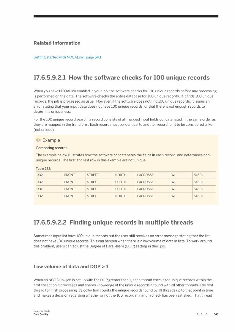
Related Information
Getting started with NCOALink [page 543]
17.6.5.9.2.1 How the software checks for 100 unique records
When you have NCOALink enabled in your job, the software checks for 100 unique records before any processing is performed on the data. The software checks the entire database for 100 unique records. If it finds 100 unique records, the job is processed as usual. However, if the software does not find 100 unique records, it issues an error stating that your input data does not have 100 unique records, or that there is not enough records to determine uniqueness.
For the 100 unique record search, a record consists of all mapped input fields concatenated in the same order as they are mapped in the transform. Each record must be identical to another record for it to be considered alike (not unique).
ExampleComparing records
The example below illustrates how the software concatenates the fields in each record, and determines non-unique records. The first and last row in this example are not unique.
Table 283:
332 FRONT STREET NORTH LACROSSE WI 54601
332 FRONT STREET SOUTH LACROSSE WI 54601
331 FRONT STREET SOUTH LACROSSE WI 54601
332 FRONT STREET NORTH LACROSSE WI 54601
17.6.5.9.2.2 Finding unique records in multiple threads
Sometimes input list have 100 unique records but the user still receives an error message stating that the list does not have 100 unique records. This can happen when there is a low volume of data in lists. To work around this problem, users can adjust the Degree of Parallelism (DOP) setting in their job.
Low volume of data and DOP > 1
When an NCOALink job is set up with the DOP greater than 1, each thread checks for unique records within the first collection it processes and shares knowledge of the unique records it found with all other threads. The first thread to finish processing it’s collection counts the unique records found by all threads up to that point in time and makes a decision regarding whether or not the 100 record minimum check has been satisfied. That thread
Designer GuideData Quality P U B L I C 545
may not necessarily be thread 1. For example, say your list has 3,050 records and you have the DOP set for 4. If the number of records per collection is 1000, each thread will have a collection of 1000 records except for the last thread which will only have 50 records. The thread processing 50 records is likely to finish its collection sooner and it may make the pass/fail decision before 100 unique records have been encountered. You may be able to successfully run this job if you lower the DOP. In this example, you could lower it to 3.
17.6.5.10 About the NCOALink daily delete file
If you are a service provider, then every day before you perform NCOALink processing, you must download the daily delete file and install it in the same folder that your NCOALink directories are located.
The daily delete file contains records that are pending deletion from the NCOALink data. For example, if Jane Doe filed a change of address with the USPS and then didn’t move, Jane’s record would be in the daily delete file. Because the change of address is stored in the NCOALink directories, and they are updated only weekly or monthly, the daily delete file is needed in the interim, until the NCOALink directories are updated again.
Download the daily delete file from the USPS's electronic product fulfillment website at https://epf.usps.gov/ . Before you can access the file, you must complete and submit the Electronic Product Fulfillment Web Access Request Form (Form 5116) to the USPS. You can obtain this form from the same website.
NoteIf you are an end user, you only need the daily delete file for processing Stage I or II files. It is not required for normal NCOALink processing.
Here are some important points to know about the daily delete file:
● The software will fail verification if NCOALink is enabled, a stage test is being performed, and the daily delete file isn't installed.
● USA Regulatory Address Cleanse transform supports only the ASCII version of the daily delete file.● Do not rename the daily delete file. It must be named dailydel.dat.● The software will issue a verification warning if the daily delete file is more than three days old.
17.6.5.10.1 Installing the NCOALink daily delete file
To download and install the NCOALink daily delete file, follow these steps:
1. Go to the USPS Electronic Product Fulfillment site at https://epf.usps.gov/ .2. Before you download the daily delete file for the first time, you must complete and fax the PS Form 5116
(Electronic Product Fulfillment Web Access Request Form) to the USPS Licensing Department.When completing the form, make sure that you select the NCOALink or NCOALink with ANKLink option, as appropriate. This allows you to access the daily delete file.
3. Log into the USPS Electronic Product Fulfillment site and download the NCOALink Daily Delete [TEXT] file to a location where the .tar file can be extracted. If your computer browser has pop-up blockers enabled, you may need to override them.
4. Extract the dailyDeletes_txt.tar file.
546 P U B L I CDesigner Guide
Data Quality
5. Copy the dailydel.dat file to the same location where your NCOALink directories are stored.
6. Repeat steps 3–5 every day before you perform NCOALink processing.
17.6.5.11 Output file strategies
You can configure your output file to meet your needs. Depending on the Field Class Selection that you choose, components in your output file contain Correct, Move-updated, or Best information:
● CORRECT: Outputs the original input address. The complete and correct value found in the directories, standardized according to any settings that you defined in the Standardization Options group in the Options tab. (CORRECT)
● MOVE-UPDATED: Outputs the address components that have been updated with move-updated address data.
NoteThe transform looks for the move-updated address information in the U.S. National Directories. When the move-updated address is not found in the U.S. National Directories, the software populates the Move Updated fields with information found in the Move Update Directories only. The Move Updated fields that are populated as a result of standardizing against the U.S. National Directories will not be updated.
● BEST: Outputs the move-updated address data if it exists and if it matches in the U.S. National directories. Or the field contains the original address data if a move does not exist or if the move does not match in the U.S. National Directories.
Based on the Apply Move to Standardized Fields option setting in the NCOA option group, standardized components can contain original or move-updated addresses.
By default the output option Apply Move to Standardized Fields is set to Yes and the software updates standardized fields to contain details about the updated address available through NCOALink.
If you want to retain the old addresses in the standardized components and append the new ones to the output file, you must change the Apply Move to Standardized Fields option to No. Then you can use output fields such as NCOALINK_RETURN_CODE to determine whether a move occurred. One way to set up your output file is to replicate the input file format, then append extra fields for move data. In the output records not affected by a move, most of the appended fields will be blank. Alternatively, you can create a second output file specifically for move records. Two approaches are possible:
● Output each record once, placing move records in the second output file and all other records in the main output file.
● Output move records twice; once to the main output file, and a second time to the second output file.
Both of these approaches require that you use an output filter to determine whether a record is a move.
17.6.5.12 Improving NCOALink processing performance
Many factors affect performance when processing NCOALink data. Generally the most critical factor is the volume of disk access that occurs. Often the most effective way to reduce disk access is to have sufficient memory available to cache data. Other critical factors that affect performance include hard drive speed, seek
Designer GuideData Quality P U B L I C 547
time, and the sustained transfer rate. When the time spent on disk access is minimized, the performance of the CPU becomes significant.
Related Information
Finding unique records in multiple threads [page 545]
17.6.5.12.1 Operating systems and processors
The computation involved in most of the software and NCOALink processing is very well-suited to the microprocessors found in most computers, such as those made by Intel and AMD. RISC style processors like those found in most UNIX systems are generally substantially slower for this type of computation. In fact a common PC can often run a single job through the software and NCOALink about twice as fast as a common UNIX system. If you’re looking for a cost-effective way of processing single jobs, a Windows server or a fast workstation can produce excellent results. Most UNIX systems have multiple processors and are at their best processing several jobs at once.
You should be able to increase the degree of parallelism (DOP) in the data flow properties to maximize the processor or core usage on your system. Increasing the DOP depends on the complexity of the data flow.
17.6.5.12.2 Memory
NCOALink processing uses many gigabytes of data. The exact amount depends on your service provider level, the data format, and the specific release of the data from the USPS.
In general, if performance is critical, and especially if you are an NCOALink full service provider and you frequently run very large jobs with millions of records, you should obtain as much memory as possible. You may want to go as far as caching the entire NCOALink data set. You should be able to cache the entire NCOALink data set using 20 GB of RAM, with enough memory left for the operating system.
17.6.5.12.3 Data storage
If at all possible, the hard drive you use for NCOALink data should be fully dedicated to that process, at least while your job is running. Other processes competing for the use of the same physical disk drive can greatly reduce your NCOALink performance.
To achieve even higher transfer rates you may want to explore the possibility of using a RAID system (redundant array of independent discs).
When the software accesses NCOALink data directly instead of from a cache, the most significant hard drive feature is the average seek time.
548 P U B L I CDesigner Guide
Data Quality
17.6.5.12.4 Data format
The software supports both hash and flat file versions of NCOALink data. If you have ample memory to cache the entire hash file data set, that format may provide the best performance. The flat file data is significantly smaller, which means a larger share can be cached in a given amount of RAM. However, accessing the flat file data involves binary searches, which are slightly more time consuming than the direct access used with the hash file format.
17.6.5.12.5 Memory usage
The optimal amount of memory depends on a great many factors. The “Auto” option usually does a good job of deciding how much memory to use, but in some cases manually adjusting the amount can be worthwhile.
17.6.5.12.6 Performance tips
Many factors can increase or decrease NCOALink processing speed. Some are within your control and others may be inherent to your business. Consider the following factors:
● Cache size—Using too little memory for NCOALink caching can cause unnecessary random file access and time-consuming hard drive seeks. Using far too much memory can cause large files to be read from the disk into the cache even when only a tiny fraction of the data will ever be used. The amount of cache that works best in your environment may require some testing to see what works best for your configuration and typical job size.
● Directory location—It’s best to have NCOALink directories on a local solid state drive or a virtual RAM drive. Using a local solid state drive or virtual RAM drive eliminates all I/O for NCOALink while processing your job. If you have the directories on a hard drive, it’s best to use a defragmented local hard drive. The hard drive should not be accessed for anything other than the NCOALink data while you are running your job.
● Match rate—The more records you process that have forwardable moves, the slower your processing will be. Retrieving and decoding the new addresses takes time, so updating a mailing list regularly will improve the processing speed on that list.
● Input format—Ideally you should provide the USA Regulatory Address Cleanse transform with discrete fields for the addressee’s first, middle, and last name, as well as for the pre-name and post-name. If your input has only a name line, the transform will have to take time to parse it before checking NCOALink data.
● File size—Larger files process relatively faster than smaller files. There is overhead when processing any job, but if a job includes millions of records, a few seconds of overhead becomes insignificant.
17.6.5.13 Enabling NCOALink processing
You must have access to the following files:
● NCOALink directories● Current version of the USPS daily delete file● DPV data files
Designer GuideData Quality P U B L I C 549
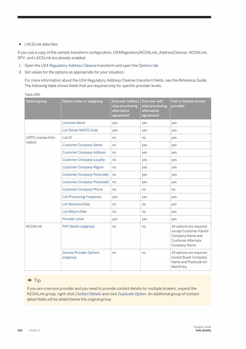
● LACSLink data files
If you use a copy of the sample transform configuration, USARegulatoryNCOALink_AddressCleanse, NCOALink, DPV, and LACSLink are already enabled.
1. Open the USA Regulatory Address Cleanse transform and open the Options tab.2. Set values for the options as appropriate for your situation.
For more information about the USA Regulatory Address Cleanse transform fields, see the Reference Guide. The following table shows fields that are required only for specific provider levels.
Table 284:
Option group Option name or subgroup End user without stop processing alternative agreement
End user with stop processing alternative agreement
Full or limited service provider
Licensee Name yes yes yes
List Owner NAICS Code yes yes yes
USPS License Information
List ID no no yes
Customer Company Name no yes yes
Customer Company Address no yes yes
Customer Company Locality no yes yes
Customer Company Region no yes yes
Customer Company Postcode1 no yes yes
Customer Company Postcode2 no yes yes
Customer Company Phone no no no
List Processing Frequency yes yes yes
List Received Date no no yes
List Return Date no no yes
Provider Level yes yes yes
NCOALink PAF Details subgroup no no All options are required, except Customer Parent Company Name and Customer Alternate Company Name.
Service Provider Options subgroup
no no All options are required, except Buyer Company Name and Postcode for Mail Entry.
TipIf you are a service provider and you need to provide contact details for multiple brokers, expand the NCOALink group, right-click Contact Details and click Duplicate Option. An additional group of contact detail fields will be added below the original group.
550 P U B L I CDesigner Guide
Data Quality
Related Information
About the NCOALink daily delete file [page 546]Output file strategies [page 547]Stop Processing Alternative [page 508]
17.6.5.14 NCOALink log files
The software automatically generates the USPS-required log files and names them according to USPS requirements. The software generates these log files to the repository where you can export them by using the Management Console.
The software creates one log file per license ID. At the beginning of each month, the software starts new log files. Each log file is then appended with information about every NCOALink job processed that month for that specific license ID.
The software produces the following move-related log files:
● CSL (Customer Service log)● PAF (Processing Acknowlagement Form) customer Information log● BALA (Broker/Agent/List Administrator) log
The PAF Customer Information Log File and the BALA Log File are not required for end users.The following table shows the log files required for Limited or Full Service Providers:
Table 285:
Log file Description
CSL This log file contains one record per list that you process. Each record details the results of change-of-address processing.
PAF customer information log
This log file contains the information that you provided for the PAF.
The log file lists each unique PAF entry. If a list is processed with the same PAF information, the information appears just once in the log file.
When contact information for the list administrator has changed, then information for both the list administrator and the corresponding broker are written to the PAF log file.
BALA This log file contains all of the contact information that you entered for the broker or list administrator.
The log file lists information for each broker or list administrator just once.
The USPS requires the Broker/Agent/List Administrator log file from service providers, even in jobs that do not involve a broker or list administrator. The software produces this log file for every job if you’re a certified service provider.
Designer GuideData Quality P U B L I C 551
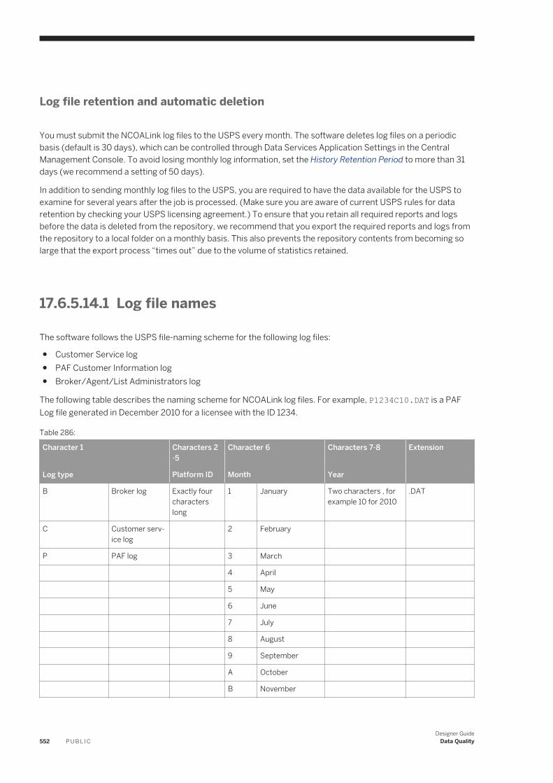
Log file retention and automatic deletion
You must submit the NCOALink log files to the USPS every month. The software deletes log files on a periodic basis (default is 30 days), which can be controlled through Data Services Application Settings in the Central Management Console. To avoid losing monthly log information, set the History Retention Period to more than 31 days (we recommend a setting of 50 days).
In addition to sending monthly log files to the USPS, you are required to have the data available for the USPS to examine for several years after the job is processed. (Make sure you are aware of current USPS rules for data retention by checking your USPS licensing agreement.) To ensure that you retain all required reports and logs before the data is deleted from the repository, we recommend that you export the required reports and logs from the repository to a local folder on a monthly basis. This also prevents the repository contents from becoming so large that the export process “times out” due to the volume of statistics retained.
17.6.5.14.1 Log file names
The software follows the USPS file-naming scheme for the following log files:
● Customer Service log● PAF Customer Information log● Broker/Agent/List Administrators log
The following table describes the naming scheme for NCOALink log files. For example, P1234C10.DAT is a PAF Log file generated in December 2010 for a licensee with the ID 1234.
Table 286:
Character 1 Characters 2 -5
Character 6 Characters 7-8 Extension
Log type Platform ID Month Year
B Broker log Exactly four characters long
1 January Two characters , for example 10 for 2010
.DAT
C Customer service log
2 February
P PAF log 3 March
4 April
5 May
6 June
7 July
8 August
9 September
A October
B November
552 P U B L I CDesigner Guide
Data Quality
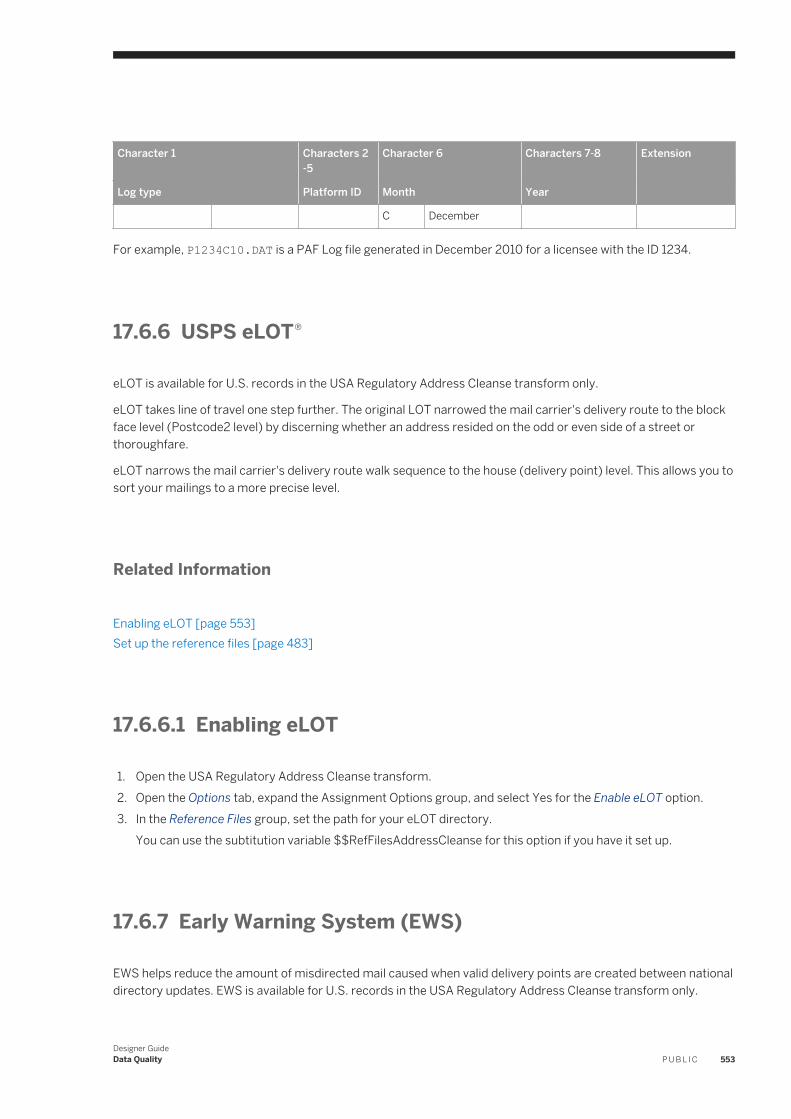
Character 1 Characters 2 -5
Character 6 Characters 7-8 Extension
Log type Platform ID Month Year
C December
For example, P1234C10.DAT is a PAF Log file generated in December 2010 for a licensee with the ID 1234.
17.6.6 USPS eLOT®
eLOT is available for U.S. records in the USA Regulatory Address Cleanse transform only.
eLOT takes line of travel one step further. The original LOT narrowed the mail carrier's delivery route to the block face level (Postcode2 level) by discerning whether an address resided on the odd or even side of a street or thoroughfare.
eLOT narrows the mail carrier's delivery route walk sequence to the house (delivery point) level. This allows you to sort your mailings to a more precise level.
Related Information
Enabling eLOT [page 553]Set up the reference files [page 483]
17.6.6.1 Enabling eLOT
1. Open the USA Regulatory Address Cleanse transform.2. Open the Options tab, expand the Assignment Options group, and select Yes for the Enable eLOT option.3. In the Reference Files group, set the path for your eLOT directory.
You can use the subtitution variable $$RefFilesAddressCleanse for this option if you have it set up.
17.6.7 Early Warning System (EWS)
EWS helps reduce the amount of misdirected mail caused when valid delivery points are created between national directory updates. EWS is available for U.S. records in the USA Regulatory Address Cleanse transform only.
Designer GuideData Quality P U B L I C 553
17.6.7.1 Overview of EWS
The EWS feature is the solution to the problem of misdirected mail caused by valid delivery points that appear between national directory updates. For example, suppose that 300 Main Street is a valid address and that 300 Main Avenue does not exist. A mail piece addressed to 300 Main Avenue is assigned to 300 Main Street on the assumption that the sender is mistaken about the correct suffix.
Now consider that construction is completed on a house at 300 Main Avenue. The new owner signs up for utilities and mail, but it may take a couple of months before the delivery point is listed in the national directory. All the mail intended for the new house at 300 Main Avenue will be mis-directed to 300 Main Street until the delivery point is added to the national directory.
The EWS feature solves this problem by using an additional directory which informs CASS users of the existence of 300 Main Avenue long before it appears in the national directory. When using EWS processing, the previously mis-directed address now defaults to a 5-digit assignment.
17.6.7.2 Start with a sample transform configuration
If you want to use the USA Regulatory Address Cleanse transform with the EWS option turned on, it is best to start with the sample transform configuration for EWS processing named USARegulatoryEWS_AddressCleanse.
17.6.7.3 EWS directory
The EWS directory contains four months of rolling data. Each week, the USPS adds new data and drops a week's worth of old data. The USPS then publishes the latest EWS data. Each Friday, SAP converts the data to our format (EWyymmdd.zip) and posts it on the SAP software download center at https://support.sap.com/swdc .
1. Select Address Directories and Reference Data.2. Click Address Directories.3. Select Early Warning System Directories to access the download.
17.6.7.4 Enabling EWS
EWS is already enabled when you use the software's EWS sample transform, USARegulatoryEWS_AddressCleanse. These steps show how to manually set EWS.
1. Open the USA Regulatory Address Cleanse transform.2. Open the Options tab and expand the Assignment Options group.3. Select Enable for the Enable EWS option.4. Expand the Reference Files group and enter a path for the EWS Directory option, or use the substitution
variable $$RefFilesAddressCleanse if you have it set up.
554 P U B L I CDesigner Guide
Data Quality
Related Information
Early Warning System (EWS) [page 553]
17.6.8 USPS RDI®
The RDI (Residential Delivery Indicator) option is available in the USA Regulatory Address Cleanse transform. RDI determines whether a given address is for a residence or non residence.
Parcel shippers can find RDI information to be very valuable because some delivery services charge higher rates to deliver to residential addresses. The USPS, on the other hand, does not add surcharges for residential deliveries. When you can recognize an address as a residence, you have increased incentive to ship the parcel with the USPS instead of with a competitor that applies a residential surcharge.
According to the USPS, 91-percent of U.S. addresses are residential. The USPS is motivated to encourage the use of RDI by parcel mailers.
You can use RDI if you are processing your data for CASS certification or if you are processing in a non-certified mode. In addition, RDI does not require that you use DPV processing.
17.6.8.1 Start with a sample transform
If you want to use the RDI feature with the USA Regulatory Address Cleanse transform, it is best to start with the sample transform configuration, USARegulatoryRDI_AddressCleanse.
Sample transforms are located in the Transforms tab of the Object Library. This sample is located under USA_Regulatory_Address_Cleanse transforms.
17.6.8.2 How RDI works
After you install the RDI directories and enable RDI processing, the software determines whether the address represented by an 11-digit postcode (Postcode1, Postcode2, and the DPBC) is a residential address. (The software can sometimes do the same with a postcode2.)
The software indicates whether an address is for a residence in the output component, RDI_INDICATOR.
Using the RDI feature involves only a few steps:
1. Install the RDI directories.2. Specify where the directories are located.3. Enable RDI processing in the software.4. Run the job.
Designer GuideData Quality P U B L I C 555
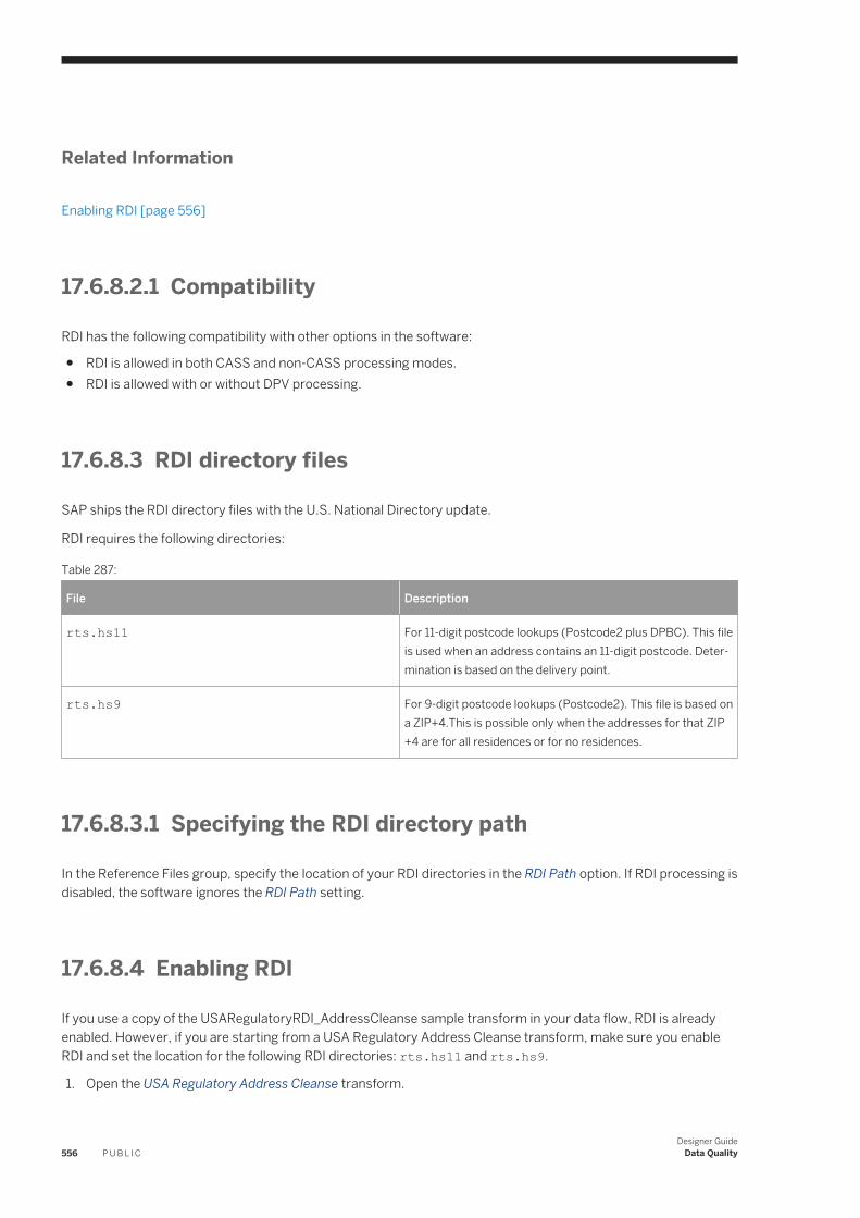
Related Information
Enabling RDI [page 556]
17.6.8.2.1 Compatibility
RDI has the following compatibility with other options in the software:
● RDI is allowed in both CASS and non-CASS processing modes.● RDI is allowed with or without DPV processing.
17.6.8.3 RDI directory files
SAP ships the RDI directory files with the U.S. National Directory update.
RDI requires the following directories:
Table 287:
File Description
rts.hs11 For 11-digit postcode lookups (Postcode2 plus DPBC). This file is used when an address contains an 11-digit postcode. Determination is based on the delivery point.
rts.hs9 For 9-digit postcode lookups (Postcode2). This file is based on a ZIP+4.This is possible only when the addresses for that ZIP+4 are for all residences or for no residences.
17.6.8.3.1 Specifying the RDI directory path
In the Reference Files group, specify the location of your RDI directories in the RDI Path option. If RDI processing is disabled, the software ignores the RDI Path setting.
17.6.8.4 Enabling RDI
If you use a copy of the USARegulatoryRDI_AddressCleanse sample transform in your data flow, RDI is already enabled. However, if you are starting from a USA Regulatory Address Cleanse transform, make sure you enable RDI and set the location for the following RDI directories: rts.hs11 and rts.hs9.
1. Open the USA Regulatory Address Cleanse transform.
556 P U B L I CDesigner Guide
Data Quality
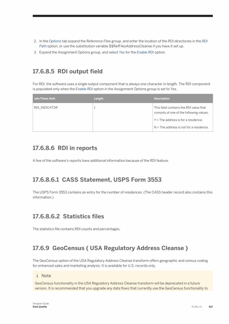
2. In the Options tab expand the Reference Files group, and enter the location of the RDI directories in the RDI Path option, or use the substitution variable $$RefFilesAddressCleanse if you have it set up.
3. Expand the Assignment Options group, and select Yes for the Enable RDI option.
17.6.8.5 RDI output field
For RDI, the software uses a single output component that is always one character in length. The RDI component is populated only when the Enable RDI option in the Assignment Options group is set to Yes.
Job/Views field Length Description
RDI_INDICATOR 1 This field contains the RDI value that consists of one of the following values:
Y = The address is for a residence.
N = The address is not for a residence.
17.6.8.6 RDI in reports
A few of the software's reports have additional information because of the RDI feature.
17.6.8.6.1 CASS Statement, USPS Form 3553
The USPS Form 3553 contains an entry for the number of residences. (The CASS header record also contains this information.)
17.6.8.6.2 Statistics files
The statistics file contains RDI counts and percentages.
17.6.9 GeoCensus ( USA Regulatory Address Cleanse )
The GeoCensus option of the USA Regulatory Address Cleanse transform offers geographic and census coding for enhanced sales and marketing analysis. It is available for U.S. records only.
NoteGeoCensus functionality in the USA Regulatory Address Cleanse transform will be deprecated in a future version. It is recommended that you upgrade any data flows that currently use the GeoCensus functionality to
Designer GuideData Quality P U B L I C 557
use the Geocoder transform. For instructions on upgrading from GeoCensus to the Geocoder transform, see the Upgrade Guide.
Related Information
How GeoCensus works [page 558]GeoCensus directories [page 559]Enabling GeoCensus coding [page 561]Geocoding [page 376]
17.6.9.1 How GeoCensus works
By using GeoCensus, the USA Regulatory Address Cleanse transform can append latitude, longitude, and census codes such as census tract and Metropolitan Statistical Area (MSA) to your records, based on ZIP+4 codes. MSA is an aggregation of US counties into Metropolitan Statistical Areas assigned by the US Office of Management and Budget. You can apply the GeoCensus codes during address standardization and postcode2 assignment for simple, “one-pass” processing.
The transform cannot, by itself, append demographic data to your records. The transform lays the foundation by giving you census coordinates via output fields. To append demographic information, you need a demographic database from another vendor. When you obtain one, we suggest that you use the matching process to match your records to the demographic database, and transfer the demographic information into your records. (You would use the MSA and census tract information as match criteria, then use the Best Record transform to post income and other information.)
Likewise, the transform does not draw maps. However, you can use the latitude and longitude assigned by the transform as input to third-party mapping applications. Those applications enable you to plot the locations of your customers and filter your database to cover a particular geographic area.
17.6.9.2 The software provides census coordinates
The software cannot, by itself, append demographic data to your records. The software simply lays the foundation by giving you census coordinates. To append demographic information, you need a demographic database from another vendor. When you get that, we suggest that you use our Match transform to match your records to the demographic database and transfer the demographic information into your records. (In technical terms, you would use the MSA and Census block/tract information as match fields, then use the Best Record post-match operation in the Match transform to transfer income and other information.
Likewise, the software does not draw maps. However, you can use the latitude and longitude assigned by the software as input to third-party mapping software. Those programs enable you to plot the locations of your customers and filter your database to cover a particular geographic area.
558 P U B L I CDesigner Guide
Data Quality
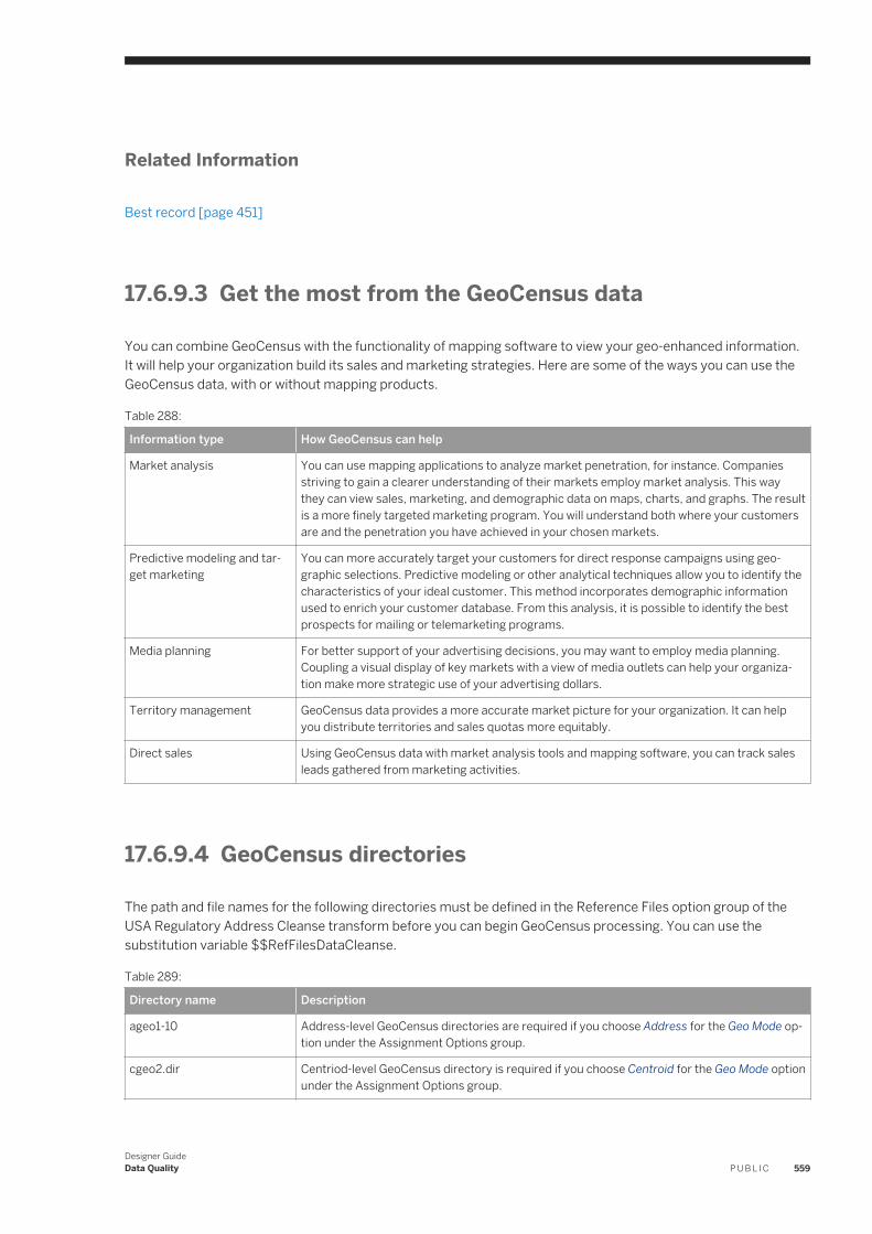
Related Information
Best record [page 451]
17.6.9.3 Get the most from the GeoCensus data
You can combine GeoCensus with the functionality of mapping software to view your geo-enhanced information. It will help your organization build its sales and marketing strategies. Here are some of the ways you can use the GeoCensus data, with or without mapping products.
Table 288:
Information type How GeoCensus can help
Market analysis You can use mapping applications to analyze market penetration, for instance. Companies striving to gain a clearer understanding of their markets employ market analysis. This way they can view sales, marketing, and demographic data on maps, charts, and graphs. The result is a more finely targeted marketing program. You will understand both where your customers are and the penetration you have achieved in your chosen markets.
Predictive modeling and target marketing
You can more accurately target your customers for direct response campaigns using geographic selections. Predictive modeling or other analytical techniques allow you to identify the characteristics of your ideal customer. This method incorporates demographic information used to enrich your customer database. From this analysis, it is possible to identify the best prospects for mailing or telemarketing programs.
Media planning For better support of your advertising decisions, you may want to employ media planning. Coupling a visual display of key markets with a view of media outlets can help your organization make more strategic use of your advertising dollars.
Territory management GeoCensus data provides a more accurate market picture for your organization. It can help you distribute territories and sales quotas more equitably.
Direct sales Using GeoCensus data with market analysis tools and mapping software, you can track sales leads gathered from marketing activities.
17.6.9.4 GeoCensus directories
The path and file names for the following directories must be defined in the Reference Files option group of the USA Regulatory Address Cleanse transform before you can begin GeoCensus processing. You can use the substitution variable $$RefFilesDataCleanse.
Table 289:
Directory name Description
ageo1-10 Address-level GeoCensus directories are required if you choose Address for the Geo Mode option under the Assignment Options group.
cgeo2.dir Centriod-level GeoCensus directory is required if you choose Centroid for the Geo Mode option under the Assignment Options group.
Designer GuideData Quality P U B L I C 559
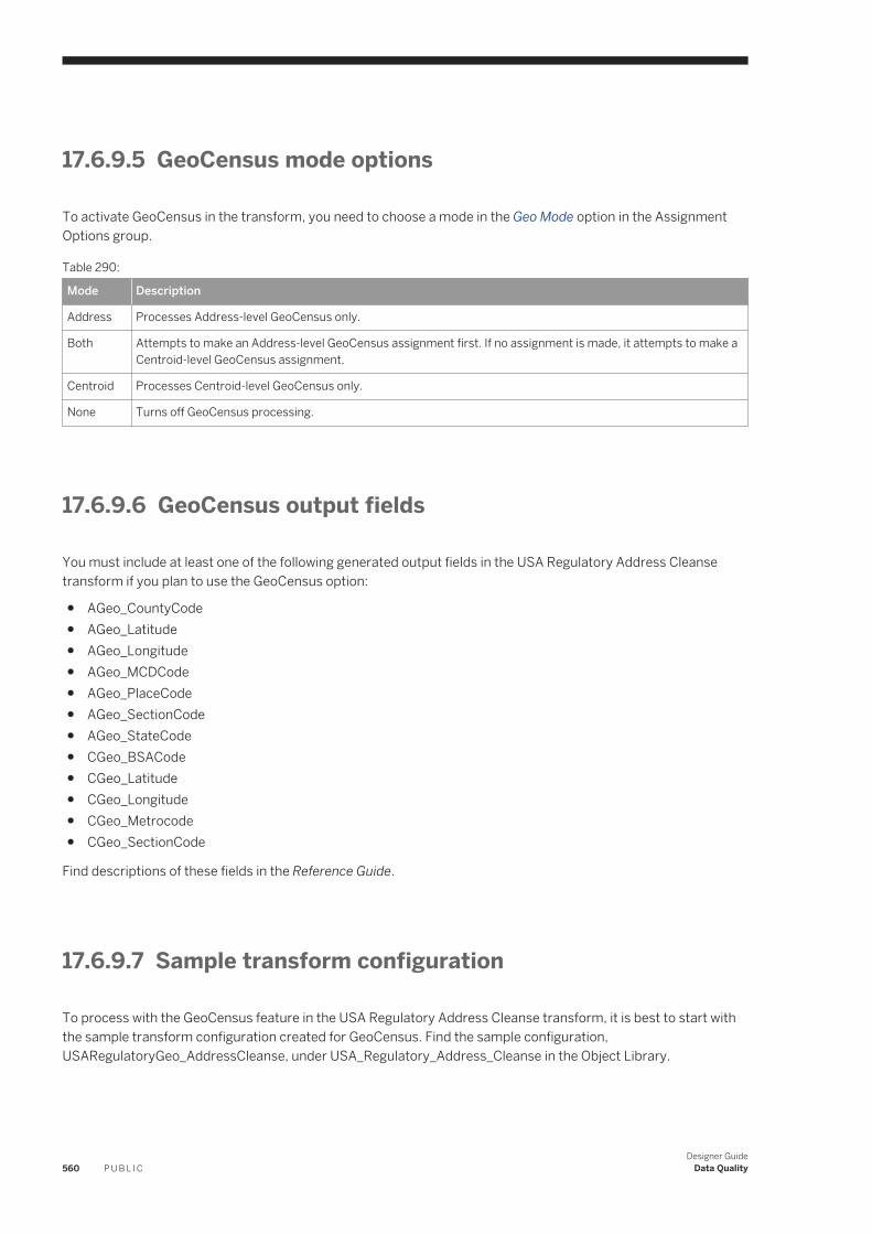
17.6.9.5 GeoCensus mode options
To activate GeoCensus in the transform, you need to choose a mode in the Geo Mode option in the Assignment Options group.
Table 290:
Mode Description
Address Processes Address-level GeoCensus only.
Both Attempts to make an Address-level GeoCensus assignment first. If no assignment is made, it attempts to make a Centroid-level GeoCensus assignment.
Centroid Processes Centroid-level GeoCensus only.
None Turns off GeoCensus processing.
17.6.9.6 GeoCensus output fields
You must include at least one of the following generated output fields in the USA Regulatory Address Cleanse transform if you plan to use the GeoCensus option:
● AGeo_CountyCode● AGeo_Latitude● AGeo_Longitude● AGeo_MCDCode● AGeo_PlaceCode● AGeo_SectionCode● AGeo_StateCode● CGeo_BSACode● CGeo_Latitude● CGeo_Longitude● CGeo_Metrocode● CGeo_SectionCode
Find descriptions of these fields in the Reference Guide.
17.6.9.7 Sample transform configuration
To process with the GeoCensus feature in the USA Regulatory Address Cleanse transform, it is best to start with the sample transform configuration created for GeoCensus. Find the sample configuration, USARegulatoryGeo_AddressCleanse, under USA_Regulatory_Address_Cleanse in the Object Library.
560 P U B L I CDesigner Guide
Data Quality
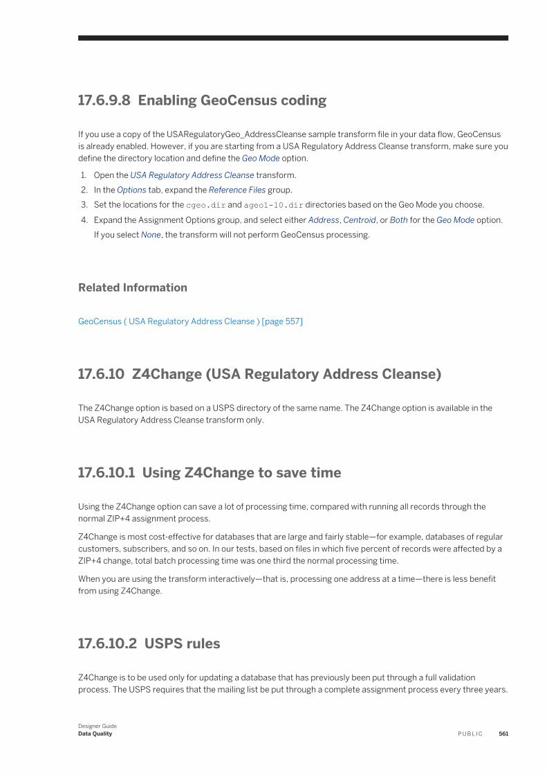
17.6.9.8 Enabling GeoCensus coding
If you use a copy of the USARegulatoryGeo_AddressCleanse sample transform file in your data flow, GeoCensus is already enabled. However, if you are starting from a USA Regulatory Address Cleanse transform, make sure you define the directory location and define the Geo Mode option.
1. Open the USA Regulatory Address Cleanse transform.2. In the Options tab, expand the Reference Files group.3. Set the locations for the cgeo.dir and ageo1-10.dir directories based on the Geo Mode you choose.
4. Expand the Assignment Options group, and select either Address, Centroid, or Both for the Geo Mode option.If you select None, the transform will not perform GeoCensus processing.
Related Information
GeoCensus ( USA Regulatory Address Cleanse ) [page 557]
17.6.10 Z4Change (USA Regulatory Address Cleanse)
The Z4Change option is based on a USPS directory of the same name. The Z4Change option is available in the USA Regulatory Address Cleanse transform only.
17.6.10.1 Using Z4Change to save time
Using the Z4Change option can save a lot of processing time, compared with running all records through the normal ZIP+4 assignment process.
Z4Change is most cost-effective for databases that are large and fairly stable—for example, databases of regular customers, subscribers, and so on. In our tests, based on files in which five percent of records were affected by a ZIP+4 change, total batch processing time was one third the normal processing time.
When you are using the transform interactively—that is, processing one address at a time—there is less benefit from using Z4Change.
17.6.10.2 USPS rules
Z4Change is to be used only for updating a database that has previously been put through a full validation process. The USPS requires that the mailing list be put through a complete assignment process every three years.
Designer GuideData Quality P U B L I C 561
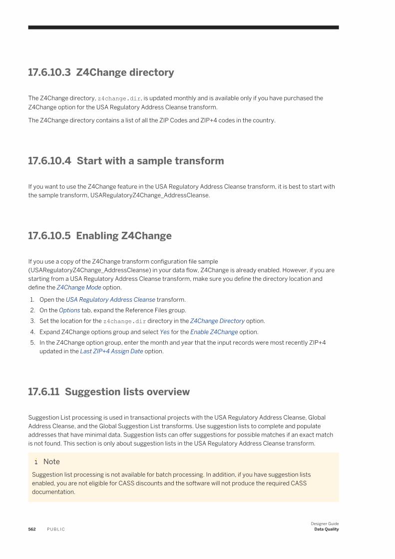
17.6.10.3 Z4Change directory
The Z4Change directory, z4change.dir, is updated monthly and is available only if you have purchased the Z4Change option for the USA Regulatory Address Cleanse transform.
The Z4Change directory contains a list of all the ZIP Codes and ZIP+4 codes in the country.
17.6.10.4 Start with a sample transform
If you want to use the Z4Change feature in the USA Regulatory Address Cleanse transform, it is best to start with the sample transform, USARegulatoryZ4Change_AddressCleanse.
17.6.10.5 Enabling Z4Change
If you use a copy of the Z4Change transform configuration file sample (USARegulatoryZ4Change_AddressCleanse) in your data flow, Z4Change is already enabled. However, if you are starting from a USA Regulatory Address Cleanse transform, make sure you define the directory location and define the Z4Change Mode option.
1. Open the USA Regulatory Address Cleanse transform.2. On the Options tab, expand the Reference Files group.3. Set the location for the z4change.dir directory in the Z4Change Directory option.
4. Expand Z4Change options group and select Yes for the Enable Z4Change option.5. In the Z4Change option group, enter the month and year that the input records were most recently ZIP+4
updated in the Last ZIP+4 Assign Date option.
17.6.11 Suggestion lists overview
Suggestion List processing is used in transactional projects with the USA Regulatory Address Cleanse, Global Address Cleanse, and the Global Suggestion List transforms. Use suggestion lists to complete and populate addresses that have minimal data. Suggestion lists can offer suggestions for possible matches if an exact match is not found. This section is only about suggestion lists in the USA Regulatory Address Cleanse transform.
NoteSuggestion list processing is not available for batch processing. In addition, if you have suggestion lists enabled, you are not eligible for CASS discounts and the software will not produce the required CASS documentation.
562 P U B L I CDesigner Guide
Data Quality
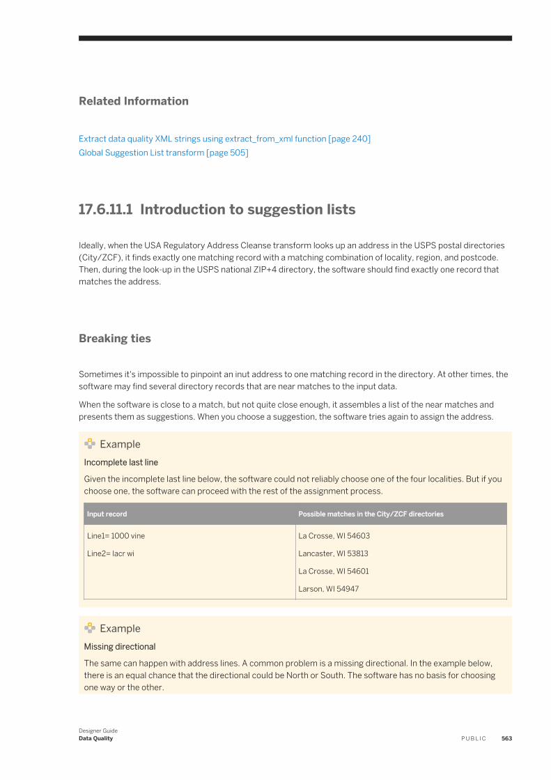
Related Information
Extract data quality XML strings using extract_from_xml function [page 240]Global Suggestion List transform [page 505]
17.6.11.1 Introduction to suggestion lists
Ideally, when the USA Regulatory Address Cleanse transform looks up an address in the USPS postal directories (City/ZCF), it finds exactly one matching record with a matching combination of locality, region, and postcode. Then, during the look-up in the USPS national ZIP+4 directory, the software should find exactly one record that matches the address.
Breaking ties
Sometimes it's impossible to pinpoint an inut address to one matching record in the directory. At other times, the software may find several directory records that are near matches to the input data.
When the software is close to a match, but not quite close enough, it assembles a list of the near matches and presents them as suggestions. When you choose a suggestion, the software tries again to assign the address.
ExampleIncomplete last line
Given the incomplete last line below, the software could not reliably choose one of the four localities. But if you choose one, the software can proceed with the rest of the assignment process.
Input record Possible matches in the City/ZCF directories
Line1= 1000 vine
Line2= lacr wi
La Crosse, WI 54603
Lancaster, WI 53813
La Crosse, WI 54601
Larson, WI 54947
ExampleMissing directional
The same can happen with address lines. A common problem is a missing directional. In the example below, there is an equal chance that the directional could be North or South. The software has no basis for choosing one way or the other.
Designer GuideData Quality P U B L I C 563
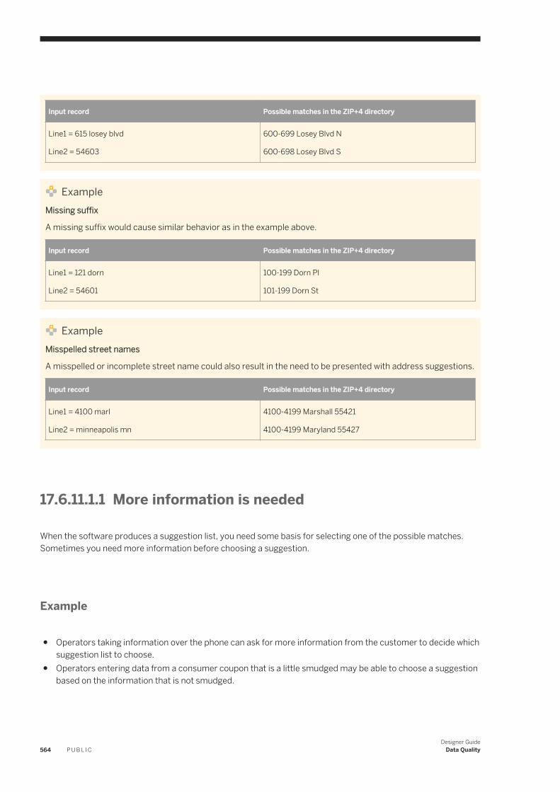
Input record Possible matches in the ZIP+4 directory
Line1 = 615 losey blvd
Line2 = 54603
600-699 Losey Blvd N
600-698 Losey Blvd S
ExampleMissing suffix
A missing suffix would cause similar behavior as in the example above.
Input record Possible matches in the ZIP+4 directory
Line1 = 121 dorn
Line2 = 54601
100-199 Dorn Pl
101-199 Dorn St
ExampleMisspelled street names
A misspelled or incomplete street name could also result in the need to be presented with address suggestions.
Input record Possible matches in the ZIP+4 directory
Line1 = 4100 marl
Line2 = minneapolis mn
4100-4199 Marshall 55421
4100-4199 Maryland 55427
17.6.11.1.1 More information is needed
When the software produces a suggestion list, you need some basis for selecting one of the possible matches. Sometimes you need more information before choosing a suggestion.
Example
● Operators taking information over the phone can ask for more information from the customer to decide which suggestion list to choose.
● Operators entering data from a consumer coupon that is a little smudged may be able to choose a suggestion based on the information that is not smudged.
564 P U B L I CDesigner Guide
Data Quality
17.6.11.1.2 CASS rule
The USPS does not permit SAP Data Services to generate a USPS Form 3553 when suggestion lists are used in address assignment. The USPS suspects that users may be tempted to guess, which may result in misrouted mail that is expensive for the USPS to handle.
Therefore, when you use the suggestion list feature, you cannot get a USPS Form 3553 covering the addresses that you assign. The form is available only when you process in batch mode with the Disable Certification option set to No.
You must run addresses from real-time processes through a batch process in order to be CASS compliant. Then the software generates a USPS Form 3553 that covers your entire mailing database, and your list may be eligible for postal discounts.
17.6.11.1.3 Integrating functionality
Suggestion Lists functionality is designed to be integrated into your own custom applications via the Web Service. For information about integrating Data Services for web applications, see the Integrator Guide.
17.6.11.1.4 Sample suggestion lists blueprint
If you want to use the suggestion lists feature, it is best to start with one of the sample transforms configured for it. The sample transform is named USARegulatorySuggestions_Address_Cleanse. It is available for the USA Regulatory Address Cleanse transform.
17.6.12 Multiple data source statistics reporting
Statistics based on logical groups
For the USA Regulatory Address Cleanse transform, an input database can be a compilation of lists, with each list containing a field that includes a unique identifier. The unique identifier can be a name or a number, but it must reside in the same field across all lists.
The software collects statistics for each list using the Data_Source_ID input field. You map the field that contains the unique identifier in your list to the software's Data_Source_ID input field. When the software generates reports, some of the reports will contain a summary for the entire list, and a separate summary per list based on the value mapped into the Data_Source_ID field.
RestrictionFor compliance with NCOALink reporting restrictions, the USA Regulatory Address Cleanse transform does not support processing multiple mailing lists associated with different PAFs. Therefore, for NCOALink processing,
Designer GuideData Quality P U B L I C 565
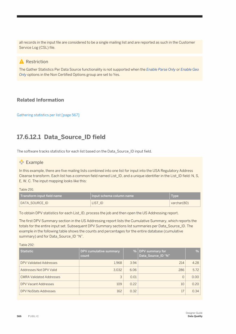
all records in the input file are considered to be a single mailing list and are reported as such in the Customer Service Log (CSL) file.
RestrictionThe Gather Statistics Per Data Source functionality is not supported when the Enable Parse Only or Enable Geo Only options in the Non Certified Options group are set to Yes.
Related Information
Gathering statistics per list [page 567]
17.6.12.1 Data_Source_ID field
The software tracks statistics for each list based on the Data_Source_ID input field.
ExampleIn this example, there are five mailing lists combined into one list for input into the USA Regulatory Address Cleanse transform. Each list has a common field named List_ID, and a unique identifier in the List_ID field: N, S, E, W, C. The input mapping looks like this:
Table 291:
Transform input field name Input schema column name Type
DATA_SOURCE_ID LIST_ID varchar(80)
To obtain DPV statistics for each List_ID, process the job and then open the US Addressing report.
The first DPV Summary section in the US Addressing report lists the Cumulative Summary, which reports the totals for the entire input set. Subsequent DPV Summary sections list summaries per Data_Source_ID. The example in the following table shows the counts and percentages for the entire database (cumulative summary) and for Data_Source_ID “N”.
Table 292:
Statistic DPV cumulative summary count
% DPV summary for Data_Source_ID “N”
%
DPV Validated Addresses 1,968 3.94 214 4.28
Addresses Not DPV Valid 3,032 6.06 286 5.72
CMRA Validated Addresses 3 0.01 0 0.00
DPV Vacant Addresses 109 0.22 10 0.20
DPV NoStats Addresses 162 0.32 17 0.34
566 P U B L I CDesigner Guide
Data Quality
Related Information
Group statistics reports [page 569]
17.6.12.2 Gathering statistics per list
Before setting up the USA Regulatory Address Cleanse transform to gather statistics per list, identify the field that uniquely identifies each list. For example, a mailing list that is comprised of more than one source might contain lists that have a field named LIST_ID that uniquely identifies each list.
1. Open the USA Regulatory Address Cleanse transform in the data flow and then click the Options tab.2. Expand the Report and Analysis group and select Yes for the Generate Report Data and the Gather Statistics
Per Data Source options.3. Click the Input tab and click the Input Schema Column Name field next to the Data_Source_ID field for
uniquely identifying a list.A drop menu appears.
4. Click the drop menu and select the input field from your database that you've chosen as the common field for uniquely identifying a list. In the scenario above, that would be the LIST_ID field.
5. Continue with the remaining job setup tasks and execute your job.
17.6.12.3 Physical Source Field and Cumulative Summary
Some reports include a report per list based on the Data_Source_ID field (identified in the report footer by “Physical Source Field”), and a summary of the entire list (identified in the report footer by “Cumulative Summary”). However, the Address Standardization, Address Information Code, and USA Regulatory Locking reports do not include a Cumulative Summary. The records in these reports are sorted by the Data Source ID value.
NoteWhen you enable NCOALink, the software reports a summary per list only for the following sections of the NCOALink Processing Summary Report:
● NCOALink Move Type Summary● NCOALink Return Code Summary● ANKLink Return Code Summary
Special circumstances
There are some circumstances when the words “Cumulative Summary” and“ Physical Source Field” will not appear in the report footer sections.
Designer GuideData Quality P U B L I C 567
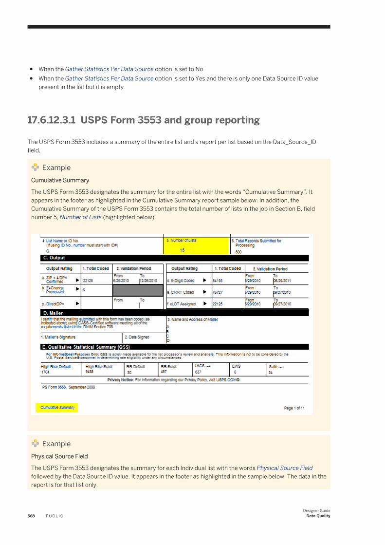
● When the Gather Statistics Per Data Source option is set to No● When the Gather Statistics Per Data Source option is set to Yes and there is only one Data Source ID value
present in the list but it is empty
17.6.12.3.1 USPS Form 3553 and group reporting
The USPS Form 3553 includes a summary of the entire list and a report per list based on the Data_Source_ID field.
ExampleCumulative Summary
The USPS Form 3553 designates the summary for the entire list with the words “Cumulative Summary”. It appears in the footer as highlighted in the Cumulative Summary report sample below. In addition, the Cumulative Summary of the USPS Form 3553 contains the total number of lists in the job in Section B, field number 5, Number of Lists (highlighted below).
ExamplePhysical Source Field
The USPS Form 3553 designates the summary for each Individual list with the words Physical Source Field followed by the Data Source ID value. It appears in the footer as highlighted in the sample below. The data in the report is for that list only.
568 P U B L I CDesigner Guide
Data Quality
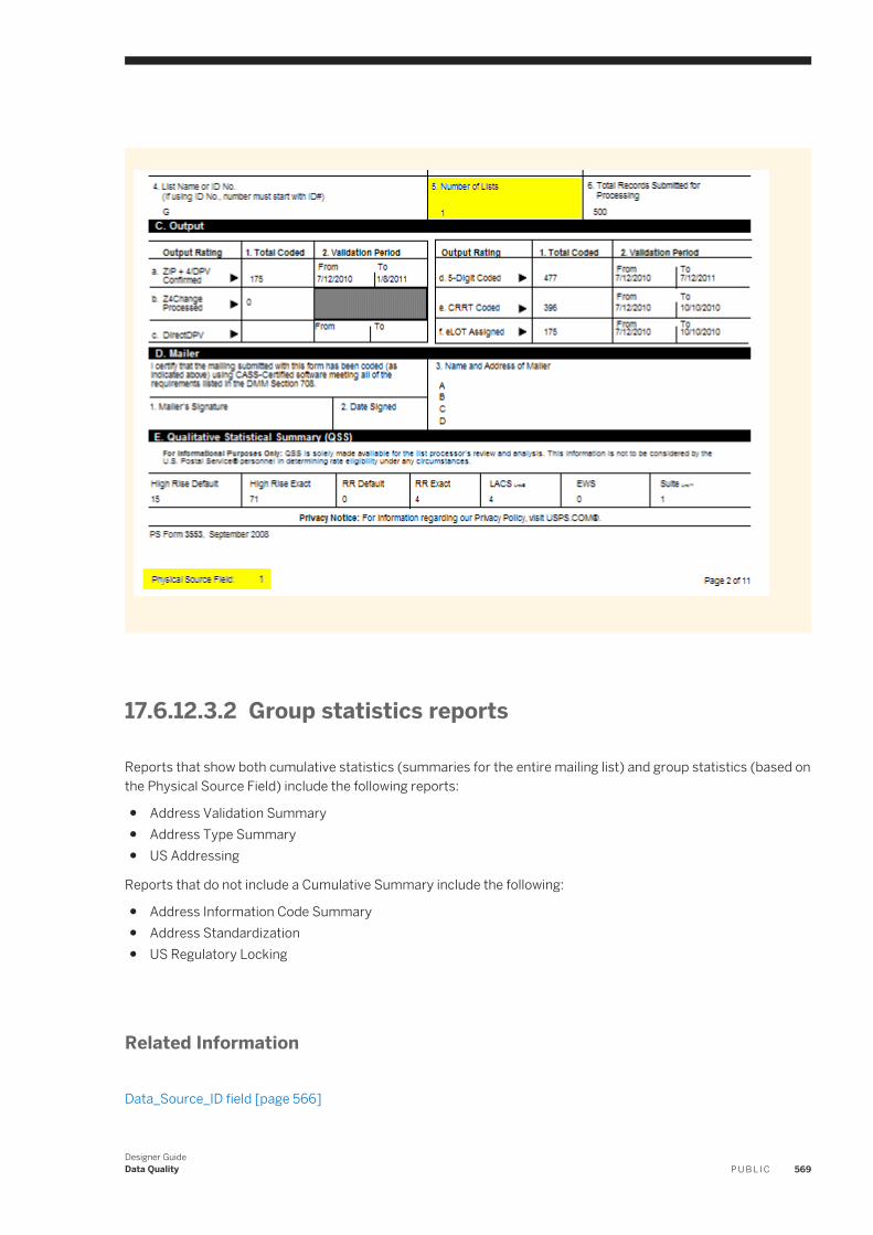
17.6.12.3.2 Group statistics reports
Reports that show both cumulative statistics (summaries for the entire mailing list) and group statistics (based on the Physical Source Field) include the following reports:
● Address Validation Summary● Address Type Summary● US Addressing
Reports that do not include a Cumulative Summary include the following:
● Address Information Code Summary● Address Standardization● US Regulatory Locking
Related Information
Data_Source_ID field [page 566]
Designer GuideData Quality P U B L I C 569
17.7 Data quality statistics repository tables
You can generate data quality statistics for the Data Cleanse, Geocoder, and Global Address Cleanse transforms.
When you enable the data quality statistics settings in the transform and run your job, the software sends statistics to tables in the repository. Based on the table you choose to generate, the statistics contain summary and non-summary information about the cleansing and assignment processes.
There are two main reasons for generating and using the data quality statistics:
● To view aggregated results and summary information about the quality of your data.● To drill into specific records that the software identified as low quality.
Enable data quality statistics tables in the applicable transform by making settings in the Data Quality Statistics Settings group under Report and Analysis.
Related Information
About cleansing data [page 346]Geocoding [page 376]Cleansing global address data [page 480]
17.8 Data Quality support for native data types
The Data Quality transforms generally process incoming data types as character data. Therefore, if a noncharacter data type is mapped as input, the software converts the data to a character string before passing it through the Data Quality transforms.
Some Data Quality data types are recognized and processed as the same data type as they were input. For example, if a date type field is mapped to a Data Quality date type input field, the software has the following advantages:
● Sortation: The transform recognizes and sorts the incoming data as the specified data type.● Efficiency: The amount of data being converted to character data is reduced making processing more
efficient.
17.8.1 Data Quality data type definitions
The Data Quality transforms have four field attributes to define the field:
● Name● Type● Length
570 P U B L I CDesigner Guide
Data Quality
● Scale
These attributes are listed in the Input and output tab of the transform editor.
In the Input tab, the attribute Name is listed under the Transform Input Field Name column. The Type, Length, and Scale attributes are listed under the Type column in the format <type>(<length>, <scale>).
The Output tab also contains the four field attributes listed above. The attribute Name is listed under the Field_Name column. The Type, Length, and Scale attributes are listed under the Type column in the format <type>(<length>, <scale>).
17.9 Data Quality support for NULL values
The Data Quality transforms process NULL values as NULL.
A field that is NULL is passed through processing with the NULL marker preserved unless there is data available to populate the field on output. When there is data available, the field is output with the data available instead of NULL. The benefit of this treatment of NULL is that the Data Quality transforms treat a NULL marker as unknown instead of empty.
NoteIf all fields of a record contain NULL, the transform will not process the record, and the record will not be a part of statistics and reports.
Designer GuideData Quality P U B L I C 571
18 Design and Debug
This section covers the following Designer features that you can use to design and debug jobs:
● Use the View Where Used feature to determine the impact of editing a metadata object (for example, at table). See which data flows use the same object.
● Use the View Data feature to view sample source, transform, and target data in a data flow after a job executes.
● Use the Design-Time Data Viewer feature to view and analyze the input and output for a data set in real time as you design a transform.
● Use the Interactive Debugger to set breakpoints and filters between transforms within a data flow and view job data row-by-row during a job execution.
● Use the Difference Viewer to compare the metadata for similar objects and their properties.● Use the auditing data flow feature to verify that correct data is processed by a source, transform, or target
object.
Related Information
Using View Where Used [page 572]Using View Data [page 576]Using the Design-Time Data Viewer [page 588]Using the interactive debugger [page 589]Comparing Objects [page 603]Using Auditing [page 332]
18.1 Using View Where Used
When you save a job, work flow, or data flow the software saves a list of related objects in your repository.
The software preserves parent-child relationship data. You can view relationships using the Tools menu ( ToolsView Where Used ). You can also access the information by clicking the View Where Used icon in the tool bar.
For example, when the following parent data flow is saved, the software also saves connections between it and its three children:
● a table source● a query transform● a file target
572 P U B L I CDesigner Guide
Design and Debug

You can use this parent/child relationship data to determine what impact a potential change will have on the other data flows that use the same object.
For example, while maintaining a data flow, you may need to delete a source table definition and re-import the table (or edit the table schema). Before doing this, find all the data flows that are using the same table and update them as needed.
The Designer counts an object's usage as the number of times it is used for a unique purpose.
For example, in a data flow named DF1, if table DEPT is used as a source twice and a target once, the number in the Usage column in the object library is 2. This occurrence should be rare. For example, a table is not often joined to itself in a job design
Related Information
Limitations [page 576]
18.1.1 Accessing View Where Used from the object library
The Designer object library contains a Usage column that shows the number of parent-child relationship for an object.
View parent-child relationships for the following object types:
● Jobs● Work flows● Data flows● Transforms (Data Quality, Text Data Processing, and ABAP transforms in Platform folder)● Datastores● Formats
When the usage value is greater than zero, there is relationship information available for you to view.
Designer GuideDesign and Debug P U B L I C 573
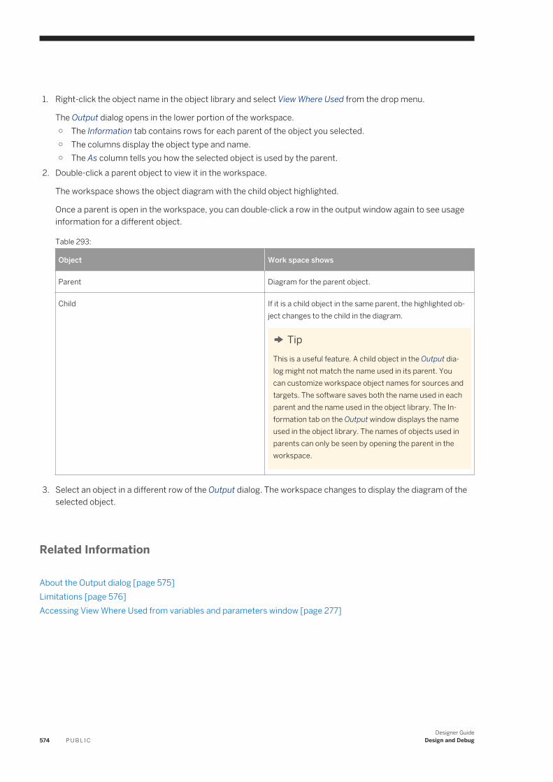
1. Right-click the object name in the object library and select View Where Used from the drop menu.
The Output dialog opens in the lower portion of the workspace.○ The Information tab contains rows for each parent of the object you selected.○ The columns display the object type and name.○ The As column tells you how the selected object is used by the parent.
2. Double-click a parent object to view it in the workspace.
The workspace shows the object diagram with the child object highlighted.
Once a parent is open in the workspace, you can double-click a row in the output window again to see usage information for a different object.
Table 293:
Object Work space shows
Parent Diagram for the parent object.
Child If it is a child object in the same parent, the highlighted object changes to the child in the diagram.
TipThis is a useful feature. A child object in the Output dialog might not match the name used in its parent. You can customize workspace object names for sources and targets. The software saves both the name used in each parent and the name used in the object library. The Information tab on the Output window displays the name used in the object library. The names of objects used in parents can only be seen by opening the parent in the workspace.
3. Select an object in a different row of the Output dialog. The workspace changes to display the diagram of the selected object.
Related Information
About the Output dialog [page 575]Limitations [page 576]Accessing View Where Used from variables and parameters window [page 277]
574 P U B L I CDesigner Guide
Design and Debug
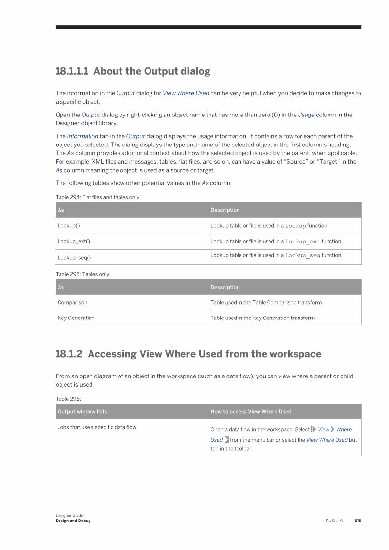
18.1.1.1 About the Output dialog
The information in the Output dialog for View Where Used can be very helpful when you decide to make changes to a specific object.
Open the Output dialog by right-clicking an object name that has more than zero (0) in the Usage column in the Designer object library.
The Information tab in the Output dialog displays the usage information. It contains a row for each parent of the object you selected. The dialog displays the type and name of the selected object in the first column's heading. The As column provides additional context about how the selected object is used by the parent, when applicable. For example, XML files and messages, tables, flat files, and so on, can have a value of “Source” or “Target” in the As column meaning the object is used as a source or target.
The following tables show other potential values in the As column.
Table 294: Flat files and tables only
As Description
Lookup() Lookup table or file is used in a lookup function
Lookup_ext() Lookup table or file is used in a lookup_ext function
Lookup_seq() Lookup table or file is used in a lookup_seq function
Table 295: Tables only
As Description
Comparison Table used in the Table Comparison transform
Key Generation Table used in the Key Generation transform
18.1.2 Accessing View Where Used from the workspace
From an open diagram of an object in the workspace (such as a data flow), you can view where a parent or child object is used.
Table 296:
Output window lists How to access View Where Used
Jobs that use a specific data flow Open a data flow in the workspace. Select View Where
Used from the menu bar or select the View Where Used button in the toolbar.
Designer GuideDesign and Debug P U B L I C 575
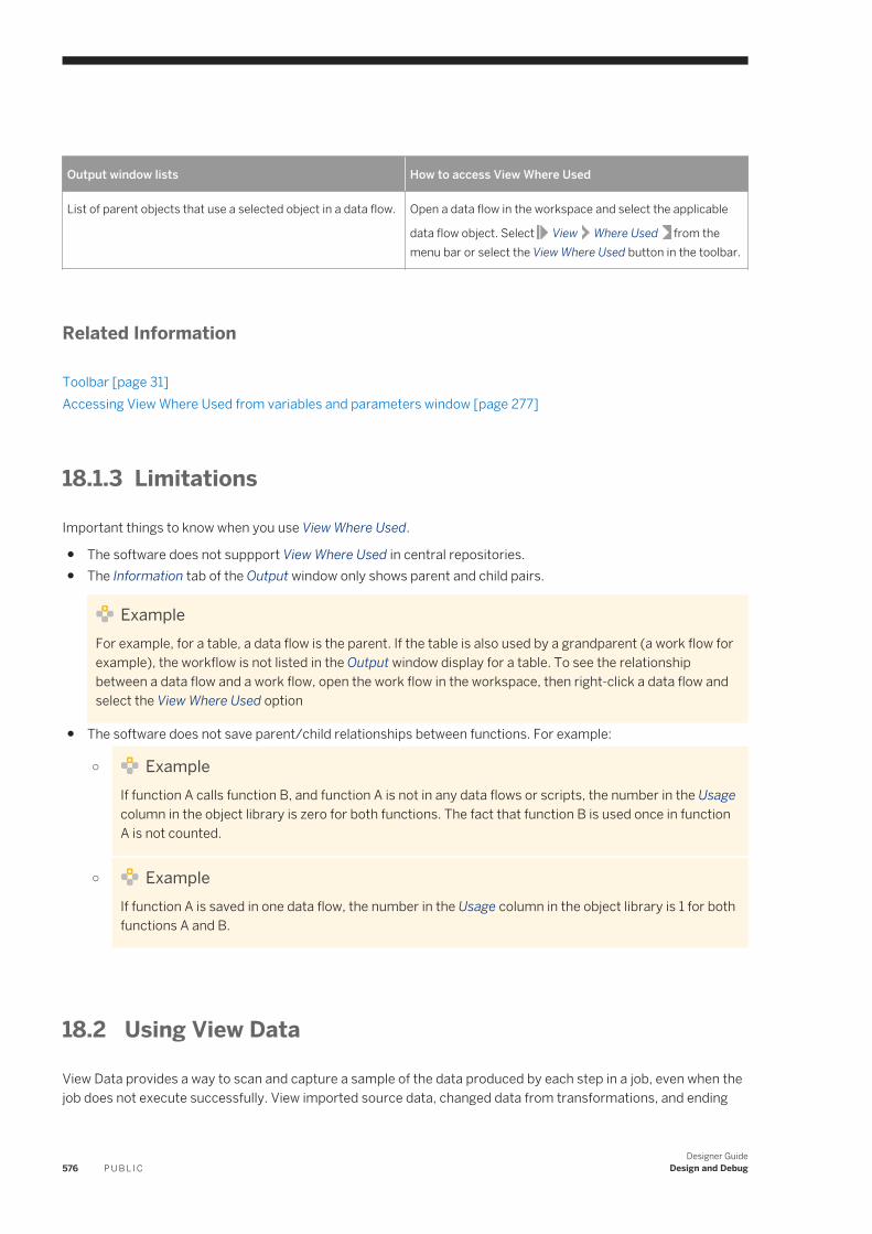
Output window lists How to access View Where Used
List of parent objects that use a selected object in a data flow. Open a data flow in the workspace and select the applicable
data flow object. Select View Where Used from the menu bar or select the View Where Used button in the toolbar.
Related Information
Toolbar [page 31]Accessing View Where Used from variables and parameters window [page 277]
18.1.3 Limitations
Important things to know when you use View Where Used.
● The software does not suppport View Where Used in central repositories.● The Information tab of the Output window only shows parent and child pairs.
ExampleFor example, for a table, a data flow is the parent. If the table is also used by a grandparent (a work flow for example), the workflow is not listed in the Output window display for a table. To see the relationship between a data flow and a work flow, open the work flow in the workspace, then right-click a data flow and select the View Where Used option
● The software does not save parent/child relationships between functions. For example:
○ ExampleIf function A calls function B, and function A is not in any data flows or scripts, the number in the Usage column in the object library is zero for both functions. The fact that function B is used once in function A is not counted.
○ ExampleIf function A is saved in one data flow, the number in the Usage column in the object library is 1 for both functions A and B.
18.2 Using View Data
View Data provides a way to scan and capture a sample of the data produced by each step in a job, even when the job does not execute successfully. View imported source data, changed data from transformations, and ending
576 P U B L I CDesigner Guide
Design and Debug
data at your targets. At any point after you import a data source, you can check on the status of that data—before and after processing your data flows.
Use View Data to check the data while designing and testing jobs to ensure that your design returns the results you expect. Using one or more View Data panes, you can view and compare sample data from different steps. View Data information is displayed in embedded panels for easy navigation between your flows and the data.
Use View Data to look at:
● Sources and targetsView Data allows you to see data before you execute a job. Armed with data details, you can create higher quality job designs. You can scan and analyze imported table and file data from the object library as well as see the data for those same objects within existing jobs. After you execute the job, you can refer back to the source data again.
● Transforms● Lines in a diagram
Note● View Data displays blob data as <blob>.● View Data is not supported for SAP IDocs. For SAP and PeopleSoft, the Table Profile tab and Column
Profile tab options are not supported for hierarchies.
Related Information
Viewing data passed by transforms [page 601]Using the interactive debugger [page 589]
18.2.1 Accessing View Data
18.2.1.1 Viewing data for sources and targets
You can view data for sources and targets from two different locations:
1. View Data button
View Data buttons appear on source and target objects when you drag them into the workspace. Click the View data button (magnifying glass icon) to open a View Data pane for that source or target object.
2. Object library
View Data in potential source or target objects from the Datastores or Formats tabs.
Open a View Data pane from the object library in one of the following ways:
○ Right-click a table object and select View Data.○ Right-click a table and select Open or Properties.
The Table Metadata, XML Format Editor, or Properties window opens. From any of these windows, you can select the View Data tab.
Designer GuideDesign and Debug P U B L I C 577
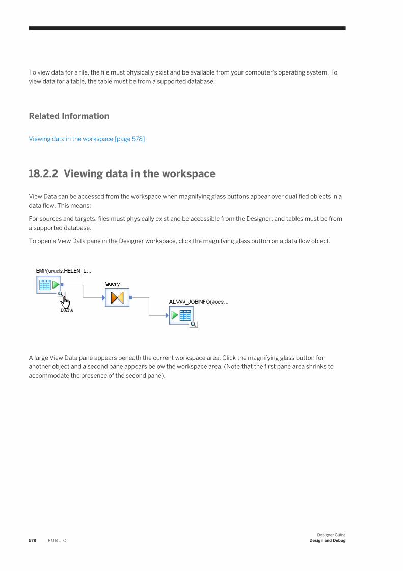
To view data for a file, the file must physically exist and be available from your computer's operating system. To view data for a table, the table must be from a supported database.
Related Information
Viewing data in the workspace [page 578]
18.2.2 Viewing data in the workspace
View Data can be accessed from the workspace when magnifying glass buttons appear over qualified objects in a data flow. This means:
For sources and targets, files must physically exist and be accessible from the Designer, and tables must be from a supported database.
To open a View Data pane in the Designer workspace, click the magnifying glass button on a data flow object.
A large View Data pane appears beneath the current workspace area. Click the magnifying glass button for another object and a second pane appears below the workspace area. (Note that the first pane area shrinks to accommodate the presence of the second pane).
578 P U B L I CDesigner Guide
Design and Debug
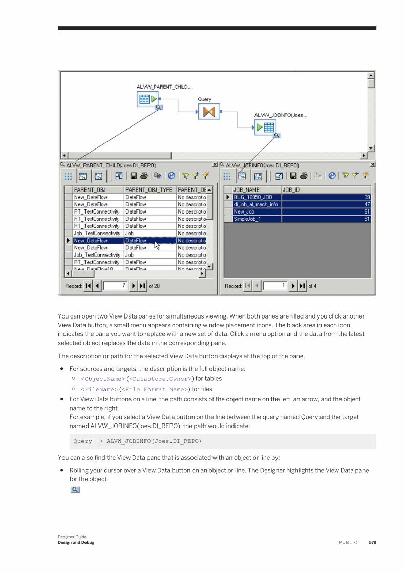
You can open two View Data panes for simultaneous viewing. When both panes are filled and you click another View Data button, a small menu appears containing window placement icons. The black area in each icon indicates the pane you want to replace with a new set of data. Click a menu option and the data from the latest selected object replaces the data in the corresponding pane.
The description or path for the selected View Data button displays at the top of the pane.
● For sources and targets, the description is the full object name:○ <ObjectName> (<Datastore.Owner>) for tables○ <FileName> (<File Format Name>) for files
● For View Data buttons on a line, the path consists of the object name on the left, an arrow, and the object name to the right.For example, if you select a View Data button on the line between the query named Query and the target named ALVW_JOBINFO(joes.DI_REPO), the path would indicate:
Query -> ALVW_JOBINFO(Joes.DI_REPO)
You can also find the View Data pane that is associated with an object or line by:
● Rolling your cursor over a View Data button on an object or line. The Designer highlights the View Data pane for the object.
Designer GuideDesign and Debug P U B L I C 579
● Looking for grey View Data buttons on objects and lines. The Designer displays View Data buttons on open objects with grey rather than white backgrounds.
Related Information
Viewing data passed by transforms [page 601]
18.2.3 View Data Properties
You can access View Data properties from tool bar buttons or the right-click menu.
View Data displays your data in the rows and columns of a data grid. The number of rows displayed is determined by a combination of several conditions:
● Sample size — The number of rows sampled in memory. Default sample size is 1000 rows for imported source and target objects. Maximum sample size is 5000 rows. Set sample size for sources and targets from
Tools Options Designer General View Data sampling size .When using the interactive debugger, the software uses the Data sample rate option instead of sample size.
● Filtering● Sorting
If your original data set is smaller or if you use filters, the number of returned rows could be less than the default.
You can see which conditions have been applied in the navigation bar.
Related Information
Filtering [page 580]Sorting [page 582]Starting and stopping the interactive debugger [page 593]
18.2.3.1 Filtering
You can focus on different sets of rows in a local or new data sample by placing fetch conditions on columns.
18.2.3.1.1 Viewing and adding filters
1. In the View Data tool bar, click the Filters button, or right-click the grid and select Filters.
580 P U B L I CDesigner Guide
Design and Debug
The Filters window opens.2. Create filters.
The Filters window has three columns:
a. Column—Select a name from the first column. Select {remove filter} to delete the filter.b. Operator—Select an operator from the second column.c. Value—Enter a value in the third column that uses one of the following data type formats
Table 297:
Data Type Format
Integer, double, real standard
date yyyy.mm.dd
time hh24:mm:ss
datetime yyyy.mm.dd hh24:mm.ss
varchar 'abc'
3. In the Concatenate all filters using list box, select an operator (AND, OR) for the engine to use in concatenating filters.
Each row in this window is considered a filter.4. To see how the filter affects the current set of returned rows, click Apply.5. To save filters and close the Filters window, click OK.
Your filters are saved for the current object and the local sample updates to show the data filtered as specified in the Filters dialog. To use filters with a new sample, see Using Refresh.
Related Information
Using Refresh [page 582]
18.2.3.1.2 Adding a filter for a selected cell
1. Select a cell from the sample data grid.
2. In the View Data tool bar, click the Add Filter button, or right-click the cell and select Add Filter.
The Add Filter option adds the new filter condition, <column> = <cell value>, then opens the Filters window so you can view or edit the new filter.
3. When you are finished, click OK.
Designer GuideDesign and Debug P U B L I C 581
To remove filters from an object, go to the View Data tool bar and click the Remove Filters button, or right-click the grid and select Remove Filters. All filters are removed for the current object.
18.2.3.2 Sorting
You can click one or more column headings in the data grid to sort your data. An arrow appears on the heading to indicate sort order: ascending (up arrow) or descending (down arrow).
To change sort order, click the column heading again. The priority of a sort is from left to right on the grid.
To remove sorting for an object, from the tool bar click the Remove Sort button, or right-click the grid and select Remove Sort.
Related Information
Using Refresh [page 582]
18.2.3.3 Using Refresh
To fetch another data sample from the database using new filter and sort settings, use the Refresh command. After you edit filtering and sorting, in the tool bar click the Refresh button in the tool bar, or right-click the data grid and select Refresh.
To stop a refresh operation, click the Stop button. While the software is refreshing the data, all View Data controls except the Stop button are disabled.
18.2.3.4 Using Show/Hide Columns
You can limit the number of columns displayed in View Data by using the Show/Hide Columns option from:
● The tool bar.● The right-click menu.● The arrow shortcut menu, located to the right of the Show/Hide Columns tool bar button. This option is only
available if the total number of columns in the table is ten or fewer. Select a column to display it.
You can also "quick hide" a column by right-clicking the column heading and selecting Hide from the menu.
582 P U B L I CDesigner Guide
Design and Debug
18.2.3.4.1 Showing or hiding columns
1. Click the Show/Hide columns tool bar button, or right-click the data grid and select Show/Hide Columns.
The Column Settings window opens.2. Select the columns that you want to display or click one of the following buttons: Show, Show All, Hide, or Hide
All.3. Click OK.
18.2.3.5 Opening a new window
To see more of the data sample that you are viewing in a View Data pane, open a full-sized View Data window. From any View Data pane, click the Open Window tool bar button to activate a separate, full-sized View Data window. Alternatively, you can right-click and select Open in new window from the menu.
18.2.4 View Data tool bar options
The following options are available on View Data panes.
Table 298:
Icon Option Description
Open in new window Opens the View Data pane in a larger window.
Save As Saves the data in the View Data pane.
Print Prints View Data pane data.
Copy Cell Copies View Data pane cell data.
Refresh data Fetches another data sample from existing data in the View Data pane using new filter and sort settings.
Open Filters window Opens the Filters window.
Add a Filter Adds a filter to a selected cell.
Remove Filter Removes all filters in the View Data pane.
Designer GuideDesign and Debug P U B L I C 583
Icon Option Description
Remove Sort Removes sort settings for the object you select.
Show/hide navigation Shows or hides the navigation bar which appears below the data table.
Show/hide columns
Related Information
Opening a new window [page 583]Using Refresh [page 582]Filtering [page 580]Sorting [page 582]Adding a filter for a selected cell [page 581]Using Show/Hide Columns [page 582]
18.2.5 View Data tabs
The View Data panel for objects contains three tabs:
● Data tab● Profile tab● Column Profile tab
Use tab options to give you a complete profile of a source or target object. The Data tab is always available. The Profile and Relationship tabs are supported with the Data Profiler. Without the Data Profiler, the Profile and Column Profile tabs are supported for some sources and targets.
Related Information
Viewing the profiler results [page 323]
18.2.5.1 Data tab
The Data tab allows you to use the properties of View Data. It also indicates nested schemas such as those used in XML files and messages. When a column references nested schemas, that column is shaded yellow and a small table icon appears in the column heading.
584 P U B L I CDesigner Guide
Design and Debug
Related Information
View Data Properties [page 580]
18.2.5.1.1 Viewing a nested schema
1. Double-click a cell.
The data grid updates to show the data in the selected cell or nested table.
In the Schema area, the selected cell value is marked by a special icon. Also, tables and columns in the selected path are displayed in blue, while nested schema references are displayed in grey.
In the Data area, data is shown for columns. Nested schema references are shown in angle brackets; for example, <CompanyName>.
2. Continue to use the data grid side of the panel to navigate. For example:○ Select a lower-level nested column and double-click a cell to update the data grid.○ Click the at the top of the data grid to move up in the hierarchy.
○ See the entire path to the selected column or table displayed to the right of the Drill Up button. Use the
path and the data grid to navigate through nested schemas.
18.2.5.2 Profile tab
If you use the Data Profiler, the Profile tab displays the profile attributes that you selected on the Submit Column Profile Request option.
The Profile tab allows you to calculate statistical information for any set of columns you choose. This optional feature is not available for columns with nested schemas or for the LONG data type.
Related Information
Executing a profiler task [page 317]
Designer GuideDesign and Debug P U B L I C 585
18.2.5.2.1 Using the Profile tab without the Data Profiler
1. Select one or more columns.
Select only the column names you need for this profiling operation because Update calculations impact performance.
You can also right-click to use the Select All and Deselect All menu options.2. Click Update.3. The statistics appear in the Profile grid.
The grid contains six columns:
Table 299:
Column Description
Column Names of columns in the current table. Select names from this column, then click Update to populate the profile grid.
Distinct Values The total number of distinct values in this column.
NULLs The total number of NULL values in this column.
Min Of all values, the minimum value in this column.
Max Of all values, the maximum value in this column.
Last Updated The time that this statistic was calculated.
Sort values in this grid by clicking the column headings. Note that Min and Max columns are not sortable.
In addition to updating statistics, you can click the Records button on the Profile tab to count the total number of physical records in the object you are profiling.
The software saves previously calculated values in the repository and displays them until the next update.
18.2.5.3 Column Profile tab
The Column Profile tab allows you to calculate statistical information for a single column. If you use the Data Profiler, the Relationship tab displays instead of the Column Profile.
NoteThis optional feature is not available for columns with nested schemas or the LONG data type.
Related Information
Viewing the relationship profile data generated by the Data Profiler [page 326]
586 P U B L I CDesigner Guide
Design and Debug
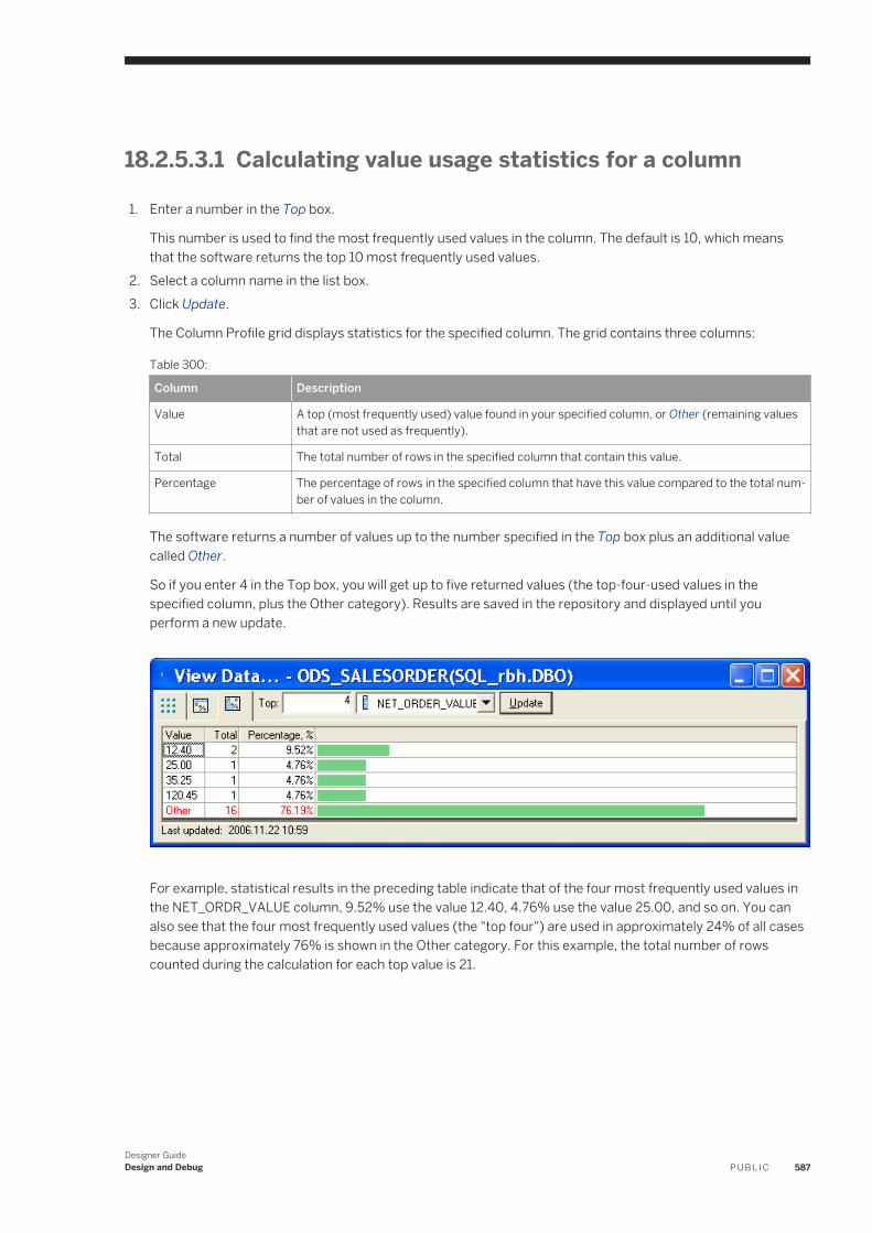
18.2.5.3.1 Calculating value usage statistics for a column
1. Enter a number in the Top box.
This number is used to find the most frequently used values in the column. The default is 10, which means that the software returns the top 10 most frequently used values.
2. Select a column name in the list box.3. Click Update.
The Column Profile grid displays statistics for the specified column. The grid contains three columns:
Table 300:
Column Description
Value A top (most frequently used) value found in your specified column, or Other (remaining values that are not used as frequently).
Total The total number of rows in the specified column that contain this value.
Percentage The percentage of rows in the specified column that have this value compared to the total number of values in the column.
The software returns a number of values up to the number specified in the Top box plus an additional value called Other.
So if you enter 4 in the Top box, you will get up to five returned values (the top-four-used values in the specified column, plus the Other category). Results are saved in the repository and displayed until you perform a new update.
For example, statistical results in the preceding table indicate that of the four most frequently used values in the NET_ORDR_VALUE column, 9.52% use the value 12.40, 4.76% use the value 25.00, and so on. You can also see that the four most frequently used values (the "top four") are used in approximately 24% of all cases because approximately 76% is shown in the Other category. For this example, the total number of rows counted during the calculation for each top value is 21.
Designer GuideDesign and Debug P U B L I C 587
18.3 Using the Design-Time Data Viewer
The Design-Time Data Viewer lets you view and analyze the input and output for a data set in real time as you design a transform. The data flow does not need to be complete or valid, although it must use a valid, accessible source that contains data.
Use the Design-Time Data Viewer to view the data while designing a transform to ensure that your design returns the results that you expect. The Design-Time Data Viewer displays as input and output panes in the transform editor so that you can compare the data before and after the transform acts on it.
To use the Design-Time Data Viewer for the Global Address Cleanse, Geocoder, and USA Regulatory Address Cleanse transforms, you must have access to the Data Quality reference data (directories).
Related Information
Viewing Design-Time Data [page 588]Configuring the Design-Time Data Viewer [page 589]
18.3.1 Viewing Design-Time Data
1. To view the input and output data for transforms in the transform editor, select Debug View Design-Time Data .
Input and output data panes open in the transform editor. Each pane may contain several tabbed views depending on how many inputs and outputs the selected transform has. For example, although most transforms have only one output, the Validation transform has three outputs.
2. To view the data for a different input or output, click the appropriate tab in the View Data pane.
3. To view the input and output data automatically after you modify a transform, select Debug View Automatically .
4. To filter the number of data rows displayed in the panes, select Debug Filter Input Dataset . Setting the filter may help increase performance while you are designing the transform and have the Design-Time Data Viewer feature set to update automatically.By default, the filter displays the first 50 rows. You can configure the number of rows that are displayed in the Options window.
5. To close the Design-Time Data Viewer panes, click the x in the upper-right corner of the pane.
Related Information
Configuring the Design-Time Data Viewer [page 589]
588 P U B L I CDesigner Guide
Design and Debug
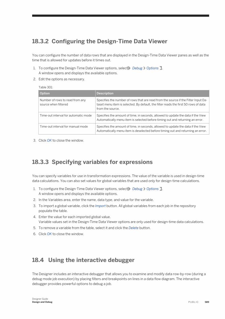
18.3.2 Configuring the Design-Time Data Viewer
You can configure the number of data rows that are displayed in the Design-Time Data Viewer panes as well as the time that is allowed for updates before it times out.
1. To configure the Design-Time Data Viewer options, select Debug Options .A window opens and displays the available options.
2. Edit the options as necessary.
Table 301:
Option Description
Number of rows to read from any source when filtered
Specifies the number of rows that are read from the source if the Filter Input Dataset menu item is selected. By default, the filter reads the first 50 rows of data from the source.
Time-out interval for automatic mode Specifies the amount of time, in seconds, allowed to update the data if the View Automatically menu item is selected before timing out and returning an error.
Time-out interval for manual mode Specifies the amount of time, in seconds, allowed to update the data if the View Automatically menu item is deselected before timing out and returning an error.
3. Click OK to close the window.
18.3.3 Specifying variables for expressions
You can specify variables for use in transformation expressions. The value of the variable is used in design-time data calculations. You can also set values for global variables that are used only for design-time calculations.
1. To configure the Design-Time Data Viewer options, select Debug Options .A window opens and displays the available options.
2. In the Variables area, enter the name, data type, and value for the variable.3. To import a global variable, click the Import button. All global variables from each job in the repository
populate the table.4. Enter the value for each imported global value.
Variable values set in the Design-Time Data Viewer options are only used for design-time data calculations.5. To remove a variable from the table, select it and click the Delete button.6. Click OK to close the window.
18.4 Using the interactive debugger
The Designer includes an interactive debugger that allows you to examine and modify data row-by-row (during a debug mode job execution) by placing filters and breakpoints on lines in a data flow diagram. The interactive debugger provides powerful options to debug a job.
Designer GuideDesign and Debug P U B L I C 589
NoteA repository upgrade is required to use this feature.
18.4.1 Before starting the interactive debugger
Like executing a job, you can start the interactive debugger from the Debug menu when a job is active in the workspace. Select Start debug, set properties for the execution, then click OK. The debug mode begins. The Debug mode provides the interactive debugger's windows, menus, and tool bar buttons that you can use to control the pace of the job and view data by pausing the job execution using filters and breakpoints.
While in debug mode, all other Designer features are set to read-only. To exit the debug mode and return other Designer features to read/write, click the Stop debug button on the interactive debugger toolbar.
All interactive debugger commands are listed in the Designer's Debug menu. The Designer enables the appropriate commands as you progress through an interactive debugging session.
Before you start a debugging session, however, you might want to set the following:
● Filters and breakpoints● Interactive debugger port between the Designer and an engine.
18.4.1.1 Setting filters and breakpoints
You can set any combination of filters and breakpoints in a data flow before you start the interactive debugger. The debugger uses the filters and pauses at the breakpoints you set.
If you do not set predefined filters or breakpoints:
● The Designer will optimize the debug job execution. This often means that the first transform in each data flow of a job is pushed down to the source database. Consequently, you cannot view the data in a job between its source and the first transform unless you set a predefined breakpoint on that line.
● You can pause a job manually by using a debug option called Pause Debug (the job pauses before it encounters the next transform).
Related Information
Push-down optimizer [page 602]
18.4.1.1.1 Setting a filter or breakpoint
1. In the workspace, open the job that you want to debug.
590 P U B L I CDesigner Guide
Design and Debug
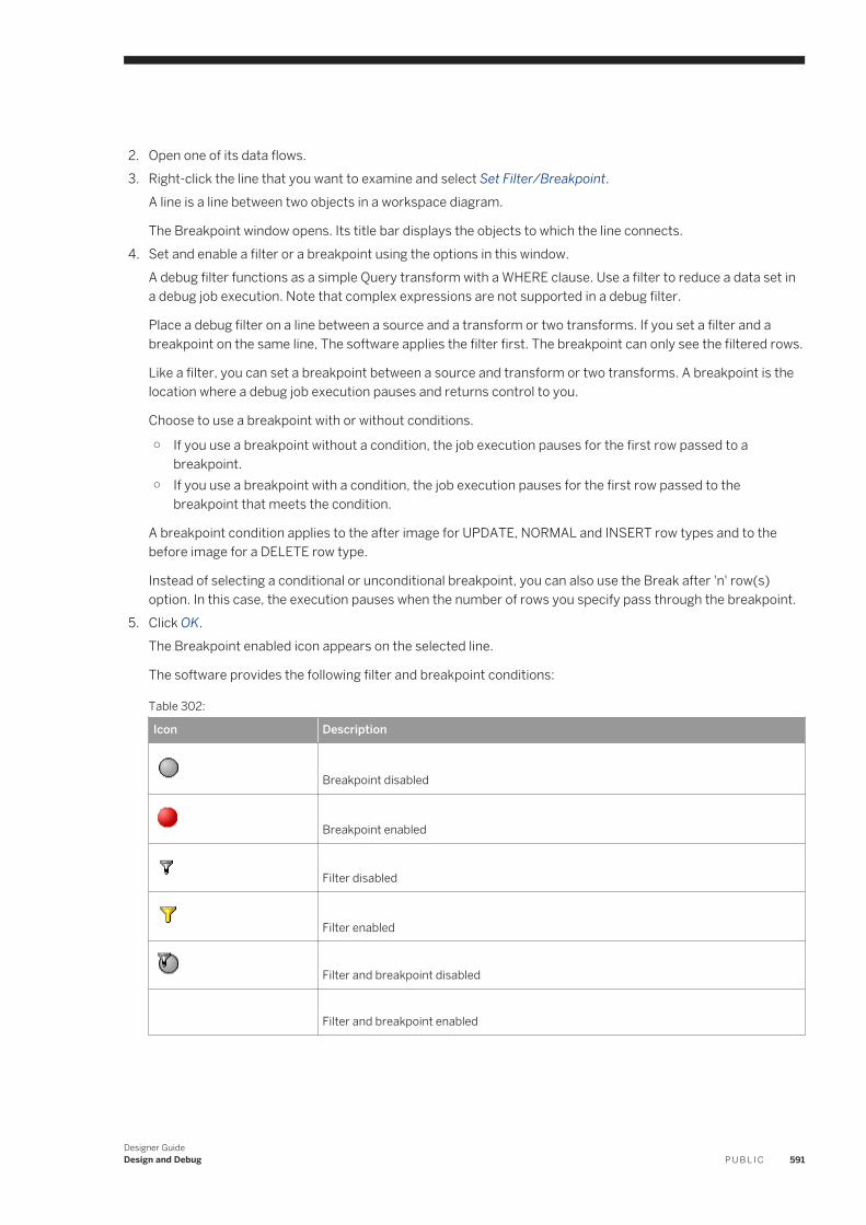
2. Open one of its data flows.3. Right-click the line that you want to examine and select Set Filter/Breakpoint.
A line is a line between two objects in a workspace diagram.
The Breakpoint window opens. Its title bar displays the objects to which the line connects.4. Set and enable a filter or a breakpoint using the options in this window.
A debug filter functions as a simple Query transform with a WHERE clause. Use a filter to reduce a data set in a debug job execution. Note that complex expressions are not supported in a debug filter.
Place a debug filter on a line between a source and a transform or two transforms. If you set a filter and a breakpoint on the same line, The software applies the filter first. The breakpoint can only see the filtered rows.
Like a filter, you can set a breakpoint between a source and transform or two transforms. A breakpoint is the location where a debug job execution pauses and returns control to you.
Choose to use a breakpoint with or without conditions.
○ If you use a breakpoint without a condition, the job execution pauses for the first row passed to a breakpoint.
○ If you use a breakpoint with a condition, the job execution pauses for the first row passed to the breakpoint that meets the condition.
A breakpoint condition applies to the after image for UPDATE, NORMAL and INSERT row types and to the before image for a DELETE row type.
Instead of selecting a conditional or unconditional breakpoint, you can also use the Break after 'n' row(s) option. In this case, the execution pauses when the number of rows you specify pass through the breakpoint.
5. Click OK.The Breakpoint enabled icon appears on the selected line.
The software provides the following filter and breakpoint conditions:
Table 302:
Icon Description
Breakpoint disabled
Breakpoint enabled
Filter disabled
Filter enabled
Filter and breakpoint disabled
Filter and breakpoint enabled
Designer GuideDesign and Debug P U B L I C 591
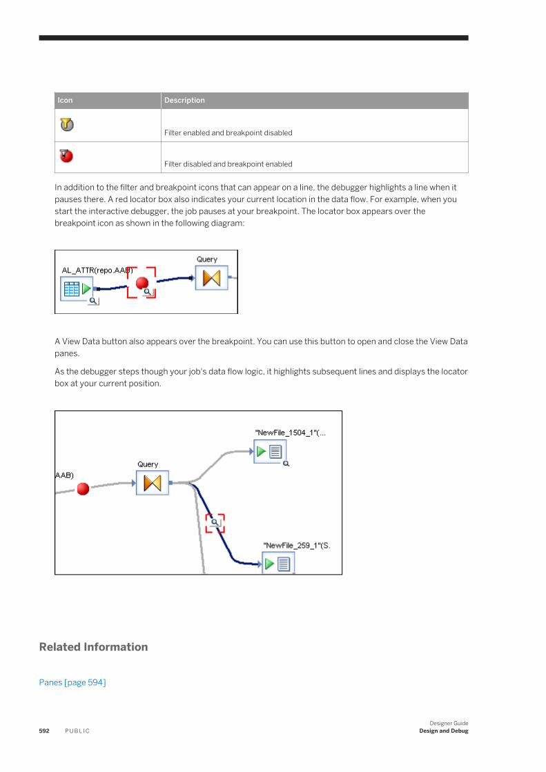
Icon Description
Filter enabled and breakpoint disabled
Filter disabled and breakpoint enabled
In addition to the filter and breakpoint icons that can appear on a line, the debugger highlights a line when it pauses there. A red locator box also indicates your current location in the data flow. For example, when you start the interactive debugger, the job pauses at your breakpoint. The locator box appears over the breakpoint icon as shown in the following diagram:
A View Data button also appears over the breakpoint. You can use this button to open and close the View Data panes.
As the debugger steps though your job's data flow logic, it highlights subsequent lines and displays the locator box at your current position.
Related Information
Panes [page 594]
592 P U B L I CDesigner Guide
Design and Debug
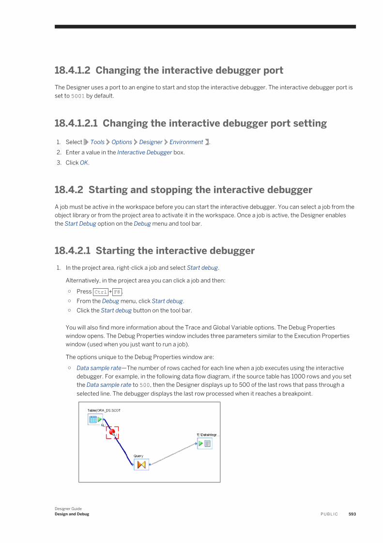
18.4.1.2 Changing the interactive debugger portThe Designer uses a port to an engine to start and stop the interactive debugger. The interactive debugger port is set to 5001 by default.
18.4.1.2.1 Changing the interactive debugger port setting1. Select Tools Options Designer Environment .2. Enter a value in the Interactive Debugger box.3. Click OK.
18.4.2 Starting and stopping the interactive debuggerA job must be active in the workspace before you can start the interactive debugger. You can select a job from the object library or from the project area to activate it in the workspace. Once a job is active, the Designer enables the Start Debug option on the Debug menu and tool bar.
18.4.2.1 Starting the interactive debugger1. In the project area, right-click a job and select Start debug.
Alternatively, in the project area you can click a job and then:
○ Press Ctrl + F8 .○ From the Debug menu, click Start debug.○ Click the Start debug button on the tool bar.
You will also find more information about the Trace and Global Variable options. The Debug Properties window opens. The Debug Properties window includes three parameters similar to the Execution Properties window (used when you just want to run a job).
The options unique to the Debug Properties window are:
○ Data sample rate—The number of rows cached for each line when a job executes using the interactive debugger. For example, in the following data flow diagram, if the source table has 1000 rows and you set the Data sample rate to 500, then the Designer displays up to 500 of the last rows that pass through a selected line. The debugger displays the last row processed when it reaches a breakpoint.
Designer GuideDesign and Debug P U B L I C 593
○ Exit the debugger when the job is finished—Click to stop the debugger and return to normal mode after the job executes. Defaults to cleared.
2. Enter the debug properties that you want to use or use the defaults.3. Click OK.
The job you selected from the project area starts to run in debug mode. The Designer:
○ Displays the interactive debugger windows.○ Adds Debugging Job <JobName> to its title bar.○ Enables the appropriate DebugThe Debug Properties window opens. The Debug menu and tool bar
options.
○ Displays the debug icon in the status bar.○ Sets the user interface to read-only.
NoteYou cannot perform any operations that affect your repository (such as dropping objects into a data flow) when you execute a job in debug mode.
When the debugger encounters a breakpoint, it pauses the job execution. You now have control of the job execution. The interactive debugger windows display information about the job execution up to this point. They also update as you manually step through the job or allow the debugger to continue the execution.
18.4.2.2 Stopping a job in debug mode and exiting the interactive debugger
Click the Stop Debug button on the tool bar, press Shift+F8, or from the Debug menu, click Stop debug.
18.4.3 Panes
When you start a job in the interactive debugger, the Designer displays three additional panes as well as the View Data panes beneath the work space. The following diagram shows the default locations for these panes.
594 P U B L I CDesigner Guide
Design and Debug
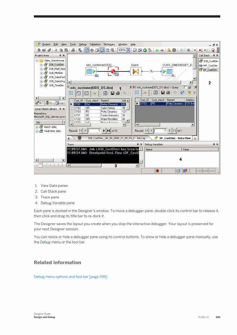
1. View Data panes2. Call Stack pane3. Trace pane4. Debug Variable pane
Each pane is docked in the Designer's window. To move a debugger pane, double-click its control bar to release it, then click and drag its title bar to re-dock it.
The Designer saves the layout you create when you stop the interactive debugger. Your layout is preserved for your next Designer session.
You can resize or hide a debugger pane using its control buttons. To show or hide a debugger pane manually, use the Debug menu or the tool bar.
Related Information
Debug menu options and tool bar [page 599]
Designer GuideDesign and Debug P U B L I C 595
18.4.3.1 Call stack window
The Call Stack window lists the objects in the path encountered so far (before either the job completes, encounters a breakpoint, or you pause it).
For example, for the job JOB_CustDim that includes a work flow and data flow, the Call Stack window might display:
JOB_CustDim
WF_CustDim
DF_CustDim
You can double-click an object in the Call Stack window to open it in the workspace. Similarly, if you click an object in a diagram, the Call Stack window highlights the object.
18.4.3.2 Trace window
The Trace window displays the debugger's output status and errors. For example:
11:22:06 AM> Job <GO> has been launched in debug mode. 11:22:07 AM> Breakpoint fired. Flow <aaa>: from <Query> to <"NewFile_773"(Simple)>
When the job completes, this window displays the following:
Job <JobName> finished. Stop debugger.
When the job completes the debugger gives you a final opportunity to examine data. When you must exit the debugger, select the Stop Debug button on the tool bar, press shift+F8, or select DebugStop Debug.
18.4.3.3 Debug Variables window
The Debug Variables window displays global variables in use by the job at each breakpoint.
18.4.3.4 View Data pane
The View Data pane for lines uses the same tool bar and navigation options described for the View Data feature.
The following View Data pane options are unique to the interactive debugger:
● Allows you to view data that passes through lines.● Displays (above the View Data tool bar) the names of objects to which a line connects using the format:
<TableName>(<DatastoreName>.<TableOwnerName>)-> <QueryName>.● Displays data one row at a time by default.● Provides the All check box which allows you to see more than one row of processed data.
596 P U B L I CDesigner Guide
Design and Debug
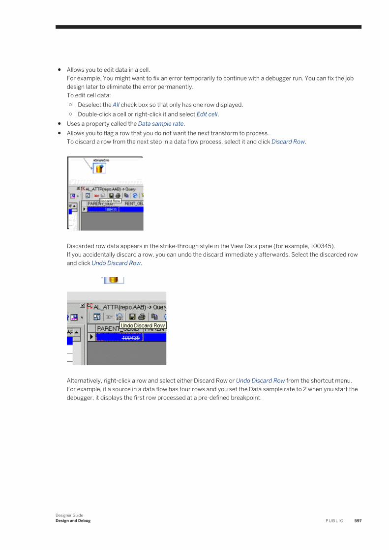
● Allows you to edit data in a cell.For example, You might want to fix an error temporarily to continue with a debugger run. You can fix the job design later to eliminate the error permanently.To edit cell data:○ Deselect the All check box so that only has one row displayed.○ Double-click a cell or right-click it and select Edit cell.
● Uses a property called the Data sample rate.● Allows you to flag a row that you do not want the next transform to process.
To discard a row from the next step in a data flow process, select it and click Discard Row.
Discarded row data appears in the strike-through style in the View Data pane (for example, 100345).If you accidentally discard a row, you can undo the discard immediately afterwards. Select the discarded row and click Undo Discard Row.
Alternatively, right-click a row and select either Discard Row or Undo Discard Row from the shortcut menu.For example, if a source in a data flow has four rows and you set the Data sample rate to 2 when you start the debugger, it displays the first row processed at a pre-defined breakpoint.
Designer GuideDesign and Debug P U B L I C 597
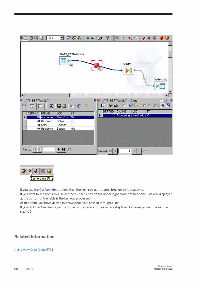
If you use the Get Next Row option, then the next row at the same breakpoint is displayed.If you want to see both rows, select the All check box on the upper-right corner of this pane. The row displayed at the bottom of the table is the last row processed.At this point, you have viewed two rows that have passed through a line.If you click Get Next Row again, only the last two rows processed are displayed because you set the sample size to 2..
Related Information
Using View Data [page 576]
598 P U B L I CDesigner Guide
Design and Debug
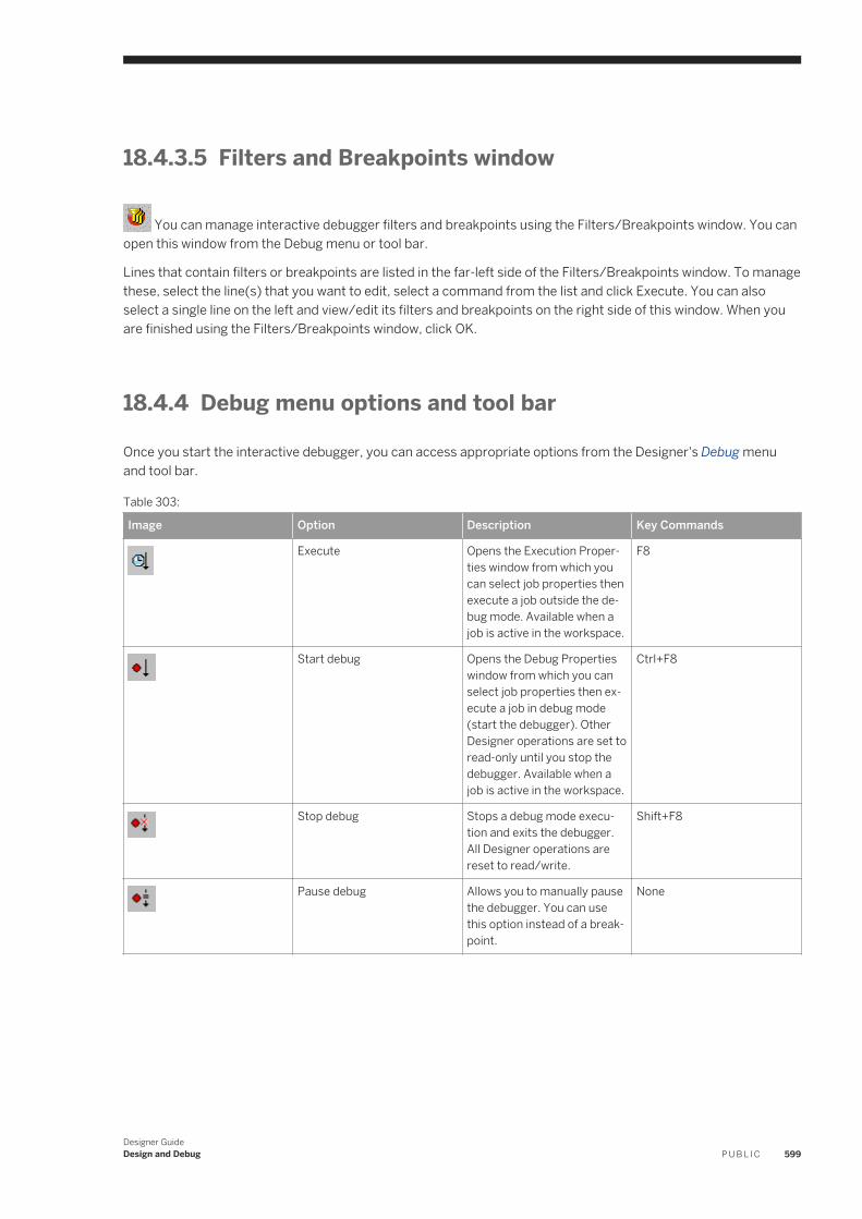
18.4.3.5 Filters and Breakpoints window
You can manage interactive debugger filters and breakpoints using the Filters/Breakpoints window. You can open this window from the Debug menu or tool bar.
Lines that contain filters or breakpoints are listed in the far-left side of the Filters/Breakpoints window. To manage these, select the line(s) that you want to edit, select a command from the list and click Execute. You can also select a single line on the left and view/edit its filters and breakpoints on the right side of this window. When you are finished using the Filters/Breakpoints window, click OK.
18.4.4 Debug menu options and tool bar
Once you start the interactive debugger, you can access appropriate options from the Designer's Debug menu and tool bar.
Table 303:
Image Option Description Key Commands
Execute Opens the Execution Properties window from which you can select job properties then execute a job outside the debug mode. Available when a job is active in the workspace.
F8
Start debug Opens the Debug Properties window from which you can select job properties then execute a job in debug mode (start the debugger). Other Designer operations are set to read-only until you stop the debugger. Available when a job is active in the workspace.
Ctrl+F8
Stop debug Stops a debug mode execution and exits the debugger. All Designer operations are reset to read/write.
Shift+F8
Pause debug Allows you to manually pause the debugger. You can use this option instead of a breakpoint.
None
Designer GuideDesign and Debug P U B L I C 599
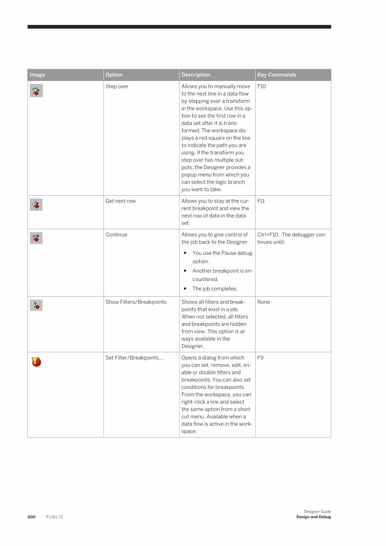
Image Option Description Key Commands
Step over Allows you to manually move to the next line in a data flow by stepping over a transform in the workspace. Use this option to see the first row in a data set after it is transformed. The workspace displays a red square on the line to indicate the path you are using. If the transform you step over has multiple outputs, the Designer provides a popup menu from which you can select the logic branch you want to take.
F10
Get next row Allows you to stay at the current breakpoint and view the next row of data in the data set.
F11
Continue Allows you to give control of the job back to the Designer
● You use the Pause debug option.
● Another breakpoint is encountered.
● The job completes.
Ctrl+F10 . The debugger continues until:
Show Filters/Breakpoints Shows all filters and breakpoints that exist in a job. When not selected, all filters and breakpoints are hidden from view. This option is always available in the Designer.
None
Set Filter/Breakpoints... Opens a dialog from which you can set, remove, edit, enable or disable filters and breakpoints. You can also set conditions for breakpoints. From the workspace, you can right-click a line and select the same option from a short cut menu. Available when a data flow is active in the workspace.
F9
600 P U B L I CDesigner Guide
Design and Debug
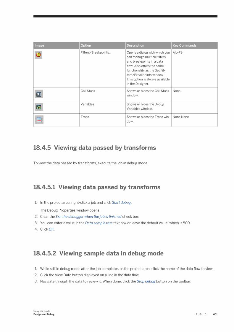
Image Option Description Key Commands
Filters/Breakpoints... Opens a dialog with which you can manage multiple filters and breakpoints in a data flow. Also offers the same functionality as the Set Filters/Breakpoints window. This option is always available in the Designer.
Alt+F9
Call Stack Shows or hides the Call Stack window.
None
Variables Shows or hides the Debug Variables window.
Trace Shows or hides the Trace window.
None None
18.4.5 Viewing data passed by transforms
To view the data passed by transforms, execute the job in debug mode.
18.4.5.1 Viewing data passed by transforms
1. In the project area, right-click a job and click Start debug.
The Debug Properties window opens.2. Clear the Exit the debugger when the job is finished check box.3. You can enter a value in the Data sample rate text box or leave the default value, which is 500.4. Click OK.
18.4.5.2 Viewing sample data in debug mode
1. While still in debug mode after the job completes, in the project area, click the name of the data flow to view.2. Click the View Data button displayed on a line in the data flow.3. Navigate through the data to review it. When done, click the Stop debug button on the toolbar.
Designer GuideDesign and Debug P U B L I C 601
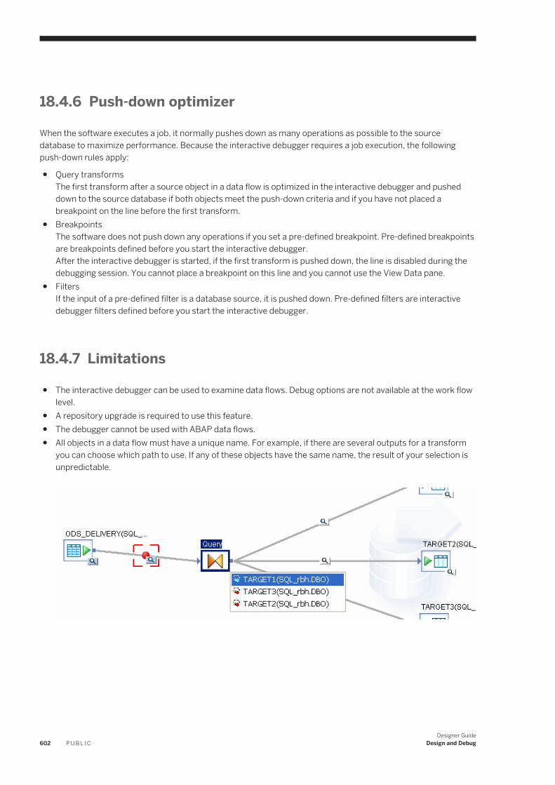
18.4.6 Push-down optimizer
When the software executes a job, it normally pushes down as many operations as possible to the source database to maximize performance. Because the interactive debugger requires a job execution, the following push-down rules apply:
● Query transformsThe first transform after a source object in a data flow is optimized in the interactive debugger and pushed down to the source database if both objects meet the push-down criteria and if you have not placed a breakpoint on the line before the first transform.
● BreakpointsThe software does not push down any operations if you set a pre-defined breakpoint. Pre-defined breakpoints are breakpoints defined before you start the interactive debugger.After the interactive debugger is started, if the first transform is pushed down, the line is disabled during the debugging session. You cannot place a breakpoint on this line and you cannot use the View Data pane.
● FiltersIf the input of a pre-defined filter is a database source, it is pushed down. Pre-defined filters are interactive debugger filters defined before you start the interactive debugger.
18.4.7 Limitations
● The interactive debugger can be used to examine data flows. Debug options are not available at the work flow level.
● A repository upgrade is required to use this feature.● The debugger cannot be used with ABAP data flows.● All objects in a data flow must have a unique name. For example, if there are several outputs for a transform
you can choose which path to use. If any of these objects have the same name, the result of your selection is unpredictable.
602 P U B L I CDesigner Guide
Design and Debug
18.5 Comparing Objects
The software allows you to compare any two objects and their properties by using the Difference Viewer utility. You can compare:
● two different objects● different versions of the same object● an object in the local object library with its counterpart in the central object library
You can compare just the top-level objects, or you can include the object's dependents in the comparison.
Objects must be of the same type; for example, you can compare a job to another job or a custom function to another custom function, but you cannot compare a job to a data flow.
18.5.1 Comparing two different objects
1. In the local or central object library, right-click an object name.2. From the shortcut menu, highlight Compare, and from the submenu, click one of the following options
(availability depends on the object you selected):
Table 304:
Option Description
Object to central Compares the selected object to its counterpart in the central object library.
Object with dependents to central Compares the selected object and its dependent objects to its counterpart in the central object library.
Object to... Compares the selected object to another similar type of object.
Object with dependents to... Compares the selected object and its dependents to another similar type of object.
The cursor changes to a target icon.
3. When you move the cursor over an object that is eligible for comparison, the target cursor changes color. Click on the desired object.
The Difference Viewer window opens in the workspace.
The window identifies changed items with a combination of icons, color, and background shading. Some of these properties are configurable.
Depending on the object type, the panes show items such as the object's properties and the properties of and connections (links) between its child objects.
18.5.2 Comparing two versions of the same object
If you are working in a multiuser environment and using a central object library, you can compare two objects that have different versions or labels.
Designer GuideDesign and Debug P U B L I C 603
1. In the central object library, right-click an object name, and from the shortcut menu click Show History.2. In the History window, Ctrl-click the two versions or labels you want to compare.3. Click Show Differences or Show Differences with Dependents.
The Difference Viewer window opens in the workspace.4. Close the History window.
Related Information
Viewing object history [page 718]
18.5.3 Overview of the Difference Viewer window
The first object you selected appears in the left pane of the window, and the second object appears on the right. Following each object name is its location.
The Difference Viewer window includes the following features:
● toolbar● navigation bar● status bar● shortcut menu
Also, when a Difference Viewer window is active, the main designer window also contains a menu called Difference Viewer. The next section describes these features.
You can have multiple Difference Viewer windows open at a time in the workspace. To refresh a Difference Viewer window, press F5.
Expanding or collapsing any property set also expands or collapses the compared object's corresponding property set.
18.5.3.1 Toolbar
The toolbar includes the following buttons.
Navigation buttons
● First Difference (Alt+Home)● Previous Difference (Alt+left arrow)● Current Difference
604 P U B L I CDesigner Guide
Design and Debug
● Next Difference (Alt+right arrow)● Last Difference (Alt+End)
Filter buttons
● Enable filter(s)—Click to open the Filters dialog box.○ Hide non-executable elements—Select this option to remove from view those elements that do not affect
job execution.○ Hide identical elements—Select this option to remove from view those elements that do not have
differences.● Disable filters—Removes all filters applied to the comparison.
Show levels
Show Level 1 shows only the objects you selected for comparison, Show Level 2 expands to the next level, etc. Show All Levels expands all levels of both trees.
Find (Ctrl+F)
Click Find to open a text search dialog box.
Open in new window
Click to open the currently active Difference Viewer in a separate window. You must close this window before continuing.
18.5.3.2 Navigation bar
The vertical navigation bar contains colored bars that represent each of the differences throughout the comparison. The colors correspond to those in the status bar for each difference. An arrow in the navigation bar indicates the difference that is currently highlighted in the panes. You can click on the navigation bar to select a difference (the cursor point will have a star on it). The purple brackets in the bar indicate the portion of the comparison that is currently in view in the panes.
Designer GuideDesign and Debug P U B L I C 605
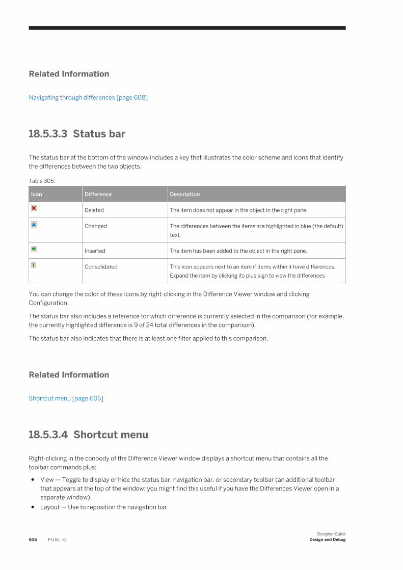
Related Information
Navigating through differences [page 608]
18.5.3.3 Status bar
The status bar at the bottom of the window includes a key that illustrates the color scheme and icons that identify the differences between the two objects.
Table 305:
Icon Difference Description
Deleted The item does not appear in the object in the right pane.
Changed The differences between the items are highlighted in blue (the default) text.
Inserted The item has been added to the object in the right pane.
Consolidated This icon appears next to an item if items within it have differences. Expand the item by clicking its plus sign to view the differences
You can change the color of these icons by right-clicking in the Difference Viewer window and clicking Configuration.
The status bar also includes a reference for which difference is currently selected in the comparison (for example, the currently highlighted difference is 9 of 24 total differences in the comparison).
The status bar also indicates that there is at least one filter applied to this comparison.
Related Information
Shortcut menu [page 606]
18.5.3.4 Shortcut menu
Right-clicking in the conbody of the Difference Viewer window displays a shortcut menu that contains all the toolbar commands plus:
● View — Toggle to display or hide the status bar, navigation bar, or secondary toolbar (an additional toolbar that appears at the top of the window; you might find this useful if you have the Differences Viewer open in a separate window).
● Layout — Use to reposition the navigation bar.
606 P U B L I CDesigner Guide
Design and Debug
● Configuration — Click to modify viewing options for elements with differences.
Related Information
Changing the color scheme [page 607]
18.5.3.4.1 Changing the color scheme
The status bar at the bottom of the Difference Viewer window shows the current color scheme being used to identify deleted, changed, inserted, or consolidated items in the comparison panes. You can customize this color scheme as follows.
1. Right-click in the conbody of the Difference Viewer window to display the shortcut toolbar.2. Click Configuration to open the Configuration window.3. Click a marker (Inserted, Deleted, Changed, or Consolidated) to change.4. Click the Color sample to open the Color palette.5. Click a Basic color or create a custom color.6. Click OK.7. Click another marker to change it, or click OK to close the Configuration window.
18.5.3.4.2 Changing the background shading
Items with differences appear with a background default color of grey. You can customize this background.
1. Right-click in the conbody of the Difference Viewer window to display the shortcut toolbar.2. Click Configuration to open the Configuration window.3. Click a marker to change, or select the Apply for all markers check box.4. Click the Background sample to open the Color palette.5. Click a Basic color or create a custom color.6. Click OK.7. To apply different background colors to different markers, click the marker to configure and repeat steps 4
through 6.8. Click OK to close the Configuration window.
18.5.3.5 Difference Viewer menu
When a Difference Viewer window is active in the workspace, the main Designer window contains a menu called Difference Viewer. The menu contains the same commands as the toolbar.
Designer GuideDesign and Debug P U B L I C 607
18.5.4 Navigating through differences
The Difference Viewer window offers several options for navigating through differences.
You can navigate through the differences between the objects using the navigation buttons on the toolbar. For example, clicking the Next Difference button highlights the next item that differs in some way from the compared object. The item is marked with the appropriate icon and only the differing text appears highlighted in the color assigned to that type of difference.
You can also use the navigation bar. Select an item in either pane that has a difference. Note that an arrow appears next to the colored bar that corresponds to that item. You can click on these bars to jump to different places in the comparison, for example to view only inserted items (with a default color of green). The purple brackets in the bar indicate the portion of the comparison that is currently in view in the panes. Use the scroll bar in either pane to adjust the bracketed view.
For text-based items such as scripts, click the magnifying glass to view the text in a set of new panes that appear below the main object panes. Use the scroll bars for these panes to navigate within them. Click the magnifying glass (or any other item) to close the text panes.
18.6 Calculating column mappings
SAP Data Services can calculate information about target tables and columns and the sources used to populate them, for example for impact and lineage or auto documentation reports.
Calculating column mappings populates the internal ALVW_MAPPING view and the AL_COLMAP_NAMES table. The ALVW_MAPPING view provides current data to metadata reporting applications like Impact and Lineage Analysis. If you need to generate a report about a data flow that processes nested (NRDM) data, query the AL_COLMAP_NAMES table using a custom report.
Whenever a column mapping calculation is in progress, the Designer displays a status icon at the bottom right of the window. You can double-click this icon to cancel the process.
To calculate column mappings, you can:
● Enable the option in the Designer to automatically calculate column mappings.● Execute the column mapping process manually from either the Designer or the Impact and Lineage Analysis
application in the Management Console.
18.6.1 Automatically calculating column mappings
To set the option to automatically calculate column mapping information, in the Designer select ToolsOptions Designer General Automatically calculate column mappings . This option is selected by default.
Note that if the Designer option Automatically calculate column mappings is cleared, any subsequent changes made to the data flow require that you manually recalculate the column mappings to ensure the ALVW_MAPPING view and the AL_COLMAP_NAMES table have the most current information.
608 P U B L I CDesigner Guide
Design and Debug
18.6.2 Manually calculating column mappings
If the Designer option Automatically calculate column mappings is cleared and you want to generate reports, you can manually calculate the mappings. You can manually calculate column mappings at any time in either the Designer or the Management Console.
In the Designer, right-click in the object library and select Repository Calculate column mappings .
In the Management Console:
1. Select Impact and Lineage Analysis.2. Open the Settings control panel.3. Click the Refresh Usage Data tab.4. Select the Job Server that is associated with the repository you want to use.5. Click Calculate Column Mapping.
On the Impact and Lineage Analysis Overview tab, you can expand Data Flow Column Mapping Calculation to view a list of data flows and the calculation status of each. If the mapping calculation is complete, the Status indicator is checked.
18.7 Bypassing specific work flows and data flows
You can bypass the execution of a work flow or data flow during design time.
The Bypass attribute can help speed up the testing process when designing jobs by allowing you to run certain work flows or data flows in the job instead of having to run them all. Note that all objects within a bypassed data flow or work flow (for example, scripts) will also be bypassed.
NoteYou must create substitution parameters to use with the Bypass option. For example, in the Substitution Parameter Editor window you might create $$BYPASSEnable with a value of Yes and $$BYPASSDisable with a value of No (or any value other than Yes).
The following limitations apply:
● Bypassed data flows and work flows are ignored in Debug mode. Bypassing works only in design mode.● ABAP data flows and embedded data flows are not supported.● Bypass attributes are not supported during export and will be removed.
There are several ways to see if an object has been bypassed:
● After validation, a message displays in the Warning tab in the Output Window (for example, Work Flow <work flow name> is bypassed.). You can click on the message to go directly to the bypassed object.
● A message displays in the trace log.● An icon (red circle with a line going through it) appears in the lower left corner of the data flow or work flow
object in the Designer workspace.
Designer GuideDesign and Debug P U B L I C 609
NoteThis icon displays as long as the bypass attribute (enabled or disabled) is applied to an object.
Related Information
Changing properties of a data flow [page 154]Order of execution in work flows [page 199]Creating a new substitution parameter [page 294]
18.7.1 Bypassing a single data flow or work flow
You can enable the Bypass attribute for a single work flow or data flow.
1. Right-click on a work flow or data flow in the Designer workspace or Project Area and select Properties.2. In the General tab, select a substitution variable from the Bypass drop-down list.3. Click Apply.
18.7.2 Bypassing multiple data flows or work flows
You can enable the Bypass attribute for multiple work flows or data flows.
1. Select work flows and data flows in the Designer workspace.2. Right-click and select Bypass.
The Set Bypass window appears.3. Select a substitution variable from the Bypass drop-down list.4. Click OK.
18.7.3 Disabling bypass
After you finish designing and testing your job, you should disable the Bypass attribute before moving the job to production mode.
To disable the Bypass attribute at the job level, right-click on a data flow or work flow in the Designer Project Area and select Remove Bypass.
To disable the Bypass attribute at the call level for multiple work flows or data flows, do the following:
1. Select work flows and data flows in the Designer workspace.2. Right-click and select Bypass.
610 P U B L I CDesigner Guide
Design and Debug

The Set Bypass window appears.3. Select {No Bypass} from the Bypass drop-down list.4. Click OK.
Designer GuideDesign and Debug P U B L I C 611
19 Recovery Mechanisms
Recovery mechanisms are available in SAP Data Services for batch jobs only.
Related Information
Recovering from unsuccessful job execution [page 612]Automatically recovering jobs [page 613]Manually recovering jobs using status tables [page 620]Processing data with problems [page 620]
19.1 Recovering from unsuccessful job execution
If an SAP Data Services job does not complete properly, you must fix the problems that prevented the successful execution of the job and run the job again.
However, during the failed job execution, some data flows in the job may have completed and some tables may have been loaded, partially loaded, or altered. Therefore, you need to design your data movement jobs so that you can recover—that is, rerun the job and retrieve all the data without duplicate or missing data.
You can use various techniques to recover from unsuccessful job executions. This section discusses two techniques:
● Automatically recovering jobs — A software feature that allows you to run unsuccessful jobs in recovery mode.
● Manually recovering jobs using status tables — A design technique that allows you to rerun jobs without regard to partial results in a previous run.
You might need to use a combination of these techniques depending on the relationships between data flows in your application.
If you do not use these techniques, you might need to roll back changes manually from target tables if interruptions occur during job execution.
Related Information
Automatically recovering jobs [page 613]Manually recovering jobs using status tables [page 620]
612 P U B L I CDesigner Guide
Recovery Mechanisms
19.2 Automatically recovering jobs
With automatic recovery, the software records the result of each successfully completed step in a job. If a job fails, you can choose to run the job again in recovery mode. During recovery mode, the software retrieves the results for successfully completed steps and reruns uncompleted or failed steps under the same conditions as the original job. For recovery purposes, the software considers steps that raise exceptions as failed steps, even if the step is caught in a try/catch block.
19.2.1 Enabling automated recovery
To use the automatic recover feature, you must enable the feature during initial execution of a job. The software saves the results from successfully completed steps when the automatic recovery feature is enabled.
19.2.1.1 Running a job from Designer with recovery enabled
1. In the project area, select the job name.2. Right-click and choose Execute.
The software prompts you to save any changes.3. Make sure that the Enable Recovery option is selected in the Execution Properties window.
If this check box is not selected, the software does not record the results from the steps during the job and cannot recover the job if it fails. In that case, you must perform any recovery operations manually.
19.2.1.2 Running a job with recovery enabled from the Administrator
When you schedule or execute a job from the Administrator, select the Enable Recovery check box.
19.2.2 Marking recovery units
In some cases, steps in a work flow depend on each other and must be executed together. Because of the dependency, you should designate the work flow as a "recovery unit." When a work flow is a recovery unit, the entire work flow must complete successfully. If the work flow does not complete successfully, the software executes the entire work flow during recovery, even steps that executed successfully in prior work flow runs.
However, there are some exceptions to recovery unit processing. For example, when you specify that a work flow or a data flow should only execute once, a job will never re-execute that work flow or data flow after it completes successfully, except if that work flow or data flow is contained within a recovery unit work flow that re-executes and has not completed successfully elsewhere outside the recovery unit.
Designer GuideRecovery Mechanisms P U B L I C 613
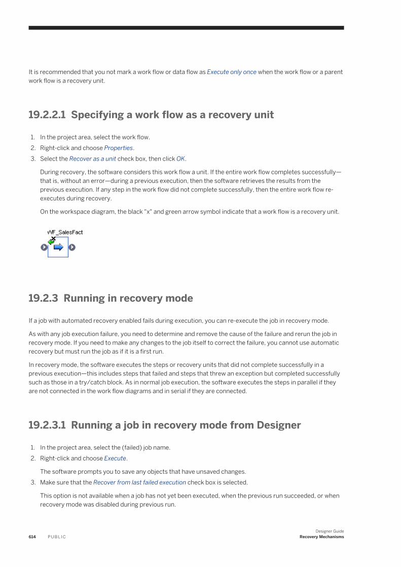
It is recommended that you not mark a work flow or data flow as Execute only once when the work flow or a parent work flow is a recovery unit.
19.2.2.1 Specifying a work flow as a recovery unit
1. In the project area, select the work flow.2. Right-click and choose Properties.3. Select the Recover as a unit check box, then click OK.
During recovery, the software considers this work flow a unit. If the entire work flow completes successfully—that is, without an error—during a previous execution, then the software retrieves the results from the previous execution. If any step in the work flow did not complete successfully, then the entire work flow re-executes during recovery.
On the workspace diagram, the black "x" and green arrow symbol indicate that a work flow is a recovery unit.
19.2.3 Running in recovery mode
If a job with automated recovery enabled fails during execution, you can re-execute the job in recovery mode.
As with any job execution failure, you need to determine and remove the cause of the failure and rerun the job in recovery mode. If you need to make any changes to the job itself to correct the failure, you cannot use automatic recovery but must run the job as if it is a first run.
In recovery mode, the software executes the steps or recovery units that did not complete successfully in a previous execution—this includes steps that failed and steps that threw an exception but completed successfully such as those in a try/catch block. As in normal job execution, the software executes the steps in parallel if they are not connected in the work flow diagrams and in serial if they are connected.
19.2.3.1 Running a job in recovery mode from Designer
1. In the project area, select the (failed) job name.2. Right-click and choose Execute.
The software prompts you to save any objects that have unsaved changes.3. Make sure that the Recover from last failed execution check box is selected.
This option is not available when a job has not yet been executed, when the previous run succeeded, or when recovery mode was disabled during previous run.
614 P U B L I CDesigner Guide
Recovery Mechanisms
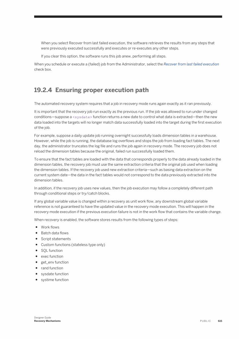
When you select Recover from last failed execution, the software retrieves the results from any steps that were previously executed successfully and executes or re-executes any other steps.
If you clear this option, the software runs this job anew, performing all steps.
When you schedule or execute a (failed) job from the Administrator, select the Recover from last failed execution check box.
19.2.4 Ensuring proper execution path
The automated recovery system requires that a job in recovery mode runs again exactly as it ran previously.
It is important that the recovery job run exactly as the previous run. If the job was allowed to run under changed conditions—suppose a <sysdate> function returns a new date to control what data is extracted—then the new data loaded into the targets will no longer match data successfully loaded into the target during the first execution of the job.
For example, suppose a daily update job running overnight successfully loads dimension tables in a warehouse. However, while the job is running, the database log overflows and stops the job from loading fact tables. The next day, the administrator truncates the log file and runs the job again in recovery mode. The recovery job does not reload the dimension tables because the original, failed run successfully loaded them.
To ensure that the fact tables are loaded with the data that corresponds properly to the data already loaded in the dimension tables, the recovery job must use the same extraction criteria that the original job used when loading the dimension tables. If the recovery job used new extraction criteria—such as basing data extraction on the current system date—the data in the fact tables would not correspond to the data previously extracted into the dimension tables.
In addition, if the recovery job uses new values, then the job execution may follow a completely different path through conditional steps or try/catch blocks.
If any global variable value is changed within a recovery as unit work flow, any downstream global variable reference is not guaranteed to have the updated value in the recovery mode execution. This will happen in the recovery mode execution if the previous execution failure is not in the work flow that contains the variable change.
When recovery is enabled, the software stores results from the following types of steps:
● Work flows● Batch data flows● Script statements● Custom functions (stateless type only)● SQL function● exec function● get_env function● rand function● sysdate function● systime function
Designer GuideRecovery Mechanisms P U B L I C 615
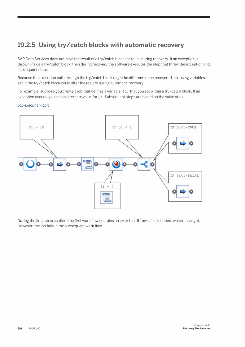
19.2.5 Using try/catch blocks with automatic recovery
SAP Data Services does not save the result of a try/catch block for reuse during recovery. If an exception is thrown inside a try/catch block, then during recovery the software executes the step that threw the exception and subsequent steps.
Because the execution path through the try/catch block might be different in the recovered job, using variables set in the try/catch block could alter the results during automatic recovery.
For example, suppose you create a job that defines a variable, $i, that you set within a try/catch block. If an exception occurs, you set an alternate value for $i. Subsequent steps are based on the value of $i.
Job execution logic
During the first job execution, the first work flow contains an error that throws an exception, which is caught. However, the job fails in the subsequent work flow.
616 P U B L I CDesigner Guide
Recovery Mechanisms
You fix the error and run the job in recovery mode. During the recovery execution, the first work flow no longer throws the exception. Thus the value of the variable, <$i> , is different, and the job selects a different subsequent work flow, producing different results.
To ensure proper results with automatic recovery when a job contains a try/catch block, do not use values set inside the try/catch block in any subsequent steps.
19.2.6 Ensuring that data is not duplicated in targets
Define work flows to allow jobs correct recovery. A data flow might be partially completed during an incomplete run. As a result, only some of the required rows could be inserted in a table. You do not want to insert duplicate rows during recovery when the data flow re-executes.
Designer GuideRecovery Mechanisms P U B L I C 617
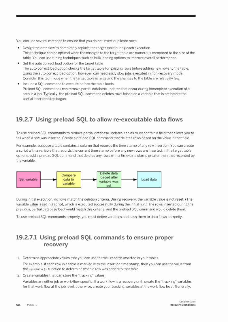
You can use several methods to ensure that you do not insert duplicate rows:
● Design the data flow to completely replace the target table during each executionThis technique can be optimal when the changes to the target table are numerous compared to the size of the table. You can use tuning techniques such as bulk loading options to improve overall performance.
● Set the auto correct load option for the target tableThe auto correct load option checks the target table for existing rows before adding new rows to the table. Using the auto correct load option, however, can needlessly slow jobs executed in non-recovery mode.Consider this technique when the target table is large and the changes to the table are relatively few.
● Include a SQL command to execute before the table loadsPreload SQL commands can remove partial database updates that occur during incomplete execution of a step in a job. Typically, the preload SQL command deletes rows based on a variable that is set before the partial insertion step began.
19.2.7 Using preload SQL to allow re-executable data flows
To use preload SQL commands to remove partial database updates, tables must contain a field that allows you to tell when a row was inserted. Create a preload SQL command that deletes rows based on the value in that field.
For example, suppose a table contains a column that records the time stamp of any row insertion. You can create a script with a variable that records the current time stamp before any new rows are inserted. In the target table options, add a preload SQL command that deletes any rows with a time-date stamp greater than that recorded by the variable.
During initial execution, no rows match the deletion criteria. During recovery, the variable value is not reset. (The variable value is set in a script, which is executed successfully during the initial run.) The rows inserted during the previous, partial database load would match this criteria, and the preload SQL command would delete them.
To use preload SQL commands properly, you must define variables and pass them to data flows correctly.
19.2.7.1 Using preload SQL commands to ensure proper recovery
1. Determine appropriate values that you can use to track records inserted in your tables.For example, if each row in a table is marked with the insertion time stamp, then you can use the value from the sysdate() function to determine when a row was added to that table.
2. Create variables that can store the "tracking" values.Variables are either job or work-flow specific. If a work flow is a recovery unit, create the "tracking" variables for that work flow at the job level; otherwise, create your tracking variables at the work flow level. Generally,
618 P U B L I CDesigner Guide
Recovery Mechanisms
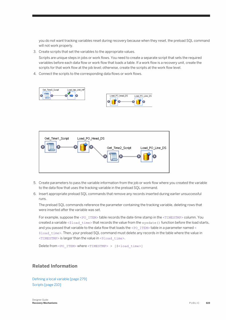
you do not want tracking variables reset during recovery because when they reset, the preload SQL command will not work properly.
3. Create scripts that set the variables to the appropriate values.Scripts are unique steps in jobs or work flows. You need to create a separate script that sets the required variables before each data flow or work flow that loads a table. If a work flow is a recovery unit, create the scripts for that work flow at the job level; otherwise, create the scripts at the work flow level.
4. Connect the scripts to the corresponding data flows or work flows.
5. Create parameters to pass the variable information from the job or work flow where you created the variable
to the data flow that uses the tracking variable in the preload SQL command.6. Insert appropriate preload SQL commands that remove any records inserted during earlier unsuccessful
runs.The preload SQL commands reference the parameter containing the tracking variable, deleting rows that were inserted after the variable was set.
For example, suppose the <PO_ITEM> table records the date-time stamp in the <TIMESTMP> column. You created a variable <$load_time> that records the value from the sysdate() function before the load starts, and you passed that variable to the data flow that loads the <PO_ITEM> table in a parameter named <$load_time>. Then, your preload SQL command must delete any records in the table where the value in <TIMESTMP> is larger than the value in <$load_time>.
Delete from <PO_ITEM> where <TIMESTMP> > [$<load_time>]
Related Information
Defining a local variable [page 279]Scripts [page 210]
Designer GuideRecovery Mechanisms P U B L I C 619
Defining parameters [page 280]
19.3 Manually recovering jobs using status tables
You can design your jobs and work flows so that you can manually recover from an unsuccessful run. A job designed for manual recovery must have certain characteristics:
● You can run the job repeatedly.● The job implements special steps to recover data when a step did not complete successfully during a previous
run.
You can use an execution status table to produce jobs that can be run multiple times without duplicating target rows. The table records a job's execution status. A "failure" value signals SAP Data Services to take a recovery execution path.
To implement a work flow with a recovery execution path:
● Define a flag that indicates when the work flow is running in recovery mode.● Store the flag value in a status table.● Check the flag value in the status table before executing a work flow to determine which path to execute in the
work flow.● Update the flag value when the work flow executes successfully.
For example, you could design a work flow that uses the auto correct load option when a previous run does not complete successfully. This work flow would have five steps, as illustrated:
1. Retrieve the flag value, which indicates the success or failure of the previous execution, from the status table. Store this value in a variable such as <$recovery_needed> .
2. In a conditional, evaluate the <$recovery_needed> variable.3. If recovery is required, execute the recovery data flow recover_customer. This data flow loads the data using
the auto correct load option.4. If recovery is not required, execute the non-recovery data flow load_customer. This data flow loads the data
without the auto correct load option.5. Update the flag value in the status table to indicate successful execution.
19.4 Processing data with problems
Jobs might not produce the results you expect because of problems with data. In some cases, the software is unable to insert a row. In other cases, the software might insert rows with missing information. You can design your data flows to anticipate and process these types of problems. For example, you might have a data flow write rows with missing information to a special file that you can inspect later.
This section describes mechanisms you can use to anticipate and process data problems. In particular, this section discusses three techniques:
● Using overflow files
620 P U B L I CDesigner Guide
Recovery Mechanisms
● Filtering missing or bad values● Handling facts with missing dimensions
19.4.1 Using overflow files
A row that cannot be inserted is a common data problem. Use the overflow file to process this type of data problem. When you specify an overflow file and the SAP Data Services cannot load a row into a table, the software writes the row to the overflow file instead. The trace log indicates the data flow in which the load failed and the location of the file.
For any table used as a target, you can set the option to use an overflow file in the Options tab. When you specify an overflow file, give a full path name to ensure that the software creates a unique file when more than one file is created in the same job. By default, the name of the overflow file is the target table name.
When you select the overflow file option, you choose what the software writes to the file about the rows that failed to load: either the data from the row or the SQL commands required to load the row. If you select data, you can use the software to read the data from the overflow file, cleanse it, and load it into the target table. If you select SQL commands, you can use the commands to load the target manually when the target is accessible.
There are many reasons for loading to fail, for example:
● Out of memory for the target● Overflow column settings● Duplicate key values
You can use the overflow information to identify invalid data in your source or problems introduced in the data movement. Every new run will overwrite the existing overflow file.
NoteYou cannot use overflow files when loading to a BW Transfer Structure.
19.4.2 Filtering missing or bad values
A missing or invalid value in the source data is another common data problem. Using queries in data flows, you can identify missing or invalid values in source data. You can also choose to include this data in the target or to disregard it.
For example, suppose you are extracting data from a source and you know that some phone numbers and customer names are missing. You can use a data flow to extract data from the source, load the data into a target, and filter the NULL values into a file for your inspection.
The data flow has five steps:
1. Extracts data from the source.2. Selects the data set to load into the target and applies new keys. (It does this by using the Key_Generation
function.)3. Loads the data set into the target, using the bulk load option for best performance.
Designer GuideRecovery Mechanisms P U B L I C 621
4. Uses the same data set for which new keys were generated in step 2, and select rows with missing customer names and phone numbers.
5. Writes the customer IDs for the rows with missing data to a file.
Now, suppose you do not want to load rows with missing customer names into your target. You can insert another query into the data flow to ensure that SAP Data Services does not insert incomplete rows into the target. The new query filters the rows with missing customer names before loading any rows into the target. The missing data query still collects those rows along with the rows containing missing phone numbers. In this version of the example, the Key_Generation transform adds keys for new rows before inserting the filtered data set into the target.
The data flow now has six steps.
1. Extracts data from the source.2. Selects the data set to load into the target by filtering out rows with no customer name values.3. Generates keys for rows with customer names.4. Loads the valid data set (rows with customer names) into the target using the bulk load option for best
performance.5. Uses a separate query transform to select rows from the source that have no names or phones.
Note that the software does not load rows with missing customer names into the target; however, the software does load rows with missing phone numbers.
6. Writes the customer IDs for the rows with missing data to a file.
You could add more queries into the data flow to select additional missing or invalid values for later inspection.
19.4.3 Handling facts with missing dimensions
Another data problem occurs when SAP Data Services searches a dimension table and cannot find the values required to complete a fact table.
You can approach this problem in several ways:
● Leave the problem row out of the fact table.Typically, this is not a good idea because analysis done on the facts will be missing the contribution from this row.
● Note the row that generated the error, but load the row into the target table anyway.You can mark the row as having an error, or pass the row information to an error file as in the examples from Filtering missing or bad values [page 621].
● Fix the problem programmatically.Depending on the data missing, you can insert a new row in the dimension table, add information from a secondary source, or use some other method of providing data outside of the normal, high-performance path.
19.5 Exchanging metadata
SAP Data Services enables you to export metadata into an XML file. After you create the file, you must manually import it into another tool.
622 P U B L I CDesigner Guide
Recovery Mechanisms
Related Information
Metadata exchange [page 623]
19.5.1 Metadata exchange
You can exchange metadata between the software and third-party tools using XML files and the Metadata Exchange option.
The software supports two built-in metadata exchange formats:
● CWM 1.0 XML/XMI 1.1CWM (the Common Warehouse Metamodel)— is a specification that enables easy interchange of data warehouse metadata between tools, platforms, and repositories in distributed heterogeneous environments.
● ERwin 4.x XML
The software can also use:
● MIMB (the Meta Integration® Model Bridge)MIMB is a Windows stand-alone utility that converts metadata models among design tool formats. By using MIMB with the software, you can exchange metadata with all formats that MIMB supports. If MIMB is installed, the additional formats it supports are listed in the Metadata Exchange window.
19.5.1.1 Importing metadata files into the software
You can import metadata from ERwin Data Modeler 4.x XML into a datastore.
19.5.1.1.1 Importing metadata using Metadata Exchange
1. From the Tools menu, select Metadata Exchange.2. In the Metadata Exchange window, select Import metadata from file.3. In the Metadata format box, select ERwin 4.x XML from the list of available formats.
4. Specify the Source file name (enter directly or click Browse to search).5. Select the Target datastore name from the list of datastores.6. Click OK to complete the import.
19.5.1.2 Exporting metadata files from the software
You can export metadata into a file that other tools can read.
Designer GuideRecovery Mechanisms P U B L I C 623
19.5.1.2.1 Exporting metadata using Metadata Exchange
1. From the Tools menu, select Metadata Exchange.2. In the Metadata Exchange window, select Export Data Services metadata to file.3. Select a Metadata format for the target from the list of available formats.
If you have MIMB installed and you select an MIMB-supported format, select the Visual check box to open the MIMB application when completing the export process.
If you do not select the Visual check box, the metadata is exported without opening the MIMB application. Using the MIMB application provides more configuration options for structuring the metadata in the exported file.
4. Specify the target file name (enter directly or click Browse to search).
When you search for the file, you open a typical browse window.
Find any of the following file formats/types:
Table 306:
Format File type
DI CWM 1.0 XML/XMI 1.1 XML
DI ERwin 4.x XML XML
MIMB format (only if installed) All
After you select a file, click Open.
5. Select the Source datastore name from the list of datastores.6. Click OK to complete the export.
19.6 Loading Big Data file with recovery option
Loading big data file with recovery option is an extension of the existing recovery mechanism in Data Services. In earlier versions of Data Services, the recovery mechanism was only supported until the data flow layer. As a result, if the engine crashed at any data flow, the whole data flow had to be restarted from the beginning in recovery mode.
However, if there is big data inside of the failed dataflow, restarting the process will involve duplicating work of cleaning and restarting. This restarting situation becomes worse if there is a reason that the job needs to be stopped periodically (for example, due to a network disconnect, database timeout or machine reboot).
To avoid this situation, when reading a big source flat file into the database tables, you have the option to turn on the big data loading recovery feature. For example, when you load a large input file into a database, the job may take several days to finish. If the engine crashes or fails in the middle of a job, the job can be resumed from the last failed check point. The last failed check point includes the failed filename and the offset of the file that has been processed so far. The recovery feature avoids restarting of the data flow and ensures that loading progresses forward from where it failed.
624 P U B L I CDesigner Guide
Recovery Mechanisms
19.6.1 Turning on the recovery option for Big Data loading
To use the automatic recovery feature for big data loading, you must enable the feature during the initial execution of a job. Consequently, when a job fails, it can resume from the last checked point and run forward instead of restarting.
To run a big data loading job from Designer with recovery enabled:
1. In the project area, select the job name.2. Right-click and choose Execute. The software prompts you to save any changes.3. Make sure that the Enable Recovery option is selected in the Execution Properties window.
NoteThe Enable Recovery checkbox must be selected for the software to record the steps during the job. If the checkbox isn't selected and the job fails, you cannot recover the job. In this case, you have to perform any recovery operation manually and restart the job.
4. Check for the primary key in the target table of the data flow that contains the big data file source. If there is no primary key, then you have the option to either add the primary key column in the target table or generate the RowID column as the primary key column in the source file, and then pass it into the target tables.a. To add the primary key in the target table: If the original schema of the target table does not have a
primary key, turn on the Use Input Keys in the target table’s option and make sure that the input to the target table has a primary key. For example, the row ID column that you enter in the source file can be passed to the target table as a primary key.
b. To generate Row ID column for the source file: Type a valid column name in the ROW ID input field located in the path File Reader General .
NoteA Row ID is automatically added into the schema as first column on the top. The column name is the name you typed, and the column Data Type is double.
A primary key column is necessary for fast recovery, as the engine uses auto correct loading for the last failed job. If the primary key column is not selected, then the auto correct loading will be very slow. To override this slow auto correct loading, you have the option to add the ROW ID column manually, if the target table does not have a primary key.
Data Services automatically turns on auto-correct loading for the recovery batch regardless of the target setting. Furthermore, for HANA, Netezza and Sybase IQ, the recovery batch auto-correct load uses bulk loading for better performance.
19.6.2 Limitations
There are some limitations that need to be met to allow a file to be loaded in recovery mode. The file along with the data flow and job contained in the file, needs to meet the following criteria:
● The file is a delimited file or fixed-width file● The file has a row delimiter
Designer GuideRecovery Mechanisms P U B L I C 625
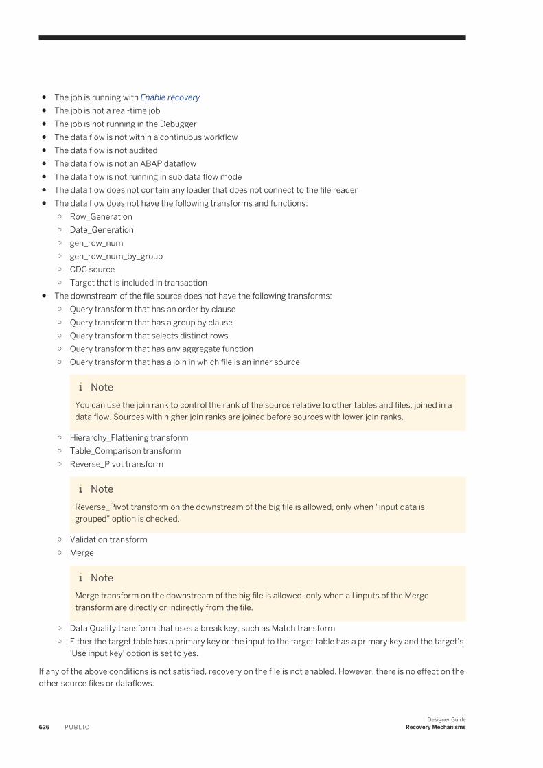
● The job is running with Enable recovery● The job is not a real-time job● The job is not running in the Debugger● The data flow is not within a continuous workflow● The data flow is not audited● The data flow is not an ABAP dataflow● The data flow is not running in sub data flow mode● The data flow does not contain any loader that does not connect to the file reader● The data flow does not have the following transforms and functions:
○ Row_Generation○ Date_Generation○ gen_row_num○ gen_row_num_by_group○ CDC source○ Target that is included in transaction
● The downstream of the file source does not have the following transforms:○ Query transform that has an order by clause○ Query transform that has a group by clause○ Query transform that selects distinct rows○ Query transform that has any aggregate function○ Query transform that has a join in which file is an inner source
NoteYou can use the join rank to control the rank of the source relative to other tables and files, joined in a data flow. Sources with higher join ranks are joined before sources with lower join ranks.
○ Hierarchy_Flattening transform○ Table_Comparison transform○ Reverse_Pivot transform
NoteReverse_Pivot transform on the downstream of the big file is allowed, only when "input data is grouped" option is checked.
○ Validation transform○ Merge
NoteMerge transform on the downstream of the big file is allowed, only when all inputs of the Merge transform are directly or indirectly from the file.
○ Data Quality transform that uses a break key, such as Match transform○ Either the target table has a primary key or the input to the target table has a primary key and the target’s
'Use input key' option is set to yes.
If any of the above conditions is not satisfied, recovery on the file is not enabled. However, there is no effect on the other source files or dataflows.
626 P U B L I CDesigner Guide
Recovery Mechanisms

If the data flow contains multiple file sources, only one file source is chosen to run in recovery mode.
Designer GuideRecovery Mechanisms P U B L I C 627
20 Changed Data capture
When you have a large amount of data to update regularly and a small amount of system down time for scheduled maintenance on a data warehouse, update data over time, or delta load. Two commonly used delta load methods are full refresh and changed-data capture (CDC).
20.1 Full refresh
Full refresh is easy to implement and easy to manage. This method ensures that no data will be overlooked or left out due to technical or programming errors. For an environment with a manageable amount of source data, full refresh is an easy method you can use to perform a delta load to a target system.
20.2 Capture only changes
After an initial load is complete, you can choose to extract only new or modified data and update the target system.
Identifying and loading only changed data is called changed-data capture (CDC). This includes only incremental data that has changed since the last refresh cycle. SAP Data Services acts as a mechanism to locate and extract only the incremental data that changed since the last refresh.
Improving performance and preserving history are the most important reasons for using changed-data capture.
● Performance improves because with less data to extract, transform, and load, the job typically takes less time.
● If the target system has to track the history of changes so that data can be correctly analyzed over time, the changed-data capture method can provide a record of these changes.
ExampleIf a customer moves from one sales region to another, simply updating the customer record to reflect the new region negatively affects any analysis by region over time because the purchases made by that customer before the move are attributed to the new region
20.3 Source-based and target-based CDC
Changed-data capture can be either source-based or target-based.
628 P U B L I CDesigner Guide
Changed Data capture
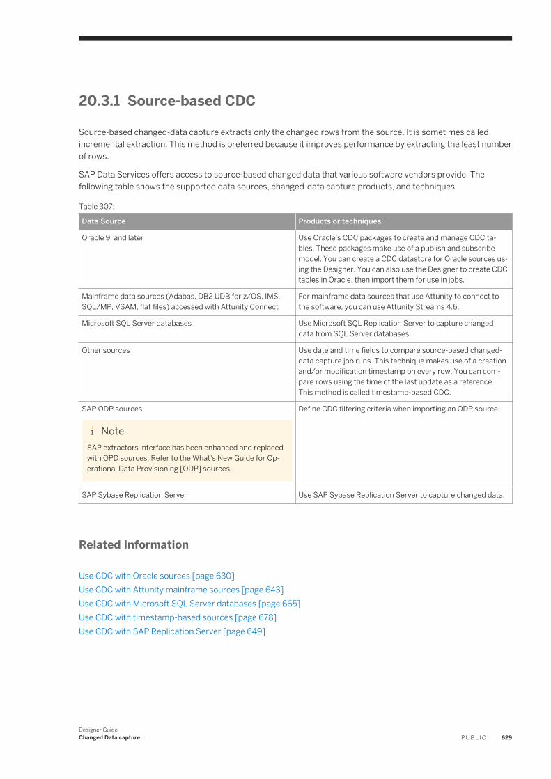
20.3.1 Source-based CDC
Source-based changed-data capture extracts only the changed rows from the source. It is sometimes called incremental extraction. This method is preferred because it improves performance by extracting the least number of rows.
SAP Data Services offers access to source-based changed data that various software vendors provide. The following table shows the supported data sources, changed-data capture products, and techniques.
Table 307:
Data Source Products or techniques
Oracle 9i and later Use Oracle's CDC packages to create and manage CDC tables. These packages make use of a publish and subscribe model. You can create a CDC datastore for Oracle sources using the Designer. You can also use the Designer to create CDC tables in Oracle, then import them for use in jobs.
Mainframe data sources (Adabas, DB2 UDB for z/OS, IMS, SQL/MP, VSAM, flat files) accessed with Attunity Connect
For mainframe data sources that use Attunity to connect to the software, you can use Attunity Streams 4.6.
Microsoft SQL Server databases Use Microsoft SQL Replication Server to capture changed data from SQL Server databases.
Other sources Use date and time fields to compare source-based changed-data capture job runs. This technique makes use of a creation and/or modification timestamp on every row. You can compare rows using the time of the last update as a reference. This method is called timestamp-based CDC.
SAP ODP sources
NoteSAP extractors interface has been enhanced and replaced with OPD sources. Refer to the What's New Guide for Operational Data Provisioning [ODP] sources
Define CDC filtering criteria when importing an ODP source.
SAP Sybase Replication Server Use SAP Sybase Replication Server to capture changed data.
Related Information
Use CDC with Oracle sources [page 630]Use CDC with Attunity mainframe sources [page 643]Use CDC with Microsoft SQL Server databases [page 665]Use CDC with timestamp-based sources [page 678]Use CDC with SAP Replication Server [page 649]
Designer GuideChanged Data capture P U B L I C 629
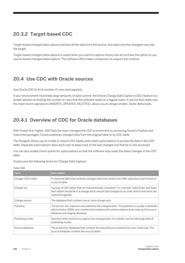
20.3.2 Target-based CDC
Target-based changed-data capture extracts all the data from the source, but loads only the changed rows into the target.
Target-based changed-data capture is useful when you want to capture history but do not have the option to use source-based changed-data capture. The software offers table comparison to support this method.
20.4 Use CDC with Oracle sources
Use Oracle CDC to limit number of rows read regularly.
If your environment must keep large amounts of data current, the Oracle Change Data Capture (CDC) feature is a simple solution to limiting the number or rows that the software reads on a regular basis. A source that reads only the most recent operations (INSERTS, UPDATES, DELETES), allows you to design smaller, faster delta loads.
20.4.1 Overview of CDC for Oracle databases
With Oracle 9i or higher, SAP Data Services manages the CDC environment by accessing Oracle's Publish and Subscribe packages. Oracle publishes changed data from the original table to its CDC table.
The Designer allows you to create or import CDC tables and create subscriptions to access the data in the CDC table. Separate subscriptions allow each user to keep track of the last changed row that he or she accessed.
You can also enable check-points for subscriptions so that the software only reads the latest changes in the CDC table.
Oracle uses the following terms for Change Data Capture:
Table 308:
Term Description
Change (CDC) table A relational table that contains changed data that results from DML operations performed on a source table.
Change set A group of CDC tables that are transactionally consistent. For example, SalesOrder and SalesItem tables should be in a change set to ensure that changes to an order and its line items are captured together.
Change source The database that contains one or more change sets.
Publisher The person who captures and publishes the changed data. The publisher is usually a database administrator (DBA) who creates and maintains the schema objects that make up the source database and staging database.
Publishing mode Specifies when and how to capture the changed data. For details, see the following table of publishing modes.
Source database The production database that contains the data that you extracted for your initial load. The source database contains the source tables.
630 P U B L I CDesigner Guide
Changed Data capture
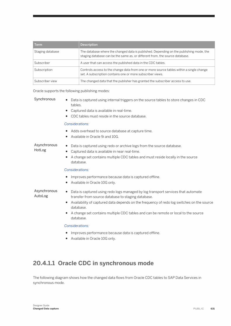
Term Description
Staging database The database where the changed data is published. Depending on the publishing mode, the staging database can be the same as, or different from, the source database.
Subscriber A user that can access the published data in the CDC tables.
Subscription Controls access to the change data from one or more source tables within a single change set. A subscription contains one or more subscriber views.
Subscriber view The changed data that the publisher has granted the subscriber access to use.
Oracle supports the following publishing modes:
Synchronous ● Data is captured using internal triggers on the source tables to store changes in CDC tables.
● Captured data is available in real-time.● CDC tables must reside in the source database.
Considerations:
● Adds overhead to source database at capture time.● Available in Oracle 9i and 10G.
Asynchronous HotLog
● Data is captured using redo or archive logs from the source database.● Captured data is available in near real-time.● A change set contains multiple CDC tables and must reside locally in the source
database.
Considerations:
● Improves performance because data is captured offline.● Available in Oracle 10G only.
Asynchronous AutoLog
● Data is captured using redo logs managed by log transport services that automate transfer from source database to staging database.
● Availability of captured data depends on the frequency of redo log switches on the source database.
● A change set contains multiple CDC tables and can be remote or local to the source database.
Considerations:
● Improves performance because data is captured offline.● Available in Oracle 10G only.
20.4.1.1 Oracle CDC in synchronous mode
The following diagram shows how the changed data flows from Oracle CDC tables to SAP Data Services in synchronous mode.
Designer GuideChanged Data capture P U B L I C 631
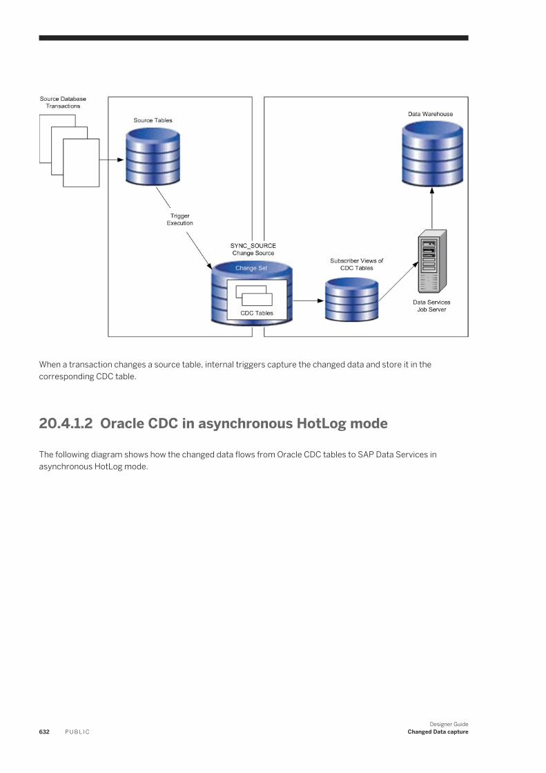
When a transaction changes a source table, internal triggers capture the changed data and store it in the corresponding CDC table.
20.4.1.2 Oracle CDC in asynchronous HotLog mode
The following diagram shows how the changed data flows from Oracle CDC tables to SAP Data Services in asynchronous HotLog mode.
632 P U B L I CDesigner Guide
Changed Data capture
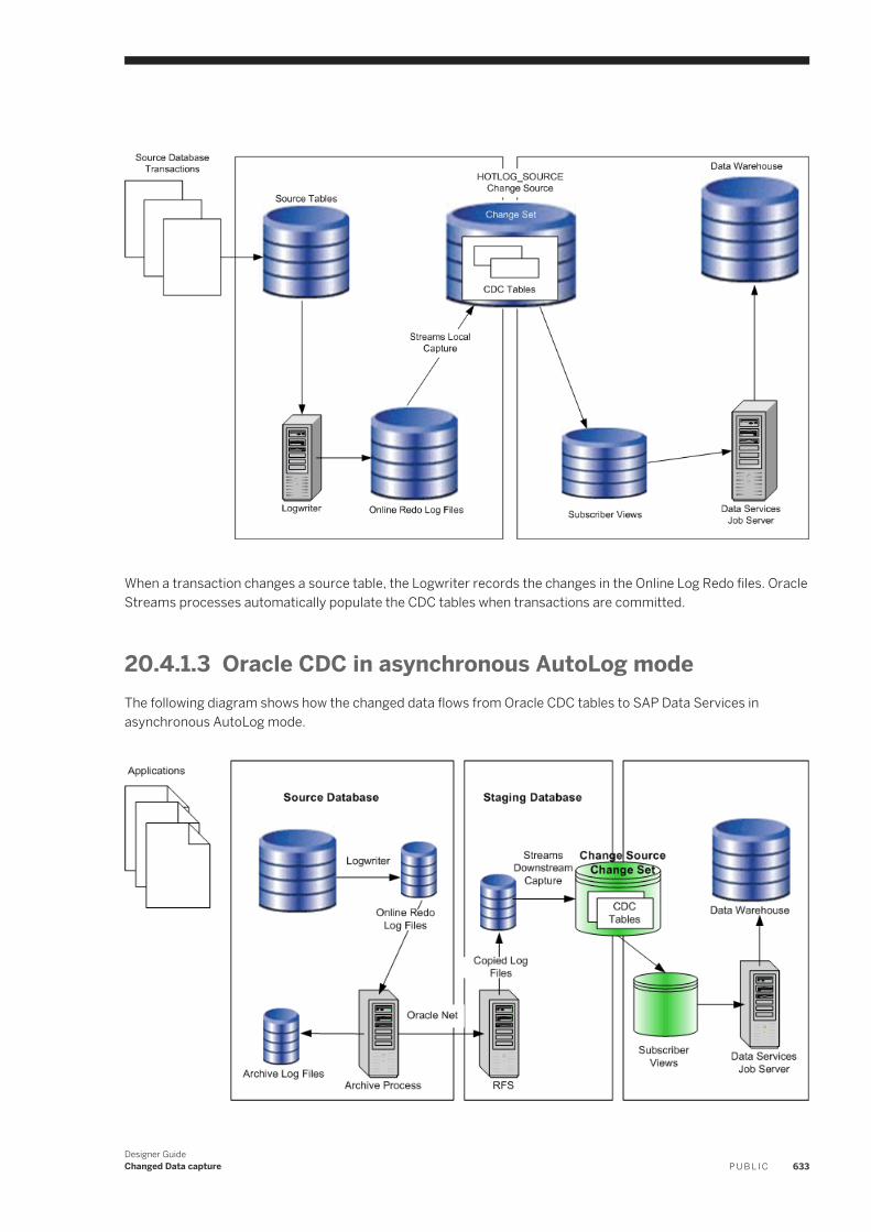
When a transaction changes a source table, the Logwriter records the changes in the Online Log Redo files. Oracle Streams processes automatically populate the CDC tables when transactions are committed.
20.4.1.3 Oracle CDC in asynchronous AutoLog modeThe following diagram shows how the changed data flows from Oracle CDC tables to SAP Data Services in asynchronous AutoLog mode.
Designer GuideChanged Data capture P U B L I C 633
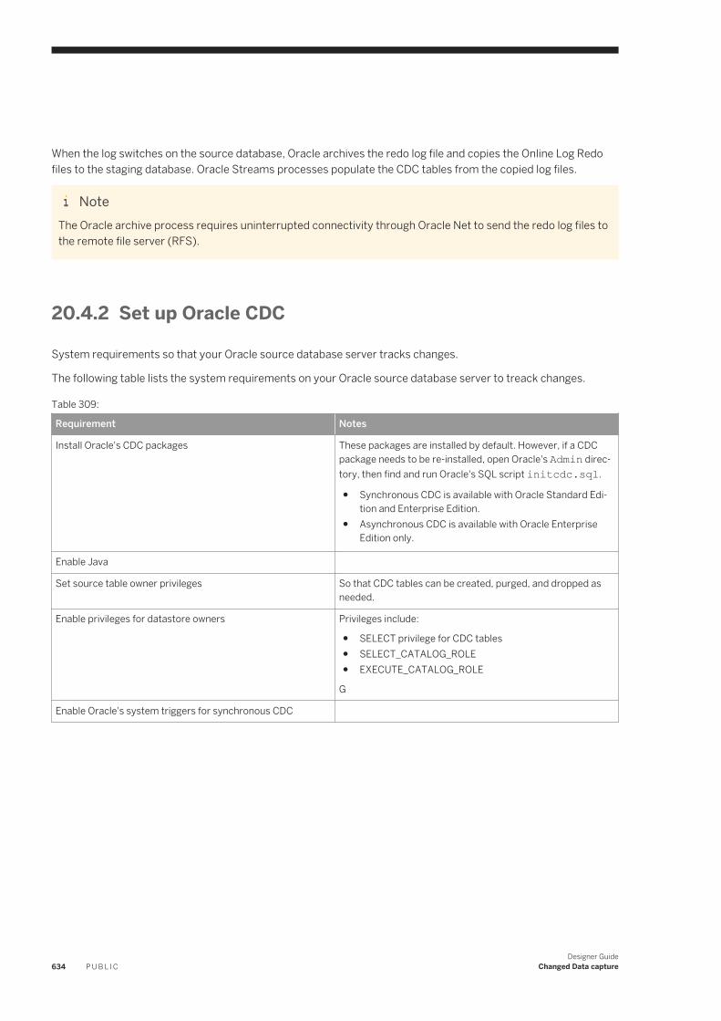
When the log switches on the source database, Oracle archives the redo log file and copies the Online Log Redo files to the staging database. Oracle Streams processes populate the CDC tables from the copied log files.
NoteThe Oracle archive process requires uninterrupted connectivity through Oracle Net to send the redo log files to the remote file server (RFS).
20.4.2 Set up Oracle CDC
System requirements so that your Oracle source database server tracks changes.
The following table lists the system requirements on your Oracle source database server to treack changes.
Table 309:
Requirement Notes
Install Oracle's CDC packages These packages are installed by default. However, if a CDC package needs to be re-installed, open Oracle's Admin directory, then find and run Oracle's SQL script initcdc.sql.
● Synchronous CDC is available with Oracle Standard Edition and Enterprise Edition.
● Asynchronous CDC is available with Oracle Enterprise Edition only.
Enable Java
Set source table owner privileges So that CDC tables can be created, purged, and dropped as needed.
Enable privileges for datastore owners Privileges include:
● SELECT privilege for CDC tables● SELECT_CATALOG_ROLE● EXECUTE_CATALOG_ROLE
G
Enable Oracle's system triggers for synchronous CDC
634 P U B L I CDesigner Guide
Changed Data capture
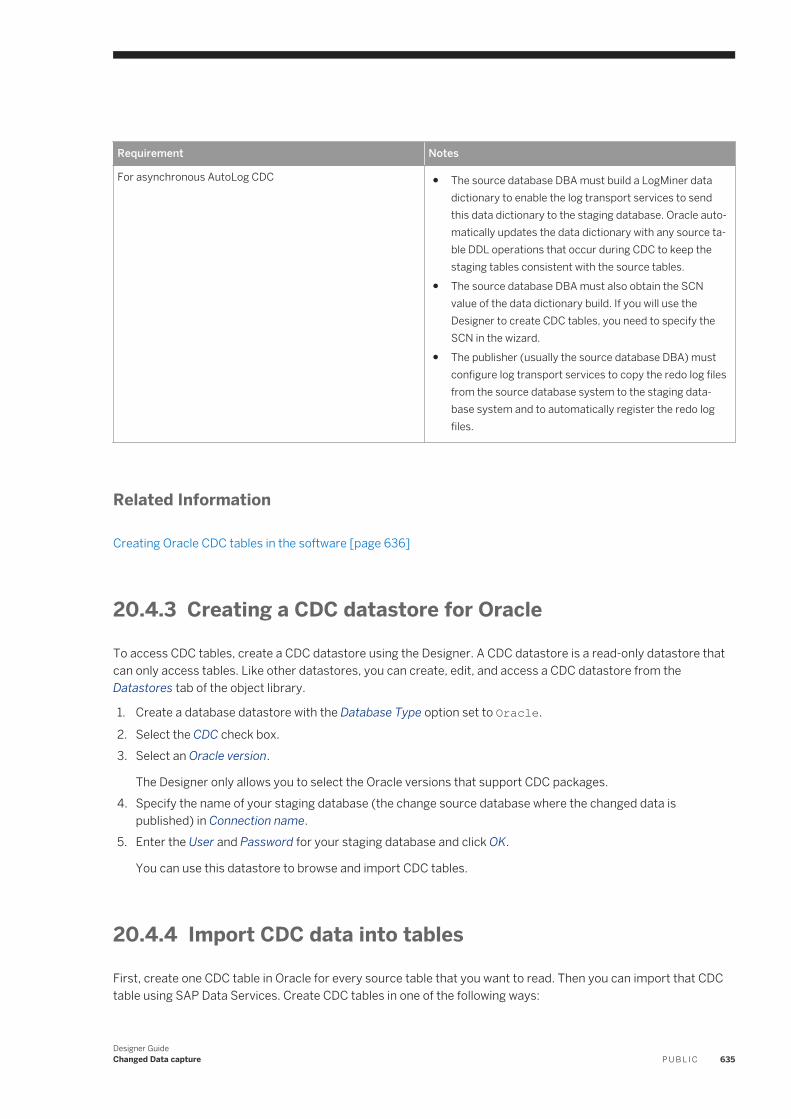
Requirement Notes
For asynchronous AutoLog CDC ● The source database DBA must build a LogMiner data dictionary to enable the log transport services to send this data dictionary to the staging database. Oracle automatically updates the data dictionary with any source table DDL operations that occur during CDC to keep the staging tables consistent with the source tables.
● The source database DBA must also obtain the SCN value of the data dictionary build. If you will use the Designer to create CDC tables, you need to specify the SCN in the wizard.
● The publisher (usually the source database DBA) must configure log transport services to copy the redo log files from the source database system to the staging database system and to automatically register the redo log files.
Related Information
Creating Oracle CDC tables in the software [page 636]
20.4.3 Creating a CDC datastore for Oracle
To access CDC tables, create a CDC datastore using the Designer. A CDC datastore is a read-only datastore that can only access tables. Like other datastores, you can create, edit, and access a CDC datastore from the Datastores tab of the object library.
1. Create a database datastore with the Database Type option set to Oracle.
2. Select the CDC check box.3. Select an Oracle version.
The Designer only allows you to select the Oracle versions that support CDC packages.4. Specify the name of your staging database (the change source database where the changed data is
published) in Connection name.5. Enter the User and Password for your staging database and click OK.
You can use this datastore to browse and import CDC tables.
20.4.4 Import CDC data into tables
First, create one CDC table in Oracle for every source table that you want to read. Then you can import that CDC table using SAP Data Services. Create CDC tables in one of the following ways:
Designer GuideChanged Data capture P U B L I C 635
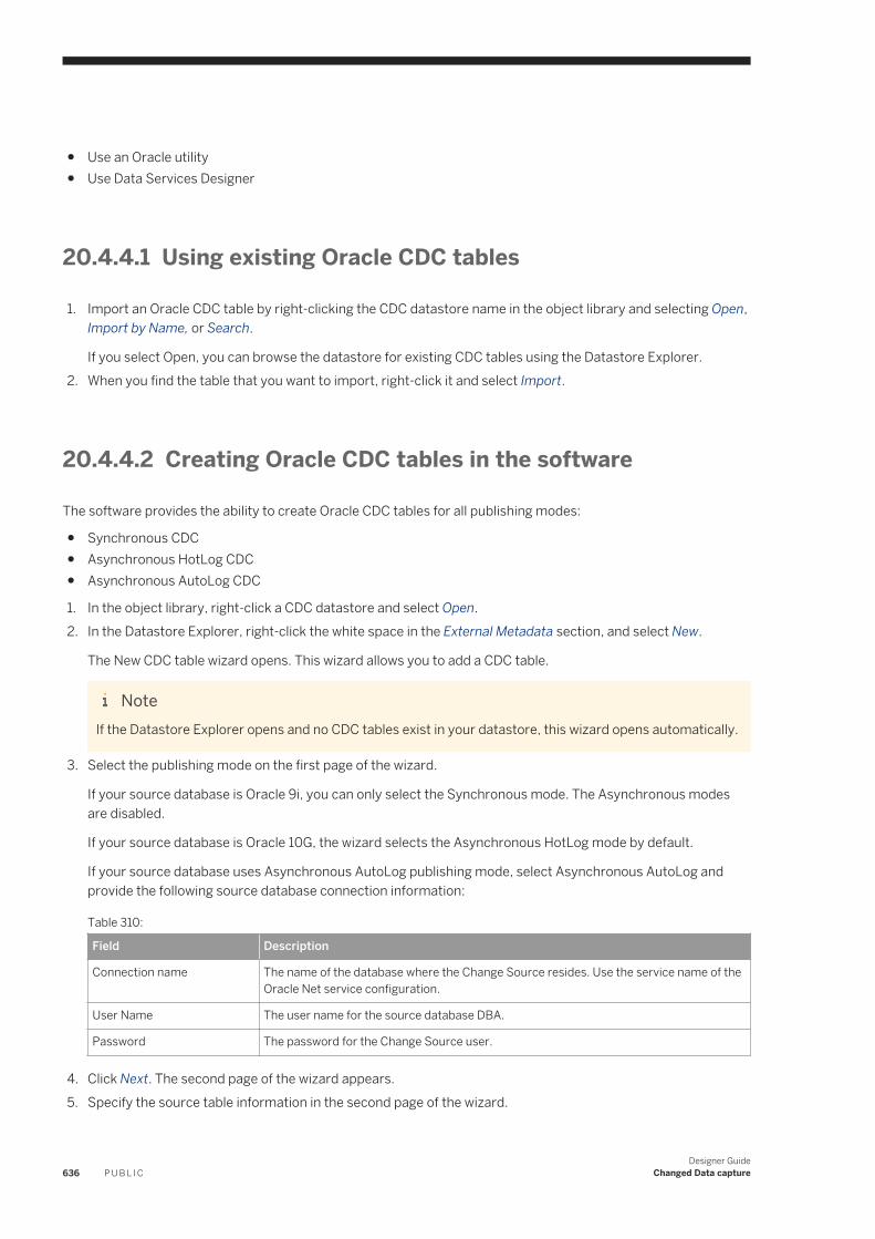
● Use an Oracle utility● Use Data Services Designer
20.4.4.1 Using existing Oracle CDC tables
1. Import an Oracle CDC table by right-clicking the CDC datastore name in the object library and selecting Open, Import by Name, or Search.
If you select Open, you can browse the datastore for existing CDC tables using the Datastore Explorer.2. When you find the table that you want to import, right-click it and select Import.
20.4.4.2 Creating Oracle CDC tables in the software
The software provides the ability to create Oracle CDC tables for all publishing modes:
● Synchronous CDC● Asynchronous HotLog CDC● Asynchronous AutoLog CDC
1. In the object library, right-click a CDC datastore and select Open.2. In the Datastore Explorer, right-click the white space in the External Metadata section, and select New.
The New CDC table wizard opens. This wizard allows you to add a CDC table.
NoteIf the Datastore Explorer opens and no CDC tables exist in your datastore, this wizard opens automatically.
3. Select the publishing mode on the first page of the wizard.
If your source database is Oracle 9i, you can only select the Synchronous mode. The Asynchronous modes are disabled.
If your source database is Oracle 10G, the wizard selects the Asynchronous HotLog mode by default.
If your source database uses Asynchronous AutoLog publishing mode, select Asynchronous AutoLog and provide the following source database connection information:
Table 310:
Field Description
Connection name The name of the database where the Change Source resides. Use the service name of the Oracle Net service configuration.
User Name The user name for the source database DBA.
Password The password for the Change Source user.
4. Click Next. The second page of the wizard appears.5. Specify the source table information in the second page of the wizard.
636 P U B L I CDesigner Guide
Changed Data capture
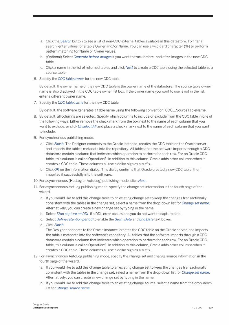
a. Click the Search button to see a list of non-CDC external tables available in this datastore. To filter a search, enter values for a table Owner and/or Name. You can use a wild-card character (%) to perform pattern matching for Name or Owner values.
b. (Optional) Select Generate before-images if you want to track before- and after-images in the new CDC table.
c. Click a name in the list of returned tables and click Next to create a CDC table using the selected table as a source table.
6. Specify the CDC table owner for the new CDC table.
By default, the owner name of the new CDC table is the owner name of the datastore. The source table owner name is also displayed in the CDC table owner list box. If the owner name you want to use is not in the list, enter a different owner name.
7. Specify the CDC table name for the new CDC table.
By default, the software generates a table name using the following convention: CDC__SourceTableName.8. By default, all columns are selected. Specify which columns to include or exclude from the CDC table in one of
the following ways: Either remove the check mark from the box next to the name of each column that you want to exclude, or click Unselect All and place a check mark next to the name of each column that you want to include.
9. For synchronous publishing mode:a. Click Finish. The Designer connects to the Oracle instance, creates the CDC table on the Oracle server,
and imports the table's metadata into the repository. All tables that the software imports through a CDC datastore contain a column that indicates which operation to perform for each row. For an Oracle CDC table, this column is called Operation$. In addition to this column, Oracle adds other columns when it creates a CDC table. These columns all use a dollar sign as a suffix.
b. Click OK on the information dialog. This dialog confirms that Oracle created a new CDC table, then imported it successfully into the software.
10. For asynchronous (HotLog or AutoLog) publishing mode, click Next.11. For asynchronous HotLog publishing mode, specify the change set information in the fourth page of the
wizard.a. If you would like to add this change table to an existing change set to keep the changes transactionally
consistent with the tables in the change set, select a name from the drop-down list for Change set name. Alternatively, you can create a new change set by typing in the name.
b. Select Stop capture on DDL if a DDL error occurs and you do not want to capture data.c. Select Define retention period to enable the Begin Date and End Date text boxes.d. Click Finish.
The Designer connects to the Oracle instance, creates the CDC table on the Oracle server, and imports the table's metadata into the software's repository. All tables that the software imports through a CDC datastore contain a column that indicates which operation to perform for each row. For an Oracle CDC table, this column is called Operation$. In addition to this column, Oracle adds other columns when it creates a CDC table. These columns all use a dollar sign as a suffix.
12. For asynchronous AutoLog publishing mode, specify the change set and change source information in the fourth page of the wizard.a. If you would like to add this change table to an existing change set to keep the changes transactionally
consistent with the tables in the change set, select a name from the drop-down list for Change set name. Alternatively, you can create a new change set by typing in the name.
b. If you would like to add this change table to an existing change source, select a name from the drop-down list for Change source name.
Designer GuideChanged Data capture P U B L I C 637
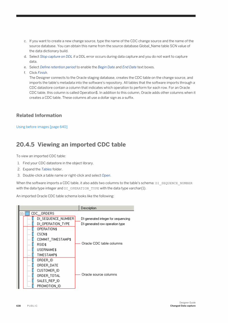
c. If you want to create a new change source, type the name of the CDC change source and the name of the source database. You can obtain this name from the source database Global_Name table SCN value of the data dictionary build.
d. Select Stop capture on DDL if a DDL error occurs during data capture and you do not want to capture data.
e. Select Define retention period to enable the Begin Date and End Date text boxes.f. Click Finish.
The Designer connects to the Oracle staging database, creates the CDC table on the change source, and imports the table's metadata into the software's repository. All tables that the software imports through a CDC datastore contain a column that indicates which operation to perform for each row. For an Oracle CDC table, this column is called Operation$. In addition to this column, Oracle adds other columns when it creates a CDC table. These columns all use a dollar sign as a suffix.
Related Information
Using before-images [page 640]
20.4.5 Viewing an imported CDC tableTo view an imported CDC table:
1. Find your CDC datastore in the object library.2. Expand the Tables folder.3. Double-click a table name or right-click and select Open.
When the software imports a CDC table, it also adds two columns to the table's schema: DI_SEQUENCE_NUMBER with the data type integer and DI_OPERATION_TYPE with the data type varchar(1).
An imported Oracle CDC table schema looks like the following:
638 P U B L I CDesigner Guide
Changed Data capture
This example has eight control columns added to the original table:
● Two generated by the software○ DI_SEQUENCE_NUMBER - Contains an integer for sequencing.○ DI_OPERATION_TYPE - Contains the row operation type.
● Six Oracle control columns: OPERATION$, CSCN$, COMMIT_TIMESTAMP$, RSID$, USERNAME$, TIMESTAMP$
NoteThe Oracle control columns vary, depending on the options that were selected when the CDC table is created. All Oracle control columns end with a dollar sign ($).
Related Information
The DI_SEQUENCE_NUMBER column [page 639]The DI_OPERATION_TYPE column [page 639]
20.4.5.1 The DI_SEQUENCE_NUMBER column
The DI_SEQUENCE_NUMBER column starts with zero at the beginning of each extraction. This field increments by one each time the software reads a row except when it encounters a pair of before- and after-images for an UPDATE operation. Both the before- and after-images receive the same sequence number. This sequencing column provides a way to collate image pairs if they are separated as a result of the data flow design.
Related Information
Using before-images [page 640]
20.4.5.2 The DI_OPERATION_TYPE column
The possible values for the DI_OPERATION_TYPE column are:
● I for INSERT● D for DELETE● B for before-image of an UPDATE● U for after-image of an UPDATE
Designer GuideChanged Data capture P U B L I C 639
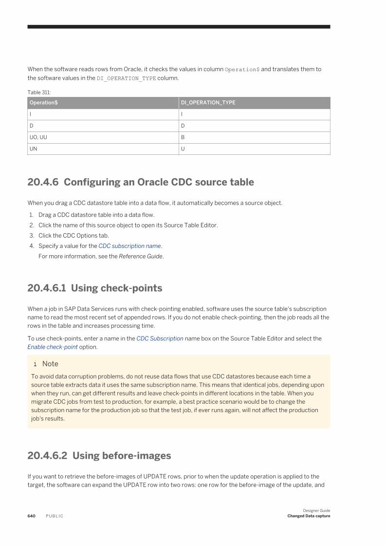
When the software reads rows from Oracle, it checks the values in column Operation$ and translates them to the software values in the DI_OPERATION_TYPE column.
Table 311:
Operation$ DI_OPERATION_TYPE
I I
D D
UO, UU B
UN U
20.4.6 Configuring an Oracle CDC source table
When you drag a CDC datastore table into a data flow, it automatically becomes a source object.
1. Drag a CDC datastore table into a data flow.2. Click the name of this source object to open its Source Table Editor.3. Click the CDC Options tab.4. Specify a value for the CDC subscription name.
For more information, see the Reference Guide.
20.4.6.1 Using check-points
When a job in SAP Data Services runs with check-pointing enabled, software uses the source table's subscription name to read the most recent set of appended rows. If you do not enable check-pointing, then the job reads all the rows in the table and increases processing time.
To use check-points, enter a name in the CDC Subscription name box on the Source Table Editor and select the Enable check-point option.
NoteTo avoid data corruption problems, do not reuse data flows that use CDC datastores because each time a source table extracts data it uses the same subscription name. This means that identical jobs, depending upon when they run, can get different results and leave check-points in different locations in the table. When you migrate CDC jobs from test to production, for example, a best practice scenario would be to change the subscription name for the production job so that the test job, if ever runs again, will not affect the production job's results.
20.4.6.2 Using before-images
If you want to retrieve the before-images of UPDATE rows, prior to when the update operation is applied to the target, the software can expand the UPDATE row into two rows: one row for the before-image of the update, and
640 P U B L I CDesigner Guide
Changed Data capture
one row for the after-image of the update. The before image of an update row is the image of the row before the row is changed, and the after image of an update row refers to the image of the row after the change is applied.
The default behavior is that a CDC reader retrieves after-images only. By not retrieving before-images, fewer rows pass through the engine which allows the job to execute in less time.
You can use before-images to:
● Update primary keys
NoteUnder most circumstances, when source tables are updated, their primary keys do not need to be updated.
● Calculate change logic between data in columnsFor example, you can calculate the difference between an employee's new and old salary by looking at the difference between the values in salary fields.
20.4.6.2.1 Capturing before-images for update rows
1. At CDC table creation time, make sure the Oracle CDC table is also setup to retrieve full before-images.If you create an Oracle CDC table using the Designer, you can select the Generate before-images to do this.
2. Select Get before-images for each update row in the CDC table's source editor.If the underlying, CDC table is not set-up properly, enabling the Get before-images for each update row option has no effect.
Once you select the Get before-images for each update row option, for every update, the software processes two rows. In addition to the performance impact of this data volume increase, the before- and after-image pairs may be separated or lost depending on the design of your data flow. This would cause data integrity issues.
The Map_CDC_Operation transform can resolve problems, but undesirable results may still occur due to programming errors. When using functions and transforms that re-order, re-direct, eliminate, and multiply the number of rows in a data flow (for example, due to the use of the group by or order by clauses in a query) be aware of the possible impact to targets.
20.4.7 Creating a data flow with an Oracle CDC source
To use an Oracle CDC source, you use a Query transform to remove the Oracle control columns and the Map_CDC_Operation transform to interpret the control columns and take appropriate actions.
1. In the Designer Object Library pane, drag the Oracle CDC table, Query, and Map_CDC_Operation transforms to the data flow workspace area.
NoteA data flow can contain only one CDC source.
2. Configure the CDC table.
Designer GuideChanged Data capture P U B L I C 641
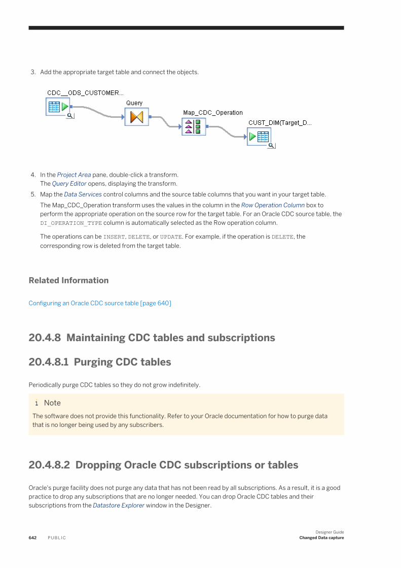
3. Add the appropriate target table and connect the objects.
4. In the Project Area pane, double-click a transform.
The Query Editor opens, displaying the transform.5. Map the Data Services control columns and the source table columns that you want in your target table.
The Map_CDC_Operation transform uses the values in the column in the Row Operation Column box to perform the appropriate operation on the source row for the target table. For an Oracle CDC source table, the DI_OPERATION_TYPE column is automatically selected as the Row operation column.
The operations can be INSERT, DELETE, or UPDATE. For example, if the operation is DELETE, the corresponding row is deleted from the target table.
Related Information
Configuring an Oracle CDC source table [page 640]
20.4.8 Maintaining CDC tables and subscriptions
20.4.8.1 Purging CDC tables
Periodically purge CDC tables so they do not grow indefinitely.
NoteThe software does not provide this functionality. Refer to your Oracle documentation for how to purge data that is no longer being used by any subscribers.
20.4.8.2 Dropping Oracle CDC subscriptions or tables
Oracle's purge facility does not purge any data that has not been read by all subscriptions. As a result, it is a good practice to drop any subscriptions that are no longer needed. You can drop Oracle CDC tables and their subscriptions from the Datastore Explorer window in the Designer.
642 P U B L I CDesigner Guide
Changed Data capture
1. In the Local Object Library pane, right-click a CDC datastore, and click Open.2. In the Datastore Explorer window, click Repository Metadata.3. Right-click a table, point to CDC maintenance, and do one of the following:
○ Point to Drop subscription.○ Drop Subscription opens the list of subscriptions you created in the software for the selected table.
Oracle subscriptions are associated with these subscription names. Select each subscription name to drop it from Oracle and delete it from the repository.
○ Click Drop table.○ This option drops the Oracle CDC table and also deletes it from the repository.
20.4.9 Limitations
The following limitations exist when using CDC with Oracle sources:
● You cannot use the following transforms and functions with a source table imported with a CDC datastore because of the existence of the SAP Data Services generated columns for CDC tables. The software cannot compare or search these columns.○ Table_Comparison, Key_Generation, and SQL transforms○ All database functions, such as lookup, lookup_ext, key_generation, sql, and total_rows
● You can only create one CDC source in a data flow.● Oracle CDC captures DML statements, including INSERT, DELETE, and UPDATE. However, Oracle CDC does
not support the following operations because they disable all database triggers:○ Direct-path INSERT statements○ The multi_table_insert statement in parallel DML mode
● If you are using check-pointing and running your job in recovery mode, the recovered job will begin to review the job at the start of the CDC table. Check-points are ignored.
20.5 Use CDC with Attunity mainframe sources
If your environment must keep large amounts of data current, the mainframe CDC feature is a simple solution to limiting the number of rows that must be read on a regular basis.
If your environment must keep large amounts of data current, the mainframe CDC feature is a simple solution to limiting the number of rows that must be read on a regular basis. A source that reads only the most recent operations (INSERTS, UPDATES, DELETES) allows you to design smaller, faster delta loads.
SAP Data Services captures changed data on Attunity mainframe data sources and applies it to a target system. The following diagram shows the path that the data takes from Attunity CDC to SAP Data Services.
Designer GuideChanged Data capture P U B L I C 643
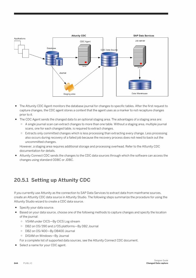
● The Attunity CDC Agent monitors the database journal for changes to specific tables. After the first request to capture changes, the CDC agent stores a context that the agent uses as a marker to not recapture changes prior to it.
● The CDC Agent sends the changed data to an optional staging area. The advantages of a staging area are:○ A single journal scan can extract changes to more than one table. Without a staging area, multiple journal
scans, one for each changed table, is required to extract changes.○ Extracts only committed changes which is less processing than extracting every change. Less processing
also occurs during recovery of a failed job because the recovery process does not need to back out the uncommitted changes.
However, a staging area requires additional storage and processing overhead. Refer to the Attunity CDC documentation for details.
● Attunity Connect CDC sends the changes to the CDC data sources through which the software can access the changes using standard ODBC or JDBC.
20.5.1 Setting up Attunity CDC
If you currently use Attunity as the connection to SAP Data Services to extract data from mainframe sources, create an Attunity CDC data source in Attunity Studio. The following steps summarize the procedure for using the Attunity Studio wizard to create a CDC data source.
● Specify your data source.● Based on your data source, choose one of the following methods to capture changes and specify the location
of the journal:○ VSAM under CICS—By CICS Log stream○ DB2 on OS/390 and z/OS platforms—By DB2 Journal○ DB2 on OS/400—By DB400 Journal○ DISAM on Windows—By Journal
For a complete list of supported data sources, see the Attunity Connect CDC document.● Select a name for your CDC agent.
644 P U B L I CDesigner Guide
Changed Data capture
● Specify if you want to capture before images for update operations. If you do not specify this option in Attunity Studio, you will not capture before images even if you specify the option Get before-image for each update row.
● Select the tables to monitor for changes.
The Attunity Studio wizard generates the following components that you need to specify on the Datastore Editor when you define an Attunity CDC datastore:
● A CDC data source name that you specify in the option Data source. Attunity generates the CDC data source on the same computer as the CDC agent by default. You have the option of placing the CDC data source on the client (same computer as SAP Data Services). Obtain the host name of this computer to specify in the option Host location.
● A workspace for the CDC agent to manage the change capture event queue. You specify the workspace name in the option Attunity workspace.
For more information, refer to the CDC setup section in the Attunity Connect: The Change Data Capture Solution.
20.5.2 Setting up the software for CDC on mainframe sources
To use SAP Data Services to read and load changed data from mainframe sources using Attunity, do the following procedures on the Designer:
● Create a CDC datastore for Attunity● Import metadata for Attunity tables● Configure a mainframe CDC source● Build real-time jobs using metadata
20.5.2.1 Creating CDC datastores
The CDC datastore option is available for all mainframe interfaces to SAP Data Services.
Related Information
Datastores [page 63]
20.5.2.1.1 Creating a CDC datastore for Attunity
1. Open the Datastore Editor.2. Enter a name for the datastore.3. In the Datastore type box, select Database.
Designer GuideChanged Data capture P U B L I C 645
4. In the Database type box, select Attunity_Connector.5. Check the Enable CDC box to enable the CDC feature. You can enable CDC for the following data sources. For
the current list of data sources, refer to the Attunity web site.○ VSAM under CICS○ DB2 UDB for z/OS○ DB2 UDB for OS/400
6. In the Data source box, specify the name of the Attunity CDC data source. You can specify more than one data source for one datastore, but you cannot join two CDC tables. You might want to specify multiple data sources in one Attunity datastore for easier management. If you can access all of the CDC tables through one Attunity data source, it is easier to create one datastore, enter the connection information once, and import the tables.
If you list multiple data source names for one Attunity Connector datastore, ensure that you meet the following requirements:
○ Do not specify regular Attunity data sources with CDC data sources in the same datastore. The software imports data from regular Attunity data sources differently than from CDC data sources.
○ All Attunity data sources must be accessible by the same user name and password.○ All Attunity data sources must use the same workspace. When you setup access to the data sources in
Attunity Studio, use the same workspace name for each data source.7. In the Host location box, specify the name of the host on which the Attunity data source daemon exists.8. In the Port box, specify the Attunity daemon port number. The default value is 2551.9. Specify the Attunity server workspace name that the CDC agent uses to manage the change capture event
queue for the CDC data source.10. Complete the rest of the dialog and click OK.
You can now use the new datastore connection to import metadata tables into the current repository.
Once saved, this datastore becomes a CDC datastore.
20.5.3 Importing mainframe CDC data
After you create a CDC datastore, you can use it to import CDC table metadata. In the object library, right-click the datastore name and select Open, Import by Name, or Search. For mainframe CDC, only the CDC tables that you selected in the procedure Setting up Attunity CDC [page 644] are visible when you browse external metadata. Functions and templates are not available because the Attunity CDC datastore is read-only.
The SAP Data Services import operation adds the following columns to the original table:
Table 312:
Column name Data type Source of column
DI_SEQUENCE_NUMBER integer Generated by SAP Data Services
DI_OPERATION_TYPE varchar(1) Generated by SAP Data Services
Context varchar(128) Supplied by Attunity Streams
646 P U B L I CDesigner Guide
Changed Data capture
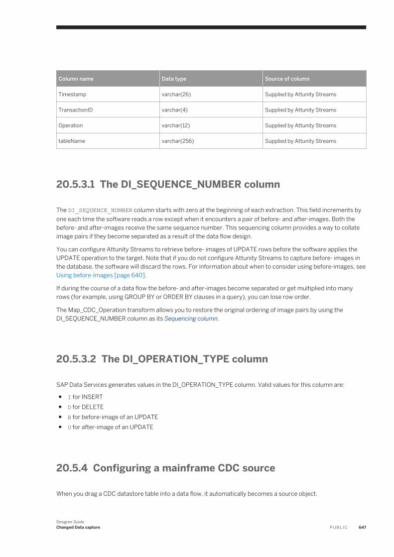
Column name Data type Source of column
Timestamp varchar(26) Supplied by Attunity Streams
TransactionID varchar(4) Supplied by Attunity Streams
Operation varchar(12) Supplied by Attunity Streams
tableName varchar(256) Supplied by Attunity Streams
20.5.3.1 The DI_SEQUENCE_NUMBER column
The DI_SEQUENCE_NUMBER column starts with zero at the beginning of each extraction. This field increments by one each time the software reads a row except when it encounters a pair of before- and after-images. Both the before- and after-images receive the same sequence number. This sequencing column provides a way to collate image pairs if they become separated as a result of the data flow design.
You can configure Attunity Streams to retrieve before- images of UPDATE rows before the software applies the UPDATE operation to the target. Note that if you do not configure Attunity Streams to capture before- images in the database, the software will discard the rows. For information about when to consider using before-images, see Using before-images [page 640].
If during the course of a data flow the before- and after-images become separated or get multiplied into many rows (for example, using GROUP BY or ORDER BY clauses in a query), you can lose row order.
The Map_CDC_Operation transform allows you to restore the original ordering of image pairs by using the DI_SEQUENCE_NUMBER column as its Sequencing column.
20.5.3.2 The DI_OPERATION_TYPE column
SAP Data Services generates values in the DI_OPERATION_TYPE column. Valid values for this column are:
● I for INSERT● D for DELETE● B for before-image of an UPDATE● U for after-image of an UPDATE
20.5.4 Configuring a mainframe CDC source
When you drag a CDC datastore table into a data flow, it automatically becomes a source object.
Designer GuideChanged Data capture P U B L I C 647
20.5.4.1 Configuring a mainframe CDC table
1. Drag a CDC datastore table into a data flow.
The table automatically becomes a source object.2. Click the name of this source object to open its Source Table Editor.3. Click the CDC Options tab.4. Specify a value for the CDC subscription name.
For more information, see the Reference Guide.
Related Information
Using mainframe check-points [page 648]Using before-images [page 640]
20.5.5 Using mainframe check-points
Attunity CDC agents read mainframe sources and load changed data either into a staging area or directly into the CDC data source. Rows of changed data append to the previous load in the CDC data source.
When you enable check-points, a CDC job in SAP Data Services uses the subscription name to read the most recent set of appended rows and to mark the end of the read. If check-points are not enabled, the CDC job reads all the rows in the Attunity CDC data source and processing time increases.
To use check-points, on the Source Table Editor enter the CDC Subscription name and select the Enable check-point option.
If you enable check-points and you run your CDC job in recovery mode, the recovered job begins to review the CDC data source at the last check-point.
NoteTo avoid data corruption problems, do not reuse data flows that use CDC datastores because each time a source table extracts data it uses the same subscription name. This means that identical jobs, depending upon when they run, can get different results and leave check-points in different locations in the file. When you migrate CDC jobs from test to production, a best-practice scenario is to change the subscription name for the production job. Therefore, if the test job ever runs again, it does not affect the production job's results.
20.5.5.1 Using before-images from mainframe sources
When you must capture before-image update rows.
1. Make sure Attunity Streams is set up to retrieve full before-images.
648 P U B L I CDesigner Guide
Changed Data capture
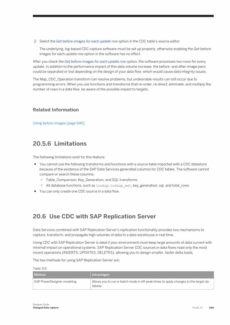
2. Select the Get before-images for each update row option in the CDC table's source editor.
The underlying, log-based CDC capture software must be set up properly, otherwise enabling the Get before-images for each update row option in the software has no effect.
After you check the Get before-images for each update row option, the software processes two rows for every update. In addition to the performance impact of this data volume increase, the before- and after-image pairs could be separated or lost depending on the design of your data flow, which would cause data integrity issues.
The Map_CDC_Operation transform can resolve problems, but undesirable results can still occur due to programming errors. When you use functions and transforms that re-order, re-direct, eliminate, and multiply the number of rows in a data flow, be aware of the possible impact to targets.
Related Information
Using before-images [page 640]
20.5.6 Limitations
The following limitations exist for this feature:
● You cannot use the following transforms and functions with a source table imported with a CDC datastore because of the existence of the SAP Data Services generated columns for CDC tables. The software cannot compare or search these columns.○ Table_Comparison, Key_Generation, and SQL transforms○ All database functions, such as lookup, lookup_ext, key_generation, sql, and total_rows
● You can only create one CDC source in a data flow.
20.6 Use CDC with SAP Replication Server
Data Services combined with SAP Replication Server's replication functionality provides two mechanisms to capture, transform, and propagate high volumes of data to a data warehouse in real time.
Using CDC with SAP Replication Server is ideal if your environment must keep large amounts of data current with minimal impact on operational systems. SAP Replication Server CDC sources in data flows read only the most recent operations (INSERTS, UPDATES, DELETES), allowing you to design smaller, faster delta loads.
The two methods for using SAP Replication Server are:
Table 313:
Method Advantages
SAP PowerDesigner modeling Allows you to run in batch mode in off-peak times to apply changes to the target database.
Designer GuideChanged Data capture P U B L I C 649
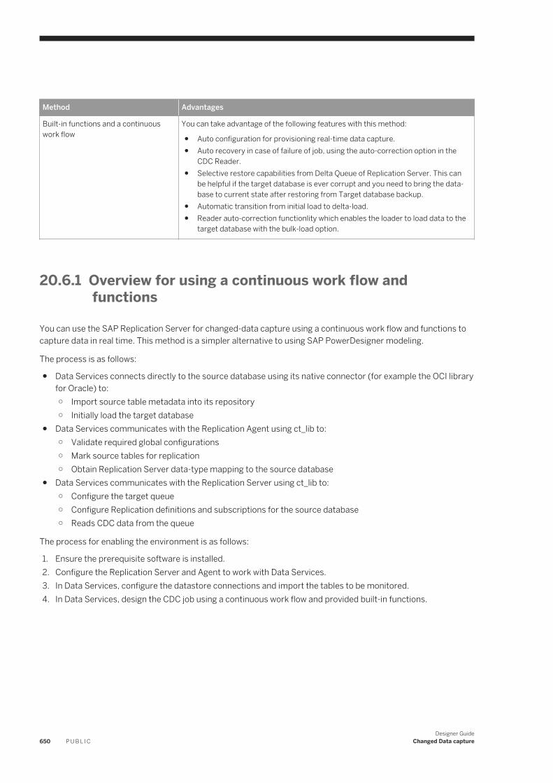
Method Advantages
Built-in functions and a continuous work flow
You can take advantage of the following features with this method:
● Auto configuration for provisioning real-time data capture.● Auto recovery in case of failure of job, using the auto-correction option in the
CDC Reader.● Selective restore capabilities from Delta Queue of Replication Server. This can
be helpful if the target database is ever corrupt and you need to bring the database to current state after restoring from Target database backup.
● Automatic transition from initial load to delta-load.● Reader auto-correction functionlity which enables the loader to load data to the
target database with the bulk-load option.
20.6.1 Overview for using a continuous work flow and functions
You can use the SAP Replication Server for changed-data capture using a continuous work flow and functions to capture data in real time. This method is a simpler alternative to using SAP PowerDesigner modeling.
The process is as follows:
● Data Services connects directly to the source database using its native connector (for example the OCI library for Oracle) to:○ Import source table metadata into its repository○ Initially load the target database
● Data Services communicates with the Replication Agent using ct_lib to:○ Validate required global configurations○ Mark source tables for replication○ Obtain Replication Server data-type mapping to the source database
● Data Services communicates with the Replication Server using ct_lib to:○ Configure the target queue○ Configure Replication definitions and subscriptions for the source database○ Reads CDC data from the queue
The process for enabling the environment is as follows:
1. Ensure the prerequisite software is installed.2. Configure the Replication Server and Agent to work with Data Services.3. In Data Services, configure the datastore connections and import the tables to be monitored.4. In Data Services, design the CDC job using a continuous work flow and provided built-in functions.
650 P U B L I CDesigner Guide
Changed Data capture
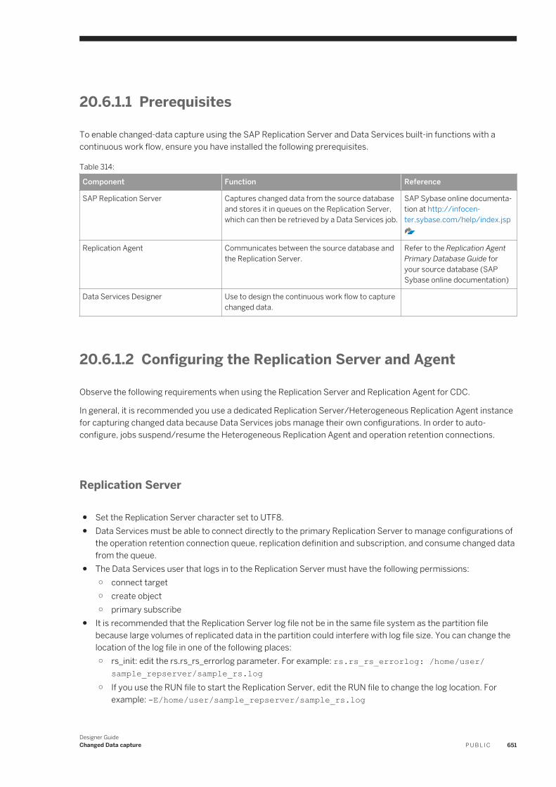
20.6.1.1 Prerequisites
To enable changed-data capture using the SAP Replication Server and Data Services built-in functions with a continuous work flow, ensure you have installed the following prerequisites.
Table 314:
Component Function Reference
SAP Replication Server Captures changed data from the source database and stores it in queues on the Replication Server, which can then be retrieved by a Data Services job.
SAP Sybase online documentation at http://infocenter.sybase.com/help/index.jsp
Replication Agent Communicates between the source database and the Replication Server.
Refer to the Replication Agent Primary Database Guide for your source database (SAP Sybase online documentation)
Data Services Designer Use to design the continuous work flow to capture changed data.
20.6.1.2 Configuring the Replication Server and Agent
Observe the following requirements when using the Replication Server and Replication Agent for CDC.
In general, it is recommended you use a dedicated Replication Server/Heterogeneous Replication Agent instance for capturing changed data because Data Services jobs manage their own configurations. In order to auto-configure, jobs suspend/resume the Heterogeneous Replication Agent and operation retention connections.
Replication Server
● Set the Replication Server character set to UTF8.● Data Services must be able to connect directly to the primary Replication Server to manage configurations of
the operation retention connection queue, replication definition and subscription, and consume changed data from the queue.
● The Data Services user that logs in to the Replication Server must have the following permissions:○ connect target○ create object○ primary subscribe
● It is recommended that the Replication Server log file not be in the same file system as the partition file because large volumes of replicated data in the partition could interfere with log file size. You can change the location of the log file in one of the following places:○ rs_init: edit the rs.rs_rs_errorlog parameter. For example: rs.rs_rs_errorlog: /home/user/
sample_repserver/sample_rs.log○ If you use the RUN file to start the Replication Server, edit the RUN file to change the log location. For
example: -E/home/user/sample_repserver/sample_rs.log
Designer GuideChanged Data capture P U B L I C 651
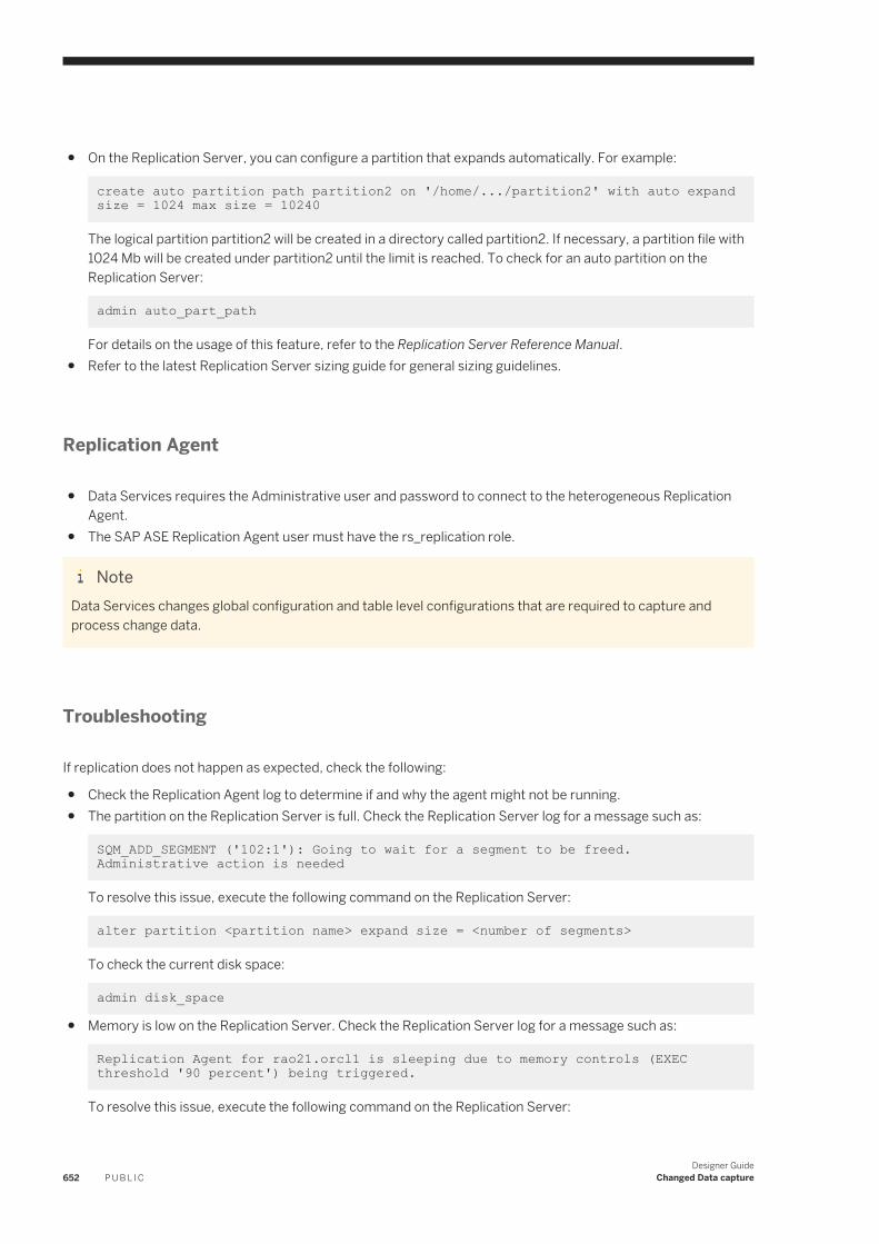
● On the Replication Server, you can configure a partition that expands automatically. For example:
create auto partition path partition2 on '/home/.../partition2' with auto expand size = 1024 max size = 10240
The logical partition partition2 will be created in a directory called partition2. If necessary, a partition file with 1024 Mb will be created under partition2 until the limit is reached. To check for an auto partition on the Replication Server:
admin auto_part_path
For details on the usage of this feature, refer to the Replication Server Reference Manual.● Refer to the latest Replication Server sizing guide for general sizing guidelines.
Replication Agent
● Data Services requires the Administrative user and password to connect to the heterogeneous Replication Agent.
● The SAP ASE Replication Agent user must have the rs_replication role.
NoteData Services changes global configuration and table level configurations that are required to capture and process change data.
Troubleshooting
If replication does not happen as expected, check the following:
● Check the Replication Agent log to determine if and why the agent might not be running.● The partition on the Replication Server is full. Check the Replication Server log for a message such as:
SQM_ADD_SEGMENT ('102:1'): Going to wait for a segment to be freed. Administrative action is needed
To resolve this issue, execute the following command on the Replication Server:
alter partition <partition name> expand size = <number of segments>
To check the current disk space:
admin disk_space
● Memory is low on the Replication Server. Check the Replication Server log for a message such as:
Replication Agent for rao21.orcl1 is sleeping due to memory controls (EXEC threshold '90 percent') being triggered.
To resolve this issue, execute the following command on the Replication Server:
652 P U B L I CDesigner Guide
Changed Data capture
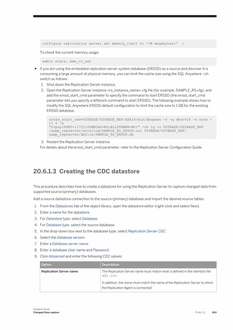
configure replication server set memory_limit to '<N megabytes>' :
To check the current memory usage:
admin stats, mem_in_use
● If you are using the embedded replication server system database (ERSSD) as a source and discover it is consuming a large amount of physical memory, you can limit the cache size using the SQL Anywhere –ch switch as follows:1. Shut down the Replication Server instance.2. Open the Replication Server instance <rs_instance_name>.cfg file (for example, SAMPLE_RS.cfg), and
add the erssd_start_cmd parameter to specify the command to start ERSSD (the erssd_start_cmd parameter lets you specify a different command to start ERSSD). The following example shows how to modify the SQL Anywhere ERSSD default configuration to limit the cache size to 1 GB for the existing ERSSD database.
erssd_start_cmd=$SYBASE/$SYBASE_REP/ASA16/bin/dbspawn -f -q dbsrv16 -s none -ti 0 -x "tcpip(PORT=11751;DOBROAD=NO;BLISTENER=NO)" -ch 1g -o $SYBASE/$SYBASE_REP /samp_repserver/errorlog/SAMPLE_RS_ERSSD.out $SYBASE/$SYBASE_REP/samp_repserver/dbfile/SAMPLE_RS_ERSSD.db
3. Restart the Replication Server instance.For details about the erssd_start_cmd parameter, refer to the Replication Server Configuration Guide.
20.6.1.3 Creating the CDC datastore
This procedure describes how to create a datastore for using the Replication Server to capture changed data from supported source (primary) databases.
Add a source datastore connection to the source (primary) database and import the desired source tables.
1. From the Datastores tab of the object library, open the datastore editor (right-click and select New).2. Enter a name for the datastore.3. For Datastore type, select Database.4. For Database type, select the source database.5. In the drop-down box next to the database type, select Replication Server CDC.6. Select the Database version.7. Enter a Database server name.8. Enter a database User name and Password.9. Click Advanced and enter the following CDC values:
Option Description
Replication Server name The Replication Server name must match what is defined in the interface file sql.ini.
In addition, the name must match the name of the Replication Server to which the Replication Agent is connected.
Designer GuideChanged Data capture P U B L I C 653
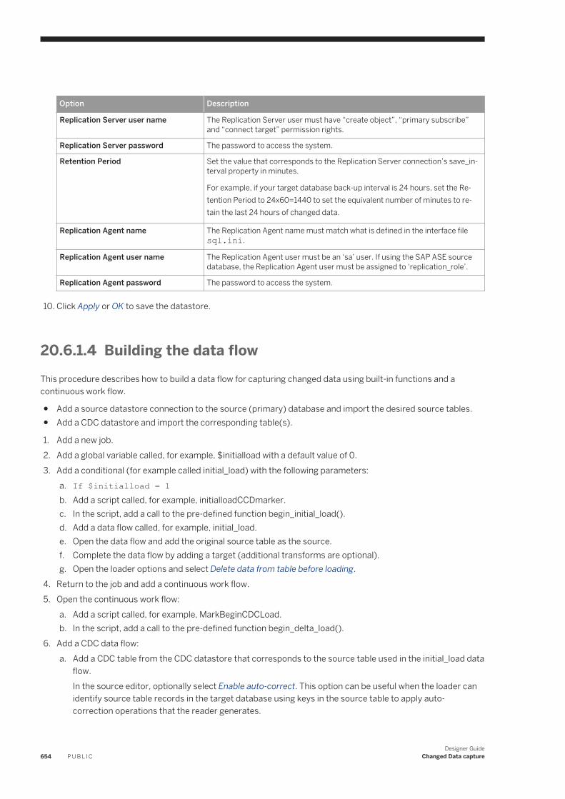
Option Description
Replication Server user name The Replication Server user must have “create object”, “primary subscribe” and “connect target” permission rights.
Replication Server password The password to access the system.
Retention Period Set the value that corresponds to the Replication Server connection’s save_interval property in minutes.
For example, if your target database back-up interval is 24 hours, set the Retention Period to 24x60=1440 to set the equivalent number of minutes to retain the last 24 hours of changed data.
Replication Agent name The Replication Agent name must match what is defined in the interface file sql.ini.
Replication Agent user name The Replication Agent user must be an ‘sa’ user. If using the SAP ASE source database, the Replication Agent user must be assigned to ‘replication_role’.
Replication Agent password The password to access the system.
10. Click Apply or OK to save the datastore.
20.6.1.4 Building the data flowThis procedure describes how to build a data flow for capturing changed data using built-in functions and a continuous work flow.
● Add a source datastore connection to the source (primary) database and import the desired source tables.● Add a CDC datastore and import the corresponding table(s).
1. Add a new job.2. Add a global variable called, for example, $initialload with a default value of 0.3. Add a conditional (for example called initial_load) with the following parameters:
a. If $initialload = 1b. Add a script called, for example, initialloadCCDmarker.c. In the script, add a call to the pre-defined function begin_initial_load().d. Add a data flow called, for example, initial_load.e. Open the data flow and add the original source table as the source.f. Complete the data flow by adding a target (additional transforms are optional).g. Open the loader options and select Delete data from table before loading.
4. Return to the job and add a continuous work flow.5. Open the continuous work flow:
a. Add a script called, for example, MarkBeginCDCLoad.b. In the script, add a call to the pre-defined function begin_delta_load().
6. Add a CDC data flow:a. Add a CDC table from the CDC datastore that corresponds to the source table used in the initial_load data
flow.In the source editor, optionally select Enable auto-correct. This option can be useful when the loader can identify source table records in the target database using keys in the source table to apply auto-correction operations that the reader generates.
654 P U B L I CDesigner Guide
Changed Data capture
a. Add a Map_CDC_Operation transform.b. Add a target and connect the objects.
7. When you execute the job for the first time, on the Global Variable tab set the $initialload variable to 1 to initialize (or reinitialize) the target datastore.
Changed data replicates to the target.
If the target database gets corrupted because of an error, you can restore the changed records from the Replication Server backlogged transactions. Use the Data Services built-in function restore_repserver_cdb_backlogged_transactions.
20.6.2 Overview for using the SAP PowerDesigner modeling method
You can use the SAP Replication Server for changed-data capture using SAP PowerDesigner modeling. This method is an alternative to using built-in functions with a continuous work flow.
Using the SAP PowerDesigner Data Movement Model, Data Services manages the CDC environment by building a CDC staging database and creating SAP Replication Server replication definitions and subscriptions. Upon deployment of the replication definitions and subscriptions and the CDC staging database definitions, SAP Replication Server publishes changed data from the source table to its corresponding CDC table that resides in the CDC staging database. The CDC table source in the Data Services data flow reads the most recently changed data from the last check-point from the CDC table and applies it to the target. The following diagram shows how the changed data moves from the Replication Server to Data Services.
Designer GuideChanged Data capture P U B L I C 655
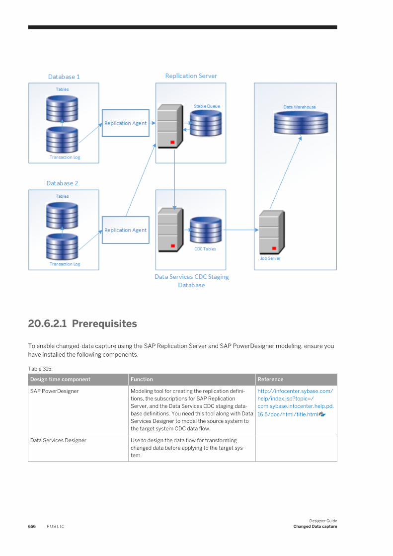
20.6.2.1 Prerequisites
To enable changed-data capture using the SAP Replication Server and SAP PowerDesigner modeling, ensure you have installed the following components.
Table 315:
Design time component Function Reference
SAP PowerDesigner Modeling tool for creating the replication definitions, the subscriptions for SAP Replication Server, and the Data Services CDC staging database definitions. You need this tool along with Data Services Designer to model the source system to the target system CDC data flow.
http://infocenter.sybase.com/help/index.jsp?topic=/com.sybase.infocenter.help.pd.16.5/doc/html/title.html
Data Services Designer Use to design the data flow for transforming changed data before applying to the target system.
656 P U B L I CDesigner Guide
Changed Data capture
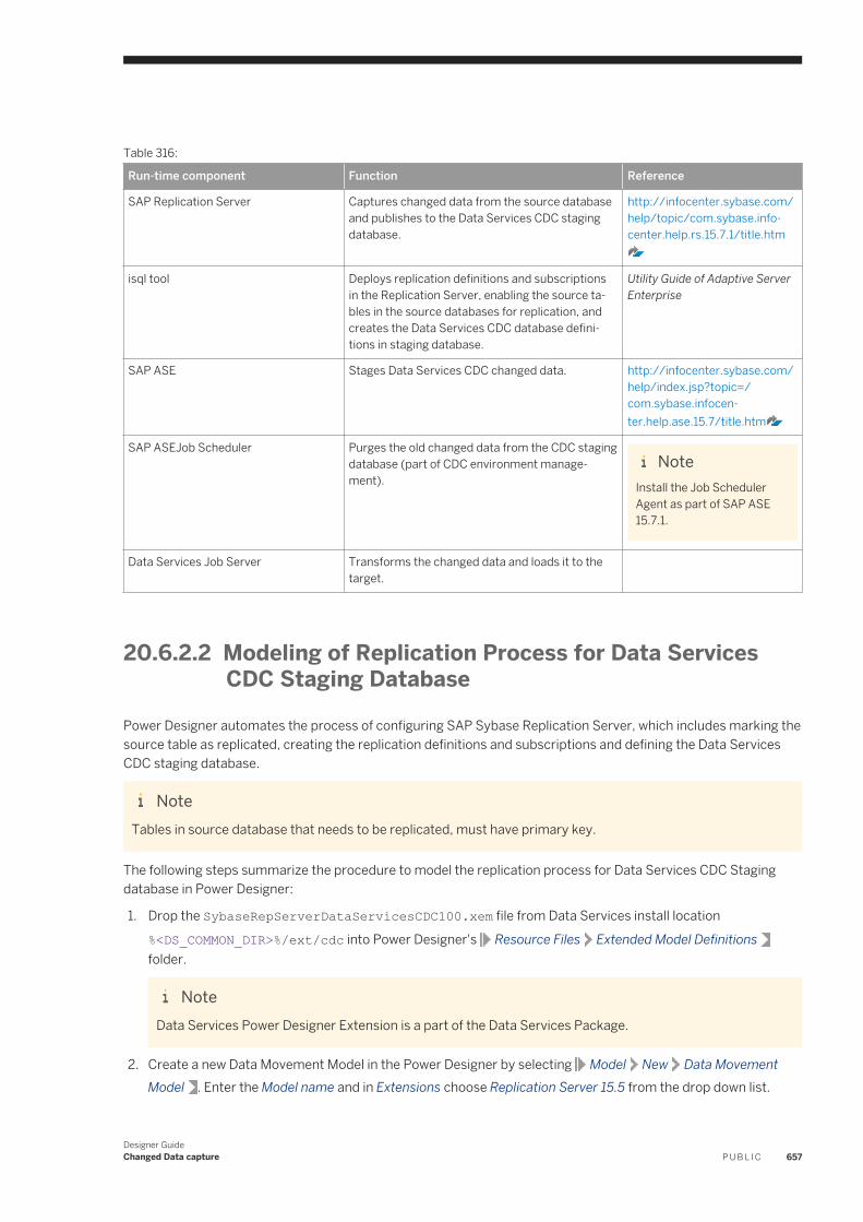
Table 316:
Run-time component Function Reference
SAP Replication Server Captures changed data from the source database and publishes to the Data Services CDC staging database.
http://infocenter.sybase.com/help/topic/com.sybase.infocenter.help.rs.15.7.1/title.htm
isql tool Deploys replication definitions and subscriptions in the Replication Server, enabling the source tables in the source databases for replication, and creates the Data Services CDC database definitions in staging database.
Utility Guide of Adaptive Server Enterprise
SAP ASE Stages Data Services CDC changed data. http://infocenter.sybase.com/help/index.jsp?topic=/com.sybase.infocenter.help.ase.15.7/title.htm
SAP ASEJob Scheduler Purges the old changed data from the CDC staging database (part of CDC environment management).
NoteInstall the Job Scheduler Agent as part of SAP ASE 15.7.1.
Data Services Job Server Transforms the changed data and loads it to the target.
20.6.2.2 Modeling of Replication Process for Data Services CDC Staging Database
Power Designer automates the process of configuring SAP Sybase Replication Server, which includes marking the source table as replicated, creating the replication definitions and subscriptions and defining the Data Services CDC staging database.
NoteTables in source database that needs to be replicated, must have primary key.
The following steps summarize the procedure to model the replication process for Data Services CDC Staging database in Power Designer:
1. Drop the SybaseRepServerDataServicesCDC100.xem file from Data Services install location %<DS_COMMON_DIR>%/ext/cdc into Power Designer's Resource Files Extended Model Definitionsfolder.
NoteData Services Power Designer Extension is a part of the Data Services Package.
2. Create a new Data Movement Model in the Power Designer by selecting Model New Data Movement Model . Enter the Model name and in Extensions choose Replication Server 15.5 from the drop down list.
Designer GuideChanged Data capture P U B L I C 657
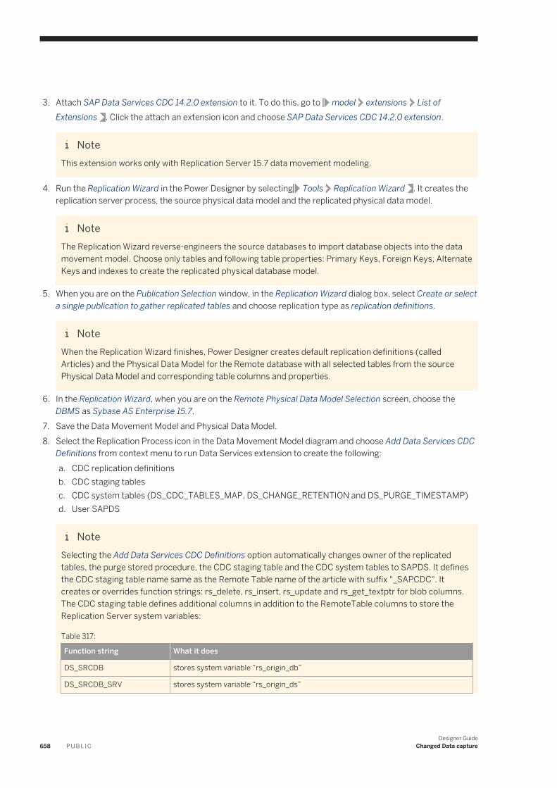
3. Attach SAP Data Services CDC 14.2.0 extension to it. To do this, go to model extensions List of Extensions . Click the attach an extension icon and choose SAP Data Services CDC 14.2.0 extension.
NoteThis extension works only with Replication Server 15.7 data movement modeling.
4. Run the Replication Wizard in the Power Designer by selecting Tools Replication Wizard . It creates the replication server process, the source physical data model and the replicated physical data model.
NoteThe Replication Wizard reverse-engineers the source databases to import database objects into the data movement model. Choose only tables and following table properties: Primary Keys, Foreign Keys, Alternate Keys and indexes to create the replicated physical database model.
5. When you are on the Publication Selection window, in the Replication Wizard dialog box, select Create or select a single publication to gather replicated tables and choose replication type as replication definitions.
NoteWhen the Replication Wizard finishes, Power Designer creates default replication definitions (called Articles) and the Physical Data Model for the Remote database with all selected tables from the source Physical Data Model and corresponding table columns and properties.
6. In the Replication Wizard, when you are on the Remote Physical Data Model Selection screen, choose the DBMS as Sybase AS Enterprise 15.7.
7. Save the Data Movement Model and Physical Data Model.8. Select the Replication Process icon in the Data Movement Model diagram and choose Add Data Services CDC
Definitions from context menu to run Data Services extension to create the following:a. CDC replication definitionsb. CDC staging tablesc. CDC system tables (DS_CDC_TABLES_MAP, DS_CHANGE_RETENTION and DS_PURGE_TIMESTAMP)d. User SAPDS
NoteSelecting the Add Data Services CDC Definitions option automatically changes owner of the replicated tables, the purge stored procedure, the CDC staging table and the CDC system tables to SAPDS. It defines the CDC staging table name same as the Remote Table name of the article with suffix "_SAPCDC". It creates or overrides function strings: rs_delete, rs_insert, rs_update and rs_get_textptr for blob columns. The CDC staging table defines additional columns in addition to the RemoteTable columns to store the Replication Server system variables:
Table 317:
Function string What it does
DS_SRCDB stores system variable “rs_origin_db”
DS_SRCDB_SRV stores system variable “rs_origin_ds”
658 P U B L I CDesigner Guide
Changed Data capture
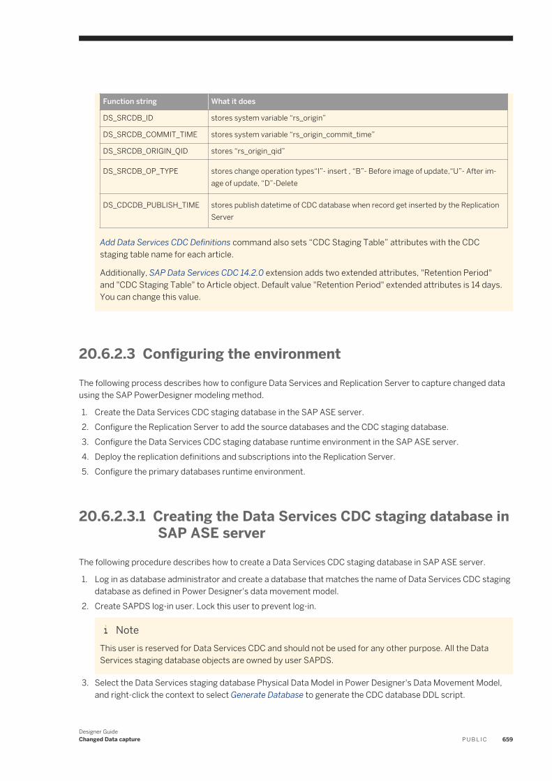
Function string What it does
DS_SRCDB_ID stores system variable “rs_origin”
DS_SRCDB_COMMIT_TIME stores system variable “rs_origin_commit_time”
DS_SRCDB_ORIGIN_QID stores “rs_origin_qid”
DS_SRCDB_OP_TYPE stores change operation types“I”- insert , “B”- Before image of update,“U”- After image of update, “D”-Delete
DS_CDCDB_PUBLISH_TIME stores publish datetime of CDC database when record get inserted by the Replication Server
Add Data Services CDC Definitions command also sets “CDC Staging Table” attributes with the CDC staging table name for each article.
Additionally, SAP Data Services CDC 14.2.0 extension adds two extended attributes, "Retention Period" and "CDC Staging Table" to Article object. Default value "Retention Period" extended attributes is 14 days. You can change this value.
20.6.2.3 Configuring the environment
The following process describes how to configure Data Services and Replication Server to capture changed data using the SAP PowerDesigner modeling method.
1. Create the Data Services CDC staging database in the SAP ASE server.2. Configure the Replication Server to add the source databases and the CDC staging database.3. Configure the Data Services CDC staging database runtime environment in the SAP ASE server.4. Deploy the replication definitions and subscriptions into the Replication Server.5. Configure the primary databases runtime environment.
20.6.2.3.1 Creating the Data Services CDC staging database in SAP ASE server
The following procedure describes how to create a Data Services CDC staging database in SAP ASE server.
1. Log in as database administrator and create a database that matches the name of Data Services CDC staging database as defined in Power Designer's data movement model.
2. Create SAPDS log-in user. Lock this user to prevent log-in.
NoteThis user is reserved for Data Services CDC and should not be used for any other purpose. All the Data Services staging database objects are owned by user SAPDS.
3. Select the Data Services staging database Physical Data Model in Power Designer's Data Movement Model, and right-click the context to select Generate Database to generate the CDC database DDL script.
Designer GuideChanged Data capture P U B L I C 659
NoteThis automatically generates DDLs of all the database objects that are required for the Data Services CDC staging database.
4. Check the CDC database DDL script that is generated as a file.5. Deploy the DDL script using the isql tool. Enter the code:
isql-Usa-Ppwd -Spds -Dpdb -i DS_CDC_staging_DDL_script.sql-oDS_CDC_staging_DDL_script.out
where:○ <sa> is the system administrator user login on the Data Services CDC staging data server.○ <pwd> is the password for the system administrator user login.○ <pds> is the name of the Data Services CDC staging data server.○ <pdb> is the name of the Data Services CDC staging database.
20.6.2.3.2 Configuring Replication Server to add source databases and CDC staging database
The following procedure describes how to configure Replication Server to add a source database and CDC staging database.
1. Add the source database and the CDC staging database to the interface file in Replication Server host.2. Run rs_init to add the source database and the CDC staging database.
20.6.2.3.3 Configuring Data Services CDC staging database in SAP ASE server
The following procedure describes how to configure the Data Services CDC staging database in the SAP ASE server.
1. Select the Data Services staging database's Physical Data Model in PowerDesigner's Data Movement Model, and right-click the context to select Generate Script.
2. Select the SAP Data Services CDC 14.2.0 extension in the dialog box. It generates a script file suffixed with _DataServices_CDC_DB_Runtime_Script.sql. This script file creates the Data Services CDC staging database runtime environment and provides the following functionalities:a. Validates the staging database to verifyt if it has been added to the Replication Server by its rs_init utility.b. Validates if the Data Services CDC staging database create script has run.c. Creates the Replication Server maintenance user that was defined in the Data Movement Model (if it was
not created before). You can change the password after creation to protect unauthorized access.d. Adds the maintenance user to database.e. Adds the TargetTable name and the CDC staging table name to DS_CDC_TABLES_MAP table for each
replication definition.
660 P U B L I CDesigner Guide
Changed Data capture
f. Adds the CDC staging table name and the retention period to DS_CHANGE_RETENTION table for each replication definition.
g. Grants select, insert, update, and delete privileges to the CDC staging tables.h. Grants execute privilege to the PURGE_OLD_CHANGE_DATA stored procedure.i. Grants the Replication Server maintenance user the privileges to execute the
PURGE_OLD_CHANGE_DATA scheduled job in theSAP ASE Job Scheduler database.j. Creates PURGE_OLD_CHANGE_DATA scheduled job in SAP ASE Job Scheduler database. The job name
is SAPDS_<CDC Staging Database Name>_PURGE_CHANGE_OLD_DATA.
3. Deploy the DDL script using the isql tool.
Database user who logs in must be a super user. Enter the code:
isql –Usa -Ppwd -Spds -Dpdb -i DS_CDC_staging_Runtime script.sql -o DS_CDC_staging_Runtime_script.out
where:○ <sa> is the system administrator user login on the Data Services CDC staging data server.○ <pwd> is the password for the system administrator user login.○ <pds> is the name of the Data Services CDC staging data server.○ <pdb> is the name of the Data Services CDC staging database.
20.6.2.3.4 Deploying replication definitions and subscriptions into the Replication Server
The following procedure describes how to deploy replication definitions and subscriptions into the Replication Server.
1. Select the Replication Process in the PowerDesigner Data Movement Model, and right-click the context to select Generate Script.
2. Set the Create Connection value to false in the dialog box, and click OK to generate the replication definitions, CDC function string definition subscriptions, and the Replication Server RCL script file.
NoteIt is recommended that you create a database connection using the rs_init tool.
3. Deploy the RCL script using the isql tool into the Replication Server that you configured for the CDC staging database and the source databases.The Replication Server user who logs in to deploy must be a super user. Enter the code:
isql –Usa -Ppwd -Spds -Dpbd -i RCL_script.sql -o RCL_script.out
where:○ <sa> is the system administrator user login on the Data Services CDC staging data server.○ <pwd> is the password for the system administrator user login.○ <pds> is the name of the Data Services CDC staging data server.○ <pdb> is the name of the Data Services CDC staging database.
Designer GuideChanged Data capture P U B L I C 661
20.6.2.3.5 Configuring the primary database environment
The following procedure describes how to configure the primary database environment.
1. Select the primary database in the PowerDesigner Data Movement Model, right-click the context to select Generate Script, and select Replication Server 15.7. It generates three script files.
2. Select the script file that includes the sp_setreptable stored procedure command.3. Check the script to make sure that the owner_on parameter is set for articles whose primary table name is
qualified by owner.The SAP Data Services CDC 14.2.0 extension turns on the multiple-owner attribute for all primary tables that are qualified by owner.
4. Deploy these scripts using the isql tool and the appropriate source database tool to create user, grants and permissions.The database user who deploys the script must be a super user. Enter the code:
isql –Usa -Ppwd -Spdb -Dpdb -i Primary_database_Runtime script.sql -o Primary_database_Runtime script.out
where:○ <sa> is the system administrator user login on the Data Services CDC staging data server.○ <pwd> is the password for the system administrator user login.○ <pds> is the name of the Data Services CDC staging data server.○ <pdb> is the name of the Data Services CDC staging database.
This marks primary tables as replicable, and changed data can be captured by the Replication Agent and propagated to the Replication Server.
20.6.2.4 Configuring Data Services
To use Data Services to read and load changed data from SAP Sybase Replication Server using the PowerDesigner modeling, do the following procedures in the Designer.
● Create a CDC datastore.● Import the metadata for SAP Replication Server tables.● Create and define a data flow.● Configure a CDC source.
662 P U B L I CDesigner Guide
Changed Data capture
20.6.2.4.1 Creating a CDC datastore and importing table metadata
This procedure describes how to create a CDC datastore using the SAP Replication Server.To access the source, create a CDC datastore using the Designer. A CDC datastore is a read-only datastore that can only access tables. After you create the CDC datastore, you use it to import CDC table metadata.
1. From the Datastores tab of the object library, open the datastore editor.2. Enter a name for the datastore.3. For Datastore type, select RepServer CDC.4. For Database type , select SAP ASE.5. Select the Database version.6. Enter a Database server name.7. Enter a Database name.8. Enter a database User name and Password.9. To create more than one configuration for this datastore, click Apply , then click Edit and enter the
configuration details.
NoteYou cannot change the database type, version, or CDC method.
10. Click OK.11. To import the tables, in the object library, right-click the datastore name and select Open, Import by Name, or
Search.Only the CDC tables that you selected when you set up SAP Replication Server for CDC are visible when you browse external metadata. You must create a CDC table in SAP ASE for every table you want to read before you can browse and import that CDC table using SAP Data Services.
Related Information
Defining a database datastore [page 67]Ways of importing metadata [page 77]
20.6.2.4.2 Creating and defining the data flow
This procedure describes how to create a data flow to read changed data using SAP Replication Server and the SAP PowerDesigner modeling.
1. In the object library, drag the CDC table, a Query transform, and a Map_CDC_Operation transform to the workspace.
Designer GuideChanged Data capture P U B L I C 663
Note○ Multiple Replication Server CDC tables are allowed in same data flow.○ The Replication Server CDC table stores data records extracted from the source database log.
However, these stored data records are not equivalent to the records available in the corresponding source table. Additionally, captured changed data records older than the retention period are also deleted from the Replication Server CDC table. Therefore, joining two or more such CDC tables may not produce the same result as joining their corresponding source database tables.
2. Configure the CDC table as described in the next section.3. Add the appropriate target table and connect the objects.4. Open the Query Editor.5. Map the Data Services control columns and the source table columns that you want in your target.
The Map_CDC_Operation transform uses the values in the column in the Row operation column box to perform the appropriate operation on the source row for the target table. For the CDC source table, the DI_OPERATION_TYPE column is automatically selected as the Row operation column.
The operations can be INSERT, DELETE, or UPDATE. For example, if the operation is DELETE, the corresponding row is deleted from the target table.
Related Information
Configuring CDC source table [page 664]
20.6.2.4.3 Configuring CDC source table
This procedure describes how to configure a CDC source table. Data Services can apply check-points across all the tables (in a given datastore configuration) for all the data flows in a job to provide data consistency.
1. Drag a CDC datastore table into a data flow.2. Click the name of this source object to open its editor.3. Click the CDC options tab.4. Optionally select Enable check-point.
Once a check-point is placed, the next time the CDC job runs, it reads only the rows inserted into the CDC table since the last check-point.
If check-points are not enabled, the CDC job reads all the rows in the CDC data source (with increased processing time).
664 P U B L I CDesigner Guide
Changed Data capture
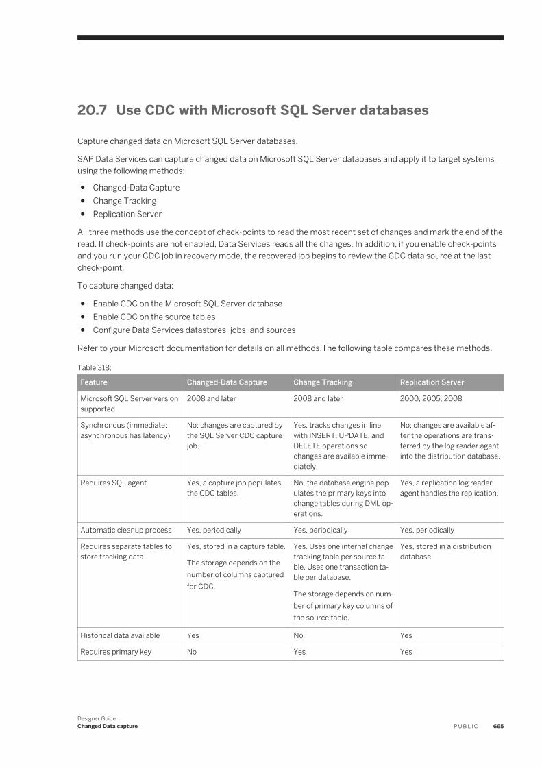
20.7 Use CDC with Microsoft SQL Server databases
Capture changed data on Microsoft SQL Server databases.
SAP Data Services can capture changed data on Microsoft SQL Server databases and apply it to target systems using the following methods:
● Changed-Data Capture● Change Tracking● Replication Server
All three methods use the concept of check-points to read the most recent set of changes and mark the end of the read. If check-points are not enabled, Data Services reads all the changes. In addition, if you enable check-points and you run your CDC job in recovery mode, the recovered job begins to review the CDC data source at the last check-point.
To capture changed data:
● Enable CDC on the Microsoft SQL Server database● Enable CDC on the source tables● Configure Data Services datastores, jobs, and sources
Refer to your Microsoft documentation for details on all methods.The following table compares these methods.
Table 318:
Feature Changed-Data Capture Change Tracking Replication Server
Microsoft SQL Server version supported
2008 and later 2008 and later 2000, 2005, 2008
Synchronous (immediate; asynchronous has latency)
No; changes are captured by the SQL Server CDC capture job.
Yes, tracks changes in line with INSERT, UPDATE, and DELETE operations so changes are available immediately.
No; changes are available after the operations are transferred by the log reader agent into the distribution database.
Requires SQL agent Yes, a capture job populates the CDC tables.
No, the database engine populates the primary keys into change tables during DML operations.
Yes, a replication log reader agent handles the replication.
Automatic cleanup process Yes, periodically Yes, periodically Yes, periodically
Requires separate tables to store tracking data
Yes, stored in a capture table.
The storage depends on the number of columns captured for CDC.
Yes. Uses one internal change tracking table per source table. Uses one transaction table per database.
The storage depends on number of primary key columns of the source table.
Yes, stored in a distribution database.
Historical data available Yes No Yes
Requires primary key No Yes Yes
Designer GuideChanged Data capture P U B L I C 665
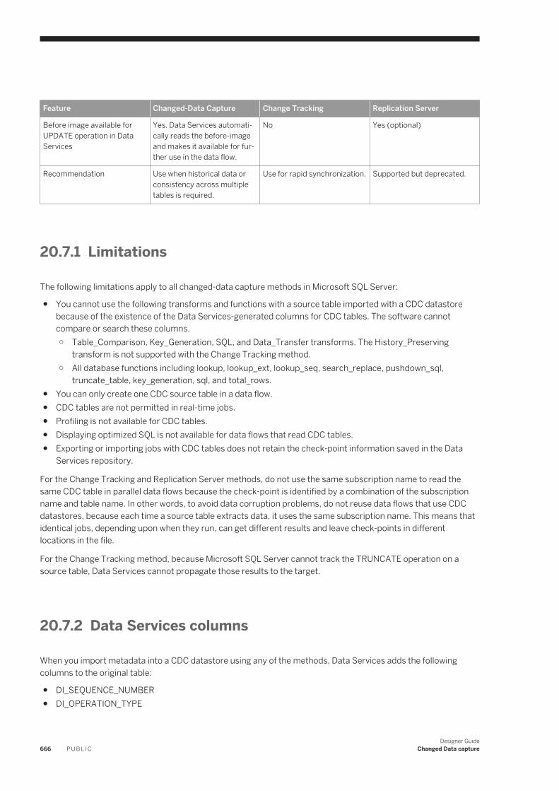
Feature Changed-Data Capture Change Tracking Replication Server
Before image available for UPDATE operation in Data Services
Yes. Data Services automatically reads the before-image and makes it available for further use in the data flow.
No Yes (optional)
Recommendation Use when historical data or consistency across multiple tables is required.
Use for rapid synchronization. Supported but deprecated.
20.7.1 Limitations
The following limitations apply to all changed-data capture methods in Microsoft SQL Server:
● You cannot use the following transforms and functions with a source table imported with a CDC datastore because of the existence of the Data Services-generated columns for CDC tables. The software cannot compare or search these columns.○ Table_Comparison, Key_Generation, SQL, and Data_Transfer transforms. The History_Preserving
transform is not supported with the Change Tracking method.○ All database functions including lookup, lookup_ext, lookup_seq, search_replace, pushdown_sql,
truncate_table, key_generation, sql, and total_rows.● You can only create one CDC source table in a data flow.● CDC tables are not permitted in real-time jobs.● Profiling is not available for CDC tables.● Displaying optimized SQL is not available for data flows that read CDC tables.● Exporting or importing jobs with CDC tables does not retain the check-point information saved in the Data
Services repository.
For the Change Tracking and Replication Server methods, do not use the same subscription name to read the same CDC table in parallel data flows because the check-point is identified by a combination of the subscription name and table name. In other words, to avoid data corruption problems, do not reuse data flows that use CDC datastores, because each time a source table extracts data, it uses the same subscription name. This means that identical jobs, depending upon when they run, can get different results and leave check-points in different locations in the file.
For the Change Tracking method, because Microsoft SQL Server cannot track the TRUNCATE operation on a source table, Data Services cannot propagate those results to the target.
20.7.2 Data Services columns
When you import metadata into a CDC datastore using any of the methods, Data Services adds the following columns to the original table:
● DI_SEQUENCE_NUMBER● DI_OPERATION_TYPE
666 P U B L I CDesigner Guide
Changed Data capture
20.7.2.1 DI_SEQUENCE_NUMBER column
The DI_SEQUENCE_NUMBER column starts with zero at the beginning of each extraction. This field increments by one each time the software reads a row except when it encounters a pair of before- and after-images. Both the before- and after-images receive the same sequence number. This sequencing column provides a way to collate image pairs if they become separated as a result of the data flow design.
If during the course of a data flow the before- and after-images become separated or get multiplied into many rows (for example, using GROUP BY or ORDER BY clauses in a query), you could lose row order.
The Map_CDC_Operation transform allows you to restore the original ordering of image pairs by using the DI_SEQUENCE_NUMBER column as its Sequencing column.
For the Replication Server method, you can configure the server to retrieve before-images of UPDATE rows before Data Services applies the UPDATE operation to the target. Note that if you do not configure the Replication Server to capture before-images in the database, only after-images are captured by default. For information about when to consider using before-images, see Using before-images [page 640].
20.7.2.2 DI_OPERATION_TYPE column
Data Services generates values in the DI_OPERATION_TYPE column. Valid values for this column are:
● I for INSERT● D for DELETE● B for before-image of an UPDATE (except for the Change Tracking method, which does not use a before-
image)● U for after-image of an UPDATE
20.7.3 Changed-data capture (CDC) method
Using the changed-data capture (CDC) method, Data Services applies check-points across all tables (in a given datastore configuration) for all the data flows in a job to provide data consistency. Enable CDC first in the datastore editor, then select the Enable check-point option in the data flow source table editor. If Enable check-point is not selected, Data Services retrieves all the available data at that time for that table. This CDC method is not available with versions prior to Microsoft SQL Server 2008.
20.7.3.1 Adding a CDC datastore
This procedure describes how to create a datastore connection to Microsoft SQL Server and enable the changed-data capture (CDC) method.
1. Open the datastore editor.2. Enter a name for the datastore.
Designer GuideChanged Data capture P U B L I C 667
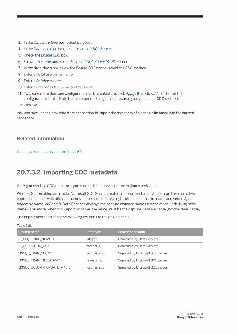
3. In the Datastore type box, select Database.4. In the Database type box, select Microsoft SQL Server.5. Check the Enable CDC box.6. For Database version, select Microsoft SQL Server 2008 or later.7. In the drop-down box below the Enable CDC option, select the CDC method.8. Enter a Database server name.9. Enter a Database name.10. Enter a database User name and Password.11. To create more than one configuration for this datastore, click Apply, then click Edit and enter the
configuration details. Note that you cannot change the database type, version, or CDC method.12. Click OK.
You can now use the new datastore connection to import the metadata of a capture instance into the current repository.
Related Information
Defining a database datastore [page 67]
20.7.3.2 Importing CDC metadata
After you create a CDC datastore, you can use it to import capture instance metadata.
When CDC is enabled on a table, Microsoft SQL Server creates a capture instance. A table can have up to two capture instances with different names. In the object library, right-click the datastore name and select Open, Import by Name, or Search. Data Services displays the capture instance name (instead of the underlying table name). Therefore, when you import by name, the name must be the capture instance name (not the table name).
The import operation adds the following columns to the original table:
Table 319:
Column name Data type Source of column
DI_SEQUENCE_NUMBER integer Generated by Data Services
DI_OPERATION_TYPE varchar(1) Generated by Data Services
MSSQL_TRAN_SEQNO varchar(256) Supplied by Microsoft SQL Server
MSSQL_TRAN_TIMESTAMP timestamp Supplied by Microsoft SQL Server
MSSQL_COLUMN_UPDATE_MASK varchar(258) Supplied by Microsoft SQL Server
668 P U B L I CDesigner Guide
Changed Data capture
20.7.3.3 Configuring a source table using CDC
This procedure describes how to configure a CDC source table when employing the Changed Data Capture (CDC) method. For more information, see the Reference Guide.
1. Drag a CDC datastore table into a data flow.The table automatically becomes a source object.
2. Click the name of this source object to open its source table editor.3. Click the CDC Options tab.4. Optionally select Enable check-point.
Once a check-point is placed, the next time the CDC job runs, it reads only the rows inserted into the CDC table since the last check-point.
5. Optionally select Automatically delete rows after reading.
20.7.3.4 Using CDC for data flows in a WHILE loop
For the CDC method, check-points apply at the job level. If you have data flows that run in a WHILE loop to retrieve the changes, then use the function set_cdc_checkpoint() for each iteration of the loop. This function instructs the source reader to set check-points so that the next iteration picks up the latest changes. Call this function for all the datastores used in all the data flows of the job. For more information, see the Reference Guide.
set_cdc_checkpoint(<datastore>)
The function returns 1 if the check-point has been successfully set; otherwise it returns 0. The value <datastore> is the name of the datastore containing the CDC tables.
Exampleset_cdc_checkpoint('MyCdcSource');
20.7.4 Change Tracking method
The Change Tracking method identifies that rows in a table have changed but ignores how many times the row has changed or the values of any intermediate changes. Data Services retrieves only the latest data available. Therefore, change tracking is limited in the historical questions it can answer compared to the Changed-Data Capture (CDC) method. However, there is far less storage overhead because the changed data is not being captured. In addition, a synchronous tracking mechanism used to track the changes has minimal overhead to operations.
Change Tracking must first be enabled for the Microsoft SQL Server database and then enabled for the tables that you want to track within that database. Change tracking information is recorded for modified rows. The values of the primary key column from the tracked table are recorded with the change information to identify the rows that have changed. To obtain the latest data for those rows, Data Services uses the primary key column values to join the source table with the tracked table. Information about the changes can include the type of operation that
Designer GuideChanged Data capture P U B L I C 669
caused the change (INSERT, UPDATE, or DELETE) or the columns that were changed as part of an UPDATE operation, for example.
This method is not available with versions prior to Microsoft SQL Server 2008.
20.7.4.1 Adding a Change Tracking datastore
This procedure describes how to create a datastore connection to Microsoft SQL Server and enable the Change Tracking method.
1. Open the datastore editor.2. Enter a name for the datastore.3. In the Datastore type box, select Database.4. In the Database type box, select Microsoft SQL Server.5. Check the Enable CDC box.6. For Database version, select Microsoft SQL Server 2008 or later.7. In the drop-down box below the Enable CDC option, select the Change tracking method.8. Enter a Database server name.9. Enter a Database name.10. Enter a database User name and Password.11. To create more than one configuration for this datastore, click Apply, then click Edit and enter the
configuration details. Note that you cannot change the database type, version, or CDC method.12. Click OK.
You can now use the new datastore connection to import table metadata into the current repository.
Related Information
Defining a database datastore [page 67]
20.7.4.2 Importing Change Tracking metadata
After you create a Change Tracking datastore, you can use it to import table metadata.
In the object library, right-click the datastore name and select Open, Import by Name, or Search. Only the CDC tables that you select when you set up Microsoft SQL Server for Change Tracking are visible when you browse external metadata.
The import operation adds the following columns to the original table:
670 P U B L I CDesigner Guide
Changed Data capture
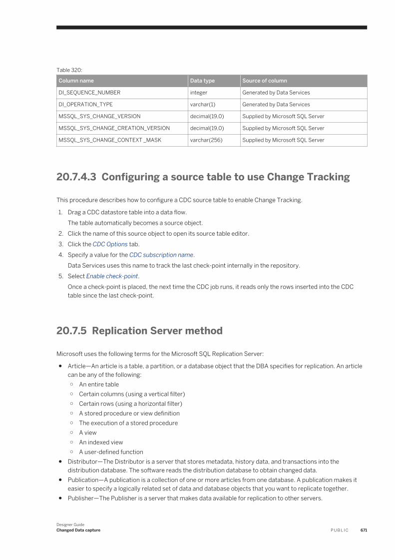
Table 320:
Column name Data type Source of column
DI_SEQUENCE_NUMBER integer Generated by Data Services
DI_OPERATION_TYPE varchar(1) Generated by Data Services
MSSQL_SYS_CHANGE_VERSION decimal(19,0) Supplied by Microsoft SQL Server
MSSQL_SYS_CHANGE_CREATION_VERSION decimal(19,0) Supplied by Microsoft SQL Server
MSSQL_SYS_CHANGE_CONTEXT _MASK varchar(256) Supplied by Microsoft SQL Server
20.7.4.3 Configuring a source table to use Change Tracking
This procedure describes how to configure a CDC source table to enable Change Tracking.
1. Drag a CDC datastore table into a data flow.The table automatically becomes a source object.
2. Click the name of this source object to open its source table editor.3. Click the CDC Options tab.4. Specify a value for the CDC subscription name.
Data Services uses this name to track the last check-point internally in the repository.5. Select Enable check-point.
Once a check-point is placed, the next time the CDC job runs, it reads only the rows inserted into the CDC table since the last check-point.
20.7.5 Replication Server method
Microsoft uses the following terms for the Microsoft SQL Replication Server:
● Article—An article is a table, a partition, or a database object that the DBA specifies for replication. An article can be any of the following:○ An entire table○ Certain columns (using a vertical filter)○ Certain rows (using a horizontal filter)○ A stored procedure or view definition○ The execution of a stored procedure○ A view○ An indexed view○ A user-defined function
● Distributor—The Distributor is a server that stores metadata, history data, and transactions into the distribution database. The software reads the distribution database to obtain changed data.
● Publication—A publication is a collection of one or more articles from one database. A publication makes it easier to specify a logically related set of data and database objects that you want to replicate together.
● Publisher—The Publisher is a server that makes data available for replication to other servers.
Designer GuideChanged Data capture P U B L I C 671
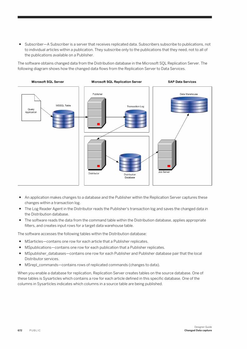
● Subscriber—A Subscriber is a server that receives replicated data. Subscribers subscribe to publications, not to individual articles within a publication. They subscribe only to the publications that they need, not to all of the publications available on a Publisher.
The software obtains changed data from the Distribution database in the Microsoft SQL Replication Server. The following diagram shows how the changed data flows from the Replication Server to Data Services.
● An application makes changes to a database and the Publisher within the Replication Server captures these changes within a transaction log.
● The Log Reader Agent in the Distributor reads the Publisher's transaction log and saves the changed data in the Distribution database.
● The software reads the data from the command table within the Distribution database, applies appropriate filters, and creates input rows for a target data warehouse table.
The software accesses the following tables within the Distribution database:
● MSarticles—contains one row for each article that a Publisher replicates.● MSpublications—contains one row for each publication that a Publisher replicates.● MSpublisher_databases—contains one row for each Publisher and Publisher database pair that the local
Distributor services.● MSrepl_commands—contains rows of replicated commands (changes to data).
When you enable a database for replication, Replication Server creates tables on the source database. One of these tables is Sysarticles which contains a row for each article defined in this specific database. One of the columns in Sysarticles indicates which columns in a source table are being published.
672 P U B L I CDesigner Guide
Changed Data capture
20.7.5.1 Configuring the distribution database
If the software connects to a Microsoft SQL Server to extract data, you need to configure the Distribution database in the Replication Server to capture changes to these tables.
20.7.5.1.1 Microsoft SQL Server 2000
The following steps summarize the procedure to configure the Replication Server for Microsoft SQL Server 2000 databases.
1. On the Replication node of the Microsoft SQL Enterprise Manager, select the Configure publishing, subscribers, and the Distribution option. Follow the wizard to create the Distributor and Distribution database.
The following steps summarize the procedure to configure SQL Replication Server for your Microsoft SQL Server 2000 database.
The wizard generates the following components that you need to specify on the Datastore Editor when you define a Microsoft SQL Server CDC datastore:○ MSSQL distribution server name○ MSSQL distribution database name○ MSSQL distribution user name○ MSSQL distribution password
2. Select the New Publications option on the Replication node of the Microsoft SQL Enterprise Manager to create new publications that specify the tables that you want to publish. The software requires the following settings in the Advanced Options:
○ Select Transactional publication on the Select Publication Type window. This type updates data at the Publisher and send changes incrementally to the Subscriber.
○ In the Commands tab of the Table Article Properties window:○ If you want before images for UPDATE and DELETE commands, select XCALL. Otherwise, select
CALL.○ Clear the options Create the stored procedures during initial synchronization of subscriptions and
Send parameters in binary format options because the software does not use store procedures and has its own internal format.
○ On the Snapshot tab of the Table Article Properties window:○ Select Keep the existing table unchanged because the software treats the table as a log.○ Clear Clustered indexes because the software treats the table as a log and reads sequentially from it.
○ Specify a publication name and description. You specify this publication name on the Datastore Editor when you define an MSSQL CDC datastore.
○ Select option Yes, allow anonymous subscriptions to save all transactions in the Distribution database.
For more information, see the Microsoft SQL Enterprise Manager online help.
Designer GuideChanged Data capture P U B L I C 673
20.7.5.1.2 Microsoft SQL Server 2005 and 2008
The following procedure summarizes how to configure publications for Microsoft SQL Server 2005 and 2008 databases for CDC.
1. Start the Microsoft SQL Server Management Studio.2. Log in and go to the Replication node in the Object Explorer.3. If this is the first time you are configuring distribution for this server, right-click the Replication node and
select Configure Distribution in the context menu. You can configure the distribution server, snapshot folder, distribution database, and the users for this distributor.
4. Right-click the Replication node again and select New Publication . The New Publication Wizard opens.5. In the New Publication Wizard, click Next.6. Select the database that you want to publish and click Next.7. Under Publication type, select Transactional publication, then click Next.8. Click to select tables and columns to publish as articles. Then open Article Properties. For each selected table,
click Set Properties of Highlighted Table Article. The Article Properties window opens:a. Set the following to False: Copy clustered index; Copy INSERT, UPDATE and DELETE stored procedures;
Create schemas at subscriber.b. Set the Action if name is in use to Keep the existing table unchanged.c. Set Update delivery format and Delete delivery format to XCALL <stored procedure>.d. Click OK to save the article properties.
9. Click Next. You can click Add to add row filters. Click Next if you do not need to filter the data in your publication.
10. Configure Agent Security and specify the account connection setting.a. For the Snapshot Agent, click Security Settings. Specify the account under which the snapshot agent will
run. Configure the account with system administration privileges. Specify the account that connects to the publisher and click OK.
b. For the Log Reader Agent, the Use the security settings from the Snapshot Agent option is selected by default. To use different settings, clear this option and click Security Settings. Note that it requires a login that grants system administration privileges.
11. In the Wizard Actions window, select Create the publication then click Next.12. To complete the wizard, enter a Publication name and click Finish.
For more information, see the Microsoft SQL Enterprise Manager documentation.
20.7.5.2 Configuring Data Services
To use Data Services to read and load changed data from SQL Server databases using the Replication Server, do the following procedures in the Designer:
● Create a CDC datastore● Import metadata for Microsoft SQL Server tables● Configure a CDC source
674 P U B L I CDesigner Guide
Changed Data capture
20.7.5.2.1 Adding the CDC datastore
This procedure describes how to create a CDC datastore using the Replication method.
1. Open the Datastore Editor.2. Enter a name for the datastore.3. In the Datastore type box, select Database.4. In the Database type box, select Microsoft SQL Server.5. Check the Enable CDC box to enable the CDC feature.6. Select a Database version.7. Enter a Database name (use the name of the Replication server).8. Enter a database User name and Password.9. In the CDC section, enter the names that you created for this datastore when you configured the Distributor
and Publisher in the Replication Server:○ MSSQL distribution server name○ MSSQL distribution database name○ MSSQL publication name○ MSSQL distribution user name○ MSSQL distribution password
10. If you want to create more than one configuration for this datastore, click Apply, then click Edit and follow step 9 again for any additional configurations.
11. Click OK.
You can now use the new datastore connection to import table metadata into the current repository.
Related Information
Defining a database datastore [page 67]
20.7.5.2.2 Importing CDC metadata
After you create a CDC datastore, you can use it to import CDC table metadata. In the object library, right-click the datastore name and select Open, Import by Name, or Search. Only the CDC tables that you select when you set up Microsoft SQL Server for CDC are visible when you browse external metadata. Data Services uses the MSpublications and MSarticles table in the Distribution database of SQL Replication Server to create a list of published tables.
When you import each CDC table, the software uses the Sysarticles table in the Publisher database of SQL Replication Server to display only published columns.
The import operation adds the following columns to the original table:
Designer GuideChanged Data capture P U B L I C 675
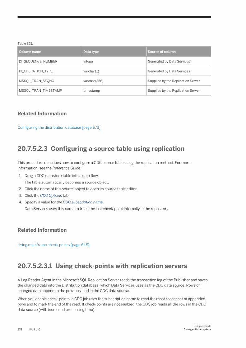
Table 321:
Column name Data type Source of column
DI_SEQUENCE_NUMBER integer Generated by Data Services
DI_OPERATION_TYPE varchar(1) Generated by Data Services
MSSQL_TRAN_SEQNO varchar(256) Supplied by the Replication Server
MSSQL_TRAN_TIMESTAMP timestamp Supplied by the Replication Server
Related Information
Configuring the distribution database [page 673]
20.7.5.2.3 Configuring a source table using replication
This procedure describes how to configure a CDC source table using the replication method. For more information, see the Reference Guide.
1. Drag a CDC datastore table into a data flow.The table automatically becomes a source object.
2. Click the name of this source object to open its source table editor.3. Click the CDC Options tab.4. Specify a value for the CDC subscription name.
Data Services uses this name to track the last check-point internally in the repository.
Related Information
Using mainframe check-points [page 648]
20.7.5.2.3.1 Using check-points with replication servers
A Log Reader Agent in the Microsoft SQL Replication Server reads the transaction log of the Publisher and saves the changed data into the Distribution database, which Data Services uses as the CDC data source. Rows of changed data append to the previous load in the CDC data source.
When you enable check-points, a CDC job uses the subscription name to read the most recent set of appended rows and to mark the end of the read. If check-points are not enabled, the CDC job reads all the rows in the CDC data source (with increased processing time).
676 P U B L I CDesigner Guide
Changed Data capture
To use check-points, on the source table editor enter the CDC Subscription name and select the Enable check-point option.
20.7.5.2.3.2 Using before-images from Microsoft SQL Server sources
When you must capture before-image UPDATE rows:
1. Make sure the Replication Server is set up to retrieve full before-images.2. When you create a Publication in the Replication Server, specify XCALL for UPDATE commands and DELETE
commands to obtain before-images.3. Select the Get before-images for each update row option in the CDC table's source editor.
After you check the Get before-images for each update row option, the software processes two rows for every update. In addition to the performance impact of this data volume increase, the before- and after-image pairs could be separated or lost depending on the design of your data flow, which would cause data integrity issues.
NoteThe Map_CDC_Operation transform can resolve problems, but undesirable results can still occur due to programming errors. When you use functions and transforms that re-order, re-direct, eliminate, and multiply the number of rows in a data flow, be aware of the possible impact to targets.
Related Information
Using before-images [page 640]
20.7.5.2.3.3 Configuring CDC source table
This procedure describes how to configure a CDC source table. Data Services can apply check-points across all the tables (in a given datastore configuration) for all the data flows in a job to provide data consistency.
1. Drag a CDC datastore table into a data flow.2. Click the name of this source object to open its editor.3. Click the CDC options tab.4. Optionally select Enable check-point.
Once a check-point is placed, the next time the CDC job runs, it reads only the rows inserted into the CDC table since the last check-point.
If check-points are not enabled, the CDC job reads all the rows in the CDC data source (with increased processing time).
Designer GuideChanged Data capture P U B L I C 677
20.8 Use CDC with timestamp-based sources
Use Timestamp-based CDC to track changes if you are using sources other than Oracle 9i, DB2 8.2, mainframes accessed through IBM II Classic Federation, or mainframes accessed through Attunity and if the following conditions are true:
● There are date and time fields in the tables being updated● You are updating a large table that has a small percentage of changes between extracts and an index on the
date and time fields● You are not concerned about capturing intermediate results of each transaction between extracts (for
example, if a customer changes regions twice in the same day).
You should not use the Timestamp-based CDC under the following circumstances:
● You have a large table, a large percentage of it changes between extracts, and there is no index on the timestamps.
● You need to capture physical row deletes.● You need to capture multiple events occurring on the same row between extracts.
Generally, the term timestamp refers to date, time, or datetime values. In the case of timestamp-based CDC, the source table has either CREATE or UPDATE timestamps for each row.
Timestamps can indicate whether a row was created or updated. Some tables have both create and update timestamps; some tables have just one. In the case of timestamp-based CDC, tables contain at least one update timestamp.
Some systems have timestamps with dates and times, some with just the dates, and some with monotonically generated increasing numbers. In the case of timestamp-based CDC, dates and generated numbers are treated the same.
NoteFor the timestamps based on real time, time zones can become important. If you keep track of timestamps using the nomenclature of the source system (that is, using the source time or source-generated number), you can treat both temporal (specific time) and logical (time relative to another time or event) timestamps the same way.
Related Information
Processing timestamps [page 679]Overlaps [page 681]Types of timestamps [page 685]
678 P U B L I CDesigner Guide
Changed Data capture
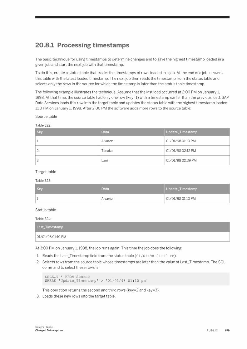
20.8.1 Processing timestamps
The basic technique for using timestamps to determine changes and to save the highest timestamp loaded in a given job and start the next job with that timestamp.
To do this, create a status table that tracks the timestamps of rows loaded in a job. At the end of a job, UPDATE this table with the latest loaded timestamp. The next job then reads the timestamp from the status table and selects only the rows in the source for which the timestamp is later than the status table timestamp.
The following example illustrates the technique. Assume that the last load occurred at 2:00 PM on January 1, 1998. At that time, the source table had only one row (key=1) with a timestamp earlier than the previous load. SAP Data Services loads this row into the target table and updates the status table with the highest timestamp loaded: 1:10 PM on January 1, 1998. After 2:00 PM the software adds more rows to the source table:
Source table
Table 322:
Key Data Update_Timestamp
1 Alvarez 01/01/98 01:10 PM
2 Tanaka 01/01/98 02:12 PM
3 Lani 01/01/98 02:39 PM
Target table
Table 323:
Key Data Update_Timestamp
1 Alvarez 01/01/98 01:10 PM
Status table
Table 324:
Last_Timestamp
01/01/98 01:10 PM
At 3:00 PM on January 1, 1998, the job runs again. This time the job does the following:
1. Reads the Last_Timestamp field from the status table (01/01/98 01:10 PM).2. Selects rows from the source table whose timestamps are later than the value of Last_Timestamp. The SQL
command to select these rows is:
SELECT * FROM Source WHERE 'Update_Timestamp' > '01/01/98 01:10 pm' This operation returns the second and third rows (key=2 and key=3).
3. Loads these new rows into the target table.
Designer GuideChanged Data capture P U B L I C 679
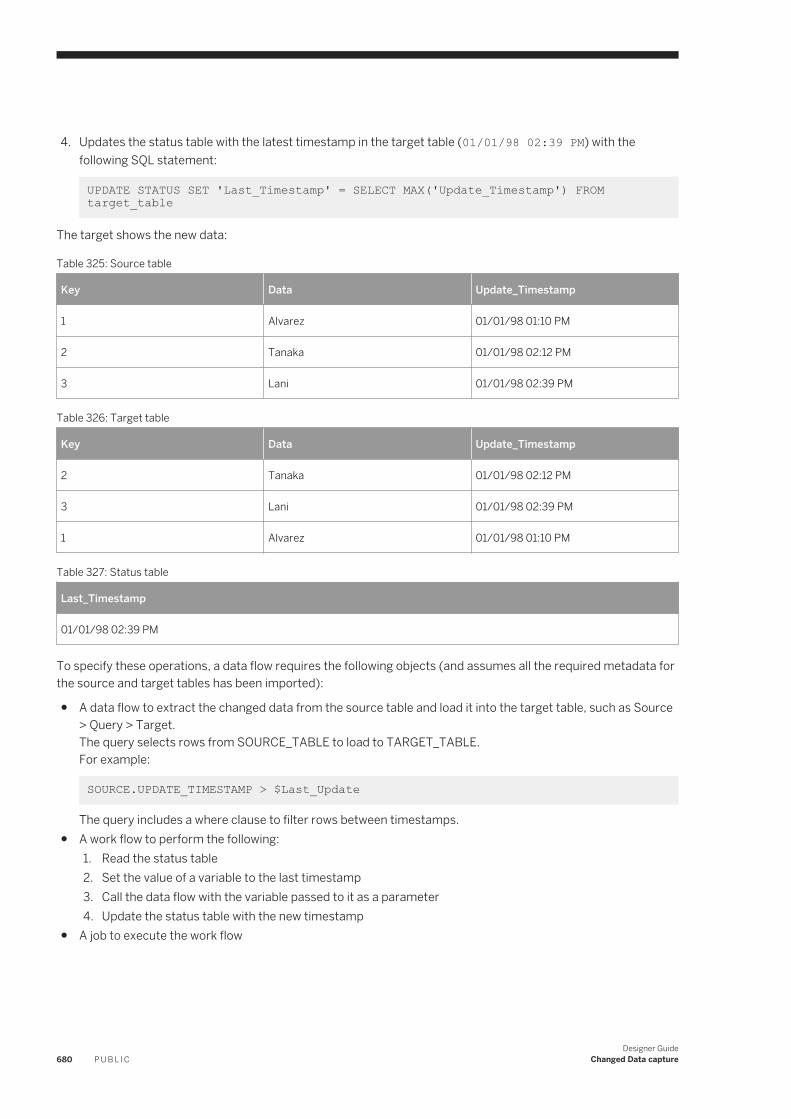
4. Updates the status table with the latest timestamp in the target table (01/01/98 02:39 PM) with the following SQL statement:
UPDATE STATUS SET 'Last_Timestamp' = SELECT MAX('Update_Timestamp') FROM target_table
The target shows the new data:
Table 325: Source table
Key Data Update_Timestamp
1 Alvarez 01/01/98 01:10 PM
2 Tanaka 01/01/98 02:12 PM
3 Lani 01/01/98 02:39 PM
Table 326: Target table
Key Data Update_Timestamp
2 Tanaka 01/01/98 02:12 PM
3 Lani 01/01/98 02:39 PM
1 Alvarez 01/01/98 01:10 PM
Table 327: Status table
Last_Timestamp
01/01/98 02:39 PM
To specify these operations, a data flow requires the following objects (and assumes all the required metadata for the source and target tables has been imported):
● A data flow to extract the changed data from the source table and load it into the target table, such as Source > Query > Target.The query selects rows from SOURCE_TABLE to load to TARGET_TABLE.For example:
SOURCE.UPDATE_TIMESTAMP > $Last_Update The query includes a where clause to filter rows between timestamps.
● A work flow to perform the following:1. Read the status table2. Set the value of a variable to the last timestamp3. Call the data flow with the variable passed to it as a parameter4. Update the status table with the new timestamp
● A job to execute the work flow
680 P U B L I CDesigner Guide
Changed Data capture
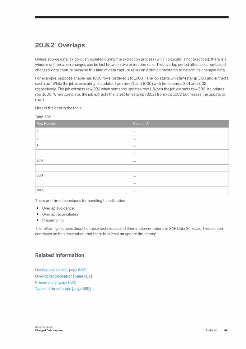
20.8.2 Overlaps
Unless source data is rigorously isolated during the extraction process (which typically is not practical), there is a window of time when changes can be lost between two extraction runs. This overlap period affects source-based changed-data capture because this kind of data capture relies on a static timestamp to determine changed data.
For example, suppose a table has 1000 rows (ordered 1 to 1000). The job starts with timestamp 3:00 and extracts each row. While the job is executing, it updates two rows (1 and 1000) with timestamps 3:01 and 3:02, respectively. The job extracts row 200 when someone updates row 1. When the job extracts row 300, it updates row 1000. When complete, the job extracts the latest timestamp (3:02) from row 1000 but misses the update to row 1.
Here is the data in the table:
Table 328:
Row Number Column A
1 ...
2 ...
3 ...
... ...
200 ...
... ...
600 ...
... ...
1000 ...
There are three techniques for handling this situation:
● Overlap avoidance● Overlap reconciliation● Presampling
The following sections describe these techniques and their implementations in SAP Data Services. This section continues on the assumption that there is at least an update timestamp.
Related Information
Overlap avoidance [page 682]Overlap reconciliation [page 682]Presampling [page 682]Types of timestamps [page 685]
Designer GuideChanged Data capture P U B L I C 681
20.8.2.1 Overlap avoidance
In some cases, it is possible to set up a system where there is no possibility of an overlap. You can avoid overlaps if there is a processing interval where no updates are occurring on the target system.
For example, if you can guarantee that the data extraction from the source system does not last more than one hour, you can run a job at 1:00 AM every night that selects only the data updated the previous day until midnight. While this regular job does not give you up-to-the-minute updates, it guarantees that you never have an overlap and greatly simplifies timestamp management.
20.8.2.2 Overlap reconciliation
Overlap reconciliation requires a special extraction process that reapplies changes that could have occurred during the overlap period. This extraction can be executed separately from the regular extraction. For example, if the highest timestamp loaded from the previous job was 01/01/98 10:30 PM and the overlap period is one hour, overlap reconciliation reapplies the data updated between 9:30 PM and 10:30 PM on January 1, 1998.
The overlap period is usually equal to the maximum possible extraction time. If it can take up to <n> hours to extract the data from the source system, an overlap period of <n> (or <n> plus some small increment) hours is recommended. For example, if it takes at most two hours to run the job, an overlap period of at least two hours is recommended.
There is an advantage to creating a separate overlap data flow. A "regular" data flow can assume that all the changes are new and make assumptions to simplify logic and improve performance. For example, rows flagged as INSERT are often loaded into a fact table, but rows flagged as UPDATE rarely are. Thus, the regular data flow selects the new rows from the source, generates new keys for them, and uses the database loader to add the new facts to the target database. Because the overlap data flow is likely to apply the same rows again, it cannot blindly bulk load them or it creates duplicates. Therefore, the overlap data flow must check whether the rows exist in the target and insert only the ones that are missing. This lookup affects performance; therefore, perform it for as few rows as possible.
If the data volume is sufficiently low, you can load the entire new data set using this technique of checking before loading, avoiding the need to create two different data flows.
20.8.2.3 Presampling
Presampling eliminates the overlap by first identifying the most recent timestamp in the system, saving it, and then extracting rows up to that timestamp.
The technique is an extension of the simple timestamp processing technique. The main difference is that the status table now contains a start and an end timestamp. The start timestamp is the latest timestamp extracted by the previous job; the end timestamp is the timestamp selected by the current job.
To return to the example: The last extraction job loaded data from the source table to the target table and updated the status table with the latest timestamp loaded:
Source table
682 P U B L I CDesigner Guide
Changed Data capture
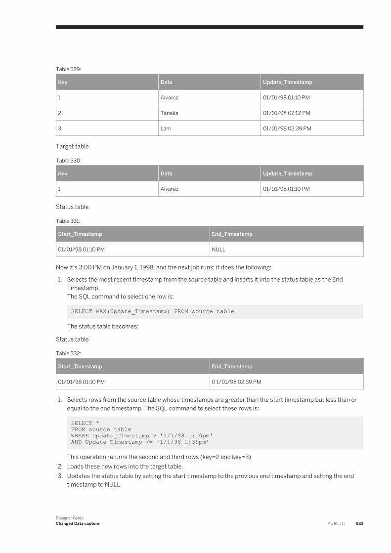
Table 329:
Key Data Update_Timestamp
1 Alvarez 01/01/98 01:10 PM
2 Tanaka 01/01/98 02:12 PM
3 Lani 01/01/98 02:39 PM
Target table
Table 330:
Key Data Update_Timestamp
1 Alvarez 01/01/98 01:10 PM
Status table
Table 331:
Start_Timestamp End_Timestamp
01/01/98 01:10 PM NULL
Now it's 3:00 PM on January 1, 1998, and the next job runs; it does the following:
1. Selects the most recent timestamp from the source table and inserts it into the status table as the End Timestamp.The SQL command to select one row is:
SELECT MAX(Update_Timestamp) FROM source table The status table becomes:
Status table
Table 332:
Start_Timestamp End_Timestamp
01/01/98 01:10 PM 0 1/01/98 02:39 PM
1. Selects rows from the source table whose timestamps are greater than the start timestamp but less than or equal to the end timestamp. The SQL command to select these rows is:
SELECT * FROM source table WHERE Update_Timestamp > '1/1/98 1:10pm' AND Update_Timestamp <= '1/1/98 2:39pm'
This operation returns the second and third rows (key=2 and key=3)2. Loads these new rows into the target table.3. Updates the status table by setting the start timestamp to the previous end timestamp and setting the end
timestamp to NULL.
Designer GuideChanged Data capture P U B L I C 683
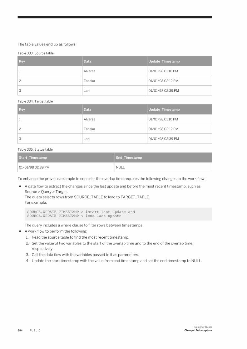
The table values end up as follows:
Table 333: Source table
Key Data Update_Timestamp
1 Alvarez 01/01/98 01:10 PM
2 Tanaka 01/01/98 02:12 PM
3 Lani 01/01/98 02:39 PM
Table 334: Target table
Key Data Update_Timestamp
1 Alvarez 01/01/98 01:10 PM
2 Tanaka 01/01/98 02:12 PM
3 Lani 01/01/98 02:39 PM
Table 335: Status table
Start_Timestamp End_Timestamp
01/01/98 02:39 PM NULL
To enhance the previous example to consider the overlap time requires the following changes to the work flow:
● A data flow to extract the changes since the last update and before the most recent timestamp, such as Source > Query > Target.The query selects rows from SOURCE_TABLE to load to TARGET_TABLE.For example:
SOURCE.UPDATE_TIMESTAMP > $start_last_update and SOURCE.UPDATE_TIMESTAMP < $end_last_update
The query includes a where clause to filter rows between timestamps.● A work flow to perform the following:
1. Read the source table to find the most recent timestamp.2. Set the value of two variables to the start of the overlap time and to the end of the overlap time,
respectively.3. Call the data flow with the variables passed to it as parameters.4. Update the start timestamp with the value from end timestamp and set the end timestamp to NULL.
684 P U B L I CDesigner Guide
Changed Data capture
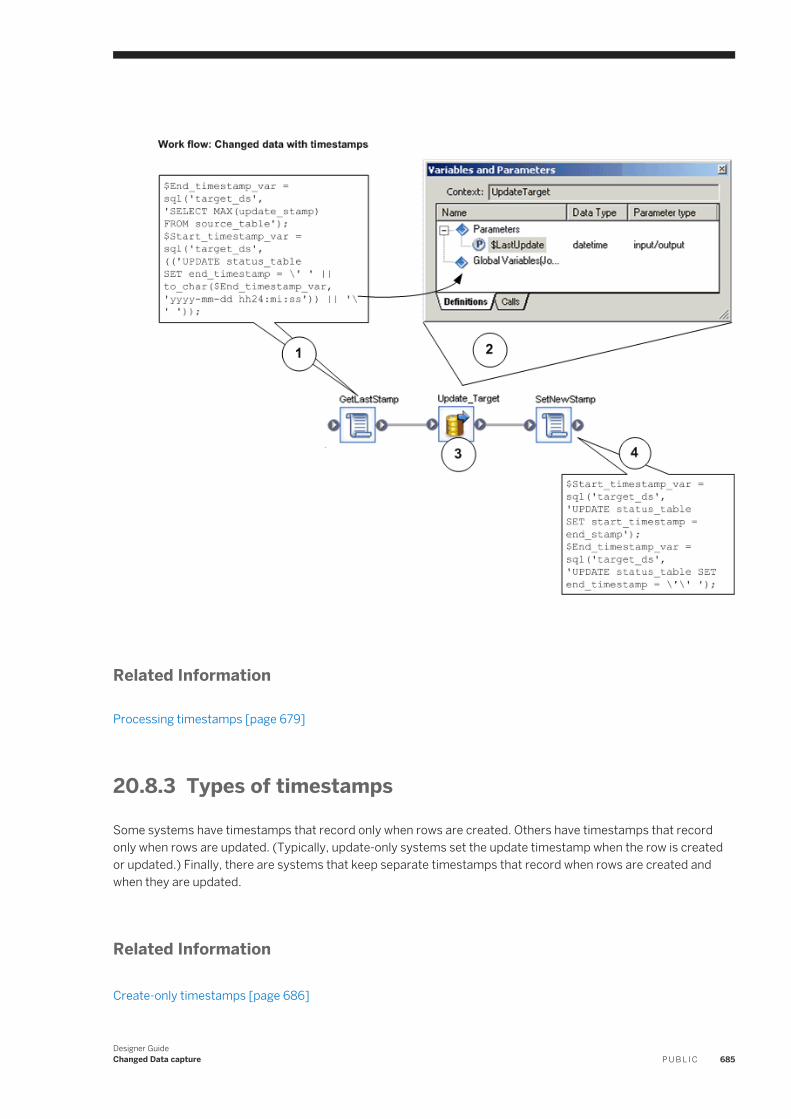
Related Information
Processing timestamps [page 679]
20.8.3 Types of timestamps
Some systems have timestamps that record only when rows are created. Others have timestamps that record only when rows are updated. (Typically, update-only systems set the update timestamp when the row is created or updated.) Finally, there are systems that keep separate timestamps that record when rows are created and when they are updated.
Related Information
Create-only timestamps [page 686]
Designer GuideChanged Data capture P U B L I C 685
Update-only timestamps [page 686]Create and update timestamps [page 686]
20.8.3.1 Create-only timestamps
If the source system provides only create timestamps, you have these options:
● If the table is small enough, you can process the entire table to identify the changes. The section Use CDC for targets [page 693], describes how to identify changes.
● If the table never gets updated, you can extract only the new rows.● If the table is large and gets updated, you can combine the following two techniques:
○ Periodically (for example, daily) extract only the new rows.○ Less frequently (for example, weekly) extract the updated rows by processing the entire table.
20.8.3.2 Update-only timestamps
Using only an update timestamp helps minimize the impact on the source systems, but it makes loading the target systems more difficult. If the system provides only an update timestamp and there is no way to tell new rows from updated rows, your job has to reconcile the new data set against the existing data using the techniques described in the section Use CDC for targets [page 693].
20.8.3.3 Create and update timestamps
Both timestamps allow you to easily separate new data from updates to the existing data. The job extracts all the changed rows and then filters unneeded rows using their timestamps.
Accomplish these extractions in the software by adding the WHERE clause from the following SQL commands into an appropriate query transform:
● Find new rows:
SELECT * FROM source_table WHERE Create_Timestamp > $Last_Timestamp ● Find updated rows:
SELECT * FROM source_table WHERE Create_Timestamp <= $Last_Timestamp AND Update_Timestamp > $Last_Timestamp)
From here, the new rows go through the key-generation process and are inserted into the target, and the updated rows go through the key-lookup process and are updated in the target.
For performance reasons, you might want to separate the extraction of new rows into a separate data flow to take advantage of bulk loading into the target. The updated rows cannot be loaded by bulk into the same target at the same time.
686 P U B L I CDesigner Guide
Changed Data capture
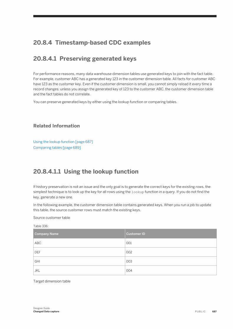
20.8.4 Timestamp-based CDC examples
20.8.4.1 Preserving generated keys
For performance reasons, many data warehouse dimension tables use generated keys to join with the fact table. For example, customer ABC has a generated key 123 in the customer dimension table. All facts for customer ABC have 123 as the customer key. Even if the customer dimension is small, you cannot simply reload it every time a record changes: unless you assign the generated key of 123 to the customer ABC, the customer dimension table and the fact tables do not correlate.
You can preserve generated keys by either using the lookup function or comparing tables.
Related Information
Using the lookup function [page 687]Comparing tables [page 689]
20.8.4.1.1 Using the lookup function
If history preservation is not an issue and the only goal is to generate the correct keys for the existing rows, the simplest technique is to look up the key for all rows using the lookup function in a query. If you do not find the key, generate a new one.
In the following example, the customer dimension table contains generated keys. When you run a job to update this table, the source customer rows must match the existing keys.
Source customer table
Table 336:
Company Name Customer ID
ABC 001
DEF 002
GHI 003
JKL 004
Target dimension table
Designer GuideChanged Data capture P U B L I C 687
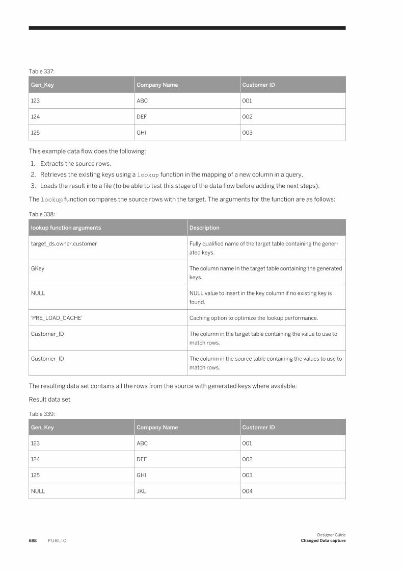
Table 337:
Gen_Key Company Name Customer ID
123 ABC 001
124 DEF 002
125 GHI 003
This example data flow does the following:
1. Extracts the source rows.2. Retrieves the existing keys using a lookup function in the mapping of a new column in a query.
3. Loads the result into a file (to be able to test this stage of the data flow before adding the next steps).
The lookup function compares the source rows with the target. The arguments for the function are as follows:
Table 338:
lookup function arguments Description
target_ds.owner.customer Fully qualified name of the target table containing the generated keys.
GKey The column name in the target table containing the generated keys.
NULL NULL value to insert in the key column if no existing key is found.
'PRE_LOAD_CACHE' Caching option to optimize the lookup performance.
Customer_ID The column in the target table containing the value to use to match rows.
Customer_ID The column in the source table containing the values to use to match rows.
The resulting data set contains all the rows from the source with generated keys where available:
Result data set
Table 339:
Gen_Key Company Name Customer ID
123 ABC 001
124 DEF 002
125 GHI 003
NULL JKL 004
688 P U B L I CDesigner Guide
Changed Data capture
Adding a new generated key to the new records requires filtering out the new rows from the existing and updated rows. In the data flow, this requires the following steps: A query to select the rows with NULL generated keys. A Key_Generation transform to determine the appropriate key to add. A target to load the new rows into the customer dimension table.
This data flow handles the new rows; however, the rows from the source whose keys were found in the target table might contain updated data. Because this example assumes that preserving history is not a requirement, the software loads all rows from the source into the target.
20.8.4.1.1.1 Handling updated rows in the data flow
The data flow requires new steps to handle updated rows, as follows:
1. A new line leaving the query that looked up the existing keys.2. A query to filter the rows with existing keys from the rows with no keys.3. A target to load the rows into the customer dimension table.
20.8.4.1.2 Comparing tables
The drawback of the generated-keys method is that even if the row has not been changed, it generates an UPDATE and is loaded into the target. If the amount of data is large, a table-comparison transform provides a better alternative by allowing the data flow to load only changed rows.
The table-comparison transform examines all source rows and performs the following operations:
● Generates an INSERT for any new row not in the target table.● Generates an UPDATE for any row in the target table that has changed.● Ignores any row that is in the target table and has not changed.● Fills in the generated key for the updated rows.
You can then run the result through the key-generation transform to assign a new key for every INSERT. This is the data set that the software loads into the target table.
The data flow that accomplishes this transformation includes the following steps:
1. A source to extract the rows from the source table(s).2. A query to map columns from the source.3. A table-comparison transform to generate INSERT and UPDATE rows and to fill in existing keys.4. A key-generation transform to generate new keys.5. A target to load the rows into the customer dimension table.
20.8.4.2 Preserving history
History preserving allows the data warehouse or data mart to maintain the history of data so you can analyze it over time. Most likely, you will perform history preservation on dimension tables.
Designer GuideChanged Data capture P U B L I C 689
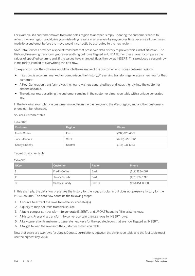
For example, if a customer moves from one sales region to another, simply updating the customer record to reflect the new region would give you misleading results in an analysis by region over time because all purchases made by a customer before the move would incorrectly be attributed to the new region.
SAP Data Services provides a special transform that preserves data history to prevent this kind of situation. The History_Preserving transform ignores everything but rows flagged as UPDATE. For these rows, it compares the values of specified columns and, if the values have changed, flags the row as INSERT. This produces a second row in the target instead of overwriting the first row.
To expand on how the software would handle the example of the customer who moves between regions:
● If Region is a column marked for comparison, the History_Preserving transform generates a new row for that customer.
● A Key_Generation transform gives the new row a new generated key and loads the row into the customer dimension table.
● The original row describing the customer remains in the customer dimension table with a unique generated key.
In the following example, one customer moved from the East region to the West region, and another customer's phone number changed.
Source Customer table
Table 340:
Customer Region Phone
Fred's Coffee East (212) 123-4567
Jane's Donuts West (650) 222-1212
Sandy's Candy Central (115) 231-1233
Target Customer table
Table 341:
GKey Customer Region Phone
1 Fred's Coffee East (212) 123-4567
2 Jane's Donuts East (201) 777-1717
3 Sandy's Candy Central (115) 454-8000
In this example, the data flow preserves the history for the Region column but does not preserve history for the Phone column. The data flow contains the following steps:
1. A source to extract the rows from the source table(s).2. A query to map columns from the source.3. A table-comparison transform to generate INSERTs and UPDATEs and to fill in existing keys.4. A History_Preserving transform to convert certain UPDATE rows to INSERT rows.5. A key-generation transform to generate new keys for the updated rows that are now flagged as INSERT.6. A target to load the rows into the customer dimension table.
Now that there are two rows for Jane's Donuts, correlations between the dimension table and the fact table must use the highest key value.
690 P U B L I CDesigner Guide
Changed Data capture
Note that updates to non-history preserving columns update all versions of the row if the update is performed on the natural key (for example, Customer), and only update the latest version if the update is on the generated key (for example, GKey). You can control which key to use for updating by appropriately configuring the loading options in the target editor.
20.8.4.2.1 valid_from date and valid_to date
To support temporal queries like "What was the customer's billing address on May 24, 1998," SAP Data Services supports Valid from and Valid to date columns.
In history-preserving techniques, there are multiple records in the target table with the same source primary key values. A record from the source table is considered valid in the dimension table for all date values t such that the Valid from date is less than or equal to t, which is less than the Valid to date. (Valid in this sense means that the record's generated key value is used to load the fact table during this time interval.)
When you specify the Valid from and Valid to entries, the History_Preserving transform generates an UPDATE record before it generates an INSERT statement for history-preservation reasons (it converts an UPDATE into an INSERT). The UPDATE record will set the Valid to date column on the current record (the one with the same primary key as the INSERT) to the value in the Valid from date column in the INSERT record.
20.8.4.2.2 Update flag
To support slowly changing dimension techniques, Data Services enables you to set an update flag to mark the current record in a dimension table.
Value Set value in column Column identifies the current valid record in the target table for a given source table primary key.
When you specify Column, the History_Preserving transform generates an UPDATE record before it generates an INSERT statement.
This UPDATE record will set the Column value to Reset value in the target table record with the same source primary key as the INSERT statement.
In the INSERT statement the Column will be set to Set value.
When you specify entries in both the groups, the History_Preserving transform generates only one extra UPDATE statement for every INSERT statement it produces. This UPDATE statement updates the Valid to value.
20.8.5 Additional job design tips
When designing a job to implement changed-data capture (CDC), you must consider:
● Synchronizing header and detail● Capturing physical deletions
Designer GuideChanged Data capture P U B L I C 691
20.8.5.1 Synchronizing header and detail
Typically, source systems keep track of header and detail information changes in an independent way. For example, if a line-item status changes, its "last modified date" column updates, but the same column at the order header level does not update. Conversely, a change to the default ship-to address in the order header might impact none of the existing line items.
In some instances, however, your source system might not consistently update those tracking columns, or you might not have access to such information (for example, when rows are physically deleted). In these cases, you might choose to extract all header and detail information whenever any changes occur at the header level or in any individual line item.
To extract all header and detail rows when any of these elements have changed, use logic similar to this SQL statement:
SELECT … FROM HEADER, DETAIL WHERE HEADER.ID = DETAIL.ID AND (HEADER.LAST_MODIFIED BETWEEN $G_SDATE AND $G_EDATE OR DETAIL.LAST_MODIFIED BETWEEN $G_SDATE AND $G_EDATE)
For some databases, this WHERE clause is not well optimized and might cause serious performance degradation. You might opt to relax that clause by removing one of the upper bounds, such as in:
… WHERE HEADER.ID = DETAIL.ID AND (HEADER.LAST_MODIFIED BETWEEN $G_SDATE AND $G_EDATE OR DETAIL.LAST_MODIFIED >= $G_SDATE) …
This might retrieve a few more rows than originally intended, but it might improve the final performance of your system while not altering the result of your target database.
20.8.5.2 Capturing physical deletions
When your source system allows rows to be physically deleted, your job should include logic to update your target database correspondingly. There are several ways to do this:
● Scan a log of operations — If your system logs transactions in a readable format or if you can alter the system to generate such a log, then you can scan that log to identify the rows you need to delete.
● Perform a full refresh — Simply reload all of the data, therefore fully synchronizing the source system and the target database.
● Perform a partial refresh based on a data-driven time-window — For example, suppose that the source system only allows physical deletion of orders that have not been closed. If the first non-closed order in your source table occurred six months ago, then by refreshing the last six months of data you are guaranteed to have achieved synchronization.
● Perform a partial refresh based on a business-driven time-window — For example, suppose that the business that the job supports usually deletes orders shortly after creating them. In this case, refreshing the last month of orders is appropriate to maintain integrity.
● Check every order that could possibly be deleted — You must verify whether any non-closed order has been deleted. To be efficient, this technique requires you to keep a record of the primary keys for every object that is a candidate for deletion.
When physical deletions of detail information in a header-detail relationship are possible (for example, removing line items from an existing order), then you must capture these physical deletions when synchronizing header and detail information.
692 P U B L I CDesigner Guide
Changed Data capture
20.9 Use CDC for targets
Source-based changed-data capture is almost always preferable to target-based capture for performance reasons.
Some source systems, however, do not provide enough information to make use of the source-based changed-data capture techniques. Target-based changed-data capture allows you to use the technique when source-based change information is limited.
Designer GuideChanged Data capture P U B L I C 693

21 Monitoring Jobs
21.1 Administrator
The Administrator application in the Management Console is the primary monitoring resource for all jobs designed in the Designer. For detailed information, see the “Administrator” section of the Management Console Guide.
694 P U B L I CDesigner Guide
Monitoring Jobs
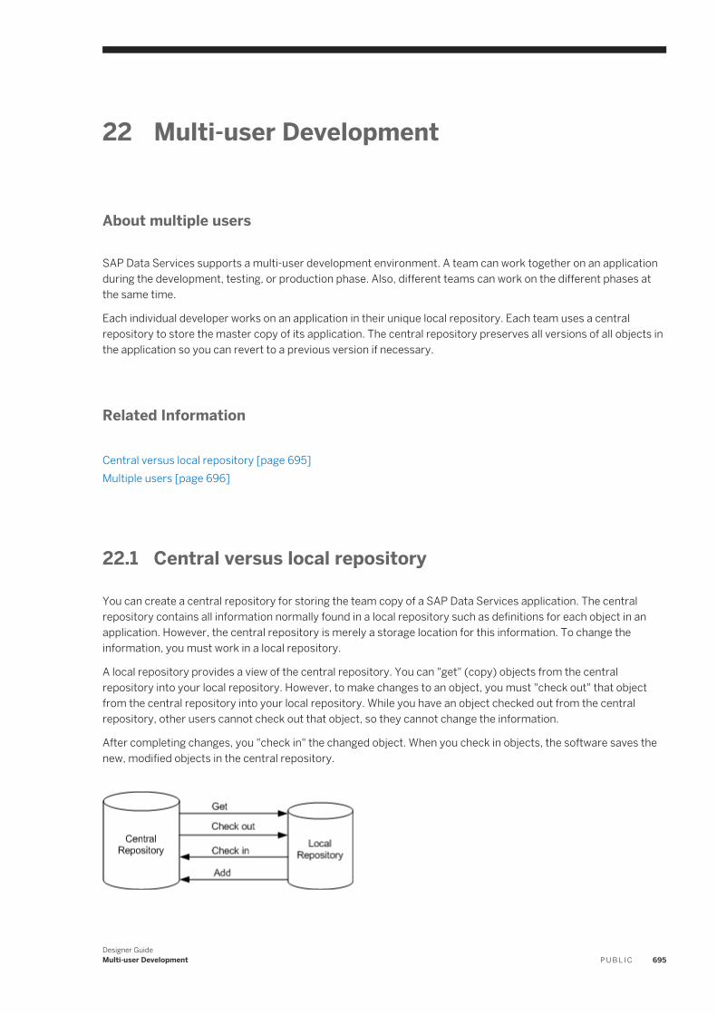
22 Multi-user Development
About multiple users
SAP Data Services supports a multi-user development environment. A team can work together on an application during the development, testing, or production phase. Also, different teams can work on the different phases at the same time.
Each individual developer works on an application in their unique local repository. Each team uses a central repository to store the master copy of its application. The central repository preserves all versions of all objects in the application so you can revert to a previous version if necessary.
Related Information
Central versus local repository [page 695]Multiple users [page 696]
22.1 Central versus local repository
You can create a central repository for storing the team copy of a SAP Data Services application. The central repository contains all information normally found in a local repository such as definitions for each object in an application. However, the central repository is merely a storage location for this information. To change the information, you must work in a local repository.
A local repository provides a view of the central repository. You can "get" (copy) objects from the central repository into your local repository. However, to make changes to an object, you must "check out" that object from the central repository into your local repository. While you have an object checked out from the central repository, other users cannot check out that object, so they cannot change the information.
After completing changes, you "check in" the changed object. When you check in objects, the software saves the new, modified objects in the central repository.
Designer GuideMulti-user Development P U B L I C 695
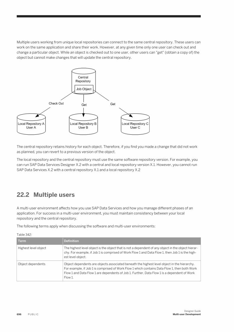
Multiple users working from unique local repositories can connect to the same central repository. These users can work on the same application and share their work. However, at any given time only one user can check out and change a particular object. While an object is checked out to one user, other users can "get" (obtain a copy of) the object but cannot make changes that will update the central repository.
The central repository retains history for each object. Therefore, if you find you made a change that did not work as planned, you can revert to a previous version of the object.
The local repository and the central repository must use the same software repository version. For example, you can run SAP Data Services Designer X.2 with a central and local repository version X.1. However, you cannot run SAP Data Services X.2 with a central repository X.1 and a local repository X.2
22.2 Multiple users
A multi-user environment affects how you use SAP Data Services and how you manage different phases of an application. For success in a multi-user environment, you must maintain consistency between your local repository and the central repository.
The following terms apply when discussing the software and multi-user environments:
Table 342:
Term Definition
Highest level object The highest level object is the object that is not a dependent of any object in the object hierarchy. For example, if Job 1 is comprised of Work Flow 1 and Data Flow 1, then Job 1 is the highest level object.
Object dependents Object dependents are objects associated beneath the highest level object in the hierarchy. For example, if Job 1 is comprised of Work Flow 1 which contains Data Flow 1, then both Work Flow 1 and Data Flow 1 are dependents of Job 1. Further, Data Flow 1 is a dependent of Work Flow 1.
696 P U B L I CDesigner Guide
Multi-user Development
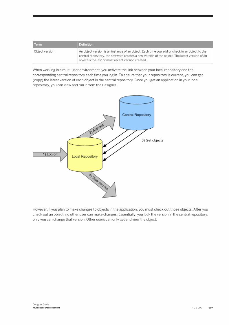
Term Definition
Object version An object version is an instance of an object. Each time you add or check in an object to the central repository, the software creates a new version of the object. The latest version of an object is the last or most recent version created.
When working in a multi-user environment, you activate the link between your local repository and the corresponding central repository each time you log in. To ensure that your repository is current, you can get (copy) the latest version of each object in the central repository. Once you get an application in your local repository, you can view and run it from the Designer.
However, if you plan to make changes to objects in the application, you must check out those objects. After you check out an object, no other user can make changes. Essentially, you lock the version in the central repository; only you can change that version. Other users can only get and view the object.
Designer GuideMulti-user Development P U B L I C 697
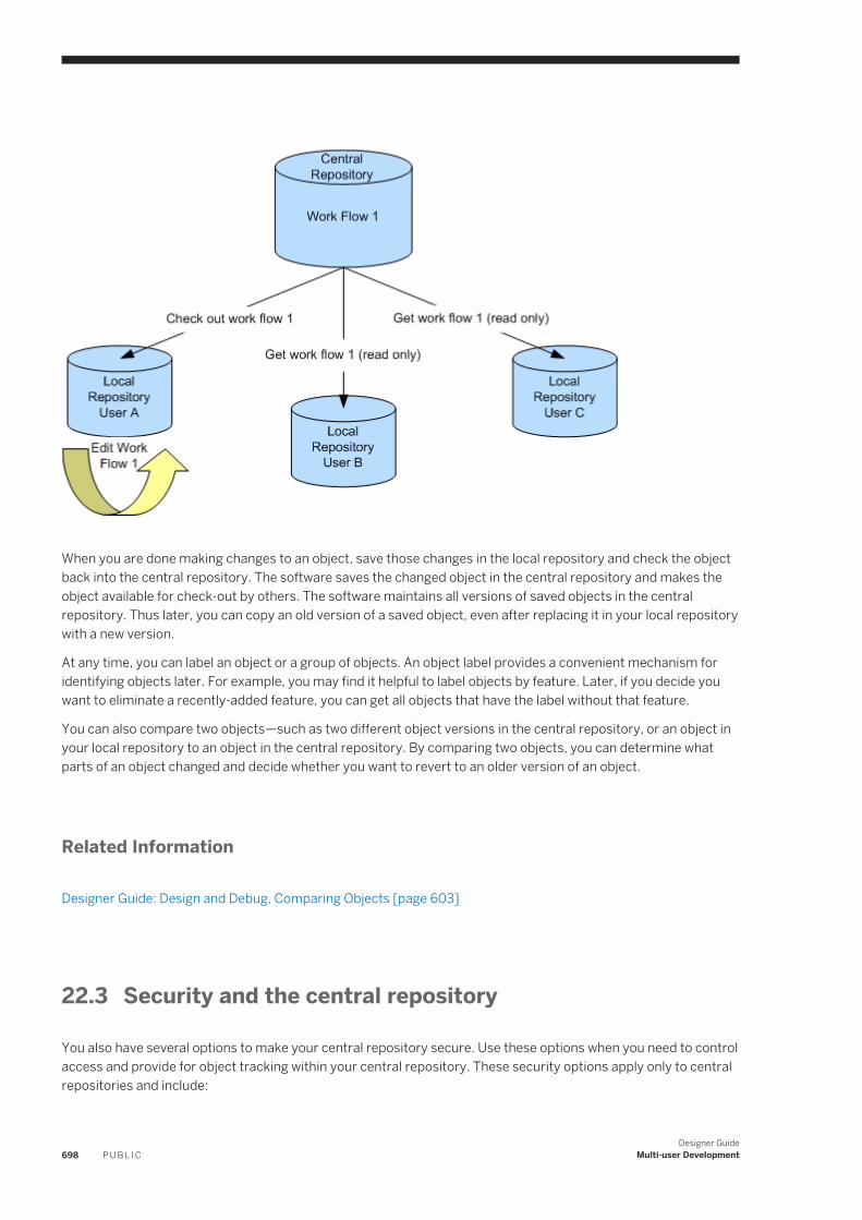
When you are done making changes to an object, save those changes in the local repository and check the object back into the central repository. The software saves the changed object in the central repository and makes the object available for check-out by others. The software maintains all versions of saved objects in the central repository. Thus later, you can copy an old version of a saved object, even after replacing it in your local repository with a new version.
At any time, you can label an object or a group of objects. An object label provides a convenient mechanism for identifying objects later. For example, you may find it helpful to label objects by feature. Later, if you decide you want to eliminate a recently-added feature, you can get all objects that have the label without that feature.
You can also compare two objects—such as two different object versions in the central repository, or an object in your local repository to an object in the central repository. By comparing two objects, you can determine what parts of an object changed and decide whether you want to revert to an older version of an object.
Related Information
Designer Guide: Design and Debug, Comparing Objects [page 603]
22.3 Security and the central repository
You also have several options to make your central repository secure. Use these options when you need to control access and provide for object tracking within your central repository. These security options apply only to central repositories and include:
698 P U B L I CDesigner Guide
Multi-user Development
● Authentication — Allows only valid users to log in to a central repository.● Authorization — Grants various levels of permissions to objects.● Auditing — Maintains a history of changes made to an object including user names.
Implement security for a central repository by establishing a structure of groups and associated users using the Administrator.
Related Information
Implementing Central Repository Security [page 702]
22.4 Multi-user Environment Setup
Overview of multi-user setup
To support multiple developers, configure a multi-user environment and set up several repositories. Specifically, you must:
● Create a local repository for each developer.● Create a central repository.● Define a connection to central repository from each local repository.● Activate the connection to a central repository.
Related Information
Creating a nonsecure central repository [page 699]Defining a connection to a nonsecure central repository [page 700]Activating a central repository [page 701]
22.4.1 Creating a nonsecure central repository
To support multiple users in a single development environment, it is recommended that you use a central repository. The central repository stores master information for the development environment.
This procedure applies to nonsecure repositories only.
1. Create a database to be used for the central repository using your database management system.
2. Choose Start Programs SAP Data Services 4.2 Data Services Repository Manager .
Designer GuideMulti-user Development P U B L I C 699
3. In the Repository Manager window, click the Central button in the Repository Type field, and enter the database connection information for the central repository.
4. Click Create.
The repository tables are created in the database you identified.
Related Information
Implementing Central Repository Security [page 702]
22.4.2 Defining a connection to a nonsecure central repository
A team working on an application only needs one central repository. However, each team member requires a local repository. Furthermore, each local repository requires connection information to any central repository it must access.
This procedure applies to nonsecure repositories only.
NoteThe version of the central repository must match the version of the local repository.
1. Start the Designer and log in to your local repository.
2. Choose Tools Central Repositories to open the Options window.
The Central Repository Connections option is selected in the Designer Options list.3. Right-click in the Central Repository Connections box and select Add.
The Repository Password window opens.4. Enter the password for the central repository.
The repository appears in the Central repository connections box.5. Click Activate.6. Again, enter the password for the central repository.7. Click OK.
Related Information
Implementing Central Repository Security [page 702]
700 P U B L I CDesigner Guide
Multi-user Development
22.4.3 Activating a central repository
To connect to a central repository, you must activate the link between your local repository and a specific central repository.
NoteWhen you start the Designer, always log in to a local repository. Never log into a central repository. If you do, then the central repository acts as a local repository. Then you run the risk of corrupting version information. If you attempt to log in to the central repository, you will see a warning message. You should log out immediately and log into a local repository.
Your local repository provides a view of the objects in the active central repository. Whenever you get or check out objects, you copy objects from the active central repository. Whenever you check in objects, you save the version from your local repository into the active central repository.
You must activate the correct central repository each time you log in. When you activate a central repository, the central object library opens and shows all the objects in the central repository and the check-out status of each object.
22.4.3.1 Activating a central repository
1. Choose Tools Central Repositories to open the Options window.
The Central Repository Connections option is selected in the Designer Options list.2. In the Central repository connections list, determine a central repository to make active.3. Check Reactivate automatically if you want the active central repository to be reactivated when you next log
on to this local repository.4. Right-click the central repository and select Activate.
The central object library opens. The Options window indicates that the selected central repository is active and closes automatically.
22.4.3.2 Opening the central object library
Click the Central Object Library button on the toolbar.
The central object library looks like the object library—it shows all the objects in the repository, grouped on appropriate tabs.
The window opens in floating mode. Drag the window to dock it. To change the docking state, right-click the Central Object Library tool bar and toggle Docking.
You can also change central repository connection information from the central object library.
Designer GuideMulti-user Development P U B L I C 701
22.4.3.3 Changing the active central repository
Select a central repository from the list on the top of the central object library.
SAP Data Services makes the selected central repository active—objects from that repository appear in the central object library. Connection information about that repository appears in the upper right corner of the central object library.
22.4.3.4 Changing central repository connections
1. Click the Edit Central Repository Connection button on the top of the central object library.
The Options window opens with the Central Repository Connections option selected in the Designer Options list.
Alternatively, you can open the Options window by selecting Tools Central Repositories .2. Select a central repository in the Central Repository Connections box, right-click, and select Edit.
When the Datastore Administrator window opens:
○ To disconnect from the currently active central repository, right-click the central repository in the Central Repository Datastores box and select Deactivate
○ To delete connection information for a central repository, right-click the central repository in the Central Repository Datastores box and select Delete.After confirming your selection, the connection information from this local repository is deleted. You can no longer connect to that central repository from this local repository.
NoteYou are not deleting the central repository; you are only deleting the connection information between your local repository and this central repository.
○ To make another repository the active central repository, right-click the central repository in the Central Repository Datastores box and select Activate.
22.5 Implementing Central Repository Security
About this section
This section describes how to implement optional security features for central repositories.
702 P U B L I CDesigner Guide
Multi-user Development
22.5.1 Overview
SAP Data Services provides options for managing secure access and tracking for objects in central repositories. Mechanisms for managing central repository security include:
● Authentication — Allows only valid users to log in to a central repository.● Authorization — Grants various levels of permissions to objects.● Auditing — Maintains a history of changes made to an object including user names.
Note that these security mechanisms and procedures apply only to central repositories.
22.5.1.1 Group-based permissions
You implement security for a central repository by establishing a structure of groups and associated users using the Administrator and the Central Management Console (CMC).
Access permissions for objects apply at the group level. More than one group can have the same permissions to the same object at a time. Groups are specific to a repository and are not visible in any other local or central repository.
Therefore, users do not get individual permissions. In the Designer, users select from the group(s) to which they belong, and the selected (current) group dictates their access to that object. Each user must have one default group but can belong to more than one group. When a user adds an object to a secure central repository, the user's current group automatically has Full permissions to that object.
User name and password authentication is required for every logon to a secure central repository. Users can change their passwords at any time in the CMC.
22.5.1.2 Permission levels
Each object in a secure central repository can have one of the following permissions levels:
● Full — This is the highest level of permission. The group can perform all possible actions including checking in, checking out, and deleting the object. You might assign this type of access to developers, for example.
● Read — Users can only get a copy of the object from the central repository or compare objects between their local and central object libraries. You might assign this type of access to QA, for example.
● None — Users cannot get copies of the object but can view it and its properties.
When an authenticated user adds an object to a secure central repository, the user's current group receives Full permissions to the object. All other groups receive Read permissions. Members of the group with Full permissions can change the other groups' permissions for that object.
22.5.1.3 Process summary
You implement security for a central repository by:
Designer GuideMulti-user Development P U B L I C 703
1. Using the Repository Manager to add a secure central repository or upgrade an existing nonsecure central repository.
2. Using the Central Management Console (CMC) to add users.3. Using the Administrator to add the users to central repository groups.4. Defining the connection from the Designer.5. Adding objects to the central repository as well as view and modify object permissions.
Related Information
Creating a secure central repository [page 704]Adding a multi-user administrator (optional) [page 705]Setting up groups and users [page 705]Defining a connection to a secure central repository [page 705]Working with objects in a secure central repository [page 706]
22.5.2 Creating a secure central repository
The first step in establishing security measures for multi-user development is to create a secure central repository or upgrade an existing nonsecure central repository.
NoteThese procedures apply to secure repositories only.
Related Information
Multi-user Environment Setup [page 699]
22.5.2.1 Creating a secure central repository
1. Create a database to be used for the central repository using your database management system.
2. Choose Start Programs SAP Data Services 4.2 Data Services Repository Manager .3. In the Repository Manager window, click the Central button in the Repository Type field and enter the
database connection information for the central repository.4. Select the Enable security check box.5. Click Create.
The software creates repository tables in the database you identified.
704 P U B L I CDesigner Guide
Multi-user Development
22.5.2.2 Upgrading a central repository from nonsecure to secure
You can modify an existing central repository to make it secure; however, you cannot undo this change.
1. Open the Repository Manager.2. In the Repository Manager window, click the Central button in the Repository Type field and enter the
database connection information for the central repository to modify.3. Select the Enable security check box.4. Click Upgrade.
The software updates the repository tables in the database you identified.
NoteWhen you upgrade an existing non-secure central repository to a secure central repository, a new group, DIGroup, is automatically created for you and displayed in Management Console AdministratorCentral Repositories . To access the repository, add existing users to the group in the Administrator.
22.5.3 Adding a multi-user administrator (optional)
In the Central Management Console (CMC), you have the option of adding a user with the role of Multi-user Administrator. This role is limited to managing secure central repositories, so it is therefore a subset of the Administrator role. For example, Multi-user Administrators cannot add a local repository or a nonsecure central repository.
Multi-user Administrators can:
● Add and remove secure central repositories.● Manage users and groups.● View secure central repository reports.
22.5.4 Setting up groups and users
The next step in implementing central repository security is to add and configure groups and users with the Central Management Console (CMC) and the Administrator.
22.5.5 Defining a connection to a secure central repository
The next step in implementing central repository security is to define a connection to the repository in the Designer.
This procedure applies to secure central repositories only.
Designer GuideMulti-user Development P U B L I C 705
1. Start the Designer and log in to your local repository.2. From the Tools menu, click Central Repositories to open the Options window.
The Central Repository Connections option should be selected in the Designer list.3. Click Add.4. Enter your CMS connection information and click Log On.5. Select the secure central repository you want to connect.6. Click OK.
The list of central repository connections now includes the newly connected central repository and it is identified as being secure.
7. With the repository selected, click Activate.8. Click OK.
Related Information
Multi-user Environment Setup [page 699]Activating a central repository [page 701]
22.5.6 Working with objects in a secure central repository
Related Information
Adding objects to the central repository [page 708]Viewing and modifying permissions [page 706]
22.5.6.1 Viewing and modifying permissions
After completing all configuration tasks and adding objects to the secure central repository, use the central object library to view and modify group permissions for objects.
22.5.6.1.1 Viewing permissions for an object
1. Start the Designer and log in to your local repository.2. Open the secure central object library.
Your default group appears in the drop-down list at the top of the window and is marked with an asterisk. The Permissions column displays the current group's access level for each object. If you add a new object to the central library, the current group gets FULL permissions and all other groups get READ permission.
706 P U B L I CDesigner Guide
Multi-user Development
22.5.6.1.2 Changing object permissions to other groups
You must have Full permissions to change object access to other groups.
1. In the central object library, right-click the object and click Permission CDC Adapter ConfigurationObject or Permission Object and dependants .
2. The Permission dialog box opens, which displays a list of available groups and the group's access level for the object(s).
3. Click in the Permission column, and from the drop-down list select a permission level for the group.4. Click Apply or OK.
22.5.6.1.3 Changing the current group or the default group
1. To change the current group, in the central object library select a group from the drop-down box.2. To change your default group, select the desired group from the drop-down box and click the save icon.
The software marks the default group with an asterisk.
22.6 Working in a Multi-user Environment
To obtain optimal results from development in a multi-user environment, it is recommended certain processes, such as checking in and checking out objects that you change, and establishing a set of conventions that your team follows, such as labeling objects.
22.6.1 Filtering
SAP Data Services allows you to customize by filtering (selectively changing) environment-specific information in object definitions. Application objects can contain repository-specific information. For example, datastores and database tables might refer to a particular database connection unique to a user or a phase of development. When multiple users work on an application, they can change repository-specific information.
Specifically, filtering allows you to:
● Change datastore and database connection information● Change the root directory for files associated with a particular file format● Select or clear specific dependent objects
The filtering process is available when adding, checking in, checking out, or getting labeled or latest objects in a central repository.
When you select any command that uses the filtering option:
1. The Version Control Confirmation window displays your selected object and any dependent objects. You can exclude objects by selecting the object and changing the Target status from create to exclude.
Designer GuideMulti-user Development P U B L I C 707
2. The Datastore Options window shows any datastores used by the object. This window only opens if the objects that you are adding, checking in, or checking out include a datastore.
22.6.2 Adding objects to the central repository
After creating a central repository, connecting it to the local repository, and activating the central repository, you can add objects from the local repository to the central repository. Remember that you do all design work—the creation of jobs, work flows, and data flows—in a local repository. Therefore, you use a local repository for the initial creation of any objects in an application. After the initial creation of an object, you add it to the central repository. Once in the central repository, the object is subject to version control and can be shared among users.
You can add a single object to the central repository, or you can add an object with all of its dependents to the central repository. When you add a single object, such as a data flow, you add only that object. No dependent objects are added.
You can add objects to the central repository at any point. However, you cannot add an object that already exists in the central repository.
You cannot add a read-only transform configuration to the repository. You can, however, replicate a transform configuration and add the replica to the repository.
22.6.2.1 Adding a single object to the central repository
1. Open the local object library.
2. Right-click the object and select Add to Central Repository Object .3. The Comments window opens. Enter any comments in the Comments field, and click OK.
The software adds the object to the active central repository.
NoteThe Add to Central Repository command is not available if the object already exists in the central repository.
22.6.2.2 Adding an object and its dependent objects to the central repository
1. Open the local object library.
2. Right-click the object and select either Add to Central Repository Object and dependents or Add to Central Repository With filtering (if filtering is required).
3. The Comments window opens. Enter any comments in the Comments field, and click OK.4. If you selected With filtering, complete the filtering windows.
708 P U B L I CDesigner Guide
Multi-user Development
5. Click Finish to add the selected objects.
Alternatively, you can select the object and drag it to the central object library to add the object and its dependents to the central repository. The filtering windows are displayed.
NoteThe Add to Central Repository command is not available if the object already exists in the central repository. However, the Add to Central Repository command is available if the object's dependents already exist in the central repository but the object itself does not.
NoteYou cannot add a read-only transform configuration to the repository. To do so, you must create a new repository, upgrade the existing repository, or import ATL that contains a new version of read-only transform configurations.
Related Information
Filtering [page 707]
22.6.3 Checking out objects
When you might change any of the objects in an application, you should check out the objects that you expect to change. When you check out an object, you make that object unavailable to other users—other users can view the object but cannot make changes to the object. Checking out an object ensures that two users do not make conflicting changes to the object simultaneously.
Data Services changes the object icons in both the local and central object libraries to indicate that the object is checked out.
When an object is checked out, your central object library shows you the local repository that has checked out the object. Based on the repository name, you can determine which user is working with that object.
To see periodic changes, refresh the central object library by clicking on the Refresh Central Object Library button in the toolbar of the central object library.
Choose a check-out command based on what you will do to an object.
22.6.3.1 Checking out single objects or objects with dependents
Dependents are objects used by another object—for example, data flows that are called from within a work flow. You can check out a single object or an object with all of its dependents (as calculated in the central repository).
Designer GuideMulti-user Development P U B L I C 709
For example, you can simply check out a work flow. In that case, you can change that work flow, such as adding a new script to the work flow; however, you cannot change dependent objects in the work flow, such as data flows, and retain the changes in the central repository. Changes to dependent objects will only be retained in the local repository. Alternatively, you can check out the work flow with all of its dependents. In that case, you can make changes to the work flow or any of its dependents and retain the changes in both central and local repositories.
Generally, it is safest to check out an object with all dependents. When you do this, you prevent others from accidentally changing dependent objects.
22.6.3.1.1 Checking out a single object
1. Open the central object library.2. Right-click the object you want to check out.
3. Choose Check Out Object .
Alternatively, you can select the object in the central object library, and click the Check Out Object button on the top of the central object library.
The software copies the most recent version of the selected object from the central repository to your local repository, then marks the object as checked out.
22.6.3.1.2 Checking out an object and its dependent objects
1. Open the central object library.2. Right-click the object you want to check out.
3. Choose Check Out Object and dependents .
Alternatively, you can select the object in the central object library, and click the Check Out Object and dependents button on the top of the central object library.
SAP Data Services copies the most recent version of the selected object and all of its dependent objects from the central repository and marks these objects as checked out.
If a dependent object is checked out by you or another user, then the software alerts you with a Check Out Alert window, asking to get the latest version of the checked out object.
Related Information
Getting objects [page 717]
710 P U B L I CDesigner Guide
Multi-user Development

22.6.3.2 Check out single objects or objects with dependents without replacement
When you check out an object, you can replace the object in your local repository with the latest version from the central repository, or you can leave the current version in your local repository intact.
When you check out an object, SAP Data Services copies the object definition from the central repository and replaces any existing definitions for that object in your local repository.
You can check out objects without replacing the objects in your local repository. For example, suppose you are working in your local repository and you make a change to an object that is not checked out. If you determine that the change improves the design or performance of your application, you will want to include that change in the central repository.
To do this, check out the object without replacing the object in your local repository—the object that you have already improved with a change. Then, check the changed object back into the central repository.
NoteUse caution when checking out objects without replacing the version in your local repository. When you do not replace the version in your local repository, you can lose changes that others have incorporated into those objects.
22.6.3.2.1 Checking out an object or an object and its dependent objects without replacement
1. Open the central object library.
2. Right-click the object you want to check out and choose Check Out Object without replacement to check out the single object or choose Check Out Object and dependents without replacement to check out the object and all of its dependent objects.
SAP Data Services marks all appropriate objects as checked out—in both the object library and in the workspace—but does not copy any objects from the central repository to the local repository.
22.6.3.3 Check out objects with filtering
When you check out an object with filtering, the object and all its dependents are checked out.
NoteWhen you check out objects with filtering, you always replace local versions with the filtered objects from the central repository.
Designer GuideMulti-user Development P U B L I C 711
22.6.3.3.1 Checking out an object and its dependent objects with filtering
1. Open the central object library.
2. Right-click the object you want to check out and choose Check Out With filtering .3. Complete the filtering windows.4. Click Finish to check out the selected objects.
Related Information
Filtering [page 707]
22.6.4 Undoing check out
Occasionally, you may decide that you did not need to check out an object because you made no changes. Or, you may decide that the changes you made to a checked-out object are not useful and you prefer to leave the master copy of the object as is. In these cases, you can undo the check out.
When you undo a check out:
● the object in the central repository remains as it was before the checkout; no changes are made and no additional version is saved in the central repository. Only the object status changes from checked out to available.
● the local version of the object maintains the changes you made. If you want the local object to be an exact copy of the central object, perform a Get latest operation on that object.
After you undo a check out, other users can check out and make changes to the object.
22.6.4.1 Undoing single object check out
1. Open the central object library.2. Select a checked-out object.
3. Click the Undo object check out button. Alternatively, right-click the object and select Undo Check OutObject .
SAP Data Services removes the check-out symbol and makes no changes to the object in the central repository. Any checked-out dependent objects remain checked out.
712 P U B L I CDesigner Guide
Multi-user Development
22.6.4.2 Undoing check out of an object and its dependents
1. Open the central object library.2. Select the checked-out object that is the highest level for which you want to undo the check out.3. Click the Undo object and dependents check out button. Alternatively, you can right-click the object in the
central object library and select Undo Check Out Object and dependents .
SAP Data Services removes the check-out symbols for the object and any dependent objects that are also checked out. No changes are made to these objects in the central repository.
22.6.5 Checking in objects
After you finish making changes to checked out objects, you must check them back into the central repository. Checking in objects creates a new version in the central repository, and allows others to get the changes that you have made. Checking in objects also preserves a copy of the changes for revision control purposes. Later, you can get a particular version of a checked in object and compare it to subsequent changes or even revert to the previous version.
Check in an object when you are done making changes, when others need the object that contains your changes, or when you want to preserve a copy of the object in its present state.
Choose a check-in command based on what you will do to an object.
Related Information
Checking in single objects, objects with dependents [page 713]Checking in an object with filtering [page 714]
22.6.5.1 Checking in single objects, objects with dependents
Just as you can check out a single object or an object with all dependent objects, you can check in a single object or an object with all checked-out dependent objects (as calculated in the local repository).
22.6.5.1.1 Checking in a single object
1. Open the central object library.2. Select the object you want to check in.3. Click Check in object button at the top of the central object library.
Alternatively, you can right-click the object in the central object library and select Check In Object .
Designer GuideMulti-user Development P U B L I C 713
4. A Check In window opens with a Comment box, in which you can enter comments. After entering any comments, click OK.
SAP Data Services copies the object from your local repository to the central repository, and removes the check-out mark.
22.6.5.1.2 Checking in an object and its dependent objects
1. Open the central object library.2. Select the highest level object you want to check in.3. Click Check in object and dependents button at the top of the central object library.
Alternatively, you can right-click the object in the central object library and select Check In Object and dependents.
4. A Check In window opens with a Comment box, in which you can enter comments. After entering any comments, click OK.
SAP Data Services copies the selected object and all of its dependent objects from your repository to the central repository and removes the check-out mark.
22.6.5.2 Checking in an object with filtering
Just as you could check out objects with filtering, you can check in objects with filtering. When you check in an object with filtering, the object and all its dependent objects are checked in.
22.6.5.2.1 Checking in an object with filtering
1. Open the central object library.
2. Right-click the object you want to check out and choose Check In With filtering .3. A Check In window opens with a Comment box, in which you can enter comments. After entering any
comments, click OK.
SAP Data Services warns you that you are about to create a new version of the object in the central repository.
4. Click Yes to continue with the check in.5. Complete the filtering windows.6. Click Finish to check in the selected objects.
714 P U B L I CDesigner Guide
Multi-user Development
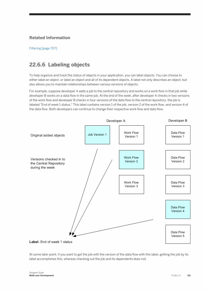
Related Information
Filtering [page 707]
22.6.6 Labeling objects
To help organize and track the status of objects in your application, you can label objects. You can choose to either label an object, or label an object and all of its dependent objects. A label not only describes an object, but also allows you to maintain relationships between various versions of objects.
For example, suppose developer A adds a job to the central repository and works on a work flow in that job while developer B works on a data flow in the same job. At the end of the week, after developer A checks in two versions of the work flow and developer B checks in four versions of the data flow to the central repository, the job is labeled "End of week 1 status." This label contains version 1 of the job, version 2 of the work flow, and version 4 of the data flow. Both developers can continue to change their respective work flow and data flow.
At some later point, if you want to get the job with the version of the data flow with this label, getting the job by its label accomplishes this, whereas checking out the job and its dependents does not.
Designer GuideMulti-user Development P U B L I C 715
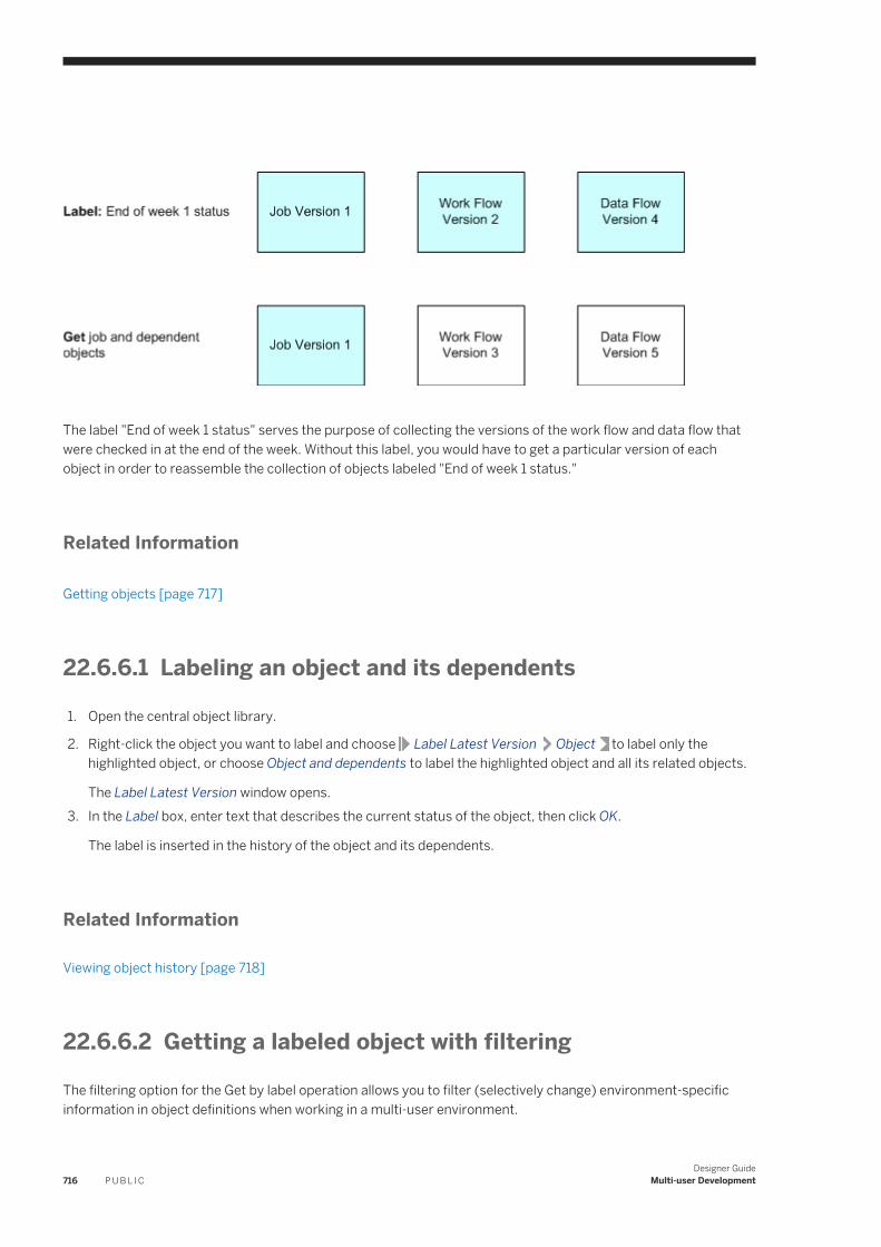
The label "End of week 1 status" serves the purpose of collecting the versions of the work flow and data flow that were checked in at the end of the week. Without this label, you would have to get a particular version of each object in order to reassemble the collection of objects labeled "End of week 1 status."
Related Information
Getting objects [page 717]
22.6.6.1 Labeling an object and its dependents
1. Open the central object library.
2. Right-click the object you want to label and choose Label Latest Version Object to label only the highlighted object, or choose Object and dependents to label the highlighted object and all its related objects.
The Label Latest Version window opens.3. In the Label box, enter text that describes the current status of the object, then click OK.
The label is inserted in the history of the object and its dependents.
Related Information
Viewing object history [page 718]
22.6.6.2 Getting a labeled object with filtering
The filtering option for the Get by label operation allows you to filter (selectively change) environment-specific information in object definitions when working in a multi-user environment.
716 P U B L I CDesigner Guide
Multi-user Development
1. Open the central object library.2. Select the highest level object you want to get.
3. Right-click the object in the central object library and select Get By Label With filtering .4. Complete the filtering window.5. Click Finish to get the selected objects.
Related Information
Filtering [page 707]
22.6.7 Getting objects
To make sure that your repository is up-to-date, you "get" objects. When you get an object, you copy the latest version of that object in the central object library and copy it into your local repository, replacing the version in your local repository. When you get an object, you do not check out the object. The object remains free for others to check out and change.
You can get an object with or without dependent objects and filtering.
Related Information
Viewing object history [page 718]
22.6.7.1 Getting a single object
1. Open the central object library.2. Select the object you want to get.3. Click Get latest version of object at the top of the central object library.
Alternatively, right-click the object in the central object library and select Get Latest Version Object .
The most recent version of the object in the central repository is copied to your local repository.
22.6.7.2 Getting an object and its dependent objects
1. Open the central object library.2. Select the highest level object you want to get.
Designer GuideMulti-user Development P U B L I C 717
3. Click Get latest version of objects and dependents at the top of the central object library.
Alternatively, right-click the object in the central object library and select Get Latest Version Object and dependents .
The most recent version of the selected object and all dependent objects from the central repository is copied to your local repository.
22.6.7.3 Getting an object and its dependent objects with filtering
1. Open the central object library.2. Select the highest level object you want to get.
3. Right-click the object in the central object library and select Get Latest Version With filtering .4. Complete the filtering windows.5. Click Finish to get the selected objects.
Related Information
Filtering [page 707]
22.6.8 Comparing objects
SAP Data Services allows you to compare two objects from local and central repositories to determine the differences between those objects.
22.6.9 Viewing object history
The central repository retains a history of all changes made to objects in the central repository. Use this history to help manage and control development of your application.
22.6.9.1 Examining the history of an object
1. Open the central object library.2. Select an object.3. Click the Show History button at the top of the central object library.
718 P U B L I CDesigner Guide
Multi-user Development
Alternatively, you can right-click the object in the central object library, and choose Show History.
The History window shows several pieces of information about each revision of the object.
Table 343:
Column Description
Version The object revision number. Each time a user saves the object, the software creates a new version.
Label Text that a user enters to describe the status of the object at a given point.
Repository Information about the local repository from which the software saved this version of the object and the username.
Date The date and time the software saved this version of the object.
Action The type of change a user made to the object. This table records actions such as:
Checked in — User checked in object
Comment Comments a user enters when adding an object or checking it into a central repository.
Related Information
Labeling objects [page 715]
22.6.9.2 Getting a previous version of an object
1. Select an object.2. Click the Show History button at the top of the central object library.3. Click the version of the object you want.4. Click the Get Obj By Version button.
NoteWhen you get a previous version of an object, you only get the object but not its dependent objects.
22.6.9.3 Getting an object with a particular label
1. Select an object.2. Click the Show History button at the top of the central object library.
Designer GuideMulti-user Development P U B L I C 719
3. Click the version of the object with the particular label you want.4. Click the Get By Label button.
22.6.10 Deleting objects
You can delete objects from either the central repository or a local repository. To delete an object from the central repository, right-click the object in the central object library and select Delete. To delete an object from the local repository, right-click on the object in the object library and select Delete.
When you delete an object from a local repository, you do not automatically delete that object from the active central repository. In fact, you can get the object from the central repository to re-insert it.
Similarly, when you delete an object from a central repository, you do not automatically delete the object from connected local repositories. Until you delete the object from the local repository, you can add the object back to the central repository.
When you delete objects from the central repository, you only delete the selected object and all versions of the selected object; you do not delete any dependent objects.
22.7 Migrating Multi-user Jobs
Overview of multi-user job migration
Job migration applies to SAP Data Services on multiple levels: application level, repository management level, and product upgrade level. Application migration is much more flexible in a multi-user environment, allowing you to maintain not only multiple versions of your objects during development, but also during test and production phases if you choose.
Related Information
Application phase management [page 720]Copying contents between central repositories [page 722]Central repository migration [page 723]
22.7.1 Application phase management
Typically, applications pass through different phases on the way from development to production. For example, an application might pass through three phases:
720 P U B L I CDesigner Guide
Multi-user Development
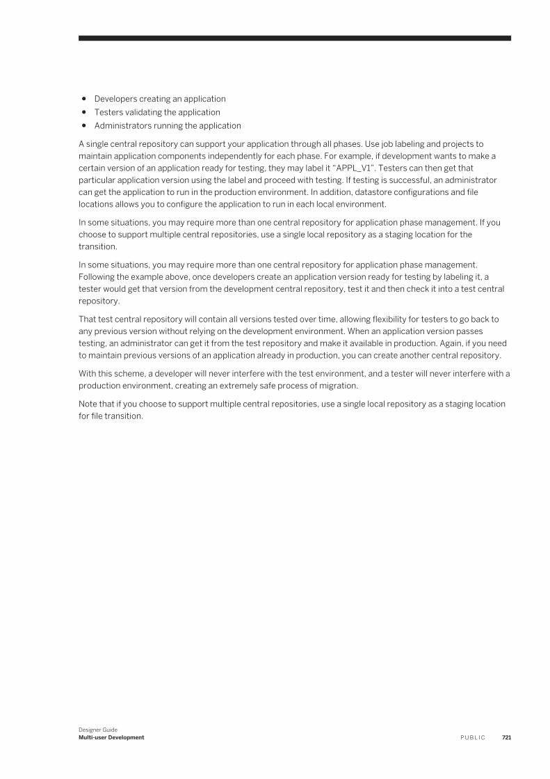
● Developers creating an application● Testers validating the application● Administrators running the application
A single central repository can support your application through all phases. Use job labeling and projects to maintain application components independently for each phase. For example, if development wants to make a certain version of an application ready for testing, they may label it “APPL_V1”. Testers can then get that particular application version using the label and proceed with testing. If testing is successful, an administrator can get the application to run in the production environment. In addition, datastore configurations and file locations allows you to configure the application to run in each local environment.
In some situations, you may require more than one central repository for application phase management. If you choose to support multiple central repositories, use a single local repository as a staging location for the transition.
In some situations, you may require more than one central repository for application phase management. Following the example above, once developers create an application version ready for testing by labeling it, a tester would get that version from the development central repository, test it and then check it into a test central repository.
That test central repository will contain all versions tested over time, allowing flexibility for testers to go back to any previous version without relying on the development environment. When an application version passes testing, an administrator can get it from the test repository and make it available in production. Again, if you need to maintain previous versions of an application already in production, you can create another central repository.
With this scheme, a developer will never interfere with the test environment, and a tester will never interfere with a production environment, creating an extremely safe process of migration.
Note that if you choose to support multiple central repositories, use a single local repository as a staging location for file transition.
Designer GuideMulti-user Development P U B L I C 721
22.7.2 Copying contents between central repositories
You cannot directly copy the contents of one central repository to another central repository. Rather, you must use your local repository as an intermediate repository.
22.7.2.1 Copying the contents of one central repository to another central repository
1. Activate the central repository whose contents you will copy.2. Get the latest version of all objects in this active central repository so they exist in your local repository.3. Activate the central repository into which you want to copy the contents.4. The first time you copy the contents, add the objects from your local repository into this central repository.
However, if you must re-copy the contents of one central repository into another (for example, during your testing phase some part of a job was reassigned to the development phase for redesign), the process is slightly more complex:
a. First check out specific objects without replacement from the second central repository.b. From your local repository, get the latest version of the objects from the first (for example, development)
central repository.
722 P U B L I CDesigner Guide
Multi-user Development
c. Then, instead of adding, check in the updated objects from your local repository to the second (for example, test) central repository.
Related Information
Activating a central repository [page 701]Getting objects [page 717]Adding objects to the central repository [page 708]Checking out objects [page 709]Checking in objects [page 713]
22.7.3 Central repository migration
When you upgrade your version of SAP Data Services, you should migrate your central repository to the new version. It is recommended that you consider the following guidelines when migrating a central repository to a new release of the software.
1. Back up all central repository (as well as local repository) database tables and associated data before upgrading.
2. Maintain a separate central repository for each version of SAP Data Services to preserve object history.To preserve the current version and history of objects in your central repository, create a new central repository of your current version of the software and copy the contents of the original central repository to the newly-created one. This way, the second central repository acts as a backup for your objects and associated history information from the older version of the software.When you install the new version of the software, upgrade the newly-created central repository to the latest version of the software.
3. Coordinate efforts to upgrade your central repositories and local repositories at the same time.Different versions of your central and local repository may not work together. You cannot perform a multi-user operation between a local and central repository of a different software version.
4. Check in all objects (or undo check-outs if objects were not modified after they were checked out) before migrating the central repositories.If you cannot upgrade your central and local repositories at the same time, you should check in all objects (or undo check-outs if objects were not modified during check-out), especially those objects checked out to a local repository you will not be immediately upgrading. After you upgrade your central repository to the new version, you will not be able to check in objects from the local repository of the older version of the software.
Related Information
Copying contents between central repositories [page 722]
Designer GuideMulti-user Development P U B L I C 723
Important Disclaimers and Legal Information
Coding SamplesAny software coding and/or code lines / strings ("Code") included in this documentation are only examples and are not intended to be used in a productive system environment. The Code is only intended to better explain and visualize the syntax and phrasing rules of certain coding. SAP does not warrant the correctness and completeness of the Code given herein, and SAP shall not be liable for errors or damages caused by the usage of the Code, unless damages were caused by SAP intentionally or by SAP's gross negligence.
AccessibilityThe information contained in the SAP documentation represents SAP's current view of accessibility criteria as of the date of publication; it is in no way intended to be a binding guideline on how to ensure accessibility of software products. SAP in particular disclaims any liability in relation to this document. This disclaimer, however, does not apply in cases of willful misconduct or gross negligence of SAP. Furthermore, this document does not result in any direct or indirect contractual obligations of SAP.
Gender-Neutral LanguageAs far as possible, SAP documentation is gender neutral. Depending on the context, the reader is addressed directly with "you", or a gender-neutral noun (such as "sales person" or "working days") is used. If when referring to members of both sexes, however, the third-person singular cannot be avoided or a gender-neutral noun does not exist, SAP reserves the right to use the masculine form of the noun and pronoun. This is to ensure that the documentation remains comprehensible.
Internet HyperlinksThe SAP documentation may contain hyperlinks to the Internet. These hyperlinks are intended to serve as a hint about where to find related information. SAP does not warrant the availability and correctness of this related information or the ability of this information to serve a particular purpose. SAP shall not be liable for any damages caused by the use of related information unless damages have been caused by SAP's gross negligence or willful misconduct. All links are categorized for transparency (see: http://help.sap.com/disclaimer).
724 P U B L I CDesigner Guide
Important Disclaimers and Legal Information

Designer GuideImportant Disclaimers and Legal Information P U B L I C 725

go.sap.com/registration/contact.html
© 2017 SAP SE or an SAP affiliate company. All rights reserved.No part of this publication may be reproduced or transmitted in any form or for any purpose without the express permission of SAP SE or an SAP affiliate company. The information contained herein may be changed without prior notice.Some software products marketed by SAP SE and its distributors contain proprietary software components of other software vendors. National product specifications may vary.These materials are provided by SAP SE or an SAP affiliate company for informational purposes only, without representation or warranty of any kind, and SAP or its affiliated companies shall not be liable for errors or omissions with respect to the materials. The only warranties for SAP or SAP affiliate company products and services are those that are set forth in the express warranty statements accompanying such products and services, if any. Nothing herein should be construed as constituting an additional warranty.SAP and other SAP products and services mentioned herein as well as their respective logos are trademarks or registered trademarks of SAP SE (or an SAP affiliate company) in Germany and other countries. All other product and service names mentioned are the trademarks of their respective companies.Please see http://www.sap.com/corporate-en/legal/copyright/index.epx for additional trademark information and notices.