delay-dependent guaranteed cost control for uncertain discrete-time systems with delay

126 IEEE TRANSACTIONS ON SYSTEMS, MAN, AND CYBERNETICS—PART B: CYBERNETICS, VOL. 38, NO. 1, FEBRUARY 2008

Delay-Dependent Guaranteed Cost Control forUncertain Stochastic Fuzzy Systems With

Multiple Time DelaysHuaguang Zhang, Senior Member, IEEE, Yingchun Wang, and Derong Liu, Fellow, IEEE

Abstract—This paper studies the guaranteed cost control prob-lem for a class of uncertain stochastic nonlinear systems withmultiple time delays represented by the Takagi–Sugeno fuzzymodel with uncertain parameters. By constructing a new sto-chastic Lyapunov–Krasovskii functional, sufficient conditions fordelay-dependent guaranteed cost control are obtained which donot require system transformation or relaxation matrices. Con-ditions for the existence of an optimal guaranteed cost controllerare presented in the linear matrix inequality format. Simulationexamples are provided to demonstrate the effectiveness of theproposed approach in this paper.

Index Terms—Delay dependence, guaranteed cost control, lin-ear matrix inequality (LMI), multiple time delays, stochastic fuzzysystems.

I. INTRODUCTION

S TABILITY analysis of stochastic systems has been wellinvestigated in past years, since stochastic modeling has

come to play an important role in many real systems, includingnuclear processes, thermal processes, chemical processes, biol-ogy, socioeconomics, and immunology (see [16] and [25] formore details). Based on the Itô stochastic differential equation,many efforts have been devoted to extend the approaches fromdeterministic systems to stochastic systems (see, e.g., [8] and[13]). The Takagi–Sugeno (T-S) fuzzy modeling approach,which has been extensively studied for deterministic nonlinearsystems (see [15], [18], [19], [22], and [30]), has also beenapplied to stochastic nonlinear systems (see, e.g., [5], [7], and[24]). On the other hand, time delays are often the sourceof instability and encountered in various engineering systems.Much attention has been devoted to the development of tools for

Manuscript received November 7, 2006; revised April 29, 2007. This workwas supported in part by the National Natural Science Foundation of China un-der Grant 60534010, Grant 60572070, Grant 60728307, and Grant 60774048,by the Funds for Creative Research Groups of China under Grant 60521003,and by the Program for Cheung Kong Scholars and Innovative Research Teamin University under Grant IRT0421. This paper was recommended by AssociateEditor W. J. Wang.

H. Zhang is with the Institute of Electric Automation, Northeastern Univer-sity, Shenyang 110004, China, and also with the Key Laboratory of IntegratedAutomation of Process Industry (Northeastern University), National EducationMinistry, Shenyang 110004, China (e-mail: [email protected]).

Y. Wang is with the School of Information Science and Engineering,Northeastern University, Shenyang 110004, China, and also with the KeyLaboratory of Integrated Automation of Process Industry (Northeastern Uni-versity), National Education Ministry, Shenyang 110004, China (e-mail:[email protected]).

D. Liu is with the Department of Electrical and Computer Engineering,University of Illinois, Chicago, IL 60607 USA (e-mail: [email protected]).

Digital Object Identifier 10.1109/TSMCB.2007.910532

stability analysis and controller design, and many results havebeen formulated [2], [4], [9], [14], [17], [21], [26], [29], [32].These existing results for deterministic or stochastic systemscan be divided into two categories: 1) delay-independent results[2], [21] and 2) delay-dependent results [4], [9], [14], [17],[26], [29], [32]. The former does not include any informationon the sizes of delays, whereas the latter category employssuch information and may be less conservative, particularly,when the sizes of delays are small. To obtain delay-dependentresults, many approaches were developed for deterministicsystems and stochastic ones. A descriptor system approachproposed in [9] was developed for stochastic systems [4],[32]. By transforming the original system into a descriptorsystem, the stability condition can be derived from analyzingthe stability of such a descriptor system with a constrainedLyapunov matrix. The relaxation matrices were introduced fordeterministic systems [14], [26] and stochastic ones [29] basedon the Newton–Leibniz formula. This kind of approach not onlyenhances the freedom of the solution space for the presentedstability criteria but is also subjected to the complexity in analy-sis. Recently, a projection approach was developed for linearuncertain time-delay systems in [17]. In addition to the simplestabilization, there have been various efforts in assigning certainperformance criteria when designing a controller. One approachto this problem is the so-called guaranteed cost control firstproposed in [3]. Its essential idea is to stabilize the systemswhile maintaining an adequate level of performance repre-sented by a quadratic cost function. Some important results onguaranteed cost control have been presented (see, e.g., [6], [12],[20], [27], [28], and [32], where [12] and [32] studied delay-dependent guaranteed cost control problems for deterministicand stochastic T-S fuzzy systems with time delay, respectively).To the best of our knowledge, there exist a few previous delay-dependent guaranteed cost control results for stochastic fuzzysystems with multiple time delays in the literature, althoughmany other results on multiple-time-delay systems have beenobtained (see, e.g., [2], [4], and [31]). This motivates ourresearch.

In this paper, we study the guaranteed cost control problemfor stochastic fuzzy systems with multiple time delays and un-certain parameters. By employing a new Lyapunov–Krasovskiifunctional with an integral quadratic term and a new integralinequality technique, delay-dependent stability criteria are ob-tained such that the closed-loop stochastic fuzzy system is as-ymptotically stable in the mean-square sense with a guaranteedcost control performance. Then, a procedure is given to selecta suitable controller that is optimal in the sense of minimizing

1083-4419/$25.00 © 2007 IEEE

ZHANG et al.: DELAY-DEPENDENT GUARANTEED COST CONTROL 127

the upper bound of the guaranteed cost function. All results areestablished in the form of linear matrix inequalities (LMIs) andcan be easily solved [1]. One of the advantages is that neithersystem transformation nor relaxation matrices are required. Inparticular, some system transformation approaches may lead toconservatism in some cases, which has been pointed out in [11].Another advantage is that the minimization of cost function canbe directly solved by the LMI toolbox of Matlab, while theoptimal control gain matrix can be obtained.

This paper is organized as follows. In Section II, the sto-chastic fuzzy system with multiple time delays and uncertainparameters is formulated. In Section III, the state feedbackguaranteed cost control approach for uncertain stochastic fuzzysystems is developed. In Section IV, two simulation examplesare provided to demonstrate the effectiveness of the presentapproach. In Section V, conclusions are given.

II. PROBLEM FORMULATION AND PRELIMINARIES

Throughout this paper, for h > 0, we let C([−h, 0];Rn)denote the family of continuous functions ϕ from [−h, 0] toRn with the norm ‖ϕ‖ = sup−h≤θ≤0 |ϕ(θ)|, where | · | denotesthe Euclidean norm in Rn. The notation M > 0 (M < 0)is used to denote a positive (negative) definite symmetricmatrix M . Moreover, let (Ω,F , Ftt>0,P) be a completeprobability space with a filtration Ftt>0 that satisfies theusual conditions (i.e., the filtration contains all P-null sets andis right continuous). Let L2

F0([−h, 0];Rn) be the family of

F0 measurable C([−h, 0];Rn)-valued random variables ζ =ζ(θ) : −h ≤ θ ≤ 0 such that sup−h≤θ≤0 E|ζ(θ)|2 <∞,where E· stands for the mathematical expectation operatorwith respect to the given probability measure P . We will use ∗to denote the transposed elements in the symmetric positions ofa matrix.

We first introduce two useful Lemmas, which will be used inthe proof of our results.Lemma 1 (cf. [23]): For matrices A ∈ Rn×n, P ∈ Rn×n,

M ∈ Rn×k,N ∈ Rl×n, and F ∈ Rk×l, withP > 0, FTF ≤ I ,and a scalar ε > 0, the following matrix inequalities hold:

1) (MFN)TP + PMFN ≤ εPMMTP + ε−1NTN ;2) If P − εMMT > 0, then (A+MFN)TP−1(A+MFN) ≤ AT (P − εMMT )−1A+ ε−1NTN .

Lemma 2: For any constant positive definite symmetric ma-trixW ∈ Rm×m, scalars β > 0 and κ > 0, and vector functionυ : [β − κ, β] → Rm×1, such that the integrations in the fol-lowing are well defined, we have

κ

β∫β−κ

υT (s)Wυ(s)ds ≥

β∫β−κ

υ(s)ds

T

W

β∫β−κ

υ(s)ds.

The proof of Lemma 2 can be found in the Appendix.Remark 1: Lemma 2 is similar to Lemma 1 in [10]. The

only difference between them is that the lower limit of theintegrations in the present case may be less than zero. Whenκ = β, it becomes the same as Lemma 1 in [10].

Now, we consider a class of uncertain stochastic fuzzysystems with multiple time delays, in which the ith rule is

formulated in the following form:

Rule i :IF z1(t) is Ri1, . . . , and zp(t) is Rip

THEN

dx(t) =m∑

k=0

(Bik + ∆Bik(t))x(t− hk)dt+Diu(t)dt

+m∑

k=0

(Cik + ∆Cik(t))x(t− hk)dw(t)

x(t) = ζ(t), t ∈ [−h, 0] (1)

where i = 1, . . . , r; r is the number of fuzzy rules;z1(t), . . . , zp(t) are the premise variables; Rij are the fuzzysets, j = 1, . . . , p; x(t) ∈ Rn is the state vector; u(t) ∈ Rq

is the control input; h0 = 0; hk > 0, k = 1, . . . ,m, denotethe state delay; h = maxhk, k ∈ [1,m]; w(t) is a standardBrownian motion; and ζ(t) ∈ Rn is a continuous initial func-tion or random variable. It is assumed that the premise variablesdo not depend on the input noise w(t) explicitly. Bik, Cik, andDi are the known matrices with compatible dimensions. Theuncertain matrix functions ∆Bik(t) and ∆Cik(t) satisfy thefollowing condition:

[∆Bik(t) ∆Cik(t)] =MiFi(t) [N1ik N2ik] (2)

where Mi ∈ Rn×f , N1ik ∈ Rf×n, and N2ik ∈ Rf×n, k =0, . . . ,m, are known constant matrices. Fi(t) is an unknownmatrix function with Lebesgue measurable elements and satis-fies FT

i (t)Fi(t) ≤ I ∈ Rf×f , where I is the identity matrix.The uncertain stochastic fuzzy system (1) is inferred as

follows:

dx(t) =m∑

k=0

Bk(δ)x(t− hk)dt+D(δ)u(t)dt

+m∑

k=0

Ck(δ)x(t− hk)dw(t) (3)

where Bk(δ)=∑r

i=1 δi(z(t))(Bik+∆Bik(t)), Ck(δ)=∑r

i=1 δi(z(t))(Cik+∆Cik(t)), D(δ)=

∑ri=1 δi(z(t))Di, δi(z(t))=σi

(z(t))/∑r

i=1 σi(z(t)), σi(z(t))=∏p

l=1 Ril(zl(t)), and Ril

(zl(t)) is the membership function of zl(t) in Ril, l = 1, . . . , p.Assume that σi(z(t)) ≥ 0 and

∑ri=1 σi(z(t)) > 0 for all

t. Therefore, we get δi(z(t))≥0 for i=1, . . . , r and∑r

i=1δi(z(t)) = 1.

We use the controller structure incorporating a set of fuzzyrules expressed in the form

Rule i : IF z1(t) is Ri1, . . . , and zp(t) is Rip

THEN u(t) = Kix(t). (4)

Hence, the inferred fuzzy controller is given by

u(t) =r∑

i=1

δi (z(t))Kix(t) (5)

where Ki is the local control gain matrix to be determined.


Substituting (5) into (3), we have the following closed-loopform of the stochastic fuzzy system:

dx(t) =m∑

k=0

(Bbk(δ) + ∆Bbk(δ))x(t− hk)dt

+m∑

k=0

(Cbk(δ) + ∆Cbk(δ))x(t− hk)dw(t) (6)

where the expressions for Bbk(δ), ∆Bbk(δ), Cbk(δ), and∆Cbk(δ) are shown as

Bbk(δ) =

∑r

i=1

∑rj=1 δi(z(t))

×δj (z(t))(Bik +DiKj), for k=0∑ri=1

∑rj=1 δi(z(t)) δj (z(t))

×Bik =∑r

i=1 δi(z(t))Bik, for k=1, . . . ,m

∆Bbk(δ) =r∑

i=1

r∑j=1

δi (z(t)) δj (z(t))∆Bik(t)

=r∑

i=1

δi (z(t))∆Bik(t)

Cbk(δ) =r∑

i=1

r∑j=1

δi (z(t)) δj (z(t))Cik

=r∑

i=1

δi (z(t))Cik

∆Cbk(δ) =r∑

i=1

r∑j=1

δi (z(t)) δj (z(t))∆Cik(t)

=r∑

i=1

δi (z(t))∆Cik(t)

The stability of stochastic fuzzy system (3) is defined asfollows.Definition 1: For system (3) with u(t) = 0, the trivial solu-

tion is asymptotically stable in the mean-square sense for everyζ ∈ L2

F0([−h, 0];Rn) if

limt→∞

E |x(t, ζ)|2 = 0.

Given positive definite symmetric matrices Ξ and Ψ, we shallconsider the cost function

J = E

∞∫0

[xT (t)Ξx(t) + uT (t)Ψu(t)

]dt

. (7)

Associated with the cost function, the guaranteed cost con-troller is defined as follows.Definition 2: Consider system (3). If there exist a control law

u∗(t) and a scalar J∗ > 0 such that the resulting closed-loopsystem is asymptotically stable in the mean-square sense andthe value of cost function (7) satisfies J ≤ J∗, then J∗ is saidto be a guaranteed cost, and u∗(t) is said to be a guaranteed costcontrol law for system (3).

Our objective is to develop a delay-dependent stabilizationapproach, which provides the state feedback control gain matrixas well as a positive scalar J∗ such that the closed-loop systemis asymptotically stable in the mean-square sense and the valueof cost function (7) satisfies J ≤ J∗.

III. MAIN RESULT

In this section, we develop our main results for the stochasticfuzzy system (6). We now state and prove our first result.Theorem 1: Given hk > 0, k = 1, . . . ,m, the closed-loop

stochastic fuzzy system (6) is asymptotically stable in themean-square sense, if there exist matrices X > 0, R > 0,Q > 0, and Ki (i = 1, . . . , r) with compatible dimensions andscalars εi1 > 0 and εi2 > 0, such that the LMIs (8), shown atthe bottom of the page, hold for 1 ≤ i ≤ j ≤ r where

Π1,ij =(Bi0X +XBT

i0 +Bj0X +XBTj0 +DjKi +DiKj

+ KTi D

Tj + KT

jDTi + εi1MiM

Ti + εj1MjM

Tj

)∈Rn×n

Πk2,ij =(BikX +BjkX) ∈ Rn×n

Πk3,ij =(−4X + 2Q) ∈ Rn×n

Πk4,ij =2hkX ∈ Rn×n

Πk5,ij = −2hkX ∈ Rn×n

Πk6,ij = −4hkX + 2hkR ∈ Rn×n

Π7,ij =[XCT

i0 XCTj0 XNT

2i0 XNT2j0

]∈ Rn×(2n+2f)

Πk7,ij =

[XCT

ik XCTjk XNT

2ik XNT2jk

]∈ Rn×(2n+2f)

Π1,ij Π12,ij . . . Πm

2,ij Π14,ij . . . Πm

4,ij Π7,ij Π9,ij Π11,ij

∗ Π13,ij 0 0 Π1

5,ij 0 0 Π17,ij Π1

9,ij 0

∗ ∗ . . . 0 0. . . 0

...... 0

∗ ∗ ∗ Πm3,ij 0 0 Πm

5,ij Πm7,ij Πm

9,ij 0∗ ∗ ∗ ∗ Π1

6,ij 0 0 0 0 0

∗ ∗ ∗ ∗ ∗ . . . 0 0 0 0∗ ∗ ∗ ∗ ∗ ∗ Πm

6,ij 0 0 0∗ ∗ ∗ ∗ ∗ ∗ ∗ Π8,ij 0 0∗ ∗ ∗ ∗ ∗ ∗ ∗ ∗ Π10,ij 0∗ ∗ ∗ ∗ ∗ ∗ ∗ ∗ ∗ Π12,ij

< 0 (8)


Π8,ij =−diag(X− εi2MiM

Ti ,X− εj2MjM

Tj , εi2I, εj2I

)∈ R(2n+2f)×(2n+2f)

Π9,ij =[XNT

1i0 XNT1j0

]∈ Rn×2f

Πk9,ij =

[XNT

1ik XNT1jk

]∈ Rn×2f

Π10,ij = −diag(εi1I, εj1I) ∈ R2f×2f

Π11,ij =[2hdX 2mX 2X KT

i KTj

]∈ Rn×(3n+2q)

Π12,ij = −diag(2hdR, 2mQ, 2Ξ−1,Ψ−1,Ψ−1)∈ R(3n+2q)×(3n+2q)

k =1, . . . ,m; hd =m∑

k=1

hk.

Moreover, the control gain matrix can be chosen as Ki =KiX

−1, and the guaranteed cost bound is determined as

J∗ = ExT (0)X−1x(0)

+ E

m∑k=1

0∫−hk

xT (τ)Q−1x(τ)dτ

+ E

m∑k=1

0∫−hk

0∫β

xT (τ)R−1x(τ)dτdβ

+ E

m∑k=1

0∫

−hk

x(τ)dτ

T

X−1

0∫−hk

x(τ)dτ

. (9)

Proof: Define the following Lyapunov–Krasovskiifunctional:

V (x, t) =xT (t)Px(t) +m∑

k=1

0∫−hk

t∫t+β

xT (τ)Rx(τ)dτdβ

+m∑

k=1

t∫t−hk

xT (τ)Qx(τ)dτ

+m∑

k=1

t∫

t−hk

x(τ)dτ

T

P

t∫t−hk

x(τ)dτ (10)

where P = X−1, R = R−1, and Q = Q−1. By the Itô formula[16], we obtain

dV (x, t) = LV (x, t)dt+ 2xT (t)Pm∑

k=0

(Cbk(δ)

+ ∆Cbk(δ))x(t− hk)dw(t) (11)

where

LV (x, t) = 2xT (t)Pm∑

k=0

(Bbk(δ) + ∆Bbk(δ))x(t− hk)

+

(m∑

k=0

(Cbk(δ) + ∆Cbk(δ))x(t− hk)

)T

P

×m∑

k=0


+m∑

k=1

hkx

T (t)Rx(t)−t∫

t−hk

xT (τ)Rx(τ)dτ

+m∑

k=1

(xT (t)Qx(t)− xT (t− hk)Qx(t− hk)

)

+m∑

k=1

2 (x(t)− x(t− hk))

T P

t∫t−hk

x(τ)dτ

.

(12)

Using Lemma 1 and considering the uncertain parameters (2),we obtain

2xT (t)Pm∑

k=0

∆Bbk(δ)x(t− hk) =r∑

i=1

δi (z(t))

× 2xT (t)PMiFi(t)Niψ(t)

≤r∑

i=1

δi (z(t))(εi1x

T (t)PMiMTi Px(t)

+ ε−1i1 ψ

T (t)NTi Niψ(t)

)(13)

where

Ni = [N1i0 N1i1 · · · N1ik · · · N1im]

ψ(t)=[xT(t) xT(t− h1) · · · xT(t− hk) · · · xT(t− hm)

]T.

Using Lemma 1, we can also obtain(m∑

k=0


)T

P

×m∑

k=0


≤ 12

r∑i=1

r∑j=1

δi (z(t)) δj (z(t))ψT (t)

×((Wi + ∆Wi(t))

T P (Wi + ∆Wi(t))

+ (Wj + ∆Wj(t))T P (Wj + ∆Wj(t))

)ψ(t)

=r∑

i=1

δi (z(t))ψT (t)

×(Wi + ∆Wi(t))T P (Wi + ∆Wi(t))ψ(t)

≤r∑

i=1

δi (z(t))ψT (t)

×(WT

i

(P−1 − εi2MiM

Ti

)−1Wi + ε−1

i2 N Ti Ni

)ψ(t)

(14)

where

Wi = [Ci0 Ci1 · · · Cik · · · Cim]∆Wi(t) = [∆Ci0(t) ∆Ci1(t) · · · ∆Cik(t) · · · ∆Cim(t)]

=MiFi(t)Ni

Ni = [N2i0 N2i1 · · · N2ik · · · N2im].


Using Lemma 2, we have

−t∫

t−hk

xT(τ)Rx(τ)dτ ≤ −h−1k

t∫

t−hk

x(τ)dτ

T

R

t∫t−hk

x(τ)dτ.

(15)

Substituting (13)–(15) into (12), we have (16), shown at thebottom of the page, where

ξ T (t) =

xT (t) xT (t− h1) · · · xT (t− hm)

t∫

t−h1

x(τ)dτ

T

· · ·

t∫

t−hm

x(τ)dτ

T

and the rest of the notation is expressed in

Zij + Zji

=

Z1,ij Z12,ij Z2

2,ij · · · Zm2,ij Z1

4,ij Z24,ij · · · Zm

4,ij

∗ Z1,13,ij Z1,2

3,ij · · · Z1,m3,ij Z1

5,ij 0 0 0∗ ∗ Z2,2

3,ij · · · Z2,m3,ij 0 Z2

5,ij 0 0

∗ ∗ ∗ . . .... 0 0

. . . 0∗ ∗ ∗ ∗ Zm,m

3,ij 0 0 0 Zm5,ij

∗ ∗ ∗ ∗ ∗ Z16,ij 0 0 0

∗ ∗ ∗ ∗ ∗ ∗ Z26,ij 0 0

∗ ∗ ∗ ∗ ∗ ∗ ∗ . . . 0∗ ∗ ∗ ∗ ∗ ∗ ∗ ∗ Zm

6,ij

(17)

and Zii = (1/2)(Zij + Zji), for i = j, with

Z1,ij =P (Bi0 +DiKj +Bj0 +DjKi)

+ (Bi0 +DiKj +Bj0 +DjKi)TP

+ εi1PMiMTi P + εj1PMjM

Tj P

+ ε−1i1 N

T1i0N1i0 + ε−1

j1NT1j0N1j0

+ CTi0

(P−1 − εi2MiM

Ti

)−1Ci0

+ CTj0

(P−1 − εj2MjM

Tj

)−1Cj0

+ ε−1i2 N

T2i0N2i0 + ε−1

j2NT2j0N2j0 + 2hdR+ 2mQ

+ 2Ξ +KTi ΨKi +KT

j ΨKj

Zk2,ij =P (Bik +Bjk) + ε−1

i1 NT1i0N1ik + ε−1

j1NT1j0N1jk

+ CTi0

(P−1 − εi2MiM

Ti

)−1Cik

+ CTj0

(P−1 − εj2MjM

Tj

)−1Cjk

+ ε−1i2 N

T2i0N2ik + ε−1

j2NT2j0N2jk

Zk,k3,ij = −2Q+ ε−1

i1 NT1ikN1ik + ε−1

j1NT1jkN1jk

+ CTik

(P−1 − εi2MiM

Ti

)−1Cik

+ CTjk

(P−1 − εj2MjM

Tj

)−1Cjk

+ ε−1i2 N

T2ikN2ik + ε−1

j2NT2jkN2jk

Zk,l3,ij = ε−1

i1 NT1ikN1il + ε−1

j1NT1jkN1jl

+ CTik

(P−1 − εi2MiM

Ti

)−1Cil

+ CTjk

(P−1 − εj2MjM

Tj

)−1Cjl

+ ε−1i2 N

T2ikN2il + ε−1

j2NT2jkN2jl (l > k)

Zk4,ij =2P Zk

5,ij = −2P

Zk6,ij = −2h−1

k R, k = 1, . . . ,m.

LV (x, t) ≤ 2xT (t)Pm∑

k=0

Bbk(δ)x(t− hk) +r∑

i=1

δi (z(t))(εi1x

T (t)PMiMTi Px(t) + ε−1

i1 ψT (t)NT

i Niψ(t))

+r∑

i=1

δi (z(t))ψT (t)(WT

i (P−1 − εi2MiMTi )−1Wi + ε−1

i2 N Ti Ni

)ψ(t)

+m∑

k=1

hkx

T (t)Rx(t)− h−1k

t∫

t−hk

x(τ)dτ

T

R

t∫t−hk

x(τ)dτ

+

m∑k=1

(xT (t)Qx(t)− xT (t− hk)Qx(t− hk)

)

+m∑

k=1

2 (x(t)− x(t− hk))

T P

t∫t−hk

x(τ)dτ

+ xT (t)Ξx(t) + uT (t)Ψu(t)− xT (t)Ξx(t)− uT (t)Ψu(t)

≤r∑

i=1

r∑j=1

δi (z(t)) δj (z(t)) ξT (t)Zij ξ(t)− xT (t)Ξx(t)− uT (t)Ψu(t)

=r∑

i=1

r∑j>i

δi (z(t)) δj (z(t)) ξT (t)(Zij + Zji)ξ(t)+r∑

i=1

δ2i (z(t)) ξT (t)Ziiξ(t)− xT (t)Ξx(t)− uT (t)Ψu(t) (16)


Note that the following result has been used in (16):

uT (t)Ψu(t) =r∑

i=1

r∑j=1

δi (z(t)) δj (z(t))xT (t)KTi ΨKjx(t)

≤ 12

r∑i=1

r∑j=1

δi (z(t)) δj (z(t))xT (t)

×(KT

i ΨKi +KTj ΨKj

)x(t)

=r∑

i=1

δi (z(t))xT (t)KTi ΨKix(t). (18)

If Zij + Zji < 0 holds for all 1 ≤ i ≤ j ≤ r, thenLV (x, t) < 0 for every ξ(t) = 0.

Because X = P−1, Q = Q−1, and R = R−1, wecan let Ki = KiX . Pre- and postmultiplying diag(P−1,P−1, . . . , P−1︸︷︷︸

m

, h1P−1, . . . , hmP

−1) to the left-hand side

of inequality Zij + Zji < 0 [cf. (17)] and using the Schurcomplement, we obtain (19), shown at the bottom of the page,where Πk

3,ij =−2XQX , Πk6,ij =−2hkXRX , k=1, . . . ,m,

and other notations are defined as in (8).The inequality (19) is not a solvable LMI because of the non-

linear terms XQX and XRX in Πk3,ij and Πk

6,ij , respectively.Because X and Q are positive definite symmetric matrices,we have

(X −Q−1)TQ(X −Q−1) = (X −Q−1)Q(X −Q−1) ≥ 0

then

−XQX ≤ −2X +Q−1. (20)

Similarly we have

−XRX ≤ −2X +R−1. (21)

Because R = R−1 and Q = Q−1, from (19)–(21), we ob-tain (8), which guarantees Zij + Zji < 0 (1 ≤ i ≤ j ≤ r).

Moreover, from (16), we have

LV (x, t) ≤ −xT (t)Ξx(t)− uT (t)Ψu(t) < 0. (22)

Therefore, system (6) is asymptotically stable in the mean-square sense with the control gain matrix Ki = KiX

−1.Integrating inequality (11) from 0 to T > 0, taking the

mathematical expectation, and considering inequality (22), weobtain

E V (x(T ), T ) − E V (x(0), 0)

= ExT (T )Px(T )

+ E

m∑k=1

T∫T−hk

xT (τ)Qx(τ)dτ

+ E

m∑k=1

0∫−hk

T∫T+β

xT (τ)Rx(τ)dτdβ

+ E

m∑k=1

T∫

T−hk

x(τ)dτ

T

P

T∫T−hk

x(τ)dτ

− ExT (0)Px(0)

− E

m∑k=1

0∫−hk

xT (τ)Qx(τ)dτ

− E

m∑k=1

0∫−hk

0∫β

xT (τ)Rx(τ)dτdβ

− E

m∑k=1

0∫

−hk

x(τ)dτ

T

P

0∫−hk

x(τ)dτ

= E

T∫0

LV (x, t)dt

≤ −E

T∫0

(xT (τ)Ξx(τ) + uT (τ)Ψu(τ)

)dτ

. (23)

Π1,ij Π12,ij · · · Πm

2,ij Π14,ij · · · Πm

4,ij Π7,ij Π9,ij Π11,ij

∗ Π13,ij 0 0 Π1

5,ij 0 0 Π17,ij Π1

9,ij 0

∗ ∗ . . . 0 0. . . 0

...... 0

∗ ∗ ∗ Πm3,ij 0 0 Πm

5,ij Πm7,ij Πm

9,ij 0

∗ ∗ ∗ ∗ Π16,ij 0 0 0 0 0

∗ ∗ ∗ ∗ ∗ . . . 0 0 0 0

∗ ∗ ∗ ∗ ∗ ∗ Πm6,ij 0 0 0

∗ ∗ ∗ ∗ ∗ ∗ ∗ Π8,ij 0 0

∗ ∗ ∗ ∗ ∗ ∗ ∗ ∗ Π10,ij 0

∗ ∗ ∗ ∗ ∗ ∗ ∗ ∗ ∗ Π12,ij

< 0 (19)


Because system (6) is asymptotically stable in the mean-squaresense, when T → ∞, we have

ExT (T )Px(T )

→ 0

E

m∑k=1

T∫T−hk

xT (τ)Qx(τ)dτ

→ 0

E

m∑k=1

0∫−hk

T∫T+β

xT (τ)Rx(τ)dτdβ

→ 0

E

m∑k=1

T∫

T−hk

x(τ)dτ

T

P

T∫T−hk

x(τ)dτ

→ 0.

Hence, we have

E

∞∫0


)dτ

≤ ExT (0)Px(0)

+ E

m∑k=1

0∫−hk

xT (τ)Qx(τ)dτ

+ E

m∑k=1

0∫−hk

0∫β

xT (τ)Rx(τ)dτdβ

+ E

m∑k=1

0∫

−hk

x(τ)dτ

T

P

0∫−hk

x(τ)dτ

(24)

that is

J = E

∞∫0


)dτ

≤ExT (0)X−1x(0)

+ E

m∑k=1

0∫−hk


+ E

m∑k=1

0∫−hk

0∫β


+ E

m∑k=1

0∫

−hk

x(τ)dτ

T

X−1

0∫−hk

x(τ)dτ

=J∗. (25)

This completes the proof. Note that the guaranteed cost bound in Theorem 1 depends

on the choice of guaranteed cost controller. The guaranteedcost controller that minimizes the guaranteed cost is called anoptimal guaranteed cost controller in [28]. Based on Theorem 1,

the design problem of the optimal guaranteed cost controller isformulated as follows.Theorem 2: Consider the stochastic fuzzy system (6) with

cost function (7). If the following optimization problem

min tr(Γ0) + tr(Γ1) + tr(Γ2) + tr(Γ3)

s.t.

(i) inequality (8)

(ii)

[−Γ0 ZT

0

Z0 −X

]< 0

(iii)[−Γ1 ZT

1

Z1 −R

]< 0

(iv)[−Γ2 ZT

2

Z2 −Q

]< 0

(v)[−Γ3 ZT

3

Z3 −X

]< 0

(26)

has a solution set Θ=(εi1, εi2,X, R, Q, Ki,Γ0,Γ1,Γ2,Γ3, 1≤i ≤ j ≤ r), where tr(·) denotes the trace of a matrix, thencontroller (5) is an optimal guaranteed cost controller, whichensures the minimization of the guaranteed cost bound (9) forsystem (6), where

Z0ZT0 = E

x(0)xT (0)

Z1ZT1 = E

m∑k=1

0∫−hk

0∫β

x(τ)xT (τ)dτdβ

Z2ZT2 = E

m∑k=1

0∫−hk

x(τ)xT (τ)dτ

Z3ZT3 = E

m∑k=1

0∫−hk

x(τ)dτ

0∫

−hk

x(τ)dτ

T

.

Proof: By Theorem 1, (i) in (26) is clear.By the Schur complement, it follows that (ii), (iii), (iv), and

(v) in (26) are equivalent to ZT0 X

−1Z0 < Γ0, ZT1 R

−1Z1 <

Γ1, ZT2 Q

−1Z2 < Γ2, and ZT3 X

−1Z3 < Γ3, respectively. Onthe other hand

ExT (0)X−1x(0)

=tr

(ExT (0)X−1x(0)

)=tr

(X−1E

x(0)xT (0)

)=tr

(X−1Z0ZT

0

)=tr

(ZT

0 X−1Z0

)< tr(Γ0) (27)


and similarly

E

m∑k=1

0∫−hk

0∫β


= E

m∑k=1

0∫−hk

0∫β

tr(xT (τ)R−1x(τ)

)dτdβ

= tr

R−1E

m∑k=1

0∫−hk

0∫β

x(τ)xT (τ)dτdβ

= tr(R−1Z1ZT

1

)< tr(Γ1) (28)

E

m∑k=1

0∫−hk


= E

m∑k=1

0∫−hk

tr(xT (τ)Q−1x(τ)

)dτ

= tr

Q−1E

m∑k=1

0∫−hk

x(τ)xT (τ)dτ

= tr(Q−1Z2ZT

2

)< tr(Γ2) (29)

E

m∑k=1

0∫

−hk

x(τ)dτ

T

X−1

0∫−hk

x(τ)dτ

= tr

X−1E

m∑k=1

0∫−hk

x(τ)dτ

0∫

−hk

x(τ)dτ

T

= tr(X−1Z3ZT

3

)< tr(Γ3). (30)

Hence, it follows from (26) that

J∗ < tr(Γ0) + tr(Γ1) + tr(Γ2) + tr(Γ3).

Then, the minimization of tr(Γ0) + tr(Γ1) + tr(Γ2) + tr(Γ3)implies the minimization of the guaranteed cost for the sto-chastic fuzzy system (6). The optimality of the solution of theoptimization problem (26) follows from the convexity of theobjective function and of the constraints.

This completes the proof. In the preceding discussion, we presented sufficient condi-

tions for delay-dependent guaranteed cost control of stochasticfuzzy systems with multiple time delays. When k = 1, simplerresults can be obtained in parallel to Theorems 1 and 2.

The closed-loop stochastic fuzzy system with single delay isdescribed as follows:

dx(t) = (Bb0(δ) + ∆Bb0(δ))x(t)dt+ (Bb1(δ) + ∆Bb1(δ))× x(t− h)dt+ (Cb0(δ) + ∆Cb0(δ))x(t)dw(t)+ (Cb1(δ) + ∆Cb1(δ))x(t− h)dw(t) (31)

where

Bb0(δ) + ∆Bb0(δ) =r∑

i=1

r∑j=1

δi (z(t)) δj (z(t))

× (Bi0 + ∆Bi0(t) +DiKj)

Bb1(δ) + ∆Bb1(δ) =r∑

i=1

r∑j=1


× (Bi1 + ∆Bi1(t))

=r∑

i=1

δi (z(t)) (Bi1 + ∆Bi1(t))

Cb0(δ) + ∆Cb0(δ) =r∑

i=1

r∑j=1


× (Ci0 + ∆Ci0(t))

=r∑

i=1

δi (z(t)) (Ci0 + ∆Ci0(t))

Cb1(δ) + ∆Cb1(δ) =r∑

i=1

r∑j=1


× (Ci1 + ∆Ci1(t))

=r∑

i=1

δi (z(t)) (Ci1 + ∆Ci1(t)) .

Bi0, Bi1, Ci0, Ci1, and Di are known constant matriceswith compatible dimensions; Ki, i = 1, . . . , r, are control gainmatrices, which are defined in (5); and the matrix functions∆Bi0(t), ∆Bi1(t), ∆Ci0(t), and ∆Ci1(t) represent norm-bounded parameter uncertainties and satisfy

[∆Bi0(t) ∆Bi1(t) ∆Ci0(t) ∆Ci1(t)]

= MiFi(t) [N1i0 N1i1 N2i0 N2i1] (32)

where Mi, N1i0, N1i1, N2i0, and N2i1 are known constantmatrices with compatible dimensions, and Fi(t) is as definedin (2).Corollary 1: Given h > 0, the closed-loop stochastic fuzzy

system (31) is asymptotically stable in the mean-square senseif there exist matrices X > 0, Q > 0, R > 0, and Ki (i =1, . . . , r) with compatible dimensions and scalars εi1 > 0 andεi2 > 0, such that the following LMIs hold for 1 ≤ i ≤ j ≤ r:

Π1,ij Π2,ij Π4,ij Π7,ij Π9,ij Π11,ij

∗ Π3,ij Π5,ij Π17,ij Π1

9,ij 0∗ ∗ Π6,ij 0 0 0∗ ∗ ∗ Π8,ij 0 0∗ ∗ ∗ ∗ Π10,ij 0∗ ∗ ∗ ∗ ∗ −Π12,ij

<0 (33)


where

Π1,ij =Bi0X+XBTi0+Bj0X+XBT

j0+DjKi+DiKj

+KTi D

Tj +KT

j DTi +εi1MiM

Ti +εj1MjM

Tj ∈Rn×n

Π2,ij =Bi1X+Bj1X∈Rn×n

Π3,ij = −4X+2Q∈Rn×n

Π4,ij =2hX∈Rn×n

Π5,ij = −2hX∈Rn×n

Π6,ij = −4hX+2hR∈Rn×n

Π7,ij =[XCT

i0 XCTj0 XNT

2i0 XNT2j0

]∈Rn×(2n+2f)

Π17,ij =

[XCT

i1 XCTj1 XNT

2i1 XNT2j1

]∈Rn×(2n+2f)

Π8,ij = −diag(X − εi2MiM

Ti ,X − εj2MjM

Tj , εi2I, εj2I

)∈R(2n+2f)×(2n+2f)

Π9,ij =[XNT

1i0 XNT1j0

]∈Rn×2f

Π19,ij =

[XNT

1i1 XNT1j1

]∈Rn×2f

Π10,ij = −diag(εi1I, εj1I)∈R2f×2f

Π11,ij =[2hX 2X 2X KT

i KTj

]∈Rn×(3n+2q)

Π12,ij =diag(2hR, 2Q, 2Ξ−1,Ψ−1,Ψ−1)∈R(3n+2q)×(3n+2q).

Moreover, the control gain matrix can be chosen as Ki =KiX

−1, and the guaranteed cost bound is given by

J∗ = ExT (0)X−1x(0)

+ E

0∫−h


+ E

0∫−h

0∫β


+ E

0∫

−h

x(τ)dτ

T

X−1

0∫−h

x(τ)dτ

. (34)

Corollary 2: Consider the stochastic fuzzy system (31) withcost function (7). If the following optimization problem:

min tr(Γ0) + tr(Γ1) + tr(Γ2) + tr(Γ3)

s.t.

(i) inequality (33);

(ii)[−Γ0 ZT

0

Z0 −X

]< 0

(iii)[−Γ1 ZT

1

Z1 −R

]< 0

(iv)[−Γ2 ZT

2

Z2 −Q

]< 0

(v)[−Γ3 ZT

3

Z3 −X

]< 0

(35)

has a solution set Θ=(εi1, εi2,X, R, Q, Ki,Γ0,Γ1,Γ2,Γ3,1 ≤i ≤ j≤r), then controller (5) is an optimal guaranteed cost

controller, which ensures the minimization of the guaranteedcost bound (34) for system (31), where

Z0ZT0 = E

x(0)xT (0)

Z1ZT1 = E

0∫−h

0∫β

x(τ)xT (τ)dτdβ

Z2ZT2 = E

0∫−h

x(τ)xT (τ)dτ

Z3ZT3 = E

0∫−h

x(τ)dτ

0∫

−h

x(τ)dτ

T

.

Remark 2: We have presented delay-dependent sufficientconditions for guaranteed cost control in terms of the convexLMI format. Next, we make a comparison with the existingdelay-dependent results in [12]. Guan and Chen [12] havepointed out that some existing approaches cannot provide suffi-cient conditions based on the convex LMI format; furthermore,the global minimum of the aforementioned minimization prob-lem cannot be found using a convex optimization algorithm,and the suboptimal solutions have to be chosen. Therefore, theirapproach may lead to a heavy computational burden. However,the approach in this paper can lead to convex LMI conditionssuch that the global minimum solution can be directly solvedby the LMI toolbox in Matlab. Therefore, our approach notonly reduced the computational cost of solution process but alsoenhanced the control performance of the closed-loop system.

IV. ILLUSTRATIVE EXAMPLES

In this section, a system with a single time delay and a systemwith two time delays are used to illustrate the effectiveness ofthe present approach in Examples 1 and 2, respectively.Example 1: Consider the following stochastic nonlinear

delayed system:

dx1(t) = (−0.1125x1(t)−0.0125x1(t−0.3)−0.02x2(t)

− 0.67x32(t)−0.005x2(t−0.3)+u(t)

)dt

+(0.5x1(t)−0.4x2(t)+0.4x3

2(t))dω(t)

dx2(t) =x1(t)dt+(0.15x1(t)+0.9x2(t)+0.4x3

2(t))dω(t).

(36)

Similar to [19], assume that x1(t) and x2(t) are measurableand x1(t) ∈ [−1.5, 1.5] and x2(t) ∈ [−1.5, 1.5]. The nonlinearterms of system can be represented as

−0.67x32(t)=R11(x2(t))·0·x2(t)−R12(x2(t))·1.5075x2(t)

0.4x32(t)=R11(x2(t))·0·x2(t)−R12(x2(t))·(−0.9)x2(t).


TABLE IDATA OF 100 EXPERIMENTS FOR THE GUARANTEED COST VALUE

Solving these equations, we obtain

R11 (x2(t)) = 1− x22(t)/2.25

R12 (x2(t)) = 1−R11 (x2(t)) = x22(t)/2.25

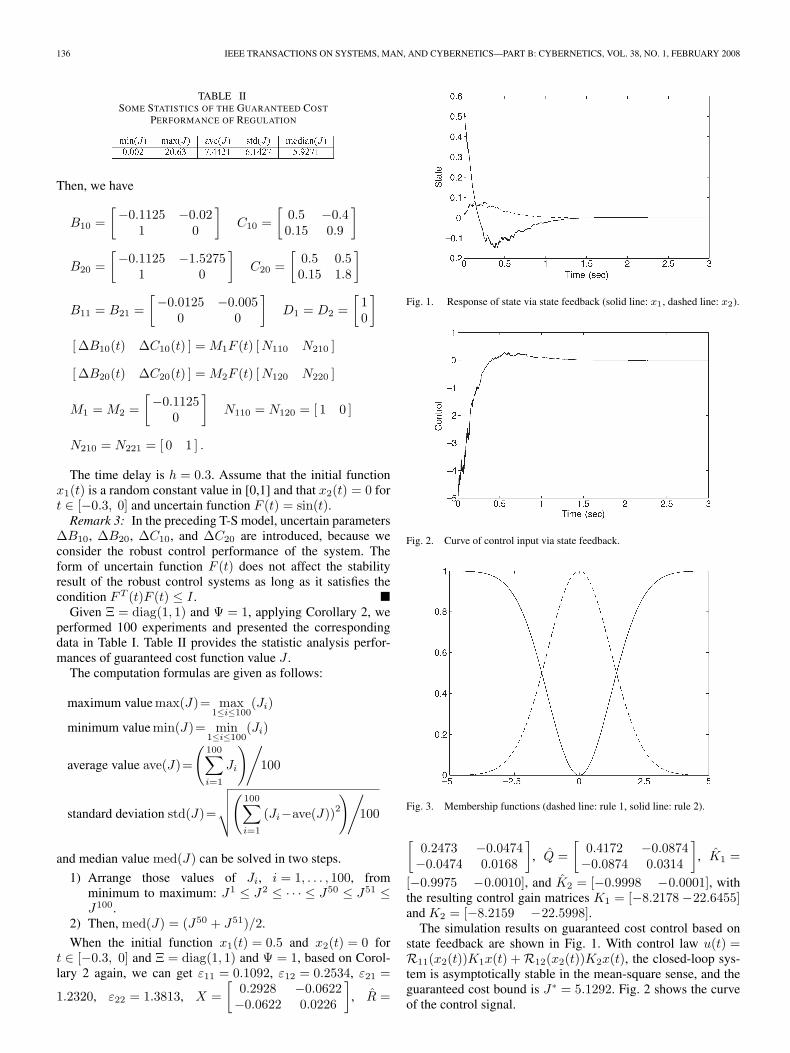
where R11(x2(t)) and R12(x2(t)) can be interpreted as mem-bership functions of fuzzy sets. Using these fuzzy sets, thestochastic nonlinear system with time delay can be expressedby the following stochastic fuzzy model:

Rule 1 : IF x2(t) is R11

THEN

dx(t)=[(B10+∆B10(t))x(t)+B11x(t−h)] dt

+D1u(t)dt+(C10+∆C10(t))x(t)dw(t)


THEN

dx(t)=[(B20+∆B20(t))x(t)+B21x(t−h)] dt

+D2u(t)dt+(C20+∆C20(t))x(t)dw(t)

where x(t) = [x1(t) x2(t)]T .

System parameters B10, B20, B11, B21, C10, C20, D1, andD2 can be solved by the following equations:

[−0.1125x1(t)− 0.02x2(t)− 0.67x3

2

x1

]

= R11(x2(t))B10x(t) +R12(x2(t))B20x(t)

=(1− x2

2(t)2.25

)B10x(t) +

x22(t)2.25

B20x(t)

[0.5x1(t)− 0.4x2(t) + 0.4x3

2(t)0.15x1(t) + 0.9x2(t) + 0.4x3

2(t)

]

= R11 (x2(t))C10x(t) +R12 (x2(t))C20x(t)

=(1− x2

2(t)2.25

)C10x(t) +

x22(t)2.25

C20x(t)

[−0.0125x1(t− 0.3)− 0.005x2(t− 0.3)

0

]

= R11 (x2(t))B11x(t− 0.3) +R12 (x2(t))B21x(t− 0.3)

[u(t)0

]= R11 (x2(t))D1u(t) +R12 (x2(t))D2u(t).


TABLE IISOME STATISTICS OF THE GUARANTEED COST

PERFORMANCE OF REGULATION

Then, we have

B10 =[−0.1125 −0.02

1 0

]C10 =

[0.5 −0.40.15 0.9

]

B20 =[−0.1125 −1.5275

1 0

]C20 =

[0.5 0.50.15 1.8

]

B11 = B21 =[−0.0125 −0.005

0 0

]D1 = D2 =

[10

][ ∆B10(t) ∆C10(t) ] =M1F (t) [N110 N210 ]

[ ∆B20(t) ∆C20(t) ] =M2F (t) [N120 N220 ]

M1 = M2 =[−0.1125

0

]N110 = N120 = [ 1 0 ]

N210 = N221 = [ 0 1 ] .

The time delay is h = 0.3. Assume that the initial functionx1(t) is a random constant value in [0,1] and that x2(t) = 0 fort ∈ [−0.3, 0] and uncertain function F (t) = sin(t).Remark 3: In the preceding T-S model, uncertain parameters

∆B10, ∆B20, ∆C10, and ∆C20 are introduced, because weconsider the robust control performance of the system. Theform of uncertain function F (t) does not affect the stabilityresult of the robust control systems as long as it satisfies thecondition FT (t)F (t) ≤ I .

Given Ξ = diag(1, 1) and Ψ = 1, applying Corollary 2, weperformed 100 experiments and presented the correspondingdata in Table I. Table II provides the statistic analysis perfor-mances of guaranteed cost function value J .

The computation formulas are given as follows:

maximum value max(J)= max1≤i≤100

(Ji)

minimum value min(J)= min1≤i≤100

(Ji)

average value ave(J)=

(100∑i=1

Ji

)/100

standard deviation std(J)=

√√√√(100∑i=1

(Ji−ave(J))2)/

100

and median value med(J) can be solved in two steps.

1) Arrange those values of Ji, i = 1, . . . , 100, fromminimum to maximum: J1 ≤ J2 ≤ · · · ≤ J50 ≤ J51 ≤J100.

2) Then, med(J) = (J50 + J51)/2.

When the initial function x1(t) = 0.5 and x2(t) = 0 fort ∈ [−0.3, 0] and Ξ = diag(1, 1) and Ψ = 1, based on Corol-lary 2 again, we can get ε11 = 0.1092, ε12 = 0.2534, ε21 =

1.2320, ε22 = 1.3813, X =[

0.2928 −0.0622−0.0622 0.0226

], R =

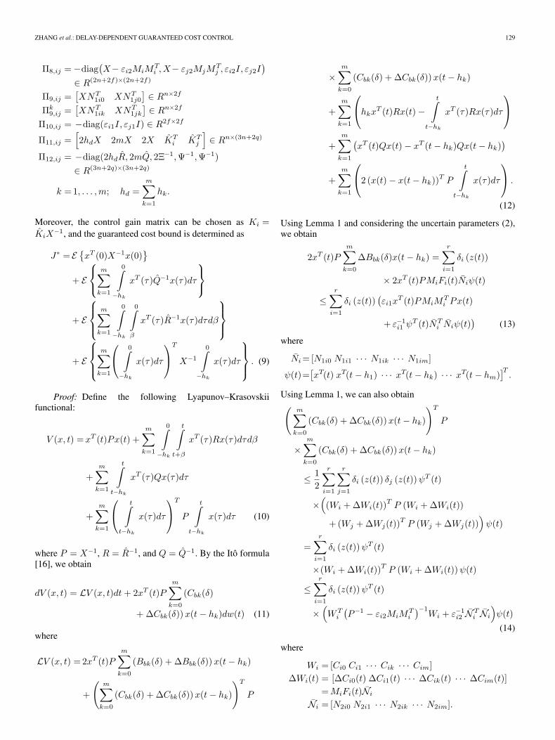
Fig. 1. Response of state via state feedback (solid line: x1, dashed line: x2).

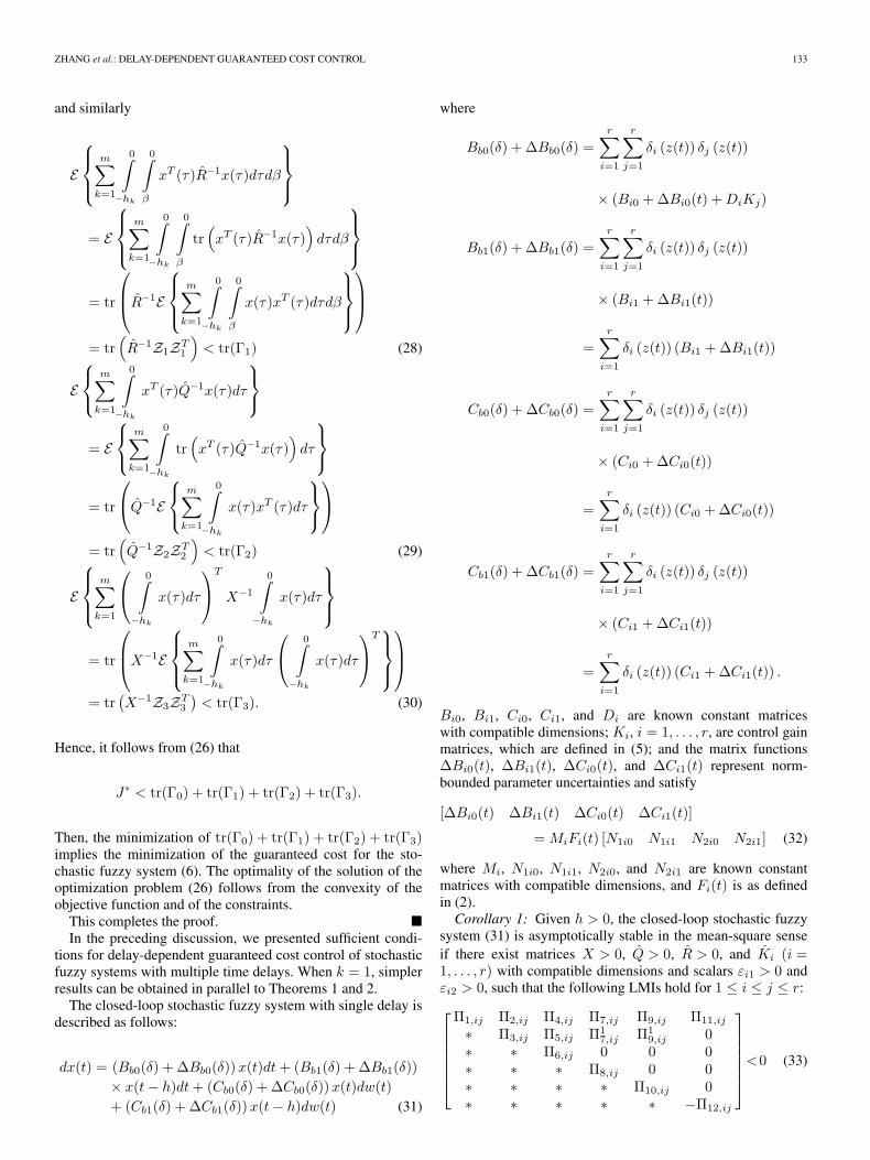
Fig. 2. Curve of control input via state feedback.

Fig. 3. Membership functions (dashed line: rule 1, solid line: rule 2).

[0.2473 −0.0474−0.0474 0.0168

], Q =

[0.4172 −0.0874−0.0874 0.0314

], K1 =

[−0.9975 −0.0010], and K2 = [−0.9998 −0.0001], withthe resulting control gain matrices K1 = [−8.2178 −22.6455]and K2 = [−8.2159 −22.5998].

The simulation results on guaranteed cost control based onstate feedback are shown in Fig. 1. With control law u(t) =R11(x2(t))K1x(t) +R12(x2(t))K2x(t), the closed-loop sys-tem is asymptotically stable in the mean-square sense, and theguaranteed cost bound is J∗ = 5.1292. Fig. 2 shows the curveof the control signal.


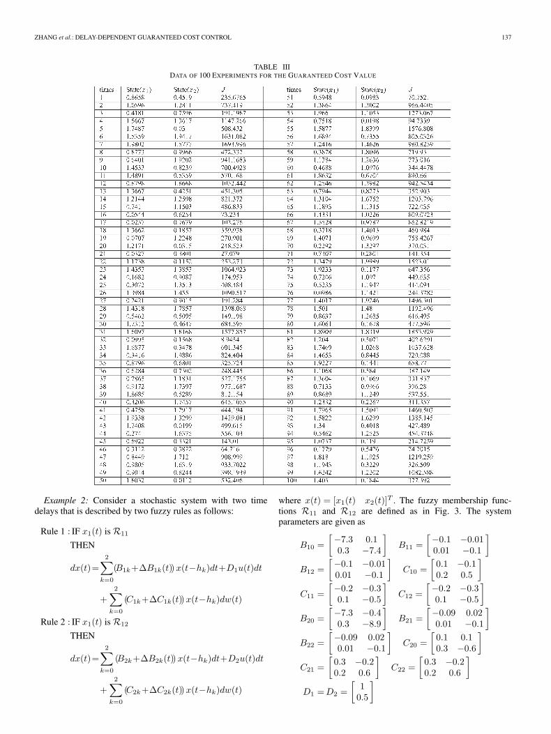
TABLE IIIDATA OF 100 EXPERIMENTS FOR THE GUARANTEED COST VALUE

Example 2: Consider a stochastic system with two timedelays that is described by two fuzzy rules as follows:


THEN

dx(t)=2∑

k=0

(B1k+∆B1k(t))x(t−hk)dt+D1u(t)dt

+2∑

k=0

(C1k+∆C1k(t))x(t−hk)dw(t)


THEN

dx(t)=2∑

k=0

(B2k+∆B2k(t))x(t−hk)dt+D2u(t)dt

+2∑

k=0

(C2k+∆C2k(t))x(t−hk)dw(t)

where x(t) = [x1(t) x2(t)]T . The fuzzy membership func-tions R11 and R12 are defined as in Fig. 3. The systemparameters are given as

B10 =[−7.3 0.10.3 −7.4

]B11 =

[−0.1 −0.010.01 −0.1

]B12 =

[−0.1 −0.010.01 −0.1

]C10 =

[0.1 −0.10.2 0.5

]C11 =

[−0.2 −0.30.1 −0.5

]C12 =

[−0.2 −0.30.1 −0.5

]B20 =

[−7.3 −0.40.3 −8.9

]B21 =

[−0.09 0.020.01 −0.1

]B22 =

[−0.09 0.020.01 −0.1

]C20 =

[0.1 0.10.3 −0.6

]C21 =

[0.3 −0.20.2 0.6

]C22 =

[0.3 −0.20.2 0.6

]D1 =D2 =

[10.5

]


TABLE IVSTATISTICS ANALYSIS OF THE GUARANTEED COST

PERFORMANCE OF REGULATION

and uncertain parameters are described by

[∆B10(t) ∆B11(t) ∆B12(t) ∆C10(t) ∆C11(t) ∆C12(t)]

= M1F1(t)[N110 N111 N112 N210 N211 N212]

[∆B20(t) ∆B21(t) ∆B22(t) ∆C20(t) ∆C21(t) ∆C22(t)]

= M2F2(t)[N120 N121 N122 N220 N221 N222]

with

M1 =[0.2 0.10.3 0.5

]N110 = N111 = N112 =

[0.5 1−0.2 0.6

]

N210 = N211 =[

1 0.50.2 −0.6

]M2 =

[0.2 0.3−0.3 0.4

]

N120 = N121 = N122 =[−0.5 0.90.2 −0.3

]

N220 = N221 =[

0.9 0.5−0.2 0.3

]N212 = N222 = [0]2×2.

The time delays are h1 = 0.25 and h2 = 0.5. Assume thatthe initial function ζ(t) = [x1(t) x2(t)]T is a random con-stant value in [0, 2] for t ∈ [−0.5, 0] and uncertainfunctions F1(t) = F2(t) = sin(t). Applying Theorem 2, weperformed 100 experiments and recorded the correspondingdata in Table III. We can also calculate the statistics of guar-anteed cost function value J as in Example 1, as shown inTable IV.

When ζ(t) = [x1(t) x2(t)]T = [0.5 1]T for t ∈ [−0.5, 0],Ξ = diag(1, 1), and Ψ = 1, based on Theorem 2, a feasible so-lution is given as follows: ε11 = 0.0516, ε12 = 1.0015, ε21 =

0.0.0629, ε22 = 0.6285, X =[

0.0615 −0.0166−0.0166 0.0658

], R =[

0.0253 −0.0142−0.0142 0.0220

], Q =

[0.0198 −0.0126−0.0126 0.0198

], K1 =

[−0.9998 −0.5000], and K2 = [−0.9925 −0.4973], with theresulting control gain matrices K1 = [−19.6567 −12.5763]and K2 = [−19.5165 −12.4999].

The simulation results of the guaranteed cost control basedon state feedback are shown in Fig. 4. With control law u(t) =R11(x2(t))K1x(t) +R12(x2(t))K2x(t), the closed-loop sys-tem is asymptotically stable in the mean-square sense, and theguaranteed cost bound is J∗ = 311.8885. Fig. 5 shows thecontrol curve. It is easy to see that all the time responses ofstates are satisfactory.

V. CONCLUSION

In this paper, a class of uncertain stochastic fuzzy sys-tems with multiple time delays is studied. A delay-dependentguaranteed cost control approach was developed such that thedesigned state feedback controller can guarantee that the

Fig. 4. Response of state via state feedback (solid line: x1, dashed line: x2).

Fig. 5. Curve of control input via state feedback.

closed-loop system is asymptotically stable in the mean-squaresense and the value of cost function is not larger than a bound.The present approach does not require system transformation orrelaxation matrices. All results were presented in the solvableform of LMIs. Simulation examples were given to illustrate thedesign procedures and the effectiveness of the approach.

APPENDIX

Proof of Lemma 2: Since W is a positive definitesymmetric constant matrix, for any nonzero c = [c1, c2, . . . ,cm+1]T

∆= [c1, qT ]T , we have(c1υ(s) +W−1q

)T ×W

(c1υ(s) +W−1q

)≥ 0, i.e., c1υ

T (s)W (c1υ(s)) +c1q

T υ(s) + c1υT (s)q + qTW−1q ≥ 0, which is equivalent to

cT[υT (s)Wυ(s) υT (s)

υ(s) W−1

]c ≥ 0. (37)

Since c is an arbitrary nonzero vector, from inequality (37), itfollows that

[υT (s)Wυ(s) υT (s)

υ(s) W−1

]≥ 0. (38)


Integrating (38) from β − κ to β yields

β∫β−κ

υT (s)Wυ(s)ds

(β∫

β−κ

υ(s)ds

)T

β∫β−κ

υ(s)ds κW−1

≥ 0.

Using the Schur complement, we have

β∫β−κ

υT (s)Wυ(s)ds− 1κ

β∫β−κ

υ(s)ds

T

W

β∫β−κ

υ(s)ds ≥ 0

or

κ

β∫β−κ

υT (s)Wυ(s)ds ≥

β∫β−κ

υ(s)ds

T

W

β∫β−κ

υ(s)ds.

This completes the proof.

REFERENCES

[1] S. Boyd, L. El Ghaoul, E. Feron, and V. Balakrishnan, Linear MatrixInequalities in System and Control Theory. Philadelphia, PA: SIAM,1994.

[2] Y. Y. Cao and Y. X. Sun, “Robust stabilization of uncertain systems withtime-varying multi-state-delay,” IEEE Trans. Autom. Control, vol. 43,no. 10, pp. 1484–1488, Oct. 1998.

[3] S. S. L. Chang and T. K. C. Peng, “Adaptive guaranteed cost controlof systems with uncertain parameters,” IEEE Trans. Autom. Control,vol. AC-17, no. 4, pp. 474–483, Aug. 1972.

[4] W. H. Chen, Z. H. Guan, and X. M. Lu, “Delay-dependent exponentialstability of uncertain stochastic systems with multiple delays: An LMIapproach,” Syst. Control Lett., vol. 54, no. 6, pp. 547–555, Jun. 2005.

[5] B. S. Chen, B. K. Lee, and L. B. Guo, “Optimal tracking design for sto-chastic fuzzy systems,” IEEE Trans. Fuzzy Syst., vol. 11, no. 6, pp. 796–813, Dec. 2003.

[6] B. Chen and X. P. Liu, “Fuzzy guaranteed cost control for nonlinearsystems with time-varying delay,” IEEE Trans. Fuzzy Syst., vol. 13, no. 2,pp. 238–249, Apr. 2005.

[7] B. S. Chen, C. S. Tseng, and H. J. Uang, “Fuzzy differential games fornonlinear stochastic systems: Suboptimal approach,” IEEE Trans. FuzzySyst., vol. 10, no. 2, pp. 222–233, Apr. 2002.

[8] P. Florchinger, “Lyapunov-like techniques for stochastic stability,” SIAMJ. Control Optim., vol. 33, no. 4, pp. 1151–1169, Jul. 1995.

[9] E. Fridman and U. Shaked, “A descriptor system approach to H∞ controlof linear time-delay systems,” IEEE Trans. Autom. Control, vol. 47, no. 2,pp. 253–270, Feb. 2002.

[10] K. Q. Gu, “An integral inequality in the stability problem of time-delaysystems,” in Proc. 39th IEEE Conf. Decision Control, Sydney, Australia,Dec. 2000, pp. 2805–2810.

[11] K. Q. Gu and S. I. Niculescu, “Additional dynamics in transformed time-delay systems,” IEEE Trans. Autom. Control, vol. 45, no. 3, pp. 572–575,Mar. 2000.

[12] X. P. Guan and C. L. Chen, “Delay-dependent guaranteed cost control forT-S fuzzy systems with time delays,” IEEE Trans. Fuzzy Syst., vol. 12,no. 2, pp. 236–249, Apr. 2004.

[13] D. Hinrichsen and A. J. Pritchard, “Stochastic H∞,” SIAM J. ControlOptim., vol. 36, no. 5, pp. 1504–1538, Sep. 1998.

[14] C. Lin, Q. G. Wang, and T. H. Lee, “A less conservative robust stabilitytest for linear uncertain time-delay systems,” IEEE Trans. Autom. Control,vol. 51, no. 1, pp. 87–91, Jan. 2005.

[15] C. Lin, Q. G. Wang, and T. H. Lee, “H∞ output tracking control fornonlinear systems via T-S fuzzy model approach,” IEEE Trans. Syst.,Man, Cybern. B, Cybern., vol. 36, no. 2, pp. 450–457, Apr. 2006.

[16] X. Mao, Stochastic Differential Equations and Applications. Chichester,U.K.: Horwood, 1997.

[17] V. Suplin, E. Fridman, and U. Shaked, “H∞ control of linear uncer-tain time-delay systems—A projection approach,” IEEE Trans. Autom.Control, vol. 51, no. 4, pp. 680–685, Apr. 2006.

[18] T. Takagi and M. Sugeno, “Fuzzy identification of systems and its ap-plications to modeling and control,” IEEE Trans. Syst., Man, Cybern.,vol. SMC-15, no. 1, pp. 116–132, Jan. 1985.

[19] K. Tanaka, T. Ikeda, and H. O. Wang, “Robust stabilization of a class ofuncertain nonlinear systems via fuzzy control: Quadratic stabilizability,H∞ control theory, and linear matrix inequalities,” IEEE Trans. FuzzySyst., vol. 4, no. 1, pp. 1–13, Feb. 1996.

[20] V. A. Ugrinovskii, “Output feedback guaranteed cost control for stochasticuncertain systems with multiplicative noise,” in Proc. 39th IEEE Conf.Decision Control, Sydney, Australia, Dec. 2000, pp. 240–245.

[21] Z. D. Wang, D. W. C. Ho, and X. H. Liu, “A note on the robust stability ofuncertain stochastic fuzzy systems with time-delays,” IEEE Trans. Syst.,Man, Cybern. A, Syst., Humans, vol. 34, no. 4, pp. 570–576, Jul. 2004.

[22] H. O. Wang, K. Tanaka, and M. F. Griffin, “Parallel distributed compensa-tion of nonlinear systems by Takagi-Sugeno fuzzy model,” in Proc. IEEEInt. Conf. Fuzzy Syst., Yokohama, Japan, Mar. 1995, pp. 531–538.

[23] Y. Wang, L. Xie, and C. E. de Souza, “Robust control of a class ofuncertain nonlinear systems,” Syst. Control Lett., vol. 19, no. 2, pp. 139–149, Aug. 1992.

[24] Y. C. Wang, H. G. Zhang, and Y. Z. Wang, “Fuzzy adaptive control ofstochastic nonlinear systems with unknown virtual control gain function,”ACTA Autom. Sin., vol. 32, no. 2, pp. 170–178, Mar. 2006.

[25] W. M. Wonham, “Random differential equations in control theory,”in Probabilistic Methods in Applied Mathematics, vol. 2. New York:Academic, 1970, pp. 131–217.

[26] S. Y. Xu and J. Lam, “Improved delay-dependent stability criteria fortime-delay systems,” IEEE Trans. Autom. Control, vol. 50, no. 3, pp. 384–387, Mar. 2005.

[27] E. E. Yaz, “Guaranteed-cost stabilization of non-linear stochastic sys-tems,” Optim. Control Appl. Methods, vol. 19, no. 1, pp. 41–54, 1998.

[28] L. Yu and J. Chu, “An LMI approach to guaranteed cost control of linearuncertain time-delay systems,” Automatica, vol. 35, no. 6, pp. 1155–1159,Jun. 1999.

[29] D. Yue and Q. L. Han, “Delay-dependent exponential stability of sto-chastic systems with time-varying delay, nonlinearity, and Markovianswitching,” IEEE Trans. Autom. Control, vol. 50, no. 2, pp. 217–222,Feb. 2005.

[30] H. B. Zhang, C. G. Li, and X. F. Liao, “Stability analysis and H∞ con-troller design of fuzzy large-scale systems based on piecewise Lyapunovfunctions,” IEEE Trans. Syst., Man, Cybern. B, Cybern., vol. 36, no. 3,pp. 685–698, Jun. 2006.

[31] H. G. Zhang, S. X. Lun, and D. Liu, “Fuzzy H∞ filter design for a classof nonlinear discrete-time systems with multiple time delay,” IEEE Trans.Fuzzy Syst., vol. 15, no. 3, pp. 453–469, Jun. 2007.

[32] H. G. Zhang and Y. C. Wang, “Delay-dependent guaranteed cost controlfor uncertain stochastic fuzzy systems with time delays,” Prog. Nat. Sci.,vol. 17, no. 1, pp. 95–101, Jan. 2007.

Huaguang Zhang (SM’04) was born in Jilin, China,in 1959. He received the B.S. and M.S. degrees incontrol engineering from the Northeastern ElectricPower University of China, Jilin, in 1982 and 1985,respectively, and the Ph.D. degree in thermal powerengineering and automation from Southeast Univer-sity, Nanjing, China, in 1991.

In 1992, he joined the Department of AutomaticControl, Northeastern University, Shenyang, China,as a Postdoctoral Fellow for two years. Since 1994,he has been a Professor and Head of the Institute

of Electric Automation, Northeastern University. He is also with the KeyLaboratory of Integrated Automation of Process Industry (Northeastern Univer-sity), National Education Ministry, Shenyang. His research interests are fuzzycontrol, stochastic system control, neural-networks-based control, nonlinearcontrol, and their applications.

Dr. Zhang is currently an Associate Editor for the IEEE TRANSACTIONS

ON SYSTEMS, MAN, AND CYBERNETICS—PART B. He was the recipient ofthe Outstanding Youth Science Foundation Award from the National NaturalScience Foundation of China in 2003 and was named the Cheung Kong Scholarby the China Education Ministry in 2005.


Yingchun Wang was born in Liaoning Province,China, in 1974. He received the B.S., M.S.,and Ph.D. degrees from Northeastern Univer-sity, Shenyang, China, in 1997, 2003, and 2006,respectively.

Since 2006, he has been with the School of In-formation Science and Engineering, NortheasternUniversity. He is also currently with the Key Lab-oratory of Integrated Automation of Process Indus-try (Northeastern University), National EducationMinistry, Shenyang. His research interests include

fuzzy control and fuzzy systems, stochastic control, time-delay systems, andnonlinear systems.

Derong Liu (S’91–M’94–SM’96–F’05) received theB.S. degree in mechanical engineering from the EastChina Institute of Technology (now Nanjing Univer-sity of Science and Technology), Nanjing, in 1982,the M.S. degree in electrical engineering from theChinese Academy of Sciences (CAS), Beijing, in1987, and the Ph.D. degree in electrical engineeringfrom the University of Notre Dame, Notre Dame, IN,in 1994.

From 1982 to 1984, he was a Product DesignEngineer with China North Industries Corporation,

Jilin, China. From 1987 to 1990, he was an Instructor with the GraduateSchool of CAS. From 1993 to 1995, he was a Staff Fellow with the GeneralMotors Research and Development Center, Warren, MI. From 1995 to 1999,he was an Assistant Professor with the Department of Electrical and ComputerEngineering, Stevens Institute of Technology, Hoboken, NJ. In 1999, he joinedthe University of Illinois, Chicago, where he is currently a Full Professor ofelectrical and computer engineering and of computer science. Since 2005, hehas been the Director of Graduate Studies with the Department of Electrical andComputer Engineering, University of Illinois. He is a coauthor of DynamicalSystems With Saturation Nonlinearities: Analysis and Design (Springer-Verlag,1994) and Qualitative Analysis and Synthesis of Recurrent Neural Networks(Marcel Dekker, 2002), and Fuzzy Modeling and Fuzzy Control (Birkhauser,2006). He is a Coeditor of Stability and Control of Dynamical Systems WithApplications (Birkhauser, 2003), Advances in Computational Intelligence:Theory and Applications (World Scientific, 2006), and Advances in NeuralNetworks-ISNN2007 (Springer-Verlag, 2007). He is also an Associate Editorof Automatica.

Dr. Liu has been an Associate Editor for the IEEE TRANSACTIONS

ON CIRCUITS AND SYSTEMS—PART I: FUNDAMENTAL THEORY AND

APPLICATIONS (1997–1999), the IEEE TRANSACTIONS ON SIGNAL

PROCESSING (2001–2003), and the IEEE TRANSACTIONS ON NEURAL

NETWORKS (2004–2006). Since 2004, he has been the Editor for theIEEE Computational Intelligence Society’s ELECTRONIC LETTER, and since2006, he has been the Letter Editor for the IEEE TRANSACTIONS ON

NEURAL NETWORKS and an Associate Editor for the IEEE COMPUTATIONAL

INTELLIGENCE MAGAZINE. He is the General Chair for the 2008 IEEEInternational Conference on Networking, Sensing and Control. He was theGeneral Chair for the 2007 International Symposium on Neural Networks(Nanjing, China). He is the Program Chair for the 2008 International JointConference on Neural Networks; the 2007 IEEE International Symposium onApproximate Dynamic Programming and Reinforcement Learning; the 21stIEEE International Symposium on Intelligent Control (2006); and the 2006International Conference on Networking, Sensing and Control. He has servedand is serving as a member of the organizing committee and the programcommittee of several other international conferences. He is an elected AdComMember of the IEEE Computational Intelligence Society (2006–2008), Chairof the Chicago Chapter of the IEEE Computational Intelligence Society, andPast Chair of the Technical Committee on Neural Systems and Applicationsof the IEEE Circuits and Systems Society. He was the recipient of theMichael J. Birck Fellowship from the University of Notre Dame (1990), theHarvey N. Davis Distinguished Teaching Award from the Stevens Institute ofTechnology (1997), the Faculty Early Career Development (CAREER) Awardfrom the National Science Foundation (1999), and the University ScholarAward from the University of Illinois (2006–2009). He is a Member ofEta Kappa Nu and the Conference Editorial Board of the IEEE Control SystemsSociety (1995–2000).

delay-dependent guaranteed cost control for uncertain discrete-time systems with delay

Documents