deep-learning based exploitation of eavesdropped images
TRANSCRIPT

THÈSE DE DOCTORAT DE
L’INSTITUT NATIONAL DES SCIENCES
APPLIQUEES DE RENNES
COMUE UNIVERSITÉ BRETAGNE LOIRE
ÉCOLE DOCTORALE N° 601Mathématiques et Sciences et Technologiesde l’Information et de la CommunicationSpécialité : Signal, Image, Vision
Par
Florian LEMARCHANDDeep-Learning Based Exploitation of Eavesdropped Images
Thèse présentée et soutenue à Rennes, le 29 Septembre 2021Unité de recherche : IETRThèse N° : 21ISAR 23 / D21 - 23
Rapporteurs avant soutenance :
Fan Yang Professeure des Universités, Université de BourgogneOlivier Strauss Maître de Conférences, HDR, Université de Montpellier
Composition du Jury :
Président : William Puech Professeur des Universités, Université de MontpellierExaminateurs : Fan Yang Professeure des Universités, Université de Bourgogne
Olivier Strauss Maître de Conférences, HDR, Université de MontpellierFrançois Berry Professeur des Universités, Université Clermont AuvergneEmmanuel Cottais Ingénieur, ANSSIBart Goossens Professeur des Universités, Ghent University
Directeur de thèse : Maxime Pelcat Maitre de Conférences, HDR, INSA RennesEncadrant : Erwan Nogues Ingénieur, DGA-MI

Table of Contents
1 Introduction 9
1.1 Context: Novel Challenges of Side-Channel Analysis . . . . . . . . . . . . . . 91.2 Objectives and Contributions of this Thesis . . . . . . . . . . . . . . . . . . . . 11
1.2.1 Benchmarking of Image Restoration Algorithms . . . . . . . . . . . . . 111.2.2 Mixture Noise Denoising Using a Gradual Strategy . . . . . . . . . . . 121.2.3 Direct Interpretation of Eavesdropped Images . . . . . . . . . . . . . . 12
1.3 Outline . . . . . . . . . . . . . . . . . . . . . . . . . . . . . . . . . . . . . . . . 13
I Open Challenges in Eavesdropped Image Information Extrac-tion 15
2 Eavesdropping 17
2.1 Introduction . . . . . . . . . . . . . . . . . . . . . . . . . . . . . . . . . . . . . 172.2 From Side-Channel Emanations to Image Eavesdropping . . . . . . . . . . . . 202.3 Eavesdropped Image Characteristics . . . . . . . . . . . . . . . . . . . . . . . . 21
2.3.1 Image Coding . . . . . . . . . . . . . . . . . . . . . . . . . . . . . . . . 232.3.2 Emission Defaults . . . . . . . . . . . . . . . . . . . . . . . . . . . . . . 252.3.3 Interception Impairments . . . . . . . . . . . . . . . . . . . . . . . . . 25
2.4 Going Further With Image Processing . . . . . . . . . . . . . . . . . . . . . . . 272.5 Conclusion . . . . . . . . . . . . . . . . . . . . . . . . . . . . . . . . . . . . . . 28
3

TABLE OF CONTENTS
3 Noisy Image Interpretation 313.1 Introduction . . . . . . . . . . . . . . . . . . . . . . . . . . . . . . . . . . . . . 313.2 What does it mean for an image to be noisy? . . . . . . . . . . . . . . . . . . . 32
3.2.1 Standard Noise Types . . . . . . . . . . . . . . . . . . . . . . . . . . . 333.2.2 Towards Real-World Noise Distributions . . . . . . . . . . . . . . . . . 34
3.3 Overview of Image Restoration Methods . . . . . . . . . . . . . . . . . . . . . 353.3.1 Expert-Based Algorithms . . . . . . . . . . . . . . . . . . . . . . . . . 363.3.2 Fully-Supervised Learning Algorithms . . . . . . . . . . . . . . . . . . 373.3.3 Weakly Supervised Algorithms . . . . . . . . . . . . . . . . . . . . . . 38
3.4 Overview of Image Interpretation Methods . . . . . . . . . . . . . . . . . . . . 393.5 Error Measurement and Quality Assessment . . . . . . . . . . . . . . . . . . . 42
3.5.1 Image Quality Metrics . . . . . . . . . . . . . . . . . . . . . . . . . . . 423.5.2 Classi�cation Metrics . . . . . . . . . . . . . . . . . . . . . . . . . . . . 43
3.6 Datasets for Learning and Evaluation . . . . . . . . . . . . . . . . . . . . . . . 463.7 Learning Algorithms: Terminology, Strengths and Open Issues . . . . . . . . . 47
3.7.1 Terminology, Learning Pipeline and Architecture Speci�city . . . . . . 473.7.2 Strengths of Learning Algorithms . . . . . . . . . . . . . . . . . . . . . 503.7.3 Two Open Issues of Deep-Learning Algorithms . . . . . . . . . . . . . 51
3.8 Conclusion . . . . . . . . . . . . . . . . . . . . . . . . . . . . . . . . . . . . . . 52
II Contributions 53
4 Benchmarking of Image Restoration Algorithms 554.1 Introduction . . . . . . . . . . . . . . . . . . . . . . . . . . . . . . . . . . . . . 554.2 Related Work . . . . . . . . . . . . . . . . . . . . . . . . . . . . . . . . . . . . . 56
4.2.1 Related Work on Benchmarks of Image Denoisers . . . . . . . . . . . . 564.2.2 Chosen Image Denoisers for Benchmarking . . . . . . . . . . . . . . . 57
4.3 Proposed Benchmark . . . . . . . . . . . . . . . . . . . . . . . . . . . . . . . . 584.4 A Comparative Study of Denoisers . . . . . . . . . . . . . . . . . . . . . . . . . 59
4.4.1 Gaussian Noise . . . . . . . . . . . . . . . . . . . . . . . . . . . . . . . 614.4.2 Mixture Noise . . . . . . . . . . . . . . . . . . . . . . . . . . . . . . . . 614.4.3 Interception Noise . . . . . . . . . . . . . . . . . . . . . . . . . . . . . 614.4.4 Discussion . . . . . . . . . . . . . . . . . . . . . . . . . . . . . . . . . . 64
4.5 Conclusion . . . . . . . . . . . . . . . . . . . . . . . . . . . . . . . . . . . . . . 65
4

TABLE OF CONTENTS
5 Mixture Noise Denoising Using a Gradual Strategy 675.1 Introduction . . . . . . . . . . . . . . . . . . . . . . . . . . . . . . . . . . . . . 675.2 Related Work . . . . . . . . . . . . . . . . . . . . . . . . . . . . . . . . . . . . . 70
5.2.1 Blind Denoising . . . . . . . . . . . . . . . . . . . . . . . . . . . . . . . 705.2.2 Noise Mixtures . . . . . . . . . . . . . . . . . . . . . . . . . . . . . . . 715.2.3 Classi�cation-Based Denoising . . . . . . . . . . . . . . . . . . . . . . 71
5.3 Gradual Denoising Guided by Noise Analysis . . . . . . . . . . . . . . . . . . . 725.3.1 Noise Analysis . . . . . . . . . . . . . . . . . . . . . . . . . . . . . . . 735.3.2 Gradual Denoising . . . . . . . . . . . . . . . . . . . . . . . . . . . . . 735.3.3 Noise Classes and Primary Denoisers . . . . . . . . . . . . . . . . . . . 74
5.4 Experiments: Noise Mixture Removal . . . . . . . . . . . . . . . . . . . . . . . 765.4.1 Data and Experimental Settings . . . . . . . . . . . . . . . . . . . . . . 765.4.2 Results . . . . . . . . . . . . . . . . . . . . . . . . . . . . . . . . . . . . 805.4.3 Errors and Limitations . . . . . . . . . . . . . . . . . . . . . . . . . . . 82
5.5 Experiments: Ablation Study . . . . . . . . . . . . . . . . . . . . . . . . . . . . 835.5.1 Impact of Classi�cation on NoiseBreaker . . . . . . . . . . . . . . . . . 83
5.5.1.1 Backbone Choice . . . . . . . . . . . . . . . . . . . . . . . . 835.5.1.2 Classi�cation Order . . . . . . . . . . . . . . . . . . . . . . . 84
5.5.2 Impact of Primary Denoisers . . . . . . . . . . . . . . . . . . . . . . . 855.5.2.1 Noise Class Re�nement . . . . . . . . . . . . . . . . . . . . . 855.5.2.2 Architecture Distinction . . . . . . . . . . . . . . . . . . . . 85
5.6 Conclusion . . . . . . . . . . . . . . . . . . . . . . . . . . . . . . . . . . . . . . 86
6 Direct Interpretation of Eavesdropped Images 876.1 Introduction . . . . . . . . . . . . . . . . . . . . . . . . . . . . . . . . . . . . . 876.2 Proposed Side-Channel Attack . . . . . . . . . . . . . . . . . . . . . . . . . . . 89
6.2.1 System Description . . . . . . . . . . . . . . . . . . . . . . . . . . . . . 896.2.2 Dataset Construction . . . . . . . . . . . . . . . . . . . . . . . . . . . . 896.2.3 Implemented Solution to Catch Compromising Data . . . . . . . . . . 91
6.3 Experimental Results . . . . . . . . . . . . . . . . . . . . . . . . . . . . . . . . 926.3.1 Experimental Setup . . . . . . . . . . . . . . . . . . . . . . . . . . . . . 926.3.2 Performance Comparison Between Data Catchers . . . . . . . . . . . . 94
6.4 An Opening to Eavesdropped Natural Images . . . . . . . . . . . . . . . . . . 976.4.1 Dataset Construction . . . . . . . . . . . . . . . . . . . . . . . . . . . . 97
5

TABLE OF CONTENTS
6.4.2 Does a Gaussian Denoiser Transfer to Eavesdropping? . . . . . . . . . 986.5 Conclusions . . . . . . . . . . . . . . . . . . . . . . . . . . . . . . . . . . . . . 102
7 Conclusion 1037.1 Research Contributions . . . . . . . . . . . . . . . . . . . . . . . . . . . . . . . 104
7.1.1 Benchmarking of Image Restoration Algorithms . . . . . . . . . . . . . 1047.1.2 Mixture Noise Denoising Using a Gradual Strategy . . . . . . . . . . . 1057.1.3 Direct Interpretation of Eavesdropped Images . . . . . . . . . . . . . . 105
7.2 Prospects – Future Works . . . . . . . . . . . . . . . . . . . . . . . . . . . . . . 1067.2.1 Signal Detection in Eavesdropping Noise . . . . . . . . . . . . . . . . . 1067.2.2 Fine-Grain Modeling of the Eavesdropping Corruption . . . . . . . . . 1067.2.3 Interpretability of Eavesdropped Images . . . . . . . . . . . . . . . . . 1077.2.4 Extension to Other Noisy Data . . . . . . . . . . . . . . . . . . . . . . 1077.2.5 Embedding of Proposed Methods . . . . . . . . . . . . . . . . . . . . . 108
A French Summary 109A.1 Contexte . . . . . . . . . . . . . . . . . . . . . . . . . . . . . . . . . . . . . . . 109A.2 Objectifs et contributions de cette thèse . . . . . . . . . . . . . . . . . . . . . . 111
A.2.1 Comparaison d’algorithmes de restauration d’images . . . . . . . . . . 111A.2.2 Débruitage graduel de mélanges de bruit . . . . . . . . . . . . . . . . . 112A.2.3 Interprétation directe d’images interceptées . . . . . . . . . . . . . . . 112
A.3 Plan du Manuscrit . . . . . . . . . . . . . . . . . . . . . . . . . . . . . . . . . . 113
List of Figures 117
List of Tables 119
Acronyms 120
Personal Publications 123
Bibliography 125
Autorisation de Reproduction 138
6

Acknowledgements
Tout d’abord, je tiens à remercier mes encadrants. Merci pour la con�ance et la liberté quevous m’avez accordées tout au long de ces trois années. Maxime merci d’être une mine d’idées.Cela m’a parfois donné des nœuds au cerveau mais aussi poussé à donner le meilleur. Erwan,merci de ta pertinence scienti�que et de ton ouverture d’esprit. J’ai apprécié nos diverses dis-cussions sur tous types de sujets intéressants, qu’elles soient de nature professionnelle ou non.
Merci aux membres du jury qui ont évalué mon manuscrit ainsi que ma soutenance. Mercipour votre temps et les orientations et propositions pertinentes que vous avez faites sur letravail présenté.
Merci à l’équipe IA de la DGA pour l’important travail sur ToxicAI et les discussions per-tinentes sur l’interprétation des images interceptées.
Je suis reconnaissant envers Eduardo et Thomas, les stagiaires qui m’ont par leur travailaidé à développer OpenDenoising-Benchmark et NoiseBreaker, deux contributions majeuresde cette thèse.
Merci à la Musique d’avoir su me proposer au jour le jour ses di�érentes facettes pours’adapter à mes humeurs.
Merci aux collègues de VAADER. Ceux avec qui j’ai pu échanger, professionnellementou personnellement. Particulièrement merci à ceux qui sont devenus des amis en partageanttoutes sortes de moments que je ne saurais lister de façon exhaustive : des relectures de pa-piers, des pauses café, des complaintes de doctorants, des soirées ou week-end raisonnables etd’autres moins.
Merci aux occupants du "Bureau 214" qui ont rendu mes journées de travail toujours plusjoyeuses avec des blagues et des surprises toutes plus rocambolesques les unes que les autres.
7

TABLE OF CONTENTS
J’aimerais aussi ne pas remercier la Covid-19 qui a fait exploser en vol mes ambitions decollaborations internationales et de voyages scienti�ques. Présenter des articles à distance futun réel non-plaisir.
Merci à ma famille et à mes amis qui rendent ma vie heureuse à chaque instant. La réussitede cette thèse n’aurait pas été possible sans les moments ressourçant que vous me faites vivre.
En�n, merci à Elisa qui m’a chéri tout au long de ces trois années, dans les moments deréussite comme dans ceux de doutes. Merci d’avoir été à mes côtés et des choix que tu as faitspour me permettre de réussir ce dé�, souvent à tes dépens.
8
CHAPTER 1
Introduction
Chapter Contents1.1 Context: Novel Challenges of Side-Channel Analysis . . . . . . . . . 9
1.2 Objectives and Contributions of this Thesis . . . . . . . . . . . . . . . 11
1.3 Outline . . . . . . . . . . . . . . . . . . . . . . . . . . . . . . . . . . . . . 13
1.1 Context: Novel Challenges of Side-Channel Analysis
The recent trend of processing is to make digital data available anytime anywhere, creat-ing new con�dentiality threats. In particular, when considering highly con�dential data, whereprinted information was kept physically protected and was accessible only to authorized per-sons, the data is nowadays digital. It is exchanged and consulted using Information ProcessingEquipments (IPEs) and their according Video Display Units (VDUs). While the main securitye�orts focus today on the network side of systems, there exist other security threats.
A side-channel corresponds to an unintended data path in opposition to the legacy channel.In particular, Electro Magnetic (EM) side-channels are due to �elds emitted by video cablesand connectors when their inner voltage changes. These side-channels are dangerous becausethey spread un-ciphered data outside the physical system. These emissions may be correlatedto a con�dential information. Therefore, an attacker receiving the signal and knowing thedata encoding mechanism may access illegally the original information handled by the IPE.Under these conditions, the attacker can reconstruct the image displayed on the attacked VDUconnected to the IPE. It has been shown that the content of screen can be recontructed from

Chapter 1 – Introduction
tens of meters [DSV20a]. Since the pionner exploits [Van85], a lot of work has been publishedon the reconstruction of images from EM side-channel emanations, and this research area isstill dynamic [Lav+21]. But until today, the work conducted on state of the art has mainlyfocused on enhancing the reconstruction from a signal processing point of view.
Recently, the image processing domain have been revolutionnized by Machine Learning(ML) and especially Deep Learning (DL). These algorithms learning tasks from data, haveoverpassed the performances of state of the art expert algorithms on several Computer Vision(CV) tasks. In particular, one of the tasks that have bene�ted from learning algorithms is thesemantic classi�cation of image content. In this task, state of the art algorithms are nowadayscapable of automating interpretation of images. However, these interpretation methods aredesigned for natural images without corruption. Image restoration is the task concerned byremoving corruptions from images. Image restoration has also bene�ted a lot from learning al-gorithms. In fact, recent algorithms outperform the former state of art expert based algorithmsboth on objective and subjective performances. However, the state of the art algorithms forimage restoration focus on well-behaved corruptions, following parametric distribution, ruledby only a few parameters.
The images reconstructed from EM emanations are highly corrupted due to several rea-sons. First there is a data loss and interferences inherent to the EM emission/reception process,similarly to a radio-frequency channel in a data wireless communication. In addition, there arealso defects in the reconstruction synchonization, when passing from 1D signal to an image.Finally, the defects of the hardware of the interception system introduce errors. Arise threequestions that we study in this manuscript: What is the type of corruption generated byEM emanations reconstruction? Can it be reduced to a composition of parametricdistribution noises? How do current DL methods for image restoration perform oneavesdropped image?
The audit of processing systems handling con�dential data, is currently executed by ex-perts. An expert, once the interception system in place, assesses the compromise of the auditedequipment, using her/his experience. This audit protocol is time consuming and subject to hu-man perception. Here comes another question we study in this manuscript: Can DL be usedto automate semantics retrieval from eavesdropped images?
10
1.2. Objectives and Contributions of this Thesis
1.2 Objectives and Contributions of this Thesis
The main objective of this thesis is to analyze how DL techniques can be applied to eaves-dropped images and if it can automate the interpretation of these images. Even though EMemanation reconstruction and DL image processing are two extensely studied domains, theirconcomitant use is a recent advance.
After the review of the seminal work of both eavesdropping and noisy image interpreta-tion, we propose a set of experiments and contributions to study the feasability of automaticeavesdropping exploitation.
Three main contributions are proposed in this document. They are among the �rst studiesof EM emanations from an image processing point of view. Accordingly, this thesis is one ofthe �rst attempt to apply DL for eavedropping image exploitation automation. The three maincontributions of this thesis are brie�y presented below.
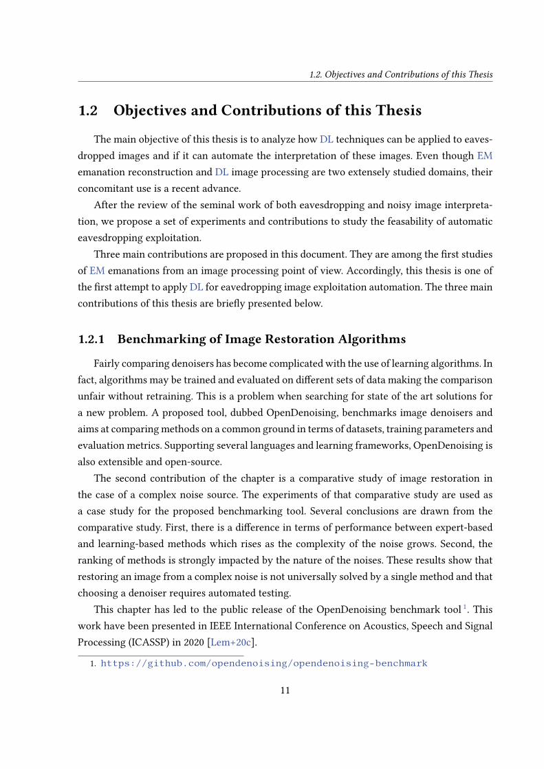
1.2.1 Benchmarking of Image Restoration Algorithms
Fairly comparing denoisers has become complicated with the use of learning algorithms. Infact, algorithms may be trained and evaluated on di�erent sets of data making the comparisonunfair without retraining. This is a problem when searching for state of the art solutions fora new problem. A proposed tool, dubbed OpenDenoising, benchmarks image denoisers andaims at comparing methods on a common ground in terms of datasets, training parameters andevaluation metrics. Supporting several languages and learning frameworks, OpenDenoising isalso extensible and open-source.
The second contribution of the chapter is a comparative study of image restoration inthe case of a complex noise source. The experiments of that comparative study are used asa case study for the proposed benchmarking tool. Several conclusions are drawn from thecomparative study. First, there is a di�erence in terms of performance between expert-basedand learning-based methods which rises as the complexity of the noise grows. Second, theranking of methods is strongly impacted by the nature of the noises. These results show thatrestoring an image from a complex noise is not universally solved by a single method and thatchoosing a denoiser requires automated testing.
This chapter has led to the public release of the OpenDenoising benchmark tool 1. Thiswork have been presented in IEEE International Conference on Acoustics, Speech and SignalProcessing (ICASSP) in 2020 [Lem+20c].
1. https://github.com/opendenoising/opendenoising-benchmark
11

Chapter 1 – Introduction
1.2.2 Mixture Noise Denoising Using a Gradual Strategy
Preliminary chapters will suggest that the corruption generated by the eavesdropping pro-cess is a sequential mixture of several primary corruptions. Accordingly, Chapter 5 intro-duces a gradual image denoising strategy called NoiseBreaker. NoiseBreaker iteratively de-tects the image dominating noise using a trained classi�er with an accuracy of 93% and 91%for grayscale and RGB samples, respectively. Under the assumption of grayscale sequentialnoise mixtures, NoiseBreaker performs 0.95dB under the supervised Multi-level Wavelet Con-volutional Neural Network (MWCNN) denoiser without being trained on any mixture noise.Neither the classi�er nor the denoisers are exposed to mixture noise during training. Noise-Breaker operates 2dB over the gradual denoising of [LSJ20] and 5dB over the state of the artself-supervised denoiser Noise2Void. When using RGB samples, NoiseBreaker operates 5dBover [LSJ20] while Noise2Void underperforms. Moreover, this paper demonstrates that mak-ing noise analysis to guide the denoising is not only e�cient on noise type, but also on noiseintensity.
This manuscript has demonstrated the practicality of NoiseBreaker on six di�erent syn-thetic noise mixtures. Nevertheless, the NoiseBreaker version proposed in the chapter has notpermited to conclude on the e�ciency of the method to restore eavesdropped images. Conse-quently, the hypothesis of the sequential composition of the eavesdropping corruption is notvalidated.
This work has lead to a presentaion in the IEEE 22nd International Workshop on Multi-media Signal Processing (MMSP) in 2020 [Lem+20a].
1.2.3 Direct Interpretation of Eavesdropped Images
This work is presented in the last contribution chapter of the manuscript. The beginning ofthe manuscript studies the applicability of DL to restore eavesdropped images. This last workfocuses on interpretation and studies its automation on text images. The introduction of deeplearning in an EM side-channel attack is studied. The proposed method, called TxicAI, usesMask R-CNN as denoiser and it automatically recovers more than 57% of characters, presentin the test set. In comparison, the best denoising/Optical Character Recognition (OCR) pairretrieves 42% of characters. The proposal is software-based, and runs on the host computerof an o�-the-shelf Software-De�ned Radio (SDR) platform.
This chapter has led to the public release of two datasets of eavesdropped samples:
12
1.3. Outline
• a dataset of eavesdropped images made of text characters and their references 2,• a dataset of eavesdropped natural images, based on Berkeley Segmentation Dataset
(BSD), dubbed Natural Interception Dataset (NID) 3.This work was presented in Conference on Arti�cal Intelligence for Defense (CAID), in
2019 [Lem+19] and in IEEE International Conference on Acoustics, Speech and Signal Pro-cessing (ICASSP) in 2020 [Lem+20b].
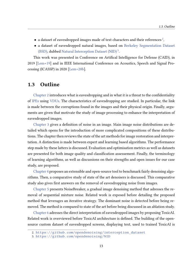
1.3 Outline
Chapter 2 introduces what is eavesdropping and in what it is a threat to the con�dentialityof IPEs using VDUs. The characteristics of eavesdropping are studied. In particular, the linkis made between the corruptions found in the images and their physical origin. Finally, argu-ments are given that motivate the study of image processing to enhance the interpretation ofeavesdropped images.
Chapter 3 gives a de�nition of noise in an image. Main image noise distributions are de-tailed which opens for the introduction of more complicated compositions of these distribu-tions. The chapter then reviews the state of the art methods for image restoration and interpre-tation. A distinction is made between expert and learning based algorithms. The performancestep made by these latters is discussed. Evaluation and optimisation metrics as well as datasetsare presented for both image quality and classi�cation assessement. Finally, the terminologyof learning algorithms, as well as discussions on their strengths and open issues for our casestudy, are proposed.
Chapter 4 proposes an extensible and open-source tool to benchmark fairly denoising algo-rithms. Then, a comparative study of state of the art denoisers is discussed. This comparativestudy also gives �rst answers on the removal of eavesdropping noise from images.
Chapter 5 presents NoiseBreaker, a gradual image denoising method that adresses the re-moval of sequential mixture noise. Related work is exposed before detailing the proposedmethod that leverages an iterative strategy. The dominant noise is detected before being re-moved. The method is compared to state of the art before being discussed in an ablation study.
Chapter 6 adresses the direct interpretation of eavesdropped images by proposing ToxicAI.Related work is overviewed before ToxicAI architecture is de�ned. The building of the open-source custom dataset of eavesdropped screens, displaying text, used to trained ToxicAI is
2. https://github.com/opendenoising/interception_dataset3. https://github.com/opendenoising/NID
13

Chapter 1 – Introduction
[Lem+20c]
Benchmarking of ImageRestoration Algorithms
Mixture Noise RemovalUsing Gradual Denoising
Chap. 4
Chap. 5
Chap. 6 Direct Interpretation of Eavesdropped Images
[Lem+19, Lem+20a]
[Lem+20b]
Chap. 2 Eavesdropping Chap. 3 Noisy Image Interpretation
Figure 1.1 – Outline of the document structure. State-of-the art chapters are displayed in whitewhile contribution chapters are in gray.
detailed. Then, experiments are conducted on the proposal and the results compared to thestate of the art. Finally, an open-source dataset of eavesdropped natural images is proposed toextend ToxicAI.
Chapter 7 concludes the manuscript. First, the questions addressed in the document arereminded and the contributions are resumed. Opened by the principles proposed in this doc-ument, research directions for the future of eavesdropped image interpretation are proposed.
Figure 1.1 illustrates the organisation of this document. This �gure highlights the linksbetween the chapters introduced here-above.
14

Part I
Open Challenges in EavesdroppedImage Information Extraction
15

CHAPTER 2
Eavesdropping
Chapter Contents2.1 Introduction . . . . . . . . . . . . . . . . . . . . . . . . . . . . . . . . . . 17
2.2 From Side-Channel Emanations to Image Eavesdropping . . . . . . . 20
2.3 Eavesdropped Image Characteristics . . . . . . . . . . . . . . . . . . . 21
2.4 Going Further With Image Processing . . . . . . . . . . . . . . . . . . 27
2.5 Conclusion . . . . . . . . . . . . . . . . . . . . . . . . . . . . . . . . . . 28
2.1 Introduction
In the last decades, Information Processing Equipments (IPEs) have become essential inprofessional everyday life. This democratization has opened new threats on data security. Thepurpose of this chapter is to give the fundamentals of Information System Security (ISS) andits speci�c application to the side-channel emanations of Video Display Units (VDUs).
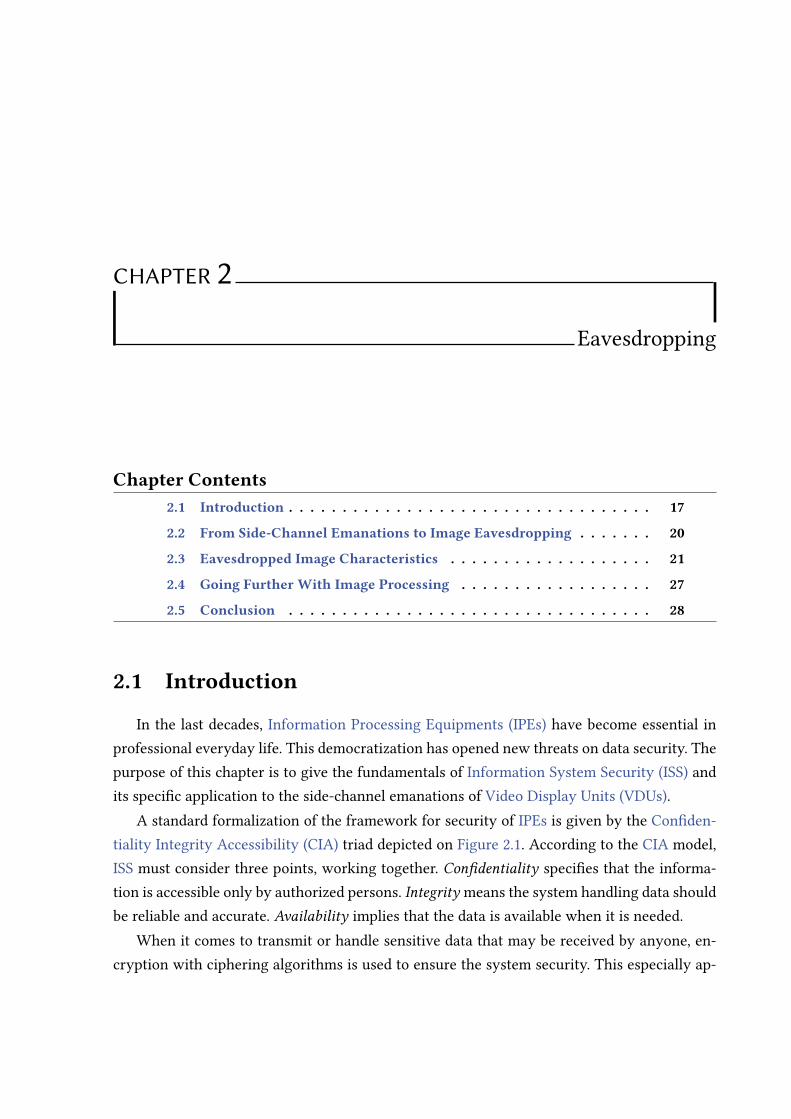
A standard formalization of the framework for security of IPEs is given by the Con�den-tiality Integrity Accessibility (CIA) triad depicted on Figure 2.1. According to the CIA model,ISS must consider three points, working together. Con�dentiality speci�es that the informa-tion is accessible only by authorized persons. Integrity means the system handling data shouldbe reliable and accurate. Availability implies that the data is available when it is needed.
When it comes to transmit or handle sensitive data that may be received by anyone, en-cryption with ciphering algorithms is used to ensure the system security. This especially ap-
Chapter 2 – Eavesdropping
Accessibility
Confidentiality
Integrity
Figure 2.1 – The three components of the CIA Triad represented as an Euler diagram: Con�-dentiality, Integrity, Accessibility. Electro Magnetic (EM) side-channels compromise con�den-tiality.
plies to wireless communications. Therefore, system or information can be considered as vul-nerable when any sensitive data (e.g. classi�ed data) is handled before encryption or afterdecryption. This is particularly the case when sensitive information is handled by the enduser on his device after decryption or before encryption.
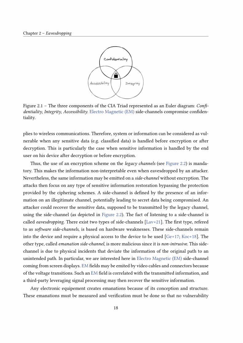
Thus, the use of an encryption scheme on the legacy channels (see Figure 2.2) is manda-tory. This makes the information non-interpretable even when eavesdropped by an attacker.Nevertheless, the same information may be emitted on a side-channel without encryption. Theattacks then focus on any type of sensitive information restoration bypassing the protectionprovided by the ciphering schemes. A side-channel is de�ned by the presence of an infor-mation on an illegitimate channel, potentially leading to secret data being compromised. Anattacker could recover the sensitive data, supposed to be transmitted by the legacy channel,using the side-channel (as depicted in Figure 2.2). The fact of listening to a side-channel iscalled eavesdropping. There exist two types of side-channels [Lav+21]. The �rst type, referedto as software side-channels, is based on hardware weaknesses. These side-channels remaininto the device and require a physical access to the device to be used [Ge+17; Koc+18]. Theother type, called emanation side-channel, is more malicious since it is non-intrusive. This side-channel is due to physical incidents that deviate the information of the original path to anunintended path. In particular, we are interested here in Electro Magnetic (EM) side-channelcoming from screen displays. EM �elds may be emited by video cables and connectors becauseof the voltage transitions. Such an EM �eld is correlated with the transmitted information, anda third-party leveraging signal processing may then recover the sensitive information.
Any electronic equipement creates emanations because of its conception and structure.These emanations must be measured and veri�cation must be done so that no vulnerability
18
2.1. Introduction
SideChannel
SensitiveData
LegacyChannel
IntendedReceiver
Eavesdropper
Figure 2.2 – An eavesdropper accesses sensitive data taking advantage of a side-channel.
leads to security failures. This is the area of the NACSIM report [Nat82]. In this report, theNSA de�nes TEMPEST and speci�es the terms of red and black signals 1. A red signal is anunencrypted signal that should be protected. For such a signal, protection measures shouldbe used such as shielding or physical distancing with wires to prevent coupling. Black signalon the other hand requires no e�ort. It is supposed not to carry compromising informationbecause of encryption that makes it unintelligible.
Countermeasures should be taken to prevent sensitive data to be intercepted using ema-nation side-channels. The most used countermeasure is shielding. In [Lav+21], Lavaud et al.detail a list of other countermeasures like changing the data-stream so that assumptions onsignal properties are not respected anymore, or the use of jamming [SA10] to hide leakages. Ifsuch measures are not used, the last resort is zoning. An air-gap should be respected to makethe interception theoretically impossible. That air gap is the minimal physical distance thatmakes impossible an external access to sensitive data using a side-channel. The fact of access-ing information from outside an organisation is called air gap bridging. The de�nition of theair gap relies on the technology used for eavesdropping. It should be chosen according to stateof the art interception methods.
The following of that chapter presents the keys that make eavesdropping images fromEM side-channels possible in Section 2.2. Section 2.3 details the speci�city of eavesdroppedimages that will be the major input data for the following of this thesis. Finally, in Section 2.4,perspectives on using image restoration to go further in the interpretation of eavesdroppedimages are presented.
1. See https://www.ssi.gouv.fr/uploads/IMG/pdf/II300_tempest_anssi.pdf
19
Chapter 2 – Eavesdropping
2.2 From Side-Channel Emanations to Image Eavesdrop-
ping
All electronic devices produce EM emanations that not only interfere with radio devicesbut also compromise the data handled by IPEs. A third party may perform a side-channelanalysis and recover the original information, hence compromising the system privacy. Thisthird-party obtaining access to potential sensitive data breaks the con�dentiality aspect ofthe CIA triad. Screens are especially sensitive since they display information, potentially red,to users. They are often the weakest link with signal being encrypted everywhere else in thetransmission pipeline. Sensitive data is exposed in a fully intelligible format and a side-channelconducted at that point could be compromising.
Pioneering work of the domain focused on Cathode Ray Tube (CRT) screens and ana-log signals. Van Eck et al. [Van85] published the �rst technical reports revealing how invol-untary emissions originating from the electronic of VDUs can be exploited to compromisedata. He mentioned that the video signal at that time does not contains synchronization in-formation required to time the beginning of an image in the 1D eavesdropped �ow. However,Van Eck proposes a simple electronic extension that �xes that synchronization issue, mak-ing the exploit easier and achievable for any electronic amateur. One would have though thetransition to digital video signals to solve the issue because of smaller voltage. However, stud-ies extend the eavesdropping exploit, using an EM side-channel attack, to digital signals andembedded circuits. Kuhn published on compromising emanations of Liquid Crystal Display(LCD) screens [Kuh13]. Other types of systems have been attacked. Vuagnoux et al. [VP09]extend the principle of EM side-channel attack to capture data from keyboards and, Hayashiet al. present interception methods based on Software-De�ned Radio (SDR) targeting laptops,tablets [Hay+14] and smartphones [Hay+17].
In the meantime, one should also note that the attacker’s pro�le is taking on a new dimen-sion with the increased performance of SDR [Mit]. With recent advances in radio equipment,an attacker can leverage advanced signal processing to further stretch the limits of the side-channel attacks using EM emanations [Gen+18]. The use of SDR increases the surface of attackfrom military organizations to hackers. It also opens up new post-processing opportunitiesthat improve attack characteristics. De Meulemeester et al. [De +18] leverage SDR to enhancethe performance of the attack and automatically �nd the structure of the captured data. By re-trieving the synchronization parameters of the targeted information system, the captured EM
20

2.3. Eavesdropped Image Characteristics
signal can be transformed from a vector to a raster image, reconstructing the 2-dimensionalsensitive visual information.
Recent works of De Meulesmeester [De 21] provide deep details on the eavesdroppingprocess. It focuses mainly on the received radio signal and proposes several techniques toenhance the quality of the attack [DSV20a] by signal processing algorithms. Today, the stateof the art research documents well the analysis of the EM spectrum to detect emanations. Thereconstruction of eavesdropped screens is also documented as well as techniques to enhancetheir quality such as averaging.
Meanwhile, advances in Machine Learning (ML) have opened the scope of automatedeavesdropped data interpretations. With the concomitant rise of powerful Graphics ProcessingUnits (GPUs) and deep neural networks, an attacker can extract patterns or even the full struc-tured content of the intercepted data with a high degree of con�dence and a limited executiontime. Previous work on the domain have mainly focused on processing the eavesdropped sig-nal using SDRs and Central Processing Units (CPUs). In this work, we mostly use image andGPU processing.
This thesis focuses on the interpretation of eavesdropped samples from an image process-ing point of view. We thus present brie�y the image formation pipeline and the key pointsthat lead to the corruptions we address. We redirect the reader to the recent thesis of PieterjanDe Meulesmeester [De 21] for deeper details on the eavesdropping process.
2.3 Eavesdropped Image Characteristics
Connectors and cables are the emission antennas that lead to side-channel emanations.They connect an IPE and its VDU which constitute the emission block, left part of Figure 2.4.The video signal is transmitted through cable using di�erent protocols like Video Graphics Ar-ray (VGA), High-De�nition Multimedia Interface (HDMI) or Digital Visual Interface (DVI). Thetransmitted signal is not encrypted. It respects the protocol de�ned by the standards [VES15].The voltage changes in the connector or cables generate EM emanations.
The reception block (right part of Figure 2.4) consists of a reception antenna, an SDR anda computer that hosts the signal processing required for the raster. The distance between thedefective element and the reception antenna is noted d. The SDR receives an analog signaland transforms it to digital. New SDR systems also enable implementing signal processing.The raster implemented in the host computer use di�erent processing to obtain and displayan intelligible images.
21
Chapter 2 – Eavesdropping
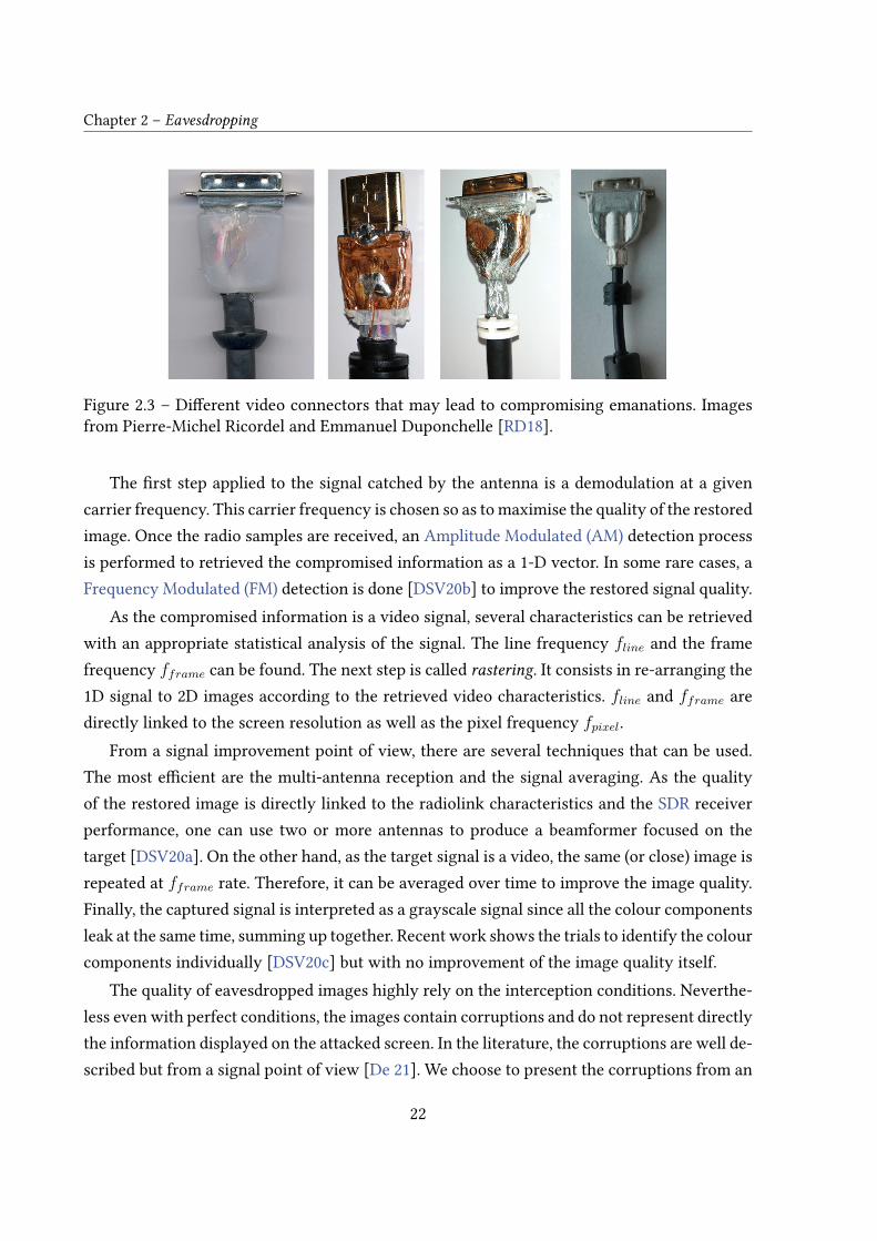
Figure 2.3 – Di�erent video connectors that may lead to compromising emanations. Imagesfrom Pierre-Michel Ricordel and Emmanuel Duponchelle [RD18].
The �rst step applied to the signal catched by the antenna is a demodulation at a givencarrier frequency. This carrier frequency is chosen so as to maximise the quality of the restoredimage. Once the radio samples are received, an Amplitude Modulated (AM) detection processis performed to retrieved the compromised information as a 1-D vector. In some rare cases, aFrequency Modulated (FM) detection is done [DSV20b] to improve the restored signal quality.
As the compromised information is a video signal, several characteristics can be retrievedwith an appropriate statistical analysis of the signal. The line frequency fline and the framefrequency fframe can be found. The next step is called rastering. It consists in re-arranging the1D signal to 2D images according to the retrieved video characteristics. fline and fframe aredirectly linked to the screen resolution as well as the pixel frequency fpixel.
From a signal improvement point of view, there are several techniques that can be used.The most e�cient are the multi-antenna reception and the signal averaging. As the qualityof the restored image is directly linked to the radiolink characteristics and the SDR receiverperformance, one can use two or more antennas to produce a beamformer focused on thetarget [DSV20a]. On the other hand, as the target signal is a video, the same (or close) image isrepeated at fframe rate. Therefore, it can be averaged over time to improve the image quality.Finally, the captured signal is interpreted as a grayscale signal since all the colour componentsleak at the same time, summing up together. Recent work shows the trials to identify the colourcomponents individually [DSV20c] but with no improvement of the image quality itself.
The quality of eavesdropped images highly rely on the interception conditions. Neverthe-less even with perfect conditions, the images contain corruptions and do not represent directlythe information displayed on the attacked screen. In the literature, the corruptions are well de-scribed but from a signal point of view [De 21]. We choose to present the corruptions from an
22

2.3. Eavesdropped Image Characteristics
2
14
RasterReception Antenna
Compromising EmanationsTarget
d
3
SDR
Figure 2.4 – Experimental setup: the attacked system includes an eavesdropped screen (1)displaying sensitive information. It is connected to an information system (2). An interceptionchain including an SDR receiver (3) sends samples to a host computer (4) that implementssignal processing.
Vertical Front Porch
Vertical Back Porch
Horiz
onta
l Fr
ont
Porch
Horiz
onta
l Ba
ck P
orch
Visible Screen
Eavesdropped Width
Eave
sdropped
Height
Figure 2.5 – Extra pixels are transmitted both vertically and horizontally and thus recontructedas data in eavesdropped images. Historically used to give time to CRT beam, the porch nowa-days may host sound or additionnal information.
image point of view as observed at the �nal step being the interpretation of images and theevaluation of the compromise.
2.3.1 Image Coding
Historically, the �rst video communication protocol was proposed for CRT displays usingthe raster scan principle. The raster scan consists in displaying the pixels on the screen oneafter the other from left to right and top to bottom using an the electron beam in the case ofCRTs. Due to that raster scan, protocols had to introduce extra pixels so that the beam hastime to go back to the beginning of the next line or to the beginning of the next image. Theseundisplayed pixels are added at the end of each line and at the end of each column. Next
23
Chapter 2 – Eavesdropping
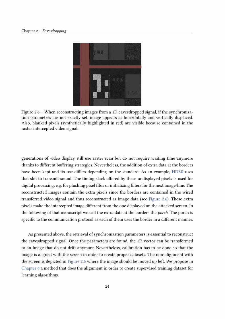
Figure 2.6 – When reconstructing images from a 1D eavesdropped signal, if the synchroniza-tion parameters are not exactly set, image appears as horizontally and vertically displaced.Also, blanked pixels (synthetically highlighted in red) are visible because contained in theraster intercepted video signal.
generations of video display still use raster scan but do not require waiting time anymorethanks to di�erent bu�ering strategies. Nevertheless, the addition of extra data at the bordershave been kept and its use di�ers depending on the standard. As an example, HDMI usesthat slot to transmit sound. The timing slack o�ered by these undisplayed pixels is used fordigital processing, e.g. for plushing pixel �fos or initializing �lters for the next image/line. Thereconstructed images contain the extra pixels since the borders are contained in the wiredtransferred video signal and thus reconstructed as image data (see Figure 2.6). These extrapixels make the intercepted image di�erent from the one displayed on the attacked screen. Inthe following of that manuscript we call the extra data at the borders the porch. The porch isspeci�c to the communication protocol as each of them uses the border in a di�erent manner.
As presented above, the retrieval of synchronization parameters is essential to reconstructthe eavesdropped signal. Once the parameters are found, the 1D vector can be transformedto an image that do not drift anymore. Nevertheless, calibration has to be done so that theimage is aligned with the screen in order to create proper datasets. The non-alignment withthe screen is depicted in Figure 2.6 where the image should be moved up left. We propose inChapter 6 a method that does the alignment in order to create supervised training dataset forlearning algorithms.
24
2.3. Eavesdropped Image Characteristics
ADC DigitalSamples
Analysis Bandwith and Aliasing
Thermal + Quantization Noise
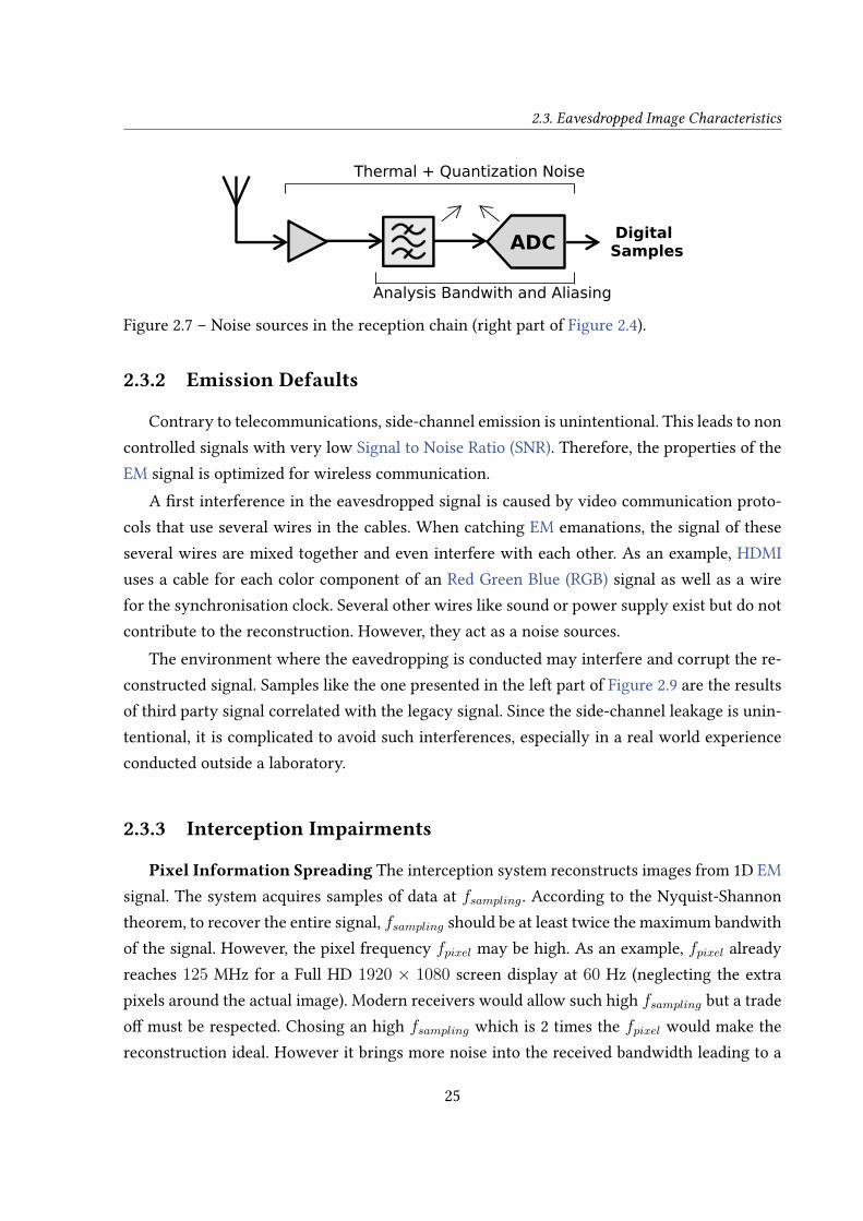
Figure 2.7 – Noise sources in the reception chain (right part of Figure 2.4).
2.3.2 Emission Defaults
Contrary to telecommunications, side-channel emission is unintentional. This leads to noncontrolled signals with very low Signal to Noise Ratio (SNR). Therefore, the properties of theEM signal is optimized for wireless communication.
A �rst interference in the eavesdropped signal is caused by video communication proto-cols that use several wires in the cables. When catching EM emanations, the signal of theseseveral wires are mixed together and even interfere with each other. As an example, HDMIuses a cable for each color component of an Red Green Blue (RGB) signal as well as a wirefor the synchronisation clock. Several other wires like sound or power supply exist but do notcontribute to the reconstruction. However, they act as a noise sources.
The environment where the eavedropping is conducted may interfere and corrupt the re-constructed signal. Samples like the one presented in the left part of Figure 2.9 are the resultsof third party signal correlated with the legacy signal. Since the side-channel leakage is unin-tentional, it is complicated to avoid such interferences, especially in a real world experienceconducted outside a laboratory.
2.3.3 Interception Impairments
Pixel Information Spreading The interception system reconstructs images from 1D EMsignal. The system acquires samples of data at fsampling. According to the Nyquist-Shannontheorem, to recover the entire signal, fsampling should be at least twice the maximum bandwithof the signal. However, the pixel frequency fpixel may be high. As an example, fpixel alreadyreaches 125 MHz for a Full HD 1920 × 1080 screen display at 60 Hz (neglecting the extrapixels around the actual image). Modern receivers would allow such high fsampling but a tradeo� must be respected. Chosing an high fsampling which is 2 times the fpixel would make thereconstruction ideal. However it brings more noise into the received bandwidth leading to a
25
Chapter 2 – Eavesdropping
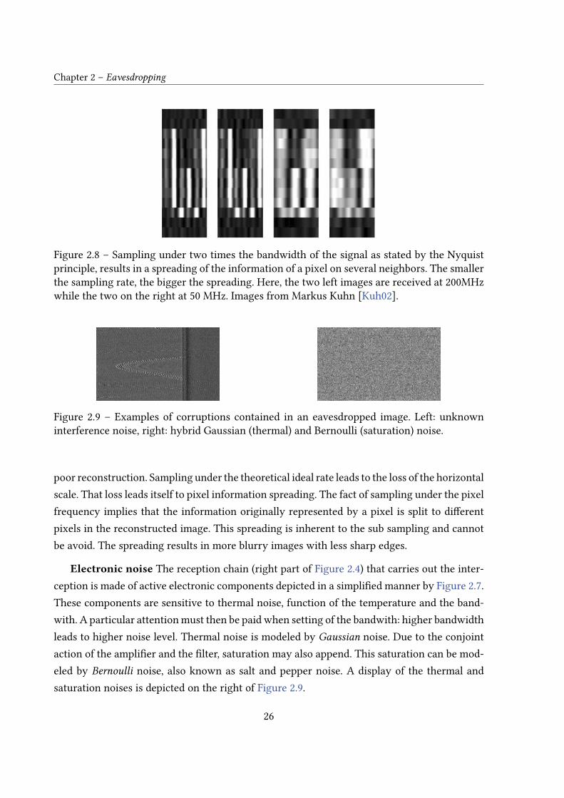
Figure 2.8 – Sampling under two times the bandwidth of the signal as stated by the Nyquistprinciple, results in a spreading of the information of a pixel on several neighbors. The smallerthe sampling rate, the bigger the spreading. Here, the two left images are received at 200MHzwhile the two on the right at 50 MHz. Images from Markus Kuhn [Kuh02].
Figure 2.9 – Examples of corruptions contained in an eavesdropped image. Left: unknowninterference noise, right: hybrid Gaussian (thermal) and Bernoulli (saturation) noise.
poor reconstruction. Sampling under the theoretical ideal rate leads to the loss of the horizontalscale. That loss leads itself to pixel information spreading. The fact of sampling under the pixelfrequency implies that the information originally represented by a pixel is split to di�erentpixels in the reconstructed image. This spreading is inherent to the sub sampling and cannotbe avoid. The spreading results in more blurry images with less sharp edges.
Electronic noise The reception chain (right part of Figure 2.4) that carries out the inter-ception is made of active electronic components depicted in a simpli�ed manner by Figure 2.7.These components are sensitive to thermal noise, function of the temperature and the band-with. A particular attention must then be paid when setting of the bandwith: higher bandwidthleads to higher noise level. Thermal noise is modeled by Gaussian noise. Due to the conjointaction of the ampli�er and the �lter, saturation may also append. This saturation can be mod-eled by Bernoulli noise, also known as salt and pepper noise. A display of the thermal andsaturation noises is depicted on the right of Figure 2.9.
26
2.4. Going Further With Image Processing
(a) (b)
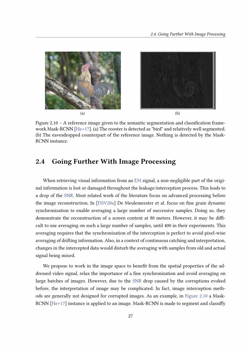
Figure 2.10 – A reference image given to the semantic segmentation and classi�cation frame-work Mask-RCNN [He+17]. (a) The rooster is detected as "bird" and relatively well segmented.(b) The eavesdropped counterpart of the reference image. Nothing is detected by the Mask-RCNN instance.
2.4 Going Further With Image Processing
When retrieving visual information from an EM signal, a non-negligible part of the origi-nal information is lost or damaged throughout the leakage/interception process. This leads toa drop of the SNR. Most related work of the literature focus on advanced processing beforethe image reconstruction. In [DSV20a] De Meulemeester et al. focus on �ne grain dynamicsynchronization to enable averaging a large number of successive samples. Doing so, theydemonstrate the reconstruction of a screen content at 80 meters. However, it may be di�-cult to use averaging on such a large number of samples, until 400 in their experiments. Thisaveraging requires that the synchronization of the interception is perfect to avoid pixel-wiseaveraging of drifting information. Also, in a context of continuous catching and interpretation,changes in the intercepted data would disturb the averaging with samples from old and actualsignal being mixed.
We propose to work in the image space to bene�t from the spatial properties of the ad-dressed video signal, relax the importance of a �ne synchronization and avoid averaging onlarge batches of images. However, due to the SNR drop caused by the corruptions evokedbefore, the interpretation of image may be complicated. In fact, image interception meth-ods are generally not designed for corrupted images. As an example, in Figure 2.10 a Mask-RCNN [He+17] instance is applied to an image. Mask-RCNN is made to segment and classi�y
27
Chapter 2 – Eavesdropping
natural images. The algorithm succeeds in �nding and segmenting the rooster. The image isthen eavesdropped, which results in nothing being detected anymore by the same algorithm.
The di�erent corruption sources presented before make the addressed problem a hybriddistortion The term hybrid distortion was introduced by Li et al. in [Li+20b]. The corruptionscontained in their work are less aggressive than those generated by eavesdropping. This un-modeled hybrid distortion breaks the semantic priors usually leveraged by state of the artlearning based algorithms to restore natural images.
Examples of useful features when reconstructing images are gradient, edges or �at re-gions. We propose to use �rst order 2D Haar Discrete Wavelet Transform (DWT) [Dau88]as a tool [Guo+17] to highlight the consequences of the hybrid distortion generated by theeavedropping process. This transform decomposes an original image into four sub-bands thatcapture the average, vertical, horizontal and diagonal frequencies. In a 2D signal, the frequencyrepresents the intensity changes, i.e. the gradients. On Figure 2.11, a DWT is applied to an im-age (a) and its intercepted counterpart (b). On both (a) and (b), top-left image is a downscaledversion of the image to transform obtained by a 2× sum-pooling. Bottom-left and top-rightimages relate to horizontal and vertical gradients, respectively. Finally, bottom-right quar-ters relate to diagonal gradients. When observing the �gures, it can be observed of (b) thatthe transforms, contrary to (a), does not visually contain much information. This observationshows that the interception process "breaks" gradients of images.
There are two majors motivations in leveraging image processing to go further in theinterpretation of intercepted images. First, interpretation of eavesdropped samples is oftendone by human operators. Automation of the interpretation would enable auditing systemscontinuously. A second motivation is to go further by enhancing the images before relying onhuman interpretation.
2.5 Conclusion
EM compromising emanations are a major issue when handling sensitive data on IPEs.An attacker can for example retrieve whole or part of a video signal transmitted between anIPE and its display. This is a threat to con�dentiality. The images reconstructed from 1D EMcompromising emanations are highly corrupted. The corruptions are diverse and come fromdi�erent origins. The mis-synchronization of the interception system results in non-alignedeavesdropped and original images. The distance between the emissions and the antenna aswell as the hardware defects result in a strong hybrid noising. These corruptions, due to the
28

2.5. Conclusion
(a)
(b)
Figure 2.11 – (a) Haar DWT applied to the reference image of Figure 2.10a. The edges ofthe rooster and the trunk are visible. (b) The transformed of the eavesdropped image of Fig-ure 2.10b. The interception process has broken the vertical gradients. horizontal gradients stillexist but are not as sharp as in the original image.
29
Chapter 2 – Eavesdropping
eavesdropping process itself, complicate the interpretation of eavesdropped images. Two maindirections appear that motivate work on removing corruptions. First, better samples wouldenable better automation of the interpretation. Indeed, standard methods developed for imageinterpretation are designed for non-corrupted images.
Second, enhance the image quality would enable human interpretation of images withmore challenging eavesdropping conditions. In particular, with a high-performance restora-tion of eavesdropped samples, at constant quality, the interception distance could be extended.
Next chapter covers state of the art for noisy image interpretation and particularly methodsfor image restoration.
30
CHAPTER 3
Noisy Image Interpretation
Chapter Contents3.1 Introduction . . . . . . . . . . . . . . . . . . . . . . . . . . . . . . . . . . 31
3.2 What does it mean for an image to be noisy? . . . . . . . . . . . . . . 32
3.3 Overview of Image Restoration Methods . . . . . . . . . . . . . . . . . 35
3.4 Overview of Image Interpretation Methods . . . . . . . . . . . . . . . 39
3.5 Error Measurement and Quality Assessment . . . . . . . . . . . . . . . 42
3.6 Datasets for Learning and Evaluation . . . . . . . . . . . . . . . . . . . 46
3.7 Learning Algorithms: Terminology, Strengths and Open Issues . . . 47
3.8 Conclusion . . . . . . . . . . . . . . . . . . . . . . . . . . . . . . . . . . 52
3.1 Introduction
Images retrieved from Electro Magnetic (EM) side-channel interception are highly cor-rupted. A �rst lever to obtain better samples could be to enhance the interception process.However, the interception process is highly dependent on its surrounding environment. Theseenvironmental conditions impose an upper bound to the interception quality and control. Incontrast, a second lever consists in leveraging image processing to improve image denoisingand interpretability. This solution acts after the image construction instead of during the in-terception process. With the recent progress in Machine Learning (ML), one can wonder if itis worth making the e�ort on improving the interception or if e�orts shall be put on improv-

Chapter 3 – Noisy Image Interpretation
Figure 3.1 – Given a noisy image, depending on the �nal aim, di�erent processing may beapplied.
ing signal interpretation. Our work consists in studying the opportunities of post-interceptionimage processing to better interpret eavesdropped images.
Two directions emerge when planning to go further using image processing and ML (seeFigure 3.1). First, a direction consists in directly interpreting the noisy samples. Interpretingthe images using an automated system pushes further the limits of side-channel attacks mak-ing it possible to monitor continuously intercepted emanations. From a protection scenarioperspective, mining information from eavesdropped samples opens for assessing how compro-mising is an emanation, therefore, critical for sensitive information. Then, a second directionis to restore the eavesdropped samples. Restoring samples is a �rst automated step preparinghuman interpretation. That is, it becomes possible as an example to read samples interceptedin worse conditions, i.e. longer distance, noisier environment. These two directions are nonexclusive. As an example it can be interesting to leverage image restoration to enhance resultsof interpretation.
This chapter �rst describes what a noisy image is in Section 3.2. Section 3.3 presents thestate of the art in noisy image restoration methods. Section 3.4 reviews image interpretationmethods. Popular metrics to assess restoration and interpretation methods for images are pre-sented in Section 3.5. Section 3.6 describes popular datasets used for image restoration andinterpretation problems. Section 3.7 introduces terminology and questions the strenghts andweakness of learning algorithms.
3.2 What does it mean for an image to be noisy?
We de�ne an image to be a 3-dimensional array of pixels. An image I has dimensions[C,H,W ] ∈ Z+, where C is the number of channels, H the height and W the width. In thismanuscript, we consider channel numbers of C = 1 for grayscale images and C = 3 for RedGreen Blue (RGB) images. Images are classi�ed by their content and many classes of image
32

3.2. What does it mean for an image to be noisy?
may be de�ned, we consider here natural and synthetic images. Natural images are issued fromphotographs that represent a given scene, that may contain people, animals, landscapes, etc. Inthe context of this thesis, synthetic images are textual contents displayed on screens. Naturaland synthetic images have di�erent properties [TO03]. Natural images are more diverse interms of shapes and textures. They most often content more smooth intensity transition whensynthetic images are more sharp.
An image is said to be noisy when an unwanted signal exists jointly with the originalexpected content. We only consider in this manuscript corruptions that keep the dimension ofthe original image and are applied pixel-wise. As an example, we do not consider corruptionsthat result in a translation between noise free and noisy samples. There exist plenty of noisesources. The multiple factors of the hybrid noise generated by the eavedropping process is aperfect example of the numerous noise sources that exist. We present in the following severalwell-known noise models and real-world noises that appear in real applications.
3.2.1 Standard Noise Types
When facing an image restoration problem with pixel-wise corruption, a designer �rst triesto de�ne a statistic model for the corruptions she/he tries to remove. There are well-knowndistributions in the literature to model noise such as the 5 following ones:• Additive White Gaussian Noise (AWGN) is denoted N (σg) and applied following pn =po + N (σg), where pn and p0 are the noisy and original pixel values, respectively. σg
is the standard deviation of the Gaussian distribution. We use only centered AWGN. Inother words, the mean of the distribution is 0.• Speckle noise is denoted S(σs) and applied following pn = po +N (σg) × po. σs is the
standard deviation of the Gaussian distributed multiplicative factor applied to po.• Uniform noise is denoted U(s) and applied following pn = po + U(s). The additive
corruption value is uniformly drew out of the range [−s, s], i.i.d. for each pixel.• Poisson noise, notedP , has no parameter and is applied following pn = P(po). The cor-
ruption for a pixel is de�ned following a Poisson distribution depending on the originalvalue.• Bernoulli noise, notedB(p), is an impulse noise. A pixel as probability p to be corrupted.
When corrupted, the pixel is set to either 0 (min) or 255 (max) with equal probability.The most used distribution is the AWGN as it �ts many case studies and its properties are
well studied. Nonetheless, some real-world corruptions, such as the ones we are interested in,do not match any of these well-behaved noise models.
33

Chapter 3 – Noisy Image Interpretation
(a) (b)
Figure 3.2 – Example of an image (a) and its Moire corrupted version (b).
3.2.2 Towards Real-World Noise Distributions
The well-behaved noises exposed in Section 3.2.1 were theorized following observation ofreal phenomena. We refer to these noise distributions as primary distributions. Primary noiseshave statistics distributions ruled by a known degree of freedom. However, most corruptionsare more complicated and do not follow primary distributions. These corruptions have anunknown degree of freedom.
For some real-world image corruptions, the noising process is known or can be esti-mated [ALB18]. While being estimated, the noising process may not be e�ciently modeledas a primary distribution or composition of primary distributions. Moire [Yua+20] is such acorruption. Moire is a sensing artifact that appears when the color array �lter of a sensorinterferes with high frequency patterns (see Figure 3.2). The most known Moire case is thephotography of Liquid Crystal Display (LCD), Light-Emitting Diode (LED) or screens usingequivalent technologies.
On the other hand, some corruptions can be modeled by composing primary noises. Com-posed noises, are more application speci�c than primary noises, but their existence constitutesan identi�ed and important issue. Many distributions of real-world noises can be approachedusing noise compositions, also called mixtures [Zha+14]. Restoration of noise mixture cor-rupted images has been less addressed in the literature than that for primary noise. Further-more, we show in Chapter 4 that the restoration methods designed for primary noises do notdirectly transfer to mixture noises.
In the literature, experimental noise mixtures are all created from the same few primarynoises presented earlier. When modeling experimental noises, noise mixtures are either spa-
34

3.3. Overview of Image Restoration Methods
tially or sequentially composed. In a spatially composed noise mixture [CPM19; BR19], eachpixel p of an image x is corrupted by a speci�c distribution η(p). A typical example of a spa-tially composed mixture noise is made of 10% of uniform noise [−s, s], 20% of Gaussian noiseN (0, σ0) and 70% of Gaussian noise N (0, σ1), where the percentages refer to the amount ofpixels, in the image, corrupted by the given noise. This type of spatial mixture noise has beenused in the experiments of GAN-CNN based Blind Denoiser (GCBD) [Che+18] and Generated-Arti�cial-Noise to Generated-Arti�cial-Noise (G2G) [CPM19] with s = {15, 25, 30, 50}, σ0 ={0.01, 15} and σ1 = {1, 25}. Real photograph noise [PR17; Abd+20] is for instance a compo-sition of primary noises [Gow+07], generated by image sensor defects.
The mixture noise can also be sequentially composed as the result of applying n primarynoises with distributions ηi, i ∈ {0..n − 1} to each pixel p of the image x. An example ofa sequential mixture noise is the one used to test the recent Noise2Self method [BR19]. It iscomposed of a combination of Poisson noise, Gaussian noise with σ = 80, and Bernoulli noisewith p = 0.2.
Despite being designed following real world scenarios, mixtures noises are also used inorder to challenge the interpretation methods. Because of the plural noise sources evoked inSection 2.3, we hypothetize that the eavesdropping corruption is a mixture made of severalprimary noises. This is the assumption made in Chapter 5.
3.3 Overview of Image Restoration Methods
Corruptions are inherent to the entire lifespan of an image, from their acquisition to theirdestination being a human looking at it or a machine interpreting its content. From the begin-ning of the pipeline with the image sensing being possibly a�ected by sensor defects and pooracquisition conditions, the image undergoes corruptions. To be transmitted easily, an imageis often lossy compressed. The transmission itself is a corruption source with potential frag-ments of the signal being lost. Image restoration, as a subset of signal processing, addressesthese issues.
Image restoration is the task of estimating the original signal content of an image froma corrupted observed version. Di�erent research areas exist within the image restoration do-main. Among them, denoising [Tia+20], deblurring [WCH20] and super-resolution [Ha+19] arethe most popular. In the recent literature most solutions propose experiments on di�erentrestoration problems. As examples, the authors of [MSY16] experiment their proposal on im-age denoising and super-resolution, when the authors of [Liu+18] add JPEG deblocking to
35

Chapter 3 – Noisy Image Interpretation
these two latters tasks. In the following of this document, for simpli�cation, we refer to theserestoration techniques as denoising methods.
Image denoising is an extensively studied problem [BCM05] though not yet a solvedone [CM10]. The objective of a denoiser is to generate a denoised image x̂ from an observationy considered to be a noisy or corrupted version of an original clean image x. y is generatedby an often unknown noise function h such that y = h(x) (as depicted in Figure 3.3). Mostmethods take into account the phenomena leading to the corruption while others completelyabstract it to extend their applicability. A vast collection of noise models exists [BJ15] to rep-resent h. Examples of frequently used models are described in Section 3.2.1. While denoisersare constantly progressing in terms of noise elimination level [Dab+07; Zha+17; Liu+18], mostof the published techniques are tailored to a given primary noise distribution (i.e. respectinga known distribution). These methods exploit probabilistic properties of the noise they arespecialised for, to distinguish noise from signal of interest.
y
xԐh
DNoisy Denoised
Reference
x̂
Figure 3.3 – Principle of a denoising algorithm. A noisy image y is given to a denoiser D thatoutputs an according denoised image x̂. Depending on the noising process h, the referenceimage x is available or not. If x is available, the denoising quality ε can be measured (see Sec-tion 3.5).
3.3.1 Expert-Based Algorithms
We denote by expert-based the methods designed by experts, by opposition to learned so-lutions that are drawn from data. All these methods rely on assumptions about the underlyingtrue signal that we want to retrieve using denoising. Expert-based denoising methods are tradi-tionally divided into transform-domain and spatial-domain methods. Spatial-domain methodsoperate directly on the pixel intensities of the images. On the contrary, transform-domainmethods rearrange the values to coe�cients using di�erent operations that de�ne the trans-form. That split is also relevant for trained methods. Some of them use transform domain for
36
3.3. Overview of Image Restoration Methods
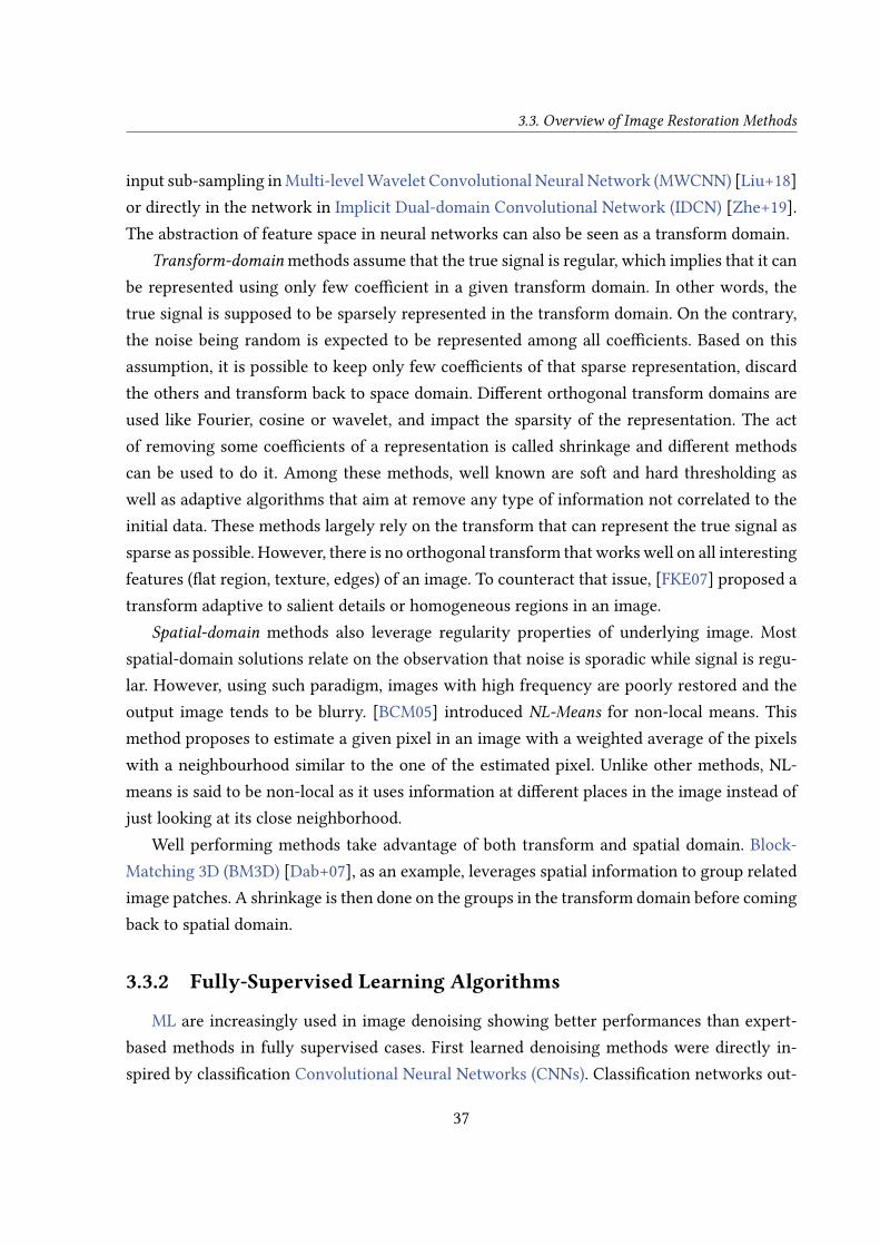
input sub-sampling in Multi-level Wavelet Convolutional Neural Network (MWCNN) [Liu+18]or directly in the network in Implicit Dual-domain Convolutional Network (IDCN) [Zhe+19].The abstraction of feature space in neural networks can also be seen as a transform domain.
Transform-domain methods assume that the true signal is regular, which implies that it canbe represented using only few coe�cient in a given transform domain. In other words, thetrue signal is supposed to be sparsely represented in the transform domain. On the contrary,the noise being random is expected to be represented among all coe�cients. Based on thisassumption, it is possible to keep only few coe�cients of that sparse representation, discardthe others and transform back to space domain. Di�erent orthogonal transform domains areused like Fourier, cosine or wavelet, and impact the sparsity of the representation. The actof removing some coe�cients of a representation is called shrinkage and di�erent methodscan be used to do it. Among these methods, well known are soft and hard thresholding aswell as adaptive algorithms that aim at remove any type of information not correlated to theinitial data. These methods largely rely on the transform that can represent the true signal assparse as possible. However, there is no orthogonal transform that works well on all interestingfeatures (�at region, texture, edges) of an image. To counteract that issue, [FKE07] proposed atransform adaptive to salient details or homogeneous regions in an image.
Spatial-domain methods also leverage regularity properties of underlying image. Mostspatial-domain solutions relate on the observation that noise is sporadic while signal is regu-lar. However, using such paradigm, images with high frequency are poorly restored and theoutput image tends to be blurry. [BCM05] introduced NL-Means for non-local means. Thismethod proposes to estimate a given pixel in an image with a weighted average of the pixelswith a neighbourhood similar to the one of the estimated pixel. Unlike other methods, NL-means is said to be non-local as it uses information at di�erent places in the image instead ofjust looking at its close neighborhood.
Well performing methods take advantage of both transform and spatial domain. Block-Matching 3D (BM3D) [Dab+07], as an example, leverages spatial information to group relatedimage patches. A shrinkage is then done on the groups in the transform domain before comingback to spatial domain.
3.3.2 Fully-Supervised Learning Algorithms
ML are increasingly used in image denoising showing better performances than expert-based methods in fully supervised cases. First learned denoising methods were directly in-spired by classi�cation Convolutional Neural Networks (CNNs). Classi�cation networks out-
37

Chapter 3 – Noisy Image Interpretation
put a prediction vector that gives in �ne an information on the content of the image. In contrastauthors of [JS09] were the �rst to propose to output an entire image given an input image.
First trained denoising methods were fully supervised, the mapping between a noisy do-main and a denoised domain was learned using back-propagation. In other words, the mappingwas learned using associated pairs of clean and noisy images. The di�erence between learnedmethods mainly lies in the architecture of the neural network that e�ectively represent themapping between the domains. While some methods were proposed to automate the design ofnetwork architecture [SOO18], this task is today mainly done empirically by expert engineers.
Following the premises of CNN based denoisers [JS09], di�erent strategies have been pro-posed such as residual learning in Denoising Convolutional Neural Network (DnCNN) [Zha+17],skip connections in Residual Encoder-Decoder Network (RED) [MSY16] or self-guidance inSelf-Guided Network (SGN) [Gu+19]. Learned methods also take inspiration from the exper-tise gained in image processing before the rise of ML. Transform domain is used in [Liu+18]where the authors consider di�erent wavelet decomposition to be used as sub and up-samplingoperator in a multi-resolution architecture. [Zhe+19] proposes to use a dual-domain architec-ture that leverages complementary of spatial and transform domain corrections directly intoresidual branches. Some methods even introduce learnable parameters directly into expertmethods like in BM3D-Net [YS18].
The weakness of discriminative denoisers is their need of large databases of independentnoise realisations, including clean reference images, to learn e�ciently the denoising task. Toovercome this limitation, di�erent weakly supervised denoisers have been proposed.
3.3.3 Weakly Supervised Algorithms
Weakly supervised methods apply when it is not possible to build a complete trainingdataset with clean references. In particular, blind denoisers are capable of e�ciently denois-ing images with noise distributions not available in the training set. First studies on blinddenoising have aimed at determining the level of a known noise so as to apply an adaptedhuman-expert based denoising. Most of the recent blind denoisers focus instead on trainingexclusively on noisy data. In [SSR11], authors propose a noise level estimation method in-tegrated to a deblurring method. Inspired from the latter proposal, the authors of [LTO13]propose to estimate the standard deviation of a Gaussian distribution corrupting an image toapply the accordingly con�gured BM3D �ltering [Dab+07].
Some recent studies aim at modelling the noise distribution corrupting an image with aGenerative Adversarial Networks (GAN)-based model. Once the noise distribution is modelled,
38

3.4. Overview of Image Interpretation Methods
it is possible to generate independent noise realisations and train a dedicated discriminativedenoiser. GCBD [Che+18] and G2G [CPM19] are examples of such denoisers.
Noise2Noise (N2N) [Leh+18] has pioneered learning-based blind denoising. Authors showthat it is possible to learn a discriminative denoiser from only a pair of images representing twoindependent realisations of the noise to be removed. Noise2Void (N2V) [KBJ19] and Noise2Self(N2S) [BR19] are recent strategies that train a denoiser from only the image to be denoised.
[UVL20] goes a step further in the non supervision and shows that the knowledge broughtby the engineering of network architecture is itself an image prior capable of denoising. Usingthis strategy, the authors with their method named Deep Image Prior (DIP) learn to denoise agiven image using only a random initialized denoiser and the image itself.
Recently, a new family of learning algorithms called transformers is getting more and moreinterest from the community. These transformers mainly rely on internal attention mecha-nisms between patches of an image i.e. on self-contextual information. Transformers were �rstproposed for Natural Language Processing (NLP) [Vas+17] and adapted to image recognitiontasks [Dos+20]. Image restoration counterparts were quickly proposed in [Che+20] with theImage Processing Transformer (IPT). While the �rst proposed methods are really data-greedy,recent publication proposes �ne-tuning strategies to limit the need for large datasets [Tou+21].
3.4 Overview of Image Interpretation Methods
Image restoration is the entry point when working with noisy input images. If the imagesare interpreted by a human operator, the automated process can be stopped. However, in somecase it is useful to automate interpretation. As an example, when auditing a system, it could beuseful to monitor permanently the emanations of an Information Processing Equipment (IPE)to ensure that it does not leak compromising data.
Interpretation automation is one of the major concern of Computer Vision (CV). Intelligentalgorithms are used to assist human operators or to fully automate the decision making pro-cess. Image interpretation groups all the tasks, that given an image return knowledge on itscontent. Among these tasks, well-known ones are classi�cation, segmentation [RFB15; Min+20]or pose estimation [CTH20].
The objective of a classi�cation algorithm is to identify to which of a set of classes a newsample belongs. Most classi�cation framework are made of two steps. First a step named fea-ture extraction is responsible for transforming the input data to a space that separates better thesamples of di�erent classes. Well known expert-based feature extractors/detectors are Scale
39

Chapter 3 – Noisy Image Interpretation
Paper Name/Acronym Adressed Corruptions(s)
Expe
rt [BCM05] NL-Means AWGN[FKE07] Pointwise SA-DCT AWGN, JPEG Compression[Dab+07] BM3D AWGN
Fully
Supe
rvise
d
[JS09] - AWGN[SSR11] - AWGN, Blur[LTO13] - AWGN[MSY16] RED AWGN, Super-Resolution[Zha+17] DnCNN AWGN, JPEG Compression, Super-Resolution[YS18] BM3D-Net AWGN[Liu+18] MWCNN AWGN, Super-Resolution[Che+18] GCBD AWGN, Spatial Mixture Noise, Sensor Noise[Gu+19] SGN AWGN, Sensor Noise[Zhe+19] IDCN JPEG Compression[CPM19] G2G AWGN, Spatial Mixture Noise
Wea
kly
Supe
rvise
d [Leh+18] N2N AWGN, Bernoulli, Poisson, Text Removal, ..[KBJ19] N2V AWGN, Microscopy Noise[BR19] N2S Mixture Noise, Sensor noise[UVL20] DIP AWGN, Super-Resolution, Inpainting[Che+20] IPT AWGN, Super-Resolution, Rain Strikes
Table 3.1 – Image restoration methods evoked in Section 3.3 and their targeted noise(s).
40
3.4. Overview of Image Interpretation Methods
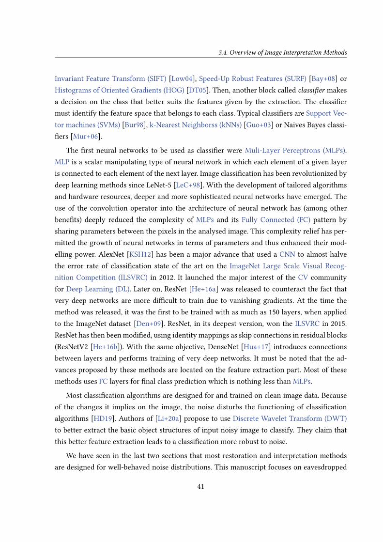
Invariant Feature Transform (SIFT) [Low04], Speed-Up Robust Features (SURF) [Bay+08] orHistograms of Oriented Gradients (HOG) [DT05]. Then, another block called classi�er makesa decision on the class that better suits the features given by the extraction. The classi�ermust identify the feature space that belongs to each class. Typical classi�ers are Support Vec-tor machines (SVMs) [Bur98], k-Nearest Neighborss (kNNs) [Guo+03] or Naives Bayes classi-�ers [Mur+06].
The �rst neural networks to be used as classi�er were Muli-Layer Perceptrons (MLPs).MLP is a scalar manipulating type of neural network in which each element of a given layeris connected to each element of the next layer. Image classi�cation has been revolutionized bydeep learning methods since LeNet-5 [LeC+98]. With the development of tailored algorithmsand hardware resources, deeper and more sophisticated neural networks have emerged. Theuse of the convolution operator into the architecture of neural network has (among otherbene�ts) deeply reduced the complexity of MLPs and its Fully Connected (FC) pattern bysharing parameters between the pixels in the analysed image. This complexity relief has per-mitted the growth of neural networks in terms of parameters and thus enhanced their mod-elling power. AlexNet [KSH12] has been a major advance that used a CNN to almost halvethe error rate of classi�cation state of the art on the ImageNet Large Scale Visual Recog-nition Competition (ILSVRC) in 2012. It launched the major interest of the CV communityfor Deep Learning (DL). Later on, ResNet [He+16a] was released to counteract the fact thatvery deep networks are more di�cult to train due to vanishing gradients. At the time themethod was released, it was the �rst to be trained with as much as 150 layers, when appliedto the ImageNet dataset [Den+09]. ResNet, in its deepest version, won the ILSVRC in 2015.ResNet has then been modi�ed, using identity mappings as skip connections in residual blocks(ResNetV2 [He+16b]). With the same objective, DenseNet [Hua+17] introduces connectionsbetween layers and performs training of very deep networks. It must be noted that the ad-vances proposed by these methods are located on the feature extraction part. Most of thesemethods uses FC layers for �nal class prediction which is nothing less than MLPs.
Most classi�cation algorithms are designed for and trained on clean image data. Becauseof the changes it implies on the image, the noise disturbs the functioning of classi�cationalgorithms [HD19]. Authors of [Li+20a] propose to use Discrete Wavelet Transform (DWT)to better extract the basic object structures of input noisy image to classify. They claim thatthis better feature extraction leads to a classi�cation more robust to noise.
We have seen in the last two sections that most restoration and interpretation methodsare designed for well-behaved noise distributions. This manuscript focuses on eavesdropped
41
Chapter 3 – Noisy Image Interpretation
images that do not follow such distributions. Adaptations of state of the art methods as wellas new strategies are then required and will be proposed in the following of this document.
3.5 Error Measurement and Quality Assessment
In image processing, error measurement is a full research area and a major concern. Eval-uating the quality of images is required to assess the e�ciency of any given method. In ML,error measurement is used not only for e�ciency evaluation but also to drive optimisationprocesses. In fact, algorithms based on gradient descent optimisation select parameters valuesby minimizing errors between intended result and obtained result. In the following, we dif-ferentiate between methods used for quality assessment and methods for classi�cation errormeasurement.
3.5.1 Image Quality Metrics
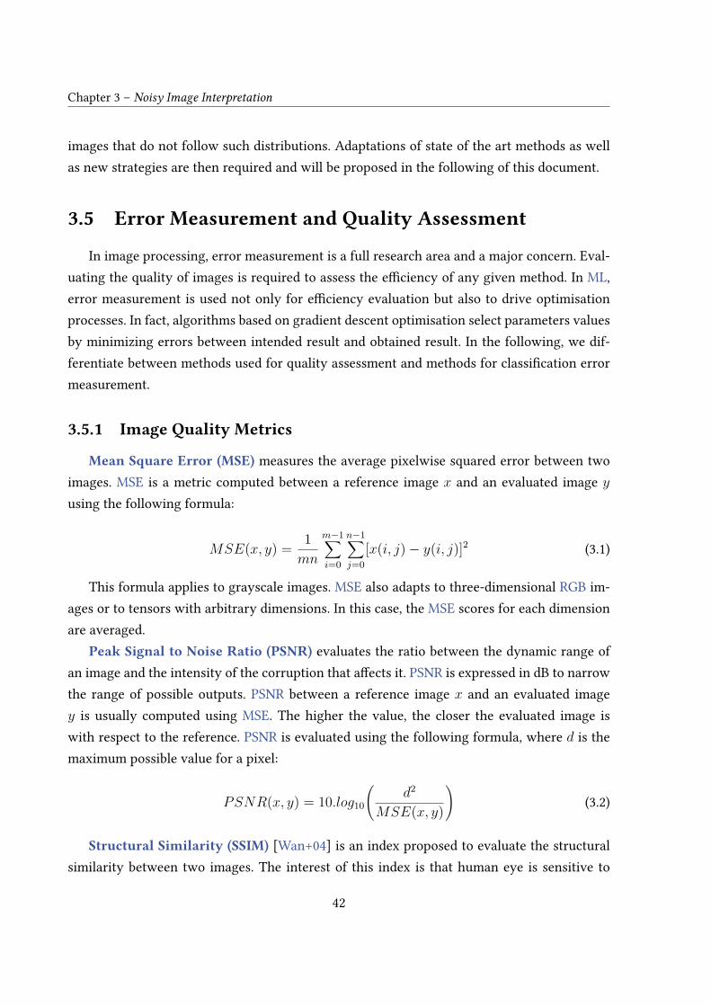
Mean Square Error (MSE) measures the average pixelwise squared error between twoimages. MSE is a metric computed between a reference image x and an evaluated image yusing the following formula:
MSE(x, y) = 1mn
m−1∑i=0
n−1∑j=0
[x(i, j)− y(i, j)]2 (3.1)
This formula applies to grayscale images. MSE also adapts to three-dimensional RGB im-ages or to tensors with arbitrary dimensions. In this case, the MSE scores for each dimensionare averaged.
Peak Signal to Noise Ratio (PSNR) evaluates the ratio between the dynamic range ofan image and the intensity of the corruption that a�ects it. PSNR is expressed in dB to narrowthe range of possible outputs. PSNR between a reference image x and an evaluated imagey is usually computed using MSE. The higher the value, the closer the evaluated image iswith respect to the reference. PSNR is evaluated using the following formula, where d is themaximum possible value for a pixel:
PSNR(x, y) = 10.log10
(d2
MSE(x, y)
)(3.2)
Structural Similarity (SSIM) [Wan+04] is an index proposed to evaluate the structuralsimilarity between two images. The interest of this index is that human eye is sensitive to
42
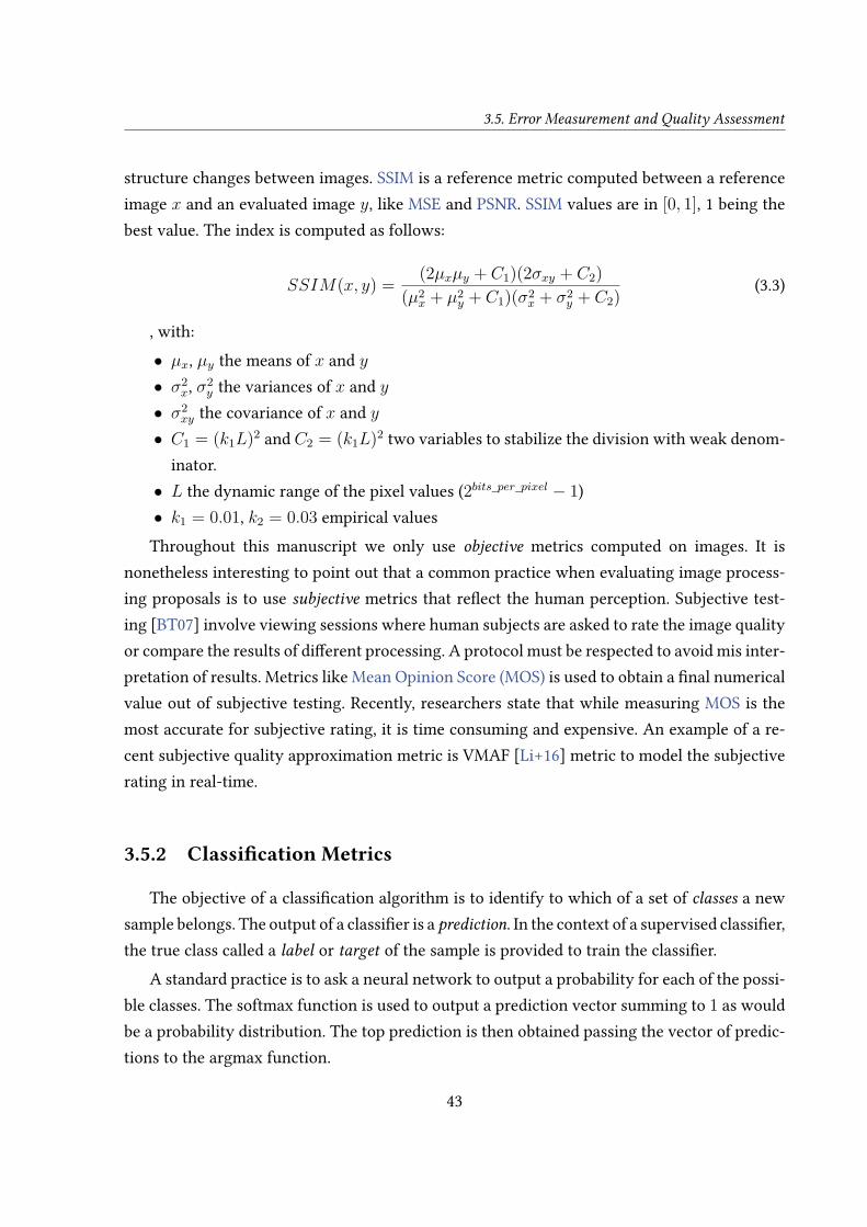
3.5. Error Measurement and Quality Assessment
structure changes between images. SSIM is a reference metric computed between a referenceimage x and an evaluated image y, like MSE and PSNR. SSIM values are in [0, 1], 1 being thebest value. The index is computed as follows:
SSIM(x, y) = (2µxµy + C1)(2σxy + C2)(µ2
x + µ2y + C1)(σ2
x + σ2y + C2) (3.3)
, with:• µx, µy the means of x and y• σ2
x, σ2y the variances of x and y
• σ2xy the covariance of x and y
• C1 = (k1L)2 and C2 = (k1L)2 two variables to stabilize the division with weak denom-inator.• L the dynamic range of the pixel values (2bits_per_pixel − 1)• k1 = 0.01, k2 = 0.03 empirical valuesThroughout this manuscript we only use objective metrics computed on images. It is
nonetheless interesting to point out that a common practice when evaluating image process-ing proposals is to use subjective metrics that re�ect the human perception. Subjective test-ing [BT07] involve viewing sessions where human subjects are asked to rate the image qualityor compare the results of di�erent processing. A protocol must be respected to avoid mis inter-pretation of results. Metrics like Mean Opinion Score (MOS) is used to obtain a �nal numericalvalue out of subjective testing. Recently, researchers state that while measuring MOS is themost accurate for subjective rating, it is time consuming and expensive. An example of a re-cent subjective quality approximation metric is VMAF [Li+16] metric to model the subjectiverating in real-time.
3.5.2 Classi�cation Metrics
The objective of a classi�cation algorithm is to identify to which of a set of classes a newsample belongs. The output of a classi�er is a prediction. In the context of a supervised classi�er,the true class called a label or target of the sample is provided to train the classi�er.
A standard practice is to ask a neural network to output a probability for each of the possi-ble classes. The softmax function is used to output a prediction vector summing to 1 as wouldbe a probability distribution. The top prediction is then obtained passing the vector of predic-tions to the argmax function.
43
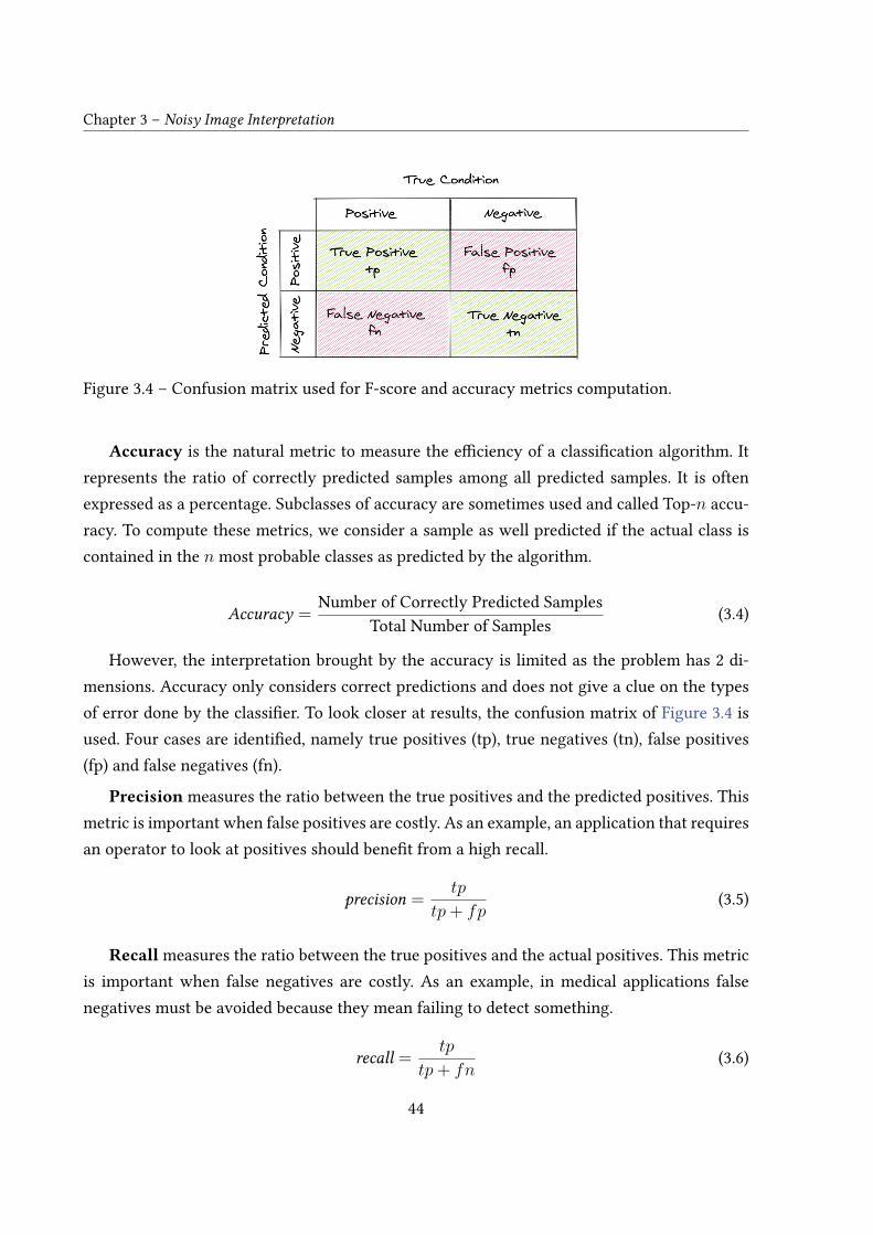
Chapter 3 – Noisy Image Interpretation
Figure 3.4 – Confusion matrix used for F-score and accuracy metrics computation.
Accuracy is the natural metric to measure the e�ciency of a classi�cation algorithm. Itrepresents the ratio of correctly predicted samples among all predicted samples. It is oftenexpressed as a percentage. Subclasses of accuracy are sometimes used and called Top-n accu-racy. To compute these metrics, we consider a sample as well predicted if the actual class iscontained in the n most probable classes as predicted by the algorithm.
Accuracy = Number of Correctly Predicted SamplesTotal Number of Samples (3.4)
However, the interpretation brought by the accuracy is limited as the problem has 2 di-mensions. Accuracy only considers correct predictions and does not give a clue on the typesof error done by the classi�er. To look closer at results, the confusion matrix of Figure 3.4 isused. Four cases are identi�ed, namely true positives (tp), true negatives (tn), false positives(fp) and false negatives (fn).
Precision measures the ratio between the true positives and the predicted positives. Thismetric is important when false positives are costly. As an example, an application that requiresan operator to look at positives should bene�t from a high recall.
precision = tp
tp+ fp(3.5)
Recall measures the ratio between the true positives and the actual positives. This metricis important when false negatives are costly. As an example, in medical applications falsenegatives must be avoided because they mean failing to detect something.
recall = tp
tp+ fn(3.6)
44
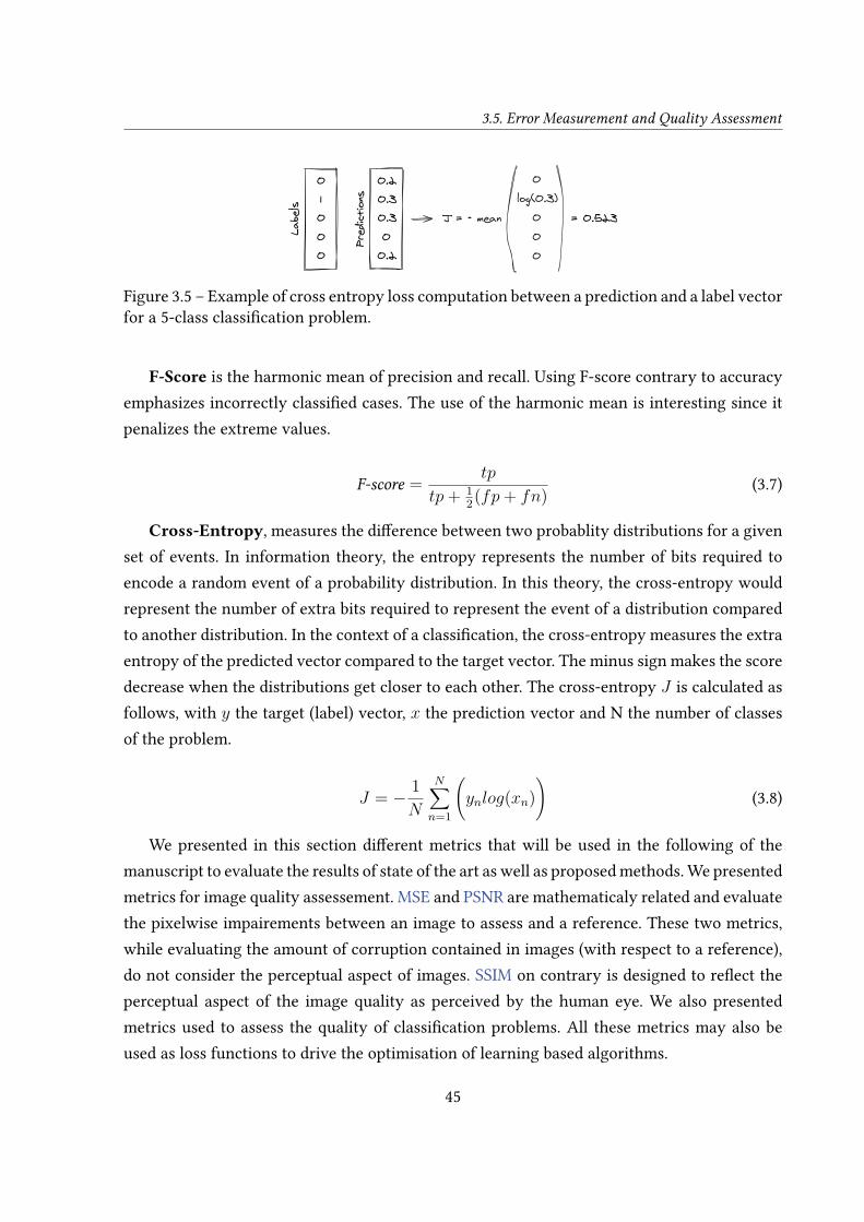
3.5. Error Measurement and Quality Assessment
Labe
ls
Pred
ictions
0.20.3
00.2
0.3
01
00
0 J = - meanlog(0.3)
0
00
0
= 0.523
Figure 3.5 – Example of cross entropy loss computation between a prediction and a label vectorfor a 5-class classi�cation problem.
F-Score is the harmonic mean of precision and recall. Using F-score contrary to accuracyemphasizes incorrectly classi�ed cases. The use of the harmonic mean is interesting since itpenalizes the extreme values.
F-score = tp
tp+ 12(fp+ fn) (3.7)
Cross-Entropy, measures the di�erence between two probablity distributions for a givenset of events. In information theory, the entropy represents the number of bits required toencode a random event of a probability distribution. In this theory, the cross-entropy wouldrepresent the number of extra bits required to represent the event of a distribution comparedto another distribution. In the context of a classi�cation, the cross-entropy measures the extraentropy of the predicted vector compared to the target vector. The minus sign makes the scoredecrease when the distributions get closer to each other. The cross-entropy J is calculated asfollows, with y the target (label) vector, x the prediction vector and N the number of classesof the problem.
J = − 1N
N∑n=1
(ynlog(xn)
)(3.8)
We presented in this section di�erent metrics that will be used in the following of themanuscript to evaluate the results of state of the art as well as proposed methods. We presentedmetrics for image quality assessement. MSE and PSNR are mathematicaly related and evaluatethe pixelwise impairements between an image to assess and a reference. These two metrics,while evaluating the amount of corruption contained in images (with respect to a reference),do not consider the perceptual aspect of images. SSIM on contrary is designed to re�ect theperceptual aspect of the image quality as perceived by the human eye. We also presentedmetrics used to assess the quality of classi�cation problems. All these metrics may also beused as loss functions to drive the optimisation of learning based algorithms.
45

Chapter 3 – Noisy Image Interpretation
3.6 Datasets for Learning and Evaluation
Data is the keystone of learning algorithms. In this manuscript, we use supervised datasetsonly. Supervised datasets are made of images jointly stored with a label being a class for classi-�cation or a clean target image for restoration. We de�ne two types of supervised dataset. The�rst type of dataset contains only non-corrupted images. We refer to these datasets as generalpurpose datasets. Most often these datasets have been created for classi�cation task. To usethem as image restoration datasets, the samples are corrupted using noise models, generatingthe noisy images while the reference image are kept as labels.
One of the most known datasets is ImageNet [Den+09]. ImageNet was �rst introduced asthe dataset for the ILSVRC contest. The ImageNet dataset contains millions of images withtheir labels for classi�cation. Berkeley Segmentation Dataset (BSD) [Mar+01] is a well-knowndataset in image restoration while it was originally built for segmentation tasks. The BSDdataset is interesting due to the variety of samples it contains in terms of content semantics.BSD is traditionally splitted into two datasets of 432 and 68 images, used for training and vali-dation/testing, respectively. The evaluation set of 68 images is refered to as BSD68. DIVerse 2K(DIV2K) [AT17] is a recent dataset created for the New Trends in Image Restoration (NTIRE)challenge in 2017. It contains 900 high resolution images which have at least one of their di-mension that reaches the 2K (2048) dimension. Among these 900 images, 800 are identi�edas training samples and 100 as validation/test samples. Other large well-known datasets likeCIFAR-10 or CIFAR-100 [Kri09] are used but their small resolution limits their interest.
We consider a second class of datasets applicable to real noise cases. When the noise modelis not perfectly known, it is not possible to create arti�cial datasets. There are di�erent meth-ods to create such datasets. A �rst strategy is to acquire another sample from the same sceneby a method that generates less noisy samples, thus considered as clean. In [AB18], authorscapture sensor noise due to low ISO acquired images. The "noise-free" counterpart is obtainedcapturing the same scene with long exposure. In [ALB18], the authors constitute a dataset ofnoisy images captured with smartphones. Due to smartphone sensors settings, the authorscannot use long exposure. Instead, they propose a software estimate of the ground truth im-ages.
We present in the following a method to generate a supervised dataset of eavesdroppedimages. This method is used to create a dataset of eavesdropped natural images and a datasetof eavesdropped textual screens in Chapter 6.
46
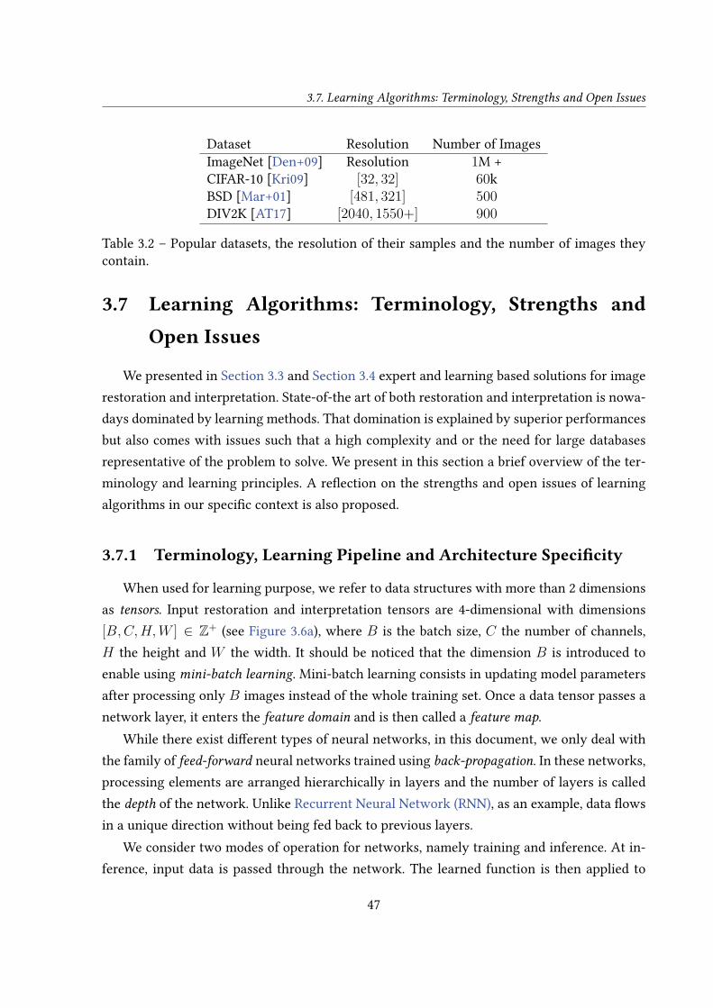
3.7. Learning Algorithms: Terminology, Strengths and Open Issues
Dataset Resolution Number of ImagesImageNet [Den+09] Resolution 1M +CIFAR-10 [Kri09] [32, 32] 60kBSD [Mar+01] [481, 321] 500DIV2K [AT17] [2040, 1550+] 900
Table 3.2 – Popular datasets, the resolution of their samples and the number of images theycontain.
3.7 Learning Algorithms: Terminology, Strengths and
Open Issues
We presented in Section 3.3 and Section 3.4 expert and learning based solutions for imagerestoration and interpretation. State-of-the art of both restoration and interpretation is nowa-days dominated by learning methods. That domination is explained by superior performancesbut also comes with issues such that a high complexity and or the need for large databasesrepresentative of the problem to solve. We present in this section a brief overview of the ter-minology and learning principles. A re�ection on the strengths and open issues of learningalgorithms in our speci�c context is also proposed.
3.7.1 Terminology, Learning Pipeline and Architecture Speci�city
When used for learning purpose, we refer to data structures with more than 2 dimensionsas tensors. Input restoration and interpretation tensors are 4-dimensional with dimensions[B,C,H,W ] ∈ Z+ (see Figure 3.6a), where B is the batch size, C the number of channels,H the height and W the width. It should be noticed that the dimension B is introduced toenable using mini-batch learning. Mini-batch learning consists in updating model parametersafter processing only B images instead of the whole training set. Once a data tensor passes anetwork layer, it enters the feature domain and is then called a feature map.
While there exist di�erent types of neural networks, in this document, we only deal withthe family of feed-forward neural networks trained using back-propagation. In these networks,processing elements are arranged hierarchically in layers and the number of layers is calledthe depth of the network. Unlike Recurrent Neural Network (RNN), as an example, data �owsin a unique direction without being fed back to previous layers.
We consider two modes of operation for networks, namely training and inference. At in-ference, input data is passed through the network. The learned function is then applied to
47

Chapter 3 – Noisy Image Interpretation
the input data. That phase is called forward pass. When training, an additional backward passis done after the data has �owed through the network. This pass updates the parameters ofthe network according to their gradients computed with respect to the errors measured afterthe forward pass. The metric used to guide the parameters update is called the loss function.We call the design of the network (number of layers, size of the �lters, etc..) the architecture.The learneable parameters that are trained and shape the �nal function are named alternatelyparameters or weights and noted θ.
HyperparametersL , Number of Layers
Training Se�ingslr , Learning Rate
Nepochs , Number of Training EpochsTensor Dimensions
B , Batch SizeC , Number of ChannelsH , HeightW , Width
Table 3.3 – Table of Notation of Learning Algorithms
Di�erence between learning Image-to-Class and Image-to-Image We previouslypresented restoration and interpretation as two di�erent tasks. Using learning algorithms,these two tasks are achieved using neural networks with di�erent architectures but with somesimilar blocks and principles. Both tasks are based on feature extraction out of input tensors.Image interpretation and restoration algorithms take the same tensors as input. The majordi�erence lies in the fact that restoration is a dense estimation task. The output has the samedimension as the input (i.e. a batch of images), unlike classi�cation that outputs classes. Forthat reason the networks are slightly di�erent.
In CNNs, the size of the receptive �eld is a major concern. The receptive �eld of a networkis the area of the input image from which a value in the network depends on (see Figure 3.6b).In other words, enlarging the receptive �eld brings more context information. In classi�cationnetworks, large receptive �elds are mainly obtained using more layers or successive down-sampling of the feature maps. Standard down-sampling strategies are striding and pooling.Striding consists in moving a �lter by a delta of several pixels instead of moving it to the nextpixel. Striding results in an output feature map spatially smaller than the input. Pooling directlyacts on the feature maps. A sub-sampling operator is applied window-wise. The di�erent pool-
48
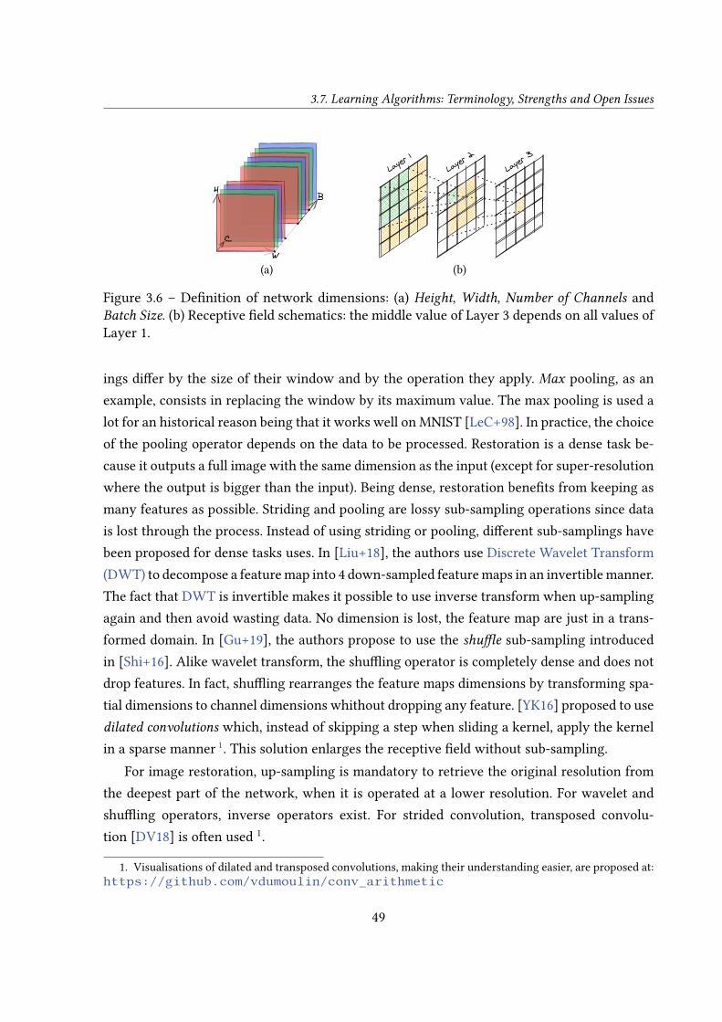
3.7. Learning Algorithms: Terminology, Strengths and Open Issues
H
C
B
W(a)
Layer
1Lay
er 2
Layer
3
(b)
Figure 3.6 – De�nition of network dimensions: (a) Height, Width, Number of Channels andBatch Size. (b) Receptive �eld schematics: the middle value of Layer 3 depends on all values ofLayer 1.
ings di�er by the size of their window and by the operation they apply. Max pooling, as anexample, consists in replacing the window by its maximum value. The max pooling is used alot for an historical reason being that it works well on MNIST [LeC+98]. In practice, the choiceof the pooling operator depends on the data to be processed. Restoration is a dense task be-cause it outputs a full image with the same dimension as the input (except for super-resolutionwhere the output is bigger than the input). Being dense, restoration bene�ts from keeping asmany features as possible. Striding and pooling are lossy sub-sampling operations since datais lost through the process. Instead of using striding or pooling, di�erent sub-samplings havebeen proposed for dense tasks uses. In [Liu+18], the authors use Discrete Wavelet Transform(DWT) to decompose a feature map into 4 down-sampled feature maps in an invertible manner.The fact that DWT is invertible makes it possible to use inverse transform when up-samplingagain and then avoid wasting data. No dimension is lost, the feature map are just in a trans-formed domain. In [Gu+19], the authors propose to use the shu�e sub-sampling introducedin [Shi+16]. Alike wavelet transform, the shu�ing operator is completely dense and does notdrop features. In fact, shu�ing rearranges the feature maps dimensions by transforming spa-tial dimensions to channel dimensions whithout dropping any feature. [YK16] proposed to usedilated convolutions which, instead of skipping a step when sliding a kernel, apply the kernelin a sparse manner 1. This solution enlarges the receptive �eld without sub-sampling.
For image restoration, up-sampling is mandatory to retrieve the original resolution fromthe deepest part of the network, when it is operated at a lower resolution. For wavelet andshu�ing operators, inverse operators exist. For strided convolution, transposed convolu-tion [DV18] is often used 1.
1. Visualisations of dilated and transposed convolutions, making their understanding easier, are proposed at:https://github.com/vdumoulin/conv_arithmetic
49

Chapter 3 – Noisy Image Interpretation
Pre-Processing Many datasets do not have a �xed resolution. Depending on the archi-tecture, a neural network may not support di�erent resolutions among images. As an ex-ample, a neural network which contains FC layers takes �xed size inputs. Resizing is oftenused to solve that issue. For example, a standard practice is to resize all ImageNet samples to224× 224 [KSH12] before feeding them to a classi�er containing FC layers.
Several network architectures like [Gu+19] or [Liu+18] require power of 2 input imagedimensions because of successive down-sampling operations. For that purpose, cropping isused instead of resizing. Doing so, only few pixels have to be removed and the other pixels arekept intact instead of being transformed by resampling.
When using small datasets in terms of number of samples like BSD or DIV2K, a commonpractice is to patch the images. One image is then split in M × N patches. For simplicity,patches are often squares. That patching enables using larger batch sizes and it reduces therequired memory, which is often an issue when using Graphics Processing Units (GPUs). Itshould be noted that the patch size cannot be smaller than the receptive �eld size. Followingthe use of patches in [BSH12], the authors of [Zha+17] propose to use di�erent patch sizesfor their di�erent experiments. Larger patch size are used for stronger corruptions to providemore information to learn.
3.7.2 Strengths of Learning Algorithms
Performance Superiority The popularity of DL methods in CV has grown because itsurpasses expert methods on many tasks. When the restoration algorithm DnCNN [Zha+17]was proposed, it outperformed BM3D [Dab+07] by 0.6dB on the task of denoising AWGN withσ=50 on the BSD68 grayscale dataset. DnCNN improved the expert-based state the art from25.62dB to 26.23dB while returning more natural looking images. The tendency is the same forclassi�cation algorithms with AlexNet [KSH12] that shortened the error rate on ILSVRC 2012by 10% compared to the state of the art method at the time [SP11].
DL methods also have the advantage to be ran e�ciently on GPUs because of their highdegree of parallelism. As an example, instead of BM3D, DnCNN being a CNN, can be ran onGPUs, making around 60 times faster at inference time for a 1024× 1024 image.
ModelingCapabilityML algorithms are very e�cient when the task is complex, i.e. whenthe problem is hardly invertible. In this context, it is complicated to design an expert-basedmethod since the problem is not precisely modeled. On contrary, DL models the problem bythe experience it acquires during training. Trained with data representative of the problem,complex function can be approached. This faculty is interesting for applications like medical
50

3.7. Learning Algorithms: Terminology, Strengths and Open Issues
imaging where it is complicated to model the sensing noise. This modeling capacity seemsalso promising for our eavesdropping image case study. We leverage this modeling power inChapter 6 to interpret eavesdropped images by learning on a custom noisy dataset.
3.7.3 Two Open Issues of Deep-Learning Algorithms
Training Data Dependency Learning algorithms are trained from data. In the case ofsupervised learning, the objective of the training procedure is to learn the function that mapsthe training inputs to the targets. The function modeled by the trained weights relies on thecontent of training input/target pairs. This is a weakness since at inference time, any inputthat diverges from the pairs seen at training time will no be processed well. The training datadependency complicates the comparison of state of the art methods. In fact, depending on thechoice of the authors, the training and evaluation dataset may change between experiments.In that case, even if the authors publish their code and trained models, it is not possible tocompare them directly. We propose in Chapter 4 a tool to ease the training and evaluation ofdenoising methods on equal basis to fairly compare them.
Once trained, the function modeled by the neural network is �xed. This is an issue whenconsidering evolving problems. An an example, one that would like to add a class to a classi�-cation problem cannot do it easily. It is not convenient to retrain all the model. In [LH18], theauthors evaluate several solutions to add new classes to a problem while minimizing the pre-diction loss on the other classes. In Chapter 5, we propose a restoration method that adressesthe training data dependency and the evolving problem.
Lack of Explainability DL models have the capability to model complex problems. How-ever, this comes at the cost of over-dimensionned networks hardly explainable. Except for veryspecial neural networks, the architecture is �xed and considered as a hyper-parameter. Thetraining process then tunes the trainable parameters to eventually obtain a modeling of thedesired function. This modeling is obtained by the action of the parameters together with non-linear functions. Made of millions of weigths, it is complicated to explain the behaviour of aneural network. This issue is addressed by a research domain named eXplainable Arti�cialIntelligence (XAI) [Gun+19]. We propose in Chapter 5 a method that makes a step towardsunderstanding of decisions by providing information about the noise classes contained in acorrupted image.
51
Chapter 3 – Noisy Image Interpretation
3.8 Conclusion
Noisy image restoration and interpretation are extensively addressed domains. We pre-sented in this chapter a de�nition of a noisy image. A noisy image is a sample that containsunwanted extra information that bothers the interpretation of legacy information. Learning-based method have strongly enhanced the performance of noisy image restoration and inter-pretation compared to expert-based methods. Di�erent classes of learning algorithms and theirstate of the art were exposed in the chapter. We also presented the metrics that are crucial toassess the performances of algorithms. These metrics are also useful to drive the optimisationprocess of learning algorithms.
The progress brought by learning comes at the cost of methods being largely reliant ondata used to train the systems. In the case of image restoration, as an example, that relianceon training data heads to methods over speci�c to the corruption they are trained for.
This chapter has shown that learning algorithms have good performance for the task weare interested in, i.e. restoration and interpretation. It has also enlighted that these algorithmsare not designed to be applied as is to the images we are interested in. The following of thatmanuscript evaluates how that issue can be addressed by studying the following question: towhat extent learning methods can reinforce the interpretation of EM compromising informa-tion?
The next chapter studies the impact of the dominance of AWGN in the data choice fordenoising architecture evaluation. In particular, a benchmark and a case study are proposedthat evaluates methods developed for AWGN applied to real-world eavesdropping noise.
52

Part II
Contributions
53


CHAPTER 4
Benchmarking of Image Restoration Algorithms
Chapter Contents4.1 Introduction . . . . . . . . . . . . . . . . . . . . . . . . . . . . . . . . . . 55
4.2 Related Work . . . . . . . . . . . . . . . . . . . . . . . . . . . . . . . . . 56
4.3 Proposed Benchmark . . . . . . . . . . . . . . . . . . . . . . . . . . . . 58
4.4 A Comparative Study of Denoisers . . . . . . . . . . . . . . . . . . . . 59
4.5 Conclusion . . . . . . . . . . . . . . . . . . . . . . . . . . . . . . . . . . 65
4.1 Introduction
State of the art denoisers are constantly progressing in terms of noise eliminationlevel [Dab+07; Zha+17; Liu+18] (see Section 3.3). However, most techniques are tailored forand evaluated on a given noise distribution, exploiting its probabilistic properties to distin-guish it from the signal of interest. On the speci�c case of Additive White Gaussian Noise(AWGN), current denoisers are approaching theoretical bounds [CM10].
Besides the largely addressedwell-behaved noise models, for which the distribution is para-metric with a few parameters, image denoising is also concerned by more complex noise dis-tributions. While these distributions are application speci�c, they are real-world cases directlyissued from identi�ed technical needs such as image interception in di�cult conditions.
In a context where new methods are constantly appearing, it is challenging to fairly com-pare emerging methods to previous ones. Moreover, when a real-world noise needs to be elim-

Chapter 4 – Benchmarking of Image Restoration Algorithms
inated, it is di�cult to determine which of the existing methods is the best for the given noisecharacteristics. Even if most state of the art methods are evaluated on the de-facto standarddatabases (e.g. the 12 well-known images such as Lenna or Cameraman, BSD [Mar+01] orDIVerse 2K (DIV2K) [AT17]), methods addressing speci�c noises and image types have to beevaluated on tailored databases. A tool that compares performances on an equal basis is thenimportant when designing denoising methods.
In this context, the contributions of this chapter are:• An extensible and open-source benchmark for comparing image restoration methods.• A comparative study of current denoisers on mixture and interception noise elimina-
tion, as a use case for the benchmark.The chapter is organized as follows. Section 4.2 presents state of the art methods for im-
age denoising as well as existing solutions to benchmark them. Section 4.3 describes the pro-posed benchmark. The comparative study, covering six restoration methods, is proposed inSection 4.4. Section 4.5 concludes the chapter.
This chapter contributions have been published in: F. Lemarchand, E. FernandesMontesuma,M. Pelcat, and E. Nogues, « OpenDenoising: an Extensible Benchmark for Building ComparativeStudies of Image Denoisers », in 2020 IEEE International Conference on Acoustics, Speech andSignal Processing (ICASSP), 2020, pp. 2648–2652.
4.2 Related Work
This section locates the proposal in the existing work and shows the novelty of the pro-posed solution. First, several existing benchmarks are reviewed. Then, di�erent state of the artimage denoisers are detailed before being assessed in the comparative study of Section 4.4.
4.2.1 Related Work on Benchmarks of Image Denoisers
An active research domain in complex noise restoration is photograph restoration. Thisdomain aims at removing a noise introduced by sensor hardware defects. Supervised datasetscan be built by calibrating a sensor and hence obtaining pairs of clean and noisy samples.Darmstadt [PR17] and PolyU [Xu+18] are such datasets. Authors propose to use their datasetsas a means for benchmarking denoising algorithms. This work is complementary to our pro-posed benchmark that can adapt to di�erent datasets.
56
4.2. Related Work
Open-source projects have been created to benchmark denoising methods. The Univer-sity of Toronto proposes a benchmark 1 to provide reproducibility for a method proposedin [EFJ09]. This benchmark is tailored to the solution and not built to be extended. Anotherunpublished benchmark exists that implements denoising as well as other restoration algo-rithms such as super-resolution or colorisation 2. The benchmark is limited to learning-based,Python-implemented and pre-trained methods. The latter limitation drastically reduces theuse of such benchmark for complex noises. Indeed, most state of the art methods, when deliv-ered trained, are trained on well-behaved noise. This chapter proposes a benchmark extensiblein several aspects. Indeed, the user can introduce his datasets, denoising methods, and metrics.
4.2.2 Chosen Image Denoisers for Benchmarking
Image denoising techniques are as old as image sensors whose defects they counteract.Current denoising solutions are either expert-based denoisers, human crafted based on anexpertise of artifacts or of statistical noise properties, or learning-based denoisers leveragingon latent image priors extracted from data (see Section 3.3). We prioritise in our tests thefollowing methods either for their state of the art performance on well-behaved noise or fortheir potential to denoise eavesdropped images.
Block-Matching 3D (BM3D) [Dab+07] is a state-of-the-art expert-based method for AWGNremoval. BM3D performs block matching to �nd patches with similar content in the imageand uses collaborative �ltering, thresholding and Wiener �ltering into the transform domainto restore the image.
Authors of [Vin+10] were the �rsts to propose an encoding/decoding model with denois-ing objective. Their proposal named "stacked auto-encoder" learns to map the noisy image toa latent space (encoding) and projects back the latent representation to the input space (decod-ing) to produce the denoised image. More recent auto-encoders have been proposed such asRED [MSY16] that adds convolutional layers and uses skip connections to better keep imagepriors throughout the encoding/decoding pipeline.
Following these premises of denoising auto-encoders, several Convolutional Neural Net-work (CNN) methods have emerged such as Denoising Convolutional Neural Network(DnCNN) [Zha+17]. DnCNN is inspired by the well-known VGG [SZ15]. It exploits resid-ual learning, i.e. it learns to isolate the noise h from the corrupted sample to later removethis noise instead of directly recovering the latent clean signal. DnCNN in its "blind" version
1. www.cs.utoronto.ca/~strider/Denoise/Benchmark/2. https://github.com/titsitits/open-image-restoration
57
Chapter 4 – Benchmarking of Image Restoration Algorithms
demonstrates its ability to handle di�erent noise levels. That makes it a potential candidatefor eavesdropping corruption removal. Multi-level Wavelet Convolutional Neural Network(MWCNN) [Liu+18] is also CNN-based. Its novelty lies in the symmetrical use of wavelet andinverse wavelet transforms into the contracting and expanding parts of a U-Net [RFB15] ar-chitecture. The use of wavelet enables safe subsampling with no information loss providing abetter recovering of textures and sharp structures. This faculty of texture and sharp structuresrecovering seems promising for eavesdropping corruption removal.
The most recent learning-based methods are less supervised, i.e. they require less noisy/-clean image pairs to train. In Noise2Noise (N2N) [Leh+18] and Noise2Void (N2V) [KBJ19] ,authors propose a tactic to train a denoising model using a single noise realisation. Authorsintroduce the idea of blind-spot masking during training. They claim that the essential advan-tage of that strategy is to avoid to learn the identity due to the masking of the central value ofthe receptive �eld.
These methods are evaluated on well-behaved noises (typically AWGN) for the tests to beeasily reproducible and comparable to state of the art. Only Noise2Void is evaluated on medicalimages subject to complex noise. In the following, our open benchmark is proposed to assessfairly the quality of denoisers.
4.3 Proposed Benchmark
Considering the above discussed issues with existing benchmarks, we propose the Open-Denoising benchmark illustrated in Figure 4.1. It is an open-source tool with tutorials anddocumentation 3 released under a CeCILL-C license. OpenDenoising is implemented in Pythonand has been designed for extensions. Adding a new denoiser to the benchmark is a matter ofminutes following a tutorial and opens for comparison with the built-in methods evoked inSection 4.4. For learning-based methods, the application is compatible and tested with mostmajor frameworks (Tensor�ow, Keras, Pytorch, Matlab). For learning-based training and eval-uation, it is possible to use one or several datasets either supervised or not. Any scalar metricbeing coded in Python can be used in the benchmark. Several pre-processing functions, e.g.for data augmentation, are provided, and custom functions can be introduced.
The user chooses whether a training is required for a method and in that case selects train-ing parameters. Once the training is launched, monitorings can be output by the benchmarkto observe the learning phase. When trained models are available, evaluation is launched with
3. https://github.com/opendenoising/benchmark
58
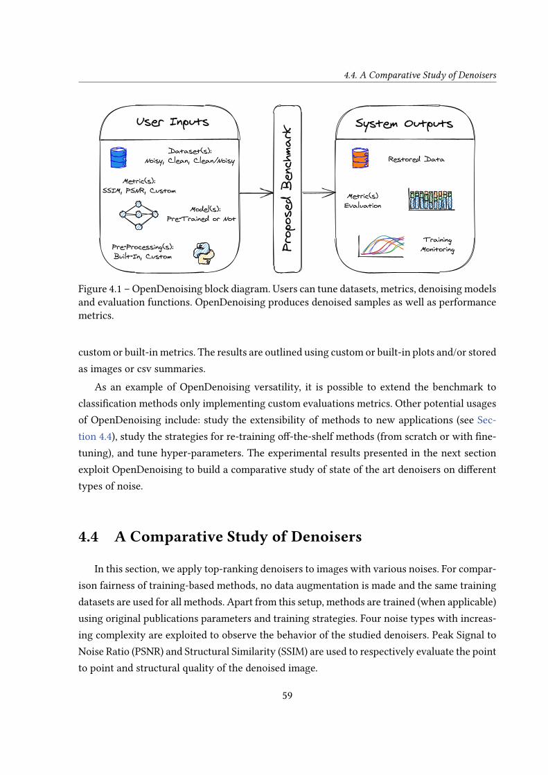
4.4. A Comparative Study of Denoisers
System Outputs
Restored Data
Metric(s)Evaluation
TrainingMonitoring
User Inputs
Dataset(s):Noisy, Clean, Clean/Noisy
Metric(s):SSIM, PSNR, Custom
Model(s):Pre-Trained or Not
Pre-Processing(s):Built-In, Custom
Prop
osed
Ben
chma
rkFigure 4.1 – OpenDenoising block diagram. Users can tune datasets, metrics, denoising modelsand evaluation functions. OpenDenoising produces denoised samples as well as performancemetrics.
custom or built-in metrics. The results are outlined using custom or built-in plots and/or storedas images or csv summaries.
As an example of OpenDenoising versatility, it is possible to extend the benchmark toclassi�cation methods only implementing custom evaluations metrics. Other potential usagesof OpenDenoising include: study the extensibility of methods to new applications (see Sec-tion 4.4), study the strategies for re-training o�-the-shelf methods (from scratch or with �ne-tuning), and tune hyper-parameters. The experimental results presented in the next sectionexploit OpenDenoising to build a comparative study of state of the art denoisers on di�erenttypes of noise.
4.4 A Comparative Study of Denoisers
In this section, we apply top-ranking denoisers to images with various noises. For compar-ison fairness of training-based methods, no data augmentation is made and the same trainingdatasets are used for all methods. Apart from this setup, methods are trained (when applicable)using original publications parameters and training strategies. Four noise types with increas-ing complexity are exploited to observe the behavior of the studied denoisers. Peak Signal toNoise Ratio (PSNR) and Structural Similarity (SSIM) are used to respectively evaluate the pointto point and structural quality of the denoised image.
59

Chapter 4 – Benchmarking of Image Restoration Algorithms
Figure 4.2 – Inference time (log scale) for di�erent denoisers. Image resolution is 256 × 256.Noise2Void is the fastest method by almost 10 folds. MWCNN, RED10, DnCNN and RED30 areclose to each other. BM3D is the slowest with an inference time over one second. Setup: IntelXeon W-2125 CPU and Nvidia GTX1080 Ti GPU. Note that BM3D runs on Central ProcessingUnit (CPU) only while the other methods run on both CPU and Graphics Processing Unit(GPU).
Dataset No Denoising BM3D RED10 RED30 DnCNN-B MWCNN Noise2Void
PSN
R
Gaussian 14.96 23.90 25.52 25.82 25.67 25.49 23.41Mixture 10.58 18.29 24.25 24.58 24.50 24.30 19.93Interception-Like 17.16 22.04 51.56 52.08 51.66 51.16 21.70Interception 9.46 9.61 22.59 23.46 23.04 23.66 9.46
SSIM
Gaussian 0.24 0.67 0.71 0.73 0.72 0.72 0.62Mixture 0.12 0.31 0.67 0.68 0.68 0.68 0.51Interception-Like 0.11 0.98 0.99 0.99 0.99 0.99 0.98Interception 0.32 0.73 0.94 0.96 0.95 0.96 0.47
Table 4.1 – Average evaluation of PSNR and SSIM metrics on test sets for, from top to bottomrow: AWGN with noise level σ = 50; Mixture noise made of AWGN with noise level σ = 50 andBernoulli noise with p = 0.2 ; Interception-Like noise being interception reference samplesnoised with AWGN with noise level σ = 50 ; Interception noise. The test set for each noise ismade of 200 samples excluded from training set.
60

4.4. A Comparative Study of Denoisers
4.4.1 Gaussian Noise
First, Gaussian noise is used to test the methods in their original conditions. Denoisers areevaluated on a common noisy dataset corrupted with AWGN. The underlying data is made of10k natural images extracted from the ImageNet [Den+09] evaluation set. Average PSNR andSSIM are shown in Table 4.1 and example images displayed on Figure 4.4. Figure 4.3 showsin boxplots the 10th, 25th, 75th and 90th percentiles of PSNR results as well as the median.To focus on di�cult noises, the maximum noise level commonly found in papers is picked,namely σ = 50. Experimental results, shown on the �rst line of Table 4.1, are coherent with thepublished ones, though slightly under because no data augmentation is applied. On Gaussiannoise, RED30 outperforms other methods (by a limited 0.15dB ∆PSNR and 1% ∆SSIM) but itis also the most costly Deep Learning (DL) solution in terms of number of parameters.
4.4.2 Mixture Noise
Complicating the denoising task, a mixture noise is then studied. This mixture noise isconstructed through the successive corruption of the samples by the previously used AWGN(σ = 50) and an additional Bernoulli corruption (20% of corrupted pixels, half 0, half maxi-mum). This noise mixture roughly models the behaviour of an image sensor introducing Gaus-sian noise because of its hardware non-uniformity and Bernoulli noise due to pixel defects.
Figure 4.3 shows that learning-based methods perform consistently better than BM3D.BM3D is here used out of its original objective (i.e. Gaussian denoising) and thus performspoorly. Another information brought by mixture noise is that Noise2Void clearly underper-forms compared to other learning-based methods. This is not surprising considering the ad-dition of Bernoulli noise that damages the spatial coherence used as a hypothesis in theNoise2Void strategy. RED10, RED30, DnCNN and MWCNN have close performances with anarrow victory for RED30 (0.08dB ∆PSNR).
4.4.3 Interception Noise
A real-world complex noise is now studied, generated by intercepting images from ElectroMagnetic (EM) emanations. Electronic devices produce EM emanations that not only inter-fere with radio devices but also compromise the data they handle. A third party performing aside-channel analysis can recover internal information from both analog [Van85], and digitalcircuits [Kuh13]. Following an eavesdropping procedure, it is possible to build a supervised
61

Chapter 4 – Benchmarking of Image Restoration Algorithms
18 20 22 24 26 28 30 32
Noise2Void
BM3D
RED10
DnCNN
RED30
MWCNN
(a) Gaussian
16 18 20 22 24 26 28 30 32
Noise2Void
BM3D
RED10
DnCNN
RED30
MWCNN
(b) Mixture
0 5 10 15 20 25 30PSNR(dB)
Noise2Void
BM3D
RED10
DnCNN
RED30
MWCNN
(c) Interception
Figure 4.3 – Peak Signal to Noise Ratio (PSNR) of denoised images on (a) Gaussian noise, (b)Mixture and (c) Interception noise. Outliers are not displayed.
62

4.4. A Comparative Study of Denoisers
Figure 4.4 – From top to bottom, one sample per dataset is shown noisy (left), denoised withdi�erent denoisers (middle) and clean (right). PSNR/SSIM are displayed for each sample. Im-ages with the best compromise between PSNR and SSIM metrics are yellow-boxed.
dataset made of pairs of reference images, originally displayed on a screen, and their inter-cepted noisy versions. Interception strongly damages the images and denoising is necessaryto interpret their content. For reproducibility, we released the dataset used for this study 4. Itcontains more than 120k samples.
To study the noise complexity, the intercepted clean samples are also arti�cially corruptedusing AWGN with σ = 50. The resulting samples are called interception-like. As shown in Ta-ble 4.1, most methods perform well on that denoising task. The clean content of the interceptedsamples contains black characters printed on a white background. The latent clean distributionof samples is thus not an issue to denoise with learning-based methods, Noise2Void excluded.Only BM3D and Noise2Void have problems with background restoration (see Figure 4.4). Thisphenomena is due to the correlation of the samples content and the noising process. The back-ground of the clean samples is fully white. When applying AWGN, half of the noise coe�cientsare negative and samples are clipped to an integer format. Thus, the assumption of a Gaussiandistribution does not hold, leading to poor restoration results with non-supervised methods,unable to adapt.
4. https://github.com/opendenoising/interception_dataset
63

Chapter 4 – Benchmarking of Image Restoration Algorithms
Table 4.1, Figure 4.3 and Figure 4.4 show the results of denoising methods applied to in-terception noise. Metrics drop for all methods on this complex noise. Noise2Void does notmanage to denoise at all. As explained in the original paper, Noise2Void has di�culties withnoise correlated between several pixels which is here the case. BM3D is built for AWGN andis not trainable, hence the poor results in that case. Others learned methods like RED10 andDnCNN produce interesting denoising but perceptual results of Figure 4.4 show some hardlyinterpretable samples, not revealed by SSIM. RED30 and MWCNN are the best-performingmethods for interception noise removal but still with some remaining artifacts.
4.4.4 Discussion
Di�erent conclusions can be drawn from the above experiments using OpenDenoising and4 di�erent datasets.
First, Figure 4.3 shows that the performance ranking between methods strongly depends onnoise type, training dataset and evaluation dataset. When calculating Kendall’s Tau correlationcoe�cient [JIP10], a value of 0.6 is obtained between Gaussian noise ranking and Interceptionnoise ranking, ranking based on the mean PSNR. This correlation coe�cient, while being high- Kendall’s Tau is in [−1; 1];−1 and 1 respectively meaning fully discordant and fully concor-dant rankings -, shows the need for a benchmark such as the proposed one. It automates thecomparison process and the selection of a given method for a denoising problem. As an exam-ple, it would be a wrong choice to pick RED30 instead of MWCNN for interception restorationbased on the original paper evaluations (e.g. Gaussian evaluation). MWCNN is indeed bothmore e�cient and less computationally intensive than RED30, as shown in Figure 4.2.
Results of Table 4.1, Figure 4.3 and Figure 4.4 show a growing gap between expert-basedand learning-based method as the complexity of the denoising increases. This can be explainedby the �exibility of learning-based models and the advanced information brought by a super-vised training. This is evidenced by the low performance of the non-supervised Noise2Voidon Mixture and Interception noises.
As stated in several studies, PSNR and SSIM do not suit well the assessment of interceptionrestoration. Figure 4.4 shows that while evaluation metrics on interception noise are reason-ably good (PSNR/SSIM values around 20dB/0.9), the perceptual quality (human looking) ispoor. The explanation lies in the latent content of the samples, made of black characters on awhite background. A good background restoration is su�cient to raise good evaluation met-rics. This issue is evoked in [JAF16] where authors propose a di�erent evaluation metric to
64
4.5. Conclusion
overcome the problem. As will be shown in Chapter 6, in that speci�c case, character recog-nition rate can be used to assess the denoising performance.
In order to go further on interception noise understanding, we propose in Chapter 6 anopen dataset of eavesdropped natural images dubbed Natural Interception Dataset (NID).
4.5 Conclusion
In this chapter, the OpenDenoising tool has been proposed. OpenDenoising benchmarksimage denoisers and aims at comparing methods on a common ground in terms of datasets,training parameters and evaluation metrics. Supporting several languages and learning frame-works, OpenDenoising is also extensible and open-source. At the time writing this manuscriptthe github repository of the OpenDenoising tool has received 16 stars. The second contribu-tion of the chapter is a comparative study of image restoration in the case of a complex noisesource.
Three major conclusions arise from the comparative study. First, the di�erence in termsof performance between expert-based and learning-based methods rises as the complexity ofthe noise grows and eavesdropping noise is clearly of high complexity, higher than mixturenoise. Second, the ranking of methods is strongly impacted by the nature of the noises. Finally,MWCNN proves to be the best method for the considered real-world interception restorationtask. It slightly outperforms DnCNN and RED30 while being substantially faster. These resultsshow that restoring an image from a complex noise is not universally solved by a single methodand that choosing a denoiser requires automated testing.
Next chapter proposes a method that adresses the removal of sequential mixture noisesfollowing the idea that eavesdropping noise may be approached by such arti�cial distributions.
65

CHAPTER 5
Mixture Noise Denoising Using a Gradual Strategy
Chapter Contents5.1 Introduction . . . . . . . . . . . . . . . . . . . . . . . . . . . . . . . . . . 67
5.2 Related Work . . . . . . . . . . . . . . . . . . . . . . . . . . . . . . . . . 70
5.3 Gradual Denoising Guided by Noise Analysis . . . . . . . . . . . . . . 72
5.4 Experiments: Noise Mixture Removal . . . . . . . . . . . . . . . . . . . 76
5.5 Experiments: Ablation Study . . . . . . . . . . . . . . . . . . . . . . . . 83
5.6 Conclusion . . . . . . . . . . . . . . . . . . . . . . . . . . . . . . . . . . 86
5.1 Introduction
Composed noises are more application speci�c than primary noises, but their removalconstitutes an identi�ed and important issue. Real photograph noise [PR17] is for instancea sequential composition of primary noises [Gow+07], generated by image sensor defects.Many distributions of real-world noises can be approached using noise compositions, alsocalled mixtures. Noise mixture removal has been less studied in the literature than primarynoise removal. When modelling experimental noises, noise mixture are either spatially or se-quentially composed. In a spatially composed noise mixture [CPM19; BR19], each pixel pn
of an image is corrupted by a speci�c distribution η(pn) such that h is composed of the set{η(pn), pn ∈ Dom(x)}. The mixture noise can also be sequentially composed as the result of

Chapter 5 – Mixture Noise Denoising Using a Gradual Strategy
Figure 5.1 – Comparison between a traditional end-to-end denoiser, removing noise mixtureat once, and gradual denoising removing primary noises one after the other. Top: clean im-age; bottom-left: traditional denoising with noisy and denoised using Denoising ConvolutionalNeural Network (DnCNN) trained on a noise mixture dataset; bottom-right: NoiseBreakertrained on primary noises.
68
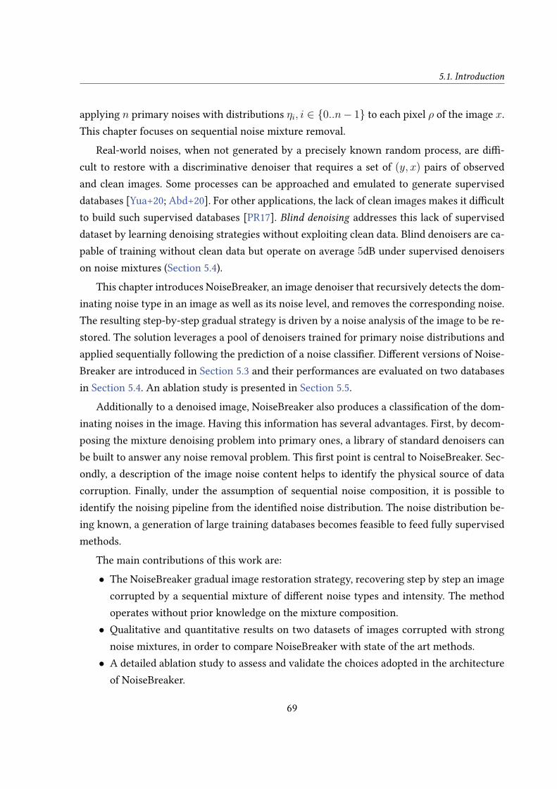
5.1. Introduction
applying n primary noises with distributions ηi, i ∈ {0..n− 1} to each pixel ρ of the image x.This chapter focuses on sequential noise mixture removal.
Real-world noises, when not generated by a precisely known random process, are di�-cult to restore with a discriminative denoiser that requires a set of (y, x) pairs of observedand clean images. Some processes can be approached and emulated to generate superviseddatabases [Yua+20; Abd+20]. For other applications, the lack of clean images makes it di�cultto build such supervised databases [PR17]. Blind denoising addresses this lack of superviseddataset by learning denoising strategies without exploiting clean data. Blind denoisers are ca-pable of training without clean data but operate on average 5dB under supervised denoiserson noise mixtures (Section 5.4).
This chapter introduces NoiseBreaker, an image denoiser that recursively detects the dom-inating noise type in an image as well as its noise level, and removes the corresponding noise.The resulting step-by-step gradual strategy is driven by a noise analysis of the image to be re-stored. The solution leverages a pool of denoisers trained for primary noise distributions andapplied sequentially following the prediction of a noise classi�er. Di�erent versions of Noise-Breaker are introduced in Section 5.3 and their performances are evaluated on two databasesin Section 5.4. An ablation study is presented in Section 5.5.
Additionally to a denoised image, NoiseBreaker also produces a classi�cation of the dom-inating noises in the image. Having this information has several advantages. First, by decom-posing the mixture denoising problem into primary ones, a library of standard denoisers canbe built to answer any noise removal problem. This �rst point is central to NoiseBreaker. Sec-ondly, a description of the image noise content helps to identify the physical source of datacorruption. Finally, under the assumption of sequential noise composition, it is possible toidentify the noising pipeline from the identi�ed noise distribution. The noise distribution be-ing known, a generation of large training databases becomes feasible to feed fully supervisedmethods.
The main contributions of this work are:• The NoiseBreaker gradual image restoration strategy, recovering step by step an image
corrupted by a sequential mixture of di�erent noise types and intensity. The methodoperates without prior knowledge on the mixture composition.• Qualitative and quantitative results on two datasets of images corrupted with strong
noise mixtures, in order to compare NoiseBreaker with state of the art methods.• A detailed ablation study to assess and validate the choices adopted in the architecture
of NoiseBreaker.
69

Chapter 5 – Mixture Noise Denoising Using a Gradual Strategy
The remaining of this chapter is organized as follows. Section 5.2 presents related work onimage noise analysis and image denoising. Section 5.3 details the proposed solution. Section 5.4evaluates the proposal on synthetic noise mixture and situates among state of the art solutions.Section 5.5 conducts an ablation study to assess the relevance of core features of NoiseBreaker.Section 6.5 concludes the chapter and gives future perspectives.
This chapter is based on our following work F. Lemarchand, T. Findeli, E. Nogues, and M.Pelcat, « Noisebreaker: Gradual image denoising guided by noise analysis », in 2020 IEEE 22ndInternational Workshop on Multimedia Signal Processing (MMSP), 2020, pp. 1–6.
5.2 Related Work
NoiseBreaker can be considered a weakly supervised method, as denoisers are trained onprimary noises and used on mixture noises. The covered related work includes not only weaklysupervised methods such as blind denoisers, but also fully supervised denoisers. Indeed, fullysupervised denoisers provide an upper bound for the performance obtained by weakly super-vised methods. Finally, the most commonly used noise mixtures are evoked, as well as theclassi�cation-based methods that address these noise mixtures.
5.2.1 Blind Denoising
Fully supervised deep learning denoisers forge a restoration model from pairs of clean andnoisy images. Following the premises of Convolutional Neural Network (CNN) based denois-ers [JS09], di�erent strategies have been proposed such as residual learning [Zha+17; Led+17],skip connections [MSY16], the use of transform domain [Liu+18] or self-guidance for fast de-noising [Gu+19]. The weakness of supervised denoisers is their need of large databases withclean images.
To overcome this limitation, di�erent weakly supervised denoisers have been proposed. Inparticular, blind denoisers are capable of removing noise without clean data as reference. The�rst studies on blind denoising have aimed at determining the level of a known noise in orderto apply an adapted human-expert based denoising (e.g. �ltering). Noise2Noise (N2N) [Leh+18]has pioneered learning-based blind denoising, using only noisy data. It demonstrates the fea-sibility of learning a discriminative denoiser from only one pair of images representing twoindependent realisations of the noise to be removed. Inspired by this work, Noise2Void (N2V)is a recent method that trains a denoiser from only noisy data.
70

5.2. Related Work
5.2.2 Noise Mixtures
To challenge denoisers and approach real-world cases, di�erent types of noise mixtureshave been proposed. Mixtures are created from the set of primary noises. A typical exampleof a spatially composed noise mixture [Zha+14] is made of 10% of uniform noise [−s, s], 20%of Gaussian noise N (0, σ0) and 70% of Gaussian noise N (0, σ1). These percentages refer tothe amount of pixels in the image corrupted by the given noise. This type of spatial noisemixture has e.g. been used in the experiments of Generated-Arti�cial-Noise to Generated-Arti�cial-Noise (G2G) [CPM19]. An example of sequential noise mixture is used to test therecent Noise2Self method [BR19]. It is composed of a combination of Poisson noise, Gaus-sian noise, and Bernoulli noise. In Chapter 4, denoising methods designed for Additive WhiteGaussian Noise (AWGN) removal are compared when retrained and evaluated on sequentialmixtures of Gaussian and Bernoulli distributions. Experimental results show that denoisingperformances severely drop on complex noises even when using fully supervised learningmethods such as DnCNN. This observation motivates the current study and the chosen se-quential noise mixture.
5.2.3 Classi�cation-Based Denoising
The image classi�cation domain has been revolutionized by deep learning methods sinceLeNet-5 [LeC+98]. With the development of tailored algorithms and hardware resources,deeper and more sophisticated neural networks have emerged. ResNet [He+16a] was re-leased to counteract the fact that very deep networks are more di�cult to train. At thetime the method was released, it was the �rst to be trained with as much as 150 layers,when applied to the ImageNet dataset [Den+09]. ResNet, in its deepest version, won the Ima-geNet Large Scale Visual Recognition Competition (ILSVRC) classi�cation challenge in 2015.ResNet has then been modi�ed, using identity mappings as skip connections in residual blocks(ResNetV2 [He+16b]). With the same objective, DenseNet [Hua+17] introduces connectionsbetween layers and performs training of very deep networks. Seeking a good trade-o� betweenclassi�cation e�ciency and hardware resources, MobileNets [How+17] is a particularly versa-tile family of classi�ers. MobileNetV2 has become a standard for resource aware classi�cation.In our study, we use MobileNetV2 network pre-trained on ImageNet and �ne-tuned [Taj+16]for noise classi�cation.
In [SSR11], authors propose a noise level estimation method integrated to a deblurringmethod. Inspired from this proposal, authors of [LTO13] estimate the standard deviation
71

Chapter 5 – Mixture Noise Denoising Using a Gradual Strategy
of a Gaussian distribution corrupting an image to apply the accordingly con�gured Block-Matching 3D (BM3D) �ltering [Dab+07]. This can be interpreted as a noise characterization,used to set parameters of a following dedicated denoising process.
Recent studies have proposed classi�cation-based solutions to the image denoising prob-lem [SDC19; LSJ20]. Sil et al. [SDC19] denoise by choosing one primary noise denoiser outof a pool, based on a classi�cation result. NoiseBreaker goes further by considering mix-ture noises, sequentially extracted from the noisy image using a sequence of classify/denoisephases. In [LSJ20], authors adopt a strategy close to NoiseBreaker. However, NoiseBreaker dif-ferentiates from that proposal by re�ning the noise classes into smaller ranges of noise levels.To the best of our knowledge, the present study is the �rst to use noise type and intensity clas-si�cation for denoising purposes. We demonstrate in the results Section 5.4 that NoiseBreakeroutperforms [LSJ20]. The main reason for NoiseBreaker to outperform the results of [LSJ20]is that the denoising pipeline is less constrained. As an example, the �rst step of [LSJ20] isto detect if the corruption is a mixture. If it is a mixture and the mixture contains Gaussiannoise then the Gaussian noise is removed �rst. Our proposal does not compel the denoisingprocess to follow a prede�ned order and lets the classi�er drive the denoising strategy to beconducted.
In this chapter, we propose to tackle the denoising of sequential noise mixtures via aniterative and joint classi�cation/denoising strategy. Our solution goes further than previouswork by separating the denoising problem into simpler steps, optimized separately.
5.3 Gradual Denoising Guided by Noise Analysis
NoiseBreaker is quali�ed as gradual because it denoises the input image step-by-step, al-ternating between noise detection and removal. NoiseBreaker leverages a classi�er acting as anoise analyser and guiding a pool of denoisers specialized to primary noise distributions. Boththe noise analyser and the gradual denoising strategy are detailed hereunder. NoiseBreakerhandles numerous noise mixtures at inference time without information on the compositionof the mixture. Neither the classi�er nor the denoisers are exposed to mixture noise duringtraining.
72
5.3. Gradual Denoising Guided by Noise Analysis
…… …
Figure 5.2 – Example of NoiseBreaker gradual denoising. A noisy input image is fed to theclassi�er C which outputs a prediction ηi. This prediction drives the gradual denoising blockG that selects the primary denoiser D(ηi) to be applied. The process runs for two steps untilno noise is detected by C.
5.3.1 Noise Analysis
The objective of the noise classi�er C is to separate images into n noise classes. A noiseclass is de�ned by a noise type and a range of parameter values. A class is denoted using ηi,j
with i an index among a listH of noise types and j an index for the di�erent ranges of a givennoise type. When no parameter exists for a noise type or an only range is used, the class isdenoted using ηi. ηi (or ηi,j) is referred to as a primary noise. One may note that one class doesnot refer to any noise and serves to identify clean images.
The architecture of the classi�er is composed of a feature extractor, called back-bone, followed by two Fully Connected (FC) layers, called head. Section 5.5 experi-ments versions of NoiseBreaker with MobileNetV2 [How+17], DenseNet121 [Hua+17] andResNet51V2 [He+16b] backbones. From these results, in NoiseBreaker, the backbone of Mo-bileNetV2 is responsible for extracting features out of the images. The two head FC layers haverespectively 1024 and n units, where n is the number of classes of the classi�cation problem.The input image resolution is chosen to be 224 × 224 as in the original MobileNetV2 imple-mentation. The �rst FC layer has ReLu activations while the second uses softmax activationsto obtain outputs in [0, 1], seen as con�dence levels. The output of this second FC layer, passedthrough an argmax function, gives the label with the highest con�dence level.
5.3.2 Gradual Denoising
A noisy image is given as an input to the classi�er C trained to di�erentiate noise classes. Csupplies a prediction ηi to G, the gradual denoising block. G selects the corresponding denoiser
73
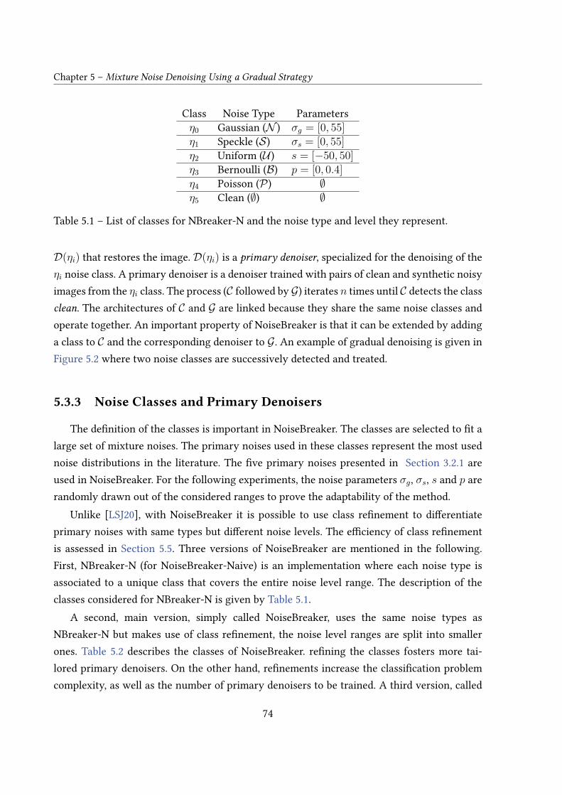
Chapter 5 – Mixture Noise Denoising Using a Gradual Strategy
Class Noise Type Parametersη0 Gaussian (N ) σg = [0, 55]η1 Speckle (S) σs = [0, 55]η2 Uniform (U ) s = [−50, 50]η3 Bernoulli (B) p = [0, 0.4]η4 Poisson (P) ∅η5 Clean (∅) ∅
Table 5.1 – List of classes for NBreaker-N and the noise type and level they represent.
D(ηi) that restores the image. D(ηi) is a primary denoiser, specialized for the denoising of theηi noise class. A primary denoiser is a denoiser trained with pairs of clean and synthetic noisyimages from the ηi class. The process (C followed by G) iterates n times until C detects the classclean. The architectures of C and G are linked because they share the same noise classes andoperate together. An important property of NoiseBreaker is that it can be extended by addinga class to C and the corresponding denoiser to G. An example of gradual denoising is given inFigure 5.2 where two noise classes are successively detected and treated.
5.3.3 Noise Classes and Primary Denoisers
The de�nition of the classes is important in NoiseBreaker. The classes are selected to �t alarge set of mixture noises. The primary noises used in these classes represent the most usednoise distributions in the literature. The �ve primary noises presented in Section 3.2.1 areused in NoiseBreaker. For the following experiments, the noise parameters σg, σs, s and p arerandomly drawn out of the considered ranges to prove the adaptability of the method.
Unlike [LSJ20], with NoiseBreaker it is possible to use class re�nement to di�erentiateprimary noises with same types but di�erent noise levels. The e�ciency of class re�nementis assessed in Section 5.5. Three versions of NoiseBreaker are mentioned in the following.First, NBreaker-N (for NoiseBreaker-Naive) is an implementation where each noise type isassociated to a unique class that covers the entire noise level range. The description of theclasses considered for NBreaker-N is given by Table 5.1.
A second, main version, simply called NoiseBreaker, uses the same noise types asNBreaker-N but makes use of class re�nement, the noise level ranges are split into smallerones. Table 5.2 describes the classes of NoiseBreaker. re�ning the classes fosters more tai-lored primary denoisers. On the other hand, re�nements increase the classi�cation problemcomplexity, as well as the number of primary denoisers to be trained. A third version, called
74

5.3. Gradual Denoising Guided by Noise Analysis
Class Noise Type Parameters Denoiserη0,0
Gaussian (N )σg = [0, 15]
MWCNN [Liu+18]η0,1 σg =]15, 35]η0,2 σg =]35, 55]η1,0
Speckle (S)σs = [0, 15]
SGN [Gu+19]η1,1 σs =]15, 35]η1,2 σs =]35, 55]η2,0 Uniform (U ) s = [−10, 10] SRResNet [Led+17]η2,1 s = [−50, 50]η3 Bernoulli (B) p = [0, 0.4] SRResNet [Led+17]η4 Poisson (P) ∅ SRResNet [Led+17]η5 Clean (∅) ∅ ∅
Table 5.2 – List of classes for NoiseBreaker, the noise type and level they represent. The de-noiser related to a class is mentioned, according to Table 5.3.
NBreaker-S (for NoiseBreaker-Same), is proposed to study the architecture distinction betweenprimary denoisers. For this version, all primary denoisers use Multi-level Wavelet Convolu-tional Neural Network (MWCNN) architectures contrary to NoiseBreaker that authorizes dif-ferent architectures to be used for di�erent classes. Lastly, a version named NBreaker-I (forNBreaker-Inverse) is introduced for further assessment of the proposed gradual denoising.NBreaker-I uses exactly the same classes as NoiseBreaker but denoises the samples in the ex-act inverse order of corruption, without using the decision of the classi�er. In this version, thenoise mixture composition is considered as known and the denoisers are manually employedto test their performance independently from the performance of the classi�er.
The choice of the primary denoisers is also of primary concern. NoiseBreaker authorizesdi�erent denoising architectures for di�erent noise classes. For each class, the best denoisingarchitecture is selected through a benchmark study. The e�ectiveness of authorizing di�erentdenoising architectures for di�erent noise types and the benchmark study used for selection ofprimary denoisers are discussed in Section 5.4. The benchmarking study has been performedusing the OpenDenoising benchmark tool. The results show that for a given noise type, thesame denoising architecture can be used for all classes. Following the benchmark study ofTable 5.3, NoiseBreaker uses MWCNN [Liu+18] for Gaussian noise type, Self-Guided Network(SGN) [Gu+19] for Speckle and Super-Resolution Residual Network (SRResNet) [Led+17] forBernoulli, Poisson and Uniform, as summarized in Table 5.2.
75
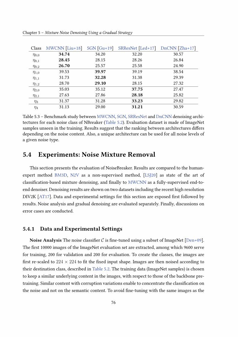
Chapter 5 – Mixture Noise Denoising Using a Gradual Strategy
Class MWCNN [Liu+18] SGN [Gu+19] SRResNet [Led+17] DnCNN [Zha+17]η0,0 34.74 34.20 32.20 30.57η0,1 28.45 28.15 28.26 26.84η0,2 26.70 25.57 25.58 24.90η1,0 39.53 39.97 39.19 38.54η1,1 31.73 32.28 31.38 29.39η1,2 28.70 29.10 28.15 27.32η2,0 35.03 35.12 37.75 27.47η2,1 27.63 27.86 28.18 25.82η3 31.37 31.28 33.23 29.82η4 31.13 29.00 31.21 30.59
Table 5.3 – Benchmark study between MWCNN, SGN, SRResNet and DnCNN denoising archi-tectures for each noise class of NBreaker (Table 5.2). Evaluation dataset is made of ImageNetsamples unseen in the training. Results suggest that the ranking between architectures di�ersdepending on the noise content. Also, a unique architecture can be used for all noise levels ofa given noise type.
5.4 Experiments: Noise Mixture Removal
This section presents the evaluation of NoiseBreaker. Results are compared to the human-expert method BM3D, N2V as a non-supervised method, [LSJ20] as state of the art ofclassi�cation-based mixture denoising, and �nally to MWCNN as a fully-supervised end-to-end denoiser. Denoising results are shown on two datasets including the recent high resolutionDIV2K [AT17]. Data and experimental settings for this section are exposed �rst followed byresults. Noise analysis and gradual denoising are evaluated separately. Finally, discussions onerror cases are conducted.
5.4.1 Data and Experimental Settings
Noise Analysis The noise classi�er C is �ne-tuned using a subset of ImageNet [Den+09].The �rst 10000 images of the ImageNet evaluation set are extracted, among which 9600 servefor training, 200 for validation and 200 for evaluation. To create the classes, the images are�rst re-scaled to 224 × 224 to �t the �xed input shape. Images are then noised according totheir destination class, described in Table 5.2. The training data (ImageNet samples) is chosento keep a similar underlying content in the images, with respect to those of the backbone pre-training. Similar content with corruption variations enable to concentrate the classi�cation onthe noise and not on the semantic content. To avoid �ne-tuning with the same images as the
76

5.4. Experiments: Noise Mixture Removal
Dataset Denoiser C0 C1 C2 C3 C4 C5
BSD68 Grayscale
Noisy 12.09/0.19 16.98/0.36 18.21/0.42 14.05/0.28 13.21/0.24 24.96/0.73BM3D [Dab+07] 21.49/0.54 24.00/0.61 24.28/0.62 22.30/0.56 22.05/0.56 24.95/0.65Noise2Void [KBJ19] 22.13/0.60 20.47/0.36 20.55/0.35 24.06/0.68 23.70/0.66 25.08/0.66Liu et al. [LSJ20] 21.04/0.52 25.96/0.74 27.17/0.82 27.11/0.80 26.83/0.77 27.52/0.83NoiseBreaker (Ours) 23.68/0.68 26.33/0.82 27.19/0.84 29.94/0.90 29.70/0.91 30.85/0.92
BSD68 RGB
Noisy 11.71/0.18 16.98/0.36 18.05/0.40 13.00/0.24 13.01/0.24 25.15/0.74BM3D 21.24/0.57 24.72/0.66 24.88/0.66 21.96/0.59 22.00/0.59 25.73/0.70Noise2Void 13.34/0.17 17.60/0.31 18.30/0.34 15.45/0.24 15.63/0.25 25.27/0.66Liu et al. 21.02/0.60 23.56/0.68 24.15/0.69 18.84/0.51 19.23/0.53 20.13/0.54NoiseBreaker (Ours) 21.88/0.71 26.81/0.82 26.58/0.82 25.45/0.81 25.20/0.80 29.77/0.88
DIV2K Grayscale
Noisy 11.69/0.15 16.80/0.32 18.18/0.37 12.36/0.18 12.95/0.22 24.47/0.70BM3D 22.05/0.64 25.36/0.71 26.23/0.71 22.36/0.65 22.75/0.65 27.20/0.76Noise2Void 22.24/0.64 21.01/0.40 21.08/0.39 22.87/0.66 24.78/0.71 26.47/0.69NoiseBreaker (Ours) 22.88/0.61 26.81/0.83 28.35/0.87 25.13/0.73 35.99/0.97 32.23/0.94
DIV2K RGB
Noisy 11.33/0.14 17.14/0.33 19.02/0.40 12.93/0.21 13.07/0.22 25.32/0.72BM3D 21.36/0.63 26.05/0.73 26.85/0.74 22.49/0.67 22.74/0.67 27.99/0.79Noise2Void 13.14/0.12 17.80/0.26 19.14/0.31 15.02/0.19 15.78/0.22 25.45/0.63NoiseBreaker (Ours) 22.35/0.71 27.57/0.84 27.68/0.83 25.62/0.81 26.48/0.83 29.82/0.87
Table 5.4 – Average PSNR(dB)/SSIM results of the proposed and competing methods forgrayscale and RGB denoising with the noise mixtures of Table 5.5 on BSD68 and DIV2K. Boldvalue indicates the best performance.
Noise 1 Noise 2C0 N ([0, 55]) B([0, 0.4])C1 N ([0, 55]) S([0, 55])C2 N ([0, 55]) PC3 B([0, 0.4]) S([0, 55])C4 B([0, 0.4]) PC5 S([0, 55]) P
Table 5.5 – De�nition of the noise mixtures used for evaluation. Noise 1 is applied �rst on thesample followed by Noise 2.
pre-training, the ImageNet evaluation set is taken. The weights for the backbone initialisation,pre-trained on ImageNet, are taken from the o�cial Keras MobileNetV2 implementation. Inthis version, NoiseBreaker contains 11 classes. Thus, the second layer of the head has accord-ingly 11 units. The classi�er is trained for 200 epochs with a batch size of 64. Optimisationis performed through an Adam optimizer with learning rate 5.10−5 and default settings forother parameters [KB14]. The optimisation is driven by a categorical cross-entropy loss. Astep scheduler halves the learning rate every 50 epochs.
Gradual Denoising For primary denoisers training, the �rst 9600 images of the ImageNetevaluation set are extracted and corrupted according to the classes mentioned in Table 5.2.For evaluation, the 68 images of the BSD68 [Mar+01] benchmark are used as well as the 100
77

Chapter 5 – Mixture Noise Denoising Using a Gradual Strategy
Figure 5.3 – Qualitative results on BSD68 dataset. Samples from the left column are cor-rupted with mixture C0 to C6, respectively. Images are tagged with Peak Signal to Noise Ratio(PSNR)/Structural Similarity (SSIM) values and the best PSNR value for an image is yellowcolored. Note that samples are chosen to be representative of the average PSNR of their corre-sponding classes. [LSJ20] not displayed because no available code. Better viewed on screen.
78

5.4. Experiments: Noise Mixture Removal
evaluation images of DIV2K [AT17]. Six di�erent sequential mixtures corrupt these images.For comparison purposes, the noise types of [LSJ20] are selected. Noise levels are shown inTable 5.5. The primary noises are either AWGN with σg ∈ [0, 55], Bernoulli noise with p ∈[0, 0.4], white Speckle noise with σs ∈ [0, 55] or Poisson noise. σg, σs and p values are randomlypicked. This random draw is used to prove the adaptability of our method to variable noiselevels. The size of BSD68 samples is either 321 × 481 or 481 × 321 and the DIV2K sampleshave a dimension larger than 2040×1550. When evaluating gradual denoising, C predicts thenoise class using a patch of size 224 × 224 cropped from the image to be denoised. Becauseof their architectures, the input resolution of MWCNN and SGN are constrained. To bypassthis issue, all samples are cropped to the closest resolution that satis�es the constraints. Thetraining of G comes down to the training of its primary denoisers. NoiseBreaker uses o�-the-shelf architectures for primary denoisers (Table 5.2) selected from results of a benchmark studydisplayed in Table 5.3. Results show that a unique architecture can be used for the di�erentclasses of a given noise type. From results of Table 5.3, the primary denoiser architectures areMWCNN [Liu+18] for Gaussian noise, SGN [Gu+19] for Speckle and SRResNet [Led+17] forBernoulli, Poisson and Uniform. These denoisers are trained with the parameters mentionedin their original papers. Only the training data di�er since it is made of the correspondingprimary noise (according to Table 5.2).
Compared methods Our solution is evaluated in comparison with BM3D [Dab+07],N2V [KBJ19], MWCNN [Liu+18] and Liu et al. [LSJ20]. Although a potential competitor,G2G [CPM19] is evaluated on other noise mixtures and no code is publicly available yet.BM3D is a human-expert method. It is not trained but requires σ, the standard deviation ofthe noise distribution. σ = 50 is chosen since it performs the best over the range of noisemixtures used for evaluation. N2V is a self-supervised denoiser. Training is carried out withthe publicly available code and the original paper strategy, and the data is corrupted withthe synthetic evaluation mixture. For [LSJ20], results are extracted from the paper tables andgiven only for BSD68 as no code is publicly available. MWCNN is used as a reference super-vised method, trained on the noise mixtures themselves. Comparison to supervised learningis unfair to NoiseBreaker because NoiseBreaker is never exposed to noise mixtures duringtraining. NoiseBreaker discovers the mixtures only when inferring. MWCNN is chosen as thesupervised reference because it performs the best on average over the classes of the bench-mark study (Table 5.3). It is worth mentioning that N2V and MWCNN models are trained foreach evaluation noise mixture while NoiseBreaker handles all evaluation classes with the samecon�guration and neither the classi�er nor the denoisers are exposed to mixture noise dur-
79
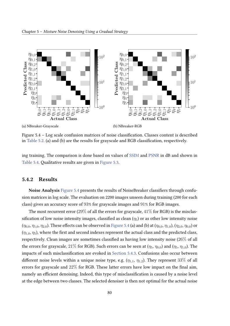
Chapter 5 – Mixture Noise Denoising Using a Gradual Strategy
η 0,0
η 0,1
η 0,2
η 1,0
η 1,1
η 1,2
η 2,0
η 2,1 η 3 η 4 η 5
Actual Class
η0,0η0,1η0,2η1,0η1,1η1,2η2,0η2,1η3η4η5
Pre
dic
ted
Cla
ss
170 1 0 1 0 0 19 0 0 2 7
6 181 11 0 0 0 0 2 0 0 0
0 0 198 0 0 2 0 0 0 0 0
1 0 0 159 6 0 5 0 0 0 29
1 0 0 8 178 7 0 0 0 6 0
0 1 0 0 9 190 0 0 0 0 0
3 0 0 0 1 0 192 0 0 2 2
0 0 1 0 0 0 0 199 0 0 0
0 0 0 0 0 0 0 0 200 0 0
2 0 0 2 4 0 0 0 0 192 0
2 0 0 8 0 0 3 0 0 0 187
100
101
102
(a) NBreaker-Grayscaleη 0,0
η 0,1
η 0,2
η 1,0
η 1,1
η 1,2
η 2,0
η 2,1 η 3 η 4 η 5
Actual Class
η0,0η0,1η0,2η1,0η1,1η1,2η2,0η2,1η3η4η5
Pre
dic
ted
Cla
ss
164 1 0 1 1 0 25 0 0 2 6
2 185 1 0 0 3 0 9 0 0 0
0 2 198 0 0 0 0 0 0 0 0
2 0 0 155 4 0 8 0 1 1 29
1 0 0 8 173 10 0 0 0 7 1
0 0 1 0 12 187 0 0 0 0 0
3 0 0 6 0 0 188 0 0 1 2
0 5 0 0 0 0 0 195 0 0 0
0 0 0 0 0 0 0 0 200 0 0
3 0 0 2 2 0 2 0 0 191 0
5 0 0 16 1 0 7 0 1 0 170
100
101
102
(b) NBreaker-RGB
Figure 5.4 – Log scale confusion matrices of noise classi�cation. Classes content is describedin Table 5.2. (a) and (b) are the results for grayscale and RGB classi�cation, respectively.
ing training. The comparison is done based on values of SSIM and PSNR in dB and shown inTable 5.4. Qualitative results are given in Figure 5.3.
5.4.2 Results
Noise Analysis Figure 5.4 presents the results of NoiseBreaker classi�ers through confu-sion matrices in log scale. The evaluation on 2200 images unseen during training (200 for eachclass) gives an accuracy score of 93% for grayscale images and 91% for RGB images.
The most recurrent error (29% of all the errors for grayscale, 41% for RGB) is the misclas-si�cation of low noise intensity images, classi�ed as clean (η5) or as other low intensity noise(η0,0, η1,0, η2,0). These e�ects can be observed in Figure 5.4 (a) and (b) at (η0,0, η1,0), (η2,0, η0,0) or(η1,0, η5), where the �rst and second indexes represent the actual class and the predicted class,respectively. Clean images are sometimes classi�ed as having low intensity noise (26% of allthe errors for grayscale, 21% for RGB). Such errors can be seen at (η5, η0,0) and (η5, η1,0). Theimpacts of such misclassi�cation are evoked in Section 5.4.3. Confusions also occur betweendi�erent noise levels within a unique noise type, e.g. (η1,1, η1,2). They represent 33% of allerrors for grayscale and 22% for RGB. These latter errors have low impact on the �nal aim,namely an e�cient denoising. Indeed, this type of misclassi�cation is caused by a noise levelat the edge between two classes. The selected denoiser is then not optimal for the actual noise
80
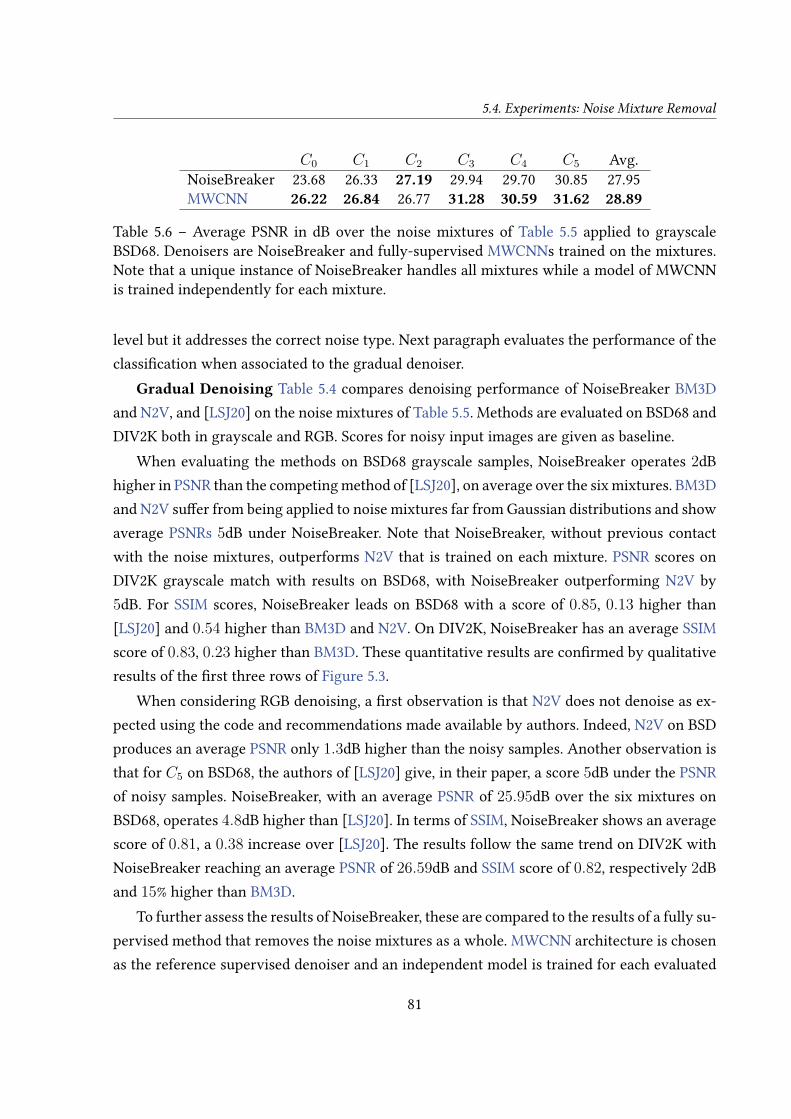
5.4. Experiments: Noise Mixture Removal
C0 C1 C2 C3 C4 C5 Avg.NoiseBreaker 23.68 26.33 27.19 29.94 29.70 30.85 27.95MWCNN 26.22 26.84 26.77 31.28 30.59 31.62 28.89
Table 5.6 – Average PSNR in dB over the noise mixtures of Table 5.5 applied to grayscaleBSD68. Denoisers are NoiseBreaker and fully-supervised MWCNNs trained on the mixtures.Note that a unique instance of NoiseBreaker handles all mixtures while a model of MWCNNis trained independently for each mixture.
level but it addresses the correct noise type. Next paragraph evaluates the performance of theclassi�cation when associated to the gradual denoiser.
Gradual Denoising Table 5.4 compares denoising performance of NoiseBreaker BM3Dand N2V, and [LSJ20] on the noise mixtures of Table 5.5. Methods are evaluated on BSD68 andDIV2K both in grayscale and RGB. Scores for noisy input images are given as baseline.
When evaluating the methods on BSD68 grayscale samples, NoiseBreaker operates 2dBhigher in PSNR than the competing method of [LSJ20], on average over the six mixtures. BM3Dand N2V su�er from being applied to noise mixtures far from Gaussian distributions and showaverage PSNRs 5dB under NoiseBreaker. Note that NoiseBreaker, without previous contactwith the noise mixtures, outperforms N2V that is trained on each mixture. PSNR scores onDIV2K grayscale match with results on BSD68, with NoiseBreaker outperforming N2V by5dB. For SSIM scores, NoiseBreaker leads on BSD68 with a score of 0.85, 0.13 higher than[LSJ20] and 0.54 higher than BM3D and N2V. On DIV2K, NoiseBreaker has an average SSIMscore of 0.83, 0.23 higher than BM3D. These quantitative results are con�rmed by qualitativeresults of the �rst three rows of Figure 5.3.
When considering RGB denoising, a �rst observation is that N2V does not denoise as ex-pected using the code and recommendations made available by authors. Indeed, N2V on BSDproduces an average PSNR only 1.3dB higher than the noisy samples. Another observation isthat for C5 on BSD68, the authors of [LSJ20] give, in their paper, a score 5dB under the PSNRof noisy samples. NoiseBreaker, with an average PSNR of 25.95dB over the six mixtures onBSD68, operates 4.8dB higher than [LSJ20]. In terms of SSIM, NoiseBreaker shows an averagescore of 0.81, a 0.38 increase over [LSJ20]. The results follow the same trend on DIV2K withNoiseBreaker reaching an average PSNR of 26.59dB and SSIM score of 0.82, respectively 2dBand 15% higher than BM3D.
To further assess the results of NoiseBreaker, these are compared to the results of a fully su-pervised method that removes the noise mixtures as a whole. MWCNN architecture is chosenas the reference supervised denoiser and an independent model is trained for each evaluated
81
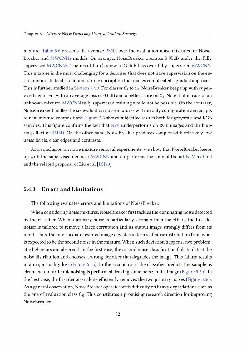
Chapter 5 – Mixture Noise Denoising Using a Gradual Strategy
mixture. Table 5.6 presents the average PSNR over the evaluation noise mixtures for Noise-Breaker and MWCNNs models. On average, NoiseBreaker operates 0.95dB under the fullysupervised MWCNNs. The result for C0 show a 2.54dB loss over fully supervised MWCNN.This mixture is the most challenging for a denoiser that does not have supervision on the en-tire mixture. Indeed, it contains strong corruption that makes complicated a gradual approach.This is further studied in Section 5.4.3. For classes C1 to C5, NoiseBreaker keeps up with super-vised denoisers with an average loss of 0.6dB and a better score on C2. Note that in case of anunknown mixture, MWCNN fully supervised training would not be possible. On the contrary,NoiseBreaker handles the six evaluation noise mixtures with an only con�guration and adaptsto new mixture compositions. Figure 5.3 shows subjective results both for grayscale and RGBsamples. This �gure con�rms the fact that N2V underperforms on RGB images and the blur-ring e�ect of BM3D. On the other hand, NoiseBreaker produces samples with relatively lownoise levels, clear edges and contrasts.
As a conclusion on noise mixture removal experiments, we show that NoiseBreaker keepsup with the supervised denoiser MWCNN and outperforms the state of the art N2V methodand the related proposal of Liu et al [LSJ20].
5.4.3 Errors and Limitations
The following evaluates errors and limitations of NoiseBreaker.
When considering noise mixtures, NoiseBreaker �rst tackles the dominating noise detectedby the classi�er. When a primary noise is particularly stronger than the others, the �rst de-noiser is tailored to remove a large corruption and its output image strongly di�ers from itsinput. Thus, the intermediate restored image deviates in terms of noise distribution from whatis expected to be the second noise in the mixture. When such deviation happens, two problem-atic behaviors are observed. In the �rst case, the second noise classi�cation fails to detect thenoise distribution and chooses a wrong denoiser that degrades the image. This failure resultsin a major quality loss (Figure 5.5a). In the second case, the classi�er predicts the sample asclean and no further denoising is performed, leaving some noise in the image (Figure 5.5b). Inthe best case, the �rst denoiser alone e�ciently removes the two primary noises (Figure 5.5c).As a general observation, NoiseBreaker operates with di�culty on heavy degradations such asthe one of evaluation class C0. This constitutes a promising research direction for improvingNoiseBreaker.
82

5.5. Experiments: Ablation Study
(a) (b) (c)
Figure 5.5 – Examples of BSD68 grayscale samples for which the gradual denoising divergesfrom the expected inverse corruption order. (a) and (b) are corrupted by C0, and (c) by C5.In (a), a second wrong denoiser is applied and damages the sample. In (b), the clean class hasbeen detected but a low strength Gaussian noise is still present. In (c), the �rst Speckle noiseremoval has also removed most of the Poisson Noise component of the mixture.
5.5 Experiments: Ablation Study
In this section, experiments are conducted separately on core features of NoiseBreaker.Experiments evaluate the respective impact on the results of NoiseBreaker of the noise classi-�cation and of the primary denoisers. For the ablation study, only grayscale images are used.The training dataset is the same as in Section 5.4.
5.5.1 Impact of Classi�cation on NoiseBreaker
NoiseBreaker performance depends on the performance of its noise classi�er and on thecapacity of each primary denoiser to remove its primary noise distribution. The followingevaluates the impact of noise classi�cation on the performance of NoiseBreaker.
5.5.1.1 Backbone Choice
Three backbones are compared to justify the choice of MobileNetV2 as the NoiseBreakerbackbone. The compared backbones are MobileNetV2, DenseNet121 and Resnet50V2. Thesethree backbones are chosen for their limited complexity and good performance on the ILSVRCvalidation set. Table 5.7 shows that the performances of the three backbones are close to eachother. Resnet50V2 and DenseNet121 reach an accuracy of 0.94 while MobileNetV2 scores 0.93.While being close in accuracy, MobileNetV2 has respectively 10 and 3 times less parametersthan Resnet50V2 and DenseNet121.
83
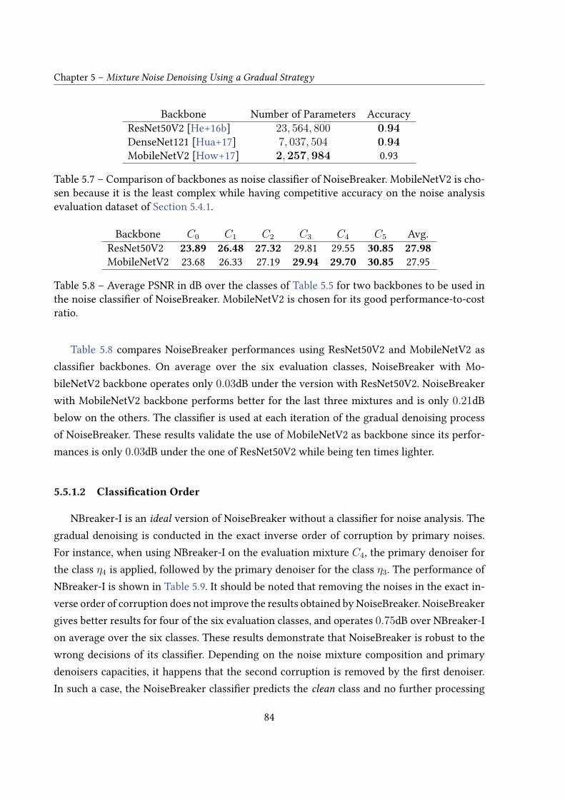
Chapter 5 – Mixture Noise Denoising Using a Gradual Strategy
Backbone Number of Parameters AccuracyResNet50V2 [He+16b] 23, 564, 800 0.94DenseNet121 [Hua+17] 7, 037, 504 0.94MobileNetV2 [How+17] 2,257,984 0.93
Table 5.7 – Comparison of backbones as noise classi�er of NoiseBreaker. MobileNetV2 is cho-sen because it is the least complex while having competitive accuracy on the noise analysisevaluation dataset of Section 5.4.1.
Backbone C0 C1 C2 C3 C4 C5 Avg.ResNet50V2 23.89 26.48 27.32 29.81 29.55 30.85 27.98MobileNetV2 23.68 26.33 27.19 29.94 29.70 30.85 27.95
Table 5.8 – Average PSNR in dB over the classes of Table 5.5 for two backbones to be used inthe noise classi�er of NoiseBreaker. MobileNetV2 is chosen for its good performance-to-costratio.
Table 5.8 compares NoiseBreaker performances using ResNet50V2 and MobileNetV2 asclassi�er backbones. On average over the six evaluation classes, NoiseBreaker with Mo-bileNetV2 backbone operates only 0.03dB under the version with ResNet50V2. NoiseBreakerwith MobileNetV2 backbone performs better for the last three mixtures and is only 0.21dBbelow on the others. The classi�er is used at each iteration of the gradual denoising processof NoiseBreaker. These results validate the use of MobileNetV2 as backbone since its perfor-mances is only 0.03dB under the one of ResNet50V2 while being ten times lighter.
5.5.1.2 Classi�cation Order
NBreaker-I is an ideal version of NoiseBreaker without a classi�er for noise analysis. Thegradual denoising is conducted in the exact inverse order of corruption by primary noises.For instance, when using NBreaker-I on the evaluation mixture C4, the primary denoiser forthe class η4 is applied, followed by the primary denoiser for the class η3. The performance ofNBreaker-I is shown in Table 5.9. It should be noted that removing the noises in the exact in-verse order of corruption does not improve the results obtained by NoiseBreaker. NoiseBreakergives better results for four of the six evaluation classes, and operates 0.75dB over NBreaker-Ion average over the six classes. These results demonstrate that NoiseBreaker is robust to thewrong decisions of its classi�er. Depending on the noise mixture composition and primarydenoisers capacities, it happens that the second corruption is removed by the �rst denoiser.In such a case, the NoiseBreaker classi�er predicts the clean class and no further processing
84

5.5. Experiments: Ablation Study
is conducted. NBreaker-I performance particularly show that an additional denoising step inthis speci�c case damages the image.
Denoiser C0 C1 C2 C3 C4 C5 Avg.NBreaker-I 23.96 25.02 25.05 30.07 28.77 30.35 27.20NoiseBreaker 23.68 26.33 27.19 29.94 29.70 30.85 27.95
Table 5.9 – Average PSNR in dB over the classes of Table 5.5 for NBreaker-I and NoiseBreaker.
5.5.2 Impact of Primary Denoisers
NoiseBreaker employs primary denoisers depending on the noise classi�er prediction. Theprimary denoisers are the actuators of the image restoration. The following study evaluatestwo points that distinguish the proposed method from state of the art, namely class re�nementand denoising architecture tailoring to each noise type.
5.5.2.1 Noise Class Re�nement
NBreaker-N is a version of NoiseBreaker that does not use class re�nement. Each noisetype is represented by a single class that includes the entire range of parameter values, whenapplicable. The results of the comparison between NoiseBreaker and NBreaker-N are shown inTable 5.10. On average over the six evaluation classes, NoiseBreaker operates 0.11dB higherthan NBreaker-N and presents the best results on four classes. This gain, while moderate,shows that class re�nement does improve denoising performance.
Denoiser C0 C1 C2 C3 C4 C5 Avg.NBreaker-N 22.80 26.86 27.59 29.86 29.65 30.29 27.84NoiseBreaker 23.68 26.33 27.19 29.94 29.70 30.85 27.95
Table 5.10 – Average PSNR in dB over the classes of Table 5.5 for NBreaker-N and NBreaker.
5.5.2.2 Architecture Distinction
Table 5.11 presents the comparison between NoiseBreaker and NBreaker-S. In NBreaker-S, all the primary denoisers use the MWCNN architecture. MWCNN is chosen here as thereference architecture since it proves to perform better on average over the classes of thebenchmark study of Table 5.3. The results of Table 5.11 show a signi�cant gain, as NoiseBreaker
85

Chapter 5 – Mixture Noise Denoising Using a Gradual Strategy
operates on average 0.21dB over NBreaker-S. The denoiser distinction makes NoiseBreakerperform better on four of the six evaluation classes.
Denoiser C0 C1 C2 C3 C4 C5NBreaker-S 22.77 26.65 27.54 29.50 29.43 30.54NoiseBreaker 23.68 26.33 27.19 29.94 29.70 30.85
Table 5.11 – Average PSNR in dB over the classes of Table 5.5 for NoiseBreaker using di�erentdenoising architectures for each noise type and a version of NoiseBreaker called NBreaker-Susing MWCNN for all primary denoisers.
5.6 Conclusion
This chapter has introduced a gradual image denoising strategy called NoiseBreaker.NoiseBreaker iteratively detects the image dominating noise using a trained classi�er withan accuracy of 93% and 91% for grayscale and RGB samples, respectively. Under the assump-tion of grayscale sequential noise mixtures, NoiseBreaker performs 0.95dB under the super-vised MWCNN denoiser without being trained on any mixture noise. Neither the classi�ernor the denoisers are exposed to mixture noise during training. NoiseBreaker operates 2dBover the gradual denoising of [LSJ20] and 5dB over the state of the art self-supervised de-noiser Noise2Void. When applied to Red Green Blue (RGB) samples, NoiseBreaker operates5dB over [LSJ20] while Noise2Void underperforms. Moreover, this chapter has demonstratedthat making noise analysis to guide the denoising is not only e�cient on noise type, but alsoon noise intensity.
This chapter has showed the practicality of NoiseBreaker on six di�erent synthetic noisemixtures. Future works include the application of NoiseBreaker to noisy images corruptedwith deeper noise mixtures, i.e. made of more than two primary noises. While the hypothesishas been made in Chapter 2 that the eavesdropping noise is a sequential mixture, NoiseBreakerhas not proven to be e�cient on its removal.
Next chapter proposes to automate the interpretation of eavesdropped samples using aDeep Learning (DL)-based textual retrieval and en according custom metric. A dataset craftedfor the task is also introduced.
86

CHAPTER 6
Direct Interpretation of Eavesdropped Images
Chapter Contents6.1 Introduction . . . . . . . . . . . . . . . . . . . . . . . . . . . . . . . . . . 87
6.2 Proposed Side-Channel Attack . . . . . . . . . . . . . . . . . . . . . . . 89
6.3 Experimental Results . . . . . . . . . . . . . . . . . . . . . . . . . . . . 92
6.4 An Opening to Eavesdropped Natural Images . . . . . . . . . . . . . . 97
6.5 Conclusions . . . . . . . . . . . . . . . . . . . . . . . . . . . . . . . . . . 102
6.1 Introduction
As introduced in Chapter 2, all electronic devices produce Electro Magnetic (EM) emana-tions that not only interfere with radio devices but also compromise the data handled by the in-formation system. A third party may perform a side-channel analysis and recover the originalinformation, hence compromising the system privacy. While pioneering work of the domainfocused on analog signals [Van85], recent studies extend the eavesdropping exploit using anEM side-channel attack to digital signals and embedded circuits [Kuh13]. The attacker’s pro�leis also taking on a new dimension with the increased performance of Software-De�ned Radio(SDR). With recent advances in radio equipment, an attacker can leverage advanced signal pro-cessing to further stretch the limits of the side-channel attack using EM emanations [Gen+18].With the fast evolution of deep neural networks, an attacker can extract patterns or even the

Chapter 6 – Direct Interpretation of Eavesdropped Images
2
1
Target
Interception System
Compromising Emanations
Reception Antenna
Raster Denoiser OCR
4
3
Figure 6.1 – Experimental setup: the attacked system includes an eavesdropped screen (1)displaying sensitive information. It is connected to an information system (2). An interceptionchain including an SDR receiver (3) sends samples to a host computer (4) that implements ourproposed automated interpretation.
full structured content of the intercepted data with a high degree of con�dence and a limitedexecution time.
In this chapter, a learning-based method is proposed to not only denoise eavesdroppedimages but also interpret them. To reduce the scope, the method focuses on textual images.In fact, we consider that con�dential documents mainly contain text. The method is based onthe specialization of Mask R-CNN [He+17] as a denoiser and classi�er. A complete system isdemonstrated, embedding SDR and deep-learning, that detects and recovers leaked informa-tion at a distance of several tens of meters. It provides an automated solution where the datais interpreted directly. The solution is compared to other system setups.
The chapter is organized as follows. ?? presents existing methods to recover informationfrom EM emanations. Section 6.2 describes the proposed method for automatic character re-trieval. Experimental results and detailed performances are exposed in Section 6.3. Section 6.4introduces an open dataset of eavesdropped natural images and proposes some experimentsto characterize the corruptions the dataset contains. Section 6.5 concludes the chapter.
This chapter contributions have been published in : F. Lemarchand, C. Marlin, F. Montreuil,E. Nogues, and M. Pelcat, « Electro-Magnetic Side-Channel Attack Through Learned Denoisingand Classi�cation », in 2020 IEEE International Conference on Acoustics, Speech and Signal Pro-cessing (ICASSP), 2020, p. 2882–2886.
88
6.2. Proposed Side-Channel Attack
6.2 Proposed Side-Channel Attack
6.2.1 System Description
Figure 6.1 shows the proposed end-to-end solution. The system is the same as the one pro-posed in Chapter 2 but the host computer implements our automated interpretation method.The interception system automatically reconstructs leaked visual information from compro-mising emanations. The setup is composed of two main elements. At �rst the antenna andSDR processing capture in the Radio Frequency (RF) domain the leaked information originat-ing from the displayed video. Then, the demodulated signal is processed by a host computer,recovering a noisy version of the original image [Kuh13] leaving room for advanced imageprocessing techniques. On top of proposing an end-to-end solution from capturing to the dataitself, the system includes machine interpretation. It captures compromising signals and recog-nizes automatically the leaked data assuming textual information. A �rst step based on a MaskR-CNN (Mask R-CNN) architecture embeds the following: denoising, segmentation, characterdetection/localization, and character recognition. A second step post-processes the Mask R-CNN output. A Hough transform is done for text line detection and a Bitap algorithm [Mye99]is applied to approximate match information. This setup detects several forms of compromis-ing emanations (analog or digital) and automatically triggers an alarm if critical informationis leaking. Next sections detail how the method is trained and integrated.
6.2.2 Dataset Construction
A substantial e�ort has been made on building a process that semi-automatically gener-ates and labels datasets for supervised training. Each sample image is made up of a uniformbackground on which varied characters are printed. Using that process, an open data corpusof 123.610 labeled samples, speci�c to the problem at hand, has been created to further be usedas training, validation and test datasets. This dataset is available online 1 to train denoiser ar-chitectures in di�cult conditions.
The proposed setup, to be trained, denoises the intercepted sample images and extractstheir content, i.e. the detected characters and their positions. The input space that should becovered by the training dataset is large and three main types of interception variability canbe observed. Firstly, interception induces an important loss of the information originally ex-isting in the intercepted data. The noise level is directly linked to the distance between the
1. https://github.com/opendenoising/interception_dataset
89

Chapter 6 – Direct Interpretation of Eavesdropped Images
ALIG
N
SCALESPLIT
INTERCEPT
SPLIT
NOISY SETREFERENCE SET
Figure 6.2 – A reference sample is displayed on the target screen (top-left). The interceptionmodule outputs uncalibrated samples. Vertical and horizontal porchs (red) helps alignmentand porch withdrawal (top-right). Samples are rescaled and split into patches to obtain thesame layout than the reference set.
antenna and the target. Several noise levels are generated by adding RF attenuation after theantenna. That loss itself causes inconsistencies in the rasterizing stage. Secondly, EM emana-tions can come from di�erent sources, using di�erent technologies, implying in turn di�erentintercepted samples for the same reference image. The dataset covers Video Graphics Array(VGA), Display Port (DP)-to-Digital Visual Interface (DVI) and High-De�nition MultimediaInterface (HDMI) cables and connectors. Besides this unwanted variability, a synthetic thirdtype of variability is introduced to solve the character retrieval problem. Many di�erent char-acters are introduced in the corpus to be displayed on the attacked screen. They range from 11to 70 points in size and they are both digits and letters, and letters are both upper and lowercases. Varied fonts, character colors and background colors, as well as varied character posi-tions in the sample are used. Considering these di�erent sources of variability, the dataset isbuilt trying to get an equi-representation of the di�erent interception conditions.
The choice has been made to display on the target screen a sample containing patches ofsize 256 × 256 pixels (top-left image of Figure 6.2). For building the dataset, having multiplepatches speeds the process up because smaller samples can be derived from a single screeninterception and more variability can be introduced in the dataset. The main challenge when
90

6.2. Proposed Side-Channel Attack
creating the dataset lies in the sample acquisition itself. Indeed, once intercepted, the samplesare not directly usable. The interception process outputs samples such as the one of Figure 6.2(middle-top) where intercepted characters are not aligned (temporally and spatially) with re-spective reference samples. An automated method is introduced that uses the porches, arti�-cially colored in red in Figure 6.2 (middle-top), to align spatially samples. Porches are detectedusing brute-force search of large horizontal and vertical gradients (to �nd vertical and hori-zontal porches, respectively). A validation step ensures the temporal alignment, based on theinsertion of a QRCode in the upper-left patch. If the QRCode is similar between the referenceand the intercepted image, the image patches are introduced in the dataset.
Data augmentation [MG18] is used to enhance the dataset coverage area. It is done ontopatches to add variability into the dataset and reinforce its learning capacity. Conventionalmethods are applied to raw samples to linearly transform them (Gaussian and median blur,salt and pepper noise, color inversion and contrast normalization).
6.2.3 Implemented Solution to Catch Compromising Data
In order to automate the interception of compromising data, the Mask R-CNN has beenturned into a denoiser and classi�er. The implementation is based on the one proposed by W.Abdulla 2. Other learning-based and expert-based signal processing methods, discussed in Sec-tion 6.3.2, are also implemented to assess the quality of the proposed framework. Mask R-CNNis a framework adapted from the previous Faster R-CNN [Ren+17]. The network consists oftwo stages. The �rst stage, also known as backbone network, is a ResNet101 convolutional net-work [He+16a] extracting features out of the input samples. Based on the extracted features,a Region Proposal Network (RPN) proposes Region of Interests (RoIs). RoIs are regions in thesample where information deserves greater attention. The second stage, called head network,classi�es the content and returns bounding box coordinates for each of the RoIs. The maindi�erence between Faster R-CNN and Mask R-CNN lies in an additional Fully ConvolutionalNetwork (FCN) branch [SLD17] running in parallel with the classi�cation and extracting abinary mask for each RoI to provide a more accurate localization of the object of interest.
Mask R-CNN is not originally designed to be used for denoising but rather for instancesegmentation. However, it �ts well the targeted problem. Indeed, the problem is similar to asegmentation where signal has to be separated from noise. As a consequence, when properlyfeeding a trained Mask R-CNN network with noisy samples containing characters, one obtains
2. https://github.com/matterport/Mask_RCNN
91

Chapter 6 – Direct Interpretation of Eavesdropped Images
ConfidenceMark
Figure 6.3 – The output of Mask R-CNN may be used in two ways. The segmentation can bedrawn (left) and further processed by an Optical Character Recognition (OCR), or the MaskR-CNN classi�er can directly infer the sample content (right) and propose some display andcon�dence information.
lists of labels (i.e. characters recognition), as well as their bounding boxes (characters local-ization) and binary masks representing the content of the original clean sample. The setupof the classi�cation branch allows to be language-independent and to add classes other thancharacters.
Two strategies can be employed to exploit Mask R-CNN components for the problem. The�rst idea is to draw the output masks of Mask R-CNN segmentation (Figure 6.3 left-hand side)and request an OCR to retrieve characters from the masks. A second possibility is to make useof the classi�cation faculty of Mask R-CNN (Figure 6.3 right-hand side) and obtain a list oflabels without using an OCR engine. The second method using the classi�er of Mask R-CNNproves to be better in practice, as shown in Section 6.3.2.
The training strategy is to initialize the training process using pre-trained weights [Mah+18]for the MS COCO [Lin+14] dataset, made available by the authors of Mask R-CNN. First, theweights of the backbone are frozen and the head is trained to adapt to the application. Then,the weights of the backbone are relaxed and both backbone and head are trained together untilconvergence. This process is done to ensure the convergence and speed up training.
6.3 Experimental Results
6.3.1 Experimental Setup
The experimental setup is de�ned as follows: the eavesdropped display is 10 meters awayfrom the interception antenna. A RF attenuator is inserted after the antenna. It ranges from 0dB to 24 dB to simulate higher interception radius and generate a wide range of noise values.
92

6.3. Experimental Results
(a) (b) (c)
Figure 6.4 – Three samples (left, middle, right) displayed at di�erent stages of the intercep-tion/denoising pipeline. From top to bottom: the reference patch displayed on the screen; thepatch after rasterization (raw patch); the patches denoised with Block-Matching 3D (BM3D),autoencoder and Mask R-CNN.
93

Chapter 6 – Direct Interpretation of Eavesdropped Images
Compromising emanations are issued either by a VGA display, a DP-to-DVI cable or an HDMIconnector. The interception system is depicted in Figure 6.1: the antenna is bilog, the SDRdevice automatically recovering parameters [De +18] is an Ettus X310 receiving with a 100MHz bandwidth to recover the compromised information with a �ne granularity [Kuh13].The host computer running post-processing has a linux operating system, an Intel®Xeon®W-2125 Central Processing Unit (CPU) and an Nvidia GTX 1080 Ti Graphics Processing Unit(GPU). The host computer rasters the compromising data using the CPU while the proposedlearning-based denoiser/classi�er runs also on the GPU.
6.3.2 Performance Comparison Between Data Catchers
The purpose of the exposed method is to analyze compromising emanations. Once a signalis detected and rasterized, intercepted emanations should be classi�ed into compromising ornot. Figure 6.4 illustrates the outputs of di�erent implemented denoisers. More examples areavailable at 3. It is proposed to assess the data leak according to the ability of a model to re-trieve original information. A ratio between the number of characters that a method correctlyclassi�es from an intercepted sample, and the true number of characters in the correspondingclean reference is used as a metric.
The quality assessment method is the following. First, a sample containing a large num-ber of characters is pseudo-randomly generated (similar to dataset construction). The sampleis displayed on the eavesdropped screen and EM emanations are intercepted. The proposeddenoising/retrieval is applied and the obtained results are compared to the reference sample.The method using Mask R-CNN produces directly a list of retrieved characters. Other meth-ods, implemented to compare the e�ciency of the proposal, use denoising in combination withthe Tesseract [Smi07] OCR. Tesseract is a well performing OCR engine, retrieving charactersfrom images. It produces a list of characters retrieved from a denoised sample. As the outputof Tesseract is of the same type as the output of Mask R-CNN classi�cation, metrics can beextracted to fairly compare methods.
An end-to-end evaluation is used measuring the quality of characters classi�cation. A F-score (see Section 3.5.2) is computed. For simpli�cation and not use an alignment process, atrue positive is chosen here to be the recognition of a character truly existing in the referencesample.
3. https://github.com/opendenoising/extension
94
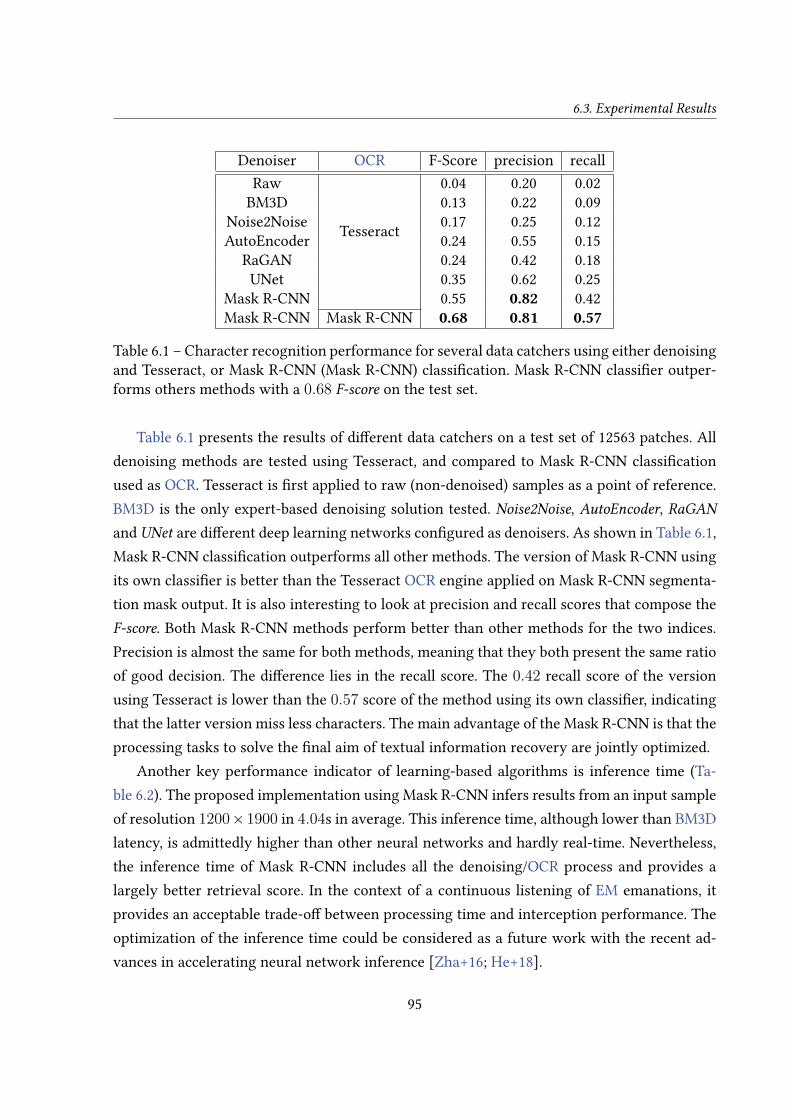
6.3. Experimental Results
Denoiser OCR F-Score precision recallRaw
Tesseract
0.04 0.20 0.02BM3D 0.13 0.22 0.09
Noise2Noise 0.17 0.25 0.12AutoEncoder 0.24 0.55 0.15
RaGAN 0.24 0.42 0.18UNet 0.35 0.62 0.25
Mask R-CNN 0.55 0.82 0.42Mask R-CNN Mask R-CNN 0.68 0.81 0.57
Table 6.1 – Character recognition performance for several data catchers using either denoisingand Tesseract, or Mask R-CNN (Mask R-CNN) classi�cation. Mask R-CNN classi�er outper-forms others methods with a 0.68 F-score on the test set.
Table 6.1 presents the results of di�erent data catchers on a test set of 12563 patches. Alldenoising methods are tested using Tesseract, and compared to Mask R-CNN classi�cationused as OCR. Tesseract is �rst applied to raw (non-denoised) samples as a point of reference.BM3D is the only expert-based denoising solution tested. Noise2Noise, AutoEncoder, RaGANand UNet are di�erent deep learning networks con�gured as denoisers. As shown in Table 6.1,Mask R-CNN classi�cation outperforms all other methods. The version of Mask R-CNN usingits own classi�er is better than the Tesseract OCR engine applied on Mask R-CNN segmenta-tion mask output. It is also interesting to look at precision and recall scores that compose theF-score. Both Mask R-CNN methods perform better than other methods for the two indices.Precision is almost the same for both methods, meaning that they both present the same ratioof good decision. The di�erence lies in the recall score. The 0.42 recall score of the versionusing Tesseract is lower than the 0.57 score of the method using its own classi�er, indicatingthat the latter version miss less characters. The main advantage of the Mask R-CNN is that theprocessing tasks to solve the �nal aim of textual information recovery are jointly optimized.
Another key performance indicator of learning-based algorithms is inference time (Ta-ble 6.2). The proposed implementation using Mask R-CNN infers results from an input sampleof resolution 1200×1900 in 4.04s in average. This inference time, although lower than BM3Dlatency, is admittedly higher than other neural networks and hardly real-time. Nevertheless,the inference time of Mask R-CNN includes all the denoising/OCR process and provides alargely better retrieval score. In the context of a continuous listening of EM emanations, itprovides an acceptable trade-o� between processing time and interception performance. Theoptimization of the inference time could be considered as a future work with the recent ad-vances in accelerating neural network inference [Zha+16; He+18].
95

Chapter 6 – Direct Interpretation of Eavesdropped Images
Denoiser OCR Inference Timing (s)Raw
Tesseract
0.19BM3D 21.8
Autoencoder 1.15Mask R-CNN 4.22Mask R-CNN Mask R-CNN 4.04
Table 6.2 – Inference time for several data catchers using Tesseract or Mask R-CNN classi�-cation as OCR. Input resolution is 1200× 1900 and it is processed using a split in 28 patches.Mask R-CNN classi�er is slower than the autoencoder but still faster than BM3D.
96

6.4. An Opening to Eavesdropped Natural Images
6.4 An Opening to Eavesdropped Natural Images
In this manuscript, we focused on textual images, when evoking eavesdropped images. Asevoked in Chapter 3, the properties of textual images are di�erent from those of natural images.To go further on the restoration and interpretation of eavesdropped images, we propose in thissection a dataset made of natural eavesdropped samples and their clean references. DubbedNatural Interception Dataset (NID), the dataset is publicly available on GitHub 4.
First, the acquisition process of the Natural Interception Dataset (NID) dataset is detailed.Discussions on the noise corrupting the dataset follow.
6.4.1 Dataset Construction
The NID is a dataset of natural eavesdropped images. The underlying data is made ofBerkeley Segmentation Dataset (BSD) [Mar+01] samples. Using the protocol described in thefollowing, we obtained the eavesdropped counterpart of all BSD68 samples as well as this of424 BSD432 samples out of the original 432.
Building a supervised dataset of eavedropped samples is complicated due to the impaire-ments evoked in Section 2.3. First, it is complicated to know the position of the desired imagepart in the eavesdropped reconstructed image. Second, the image is noisy by nature whichmakes di�cult any correlation or corner detection technique. Identi�cation markings like QRcodes are also di�cult to detect for noisy/reference pairing.
We use a method for building the dataset which is close but not equal to the one used inSection 6.2.2 to contruct the dataset of eavesdropped text images. The dataset is contructedin two phases. First, the images are displayed on a screen and eavesdropped with the sameexperimental system as the one of Figure 2.4. The images are jointly displayed with a QRcode. This QR code enables pairing noisy and reference images since each image as its own.A cross sight is also drawn and used to retrieved the position of the data of interest in theeavesdropped image. Indeed, as can be seen on the top-right part of Figure 6.5, such sight stillappears clearly in eavesdropped samples. The QR code cannot be used for this purpose since itscontent changes and no corner is always visible, depending on the encoded value. The imagecannot be used either since the sharpness of its corner depends on its original content.
Second, the images are post-processed. The cross sight is �rst retrieved. The QR code be-ing positioned directly on the right-bottom quarter, created by the sight, is cropped and inter-preted. The top-left corner of the image is always positioned at the same position with respect
4. https://github.com/opendenoising/NID
97
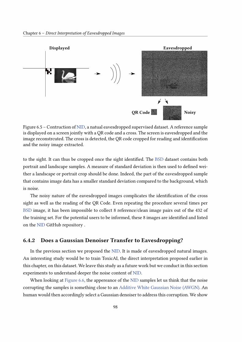
Chapter 6 – Direct Interpretation of Eavesdropped Images
Displayed Eavesdropped
Noisy QR Code
Figure 6.5 – Contruction of NID, a natual eavesdropped supervised dataset. A reference sampleis displayed on a screen jointly with a QR code and a cross. The screen is eavesdropped and theimage reconstrcuted. The cross is detected, the QR code cropped for reading and identi�cationand the noisy image extracted.
to the sight. It can thus be cropped once the sight identi�ed. The BSD dataset contains bothportrait and landscape samples. A measure of standard deviation is then used to de�ned wei-ther a landscape or portrait crop should be done. Indeed, the part of the eavesdropped samplethat contains image data has a smaller standard deviation compared to the background, whichis noise.
The noisy nature of the eavesdropped images complicates the identi�cation of the crosssight as well as the reading of the QR Code. Even repeating the procedure several times perBSD image, it has been impossible to collect 8 reference/clean image pairs out of the 432 ofthe training set. For the potential users to be informed, these 8 images are identi�ed and listedon the NID GitHub repository .
6.4.2 Does a Gaussian Denoiser Transfer to Eavesdropping?
In the previous section we proposed the NID. It is made of eavesdropped natural images.An interesting study would be to train ToxicAI, the direct interpretation proposed earlier inthis chapter, on this dataset. We leave this study as a future work but we conduct in this sectionexperiments to understand deeper the noise content of NID.
When looking at Figure 6.6, the appereance of the NID samples let us think that the noisecorrupting the samples is something close to an Additive White Gaussian Noise (AWGN). Anhuman would then accordingly select a Gaussian denoiser to address this corruption. We show
98
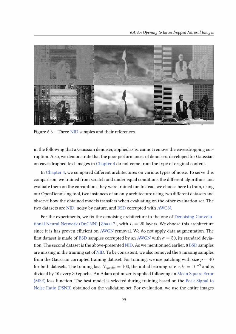
6.4. An Opening to Eavesdropped Natural Images
Figure 6.6 – Three NID samples and their references.
in the following that a Gaussian denoiser, applied as is, cannot remove the eavesdropping cor-ruption. Also, we demonstrate that the poor performances of denoisers developed for Gaussianon eavesdropped text images in Chapter 4 do not come from the type of original content.
In Chapter 4, we compared di�erent architectures on various types of noise. To serve thiscomparison, we trained from scratch and under equal conditions the di�erent algorithms andevaluate them on the corruptions they were trained for. Instead, we choose here to train, usingour OpenDenoising tool, two instances of an only architecture using two di�erent datasets andobserve how the obtained models transfers when evaluating on the other evaluation set. Thetwo datasets are NID, noisy by nature, and BSD corrupted with AWGN.
For the experiments, we �x the denoising architecture to the one of Denoising Convolu-tional Neural Network (DnCNN) [Zha+17], with L = 20 layers. We choose this architecturesince it is has proven e�cient on AWGN removal. We do not apply data augmentation. The�rst dataset is made of BSD samples corrupted by an AWGN with σ = 50, its standard devia-tion. The second dataset is the above-presented NID. As we mentionned earlier, 8 BSD samplesare missing in the training set of NID. To be consistent, we also removed the 8 missing samplesfrom the Gaussian corrupted training dataset. For training, we use patching with size p = 40for both datasets. The training last Nepochs = 100, the initial learning rate is lr = 10−3 and isdivided by 10 every 30 epochs. An Adam optimizer is applied following an Mean Square Error(MSE) loss function. The best model is selected during training based on the Peak Signal toNoise Ratio (PSNR) obtained on the validation set. For evaluation, we use the entire images
99

Chapter 6 – Direct Interpretation of Eavesdropped Images
TrainingEvaluation AWGN σ = 50 Eavesdropping
AWGN σ = 50 25.57/0.71 9.68/0.40Eavesdropping 6.51/0.16 16.29/0.52No Denoising 14.15/0.15 9.27/0.25
Table 6.3 – PSNR (dB) and SSIM measures for two DnCNNs. The models are trained on a datasetcorrupted by AWGN and by eavesdropping. The evaluation is conducted for both models onthe two corruptions. Metrics on the noisy sets are given as a reference.
of BSD68 accordingly corrupted and measure the performances using PSNR and StructuralSimilarity (SSIM).
Table 6.3 presents the results of the evaluation of the two trained models on the two cor-rupted evaluation sets. The metrics computed on the noisy sets are given as a reference. Weobserve from this tab that a denoiser trained for AWGN does not operate well when appliedas is on eavesdropping samples. In fact, the model trained on AWGN obtains an average PSNRof 9.68dB on the eavesdropped evaluation set while its score was 25.57dB on its own evalu-ation set. regarding SSIM, the denoising results in a progressiion of 46%. However, the indexvalue is still limited with a value of 0.4. The conclusion is the same on the opposite way,a denoiser trained on eavesdropped samples cannot restore AWGN-corrupted samples. Themodel trained on eavesdropped images obtains an average PSNR of 16.29dB on the eaves-dropped evaluation set while its score drops to 6.51dB on the AWGN evaluation set. Applyinga denoiser for eavesdropped samples on AWGN-corrupted samples even degrades the imagequality.
Figure 6.7 displays visual results of applying the two models on the evaluation sets, fortwo images. The �rst column shows the noisy versions of the two images. The second columndisplays the images denoised using the model trained for AWGN removal. The third columnpresents the images denoised using the model trained for eavesdropping corruption removal.Finally, the clean images are given as reference. This �gure shows that the eavesdropping cor-ruption is poorly removed, even when using the model trained accordingly. It also con�rmsthat it is not possible to transfer a model, learned on a denoising corruption, to another cor-ruption. In fact, the images denoised by the model that was not trained for this corruptionhave a poor quality. As an example, on the second image, corrupted with AWGN and denoisedwith the model for eavesdropping corruption, the train is not visible after denoising.
These experiments bring three majors conclusions. First, it is not possible to transfer di-rectly a denoiser trained on a corruption A to the removal of a corruption B. Second, the
100
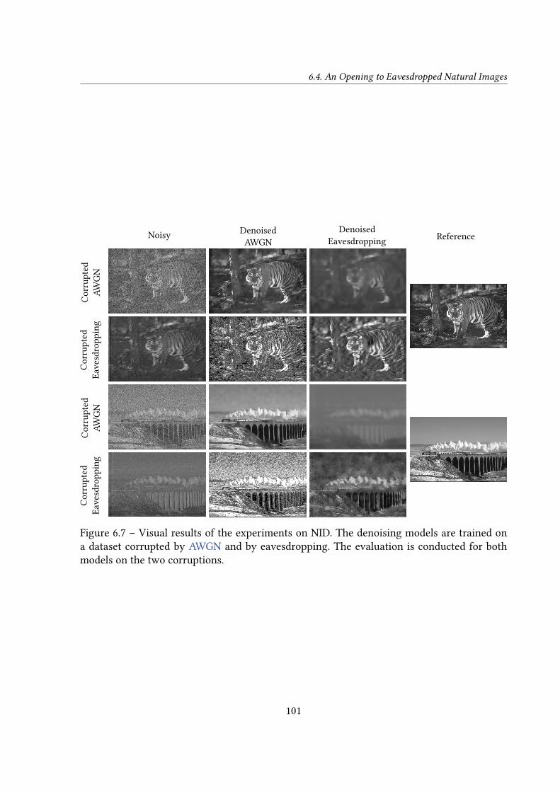
6.4. An Opening to Eavesdropped Natural ImagesC
orru
pted
AW
GN
C
orru
pted
Eave
sdro
ppin
g
Noisy DenoisedAWGN
DenoisedEavesdropping Reference
Cor
rupt
edA
WG
N
Cor
rupt
edEa
vesd
ropp
ing
Figure 6.7 – Visual results of the experiments on NID. The denoising models are trained ona dataset corrupted by AWGN and by eavesdropping. The evaluation is conducted for bothmodels on the two corruptions.
101
Chapter 6 – Direct Interpretation of Eavesdropped Images
eavesdropping noise cannot be simulated using an AWGN distribution. Finally, the results ofTable 6.3 suggest that the DnCNN architecture designed for AWGN does not perform wellon eavesdropped image removal, even with according training. In fact, we observe that the∆P SNR (denoised PSNR - noisy PSNR) is 4.4dB lower for eavesdropping, compared to AWGN.It must be noted that the initial eavesdropped samples have a worst quality with an averagePSNR of 9.27dB compared to the 14.15dB of the AWGN dataset.
Finally, a second case study is conducted. It aims at evaluating how a gaussian denoiserextend to the removal of eavedropping corruption. Two conclusions are drawn from the ex-periments. First, a model trained for AWGN cannot be used as is on eavesdropped samples.Second, when properly trained, the DnCNN architecture brings the same denoising ratio onAWGN and eavesdropping corruption.
6.5 Conclusions
This chapter has presented how an EM side-channel attack can be automated, from dataretrieval to data interpretation, by employing deep learning methods. The employed experi-mental setup for demonstrating fully automated information extraction is based on the MaskR-CNN network and on the eavesdropping of textual information. The �nal setup is capableof recovering 57% of a leaked textual information from a standard screen.
This chapter shows that taking some assumptions on image content, the information inter-ception process can be fully automated until semantic extraction. Such an automation opensfor future work on automated audit and countermeasures.
102
CHAPTER 7
Conclusion
As shown throughout this document, Electro Magnetic (EM) compromising emanationsare a threat to the con�dentiality of Information Processing Equipments (IPEs) that handlesensitive information. Analyzing a side-channel, an attacker may have access to con�dentialinformation. Due to voltage changes, video signals transmitted through cables and connectorsare subject to EM side-channel emanations. The transmitted images may be recovered fromthis side-channel but reconstructed images are strongly corrupted. At the same time as theresearch on enhancing EM side-channel attacks progresses, Deep Learning (DL) has revolu-tionnized image restoration and interpretation. In this context, this document has proposedstudies to evaluate the interest of image processing and DL to reinforce the restoration andinterpretation of eavesdropped images.
These studies demonstrate several elements. State of the art restoration and interpretationmethods do not directly transfer to eavesdropped images. In fact, the corruption contained inthese images is hybrid, because of the origins of the corruption (noise, interferences, informa-tion overlap), and does not follow simple parametric distributions. However, it is di�cult toseparate the di�erent contributions of that hybrid corruption. While using a gradual removalstrategy has proven its e�ciency on mixtures of simple parametric noises, eavesdropping noisecannot be removed based on an usual parametric noise using such method. Training learningbased image restoration with custom data, it is nevertheless possible to remove part of thiscomplicated corruption. Finally, it has been proven that DL can automate the interpretation ofeavesdropped images containing textual information. With an automated synchronization of
the interception process, this is a step further towards fully automated EM emanations exloi-tation.
The contributions presented in this thesis are among the �rst published on the use of imageprocessing to enhance and automate the interpretation of images reconstructed from EM side-channel emanations. In addition to providing promising results, several implementations areprovided open source on GitHub.
7.1 Research Contributions
To progress on the interpretation of eavesdropped images, Chapter 2 has given an overviewof the state of the art rastering techniques as well as on the origins of the hybrid noise gen-erated by the eavesdropping process. Given these �ndings, Chapter 3 has introduced imageprocessing features likely to be used for eavesdropped image restoration and interpretation.The three main contributions proposed in this manuscript rely on these preliminary chaptersand are summarized in this section.
7.1.1 Benchmarking of Image Restoration Algorithms
Chapter 3 has highlighted the complexity of fairly comparing methods evaluated in di�er-ent conditions. To solve this issue, the OpenDenoising tool has been proposed in Chapter 4.OpenDenoising benchmarks image denoisers and aims at comparing methods on a commonground in terms of datasets, training parameters and evaluation metrics. Supporting severallanguages and learning frameworks, OpenDenoising is also extensible and open-source.
The second contribution of the chapter is a comparative study of image restoration inthe case of a complex noise source, including eavesdropped images. Three major conclusionsarise from the comparative study. First, the di�erence in terms of performance between expert-based and learning-based methods rises as the complexity of the noise grows. Second, the rank-ing of methods is strongly impacted by the nature of the noises. Finally, Multi-level WaveletConvolutional Neural Network (MWCNN) proves to be the best method for the consideredreal-world interception restoration task. It slightly outperforms Denoising Convolutional Neu-ral Network (DnCNN) and RED30 while being substantially faster, in inference mode.
These results show that restoring an image from a complex noise is not universally solvedby a single method and that choosing a denoiser requires automated testing.
104
This chapter has led to the public release of the OpenDenoising benchmark tool 1.
7.1.2 Mixture Noise Denoising Using a Gradual Strategy
Chapter 2 and Chapter 3 have suggested that the corruption generated by the eavesdrop-ping process is a sequential mixture of several primary corruptions.
Chapter 5 introduces a gradual image denoising strategy called NoiseBreaker. Noise-Breaker iteratively detects the image dominating noise using a trained classi�er with an ac-curacy of 93% and 91% for grayscale and RGB samples, respectively, when primary noisesare known and parametrized. Under the assumption of grayscale sequential noise mixtures,NoiseBreaker performs only 0.95dB under the supervised MWCNN denoiser without beingtrained on any mixture noise. Neither the classi�er nor the denoisers are exposed to mixturenoise during training. NoiseBreaker operates 2dB over the gradual denoising of [LSJ20] and5dB over the state of the art self-supervised denoiser Noise2Void. When using RGB samples,NoiseBreaker operates 5dB over [LSJ20] while Noise2Void underperforms. Moreover, this pa-per demonstrates that making noise analysis guide the denoising is not only e�cient on noisetype, but also on noise intensity.
This chapter has demonstrated the practicality of NoiseBreaker on six di�erent syntheticnoise mixtures. Nevertheless, the NoiseBreaker version proposed in the chapter has not per-mitted to conclude on the e�ciency of the method to restore eavesdropped images. Con-sequently, it is not possible to validate the hypothesis of the sequential composition of theeavesdropping corruption.
7.1.3 Direct Interpretation of Eavesdropped Images
Handling data while ensuring trust and privacy is challenging for information system de-signers. Chapter 6 presents how the attack surface can be enlarged with the introduction ofdeep learning in an EM side-channel attack. The proposed method, called ToxicAI, uses MaskR-CNN as denoiser and it automatically recovers more than 57% of characters, present in thetest set. In comparison, the best denoising/Optical Character Recognition (OCR) pair retrieves42% of characters. The proposal is software-based, and runs on the host computer of an o�-the-shelf Software-De�ned Radio (SDR) platform.
This chapter has led to the public release of two datasets of eavesdropped samples:
1. https://github.com/opendenoising/opendenoising-benchmark
105

• a dataset of eavesdropped images made of text characters and their references 2,• a dataset of eavesdropped natural images, based on Berkeley Segmentation Dataset
(BSD), dubbed Natural Interception Dataset (NID) 3.
7.2 Prospects – Future Works
The work presented in this document opens opportunities for future research on eaves-dropped image restoration and interpretation. This section proposes research directions to godeeper using our proposed methods, but also more general research directions.
7.2.1 Signal Detection in Eavesdropping Noise
In Chapter 2 we explained why we study the application of image processing techniques toeavesdropped images. We then hypothetised that leveraging such methods, it could be possibleto relax the required precision when setting up the raster process that transform the 1D signalinto an image.
To continue in this direction it would be interesting to design a signal detection method ineavesdropped images. In fact, we hypothetize that when the interception system reconstructsan image from a signal that contains no information (no screen emanations or nothing dis-played on the screen), the reconstruction should be composed of pure noise. Once a signalmixes to this pure noise (content on the screen), the recontructed image ditribution shoulddeviate. Identi�ng these two cases would enable predicting whether a screen with potentialcompromising content is present in the area. Such problem may be solved creating a customdataset and using a binary classi�er predicting whether there is signal or not in an image.
7.2.2 Fine-Grain Modeling of the Eavesdropping Corruption
We proposed in Chapter 2 a list of the contributing elements to the strong hybrid corrup-tion generated by the eavesdropping process. While questionning the content of this hybridcorruption, we did not give a �ne-grain modeling.
Following the previous point on signal detection in noise, the same data could be used tomodel the noise generated by the side-channel. In fact, when no screen data is contained in thereconstructed image, an illustration of the noise distribution is accessible. The modeling of the
2. https://github.com/opendenoising/interception_dataset3. https://github.com/opendenoising/NID
106
other part of the corruption seems more complicated since it depends on the characteristicsof the data to be eavesdropped.
Additionally, leveraging learning algorithms, modeling the eavesdropping corruption us-ing Generative Adversarial Networks (GAN) could also be a promising direction. Once a gener-ative model is trained, it would be possible to generate training datasets for further restorationand interpretation methods.
7.2.3 Interpretability of Eavesdropped Images
In Chapter 6, we presented ToxicAI as proof of concept on the e�ciency of learning algo-rithms on interpretation of eavesdropped images. ToxicAI is designed to retrieve charactersin eavesdropped images. This contribution introduces a custom metric that consists in mea-suring the number of character retrieved in an image instead of using classical metrics likePeak Signal to Noise Ratio (PSNR) or Structural Similarity (SSIM). This metric is a �rst stepin measuring the interpretability of eavesdropped images. However, this metric is limited totextual content.
A future work could consist in developing new methods to assess further the interpretabil-ity of eavesdropped images. As an example, a progressive tree testing could be proposed. Fromthe root to the leafs, each node represents a test on the information extracted from the inputimage. The deeper the process goes, the deeper the knowledge extractable from the image andthe higher the interpretability. The interpretability of eavesdropped images is a crucial pa-rameter since it enables assessing the potential compromise of detected emanations. Knowingsuch measure would enable �ner countermeasures to avoid sensitive information di�usion.
7.2.4 Extension to Other Noisy Data
Throughout this manuscript, we have worked with noisy data. In particular, the eaves-dropped images that motivated our studies are corrupted by complex noises. There are otherdomains that deal with noisy images because of their acquisition conditions or sensing tech-nologies. Among these domains medical images and spatial imaging seems related to our workbecause of their high corruption levels. Adapting our proposed methods to these applicationsmay be a promising direction. Also, we hypothesize that the diversity of the corruption, con-tained in the two datasets we propose (NID in particular), may make our methods applicabledirectly to other complex problems. As an example, we have experienced good results at de-
107
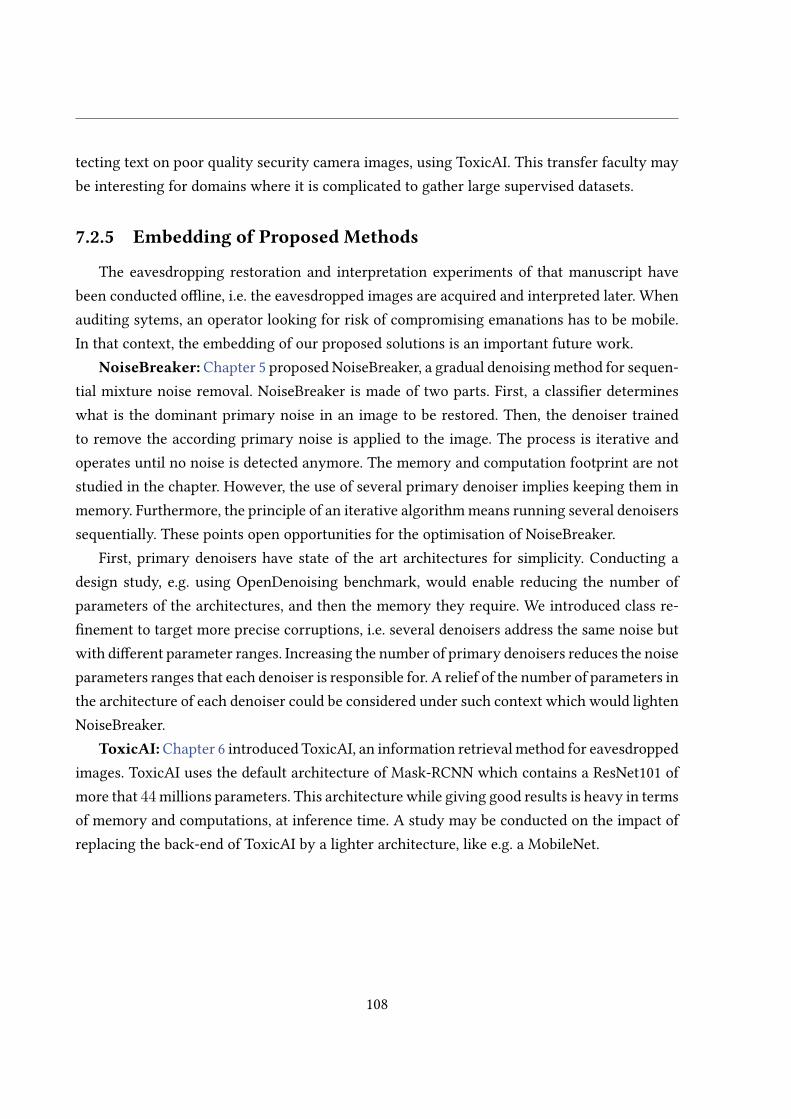
tecting text on poor quality security camera images, using ToxicAI. This transfer faculty maybe interesting for domains where it is complicated to gather large supervised datasets.
7.2.5 Embedding of Proposed Methods
The eavesdropping restoration and interpretation experiments of that manuscript havebeen conducted o�ine, i.e. the eavesdropped images are acquired and interpreted later. Whenauditing sytems, an operator looking for risk of compromising emanations has to be mobile.In that context, the embedding of our proposed solutions is an important future work.
NoiseBreaker: Chapter 5 proposed NoiseBreaker, a gradual denoising method for sequen-tial mixture noise removal. NoiseBreaker is made of two parts. First, a classi�er determineswhat is the dominant primary noise in an image to be restored. Then, the denoiser trainedto remove the according primary noise is applied to the image. The process is iterative andoperates until no noise is detected anymore. The memory and computation footprint are notstudied in the chapter. However, the use of several primary denoiser implies keeping them inmemory. Furthermore, the principle of an iterative algorithm means running several denoiserssequentially. These points open opportunities for the optimisation of NoiseBreaker.
First, primary denoisers have state of the art architectures for simplicity. Conducting adesign study, e.g. using OpenDenoising benchmark, would enable reducing the number ofparameters of the architectures, and then the memory they require. We introduced class re-�nement to target more precise corruptions, i.e. several denoisers address the same noise butwith di�erent parameter ranges. Increasing the number of primary denoisers reduces the noiseparameters ranges that each denoiser is responsible for. A relief of the number of parameters inthe architecture of each denoiser could be considered under such context which would lightenNoiseBreaker.
ToxicAI:Chapter 6 introduced ToxicAI, an information retrieval method for eavesdroppedimages. ToxicAI uses the default architecture of Mask-RCNN which contains a ResNet101 ofmore that 44 millions parameters. This architecture while giving good results is heavy in termsof memory and computations, at inference time. A study may be conducted on the impact ofreplacing the back-end of ToxicAI by a lighter architecture, like e.g. a MobileNet.
108

APPENDIXA
French Summary
A.1 Contexte
La tendance récente consiste à rendre les données numériques disponibles à tout momentet en tout lieu, ce qui crée de nouvelles menaces pour la con�dentialité. En particulier, si l’onconsidère les données hautement con�dentielles, là où les informations imprimées étaient pro-tégées physiquement et n’étaient accessibles qu’aux personnes autorisées, les données sontaujourd’hui numériques. Les données sont échangées et consultées en utilisant des systèmesd’information (SI) et leurs a�cheurs vidéo correspondants. Si les principaux e�orts de sécu-rité se concentrent aujourd’hui sur le côté réseau des systèmes, il existe d’autres menaces desécurité.
Un canal auxiliaire est un chemin de données non intentionnel en opposition avec lecanal traditionnel. En particulier, les canaux auxiliaires électro-magnétiques (EM) sont dusaux champs émis par les câbles et connecteurs vidéo lorsque leur tension interne change. Cescanaux auxiliaires sont dangereux car ils propagent des données non chi�rées en dehors dusystème physique. Ces émissions peuvent être corrélées à une information con�dentielle. Unattaquant recevant le signal et connaissant les protocoles de communication peut accéder illé-galement aux informations originales traitées par le SI. Dans ces conditions, l’attaquant peutreconstruire l’image a�chée sur l’écran attaqué connecté au SI. Il a été démontré que le con-tenu d’un écran peut être recontruit à des dizaines de mètres [DSV20a]. Depuis les exploitsdes pionniers [Van85], de nombreux travaux ont été publiés sur la reconstruction d’imagesà partir d’émanations EM par canal auxiliaire, et ce domaine de recherche est toujours dy-

namique [Lav+21]. Les travaux de l’état de l’art menés sur ce sujet ont principalement portésur l’amélioration de la reconstruction d’un point de vue du traitement du signal.
Récemment, le domaine du traitement d’images a été révolutionné par l’apparentissagemachine et surtout l’apprentissage profond. Ces algorithmes, qui apprennent des tâches à par-tir de données, ont dépassé les performances des algorithmes experts de l’état de l’art surplusieurs tâches de vision par ordinateur. En particulier, l’une des tâches qui a béné�cié desalgorithmes d’apprentissage est la classi�cation sémantique du contenu des images. Dans cettetâche, les algorithmes de l’état de l’art sont aujourd’hui capables d’automatiser l’interprétationdes images. Cependant, ces méthodes d’interprétation sont conçues pour des images naturellesnon corrompues. La restauration d’images est la tâche qui consiste à supprimer les altéra-tions des images. La restauration d’images a également beaucoup béné�cié des algorithmesd’apprentissage. En e�et, les algorithmes récents surpassent les anciens algorithmes de l’étatde l’art, tant sur les performances objectives que subjectives. Cependant, les algorithmes derestauration d’images de l’état de l’art se concentrent sur des corruptions bien dé�nies, quisuivent une distribution paramétrique, régie par quelques paramètres.
Les images reconstruites à partir des émanations EM sont fortement corrompues pourplusieurs raisons. Il y a d’abord une perte de données et des interférences inhérentes au pro-cessus d’émission/réception EM. Il existe également des défauts dans la synchronisation de lareconstruction, lors du passage du signal 1D à une image. En�n, les défauts du matériel dusystème d’interception introduisent des erreurs. Il en découle trois questions que nous étu-dions dans ce manuscrit : Quel est le type de corruption généré par la reconstructiond’émanations EM ? Peut-elle être réduite à une composition de bruits aux distribu-tion paramétriques ? Comment les méthodes actuelles de restauration d’images secomportent-elles sur une image interceptée ?
L’audit des systèmes d’information traitant des données con�dentielles est actuellementréalisé par des experts. Une fois le système d’interception en place, l’expert évalue la com-promission de l’équipement audité, en s’appuyant sur son expérience. Ce protocole d’auditprend du temps et est sujet à la perception humaine. Vient alors une autre question que nousétudions dans ce manuscrit : Peut-on utiliser l’apprentissage profond pour automatiserl’interprétation sémantique d’images interceptées ?
110

A.2 Objectifs et contributions de cette thèse
L’objectif principal de cette thèse est d’analyser comment les techniques d’apprentissageprofond peuvent être appliquées aux images interceptées et si elles peuvent automatiserl’interprétation de ces images. Bien que la reconstruction d’émanations EM et le traitementd’images par apprentissage profond soient deux domaines très étudiés, leur utilisation con-comitante est une avancée récente.
Après avoir passé en revue les travaux fondamentaux sur l’interception et l’interprétationd’images bruitées, nous proposons un ensemble d’expériences et de contributions pour étudierla faisabilité de l’exploitation automatique des images d’interception.
Trois contributions principales sont proposées dans ce document. Elles sont parmi les pre-mières études des émanations EM d’un point de vue traitement d’image. En conséquence,cette thèse est l’une des premières tentatives d’application de l’apprentissage profond pourl’automatisation de l’exploitation d’images d’interception. Les trois principales contributionsde cette thèse sont brièvement présentées ci-dessous.
A.2.1 Comparaison d’algorithmes de restauration d’images
Comparer équitablement les débruiteurs est devenu compliqué avec l’utilisation d’algorithmesd’apprentissage. En e�et, les algorithmes peuvent être entraînés et évalués sur di�érents en-sembles de données, ce qui rend la comparaison injuste sans ré-entraînement. C’est un prob-lème lorsqu’on cherche des méthodes pour un nouveau système. L’outil proposé, nomméOpenDenoising, évalue les débruiteurs d’images et vise à comparer les méthodes sur un ter-rain commun en termes de jeux de données, de paramètres d’apprentissage et de métriquesd’évaluation. Supportant plusieurs langages et outils d’apprentissage, OpenDenoising estégalement extensible et open-source.
La deuxième contribution du chapitre est une étude comparative de la restaurationd’images dans le cas d’une source de bruit complexe. Les expériences de cette étude compar-ative sont utilisées comme étude de cas pour l’outil proposé. Plusieurs conclusions sont tiréesde l’étude comparative. Premièrement, il existe une di�érence en termes de performance entreles méthodes basées sur l’expertise et celles basées sur l’apprentissage. Cette di�érence aug-mente avec la complexité du bruit. Deuxièmement, le classement des méthodes est fortementin�uencé par la nature des bruits. Ces résultats montrent que la restauration d’une image cor-rompue par un bruit complexe n’est pas universellement résolue par une seule méthode et quele choix d’un débruiteur nécessite des tests automatisés.
111

Ce chapitre a conduit à la publication de l’outil OpenDenoising 1. Ces travaux ont étéprésentés lors de la conférence internationale IEEE International Conference on Acoustics,Speech and Signal Processing (ICASSP) en 2020 [Lem+20c].
A.2.2 Débruitage graduel de mélanges de bruit
Les chapitres préliminaires suggèrent que la corruption générée par le processusd’interception EM est un mélange séquentiel de plusieurs corruptions primaires. En con-séquence, le chapitre 5 introduit une stratégie graduelle de débruitage d’image appelée Noise-Breaker. NoiseBreaker détecte itérativement le bruit dominant de l’image à l’aide d’un classi�-cateur entraîné avec une précision de 93 % et 91 % pour les échantillons en niveaux de gris etrouge-vert-bleu (RVB), respectivement. Dans l’hypothèse de mélanges de bruits séquentiels enniveaux de gris, NoiseBreaker obtient une performance de 0, 95dB en dessous du débruitagesupervisé utilisant MWCNN sans avoir été entraîné sur un quelconque mélange de bruits. Ni leclassi�cateur, ni les débruiteurs ne sont exposés au mélanges de bruit pendant l’entraînement.NoiseBreaker opère 2dB au dessus du débruitage graduel de [LSJ20] et 5dB au dessus de l’étatde l’art du débruitage auto-supervisé Noise2Void. Lorsqu’il utilise des échantillons RVB, Noise-Breaker a une performance supérieure de 5dB à celle de [LSJ20] alors que Noise2Void est moinsperformant. De plus, cet article démontre que l’utilisation de l’analyse du bruit pour guider ledébruitage est e�cace non seulement sur le type de bruit, mais aussi sur son intensité.
Ce chapitre démontre l’aspect pratique de NoiseBreaker sur six di�érents mélanges debruits synthétiques. Néanmoins, la version de NoiseBreaker proposée dans le chapitre n’a paspermis de conclure quand à l’e�cacité de la méthode pour restaurer des images interceptées.Par conséquent, l’hypothèse de la composition séquentielle de la corruption d’interceptionn’est pas validée.
Ce travail a donné lieu à une présentation lors du workshop IEEE 22nd International Work-shop on Multimedia Signal Processing (MMSP) en 2020 [Lem+20a].
A.2.3 Interprétation directe d’images interceptées
Ce travail est présenté dans le dernier chapitre de contribution du manuscrit. Le débutdu manuscrit étudie l’applicabilité de l’apprentissage profond pour restaurer des images in-terceptées. Ce dernier travail se concentre sur l’interprétation et étudie son automatisationsur des images textuelles. L’introduction de l’apprentissage profond dans une attaque de type
1. https://github.com/opendenoising/opendenoising-benchmark
112

canal auxiliaire EM est étudiée. La méthode proposée utilise Mask R-CNN comme débruiteuret récupère automatiquement plus de 57% des caractères présents dans le jeu de test et cepour une large gamme de distances d’interception. La proposition est logicielle et s’exécutesur l’ordinateur hôte d’une plateforme radio-logicielle prête à l’emploi.
Ce chapitre a conduit à la di�usion publique de deux ensembles de données d’images in-terceptées :• un jeu de données d’images synthétiques d’interception composées de caractères de
texte et de leurs références 2,• un jeu de données d’images naturelles interceptées, basé sur BSD, nommé NID 3.Ce travail a été présenté lors de la conférence Conference on Arti�cal Intelligence for Defense
(CAID), en 2019 [Lem+19] et lors de la conférence IEEE International Conference on Acoustics,Speech and Signal Processing (ICASSP) en 2020 [Lem+20b].
A.3 Plan du Manuscrit
Le chapitre 2 présente ce qu’est une interception électro-magnétique et en quoi elle con-stitue une menace pour la con�dentialité des système d’information utilisant des écrans. Lescaractéristiques de l’interception sont étudiées. En particulier, le lien est fait entre les corrup-tions trouvées dans les images et leur origine physique. En�n, des arguments sont donnés quimotivent l’étude du traitement d’images pour améliorer l’interprétation des images intercep-tées.
Le chapitre 3 donne une dé�nition du bruit dans une image. Les principales distributions debruit dans les images sont détaillées, ce qui ouvre la voie à l’introduction de compositions pluscomplexes de ces distributions. Le chapitre passe ensuite en revue l’état de l’art des méthodesde restauration et d’interprétation d’images. Une distinction est faite entre les algorithmesexperts et ceux basés sur l’apprentissage. L’avancée en termes de performance permise parces derniers est discutée. Des métriques d’évaluation et d’optimisation ainsi que des jeux dedonnées sont présentés pour l’évaluation de la qualité des images et de la classi�cation. En�n,la terminologie des algorithmes d’apprentissage ainsi que des discussions sur leurs forces etles questions ouvertes pour notre étude de cas sont proposées.
Le chapitre 4 propose un outil extensible et open-source pour évaluer les algorithmes dedébruitage équitablement. Ensuite, une étude comparative de l’état de l’art des débruiteurs est
2. https://github.com/opendenoising/interception_dataset3. https://github.com/opendenoising/NID
113

présentée. Cette étude comparative apporte également des premières réponses sur la suppres-sion du bruit d’interception dans les images.
Le chapitre 5 présente NoiseBreaker, une méthode progressive de débruitage d’images quis’attaque à la suppression du bruit de mélange séquentiel. Les travaux connexes de l’état del’art sont exposés avant de détailler la méthode proposée qui s’appuie sur une stratégie itéra-tive. Le bruit dominant est détecté avant d’être supprimé. La méthode est comparée à l’état del’art avant d’être discutée dans une étude d’ablation.
Le chapitre 6 aborde l’interprétation directe d’images interceptées en proposant ToxicAI.Les travaux connexes sont présentés avant de dé�nir l’architecture de ToxicAI. La constructionde l’ensemble de données personnalisées, open-source, d’écrans interceptées contenant descaractères, utilisé pour former ToxicAI, est détaillée. Ensuite, des expériences sont menées surla proposition et les résultats sont comparés à l’état de l’art. En�n, un jeu de données open-source d’images naturelles interceptées est proposé pour étendre ToxicAI.
Le chapitre 7 conclut le manuscrit. Tout d’abord, les questions adressées dans le documentsont rappelées et les contributions sont résumées. En s’appuyant sur les principes proposésdans ce document, des directions de recherche pour le futur de l’interprétation des imagesinterceptées sont proposées.
La �gure A.1 illustre l’organisation de ce document. Cette �gure met en évidence les liensentre les chapitres présentés ci-dessus.
114
[Lem+20c]
Comparaison d'Algorithmes de Restauration d'Images
Débruitage Graduelde Mélanges de Bruit
Chap. 4
Chap. 5
Chap. 6 Interprétation Directed'Images Interceptées
[Lem+19, Lem+20a]
[Lem+20b]
Chap. 2 Interception d'Émissions Électro-Magnétiques
Chap. 3 Interprétationd'Images Bruitées
Figure A.1 – Structure générale du document. Les chapitres sur l’état de l’art sont a�chés enblanc, tandis que les chapitres de contribution sont en gris.
115

List of Figures
1.1 Outline of the overall document structure . . . . . . . . . . . . . . . . . . . . . 14
2.1 Con�dentiality, Integrity, Accessibility (CIA) triad schematic . . . . . . . . . . 182.2 Principle schematic of a Side-Channel . . . . . . . . . . . . . . . . . . . . . . 192.3 Di�erent video connectors that may emit compromising emanations. . . . . . 222.4 EM Side-Channel attack system setup . . . . . . . . . . . . . . . . . . . . . . . 232.5 Display of the extra borders of an eavesdropped image . . . . . . . . . . . . . 232.6 Display of mis-synchronization and borders in an eavesdropped image . . . . 242.7 Schematic of the noise sources in the reception chain . . . . . . . . . . . . . . 252.8 Display of horizontal spreading due to sampling under the pixel frequency . . 262.9 Examples of corruptions contained in an eavesdropped image . . . . . . . . . 262.10 Segmentation and classi�cation applied to an eavesdropped image. . . . . . . 272.11 Haar discrete wavelet transform applied to an eavesdropped image. . . . . . . 29
3.1 Processings to be applied to a noisy image . . . . . . . . . . . . . . . . . . . . 323.2 Example of a Moire corruption . . . . . . . . . . . . . . . . . . . . . . . . . . . 343.3 Principle schematic of a denoising algorithm . . . . . . . . . . . . . . . . . . . 363.4 Confusion matrix used for F-score and accuracy metrics computation. . . . . . 443.5 Cross-entropy computation example . . . . . . . . . . . . . . . . . . . . . . . . 453.6 Schematic of the main network dimensions . . . . . . . . . . . . . . . . . . . . 49
4.1 OpenDenoising benchmark block diagram . . . . . . . . . . . . . . . . . . . . 594.2 Comparison of the inference times of denoisers using OpenDenoising benchmark 60
116
4.3 Boxplot of denoised images PSNR from results of OpenDenoising benchmark 624.4 Visual results display from benchmark study . . . . . . . . . . . . . . . . . . . 63
5.1 Visual comparison between the denoising of traditional and gradual denoising 685.2 Example of NoiseBreaker gradual denoising . . . . . . . . . . . . . . . . . . . 735.3 Qualitative results of NoiseBreaker on BSD68 dataset . . . . . . . . . . . . . . 785.4 Log scale confusion matrices of noise classi�cation in NoiseBreaker . . . . . . 805.5 Display of images where the NiseBreaker diverges from the expectation . . . . 83
6.1 Automated EM Side-Channel Interpretation Setup . . . . . . . . . . . . . . . . 886.2 Principle of the eavesdropped character dataset construction . . . . . . . . . . 906.3 The di�erent outputs of Mask R-CNN given an eveasdropped sample . . . . . 926.4 Visual denoising results comparison between ToxicAI and compared methods 936.5 NID construction . . . . . . . . . . . . . . . . . . . . . . . . . . . . . . . . . . 986.6 Three NID samples and their references. . . . . . . . . . . . . . . . . . . . . . 996.7 Visual results for the evaluation of models on corruptions they are not trained
for. . . . . . . . . . . . . . . . . . . . . . . . . . . . . . . . . . . . . . . . . . . 101
A.1 Schéma de la structure générale du document . . . . . . . . . . . . . . . . . . 115
117

List of Tables
3.1 Presented restoration methods and their targeted noise . . . . . . . . . . . . . 403.2 Popular datasets for learning algorithms . . . . . . . . . . . . . . . . . . . . . 473.3 Table of Notation of Learning Algorithms . . . . . . . . . . . . . . . . . . . . . 48
4.1 Benchmarking results expressed in SSIM and PSNR . . . . . . . . . . . . . . . 60
5.1 List of classes for NBreaker-N and the noise type and level they represent. . . 745.2 List of classes for NBreaker, the noise type/level and related denoiser. . . . . . 755.3 PSNR results of the enchmark study of primary denoisers to be used in Noise-
Breaker . . . . . . . . . . . . . . . . . . . . . . . . . . . . . . . . . . . . . . . . 765.4 Average PSNR(dB)/SSIM results on BSD and DIV2K of NoiseBreaker and com-
peting methods . . . . . . . . . . . . . . . . . . . . . . . . . . . . . . . . . . . 775.5 De�nition of the noise mixtures used for NoiseBreaker evaluation . . . . . . . 775.6 PSNR results of the comparison between NoiseBreaker and a fully-supervised
MWCNN . . . . . . . . . . . . . . . . . . . . . . . . . . . . . . . . . . . . . . . 815.7 Backbone comparison for the noise classi�er of NoiseBreaker . . . . . . . . . 845.8 PSNR results of comparison of backbone to be used as the classi�er of Noise-
Breaker . . . . . . . . . . . . . . . . . . . . . . . . . . . . . . . . . . . . . . . . 845.9 PSNR results of the comparison between NBreaker-I and NoiseBreaker . . . . 855.10 PSNR results of the comparison between NBreaker-N and NoiseBreaker . . . . 855.11 PSNR results of the comparison between NBreaker-S and NoiseBreaker . . . . 86
6.1 Character recognition performance comparison between several data catchers 95
118
6.2 Inference time comparison between several data catchers . . . . . . . . . . . . 966.3 PSNR results for the evaluation of models on corruptions they are not trained
for. . . . . . . . . . . . . . . . . . . . . . . . . . . . . . . . . . . . . . . . . . . 100
119

Acronyms
AM Amplitude Modulated. 22
AWGN Additive White Gaussian Noise. 33, 40, 50, 52, 55, 57, 58, 60, 61, 63, 64, 71, 79,98–102
BM3D Block-Matching 3D. 37, 38, 40, 50, 57, 60, 61, 63, 64, 72, 76, 79, 81, 82, 93, 95
BSD Berkeley Segmentation Dataset. 13, 46, 50, 97–99, 106, 113
CIA Con�dentiality Integrity Accessibility. 17, 20
CNN Convolutional Neural Network. 37, 38, 41, 48, 50, 57, 58, 70
CPU Central Processing Unit. 21, 60, 94
CRT Cathode Ray Tube. 20, 23
CV Computer Vision. 10, 39, 41, 50
DIP Deep Image Prior. 39, 40
DIV2K DIVerse 2K. 46, 50, 56
DL Deep Learning. 10–12, 41, 50, 51, 61, 86, 103
DnCNN Denoising Convolutional Neural Network. 38, 40, 50, 57, 60, 61, 64, 65, 68, 71, 76,99, 100, 102, 104
DP Display Port. 90, 94
DVI Digital Visual Interface. 21, 90, 94
DWT Discrete Wavelet Transform. 28, 29, 41, 49
EM Electro Magnetic. 9–12, 18–21, 25, 27, 28, 31, 52, 61, 87, 88, 90, 94, 95, 103–105, 116, 117
120

FC Fully Connected. 41, 50, 73
FCN Fully Convolutional Network. 91
FM Frequency Modulated. 22
G2G Generated-Arti�cial-Noise to Generated-Arti�cial-Noise. 35, 39, 40, 71, 79
GAN Generative Adversarial Networks. 38, 107
GCBD GAN-CNN based Blind Denoiser. 35, 39, 40
GPU Graphics Processing Unit. 21, 50, 60, 94
HDMI High-De�nition Multimedia Interface. 21, 24, 25, 90, 94
HOG Histograms of Oriented Gradients. 41
IDCN Implicit Dual-domain Convolutional Network. 37, 40
ILSVRC ImageNet Large Scale Visual Recognition Competition. 41, 46, 50, 71, 83
IPE Information Processing Equipment. 9, 13, 17, 20, 21, 28, 39, 103
IPT Image Processing Transformer. 39, 40
ISS Information System Security. 17
kNN k-Nearest Neighbors. 41
LCD Liquid Crystal Display. 20, 34
LED Light-Emitting Diode. 34
ML Machine Learning. 10, 21, 31, 32, 37, 38, 42, 50
MLP Muli-Layer Perceptron. 41
MOS Mean Opinion Score. 43
MSE Mean Square Error. 42, 43, 45, 99
MWCNN Multi-level Wavelet Convolutional Neural Network. 12, 37, 40, 58, 60, 61, 64, 65,75, 76, 79, 81, 82, 85, 86, 104, 105, 112
N2N Noise2Noise. 39, 40, 58, 70
N2S Noise2Self. 39, 40
N2V Noise2Void. 39, 40, 58, 70, 76, 79, 81, 82
NID Natural Interception Dataset. 13, 65, 97–99, 106, 107, 113, 117
NLP Natural Language Processing. 39
NTIRE New Trends in Image Restoration. 46
121

OCR Optical Character Recognition. 12, 92, 94–96, 105
PSNR Peak Signal to Noise Ratio. 42, 43, 45, 62, 78, 80–82, 99, 100, 102, 107
RED Residual Encoder-Decoder Network. 38, 40
RF Radio Frequency. 89, 90, 92
RGB Red Green Blue. 25, 32, 42, 86
RNN Recurrent Neural Network. 47
RoI Region of Interest. 91
RPN Region Proposal Network. 91
SDR Software-De�ned Radio. 12, 20–23, 87–89, 94, 105
SGN Self-Guided Network. 38, 40, 75, 76, 79
SIFT Scale Invariant Feature Transform. 39
SNR Signal to Noise Ratio. 25, 27
SRResNet Super-Resolution Residual Network. 75, 76, 79
SSIM Structural Similarity. 42, 43, 45, 78, 80, 81, 100, 107
SURF Speed-Up Robust Features. 41
SVM Support Vector machine. 41
VDU Video Display Unit. 9, 13, 17, 20, 21
VGA Video Graphics Array. 21, 90, 94
XAI eXplainable Arti�cial Intelligence. 51
122
Personal Publications
[Lem+19] Florian Lemarchand, Cyril Marlin, Florent Montreuil, Erwan Nogues, andMaxime Pelcat, « ToxicIA: Apprentissage Profond Appliquéà l’Analyse des Sig-naux Parasites Compromettants », in: C&ESAR 2019 IA & Défense, 2019.
[LNP19] Florian Lemarchand, Erwan Nogues, and Maxime Pelcat, « Real-Time Image De-noising with Embedded Deep Learning: Review, Perspectives and Application toInformation System Security », in: RESSI 2019 Rendez-Vous de la Recherche et del’Enseignement de la Sécurité des Systèmes d’Information, 2019.
[Lem+20a] Florian Lemarchand, Thomas Findeli, Erwan Nogues, and Maxime Pelcat,« Noisebreaker: Gradual image denoising guided by noise analysis », in: 2020IEEE 22nd International Workshop on Multimedia Signal Processing (MMSP), IEEE,2020, pp. 1–6.
[Lem+20b] Florian Lemarchand, Cyril Marlin, Florent Montreuil, Erwan Nogues, andMaxime Pelcat, « Electro-Magnetic Side-Channel Attack Through Learned De-noising and Classi�cation », in: ICASSP 2020-2020 IEEE International Conferenceon Acoustics, Speech and Signal Processing (ICASSP), 2020, pp. 2882–2886.
[Lem+20c] Florian Lemarchand, Eduardo Fernandes Montesuma, Maxime Pelcat, and ErwanNogues, « OpenDenoising: an Extensible Benchmark for Building ComparativeStudies of Image Denoisers », in: ICASSP 2020-2020 IEEE International Conferenceon Acoustics, Speech and Signal Processing (ICASSP), IEEE, 2020, pp. 2648–2652.
123

Bibliography
[AB18] Josue Anaya and Adrian Barbu, « RENOIR-A benchmark dataset for real noisereduction evaluation », in: Journal of Visual Communication and Image Represen-tation (2018), pp. 144–154 (cit. on p. 46).
[Abd+20] A. Abdelhamed, M. A��, R. Timofte, and M. S. Brown, « Ntire 2020 challengeon real image denoising: Dataset, methods and results », in: Proceedings of theIEEE/CVF Conference on Computer Vision and Pattern Recognition Workshops,2020, pp. 496–497 (cit. on pp. 35, 69).
[ALB18] Abdelrahman Abdelhamed, Stephen Lin, and Michael S. Brown, « A High-Quality Denoising Dataset for Smartphone Cameras », in: Proceedings of the IEEEConference on Computer Vision and Pattern Recognition (CVPR), June 2018 (cit. onpp. 34, 46).
[AT17] E. Agustsson and R. Timofte, « NTIRE 2017 Challenge on Single Image Super-Resolution: Dataset and Study », en, in: 2017 IEEE Conference on Computer Visionand Pattern RecognitionWorkshops (CVPRW), Honolulu, HI, USA: IEEE, July 2017,pp. 1122–1131 (cit. on pp. 46, 47, 56, 76, 79).
[Bay+08] Herbert Bay, Andreas Ess, Tinne Tuytelaars, and Luc Van Gool, « Speeded-UpRobust Features (SURF) », en, in: Computer Vision and Image Understanding 110.3(June 2008), pp. 346–359 (cit. on p. 41).
[BCM05] A. Buades, B. Coll, and J. M. Morel, « A Review of Image Denoising Algorithms,with a New One », en, in: Multiscale Modeling & Simulation 4.2 (2005), pp. 490–530 (cit. on pp. 36, 37, 40).
125

[BJ15] A. K. Boyat and B. K. Joshi, « A Review Paper : Noise Models in Digital ImageProcessing », en, in: Signal & Image Processing : An International Journal 6.2 (Apr.2015), pp. 63–75 (cit. on p. 36).
[BR19] J. Batson and L. Royer, « Noise2Self: Blind Denoising by Self-Supervision », in:International Conference on Machine Learning, 2019, pp. 524–533 (cit. on pp. 35,39, 40, 67, 71).
[BSH12] Harold C Burger, Christian J Schuler, and Stefan Harmeling, « Image denoising:Can plain neural networks compete with BM3D? », in: 2012 IEEE conference oncomputer vision and pattern recognition, IEEE, 2012, pp. 2392–2399 (cit. on p. 50).
[BT07] ITU-R Recommendation BT, « Methodology for the subjective assessment ofvideo quality in multimedia applications », in: Proceedings of the InternationalTelecommunication Union (2007) (cit. on p. 43).
[Bur98] Christopher JC Burges, « A tutorial on support vector machines for patternrecognition », in: Data mining and knowledge discovery 2.2 (1998), pp. 121–167(cit. on p. 41).
[Che+18] J. Chen, J. Chen, H. Chao, and M. Yang, « Image Blind Denoising with GenerativeAdversarial Network Based Noise Modeling », en, in: 2018 IEEE/CVF Conferenceon Computer Vision and Pattern Recognition, Salt Lake City, UT: IEEE, June 2018,pp. 3155–3164 (cit. on pp. 35, 39, 40).
[Che+20] Hanting Chen et al., « Pre-Trained Image Processing Transformer », en, in:arXiv:2012.00364 [cs] (Dec. 2020), arXiv: 2012.00364 (cit. on pp. 39, 40).
[CM10] P. Chatterjee and P. Milanfar, « Is Denoising Dead? », in: IEEE Transactions onImage Processing 19.4 (Apr. 2010), pp. 895–911 (cit. on pp. 36, 55).
[CPM19] S. Cha, T. Park, and T. Moon, « GAN2GAN: Generative Noise Learning for BlindImage Denoising with Single Noisy Images », en, in: arXiv:1905.10488 [cs, eess](May 2019), arXiv: 1905.10488 (cit. on pp. 35, 39, 40, 67, 71, 79).
[CTH20] Yucheng Chen, Yingli Tian, and Mingyi He, « Monocular Human Pose Estima-tion: A Survey of Deep Learning-based Methods », en, in: Computer Vision andImage Understanding 192 (Mar. 2020), arXiv: 2006.01423, p. 102897 (cit. on p. 39).
126

[Dab+07] K. Dabov, A. Foi, V. Katkovnik, and K. Egiazarian, « Image Denoising by Sparse3-D Transform-Domain Collaborative Filtering », en, in: IEEE Transactions on Im-age Processing 16.8 (Aug. 2007), pp. 2080–2095 (cit. on pp. 36–38, 40, 50, 55, 57,72, 77, 79).
[Dau88] Ingrid Daubechies, « Orthonormal bases of compactly supported wavelets », in:Communications on pure and applied mathematics 41.7 (1988), pp. 909–996 (cit.on p. 28).
[De +18] P. De Meulemeester, L. Bontemps, B. Scheers, and G. A. E. Vandenbosch, « Syn-chronization retrieval and image reconstruction of a video display unit exploitingits compromising emanations », en, in: 2018 International Conference on MilitaryCommunications and Information Systems (ICMCIS), Warsaw: IEEE, 2018, pp. 1–7(cit. on pp. 20, 94).
[De 21] Pieterjan De Meulemeester, Compromising Electromagnetic Radiation of Informa-tion Displays, eng, 2021 (cit. on pp. 21, 22).
[Den+09] J. Deng, W. Dong, R. Socher, L. Li, Kai L., and Li F-F., « ImageNet: A large-scalehierarchical image database », en, in: 2009 IEEE Conference on Computer Visionand Pattern Recognition, Miami, FL: IEEE, June 2009, pp. 248–255 (cit. on pp. 41,46, 47, 61, 71, 76).
[Dos+20] Alexey Dosovitskiy et al., « An Image is Worth 16x16 Words: Transformers forImage Recognition at Scale », en, in: arXiv:2010.11929 [cs] (Oct. 2020), arXiv:2010.11929 (cit. on p. 39).
[DSV20a] P. De Meulemeester, B. Scheers, and G.A.E. Vandenbosch, « Eavesdropping a(Ultra-)High-De�nition Video Display from an 80 Meter Distance Under Real-istic Circumstances », en, in: 2020 IEEE International Symposium on Electromag-netic Compatibility & Signal/Power Integrity (EMCSI), Reno, NV, USA: IEEE, July2020, pp. 517–522 (cit. on pp. 10, 21, 22, 27, 109).
[DSV20b] Pieterjan De Meulemeester, Bart Scheers, and Guy A.E. Vandenbosch, « Di�er-ential Signaling Compromises Video Information Security Through AM and FMLeakage Emissions », en, in: IEEE Transactions on Electromagnetic Compatibility62.6 (Dec. 2020), pp. 2376–2385 (cit. on p. 22).
127

[DSV20c] Pieterjan De Meulemeester, Bart Scheers, and Guy A.E. Vandenbosch, « Recon-structing Video Images in Color Exploiting Compromising Video Emanations »,en, in: 2020 International Symposium on Electromagnetic Compatibility - EMC EU-ROPE, Rome, Italy: IEEE, Sept. 2020, pp. 1–6 (cit. on p. 22).
[DT05] N. Dalal and B. Triggs, « Histograms of Oriented Gradients for Human Detec-tion », en, in: 2005 IEEE Computer Society Conference on Computer Vision and Pat-tern Recognition (CVPR’05), vol. 1, San Diego, CA, USA: IEEE, 2005, pp. 886–893(cit. on p. 41).
[DV18] Vincent Dumoulin and Francesco Visin, « A guide to convolution arithmetic fordeep learning », en, in: arXiv:1603.07285 [cs, stat] (Jan. 2018), arXiv: 1603.07285(cit. on p. 49).
[EFJ09] F. Estrada, D. Fleet, and A. Jepson, « Stochastic Image Denoising », en, in: Pro-cedings of the British Machine Vision Conference 2009, London: British MachineVision Association, 2009, pp. 117.1–117.11 (cit. on p. 57).
[FKE07] Alessandro Foi, Vladimir Katkovnik, and Karen Egiazarian, « Pointwise Shape-Adaptive DCT for High-Quality Denoising and Deblocking of Grayscale andColor Images », en, in: IEEE Transactions on Image Processing 16.5 (May 2007),pp. 1395–1411 (cit. on pp. 37, 40).
[Ge+17] Qian Ge, Yuval Yarom, Frank Li, and Gernot Heiser, « Your Processor Leaks In-formation - and There’s Nothing You Can Do About It », en, in: arXiv:1612.04474[cs] (Sept. 2017), arXiv: 1612.04474 (cit. on p. 18).
[Gen+18] D. Genkin, M. Pattani, R. Schuster, and E. Tromer, « Synesthesia: DetectingScreen Content via Remote Acoustic Side Channels », en, in: arXiv:1809.02629(2018) (cit. on pp. 20, 87).
[Gow+07] R.D. Gow et al., « A comprehensive tool for modeling CMOS image-sensor-noiseperformance », in: IEEE Transactions on Electron Devices 54.6 (2007), pp. 1321–1329 (cit. on pp. 35, 67).
[Gu+19] Shuhang Gu, Yawei Li, Luc Van Gool, and Radu Timofte, « Self-Guided Networkfor Fast Image Denoising », in: Proceedings of the IEEE International Conferenceon Computer Vision, 2019, pp. 2511–2520 (cit. on pp. 38, 40, 49, 50, 70, 75, 76, 79).
128
[Gun+19] David Gunning, Mark Ste�k, Jaesik Choi, Timothy Miller, Simone Stumpf,and Guang-Zhong Yang, « XAI—Explainable arti�cial intelligence », in: ScienceRobotics 4.37 (2019) (cit. on p. 51).
[Guo+03] Gongde Guo, Hui Wang, David Bell, Yaxin Bi, and Kieran Greer, « KNN model-based approach in classi�cation », in: OTM Confederated International Confer-ences" On the Move to Meaningful Internet Systems", Springer, 2003, pp. 986–996(cit. on p. 41).
[Guo+17] Tiantong Guo, Hojjat Seyed Mousavi, Tiep Huu Vu, and Vishal Monga, « Deepwavelet prediction for image super-resolution », in: Proceedings of the IEEE Con-ference on Computer Vision and Pattern Recognition Workshops, 2017, pp. 104–113(cit. on p. 28).
[Ha+19] Viet Khanh Ha et al., « Deep Learning Based Single Image Super-resolution: ASurvey », en, in: International Journal of Automation and Computing 16.4 (Aug.2019), pp. 413–426 (cit. on p. 35).
[Hay+14] Y. Hayashi, N. Homma, M. Miura, T. Aoki, and H. Sone, « A Threat for TabletPCs in Public Space: Remote Visualization of Screen Images Using EM Emana-tion », en, in: Proceedings of the 2014 ACM SIGSAC Conference on Computer andCommunications Security - CCS ’14, Scottsdale, Arizona, USA: ACM Press, 2014,pp. 954–965 (cit. on p. 20).
[Hay+17] Y. Hayashi, N. Homma, Y. Toriumi, K. Takaya, and T. Aoki, « Remote Visual-ization of Screen Images Using a Pseudo-Antenna That Blends Into the MobileEnvironment », en, in: IEEE Transactions on Electromagnetic Compatibility 59.1(2017), pp. 24–33 (cit. on p. 20).
[HD19] Dan Hendrycks and Thomas Dietterich, « Benchmarking Neural Network Ro-bustness to Common Corruptions and Perturbations », en, in: (2019), p. 16 (cit.on p. 41).
[He+16a] K. He, X. Zhang, S. Ren, and J. Sun, « Deep Residual Learning for Image Recog-nition », en, in: 2016 IEEE Conference on Computer Vision and Pattern Recognition(CVPR), Las Vegas, NV, USA: IEEE, 2016, pp. 770–778 (cit. on pp. 41, 71, 91).
[He+16b] K. He, X. Zhang, S. Ren, and J. Sun, « Identity Mappings in Deep Residual Net-works », en, in: Computer Vision – ECCV 2016, vol. 9908, Cham: Springer Inter-national Publishing, 2016, pp. 630–645 (cit. on pp. 41, 71, 73, 84).
129

[He+17] K. He, G. Gkioxari, P. Dollar, and R. Girshick, « Mask R-CNN », en, in: 2017 IEEEInternational Conference on Computer Vision (ICCV), Venice: IEEE, 2017, pp. 2980–2988 (cit. on pp. 27, 88).
[He+18] Y. He, J. Lin, Z. Liu, H. Wang, L-J. Li, and S. Han, « AMC: AutoML for ModelCompression and Acceleration on Mobile Devices », en, in: Computer Vision –ECCV 2018, ed. by Vittorio Ferrari, Martial Hebert, Cristian Sminchisescu, andYair Weiss, vol. 11211, Cham: Springer International Publishing, 2018, pp. 815–832 (cit. on p. 95).
[How+17] A.G. Howard et al., « MobileNets: E�cient Convolutional Neural Networks forMobile Vision Applications », en, in: arXiv:1704.04861 (2017) (cit. on pp. 71, 73,84).
[Hua+17] G. Huang, Z. Liu, L. Van Der Maaten, and K. Q. Weinberger, « Densely ConnectedConvolutional Networks », en, in: 2017 IEEE Conference on Computer Vision andPattern Recognition (CVPR), Honolulu, HI: IEEE, July 2017, pp. 2261–2269 (cit. onpp. 41, 71, 73, 84).
[JAF16] J. Johnson, A. Alahi, and L. Fei-Fei, « Perceptual Losses for Real-Time Style Trans-fer and Super-Resolution », en, in: Computer Vision – ECCV 2016, ed. by B. Leibe,J. Matas, N. Sebe, and M. Welling, vol. 9906, Cham: Springer International Pub-lishing, 2016, pp. 694–711 (cit. on p. 64).
[JIP10] Haris Javaid, Aleksander Ignjatovic, and Sri Parameswaran, « Fidelity metricsfor estimation models », en, in: 2010 IEEE/ACM International Conference onComputer-Aided Design (ICCAD), San Jose, CA, USA: IEEE, Nov. 2010, pp. 1–8(cit. on p. 64).
[JS09] V. Jain and S. Seung, « Natural image denoising with convolutional networks »,in: Advances in neural information processing systems, 2009, pp. 769–776 (cit. onpp. 38, 40, 70).
[KB14] D. P. Kingma and J. Ba, « Adam: A method for stochastic optimization », in: arXivpreprint arXiv:1412.6980 (2014) (cit. on p. 77).
[KBJ19] A. Krull, T-O. Buchholz, and F. Jug, « Noise2Void - Learning Denoising FromSingle Noisy Images », en, in: 2019 IEEE/CVF Conference on Computer Vision andPattern Recognition (CVPR) (2019), p. 9 (cit. on pp. 39, 40, 58, 77, 79).
130

[Koc+18] Paul Kocher et al., « Spectre Attacks: Exploiting Speculative Execution », en, in:arXiv:1801.01203 [cs] (Jan. 2018), arXiv: 1801.01203 (cit. on p. 18).
[Kri09] Alex Krizhevsky, « Learning Multiple Layers of Features from Tiny Images », en,in: (2009), p. 60 (cit. on pp. 46, 47).
[KSH12] Alex Krizhevsky, Ilya Sutskever, and Geo�rey E Hinton, « ImageNet Classi�ca-tion with Deep Convolutional Neural Networks », in: Advances in Neural Infor-mation Processing Systems, ed. by F. Pereira, C. J. C. Burges, L. Bottou, and K. Q.Weinberger, vol. 25, Curran Associates, Inc., 2012 (cit. on pp. 41, 50).
[Kuh02] Markus Guenther Kuhn, « Compromising emanations: eavesdropping risks ofcomputer displays », PhD Thesis, Citeseer, 2002 (cit. on p. 26).
[Kuh13] M. G. Kuhn, « Compromising Emanations of LCD TV Sets », en, in: IEEE Trans-actions on Electromagnetic Compatibility 55.3 (2013), pp. 564–570 (cit. on pp. 20,61, 87, 89, 94).
[Lav+21] Corentin Lavaud, Robin Gerzaguet, Matthieu Gautier, Olivier Berder, ErwanNogues, and Stephane Molton, « Whispering Devices: A Survey on How Side-channels Lead to Compromised Information », en, in: Journal of Hardware andSystems Security (Mar. 2021) (cit. on pp. 10, 18, 19, 110).
[LeC+98] Y. LeCun, L. Bottou, Y. Bengio, P. Ha�ner, et al., « Gradient-based learning ap-plied to document recognition », in: Proceedings of the IEEE 86.11 (1998), pp. 2278–2324 (cit. on pp. 41, 49, 71).
[Led+17] C. Ledig et al., « Photo-Realistic Single Image Super-Resolution Using a Genera-tive Adversarial Network », en, in: 2017 IEEE Conference on Computer Vision andPattern Recognition (CVPR), Honolulu, HI: IEEE, July 2017, pp. 105–114 (cit. onpp. 70, 75, 76, 79).
[Leh+18] J. Lehtinen et al., « Noise2Noise: Learning Image Restoration without CleanData », en, in: CoRR (2018) (cit. on pp. 39, 40, 58, 70).
[Lem+19] Florian Lemarchand, Cyril Marlin, Florent Montreuil, Erwan Nogues, andMaxime Pelcat, « ToxicIA: Apprentissage Profond Appliquéà l’Analyse des Sig-naux Parasites Compromettants », in: C&ESAR 2019 IA & Défense, 2019 (cit. onpp. 13, 113).
131

[Lem+20a] Florian Lemarchand, Thomas Findeli, Erwan Nogues, and Maxime Pelcat,« Noisebreaker: Gradual image denoising guided by noise analysis », in: 2020IEEE 22nd International Workshop on Multimedia Signal Processing (MMSP), IEEE,2020, pp. 1–6 (cit. on pp. 12, 112).
[Lem+20b] Florian Lemarchand, Cyril Marlin, Florent Montreuil, Erwan Nogues, andMaxime Pelcat, « Electro-Magnetic Side-Channel Attack Through Learned De-noising and Classi�cation », in: ICASSP 2020-2020 IEEE International Conferenceon Acoustics, Speech and Signal Processing (ICASSP), 2020, pp. 2882–2886 (cit. onpp. 13, 113).
[Lem+20c] Florian Lemarchand, Eduardo Fernandes Montesuma, Maxime Pelcat, and ErwanNogues, « OpenDenoising: an Extensible Benchmark for Building ComparativeStudies of Image Denoisers », in: ICASSP 2020-2020 IEEE International Conferenceon Acoustics, Speech and Signal Processing (ICASSP), IEEE, 2020, pp. 2648–2652(cit. on pp. 11, 112).
[LH18] Zhizhong Li and Derek Hoiem, « Learning without Forgetting », en, in: IEEETransactions on Pattern Analysis and Machine Intelligence 40.12 (Dec. 2018),pp. 2935–2947 (cit. on p. 51).
[Li+16] Zhi Li, Anne Aaron, Ioannis Katsavounidis, Anush Moorthy, and MeghaManohara, « Toward a practical perceptual video quality metric », in: The Net�ixTech Blog 6.2 (2016) (cit. on p. 43).
[Li+20a] Qiufu Li, Linlin Shen, Sheng Guo, and Zhihui Lai, « Wavelet Integrated CNNs forNoise-Robust Image Classi�cation », en, in: 2020 IEEE/CVF Conference on Com-puter Vision and Pattern Recognition (CVPR), Seattle, WA, USA: IEEE, June 2020,pp. 7243–7252 (cit. on p. 41).
[Li+20b] Xin Li et al., « Learning Disentangled Feature Representation for Hybrid-distorted Image Restoration », en, in: arXiv:2007.11430 [cs, eess] (July 2020), arXiv:2007.11430 (cit. on p. 28).
[Lin+14] T.-Y. Lin et al., « Microsoft COCO: Common Objects in Context », en, in: Com-puter Vision – ECCV 2014, Lecture Notes in Computer Science, Springer Interna-tional Publishing, 2014, pp. 740–755 (cit. on p. 92).
132

[Liu+18] P. Liu, H. Zhang, K. Zhang, L. Lin, and W. Zuo, « Multi-level Wavelet-CNN forImage Restoration », en, in: 2018 IEEE/CVF Conference on Computer Vision andPattern Recognition Workshops (CVPRW), Salt Lake City, UT: IEEE, June 2018,pp. 886–88609 (cit. on pp. 35–38, 40, 49, 50, 55, 58, 70, 75, 76, 79).
[Low04] David G. Lowe, « Distinctive Image Features from Scale-Invariant Keypoints »,en, in: International Journal of Computer Vision 60.2 (Nov. 2004), pp. 91–110 (cit.on p. 41).
[LSJ20] F. Liu, Q. Song, and G. Jin, « The classi�cation and denoising of image noise basedon deep neural networks », en, in: Applied Intelligence (Mar. 2020) (cit. on pp. 12,72, 74, 76–79, 81, 82, 86, 105, 112).
[LTO13] X. Liu, M. Tanaka, and M. Okutomi, « Single-image noise level estimation forblind denoising », in: IEEE transactions on image processing 22.12 (2013), pp. 5226–5237 (cit. on pp. 38, 40, 71).
[Mah+18] D. Mahajan et al., « Exploring the Limits of Weakly Supervised Pretraining »,en, in: Computer Vision – ECCV 2018, ed. by Martial Hebert, Cristian Sminchis-escu, and Yair Weiss, vol. 11206, Cham: Springer International Publishing, 2018,pp. 185–201 (cit. on p. 92).
[Mar+01] D. Martin, C. Fowlkes, D. Tal, and J. Malik, « A database of human segmentednatural images and its application to evaluating segmentation algorithms andmeasuring ecological statistics », en, in: Proceedings Eighth IEEE InternationalConference on Computer Vision. ICCV 2001, vol. 2, Vancouver, BC, Canada: IEEEComput. Soc, 2001, pp. 416–423 (cit. on pp. 46, 47, 56, 77, 97).
[MG18] A. Mikolajczyk and M. Grochowski, « Data augmentation for improving deeplearning in image classi�cation problem », en, in: 2018 International Interdisci-plinary PhD Workshop (IIPhDW), Swinoujście: IEEE, 2018, pp. 117–122 (cit. onp. 91).
[Min+20] Shervin Minaee, Yuri Boykov, Fatih Porikli, Antonio Plaza, Nasser Kehtarnavaz,and Demetri Terzopoulos, « Image Segmentation Using Deep Learning: A Sur-vey », en, in: arXiv:2001.05566 [cs] (Nov. 2020), arXiv: 2001.05566 (cit. on p. 39).
[Mit] Joe Mitola, « As communications technology continues its rapid transition fromanalog to digital, more functions of contemporary radio systems are imple-mented in software, leading toward the software radio. What distinguishes soft-
133
ware radio architectures? What new capabilities are more economically accessi-ble in software radios than digital radios? What are the pitfalls? And the prog-nosis? », en, in: (), p. 13 (cit. on p. 20).
[MSY16] X. Mao, C. Shen, and Y-B. Yang, « Image Restoration Using Very Deep Convo-lutional Encoder-Decoder Networks with Symmetric Skip Connections », en, in:Advances in Neural Information Processing Systems 29 (NIPS 2016) (2016), p. 9 (cit.on pp. 35, 38, 40, 57, 70).
[Mur+06] Kevin P Murphy et al., « Naive bayes classi�ers », in: University of BritishColumbia 18.60 (2006) (cit. on p. 41).
[Mye99] G. Myers, « A Fast Bit-vector Algorithm for Approximate String Matching Basedon Dynamic Programming », in: J. ACM 46.3 (1999), pp. 395–415 (cit. on p. 89).
[Nat82] National Security Agency, NACSIM 5000 TEMPEST FUNDAMENTALS, 1982 (cit.on p. 19).
[PR17] T. Plotz and S. Roth, « Benchmarking Denoising Algorithms with Real Pho-tographs », en, in: 2017 IEEE Conference on Computer Vision and Pattern Recogni-tion (CVPR), Honolulu, HI: IEEE, July 2017, pp. 2750–2759 (cit. on pp. 35, 56, 67,69).
[RD18] P.-M. Ricordel and E. Duponchelle, « Risques associés aux signaux parasites com-promettants : le cas des câbles DVI et HDMI », in: Symposium sur la Sécurité desTechnologies de l’Information et des Communications (SSTIC), 2018 (cit. on p. 22).
[Ren+17] S. Ren, K. He, R. Girshick, and J. Sun, « Faster R-CNN: Towards Real-Time ObjectDetection with Region Proposal Networks », en, in: IEEE Transactions on PatternAnalysis and Machine Intelligence 39.6 (2017), pp. 1137–1149 (cit. on p. 91).
[RFB15] O. Ronneberger, P. Fischer, and T. Brox, « U-Net: Convolutional Networksfor Biomedical Image Segmentation », en, in: Medical Image Computing andComputer-Assisted Intervention – MICCAI 2015, Lecture Notes in Computer Sci-ence, Springer, 2015, pp. 234–241 (cit. on pp. 39, 58).
[SA10] Y Suzuki and Y Akiyama, « Jamming technique to prevent information leakagecaused by unintentional emissions of PC video signals », en, in: 2010 IEEE Inter-national Symposium on Electromagnetic Compatibility, Fort Lauderdale, FL: IEEE,July 2010, pp. 132–137 (cit. on p. 19).
134

[SDC19] D. Sil, A. Dutta, and A. Chandra, « Convolutional Neural Networks for NoiseClassi�cation and Denoising of Images », en, in: TENCON 2019 - 2019 IEEE Region10 Conference (TENCON), Kochi, India: IEEE, Oct. 2019, pp. 447–451 (cit. on p. 72).
[Shi+16] Wenzhe Shi et al., « Real-Time Single Image and Video Super-Resolution Usingan E�cient Sub-Pixel Convolutional Neural Network », en, in: 2016 IEEE Con-ference on Computer Vision and Pattern Recognition (CVPR), Las Vegas, NV, USA:IEEE, June 2016, pp. 1874–1883 (cit. on p. 49).
[SLD17] E. Shelhamer, J. Long, and T. Darrell, « Fully Convolutional Networks for Se-mantic Segmentation », en, in: IEEE Transactions on Pattern Analysis and MachineIntelligence 39.4 (Apr. 2017), pp. 640–651 (cit. on p. 91).
[Smi07] R. Smith, « An Overview of the Tesseract OCR Engine », en, in: Ninth Interna-tional Conference on Document Analysis and Recognition (ICDAR 2007) Vol 2, Cu-ritiba, Parana, Brazil: IEEE, Sept. 2007, pp. 629–633 (cit. on p. 94).
[SOO18] M. Suganuma, M. Ozay, and T. Okatani, « Exploiting the Potential of StandardConvolutional Autoencoders for Image Restoration by Evolutionary Search », in:Proceedings of the 35th International Conference on Machine Learning, ed. by Jen-nifer Dy and Andreas Krause, vol. 80, Proceedings of Machine Learning Research,Stockholmsmässan, Stockholm Sweden: PMLR, July 2018, pp. 4771–4780 (cit. onp. 38).
[SP11] Jorge Sánchez and Florent Perronnin, « High-dimensional signature compressionfor large-scale image classi�cation », in: CVPR 2011, IEEE, 2011, pp. 1665–1672(cit. on p. 50).
[SSR11] U. Schmidt, K. Schelten, and S. Roth, « Bayesian deblurring with integrated noiseestimation », in: CVPR 2011, IEEE, 2011, pp. 2625–2632 (cit. on pp. 38, 40, 71).
[SZ15] Karen Simonyan and Andrew Zisserman, « Very Deep Convolutional Networksfor Large-Scale Image Recognition », en, in: arXiv:1409.1556 [cs] (Apr. 2015),arXiv: 1409.1556 (cit. on p. 57).
[Taj+16] N. Tajbakhsh et al., « Convolutional Neural Networks for Medical Image Analy-sis: Full Training or Fine Tuning? », en, in: IEEE Transactions on Medical Imaging35.5 (May 2016), arXiv: 1706.00712, pp. 1299–1312 (cit. on p. 71).
135

[Tia+20] C. Tian, L. Fei, W. Zheng, Y. Xu, W. Zuo, and C-W. Lin, « Deep Learning on ImageDenoising: An overview », en, in: arXiv:1912.13171 [cs, eess] (Jan. 2020), arXiv:1912.13171 (cit. on p. 35).
[TO03] Antonio Torralba and Aude Oliva, « Statistics of natural image categories », in:Network: computation in neural systems 14.3 (2003), pp. 391–412 (cit. on p. 33).
[Tou+21] Hugo Touvron, Matthieu Cord, Matthijs Douze, Francisco Massa, AlexandreSablayrolles, and Hervé Jégou, « Training data-e�cient image transformers &distillation through attention », en, in: arXiv:2012.12877 [cs] (Jan. 2021), arXiv:2012.12877 (cit. on p. 39).
[UVL20] Dmitry Ulyanov, Andrea Vedaldi, and Victor Lempitsky, « Deep Image Prior »,en, in: International Journal of Computer Vision 128.7 (July 2020), pp. 1867–1888(cit. on pp. 39, 40).
[Van85] W. Van Eck, « Electromagnetic radiation from video display units: An eavesdrop-ping risk? », en, in: Computers & Security 4.4 (1985), pp. 269–286 (cit. on pp. 10,20, 61, 87, 109).
[Vas+17] Ashish Vaswani et al., « Attention Is All You Need », en, in: arXiv:1706.03762 [cs](Dec. 2017), arXiv: 1706.03762 (cit. on p. 39).
[VES15] VESA, About DisplayPort, en-US, 2015 (cit. on p. 21).
[Vin+10] P. Vincent, H. Larochelle, I. Lajoie, Y. Bengio, and P.A. Manzagol, « Stacked De-noising Autoencoders: Learning Useful Representations in a Deep Network witha Local Denoising Criterion », en, in: Journal of Machine Learning Research 11(2010), pp. 3371–3408 (cit. on p. 57).
[VP09] M. Vuagnoux and S. Pasini, « Compromising Electromagnetic Emanations ofWired and Wireless Keyboards », fr, in: Proceedings of the 18th USENIX SecuritySymposium (2009), pp. 1–16 (cit. on p. 20).
[Wan+04] Z. Wang, A.C. Bovik, H.R. Sheikh, and E.P. Simoncelli, « Image Quality Assess-ment: From Error Visibility to Structural Similarity », en, in: IEEE Transactionson Image Processing 13.4 (Apr. 2004), pp. 600–612 (cit. on p. 42).
[WCH20] Zhihao Wang, Jian Chen, and Steven C.H. Hoi, « Deep Learning for Image Super-resolution: A Survey », in: IEEE Transactions on Pattern Analysis and MachineIntelligence (2020), pp. 1–1 (cit. on p. 35).
136

[Xu+18] J. Xu, H. Li, Z. Liang, D. Zhang, and L. Zhang, « Real-world Noisy Image De-noising: A New Benchmark », en, in: arXiv:1804.02603 [cs] (Apr. 2018), arXiv:1804.02603 (cit. on p. 56).
[YK16] Fisher Yu and Vladlen Koltun, « MULTI-SCALE CONTEXT AGGREGATION BYDILATED CONVOLUTIONS », en, in: (2016), p. 13 (cit. on p. 49).
[YS18] Dong Yang and Jian Sun, « BM3D-Net: A Convolutional Neural Network forTransform-Domain Collaborative Filtering », en, in: IEEE Signal Processing Letters25.1 (Jan. 2018), pp. 55–59 (cit. on pp. 38, 40).
[Yua+20] S. Yuan, R. Timofte, A. Leonardis, and G. Slabaugh, « Ntire 2020 challenge onimage demoireing: Methods and results », in: Proceedings of the IEEE/CVF Con-ference on Computer Vision and Pattern Recognition Workshops, 2020, pp. 460–461(cit. on pp. 34, 69).
[Zha+14] Qian Zhao, Deyu Meng, Zongben Xu, Wangmeng Zuo, and Lei Zhang, « RobustPrincipal Component Analysis with Complex Noise », en, in: International Con-ference on Machine Learning (ICML) (2014), p. 9 (cit. on pp. 34, 71).
[Zha+16] C. Zhang, Z. Fang, P. Zhou, P. Pan, and J. Cong, « Ca�eine: towards uniformedrepresentation and acceleration for deep convolutional neural networks », en,in: Proceedings of the 35th International Conference on Computer-Aided Design -ICCAD ’16, Austin, Texas: ACM Press, 2016, pp. 1–8 (cit. on p. 95).
[Zha+17] K. Zhang, W. Zuo, Y. Chen, D. Meng, and L. Zhang, « Beyond a Gaussian De-noiser: Residual Learning of Deep CNN for Image Denoising », en, in: IEEE Trans-actions on Image Processing 26.7 (July 2017), pp. 3142–3155 (cit. on pp. 36, 38, 40,50, 55, 57, 70, 76, 99).
[Zhe+19] B. Zheng, Y. Chen, X. Tian, F. Zhou, and X. Liu, « Implicit Dual-domain Convo-lutional Network for Robust Color Image Compression Artifact Reduction », en,in: IEEE Transactions on Circuits and Systems for Video Technology (2019), pp. 1–1(cit. on pp. 37, 38, 40).
137


Titre : Exploitation d’Images Interceptées Basée Apprentissage Profond
Mot clés : Interception, Emanations Electro-Magnétiques, Apprentissage Profond, Débruitage
Résumé : La tendance récente est de rendre lesdonnées numériques disponibles à tout momentet en tout lieu, ce qui crée de nouvelles menacesde confidentialité. Les données sont échangéeset consultées à l’aide de systèmse d’informa-tion (SI) et de leurs écrans. Un canal auxiliairecorrespond à un chemin de données non inten-tionnel en opposition avec le canal traditionnel.En particulier, les canaux auxiliaires électro-magnétiques (EM) sont dus aux champs émispar les câbles et les connecteurs vidéo lorsqueleur tension interne change. Il a été démontréque le contenu d’un écran peut être recontruità des dizaines de mètres à partir des émana-tions par canal auxiliaire. Jusqu’à aujourd’hui,les travaux menés de l’état de l’art sur la re-construction d’images, à partir d’émanations
EM, se sont principalement concentrés sur unpoint de vue traitement du signal.
Récemment, le domaine du traitementd’image a été révolutionné par l’apprentissageprofond. Ces algorithmes ont dépassé les per-formances des algorithmes experts de l’état del’art. Dans ce manuscrit, il est montré queles méthodes par apprentissage profond pourla restauration et l’interprétation d’imagespeuvent être appliquées aux images recons-truites depuis l’interception d’émanations EM.Le manuscrit étudie la corruption impliquéepar l’interception et démontre que cette cor-ruption est complexe. Le manuscrit propose desexpériences et des contributions sur l’applica-tion des techniques par apprentissage profondà la restauration et à l’automatisation de l’in-terprétation des images interceptées.
Title: Deep-Learning Based Exploitation of Eavesdropped Images
Keywords: Eavesdropping, Electro-Magnetic Emanations, Deep Learning, Denoising
Abstract: The recent trend of processing is tomake digital data available anytime anywhere,creating new confidentiality threats. Data is ex-changed and consulted using Information Pro-cessing Equipments(IPEs) and their accordingVideo Display Units (VDUs). A side-channelcorresponds to an unintended data path in op-position to the legacy channel. In particular,Electro Magnetic (EM) side-channels are dueto fields emitted by video cables and connectorswhen their inner voltage changes. It has beenshown that the content of screen can be recon-tructed from tens of meters using side-channelemanations. Until today, the work conductedon state of the art of image reconstruction, from
EM emanations has focused on a signal process-ing point of view. Image processing has recentlybeen revolutionnized by Deep Learning (DL).These algorithms have overpassed the perfor-mances of state of the art expert algorithms.In this thesis, we show that DL methods forimage restoration and interpretation can suc-cessfully be applied to images reconstructedfrom EM emanations. The manuscript studiesthe image corruptions implied by eavesdrop-ping and demonstrates that these corruptionsare complex. The manuscript proposes experi-ments and contributions on the application ofDL techniques to eavesdropped image restora-tion and interpretation automation.