D 4.5

Optimization models for long-reach access networks

Dissemination Level:

Dissemination level:

PU = Public, RE = Restricted to a group specified by the consortium (including the

Commission Services), PP = Restricted to other programme participants (including the Commission

Services), CO = Confidential, only for members of the consortium (including the

Commission Services)

08 Fall

08

FP7 – ICT – GA 318137 2 DISCUS

Abstract:

The major objective of DISCUS is to produce an end to end design for a future network architecture that can deliver very high speed broadband services to their users. The architectural design must meet this objective while remaining economically viable and scalable.

The goal of Task 4.4 is to provide mathematical models and tools for optimizing Optical Access Networks based on Long-Reach PON technology. The resulting models should allow running different techno-economic studies, to assess architectural alternatives, and to provide inputs and insights for the overall DISCUS network architecture discussion. In this deliverable we aim at defining the different optimization scenarios studied within Task 4.4 thereby clarifying the required input in the form of system data models.

FP7 – ICT – GA 318137 3 DISCUS

COPYRIGHT

© Copyright by the DISCUS Consortium. The DISCUS Consortium consists of: Participant

Number

Participant organization name Participant org.

short name

Country

Coordinator

1 Trinity College Dublin TCD Ireland

Other Beneficiaries

2 Alcatel-Lucent Deutschland AG ALUD Germany

3 Coriant R&D GMBH COR Germany

4 Telefonica Investigacion Y Desarrollo SA TID Spain

5 Telecom Italia S.p.A TI Italy

6 Aston Universtity ASTON United

Kingdom

7 Interuniversitair Micro-Electronica Centrum

VZW

IMEC Belgium

8 III V Lab GIE III-V France

9 University College Cork, National University of

Ireland, Cork

Tyndall & UCC Ireland

10 Polatis Ltd POLATIS United

Kingdom

11 atesio GMBH ATESIO Germany

12 Kungliga Tekniska Hoegskolan KTH Sweden

This document may not be copied, reproduced, or modified in whole or in part for any purpose without written permission from the DISCUS Consortium. In addition to such written permission to copy, reproduce, or modify this document in whole or part, an acknowledgement of the authors of the document and all applicable portions of the copyright notice must be clearly referenced. All rights reserved.

FP7 – ICT – GA 318137 4 DISCUS

Authors:

Name Affiliation

Norbert Ascheuer atesio

Deepak Mehta UCC

Barry O’Sullivan UCC

Luis Quesada UCC

Christian Raack atesio

Roland Wessäly atesio

Internal reviewers:

Name Affiliation

Farsheed Farjady ASTON

Thomas Pfeiffer ALUD

Due date: 30.04.2014

Contents

1 Introduction 7

2 The DISCUS architecture from WP4-perspective 8

3 Aspects of modelling 10

3.1 Modelling approach . . . . . . . . . . . . . . . . . . . . . . . . . . . . . . . . . . 10

3.2 Output of WP4-optimization . . . . . . . . . . . . . . . . . . . . . . . . . . . . . . 11

3.3 The data-model . . . . . . . . . . . . . . . . . . . . . . . . . . . . . . . . . . . . 12

3.3.1 The reference networks . . . . . . . . . . . . . . . . . . . . . . . . . . . . 12

3.3.2 LE node modelling . . . . . . . . . . . . . . . . . . . . . . . . . . . . . . 13

3.3.3 Metro/Core node modelling . . . . . . . . . . . . . . . . . . . . . . . . . . 14

3.3.4 Backhaul link modelling . . . . . . . . . . . . . . . . . . . . . . . . . . . . 15

3.3.5 Splitter modelling . . . . . . . . . . . . . . . . . . . . . . . . . . . . . . . . 15

3.4 Fixed input data . . . . . . . . . . . . . . . . . . . . . . . . . . . . . . . . . . . . 15

3.5 Parameter . . . . . . . . . . . . . . . . . . . . . . . . . . . . . . . . . . . . . . . . 16

4 Optimisation models for the Backhaul Network 17

4.1 High level view . . . . . . . . . . . . . . . . . . . . . . . . . . . . . . . . . . . . . 17

4.2 Metro/Core-node selection and LE assignment . . . . . . . . . . . . . . . . . . . 18

4.2.1 Selecting potential MC-node locations . . . . . . . . . . . . . . . . . . . . 20

4.2.2 Placing Metro/Core-nodes by Solving Facility Location Models . . . . . . 20

4.3 Optimizing fiber routes : A path based model . . . . . . . . . . . . . . . . . . . . 25

4.3.1 Connection paths . . . . . . . . . . . . . . . . . . . . . . . . . . . . . . . 26

4.3.2 Notation summary . . . . . . . . . . . . . . . . . . . . . . . . . . . . . . . 26

4.3.3 Variables . . . . . . . . . . . . . . . . . . . . . . . . . . . . . . . . . . . . 27

4.3.4 Cost terms . . . . . . . . . . . . . . . . . . . . . . . . . . . . . . . . . . . 27

4.3.5 Objective . . . . . . . . . . . . . . . . . . . . . . . . . . . . . . . . . . . . 27

4.3.6 Constraints . . . . . . . . . . . . . . . . . . . . . . . . . . . . . . . . . . . 28

4.4 Combined model for MC-Assignment and Fiber routes optimization . . . . . . . 29

4.5 Other Aspects . . . . . . . . . . . . . . . . . . . . . . . . . . . . . . . . . . . . . 29

4.5.1 Placing Metro/Core-nodes by Minimising Overprovision-based Cost . . . 29

4.5.2 Routing and Branching Cables through Edge Disjoint Paths . . . . . . . . 32

4.5.3 Routing and Branching Cables through Node Disjoint Paths . . . . . . . 33

4.6 Preliminary computational results . . . . . . . . . . . . . . . . . . . . . . . . . . . 35

4.6.1 Preliminary results for Facility Location Models . . . . . . . . . . . . . . . 35

4.6.2 Placing Metro/Core-nodes by Minimising Overprovision-based Cost. . . . 37

4.6.3 Routing and Branching Cables through Edge Disjoint Paths . . . . . . . . 38

FP7-ICT-GA 3181375

5 Optimisation models for the Optical Distribution Network (ODN) 39

5.1 Estimating Number of PONs . . . . . . . . . . . . . . . . . . . . . . . . . . . . . 40

5.2 Selection of Splitter locations . . . . . . . . . . . . . . . . . . . . . . . . . . . . . 42

5.3 Consolidation of Local Exchange-Sites . . . . . . . . . . . . . . . . . . . . . . . . 44

6 Conclusions 47

References 48

A Notation 50

B Mathematical background 51

B.1 Graph theory . . . . . . . . . . . . . . . . . . . . . . . . . . . . . . . . . . . . . . 51

B.2 Mixed Integer Programming . . . . . . . . . . . . . . . . . . . . . . . . . . . . . 51

B.3 Constraint Programming . . . . . . . . . . . . . . . . . . . . . . . . . . . . . . . 51

C Abbreviations 52

FP7-ICT-GA 3181376

1 Introduction

The optimization models developed in Task 4.4 (Optimization methods for long-reach accessnetworks) and documented in this deliverable should be used as a basis for techno-economicstudies that assess and quantify the architecture alternatives of optical access networks pro-posed within DISCUS. These architectures are based on Long-Reach Passive Optical AccessNetwork (LR-PON) technology (and wireless integration) following the principles described inDeliverable 2.1 [14] of the DISCUS project.

Based on the description of the proposed access network architectures we see two main opti-mization scenarios.

1. Optimizing the Backhaul network – Metro/Core-node consolidation: We consider a nation-wide network going down to the level of current central office locations (LE = local ex-change sites). We determine the optimal number of metro/core (MC) nodes therebyassigning local exchange to metro-core sites and letting the customer signals opticallybypass the local exchange site towards the metro-core.

2. Optimizing the Optical Distribution Network (ODN) – Resilience, Wireless Integration, andSparsely Populated Regions: For a sub-region, e.g. the level of a town, we go down to thelevel of streets and current cabinet locations (distribution points) and optimize the locationand length of fiber and splitter hardware as well as fiber routes.

These two high-level scenarios and their computational solution depend on the different ref-erence networks developed in Task 2.3. They also depend on the data modelling activitiesin Tasks 2.4 (resilience, reliability) as well as the concrete definition of the Metro/Core nodedesign from Work Package 6 (see e.g. [1]).

This deliverable is organized as follows: In Section 2 we briefly describe the DISCUS architec-ture as it is needed from WP4-perspective. Section 3 contains a high-level description of mod-elling aspects including the data-model. Section 3.3 outlines the data-model as it is neededfor optimization. Section 4 and Section 5 contain a detailed description and discussion of theoptimization models for backhaul- and ODN-optimization. For backhaul-optimization we giveas well preliminary computational results of the already realized proof-of-concept implementa-tions. The deliverable is completed with some concluding remarks (Section 6). In the appendixthe interested reader will find a list of abbreviations and notation as well as some further detailsto the mathematical background.

Scope of this deliverable

This deliverable contains a description of the data model and the mathematical models to tacklethe optimization problems that are related to the long-reach access network. To this end, theDISCUS architecture is considered up to the MC. Problems related to the flat optical core net-work are not considered here, but are content of Deliverable 7.6 (Core network optimizationmethods). Furthermore, all questions related to wireless connections will be discussed in theforthcoming Deliverable 4.10 (Updated optimization models and methods for wireless /wirelineintegration).

This deliverable only contains the description of the models and some preliminary results. Itdoes not contain a description of the methods, algorithmic aspects and full detail results - thesewill be part of Deliverable D4.7 Optimization methods and algorithms for long-reach accessnetworks.

FP7-ICT-GA 3181377

2 The DISCUS architecture from WP4-perspective

We describe the DISCUS architecture as it is necessary to develop the optimization modelsof this deliverable. For a more detailed description the interested reader is referred to otherDISCUS deliverables (e.g., [14, 13])

The project DISCUS defines a future proof end-to-end reference network architecture for next-generation communication networks, see [13]. This end-to-end network architecture shall op-timally exploit the capabilities of optical transport in access, metro, and core networks, and itshall be designed to share network resources over as many users as possible.

A major reasoning behind the suggested DISCUS architecture is the general observation, thatit is not possible to just grow today’s network architectures. In [3] it has been predicted that theannual global IP traffic will surpass the zettabyte threshold (1.4 ZB) by the end of 2017. Thisis based on the observation that global IP traffic has increased more than fourfold in the past5 years, and it is based on the prediction that it will increase threefold over the next 5 years. Ifthis holds true, carrying forward with today’s architecture will result in a tremendous growth ofthe number of power consuming and expensive electronic network elements.

As an alternative, it has been described in [13] that the essential DISCUS concepts apply opticaltechnologies through the fixed network eliminating traditional demarcations of metro, regionalcore and access, and avoiding the digital division between users regardless of geographic loca-tion, thus providing the unique feature of “principle of equivalence” whereby all network accesspoints have equal bandwidth and service capabilities. Following this way, DISCUS aims at as-sessing to which extent the suggested architecture can help to develop cost-efficient networkswhich have low energy consumption and a high degree of resilience – in this combination surelya challenging task.

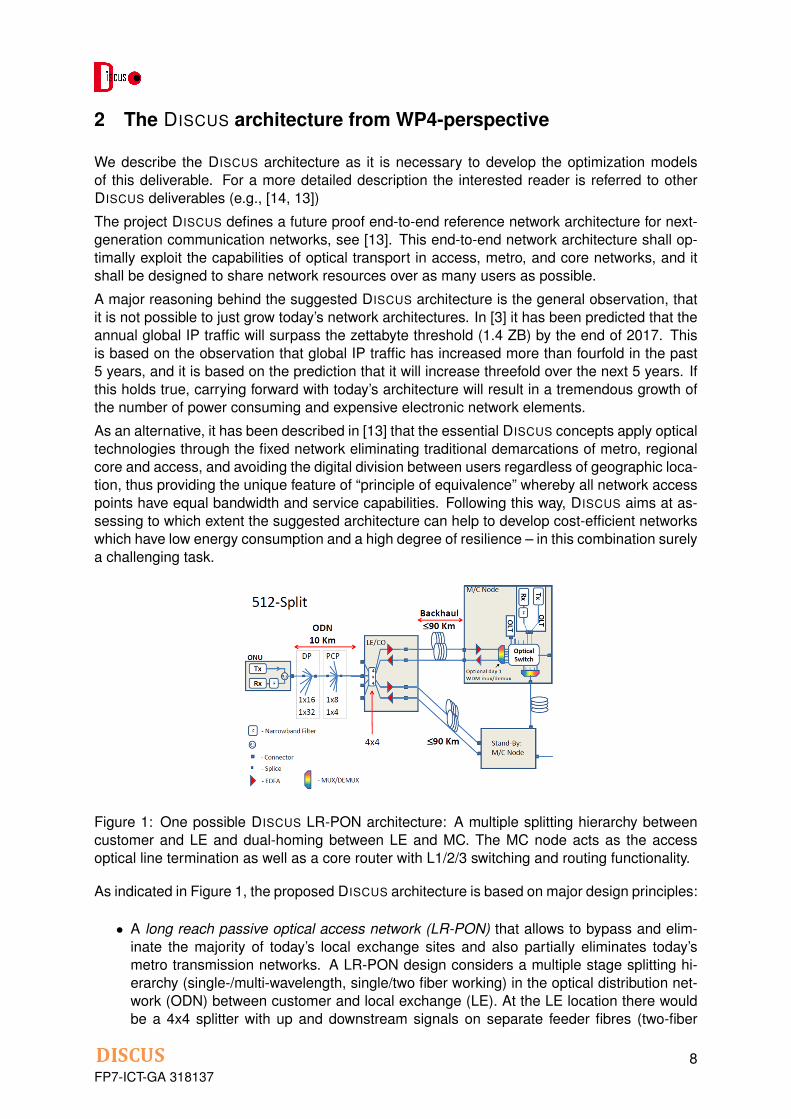
Figure 1: One possible DISCUS LR-PON architecture: A multiple splitting hierarchy betweencustomer and LE and dual-homing between LE and MC. The MC node acts as the accessoptical line termination as well as a core router with L1/2/3 switching and routing functionality.

As indicated in Figure 1, the proposed DISCUS architecture is based on major design principles:

• A long reach passive optical access network (LR-PON) that allows to bypass and elim-inate the majority of today’s local exchange sites and also partially eliminates today’smetro transmission networks. A LR-PON design considers a multiple stage splitting hi-erarchy (single-/multi-wavelength, single/two fiber working) in the optical distribution net-work (ODN) between customer and local exchange (LE). At the LE location there wouldbe a 4x4 splitter with up and downstream signals on separate feeder fibres (two-fiber

FP7-ICT-GA 3181378

working) towards the metro/core node. Implementing a dual-homing concept, each LElocation is redundantly connected to two different metro/core nodes using geographicallyseparate paths. Besides potential use of optical amplification, the LR-PON is assumed tobe completely passive – without power consumption.

• The metro/core (MC) nodes which are the connecting locations between the access andthe core network. As the name indicates these nodes bundle the functions of today’smetro and core nodes. These locations are the only locations where opto-electronic con-version is allowed. In order to maximize the sharing of resources, DISCUS aims at arelatively small number of MC nodes by optimally exploiting the assumed optical trans-mission distance of up to 100 kilometer between the customer location and the MC node.

The LR-PON is connected to a flat optical core network with a small number of large-scaleMC nodes organized in so-called optical islands. An optical island is defined by a full mesh ofoptical connections between the MC nodes of the island. For smaller countries it is expected,that a single optical island with a full optical mesh of high capacity optical channels suffices andfor larger countries it is expected that a small number of interconnected optical islands (withthe same internal full optical mesh) is necessary. There is no electronic processing of transittraffic in an optical island. Ideally, any two MC nodes are directly connected without add-dropfunctions used at any of the optical nodes. The optimization methods for the flat optical corenetwork are subject to Deliverable 7.6 (Core network optimization methods).

FP7-ICT-GA 3181379

3 Aspects of modelling

3.1 Modelling approach

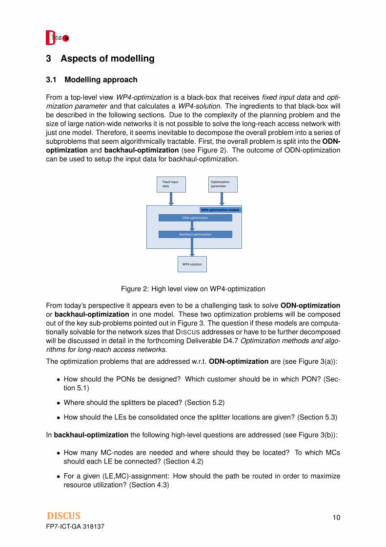
From a top-level view WP4-optimization is a black-box that receives fixed input data and opti-mization parameter and that calculates a WP4-solution. The ingredients to that black-box willbe described in the following sections. Due to the complexity of the planning problem and thesize of large nation-wide networks it is not possible to solve the long-reach access network withjust one model. Therefore, it seems inevitable to decompose the overall problem into a series ofsubproblems that seem algorithmically tractable. First, the overall problem is split into the ODN-optimization and backhaul-optimization (see Figure 2). The outcome of ODN-optimizationcan be used to setup the input data for backhaul-optimization.

WP4-solution

Fixed input data

Optimization parameter

WP4-optimization-models

ODN-optimization

Backhaul-optimization

Figure 2: High level view on WP4-optimization

From today’s perspective it appears even to be a challenging task to solve ODN-optimizationor backhaul-optimization in one model. These two optimization problems will be composedout of the key sub-problems pointed out in Figure 3. The question if these models are computa-tionally solvable for the network sizes that DISCUS addresses or have to be further decomposedwill be discussed in detail in the forthcoming Deliverable D4.7 Optimization methods and algo-rithms for long-reach access networks.

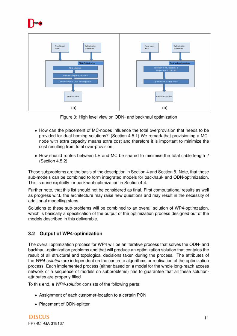
The optimization problems that are addressed w.r.t. ODN-optimization are (see Figure 3(a)):

• How should the PONs be designed? Which customer should be in which PON? (Sec-tion 5.1)

• Where should the splitters be placed? (Section 5.2)

• How should the LEs be consolidated once the splitter locations are given? (Section 5.3)

In backhaul-optimization the following high-level questions are addressed (see Figure 3(b)):

• How many MC-nodes are needed and where should they be located? To which MCsshould each LE be connected? (Section 4.2)

• For a given (LE,MC)-assignment: How should the path be routed in order to maximizeresource utilization? (Section 4.3)

FP7-ICT-GA 31813710

ODN-solution

ODN-Optimization

PON-selection

Consolidation of Local Exchange sites

Selection of splitter locations

Fixed input data

Optimization parameter

Backhaul-solution

Backhaul optimization

Fixed input data

Optimization parameter

Optimization of fiber-routes

Selection of MC-locations & Assignment of LE to MC

(a) (b)

Figure 3: High level view on ODN- and backhaul optimization

• How can the placement of MC-nodes influence the total overprovision that needs to beprovided for dual homing solutions? (Section 4.5.1) We remark that provisioning a MC-node with extra capacity means extra cost and therefore it is important to minimize thecost resulting from total over-provision.

• How should routes between LE and MC be shared to minimise the total cable length ?(Section 4.5.2)

These subproblems are the basis of the description in Section 4 and Section 5. Note, that thesesub-models can be combined to form integrated models for backhaul- and ODN-optimization.This is done explicitly for backhaul-optimization in Section 4.4.

Further note, that this list should not be considered as final. First computational results as wellas progress w.r.t. the architecture may raise new questions and may result in the necessity ofadditional modelling steps.

Solutions to these sub-problems will be combined to an overall solution of WP4-optimzation,which is basically a specification of the output of the optimization process designed out of themodels described in this deliverable.

3.2 Output of WP4-optimization

The overall optimization process for WP4 will be an iterative process that solves the ODN- andbackhaul-optimization problems and that will produce an optimization solution that contains theresult of all structural and topological decisions taken during the process. The attributes ofthe WP4-solution are independent on the concrete algorithms or realisation of the optimizationprocess. Each implemented process (either based on a model for the whole long-reach accessnetwork or a sequence of models on subproblems) has to guarantee that all these solution-attributes are properly filled.

To this end, a WP4-solution consists of the following parts:

• Assignment of each customer-location to a certain PON

• Placement of ODN-splitter

FP7-ICT-GA 31813711

• Routing of fiber-connections from each customer to one (or two) LE

• Selection of MC-nodes

• Assignment of LE to MC

• Routing of fiber/cable/duct-connections from LE to MC

Note, that the concrete dimensioning or the placement of equipment at the MC is not part ofWP4, as the core network has to be considered as well.

3.3 The data-model

In this section we describe the main technical components that are relevant for WP4-optimization and their attributes considered in the optimization-models. As mentioned earlier itis not necessary to model all technical detail but only those aspects that have a strong influenceon the solution structure.

3.3.1 The reference networks

The reference networks considered in the DISCUS project are not randomly generated inputdata sets, but reflect (non confidential) data from telecommunication companies like TELECOM

ITALIA.

The data-set provided by TELECOM ITALIA contains coordinates of their current Local Exchange(LE) locations in Italy and for each of these LE the number of connected (residential and busi-ness) customers. This data-set was anonymized in the sense that the coordinates of the localexchanges have been slightly shifted. Hence, the network contains a realistic amount anddistribution of the locations but not the real coordinates.

To compute a realistic fiber topology (i.e. the network from which we select the eventual fiberpaths), the available non-confidential operator-specific key-information was combined with pub-lic data (namely OSM). Geo-referenced data from street networks are a good candidate aslaying fibres is typically done along streets and street networks provide a reasonable notion ofdistance. Furthermore, they reflect dense and sparse structures in towns and rural areas andthey reflect forbidden fiber-routes as those across mountains or rivers.

Thus, these networks reflect realistic link length and connectivity as well as sparsity aspects ofthe telecommunication network.

The topology of such a network is described by its set of nodes and edges. The nodes of thisnetwork are given by

• existing LE sites

• potential locations to place metro-core nodes or any additional equipment (optical lineamplifier, etc.)

• nodes to reflect the topological structure of the network (junctions, etc.)

• customer locations

Each node in the network might carry a set of attributes, e.g., the number of customers atan LE. The links of this network describe existing and potential fiber routes and duct systems.

FP7-ICT-GA 31813712

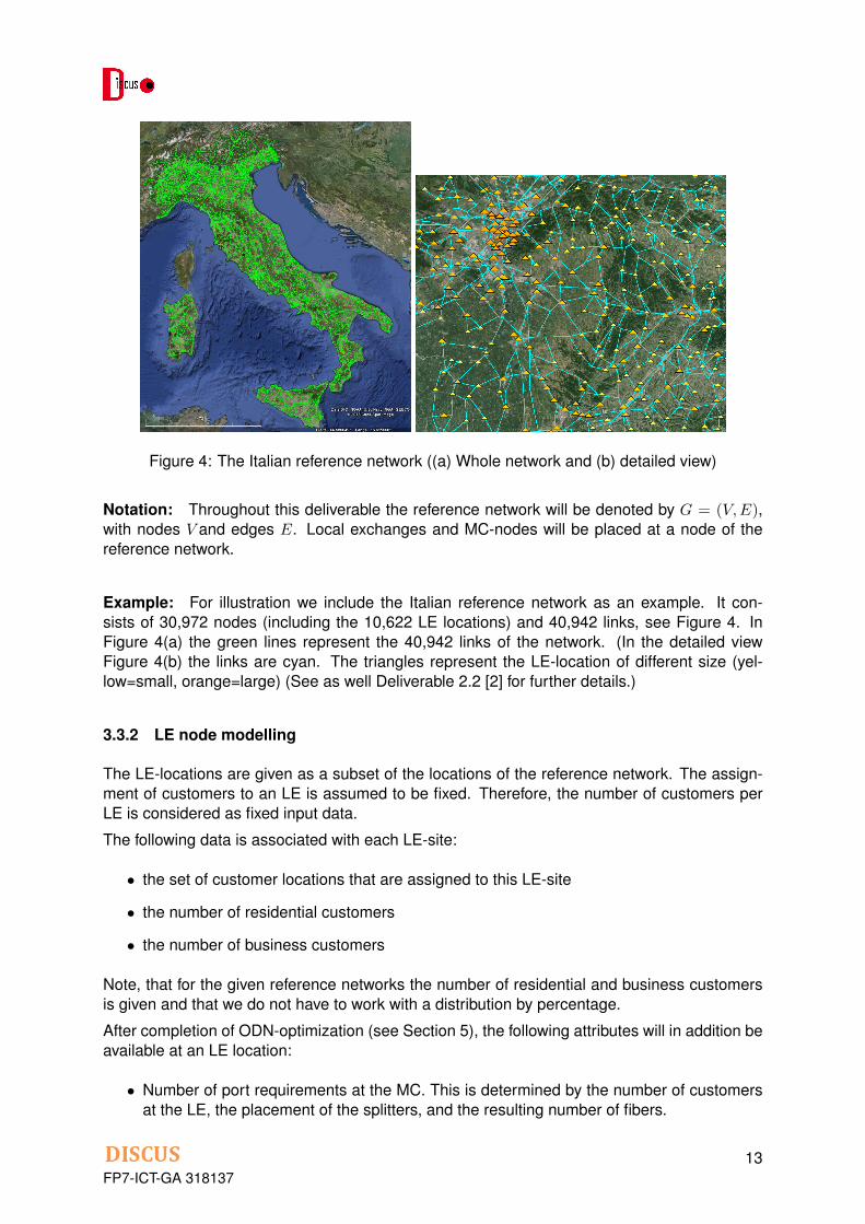
Figure 4: The Italian reference network ((a) Whole network and (b) detailed view)

Notation: Throughout this deliverable the reference network will be denoted by G = (V,E),with nodes V and edges E. Local exchanges and MC-nodes will be placed at a node of thereference network.

Example: For illustration we include the Italian reference network as an example. It con-sists of 30,972 nodes (including the 10,622 LE locations) and 40,942 links, see Figure 4. InFigure 4(a) the green lines represent the 40,942 links of the network. (In the detailed viewFigure 4(b) the links are cyan. The triangles represent the LE-location of different size (yel-low=small, orange=large) (See as well Deliverable 2.2 [2] for further details.)

3.3.2 LE node modelling

The LE-locations are given as a subset of the locations of the reference network. The assign-ment of customers to an LE is assumed to be fixed. Therefore, the number of customers perLE is considered as fixed input data.

The following data is associated with each LE-site:

• the set of customer locations that are assigned to this LE-site

• the number of residential customers

• the number of business customers

Note, that for the given reference networks the number of residential and business customersis given and that we do not have to work with a distribution by percentage.

After completion of ODN-optimization (see Section 5), the following attributes will in addition beavailable at an LE location:

• Number of port requirements at the MC. This is determined by the number of customersat the LE, the placement of the splitters, and the resulting number of fibers.

FP7-ICT-GA 31813713

• Maximum distance from the LE to his associated customers. This attribute is an impor-tant input data for backhaul-optimization. In case that this data is not available it seemsreasonable to apply a constant value for all LE.

• Attribute that indicates if the node has to be single- or dual-connected, or if it may bechosen by the optimization model (possible values are {SINGLE, DUAL, OPEN}). SINGLE

(respectively DUAL) implies that the LE has to be single (respectively dual)-connected,whereas OPEN allows the optimizer to choose (respecting the model-restrictions).

Notation: Throughout this document we denote the set of LE sites with L.

3.3.3 Metro/Core node modelling

The metro/core (MC) nodes are the connecting locations between the access and the corenetwork. One main optimization question discussed in this deliverable is how many MC nodesare needed and where to place them. But based on the WP4-solution only, it will not be possibleto dimension the MC node as the solution for the core-network influences the MC-node as well.Thus, for WP4-optimization we will have to work with an abstraction of the ”real” MC-node thatconsiders the attributes that influence the structure of the access-network.

To this end, the following attributes will be available to a potential MC location:

• A setup-cost, that might reflect some organisational-, location-dependent and basic-infrastructure cost in case an MC is opened. (We say that an MC is opened if at leastone LE is assigned to it.)

• A size-dependent cost, that might reflect installed hardware-components that have to beinstalled and that depend, e.g., on the number of LE/customers/fibres that are assignedto this MC.

In order to balance the size of the opened MC the following attributes can be used:

• The maximum number of LE that might be assigned to the MC-node.

• The maximum number of customers that might be assigned to the MC-node.

• The maximum number of ports that might be used at the MC-node .

This will allow us to reflect the important aspects in the optimization models that influencestructural design.

It is reasonable to restrict the MC nodes to locations that can house the necessary equipment.Therefore, we assume that an MC-node is opened only at existing LE locations.

Notation: Throughout this document we denote the set of MC nodes with M .

FP7-ICT-GA 31813714

3.3.4 Backhaul link modelling

From WP4-perspective the backhaul-links connect the LE sites to potential MC nodes. Ba-sically, each edge in the reference network corresponds to a backhaul link. To each suchbackhaul link we associate a number of attributes, among them

• Setup-cost of the link which might refer, e.g., to trenching costs,

• Length of the link which might be input to length dependent cost, e.g., for fibers,

• the remaining capacity of the link w.r.t. existing cables and/or ducts.

Recall that every link in the reference network might already provide some duct capacity. Inprinciple, depending on the optimization scenario, one might also assume that enough ductcapacity is always available.The initial LR-PON design considered for DISCUS uses uni-directional fibre pairs in the backhaulsection and a single wavelength system (no WDM). For resilience, in the default scenario, everyLE site is connected to two MC nodes using a node-disjoint connection.The actual number of fibres needed for a given LE site (independent of the MC to connect to) isa direct consequence of number of households connected to the LE and the splitting hierarchyused in the ODN section.

3.3.5 Splitter modelling

Using a LR-PON enables sharing of fibre infrastructure as close to the customer as possibleusing a passive optical splitting. This passive splitter requires no power and is a highly reliablecomponent. The LR-PON uses optical amplification to support 512-split. Although we areassuming that a splitter placed at LE-site would be 4x4 and the other splitters in ODN would beof 1xN splitters where N is a power of 2 and goes up to 32, the presented models can easilybe adapted to other configurations.With each splitter s we associate the following attributes:

• Setup-cost of a splitter s refers to the cost of placing splitter s at a location. For themoment we will assume that this cost is independent of the location.

• Size of a splitter s refers to the number of fibres that emanate from the splitter.

• Loss of a splitter s refers to the loss associated with using a splitter s. Usually the lossassociated with a splitter depends on its size.

3.4 Fixed input data

The optimization models assume a set of input data that is considered to be fixed, i.e. it cannotbe changed or modified within the optimization process. These include:

• Topology of network (i.e., the location of the LE-sites, and the potential fiber connectionsgiven by the edges of the graph/reference network).

• Number and type (residential, business) of customers at a certain location

• LE locations

• Assignment of the customer locations to the LE. Thus, the number of customers of anLE is assumed to be fixed. Due to ODN-optimization is the hierarchy and placement ofspitters and therefore the port-requirements of the LE.

FP7-ICT-GA 31813715

3.5 Parameter

The optimization models that will be described in detail in the following sections can beparametrized in order to set set up different scenarios for which a optimized long-reach accessnetwork is calculated These scenarios allow to study the impact of structural and technicaldecisions.

It is possible to vary general design questions like

• Resilience strategy

• architectural design of long-reach access network

as well as the parameters

• Maximum distance between customer and MC (Within the DISCUS architecture a ”stan-dard” distance of 100 km is assumed. Nevertheless, the models offer the option to varythis parameter to analyse what influence a decrease or increase of this length will have,e.g., on the number of required MC nodes.)

• size of splitters,

• signal loss function both in terms of the size of the splitters and the length of the cable,

• cost model covering all aspects of the network,

• demand per customer.

FP7-ICT-GA 31813716

4 Optimisation models for the Backhaul Network

In this section we describe the optimization models used for backhaul-optimization. We startwith a high-level view on the optimization problem before we derive the mathematical model.To illustrate the potential of these models we present first computational results achieved withour proof-of-concept implementations.

4.1 High level view

The central questions that have to be answered in the backhaul optimization are:

• How many MC nodes are needed to satisfy the fibre demand of all LE sites and whereshould they be placed? (A low number of MC-nodes is necessary for the concept of anoptical island, due to the quadratic scaling of the interconnecting optical channels in a fullmesh.)

• To which MC node(s) should the LE be connected?

• How should the connection fibres between the LE and the MC be routed in order to fulfillthe resilience requirements? Is it possible to share cables or ducts in order to maximizeresource utilization?

These questions are addressed in the described optimization model. The first two questionsare tackled with Facility Location models described in Section 4.2. The additional aspect ofconsidering overprovisioning is discussed in Section 4.5.1. Section 4.3 contains a discussionof the fiber-routing.Answers to these question have to fulfil the following restrictions:

• Every LE gets two MC disjoint fiber routes (dual-homing with disjoint paths). It will be pos-sible to change the resilience concept and evaluate solutions that respect single-homingor dual-homing without disjointness restrictions.

• The fiber connections between the customer and the MC has to fulfil some distance con-straints. In DISCUS we work with a maximum distance of 100km, but case studies shouldallow other distances as well.

• Node capacities at the MC (e.g., do not assign too many customers/LEs to one MC)

• Respect link capacities (e.g., respect fiber/cable/duct capacities)

and should be cost-optimal, i.e., minimize setup- and equipment-cost. Note, that the DISCUS

cost-model is still under discussion.When optimizing the backhaul we assume the ODN architecture to be part of the input, that is,the connection of customers to LE sites is not subject to optimization. To this end we assumethat

• the LE locations and the assignment of customers to these LE locations are fixed.

• for the LE sites we are given the number of connected customers/households and thesplitting hierarchy towards the LE. These numbers result in a set of ports with given upand downstream bitrate capacity that have to be realized towards the Metro/Core site(MC). The number of ports, in turn, can be translated into a fibre demand at the LE site.

• on the network site, the backhaul fibres (and optical signals) are terminated by an MCnode.

FP7-ICT-GA 31813717

Cable Optimization: Backhaul optimization has to take care of optimizing the fiber routes inorder to share trails. The aim is that shared trails will result in synergistic effects on cable andduct usage as well as on trenching costs.

This is illustrated in Figure 5 where the total path length in Figure 5(a) is less than in Figure 5(b),but due to the sharing of resources the solution in Figure 5(b) is cheaper.

More precisely, we

• decide about individual fiber routes for every LE to MC assignment, and

• install cables and ducts on the links

such that for every link

• the installed cables contain sufficient fibres (cable capacity constraints), and

• the available duct slot capacity covers the number of installed cables (duct capacity con-straints).

Thereby minimizing the edge-costs, which might consist of trenching-costs and cost for fiber,cables, and ducts.

(a) No sharing (b) Path sharing

Figure 5: Optimizing fiber routes (The triangles correspond to LE, the diamonds to MC)

4.2 Metro/Core-node selection and LE assignment

In this section we discuss the problem of placing the MC-nodes in more detail. As describedearlier the optimization question involves

• opening MC nodes at potential locations in the reference network,

• assigning every LE site to an opened MC node (or two MC nodes in case of dual homing),

respecting

• distance constraints (maximal reach of signals)

• resilience restrictions (single- or dual-homing, see Figure 6)

• capacity constraints at the MC node (e.g., maximum number of customers)

FP7-ICT-GA 31813718

Figure 6: Single vs. dual parenting (The triangles correspond to LE, the diamonds to MC.The coloured MC are actually opened, the blue dotted lines correspond to the selected assign-ments)

thereby minimizing

• the number of required MC nodes (directly resulting in setup-cost, equipment cost and/orpower consumption), and

• an (LE,MC)-distance dependent cost (modelling fiber/cable/duct costs)

In this optimization setting we omit a precise modelling of the capacities, both node capacities(MC nodes equipment) and link capacities (cables/ducts/fiber). Instead we assume that wemay estimate a fixed cost κm for opening an MC node at m ∈ M and a fixed cost κe for usinga fiber on link e, which of course is a function of the link length. In the simplest case (if noother data is available) we might set κi := 1 which refers to minimizing the number of openedMC nodes (not its cost). Similarly we might set κe to the length of the corresponding link inkilometer, which refers to minimizing distances instead of fiber cost.

The MC-selection and assignment problem will be modelled as an extension to the classicalFacility Location Problem (see e.g., [16, 4]). The hardware cost at the MC nodes can be seenas facility opening cost. Similarly, the fibre cost between LE and MC node acts as the ‘LE toMC ’ assignment cost in this setup. This cost is, of course, length-dependent.

The initial LR-PON design considered for DISCUS uses uni-directional fibre pairs in the backhaulsection and a single wavelength system (no WDM). For resilience, in the default scenario, everyLE site is connected to two MC nodes using a node-disjoint connection.

The actual number of fibres needed for a given LE site (independent of the MC to connect to) isa direct consequence of number of households connected to the LE and the splitting hierarchyused in the ODN section.

Depending on the availability of the data the following additional general cost-coefficients canbe used to setup the LE to MC assignment cost:

• The fibre (pair) cost per kilometre

• The cost of an optical amplifier (OLA)

• The maximum fibre distance without amplification

Furthermore, other parameter could be incorporated into the assignment-cost in order to makecertain assignments more attractive over others.

In addition the following attributes of the LE can be handled at every MC-location:

• The number of connected households

FP7-ICT-GA 31813719

• The number of connected business units

• The number of required ports

4.2.1 Selecting potential MC-node locations

Basically, any node in the given reference topology could be a MC location. However, it isreasonable to restrict MC nodes to locations that can house the necessary equipment. To thisend, we restrict the set of potential MC locations to set of LE location.

From the practical perspective there are several criteria to decide whether an LE location canbe upgraded to an MC location or not. These are naturally related to its size (e.g., number ofconnected customers (residential and business) or the number of connected cabinets).

In the context of resilience, another important aspect in computing ’interesting’ locations is todecide about the connectivity of the corresponding network node:

• The simplest such property is the node degree (e.g., nodes with degree larger or equalto three indicate high connectivity).

• A more powerful criterion is based on computing all biconnected components of the net-work G = (V,E), which can be done in linear time, see [7]. A biconnected component isa (connected) sub-network with the property that it cannot be broken into disconnectedpieces by deleting any single node (and its incident links). For every component of sizeat least 3 it holds that there exists a node-disjoint pair of paths between any two nodes inthis component. Consequently, (larger) biconnected components provide nodes that arewell connected within the network.

Notice that for a single LE site only those locations can be potential MC nodes that are reach-able in the distance limit of lmax km.

4.2.2 Placing Metro/Core-nodes by Solving Facility Location Models

4.2.2.1 Notation summary For the optimization models that select and place the MC-nodeswe give a summary of the most important notation used throughout the model description:

Input data:G = (V,E) This basically corresponds to the reference network with nodeset V

and edgeset E.L Set of existing LE sites (L ⊆ V ). A single LE is denoted by l ∈ L.M Set of potential MC-nodes (M ⊆ L). A single MC is denoted by m ∈M .custl Number of customers under one LE l ∈ L

Optional input data:maxcustm Maximum number of customers that might be assigned to an MC node m ∈Mmaxlem Maximum number of LE that might be assigned to an MC node m ∈Mmaxportsm Maximum number of ports that can be used at an MC node m ∈M

Parameter:lmax Maximum distance between LE and MC

FP7-ICT-GA 31813720

Derived data:Ml For a given LE l: All potential MC that can be reached within lmax kmM (2) The set of all pairs of potential MC nodes.M l The set of feasible pairs of paths that connect LE l to a pair of MC

Variables:xm Indicates whether or not an MC site m is openedxlm Indicates whether or not an LE l is assigning to MC site mxlp Indicates whether or not an LE l is assigning to a pair p of MC sites

Cost-coefficients:κm Setup cost for opening an MC site mκlm Cost for assigning an LE l to an MC site mκlp Cost for assigning an LE l to a p of MC sites

4.2.2.2 Facility Location models

Selecting a set of serving locations in a network and assigning client locations to these serversby choosing network paths is a classical facility location or plant location problem, see [16, 4, 6].In principle, it can formulated as follows. We introduce the reference network as an undirectedgraph G = (V,E) with locations V and links E. The set of existing LE sites (the clients) is givenby L ⊆ V and the set of potential MC nodes (the servers or facilities) by M ⊆ V with M beinga subset of L, i.e. M ⊆ L. Given an arbitrary LE site l ∈ L, we denote by Ml all MC locationsthat are within the reach of l, that is, there exists a path with a total length in km less than orequal to lmax between l and m. We also say that Ml is the set of MC nodes feasible for l ∈ L.

We introduce a binary variable xm for every potential MC locationm ∈M that indicates whetheror not the MC site is opened at node m ∈ M . Similarly, an indicator variable xlm decideswhether or not we assign LE site l ∈ L to MC node m ∈ M . Let further κm be the cost foropening m ∈M and let κlm be the cost for assigning l ∈ L to m ∈M .

If we omit the disjointness restriction and assume that n ∈ {1, 2}, the single- and dual-homingcase (LE to MC) with just distance cost and node opening cost can be modelled as the FacilityLocation model (FL)

min

(∑l∈L

∑m∈M

κlmxlm +∑m∈M

κmxm

)(1)

(FL)∑m∈M

xlm = n ∀l ∈ L (2)

xlm ≤ xm ∀l ∈ L,m ∈M (3)

Equations (2) guarantee that every LE is assigned n times and inequalities (3) ensure that ev-ery MC with at least one connected LE is actually opened. Models of this type can becomerelatively large as the number of potential assignments might grow quadratically with the num-ber of (client and server) nodes. However, in our case there is a strong restriction coming fromthe distance constraint such that the sets Ml of feasible MCs are small (in the order of a fewhundred locations depending on l ∈ L).

With respect to the cost objective function in the model (FL), the cost values κm could inprinciple be used to model the cost for necessary equipment at the MC location m ∈ M .

FP7-ICT-GA 31813721

Similarly, fiber and cable cost could be mapped to the cost values κlm based on the distancebetween LE site l ∈ L and the MC node m ∈ Ml. There is a trade-off between the assignmentcost and the facility opening cost. Increasing the assignment cost will increase the optimalnumber of opened MC locations with shorter fiber routes between LE and MC nodes whileincreasing the opening cost will decrease the number of opened MC locations with longer fiberconnections.

As long as the cost for opening an MC node does not depend on the actual location, we canfix κm := c with c > 0 being a positive scalar. Let us further introduce llm as the shortest pathdistance between l ∈ L and m ∈ M in kilometer and set κlm := llm, that is, the assignmentcost is proportional to the shortest path distance. Clearly, setting c to a large enough numberleads to a model that minimizes the number of necessary MC locations (respecting the distanceconstraint).

With this settings we can define N(n, c, lmax) as the smallest number of MC nodes in an optimalsolution to (FL). This number depends on the number of MCs to connect to n, the cost c, andthe LE to MC maximum path distance lmax. We set N(n, lmax) := minc{N(n, c, lmax)} obtainedby setting c to a large value. We are mainly interested in computing N(1, lmax) and N(2, lmax).These numbers correspond to the minimal number of MC nodes needed to cover the givenreference network such that every LE is able to connect within the distance lmax km to one ortwo MC nodes, respectively. Clearly N(1, lmax) ≤ N(2, lmax).

However, as model (FL) ignores the concept of disjointedness, N(2, lmax) many MC nodesmight not be sufficient to cover the region such that all LE are able to connect using disjointpaths. Although it is reasonable to use model (FL) as a first approximation, we cannot use it tosolve our problem directly. It does not properly account for the disjointedness of fiber routes andit is not flexible enough to model assignments of LEs to pairs (!) of MCs and the correspondingdistances.

4.2.2.3 Facility Location models with disjointness

Enhancing the above model, we introduce M (2) as the set of all pairs of potential MC sites, thatis M (2) := {p = {m,n} : m,n ∈M}. Let

• M l denote all feasible pairs of paths that connect l ∈ L to an MC-pair {m,n}

• A be the union of all feasible connections of an LE to an MC-pair, i.e, A := ∪l∈LM l.This corresponds the set of all generated assignments. An assignment a ∈ A is a tuplea :=< l, p > where l corresponds to an LE-location and p = {m,n} to a pair of MC-nodes. Whenever appropriate, a single assignment is either denoted with a or in tuple-form < l, p >.

• A(m) the set of all assignments that contain the MC m., i.e., A(m) := {< l, p >∈A | m ∈ p}

VariablesWe now introduce binary variables

• xlp ∈ {0, 1} that indicate whether or not we assign l ∈ L to the pair p = {m,n} ∈ M (2) ofMC nodes,

• xm ∈ {0, 1} that indicate whether the MC-location m is opened or not.

FP7-ICT-GA 31813722

Cost coefficientsFor each type of variables we have a cost-coefficient, i.e.

• κlp which corresponds to the paths-cost of assigning LE l to the pair of MC-node p.

• κm which correspond to the setup-cost for opening MC-node m is.

It should be clear that the number of MC nodes in a cost-optimal DISCUS solution stronglydepends on the ratio between the cost for assigning LE sites to MC nodes (distance depen-dent fiber/cable/duct and trenching cost) and the cost for opening MC nodes (equipment cost).Huge assignment cost (or equivalently small MC investment cost) will result in many MC nodesopened with short fibre connections between LE and MC, while huge MC cost results in veryfew MC nodes opened and longer fibre connections. Consequently, any result with respectto the consolidation of current central office locations towards a small number of Metro/Corenodes strongly depends on the assumed cost and data model.

ModelNow we may rewrite model (FL) as the the Disjoint Facility Location model (DFL):

min

(∑l∈L

∑p∈M(2)

κlpxlp +∑m∈M

κmxm

)(DFL)

∑p∈M l

xlp = 1 ∀l ∈ L (4)

xlp ≤ xm ∀l ∈ L, p = {m,n} ∈M l (5)

xlp ≤ xn ∀l ∈ L, p = {m,n} ∈M l (6)

Here we assign LE sites to pairs instead of single MC sites (equation (4)). Whenever a pair ischosen, the two corresponding MC locations are opened, which is guaranteed by inequalities(5) and (6).

Using the sets M l we have the flexibility to define pairs of MC nodes to be feasible for a certainLE location or not depending on the level of connectivity. Any pair p ∈M l is said to be a feasiblepair of MC nodes for l. Clearly, a pair of MCs can only be feasible if the individual sites arefeasible, that is M l is a subset of all pairs of feasible MCs: M l ⊆ M (2)

l := {p = {m,n} : m, l ∈Ml}, for all l ∈ L. However, not every pair of feasible MCs is feasible itself since a disjoint pair ofpaths is not necessarily available. Moreover, there are different notions of path disjointedness.We will define our resilient assignment policy below.

Similar to the above, we define llp as the total length of shortest disjoint connection of l to thepair of MCs p and set κlp := llp and κm := c > 0. We can now introduce the number N(c, lmax)as the smallest number of MC nodes in an optimal solution to (DFL) using facility opening costc and maximum distance lmax. Again we are mainly interested in N(lmax) := minc{N(c, lmax)}which gives the minimal number of MCs to cover the network such that all LEs may connect totwo MCs by disjoint fiber paths. Following from the above we have N(1, lmax) ≤ N(2, lmax) ≤N(lmax).

It remains to show how we parametrize model (DFL). We will first clarify how we compute setsof potential MC locations M . In fact we will see that the easier model (FL) can be used asan input generator for model (DFL). We will show how we compute disjoint fiber routes, whichlevels of disjointedness we consider, and, eventually, we will provide the resilient assignmentpolicy to define the sets M l of feasible pairs of MC nodes for LE locations l ∈ L.

FP7-ICT-GA 31813723

4.2.2.4 Alternative model for disjointnessThere is a second model for dual homing possible which is as follows:

min

(∑l∈L

∑m∈M

κlmxlm +∑m∈M

κmxm

)(7)

(DFL2)∑m∈M

xlm = 2 ∀ l ∈ L (8)

xlm ≤ xm ∀l ∈ L,m ∈M (9)

xlm + xln ≤ 1 ∀l ∈ L,∀{m,n} ∈M l (10)

where M l ⊂M (2) denotes all pairs of MC nodes that are in conflict for LE l (for which there areno disjoint paths from l to n and from l to m). In this model we cannot explicitly map a cost tothe assignment of l to a pair of MC nodes. Notice that the path (and hence distance cost) tothe first MC depends on the choice of the second MC.

4.2.2.5 Modelling further aspectsIn this paragraph we describe how other aspects of practical relevance can be integrated into

the models. We limit ourselves to describe how they are used with model (DFL).

Limit the number of customers per MC nodeLet maxcustm be the maximum number of customers that might be assigned to an MC nodem ∈ M . Recall that custl denotes the number of customers under one l ∈ L and A(m)corresponds to the set of all assignments that contain the MC m. The inequality system∑

<l,p>∈A(m)

custl · xlp ≤ maxcustm ∀ m ∈M (11)

limits the number of customers assigned to an MC.

Limit the number of LE per MC nodeLet maxlem be the maximum number of LE that might be assigned to an MC node m ∈ M . Theinequality system ∑

<l,p>∈A(m)

xlp ≤ maxlem ∀ m ∈M (12)

limits the number of LE assigned to an MC.

Limit the number of used ports per MC nodeLet maxportsm be the maximum number of ports that can be used at an MC node m ∈ M . Theinequality system ∑

<l,p>∈A(m)

portsl · xlp ≤ maxportsm ∀ m ∈M (13)

limits the number of ports used at an MC.

FP7-ICT-GA 31813724

Partial dual-homingIn general, instead of providing 100% dual coverage, one could provide α% dual coverage(where α is any value between say 70% and 100%).

Let custG be the total number of customers in the reference networkG and let custd = α100 ·cust

G

be the minimum number of customers that have to have a dual-homing connection.

In contrast to the models described so far we generate for each l ∈ L both single connectingpaths (e.g., the shortest path) and dual-homing paths (i.e, disjoint paths to pairs of MC-nodes).Let M (1)

l , resp. M (2)l be the set of single, resp. dual, connecting paths for LE l ∈ L. Let

M∗l := M(1)l ∪M

(2)l be the set of all connecting paths for LE l ∈ L.

This allows us to formulate the following inequality-system:∑p∈M∗l

xlp = 1 ∀l ∈ L (14)

∑l∈L

∑p∈M(2)

l

custl · xlp ≥ custd (15)

Equation (6) guarantees that for each l ∈ L one connecting path (either single-homing or dual-homing) is chosen, whereas inequality (15) assures that enough LE (and therefore customers)are provided with a dual-homing connection.

This results in the overall model

min

(∑l∈L

∑p∈M∗l

κlpxlp +∑m∈M

κmxm

)(DFLp)

∑p∈M∗l

xlp = 1 ∀ l ∈ L (16)

∑l∈L

∑p∈M(2)

l

custl · xlp ≥ custd (17)

xlp ≤ xm ∀l ∈ L, p = {m} ∈M (1)l (18)

xlp ≤ xm ∀l ∈ L, p = {m,n} ∈M (2)l (19)

xlp ≤ xn ∀l ∈ L, p = {m,n} ∈M (2)l (20)

Inequaltites (18) (resp. (19) and (20)) guarantee that the MC m is opened if a connecting pathto m is chosen.

4.3 Optimizing fiber routes : A path based model

This model is based on the idea to generate a set possible feasible paths for each LE-MC-connection and choose the connection paths that share the most edges. To this end, we needthe concept of a connection path that is introduced in Section 4.3.1.

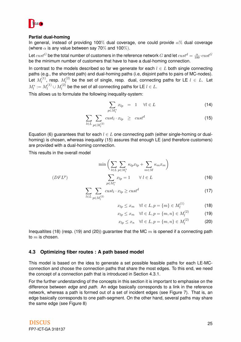
For the further understanding of the concepts in this section it is important to emphasise on thedifference between edge and path. An edge basically corresponds to a link in the referencenetwork, whereas a path is formed out of a set of incident edges (see Figure 7). That is, anedge basically corresponds to one path-segment. On the other hand, several paths may sharethe same edge (see Figure 8)

FP7-ICT-GA 31813725

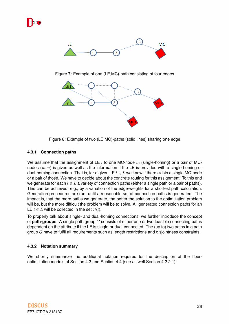
Figure 7: Example of one (LE,MC)-path consisting of four edges

Figure 8: Example of two (LE,MC)-paths (solid lines) sharing one edge

4.3.1 Connection paths

We assume that the assignment of LE l to one MC-node m (single-homing) or a pair of MC-nodes (m,n) is given as well as the information if the LE is provided with a single-homing ordual-homing connection. That is, for a given LE l ∈ L we know if there exists a single MC-nodeor a pair of those. We have to decide about the concrete routing for this assignment. To this endwe generate for each l ∈ L a variety of connection paths (either a single path or a pair of paths).This can be achieved, e.g., by a variation of the edge-weights for a shortest path calculation.Generation procedures are run, until a reasonable set of connection paths is generated. Theimpact is, that the more paths we generate, the better the solution to the optimization problemwill be, but the more difficult the problem will be to solve. All generated connection paths for anLE l ∈ L will be collected in the set P(l).

To properly talk about single- and dual-homing connections, we further introduce the conceptof path-groups. A single path group G consists of either one or two feasible connecting pathsdependent on the attribute if the LE is single-or dual-connected. The (up to) two paths in a pathgroup G have to fulfil all requirements such as length restrictions and disjointness constraints.

4.3.2 Notation summary

We shortly summarize the additional notation required for the description of the fiber-optimization models of Section 4.3 and Section 4.4 (see as well Section 4.2.2.1):

FP7-ICT-GA 31813726

E : Set of all edges of the graph G = (V,E)G : A single path-groupPG(l) : Set of path-groups for LE l. Each path-group G ∈ PG(l) consists of one or two

connecting-path, dependent on the single- or dual-connection of the LE l.PG : The set of all path-groups, i.e. PG := ∪l∈LPG(l).P(l) : Connection paths for LE l ∈ L. P(l) is a set of single (LE,MC)-paths.P : Set of all connection paths, i.e., P := ∪l∈LP(l)Ep : set of edges of a given connection path p ∈ P.custp : Number of customers served by path p ∈ P, i.e., number of customers

of the originating LE.P(e) : Set of paths p ∈ P that contain edge e.

Additional parameter:max

pe : maximum number of paths, that can be routed over edge e ∈ E

maxcuste : maximum number of customers, that can be routed over edge e ∈ E

4.3.3 Variables

In addition to the models described so far, we need additional types of variables, namely

yG ∈ {0, 1} (= 1, if path-group G is used to connect an LE to one MC or to a pair of MC-nodes.)zp ∈ {0, 1} (= 1, if path p is used to connect an LE to an MC)ue ∈ {0, 1} (= 1, if edge e is used in any of the connection paths)

4.3.4 Cost terms

Edge setup costsFor each edge e ∈ E we are given setup costs κe that are incurred whenever this edge is used.This cost is paid only once, even if this edge is used by several paths. The setup costs maycomprise, e.g., trenching costs and approximate duct costs.

Path costsEach connection path p ∈ P has a length dependent path cost κp. The cost κp for a connectionpath p ∈ P is given by

κp := p.length · costPerMeter

For pairs of paths p.length is the sum of both single-path lengths. The path-cost can be used,e.g., to model fiber costs.

4.3.5 Objective

The objective is to minimize the sum of all involved costs, i.e.,

min∑

e∈E κe · ue +∑p∈P κp · zp

Note that if κe >> κp, i.e. setup costs dominate the paths cost the solution will tend to have anincreased number of shared trails, whereas the total path-length will increase.

FP7-ICT-GA 31813727

4.3.6 Constraints

Choose a connecting path-groupFor each l ∈ L we have to guarantee that a connecting path-group is chosen that connects theLE to an MC-node (or to a pair of MC-nodes).∑

G∈PG(l)

yG = 1 ∀ l ∈ L (21)

The constraint system guarantees that for each LE l ∈ L exactly one path-group, is selected.Due to the construction of the path-groups this implies the single- or dual-homing connection.

The base model, where the (LE-MC)-assignment is fixed, can easily be extended to allow somemore flexibility in the assignment. To this end for one l ∈ L not only paths to one MC are gen-erated, but paths to several MC. Combining this with the modelling aspects from Section 4.2yields a model where fiber routes are optimized jointly with the MC-node selection and place-ment.

Activate connecting pathsIn case that a path-group G is chosen the paths in that path-group have to be activated. This isachieved by the inequality system

zp ≥ yG ∀ G ∈ PG, ∀ p ∈ G (22)

Activate edges for chosen connecting pathsIn case that a connecting-path p ∈ P is chosen we have to assure that all edges of this pathare activated as well. Thus, we have the following set of inequalities

ue ≥ zp ∀p ∈ P, ∀e ∈ Ep (23)

For a chosen connecting path p (zp = 1), the variables corresponding to the edges of this path(ue) cannot be 0.

Limit edge utilizationAs the number of fibres on an edge e ∈ E directly corresponds to the number of customersconnected over this edge, it might be reasonable to limit the number of paths and/or number ofcustomers routed over this edge. This can be done by the following set of constraints∑

p∈P(e)

zp ≤ maxpe (24)

resp. ∑p∈P(e)

custp · zp ≤ maxcuste (25)

Constraints 24 (resp. 25) limits the number of paths (resp. customers) routed over edge e to amaximum value.

FP7-ICT-GA 31813728

4.4 Combined model for MC-Assignment and Fiber routes optimization

Combining the ingredients from Section 4.2.2 and Section 4.3 leads to a model that solvesthe problems of selecting MC-locations, assigning LE-locations to MC and optimizing the fiberroutes in one model.

We basically solve the following Backhaul-Optimization model (BO) (we refer to Section 4.2.2.1and Section 4.3.2 for on overview on used notation):

min(∑

l∈L∑

p∈M∗lκlpxlp +∑

m∈M κmxm +∑e∈E κe · ue +∑p∈P κp · zp

)∑

p∈M∗lxlp = 1 ∀ l ∈ L (26)∑

l∈L∑

p∈M(2)l

custl · xlp ≥ custd (27)

xlp ≤ xm ∀l ∈ L, p = {m} ∈M (1)l (28)

xlp ≤ xm ∀l ∈ L, p = {m,n} ∈M (2)l (29)

(BO) xlp ≤ xn ∀l ∈ L, p = {m,n} ∈M (2)l (30)∑

G∈PG(l) yG = 1 ∀ l ∈ L (31)zp ≥ yG ∀ G ∈ PG,∀ p ∈ G (32)ue ≥ zp ∀p ∈ P, ∀e ∈ Ep (33)∑

p∈P(e) zp ≤ maxpe ∀e ∈ E (34)∑p∈P(e) custp · zp ≤ maxcuste ∀e ∈ E (35)

The first two terms in the objective and inequalities (28)-(30) correspond to the (LE,MC) as-signment part discussed in Section 4.2.2, whereas the last tow terms in the objective andinequalities (31)-(35) represent the fiber-routes optimization discussed in Section 4.3. In ordernot to overload the formulation, the inequalities discussed in Section 4.2.2.5 ( Modelling furtheraspects) were omitted from the model (BO). They could easily be considered by adding theinequalities discussed there to the model (BO).

It is unclear so far, if the model above can be solved for a nation-wide reference network, likeItaly. This has to be discussed in the forthcoming deliverable Deliverable D4.7 Optimizationmethods and algorithms for long-reach access networks.

4.5 Other Aspects

4.5.1 Placing Metro/Core-nodes by Minimising Overprovision-based Cost

A basic and effective protection mechanism for LR-PON is to dual-parent each system ontotwo MC nodes [12, 8]. Figure 9 shows an example of a PON network, together with its WDMbackbone interconnections. Each PON is dual-parented, with the dashed lines representingthe protection links. In this work we have considered protection links up to the first PON split,leaving the “last-mile” unprotected. This is a common choice for residential customers, whileprotection can be extended to the user premises for business customers.

[15] introduced a mechanism that reduces the installation of additional IP routing capacity re-quired for protection compared to simple 1+1 protection methods (a typical strategy used in

FP7-ICT-GA 31813729

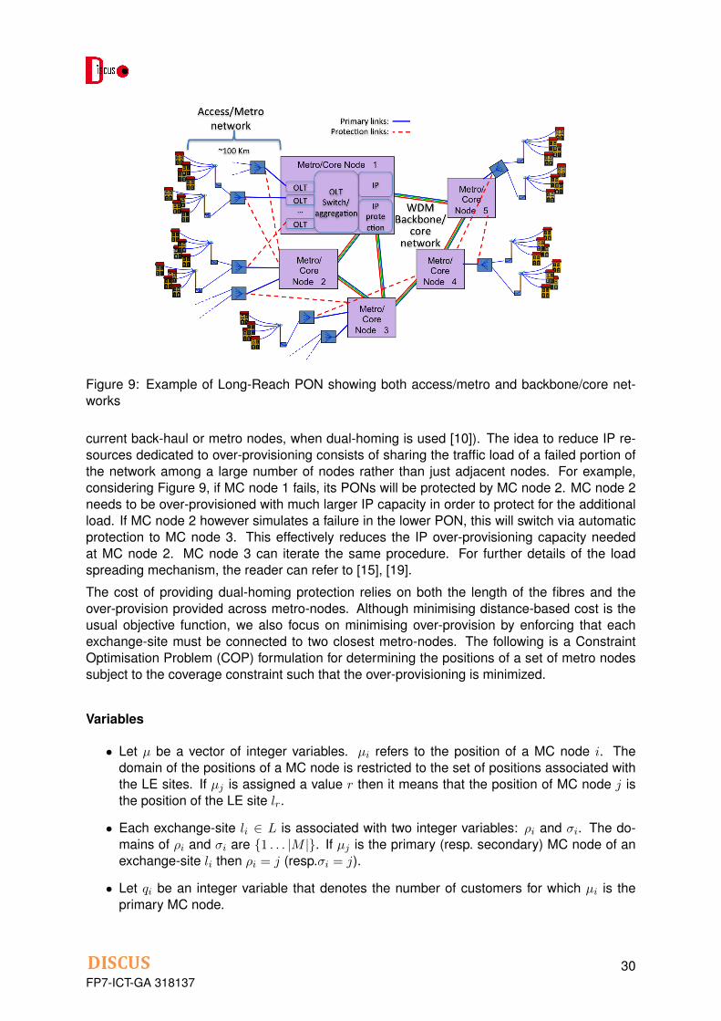
Figure 9: Example of Long-Reach PON showing both access/metro and backbone/core net-works

current back-haul or metro nodes, when dual-homing is used [10]). The idea to reduce IP re-sources dedicated to over-provisioning consists of sharing the traffic load of a failed portion ofthe network among a large number of nodes rather than just adjacent nodes. For example,considering Figure 9, if MC node 1 fails, its PONs will be protected by MC node 2. MC node 2needs to be over-provisioned with much larger IP capacity in order to protect for the additionalload. If MC node 2 however simulates a failure in the lower PON, this will switch via automaticprotection to MC node 3. This effectively reduces the IP over-provisioning capacity neededat MC node 2. MC node 3 can iterate the same procedure. For further details of the loadspreading mechanism, the reader can refer to [15], [19].

The cost of providing dual-homing protection relies on both the length of the fibres and theover-provision provided across metro-nodes. Although minimising distance-based cost is theusual objective function, we also focus on minimising over-provision by enforcing that eachexchange-site must be connected to two closest metro-nodes. The following is a ConstraintOptimisation Problem (COP) formulation for determining the positions of a set of metro nodessubject to the coverage constraint such that the over-provisioning is minimized.

Variables

• Let µ be a vector of integer variables. µi refers to the position of a MC node i. Thedomain of the positions of a MC node is restricted to the set of positions associated withthe LE sites. If µj is assigned a value r then it means that the position of MC node j isthe position of the LE site lr.

• Each exchange-site li ∈ L is associated with two integer variables: ρi and σi. The do-mains of ρi and σi are {1 . . . |M |}. If µj is the primary (resp. secondary) MC node of anexchange-site li then ρi = j (resp.σi = j).

• Let qi be an integer variable that denotes the number of customers for which µi is theprimary MC node.

FP7-ICT-GA 31813730

• Let ωij be an integer variable that denotes the number of customers that are connected toboth metro-nodes µi and µj . In other words, ωij is the load (or the number of customers)that can be transferred from a metro-node µi to another metro-node µj when µi fails.

• For each triplet of MC nodes i, j and k, an integer variable tijk is used to represent theload that is transferred from i to j when k fails.

• For each MC node i an integer variable θi is used to represent maximum load capacityrequired for any single metro-node failure.

Constraints

Coverage. The primary and secondary MC nodes of an LE site li are different: ρi 6= σi. Thedistance between an exchange-site li ∈ L and any of its MC nodes should not be greater thanlmax, i.e., κi,µρi ≤ lmax and κi,µσi ≤ lmax.

Closest. The sum of the distances between an LE site li and its primary and secondary MCnodes is not greater than that of between li and any other pair of metro-nodes say r′ and r′′

(r′ 6= r′′):κi,µρi + κi,µσi ≤ κi,µr′ + κi,µr”

Load. The load of a MC node i is θi =∑

ρj=icustlj .

Max Load Transfer. The maximum load that can be transferred from an MC node i to anotherMC node j is the sum of the loads of all exchange sites whose primary MC node is i andsecondary MC node is j:

ωij =∑

k∈L,ρk=i,σk=jcustlk .

Consequently, the load transferred from i to j has to be less than or equal to ωij for a singlenode failure k, i.e., tijk ≤ ωij .

Capacity. When an MC node k fails, the over-provision capacity required on a MC node isuch that i 6= k is the difference between its incoming load and outgoing load. Therefore, therequired capacity on a node i when a node k fails is the sum of its load and the over-provisioncapacity. The load capacity of a node i should be maximum of the required capacities on i forall possible node failures k, i.e., θi = maxk qi +

∑∀j tjik −

∑∀j tijk.

Objective

The objective is to minimize the total amount of IP over-provision capacity required over allmetro nodes:

min∑

1≤i≤mθi − qi

FP7-ICT-GA 31813731

4.5.2 Routing and Branching Cables through Edge Disjoint Paths

In LR-PON fibres are distributed from the Metro-Nodes (MC nodes) to the Exchange-Sites (LEsites) through cables that forms a tree distribution network. The assumption here is that weare minimising cable cost only, so the structure associated with every MC node should be atree. As our links are directed, we assume that the tree is rooted at the MC node and thedirection of the links are going from the root the leaves. A major fault occurrence in LR-PONwould be a complete failure of the MC node, which could affect tens of thousands of customers.The dual homing protection mechanism for LR-PON enables customers to be connected to twoMC nodes, so that whenever a single MC node fails all customers are still connected to aback-up. Notice that the paths from an LE site to its two MC nodes cannot contain the samelink. Otherwise, this would void the purpose of having two MC nodes. Given an assignmentof MC nodes to LE sites the problem is to determine the routes of cables such that there aretwo edge-disjoint paths from an LE site to its two MC nodes, the length of each path is belowa threshold value and the total cable length required for connecting each LE site to two MCnodes is minimised.

Let Li ⊆ LE be the set of exchange-sites that are associated with metro-node mi ∈ M . Weuse N to denote the set of nodes, which is equal to M ∪ L 1. We use Ti to denote the treenetwork associated with metro-node i. We also use Ni ⊆ N = LEi ∪ {mi} to denote the set ofnodes in Ti.

Given a set of metro-nodesM , a set of exchange-sites LE, a set of feasible (directed) links E ⊆N2, two positive real numbers, a cost κe and a distance le for each link e ∈ E, an associationof LE sites with two MC nodes π : L → M2, and a real number lmax, the problem is to find aspanning tree Ti for each metro-node mi such that:

1. The length of the unique path from the MC node mi to any exchange-site is not greaterthan lmax.

2. For each LE site lk, the two paths connecting lk to mi and to mj , where π(lk) = 〈mi,mj〉,are edge disjoint.

3. The sum of the costs of the edges in all the spanning trees is minimum.

We now present the constraint optimisation formulation of this problem.

Variables.

• Let xijk be a Boolean variable that denotes whether a link between LE sites j ∈ Li andk ∈ Li is chosen for Ti. Each link (i, j) has an associated cost κij .

• Let f ij be a positive real variable that denotes the cost of the path from the MC node i toits LE site j.

1The graph obtained from the actual reference network involves optional nodes. In the preprocessing phase, weremove such nodes and create links between the remaining nodes if there is a path connecting them that only usesoptional nodes. That is, a link in the resulting graph between two nodes means that it is possible to go from on onenode to the other via optional nodes only in the original graph.

FP7-ICT-GA 31813732

Constraints. Each exchange-site associated with each MC node has only one incominglink: ∑

lj∈Ni

xijk = 1, ∀mi∈M∀lk∈Li

xijk + xikj ≤ 1, ∀mi∈M∀{lj ,lk}⊆NiEach MC node is connected to at least one of its exchange-sites:∑

lj∈Li

xiij ≥ 1, ∀mi∈M

The total number of links in any Ti is equal to |Li|:∑lj∈Ni

∑lk∈Li,lj 6=lk

xijk = |Li|, ∀mi∈M

If there is a link from lj ∈ Li to lk ∈ Li then the cost of the path from mi to lk is greater than orequal to the sum of the cost from mi to lj plus the cost between lj and lk:

xijk = 1⇒ f ik ≥ f ij + κjk, ∀mi∈M∀{lj ,lk}∈NiAt any node in the tree the cost of the path from a metro-node mi to a exchange-site lj andthe cost of the path from lj to the farthest exchange-site on the same path should be less thanlmax:

f ij ≤ lmax, ∀mi∈M∀lj∈Ni

Edge-Disjoint Constraint. If mi and m′i are the metro-nodes of the LE site j, and if thereexists any path in the subnetwork associated with metro-node i that includes the arc 〈lj , lk〉,then metro-node i′ cannot use the same arc. Therefore, we enforce the following constraint:

xijk + xi′jk ≤ 1, ∀{mi,mi′}∈M∀{lj ,lk}∈Li∩Li′

xijk + xi′kj ≤ 1, ∀{mi,mi′}∈M∀{lj ,lk}∈Li∩Li′

Objective. The objective is to minimize the total cost:

min∑mi∈M

∑{lj ,lk}∈Li

κjk · xijk

4.5.3 Routing and Branching Cables through Node Disjoint Paths

In the previous section we presented a model to address edge disjointness at the level ofthe backhaul. However, it is reasonable to consider a stronger policy of resiliency taking intoaccount that a failure can take place at the level of an LE site itself. Therefore, in this sectionwe present a model to address node disjointness.We create a graph per LE site. In what follows, Ni denotes, the set of nodes in the graphassociated with LE site i, is equal to L′ ∪ {m1,m2}, where m1 and m2 are the primary andsecondary MC nodes of LE site i. L′ ⊆ L is the set of local exchanges that participate in a pathfrom either m1 or m2 to LE site i that respects the length constraint. That is, if sp(i, j) is theshortest path length between i and j, then:

L′ = {l ∈ L|sp(m1, l) + sp(l, i) ≤ lmax ∨ sp(m2, l) + sp(l, i) ≤ lmax}

.

FP7-ICT-GA 31813733

Variables.

• Let xijk be a Boolean variable that denotes whether a link between node j ∈ Ni andk ∈ Ni. Each link (j, k) has an associated cost κjk in graph associated with LE site i.

• Let yjk be a Boolean variable that denotes whether a link between node j ∈ M ∪ L andk ∈M ∪ L, considering all graphs associated with LE sites.

• Let f ij be a variable that denotes the cost of the path from the MC node i to its LE site j.

• Let bij be a variable that denotes the maximum cost of the path from the LE site j to theleaf in the path.

Constraints. LE site i has two incoming edges, and m1 and m2 have no incoming edges:∑j∈Ni

xiji = 2, ∀i ∈ L

∑j∈Ni

xijm1= 0, ∀i ∈ L

∑j∈Ni

xijm2= 0, ∀i ∈ L

The graph is undirected:xijk + xikj ≤ 1, ∀i ∈ L,∀{j,k}⊆Ni

Both m1 and m2 are connected to at least one local exchange:∑j∈Ni

xim1j = 1, ∀i ∈ L

∑j∈Ni

xim2j = 1, ∀i ∈ L

Any LE site k in the graph of LE site i has at most one incoming edge, and conserves the flow :∑j∈Ni

xijk ≤ 1, ∀i ∈ L,∀k ∈ Ni

∑j∈Ni

xijk =∑j∈Ni

xikj , ∀i ∈ L

A link is used if it is used in any of the graphs asociated with LE sites:

xijk ≤ yjk, ∀i ∈ L,∀{j,k}⊆Ni

If there is a link from j ∈ Ni to k ∈ Ni then the cost of the path from mi to k is greater than orequal to the sum of the cost from mi to j plus the cost between j and k:

xijk = 1⇒ f ik ≥ f ij + κjk, ∀i ∈ L,∀mi∈{m1,m2}∀{j,k}∈L′

If there is a link from j ∈ Ni to k ∈ Ni then the cost of the path from j to its leaf-node is greaterthan or equal to the sum of the cost from k to its leaf-node plus the cost between lj and lk:

xijk = 1⇒ bij ≥ bik + κjk, ∀i ∈ L,∀mi∈{m1,m2}∀{j,k}∈L′

At any node in the tree the cost of the path from a metro-node mi to a LE site lj and the cost ofthe path from lj to the farthest exchange-site on the same path should be less than lmax:

f ij + bij ≤ lmax, ∀i ∈ L,∀mi∈{m1,m2}∀j∈L′

FP7-ICT-GA 31813734

Objective. The objective is to minimize the total cost:

min∑

{j,k}⊆M∪L

κjk · yjk

4.6 Preliminary computational results

4.6.1 Preliminary results for Facility Location Models

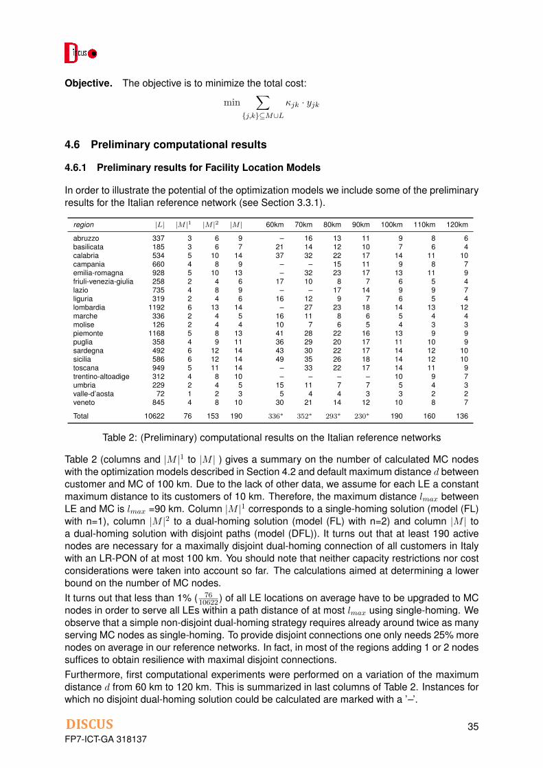
In order to illustrate the potential of the optimization models we include some of the preliminaryresults for the Italian reference network (see Section 3.3.1).

region |L| |M |1 |M |2 |M | 60km 70km 80km 90km 100km 110km 120km

abruzzo 337 3 6 9 – 16 13 11 9 8 6basilicata 185 3 6 7 21 14 12 10 7 6 4calabria 534 5 10 14 37 32 22 17 14 11 10campania 660 4 8 9 – – 15 11 9 8 7emilia-romagna 928 5 10 13 – 32 23 17 13 11 9friuli-venezia-giulia 258 2 4 6 17 10 8 7 6 5 4lazio 735 4 8 9 – – 17 14 9 9 7liguria 319 2 4 6 16 12 9 7 6 5 4lombardia 1192 6 13 14 – 27 23 18 14 13 12marche 336 2 4 5 16 11 8 6 5 4 4molise 126 2 4 4 10 7 6 5 4 3 3piemonte 1168 5 8 13 41 28 22 16 13 9 9puglia 358 4 9 11 36 29 20 17 11 10 9sardegna 492 6 12 14 43 30 22 17 14 12 10sicilia 586 6 12 14 49 35 26 18 14 12 10toscana 949 5 11 14 – 33 22 17 14 11 9trentino-altoadige 312 4 8 10 – – – – 10 9 7umbria 229 2 4 5 15 11 7 7 5 4 3valle-d’aosta 72 1 2 3 5 4 4 3 3 2 2veneto 845 4 8 10 30 21 14 12 10 8 7

Total 10622 76 153 190 336∗ 352∗ 293∗ 230∗ 190 160 136

Table 2: (Preliminary) computational results on the Italian reference networks

Table 2 (columns and |M |1 to |M | ) gives a summary on the number of calculated MC nodeswith the optimization models described in Section 4.2 and default maximum distance d betweencustomer and MC of 100 km. Due to the lack of other data, we assume for each LE a constantmaximum distance to its customers of 10 km. Therefore, the maximum distance lmax betweenLE and MC is lmax =90 km. Column |M |1 corresponds to a single-homing solution (model (FL)with n=1), column |M |2 to a dual-homing solution (model (FL) with n=2) and column |M | toa dual-homing solution with disjoint paths (model (DFL)). It turns out that at least 190 activenodes are necessary for a maximally disjoint dual-homing connection of all customers in Italywith an LR-PON of at most 100 km. You should note that neither capacity restrictions nor costconsiderations were taken into account so far. The calculations aimed at determining a lowerbound on the number of MC nodes.It turns out that less than 1% ( 76

10622 ) of all LE locations on average have to be upgraded to MCnodes in order to serve all LEs within a path distance of at most lmax using single-homing. Weobserve that a simple non-disjoint dual-homing strategy requires already around twice as manyserving MC nodes as single-homing. To provide disjoint connections one only needs 25% morenodes on average in our reference networks. In fact, in most of the regions adding 1 or 2 nodessuffices to obtain resilience with maximal disjoint connections.Furthermore, first computational experiments were performed on a variation of the maximumdistance d from 60 km to 120 km. This is summarized in last columns of Table 2. Instances forwhich no disjoint dual-homing solution could be calculated are marked with a ’–’.

FP7-ICT-GA 31813735

The number of MC nodes reduces almost logarithmically when d is increased.

It is interesting to observe that under the default parameter settings for some of the regions notwo connections to potential MC-locations within the distance of d exist. This results from therestriction that potential MC nodes have to belong to a larger biconnected component. Thisdoes not hold for some of the mountainous region in Italy, where only a single path connects avalley to the biconnected centre of the network. In Table 2 the Total for columns with missingvalues is marked with a ∗.

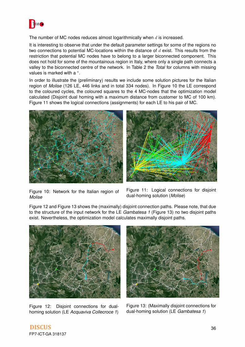
In order to illustrate the (preliminary) results we include some solution pictures for the Italianregion of Molise (126 LE, 446 links and in total 334 nodes). In Figure 10 the LE correspondto the coloured cycles, the coloured squares to the 4 MC-nodes that the optimization modelcalculated (Disjoint dual homing with a maximum distance from customer to MC of 100 km).Figure 11 shows the logical connections (assignments) for each LE to his pair of MC.

Figure 10: Network for the Italian region ofMolise

Figure 11: Logical connections for disjointdual-homing solution (Molise)

Figure 12 and Figure 13 shows the (maximally) disjoint connection paths. Please note, that dueto the structure of the input network for the LE Gambatesa 1 (Figure 13) no two disjoint pathsexist. Nevertheless, the optimization model calculates maximally disjoint paths.

Figure 12: Disjoint connections for dual-homing solution (LE Acquaviva Collecroce 1)

Figure 13: (Maximally disjoint connections fordual-homing solution (LE Gambatesa 1)

FP7-ICT-GA 31813736

0

10

20

30

40

50

60

1 2 3 4 5

Perc

enta

ge o

f IP

Pro

tection C

apacity R

educed

Number of Hops from Failed Load

Italy-dist-100

Italy-pcap-100

UK-dist-75

UK-pcap-75

Ireland-dist-18

Ireland-pcap-18

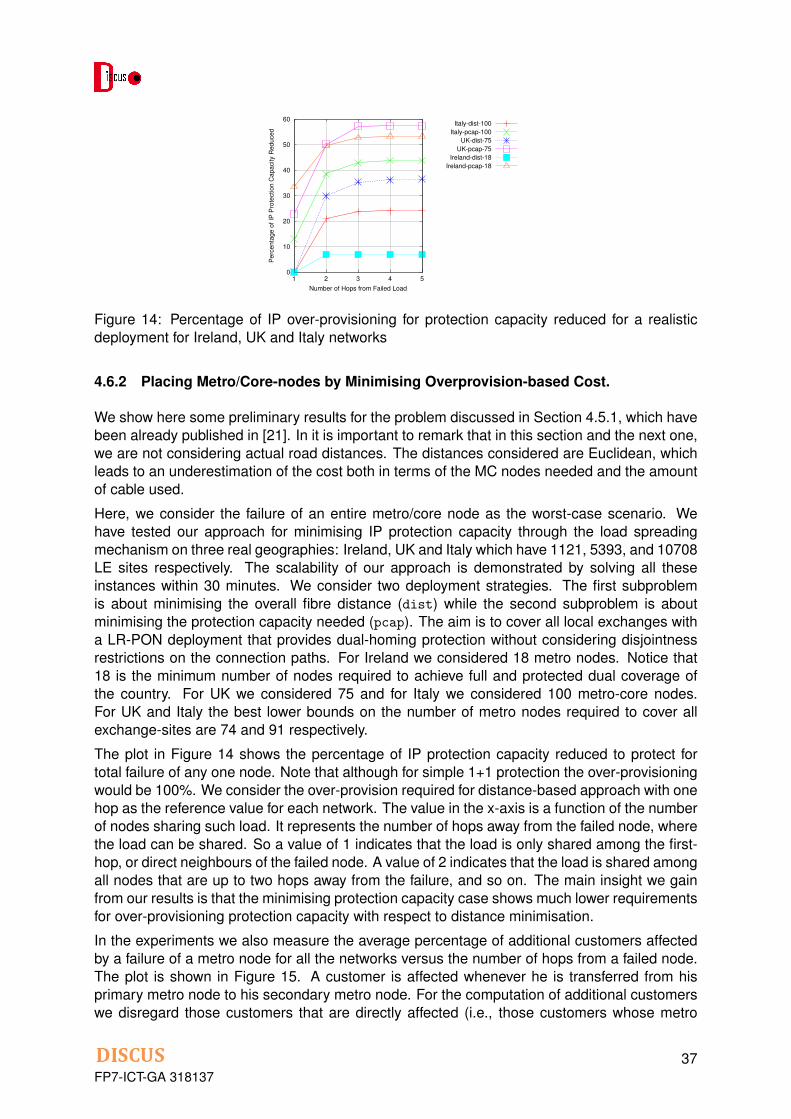
Figure 14: Percentage of IP over-provisioning for protection capacity reduced for a realisticdeployment for Ireland, UK and Italy networks

4.6.2 Placing Metro/Core-nodes by Minimising Overprovision-based Cost.

We show here some preliminary results for the problem discussed in Section 4.5.1, which havebeen already published in [21]. In it is important to remark that in this section and the next one,we are not considering actual road distances. The distances considered are Euclidean, whichleads to an underestimation of the cost both in terms of the MC nodes needed and the amountof cable used.

Here, we consider the failure of an entire metro/core node as the worst-case scenario. Wehave tested our approach for minimising IP protection capacity through the load spreadingmechanism on three real geographies: Ireland, UK and Italy which have 1121, 5393, and 10708LE sites respectively. The scalability of our approach is demonstrated by solving all theseinstances within 30 minutes. We consider two deployment strategies. The first subproblemis about minimising the overall fibre distance (dist) while the second subproblem is aboutminimising the protection capacity needed (pcap). The aim is to cover all local exchanges witha LR-PON deployment that provides dual-homing protection without considering disjointnessrestrictions on the connection paths. For Ireland we considered 18 metro nodes. Notice that18 is the minimum number of nodes required to achieve full and protected dual coverage ofthe country. For UK we considered 75 and for Italy we considered 100 metro-core nodes.For UK and Italy the best lower bounds on the number of metro nodes required to cover allexchange-sites are 74 and 91 respectively.

The plot in Figure 14 shows the percentage of IP protection capacity reduced to protect fortotal failure of any one node. Note that although for simple 1+1 protection the over-provisioningwould be 100%. We consider the over-provision required for distance-based approach with onehop as the reference value for each network. The value in the x-axis is a function of the numberof nodes sharing such load. It represents the number of hops away from the failed node, wherethe load can be shared. So a value of 1 indicates that the load is only shared among the first-hop, or direct neighbours of the failed node. A value of 2 indicates that the load is shared amongall nodes that are up to two hops away from the failure, and so on. The main insight we gainfrom our results is that the minimising protection capacity case shows much lower requirementsfor over-provisioning protection capacity with respect to distance minimisation.

In the experiments we also measure the average percentage of additional customers affectedby a failure of a metro node for all the networks versus the number of hops from a failed node.The plot is shown in Figure 15. A customer is affected whenever he is transferred from hisprimary metro node to his secondary metro node. For the computation of additional customerswe disregard those customers that are directly affected (i.e., those customers whose metro

FP7-ICT-GA 31813737

node is the one that is failing). In the plots we show the percentage of customers affectedwhich is measured with respect to the total number of customers. The results show that thepercentage of customers affected decreases as the network size increases, while it increasesas we reduce the IP over-provisioning by sharing the load between more nodes. The drawbackof a larger sharing is that more customers not directly affected by the node failure becomeaffected by the protection process. The plots in Figures 14 and 15 show that the load-spreadingmechanism can reduce the over-provisioning requirement significantly while only affecting 3%additional customers at most.

0

0.5

1

1.5

2

2.5

3

1 2 3 4 5

Perc

enta

ge o

f A

dditio

nal C

usto

mers

Affecte

d

Number of Hops from Failed Load

Italy-dist-100

Italy-pcap-100

UK-dist-75

UK-pcap-75

Ireland-dist-18

Ireland-pcap-18

Figure 15: Additional customers affected by a total node failure because of the load sharingmechanism, versus the number of hops from failed node

4.6.3 Routing and Branching Cables through Edge Disjoint Paths

In this section we share some preliminary results for the problem presented in Section 4.5.2.

Table 3: Results for Ireland, UK and ItalyCountry |M | LS Naive LB

18 17074 87477.03 14809Ireland 20 16808 86583.68 14845|L|=1121 22 16693 82131.43 14990

24 16138 78118.75 1457075 65211 386891.89 54720

UK 80 64446 384059.95 54975|L|=5393 85 63511 366558.48 55087

90 62256 357471.67 55035140 89636 644139.37 76457

Italy 150 88514 618810.22 76479|L|=10708 160 88628 602305.77 76794

170 87836 583626.40 77013

In Table 3 we consider 12 instances coming from three different countries. Each country is as-sociated with its corresponding number of LE sites. For each country we consider four differentMC placements. The first column is identifying the LE instances. The second column refers tothe MC placements, which are identified by their number of MC nodes. Column LS refers tothe cost that we have obtained using our current best approach to this problem. Column Naiverefers to the cost obtained when we connect each LE node directly to its MC nodes. ColumnLB refers to lower bounds that we have computed for these instances (i.e., it is ensured thatthe cost cannot go bellow these number). From these numbers we can observe that the costis reduced considerably when sharing takes place. We can also observe that the quality of ourbest approach is very close to optimality.

FP7-ICT-GA 31813738

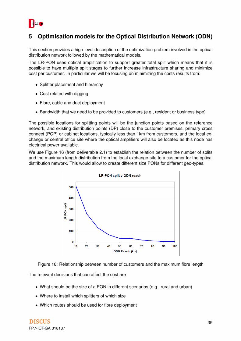
5 Optimisation models for the Optical Distribution Network (ODN)

This section provides a high-level description of the optimization problem involved in the opticaldistribution network followed by the mathematical models.

The LR-PON uses optical amplification to support greater total split which means that it ispossible to have multiple split stages to further increase infrastructure sharing and minimizecost per customer. In particular we will be focusing on minimizing the costs results from:

• Splitter placement and hierarchy

• Cost related with digging

• Fibre, cable and duct deployment

• Bandwidth that we need to be provided to customers (e.g., resident or business type)

The possible locations for splitting points will be the junction points based on the referencenetwork, and existing distribution points (DP) close to the customer premises, primary crossconnect (PCP) or cabinet locations, typically less than 1km from customers, and the local ex-change or central office site where the optical amplifiers will also be located as this node haselectrical power available.

We use Figure 16 (from deliverable 2.1) to establish the relation between the number of splitsand the maximum length distribution from the local exchange-site to a customer for the opticaldistribution network. This would allow to create different size PONs for different geo-types.

Figure 16: Relationship between number of customers and the maximum fibre length

The relevant decisions that can affect the cost are

• What should be the size of a PON in different scenarios (e.g., rural and urban)

• Where to install which splitters of which size

• Which routes should be used for fibre deployment

FP7-ICT-GA 31813739

Table 4: Relation between the split-size and the maximum allowed distancecustomers length

512 10256 20128 3064 40

Given a local exchange-site and the number of customers associated with it, the problem is toconstruct a set of optimal PONs. We decompose this problem in to three subproblems.

• The first subproblem is to estimate the number of PONs for each exchange-site by parti-tioning the set of customers such that each subset of customers will be associated withone PON. Notice that here we would like to take in to account different geo-types whichwould have an impact on the sizes (number of customers) of PONs.

• The second subproblem is to find the locations of a set of splitters required to connect agiven set of customers. Here the assumption is that the first-level splitter in the splitter-hierarchy is always placed in the local exchange-site.

• The third subproblem is to consolidate some of the local exchange-sites, where possible,by moving the locations of the first-level splitters.

For the ODN-optimization the following basic optimization questions have been identified:

• Where should splitters be placed?

• What splitter hierarchy should be applied?

• What should be the size of each splitter?

• Which customers should we associate with each splitter?

• How do we route the cable once the association of splitters with customers is set?

5.1 Estimating Number of PONs

In order to partition the set of customers associated with a given exchange-site, denoted by C,we construct a rooted distance bounded spanning tree. The size of the partition is the numberof PONs. Here the root node is the local exchange-site and the number of immediate childrenof the root-node is associated with the number PONs.

For solving this problem we assume that we are given the following as an input:

• Network topology (locations of customers and local exchange-sites)• (LE,Customers) assignment• Relation between split-size and maximum allowed distance as shown in Table 4

The maximum distance for each PON is dependent on the number of customers involved in thePON as shown in Table 4. The root-node (i.e., an exchange-site) is denoted by r and the setof all nodes associated with customers and the exchange-site is denoted by N . In case whenmultiple customers are at the same location, we can create as many nodes as the number ofcustomers. Therefore, without loss of generality we assume that one node is associated withone customer. We use N2 to denote the pairs of customers. We assume that there exists at

FP7-ICT-GA 31813740

least one path between any pair of customers and between exchange-site to any customer. Letdij denote the distance between any pair of nodes. The direction of the link in the tree is fromroot-node to a leaf-node. We remark that here distance bounded spanning tree is basicallyused for partitioning the customers and the links that are used in the tree has no implication onhow the fibers would be deployed or where the splitters would be placed.

Variables

• Let xij be a Boolean variable for each 〈i, j〉 ∈ N2 that denotes whether a link betweennode i and node j exists in the tree.

• Let yij be a non-negative integer variable that denotes the number of customers in thesub-tree emanating from node j.

• Let zi be a non-negative integer variable that denotes the length of the path from theexchange-site to its customer j.

ConstraintsEach node (except root-node) must have one incoming link:

∑i∈N xij = 1, ∀j∈C .

The root-node is connected to at least one another node:∑

j∈C xrj ≥ 1. The total number oflinks in any tree is equal to |C|:

∑i∈N

∑j∈N xij = |C|.

If there is a link from i ∈ N to j ∈ N then the length of the path from root-node to j is equal tothe length of the path from root-node to i plus the distance between nodes i and j:

xij = 1⇒ zj = zi + dij , ∀{i,j}⊆N

The number of customers at each node is one more than the number of nodes in the sub-treeemanating from that node. ∑

j∈Nyji =

∑j∈N

yij + 1, ∀i∈N

If there is no link between nodes i and j then of course no customers are relying on this link inthe tree ∀{i,j}∈N : xij = 0 =⇒ yij = 0. The number of customers in any PON is dependent onthe maximum distance between a customer and the exchange-site:

yij ≥ 512 =⇒ zi ≤ 0, ∀{i,j}⊆N

yij ≥ 256 =⇒ zi ≤ 10, ∀{i,j}⊆Nyij ≥ 128 =⇒ zi ≤ 20, ∀{i,j}⊆Nyij ≥ 64 =⇒ zi ≤ 30, ∀{i,j}⊆N

Objective Function

There are two different criteria. The objective function could be either based on one of them orwe can aggregate them:

• Minimising the number of PONs: min∑

j∈C xrj

• Minimising the total distance: min∑

i∈N∑

j∈N dij · xij

FP7-ICT-GA 31813741

5.2 Selection of Splitter locations

Once the set of customers have been partitioned and the number of PONs is identified, the taskis to define a hierarchy of splitters (a tree) for each PON taking into account the loss associatedwith the length of the cable and the size of the splitters.

The following is the input for solving this problem:

• Network topology (locations of customers, locations of exchange-sites, and locations ofpossible positions for the splitters)

• Set of PONs• Loss function.

The output is a splitter hierarchy for each PON.

Remarks:

• We assume that the first-level splitter is placed in the local exchange-site

• No assumption on the number of splitters in the path to a customers is made. The struc-ture of the tree is driven by the loss.

• The domain of the size of the splitters is {4, 8, 16, 32}.

Notations

• Let S = {0, 1, . . . ,m} be the set of all possible locations where a splitter can be placed.We use index 0 to denote the position of the exchange-site where the first splitter isplaced.

Let C be the set of the locations of all the customers. Let U = S ∪ C − {0}.

• Let in(i) be the set of splitters from which the splitter si can receive fibre. Let out(i) bethe set of splitters/customers that can receive fibres from si.

• Let sizes = {λ1, λ2, . . . , λk} be the set of all sizes of splitters that are allowed. Here λkmeans the fibre can be splitted in to 2k fibres. The cost of each splitter of size 2k is ck.We assume that the size of the first splitter is either 4 or 8 which is denoted by λf . Themaximum size of any splitter is 32.

• Let dij denote the road distance between points i and j. If the road-distance between anytwo points is not given then we compute it based on the Euclidean distance multiplied bythe routing factor denoted by r. Notice that the exact road-distance is know the value of ris set to 1.

• The loss of signal due to fibre length is computed by using lossd(i, j) = 0.3 · r · dij . Theloss due to using a splitter of size λk is computed by losss(k) = 10 log10 2k + 0.2k. Themaximum loss between a customer and the first splitting point is denoted by maxLoss.which is set to 31.093 based on Table 4.

Variables

• Let xij be a Boolean variable that denotes whether there is any link between i ∈ S andj ∈ out(i).

FP7-ICT-GA 31813742

• Let yik be an integer variable that denotes whether the size of the splitter i ∈ S is λk ornot.

• Let zi be a Boolean variable that denotes whether a splitter is placed at location i ∈ S ornot.

• The forward signal loss at point i ∈ S ∪C is defined by the loss occurred between the firstlevel splitter point and the point i. Similarly the backward signal loss at point i ∈ S ∪ Cis defined by maximum loss occurred between the point i and any customer connectedto point i via some path. Let fli and bli be non-negative continuous variables that denotethe forward and backward signal loss at point i respectively.

Constraints

Splitter Size Constraints. For each selected splitter is associated with at most 1 size:

∀i∈S : zi =∑

λk∈sizesyik

The size of the first splitting point is fixed to λf :

y0f = 1

Incoming/Outgoing degree Constraints. Each customer is connected to 1 splitter throughone incoming fibre:

∀j∈C :∑

i∈in(j)

xij = 1

Each non-root splitter is connected to at most 1 other splitter through one incoming fibre:

∀j∈S−{0} : zj =∑

i∈in(j)

xij

The number of outgoing ports used at splitting point i should be less than or equal to the sizeof the splitter i:

∀i∈S :∑

j∈out(i)

xij ≤∑

λk∈sizes2k · yik

If the splitter i has one incoming fibre then there should be at least one outgoing fibre:

∀i∈S−{0} : zi −∑

j∈out(i)

xji ≤ 0

If the splitter i has at least one outgoing fibre then there should be one incoming fibre:

∀i∈S−{0} :∑

j∈out(i)

xij ≤ max(sizes)zi

The number of edges in the tree is one less than the number of nodes:∑i∈S

∑j∈out(i)

xij =∑i∈S

zi + |C| − 1

FP7-ICT-GA 31813743

Loss Constraints. The forward loss at the first-level splitter is:

fl0 = losss(f)

If i ∈ S is connected to another splitter point j ∈ S ∩ out(i) then the forward loss at j is asfollows:

∀i∈S∀j∈S∩out(i) : xij = 1⇒ flj = fli +

lossd(i, j) +∑

λk∈sizesyjk · losss(k)

If i ∈ S is connected to customer j ∈ C ∩ out(i) then the forward loss at customer point j is asfollows:

∀i∈S∀j∈C∩out(i) : xij = 1⇒ flj = fli + dloss(i, j)

The backward loss at each customer is 0:

∀i∈C : bli = 0

If i ∈ S is connected to another splitter point j ∈ S ∩ out(i) then the backward loss at i is asfollows:

∀i∈S∀j∈S∩out(i) : xij = 1⇒ bli ≤ maxLoss−

blj + lossd(i, j) +∑

λk∈sizesyjk · losss(k)

If i ∈ S is connected to customer j ∈ C ∩ out(i) then the backward loss at i is as follows:

∀i∈S∀j∈C∩out(i) : xij = 1⇒ bli ≤ maxLoss− (blj + lossd(i, j))

The loss at any node should be less than maxLoss, and therefore:

∀i∈S : fli + bli ≤ maxLoass

Objective The objective is composed of two criteria:

• Minimise the cost of deploying fibres: min∑

j∈C∑

i∈S dij · xij

• Minimise the cost of splitters: min∑

j∈S cj × zj

5.3 Consolidation of Local Exchange-Sites

In order to use existing infrastructure, normally all customers would be connected to their localexchanges in the optical distribution network. However, it is not necessary to put the first-levelsplitters in all local exchanges.

We remark that there is a high variance with respect to the load of the local exchanges as canbe observed in Figure 17(a) and Figure 17(b). In these figures, a point (x, y), means that theprobability of having a load greater than x×maxLoad (where maxLoad is the maximum load inthe distribution) is y × 100%.

While there are local exchanges associated with a high number of customers that will need tobe split into several PONs, there are also small local exchanges that would need to be mergedwith other small local exchanges to form a PON. We observe, for instance, that for Italy, theprobability of having a local exchange whose load is greater than 0.1 × maxLoad is only 20%

FP7-ICT-GA 31813744

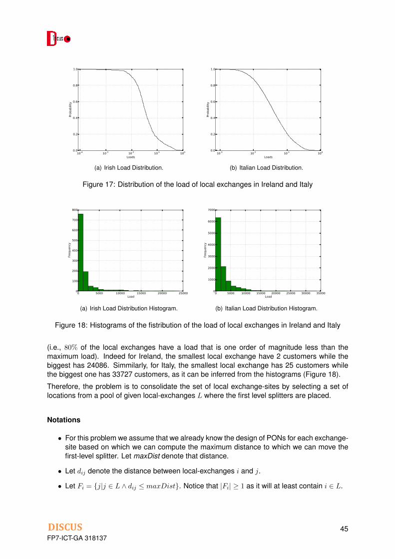
10-4 10-3 10-2 10-1 100

Loads

0.0

0.2

0.4

0.6

0.8

1.0Pro

babili

ty

(a) Irish Load Distribution.

10-3 10-2 10-1 100

Loads

0.0

0.2

0.4

0.6

0.8

1.0

Pro

babili

ty

(b) Italian Load Distribution.

Figure 17: Distribution of the load of local exchanges in Ireland and Italy

0 5000 10000 15000 20000 25000Load

0

100

200

300

400

500

600

700

800

Frequency

(a) Irish Load Distribution Histogram.

0 5000 10000 15000 20000 25000 30000 35000Load

0

1000

2000

3000

4000

5000

6000

7000

Frequency

(b) Italian Load Distribution Histogram.

Figure 18: Histograms of the fistribution of the load of local exchanges in Ireland and Italy

(i.e., 80% of the local exchanges have a load that is one order of magnitude less than themaximum load). Indeed for Ireland, the smallest local exchange have 2 customers while thebiggest has 24086. Simmilarly, for Italy, the smallest local exchange has 25 customers whilethe biggest one has 33727 customers, as it can be inferred from the histograms (Figure 18).

Therefore, the problem is to consolidate the set of local exchange-sites by selecting a set oflocations from a pool of given local-exchanges L where the first level splitters are placed.

Notations

• For this problem we assume that we already know the design of PONs for each exchange-site based on which we can compute the maximum distance to which we can move thefirst-level splitter. Let maxDist denote that distance.

• Let dij denote the distance between local-exchanges i and j.

• Let Fi = {j|j ∈ L ∧ dij ≤ maxDist}. Notice that |Fi| ≥ 1 as it will at least contain i ∈ L.

FP7-ICT-GA 31813745

Variables

• Let xij be a Boolean variable that denotes whether the first level splitter for ei is ej or not.

• Let yj be a Boolean variable that denotes whether a first-level splitter is placed at ej ornot.

Constraints Each exchange-site ei is associated with exactly one location ej where the first-level splitters will be placed for the customers associated with ei:

∀ei∈E :∑ej∈Fi

xij = 1

∀ei∈E :∑

ej∈E−Fi

xij = 0

The location ej is selected for placement of first-level splitter if at least one exchange-site eirequires that the first-level splitter of its customers should be at ej :

∀ei∈E∀ej∈Fi : xij ≤ yj

Objective The primary objective is to minimise the number of locations where the first-levelsplitters are placed and the secondary objective is to minimise the distance based cost.

minα ·

∑ei∈E

yi

+∑ei∈E

∑ej∈Fi

dij · xij

Here α is a constant that is greater than the cost related with total distances.

FP7-ICT-GA 31813746

6 Conclusions

In this deliverable we have formulated the key combinatorial optimisation problems that arise inthe design of long-reach access networks. Due to the complexity of the planning problem andthe size of the reference networks the overall problem is decomposed into the two subproblemsof ODN-optimization and backhaul-optimization.

As a single PON of the DISCUS architecture can support up to 512 customers (see Table 4 onpage 40) and the current local exchanges are supporting up to several thousands customersthe design of ODN is divided in to three subproblems. The first problem is to identify thenumber of PONs that would partition the customers associated with the exchange-site. Thesecond problem is to design PON network for each element of the partition by finding thelocation of splitter points, deciding the links between pairs of splitters or between customersand splitters. The third problem is to consolidate a set of exchange-sites by taking into accountthat the number of customers supported by different exchange-site could vary a lot. We havepresented the mathematical models of these problems. The presented models are general andrely on minimal assumptions. They can be used for different geo-types like urban and rural,different ways of calculating distances like Euclidean or road-distance, different loss functions,different sizes of splitters etc. In Deliverable 4.7 we will present approaches to solve thesemodels and present the results for Ireland and the results for Italy will be available for only afew regions.

For backhaul optimization we presented an Integer Programming model that selects the min-imum number of MC nodes, determines their locations and optimizes the (LE,MC)-connections(see Section 4.2). An initial proof-of-concept implementation was able to determine a solutionfor the Italian reference network that minimizes the number of necessary MC nodes (Sec-tion 4.6.1). This solution was calculated region by region and combining the regional solutionsto a overall solution for Italy. This is a reasonable approach for Italy as, for historical reasons, the(LE,MC)-connections do not cross region borders. These calculations did neither take capacityrestrictions nor a cost-model (which is not yet defined for the DISCUS project) into account. Itaimed at determining a lower bound on the number of MC nodes needed.

While a single- or dual-homing solution is relatively easy to calculate this certainly does nothold for a dual-homing solution with disjoint paths. It turned out that the calculation bottleneckis not only the solution of the optimization model, but as well the generation of the input data forthese models. The calculation of the disjoint paths for each LE is a difficult problem in itself andthe initial computational experiments indicate that this part is computationally as expensive asthe calculation of the optimization solution (with respect to computing time). The developmentof further algorithmic approaches and proper handling of various implementation details ofthe disjoint path-generation seem necessary in order to calculate nation-wide solutions in areasonable amount of time.

In order to further speed up the calculation we will develop and implement further decomposi-tion techniques, like, e.g., a sliding window approach where starting with an initial solution (e.g.calculated by the approaches we have so far) iteratively a major part of the solution is fixed andonly some part of the network is due to optimization.

Furthermore a realistic cost-model as well as capacity restrictions have to be taken into ac-count. The models presented in Section 4.2 are able to cope with them. The path-generation isin influenced by them and we are expect that the models will be able to handle these. But thishas to be proven by further computational test. These are topics that will be discussed in detailin Deliverable D4.7 (Optimization methods and algorithms for long-reach access networks).

FP7-ICT-GA 31813747

References

[1] J. Chen, et al. “First Report on the Specification of the Metro/Core Node Architecture,”DISCUS Deliverable 6.1, August 2013

[2] F. Farjady et al. “First WP2 progress report,” DISCUS Deliverable 2.2, 2013

[3] Cisco, “Cisco Visual Networking Index: Forecast and Methodology, 2012–2017,” 2012.[Online]. Available: http://www.cisco.com/en/US/solutions/collateral/ns341/

ns525/ns537/ns705/ns827/white_paper_c11-481360_ns827_Networking_Solutions_

White_Paper.html

[4] G. Cornuejols, R. Sridharan, and J.-M. Thizy, “A comparison of heuristics and relaxationsfor the Capacitated Plant Location Problem ,” European Journal of Operational Research,vol. 50, pp. 280–297, 1991.

[5] R. Diestel, Graph Theory, Graduate Texts in Mathematics, Vol. 173, Springer, 2010

[6] M. Grotschel, C. Raack, and A. Werner, “Towards optimizing the deployment of opticalaccess networks,” EURO Journal on Computational Optimization, no. to appear, availableas Springer Online First, 2013.

[7] J. Hopcroft and R. Tarjan, “Algorithm 447: Efficient algorithms for graph manipulation,”Commun. ACM, vol. 16, no. 6, pp. 372–378, Jun. 1973.

[8] D. K. Hunter et al., Protection of long-reach PON traffic through router database synchro-nization. Journal of Optical Networking 6(5):535-549, 2007

[9] Arie M. C. A. Koster and Xavier Munoz, Graphs and Algorithms in Communication Net-works, Springer, 2009

[10] S. D. Maesschalck et al., Intelligent optical networking for multilayer survivability. IEEECommunications Magazine 40(1):42-49, 2002

[11] G. L. Nemhauser and L. A. Wolsey, Integer and Combinatorial Optimization, Wiley-Interscience, New York, 1988

[12] A. J. Phillips et al., Redundancy Strategies for a High Splitting Optically Amplified PassiveOptical Network. Journal of Lightwave Technology, 19(2):137-149, 2001

[13] M. Ruffini, L. Wosinska, M. Achouche, J. Chen, N. J. Doran, F. Farjady, J. Montalvo, P.Ossieur, B. O’Sullivan, N. Parsons, T. Pfeiffer, X.-Z. Qiu, C. Raack, H. Rohde, M. Schi-ano, P. Townsend, R. Wessaly, X. Yin, D. B. Payne, “DISCUS: An end-to-end solution forubiquitous broadband optical access,” IEEE Com. Mag., vol. 52, no. 2, February 2014

[14] M. Ruffini, D. Payne, et al. “Report on the initial DISCUS End to End Architecture,” DISCUSDeliverable 2.1, April 2013

[15] M. Ruffini et al., Protection strategies for long-reach PON, in proceedings of ECOC 10,paper Tu.5.B.2

[16] R. Sridharan, “The capacitated plant location problem,” European Journal of OperationalResearch, vol. 87, pp. 203–213, 1995.

[17] R. Wessaly, C. Raack, N. Ascheuer, “A nation-wide optimization study on the consolidationof local exchanges using long-reach passive optical networks,” (Submitted to ICTON), April2014.

FP7-ICT-GA 31813748

[18] H. Paul Williams, Model building in Mathematical Programming, 5th Edition, Wiley, Febru-ary 2013.

[19] M. Ruffini, et al., Deployment Strategies for Protected Long-Reach PON. IEEE/OSA Jour-nal of Optical Communications and Networking, 4(2):118 D 129, 2012.

[20] F. Rossi et al., Handbook of Constraint Programming (Foundations of Artificial Intelli-gence). Elsevier Science Inc. New York, NY, USA,2006

[21] Deepak Mehta, Barry O’Sullivan, Luis Quesada, Marco Ruffini, David B Payne, LindaDoyle A Scalable Optimisation Approach to Minimising IP Protection Capacity for Long-Reach PON ONDM, 2014

FP7-ICT-GA 31813749

A Notation

In this section we summarize the notation used throughout this deliverable.

Input data:G = (V,E) : The reference network with nodeset V and edgeset EL : Set of existing Local Exchange sites (L ⊆ V ). A single LE is denoted by l ∈ L.M : Set of (potential) MC-nodes (M ⊆ L). A single MC is denoted by m ∈M .custl : Number of customers under one LE l ∈ L

lmax : Maximum distance between LE and corresponding MC-node (in km)

maxcustm : Maximum number of customers that might be assigned to an MC node m ∈Mmaxlem : Maximum number of LE that might be assigned to an MC node m ∈Mmaxportsm : Maximum number of ports that can be used at an MC node m ∈M

Derived data:Ml : For a given LE l: All potential MC that can be reached within lmax kmM (2) : The set of all pairs of potential MC nodes.M l : The set of feasible pairs of paths that connect LE l to a pair of MC

Related to paths (Section 4.3):G : A single path-groupPG(l) : Set of path-groups for LE l. Each path-group G ∈ PG(l) consists of one or two

connecting-path, dependent on the single- or dual-connection of the LE l.PG : The set of all path-groups, i.e. PG := ∪l∈LPG(l).P(l) : Connection paths for LE l ∈ L. P(l) is a set of single (LE,MC)-paths.P : Set of all connection paths, i.e., P := ∪l∈LP(l)Ep : Set of edges of a given connection path p ∈ P.custp : Number of customers served by path p ∈ P, i.e., number of customers

of the originating LE.P(e) : Set of paths p ∈ P that contain edge e.max

pe : Maximum number of paths, that can be routed over edge e ∈ E

maxcuste : Maximum number of customers, that can be routed over edge e ∈ E

Variables:xm ∈ {0, 1} : Indicates whether or not an MC site m is openedxlm ∈ {0, 1} : Indicates whether or not an LE l is assigning to MC site mxlp ∈ {0, 1} : Indicates whether or not an LE l is assigning to a pair p of MC sitesyG ∈ {0, 1} : Indicates if path-group G is used to connect an LE to one MC or to a pair of MCs.zp ∈ {0, 1} : Indicates if path p is used to connect an LE to an MC.ue ∈ {0, 1} : Indicates if if edge e is used in any of the connection paths.

Cost-coefficients:κm : Setup cost for opening an MC site mκlm : Cost for assigning an LE l to an MC site mκlp : Cost for assigning an LE l to a p of MC sitesκe : Setup cost for edge e, in case it is used within (at least) one (LE,MC)-connectionκp : Cost for the (LE,MC)-connection path p

FP7-ICT-GA 31813750

B Mathematical background

In this section we briefly outline the mathematical modelling concepts used in this deliverable.The focus in this section is not to be correct in a formal mathematical sense but to give thebasic ideas that might be helpful in the further understanding of the deliverable.

B.1 Graph theory

In graph-theory a graph is an abstract structure of objects and connections between them. Theabstract objects are denoted nodes of the graph, the pairwise connections between the nodesare called edges. Formally a graph G = (V,E) is defined by its nodeset V and its edgeset E.There might be weights (e.g., the length or costs) assigned to each edge e ∈ E. In that casewe speak about a weighted graph.

Figure 19: Example of a graph G.

For further details on Graph Theory we refer to standard textbooks like [5] or to telecommuni-cation related publication like [9].

B.2 Mixed Integer Programming

Integer Programming is a branch of Applied Mathematics and deals with the optimization ofa linear objective over a finite set that is described by means of equations and inequalities andwhere some (or all) variables have to have an integer value. In case that only some of thevariables are required to have an integer value we have a Mixed Integer Program (MIP).

In the sequel we restrict ourselves to minimization problems (the statements hold in a similarmanner for maximization problems). Formally, an integer linear optimization problem is definedas min{cT · x|Ax ≤ b, x ≥ 0, x ∈ Zn} where the entries of c, b are vectors and A is a matrix.Therefore, in order to define a MIP we have to specify variables x, objective function cT · xand the constraint set Ax ≤ b. To simplify it even further, the variables are the ”adjustablescrews” of the problem, the constraints defines the set of feasible solutions and the objectivedistinguishes good from bad (feasible) solutions.

For further details we refer to one of the standard textbooks on Integer Programming (see [11],among others). For basic concepts of model building we refer to [18].

B.3 Constraint Programming

Constraint programming is a branch of Artificial Intelligence where problems are expressedin terms of constraints denoting relations between variables. Contrary to what happens inimperative programming where the programmer is expected to specify the steps towards thesolution, in this paradigm the programmer focuses on stating the properties of the solutionthrough the use of constraints.

FP7-ICT-GA 31813751

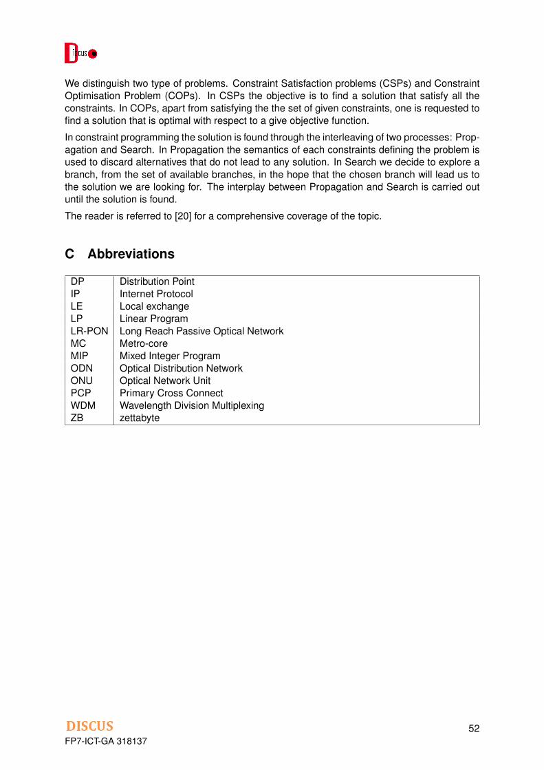
We distinguish two type of problems. Constraint Satisfaction problems (CSPs) and ConstraintOptimisation Problem (COPs). In CSPs the objective is to find a solution that satisfy all theconstraints. In COPs, apart from satisfying the the set of given constraints, one is requested tofind a solution that is optimal with respect to a give objective function.

In constraint programming the solution is found through the interleaving of two processes: Prop-agation and Search. In Propagation the semantics of each constraints defining the problem isused to discard alternatives that do not lead to any solution. In Search we decide to explore abranch, from the set of available branches, in the hope that the chosen branch will lead us tothe solution we are looking for. The interplay between Propagation and Search is carried outuntil the solution is found.

The reader is referred to [20] for a comprehensive coverage of the topic.

C Abbreviations

DP Distribution PointIP Internet ProtocolLE Local exchangeLP Linear ProgramLR-PON Long Reach Passive Optical NetworkMC Metro-coreMIP Mixed Integer ProgramODN Optical Distribution NetworkONU Optical Network UnitPCP Primary Cross ConnectWDM Wavelength Division MultiplexingZB zettabyte

FP7-ICT-GA 31813752