cure cycle design for thermosetting-matrix composites fabrication under uncertainty

Annals of Operations Research 132, 19–45, 2004 2004 Kluwer Academic Publishers. Manufactured in The Netherlands.

Cure Cycle Design for Thermosetting-MatrixComposites Fabrication under Uncertainty

A. MAWARDI and R. PITCHUMANI ∗Composites Processing Laboratory, Department of Mechanical Engineering, University of Connecticut,Storrs, CT 06269-3139, USA

Abstract. Design of the optimal cure temperature cycle is imperative for low-cost of manufacturingthermosetting-matrix composites. Uncertainties exist in several material and process parameters, whichlead to variability in the process performance and product quality. This paper addresses the problem ofdetermining the optimal cure temperature cycles under uncertainty. A stochastic model is developed, inwhich the parameter uncertainties are represented as probability density functions, and deterministic nu-merical process simulations based on the governing process physics are used to determine the distributionsquantifying the output parameter variability. A combined Nelder–Mead Simplex method and the simulatedannealing algorithm is used in conjunction with the stochastic model to obtain time-optimal cure cycles,subject to constraints on parameters influencing the product quality. Results are presented to illustrate theeffects of a degree of parameter uncertainty, constraint values, and material kinetics on the optimal cycles.The studies are used to identify a critical degree of uncertainty in practice above which a rigorous analysisand design under uncertainty is warranted; below this critical value, a deterministic optimal cure cycle maybe used with reasonable confidence.

Keywords: design under uncertainty, sampling, stochastic model, optimization, composites fabrication,Nelder–Mead

1. Introduction

Fabrication of thermosetting-matrix composites is accomplished by subjecting the fiber-resin mixture to a prescribed temperature cycle in order to initiate and sustain irreversiblecross-linking exothermic chemical reaction in the resin, called cure. This fabricationstep is common to all the manufacturing processes including autoclave molding, pul-trusion, and liquid molding techniques. The cure process transforms the initial mixtureinto a rigid structural component of which the structural integrity is retained upon thewithdrawal of the external temperature variation. The magnitude and duration of thetemperature variation, referred to as the cure temperature cycle, or in short, cure cycle,is one of the important process parameters affecting the final quality of the composite.

Design of cure cycles in practice has been based on trial-and-error or empiricalprocedure where either simulations utilizing physics-based process models, or experi-mental trials are carried out for several candidate cure cycles (Pillai, Beris, and Dhurjati,1994; Loos and Springer, 1983; Han, Lee, and Chin, 1986; Bogetti and Gillespie, 1991;

∗ Corresponding author.

20 MAWARDI AND PITCHUMANI

Ciriscioli, Wang, and Springer, 1992; Watkins, Mantell, and Ciriscioli, 1995). This ap-proach does not warrant the best possible process parameters, which in turn could leadto suboptimal manufacturing times and cost. Toward addressing this problem, Rai andPitchumani (1997) presented an approach in which the cure cycle design was formulatedas an optimization problem and solved using a nonlinear programming scheme. In thisapproach, a numerical process model was used to evaluate the objective function andconstraints in the optimization problem. Other studies employing the approach of Raiand Pitchumani (1997) have also been reported in the literature (Li et al., 2001).

Although numerical process simulations prove to be an effective tool in processdesign, it must be realized that there exists a fundamental gap between theoretical sim-ulations and practice, in that practical manufacturing is conducted under a cloud of im-preciseness in the material and process parameter values, while the theoretical processsimulations treat the parameters deterministically. The uncertainty in the parametersarise from sources such as: microstructural variations which leads to uncertainties inmaterial properties, uncertainty in rheological and kinetic parameters, inaccuracies inprocess control, material variabilities and environmental uncertainties. The combinedeffects of the uncertainties potentially cause large variability in the product quality andprocessing time. An effective process design calls for incorporation of these parameteruncertainties into the process modeling and optimization, which is the objective of thisstudy.

This paper presents a framework for analysis and optimization of the compositecure process under uncertainty. In the composites manufacturing area, there has beenlittle attention toward design of processes under uncertainty, and the methodology pre-sented in this paper represents the first systematic study in this regard. The optimiza-tion under uncertainty framework consists of a stochastic model and an optimizationtechnique. In the stochastic model, the parameters with uncertainty are represented asprobability distributions which can be quantified in terms of suitable parameters of thedistribution (such as the mean and the variance in the case of a Gaussian distribution).A sampling method is used to generate combinations of the input parameters from theirrespective distributions to be passed on to a numerical simulation model of the cureprocess, to determine the variability in the outputs in the form of distributions. The sto-chastic model serves as the basis of the optimization problem; the decision variables areamong the inputs to the stochastic model, while the objective function and the constraintsinformation are obtained from the outputs of the stochastic model. The optimizationproblem is solved using a Simplex search based simulated annealing algorithm.

The problem addressed specifically in this paper is that of determining the time-optimal cure cycles for the fabrication of thermosetting-matrix composites using a pul-trusion process, while considering uncertainties in the temperature cycle magnitude, andthe resin kinetic parameters values. The objective is to minimize the cycle time whilesimultaneously satisfying constraints on (a) the maximum material temperature, (b) themaximum temperature difference within the material, and (c) the minimum degree ofcure desired in the product. The optimization results are presented for various degreesof uncertainty in the input parameters, process constraint values, and material reaction

CURE CYCLE DESIGN 21

kinetics. Although the optimization under uncertainty approach is discussed by consid-ering the pultrusion process, the methodology is readily applicable to a wide range ofother fabrication processes as well.

The organization of the paper is as follows. The numerical model, which consti-tutes the core of the approach, is presented in section 2, followed by a discussion of thestochastic model formulation and optimization problem in section 3. The optimizationresults along with parametric studies are discussed in section 4.

2. Deterministic process model

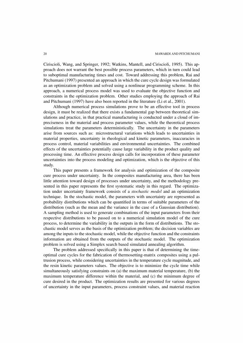
Figure 1 presents a schematic illustration of the pultrusion process for composite fabri-cation. At the beginning of the line, a bundle of fibers is pulled at a constant line speedfrom supply reels through a resin impregnating bath. The resin-impregnated fibers arethen shaped through a preformer, before entering a long heated die where the fiber-resinmixture is heated through a prescribed temperature variation. The elevated temperaturesinitiate and sustain an exothermic, irreversible chemical reaction, called cure, whichtransforms the soft initial mixture entering the die to a hard product at the die exit. Atthe end of the line, the cured composite is cut-off as the final products. The process iscapable of manufacturing composites of cross sections that are constant along the length,such as tubes, I-beams, rods, etc., and being a continuous process, offers high throughputadvantage over a batch process such as autoclave curing.

In this study, the pultrusion process is considered to be at steady-state, and the dieis considered to be of cylindrical section, such that the heating in the die is axisymmetric.The dominant physical phenomena in the process are: (a) the steady-state heat transferassociated with the heating of the composite, and (b) the chemical reaction leading thecure process. Mathematical models for the heat transfer inside the pultrusion die canbe formulated as that of steady-state conduction heat transfer in a cylindrical coordinatesystem, with a volumetric generation term reflecting the exothermic chemical reaction.Since the heat transfer within the composite in the axial direction is predominantly due tobulk motion of the material, axial heat diffusion is neglected. The cure reaction kineticsis modeled using the empirical rate expression, as reported in the literature (Bogetti andGillespie, 1991; Han, Lee, and Chin, 1986; Loos and Springer, 1983). The equations

Figure 1. Illustration of a pultrusion process for fabrication of thermosetting-matrix composites.


governing the coupled thermochemical process may be written in a Lagrangian sense bytracking a cross-section of the composite as it moves along the pultrusion die, as:

ρcp

∂T

∂t= 1

r

∂

∂r

[r

(k∂T

∂r

)]+ �HrCA0

∂ε

∂t, (1)

∂ε

∂t=

[K10 exp

(− E1

RT

)+ K20 exp

(− E2

RT

)εm

](1 − ε)n, (2)

where t is the Lagrangian time related to the line speed, V , and z is the distance fromthe die entrance measured along the die axis as t = z/V . Further, r0 is the inner radiusof the die which is also the radius of the composite rod, �Hr is the heat of reactiondue to cure, CA0 is the initial concentration of the reactive resin at the die entrance, andT is temperature of the material. In the kinetics equation, equation (2), K10 and K20

are frequency factors, E1 and E2 are activation energies, and R is the Universal gasconstant. Since the mixture being heated consists of three components: resin, fibers, andcured resin, the thermal conductivity, k, the density, ρ, and specific heat, cp , appearing inthe above equations are evaluated based on the relative weight fractions of the individualcomponents (Han, Lee, and Chin, 1986).

Equations (1) and (2) are solved simultaneously, subject to the following boundaryconditions. The temperature at the surface of the material corresponds to the temperatureof the die wall, Tc(t), which is the prescribed cure cycle, while the temperature of theresin at the die entrance is specified to be Ti , and the degree of cure in the materialat the die entrance is taken to be zero, corresponding to an unreacted initial mixture.Further, symmetric conditions exist at the centerline of the die. These conditions can beexpressed mathematically as:

T (r0, t) = Tc(t), (3)

T (r, 0) = Ti; ε(r, 0) = 0, (4)∂T

∂r(0, t) = 0. (5)

The governing equations (equations (1) and (2)) along with their boundary condi-tions (equations (3)–(5)) were solved using an implicit finite-difference scheme with acontrol volume formulation (Patankar, 1980; Anderson, Tannehill, and Pletcher, 1984).The mesh contained 32 numerical grids along the radial direction, and the time step �t

was determined such that the mesh Fourier number, α�t/�r2, where α = k/ρcp is theeffective thermal diffusivity of the composite being cured, is less then unity. The numer-ical simulator had two stopping criteria, namely, all sections of the composite attained adesired minimum degree of cure, which was set to be 0.97, or the end of the specifiedcure cycle was reached; the corresponding time was the cure time of the process. Notethat since the present formulation is in a Lagrangian framework, a cure time translatesto a line speed V , for a given die length, L. In addition to the cure time and minimumdegree of cure, the process model also yields the temperature history at discrete radiallocations, as a function of time (axial location along the die axis). The values for the


maximum temperature and the maximum temperature difference within the compositeduring the process were extracted from the thermal history. These parameters were usedin the constraints evaluation in the optimization problem, discussed in the followingsection.

3. Optimization under uncertainty

The objective of the optimization is to determine the cure temperature cycle for minimiz-ing the time for curing of composites under uncertainty. With reference to the pultrusionprocess, minimizing the cure time is tantamount to maximizing the line speed, for agiven die length. The discussion, however, will be presented in terms of the time, whichalso bears a broader relevance to include batch processes such as autoclave curing. Theoptimization is subject to physical constraints on the temperature-related parameters andthe degree of cure during the process.

Figure 2(a) shows a schematic description of optimization under uncertainty ap-proach, which can be considered as comprising three main steps. First, the parameterswith uncertainties are represented by probability distribution functions which can bequantified in terms of appropriate shape parameters. Secondly, a sampling method isused to generate combinations of the parameters with uncertainties. The deterministicprocess model presented in the previous section serves as the basis for propagating the

Figure 2. Schematic of (a) optimization under uncertainty approach, and (b) the details of the stochasticmodel used in this study.


uncertainties incorporated in the input parameters to shape the output parameter distribu-tions. The sampling method and the deterministic model together constitute a stochasticmodel. The third component in the approach is the optimization procedure which solvesthe design problem by utilizing the stochastic model to obtain the objective functionand constraint information. The stochastic model including the sampling technique andthe parameters related to the quantification of uncertainty are discussed in section 3.1,followed by the formulation of the optimization problem and solution, presented on sec-tion 3.2.

3.1. Stochastic model

The stochastic model principally consists of (a) representation, quantification, and sam-pling of the parameters under uncertainty, and (b) propagation of the uncertaintiesthrough a deterministic numerical model to shape the output parameter distributions.In this study, the magnitude of the temperature in the cure cycle is considered to beuncertain, corresponding to the fact that, in practice, temperature is subject to controlfluctuations, while the durations of the stages in the cycle are kept deterministic. Fur-ther, the parameters of the kinetics model, namely, K10, K20, E1 and E2 in equation (2),are also considered to be uncertain reflecting the inherent errors in the empirical deter-mination of these parameters as well as the variabilities in the component concentrationin the catalyzed resin mixture from run-to-run, and relative to the composition of thesample used in the empirical cure kinetics characterization.

Each of the parameters under uncertainty is represented by a Gaussian distribution,which is quantified by its mean value µ and standard deviation σ . The mean, µ, denotesthe nominal value of the parameter, while the uncertainty in the parameter is propor-tional to the standard deviation, σ . A degree of uncertainty is expressed in terms of thecoefficient of variance, defined as σ/µ; thus, a deterministic parameter (i.e., one with nouncertainty in its value) corresponds to the coefficient of variance of zero (σ/µ = 0),while a distribution with a large standard deviation corresponds to a high coefficient ofvariance.

The distributions are sampled to form sets of input parameters to be used bythe deterministic process simulation model. The Latin Hypercube Sampling technique(LHS) (Iman and Shortencarier, 1984) was used to generate the samples for the stochas-tic simulations. LHS is a stratified sampling method in which if N number of samplesare required, the distribution is divided into N intervals (strata) of equal probability, andone sample is picked randomly from each interval to generate the samples. Thus, fora given number number of samples, LHS generates samples that better represent theentire distribution, compared to the Monte Carlo technique, in which the samples areselected randomly and may not cover the entire distribution (Padmanabhan and Pitchu-mani, 1999a). The number of samples used in this study is determined by means ofconvergence analysis of the output distribution parameters, which is discussed in a latersection on presentation of results. Note that other sampling methods such as the Ham-


mersley Sequence Sampling (Kalagnanam and Diwekar, 1997) may also be used follow-ing the methodology presented in this paper.

The samples set representing combinations of the uncertain input parameters arepassed through the numerical model of the pultrusion process to shape the output dis-tributions, as shown schematically in figure 2(b). The outputs of interest are the curetime, which is the objective function, along with the maximum temperature experiencedby the material during cure, maximum temperature difference across the diameter ofthe composite rod being cured, and the degree of cure at the die exit (i.e., at the end ofthe cure cycle). It must be recognized that even though the input parameter uncertaintiesare specified to be Gaussian distributions, the shapes of the output distributions may notbe Gaussian since the numerical model is highly nonlinear. In order to quantify the out-put parameter distributions, for each distribution, x, its cumulative density function isused to determine the expected value Epc

(x), which corresponds to a cumulative prob-ability of pc. Thus, E0.5(x) denotes the mean value of the distribution, whereas E1.0(x)

represents the distribution’s maximum value. The expected values of the cure time, andthe constraint parameters, corresponding to a probability pc are used in the optimizationproblem formulation. The stochastic model, therefore, forms the basis of the optimiza-tion problem detailed in the following subsection.

3.2. The optimization problem

The objective of the optimization is to determine the cure temperature cycle for min-imizing the time for curing of composites, or equivalently, maximizing the pultrusionspeed, V , since the cure time is related to the speed and the die length L, as L/V . Theoptimization is subject to physical constraints on the (a) maximum material tempera-ture during the cure process, (b) maximum temperature difference across the compositecross section, and (c) minimum degree of cure in the composite section at die exit, whichpertain to, respectively, limiting the residual/thermal stresses induced during processing,maintaining temperature and property homogeneity across the section, and ensuring cur-ing of composite to a desired minimum degree, εcrit. The presence of uncertainty in theparameters implies that the objective function and constraints in the optimization areno longer deterministic; instead their distributions are provided by the stochastic modeldiscussed in the previous subsection.

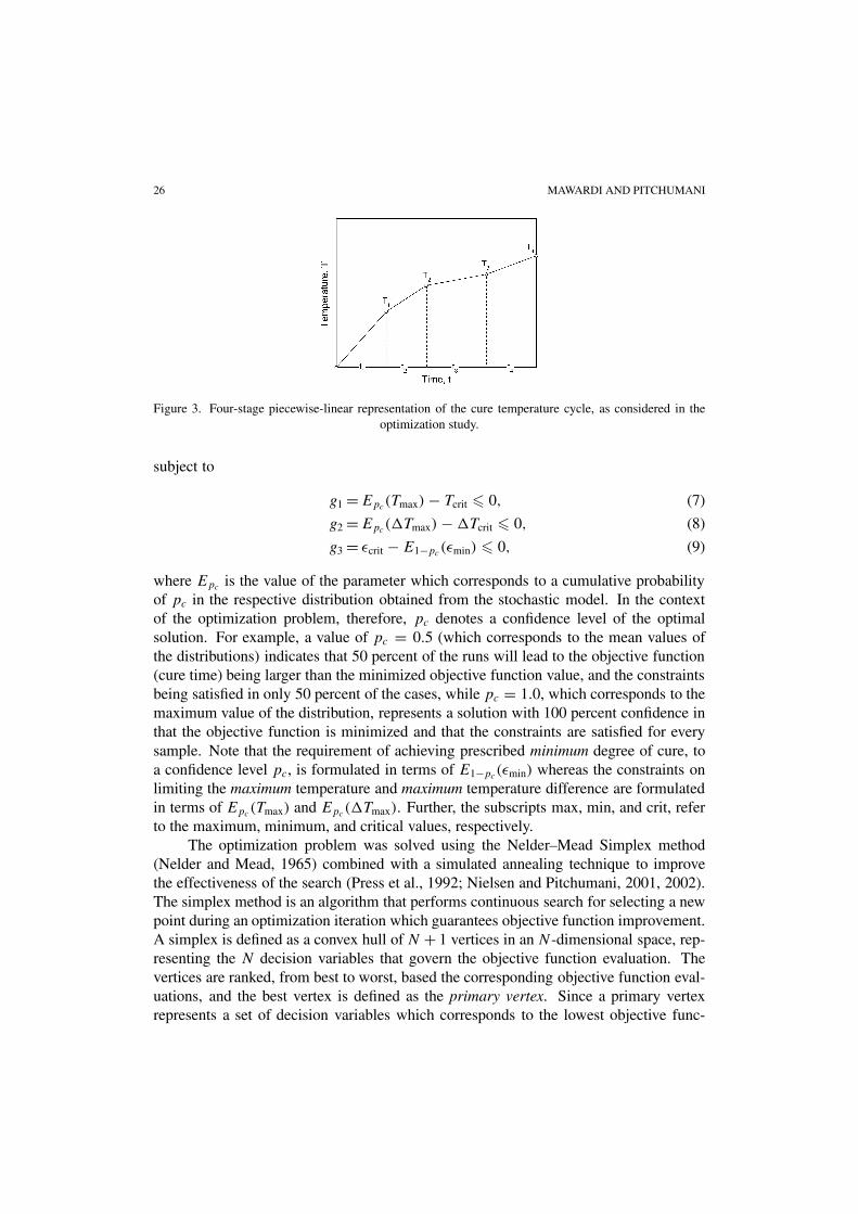
The decision variables in the optimization are the temperature magnitudes Tk, anddurations of each stage tk of the cure cycle. In the present implementation, the cure cycleis considered to be made of four stages as shown in figure 3, which corresponds to eightdecision variables. As mentioned previously, since the stage end point temperatures inthe cycle are considered to be uncertain parameters in the stochastic modeling, the meanvalue of the stage end point temperatures are treated to be the decision variables in theoptimization problem.

The optimization problem may be written mathematically as

MinimizeTk(tk)

Epc(tcure) (6)


Figure 3. Four-stage piecewise-linear representation of the cure temperature cycle, as considered in theoptimization study.

subject to

g1 = Epc(Tmax) − Tcrit � 0, (7)

g2 = Epc(�Tmax) − �Tcrit � 0, (8)

g3 = εcrit − E1−pc(εmin) � 0, (9)

where Epcis the value of the parameter which corresponds to a cumulative probability

of pc in the respective distribution obtained from the stochastic model. In the contextof the optimization problem, therefore, pc denotes a confidence level of the optimalsolution. For example, a value of pc = 0.5 (which corresponds to the mean values ofthe distributions) indicates that 50 percent of the runs will lead to the objective function(cure time) being larger than the minimized objective function value, and the constraintsbeing satisfied in only 50 percent of the cases, while pc = 1.0, which corresponds to themaximum value of the distribution, represents a solution with 100 percent confidence inthat the objective function is minimized and that the constraints are satisfied for everysample. Note that the requirement of achieving prescribed minimum degree of cure, toa confidence level pc, is formulated in terms of E1−pc

(εmin) whereas the constraints onlimiting the maximum temperature and maximum temperature difference are formulatedin terms of Epc

(Tmax) and Epc(�Tmax). Further, the subscripts max, min, and crit, refer

to the maximum, minimum, and critical values, respectively.The optimization problem was solved using the Nelder–Mead Simplex method

(Nelder and Mead, 1965) combined with a simulated annealing technique to improvethe effectiveness of the search (Press et al., 1992; Nielsen and Pitchumani, 2001, 2002).The simplex method is an algorithm that performs continuous search for selecting a newpoint during an optimization iteration which guarantees objective function improvement.A simplex is defined as a convex hull of N + 1 vertices in an N-dimensional space, rep-resenting the N decision variables that govern the objective function evaluation. Thevertices are ranked, from best to worst, based the corresponding objective function eval-uations, and the best vertex is defined as the primary vertex. Since a primary vertexrepresents a set of decision variables which corresponds to the lowest objective func-


tion evaluation, the finding of a new primary vertex constitutes an improvement to theobjective function evaluation.

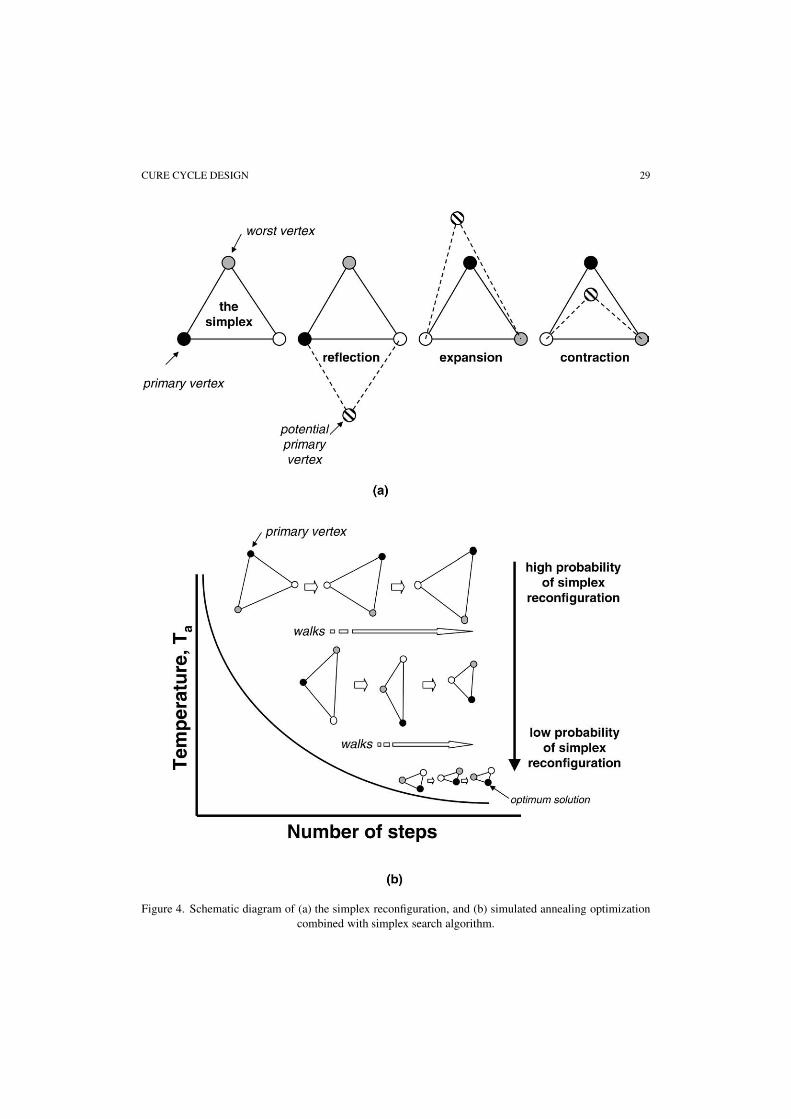
The algorithm searches for a new simplex by replacing the worst vertex by a poten-tial new primary vertex, through a set of predefined simplex movements, which includereflection, expansion, and contraction, illustrated in figure 4(a) for a two-dimensionalsimplex. The primary movement is the reflection of the worst vertex, while expansionand contraction are secondary movements dependent on the result of the reflection. Ifthe reflection results in a new vertex that is better than the current primary vertex (i.e.,has a lower objective function value), an expansion of the reflected simplex will follow,recognizing that a further movement of the new vertices in the direction of the reflectionmight lead to a much better vertex. If the reflection of the worst vertex does not lead to anew vertex that is better than the current primary vertex but still better than the next worstvertex, the new simplex is accepted. However, if the reflection of the worst vertex doesnot result in a vertex that is better than the next worst vertex, contraction of the originalsimplex is executed to reduce its size. Additional details on the Nelder–Mead algorithm,including parameter selection for the various movement and tie-breaking rules (if twovertices of equal objective function value are evaluated), may be found in Lagarias etal. (1998).

In the Nelder–Mead method, the decision to accept or reject each movement ismade based solely on the criterion of reducing the objective function value. This couldpotentially result in the entrapment of the solution in a local minimum. However, if theNelder–Mead method were combined with a simulated annealing technique, the movesin the design exploration would be subject to a probabilistic acceptance criterion (theMetropolis equation), which offers a better opportunity to arrive at a global minimum.The optimization approach used in the present application, therefore, uses a combinedNelder–Mead simplex method and simulated annealing algorithm, as discussed below.

Simulated annealing is an optimization technique which mimics the physicalprocess of annealing (slow cooling) of metals, in which the molecules are free to moveat high temperatures, but as the annealing temperature slowly decreases, the molecularmovement becomes increasingly restricted before finally settling down to a configura-tion of the lowest energy state. Relating to the optimization problem, the molecularconfiguration represents the decision variables, while the energy state represents the ob-jective function to be minimized. Starting at high temperature in the annealing schedule,an initial trial simplex undergoes reconfigurations based on the movements defined inthe Nelder–Mead method. Each reconfiguration of the simplex is accepted based on anassociated probability p, given by the Metropolis criterion (Metropolis et al., 1953)

p = min

(exp

[−Zn+1 − Zn

kbTa

], 1

), (10)

where Ta is the annealing temperature, kb is the Boltzmann constant, Zn is the objectivefunction corresponding to the primary vertex prior to reconfiguration, and Zn+1 is theobjective function corresponding to the new primary vertex in the reconfigured potentialsimplex. If Zn+1 < Zn, the probability of acceptance is unity, as per equation (10), which


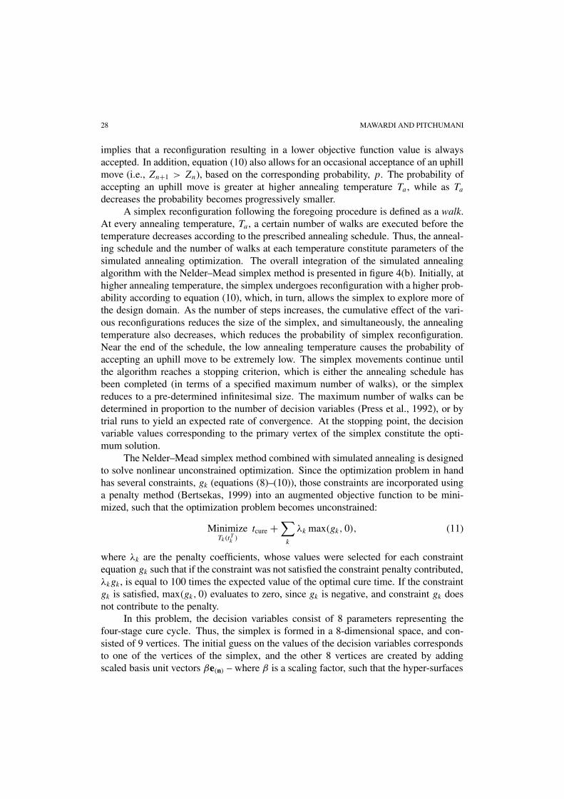
implies that a reconfiguration resulting in a lower objective function value is alwaysaccepted. In addition, equation (10) also allows for an occasional acceptance of an uphillmove (i.e., Zn+1 > Zn), based on the corresponding probability, p. The probability ofaccepting an uphill move is greater at higher annealing temperature Ta , while as Ta

decreases the probability becomes progressively smaller.A simplex reconfiguration following the foregoing procedure is defined as a walk.

At every annealing temperature, Ta , a certain number of walks are executed before thetemperature decreases according to the prescribed annealing schedule. Thus, the anneal-ing schedule and the number of walks at each temperature constitute parameters of thesimulated annealing optimization. The overall integration of the simulated annealingalgorithm with the Nelder–Mead simplex method is presented in figure 4(b). Initially, athigher annealing temperature, the simplex undergoes reconfiguration with a higher prob-ability according to equation (10), which, in turn, allows the simplex to explore more ofthe design domain. As the number of steps increases, the cumulative effect of the vari-ous reconfigurations reduces the size of the simplex, and simultaneously, the annealingtemperature also decreases, which reduces the probability of simplex reconfiguration.Near the end of the schedule, the low annealing temperature causes the probability ofaccepting an uphill move to be extremely low. The simplex movements continue untilthe algorithm reaches a stopping criterion, which is either the annealing schedule hasbeen completed (in terms of a specified maximum number of walks), or the simplexreduces to a pre-determined infinitesimal size. The maximum number of walks can bedetermined in proportion to the number of decision variables (Press et al., 1992), or bytrial runs to yield an expected rate of convergence. At the stopping point, the decisionvariable values corresponding to the primary vertex of the simplex constitute the opti-mum solution.

The Nelder–Mead simplex method combined with simulated annealing is designedto solve nonlinear unconstrained optimization. Since the optimization problem in handhas several constraints, gk (equations (8)–(10)), those constraints are incorporated usinga penalty method (Bertsekas, 1999) into an augmented objective function to be mini-mized, such that the optimization problem becomes unconstrained:

MinimizeTk(t

Tk )

tcure +∑

k

λk max(gk, 0), (11)

where λk are the penalty coefficients, whose values were selected for each constraintequation gk such that if the constraint was not satisfied the constraint penalty contributed,λkgk, is equal to 100 times the expected value of the optimal cure time. If the constraintgk is satisfied, max(gk, 0) evaluates to zero, since gk is negative, and constraint gk doesnot contribute to the penalty.

In this problem, the decision variables consist of 8 parameters representing thefour-stage cure cycle. Thus, the simplex is formed in a 8-dimensional space, and con-sisted of 9 vertices. The initial guess on the values of the decision variables correspondsto one of the vertices of the simplex, and the other 8 vertices are created by addingscaled basis unit vectors βe(n) – where β is a scaling factor, such that the hyper-surfaces


Figure 4. Schematic diagram of (a) the simplex reconfiguration, and (b) simulated annealing optimizationcombined with simplex search algorithm.


of the simplex are linearly independent of each other. The numerical process simulatoris invoked to determine the augmented objective function corresponding to each ver-tex at every step of the optimization procedure. At the completion of the optimizationalgorithm, the primary vertex of the final simplex represents the optimal decision vari-ables, and the corresponding objective function evaluation represents the optimal curetime, tcure.

4. Results and discussion

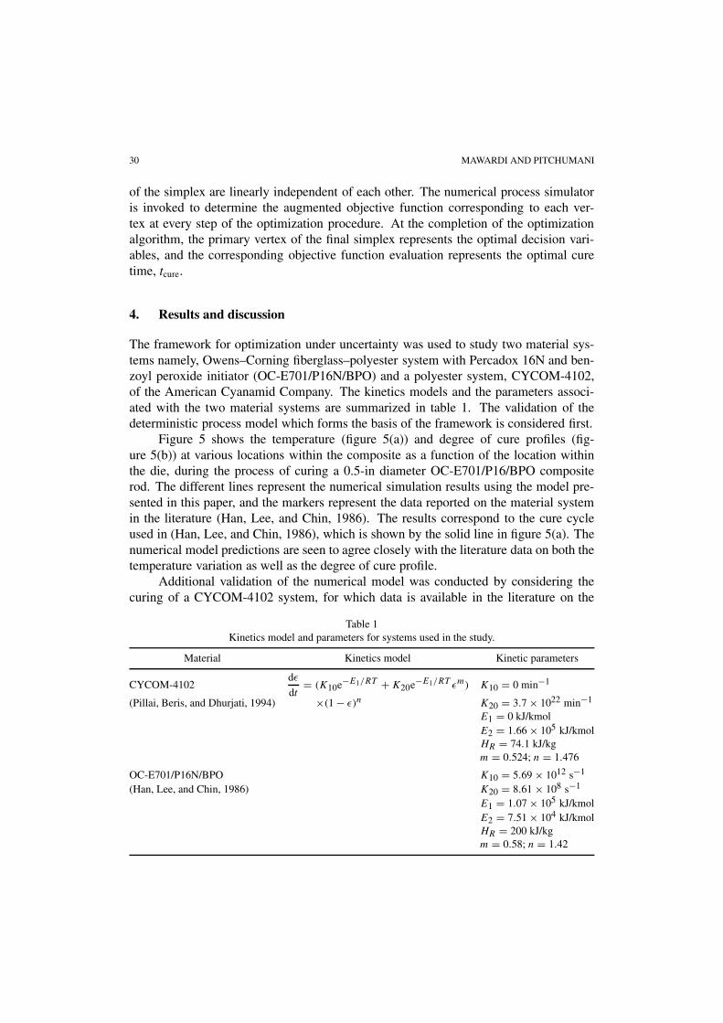
The framework for optimization under uncertainty was used to study two material sys-tems namely, Owens–Corning fiberglass–polyester system with Percadox 16N and ben-zoyl peroxide initiator (OC-E701/P16N/BPO) and a polyester system, CYCOM-4102,of the American Cyanamid Company. The kinetics models and the parameters associ-ated with the two material systems are summarized in table 1. The validation of thedeterministic process model which forms the basis of the framework is considered first.

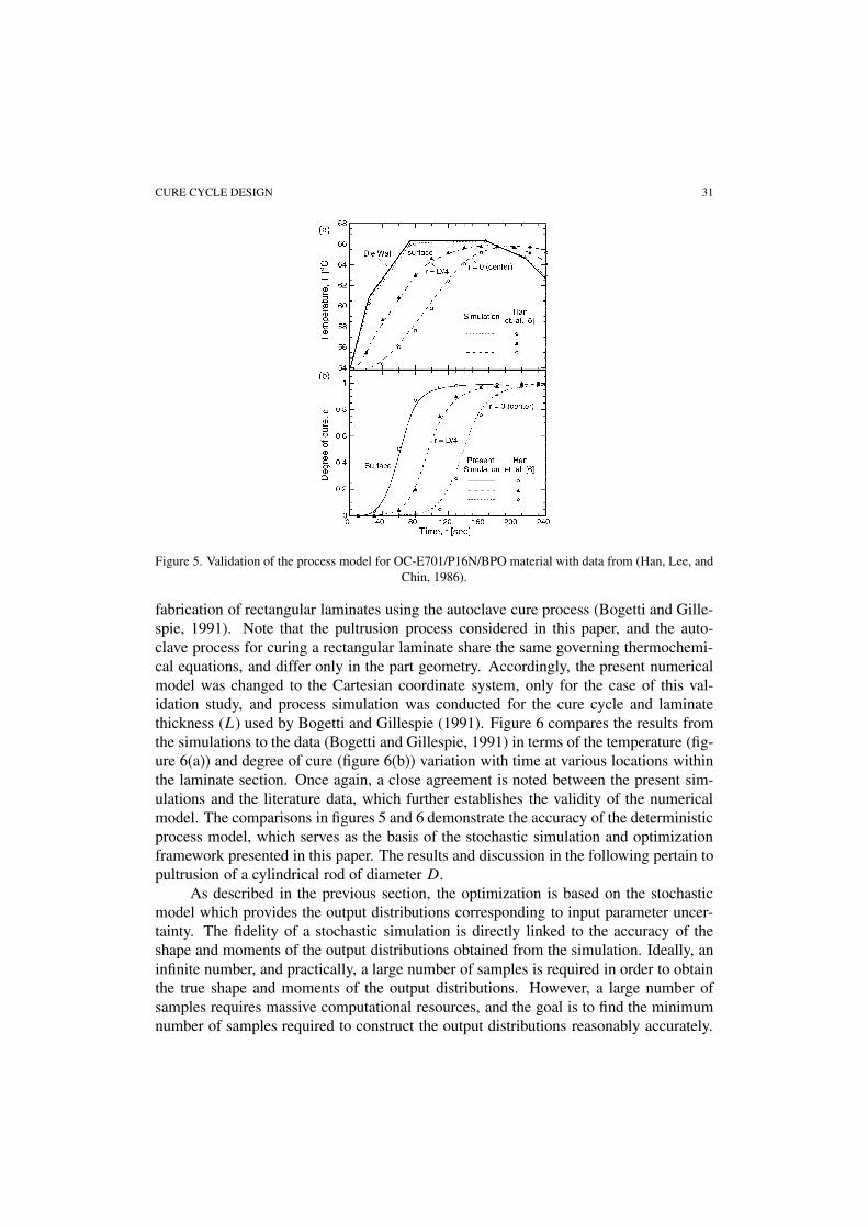
Figure 5 shows the temperature (figure 5(a)) and degree of cure profiles (fig-ure 5(b)) at various locations within the composite as a function of the location withinthe die, during the process of curing a 0.5-in diameter OC-E701/P16/BPO compositerod. The different lines represent the numerical simulation results using the model pre-sented in this paper, and the markers represent the data reported on the material systemin the literature (Han, Lee, and Chin, 1986). The results correspond to the cure cycleused in (Han, Lee, and Chin, 1986), which is shown by the solid line in figure 5(a). Thenumerical model predictions are seen to agree closely with the literature data on both thetemperature variation as well as the degree of cure profile.

Additional validation of the numerical model was conducted by considering thecuring of a CYCOM-4102 system, for which data is available in the literature on the

Table 1Kinetics model and parameters for systems used in the study.

Material Kinetics model Kinetic parameters

CYCOM-4102dε

dt= (K10e−E1/RT + K20e−E1/RT εm) K10 = 0 min−1

(Pillai, Beris, and Dhurjati, 1994) ×(1 − ε)n K20 = 3.7 × 1022 min−1

E1 = 0 kJ/kmolE2 = 1.66 × 105 kJ/kmolHR = 74.1 kJ/kgm = 0.524; n = 1.476

OC-E701/P16N/BPO K10 = 5.69 × 1012 s−1

(Han, Lee, and Chin, 1986) K20 = 8.61 × 108 s−1

E1 = 1.07 × 105 kJ/kmolE2 = 7.51 × 104 kJ/kmolHR = 200 kJ/kgm = 0.58; n = 1.42


Figure 5. Validation of the process model for OC-E701/P16N/BPO material with data from (Han, Lee, andChin, 1986).

fabrication of rectangular laminates using the autoclave cure process (Bogetti and Gille-spie, 1991). Note that the pultrusion process considered in this paper, and the auto-clave process for curing a rectangular laminate share the same governing thermochemi-cal equations, and differ only in the part geometry. Accordingly, the present numericalmodel was changed to the Cartesian coordinate system, only for the case of this val-idation study, and process simulation was conducted for the cure cycle and laminatethickness (L) used by Bogetti and Gillespie (1991). Figure 6 compares the results fromthe simulations to the data (Bogetti and Gillespie, 1991) in terms of the temperature (fig-ure 6(a)) and degree of cure (figure 6(b)) variation with time at various locations withinthe laminate section. Once again, a close agreement is noted between the present sim-ulations and the literature data, which further establishes the validity of the numericalmodel. The comparisons in figures 5 and 6 demonstrate the accuracy of the deterministicprocess model, which serves as the basis of the stochastic simulation and optimizationframework presented in this paper. The results and discussion in the following pertain topultrusion of a cylindrical rod of diameter D.

As described in the previous section, the optimization is based on the stochasticmodel which provides the output distributions corresponding to input parameter uncer-tainty. The fidelity of a stochastic simulation is directly linked to the accuracy of theshape and moments of the output distributions obtained from the simulation. Ideally, aninfinite number, and practically, a large number of samples is required in order to obtainthe true shape and moments of the output distributions. However, a large number ofsamples requires massive computational resources, and the goal is to find the minimumnumber of samples required to construct the output distributions reasonably accurately.


Figure 6. Validation of the process model for CYCOM-4102 material with the data from (Bogetti andGillespie, 1991).

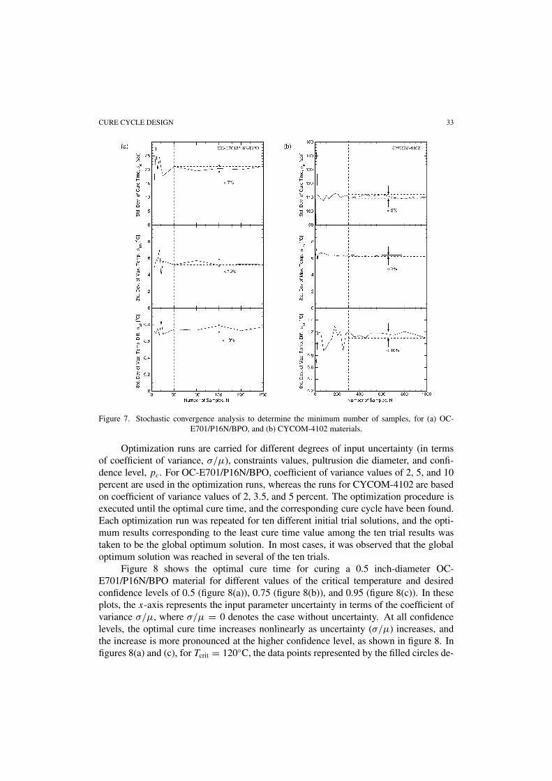
The minimum number of samples for the stochastic simulations was determined usinga stochastic convergence analysis of the output distributions, in which the mean andstandard deviation values are examined for varying number of samples of the input pa-rameters. Since the standard deviation, a higher order moment than the mean, convergesmuch slower than the mean with increasing number of samples, the determination of theminimum number of samples was based on the convergence of the standard deviation.Figure 7 shows the results of the convergence analysis on the standard deviations of thecure time, the maximum material temperature, and the maximum temperature differ-ence, for OC-E701/P16N/BPO (figure 7(a)) and CYCOM-4102 (figure 7(b)) compositesystems using samples generated by the Latin Hypercube Sampling (LHS) method. Theanalysis indicates that for OC-E701/P16N/BPO, 50 samples is an adequate number toproduce less than ±5% convergence in the output standard deviation values, while 300samples are required for CYCOM-4102, which has higher reactivity, to produce similarconvergence result. The results show that the minimum sample size is dependent on theresin reactivity, as also reported by Padmanabhan and Pitchumani (1999a, 1999b). Itmust be mentioned that the convergence plot changes with the initial random seed usedin the Latin Hypercube sampling method. However, the convergence characteristic –i.e., the number of samples beyond which the standard deviation falls within the speci-fied convergence tolerance – was found to be practically invariant with the change in theinitial random seed. The minimum numbers of samples obtained as above were used inthe results presented in this section.


Figure 7. Stochastic convergence analysis to determine the minimum number of samples, for (a) OC-E701/P16N/BPO, and (b) CYCOM-4102 materials.

Optimization runs are carried for different degrees of input uncertainty (in termsof coefficient of variance, σ/µ), constraints values, pultrusion die diameter, and confi-dence level, pc. For OC-E701/P16N/BPO, coefficient of variance values of 2, 5, and 10percent are used in the optimization runs, whereas the runs for CYCOM-4102 are basedon coefficient of variance values of 2, 3.5, and 5 percent. The optimization procedure isexecuted until the optimal cure time, and the corresponding cure cycle have been found.Each optimization run was repeated for ten different initial trial solutions, and the opti-mum results corresponding to the least cure time value among the ten trial results wastaken to be the global optimum solution. In most cases, it was observed that the globaloptimum solution was reached in several of the ten trials.

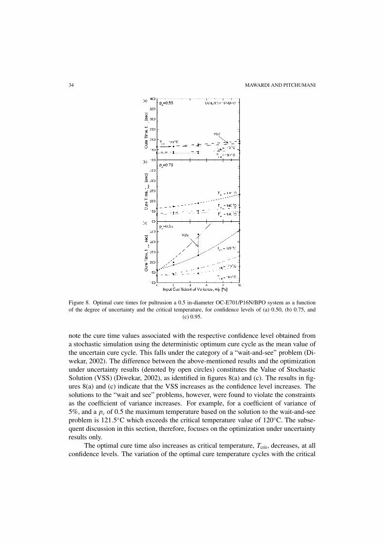
Figure 8 shows the optimal cure time for curing a 0.5 inch-diameter OC-E701/P16N/BPO material for different values of the critical temperature and desiredconfidence levels of 0.5 (figure 8(a)), 0.75 (figure 8(b)), and 0.95 (figure 8(c)). In theseplots, the x-axis represents the input parameter uncertainty in terms of the coefficient ofvariance σ/µ, where σ/µ = 0 denotes the case without uncertainty. At all confidencelevels, the optimal cure time increases nonlinearly as uncertainty (σ/µ) increases, andthe increase is more pronounced at the higher confidence level, as shown in figure 8. Infigures 8(a) and (c), for Tcrit = 120◦C, the data points represented by the filled circles de-


Figure 8. Optimal cure times for pultrusion a 0.5 in-diameter OC-E701/P16N/BPO system as a functionof the degree of uncertainty and the critical temperature, for confidence levels of (a) 0.50, (b) 0.75, and

(c) 0.95.

note the cure time values associated with the respective confidence level obtained froma stochastic simulation using the deterministic optimum cure cycle as the mean value ofthe uncertain cure cycle. This falls under the category of a “wait-and-see” problem (Di-wekar, 2002). The difference between the above-mentioned results and the optimizationunder uncertainty results (denoted by open circles) constitutes the Value of StochasticSolution (VSS) (Diwekar, 2002), as identified in figures 8(a) and (c). The results in fig-ures 8(a) and (c) indicate that the VSS increases as the confidence level increases. Thesolutions to the “wait and see” problems, however, were found to violate the constraintsas the coefficient of variance increases. For example, for a coefficient of variance of5%, and a pc of 0.5 the maximum temperature based on the solution to the wait-and-seeproblem is 121.5◦C which exceeds the critical temperature value of 120◦C. The subse-quent discussion in this section, therefore, focuses on the optimization under uncertaintyresults only.

The optimal cure time also increases as critical temperature, Tcrit, decreases, at allconfidence levels. The variation of the optimal cure temperature cycles with the critical


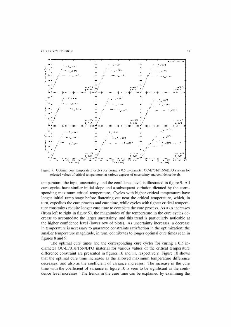
Figure 9. Optimal cure temperature cycles for curing a 0.5 in-diameter OC-E701/P16N/BPO system forselected values of critical temperature, at various degrees of uncertainty and confidence levels.

temperature, the input uncertainty, and the confidence level is illustrated in figure 9. Allcure cycles have similar initial slope and a subsequent variation dictated by the corre-sponding maximum critical temperature. Cycles with higher critical temperature havelonger initial ramp stage before flattening out near the critical temperature, which, inturn, expedites the cure process and cure time, while cycles with tighter critical tempera-ture constraints require longer cure time to complete the cure process. As σ/µ increases(from left to right in figure 9), the magnitudes of the temperature in the cure cycles de-crease to accomodate the larger uncertainty, and this trend is particularly noticable atthe higher confidence level (lower row of plots). As uncertainty increases, a decreasein temperature is necessary to guarantee constraints satisfaction in the optimization; thesmaller temperature magnitude, in turn, contributes to longer optimal cure times seen infigures 8 and 9.

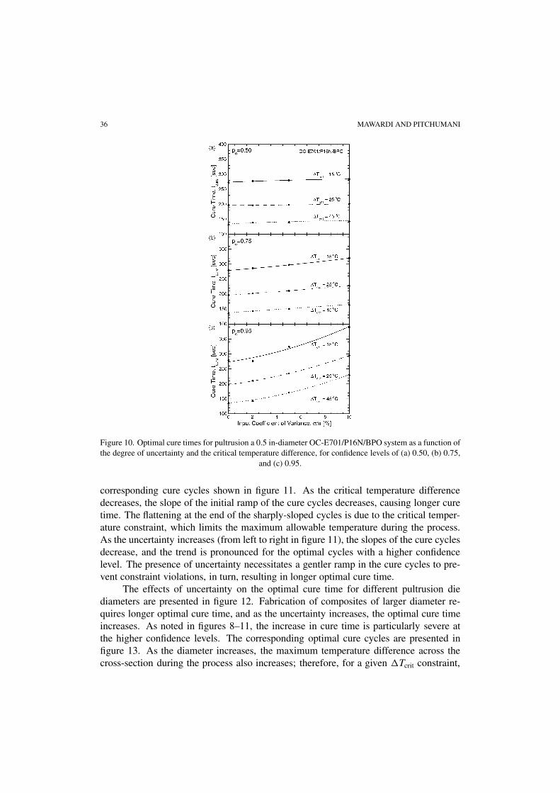
The optimal cure times and the corresponding cure cycles for curing a 0.5 in-diameter OC-E701/P16N/BPO material for various values of the critical temperaturedifference constraint are presented in figures 10 and 11, respectively. Figure 10 showsthat the optimal cure time increases as the allowed maximum temperature differencedecreases, and also as the coefficient of variance increases. The increase in the curetime with the coefficient of variance in figure 10 is seen to be significant as the confi-dence level increases. The trends in the cure time can be explained by examining the


Figure 10. Optimal cure times for pultrusion a 0.5 in-diameter OC-E701/P16N/BPO system as a function ofthe degree of uncertainty and the critical temperature difference, for confidence levels of (a) 0.50, (b) 0.75,

and (c) 0.95.

corresponding cure cycles shown in figure 11. As the critical temperature differencedecreases, the slope of the initial ramp of the cure cycles decreases, causing longer curetime. The flattening at the end of the sharply-sloped cycles is due to the critical temper-ature constraint, which limits the maximum allowable temperature during the process.As the uncertainty increases (from left to right in figure 11), the slopes of the cure cyclesdecrease, and the trend is pronounced for the optimal cycles with a higher confidencelevel. The presence of uncertainty necessitates a gentler ramp in the cure cycles to pre-vent constraint violations, in turn, resulting in longer optimal cure time.

The effects of uncertainty on the optimal cure time for different pultrusion diediameters are presented in figure 12. Fabrication of composites of larger diameter re-quires longer optimal cure time, and as the uncertainty increases, the optimal cure timeincreases. As noted in figures 8–11, the increase in cure time is particularly severe atthe higher confidence levels. The corresponding optimal cure cycles are presented infigure 13. As the diameter increases, the maximum temperature difference across thecross-section during the process also increases; therefore, for a given �Tcrit constraint,


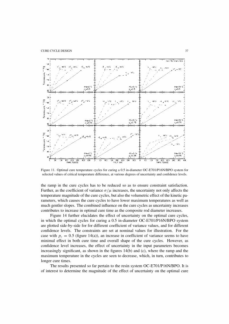
Figure 11. Optimal cure temperature cycles for curing a 0.5 in-diameter OC-E701/P16N/BPO system forselected values of critical temperature difference, at various degrees of uncertainty and confidence levels.

the ramp in the cure cycles has to be reduced so as to ensure constraint satisfaction.Further, as the coefficient of variance σ/µ increases, the uncertainty not only affects thetemperature magnitude of the cure cycles, but also the volumetric effect of the kinetic pa-rameters, which causes the cure cycles to have lower maximum temperatures as well asmuch gentler slopes. The combined influence on the cure cycles as uncertainty increasescontributes to increase in optimal cure time as the composite rod diameter increases.

Figure 14 further elucidates the effect of uncertainty on the optimal cure cycles,in which the optimal cycles for curing a 0.5 in-diameter OC-E701/P16N/BPO systemare plotted side-by-side for for different coefficient of variance values, and for differentconfidence levels. The constraints are set at nominal values for illustration. For thecase with pc = 0.5 (figure 14(a)), an increase in coefficient of variance seems to haveminimal effect in both cure time and overall shape of the cure cycles. However, asconfidence level increases, the effect of uncertainty in the input parameters becomesincreasingly significant, as shown in the figures 14(b) and (c), where the ramp and themaximum temperature in the cycles are seen to decrease, which, in turn, contributes tolonger cure times.

The results presented so far pertain to the resin system OC-E701/P16N/BPO. It isof interest to determine the magnitude of the effect of uncertainty on the optimal cure


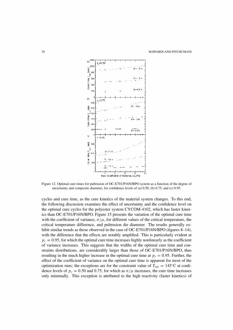
Figure 12. Optimal cure times for pultrusion of OC-E701/P16N/BPO system as a function of the degree ofuncertainty and composite diameter, for confidence levels of (a) 0.50, (b) 0.75, and (c) 0.95.

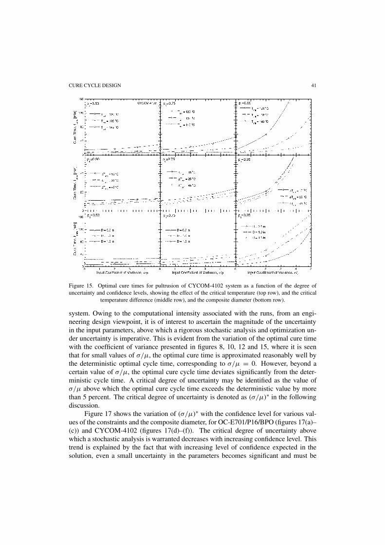
cycles and cure time, as the cure kinetics of the material system changes. To this end,the following discussion examines the effect of uncertainty and the confidence level onthe optimal cure cycles for the polyester system CYCOM-4102, which has faster kinet-ics than OC-E701/P16N/BPO. Figure 15 presents the variation of the optimal cure timewith the coefficient of variance, σ/µ, for different values of the critical temperature, thecritical temperature difference, and pultrusion die diameter. The results generally ex-hibit similar trends as those observed in the case of OC-E701/P16N/BPO (figures 8–14),with the difference that the effects are notably amplified. This is particularly evident atpc = 0.95, for which the optimal cure time increases highly nonlinearly as the coefficientof variance increases. This suggests that the widths of the optimal cure time and con-straints distributions, are considerably larger than those of OC-E701/P16N/BPO, thusresulting in the much higher increase in the optimal cure time at pc = 0.95. Further, theeffect of the coefficient of variance on the optimal cure time is apparent for most of theoptimization runs; the exceptions are for the constraint value of Tcrit = 145◦C at confi-dence levels of pc = 0.50 and 0.75, for which as σ/µ increases, the cure time increasesonly minimally. This exception is attributed to the high reactivity (faster kinetics) of


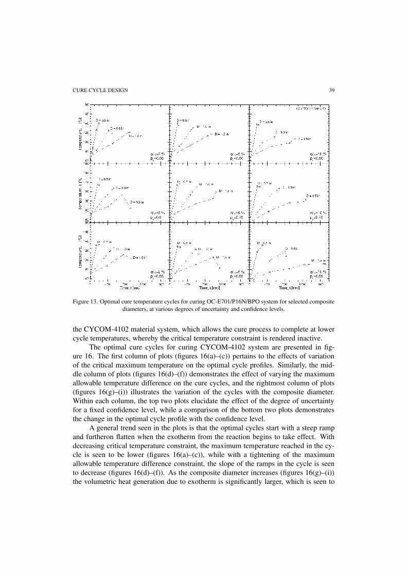
Figure 13. Optimal cure temperature cycles for curing OC-E701/P16N/BPO system for selected compositediameters, at various degrees of uncertainty and confidence levels.

the CYCOM-4102 material system, which allows the cure process to complete at lowercycle temperatures, whereby the critical temperature constraint is rendered inactive.

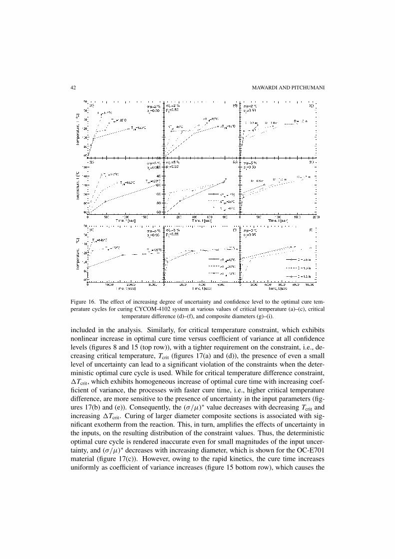
The optimal cure cycles for curing CYCOM-4102 system are presented in fig-ure 16. The first column of plots (figures 16(a)–(c)) pertains to the effects of variationof the critical maximum temperature on the optimal cycle profiles. Similarly, the mid-dle column of plots (figures 16(d)–(f)) demonstrates the effect of varying the maximumallowable temperature difference on the cure cycles, and the rightmost column of plots(figures 16(g)–(i)) illustrates the variation of the cycles with the composite diameter.Within each column, the top two plots elucidate the effect of the degree of uncertaintyfor a fixed confidence level, while a comparison of the bottom two plots demonstratesthe change in the optimal cycle profile with the confidence level.

A general trend seen in the plots is that the optimal cycles start with a steep rampand furtheron flatten when the exotherm from the reaction begins to take effect. Withdecreasing critical temperature constraint, the maximum temperature reached in the cy-cle is seen to be lower (figures 16(a)–(c)), while with a tightening of the maximumallowable temperature difference constraint, the slope of the ramps in the cycle is seento decrease (figures 16(d)–(f)). As the composite diameter increases (figures 16(g)–(i))the volumetric heat generation due to exotherm is significantly larger, which is seen to


Figure 14. The effect of uncertainty on the optimal temperature cycles for pultrusion of a 0.5 in-thick OC-E701/P16N/BPO system at nominal values of the constraints, and confidence levels of (a) 0.50 (b) 0.75,

and (c) 0.95.

necessitate a smaller temperature ramp in the cycle, thereby increasing the overall cycletime. With increasing degree of uncertainty, the slope of the temperature variation andthe maximum temperature in the cycle decrease, so as to ensure constraint satisfaction.Further, as the desired confidence level of the solution increases, the optimal cure cy-cles generally incorporate smaller ramps and lower temperatures in order to control thewidth of the output distribution, albeit at the expense of significantly longer cycle times.Overall, a comparison of the results for CYCOM-4102 system with the correspondingresults for the Owens–Corning system (OC-E701/P16/BPO) suggests that the effects ofuncertainty manifest themselves significantly for the highly reacting systems.

All computations presented in this section were performed on a SUN Ultra10 work-station. The CPU time required for convergence varied, and was a function of the sizeof the numerical time step, and the actual cure time of the process. As an example,for a case with 50 samples and a nominal uncertainty and constraint values, one set ofoptimization runs for OC-E701/P16N/BPO required an average of 24 hours. A similarcomputational time was required for the optimization runs for the CYCOM-4102 resin


Figure 15. Optimal cure times for pultrusion of CYCOM-4102 system as a function of the degree ofuncertainty and confidence levels, showing the effect of the critical temperature (top row), and the critical

temperature difference (middle row), and the composite diameter (bottom row).

system. Owing to the computational intensity associated with the runs, from an engi-neering design viewpoint, it is of interest to ascertain the magnitude of the uncertaintyin the input parameters, above which a rigorous stochastic analysis and optimization un-der uncertainty is imperative. This is evident from the variation of the optimal cure timewith the coefficient of variance presented in figures 8, 10, 12 and 15, where it is seenthat for small values of σ/µ, the optimal cure time is approximated reasonably well bythe deterministic optimal cycle time, corresponding to σ/µ = 0. However, beyond acertain value of σ/µ, the optimal cure cycle time deviates significantly from the deter-ministic cycle time. A critical degree of uncertainty may be identified as the value ofσ/µ above which the optimal cure cycle time exceeds the deterministic value by morethan 5 percent. The critical degree of uncertainty is denoted as (σ/µ)∗ in the followingdiscussion.

Figure 17 shows the variation of (σ/µ)∗ with the confidence level for various val-ues of the constraints and the composite diameter, for OC-E701/P16/BPO (figures 17(a)–(c)) and CYCOM-4102 (figures 17(d)–(f)). The critical degree of uncertainty abovewhich a stochastic analysis is warranted decreases with increasing confidence level. Thistrend is explained by the fact that with increasing level of confidence expected in thesolution, even a small uncertainty in the parameters becomes significant and must be


Figure 16. The effect of increasing degree of uncertainty and confidence level to the optimal cure tem-perature cycles for curing CYCOM-4102 system at various values of critical temperature (a)–(c), critical

temperature difference (d)–(f), and composite diameters (g)–(i).

included in the analysis. Similarly, for critical temperature constraint, which exhibitsnonlinear increase in optimal cure time versus coefficient of variance at all confidencelevels (figures 8 and 15 (top row)), with a tighter requirement on the constraint, i.e., de-creasing critical temperature, Tcrit (figures 17(a) and (d)), the presence of even a smalllevel of uncertainty can lead to a significant violation of the constraints when the deter-ministic optimal cure cycle is used. While for critical temperature difference constraint,�Tcrit, which exhibits homogeneous increase of optimal cure time with increasing coef-ficient of variance, the processes with faster cure time, i.e., higher critical temperaturedifference, are more sensitive to the presence of uncertainty in the input parameters (fig-ures 17(b) and (e)). Consequently, the (σ/µ)∗ value decreases with decreasing Tcrit andincreasing �Tcrit. Curing of larger diameter composite sections is associated with sig-nificant exotherm from the reaction. This, in turn, amplifies the effects of uncertainty inthe inputs, on the resulting distribution of the constraint values. Thus, the deterministicoptimal cure cycle is rendered inaccurate even for small magnitudes of the input uncer-tainty, and (σ/µ)∗ decreases with increasing diameter, which is shown for the OC-E701material (figure 17(c)). However, owing to the rapid kinetics, the cure time increasesuniformly as coefficient of variance increases (figure 15 bottom row), which causes the


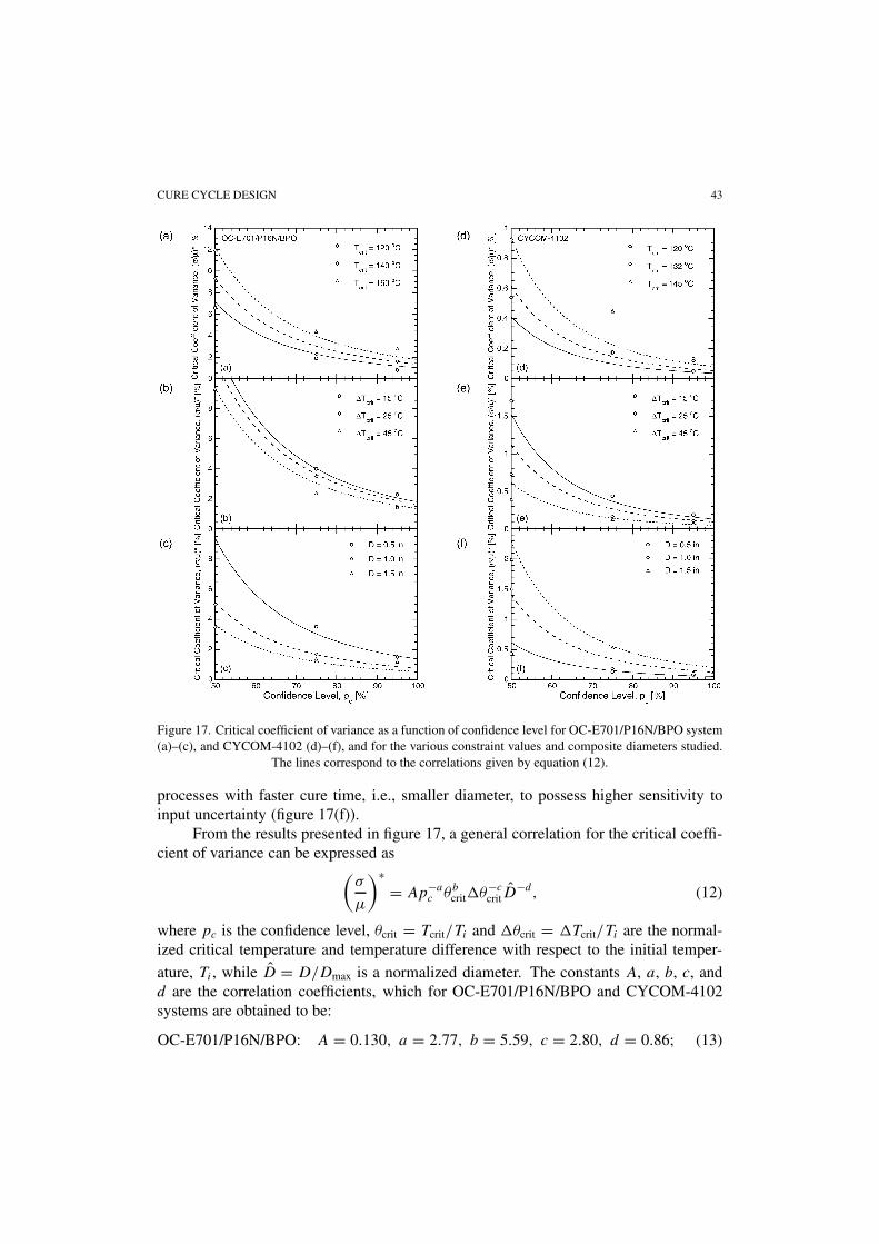
Figure 17. Critical coefficient of variance as a function of confidence level for OC-E701/P16N/BPO system(a)–(c), and CYCOM-4102 (d)–(f), and for the various constraint values and composite diameters studied.

The lines correspond to the correlations given by equation (12).

processes with faster cure time, i.e., smaller diameter, to possess higher sensitivity toinput uncertainty (figure 17(f)).

From the results presented in figure 17, a general correlation for the critical coeffi-cient of variance can be expressed as(

σ

µ

)∗= Ap−a

c θbcrit�θ−c

critD̂−d, (12)

where pc is the confidence level, θcrit = Tcrit/Ti and �θcrit = �Tcrit/Ti are the normal-ized critical temperature and temperature difference with respect to the initial temper-

ature, Ti , while D̂ = D/Dmax is a normalized diameter. The constants A, a, b, c, andd are the correlation coefficients, which for OC-E701/P16N/BPO and CYCOM-4102systems are obtained to be:

OC-E701/P16N/BPO: A = 0.130, a = 2.77, b = 5.59, c = 2.80, d = 0.86; (13)


CYCOM-4102: A = 0.009, a = 3.50, b = 1.32, c = 9.21, d = −1.20. (14)

The results from the correlation equations are shown in figure 17 as the lines fittingthe data points. Using the correlation equation, equation (12), the expected critical co-efficient of variance can be determined for any combination of constraint values andconfidence level, and these serve as useful tool for selection of the appropriate approachfor design of the processes under uncertainty.

The optimization under uncertainty framework presented in this study uses a nu-merical process model as the basis. Although the manufacturing process considered inthis study is that of composite fabrication using the pultrusion process, the methodol-ogy presented is readily applicable to other manufacturing processes. The applicationof the methodology to large scale manufacturing process simulations presents challengein regard to the computational intensity. Advanced computational strategies employingmassively parallel computing as well as development of non-sampling based strategiesare currently under development and will be reported in a future publication.

5. Conclusions

A numerical simulation based framework was presented for designing a thermosetting-matrix composite manufacturing process under uncertainty. The objective is to deter-mine the optimal cure cycles for minimizing manufacturing time subject to constraintsrelated to the product quality. The framework was used to investigate the process designfor two material systems which differ in their reactivity. The results of the study may besummarized as follows. The optimal cure time was shown to increase in the presence ofuncertainty in the input parameters, and the increase was seen to be more pronouncedfor higher values of the confidence level of the optimal solution. As temperature dif-ference constraint decreases and as the diameter of the product being cured increases,the optimal cure time was found to increase due to the smaller ramps necessitated in thecorresponding optimal cure temperature cycles. As maximum allowable temperaturedecreases, the cure cycles were longer due to the smaller magnitude of the temperaturein the cure cycles. The presence of uncertainty led to significantly longer cycles withincreasing resin reactivity. Critical values of the degree of uncertainty, above which arigorous stochastic analysis and optimization is warranted, were identified. The criti-cal degree of uncertainty decreases as the confidence level requirement increases and itsvariation with the constraint values, the composite diameter, and the confidence levelwas presented in the form of an empirical correlation for the resin system studied.

Acknowledgment

The study was funded by the National Science Foundation through Grant Nos. DMI-0119430 and CTS-0112822. The authors gratefully acknowledge the support.


References

Anderson, D.A., J.C. Tannehill, and R.H. Pletcher. (1984). Computational Fluid Mechanics and Heat Trans-fer. Washington, DC: Hemisphere.

Bertsekas, D.P. (1999). Nonlinear Programming. Belmont, MA: Athena Scientific.Bogetti, T.A. and J.W. Gillespie. (1991). “Two Dimensional Cure Simulation of Thick Thermosetting Com-

posites.” Journal of Composite Materials 25, 239–250.Ciriscioli, P.R., Q. Wang, and G.S. Springer. (1992). “Autoclave Curing – Comparisons of Model and Test

Results.” Journal of Composite Materials 26, 90–103.Diwekar, U. (2002). “Optimization under Uncertainty.” SIAG/OPT Views-and-News 13, 1–8.Han C.D., D.S. Lee, and H.B. Chin. (1986). “Development of a Mathematical Model for the Pultrusion

Process.” Polymer Engineering Science 26, 393–404.Iman, R.L. and M.J. Shortencarier. (1984). “A FORTRAN77 Program and User’s Guide for Genera-

tion of Latin Hypercube and Random Samples for Use with Computer Models.” Technical Report,NUREG/CR-3624, SAND83-2365, Sandia National Laboratories, Albuquerque, NM.

Kalagnanam, J. and U. Diwekar. (1997). “An Efficient Sampling Technique for Off-Line Quality Control.”Technometrics 39, 308–319.

Lagarias, J.C., J.A. Reeds, M.A. Wright, and P.E. Wright. (1998). “Convergence Properties of the Nelder–Mead Simplex Method in Low Dimensions.” SIAM Journal of Optimization 9, 112–147.

Li, M., Q. Zhu, P.H. Geubelle, and C.L. Tucker III. (2001). “Optimal Curing for Thermoset Matrix Com-posites: Thermochemical Considerations.” Polymer Composites 22, 118–131.

Loos, A.C. and G.S. Springer. (1983). “Curing of Epoxy Matrix Composites.” Journal of Composite Mate-rials 17, 135–169.

Metropolis, N., A. Rosenbluth, M. Rosenbluth, and A. Teller. (1953). “Equation of State Calculations byFast Computing Machines.” Journal of Chemical Physics 21, 1087–1092.

Nelder, J.A. and R. Mead. (1965). “A Simplex Method for Function Minimization.” Computer Journal 7,308–313.

Nielsen, D. and R. Pitchumani. (2001). “Intelligent Model-Based Control of Preform Permeation in LiquidComposite Molding Processes, with Online Optimization.” Composites: Part A 32, 1789–1803.

Nielsen, D. and R. Pitchumani. (2002). “Control of Flow in Resin Transfer Molding with Real-Time Pre-form Permeability Estimation.” Polymer Composites 23, 1087–1110.

Padmanabhan, S.K. and R. Pitchumani. (1999a). “Stochastic Analysis of Isothermal Cure of Resin Sys-tems.” Polymer Composites 20, 72–85.

Padmanabhan, S.K. and R. Pitchumani. (1999b). “Stochastic Analysis of Nonisothermal Flow during ResinTransfer Molding.” International Journal of Heat and Mass Transfer 42, 3057–3070.

Patankar, S.V. (1980). Numerical Heat Transfer and Fluid Flow. Washington, DC: Hemisphere.Pillai, V.K., A.N. Beris, and P.S. Dhurjati. (1994). “Implementation of Model-Based Optimal Temperature

Profiles for Autoclave Curing of Composites Using a Knowledge-Based System.” Industrial Engineer-ing and Chemistry Research 33, 2443–2452.

Press, W.H., B.P. Flannery, S.A. Teukolsky, and W.T. Vettering. (1992). Numerical Recipes in FORTRAN.New York: Cambridge University Press.

Rai, N. and R. Pitchumani. (1997). “Optimal Cure Cycles for the Fabrication of Thermosetting-MatrixComposites.” Polymer Composites 18, 566–581.

Watkins, E., S.C. Mantell, and P.R. Ciriscioli. (1995). “Optimization of Autoclave Curing of Composites:An Expert System Approach.” In Proceedings of the ASME Materials Division, Vol. MD 69-2, pp. 931–946.

cure cycle design for thermosetting-matrix composites fabrication under uncertainty

Documents