Should We Worry about Deflation? ∗

Prevention and Cure

2003 McKenna Lecture on International Trade and Economics; Perspective on the Economy

Willem H. Buiter∗∗ ***

European Bank for Reconstruction and Development NBER and CEPR

∗ Lecture given at Claremont McKenna College, on November 24, 2003. ∗∗ The views and opinions expressed are those of the author and not necessarily those of the European Bank for Reconstruction and Development. *** © Willem H. Buiter 2003, 2004.

Abstract After an absence of almost half a century, the spectre of deflation is once again haunting the corridors of central banks and finance ministries in the industrial world. While preventing or combating deflation poses some unique difficulties not present in preventing or combating inflation, deflation can be prevented and, if it has taken hold, can be overcome, using conventional instruments of monetary and fiscal policy. These include changes in the short nominal interest rate (when the zero bound constraint is not binding), the intentional depreciation of the external value of the currency, open market purchases of government securities and monetary financing of government deficits caused by expansionary tax cuts, increases in transfers or higher public spending on goods and services. Base money-financed tax cuts or transfer payments – the mundane version of Friedman’s helicopter drop of money – will (almost) always boost aggregate demand, but require coordination of monetary and fiscal policy.

Unconventional monetary and fiscal measures are also available. These include open market purchases of private and foreign securities, negative nominal interest rates (through a carry tax on currency) and temporary tax measures aimed at shifting private consumption from the future to the present, by tilting the intertemporal terms of trade. An example is Feldstein’s proposal for a cut in VAT today coupled to the credible commitment of a VAT increase in the future.

Deflation results from a combination of bad luck and poor economic management, including the failure to coordinate monetary and fiscal policy. Sustained unwanted deflation is evidence of policy failure. Both the knowledge and the tools exist to prevent unwanted deflation.

1

1. Introduction

After an absence of almost half a century, the spectre of deflation is once again

haunting the corridors of central banks and finance ministries in the industrial world.

The great deflations of the 19th century and 1930s made way for the post-World War

II era of persistent inflation – low to moderate in the advanced industrial countries,

moderate to high (with occasional bursts of hyperinflation) in developing and

transition countries and in emerging markets. The recent renewed concern with

deflation is due in part to the historical association, at least during the interwar years,

of deflationary episodes with financial crises, recession, stagnation and even

depression. It is also prompted by the fear that, in deflationary conditions, nominal

interest rates may come close to their lower bound of zero, at which point

conventional monetary policy is thought to lose most if not all of its effectiveness.

Here I define deflation to be a sustained decline in the general price level of

current goods and services, i.e. a persistently negative rate of inflation. In principle,

the price index is the ideal cost of living index. Real-world approximations include

the Consumer Price Index (CPI) in the US, the Retail Price Indexes (RPI, RPIX and

RPIY) in the UK and the Harmonised Index of Consumer Prices (HICP) in the EMU

area, now called the CPI in the UK. For many practical and policy issues, the

distinctions between these indices are important. For the purpose of this lecture, they

are irrelevant.1

1 There is a widely held view that real-world price indices present us with systematically upward-biased estimates of true inflation. This is important for issues ranging from cost-of-living indexation to the choice of an appropriate inflation target by the monetary authority. A commission headed by Michael Boskin studied the CPI bias and presented the results of its report in December 1996. It concluded that that CPI inflation in the US was likely to overestimate true inflation by about 1 to 2% a year. The sources of this bias in CPI inflation identified by the Boskin Commission were: 1. substitution bias (0.2 - 0.4 points per year); 2. outlet bias (0.1 - 0.3 points); 3. quality changes (0.2 - 0.6 points); 4. new products (0.2 - 0.7 points); 5. formula bias (0.3 - 0.4 points) (see Boskin et. al. (1996, 1997)). While not every aspect of the methodology used by the Commission, or the magnitude of the bias it found, have been universally accepted, there is widespread agreement that there was a

2

What is important is that deflation, as defined here, refers to a declining

general price level for current goods and services. It does not refer to asset price

deflation – a fall in the prices of existing stores of value, either real or financial. Asset

price movements are an important part of the transmission mechanism of monetary

and fiscal policy. They also transmit other developments and shocks, domestic and

foreign. They may even, when asset prices depart from fundamental valuations, be a

source of extraneous shocks themselves. They often complicate the task of the

monetary and fiscal authorities and prevent the simultaneous achievement of price

stability, full employment and a balanced structure of production and demand. Asset

price deflation may at times precede, be associated with, or even cause downward

movement in the general price level of goods and services. Asset price deflation is,

however, conceptually quite distinct from deflation in the sense I use in this Lecture. .

The timing of the renewal of political concern with (and scholarly interest in)

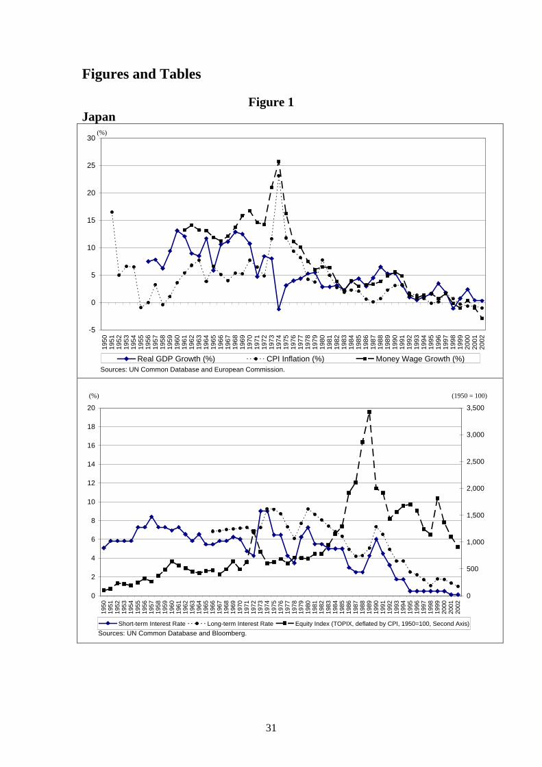
deflation is not surprising. As shown in Figure 1, in Japan the central bank discount

rate has been at 50 basis points or less since 1995, raising concern about the zero

lower bound on nominal interest rates, at least at the short end of the maturity

spectrum. Until 2003, when GDP grew at 3.1%, Japan was in a protracted economic

slump, which started in 1992. Money wages have declined in four of the past five

years; the GDP deflator has declined in each of the past five years and the CPI in four

out of the past five years (CPI inflation in 2003 was -0.3%). Short-term nominal

interest rates in Japan are near zero.

[Figure 1 about here]

A number of observers have concluded that Japan is in a liquidity trap, i.e.

monetary policy of any kind is incapable of stimulating aggregate demand.

significant upward bias. Changes made since then by the Bureau of Labor Statistics have probably reduced the magnitude of the bias.

3

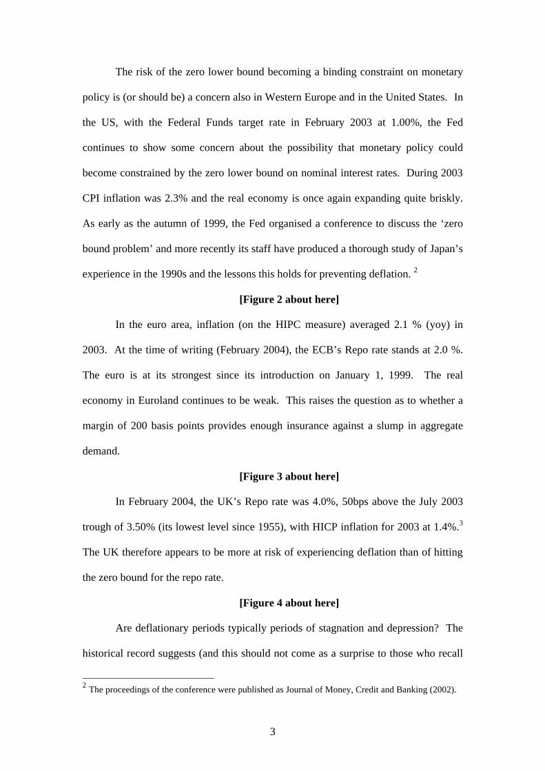
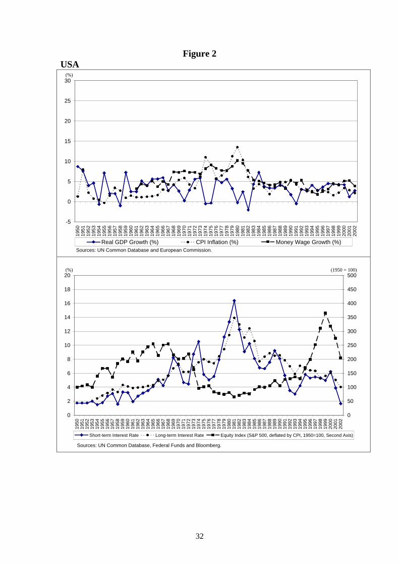
The risk of the zero lower bound becoming a binding constraint on monetary

policy is (or should be) a concern also in Western Europe and in the United States. In

the US, with the Federal Funds target rate in February 2003 at 1.00%, the Fed

continues to show some concern about the possibility that monetary policy could

become constrained by the zero lower bound on nominal interest rates. During 2003

CPI inflation was 2.3% and the real economy is once again expanding quite briskly.

As early as the autumn of 1999, the Fed organised a conference to discuss the ‘zero

bound problem’ and more recently its staff have produced a thorough study of Japan’s

experience in the 1990s and the lessons this holds for preventing deflation. 2

[Figure 2 about here]

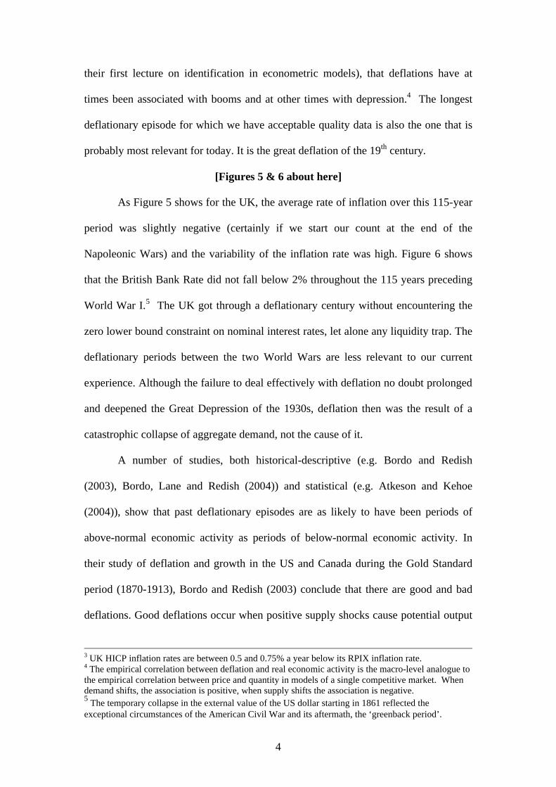
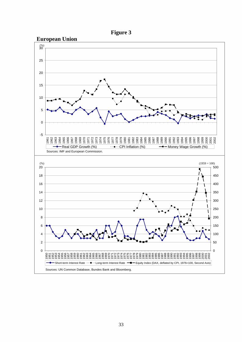
In the euro area, inflation (on the HIPC measure) averaged 2.1 % (yoy) in

2003. At the time of writing (February 2004), the ECB’s Repo rate stands at 2.0 %.

The euro is at its strongest since its introduction on January 1, 1999. The real

economy in Euroland continues to be weak. This raises the question as to whether a

margin of 200 basis points provides enough insurance against a slump in aggregate

demand.

[Figure 3 about here]

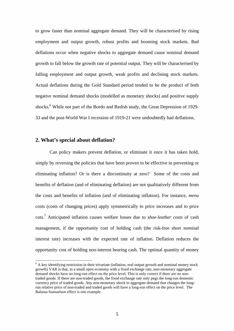
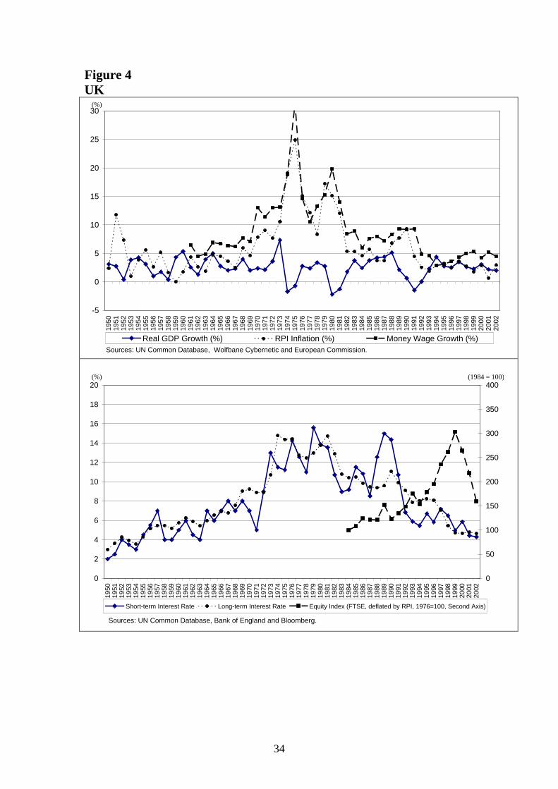
In February 2004, the UK’s Repo rate was 4.0%, 50bps above the July 2003

trough of 3.50% (its lowest level since 1955), with HICP inflation for 2003 at 1.4%.3

The UK therefore appears to be more at risk of experiencing deflation than of hitting

the zero bound for the repo rate.

[Figure 4 about here]

Are deflationary periods typically periods of stagnation and depression? The

historical record suggests (and this should not come as a surprise to those who recall

2 The proceedings of the conference were published as Journal of Money, Credit and Banking (2002).

4

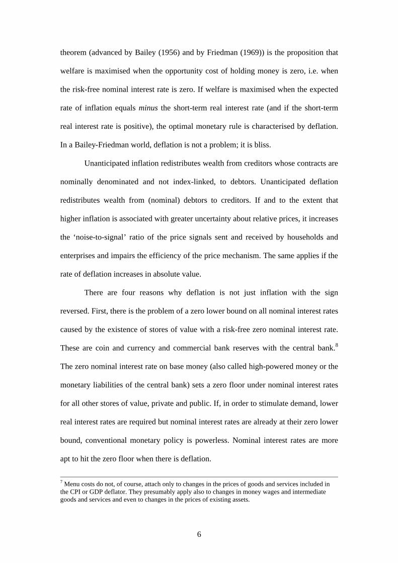
their first lecture on identification in econometric models), that deflations have at

times been associated with booms and at other times with depression.4 The longest

deflationary episode for which we have acceptable quality data is also the one that is

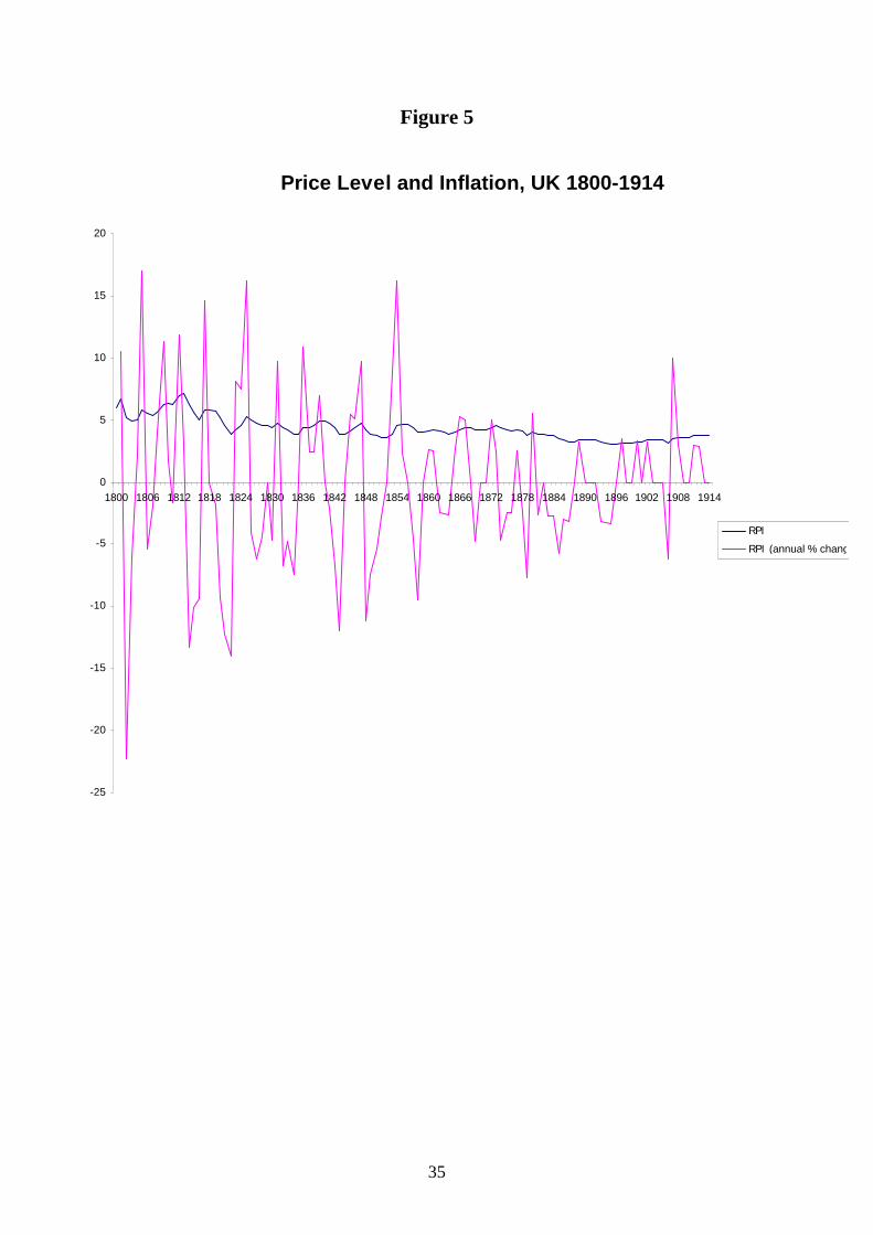
probably most relevant for today. It is the great deflation of the 19th century.

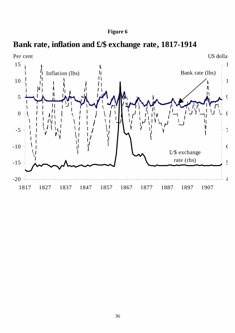
[Figures 5 & 6 about here]

As Figure 5 shows for the UK, the average rate of inflation over this 115-year

period was slightly negative (certainly if we start our count at the end of the

Napoleonic Wars) and the variability of the inflation rate was high. Figure 6 shows

that the British Bank Rate did not fall below 2% throughout the 115 years preceding

World War I.5 The UK got through a deflationary century without encountering the

zero lower bound constraint on nominal interest rates, let alone any liquidity trap. The

deflationary periods between the two World Wars are less relevant to our current

experience. Although the failure to deal effectively with deflation no doubt prolonged

and deepened the Great Depression of the 1930s, deflation then was the result of a

catastrophic collapse of aggregate demand, not the cause of it.

A number of studies, both historical-descriptive (e.g. Bordo and Redish

(2003), Bordo, Lane and Redish (2004)) and statistical (e.g. Atkeson and Kehoe

(2004)), show that past deflationary episodes are as likely to have been periods of

above-normal economic activity as periods of below-normal economic activity. In

their study of deflation and growth in the US and Canada during the Gold Standard

period (1870-1913), Bordo and Redish (2003) conclude that there are good and bad

deflations. Good deflations occur when positive supply shocks cause potential output

3 UK HICP inflation rates are between 0.5 and 0.75% a year below its RPIX inflation rate. 4 The empirical correlation between deflation and real economic activity is the macro-level analogue to the empirical correlation between price and quantity in models of a single competitive market. When demand shifts, the association is positive, when supply shifts the association is negative. 5 The temporary collapse in the external value of the US dollar starting in 1861 reflected the exceptional circumstances of the American Civil War and its aftermath, the ‘greenback period’.

5

to grow faster than nominal aggregate demand. They will be characterised by rising

employment and output growth, robust profits and booming stock markets. Bad

deflations occur when negative shocks to aggregate demand cause nominal demand

growth to fall below the growth rate of potential output. They will be characterised by

falling employment and output growth, weak profits and declining stock markets.

Actual deflations during the Gold Standard period tended to be the product of both

negative nominal demand shocks (modelled as monetary shocks) and positive supply

shocks.6 While not part of the Bordo and Redish study, the Great Depression of 1929-

33 and the post-World War I recession of 1919-21 were undoubtedly bad deflations.

2. What’s special about deflation?

Can policy makers prevent deflation, or eliminate it once it has taken hold,

simply by reversing the policies that have been proven to be effective in preventing or

eliminating inflation? Or is there a discontinuity at zero? Some of the costs and

benefits of deflation (and of eliminating deflation) are not qualitatively different from

the costs and benefits of inflation (and of eliminating inflation). For instance, menu

costs (costs of changing prices) apply symmetrically to price increases and to price

cuts.7 Anticipated inflation causes welfare losses due to shoe-leather costs of cash

management, if the opportunity cost of holding cash (the risk-free short nominal

interest rate) increases with the expected rate of inflation. Deflation reduces the

opportunity cost of holding non-interest bearing cash. The optimal quantity of money

6 A key identifying restriction in their trivariate (inflation, real output growth and nominal money stock growth) VAR is that, in a small open economy with a fixed exchange rate, non-monetary aggregate demand shocks have no long-run effect on the price level. This is only correct if there are no non-traded goods. If there are non-traded goods, the fixed exchange rate only pegs the long-run domestic currency price of traded goods. Any non-monetary shock to aggregate demand that changes the long-run relative price of non-traded and traded goods will have a long-run effect on the price level. The Balassa-Samuelson effect is one example.

6

theorem (advanced by Bailey (1956) and by Friedman (1969)) is the proposition that

welfare is maximised when the opportunity cost of holding money is zero, i.e. when

the risk-free nominal interest rate is zero. If welfare is maximised when the expected

rate of inflation equals minus the short-term real interest rate (and if the short-term

real interest rate is positive), the optimal monetary rule is characterised by deflation.

In a Bailey-Friedman world, deflation is not a problem; it is bliss.

Unanticipated inflation redistributes wealth from creditors whose contracts are

nominally denominated and not index-linked, to debtors. Unanticipated deflation

redistributes wealth from (nominal) debtors to creditors. If and to the extent that

higher inflation is associated with greater uncertainty about relative prices, it increases

the ‘noise-to-signal’ ratio of the price signals sent and received by households and

enterprises and impairs the efficiency of the price mechanism. The same applies if the

rate of deflation increases in absolute value.

There are four reasons why deflation is not just inflation with the sign

reversed. First, there is the problem of a zero lower bound on all nominal interest rates

caused by the existence of stores of value with a risk-free zero nominal interest rate.

These are coin and currency and commercial bank reserves with the central bank.8

The zero nominal interest rate on base money (also called high-powered money or the

monetary liabilities of the central bank) sets a zero floor under nominal interest rates

for all other stores of value, private and public. If, in order to stimulate demand, lower

real interest rates are required but nominal interest rates are already at their zero lower

bound, conventional monetary policy is powerless. Nominal interest rates are more

apt to hit the zero floor when there is deflation.

7 Menu costs do not, of course, attach only to changes in the prices of goods and services included in the CPI or GDP deflator. They presumably apply also to changes in money wages and intermediate goods and services and even to changes in the prices of existing assets.

7

Second, redistributions from debtors to creditors associated with unexpectedly

high deflation in a world with imperfectly index-linked debt contracts is more likely

to lead to default, bankruptcy and other forms of financial distress than redistributions

from creditors to debtors associated with unexpectedly high inflation. Default,

bankruptcy and corporate restructuring are not just mechanisms for redistributing

ownership and control of assets. These processes also destroy real resources.

‘Debt deflation’, the increase in the real value of nominal debt caused by a

falling general price level, was considered an important source of financial distress by

the great monetary economists of the 19th century and the first half of the 20th century

(although much of this literature failed to distinguish between anticipated and

unanticipated deflation). Irving Fisher (1932, 1933a) went as far as arguing that the

interaction of deflation and large accumulations of private nominal debt could account

for every major recession in the US. Borrowers with short-maturity nominal liabilities

and illiquid and/or real or foreign currency-denominated assets are especially

vulnerable to deflationary shocks. Commercial banks fit that description and the

incidence of banking crises and bank defaults during the Great Depression of the

1930s and other severe recessions are consistent with a role for (unanticipated) debt

deflation in the propagation of the business cycle. Homeowners with mortgages, or

households with significant outstanding unsecured consumer debt, have similar

vulnerabilities in their portfolios, as do highly indebted enterprises.

Third, there is a widely held view that there exists an asymmetry in nominal

wage and price adjustment. According to this view, the degree of downward rigidity

in some nominal prices (and especially in money wages) is not matched by a similar

degree of upward nominal rigidity. This means that disinflation, the process of

8 There are countries where commercial bank reserves with the central bank are remunerated, sometimes with close-to-market interest rates.

8

bringing down the rate of inflation through a reduction in the growth rate of nominal

demand, will be more costly in terms of output and employment foregone (i.e. the

sacrifice ratio will be higher) when the inflation rate falls into the negative range than

when it remains in the positive range.

Fourth, in living memory, there has been considerable experience of inflation

(and even of hyperinflation), while there has been only limited experience of deflation

(and none of hyperdeflation). This fourth point will turn out to be relevant also to the

interpretation of the third point.

The proximate cause of deflation is the failure of nominal demand to grow at

least at the rate of growth of potential output. It may, therefore, be descriptively

correct that recent deflationary episodes have been the result of faster than expected

productivity growth in some (significant) parts of the world – the USA and emerging

Asia (China, India etc.) are often mentioned in this context. Even if, in an accounting

sense, a reduction in inflation is associated mainly with an increase in real GDP

growth driven by higher productivity growth, rather than with a reduction in nominal

GDP growth, such a diagnosis does not absolve the monetary and fiscal policy

authorities. Whatever the supply side of the economy may generate by way of a

growth rate of potential output, it is always possible to use monetary and fiscal policy

to generate any growth rate of nominal demand and, therefore, any rate of inflation in

the medium term.9 Sustained deflation is, therefore, either a policy choice, or the

result of policy failure.

This leads us to three key questions.

9 Governor Hayami of the Bank of Japan gets part of the way to a correct understanding of the relationship between technological change, changes in market structure, relative price changes and inflation in the following quote from a speech given at the Keizai (Economic) Club on 29 January 2002: “The recent price decline is attributable to various factors such as technological innovation, deregulation and an increase in low-priced imports. But, above all, the major factor is that Japan's

9

1. Why don’t we see negative nominal interest rates?

The nominal interest rate on any financial instrument, i , say, cannot be lower

than the risk-free nominal interest rate on the safest and most liquid financial

instrument (base money, that is, coin and currency and commercial bank balances

with the central bank), Mi , say, that is, Mi i≥ . If the nominal interest rate on base

money is zero, nominal interest rates in general cannot be below zero. If we wish to

lower the zero floor for nominal interest rates in general, the authorities must be able

to pay a negative nominal interest rate on base money. Why doesn’t this happen?

Financial instruments can be divided into two categories: bearer securities and

registered securities. Registered securities are financial instruments for which the

identity of the owner is known to the issuer and can be verified by third parties.

Bearer securities are financial instruments for which the owner is anonymous – the

identity of the owner is unknown to the issuer and cannot be verified by third parties.

Paying interest at a positive or a negative rate on registered securities is a

simple task. Take, for instance, checking accounts or deposit accounts. The bank

knows the owner of each account. Payment of interest at any rate – positive, zero or

negative – is administratively straightforward. The bank just periodically credits or

debits the account.10

With bearer securities, paying any non-zero interest rate is not

administratively trivial. If the interest rate is positive, care must be taken that the

interest due is paid only once during a given payment period. Since the identity of the

economy was not able to achieve a full-scale recovery in the 1990s and that the negative output gap expanded due to lack of demand.” 10 Positive nominal interest rates on bank accounts have been common for decades. During the 1970s, the Swiss authorities taxed non-resident holders of Swiss bank accounts by paying a negative nominal interest rate. After allowing for bank fees, the net nominal rate of return on many checking accounts with a (low) positive nominal interest rate is frequently negative.

10

owner is unknown to the issuer, the same security could be presented multiple times

during any given payment period, either by the same holder or by a sequence of

different holders. The way around this is to identify, label or mark the security rather

than the owner. The security in question is marked in a verifiable manner by the issuer

or his agent, whenever the security is presented for payment of interest due.

Historically, bearer securities had coupons attached to them, which were cut off

(clipped) one at a time whenever an interest payment was made.11 Other ways of

identifying bearer securities as being ‘ex-interest’12, such as stamping, or more high-

tech identification methods, can no doubt be thought of.

If the interest rate on the bearer security is negative, the issuer faces the

opposite problem of the holder not presenting himself to pay the issuer the negative

interest due on the security. The solution is to find a way, first, of identifying the

bearer security as being ex-interest and, second, of ensuring that securities that are not

ex-interest are unattractive to potential owners.

The reason for the second condition becomes clear when one considers the

bearer security that is of special interest to this lecture: currency, that part of the

monetary liabilities of the central bank that is generally accepted as means of payment

and medium of exchange in the central bank’s jurisdiction.13 Today, currency is fiat

money. It has no intrinsic value as a consumer good, a capital good or an intermediate

input other than the value of the paper it is printed on. It has value today if, and only

if, the public believes it will have value tomorrow – valuable fiat money is a gigantic,

11 This would be problematic for a bearer perpetuity, such as British Consols. 12 I use ‘ex-interest’ analogously with ‘ex-dividend’ for common stock. A security is ex-interest for a given payment period if the interest due on it (positive or negative) has been paid. 13 The monetary liabilities of the central bank consist of currency in circulation and commercial bank balances with the central bank. Banks’ balances with the central bank are registered securities. The identity of the owner is known to the issuer. Any interest rate, positive or negative, can be charged on it with negligible administrative expense. (Sometimes, of course, currencies are accepted outside their central bank’s jurisdiction, as with the US dollar and the Euro today.)

11

and socially most beneficial, confidence trick. For the issuer (the central bank) to put

an expiry date on a bank note would be ineffective if the public chose to ignore it. To

make paying negative interest on currency possible it must be possible (a) to identify

bank notes as being ex-interest and (b) to attach a sufficiently severe penalty to

holding money that is not ex-interest after the date the interest is due. Fines and, in the

limit, confiscation or worse would be required to enforce negative interest on

currency.

The idea of taxing currency is not new. It goes back at least to Gesell (1949)

and the Social Credit movement in the second and third decades of the 20th century.

No less an economist than Irving Fisher (1933b) viewed the idea sympathetically. It

has recently been revived by Panigirtzoglou and myself (Buiter and Panigirtzoglou

(2001, 2003), and by Goodfriend (2000). Taxing currency by paying negative interest

on it would be a costly administrative exercise. These costs must be set against the

cost of being stuck at the zero nominal interest rate floor, or the cost of pursuing a

sufficiently high inflation target to minimise the risk of the zero nominal interest rate

floor becoming a binding constraint.

2. Do asymmetric, downward nominal price and wage rigidities make deflation particularly costly?

Conventional economic theory has a rather easy time explaining real rigidities,

but a hard time explaining any kind of nominal rigidities, let alone asymmetric

nominal rigidities. Empirically, there appear to be important nominal rigidities, but

mainstream economic theory does a poor job explaining why the numéraire matters.

A fortiori, mainstream economic theory has little to say about asymmetries in the

incidence and/or severity of nominal rigidities. For instance, menu costs do not

generate asymmetries between upward and downward price adjustments, although

12

they can account for the spike in the frequency distribution of individual price

changes at zero. Neither do other state-contingent or time-contingent contracting

stories.14

Nominal price rigidity, symmetric or asymmetric, has never been attributed to

nominal asset prices, nor to the prices of freely traded homogeneous commodities. Its

domain has never been argued to encompass more than the money prices of highly

processed goods and services and to money wages. With nominal price cuts becoming

more frequent in the low inflation environment of the last ten years (see e.g. the

divergent behaviour of prices for goods and prices for services in the UK, shown in

Table 1), those who argue for the importance of asymmetric downward nominal

rigidity are focussing mainly on the labour markets.

[Table 1 about here]

There is no coherent theory of asymmetric nominal rigidity in the labour

market. Arguments based on fairness, justice and morale miss the point, since

fairness, justice and morale should concern real wages and/or relative real wages over

time and across reference groups, not money wages. The observation, painstakingly

documented in hundreds of interviews by Bewley (1999), that both workers and

managers will strongly resist money wage cuts can plausibly be attributed to the fact

that the interviewees (in the 1990s) had known only positive inflation rates during

their working lives. When nominal prices and wages have on average been rising for

more than forty years, a nominal wage cut is also likely to be a real wage cut.

Resisting a cut in money wages is a pretty good first stab at (indeed almost certainly a

14 For instance, surveys on price setting by supermarkets and other firms show a marked bunching of the frequency distribution of price changes at zero, but such observations tell us nothing about the existence of asymmetries in the degrees of downward and upward nominal price stickiness or rigidity.

13

necessary condition for) resisting a real wage cut and, in decentralised labour markets,

a relative wage cut.

Nickell and Quintini (2003), using a unique UK micro-data set on nominal

wage changes for the period 1975-99, found that the proportion of individuals whose

nominal wages fall from one year to the next is large (reaching 20% in periods of low

inflation). They also found that there is evidence of some rigidity at a nominal wage

change of zero. However, while this causes a statistically significant distortion in the

distribution of real wage changes, the magnitude of the impact is ‘very modest’.15

The policy relevance of even this ‘very modest’ estimated impact is contingent

on the degree of downward nominal wage rigidity being ‘structural’, i.e. invariant

under changes in the long-run rate of inflation. With high and even moderate inflation

becoming a thing of the past throughout the industrial world, any nominal rigidities

and asymmetries in downward and upward nominal wage rigidity (due to memories

acquired and mental reference frames constructed during inflationary episodes) will

become less important as time passes. Finally, the spike in the empirical frequency

distribution of contract wage changes at zero is, at most, evidence of nominal wage

rigidity, not of asymmetric nominal wage rigidity. I conclude that, while there is

convincing empirical evidence that nominal price and wage rigidities exist, there is no

evidence that these nominal rigidities are asymmetric.

3. How can we disentangle the effects of monetary and fiscal policy?

The distinction between monetary and fiscal policy and monetary and fiscal

policy instruments is an unimportant definitional issue. It sometimes gets tangled up

with important issues involving the institutional arrangements for the decentralisation

15 Nickell and Quintini calculate that, if long-run inflation were to rise from 2.5 to 5.5% a year, the equilibrium unemployment rate would fall from around 6 to around 5.87%.

14

and delegation of the fiscal, financial and monetary management activities of the

State, such as central bank independence (both operational independence and

combined operational and target independence).

To understand the economic fundamentals that determine how monetary and

fiscal policy affect aggregate demand one should think of the central bank and the

general government sector as a single, consolidated unit – the state, or the sovereign.

The balance sheet, budget constraint and solvency constraint that matter are the

balance sheet, budget constraint and solvency constraint of the consolidated general

government and central bank. This consolidation makes sense, because the central

bank is generally majority owned or wholly owned by the Treasury (Ministry of

Finance). Central bank profits go to the Treasury and the Treasury has an (implicit)

obligation to ‘stand behind’ the central bank, that is, to recapitalise the central bank

should it take a dangerous hit on its balance sheet.

When we consider the practical, operational aspects of implementing certain

policies in a specific country, it is indeed helpful to consider the particular

institutional arrangements in that country. Often we have to focus on the central bank

as a separate agency of the state, with a distinct legal personality, charged with the

management of the legal tender liabilities of the state and frequently also with the

management of the official international foreign exchange reserves.

Monetary policy could be defined as ‘whatever the central bank does’, but a

slightly more restrictive definition will turn out to be more useful in framing the

analysis and organising the argument. I consider four potential monetary instruments:

one of them unconventional, the other three conventional.16 The unconventional

16 I restrict the analysis to monetary and fiscal policy in reasonably well-functioning market economies. Quantitative credit controls and other government-imposed forms of credit rationing are not considered. Changes in deposit reserve requirements are best viewed as fiscal measures (changes in the taxation of deposit-taking activities).

15

monetary instrument is the nominal interest rate on base money (conventionally zero

on coin and currency, but not necessarily zero on the other component of the

monetary base, commercial bank reserves held with the central bank). The three

conventional monetary policy instruments are: (1) the short-term risk-free nominal

interest rate on non-monetary financial claims (in the UK this would be the 2-week

Repo rate; in the US the Federal Funds rate, although the Fed does not peg that rate

exactly); (2) the stock of base money; and (3) the nominal spot exchange rate (the

relative price of foreign currency in terms of domestic currency). If there is

unrestricted international capital mobility and the country is small in global capital

markets, out of the short nominal interest rate, the quantity of base money and the

exchange rate only one can be chosen independently by the authorities.17

In practice, countries either have a managed exchange rate (the exchange rate

is the policy instrument), or they use the short nominal interest rate itself as the

monetary instrument. I know of no country that uses (or used) the monetary base as

the policy instrument, although in principle it is possible.

I am here defining a conventional monetary policy action as any change in the

quantity of base money, in the short nominal interest rate or in the exchange rate that,

at given prices and activity levels, does not change the financial net worth of the State

(the consolidated general government and central bank), now or in the future.

Conventional monetary policy is, therefore, a subset of the State’s financial portfolio

management. This includes the sale and purchase of long-dated government debt

instruments, financed by matching changes in shorter-maturity instruments, and

changes in the currency composition of the government’s financial assets and

liabilities (including sterilised and non-sterilised foreign exchange market

17 A ‘small’ country in a particular market is a price taker in that market. All countries, except the US, can for practical policy purposes be treated as small in global capital markets.

16

intervention, changes in the mix of nominal and index-linked debt, public debt

retirement financed through privatisation of state assets, swaps, trading in contingent

claims markets etc).

Monetary policy involves a subset of such asset swaps. For our purposes, it

always includes issuance or retirement (contraction) of base money, financed through

the purchase or sale of government interest-bearing debt (generally of a short

maturity) or of foreign exchange reserves. Sterilised foreign exchange market

intervention (purchases or sales of foreign currency with the impact on the monetary

base neutralised by sales of purchases of non-monetary liabilities of the government)

also are generally conducted by the central bank. Note, however, that in the UK most

of the foreign exchange reserves are owned by the general government (the Treasury),

although the Bank of England manages them as the government’s agent. Most debt

management operations not involving changes in the monetary base are no longer

conducted by the Bank of England. Fiscal policy includes any change in public

spending or tax rules, regardless of whether it alters, at given prices and activity

levels, the sequence of net financial balances of the State.

3. Policies to stimulate demand

To guide the discussion of the conditions under which monetary and fiscal policy

(conventional and unconventional) can or cannot stimulate aggregate demand, I will

appeal to some well-known properties of a standard formal model of aggregate

demand (see Buiter (2003a,b). Monetary (and fiscal) policy ineffectiveness concerns

the inability of monetary and fiscal policy to influence nominal aggregate demand.

The precise question I will ask is how monetary and fiscal policy can be used to

stimulate aggregate demand, holding constant (that is, for given) current and future

17

prices, wages, exchange rates, employment, output and initial stocks of financial and

real assets. How the change in nominal aggregate demand is translated into changes in

real GDP and/or in the general price level, depends on the details of the specification

of the ‘supply side’ of the economy and is not relevant in this discussion of how

policy can affect demand. All that matters is whether a given policy (or combination

of policies) can boost nominal aggregate demand.18 – when policy effectiveness is in

question, both higher real output and a higher price level are welcome.

The key building blocks of the aggregate demand model are as follows: the

demand for real domestic output, HD is the sum of private consumption demand for

domestic output, HC , private investment demand for domestic output, HI ,

government demand for domestic output, HG and export demand, X .

H H H HD C I G X= + + + (1)

Export demand and the shares of total private consumption, total private

investment, and total government spending allocated to domestic output depends on

the relative price of imports and domestic goods. Holding constant total private

consumption, private investment and government spending as well as the domestic

currency price of exports and the foreign currency price of imports, aggregate demand

for domestic output will increase when the exchange rate is devalued if the Marshall-

Lerner condition is satisfied. If the initial trade balance is zero, the Marshall-Lerner

conditions are satisfied if the sum of relative price elasticities of import and export

demand is greater than one in absolute value. From now on, the exchange rate is

treated as given.

18 In Buiter and Panigirtzoglou (2001, 2003), a simple continuous time, closed endowment economy, representing an agent version of the aggregate demand and money demand model developed here, is combined with an old Keynesian (in Buiter and Panigirtzoglou (2001)) and a new Keynesian Phillips curve (in Buiter and Panigirtzoglou (2003)).

18

Private investment is modelled as an increasing function of Tobin’s q, the ratio

of the present discounted value of future profits over the current reproduction cost of

capital. Government spending is exogenous, as is export demand at a given exchange

rate and domestic and foreign prices.

Total private consumption is the sum of consumption by ‘Keynesian’

consumers, who always spend their current disposable income and ‘permanent

income’ consumers who smooth consumption over the life cycle by borrowing and

lending freely in efficient financial markets. A fraction σ of households is

Keynesian. The real wage bill is W and real labour income tax payments are T. Total

real consumption is C, real financial wealth is A and H is human wealth, the present

discounted value of current and future labour income of households currently alive.

The marginal propensity to consume out of comprehensive (financial plus human)

wealth of permanent income consumers is µ . The consumption function can

therefore be written as:

[ ](1 ) ( )C A H W Tµ σ σ= + − + − (2) Note that private financial wealth, A, includes stock market wealth, the present

discounted value of current and future profits.

Conventional monetary policy

For the moment assume that Mi , the nominal interest rate on base money, is

zero and that i , the short nominal interest rate on non-monetary financial claims, is

above zero. Conventional monetary policy attempts to stimulate demand through a

cut in the short nominal interest rate. At given current and future expected prices, a

cut in the short nominal interest rate, i is a cut in the short real interest rate, r i π≡ − ,

where π is the rate of inflation. A cut in the short real interest rate will boost Tobin’s

19

q because it lowers the discount factor applied to near-term future profits. It may

also boost investment through other channels, such as the credit channel (including

the bank-lending channel).

A lower short-term nominal interest itself may affect consumption, because

the marginal propensity to consume out of comprehensive wealth, µ , may depend on

current and future nominal interest rates as well as on current and future real interest

rates. A lower short-term nominal interest rate will also affect consumption, at given

current and future prices, because it lowers the current short real interests rate. This

works through three channels: (1) the substitution effect; (2) the income effect, and

(3) the valuation effect. The substitution and income effects of a change in the current

real rate of interest both work through µ . The substitution effect of a lower real

interest rate will boost current consumption. The income effect depends on whether

the household is a net debtor, in which case a lower real interest rate boosts current

consumption or a net creditor, in which case it lowers consumption. If the

intertemporal substitution elasticity is 1, the substitution effect and income effect of a

change in real interest rates cancel out and µ is a constant. Valuation effects of a

lower real interest rate work through A, by lowering the discount factors applied to

current and future profits, and through H, by lowering the discount factors applied to

current and future after-tax wages.

Cutting the nominal (and real) interest rate for just the current period is

unlikely to do much for private consumption and investment demand. However, the

effect is strengthened if a cut in the current interest rate leads to expectations of future

cuts in nominal interest rates. None of this works, however, if the short nominal

interest rate cannot be cut because it is at the (zero) floor set by the (zero) nominal

interest rate on base money. In that case unconventional monetary policy is called

20

for. I start with the least unconventional policy: open market purchases of anything

and everything.

Unconventional monetary policy

Fundamentally, as long as there is any nominal interest rate, at any maturity,

that is positive, monetary policy has not exhausted its capacity to stimulate demand.

The central bank can purchase government securities, long-dated and short-dated, in

principle until all government interest-bearing debt is held by the central bank. It can

engage in purchases of foreign exchange, sterilised or non-sterilised. It can purchase

other public or private foreign currency assets. It can purchase private domestic

securities, financial or real, including bonds, stocks, real estate and options. It can

also ease the eligibility requirements for securities acceptable as collateral in repo

operations, and it can expand the list of eligible counterparties.

Clearly, there is a downside to the central bank purchasing private securities

on a significant scale. There is risk of moral hazard and adverse selection on the part

of the private counterparties to these transactions. To avoid favouritism the central

bank would have to “buy the market”, that is, buy a representative, value-weighted

index fund. There is risk of back-door socialisation of the means of production,

distribution and exchange and of central bank interference in the management of the

enterprises in which they obtain a significant share holding. None of these problems

apply to the public debt, however. As long as there is any public debt held outside the

central bank, monetary policy is not out of ammunition.

What to do when the ‘foolproof’ way is not foolproof?

21

Now consider the case where nominal interest rates at all maturities, from zero

to infinity, have been brought down to their (zero) floor. In this case there is no

escape using conventional monetary policy, including devaluations, or even using

generalised open market purchases of everything. Svensson (2000, 2003) proposes a

‘foolproof; way out of a liquidity trap and deflation consisting of three key elements,

(1) an explicit central-bank commitment to a higher future price level; (2) a concrete

action (concretely a devaluation or intentional depreciation of the currency) that

demonstrates the central bank’s commitment, induces expectations of a higher future

price level and jump-starts the economy; and (3) an exit strategy that specifies when

and how to get back to normal.

It is immediately clear that Svensson’s ‘liquidity trap’ refers to the rather

benign case where only the current short-term nominal interest rate is at its lower

bound.19 It that case the ‘foolproof’ way and many others would work – they would

stimulate demand. My definition of ‘liquidity trap’ is rather more demanding. It

refers to a situation where the current short nominal interest rate and current

expectations of future short nominal interest rates over the indefinite future are zero,

as well as current interest rates on longer-dated securities with every maturity, from

zero to infinity. Under these conditions, the ‘foolproof’ way is not foolproof.

Announcing a planned, expected or desired future price level (or announcing an

inflation target) is spitting in the wind. There is no instrument, now or in the future,

to drive the future price level (or inflation rate) to its announced target.

When all current and future short nominal interest rates and long-term interest

rates at all maturities are zero, negative nominal interest rates on base money are one

19 Or at most, the current short-term nominal interest rate, current expectations of future short-term nominal interest rates over some limited period and nominal interest rates on current longer but finite maturity securities are at their zero lower bound.

22

way of lowering the floor for the nominal interest rates on non-monetary financial

instruments. Paying a negative nominal interest rate on commercial bank balances

with the central bank is administratively trivial. Paying a negative nominal interest

rate on currency through a “carry tax” on currency is, as argued in Section 2 feasible

but costly. If that is not possible, fiscal policy has to come to the rescue.

Fiscal policies to stimulate aggregate demand.

It is clear from the consumption function in equation (2), that a debt-financed

or money-financed tax cut will always stimulate aggregate demand if there are

Keynesian consumers, as these will simply consume all of their tax cut. If 0σ = , and

there are only permanent income consumers, debt-financed current tax cuts will raise

aggregate consumption demand if they raise the permanent income of households

currently alive (by raising H in equation (2)). This can happen, even if households are

fully rational and realise that, holding constant government spending, a tax cut today

must imply that the present discounted value of future taxes has gone up by the full

amount of the tax cut. A necessary and sufficient reason for aggregate demand to be

stimulated by a debt-financed tax cut is that the tax cut (together with the future tax

increases) redistributes resources from households with a low marginal propensity to

consume (the young and, a fortiori, those who have not been born yet) to consumers

with a high marginal propensity to consume (the old). Only if the existing

generations are linked to all future generations through an operative intergenerational

motive will there be ‘Ricardian equivalence’ or ‘debt neutrality’. In all other cases,

postponing taxes while keeping the present discounted value of current and future

taxes constant, will boost aggregate demand.

23

When there is debt neutrality, debt-financed tax cuts do not boost demand.

Under these conditions, a temporary increase in public spending on goods and

services will boost demand. It will make no difference in this case whether the public

spending increase is financed with current taxes or with future taxes (by borrowing

today). The negative effect on permanent income and thus on current private

consumption of the tax increase is smaller, in the short run, than the positive effect on

demand of the temporary increase in public spending. A permanent increase in public

spending would have no effect.

There is a non-Keynesian tax policy that could boost aggregate demand in the

short run even when there is debt-neutrality. The idea (advocated by Feldstein

(2003)) is to use non-lump-sum (distortionary) taxes on consumption (such as VAT)

to twist the pattern of consumption over time towards earlier consumption. By

cutting VAT today and raising it in the future (ensuring that the present value of

current and future taxes is not affected), the intertemporal terms of trade are turned in

favour of current consumption. Because the tax measure leaves the present value of

taxes unchanged, the income effect of the change in the intertemporal terms of trade is

(approximately) neutralised and the substitution effect boosts consumption today.

Last but not least, there is the combined monetary-fiscal policy action of a tax

cut (or increase in government transfer payments) financed by issuing (printing) base

money. This is the humdrum version of Milton Friedman’s famous helicopter drop of

money. It is different from a debt-financed tax cut, even if nominal interest rates are

zero, because base money is irredeemable or inconvertible: the individual private

holder views is as an asset, but to the issuer it does not constitute a liability in any

meaningful sense. With zero interest bonds, the principal still has to be redeemed.

24

With base money, the principal is irredeemable: a £10 banknote gives the holder no

claim on the issuer for anything else than the £10 banknote itself.

Therefore, if a tax cut is financed by issuing base money, and if the public

does not expect the central bank to reverse this action in the future, consumption

demand can increase. The magnitude of the increase is given by the marginal

propensity to consume out of comprehensive wealth, µ times the change in the

present value of the terminal (very long run) money stock (see Buiter (2003c)).

An attractive feature of the money-financed tax cut or transfer payment is that

it can bypass the banking sector completely. If sending cash by mail is deemed

dangerous, households could be sent a cheque drawn on the government’s account

with the central bank. The cheque could be cashed at any commercial bank, post

office or benefit office in the country. In a country like Japan, which until 2003 was

mired in a persistent recession, the ability of the authorities to bypass the banking

system when implementing a money-financed tax cut would have been especially

welcome in view of the precarious state of its banking system.20

How much can the central bank do on its own?

As regards open market purchases of “everything”, it may be the case that

existing constraints range of financial claims the central bank can hold in its portfolio

have to be relaxed. Can the central bank implement a helicopter drop of money on its

own. In the USA this would mean that the Chairman of the Federal Reserve Board,

Alan Greenspan, would send a cheque for, say, $1000 to each man, woman and child,

drawn on the Fed. If suspicious recipients decided to save the money, more cheques

20 Late 1989 Japan experienced the beginning of the largest stock market collapse and debt deflation in modern history. From the early 1990s until 2003, the country has experienced recession, and since 1998, deflation.

25

could be sent out, each one with a larger number of zeros before the decimal point.

At some point the consumer would cry uncle and spend at least some of the money.

For better or worse, by law, central banks are not generally permitted to act as

a fiscal agents capable of making transfer payments to private recipients.21

Implementing a helicopter money drop therefore requires the cooperation of the

Treasury. The Treasury would but taxes or increase transfer payments and borrow

from the central bank to finance this. If direct borrowing by the government from the

central bank is nor permitted (which is the case in the EMU), then the government

could borrow in the markets (issue new debt) and the central bank could buy a

corresponding amount of government debt in the secondary market.

4. Conclusions

First, although preventing or combating deflation poses some unique

difficulties for the monetary authorities – difficulties that are not present in preventing

or combating inflation – deflation can always be prevented and, if it has taken hold,

can always be overcome by co-ordinated actions of the monetary and fiscal

authorities.

Second, monetary policy alone cannot always prevent or cure deflation, if we

restrict ourselves to conventional monetary policy, i.e. reductions in the risk-free

short-term nominal interest rate, or a devaluation of the nominal exchange rate.

Monetary policy alone is likely to prevent or cure deflation, if one is willing to

consider the monetisation (if necessary without limit) of the public debt (short, long,

21 In the USA, the Treasury could implement a money drop on its own, without the assistance of the Federal Reserve Board, if it were willing to issue more “Treasury notes”. So-called US notes, issued by the Department of the Treasury since the Legal Tender Act of 1862 (as gold or silver certificates) are part of the stock of US currency. Like Federal Reserve notes (authorised by the Federal Reserve Act of 1913), they are non-interest-bearing irredeemable bearer notes and constitute legal tender. They

26

nominal or index-linked) and/or open market purchases of a wide range of foreign and

private domestic securities. If one is willing to contemplate an even more

unconventional monetary instrument – the payment of negative nominal interest rates

on base money through the imposition of a carry tax on currency – the zero lower

bound on nominal interest rates disappears as a constraint on monetary policy.

To say that deflation can be prevented or cured using conventional monetary

and fiscal policy is not to say that all the economic problems faced by the most

prominent recent example of a deflation-afflicted economy – Japan – could have been

solved this way. The Japanese banking sector is paralysed by a massive overhang of

bad debt. Other financial intermediaries, especially insurance companies, are suffering

the cumulative impact on their balance sheets of the most spectacular asset boom and

collapse in modern history – the stock market and real estate boom of the 1980s and

its unravelling since 1989.

Cleaning up the balance sheet of the Japanese banking sector, reducing the

size of the banking sector and recapitalising key viable non-bank intermediaries will

be a painful and protracted process. However, this inevitably painful structural

adjustment was not facilitated by the deflationary monetary policies of the previous

Governor of the Bank of Japan, Mr. Hayami.

Deflation is problem that can be avoided. If it has taken hold, it is a problem

that can be solved. A tax cut (or transfer payment) directly aimed at households and

financed by increasing the stock of base money will surely boost aggregate demand.

So will a base-money-financed increase in public spending.

Inflation-reducing policies involve tax increases or public spending cuts and,

therefore, tend to be politically unpopular. Anti-deflationary policies involve tax cuts,

were issued until January 21, 1971. Those that remain in circulation are obligations of the U.S.

27

increased transfer payment or higher public spending on goods and services. They

will tend to be politically popular. It is, therefore, somewhat of a mystery why a

policy programme that makes economic sense and should be politically popular does

not get implemented.

The clue to the mystery probably lies in the fact that, with conventional

monetary policy nearly exhausted, further effective anti-deflationary policy requires

the co-operation of the central bank and the Ministry of Finance in the design and

implementation of a co-ordinated monetary and fiscal stimulus. Some of the central

banks that acquired operational independence only recently have interpreted central

bank independence to require no co-operation, no co-ordination and at times even no

communication with the fiscal authorities. An atmosphere of mutual distrust between

operationally independent monetary and fiscal authorities is probably the root cause

of the observed failure to address the deflation problem.

Milton Friedman argued that inflation (and by implication deflation) is always

and everywhere a monetary phenomenon – and he was right.22 Sargent and Wallace

[1981] have told us that, in the long-run, money (and, therefore, inflation and

deflation) is always and everywhere a fiscal phenomenon – and they too were right.

Structuralists and political economists inform us that excessive public sector deficits

are the result of unresolved social and political conflict about the size and

composition of state spending and about who should pay for it. They, too, may well

be right.

government. 22 ‘It follows from the propositions I have so far stated that inflation is always and everywhere a monetary phenomenon in the sense that it is and can be produced only by a more rapid increase in the quantity of money than in output. However, the reason for the rapid increase in the quantity of money may be very different under different circumstances. It has sometimes reflected gold discoveries, sometimes changes in banking systems, sometimes the financing of private spending, sometimes – perhaps most of the time – the financing of governmental spending.’ (Friedman (1973))

28

I would like to add to this sequence of truths the proposition that persistent

unwanted deflation is always and everywhere evidence of unnecessary, avoidable

macroeconomic mismanagement. Governments through the ages have demonstrated

their ability to create inflation, often to undesirable and at times disastrous levels. It is

hard to believe that the very simple analytics and attractive politics of making

inflation have been forgotten in the new Millennium.

29

References & further reading

Atkeson, Andrew and Patrick J. Kehoe (2004), “Deflation and Depression: Is There an Empirical Link”, NBER Working Paper No. 10268, January. Bailey, Martin J. (1956), ‘The Welfare Costs of Inflationary Finance’, Journal of Political Economy, vol. 64, no. 2, April, pp. 93–110. Bewley, T.F. (1999), Why Wages Don’t Fall During a Recession, Harvard University Press, Cambridge MA. Bordo, Michael D. and Angela Redish [2003], ‘Is Deflation Depressing? Evidence from the Classical Gold Standard’”, NBER Working Paper No. 9520, February. Bordo, Michael D., John Landon Lane and Angela Redish (2004), “Good Versus Bad Deflation: Lessons From the Gold Standard Era”, NBER Working Paper 10329, February. Boskin, Michael J., E. Dulberger, R. Gordon, Z. Griliches and D. Jorgenson (1996), "Toward a More Accurate Measure of the Cost of Living: Final Report to the Senate Finance Committee,", Washington, DC, U.S. Government Printing Office, for the U.S. Senate Committee on Finance, December. Boskin, Michael J., E. Dulberger, R. Gordon, Z. Griliches, and D. Jorgenson (1997), "Consumer Prices, the Consumer Price Index and the Cost of Living," Journal of Economic Perspectives, Fall 1997. Buiter, Willem H. (2003a), "Deflation; Prevention and Cure", NBER Working Paper W9623, April. Buiter, Willem H. (2003b), Appendix to ‘Deflation: Prevention and Cure’, European Bank for Reconstruction and Development Mimeo, 13-07-2003, available at http://www.nber.org/~wbuiter/defap.pdf . Buiter, Willem H. (2003c), "Helicopter Money: Irredeemable Fiat Money and the Liquidity Trap" , NBER Working Paper No. W10163, December. Buiter, Willem H. and Nikolaos Panigirtzoglou (2001), ‘Liquidity Traps: How to Avoid Them and How to Escape Them’, in Wim F.V. Vanthoor and Joke Mooi, Reflections on Economics and Econometrics, Essays in Honour of Martin M. G. Fase, 2001, De Nederlandsche Bank, pp. 13-58. Buiter, Willem H. and Nikolaos Panigirtzoglou (2003), ‘Overcoming the Zero Bound on Nominal Interest Rates with Negative Interest on Currency: Gesell’s Solution’, Economic Journal, Vol. 31, No. 490, pp. 723-746, October. Feldstein, Martin (2003), ‘The Role for Discretionary Fiscal Policy in a Low Interest Rate Environment’, in the 2002 Federal Reserve Bank of Kansas City Annual Conference volume, Rethinking Stabilization Policy, 2003.

30

Fisher, Irving, [1932], Booms and Depressions, New York: Adelphi Company. Fisher, Irving [1933a], ‘The Debt-Deflation Theory of Great Depressions’, Econometrica, March, pp. 337-57. Fisher, Irving [1933b], Stamp Scrip, Adelphi Company, New York. Friedman, Milton (1969), ‘The Optimum Quantity of Money’, in The Optimum Quantity of Money and Other Essays, Chicago: Aldine, 1969, pp.1–50. Friedman, Milton (1973), Money and Economic Development; the Horowitz Lectures of 1972. Praeger, New York. Gesell, Silvio (1949), Die Natuerliche Wirtschaftsordnung, Rudolf Zitzman Verlag, available in English as The Natural Economic Order, Peter Owen Ltd, London, 1958. Goodfriend, Marvin (2000), ‘Overcoming the Zero Bound on Interest Rate Policy’, Journal of Money, Credit and Banking, Vol. 32, No. 4, Pt. 2, November, pp. 1007-1035. Journal of Money, Credit and Banking(2002), Monetary Policy in a Low-Inflation Environment, Vol. 32, No 4, Part 2, November. Nickell, S. and G. Quintini (2003), ‘Nominal wage rigidity and the rate of inflation’, Economic Journal, Vol. 113 No.490, pp. 762-746, October. Svensson, Lars .E.O. (2000), ‘The Zero Bound in an Open Economy: A Foolproof Way of Escaping from a Liquidity Trap’, Monetary and Economic Studies (Special Edition), February, pp. 277-316. Svensson, Lars E. O. (2003), “Escaping from a liquidity trap and deflation: a foolproof way and others”, NBER Working Paper 10195, December.

31

Figures and Tables

Figure 1 Japan

-5

0

5

10

15

20

25

30

1950

1951

1952

1953

1954

1955

1956

1957

1958

1959

1960

1961

1962

1963

1964

1965

1966

1967

1968

1969

1970

1971

1972

1973

1974

1975

1976

1977

1978

1979

1980

1981

1982

1983

1984

1985

1986

1987

1988

1989

1990

1991

1992

1993

1994

1995

1996

1997

1998

1999

2000

2001

2002

Real GDP Growth (%) CPI Inflation (%) Money Wage Growth (%)Sources: UN Common Database and European Commission.

(%)

0

2

4

6

8

10

12

14

16

18

20

1950

1951

1952

1953

1954

1955

1956

1957

1958

1959

1960

1961

1962

1963

1964

1965

1966

1967

1968

1969

1970

1971

1972

1973

1974

1975

1976

1977

1978

1979

1980

1981

1982

1983

1984

1985

1986

1987

1988

1989

1990

1991

1992

1993

1994

1995

1996

1997

1998

1999

2000

2001

2002

0

500

1,000

1,500

2,000

2,500

3,000

3,500

Short-term Interest Rate Long-term Interest Rate Equity Index (TOPIX, deflated by CPI, 1950=100, Second Axis)

Sources: UN Common Database and Bloomberg.

(%) (1950 = 100)

32

Figure 2 USA

-5

0

5

10

15

20

25

3019

5019

5119

5219

5319

5419

5519

5619

5719

5819

5919

6019

6119

6219

6319

6419

6519

6619

6719

6819

6919

7019

7119

7219

7319

7419

7519

7619

7719

7819

7919

8019

8119

8219

8319

8419

8519

8619

8719

8819

8919

9019

9119

9219

9319

9419

9519

9619

9719

9819

9920

0020

0120

02

Real GDP Growth (%) CPI Inflation (%) Money Wage Growth (%)Sources: UN Common Database and European Commission.

(%)

0

2

4

6

8

10

12

14

16

18

20

1950

1951

1952

1953

1954

1955

1956

1957

1958

1959

1960

1961

1962

1963

1964

1965

1966

1967

1968

1969

1970

1971

1972

1973

1974

1975

1976

1977

1978

1979

1980

1981

1982

1983

1984

1985

1986

1987

1988

1989

1990

1991

1992

1993

1994

1995

1996

1997

1998

1999

2000

2001

2002

0

50

100

150

200

250

300

350

400

450

500

Short-term Interest Rate Long-term Interest Rate Equity Index (S&P 500, deflated by CPI, 1950=100, Second Axis)

Sources: UN Common Database, Federal Funds and Bloomberg.

(%) (1950 = 100)

33

Figure 3 European Union

-5

0

5

10

15

20

25

3019

6119

6219

6319

6419

6519

6619

6719

6819

6919

7019

7119

7219

7319

7419

7519

7619

7719

7819

7919

8019

8119

8219

8319

8419

8519

8619

8719

8819

8919

9019

9119

9219

9319

9419

9519

9619

9719

9819

9920

0020

0120

02

Real GDP Growth (%) CPI Inflation (%) Money Wage Growth (%)Sources: IMF and European Commission.

(%)

0

2

4

6

8

10

12

14

16

18

20

1950

1951

1952

1953

1954

1955

1956

1957

1958

1959

1960

1961

1962

1963

1964

1965

1966

1967

1968

1969

1970

1971

1972

1973

1974

1975

1976

1977

1978

1979

1980

1981

1982

1983

1984

1985

1986

1987

1988

1989

1990

1991

1992

1993

1994

1995

1996

1997

1998

1999

2000

2001

2002

0

50

100

150

200

250

300

350

400

450

500

Short-term Interest Rate Long-term Interest Rate Equity Index (DAX, deflated by CPI, 1976=100, Second Axis)

Sources: UN Common Database, Bundes Bank and Bloomberg.

(%) (1959 = 100)

34

Figure 4 UK

-5

0

5

10

15

20

25

3019

5019

5119

5219

5319

5419

5519

5619

5719

5819

5919

6019

6119

6219

6319

6419

6519

6619

6719

6819

6919

7019

7119

7219

7319

7419

7519

7619

7719

7819

7919

8019

8119

8219

8319

8419

8519

8619

8719

8819

8919

9019

9119

9219

9319

9419

9519

9619

9719

9819

9920

0020

0120

02

Real GDP Growth (%) RPI Inflation (%) Money Wage Growth (%)Sources: UN Common Database, Wolfbane Cybernetic and European Commission.

(%)

0

2

4

6

8

10

12

14

16

18

20

1950

1951

1952

1953

1954

1955

1956

1957

1958

1959

1960

1961

1962

1963

1964

1965

1966

1967

1968

1969

1970

1971

1972

1973

1974

1975

1976

1977

1978

1979

1980

1981

1982

1983

1984

1985

1986

1987

1988

1989

1990

1991

1992

1993

1994

1995

1996

1997

1998

1999

2000

2001

2002

0

50

100

150

200

250

300

350

400

Short-term Interest Rate Long-term Interest Rate Equity Index (FTSE, deflated by RPI, 1976=100, Second Axis)

Sources: UN Common Database, Bank of England and Bloomberg.

(%) (1984 = 100)

35

Figure 5

Price Level and Inflation, UK 1800-1914

-25

-20

-15

-10

-5

0

5

10

15

20

1800 1806 1812 1818 1824 1830 1836 1842 1848 1854 1860 1866 1872 1878 1884 1890 1896 1902 1908 1914

RPI

RPI (annual % change)

36

Figure 6

-20

-15

-10

-5

0

5

10

15

1817 1827 1837 1847 1857 1867 1877 1887 1897 19074

5

6

7

8

9

10

11

Bank rate, inflation and £/$ exchange rate, 1817-1914

Bank rate (lhs)Inflation (lhs)

Per cent US dollar

£/$ exchangerate (rhs)

37

Table 1

Total, Goods and Services Inflation in the UK

UK US Euro area Japan

CPI inflation* 1.9 1.7 2.2 -0.9

CPI goods* -1.1 -0.1 1.4 -1.6

CPI services* 4.6 3.1 3.3 0.0

Services - goods inflation,

1990-97

1.6 1.6 1.6 1.3

Services - goods inflation,

1990-2002

2.3 1.8 1.3 1.3

* year to August 2002. Inflation rates are calculated as the total increase in the price index over the indicated period, based on monthly data , expressed as a twelve month growth rate. Sources: Table taken from King [2002]; ultimate source: ONS (for UK) and Thomson Financial Datastream for data on US, Euro Area and Japan.

Willem Buiter is Chief Economist at the European Bank for Reconstruction and Development.