Project Title: Preparations for Field Testing of Combined

Variable Speed Advisory (VSA) and Coordinated Ramp

Metering (CRM) for Freeway Traffic Control

Final Report

UCB-ITS-PRR-2014-1

Project Team:

Dr. Xiao-Yun Lu, Dr. Danjue Chen, and Dr. Steven E. Shladover

California PATH Program Institute of Transportation Studies University of California Berkeley

Richmond Field Station, Building 452 1357 S. 46th Street, Richmond, CA 94804-4648

January 15 2014

ii

iii

Key Words: freeway traffic control, ramp metering (RM), Coordinated Ramp Metering (CRM), site selection, modeling and model calibration, microscopic simulation, Aimsun, PeMS data

Abstract

Extensive site selection has been conducted for future testing of the Coordinated Ramp Metering (CRM) algorithm developed in a previous project supported by the FHWA Exploratory Advanced Research (EAR) program. Two major corridors have been analyzed: I-880 between SR237 and Auto Mall Parkway in Bay Area and SR99 NB between Elk Grove and the intersection with SR50 (about 13 miles long) in Sacramento. Main factors for site selection include: road geometry, traffic volume, bottleneck locations and traffic situations, traffic data quality, and availability of ramp meter facility. This report focuses on SR99 NB. PeMS data has been used for modeling and model calibration of the two corridors in Aimsun microscopic traffic simulation. Based on the calibrated model, the default field operational Local Adaptive Ramp Metering (LARM) and the Optimal CRM with Queue-Overwrite algorithm has been applied. Simulation has been conducted for multiple replications. Preliminary simulation results show that, on average, Total Travel Time (TTT) of the overall system could be reduced by 8%, Total Delay (TD) on the mainline could be reduced by 15%, Total Travel Distance could be increased by 0.5% and Total Number of Stops could be reduced by 2.9%. The number will depend on traffic volume. The microscopic simulation results need further fine tuning and field testing at the selected site(s) in the next phase of the project.

iv

Acknowledgement

This work was performed as part of the California PATH Program of the University of California, in cooperation with the State of California Transportation Agency, Department of Transportation (Caltrans). The contents of this report reflect the views of the authors who are responsible for the facts and the accuracy of the data presented herein. The contents do not necessarily reflect the official views or policies of the State of California. This report does not constitute a standard, specification, or regulation.

The guidance and support from the project panel are gratefully acknowledged.

Project Panel

Greg Larson, Caltrans HQ, Division of Research and Innovation, Tel: (916) 657-4369, email: greg_larson@dot.ca.gov Gurprit Hansra, Caltrans HQ, Division of Research and Innovation, Tel: (916) 654-7252, email: gurprit_hansra@dot.ca.gov Jim Calkins: Caltrans District 3, Chief, Freeway Operations, Tel: (916) 859-7940, email: jim_calkins@dot.ca.gov, Alan S Chow, Caltrans District 4, Chief, Traffic Operations, Tel: (510) 286-4577, email: alan_s_chow@dot.ca.gov Zhongren Wang, Caltrans Traffic Ops. Division, State-Wide Ramp Metering Program, Tel: (916) 654-6133, email: zhongren_wang@dot.ca.gov Brian Simi, Caltrans District 3, Freeway Traffic Operation, Tel: (916) 651-1251, email: brian_simi@dot.ca.gov; Leo Anselmo, Caltrans District 3, Freeway Traffic Operation, Tel: (916) 859-7954, email: leo_anselmo@dot.ca.gov

Lester Lee, Caltrans District 4, Traffic Systems, Tel: (510) 286-4528, lester.s.lee@dot.ca.gov Sean Coughlin, Caltrans District 4, Electrical Systems, Tel: (510) 286-4804, email: sean.coughlin@dot.ca.gov

David Wells, Caltrans HQ, Traffic Operations, ITS Projects & Standards, Tel: (916) 653-1342, email: david_j_wells@dot.ca.gov

v

Hassan Aboukhadijeh, Project Manager, Caltrans Division of Research and Innovation, Tel: (916) 654-8630, email: hassan_aboukhadijeh@dot.ca.gov Xiao-Yun Lu, PATH, University of California, Berkeley Tel: (510) 665-3644, email: xylu@path.berkeley.edu Steven E. Shladover, PATH, University of California, Berkeley Tel: (510) 665-3514, email: steve@path.berkeley.edu

vi

Disclaimer Statement

This document is disseminated in the interest of information exchange. The contents of this report reflect the views of the authors, who are responsible for the facts and accuracy of the data presented herein. The contents do not necessarily reflect the official views or policies of the State of California or the Federal Highway Administration. This publication does not constitute a standard, specification or regulation. This report does not constitute an endorsement by the Department of any product described herein.

For individuals with sensory disabilities, this document is available in Braille, large print, audiocassette, or compact disk. To obtain a copy of this document in one of these alternate formats, please contact: the Division of Research and Innovation, MS-83, California Department of Transportation, Division of Research, Innovation, and System Information, P.O. Box 942873, Sacramento, CA 94273-0001.

vii

Table of Contents

Page

Technical Report Documentation Page .................................................................................... ii

Key Words .................................................................................................................................. iii

Abstract ....................................................................................................................................... iii

Acknowledgements .................................................................................................................... iv

Project Panel ............................................................................................................................... iv

Disclaimer Statement ................................................................................................................. vi

Table of Contents ...................................................................................................................... vii

List of Figures and Tables ......................................................................................................... ix

List of Acronyms and Abbreviations ...................................................................................... xii

Executive Summary ................................................................................................................. xiv

Chapter 1 Introduction .............................................................................................................. 1

Chapter 2 Literature Review .................................................................................................... 3

2.1 Freeway Ramp Metering ........................................................................................... 3

2.2 Variable Speed Limit/Advisory ................................................................................. 9

2.3 Combined VSL and CRM ....................................................................................... 19

2.4 Concluding Remarks ............................................................................................... 21

Chapter 3 Test Site Selection Considerations ....................................................................... 24

3.1 Introduction .............................................................................................................. 24

3.2 Site Selection Criteria .............................................................................................. 24

3.3 Site Selection Method .............................................................................................. 25

3.4 SR99 NB in Sacramento .......................................................................................... 25

3.5 I-880 NB near Auto Mall Parkway .......................................................................... 36

3.6 Preliminary Recommendation ................................................................................. 45

Chapter 4 System Modeling and Calibration ........................................................................ 46

4.1 Traffic Network for SR99 ........................................................................................ 46

4.2 Data Quality ............................................................................................................. 46

4.3 Traffic Demand ........................................................................................................ 50

4.4 Traffic Pattern .......................................................................................................... 54

viii

4.5 Model Calibration .................................................................................................... 61

4.6 Calibrated Results .................................................................................................... 63

Page

Chapter 5 Coordinated Ramp Metering Algorithm .......................................................... 73

5.1 CRM Design with Model Predictive Control .......................................................... 73

5.2 Modeling .................................................................................................................. 73

5.3 Implementation of CRM Algorithm in Simulation ................................................. 76

5.4 Simulation Results ................................................................................................... 81

5.5 Summary of CRM Algorithm Characteristics ......................................................... 95

Chapter 6 Performance Parameter for Evaluation of VSL and CRM ............................. 96

Chapter 7 Concluding Remarks ........................................................................................... 99

References ................................................................................................................................ 102

Appendix A: Traffic Data Analysis for SR99 NB Bottleneck ............................................ 110

Appendix B: Traffic Data Analysis for I-880 NB near Auto Mall Parkway .................... 158

Appendix C: Model Calibration Performance Comparison Plots at Bottlenecks ........... 212

Appendix D: More Simulation Data Analysis Plots .......................................................... 228

ix

List of Figures and Tables

Figure Page

3-1 Road map of SR99 between 47th Ave and SR50 interchange ............................................. 27

3-2 Postmile (PM), lane geometry, onramp/off-ramp info, and sensor locations and health ..... 29

3-3 SR99 NB AM peak recurrent bottleneck location on and affect .......................................... 30

3-4 Evidence of middle bottleneck - occupancy ......................................................................... 31

3-5 Evidence of middle bottleneck – speed ................................................................................ 32

3-6 Evidence of middle bottleneck – occupancy ........................................................................ 33

3-7 Evidence of middle bottleneck - speed ................................................................................. 34

3-8 Road Geometry and sensor locations from Google Map for I-880 Section ......................... 37

3-9 Lane Geometry, Onramp/off-ramp and sensor locations/IDs for I-880 Section .................. 38

3-10 2D Time-Space contour plot of traffic occupancy, date: 08/29/12 .................................... 39

3-11 Significant Traffic Occupancy increase at the bottleneck location .................................... 41

3-12 Significant Traffic Speed Drop at the bottleneck location ................................................. 42

3-13 Traffic Occupancy very low downstream of the bottleneck ............................................... 43

3-14 Traffic Speed – almost free-flow at the downstream of the bottleneck .............................. 44

4-1 Road/Lane geometry and detector locations for SR99 Section ............................................ 47

4-2 Flow of HOV 1-6 on 3/5/2013 ............................................................................................. 48

4-3 Interpreted flow for OFR8 and 9 on 3/5/2013 ...................................................................... 50

4-4 SR99 NB AM peak recurrent bottleneck location on and affected range, time interval, and intensity ..................................................................................................................... 55

4-5 Evidence of bottleneck at PM 298.5 ..................................................................................... 57

4-6 Evidence of bottleneck at PM 296.54 ................................................................................... 58

4-7 Traffic condition at WB 47th Ave merge at PM 295.7 ........................................................ 59

4-8 Evidence of bottleneck at PM 290.76. .................................................................................. 60

4-9 Vehicle type parameters selection ........................................................................................ 64

4-10 Reaction Time parameter selection .................................................................................... 65

4-11 Section parameter selection ................................................................................................ 66

4-12 BN1 Occupancy on 2/26/2013 .......................................................................................... 70

4-13 BN2 occupancy on 2/26/2013 ............................................................................................ 72

5-1 Empirical traffic speed drop probability contour vs. flow contour ...................................... 75

x

5-2 Scenario 1: System-wide performance parameter changes .................................................. 84

5-3 Scenario 1: Average Lane RM rate for LARM and Optimal CRM ..................................... 85

5-4 Scenario 1: Onramp queue changes ...................................................................................... 86

5-5 Scenario 1: Onramp cumulative flow changes .................................................................... 87

5-6 Scenario 1: Mainline cumulative flow changes .................................................................... 88

5-7 Scenario 2: System-wide performance parameter changes .................................................. 90

5-8 Scenario 2: Average Lane RM rate for LARM and Optimal CRM ..................................... 91

5-9 Scenario 2: Onramp queue changes ...................................................................................... 92

5-10 Scenario 2: Onramp cumulative flow changes .................................................................. 93

5-11 Scenario 2: Mainline cumulative flow changes .................................................................. 94

xi

Table Page

2-1 Summary of Some Major VSL Practices ............................................................................. 23

4-1 Mainline detector record ....................................................................................................... 51

4-2 On ramp detector record ....................................................................................................... 52

4-3 Off ramp detector record ...................................................................................................... 53

4-4 GEH statistic guideline ......................................................................................................... 62

4-5 Onramp Model Calibration Error ......................................................................................... 68

4-6 Off-ramp Model Calibration Error ....................................................................................... 69

4-7 BN1 flow calibration error ................................................................................................... 69

4-8 BN1 occupancy calibration error .......................................................................................... 70

4-9 BN2 flow calibration error ................................................................................................... 71

4-10 BN2 occupancy calibration error ........................................................................................ 71

5-1 Model Parameter Selection for Simulation .......................................................................... 79

5-2 Field Operational Local Adaptive RM Strategy in AM hours ............................................. 80

5-3 Onramp ID, Street Names and Control Strategies ................................................................ 80

5-4 Scenario 1: System-wide performance parameter changes with CRM ................................ 83

5-5 Scenario 2: System-wide performance parameter changes with CRM ................................ 89

6-1 Candidate Performance Parameters for Evaluation .............................................................. 97

6-2 Candidate Performance Parameters for Evaluation of this project ....................................... 98

xii

List of Acronyms and Abbreviations

ALINEA A local occupancy based traffic responsive ramp metering algorithm

ATM Active Traffic Management

BN Bottleneck

Caltrans California Department of Transportation

CMS Changeable Message Sign

CRM Coordinated Ramp Metering

CTM Cell Transmission Model

EAR Exploratory Advanced Research

FD Fundamental Diagram

FHWA Federal Highway Administration

FLOW A coordinated ramp metering algorithm

GEH after the name of Geoffrey E. Havers, who created a statistics test similar to a chi-

squared test

GPL General Purpose Lane

HERO HEuristic Ramp metering coOrdination

HOV High Occupancy Vehicle

LARM Local Adaptive Ramp Metering

LP Linear Programming

LQI Linear Quadratic Control with Integral Action

LWR Lighthill-Witham-Richards

METANET A second order traffic model including speed and density as state variables

MPC Model Predictive Control

NGSIM Next Generation Simulation

OFR Exit ramp

ONR Entrance ramp

OpenStreetMap A map of the world, an open source

PATH California Partners for Advanced Transportation Technology

PeMS Performance Measurement System

xiii

PM Postmile

RM Ramp Metering

RMSE Root Mean Square Error

RMSP Root Mean Square Percentage

SR State Route

SVO Speed, Volume, Occupancy

SWARM System-wide Adaptive Ramp Metering

TD Total Delay

TMC Traffic Management Center

TOD Time-of-Day

TOPL Tools for Traffic Operation Planning

TNOS Total Number of Stops

TTD Total Travel Distance

TTS Total Time Spent

TTT Total Travel Time

VDS Vehicle Detector System

VHT Vehicle Hours Travelled

VII Vehicle Infrastructure Integration

VMS Variable Message Signs

VMT Vehicle Miles Travelled

VSA Variable Speed Advisory

VSL Variable Speed Limit

xiv

Executive Summary

This report documents the work conducted in the project: Preparations for Field Testing of Combined Variable Speed Advisory (VSA) and Coordinated Ramp Metering (CRM) for Freeway Traffic Control.

The objective of this project is to prepare for a limited field test of an Optimal Coordinated Ramp Metering (CRM) algorithm developed in a previous project funded by the FHWA Exploratory Advanced Research (EAR) program. The main tasks of this project include: site section, extensive data analysis of the selected site, the selection of performance criteria for CRM, modeling of selected sites for microscopic simulation in Aimsun, applying the field operation RM algorithm and the proposed Optimal CRM to the calibrated model and selecting control parameters, and evaluating the overall traffic system performance.

Two major corridors have been analyzed: I-880 in Bay Area and SR99 in Sacramento based on proposed site selection criteria. Main factors for site selection include: road geometry, traffic volume, bottleneck locations and traffic situations, traffic data quality, and availability of ramp meter facility. SR99 North Bound (NB) stretch is between Elk Grove Street and the interchange with SR50; and I-880 NB is between SR237 and Auto Mall Parkway. This report focuses on SR99 ND stretch. I-880 NB has been documented in a separate report.

PeMS data has been used for modeling and model calibration of those two corridors in an Aimsun microscopic traffic simulation. Both Root Mean Squared Error (RMSE) and GEH flow calibration criteria have been used to quantify the closeness of the data generated by the microscopic network model in Aimsun and the field data. The former criterion is mainly for occupancy and the latter is mainly for flow.

Two control strategies have been implemented: field operational LARM (Local Adaptive Ramp Metering) has been implemented to the all the 16 onramps; the proposed Optimal CRM has been implemented only for the 11 downstream ramp meters. Performance analysis has been conducted by comparing those two controls for all the simulation scenarios and model dates.

Based on the calibrated model, the Optimal CRM algorithm with Queue-Overwrite has been implemented as follows: (1) the roadway is divided into cells: each cell usually has exactly one entrance ramp, and may be with or without exit ramps; for this network, the road has been divided into 16 cells with 16 onramps; (2) for each entrance ramp, it is assumed that advance detectors (upstream of the entrance ramp) and arrival/departure detectors at the RM are available, which coincides with the real situation; (3) the detector provides vehicle counts and occupancy measurement every 30 s; (4) the RM rate is updated every 30 s, which is compatible with the data availability; (5) the performance parameters used to evaluate the controller include: Total Travel Time (TTT) of all the vehicles into the system; Total Travel Distance (TTD); Total

xv

Delays of mainline with respect to free-flow; and Total Number of Stops (TNOS). It is noted that vehicle queues on both mainline and onramps have been taken into account; the use of TTD implicitly measures the number of vehicles getting into the system; lower TTD than the default field data indicates that some vehicles do not get into the system, which means that those vehicles are still queuing on local streets or arterials; (6) RM rate generated by the algorithm should be within a practically feasible range. For example, maximum RM rate is no more than 950 veh/hr.

Simulations have been conducted for two traffic demand scenarios: (1) demands of a selected set of onramps (with IDs: 1, 6, 7, 8, 9 from the most upstream at Elk Grove) were obtained by increasing 5% over the corresponding field measured throughputs; (2) all the entrance ramp demands were obtained by increasing 5% over the corresponding field measured throughput. Simulation results showed that, on average, Total Travel Time (TTT) of the overall system could be reduced by 8%, Total Delay (TD) on the mainline could be reduced by 15%, Total Travel Distance could be increased by 0.5% and Total Number of Stops could be reduced by 2.9%. The number will depend on traffic volume. The microscopic simulation results need further fine tuning and field test at the selected site(s) in the next phase of the project.

1

Chapter 1. Introduction

This research report documents the work performed under California Department of Transportation contract 65A0399 for the project titled “Preparations for Field Testing of Combined Variable Speed Advisory (VSA) and Coordinated Ramp Metering (CRM) for Freeway Traffic Control”.

The project was sponsored by the California Department of Transportation (Caltrans) and undertaken by the California Partners for Advanced Transportation Technology (PATH). The project duration was from 7/15/2011 to 8/31/2013.

The objective of this project is to prepare for a limited field test of a newly developed control algorithm for Coordinated Ramp Metering in the next project. The main tasks of this project include: site section, extensive data analysis of the selected site, the selection of performance criteria for CRM, modeling of selected sites for microscopic simulation in Aimsun, applying the algorithm to the calibrated model and evaluating its performance, and selecting a set of system parameters for field implementation of the algorithm based on the performance evaluation.

Most Ramp Metering (RM) operations in California are fixed by Time-of-Day (TOD) or locally responsive to occupancy measurement immediately upstream of the entrance ramp merge. The locally responsive RM strategy adjusts the RM rate to improve traffic flow at entrance ramp merge area. Since traffic on each section of a freeway affects each other dynamically: downstream section flow depends on the demand flow from its upstream, and downstream congestion could back-propagate to the upstream, corridor CRM can go further by coordinating the entrance ramp flow of relevant sections such that the whole corridor could achieve better throughput and accommodate more traffic. CRM has been studied in analysis and simulation in several previous works, which have indicated some potential in reducing freeway congestion at recurrent bottleneck locations. These concepts need to be tested in the field to determine whether the projected benefits could be achieved in practice in California. If the results of field testing are favorable, it could provide the basis for future widespread adoption of CRM control strategies to further improve mobility and safety and reduce energy and emissions impacts of freeway congestion.

Freeway corridor traffic flow is limited by bottleneck flow. If the section upstream of a bottleneck is congested, the bottleneck flow will drop well below its capacity. A logical approach to maximize recurrent bottleneck flow is to create a discharge section immediately upstream of the bottleneck. Basically, RM controls the entrance flow into the freeway from the entrance ramp. However, RM/CRM cannot control the driver behavior on the mainline. Therefore, mainline traffic flow is still mainly dominated by driver behaviors which have significant differences from driver to driver. VSL, on the other hand, compensates for this defect by

2

controlling traffic speed (and thus flow and density) such that mainline traffic flows better, which could potentially improve safety and throughput, particularly at congested bottlenecks. A new strategy of Combined Variable Speed Limits (VSL) and CRM was designed in our previous project to achieve this objective when the bottleneck type is lane reduction or virtual lane reduction due to merging and/or weaving. The algorithm was designed such that VSL and CRM can be applied separately or jointly.

Due to the task sequence change for the later phases of the project, CRM will be tested first before VSL. The main tasks in this project have been changed accordingly, with focus on preparation for CRM test in the next phase. Therefore, all the aspects are RM oriented including: institutional issues, site section, network modeling for microscopic traffic simulation, application of CRM algorithm to the model, and performance parameter selection, etc.

However, in the literature review part, extensive reviews of both RM/CRM and VSL have been conducted.

3

Chapter 2. Literature Review

Active Traffic Management (ATM) has several approaches. Combination of Variable Speed Limit (VSL) and Coordinated Ramp Metering (CRM) are the backbone of freeway traffic control systems. Other ATM measures include:

Dynamic routing in case of work zones, incident/accident, or too high demand to balance the road use (or density) over the whole system

Dynamic hard shoulder use in peak hours

Merging/weaving assistance

Gap/speed advice

Since this project is focused on the Field Test of Combined VSL and CRM, the literature review will concentrate on those two approaches.

2.1 Freeway Ramp Metering (RM)

Freeway traffic management has been developing very rapidly in recent years. There are many strategies to manage the traffic on freeways. However, RM is the most widely practiced strategy to control freeway traffic. Ramp metering (RM) is the most widely practiced strategy to control freeway traffic in the US, particularly in California. It is recognized that ramp metering can directly control the flow into the freeway (demand) and the average density immediately downstream, which indirectly affects the traffic upstream. After entering the freeway, the collective behaviors of the drivers are not controlled, which determines the traffic flow pattern. In addition, from the perspective of equity among the onramps along a corridor and the ramp queue length limits due to road geometry, ramp metering has to be switched off if the demand from that entrance ramp is too high to avoid traffic spilling back onto arterials. Therefore, from a systems and control viewpoint, using ramp metering alone cannot fully control the freeway traffic in practice. A recent FHWA report [1] summarizes the benefits of using VSL, RM and other traffic control strategies in Active Traffic Management (ATM).

An extensive review on ramp metering algorithms is referred to the work of Bogenberger and May in [2], in which 17 algorithms were reviewed with 10 presented in some level of detail. Some of those algorithms have been implemented in the world, which are either model based or empirical. Among those model based approaches, most models adopted are of first order, i.e. the conservation law of vehicles. However, there was one exception which used second model originated from [3]. The report recommended two methods in coordinated ramp metering strategies: on-line simulation and fuzzy logic which the authors believed the most promising. The advantage of the on-line simulation approach, according to the author’s opinion, included:

4

(a) scalable with the system development; (b) real-time traffic data directly incorporated to update the system model and thus the controller; (c) able to handle recurrent and non-recurrent bottlenecks; and (d) able to use different controller in the implementation to adapt to the demand, capacity, and operational conditions, and possibly with system wide optimization. The advantages of the fuzzy logic approach included: (i) handling nonlinear system; (ii) no model required for control design – the control specification was only based on current traffic situation perceived from monitoring system and fuzzy logic rules; (iii) allowing fast calibration of control parameters; and (iv) human expertise incorporated in fuzzy logic control design. The authors also recognized the feasibility and importance of coordinated ramp metering for distributing the necessary metering rate over several onramps.

Zhang [4] followed up with a simulation of many of these algorithms on I-405 in Orange County. They found that ramp metering tends to be more effective in reducing system travel time as traffic demand increases and that it could reduce total vehicle travel time in the test location by up to 7% compared with no metering. At their test site, they did not find significant performance differences among ALINEA, the modified Bottleneck method, System-wide Adaptive Ramp Metering (SWARM) with 1-time-step-ahead prediction, and the Zone algorithms. SWARM with 5-step-ahead prediction had the poorest performance among the tested algorithms due to the inaccuracy of the prediction model. They found that coordinated ramp metering algorithms do not necessarily perform better than local control algorithms if their key parameters are not well calibrated.

The paper by Hadi [5] focused on the evaluation of practically implemented CRM including: Washington’s Bottleneck Algorithm and Fuzzy Logic Algorithm, Minnesota’ Zone Metering Algorithm and Stratified Zone Metering Algorithm, Dever’s Helper Algorithm and SWARM in California. Those methods covered local versus coordinated ramp-meter strategies, Time-of-Day (TOD) versus traffic responsive, and speed based versus demand/capacity based. It concluded that traffic responsive ramp metering over-performed the TOD algorithm.

Cassidy [6, 7, 8] took a different approach, focusing more on the cause of the traffic problem and how ramp metering might be used to address it rather than on generic ramp metering methods. His work has been emphasizing on maximizing exit flows and flows through the bottleneck. The authors is currently studying a merge site in San Diego, experimenting with different ramp metering strategies to determine the maximum delay reduction that could be achieved by ramp metering.

California PATH supported an evaluation of ramp metering as part of a simulation of traffic improvements on I-680 over the Sunol grade as presented in [9]. Effects were reported very small. To enable the simulation tests, PATH developed application program interfaces that simulate ramp metering logic for the Paramics traffic simulation program.

5

Another paper is by Arnold [10]. This is good systematic review of ramp-metering practices in the US. Cost and benefit have been summarized based on field evaluation of practically implemented projects, instead of from an algorithm viewpoint. The review is in high level and concise. Most important factors for practical implementation of ramp-metering were considered: speed, flow, emission, Total Travel Time (TTT), capacity use, interaction with arterial traffic, equity along a freeway corridor, public acceptance, storage limit of entrance ramp, and guidelines for ramp-metering. The results supported the ramp-meter strategy as well speed regulation. A report in [11] also reviewed ramp metering practices in several states in the US from different aspects including methodology, implementation issues, simulation and findings. From those evaluation studies, one can draw the following facts about ramp-metering approaches:

It helps freeway traffic to some extent;

Traffic responsive-ramp metering out-performs TOD strategy;

Coordinated ramp metering does not necessarily out-performance local ramp meter for several reasons: too high demand at some onramps, equity problem if too restrictive to metering rate at some onramps, density measurement and prediction were problems due to sensor availability, and lack of proper ramp metering strategies;

Several works recognized the necessity for a combined speed regulation with ramp meter.

Many Ramp Metering (RM) strategies have been developed theoretically or practically: time-of-day versus traffic responsive, heuristic versus model based, local versus corridor-wide or network-wide coordinated. Those methods can be roughly classified by two strategies: data based or model based. Basically, most practically implemented RM strategies were data based. Such approach use real-time data for traffic state parameter estimation, based on which a control command is determined. The main characteristic is: there is no model-based traffic prediction involved. However, it is still possible to predict the traffic from statistical (time series) approach from both historical data and real-time data to some extent, though such prediction my not be able to capture accurately the traffic dynamics.

As early as 1991, work in [12] suggested controlling the motorway traffic reliability. This paper presented an analysis of the instability phenomenon on motorways. It was to define a control strategy suitable for keeping the flow stable, or to keep the flow at some equilibrium state or homogenous flow. By using some results of the motorway reliability theory, a relationship between reliability and some flow characteristics was obtained, which showed the existence of a reliability threshold critical for flow stability.

Our comments are: a good control or coordination strategy would be to select the reliability threshold optimally based on current traffic situation. Primary control strategy only deals with two traffic phases. In practice, it may not be possible to bring traffic from congested state back to free-flow in a short period of time due to large demand or accumulated queue. To optimize

6

traffic, besides higher level demand management, it is necessary to have finer strategies to control the traffic to maximize the bottleneck flow which is the only way to relive the congestion at shortest time.

A good review of freeway RM approaches is found in [13]. The RM methods are mainly two: ALINEA, and CRM, with extension over traffic networks. Several RM strategies were also reviewed and compared in [4]. ALINEA, a local traffic responsive RM, is getting more and more popular in practice. Reference [14] evaluated four ramp metering methods: ALINEA-local traffic responsive; ALINEA/Q with entrance ramp queue handling; FLOW - a coordinated algorithm that tries to keep the traffic at a predefined bottleneck below capacity; and the Linked Algorithm, which is a coordinated algorithm that seeks to optimize a linear quadratic objective function. The most significant result was that RM, especially the coordinated algorithms, was only effective when the ramps are spaced closely together, which is intuitively understandable.

Quite a few works on RM design uses Fundamental Diagram (FD) for traffic prediction such as those in [15]. FD is a static relationship between traffic flow (speed) and density (occupancy). Such a relationship only exists for highly aggregated data, which is suitable for planning but not operation. It is intuitive that highly aggregated data will bring significant time delay to the state parameter estimation and thus the controller, which will definitely degrade the control performance significantly. It is unlikely that the RM strategy based on FD can outperform the time of day strategy. However, if sensor measurement is limited, FD based RM is a reasonable statistical approach.

The Cell Transmission Model (CTM) started from the nominal paper by Daganzo [16] based on the first order Lighthill-Witham-Richards (LWR) model [17], under the assumption of a triangular type of FD. Reference [18] further analyzed the CTM in detail. The model was refined into five modes for each cell according to the traffic situation. The RM strategy in TOPL (Tools for Traffic Operation Planning) [19] is designed based on CTM. The controller determines the maximum flow that an on-ramp can release into the freeway. If no controller is assigned to an on-ramp, its flow is restricted by the ramp capacity and available capacity of the cell to which this on-ramp belongs. CTMSIM [20], as part of the TOPL macroscopic traffic simulation package [19], provided several on-ramp metering control options, including ALINEA, Linear Quadratic Control with Integral action (LQI).

It is noted that the FD used in [15] and in [16, 18, 19] have quite different scope: the work in [15] fully rely on the static FD relationship, while the work in [19] used FD to reduce the traffic dynamical model from 2nd order to 1st order density dynamics – essentially eliminated the speed dynamics. Therefore, RM design in [19] is model based while that in [15] is not.

SWARM is a relatively new ramp meter operating system developed by National Engineering Technology Corporation (Delcan). It is totally based on linear regression of measured data for prediction of density instead of model-based. A good review and

7

implementation of SWARM is documented in [29]. The performance of SWARM in practical implementation is rather controversial which will not be discussed here.

Work in [30] investigated through simulation the traffic for the morning commute with a single route (with many Origins and one Destination). If the traffic demand change over time in response to travel delay (that is, people can choose their departure times) is considered, then a simple Bang-Bang type of control can be quite effective. In the extreme, you could close some ramps (or prohibit left turns, for example, in the arterial context) for a period of time, and open it with no metering for another time period, etc.

Our comments are that such work takes the freeway as the highest priority and disregard any traffic from arterial. It may benefit the free traffic flow from upstream, but will likely be very bad to the arterial traffic where the freeway entrance ramp is completely closed. If the arterial traffic demand is high, the closure of the entrance ramp could even cause local area traffic gridlock which should always be avoided.

The most recent implementation claimed very successful for CRM is the HEuristic Ramp metering coordination (HERO) project in Australia [31]. The algorithm is essentially to maximally use the entrance ramp storage if both mainline and entrance ramp demand is too high to reduce the input to mainline. The coordination strategy is to fill up the onramps from downstream to upstream progressively, which was claimed to work very successfully.

It has been claimed at the 2010 TRB Annual Meeting as a great success in the CRM project in Australia on the Monash Freeway [32] which implemented the HERO algorithm. The presentation summarized the shortcomings of traditional RM as follows:

delay the onset of traffic break down instead of preventing it

speed up the flow recovery only shorten the peak period

improve throughput during peak period only 2~10%, but does not deliver sustained capacity flow

crash reduction is not significant

improve travel reliability unsatisfactorily

Their key points to Coordinated Ramp Metering include:

all onramps must be metered

systems require > 3000 SVO (speed, volume, occupancy) detectors; sensor are dense enough to detect shockwave

signal update every 20s in response to freeway traffic conditions

signal switch ON/OFF adaptive to traffic condition

reconfiguration capability: each signal can work independently or for self-organizing clusters to resolve complex traffic problems

8

queues (waiting times) managed to best use all entrance ramp storage spaces

maximize exit ramp flow

using occupancy to optimize throughput instead of volume and speed since occupancy is more stable in measurement

recommended to measure downstream of entrance ramp to determine RM rate instead of upstream

when congestion is present, the operation policy is based on equity of access along the corridor – “everybody shares the pain”

Their approaches are summarized as follows:

principles of traditional and contemporary traffic flow theory

principle of RM

criteria for providing ramp signals

data needs

design guidelines

operation for ramp signals

control logic and algorithms

managing the arterial road interface The project involved investment

redesign the freeway mainline

redefine the role of and redesign ramps

use state-of the-art industrial technologies

use contemporary capacity optimization algorithm

install appropriate ITS devices and services With all the systematic approaches as above, the performance achieved include

provide up to 20~25% additional throughput

reduce travel time delay up to 50%

improve travel time reliability

reduce crashes up to 50% The algorithm for the coordinated ramp metering part of HERO project [33] Monash

freeway of Australia is to fully use the entrance ramp storage capacity for Ramp Metering performance improvement. The algorithm can be divided into two layers. The upper layer is the coordination and the lower layer is the local feedback control, ALINEA. The basic idea for peak hour coordination is as follows: starting from most downstream entrance ramp close to the recurrent bottleneck, the onramps are filled up successively from downstream to upstream sequentially along the corridor if the corresponding section mainline flow is close to the capacity

9

flow and the entrance ramp demand keeps adequately high. The coordination is not model based. It simply based on sensor measurement. This strategy seems to work well if the demand is high but not saturated and the onramps have adequate storages. The local responsive RM ALINEA is to keep the immediate downstream traffic at its maximum flow possible instead of operating at a fixed flow rate. This seems to be more reasonable. The immediate downstream is at the merging area of an entrance ramp. The control is sensor measurement based instead of model based. It uses occupancy instead of flow, which automatically takes into account the vehicle types effect on density and flow. This is more robust than flow and density in practice. 2.2 Variable Speed Limit/Advisory (VSL/VSA)

Variable Speed Limits (VSL) have been used in UK since the 1960s for safety purposes. In the last decade, some VSL algorithms were developed through simulation for both safety and mobility improvement. VSL have been widely practiced in Europe in last 5 years, particularly in Germany, the Netherlands, France and Sweden. In recent years, several states have field tested some simple VSL algorithms, starting from Washington State DOT in 2009. The main objective of using VSL in the US was to improve safety and traffic flow, but primarily safety. VSL could be enforced or advisory, locally applied or along a freeway corridor, or at work zones or other types of recurrent bottleneck. VSL displayed on road-side Variable Message Signs (VMS) have emerged as a quite widespread traffic control measure on motorways in many countries leading to substantial traffic safety benefits. Some work in this aspect has also been reviewed.

This part reviews VSL development in the following aspects: (a) simulation for algorithm development and evaluation; (b) main practices and their evaluations; and (c) combination of VSL with CRM in a larger framework for Active Traffic Management (ATM). This report has not exhausted all the literature in VSL algorithm development and practice; however, it has reviewed the most relevant literature which could benefit the VSL/VSA (Variable Speed Advisory) part of the project. The project team will continue watching the recent developments of this field in theory, algorithm, and practice around the world.

2.2.1 Simulations

The paper [34] used VGrid, a Vehicle Infrastructure Integration (VII) based networked computer system developed from simulation for real-time operation purposes. It was intended to achieve: information broadcasting, safety alert, traffic parameter estimation, and/or VSL information. The approach tried to maximize throughput and reduce latency without optimization process. Instead, each vehicle calculates the VSL by itself. There is a problem here: (a) there is no coordination unless all the vehicles calculate with the same algorithm with the same set of data; (b) if this cannot be achieved, each vehicle may have a different VSL value, which cannot help to reduce speed variance and shock-waves. The idea in this paper sounded good but there were no techniques to implement them. The work used a simulation approach and assumed the communicating vehicles to have partial market penetration.

10

Reference [35] presents two VSL algorithms for traffic improvement, combined with RM. The authors believe that VSL can not only improve safety and emissions, but can also improve traffic performance by increasing throughput and reducing time delay, primarily for work zones. Two control algorithms were presented. VSL-1 was for reducing time delay by minimizing the queue upstream of the work zone; and VSL-2 was for reducing TTS (Total Time Spent) by maximizing throughput over the entire work zone area. Simulation results showed that VSL-1 may even outperform VSL-2 in speed variance reduction. Reference [36] designed VSL using the second order METANET model. It assumed that the entrance ramp and off ramp flows were stochastic variables with known PDF in an optimal control approach. An Extended Kalman filter was used for traffic state estimation. Based on that, a VSL strategy was designed by minimizing an objective function. Several objective functions were proposed including TTT (Total Travel Time) and throughput.

In the work of [37], freeway congestion was classified in two types: (a) demand driven - due to the increase of traffic volume; and (b) supply driven - due to the road geometric condition, weather or traffic incident/accident. Simulation was conducted in view of the cause of congestion and several factors that led to the instability of freeway traffic flow, including:

small time headway,

large speed variance, and

frequent disturbances. Many scenarios of VSL were simulated. The results indicated that the VSL benefits were

obvious when the traffic volume was equal to or greater than 2800 veh/hr (double lane). It was suggested that VSL needed to be combined with ramp metering to control the traffic when the traffic volume was higher than 2800 veh/hr for a 2-lane freeway.

The work in [38] suggested using VSL to suppress shockwaves at the end of queues in freeway traffic. The work in [39] further identified two functions of VSL: speed homogenization and prevention of traffic breakdown. Prevention of traffic breakdown avoided high density, which achieved density distribution control through VSL. As an example, a VSL strategy was used to suppress shockwaves considering the whole traffic network as a system.

Wang et al [40] used an empirical approach to investigate the effectiveness of reducing congestion at a recurrent bottleneck and improving driver safety by using feedback to the driver with advisory VMS on an 18 km highway stretch. The feedback includes: (a) speed limit (piecewise constant in 12 km/h increments); and (b) warning information (attention, congestion, and slippery). The VSL strategy was based on the traffic situation upstream and downstream of the bottleneck. Data analysis showed that driver response to the speed limit and messages on the VMS was reasonable, speed was regulated to some extent, and safety was improved by a 20%~30% incident/accident frequency reduction, which was more significant than the mobility improvements.

11

A simple real-time merging traffic control concept was proposed [41] for efficient toll plaza management in cases where the total flow exiting from the toll booths exceeded the capacity of the downstream highway, bridge, or tunnel, which would otherwise lead to congestion and reduced efficiency due to capacity drop. The merging control strategy for toll plazas was similar to RM - ALINEA, which is different from VSL since VSL does not completely stop the vehicles. RM using traffic signals decoupled the platoons into individual vehicles, while VSL intended to keep the platoons intact.

For reducing shock waves or damping shock waves faster, [42] incorporates several techniques such as coordination, adaptive control, model based predictive control, and minimized travel time. It was assumed that dynamic OD information was available, although this was impractical. It also incorporated the fundamental diagram in the model. As a consequence of damping the shockwave more quickly, it claimed to have reduced the total travel time. Due to measurement delay and the effect of hysteresis, it was necessary to predict the traffic over the network. In addition to the network wide prediction, coordination and control, it was also necessary to estimate/predict the uncertainty of the model over the traffic network. Two approaches were adopted for VSL: speed homogenization and prevention of traffic breakdown.

Homogenization: to reduce speed variance: Using a reference speed close to the critical speed corresponding to the maximum flow [43];

Prevention of traffic breakdown: to avoid/delay high density at the bottleneck and its immediate upstream achieved with upstream speed control, assuming critical density at the capacity flow.

This work used an online optimization approach to adapt to traffic condition changes. The main thing was to determine the preferred reference speed trajectory. Most previous works used a downscaled Fundamental Diagram, which produced overly optimistic results. A second order model was adopted in this work.

Simulations have been conducted to explore the impacts of various factors on the operational and safety benefits of VSL. These studies found positive potentials when the algorithm was well implemented.

Waller et al [44] conducted a good review of VSL and hard shoulder use practices up to the year 2009. This paper investigated the effect of VSL and hard shoulder use on traffic improvement and safety with a microscopic simulation. It concluded that VSL can improve safety but not throughput.

VSL algorithm development still needs extensive research. The paper by Yang et al [45] proposed some new VSL algorithms based on traffic prediction to relieve traffic at a recurrent bottleneck. The proposed basic model uses embedded traffic flow relations to predict the evolution of congestion pattern over the projected time horizon, and computes the optimal speed limit. A VISSIM simulation network model calibrated with field data has been used for the

12

validation of the algorithm. Simulation results showed some positive improvement of those models compared with the case without VSL, measured in travel time reduction and the number of vehicle stop times, which is a quantitative measure of Stop&Go traffic. However, those algorithms need to be field tested to evaluate their effectiveness.

Wyoming Department of Transportation (WYDOT) implemented a VSL system in 2009 for traffic safety improvement. The system currently uses a manual protocol to determine appropriate speed limits to post on the VSL signs. The posted speed is initiated by either highway patrol or maintenance personnel who request a change based on the visual perception of road conditions. To support an automatic VSL operation, the work in [46] proposed a methodology for the determination of VSL based on the real time traffic speeds and weather variables. Simulation results indicated that there could be a significant increase in speed compliance and reduced speed variations with this strategy over the current manual protocol.

The work in [47] studied the combination of different compliance rates and congestion levels and found that the safety and operational benefits varied with these two factors. Yang et al [45] found that the accuracy of the predicted traffic state may significantly affect the performance of VSL (e.g., VSL with bad prediction may deteriorate the traffic). So did the objective function used in the optimization. Islam et al [48] focused on the VSL update frequency and safety constraints to improve VSL performance. Li and Ranjitkar [49] examined the combination of ramp metering and VSL strategy and found that both strategies could lead to improvement and the improvement would be best when VSL is combined with a coordinated ramp metering algorithm. In these studies, [49] adopted the flow-based VSL algorithm for M25 in England, but the VSL algorithms in [50] and [47] were not fully introduced. The VSL algorithm adopted by Yang et al [45] and by [48] is implicit since the VSL were generated using an optimization function.

Yeo and Skabardonis [51, 19] developed a new microscopic traffic model based on NGSIM data [53] which is microscopic in nature. The data has individual vehicle space-time trajectories along two freeway stretches (I-80 in Berkeley and US101 in LA) in oversaturated traffic. The calibrated model includes driver following, lane changing and merging/weaving and transition logics. The model is quite different from all other models used so far in traffic simulation. The model was originally implemented in Aimsun, and the refinement of the model in Aimsun is underway, which could possibly be used for this project if it is ready.

Talebpour and Mahmassani [88] developed a speed harmonization approach assuming early detection of shockwaves and traffic breakdowns under the V2V (vehicle-to-vehicle communication) connected vehicle framework. The advantage of V2V is to allow vehicles upstream to gain information about the traffic situation downstream, which removes time delays. A microscopic simulation is used to evaluate the impact of the speed harmonization on traffic characteristics and improvements in safety. The speed harmonization approach included two

13

parts: (1) shockwave detection using wavelet transform algorithm (basically, pattern recognition in a non-stationary situation); (2) VSL determination based on the traffic situation. Simulation results showed significant improvements in traffic flow and safety. The work also found through Fundamental Diagram analysis the optimal location/time for the VSL transition according to traffic phases. Work in [54] proposed an approach in microscopic simulation to create a traffic breakdown scenario which is a macroscopic traffic characteristic by changing driver behavior in the microscopic level. This could possibly help researchers to understand how the macroscopic level traffic breakdown is caused by microscopic vehicle following and stochastic characteristics due to driver behavior differences. This is naturally related to travel time reliability.

2.2.2 VSL Practices and Their Evaluations

Variable speed limits are well-known in British traffic practice on the motorways M25 and M4 [55, 56]. The objectives were to improve traffic throughput (reduced delay), safety and emission. VSL is activated/modified/de-activated when flow and/or speed measurements cross pre-set thresholds between 35 and 65 mph. Evaluation [55, 56] showed very positive results in many aspects including: reduction in incidents, increased flow, less lane changing; reduced number of breakdown times; improved throughput; decreased injury accidents by 10% and property damage only accidents by 30%; overall decreased emissions between 2% and 8%; improved lane utilization and headway distribution; reduced driver stress; increased driver acceptance (2/3 of drivers would like VSL to be extended to other motorways); and the critical occupancy shifted to higher values in the fundamental diagram.

Preliminary VSL strategies were used in Germany [57, 58] and the Netherlands to improve traffic flow [59, 58]. The research in [57] used an empirical approach to investigate the effectiveness of the German approach in reducing congestion at a recurrent bottleneck and to improve driver safety by using feedback to the driver with advisory variable message signs (VMS) at certain locations along a stretch of highway (18 km long). The feedback included (a) speed limit (piecewise constant with 12 km/h increment) and start/end time/location; and (b) warning information (attention, congestion, slippery road). The suggested speed was based on the traffic situation upstream and downstream of the bottleneck. Data analysis showed that driver responses to the speed limits and messages on the VMS were reasonable, speed was regulated to some extent, and the improvements in safety were more significant than on traffic, up to 20%~30%.

The Dutch experiment [59] intended to smooth or homogenize the traffic flow along a stretch of the highway using VSL. The VSL was enforced when volume approached the capacity, and kept constant along a section of the freeway. Only two speed limits were practically used: 70 km/h and 90 km/h, with an update interval of one minute. Real-time measurements were the traffic volume and average traffic speed in each section. Tests were conducted on multiple stretches totaling 200 km in the Netherlands. Analysis showed that speed control was effective to some extent in reducing speed and speed-variation, as well as the

14

number of shockwaves. Moreover, it was particularly effective on the portions of freeway where vehicles maintained a small driving headway. However, flow and volume were observed [59] without significantly positive effect on capacity. Besides, the overall performance of the freeway was not significantly enhanced. This may suggest combining variable speed recommendation with other methods, such as ramp metering.

Several traffic management and driver information data sources along an 18-km (11.2-mi) section of Autobahn 9 near Munich, Germany have been used to analyze traffic dynamics and driver behavior before, during, and after bottleneck activation [57]. The main focus was on the effect on driver behavior and traffic (bottleneck formation) of VSL displayed on overhead gantries. It was found that VSL and traffic information did affect driver behavior by slowing down, which delayed bottleneck activation, traffic density increased but the traffic was still moving at 35~40 km/h. The algorithms for the VSL were based on the fundamental relationships of speed, flow, and density between detector stations. Transformed curves of cumulative count and time-averaged velocity versus time were used in this study to diagnose bottleneck activation. However, the shockwave back-propagation speed when VSL was on was still 18 km/h.

VSL started in France in 2007 on A7/E15 south of Lyon [60]. It has spread to over 650 km in 2011, covering several highways. The main objectives are for traffic throughput and safety improvement. Overhead gantries were used for driver feedback. The VSL algorithms used include: maximum VSL is 110 km/h. The VSL control is triggered when the total flow exceeds 3000 veh/h. Truck access is banned for some areas in peak hours. Observed results include the increase of lane utilization, improved safety and positive impact on lane flow distribution. The evaluation on A13 with a similar VSL strategy showed more positive results [61]: increased average speed by 4 to 10%; reduced number of bottlenecks (jams) by 50%; reduced average travel time by 30s; no change in lane capacity; improved level of service; reduced crashes by 17%; no change in time gaps; but compliance rate still low.

Hoogendoorn et al [62] systematically evaluated performance of enforced VSL on the A20 highway near Rotterdam, the Netherlands, using “before” and “after” data in many aspects including driver behavior change, traffic mobility and safety improvement, emissions and noise reduction. The comparison approach they used is reasonably objective since data affected by external factors such as bad weather, special events, incidents/accidents road work etc. were eliminated. The previous VSL was applied using a fixed speed of 80 km/h. Such fixed VSL strategy significantly reduced the flow of the overall system, worsened traffic congestion, changed driver behavior in lane change, and merge, etc. Therefore, a dynamic VSL was used – to change VSL between 80 km/h and 100 km/h according to the traffic situation.

Parameters used for performance evaluation include: driver behavior related – adaptation of the speed to the (dynamic) speed limit, speed per vehicle type, speed per lane, exceed of the speed limit, distribution of the traffic over the lanes, changes in traffic operations, capacity,

15

congestion, travel time, and throughput; air quality related – NOx, PM10, and NO2; changes in noise level; safety related factors – standard deviation of speeds; speed differences between lanes, frequency of short headways, and frequency of short time-to-collision values. Data used for evaluation: aggregated loop data, individual vehicle loop signature, VSL posted, incident, road work, weather, holiday and special events, monthly classified vehicle data. Those data are used to eliminate the difference between “before” and “after” test data sets. Evaluation results showed that: (a) there was a driver response delay which was different for VSL increase and decrease; (b) response difference between lanes was observed; (c) higher VSL led to higher compliance; (d) VSL affected central lanes less than other lanes; (e) the improvement in mobility was about 4%, with queue duration decreased by 7-18%; and (f) emission improvement was not observed.

Weikl et al [63] systematically analyzed the effect of VSL on German Autobahn A99 (16.3 km) near Munich Germany, using loop detector data. The control means are enforced VSL and traveler information about weather, incident, and traffic congestion downstream. The VSL algorithms were based on the fundamental relationship between speed, density and flow, but it was not stated clearly what was the objective of the algorithm. This VSL system used incrementally spaced (every 1-2 km) overhead dynamic message signs designed to postpone or prevent freeway breakdown, dampen upstream moving shockwaves, harmonize traffic flow and speed across lanes during peak periods and reduce vehicle crashes. Traffic aspects analyzed include: speed, spatial-temporal extent of the queue (congestion), the flow changes caused by identified bottlenecks, the distribution of flow across lanes, the percent trucks per lane as well as the flow homogeneity between lanes. Bottlenecks were first identified with oblique accumulated flow. Then the traffic performance near the bottleneck was also analyzed with the same approach.

The oblique accumulated flow is defined as follows: Assuming the accumulated number of

vehicles starting from time 0t at a fixed sensor (inductive loop in this case) location is denoted

as: 0, ,N x t t , 0q is oblique scaling rate, which could be taken as capacity or maximum flow at

free-flow situation; the oblique transformation is defined as

0 0 0, ,N x t t q t t

which is the relative accumulated flow with respect to the accumulated maximum-flow or accumulated threshold flow. The threshold flow could be determined by the user according to practical situations.

In particular, this study [63] found that the lane flow distribution was much better balanced when VSL was in operation. Associated with smaller differences in lane flow, the incident rate was expected to be lower. On the other hand, the impacts of VSL on bottleneck capacity varied in the field tests. The capacity drop when congestion happened with VSL on was slightly larger

16

than with VSL off (from 4% to 3%). Several factors may affect the capacity observed: (1) the bottleneck location was changed due to the VSL and therefore comparison was conducted for two different bottlenecks. (2) drivers did not know where VSL is enforced and it is likely that they assumed that VSL was still enforced downstream of the bottleneck. (3) Traffic conditions were different in the VSL-on and VSL-off cases. The former was dominated by wide jams (characterized by low but small-variation speed) while the latter was dominated by stop and go traffic (characterized by large variation in speed). (4) The driver compliance rate was unknown. With these factors, the performance reported about VSL on capacity is not very solid either.

Variable Speed Advisory (VSA) and enforced VSL could generate different driver compliance rate. The focus of the work in [50] was to examine the impacts of VSA/VSL by analyzing the driver compliance effect using microscopic simulation with a case study on the E4 motorway in Stockholm, Sweden. Simulation results showed that the effect of VSL increases as the compliance rate increases. Simulations indicated that higher compliance rate resulted in a delayed onset of the congestion and associated speed breakdowns, and higher overall speeds. It also showed that, with 25% or less compliance rate, the VSL has almost no effect on traffic. Two generations of weather related VSL have also been evaluated in [64].

Several empirical studies have been conducted in the US since the 1960’s in several states with varying levels of development primarily for safety improvement (to improve traffic safety, work-zone safety) and secondary for traffic flow improvement [65]. The outcomes were diverse, with some positive and most negative results. The most impressive positive outcome was the work conducted by the State of New Jersey, which was similar to the approach in Germany, but with the speed enforced instead of advised. Some experiments on individual vehicle speed advisory/enforcement were also been successfully conducted for trucks downhill [65].

On April 27th, 2009 the Washington State Department of Transportation (WSDOT) began operation of VSL on westbound I-90 between I-5 and I-405 as part of the I-90 Two-Way Transit Project. WSDOT aimed to relieve congestion and increase throughput along the corridor as well as reduce the occurrence of rear-end collisions with operation of the VSL system. Later, the VSL strategy was developed into an Active Traffic Management System, which included VSL as one of the strategies. At the beginning the VSL algorithm was ad hoc and the VSL signs were controlled by engineers in the TMC. Recently, some automatic algorithms have been implemented. An extensive study has been conducted for the performance of the system with VSL [66]. The evaluation has observed some interesting thresholds which may be useful for the determination of proper VSL for road sections in practice:

Posted speed (60 mph): The posted speed cannot be achieved in most cases, particularly in peak hours. This means that this speed cannot be the operating speed in peak hours.

Maximum throughput speeds (optimal flow speed) thresholds: 70%-85% of posted speed (About 42-51 mph): When speed is below this threshold, flow (throughput) will

17

drop. Maximum throughput speeds vary from one highway segment to the next depending on prevailing roadway design (roadway alignment, lane width, slope, shoulder width, pavement conditions, presence or absence of median barriers) and traffic conditions (traffic composition, conflicting traffic movements, heavy truck traffic, etc.). The maximum throughput speed is not static and can change over time as conditions change. It may also be related to arterial traffic.

Duration of congested period (urban commute routes): Percent of total state highway in miles that drop below 70% of the posted speed limit.

Severe congestion (Less than 60% of posted speed, 36 mph): when traffic speed is below this threshold, speeds and spacing between vehicles continue to decline on a highway segment and highway efficiency operates well below maximum productivity – significant flow drop.

Flow Drop speed Threshold (30 mph): Throughput productivity may decline from a maximum of about 2,000 vehicles per hour per lane traveling at speeds between 42 and 51 mph (100% efficiency) to as low as 700 vehicles per hour per lane (35% efficiency) at speeds less than 30 mph.

The work in [67] focused on travel time reliability through analysis of 5 minute data over 19 detector station on I-5 in Washington State, where the VSL was enforced. Two reliability indices, the planning time index (PTI) and buffer index (BI) have been used. The results showed significant improvements in travel time reliability in most cases except during the AM peak between 6:00 am-8:00 am. It also found a 5 to 10% flow drop, which may be due to the impact of VSL on driver route choice.

VSL has been deployed on Interstate 270 in Missouri. The performance has been evaluated recently in [68]. The effect of VSL on traffic performance was investigated at eight heavily congested locations. Traffic sensor data was used to determine the speed limits that ranged from 40 mph to 60 mph in 5 mph increments, in order to reduce the vehicle speed before reaching a congested area (congestion due to a bottleneck, a crash, or a work-zone). The “before” and “after” field data indicated that differences in the two-dimensional flow-occupancy and speed occupancy diagrams (two forms of the Fundamental Diagram) changes were statistically significant at seven out of eight locations. The slopes of the flow-occupancy plots for over critical occupancies were found to be steeper after VSL. Slight changes in critical occupancy were observed. The changes in maximum flows before and after traffic breakdown were inconsistent: increased in some locations but decreased in other locations.

Papageorgiou [69] evaluated implemented VSL strategies based on data analysis. The paper summarizes available information on the VSL impact on FD-aggregate traffic flow behavior as follows:

decrease the slope of the flow-occupancy diagram at under-critical conditions,

shift the critical occupancy to higher values, and

18

enable higher flows at the same occupancy values in overcritical conditions.

The paper summarizes available information on the VSL impact on aggregate traffic flow behavior (flow-occupancy diagram) and investigated this issue in more detail by the use of real traffic data from a European motorway. Rules learned for efficient switching of VSL:

VSL activation at occupancies lower than the crossing-point of the two curves (flow-occupancy diagram, i.e. fundamental diagrams) corresponding to VSL and non-VSL decreases the traffic flow efficiency (increases travel times), unless it was used to address a downstream bottleneck.

VSL-activation at the cross-point occupancy or (the latest) at the non-VSL critical occupancy was likely to improve the traffic flow efficiency due to avoidance or delay of congestion as well as improved traffic flow stability, which might allow for higher flows under overcritical occupancies.

It concluded that there was no clear evidence of improved traffic flow efficiency in operational VSL systems for the implemented VSL strategies.

Our comments on [69] are: the practices were mainly for safety improvement rather than traffic flow. The algorithms implemented were all ad hoc. The results did not mean that VSL could not improve traffic flow. The problem is how to design the VSL algorithm, where and when to use it, and what are the available sensor measurements.

In general, traffic conditions and driving behavior are simplified and well controlled for the enforced VSL as evaluated in [69]. That may explain why VSL shows positive potentials in safety and operational improvement. However, in reality the traffic is much more complex and it is very often difficult to comprehensively measure and understand the effects of VSL. Nevertheless, the safety improvement and harmonization effects of VSL seem convincing and more empirical tests are needed to further investigate other operational impacts.

This work of [70] focused on the evaluation of a field test of VSA on the two –lane MD 100 West from MD 713 to Coca Cola Drive over 7 weeks. This section has a recurrent bottleneck and high rate of accidents/incidents with default speed limit of 55mph. The speed drop is significant in the PM peak around 5:00 pm – dropping from 60 mph to 20mph in five minutes. The main bottleneck is at the freeway merge of MD 100 with I-295. The estimated travel time for the congested section was displayed in the demo to show the effect of VSL. The VSL update rate was one minute. The traffic detection sensor was Wavetronix. Automatic license plate recognition unit was used for estimating section travel time. The algorithm used can be described as: (1) Reducing approaching traffic speed so as to smooth the transition between the free flow and congested-flow states; and (2) Taking into account the responses of drivers in dynamically setting the appropriate control speed for each transition location [35]. The algorithm was based on a model similar to the Cell Transmission Model. Test results showed that the proposed VSA strategy was effective at the recurrent bottleneck in the following aspects: higher

19

average speed and throughput, shorter travel time, and smoothing the transition between the free-flow speed and the stop-and-go traffic.

Hegyi et al [71] developed an algorithm to remove or reduce moving jams (shockwaves) at recurrent or non-recurrent bottlenecks using the second order METANET model with model predictive control. The basic idea is to reduce the feeding flow into the moving bottleneck and coordinate the traffic flow along a corridor. This idea can be explained in detail with space time trajectories as in [72]. The algorithm is further refined as the SPECIALIST, which was tested in the field with some results that were presented in [72]. This is basically a feed-forward (open-loop) approach. The implementation requires the detection of shockwave fronts for both congestion and discharge waves, which requires high density road sensors and/or significant market penetration of V2I (vehicle-to-infrastructure) communication. Field experiments showed some effectiveness of the algorithm. However, care needs to be taken in that if the VSL is too restrictive, it will cause new shockwaves upstream of the previous shockwave.

VSL/VSA was implemented at recurrent bottleneck which was one of the I-494 work zones in the Twin Cities, Minnesota, and tested for a 3-week period in 2006 [89]. The algorithm adopted a two stage speed reduction scheme by reducing the traffic flow into the end of the queue upstream of the bottleneck. Two VSL displays were used: one is in the WZ and the other was at the upstream of the WZ.

Field test data showed a 25% to 35% reduction in speed variation in WZ AM peak, 7% increase of the total throughput between 6:00 to 7:00 AM. The throughput increase during 7:00 to 8:00 AM was not significant. Driver compliance rate had statistically 20% to 60% correlation with VSL in the morning peak.

Minnesota DOT also implemented and tested VSL on I-35W in MnBYPASS section in Twin Cities [90]. The algorithm uses detection of traffic downstream to determine VSL display 1.5 miles upstream. It gradually reduces speed of the incoming traffic to the end of the queue at the bottleneck. The VSL values depend on current speed ta the upstream (measured), end speed near the end of the queue (measured), travel distance, constant deceleration etc. This is clearly to reduce the feeding traffic into the queue and to reduce/avoid shockwave effect. The upper bound of VSL is 5mph less than the fixed roadside speed limit. The VSL display update rate is 30s. 60mph is used when it is snowing. Current phase is for data collection. Evaluation of the effectiveness is not available yet.

2.3 Combined VSL and CRM

An example use of the second order model for combined VSL and CRM control design is reported in [73]. Abdel-Aty and Dhindsa [74] considered the combined effect of VSL and CRM in reducing the risk of crashes and improving operational parameters such as speeds and travel times on congested freeways. Those two control approaches were believed to be key tools that

20

could help in influencing conditions on congested freeways. Using micro-simulation, this paper showed the positive effect of the individual VSL. Their combined effect was also studied with regard to reducing the risk of crash and improvements in operational parameters such as speeds and travel times. Preliminary micro-simulation work combining ramp metering with VSL was reported. The model and ramp meter strategy adopted there were rather simple and might not reflect the true corridor traffic dynamics and driver behavior, and might not be able to handle significant traffic uncertainties.

Work in [75] adopted the METANET model adapted to different vehicle classes for combined VSL and CRM design with model predictive control (MPC). Reference [76] used a second order model for optimal VSL and RM plus extended Kalman filter for state estimation. Optimization was done by minimizing (or maximizing) an empirical mean cost function according to the Monte Carlo method. Reference [77] considered combined VSL and CRM with an optimal control approach. It claimed an algorithm feasible for large scale systems and showed by simulation that traffic flow significantly improved with combined VSL and CRM versus using each strategy alone.

Work in [78, 79, 80] designed coordinated VSL and CRM using Model Predictive Control with a second order METANET model. It particularly considered how the combination would work based on the Fundamental Diagram. The authors believed that ramp metering was useful only when the traffic demand was not too high. Otherwise, it would break down and ramp metering had no use. The basic idea of the paper was summarized as the following logical sequence (causal relationship):

Coordinated VSL upstream Reduce density downstream Changing the shape of the fundamental Diagram Allowing more vehicles in from entrance ramp Consequences:

(1) Mainline traffic harmonization if there was no demand from on-ramp; or (2) Postponing traffic breakdown if there were large demand from on-ramp

Increasing the effective range of ramp metering

The explanation was based on the fundamental diagram. This was due to the capacity drop phenomenon when congested: the outflow was lower than in the non-congested situation for the same bottleneck in general. Just because of this, it is concluded that the VSL could help to reduce TTS (Total Time Spent). In this paper, the combined VSL and CRM design took into account mobility, safety, equity and driver acceptance instead of just safety as in most previous VSL practice. However, the results were sub-optimal from the overall system viewpoint.

Mainline traffic flow control using combined VSL and CRM was investigated in [81, 49]. These papers used an extended METANET model for tightly coupled VSL and CRM control

21

design for freeway network traffic. A nonlinear optimization process was necessary at each time step. Simulation with field data support was used to show the effectiveness of the algorithm proposed.

Lu et al [83] considered a loosely combined VSL and coordinated ramp metering (CRM) to maximize the flow of a recurrent bottleneck which can be modeled as a lane reduction. The control strategy can be simply described as: (a) assuming a known ramp metering rate for each entrance ramp; (b) using finite time horizon model predictive control to design VSL for each link; (3) designing VSL based on a simplified 2nd order METANET model with density (or occupancy) and mean speed as the state variables. Simulations were conducted in Matlab with several performance measures to evaluate the control strategy quantitatively. This approach is more appealing theoretically, but may have some difficulties in the implementation since the nonlinear optimization may require frequent changes in VSL, which is unlikely to be acceptable to public drivers.

Lu et al [84, 85, 86, 87] developed another combined VSL and CRM approach for freeway corridor traffic control. The main idea was that freeway corridor traffic flow was limited by bottleneck flow; if the section upstream of a bottleneck was congested, the bottleneck flow would drop well below its capacity. Therefore, a logical approach to maximize recurrent bottleneck flow was to create a discharge section immediately upstream of the bottleneck. This work proposed a control strategy for combining VSL and CRM design to achieve this objective when the bottleneck could be represented as a lane (or virtual lane) reduction. The CRM could be implemented as a standalone algorithm without VSL: the speed in the model was just the measured traffic speed estimation. In this way, the system model for CRM was linearized. The CRM was then designed by an optimal control approach. The objective function was the difference between scaled TTT or Vehicle Hours Travelled (VHT) and the Total Travel Distance (TTD), equivalent to Vehicle Miles Travelled (VMT). The control problem was further simplified as a Finite Time Horizon Model Predictive Control. It ended up with a linear programming (LP) problem in each time step, which could be solved efficiently. The algorithm took into account the following factors:

Demand variation at each entrance ramp,

Demand and capacity of the upstream links,

Entrance ramp storage capacity (queue length limit), and

Entrance ramp capacity flow.

2.4 Concluding Remarks

The following briefly summarizes some lessons and experience from the previous work that could benefit our project:

(1) The overall strategy for VSL used for traffic flow improvements needs some reconsideration for different traffic situations in conditions such as free-flow in non-

22

peak hours, immediately before congestion starts, and immediately after congested traffic has been released.

(2) The overall strategy also needs to reconsider how to transfer in space and time for traffic harmonization and bottleneck flow maximization. Care needs to be taken not to reduce flow unnecessarily, which could possibly activate traffic congestion earlier.

(3) We need to take into account the driver response delay and the delay differences for VSL increase and decrease when we conduct field tests in this project.

(4) Some evaluation aspects reported in [62] could be borrowed in our project for performance evaluation.

(5) The oblique accumulated flow approach used in [63] could possibly be used in analyzing aggregated traffic data for performance evaluation of our project.

(6) The VSL thresholds related to traffic flow drop observed in [66] are interesting, and could be used as reference in our field test. This does not mean that we are going to use it as our algorithm; rather, we will use our own algorithm for bottleneck flow maximization and traffic harmonization. Besides, we need to find out the reasons for those thresholds.

(7) In the long run, VSL needs to be combined with CRM since the latter controls the demand from the entrance ramp and the former controls driver behavior. Their combined effect would be more significant than just using one of them

(8) If there is no institutional issue, VSL should be enforced for effectiveness. However, VSA may still have some positive effect if the posted information can convince the general public drivers that following the posted VSA will lead to better flow, which will need adequate outreach to the public.

The following Table 1 briefly summarizes some major VSL practices around the world and in the US.

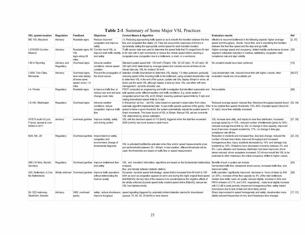
23

Table 2-1. Summary of Some Major VSL Practices VSL system location Regulation Feedback Objectives Control Means & Algorithm Evaluation results RefMD 100, Maryland Advisory Roadside signs Reduce recurrent

congestion and improve safety

(1) Reducing approaching traffic speed so as to smooth the transition between the free flow and congested-flow states; (2) Take into account the responses of drivers in dynamically setting the appropriate control speed for each transition location.

effective to recurrent bottleneck in the following aspects: higher average speed and throughput, shorter travel time, and in smoothing the transition between the free-flow speed and the stop-and-go traffic

[2, 37]

I-270/I255 Corridor , Missouri

Advisory Roadside signs: 65 VSLsigns along 38 miles

Corridor level VSL: to improve both traffic mobility and safety

Traffic sensor data was used to determine the speed limits that 10 ranged from 40 mph to 60 mph with 5 mph increments; to reduce the vehicle speed before reaching a congested area (congestion due to a bottleneck, a crash, or a workzone.

Higher average speed and occupancy, limited mobility performance at some segment; noticeable reduction in crashes; satisfactory congestion relief, compliance rate and sign visibility

[35]

I-80 in Wyoming Advisory and Regulatory

Overhead signs Adverse weather conditions; reduce speed variation

Standard posted speed limit : 120 km/h (75mph); VSL: 50 (32 mph), 70 (43 mph), 90 (56 mph) km/h determined by average speed and volumes across all lanes at one minute intervals. VSL for incident: 50 km/h

No constant results have been achieved [13]

I-35W, Twin Cities, Minnesota

Advisory Overhead signs; lane-wise display; all lanes same speed; every 1.5 miles

Prevent the propagation of the shock waves

detection of traffic downstream to determine VSL display 1.5 miles upstream; gradually reducing speed of the incoming traffic to the bottleneck; using constant deceleration rate to determine VSL in the end of the queue; update rate 30s; display 60mph in snow; all lanes use the same VSL although display is lane-by-lane; VSL use tother with lane management - dynamic shoulder use.

Less deceleration rate, reduced travel time with higher volume; other evaluation results are not available yet

[56,57]

I-4, Florida Regulatory Roadside signs to improve traffic flow; to reduce rear-end and lane-change crash risks

FDOT conducted an engineering and traffic investigation that identified reasonable and safe speeds under different weather and traffic conditions. E.g. some section in congested period has VSL at 20-30mph; lowering upstream speed limits by 5 mph and raising downstream speed limits by 5 mph

Not available. [58]

I-5,I-90, Washington Regulatory Overhead signs Adverse weather conditions; reduce congestion; improve traffic flow

In first period: ad hoc - set VSL value based on operator's observation from video; automatic algorithm implemented later. It uses traffic speeds upstream of the gantry. If the speed is below a given threshold, the system automatically adjusts the posted speed in 5mph increments. The lower bound of VSL is 35mph. Manual VSL set can overwrite VSL determined by sensor estimation.

Reduced average speed; reduced flow; Maximum throughput speeds found to be (optimal flow speed) thresholds: 70% -85% of posted speed (About 42-51 mph); travel time reliability increased

[33, 34]

A7/E15 south of Lyon, France; spread to over 650km in 2011

advisory overhead gantries Improve mobility, safety and driving confort

VSL with the maximum speed of 110 [km/h]; triggered when the total flow exceeded 3000 [veh/h]; ban truck access in peak hours

VSL increase lane utility, and impact on lane flow distribution; increased average speed by 4~10% ; reduced number of bottlenecks (jams) by 50% ; reduced average travel time by 30s; no change in lane capacity; improved level of services; dropped accident by 17% ; no change in time gap; compliance rate still low.

[27, 28]

M25, M4, UK Regulatory Overhead gantries imrpovmeent on safety, congestion and environment, change of fundamantal diagramp VSL is activated/modified/de-activated when flow and/or speed measurements cross

pre-set thresholds between 35 ~ 65mph; in bad weather, different thresholds will be used; the thresholds are based on traffic flow or speed measurement.

Reduction in incidents and increased flow, less lane change; reduced the number of break down times; improved throughput and increased homogeneous flow; Injury accidents decreased by 10% and damage only accidents by 30% ; Emissions have decreased overall by between 2% and 8% ; Lane utilisation and headway distribution had been improved; driver stress reduced; driver acceptane increased: 2/3 drivers would like VSL to be extended to other motoways; the critical occupancy shifted to higher values;

[22, 23]

A99 (16.3km), Munich, Germany

Regulatory Overhead gantries Improve botteleneck flow and safety

VSL and travellers' information; algorithms are based on the fundamental relationships of speed,flow, and density between detector stations.

Benefits of such a system can includeharmonized traffic flow, dampened shock waves, increased traffic flow, and improved safety

[24]

A20, Notterdam, 4.2 km, the Netherlands

Strictly enforced Overhead gantries improve traffic operations without deteriorating the local air quality

Dynamax: dynamic speed limit strategy: speed limit is increased from 80 km/h to 100 km/h as soon as congestion appears to set in and during the night; original fixed speed limit 80[km/h]; the key idea of the measure is to counterbalance the negative effects of the strictly enforced dynamic speed limits; incident speed limit is 80[km/h]; manual set VSL has highets priority;

traffic operation: significantly improved- decrease in hours of delay by 600 (or 20% ); increase of free flow capacity by 4% of the main bottleneck; median lane better used; air quality reduced slightly: increase in NOx and PM10 emission of 3.7% and 3.6% respectively; noise level slightly increase with 0.2 dB in peak periods; imrpoeved homogeneous flow; safety impact inconclusve due to lack of data and short study period

[29]

E4, E22 motorway, Stockholm, Sweden

Advisory VMS, overhead gantry

safety, reduce shockwave, improve troughput

speed signalling triggered by automatic incident detection alarms for downstream queues; 70, 60, 50, 30 [km/h] or lane closure

Sharp improvement in speed homogeneity and safety; decelreration more stable;reduced frequencies of very short headways lane changes

[17, 31]

24

Chapter 3. Test Site Selection Considerations

3.1 Introduction

The objective of this project is to conduct limited field testing of a newly developed control algorithm for Coordinated Ramp Metering in the first stage. Therefore, test site selection criteria are proposed mainly based on the characteristics and infrastructure requirements of CRM. Since Changeable Message Signs (CMS) could be added for VSL testing to any site with proper type of bottleneck, site selection criteria also include the factors related to VSL, mainly, the bottleneck types.

3.2 Site Selection Criteria

The proposed site selection criteria are based on freeway traffic characteristics and the control algorithm.

Traffic demand is high to over-saturated in peak hours;

The corridor has a recurrent bottleneck downstream;

The most downstream bottleneck has the most serious traffic drop (the minimum capacity or largest v/c ratio);

The downstream main bottleneck has the most significant traffic flow drop when congested, and the congestion is mainly caused by high demand flow from upstream plus one of the following factors: o Lane reduction o Controlled entrance ramp flow (ideally with ramp meter) with a long enough

acceleration lane section o “Virtual” lane reduction caused by other phenomena such as excessive weaving o Special road geometry such as grade or curve that leads to physical capacity drop

The main bottleneck must NOT be caused by the following factors: o Further downstream congestion back-propagation due to other factors o Un-controlled freeway to freeway exchange o Freeway to arterial spill back (if exit ramp flow is high and the intersection traffic

signal timing cannot serve it)

All the onramps are metered in the corridor; otherwise, the one without meter will cause problems;

Upstream of the main bottleneck has adequate storage section;

Vehicle storage upstream section would not affect exit ramp flow - ideally, there is a lane protected for exit ramp traffic;

Sensors at critical locations: at the start of the bottleneck, and 500m upstream of bottleneck (those two locations are important for VSL);

25

Sensor density: each upstream section has at least one detector 300~700m apart;

Sensor health: sensor healthy is critical for good performance; in sensor fault, controller return to time-of-day (as default and non-coordinated);

Entrance ramp flow and queue detection is critical for CRM to avoid spills back to arterial; to achieve such queue estimation, the minimum requirement are traffic detectors at meter location and upstream of the entrance ramp (70~85% from the meter);

Exit ramp flow detection is ideal but not critical;

Roadside would allow installation of VMS units;

Hardware setup for RM would allow for Coordinated RM strategy to be implemented: the ramp meters are controlled in TMC by sending a control command from TMC server to Entrance ramp Metering Controller. This setup would allow CRM to be implemented easily.

3.3 Site Selection Method

Based on the site selection criteria, we have used the following approaches to select the site – to exclude it from situation of congestion caused by some other factor which cannot be handled by the algorithm to be tested.

We first look at the traffic from a macroscopic approach using Performance Measurement

System (PeMS) 2D (time and space) contour plot in PeMS to roughly locate the bottleneck, its scope (starting and end of location and time) and intensity, and its possible relationship with other nearby bottlenecks. The observation in the first step may not be correct since some sensors error may cause some incorrect observations.

The second step to look at the candidate site identified in the first step by more detailed

data analysis. In this step, we download 5 min PeMS data for a stretch of the location, both downstream and upstream, to analyze the flow, occupancy and speed if they are available. This can also find out the sensor health condition. In this step, we also take into consideration of several other factors including road geometry such as lane drop etc, traffic congestion back-propagate characteristics, and entrance ramp and exit ramp impact.

3.4 SR99 NB in Sacramento

Traffic of SR99 NB between Elk Grove and SR50 interchange after 12th Ave has been analyzed. This section has bottlenecks in both SB and NB. The locations are almost in the same Postmile (PM) range: PM 285 ~ 305. Both are recurrent bottlenecks. SB bottleneck happens in PM peak hours, and NB one happens at AM peak hours. The reason to the congestion is mainly

26

due to high flow of commuters to the city of Sacramento for work in the morning and back home in the PM peak hours.

This report focuses on SR99 NB between PM 285~305 (between Stockton and SR50-Interchange) as shown in Figure 3-1. Loop detector has some improvement. Besides, entrance ramp and exit ramp data are available from PeMS now, which will be very useful for system modeling and simulation. However, some sensors speed estimations are still not available, but flow data of some lanes are available, which are important for system analysis and RM control.

3.4.1 Road Geometry and Sensor Location:

The overall road map of the section in consideration is shown in Figure 3-1, and the lane/entrance ramp/exit ramp geometry and sensor locations are shown in Figure 3-2.

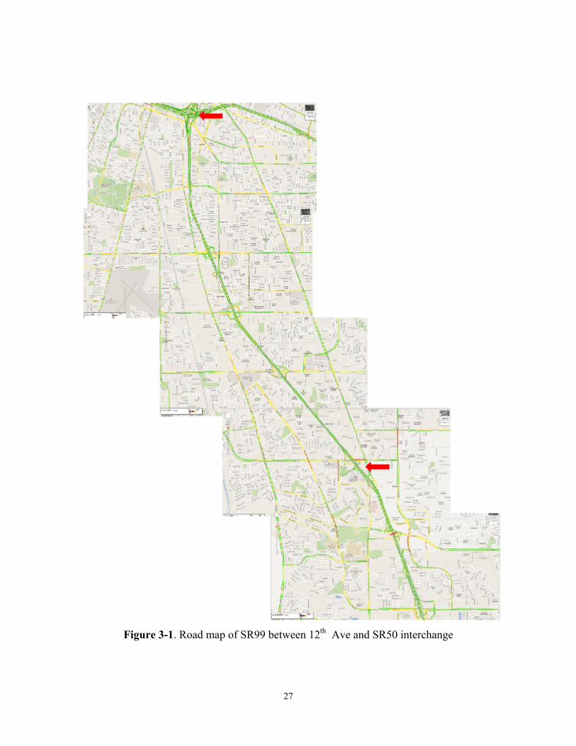
27

Figure 3-1. Road map of SR99 between 12th Ave and SR50 interchange

28

In Figure 3-1, the potential candidate bottleneck and the downstream bottleneck are indicated with red arrows. In Figure 3-2, only the candidate bottleneck is indicated with a red spot, which is near the 47th Ave entrance ramp.

In addition to mainline sensors, entrance ramp flows are also available now from PeMS, which were not there before. This will benefit traffic analysis and RM control. Some exit ramp flow is also available. Historical entrance ramp and exit ramp data are available back to May 2010. 3.4.2 Bottleneck Location Observation from Macroscopic Contour Plot

Macroscopic contour plot of the traffic data on 10/19/12 is shown in Figure 3-3.

From the macroscopic contour plot (Figure 3-3), it can be observed that there are two bottlenecks in the range of PM 286 ~ PM 299, which are very close. If downstream traffic is very heavy, they could be combined as one.

This is consistent for 2012 and 2013 data. Therefore, the coordination should include the whole section. The overall system should be controlled through TMC to reduce interface with individual and communication between onramps.

3.4.3 More Details Traffic Analysis Using VDS Raw Data

Identified Major Bottlenecks (all activates in AM traffic): (1) PM 298.5: downstream congestion caused by diverging traffic to US 50 EB and WB.

This one may back-propagate to upstream bottleneck at PM 296.54. (2) PM 296.54: middle congestion caused by merging traffic from Fruitridge Rd (EB and

WB). Two on-ramps (one from EB and one from WB) are close. The merging lane doesn’t drop (until the split of SR 99 and S Sacramento Freeway; i.e., there’s a lane addition. Thus, congestion is light at this location, but it becomes more severe as it propagates upstream passing on-ramps from 47th Ave (at PM 295.7) (Figure 3-4 ~ Figure 3-7).

(3) PM 290.76: upstream congestion caused by merging traffic from Calvine Rd. (EB and

WB). The congestion is light. It starts earlier and may merge with congestion from downstream bottleneck congestion back-propagation. This will need further investigation. Its road geometry may be interesting: the entrance ramp leads to an added lane extended to the exit to E. Stockton Blvd.

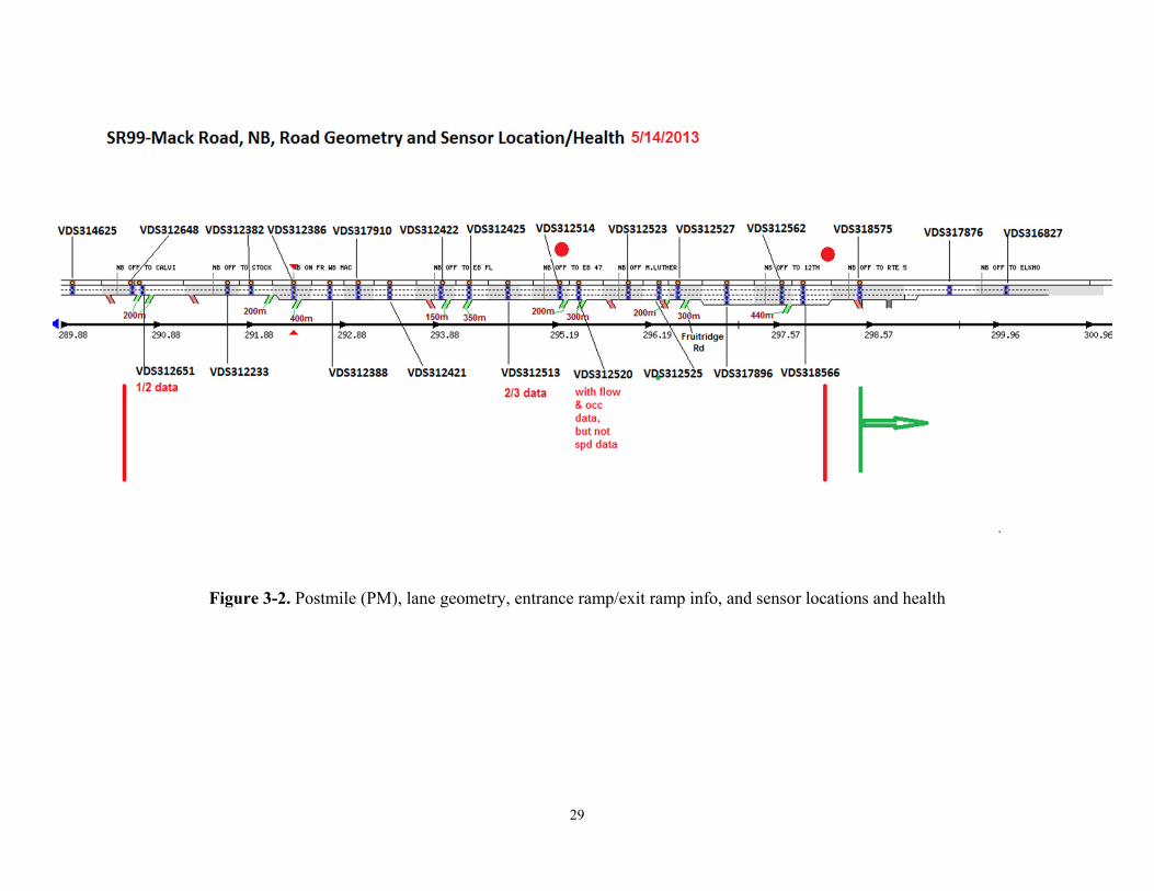
29

Figure 3-2. Postmile (PM), lane geometry, entrance ramp/exit ramp info, and sensor locations and health

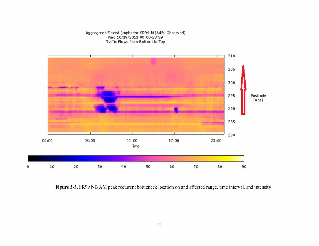
30

Figure 3-3. SR99 NB AM peak recurrent bottleneck location on and affected range, time interval, and intensity

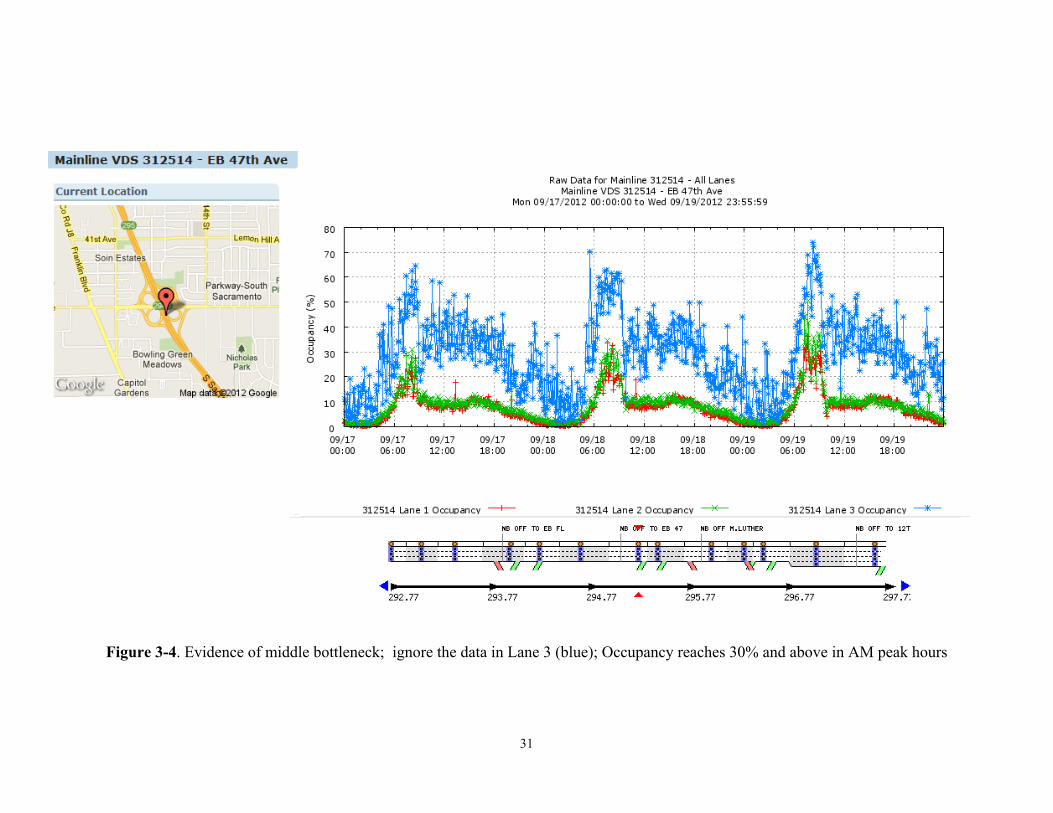
31

Figure 3-4. Evidence of middle bottleneck; ignore the data in Lane 3 (blue); Occupancy reaches 30% and above in AM peak hours

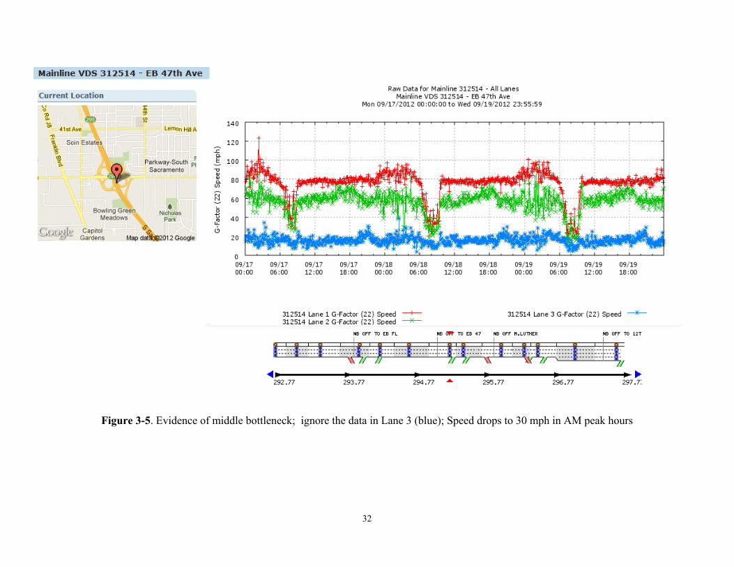
32

Figure 3-5. Evidence of middle bottleneck; ignore the data in Lane 3 (blue); Speed drops to 30 mph in AM peak hours

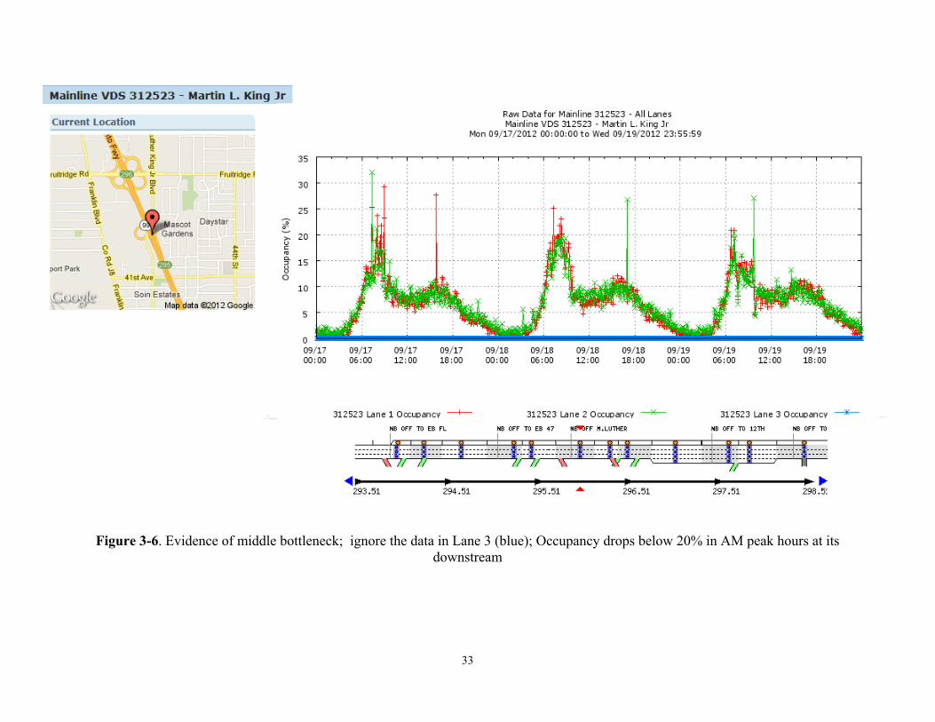
33

Figure 3-6. Evidence of middle bottleneck; ignore the data in Lane 3 (blue); Occupancy drops below 20% in AM peak hours at its downstream

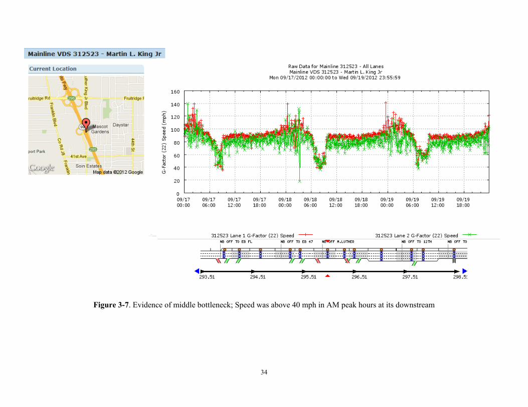
34

Figure 3-7. Evidence of middle bottleneck; Speed was above 40 mph in AM peak hours at its downstream

35

3.4.4 Traffic Volume

Traffic volume is very high in AM peak hours. There is a significant occupancy increase, speed and flow drop for the stop & go traffic. 3.4.5 Senor Locations and Health

#312651: one lane is down, no speed estimation #312382: has no data #312386: has no data (Mack Rd) #312425: partial data missing #312513: 2/3 are Ok #312520: Good now

3.4.6 RM availability From 12th Ave: metered

From Fruitridge Road EB: metered

From Fruitridge Road WB: metered

From 47th Ave EB: metered

From 47th Ave WB: metered

From Florin Rd EB: metered

From Florin Rd WB: metered

From Mack Rd EB: metered

From Mack Rd WB: metered

From Calvine Rd EB: metered

From Calvine Rd WB: metered

3.4.7 Preliminary Suggestion

If the two bottlenecks are not connected, we could just consider the one from Calvine Road entrance ramp with PM 290.76. If the congestion pack-propagated from the merge of SR 99 with SR 50, this may not be an option since the cause of the congestion is outside of the system in consideration. This site will need further investigation including discussion with D3 traffic engineers and site visit for direct observation.

After detailed data analysis, the most promising bottleneck is middle one at PM 295.19 close to VDS312514 as indicated in Figure 3-2 with the red spot. Its downstream is almost free-flow (speed above 40 mph) in AM peak hours. This has been confirmed with multiple day data analysis as listed in the Appendix. We will focus on this one for more analysis although we will look at other possibilities.

36

Also in the Appendix, traffic data for the week of September 17-22, 2012 have been examined. Flow, occupancy and speed are shown. The figures (Figure A1-1 ~ Figure A9-6) have been listed from upstream to downstream in the stretch as shown in Figure 3-2. The traffic pattern is very similar to that described above.

3.5 I-880 NB near Auto Mall Parkway

We have preliminarily considered the Interstate 880 section from Fremont to Oakland.

Since the freeway to freeway interchanges are not controlled, such as the interchanges with SR-92 and I-238, we have concentrated on sites away from those interchange locations. Although there are several bottlenecks according to PeMS data analysis, some of them are caused by freeway-to-freeway interchanges. We have preliminarily identified one possible candidate, which is I-880 NB near Auto Mall Parkway. However, this needs further investigation including data analysis and discussion with Caltrans District 4 traffic engineers. 3.5.1 Road/Lane Geometry and Sensor Locations

The road geometry of the I-880 Nimitz Freeway North Bound near Auto Mall Parkway is

shown in Figure 3-8. The lane geometry, entrance ramp and exit ramp and sensor location and IDs are shown in Figure 3-9. It is clear that this section of road is away from the disturbance caused by the freeway-to-freeway interchange. The bottleneck location is at PM15.7 as shown in Figure 3-9.

3.5.2. Traffic Volume:

It is high in general and congested in PM peak hours.

3.5.3. Bottleneck Location Observation from Macroscopic Contour Plot

The bottleneck location, scope, time range, and intensity can be observed from a macroscopic 2D Time-Space plot of the traffic from PeMS as shown in Figure 3-10 and Figure 3-11.

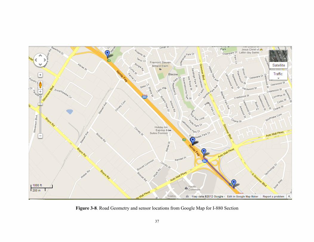
37

Figure 3-8. Road Geometry and sensor locations from Google Map for I-880 Section

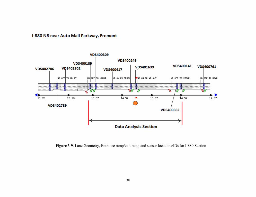
38

Figure 3-9. Lane Geometry, Entrance ramp/exit ramp and sensor locations/IDs for I-880 Section

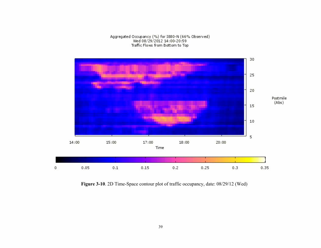
39

Figure 3-10. 2D Time-Space contour plot of traffic occupancy, date: 08/29/12 (Wed)

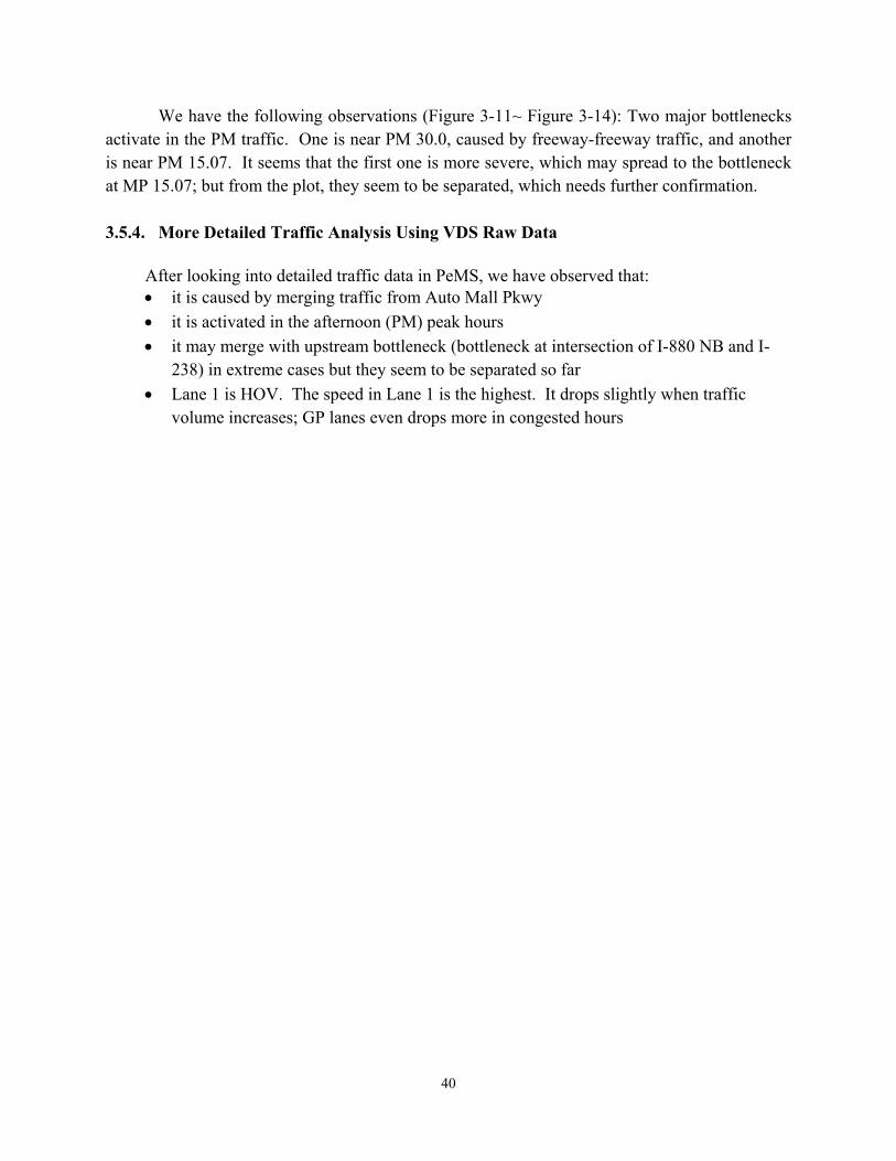
40

We have the following observations (Figure 3-11~ Figure 3-14): Two major bottlenecks activate in the PM traffic. One is near PM 30.0, caused by freeway-freeway traffic, and another is near PM 15.07. It seems that the first one is more severe, which may spread to the bottleneck at MP 15.07; but from the plot, they seem to be separated, which needs further confirmation.

3.5.4. More Detailed Traffic Analysis Using VDS Raw Data

After looking into detailed traffic data in PeMS, we have observed that: it is caused by merging traffic from Auto Mall Pkwy

it is activated in the afternoon (PM) peak hours

it may merge with upstream bottleneck (bottleneck at intersection of I-880 NB and I-238) in extreme cases but they seem to be separated so far

Lane 1 is HOV. The speed in Lane 1 is the highest. It drops slightly when traffic volume increases; GP lanes even drops more in congested hours

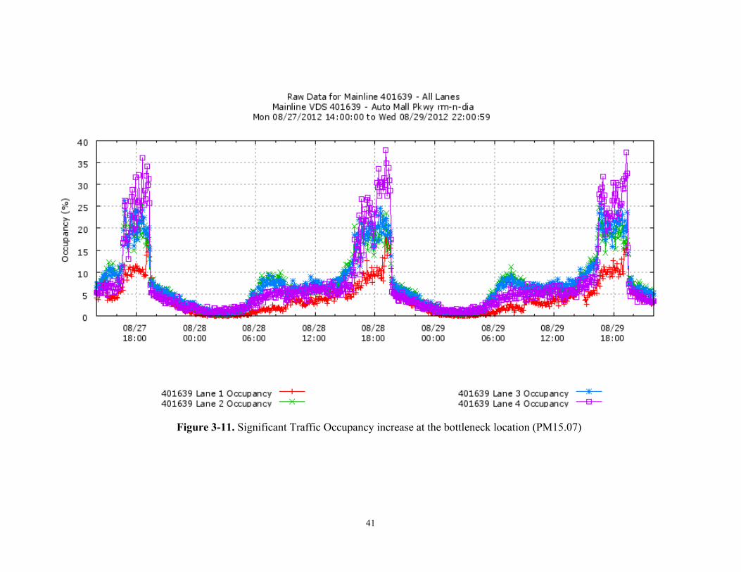
41

Figure 3-11. Significant Traffic Occupancy increase at the bottleneck location (PM15.07)

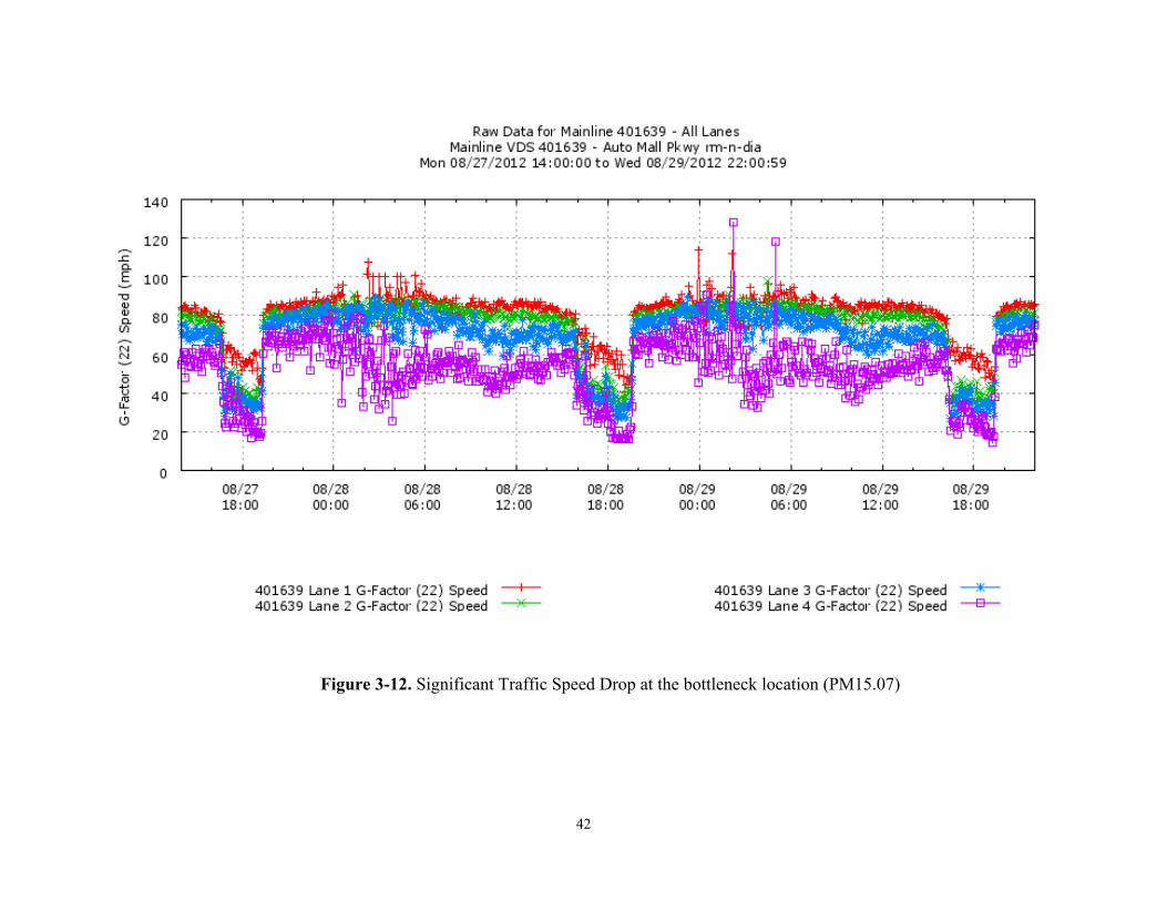
42

Figure 3-12. Significant Traffic Speed Drop at the bottleneck location (PM15.07)

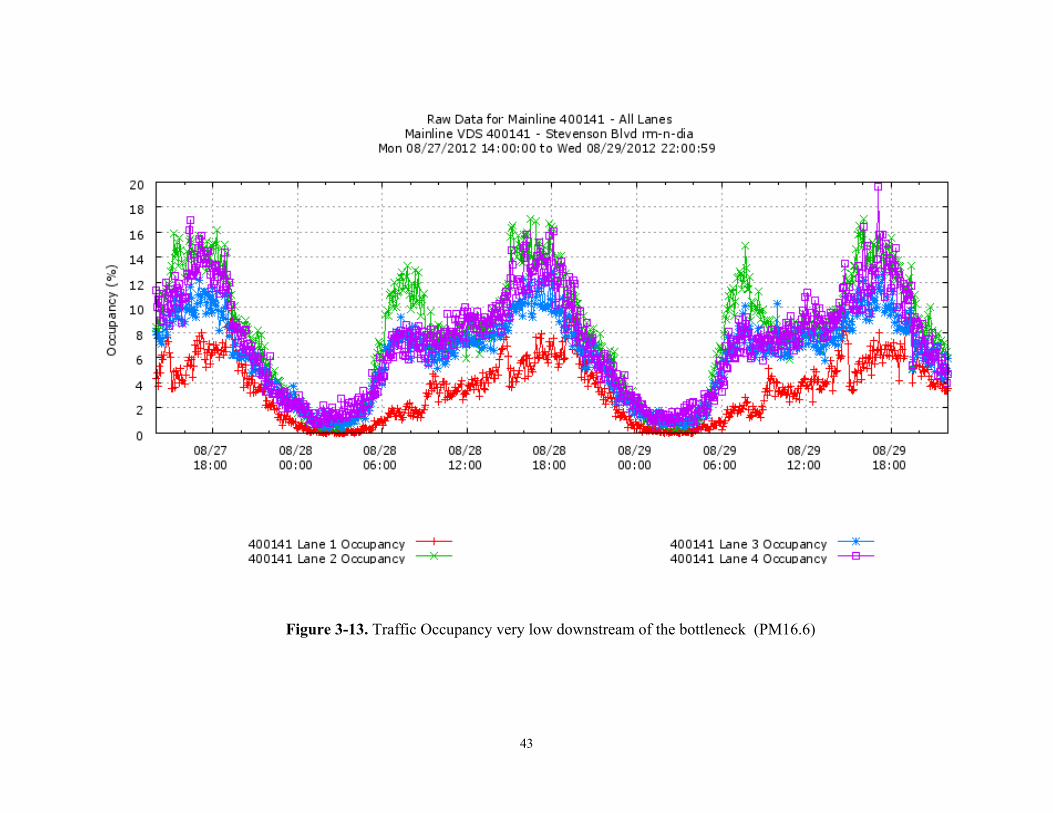
43

Figure 3-13. Traffic Occupancy very low downstream of the bottleneck (PM16.6)

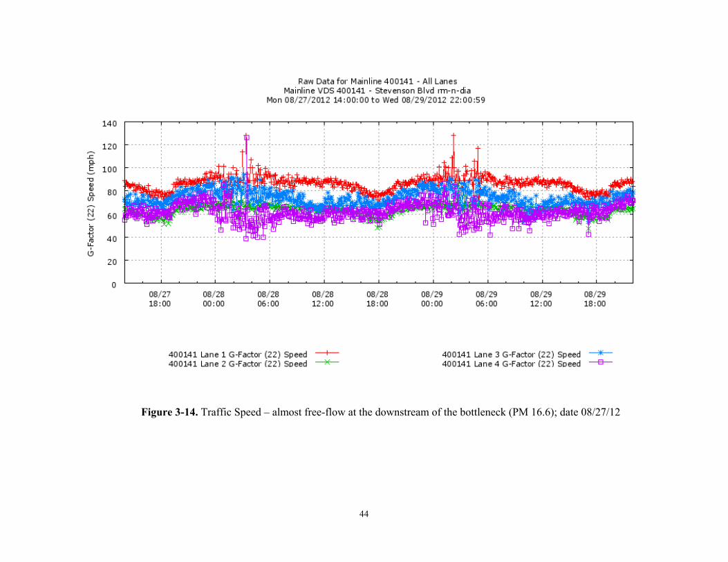
44

Figure 3-14. Traffic Speed – almost free-flow at the downstream of the bottleneck (PM 16.6); date 08/27/12

45

In the Appendix, further traffic data at detector stations near the bottleneck have been checked as shown in Figures B1-B12. They indicate that the observations are correct.

Also in the Appendix, traffic data for the week of 11/17/2011 – 11/22/2011 have been

examined. Flow, occupancy and speed are shown. The figures (Figure B13-1 ~ Figure B19-6) have been listed from upstream to downstream in the stretch as shown in Figure 3-1 and Figure 3-2. The traffic pattern is very similar as described before. This means that the observation is correct. 3.5.5 Sensor Health

Detector at PM 16.45 has not functioned since 7/28/2012. Detector at PM 15.07 has not

functioned since 9/28/2012.

3.5.6 RM availability All onramps in the stretch have RM.

3.5.7 Preliminary Suggestions

We have preliminarily identified one possible candidate which is the I-880 NB near Auto Mall Parkway. However, this needs further confirmation including data analysis and discussion with Caltrans District 4 traffic engineers in the next phase of the project.

3.6 Preliminary Recommendation

After first round site selection, we would suggest the following two sites for further analysis to confirm that they are the type of bottleneck suitable for field testing. However, this needs to be confirmed with further data analysis. Interstate-880 NB near Auto Mall Parkway

We have preliminarily identified one possible candidate which is the Interstate-880 NB near Auto Mall Parkway. However, this needs further investigation including more extensive data analysis and discussion with Caltrans District 4 traffic engineers. SR99 NB in Caltrans D3

After detailed data analysis, the most promising bottleneck is the middle one at PM 295.19 close to VDS312514. Its downstream is almost free-flow (speed above 40 mph) in AM peak hours. We will focus on this one for more analysis in the next phase of the project. This will also need discussion with Caltrans D3 traffic engineers and site visit.

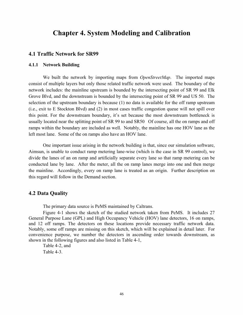
46

Chapter 4. System Modeling and Calibration

4.1 Traffic Network for SR99

4.1.1 Network Building

We built the network by importing maps from OpenStreetMap. The imported maps consist of multiple layers but only those related traffic network were used. The boundary of the network includes: the mainline upstream is bounded by the intersecting point of SR 99 and Elk Grove Blvd, and the downstream is bounded by the intersecting point of SR 99 and US 50. The selection of the upstream boundary is because (1) no data is available for the off ramp upstream (i.e., exit to E Stockton Blvd) and (2) in most cases traffic congestion queue will not spill over this point. For the downstream boundary, it’s set because the most downstream bottleneck is usually located near the splitting point of SR 99 to and SR50 Of course, all the on ramps and off ramps within the boundary are included as well. Notably, the mainline has one HOV lane as the left most lane. Some of the on ramps also have an HOV lane.

One important issue arising in the network building is that, since our simulation software, Aimsun, is unable to conduct ramp metering lane-wise (which is the case in SR 99 control), we divide the lanes of an on ramp and artificially separate every lane so that ramp metering can be conducted lane by lane. After the meter, all the on ramp lanes merge into one and then merge the mainline. Accordingly, every on ramp lane is treated as an origin. Further description on this regard will follow in the Demand section.

4.2 Data Quality

The primary data source is PeMS maintained by Caltrans. Figure 4-1 shows the sketch of the studied network taken from PeMS. It includes 27

General Purpose Lane (GPL) and High Occupancy Vehicle (HOV) lane detectors, 16 on ramps, and 12 off ramps. The detectors on these locations provide necessary traffic network data. Notably, some off ramps are missing on this sketch, which will be explained in detail later. For convenience purpose, we number the detectors in ascending order towards downstream, as shown in the following figures and also listed in Table 4-1,

Table 4-2, and Table 4-3.

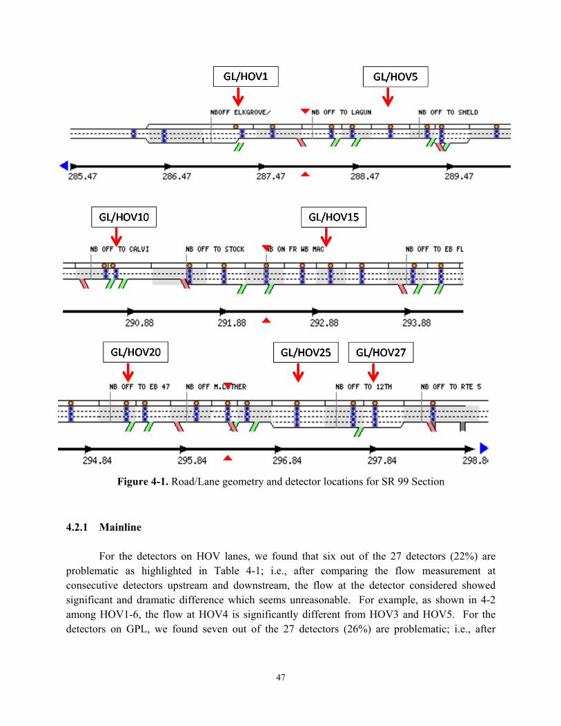
47

Figure 4-1. Road/Lane geometry and detector locations for SR 99 Section

4.2.1 Mainline

For the detectors on HOV lanes, we found that six out of the 27 detectors (22%) are problematic as highlighted in Table 4-1; i.e., after comparing the flow measurement at consecutive detectors upstream and downstream, the flow at the detector considered showed significant and dramatic difference which seems unreasonable. For example, as shown in 4-2 among HOV1-6, the flow at HOV4 is significantly different from HOV3 and HOV5. For the detectors on GPL, we found seven out of the 27 detectors (26%) are problematic; i.e., after

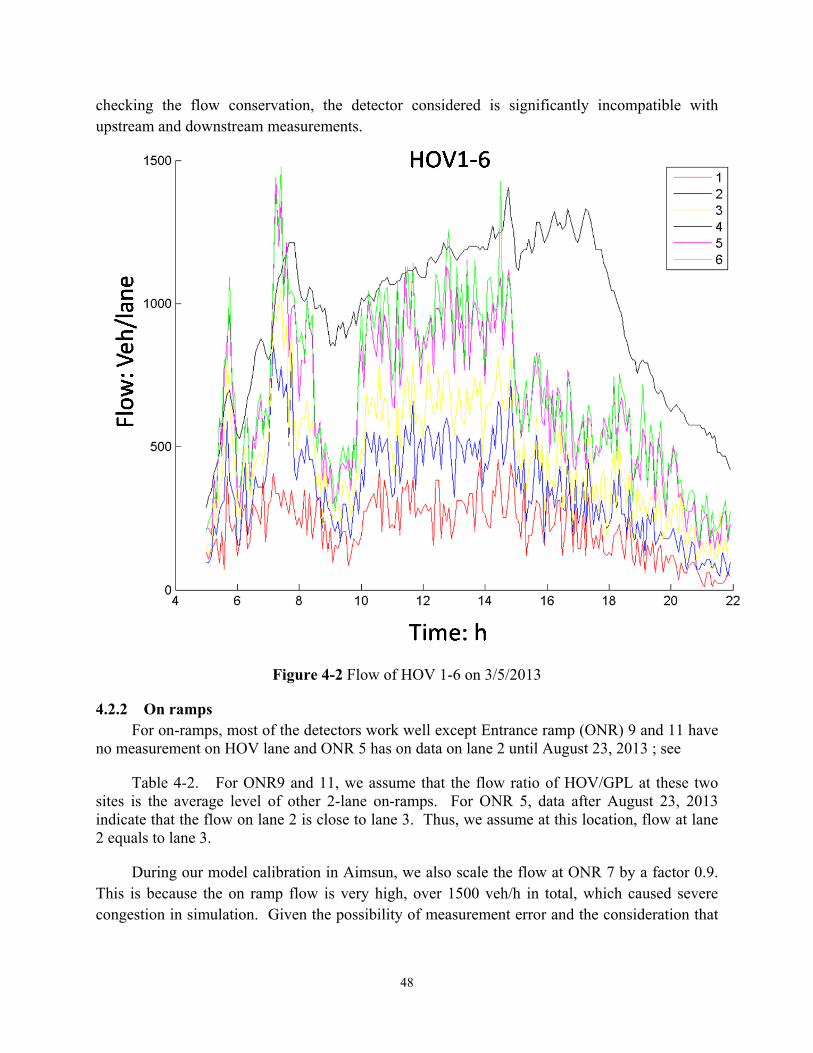
48

checking the flow conservation, the detector considered is significantly incompatible with upstream and downstream measurements.

Figure 4-2 Flow of HOV 1-6 on 3/5/2013

4.2.2 On ramps For on-ramps, most of the detectors work well except Entrance ramp (ONR) 9 and 11 have

no measurement on HOV lane and ONR 5 has on data on lane 2 until August 23, 2013 ; see

Table 4-2. For ONR9 and 11, we assume that the flow ratio of HOV/GPL at these two sites is the average level of other 2-lane on-ramps. For ONR 5, data after August 23, 2013 indicate that the flow on lane 2 is close to lane 3. Thus, we assume at this location, flow at lane 2 equals to lane 3.

During our model calibration in Aimsun, we also scale the flow at ONR 7 by a factor 0.9. This is because the on ramp flow is very high, over 1500 veh/h in total, which caused severe congestion in simulation. Given the possibility of measurement error and the consideration that

49

it is not common to achieve 1500 veh/h at a metered on ramp, we believe that such adjustment is reasonable.

4.2.3 Off ramps For the exit ramps, we have found that four exit ramps are missing on this sketch: Exit

ramp (OFR) 6, 7, 8, and 11; see

Table 4-3. For OFR9, the detector is not working. Besides, we found that the geometry of the exit ramp to Sheldon Rd (OFR2) is problematic (it has two lanes but PeMS shows three) but the data is credible. Finally, OFR 12, which measures SR 99 flow after the splitting of SR 99 and I-80B, is not available after March 6, 2013. This detector is critical since it is the only source to obtain the flow. Therefore, our study has to focus on the days before March 6, 2013. In summary, for exit ramps, six out of the 12 detectors (about 50%) are not working.

For the off ramps that do not have valid data, we interpreted the flow from upstream and (or) downstream measurement. In particular, for OFR 6, 7, and 11, they can be interpreted directly from the difference of upstream and downstream measurement; see (Eq. 4.1), (Eq. 4.2), and (Eq. 4.3) for the interpretation of OFR6, 7, and 9 respectively.

OFR6 = (GPL17+HOV17) +ONR10 - (GPL18+HOV18); (Eq. 4.1)

OFR7 = (GPL18+HOV18) +ONR11 - (GPL20+HOV20); (Eq. 4.2)

OFR11 = (GPL24+HOV24) - (GPL25+HOV25); (Eq. 4.3)

For OFR 8 and 9, the interpretation is much more complex and needs special treatment. For OFR8, the mainline measurement downstream of the off ramp, GPL/HOV21, is not working. Thus, it cannot be interpreted directly from GPL/HOV 20, ONR12, and GPL/HOV 21. For OFR9, the absence of valid data at GPL/HOV21 makes it impossible to directly interpret the flow from GPL/HOV 21, ONR13, and GPL/HOV 22. Thus, we decide to consider the two exit ramps together; i.e., obtaining the sum of the flow at those two exit ramps and then assume that they have the same flow as shown by (Eq. 4.4).

OFR8 = OFR9 = ((GPL20 + HOV20) + ONR12 + ONR13 - (GPL22 + HOV22))/2 (Eq. 4.4)

Notably, we found that this segment has a flow incompatibility issue: (i) the flow conservation holds at GPL/HOV20 and its upstream measurement (e.g., GPL/HOV16, 17, 18 with on ramps and exit ramps accounted accordingly), and (ii) holds at GPL/HOV22 and its

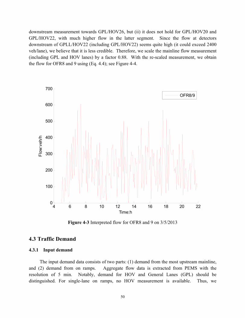
50

downstream measurement towards GPL/HOV26, but (ii) it does not hold for GPL/HOV20 and GPL/HOV22, with much higher flow in the latter segment. Since the flow at detectors downstream of GPLL/HOV22 (including GPL/HOV22) seems quite high (it could exceed 2400 veh/lane), we believe that it is less credible. Therefore, we scale the mainline flow measurement (including GPL and HOV lanes) by a factor 0.88. With the re-scaled measurement, we obtain the flow for OFR8 and 9 using (Eq. 4.4); see Figure 4-4.

Figure 4-3 Interpreted flow for OFR8 and 9 on 3/5/2013

4.3 Traffic Demand

4.3.1 Input demand

The input demand data consists of two parts: (1) demand from the most upstream mainline, and (2) demand from on ramps. Aggregate flow data is extracted from PEMS with the resolution of 5 min. Notably, demand for HOV and General Lanes (GPL) should be distinguished. For single-lane on ramps, no HOV measurement is available. Thus, we

4 6 8 10 12 14 16 18 20 220

100

200

300

400

500

600

700

Time:h

Flo

w:v

eh/h

OFR8/9

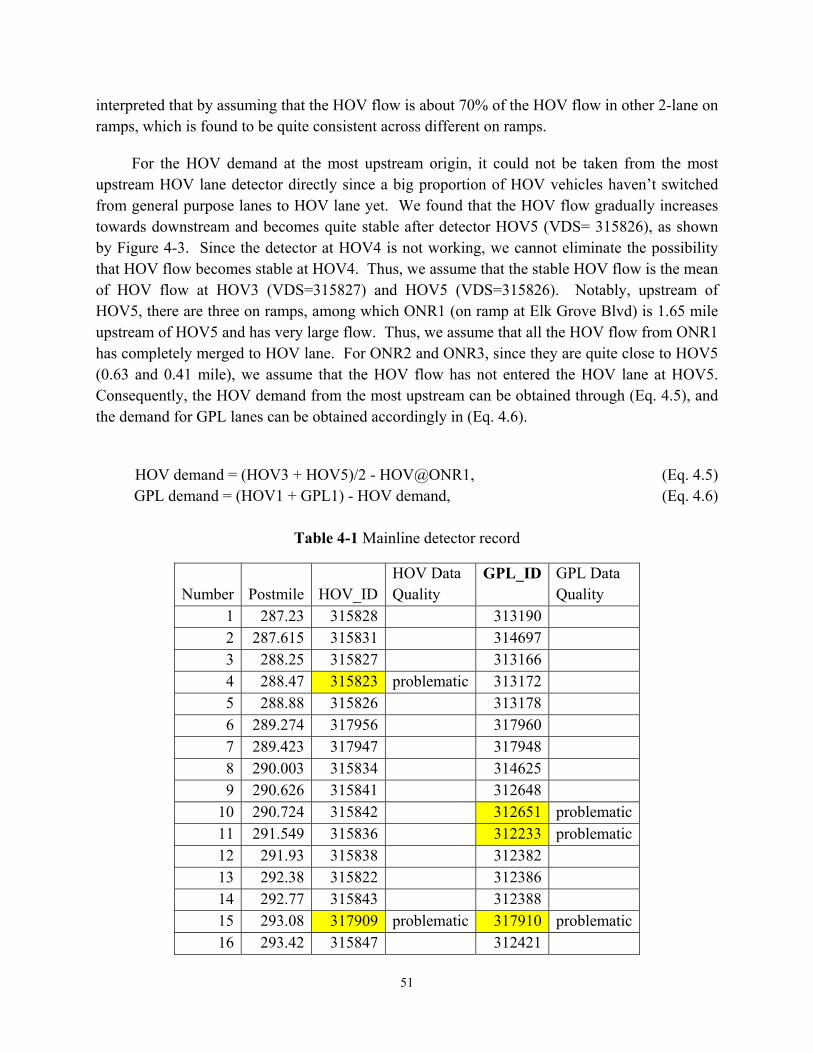
51

interpreted that by assuming that the HOV flow is about 70% of the HOV flow in other 2-lane on ramps, which is found to be quite consistent across different on ramps.

For the HOV demand at the most upstream origin, it could not be taken from the most upstream HOV lane detector directly since a big proportion of HOV vehicles haven’t switched from general purpose lanes to HOV lane yet. We found that the HOV flow gradually increases towards downstream and becomes quite stable after detector HOV5 (VDS= 315826), as shown by Figure 4-3. Since the detector at HOV4 is not working, we cannot eliminate the possibility that HOV flow becomes stable at HOV4. Thus, we assume that the stable HOV flow is the mean of HOV flow at HOV3 (VDS=315827) and HOV5 (VDS=315826). Notably, upstream of HOV5, there are three on ramps, among which ONR1 (on ramp at Elk Grove Blvd) is 1.65 mile upstream of HOV5 and has very large flow. Thus, we assume that all the HOV flow from ONR1 has completely merged to HOV lane. For ONR2 and ONR3, since they are quite close to HOV5 (0.63 and 0.41 mile), we assume that the HOV flow has not entered the HOV lane at HOV5. Consequently, the HOV demand from the most upstream can be obtained through (Eq. 4.5), and the demand for GPL lanes can be obtained accordingly in (Eq. 4.6).

HOV demand = (HOV3 + HOV5)/2 - HOV@ONR1, (Eq. 4.5) GPL demand = (HOV1 + GPL1) - HOV demand, (Eq. 4.6)

Table 4-1 Mainline detector record

Number Postmile HOV_IDHOV Data Quality

GPL_ID GPL Data Quality

1 287.23 315828 313190 2 287.615 315831 314697 3 288.25 315827 313166 4 288.47 315823 problematic 313172 5 288.88 315826 313178 6 289.274 317956 317960 7 289.423 317947 317948 8 290.003 315834 314625 9 290.626 315841 312648

10 290.724 315842 312651 problematic 11 291.549 315836 312233 problematic 12 291.93 315838 312382 13 292.38 315822 312386 14 292.77 315843 312388 15 293.08 317909 problematic 317910 problematic 16 293.42 315847 312421

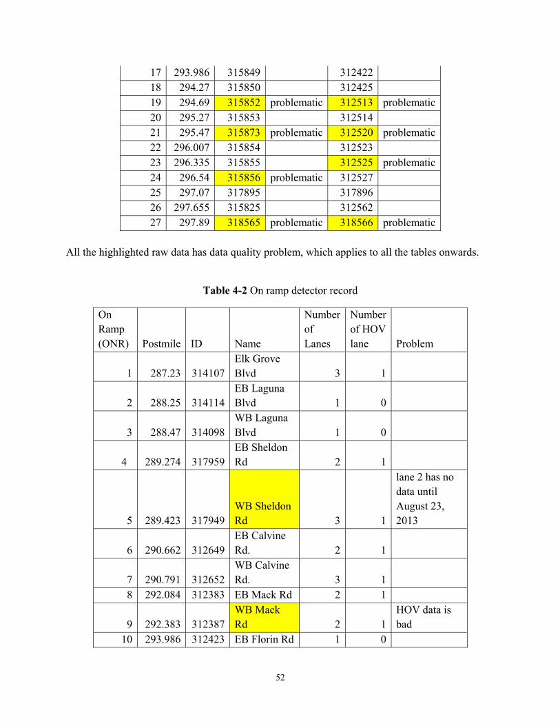
52

17 293.986 315849 312422 18 294.27 315850 312425 19 294.69 315852 problematic 312513 problematic 20 295.27 315853 312514 21 295.47 315873 problematic 312520 problematic 22 296.007 315854 312523 23 296.335 315855 312525 problematic 24 296.54 315856 problematic 312527 25 297.07 317895 317896 26 297.655 315825 312562 27 297.89 318565 problematic 318566 problematic

All the highlighted raw data has data quality problem, which applies to all the tables onwards.

Table 4-2 On ramp detector record

On Ramp (ONR) Postmile ID Name

Number of Lanes

Number of HOV lane Problem

1 287.23 314107 Elk Grove Blvd 3 1

2 288.25 314114 EB Laguna Blvd 1 0

3 288.47 314098 WB Laguna Blvd 1 0

4 289.274 317959 EB Sheldon Rd 2 1

5 289.423 317949 WB Sheldon Rd 3 1

lane 2 has no data until August 23, 2013

6 290.662 312649 EB Calvine Rd. 2 1

7 290.791 312652 WB Calvine Rd. 3 1

8 292.084 312383 EB Mack Rd 2 1

9 292.383 312387 WB Mack Rd 2 1

HOV data is bad

10 293.986 312423 EB Florin Rd 1 0

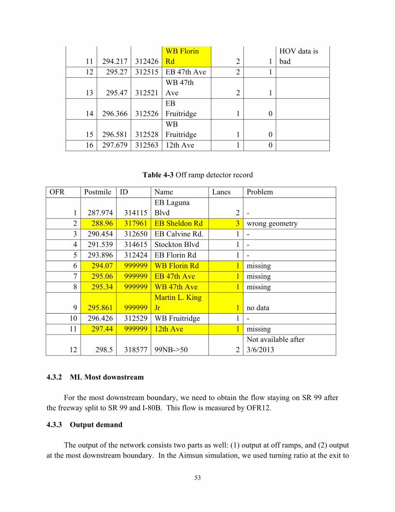
53

11 294.217 312426 WB Florin Rd 2 1

HOV data is bad

12 295.27 312515 EB 47th Ave 2 1

13 295.47 312521 WB 47th Ave 2 1

14 296.366 312526 EB Fruitridge 1 0

15 296.581 312528 WB Fruitridge 1 0

16 297.679 312563 12th Ave 1 0

Table 4-3 Off ramp detector record

OFR Postmile ID Name Lanes Problem

1 287.974 314115 EB Laguna Blvd 2 -

2 288.96 317961 EB Sheldon Rd 3 wrong geometry 3 290.454 312650 EB Calvine Rd. 1 - 4 291.539 314615 Stockton Blvd 1 - 5 293.896 312424 EB Florin Rd 1 - 6 294.07 999999 WB Florin Rd 1 missing 7 295.06 999999 EB 47th Ave 1 missing 8 295.34 999999 WB 47th Ave 1 missing

9 295.861 999999 Martin L. King Jr 1 no data

10 296.426 312529 WB Fruitridge 1 - 11 297.44 999999 12th Ave 1 missing

12 298.5 318577 99NB->50 2Not available after 3/6/2013

4.3.2 ML Most downstream For the most downstream boundary, we need to obtain the flow staying on SR 99 after

the freeway split to SR 99 and I-80B. This flow is measured by OFR12.

4.3.3 Output demand The output of the network consists two parts as well: (1) output at off ramps, and (2) output

at the most downstream boundary. In the Aimsun simulation, we used turning ratio at the exit to

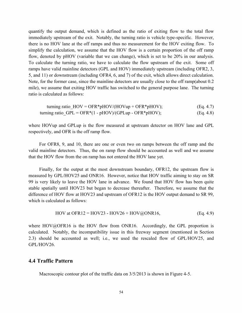
54

quantify the output demand, which is defined as the ratio of exiting flow to the total flow immediately upstream of the exit. Notably, the turning ratio is vehicle type-specific. However, there is no HOV lane at the off ramps and thus no measurement for the HOV exiting flow. To simplify the calculation, we assume that the HOV flow is a certain proportion of the off ramp flow, denoted by pHOV (variable that we can change), which is set to be 20% in our analysis. To calculate the turning ratio, we have to calculate the flow upstream of the exit. Some off ramps have valid mainline detectors (GPL and HOV) immediately upstream (including OFR2, 3, 5, and 11) or downstream (including OFR4, 6, and 7) of the exit, which allows direct calculation. Note, for the former case, since the mainline detectors are usually close to the off ramp(about 0.2 mile), we assume that exiting HOV traffic has switched to the general purpose lane. The turning ratio is calculated as follows:

turning ratio_HOV = OFR*pHOV/(HOVup + OFR*pHOV); (Eq. 4.7)

turning ratio_GPL = OFR*(1 - pHOV)/(GPLup - OFR*pHOV); (Eq. 4.8) where HOVup and GPLup is the flow measured at upstream detector on HOV lane and GPL respectively, and OFR is the off ramp flow.

For OFR8, 9, and 10, there are one or even two on ramps between the off ramp and the

valid mainline detectors. Thus, the on ramp flow should be accounted as well and we assume that the HOV flow from the on ramp has not entered the HOV lane yet.

Finally, for the output at the most downstream boundary, OFR12, the upstream flow is

measured by GPL/HOV25 and ONR16. However, notice that HOV traffic aiming to stay on SR 99 is very likely to leave the HOV lane in advance. We found that HOV flow has been quite stable spatially until HOV23 but began to decrease thereafter. Therefore, we assume that the difference of HOV flow at HOV23 and upstream of OFR12 is the HOV output demand to SR 99, which is calculated as follows:

HOV at OFR12 = HOV23 - HOV26 + HOV@ONR16, (Eq. 4.9)

where HOV@OFR16 is the HOV flow from ONR16. Accordingly, the GPL proportion is calculated. Notably, the incompatibility issue in this freeway segment (mentioned in Section 2.3) should be accounted as well; i.e., we used the rescaled flow of GPL/HOV25, and GPL/HOV26.

4.4 Traffic Pattern Macroscopic contour plot of the traffic data on 3/5/2013 is shown in Figure 4-5.

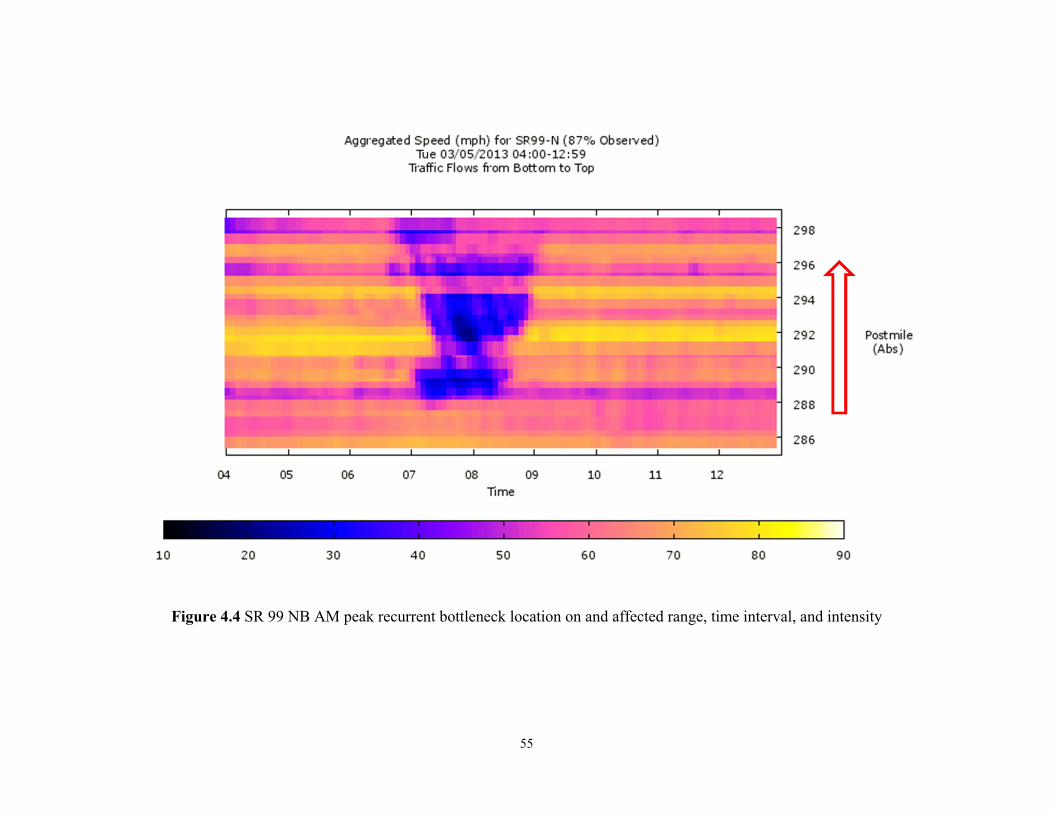
55

Figure 4.4 SR 99 NB AM peak recurrent bottleneck location on and affected range, time interval, and intensity

56

From the macroscopic contour plot (Figure 4-4), it can be observed that there are three

bottlenecks in the range of PM286 ~ PM299, which are very close. This is consistent for 2012 and 2013 data. Therefore, the coordination should include the whole section. The overall system should be controlled through TMC to reduce interface with individual and communication between onramps.

Identified Major Bottlenecks (all activates in AM traffic) are as follows: (1) PM 298.5: downstream congestion caused by diverging traffic to US 50 EB and WB.

This one may back-propagate to upstream bottleneck at PM 296.54. Figure 4-6 illustrates the traffic pattern upstream of 12th Ave merge (Note: detectors downstream of the merge are not working). One can see that the right two lanes, aiming to SR 99, are less congested, but the left two lanes are severely congested during the morning peak.

(2) PM 296.54: middle congestion caused by merging traffic from Fruitridge Rd (EB and

WB); see Figure 4-7. Two on-ramps (one from EB and one from WB) are close. The merging lane doesn’t drop (until the split of SR 99 and S Sacramento Freeway); i.e., there’s lane addition. Thus, congestion is light at this location, but it becomes more severe as it propagates upstream passing on-ramps from 47th Ave (at PM 295.7) (Figure 4-8).

(3) PM 290.76: upstream congestion caused by merging traffic from Calvine Rd. (EB and

WB). The arising of congestion can be seen on Figure 4-9 which is upstream of EB Calvine Rd merge (Note: the detector upstream of WB Calvine Rd. is not working). The two closely located on ramps from Calvine Rd. have very high demand, particularly the WB Calvine Rd. merge, which could exceed 1700 veh/h (total flow of three lanes) during morning peak. A merging lane is added at the EB Calvine Rd. merge but it drops at the exit to E. Stockton Blvd. This indicates the complexity of this bottleneck: frequent weaving maneuvers due to the compound effects of road geometry and traffic demand. Congestion arising at this location grows as it spreads upstream, but the queue does not pass GPL/HOV2 located immediately upstream of the Laguna off ramp. This bottleneck may merge with congestion from downstream bottleneck congestion back-propagation.

Notably, the first two bottlenecks are very close, only about two miles apart. Thus, we

combine the first two into one in our simulation comparison later, named as BN1, and the other one is named as BN2.

57

Figure 4-5 Evidence of bottleneck at PM 298.5. Top: speed plot; bottom: occupancy plot.

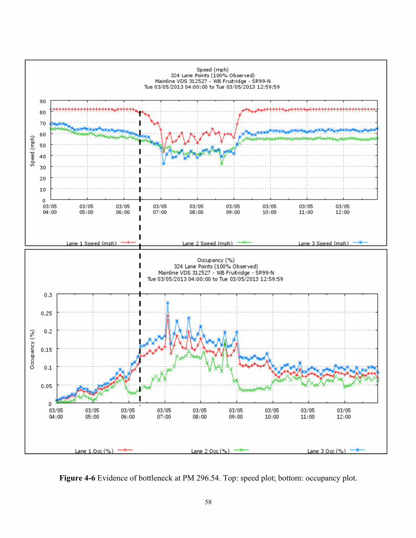
58

Figure 4-6 Evidence of bottleneck at PM 296.54. Top: speed plot; bottom: occupancy plot.

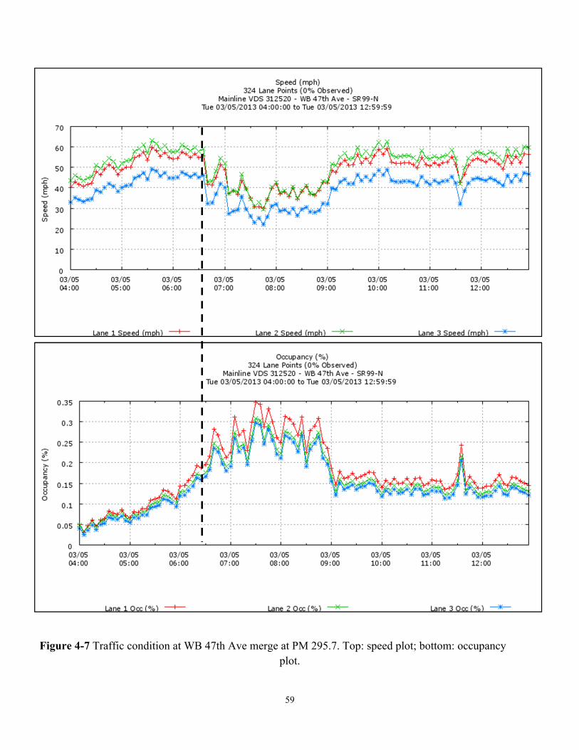
59

Figure 4-7 Traffic condition at WB 47th Ave merge at PM 295.7. Top: speed plot; bottom: occupancy plot.

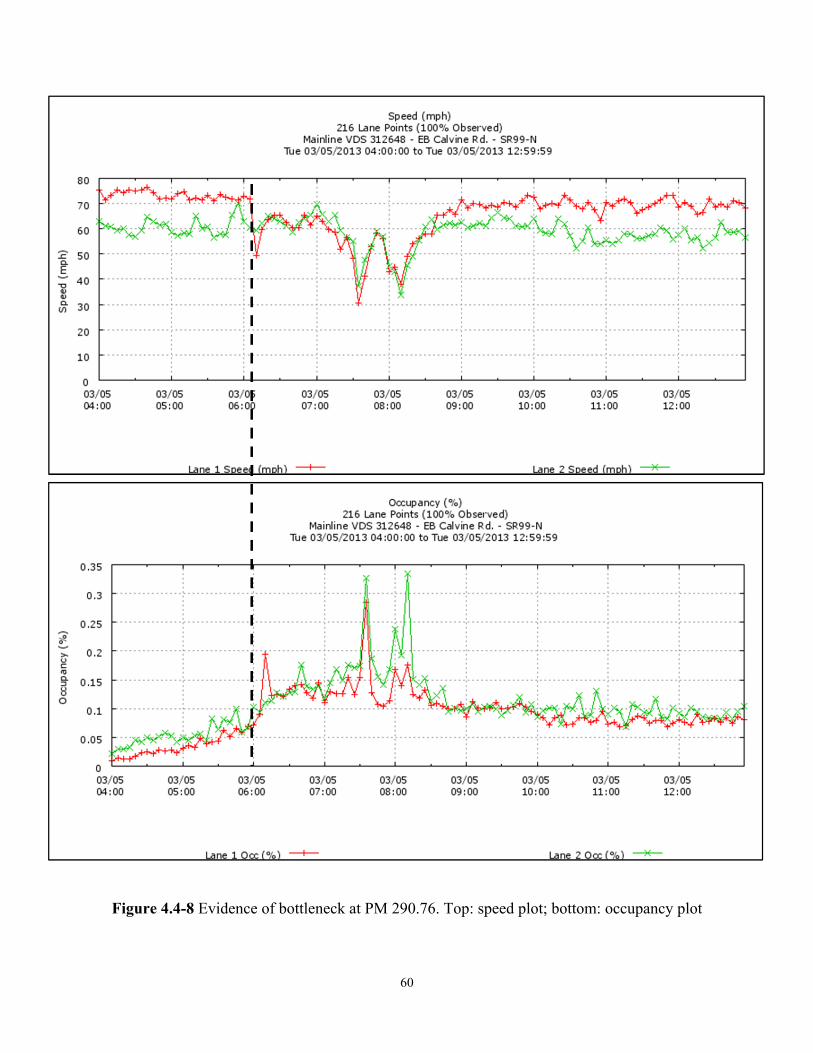
60

Figure 4.4-8 Evidence of bottleneck at PM 290.76. Top: speed plot; bottom: occupancy plot

61

4.5 Model Calibration

4.5.1 Comparison location In our calibration, we selected some key locations to compare the simulation results and

field data. The selected locations fall into three categories: (i) mainline locations (including general lane and HOV lanes), (ii) on ramps, and (iii) off ramps.

For mainline locations, recall that the network has two major bottlenecks, BN1 and BN2.

For each bottleneck, we select four key locations for comparison. In particular, for BN1, GPL/HOV25, GPL/HOV20, GPL/HOV17, and GPL/HOV12 are selected. GPL/HOV25 is used to represent the most downstream traffic of BN1, while GPL/HOV20 captures the instance when congestion becomes worse after passing WB and EB 47th Ave on ramps. GPL/HOV17 is a middle location of the congested segment. GPL/HOV12 is used to capture the tail of this segment since its upstream detectors GPL/HOV11 are not valid. Notably, GPL/HOV27 or GPL/HOV26 would have been a better option to represent the most downstream traffic, but the former has problematic measurement data while for the latter, there is a discrepancy between simulated and field flow due to a limitation of the simulation software: when turning ratio is used, simulated vehicles make turning decisions (which follows the turning ratio probability) when there is a turning node immediate downstream. In other words, simulated vehicles do not make turning decisions in advance. Following this logic, the simulated HOV vehicles that will take exit OFR12 do NOT switch to general purpose lanes in advance as vehicles do in reality (as mentioned in section 4.3.3). Consequently, the simulated HOV flow at HOV26 is higher than the field data. Fortunately, we found that such a discrepancy is local since eventually the HOV vehicles will take the exit and the flow going to OFR12 matches the field data.

For BN2, GPL/HOV9, GPL/HOV8, GPL/HOV6, and GPL/HOV2 are selected. The

former are used to capture the formation of congestion at this bottleneck, while GPL/HOV6 shows a middle location of the congested segment where congestion has grown to be heavy. GPL/HOV2 is the tail of the congested segment, indicating that the queue has vanished downstream of this location.

For on ramps and off ramps, all locations are selected to make sure that the input and

output are consistent with the field data, which also help to detect problems in the calibration process.

4.5.2 Measurement For the selected locations, different measurements are used in comparison. For mainline

locations, we compare the flow and occupancy (average across all lanes) for GPL and HOV.

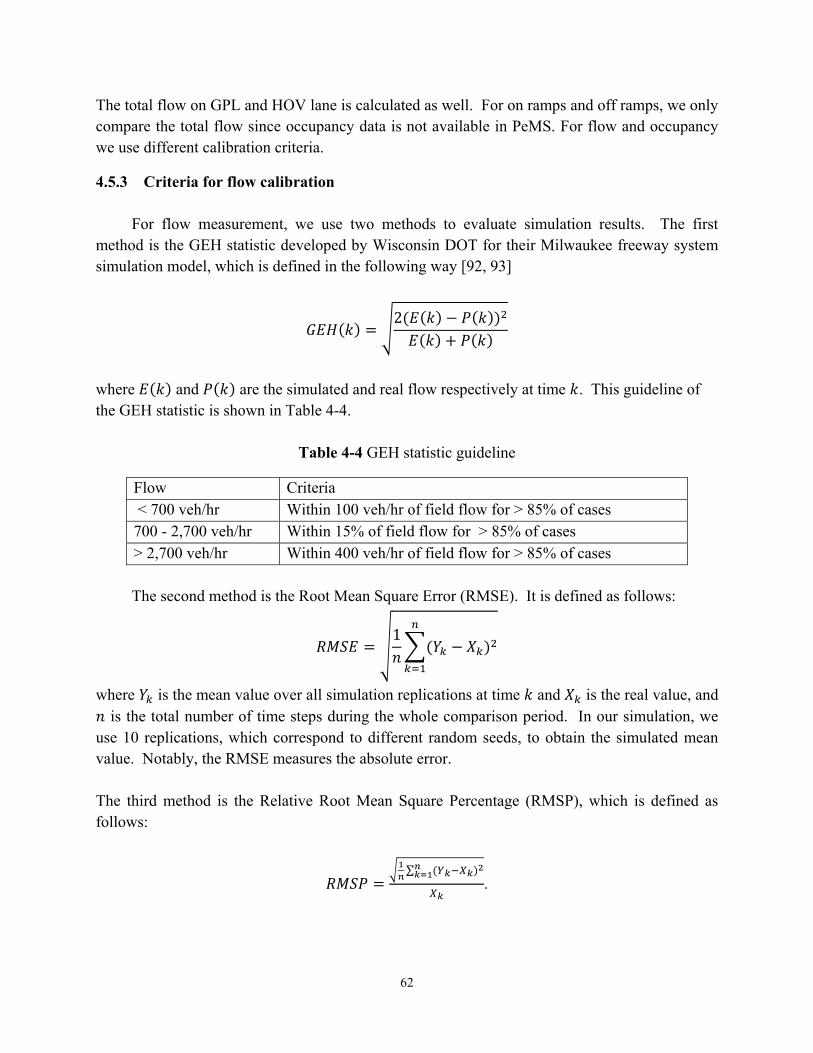
62

The total flow on GPL and HOV lane is calculated as well. For on ramps and off ramps, we only compare the total flow since occupancy data is not available in PeMS. For flow and occupancy we use different calibration criteria.

4.5.3 Criteria for flow calibration For flow measurement, we use two methods to evaluate simulation results. The first

method is the GEH statistic developed by Wisconsin DOT for their Milwaukee freeway system simulation model, which is defined in the following way [92, 93]

2

where and are the simulated and real flow respectively at time . This guideline of the GEH statistic is shown in Table 4-4.

Table 4-4 GEH statistic guideline

Flow Criteria < 700 veh/hr Within 100 veh/hr of field flow for > 85% of cases 700 - 2,700 veh/hr Within 15% of field flow for > 85% of cases > 2,700 veh/hr Within 400 veh/hr of field flow for > 85% of cases

The second method is the Root Mean Square Error (RMSE). It is defined as follows:

1

where is the mean value over all simulation replications at time and is the real value, and is the total number of time steps during the whole comparison period. In our simulation, we

use 10 replications, which correspond to different random seeds, to obtain the simulated mean value. Notably, the RMSE measures the absolute error. The third method is the Relative Root Mean Square Percentage (RMSP), which is defined as follows:

∑.

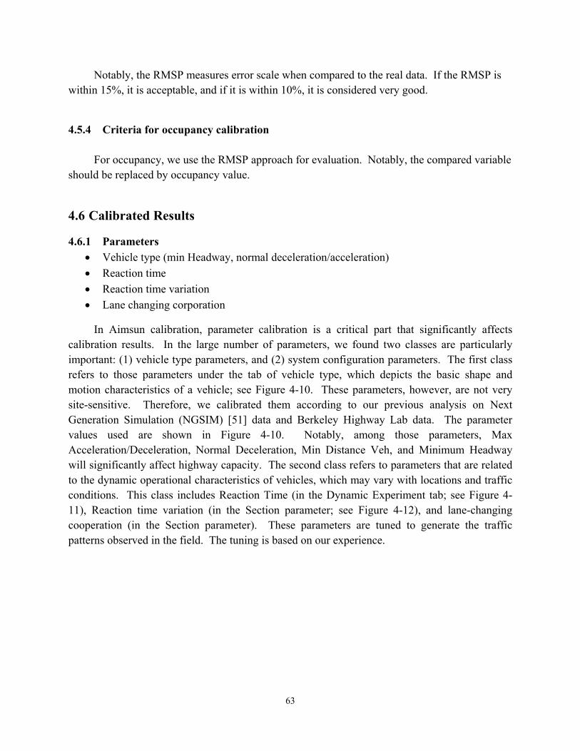
63

Notably, the RMSP measures error scale when compared to the real data. If the RMSP is within 15%, it is acceptable, and if it is within 10%, it is considered very good.

4.5.4 Criteria for occupancy calibration

For occupancy, we use the RMSP approach for evaluation. Notably, the compared variable should be replaced by occupancy value.

4.6 Calibrated Results

4.6.1 Parameters Vehicle type (min Headway, normal deceleration/acceleration)

Reaction time

Reaction time variation

Lane changing corporation

In Aimsun calibration, parameter calibration is a critical part that significantly affects calibration results. In the large number of parameters, we found two classes are particularly important: (1) vehicle type parameters, and (2) system configuration parameters. The first class refers to those parameters under the tab of vehicle type, which depicts the basic shape and motion characteristics of a vehicle; see Figure 4-10. These parameters, however, are not very site-sensitive. Therefore, we calibrated them according to our previous analysis on Next Generation Simulation (NGSIM) [51] data and Berkeley Highway Lab data. The parameter values used are shown in Figure 4-10. Notably, among those parameters, Max Acceleration/Deceleration, Normal Deceleration, Min Distance Veh, and Minimum Headway will significantly affect highway capacity. The second class refers to parameters that are related to the dynamic operational characteristics of vehicles, which may vary with locations and traffic conditions. This class includes Reaction Time (in the Dynamic Experiment tab; see Figure 4-11), Reaction time variation (in the Section parameter; see Figure 4-12), and lane-changing cooperation (in the Section parameter). These parameters are tuned to generate the traffic patterns observed in the field. The tuning is based on our experience.

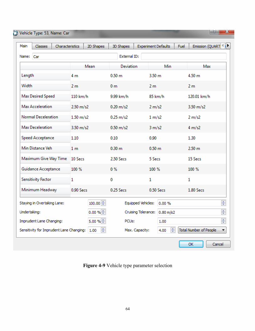
64

Figure 4-9 Vehicle type parameter selection

65

Figure 4-10 Reaction Time parameter selection

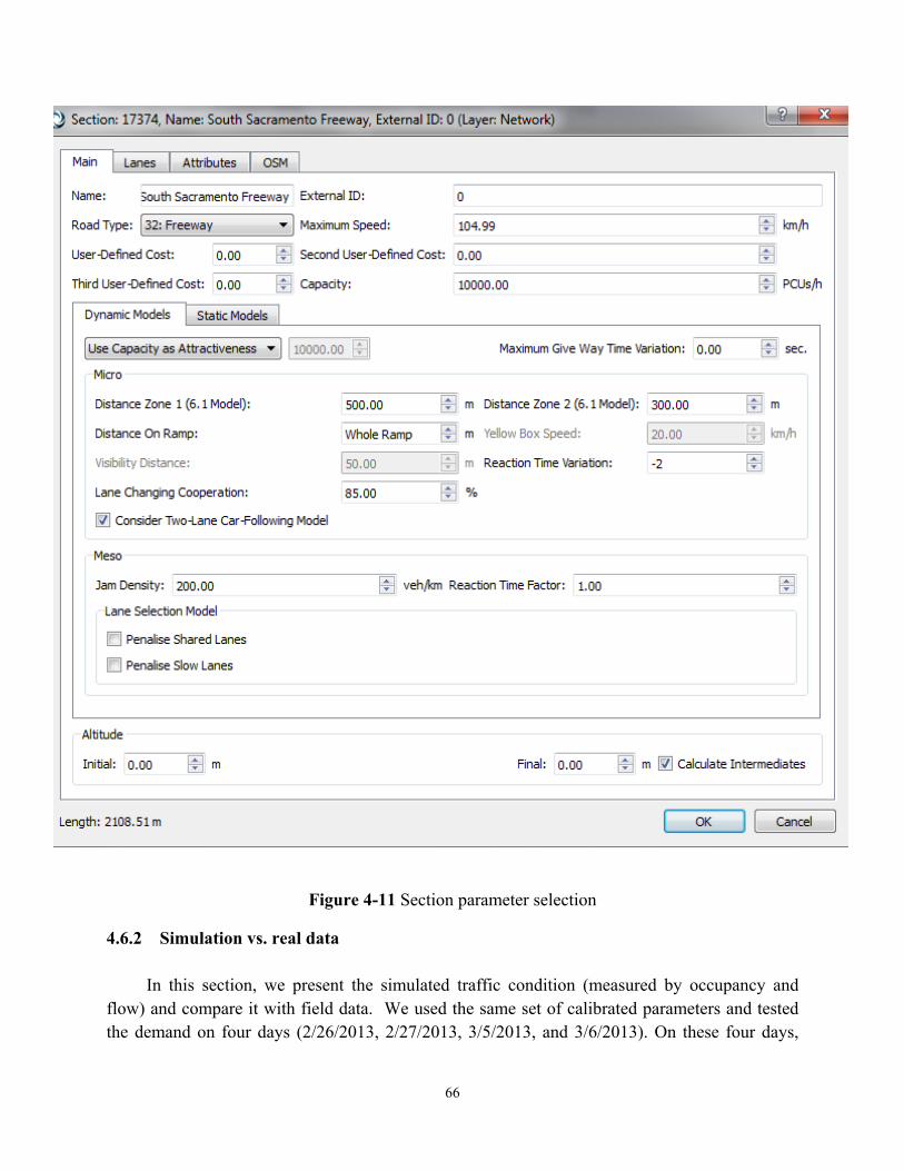
66

Figure 4-11 Section parameter selection

4.6.2 Simulation vs. real data In this section, we present the simulated traffic condition (measured by occupancy and

flow) and compare it with field data. We used the same set of calibrated parameters and tested the demand on four days (2/26/2013, 2/27/2013, 3/5/2013, and 3/6/2013). On these four days,

67

congestion is more severe (in terms of occupancy level during the congested period and congestion duration) on 3/6/2013 and lightest on 2/26/2013. We believe that’s a good representation of the traffic conditions for this network. Simulated results are averages of multiple runs (it’s set to be 10 here) with different random seeds.

4.6.2.1 On ramps We first compared the on ramp flow data to make sure that the demand input is reasonable.

The results are summarized in Table 4-5. As expected, the simulation input matches the data well for all on ramps (with RMSP <0.2) but ONR7. This is because the demand at ONR 7 is extremely high as discussed in Chapter 4. Results of flow consistency check for upstream and downstream of this on ramp (i.e., GPL/HOV 9, GPL/HOV 11 and GPL/HOV12 and the on/off ramps in between) suggested that the flow is conserved (the error is within 10% most of the time). Additionally, since this on ramp has three lanes before merging (two general purpose lanes and one HOV lane), the high total flow seemed reasonable. However, this is very difficult to achieve in simulation. In simulations, after mainline flow increases (usually starts around 7 am) the on ramp flow from ONR7 is significantly reduced and a long queue is built. Consequently, the input to the sub-network BN 1 is lower than the field data. That is why BN1 is under-congested.

4.6.2.2 Off ramps

We also analyzed the off ramp flow to make sure that that output of the network is reasonable. The flow comparison is summarized in Table 4-6. Notably, for the off ramp results, the RMSP may not be a very good measurement since the flow may be zero for some time stamps. Additionally, there are several off ramps that have very low volume (e.g., OFR 10), which will have a large RMSP even when the absolute error is small. Thus, the RMSE may be a better indicator of the error. Note that the under-congestion in BN 1 also affects the off ramp flow (including OFR4 – OFR12) since the exiting demand is defined through turning ratio.

The results indicate that for the flow at most of the off ramps matches field data, but there

are some significant discrepancies in OFR6 and OFR10. This is again due to the problem in the model of turning decision making for vehicles as discussed in Section 4.5.1. For example, for OFR6 the road segment immediately upstream (i.e., bounded by the node at OFR6 diverge and the node further upstream at ONR10 merge) is very short (113 ft) and HOV vehicles can hardly change from the left-most lane to the exit lane in this segment. Consequently, the exiting HOV flow is much lower than the field measurement. Similar case applies to OFR10. Fortunately, since the off ramp flow is not very large, the discrepancies do not affect the traffic pattern significantly.

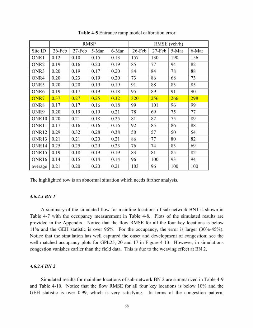
68

Table 4-5 Entrance ramp model calibration error

RMSP RMSE (veh/h)

Site ID 26-Feb 27-Feb 5-Mar 6-Mar 26-Feb 27-Feb 5-Mar 6-Mar ONR1 0.12 0.10 0.15 0.13 157 130 190 156 ONR2 0.19 0.16 0.20 0.19 85 77 94 82 ONR3 0.20 0.19 0.17 0.20 84 84 78 88 ONR4 0.20 0.23 0.19 0.20 73 86 68 73 ONR5 0.20 0.20 0.19 0.19 91 88 83 85 ONR6 0.19 0.17 0.19 0.18 95 89 91 90 ONR7 0.37 0.27 0.25 0.32 320 256 266 298 ONR8 0.17 0.17 0.16 0.18 99 101 96 99 ONR9 0.20 0.19 0.19 0.21 78 69 75 77 ONR10 0.20 0.21 0.18 0.25 81 82 75 89 ONR11 0.17 0.16 0.16 0.16 92 85 86 88 ONR12 0.29 0.32 0.28 0.38 50 57 50 54 ONR13 0.21 0.21 0.20 0.21 86 77 80 82 ONR14 0.25 0.25 0.29 0.23 76 74 83 69 ONR15 0.19 0.18 0.19 0.19 83 81 85 82 ONR16 0.14 0.15 0.14 0.14 96 100 93 94

average 0.21 0.20 0.20 0.21 103 96 100 100

The highlighted row is an abnormal situation which needs further analysis.

4.6.2.3 BN 1

A summary of the simulated flow for mainline locations of sub-network BN1 is shown in Table 4-7 with the occupancy measurement in Table 4-8. Plots of the simulated results are provided in the Appendix. Notice that the flow RMSE for all the four key locations is below 11% and the GEH statistic is over 96%. For the occupancy, the error is larger (30%-45%). Notice that the simulation has well captured the onset and development of congestion; see the well matched occupancy plots for GPL25, 20 and 17 in Figure 4-13. However, in simulations congestion vanishes earlier than the field data. This is due to the weaving effect at BN 2.

4.6.2.4 BN 2 Simulated results for mainline locations of sub-network BN 2 are summarized in Table 4-9

and Table 4-10. Notice that the flow RMSE for all four key locations is below 10% and the GEH statistic is over 0.99, which is very satisfying. In terms of the congestion pattern,

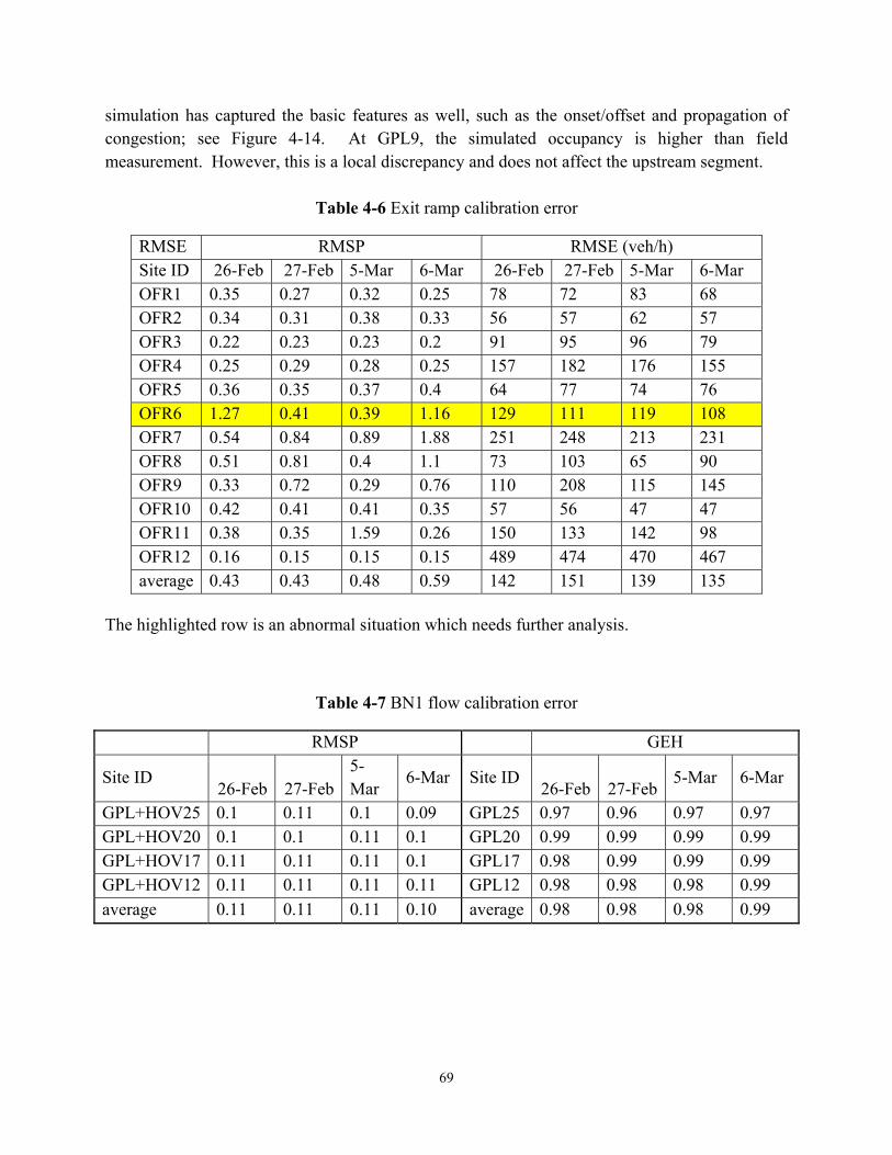
69

simulation has captured the basic features as well, such as the onset/offset and propagation of congestion; see Figure 4-14. At GPL9, the simulated occupancy is higher than field measurement. However, this is a local discrepancy and does not affect the upstream segment.

Table 4-6 Exit ramp calibration error

RMSE RMSP RMSE (veh/h) Site ID 26-Feb 27-Feb 5-Mar 6-Mar 26-Feb 27-Feb 5-Mar 6-Mar OFR1 0.35 0.27 0.32 0.25 78 72 83 68 OFR2 0.34 0.31 0.38 0.33 56 57 62 57 OFR3 0.22 0.23 0.23 0.2 91 95 96 79 OFR4 0.25 0.29 0.28 0.25 157 182 176 155 OFR5 0.36 0.35 0.37 0.4 64 77 74 76 OFR6 1.27 0.41 0.39 1.16 129 111 119 108 OFR7 0.54 0.84 0.89 1.88 251 248 213 231 OFR8 0.51 0.81 0.4 1.1 73 103 65 90 OFR9 0.33 0.72 0.29 0.76 110 208 115 145 OFR10 0.42 0.41 0.41 0.35 57 56 47 47 OFR11 0.38 0.35 1.59 0.26 150 133 142 98 OFR12 0.16 0.15 0.15 0.15 489 474 470 467 average 0.43 0.43 0.48 0.59 142 151 139 135

The highlighted row is an abnormal situation which needs further analysis.

Table 4-7 BN1 flow calibration error

RMSP GEH

Site ID 26-Feb 27-Feb

5-Mar

6-Mar Site ID 26-Feb 27-Feb

5-Mar 6-Mar

GPL+HOV25 0.1 0.11 0.1 0.09 GPL25 0.97 0.96 0.97 0.97 GPL+HOV20 0.1 0.1 0.11 0.1 GPL20 0.99 0.99 0.99 0.99 GPL+HOV17 0.11 0.11 0.11 0.1 GPL17 0.98 0.99 0.99 0.99 GPL+HOV12 0.11 0.11 0.11 0.11 GPL12 0.98 0.98 0.98 0.99

average 0.11 0.11 0.11 0.10 average 0.98 0.98 0.98 0.99

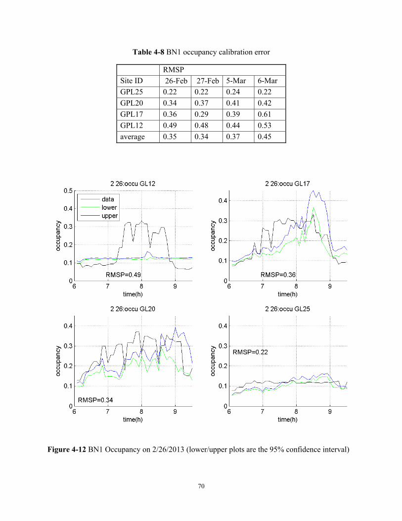
70

Table 4-8 BN1 occupancy calibration error

RMSP

Site ID 26-Feb 27-Feb 5-Mar 6-Mar

GPL25 0.22 0.22 0.24 0.22

GPL20 0.34 0.37 0.41 0.42

GPL17 0.36 0.29 0.39 0.61

GPL12 0.49 0.48 0.44 0.53

average 0.35 0.34 0.37 0.45

Figure 4-12 BN1 Occupancy on 2/26/2013 (lower/upper plots are the 95% confidence interval)  

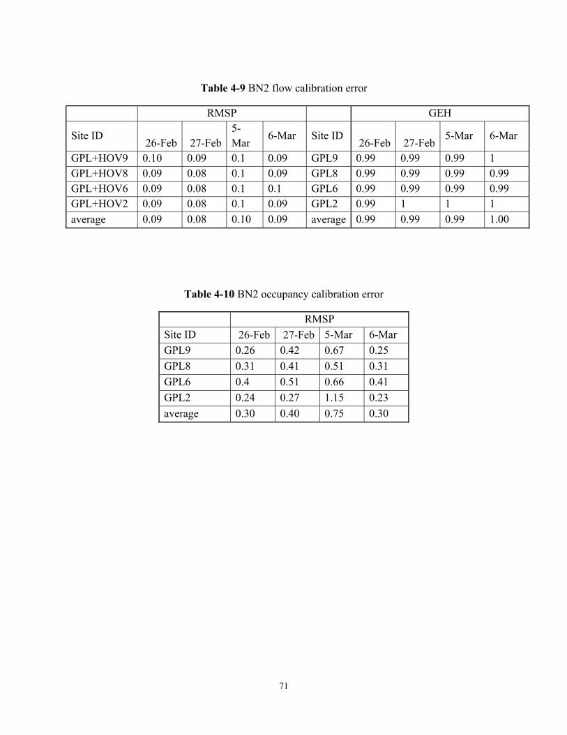
71

Table 4-9 BN2 flow calibration error

RMSP GEH

Site ID 26-Feb 27-Feb

5-Mar

6-Mar Site ID 26-Feb 27-Feb

5-Mar 6-Mar

GPL+HOV9 0.10 0.09 0.1 0.09 GPL9 0.99 0.99 0.99 1 GPL+HOV8 0.09 0.08 0.1 0.09 GPL8 0.99 0.99 0.99 0.99 GPL+HOV6 0.09 0.08 0.1 0.1 GPL6 0.99 0.99 0.99 0.99 GPL+HOV2 0.09 0.08 0.1 0.09 GPL2 0.99 1 1 1

average 0.09 0.08 0.10 0.09 average 0.99 0.99 0.99 1.00

Table 4-10 BN2 occupancy calibration error

RMSP

Site ID 26-Feb 27-Feb 5-Mar 6-Mar

GPL9 0.26 0.42 0.67 0.25

GPL8 0.31 0.41 0.51 0.31

GPL6 0.4 0.51 0.66 0.41

GPL2 0.24 0.27 1.15 0.23

average 0.30 0.40 0.75 0.30

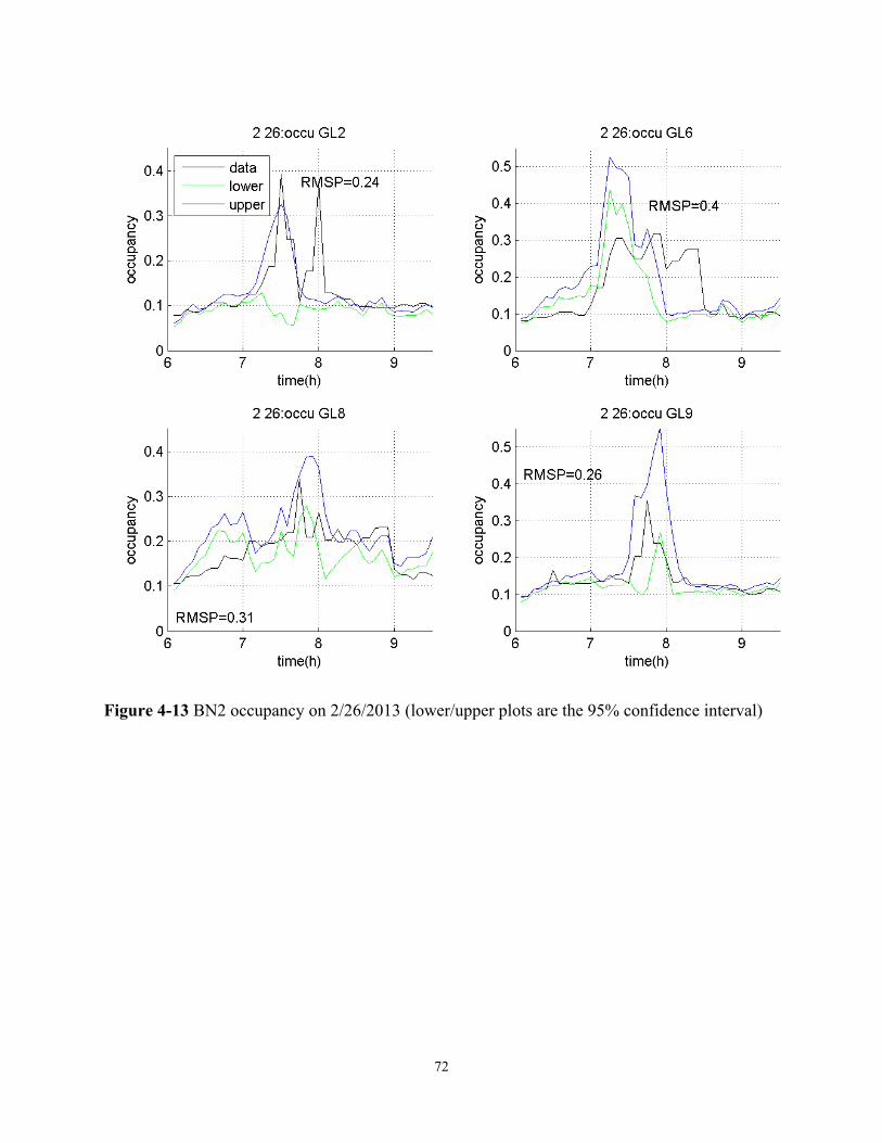
72

Figure 4-13 BN2 occupancy on 2/26/2013 (lower/upper plots are the 95% confidence interval)

73

Chapter 5. Coordinated Ramp Metering Algorithm

This chapter documents the CRM algorithm developed in the former FHWA EAR program supported project and its implementation in the Aimsun microscopic simulation model and evaluation.

5.1 CRM Design with Model Predictive Control

The main idea for design of the CRM is to use a simplified optimal control approach, called Model Predictive Control (MPC). The characteristics of MPC can be summarized as follows:

The system in consideration needs to have a dynamical mathematical model with all the state variables estimated or measured;

The control problem is usually formulated as an optimal control with a proper objective function with the model plus appropriate constraint; as default, the optimal control problem is formulated in an infinite time horizon;

The problem is then simplified by assuming a finite look ahead time horizon on which the system dynamics are discretized;

Correspondingly, the objective function and the constraints are also discretized in the finite time horizon; as a consequence, the optimal control problems has been simplified as a sequential optimization rolling with the time;

At each time step, the system model is used to predict the system states in the given finite time horizon;

Optimization is conducted at each time step; for the control variable obtained in the finite time horizon, the first one corresponding to the first time step is actually applied to the system for feedback control.

5.2 Modeling 5.2.1 Nomenclature

Model Parameters m link index; M Critical VSL Control link index; M+1 discharge link index; k time index

mL length of link m

pN prediction steps for each k in Model Predictive Control State and Control Variables

mq k - estimated mainline flow at time k

m k density of link m at time k

mr k metering flow rate (veh/hr), control variable

74

Measured or Estimated Traffic State Parameters

1mq k flow at time k-1, measured

mv k time mean speed at fixed sensor location within link m at time k, measured

mu k distance mean speed of the link m, estimated

1M discharge link density, measured/estimated

ms k total exit ramp flow of a link (veh/hr), measured

md demand from entrance ramp m, measured or estimated

mQ mainline capacity of link m, known

bQ bottleneck capacity flow, known

,m oQ entrance ramp m capacity, known

,m oL entrance ramp m length, known;

fV free-flow speed, known

cO critical occupancy, known

c critical density, known

Here, each link is considered as one cell for simplicity. It is assumed that each link has

exactly one on-ramp but may contain more than one exit ramp. The first equation in (Eq. 5.1) is the conservation of flow. It is linear since the speed

variables 1mu k and mu k can be estimated from the sensor detection in the field. Such

linearization and decoupling bring great advantages to control design. 5.2.2 Dynamical Model of The System The following linearized density and entrance ramp queue dynamics model are adopted:

1 1 1

,

1

1

m m m m m m m m m mm m

m m m m o

Tk k k u k k u k r k s k

L

w k w k T d k q k

(Eq. 5.1)

5.2.3 Constraints

The following constraints (Equation 5.2) are adopted for CRM design.

( )

, 1

0

0 min , , ,

0 min ,

rm m J

m m m o m m m m m J m

m J m

w k L

r k d k Q Q q k u k k

k u k

(Eq. 5.2)

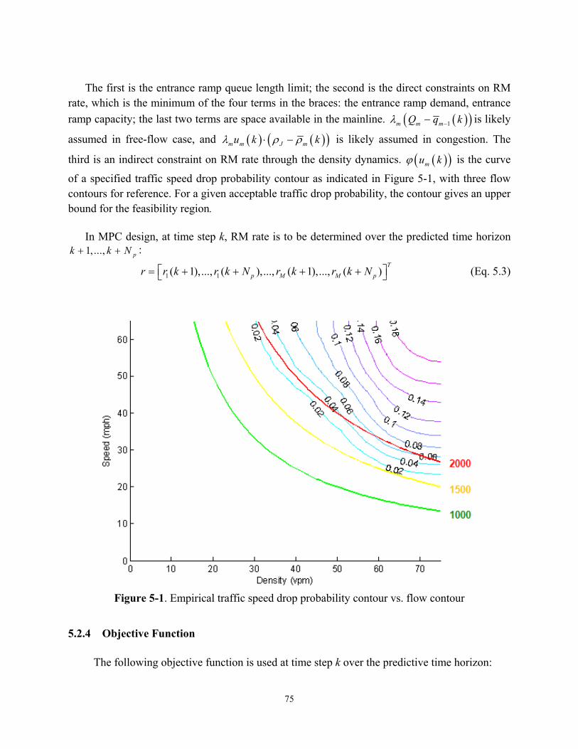
75

The first is the entrance ramp queue length limit; the second is the direct constraints on RM

rate, which is the minimum of the four terms in the braces: the entrance ramp demand, entrance

ramp capacity; the last two terms are space available in the mainline. 1m m mQ q k is likely

assumed in free-flow case, and m m J mu k k is likely assumed in congestion. The

third is an indirect constraint on RM rate through the density dynamics. mu k is the curve

of a specified traffic speed drop probability contour as indicated in Figure 5-1, with three flow contours for reference. For a given acceptable traffic drop probability, the contour gives an upper bound for the feasibility region.

In MPC design, at time step k, RM rate is to be determined over the predicted time horizon 1, ..., pk k N :

1 1( 1),..., ( ),..., ( 1),..., ( )T

p M M pr r k r k N r k r k N (Eq. 5.3)

Figure 5-1. Empirical traffic speed drop probability contour vs. flow contour

5.2.4 Objective Function

The following objective function is used at time step k over the predictive time horizon:

76

1 1

1

1

,0 ,1 1 1

, ,0

(TTT)

(Time Delay Due to Onramp Queue)

0

p

p

p p

N M

m m mj m

N

w oj o

N NM

TTD m m m TTD M M M Mj m j

TTD M TTD

J TTS TTD

TTS T L k j

T w k j

TTD T L q k j T L q k j

(Eq. 5.4)

Minimizing J minimizes TTS (or density), and maximizes TTD (to maximize mainline

flow). Choosing , ,0TTD M TTD emphasizes maximizing the flow on link M.

The reasons for choosing this objective function are as follows: minimizing TTS may

discourage vehicles get into the freeway so that the mainline could have better flow when the mainline density is higher. To minimize negative TTD is equivalent to maximize TTD which is to encourage vehicle get into the freeway. Therefore, to minimize the difference of the two is somehow intended to formulate the problem as a non-zero sum game. It is important to note that the units of the two system performance parameters are different. To put them in the same objective function, the coefficient choice need to be appropriate.

5.2.5 Algorithm Modification by Queue Override

Beside the systematic consideration in optimization process with entrance ramp queue length taken into account, the entrance ramp queue has been further taken into consideration for onramps with very high demands. If the queue reaches 85% of the entrance ramp, then the meter will be green for at least 10[s] which is to make sure the queue has been adequately flushed.

5.3 Implementation of the CRM Algorithm in Simulation

Based on the preliminarily calibrated network traffic model for SR99, the optimization code in the API (Application Program Interface) part developed in previous work [87] has been adapted to this network model in Aimsun. Since the road geometries for I-80 WB developed in [87] is quite different from SR99 of this project, several changes are made. The critical points for the application of the algorithms include: road network divided into section, sensor locations, the way a ramp meter is activated, etc. 5.3.1. Section division, Sensor Locations, Number of Lanes

77

Section division: to use the linearized CTM for CRM algorithm development, it is necessary to divide the road network into sections. Since all the onramps are metered for the system concerned, the road network is divided into sections according to sections according to the sensor locations: in general, section boundaries are at the mid-point between the entrance ramp merge point and the its immediate upstream sensor location. With this division principle, the overall system has the following components:

17 sections

16 entrance ramp (each section has a metered entrance ramp except the most upstream one)

12 exit ramps (not all sections have ramp) It is noted that this does not mean that all the onramps are to be coordinated. Instead, only a subset of entrance ramp meters is coordinated. The main points for the selection of RM for coordination include:

Demand is high enough so that its flow into the system would significantly affect the overall traffic and its queue would affect overall system TTT;

To be coordinated onramps are located close enough: if two groups of onramps are far separated and their traffic rarely affects each other, it does not make sense to coordinate them; instead, it would be simpler to just operate them separately;

The following is a list of onramps (11 in total) from upstream to downstream that the project preliminarily selected for coordination:

Calvine EB , WB

Mark Road EB, WB

Florine EB, WB

47th Ave EB, WB

Fruitridge EB, WB

12th Ave Number of Lanes: With the section division above in mind, an immediate question is how to determine the number of lanes since it is a model parameter in (Eq. 5-1 ~ Eq. 5-4). The reason is that the number of lanes in each section may not be homogeneous. To resolve this problem, we used the distance-based weighted number of lanes for each section. This is done as follows.

Assuming that a section with length mL is divided into two subsections: the first has ,1m lanes

with lengths ,1mL ; and the second has ,2m lanes with length ,2 ,1 ,2( )m m m mL L L L . Now a

composite number of lanes m is determined as follows:

78

,1 ,1 ,2 ,2m m m mm

m

L L

L

(Eq. 5.5)

It is noted that: (a) a composite number of lanes for a section could be a decimal; (b) such a number is inconsistent with density estimation across the section; (c) this method could be applied to a section with more than two subsections with different number of lanes. Sensor Locations:

As shown in Figure 3-2, the locations of sensors used for RM are immediately upstream of the entrance ramp. The simulation model created sensors at similar locations. There are two ways to create sensors in Aimsun: either lane-by-lane or one sensor (such as loop detector) across all lanes. For model calibration above, lane-by-lane sensors are used since it is necessary to distinguish between GP lanes and the HOV lane. After model calibration, RM does not need to distinguish flows between lanes. Therefore, cross-lane single sensors are used for convenience. 5.3.2 Traffic State Parameters

In Eq. 5.1 – 5.4, there are three traffic state parameters: density, speed and entrance ramp

queue length. Since the problem here is for RM only with speed control, we can use sensor

measured speed to replace the unknown with known values. Strictly speaking, the speed mu k at

time step k is a distance mean speed, while a sensor can only measure at a point to get time mean speed. For this reason, it is necessary to convert time mean speed at a point into a distance mean speed with the harmonization mean as follows:

1 ,

11 1m m

i m i i

u k

m v t

(Eq. 5.6)

where ,m i iv t is the measured speed at the point sensor during time interval k, and all the time

points 0 1, ,..., mt t t fall into this time interval. Clearly, to get proper distance mean speed, the

sampling rate at the fixed detector should be much higher. However, in practice, one can just use time mean speed to replace the distance mean speed for operation. 5.3.3 Lane-wise Metering

In Aimsun, an entrance ramp with multiple lanes has to be set with a single metering rate

which controls all the lanes, essentially, with flow control of all lanes together. However, this is different from what is in the field for California highways, where each lane of a metered entrance ramp has an individual meter including the HOV lane. Besides, the green time intervals of different lanes are shifted to avoid time-space conflicts of vehicles from different lanes at the merge after the meter. It is clear that this is more efficient for vehicles entering the freeway with

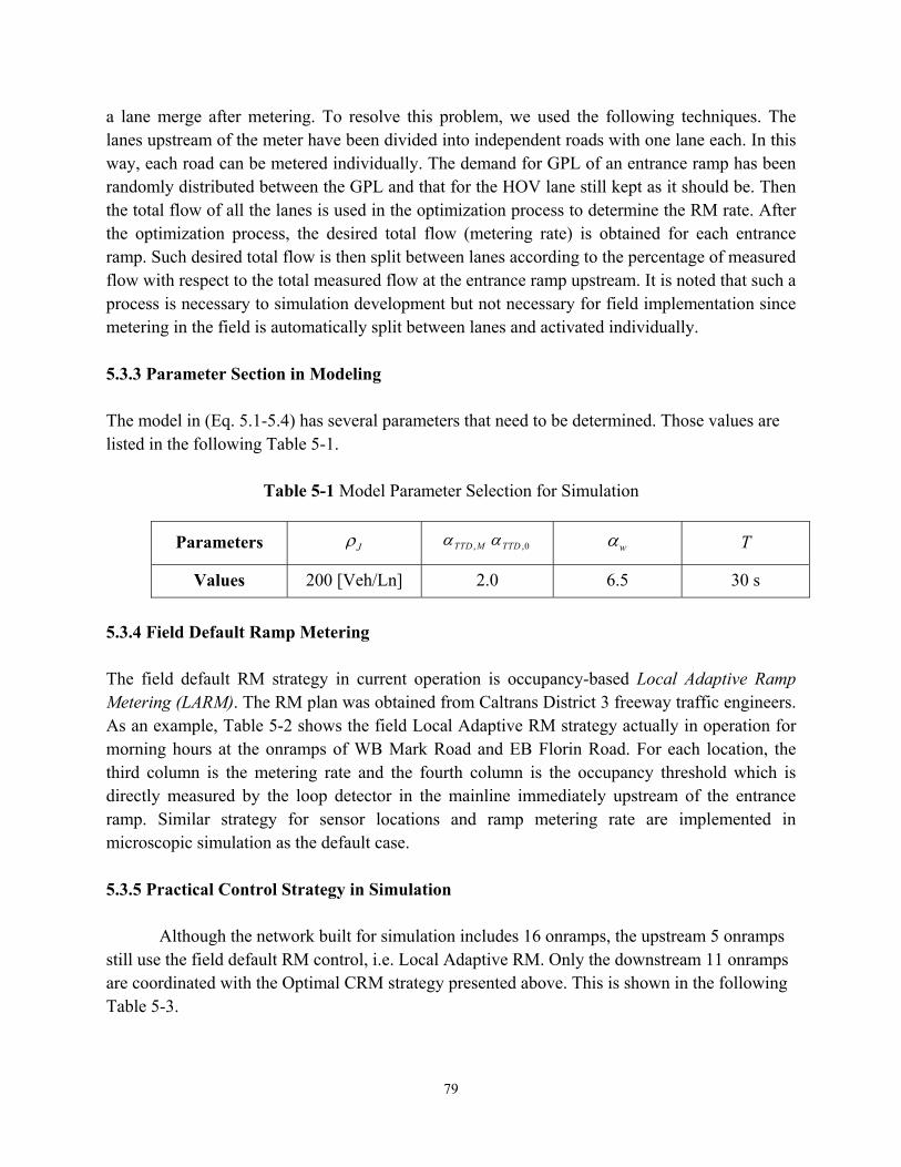
79

a lane merge after metering. To resolve this problem, we used the following techniques. The lanes upstream of the meter have been divided into independent roads with one lane each. In this way, each road can be metered individually. The demand for GPL of an entrance ramp has been randomly distributed between the GPL and that for the HOV lane still kept as it should be. Then the total flow of all the lanes is used in the optimization process to determine the RM rate. After the optimization process, the desired total flow (metering rate) is obtained for each entrance ramp. Such desired total flow is then split between lanes according to the percentage of measured flow with respect to the total measured flow at the entrance ramp upstream. It is noted that such a process is necessary to simulation development but not necessary for field implementation since metering in the field is automatically split between lanes and activated individually. 5.3.3 Parameter Section in Modeling The model in (Eq. 5.1-5.4) has several parameters that need to be determined. Those values are listed in the following Table 5-1.

Table 5-1 Model Parameter Selection for Simulation

Parameters J ,0TTD,TTD M w T

Values 200 [Veh/Ln] 2.0 6.5 30 s

5.3.4 Field Default Ramp Metering The field default RM strategy in current operation is occupancy-based Local Adaptive Ramp Metering (LARM). The RM plan was obtained from Caltrans District 3 freeway traffic engineers. As an example, Table 5-2 shows the field Local Adaptive RM strategy actually in operation for morning hours at the onramps of WB Mark Road and EB Florin Road. For each location, the third column is the metering rate and the fourth column is the occupancy threshold which is directly measured by the loop detector in the mainline immediately upstream of the entrance ramp. Similar strategy for sensor locations and ramp metering rate are implemented in microscopic simulation as the default case. 5.3.5 Practical Control Strategy in Simulation

Although the network built for simulation includes 16 onramps, the upstream 5 onramps still use the field default RM control, i.e. Local Adaptive RM. Only the downstream 11 onramps are coordinated with the Optimal CRM strategy presented above. This is shown in the following Table 5-3.

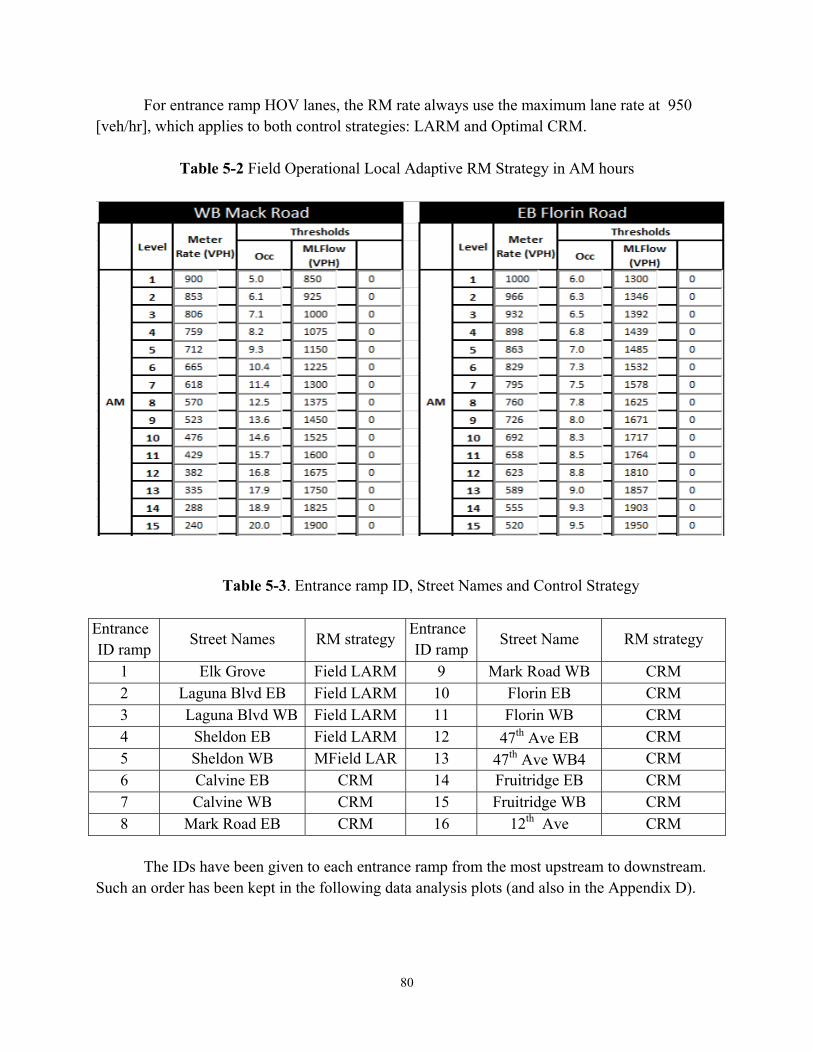
80

For entrance ramp HOV lanes, the RM rate always use the maximum lane rate at 950 [veh/hr], which applies to both control strategies: LARM and Optimal CRM.

Table 5-2 Field Operational Local Adaptive RM Strategy in AM hours

Table 5-3. Entrance ramp ID, Street Names and Control Strategy

Entrance ramp ID

Street Names RM strategy Entrance

ramp ID Street Name RM strategy

1 Elk Grove Field LARM 9 Mark Road WB CRM 2 Laguna Blvd EB Field LARM 10 Florin EB CRM 3 Laguna Blvd WB Field LARM 11 Florin WB CRM 4 Sheldon EB Field LARM 12 47th Ave EB CRM 5 Sheldon WB Field LARM 13 447th Ave WB CRM 6 Calvine EB CRM 14 Fruitridge EB CRM 7 Calvine WB CRM 15 Fruitridge WB CRM 8 Mark Road EB CRM 16 12th Ave CRM

The IDs have been given to each entrance ramp from the most upstream to downstream.

Such an order has been kept in the following data analysis plots (and also in the Appendix D).

81

All the mainline section ID corresponds to the entrance ramp ID in the sense that the section is the one immediately upstream of the entrance ramp. 5.3.6 Entrance ramp Queue Overwrite The following entrance ramp queue overwrite scheme has been used jointly with the Optimal CRM algorithm. The queue detector is located about 15% distance to the upstream end of the entrance ramp. The schematic overwrite algorithms is as follows:

If the occupancy of the queue detector is over 70%, then use the maximum lane RM rate 950 [veh/hr] for 3 cycles (or 1.5 minutes)

If the occupancy of the queue detector continues to be higher than 70%, then this maximum lane RM will remain.

It has been observed from simulation that this strategy can effectively reduce the queue end to the downstream of the queue detector.

5.4 Simulation Results

5.4.1 Systems Performance Parameters in Aimsun

Three system performance parameters have been used for evaluation of the algorithm implemented in the simulation model:

Total Travel Time (TTT): this includes the queue time at entrance ramp; if the vehicle is not able to get into the entrance ramp due to traffic over-flow at entrance ramp, the wait time is also included;

Total Delay (TD): it is obtained by comparing the simulated traffic with mainline free-flow assumption;

Total Number of Stops (TNOS): In Aimsun, the total number of stops of all the vehicles is recorded and used as the system performance parameter. Those parameters could be used to indicate traffic smoothness. As is generally recognized, Stop & Go traffic will significantly affect traffic throughput as well as safety since a significant portion of collisions happened due to resulting shockwaves [95, 96]. Since the simulation model is set between AM peak hours 6:00 am ~ 9:30 am, different

random seeds may produce slightly different ways of generating the demand flow from the entrance ramp and freeway mainline, which will result in slightly different total (cumulative) demand. It is clear that higher total demand in the simulation time interval could result in longer TTT. To overcome this problem, the following correction has been conducted in the estimation of the percentage time improvement for TTT and TD.

82

% Change =

% Change =

default CRM default CRM

default default

default CRM default CRM

default default

TTT TTT TTD TTDTTT

TTT TTD

TD TD TTD TTDTD

TD TTD

(Eq. 5.7)

It says that if the TTD is reduced (increased) by x% after the simulation run, then TTT

and TD should be increased (decreased) by x% as penalty accordingly. Here the subscripts indicate whether the parameter is estimated from default scenario or from data with CRM activated. 5.4.2. Simulation Scenario Description

Simulation runs were conducted for 4 model days in 2013: 2/26 (Tue), 2/27 (Wed), 3/5

(Tue), and 3/6(Wed). This means that, for the simulation of the status quo, traffic demands were obtained from the data collected for all the onramps and freeway most upstream mainlines for those days. Each day was run for 10 replications (random seeds). The 10 replications for each model day were also different. The results were then averaged over the 10 replications.

Those simulation dates and replications have been run for both control strategies: default

LARM and propose Optimal CRM. It is reminded that the coordination has been applied to the 11 downstream onramps only. The upstream 5 onramps still use LARM.

Simulations have been conducted for two traffic demand scenarios: Scenario 1: Demands for selected 5 onramps with significant queues (IDs: 1, 6, 7, 8, 9) were obtained by adding 5% over the field measured throughput; others use the throughput as the demands; Scenario 2: Demands for all the onramps were obtained by adding 5% over the field measured throughput.

Since the field data we used for traffic network modeling was collected when the field RM was on, it should be throughput instead of practical demand. Therefore, use throughput as demand may not completely reflect the traffic situation. This problem could be analyzed as follows: (a) if an entrance ramp has no queue or has little queues, use entrance ramp throughput as its demand is reasonable; to add extra flow to the throughput to generate the demand would excessive; (b) for an entrance ramp with some queue but the queue could be cleared up once for a while; in this case, demand increase of the entrance ramp would affect mainline traffic flow; use entrance ramp throughput to represent the demand should be reasonable too; (c) for an entrance ramp with persistent queue which cannot be cleared up at all in peak hours; the effect to mainline traffic will not change even if the demand is increased a little; however, it would affect the queue clear up time and queue length; such increase would be necessary in traffic simulation to check the

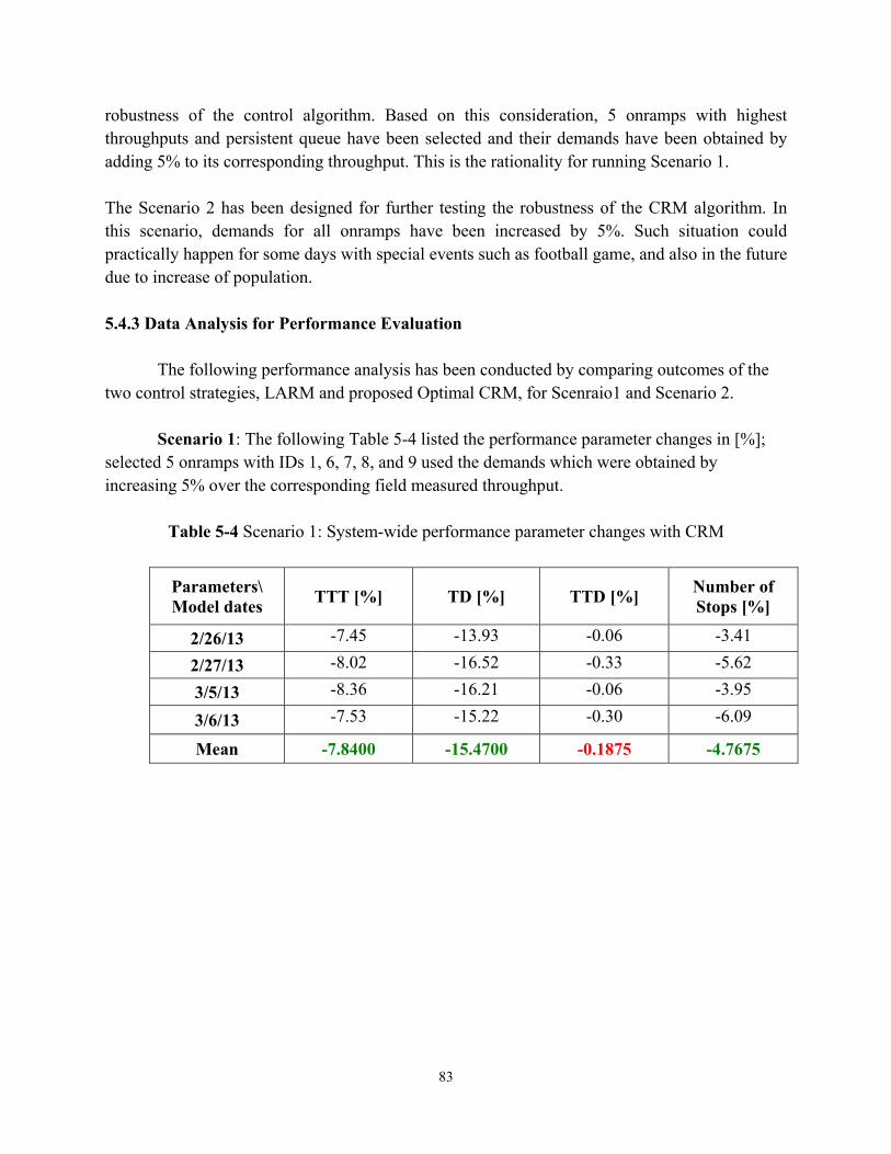
83

robustness of the control algorithm. Based on this consideration, 5 onramps with highest throughputs and persistent queue have been selected and their demands have been obtained by adding 5% to its corresponding throughput. This is the rationality for running Scenario 1. The Scenario 2 has been designed for further testing the robustness of the CRM algorithm. In this scenario, demands for all onramps have been increased by 5%. Such situation could practically happen for some days with special events such as football game, and also in the future due to increase of population. 5.4.3 Data Analysis for Performance Evaluation

The following performance analysis has been conducted by comparing outcomes of the two control strategies, LARM and proposed Optimal CRM, for Scenraio1 and Scenario 2.

Scenario 1: The following Table 5-4 listed the performance parameter changes in [%];

selected 5 onramps with IDs 1, 6, 7, 8, and 9 used the demands which were obtained by increasing 5% over the corresponding field measured throughput.

Table 5-4 Scenario 1: System-wide performance parameter changes with CRM

Parameters\ Model dates

TTT [%] TD [%] TTD [%] Number of Stops [%]

2/26/13 -7.45 -13.93 -0.06 -3.41

2/27/13 -8.02 -16.52 -0.33 -5.62

3/5/13 -8.36 -16.21 -0.06 -3.95

3/6/13 -7.53 -15.22 -0.30 -6.09

Mean -7.8400 -15.4700 -0.1875 -4.7675

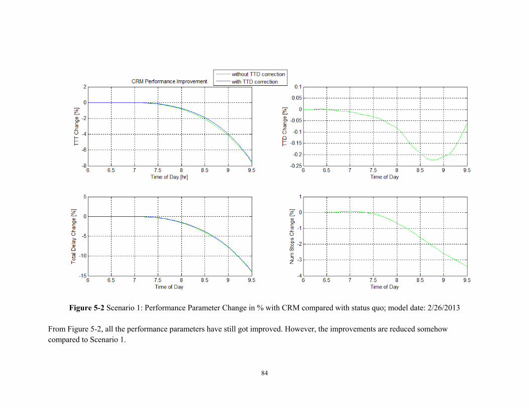
84

Figure 5-2 Scenario 1: Performance Parameter Change in % with CRM compared with status quo; model date: 2/26/2013

From Figure 5-2, all the performance parameters have still got improved. However, the improvements are reduced somehow compared to Scenario 1.

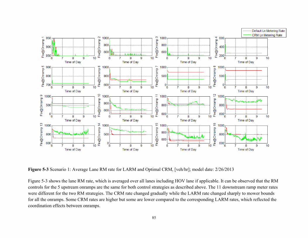
85

Figure 5-3 Scenario 1: Average Lane RM rate for LARM and Optimal CRM, [veh/hr]; model date: 2/26/2013 Figure 5-3 shows the lane RM rate, which is averaged over all lanes including HOV lane if applicable. It can be observed that the RM controls for the 5 upstream onramps are the same for both control strategies as described above. The 11 downstream ramp meter rates were different for the two RM strategies. The CRM rate changed gradually while the LARM rate changed sharply to mower bounds for all the onramps. Some CRM rates are higher but some are lower compared to the corresponding LARM rates, which reflected the coordination effects between onramps.

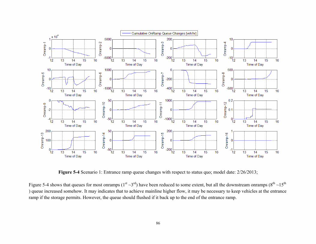
86

Figure 5-4 Scenario 1: Entrance ramp queue changes with respect to status quo; model date: 2/26/2013;

Figure 5-4 shows that queues for most onramps (1st ~3rd) have been reduced to some extent, but all the downstream onramps (8th ~15th ) queue increased somehow. It may indicates that to achieve mainline higher flow, it may be necessary to keep vehicles at the entrance ramp if the storage permits. However, the queue should flushed if it back up to the end of the entrance ramp.

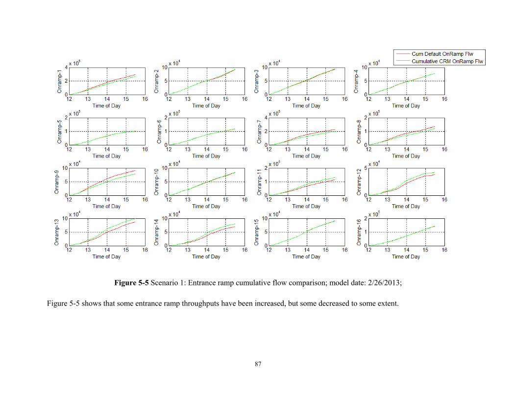
87

Figure 5-5 Scenario 1: Entrance ramp cumulative flow comparison; model date: 2/26/2013;

Figure 5-5 shows that some entrance ramp throughputs have been increased, but some decreased to some extent.

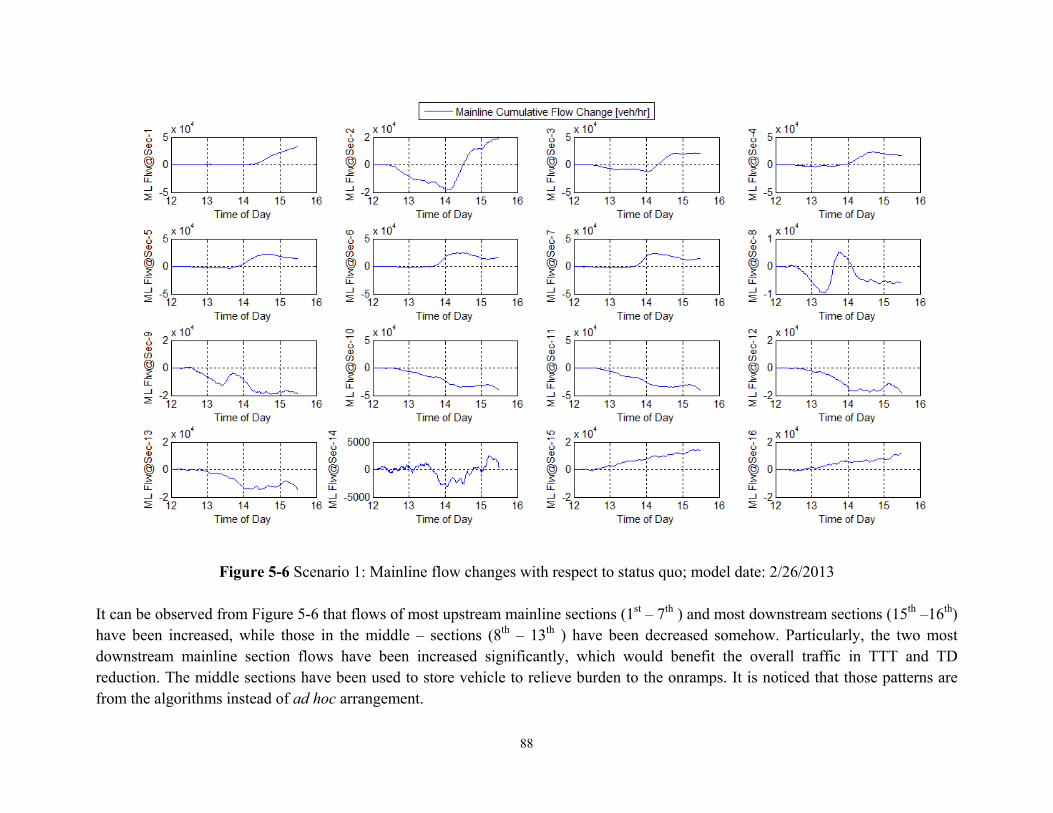
88

Figure 5-6 Scenario 1: Mainline flow changes with respect to status quo; model date: 2/26/2013

It can be observed from Figure 5-6 that flows of most upstream mainline sections (1st – 7th ) and most downstream sections (15th –16th) have been increased, while those in the middle – sections (8th – 13th ) have been decreased somehow. Particularly, the two most downstream mainline section flows have been increased significantly, which would benefit the overall traffic in TTT and TD reduction. The middle sections have been used to store vehicle to relieve burden to the onramps. It is noticed that those patterns are from the algorithms instead of ad hoc arrangement.

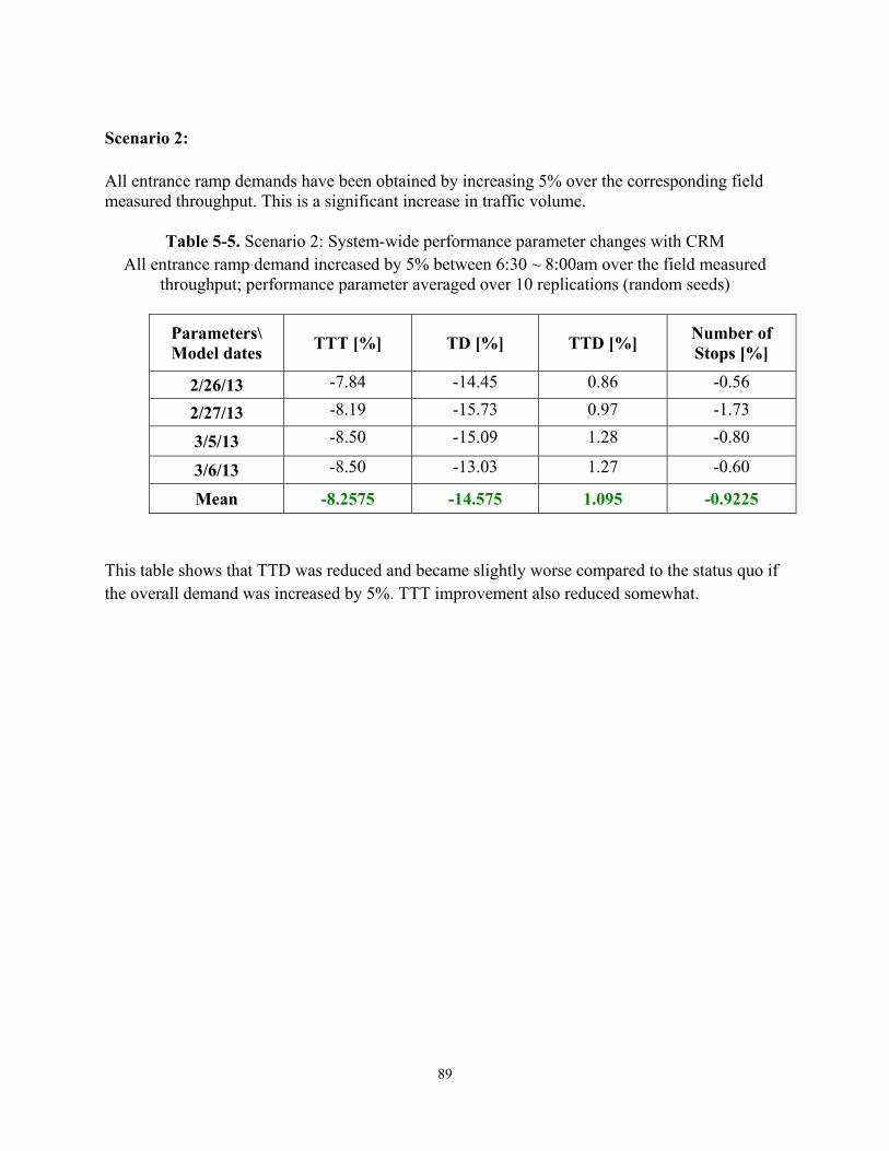
89

Scenario 2:

All entrance ramp demands have been obtained by increasing 5% over the corresponding field measured throughput. This is a significant increase in traffic volume.

Table 5-5. Scenario 2: System-wide performance parameter changes with CRM All entrance ramp demand increased by 5% between 6:30 ~ 8:00am over the field measured

throughput; performance parameter averaged over 10 replications (random seeds)

Parameters\ Model dates

TTT [%] TD [%] TTD [%] Number of Stops [%]

2/26/13 -7.84 -14.45 0.86 -0.56

2/27/13 -8.19 -15.73 0.97 -1.73

3/5/13 -8.50 -15.09 1.28 -0.80

3/6/13 -8.50 -13.03 1.27 -0.60

Mean -8.2575 -14.575 1.095 -0.9225

This table shows that TTD was reduced and became slightly worse compared to the status quo if the overall demand was increased by 5%. TTT improvement also reduced somewhat.

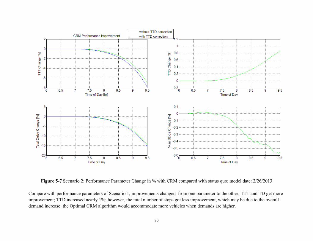
90

Figure 5-7 Scenario 2: Performance Parameter Change in % with CRM compared with status quo; model date: 2/26/2013

Compare with performance parameters of Scenario 1, improvements changed from one parameter to the other: TTT and TD get more improvement; TTD increased nearly 1%; however, the total number of stops got less improvement, which may be due to the overall demand increase: the Optimal CRM algorithm would accommodate more vehicles when demands are higher.

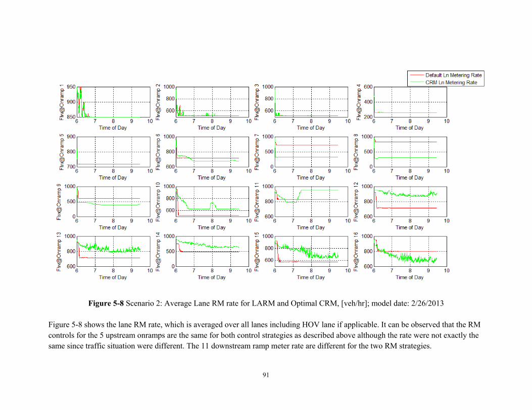
91

Figure 5-8 Scenario 2: Average Lane RM rate for LARM and Optimal CRM, [veh/hr]; model date: 2/26/2013

Figure 5-8 shows the lane RM rate, which is averaged over all lanes including HOV lane if applicable. It can be observed that the RM controls for the 5 upstream onramps are the same for both control strategies as described above although the rate were not exactly the same since traffic situation were different. The 11 downstream ramp meter rate are different for the two RM strategies.

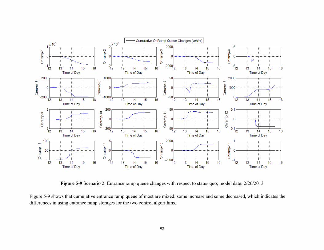
92

Figure 5-9 Scenario 2: Entrance ramp queue changes with respect to status quo; model date: 2/26/2013

Figure 5-9 shows that cumulative entrance ramp queue of most are mixed: some increase and some decreased, which indicates the differences in using entrance ramp storages for the two control algorithms..

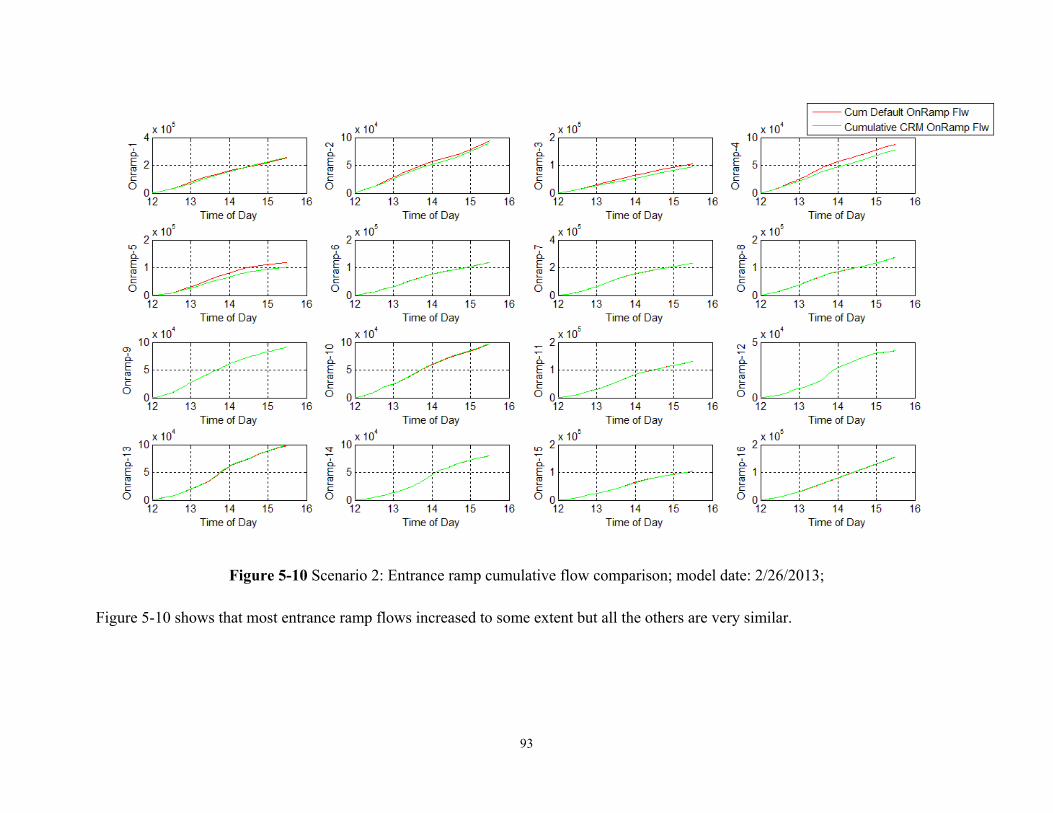
93

Figure 5-10 Scenario 2: Entrance ramp cumulative flow comparison; model date: 2/26/2013;

Figure 5-10 shows that most entrance ramp flows increased to some extent but all the others are very similar.

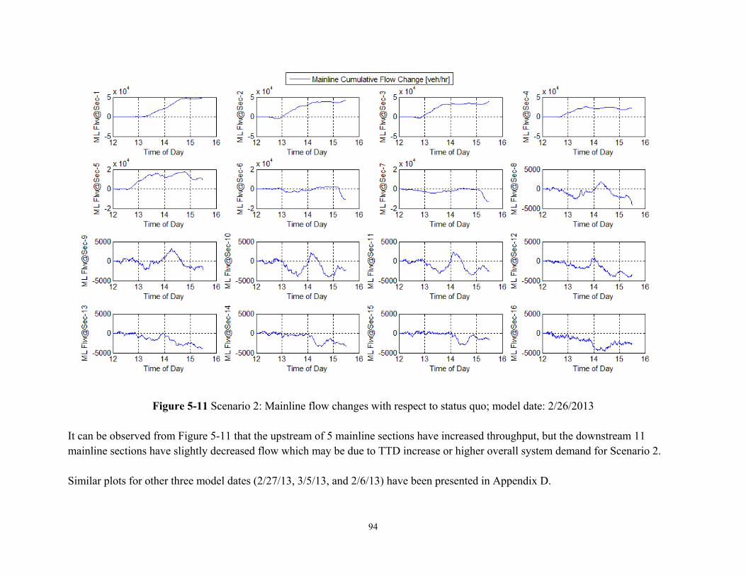
94

Figure 5-11 Scenario 2: Mainline flow changes with respect to status quo; model date: 2/26/2013

It can be observed from Figure 5-11 that the upstream of 5 mainline sections have increased throughput, but the downstream 11 mainline sections have slightly decreased flow which may be due to TTD increase or higher overall system demand for Scenario 2. Similar plots for other three model dates (2/27/13, 3/5/13, and 2/6/13) have been presented in Appendix D.

95

5.5 Summary of CRM Algorithm Characteristics

Comparing the simulation results of the three traffic scenarios, we could draw the following conclusions, which need to be checked with field tests:

(1) Optimal CRM with Queue-Overwrite could potentially achieve mobility as well as safety improvement compared to LARM since TTT, TD and TNOS has been reduced in simulation;

(2) The CRM algorithm with Queue Overwrite tends to improve TTT and TD; and to improve Total Number of Stops if the demand is not too high;

(3) if the overall system demand is higher, the improvement in TTD increased to nearly 1%, but the total number of stops reduced to below 1% which may be due to the need for the system to accommodate more vehicles;

(4) The improvement for flows of mainline sections are mixed: some sections increased and some decreased; with the overall system demand increase to 5%, throughput improvement for sections reduced somehow;

(5) It is not that all entrance ramp queues will be reduced; instead, some onramps have to be used to hold some vehicles to guarantee that the mainline has better throughput when the demand is too high.

(6) On average (of Table 5-4 and Table 5-5), the following performance improvement could be achieved:

TTT reduction is over 8%

TD reduction is over 15%

TTD decreases 0.5%

TNOS reduction about 2.9%

96

Chapter 6. Performance Parameters for Evaluation of VSL and CRM

The performance parameters are very important in the evaluation of the algorithm for field testing. Firstly, they should reflect the performance of the traffic in some essential aspects considering the collective and stochastic behavior of the traffic; secondly, they should be quantifiable for evaluation and should be uniform for all the algorithms/methods implemented – using the same ruler for all; thirdly, it should be practical in the sense that the required sensor measurement data are available; and lastly, it should be simple enough for calculation. The enclosed table summarizes some candidate performance parameters used in VSL/VSA and CRM. However, for this project, it is only necessary to select a subset from it since some performance parameters would need longer time data for evaluation. Some will need higher resolution data including vehicle data for evaluation, which is out of the scope of this project.

Table 6-1 lists the parameters used in research for performance evaluation of VSL and CRM. Table 6-2 lists a set of suggested performance parameters which could be used in this project based on the available sensor detection.

It is noted that Caltrans District 4 can access the event loop data (60 Hz or higher frequency) which is necessary and sufficient for better traffic speed estimation and vehicle-length-based classification. Those estimations will be used for performance evaluation. Most other performance parameters listed in Table 6-2 can be evaluated with 30 s PeMS raw data.

For combined VSL and CRM one could use the combined set of parameters for both of them.

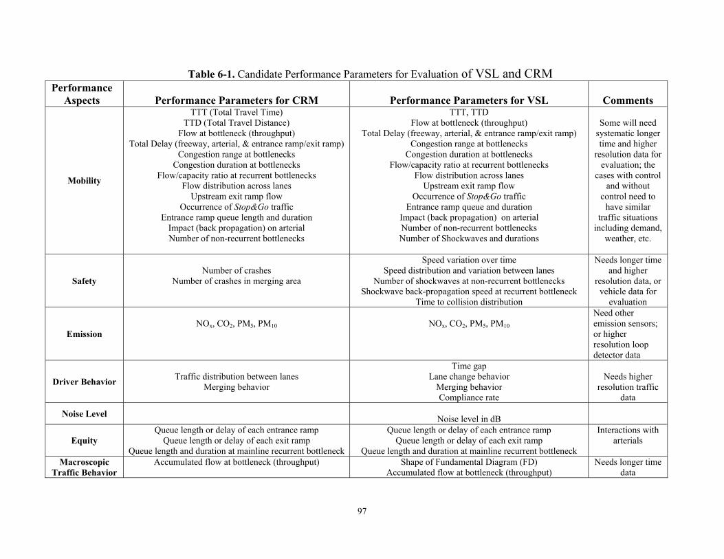
97

Table 6-1. Candidate Performance Parameters for Evaluation of VSL and CRM Performance

Aspects

Performance Parameters for CRM

Performance Parameters for VSL

Comments

Mobility

TTT (Total Travel Time) TTD (Total Travel Distance)

Flow at bottleneck (throughput) Total Delay (freeway, arterial, & entrance ramp/exit ramp)

Congestion range at bottlenecks Congestion duration at bottlenecks

Flow/capacity ratio at recurrent bottlenecks Flow distribution across lanes

Upstream exit ramp flow Occurrence of Stop&Go traffic

Entrance ramp queue length and duration Impact (back propagation) on arterial Number of non-recurrent bottlenecks

TTT, TTD Flow at bottleneck (throughput)

Total Delay (freeway, arterial, & entrance ramp/exit ramp) Congestion range at bottlenecks

Congestion duration at bottlenecks Flow/capacity ratio at recurrent bottlenecks

Flow distribution across lanes Upstream exit ramp flow

Occurrence of Stop&Go traffic Entrance ramp queue and duration

Impact (back propagation) on arterial Number of non-recurrent bottlenecks Number of Shockwaves and durations

Some will need

systematic longer time and higher

resolution data for evaluation; the

cases with control and without

control need to have similar

traffic situations including demand,

weather, etc.

Safety

Number of crashes

Number of crashes in merging area

Speed variation over time Speed distribution and variation between lanes

Number of shockwaves at non-recurrent bottlenecks Shockwave back-propagation speed at recurrent bottleneck

Time to collision distribution

Needs longer time and higher

resolution data, or vehicle data for

evaluation

Emission

NOx, CO2, PM5, PM10

NOx, CO2, PM5, PM10

Need other emission sensors; or higher resolution loop detector data

Driver Behavior

Traffic distribution between lanes

Merging behavior

Time gap Lane change behavior

Merging behavior Compliance rate

Needs higher

resolution traffic data

Noise Level

Noise level in dB

Equity Queue length or delay of each entrance ramp

Queue length or delay of each exit ramp Queue length and duration at mainline recurrent bottleneck

Queue length or delay of each entrance ramp Queue length or delay of each exit ramp

Queue length and duration at mainline recurrent bottleneck

Interactions with arterials

Macroscopic Traffic Behavior

Accumulated flow at bottleneck (throughput) Shape of Fundamental Diagram (FD) Accumulated flow at bottleneck (throughput)

Needs longer time data

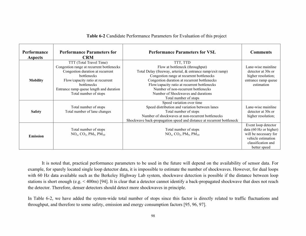
98

Table 6-2 Candidate Performance Parameters for Evaluation of this project

Performance Aspects

Performance Parameters for

CRM

Performance Parameters for VSL

Comments

Mobility

TTT (Total Travel Time) Congestion range at recurrent bottlenecks

Congestion duration at recurrent bottlenecks

Flow/capacity ratio at recurrent bottlenecks

Entrance ramp queue length and duration Total number of stops

TTT, TTD Flow at bottleneck (throughput)

Total Delay (freeway, arterial, & entrance ramp/exit ramp) Congestion range at recurrent bottlenecks

Congestion duration at recurrent bottlenecks Flow/capacity ratio at recurrent bottlenecks

Number of non-recurrent bottlenecks Number of Shockwaves and durations

Total number of stops

Lane-wise mainline

detector at 30s or higher resolution;

entrance ramp queue estimation

Safety

Total number of stops

Total number of lane changes

Speed variation over time Speed distribution and variation between lanes

Total number of stops Number of shockwaves at non-recurrent bottlenecks

Shockwave back-propagation speed and distance at recurrent bottleneck

Lane-wise mainline

detector at 30s or higher resolution;

Emission

Total number of stops NOx, CO2, PM5, PM10

Total number of stops NOx, CO2, PM5, PM10

Event loop detector data (60 Hz or higher) will be necessary for vehicle estimation classification and

better speed

It is noted that, practical performance parameters to be used in the future will depend on the availability of sensor data. For example, for sparely located single loop detector data, it is impossible to estimate the number of shockwaves. However, for dual loops with 60 Hz data available such as the Berkeley Highway Lab system, shockwave detection is possible if the distance between loop stations is short enough (e.g. < 400m) [94]. It is clear that a detector cannot identify a back-propagated shockwave that does not reach the detector. Therefore, denser detectors should detect more shockwaves in principle.

In Table 6-2, we have added the system-wide total number of stops since this factor is directly related to traffic fluctuations and throughput, and therefore to some safety, emission and energy consumption factors [95, 96, 97].

99

Chapter 7. Concluding Remarks and Future Research

RM is the most widely used freeway traffic congestion mitigation means in California. However, current RM for freeway operation are fixed rate, TOD or TOD adaptive. They are all local RM strategies. It has been recognized that, for better system performance, it is necessary coordinate the metering rate along a freeway corridor. How long a freeway corridor, or the scope of the system, should be determined by traffic demand from onramps, road geometry, and distances between onramps. It only makes sense to coordinate onramps that are close together. How close should they be? In general, if the traffic congestion near the downstream entrance ramp would affect the traffic near the upstream entrance ramp, then those two entrance ramp meters should be coordinated.

The objective of this project is to select one or two sites among CA freeways that are suitable for the implementation of a test of the algorithm developed in a former project funded by the FHWA Exploratory Advanced Research Program.

Site selection is critical to the success of the project. On one hand, the site should represent most freeway corridors in CA. On the other hand, the scope of work should be accomplished within the limited budget, which limits the system scale. The most important factors for site selection include but not limited to:

Traffic demand is high to over-saturated in peak hours

The corridor has a recurrent bottleneck downstream

The most downstream bottleneck has the most significant traffic drop (the minimum capacity or largest v/c ratio)

Only closely located entrance ramp meter coordination could bring benefit

All the onramps are metered in the corridor

Upstream of the main bottleneck has adequate storage section

Sensors density, location and sensor data quality are very important

Sensor density: each upstream section has at least one detector 300~700 m apart

Entrance ramp flow and queue detection is critical for CRM to avoid spills back to arterials

Hardware setup for RM would allow for Coordinated RM strategy to be implemented

Then the team investigated several freeway corridors by extensive analysis of PeMS data and discussions with traffic engineers in Caltrans District 3 and District 4. As the outcome of those activities, the project team selected two candidate site suitable for implementation of the CRM field test. One is SR 99NB between Elk Grove and SR 50 interchange (Caltrans District 3). The other is I-880 NB near Auto Mall Parkway (Caltrans District 4).

100

After site selection, the project team modeled the network and calibrated the model against collected field data from PeMS of each VDS in the system. The model calibration criteria include the FHWA recommended GEH criterion for flow of freeway main lanes, RMSE and RMSQ of flow and occupancies on freeway main lanes, onramps and exit ramps. The HOV lane has been modeled and calibrated separately. The demand for HOV lane is estimated and calibrated based on HOV flow measurement of all the onramps and the most upstream of the freeway. The model has been preliminarily calibrated against 4 days of traffic data. The calibrated model is reasonably close to the real traffic.

The I-880 NB section was modeled by a visiting graduate student researcher and tested with a combined VSL and CRM algorithm, which indicated 5% traffic throughput and Total Delay improvements. There is a separate report documenting this modeling and simulation in Aimsun for the I-880 section [98].

This report is focused on the modeling of SR99 NB between upstream of Elk Grove and SR50 interchange after 12th Ave, which is about 13 miles long. Although it is not necessary to coordinate all the onramps for CRM since RMs with large separations do not need to be coordinated, they should be included in the simulation model since traffic in each section affects each other over the whole stretch. The selection of onramps that need to be coordinated is not trivial. It needs extensive traffic data analysis to make sure that their traffic would affect each other and their traffic conditions are relatively independent from upstream and downstream traffic. It is also necessary to investigate if the proposed CRM strategy would still contain the effects within the selected onramps to be coordinated since the coordination may change the overall traffic along the corridor. The project team preliminarily suggests that the following 11 downstream entrance ramp meters on SR99 NB be coordinated:

Calvine EB, WB

Mark Road EB, WB

Florine EB, WB

47th Ave EB, WB

Fruitridge EB, WB

12th Ave

However, such a list needs further confirmation though more data analysis and simulation to observe the effect of the proposed CRM strategy.

Two control strategies have been implemented: the field LARM (Local Adaptive Ramp Metering) have been implemented to the all the 16 onramps; the proposed Optimal CRM is only implemented for the 11 downstream ramp meters as listed above. Performance analysis has been conducted by comparing those two controls for all the simulation scenarios to be described below.

101

Based on the calibrated model, the CRM algorithm has been implemented and evaluated with respect to TTT, TD, TNOS. The latter are corrected with the percentage changes of TTD (Total Travel Distance) with respect to the status quo.

Simulations have been conducted for two traffic scenarios: (1) demands of a selected set of onramps (with IDs: 1, 6, 7, 8, 9) were obtained by increasing 5% over the corresponding field measured throughputs; (2) all the entrance ramp demands were obtained by increasing 5% over the corresponding field measured throughput. The reason for doing so is that those demand scenarios should capture wide range traffic situations. Each scenario has been simulated for 10 replications (random seeds) for each model date (2/26, 2/27, 3/5, 3/6) and the performance parameters were averaged over all the replications. Simulation results showed that traffic improvement can be obtained for the four parameters mentioned above for both scenario (1) and (2). Of all the performance parameters, improvements in TD (15%) and TTT (8%) are more significant than TNOS (2.9%) and TTD ( 0.5%).

The results here are just some preliminary results. There is still space for improvement of the performance of the algorithm with fining in simulation. This will include:

Tuning the weight between TTT and TD in the objective function to improve TD when only the demands for a selected set of onramps increased by 5%;

To improve the Total Number of Stops when the overall system demand is increased by 5%; Besides, the algorithm simulated here needs field test to confirm the performance

improvement.

102

References

[1]. Brinckerhoff, P., Synthesis of Active Traffic Management Experiences in Europe and the United States, Final Report, Pub. #FHWA-HOP-10-031, March 2010

[2] Bogenberger, K., and A. May, Advanced Coordinated Traffic Responsive Ramp Metering Strategies, California PATH Working Paper, UCB-ITS-PWP-99-19, 1999

[3] Payne H. J. (1971) Models of freeway traffic and control. Simulation Council Proc. 1, 5 l-6 1.

[4] Zhang, M., Kim, T., Nie, X., Jin, W., Chu, L., Recker, W. (2001) Evaluation of On-ramp Control Algorithms. California PATH Research Report UCB-ITS-PRR-2001-36, Berkeley, CA.

[5] Hadi, M. A., Coordinated traffic responsive ramp metering strategies – an assessment based on previous studies, Proc. of 12th ITS World Congress, San Francisco, CA, Nov. 2005

[6] Cassidy, M., Critique of a Freeway On-Ramp Metering Scheme and Broader Related Issues, Cassidy, University of California Institute of Transportation Studies Research Report UCB-ITS-RR-2002-04, 2002;

[7] Cassidy, M., Study of Traffic at a Freeway Merge and Roles for Ramp Metering, Cassidy, University of California Institute of Transportation Studies Research Report, UCB-ITS-RR-2002-02, 2002,

[8] Cassidy, M., Empirical Study of Ramp Metering and Capacity, Cassidy, University of California Institute of Transportation Studies Research Report UCB-ITS-RR-2002-05, 2002

[9] Gardes, Y., A. D., May, J. Dahlgren, and A. Skarbardonis, Bay Area Simulation and Ramp Metering Study,; California PATH Research Report UCB-ITS-PRR-2002-06, 2002

[10] Arnold, E. D. Jr., Ramp metering, a review of the literature, Virginia Transportation Research Council, (1998)

[11] Sisiopicu, V. P., Das, A., and Sullivan A., Application of freeway ramp metering in Alabama, Report of UTCA, Univ. Transportation Center in Alabama, 2005

[12] Ferrari, P., (1991). The control of motorway reliability, Transportation Research Part A., Vol. 25A, No. 6. pp. 419-427

[13] Papageorgiou, M., Kotsialos, A., 2002. Freeway ramp metering: an overview. IEEE Transactions on Intelligent Transportation Systems, 3 (4), 271–281.

103

[14] Scariza, J. R., Evaluation of Coordinated and Local Ramp Metering Algorithms using Microscopic Traffic Simulation, MSc. Thesis, MIT, 2003

[15] Recker, W., Development of an Adaptive Corridor Traffic Control Model, California PATH Research Report, UCB-ITS-PRR-2008-22

[16] Daganzo, C. F. The Cell Transmission Model: A Dynamic Representation of Highway Traffic Consistent with the Hydrodynamic Theory. Transportation Research, B, Vol. 28 (4), 1994, pp. 269-287.

[17] Lighthill M. J. and Whitham G. B. (1955a) On kinematic waves I. Flood movement on long rivers. Proc. Royal Society of London, Series A, 229, 281-316.

[18] Muñoz, L., Sun, X., Horowitz, R., and Alvarez, L., A Piecewise-Linearized Cell Transmission Model and Parameter Calibration Methodology, Trans. Research Record 1965, (2006), p183-191

[19] TOPL Project: http://path.berkeley.edu/topl/

[20] Kurzhanskiy, A. A., Modeling and Software Tools for Freeway Operational Planning, Ph D dissertation, University of California Berkeley, 2007

[29] Caltrans District 7, Ramp Metering Annual Report, Los Angeles and Ventura Counties, 2005-2006

[30] Shen W., and H.M. Zhang, Pareto-improving ramp metering strategies for reducing congestion in the morning commute, Transportation Research Part A, Vol. 44, 2010, p676–696

[31] Vong, V., Implementing Traffic Management Tools to Mitigate Freeway Congestion, CD ROM of 12th IFAC Symposium on Control in Transportation Systems, Redondo Beach, CA, USA, September 2 - 4, 2009

[32] Gaffney, J., Managed Motorways, A Matter of Control - VicRoads of Australia, Presentation at Session 254 (International Developments in Traffic Management), TRB Annual Meeting, Washington D. C., Jan 22-26, 2012

[33] Papamichail, I., Kosmatopoulos, E., Papageorgiou, M., Chrysoulakis, I., Gaffney, J. and Vong, V., HERO coordinated ramp metering implemented at the Monash Freeway, CD ROM, 89th Transportation Research Board Annual Meeting, Washington, D.C., January 10-14, 2010.

104

[34] Chen, A.; Khorashadi, B.; Chen-Nee Chuah; Ghosal, D.; Zhang, M., Smoothing Vehicular Traffic Flow Using Vehicular-Based Ad Hoc Networking & Computing Grid (VGrid), Proc. IEEE Conf. on Intelligent Transportation Syst., 2006, p349 – 354

[35]. Lin, P.-W., K.-P. Kang, and G.-L. Chang. Exploring the effectiveness of Variable Speed Limit controls on highway work-zone operations, Int. J. of Intelligent Transportation Systems, vol. 8, 2004, pp155–168

[36]. Alessandri, A., A. D. Febbraro, A. Ferrara, and E. Punta. Nonlinear optimization for freeway control using variable-speed signaling, IEEE Trans on Veh. Tech, 48(6), 1999, pp2042-2052

[37] Juan Z.; Zhang X., and Yao H., Simulation research and implemented effect analysis of variable speed limits on freeway, Proc. of the 7th IEEE Conference on Intelligent Transportation Systems, Oct. 3-6, 2004, p894 - 898

[38]. Hegyi, A.; De Schutter, B.; Hellendoorn, H., Optimal coordination of variable speed limits to suppress shock waves, Proc. 42nd IEEE CDC, Dec.9-12, 2003, p2768 - 2773

[39]. Hegyi, A., B. D. Schutter, and H. Hellendoorn. Optimal coordination of variable speed limits to suppress shock waves, IEEE Trans. on Intelligent Trans. Syst., vol. 6, 2005, pp102–112

[40]. Wang, H., W. Wang, X. Chen, J. Chen, and J. Li. Experimental features and characteristics of speed dispersion in urban freeway traffic, 86th TRB Annual Meeting, Jan 2007, Washington D. C.

[41]. Spiliopoulou, A. D., I. Papamichail, I., and M. Papageorgiou. Toll Plaza merging traffic control for throughput maximization, J. of Transportation Engineering , ASCE, 2010, pp 67

[42] Breton, P.; Hegyi, A.; De Schutter, B.; Hellendoorn, H., Shock wave elimination/reduction by optimal coordination of variable speed limits, Proceedings of the IEEE 5th International Conference on Intelligent Transportation Systems, 2002, Page(s):225 - 230

[43] van der Hoogen, E. and Smulders, S., Control by variable speed sign: results of the Dutch experiment, On 7th International Conference on Traffic Monitoring and Control, IEE Conference Publication, No. 391 p145-149, London, England, April 26-28, 1994

[44] Waller, S. T., Man WoNg, E. Ferguson, N. Nezamuddin, and D. Sun, Speed Harmonization and Peak-period Shoulder Use to Manage Urban Freeway Congestion, Center for Transportation Research at The University of Texas at Austin, October, 2009

105

[45] Yang, X., Y. Lu, and G. Chang, 2013. Proactive optimal variable speed limit control for recurrently congested freeway bottlenecks. The 92nd Transportation Research Board Annual Meeting, Jan 13-17, 2013, Washington DC.

[46] Sabawat, V and R. Young, Control Strategy for Rural Variable Speed Limit Corridor, 92nd TRB Annual Meeting, Jan 13-17, 2013,Washington D. C.

[47] Habtemichael, F., and L., de Picado Santos, 2013. Safety and operational benefits of VSL under different traffic conditions and driver compliance levels. The 92nd Transportation Research Board Annual Meeting, Washington DC.

[48] Islam, M., M., Hadiuzzaman, J., Fang, T., Qiu, and K., El-Basyouny, 2013. Assessing mobility and safety impacts of a variable speed limit control strategy. The 92nd Transportation Research Board Annual Meeting, Washington DC.

[49] Li, D., and P. Ranjitkar, performance evaluation of ramp metering algorithms combined with variable speed limits for Auckland motorway, 92nd TRB Annual Meeting, Jan 13-17, 2013, Washington D. C.

[50] Nissan, A., Evaluation of recommended variable speed limits for motorway traffic control: the case of E4-motorway in Stockholm, 92nd TRB Annual Meeting, Jan 13-17, 2013, Washington D. C.

[51] Yeo, H., and A. Skabardonis, Next Generation Simulation (NGSIM) Oversaturated Freeway Flow Algorithm: Task Order 9 Final Report, FHWA-HOP-07-098, Federal Highway Administration, US Department of Transportation, April 2007, 132 pp

[52] Yeo, H., A. Skabardonis, J. Halkias, J. Colyar, and V. Alexiadis, Oversaturated Freeway Flow Algorithm for Use in Next Generation Simulation, TRR No. 2088, TRB, Washington, D.C., 2008, pp. 68–79.

[53] Alexiadis, V., Colyar, J., Halkias, J., Hranac, R., and McHale, G. The Next Generation Simulation Program. ITE Journal, Vol. 74, No. 8, 2004, pp. 22-26.

[54] Dong J., and H. S. Mahmassani , Stochastic modeling of traffic flow breakdown phenomenon: application to predicting travel time reliability, 2011 14th Int. IEE ITS, Washington, DC, USA. Oct 5-7, 2011

[55] Harbord, B., J. White, K. McCabe, A. Riley, and S. Tarry, A flexible approach to motorway control, 13th ITS World Congress, London, Oct. 13, 2006

[56] Highway Agency, M25 Controller Motorways, Summary Report, 2007

106

[57] Bertini, R. L., Boice, S., and Bogenberger, K., Dynamics of a Variable Speed Limit System Surrounding a Bottleneck on a German Autobahn, 85th TRB Annual Meeting, Washington D. C., Jan. , 2006; also TRR, No. 1978, 2006, pp. 149–159.

[58] Robinson, M. D., Examples of Variable Speed Limit Applications, Speed Management Workshop, 79th TRB Annual Meeting, Jan. 9-13, 2000

[59] van den Hoogen, E., Smulders, and S., Advies, H., Control by variable speed signs: the results of the Dutch Experiment, IEE Conference on Road Monitoring and Control, April 26-28, 1994

[60] Dynamic Traffic Management, the ASF experience, EasyWay Annual Forum, Lisboa, Nov. 17th, 2010

[61] Rivey, F., Evaluation of the Dynamic Speed Limit System on the A13 motorway in France, EasyWay Annual Forum, Lisboa, Nov. 17th, 2010

[62] Hoogendoorn, S. P., W. Daamen, R.G. Hoogendoorn, and J.W. Goemans, Assessment of Dynamic Speed Limits on freeway A20 near Rotterdam, the Netherlands, CD ROM, 92nd TRB Annual Meeting, Jan 13-17, 2013,Washing D. C.

[63] Weikl, S., K. Bogenberger, and R. L. Bertini, Empirical Assessment of Traffic Management Effects of a Variable Speed Limit 3 System on a German Autobahn: Before and After, 92nd TRB Annual Meeting, Jan 13-17, 2013,Washington D. C.

[64] E22 Blekinge: Improvements of VSL system, East West Transportation Corridor II, EWTC II report Sweden, v0.5, 2012-05-16

[65] Warren, D., Variable Speed Limits, Making Work Zones Work Better Workshop, Orlando, Fl., 17/09/03, accessible at: http://ops.fhwa.dot.gov/wz/workshops/originals/Warren.ppt

[66] Hammond, P. J., The 2012 Congestion Report, WSDOT’s comprehensive annual analysis of state highway system performance, 11th edition, Washington State DOT, Aug. 26, 2012

[67] DeGaspari, M., P. J. Jin, W. Wall, and C. M. Walton, The effect of active traffic management on travel time reliability: a case study of i-5 in Seattle, 92nd TRB Annual Meeting, Jan 13-17, 2013, Washington D. C.

[68] Kianfar, J., P. Edara, and C. Sun, 2013. Operational analysis of a freeway variable speed limit system- case study of deployment in Missouri, 92nd TRB Annual Meeting, Jan 13-17, 2013, Washington D. C.

107

[69]. Papageorgiou, M., E. Kosmatopoulos, and I. Papamichail. Effects of Variable Speed Limits on motorway traffic, TRR No. 2047, TRB, 2008, pp37-48

[70] Chang, G.-L., S. Y. Park, and J. Paracha, ITS field demonstration: integration of variable speed limit control and travel time estimation for a recurrently congested highway, The 91st Transportation Research Board Annual Meeting, Washington DC.

[71] Hegyi, A., B. D. Schutter, and H. Hellendoorn. Optimal Coordination of Variable Speed Limits to Suppress Shock Waves. IEEE Transactions on Intelligent Transportation Systems, Vol. 6, 2005, pp. 102–112.

[72] Hegyi, A. and S.P. Hoogendoorn, Dynamic speed limit control to resolve shock waves on freeways – Field test results of the SPECIALIST algorithm, 13th Int. IEEE ITS, Madeira Island, Portugal, September 19-22, 2010

[73]. Papageorgiou, M., (1983). Applications of Automatic Control Concepts to Traffic Flow Modeling and Control. Lect. Notes in Control and Inf. Sc., Berlin, Germany: Springer

[74]. Abdel-Aty, M., and A. Dhindsa. Coordinated use of Variable Speed Limits and Ramp Metering for Improving Safety on Congested Freeways, 86th TRB Annual Meeting, Washington, D.C., January 21-25, 2007

[75]. Caligaris, C., S. Sacone, and S. Siri. Optimal ramp metering and variable speed signs for multiclass freeway traffic, Proc. of European Control Conference, Kos Greece, July 2-5, 2007

[76]. Alessandri, A., A. Di Febbraro, A. Ferrara, and E. Punta. Optimal control of freeways via speed signaling and ramp metering, Control Engineering Practice, vol. 6, 1998, pp771–780

[77]. Papamichail, I., K. Kampitaki, M. Papageorgiou, A. Messmer. Integrated Ramp Metering and Variable Speed Limit Control of Motorway Traffic Flow. CD-ROM of 17th IFAC World Congress, Seoul, Korea, 2008

[78] Hegyi, A.; De Schutter, B.; Hellendoorn, H.; van den Boom, T., Optimal coordination of ramp metering and variable speed control-an MPC approach, Proc. of the 2002 American Control Conference, vol.5, May 8-10, 2002, pp. 3600 - 3605

[79] Hegyi, A.; De Schutter, B.; Heelendoorn, J., MPC-based optimal coordination of variable speed limits to suppress shock waves in freeway traffic, Proceedings of the 2003 American Control Conference, vol. 5, June 4-6, 2003, pp. 4083 - 4088

108

[80]. Hegyi, A., B. D. Schutter, and H. Hellendoorn. Model predictive control for optimal coordination of ramp metering and variable speed limits, Transportation Research C, vol. 13, 2005, pp185–209

[81]. Carlson R.C., Papamichail I., Papageorgiou M. and Messmer A., Optimal mainstream traffic flow control of large scale motorway networks, Transportation Research Part C , Vol. 18, 2010, pp193-212

[82]. Carlson R.C., Papamichail I., Papageorgiou M. and Messmer A., Optimal motorway traffic flow control involving variable speed limits and ramp metering, Transportation Science , Vol. 44, pp.238-253, 2010.

[83] Lu, X. Y., T. Z. Qiu, P. Varaiya, R. Horowitz, and S. Shladover, Combining Variable Speed Limits with Ramp Metering for freeway traffic control, CD ROM of 2010 American Control Conference, Baltimore, Maryland, June 30 - July 2, 2010

[84] Lu, X. Y., P. Varaiya, R. Horowitz, D. Su and S. E. Shladover A novel freeway traffic control with variable speed limit and coordinated ramp metering, 90th TRB Annual Meeting, Washington, D. C., Jan. 23-27, 2011

[85] Lu, X. Y., P. Varaiya, R. Horowitz, D. y. Su, and S. E. Shladover, New Approach for Combined Freeway Variable Speed Limits and Coordinated Ramp Metering, IEEE ITS Conference, Sept. 19-22, Madeira Island, Portugal.

[86] Lu, X. Y., P. Varaiya, R. Horowitz, D. y. Su, and S. E. Shladover, New Approach for Combined Freeway Variable Speed Limits and Coordinated Ramp Metering, IEEE ITS Conf., Sept. 19-22, 2010, Madeira Island, Portugal

[87] Su, D., X. Y. Lu, P. Varaiya, R. Horowitz and S. E. Shladover, Integrated microscopic traffic control simulation and macroscopic traffic control design, 90th TRB Annual Meeting, Washington, D. C., Jan. 23-27, 2011

[88] Talebpour, A., and Hani S. Mahmassani, Speed Harmonization: Effectiveness Evaluation under Congested Conditions, 92nd TRB Annual Meeting, Jan 13-17, 2013, Washington D. C.

[89] Kwon, E., D. Brannan, K. Shouman, C. Isackson, and B. Arseneau, Development and Field Evaluation of Variable Advisory Speed Limit System for Work Zones, TRR No. 2015, TRB, Washington, D.C., 2007, pp. 12–18.

[90] Kwon, E., C. Park, D. Lau, and B. Kary, Minneosta Variable Speed Limit System -Adaptive Mitigation of Shock Waves for Safety and Efficiency of Traffic Flows, TRB Annual Meeting, Jan 2011

109

[91] http://www.dot.state.fl.us/trafficoperations/newsletters/2008/2008-010-oct.pdf: accessed in March 2013

[92] UK Highways Agency, Design Manual for Roads and Bridges: Volume 12, Section 2, Department for Transport, London, England, May 1996.

[93] WSDOT, Freeway System Operational Assessment - Paramics Calibration and Validation Guidelines (Draft), Technical Report I-33, Wisconsin DOT, District 2, June 2002. (http://www.wisdot.info/microsimulation/index.php?title=Model_Calibration)

[94] Lu, X. Y., Z. W. Kim, M. Cao, P. Varaiya, and R. Horowitz, Deliver a Set of Tools for Resolving Bad Inductive Loops and Correcting Bad Data, California PATH Report, UCB-ITS-PRR-2010-5

[95] Barth, M., and K. Boriboonsomsin, Traffic Congestion and Greenhouse Gases, ACCESS, No. 35, pp2-9

[96] Rakha, H., and Y. Ding, Impact of Stops on Vehicle Fuel Consumption, J. of Transp.

Engineering, Vol. 129, No. 1, January/February 2003, pp. 23-32, [97] Nesamani, K., L. Chu, M. McNally and R. Jayakrishnan, Estimation of Vehicular Emissions

by Capturing Traffic Variations, UCI-ITS-WP-05-6, Institute of Transportation Studies and Department of Civil and Environmental Engineering, U. C. Irvine, 2005

[98] Eikenbroek, O. A. L., Integrated Traffic Control with Variable Speed Limits and Coordinated Ramp Metering based on Traffic Stability, Final Report, University of Twente, the Netherlands, and California PATH, University of California, Berkeley, April to July, 2013

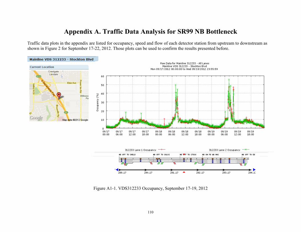
110

Appendix A. Traffic Data Analysis for SR99 NB Bottleneck

Traffic data plots in the appendix are listed for occupancy, speed and flow of each detector station from upstream to downstream as shown in Figure 2 for September 17-22, 2012. Those plots can be used to confirm the results presented before.

Figure A1-1. VDS312233 Occupancy, September 17-19, 2012

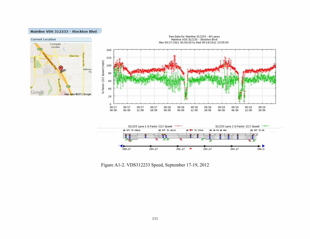
111

Figure A1-2. VDS312233 Speed, September 17-19, 2012

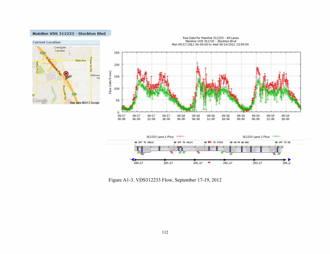
112

Figure A1-3. VDS312233 Flow, September 17-19, 2012

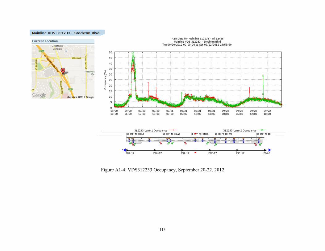
113

Figure A1-4. VDS312233 Occupancy, September 20-22, 2012

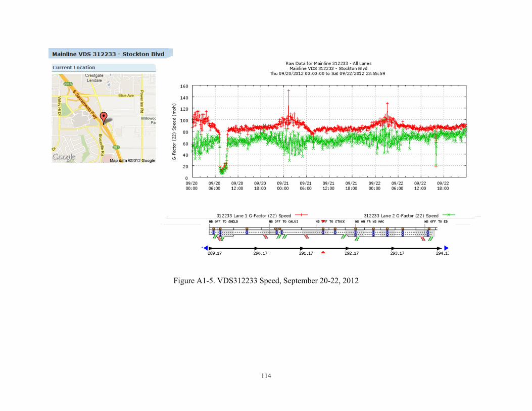
114

Figure A1-5. VDS312233 Speed, September 20-22, 2012

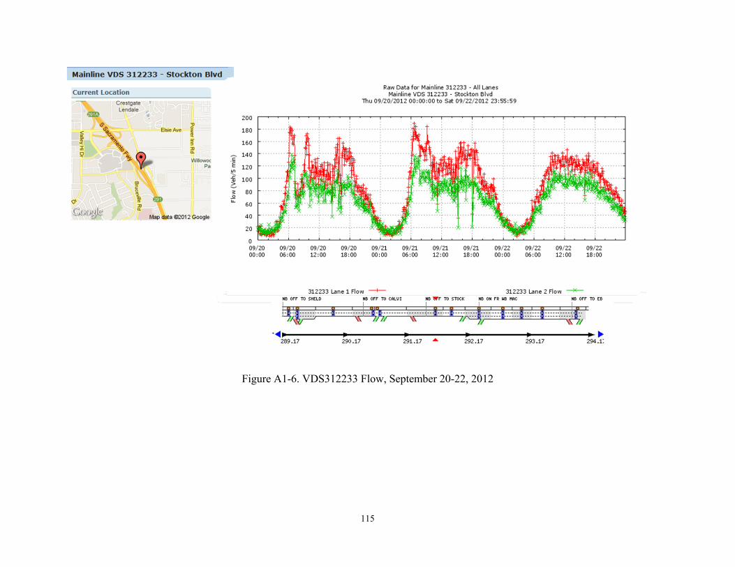
115

Figure A1-6. VDS312233 Flow, September 20-22, 2012

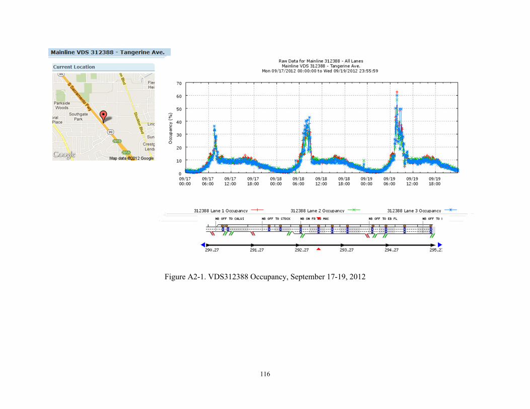
116

Figure A2-1. VDS312388 Occupancy, September 17-19, 2012

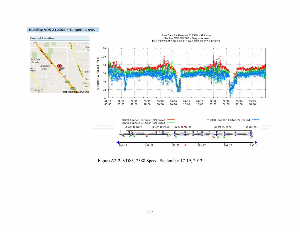
117

Figure A2-2. VDS312388 Speed, September 17-19, 2012

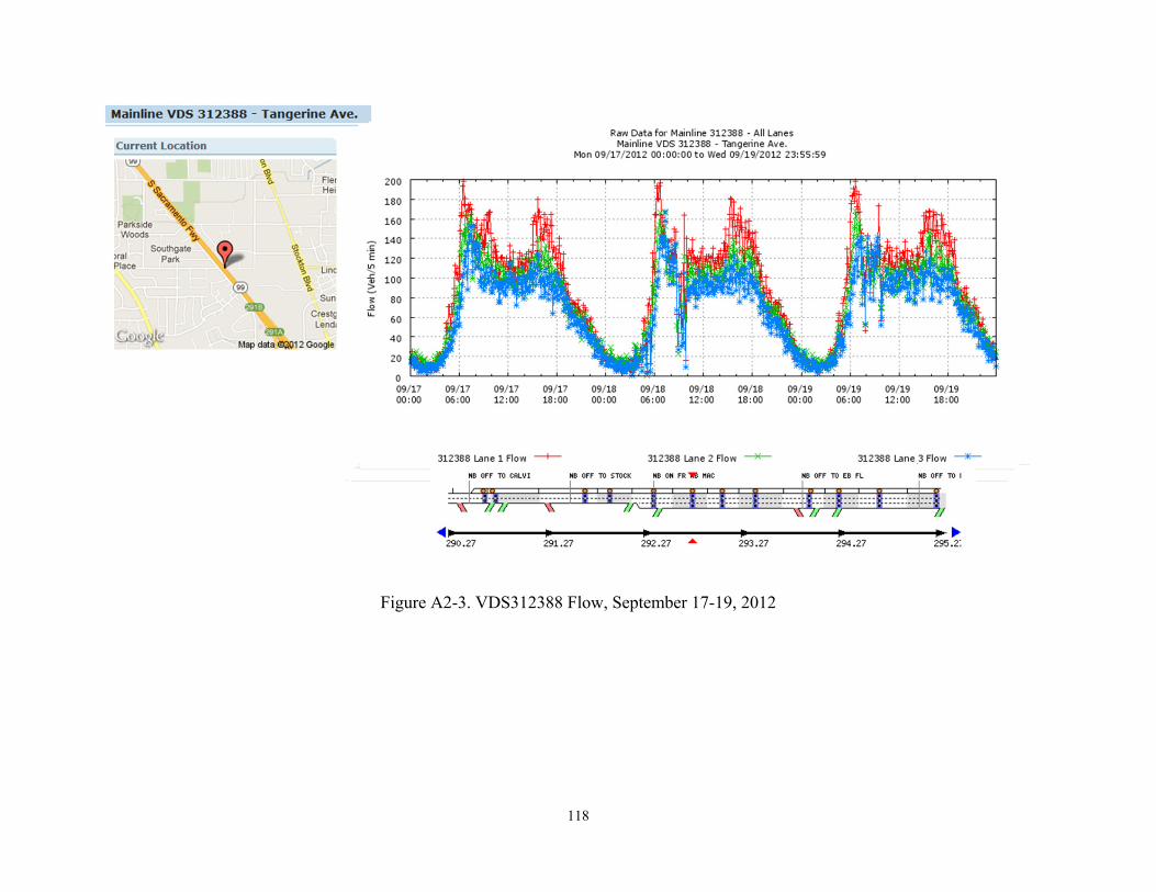
118

Figure A2-3. VDS312388 Flow, September 17-19, 2012

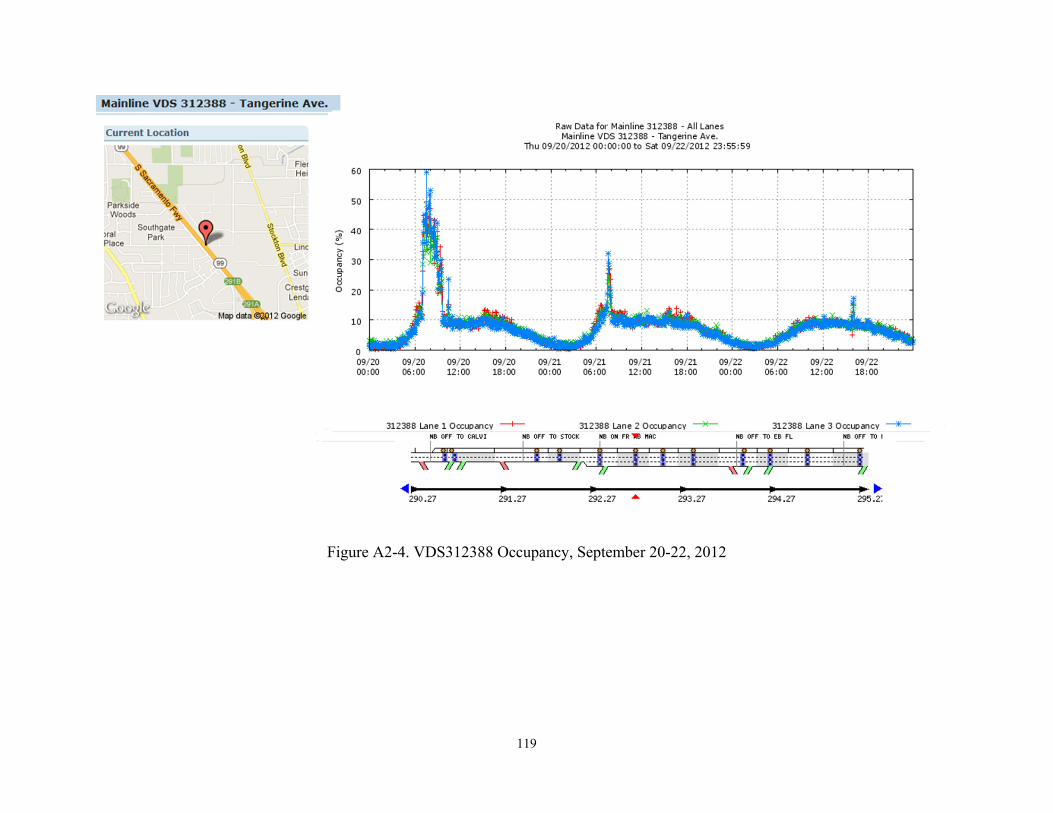
119

Figure A2-4. VDS312388 Occupancy, September 20-22, 2012

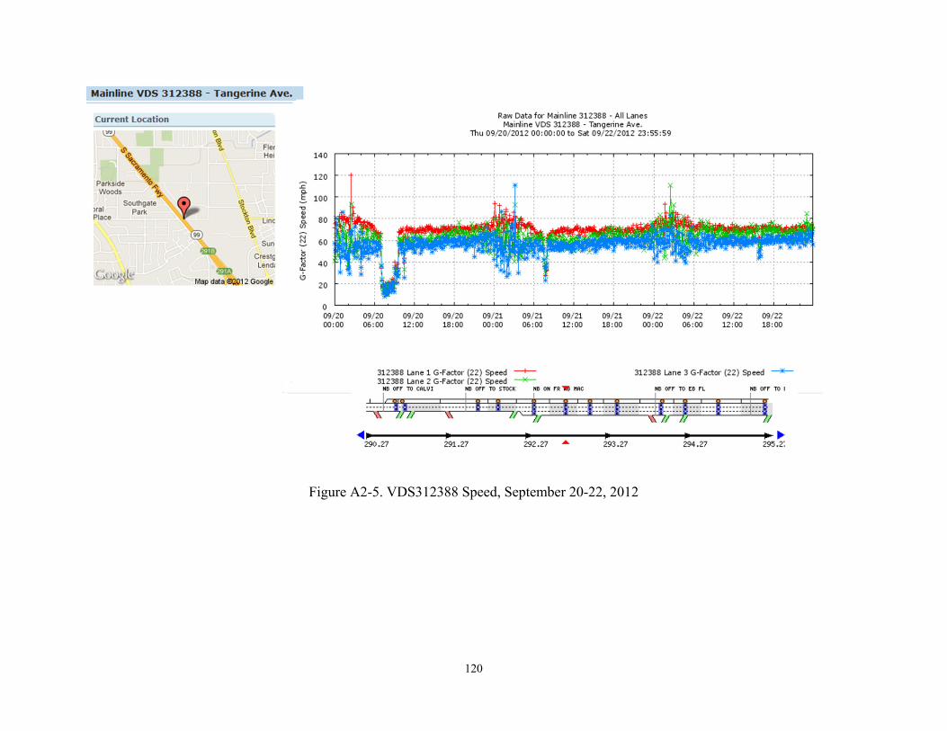
120

Figure A2-5. VDS312388 Speed, September 20-22, 2012

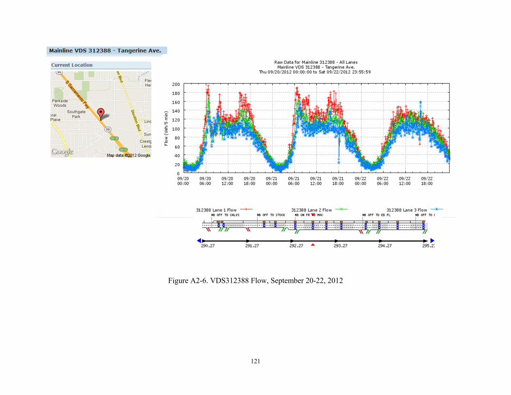
121

Figure A2-6. VDS312388 Flow, September 20-22, 2012

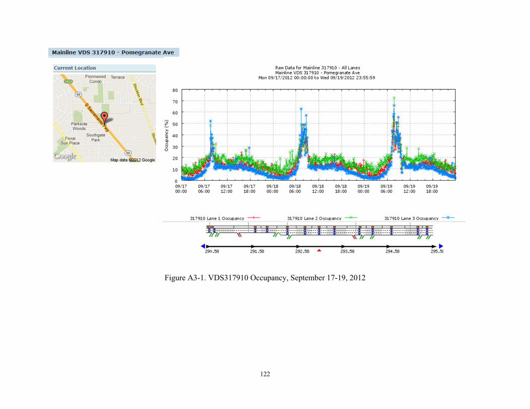
122

Figure A3-1. VDS317910 Occupancy, September 17-19, 2012

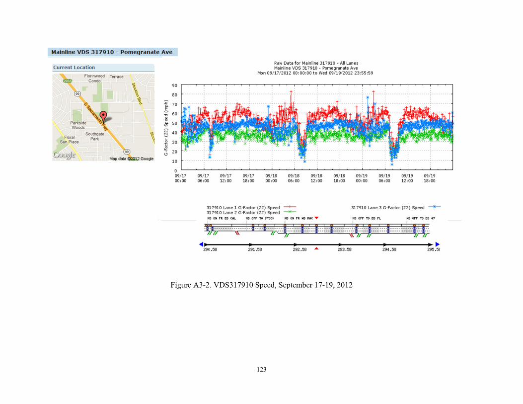
123

Figure A3-2. VDS317910 Speed, September 17-19, 2012

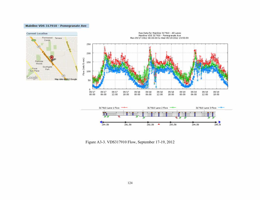
124

Figure A3-3. VDS317910 Flow, September 17-19, 2012

125

Figure A3-4. VDS317910 Occupancy, September 20-22, 2012

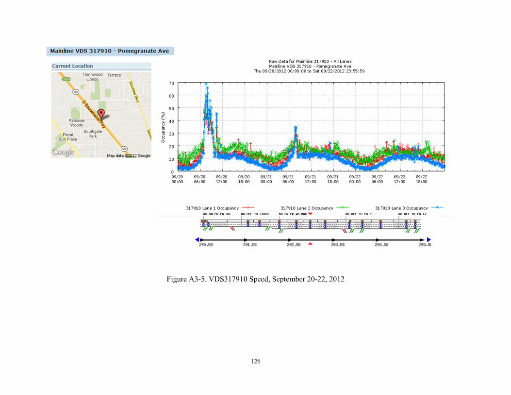
126

Figure A3-5. VDS317910 Speed, September 20-22, 2012

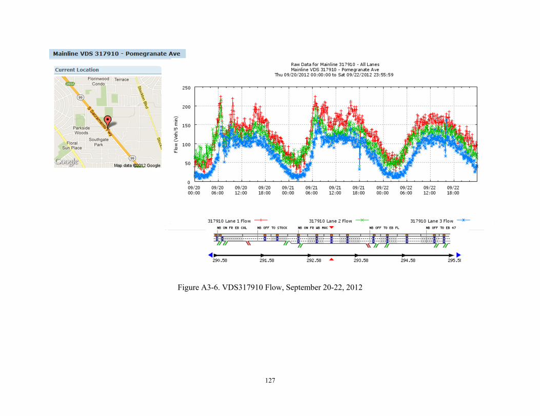
127

Figure A3-6. VDS317910 Flow, September 20-22, 2012

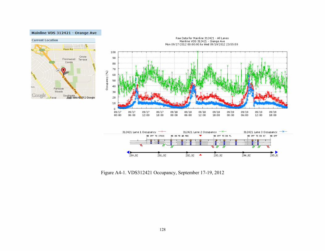
128

Figure A4-1. VDS312421 Occupancy, September 17-19, 2012

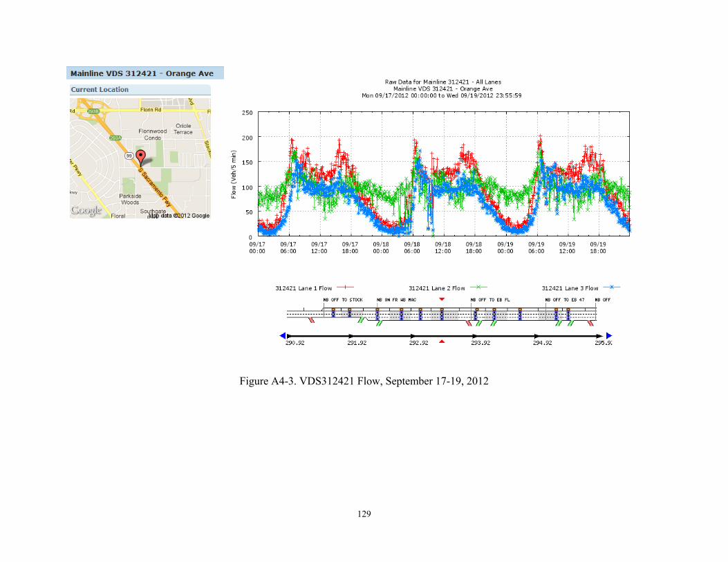
129

Figure A4-3. VDS312421 Flow, September 17-19, 2012

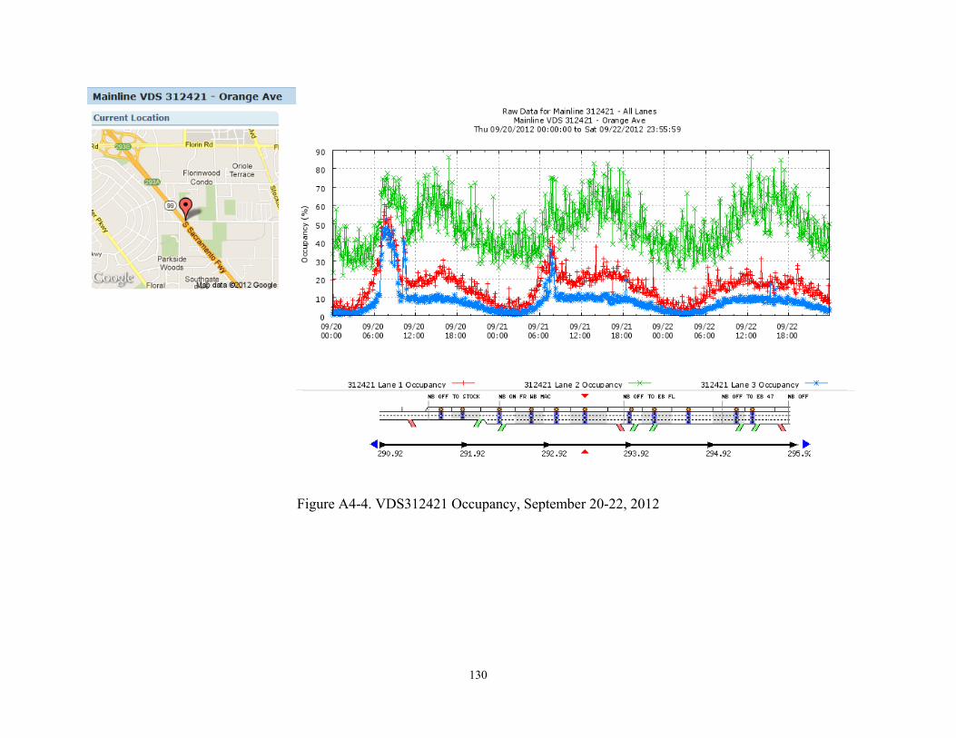
130

Figure A4-4. VDS312421 Occupancy, September 20-22, 2012

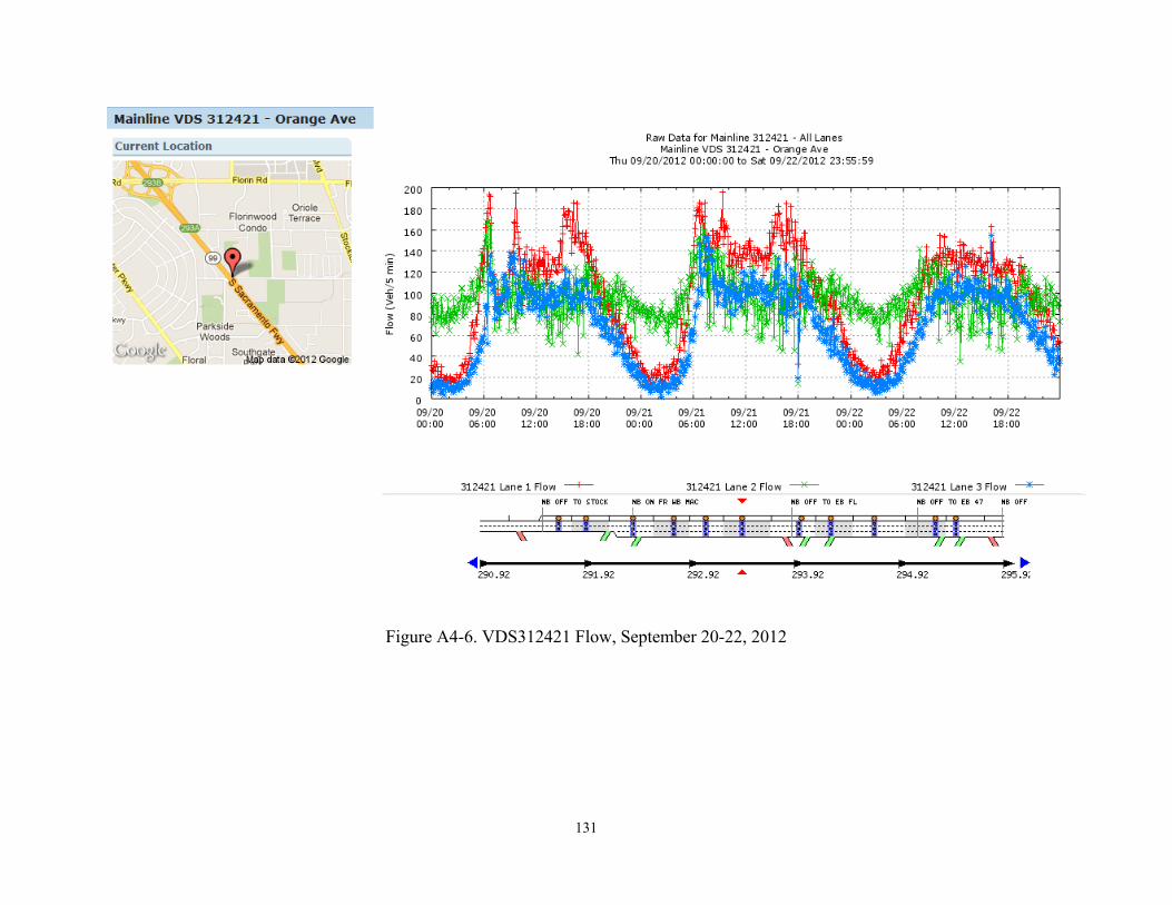
131

Figure A4-6. VDS312421 Flow, September 20-22, 2012

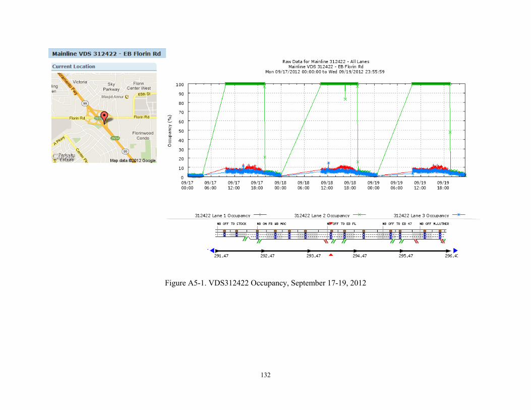
132

Figure A5-1. VDS312422 Occupancy, September 17-19, 2012

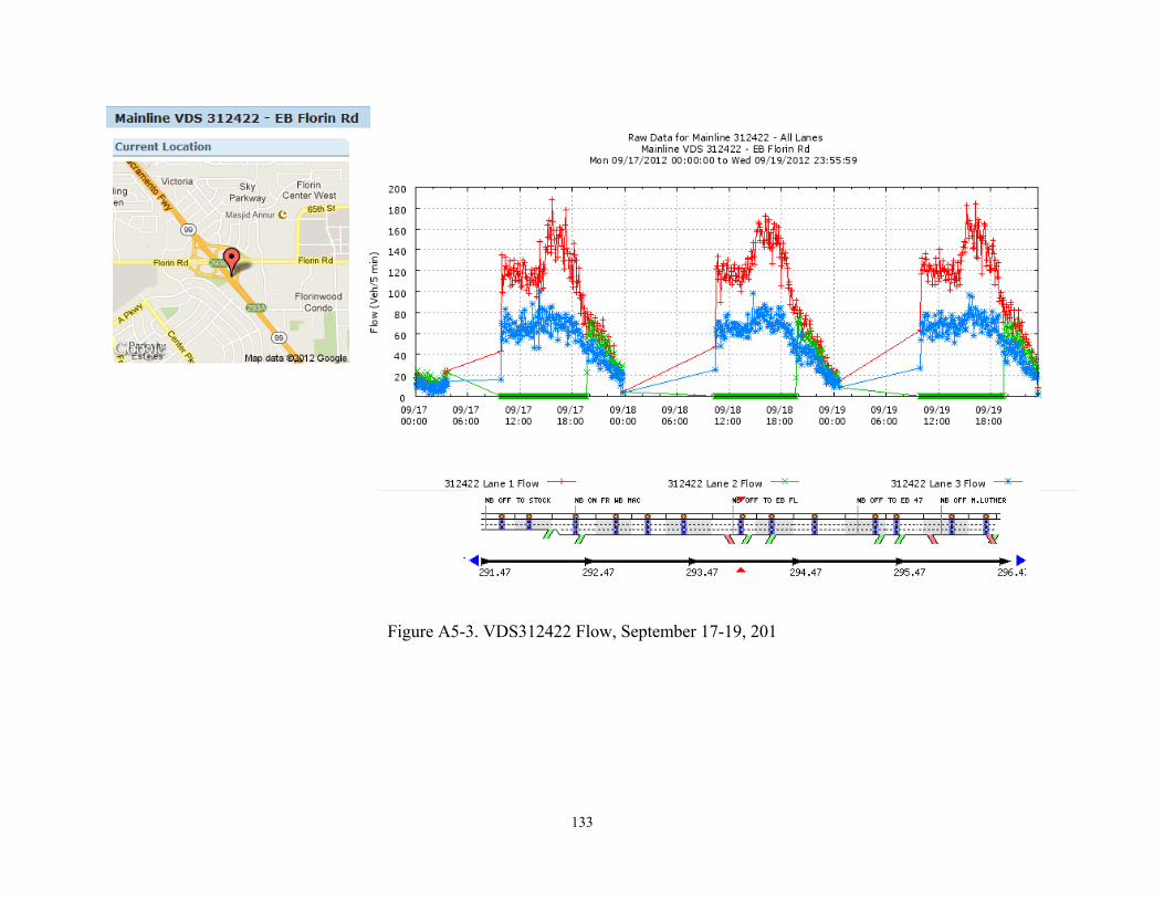
133

Figure A5-3. VDS312422 Flow, September 17-19, 201

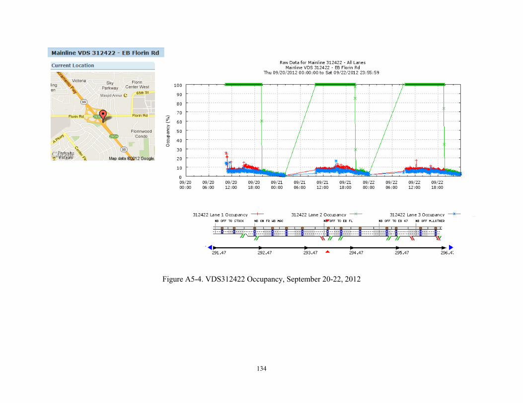
134

Figure A5-4. VDS312422 Occupancy, September 20-22, 2012

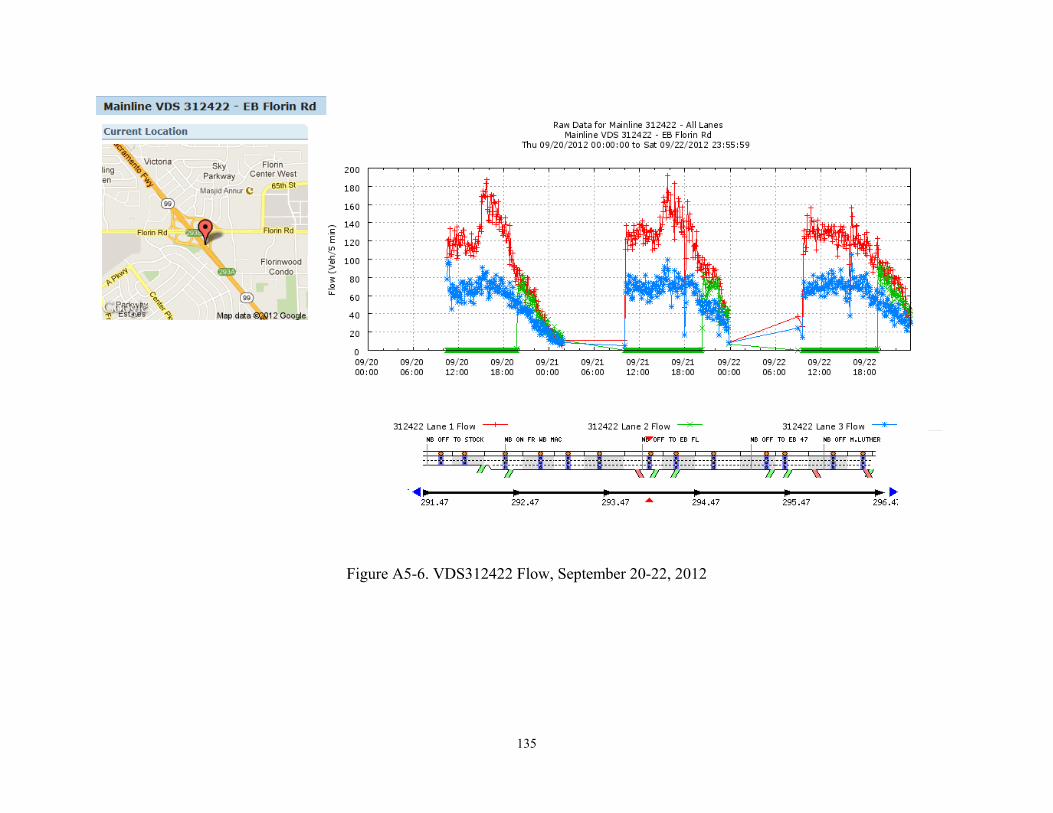
135

Figure A5-6. VDS312422 Flow, September 20-22, 2012

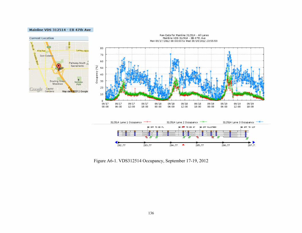
136

Figure A6-1. VDS312514 Occupancy, September 17-19, 2012

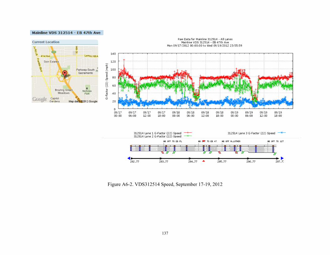
137

Figure A6-2. VDS312514 Speed, September 17-19, 2012

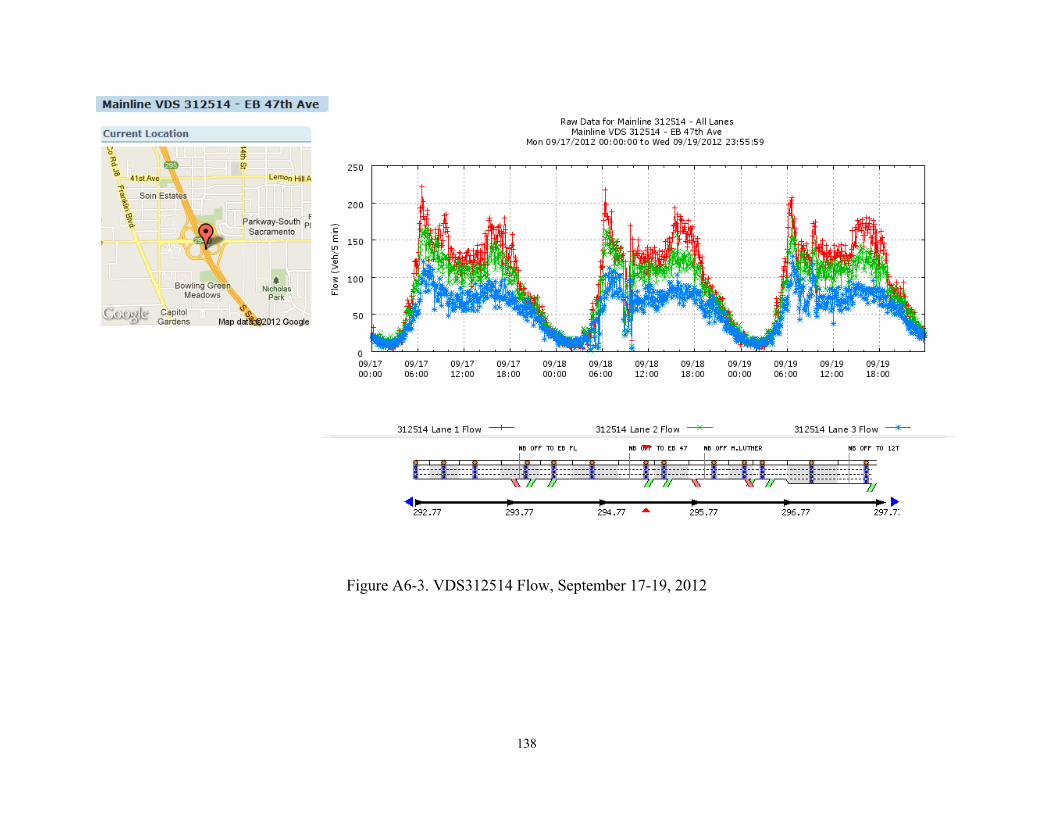
138

Figure A6-3. VDS312514 Flow, September 17-19, 2012

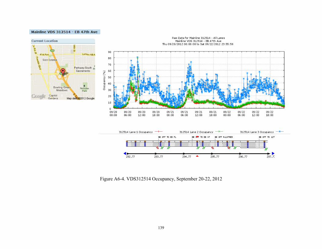
139

Figure A6-4. VDS312514 Occupancy, September 20-22, 2012

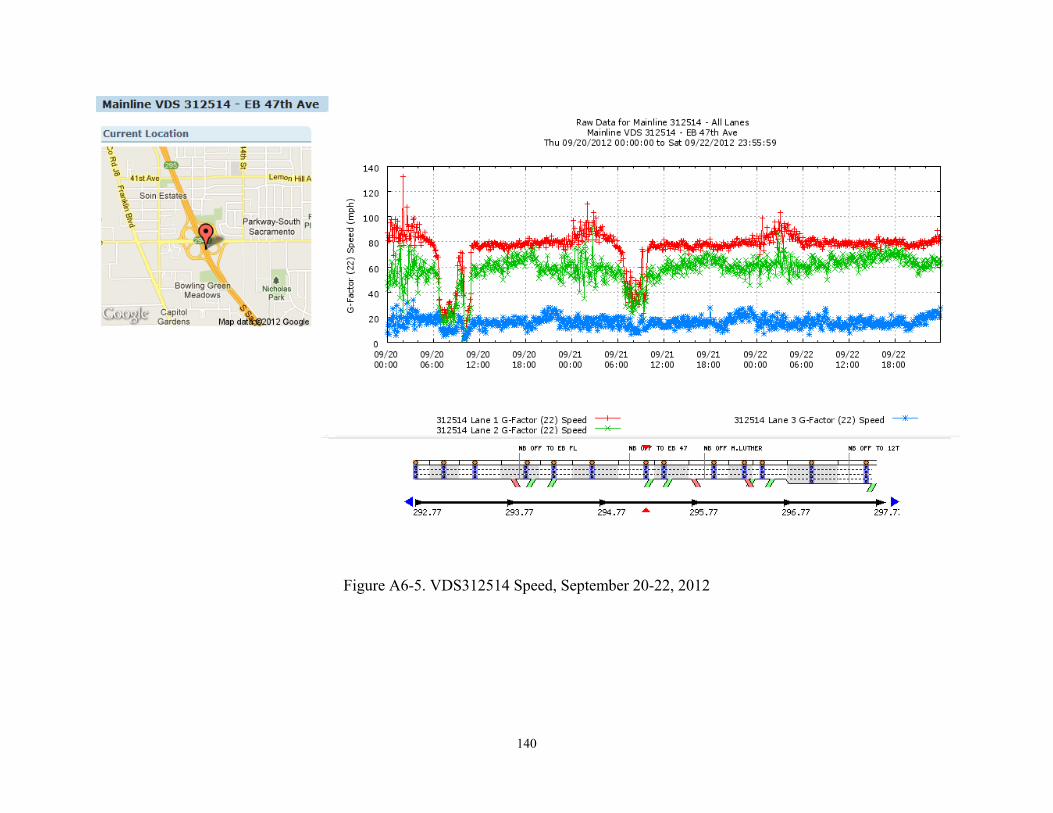
140

Figure A6-5. VDS312514 Speed, September 20-22, 2012

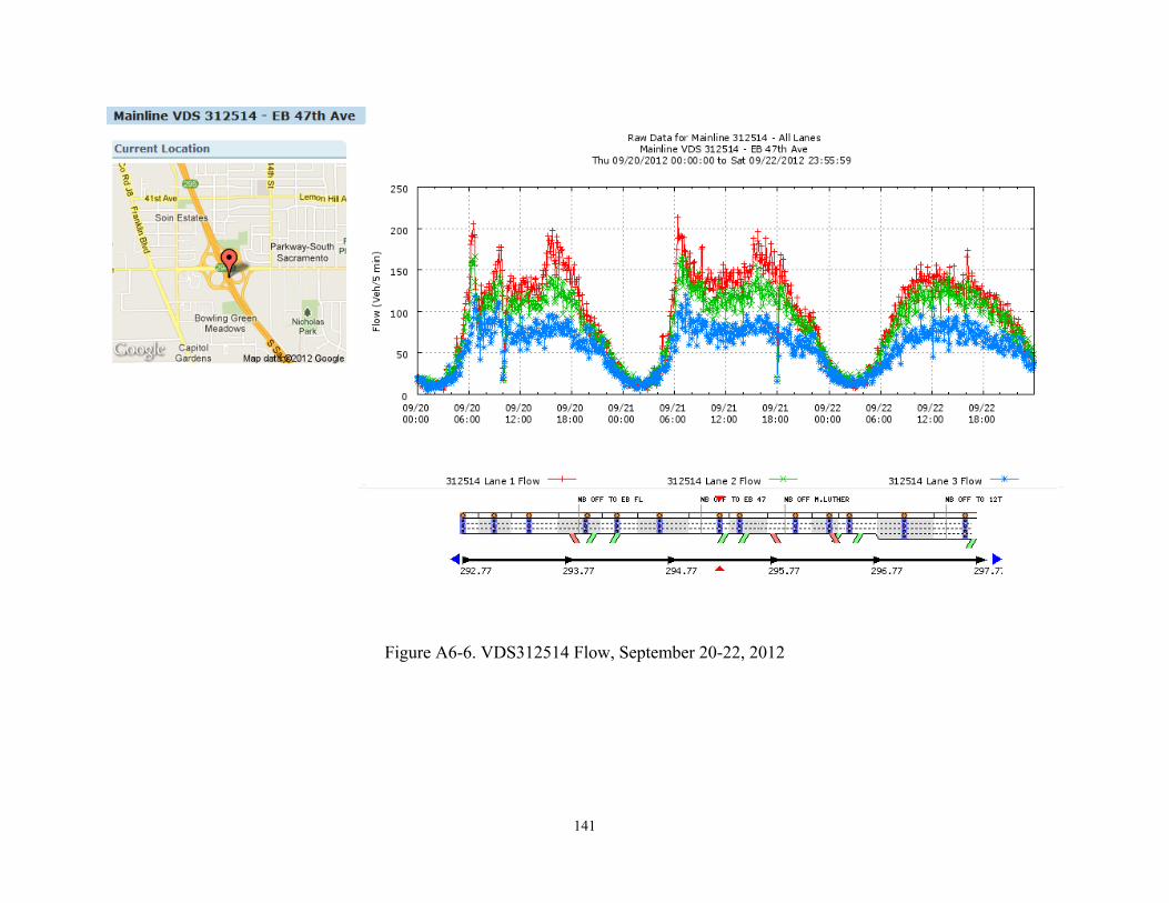
141

Figure A6-6. VDS312514 Flow, September 20-22, 2012

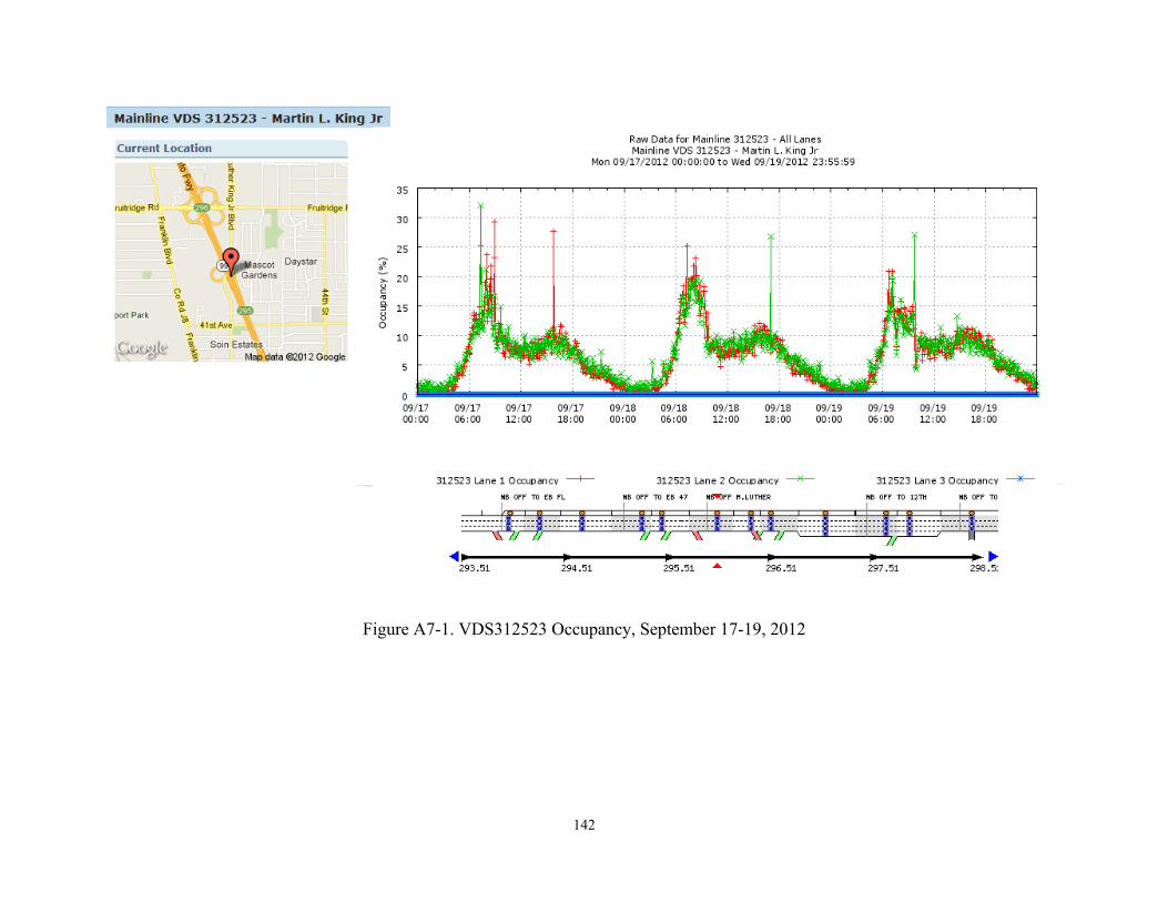
142

Figure A7-1. VDS312523 Occupancy, September 17-19, 2012

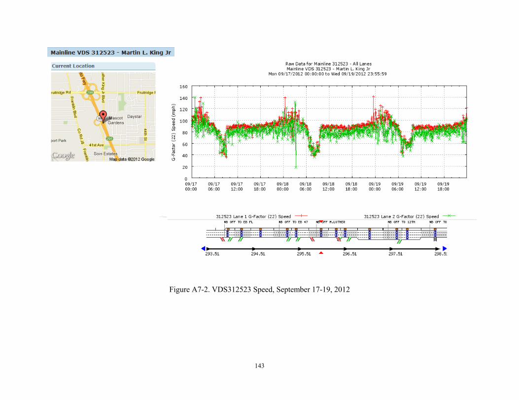
143

Figure A7-2. VDS312523 Speed, September 17-19, 2012

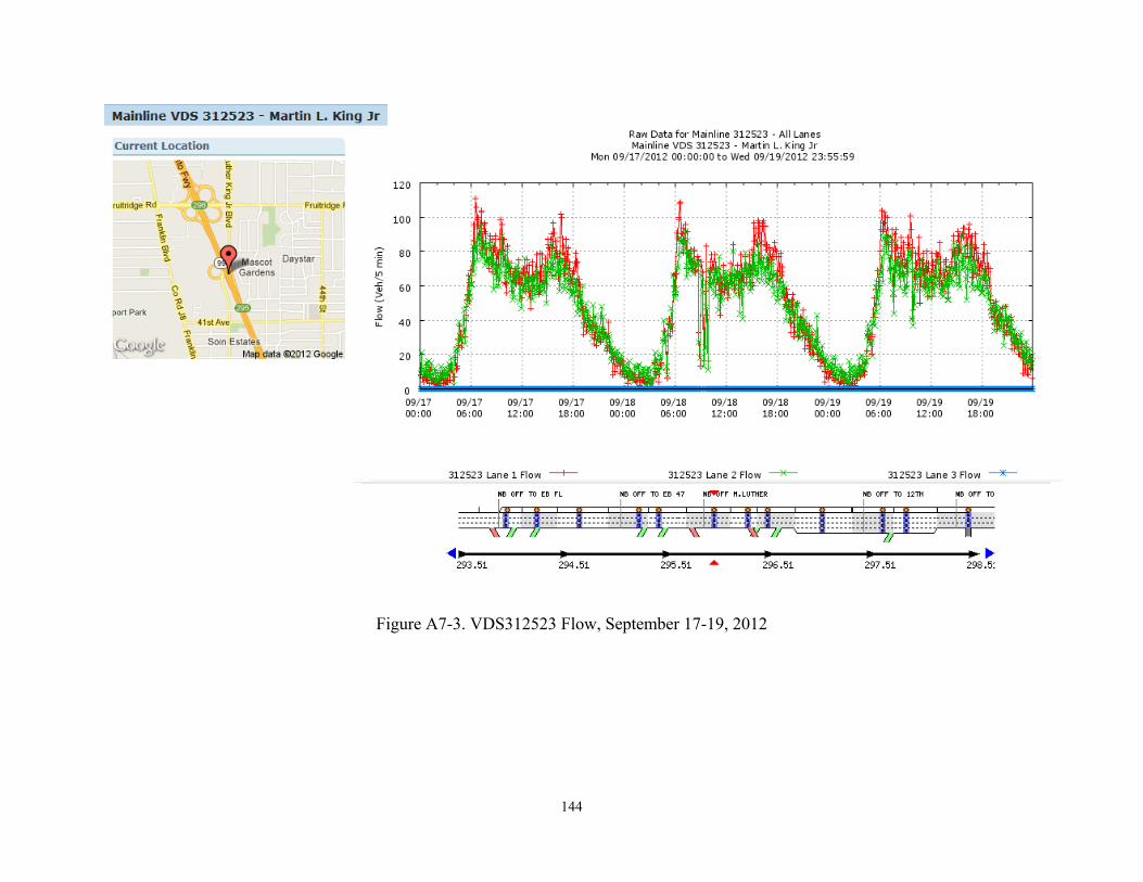
144

Figure A7-3. VDS312523 Flow, September 17-19, 2012

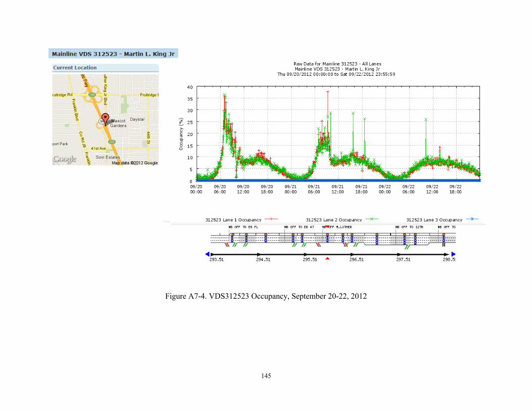
145

Figure A7-4. VDS312523 Occupancy, September 20-22, 2012

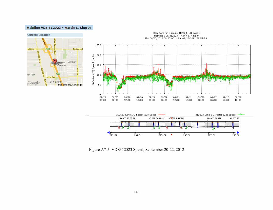
146

Figure A7-5. VDS312523 Speed, September 20-22, 2012

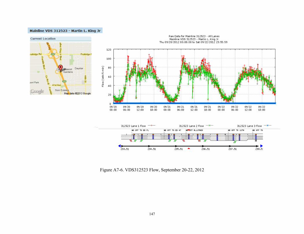
147

Figure A7-6. VDS312523 Flow, September 20-22, 2012

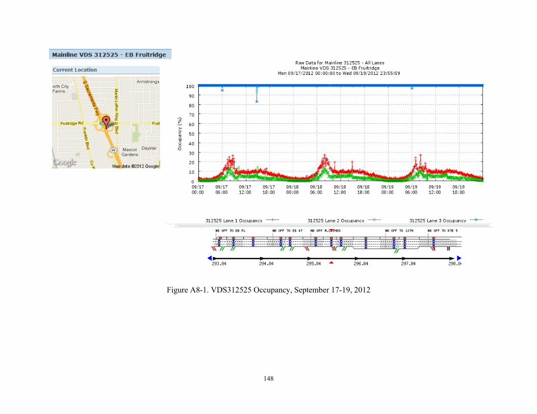
148

Figure A8-1. VDS312525 Occupancy, September 17-19, 2012

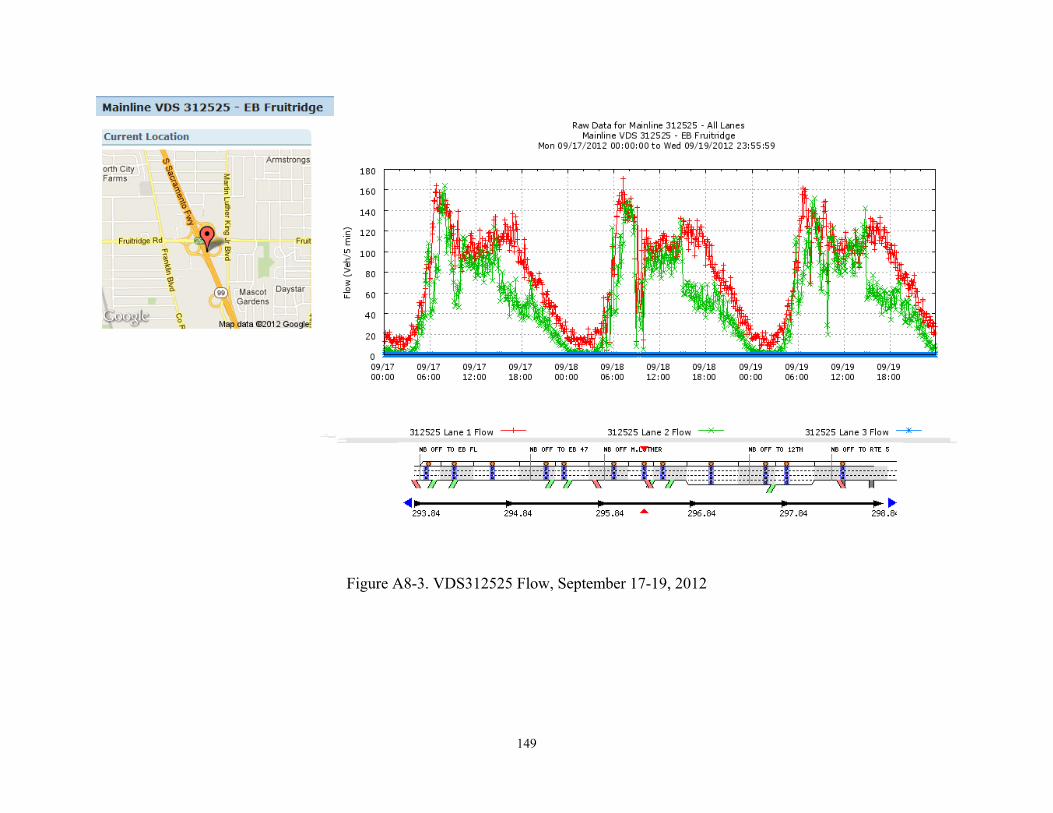
149

Figure A8-3. VDS312525 Flow, September 17-19, 2012

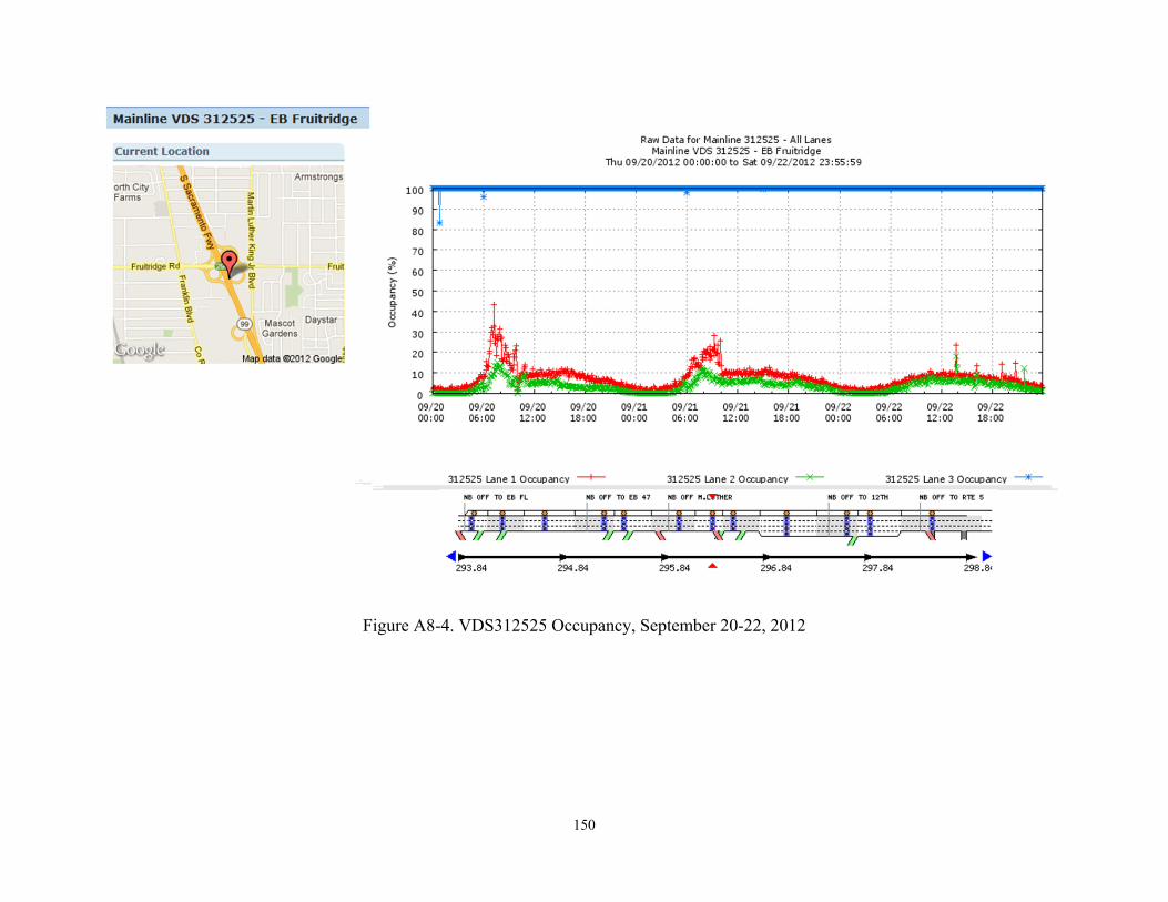
150

Figure A8-4. VDS312525 Occupancy, September 20-22, 2012

151

Figure A8-6. VDS312525 Flow, September 20-22, 2012

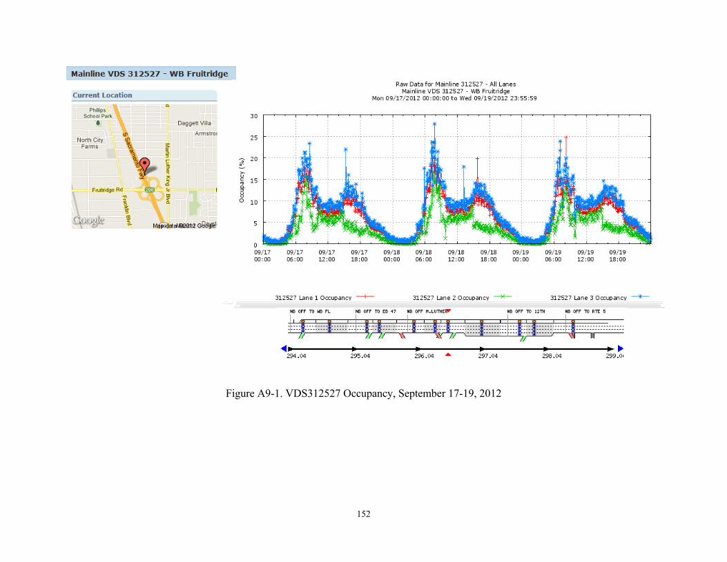
152

Figure A9-1. VDS312527 Occupancy, September 17-19, 2012

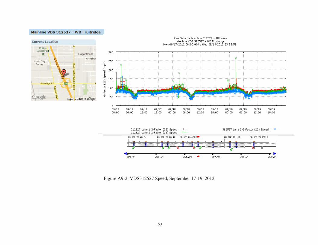
153

Figure A9-2. VDS312527 Speed, September 17-19, 2012

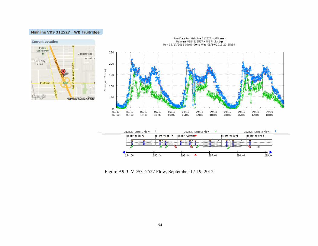
154

Figure A9-3. VDS312527 Flow, September 17-19, 2012

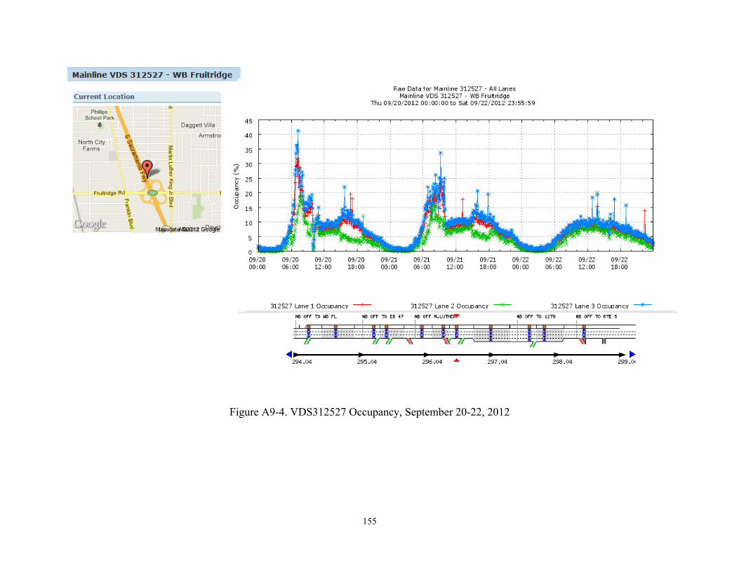
155

Figure A9-4. VDS312527 Occupancy, September 20-22, 2012

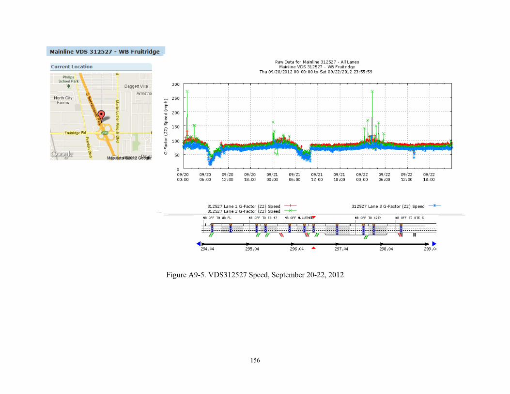
156

Figure A9-5. VDS312527 Speed, September 20-22, 2012

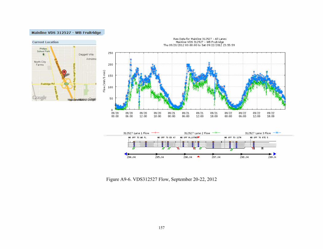
157

Figure A9-6. VDS312527 Flow, September 20-22, 2012

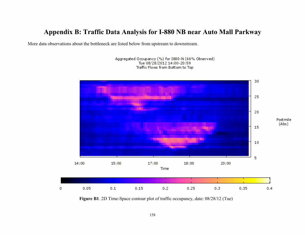
158

Appendix B: Traffic Data Analysis for I-880 NB near Auto Mall Parkway More data observations about the bottleneck are listed below from upstream to downstream.

Figure B1. 2D Time-Space contour plot of traffic occupancy, date: 08/28/12 (Tue)

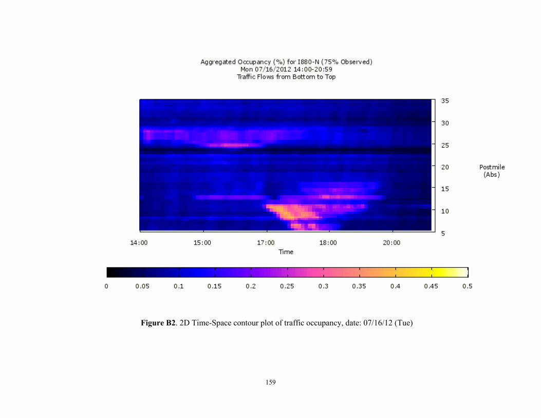
159

Figure B2. 2D Time-Space contour plot of traffic occupancy, date: 07/16/12 (Tue)

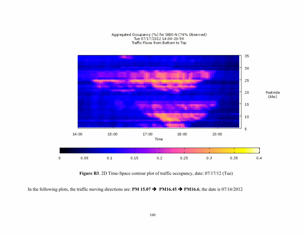
160

Figure B3. 2D Time-Space contour plot of traffic occupancy, date: 07/17/12 (Tue)

In the following plots, the traffic moving directions are: PM 15.07 PM16.45 PM16.6; the date is 07/16/2012

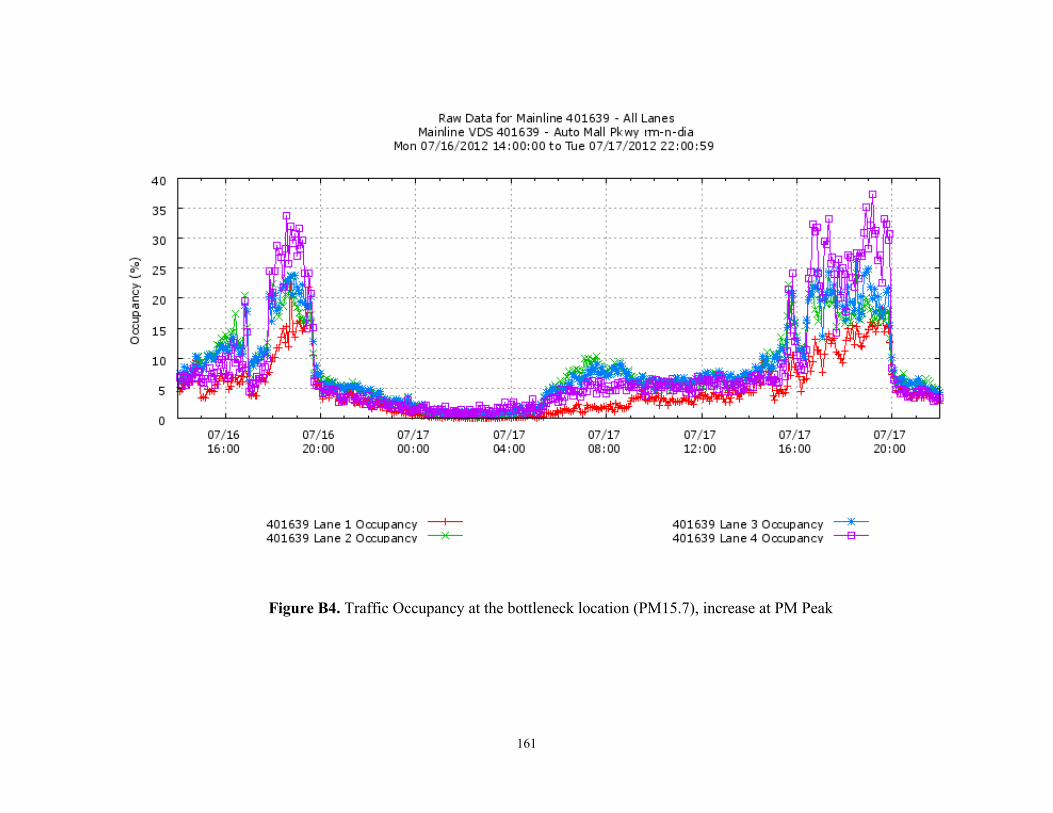
161

Figure B4. Traffic Occupancy at the bottleneck location (PM15.7), increase at PM Peak

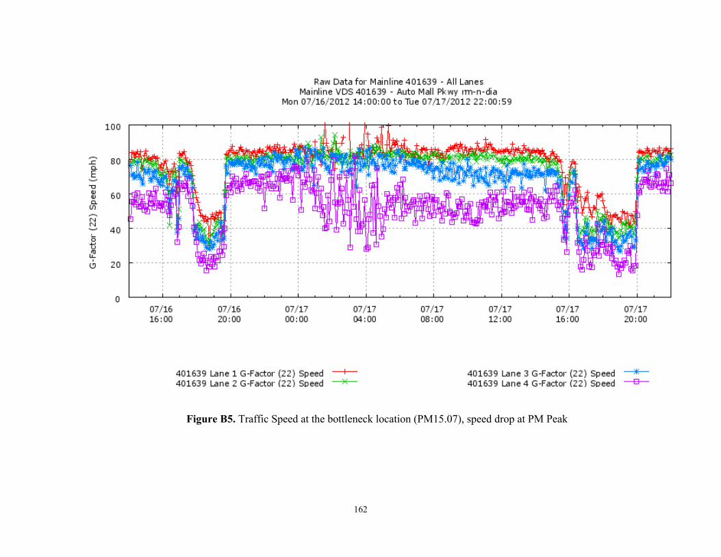
162

Figure B5. Traffic Speed at the bottleneck location (PM15.07), speed drop at PM Peak

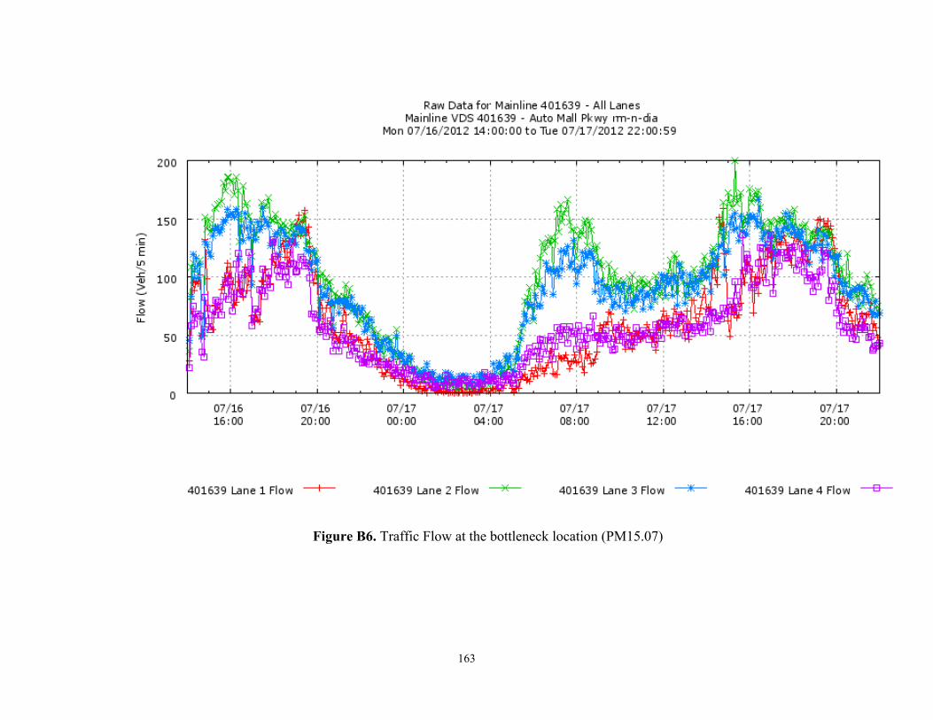
163

Figure B6. Traffic Flow at the bottleneck location (PM15.07)

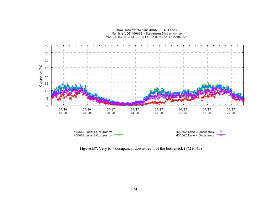
164

Figure B7. Very low occupancy, downstream of the bottleneck (PM16.45)

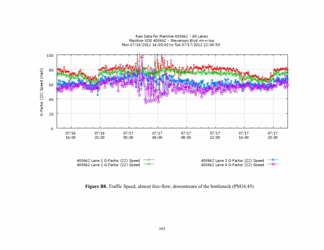
165

Figure B8. Traffic Speed, almost free-flow, downstream of the bottleneck (PM16.45)

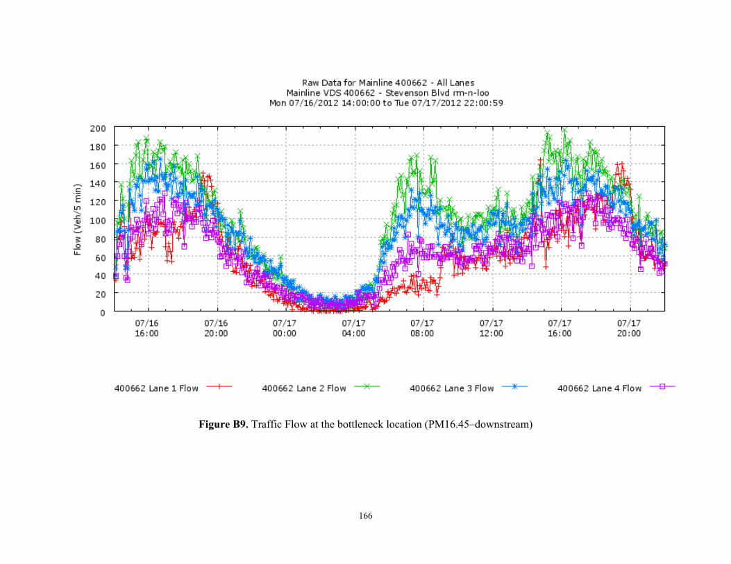
166

Figure B9. Traffic Flow at the bottleneck location (PM16.45–downstream)

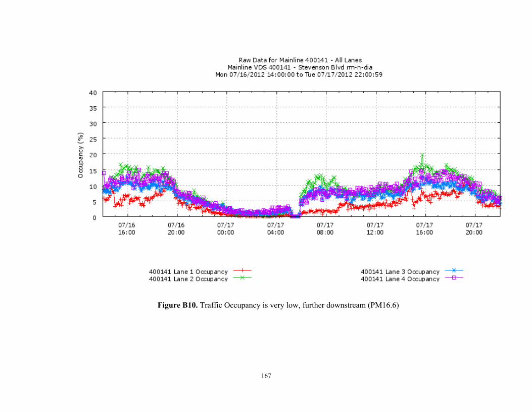
167

Figure B10. Traffic Occupancy is very low, further downstream (PM16.6)

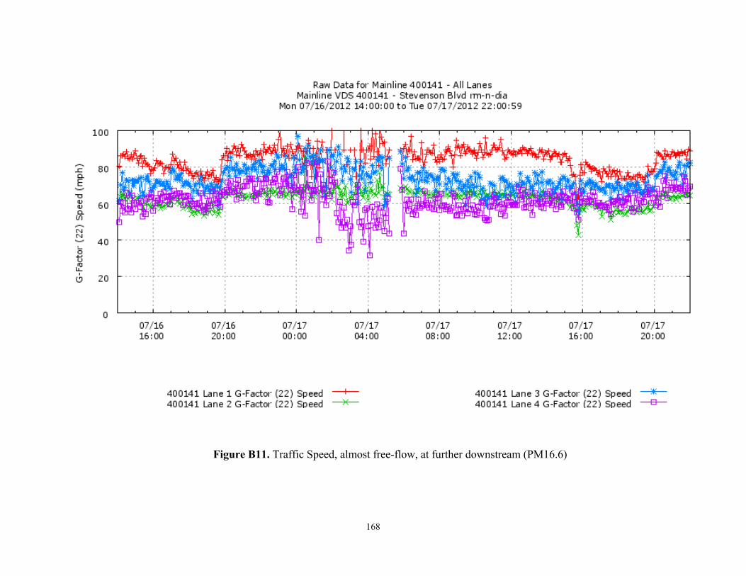
168

Figure B11. Traffic Speed, almost free-flow, at further downstream (PM16.6)

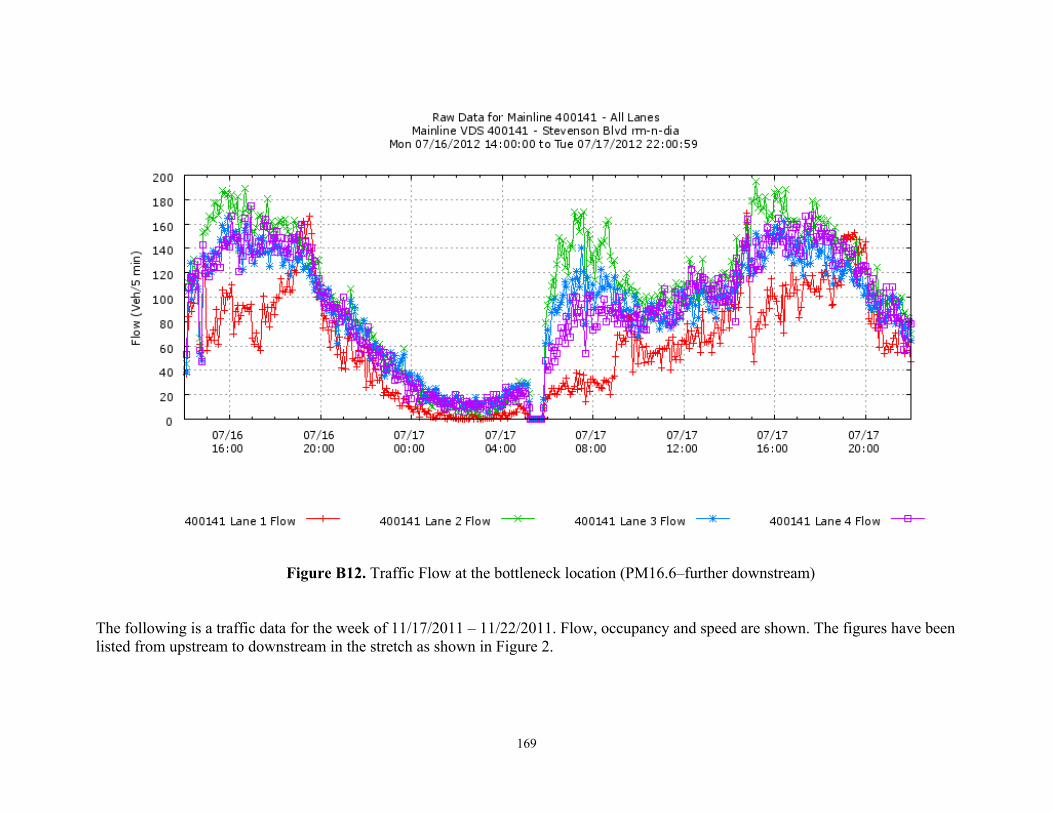
169

Figure B12. Traffic Flow at the bottleneck location (PM16.6–further downstream)

The following is a traffic data for the week of 11/17/2011 – 11/22/2011. Flow, occupancy and speed are shown. The figures have been listed from upstream to downstream in the stretch as shown in Figure 2.

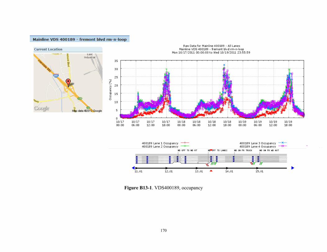
170

Figure B13-1. VDS400189, occupancy

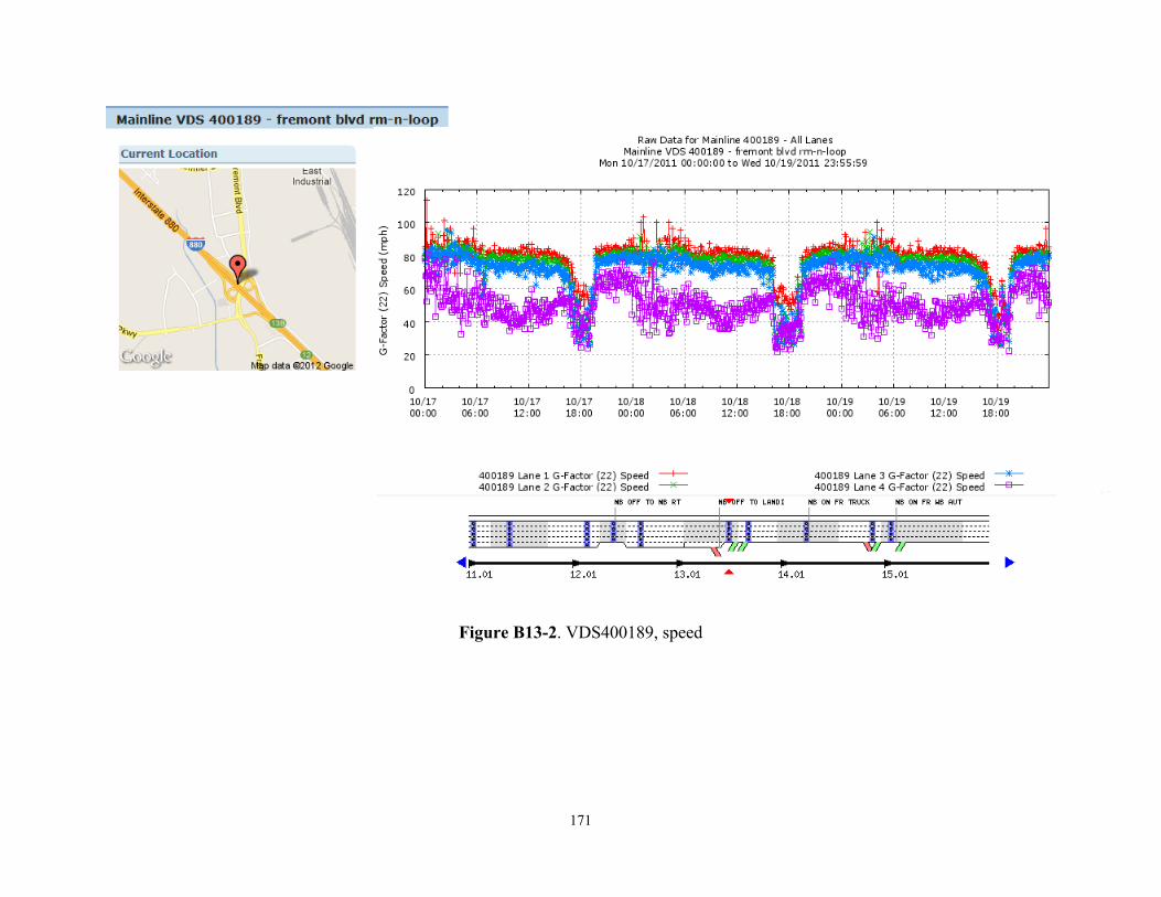
171

Figure B13-2. VDS400189, speed

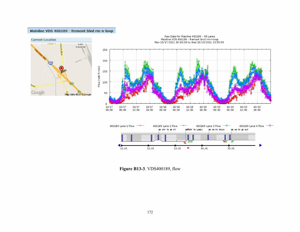
172

Figure B13-3. VDS400189, flow

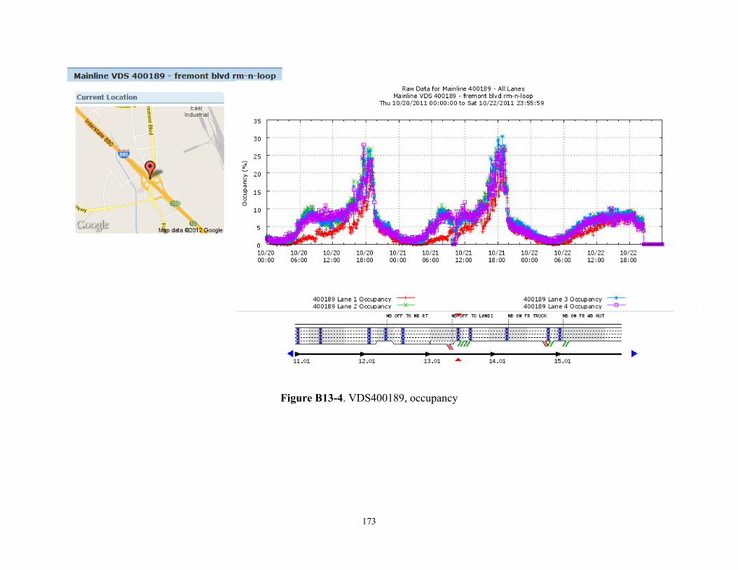
173

Figure B13-4. VDS400189, occupancy

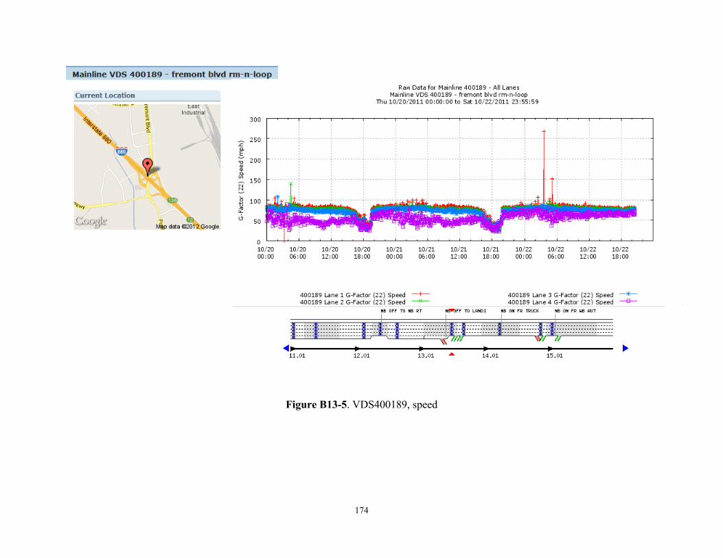
174

Figure B13-5. VDS400189, speed

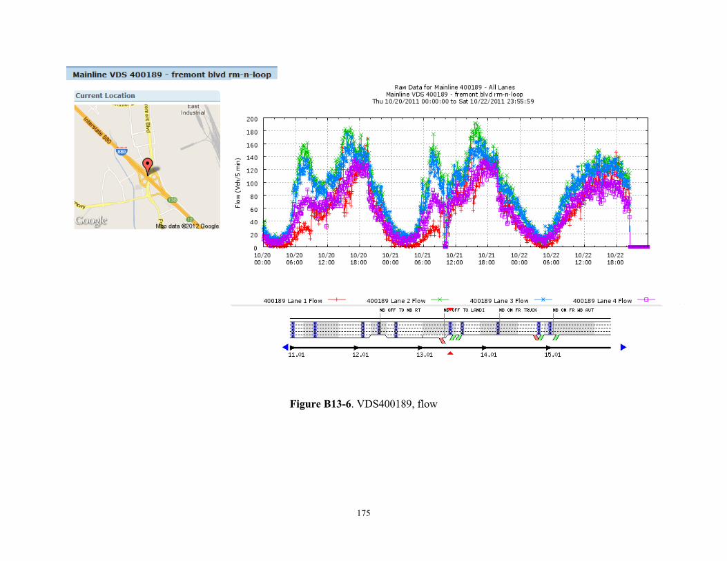
175

Figure B13-6. VDS400189, flow

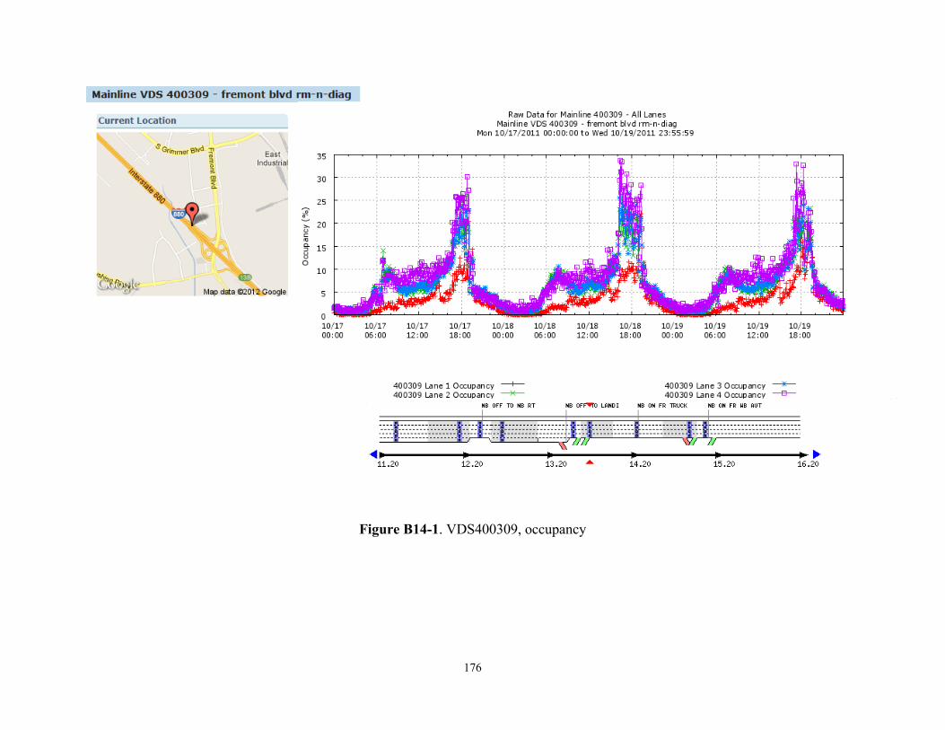
176

Figure B14-1. VDS400309, occupancy

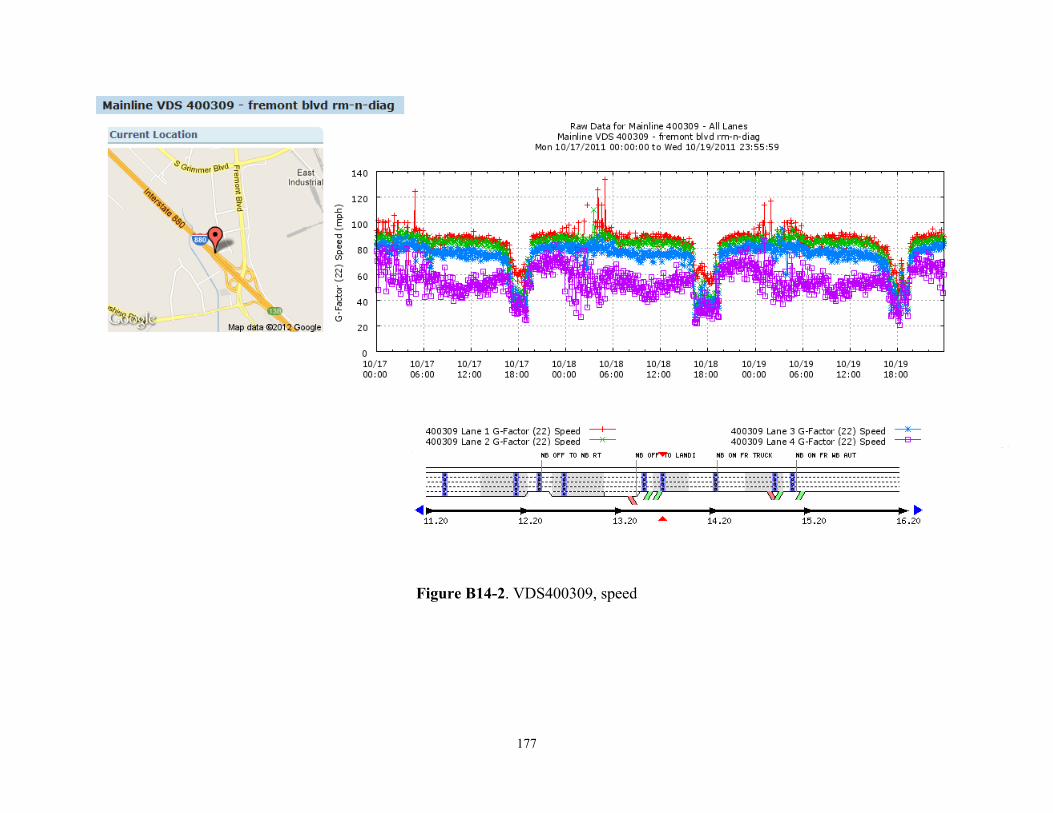
177

Figure B14-2. VDS400309, speed

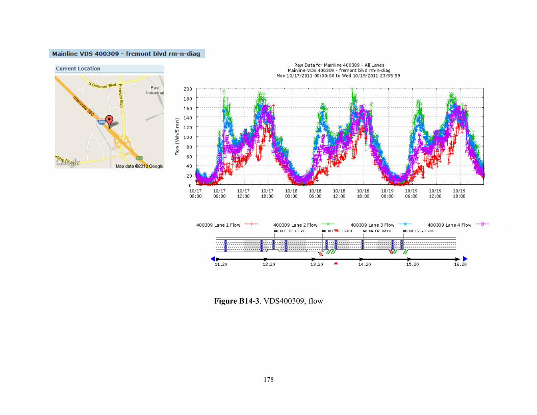
178

Figure B14-3. VDS400309, flow

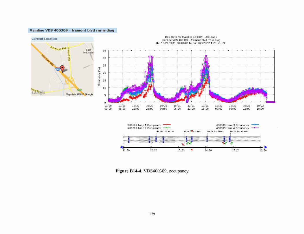
179

Figure B14-4. VDS400309, occupancy

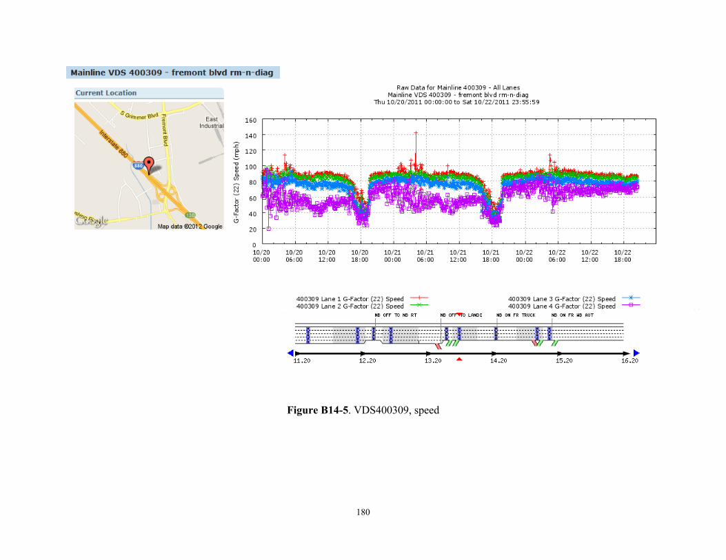
180

Figure B14-5. VDS400309, speed

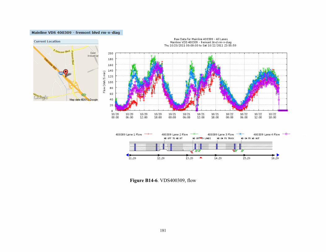
181

Figure B14-6. VDS400309, flow

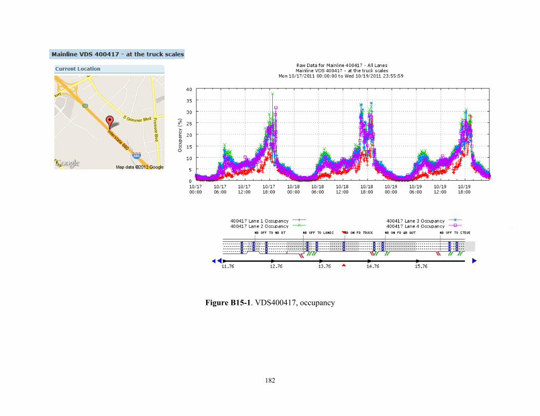
182

Figure B15-1. VDS400417, occupancy

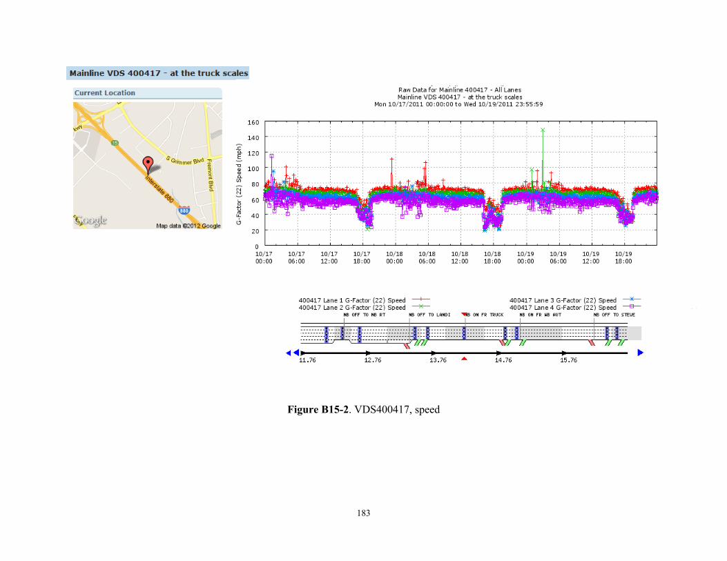
183

Figure B15-2. VDS400417, speed

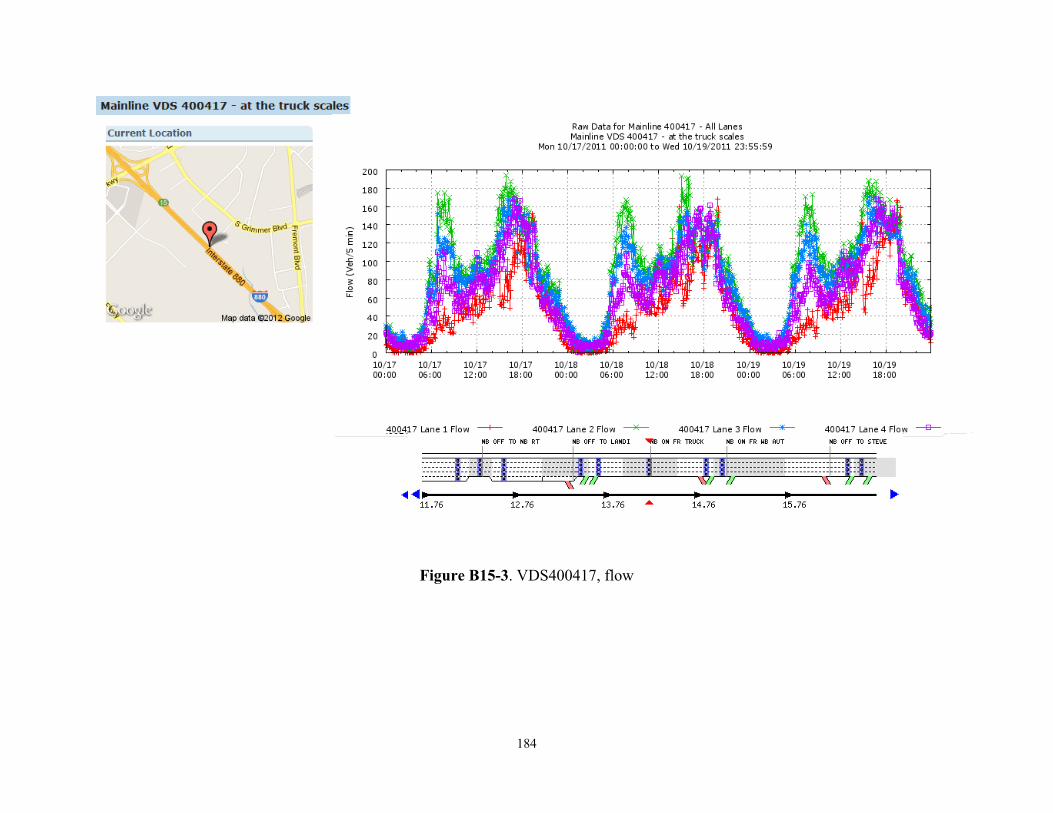
184

Figure B15-3. VDS400417, flow

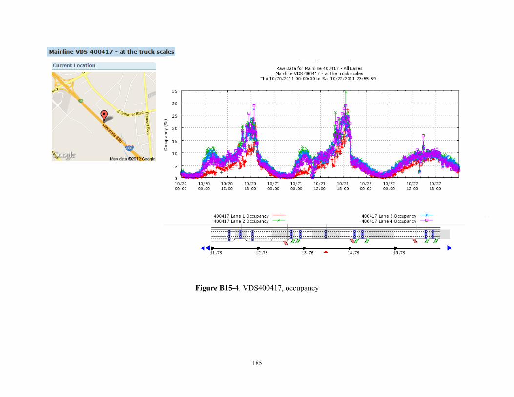
185

Figure B15-4. VDS400417, occupancy

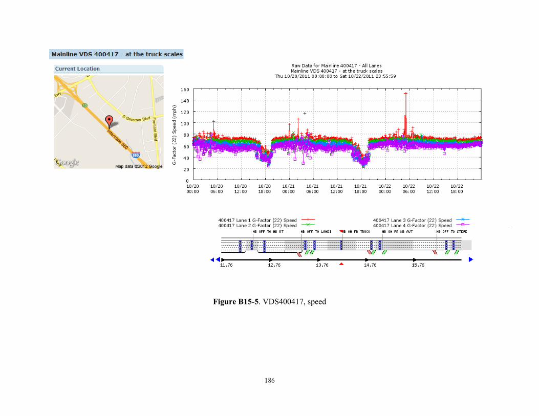
186

Figure B15-5. VDS400417, speed

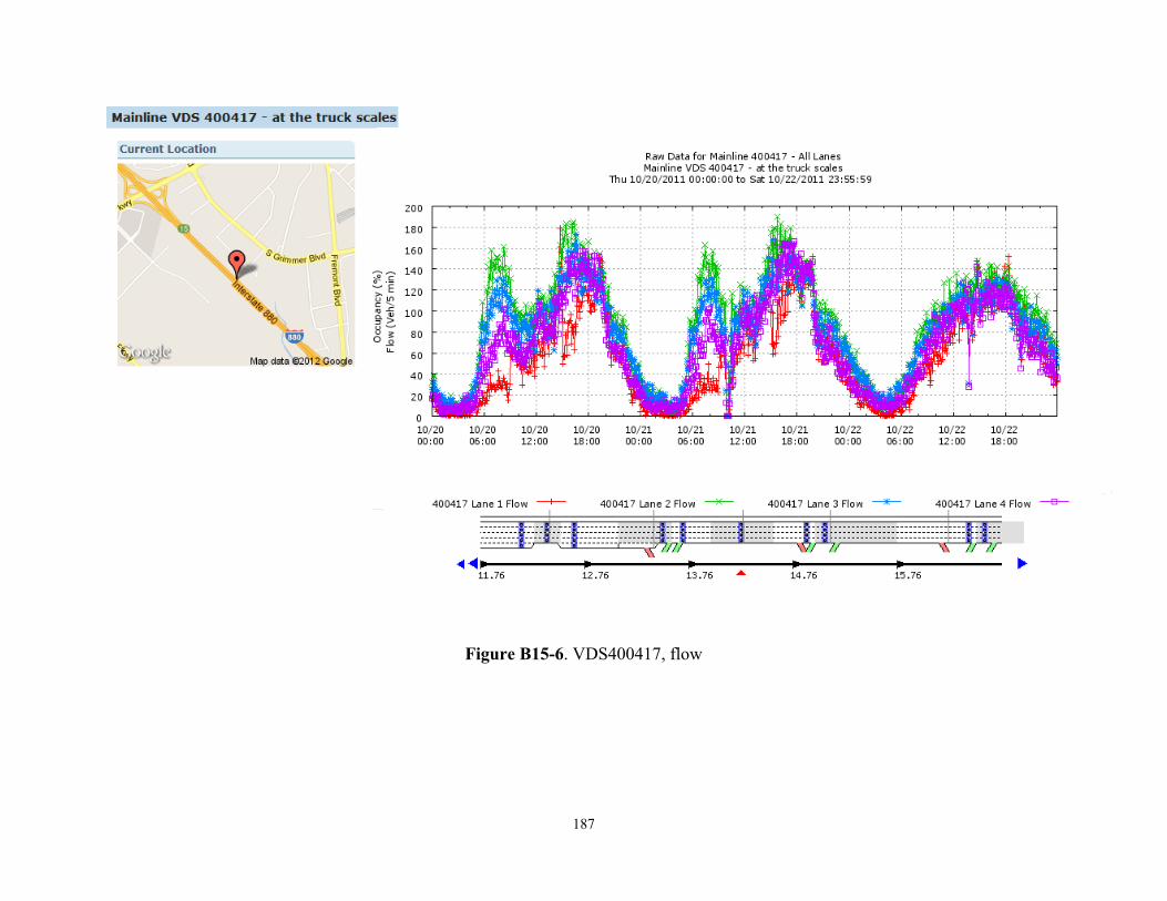
187

Figure B15-6. VDS400417, flow

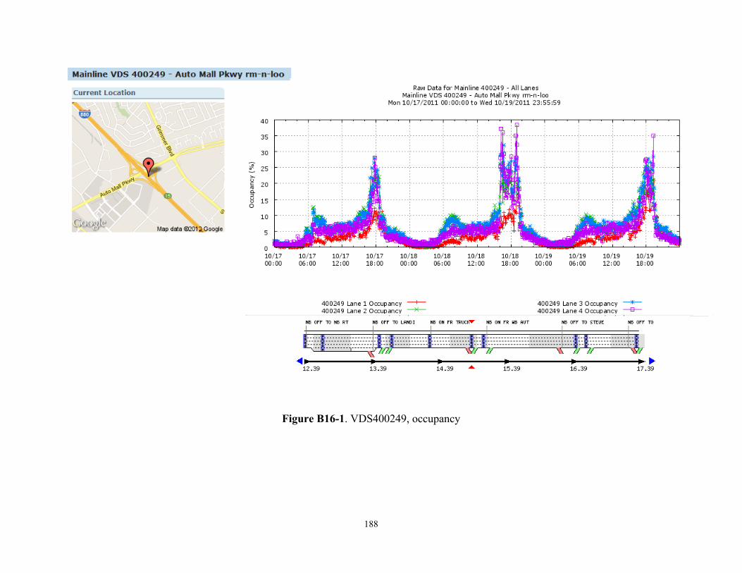
188

Figure B16-1. VDS400249, occupancy

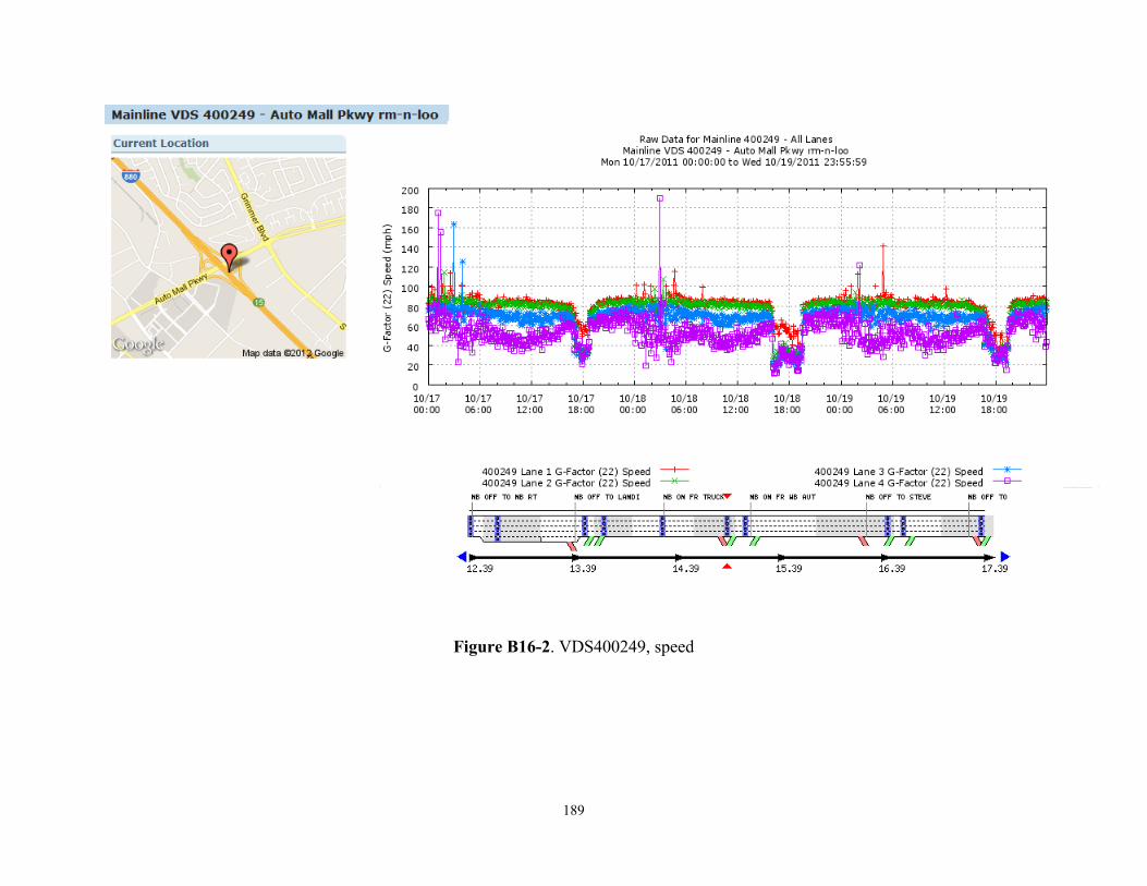
189

Figure B16-2. VDS400249, speed

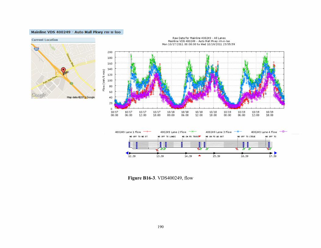
190

Figure B16-3. VDS400249, flow

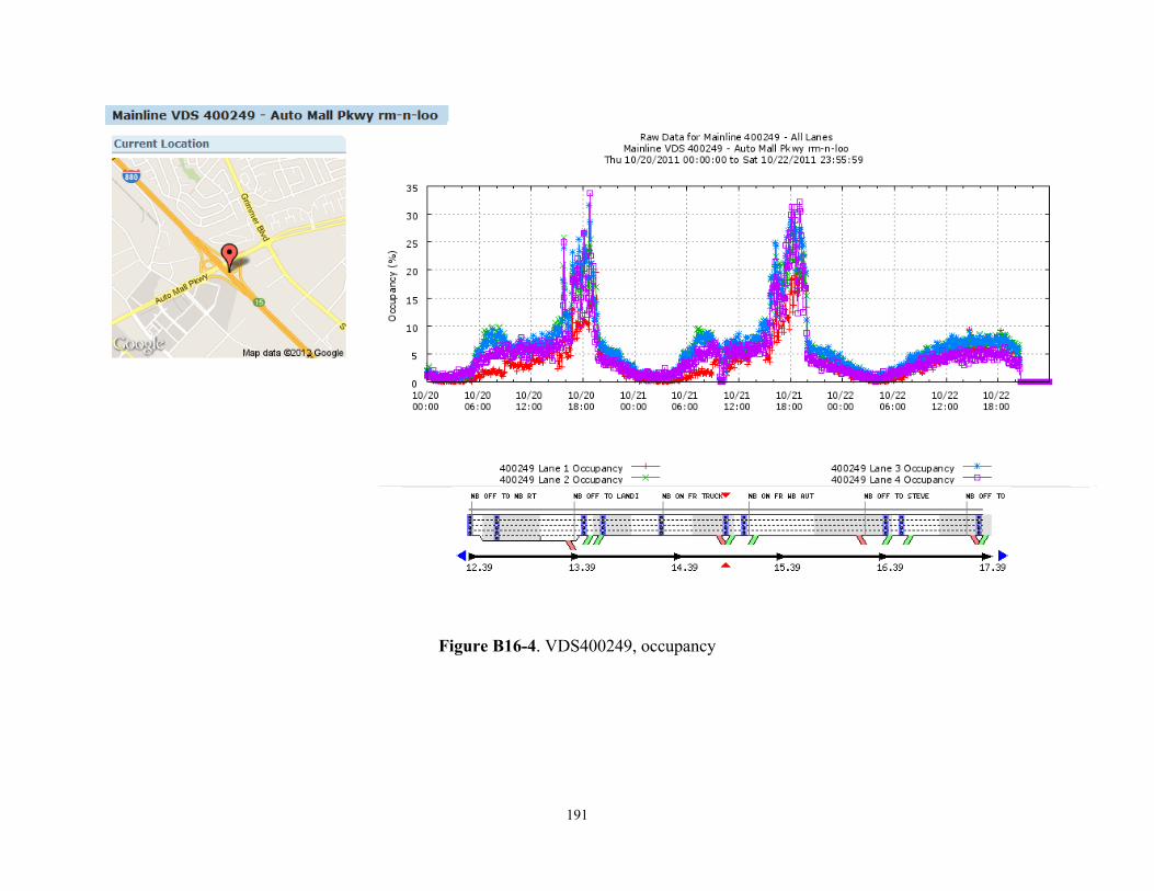
191

Figure B16-4. VDS400249, occupancy

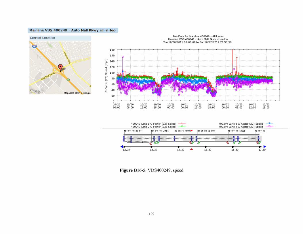
192

Figure B16-5. VDS400249, speed

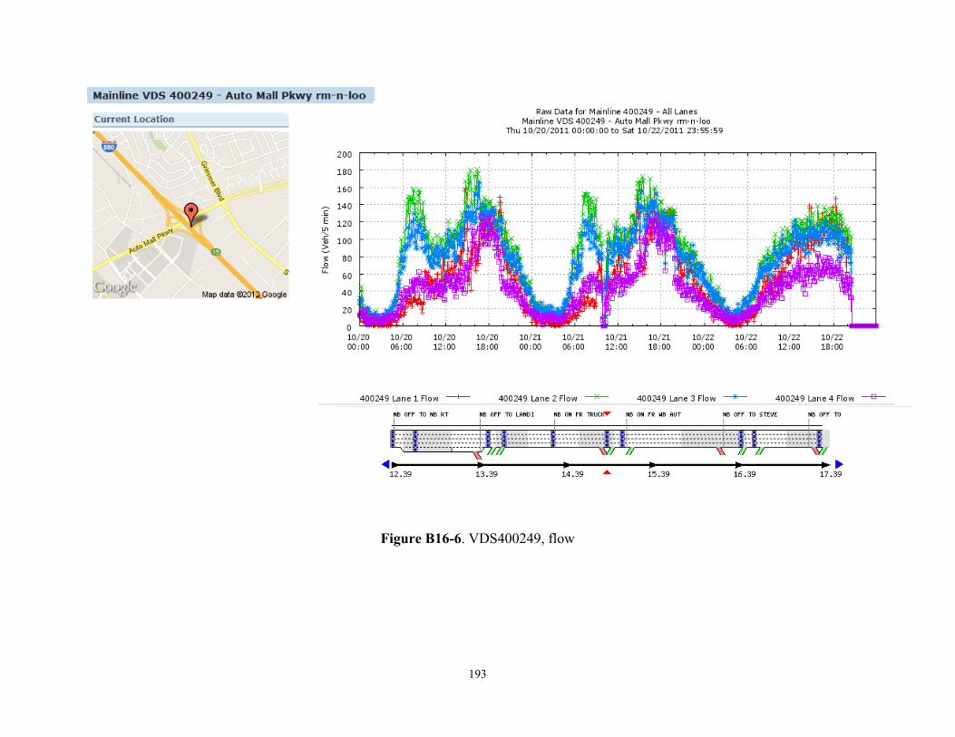
193

Figure B16-6. VDS400249, flow

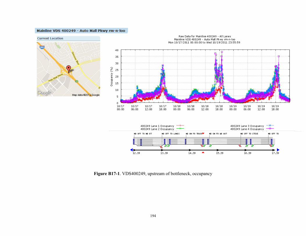
194

Figure B17-1. VDS400249, upstream of bottleneck, occupancy

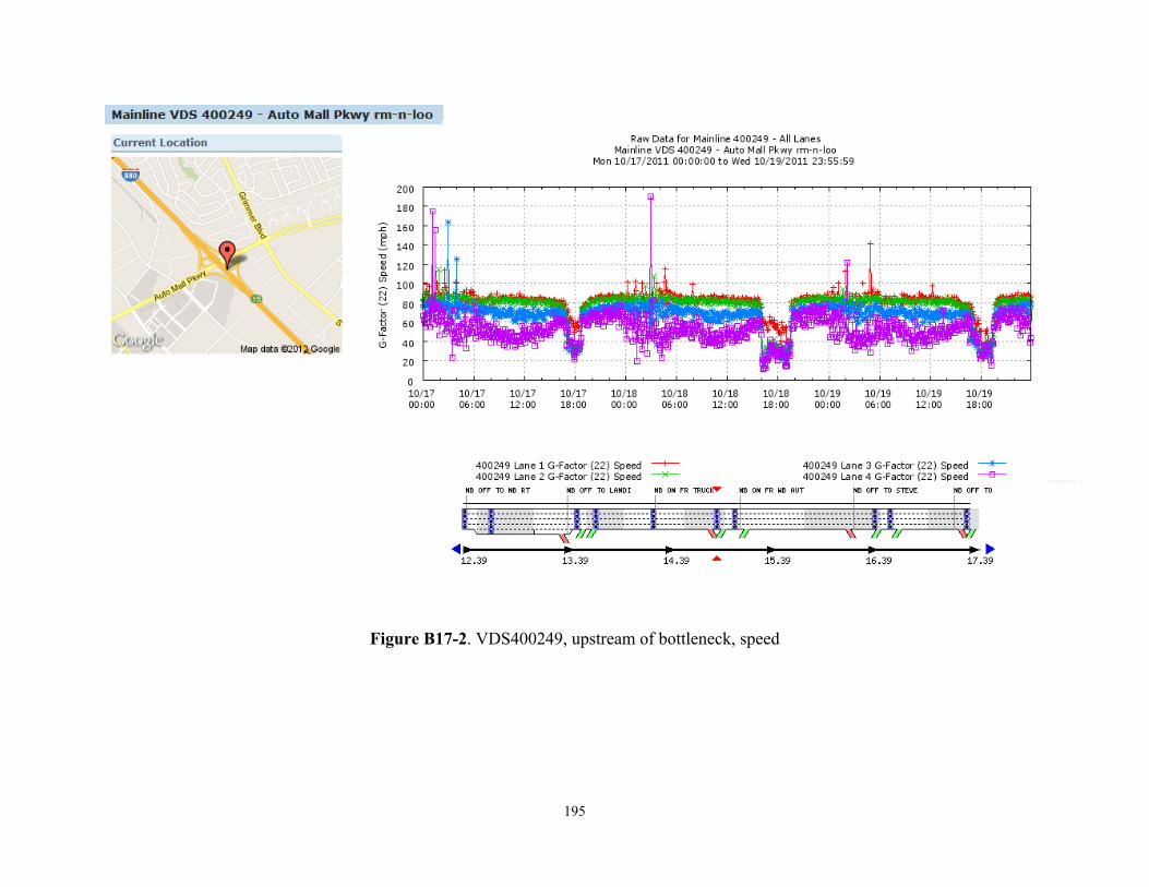
195

Figure B17-2. VDS400249, upstream of bottleneck, speed

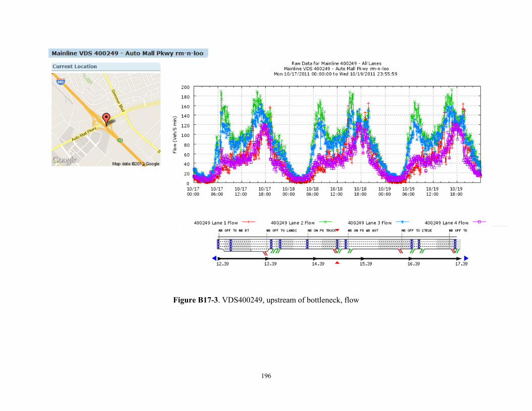
196

Figure B17-3. VDS400249, upstream of bottleneck, flow

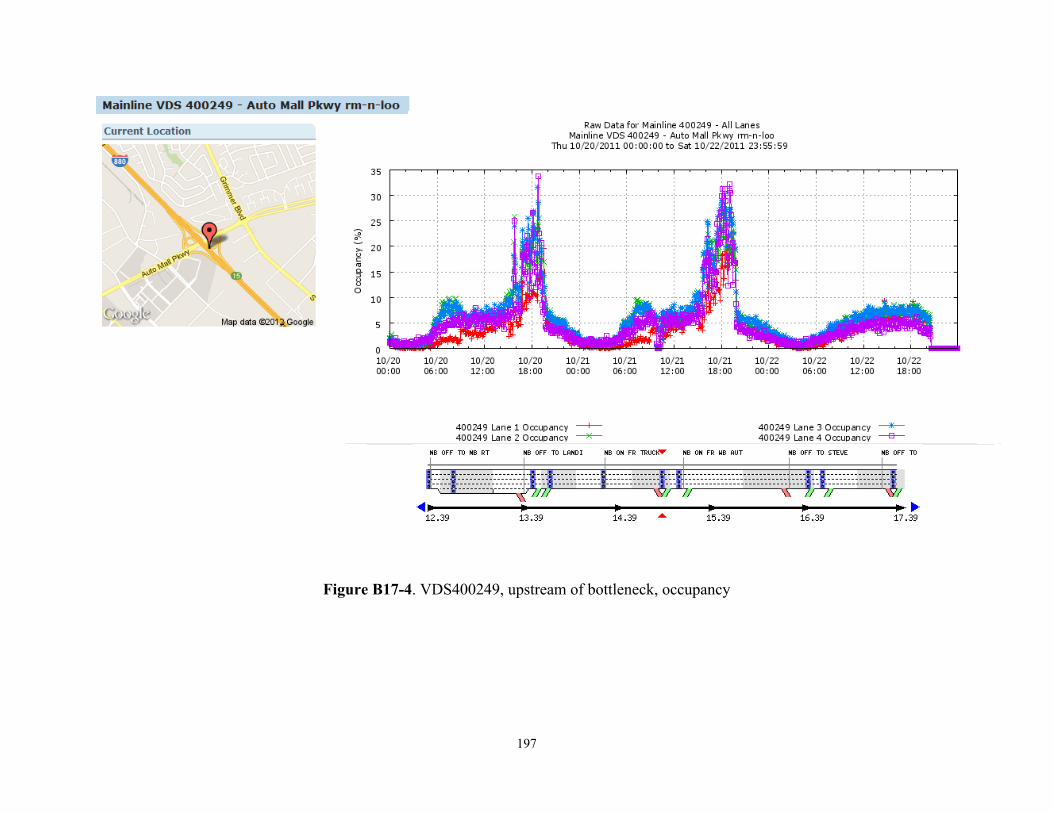
197

Figure B17-4. VDS400249, upstream of bottleneck, occupancy

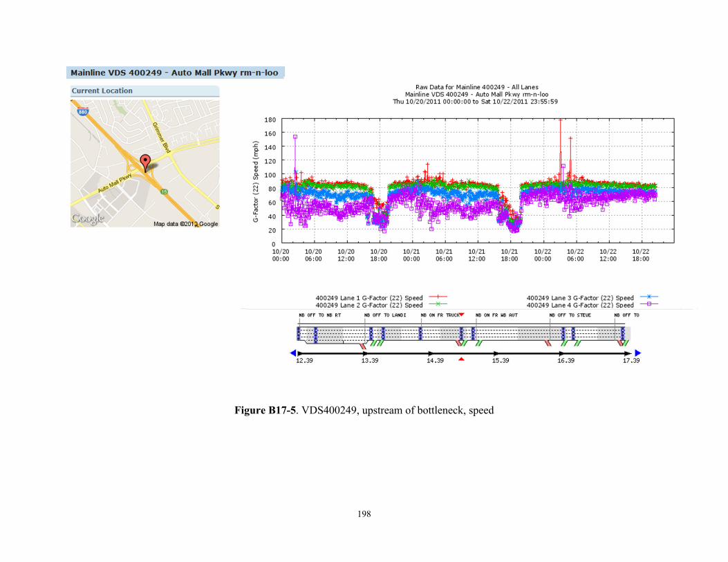
198

Figure B17-5. VDS400249, upstream of bottleneck, speed

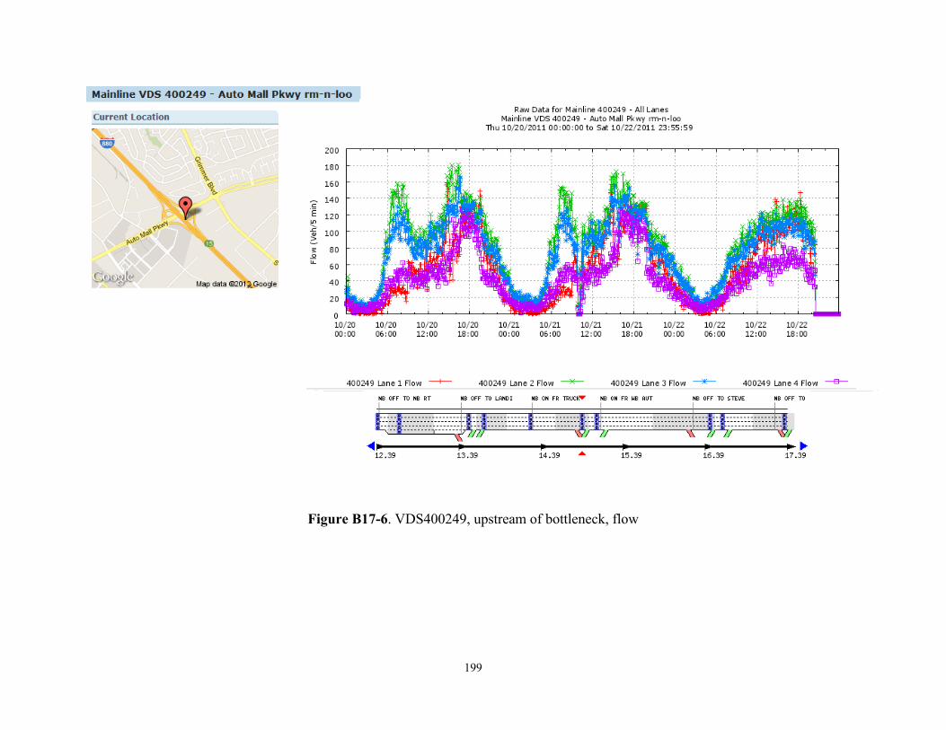
199

Figure B17-6. VDS400249, upstream of bottleneck, flow

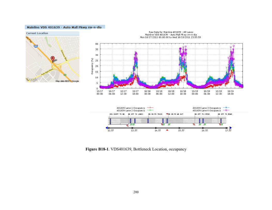
200

Figure B18-1. VDS401639, Bottleneck Location, occupancy

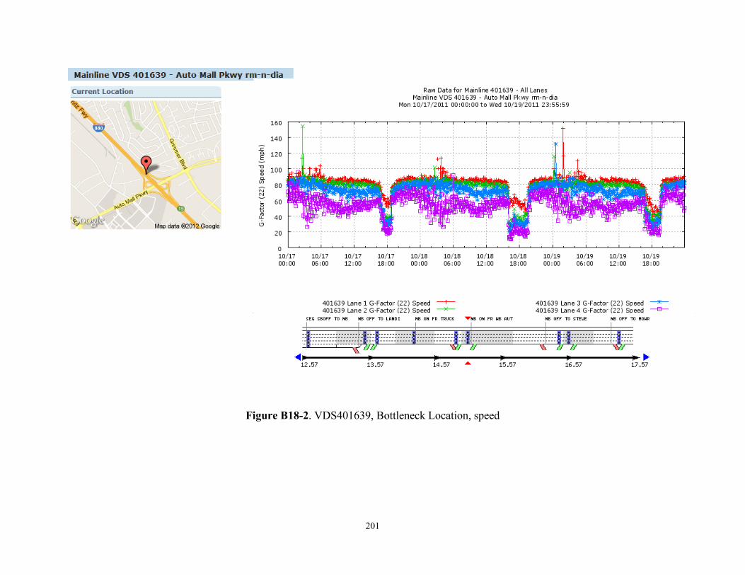
201

Figure B18-2. VDS401639, Bottleneck Location, speed

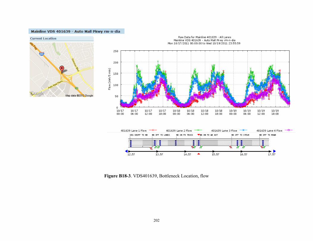
202

Figure B18-3. VDS401639, Bottleneck Location, flow

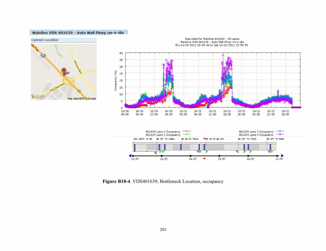
203

Figure B18-4. VDS401639, Bottleneck Location, occupancy

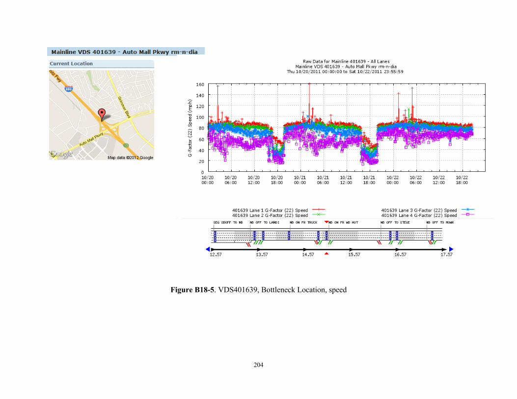
204

Figure B18-5. VDS401639, Bottleneck Location, speed

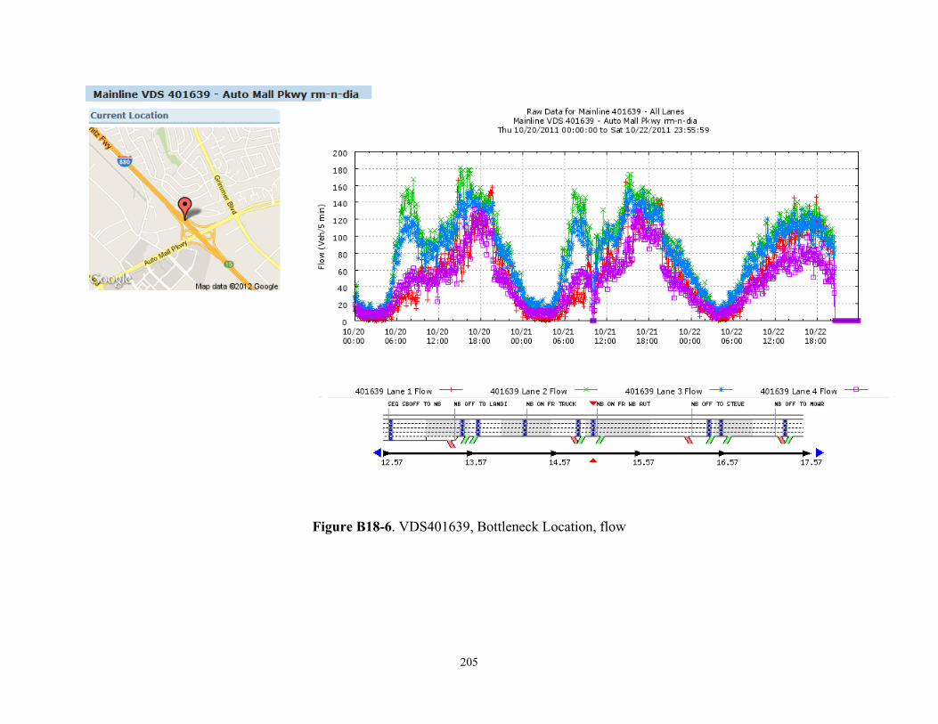
205

Figure B18-6. VDS401639, Bottleneck Location, flow

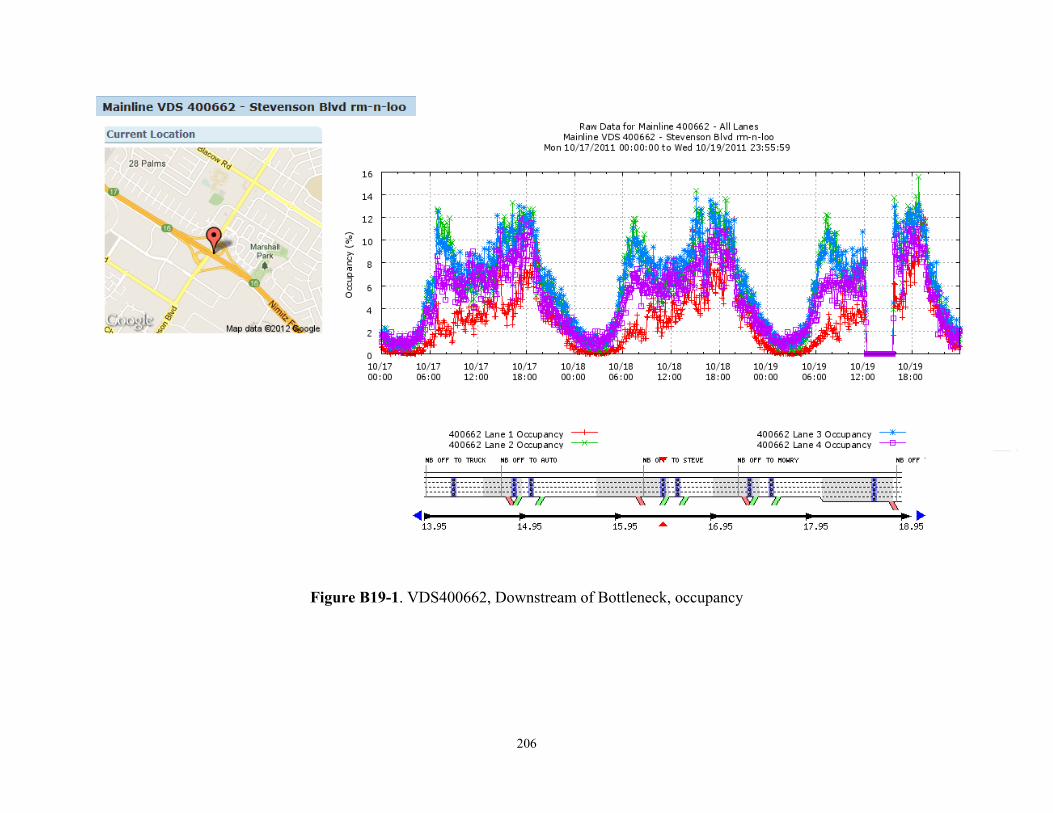
206

Figure B19-1. VDS400662, Downstream of Bottleneck, occupancy

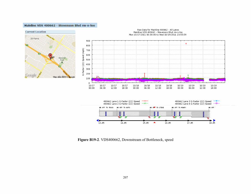
207

Figure B19-2. VDS400662, Downstream of Bottleneck, speed

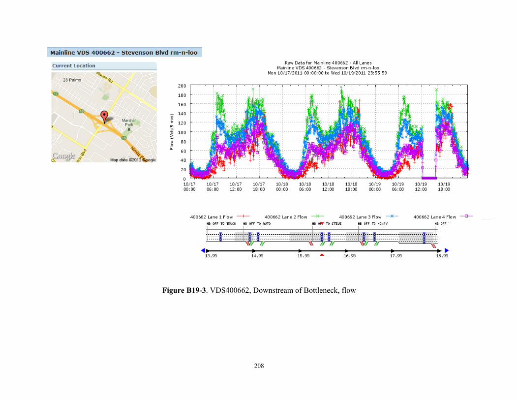
208

Figure B19-3. VDS400662, Downstream of Bottleneck, flow

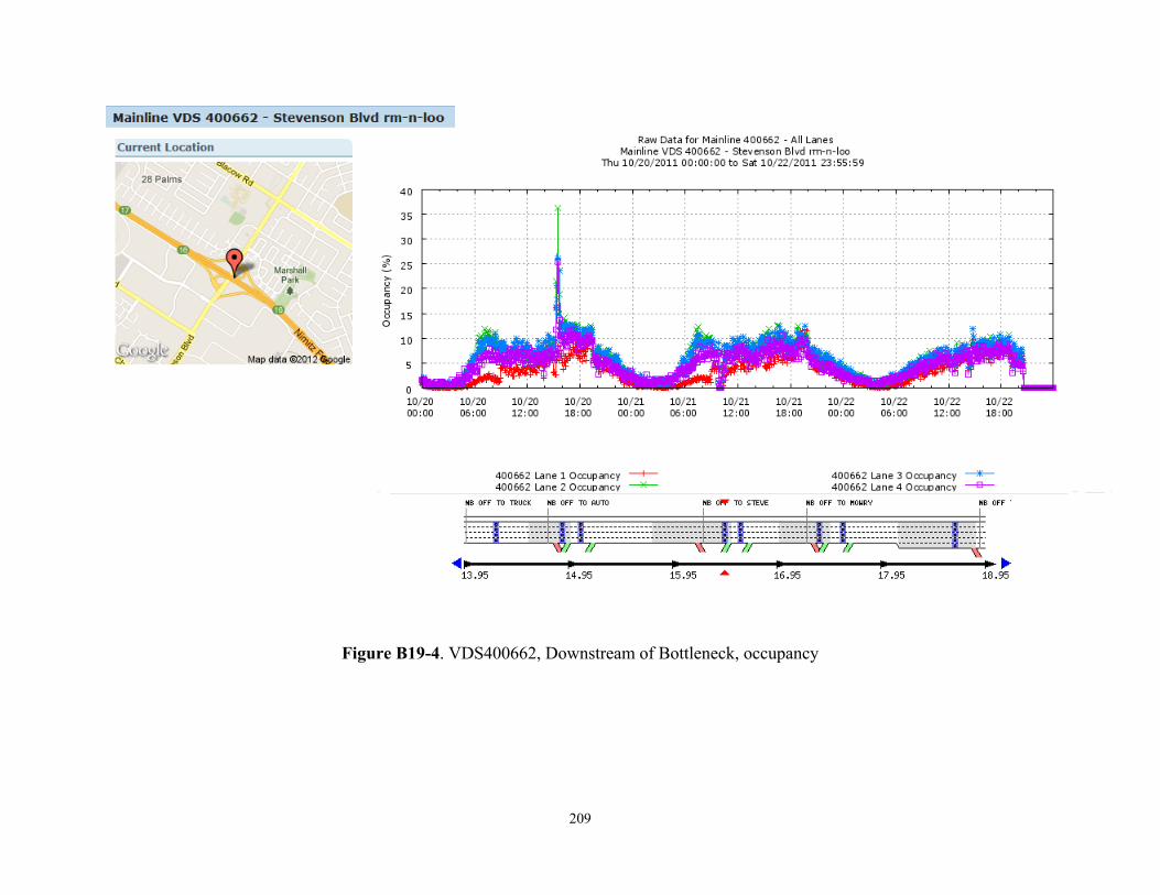
209

Figure B19-4. VDS400662, Downstream of Bottleneck, occupancy

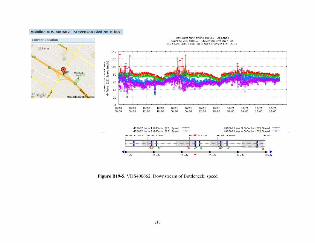
210

Figure B19-5. VDS400662, Downstream of Bottleneck, speed

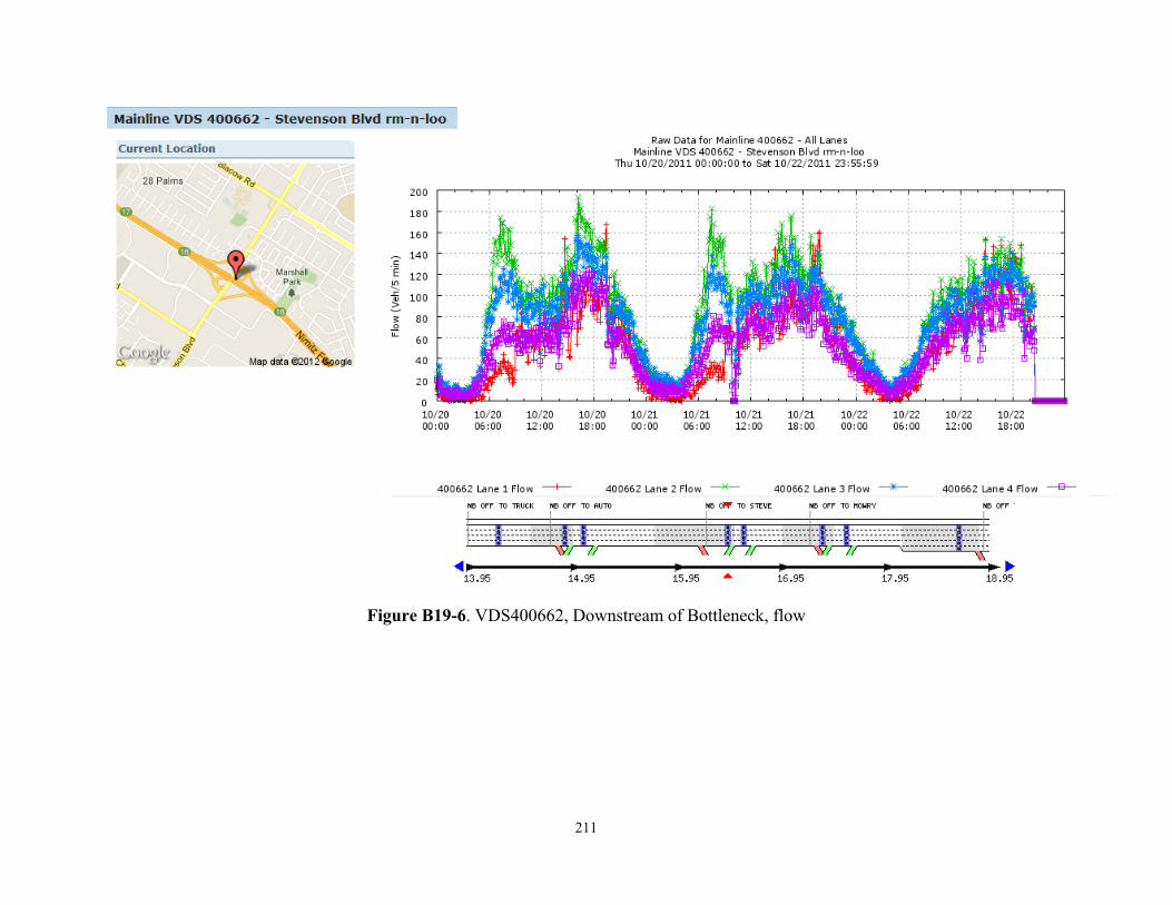
211

Figure B19-6. VDS400662, Downstream of Bottleneck, flow

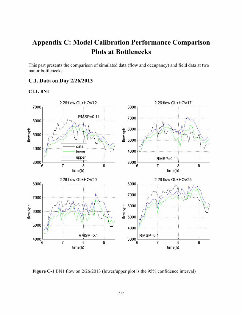
212

Appendix C: Model Calibration Performance Comparison Plots at Bottlenecks

This part presents the comparison of simulated data (flow and occupancy) and field data at two major bottlenecks.

C.1. Data on Day 2/26/2013

C1.1. BN1

Figure C-1 BN1 flow on 2/26/2013 (lower/upper plot is the 95% confidence interval)

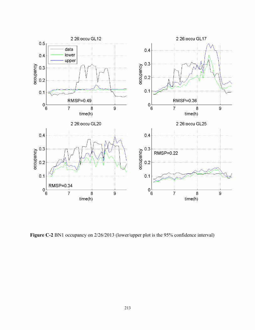
213

Figure C-2 BN1 occupancy on 2/26/2013 (lower/upper plot is the 95% confidence interval)

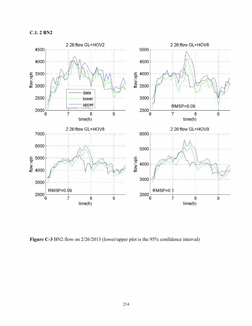
214

C.1. 2 BN2

Figure C-3 BN2 flow on 2/26/2013 (lower/upper plot is the 95% confidence interval)

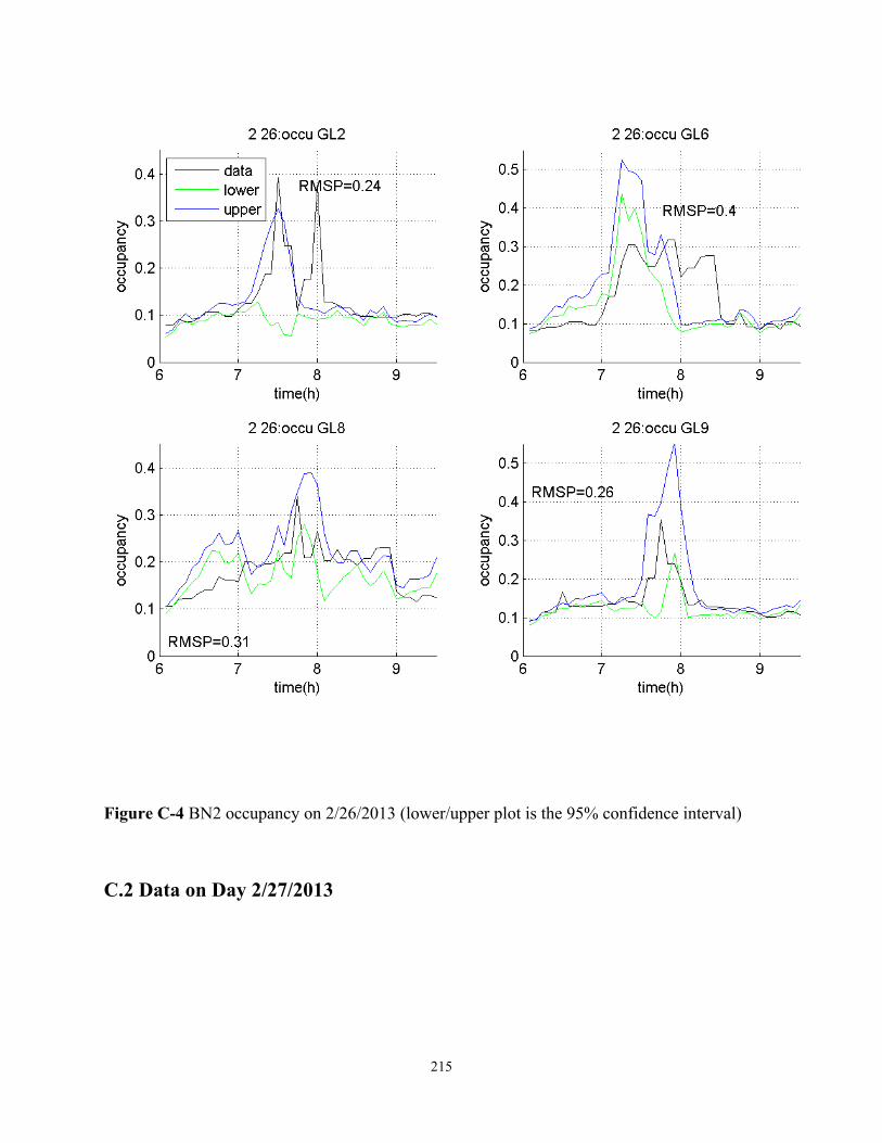
215

Figure C-4 BN2 occupancy on 2/26/2013 (lower/upper plot is the 95% confidence interval)

C.2 Data on Day 2/27/2013

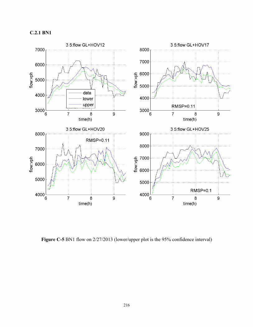
216

C.2.1 BN1

Figure C-5 BN1 flow on 2/27/2013 (lower/upper plot is the 95% confidence interval)

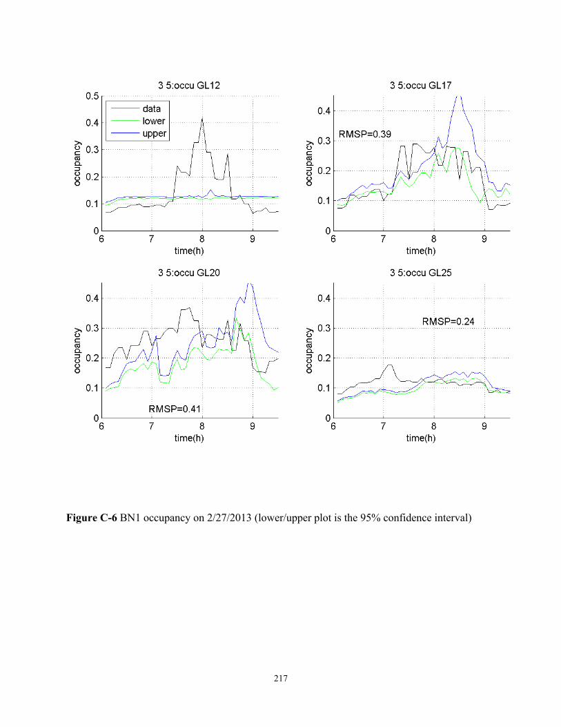
217

Figure C-6 BN1 occupancy on 2/27/2013 (lower/upper plot is the 95% confidence interval)

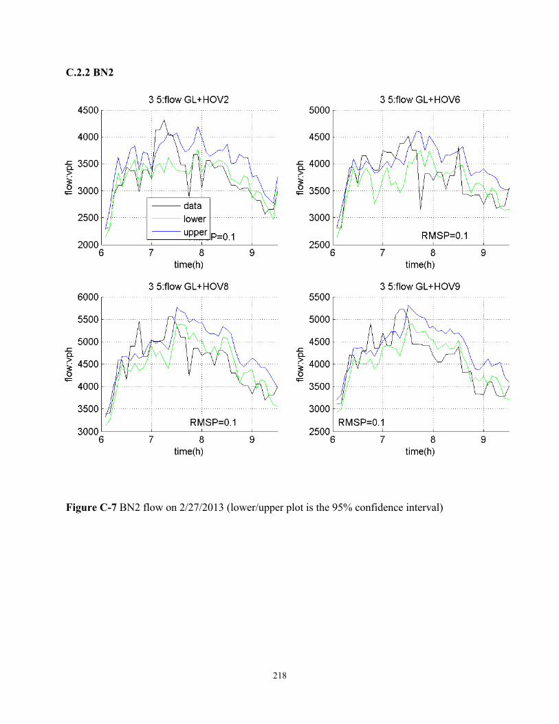
218

C.2.2 BN2

Figure C-7 BN2 flow on 2/27/2013 (lower/upper plot is the 95% confidence interval)

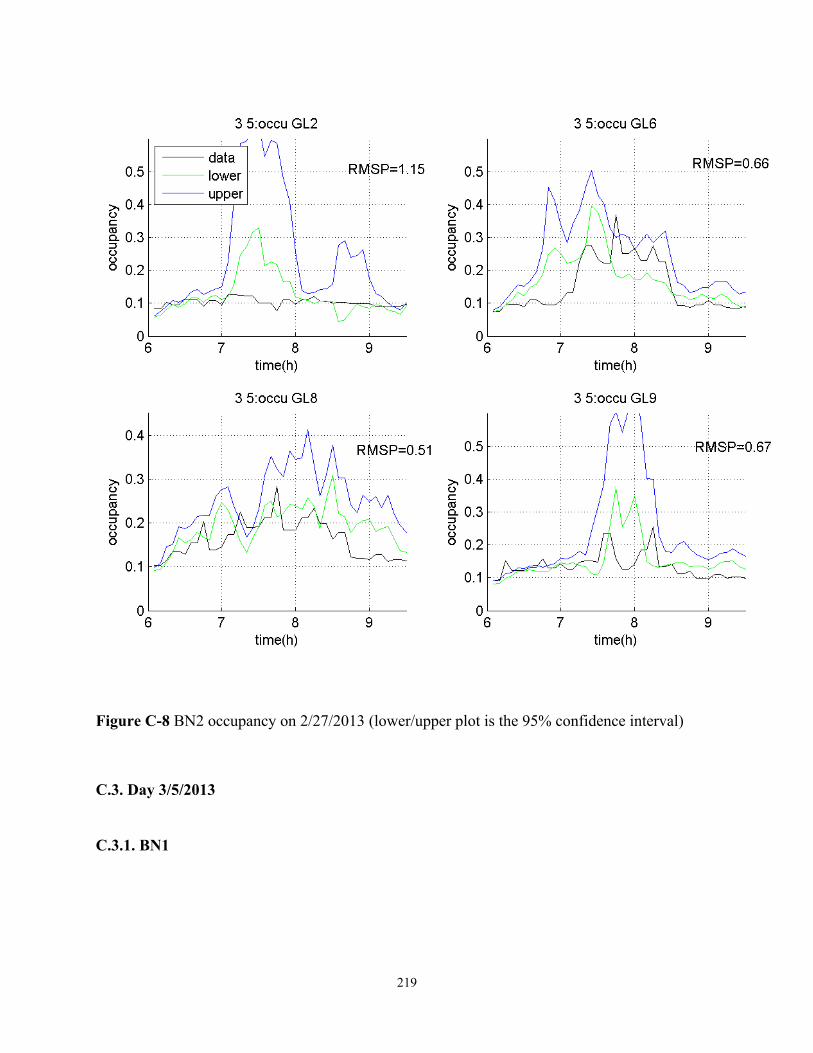
219

Figure C-8 BN2 occupancy on 2/27/2013 (lower/upper plot is the 95% confidence interval)

C.3. Day 3/5/2013

C.3.1. BN1

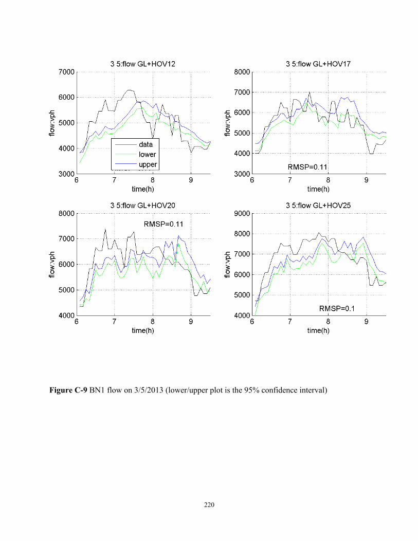
220

Figure C-9 BN1 flow on 3/5/2013 (lower/upper plot is the 95% confidence interval)

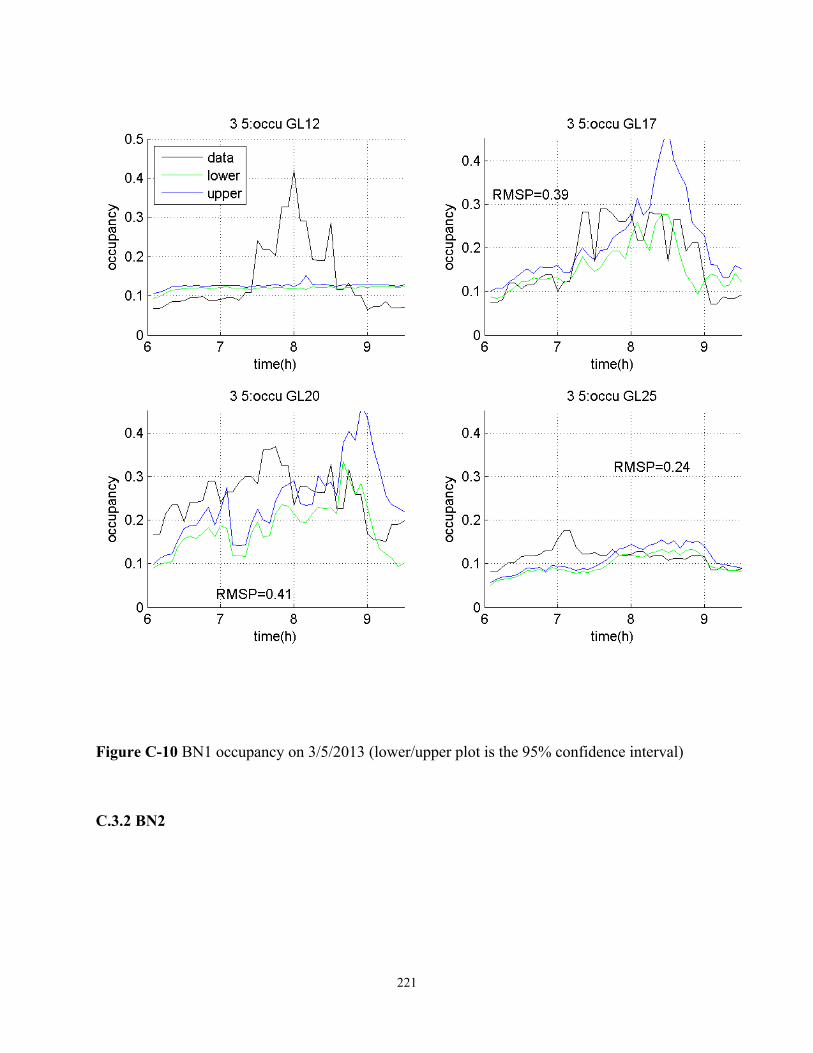
221

Figure C-10 BN1 occupancy on 3/5/2013 (lower/upper plot is the 95% confidence interval)

C.3.2 BN2

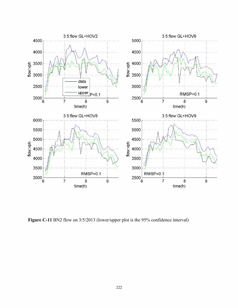
222

Figure C-11 BN2 flow on 3/5/2013 (lower/upper plot is the 95% confidence interval)

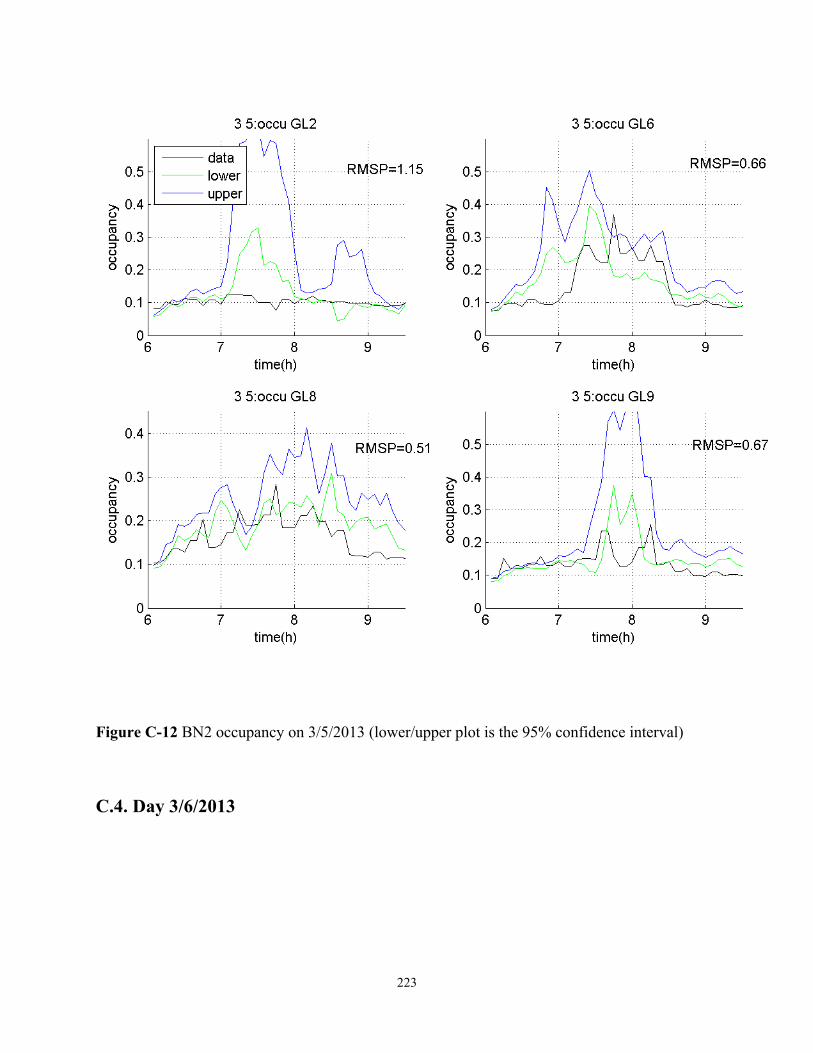
223

Figure C-12 BN2 occupancy on 3/5/2013 (lower/upper plot is the 95% confidence interval)

C.4. Day 3/6/2013

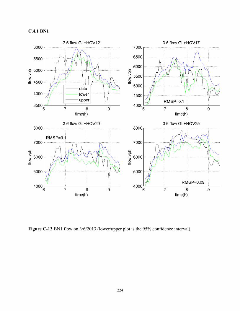
224

C.4.1 BN1

Figure C-13 BN1 flow on 3/6/2013 (lower/upper plot is the 95% confidence interval)

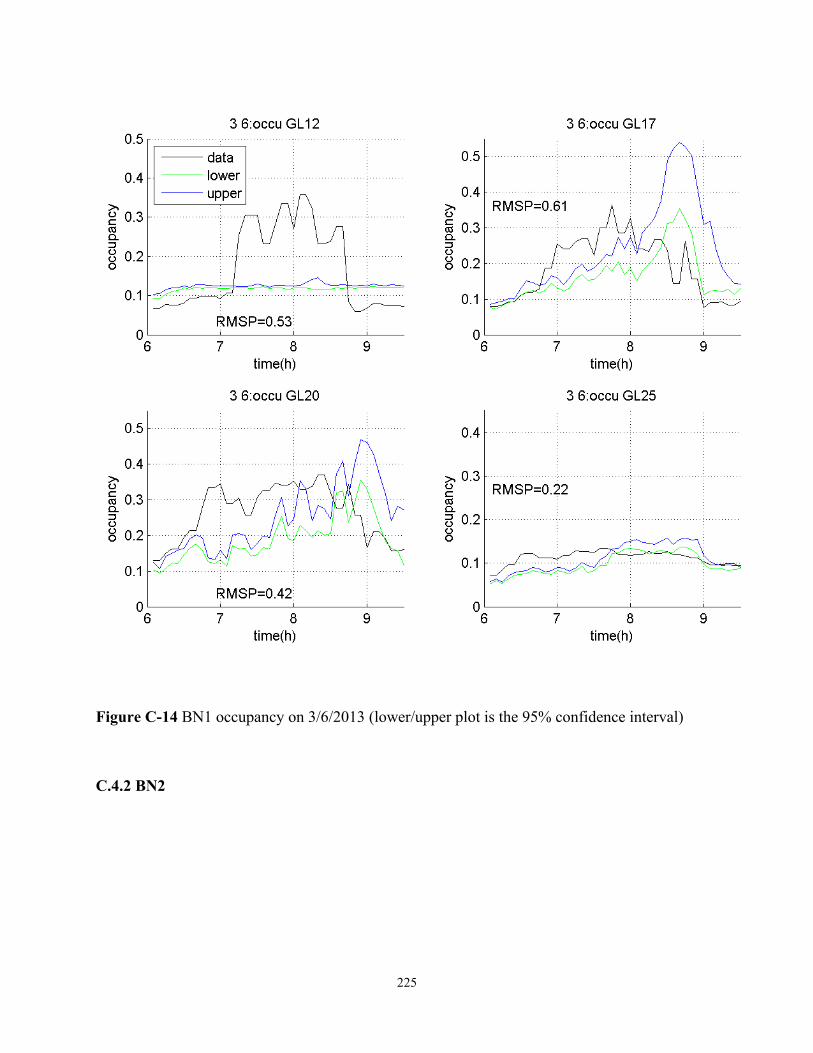
225

Figure C-14 BN1 occupancy on 3/6/2013 (lower/upper plot is the 95% confidence interval)

C.4.2 BN2

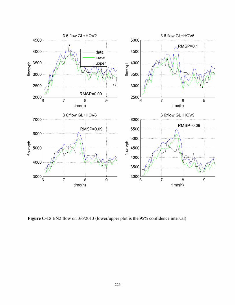
226

Figure C-15 BN2 flow on 3/6/2013 (lower/upper plot is the 95% confidence interval)

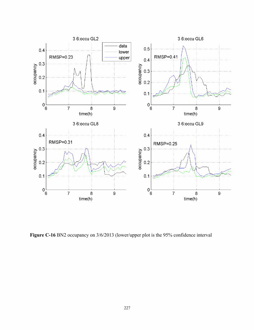
227

Figure C-16 BN2 occupancy on 3/6/2013 (lower/upper plot is the 95% confidence interval

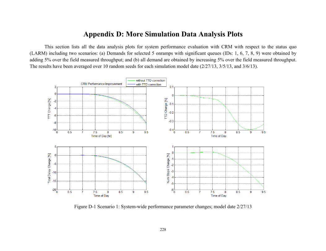
228

Appendix D: More Simulation Data Analysis Plots

This section lists all the data analysis plots for system performance evaluation with CRM with respect to the status quo (LARM) including two scenarios: (a) Demands for selected 5 onramps with significant queues (IDs: 1, 6, 7, 8, 9) were obtained by adding 5% over the field measured throughput; and (b) all demand are obtained by increasing 5% over the field measured throughput. The results have been averaged over 10 random seeds for each simulation model date (2/27/13, 3/5/13, and 3/6/13).

Figure D-1 Scenario 1: System-wide performance parameter changes; model date 2/27/13

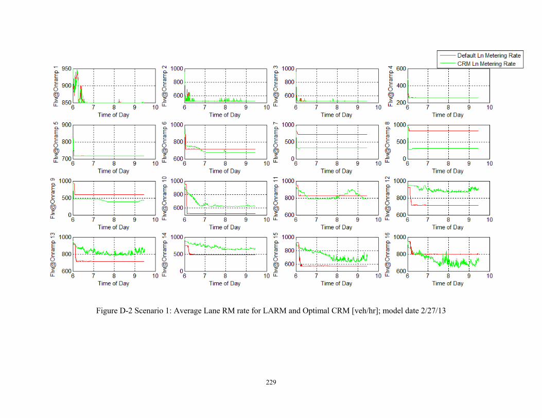
229

Figure D-2 Scenario 1: Average Lane RM rate for LARM and Optimal CRM [veh/hr]; model date 2/27/13

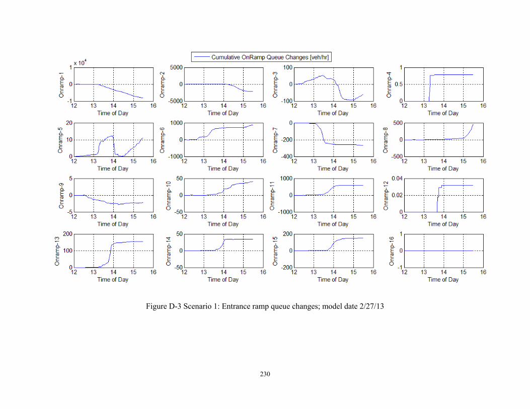
230

Figure D-3 Scenario 1: Entrance ramp queue changes; model date 2/27/13

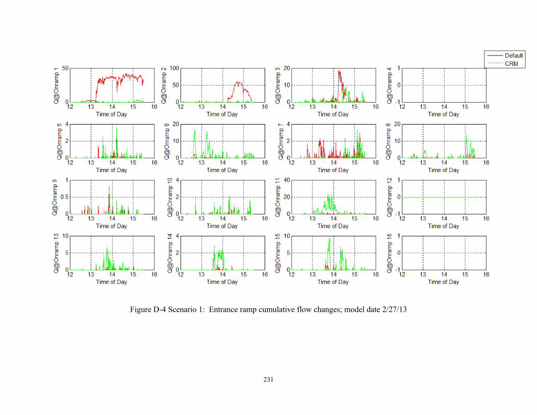
231

Figure D-4 Scenario 1: Entrance ramp cumulative flow changes; model date 2/27/13

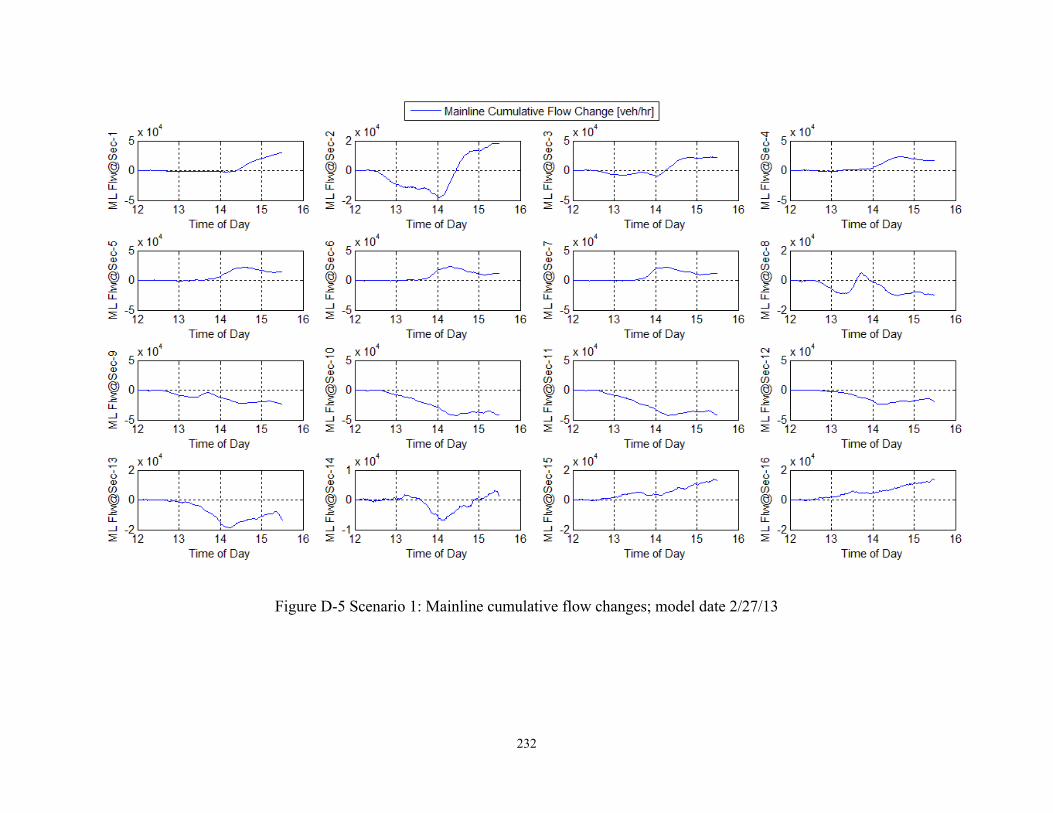
232

Figure D-5 Scenario 1: Mainline cumulative flow changes; model date 2/27/13

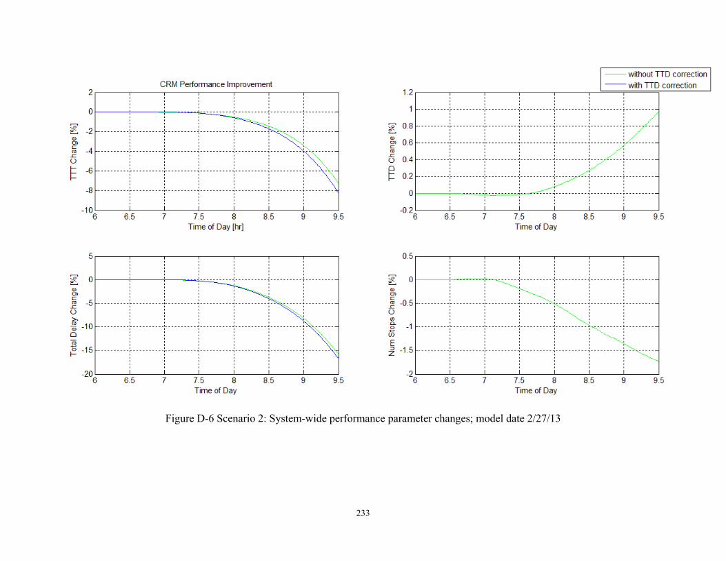
233

Figure D-6 Scenario 2: System-wide performance parameter changes; model date 2/27/13

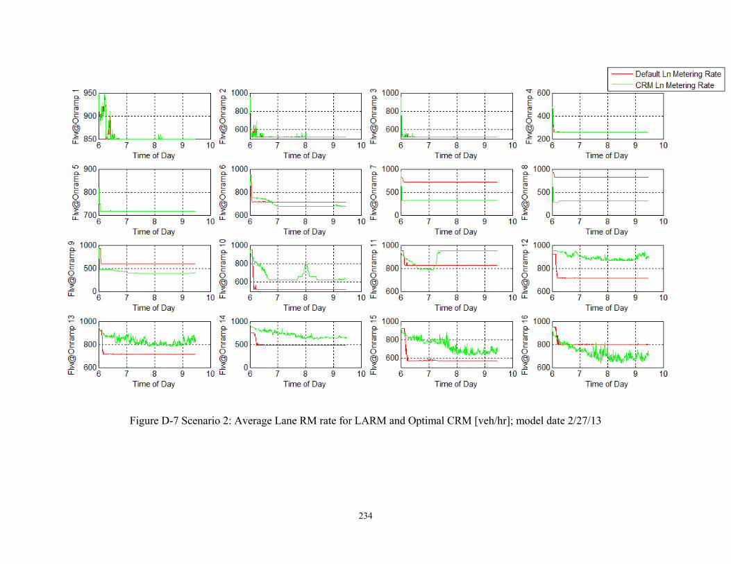
234

Figure D-7 Scenario 2: Average Lane RM rate for LARM and Optimal CRM [veh/hr]; model date 2/27/13

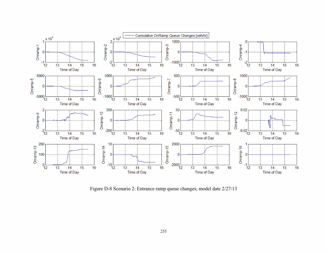
235

Figure D-8 Scenario 2: Entrance ramp queue changes; model date 2/27/13

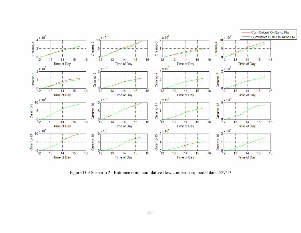
236

Figure D-9 Scenario 2: Entrance ramp cumulative flow comparison; model date 2/27/13

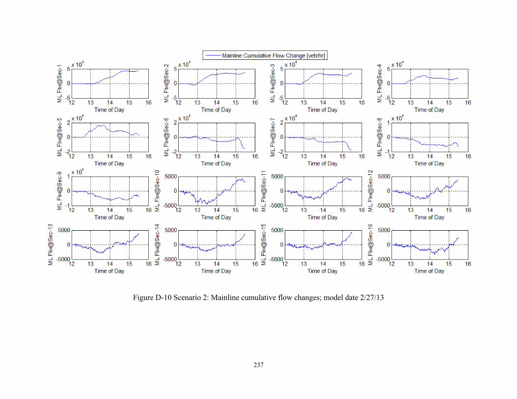
237

Figure D-10 Scenario 2: Mainline cumulative flow changes; model date 2/27/13

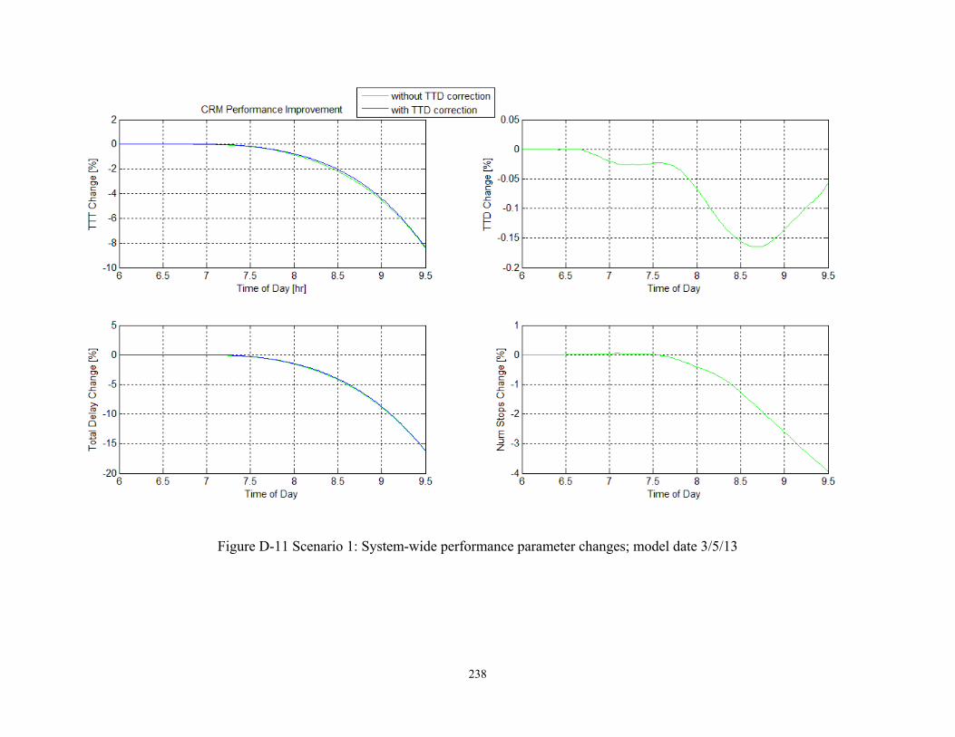
238

Figure D-11 Scenario 1: System-wide performance parameter changes; model date 3/5/13

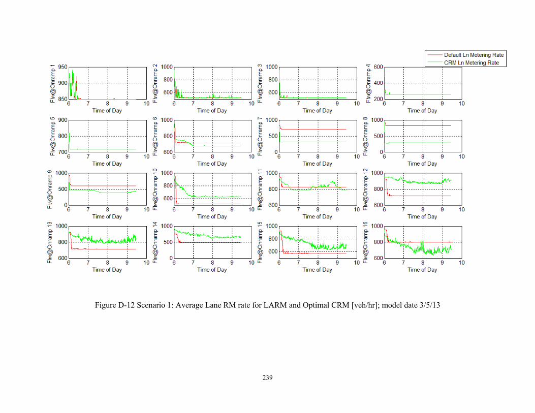
239

Figure D-12 Scenario 1: Average Lane RM rate for LARM and Optimal CRM [veh/hr]; model date 3/5/13

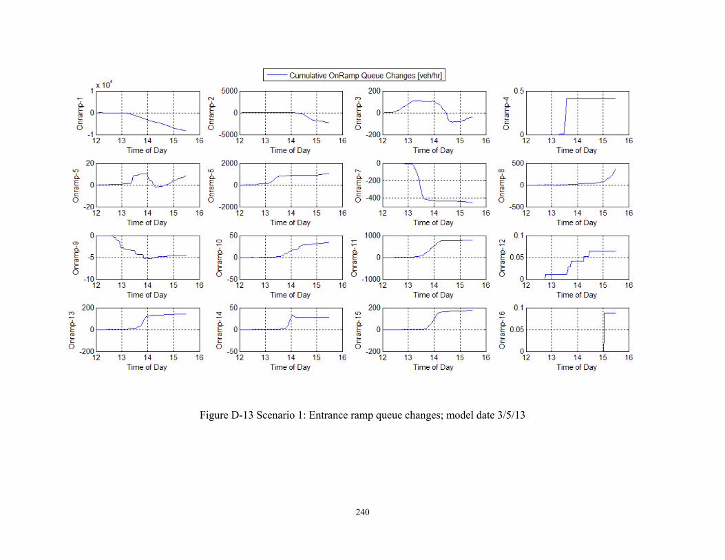
240

Figure D-13 Scenario 1: Entrance ramp queue changes; model date 3/5/13

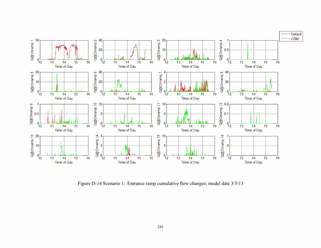
241

Figure D-14 Scenario 1: Entrance ramp cumulative flow changes; model date 3/5/13

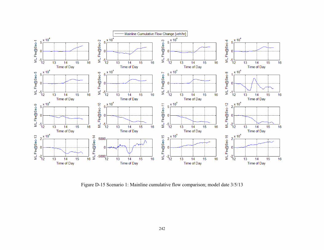
242

Figure D-15 Scenario 1: Mainline cumulative flow comparison; model date 3/5/13

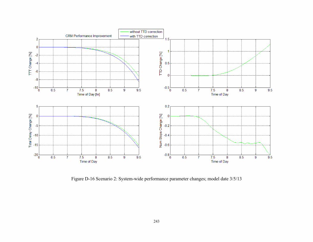
243

Figure D-16 Scenario 2: System-wide performance parameter changes; model date 3/5/13

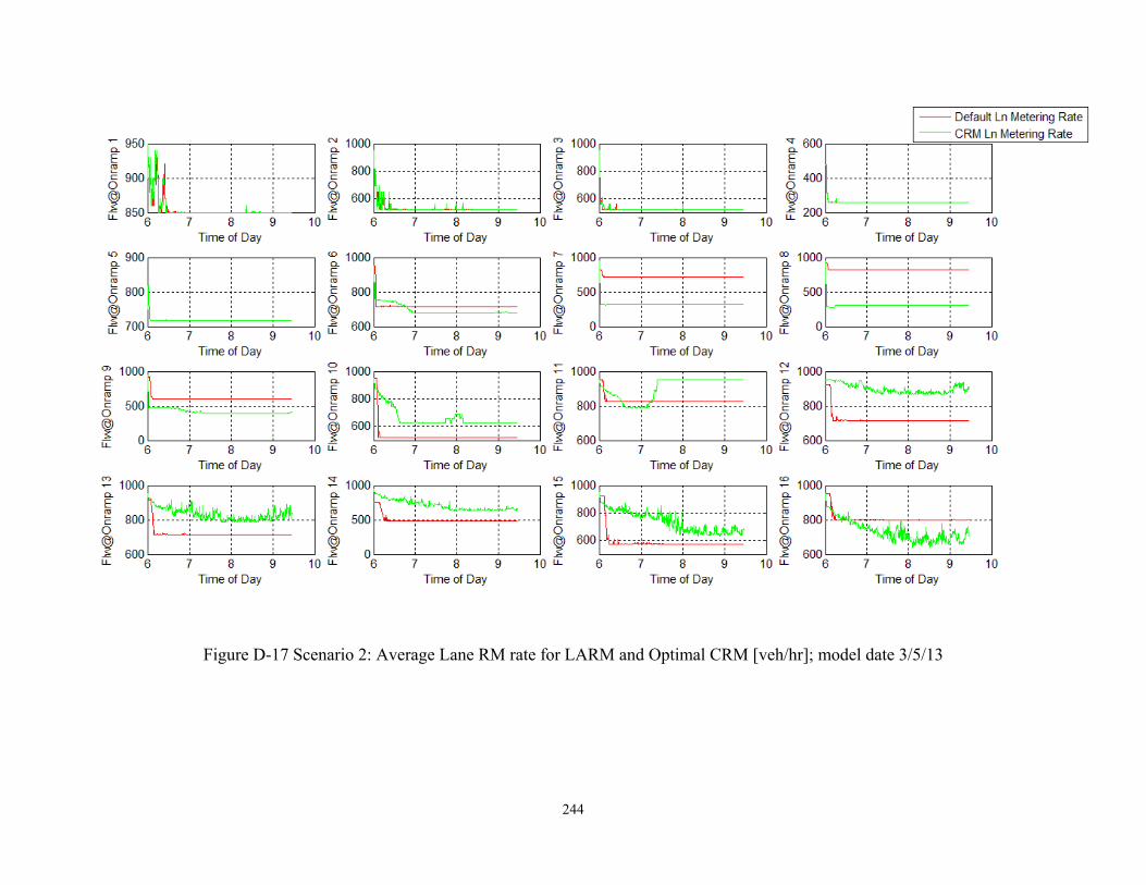
244

Figure D-17 Scenario 2: Average Lane RM rate for LARM and Optimal CRM [veh/hr]; model date 3/5/13

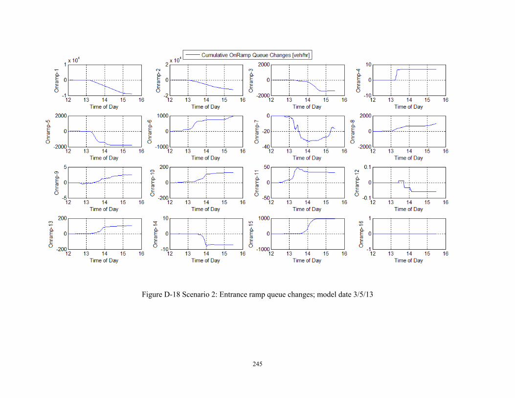
245

Figure D-18 Scenario 2: Entrance ramp queue changes; model date 3/5/13

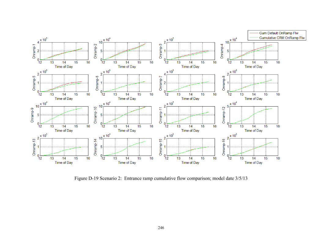
246

Figure D-19 Scenario 2: Entrance ramp cumulative flow comparison; model date 3/5/13

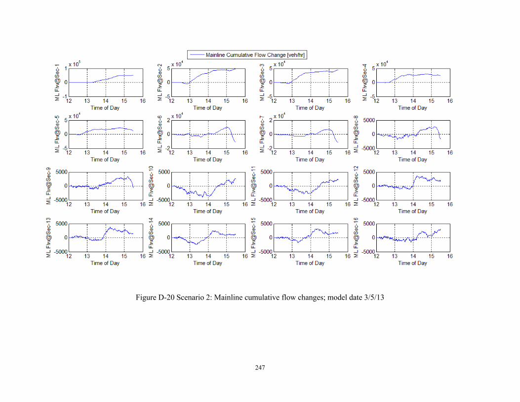
247

Figure D-20 Scenario 2: Mainline cumulative flow changes; model date 3/5/13

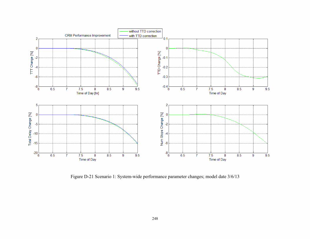
248

Figure D-21 Scenario 1: System-wide performance parameter changes; model date 3/6/13

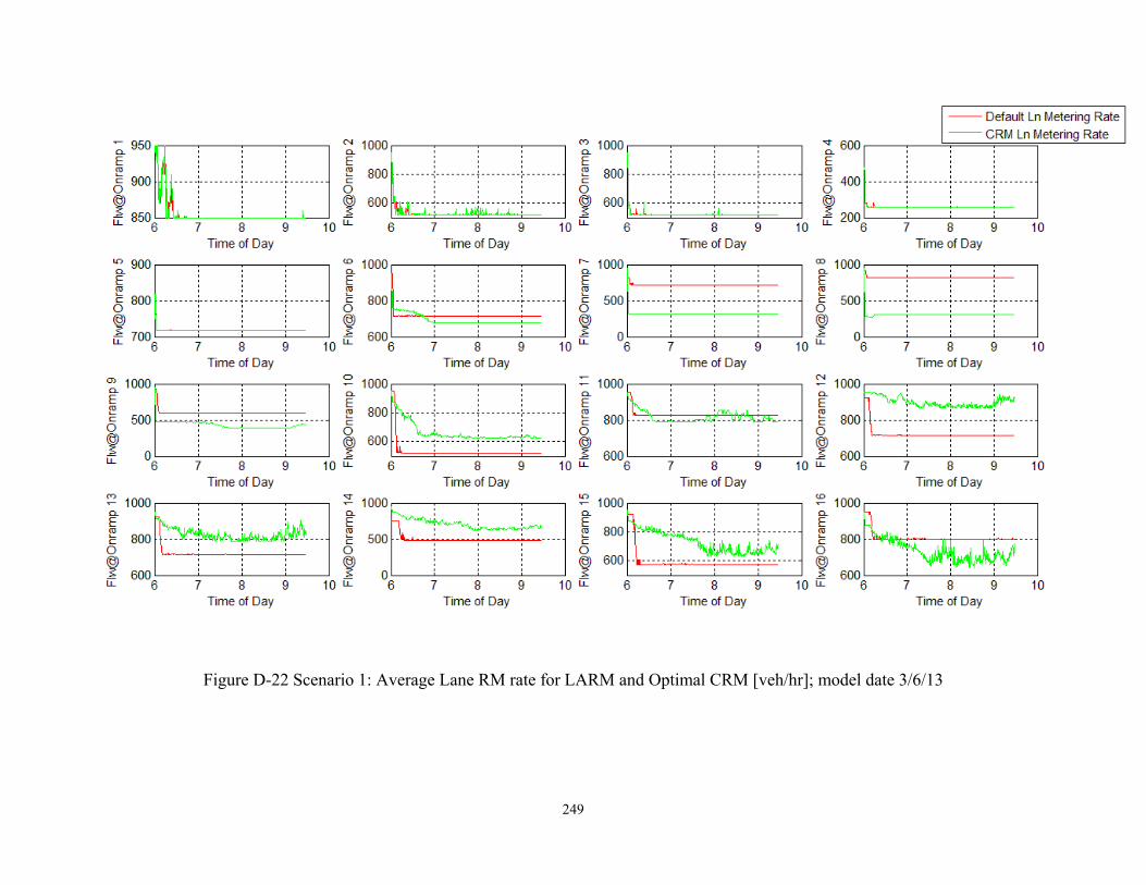
249

Figure D-22 Scenario 1: Average Lane RM rate for LARM and Optimal CRM [veh/hr]; model date 3/6/13

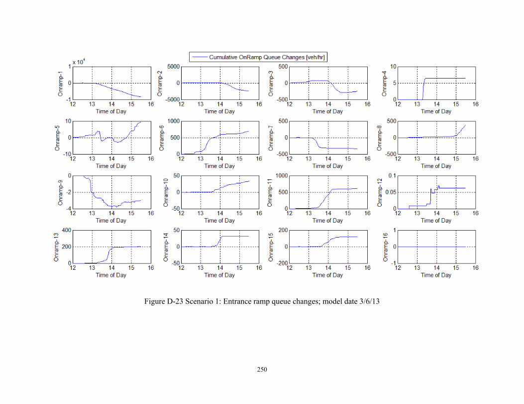
250

Figure D-23 Scenario 1: Entrance ramp queue changes; model date 3/6/13

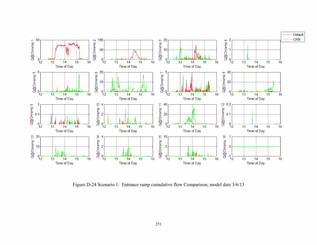
251

Figure D-24 Scenario 1: Entrance ramp cumulative flow Comparison; model date 3/6/13

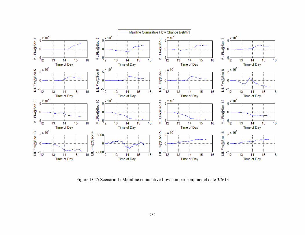
252

Figure D-25 Scenario 1: Mainline cumulative flow comparison; model date 3/6/13

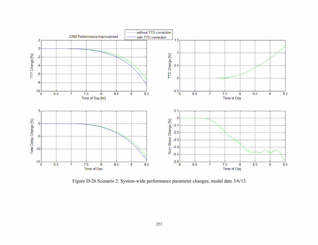
253

Figure D-26 Scenario 2: System-wide performance parameter changes; model date 3/6/13

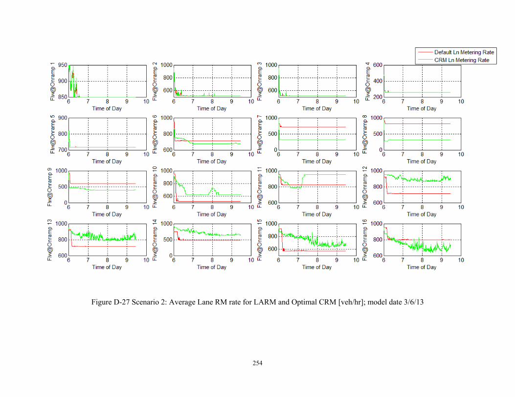
254

Figure D-27 Scenario 2: Average Lane RM rate for LARM and Optimal CRM [veh/hr]; model date 3/6/13

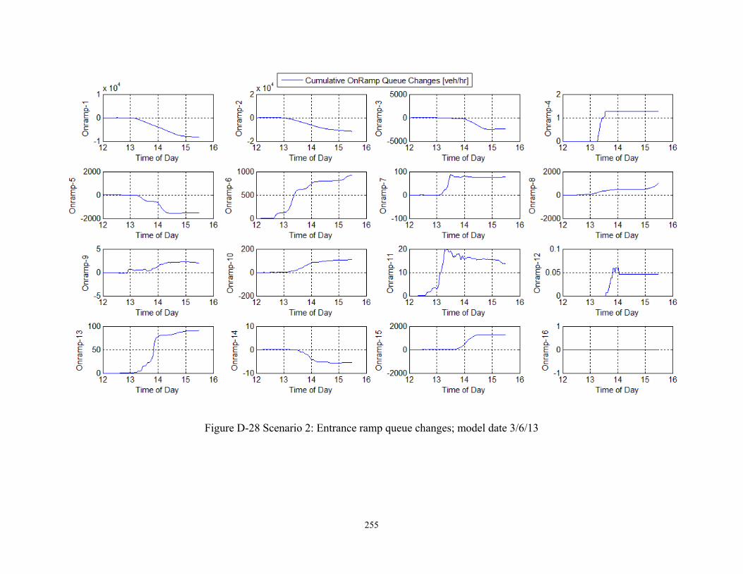
255

Figure D-28 Scenario 2: Entrance ramp queue changes; model date 3/6/13

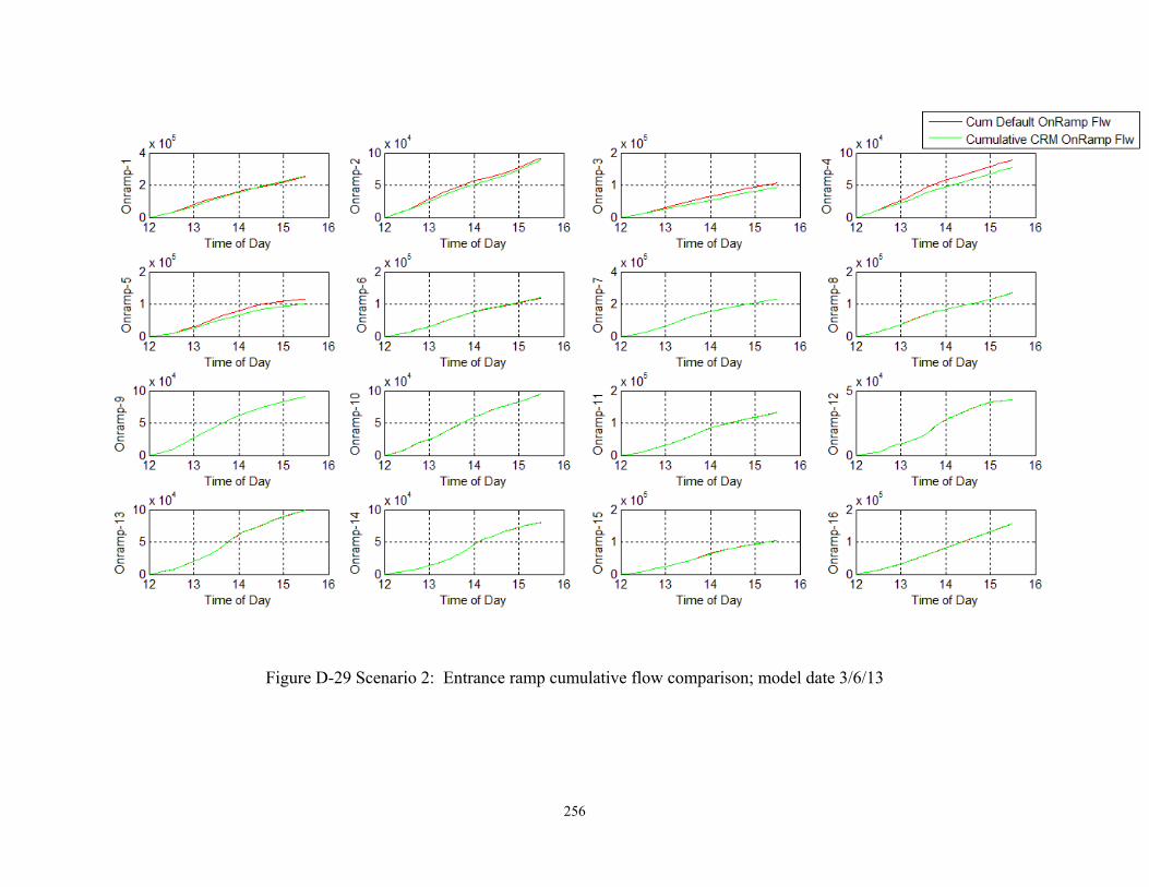
256

Figure D-29 Scenario 2: Entrance ramp cumulative flow comparison; model date 3/6/13

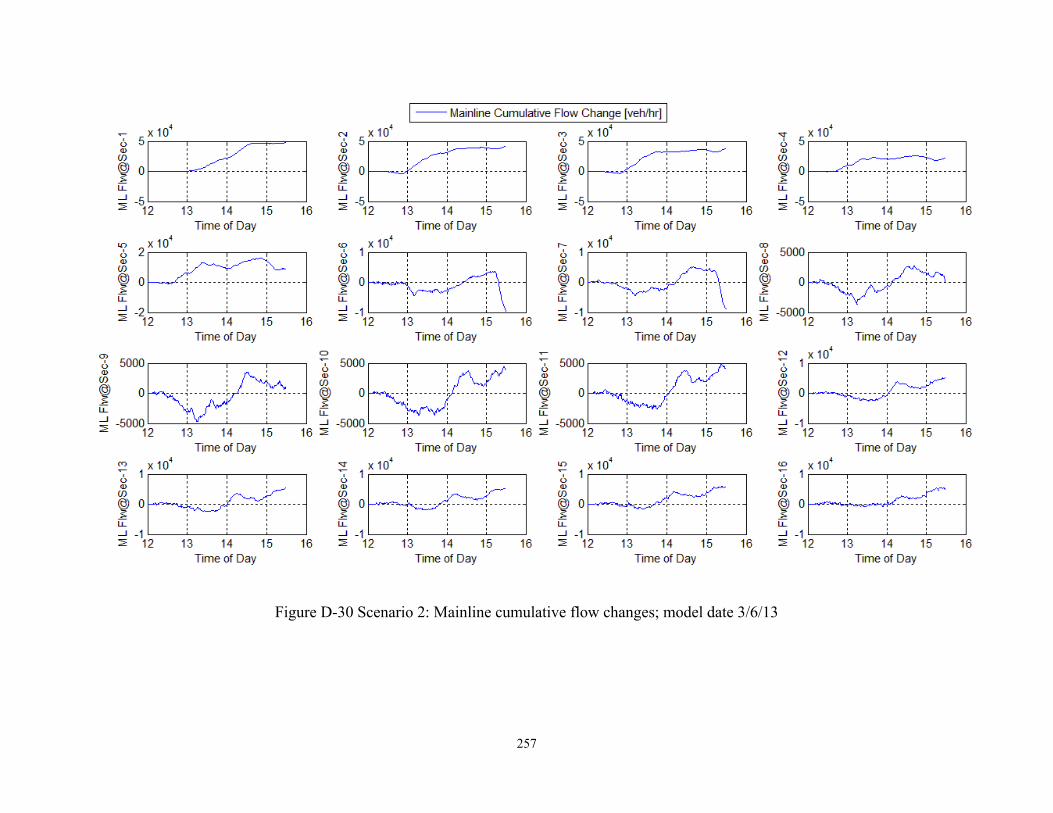
257

Figure D-30 Scenario 2: Mainline cumulative flow changes; model date 3/6/13