credit cycles in a neo-austrian economy

Structural Change and Economic Dynamics18 (2007) 249–269

Credit cycles in a Neo-Austrian economy

Andrea Attar a, Eloisa Campioni b,∗a IDEI, Universite de Toulouse I and Universita di Roma, La Sapienza, Italy

b DPTEA, Universita Luiss – G. Carli, Roma, Italy

Received 1 November 2004; received in revised form 1 February 2005; accepted 1 November 2006Available online 26 January 2007

Abstract

This paper discusses the relationship between firms’ access to credit market and business fluctuations ina sequential Neo-Austrian economy. Existence of cycles reflects a fundamental distortion in the intertem-poral structure of production, that is a lack of coordination between utilization of productive capacity andconstruction of new machines. The role of credit market institutions is to sustain viability of the economyalong an out-of-equilibrium transition. Allowing for a high degree of price flexibility turns out not to be ageneral response to boosts in capital accumulation and employment. When we focus on an irreversible, off-equilibrium dynamics the coordination of policy interventions becomes a relevant tool to govern fluctuations.© 2007 Elsevier B.V. All rights reserved.

JEL Classification: E23; E32; E37; E44

Keywords: Production processes; Cycles; Complex dynamics

1. Introduction

This work discusses the interaction between the characteristics of firms’ financial constraintsand economic fluctuations.

There has been a great resurgence of interest in the last decades for the thesis that a deeperunderstanding of the conditions of entrepreneurs’ access to credit may be helpful in characterizingeconomic cycles.

Several different approaches have been developed to support the conviction that the way inwhich agents finance their activities, interact with financial institutions and choose their contrac-tual arrangements is to be conceived as the main source of economic fluctuations (Gurley and

∗ Corresponding author.E-mail address: [email protected] (E. Campioni).

0954-349X/$ – see front matter © 2007 Elsevier B.V. All rights reserved.doi:10.1016/j.strueco.2006.11.003

mailto:[email protected]

dx.doi.org/10.1016/j.strueco.2006.11.003

250 A. Attar, E. Campioni / Structural Change and Economic Dynamics 18 (2007) 249–269

Shaw, 1955). Generally speaking, we may say that the majority of these studies followed the moststandard approach in business cycle theories. They represent an intrinsically stable economicsystem whose dynamics might become erratic and cyclical because of the impact of exogenousstochastic shocks. The shocks, either monetary or real, affect firms balance sheets, limiting in thisway their access to financial markets. This is the reference framework of very influential works,such as Bernanke and Gertler (1989); Bernanke et al. (1996), and Kiyiotaki and Moore (1997).A somehow less popular research line analyses competitive economies where frictions in themarket for loans, due to asymmetric information, are responsible for the existence of endogenousbusiness fluctuations. In such a perspective, the way in which financial markets work is a sourceof instability that prevents economic dynamics from gravitating around its stationary position(Woodford, 1989; Suarez and Sussman, 1997).

Despite their heterogeneous findings, all these approaches share an important methodologicalreference. That is, they state that business cycle fluctuations can be analyzed as an (intertemporal)equilibrium phenomenon, thereby denying the traditional view that interprets them as a form ofcoordination failure. Such a perspective is shared by the real business cycle school as well as bythe so-called endogenous cycle theories:

To a modern business cycle economist, the economy remains in continuous equilibriumalong the adjustment path towards the steady-growth time path. Any trajectory is calledintertemporal equilibrium. On the contrary, earlier economists (and, for that matter, tem-porary equilibrium theorists as well) would have reserved the intertemporal equilibriumterm for the single time path acting as an attractor for the other trajectories.1

In other words, the domain of equilibrium analysis and welfare theorems has been extended toeconomies exhibiting systematic (and potentially persistent) oscillations of output, employmentand capital accumulation.

The present work suggests an alternative research perspective which is in several respectscloser to the Neoclassical view of fluctuations as phenomena taking place along the out-of-equilibrium transition to a predefinite stationary position. The development of a logical structurethat allows for disequilibria to transmit from one period to the other is the distinguishing featureof the approach. In our perspective, business cycles are a direct consequence of the coordinationproblems emerging in an economy evolving over real time. In particular, existence of fluctuationsreflects fundamental distortions in the structure of productive capacity. In other words, a properanalysis of business fluctuations cannot take either the production technique or the capital stockas given:

[such a] restrictive assumption excludes the very essence of capitalistic reality, all thephenomena and problems of which – including the short run phenomena – hinge upon theincessant creation of new and novel equipment. 2

The pivotal element is the belief that complementarity rather than substitutability relationshipsare best suited to characterize phenomena directly related to the temporal evolution of the eco-nomic activity. We stress the role of two complementarity relationships: the first is induced bythe intertemporal articulation of the production process and the second comes from the expec-tations’ revision mechanism. The original contribution of this work is to emphasize the role of

1 DeVroey (2002, p. 18).2 Schumpeter (1954, p. 280).

A. Attar, E. Campioni / Structural Change and Economic Dynamics 18 (2007) 249–269 251

credit market channeling resources towards the productive sector in a sequential Neo-Austrianeconomy as developed by Hicks (1973); Amendola and Gaffard (1998, 2003). Once fluctuationsare represented as an irreversible phenomenon arising in economies with a persistent lack ofcoordination over time, then the role of credit becomes crucial in guaranteeing that the economymay remain viable. Here comes the interaction with the Wicksellian tradition: when disequilibriabecome effective, that is, when they take place in the markets, then a gap between the naturalrate of interest and the market interest for loans emerges.3 The existence of such a gap reflects afundamental distortion between demand and supply of loanable funds. This, in turn, affects theintertemporal structure of production altering the relationship between the amount of resourcesavailable for sustaining current production and those devoted to the construction of new productivecapacity.

2. The economy

Our target is the definition of a theoretical framework that may enable to conceive off-equilibrium fluctuations in employment, capital accumulation, and financial resources as themain outcome of an economy hit by a liquidity shock.

The intertemporal complementarities and the irreversibilities induced by a time-articulatedproduction structure are the first building block of the analysis. We consider production as aprocess transforming primary inputs into final output. The crucial variable describing the evolutionover time of this economy is the rate of starts of new production processes. In the Hicksian modelof Capital and Time (1973), the dynamics of the rate of starts is driven by the assumption offull performance that imposes an instantaneous modification so to maintain a systematic balancebetween the productive capacity inherited from the past and the current demand. In other words,an endogenous rate of starts guarantees the transition to take place with a market for final goodwhich is instantaneously in equilibrium, so that savings and investments are balanced.

We definitely believe that economic fluctuations are associated to fundamental imbalances infinancial markets, as well as to systematic modifications and revisions of individual expectations.That is, the lack of intertemporal coordination characterizing business fluctuations should beproperly represented using out-of-equilibrium analysis:

The equilibrium forces are relatively dependable; the disequilibrium forces are less depend-able. We can invent rules for their working and calculate the behavior of the resultingmodels; but such calculations are of illustrative value only.4

We therefore follow the Amendola and Gaffard (1998, 2003) and Amendola et al. (2005)(AG, henceforth) approach in introducing a decision mechanism allowing for disequilibria to beeffective in the Neo-Austrian framework. In other words, the outcomes of individual interactionsmay not coincide with individuals (ex ante) plans of action. Along the lines of the TemporaryEquilibrium methodology, agents form their decision plans taking expectations as given. AGdepart from that perspective in stating that there is no adjustment mechanism at work to makeindividual plans fully compatible in the current period.5 In order for disequilibria to be effective,

3 In the Wicksellian terminology the natural rate of interest is the real return on capital, that is the rate of interestdetermined within the stationary equilibrium construction.

4 Hicks (1985, p. 87).5 The role for disequilibrium outcomes in temporary equilibrium constructions has typically been restricted to a virtual

dimension, that is to the whole sequence of future periods, distinct from the immanent one. This methodology is unchanged


the absence of any price-based adjustment mechanism is postulated even in the very short period,following what Hicks defined the fix-price method. Prices are set at the initial instant of everyperiod and are kept constant throughout the period.

The main contribution of the present work is the explicit introduction of lending and borrowingactivities in the sequential framework a la AG. The goal is to understand whether and how aloan market may alleviate harsh fluctuations, making economic dynamics viable. If we think ofdynamics as an irreversible phenomenon, where production and investment decisions are notcoordinated, then liquidity plays two relevant roles. The first is a transactional one: liquiditysustains coordination over time, in that production costs cannot be paid using contemporaneousproceeds only. The second is that it matters as a source of flexibility. In a sequential economy aliquid asset is flexible because it discloses a wide set of future opportunities.6 This emphasizesthe need of liquidity holding for precautionary reasons:

This interpretation of liquidity as freedom of action over time emphasizes the need for coveragainst emergencies or unexpected events, and hence the motive of precaution.7

Actually, an explicit role for liquidity emerges only as far as out-of-equilibrium dynamics areconcerned. In a stationary equilibrium position future expectations are systematically fulfilled, sothat no demand for reserve assets is formulated.

This work insists on the interpretation of liquidity as flexibility, but it departs from AG inallowing for consumers to hold financial resources in the form of risky bonds. That is, we arguethat precautionary demand for liquidity coexists with investment in risky financial assets, whichbecome loanable funds available to sustain construction of new production capacity. We try toshow that once the precautionary idle balances are put back on the markets, then credit institutionsmight be able to restore viability in economies with financial distress.

The paper is organized in the following way: Section 3 presents the model that extends the AGscheme by explicitly considering a (spot) market for loans. Sections 4 and 5 examine the dynamicproperties of the economy. Section 6 concludes.

3. The model

We consider a deterministic economy evolving in discrete time t = 1, 2, . . ., where only onefinal good is produced.

The economy is populated by two categories of agents: consumers and firms, who organizeproduction.

Wages are paid at the beginning of each period. In other words, a cash-in-advance constraintis imposed to generate a significant role for money. Money is also the numeraire of the system.

Furthermore, in every period there exists one risky asset yielding a return of r(t) units ofthe numeraire per unit invested in t − 1. Every firm can finance her investment decisions both

even in the so-called fix-price temporary equilibrium constructions, see Dreze (1975), where in every period agents areassumed to receive quantity signals together with price ones. Those signals have the role of ensuring that agents’ plansfor the current period are ex ante fully coordinated. As a by-product, there is no room for unintentional consequences ofagents’ behavior.

6 “For liquidity is not a property of a single choice; it is a matter of a sequence of choices, a related sequence. It isconcerned with the passage from the known to the unknown—with the knowledge that if we wait we can have moreknowledge”, Hicks (1974, p. 39).

7 Amendola (1989, p. 336).


by using internal revenues and by borrowing from consumers. The decision on the amount ofexternal financing to borrow will depend on the expected level of demand as well as on thecomparison between the cost of financing r(t) and the rate of return on the project the firm owns.As a consequence, three spot markets are opened in every period t: a labor market where workersare hired at the wage w(t), a final good market with relevant price p(t), and a market for loanswhere r(t) is determined.

Intertemporal complementarities arise because of two factors: production has a time articu-lated dimension and individual expectations are revised according to previous periods’ outcomes.These factors characterize the inter-period sequence. With the aim of representing an economicdynamics taking place in real time, an intra-period sequence is also considered. A period isdivided into a finite sequence of instants. Markets open at different instants in time: the loanmarket is the first one, then the labor market opens, while the product market closes the sequence.Disequilibria will take place because prices are fixed at the beginning of each period, but thenature and the magnitude of such disequilibria depend on the timing of decisions within eachperiod. Every agent takes her decisions sequentially, in different instants ε1, ε2, ε3 . . . ∈ t. Ateach stage she is not able to perfectly predict the values of every future variable. Hence, she takesher decisions on the basis of expectations over period t realizations (that we call intra-periodexpectations).

3.1. Technology

We consider the same Neo-Austrian technology as AG.Production lasts T = T c + T u periods, where T c and T u are the length of construction

and utilization, respectively. Technology is linear with constant labor coefficients definedby the arrays ac ∈RT c

+ and au ∈RT u

+ . We denote b∈RT+ the output vector with the coeffi-cients b1 = b2 = · · · = bT c = 0, given that the construction phase lasts T c periods. We alsodefine A ≡ [ac au ] as the vector of labor coefficients for each of the relevant phases ofproduction.

The vectors xc ∈RT cand xu ∈RT u

specify the number of processes in construction andutilization phase; thus, we can define the existing production processes as:

x(t) ≡ xc0(t), . . . , xc

T c−1(t), xuT c (t), . . . , xu

T−1(t) (subscripts stay for age of processes)

(1)

for every t. We remark that the processes of age i at time t + 1 are, in absence of scrapping, justthe processes of age i− 1 at time t, i.e. the aging dynamics is given by:

xi(t + 1) = xi−1(t) (2)

For given p(t) and w(t) we can associate every production process to its internal rate ofreturn, that is the rate of return of the process in a long period stationary position whereextra-profits have disappeared. Let us define the discounted value formula for the investmentproject as:

K(0) =n∑t=1

ψ(t)

(1 + r)t−1 (3)


where ψ(t) = ones · (p(t)b− w(t)A) and ones is a [1 × T ] vector of 1s.8 The internal rate ofinterest is the discount rate that sets K(0) = 0. If we denote this rate with r = r∗, we get:

ψ(1) + ψ(2)

(1 + r∗)+ ψ(3)

(1 + r∗)2 + · · · + ψ(n)

(1 + r∗)n−1 = 0 (4)

In other words:

The rate of interest which is thus identified is (of course) what is commonly called the yieldof the process.[. . .] It is the rate of interest which belongs to the process. The yield must begreater than the market rate of interest, if the process is to be viable.9

The equation K(0) = 0 admits in general multiple solutions, but some of them may not beeconomically meaningful (i.e. they could imply a negative r∗). All the examples that we presentin this work involve a unique, positive value for r∗.

3.2. Prices

All relevant prices can only change at the junction between periods. That is, the economy isbuilt in the spirit of Hicksian fix-price method:

The fix-price method is a disequilibrium method [. . .]. If flow demand is less than flowsupply, a stock will have to be carried over; we say that it has to be carried over, for thealternative policy of cutting price so as to dispose of them within the current period is notseriously considered. [. . .] In describing this model as a fix-price model it is not assumedthat prices are unchanging over time, or from one single period to his successor; only thatthey do not necessarily change whenever there is a demand–supply disequilibrium.10

Hence, the period-t price p(t), the wage rate w(t) and the market interest rate r(t) will movein the direction implied by market disequilibria. In particular, we introduce the same dynamicequations as AG:

p(t) = p(t − 1)

[1 + k

d(t − 1) − s(t − 1)

s(t − 1)

](5)

w(t) = w(t − 1)

[1 + ν

Ld(t − 1) − Ls(t − 1)

Ls(t − 1)

](6)

r(t) = r(t − 1)

[1 + j

inv(t − 1) − sav(t − 1)

sav(t − 1)

](7)

where k, ν and j are the positive parameters. Then, p(t) positively reacts to previous periodexcess demand for the final good d(t − 1) − s(t − 1) and the same holds for the wage rate. Givenfirms–borrowers’ demand for external funds inv(t − 1) and consumers–lenders’ supply of fundssav(t − 1), r(t) will also raise whenever a positive excess demand for external funds emerges.

8 Observe that we are considering a stationary situation where prices and wages are constant over time.9 Hicks (1973, p. 22).

10 Hicks (1982, p. 232).


In the AG framework, the parameters k, ν and j reflect the degree of flexibility in the econ-omy. The suggested notion of flexibility refers to the speed of the price system as a mechanismto coordinate individuals’ behaviors that are not instantaneously compatible. At this point, it isimportant to remark that in the intertemporal equilibrium macroeconomic tradition, prices and/orwages rigidities are neither represented as a reduced speed in the adjustment towards an equi-librium, nor as an absence of coordination (that is, as a permanent disequilibrium), rather as acoordination on an equilibrium position alternative to the perfectly competitive one.

3.3. Firms and sequential analysis

The specification of firms’ behavior is the crucial feature of the economy. The way in whichfirms form their expectations, take their production and investment decisions is deeply intercon-nected with the sequential structure of the economy. Hence, the analysis of firms’ behaviors willbe provided together with a characterization of the intra-period sequence.

At the beginning of period t, p(t), w(t) and r(t) are given. Firms inherit from period t − 1 themonetary proceeds from their salesm(t − 1), the stock of unsold consumption good o(t − 1) andthe stock of money they previously retained for undesired reasons hf(t − 1). The amountW(t) offinancial resources available for firms to sustain production and investment is given by:

W(t) = m(t − 1) + hf(t − 1) − I(t − 1)(1 + r(t)) (8)

where I(t − 1) is the amount of external funds effectively borrowed at t − 1. Eq. (8) imposesthat wages have to be paid in advance using the monetary proceeds from sales m(t − 1) andthe stock of firms’ financial resources hf(t − 1) from previous period. In addition, firms shouldrepay the amount of funds borrowed at t − 1 and the interests matured between t − 1 and t, sayI(t − 1)(1 + r(t)). Eq. (8) is therefore a cash-in-advance constraint, imposing that all transactionstake place in the same good, namely money.

The first relevant decision for firms is to determine the current-period level of production. Todo so, they form an expectation on the level of consumers’ demand d(t) that will become effectiveat the end of period t.11 Firms form their expectations following an adaptive rule, in accordancewith the literature on bounded rational agents. In the particular case of final consumption demand,let this expectation be dE(t), the general expression used by AG is:

dE(t) = dE(t − 1)

⎡⎣1 +

T ′∑i=1

θigm(t − i)

⎤⎦ (9)

where gm(t) ≡ (m(t) −m(t − 1))/(m(t − 1)) is the monetary growth rate, T ′ is the relevant timehorizon for the adaptive rule and θ ≡ [ θ1 · · · θT ] is a vector of non-negative parametersindexed by time. In a steady state equilibrium pathgm(t) does coincide with the (constant) balancedgrowth rate.

The expected demand is therefore a linear function of past expectations and of a weightedaverage of the sequence of past growth rates.12Appendix A illustrates the particular specificationwe used.

11 In other words, this expectation is formulated at the beginning of the period, before consumption demand is madeexplicit.12 The formulation in Eq. (9) is similar to those used in the least squares learning literature (see, for instance, Marcet and

Sargent, 1989). In order to interpret (9) as a least squares learning equation, we should think of the θ s as the coefficients


Given such an expectation scheme and denoting with o(t − 1) the stock of unsold final goodsfrom previous period, firms define their planned production for period t, q′(t). We keep the AGassumption of firms using a simple demand targeting:13

q′(t) = dE(t) − o(t − 1) (10)

Then, firms compare the planned output with the available productive capacity. Thus, period-tproduction q(t) is given by:

q(t) = min{q′(t), b · xu} (11)

Whenever q′(t) ≤ b · xu, then scrapping of processes in the utilization stage will take place,so that the array xu(t) will be properly updated.

As a by-product, the amount of resources devoted to sustain utilization turns out to be:

Wu(t) = w(t)[au · xu(t)

](12)

Period-t internal resources available to finance construction of new productive capacity arehence defined residually: they amount to W(t) −Wu(t).

At this stage the market for loans opens and firms may have access to additional externalresources.

3.3.1. The demand for loansHaving taken their decisions over utilization of existing productive capacity, firms formulate a

demand for loans and offer to the lenders claims on their revenues, promising a rate of return r att + 1. In period t + 1, the assets traded at time t have to be repaid. There exists the possibility thatat the beginning of period t + 1 inherited internal revenuesm(t) will be so low not to allow firmsto pay back their liabilities. In this case bankruptcy takes place and lenders seize all availableresources.14

Firms formulate a demand for external financing inv(t) in the following way:

inv(t) ={a(t) − B(t)r(t), if r(t) < r∗

z(t), if r(t) < r∗(13)

where a(t), B(t) and z(t) are positive for every t = 1, 2, . . .. Whenever the cost of external fundsis lower than the internal rate of return on the process r∗, firms finance their investments alsothrough external funds. The demand for such funds is negatively correlated to the market interestrate r; B(t) is a coefficient growing over time at the exogenous rate of population growth n: 15

B(t) = (1 + n)B(t − 1)

The demand for external financial resources inv(t) also involves the autonomous componenta(t), which relates the demand for external financing to the expected period-t final demand. Thehigher the expected demand, the higher the autonomous component of investments. The relevantexpectation over period-t demand is formulated in the usual adaptive way.

of an OLS regression between d and m. The further step in models of learning is usually to build an algorithm which canguarantee the convergence to the rational expectations equilibrium.13 This behavior is just assumed to be a reliable one (Heiner, 1983).14 In the financial literature, this is usually referred to as full recovery.15 Dealing with an exogenous growth model, the rate of population growth is the steady state growth rate of the economy.


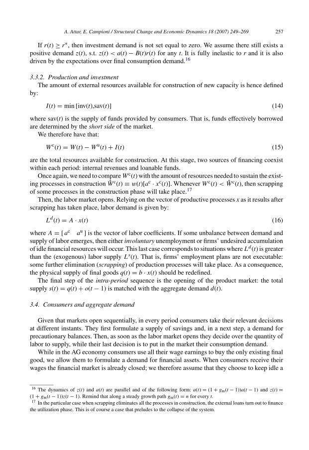
If r(t) ≥ r∗, then investment demand is not set equal to zero. We assume there still exists apositive demand z(t), s.t. z(t) < a(t) − B(t)r(t) for any t. It is fully inelastic to r and it is alsodriven by the expectations over final consumption demand.16

3.3.2. Production and investmentThe amount of external resources available for construction of new capacity is hence defined

by:

I(t) = min [inv(t),sav(t)] (14)

where sav(t) is the supply of funds provided by consumers. That is, funds effectively borrowedare determined by the short side of the market.

We therefore have that:

Wc(t) = W(t) −Wu(t) + I(t) (15)

are the total resources available for construction. At this stage, two sources of financing coexistwithin each period: internal revenues and loanable funds.

Once again, we need to compareWc(t) with the amount of resources needed to sustain the exist-ing processes in construction Wc(t) ≡ w(t)[ac · xc(t)]. WheneverWc(t) < Wc(t), then scrappingof some processes in the construction phase will take place.17

Then, the labor market opens. Relying on the vector of productive processes x as it results afterscrapping has taken place, labor demand is given by:

Ld(t) = A · x(t) (16)

where A = [ac au ] is the vector of labor coefficients. If some unbalance between demand andsupply of labor emerges, then either involuntary unemployment or firms’ undesired accumulationof idle financial resources will occur. This last case corresponds to situations whereLd(t) is greaterthan the (exogenous) labor supply Ls(t). That is, firms’ employment plans are not executable:some further elimination (scrapping) of production processes will take place. As a consequence,the physical supply of final goods q(t) = b · x(t) should be redefined.

The final step of the intra-period sequence is the opening of the product market: the totalsupply s(t) = q(t) + o(t − 1) is matched with the aggregate demand d(t).

3.4. Consumers and aggregate demand

Given that markets open sequentially, in every period consumers take their relevant decisionsat different instants. They first formulate a supply of savings and, in a next step, a demand forprecautionary balances. Then, as soon as the labor market opens they decide over the quantity oflabor to supply, while their last decision is to put in the market their consumption demand.

While in the AG economy consumers use all their wage earnings to buy the only existing finalgood, we allow them to formulate a demand for financial assets. When consumers receive theirwages the financial market is already closed; we therefore assume that they choose to keep idle a

16 The dynamics of z(t) and a(t) are parallel and of the following form: a(t) = (1 + gm(t − 1))a(t − 1) and z(t) =(1 + gm(t − 1))z(t − 1). Remind that along a steady growth path gm(t) = n for every t.17 In the particular case when scrapping eliminates all the processes in construction, the external loans turn out to finance

the utilization phase. This is of course a case that preludes to the collapse of the system.


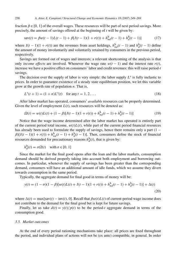
fraction β∈ [0, 1] of the overall wages. These resources will be part of next period savings. Moreprecisely, the amount of savings offered at the beginning of t will be given by:

sav(t) = βw(t − 1)L(t − 1) + β[I(t − 1)(1 + r(t)) + hhnd(t − 1) + hh

d(t − 1)] (17)

where I(t − 1)(1 + r(t)) are the revenues from asset holdings, hhnd(t − 1) and hh

d(t − 1) definethe amount of money involuntarily and voluntarily retained by consumers in the previous period,respectively.

Savings are formed out of wages and interests; a relevant shortcoming of the analysis is thatonly income effects are involved. Whenever the wage rate w(t − 1) and the interest rate r(t),increase we have a positive effect on consumers’ labor and credit revenues: this will raise period-tsavings.

The decision over the supply of labor is very simple: the labor supply Ls is fully inelastic toprices. In order to guarantee existence of a steady state equilibrium position, we let this variablegrow at the growth rate of population n. That is,

Ls(t + 1) = (1 + n)Ls(t) for any t = 1, 2, . . . (18)

After labor market has operated, consumers’ available resources can be properly determined.Given the level of employment L(t), such resources will be denoted as:

Ω(t) = w(t)L(t) + (1 − β)[I(t − 1)(1 + r(t)) + hhnd(t − 1) + hh

d(t − 1)] (19)

Notice that the wage income determined after the labor market has operated is entirely partof the current period total income, w(t)L(t), while part of the current period financial resourceshas already been used to formulate the supply of savings, hence there remains only a part (1 −β)[I(t − 1)(1 + r(t)) + hh

nd(t − 1) + hhd(t − 1)]. Then, consumers define the stock of financial

resources demanded for precautionary reasons hhd(t), that is given by:

hhd(t) = σΩ(t) with σ ∈ [0, 1]

Since the market for the final good opens after the loan and the labor markets, consumptiondemand should be derived properly taking into account both employment and borrowing out-comes. In particular, whenever the supply of savings has been greater than the correspondingdemand, consumers will have an additional amount of idle funds, which we assume they diverttowards consumption in the same period.

Typically, the aggregate demand for final good in terms of money will be:

y(t) = (1 − σ)(1 − β)[w(t)L(t) + I(t − 1)(1 + r(t)) + hhnd(t − 1) + hh

d(t − 1)] +(t)

(20)

where(t) = max[sav(t) − inv(t), 0]. Recall that βw(t)L(t) of current-period wage income doesnot contribute to the demand for the final good but is kept for future savings.

Finally, let us take d(t) = y(t)/p(t) to be the period-t aggregate demand in terms of theconsumption good.

3.5. Market outcomes

At the end of every period rationing mechanisms take place: all prices are fixed throughoutthe period, and individual plans of actions will not be (ex ante) compatible, in general. In order


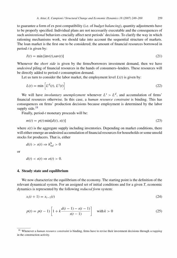
to guarantee a form of ex post compatibility (i.e. of budget balancing), quantity adjustments haveto be properly specified. Individual plans are not necessarily executable and the consequences ofsuch unintentional behaviors crucially affect next periods’ decisions. To clarify the way in whichrationing mechanisms work, we should take into account the sequential structure of markets.The loan market is the first one to be considered; the amount of financial resources borrowed inperiod t is given by:

I(t) = min [inv(t),sav(t)] (21)

Whenever the short side is given by the firms/borrowers investment demand, then we haveundesired piling of financial resources in the hands of consumers–lenders. These resources willbe directly added to period-t consumption demand.

Let us turn to consider the labor market, the employment level L(t) is given by:

L(t) = min[Ld(t), Ls(t)

](22)

We will have involuntary unemployment whenever Ls > Ld , and accumulation of firms’financial resources otherwise. In this case, a human resource constraint is binding. This hasconsequences on firms’ production decisions because employment is determined by the laborsupply side.18

Finally, period-t monetary proceeds will be:

m(t) = p(t) min[d(t), s(t)] (23)

where s(t) is the aggregate supply including inventories. Depending on market conditions, therewill either emerge an undesired accumulation of financial resources for households or some unsoldstocks for producers. That is, either

d(t) > s(t) ⇒ hhnd > 0

or

d(t) < s(t) ⇒ o(t) > 0.

4. Steady state and equilibrium

We now characterize the equilibrium of the economy. The starting point is the definition of therelevant dynamical system. For an assigned set of initial conditions and for a given T, economicdynamics is represented by the following reduced form system:

xi(t + 1) = xi−1(t) (24)

p(t) = p(t − 1)

[1 + k

d(t − 1) − s(t − 1)

s(t − 1)

]with k > 0 (25)

18 Whenever a human resource constraint is binding, firms have to revise their investment decisions through scrappingin the construction activity.


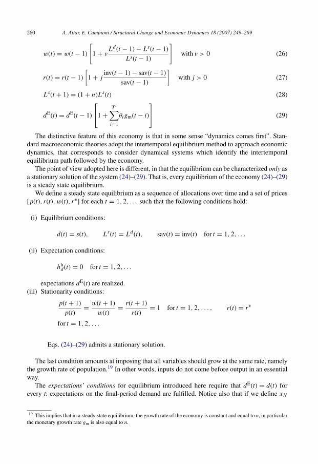
w(t) = w(t − 1)

[1 + ν

Ld(t − 1) − Ls(t − 1)

Ls(t − 1)

]with ν > 0 (26)

r(t) = r(t − 1)

[1 + j

inv(t − 1) − sav(t − 1)

sav(t − 1)

]with j > 0 (27)

Ls(t + 1) = (1 + n)Ls(t) (28)

dE(t) = dE(t − 1)

⎡⎣1 +

T ′∑i=1

θigm(t − i)

⎤⎦ (29)

The distinctive feature of this economy is that in some sense “dynamics comes first”. Stan-dard macroeconomic theories adopt the intertemporal equilibrium method to approach economicdynamics, that corresponds to consider dynamical systems which identify the intertemporalequilibrium path followed by the economy.

The point of view adopted here is different, in that the equilibrium can be characterized only asa stationary solution of the system (24)–(29). That is, every equilibrium of the economy (24)–(29)is a steady state equilibrium.

We define a steady state equilibrium as a sequence of allocations over time and a set of prices[p(t), r(t), w(t), r∗] for each t = 1, 2, . . . such that the following conditions hold:

(i) Equilibrium conditions:

d(t) = s(t), Ls(t) = Ld(t), sav(t) = inv(t) for t = 1, 2, . . .

(ii) Expectation conditions:

hhd(t) = 0 for t = 1, 2, . . .

expectations dE(t) are realized.(iii) Stationarity conditions:

p(t + 1)

p(t)= w(t + 1)

w(t)= r(t + 1)

r(t)= 1 for t = 1, 2, . . . , r(t) = r∗

for t = 1, 2, . . .

Eqs. (24)–(29) admits a stationary solution.

The last condition amounts at imposing that all variables should grow at the same rate, namelythe growth rate of population.19 In other words, inputs do not come before output in an essentialway.

The expectations’ conditions for equilibrium introduced here require that dE(t) = d(t) forevery t: expectations on the final-period demand are fulfilled. Notice also that if we define xN

19 This implies that in a steady state equilibrium, the growth rate of the economy is constant and equal to n, in particularthe monetary growth rate gm is also equal to n.


as the number of processes of age N = T c + T u − 1, then in every steady state equilibrium thefollowing relationship will hold:

xi = xN (1 + gm)N−i (30)

where gm = n is the uniform growth rate and i is the age of the process.Thus, in steady state the composition of output and investments can be inferred from the

utilization phase alone, since gm is exogenously given.It is a direct implication of our definitions that any market equilibrium must be a steady state

equilibrium.To summarize, the steady state equilibrium considered in this section devotes the same amount

of resources to construction as a standard Neo-Austrian economy in the formulation offered byAG. It departs from that framework stating that construction of new capacity is sustained in steadystate both by internal funding and external loans.

As a consequence, the (steady state) aggregate demand and the set of resources available forcurrent production are systematically lower than those available in the benchmark AG economy.The dynamic analysis will provide evidence about the influence of loan market relationships oneconomic fluctuations.

5. Dynamics: the simulation of the economy

Studying dynamical systems by means of computational techniques stems from the idea thatinductive (mathematical) methods are the most appropriate to deal with agents having cognitivelimitations and, more generally, incomplete information on the (non-linear) environment they livein. W. Baumol has recently remarked their potential relevance in economic environments:

Can also yield affirmative generalizations of great power and significance. Their natureis best illustrated by analogy with engineering control analysis and its implications aboutautomatic control mechanisms such as thermostats that regulate temperature. Because theseapparatuses are characterized by lags and inertia, one can easily show that a mechanismthat makes moderate corrections can be stabilizing, while a similar apparatus that makescorrections that still go in the proper direction but that are excessively powerful will movethe controlled object away from the desired trajectory and are likely to generate oscillationsthat can well be severely destabilizing. 20

This section will develop the analysis of the out-of-equilibrium evolution of the economydescribed by the dynamical system presented above through numerical simulations. For anassigned set of initial conditions, we simulate the qualitative behavior of this system in pres-ence of a temporary increase in the amount of consumers’ desired balances, hh

d .21 If a creditmarket was not opened, a more pessimistic attitude of consumers would induce an increase intheir liquidity preference, this reduces final demand and

[this] implies the appearance of an excess supply of final output. This affects in turn the short-run expectations of producers and leads to a reduction in the degree of utilization of existingproductive capacity. This is a source of instability. When, to remain with Harrod, investments

20 Baumol (2000, p. 231).21 The code for simulations has been written in MATLAB building on previous work by A. Attar, E. Campioni and M.

Franchi and it is available upon request. Numerical parameters used in the simulations are reported in Appendix A.


are affected by the current performance of the economy, the reduction in the utilization ofproductive capacity also brings about a reduction in the activity of construction.22

In a structure where consumers can allocate their resources within alternative uses, a modifica-tion of consumers’ expectations translates into a different composition of demand for final goodand savings. This affects in turn the availability of resources that entrepreneurs can get through theaccess to financial markets. Our task is to check whether such a change in expectations can sustainthe viability of the economy via a market for loans. That is, we are considering an external shockon the composition of firms’ financing induced by a temporary change in consumers’ expectationsvia an increase in the coefficient of consumers’ desired balances σ occurring at a certain point intime.

The shock produces a distortion between savings and consumption demand at t, in t + 1 theseresources will be put back both on the loans market and on the final good one.

We remark that our economy exhibits the same dynamical features as the AG economywhenever savings are set equal to zero, i.e. β = 0.23

We will consider three different scenarios corresponding to alternative assumptions on prices’and wages’ flexibility parameters.

5.1. Rigidity case: k = ν = 0

We start analyzing a fully rigid scenario, where prices and wages do not react to marketdisequilibria, i.e. k = ν = 0.

The increase in the amount of consumers’ desired liquidity hhd has the first effect of contracting

the aggregate demand d. This induces scrapping of processes in the utilization phase and furtherreductions in net supply. In case of a temporary shock on desired liquidity holdings in an economywithout credit, d goes back soon to its initial level given that desired liquidity in t becomes demandin t + 1 (see Eq. (19)). On the contrary, the reduction in available resources transmits to nextperiods aggregate supply through a reduced investment activity (scrapping in the constructionphase). The economy experiences a persistent excess of aggregate demand, so firms’ wage fundis systematically insufficient to sustain both utilization and construction of productive capacity.

In order to understand how loan market works in an economy with rigid prices and wages,we focus on economies that remain viable after a liquidity shock. That is, we assume that theinjection of external financial resources is sufficiently high to keep distortions under control. If aloan market is open, then n = 0.15 is sufficient to guarantee viability: an increase in the exogenousgrowth rate of the economy raises the amount of borrowing and provides additional resources forentrepreneurs.24

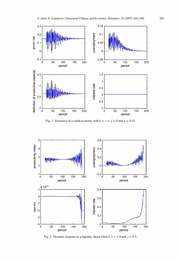
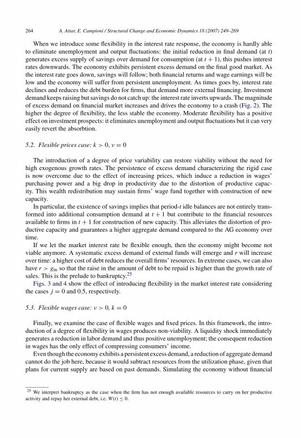
With flexibility in the market for loans (i.e. higher values of j), there emerges a trade-off betweenthe degree of flexibility and severe distortions of productive capacity. As we can see comparingFigs. 1 and 2, alternative values of the parameter j measure how sensitive the market interest rateis to previous-period excess demand. In the case j = 0 there is some inherent instability in theeconomy, the distortion of the productive capacity index remains within bounds but exhibits atendency towards an excess construction over utilization processes.

22 Amendola and Gaffard (1998, p. 231).23 AG do not deal explicitly with shocks in consumers’ expectations. We simulated the effects of these shocks in their

economy and we found out that they correspond to the ones taking place in the modified economy when β = 0.24 In the AG economy, simulative analysis shows that a growth rate ofLs equal to 0.22 is necessary to reabsorb fluctuations.


Fig. 1. Dynamics of a credit economy with k = ν = j = 0 and n = 0.15.

Fig. 2. Dynamic response to a liquidity shock when k = ν = 0 and j = 0.5.


When we introduce some flexibility in the interest rate response, the economy is hardly ableto eliminate unemployment and output fluctuations: the initial reduction in final demand (at t)generates excess supply of savings over demand for consumption (at t + 1), this pushes interestrates downwards. The economy exhibits persistent excess demand on the final good market. Asthe interest rate goes down, savings will follow; both financial returns and wage earnings will below and the economy will suffer from persistent unemployment. As times goes by, interest ratedeclines and reduces the debt burden for firms, that demand more external financing. Investmentdemand keeps raising but savings do not catch up: the interest rate inverts upwards. The magnitudeof excess demand on financial market increases and drives the economy to a crash (Fig. 2). Thehigher the degree of flexibility, the less stable the economy. Moderate flexibility has a positiveeffect on investment prospects: it eliminates unemployment and output fluctuations but it can veryeasily revert the absorbtion.

5.2. Flexible prices case: k > 0, ν = 0

The introduction of a degree of price variability can restore viability without the need forhigh exogenous growth rates. The persistence of excess demand characterizing the rigid caseis now overcome due to the effect of increasing prices, which induce a reduction in wages’purchasing power and a big drop in productivity due to the distortion of productive capac-ity. This wealth redistribution may sustain firms’ wage fund together with construction of newcapacity.

In particular, the existence of savings implies that period-t idle balances are not entirely trans-formed into additional consumption demand at t + 1 but contribute to the financial resourcesavailable to firms in t + 1 for construction of new capacity. This alleviates the distortion of pro-ductive capacity and guarantees a higher aggregate demand compared to the AG economy overtime.

If we let the market interest rate be flexible enough, then the economy might become notviable anymore. A systematic excess demand of external funds will emerge and r will increaseover time: a higher cost of debt reduces the overall firms’ resources. In extreme cases, we can alsohave r > gm so that the raise in the amount of debt to be repaid is higher than the growth rate ofsales. This is the prelude to bankruptcy.25

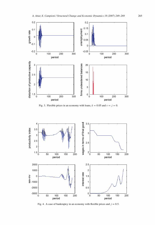
Figs. 3 and 4 show the effect of introducing flexibility in the market interest rate consideringthe cases j = 0 and 0.5, respectively.

5.3. Flexible wages case: ν > 0, k = 0

Finally, we examine the case of flexible wages and fixed prices. In this framework, the intro-duction of a degree of flexibility in wages produces non-viability. A liquidity shock immediatelygenerates a reduction in labor demand and thus positive unemployment; the consequent reductionin wages has the only effect of compressing consumers’ income.

Even though the economy exhibits a persistent excess demand, a reduction of aggregate demandcannot do the job here, because it would subtract resources from the utilization phase, given thatplans for current supply are based on past demands. Simulating the economy without financial

25 We interpret bankruptcy as the case when the firm has not enough available resources to carry on her productiveactivity and repay her external debt, i.e. W(t) ≤ 0.


Fig. 3. Flexible prices in an economy with loans, k = 0.05 and ν = j = 0.

Fig. 4. A case of bankruptcy in an economy with flexible prices and j = 0.5.


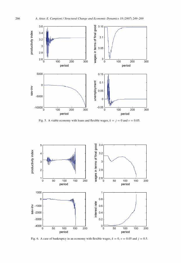
Fig. 5. A viable economy with loans and flexible wages, k = j = 0 and ν = 0.05.

Fig. 6. A case of bankruptcy in an economy with flexible wages, k = 0, ν = 0.05 and j = 0.5.


markets, we would observe a persistent fall in wages and an increasing distortion of productivecapacity that leads the economy to collapse.

Explicit consideration of a credit market implies a reduced impact of wage flexibility onaggregate demand but does not qualitatively alter the basic results.

Consumers’ income consists in fact of both wages and interests on debt paid byfirms–borrowers: hence, a wage reduction has a smaller effect on the resources available forutilization and on the overall employment. As we can observe in Fig. 5, the reaction to this liquid-ity shock is relatively controlled and is reabsorbed very soon. The initial raise in unemploymentdue to the temporary excess demand of labor is soon inverted towards a stationary position. Fur-thermore, the reduction in the funds for utilization does not affect the overall wage fund of firmsW(t) because firms have also access to external financial resources at unchanged price. In caseof reactive loan markets, i.e. j > 0, the interest rate raises over time, in response to a persistentexcess of investments over savings. Notice though that if r raises too much (i.e. j is very high),bankruptcy might happen again (Fig. 6). Once again, our sequential economy delivers a generalprediction that is in the spirit of the AG findings: viability is not compatible with a high degreeof flexibility in all relative prices.

6. Concluding remarks

This work discusses the role of firms’ borrowing conditions in affecting economic fluctua-tions in a sequential Neo-Austrian economy. The distinguishing feature of this approach is theexplicit consideration of the interaction between firms’ bounded rationality and time-articulatedproduction processes in inducing off-equilibrium complex dynamics.

The role of loan market institutions turns out to be crucial in sustaining economic evolution. Ahigh degree of interest rate flexibility is not necessarily the most adequate prescription when thereexist a systematic imbalance between utilization of existing productive capacity and constructionof new one.

A relevant coordination of policy interventions and institutional design all along an off-equilibrium transition is needed to guarantee viability of the economic process.

Acknowledgements

We are grateful to Mario Amendola, Giovanni Di Iasio, Massimo Franchi and Marcello Messorifor constructive suggestions. We also thank seminar audiences at Universita di Roma, La Sapienzaand at ICSIM-Piediluco and two anonymous referees for their careful comments. All errors remain,of course, ours.

Appendix A. Parameters of the simulations

• Steady state equilibriumAll simulations have been run assuming a steady growth rate gm = n = 0.02.The technology is characterized by:

◦ lengths of construction and utilization phases T c = 2, T u = 2;◦ the labor coefficients A = ( 2 2 1 1 );◦ the output coefficients b = ( 0 0 10 10 ).


In the steady state equilibriump = 1,w = 3.1442, r = r∗ = 0.029. Consumers’ preferencesare such that β = 0.1351.

• ShocksWe consider a temporary shock in the consumers’ precautionary demand for money with the

following characteristics:

σ ={

0.04 when t = 20

0 otherwise

• ExpectationsThe relevant formulas used to compute expectations in the simulations’ exercises are:

dE(t) = dE(t − 1)(1 + gav)

where gav = (gm(t − 1) + gm(t − 2))/2 is the arithmetic average of the previous two periodsgrowth rates.

• Flexibility coefficientsWe remark that k is the flexibility coefficient for the price of the consumption good, v the

coefficient associated to wages and j is the relevant coefficient for the market interest rate. Wewill summarize here the three scenarios of the simulations:

(i) Rigidity case: k = ν = 0; j = 0.0 and j = 0.5.(ii) Flexible price case: k = 0.05, ν = 0; j = 0.0 and j = 0.5.

(iii) Flexible wage case: k = 0, ν = 0.05; j = 0.0 and j = 0.5.

References

Amendola, M., 1989. Liquidity, flexibility and processes of economic change. In: Value and Capital Fifty Years Later.International Economic Association Conference Volume.

Amendola, M., Gaffard, J., 1998. Out of Equilibrium. Oxford University Press.Amendola, M., Gaffard, J., 2003. Persistent unemployment and co-ordination issues: an evolutionary perspective. Journal

of Evolutionary Economics 13 (1), 1–27.Amendola, M., Gaffard, J., Saraceno, F., 2005. Technical progress, accumulation of capital and financial constraints: is

the productivity paradox really a paradox? Structural Change and Economic Dynamics 2, 243–261.Baumol, W., 2000. Review: out of equilibrium. Structural Change and Economic Dynamics 11, 227–233.Bernanke, B., Gertler, M., 1989. Agency costs, net worth and business fluctuations. American Economic Review 79,

14–31.Bernanke, B., Gertler, M., Gilchrist, S., 1996. The financial accelerator and the flight to quality. Review of Economics

and Statistics 78 (1), 1–15.DeVroey, M., 2002. Equilibrium and disequilibrium in walrasian and neo-Walrasian economics. Journal of the History

of Economic Thought 24, 405–426.Dreze, J., 1975. Existence of an equilibrium under price rigidity and quantity rationing. International Economic Review

16 (2), 301–320.Gurley, J., Shaw, E., 1955. Financial aspects of economic development. American Economic Review 65, 515–538.Heiner, R., 1983. The origin of predictable behaviour. American Economic Review 73 (4), 560–595.Hicks, J., 1973. Capital and Time. Oxford University Press, Oxford.Hicks, J., 1974. The Crisis in Keynesian Economics. Basic Blackwell, Oxford.Hicks, J., 1982. Methods of Dynamic Analysis. Money, Interest and Wages, Collected Essays on Economic Theory, vol.

II. International Economic Association Conference Volume.Hicks, J., 1985. Methods of Dynamic Economics. Basic Blackwell, Oxford.Kiyiotaki, N., Moore, J., 1997. Credit cycles. Journal of Political Economy 105, 211–248.


Marcet, A., Sargent, T., 1989. Convergence of least squares learning mechanisms in self referential linear stochasticmodels. Journal of Economic Theory 2 (48), 337–368.

Schumpeter, J., 1954. History of Economic Analysis. Allen and Unwin, London.Suarez, J., Sussman, O., 1997. Endogenous cycles in a Stigliz–Weiss economy. Journal of Economic Theory 76, 47–71.Woodford, M., 1989. Imperfect financial intermediation and complex dynamics. In: Barnett, W., et al. (Eds.), Economic

Complexity: Chaos, Sunspots, Bubbles, and Nonlinearity. Cambridge University Press, New York.

credit cycles in a neo-austrian economy

Documents