corrosion of stainless and carbon steel in aqueous amine
TRANSCRIPT

Copyright
by
Kent Billington Fischer
2019
The Dissertation Committee for Kent Billington Fischer Certifies that this is the
approved version of the following Dissertation:
Corrosion of Stainless and Carbon Steel in Aqueous Amine for CO2
Capture
Committee:
Gary T. Rochelle, Supervisor
Gyeong S. Hwang
Benjamin Keith Keitz
Harovel G. Wheat

Corrosion of Stainless and Carbon Steel in Aqueous Amine for CO2
Capture
by
Kent Billington Fischer
Dissertation
Presented to the Faculty of the Graduate School of
The University of Texas at Austin
in Partial Fulfillment
of the Requirements
for the Degree of
Doctor of Philosophy
The University of Texas at Austin
May 2019

Dedication
To my parents, Anne and Duncan
v
Acknowledgements
I could not have asked for a better advisor than Dr. Rochelle. He is an exacting and
brilliant scientist, but he never let that take priority over being kind and patient. “Re-
treading” me from a chemist into a chemical engineer was not an easy task, and I will
always be grateful that he took a chance on me. I would also like to thank Keith Keitz,
Gyeong Hwang, and Harovel Wheat for serving on my supervising committee and for their
feedback on this project.
I would also like to thank several key mentors in the Rochelle group who helped
me with this work. Dr. Eric Chen trained me how to design, procure, and fabricate
experimental equipment. He also trained me how to work responsibly and safely in an
industrial environment at the Pickle Research Center. Omkar Namjoshi trained me in
several experimental and analytical techniques, and was in general a kind and supportive
friend. Paul Nielsen provided analytical training and support, and was also the source of
many insights into the autocatalytic nature of amine degradation and corrosion. Matthew
Beaudry blazed the trail for my pilot work with his significant, independent pilot work.
Without his training, I would have been unable to complete the ambitious 2018 piperazine
pilot campaign. Maeve Cooney has been a constant source of advice, wit, and fondly
remembered conversations—thanks for your patience and help with writing. Thanks to
Matthew Walters, Darshan Sachde, Yu-Jeng Lin, and Brent Sherman for teaching me about
the subtleties of process modeling and optimization. Former group members that I also owe
gratitude are: Yang Du, Nathan Fine, Peter Frailie, Steven Fulk, Lynn Li, and Di Song.
This work would not have been possible without the help of my undergraduate
research assistants: Akshay Daga, Shyam Sharma, and Victor Chan Wai Han. I am

vi
exceptionally proud of your dedication and accomplishments in the lab, and I am very
lucky to know and have worked with you. Thanks to the other undergraduates who assisted
me when we briefly crossed paths: Daniel Hatchell, Hanbi Liu, and Mark Tomasovic.
Thanks to my recently graduated cohort in the Rochelle group: Ye Yuan, Yue
Zhang, and Joseph Selinger. I have really appreciated your help with this project and your
friendship. Among the current cohort, I owe special thanks to Korede Akinpelumi and
Ching-Ting Liu, both of whom helped me during the 2018 piperazine pilot campaign.
Ching-Ting is continuing this corrosion work, and her help and insights have been
invaluable. I also owe gratitude to Tianyu Gao, Athreya Suresh, and Yuying Wu.
Experiments at the pilot scale are very much a team effort. I would like to thank
Tony Wu, John Carroll and all the engineers and operators at the National Carbon Capture
Center who contributed to this work. Significant planning for the 2018 piperazine pilot
campaign was done by Katherine Dombrowski, Andrew Sexton, and Karen Farmer.
Thanks also to Eric Chen, Frank Seibert, and all the personnel and operators at the UT
Separations Research Program who coordinated the 2017 piperazine pilot campaign.
I am also grateful for the assistance of Andrei Dolocan and Richard Piner with SEM
and Vincent Lynch with X-ray diffraction. Shallaco McDonald provided frequent
mechanical assistance, particularly with fabricating and welding the corrosion loop
apparatus.
Thanks to my friends, with whom I remember especially fondly many excellent
conversations over Saturday morning pancake breakfasts at Kerbey Lane Café.
Financial support for this project was provided by the Texas Carbon Management
Program and the Cockrell Foundation.
Finally, thanks to my fiancée Carly Holcomb. Without your love and support, I
wouldn’t have been able to finish this project.
vii
Abstract
Corrosion of Stainless and Carbon Steel in Amine Solutions for CO2
Capture
Kent Billington Fischer, Ph.D.
The University of Texas at Austin, 2019
Supervisor: Gary T. Rochelle
Post-combustion carbon capture and storage with amine absorbents is a key
technology needed to provide low-cost decarbonized electricity. Improving understanding
of corrosion by amines may reveal a solvent system compatible with carbon steel, which
would reduce plant capital costs.
Corrosion of stainless and carbon steel in aqueous monoethanolamine (MEA) and
piperazine (PZ) has been measured. High temperature amine corrosion was measured in a
bench-scale pressure vessel and iron solubility in amines was screened in stirred reactors.
Corrosion was measured at two PZ pilot plants and one MEA pilot plant, using coupons
and electrical resistance probes. Corrosion products were characterized by SEM and
powder X-ray diffraction.
Carbon steel (C1010) often performs well in 5 molal PZ up to 150 °C due to the
formation of a passivating FeCO3 layer. This layer is promoted at high temperature, high
CO2 loading, low solution velocity, and in amines with low Fe2+ solubility. FeCO3
formation is favorable at high temperature because Fe2+ solubility decreases and the
kinetics of FeCO3 formation are faster. This also means that FeCO3 is not observed at low
viii
temperature. Despite this, carbon steel performs well at low temperature due to slower
kinetics of metal oxidation.
Depassivation and high corrosion of stainless steel (316L) can occur in amine
solutions at high temperature (150 °C) when conditions are relatively anoxic and reducing.
Performance of stainless at high temperature in PZ suggests that it can be pushed into and
out of the passive state by small process changes, such as different flue gas O2
concentrations. However, stainless performs well in both MEA and PZ in pilot plants at
≈120 °C.
Fe3+ corrosion products are generated in the absorber, then reduced to Fe2+ in the
high temperature, anoxic conditions of the stripper. In this way, carried-over Fe3+ is
responsible for oxidation of amine and corrosion at high temperature.
Certain highly corrosive amines also have high Fe2+ solubility. Ethylamines like
MEA are likely the correct chain length to form stable complexes with Fe2+ in solution.
Stable Fe2+-amine complexes cause high Fe2+ solubility, which prevents FeCO3 formation
and leads to high corrosion.
ix
Table of Contents
Dedication .......................................................................................................................... iv
Acknowledgements ..............................................................................................................v
Table of Contents ............................................................................................................... ix
List of Tables ................................................................................................................... xvi
List of Figures .................................................................................................................. xix
Chapter 1. Introduction ........................................................................................................1
Chapter 2. Background ........................................................................................................5
2.1. Argument for the implementation of carbon capture and storage ............5
2.1.1. Atmospheric carbon dioxide and temperature .................................5
2.1.2. Impacts of rising global temperature ...............................................6
2.1.3. Sources of atmospheric carbon dioxide ...........................................7
2.1.4. Mitigating carbon dioxide emissions from electricity
generation ..................................................................................................8
2.1.5. Mitigating carbon dioxide emissions with carbon capture and
storage .....................................................................................................10
2.2. Post-combustion carbon capture with chemical absorption ....................11
2.2.1. Description of a typical amine absorption process ........................11
2.2.2. Developments in PCCC with chemical absorption ........................12
2.3. Corrosion in PCCC with chemical absorption ........................................15
2.3.1. Motivation ......................................................................................15
2.3.2. Corrosion thermodynamics ............................................................17
2.3.3. Passive film formation ...................................................................24
2.3.4. Corrosion experience in natural gas sweetening ............................26

x
2.3.5. Corrosion measurements at PCCC conditions ...............................29
2.3.6. Corrosion measurement at PCCC conditions in pilot plants .........32
Chapter 3. Experimental Methods .....................................................................................35
3.1. Techniques for Measurement of Corrosion ............................................35
3.1.1. Electrical Resistance Corrosion Probes .........................................35
3.1.2. Oxidation-Reduction Probes ..........................................................38
3.1.3. Corrosion Coupons ........................................................................39
3.1.4. Coupon Characterization ...............................................................41
3.2. Equipment for Simulating Amine Corrosion at the Bench-Scale ...........44
3.2.1. Corrosion Loop Apparatus .............................................................44
3.2.2. Thermal Degradation Cylinders .....................................................47
3.2.3. Equilibrium Fe2+ Solubility Measurement .....................................49
3.3. Amine Solution Characterization ............................................................50
3.3.1. Preparation of Amine Solutions .....................................................50
3.3.2. Anion Chromatography .................................................................51
3.3.3. Cation Chromatography .................................................................51
3.3.4. Inductively Coupled Plasma Optical Emission Spectroscopy .......52
3.3.5. Total Inorganic Carbon Measurement ...........................................53
3.4. Miscellaneous Equipment and Equipment Part Numbers ......................54
3.4.1. Corrosion Coupon Mounting Hardware ........................................54
3.4.2. Bench-Scale Data Logger ..............................................................56
3.4.3. Equipment Part Numbers ...............................................................58
xi
Chapter 4. Bench-Scale Corrosion Measurement ..............................................................59
4.1. Corrosion Loop Results: Piperazine .......................................................60
4.2. Corrosion Loop Results: Linear Amines ................................................65
4.3. Limitations of Corrosion Loop results ....................................................67
4.4. Thermal Cylinder Results: Linear Amines .............................................68
4.5. Conclusions .............................................................................................75
4.5.1. Corrosion in steel thermal degradation cylinders and corrosion
by measurement of electrical resistance in a loop apparatus gave
similar results for relative amine corrosivity. .........................................75
4.5.2. Thermal cylinders are useful for predicting relative corrosivity
of amines, but they underpredict carbon steel corrosion rates and
overpredict stainless steel corrosion rates.. .............................................75
4.5.3. Thermal cylinders suggest that each mol of formate generation
is accompanied by 2.75 mol of steel corrosion. ......................................76
4.5.4. Ethylamines, such as, MEA and EDA, are more corrosive than
their propylamine counterparts, EDA and PDA. The ethyl- backbone
amines likely form more stable coordination complexes with
oxidized iron, increasing corrosion. ........................................................76
4.5.5. The corrosion loop with an electrical resistance probe yields
realistic corrosion rates for C1010 in amines. ........................................77
4.5.6. Stainless steel sometimes experiences attack in PZ at high
temperature, anoxic conditions. ..............................................................77
4.5.7. Carbon steel experiences low corrosion at high temperature in
PZ solutions. ...........................................................................................77
4.5.8. PZ degradation apparently accelerates corrosion of carbon and
stainless steel. ..........................................................................................78
Chapter 5. Fe2+ Solubility and Siderite Formation in Monoethanolamine and
Piperazine .....................................................................................................................79
5.1. Introduction .............................................................................................80
xii
5.2. Methods...................................................................................................81
5.3. Results .....................................................................................................83
5.4. Conclusions .............................................................................................92
5.4.1. In loaded amine solutions, Fe2+ solubility is a strong negative
function of temperature. ..........................................................................92
5.4.2. Fe2+ is significantly more soluble in MEA than clean PZ at rich
loadings. ..................................................................................................92
5.4.3. The effect of CO2 loading on Fe2+ solubility is affected by
amine type. ..............................................................................................92
5.4.4. The presence of amine degradation products significantly
increased Fe2+ solubility in PZ. ...............................................................93
5.4.5. In low temperature, agitated solubility experiments, Fe2+ is
frequently converted to Fe3+, except in PZ at high CO2 loadings. ..........93
5.4.6. Fe3+ has limited solubility in PZ solutions. ....................................94
5.4.7. The strong effects of CO2 loading and T on Fe2+ solubility
suggest the equilibrium concentration of Fe2+ will change as the
solvent moves through a real plant. ........................................................94
Chapter 6. Corrosion in Monoethanolamine and Piperazine during 2017 Pilot
Campaigns....................................................................................................................95
6.1. SRP 2017 PZ Campaign Measurement Locations ..................................96
6.2. NCCC 2017 MEA Campaign Measurement Locations ..........................99
6.3. SRP 2017 PZ campaign ER probe results.............................................100
6.4. SRP 2017 PZ campaign corrosion coupon results ................................103
6.5. NCCC 2017 MEA campaign corrosion coupon results ........................109
6.6. Discussion .............................................................................................115
6.7. Conclusions ...........................................................................................117
xiii
6.7.1. FeCO3 formation at 150°C in 5 m PZ protects carbon steel,
leading to low corrosion rates. ..............................................................117
6.7.2. Equipment commissioning with water and steam appears more
corrosive to carbon steel than PZ operation. .........................................117
6.7.3. Absorber corrosion of carbon steel can be moderate, but this
may be due to equipment commissioning rather than exposure to PZ
operation. ..............................................................................................117
6.7.4. Stainless steel performed well in 5 m PZ both in the absorber
and in the hot, lean stream. This may be partially due to the high O2
content at SRP. ......................................................................................118
6.7.5. Carbon steel performs well at 40-70 °C in 7 m MEA, but it is
unacceptable at 120 °C. ........................................................................118
6.7.6. Stainless steel performs well in 7 m MEA at both absorber and
stripper conditions. ................................................................................118
6.7.7. Corrosion products on carbon steel are largely Ferric (Fe3+) in
7 m MEA service, suggesting more oxidizing conditions than PZ.
Protective corrosion product layers were not observed. .......................118
Chapter 7. Corrosion in Piperazine during 2018 Pilot Campaign ...................................120
7.1. Corrosion Measurement Locations .......................................................120
7.2. Coupon Batching Schedule ...................................................................125
7.3. Corrosion Results ..................................................................................127
7.3.1. Effect of Temperature and Velocity ............................................127
7.3.2. Summary of corrosion by location ...............................................132
7.3.3. Corrosion compared between batches .........................................134
7.4. Corrosion by Location ..........................................................................137
7.4.1. Absorber Middle ..........................................................................137
7.4.2. Absorber Sump ............................................................................139
7.4.3. Absorber Top ...............................................................................143

xiv
7.4.4. Cold Lean .....................................................................................144
7.4.5. Cold Rich Bypass .........................................................................147
7.4.6. Warm Rich Bypass ......................................................................150
7.4.7. Hot rich ........................................................................................154
7.4.8. Hot lean ........................................................................................158
7.4.9. AFS Sump ....................................................................................162
7.5. Powder X-ray diffraction of corrosion products. ..................................166
7.6. ER Probe Corrosion Measurement .......................................................170
7.7. ER Probe Corrosion by location ...........................................................175
7.7.1. Absorber middle and sump ..........................................................176
7.7.2. Cold rich bypass ...........................................................................177
7.7.3. Warm rich bypass ........................................................................179
7.7.4. Hot Rich .......................................................................................181
7.7.5. Hot Lean.......................................................................................182
7.8. Conclusions ...........................................................................................184
7.8.1. Carbon steel performs well in 5 m PZ at lean and rich loadings,
at 116 – 150 °C, when fluid velocities are low. This good
performance is due to the formation of a protective FeCO3 film. ........184
7.8.2. At 150 – 155 °C, at lean and rich loadings, when fluid velocity
is moderate or high (> 0.8 m/s), FeCO3 films are sometimes not
protective to carbon steel, leading to high corrosion in 5 m PZ. ..........184
7.8.3. Limited evidence suggests environmentally induced cracking
of carbon steel can occur in 5 m PZ at 155 °C at high fluid velocity. ..185
7.8.4. At 50 °C, carbon steel performs well in 5 m PZ, despite not
forming protective FeCO3 layers. .........................................................185
7.8.5. At 150 – 155 °C, stainless steel sometimes experiences high
corrosion in 5 m PZ...............................................................................185

xv
7.8.6. At 50 – 116 °C, stainless steel performs well in 5 m PZ. ............186
7.8.7. Fe3+ products are observed at rich conditions, which are
relatively oxidizing, but Fe2+ is observed at lean conditions, which
are reducing. The cyclic oxidation and reduction of Fe3+ likely plays
a role in high temperature oxidation of PZ. ..........................................186
7.8.8. Equipment commissioning with water and steam appears more
corrosive to carbon steel than PZ operation. .........................................187
Chapter 8. Conclusions ....................................................................................................188
8.1. Carbon steel often performs well in 5 molal PZ due to the formation
of a passivating FeCO3 layer. This layer is promoted at high T, high CO2
loading, low solution velocity, and in amines with low Fe2+ solubility. ..........188
8.2. Depassivation and high corrosion of stainless steel can occur in
amine solutions at high temperature. Depassivation of stainless is promoted
by higher T (150 °C) when conditions are relatively anoxic and reducing. .....192
8.3. Ferric products are generated in the absorber, then reduced at high
temperature, anoxic conditions. This reduction reaction increases the
oxidation of steel and amine. ............................................................................195
8.4. Certain amines and amine degradation products have high iron
solubility. These amines likely complex iron and stabilize it in solution,
accelerating corrosion. ......................................................................................197
APPENDICES ......................................................................................................................201
Appendix A. Operating Procedures .................................................................................202
A.1. Corrosion Loop Procedure and Safety Analysis ...................................202
A.2. ER Probe Insertion Procedure ...............................................................204
Appendix B. ORP Measurement in Piperazine during Pilot Campaigns.........................209
References ........................................................................................................................215
Vita ...................................................................................................................................224
xvi
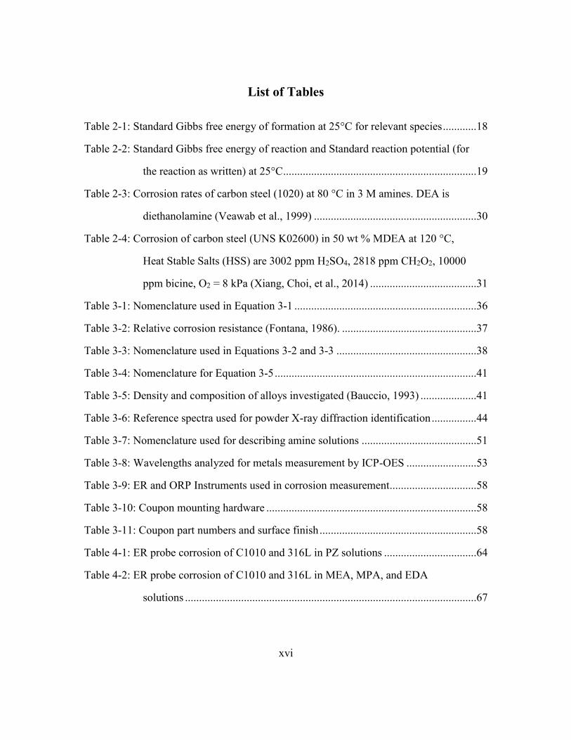
List of Tables
Table 2-1: Standard Gibbs free energy of formation at 25°C for relevant species ............18
Table 2-2: Standard Gibbs free energy of reaction and Standard reaction potential (for
the reaction as written) at 25°C .....................................................................19
Table 2-3: Corrosion rates of carbon steel (1020) at 80 °C in 3 M amines. DEA is
diethanolamine (Veawab et al., 1999) ..........................................................30
Table 2-4: Corrosion of carbon steel (UNS K02600) in 50 wt % MDEA at 120 °C,
Heat Stable Salts (HSS) are 3002 ppm H2SO4, 2818 ppm CH2O2, 10000
ppm bicine, O2 = 8 kPa (Xiang, Choi, et al., 2014) ......................................31
Table 3-1: Nomenclature used in Equation 3-1 .................................................................36
Table 3-2: Relative corrosion resistance (Fontana, 1986). ................................................37
Table 3-3: Nomenclature used in Equations 3-2 and 3-3 ..................................................38
Table 3-4: Nomenclature for Equation 3-5 ........................................................................41
Table 3-5: Density and composition of alloys investigated (Bauccio, 1993) ....................41
Table 3-6: Reference spectra used for powder X-ray diffraction identification ................44
Table 3-7: Nomenclature used for describing amine solutions .........................................51
Table 3-8: Wavelengths analyzed for metals measurement by ICP-OES .........................53
Table 3-9: ER and ORP Instruments used in corrosion measurement...............................58
Table 3-10: Coupon mounting hardware ...........................................................................58
Table 3-11: Coupon part numbers and surface finish ........................................................58
Table 4-1: ER probe corrosion of C1010 and 316L in PZ solutions .................................64
Table 4-2: ER probe corrosion of C1010 and 316L in MEA, MPA, and EDA
solutions ........................................................................................................67
xvii
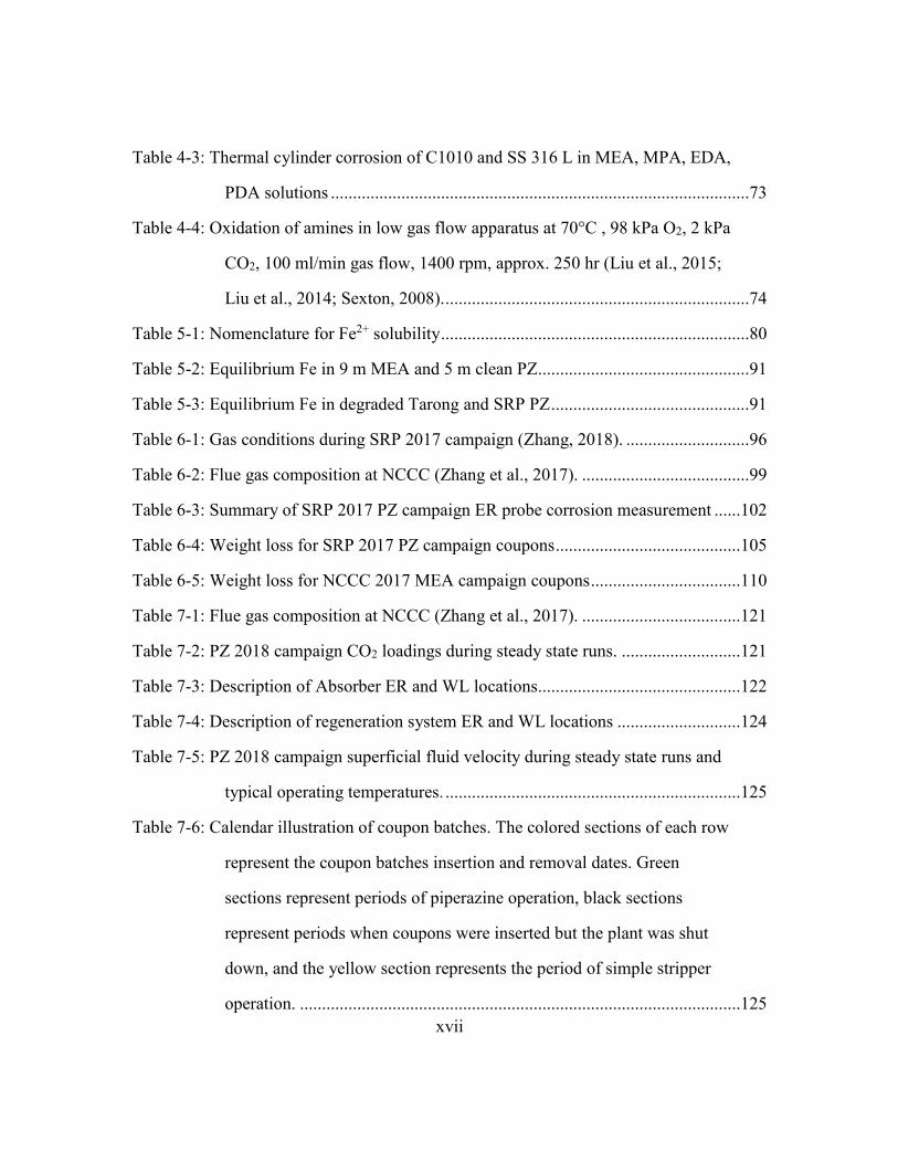
Table 4-3: Thermal cylinder corrosion of C1010 and SS 316 L in MEA, MPA, EDA,
PDA solutions ...............................................................................................73
Table 4-4: Oxidation of amines in low gas flow apparatus at 70°C , 98 kPa O2, 2 kPa
CO2, 100 ml/min gas flow, 1400 rpm, approx. 250 hr (Liu et al., 2015;
Liu et al., 2014; Sexton, 2008). .....................................................................74
Table 5-1: Nomenclature for Fe2+ solubility ......................................................................80
Table 5-2: Equilibrium Fe in 9 m MEA and 5 m clean PZ................................................91
Table 5-3: Equilibrium Fe in degraded Tarong and SRP PZ .............................................91
Table 6-1: Gas conditions during SRP 2017 campaign (Zhang, 2018). ............................96
Table 6-2: Flue gas composition at NCCC (Zhang et al., 2017). ......................................99
Table 6-3: Summary of SRP 2017 PZ campaign ER probe corrosion measurement ......102
Table 6-4: Weight loss for SRP 2017 PZ campaign coupons ..........................................105
Table 6-5: Weight loss for NCCC 2017 MEA campaign coupons ..................................110
Table 7-1: Flue gas composition at NCCC (Zhang et al., 2017). ....................................121
Table 7-2: PZ 2018 campaign CO2 loadings during steady state runs. ...........................121
Table 7-3: Description of Absorber ER and WL locations..............................................122
Table 7-4: Description of regeneration system ER and WL locations ............................124
Table 7-5: PZ 2018 campaign superficial fluid velocity during steady state runs and
typical operating temperatures. ...................................................................125
Table 7-6: Calendar illustration of coupon batches. The colored sections of each row
represent the coupon batches insertion and removal dates. Green
sections represent periods of piperazine operation, black sections
represent periods when coupons were inserted but the plant was shut
down, and the yellow section represents the period of simple stripper
operation. ....................................................................................................125

xviii
Table 7-7: Apparent activation energies for coupon corrosion rates. ..............................130
Table 7-8: Coupon weight loss corrosion rates (μm/yr) of carbon steel (C1010) by
batch and location .......................................................................................136
Table 7-9: Coupon weight loss corrosion rates (μm/yr) of stainless steel (316L and
304) by batch and location ..........................................................................137
Table 7-10: Summary of coupon weight loss for ER2 and WL2 (Absorber Middle
locations) .....................................................................................................138
Table 7-11: Summary of coupon weight loss for ER3 (Absorber Sump)........................141
Table 7-12: Summary of coupon weight loss for WL4 (Absorber Top) .........................144
Table 7-13: Summary of coupon weight loss for WL12 (Cold lean) ..............................145
Table 7-14: Summary of coupon weight loss for WL13 (Cold rich bypass) ...................148
Table 7-15: Summary of coupon weight loss for WL14 (Warm rich bypass) .................152
Table 7-16: Summary of coupon weight loss for WL19 (Hot rich) ................................156
Table 7-17: Summary of coupon weight loss for WL21 (Hot lean) ................................160
Table 7-18: Summary of coupon weight loss for WL22 (AFS Sump) ............................164
Table 7-19: Coupon weight loss (WL) corrosion rates (μm/yr) compared to ER
corrosion rates (μm/yr) of carbon steel (C1010) by batch and location .....172
Table 7-20: Coupon weight loss (WL) corrosion rates (μm/yr) compared to ER
corrosion rates (μm/yr) of stainless steel (316L and 304) by batch and
location ........................................................................................................173
Table 7-21: Comparison of ER and coupon corrosion rates. ...........................................174
Table 7-22: Summary Table of ER Probe corrosion rate regression parameters. ...........175
xix
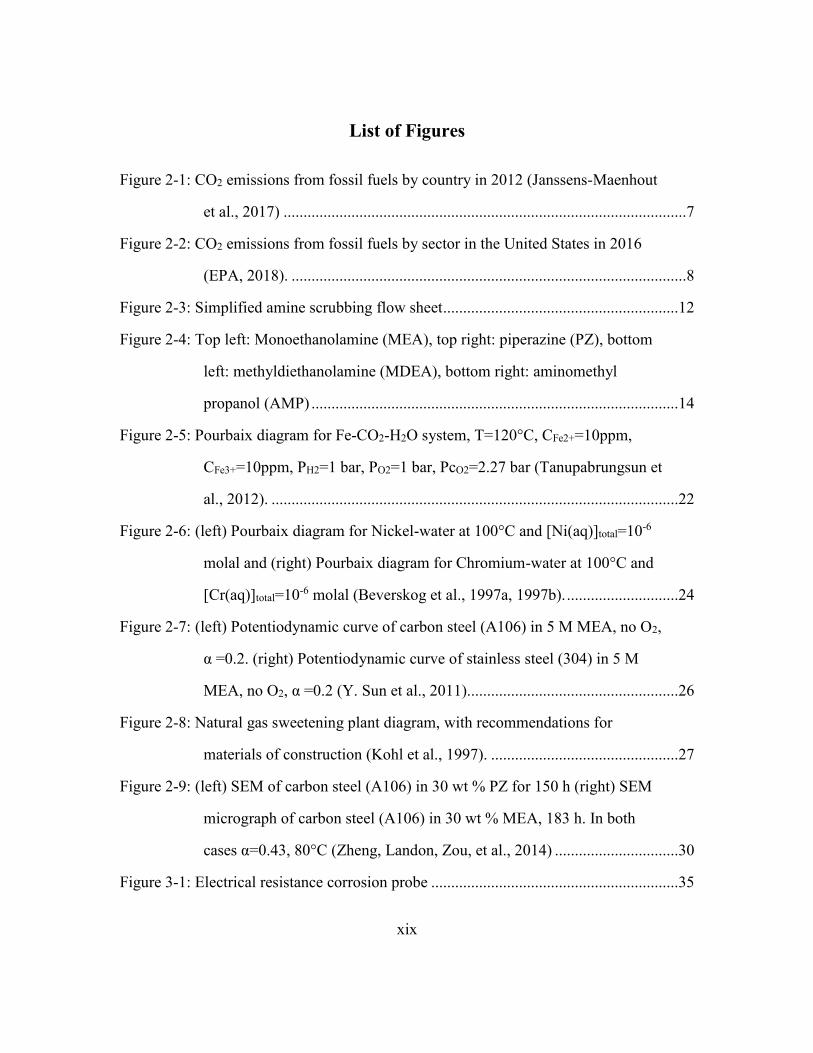
List of Figures
Figure 2-1: CO2 emissions from fossil fuels by country in 2012 (Janssens-Maenhout
et al., 2017) .....................................................................................................7
Figure 2-2: CO2 emissions from fossil fuels by sector in the United States in 2016
(EPA, 2018). ...................................................................................................8
Figure 2-3: Simplified amine scrubbing flow sheet ...........................................................12
Figure 2-4: Top left: Monoethanolamine (MEA), top right: piperazine (PZ), bottom
left: methyldiethanolamine (MDEA), bottom right: aminomethyl
propanol (AMP) ............................................................................................14
Figure 2-5: Pourbaix diagram for Fe-CO2-H2O system, T=120°C, CFe2+=10ppm,
CFe3+=10ppm, PH2=1 bar, PO2=1 bar, PcO2=2.27 bar (Tanupabrungsun et
al., 2012). ......................................................................................................22
Figure 2-6: (left) Pourbaix diagram for Nickel-water at 100°C and [Ni(aq)]total=10-6
molal and (right) Pourbaix diagram for Chromium-water at 100°C and
[Cr(aq)]total=10-6 molal (Beverskog et al., 1997a, 1997b). ............................24
Figure 2-7: (left) Potentiodynamic curve of carbon steel (A106) in 5 M MEA, no O2,
α =0.2. (right) Potentiodynamic curve of stainless steel (304) in 5 M
MEA, no O2, α =0.2 (Y. Sun et al., 2011).....................................................26
Figure 2-8: Natural gas sweetening plant diagram, with recommendations for
materials of construction (Kohl et al., 1997). ...............................................27
Figure 2-9: (left) SEM of carbon steel (A106) in 30 wt % PZ for 150 h (right) SEM
micrograph of carbon steel (A106) in 30 wt % MEA, 183 h. In both
cases α=0.43, 80°C (Zheng, Landon, Zou, et al., 2014) ...............................30
Figure 3-1: Electrical resistance corrosion probe ..............................................................35
xx
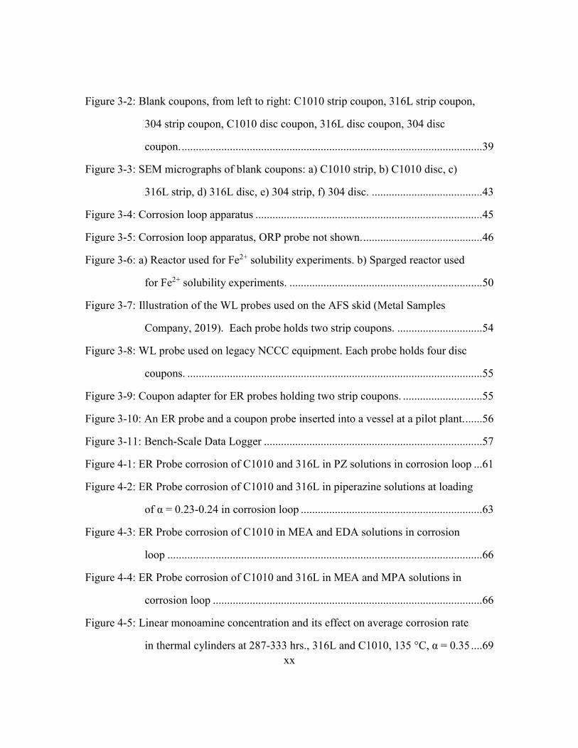
Figure 3-2: Blank coupons, from left to right: C1010 strip coupon, 316L strip coupon,
304 strip coupon, C1010 disc coupon, 316L disc coupon, 304 disc
coupon. ..........................................................................................................39
Figure 3-3: SEM micrographs of blank coupons: a) C1010 strip, b) C1010 disc, c)
316L strip, d) 316L disc, e) 304 strip, f) 304 disc. .......................................43
Figure 3-4: Corrosion loop apparatus ................................................................................45
Figure 3-5: Corrosion loop apparatus, ORP probe not shown. ..........................................46
Figure 3-6: a) Reactor used for Fe2+ solubility experiments. b) Sparged reactor used
for Fe2+ solubility experiments. ....................................................................50
Figure 3-7: Illustration of the WL probes used on the AFS skid (Metal Samples
Company, 2019). Each probe holds two strip coupons. ..............................54
Figure 3-8: WL probe used on legacy NCCC equipment. Each probe holds four disc
coupons. ........................................................................................................55
Figure 3-9: Coupon adapter for ER probes holding two strip coupons. ............................55
Figure 3-10: An ER probe and a coupon probe inserted into a vessel at a pilot plant. ......56
Figure 3-11: Bench-Scale Data Logger .............................................................................57
Figure 4-1: ER Probe corrosion of C1010 and 316L in PZ solutions in corrosion loop ...61
Figure 4-2: ER Probe corrosion of C1010 and 316L in piperazine solutions at loading
of α = 0.23-0.24 in corrosion loop ................................................................63
Figure 4-3: ER Probe corrosion of C1010 in MEA and EDA solutions in corrosion
loop ...............................................................................................................66
Figure 4-4: ER Probe corrosion of C1010 and 316L in MEA and MPA solutions in
corrosion loop ...............................................................................................66
Figure 4-5: Linear monoamine concentration and its effect on average corrosion rate
in thermal cylinders at 287-333 hrs., 316L and C1010, 135 °C, α = 0.35 ....69
xxi
Figure 4-6: Linear monoamine loading and its effect on average corrosion rate in
thermal cyinders at 287-333 hrs., 316L and C1010, 135 °C, 10 m ..............70
Figure 4-7: Formate production and average corrosion rate in thermal cylinders, 287-
333 hrs., 316L and C1010, 135 °C, 10 m, α = 0.35. .....................................71
Figure 4-8: Hypothetical Stable MEA carbamate metal catalytic center (left) and
unstable MPA carbamate metal catalytic center (right) ................................75
Figure 5-1: Soluble Fe in 9 m MEA with the addition of 0.25 M FeSO4 and Na2CO3. ....84
Figure 5-2: Soluble Fe in 5 m clean PZ with the addition of 0.25 M FeSO4 and
Na2CO3. .........................................................................................................85
Figure 5-3: a) Rich MEA soluble Fe as a function of temperature. b) Rich PZ soluble
Fe as a function of temperature (Fytianos, 2016). ........................................86
Figure 5-4: Soluble Fe in 5 m degraded SRP PZ with the addition of 0.25 M FeSO4
and 0.25 M Na2CO3. .....................................................................................87
Figure 5-5: Soluble Fe in 3 m degraded Tarong PZ with the addition of 0.25 M FeSO4
and Na2CO3. ..................................................................................................88
Figure 5-6: Soluble Fe as a function of CO2 loading for 9 m MEA and 5 m PZ...............89
Figure 5-7: Soluble Fe as a function of CO2 loading for degraded PZ. .............................90
Figure 6-1: Simplified PFD for the SRP pilot plant highlighting location of ER probes ..98
Figure 6-2: Simplified PFD for the NCCC PSTU highlighting location of WL
(coupon) probes ..........................................................................................100
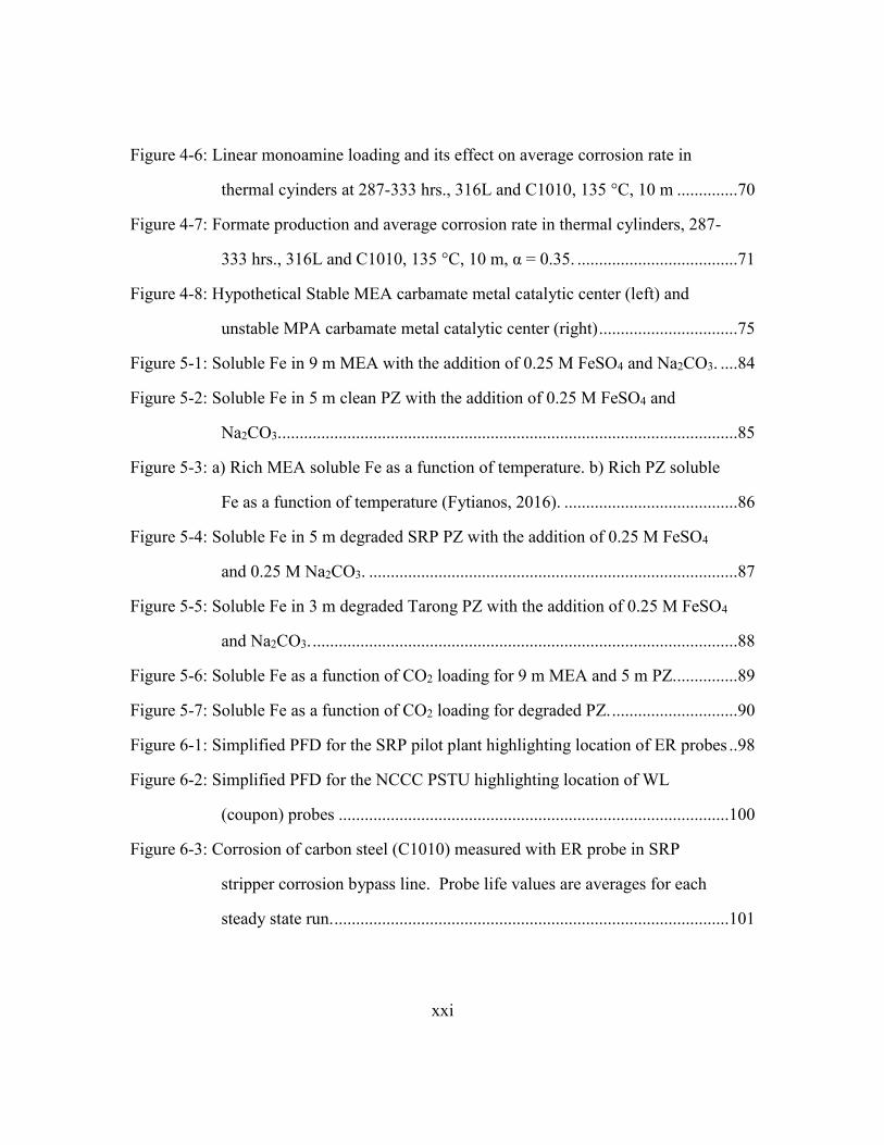
Figure 6-3: Corrosion of carbon steel (C1010) measured with ER probe in SRP
stripper corrosion bypass line. Probe life values are averages for each
steady state run. ...........................................................................................101

xxii
Figure 6-4: Corrosion of stainless steel (316L) measured with ER probe in SRP
stripper corrosion bypass line. Probe life values are averages for each
steady state run. ...........................................................................................101
Figure 6-5: Corrosion of carbon steel (C1010) measured with ER probe in SRP
absorber sump. Readings are instantaneous values recorded with
handheld ER reader. ....................................................................................102
Figure 6-6: Pilot- vs bench-scale SRP PZ, 150° C, 95% confidence intervals shown.
5 m PZ results are from SRP 2017 pilot plant campaign; 8 m PZ results
are from a bench-scale experiment using a SRP 2011 pilot plant
campaign sample. ........................................................................................103
Figure 6-7: Coupon removal timeline for SRP 2017 PZ campaign .................................104
Figure 6-8: 316L and C1010 coupons after removal from SRP stripper. Coupons
experienced approximately 340 hours of water testing and 167 hours
operating at temperature in PZ solution. Average α = 0.21. T = 150 °C. ..105
Figure 6-9: (a) SEM micrograph of red product on C1010 coupon after removal from
SRP stripper. Identified with powder XRD as FeO(OH). (b) SEM
micrograph of black product on C1010 coupon after removal from SRP
stripper. Identified with powder XRD as Fe3O4. Probe experienced
approximately 340 hours of water testing and 167 hours operating at
temperature in PZ solution. .........................................................................106
Figure 6-10: (a) 316L and C1010 coupons after removal from SRP stripper. (b) SEM
micrograph of black product on C1010 coupon. Identified with powder
XRD as FeCO3. Probe experienced 152 hours operating at temperature
in PZ solution. Average α = 0.21. T = 150 °C ...........................................107
xxiii
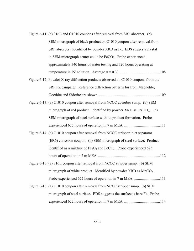
Figure 6-11: (a) 316L and C1010 coupons after removal from SRP absorber. (b)
SEM micrograph of black product on C1010 coupon after removal from
SRP absorber. Identified by powder XRD as Fe. EDS suggests crystal
in SEM micrograph center could be FeCO3. Probe experienced
approximately 340 hours of water testing and 320 hours operating at
temperature in PZ solution. Average α = 0.33. ..........................................108
Figure 6-12: Powder X-ray diffraction products observed on C1010 coupons from the
SRP PZ campaign. Reference diffraction patterns for Iron, Magnetite,
Goethite and Siderite are shown. ................................................................109
Figure 6-13: (a) C1010 coupon after removal from NCCC absorber sump. (b) SEM
micrograph of red product. Identified by powder XRD as Fe(OH)3. (c)
SEM micrograph of steel surface without product formation. Probe
experienced 625 hours of operation in 7 m MEA. ......................................111
Figure 6-14: (a) C1010 coupon after removal from NCCC stripper inlet separator
(ER6) corrosion coupon. (b) SEM micrograph of steel surface. Product
identified as a mixture of Fe3O4 and FeCO3. Probe experienced 625
hours of operation in 7 m MEA. .................................................................112
Figure 6-15: (a) 316L coupon after removal from NCCC stripper sump. (b) SEM
micrograph of white product. Identified by powder XRD as MnCO3.
Probe experienced 622 hours of operation in 7 m MEA. ...........................113
Figure 6-16: (a) C1010 coupon after removal from NCCC stripper sump. (b) SEM
micrograph of steel surface. EDS suggests the surface is bare Fe. Probe
experienced 622 hours of operation in 7 m MEA. ......................................114
xxiv
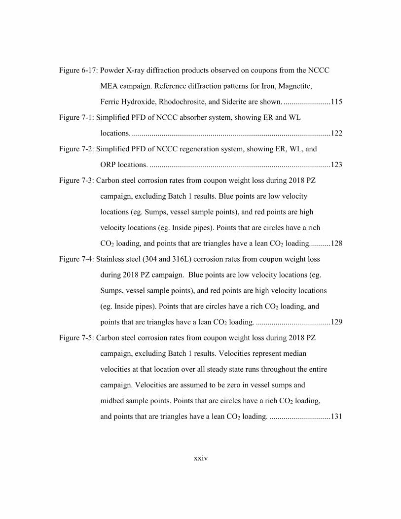
Figure 6-17: Powder X-ray diffraction products observed on coupons from the NCCC
MEA campaign. Reference diffraction patterns for Iron, Magnetite,
Ferric Hydroxide, Rhodochrosite, and Siderite are shown. ........................115
Figure 7-1: Simplified PFD of NCCC absorber system, showing ER and WL
locations. .....................................................................................................122
Figure 7-2: Simplified PFD of NCCC regeneration system, showing ER, WL, and
ORP locations. ............................................................................................123
Figure 7-3: Carbon steel corrosion rates from coupon weight loss during 2018 PZ
campaign, excluding Batch 1 results. Blue points are low velocity
locations (eg. Sumps, vessel sample points), and red points are high
velocity locations (eg. Inside pipes). Points that are circles have a rich
CO2 loading, and points that are triangles have a lean CO2 loading...........128
Figure 7-4: Stainless steel (304 and 316L) corrosion rates from coupon weight loss
during 2018 PZ campaign. Blue points are low velocity locations (eg.
Sumps, vessel sample points), and red points are high velocity locations
(eg. Inside pipes). Points that are circles have a rich CO2 loading, and
points that are triangles have a lean CO2 loading. ......................................129
Figure 7-5: Carbon steel corrosion rates from coupon weight loss during 2018 PZ
campaign, excluding Batch 1 results. Velocities represent median
velocities at that location over all steady state runs throughout the entire
campaign. Velocities are assumed to be zero in vessel sumps and
midbed sample points. Points that are circles have a rich CO2 loading,
and points that are triangles have a lean CO2 loading. ...............................131
xxv
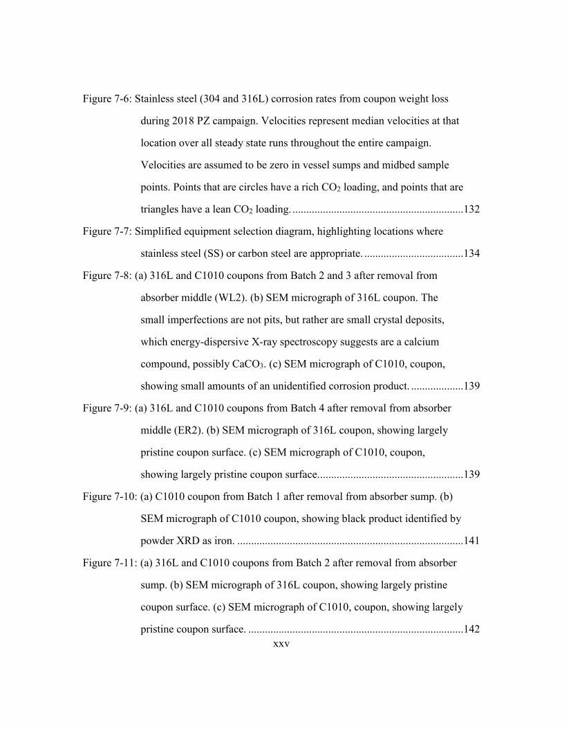
Figure 7-6: Stainless steel (304 and 316L) corrosion rates from coupon weight loss
during 2018 PZ campaign. Velocities represent median velocities at that
location over all steady state runs throughout the entire campaign.
Velocities are assumed to be zero in vessel sumps and midbed sample
points. Points that are circles have a rich CO2 loading, and points that are
triangles have a lean CO2 loading. ..............................................................132
Figure 7-7: Simplified equipment selection diagram, highlighting locations where
stainless steel (SS) or carbon steel are appropriate. ....................................134
Figure 7-8: (a) 316L and C1010 coupons from Batch 2 and 3 after removal from
absorber middle (WL2). (b) SEM micrograph of 316L coupon. The
small imperfections are not pits, but rather are small crystal deposits,
which energy-dispersive X-ray spectroscopy suggests are a calcium
compound, possibly CaCO3. (c) SEM micrograph of C1010, coupon,
showing small amounts of an unidentified corrosion product. ...................139
Figure 7-9: (a) 316L and C1010 coupons from Batch 4 after removal from absorber
middle (ER2). (b) SEM micrograph of 316L coupon, showing largely
pristine coupon surface. (c) SEM micrograph of C1010, coupon,
showing largely pristine coupon surface.....................................................139
Figure 7-10: (a) C1010 coupon from Batch 1 after removal from absorber sump. (b)
SEM micrograph of C1010 coupon, showing black product identified by
powder XRD as iron. ..................................................................................141
Figure 7-11: (a) 316L and C1010 coupons from Batch 2 after removal from absorber
sump. (b) SEM micrograph of 316L coupon, showing largely pristine
coupon surface. (c) SEM micrograph of C1010, coupon, showing largely
pristine coupon surface. ..............................................................................142
xxvi
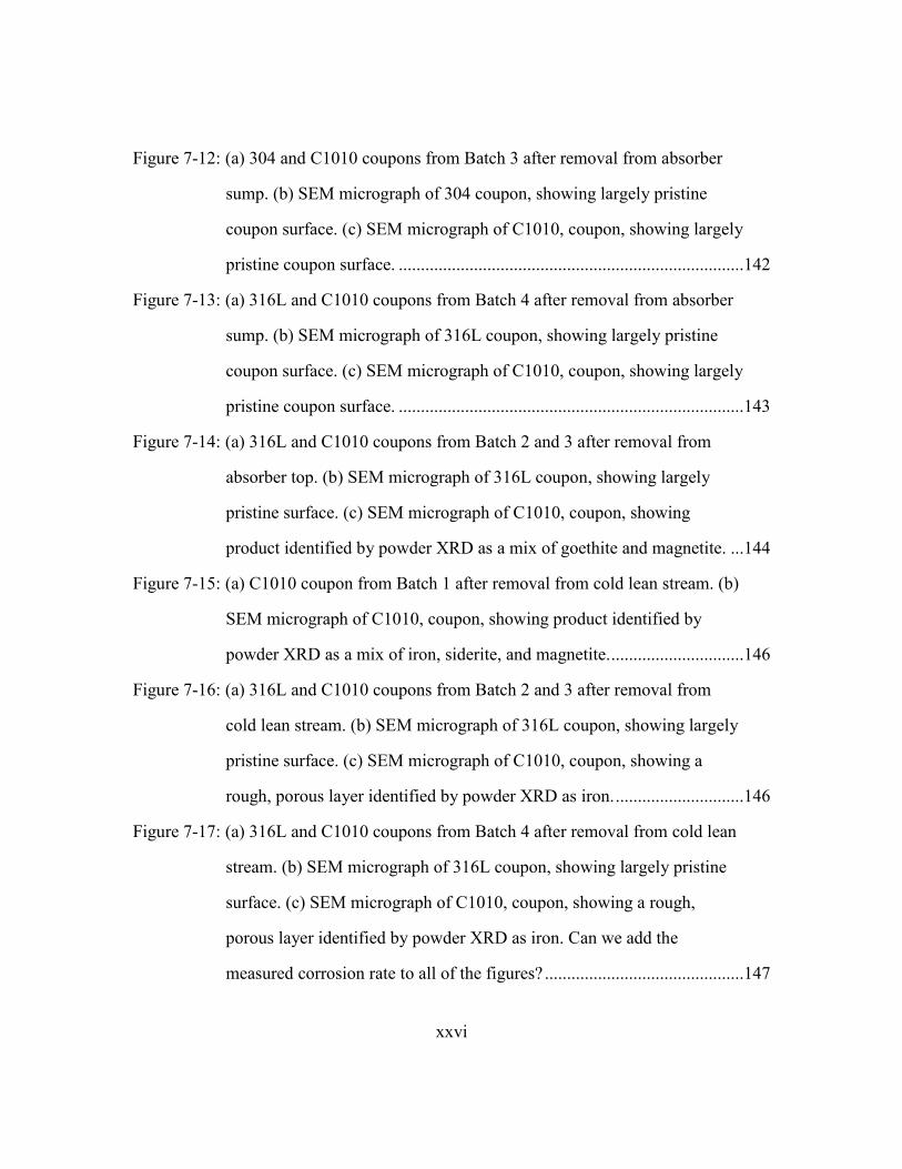
Figure 7-12: (a) 304 and C1010 coupons from Batch 3 after removal from absorber
sump. (b) SEM micrograph of 304 coupon, showing largely pristine
coupon surface. (c) SEM micrograph of C1010, coupon, showing largely
pristine coupon surface. ..............................................................................142
Figure 7-13: (a) 316L and C1010 coupons from Batch 4 after removal from absorber
sump. (b) SEM micrograph of 316L coupon, showing largely pristine
coupon surface. (c) SEM micrograph of C1010, coupon, showing largely
pristine coupon surface. ..............................................................................143
Figure 7-14: (a) 316L and C1010 coupons from Batch 2 and 3 after removal from
absorber top. (b) SEM micrograph of 316L coupon, showing largely
pristine surface. (c) SEM micrograph of C1010, coupon, showing
product identified by powder XRD as a mix of goethite and magnetite. ...144
Figure 7-15: (a) C1010 coupon from Batch 1 after removal from cold lean stream. (b)
SEM micrograph of C1010, coupon, showing product identified by
powder XRD as a mix of iron, siderite, and magnetite. ..............................146
Figure 7-16: (a) 316L and C1010 coupons from Batch 2 and 3 after removal from
cold lean stream. (b) SEM micrograph of 316L coupon, showing largely
pristine surface. (c) SEM micrograph of C1010, coupon, showing a
rough, porous layer identified by powder XRD as iron. .............................146
Figure 7-17: (a) 316L and C1010 coupons from Batch 4 after removal from cold lean
stream. (b) SEM micrograph of 316L coupon, showing largely pristine
surface. (c) SEM micrograph of C1010, coupon, showing a rough,
porous layer identified by powder XRD as iron. Can we add the
measured corrosion rate to all of the figures? .............................................147
xxvii
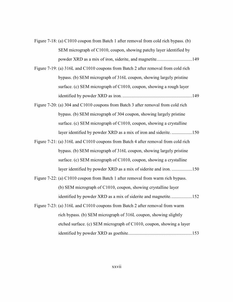
Figure 7-18: (a) C1010 coupon from Batch 1 after removal from cold rich bypass. (b)
SEM micrograph of C1010, coupon, showing patchy layer identified by
powder XRD as a mix of iron, siderite, and magnetite. ..............................149
Figure 7-19: (a) 316L and C1010 coupons from Batch 2 after removal from cold rich
bypass. (b) SEM micrograph of 316L coupon, showing largely pristine
surface. (c) SEM micrograph of C1010, coupon, showing a rough layer
identified by powder XRD as iron. .............................................................149
Figure 7-20: (a) 304 and C1010 coupons from Batch 3 after removal from cold rich
bypass. (b) SEM micrograph of 304 coupon, showing largely pristine
surface. (c) SEM micrograph of C1010, coupon, showing a crystalline
layer identified by powder XRD as a mix of iron and siderite. ..................150
Figure 7-21: (a) 316L and C1010 coupons from Batch 4 after removal from cold rich
bypass. (b) SEM micrograph of 316L coupon, showing largely pristine
surface. (c) SEM micrograph of C1010, coupon, showing a crystalline
layer identified by powder XRD as a mix of siderite and iron. ..................150
Figure 7-22: (a) C1010 coupon from Batch 1 after removal from warm rich bypass.
(b) SEM micrograph of C1010, coupon, showing crystalline layer
identified by powder XRD as a mix of siderite and magnetite. ..................152
Figure 7-23: (a) 316L and C1010 coupons from Batch 2 after removal from warm
rich bypass. (b) SEM micrograph of 316L coupon, showing slightly
etched surface. (c) SEM micrograph of C1010, coupon, showing a layer
identified by powder XRD as goethite........................................................153
xxviii
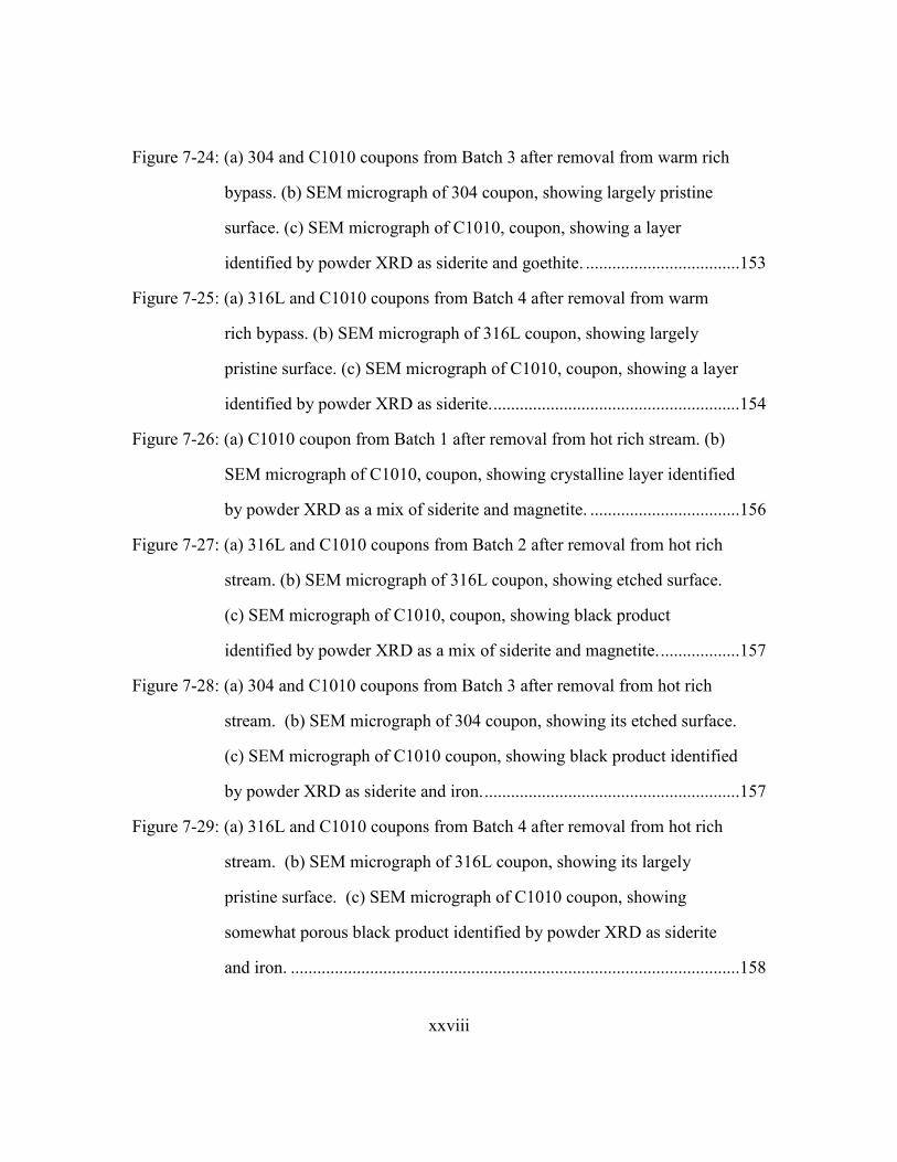
Figure 7-24: (a) 304 and C1010 coupons from Batch 3 after removal from warm rich
bypass. (b) SEM micrograph of 304 coupon, showing largely pristine
surface. (c) SEM micrograph of C1010, coupon, showing a layer
identified by powder XRD as siderite and goethite. ...................................153
Figure 7-25: (a) 316L and C1010 coupons from Batch 4 after removal from warm
rich bypass. (b) SEM micrograph of 316L coupon, showing largely
pristine surface. (c) SEM micrograph of C1010, coupon, showing a layer
identified by powder XRD as siderite. ........................................................154
Figure 7-26: (a) C1010 coupon from Batch 1 after removal from hot rich stream. (b)
SEM micrograph of C1010, coupon, showing crystalline layer identified
by powder XRD as a mix of siderite and magnetite. ..................................156
Figure 7-27: (a) 316L and C1010 coupons from Batch 2 after removal from hot rich
stream. (b) SEM micrograph of 316L coupon, showing etched surface.
(c) SEM micrograph of C1010, coupon, showing black product
identified by powder XRD as a mix of siderite and magnetite. ..................157
Figure 7-28: (a) 304 and C1010 coupons from Batch 3 after removal from hot rich
stream. (b) SEM micrograph of 304 coupon, showing its etched surface.
(c) SEM micrograph of C1010 coupon, showing black product identified
by powder XRD as siderite and iron. ..........................................................157
Figure 7-29: (a) 316L and C1010 coupons from Batch 4 after removal from hot rich
stream. (b) SEM micrograph of 316L coupon, showing its largely
pristine surface. (c) SEM micrograph of C1010 coupon, showing
somewhat porous black product identified by powder XRD as siderite
and iron. ......................................................................................................158

xxix
Figure 7-30: (a) C1010 coupon from Batch 1 after removal from hot lean stream. (b)
SEM micrograph of C1010, coupon, showing crystalline layer identified
by powder XRD as siderite. ........................................................................160
Figure 7-31: (a) 316L and C1010 coupons from Batch 2 after removal from hot lean
stream. (b) SEM micrograph of 316L coupon, showing etched surface.
(c) SEM micrograph of C1010 coupon, showing black product identified
by powder XRD as siderite. ........................................................................161
Figure 7-32: (a) 304 and C1010 coupons from Batch 3 after removal from hot lean
stream. (b) SEM micrograph of 304 coupon, showing its relatively clean
surface. (c) SEM micrograph of C1010 coupon, showing black product
identified by XRD as siderite and iron. ......................................................161
Figure 7-33: (a) 316L and C1010 coupons from Batch 4 after removal from hot lean
stream. (b) SEM micrograph of 316L coupon, showing its relatively
clean surface. (c) SEM micrograph of C1010 coupon, showing black
product identified by XRD as siderite and magnetite. ................................162
Figure 7-34: (a) C1010 coupon from Batch 1 after removal from AFS sump. (b) SEM
micrograph of C1010, coupon, showing crystalline layer identified by
powder XRD as siderite and magnetite. .....................................................164
Figure 7-35: (a) 316L and C1010 coupons from Batch 2 after removal from AFS
sump. (b) SEM micrograph of 316L coupon, showing yellow product
identified by powder XRD as siderite. (c) SEM micrograph of C1010
coupon, showing black product identified by powder XRD as siderite. ....165

xxx
Figure 7-36: (a) 304 and C1010 coupons from Batch 3 after removal from AFS sump.
(b) SEM micrograph of 304 coupon, showing its relatively clean surface.
(c) SEM micrograph of C1010 coupon, showing black product identified
by XRD as siderite and iron. .......................................................................165
Figure 7-37:(a) 316L and C1010 coupons from Batch 4 after removal from AFS
sump. (b) SEM micrograph of 316L coupon, showing slightly etched
surface. (c) SEM micrograph of C1010 coupon, showing black product
identified by powder XRD as a mix of iron and siderite. ...........................166
Figure 7-38: Powder X-ray diffraction products observed on C1010 coupons from
Batch 1. Reference diffraction patterns for Iron, Magnetite, Goethite and
Siderite are shown. ......................................................................................167
Figure 7-39: Powder X-ray diffraction products observed on coupons from Batch 2.
All coupons are C1010 except one from WL22. Reference diffraction
patterns for Iron, Magnetite, Goethite and Siderite are shown. ..................168
Figure 7-40: Powder X-ray diffraction products observed on C1010 coupons from
Batch 3. Coupons from WL12 and WL4 experienced corrosion during
Batch 2 and Batch 3. Reference diffraction patterns for Iron, Magnetite,
Goethite and Siderite are shown. ................................................................169
Figure 7-41: Powder X-ray diffraction products observed on C1010 coupons from
Batch 4. Reference diffraction patterns for Iron, Magnetite, and Siderite
are shown. ...................................................................................................170
Figure 7-42: Corrosion of carbon steel (C1010) at absorber middle (ER2) ER Probe
during Batch 4. ............................................................................................176
Figure 7-43: Corrosion of carbon steel (C1010) at absorber sump (ER3) ER Probe
during Batch 3. ............................................................................................177
xxxi
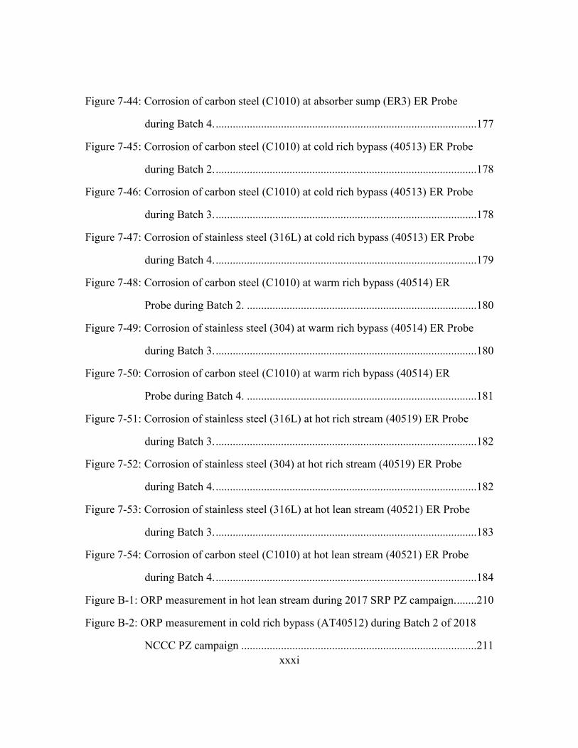
Figure 7-44: Corrosion of carbon steel (C1010) at absorber sump (ER3) ER Probe
during Batch 4. ............................................................................................177
Figure 7-45: Corrosion of carbon steel (C1010) at cold rich bypass (40513) ER Probe
during Batch 2. ............................................................................................178
Figure 7-46: Corrosion of carbon steel (C1010) at cold rich bypass (40513) ER Probe
during Batch 3. ............................................................................................178
Figure 7-47: Corrosion of stainless steel (316L) at cold rich bypass (40513) ER Probe
during Batch 4. ............................................................................................179
Figure 7-48: Corrosion of carbon steel (C1010) at warm rich bypass (40514) ER
Probe during Batch 2. .................................................................................180
Figure 7-49: Corrosion of stainless steel (304) at warm rich bypass (40514) ER Probe
during Batch 3. ............................................................................................180
Figure 7-50: Corrosion of carbon steel (C1010) at warm rich bypass (40514) ER
Probe during Batch 4. .................................................................................181
Figure 7-51: Corrosion of stainless steel (316L) at hot rich stream (40519) ER Probe
during Batch 3. ............................................................................................182
Figure 7-52: Corrosion of stainless steel (304) at hot rich stream (40519) ER Probe
during Batch 4. ............................................................................................182
Figure 7-53: Corrosion of stainless steel (316L) at hot lean stream (40521) ER Probe
during Batch 3. ............................................................................................183
Figure 7-54: Corrosion of carbon steel (C1010) at hot lean stream (40521) ER Probe
during Batch 4. ............................................................................................184
Figure B-1: ORP measurement in hot lean stream during 2017 SRP PZ campaign. .......210
Figure B-2: ORP measurement in cold rich bypass (AT40512) during Batch 2 of 2018
NCCC PZ campaign ...................................................................................211
xxxii
Figure B-3: ORP measurement in hot lean stream (AT40522) during Batch 2 of 2018
NCCC PZ campaign ...................................................................................212
Figure B-4: ORP measurement in cold rich bypass (AT40512) during Batch 3 of 2018
NCCC PZ campaign ...................................................................................212
Figure B-5: ORP measurement in hot lean stream (AT40522) during Batch 3 of 2018
NCCC PZ campaign ...................................................................................213
Figure B-6: ORP measurement in cold rich bypass (AT40512) during Batch 4 of 2018
NCCC PZ campaign ...................................................................................213
Figure B-7: ORP measurement in hot lean stream (AT40522) during Batch 4 of 2018
NCCC PZ campaign ...................................................................................214
1
Chapter 1. Introduction
Post combustion carbon capture and storage (PCCC) with amine absorbents is a
key technology needed to provide low-cost decarbonized electricity (Boot-Handford et al.,
2014; Edenhofer et al., 2014; Pacala et al., 2004; Parson et al., 1998; G. T. Rochelle, 2009)
in a timeframe quick enough to avert the worst consequences of rising atmospheric CO2
concentration (Pachauri et al., 2015).
PCCC amine plants capture CO2 from power plant flue gas into an aqueous
solution, then high temperature is used to reverse the reaction and create a gas stream
containing only CO2. The pure CO2 gas is compressed and pumped underground for
permanent storage. Significant work has been done to improve the energy performance of
amine absorbents (Frailie, 2014; Ramezan et al., 2007; G. T. Rochelle, 2009), such that
future gains in energy performance will suffer from diminishing returns (Boot-Handford
et al., 2014; Lin et al., 2016). Reducing plant capital costs will be a crucial way to reduce
the cost of decarbonized electricity going forward. It is likely that the lowest-cost solvent
system will be whichever of the current high energy-efficiency solvents has the lowest
capital costs.
Most capital cost estimates for PCCC plants assume largely stainless steel
construction. Plant capital costs are a strong function of materials choice, with stainless
process equipment costing 2-3.5X that of carbon steel (Turton et al., 2008). Although
stainless steel is required for first generation solvents (ethanolamine), several second
generation solvents such as piperazine appear significantly less corrosive (K. L. S.
Campbell et al., 2016; Gunasekaran et al., 2013; Zheng, Landon, Zou, et al., 2014).
Improving understanding of corrosion in PCCC amine plants may reveal a solvent system
compatible with carbon steel, which would reduce plant capital costs.
2
Corrosion of steel is well understood in aqueous solutions (Beverskog et al., 1996;
Pourbaix, 1974) and in H2O-CO2 systems (Nešić & Lee, 2003; Nešić, Nordsveen, et al.,
2003; Nordsveen et al., 2003; Tanupabrungsun et al., 2012). However, a lack of
thermodynamic data in complex metal-amine-H2O-CO2 mixtures prevents accurate
corrosion predictions in amine systems. Strong complexation of metal species by amines
is one such complicating factor (Ibanez et al., 1987) that is poorly characterized. However
corrosion behavior in simpler systems is used to explain phenomena observed in this work.
Notably, depassivation of stainless steel can occur at reducing conditions in aqueous
systems (Jones, 1996; Raja et al., 2006), and passivation of carbon steel by FeCO3
formation depends on T, fluid velocity, and local Fe2+ and CO32- activities in H2O-CO2
systems (Nešić & Lee, 2003).
Corrosion data is abundant in amine natural gas sweetening systems, which use the
same process as PCCC plants except to remove H2S and CO2 from high pressure natural
gas (DuPart et al., 1993; Kohl et al., 1997). Experience from natural gas sweetening is
difficult to apply to PCCC systems because the conditions are substantially different and
more corrosive. PCCC systems use higher amine concentrations, absorb O2, and do not
contain H2S, all of which increase corrosion (DuPart et al., 1993; Xiang, Yan, et al., 2014).
Despite these differences, experience with corrosion in natural gas sweetening supplies
several common assumptions about corrosion in PCCC systems. For example, stainless
performs well at all locations and higher CO2 concentrations increase corrosion in
ethanolamine natural gas sweetening units. Both of these assumptions are shown in this
work to be sometimes incorrect in PCCC units because the solvent and process conditions
are different.
Bench-scale work indicates that carbon steel is protected by FeCO3 in many second
generation amines, including piperazine, which is the reason these solvents are less
3
corrosive (K. L. S. Campbell et al., 2016; Gunasekaran et al., 2013; Zheng, Landon, Zou,
et al., 2014). Bench-scale efforts have focused on the performance of carbon steel in second
generation solvents. Notably missing is work on performance of stainless steel, particularly
at high temperatures. This is likely because stainless steel is presumed passive at most
conditions in amine service due to experience from natural gas sweetening.
Corrosion is seldom measured in amines other than ethanolamine at the pilot scale
(Cousins et al., 2013; Flø et al., 2019; Hjelmaas et al., 2017; Khakharia et al., 2015; Kittel
et al., 2009; Li et al., 2017). Corrosion measurements at the pilot scale are important to
validate bench-scale measurements at fully representative conditions. Bench-scale
measurements may not capture small subtleties that may impact corrosion in a real plant,
like the role of solvent degradation, O2 absorption, and flue gas impurities.
Finally, both bench and pilot corrosion data in PCCC systems are typically at or
below 120 °C, which is the typical operating temperature for ethanolamine. Piperazine is
typically operated at 150-160 °C, and data at that elevated temperature is lacking.
To briefly summarize: there is a need for low-cost PCCC amine plants to combat
rising atmospheric CO2 concentrations. Capital cost reduction in these plants can be
achieved through proper materials choice, which requires understanding corrosion in these
systems. Predicting corrosion behavior in these systems is difficult because
thermodynamic data is incomplete in the H2O-CO2-amine system, and because analogous
corrosion work in natural gas sweetening is at substantially different conditions. Despite
recent interest in corrosion in PCCC systems, several crucial gaps in knowledge include:
incomplete understanding of the relationship between amine structure and corrosivity, the
lack of high T measurements, limited investigation of stainless behavior in second
generation amines, and limited pilot work in second-generation amines. The practical goal
of this dissertation is to contribute to closing these knowledge gaps, reduce uncertainty

4
about materials choices in piperazine systems, and thereby reduce capital costs in future
PCCC plants. This goal is accomplished through four specific objectives:
1. Quantify the corrosion performance of stainless and carbon steel in several primary
and secondary amine solutions to understand the effect of temperature, CO2
loading, amine structure and amine degradation on corrosion.
2. Measure Fe2+ solubility in amine solutions to improve understanding of formation
of protective FeCO3 films as a function of amine type, CO2 loading, amine structure
and amine degradation.
3. Quantify the corrosion performance of stainless and carbon steel in piperazine and
ethanolamine in PCCC pilot plants. Characterize corrosion products to understand
the effect of temperature, loading, and fluid velocity on protective FeCO3 films.
4. Identify any process conditions in piperazine that cause acute corrosion failure of
an alloy and develop a strategy to mitigate corrosion. Make recommendations about
what materials of construction are appropriate for each unit operation in a PCCC
plant.
5
Chapter 2. Background
The context, need, and goals for the study of corrosion in amine solvents for CO2
capture are discussed in this Chapter. Section 2.1 presents a brief argument for the use of
CO2 capture to stop rising atmospheric CO2 concentration. Next, Section 2.2 introduces the
amine scrubbing process and briefly highlights active areas of development. Section 2.3
discusses corrosion research relevant to amine scrubbing.
2.1. ARGUMENT FOR THE IMPLEMENTATION OF CARBON CAPTURE AND STORAGE
2.1.1. Atmospheric carbon dioxide and temperature
The concentration of CO2 in the atmosphere has been rising steadily since 1750
AD, and current CO2 levels are at the highest they’ve been in at least 800,000 years.
Precise, direct measurement of atmospheric CO2 began in 1958, when the annual average
CO2 concentration was 316.1 ppm. CO2 concentration has steadily increased to 406.6 ppm
since then (Keeling, 2017). Measurement of air trapped in Antarctic ice cores shows that
pre-industrial (1750 AD) CO2 concentration was approximately 277 ppm (Etheridge et al.,
1996), and that over the last 800,000 years CO2 has varied between 172-300 ppm (Lüthi et
al., 2008). That CO2 had exceeded these long-held bounds is somewhat concerning.
Atmospheric CO2 concentration is very strongly related to the average global
temperature. Average global temperature in the past can be estimated by measuring the
ratio of 18O to 16O in Antarctic ice cores, then converting that ratio to precipitation rates
and temperatures (Petit et al., 1999). These cores show that there is a strong positive
correlation between past CO2 concentration and temperature going back at least 800,000
years. Temperature variations caused by astronomical cycles increased CO2 concentration,
and higher CO2 concentration further increased temperature in periodic cycles that only
abated when radiative forcing significantly decreased. This periodic temperature

6
fluctuation is caused by astronomical cycles that affect incident solar radiation (Imbrie et
al., 1992). The correlated CO2 level oscillations were the product of temperature-dependent
changes in precipitation and weathering of CO2 containing minerals (Kump et al., 2000)
and in oceanic capture of CO2 (Wang et al., 2004). Since CO2 absorbs infrared radiation
(Tyndall, 1859), increasing atmospheric concentration of CO2 exacerbates rising
temperature (Arrhenius, 1896). The relationship between increasing CO2 concentration and
increasing global temperature is exceptionally strong, which has ominous implications for
future temperature.
2.1.2. Impacts of rising global temperature
If atmospheric CO2 concentration continues to increase, average global temperature
will rise, which has serious negative consequences. If CO2 concentration continues to
increase at current rates, average global temperature is likely to be 2° C higher in 2100 AD
than they were in 1850-1900 AD. Such a temperature increase would likely be
accompanied by a decrease in oceanic pH by 0.2 to 0.32 points, changes in global
precipitation, a decrease in Arctic and Antarctic ice volume, and a rise of sea levels by 0.45
to 0.82 m (Pachauri et al., 2015). A few of the likely consequences of these changes are
(Field et al., 2014):
Increased local and global extinction risk for terrestrial and freshwater species, which
are unable to adjust their range quickly and relocate to suitable climates.
Loss of marine-biodiversity and disruption of marine ecosystems, particularly reef-
building corals, which are vulnerable to ocean acidification.
Disruption of major crops (wheat, rice, maize) production in vulnerable regions and
reduction of food security.
Increased displacement of people from vulnerable regions.
7
Reduction of renewable surface freshwater and groundwater resources and an increase
in the frequency of drought in vulnerable regions.
These consequences are significant and broadly negative, so strategies to stop the
increase of atmospheric CO2 should be investigated.
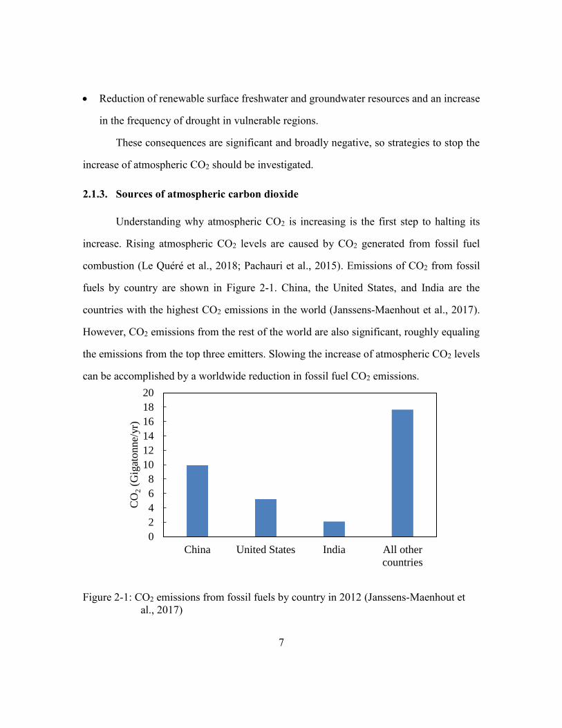
2.1.3. Sources of atmospheric carbon dioxide
Understanding why atmospheric CO2 is increasing is the first step to halting its
increase. Rising atmospheric CO2 levels are caused by CO2 generated from fossil fuel
combustion (Le Quéré et al., 2018; Pachauri et al., 2015). Emissions of CO2 from fossil
fuels by country are shown in Figure 2-1. China, the United States, and India are the
countries with the highest CO2 emissions in the world (Janssens-Maenhout et al., 2017).
However, CO2 emissions from the rest of the world are also significant, roughly equaling
the emissions from the top three emitters. Slowing the increase of atmospheric CO2 levels
can be accomplished by a worldwide reduction in fossil fuel CO2 emissions.
Figure 2-1: CO2 emissions from fossil fuels by country in 2012 (Janssens-Maenhout et
al., 2017)
0
2
4
6
8
10
12
14
16
18
20
China United States India All other
countries
CO
2(G
igat
onne/
yr)

8
In the United States, the largest sources of CO2 emissions are electric power
generation and transportation, and the magnitude of these emissions is shown in Figure 2-2
(EPA, 2018). Reducing CO2 emissions from transportation can be achieved through
reduction of CO2 intensity of fuels (I.e. switching from oil-based to biofuels, electric, or
hydrogen), but there has been lack of progress to date in slowing transport emissions in
OECD countries (Edenhofer et al., 2014). Reducing emissions from electric power
generation is particularly attractive because: these emissions come from relatively few,
concentrated point-sources, and several viable technologies exist that allow
decarbonization of electric power generation.
Figure 2-2: CO2 emissions from fossil fuels by sector in the United States in 2016 (EPA,
2018).
2.1.4. Mitigating carbon dioxide emissions from electricity generation
Viable decarbonized electric power generation technologies include renewable
energy sources (photovoltaics, wind, hydro), nuclear power, and carbon capture and
0.0
0.5
1.0
1.5
2.0
CO
2(G
igat
onne/
yr)
9
storage (CCS) (Edenhofer et al., 2014). Each of these technologies should be considered
for implementation, although this work focuses on carbon capture and storage.
A renewable-only strategy is unlikely to be a cost effective strategy to mitigate CO2
emissions because the intermittency problems of renewable energy have not yet been
solved. Recent price reductions in renewable energy sources have led to quick growth, such
that half of all new installed capacity in 2012 was renewable, bringing renewables share of
global electricity generation to 21 % (Edenhofer et al., 2014). There is significant debate
over whether electricity generation can be accomplished with a renewables-only strategy
(Clack et al., 2017; Jacobson et al., 2015, 2017), but most researchers estimate that the
most cost-effective strategy of decarbonization involves a mixture of renewables and other
technologies, such as: energy efficiency, fuel switching, nuclear, and carbon capture and
storage (Edenhofer et al., 2014; MacDonald et al., 2016; Pacala et al., 2004). Briefly, this
is because at high penetration rates, the intermittency of renewables means that larger
amounts of reserve renewable capacity are required and the efficiency of traditional power
generation is negatively impacted due to increased cycling (Brouwer et al., 2014;
Heuberger et al., 2017).
Nuclear energy is CO2-free and clearly scalable; for example nuclear energy
provided 20% of electricity in the USA and 72% in France in 2017 (IAEA, 2018).
Unfortunately, expansion of nuclear power is blocked by political issues, including concern
about operational risks and safety, unresolved waste management issues, concern about
nuclear weapon proliferation, and adverse public opinion. The effect of these political
issues is heightened regulation which increases plant costs and construction times
(Lovering et al., 2016). Partially as a result of these issues, the nuclear share of worldwide
electricity generation has declined from a high of 17 % in 1993 to 11 % in 2012 (Edenhofer
et al., 2014). This decrease is because retirement of nuclear facilities exceeds their
10
replacement rate in the USA and because Japan and Germany have retired nuclear facilities
in the wake of the Fukushima Daiichi nuclear accident (IAEA, 2018). Without resolution
of its political issues, nuclear energy will likely struggle to achieve widespread
deployment.
2.1.5. Mitigating carbon dioxide emissions with carbon capture and storage
CCS is the capture of CO2 generated from combustion or industry and the
sequestering of it away from the atmosphere indefinitely. Capture involves separating and
concentrating the CO2 from a dilute stream into a pure CO2 stream, which is a technique
widely employed in natural gas purification (Kohl et al., 1997). The CO2 is then
compressed and then transported by pipeline to a storage location. CO2 can be permanently
sequestered in underground deep saline formations, injected into unminable coal beds, or
injected into oil fields for enhanced oil recovery (Metz et al., 2005). Sufficient storage sites
exist in the US to allow storage of all CO2 generated for the next 100 years (Szulczewski
et al., 2012). Among the options for mitigation, CCS is particularly attractive because:
It lacks the intermittency problems of renewables and the political problems of nuclear
energy.
A mix of CCS and other technologies (renewables, nuclear) is expected to minimize
the cost of decarbonized electricity (Boot-Handford et al., 2014; Parson et al., 1998).
This is partially because CCS plants can be operated flexibly to complement
intermittent renewables (Bui et al., 2014; Wiley et al., 2011).
CCS is a mature technology, in use at commercial-scale (Bui et al., 2018; M. Campbell,
2014; DOE, 2017; Singh et al., 2014), so it can be deployed quickly enough to achieve
ambitious CO2 emission reduction targets (Metz et al., 2005; Pacala et al., 2004; G. T.
Rochelle, 2009).
11
There are no obvious alternatives to CCS for decarbonizing the industrial sector (ie,
steel cement, oil refining) (Bui et al., 2018).
There are risks associated with carbon capture and storage too, including:
(Edenhofer et al., 2014)
Potential lifecycle toxicity of some capture solvents.
Safety and long-term integrity of CO2 storage sites.
Risks of transporting CO2 by pipeline.
Nevertheless, the advantages of CCS suggest it should be considered for
implementation. The remainder of this report focuses specifically on post-combustion
carbon capture (PCCC). Although they are not considered here, two other forms of CCS
are currently in development: coal gasification (pre-combustion capture) and oxy-fuel
combustion. However, coal-gasification is expected to be more expensive than PCCC and
oxy-fuel combustion is still in the early stages of development (Rubin et al., 2015).
2.2. POST-COMBUSTION CARBON CAPTURE WITH CHEMICAL ABSORPTION
2.2.1. Description of a typical amine absorption process
Currently, the most cost-effective PCCC systems use a chemical solvent, typically
an aqueous amine solution, to capture CO2 (Metz et al., 2005). Amines act as a base and
react with CO2, capturing the gas into the aqueous solution. Equation 2-1 summarizes this
reaction, in which two moles of a secondary amine are consumed for each mole of CO2
absorbed (Kohl et al., 1997; Shrier et al., 1969).
2 R1R2NH (aq) + CO2 (g) ↔ R1R2NCO2−(aq) + R1R2NH2
+(aq) (2-1)
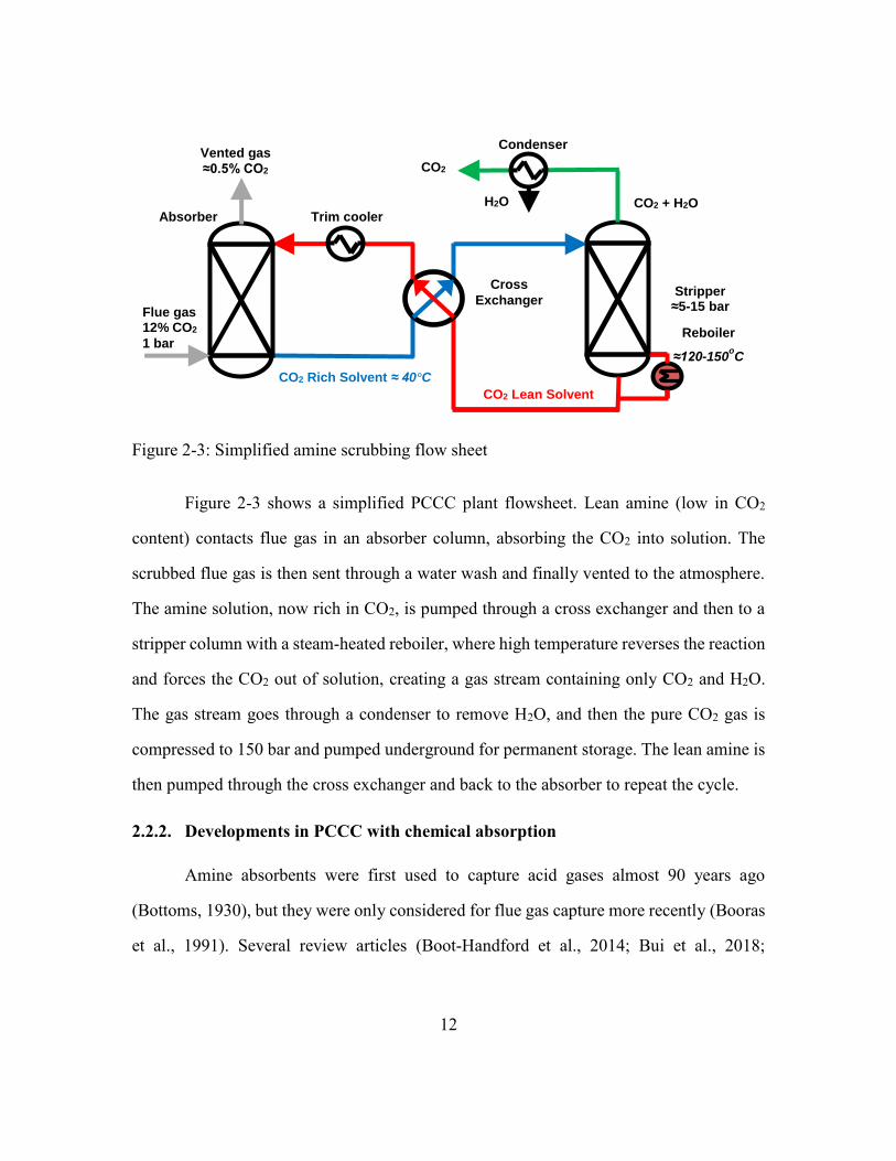
12
Figure 2-3: Simplified amine scrubbing flow sheet
Figure 2-3 shows a simplified PCCC plant flowsheet. Lean amine (low in CO2
content) contacts flue gas in an absorber column, absorbing the CO2 into solution. The
scrubbed flue gas is then sent through a water wash and finally vented to the atmosphere.
The amine solution, now rich in CO2, is pumped through a cross exchanger and then to a
stripper column with a steam-heated reboiler, where high temperature reverses the reaction
and forces the CO2 out of solution, creating a gas stream containing only CO2 and H2O.
The gas stream goes through a condenser to remove H2O, and then the pure CO2 gas is
compressed to 150 bar and pumped underground for permanent storage. The lean amine is
then pumped through the cross exchanger and back to the absorber to repeat the cycle.
2.2.2. Developments in PCCC with chemical absorption
Amine absorbents were first used to capture acid gases almost 90 years ago
(Bottoms, 1930), but they were only considered for flue gas capture more recently (Booras
et al., 1991). Several review articles (Boot-Handford et al., 2014; Bui et al., 2018;
Condenser
Flue gas 12% CO2
1 bar
Cross
Exchanger
CO2 Rich Solvent ≈ 40°C
Vented gas
≈0.5% CO2
CO2 + H2O Absorber
Stripper ≈5-15 bar
CO2 Lean Solvent
CO2
H2O Trim cooler
Reboiler
≈120-150oC

13
MacDowell et al., 2010) and a book (Kohl et al., 1997) cover the development history and
challenges comprehensively. A few key developments will be highlighted here.
The main obstacle to widespread deployment of PCCC is cost. Both the plant
capital cost and the cost of steam used in the stripper reboiler are significant. Early designs
with MEA estimated the total cost of capture and compression to be 57-85 $/MT CO2
(Ramezan et al., 2007; G. T. Rochelle, 2009). Improved designs with new solvents estimate
total cost to be 35.5 $/MT CO2 (Frailie, 2014).
Careful solvent selection and process optimization has improved the energy
performance of amine plants. MEA has an expected energy performance of 3.6-4.0 GJ/MT
CO2 (Cousins et al., 2012), and PZ performance is as low as 2.1-2.5 GJ/MT CO2 (E. Chen
et al., 2017). Future advances in energy performance will not be dramatic because the
overall process is already at about 53% thermodynamic efficiency (Lin et al., 2016).
Significant work has been done in solvent selection because the thermodynamic
and kinetic properties of the solvent ultimately determine the process performance.
Frequently, alkanolamines are used, as the hydroxyl group is necessary to increase water
solubility and lower vapor pressure compared to organic amines. Amine scrubbing solvents
can be broadly classified into three groups:
Primary and secondary amines, such as monoethanolamine (MEA) and piperazine
(PZ), shown in Figure 2-4. These amines are typically the most alkaline and thus have
the highest absorption rates which proceed via the carbamate reaction shown in
Equation 2-1(MacDowell et al., 2010).

14
Figure 2-4: Top left: Monoethanolamine (MEA), top right: piperazine (PZ), bottom left:
methyldiethanolamine (MDEA), bottom right: aminomethyl propanol
(AMP)
Tertiary amines, such as methyldiethanolamine (MDEA), typically have higher CO2
capacity due to their reaction with CO2, shown in Equation 2-2, which only consumes
one mol of amine per mol of CO2. Tertiary amines also have a lower rate of absorption.
MDEA is important industrially because it is selective for H2S in the presence of CO2
(Kohl et al., 1997).
R1R2R3N (aq) + CO2 (g) + H2O (l) ↔ HCO3− (aq) + R1R2R3NH+(aq) (2-2)
Sterically-hindered amines, such as aminomethyl propanol (AMP), form an unstable
carbamate that rapidly converts to bicarbonate by the reaction shown in Equation 2-3.
As a result, hindered amines have somewhat elevated rates associated with carbamate
formation but also somewhat higher capacity associated with bicarbonate formation
(Sartori et al., 1983).
R1R2NCO2− (aq) + H2O (l) ↔ HCO3
− (aq) + R1R2NH(aq) (2-3)
15
In general, amines used for PCCC must have high absorption rates to compensate
for the low partial pressure of CO2 in flue gas compared to natural gas streams, so primary
and secondary amines are typically used.
Significant work has been conducted to ensure there are no negative environmental
impacts associated with PCCC. Solvent degradation has been studied to reduce amine
makeup cost and also to understand potentially toxic and carcinogenic degradation
products. Thermal and oxidative degradation rates and products appear manageable
(Namjoshi, 2015; Paul Thomas Nielsen, 2018). Nitrosamines form when NO2 reacts with
amines, but it can be controlled with pretreatment of gas or high temperature in the stripper
(Fine, 2015). Amine aerosols sometimes form in the absorber, but these can be removed
with a demister or gas pretreatment or passively controlled with careful process design
(Beaudry, 2017; Zhang, 2018).
2.3. CORROSION IN PCCC WITH CHEMICAL ABSORPTION
2.3.1. Motivation
Future improvements in PCCC energy performance will suffer from diminishing
returns because current solvents and plant designs have high thermodynamic efficiency
and likely cannot improve dramatically (Lin et al., 2016). Future cost reductions will have
to come from capital expenses, which contribute about half of the total cost of an amine
plant (Capital Cost: 16 $/MT CO2; Energy cost: 19 $/MT CO2 (Frailie, 2014)). If PCCC
plants are operated at low load factors to complement renewable generation (Bui et al.,
2014; Wiley et al., 2011), capital costs will become even more significant (compared to
energy costs, which decrease at lower load factors). It is likely that the lowest-cost solvent
system will be whichever of the current high energy-efficiency solvents has the lowest
capital costs.

16
Most capital cost estimates for PCCC plants assume largely stainless steel
construction. Plant capital costs are a strong function of materials choice, with stainless
process equipment costing 2-3.5X that of carbon steel (Turton et al., 2008). Although
stainless steel is required for MEA, several second generation solvents such as PZ appear
significantly less corrosive than MEA (Gunasekaran et al., 2013). Thorough investigations
into carbon steel compatibility are needed for second generation PCCC solvents because a
solvent that is largely compatible with carbon steel will have significantly lower capital
costs.
In addition, the current use of stainless steel process equipment in PCCC is based
on general good corrosion performance of this material in MEA in natural gas sweetening
plants. Performance of stainless steel in second generation solvents could be substantially
different than in MEA. Stainless steel needs to be thoroughly evaluated to ensure this
material performs well and is safe at all conditions in second generation solvents.
Although there is past experience with corrosion in amine plants, prior work is
difficult to adapt because critical corrosion parameters are different in PCCC plants. For
example, natural gas sweetening typically has H2S present, which can inhibit corrosion,
and it lacks O2, which exacerbates corrosion. This means there is significant uncertainty
about whether prior corrosion results in acid-gas treating plants can be generalized to
PCCC plants.
The potential benefit to capital costs and the lack of data about corrosion
performance of second generation solvents at PCCC conditions motivated this work.
17
2.3.2. Corrosion thermodynamics
Corrosion is fundamentally a charge transfer reaction between a metal surface and
its surroundings. In the case of carbon steel, iron is oxidized (Equation 2-4). Ferrous can
be further oxidized to ferric, but this requires quite oxidizing conditions (Equation 2-5).
Fe ↔ Fe2+ + 2e− (2-4)
Fe2+ ↔ Fe3+ + e− (2-5)
This oxidation is always accompanied by a reduction. In oxygen containing, high
pH aqueous solutions, the reduction is typically Equation 2-6. In anoxic, high pH aqueous
solutions, this reduction is typically Equation 2-7 (Jones, 1996).
O2 + 2H2O + 4e− ↔ 4 OH− (2-6)
2H2O + 2e− ↔ H2 + 2OH− (2-7)
Other electrochemical reductions may be relevant. Equation 2-8 is likely an
important reduction in PCCC solutions (Veawab et al., 2002).
2HCO3− + 2e− ↔ 2CO3
2− + H2 (2-8)
Reduction of bicarbonate to formate is possible (Equation 2-9), but it seems
unlikely and is usually only seen at very reducing electrode potentials or on catalysts (L.
Chen et al., 2017; Sreekanth et al., 2014).
HCO3− + H2O + 2e− ↔ HCO2
− + 2OH− (2-9)
Amines undergo oxidative degradation in PCCC systems. Although there are a
variety of degradation pathways for MEA, ammonia and formaldehyde are important
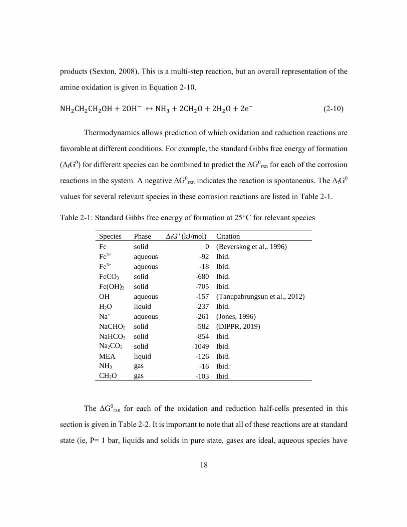
18
products (Sexton, 2008). This is a multi-step reaction, but an overall representation of the
amine oxidation is given in Equation 2-10.
NH2CH2CH2OH + 2OH− ↔ NH3 + 2CH2O + 2H2O + 2e− (2-10)
Thermodynamics allows prediction of which oxidation and reduction reactions are
favorable at different conditions. For example, the standard Gibbs free energy of formation
(ΔfG0) for different species can be combined to predict the ΔG0
rxn for each of the corrosion
reactions in the system. A negative ΔG0rxn indicates the reaction is spontaneous. The ΔfG
0
values for several relevant species in these corrosion reactions are listed in Table 2-1.
Table 2-1: Standard Gibbs free energy of formation at 25°C for relevant species
Species Phase ΔfG0 (kJ/mol) Citation
Fe solid 0 (Beverskog et al., 1996)
Fe2+ aqueous -92 Ibid.
Fe3+ aqueous -18 Ibid.
FeCO3 solid -680 Ibid.
Fe(OH)3 solid -705 Ibid.
OH- aqueous -157 (Tanupabrungsun et al., 2012)
H2O liquid -237 Ibid.
Na+ aqueous -261 (Jones, 1996)
NaCHO2 solid -582 (DIPPR, 2019)
NaHCO3 solid -854 Ibid.
Na2CO3 solid -1049 Ibid.
MEA liquid -126 Ibid.
NH3 gas -16 Ibid.
CH2O gas -103 Ibid.
The ΔG0rxn for each of the oxidation and reduction half-cells presented in this
section is given in Table 2-2. It is important to note that all of these reactions are at standard
state (ie, P= 1 bar, liquids and solids in pure state, gases are ideal, aqueous species have
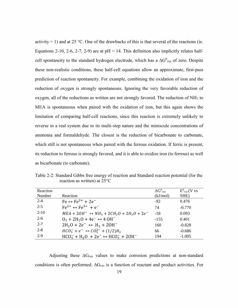
19
activity = 1) and at 25 °C. One of the drawbacks of this is that several of the reactions (ie.
Equations 2-10, 2-6, 2-7, 2-9) are at pH = 14. This definition also implicitly relates half-
cell spontaneity to the standard hydrogen electrode, which has a ΔG0rxn of zero. Despite
these non-realistic conditions, these half-cell equations allow an approximate, first-pass
prediction of reaction spontaneity. For example, combining the oxidation of iron and the
reduction of oxygen is strongly spontaneous. Ignoring the very favorable reduction of
oxygen, all of the reductions as written are not strongly favored. The reduction of NH3 to
MEA is spontaneous when paired with the oxidation of iron, but this again shows the
limitation of comparing half-cell reactions, since this reaction is extremely unlikely to
reverse in a real system due to its multi-step nature and the miniscule concentrations of
ammonia and formaldehyde. The closest is the reduction of bicarbonate to carbonate,
which still is not spontaneous when paired with the ferrous oxidation. If ferric is present,
its reduction to ferrous is strongly favored, and it is able to oxidize iron (to ferrous) as well
as bicarbonate (to carbonate).
Table 2-2: Standard Gibbs free energy of reaction and Standard reaction potential (for the
reaction as written) at 25°C
Reaction
Number Reaction
ΔG0rxn
(kJ/mol)
E0rxn (V vs
SHE)
2-4 Fe ↔ Fe2+ + 2e− -92 0.476
2-5 Fe2+ ↔ Fe3+ + e− 74 -0.770
2-10 𝑀𝐸𝐴 + 2𝑂𝐻− ↔ 𝑁𝐻3 + 2𝐶𝐻2𝑂 + 2𝐻2𝑂 + 2𝑒− -18 0.093
2-6 O2 + 2H2O + 4e− ↔ 4 OH− -155 0.401
2-7 2H2O + 2e− ↔ H2 + 2OH− 160 -0.828
2-8 𝐻𝐶𝑂3− + 𝑒− ↔ 𝐶𝑂3
2− + (1/2)𝐻2 66 -0.686
2-9 HCO3− + H2O + 2e− ↔ HCO2
− + 2OH− 194 -1.005
Adjusting these ΔGrxn values to make corrosion predictions at non-standard
conditions is often performed. ΔGrxn is a function of reactant and product activities. For
20
example, at pH = 7, the reduction of oxygen (Equation 1-6) becomes even more favorable
(ΔGrxn= -316 kJ/mol) and becomes able to oxidize the ferrous half-cell to ferric (Jones,
1996). The general form of the relationship between ΔG0 and solution composition is given
by Equation 2-11, where K is the equilibrium constant for the reaction, R is the universal
gas constant, and T is temperature (Smith et al., 2005). Knowledge of solution activities at
equilibrium (and thus K) allows the calculation of ΔG at non-standard conditions. In charge
transfer reactions, it is often convenient to express ΔG as a solution potential, which more
accurately represents the free energy change per unit charge transferred. Solution potential,
E, is given in 2-12, where n is the number of electrons exchanged and F is Faraday’s
constant. These equations can be combined into the Nernst equation, given in Equation
2-13, where Q is the reaction quotient.
−∆𝐺0
𝑅𝑇= ln (𝐾) (2-11)
E = ΔG/(−nF) (2-12)
𝐸 = 𝐸0 −𝑅𝑇
n𝐹ln (𝑄) (2-13)
ΔGrxn is also a function of temperature. The relationship is given by Equation 2-14,
where ΔH0 is the standard enthalpy of reaction.
𝑑 ln(𝐾)
𝑑(𝑇)=
∆𝐻0
𝑅𝑇2 (2-14)
Knowing the thermodynamically favorable redox couple important for making
corrosion predictions, but several additional non-charge transfer reactions are also
important. Particularly insoluble corrosion products sometimes form and can act as a
barrier that prevents further corrosion. Two such products are shown for iron in Equations
21
2-15 and 2-16. Typically, careful measurement of equilibrium solubilities for these species
is used to determine a ΔG0, which can be used with Equations 2-11 and 2-14 to determine
if formation of these species is favorable at different solution compositions and
temperature.
Fe2+ + CO32− ↔ FeCO3 (2-15)
Fe3+ + 3OH− ↔ Fe(OH)3 (2-16)
Knowing the effect of solution composition and T on ΔGrxn for both redox and
precipitation reactions allows the general prediction of corrosion. This is often plotted as a
Pourbaix diagram. A Pourbaix diagram for an Fe-CO2-H2O system is shown in Figure 2-5.
This technique shows what phase is thermodynamically stable as a function of pH and
solution potential. These plots only represent the metal half-cell equations, and this can
make interpreting the solution potential somewhat confusing. On the plot below, at pH=0,
the oxidation of iron to ferrous is favorable as long as the reduction occurring in solution
has an Erxn greater than -0.625 volts. At more reducing conditions (lower E), iron will not
be oxidized. The solution pH is plotted as the x-axis because many of the charge transfer
reactions as well as the precipitation reactions are functions of pH. Note that this plot
predicts regions of FeCO3 and Fe3O4 stability at high pH and somewhat reducing
conditions. Depending on the quality of the corrosion product layer, iron may be protected
in these regions. Pourbaix diagrams have been made for Fe-H2O (Beverskog et al., 1996),
Fe-H2O-CO2 (Tanupabrungsun et al., 2012), and Fe-H2O-MEA-CO2 (Soosaiprakasam et
al., 2008).
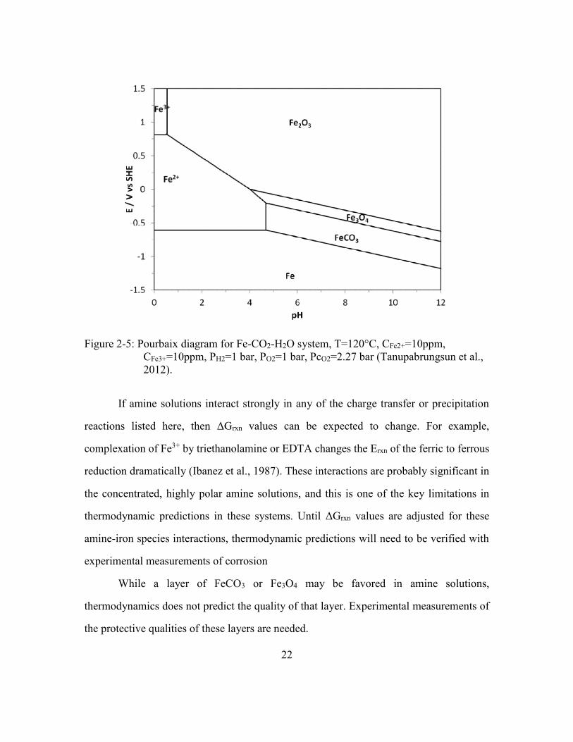
22
Figure 2-5: Pourbaix diagram for Fe-CO2-H2O system, T=120°C, CFe2+=10ppm,
CFe3+=10ppm, PH2=1 bar, PO2=1 bar, PcO2=2.27 bar (Tanupabrungsun et al.,
2012).
If amine solutions interact strongly in any of the charge transfer or precipitation
reactions listed here, then ΔGrxn values can be expected to change. For example,
complexation of Fe3+ by triethanolamine or EDTA changes the Erxn of the ferric to ferrous
reduction dramatically (Ibanez et al., 1987). These interactions are probably significant in
the concentrated, highly polar amine solutions, and this is one of the key limitations in
thermodynamic predictions in these systems. Until ΔGrxn values are adjusted for these
amine-iron species interactions, thermodynamic predictions will need to be verified with
experimental measurements of corrosion
While a layer of FeCO3 or Fe3O4 may be favored in amine solutions,
thermodynamics does not predict the quality of that layer. Experimental measurements of
the protective qualities of these layers are needed.
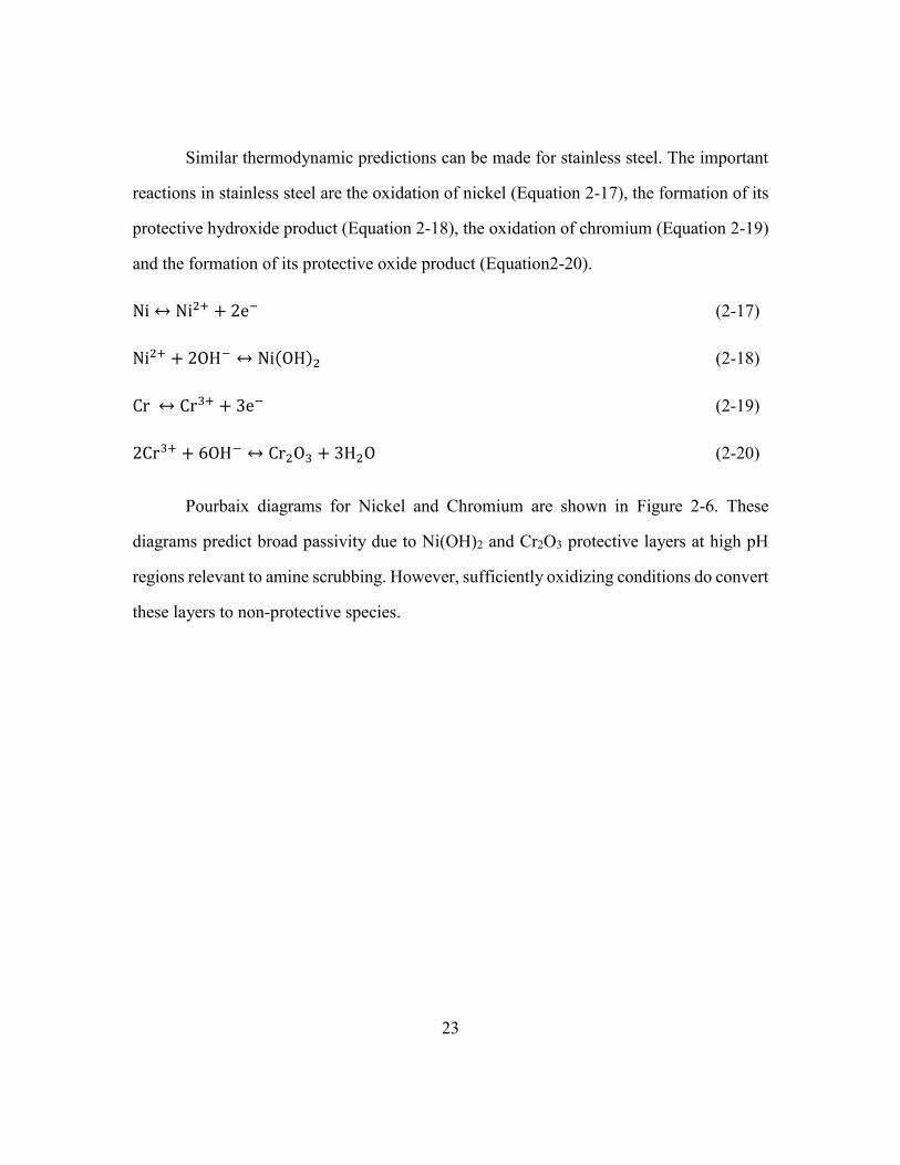
23
Similar thermodynamic predictions can be made for stainless steel. The important
reactions in stainless steel are the oxidation of nickel (Equation 2-17), the formation of its
protective hydroxide product (Equation 2-18), the oxidation of chromium (Equation 2-19)
and the formation of its protective oxide product (Equation2-20).
Ni ↔ Ni2+ + 2e− (2-17)
Ni2+ + 2OH− ↔ Ni(OH)2 (2-18)
Cr ↔ Cr3+ + 3e− (2-19)
2Cr3+ + 6OH− ↔ Cr2O3 + 3H2O (2-20)
Pourbaix diagrams for Nickel and Chromium are shown in Figure 2-6. These
diagrams predict broad passivity due to Ni(OH)2 and Cr2O3 protective layers at high pH
regions relevant to amine scrubbing. However, sufficiently oxidizing conditions do convert
these layers to non-protective species.

24
Figure 2-6: (left) Pourbaix diagram for Nickel-water at 100°C and [Ni(aq)]total=10-6 molal
and (right) Pourbaix diagram for Chromium-water at 100°C and
[Cr(aq)]total=10-6 molal (Beverskog et al., 1997a, 1997b).
2.3.3. Passive film formation
Although passive films are thermodynamically predicted at the high pH, reducing
conditions expected in amine scrubbing, the rate of passive film formation controls whether
that film is protective. This can lead to counterintuitive corrosion behavior at reducing
conditions. For example, formation of FeCO3 depends on the activity of CO32-. Likewise,
formation of Cr2O3 requires OH-. At reducing conditions, the rate of formation of these
product layers is unable to keep up with the rate of oxidation of the metal. This is because
as oxidizer concentration decreases (ie, the solution potential is lower) the total rate of the
reduction reactions in solution becomes smaller. Although the metal surface is still
oxidizing, the lower rate of the reduction reactions in solution reduces the production of
CO32- and OH-. This is known as the metals active state, where passive product formation

25
is thermodynamically favorable, but its formation is slower than the oxidation of the metal
(Jones, 1996; Raja et al., 2006).
The passivation of metals requires slightly more oxidizing conditions than indicated
by their Pourbaix diagrams to avoid this active state. This active to passive transition can
be studied electrochemically through the use of potentiodynamic polarization. This
technique applies a controlled voltage to a solution, then measures the resulting current
through the electrode. High currents correspond to a high rate of oxidation of the steel and
thus corrosion. Although solution potential is applied artificially, it can be understood as
corresponding to the potential of the reduction half-cell of a corrosion reaction. Lower
solution potentials represent a more reducing solution, and higher potentials represent a
more oxidizing solution. Two such experiments are shown for carbon steel and stainless
steel in 5 M MEA in Figure 2-7 (Y. Sun et al., 2011). At very low potentials (below 900
mV), the solution is so reducing that the metal is inert, and cannot be oxidized. Large
currents below that potential reflect the reduction of water to hydrogen, not the oxidation
of the metal. As potential increases, first current increases in the active region, then
decreases in the passive region. In the passive region, formation of protective products is
rapid enough to limit oxidation of the metal. At very oxidizing conditions, the formation
of protective products is no longer rapid enough to keep up with the very quick oxidation
of the metal, and corrosion resumes. Note that in MEA at these conditions, stainless steel
has a very small active window. Presumably, the favorable oxidation of MEA has a high
rate, which increases the rate of redox reactions in solution, leading to higher production
of CO32- and OH-, even at reducing conditions. Also note that increasing T increases the
current (and thus corrosion rate) in both the active and the passive region. One of the
implications of this analysis is that a metal in the active state can experience a decrease in
corrosion rate from a decrease in solution potential (ie, reduction and oxidation reactions
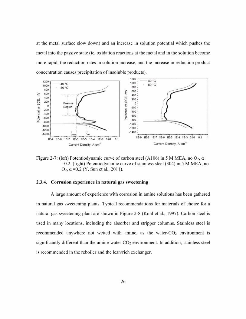
26
at the metal surface slow down) and an increase in solution potential which pushes the
metal into the passive state (ie, oxidation reactions at the metal and in the solution become
more rapid, the reduction rates in solution increase, and the increase in reduction product
concentration causes precipitation of insoluble products).
Figure 2-7: (left) Potentiodynamic curve of carbon steel (A106) in 5 M MEA, no O2, α
=0.2. (right) Potentiodynamic curve of stainless steel (304) in 5 M MEA, no
O2, α =0.2 (Y. Sun et al., 2011).
2.3.4. Corrosion experience in natural gas sweetening
A large amount of experience with corrosion in amine solutions has been gathered
in natural gas sweetening plants. Typical recommendations for materials of choice for a
natural gas sweetening plant are shown in Figure 2-8 (Kohl et al., 1997). Carbon steel is
used in many locations, including the absorber and stripper columns. Stainless steel is
recommended anywhere not wetted with amine, as the water-CO2 environment is
significantly different than the amine-water-CO2 environment. In addition, stainless steel
is recommended in the reboiler and the lean/rich exchanger.
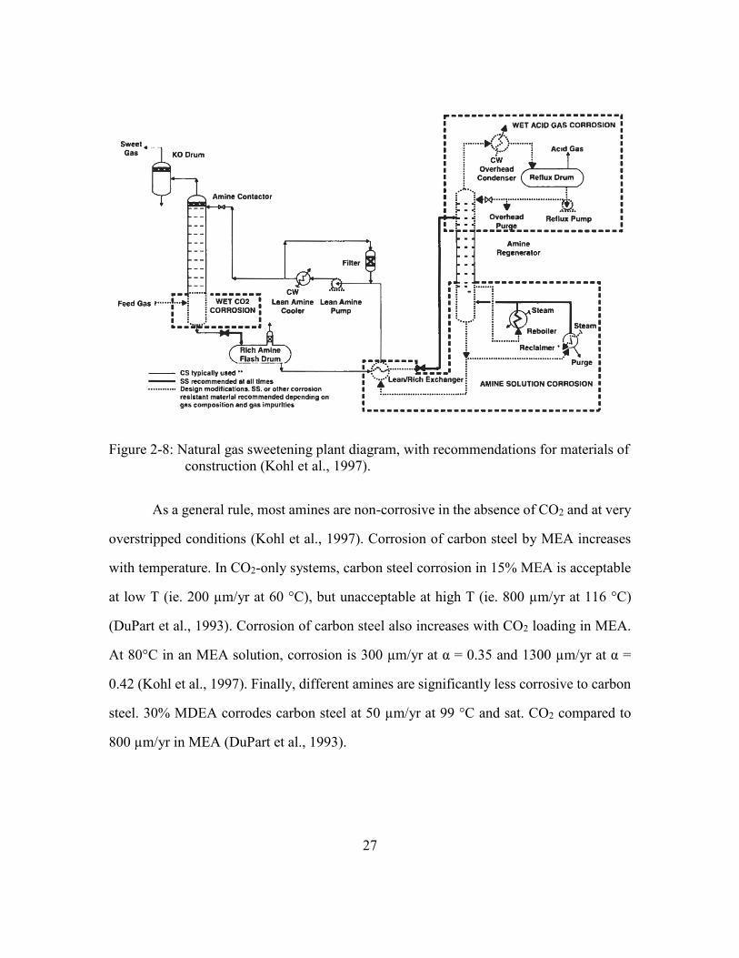
27
Figure 2-8: Natural gas sweetening plant diagram, with recommendations for materials of
construction (Kohl et al., 1997).
As a general rule, most amines are non-corrosive in the absence of CO2 and at very
overstripped conditions (Kohl et al., 1997). Corrosion of carbon steel by MEA increases
with temperature. In CO2-only systems, carbon steel corrosion in 15% MEA is acceptable
at low T (ie. 200 µm/yr at 60 °C), but unacceptable at high T (ie. 800 µm/yr at 116 °C)
(DuPart et al., 1993). Corrosion of carbon steel also increases with CO2 loading in MEA.
At 80°C in an MEA solution, corrosion is 300 µm/yr at α = 0.35 and 1300 µm/yr at α =
0.42 (Kohl et al., 1997). Finally, different amines are significantly less corrosive to carbon
steel. 30% MDEA corrodes carbon steel at 50 µm/yr at 99 °C and sat. CO2 compared to
800 µm/yr in MEA (DuPart et al., 1993).

28
Stainless steel (316L) performs well (<25 µm/yr) in 20 wt % MEA at 116 °C sat.
to CO2 (Kohl et al., 1997). Although higher concentration of MEA (30 wt %) sees higher
corrosion of 316L (≈130 µm/yr at 121 °C, CO2 sat.) (DuPart et al., 1993).
Ultimately, corrosion of carbon steel in natural gas sweetening units is controlled
by limiting MEA concentration to 20% and restricting rich loadings to a maximum of α=
0.35 (DuPart et al., 1993). Pipe velocities for carbon steel are limited to 0.9 M/s, whereas
stainless steel is less sensitive and can be used at velocities up to 2.4 m/s (DuPart et al.,
1993). MEA units are usually limited to operation at 120 °C because thermal degradation
of the solvent becomes excessive at higher temperature (Davis, 2009). Stainless steel is
used when needed because it performs well in 20 wt % MEA at all conditions.
Stress corrosion cracking of carbon steel is sometimes observed in natural gas
sweetening plants. A large investigation into stress corrosion cracking in gas sweetening
plants was undertaken after a vessel rupture in an MEA contactor in the 1980s caused 17
fatalities (McHenry et al., 1987). That particular incident was caused by hydrogen-induced
cracking, which is associated with the presence of H2S in gas sweetening plants. Stress
corrosion cracking seems to occur in MEA solutions, but rarely in other amines like
MDEA, when post-weld heat treatments are not used to relieve stress in carbon steel after
welding (Richert et al., 1989). Stress corrosion cracking involves local disruption and
attack of passive films at locations of high stress in the material. It typically occurs at
solution potentials where the material should be passive, and it seems to require certain
species such as OH- or CO32- (Sutcliffe et al., 1972). In amine units this can be avoided by
proper heat treatment of carbon steel and by avoiding MEA (API, 2003).
Corrosion results from natural gas sweetening plants are difficult to adapt because
critical corrosion parameters (amine concentration, presence of H2S, presence of O2) are
29
different in PCCC plants. However, experience from natural gas sweetening informs
corrosion study in PCCC plants.
2.3.5. Corrosion measurements at PCCC conditions
There has been significant recent work at conditions relevant to PCCC plants.
Efforts have largely focused on the conditions that are unique to PCCC work (ie, presence
of O2 and higher amine concentration). However other areas of interest have been intrinsic
differences in corrosivities between amines, the performance of carbon steel when it is
protected by FeCO3, and the effect of degradation products on corrosion.
The addition of oxygen (6% O2) was shown to increase the corrosion rate of carbon
steel in 30 wt % MEA at absorber conditions (50°C, 12% O2) from 50 µm/yr to 300 µm/yr
(Xiang, Yan, et al., 2014).
Amines have been shown to have different intrinsic corrosivities (Table 2-3). It was
proposed that amines with greater bicarbonate concentration, or with higher tendency to
form bicarbonate (ie hindered amines like AMP) are expected to be more corrosive
(Veawab et al., 1999). Higher bicarbonate concentration promotes the bicarbonate
reduction to carbonate, which is a crucial reduction reaction coupled with oxidation of a
metal surface. Carbon steel in MEA was noted to be in the active state at typical PCCC
conditions, although at oxidizing conditions, it could be passivated by hematite (Fe2O3)
(Soosaiprakasam et al., 2008). PZ was noted to have moderate corrosion of carbon steel at
80°C, 4 M, CO2 sat, performing worse than MDEA but better than DEA (Gunasekaran et
al., 2013).

30
Table 2-3: Corrosion rates of carbon steel (1020) at 80 °C in 3 M amines. DEA is
diethanolamine (Veawab et al., 1999)
Amine Lean (α = 0.2)
Corrosion Rate (μm/yr)
Rich (CO2 sat.)
Corrosion Rate (μm/yr)
MEA 508 3465
AMP 762 3198
DEA 483 2263
MDEA - 1717
Carbon steel (A106) coupons exposed to PZ at 80 °C show a tight, coherent layer
of FeCO3, but coupons exposed to MEA show a porous, loose layer of Fe3C. The Pourbaix
diagrams constructed by the researchers predicted FeCO3 for both cases (Zheng, Landon,
Zou, et al., 2014).
Figure 2-9: (left) SEM of carbon steel (A106) in 30 wt % PZ for 150 h (right) SEM
micrograph of carbon steel (A106) in 30 wt % MEA, 183 h. In both cases
α=0.43, 80°C (Zheng, Landon, Zou, et al., 2014)
Experiments show that 5 M MDEA and 5 M AMP also form protective FeCO3
layers (80°C and 120°C), whereas 5 M MEA had no protective layer (K. L. S. Campbell et
al., 2016; Yu et al., 2016). Protective films can be formed in comparable MEA solutions
but only at very high CO2 loading (L. Zheng, N. S. Matin, et al., 2016) or at controlled pH
conditions (L. Zheng, J. Landon, et al., 2016).
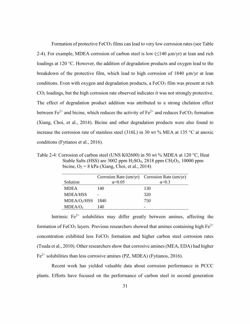
31
Formation of protective FeCO3 films can lead to very low corrosion rates (see Table
2-4). For example, MDEA corrosion of carbon steel is low (≤140 µm/yr) at lean and rich
loadings at 120 °C. However, the addition of degradation products and oxygen lead to the
breakdown of the protective film, which lead to high corrosion of 1840 µm/yr at lean
conditions. Even with oxygen and degradation products, a FeCO3 film was present at rich
CO2 loadings, but the high corrosion rate observed indicates it was not strongly protective.
The effect of degradation product addition was attributed to a strong chelation effect
between Fe2+ and bicine, which reduces the activity of Fe2+ and reduces FeCO3 formation
(Xiang, Choi, et al., 2014). Bicine and other degradation products were also found to
increase the corrosion rate of stainless steel (316L) in 30 wt % MEA at 135 °C at anoxic
conditions (Fytianos et al., 2016).
Table 2-4: Corrosion of carbon steel (UNS K02600) in 50 wt % MDEA at 120 °C, Heat
Stable Salts (HSS) are 3002 ppm H2SO4, 2818 ppm CH2O2, 10000 ppm
bicine, O2 = 8 kPa (Xiang, Choi, et al., 2014)
Solution
Corrosion Rate (um/yr)
α=0.05
Corrosion Rate (um/yr)
α=0.3
MDEA 140 130
MDEA/HSS - 320
MDEA/O2/HSS 1840 750
MDEA/O2 140 -
Intrinsic Fe2+ solubilities may differ greatly between amines, affecting the
formation of FeCO3 layers. Previous researchers showed that amines containing high Fe2+
concentration exhibited less FeCO3 formation and higher carbon steel corrosion rates
(Tsuda et al., 2010). Other researchers show that corrosive amines (MEA, EDA) had higher
Fe2+ solubilities than less corrosive amines (PZ, MDEA) (Fytianos, 2016).
Recent work has yielded valuable data about corrosion performance in PCCC
plants. Efforts have focused on the performance of carbon steel in second generation
32
solvents. Notably missing is work on performance of stainless steel, particularly at high
temperature. This is likely because stainless steel is presumed passive at most conditions
in amine service due to experience from natural gas sweetening.
2.3.6. Corrosion measurement at PCCC conditions in pilot plants
Corrosion in amine units for CO2 capture has been measured at several pilot plants
(Cousins et al., 2013; Hjelmaas et al., 2017; Khakharia et al., 2015; Kittel et al., 2009; Li
et al., 2017). These studies all investigated MEA, and as a consequence are typically
limited to operation at 120 °C. To date there is limited published data on pilot scale
corrosion in second generation solvents, like PZ.
Corrosion of stainless steel (316L) and carbon steel (C1018) was measured in 30
wt % MEA at a pilot plant treating flue gas from a coal power station in Esbjerg, Denmark.
Carbon steel performed acceptably in the absorber (<300 µm/yr), but poorly in the stripper
sump (4500-8500 µm/yr). Stainless steel performed well (< 5 µm/yr) at all locations tested
(Kittel et al., 2009).
Corrosion of stainless steel (316L), carbon steel (C1018), and galvanized carbon
steel (C1018 GLV) was measured in 30 wt % MEA at a pilot plant treating flue gas from
the Tarong coal power station in Australia. Stainless steel performed well at all locations
tested (< 3 µm/yr). Galvanized coupons performed worse than corresponding carbon steel
coupons at almost all locations. Carbon steel performance was moderate in the absorber
(200-700 µm/yr), and unexpectedly poor (700 µm/yr) in the water wash. Carbon steel
performance was acceptable in the column (≈50 µm/yr), but unacceptable (1000 µm/yr) in
the sump. scale of Fe2O3 was observed in the sump (Cousins et al., 2013).
Corrosion of stainless steel (some 316L, some 304L) was measured in the hot lean
stream (120 °C) of a 30 wt % MEA plant treating flue gas from a coal fired power plant in
33
Maasvlakte, the Netherlands. Corrosion varied from 4 – 130 µm/yr. The higher corrosion
rate was attributed to a higher oxygen content in the flue gas (17 % by volume, instead of
7 % typically) used during one campaign to imitate natural gas conditions (Khakharia et
al., 2015).
Extensive corrosion measurements of several alloys was made at the Technology
Centre Mongstad in Norway. 30 wt % MEA was operated at 120 °C, capturing flue gas
from a natural gas burner that was typically 4 % CO2, 14 % O2. Coupons were only
evaluated at hot lean and hot rich locations. Carbon steel (S235) experienced high corrosion
(>1400 µm/yr) in both the hot lean and hot rich locations. The corrosion rates for 304L,
316L, and 22 Cr duplex were << 100 µm/yr for all locations. Some pits were found on
316L coupons in the hot rich solvent with a pit depth of 0.15 mm/yr. No pitting was
observed on 304L, Inconel 600, or 22 Cr Duplex. Inconel 600 was attacked in hot lean
solvent (840 µm/yr), but performed well at rich conditions (<< 100 µm/yr) (Hjelmaas et
al., 2017).
Corrosion of carbon steel (A106) and stainless steel (304) was evaluated at a pilot
plant treating coal flue gas in Harrodsburg, Kentucky. The stripper operated up to 130 °C.
One campaign evaluated 30 wt % MEA. Stainless steel performed well at all locations (<
100 µm/yr). Carbon steel performed well in the absorber and the cold lean location (< 100
µm/yr), but performed unacceptably in the hot rich location and in the stripper (3000-16000
µm/yr). Protective products were not observed on carbon steel coupons. A second
campaign used a proprietary solvent that is a blend of primary amines with a corrosion
inhibitor (1000 ppm 2-Mercaptobenzothiazole). Corrosion was only evaluated in the
stripper and in the hot rich location in this campaign. Stainless steel performed well at all
locations (< 100 µm/yr). Carbon steel performance was moderate at both locations (0-2000
µm/yr for the first 500 hours of the campaign. After that, the corrosion of carbon steel

34
increased (4000-7000 µm/yr), which was attributed to the eventual degradation of the
inhibitor. FeCO3 was observed in the hot rich stream only at the end of the campaign (850
hours), but not on samples removed prior to that. FeCO3 was not observed in the stripper
(Li et al., 2018; Li et al., 2017).
Pilot experience with corrosion in PCCC systems is that MEA is more corrosive to
carbon steel than at comparable natural gas sweetening conditions. Stainless typically
performs very well in MEA at PCCC conditions. Although there is substantial interest in
low corrosivity amines at the bench scale, only one pilot-scale study of a low-corrosion
second generation amine has been published (Li et al., 2018).

35
Chapter 3. Experimental Methods
Experimental methods used throughout this work are grouped by their type in this
chapter. Techniques used for the measurement of corrosion are presented in Section 3.1.
Section 3.2 discusses equipment that was used to simulate corrosive conditions in amine
solutions. Section 3.3 describes analytical techniques that are used to characterize amine
solutions. Finally, Section 3.4 presents some miscellaneous equipment as well as several
tables of equipment part numbers.
3.1. TECHNIQUES FOR MEASUREMENT OF CORROSION
3.1.1. Electrical Resistance Corrosion Probes
Electrical resistance (ER) probes are used for online corrosion measurement at the
bench-scale in Chapter 4, and in several pilot plant campaigns in Chapter 6 and Chapter 7.
The ER probe exposes a thin carbon steel or stainless steel wire to the process fluid,
allowing it to slowly corrode. The thin wire element of the corrosion probe is shown in
Figure 3-1.
Figure 3-1: Electrical resistance corrosion probe

36
As the wire corrodes and loses metal to solution, the wire cross-sectional area
decreases, thus increasing resistance in the wire. Resistance in a conductor is linearly
proportional to the conductor cross sectional area (Equation 3-1). A transmitter connected
to the ER probe constantly measures this resistance and outputs a signal that reflects the
wire thickness remaining. Resistivity of metallic conductors generally increases with
temperature, so the probe contains a reference element that is sealed within the probe body
and shielded from the corrosive environment. Because the reference element and the
exposed element are the same material and exposed to the same temperature, their
resistivity is the same. The ER probe reports the ratio of the exposed element resistance
and the reference element resistance, which eliminates the effect of temperature
R = ρL
A (3-1)
Table 3-1: Nomenclature used in Equation 3-1
R Electrical Resistance (Ω)
ρ Electrical resistivity (Ω∙meters)
L Length of conductor (meters)
A Cross sectional area of conductor (meters2)
Different methods were used for processing the data depending on the length of the
experiment. Bench-scale experiments took one probe life reading per second, and this data
was then directly regressed to determine a corrosion rate. For the SRP 2017 PZ campaign,
one ER probe signal reading per minute was taken during operation. During each period of
steady state operation (periods in this campaign were typically 1-3 hours long, after which
conditions are changed), these measurements were averaged to give an average ER probe
reading during that steady state period. Plotting the average ER probe readings
chronologically showed that the probe life decreased over the course of the campaign. For

37
the NCCC 2018 PZ campaign, one ER probe signal reading per minute was taken during
operation, and these data averaged to yield an average daily corrosion probe reading for
each probe. Plotting the average probe life remaining for each day chronologically gives
a corrosion rate over the entire exposure time for each probe. The corrosion rates were
then determined using the method of least squares. For pilot scale work, ER probes were
cleaned between batches using the same procedure described below for coupons (See
Section 3.1.3). Table 3-9 lists the part numbers of ER used. In Chapter 6, bench-scale ER
corrosion rates are compared to pilot-scale ER corrosion rates. In Chapter 6 and Chapter 7,
simultaneous pilot ER corrosion rates and coupon corrosion rates are compared.
Ultimately, the ER probe gave reliable corrosion rates at the bench-scale, but pilot-scale
ER measurements were sometimes inconsistent.
Qualitative judgements about corrosion rates are given in Table 3-2 to give an idea
about what an acceptable corrosion rate is. These judgements are appropriate for certain
equipment with thick walls, like piping or vessels. However these corrosion rates may be
too high for equipment with thin surfaces, like heat exchangers.
Table 3-2: Relative corrosion resistance (Fontana, 1986).
Qualitative Corrosion Resistance μm/yr
Outstanding <25
Excellent 25 to 100
Good 100 to 500
Fair 500 to 1000
Poor 1000 to 5000
Unacceptable 5000 +
38
3.1.2. Oxidation-Reduction Probes
Solution potential was measured in amine solutions at the bench-scale in Chapter
4. ORP measurements were made during the SRP 2017 PZ campaign (Chapter 6) and the
NCCC 2018 PZ campaign (Chapter 7). Pilot ORP measurements at NCCC were slightly
erratic because frequent retraction and recalibration of the ORP probes was not performed.
These pilot ORP results are briefly discussed in Appendix B. The ORP probe measures the
platinum electrode potential of solutions in the corrosion loop compared to a Ag/AgCl
reference cell. Cell potential measures how thermodynamically favorable a redox reaction
is. For example, Equation 3-2 shows the oxidation of iron at high pH and in the presence
of O2. If this reaction were separated into two half-cells, connected by a junction, the
potential between the cells is given by Equation 3-3. Nomenclature for these equations is
given in Table 3-3.
2Fe + O2 + 2H2O ↔ 2Fe2+ + 4 OH− (3-2)
𝑒 = 𝑒0 −𝑅𝑇
4𝐹ln (
(𝐹𝑒2+)2(𝑂𝐻−)4
(𝑂2)) (3-3)
Table 3-3: Nomenclature used in Equations 3-2 and 3-3
e Cell potential (volts)
e0 Standard cell potential (volts)
R Universal gas constant
T Temperature
F Faraday’s constant
(Fe2+), (OH-)… Activity of a species
Unlike iron, platinum is inert to oxidation at most conditions. This means the
reaction at the electrode is likely Equation 3-4. Thus in this system, the potential measured
at a platinum electrode reflects the thermodynamic favorability of the reduction of O2 to
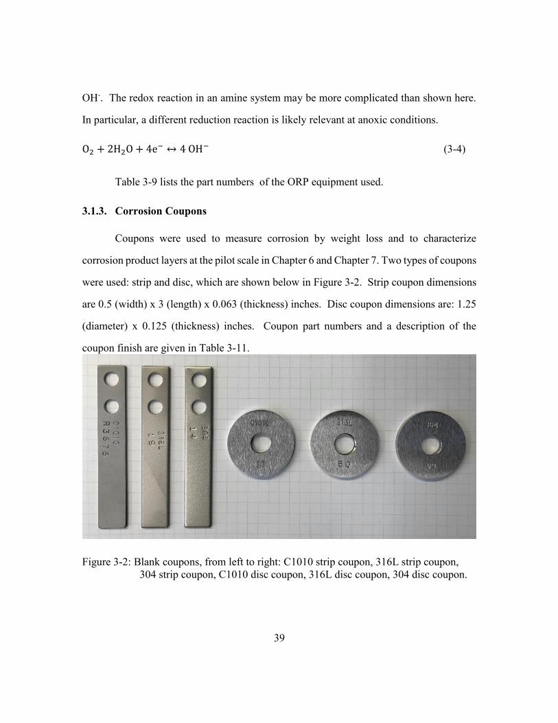
39
OH-. The redox reaction in an amine system may be more complicated than shown here.
In particular, a different reduction reaction is likely relevant at anoxic conditions.
O2 + 2H2O + 4e− ↔ 4 OH− (3-4)
Table 3-9 lists the part numbers of the ORP equipment used.
3.1.3. Corrosion Coupons
Coupons were used to measure corrosion by weight loss and to characterize
corrosion product layers at the pilot scale in Chapter 6 and Chapter 7. Two types of coupons
were used: strip and disc, which are shown below in Figure 3-2. Strip coupon dimensions
are 0.5 (width) x 3 (length) x 0.063 (thickness) inches. Disc coupon dimensions are: 1.25
(diameter) x 0.125 (thickness) inches. Coupon part numbers and a description of the
coupon finish are given in Table 3-11.
Figure 3-2: Blank coupons, from left to right: C1010 strip coupon, 316L strip coupon,
304 strip coupon, C1010 disc coupon, 316L disc coupon, 304 disc coupon.

40
Once removed from pilot plants, coupons were immediately rinsed with deionized
H2O, air dried, photographed, wrapped with paper containing a volatile corrosion inhibitor,
placed into plastic Ziploc bags, transported back to Austin, and finally placed into a glass
desiccator until analysis was performed. Coupons were first mounted for scanning electron
microscope imaging. Afterward, a small portion of corrosion product, if present, was
gently scraped off and analyzed by powder X-Ray diffraction. Any residual corrosion
product was removed using concentrated HCl inhibited with N,N’-Dibutylthiourea as
recommended in literature (Kayafas, 1980; NACE, 2013), and the coupons were weighed
for a final weight-loss measurement.
Coupons were cleaned and weighed by the following procedure. After all SEM and
powder X-ray diffraction characterization, coupons were rinsed in acetone and then air
dried. The coupons were then weighed in triplicate to measure the mass of the corroded
coupon with its product layer. After this, each coupon was dipped in an inhibited HCl
solution for 60 s with gentle stirring. Next, the coupon was immediately transferred to a
saturated solution of NaHCO3 in water, where it was gently stirred for 60 s. The coupon
then was rinsed in water, then in acetone, then air dried. Finally the coupon was weighed
in triplicate to measure the mass of the corroded coupon without its product layer. This
final mass was used for all corrosion rates reported here. To prepare the inhibited HCl
solution, 10 g/L of N,N’-Dibutylthiourea from Alfa Aesar was added to conc. HCl (37.5
wt. %) while stirring with a Teflon stir bar. The solid dissolved completely, leaving a clear
“stock” solution. Immediately prior to use, this stock solution was diluted 50 % by volume
with water.
One minor issue with this work is that stainless steel coupons were cleaned with
concentrated HCl for final weight loss measurements. HCl is not recommended for use
with stainless (ASTM, 2017) due to pitting (Jones, 1996). Future work should use a

41
different cleaning procedure for stainless steel. However, since coupons were evaluated by
SEM for pitting before corrosion product removal, this error should not impact the
accuracy of this work.
Corrosion by coupon weight loss is calculated by Equation 3-5 (Jones, 1996). The
proportionality constant is a simple unit conversion. Densities and physical properties of
alloys investigated in this report are given in Table 3-5.
𝐶 = 87600 𝑊
𝐷𝐴𝑇 (3-5)
Table 3-4: Nomenclature for Equation 3-5
C corrosion rate (µm/yr)
W coupon mass loss (mg)
D density of metal (g/cm3)
A surface area of coupon (cm2)
T duration of experiment (hours)
Table 3-5: Density and composition of alloys investigated (Bauccio, 1993)
Composition (wt %)
Alloy UNS # Density
(g/cm3)
C Mn Si Cr Ni P S Mo Fe
C1010 G10100 7.87 0.8-
0.13
0.30-
0.60
0 0 0 0 0 0 Bal.
316L S31603 7.98 0.03 2.00 1.00 16.0-
18.0
10.0-
14.0
0.045 0.03 2.0-
3.0
Bal.
304 S30400 8.00 0.08 2.00 1.00 18.0-
20.0
8.0-
10.5
0.045 0.03 0 Bal.
3.1.4. Coupon Characterization
Corrosion product films on coupons were imaged using either a FEI Quanta 650
scanning electron microscope or a FEI Quanta 600 FEG scanning electron microscope.
42
Accelerating voltage was typically 20 kV and magnification was typically 1000x-5000x.
Details are included in each SEM micrograph. Corrosion product films were gently
scraped off and the resulting powder product was analyzed by powder X-ray diffraction
using a Rigaku R-Axis Spider instrument with a Cu Kα radiation source at 40 kV and 40
mA. Reference spectra are given in Table 3-6. Powder X-ray diffraction was also used to
characterize the solid phase present in Fe2+ solubility experiments (Chapter 5). SEM
micrographs of blank coupons are shown in Figure 3-3. Blank coupon micrographs show
the significant difference between the finish on disc coupons (120 grit) and on strip
coupons (glass bead). In general the blank coupons are unremarkable and free of features
or corrosion products.
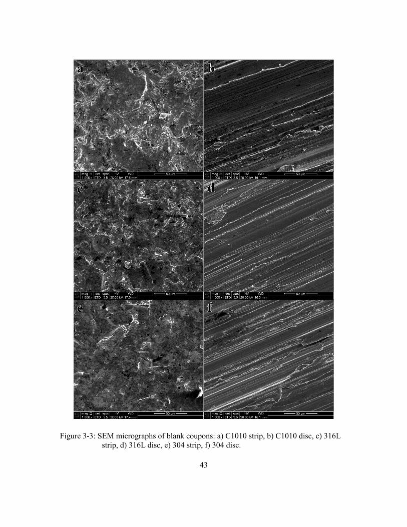
43
Figure 3-3: SEM micrographs of blank coupons: a) C1010 strip, b) C1010 disc, c) 316L
strip, d) 316L disc, e) 304 strip, f) 304 disc.
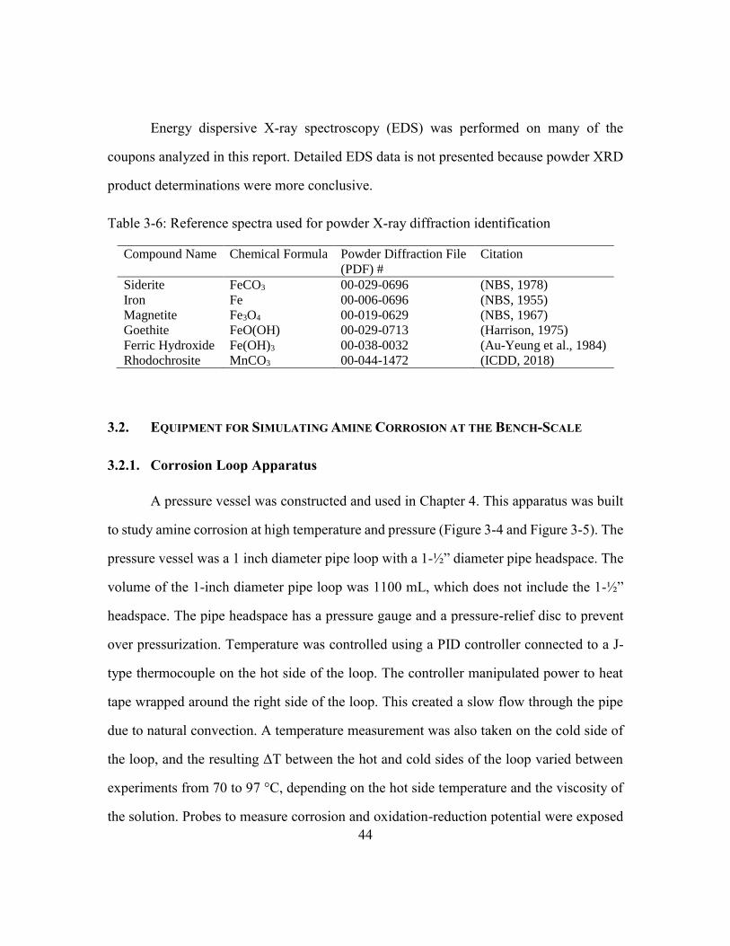
44
Energy dispersive X-ray spectroscopy (EDS) was performed on many of the
coupons analyzed in this report. Detailed EDS data is not presented because powder XRD
product determinations were more conclusive.
Table 3-6: Reference spectra used for powder X-ray diffraction identification
Compound Name Chemical Formula Powder Diffraction File
(PDF) #
Citation
Siderite FeCO3 00-029-0696 (NBS, 1978)
Iron Fe 00-006-0696 (NBS, 1955)
Magnetite Fe3O4 00-019-0629 (NBS, 1967)
Goethite FeO(OH) 00-029-0713 (Harrison, 1975)
Ferric Hydroxide Fe(OH)3 00-038-0032 (Au-Yeung et al., 1984)
Rhodochrosite MnCO3 00-044-1472 (ICDD, 2018)
3.2. EQUIPMENT FOR SIMULATING AMINE CORROSION AT THE BENCH-SCALE
3.2.1. Corrosion Loop Apparatus
A pressure vessel was constructed and used in Chapter 4. This apparatus was built
to study amine corrosion at high temperature and pressure (Figure 3-4 and Figure 3-5). The
pressure vessel was a 1 inch diameter pipe loop with a 1-½” diameter pipe headspace. The
volume of the 1-inch diameter pipe loop was 1100 mL, which does not include the 1-½”
headspace. The pipe headspace has a pressure gauge and a pressure-relief disc to prevent
over pressurization. Temperature was controlled using a PID controller connected to a J-
type thermocouple on the hot side of the loop. The controller manipulated power to heat
tape wrapped around the right side of the loop. This created a slow flow through the pipe
due to natural convection. A temperature measurement was also taken on the cold side of
the loop, and the resulting ΔT between the hot and cold sides of the loop varied between
experiments from 70 to 97 °C, depending on the hot side temperature and the viscosity of
the solution. Probes to measure corrosion and oxidation-reduction potential were exposed
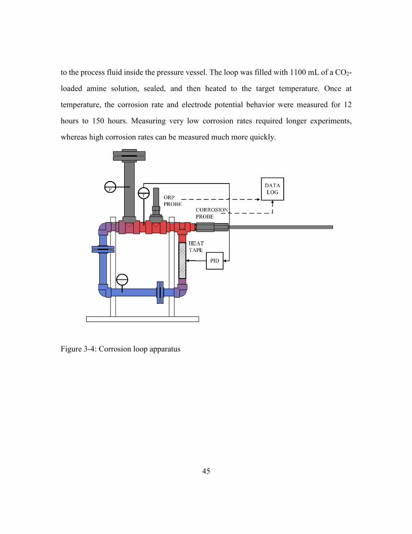
45
to the process fluid inside the pressure vessel. The loop was filled with 1100 mL of a CO2-
loaded amine solution, sealed, and then heated to the target temperature. Once at
temperature, the corrosion rate and electrode potential behavior were measured for 12
hours to 150 hours. Measuring very low corrosion rates required longer experiments,
whereas high corrosion rates can be measured much more quickly.
Figure 3-4: Corrosion loop apparatus
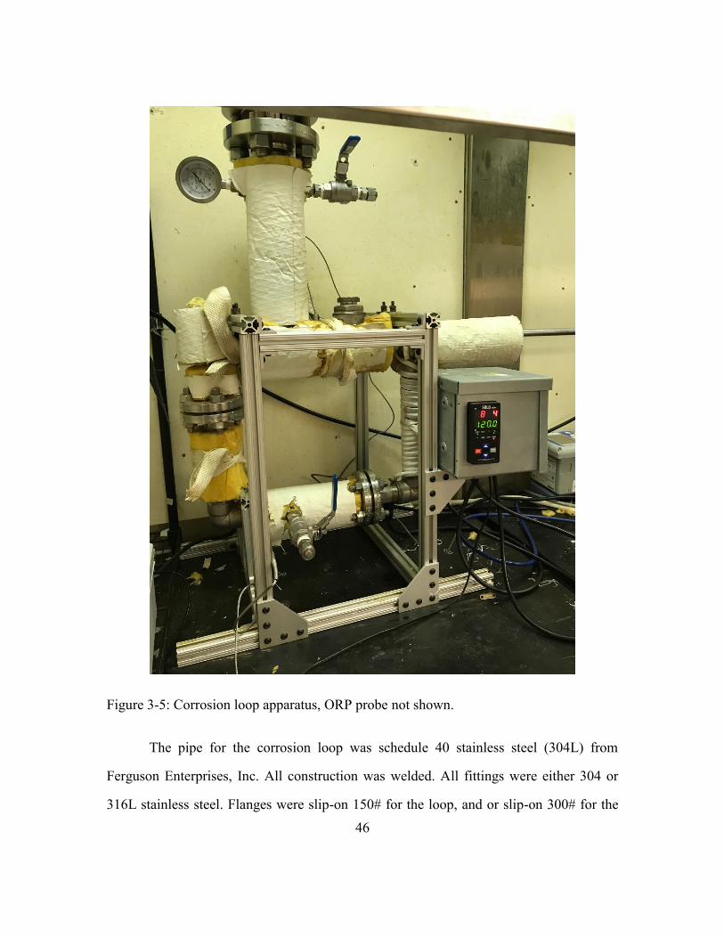
46
Figure 3-5: Corrosion loop apparatus, ORP probe not shown.
The pipe for the corrosion loop was schedule 40 stainless steel (304L) from
Ferguson Enterprises, Inc. All construction was welded. All fittings were either 304 or
316L stainless steel. Flanges were slip-on 150# for the loop, and or slip-on 300# for the

47
headspace. Gaskets were 1/16” gylon from GHX Industrial, LLC. Pipe fittings and ball
valves are typically rated for 150# and sourced from Ferguson Enterprises, Inc. Several
tube adapters are from Swagelok® Company. The frame supporting the equipment was
built with 1” x 1” aluminum T-slotted frame (Part No. 1010) and adapters from 80/20®
Inc. The pressure burst disc was a 1-½” RA8 series stainless (316) metal burst disc
specified to burst at 176 psig at 160°C (or 200 psig at 20 °C) and was manufactured by
Zook Enterprises, LLC. The loop was insulated with 1” fiberglass insulation from W.W.
Grainger, Inc. Two 400 Watt heating tapes (Glas-Col® Part No. 103B-SCC4) supplied heat
and were controlled by a PID controller (AutomationDirect.com Part No. SL4896-RRE)
with a J-type thermocouple (AutomationDirect.com Part No. THMJ-T06L06-01). The loop
pressure was measured with a 0 – 300 psig analog gauge (AutomationDirect.com Part No.
G25-SD300-4LS). A procedure for operating the corrosion loop and an analysis of its
potential hazards is given in Appendix A.
3.2.2. Thermal Degradation Cylinders
Thermal cylinders were used to measure amine corrosion in Chapter 4. Swagelok®
stainless steel cylinders have been extensively used for the measurement of thermal
degradation of amines (Freeman, 2011; Namjoshi, 2015). Measuring the dissolved metal
content in these thermal cylinders provides a way to estimate the corrosion rate of amines.
This method has been used by other researchers to investigate the effect of degradation
products on corrosion of 316L in MEA (Fytianos et al., 2014; Fytianos et al., 2016). That
work showed comparably high corrosion of 316L in MEA. Two alloys were tested using
this method: 316L stainless steel and 1010 carbon steel. These cylinders consist of a 10 cm
long steel tube with an outer diameter of 0.95 cm and inner diameter of 0.77 cm. The inner
surface area of steel used for the corrosion calculation was 25.67 cm2. On both ends, the

48
cylinder has a Swagelok® ferrule fitting and cap that allows it to be sealed. The cylinders
have a volume of 4.5 mL and a pressure rating above 130 barg. Amine solutions were
prepared, and 4 mL added to each cylinder. This left headspace in the cylinder to prevent
cylinder failure due to liquid expansion. The cylinders were sealed and placed into a Lab-
Line Imperial V convection oven with a Eurotherm 2100-series digital temperature control.
After a specified period of time, the cylinders were removed from the oven, weighed to
ensure they had not leaked, quenched in water, opened, and emptied into clean glass vials.
The vial contents were later analyzed for dissolved metals (by inductively coupled plasma
optical emission spectroscopy), which were converted to corrosion rates.
Corrosion rates from the cylinders are calculated using the same equation used for
coupon weight loss (Equation 3-5), except W is defined as the total metal mass in solution
determined by ICP (mg), and A is defined as the inner surface area of the steel cylinder
(cm2). Several time series were conducted, and these show that the corrosion rate slowly
decreases in the cylinders. When a time series is taken like this, it allows a curve to be fit
so that the instantaneous corrosion rate at time = 0 can be estimated. However, to quickly
screen a large number of amines and conditions, detailed time series were not done for each
amine. Most amines and conditions have one time point taken at 333 hours. This allows
only an average corrosion rate to be reported. These average corrosion rates probably
underestimate the instantaneous corrosion rate. However, because all average corrosion
rates are taken at the same time, they provide a good indicator of the relative corrosivity of
different amines and process conditions.
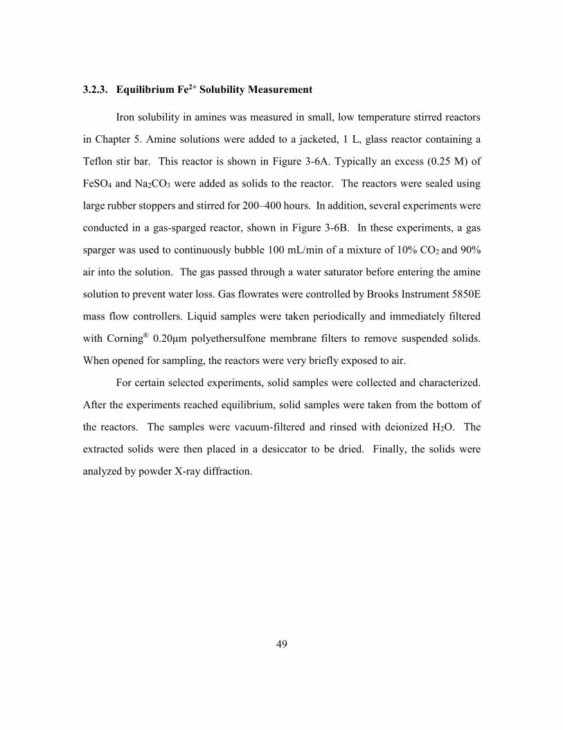
49
3.2.3. Equilibrium Fe2+ Solubility Measurement
Iron solubility in amines was measured in small, low temperature stirred reactors
in Chapter 5. Amine solutions were added to a jacketed, 1 L, glass reactor containing a
Teflon stir bar. This reactor is shown in Figure 3-6A. Typically an excess (0.25 M) of
FeSO4 and Na2CO3 were added as solids to the reactor. The reactors were sealed using
large rubber stoppers and stirred for 200–400 hours. In addition, several experiments were
conducted in a gas-sparged reactor, shown in Figure 3-6B. In these experiments, a gas
sparger was used to continuously bubble 100 mL/min of a mixture of 10% CO2 and 90%
air into the solution. The gas passed through a water saturator before entering the amine
solution to prevent water loss. Gas flowrates were controlled by Brooks Instrument 5850E
mass flow controllers. Liquid samples were taken periodically and immediately filtered
with Corning® 0.20μm polyethersulfone membrane filters to remove suspended solids.
When opened for sampling, the reactors were very briefly exposed to air.
For certain selected experiments, solid samples were collected and characterized.
After the experiments reached equilibrium, solid samples were taken from the bottom of
the reactors. The samples were vacuum-filtered and rinsed with deionized H2O. The
extracted solids were then placed in a desiccator to be dried. Finally, the solids were
analyzed by powder X-ray diffraction.

50
Figure 3-6: a) Reactor used for Fe2+ solubility experiments. b) Sparged reactor used for
Fe2+ solubility experiments.
3.3. AMINE SOLUTION CHARACTERIZATION
3.3.1. Preparation of Amine Solutions
Amine solutions are prepared by diluting commercially purchased amines to target
concentration with deionized water. All water used was purified to 18.2MΩ∙cm by
deionization beds followed by a Millipore Direct-Q® membrane unit. All amine
preparation was performed gravimetrically, so concentration units are reported in molality,
which is defined in Table 3-7. CO2 is added to amine solutions by transferring the solution
to a gas washing bottle, which allows CO2 gas to be slowly bubbled through the solution.
This gas washing bottle is placed onto a scale (± 0.1 g) during the bubbling procedure, so
that the amount of gas added to the solution can be determined. CO2 content in an amine
solution is reported as CO2 loading: “α”, which is defined in Table 3-7. CO2 loading
captures the molar ratio of CO2 in a solution to the amine alkalinity, or the moles of amine
nitrogen groups available to complex CO2. As a brief example, a solution of 5 m MEA
prepared using 1 kg of H2O has 5 mol of MEA, and 5 mol of alkalinity. A solution of 5 m
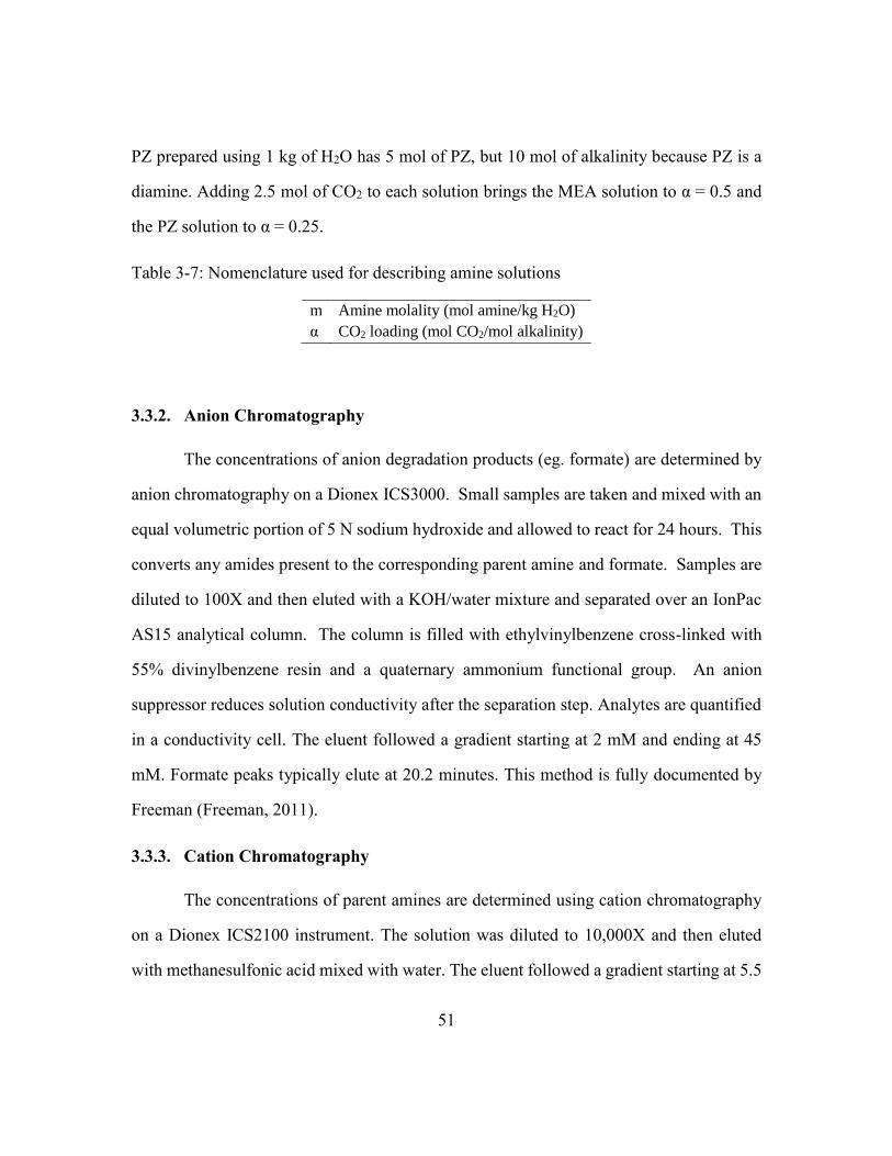
51
PZ prepared using 1 kg of H2O has 5 mol of PZ, but 10 mol of alkalinity because PZ is a
diamine. Adding 2.5 mol of CO2 to each solution brings the MEA solution to α = 0.5 and
the PZ solution to α = 0.25.
Table 3-7: Nomenclature used for describing amine solutions
m Amine molality (mol amine/kg H2O)
α CO2 loading (mol CO2/mol alkalinity)
3.3.2. Anion Chromatography
The concentrations of anion degradation products (eg. formate) are determined by
anion chromatography on a Dionex ICS3000. Small samples are taken and mixed with an
equal volumetric portion of 5 N sodium hydroxide and allowed to react for 24 hours. This
converts any amides present to the corresponding parent amine and formate. Samples are
diluted to 100X and then eluted with a KOH/water mixture and separated over an IonPac
AS15 analytical column. The column is filled with ethylvinylbenzene cross-linked with
55% divinylbenzene resin and a quaternary ammonium functional group. An anion
suppressor reduces solution conductivity after the separation step. Analytes are quantified
in a conductivity cell. The eluent followed a gradient starting at 2 mM and ending at 45
mM. Formate peaks typically elute at 20.2 minutes. This method is fully documented by
Freeman (Freeman, 2011).
3.3.3. Cation Chromatography
The concentrations of parent amines are determined using cation chromatography
on a Dionex ICS2100 instrument. The solution was diluted to 10,000X and then eluted
with methanesulfonic acid mixed with water. The eluent followed a gradient starting at 5.5

52
mM and ending at 38.5 mM methanesulfonic acid. The samples were eluted over an IonPac
GC 17 guard column followed by an IonPac CS 17 analytical column. These columns
contain ethylvinylbenzene cross-linked with 55% divinylbenzene resin. A cation
suppressor reduces solution conductivity after the separation step. Analytes are quantified
in a conductivity cell. This method is fully documented by Namjoshi (Namjoshi, 2015).
3.3.4. Inductively Coupled Plasma Optical Emission Spectroscopy
Metals dissolved in amine solutions were measured to estimate corrosion in thermal
cylinders (Chapter 4) and to determine equilibrium Fe2+ solubility in amines (Chapter 5).
All metals analysis was done by inductively coupled plasma optical emission spectroscopy
using a Varian 710-ES instrument run in axial configuration. Samples are diluted 25X-30X
with 2 wt % HNO3 prepared from 70 wt % trace metal grade HNO3 and doubly deionized
H2O. Metal standards are prepared by diluting 1000 ppm Atomic Emission Spectroscopy
standards obtained from Fisher Scientific® and Ricca Chemical Company®. The solution
is nebulized through a small nozzle and injected into a plasma flame at 7000 K. Metal ions
are excited, then relax, emitting energy at a characteristic wavelength. Wavelengths
analyzed are given in Table 3-8. Results for each wavelength were averaged with other
wavelengths for the same ion. When corrosion rates were estimated, dissolved metals were
converted to an estimated corrosion rate using the surface area of the thermal cylinder and
the density of the alloy.
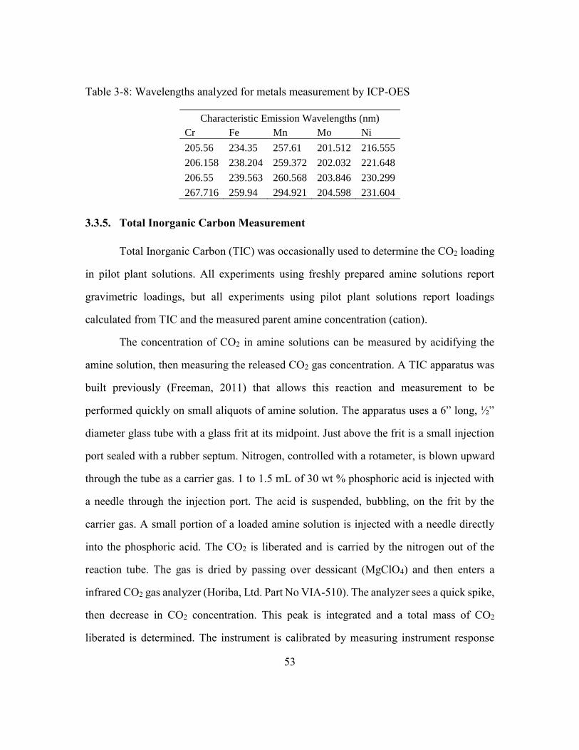
53
Table 3-8: Wavelengths analyzed for metals measurement by ICP-OES
Characteristic Emission Wavelengths (nm)
Cr Fe Mn Mo Ni
205.56 234.35 257.61 201.512 216.555
206.158 238.204 259.372 202.032 221.648
206.55 239.563 260.568 203.846 230.299
267.716 259.94 294.921 204.598 231.604
3.3.5. Total Inorganic Carbon Measurement
Total Inorganic Carbon (TIC) was occasionally used to determine the CO2 loading
in pilot plant solutions. All experiments using freshly prepared amine solutions report
gravimetric loadings, but all experiments using pilot plant solutions report loadings
calculated from TIC and the measured parent amine concentration (cation).
The concentration of CO2 in amine solutions can be measured by acidifying the
amine solution, then measuring the released CO2 gas concentration. A TIC apparatus was
built previously (Freeman, 2011) that allows this reaction and measurement to be
performed quickly on small aliquots of amine solution. The apparatus uses a 6” long, ½”
diameter glass tube with a glass frit at its midpoint. Just above the frit is a small injection
port sealed with a rubber septum. Nitrogen, controlled with a rotameter, is blown upward
through the tube as a carrier gas. 1 to 1.5 mL of 30 wt % phosphoric acid is injected with
a needle through the injection port. The acid is suspended, bubbling, on the frit by the
carrier gas. A small portion of a loaded amine solution is injected with a needle directly
into the phosphoric acid. The CO2 is liberated and is carried by the nitrogen out of the
reaction tube. The gas is dried by passing over dessicant (MgClO4) and then enters a
infrared CO2 gas analyzer (Horiba, Ltd. Part No VIA-510). The analyzer sees a quick spike,
then decrease in CO2 concentration. This peak is integrated and a total mass of CO2
liberated is determined. The instrument is calibrated by measuring instrument response

54
after injection of standards prepared from a 1000 ppm Inorganic Carbon standard solution
(Ricca Chemical Company®).
3.4. MISCELLANEOUS EQUIPMENT AND EQUIPMENT PART NUMBERS
3.4.1. Corrosion Coupon Mounting Hardware
Several types of coupon mounting hardware were used at the pilot scale. WL
probes on the AFS skid (NCCC 2018 PZ campaign) use a retractable probe that holds two
strip coupons. This WL probe is illustrated in Figure 3-7, which also shows the
compression fitting that allows the probe to be inserted and retracted.
Figure 3-7: Illustration of the WL probes used on the AFS skid (Metal Samples
Company, 2019). Each probe holds two strip coupons.
During the NCCC 2018 PZ campaign, coupons were inserted at several locations
using a retractable probe that holds four disc coupons. This hardware was used in the cold
lean stream and several locations in the absorber. The probe body is similar to Figure 3-7,
but the coupon adapter holds disc coupons, as shown in Figure 3-8.
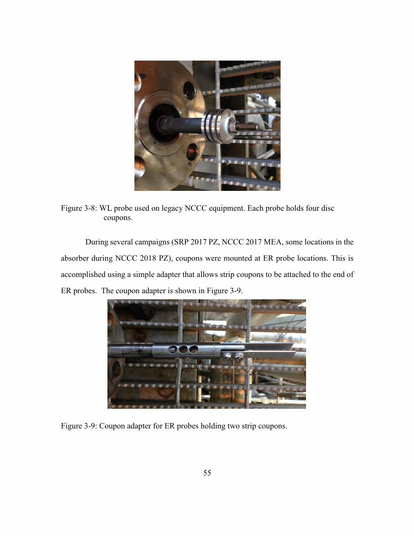
55
Figure 3-8: WL probe used on legacy NCCC equipment. Each probe holds four disc
coupons.
During several campaigns (SRP 2017 PZ, NCCC 2017 MEA, some locations in the
absorber during NCCC 2018 PZ), coupons were mounted at ER probe locations. This is
accomplished using a simple adapter that allows strip coupons to be attached to the end of
ER probes. The coupon adapter is shown in Figure 3-9.
Figure 3-9: Coupon adapter for ER probes holding two strip coupons.
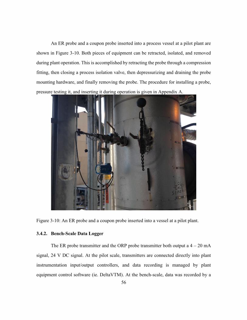
56
An ER probe and a coupon probe inserted into a process vessel at a pilot plant are
shown in Figure 3-10. Both pieces of equipment can be retracted, isolated, and removed
during plant operation. This is accomplished by retracting the probe through a compression
fitting, then closing a process isolation valve, then depressurizing and draining the probe
mounting hardware, and finally removing the probe. The procedure for installing a probe,
pressure testing it, and inserting it during operation is given in Appendix A.
Figure 3-10: An ER probe and a coupon probe inserted into a vessel at a pilot plant.
3.4.2. Bench-Scale Data Logger
The ER probe transmitter and the ORP probe transmitter both output a 4 – 20 mA
signal, 24 V DC signal. At the pilot scale, transmitters are connected directly into plant
instrumentation input/output controllers, and data recording is managed by plant
equipment control software (ie. DeltaVTM). At the bench-scale, data was recorded by a
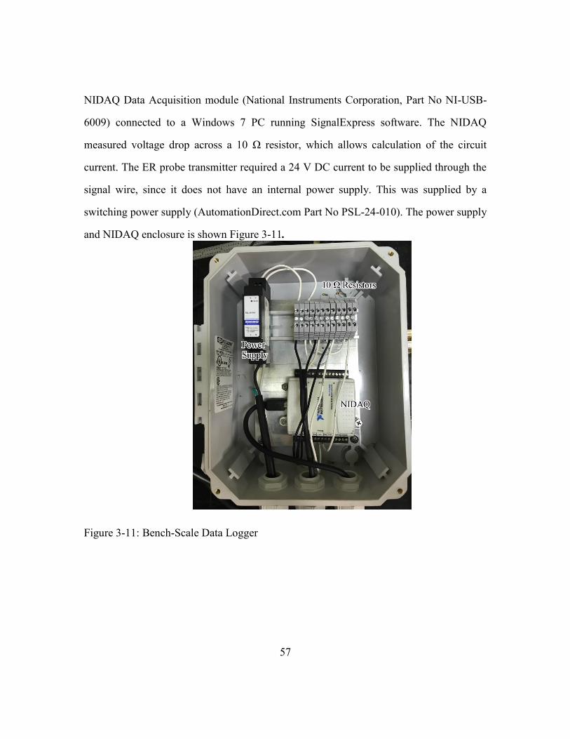
57
NIDAQ Data Acquisition module (National Instruments Corporation, Part No NI-USB-
6009) connected to a Windows 7 PC running SignalExpress software. The NIDAQ
measured voltage drop across a 10 Ω resistor, which allows calculation of the circuit
current. The ER probe transmitter required a 24 V DC current to be supplied through the
signal wire, since it does not have an internal power supply. This was supplied by a
switching power supply (AutomationDirect.com Part No PSL-24-010). The power supply
and NIDAQ enclosure is shown Figure 3-11.
Figure 3-11: Bench-Scale Data Logger
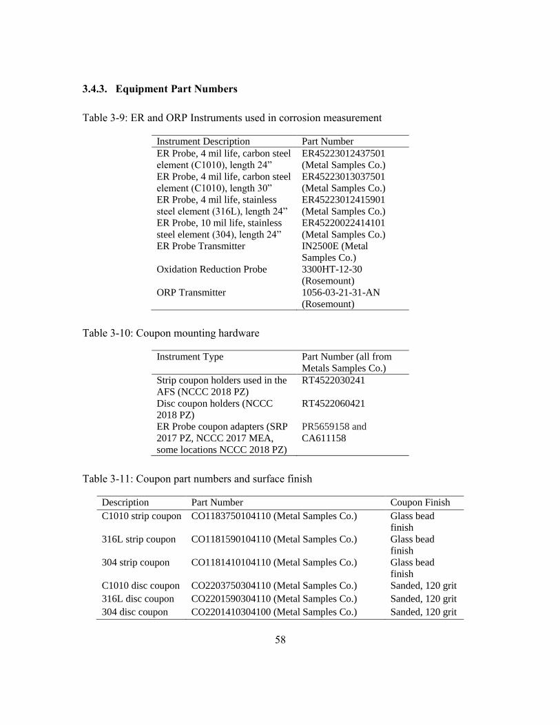
58
3.4.3. Equipment Part Numbers
Table 3-9: ER and ORP Instruments used in corrosion measurement
Instrument Description Part Number
ER Probe, 4 mil life, carbon steel
element (C1010), length 24”
ER45223012437501
(Metal Samples Co.)
ER Probe, 4 mil life, carbon steel
element (C1010), length 30”
ER45223013037501
(Metal Samples Co.)
ER Probe, 4 mil life, stainless
steel element (316L), length 24”
ER45223012415901
(Metal Samples Co.)
ER Probe, 10 mil life, stainless
steel element (304), length 24”
ER45220022414101
(Metal Samples Co.)
ER Probe Transmitter IN2500E (Metal
Samples Co.)
Oxidation Reduction Probe 3300HT-12-30
(Rosemount)
ORP Transmitter 1056-03-21-31-AN
(Rosemount)
Table 3-10: Coupon mounting hardware
Instrument Type Part Number (all from
Metals Samples Co.)
Strip coupon holders used in the
AFS (NCCC 2018 PZ)
RT4522030241
Disc coupon holders (NCCC
2018 PZ)
RT4522060421
ER Probe coupon adapters (SRP
2017 PZ, NCCC 2017 MEA,
some locations NCCC 2018 PZ)
PR5659158 and
CA611158
Table 3-11: Coupon part numbers and surface finish
Description Part Number Coupon Finish
C1010 strip coupon CO1183750104110 (Metal Samples Co.) Glass bead
finish
316L strip coupon CO1181590104110 (Metal Samples Co.) Glass bead
finish
304 strip coupon CO1181410104110 (Metal Samples Co.) Glass bead
finish
C1010 disc coupon CO2203750304110 (Metal Samples Co.) Sanded, 120 grit
316L disc coupon CO2201590304110 (Metal Samples Co.) Sanded, 120 grit
304 disc coupon CO2201410304100 (Metal Samples Co.) Sanded, 120 grit
59
Chapter 4. Bench-Scale Corrosion Measurement
The work in this chapter was published as a paper in the proceedings of the 13th
international conference on Greenhouse Gas Control Technologies (Fischer et al., 2017).
Some early work on corrosion in thermal cylinders was performed by Daniel Hatchell, an
undergraduate researcher (Hatchell et al., 2015; Hatchell et al., 2014). The experimental
work with thermal cylinders and several of the experiments in the corrosion loop in this
chapter was performed by Akshay Daga, another undergraduate researcher.
Two methods were developed to measure the corrosion of carbon steel (C1010) and
stainless steel (316L) in solutions of ethanolamine, piperazine, and several other linear
amines at high temperature and pressure. The effect of amine concentration, CO2 loading,
and temperature were measured. The first method uses Swagelok® steel cylinders heated
in ovens to accelerate corrosion of the metal surface, which is then estimated by measuring
dissolved metal. Although the steel cylinder method gave reasonable corrosion rates for
316L, it significantly under predicted the corrosion rate of C1010. This is likely due to the
weakly adhering passive film that was protective only at the stagnant conditions in the non-
agitated cylinders. The second method uses an electrical resistance probe to measure
corrosion in a bench-scale thermosiphon apparatus, which was constructed to simulate
more realistic flow conditions. Both methods were used to examine a series of linear
amines and their results were compared. Corrosion of the electrical resistance probe by a
variety of degraded piperazine solutions from pilot plants was measured. Loading was
found to be the dominant factor in piperazine corrosion. Unexpectedly, corrosion rates of
stainless steel decrease at high CO2 loadings. Degraded piperazine was only slightly more
corrosive than clean piperazine at most conditions. Over a wide variety of conditions, 1010
carbon steel showed lower corrosion rates in piperazine solutions than 316L stainless steel.
60
4.1. CORROSION LOOP RESULTS: PIPERAZINE
A large variety of piperazine (PZ) solutions were screened using ER corrosion
probes in the corrosion loop apparatus. A summary of all PZ experiments conducted with
the corrosion loop is given in Table 4-1. Concentration varied from 3 m to 8 m, loading
from 0.20 to 0.32, temperature from 100°C to 160 °C, and both C1010 and 316L were
evaluated using two separate ER probes. Amine loading here is defined as mol CO2 per
mol alkalinity. In addition to clean PZ, a variety of amines previously used in pilot plant
campaigns were tested to evaluate the effect of amine degradation on corrosion. One of the
pilot plant solutions was used in the CSIRO pilot plant (2013) at the coal-fired Tarong
power station in Queensland, Australia. Degradation products in Tarong PZ have been
characterized by Cousins (Cousins et al., 2015). The Tarong PZ was diluted during
transport to a concentration of 3 m. PZ from the 2011 pilot plant campaign of the
Separations Research Program (SRP) of the University of Texas was also used. The SRP
campaign used a synthetic flue gas consisting of CO2 mixed with air, and the PZ contains
an oxidation inhibitor referred to here as inhibitor A (Paul T. Nielsen et al., 2013).
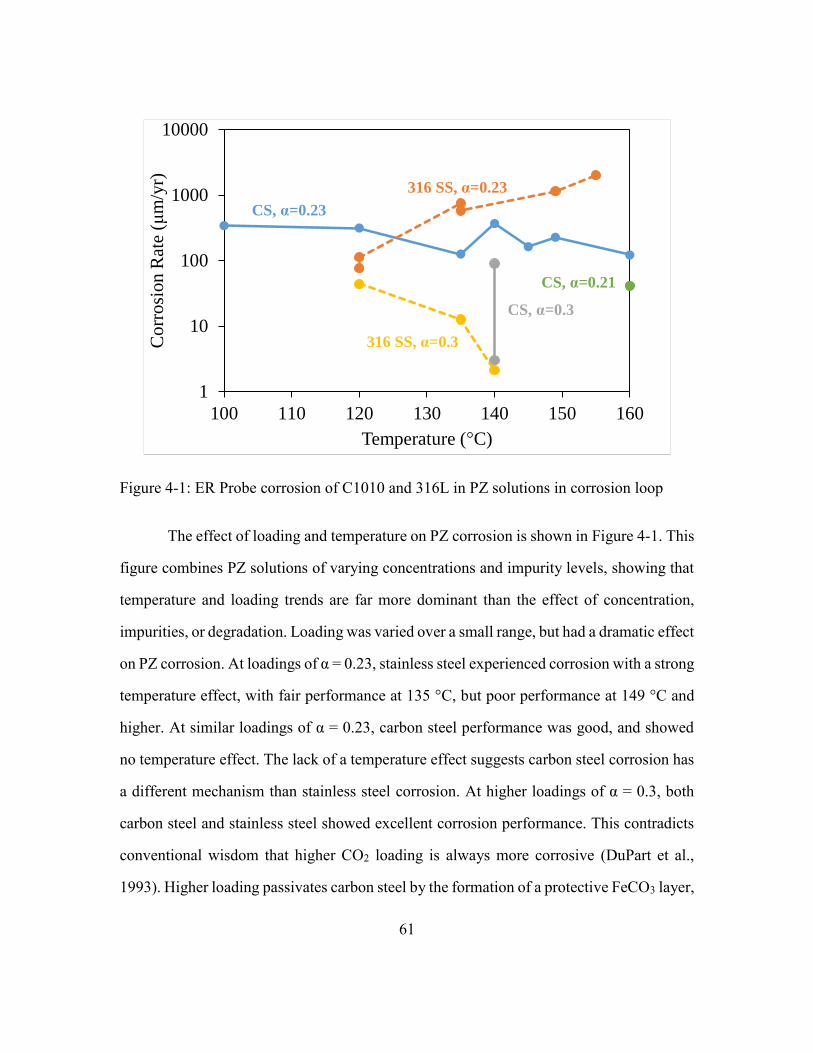
61
Figure 4-1: ER Probe corrosion of C1010 and 316L in PZ solutions in corrosion loop
The effect of loading and temperature on PZ corrosion is shown in Figure 4-1. This
figure combines PZ solutions of varying concentrations and impurity levels, showing that
temperature and loading trends are far more dominant than the effect of concentration,
impurities, or degradation. Loading was varied over a small range, but had a dramatic effect
on PZ corrosion. At loadings of α = 0.23, stainless steel experienced corrosion with a strong
temperature effect, with fair performance at 135 °C, but poor performance at 149 °C and
higher. At similar loadings of α = 0.23, carbon steel performance was good, and showed
no temperature effect. The lack of a temperature effect suggests carbon steel corrosion has
a different mechanism than stainless steel corrosion. At higher loadings of α = 0.3, both
carbon steel and stainless steel showed excellent corrosion performance. This contradicts
conventional wisdom that higher CO2 loading is always more corrosive (DuPart et al.,
1993). Higher loading passivates carbon steel by the formation of a protective FeCO3 layer,
1
10
100
1000
10000
100 110 120 130 140 150 160
Co
rro
sion
Rat
e (μ
m/y
r)
Temperature (°C)
316 SS, α=0.23
316 SS, α=0.3
CS, α=0.23
CS, α=0.3
CS, α=0.21

62
as other researchers have observed (Zheng, Landon, Matin, et al., 2014). The reason for
improved stainless performance at higher CO2 loadings is not immediately apparent.
PZ degradation apparently increased corrosion, although its effect was not as
significant as either CO2 loading or temperature. The effect of PZ degradation and
temperature on corrosion with loading held constant at α = 0.23-0.24 is shown in Figure
4-2. PZ heavily degraded in the High Temperature Oxidation Reactor (HTOR) developed
by Voice (Voice, 2013) was compared to several other solutions to see if a heavily degraded
solution caused rapid corrosion. The HTOR PZ was compared to the Tarong PZ (slightly
degraded) and the SRP PZ (clean with Inhibitor A). Stainless steel corrosion varied
strongly with temperature from good at 120 °C to poor at 149 °C. The slightly degraded
Tarong PZ experienced more severe corrosion than the clean SRP PZ, especially at high
temperature. At 155 °C, the Tarong PZ caused 316L corrosion at a rate of 2010 μm/yr,
70% faster than the clean SRP PZ at 1140 μm/yr and 149 °C. Both of these corrosion rates
are poor, but the difference is significant and shows that stainless steel corrosion is
impacted by degradation products at intermediate loadings. However, at higher loading of
α = 0.30, the Tarong PZ becomes non-corrosive to stainless steel (13 μm/yr at 135 °C).
Carbon steel showed low corrosion for all three solutions tested, and apparently
temperature did not affect corrosion. Both the clean SRP PZ and the slightly degraded
Tarong PZ showed good performance, even at high temperature. The heavily degraded
HTOR PZ had a slightly higher corrosion rate, although its performance was still good.
ORP did not show a clear relationship with corrosivity. In addition ORP values of
the same solution were occasionally different between experiments. This might be a
hysteresis effect on the platinum electrode between experiments. However, we expect the
electrode potential to be relatively reducing in these experiments, because any dissolved
oxygen in solution should rapidly be consumed by reaction with the amine (Voice, 2013).
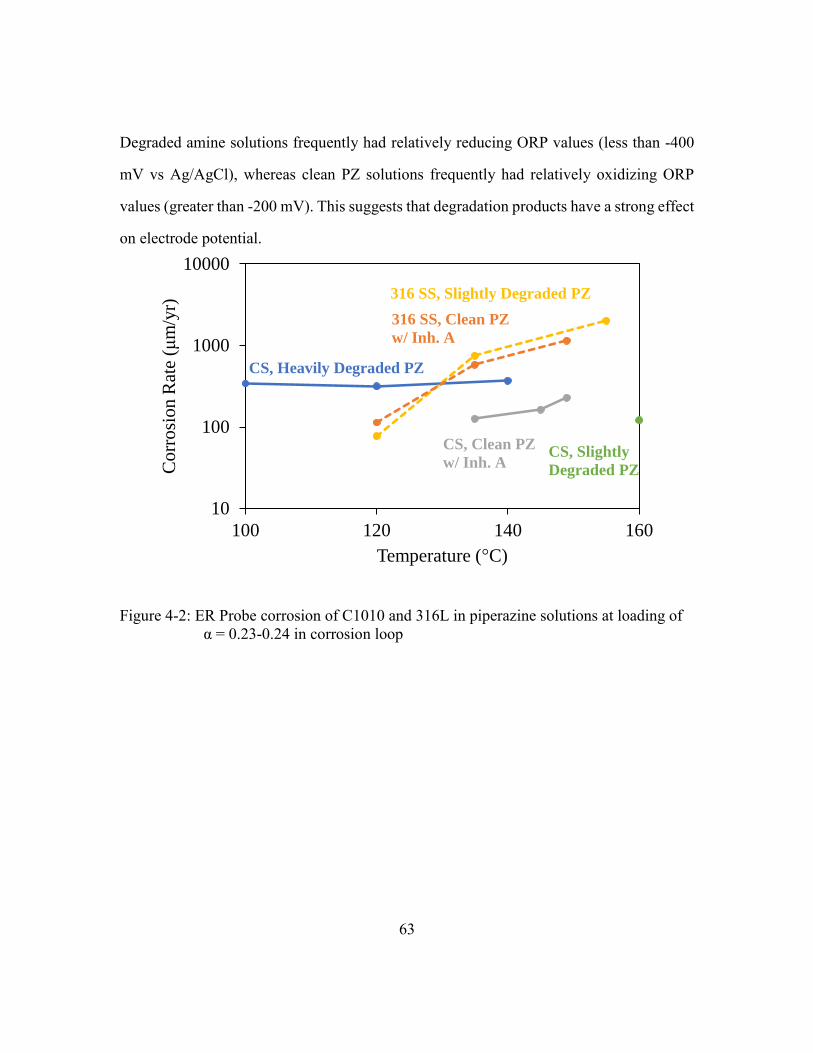
63
Degraded amine solutions frequently had relatively reducing ORP values (less than -400
mV vs Ag/AgCl), whereas clean PZ solutions frequently had relatively oxidizing ORP
values (greater than -200 mV). This suggests that degradation products have a strong effect
on electrode potential.
Figure 4-2: ER Probe corrosion of C1010 and 316L in piperazine solutions at loading of
α = 0.23-0.24 in corrosion loop
10
100
1000
10000
100 120 140 160
Co
rro
sion
Rat
e (μ
m/y
r)
Temperature (°C)
CS, Heavily Degraded PZ
CS, Clean PZ
w/ Inh. ACS, Slightly
Degraded PZ
316 SS, Slightly Degraded PZ
316 SS, Clean PZ
w/ Inh. A
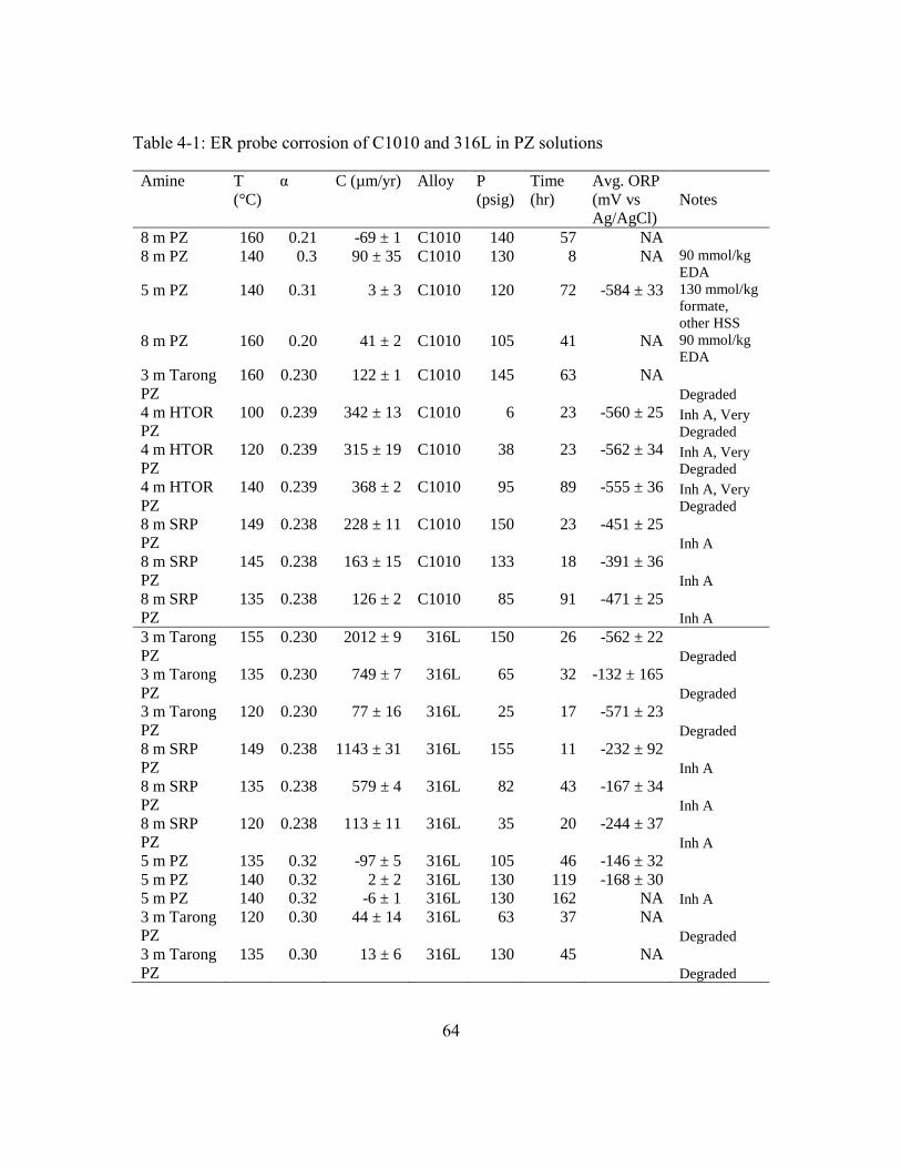
64
Table 4-1: ER probe corrosion of C1010 and 316L in PZ solutions
Amine T
(°C)
α C (µm/yr) Alloy P
(psig)
Time
(hr)
Avg. ORP
(mV vs
Ag/AgCl)
Notes
8 m PZ 160 0.21 -69 ± 1 C1010 140 57 NA
8 m PZ 140 0.3 90 ± 35 C1010 130 8 NA 90 mmol/kg
EDA
5 m PZ 140 0.31 3 ± 3 C1010 120 72 -584 ± 33 130 mmol/kg
formate,
other HSS
8 m PZ 160 0.20 41 ± 2 C1010 105 41 NA 90 mmol/kg
EDA
3 m Tarong
PZ
160 0.230 122 ± 1 C1010 145 63 NA
Degraded
4 m HTOR
PZ
100 0.239 342 ± 13 C1010 6 23 -560 ± 25 Inh A, Very
Degraded
4 m HTOR
PZ
120 0.239 315 ± 19 C1010 38 23 -562 ± 34 Inh A, Very
Degraded
4 m HTOR
PZ
140 0.239 368 ± 2 C1010 95 89 -555 ± 36 Inh A, Very
Degraded
8 m SRP
PZ
149 0.238 228 ± 11 C1010 150 23 -451 ± 25
Inh A
8 m SRP
PZ
145 0.238 163 ± 15 C1010 133 18 -391 ± 36
Inh A
8 m SRP
PZ
135 0.238 126 ± 2 C1010 85 91 -471 ± 25
Inh A
3 m Tarong
PZ
155 0.230 2012 ± 9 316L 150 26 -562 ± 22
Degraded
3 m Tarong
PZ
135 0.230 749 ± 7 316L 65 32 -132 ± 165
Degraded
3 m Tarong
PZ
120 0.230 77 ± 16 316L 25 17 -571 ± 23
Degraded
8 m SRP
PZ
149 0.238 1143 ± 31 316L 155 11 -232 ± 92
Inh A
8 m SRP
PZ
135 0.238 579 ± 4 316L 82 43 -167 ± 34
Inh A
8 m SRP
PZ
120 0.238 113 ± 11 316L 35 20 -244 ± 37
Inh A
5 m PZ 135 0.32 -97 ± 5 316L 105 46 -146 ± 32
5 m PZ 140 0.32 2 ± 2 316L 130 119 -168 ± 30
5 m PZ 140 0.32 -6 ± 1 316L 130 162 NA Inh A
3 m Tarong
PZ
120 0.30 44 ± 14 316L 63 37 NA
Degraded
3 m Tarong
PZ
135 0.30 13 ± 6 316L 130 45 NA
Degraded

65
4.2. CORROSION LOOP RESULTS: LINEAR AMINES
Several linear amine solutions were screened using ER corrosion probes in the
corrosion loop apparatus. Table 4-2 summarizes all linear amine experiments conducted in
the corrosion loop. The amines tested were ethanolamine (MEA), 3-amino-1-propanol
(MPA), and ethylenediamine (EDA). Temperature was varied from 80 to 120 °C over
moderate loadings (α = 0.37 to 0.46) to study the relationship between amine structure and
corrosion. Figure 4-3 shows that amines can have dramatically different intrinsic corrosion
rates. At 120 °C and α = 0.42, EDA, although structurally similar to MEA corrodes carbon
steel at 42300 μm/yr compared to an MEA (α = 0.44) corrosion rate of 14000 μm/yr. Both
rates are unacceptable, and even at 80 °C MEA corrosion of carbon steel is close to
unacceptable. However, with MEA at very lean conditions of α = 0.2, carbon steel has
outstanding corrosion performance of 19 μm/yr.
316L stainless steel exhibits good corrosion resistance to MEA at α = 0.42, with an
apparently strong effect of temperature. MPA is intrinsically less corrosive to both carbon
steel and stainless steel, as shown in Figure 4-4. At loadings of α = 0.37, carbon steel
showed good corrosion resistance, while 316 SS had outstanding resistance. Despite the
structural similarities of MEA and MPA, they display remarkably different intrinsic
corrosivities. This may be because MPA is longer and more labile than MEA, which
prevents it from forming stable amine-metal complexes and keeps iron from being
stabilized in solution. Interestingly, the corrosion of carbon steel in MPA shows a decrease
at higher temperature.
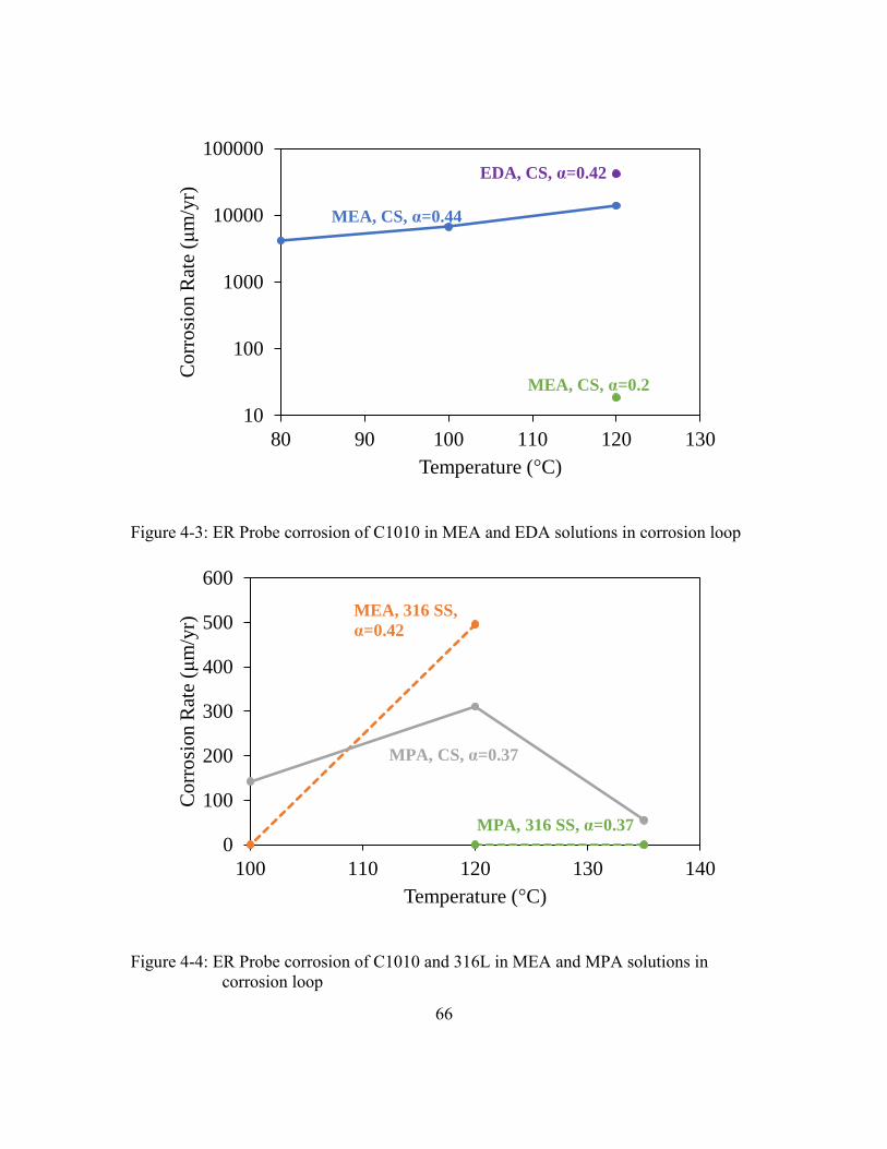
66
Figure 4-3: ER Probe corrosion of C1010 in MEA and EDA solutions in corrosion loop
Figure 4-4: ER Probe corrosion of C1010 and 316L in MEA and MPA solutions in
corrosion loop
10
100
1000
10000
100000
80 90 100 110 120 130
Co
rro
sion
Rat
e (μ
m/y
r)
Temperature (°C)
MEA, CS, α=0.44
EDA, CS, α=0.42
MEA, CS, α=0.2
0
100
200
300
400
500
600
100 110 120 130 140
Co
rro
sion
Rat
e (μ
m/y
r)
Temperature (°C)
MEA, 316 SS,
α=0.42
MPA, CS, α=0.37
MPA, 316 SS, α=0.37

67
Table 4-2: ER probe corrosion of C1010 and 316L in MEA, MPA, and EDA solutions
Amine T
(°C)
α C
(µm/yr)
Alloy P (psig) Time (hr) Avg. ORP
(mV vs
Ag/AgCl)
9 m MEA 120 0.20 19 ± 1 C1010 12 43 NA
9 m MEA 120 0.19 -2 ± 1 C1010 10 133 NA
9 m MEA 80 0.46 4192 ±
56
C1010 150 3 NA
9 m MEA 100 0.44 6754 ±
111
C1010 45 2 NA
9 m MEA 120 0.44 14006 ±
66
C1010 82 4 NA
12 m EDA 120 0.42 42254 ±
161
C1010 89 5 NA
10 m MPA 100 0.37 142 ± 4 C1010 5 45 -406 ± 58
10 m MPA 120 0.37 311 ± 12 C1010 25 21 -560 ± 59
10 m MPA 135 0.37 55 ± 11 C1010 65 23 -253 ± 37
9 m MEA 120 0.42 496 ± 23 316L 65 19 -494 ± 50
9 m MEA 100 0.42 -155 ± 1 316L 20 35 -360 ± 29
10 m MPA 120 0.37 -79 ± 4 316L 25 51 -262 ± 36
10 m MPA 135 0.37 -1 ± 1 316L 65 164 -239 ± 77
4.3. LIMITATIONS OF CORROSION LOOP RESULTS
Clearly the formation of protective products is an important factor in the corrosion
of C1010 in PZ solutions. One limitation of this work is that the protective products formed
on the ER probe element were not cleaned between experiments. Although the probe
elements were washed with water, the literature-recommended acid cleaning procedure
(ASTM, 2017) was not performed to ensure products had been removed. Apparently, the
effect of this was not significant. For example, frequently a temperature series was
generated by running one experiment after another, using the same solution, without
shutting down. Despite the lack of cleaning and the similar conditions in these time series,
significantly different corrosion rates were determined for the different temperatures. This
suggests that corrosion product films rapidly equilibrate with surrounding amine solutions
when conditions change. Film formation on carbon steel in H2O-CO2 occurs rapidly (5
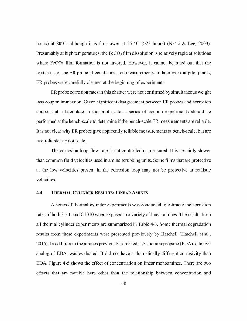
68
hours) at 80°C, although it is far slower at 55 °C (>25 hours) (Nešić & Lee, 2003).
Presumably at high temperatures, the FeCO3 film dissolution is relatively rapid at solutions
where FeCO3 film formation is not favored. However, it cannot be ruled out that the
hysteresis of the ER probe affected corrosion measurements. In later work at pilot plants,
ER probes were carefully cleaned at the beginning of experiments.
ER probe corrosion rates in this chapter were not confirmed by simultaneous weight
loss coupon immersion. Given significant disagreement between ER probes and corrosion
coupons at a later date in the pilot scale, a series of coupon experiments should be
performed at the bench-scale to determine if the bench-scale ER measurements are reliable.
It is not clear why ER probes give apparently reliable measurements at bench-scale, but are
less reliable at pilot scale.
The corrosion loop flow rate is not controlled or measured. It is certainly slower
than common fluid velocities used in amine scrubbing units. Some films that are protective
at the low velocities present in the corrosion loop may not be protective at realistic
velocities.
4.4. THERMAL CYLINDER RESULTS: LINEAR AMINES
A series of thermal cylinder experiments was conducted to estimate the corrosion
rates of both 316L and C1010 when exposed to a variety of linear amines. The results from
all thermal cylinder experiments are summarized in Table 4-3. Some thermal degradation
results from these experiments were presented previously by Hatchell (Hatchell et al.,
2015). In addition to the amines previously screened, 1,3-diaminopropane (PDA), a longer
analog of EDA, was evaluated. It did not have a dramatically different corrosivity than
EDA. Figure 4-5 shows the effect of concentration on linear monoamines. There are two
effects that are notable here other than the relationship between concentration and
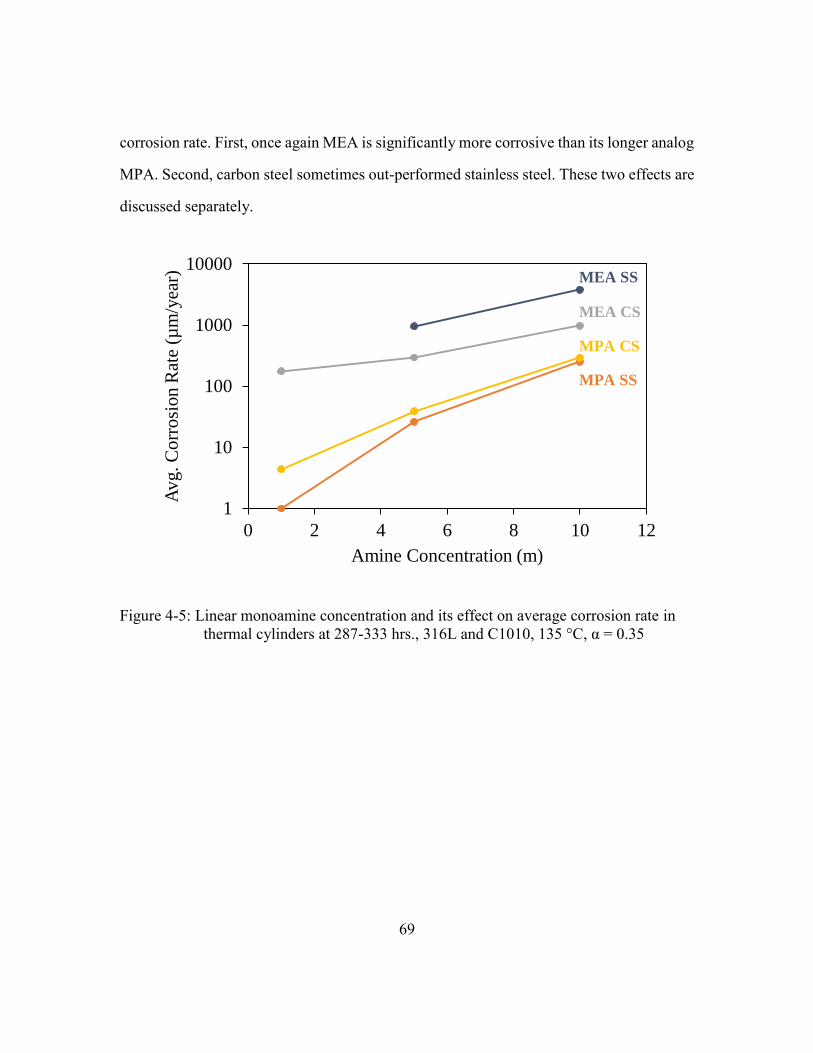
69
corrosion rate. First, once again MEA is significantly more corrosive than its longer analog
MPA. Second, carbon steel sometimes out-performed stainless steel. These two effects are
discussed separately.
Figure 4-5: Linear monoamine concentration and its effect on average corrosion rate in
thermal cylinders at 287-333 hrs., 316L and C1010, 135 °C, α = 0.35
1
10
100
1000
10000
0 2 4 6 8 10 12
Av
g. C
orr
osi
on R
ate
(µm
/yea
r)
Amine Concentration (m)
MEA SS
MEA CS
MPA CS
MPA SS

70
Figure 4-6: Linear monoamine loading and its effect on average corrosion rate in thermal
cyinders at 287-333 hrs., 316L and C1010, 135 °C, 10 m
Increasing monoamine loading always increased corrosion for stainless steel
(Figure 4-6). However, with carbon steel, increasing loading only increased corrosion up
to a point, after which corrosion started decreasing. This can be attributed to increased
precipitation of FeCO3, forming a protective film at high loading.
Carbon steel seemed to outperform stainless steel in these experiments, despite
significant industrial experience that suggests MEA corrodes stainless steel much less
quickly than carbon steel. This is most evident in Figure 4-6, where carbon steel corroded
less than stainless steel for MEA. During the experiments, scale was found on the inner
surface of carbon steel cylinders, but was not found on the inner surface of stainless steel
cylinders. Although corrosion products were not identified in this thermal cylinder work,
the scale was likely FeCO3 in some cases. This film did not adhere tightly in all cases, so
it was probably sometimes only protective because the corrosion cylinders are stagnant and
1
10
100
1000
10000
0.2 0.25 0.3 0.35 0.4 0.45
Av
g. C
orr
osi
on R
ate
(µm
/yea
r)
Loading (mol CO2/mol alkalinity)
MEA SS
MEA CS
MPA CS
MPA SS
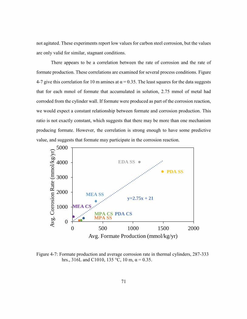
71
not agitated. These experiments report low values for carbon steel corrosion, but the values
are only valid for similar, stagnant conditions.
There appears to be a correlation between the rate of corrosion and the rate of
formate production. These correlations are examined for several process conditions. Figure
4-7 give this correlation for 10 m amines at α = 0.35. The least squares for the data suggests
that for each mmol of formate that accumulated in solution, 2.75 mmol of metal had
corroded from the cylinder wall. If formate were produced as part of the corrosion reaction,
we would expect a constant relationship between formate and corrosion production. This
ratio is not exactly constant, which suggests that there may be more than one mechanism
producing formate. However, the correlation is strong enough to have some predictive
value, and suggests that formate may participate in the corrosion reaction.
Figure 4-7: Formate production and average corrosion rate in thermal cylinders, 287-333
hrs., 316L and C1010, 135 °C, 10 m, α = 0.35.
0
1000
2000
3000
4000
5000
0 500 1000 1500 2000
Av
g. C
orr
osi
on R
ate
(mm
ol/
kg
/yr)
Avg. Formate Production (mmol/kg/yr)
y=2.75x + 21
MPA SS
MEA SS
PDA SS
EDA SS
MPA CS PDA CS
MEA CS
72
The thermal cylinder method yields useful qualitative data—for instance, showing
the differences in intrinsic corrosivity between MEA, MPA, and EDA. However, this
method significantly under predicted the corrosion of carbon steel by MEA. Thermal
cylinders suggested a carbon steel corrosion rate of 121 μm/yr for a 10 m MEA solution (α
= 0.45, 120 °C), whereas the ER corrosion probe gave a corrosion rate of 14000 μm/yr for
a similar solution (9 m, α = 0.44, 120 °C). The thermal cylinder data for stainless steel
actually over predicted corrosion relative to the ER corrosion probe, although it was much
closer. We attribute these discrepancies to the stagnant conditions present in the thermal
cylinders, which promotes formation of passivating films that are not representative of
actual flow conditions.
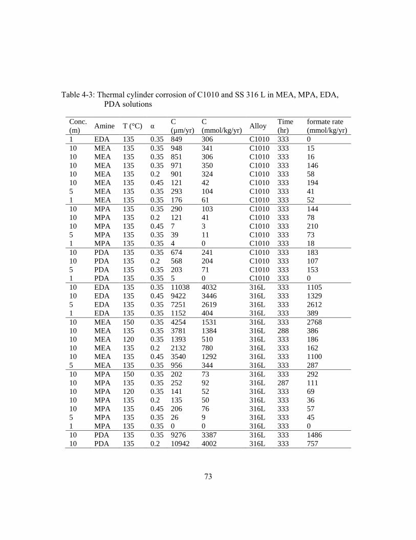
73
Table 4-3: Thermal cylinder corrosion of C1010 and SS 316 L in MEA, MPA, EDA,
PDA solutions
Conc.
(m) Amine T (°C) α
C
(µm/yr)
C
(mmol/kg/yr) Alloy
Time
(hr)
formate rate
(mmol/kg/yr)
1 EDA 135 0.35 849 306 C1010 333 0
10 MEA 135 0.35 948 341 C1010 333 15
10 MEA 135 0.35 851 306 C1010 333 16
10 MEA 135 0.35 971 350 C1010 333 146
10 MEA 135 0.2 901 324 C1010 333 58
10 MEA 135 0.45 121 42 C1010 333 194
5 MEA 135 0.35 293 104 C1010 333 41
1 MEA 135 0.35 176 61 C1010 333 52
10 MPA 135 0.35 290 103 C1010 333 144
10 MPA 135 0.2 121 41 C1010 333 78
10 MPA 135 0.45 7 3 C1010 333 210
5 MPA 135 0.35 39 11 C1010 333 73
1 MPA 135 0.35 4 0 C1010 333 18
10 PDA 135 0.35 674 241 C1010 333 183
10 PDA 135 0.2 568 204 C1010 333 107
5 PDA 135 0.35 203 71 C1010 333 153
1 PDA 135 0.35 5 0 C1010 333 0
10 EDA 135 0.35 11038 4032 316L 333 1105
10 EDA 135 0.45 9422 3446 316L 333 1329
5 EDA 135 0.35 7251 2619 316L 333 2612
1 EDA 135 0.35 1152 404 316L 333 389
10 MEA 150 0.35 4254 1531 316L 333 2768
10 MEA 135 0.35 3781 1384 316L 288 386
10 MEA 120 0.35 1393 510 316L 333 186
10 MEA 135 0.2 2132 780 316L 333 162
10 MEA 135 0.45 3540 1292 316L 333 1100
5 MEA 135 0.35 956 344 316L 333 287
10 MPA 150 0.35 202 73 316L 333 292
10 MPA 135 0.35 252 92 316L 287 111
10 MPA 120 0.35 141 52 316L 333 69
10 MPA 135 0.2 135 50 316L 333 36
10 MPA 135 0.45 206 76 316L 333 57
5 MPA 135 0.35 26 9 316L 333 45
1 MPA 135 0.35 0 0 316L 333 0
10 PDA 135 0.35 9276 3387 316L 333 1486
10 PDA 135 0.2 10942 4002 316L 333 757
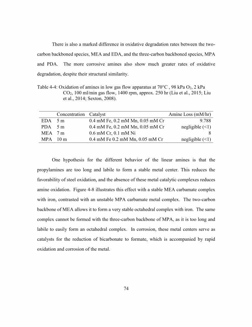
74
There is also a marked difference in oxidative degradation rates between the two-
carbon backboned species, MEA and EDA, and the three-carbon backboned species, MPA
and PDA. The more corrosive amines also show much greater rates of oxidative
degradation, despite their structural similarity.
Table 4-4: Oxidation of amines in low gas flow apparatus at 70°C , 98 kPa O2, 2 kPa
CO2, 100 ml/min gas flow, 1400 rpm, approx. 250 hr (Liu et al., 2015; Liu
et al., 2014; Sexton, 2008).
Concentration Catalyst Amine Loss (mM/hr)
EDA 5 m 0.4 mM Fe, 0.2 mM Mn, 0.05 mM Cr 9.788
PDA 5 m 0.4 mM Fe, 0.2 mM Mn, 0.05 mM Cr negligible (<1)
MEA 7 m 0.6 mM Cr, 0.1 mM Ni 8
MPA 10 m 0.4 mM Fe 0.2 mM Mn, 0.05 mM Cr negligible (<1)
One hypothesis for the different behavior of the linear amines is that the
propylamines are too long and labile to form a stable metal center. This reduces the
favorability of steel oxidation, and the absence of these metal catalytic complexes reduces
amine oxidation. Figure 4-8 illustrates this effect with a stable MEA carbamate complex
with iron, contrasted with an unstable MPA carbamate metal complex. The two-carbon
backbone of MEA allows it to form a very stable octahedral complex with iron. The same
complex cannot be formed with the three-carbon backbone of MPA, as it is too long and
labile to easily form an octahedral complex. In corrosion, these metal centers serve as
catalysts for the reduction of bicarbonate to formate, which is accompanied by rapid
oxidation and corrosion of the metal.
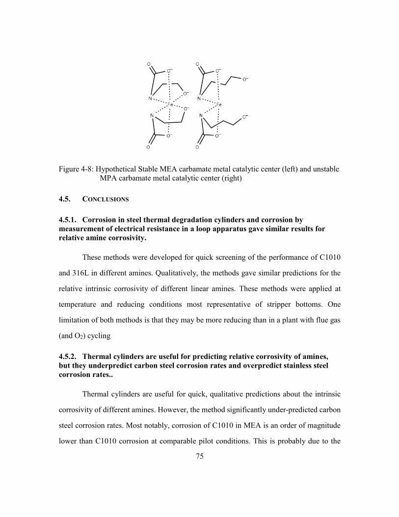
75
Figure 4-8: Hypothetical Stable MEA carbamate metal catalytic center (left) and unstable
MPA carbamate metal catalytic center (right)
4.5. CONCLUSIONS
4.5.1. Corrosion in steel thermal degradation cylinders and corrosion by
measurement of electrical resistance in a loop apparatus gave similar results for
relative amine corrosivity.
These methods were developed for quick screening of the performance of C1010
and 316L in different amines. Qualitatively, the methods gave similar predictions for the
relative intrinsic corrosivity of different linear amines. These methods were applied at
temperature and reducing conditions most representative of stripper bottoms. One
limitation of both methods is that they may be more reducing than in a plant with flue gas
(and O2) cycling
4.5.2. Thermal cylinders are useful for predicting relative corrosivity of amines,
but they underpredict carbon steel corrosion rates and overpredict stainless steel
corrosion rates..
Thermal cylinders are useful for quick, qualitative predictions about the intrinsic
corrosivity of different amines. However, the method significantly under-predicted carbon
steel corrosion rates. Most notably, corrosion of C1010 in MEA is an order of magnitude
lower than C1010 corrosion at comparable pilot conditions. This is probably due to the
76
non-agitated, stagnant conditions in the thermal cylinders, which promote formation of
passivating films that may not be protective at representative flow conditions. Stainless
steel (316L) corrosion measurements in MEA appear significantly higher than in
comparable pilot plants. This is likely because the anoxic, reducing environment of
corrosion cylinders is particularly challenging for 316L.
4.5.3. Thermal cylinders suggest that each mol of formate generation is
accompanied by 2.75 mol of steel corrosion.
Formate generation in C1010 and 316L thermal cylinders containing MEA, MPA,
EDA, PDA was compared to corrosion rates. There is a correlation between formate
generation and corrosion. This suggests that the reduction of bicarbonate to formate could
be a dominant reduction accompanying corrosion in anoxic conditions.
4.5.4. Ethylamines, such as, MEA and EDA, are more corrosive than their
propylamine counterparts, EDA and PDA. The ethyl- backbone amines likely form
more stable coordination complexes with oxidized iron, increasing corrosion.
The amines evaluated were: ethanolamine (MEA), 3-amino-1-propanol (MPA),
ethylenediamine (EDA), and 1,3-diaminopropane (PDA). MEA was significantly more
corrosive to C1010 and 316L than MPA in both thermal cylinders and the corrosion loop.
EDA. The results are less complete for EDA/PDA, but PDA appears to be less corrosive
than EDA to 316L in thermal cylinders. One hypothesis is that ethylamine carbamates form
very stable octahedral complexes with iron. The same complex cannot be formed with the
longer propylamine carbamates as it is too long and labile to easily form an octahedral
complex
77
4.5.5. The corrosion loop with an electrical resistance probe yields realistic
corrosion rates for C1010 in amines.
Unlike thermal cylinders, which gave unrealistic C1010 corrosion rates due to its
stagnant conditions, the corrosion loop appears to accurately represent conditions of amine
corrosion. The ER probe gave apparently realistic corrosion rates during short bench-scale
experiments, unlike later experiments at the pilot scale.
The corrosion rates for 316L in MEA seem to be higher than in representative pilot
plants. This is likely because the reducing environment of the corrosion loop is particularly
challenging for 316L.
4.5.6. Stainless steel sometimes experiences attack in PZ at high temperature,
anoxic conditions.
In several solutions of slightly degraded PZ, at lean loadings (α ≈ 0.23), 316L
experienced corrosion with a strong temperature effect, with good performance at 120 °C
(<150 μm/yr), but poor performance (>1000 μm/yr) at 149 °C and higher. Notably, attack
of stainless was not observed in completely clean PZ at similar conditions.
Counterintuitively, at higher loading of α = 0.3, both carbon steel and stainless steel showed
excellent corrosion performance (<100 µm/yr). It is not clear why stainless steel performed
well at higher CO2 loadings. These stainless corrosion rates may be higher than in a real
plant, because the reducing environment of the corrosion loop is particularly challenging
for 316L.
4.5.7. Carbon steel experiences low corrosion at high temperature in PZ solutions.
From 100°C to 160°C, at lean loadings (α ≈ 0.23), even in very degraded solutions
of PZ, C1010 performance was good to moderate (< 400 μm/yr), and showed no strong
increase with temperature. Counterintuitively, at higher loading of α = 0.3, both carbon

78
steel and stainless steel showed excellent corrosion performance (<100 µm/yr). Higher
loading probably passivates carbon steel by promoting the formation of a FeCO3 layer.
4.5.8. PZ degradation apparently accelerates corrosion of carbon and stainless
steel.
PZ degradation apparently increased corrosion of both C1010 and 316L.
Completely fresh PZ solutions were often non-corrosive to both C1010 and 316L. Pilot
plant degraded amines corroded both materials more quickly. A more deliberate study is
needed to clearly separate the effects of amine concentration, CO2 loading, and
degradation.
79
Chapter 5. Fe2+ Solubility and Siderite Formation in Monoethanolamine
and Piperazine
The work in this chapter was submitted as a paper to the proceedings of the 14th
international conference on Greenhouse Gas Control Technologies. Significant
experimental work in this chapter was performed by Shyam S. Sharma, an undergraduate
researcher.
A protective FeCO3 layer is known to sometimes form on carbon steel and can
inhibit corrosion. Although the formation of this layer is understood in simple aqueous
systems, its behavior in CO2 capture solutions is not well understood. FeCO3 layer
formation is driven by supersaturation, so accurate measurements of equilibrium Fe2+
solubility need to be made. The relationship between amine type, degradation level, CO2
loading, and temperature on Fe2+ solubility was measured with the goal of determining at
what conditions FeCO3 precipitates out of amines. MEA and PZ solutions with differing
CO2 loadings and degradation levels were placed in agitated, sealed reactors with 0.25 M
FeSO4 and Na2CO3. Several experiments used air and CO2 sparged reactors to simulate
absorber conditions. Liquid samples were taken from the reactors over time and analyzed
for dissolved Fe+2/Fe+3 using ICP-OES. After the experiments reached equilibrium, solid
samples were taken from the reactors and characterized using powder X-ray diffraction
(XRD). 9 m MEA was found to have Fe2+ solubility 10X-100X higher than clean 5 m PZ.
Degraded PZ showed Fe2+ solubility 10X-700X higher than clean PZ. FeCO3 was only
found to form in rich clean PZ and rich degraded PZ. Lean MEA and lean PZ (both clean
and degraded) formed magnetite while rich MEA formed goethite. Similar to
measurements in aqueous systems, iron solubility for both MEA and PZ decreased with
increasing temperature. CO2 loading effects were a little more complicated. In MEA, Fe2+
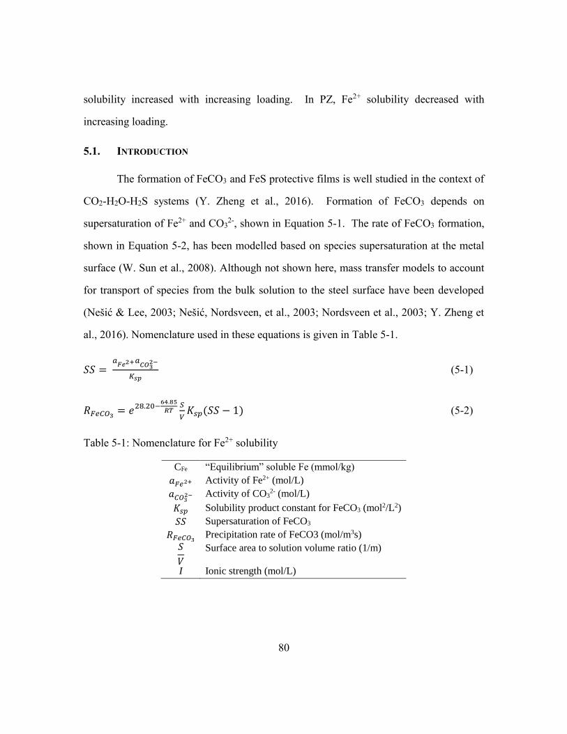
80
solubility increased with increasing loading. In PZ, Fe2+ solubility decreased with
increasing loading.
5.1. INTRODUCTION
The formation of FeCO3 and FeS protective films is well studied in the context of
CO2-H2O-H2S systems (Y. Zheng et al., 2016). Formation of FeCO3 depends on
supersaturation of Fe2+ and CO32-, shown in Equation 5-1. The rate of FeCO3 formation,
shown in Equation 5-2, has been modelled based on species supersaturation at the metal
surface (W. Sun et al., 2008). Although not shown here, mass transfer models to account
for transport of species from the bulk solution to the steel surface have been developed
(Nešić & Lee, 2003; Nešić, Nordsveen, et al., 2003; Nordsveen et al., 2003; Y. Zheng et
al., 2016). Nomenclature used in these equations is given in Table 5-1.
𝑆𝑆 = 𝑎
𝐹𝑒2+𝑎𝐶𝑂3
2−
𝐾𝑠𝑝 (5-1)
𝑅𝐹𝑒𝐶𝑂3= 𝑒28.20−
64.85
𝑅𝑇𝑆
𝑉𝐾𝑠𝑝(𝑆𝑆 − 1) (5-2)
Table 5-1: Nomenclature for Fe2+ solubility
CFe “Equilibrium” soluble Fe (mmol/kg)
𝑎𝐹𝑒2+ Activity of Fe2+ (mol/L)
𝑎𝐶𝑂32− Activity of CO3
2- (mol/L)
𝐾𝑠𝑝 Solubility product constant for FeCO3 (mol2/L2)
𝑆𝑆 Supersaturation of FeCO3
𝑅𝐹𝑒𝐶𝑂3 Precipitation rate of FeCO3 (mol/m3s)
𝑆
𝑉
Surface area to solution volume ratio (1/m)
I Ionic strength (mol/L)
81
The accuracy of this model depends on having high quality values of Ksp. The Ksp
values used by previous researchers were measured in aqueous systems of pH 4-6, which
have low iron solubilities and thus low Ksp values (W. Sun et al., 2009). Ksp in these
systems has been reported as 1.28x10⁻¹¹ mol2/L2 at T = 25 °C and I ≈ 0, and varies with Tk
and I as given below in Equation 5-3 (W. Sun et al., 2009), where Tk is temperature
(Kelvin) and I is ionic strength (mol/L). This equation shows that Ksp generally decreases
with increasing T and increases with increasing I at low values of I.
𝑙𝑜𝑔(𝐾𝑠𝑝) = −59.3498 − 0.041377𝑇𝑘 −2.1963
𝑇𝑘+ 24.5724 𝑙𝑜𝑔(𝑇𝑘) + 2.518𝐼0.5 −
0.657𝐼 (5-3)
Ksp values measured in simple aqueous systems are not representative of
multicomponent, high ionic strength amine solutions used for CO2 capture. Accurate Fe2+
solubility data is crucial to developing a model that allows prediction of the conditions
under which FeCO3 will form. Understanding when this FeCO3 layer forms is crucial for
understanding which amines and conditions are compatible with carbon steel construction.
5.2. METHODS
A series of bench-scale experiments was conducted to determine Fe2+ solubility
while varying amine type, degradation level, CO2 loading, and temperature. Amine
solutions (Alfa Aesar) were added to a jacketed, 1 L, glass reactor containing a Teflon stir
bar. Next, 0.25 M FeSO4 and 0.25 M Na2CO3 from (Fisher Scientific) were added as solids
to the reactor. Several experiments used FeCl3 (Fisher Scientific) rather than FeSO4 to
investigate Fe3+ solubility.
9 m MEA, 5 m clean PZ, and several degraded pilot plant PZ solutions were
evaluated at rich and lean loading. Three pilot plant piperazine solutions were evaluated to
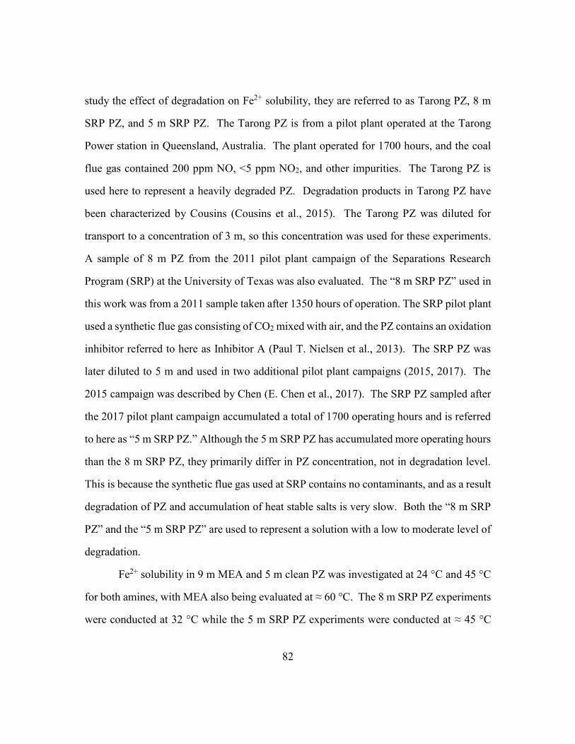
82
study the effect of degradation on Fe2+ solubility, they are referred to as Tarong PZ, 8 m
SRP PZ, and 5 m SRP PZ. The Tarong PZ is from a pilot plant operated at the Tarong
Power station in Queensland, Australia. The plant operated for 1700 hours, and the coal
flue gas contained 200 ppm NO, <5 ppm NO2, and other impurities. The Tarong PZ is
used here to represent a heavily degraded PZ. Degradation products in Tarong PZ have
been characterized by Cousins (Cousins et al., 2015). The Tarong PZ was diluted for
transport to a concentration of 3 m, so this concentration was used for these experiments.
A sample of 8 m PZ from the 2011 pilot plant campaign of the Separations Research
Program (SRP) at the University of Texas was also evaluated. The “8 m SRP PZ” used in
this work was from a 2011 sample taken after 1350 hours of operation. The SRP pilot plant
used a synthetic flue gas consisting of CO2 mixed with air, and the PZ contains an oxidation
inhibitor referred to here as Inhibitor A (Paul T. Nielsen et al., 2013). The SRP PZ was
later diluted to 5 m and used in two additional pilot plant campaigns (2015, 2017). The
2015 campaign was described by Chen (E. Chen et al., 2017). The SRP PZ sampled after
the 2017 pilot plant campaign accumulated a total of 1700 operating hours and is referred
to here as “5 m SRP PZ.” Although the 5 m SRP PZ has accumulated more operating hours
than the 8 m SRP PZ, they primarily differ in PZ concentration, not in degradation level.
This is because the synthetic flue gas used at SRP contains no contaminants, and as a result
degradation of PZ and accumulation of heat stable salts is very slow. Both the “8 m SRP
PZ” and the “5 m SRP PZ” are used to represent a solution with a low to moderate level of
degradation.
Fe2+ solubility in 9 m MEA and 5 m clean PZ was investigated at 24 °C and 45 °C
for both amines, with MEA also being evaluated at ≈ 60 °C. The 8 m SRP PZ experiments
were conducted at 32 °C while the 5 m SRP PZ experiments were conducted at ≈ 45 °C
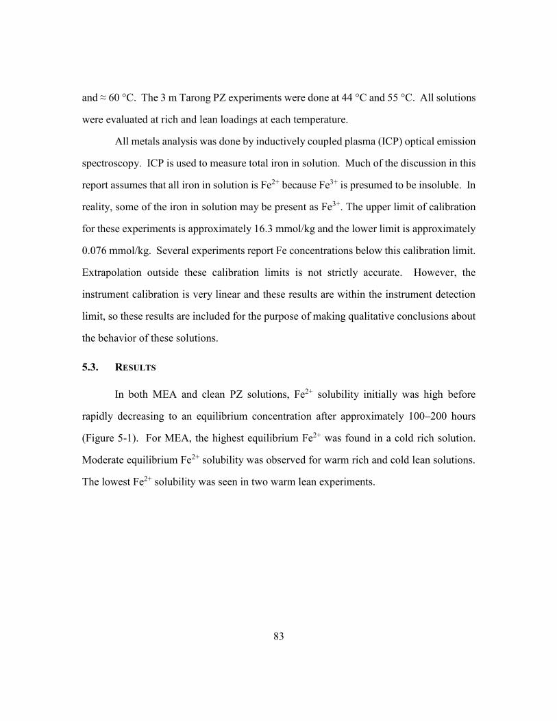
83
and ≈ 60 °C. The 3 m Tarong PZ experiments were done at 44 °C and 55 °C. All solutions
were evaluated at rich and lean loadings at each temperature.
All metals analysis was done by inductively coupled plasma (ICP) optical emission
spectroscopy. ICP is used to measure total iron in solution. Much of the discussion in this
report assumes that all iron in solution is Fe2+ because Fe3+ is presumed to be insoluble. In
reality, some of the iron in solution may be present as Fe3+. The upper limit of calibration
for these experiments is approximately 16.3 mmol/kg and the lower limit is approximately
0.076 mmol/kg. Several experiments report Fe concentrations below this calibration limit.
Extrapolation outside these calibration limits is not strictly accurate. However, the
instrument calibration is very linear and these results are within the instrument detection
limit, so these results are included for the purpose of making qualitative conclusions about
the behavior of these solutions.
5.3. RESULTS
In both MEA and clean PZ solutions, Fe2+ solubility initially was high before
rapidly decreasing to an equilibrium concentration after approximately 100–200 hours
(Figure 5-1). For MEA, the highest equilibrium Fe2+ was found in a cold rich solution.
Moderate equilibrium Fe2+ solubility was observed for warm rich and cold lean solutions.
The lowest Fe2+ solubility was seen in two warm lean experiments.
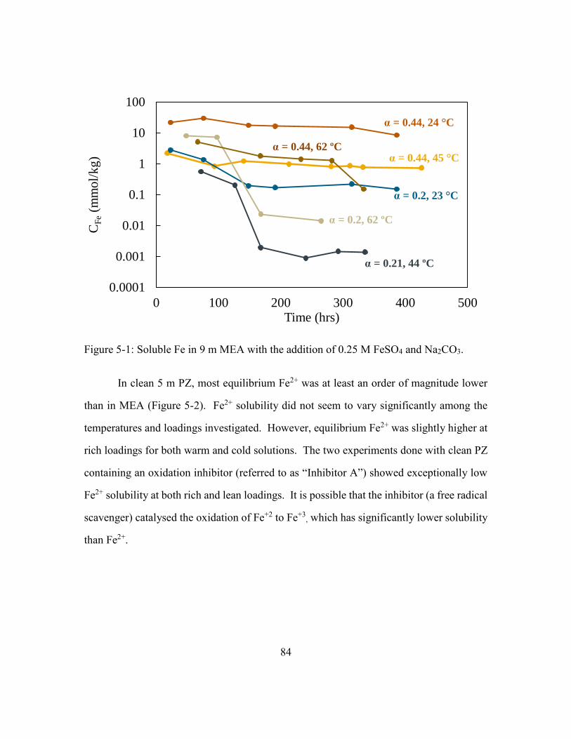
84
Figure 5-1: Soluble Fe in 9 m MEA with the addition of 0.25 M FeSO4 and Na2CO3.
In clean 5 m PZ, most equilibrium Fe2+ was at least an order of magnitude lower
than in MEA (Figure 5-2). Fe2+ solubility did not seem to vary significantly among the
temperatures and loadings investigated. However, equilibrium Fe2+ was slightly higher at
rich loadings for both warm and cold solutions. The two experiments done with clean PZ
containing an oxidation inhibitor (referred to as “Inhibitor A”) showed exceptionally low
Fe2+ solubility at both rich and lean loadings. It is possible that the inhibitor (a free radical
scavenger) catalysed the oxidation of Fe+2 to Fe+3, which has significantly lower solubility
than Fe2+.
0.0001
0.001
0.01
0.1
1
10
100
0 100 200 300 400 500
CF
e(m
mo
l/k
g)
Time (hrs)
α = 0.44, 45 °C
α = 0.44, 24 °C
α = 0.2, 23 °C
α = 0.21, 44 ºC
α = 0.2, 62 ºC
α = 0.44, 62 ºC
85
Figure 5-2: Soluble Fe in 5 m clean PZ with the addition of 0.25 M FeSO4 and Na2CO3.
The MEA and clean PZ experiments reported in this paper are compared to those
done by Fytianos (Fytianos, 2016) at similar conditions, as shown in Figure 5-3. This
figure shows rich MEA and PZ Fe2+ solubilities with changing temperatures. The MEA
and PZ experiments reported in this paper showed the same general trend. As temperature
increased, Fe2+ solubility in rich MEA and PZ tended to decrease. The magnitude of this
temperature effect in MEA was more significant in the current work. The temperature
effect for PZ in this work seemed comparable to that for rich loading in Fytianos. Although
Fytianos reported the PZ experiment as having a lean loading, it is likely that the loading
was higher than α = 0.2 since the reactors were sparged with small amounts of CO2.
Regardless, he found higher Fe2+ solubility in PZ than this work. A key difference is that
his experiments were shorter (72 hrs), and he did not add Na2CO3.
0.0001
0.001
0.01
0.1
1
0 100 200 300 400 500
CF
e(m
mo
l/k
g)
Time (hrs)
α = 0.2, 24 ºC
α ≈ 0.45, 43 ºC, 2 wt % Inhibitor
α = 0.3, 45 ºC, 2 wt % Inhibitor
α = 0.2,
46 ºC
α = 0.4, 23 ºC
α = 0.4, 46 ºC

86
Figure 5-3: a) Rich MEA soluble Fe as a function of temperature. b) Rich PZ soluble Fe
as a function of temperature (Fytianos, 2016).
At most conditions in the degraded SRP PZ, Fe2+ solubility was 10–100X higher
than in clean PZ (Figure 5-4). In all degraded PZ solutions, Fe2+ solubility decreased as
CO2 loading increased. The highest equilibrium Fe2+ was observed for warm lean 5 m SRP
PZ. 8 m SRP PZ showed comparable solubility to similar 5 m SRP solutions. Moderate
Fe2+ was seen for warm rich 5 m solutions. The two experiments using Fe3+ showed very
low Fe concentrations in warm solutions with both rich and moderate loadings. This shows
that Fe3+ is not readily soluble in these solutions, and that Fe3+ is not readily converted to
the more soluble Fe2+ under these conditions. The experiment conducted in the sparged
reactor showed low Fe2+ solubility when sparged with 10% CO2, 90% air. Switching the
gas feed to 10% CO2, 90% N2 did not appreciably increase Fe2+ solubility. Experiments in
prior work (Voice, 2013), showed that switching from an O2/CO2 to an N2/CO2 atmosphere
contacting 8 m PZ in a cyclic oxidation reactor at 120 °C caused a rapid increase in
dissolved metals, presumably due to corrosion of the stainless steel apparatus. The sparged
0.1
1
10
100
20 40 60 80
CF
e(m
mo
l/k
g)
Temperature (ºC)
Fytianos: α = 0.4
exp
This work: α = 0.44
a
0.01
0.1
1
10
20 40 60
CF
e(m
mo
l/k
g)
Temperature (ºC)
Fytianos: α = 0.2
This work: α = 0.2
This work: α = 0.4
b
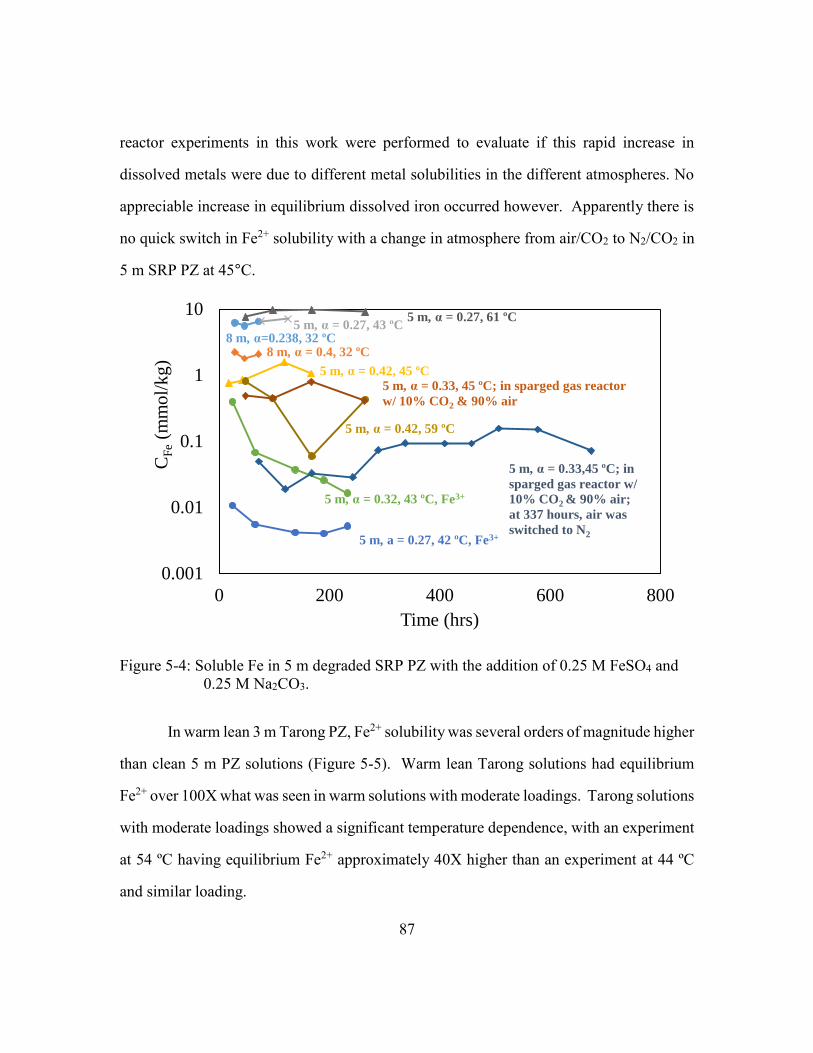
87
reactor experiments in this work were performed to evaluate if this rapid increase in
dissolved metals were due to different metal solubilities in the different atmospheres. No
appreciable increase in equilibrium dissolved iron occurred however. Apparently there is
no quick switch in Fe2+ solubility with a change in atmosphere from air/CO2 to N2/CO2 in
5 m SRP PZ at 45°C.
Figure 5-4: Soluble Fe in 5 m degraded SRP PZ with the addition of 0.25 M FeSO4 and
0.25 M Na2CO3.
In warm lean 3 m Tarong PZ, Fe2+ solubility was several orders of magnitude higher
than clean 5 m PZ solutions (Figure 5-5). Warm lean Tarong solutions had equilibrium
Fe2+ over 100X what was seen in warm solutions with moderate loadings. Tarong solutions
with moderate loadings showed a significant temperature dependence, with an experiment
at 54 ºC having equilibrium Fe2+ approximately 40X higher than an experiment at 44 ºC
and similar loading.
0.001
0.01
0.1
1
10
0 200 400 600 800
CF
e(m
mo
l/k
g)
Time (hrs)
8 m, α=0.238, 32 ºC5 m, α = 0.27, 43 ºC
5 m, α = 0.27, 61 ºC
8 m, α = 0.4, 32 ºC
5 m, α = 0.42, 45 ºC
5 m, α = 0.42, 59 ºC
5 m, α = 0.33,45 ºC; in
sparged gas reactor w/
10% CO2 & 90% air;
at 337 hours, air was
switched to N2
5 m, α = 0.32, 43 ºC, Fe3+
5 m, a = 0.27, 42 ºC, Fe3+
5 m, α = 0.33, 45 ºC; in sparged gas reactor
w/ 10% CO2 & 90% air
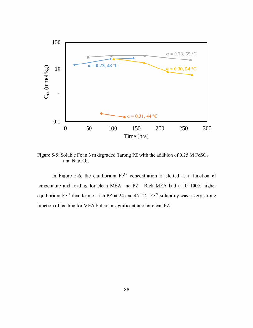
88
Figure 5-5: Soluble Fe in 3 m degraded Tarong PZ with the addition of 0.25 M FeSO4
and Na2CO3.
In Figure 5-6, the equilibrium Fe2+ concentration is plotted as a function of
temperature and loading for clean MEA and PZ. Rich MEA had a 10–100X higher
equilibrium Fe2+ than lean or rich PZ at 24 and 45 °C. Fe2+ solubility was a very strong
function of loading for MEA but not a significant one for clean PZ.
0.1
1
10
100
0 50 100 150 200 250 300
CF
e(m
mo
l/k
g)
Time (hrs)
α = 0.31, 44 ºC
α = 0.23, 55 ºC
α = 0.23, 43 ºCα = 0.30, 54 ºC
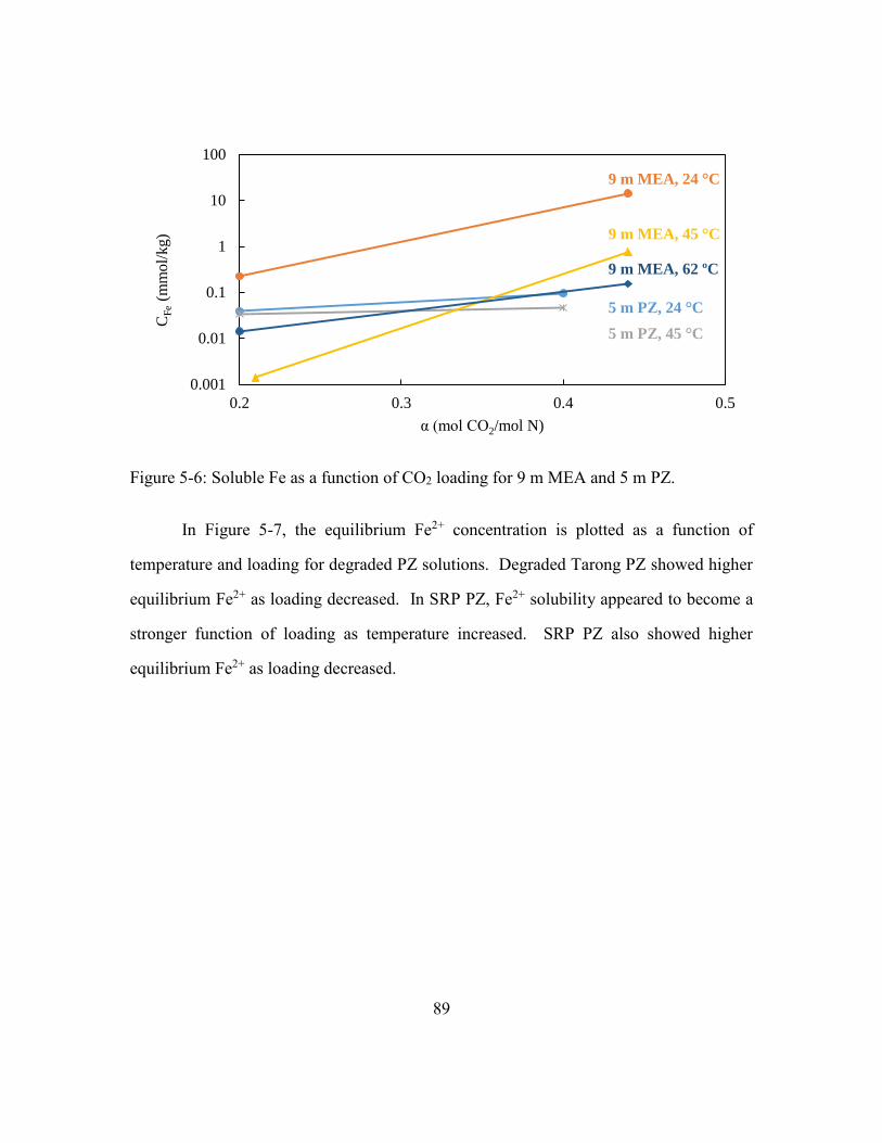
89
Figure 5-6: Soluble Fe as a function of CO2 loading for 9 m MEA and 5 m PZ.
In Figure 5-7, the equilibrium Fe2+ concentration is plotted as a function of
temperature and loading for degraded PZ solutions. Degraded Tarong PZ showed higher
equilibrium Fe2+ as loading decreased. In SRP PZ, Fe2+ solubility appeared to become a
stronger function of loading as temperature increased. SRP PZ also showed higher
equilibrium Fe2+ as loading decreased.
0.001
0.01
0.1
1
10
100
0.2 0.3 0.4 0.5
CF
e(m
mo
l/kg)
α (mol CO2/mol N)
9 m MEA, 24 °C
5 m PZ, 24 °C
9 m MEA, 45 °C
5 m PZ, 45 °C
9 m MEA, 62 ºC

90
Figure 5-7: Soluble Fe as a function of CO2 loading for degraded PZ.
The solid phases characterized in these experiments showed that FeCO3 only
formed under specific conditions. As seen in Table 5-2 and Table 5-3, FeCO3 (siderite)
was only identified in PZ solutions with rich CO2 loading. Since siderite was found in both
rich clean PZ and rich SRP PZ, its formation is independent of amine degradation level.
Lean PZ solutions tended to form magnetite, as did lean MEA solutions. The solid sample
from a rich MEA experiment that was characterized appeared to be FeO(OH) (goethite).
The solid sample analyzed from the 5 m SRP PZ sparged gas reactor experiment with air
and CO2 formed goethite.
0.1
1
10
100
0.2 0.3 0.4 0.5
CF
e(m
mo
l/k
g)
α (mol CO2/mol N)
5 m SRP PZ
(2017), 44 °C
3 m Tarong PZ, 44 °C
8 m SRP PZ (2011), 32 °C
5 m SRP PZ
(2017), 60 °C
3 m Tarong PZ, 55 ºC

91
Table 5-2: Equilibrium Fe in 9 m MEA and 5 m clean PZ
Amine CO2
Loading (α)
T
(°C)
Experiment
Length (hrs)
CFe
(mmol/kg)
Solid Phase (if
identified)
9 m MEA 0.44 45 426 0.765
9 m MEA 0.44 24 386 14.334
9 m MEA 0.44 24 166 7.13 Goethite (FeO(OH))
9 m MEA 0.44 62 333 0.153
9 m MEA 0.2 23 386 0.225
9 m MEA 0.2 45 335 0.0014 Magnetite (Fe3O4)
9 m MEA 0.2 62 265 0.014 Magnetite (Fe3O4)
5 m PZ 0.4 46 191 0.046
5 m PZ 0.4 45 167 0.047 Siderite (FeCO3)
5 m PZ 0.4 23 386 0.095
5 m PZ 0.2 24 386 0.038
5 m PZ 0.2 45 94 0.034
Table 5-3: Equilibrium Fe in degraded Tarong and SRP PZ
Amine CO2 Loading
(α)
T
(°C)
Experiment
Length (hrs)
CFe
(mmol/kg)
Solid Phase
(if identified)
3 m Tarong 0.23 44 144 25.8
3 m Tarong 0.23 55 386 21.36 Magnetite
(Fe3O4)
3 m Tarong 0.31 44 125 0.147
3 m Tarong 0.30 54 268 5.95
8 m SRP 0.238 32 75 6.49
8 m SRP 0.4 32 191 2.08
5 m SRP 0.42 44 167 1.06
5 m SRP 0.42 60 265 0.427 Siderite
(FeCO3)
5 m SRP 0.27 45 125 7.18
5 m SRP 0.27 60 265 9.13 Magnetite
(Fe3O4)
5 m SRP (w/Fe3+) 0.32 43 233 0.0163
5 m SRP (w/Fe3+) 0.27 42 233 0.00519
5 m SRP (in sparged
gas reactor w/CO2 &
air)
0.33 45 264 0.412 Goethite
(FeO(OH))
5 m SRP (in sparged
gas reactor w/CO2 &
air; switched to N2)
0.33 45 674 0.0717
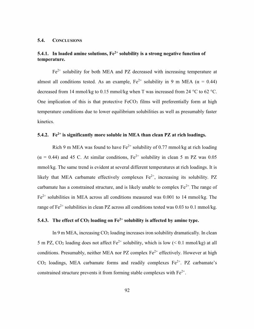
92
5.4. CONCLUSIONS
5.4.1. In loaded amine solutions, Fe2+ solubility is a strong negative function of
temperature.
Fe2+ solubility for both MEA and PZ decreased with increasing temperature at
almost all conditions tested. As an example, Fe2+ solubility in 9 m MEA (α = 0.44)
decreased from 14 mmol/kg to 0.15 mmol/kg when T was increased from 24 °C to 62 °C.
One implication of this is that protective FeCO3 films will preferentially form at high
temperature conditions due to lower equilibrium solubilities as well as presumably faster
kinetics.
5.4.2. Fe2+ is significantly more soluble in MEA than clean PZ at rich loadings.
Rich 9 m MEA was found to have Fe2+ solubility of 0.77 mmol/kg at rich loading
(α = 0.44) and 45 C. At similar conditions, Fe2+ solubility in clean 5 m PZ was 0.05
mmol/kg. The same trend is evident at several different temperatures at rich loadings. It is
likely that MEA carbamate effectively complexes Fe2+, increasing its solubility. PZ
carbamate has a constrained structure, and is likely unable to complex Fe2+. The range of
Fe2+ solubilities in MEA across all conditions measured was 0.001 to 14 mmol/kg. The
range of Fe2+ solubilities in clean PZ across all conditions tested was 0.03 to 0.1 mmol/kg.
5.4.3. The effect of CO2 loading on Fe2+ solubility is affected by amine type.
In 9 m MEA, increasing CO2 loading increases iron solubility dramatically. In clean
5 m PZ, CO2 loading does not affect Fe2+ solubility, which is low (< 0.1 mmol/kg) at all
conditions. Presumably, neither MEA nor PZ complex Fe2+ effectively. However at high
CO2 loadings, MEA carbamate forms and readily complexes Fe2+. PZ carbamate’s
constrained structure prevents it from forming stable complexes with Fe2+.

93
5.4.4. The presence of amine degradation products significantly increased Fe2+
solubility in PZ.
Degraded PZ had much higher Fe2+ solubility (up to 26 mmol/kg) than clean PZ.
Degraded PZ has linear amine degradation products, such as EDA, which likely chelate
Fe2+. Apparently, this EDA complex increases Fe2+ solubility in PZ at all conditions. The
range of Fe2+ solubilities in degraded PZ across all conditions tested was 0.1 to 26
mmol/kg.
In degraded PZ, Fe2+ solubility decreased with increasing loadings. This is
counterintuitive, because presumably EDA carbamate is also an effective complexing
agent for Fe2+. The reason for the decrease of Fe2+ solubility in degraded PZ at high loadings
is not known.
As PZ degrades, its increasing Fe2+ solubility might keep Fe2+ in solution,
preventing formation of FeCO3 films. This explains the observed relationship between PZ
degradation and accelerated C1010 corrosion.
5.4.5. In low temperature, agitated solubility experiments, Fe2+ is frequently
converted to Fe3+, except in PZ at high CO2 loadings.
The solid phases characterized in these experiments showed that FeCO3 only
formed under specific conditions. Siderite (FeCO3) was only identified in PZ solutions
with rich CO2 loading. Since siderite was found in both rich clean PZ and rich SRP PZ, its
formation appears to be relatively independent of amine degradation level. Lean PZ
solutions tended to form magnetite (Fe3O4), as did lean MEA solutions. The solid sample
from a rich MEA experiment that was characterized appeared to be FeO(OH) (goethite).
A special air and CO2-sparged experiment with 5 m SRP PZ air and CO2 also formed
goethite. The conversion of Fe2+ to Fe3+ requires relatively oxidizing conditions. These
94
experiments suggest that MEA and lean PZ are somewhat more oxidizing than rich PZ
solutions.
5.4.6. Fe3+ has limited solubility in PZ solutions.
Fe3+ has apparent solubility of 0.01 mmol/kg in slightly degraded 5 m PZ solution
at 42°C. At comparable conditions, Fe2+ solubility is 7 mmol/kg. This suggests that at a
commercial plant, Fe3+ may be precipitated out when it is formed. Fe3+ is probably formed
at oxidizing conditions in the amine absorber.
5.4.7. The strong effects of CO2 loading and T on Fe2+ solubility suggest the
equilibrium concentration of Fe2+ will change as the solvent moves through a real
plant.
One implication of these results is that there will be strong fluctuations in
equilibrium Fe2+ concentration as solvent moves through a real plant. In degraded PZ for
example, Fe2+ solubility is apparently highest at low temperatures and lean loadings, so
these conditions are least likely to be protected by FeCO3 and may experience corrosion.
However an amine stream that is unsaturated at cold, lean conditions may be supersaturated
at hot, rich conditions. This means corrosion could occur in the absorber, and those
corrosion products are deposited in the stripper. This also means that the observed Fe2+
concentration at a plant may not be an equilibrium value, but rather a complicated average
value affected by the residence times at unsaturated and supersaturated parts of the process.

95
Chapter 6. Corrosion in Monoethanolamine and Piperazine during 2017
Pilot Campaigns
The work in this chapter was submitted as a paper to the proceedings of the 14th
international conference on Greenhouse Gas Control Technologies.
Corrosion measurements are presented from two 2017 pilot plant campaigns.
Corrosion was evaluated at the Separations Research Program (SRP) pilot plant in April
2017. The SRP pilot plant uses air/CO2 and 5 m piperazine (PZ) with an oxidation
inhibitor. Stainless steel (316L) and carbon steel (C1010) were evaluated with electrical
resistance corrosion probes and corrosion coupons at two locations in the process. A
second pilot plant campaign was conducted in June 2017 at the National Carbon Capture
Center (NCCC) with 7 m monoethanolamine (MEA). Stainless steel and carbon steel were
evaluated with corrosion coupons at four locations in the process.
This work seeks to replicate the bench-scale corrosion benefits of PZ at the pilot
scale and gain insight into how temperature, CO2 loading, and amine type affect the
formation of passivating FeCO3 layers. These two pilot plant campaigns allow the direct
comparison between corrosion in MEA and PZ systems. Protective product layers were
not seen on carbon steel in 7 m MEA. This is likely because high ferrous solubility in
MEA solutions prevents precipitation of ferrous products. This led to unacceptably high
carbon steel corrosion at high temperature. Despite the lack of protective ferrous corrosion
products, corrosion of carbon steel was slow at absorber conditions, suggesting carbon steel
construction is appropriate for at least low temperature equipment in MEA operation.
In 5 m PZ at hot lean conditions protective layers of Fe3O4 and FeCO3 were
observed, suggesting that ferrous products are either less soluble in PZ than MEA, or that
ferric production is slow or minor. These protective films sometimes led to very low
corrosion rates at hot, lean conditions. Protective films formed preferentially at higher
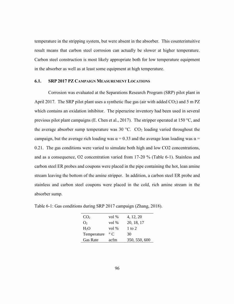
96
temperature in the stripping system, but were absent in the absorber. This counterintuitive
result means that carbon steel corrosion can actually be slower at higher temperature.
Carbon steel construction is most likely appropriate both for low temperature equipment
in the absorber as well as at least some equipment at high temperature.
6.1. SRP 2017 PZ CAMPAIGN MEASUREMENT LOCATIONS
Corrosion was evaluated at the Separations Research Program (SRP) pilot plant in
April 2017. The SRP pilot plant uses a synthetic flue gas (air with added CO2) and 5 m PZ
which contains an oxidation inhibitor. The piperazine inventory had been used in several
previous pilot plant campaigns (E. Chen et al., 2017). The stripper operated at 150 °C, and
the average absorber sump temperature was 30 °C. CO2 loading varied throughout the
campaign, but the average rich loading was α = 0.33 and the average lean loading was α =
0.21. The gas conditions were varied to simulate both high and low CO2 concentrations,
and as a consequence, O2 concentration varied from 17-20 % (Table 6-1). Stainless and
carbon steel ER probes and coupons were placed in the pipe containing the hot, lean amine
stream leaving the bottom of the amine stripper. In addition, a carbon steel ER probe and
stainless and carbon steel coupons were placed in the cold, rich amine stream in the
absorber sump.
Table 6-1: Gas conditions during SRP 2017 campaign (Zhang, 2018).
CO2 vol % 4, 12, 20
O2 vol % 20, 18, 17
H2O vol % 1 to 2
Temperature ° C 30
Gas Rate acfm 350, 550, 600
97
A C1010 corrosion probe was mounted in a small 1” bypass line connected to the
hot, lean amine pipe leaving the bottom of the advanced flash stripper (AFS) flash tank. A
diagram of the SRP pilot plant equipment is given in Figure 6-1. This probe collected
corrosion data for 502 hours at the beginning of the campaign until the probe was removed.
The C1010 corrosion probe was replaced with a 316L corrosion probe which collected
corrosion data for 134 hours during the second half of the campaign. The stripper corrosion
probes were connected to a transmitter that continuously logged data throughout the
campaign.
Solution potential was measured with an ORP probe in the hot lean bypass line
throughout the campaign. The potential stayed between -400 and -600 mV (vs Ag/AgCl)
for most of the campaign. Data from the ORP probe is presented in Appendix B.
Absorber corrosion was monitored using a C1010 corrosion probe mounted in the
absorber sump. This probe collected corrosion data for 636 hours over the course of the
entire campaign. The absorber corrosion probe was not connected to a transmitter for
continuous data collection. Instead, a handheld ER probe reader was used throughout the
campaign to take periodic corrosion measurements.
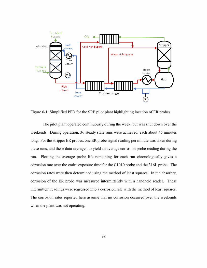
98
Figure 6-1: Simplified PFD for the SRP pilot plant highlighting location of ER probes
The pilot plant operated continuously during the week, but was shut down over the
weekends. During operation, 36 steady state runs were achieved, each about 45 minutes
long. For the stripper ER probes, one ER probe signal reading per minute was taken during
these runs, and these data averaged to yield an average corrosion probe reading during the
run. Plotting the average probe life remaining for each run chronologically gives a
corrosion rate over the entire exposure time for the C1010 probe and the 316L probe. The
corrosion rates were then determined using the method of least squares. In the absorber,
corrosion of the ER probe was measured intermittently with a handheld reader. These
intermittent readings were regressed into a corrosion rate with the method of least squares.
The corrosion rates reported here assume that no corrosion occurred over the weekends
when the plant was not operating.
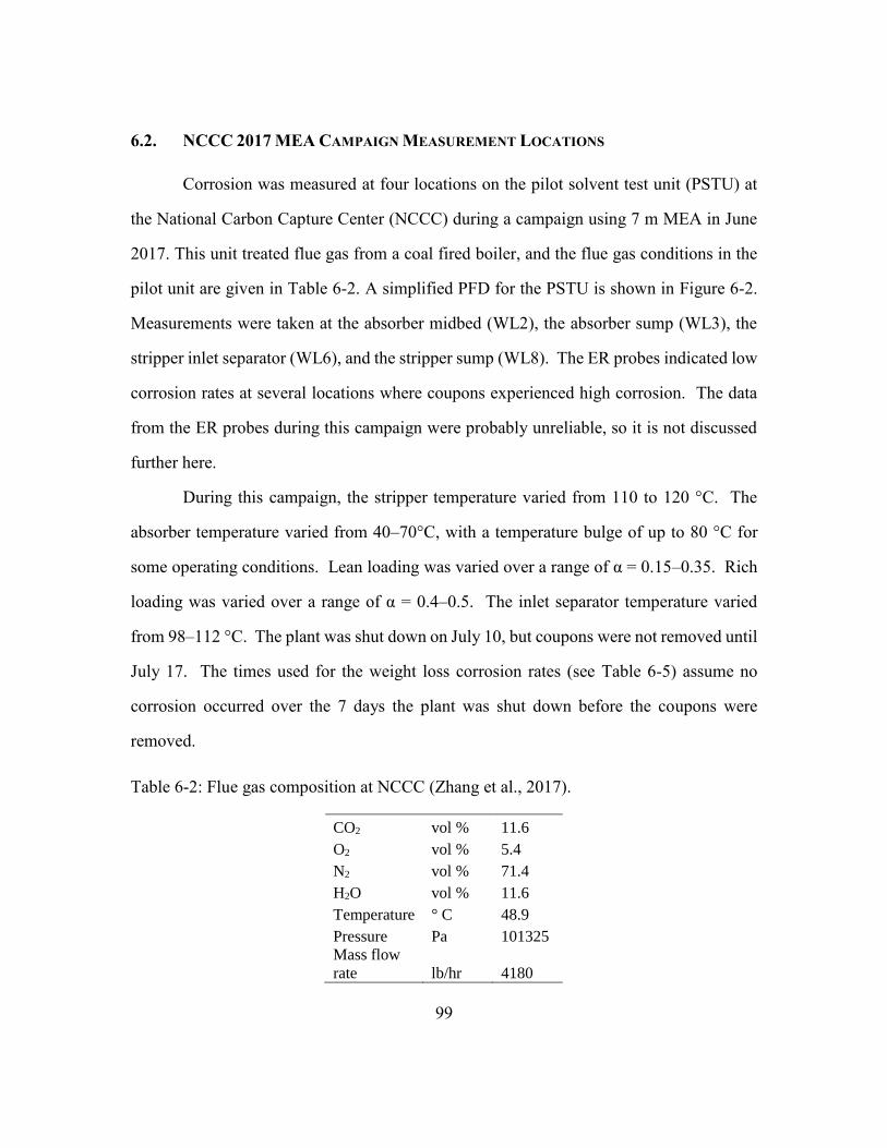
99
6.2. NCCC 2017 MEA CAMPAIGN MEASUREMENT LOCATIONS
Corrosion was measured at four locations on the pilot solvent test unit (PSTU) at
the National Carbon Capture Center (NCCC) during a campaign using 7 m MEA in June
2017. This unit treated flue gas from a coal fired boiler, and the flue gas conditions in the
pilot unit are given in Table 6-2. A simplified PFD for the PSTU is shown in Figure 6-2.
Measurements were taken at the absorber midbed (WL2), the absorber sump (WL3), the
stripper inlet separator (WL6), and the stripper sump (WL8). The ER probes indicated low
corrosion rates at several locations where coupons experienced high corrosion. The data
from the ER probes during this campaign were probably unreliable, so it is not discussed
further here.
During this campaign, the stripper temperature varied from 110 to 120 °C. The
absorber temperature varied from 40–70°C, with a temperature bulge of up to 80 °C for
some operating conditions. Lean loading was varied over a range of α = 0.15–0.35. Rich
loading was varied over a range of α = 0.4–0.5. The inlet separator temperature varied
from 98–112 °C. The plant was shut down on July 10, but coupons were not removed until
July 17. The times used for the weight loss corrosion rates (see Table 6-5) assume no
corrosion occurred over the 7 days the plant was shut down before the coupons were
removed.
Table 6-2: Flue gas composition at NCCC (Zhang et al., 2017).
CO2 vol % 11.6
O2 vol % 5.4
N2 vol % 71.4
H2O vol % 11.6
Temperature ° C 48.9
Pressure Pa 101325
Mass flow
rate lb/hr 4180
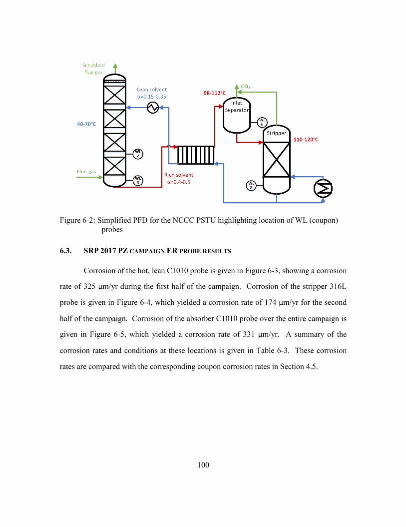
100
Figure 6-2: Simplified PFD for the NCCC PSTU highlighting location of WL (coupon)
probes
6.3. SRP 2017 PZ CAMPAIGN ER PROBE RESULTS
Corrosion of the hot, lean C1010 probe is given in Figure 6-3, showing a corrosion
rate of 325 µm/yr during the first half of the campaign. Corrosion of the stripper 316L
probe is given in Figure 6-4, which yielded a corrosion rate of 174 µm/yr for the second
half of the campaign. Corrosion of the absorber C1010 probe over the entire campaign is
given in Figure 6-5, which yielded a corrosion rate of 331 µm/yr. A summary of the
corrosion rates and conditions at these locations is given in Table 6-3. These corrosion
rates are compared with the corresponding coupon corrosion rates in Section 4.5.
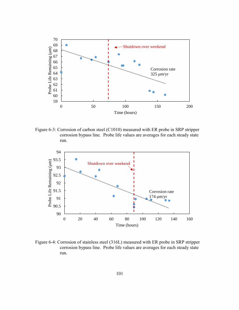
101
Figure 6-3: Corrosion of carbon steel (C1010) measured with ER probe in SRP stripper
corrosion bypass line. Probe life values are averages for each steady state
run.
Figure 6-4: Corrosion of stainless steel (316L) measured with ER probe in SRP stripper
corrosion bypass line. Probe life values are averages for each steady state
run.
59
60
61
62
63
64
65
66
67
68
69
70
0 50 100 150 200
Pro
be
Lif
e R
emai
nin
g (
μm
)
Time (hours)
Shutdown over weekend
Corrosion rate
325 μm/yr
90
90.5
91
91.5
92
92.5
93
93.5
94
0 20 40 60 80 100 120 140 160
Pro
be
Lif
e R
emai
nin
g (
μm
)
Time (hours)
Corrosion rate
174 μm/yr
Shutdown over weekend
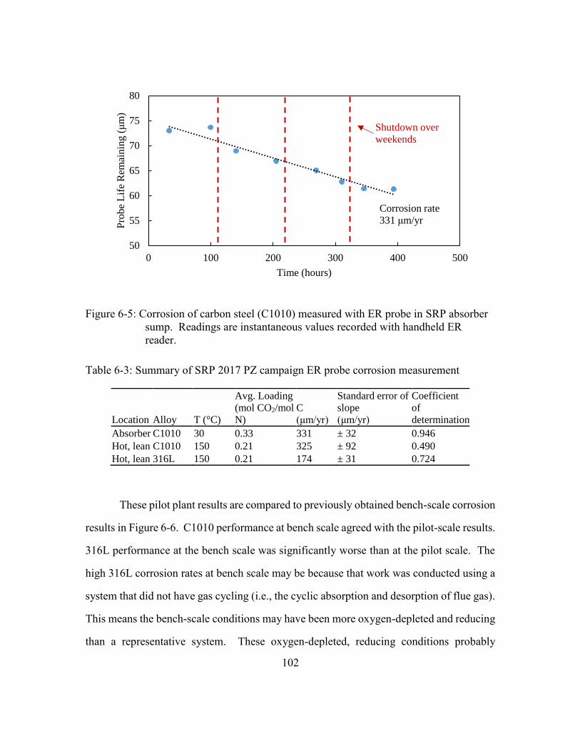
102
Figure 6-5: Corrosion of carbon steel (C1010) measured with ER probe in SRP absorber
sump. Readings are instantaneous values recorded with handheld ER
reader.
Table 6-3: Summary of SRP 2017 PZ campaign ER probe corrosion measurement
Location Alloy T (°C)
Avg. Loading
(mol CO2/mol
N)
C
(μm/yr)
Standard error of
slope
(μm/yr)
Coefficient
of
determination
Absorber C1010 30 0.33 331 ± 32 0.946
Hot, lean C1010 150 0.21 325 ± 92 0.490
Hot, lean 316L 150 0.21 174 ± 31 0.724
These pilot plant results are compared to previously obtained bench-scale corrosion
results in Figure 6-6. C1010 performance at bench scale agreed with the pilot-scale results.
316L performance at the bench scale was significantly worse than at the pilot scale. The
high 316L corrosion rates at bench scale may be because that work was conducted using a
system that did not have gas cycling (i.e., the cyclic absorption and desorption of flue gas).
This means the bench-scale conditions may have been more oxygen-depleted and reducing
than a representative system. These oxygen-depleted, reducing conditions probably
50
55
60
65
70
75
80
0 100 200 300 400 500
Pro
be
Lif
e R
emai
nin
g (
μm
)
Time (hours)
Shutdown over
weekends
Corrosion rate
331 μm/yr
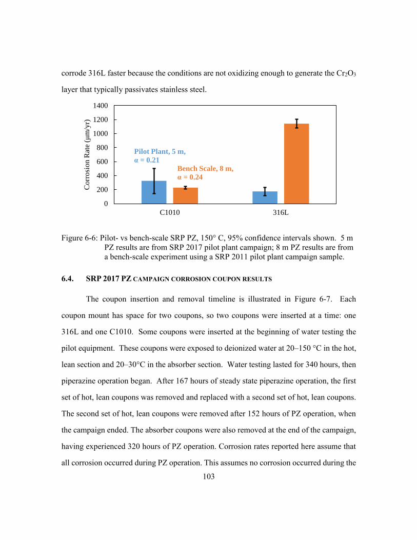
103
corrode 316L faster because the conditions are not oxidizing enough to generate the Cr2O3
layer that typically passivates stainless steel.
Figure 6-6: Pilot- vs bench-scale SRP PZ, 150° C, 95% confidence intervals shown. 5 m
PZ results are from SRP 2017 pilot plant campaign; 8 m PZ results are from
a bench-scale experiment using a SRP 2011 pilot plant campaign sample.
6.4. SRP 2017 PZ CAMPAIGN CORROSION COUPON RESULTS
The coupon insertion and removal timeline is illustrated in Figure 6-7. Each
coupon mount has space for two coupons, so two coupons were inserted at a time: one
316L and one C1010. Some coupons were inserted at the beginning of water testing the
pilot equipment. These coupons were exposed to deionized water at 20–150 °C in the hot,
lean section and 20–30°C in the absorber section. Water testing lasted for 340 hours, then
piperazine operation began. After 167 hours of steady state piperazine operation, the first
set of hot, lean coupons was removed and replaced with a second set of hot, lean coupons.
The second set of hot, lean coupons were removed after 152 hours of PZ operation, when
the campaign ended. The absorber coupons were also removed at the end of the campaign,
having experienced 320 hours of PZ operation. Corrosion rates reported here assume that
all corrosion occurred during PZ operation. This assumes no corrosion occurred during the
0
200
400
600
800
1000
1200
1400
C1010 316L
Co
rro
sio
n R
ate
(μm
/yr)
Pilot Plant, 5 m,
α = 0.21
Bench Scale, 8 m,
α = 0.24
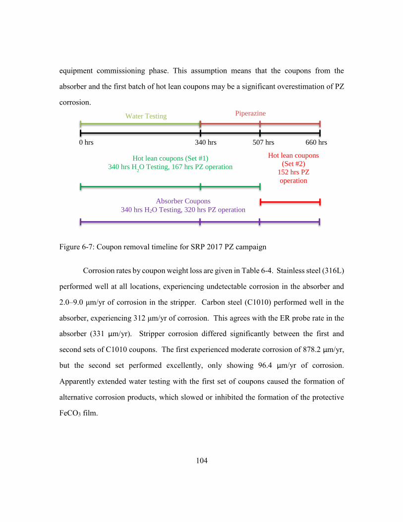
104
equipment commissioning phase. This assumption means that the coupons from the
absorber and the first batch of hot lean coupons may be a significant overestimation of PZ
corrosion.
Figure 6-7: Coupon removal timeline for SRP 2017 PZ campaign
Corrosion rates by coupon weight loss are given in Table 6-4. Stainless steel (316L)
performed well at all locations, experiencing undetectable corrosion in the absorber and
2.0–9.0 μm/yr of corrosion in the stripper. Carbon steel (C1010) performed well in the
absorber, experiencing 312 μm/yr of corrosion. This agrees with the ER probe rate in the
absorber (331 µm/yr). Stripper corrosion differed significantly between the first and
second sets of C1010 coupons. The first experienced moderate corrosion of 878.2 µm/yr,
but the second set performed excellently, only showing 96.4 µm/yr of corrosion.
Apparently extended water testing with the first set of coupons caused the formation of
alternative corrosion products, which slowed or inhibited the formation of the protective
FeCO3 film.
0 hrs 340 hrs 507 hrs 660 hrs
Water Testing Piperazine
Operation
Hot lean coupons (Set #1)
340 hrs H2O Testing, 167 hrs PZ operation
Hot lean coupons
(Set #2)
152 hrs PZ
operation
Absorber Coupons
340 hrs H2O Testing, 320 hrs PZ operation
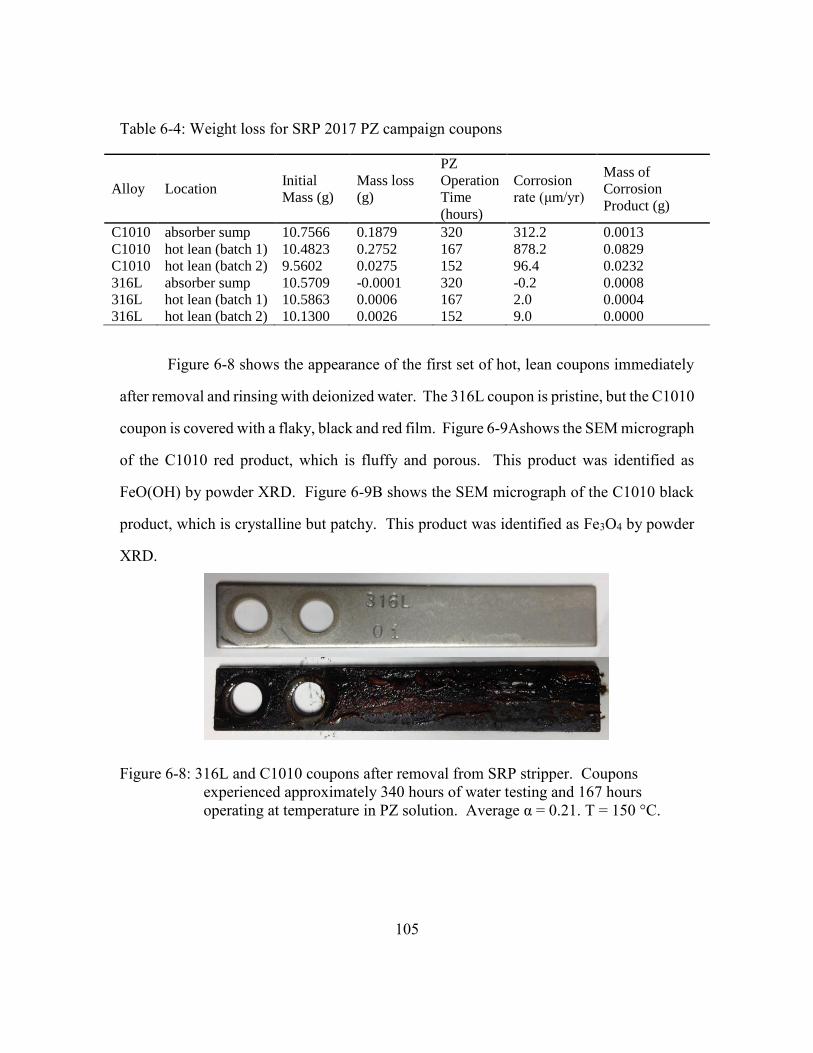
105
Table 6-4: Weight loss for SRP 2017 PZ campaign coupons
Alloy Location Initial
Mass (g)
Mass loss
(g)
PZ
Operation
Time
(hours)
Corrosion
rate (μm/yr)
Mass of
Corrosion
Product (g)
C1010 absorber sump 10.7566 0.1879 320 312.2 0.0013
C1010 hot lean (batch 1) 10.4823 0.2752 167 878.2 0.0829
C1010 hot lean (batch 2) 9.5602 0.0275 152 96.4 0.0232
316L absorber sump 10.5709 -0.0001 320 -0.2 0.0008
316L hot lean (batch 1) 10.5863 0.0006 167 2.0 0.0004
316L hot lean (batch 2) 10.1300 0.0026 152 9.0 0.0000
Figure 6-8 shows the appearance of the first set of hot, lean coupons immediately
after removal and rinsing with deionized water. The 316L coupon is pristine, but the C1010
coupon is covered with a flaky, black and red film. Figure 6-9Ashows the SEM micrograph
of the C1010 red product, which is fluffy and porous. This product was identified as
FeO(OH) by powder XRD. Figure 6-9B shows the SEM micrograph of the C1010 black
product, which is crystalline but patchy. This product was identified as Fe3O4 by powder
XRD.
Figure 6-8: 316L and C1010 coupons after removal from SRP stripper. Coupons
experienced approximately 340 hours of water testing and 167 hours
operating at temperature in PZ solution. Average α = 0.21. T = 150 °C.
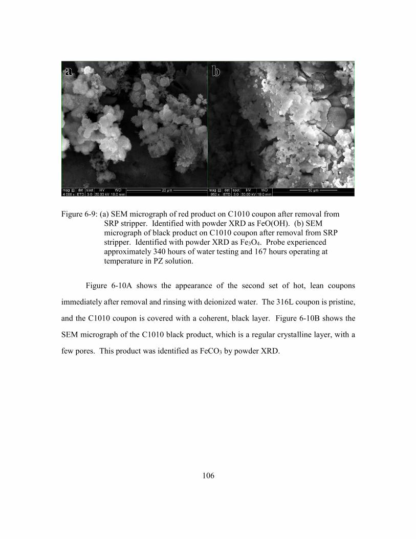
106
Figure 6-9: (a) SEM micrograph of red product on C1010 coupon after removal from
SRP stripper. Identified with powder XRD as FeO(OH). (b) SEM
micrograph of black product on C1010 coupon after removal from SRP
stripper. Identified with powder XRD as Fe3O4. Probe experienced
approximately 340 hours of water testing and 167 hours operating at
temperature in PZ solution.
Figure 6-10A shows the appearance of the second set of hot, lean coupons
immediately after removal and rinsing with deionized water. The 316L coupon is pristine,
and the C1010 coupon is covered with a coherent, black layer. Figure 6-10B shows the
SEM micrograph of the C1010 black product, which is a regular crystalline layer, with a
few pores. This product was identified as FeCO3 by powder XRD.
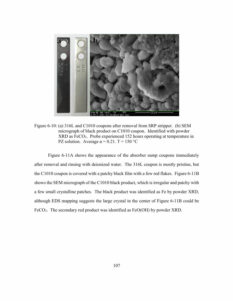
107
Figure 6-10: (a) 316L and C1010 coupons after removal from SRP stripper. (b) SEM
micrograph of black product on C1010 coupon. Identified with powder
XRD as FeCO3. Probe experienced 152 hours operating at temperature in
PZ solution. Average α = 0.21. T = 150 °C
Figure 6-11A shows the appearance of the absorber sump coupons immediately
after removal and rinsing with deionized water. The 316L coupon is mostly pristine, but
the C1010 coupon is covered with a patchy black film with a few red flakes. Figure 6-11B
shows the SEM micrograph of the C1010 black product, which is irregular and patchy with
a few small crystalline patches. The black product was identified as Fe by powder XRD,
although EDS mapping suggests the large crystal in the center of Figure 6-11B could be
FeCO3. The secondary red product was identified as FeO(OH) by powder XRD.
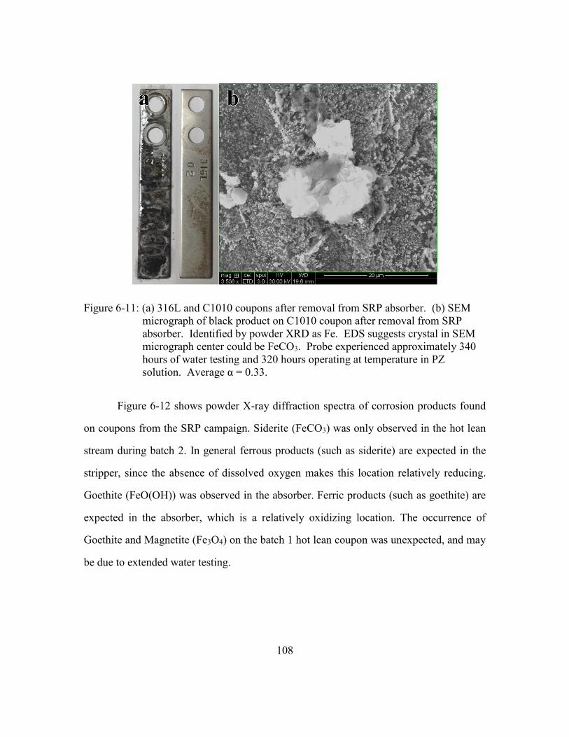
108
Figure 6-11: (a) 316L and C1010 coupons after removal from SRP absorber. (b) SEM
micrograph of black product on C1010 coupon after removal from SRP
absorber. Identified by powder XRD as Fe. EDS suggests crystal in SEM
micrograph center could be FeCO3. Probe experienced approximately 340
hours of water testing and 320 hours operating at temperature in PZ
solution. Average α = 0.33.
Figure 6-12 shows powder X-ray diffraction spectra of corrosion products found
on coupons from the SRP campaign. Siderite (FeCO3) was only observed in the hot lean
stream during batch 2. In general ferrous products (such as siderite) are expected in the
stripper, since the absence of dissolved oxygen makes this location relatively reducing.
Goethite (FeO(OH)) was observed in the absorber. Ferric products (such as goethite) are
expected in the absorber, which is a relatively oxidizing location. The occurrence of
Goethite and Magnetite (Fe3O4) on the batch 1 hot lean coupon was unexpected, and may
be due to extended water testing.
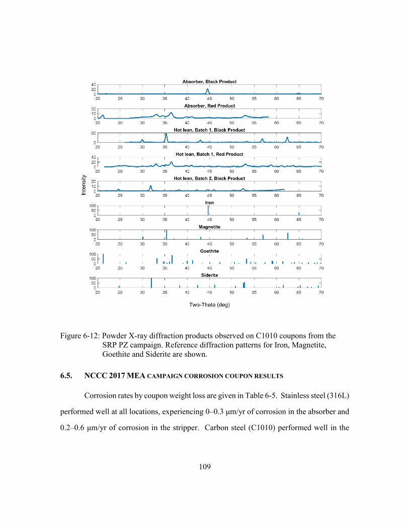
109
Figure 6-12: Powder X-ray diffraction products observed on C1010 coupons from the
SRP PZ campaign. Reference diffraction patterns for Iron, Magnetite,
Goethite and Siderite are shown.
6.5. NCCC 2017 MEA CAMPAIGN CORROSION COUPON RESULTS
Corrosion rates by coupon weight loss are given in Table 6-5. Stainless steel (316L)
performed well at all locations, experiencing 0–0.3 μm/yr of corrosion in the absorber and
0.2–0.6 μm/yr of corrosion in the stripper. Carbon steel (C1010) performed well in the
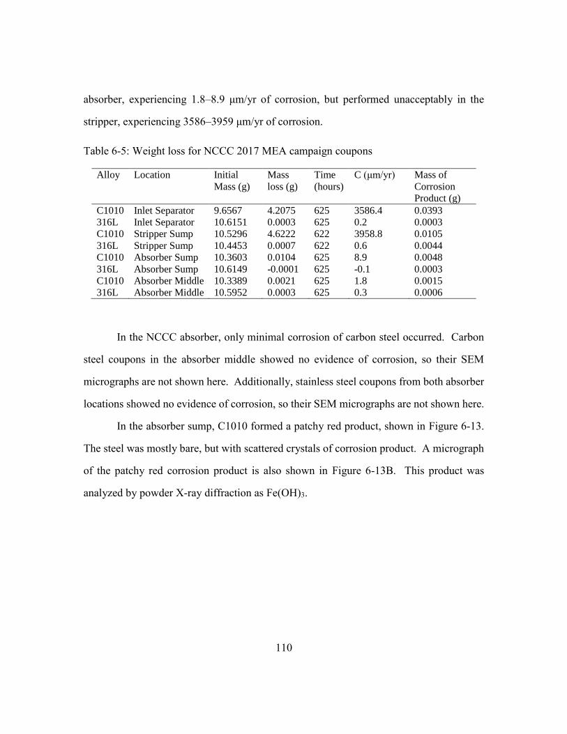
110
absorber, experiencing 1.8–8.9 μm/yr of corrosion, but performed unacceptably in the
stripper, experiencing 3586–3959 μm/yr of corrosion.
Table 6-5: Weight loss for NCCC 2017 MEA campaign coupons
Alloy Location Initial
Mass (g)
Mass
loss (g)
Time
(hours)
C (μm/yr) Mass of
Corrosion
Product (g)
C1010 Inlet Separator 9.6567 4.2075 625 3586.4 0.0393
316L Inlet Separator 10.6151 0.0003 625 0.2 0.0003
C1010 Stripper Sump 10.5296 4.6222 622 3958.8 0.0105
316L Stripper Sump 10.4453 0.0007 622 0.6 0.0044
C1010 Absorber Sump 10.3603 0.0104 625 8.9 0.0048
316L Absorber Sump 10.6149 -0.0001 625 -0.1 0.0003
C1010 Absorber Middle 10.3389 0.0021 625 1.8 0.0015
316L Absorber Middle 10.5952 0.0003 625 0.3 0.0006
In the NCCC absorber, only minimal corrosion of carbon steel occurred. Carbon
steel coupons in the absorber middle showed no evidence of corrosion, so their SEM
micrographs are not shown here. Additionally, stainless steel coupons from both absorber
locations showed no evidence of corrosion, so their SEM micrographs are not shown here.
In the absorber sump, C1010 formed a patchy red product, shown in Figure 6-13.
The steel was mostly bare, but with scattered crystals of corrosion product. A micrograph
of the patchy red corrosion product is also shown in Figure 6-13B. This product was
analyzed by powder X-ray diffraction as Fe(OH)3.

111
Figure 6-13: (a) C1010 coupon after removal from NCCC absorber sump. (b) SEM
micrograph of red product. Identified by powder XRD as Fe(OH)3. (c)
SEM micrograph of steel surface without product formation. Probe
experienced 625 hours of operation in 7 m MEA.
Stainless steel coupons from the stripper inlet separator showed no evidence of
corrosion, so their SEM micrographs are not shown here. Corrosion in the stripper inlet
separator was severe for carbon steel. The coupon appearance and SEM micrograph is
shown in Figure 6-14. The micrograph shows the coupon surface is about half bare steel
and half red product. EDS mapping suggests the surface is bare iron with small clusters of
oxide or carbon. Powder X-ray diffraction of this product appears to show a combination
of several products, possibly a mixture of Fe3O4 and FeCO3.
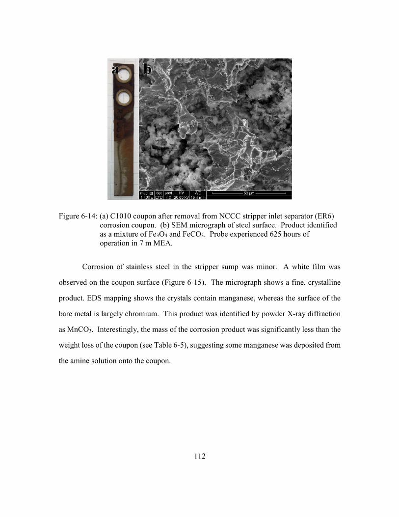
112
Figure 6-14: (a) C1010 coupon after removal from NCCC stripper inlet separator (ER6)
corrosion coupon. (b) SEM micrograph of steel surface. Product identified
as a mixture of Fe3O4 and FeCO3. Probe experienced 625 hours of
operation in 7 m MEA.
Corrosion of stainless steel in the stripper sump was minor. A white film was
observed on the coupon surface (Figure 6-15). The micrograph shows a fine, crystalline
product. EDS mapping shows the crystals contain manganese, whereas the surface of the
bare metal is largely chromium. This product was identified by powder X-ray diffraction
as MnCO3. Interestingly, the mass of the corrosion product was significantly less than the
weight loss of the coupon (see Table 6-5), suggesting some manganese was deposited from
the amine solution onto the coupon.
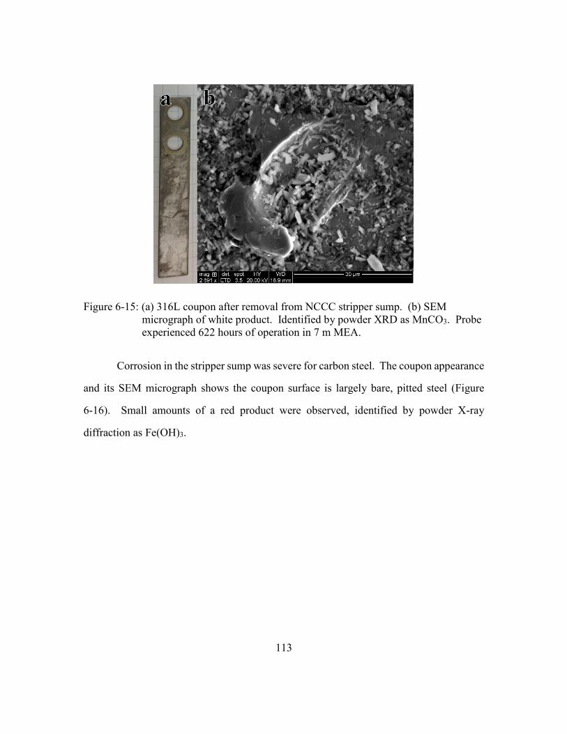
113
Figure 6-15: (a) 316L coupon after removal from NCCC stripper sump. (b) SEM
micrograph of white product. Identified by powder XRD as MnCO3. Probe
experienced 622 hours of operation in 7 m MEA.
Corrosion in the stripper sump was severe for carbon steel. The coupon appearance
and its SEM micrograph shows the coupon surface is largely bare, pitted steel (Figure
6-16). Small amounts of a red product were observed, identified by powder X-ray
diffraction as Fe(OH)3.
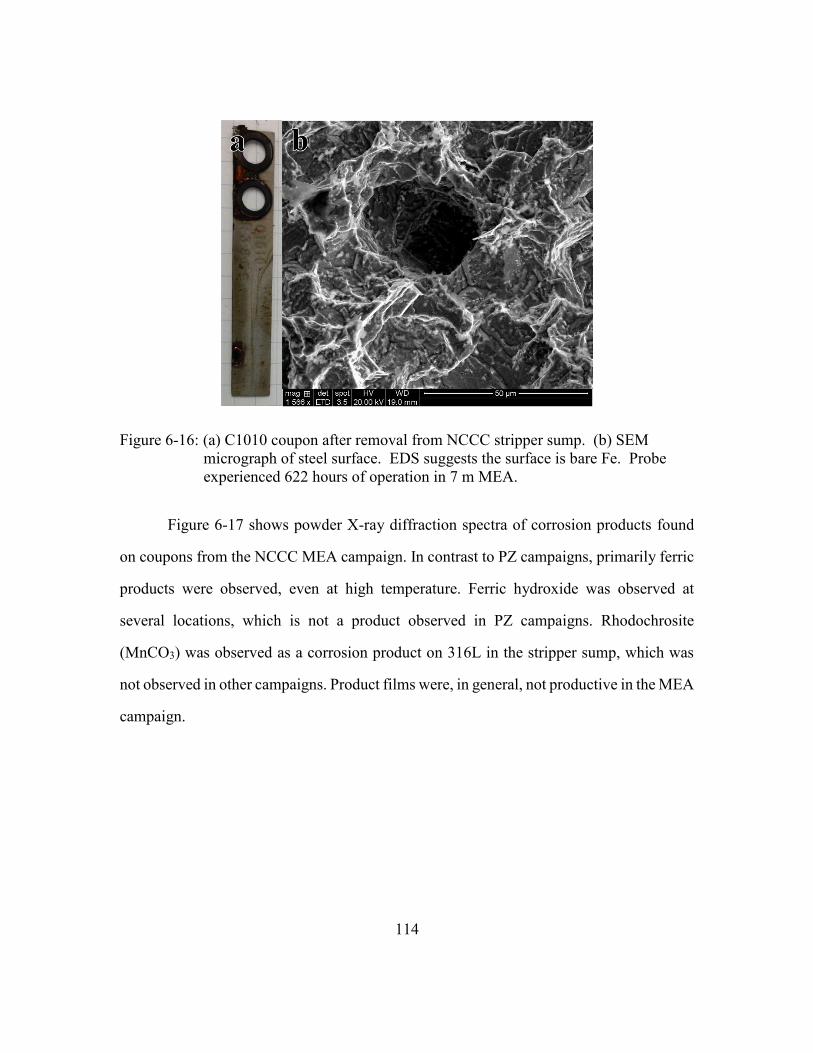
114
Figure 6-16: (a) C1010 coupon after removal from NCCC stripper sump. (b) SEM
micrograph of steel surface. EDS suggests the surface is bare Fe. Probe
experienced 622 hours of operation in 7 m MEA.
Figure 6-17 shows powder X-ray diffraction spectra of corrosion products found
on coupons from the NCCC MEA campaign. In contrast to PZ campaigns, primarily ferric
products were observed, even at high temperature. Ferric hydroxide was observed at
several locations, which is not a product observed in PZ campaigns. Rhodochrosite
(MnCO3) was observed as a corrosion product on 316L in the stripper sump, which was
not observed in other campaigns. Product films were, in general, not productive in the MEA
campaign.
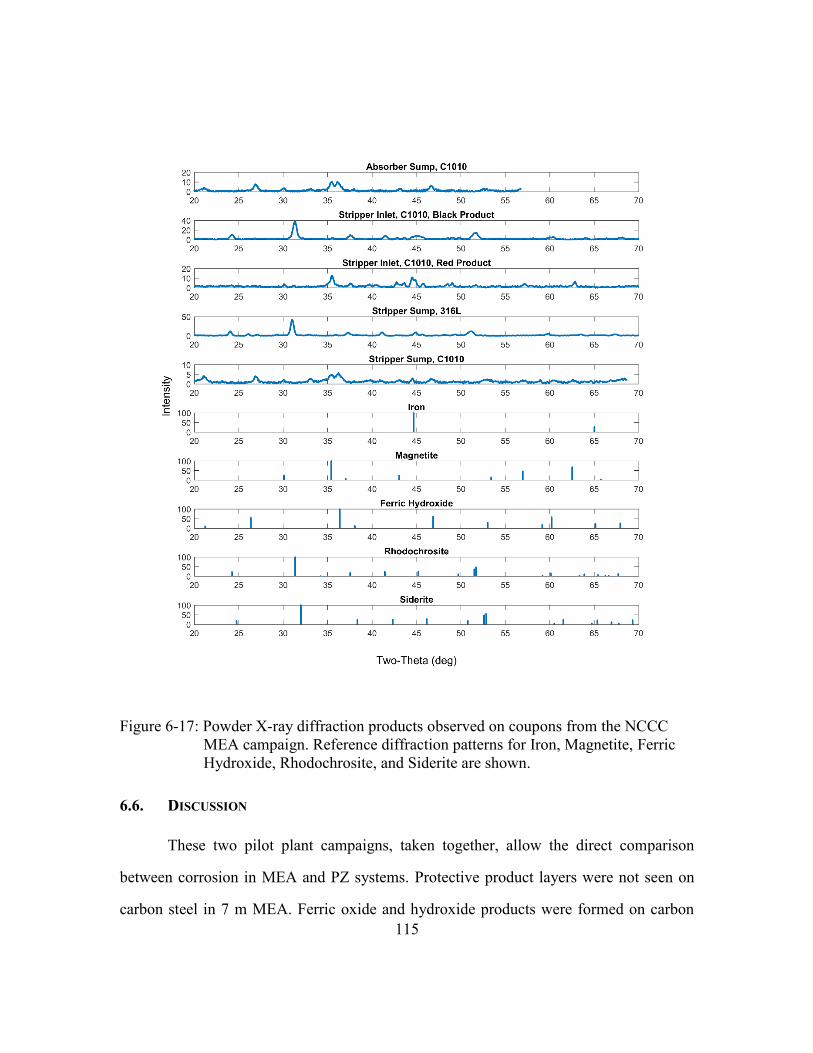
115
Figure 6-17: Powder X-ray diffraction products observed on coupons from the NCCC
MEA campaign. Reference diffraction patterns for Iron, Magnetite, Ferric
Hydroxide, Rhodochrosite, and Siderite are shown.
6.6. DISCUSSION
These two pilot plant campaigns, taken together, allow the direct comparison
between corrosion in MEA and PZ systems. Protective product layers were not seen on
carbon steel in 7 m MEA. Ferric oxide and hydroxide products were formed on carbon
116
steel in MEA, but few ferrous products were observed. This is likely because high ferrous
solubility in MEA solutions prevents precipitation of ferrous products. Alternatively,
oxidation of Fe2+ to Fe3+ by Equation 6-1 could be rapid or thermodynamically favored in
MEA, reducing availability of Fe2+ to form ferrous corrosion products. Despite the lack of
protective ferrous corrosion products, corrosion of carbon steel was slow at absorber
conditions, suggesting carbon steel construction is appropriate for at least low temperature
equipment in MEA operation.
𝑂2 + 2𝐻2𝑂 + 4𝐹𝑒2+ ↔ 4𝐹𝑒3+ + 4𝑂𝐻− (6-1)
In 5 m PZ at hot lean conditions protective layers of Fe3O4 and FeCO3 were
observed, suggesting that ferrous products are either less soluble in PZ than MEA, or that
ferric production by Equation 2-2 is slow or minor. These protective films sometimes led
to very low corrosion rates at hot, lean conditions. Protective films formed preferentially
at higher temperatures in the stripping system, but were absent in the absorber. This
counterintuitive result means that carbon steel corrosion can actually be slower at higher
temperatures. Protective product formation was inhibited in the absorber, likely due to
higher ferrous solubility at low T, high α, or because the rate of ferrous product formation
is kinetically limited. Although protective films were absent, corrosion was still slow in
the absorber.

117
6.7. CONCLUSIONS
6.7.1. FeCO3 formation at 150°C in 5 m PZ protects carbon steel, leading to low
corrosion rates.
Corrosion coupons from the 2017 SRP pilot plant campaign show a protective,
crystalline layer of FeCO3 forms on C1010 in 5 m PZ at 150 °C and α = 0.21.When this
layer formed, corrosion performance was good (96.4 µm/yr).
6.7.2. Equipment commissioning with water and steam appears more corrosive to
carbon steel than PZ operation.
Commissioning of equipment with water and steam generated a non-protective
layer of FeO(OH) and Fe3O4 on C1010 in the stripper sump. The C1010 coupon corroded
at 878 µm/yr (assumes all corrosion occurred during PZ operation). Significant corrosion
of this coupon likely occurred during extended water testing, rather than during PZ
operation. . This period of PZ operation apparently was not sufficient to generate a FeCO3
layer on the water-corroded coupon.
6.7.3. Absorber corrosion of carbon steel can be moderate, but this may be due to
equipment commissioning rather than exposure to PZ operation.
Primarily non-protective products form on C1010 in 5 m PZ at absorber conditions
(α = 0.33 and 30 °C). A patchy black layer of Fe with flakes of red FeO(OH) were
observed. C1010 experienced 312 μm/yr of corrosion (assumes all corrosion occurred
during PZ operation). Significant corrosion of this coupon likely occurred during extended
water testing, rather than during PZ operation.
118
6.7.4. Stainless steel performed well in 5 m PZ both in the absorber and in the hot,
lean stream. This may be partially due to the high O2 content at SRP.
Stainless steel (316L) performed excellently in the absorber (α = 0.33 and 30 °C)
corroding at 0 µm/yr. Stainless steel also performed excellently in the hot (150°C), lean (α
= 0.21) stream, showing 2.0–9.0 µm/yr of corrosion. Stainless steel is clearly not attacked
by either PZ operation or water commissioning at these conditions. This may be due to
higher O2 concentration at in SRP synthetic flue gas (≈18 %) compared to a coal flue gas
stream (5.4 %), which may lead to more oxidizing conditions which can support chromium
oxide passive film formation on stainless steel.
6.7.5. Carbon steel performs well at 40-70 °C in 7 m MEA, but it is unacceptable at
120 °C.
Carbon steel (C1010) performed well in the absorber (40-70 °C), experiencing 1.8–
8.9 μm/yr of corrosion, but performed unacceptably in the stripper (110-120°C),
experiencing 3586–3959 μm/yr of corrosion.
6.7.6. Stainless steel performs well in 7 m MEA at both absorber and stripper
conditions.
Stainless steel (316L) performed well at all locations, experiencing 0–0.3 μm/yr of
corrosion in the absorber (40-70 °C), and 0.2–0.6 μm/yr of corrosion in the stripper (110-
120°C).
6.7.7. Corrosion products on carbon steel are largely Ferric (Fe3+) in 7 m MEA
service, suggesting more oxidizing conditions than PZ. Protective corrosion product
layers were not observed.
In 7 m MEA, Fe(OH)3 was observed on carbon steel coupons in the absorber sump
and the stripper sump. This ferric product, particularly at relatively reducing stripper sump
conditions, suggests MEA is more oxidizing than PZ. In general corrosion product films

119
on C1010 in MEA were not thick or tightly adhering. Presumably higher Fe2+ solubilities
prevent precipitation of protective ferrous films. Alternatively, ferrous product formation
is prevented at most conditions because MEA rapidly oxidizes Fe2+ to Fe3+.
120
Chapter 7. Corrosion in Piperazine during 2018 Pilot Campaign
Corrosion in amine units for CO2 capture has been measured at several pilot plants
(Cousins et al., 2013; Flø et al., 2019; Hjelmaas et al., 2017; Khakharia et al., 2015; Kittel
et al., 2009; Li et al., 2018; Li et al., 2017). All these studies (except one) investigated
MEA, and as a consequence are typically limited to operation at 120 °C. To date there is
limited published data on pilot scale corrosion in second generation solvents, like PZ. The
following pilot campaign was conducted at the National Carbon Capture Center in
Wilsonville, AL. Some details about the pilot plant campaign were published (Gao et al.,
2019; G. Rochelle et al., 2019; Selinger, 2018), but detailed corrosion measurements were
not published. Ching-Ting Liu assisted with equipment installation and coupon analysis
during this pilot campaign.
Corrosion was measured with weight loss coupons and ER probes, but ultimately
the coupon weight loss measurements were determined to be more reliable. Coupon
surfaces were imaged, showing protective FeCO3 film on carbon steel at many conditions.
Significant carbon steel corrosion occurred primarily at high temperature, high velocity
locations where increased mass transfer or erosion removed protective films. Stainless steel
was found to be occasionally vulnerable at high temperature, which is likely a consequence
of the uniquely high operating temperatures used with PZ. The effect of temperature and
solution velocity on corrosion of carbon and stainless steel are evaluated, and tentative
materials choice recommendations are given for different locations in the PZ process.
7.1. CORROSION MEASUREMENT LOCATIONS
The National Carbon Capture Center pilot unit captures CO2 from a 0.6 MWe coal
flue gas stream. Flue gas details for the pilot unit are given in Table 7-1. The campaign
used 5 m PZ, and ranges of CO2 loadings during the PZ campaign are given in Table 7-2.

121
The pilot unit uses a conventional absorber and an advanced stripper configuration called
the Advanced Flash Stripper (AFS). Corrosion measurements were made at many locations
on the pilot unit to measure corrosion in each unit operation.
Table 7-1: Flue gas composition at NCCC (Zhang et al., 2017).
CO2 vol % 11.6
O2 vol % 5.4
N2 vol % 71.4
H2O vol % 11.6
Temperature ° C 48.9
Pressure Pa 101325
Mass flow
rate lb/hr 4180
Table 7-2: PZ 2018 campaign CO2 loadings during steady state runs.
α min
(mol CO2/ mol N)
α max
(mol CO2/ mol N)
α median
(mol CO2/ mol N)
Lean 0.20 0.27 0.23
Rich 0.38 0.42 0.40
In the absorber system, coupon measurements were made at 7 locations and ER
probe measurements were made at 2 locations. These locations are illustrated in Figure
7-1 and listed in Table 7-3. Coupons were not inserted at one planned location (WL3),
because a nitrogen injection system was installed at that location instead for solvent
oxidation control.

122
Figure 7-1: Simplified PFD of NCCC absorber system, showing ER and WL locations.
Table 7-3: Description of Absorber ER and WL locations
Tag Location Description Instrument Type
WL1 Absorber between beds 2 and 3 Coupon probe
WL2 Absorber between beds 1 and 2 Coupon probe
WL3 Absorber sump (below bed 1) Coupon Probe
ER2 Absorber between beds 1 and 2 ER Probe & ER coupon
adapter
ER3 Absorber sump (below bed 1) ER probe & ER coupon
adapter
WL4 Absorber above mist eliminator Coupon probe
WL5 Water wash below mist eliminator Coupon probe
WL12 Cold lean solvent downstream of HX20404 and upstream
of HX20405 (trim cooler)
Coupon probe
In the regeneration system, coupon measurements were made at 5 locations, ER
probe measurements were made at 4 locations, and ORP measurements were made at 2
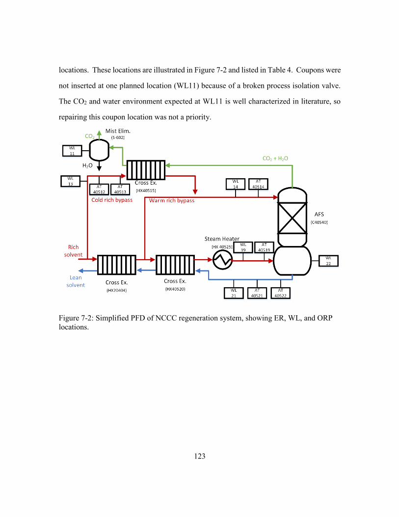
123
locations. These locations are illustrated in Figure 7-2 and listed in Table 4. Coupons were
not inserted at one planned location (WL11) because of a broken process isolation valve.
The CO2 and water environment expected at WL11 is well characterized in literature, so
repairing this coupon location was not a priority.
Figure 7-2: Simplified PFD of NCCC regeneration system, showing ER, WL, and ORP
locations.
124
Table 7-4: Description of regeneration system ER and WL locations
Tag Location Description Instrument Type
WL11 In mist elimination tank for CO2 stream Coupon probe
AT40512 Rich solvent to cold rich bypass exchanger ORP probe
AT40513 Rich solvent to cold rich bypass exchanger ER probe
WL13 Rich solvent to cold rich bypass exchanger Coupon probe
AT40519 Rich solvent from steam heater to AFS ER probe
WL19 Rich solvent from steam heater to AFS Coupon probe
AT40514 Rich solvent from cold rich bypass exchanger to AFS ER probe
WL14 Rich solvent from cold rich bypass exchanger to AFS Coupon probe
AT40521 Lean solvent from AFS to hot cross exchanger ER probe
AT40522 Lean solvent from AFS to hot cross exchanger ORP probe
WL21 Lean solvent from AFS to hot cross exchanger Coupon probe
WL22 Stripper sump Coupon probe
Superficial fluid velocities and typical operating temperatures are shown in Table
7-5 for several corrosion coupon locations. Velocity has a strong effect on carbon steel
corrosion because it removes protective corrosion product films. Velocities were typically
under 1 m/s, but were as high as 2.16 m/s at one location during a steady state run. These
velocities do not include flashing or two phase flow, and thus underestimate fluid velocity,
particularly in the hot rich location, where flashing is expected. In addition, coupon
orientation was not controlled in this campaign, and coupons may have been inserted
perpendicular rather than parallel to flow. Strip coupons inserted perpendicular to flow
obstruct 30-39 % of the pipe’s cross sectional area, which is also shown in Table 7-5,
compared to parallel insertion, which only obstructs 4-5% of the pipe’s cross sectional area.
High fluid velocities and turbulence caused by coupons inserted perpendicularly could
have contributed to some carbon steel corrosion measurements being not entirely
reproducible.

125
Table 7-5: PZ 2018 campaign superficial fluid velocity during steady state runs and
typical operating temperatures.
Location V min (m/s) V max (m/s) V median
(m/s)
T (° C) Pipe
Area
Blocked
Max
(%)
Pipe
Area
Blocked
Min
(%)
Cold Lean 0.42 0.85 0.50 50 - -
Cold Rich Bypass 0.03 0.08 0.04 50 30 4
Warm Rich Bypass 0.23 0.66 0.39 116 39 5
Hot Rich 0.65 2.16 0.83 155 39 5
Hot Lean 0.64 1.31 0.77 150 30 4
Absorber Sump - - - 50 - -
AFS Sump - - - 150 - -
7.2. COUPON BATCHING SCHEDULE
Coupons were inserted and removed in four chronological batches. This allowed
more coupons to be examined, and allowed an investigation of whether corrosion
conditions changed over the course of the campaign. An illustration of the coupon batch
insertion and removal dates is given in Table 7-6.
Table 7-6: Calendar illustration of coupon batches. The colored sections of each row
represent the coupon batches insertion and removal dates. Green sections represent
periods of piperazine operation, black sections represent periods when coupons were
inserted but the plant was shut down, and the yellow section represents the period of
simple stripper operation.
February March April May June July August
Batch 1
Batch 2
Batch 3
Batch 4
126
Batch 1 was a period of parametric testing over February 21–28, 2018. The
coupons were inserted during equipment water and steam testing, which lasted 47 hours
after insertion. The coupons then experienced 66 hours of PZ operation, after which the
plant was unexpectedly shut down, drained, and rinsed with water. Water was circulated
through the plant for 168 hours. Finally the system was drained again, and the coupons
remained in the drained, shut down state for 48 hours before retrieval. The corrosion rates
for this period assume that all corrosion ocurred during the 66 hours of PZ operation.
Assuming all corrosion happened during this short interval gives the most conservative (ie,
the highest) corrosion rates. Given the significant water testing before and after the period
of PZ operation, the corrosion rates for this period significantly overestimate PZ corrosion.
Batch 1 evaluated carbon steel (C1010) in the AFS locations. Because of the uncertainty
of the corrosion rates observed in Batch 1, these rates are excluded when drawing
conclusions about PZ performance.
Batch 2 experienced 388 hours of operation on the AFS skid between March 26,
2018 and April 21, 2018. After this period, an unexpected shutdown occurred, and the
coupons were left in the shut-down, drained plant for 720 hours before they were retrieved.
The corrosion rates reported here assume no corrosion occurred during the shut-down
period. Batch 2 evaluated carbon steel (C1010) and stainless steel (316L) in the AFS
locations. Several coupon locations on the absorber side (WL1, WL2, WL4, WL5, WL12)
were not removed at the end of Batch 2. This set of coupons experienced both Batch 2 and
Batch 3 before removal.
At the beginning of Batch 3, there was a 256 hour period of simple stripper
operation. This was an equipment configuration that bypassed the AFS skid, instead using
a simple stripper for regeneration. This was performed to compare the energy performance
of the AFS to the simple stripper, but corrosion was not evaluated in the simple stripper
127
during this time. Coupons in the absorber equipment experienced corrosion, but AFS
coupons were in shut-down, drained lines and experienced no corrosion. After simple
stripper operation, Batch 3 experienced 879 hours of operation on the AFS skid between
June 3, 2018 and July 17, 2018. The plant was shut down for a 120 hour period during the
middle of Batch 3. Test conditions were slightly different during Batch 3 because two
strategies were implemented to reduce amine oxidation. Batch 3 evaluated carbon steel
(C1010) and stainless steel (304) in the AFS locations.
Batch 4 experienced 363 hours of operation on the AFS skid between July 21, 2018
and August 15, 2018. The plant was shut down for a 200 hour period during the middle of
Batch 4. Batch 4 evaluated carbon steel (C1010) and stainless steel (316L) in the AFS
locations. Similar to Batch 3, Batch 4 test conditions were slightly different because two
strategies were implemented to reduce amine oxidation.
7.3. CORROSION RESULTS
7.3.1. Effect of Temperature and Velocity
There was a clear effect of temperature and fluid velocity on carbon steel corrosion.
These effects are illustrated in Figure 7-3. High velocity locations had higher corrosion
than low velocity locations regardless of temperature or CO2 loading. High fluid velocity
exacerbated carbon steel corrosion because it removes the protective FeCO3 layer. A strong
effect of CO2 loading was not apparent. The effect of temperature on carbon steel corrosion
was apparently weaker than its effect on stainless steel. This weak temperature effect is
counterintuitive, but it is driven by several factors:
1. FeCO3 solubility is lower at elevated temperatures, increasing the driving
force for precipitation of FeCO3 protective films.
2. Kinetics of FeCO3 formation are faster at higher temperatures.

128
3. Oxidation of Fe is faster at higher temperatures, but this is irrelevant
because the rate of corrosion is limited by FeCO3 formation.
Figure 7-3: Carbon steel corrosion rates from coupon weight loss during 2018 PZ
campaign, excluding Batch 1 results. Blue points are low velocity locations
(eg. Sumps, vessel sample points), and red points are high velocity locations
(eg. Inside pipes). Points that are circles have a rich CO2 loading, and points
that are triangles have a lean CO2 loading.
There was no clear effect of velocity on stainless steel corrosion, which is illustrated in
Figure 7-4. Low velocity locations did not demonstrate notably lower corrosion than high
velocity locations. Velocity has no strong effect on stainless corrosion because stainless
corrosion is not controlled by the formation of a product layer. Likewise there is a clear
0.1
1
10
100
1000
10000
0 50 100 150 200
Co
rro
sio
n R
ate
(μm
/yr)
Avg. T (°C)
HIGH VELOCITY, C1010
LOW VELOCITY, C1010
Rich: ●Lean: ▲
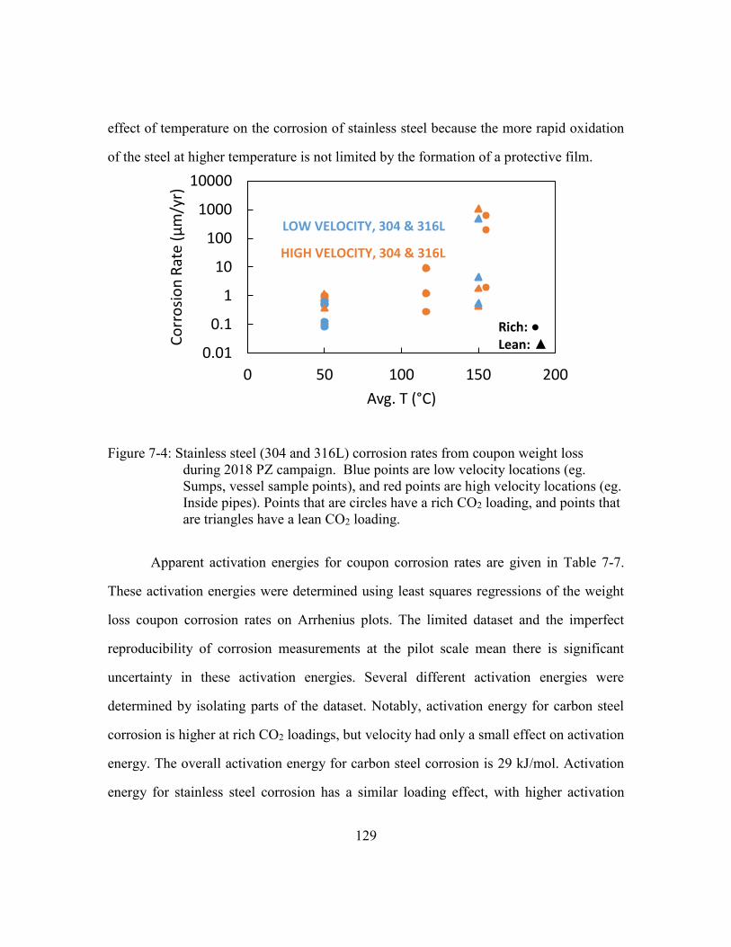
129
effect of temperature on the corrosion of stainless steel because the more rapid oxidation
of the steel at higher temperature is not limited by the formation of a protective film.
Figure 7-4: Stainless steel (304 and 316L) corrosion rates from coupon weight loss
during 2018 PZ campaign. Blue points are low velocity locations (eg.
Sumps, vessel sample points), and red points are high velocity locations (eg.
Inside pipes). Points that are circles have a rich CO2 loading, and points that
are triangles have a lean CO2 loading.
Apparent activation energies for coupon corrosion rates are given in Table 7-7.
These activation energies were determined using least squares regressions of the weight
loss coupon corrosion rates on Arrhenius plots. The limited dataset and the imperfect
reproducibility of corrosion measurements at the pilot scale mean there is significant
uncertainty in these activation energies. Several different activation energies were
determined by isolating parts of the dataset. Notably, activation energy for carbon steel
corrosion is higher at rich CO2 loadings, but velocity had only a small effect on activation
energy. The overall activation energy for carbon steel corrosion is 29 kJ/mol. Activation
energy for stainless steel corrosion has a similar loading effect, with higher activation
0.01
0.1
1
10
100
1000
10000
0 50 100 150 200
Co
rro
sio
n R
ate
(μm
/yr)
Avg. T (°C)
HIGH VELOCITY, 304 & 316L
LOW VELOCITY, 304 & 316L
Rich: ●Lean: ▲
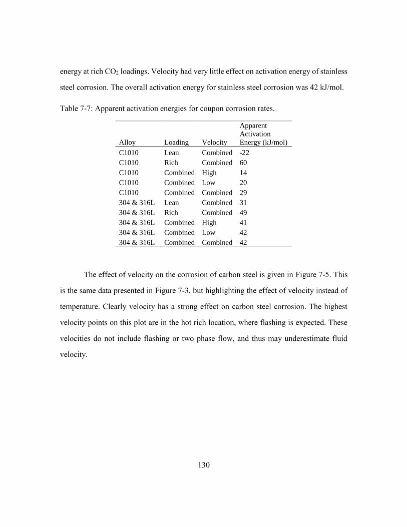
130
energy at rich CO2 loadings. Velocity had very little effect on activation energy of stainless
steel corrosion. The overall activation energy for stainless steel corrosion was 42 kJ/mol.
Table 7-7: Apparent activation energies for coupon corrosion rates.
Alloy Loading Velocity
Apparent
Activation
Energy (kJ/mol)
C1010 Lean Combined -22
C1010 Rich Combined 60
C1010 Combined High 14
C1010 Combined Low 20
C1010 Combined Combined 29
304 & 316L Lean Combined 31
304 & 316L Rich Combined 49
304 & 316L Combined High 41
304 & 316L Combined Low 42
304 & 316L Combined Combined 42
The effect of velocity on the corrosion of carbon steel is given in Figure 7-5. This
is the same data presented in Figure 7-3, but highlighting the effect of velocity instead of
temperature. Clearly velocity has a strong effect on carbon steel corrosion. The highest
velocity points on this plot are in the hot rich location, where flashing is expected. These
velocities do not include flashing or two phase flow, and thus may underestimate fluid
velocity.

131
Figure 7-5: Carbon steel corrosion rates from coupon weight loss during 2018 PZ
campaign, excluding Batch 1 results. Velocities represent median velocities
at that location over all steady state runs throughout the entire campaign.
Velocities are assumed to be zero in vessel sumps and midbed sample
points. Points that are circles have a rich CO2 loading, and points that are
triangles have a lean CO2 loading.
The effect of velocity on the corrosion of stainless steel is given in Figure 7-6. This
is the same data presented in Figure 7-4, but highlighting the effect of velocity instead of
temperature. Apparently velocity has a negligible effect on the corrosion of stainless steel.
0.1
1
10
100
1000
10000
0 0.2 0.4 0.6 0.8 1
Co
rro
sio
n R
ate
(μm
/yr)
Median Pipe Velocity (m/s)
150 - 155 °C
116 °C50 °C
Rich: ●Lean: ▲

132
Figure 7-6: Stainless steel (304 and 316L) corrosion rates from coupon weight loss
during 2018 PZ campaign. Velocities represent median velocities at that
location over all steady state runs throughout the entire campaign. Velocities
are assumed to be zero in vessel sumps and midbed sample points. Points
that are circles have a rich CO2 loading, and points that are triangles have a
lean CO2 loading.
7.3.2. Summary of corrosion by location
Performance of both carbon steel (C1010) and stainless steel (some 316L, others
304) were excellent (≈1μm/yr) in the absorber middle and absorber sump. Problems may
occur at locations that are not adequately wetted with amine, where carbonic acid attack
may occur—for example the absorber top. Non amine-wetted locations were not
thoroughly investigated in this report.
In relatively low temperature piping, carbon steel is likely acceptable for some
equipment. In the cold lean piping, C1010 corrosion was moderate (108 – 210 µm/yr)
0.01
0.1
1
10
100
1000
10000
0 0.2 0.4 0.6 0.8 1
Co
rro
sio
n R
ate
(μm
/yr)
Median Pipe Velocity (m/s)
150 - 155 °C
116 °C
50 °C
Rich: ●Lean: ▲

133
during most batches (2, 3, 4). Performance in the cold rich piping was comparable (50 –
202 µm/yr). Stainless performance (some 304, others 316L) at both cold lean location and
the cold rich location was excellent (0 – 1 µm/yr). The moderate performance of C1010
here suggest that it may be acceptable for some equipment at this condition, although the
corrosion rates may still be too high for very thin surfaces (ie, heat exchanger surfaces).
At some elevated temperature locations, carbon steel is likely appropriate for some
equipment. C1010 performance in the warm rich bypass was good (55 – 158 µm/yr). C1010
also performed well in the AFS sump (7 – 11 µm/yr). The surprising performance of C1010
at elevated temperature is due to the presence of protective siderite and magnetite films.
Stainless steel (some 304, others 316L) also typically performs well at these locations (0 –
9 µm/yr). However stainless steel was attacked (489 µm/yr) during Batch 2 in the AFS
sump. The occasional vulnerability of stainless steel at this location suggests that carbon
steel may be a preferable material of construction for the AFS sump.
At high temperature, high fluid velocity locations, protective films are not adequate
to protect carbon steel, and corrosion can be high. Overall performance of C1010 was poor
(50 – 711 µm/yr) in the hot lean stream and poor in the hot rich stream (36 – 9621 µm/yr).
At high temperature, high fluid velocity locations, stainless steel is also frequently
attacked. In the hot rich location, stainless performance (some 304, others 316L) was poor
(1 – 629 µm/yr). In the hot lean stream, stainless (some 304, others 316L) performed well
for Batches 3 and 4 (1 – 2 µm/yr), but experienced high corrosion (1095 µm/yr) during
Batch 2. Until the occasional vulnerability of stainless steel at these locations is understood,
higher alloy steels (ie, duplex stainless) should be investigated.
A simplified diagram showing equipment selection recommendations is shown in
Figure 7-7.
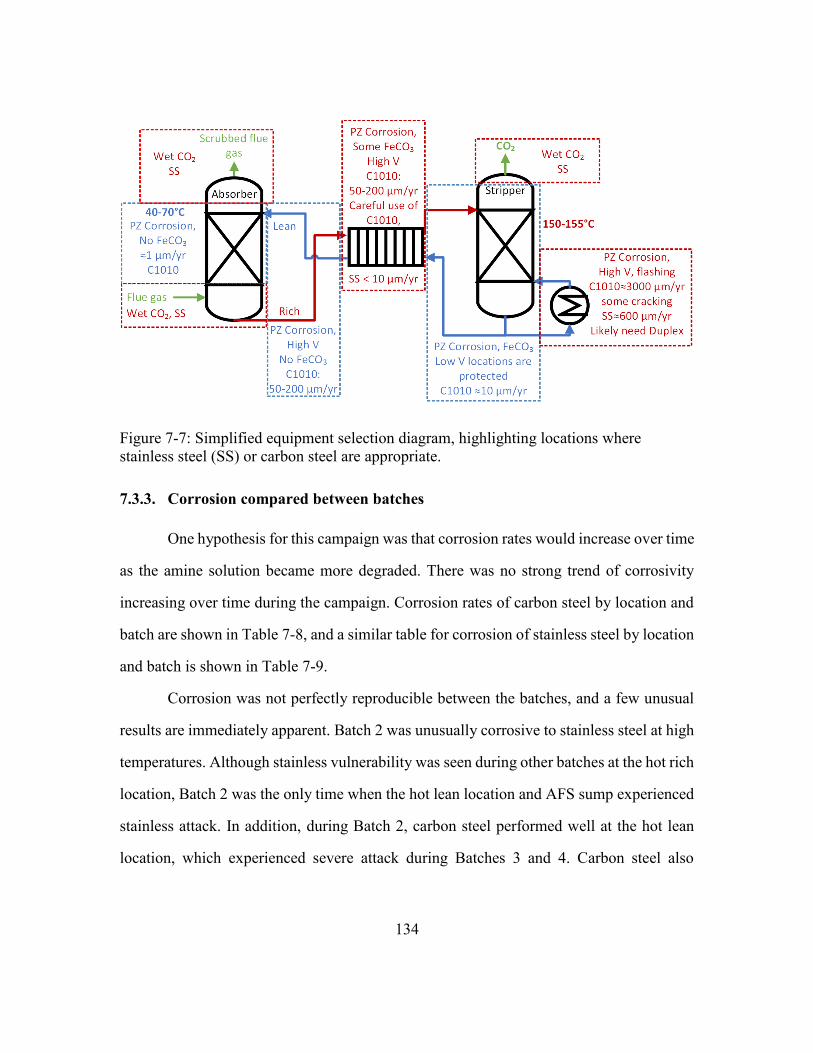
134
Figure 7-7: Simplified equipment selection diagram, highlighting locations where
stainless steel (SS) or carbon steel are appropriate.
7.3.3. Corrosion compared between batches
One hypothesis for this campaign was that corrosion rates would increase over time
as the amine solution became more degraded. There was no strong trend of corrosivity
increasing over time during the campaign. Corrosion rates of carbon steel by location and
batch are shown in Table 7-8, and a similar table for corrosion of stainless steel by location
and batch is shown in Table 7-9.
Corrosion was not perfectly reproducible between the batches, and a few unusual
results are immediately apparent. Batch 2 was unusually corrosive to stainless steel at high
temperatures. Although stainless vulnerability was seen during other batches at the hot rich
location, Batch 2 was the only time when the hot lean location and AFS sump experienced
stainless attack. In addition, during Batch 2, carbon steel performed well at the hot lean
location, which experienced severe attack during Batches 3 and 4. Carbon steel also
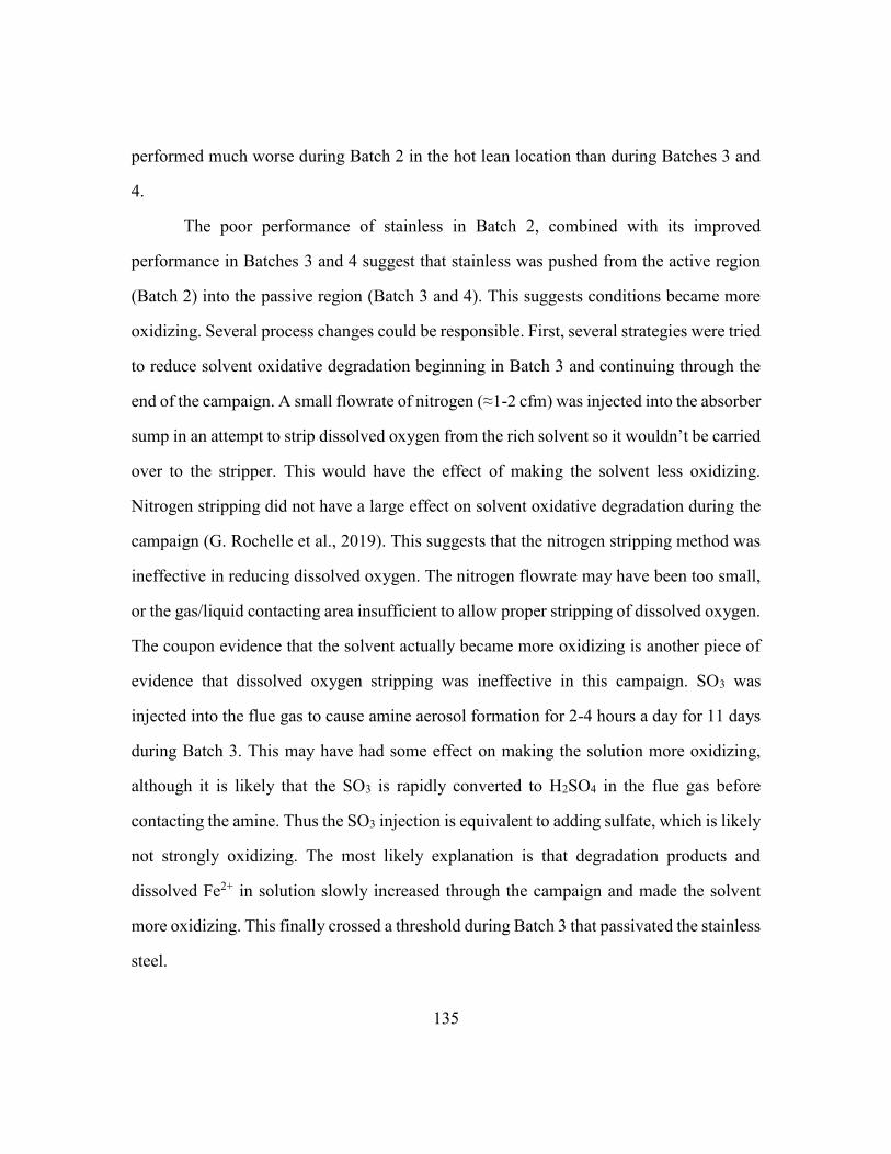
135
performed much worse during Batch 2 in the hot lean location than during Batches 3 and
4.
The poor performance of stainless in Batch 2, combined with its improved
performance in Batches 3 and 4 suggest that stainless was pushed from the active region
(Batch 2) into the passive region (Batch 3 and 4). This suggests conditions became more
oxidizing. Several process changes could be responsible. First, several strategies were tried
to reduce solvent oxidative degradation beginning in Batch 3 and continuing through the
end of the campaign. A small flowrate of nitrogen (≈1-2 cfm) was injected into the absorber
sump in an attempt to strip dissolved oxygen from the rich solvent so it wouldn’t be carried
over to the stripper. This would have the effect of making the solvent less oxidizing.
Nitrogen stripping did not have a large effect on solvent oxidative degradation during the
campaign (G. Rochelle et al., 2019). This suggests that the nitrogen stripping method was
ineffective in reducing dissolved oxygen. The nitrogen flowrate may have been too small,
or the gas/liquid contacting area insufficient to allow proper stripping of dissolved oxygen.
The coupon evidence that the solvent actually became more oxidizing is another piece of
evidence that dissolved oxygen stripping was ineffective in this campaign. SO3 was
injected into the flue gas to cause amine aerosol formation for 2-4 hours a day for 11 days
during Batch 3. This may have had some effect on making the solution more oxidizing,
although it is likely that the SO3 is rapidly converted to H2SO4 in the flue gas before
contacting the amine. Thus the SO3 injection is equivalent to adding sulfate, which is likely
not strongly oxidizing. The most likely explanation is that degradation products and
dissolved Fe2+ in solution slowly increased through the campaign and made the solvent
more oxidizing. This finally crossed a threshold during Batch 3 that passivated the stainless
steel.
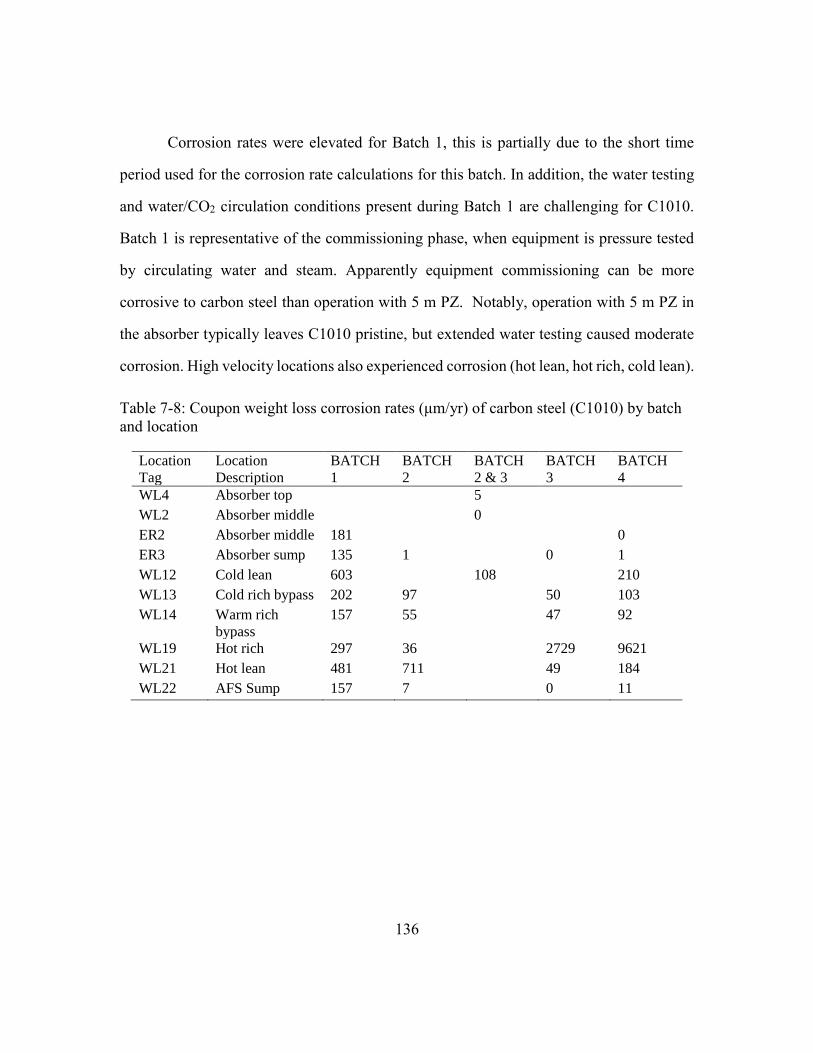
136
Corrosion rates were elevated for Batch 1, this is partially due to the short time
period used for the corrosion rate calculations for this batch. In addition, the water testing
and water/CO2 circulation conditions present during Batch 1 are challenging for C1010.
Batch 1 is representative of the commissioning phase, when equipment is pressure tested
by circulating water and steam. Apparently equipment commissioning can be more
corrosive to carbon steel than operation with 5 m PZ. Notably, operation with 5 m PZ in
the absorber typically leaves C1010 pristine, but extended water testing caused moderate
corrosion. High velocity locations also experienced corrosion (hot lean, hot rich, cold lean).
Table 7-8: Coupon weight loss corrosion rates (μm/yr) of carbon steel (C1010) by batch
and location
Location
Tag
Location
Description
BATCH
1
BATCH
2
BATCH
2 & 3
BATCH
3
BATCH
4
WL4 Absorber top
5
WL2 Absorber middle
0
ER2 Absorber middle 181
0
ER3 Absorber sump 135 1
0 1
WL12 Cold lean 603
108
210
WL13 Cold rich bypass 202 97
50 103
WL14 Warm rich
bypass
157 55
47 92
WL19 Hot rich 297 36
2729 9621
WL21 Hot lean 481 711
49 184
WL22 AFS Sump 157 7
0 11
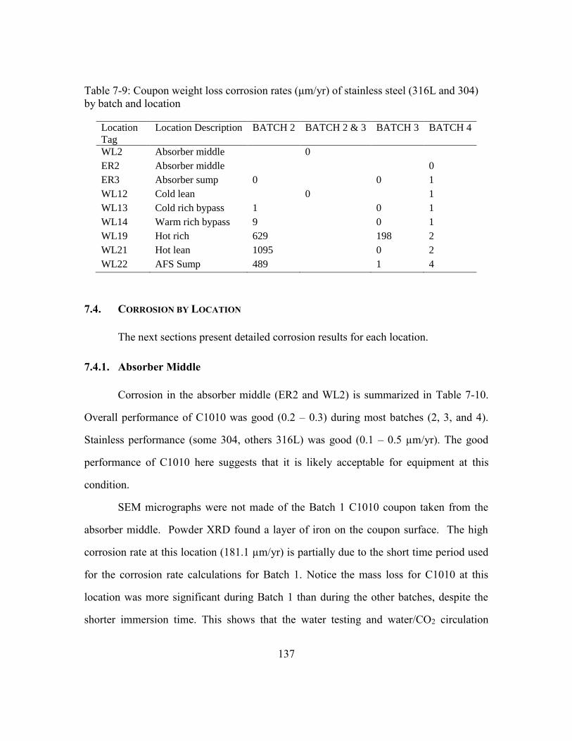
137
Table 7-9: Coupon weight loss corrosion rates (μm/yr) of stainless steel (316L and 304)
by batch and location
Location
Tag
Location Description BATCH 2 BATCH 2 & 3 BATCH 3 BATCH 4
WL2 Absorber middle
0
ER2 Absorber middle
0
ER3 Absorber sump 0
0 1
WL12 Cold lean
0
1
WL13 Cold rich bypass 1
0 1
WL14 Warm rich bypass 9
0 1
WL19 Hot rich 629
198 2
WL21 Hot lean 1095
0 2
WL22 AFS Sump 489
1 4
7.4. CORROSION BY LOCATION
The next sections present detailed corrosion results for each location.
7.4.1. Absorber Middle
Corrosion in the absorber middle (ER2 and WL2) is summarized in Table 7-10.
Overall performance of C1010 was good (0.2 – 0.3) during most batches (2, 3, and 4).
Stainless performance (some 304, others 316L) was good (0.1 – 0.5 µm/yr). The good
performance of C1010 here suggests that it is likely acceptable for equipment at this
condition.
SEM micrographs were not made of the Batch 1 C1010 coupon taken from the
absorber middle. Powder XRD found a layer of iron on the coupon surface. The high
corrosion rate at this location (181.1 µm/yr) is partially due to the short time period used
for the corrosion rate calculations for Batch 1. Notice the mass loss for C1010 at this
location was more significant during Batch 1 than during the other batches, despite the
shorter immersion time. This shows that the water testing and water/CO2 circulation
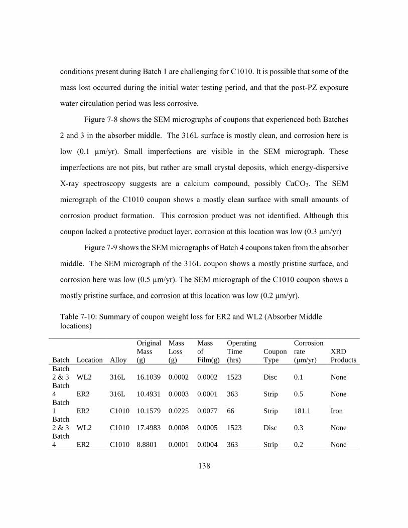
138
conditions present during Batch 1 are challenging for C1010. It is possible that some of the
mass lost occurred during the initial water testing period, and that the post-PZ exposure
water circulation period was less corrosive.
Figure 7-8 shows the SEM micrographs of coupons that experienced both Batches
2 and 3 in the absorber middle. The 316L surface is mostly clean, and corrosion here is
low (0.1 µm/yr). Small imperfections are visible in the SEM micrograph. These
imperfections are not pits, but rather are small crystal deposits, which energy-dispersive
X-ray spectroscopy suggests are a calcium compound, possibly CaCO3. The SEM
micrograph of the C1010 coupon shows a mostly clean surface with small amounts of
corrosion product formation. This corrosion product was not identified. Although this
coupon lacked a protective product layer, corrosion at this location was low (0.3 µm/yr)
Figure 7-9 shows the SEM micrographs of Batch 4 coupons taken from the absorber
middle. The SEM micrograph of the 316L coupon shows a mostly pristine surface, and
corrosion here was low (0.5 µm/yr). The SEM micrograph of the C1010 coupon shows a
mostly pristine surface, and corrosion at this location was low (0.2 µm/yr).
Table 7-10: Summary of coupon weight loss for ER2 and WL2 (Absorber Middle
locations)
Batch Location Alloy
Original
Mass
(g)
Mass
Loss
(g)
Mass
of
Film(g)
Operating
Time
(hrs)
Coupon
Type
Corrosion
rate
(μm/yr)
XRD
Products
Batch
2 & 3 WL2 316L 16.1039 0.0002 0.0002 1523 Disc 0.1 None
Batch
4 ER2 316L 10.4931 0.0003 0.0001 363 Strip 0.5 None
Batch
1 ER2 C1010 10.1579 0.0225 0.0077 66 Strip 181.1 Iron
Batch
2 & 3 WL2 C1010 17.4983 0.0008 0.0005 1523 Disc 0.3 None
Batch
4 ER2 C1010 8.8801 0.0001 0.0004 363 Strip 0.2 None
139
Figure 7-8: (a) 316L and C1010 coupons from Batch 2 and 3 after removal from absorber
middle (WL2). (b) SEM micrograph of 316L coupon. The small imperfections are not
pits, but rather are small crystal deposits, which energy-dispersive X-ray spectroscopy
suggests are a calcium compound, possibly CaCO3. (c) SEM micrograph of C1010,
coupon, showing small amounts of an unidentified corrosion product.
Figure 7-9: (a) 316L and C1010 coupons from Batch 4 after removal from absorber
middle (ER2). (b) SEM micrograph of 316L coupon, showing largely pristine coupon
surface. (c) SEM micrograph of C1010, coupon, showing largely pristine coupon surface.
7.4.2. Absorber Sump
Corrosion in the absorber sump (ER3) is summarized in Table 7-11Table 7-16.
Overall performance of C1010 was good (0.3 – 0.9) during most batches (2, 3, and 4).
140
Stainless performance (some 304, others 316L) was good (0.1 – 0.6 µm/yr). The good
performance of C1010 here suggests that it is likely acceptable for equipment at this
condition.
Figure 7-10 shows the SEM micrograph of a Batch 1 C1010 coupon taken from the
absorber sump. The SEM micrograph of this coupon shows a patchy crystalline layer. This
product was identified as iron by powder XRD. The high corrosion rate at this location
(135.3 µm/yr) is partially due to the short time period used for the corrosion rate
calculations for Batch 1. Notice the mass loss for C1010 at this location was more
significant during Batch 1 than during the other batches, despite the shorter immersion
time. This shows that the water testing and water/CO2 circulation conditions present during
Batch 1 are challenging for C1010. It is possible that some of the mass lost occurred during
the initial water testing period, and that the post-PZ exposure water circulation period was
less corrosive.
Figure 7-11, Figure 7-12, and Figure 7-13 show the coupon images and SEM
micrographs of coupons from the absorber sump during Batch 2, Batch 3, and Batch 4,
respectively. Corrosion of C1010 during these batches was low (0.3 – 0.9 µm/yr), the SEM
micrographs look pristine, and no corrosion products were observed. Corrosion of stainless
steel (some 304, others 316L) was low (0.1 – 0.6 µm/yr), the SEM micrographs look
pristine, and no corrosion products were observed.
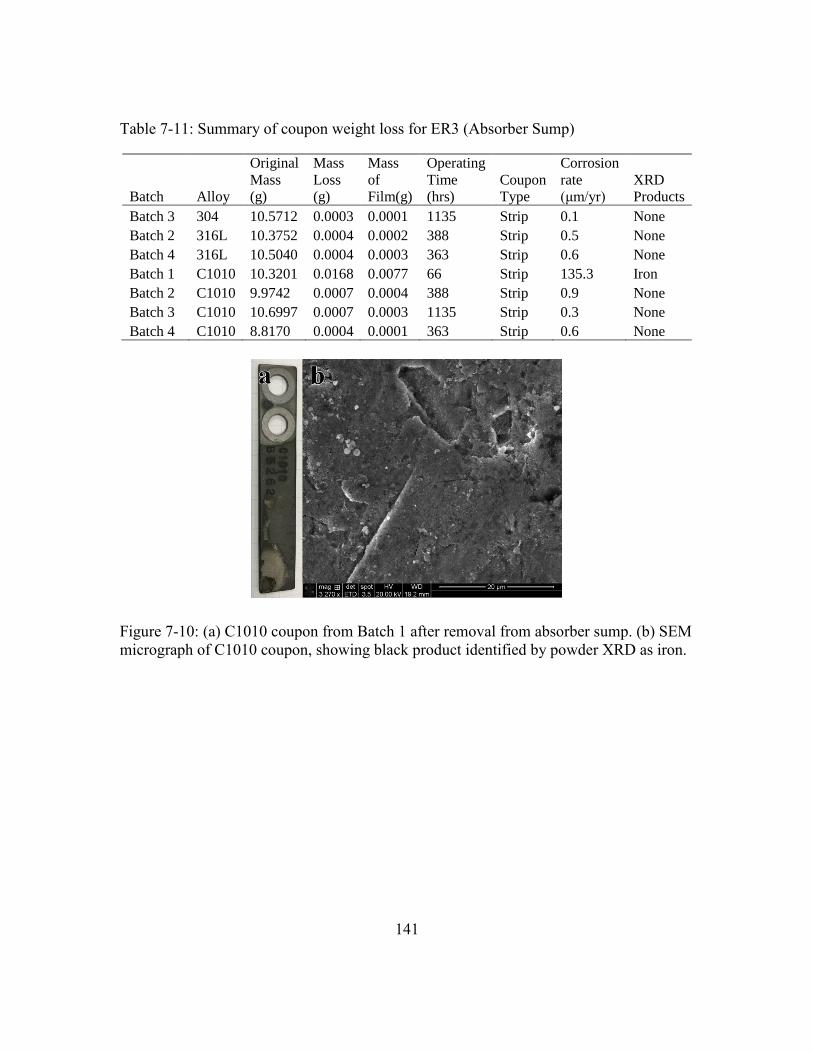
141
Table 7-11: Summary of coupon weight loss for ER3 (Absorber Sump)
Batch Alloy
Original
Mass
(g)
Mass
Loss
(g)
Mass
of
Film(g)
Operating
Time
(hrs)
Coupon
Type
Corrosion
rate
(μm/yr)
XRD
Products
Batch 3 304 10.5712 0.0003 0.0001 1135 Strip 0.1 None
Batch 2 316L 10.3752 0.0004 0.0002 388 Strip 0.5 None
Batch 4 316L 10.5040 0.0004 0.0003 363 Strip 0.6 None
Batch 1 C1010 10.3201 0.0168 0.0077 66 Strip 135.3 Iron
Batch 2 C1010 9.9742 0.0007 0.0004 388 Strip 0.9 None
Batch 3 C1010 10.6997 0.0007 0.0003 1135 Strip 0.3 None
Batch 4 C1010 8.8170 0.0004 0.0001 363 Strip 0.6 None
Figure 7-10: (a) C1010 coupon from Batch 1 after removal from absorber sump. (b) SEM
micrograph of C1010 coupon, showing black product identified by powder XRD as iron.
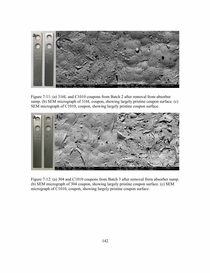
142
Figure 7-11: (a) 316L and C1010 coupons from Batch 2 after removal from absorber
sump. (b) SEM micrograph of 316L coupon, showing largely pristine coupon surface. (c)
SEM micrograph of C1010, coupon, showing largely pristine coupon surface.
Figure 7-12: (a) 304 and C1010 coupons from Batch 3 after removal from absorber sump.
(b) SEM micrograph of 304 coupon, showing largely pristine coupon surface. (c) SEM
micrograph of C1010, coupon, showing largely pristine coupon surface.
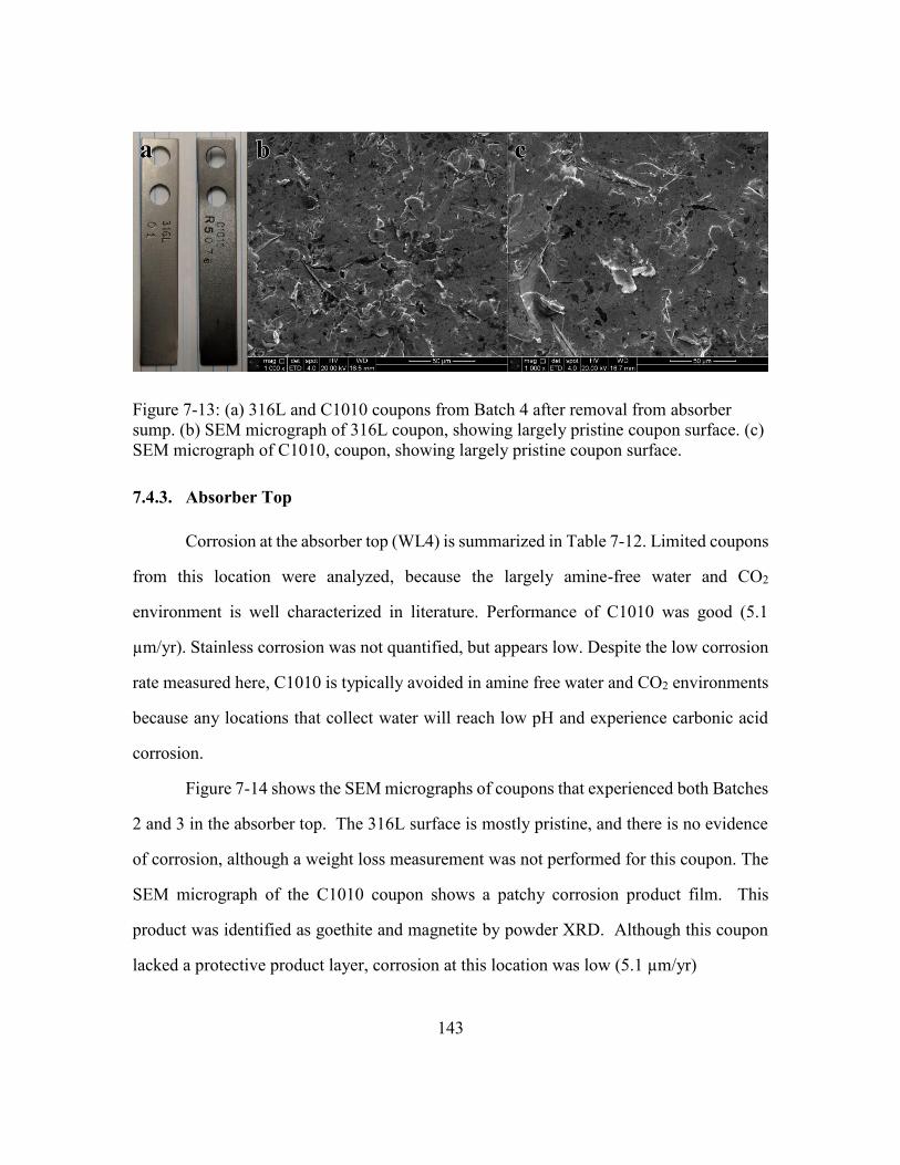
143
Figure 7-13: (a) 316L and C1010 coupons from Batch 4 after removal from absorber
sump. (b) SEM micrograph of 316L coupon, showing largely pristine coupon surface. (c)
SEM micrograph of C1010, coupon, showing largely pristine coupon surface.
7.4.3. Absorber Top
Corrosion at the absorber top (WL4) is summarized in Table 7-12. Limited coupons
from this location were analyzed, because the largely amine-free water and CO2
environment is well characterized in literature. Performance of C1010 was good (5.1
µm/yr). Stainless corrosion was not quantified, but appears low. Despite the low corrosion
rate measured here, C1010 is typically avoided in amine free water and CO2 environments
because any locations that collect water will reach low pH and experience carbonic acid
corrosion.
Figure 7-14 shows the SEM micrographs of coupons that experienced both Batches
2 and 3 in the absorber top. The 316L surface is mostly pristine, and there is no evidence
of corrosion, although a weight loss measurement was not performed for this coupon. The
SEM micrograph of the C1010 coupon shows a patchy corrosion product film. This
product was identified as goethite and magnetite by powder XRD. Although this coupon
lacked a protective product layer, corrosion at this location was low (5.1 µm/yr)
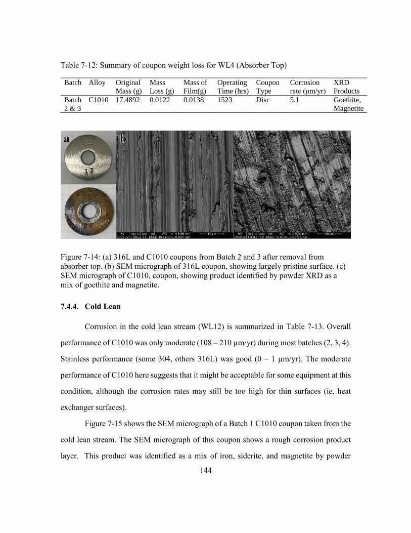
144
Table 7-12: Summary of coupon weight loss for WL4 (Absorber Top)
Batch Alloy Original
Mass (g)
Mass
Loss (g)
Mass of
Film(g)
Operating
Time (hrs)
Coupon
Type
Corrosion
rate (μm/yr)
XRD
Products
Batch
2 & 3
C1010 17.4892 0.0122 0.0138 1523 Disc 5.1 Goethite,
Magnetite
Figure 7-14: (a) 316L and C1010 coupons from Batch 2 and 3 after removal from
absorber top. (b) SEM micrograph of 316L coupon, showing largely pristine surface. (c)
SEM micrograph of C1010, coupon, showing product identified by powder XRD as a
mix of goethite and magnetite.
7.4.4. Cold Lean
Corrosion in the cold lean stream (WL12) is summarized in Table 7-13. Overall
performance of C1010 was only moderate (108 – 210 µm/yr) during most batches (2, 3, 4).
Stainless performance (some 304, others 316L) was good (0 – 1 µm/yr). The moderate
performance of C1010 here suggests that it might be acceptable for some equipment at this
condition, although the corrosion rates may still be too high for thin surfaces (ie, heat
exchanger surfaces).
Figure 7-15 shows the SEM micrograph of a Batch 1 C1010 coupon taken from the
cold lean stream. The SEM micrograph of this coupon shows a rough corrosion product
layer. This product was identified as a mix of iron, siderite, and magnetite by powder
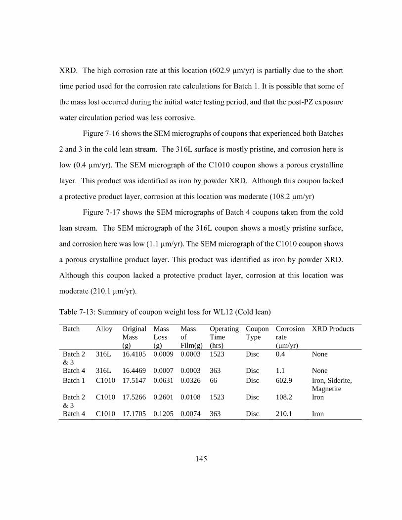
145
XRD. The high corrosion rate at this location (602.9 µm/yr) is partially due to the short
time period used for the corrosion rate calculations for Batch 1. It is possible that some of
the mass lost occurred during the initial water testing period, and that the post-PZ exposure
water circulation period was less corrosive.
Figure 7-16 shows the SEM micrographs of coupons that experienced both Batches
2 and 3 in the cold lean stream. The 316L surface is mostly pristine, and corrosion here is
low (0.4 µm/yr). The SEM micrograph of the C1010 coupon shows a porous crystalline
layer. This product was identified as iron by powder XRD. Although this coupon lacked
a protective product layer, corrosion at this location was moderate (108.2 µm/yr)
Figure 7-17 shows the SEM micrographs of Batch 4 coupons taken from the cold
lean stream. The SEM micrograph of the 316L coupon shows a mostly pristine surface,
and corrosion here was low (1.1 µm/yr). The SEM micrograph of the C1010 coupon shows
a porous crystalline product layer. This product was identified as iron by powder XRD.
Although this coupon lacked a protective product layer, corrosion at this location was
moderate (210.1 µm/yr).
Table 7-13: Summary of coupon weight loss for WL12 (Cold lean)
Batch Alloy Original
Mass
(g)
Mass
Loss
(g)
Mass
of
Film(g)
Operating
Time
(hrs)
Coupon
Type
Corrosion
rate
(μm/yr)
XRD Products
Batch 2
& 3
316L 16.4105 0.0009 0.0003 1523 Disc 0.4 None
Batch 4 316L 16.4469 0.0007 0.0003 363 Disc 1.1 None
Batch 1 C1010 17.5147 0.0631 0.0326 66 Disc 602.9 Iron, Siderite,
Magnetite
Batch 2
& 3
C1010 17.5266 0.2601 0.0108 1523 Disc 108.2 Iron
Batch 4 C1010 17.1705 0.1205 0.0074 363 Disc 210.1 Iron
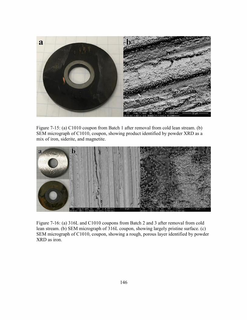
146
Figure 7-15: (a) C1010 coupon from Batch 1 after removal from cold lean stream. (b)
SEM micrograph of C1010, coupon, showing product identified by powder XRD as a
mix of iron, siderite, and magnetite.
Figure 7-16: (a) 316L and C1010 coupons from Batch 2 and 3 after removal from cold
lean stream. (b) SEM micrograph of 316L coupon, showing largely pristine surface. (c)
SEM micrograph of C1010, coupon, showing a rough, porous layer identified by powder
XRD as iron.
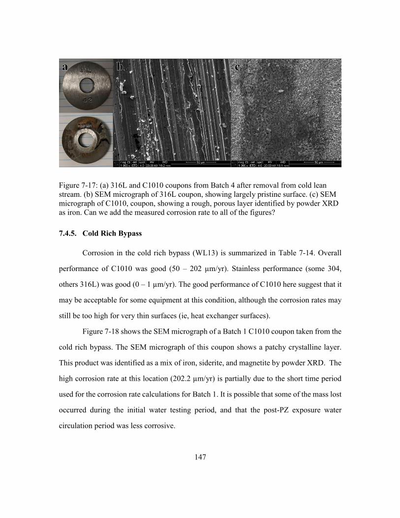
147
Figure 7-17: (a) 316L and C1010 coupons from Batch 4 after removal from cold lean
stream. (b) SEM micrograph of 316L coupon, showing largely pristine surface. (c) SEM
micrograph of C1010, coupon, showing a rough, porous layer identified by powder XRD
as iron. Can we add the measured corrosion rate to all of the figures?
7.4.5. Cold Rich Bypass
Corrosion in the cold rich bypass (WL13) is summarized in Table 7-14. Overall
performance of C1010 was good (50 – 202 µm/yr). Stainless performance (some 304,
others 316L) was good (0 – 1 µm/yr). The good performance of C1010 here suggest that it
may be acceptable for some equipment at this condition, although the corrosion rates may
still be too high for very thin surfaces (ie, heat exchanger surfaces).
Figure 7-18 shows the SEM micrograph of a Batch 1 C1010 coupon taken from the
cold rich bypass. The SEM micrograph of this coupon shows a patchy crystalline layer.
This product was identified as a mix of iron, siderite, and magnetite by powder XRD. The
high corrosion rate at this location (202.2 µm/yr) is partially due to the short time period
used for the corrosion rate calculations for Batch 1. It is possible that some of the mass lost
occurred during the initial water testing period, and that the post-PZ exposure water
circulation period was less corrosive.
148
Figure 7-19 shows the SEM micrographs of Batch 2 coupons taken from the warm
rich bypass. The 316L surface is mostly pristine, and corrosion here is low (0.7 µm/yr).
The SEM micrograph of the C1010 coupon shows a somewhat porous crystalline layer.
This product was identified as iron by powder XRD. Although this coupon lacked a
protective product layer, corrosion at this location was moderate (96.8 µm/yr)
Figure 7-20Figure 7-28 shows the SEM micrographs of Batch 3 coupons taken
from the warm rich bypass. The 304 coupon has a mostly pristine appearance and corrosion
was low (0.0 µm/yr). The SEM micrograph of the C1010 coupon shows a crystalline
product layer. This product was identified as a mix of iron and siderite by powder XRD.
This layer was apparently protective, and corrosion at this location was low (50.3 µm/yr).
Figure 7-21 shows the SEM micrographs of Batch 4 coupons taken from the warm
rich bypass. The SEM micrograph of the 316L coupon shows a mostly pristine surface,
and corrosion here was low (1.0 µm/yr). The SEM micrograph of the C1010 coupon shows
a crystalline product layer. This product was identified as a mix of siderite and iron by
powder XRD. Corrosion at this location was moderate (103.4 µm/yr).
Table 7-14: Summary of coupon weight loss for WL13 (Cold rich bypass)
Batch Alloy Original
Mass
(g)
Mass
Loss
(g)
Mass
of
Film(g)
Operating
Time
(hrs)
Coupon
Type
Corrosion
rate
(μm/yr)
XRD Products
Batch 3 304 10.5690 0.0000 -
0.0001
879 Strip 0.0 None
Batch 2 316L 10.3744 0.0005 0.0001 388 Strip 0.7 None
Batch 4 316L 10.3729 0.0007 0.0003 363 Strip 1.0 None
Batch 1 C1010 9.9648 0.0252 0.0119 66 Strip 202.2 Iron, Siderite,
Magnetite
Batch 2 C1010 9.8353 0.0705 0.0453 388 Strip 96.8 Iron
Batch 3 C1010 9.8037 0.0831 0.0319 879 Strip 50.3 Iron, Siderite
Batch 4 C1010 10.7251 0.0705 0.0282 363 Strip 103.4 Siderite, Iron

149
Figure 7-18: (a) C1010 coupon from Batch 1 after removal from cold rich bypass. (b)
SEM micrograph of C1010, coupon, showing patchy layer identified by powder XRD as
a mix of iron, siderite, and magnetite.
Figure 7-19: (a) 316L and C1010 coupons from Batch 2 after removal from cold rich
bypass. (b) SEM micrograph of 316L coupon, showing largely pristine surface. (c) SEM
micrograph of C1010, coupon, showing a rough layer identified by powder XRD as iron.
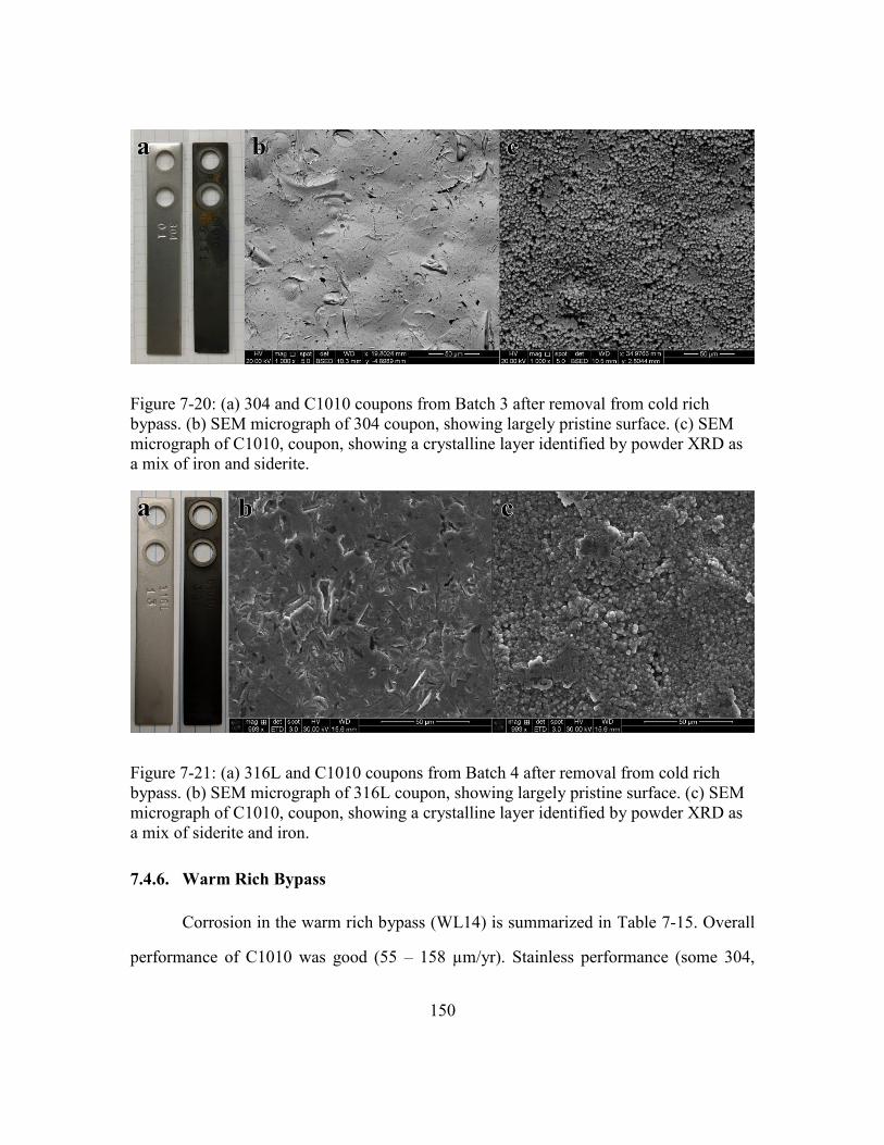
150
Figure 7-20: (a) 304 and C1010 coupons from Batch 3 after removal from cold rich
bypass. (b) SEM micrograph of 304 coupon, showing largely pristine surface. (c) SEM
micrograph of C1010, coupon, showing a crystalline layer identified by powder XRD as
a mix of iron and siderite.
Figure 7-21: (a) 316L and C1010 coupons from Batch 4 after removal from cold rich
bypass. (b) SEM micrograph of 316L coupon, showing largely pristine surface. (c) SEM
micrograph of C1010, coupon, showing a crystalline layer identified by powder XRD as
a mix of siderite and iron.
7.4.6. Warm Rich Bypass
Corrosion in the warm rich bypass (WL14) is summarized in Table 7-15. Overall
performance of C1010 was good (55 – 158 µm/yr). Stainless performance (some 304,

151
others 316L) was good (0 – 9 µm/yr). The good performance of C1010 here suggests that
it may be acceptable for some equipment at this condition, although the corrosion rates
may still be too high for very thin surfaces (ie, heat exchanger surfaces).
Figure 7-22 shows the SEM micrograph of a Batch 1 C1010 coupon taken from the
warm rich bypass. The SEM micrograph of this coupon shows a regular, crystalline layer.
This product was identified as a mix of siderite and magnetite by powder XRD. The high
corrosion rate at this location (157.5 µm/yr) is partially due to the short time period used
for the corrosion rate calculations for Batch 1. It is possible that some of the mass lost
occurred during the initial water testing period, and that the post-PZ exposure water
circulation period was slightly more protected by the siderite/magnetite layer.
Figure 7-23 shows the SEM micrographs of Batch 2 coupons taken from the warm
rich bypass. The 316L surface is slightly etched, but corrosion here is low (9.0 µm/yr).
The SEM micrograph of the C1010 coupon shows an irregular crystalline layer. This
product was identified as goethite by powder XRD. Despite the irregular product layer,
corrosion at this location was low (54.8 µm/yr)
Figure 7-24 shows the SEM micrographs of Batch 3 coupons taken from the warm
rich bypass. The 304 coupon has a mostly pristine appearance and corrosion was low (0.3
µm/yr). The SEM micrograph of the C1010 coupon shows an irregular product layer. This
product was identified as a mix of siderite and goethite by powder XRD. Despite the
irregular product layer, corrosion at this location was low (47.0 µm/yr)
Figure 7-25 shows the SEM micrographs of Batch 4 coupons taken from the warm
rich bypass. The SEM micrograph of the 316L coupon shows a mostly pristine surface,
and corrosion here was low (1.2 µm/yr). The SEM micrograph of the C1010 coupon shows
a patchy, crystalline product layer. This product was identified as a mix of siderite by
powder XRD. Corrosion at this location was moderate (92.2 µm/yr)
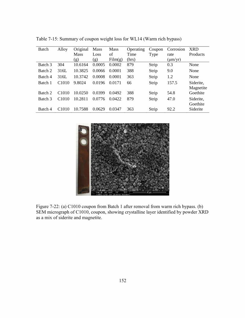
152
Table 7-15: Summary of coupon weight loss for WL14 (Warm rich bypass)
Batch Alloy Original
Mass
(g)
Mass
Loss
(g)
Mass
of
Film(g)
Operating
Time
(hrs)
Coupon
Type
Corrosion
rate
(μm/yr)
XRD
Products
Batch 3 304 10.6164 0.0005 0.0002 879 Strip 0.3 None
Batch 2 316L 10.3825 0.0066 0.0001 388 Strip 9.0 None
Batch 4 316L 10.3742 0.0008 0.0001 363 Strip 1.2 None
Batch 1 C1010 9.8024 0.0196 0.0171 66 Strip 157.5 Siderite,
Magnetite
Batch 2 C1010 10.0250 0.0399 0.0492 388 Strip 54.8 Goethite
Batch 3 C1010 10.2811 0.0776 0.0422 879 Strip 47.0 Siderite,
Goethite
Batch 4 C1010 10.7588 0.0629 0.0347 363 Strip 92.2 Siderite
Figure 7-22: (a) C1010 coupon from Batch 1 after removal from warm rich bypass. (b)
SEM micrograph of C1010, coupon, showing crystalline layer identified by powder XRD
as a mix of siderite and magnetite.
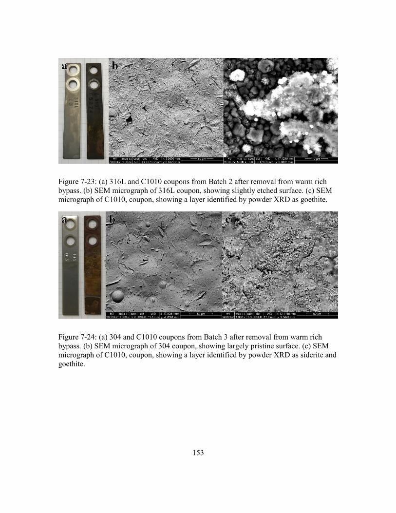
153
Figure 7-23: (a) 316L and C1010 coupons from Batch 2 after removal from warm rich
bypass. (b) SEM micrograph of 316L coupon, showing slightly etched surface. (c) SEM
micrograph of C1010, coupon, showing a layer identified by powder XRD as goethite.
Figure 7-24: (a) 304 and C1010 coupons from Batch 3 after removal from warm rich
bypass. (b) SEM micrograph of 304 coupon, showing largely pristine surface. (c) SEM
micrograph of C1010, coupon, showing a layer identified by powder XRD as siderite and
goethite.
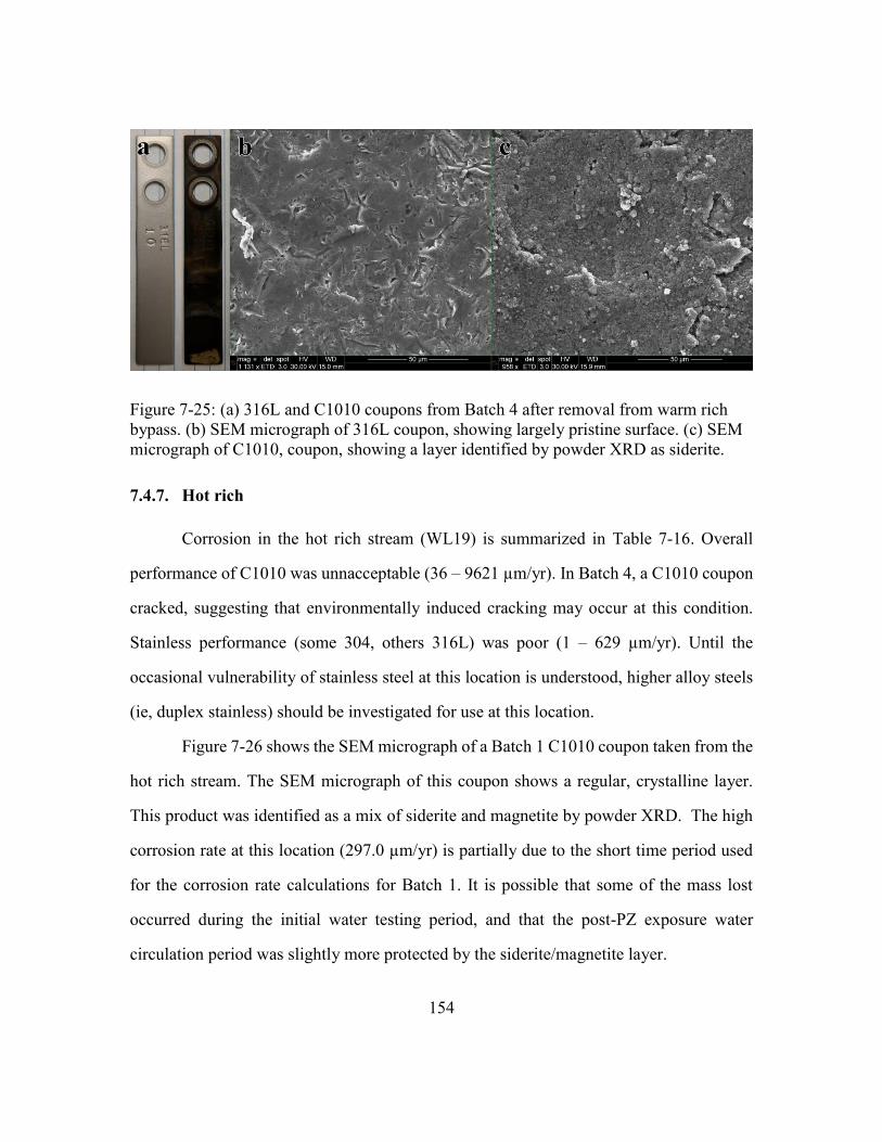
154
Figure 7-25: (a) 316L and C1010 coupons from Batch 4 after removal from warm rich
bypass. (b) SEM micrograph of 316L coupon, showing largely pristine surface. (c) SEM
micrograph of C1010, coupon, showing a layer identified by powder XRD as siderite.
7.4.7. Hot rich
Corrosion in the hot rich stream (WL19) is summarized in Table 7-16. Overall
performance of C1010 was unnacceptable (36 – 9621 µm/yr). In Batch 4, a C1010 coupon
cracked, suggesting that environmentally induced cracking may occur at this condition.
Stainless performance (some 304, others 316L) was poor (1 – 629 µm/yr). Until the
occasional vulnerability of stainless steel at this location is understood, higher alloy steels
(ie, duplex stainless) should be investigated for use at this location.
Figure 7-26 shows the SEM micrograph of a Batch 1 C1010 coupon taken from the
hot rich stream. The SEM micrograph of this coupon shows a regular, crystalline layer.
This product was identified as a mix of siderite and magnetite by powder XRD. The high
corrosion rate at this location (297.0 µm/yr) is partially due to the short time period used
for the corrosion rate calculations for Batch 1. It is possible that some of the mass lost
occurred during the initial water testing period, and that the post-PZ exposure water
circulation period was slightly more protected by the siderite/magnetite layer.
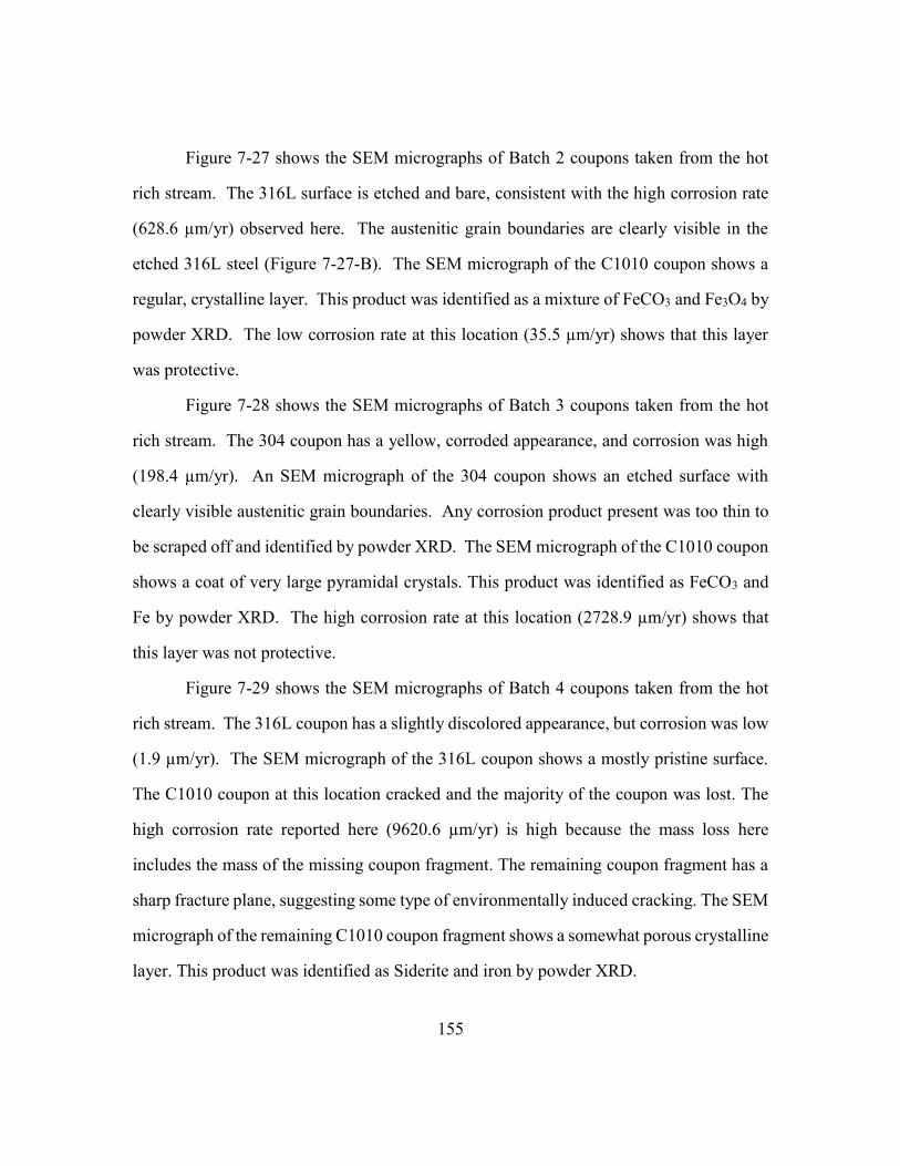
155
Figure 7-27 shows the SEM micrographs of Batch 2 coupons taken from the hot
rich stream. The 316L surface is etched and bare, consistent with the high corrosion rate
(628.6 µm/yr) observed here. The austenitic grain boundaries are clearly visible in the
etched 316L steel (Figure 7-27-B). The SEM micrograph of the C1010 coupon shows a
regular, crystalline layer. This product was identified as a mixture of FeCO3 and Fe3O4 by
powder XRD. The low corrosion rate at this location (35.5 µm/yr) shows that this layer
was protective.
Figure 7-28 shows the SEM micrographs of Batch 3 coupons taken from the hot
rich stream. The 304 coupon has a yellow, corroded appearance, and corrosion was high
(198.4 µm/yr). An SEM micrograph of the 304 coupon shows an etched surface with
clearly visible austenitic grain boundaries. Any corrosion product present was too thin to
be scraped off and identified by powder XRD. The SEM micrograph of the C1010 coupon
shows a coat of very large pyramidal crystals. This product was identified as FeCO3 and
Fe by powder XRD. The high corrosion rate at this location (2728.9 µm/yr) shows that
this layer was not protective.
Figure 7-29 shows the SEM micrographs of Batch 4 coupons taken from the hot
rich stream. The 316L coupon has a slightly discolored appearance, but corrosion was low
(1.9 µm/yr). The SEM micrograph of the 316L coupon shows a mostly pristine surface.
The C1010 coupon at this location cracked and the majority of the coupon was lost. The
high corrosion rate reported here (9620.6 µm/yr) is high because the mass loss here
includes the mass of the missing coupon fragment. The remaining coupon fragment has a
sharp fracture plane, suggesting some type of environmentally induced cracking. The SEM
micrograph of the remaining C1010 coupon fragment shows a somewhat porous crystalline
layer. This product was identified as Siderite and iron by powder XRD.
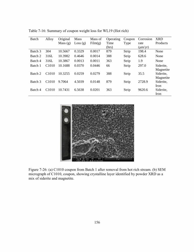
156
Table 7-16: Summary of coupon weight loss for WL19 (Hot rich)
Batch Alloy Original
Mass (g)
Mass
Loss (g)
Mass of
Film(g)
Operating
Time
(hrs)
Coupon
Type
Corrosion
rate
(μm/yr)
XRD
Products
Batch 3 304 10.5667 0.3329 0.0017 879 Strip 198.4 None
Batch 2 316L 10.3982 0.4646 0.0014 388 Strip 628.6 None
Batch 4 316L 10.3867 0.0013 0.0011 363 Strip 1.9 None
Batch 1 C1010 10.1688 0.0370 0.0446 66 Strip 297.0 Siderite,
Magnetite
Batch 2 C1010 10.3255 0.0259 0.0279 388 Strip 35.5 Siderite,
Magnetite
Batch 3 C1010 9.7064 4.5039 0.0148 879 Strip 2728.9 Siderite,
Iron
Batch 4 C1010 10.7431 6.5638 0.0201 363 Strip 9620.6 Siderite,
Iron
Figure 7-26: (a) C1010 coupon from Batch 1 after removal from hot rich stream. (b) SEM
micrograph of C1010, coupon, showing crystalline layer identified by powder XRD as a
mix of siderite and magnetite.
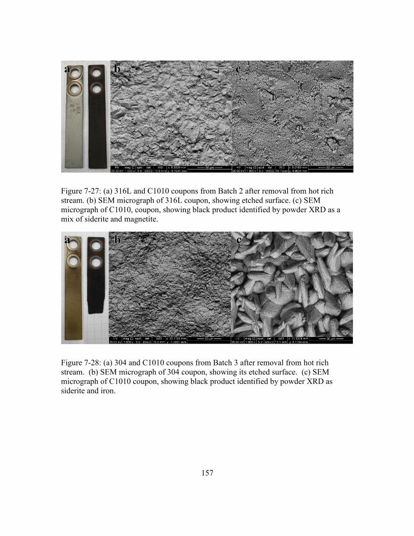
157
Figure 7-27: (a) 316L and C1010 coupons from Batch 2 after removal from hot rich
stream. (b) SEM micrograph of 316L coupon, showing etched surface. (c) SEM
micrograph of C1010, coupon, showing black product identified by powder XRD as a
mix of siderite and magnetite.
Figure 7-28: (a) 304 and C1010 coupons from Batch 3 after removal from hot rich
stream. (b) SEM micrograph of 304 coupon, showing its etched surface. (c) SEM
micrograph of C1010 coupon, showing black product identified by powder XRD as
siderite and iron.
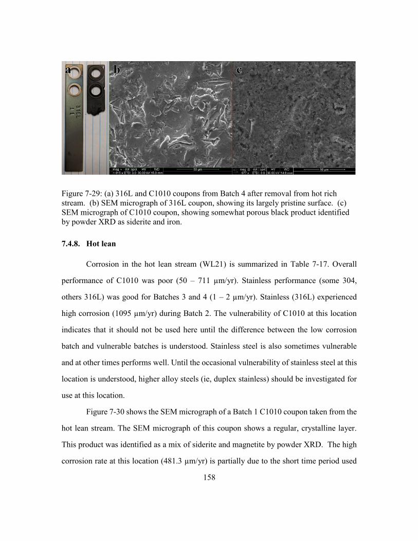
158
Figure 7-29: (a) 316L and C1010 coupons from Batch 4 after removal from hot rich
stream. (b) SEM micrograph of 316L coupon, showing its largely pristine surface. (c)
SEM micrograph of C1010 coupon, showing somewhat porous black product identified
by powder XRD as siderite and iron.
7.4.8. Hot lean
Corrosion in the hot lean stream (WL21) is summarized in Table 7-17. Overall
performance of C1010 was poor (50 – 711 µm/yr). Stainless performance (some 304,
others 316L) was good for Batches 3 and 4 (1 – 2 µm/yr). Stainless (316L) experienced
high corrosion (1095 µm/yr) during Batch 2. The vulnerability of C1010 at this location
indicates that it should not be used here until the difference between the low corrosion
batch and vulnerable batches is understood. Stainless steel is also sometimes vulnerable
and at other times performs well. Until the occasional vulnerability of stainless steel at this
location is understood, higher alloy steels (ie, duplex stainless) should be investigated for
use at this location.
Figure 7-30 shows the SEM micrograph of a Batch 1 C1010 coupon taken from the
hot lean stream. The SEM micrograph of this coupon shows a regular, crystalline layer.
This product was identified as a mix of siderite and magnetite by powder XRD. The high
corrosion rate at this location (481.3 µm/yr) is partially due to the short time period used
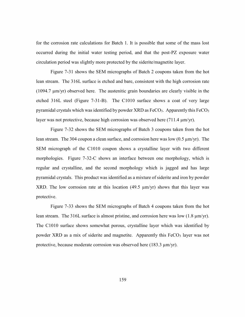
159
for the corrosion rate calculations for Batch 1. It is possible that some of the mass lost
occurred during the initial water testing period, and that the post-PZ exposure water
circulation period was slightly more protected by the siderite/magnetite layer.
Figure 7-31 shows the SEM micrographs of Batch 2 coupons taken from the hot
lean stream. The 316L surface is etched and bare, consistent with the high corrosion rate
(1094.7 µm/yr) observed here. The austenitic grain boundaries are clearly visible in the
etched 316L steel (Figure 7-31-B). The C1010 surface shows a coat of very large
pyramidal crystals which was identified by powder XRD as FeCO3. Apparently this FeCO3
layer was not protective, because high corrosion was observed here (711.4 µm/yr).
Figure 7-32 shows the SEM micrographs of Batch 3 coupons taken from the hot
lean stream. The 304 coupon a clean surface, and corrosion here was low (0.5 µm/yr). The
SEM micrograph of the C1010 coupon shows a crystalline layer with two different
morphologies. Figure 7-32-C shows an interface between one morphology, which is
regular and crystalline, and the second morphology which is jagged and has large
pyramidal crystals. This product was identified as a mixture of siderite and iron by powder
XRD. The low corrosion rate at this location (49.5 µm/yr) shows that this layer was
protective.
Figure 7-33 shows the SEM micrographs of Batch 4 coupons taken from the hot
lean stream. The 316L surface is almost pristine, and corrosion here was low (1.8 µm/yr).
The C1010 surface shows somewhat porous, crystalline layer which was identified by
powder XRD as a mix of siderite and magnetite. Apparently this FeCO3 layer was not
protective, because moderate corrosion was observed here (183.3 µm/yr).

160
Table 7-17: Summary of coupon weight loss for WL21 (Hot lean)
Batch Alloy Original
Mass (g)
Mass
Loss (g)
Mass of
Film(g)
Operating
Time
(hrs)
Coupon
Type
Corrosion
rate
(μm/yr)
XRD
Products
Batch 3 304 10.6129 0.0008 0.0000 879 Strip 0.5 None
Batch 2 316L 10.3775 0.8091 0.0002 388 Strip 1094.7 None
Batch 4 316L 10.3820 0.0013 0.0001 363 Strip 1.8 None
Batch 1 C1010 10.2730 0.0599 0.0517 66 Strip 481.3 Siderite,
Magnetite
Batch 2 C1010 9.6961 0.5186 0.0349 388 Strip 711.4 Siderite
Batch 3 C1010 9.8722 0.0816 0.0180 879 Strip 49.5 Siderite,
Iron
Batch 4 C1010 10.7270 0.1254 0.0471 363 Strip 183.8 Siderite,
Magnetite
Figure 7-30: (a) C1010 coupon from Batch 1 after removal from hot lean stream. (b)
SEM micrograph of C1010, coupon, showing crystalline layer identified by powder XRD
as siderite.
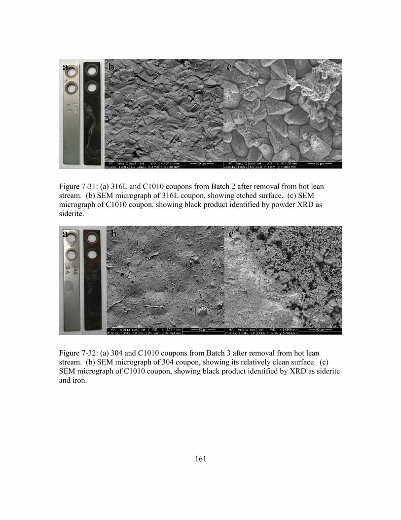
161
Figure 7-31: (a) 316L and C1010 coupons from Batch 2 after removal from hot lean
stream. (b) SEM micrograph of 316L coupon, showing etched surface. (c) SEM
micrograph of C1010 coupon, showing black product identified by powder XRD as
siderite.
Figure 7-32: (a) 304 and C1010 coupons from Batch 3 after removal from hot lean
stream. (b) SEM micrograph of 304 coupon, showing its relatively clean surface. (c)
SEM micrograph of C1010 coupon, showing black product identified by XRD as siderite
and iron.
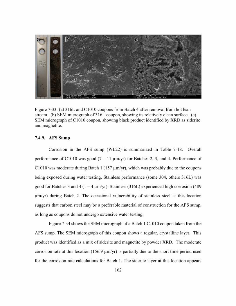
162
Figure 7-33: (a) 316L and C1010 coupons from Batch 4 after removal from hot lean
stream. (b) SEM micrograph of 316L coupon, showing its relatively clean surface. (c)
SEM micrograph of C1010 coupon, showing black product identified by XRD as siderite
and magnetite.
7.4.9. AFS Sump
Corrosion in the AFS sump (WL22) is summarized in Table 7-18. Overall
performance of C1010 was good (7 – 11 µm/yr) for Batches 2, 3, and 4. Performance of
C1010 was moderate during Batch 1 (157 µm/yr), which was probably due to the coupons
being exposed during water testing. Stainless performance (some 304, others 316L) was
good for Batches 3 and 4 (1 – 4 µm/yr). Stainless (316L) experienced high corrosion (489
µm/yr) during Batch 2. The occasional vulnerability of stainless steel at this location
suggests that carbon steel may be a preferable material of construction for the AFS sump,
as long as coupons do not undergo extensive water testing.
Figure 7-34 shows the SEM micrograph of a Batch 1 C1010 coupon taken from the
AFS sump. The SEM micrograph of this coupon shows a regular, crystalline layer. This
product was identified as a mix of siderite and magnetite by powder XRD. The moderate
corrosion rate at this location (156.9 µm/yr) is partially due to the short time period used
for the corrosion rate calculations for Batch 1. The siderite layer at this location appears
163
crystalline, but it was not fully protective. Notice the mass loss for C1010 at this location
was more significant than during the other batches, despite the shorter immersion time.
This shows that the water testing and water/CO2 circulation conditions present during
Batch 1 are challenging for C1010. It is possible that most of the mass lost occurred during
the initial water testing period, and that the post-PZ exposure water circulation period was
protected by the siderite/magnetite layer. Magnetite was only detected at this location in
Batch 1, which suggests that water/CO2 circulation converts the PZ-promoted siderite layer
to magnetite.
Figure 7-35 shows the SEM micrographs of Batch 2 coupons taken from the AFS
sump. The 316L coupon is covered with a flakey, non-protective layer of rosette crystals.
This was the only coupon where a thick corrosion product film was detected on stainless
steel. Powder XRD identified this layer as siderite. The high corrosion rate (488.8 µm/yr)
shows that this layer was not protective. The SEM micrograph of the C1010 coupon shows
a regular, crystalline layer. This product was identified as FeCO3 by powder XRD. The
low corrosion rate at this location (6.9 µm/yr) shows that this layer was protective.
Figure 7-36 shows the SEM micrographs of Batch 3 coupons taken from the AFS
sump. The 304 coupon had nearly pristine appearance, and corrosion was very low (0.6
µm/yr). The SEM micrograph of the C1010 coupon shows a regular, crystalline layer.
This product was identified as FeCO3 by powder XRD. The low corrosion rate at this
location (6.9 µm/yr) shows that this layer was protective.
Figure 7-37 shows the SEM micrographs of Batch 4 coupons taken from the AFS
sump. The 316L coupon looks slightly etched, but and corrosion was very low (4.4 µm/yr).
The SEM micrograph of the C1010 coupon shows a regular, crystalline layer. This product
was identified as a mix of iron and siderite by powder XRD. The low corrosion rate at this
location (11.1 µm/yr) shows that this layer was protective.
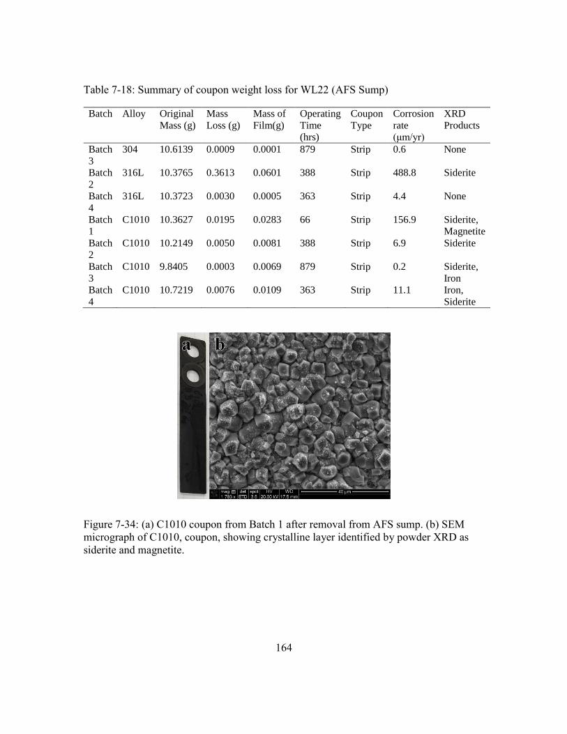
164
Table 7-18: Summary of coupon weight loss for WL22 (AFS Sump)
Batch Alloy Original
Mass (g)
Mass
Loss (g)
Mass of
Film(g)
Operating
Time
(hrs)
Coupon
Type
Corrosion
rate
(μm/yr)
XRD
Products
Batch
3
304 10.6139 0.0009 0.0001 879 Strip 0.6 None
Batch
2
316L 10.3765 0.3613 0.0601 388 Strip 488.8 Siderite
Batch
4
316L 10.3723 0.0030 0.0005 363 Strip 4.4 None
Batch
1
C1010 10.3627 0.0195 0.0283 66 Strip 156.9 Siderite,
Magnetite
Batch
2
C1010 10.2149 0.0050 0.0081 388 Strip 6.9 Siderite
Batch
3
C1010 9.8405 0.0003 0.0069 879 Strip 0.2 Siderite,
Iron
Batch
4
C1010 10.7219 0.0076 0.0109 363 Strip 11.1 Iron,
Siderite
Figure 7-34: (a) C1010 coupon from Batch 1 after removal from AFS sump. (b) SEM
micrograph of C1010, coupon, showing crystalline layer identified by powder XRD as
siderite and magnetite.
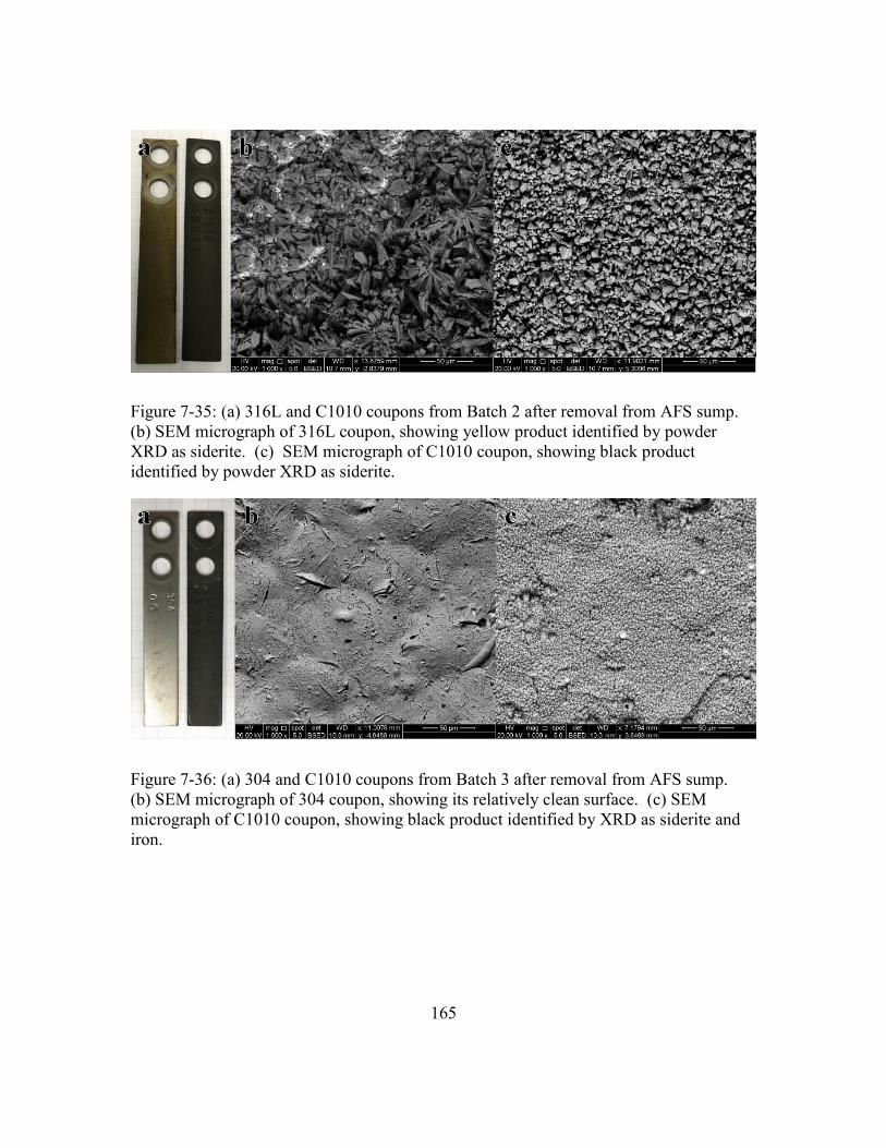
165
Figure 7-35: (a) 316L and C1010 coupons from Batch 2 after removal from AFS sump.
(b) SEM micrograph of 316L coupon, showing yellow product identified by powder
XRD as siderite. (c) SEM micrograph of C1010 coupon, showing black product
identified by powder XRD as siderite.
Figure 7-36: (a) 304 and C1010 coupons from Batch 3 after removal from AFS sump.
(b) SEM micrograph of 304 coupon, showing its relatively clean surface. (c) SEM
micrograph of C1010 coupon, showing black product identified by XRD as siderite and
iron.
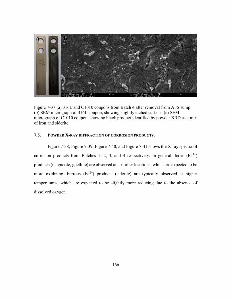
166
Figure 7-37:(a) 316L and C1010 coupons from Batch 4 after removal from AFS sump.
(b) SEM micrograph of 316L coupon, showing slightly etched surface. (c) SEM
micrograph of C1010 coupon, showing black product identified by powder XRD as a mix
of iron and siderite.
7.5. POWDER X-RAY DIFFRACTION OF CORROSION PRODUCTS.
Figure 7-38, Figure 7-39, Figure 7-40, and Figure 7-41 shows the X-ray spectra of
corrosion products from Batches 1, 2, 3, and 4 respectively. In general, ferric (Fe3+)
products (magnetite, goethite) are observed at absorber locations, which are expected to be
more oxidizing. Ferrous (Fe2+) products (siderite) are typically observed at higher
temperatures, which are expected to be slightly more reducing due to the absence of
dissolved oxygen.
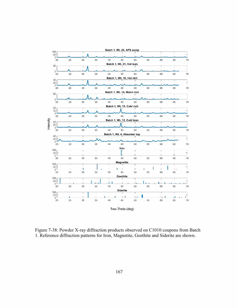
167
Figure 7-38: Powder X-ray diffraction products observed on C1010 coupons from Batch
1. Reference diffraction patterns for Iron, Magnetite, Goethite and Siderite are shown.
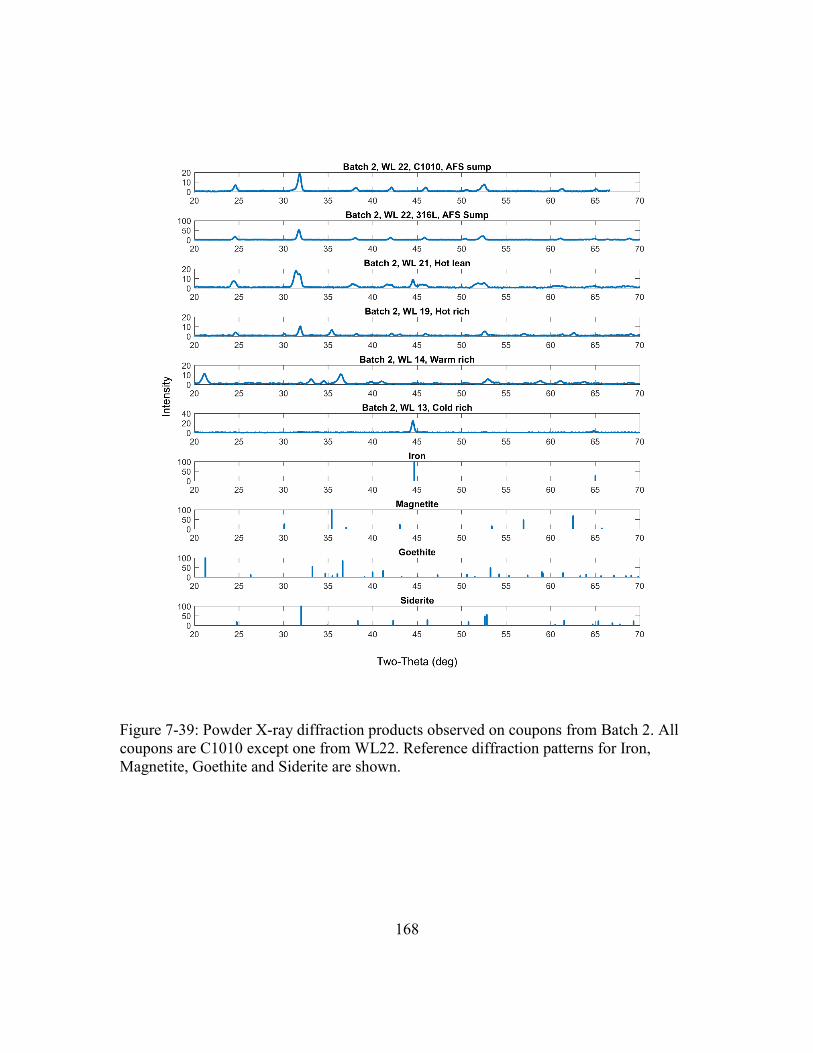
168
Figure 7-39: Powder X-ray diffraction products observed on coupons from Batch 2. All
coupons are C1010 except one from WL22. Reference diffraction patterns for Iron,
Magnetite, Goethite and Siderite are shown.

169
Figure 7-40: Powder X-ray diffraction products observed on C1010 coupons from Batch
3. Coupons from WL12 and WL4 experienced corrosion during Batch 2 and Batch 3.
Reference diffraction patterns for Iron, Magnetite, Goethite and Siderite are shown.
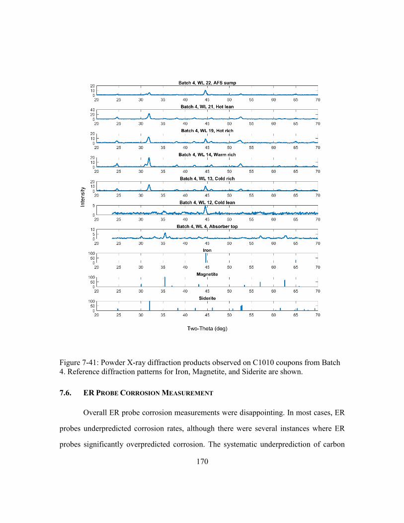
170
Figure 7-41: Powder X-ray diffraction products observed on C1010 coupons from Batch
4. Reference diffraction patterns for Iron, Magnetite, and Siderite are shown.
7.6. ER PROBE CORROSION MEASUREMENT
Overall ER probe corrosion measurements were disappointing. In most cases, ER
probes underpredicted corrosion rates, although there were several instances where ER
probes significantly overpredicted corrosion. The systematic underprediction of carbon
171
steel corrosion rates could be because corrosion product films altered the electrical
resistance measurement. Stainless steel measurements could have been impacted by
periodic cleaning of the probes with concentrated HCl, which is not recommended for use
with stainless (ASTM, 2017) due to pitting (Jones, 1996).
ER readings were continuous, but daily averages are used for corrosion rate
determination to reduce instrument noise. Daily readings were plotted versus operating
hours, then the method of least squares was used to determine a corrosion rate over the
operating period. Using operating hours assumes that no probe corrosion occurred during
shutdowns.
Table 7-19 gives a summary of corrosion rates measured by carbon steel ER probes
by batch and location. The table highlights the difference between ER probe corrosion
rates and comparable coupon corrosion rates. Several ER corrosion rates are negative,
which appears to be due several temperature fluctuations in Batch 4, which caused erratic
ER results. This reveals apparently inadequate temperature compensation in the ER
instrument. Figure 7-47 is a good example of the shift in instrument reading with
temperature. There is significant disagreement between ER probe corrosion rates and
coupon corrosion rates. Notably ER probes reported higher significantly higher corrosion
of C1010 at the warm rich bypass in Batch 2. The ER probes reported significantly lower
corrosion of C1010 at the warm rich bypass and the hot lean stream during Batch 4.
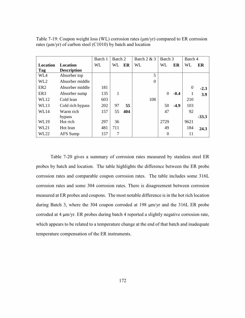
172
Table 7-19: Coupon weight loss (WL) corrosion rates (μm/yr) compared to ER corrosion
rates (μm/yr) of carbon steel (C1010) by batch and location
Table 7-20 gives a summary of corrosion rates measured by stainless steel ER
probes by batch and location. The table highlights the difference between the ER probe
corrosion rates and comparable coupon corrosion rates. The table includes some 316L
corrosion rates and some 304 corrosion rates. There is disagreement between corrosion
measured at ER probes and coupons. The most notable difference is in the hot rich location
during Batch 3, where the 304 coupon corroded at 198 µm/yr and the 316L ER probe
corroded at 4 µm/yr. ER probes during batch 4 reported a slightly negative corrosion rate,
which appears to be related to a temperature change at the end of that batch and inadequate
temperature compensation of the ER instruments.
Batch 1 Batch 2 Batch 2 & 3 Batch 3 Batch 4
Location
Tag
Location
Description
WL WL ER WL WL ER WL ER
WL4 Absorber top
5
WL2 Absorber middle
0
ER2 Absorber middle 181
0 -2.3
ER3 Absorber sump 135 1
0 -0.4 1 3.9
WL12 Cold lean 603
108
210
WL13 Cold rich bypass 202 97 55 50 -4.9 103
WL14 Warm rich
bypass
157 55 404 47 92
-33.3
WL19 Hot rich 297 36
2729 9621
WL21 Hot lean 481 711
49 184 24.3
WL22 AFS Sump 157 7
0 11
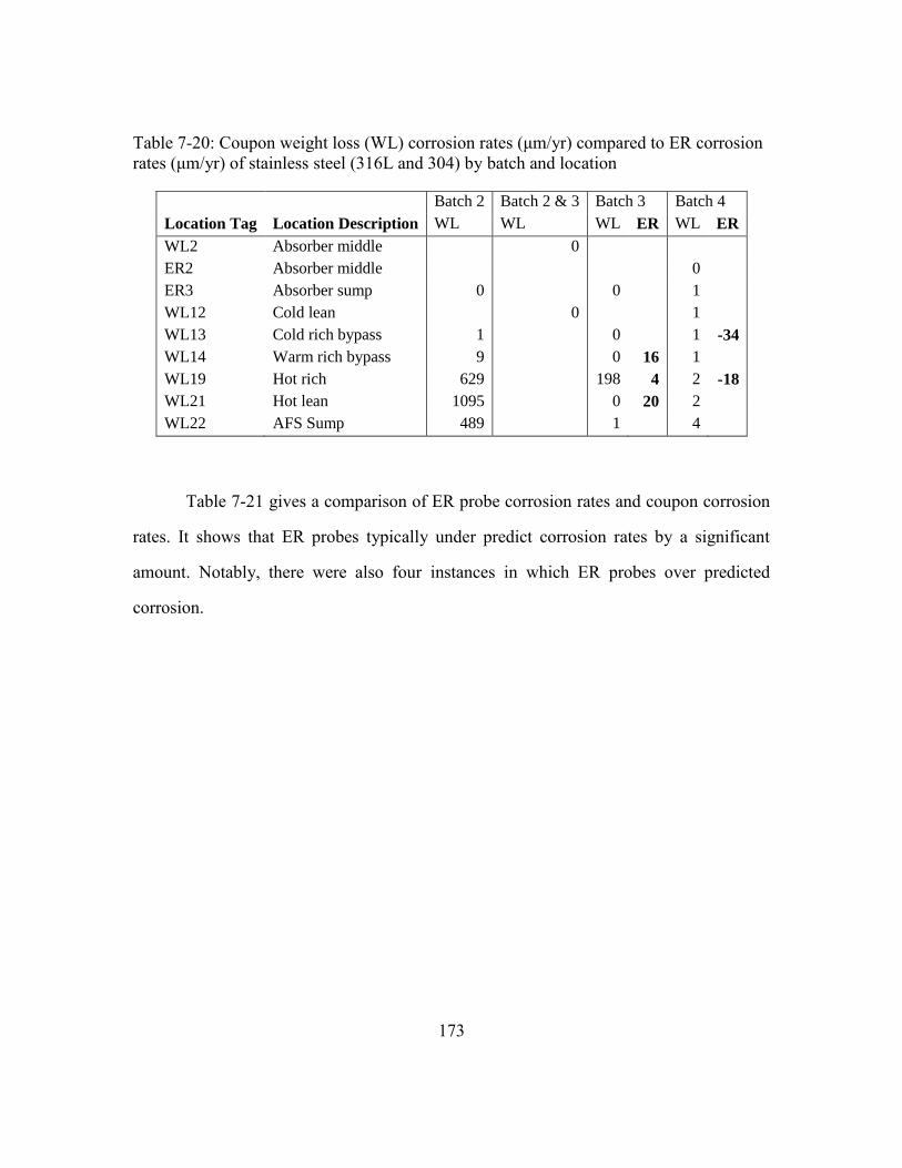
173
Table 7-20: Coupon weight loss (WL) corrosion rates (μm/yr) compared to ER corrosion
rates (μm/yr) of stainless steel (316L and 304) by batch and location
Batch 2 Batch 2 & 3 Batch 3 Batch 4
Location Tag Location Description WL WL WL ER WL ER
WL2 Absorber middle 0
ER2 Absorber middle 0
ER3 Absorber sump 0 0 1
WL12 Cold lean 0 1
WL13 Cold rich bypass 1 0 1 -34
WL14 Warm rich bypass 9 0 16 1
WL19 Hot rich 629 198 4 2 -18
WL21 Hot lean 1095 0 20 2
WL22 AFS Sump 489 1 4
Table 7-21 gives a comparison of ER probe corrosion rates and coupon corrosion
rates. It shows that ER probes typically under predict corrosion rates by a significant
amount. Notably, there were also four instances in which ER probes over predicted
corrosion.

174
Table 7-21: Comparison of ER and coupon corrosion rates.
Location Batch ER
Alloy
Coupon
Alloy
ER
Corrosion
Rate
(µm/yr)
Coupon
Corrosion
Rate
(µm/yr)
ER
Error
(μm/yr)
ER
Percent
Error
40513 Batch 2 C1010 C1010 55 96.8 -41 -43
40514 Batch 2 C1010 C1010 404 54.8 349 637
ER3 Batch 3 C1010 C1010 -0.4 0.3 -1 -217
40513 Batch 3 C1010 C1010 -5 50.3 -55 -110
40514 Batch 3 304 304 16 0.3 16 5796
40519 Batch 3 316L 304 4.4 198.4 -194 -98
40521 Batch 3 316L 304 20 0.5 20 4355
ER2 Batch 4 C1010 C1010 -2.3 0.2 -2 -1268
ER3 Batch 4 C1010 C1010 3.9 0.6 3 565
40513 Batch 4 316L 316L -34 1.0 -35 -3493
40514 Batch 4 C1010 C1010 -33 92.2 -126 -136
40519 Batch 4 304 316L -18 1.9 -19 -1010
40521 Batch 4
Period 1
C1010 C1010 24 183.8 -159 -87
40521 Batch 4
Period 2
C1010 C1010 51 183.8 -133 -72
Table 7-22 gives detailed information about the ER probe corrosion rate
determinations. Corrosion rates were determined based on the method of least squares,
and regression parameters are shown.
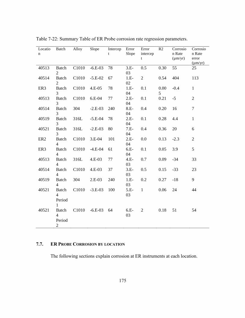
175
Table 7-22: Summary Table of ER Probe corrosion rate regression parameters.
Locatio
n
Batch Alloy Slope Intercep
t
Error
Slope
Error
intercep
t
R2 Corrosio
n Rate
(µm/yr)
Corrosio
n Rate
error
(µm/yr)
40513 Batch
2
C1010 -6.E-03 78 3.E-
03
0.5 0.30 55 25
40514 Batch
2
C1010 -5.E-02 67 1.E-
02
2 0.54 404 113
ER3 Batch
3
C1010 4.E-05 78 1.E-
04
0.1 0.00
5
-0.4 1
40513 Batch
3
C1010 6.E-04 77 2.E-
04
0.1 0.21 -5 2
40514 Batch
3
304 -2.E-03 240 8.E-
04
0.4 0.20 16 7
40519 Batch
3
316L -5.E-04 78 2.E-
04
0.1 0.28 4.4 1
40521 Batch
3
316L -2.E-03 80 7.E-
04
0.4 0.36 20 6
ER2 Batch
4
C1010 3.E-04 101 2.E-
04
0.0 0.13 -2.3 2
ER3 Batch
4
C1010 -4.E-04 61 6.E-
04
0.1 0.05 3.9 5
40513 Batch
4
316L 4.E-03 77 4.E-
03
0.7 0.09 -34 33
40514 Batch
4
C1010 4.E-03 37 3.E-
03
0.5 0.15 -33 23
40519 Batch
4
304 2.E-03 240 1.E-
03
0.2 0.27 -18 9
40521 Batch
4
Period
1
C1010 -3.E-03 100 5.E-
03
1 0.06 24 44
40521 Batch
4
Period
2
C1010 -6.E-03 64 6.E-
03
2 0.18 51 54
7.7. ER PROBE CORROSION BY LOCATION
The following sections explain corrosion at ER instruments at each location.
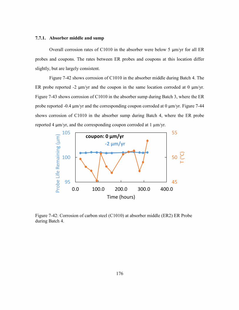
176
7.7.1. Absorber middle and sump
Overall corrosion rates of C1010 in the absorber were below 5 µm/yr for all ER
probes and coupons. The rates between ER probes and coupons at this location differ
slightly, but are largely consistent.
Figure 7-42 shows corrosion of C1010 in the absorber middle during Batch 4. The
ER probe reported -2 µm/yr and the coupon in the same location corroded at 0 µm/yr.
Figure 7-43 shows corrosion of C1010 in the absorber sump during Batch 3, where the ER
probe reported -0.4 µm/yr and the corresponding coupon corroded at 0 µm/yr. Figure 7-44
shows corrosion of C1010 in the absorber sump during Batch 4, where the ER probe
reported 4 µm/yr, and the corresponding coupon corroded at 1 µm/yr.
Figure 7-42: Corrosion of carbon steel (C1010) at absorber middle (ER2) ER Probe
during Batch 4.
45
50
55
95
100
105
0.0 100.0 200.0 300.0 400.0
T (°
C)
Pro
be
Life
Rem
ain
ing
(μm
)
Time (hours)
-2 μm/yr
coupon: 0 μm/yr
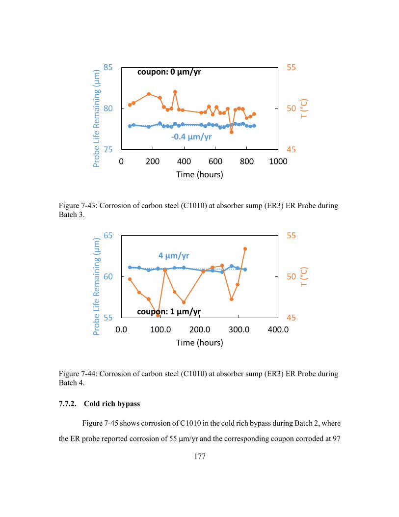
177
Figure 7-43: Corrosion of carbon steel (C1010) at absorber sump (ER3) ER Probe during
Batch 3.
Figure 7-44: Corrosion of carbon steel (C1010) at absorber sump (ER3) ER Probe during
Batch 4.
7.7.2. Cold rich bypass
Figure 7-45 shows corrosion of C1010 in the cold rich bypass during Batch 2, where
the ER probe reported corrosion of 55 µm/yr and the corresponding coupon corroded at 97
45
50
55
75
80
85
0 200 400 600 800 1000
T (°
C)
Pro
be
Life
Rem
ain
ing
(μm
)
Time (hours)
-0.4 μm/yr
coupon: 0 μm/yr
45
50
55
55
60
65
0.0 100.0 200.0 300.0 400.0
T (°
C)
Pro
be
Life
Rem
ain
ing
(μm
)
Time (hours)
4 μm/yr
coupon: 1 μm/yr
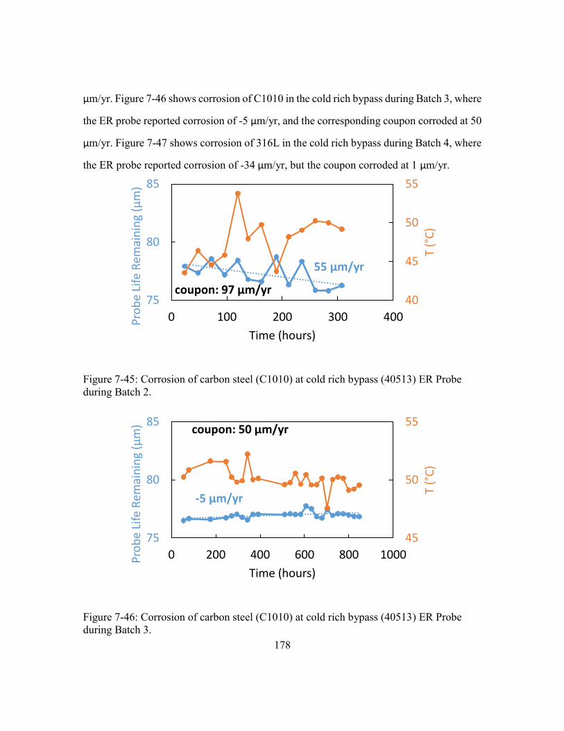
178
µm/yr. Figure 7-46 shows corrosion of C1010 in the cold rich bypass during Batch 3, where
the ER probe reported corrosion of -5 µm/yr, and the corresponding coupon corroded at 50
µm/yr. Figure 7-47 shows corrosion of 316L in the cold rich bypass during Batch 4, where
the ER probe reported corrosion of -34 µm/yr, but the coupon corroded at 1 µm/yr.
Figure 7-45: Corrosion of carbon steel (C1010) at cold rich bypass (40513) ER Probe
during Batch 2.
Figure 7-46: Corrosion of carbon steel (C1010) at cold rich bypass (40513) ER Probe
during Batch 3.
40
45
50
55
75
80
85
0 100 200 300 400
T (°
C)
Pro
be
Life
Rem
ain
ing
(μm
)
Time (hours)
55 μm/yr
coupon: 97 μm/yr
45
50
55
75
80
85
0 200 400 600 800 1000
T (°
C)
Pro
be
Life
Rem
ain
ing
(μm
)
Time (hours)
-5 μm/yr
coupon: 50 μm/yr
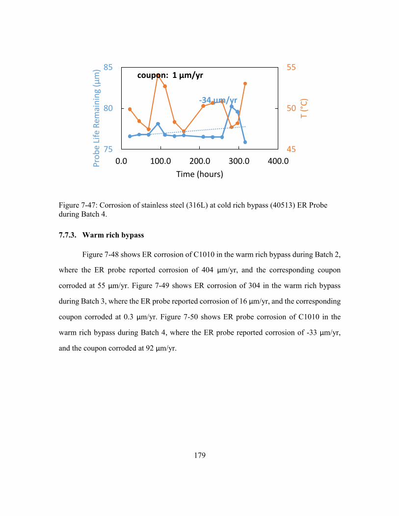
179
Figure 7-47: Corrosion of stainless steel (316L) at cold rich bypass (40513) ER Probe
during Batch 4.
7.7.3. Warm rich bypass
Figure 7-48 shows ER corrosion of C1010 in the warm rich bypass during Batch 2,
where the ER probe reported corrosion of 404 µm/yr, and the corresponding coupon
corroded at 55 µm/yr. Figure 7-49 shows ER corrosion of 304 in the warm rich bypass
during Batch 3, where the ER probe reported corrosion of 16 µm/yr, and the corresponding
coupon corroded at 0.3 µm/yr. Figure 7-50 shows ER probe corrosion of C1010 in the
warm rich bypass during Batch 4, where the ER probe reported corrosion of -33 µm/yr,
and the coupon corroded at 92 µm/yr.
45
50
55
75
80
85
0.0 100.0 200.0 300.0 400.0
T (°
C)
Pro
be
Life
Rem
ain
ing
(μm
)
Time (hours)
-34 μm/yr
coupon: 1 μm/yr

180
Figure 7-48: Corrosion of carbon steel (C1010) at warm rich bypass (40514) ER Probe
during Batch 2.
Figure 7-49: Corrosion of stainless steel (304) at warm rich bypass (40514) ER Probe
during Batch 3.
100
110
120
130
50
55
60
65
70
0 100 200 300 400
T (°
C)
Pro
be
Life
Rem
ain
ing
(μm
)
Time (hours)
404 μm/yr
coupon: 55 μm/yr
100
110
120
130
235
240
245
0 200 400 600 800 1000
T (°
C)
Pro
be
Life
Rem
ain
ing
(μm
)
Time (hours)
16 μm/yr
coupon: 0.3 μm/yr

181
Figure 7-50: Corrosion of carbon steel (C1010) at warm rich bypass (40514) ER Probe
during Batch 4.
7.7.4. Hot Rich
Figure 7-51 shows corrosion of 316L in the hot rich stream during Batch 3, where
the ER probe corroded at 4 µm/yr. There was no 316L coupon in the hot rich stream during
this batch, but there was a 304 coupon, which corroded at 198 µm/yr. Figure 7-52 shows
corrosion of 304 in the hot rich stream during Batch 4, where the ER probe reported
corrosion of -18 µm/yr. There was no 304 coupon in the hot rich stream during this batch,
but there was a 316L coupon, which corroded at 1.9 µm/yr.
90
100
110
120
130
30
35
40
0.0 100.0 200.0 300.0 400.0
T (°
C)
Pro
be
Life
Rem
ain
ing
(μm
)
Time (hours)
-33 μm/yr
coupon: 92 μm/yr
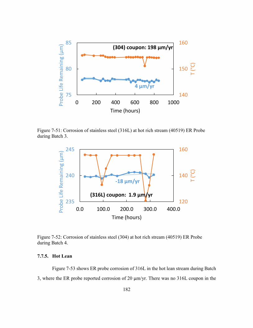
182
Figure 7-51: Corrosion of stainless steel (316L) at hot rich stream (40519) ER Probe
during Batch 3.
Figure 7-52: Corrosion of stainless steel (304) at hot rich stream (40519) ER Probe
during Batch 4.
7.7.5. Hot Lean
Figure 7-53 shows ER probe corrosion of 316L in the hot lean stream during Batch
3, where the ER probe reported corrosion of 20 µm/yr. There was no 316L coupon in the
140
150
160
75
80
85
0 200 400 600 800 1000
T (°
C)
Pro
be
Life
Rem
ain
ing
(μm
)
Time (hours)
4 μm/yr
(304) coupon: 198 μm/yr
120
140
160
235
240
245
0.0 100.0 200.0 300.0 400.0
T (°
C)
Pro
be
Life
Rem
ain
ing
(μm
)
Time (hours)
-18 μm/yr
(316L) coupon: 1.9 μm/yr

183
hot lean stream during this batch, but there was a 304 coupon, which corroded at 0.5 µm/yr.
Figure 7-54 shows ER probe corrosion of C1010 in the hot lean stream during Batch 4.
There was a discontinuity in corrosion measurement during this batch, where probe life
suddenly decreased sharply. This discontinuity was not included when regressing the
corrosion rate. During the first period of Batch 4, the ER probe reported corrosion of 24
µm/yr . After the discontinuity, the ER probe reported corrosion of 51 µm/yr. The
corresponding Batch 4 coupon corroded at 184 µm/yr.
Figure 7-53: Corrosion of stainless steel (316L) at hot lean stream (40521) ER Probe
during Batch 3.
140
150
160
75
80
85
0 200 400 600 800 1000
T (°
C)
Pro
be
Life
Rem
ain
ing
(μm
)
Time (hours)
20 μm/yr
(304) coupon: 0.5 μm/yr

184
Figure 7-54: Corrosion of carbon steel (C1010) at hot lean stream (40521) ER Probe
during Batch 4.
7.8. CONCLUSIONS
7.8.1. Carbon steel performs well in 5 m PZ at lean and rich loadings, at 116 – 150
°C, when fluid velocities are low. This good performance is due to the formation of a
protective FeCO3 film.
Carbon steel (C1010) in 5 m PZ is frequently protected by a crystalline siderite
(FeCO3) layer at 116 - 150 oC. Siderite is observed at both lean (α = 0.23) and rich (α =
0.4) CO2 loadings at these temperatures. At 116°C and rich loading, corrosion varied from
47 - 92 µm/yr. At 150°C and lean loadings, corrosion ranged from 0 - 11 µm/yr. These
measurements were in vessels or low velocity pipes (≈0.39 m/s).
7.8.2. At 150 – 155 °C, at lean and rich loadings, when fluid velocity is moderate or
high (> 0.8 m/s), FeCO3 films are sometimes not protective to carbon steel, leading
to high corrosion in 5 m PZ.
At high temperature (150-155 °C), high fluid velocity locations (≈ 0.8 m/s, not
accounting for two phase flow), protective films are sometimes not adequate to protect
carbon steel in 5 m PZ, and corrosion can be high (up to 2800 μm/yr). High fluid velocity
110
135
160
50
60
70
80
90
100
110
0.0 100.0 200.0 300.0 400.0
T (°
C)
Pro
be
Life
Rem
ain
ing
(μm
)
Time (hours)
24 μm/yr
51 μm/yr
coupon: 184 μm/yr
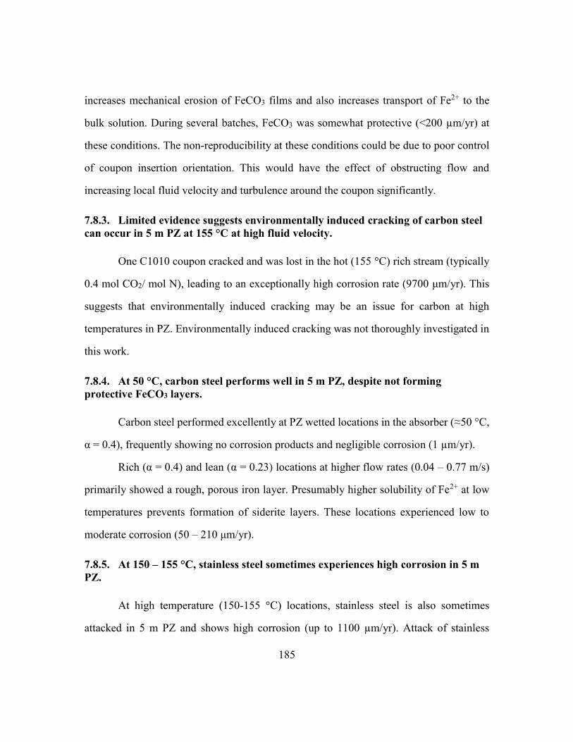
185
increases mechanical erosion of FeCO3 films and also increases transport of Fe2+ to the
bulk solution. During several batches, FeCO3 was somewhat protective (<200 µm/yr) at
these conditions. The non-reproducibility at these conditions could be due to poor control
of coupon insertion orientation. This would have the effect of obstructing flow and
increasing local fluid velocity and turbulence around the coupon significantly.
7.8.3. Limited evidence suggests environmentally induced cracking of carbon steel
can occur in 5 m PZ at 155 °C at high fluid velocity.
One C1010 coupon cracked and was lost in the hot (155 °C) rich stream (typically
0.4 mol CO2/ mol N), leading to an exceptionally high corrosion rate (9700 μm/yr). This
suggests that environmentally induced cracking may be an issue for carbon at high
temperatures in PZ. Environmentally induced cracking was not thoroughly investigated in
this work.
7.8.4. At 50 °C, carbon steel performs well in 5 m PZ, despite not forming
protective FeCO3 layers.
Carbon steel performed excellently at PZ wetted locations in the absorber (≈50 °C,
α = 0.4), frequently showing no corrosion products and negligible corrosion (1 µm/yr).
Rich (α = 0.4) and lean (α = 0.23) locations at higher flow rates (0.04 – 0.77 m/s)
primarily showed a rough, porous iron layer. Presumably higher solubility of Fe2+ at low
temperatures prevents formation of siderite layers. These locations experienced low to
moderate corrosion (50 – 210 μm/yr).
7.8.5. At 150 – 155 °C, stainless steel sometimes experiences high corrosion in 5 m
PZ.
At high temperature (150-155 °C) locations, stainless steel is also sometimes
attacked in 5 m PZ and shows high corrosion (up to 1100 µm/yr). Attack of stainless
186
occurred at high and low fluid velocities, and lean and rich loadings. Both 316L and 304
experienced high corrosion. During some batches, stainless performed excellently at these
locations. It is not clear why stainless was attacked during some batches, but not others at
similar conditions. Vulnerability of stainless steel could be due to the uniquely high
operating temperature of PZ compared to other amines, which typically operate at 120 °C.
Until the occasional vulnerability of stainless steel at these locations is understood, higher
alloy steels (ie, duplex stainless) should be investigated.
7.8.6. At 50 – 116 °C, stainless steel performs well in 5 m PZ.
In the absorber and 50 – 116 °C piping, stainless steel (304 and 316L) performed
excellently (0 – 9 µm/yr). CO2 loading and fluid velocity did not appear to have a strong
effect on stainless performance at these conditions.
7.8.7. Fe3+ products are observed at rich conditions, which are relatively oxidizing,
but Fe2+ is observed at lean conditions, which are reducing. The cyclic oxidation and
reduction of Fe3+ likely plays a role in high temperature oxidation of PZ.
At warm or hot rich conditions, the corrosion products on carbon steel include
oxidized species, but not at lean conditions, suggesting that dissolved Fe3+ is depleted in
the stripper sump by reaction with piperazine. Magnetite (Fe3O4) or goethite (Fe(O)OH)
are often observed in addition to siderite at warm (116 °C) and hot rich (155 °C) locations.
Presumably, these ferric species are generated in the absorber, which is relatively oxidizing
due to O2 in the flue gas. The absence of ferric products in the stripper sump suggests that
ferric is reduced back to ferrous at the high temperature, anoxic conditions of the stripper.
Presumably this reduction is accompanied by an oxidation of an amine, degrading it. This
Fe3+ to Fe2+ reduction is probably the cyclic oxidizer hypothesized by other researchers to
play a significant role in PZ oxidation (Paul Thomas Nielsen, 2018).
187
7.8.8. Equipment commissioning with water and steam appears more corrosive to
carbon steel than PZ operation.
There is evidence that the commissioning phase, when equipment is pressure tested
by circulating water and steam, is more corrosive to carbon steel than operation with 5 m
PZ. Notably, operation with 5 m PZ in the absorber typically leaves C1010 pristine, but
extended water testing caused moderate corrosion. High velocity locations also
experienced corrosion (hot lean, hot rich, cold lean). If carbon steel is used, care should be
taken to avoid extended equipment water testing. CO2 circulation should be avoided during
equipment commissioning with water.

188
Chapter 8. Conclusions
This work yielded four conclusions that shed light on the effect of amine structure
and several process variables on corrosion in PCCC systems. Section 8.1 describes what
conditions promote protective FeCO3 films on carbon steel. Section 8.2 describes
conditions that can sometimes lead to attack of stainless steel at high T. Section 8.3 gives
evidence that the conversion of ferric to ferrous plays a key role in high temperature
corrosion. Finally Section 8.4 develops a relationship between amine structure, iron
solubility, and corrosion.
8.1. CARBON STEEL OFTEN PERFORMS WELL IN 5 MOLAL PZ DUE TO THE
FORMATION OF A PASSIVATING FECO3 LAYER. THIS LAYER IS PROMOTED AT HIGH T,
HIGH CO2 LOADING, LOW SOLUTION VELOCITY, AND IN AMINES WITH LOW FE2+
SOLUBILITY.
When protective FeCO3 layers form, the corrosion rate of carbon steel in amine
solutions can be very low. The formation of FeCO3 layers is controlled by local
supersaturation of Fe2+ and CO32- near the metal surface. Higher intrinsic Fe2+ solubility in
MEA explains its lack of FeCO3 formation. High fluid velocities reduce local
supersaturation of Fe2+ and CO32- and can lead to limited FeCO3 formation and high
corrosion rates. FeCO3 formation is favored at high temperatures because Fe2+ solubility
decreases at high T and because kinetics of FeCO3 formation are likely faster at higher T.
These reasons also mean that FeCO3 is not observed at low T conditions. Despite the lack
of FeCO3 formation, carbon steel performs well at low T due to slower kinetics of metal
oxidation. Limited evidence of environmentally induced cracking of carbon steel was
observed at high T in 5 m PZ. Finally, FeCO3 films do not form on carbon steel in the
absence of amine and CO2, so care must be taken when water testing carbon steel
equipment.
189
This conclusion is supported by the following experimental observations:
Carbon steel performs well at 40-70 °C in 7 m MEA, but it is unacceptable at
120 °C.
With 7 m MEA carbon steel (C1010) performed well in the absorber (40-70 °C),
experiencing 1.8–8.9 μm/yr of corrosion, but performed unacceptably in the stripper (110-
120°C), experiencing 3600–4000 μm/yr of corrosion.
The strong effects of CO2 loading and T on Fe2+ solubility suggest the
equilibrium concentration of Fe2+ will change as the solvent moves through a
real plant.
One implication of bench-scale Fe2+ solubility experiments is that there will be
strong fluctuations in equilibrium Fe2+ concentration as solvent moves through a real plant.
In degraded PZ for example, Fe2+ solubility is apparently highest at low temperature and
lean loading, so these conditions are least likely to be protected by FeCO3 and may
experience corrosion. However an amine stream that is unsaturated at cold, lean conditions
may be supersaturated at hot, rich conditions. This means corrosion could occur in the
absorber, and those corrosion products are deposited in the stripper. This also means that
the observed Fe2+ concentration at a plant may not be an equilibrium value, but rather a
complicated average value affected by the residence times at unsaturated and
supersaturated parts of the process.
Carbon steel experiences low corrosion at high temperature in PZ solution.
In a set of bench-scale experiments from 100°C to 160°C, at lean loading (α ≈ 0.23),
even in very degraded solutions of PZ, C1010 performance was good to moderate (< 400
μm/yr), and showed no strong increase with temperature. Counterintuitively, at higher

190
loading of α = 0.3 carbon steel performed better (<100 µm/yr). Higher loading likely
promotes the formation of a FeCO3 layer.
At 50 °C, carbon steel performs well in 5 m PZ, despite not forming protective
FeCO3 layers.
Carbon steel performed well at PZ wetted locations in the absorber (≈50 °C, α =
0.4), frequently showing no corrosion products and negligible corrosion (1 µm/yr).
Rich (α = 0.4) and lean (α = 0.23) locations at higher flow rate (0.04 – 0.77 m/s)
primarily showed a rough, porous iron layer. Presumably higher solubility of Fe2+ at low
temperature prevents formation of siderite layers. These locations experienced low to
moderate corrosion (50 – 210 μm/yr).
Carbon steel performs well in 5 m PZ at lean and rich loading, at 116 – 150 °C,
when fluid velocity is low. This good performance is due to the formation of a
protective FeCO3 film.
Carbon steel (C1010) in 5 m PZ is frequently protected by a crystalline siderite
(FeCO3) layer at 116 - 150 oC. Siderite is observed at both lean (α = 0.23) and rich (α =
0.4) CO2 loading at these temperatures. At 116°C and rich loading, corrosion varied from
47 - 92 µm/yr. At 150°C and lean loading, corrosion ranged from 0 - 11 µm/yr. These
measurements were in vessels or low velocity pipes (≈0.39 m/s).
Corrosion coupons from the 2017 SRP pilot plant campaign show a protective,
crystalline layer of FeCO3 forms on C1010 in 5 m PZ at 150 °C and α = 0.21. When this
layer formed, corrosion performance was good (96.4 µm/yr).
191
At 150 – 155 °C, at lean and rich loading, when fluid velocity is moderate or high
(> 0.8 m/s), FeCO3 films are sometimes not protective to carbon steel, leading to
high corrosion in 5 m PZ.
At high temperature (150-155 °C), high fluid velocity locations (≈ 0.8 m/s, not
accounting for two phase flow), protective films are sometimes not adequate to protect
carbon steel in 5 m PZ, and corrosion can be high (up to 2800 μm/yr). High fluid velocity
increases transport of Fe2+ to the bulk solution and may cause mechanical erosion of FeCO3
films. During several batches, FeCO3 was somewhat protective (<200 µm/yr) at these
conditions. The non-reproducibility at these conditions could be due to poor control of
coupon insertion orientation. This would have the effect of obstructing flow and increasing
local fluid velocity and turbulence around the coupon significantly.
Limited evidence suggests environmentally induced cracking of carbon steel can
occur in 5 m PZ at 155 °C at high fluid velocity.
One C1010 coupon cracked and was lost in the hot (155 °C) rich stream (typically
α = 0.4), leading to an exceptionally high corrosion rate (9700 μm/yr). This suggests that
environmentally induced cracking may be an issue for carbon at high temperatures in PZ.
Environmentally induced cracking was not thoroughly investigated in this work.
Equipment commissioning with water and steam appears more corrosive to
carbon steel than PZ operation.
There is evidence that the commissioning phase, when equipment is pressure tested
by circulating water and steam, is more corrosive to carbon steel than operation with 5 m
PZ. Notably, operation with 5 m PZ in the absorber typically leaves C1010 pristine, but
extended water testing caused moderate corrosion. High velocity locations also
experienced corrosion (hot lean, hot rich, cold lean). If carbon steel is used, care should be

192
taken to avoid extended equipment water testing. CO2 circulation should be avoided during
equipment commissioning with water.
8.2. DEPASSIVATION AND HIGH CORROSION OF STAINLESS STEEL CAN OCCUR IN
AMINE SOLUTIONS AT HIGH TEMPERATURE. DEPASSIVATION OF STAINLESS IS
PROMOTED BY HIGHER T (150 °C) WHEN CONDITIONS ARE RELATIVELY ANOXIC AND
REDUCING.
Stainless steel (316L) appears to be very close to the active/passive transition in
amine solutions at high T in PCCC conditions.
Bench-scale screening suggests that MEA and PZ solutions can attack stainless at
anoxic, high T conditions. Very anoxic conditions at the bench scale cause corrosion in PZ
especially above 120 °C. Attack of stainless in MEA was also observed at 120 °C in anoxic
conditions, but higher temperatures were not evaluated with MEA. This behavior has not
been well reported in MEA since operation for MEA units is limited to 120 °C by thermal
degradation of the solvent. PCCC pilot plants contain oxygen, and thus stainless
performance is better than in the anoxic bench-scale experiments. Stainless performs well
at 120 °C in MEA in pilot plants. Stainless performed well up to 116 °C in PZ at pilot
plants at all times.
At high temperatures (150°C) in pilot plants, stainless steel in PZ is sometimes
attacked, but is passivated at other times. Performance of stainless steel in PZ at pilot plants
suggests that it can be pushed into and out of the active state by small process changes.
One hypothesis is that stainless steel performs better when flue gas O2 concentration is
higher. High flue gas O2 means that oxidizing species (dissolved O2, Fe3+) are carried over
to the stripper. These oxidizing species increase the solution potential and push stainless
into the passive state. In a pilot plant with 17 – 20% O2 in the flue gas, stainless was passive
in 5 m PZ at 150 °C (<9 µm/yr). In a pilot plant with 5.4 % O2 in the flue gas, stainless
193
performance was initially very poor (500 – 1100 µm/yr) at high T (150-155 °C), suggesting
it was in the active state.
However this hypothesis does not explain all observed behavior of stainless in PZ.
Later in the low O2 flue gas campaign, stainless performance at high T improved (5-200
µm/yr). Several process changes in the second half of the campaign could be responsible,
including increasing degradation products and iron in solution, stripping of dissolved O2
from rich solvent, and injection of SO3 into the flue gas to study aerosol. Whatever the
cause, it is clear that small process changes made the solution overall more oxidizing,
leading to stainless passivation. The tentative conclusion from this work is that stainless
may experience lower corrosion at high T when the solvent is more oxidizing. However,
until the occasional vulnerability of stainless steel is better understood, higher alloy steels
(ie, duplex stainless) should be investigated for use at these locations.
This conclusion is supported by the following experimental observations:
Stainless steel performs well in 7 m MEA at both absorber and stripper
conditions.
Stainless steel (316L) performed well in a pilot plant campaign at all locations,
experiencing 0–0.3 μm/yr of corrosion in the absorber (40-70 °C), and 0.2–0.6 μm/yr of
corrosion in the stripper (110-120°C).
At 50 – 116 °C, stainless steel performs well in 5 m PZ.
During a pilot plant campaign, in the absorber and 50 – 116 °C piping, stainless
steel (304 and 316L) performed well (0 – 9 µm/yr). CO2 loading and fluid velocity did not
appear to have a strong effect on stainless performance at these conditions.
194
Stainless steel sometimes experiences attack in PZ and MEA at high
temperature, anoxic conditions.
In bench-scale experiments, several solutions of slightly degraded PZ, at lean
loadings (α ≈ 0.23), 316L experienced corrosion with a strong temperature effect, with
good performance at 120 °C (<150 μm/yr), but poor performance (>1000 μm/yr) at 149 °C
and higher. Notably, attack of stainless was not observed in completely clean PZ at similar
conditions. At higher loading of α = 0.3, stainless steel showed excellent corrosion
performance (<100 µm/yr). It is not clear why stainless steel performed well at higher CO2
loading. Attack of 316L was also seen in 9 m MEA (500 µm/yr at 120 °C, α = 0.42),
although higher temperature were not evaluated. These stainless corrosion rates may be
higher than in a real plant, because the reducing environment of the corrosion loop is
particularly challenging for 316L.
Stainless steel performed well in 5 m PZ both in the absorber and in the hot, lean
stream. This may be partially due to the high O2 content at SRP.
Stainless steel (316L) performed excellently in the absorber (α = 0.33 and 30 °C)
corroding at 0 µm/yr. Stainless steel also performed excellently in the hot (150°C), lean (α
= 0.21) stream, showing 2.0–9.0 µm/yr of corrosion. Stainless steel is clearly not attacked
by either PZ operation or water commissioning at these conditions. This may be due to
higher O2 concentration at in SRP synthetic flue gas (17-20 %) compared to a coal flue gas
stream (5.4 %), which may lead to more oxidizing conditions which can support chromium
oxide passive film formation on stainless steel.
At 150 – 155 °C, stainless steel sometimes experiences high corrosion in 5 m PZ.
At high temperature (150-155 °C), stainless steel is also sometimes attacked in 5 m
PZ and shows high corrosion (up to 1100 µm/yr). Attack of stainless occurred at high and
195
low fluid velocity, and lean and rich loading. Both 316L and 304 experienced high
corrosion. During some batches, stainless performed well at these locations. It is not clear
why stainless was attacked during some batches, but not others at similar conditions.
Vulnerability of stainless steel could be due to the uniquely high operating temperature of
PZ compared to other amines, which typically operate at 120 °C. Until the occasional
vulnerability of stainless steel at these locations is understood, higher alloy steels (ie,
duplex stainless) should be investigated.
8.3. FERRIC PRODUCTS ARE GENERATED IN THE ABSORBER, THEN REDUCED AT HIGH
TEMPERATURE, ANOXIC CONDITIONS. THIS REDUCTION REACTION INCREASES THE
OXIDATION OF STEEL AND AMINE.
Other researchers have determined that amine oxidation at high temperatures
proceeds through the carryover of oxidizers from the absorber to the stripper, even in the
absence of dissolved O2. The conversion of Fe3+ to Fe2+ has been suggested as a likely
culprit (Paul Thomas Nielsen, 2018). Observation of corrosion products supports this
theory. Ferric products are frequently found in the rich amine stream in PZ pilot plants, but
only ferrous products are observed in the stripper, after dissolved O2 has been stripped out
or reacted away. Presumably, the conversion of Fe3+ to Fe2+ is a very favorable reduction
reaction in the absence of O2. In this way, carried-over ferric likely is responsible for
oxidation of amine and corrosion at high temperature. Thus lowering Fe2+ concentration in
amine solutions could be a key way to limit amine oxidation and corrosion. Alternatively,
increasing Fe2+ concentration would increase the generation of Fe3+ and make the solution
more oxidizing. This could be used to increase the solution potential at high T, possibly
pushing stainless into the passive region in PZ.
196
Ferrous products were not observed in MEA at pilot plants. The prevalence of ferric
in MEA suggests MEA is more oxidizing, or perhaps ferric is strongly complexed and
stabilized in MEA.
This conclusion is supported by the following experimental observations:
In low temperature, agitated solubility experiments, Fe2+ is frequently converted
to Fe3+, except in PZ at high CO2 loadings.
The solid phases characterized in these experiments showed that FeCO3 only
formed under specific conditions. Siderite (FeCO3) was only identified in PZ solutions
with rich CO2 loading. Since siderite was found in both rich clean PZ and rich degraded
PZ, its formation appears to be relatively independent of amine degradation level. Lean
PZ solutions tended to form magnetite (Fe3O4), as did lean MEA solutions. The solid
sample from a rich MEA experiment that was characterized appeared to be goethite
(FeO(OH)). An air and CO2-sparged experiment with 5 m SRP PZ air and CO2 also formed
goethite. The conversion of Fe2+ to Fe3+ requires relatively oxidizing conditions. These
experiments suggest that MEA and lean PZ are somewhat more oxidizing than rich PZ
solutions.
Corrosion products on carbon steel are largely Ferric (Fe3+) in 7 m MEA,
suggesting more oxidizing conditions than PZ. Protective corrosion product
layers were not observed.
In 7 m MEA, Fe(OH)3 was observed on carbon steel coupons in the absorber sump
and the stripper sump. This ferric product, particularly at relatively reducing stripper sump
conditions, suggests MEA is more oxidizing than PZ. Corrosion product films on C1010
in MEA were not thick or tightly adhering. Presumably higher Fe2+ solubilities prevent
precipitation of protective ferrous films. Alternatively, ferrous product formation is
prevented at most conditions because MEA conditions rapidly oxidize Fe2+ to Fe3+.

197
Fe3+ products are observed at rich conditions, which are relatively oxidizing, but
Fe2+ is observed at lean conditions, which are reducing. The cyclic oxidation and
reduction of Fe3+ likely plays a role in high temperature oxidation of PZ.
At warm or hot rich conditions, the corrosion products on carbon steel include
oxidized species, but not at lean conditions, suggesting that dissolved Fe3+ is depleted in
the stripper sump by reaction with piperazine. Magnetite (Fe3O4) or goethite (Fe(O)OH)
are often observed in addition to siderite at warm (116 °C) and hot rich (155 °C) locations.
Presumably, these ferric species are generated in the absorber, which is relatively oxidizing
due to O2 in the flue gas. The absence of ferric products in the stripper sump suggests that
ferric is reduced back to ferrous at the high temperature, anoxic conditions of the stripper.
Presumably this reduction is accompanied by an oxidation of an amine, degrading it. This
Fe3+ to Fe2+ reduction is probably the cyclic oxidizer hypothesized by other researchers to
play a significant role in PZ oxidation (Paul Thomas Nielsen, 2018).
8.4. CERTAIN AMINES AND AMINE DEGRADATION PRODUCTS HAVE HIGH IRON
SOLUBILITY. THESE AMINES LIKELY COMPLEX IRON AND STABILIZE IT IN SOLUTION,
ACCELERATING CORROSION.
Ethylamines were found to be more corrosive than their propylamine counterparts.
It was also found that MEA had higher Fe2+ solubility than clean PZ at rich CO2 loadings.
Ethylamines are likely the correct chain length to form stable iron complexes with iron in
solution. Longer amines, and particularly sterically hindered amines like PZ, are less likely
to form such stable complexes with iron. This iron complexation hypothesis explains why
FeCO3 films are not observed in MEA solutions, but they are observed in PZ solutions.
Effective Fe complexation in MEA increases solubility and prevents FeCO3 formation.
One of these high iron solubility ethylamines is ethylenediamine (EDA), which is
a key degradation product in PZ solutions. As PZ solutions degrade, increasing EDA
increases stabilization and solubility of Fe in solution. Eventually, iron solubility is
198
elevated enough to reduce formation of FeCO3 films, which accelerates corrosion. This
hypothesis explains the correlation between PZ degradation and increased corrosion.
This conclusion is supported by the following experimental observations:
Ethylamines, such as, MEA and EDA, are more corrosive than their
propylamine counterparts, EDA and PDA. The ethyl- backbone amines likely
form more stable coordination complexes with oxidized iron, increasing
corrosion.
MEA, 3-amino-1-propanol (MPA), ethylenediamine (EDA), and 1,3-
diaminopropane (PDA) were evaluated to determine a relationship between amine chain
length and corrosion. MEA was significantly more corrosive to C1010 and 316L than MPA
in both thermal cylinders and the corrosion loop. The results are less complete for
EDA/PDA, but PDA appears to be less corrosive than EDA to 316L in thermal cylinders.
One hypothesis is that ethylamine carbamates form very stable octahedral complexes with
iron. The same complex cannot be formed with the longer propylamine carbamates as it is
too long and labile to easily form an octahedral complex
Fe2+ is significantly more soluble in MEA than clean PZ at rich loading.
Rich 9 m MEA was found to have Fe2+ solubility of 0.77 mmol/kg at rich loading
(α = 0.44) and 45 C. At similar conditions, Fe2+ solubility in clean 5 m PZ was 0.05
mmol/kg. The same trend is evident at several different temperatures at rich loadings. It is
likely that MEA carbamate effectively complexes Fe2+, increasing its solubility. PZ
carbamate has a constrained structure, and is likely unable to complex Fe2+. The range of
Fe2+ solubilities in MEA across all conditions measured was 0.001 to 14 mmol/kg. The
range of Fe2+ solubilities in clean PZ across all conditions tested was 0.03 to 0.1 mmol/kg.
199
The effect of CO2 loading on Fe2+ solubility is affected by amine type.
In 9 m MEA, increasing CO2 loading increases iron solubility dramatically. In clean
5 m PZ, CO2 loading does not affect Fe2+ solubility, which is low (< 0.1 mmol/kg) at all
conditions. Presumably, neither MEA nor PZ complex Fe2+ effectively. However at high
CO2 loadings, MEA carbamate forms and readily complexes Fe2+. PZ carbamate’s
constrained structure prevents it from forming stable complexes with Fe2+.
PZ degradation apparently accelerates corrosion of carbon and stainless steel.
In anoxic, bench-scale experiments, PZ degradation apparently increased corrosion
of both C1010 and 316L. Completely fresh PZ solutions were often non-corrosive to both
C1010 and 316L. Pilot plant degraded amines corroded both materials more quickly. A
more deliberate study is needed to clearly separate the effects of amine concentration, CO2
loading, and degradation.
The presence of amine degradation products significantly increased Fe2+
solubility in PZ.
Degraded PZ had much higher Fe2+ solubility (up to 26 mmol/kg) than clean PZ.
Degraded PZ has linear amine degradation products, such as EDA, which likely chelate
Fe2+. Apparently, this EDA complex increases Fe2+ solubility in PZ at all conditions. The
range of Fe2+ solubilities in degraded PZ across all conditions tested was 0.1 to 26
mmol/kg.
In degraded PZ, Fe2+ solubility decreased with increasing loading. This is
counterintuitive, because presumably EDA carbamate is also an effective complexing
agent for Fe2+. The reason for the decrease of Fe2+ solubility in degraded PZ at high loadings
is not known.

200
As PZ degrades, its increasing Fe2+ solubility might keep Fe2+ in solution,
preventing formation of FeCO3 films. This explains the observed relationship between PZ
degradation and accelerated C1010 corrosion.

201
APPENDICES

202
Appendix A. Operating Procedures
A.1. CORROSION LOOP PROCEDURE AND SAFETY ANALYSIS
JOB SAFETY ANALYSIS DATE 5/15/15 ☒NEW
☐REVISED
Operation of Corrosion Loop Apparatus
☐LABORATORY
☐PILOT PLANT
DEVELOPMENT TEAM POSITION/TITLE DEVELOPMENT
TEAM
POSITION/TITLE
Kent Fischer Graduate Researcher
REQUIRED AND/OR RECOMMENDED PERSONAL PROTECTIVE EQUIPMENT
☒SAFETY GLASSES
☒LAB COAT
☒NITRILE GLOVES
☐FRC
☐HARD HAT
☐HEARING
PROTECTION
☐FACE SHIELD
☐AIR PURIFYING
RESPIRATOR
☐LEATHER GLOVES
☐OTHER
JOB STEPS POTENTIAL HAZARDS CRITICAL ACTIONS
1. Pressure test apparatus
with compressed air line to
ensure no leaks.
If a leak is present, when the
loop is filled with amine, the
amine could be released.
Open ball valve to compressed air
line. Allow apparatus to fill until
100psig is reached. Shut ball valve
and wait to see if pressure
decreases over time. If pressure
decreases, there is a leak in the
system.
Depressurize by very slowly
opening the top ball valve.
2. Ensure ball valves are
closed. Remove the ORP
probe and fill the corrosion
loop with liquid to be tested.
Do not overfill the loop.
DO NOT PUT RICH AMINE
IN THE LOOP FOR HIGH T
EXPERIMENTS
The loop has a liquid volume of
1070 mL, do not add more than
this.
The Loop has a pressure relief
disk (PRD) that will burst at 200
PSIG at room temperature. The
disk ruptures at 176 PSIG at 160
°C. You must ensure that the
amine solution is lean, because
rich solutions will have a total
pressure at elevated temperatures
that will rupture the disk.
3. Reinsert the ORP probe.
Potential site of leak.
Make sure to reapply Teflon tape
to the ORP threaded fitting and to
tighten the ORP probe thoroughly.
4. Fasten Swagelok plugs
onto ball valves to prevent
apparatus being accidentally
opened.
Accidental ball valve open
during operation.
If ball valves are accidentally
opened, the user will be sprayed
with high temperature amine and
CO2. Make sure both ball valves

203
are capped with the appropriate
Swagelok plugs.
5. Plug in PID controller
and set desired temperature.
6. Watch apparatus pressure
while heating to avoid
overpressure.
Loop overpressure and PRD
rupture.
It is possible that your solution has
a higher vapor pressure than you
anticipated. Watch the apparatus
carefully as the temperature
increases. Pressure should rise
slowly with temperature and never
exceed 150 PSIG.
If pressure is not rising with
temperature, the pressure gauge
has probably failed. Unplug the
apparatus and abort run.
If pressure exceeds 150 PSIG,
immediately unplug the apparatus
and abort run.
7. Run Data acquisition
software and observe.
Once target temperature is reached
and pressure is no longer increasing,
the apparatus no longer needs to be
watched as closely. Check back
while it runs to ensure nothing goes
wrong.
8. Once run is complete, set
PID to zero to stop heating.
Allow apparatus to cool to
room temperature. This may
take several hours.
Accidental release of pressure DO NOT OPEN BALL VALVES
WHILE SYSTEM IS HOT.
9. Once system is at room
temperature (verify by
touching steel pipe to see
that it is cool), you may
unfasten Swagelok plug on
TOP ball valve.
Slowly open the TOP ball
valve to release pressure
from headspace.
Accidental release of pressure
ONLY OPEN THE TOP BALL
VALVE.
ONLY OPEN BALL VALVE
IF SYSTEM IS AT ROOM
TEMPERATURE.
Make sure to only open the top
ball valve in the system (the one
near the pressure gauge). If you
open the bottom ball valve, you
will be sprayed with amine.
Slowly open the top ball valve,
allowing any excess pressure to
vent.
10. Once system pressure
has been vented, you may
unscrew the Swagelok plug
from the bottom ball valve
and then open it to drain out
the amine.
Amine spill
Make sure to have a tubing
connected to the ball valve to
collect amine in an appropriate
waste container.
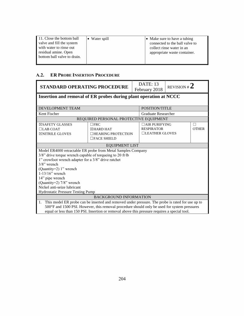
204
11. Close the bottom ball
valve and fill the system
with water to rinse out
residual amine. Open
bottom ball valve to drain.
Water spill Make sure to have a tubing
connected to the ball valve to
collect rinse water in an
appropriate waste container.
A.2. ER PROBE INSERTION PROCEDURE
STANDARD OPERATING PROCEDURE DATE: 13
February 2018 REVISION # 2
Insertion and removal of ER probes during plant operation at NCCC
DEVELOPMENT TEAM POSITION/TITLE
Kent Fischer Graduate Researcher
REQUIRED PERSONAL PROTECTIVE EQUIPMENT
☒SAFETY GLASSES
☐LAB COAT
☒NITRILE GLOVES
☐FRC
☒HARD HAT
☐HEARING PROTECTION
☐FACE SHIELD
☐AIR PURIFYING
RESPIRATOR
☐LEATHER GLOVES
☐OTHER
EQUIPMENT LIST
Model ER4000 retractable ER probe from Metal Samples Company
3/8” drive torque wrench capable of torqueing to 20 ft∙lb
1” crowfoot wrench adapter for a 3/8” drive ratchet
3/8” wrench
(Quantity=2) 1” wrench
1-13/16” wrench
14” pipe wrench
(Quantity=2) 7/8” wrench
Nickel anti-seize lubricant
Hydrostatic Pressure Testing Pump
BACKGROUND INFORMATION
1. This model ER probe can be inserted and removed under pressure. The probe is rated for use up to
500°F and 1500 PSI. However, this removal procedure should only be used for system pressures
equal or less than 150 PSI. Insertion or removal above this pressure requires a special tool.
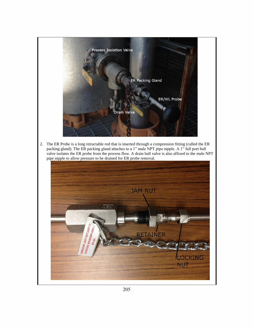
205
2. The ER Probe is a long retractable rod that is inserted through a compression fitting (called the ER
packing gland). The ER packing gland attaches to a 1” male NPT pipe nipple. A 1” full port ball
valve isolates the ER probe from the process flow. A drain ball valve is also affixed to the male NPT
pipe nipple to allow pressure to be drained for ER probe removal.
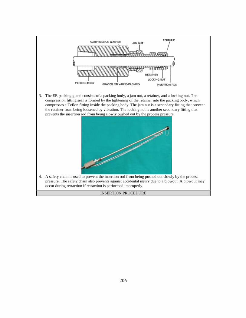
206
3. The ER packing gland consists of a packing body, a jam nut, a retainer, and a locking nut. The
compression fitting seal is formed by the tightening of the retainer into the packing body, which
compresses a Teflon fitting inside the packing body. The jam nut is a secondary fitting that prevent
the retainer from being loosened by vibration. The locking nut is another secondary fitting that
prevents the insertion rod from being slowly pushed out by the process pressure.
4. A safety chain is used to prevent the insertion rod from being pushed out slowly by the process
pressure. The safety chain also prevents against accidental injury due to a blowout. A blowout may
occur during retraction if retraction is performed improperly.
INSERTION PROCEDURE
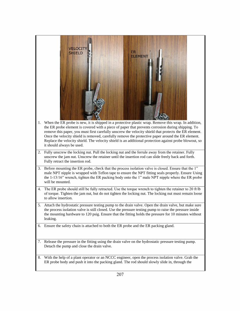
207
1. When the ER probe is new, it is shipped in a protective plastic wrap. Remove this wrap. In addition,
the ER probe element is covered with a piece of paper that prevents corrosion during shipping. To
remove this paper, you must first carefully unscrew the velocity shield that protects the ER element.
Once the velocity shield is removed, carefully remove the protective paper around the ER element.
Replace the velocity shield. The velocity shield is an additional protection against probe blowout, so
it should always be used.
2. Fully unscrew the locking nut. Pull the locking nut and the ferrule away from the retainer. Fully
unscrew the jam nut. Unscrew the retainer until the insertion rod can slide freely back and forth.
Fully retract the insertion rod.
3. Before mounting the ER probe, check that the process isolation valve is closed. Ensure that the 1”
male NPT nipple is wrapped with Teflon tape to ensure the NPT fitting seals properly. Ensure Using
the 1-13/16” wrench, tighten the ER packing body onto the 1” male NPT nipple where the ER probe
will be mounted.
4. The ER probe should still be fully retracted. Use the torque wrench to tighten the retainer to 20 ft∙lb
of torque. Tighten the jam nut, but do not tighten the locking nut. The locking nut must remain loose
to allow insertion.
5. Attach the hydrostatic pressure testing pump to the drain valve. Open the drain valve, but make sure
the process isolation valve is still closed. Use the pressure testing pump to raise the pressure inside
the mounting hardware to 120 psig. Ensure that the fitting holds the pressure for 10 minutes without
leaking.
6. Ensure the safety chain is attached to both the ER probe and the ER packing gland.
7. Release the pressure in the fitting using the drain valve on the hydrostatic pressure testing pump.
Detach the pump and close the drain valve.
8. With the help of a plant operator or an NCCC engineer, open the process isolation valve. Grab the
ER probe body and push it into the packing gland. The rod should slowly slide in, through the

208
compression fitting. Because the compression fitting is tight, this may require some force. Twisting
the probe can help.
9. Once the probe is fully inserted, tighten the locking nut to prevent the rod from sliding back out.
10. The safety chain should now have some slack in it. Refasten the chain to take in the slack.
209
Appendix B. ORP Measurement in Piperazine during Pilot Campaigns
Pilot ORP measurements were made at SRP during the 2017 PZ campaign. The
ORP probe was calibrated with Light’s solution prior to insertion, then was exposed to 340
hours of water testing, then 300 hours of piperazine operation. During operation of the pilot
plant, 36 steady state runs were achieved, each about 45 minutes long. One ORP reading
per minute was taken during these runs, and these data averaged to yield an average ORP
reading during the run. These average ORP readings during a steady state run are plotted
chronologically for the pilot campaign in Figure B-1. Times reported here are operating
hours with PZ. A dramatic decrease in ORP at 250 hours likely represents probe failure at
that point, rather than a real process change. These pilot ORP measurements can be directly
compared to ORP measurement in the corrosion loop (Table 4-1). Surprisingly, these ORP
values are not dramatically different than in the corrosion loop. This was unexpected,
because the loop has no gas cycling, so it is expected to be oxygen-depleted and reducing
compared to the pilot plant. These ORP readings at the bench and pilot scale need to be
reproduced to ensure they are reliable.
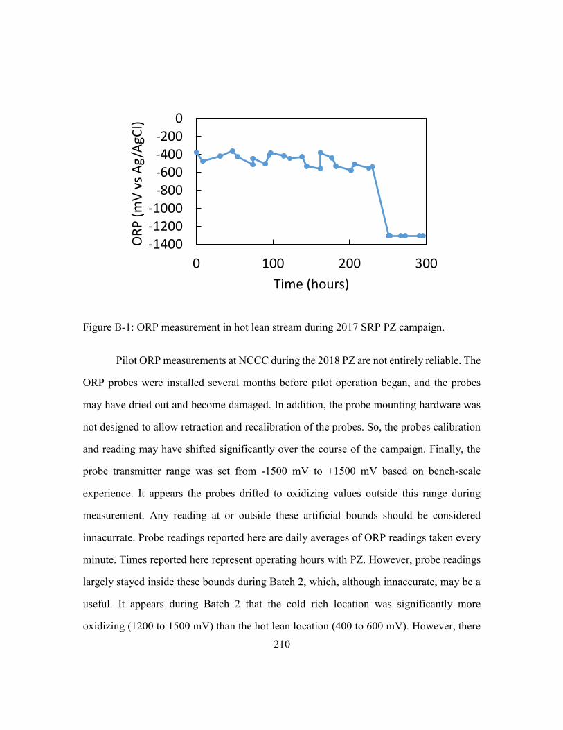
210
Figure B-1: ORP measurement in hot lean stream during 2017 SRP PZ campaign.
Pilot ORP measurements at NCCC during the 2018 PZ are not entirely reliable. The
ORP probes were installed several months before pilot operation began, and the probes
may have dried out and become damaged. In addition, the probe mounting hardware was
not designed to allow retraction and recalibration of the probes. So, the probes calibration
and reading may have shifted significantly over the course of the campaign. Finally, the
probe transmitter range was set from -1500 mV to +1500 mV based on bench-scale
experience. It appears the probes drifted to oxidizing values outside this range during
measurement. Any reading at or outside these artificial bounds should be considered
innacurrate. Probe readings reported here are daily averages of ORP readings taken every
minute. Times reported here represent operating hours with PZ. However, probe readings
largely stayed inside these bounds during Batch 2, which, although innaccurate, may be a
useful. It appears during Batch 2 that the cold rich location was significantly more
oxidizing (1200 to 1500 mV) than the hot lean location (400 to 600 mV). However, there
-1400-1200-1000
-800-600-400-200
0
0 100 200 300
OR
P (
mV
vs
Ag
/AgC
l)
Time (hours)
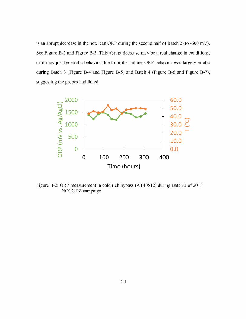
211
is an abrupt decrease in the hot, lean ORP during the second half of Batch 2 (to -600 mV).
See Figure B-2 and Figure B-3. This abrupt decrease may be a real change in conditions,
or it may just be erratic behavior due to probe failure. ORP behavior was largely erratic
during Batch 3 (Figure B-4 and Figure B-5) and Batch 4 (Figure B-6 and Figure B-7),
suggesting the probes had failed.
Figure B-2: ORP measurement in cold rich bypass (AT40512) during Batch 2 of 2018
NCCC PZ campaign
0.0
10.0
20.0
30.0
40.0
50.0
60.0
0
500
1000
1500
2000
0 100 200 300 400
T (°
C)
OR
P (
mV
vs.
Ag
/AgC
l)
Time (hours)
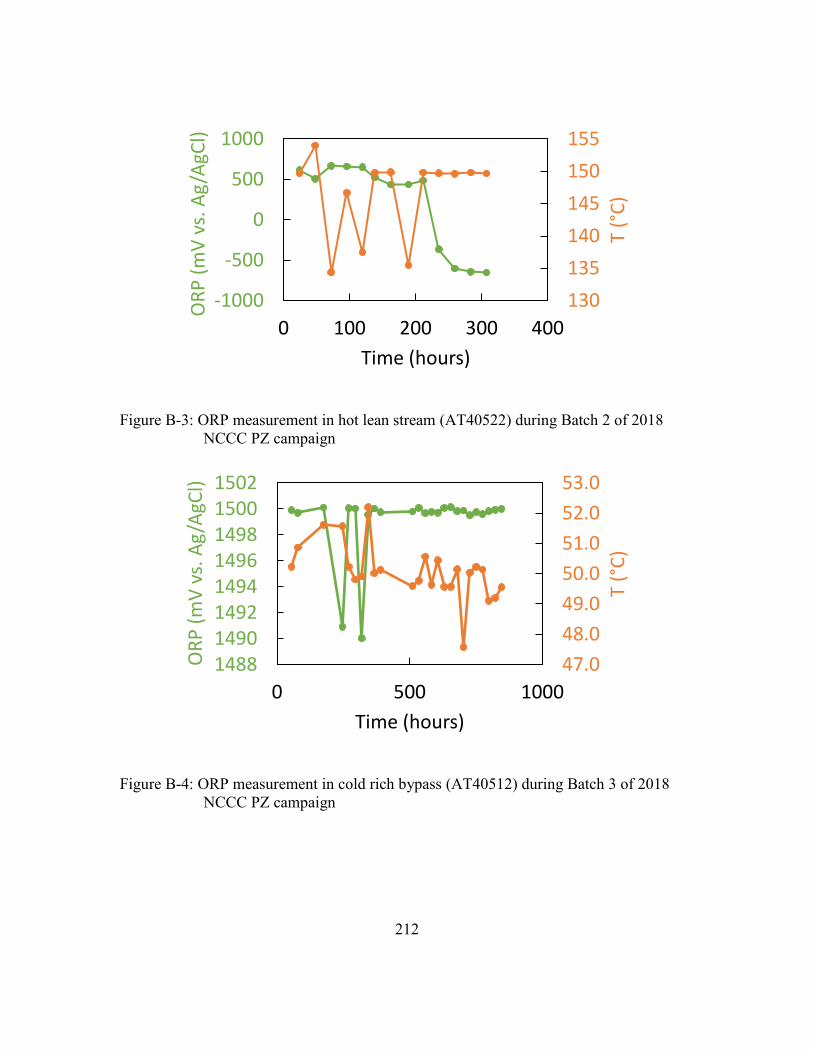
212
Figure B-3: ORP measurement in hot lean stream (AT40522) during Batch 2 of 2018
NCCC PZ campaign
Figure B-4: ORP measurement in cold rich bypass (AT40512) during Batch 3 of 2018
NCCC PZ campaign
130
135
140
145
150
155
-1000
-500
0
500
1000
0 100 200 300 400
T (°
C)
OR
P (
mV
vs.
Ag
/AgC
l)
Time (hours)
47.0
48.0
49.0
50.0
51.0
52.0
53.0
14881490149214941496149815001502
0 500 1000
T (°
C)
OR
P (
mV
vs.
Ag
/AgC
l)
Time (hours)
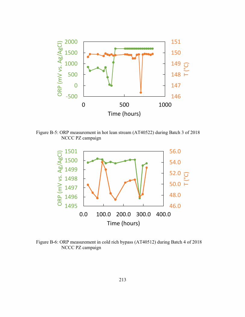
213
Figure B-5: ORP measurement in hot lean stream (AT40522) during Batch 3 of 2018
NCCC PZ campaign
Figure B-6: ORP measurement in cold rich bypass (AT40512) during Batch 4 of 2018
NCCC PZ campaign
146
147
148
149
150
151
-500
0
500
1000
1500
2000
0 500 1000
T (°
C)
OR
P (
mV
vs.
Ag
/AgC
l)
Time (hours)
46.0
48.0
50.0
52.0
54.0
56.0
1495
1496
1497
1498
1499
1500
1501
0.0 100.0 200.0 300.0 400.0
T (°
C)
OR
P (
mV
vs.
Ag
/AgC
l)
Time (hours)
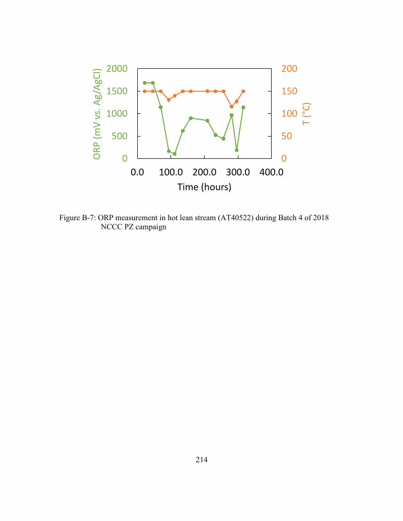
214
Figure B-7: ORP measurement in hot lean stream (AT40522) during Batch 4 of 2018
NCCC PZ campaign
0
50
100
150
200
0
500
1000
1500
2000
0.0 100.0 200.0 300.0 400.0
T (°
C)
OR
P (
mV
vs.
Ag
/AgC
l)
Time (hours)

215
References
API. (2003). Avoiding environmental cracking in amine units. In (Vol. RP945): American
Petroleum Institute.
Arrhenius, S. (1896). XXXI. On the influence of carbonic acid in the air upon the
temperature of the ground. The London, Edinburgh, and Dublin Philosophical
Magazine and Journal of Science, 41(251), 237-276.
ASTM. (2017). Standard Practice for Preparing, Cleaning, and Evaluating Corrosion Test
Specimens. In G1-03(2017)e1. West Conshohocken, PA: ASTM International.
Au-Yeung, S. C. F., Denes, G., Greedan, J. E., Eaton, D. R., & Birchall, T. (1984). A novel
synthetic route to "iron trihydroxide, Fe(OH)3": characterization and magnetic
properties. Inorganic Chemistry, 23(11), 1513-1517. doi:10.1021/ic00179a009
Bauccio, M. (1993). ASM metals reference book (3rd ed.). Materials Park, OH: ASM
international.
Beaudry, M. R. (2017). Aerosol Measurement and Mitigation in CO2 Capture by Amine
Scrubbing. (Ph.D. Dissertation), The University of Texas at Austin,
Beverskog, B., & Puigdomenech, I. (1996). Revised pourbaix diagrams for iron at 25–300
°C. Corrosion Science, 38(12), 2121-2135. doi:10.1016/S0010-938X(96)00067-4
Beverskog, B., & Puigdomenech, I. (1997a). Revised pourbaix diagrams for chromium at
25–300 °C. Corrosion Science, 39(1), 43-57. doi:10.1016/S0010-938X(97)89244-
X
Beverskog, B., & Puigdomenech, I. (1997b). Revised Pourbaix diagrams for nickel at 25–
300 °C. Corrosion Science, 39(5), 969-980. doi:10.1016/S0010-938X(97)00002-4
Booras, G. S., & Smelser, S. C. (1991). An engineering and economic evaluation of CO2
removal from fossil-fuel-fired power plants. Energy, 16(11), 1295-1305.
doi:10.1016/0360-5442(91)90003-5
Boot-Handford, M. E., Abanades, J. C., Anthony, E. J., Blunt, M. J., Brandani, S., Mac
Dowell, N., . . . Fennell, P. S. (2014). Carbon capture and storage update. Energy
& Environmental Science, 7(1), 130-189. doi:10.1039/C3EE42350F
Bottoms, R. R. (1930). Process for separating acidic gases. In: Google Patents.
Brouwer, A. S., van den Broek, M., Seebregts, A., & Faaij, A. (2014). Impacts of large-
scale Intermittent Renewable Energy Sources on electricity systems, and how these
can be modeled. Renewable and Sustainable Energy Reviews, 33, 443-466.
doi:10.1016/j.rser.2014.01.076
Bui, M., Adjiman, C. S., Bardow, A., Anthony, E. J., Boston, A., Brown, S., . . . Mac
Dowell, N. (2018). Carbon capture and storage (CCS): the way forward. Energy &
Environmental Science, 11(5), 1062-1176. doi:10.1039/C7EE02342A
Bui, M., Gunawan, I., Verheyen, V., Feron, P., Meuleman, E., & Adeloju, S. (2014).
Dynamic modelling and optimisation of flexible operation in post-combustion CO2
capture plants—A review. Computers & Chemical Engineering, 61, 245-265.
doi:10.1016/j.compchemeng.2013.11.015

216
Campbell, K. L. S., Zhao, Y., Hall, J. J., & Williams, D. R. (2016). The effect of CO2-
loaded amine solvents on the corrosion of a carbon steel stripper. International
Journal of Greenhouse Gas Control, 47, 376-385. doi:10.1016/j.ijggc.2016.02.011
Campbell, M. (2014). Technology Innovation & Advancements for Shell Cansolv CO2
capture solvents. Energy Procedia, 63, 801-807. doi:10.1016/j.egypro.2014.11.090
Chen, E., Zhang, Y., Lin, Y., Nielsen, P., & Rochelle, G. (2017). Review of Recent Pilot
Plant Activities with Concentrated Piperazine. Energy Procedia, 114, 1110-1127.
doi:10.1016/j.egypro.2017.03.1266
Chen, L., Li, F., Zhang, Y., Bentley, C. L., Horne, M., Bond, A. M., & Zhang, J. (2017).
Electrochemical Reduction of Carbon Dioxide in a Monoethanolamine Capture
Medium. ChemSusChem, 10(20), 4109-4118. doi:10.1002/cssc.201701075
Clack, C. T. M., Qvist, S. A., Apt, J., Bazilian, M., Brandt, A. R., Caldeira, K., . . .
Whitacre, J. F. (2017). Evaluation of a proposal for reliable low-cost grid power
with 100% wind, water, and solar. Proceedings of the National Academy of
Sciences, 114(26), 6722-6727. doi:10.1073/pnas.1610381114
Cousins, A., Cottrell, A., Lawson, A., Huang, S., & Feron, P. H. M. (2012). Model
verification and evaluation of the rich-split process modification at an Australian-
based post combustion CO2 capture pilot plant. Greenhouse Gases: Science and
Technology, 2(5), 329-345. doi:10.1002/ghg.1295
Cousins, A., Ilyushechkin, A., Pearson, P., Cottrell, A., Huang, S., & Feron, P. H. M.
(2013). Corrosion coupon evaluation under pilot-scale CO2 capture conditions at
an Australian coal-fired power station. Greenhouse Gases: Science & Technology,
3(3), 169-184. doi:10.1002/ghg.1341
Cousins, A., Nielsen, P. T., Huang, S., Rowland, R., Edwards, B., Cottrell, A., . . . Feron,
P. H. M. (2015). Pilot-scale evaluation of concentrated piperazine for CO2 capture
at an Australian coal-fired power station: Nitrosamine measurements. International
Journal of Greenhouse Gas Control, 37, 256-263. doi:10.1016/j.ijggc.2015.03.007
Davis, J. (2009). Thermal Degradation of Aqueous Amines Used for Carbon Dioxide
Capture. (Ph.D. Dissertation), The University of Texas at Austin,
DIPPR. (2019). DIPPR 801 Database. from Design Institute for Physical Property Data,
https://dippr.aiche.org
DOE. (2017). WA Parish Project, Office of Fossil Energy, US Department of Energy
(DOE). Retrieved from www.energy.gov/fe/petra-nova-wa-parish-project
DuPart, M., Bacon, T., & Edwards, D. (1993). Understanding corrosion in alkanolamine
gas treating plants. Hydrocarbon Processing, 72(5), 89-94.
Edenhofer, O., Pichs-Madruga, R., Sokona, Y., Farahani, E., Kadner, S., Seyboth, K., . . .
Minx, J. (2014). Climate Change 2014: Mitigation of Climate Change.
Contribution of Working Group III to the Fifth Assessment Report of the
Intergovernmental Panel on Climate Change: Cambridge University Press.
EPA. (2018). Inventory of US Greenhouse Gas Emissions and Sinks: 1990–2016. (430-R-
18-003).

217
Etheridge, D., Steele, L., Langenfelds, R., & Francey, R. (1996). Natural and
anthropogenic changes in atmospheric CO2 over the last 1000 years from air in
Antarctic ice and firn. Journal of Geophysical Research, 101(D2), 4115-4128.
Field, C., Barros, V., Dokken, D., Mastrandrea, M., Mach, K., Bilir, T., . . . Genova, R.
(2014). Climate change 2014: impacts, adaptation, and vulnerability-Part A:
global and sectoral aspects-Contribution of working group II to the fifth assessment
report of the Intergovernmental Panel on Climate Change: Cambridge University
Press.
Fine, N. A. (2015). Nitrosamine Management in Aqueous Amines for Post-Combustion
Carbon Capture. (Ph.D. Dissertation), The University of Texas at Austin,
Fischer, K. B., Daga, A., Hatchell, D., & Rochelle, G. T. (2017). MEA and Piperazine
Corrosion of Carbon Steel and Stainless Steel. Energy Procedia, 114, 1751-1764.
doi:10.1016/j.egypro.2017.03.1303
Flø, N. E., Faramarzi, L., Iversen, F., Kleppe, E. R., Graver, B., Bryntesen, H. N., &
Johnsen, K. (2019). Assessment of material selection for the CO2 absorption
process with aqueous MEA solution based on results from corrosion monitoring at
Technology Centre Mongstad. International Journal of Greenhouse Gas Control,
84, 91-110. doi:10.1016/j.ijggc.2019.02.004
Fontana, M. G. (1986). Corrosion Engineering (3rd ed.): McGraw-Hill.
Frailie, P. T. I. (2014). Modeling of Carbon Dioxide Absorption/Stripping by Aqueous
Methyldiethanolamine/Piperazine. (Ph.D. Dissertation), The University of Texas at
Austin,
Freeman, S. A. (2011). Thermal Degradation and Oxidation of Aqueous Piperazine for
Carbon Dioxide Capture. (Ph.D. Dissertation), The University of Texas at Austin,
Fytianos, G. (2016). (Ph.D. Dissertation), Norwegian University of Science and
Technology,
Fytianos, G., Grimstvedt, A., Knuutila, H., & Svendsen, H. F. (2014). Effect of MEA's
Degradation Products on Corrosion at CO2 Capture Plants. Energy Procedia, 63,
1869-1875. doi:10.1016/j.egypro.2014.11.195
Fytianos, G., Ucar, S., Grimstvedt, A., Hyldbakk, A., Svendsen, H. F., & Knuutila, H. K.
(2016). Corrosion and degradation in MEA based post-combustion CO2 capture.
International Journal of Greenhouse Gas Control, 46, 48-56.
doi:10.1016/j.ijggc.2015.12.028
Gao, T., Selinger, J. L., & Rochelle, G. T. (2019). Demonstration of 99% CO2 removal
from coal flue gas by amine scrubbing. International Journal of Greenhouse Gas
Control, 83, 236-244. doi:10.1016/j.ijggc.2019.02.013
Gunasekaran, P., Veawab, A., & Aroonwilas, A. (2013). Corrosivity of Single and Blended
Amines in CO2 Capture Process. Energy Procedia, 37, 2094-2099.
doi:10.1016/j.egypro.2013.06.088
Harrison, R. (1975). Goethite from Hindlow, Derbyshire. Bulletin of the Geological Survey
of Great Britain, 52.
218
Hatchell, D., Liu, H., Namjoshi, O. A., & Rochelle, G. T. (2015). Thermal Degradation
and Corrosion of Amines for CO2 Capture. (Honors Thesis), The University of
Texas at Austin,
Hatchell, D., Namjoshi, O., Fischer, K., & Rochelle, G. T. (2014). Thermal Degradation of
Linear Amines for CO2 Capture. Energy Procedia, 63, 1558-1568.
doi:10.1016/j.egypro.2014.11.165
Heuberger, C. F., Staffell, I., Shah, N., & Dowell, N. M. (2017). A systems approach to
quantifying the value of power generation and energy storage technologies in future
electricity networks. Computers & Chemical Engineering, 107, 247-256.
doi:10.1016/j.compchemeng.2017.05.012
Hjelmaas, S., Storheim, E., Flø, N. E., Thorjussen, E. S., Morken, A. K., Faramarzi, L., . .
. Hamborg, E. S. (2017). Results from MEA Amine Plant Corrosion Processes at
the CO2 Technology Centre Mongstad. Energy Procedia, 114, 1166-1178.
doi:10.1016/j.egypro.2017.03.1280
IAEA. (2018). Nuclear Power Reactors in the World. Vienna: International Atomic Energy
Agency.
Ibanez, J. G., Choi, C. S., & Becker, R. S. (1987). Aqueous Redox Transition Metal
Complexes for Electrochemical Applications as a Function of pH. Journal of The
Electrochemical Society, 134(12), 3083-3089. doi:10.1149/1.2100344
ICDD. (2018). PDF-4+ 2019 Database. from International Centre for Diffraction Data
Imbrie, J., Boyle, E. A., Clemens, S. C., Duffy, A., Howard, W. R., Kukla, G., . . .
Toggweiler, J. R. (1992). On the Structure and Origin of Major Glaciation Cycles
1. Linear Responses to Milankovitch Forcing. 7(6), 701-738.
doi:doi:10.1029/92PA02253
Jacobson, M. Z., Delucchi, M. A., Cameron, M. A., & Frew, B. A. (2015). Low-cost
solution to the grid reliability problem with 100% penetration of intermittent wind,
water, and solar for all purposes. Proceedings of the National Academy of Sciences,
201510028. doi:10.1073/pnas.1510028112
Jacobson, M. Z., Delucchi, M. A., Cameron, M. A., & Frew, B. A. (2017). The United
States can keep the grid stable at low cost with 100% clean, renewable energy in
all sectors despite inaccurate claims. Proceedings of the National Academy of
Sciences, 114(26), E5021-E5023. doi:10.1073/pnas.1708069114
Janssens-Maenhout, G., Crippa, M., Guizzardi, D., Muntean, M., Schaaf, E., Dentener, F.,
. . . Olivier, J. (2017). EDGAR v4.3.2 Global Atlas of the three major Greenhouse
Gas Emissions for the period 1970–2012 (Publication no.
10.2904/JRC_DATASET_EDGAR). Retrieved 12/30/2018
Jones, D. A. (1996). Principles and prevention of corrosion (2nd ed.). Upper Saddle River,
NJ: Prentice-Hall.
Kayafas, I. (1980). Technical Note: Corrosion Product Removal From Steel Fracture
Surfaces for Metallographic Examination. CORROSION, 36(8), 443-445.
doi:10.5006/0010-9312-36.8.443
Keeling, R. F. K., Charles D. (2017). Atmospheric Monthly In Situ CO2 Data - Mauna Loa
Observatory, Hawaii. In Scripps CO2 Program Data. doi:10.6075/J08W3BHW
219
Khakharia, P., Mertens, J., Huizinga, A., De Vroey, S., Sanchez Fernandez, E., Srinivasan,
S., . . . Goetheer, E. (2015). Online Corrosion Monitoring in a Postcombustion CO2
Capture Pilot Plant and its Relation to Solvent Degradation and Ammonia
Emissions. Industrial & Engineering Chemistry Research, 54(19), 5336-5344.
doi:10.1021/acs.iecr.5b00729
Kittel, J., Idem, R., Gelowitz, D., Tontiwachwuthikul, P., Parrain, G., & Bonneau, A.
(2009). Corrosion in MEA units for CO2 capture: Pilot plant studies. Energy
Procedia, 1(1), 791-797. doi:10.1016/j.egypro.2009.01.105
Kohl, A. L., & Nielsen, R. (1997). Gas purification: Elsevier.
Kump, L. R., Brantley, S. L., & Arthur, M. A. (2000). Chemical Weathering, Atmospheric
CO2, and Climate. 28(1), 611-667. doi:10.1146/annurev.earth.28.1.611
Le Quéré, C., Andrew, R. M., Friedlingstein, P., Sitch, S., Pongratz, J., Manning, A. C., . .
. Zhu, D. (2018). Global Carbon Budget 2017. Earth Syst. Sci. Data, 10(1), 405-
448. doi:10.5194/essd-10-405-2018
Li, W., Landon, J., Irvin, B., Thompson, J., Nikolic, H., & Liu, K. (2018). A Corrosion
Inhibition Study of Carbon Steel in a 0.7 MWe Pilot CO2 Capture Process. Paper
presented at the CORROSION 2018, Phoenix, Arizona, USA.
Li, W., Landon, J., Irvin, B., Zheng, L., Ruh, K., Kong, L., . . . Liu, K. (2017). Use of
Carbon Steel for Construction of Post-combustion CO2 Capture Facilities: A Pilot-
Scale Corrosion Study. Industrial & Engineering Chemistry Research, 56(16),
4792-4803. doi:10.1021/acs.iecr.7b00697
Lin, Y.-J., & Rochelle, G. T. (2016). Approaching a reversible stripping process for CO2
capture. Chemical Engineering Journal, 283, 1033-1043.
doi:10.1016/j.cej.2015.08.086
Liu, H., Hatchell, D., Namjoshi, O. A., & Rochelle, G. (2015). Oxidative degradation of
amine solvents for CO2 capture. (Honors Thesis), The University of Texas at
Austin,
Liu, H., Namjoshi, O. A., & Rochelle, G. T. (2014). Oxidative Degradation of Amine
Solvents for CO2 Capture. Energy Procedia, 63, 1546-1557.
doi:10.1016/j.egypro.2014.11.164
Lovering, J. R., Yip, A., & Nordhaus, T. (2016). Historical construction costs of global
nuclear power reactors. Energy Policy, 91, 371-382.
doi:10.1016/j.enpol.2016.01.011
Lüthi, D., Le Floch, M., Bereiter, B., Blunier, T., Barnola, J.-M., Siegenthaler, U., . . .
Stocker, T. F. (2008). High-resolution carbon dioxide concentration record
650,000–800,000 years before present. Nature, 453, 379. doi:10.1038/nature06949
MacDonald, A. E., Clack, C. T. M., Alexander, A., Dunbar, A., Wilczak, J., & Xie, Y.
(2016). Future cost-competitive electricity systems and their impact on US CO2
emissions. Nature Climate Change, 6, 526. doi:10.1038/nclimate2921
MacDowell, N., Florin, N., Buchard, A., Hallett, J., Galindo, A., Jackson, G., . . . Fennell,
P. (2010). An overview of CO2 capture technologies. Energy & Environmental
Science, 3(11), 1645-1669. doi:10.1039/C004106H

220
McHenry, H., Purtscher, P., & Shives, T. (1987). Observations of hydrogen damage in a
failed pressure vessel. Corrosion Science, 27(10-11), 1041-1057.
Metal Samples Company. (2019). Model RT4000. Retrieved from
www.alspi.com/rt4000.htm
Metz, B., Davidson, O., De Coninck, H., Loos, M., & Meyer, L. (2005). IPCC, 2005: IPCC
special report on carbon dioxide capture and storage. Prepared by Working Group
III of the Intergovernmental Panel on Climate Change (Vol. 442). Cambridge,
United Kingdom: Cambridge University Press.
NACE. (2013). Preparation, Installation, Analysis, and Interpretation of Corrosion
Coupons in Oilfiled Operations. In SP0775-2013. Houston, TX: NACE
International.
Namjoshi, O. A. (2015). Thermal Degradation of PZ-Promoted Tertiary Amines for CO2
Capture. (Ph.D. Dissertation), The University of Texas at Austin,
NBS. (1955). Standard X-ray diffraction powder patterns. In Circular 539 (Vol. 4):
National Bureau of Standards.
NBS. (1967). Standard X-ray diffraction powder patterns. In Monograph 25 (Vol. 5):
National Bureau of Standards.
NBS. (1978). Standard X-ray diffraction powder patterns. In Monograph 25 (Vol. 15):
National Bureau of Standards.
Nešić, S., & Lee, K.-L. J. (2003). A Mechanistic Model for Carbon Dioxide Corrosion of
Mild Steel in the Presence of Protective Iron Carbonate Films—Part 3: Film
Growth Model. 59(7), 616-628. doi:10.5006/1.3277592
Nešić, S., Nordsveen, M., Nyborg, R., & Stangeland, A. (2003). A Mechanistic Model for
Carbon Dioxide Corrosion of Mild Steel in the Presence of Protective Iron
Carbonate Films—Part 2: A Numerical Experiment. CORROSION, 59(6), 489-497.
doi:10.5006/1.3277579
Nielsen, P. T. (2018). Oxidation of Piperazine in Post-Combustion Carbon Capture. (Ph.D.
Dissertation), The University of Texas at Austin,
Nielsen, P. T., Li, L., & Rochelle, G. T. (2013). Piperazine Degradation in Pilot Plants.
Energy Procedia, 37, 1912-1923. doi:10.1016/j.egypro.2013.06.072
Nordsveen, M., Nešić, S., Nyborg, R., & Stangeland, A. (2003). A Mechanistic Model for
Carbon Dioxide Corrosion of Mild Steel in the Presence of Protective Iron
Carbonate Films—Part 1: Theory and Verification. 59(5), 443-456.
doi:10.5006/1.3277576
Pacala, S., & Socolow, R. (2004). Stabilization Wedges: Solving the Climate Problem for
the Next 50 Years with Current Technologies. Science, 305(5686), 968-972.
doi:10.1126/science.1100103
Pachauri, R. K., Allen, M. R., Barros, V. R., Broome, J., Cramer, W., Christ, R., . . .
Dasgupta, P. (2015). Climate change 2014: synthesis report. Contribution of
Working Groups I, II and III to the fifth assessment report of the Intergovernmental
Panel on Climate Change: Cambridge University Press.
Parson, E. A., & Keith, D. W. (1998). Fossil Fuels Without CO<sub>2</sub> Emissions.
Science, 282(5391), 1053-1054. doi:10.1126/science.282.5391.1053
221
Petit, J. R., Jouzel, J., Raynaud, D., Barkov, N. I., Barnola, J. M., Basile, I., . . . Stievenard,
M. (1999). Climate and atmospheric history of the past 420,000 years from the
Vostok ice core, Antarctica. Nature, 399, 429. doi:10.1038/20859
Pourbaix, M. (1974). Atlas of electrochemical equilibria in aqueous solution. NACE, 307.
Raja, K. S., & Jones, D. A. (2006). Effects of dissolved oxygen on passive behavior of
stainless alloys. Corrosion Science, 48(7), 1623-1638.
doi:10.1016/j.corsci.2005.05.048
Ramezan, M., Skone, T. J., Nsakala, N., & Liljedahl, G. N. (2007). Carbon Dioxide
Capture from Existing Coal-Fired Power Plants. (DOE/NETL-401/110907).
Richert, J., Bagdasarian, A., & Shargay, C. (1989). Extent of stress corrosion cracking in
amine plants revealed by survey. Oil Gas J.;(United States), 87(23).
Rochelle, G., Liu, C., Chen, E., Selinger, J., Fischer, K., Akinpelumi, K., . . . Wu, Y. (2019).
Pilot plant demonstration of piperazine with the advanced flash stripper.
International Journal of Greenhouse Gas Control.
Rochelle, G. T. (2009). Amine Scrubbing for CO2 Capture. Science, 325(5948), 1652-
1654. doi:10.1126/science.1176731
Rubin, E. S., Davison, J. E., & Herzog, H. J. (2015). The cost of CO2 capture and storage.
International Journal of Greenhouse Gas Control, 40, 378-400.
doi:10.1016/j.ijggc.2015.05.018
Sartori, G., & Savage, D. W. (1983). Sterically hindered amines for carbon dioxide removal
from gases. Industrial & Engineering Chemistry Fundamentals, 22(2), 239-249.
doi:10.1021/i100010a016
Selinger, J. (2018). Pilot Plant Modeling of Advanced Flash Stripper with Piperazine.
(M.S.E. Thesis), The University of Texas at Austin,
Sexton, A. J. (2008). Amine Oxidation in CO2 Capture Processes. (Ph.D. Dissertation),
The University of Texas at tAustin,
Shrier, A. L., & Danckwerts, P. V. (1969). Carbon Dioxide Absorption into Amine-
Promoted Potash Solutions. Industrial & Engineering Chemistry Fundamentals,
8(3), 415-423. doi:10.1021/i160031a009
Singh, A., & Stéphenne, K. (2014). Shell Cansolv CO2 capture technology: Achievement
from First Commercial Plant. Energy Procedia, 63, 1678-1685.
doi:10.1016/j.egypro.2014.11.177
Smith, J., Van ness, H., & Abbott, M. (2005). Introduction to Chemical Engineering
Thermodynamics (7th ed.).
Soosaiprakasam, I. R., & Veawab, A. (2008). Corrosion and polarization behavior of
carbon steel in MEA-based CO2 capture process. International Journal of
Greenhouse Gas Control, 2(4), 553-562. doi:10.1016/j.ijggc.2008.02.009
Sreekanth, N., & Phani, K. L. (2014). Selective reduction of CO2 to formate through
bicarbonate reduction on metal electrodes: new insights gained from SG/TC mode
of SECM. Chemical Communications, 50(76), 11143-11146.
Sun, W., & Nešić, S. (2008). Kinetics of Corrosion Layer Formation: Part 1—Iron
Carbonate Layers in Carbon Dioxide Corrosion. CORROSION, 64(4), 334-346.
doi:10.5006/1.3278477
222
Sun, W., Nešić, S., & Woollam, R. C. (2009). The effect of temperature and ionic strength
on iron carbonate (FeCO3) solubility limit. Corrosion Science, 51(6), 1273-1276.
doi:10.1016/j.corsci.2009.03.009
Sun, Y., Remias, J. E., Neathery, J. K., & Liu, K. (2011). Electrochemical study of
corrosion behaviour of carbon steel A106 and stainless steel 304 in aqueous
monoethanolamine. Corrosion Engineering, Science & Technology, 46(6), 724-
731. doi:10.1179/1743278210Y.0000000001
Sutcliffe, J. M., Fessler, R. R., Boyd, W. K., & Parkins, R. N. (1972). Stress Corrosion
Cracking of Carbon Steel in Carbonate Solutions. CORROSION, 28(8), 313-320.
doi:10.5006/0010-9312-28.8.313
Szulczewski, M. L., MacMinn, C. W., Herzog, H. J., & Juanes, R. (2012). Lifetime of
carbon capture and storage as a climate-change mitigation technology. 109(14),
5185-5189. doi:10.1073/pnas.1115347109 %J Proceedings of the National
Academy of Sciences
Tanupabrungsun, T., Young, D., Brown, B., & Nešic, S. (2012). Construction And
Verification of Pourbaix Diagrams For CO2 Corrosion of Mild Steel Valid Up to
250°C. Paper presented at the CORROSION 2012, Salt Lake City, Utah.
Tsuda, T., Takeda, M., & Hosoya, K. (2010). Effect Of Iron Carbonate On The Corrosivity
Of Amine Solutions In CO2 Removal Units. Paper presented at the CORROSION
2010, San Antonio, Texas.
Turton, R., Bailie, R. C., Whiting, W. B., & Shaeiwitz, J. A. (2008). Analysis, synthesis
and design of chemical processes: Pearson Education.
Tyndall, J. (1859). On the transmission of heat of different qualities through gases of
different kinds. Paper presented at the Proceedings of the Royal Institution.
Veawab, A., & Aroonwilas, A. (2002). Identification of oxidizing agents in aqueous
amine–CO2 systems using a mechanistic corrosion model. Corrosion Science,
44(5), 967-987. doi:10.1016/S0010-938X(01)00125-1
Veawab, A., Tontiwachwuthikul, P., & Chakma, A. (1999). Corrosion Behavior of Carbon
Steel in the CO2 Absorption Process Using Aqueous Amine Solutions. Industrial
& Engineering Chemistry Research, 38(10), 3917-3924. doi:10.1021/ie9901630
Voice, A. K. (2013). Amine Oxidation in Carbon Dioxide Capture by Aqueous Scrubbing.
(Ph.D. Dissertation), The University of Texas at Austin,
Wang, P., Tian, J., Cheng, X., Liu, C., & Xu, J. (2004). Major Pleistocene stages in a carbon
perspective: The South China Sea record and its global comparison. 19(4).
doi:10.1029/2003PA000991
Wiley, D. E., Ho, M. T., & Donde, L. (2011). Technical and economic opportunities for
flexible CO2 capture at Australian black coal fired power plants. Energy Procedia,
4, 1893-1900.
Xiang, Y., Choi, Y.-S., Yang, Y., & Nešić, S. (2014). Corrosion of Carbon Steel in MDEA-
Based CO2 Capture Plants Under Regenerator Conditions: Effects of O2 and Heat-
Stable Salts. CORROSION, 71(1), 30-37. doi:10.5006/1354
Xiang, Y., Yan, M., Choi, Y.-S., Young, D., & Nesic, S. (2014). Time-dependent
electrochemical behavior of carbon steel in MEA-based CO2 capture process.
223
International Journal of Greenhouse Gas Control, 30, 125-132.
doi:10.1016/j.ijggc.2014.09.003
Yu, L. C. Y., Sedransk Campbell, K. L., & Williams, D. R. (2016). Using carbon steel in
the stripper and reboiler for post-Combustion CO2 capture with aqueous amine
blends. International Journal of Greenhouse Gas Control, 51, 380-393.
doi:10.1016/j.ijggc.2016.04.031
Zhang, Y. (2018). Absorber and Aerosol Modeling in Amine Scrubbing for Carbon
Capture. (Ph.D. Dissertation), The University of Texas at Austin,
Zhang, Y., Kang, J.-L., Fulk, S., & Rochelle, G. (2017). Modeling Amine Aerosol Growth
at Realistic Pilot Plant Conditions. Energy Procedia, 114, 1045-1060.
doi:10.1016/j.egypro.2017.03.1251
Zheng, L., Landon, J., Matin, N. S., Li, Z., Qi, G., & Liu, K. (2014). Corrosion Behavior
of Carbon Steel in Piperazine Solutions for Post-Combustion CO2 Capture. ECS
Transactions(20), 81-95.
Zheng, L., Landon, J., Matin, N. S., Thomas, G. A., & Liu, K. (2016). Corrosion mitigation
via a pH stabilization method in monoethanolamine-based solutions for post-
combustion CO2 capture. Corrosion Science, 106, 281-292.
doi:10.1016/j.corsci.2016.02.013
Zheng, L., Landon, J., Zou, W., & Liu, K. (2014). Corrosion Benefits of Piperazine As an
Alternative CO2 Capture Solvent. Industrial & Engineering Chemistry Research,
53(29), 11740-11746. doi:10.1021/ie501346z
Zheng, L., Matin, N. S., Landon, J., Thomas, G. A., & Liu, K. (2016). CO2 loading-
dependent corrosion of carbon steel and formation of corrosion products in anoxic
30wt.% monoethanolamine-based solutions. Corrosion Science, 102, 44-54.
doi:10.1016/j.corsci.2015.09.015
Zheng, Y., Ning, J., Brown, B., & Nešić, S. (2016). Advancement in Predictive Modeling
of Mild Steel Corrosion in CO2- and H2S-Containing Environments.
CORROSION, 72(5), 679-691. doi:10.5006/1667
224
Vita
Kent Billington Fischer grew up in San Angelo, TX. He attended Southern
Methodist University and received a B.S. in Chemistry. While there, he spent several
influential summers synthesizing organometallic compounds in Dr. Michael Lattman’s lab.
Shortly after receiving his B.S., he joined the Rochelle group at the University of Texas at
Austin. Upon graduation, Kent will begin employment with REXtac, LLC in Odessa, TX.
Permanent email: [email protected]
This dissertation was typed by Kent Fischer.