arX

iv:1

204.

0679

v1 [

cond

-mat

.sta

t-m

ech]

3 A

pr 2

012

Correlations equalities and some upper bounds for the critical

temperature for spin one systems.

F. C. Sa Barretoa, A. L. Motaa

aDepartamento de Ciencias Naturais, Universidade Federal de Sao Joao del Rei, C.P. 110, CEP

36301-160, Sao Joao del Rei, Brazil

Abstract

Starting from correlation identities for the Blume-Capel spin 1 systems and using cor-relation inequalities, we obtain rigorous upper bounds for the critical temperature.Theobtained results improve over effective field type results.

1. Introduction

Correlation inequalities combined with exact identities are useful in obtaining rigorousresults in statistical mechanics. Among the various questions that are resolved by themone is the decay of the correlation functions. The decay of the correlation functions giveinformation about the critical couplings of statistical mechanics models. In this work, themethod will be applied to study systems described by the spin one Blume-Capel model[1, 2]. Firstly, we present the derivation of an exact relation for the two spin correlationfunction, valid in any dimension, which is an extension of Callen’s identity for spin 1/2Ising model [3]. Starting from these identities we will then make use of the first andsecond Griffiths inequalities and Newman’s inequalities to obtain the exponential decayof the two spin correlation function . The coupling constant which are the upper boundsfor the critical temperature are obtained for d=2 and d=3 dimensions. In this studythe coupling parameters obtained improve effective field results. Upper bounds for thecritical temperature Tc for Ising and multi-component spin systems have been obtainedby showing (for T > Tc) the exponential decay of the two-point function [4, 5, 6]. Spincorrelation inequalities and their iteration are used by Brydges et al [6], Lieb [7] andSimon [5]. The procedure to improve the bound for the critical temperature over theeffective field result for the classical S = 1 model is as follows: starting from a two-pointcorrelation function identity, a generalization of Callen’s identity [3] for this model [8]and using Griffiths 1st and 2nd inequalities (Griffith I, II) (see [9], [10],[11],[12],[13],[14])and Newman’s inequalities [10, 15] we establish the inequality for the two-point function,< S0Sl >, as

< S0Sl >≤∑

j

aj < SjSl >, 0 ≤ aj ≤ 1 (1)

Email addresses: fcsabarreto@gmail.com (F. C. Sa Barreto), motaal@ufsj.edu.br (A. L. Mota)

Preprint submitted to Elsevier April 4, 2012

which when iterated (see [5]) implies exponential decay for T > Tc. In section 2 wepresent the derivation of the correlation identities for the Blume-Capel model [8]. Insection 3, we apply these identities to the d = 2 and d = 3 lattices. Next, in section 4, weapply the correlation inequalities to obtain the upper bounds for Tc. Numerical resultscan be found in section 5, and in section 6 we present our concluding remarks.

We write the Hamiltonian for the classical spin one system, known as the Blume-Capelmodel, as

H = −J∑

i,j

SiSj −D∑

i

S2i , (2)

where J > 0,D is the single ion anisotropy and the first sum is over the nearest neighboursspins on the lattice. We define the thermal average < ... > by

< ... >= Z−1∑

{Si}

(...)e−βH , Z =∑

{Si}

e−βH (3)

where each Si is restricted by Si = −1, 0,+1.

2. Correlation identity for the spin one model

We reproduce the generalization of Callen’s identity for the spin 1 Blume-Capel modelwhich has been obtained previously by Siqueira and Fittipaldi [8]. Let

< F (S)Si >=Tr(F (S)Sie

−βH)

Tr(e−βH), (4)

where F (S) is any function of S different from Si. We can write H = Hi +H ′, where

Hi = −(∑

|j|=1

JijSj)Si −DS2i , (5)

is the Hamiltonian describing site i and its neighbours, and H ′ corresponds to the Hamil-tonian of the rest of the lattice. Consequently [Hi, H

′] = 0. From Eq.(2) and Eq.(3), weget,

< F (S)Si >=TrF (S)e−β(Hi+H′)Si

Tre−β(Hi+H′)=

Tr′TriF (S)e−βHiSie−βH′

Tr′Trie−βHie−βH′(6)

or

< F (S)Si >=Tr′TriF (S)e−βHie−βH′ Trie

−βHiSi

Trie−βHi

Tr′Trie−βHie−βH′(7)

where Tr′Tri = Tr. Finally, we obtain,

< F (S)Si >=⟨

F (S)Trie

−βHiSi

Trie−βHi

⟩

. (8)

Explicitly operating the trace Tri, we get,

< F (S)Si > =⟨

F (S)2eβDsinh(

∑

j βJijSj)

2eβDcosh(∑

j βJijSj) + 1

⟩

=⟨

F (S)∏

|j|=1

eβJijSj∇⟩

f(x)|x=0, (9)

2

with ∇ ≡ ∂∂x

, such that eα∇f(x) = f(x+ α), and

f(x) =2eβDsinh(x)

2eβDcosh(x) + 1. (10)

As S2nj = S2

j and S2n+1j = Sj for n = 0, 1, 2, 3, ..., we obtain,

eSjA = S2j cosh(A) + Sjsinh(A) + 1− S2

j , (11)

and, applying Eq.(10) and Eq.(11) in Eq.(9), we get

< F (S)Si >=⟨

F (S)∏

j 6=i,|j|=1

(S2j cosh(βJij∇)+Sjsinh(βJij∇)+1−S2

j )⟩

f(x)|x=0 (12)

Similarly for the correlation function involving the square of the spin function S2i , we

obtain,

< G(S)S2i >=

⟨

G(S)∏

j 6=i,|j|=1

eβJijSj∇⟩

g(x)|x=0, (13)

with,

g(x) =2eβDcosh(x)

2eβDcosh(x) + 1, (14)

resulting in,

< G(S)S2i >=

⟨

G(S)∏

j 6=i,|j|=1

(S2j cosh(βJij∇)+Sjsinh(βJij∇)+1−S2

j )⟩

g(x)|x=0. (15)

The function G(S) is any function of S, except S2i . The equations (12) and (15) are exact

and generalize Callen’s identity which was obtained for the S = 1/2 Ising model [3].

3. Exact correlation identities applied to the d=2 and d=3 lattices

Let us apply the previous results for < F (S)Si > and < G(S)S2i > given by equations

(12) and (15) for specific lattices in two- and three-dimensions.The two spins correlationfunctions, < S0Sl >, are obtained from equations (12) and (15) by defining F (S) = Sl.

3.1. For the d = 2 and z = 3, the honeycomb lattice

We obtain from Eq.(12)

< S0Sl > = A1

∑

i

< SiSl > +A2

∑

i<j

< SiS2jSl >

+A3

∑

i<j<k

< SiSjSkSl > +A4

∑

i<j<k

< SiS2jS

2kSl >, (16)

3

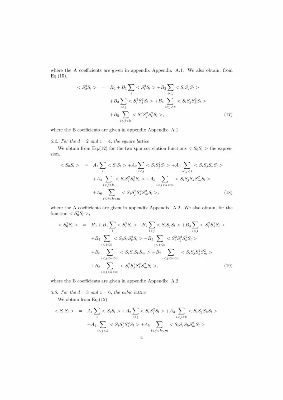
where the A coefficients are given in appendix Appendix A.1. We also obtain, fromEq.(15),

< S20Sl > = B0 +B1

∑

i

< S2i Sl > +B2

∑

i<j

< SiSjSl >

+B3

∑

i<j

< S2i S

2jSl > +B4

∑

i<j<k

< SiSjS2kSl >

+B5

∑

i<j<k

< S2i S

2jS

2kSl >, (17)

where the B coefficients are given in appendix Appendix A.1.

3.2. For the d = 2 and z = 4, the square lattice

We obtain from Eq.(12) for the two spin correlation functions < S0Sl > the expres-sion,

< S0Sl > = A1

∑

i

< SiSl > +A2

∑

i<j

< SiS2jSl > +A3

∑

i<j<k

< SiSjSkSl >

+A4

∑

i<j<k

< SiS2jS

2kSl > +A5

∑

i<j<k<m

< SiSjSkS2mSl >

+A6

∑

i<j<k<m

< SiS2jS

2kS

2mSl >, (18)

where the A coefficients are given in appendix Appendix A.2. We also obtain, for thefunction < S2

0Sl >,

< S20Sl > = B0 +B1

∑

i

< S2i Sl > +B2

∑

i<j

< SiSjSl > +B3

∑

i<j

< S2i S

2jSl >

+B4

∑

i<j<k

< SiSjS2kSl > +B5

∑

i<j<k

< S2i S

2jS

2kSl >

+B6

∑

i<j<k<m

< SiSiSkSm > +B7

∑

i<j<k<m

< SiSjS2kS

2m >

+B8

∑

i<j<k<m

< S2i S

2jS

2kS

2mSl >, (19)

where the B coefficients are given in appendix Appendix A.2.

3.3. For the d = 3 and z = 6, the cubic lattice

We obtain from Eq.(12)

< S0Sl > = A1

∑

i

< SiSl > +A2

∑

i<j

< SiS2jSl > +A3

∑

i<j<k

< SiSjSkSl >

+A4

∑

i<j<k

< SiS2jS

2kSl > +A5

∑

i<j<k<m

< SiSjSkS2mSl >

4

+A6

∑

i<j<k<m

< SiS2jS

2kS

2mSl > +A7

∑

i<j<k<m<n

< SiSjSkSmSnSl >

+A8

∑

i<j<k<m<n

< SiSjSkS2mS2

nSl >

+A9

∑

i<j<k<m<n<p

< SiSjSkSmSnS2pSl >

+A10

∑

i<j<k<m<n

< SiS2jS

2kS

2mS2

nSl >

+A11

∑

i<j<k<m<n<p

< SiSjSkS2mS2

nS2pSl >, (20)

where the A coefficients are given in appendix Appendix A.3. We also obtain, for thefunction < S2

0Sl >,

< S20Sl > = B0 +B1

∑

i

< S2i Sl > +B2

∑

i<j

< SiSjSl > +B3

∑

i<j

< S2i S

2jSl >

+B4

∑

i<j<k

< SiSjS2kSl > +B5

∑

i<j<k

< S2i S

2jS

2kSl >

+B6

∑

i<j<k<m

< SiSiSkSm > +B7

∑

i<j<k<m

< SiSjS2kS

2m >

+B8

∑

i<j<k<m

< S2i S

2jS

2kS

2mSl >

+B9

∑

i<j<k<m<n<p

< SiSjSkSmSnSpSl >

+B10

∑

i<j<k<m<n

< S2i S

2jS

2kS

2mS2

nSl >

+B11

∑

i<j<k<m<n<p

< S2i S

2jS

2kS

2mS2

nS2pSl >

+B12

∑

i<j<k<m<n

< S2i S

2jS

2kSmSnSl >

+B13

∑

i<j<k<m<n<p

< S2i S

2jS

2kS

2mSnSpSl >

+B14

∑

i<j<k<m<n

< S2i SjSkSmSnSl >

+B15

∑

i<j<k<m<n<p

< S2i S

2jSkSmSnSpSl >, (21)

where the B coefficients are given in appendix Appendix A.3.The sums over i, j, k,m, n and p are over the nearest neighbors of 0 to which we have

given a numerical ordering. The proof of results (16) for the case (3.1), the honeycomblattice, is presented in the appendix Appendix B, as an example for the other cases.

5

4. Application of the correlation inequalities

In the following results we will made use of the following inequalities: < SA >≥ 0(Griffiths I), < SASB > − < SA >< SB >≥ 0 (Griffiths II) (see [9], [10],[11],[14]),< SiF >≤

∑

j < SiSj >< dF/dSj > (Newman’s) ([15, 10])and < S2i SA >≤< SA >

([12],[13]), where < SA >=∏

i Si, < SB >=∏

i Si and F is a polynomial function ofvariables S.

From the equations for the two spin correlation functions obtained in subsections(3.1) , (3.2) and (3.3) and applying the Griffith’s and Newman’s inequalities we obtainan inequality of the form

< S0Sl >≤∑

|i|=1

ai < SiSl >, (22)

where ai is a sum of products of two-point functions.

(a) Case d = 2, z = 3, honeycomb lattice.

Using< S2

jSiSl >≤< SiSl > (23)

in equation (19), in the A2 term and Griffiths II , i.e.,

< SiSjSkSl >≥< SiSj >< SkSl > (24)

in the A3 term, and noticing that A2 and A3 are negative, we get for d=2, z=3,

< S0Sl >≤ (A1− | A2 | − | A3 |< S0S1 >1D +A4)∑

|i=1|

< SiSl >, (25)

(b) Case d = 2, z = 4, square lattice.

Using inequality (23) in equation (20), in the A2 term (A2 < 0) term, Griffiths II inthe A3 term (A3 < 0), the inequalities

< S2jS

2kSiSl >≤< SiSl > (26)

in the A4 term (A4 > 0) and

< S2jS

2kS

2mSiSl >≤< SiSl > (27)

in the A6 term (A6 > 0) and in the A5 term using Griffiths II, we get for d=2, z=4,

< S0Sl > ≤ (A1− | A2 | − < S1S2 >1D| A3 |

+A4+ < S1S2 >1D A5 +A6)∑

|i=1|

< SiSl >, (28)

6

(c) Case d = 3, z = 6, cubic lattice.

As before, we use in equation (20), inequality (23) in the A2 term (A2 < 0) term,Griffiths II in the A3 term (A3 < 0), the inequalities (26) in the A4 term (A4 > 0),inequality (24) in the A6 term (A6 > 0) , and Griffiths II in the A5 term. For the termA7(> 0) we use Newman’s inequality and for the terms A8(> 0), A9(> 0), A10(> 0) andA11(> 0), we use inequality (22). Then, we get for d=3, z=6,

< S0Sl > ≤ (A1− | A2 | − < S1S2 >1D| A3 | +A4

+ < S1S2 >1D A5

+A6 +A7 +A8 +A9 +A10 +A11)∑

|i=1|

< SiSl > (29)

The two-spin correlation function < S1S2 >1D is the one-dimension model two spincorrelation separated by a distance of two lattice sites. By bounding the resulting two-point function occurring in the previous results from below with the two-point functionof the one-dimensional infinite chain (see Appendix Appendix B), we get:

< S0Sl >≤∑

|i=1|

ai < SiSl >, (30)

where,

(a) For d = 2, z = 3, honeycomb lattice.

aj = A1− | A2 | − | A3 |< S0S1 >1D +A4; (31)

(b)For d = 2, z = 4, square lattice.

aj = A1− | A2 | − < S1S2 >1D| A3 | +A4

+ < S1S2 >1D A5 +A6; (32)

(c)For d = 3, z = 6, cubic lattice.

aj = A1− | A2 | − < S1S2 >1D| A3 | +A4

+ < S1S2 >1D A5 +A6

+A7 +A8 +A9 +A10 +A11. (33)

The one-dimensional correlation function is given by (see Appendix Appendix C):

< S1S2 >1D=1 +

√

(1− 2f(2βJ)

f(2βJ)(34)

and f(2βJ) is given by (10).

7

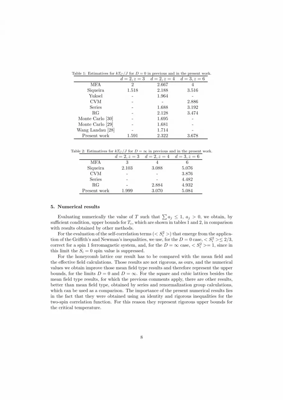
Table 1: Estimatives for kTC/J for D = 0 in previous and in the present work.

d = 2, z = 3 d = 2, z = 4 d = 3, z = 6MFA 2 2.667 4

Siqueira 1.518 2.188 3.516Yuksel - 1.964 -CVM - - 2.886Series - 1.688 3.192RG - 2.128 3.474

Monte Carlo [30] - 1.695 -Monte Carlo [29] - 1.681 -Wang Landau [28] - 1.714 -

Present work 1.591 2.322 3.678

Table 2: Estimatives for kTC/J for D = ∞ in previous and in the present work.

d = 2, z = 3 d = 2, z = 4 d = 3, z = 6MFA 3 4 6

Siqueira 2.103 3.088 5.076CVM - - 3.876Series - - 4.482RG - 2.884 4.932

Present work 1.999 3.070 5.084

5. Numerical results

Evaluating numerically the value of T such that∑

aj ≤ 1, aj > 0, we obtain, bysufficient condition, upper bounds for Tc, which are shown in tables 1 and 2, in comparisonwith results obtained by other methods.

For the evaluation of the self-correlation terms (< S2i >) that emerge from the applica-

tion of the Griffith’s and Newman’s inequalities, we use, for theD = 0 case, < S2i >≤ 2/3,

correct for a spin 1 ferromagnetic system, and, for the D = ∞ case, < S2i >= 1, since in

this limit the Si = 0 spin value is suppressed.For the honeycomb lattice our result has to be compared with the mean field and

the effective field calculations. Those results are not rigorous, as ours, and the numericalvalues we obtain improve those mean field type results and therefore represent the upperbounds, for the limits D = 0 and D = ∞. For the square and cubic lattices besides themean field type results, for which the previous comments apply, there are other results,better than mean field type, obtained by series and renormalization group calculations,which can be used as a comparison. The importance of the present numerical results liesin the fact that they were obtained using an identity and rigorous inequalities for thetwo-spin correlation function. For this reason they represent rigorous upper bounds forthe critical temperature.

8

6. Final Comments

We have presented the derivation of correlation identities for the Blume-Capel spin-1model which are exact in all dimensions, and we have made use of correlation inequalitiesto obtain the upper bounds for the transition temperature. The coupling constantsobtained for those bounds are calculated for d=2 (honeycomb and square lattices) andd=3 (cubic lattice). We obtain rigorous results that improve mean field type calculations.

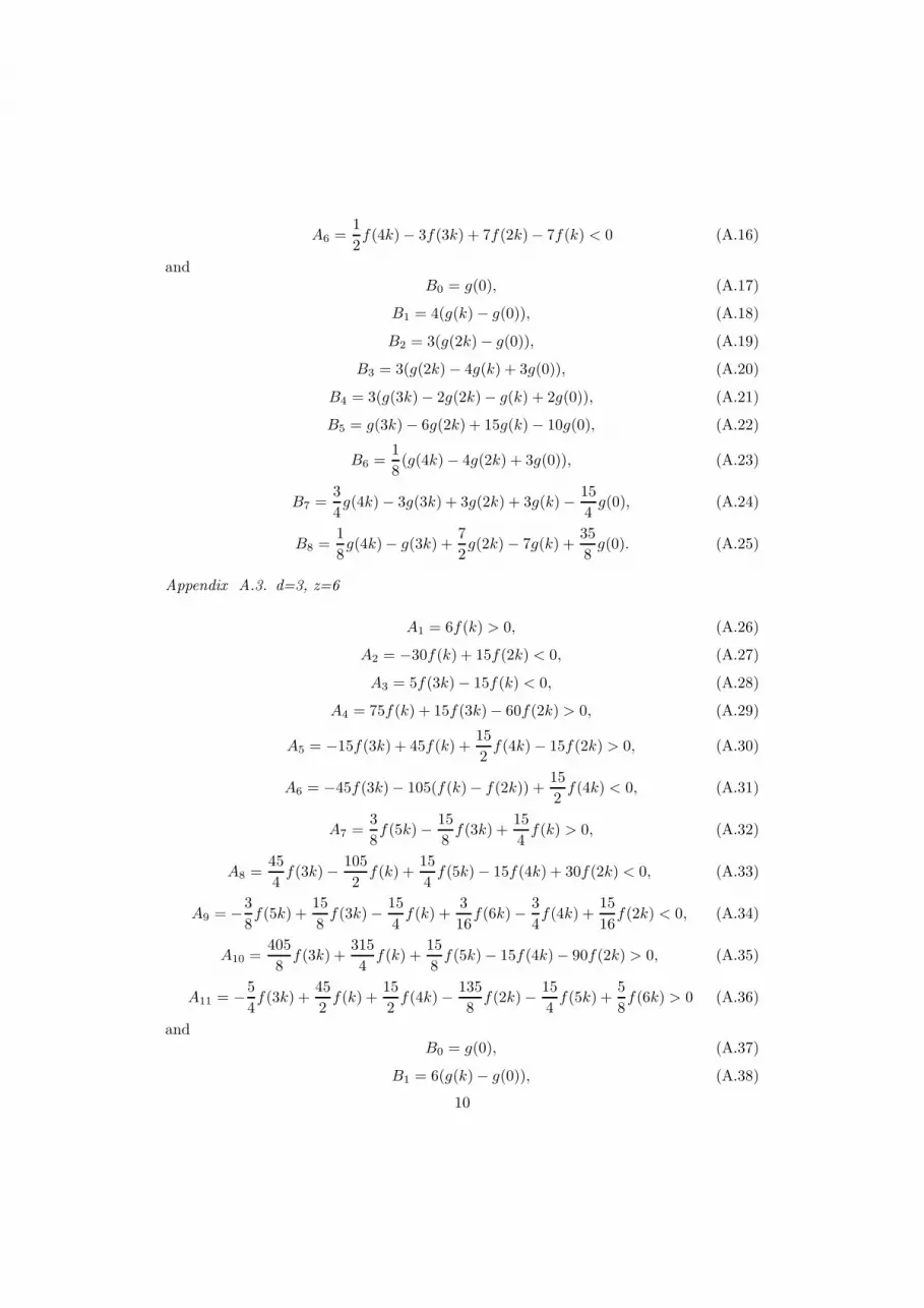
Appendix A. Coefficients of the Spin Correlation Identities for d=2, z=3

and z=4.

With k = βJ and f(x) given by relation (10), we have for

Appendix A.1. d=2, z=3

A1 = 3f(k) > 0, (A.1)

A2 = (3f(2k)− 6f(k)) < 0, (A.2)

A3 =1

4

(

f(3k)− 3f(k))

< 0 (A.3)

A4 =3

4

(

5f(k) + f(3k)− 4f(2k))

> 0 (A.4)

andB0 = g(0), (A.5)

B1 = 3(g(k)− g(0)), (A.6)

B2 =3

2(g(2k)− g(0)), (A.7)

B3 =3

2g(2k) +−6g(k) +

9

2g(0), (A.8)

B4 =3

4(g(3k)− g(k)− 2g(2k) + 2g(0)), (A.9)

B5 =1

4g(3k)−

3

2g(2k) +

15

4g(k)−

5

2g(0). (A.10)

Appendix A.2. d=2, z=4

A1 = 4f(k) > 0, (A.11)

A2 = 6f(2k)− 12f(k) < 0, (A.12)

A3 = f(3k)− 3f(k) < 0, (A.13)

A4 = 15f(k)− 12f(2k) + 3f(3k)) > 0, (A.14)

A5 =1

2f(4k)− f(3k)− f(2k) + 3f(k) > 0 (A.15)

9

A6 =1

2f(4k)− 3f(3k) + 7f(2k)− 7f(k) < 0 (A.16)

andB0 = g(0), (A.17)

B1 = 4(g(k)− g(0)), (A.18)

B2 = 3(g(2k)− g(0)), (A.19)

B3 = 3(g(2k)− 4g(k) + 3g(0)), (A.20)

B4 = 3(g(3k)− 2g(2k)− g(k) + 2g(0)), (A.21)

B5 = g(3k)− 6g(2k) + 15g(k)− 10g(0), (A.22)

B6 =1

8(g(4k)− 4g(2k) + 3g(0)), (A.23)

B7 =3

4g(4k)− 3g(3k) + 3g(2k) + 3g(k)−

15

4g(0), (A.24)

B8 =1

8g(4k)− g(3k) +

7

2g(2k)− 7g(k) +

35

8g(0). (A.25)

Appendix A.3. d=3, z=6

A1 = 6f(k) > 0, (A.26)

A2 = −30f(k) + 15f(2k) < 0, (A.27)

A3 = 5f(3k)− 15f(k) < 0, (A.28)

A4 = 75f(k) + 15f(3k)− 60f(2k) > 0, (A.29)

A5 = −15f(3k) + 45f(k) +15

2f(4k)− 15f(2k) > 0, (A.30)

A6 = −45f(3k)− 105(f(k)− f(2k)) +15

2f(4k) < 0, (A.31)

A7 =3

8f(5k)−

15

8f(3k) +

15

4f(k) > 0, (A.32)

A8 =45

4f(3k)−

105

2f(k) +

15

4f(5k)− 15f(4k) + 30f(2k) < 0, (A.33)

A9 = −3

8f(5k) +

15

8f(3k)−

15

4f(k) +

3

16f(6k)−

3

4f(4k) +

15

16f(2k) < 0, (A.34)

A10 =405

8f(3k) +

315

4f(k) +

15

8f(5k)− 15f(4k)− 90f(2k) > 0, (A.35)

A11 = −5

4f(3k) +

45

2f(k) +

15

2f(4k)−

135

8f(2k)−

15

4f(5k) +

5

8f(6k) > 0 (A.36)

andB0 = g(0), (A.37)

B1 = 6(g(k)− g(0)), (A.38)

10

B2 =15

2(g(2k)− g(0)), (A.39)

B3 =15

2(g(2k)− 4g(k) + 3g(0)), (A.40)

B4 = 15(g(3k)− 2g(2k)− g(k) + 2g(0)), (A.41)

B5 = 5(g(3k)− 6g(2k) + 15g(k)− 10g(0)), (A.42)

B6 =15

8(g(4k)− 4g(2k) + 3g(0)), (A.43)

B7 = 45(1

4g(4k)− g(3k) + g(2k) + g(k)−

5

4g(0)

)

, (A.44)

B8 = 15(1

8g(4k)− g(3k) +

7

2g(2k)− 7g(k) +

35

8g(0)

)

, (A.45)

B9 =1

32(g(6k)− 6g(4k) + 15g(2k)− 10g(0)), (A.46)

B10 =3

8(−126g(0) + 45g(3k) + 210g(k)− 120g(2k)− 10g(4k) + g(5k)), (A.47)

B11 =3

8

(

−55

3g(3k)−66g(k)+

165

4g(2k)+

77

2g(0)+

1

12g(6k)+

11

2g(4k)−g(5k)

)

, (A.48)

B12 =15

4(−8g(2k) + 14g(0) + g(5k)− 14g(k) + 13g(3k)− 6g(4k)), (A.49)

B13 =15

32(−40g(3k) + 48g(k) + 15g(2k)− 42g(0) + 26g(4k) + g(6k)− 8g(5k)), (A.50)

B14 =15

8(−2g(4k) + 8g(2k)− 6g(0) + g(5k)− 3g(3k) + 2g(k)), (A.51)

B15 =15

32(2g(4k)− 17g(2k) + 14g(0)− 4g(5k) + 12g(3k)− 8g(k) + g(6k)). (A.52)

Appendix B. Proof of the correlation identity for the honeycomb lattice

From equation (12)

< F (S)Si >=⟨

F (S)∏

j 6=i

(S2j cosh(βJij∇) + Sjsinh(βJij∇) + 1− S2

j )⟩

f(x)|x=0 (B.1)

where,

f(x) =2eβDsinh(x)

2eβDcosh(x) + 1, (B.2)

we obtain < S0Sl >, for the honeycomb lattice,

< S0Sl >=< Sl(1 + S1 sinhJ∇+ S21 [coshJ∇− 1])

×(1 + S2 sinh J∇+ S22 [coshJ∇− 1])

×(1 + S3 sinh J∇+ S23 [coshJ∇− 1]) >

(B.3)11

where S1, S2 and S3 are the neighbours of S0.Or,

< S0Sl >= 3a1 < S1Sl > +6(a2 − a1) < S1S22 >

+a3 < S1S2S3 > +(a1 − 2a2 + a4) < S1S22S

23 >, (B.4)

where,

a1 = sinh J∇ · f(x) |x=0= f(βJ)

a2 = sinh J∇ coshJ∇ · f(x) |x=0= 1/2f(2βJ)

a3 = sinh J3∇ · f(x) |x=0= 1/4[f(3βJ)− 3f(βJ)]

a4 = sinh J∇ cosh2 J∇ · f(x) |x=0= 1/4[f(3βJ) + f(βJ)] (B.5)

From those results we obtain equations (16) and (17) of section 3.1.

Appendix C. Spin Correlation for the One-Dimensional S=1 Blume-Capel

Model

For the linear chain, we have,

< S0 >=< (1 + S1 sinh J∇+ S21 [coshJ∇− 1])

(1 + S−1 sinhJ∇+ S2−1[coshJ∇− 1]) > ·f(x) |x=0

(C.1)

with f(x) given by expression (10) and S1 and S−1 are neighbors of S0. We obtain forthe two-spin correlation function

< S0SR >=< (S1SR + S−1SR) > f(k)

+ < (S1S−1S1SR + S1S−1S−1SR) > (1

2f(2k)− f(k)) (C.2)

where k = βJ . Applying the inequalities ([12],[13])

< S21S−1SR >≤< S−1SR >

< S2−1S1SR >≤< S1SR > (C.3)

we get,

< S0SR >≤ (< S1SR > + < S−1SR >)f(k)

+(< S−1SR > + < S1SR >)[1/2f(2k)− f(k)] (C.4)

Defining C(R) =< S0SR > we get

C(R) = A(k)(C(R + 1) + C(R − 1)), (C.5)

where A(k) = f(2k)/2.If γ(R) = C(R + 1)/C(R) is inserted in the previous equation we get

1 = A(k)(γ(R) + γ(R)−1). (C.6)

So, C(R) = γR and

γ =1 +

√

1− 2f(2βJ)

f(2βJ). (C.7)

12

Acknowledgements

FCSB is grateful to CAPES/Brazil for the financial support that made possible hisvisit to the UFSJ/Brazil. ALM acknowledges financial support from CNPq-Brazil andFAPEMIG-Brazil.

References

[1] Capel H W 1966 Physica 32 966[2] Blume M 1966 Phys.Rev. 141 517[3] Callen H B 1963 Phys.Lett. 4 161[4] Fisher M 1967 Phys.Rev. 162 480[5] Simon B 1980 Commun.Math Phys. 77 111[6] Brydges D, Frohlich J and Spencer T 1982 Commun.Math.Phys. 83 123[7] Lieb E 1980 Commun.Math.Phys. 77 127[8] Siqueira A F and Fittipaldi I P 1986 Physica A 138 592[9] Griffiths R B 1969 J.Math.Phys. 10 1559

[10] Sylvester G S 1976 J.Stat.Phys. 15 327[11] Fernandez R., Frohlich J. and Sokal A. D. 1992 Random Walks, Critical Phenomena and Triviality

in Quantum Field Theory (Springer-Verlag, Berlim)[12] Braga G A, Ferreira S J and Sa Barreto F C 1993 Braz.J.Phys. 23 343[13] Braga G A, Ferreira S J and Sa Barreto F C 1994 J.Stat.Phys. 76 819[14] Szasz D 1978 J.Stat.Phys. 19 453[15] Newman C 1975 Zeitschriftfur Wahrscheinlichkeits Theorie 33 75[16] Ginibre J 1969 Phys.Rev.Lett. 23 828[17] Yuksel Y, Akinsi and Polat H 2009 Phys.Scr. 79 1[18] Wilson K 1974 Phys. Rev. D 10 2445-59[19] Seiler E 1982 Gauge Theories as a Problem of Constructive Quantum Field Theory and Statistical

Mechanics, Lect. Notes in Physics 159[20] Kogut J 1979 Rev. Mod. Phys. 51 659[21] Sa Barreto F C and O‘Carroll M L 1983 J.Phys.A 16 L431[22] Glimm J and Jaffe A 1981 Quantum Physics (New York: Springer)[23] Sa Barreto F C and O‘Carroll M L 1983 J.Phys.A 16 1035[24] Tomboulis E, Ukawa A and Windey P 1981 Nucl. Phys. B 180 [FS2] 294-300[25] Griffiths R B 1967 J.Math.Phys. 8 478[26] Griffiths R B 1967 J.Math.Phys. 8 484[27] Griffiths R B 1967 Commun.Math.Phys. 9 121[28] Plascak J A ; Caparica A A; Silva C J 2006 Phys. Rev. E 73 36702[29] Xavier J C, Alcaraz F C, Pena Lara D and Plascak J A 1998 Phys. Rev. B 57 11575[30] Beale P D 1986 Phys. Rev. B 33 1717

13