sharp bounds for generalized uniformity testing - electronic
TRANSCRIPT
Sharp Bounds for Generalized Uniformity Testing
Ilias Diakonikolas∗
University of Southern [email protected]
Daniel M. Kane†
University of California, San [email protected]
Alistair StewartUniversity of Southern California
September 6, 2017
Abstract
We study the problem of generalized uniformity testing [BC17] of a discrete probabilitydistribution: Given samples from a probability distribution p over an unknown discrete domainΩ, we want to distinguish, with probability at least 2/3, between the case that p is uniform onsome subset of Ω versus ε-far, in total variation distance, from any such uniform distribution.
We establish tight bounds on the sample complexity of generalized uniformity testing. Inmore detail, we present a computationally efficient tester whose sample complexity is optimal,up to constant factors, and a matching information-theoretic lower bound. Specifically, we showthat the sample complexity of generalized uniformity testing is Θ
(1/(ε4/3‖p‖3) + 1/(ε2‖p‖2)
).
1 Introduction
Consider the following statistical task: Given independent samples from a distribution over anunknown discrete domain Ω, determine whether it is uniform on some subset of the domain versus
significantly different from any such uniform distribution. Formally, let CUdef= uS : S ⊆ Ω denote
the set of uniform distributions uS over subsets S of Ω. Given sample access to an unknowndistribution p on Ω and a proximity parameter ε > 0, we want to correctly distinguish between
the case that p ∈ CU versus dTV (p, CU )def= minS⊆Ω dTV (p,uS) ≥ ε, with probability at least 2/3.
Here, dTV (p, q) = (1/2)‖p − q‖1 denotes the total variation distance between distributions p andq. This natural problem, termed generalized uniformity testing, was recently studied by Batu andCanonne [BC17], who gave the first upper and lower bounds on its sample complexity.
Generalized uniformity testing bears a strong resemblance to the familiar task of uniformitytesting, where one is given samples from a distribution p on an explicitly known domain of size nand the goal is to determine, with probability at least 2/3, whether p is the uniform distribution unon this domain versus dTV (p,un) ≥ ε. Uniformity testing is arguably the most extensively studiedproblem in distribution property testing [GR00, Pan08, VV14, DKN15b, Gol16, DGPP16, DGPP17]and its sample complexity is well understood. Specifically, it is known [Pan08, CDVV14, VV14,DKN15b] that Θ(n1/2/ε2) samples are necessary and sufficient for this task.
∗Supported by NSF Award CCF-1652862 (CAREER) and a Sloan Research Fellowship.†Supported by NSF Award CCF-1553288 (CAREER) and a Sloan Research Fellowship.
ISSN 1433-8092
Electronic Colloquium on Computational Complexity, Report No. 132 (2017)
The field of distribution property testing [BFR+00] has seen substantial progress in the pastdecade, see [Rub12, Can15] for two recent surveys. A large body of the literature has focused oncharacterizing the sample size needed to test properties of arbitrary distributions of a given supportsize. This regime is fairly well understood: for many properties of interest there exist sample-efficient testers [Pan08, CDVV14, VV14, DKN15b, ADK15, CDGR16, DK16, DGPP16, CDS17,DGPP17]. Moreover, an emerging body of work has focused on leveraging a priori structure of theunderlying distributions to obtain significantly improved samples complexities [BKR04, DDS+13,DKN15b, DKN15a, CDKS17, DP17, DDK16, DKN17].
Perhaps surprisingly, the natural setting where the distribution is arbitrary on a discrete butunknown domain (of unknown size) does not seem to have been explicitly studied before the recentwork of Batu and Canonne [BC17]. Returning to the specific problem studied here, at first sightit might seem that generalized uniformity testing and uniformity testing are essentially the sametask. However, as shown in [BC17], the sample complexities of these two problems are significantlydifferent. Specifically, [BC17] gave a generalized uniformity tester with expected sample complexityO(1/(ε6‖p‖3)) and showed a lower bound of Ω(‖p‖3). Since generalized uniformity is a symmetricproperty, any tester should essentially rely on the empirical moments (collision statistics) of thedistribution [RRSS09, Val11]. The algorithm in [BC17] uses sufficiently accurate approximationsof the second and third moments of the unknown distribution. Their lower bound formalizes theintuition that an approximation of the third norm is in some sense necessary to solve this problem.
1.1 Our Results and Techniques
An immediate open question arising from the work of [BC17] is to precisely characterize the samplecomplexity of generalized uniformity testing, as a function of all relevant parameters. The mainresult of this paper provides an answer to this question. In particular, we show the following:
Theorem 1.1 (Main Result). There is an algorithm with the following performance guarantee:Given sample access to an arbitrary distribution p over an unknown discrete domain Ω and aparameter 0 < ε < 1, the algorithm uses O
(1/(ε4/3‖p‖3) + 1/(ε2‖p‖2)
)independent samples from
p in expectation, and distinguishes between the case p ∈ CU versus dTV (p, CU ) ≥ ε with probabilityat least 2/3. Moreover, for every 0 < ε < 1/0 and n > 1, any algorithm that distinguishes betweenp ∈ CU and dTV (p, CU ) ≥ ε requires at least Ω(n2/3/ε4/3 + n1/2/ε2) samples, where p is guaranteedto have ‖p‖3 = Θ(n−2/3) and ‖p‖2 = Θ(n−1/2).
In the following paragraphs, we provide an intuitive explanation of our algorithm and ourmatching sample size lower bound, in tandem with a comparison to the prior work [BC17].
Sample-Optimal Generalized Uniformity Tester. Our algorithm requires considering twocases based on the relative size of ε and ‖p‖22. This case analysis seems somewhat intrinsic to theproblem as the correct sample complexity branches into these cases.
For large ε, we use the same overall technique as [BC17], noting that p is uniform if and only
if ‖p‖3 = ‖p‖4/32 , and that for p far from uniform, ‖p‖3 must be substantially larger. The basicidea from here is to first obtain rough approximations to ‖p‖2 and ‖p‖3 in order to ascertain thecorrect number of samples to use, and then use standard unbiased estimators of ‖p‖22 and ‖p‖33to approximate them to appropriate precision, so that their relative sizes can be compared withappropriate accuracy.
We improve upon the work of [BC17] in this parameter regime in a couple of ways. First, weobtain more precise lower bounds on the difference ‖p‖33 − ‖p‖42 in the case where p is far fromuniform (Lemma 2.4). This allows us to reduce the accuracy needed in estimating ‖p‖2 and ‖p‖3.
2
Second, we refine the method used for performing the approximations to these moments (`r-norms).In particular, we observe that using the generic estimators for these quantities yields sub-optimalbounds for the following reason: The error of the unbiased estimators is related to their variance,which in turn can be expressed in terms of the higher moments of p (Fact 2.1). This implies forexample that the worst case sample complexity for estimating ‖p‖3 comes when the fourth andfifth moments of p are large. However, since we are trying to test for the case of uniformity (wherethese higher moments are minimal), we do not need to worry about this worst case. In particular,after applying sample efficient tests to ensure that the higher moments of p are not much largerthan expected (Lemma 2.2 (ii)), the standard estimators for the second and third moments of pcan be shown to converge more rapidly than they would in the worst case (Lemma 2.5).
The above algorithm is not sufficient for small values of ε. For ε sufficiently small, we employa different, perhaps more natural, algorithm. Here we take m samples (for m appropriately chosenbased on an approximation to ‖p‖2) and consider the subset S of the domain that appears in thesample. We then test whether the conditional distribution p on S is uniform, and output theanswer of this tester. The number of samples m drawn in the first step is sufficiently large so thatp(S), the probability mass of S under p, is relatively high. Hence, it is easy to sample from theconditional distribution using rejection sampling. Furthermore, we can use a standard uniformitytesting algorithm requiring O(
√|S|/ε2) samples.
To establish correctness of this algorithm, we need to show that if p is far from uniform, then theconditional distribution p on S is far from uniform as well. To prove this statement, we distinguishtwo further subcases. If ε is “very small”, then we can afford to set m sufficiently large so thatp(S) is at least 1− ε/10. In this case, our claim follows straightforwardly. For the remaining valuesof ε, we can only guarantee that p(S) = Ω(1), hence we require a more sophisticated argument.Specifically, we show (Lemma 2.6) that for any x in an appropriate interval, with high constantprobability, the random variable Z(x) =
∑i∈S |pi−x| is large. It is not hard to show that this holds
with high probability for each fixed x, as p being far from uniform implies that∑
i∈Ω min(pi, |pi−x|)is large. This latter condition can be shown to provide a clean lower bound for the expectation ofZ(x). To conclude the argument, we show that Z(x) is tightly concentrated around its expectation.
Sample Complexity Lower Bound. The lower bound of Ω(1/(ε2‖p‖2)) follows directly fromthe standard lower bound of Ω(n1/2/ε2) [Pan08] for uniformity testing on a given domain of size n.Specifically, it is implied from the fact that the hard instances satisfy ‖p‖2 = Θ(n−1/2). The otherbranch of the lower bound, namely Ω(1/(ε4/3‖p‖3)), is more involved. To prove this lower bound,we use the shared information method [DK16] for the following family of hard instances: In the“YES” case, we consider the distribution over (pseudo-)distributions on N bins, where each pi is(1 + ε2)/N with probability n/(N(1 + ε2)), and 0 otherwise. (Here we assume that the parameterN is sufficiently large compared to the other parameters.) In the “NO” case, we consider thedistribution over (pseudo-)distributions on N bins, where each pi is (1 + ε)/N with probabilityn/(2N), (1− ε)/N with probability n/(2N), and 0 otherwise.
1.2 Notation
Let Ω denote the unknown discrete domain. Each probability distribution over Ω can be associatedwith a probability mass function p : Ω → R+ such that
∑i∈Ω pi = 1. We will use pi, instead of
p(i), to denote the probability of element i ∈ Ω in p. For a distribution (with mass function) p
and a set S ⊆ Ω, we denote by p(S)def=∑
i∈S pi and by (p|S) the conditional distribution of p on
S. For r ≥ 1, the `r-norm of a function p : Ω→ R is ‖p‖rdef=(∑
i∈Ω |pi|r)1/r
. For convenience, we
3

will denote Fr(p)def= ‖p‖rr =
∑i∈Ω |pi|r. For ∅ 6= S ⊆ Ω, let uS be the uniform distribution over
S. Let CUdef= uS : ∅ 6= S ⊆ Ω be the set of uniform distributions over subsets of Ω. The total
variation distance between distributions p, q on Ω is defined as dTV (p, q)def= maxS⊆Ω |p(S)−q(S)| =
(1/2) · ‖p− q‖1. Finally, we denote by Poi(λ) the Poisson distribution with parameter λ.
2 Generalized Uniformity Tester
In this section, we give our sample-optimal generalized uniformity tester, Gen-Uniformity-Test.Before we describe our algorithm, we summarize a few preliminary results on estimating the powersums Fr(p) =
∑i∈Ω |pi|r of an unknown distribution p. We present these results in Section 2.1.
In Section 2.2, we give a detailed pseudo-code for our algorithm. In Section 2.3, we analyze thesample complexity, and in Section 2.4 we provide the proof of correctness.
2.1 Estimating the Power Sums of a Discrete Distribution
We will require various notions of approximation for the power sums of a discrete distribution. Westart with the following fact:
Fact 2.1 ([AOST17]). Let p be a probability distribution on an unknown discrete domain. For anyr ≥ 1, there exists an estimator Fr(p) for Fr(p) that draws Poi(m) samples from p and satisfies
the following: E[Fr(p)
]= Fr(p) and Var
[Fr(p)
]= m−2r
∑r−1t=0 m
r+t(rt
)rr−tFr+t(p).
The estimator Fr(p) is standard: It draws Poi(m) samples from p and mr · Fr(p) equals thenumber of r-wise collisions, i.e., ordered r-tuples of samples that land in the same bin. UsingFact 2.1, we get the following lemma which will be crucial for our generalized uniformity tester:
Lemma 2.2. Let p be a probability distribution on an unknown discrete domain and r ≥ 1. Wehave the following:
(i) There exists an algorithm that, given a parameter 0 < δ < 1 and sample access to p, drawsO( 1
δ2‖p‖r ) samples from p in expectation and outputs an estimate γr that with probability at
least 19/20 satisfies: |γr − Fr(p)| ≤ δ · Fr(p).
(ii) For any c ≥ 1, there exist an algorithm that draws Poi (O(m)) samples from p and correctlydistinguishes with probability at least 19/20 between the case that mrFr(p) ≥ 20c versusmrFr(p) ≤ c/20.
Proof. Using Fact 2.1, it is shown in [AOST17] that if we draw m = O( 1δ2‖p‖r ) samples from p,
then with high constant probability we have that |Fr(p) − Fr(p)| ≤ δ · Fr(p). Since the value of‖p‖r is unknown, this guarantee does not quite suffice for (i). We instead start by approximating1/‖p‖rr within a constant factor. We do this by counting the number of samples we need to drawfrom p until we see the first r-wise collision. By Fact 2.1 and Chebyshev’s inequality, this gives aconstant factor approximation to 1/‖p‖rr with expected sample size of O(1/‖p‖r). We thus get (i).
We now proceed to show (ii). The algorithm is straightforward: Draw Poi (O(m)) samplesfrom p and calculate Fr(p). If mrFr(p) > c, output “large”; otherwise output “small”. Supposethat mrFr(p) ≤ c/20. By Markov’s inequality, with probability at least 19/20 we will have thatmrFr(p) ≤ c, in which case we output “small”. Now suppose that mrFr(p) ≥ 20c. Since c ≥ 1, thisgives that ‖p‖r ≥ 1/m. Therefore, after we draw Poi(O(m)) samples from p, with probability atleast 19/20 we have that Fr(p) is a factor 2 approximation to Fr(p). In other words, mrFr(p) ≥ 10cand the algorithm outputs “large”.
4

2.2 Pseudo-code for Gen-Uniformity-Test Algorithm
The algorithm is given in the following pseudo-code:
Algorithm 1 Sample-Optimal Algorithm for Generalized Uniformity Testing
1: procedure Gen-Uniformity-Test(p, ε)input: Sample access to arbitrary distribution p on unknown discrete domain Ω and ε > 0.output: “YES” with probability 2/3 if p ∈ CU , “NO” with probability 2/3 if dTV (p, CU ) ≥ ε.2: Compute an estimate γ2 satisfying |γ2 − F2(p)| ≤ (1/2) · F2(p) with probability 19/20.3: n← d2/γ2e.4: if (ε ≥ n−1/4) then5: Compute an estimate γ3 satisfying |γ3 − F3(p)| ≤ (1/2) · F3(p) with probability 19/20.6: if (γ3 ≥ 8/n2 or γ3 ≤ 1/(8n2)) then return “NO”.
7: Let m← Θ(n2/3/ε4/3), for a sufficiently large constant in the Θ().8: Let c4 = Θ(1 +m4/n3), for a sufficiently large constant in the Θ().9: Draw Poi(O(m)) samples from p and let γ4 denote the value of F4(p) on this sample.
10: if m4γ4 > 20c4 then return “NO”.
11: Let c5 = Θ(1 +m5/n4), for a sufficiently large constant in the Θ().12: Draw Poi(O(m)) samples from p and let γ5 denote the value of F5(p) on this sample.13: if m5γ5 > 20c5 then return “NO”.
14: Compute the estimates F2(p), F3(p) on two separate sets of Poi(m) samples.
15: if(F3(p)− F2(p)2 ≤ ε2/(300n2)
)then return “YES”.
16: else return “NO”.17: if (n−1/4 log−1(n) ≤ ε < n−1/4) then18: Let m1 ← Θ(n), for an appropriately large constant in the Θ().19: Draw Poi(m1) samples from p. Let S be the subset of Ω that appears in the sample.20: Verify the following conditions: (i) Each i ∈ S appears O(log n) times;21: (ii) |S| ≥ n/2; (iii) p(S) ≥ 1/2.22: if (any of conditions (20), (21) is violated) then return “NO”.
23: Using rejection sampling, draw m2 ← O(n1/2/ε2) samples from (p|S).24: Test whether (p|S) = uS versus ε/10-far from uS with confidence probability 19/20.25: return the answer of the tester in Step 24.
26: if (ε < n−1/4 log−1(n)) then27: m1 ← Θ(n log n), for an appropriately large constant in the Θ().28: Draw Poi(m1) samples from p. Let S be the subset of Ω that appears in the sample.29: Draw m2 ← O(n1/2/ε2) samples from p.30: if (any of the above samples lands outside S) then return “NO”.
31: Test whether (p|S) = uS versus ε/2-far from uS with confidence probability 19/20.32: return the answer of the tester in Step 31.
2.3 Bounding the Sample Complexity
We start by analyzing the sample complexity of the algorithm. We claim that the expected samplecomplexity is O
(1/(ε4/3‖p‖3
))for ε ≥ n−1/4 and O
(1/(ε2‖p‖2
))for ε < n−1/4.
By Lemma 2.2 (i), Step 2 can be implemented with expected sample complexity O(1/‖p‖2) andStep 5 with expected sample complexity O(1/‖p‖3).
5
We start with the case ε ≥ n−1/4. If Steps 2, 5, and 6 succeed, then we have that F2(p) = Θ(1/n)and F3(p) = Θ(1/n2). Also note that no further steps are executed unless the condition of Step 6holds. Note that all subsequent steps that draw samples (Steps 9, 12, and 14) by definition use atmost Poi(O(m)) additional samples. Since Step 14 is executed only if γ3 = Θ(1/n2), we have that
m = O(γ−1/33 /ε4/3) = O(1/(ε4/3‖p‖3)). Therefore, for ε ≥ n−1/4, the expected sample complexity
of the algorithm is bounded by
O (1/‖p‖2) +O (1/‖p‖3) +O(
1/(ε4/3‖p‖3
))= O
(1/(ε4/3‖p‖3
)).
For the case of n−1/4 log−1(n) ≤ ε < n−1/4, the additional sample size drawn on top of Step 2is O(n+ n1/2/ε2) = O(n1/2/ε2). Since n = Θ(1/‖p‖22), the total sample complexity in this case is
O (1/‖p‖2) +O(1/(ε2‖p‖2
))= O
(1/(ε2‖p‖2
)).
Finally, for ε < n−1/4 log−1(n), the sample size drawn on top of Step 2 is O(n log n + n1/2/ε2) =O(n1/2/ε2). Since n = Θ(1/‖p‖22), the total sample complexity in this case is O
(1/(ε2‖p‖2
)), as
before. This completes the analysis of the sample complexity.
2.4 Correctness Proof
This section is devoted to the correctness proof of Gen-Uniformity-Test. In particular, we willshow that if p ∈ CU , the algorithm outputs “YES” with probability at least 2/3 (completeness);and if dTV (p, CU ) ≥ ε, the algorithm outputs “NO” with probability at least 2/3 (soundness).
We start with the following simple claim giving a useful condition for the soundness case:
Claim 2.3. If dTV (p, CU ) ≥ ε, then for all x ∈ [0, 1] we have that∑
i∈Ω minpi, |x− pi| ≥ ε/2.
Proof. Let Sh be the set of i ∈ Ω on which pi > x/2. Let δ =∑
i∈Ω minpi, |x − pi|. Note thatδ = ‖p− cx,Sh
‖1, where cx,Shis the pseudo-distribution that is x on Sh on 0 elsewhere. If ‖cx,Sh
‖1were 1, cx,Sh
would be the uniform distribution uShand we would have δ ≥ ε. However, this need
not be the case. That said, it is easy to see that ‖uSh− cx,Sh
‖1 = |1−‖cx,Sh‖1| ≤ ‖p− cx,Sh
‖1 = δ.Therefore, by the triangle inequality
2δ ≥ ‖p− cx,Sh‖1 + ‖uSh
− cx,Sh‖1 ≥ ‖p− uSh
‖1 ≥ ε .
This completes the proof of Claim 2.3.
We now proceed to analyze correctness for the various ranges of ε.
Case I: [ε ≥ n−1/4]. The following structural lemma provides a reformulation of generalizeduniformity testing in terms of the second and third norms of the unknown distribution:
Lemma 2.4. We have the following:
(i) If p ∈ CU , then F3(p) = F22(p).
(ii) If dTV (p, CU ) ≥ ε, then F3(p)− F22(p) > ε2F2
2(p)/64.
Proof. The proof of (i) is straightforward. Suppose that p = uS for some ∅ 6= S ⊆ Ω. It thenfollows that F2(p) = 1/|S| and F3(p) = 1/|S|2, yielding part (i) of the lemma.
6
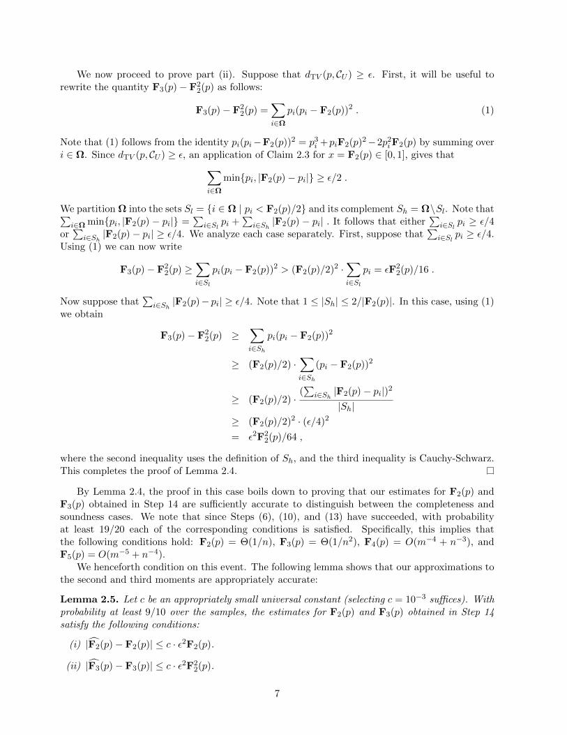
We now proceed to prove part (ii). Suppose that dTV (p, CU ) ≥ ε. First, it will be useful torewrite the quantity F3(p)− F2
2(p) as follows:
F3(p)− F22(p) =
∑i∈Ω
pi(pi − F2(p))2 . (1)
Note that (1) follows from the identity pi(pi−F2(p))2 = p3i +piF2(p)2−2p2
iF2(p) by summing overi ∈ Ω. Since dTV (p, CU ) ≥ ε, an application of Claim 2.3 for x = F2(p) ∈ [0, 1], gives that∑
i∈Ωminpi, |F2(p)− pi| ≥ ε/2 .
We partition Ω into the sets Sl = i ∈ Ω | pi < F2(p)/2 and its complement Sh = Ω\Sl. Note that∑i∈Ω minpi, |F2(p) − pi| =
∑i∈Sl
pi +∑
i∈Sh|F2(p) − pi| . It follows that either
∑i∈Sl
pi ≥ ε/4or∑
i∈Sh|F2(p)− pi| ≥ ε/4. We analyze each case separately. First, suppose that
∑i∈Sl
pi ≥ ε/4.Using (1) we can now write
F3(p)− F22(p) ≥
∑i∈Sl
pi(pi − F2(p))2 > (F2(p)/2)2 ·∑i∈Sl
pi = εF22(p)/16 .
Now suppose that∑
i∈Sh|F2(p)− pi| ≥ ε/4. Note that 1 ≤ |Sh| ≤ 2/|F2(p)|. In this case, using (1)
we obtain
F3(p)− F22(p) ≥
∑i∈Sh
pi(pi − F2(p))2
≥ (F2(p)/2) ·∑i∈Sh
(pi − F2(p))2
≥ (F2(p)/2) ·(∑
i∈Sh|F2(p)− pi|)2
|Sh|≥ (F2(p)/2)2 · (ε/4)2
= ε2F22(p)/64 ,
where the second inequality uses the definition of Sh, and the third inequality is Cauchy-Schwarz.This completes the proof of Lemma 2.4.
By Lemma 2.4, the proof in this case boils down to proving that our estimates for F2(p) andF3(p) obtained in Step 14 are sufficiently accurate to distinguish between the completeness andsoundness cases. We note that since Steps (6), (10), and (13) have succeeded, with probabilityat least 19/20 each of the corresponding conditions is satisfied. Specifically, this implies thatthe following conditions hold: F2(p) = Θ(1/n), F3(p) = Θ(1/n2), F4(p) = O(m−4 + n−3), andF5(p) = O(m−5 + n−4).
We henceforth condition on this event. The following lemma shows that our approximations tothe second and third moments are appropriately accurate:
Lemma 2.5. Let c be an appropriately small universal constant (selecting c = 10−3 suffices). Withprobability at least 9/10 over the samples, the estimates for F2(p) and F3(p) obtained in Step 14satisfy the following conditions:
(i) |F2(p)− F2(p)| ≤ c · ε2F2(p).
(ii) |F3(p)− F3(p)| ≤ c · ε2F22(p).
7
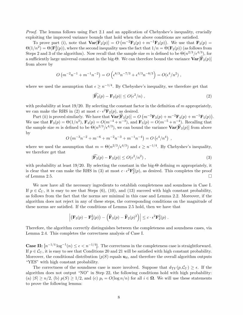
Proof. The lemma follows using Fact 2.1 and an application of Chebyshev’s inequality, cruciallyexploiting the improved variance bounds that hold when the above conditions are satisfied.
To prove part (i), note that Var[F2(p)] = O(m−2F2(p) +m−1F3(p)
). We use that F3(p) =
Θ(1/n2) = Θ(F22(p)), where the second inequality uses the fact that 1/n = Θ(F2(p)) (as follows from
Steps 2 and 3 of the algorithm). Now recall that the sample size m is defined to be Θ(n2/3/ε4/3), fora sufficiently large universal constant in the big-Θ. We can therefore bound the variance Var[F2(p)]from above by
O(m−2n−1 +m−1n−2
)= O
(ε8/3n−7/3 + ε4/3n−8/3
)= O(ε4/n2) ,
where we used the assumption that ε ≥ n−1/4. By Chebyshev’s inequality, we therefore get that
|F2(p)− F2(p)| ≤ O(ε2/n) , (2)
with probability at least 19/20. By selecting the constant factor in the definition of m appropriately,we can make the RHS in (2) at most c · ε2F2(p), as desired.
Part (ii) is proved similarly. We have that Var[F3(p)] = O(m−3F3(p) +m−2F4(p) +m−1F5(p)
).
We use that F3(p) = Θ(1/n2), F4(p) = O(m−4 +n−3), and F5(p) = O(m−5 +n−4). Recalling thatthe sample size m is defined to be Θ(n2/3/ε4/3), we can bound the variance Var[F3(p)] from aboveby
O(m−3n−2 +m−6 +m−2n−3 +m−1n−4
)= O
(ε4/n4
),
where we used the assumption that m = Θ(n2/3/ε4/3) and ε ≥ n−1/4. By Chebyshev’s inequality,we therefore get that
|F3(p)− F3(p)| ≤ O(ε2/n2) , (3)
with probability at least 19/20. By selecting the constant in the big-Θ defining m appropriately, itis clear that we can make the RHS in (3) at most c · ε2F2
2(p), as desired. This completes the proofof Lemma 2.5.
We now have all the necessary ingredients to establish completeness and soundness in Case I.If p ∈ CU , it is easy to see that Steps (6), (10), and (13) succeed with high constant probability,as follows from the fact that the norms are minimal in this case and Lemma 2.2. Moreover, if thealgorithm does not reject in any of these steps, the corresponding conditions on the magnitude ofthese norms are satisfied. If the conditions of Lemma 2.5 hold, then we have that∣∣∣(F3(p)− F2
2(p))−(F3(p)− F2(p)2
)∣∣∣ ≤ c · ε2F22(p) .
Therefore, the algorithm correctly distinguishes between the completeness and soundness cases, viaLemma 2.4. This completes the correctness analysis of Case I.
Case II: [n−1/4 log−1(n) ≤ ε < n−1/4]. The correctness in the completeness case is straightforward.If p ∈ CU , it is easy to see that Conditions 20 and 21 will be satisfied with high constant probability.Moreover, the conditional distribution (p|S) equals uS , and therefore the overall algorithm outputs“YES” with high constant probability.
The correctness of the soundness case is more involved. Suppose that dTV (p, CU ) ≥ ε. If thealgorithm does not output “NO” in Step 22, the following conditions hold with high probability:(a) |S| ≥ n/2, (b) p(S) ≥ 1/2, and (c) pi = O(log n/n) for all i ∈ Ω. We will use these statementsto prove the following lemma:
8
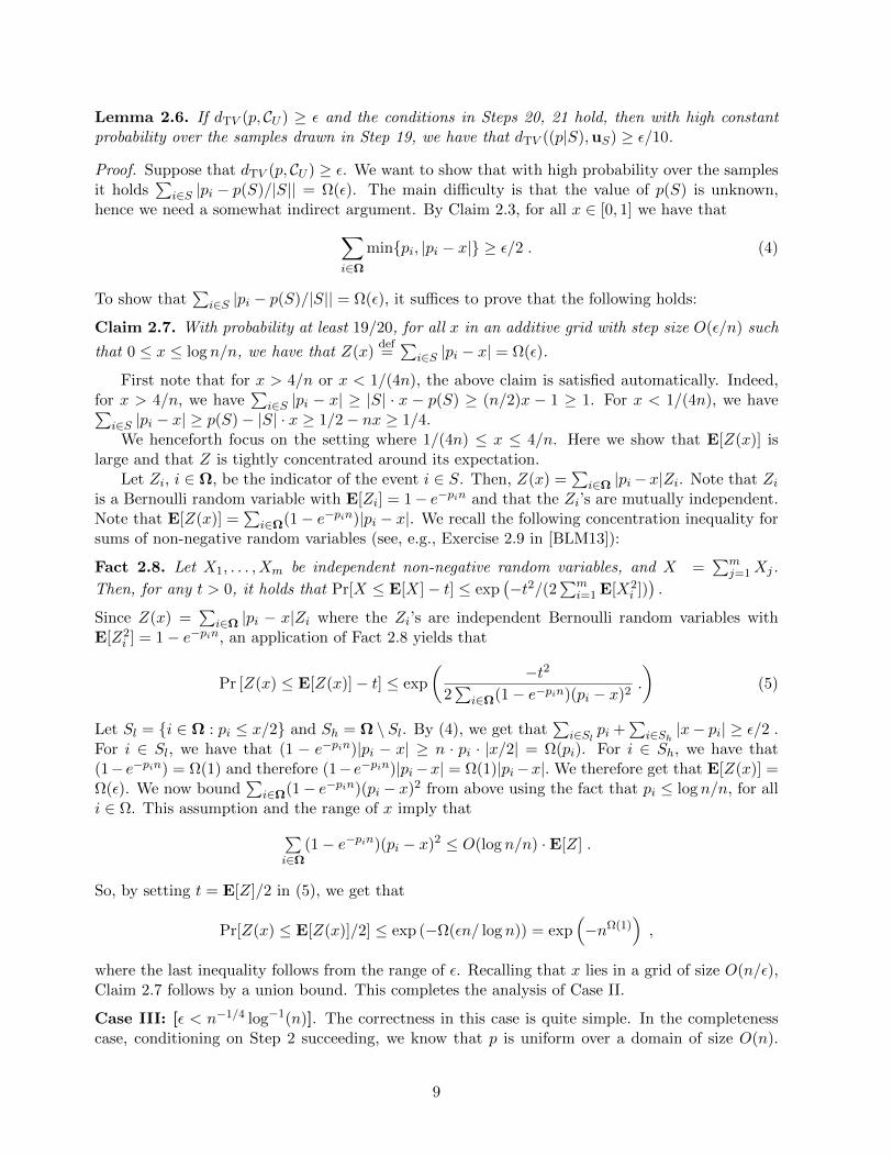
Lemma 2.6. If dTV (p, CU ) ≥ ε and the conditions in Steps 20, 21 hold, then with high constantprobability over the samples drawn in Step 19, we have that dTV ((p|S),uS) ≥ ε/10.
Proof. Suppose that dTV (p, CU ) ≥ ε. We want to show that with high probability over the samplesit holds
∑i∈S |pi − p(S)/|S|| = Ω(ε). The main difficulty is that the value of p(S) is unknown,
hence we need a somewhat indirect argument. By Claim 2.3, for all x ∈ [0, 1] we have that∑i∈Ω
minpi, |pi − x| ≥ ε/2 . (4)
To show that∑
i∈S |pi − p(S)/|S|| = Ω(ε), it suffices to prove that the following holds:
Claim 2.7. With probability at least 19/20, for all x in an additive grid with step size O(ε/n) such
that 0 ≤ x ≤ log n/n, we have that Z(x)def=∑
i∈S |pi − x| = Ω(ε).
First note that for x > 4/n or x < 1/(4n), the above claim is satisfied automatically. Indeed,for x > 4/n, we have
∑i∈S |pi − x| ≥ |S| · x − p(S) ≥ (n/2)x − 1 ≥ 1. For x < 1/(4n), we have∑
i∈S |pi − x| ≥ p(S)− |S| · x ≥ 1/2− nx ≥ 1/4.We henceforth focus on the setting where 1/(4n) ≤ x ≤ 4/n. Here we show that E[Z(x)] is
large and that Z is tightly concentrated around its expectation.Let Zi, i ∈ Ω, be the indicator of the event i ∈ S. Then, Z(x) =
∑i∈Ω |pi− x|Zi. Note that Zi
is a Bernoulli random variable with E[Zi] = 1− e−pin and that the Zi’s are mutually independent.Note that E[Z(x)] =
∑i∈Ω(1− e−pin)|pi − x|. We recall the following concentration inequality for
sums of non-negative random variables (see, e.g., Exercise 2.9 in [BLM13]):
Fact 2.8. Let X1, . . . , Xm be independent non-negative random variables, and X =∑m
j=1Xj.
Then, for any t > 0, it holds that Pr[X ≤ E[X]− t] ≤ exp(−t2/(2
∑mi=1 E[X2
i ])).
Since Z(x) =∑
i∈Ω |pi − x|Zi where the Zi’s are independent Bernoulli random variables withE[Z2
i ] = 1− e−pin, an application of Fact 2.8 yields that
Pr [Z(x) ≤ E[Z(x)]− t] ≤ exp
(−t2
2∑
i∈Ω(1− e−pin)(pi − x)2.
)(5)
Let Sl = i ∈ Ω : pi ≤ x/2 and Sh = Ω \ Sl. By (4), we get that∑
i∈Slpi +
∑i∈Sh|x− pi| ≥ ε/2 .
For i ∈ Sl, we have that (1 − e−pin)|pi − x| ≥ n · pi · |x/2| = Ω(pi). For i ∈ Sh, we have that(1− e−pin) = Ω(1) and therefore (1− e−pin)|pi−x| = Ω(1)|pi−x|. We therefore get that E[Z(x)] =Ω(ε). We now bound
∑i∈Ω(1− e−pin)(pi − x)2 from above using the fact that pi ≤ log n/n, for all
i ∈ Ω. This assumption and the range of x imply that∑i∈Ω
(1− e−pin)(pi − x)2 ≤ O(log n/n) ·E[Z] .
So, by setting t = E[Z]/2 in (5), we get that
Pr[Z(x) ≤ E[Z(x)]/2] ≤ exp (−Ω(εn/ log n)) = exp(−nΩ(1)
),
where the last inequality follows from the range of ε. Recalling that x lies in a grid of size O(n/ε),Claim 2.7 follows by a union bound. This completes the analysis of Case II.
Case III: [ε < n−1/4 log−1(n)]. The correctness in this case is quite simple. In the completenesscase, conditioning on Step 2 succeeding, we know that p is uniform over a domain of size O(n).
9

Therefore, after Θ(n log n) samples, we have seen all the elements of the domain with high probabil-ity, i.e., the set S has p(S) = 1. Therefore, the conditional distribution p|S is identified with p, andthe final tester outputs “YES”. On the other hand, if p is ε-far from uniform. and the algorithmdoes not reject in Step 30, then it follows that p(S) ≥ 1 − O(ε/n1/4) > 1 − ε/10. Therefore, p|Sshould be at least ε/2-far from uS and the tester will output “NO.” This completes the proof ofcorrectness.
3 Sample Complexity Lower Bound
In this section, we prove a sample size lower bound matching our algorithm Gen-Uniformity-Test. One part of the lower bound is fairly easy. In particular, it is known [Pan08] that Ω(
√n/ε2)
samples are required to test uniformity of a distribution with a known support of size n. It is easyto see that the hard cases for this lower bound still work when ‖p‖2 = Θ(n−1/2).
The other half of the lower bound is somewhat more difficult and we rely on the lower boundtechniques of [DK16]. In particular, for n > 0, and 1/10 > ε > n−1/4 and for N sufficiently large,we produce a pair of distributions D and D′ over positive measures on [N ], so that:
1. A random sample from D or D′ has total mass Θ(1) with high probability.
2. A random sample from D or D′ has support of size Θ(n) with high probability.
3. A sample from µ ∈ D has µ/‖µ‖1 be the uniform distribution over some subset of [N ] withprobability 1.
4. A sample from µ ∈ D′ has µ/||µ‖1 be at least Ω(ε)-far from any uniform distribution withhigh probability.
5. Given a measure µ taking randomly from either D or D′, no algorithm given the outputof a Poisson process with intensity kµ for k = o(min(n2/3/ε4/3, n)) can reliably distinguishbetween a µ taken from D and µ taken from D′.
Before we exhibit these families, we first discuss why the above is sufficient. This Poissonizationtechnique has been used previously in various settings [VV14, DK16, WY16, DGPP17], so we onlyprovide a sketch here. In particular, suppose that we have such families D and D′, but that there isalso an algorithm A that distinguishes between a distribution p being uniform and being ε-far fromuniform in m = o(ε−4/3/‖p‖3) samples. We show that we can use algorithm A to violate property 5above. In particular, letting p = µ/‖µ‖1 for µ a random measure taken from either D or D′, wenote that with high probability p has support of size Θ(n), and thus ‖p‖3 = O(n−2/3). Therefore,m′ = o(n2/3/ε4/3) samples are sufficient to distinguish between p being uniform and being Ω(ε) farfrom uniform. However, by properties 3 and 4, this is equivalent to distinguish between µ beingtaken from D and being taken from D′. On the other hand, given the output of a Poisson processwith intensity Cm′µ, for C a sufficiently large constant, a random m′ of these samples (note thatthere are at least m′ total samples with high probability) are distributed identically to m′ samplesfrom p. Thus, applying A to these samples distinguishes between µ taken from D and µ taken fromD′, thus contradicting property 5.
We now exhibit the families D and D′. In both cases, we want to arrange µi := µ(i) to bei.i.d. for different i. We also want it to be the case that the first and second moments of µi are thesame for D and D′. Combining this with requirements on closeness to uniform, we are led to thefollowing definitions:
10
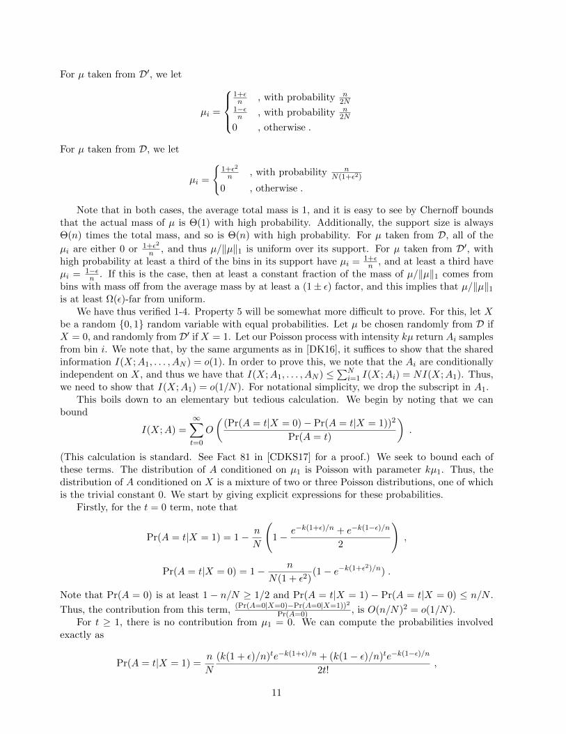
For µ taken from D′, we let
µi =
1+εn , with probability n
2N1−εn , with probability n
2N
0 , otherwise .
For µ taken from D, we let
µi =
1+ε2
n , with probability nN(1+ε2)
0 , otherwise .
Note that in both cases, the average total mass is 1, and it is easy to see by Chernoff boundsthat the actual mass of µ is Θ(1) with high probability. Additionally, the support size is alwaysΘ(n) times the total mass, and so is Θ(n) with high probability. For µ taken from D, all of the
µi are either 0 or 1+ε2
n , and thus µ/‖µ‖1 is uniform over its support. For µ taken from D′, withhigh probability at least a third of the bins in its support have µi = 1+ε
n , and at least a third haveµi = 1−ε
n . If this is the case, then at least a constant fraction of the mass of µ/‖µ‖1 comes frombins with mass off from the average mass by at least a (1± ε) factor, and this implies that µ/‖µ‖1is at least Ω(ε)-far from uniform.
We have thus verified 1-4. Property 5 will be somewhat more difficult to prove. For this, let Xbe a random 0, 1 random variable with equal probabilities. Let µ be chosen randomly from D ifX = 0, and randomly from D′ if X = 1. Let our Poisson process with intensity kµ return Ai samplesfrom bin i. We note that, by the same arguments as in [DK16], it suffices to show that the sharedinformation I(X;A1, . . . , AN ) = o(1). In order to prove this, we note that the Ai are conditionallyindependent on X, and thus we have that I(X;A1, . . . , AN ) ≤
∑Ni=1 I(X;Ai) = NI(X;A1). Thus,
we need to show that I(X;A1) = o(1/N). For notational simplicity, we drop the subscript in A1.This boils down to an elementary but tedious calculation. We begin by noting that we can
bound
I(X;A) =∞∑t=0
O
((Pr(A = t|X = 0)− Pr(A = t|X = 1))2
Pr(A = t)
).
(This calculation is standard. See Fact 81 in [CDKS17] for a proof.) We seek to bound each ofthese terms. The distribution of A conditioned on µ1 is Poisson with parameter kµ1. Thus, thedistribution of A conditioned on X is a mixture of two or three Poisson distributions, one of whichis the trivial constant 0. We start by giving explicit expressions for these probabilities.
Firstly, for the t = 0 term, note that
Pr(A = t|X = 1) = 1− n
N
(1− e−k(1+ε)/n + e−k(1−ε)/n
2
),
Pr(A = t|X = 0) = 1− n
N(1 + ε2)(1− e−k(1+ε2)/n) .
Note that Pr(A = 0) is at least 1 − n/N ≥ 1/2 and Pr(A = t|X = 1) − Pr(A = t|X = 0) ≤ n/N .
Thus, the contribution from this term, (Pr(A=0|X=0)−Pr(A=0|X=1))2
Pr(A=0) , is O(n/N)2 = o(1/N).For t ≥ 1, there is no contribution from µ1 = 0. We can compute the probabilities involved
exactly as
Pr(A = t|X = 1) =n
N
(k(1 + ε)/n)te−k(1+ε)/n + (k(1− ε)/n)te−k(1−ε)/n
2t!,
11

Pr(A = t|X = 0) =n
N(1 + ε2)
(k(1 + ε2)/n)te−k(1+ε2)/n
t!,
and obtain that (Pr(A=t|X=0)−Pr(A=t|X=1))2
Pr(A=t) is
O
(n1−tkt
2Nt!
) ((1 + ε)te−k(1+ε)/n + (1− ε)te−k(1−ε)/n − 2(1 + ε2)t−1e−k(1+ε2)/n)2
(1 + ε)te−k(1+ε)/n + (1− ε)te−k(1−ε)/n + 2(1 + ε2)t−1e−k(1+ε2)/n
.
Factoring out the e−k/n terms and noting that, since kε/n = o(1), the denominator is Ω(e−k/n)yields that
O
((n1−tkte−k/n
2Nt!
)((1 + ε)te−k(1+ε)/n + (1− ε)te−k(1−ε)/n − 2(1 + ε2)t−1e−k(1+ε2)/n
)2).
Noting that k/n = o(1), we can ignore this e−kn term and Taylor expanding the exponentials, wehave that
(Pr(A = t|X = 0)− Pr(A = t|X = 1))2
Pr(A = t)=
O
((n1−tkt
2Nt!
)((1 + ε)t(1− k(1 + ε)/n) + (1− ε)t(1 + k(1− ε)/n)
− 2(1 + ε2)t−1(1− k(1 + ε2)/n) +O((kε/n)2(1 + ε)t))2)
.
We deal separately with the cases t = 1, t = 2 and t > 2. For the t = 1 term, we have
O
((k
N
)((1 + ε)(1− kε/n) + (1− ε)(1 + kε/n)− 2(1− kε2/n) +O((kε/n)2)
)2)=O
((k
N
)O((kε/n)2)2
).
Since k = o(n2/3/ε4/3) and ε > n−1/4, εk/n = o(n−1/3/ε1/3) = o(n−1/4), and we find that this is
O
((k
N
)o(1/n)
)= o(1/N) .
This appropriately bounds the contribution from this term.When t = 2, we have
O
((k2
nN
)((1 + ε)2(1− k(1 + ε)/n) + (1− ε)2(1− k(1− ε)/n)
−2(1 + ε2)(1− k(1 + ε2)/n) +O((kε/n)2))2)
.
Note that the terms without k/n factors cancel out, (1 + ε)2 + (1− ε)2 − 2(1 + ε2) = 0, yielding
O(k2/nN)(kε2/n+ o(n−1/2))2 = O(k4ε4/n3N) + o(k2/n2N) = o(k3ε4/n2N) + o(1/N) = o(1/N) ,
using both k = o(n2/3/ε4/3) and k = o(n).
12
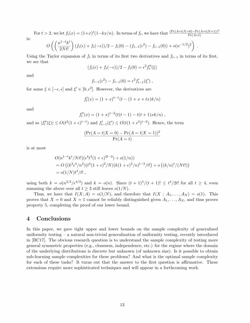
For t > 2, we let ft(x) = (1+x)t(1−kx/n). In terms of ft, we have that (Pr(A=t|X=0)−Pr(A=t|X=1))2
Pr(A=t)is:
O
((n1−tkt
2Nt!
)(ft(ε) + ft(−ε))/2− ft(0)− (ft−1(ε2)− ft−1(0)) + o(n−1/2)2
).
Using the Taylor expansion of ft in terms of its first two derivatives and ft−1 in terms of its first,we see that
(ft(ε) + ft(−ε))/2− ft(0) = ε2f ′′t (ξ)
andft−1(ε2)− ft−1(0) = ε2f ′t−1(ξ′) ,
for some ξ ∈ [−ε, ε] and ξ′ ∈ [0, ε2]. However, the derivatives are
f ′t(x) = (1 + x)t−1(t− (1 + x+ tx)k/n)
andf ′′t (x) = (1 + x)t−2(t(t− 1)− t(t+ 1)xk/n) ,
and so |f ′′t (ξ)| ≤ O(t2(1 + ε)t−1) and f ′t−1(ξ′) ≤ O(t(1 + ε2)t−2). Hence, the term
(Pr(A = t|X = 0)− Pr(A = t|X = 1))2
Pr(A = t)
is at most
O(n1−tkt/Nt!)(ε4t4(1 + ε)2t−2) + o(1/n))
= O((k3ε4/n2)(t4(1 + ε)2/N)(k(1 + ε)2/n)t−3/t!
)+ o
((k/n)t/(Nt!)
)= o(1/N)t4/t! ,
using both k = o(n2/3/ε4/3) and k = o(n). Since (t + 1)4/(t + 1)! ≤ t4/2t! for all t ≥ 4, evensumming the above over all t ≥ 3 still leaves o(1/N).
Thus, we have that I(X;A) = o(1/N), and therefore that I(X : A1, . . . , AN ) = o(1). Thisproves that X = 0 and X = 1 cannot be reliably distinguished given A1, . . . , AN , and thus provesproperty 5, completing the proof of our lower bound.
4 Conclusions
In this paper, we gave tight upper and lower bounds on the sample complexity of generalizeduniformity testing – a natural non-trivial generalization of uniformity testing, recently introducedin [BC17]. The obvious research question is to understand the sample complexity of testing moregeneral symmetric properties (e.g., closeness, independence, etc.) for the regime where the domainof the underlying distributions is discrete but unknown (of unknown size). Is it possible to obtainsub-learning sample complexities for these problems? And what is the optimal sample complexityfor each of these tasks? It turns out that the answer to the first question is affirmative. Theseextensions require more sophisticated techniques and will appear in a forthcoming work.
13
References
[ADK15] J. Acharya, C. Daskalakis, and G. Kamath. Optimal testing for properties of distribu-tions. In NIPS, pages 3591–3599, 2015.
[AOST17] J. Acharya, A. Orlitsky, A. T. Suresh, and H. Tyagi. Estimating renyi entropy ofdiscrete distributions. IEEE Trans. Information Theory, 63(1):38–56, 2017.
[BC17] T. Batu and C. Canonne. Generalized uniformity testing. CoRR, abs/1708.04696, 2017.To appear in FOCS’17.
[BFR+00] T. Batu, L. Fortnow, R. Rubinfeld, W. D. Smith, and P. White. Testing that distri-butions are close. In IEEE Symposium on Foundations of Computer Science, pages259–269, 2000.
[BKR04] T. Batu, R. Kumar, and R. Rubinfeld. Sublinear algorithms for testing monotone andunimodal distributions. In ACM Symposium on Theory of Computing, pages 381–390,2004.
[BLM13] S. Boucheron, G. Lugosi, and P. Massart. Concentration Inequalities: A NonasymptoticTheory of Independence. OUP Oxford, 2013.
[Can15] C. L. Canonne. A survey on distribution testing: Your data is big. but is it blue?Electronic Colloquium on Computational Complexity (ECCC), 22:63, 2015.
[CDGR16] C. L. Canonne, I. Diakonikolas, T. Gouleakis, and R. Rubinfeld. Testing shape restric-tions of discrete distributions. In 33rd Symposium on Theoretical Aspects of ComputerScience, STACS 2016, pages 25:1–25:14, 2016.
[CDKS17] C. L. Canonne, I. Diakonikolas, D. M. Kane, and A. Stewart. Testing bayesian networks.In Proceedings of the 30th Conference on Learning Theory, COLT 2017, pages 370–448,2017.
[CDS17] C. L. Canonne, I. Diakonikolas, and A. Stewart. Fourier-based testing for families ofdistributions. CoRR, abs/1706.05738, 2017.
[CDVV14] S. Chan, I. Diakonikolas, P. Valiant, and G. Valiant. Optimal algorithms for testingcloseness of discrete distributions. In SODA, pages 1193–1203, 2014.
[DDK16] C. Daskalakis, N. Dikkala, and G. Kamath. Testing ising models. CoRR,abs/1612.03147, 2016.
[DDS+13] C. Daskalakis, I. Diakonikolas, R. Servedio, G. Valiant, and P. Valiant. Testing k-modaldistributions: Optimal algorithms via reductions. In SODA, pages 1833–1852, 2013.
[DGPP16] I. Diakonikolas, T. Gouleakis, J. Peebles, and E. Price. Collision-based testers are opti-mal for uniformity and closeness. Electronic Colloquium on Computational Complexity(ECCC), 23:178, 2016.
[DGPP17] I. Diakonikolas, T. Gouleakis, J. Peebles, and E. Price. Sample-optimal identity testingwith high probability. CoRR, abs/1708.02728, 2017.
[DK16] I. Diakonikolas and D. M. Kane. A new approach for testing properties of discretedistributions. In FOCS, pages 685–694, 2016. Full version available at abs/1601.05557.
14
[DKN15a] I. Diakonikolas, D. M. Kane, and V. Nikishkin. Optimal algorithms and lower boundsfor testing closeness of structured distributions. In IEEE 56th Annual Symposium onFoundations of Computer Science, FOCS 2015, pages 1183–1202, 2015.
[DKN15b] I. Diakonikolas, D. M. Kane, and V. Nikishkin. Testing identity of structured distribu-tions. In Proceedings of the Twenty-Sixth Annual ACM-SIAM Symposium on DiscreteAlgorithms, SODA 2015, pages 1841–1854, 2015.
[DKN17] I. Diakonikolas, D. M. Kane, and V. Nikishkin. Near-optimal closeness testing of discretehistogram distributions. In 44th International Colloquium on Automata, Languages,and Programming, ICALP 2017, pages 8:1–8:15, 2017.
[DP17] C. Daskalakis and Q. Pan. Square hellinger subadditivity for bayesian networks andits applications to identity testing. In Proceedings of the 30th Conference on LearningTheory, COLT 2017, pages 697–703, 2017.
[Gol16] O. Goldreich. The uniform distribution is complete with respect to testing identity toa fixed distribution. ECCC, 23, 2016.
[GR00] O. Goldreich and D. Ron. On testing expansion in bounded-degree graphs. TechnicalReport TR00-020, Electronic Colloquium on Computational Complexity, 2000.
[Pan08] L. Paninski. A coincidence-based test for uniformity given very sparsely-sampled dis-crete data. IEEE Transactions on Information Theory, 54:4750–4755, 2008.
[RRSS09] S. Raskhodnikova, D. Ron, A. Shpilka, and A. Smith. Strong lower bounds for approxi-mating distribution support size and the distinct elements problem. SIAM J. Comput.,39(3):813–842, 2009.
[Rub12] R. Rubinfeld. Taming big probability distributions. XRDS, 19(1):24–28, 2012.
[Val11] P. Valiant. Testing symmetric properties of distributions. SIAM J. Comput.,40(6):1927–1968, 2011.
[VV14] G. Valiant and P. Valiant. An automatic inequality prover and instance optimal identitytesting. In FOCS, 2014.
[WY16] Y. Wu and P. Yang. Minimax rates of entropy estimation on large alphabets via bestpolynomial approximation. IEEE Transactions on Information Theory, 62(6):3702–3720, June 2016.
15ECCC ISSN 1433-8092
https://eccc.weizmann.ac.il