arX

iv:0

807.

3065

v1 [

cs.I

T]

19

Jul 2

008

Sharp Bounds for Optimal Decoding of Low

Density Parity Check Codes

Shrinivas Kudekar and Nicolas Macris

Ecole Polytechnique Federale de LausanneSchool of Computer and Communication Sciences

LTHC, I&C, Station 14, CH-1015 Lausanneshrinivas.kudekar@epfl.ch, nicolas.macris@epfl.ch

July 19, 2008

Abstract

Consider communication over a binary-input memoryless output-symmetric channel with low density parity check (LDPC) codes andmaximum a posteriori (MAP) decoding. The replica method of spinglass theory allows to conjecture an analytic formula for the averageinput-output conditional entropy per bit in the infinite block lengthlimit. Montanari proved a lower bound for this entropy, in the case ofLDPC ensembles with convex check degree polynomial, which matchesthe replica formula. Here we extend this lower bound to any irregularLDPC ensemble. The new feature of our work is an analysis of thesecond derivative of the conditional input-output entropy with respectto noise. A close relation arises between this second derivative andcorrelation or mutual information of codebits. This allows us to extendthe realm of the “interpolation method”, in particular we show howchannel symmetry allows to control the fluctuations of the “overlapparameters”.

1

1 Introduction and Main Results

Linear codes based on sparse random graphs have emerged as a major chap-ter of coding theory [1]. While the belief propagation (BP) decoding algo-rithm and density evolution method have been explored in detail because oftheir low algorithmic complexity and good performance, much remains to beunderstood about the optimal (MAP) performance bounds of sparse graphcodes. Recent theoretical progress on the binary erasure channel (BEC) hasconvincingly shown that BP and MAP decoding have intimate relationships(see [1] and in particular [4]), but understanding this relationship for otherchannels is still a largely open problem. In fact, the replica and/or cavitymethods of statistical mechanics of dilute spin glass models allow to conjec-ture an analytic formula forHn(X|Y ), the entropy of the transmitted messageX = (X1, ..., Xn) conditional to the received message Y = (Y1, ..., Yn) in thelarge block length limit n → +∞. The replica formula expresses the condi-tional entropy as the solution of a variational problem whose critical pointsare given by the density evolution fixed point equation (see [2], [3]). If oneis to solve the fixed point equation iteratively, the choice of initial conditionsis not necessarily the one given by channel outputs (as in standard densityevolution) but the one which yields the maximum conditional entropy. Notethat a byproduct of the replica formula is the determination of the maximuma posteriori (MAP) noise threshold, above which reliable communication isnot possible whatever the decoding algorithm.

The proof of the replica formulas is, in general, an open problem1. In thecontext of communication they have been proven for a class of low densityparity check codes (LDPC) codes on the BEC [11], [12] (see also [13] forrecent work going beyond the BEC) and for low density generator codes(LDGM) on a class of channels [14].

A promising approach towards a general proof of the replica formulasseems to be the use of the so-called interpolation method first developpedin the context of the SK model [15], [16], [17]. Consider an LDPC(n,Λ, P )ensemble where Λ(x) =

∑

d Λdxd, P (x) =

∑

k Pkxk are the variable and

check degree distributions from the node perspective. We will always assumethat the maximal degrees are finite. Montanari [7] (see also the related

1In a few spin glass models the replica formulas have been fully demonstrated. Re-markably Talagrand [5] has proven the Parisi formula with full symmetry breaking [6] forthe Sherrington-Kirkpatrick (SK) model. In [10] it is shown that the replica symmetricformula holds for a complete p-spin model with gauge symmetry.

2

work of Franz-Leone [8] and Talagrand- Pachenko [9]) has developped theinterpolation method for such a system and has derived a lower bound forthe conditional entropy for ensembles with any polynomial Λ(x) but P (x)restricted to be convex for −e ≤ x ≤ e (in particular if the check degreeis constant this means it has to be even). An important fact is that theselower bounds match the replica solution, and are thus believed to be tight.Since Fano’s inequality tells us that the block error probability for a codehaving length n and rate r is lower bounded by 1

rnHn(X|Y ), an immediate

application of the lower bound is the numerical computation of a rigorousupper bound on the MAP threshold.

In the present paper we drop the convexity requirement for P (x) in thecases of the BEC, BIAWGNC with any noise level an in the case of generalbinary memoryless (BMS) channels in a high noise regime. In other words weprove the lower bound for any standard regular (so odd degrees are allowed)or irregular code ensemble.

Besides the main result itself, we introduce a new tool in the form of arelationship between the second derivative of the conditional entropy withrespect to the noise and correlations functions of codebits. These correlationfunctions are shown to be intimately related to the mutual information be-tween two codebits. The formulas are somewhat similar to those for GEXITfunctions [1] which relate the first derivative of conditional entropy to softbit estimates. By combining these relations with the interpolation methodwe are able to control the fluctuations of the so-called overlap parameters.This part of our analysis is crucial for proving the general lower bound onthe conditional entropy and relies heavily on channel symmetry.

A preliminary summary of the present work has appeared in [20].

1.1 Variational bound on the conditional entropy

Let pY |X(y|x) be the transition probability of a BMS(ǫ) channel where ǫ isthe noise parameter (understood to vary in the appropriate range). We willwork in terms of both the likelihood

l = ln

[

pY |X(y|0)

pY |X(y|1)

]

and difference

t = pY |X(y|0)− pY |X(y|1) = tanhl

2

3

variables. It will be convenient to use the notation cL(l) and cD(t) for thedistributions of l and t, assuming that the all zero codeword is transmitted(that is to say that cL(l)dl = cD(t)dt = pY |X(y|0)dy).

Let V be some random variable with an arbitrary density dV (v) satisfyingthe symmetry condition dV (v) = evdV (−v). Also let

U = tanh−1

[k−1∏

i=1

tanhVi

]

(1)

where Vi are i.i.d copies of V and k is the (random) degree of a check node.We denote by Uc, c = 1, ..., d i.i.d copies of U where d is the (random)degree of variable nodes. Notice that in the belief propagation (BP) decodingalgorithm U appears as the check to variable node message and V appearsas the variable to check node message. Define the functional2 (we view it asa functional of the probability distribution dV )

hRS [dV ; Λ, P ] =El,d,Uc

[

ln

(

el2

d∏

c=1

(1 + tanhUc) + e−l2

d∏

c=1

(1 − tanhUc)

)]

+Λ′(1)

P ′(1)Ek,Vi

[

ln(1 +

k∏

i=1

tanhVi)

]

− Λ′(1)EV,U

[

ln(1 + tanhV tanhU)

]

− Λ′(1)

P ′(1)ln 2

Our main result is about the conditional entropy per bit, averaged over thecode ensemble C = LDPC(n,Λ, P ).

EC[hn] =1

nEC[Hn(X|Y )]

Definition H. We define the parameters (p an integer)

m(2p)0 = E[t2p], m

(2p)1 =

d

dǫE[t2p], m

(2p)2 =

d2

dǫ2E[t2p] (2)

2The subscript RS stands for “replica symmetric” because this functional has beenobtained from the replica symmetric ansatz for an appropriate spin glass, see for example[3], [2]

4

and say that a BMS(ǫ) channel is in the high noise regime if the followingseries expansions

∑

p

(p+ 1)m(2p)0

∑

p

(5

2

)2p|m(2p)1 |

∑

p

|m(2p)2 |

2p(2p− 1)(3)

are convergent and if

(√

2 − 1)(5

2

)2|m(2)1 | >

∑

p≥2

(5

2

)2p|m(2p)1 |

For example the BSC(ǫ) certainly satisfies H if the crossover noise pa-rameter is close enough to 1

2, because E[t2p] = (1 − 2ǫ)2p. More generaly

any channel with bounded likehood variables satisfies H for a regime of suf-ficiently high noise. For channels with unbounded likehoods the conditionwill be satisfied if cL(l) has sufficiently good decay properties. But note thatthe BEC(ǫ) which has mass at l = +∞ does not satisfy this condition sinceE[t2p] = 1− ǫ. However as we will see for the BEC(ǫ) and the BIAWGNC(ǫ)we do not need condition H . For these two channels our analysis can bemade fully non-perturbative, and holds for all noise levels.

Theorem 1 (Variational Bound). Assume communication using a stan-dard irregular C = LDPC(n,Λ, P ) code ensemble, through a BEC(ǫ) orBIAWGNC(ǫ) with any noise level or a BMS(ǫ) channel satisfying H. Forall ǫ in the above ranges we have,

lim infn→+∞

EC[hn] ≥ supdV

hRS [dV ; Λ, P ]

Let us note that this theorem already appears in [18] for the special caseof the BIAWGNC for a Poissonnian Λ(x). We stress again that a formalcalculation using the replica method yields

limn→+∞

EC [hn] = supdV

hRS[dV ; Λ, P ]

For this reason it is strongly suspected that the converse inequality holds aswell, but so far no progress has been made except in a limited number ofsituations alluded to before.

5

1.2 Derivatives of the conditional entropy

Our proof of the variational bound uses integral formulas for the first and sec-ond derivatives of EC[hn] with respect to the noise parameter. The ensembleformulas follow from slightly more general ones that are valid for any fixedlinear code. To give the formulation for a fixed linear code it is convenientto introduce a noise vector ǫ = (ǫ1, ..., ǫn) and a BMS(ǫ) channel with noiselevel ǫi when bit xi is sent. When all noise levels are set to the same valueǫ the channel is denoted BMS(ǫ). The distributions of the likelihood li ordifference domain ti representations of the channel outputs now depend onǫi. In order to keep the notation simpler we do not explicitely indicate theǫi dependence and still denote them as cL(li) and cD(ti) respectively.

We introduce the soft MAP estimates of bit Xi

Li = ln

[

pXi|Y (0|y)pXi|Y (1|y)

]

, Ti = pXi|Y (0|y) − pXi|Y (1|y) = tanhLi

2

and the soft estimate for the modulo 2 sum Xi ⊕Xj,

Lij = ln

[

pXi⊕Xj |Y (0|y)pXi⊕Xj |Y (1|y)

]

, Tij = pXi⊕Xj |Y (0|y) − pXi⊕Xj |Y (1|y) = tanhLij

2

In the sequel the notations v∼i (resp. v∼ij) means that component vi (resp.vi and vj) are omitted from the vector v. The following is known [1] but westate it for completeness. A derivation in the spirit of the present paper canalso be found in [19].

Proposition 1 (GEXIT formula). For any BMS(ǫ) channel and any fixedlinear code we have

∂

∂ǫiHn(X | Y ) =

∫ +1

−1

dti∂cD(ti)

∂ǫig1(ti)

where

g1(ti) = −Et∼i

[

ln

(

1 − tiTi

1 − ti

)]

This formula will be used for an ensemble that is symmetric under per-mutation of bits and a BMS(ǫ) channel. Using

d

dǫHn(X | Y ) =

n∑

i=1

∂

∂ǫiHn(X | Y )

∣

∣

∣

∣

ǫi=ǫ

6

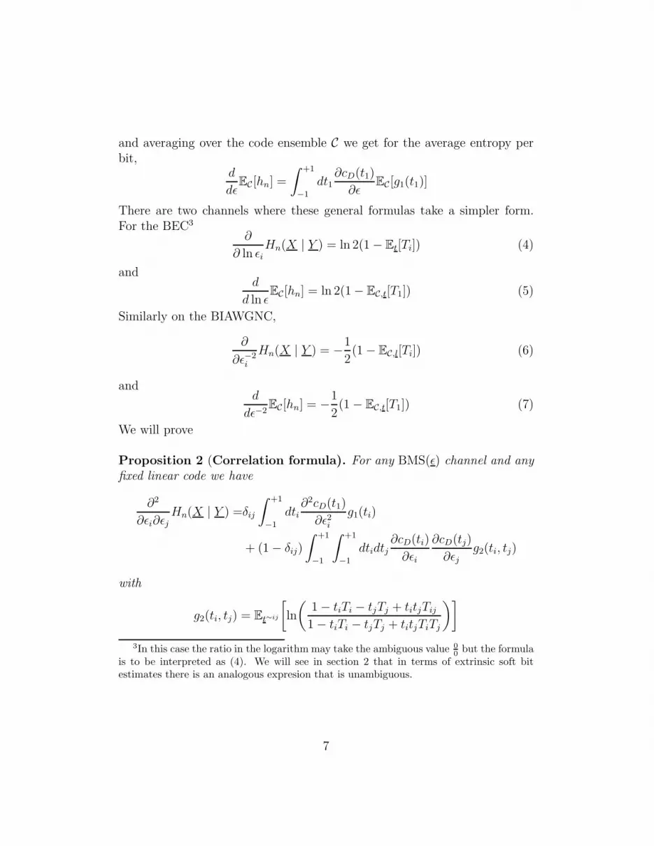
and averaging over the code ensemble C we get for the average entropy perbit,

d

dǫEC[hn] =

∫ +1

−1

dt1∂cD(t1)

∂ǫEC [g1(t1)]

There are two channels where these general formulas take a simpler form.For the BEC3

∂

∂ ln ǫiHn(X | Y ) = ln 2(1 − Et[Ti]) (4)

andd

d ln ǫEC[hn] = ln 2(1 − EC,t[T1]) (5)

Similarly on the BIAWGNC,

∂

∂ǫ−2i

Hn(X | Y ) = −1

2(1 − EC,l[Ti]) (6)

andd

dǫ−2EC[hn] = −1

2(1 − EC,t[T1]) (7)

We will prove

Proposition 2 (Correlation formula). For any BMS(ǫ) channel and anyfixed linear code we have

∂2

∂ǫi∂ǫjHn(X | Y ) =δij

∫ +1

−1

dti∂2cD(t1)

∂ǫ2ig1(ti)

+ (1 − δij)

∫ +1

−1

∫ +1

−1

dtidtj∂cD(ti)

∂ǫi

∂cD(tj)

∂ǫjg2(ti, tj)

with

g2(ti, tj) = Et∼ij

[

ln

(

1 − tiTi − tjTj + titjTij

1 − tiTi − tjTj + titjTiTj

)]

3In this case the ratio in the logarithm may take the ambiguous value 0

0but the formula

is to be interpreted as (4). We will see in section 2 that in terms of extrinsic soft bitestimates there is an analogous expresion that is unambiguous.

7

Again, for the case of interest later on, we have a BMS(ǫ) channel and alinear code ensemble that is symmetric under permutations of bits, thus

d2

dǫ2EC [hn] =

∫ +1

−1

dt1∂2cD(t1)

∂ǫ2EC[g1(t1)] (8)

+∑

i6=1

∫ +1

−1

∫ +1

−1

dt1dti∂cD(t1)

∂ǫ

∂cD(ti)

∂ǫEC [g2(t1, ti)]

For the BEC4 these formulas simplify

∂2

∂ ln ǫi∂ ln ǫjHn(X | Y ) = (1 − δij) ln 2Et

[

Tij − TiTj ]

and

d2

(d ln ǫ)2EC[hn] = ln 2

n∑

i6=1

EC,t

[

T1i − T1Ti] (9)

For the BIAWGNC

∂2

∂ǫ−2i ∂ǫ−2

j

Hn(X | Y ) =1

2Et[(

Tij − TiTj

)2], (10)

and

d2

(dǫ−2)2EC[hn] =

1

2

n∑

i=1

EC,t[(

T1i − T1Ti

)2] (11)

Formulas (9) and (11) involve the “correlation” (Tij − TiTj) for bits Xi andXj. The general formula (8) can also be recast in terms of powers of suchcorrelations by expanding the logarithm (see section 3). Loosely speaking,in the infinite block length limit n → +∞, the second derivative will bewell defined only if the correlations have sufficient decay with respect to thegraph distance (the minimal length among all paths joining i and j on theTanner graph). Thus we expect good decay properties for all noise levelsexcept at the phase transition thresholds where, in the limit n → +∞, thefirst derivative generally has bounded discontinuities, and thus the secondderivative cannot be uniformly bounded in n.

4The same remark than before applies here.

8

1.3 Relation to mutual information

The correlation Tij − TiTj is basicaly a measure of the independence of twocodebits, thus it is natural to expect that it should be related to the mutualinformation I(Xi;Xj | Y ). We do not pursue this issue in all details becauseit is not used in the rest of the paper, but wish to briefly state the mainrelations which follow naturaly form the previous formulas.

The BEC(ǫ). Take i 6= j. The chain rule implies Hn(X | Y ) = H(XiXj |Y ) + H(X∼ij | XiXjY ). Also H(X∼ij | XiXjY ) = H(X∼ij | XiXjY

∼ij).Since H(X∼ij | XiXjY

∼ij) does not depend on ǫi, ǫj we have

∂2

∂ǫi∂ǫjHn(X | Y ) =

∂2

∂ǫi∂ǫjH(XiXj | Y )

The conditional entropy on the r.h.s is explicitly ǫiǫjH(XiXj |Y ∼ij) + ǫi(1 −ǫj)H(Xi|XjY

∼ij) + (1 − ǫi)ǫjH(Xj|XiY∼ij). In this expression the three

conditional entropies are independent of the channel parameters ǫi and ǫj .Thus

∂2

∂ǫi∂ǫjHn(X | Y ) = H(XiXj | Y ∼ij) −H(Xi | XjY

∼ij) −H(Xj | XiY∼ij)

= H(Xj | Y ∼ij) −H(Xj | XiY∼ij)

= I(Xi;Xj | Y ∼ij) =1

ǫiǫjI(Xi;Xj | Y )

Summarizing, we have obtained for i 6= j,

∂2

∂ ln ǫi∂ ln ǫjHn(X | Y ) = I(Xi;Xj | Y ) = Et[Tij − TiTj]

The BIAWGNC(ǫ). Take i 6= j. We note that

Tij = pXiXj |Y (00 | y) + pXiXj |Y (11 | y) − pXiXj |Y (01 | y) − pXiXj |Y (10 | y)

from which it follows

(Tij − TiTj)2 ≤ 4

∑

xi,xj

∣

∣

∣

∣

pXiXj |Y (xixj | y) − pXi|Y (xi | y)pXj |Y (xj | y)∣

∣

∣

∣

2

9

Applying the inequality

1

2

∑

x

|P (x) −Q(x)|2 ≤ D(P‖Q)

for the Kullback-Leibler divergence of the two distributions P = pXiXj |y andQ = pXi|Y pXj |y, we get for i 6= j

(Tij − TiTj)2 ≤ 8I(Xi;Xj | y)

Averaging over the outputs we get

∂2

∂ǫ−2i ∂ǫ−2

j

Hn(X | Y ) = Et[(Tij − TiTj)2] ≤ 8I(Xi;Xj | Y )

Highly noisy BMS channels. From the high noise expansion (see section3 and the above remarks, we can derive an inequality like the preceding one,which holds in the high noise regime for general BMS channels. The number8 gets replaced by some suitable factor which depends on the channel noise.

1.4 Organisation of the paper

The statistical mechanics formulation is very convenient to perform many ofthe necessary calculations, but also the interpolation method is best formu-lated in that framework. Thus we briefly recall it in section 2 as well as a fewconnections to the information theoretic language. Section 3 contains thederivation of the correlation formula (proposition 2) and other useful mate-rial. The interpolation method that is used to prove the variational bound(theorem 1) is presented in section 4. The main new ingredient of the proofis an estimate (see proposition 3 in section 4) on the fluctuations of over-lap parameters. The proof of proposition 3 is the object of section 5. Theappendices contain technical calculations involved in the proofs.

2 Statistical Mechanics Formulation

Consider a fixed code belonging to the ensemble C = LDPC(n,Λ, P ). Theposterior distribution pX|Y (x|y) used in MAP decoding can be viewed as the

10

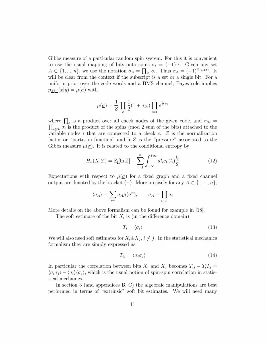
Gibbs measure of a particular random spin system. For this it is convenientto use the usual mapping of bits onto spins σi = (−1)xi . Given any setA ⊂ {1, ..., n}, we use the notation σA =

∏

i∈ σi. Thus σA = (−1)⊕i∈Axi. Itwill be clear from the context if the subscript is a set or a single bit. For auniform prior over the code words and a BMS channel, Bayes rule impliespX|Y (x|y) = µ(σ) with

µ(σ) =1

Z

∏

c

1

2(1 + σ∂c)

n∏

i=1

eli2

σi

where∏

c is a product over all check nodes of the given code, and σ∂c =∏

i∈∂c σi is the product of the spins (mod 2 sum of the bits) attached to thevariable nodes i that are connected to a check c. Z is the normalizationfactor or “partition function” and lnZ is the “pressure” associated to theGibbs measure µ(σ). It is related to the conditional entropy by

Hn(X|Y ) = El[lnZ] −n∑

i=1

∫ +∞

−∞

dlicL(li)li2

(12)

Expectations with respect to µ(σ) for a fixed graph and a fixed channeloutput are denoted by the bracket 〈−〉. More precisely for any A ⊂ {1, ..., n},

〈σA〉 =∑

σn

σAµ(σn), σA =∏

i∈A

σi

More details on the above formalism can be found for example in [18].The soft estimate of the bit Xi is (in the difference domain)

Ti = 〈σi〉 (13)

We will also need soft estimates forXi⊕Xj , i 6= j. In the statistical mechanicsformalism they are simply expressed as

Tij = 〈σiσj〉 (14)

In particular the correlation between bits Xi and Xj becomes Tij − TiTj =〈σiσj〉 − 〈σi〉〈σj〉, which is the usual notion of spin-spin correlation in statis-tical mechanics.

In section 3 (and appendices B, C) the algebraic manipulations are bestperformed in terms of “extrinsic” soft bit estimates. We will need many

11

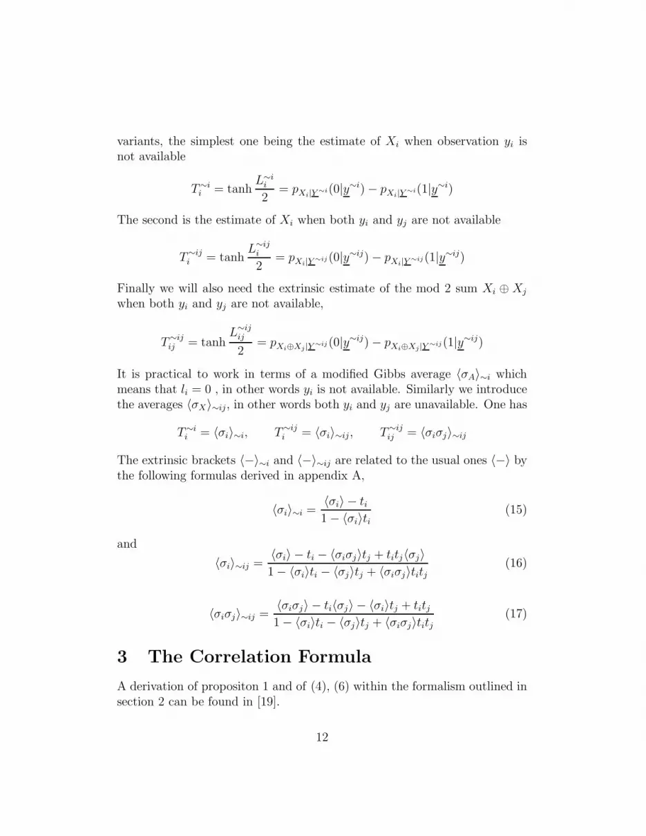
variants, the simplest one being the estimate of Xi when observation yi isnot available

T∼ii = tanh

L∼ii

2= pXi|Y

∼i(0|y∼i) − pXi|Y∼i(1|y∼i)

The second is the estimate of Xi when both yi and yj are not available

T∼iji = tanh

L∼iji

2= pXi|Y

∼ij (0|y∼ij) − pXi|Y∼ij (1|y∼ij)

Finally we will also need the extrinsic estimate of the mod 2 sum Xi ⊕ Xj

when both yi and yj are not available,

T∼ijij = tanh

L∼ijij

2= pXi⊕Xj |Y

∼ij (0|y∼ij) − pXi⊕Xj |Y∼ij(1|y∼ij)

It is practical to work in terms of a modified Gibbs average 〈σA〉∼i whichmeans that li = 0 , in other words yi is not available. Similarly we introducethe averages 〈σX〉∼ij, in other words both yi and yj are unavailable. One has

T∼ii = 〈σi〉∼i, T∼ij

i = 〈σi〉∼ij, T∼ijij = 〈σiσj〉∼ij

The extrinsic brackets 〈−〉∼i and 〈−〉∼ij are related to the usual ones 〈−〉 bythe following formulas derived in appendix A,

〈σi〉∼i =〈σi〉 − ti1 − 〈σi〉ti

(15)

and

〈σi〉∼ij =〈σi〉 − ti − 〈σiσj〉tj + titj〈σj〉1 − 〈σi〉ti − 〈σj〉tj + 〈σiσj〉titj

(16)

〈σiσj〉∼ij =〈σiσj〉 − ti〈σj〉 − 〈σi〉tj + titj1 − 〈σi〉ti − 〈σj〉tj + 〈σiσj〉titj

(17)

3 The Correlation Formula

A derivation of propositon 1 and of (4), (6) within the formalism outlined insection 2 can be found in [19].

12

3.1 Proof of proposition 2

For any BMS(ǫ) channel and linear code we have from (12)

∂

∂ǫiHn(X | Y ) = El∼j

[∫ +∞

−∞

dlj∂cL(lj)

∂ǫj(lnZ − lj

2)

]

The second equality follows by permutation symmetry of code bits. Differ-entiating once more, we get

∂2

∂ǫi∂ǫjHn(X | Y ) = δijS1 + (1 − δij)S2 (18)

where

S1 = El∼i

[∫ +∞

−∞

dli∂2cL(li)

∂ǫ2i(lnZ − li

2)

]

(19)

and

S2 = El∼ij

[∫ +∞

−∞

dlidlj∂cL(li)

∂ǫi

∂cL(lj)

∂ǫj(lnZ − li

2)

]

First we consider S1. Let

Z∼i =∑

σ

∏

c∈C

1

2(1 + σ∂c)

∏

k 6=i

elk2

σk

be the partition function for the Gibbs measure 〈−〉∼i introduced in section2 and consider

lnZ

Z∼i= ln〈e

li2

σi〉∼i

Using the identity

eli2

σi = eli2

1 + tiσi

1 + ti(20)

we get

lnZ − li2

= lnZ∼i + ln

(

1 + ti〈σi〉∼i

1 + ti

)

When we replace this expression in the integral (19) we see that the con-tribution of lnZ∼i vanishes because this later quantity is independent of li.Indeed

∫ +∞

−∞

dli∂2cL(li)

∂ǫ2ilnZ∼i = lnZ∼i

∂2

∂ǫ2i

∫ +∞

−∞

dl1cL(li) = 0

13

since cL(li) is a normalized probability distribution. Then, using (15) leadsto

S1 =

∫ +1

−1

dti∂2cD(ti)

∂ǫ2iEt∼i

[

ln

(

1 + ti〈σi〉∼i

1 + ti

)]

(21)

= −∫ +1

−1

dti∂2cD(ti)

∂ǫ2iEt∼i

[

ln

(

1 − ti〈σi〉1 − ti

)]

(22)

which (because of (13)) coincides with the first term in the correlation for-mula.

Now we consider the term S2. Notice that∫ +∞

−∞

dlidlj∂cL(li)

∂ǫi

∂cL(lj)

∂ǫj

lj2

=

∫ +∞

−∞

dlj∂cL(lj)

∂ǫj

lj2

∂

∂ǫi

∫ +∞

−∞

dlicL(li) = 0

Thus we can rewrite S2 as

S2 = El∼ij

[∫ +∞

−∞

dlidlj∂cL(li)

∂ǫi

∂cL(lj)

∂ǫj(lnZ − li

2− lj

2)

]

Let Z∼ij =∑

σ

∏

c∈C12(1 + σ∂c)

∏

k 6=i,j elk2

σk be the partition function for theGibbs measure 〈·〉∼ij, and consider

lnZ

Z∼ij= ln〈e

li2

σi+lj2

σj〉∼ij

Using again (20) we get

lnZ − li2− lj

2= lnZ∼ij + ln

(

1 + ti〈σi〉∼ij + tj〈σj〉∼ij + titj〈σiσj〉∼ij

1 + ti + tj + titj

)

As before the contribution of lnZ∼ij vanishes because it is independent of li,lj. Similarly we have∫ +∞

−∞

dlidlj∂cL(li)

∂ǫi

∂cL(lj)

∂ǫjln(1 + ti〈σi〉∼ij) = same with i and j exchanged

= 0

∫ +∞

−∞

dlidlj∂c(li)

∂ǫi

∂c(lj)

∂ǫjln(1 + ti) = same with i and j exchanged

= 0

14

Using these four identities then leads to

S2 =El∼ij

[∫ +1

−1

dtidtj∂cD(ti)

∂ǫi

∂cD(tj)

∂ǫj(23)

× ln

(

1 + ti〈σi〉∼ij + tj〈σj〉∼ij + titj〈σiσj〉∼ij

1 + ti〈σi〉∼ij + tj〈σj〉∼ij + titj〈σi〉∼ij〈σj〉∼ij

)]

To get the formulas in terms of usual averages we use the relations (16), (17).Hence

S2 = El∼ij

[∫ +1

−1

dtidtj∂cD(ti)

∂ǫi

∂cD(tj)

∂ǫjln

(

1 − ti〈σi〉 − tj〈σj〉 + titj〈σiσj〉1 − ti〈σi〉 − tj〈σj〉 + titj〈σi〉〈σj〉

)]

(24)

Because of (13) and (14) this coincides with the second term in the correlationformula. The proposition now follows from (18), (22) and (24).

3.2 Expressions in terms of the spin-spin correlation

The BEC. From cD(t) = (1 − ǫ)δ(t − 1) + ǫδ(t), the second derivative interms of extrinsic quantities (formulas (21) and (23)) reduces to

∂2

∂ǫi∂ǫjHn(X | Y ) = (1 − δij)Et∼ij

[

ln

(

1 + 〈σi〉∼ij + 〈σj〉∼ij + 〈σiσj〉∼ij

1 + 〈σi〉∼ij + 〈σj〉∼ij + 〈σi〉∼ij〈σj〉∼ij

)]

There are various ways to see that for the BEC any Gibbs average 〈σA〉 or〈σA〉∼ij takes values in {0, 1}. A heuristic explanation is that bits (or theirmod 2 sums) are either perfectly known or erased. A more formal explanationfollows from a Nishimori identity5 combined with the Griffith-Kelly-Sherman(GKS) correlation inequality [18]. For example, E[〈σA〉2] = E[〈σA〉] (Nishi-mori) and 〈σA〉 ≥ 0 (GKS). Thus 〈σA〉(1−〈σA〉) is a positive random variablewith zero expectation and is therefore equal to 0 with probability one. Theseremarks imply that

∂2

∂ǫi∂ǫjHn(X | Y ) =

1

ǫiǫj(1 − δij)Et

[

ln

(

1 + 〈σi〉 + 〈σj〉 + 〈σiσj〉1 + 〈σi〉 + 〈σj〉 + 〈σi〉〈σj〉

)]

5We will use various such identities. A proof of their most general form can be foundin [18]. A general reference is [21].

15

Note that in deriving the last expression we used the fact that li = ∞ (lj =∞) implies that σi = +1 (σj = +1) which makes the logarithm term equalto zero. From the previous remarks we also have

ln(

1 + 〈σi〉 + 〈σj〉 + 〈σiσj〉)

=(ln 2)(

〈σi〉 + 〈σj〉 + 〈σiσj〉)

+ (ln 3 − 2 ln 2)(

〈σi〉〈σj〉 + 〈σi〉〈σiσj〉 + 〈σj〉〈σiσj〉)

+ (5 ln 2 − 3 ln 3)〈σi〉〈σj〉〈σiσj〉

and

ln(

1 + 〈σi〉 + 〈σj〉 + 〈σi〉〈σj〉)

= (ln 2)(

〈σi〉 + 〈σj〉)

The difference of the two logarithms is simplified using the following fourNishimori identities,

Et[〈σi〉〈σj〉] = Et[〈σi〉〈σiσj〉] = Et[〈σj〉〈σiσj〉] = Et[〈σiσj〉〈σi〉〈σj〉]

Finaly we obtain the simple expression

∂2

∂ǫi∂ǫjHn(X | Y ) =

ln 2

ǫiǫj(1 − δij)Et

[

〈σiσj〉 − 〈σi〉〈σj〉]

=ln 2

ǫiǫj(1 − δij)Et

[

Tij − TiTj

]

Let us point out that the second GKS inequality (for the BEC) implies that〈σiσj〉− 〈σi〉〈σj〉 ≥ 0, thus the correlation takes values in {0, 1} and we haveEt

[

Tij − TiTj

]

= Et

[

(Tij − TiTj)2]

.

The BIAWGNC. From the explicit form

cL(l) =1√

2πǫ−2exp

(

−(l − ǫ−2)2

2ǫ−2

)

one can show that the correlation formula reduces to

∂2

∂ǫ−2i ∂ǫ−2

j

Hn(X | Y ) = Et[(〈σiσj〉 − 〈σi〉〈σj〉)2]

= Et

[(

Tij − TiTj

)2]

16

Otherwise diffrentiating (12) thanks to

d2cL(l)

(dǫ−2)2=

(

− ∂

∂l+∂2

∂l2

)2

cL(l)

and using integration by parts also leads to this simpler form. This route ismuch simpler and the details can be found in [18].

Highly noisy BMS channels. We use the extrinsic form of the correlationformula given by (21) and (23). First we expand the logarithms in S1 and S2

in powers of ti and tj and then use various Nishimori identities. After sometedious algebra (see Appendices B and C) we can organize the expansion inpowers of the channel parameters (2). In the high noise regime this expansionis absolutely convergent. To lowest order we have

∂2

∂ǫi∂ǫjHn(X | Y ) = δijS1 + (1 − δij)S2

≈ 1

2δijm2

(2)(El[〈σi〉2] − 1) +1

2(1 − δij)[m1

(2)]2El

[

(

〈σiσj〉 − 〈σi〉〈σj〉)2]

+ . . .

=1

2δijm2

(2)(Et[T2i ] − 1) +

1

2(1 − δij)[m1

(2)]2Et

[

(

Tij − TiTj

)2]

+ . . . (25)

The second derivative of the conditional entropy is directly related to theaverage square of the code-bit or spin-spin correlation.

4 The Interpolation Method

We use the interpolation method in the form developed by Montanari. Asexplained in [7] it is difficult to establish directly the bounds for the stan-dard ensembles. Rather, one introduces a “multi-Poisson” ensemble whichapproximates the standard ensemble. Once the bounds are derived for themulti-Poisson ensemble they are extended to the standard ensemble by alimiting procedure. The interpolation construction is fairly complicated sothat it helpful to briefly review the simpler pure Poisson case.

4.1 Poisson ensemble

We introduce the ensemble Poisson-LDPC(n, 1 − r, P ) = P where n is theblock length, r the rate and P (x) =

∑

k Pkxk the check degree distribution.

17

A bipartite graph from the Poisson ensemble is constructed as follows. Thegraph has n variable nodes. For any k choose a Poisson number mk of checknodes with mean n(1 − r)Pk. Thus graph has a total of m =

∑

k mk checknodes which is also a Poisson variable with mean n(1 − r). For each checknode c of degree k, choose k variable nodes uniformly at random and connectthem to c. One can show that the left degree distribution concentrates arounda Poisson distribution ΛP(x) = eP ′(1)(1−r)(x−1). In other words the fractionΛl of variable nodes with degree l is Poisson with mean P ′(1)(1 − r).

The main idea behind the interpolation technique is to recursively removethe check node constraints and compensate them with extra observations Udistributed as (1) where dV is a trial distribution to be optimized in thefinal inequality. One can interpret these extra observations as coming from arepetition code whose rate is tuned in a such a way that the total design rater remains fixed. More precisely let s ∈ [0, 1] be an interpolating parameter.At “time” s we have a Poisson-LDPC(n, (1 − r)s, P ) = Ps code. Besidesthe usual channel outputs li, each node i receives ei extra i.i.d observationsU i

a, a = 1, ..., ei, where ei is Poisson with mean n(1 − r)(1 − s) (so the totaleffective rate is fixed to r). The interpolating Gibbs measure is

µs(σ) =1

Zs

∏

c

1

2(1 + σ∂c)

n∏

i=1

e(li2

+Pei

a=1U i

a)σi (26)

Here∏

c is a product over checks of a given graph in the ensemble Ps. Ats = 1 one recovers the original measure while at s = 0 (no checks) wehave a simple product measure (corresponding to a repetition code) whichis tailored to yield the replica symmetric entropy hRS[dV ; ΛP , P ] (up to anextra constant).

The central result of [7] is the sum rule

EP [hn] = hRS[dV ; ΛP , P ] +

∫ 1

0

Rn(s)ds (27)

Let us explain the notation. The first term on the right hand side hRS,P [dV ; ΛP , P ]is the replica symmetric functional of section 1 evaluated for the Poisson en-semble. The remainder term Rn(s) is

Rn(s) =

∞∑

p=1

1

2p(2p− 1)Es

[

⟨

P (Q2p) − P ′(q2p)(Q2p − q2p) − P (q2p)⟩

2p,s

]

18

with q2p = EV [(tanhV )2p] and Q2p the overlap parameters

Q2p =1

n

n∑

i=1

σ(1)i σ

(2)i · · ·σ(2p)

i (28)

Here σ(α)i , α = 1, 2, . . . , 2p are 2p independent copies (replicas) of the spin σi

and 〈−〉2p,s is the Gibbs bracket associated to the product measure (replicameasure)

2p∏

α=1

µs(σ(α))

4.2 Multi-Poisson ensemble

The multi-Poisson-LDPC(n,Λ, P, γ) = MP ensemble, is a more elaborateconstruction which allows to approximate a target LDPC(n,Λ, P ) ensemble.Its parameters are the block length n, the target variable and check nodedegree distributions Λ(x) and P (x) and the real number γ which controlsthe closeness to the standard ensemble. We recall that variable and checknode degrees have finite maximum degrees. The construction of a bipartitegraph from the multi-Poisson ensemble proceeds via rounds: the processstarts with a high rate code and at each round one adds a very small numberof check nodes till one ends up with a code

with almost the desired rate and degree distribution. A graph process Gt

is defined for discrete times t = 0, ..., tmax, tmax = ⌊Λ′(1)/γ⌋ − 1 as follows.For t = 0, G0 has no check nodes and has n variable nodes. The set ofvariable nodes is partitioned into the subsets Vl of cardinality nΛl for every land every node i ∈ Vl is decorated with l free sockets. The number di(t) keepstrack of the number of free sockets on node i once round t is completed. Sofor t = 0, G0 has no check nodes and each variable node i ∈ Vl has di(0) = lfree sockets. At round t, Gt is constructed from Gt−1 as follows. For all k,choose a Poisson number mt

k of check nodes with mean nγPk/P′(1). Connect

each outgoing edge of these new degree k check nodes (added at time t) to

variable node i according to the probability wi(t) = di(t−1)P

i di(t−1). This is the

fraction of free sockets at node i after round t − 1 was completed. Onceall new check nodes are connected, update the number of free sockets foreach variable node di(t) = di(t − 1) − ∆i(t). where ∆i(t) is the numberof times the variable node i was chosen during the round t. For n → ∞

19

this construction yields graphs with variable degree distributions Λγ(x) (thecheck degree distribution remains P (x)). The variational distance betweenΛγ(x) and P (x) tends to zero as γ → 0.

The interpolating ensemble now uses two parameters (t∗, s) where t∗ ∈{0, ..., tmax} and 0 ≤ s ≤ γ. For rounds 0, ..., t∗ − 1 one proceeds exactlyas before to obtain a graph Gt∗−1. At the next round t∗, one proceeds asbefore but with γ replaced by s. The rate loss is compensated by adding ei

extra observations for each node i, where ei is a Poisson integer with meann(γ − s)wi(t∗). The round is ended by updating the number of free socketsdi(t∗) = di(t∗−1)−∆i(t∗)−ei(t∗). Finally, for rounds after t∗ +1, ..., tmax nonew check node is added but for each variable node i, ei external observationsare added, where ei is a Poisson integer with mean nγwi(t∗). Moreover thefree socket counter is updated as di(t) = di(t − 1) − ei(t). Recall that theexternal observations are i.i.d copies of the random variable U (see (1)).

The interpolating Gibbs measure µt∗,s(σ) has the same form than (26)with the appropriate products over checks and extra observations. Let hn,γ

the conditional entropy of the multi-Poisson ensemble MP (correspondingto t∗ = tmax and s = γ). Again, the central result of [7] is the sum rule

EMP [hn,γ] = hRS [dV ; Λγ, P ] +

tmax−1∑

t∗=0

∫ γ

0

Rn(t∗, s)ds+ on(1) (29)

Explanations on the notation are in order. The first term hRS,γ[dV ; Λγ, P ] isthe replica symmetric functional of 1 evaluated for the multi-Poisson ensem-ble. The remainder term Rn(t∗, s) is given by

Rn(t∗, s) =

∞∑

p=1

1

(2p)(2p− 1)Es

[

⟨

P (Q2p) − P ′(q2p)(Q2p − q2p) − P (q2p)⟩

2p,t∗,s

]

(30)

where q2p = EV [(tanhV )2p] as before and Q2p are modified overlap parame-ters

Q2p =

n∑

i=1

wi(t∗)Xi(t∗)σ(1)i σ

(2)i · · ·σ(2p)

i (31)

Here as before σ(α)i , α = 1, 2, . . . , 2p are 2p independent copies (replicas) of

the spin σi and 〈−〉2p,t∗,s is the Gibbs bracket associated to the product

20

measure2p∏

α=1

µt∗,s(σ(α))

The overlap parameter is now more complicated than in the Poisson casebecause of the (positive) terms wi(t∗) and Xi(t∗). Here Xi(t∗) are new i.i.drandom variables whose precise description is quite technical and can befound in [7]. The reader may think of the terms wi(t∗)Xi(t∗) as behavinglike the 1

nfactor of the pure Poisson ensemble overlap parameter (28). More

precisely the only properties (see Appendix E in [7]) that we need are

n∑

i=1

wi(t∗) = 1, P[

wi(t∗) ≤A

n

]

≥ 1 − e−Bn (32)

and0 ≤ Xi(t∗) ≤ x, E[xk] ≤ Ak (33)

for any finite k and finite positive constants A, B, Ak independent of n(they may depend on some of the other parameters but this turns out to beunimportant). Finaly we use the shorthand Es[−] for the expectation withrespect to all random variables involved in the interpolation measure. Thesubscript s is here to remind us that this expectation depends on s, afactthat is important to keep in mind because the remainder involves an intgralover s. When we use E (without the subscript s; as in (33) for example) itmeans that the quantity does not depend on s. In the sequel the replcatedGibbs bracket 〈−〉2p,t∗,s is simply denoted by 〈−〉s. There will be no risk ofconfusion because the only property that we us is its linearity.

In [7] it is shown that

EC [hn] = EMP [hn,γ] +O(γb) + on(1) (34)

where O(γb) is uniform in n (b > 0 a numerical constant) and on(1) (dependson γ) tends to 0 as n→ +∞.

In the next paragraph we prove the variational bound on the conditionalentropy of the multi-Poisson ensemble, namely

lim infn→+∞

EMP [hn,γ] ≥ hRS[dV ; Λγ, P ] (35)

21

Note that here on(1) again depends on γ. By combining this bound with(34) and taking limits

lim infn→+∞

EC[hn] = limγ→0

lim infn→+∞

EMP [hn,γ] ≥ limγ→0

hRS[dV ; Λγ, P ] = hRS [dV ; Λ, P ]

(36)The main theorem 1 then follows by maximizing the right hand side over dV .

4.3 Proof of the Variational Bound (35)

In view of the sum rule (29) it is sufficient to prove that lim infn→+∞Rn(t∗, s) ≥0. In the case of a convex P considered in [7] this is immediate because con-vexity is equivalent to

P (Q2p) − P (q2p) ≥ P ′(q2p)(Q2p − q2p)

Note that P (x) =∑

k Pkxk is anyway convex for x ≥ 0 since all Pk ≥ 0. So

if do not assume convexity of the check node degree distribution we have tocircumvent the fact that Q2p can be negative. But note

〈Q2p〉 =n∑

i=1

wi(t∗)Xi(t∗)〈σ(1)i σ

(2)i · · ·σ(2p)

i 〉

=

n∑

i=1

wi(t∗)Xi(t∗)〈σ(1)i 〉〈σ(2)

i 〉 · · · 〈σ(2p)i 〉

=

n∑

i=1

wi(t∗)Xi(t∗)〈σi〉2p ≥ 0

Therefore we are assured that for any P (i.e not necessarily convex for x ∈ R)we have

P (〈Q2p〉) − P (q2p) ≥ P ′(q2p)(〈Q2p〉 − q2p) (37)

and the proof will follow if we can show that with high probability

P (Q2p) ≈ P (〈Q2p〉)The following concentration estimate will suffice and is proven in section 5.

Proposition 3. Fix any δ < 14. On the BEC(ǫ) and BIAWGNC(ǫ) for a.e

ǫ, or on general BMS(ǫ) satisfying H, we have for a.e ǫ,

limn→∞

∫ γ

0

dsPs

[

|P (Q2p) − P (〈Q2p〉s)| >2p

nδ

]

= 0 (38)

22

Here Ps(X) is the probability distribution Es〈IX〉s.This proposition can presumably be strengthened in two directions. First

we conjecture that hypothesis H is not needed (this is indeed the case for theBEC and BIAWGNC). Secondly the statement should hold for all ǫ exceptat a finite set of threshold values of ǫ where the conditional entropy is notdifferentiable, and its first derivative is expected to have jumps (except forcycle codes where higher order derivatives are singular). Since we are unableto control the locations of theses jumps our proof only works for Lebesguealmost every ǫ.

We are now ready to complete the proof of the variational bound (35).

End of Proof of (35). From (31) and (33)

|Q2p| ≤n∑

i=1

wi(t∗)Xi(t∗) ≤ x (39)

and

Es[〈Qk2p〉s] ≤ Ak (40)

Combined with q2p ≤ 1, this implies (since the maximal degree of P is finite)that

Es[〈P (Q2p) − P ′(q2p)(Q2p − q2p) − P (q2p)〉s] ≤ C1 (41)

for some positive constant C1. The only crucial feature here is that thisconstant does not depend on n and on the number of replicas 2p (a moredetailed analysis shows that it depends only on the degree of P (x)).

Now we split the sum (30) into terms with 1 ≤ p ≤ nδ (call this contri-bution RA) and terms with p ≥ nδ (call this contribution RB), where δ > 0is the constant of proposition 3. For the second contribution (41) implies

RB ≤ C1

∑

p≥nδ

1

2p(2p− 1)= O(n−δ) (42)

For the first contribution we write

RA =∑

p≤nδ

1

2p(2p− 1)Es[〈P (Q2p)〉s − P (〈Q2p〉s)]

+∑

p≤nδ

1

2p(2p− 1)E[P (〈Q2p)〉s) − P ′(q2p)(〈Q2p)〉s − q2p) − P (q2p)]

23

In this equation, the second sum is positive due to (37). Thus we find

Rn(t∗, s) = RA +RB

≥∑

p≤nδ

1

2p(2p− 1)E[〈P (Q2p)〉s − P (〈Q2p〉s)] −O(n−δ)

Below we use proposition 3 to show that for almost every ǫ in the appropriaterange

limn→+∞

∫ γ

0

ds∑

p≤nδ

1

2p(2p− 1)Es[〈P (Q2p)〉s − P (〈Q2p〉s)] = 0 (43)

which implies by Fatou’s lemma

lim infn→+∞

tmax−1∑

t∗=0

∫ γ

0

Rn(t∗, s)ds ≥ 0

and thus proves (35) for almost every ǫ in the appropriate range. A generalconvexity argument allows to extend this result to all ǫ in the same range.Indeed convexity arguments imply that both sides of the inequality (35) arecontinuous functions of ǫ6. To show continuity of the left hand side we useinequality (56) in Appendix C: it implies that there exists a positive number ρ(independent of ǫ and n) such that d2

dǫ2Es[hn,γ] ≥ −ρ. Therefore Es[hn,γ]+

ρ2ǫ2

is convex in ǫ; so the lim infn→+∞ is also convex and thus continuous on anyopen ǫ set. To show continuity of the right hand side we first note that foreach dV , hRS is a linear functional of the channel distribution cL(l); thusthe supdV

is a convex functional of cL(l); thus it is continuous in any openǫ where cL(l) varies smoothly in ǫ (this last point can be made more preciseusing tools from functional analysis).

Let us now prove (43). First we set

F2p =∣

∣〈P (Q2p)〉s − P (〈Q2p〉s)∣

∣

6At this point one could use arguments involving physical degradation if BMS(ǫ) isdegraded as a function of ǫ. But we take a more direct route that does not assumephysical degraddation as a function of ǫ

24

and use Cauchy-Schwarz and then (40) to obtain

E[F2p] = Es

[

F2pIF2p≤2p

nδ

]

+ Es

[

F2pIF2p≥2p

nδ

]

≤ 2p

nδ+ Es

[

F 22p

]1/2Ps

[

F2p ≥ 2p

nδ

]1/2

≤ 2p

nδ+ C2Ps

[

F2p ≥ 2p

nδ

]1/2

for some positive constant C2 independent of n and p (depending only on thedegree of P (x)). Thus

∫ γ

0

ds∑

p≤nδ

1

2p(2p− 1)E[F2p]

≤ 1

nδ

∑

p≤nδ

1

2p− 1+ C2

∫ γ

0

ds∑

p≤nδ

1

2p(2p− 1)Ps

[

F2p ≥ 2p

nδ

]1/2

≤ O( lnnδ

nδ

)

+ C2

∑

p≤nδ

√γ

2p(2p− 1)

(∫ γ

0

dsPs

[

F2p ≥ 2p

nδ

]

)1/2

In the second inequality we have permuted the integral with a finite sum andused Cauchy-Schwarz. Finaly we can apply proposition 3 and Lebesgue’sdominated convergence theorem to the last sum over p, to conclude that (43)holds.

5 Fluctuations of overlap parameters

In this section we prove proposition 3. The proofs are done directly forthe multi-Poisson ensemble. We start by a relation between the overlapfluctuation and the spin-spin correlation.

Lemma 1. For any BMS(ǫ) channel there exists a finite constant C3 inde-pendent of n and p (dpending only on the maximal check degree) such that

Ps

[

∣

∣P (Q2p)−P (〈Q2p〉s)∣

∣ ≥ 2p

nδ

]

≤ C3

p2n2δ− 1

2

( n∑

i=1

Es

[

(〈σ1σi〉s−〈σ1〉s〈σi〉s)2]

)1/2

(44)

25

Proof. Using the identity

Qk2p − 〈Q2p〉ks = (Q2p − 〈Q2p〉s)

k−1∑

l=0

Qk−l−12p 〈Q2p〉ls (45)

and (33) we get

|P (Q2p) − 〈P (Q2p〉s| = |Q2p − 〈Q2p〉s||∑

k

Pk

k−1∑

l=0

Qk−l−12p 〈Q2p〉ls|

≤ |Q2p − 〈Q2p〉s|∑

k

kPkxk−1

≤ P ′(x)|Q2p − 〈Q2p〉|

Here x is the bound in (39). Therefore applying the Chebycheff inequality

Ps

[

|P (Q2p) − P (〈Q2p〉s)| ≥2p

nδ

]

≤ n2δ

4p2Es

[

P ′(x)2(

〈Q22p〉s − 〈Q2p〉2s

)

]

(46)

From the definition of the overlap parameters it follows that

〈Q22p〉s − 〈Q2p〉2s =

n∑

i,j=1

wi(t∗)wj(t∗)Xi(t∗)Xj(t∗)(

〈σiσj〉2ps − 〈σi〉2p

s 〈σj〉2ps

)

≤ 2p

n∑

i,j=1

x2wi(t∗)wj(t∗)(

〈σiσj〉 − 〈σi〉〈σj〉)

Substituting in (46) and applying Cauchy-Schwarz to∑

i,j Es[−] we get

Ps

[

|P (Q2p) − P (〈Q2p〉s)| ≥2p

nδ

]

≤n2δ

2p

( n∑

i,j=1

Es[x4P ′(x)4wi(t∗)

2wj(t∗)2]

)1/2

×( n∑

i,j=1

Es[(〈σiσj〉s − 〈σi〉s〈σj〉s)2]

)1/2

From (32), (33) it is easy to see that for any i, j

Es[x4P ′(x)4wi(t∗)

2wj(t∗)2] ≤ C2

3

n4

26

where C3 is independent of n. It follows that

Ps

[

|P (Q2p) − P (〈Q2p〉s)| ≥2p

nδ

]

≤ n2δ−1

2pC3

( n∑

i,j=1

Es[(〈σiσj〉s − 〈σi〉s〈σj〉s)2]

)1/2

=n2δ− 1

2

2pC3

( n∑

i=1

Es[(〈σiσ1〉s − 〈σi〉s〈σ1〉s)2]

)1/2

(47)

In the last equality we have used the symmetry of the ensemble with respectto variable node permutations.

Denote by hn,γ(t∗, s) the entropy of the µt∗,s interpolating measure. Notethat this should not be confused with the multi-Poisson ensemble entropyhn,γ (which corresponds to t∗ = tmax and s = γ).

Lemma 2. For the BEC and BIAWGNC with any noise value and for generalBMS(ǫ) channels satisfying H we have

n∑

i=1

Es[(〈σ1σi〉s − 〈σ1〉s〈σi〉s)2] ≤ F (ǫ) +G(ǫ)d2

dǫ2Es[hn,γ(t∗, s)] (48)

where F (ǫ) and G(ǫ) are two finite constants depending only on the channelparameter.

The proof of lemma 2 is based on the correlation formula of section 1.These are true for any linear code ensemble so they are in particular true forthe interpolating (t∗, s) ensemble7. For the BEC and BIAWGNC we havealready shown the two equalities (9) and (11): thus the inequality (48) isin fact an equality for appropriate values of F and G. The case of general(but highly noisy) BMS channels is presented in appendix C. A converseinequality can also be proven by the methods of appendices B and C.

Proof of proposition 3. Note that for all points of the parameter space (ǫ, s)such that the second derivative of the average conditional entropy is boundeduniformly in n the proof immediately follows from (47), (48) (and the last

7in fact one has to check that the addition of∑

ei

a=1U i

ato li does not change the

derivation and the final formulas. For this it sufices to follow the calculation of section 3

27

inequality before that one) by choosing δ < 14. However, in the large block

length limit n → +∞, genericaly the first derivative of the average condi-tional entropy has jumps for some threshold values of ǫ (these values dependon the interpolation parameter s). This means that for these threshold valuesthe second derivative cannot be bounded uniformly in n. Since we cannotcontrol these locations we introduce a test function ψ(ǫ): non negative, in-finitely differentiable and with small enough bounded support included inthe range of ǫ satisfying H . We consider the averaged quantity

Q =

∫

dǫψ(ǫ)

∫ γ

0

dsPs

[

|P (Q2p) − P (〈Q2p〉)| ≥2p

nδ

]

(49)

Writing ψ(ǫ) =√

ψ(ǫ)√

ψ(ǫ) Cauchy-Schwarz implies

Q ≤∫ γ

0

ds

(∫

dǫψ(ǫ)Ps

[

|P (Q2p) − P (〈Q2p〉)| ≥2p

nδ

]2)1/2

Combining this inequality with (47) and (48) we get

Q ≤ n2δ− 1

2

2pC3

∫ γ

0

ds

(∫

dǫψ(ǫ)(

F (ǫ) +G(ǫ)d2

dǫ2Es[hn,γ(t∗, s)]

)

)1/2

=n2δ− 1

2

2pC3

∫ γ

0

ds

(∫

dǫψ(ǫ)F (ǫ) −∫

dǫd

dǫ

(

ψ(ǫ)G(ǫ)) d

dǫEs[hn,γ(t∗, s)]

)1/2

Note that from the bounds in appendix C F (ǫ), G(ǫ) and G′(ǫ) are integrableexcept possibly at the edge of the ǫ range defined by H . This is not aproblem because we can take the support of ψ(ǫ) away from such pointsor alternatively take a ψ(ǫ) which vanishes sufficiently fast at these points.Moreover the first derivative of the average conditional entropy is boundeduniformly in n and s (see appendix D) by a constant k(ǫ) that has at most apower singularity at ǫ = 0, and again this is not a problem. Thus by choosing0 < δ < 1

4we obtain

limn→+∞

Q = 0

Applying Lebesgue’s dominated convergence theorem to convergent subse-quences (of the integrand of

∫

dǫψ(ǫ) in (49)) we deduce that

∫

dǫψ(ǫ) limnk→+∞

∫ γ

0

dsPs[|P (Q2p) − P (〈Q2p〉s)| ≥2p

nδk

] = 0

28

which implies that along any convergent subsequences, for almost all ǫ

limnk→+∞

∫ γ

0

dsPs

[

|P (Q2p) − P (〈Q2p〉s)| ≥2p

nδk

]

= 0 (50)

as long as δ ≤ 14. Now we apply this last statement to two subsequences that

attain the lim inf and the lim sup (on the intersection of the two measure oneǫ sets). This proves that the limn→+∞ exists and vanishes.

6 Conclusion

The main new tool introduced in this paper are relationships between thesecond derivative of the conditional entropy and correlation functions or mu-tual information between code bits. This allowed us to estimate the overlapfluctuations in order to get a better handle on the remainder. Some aspects ofour analysis bear some similarity with techniques introduced by Talagrand[17] but is independent. One difference is that we use specific symmetryproperties of the communications problem.

We expect that the technique developped here can be extended to re-move the restriction to high noise (condition H). Indeed the only place inthe analysis where we need this restriction is lemma 2. For the BEC and BI-AWGNC the lemma is trivialy satisfied for any noise level (with appropriateconstants). Another issue that would be worthwhile investigating is whetherthe related inequalities of paragraph 1.3 and the converse of lemma 2 can bederived irrespective of the noise level.

The next obvious problem is to prove the converse of the variationalbound (theorem 1).

For this one should show that the remainder vanishes when dV is replacedby the maximizing distribution of hRS[dV ; Λ, P ]. This program has beencarried out explicitely in the case of the BEC and the Poisson ensemble [12].It would be desirable to extend this to more general ensembles and channelsbut the problem becomes quite hard. However a similar program has beensuccesfuly carried out for a p-spin model with gauge symmetry8 (see [10]). Asolution of these problems would allow for a rigorous determination of MAPthresholds and would extend our understanding of the intimate relationshipbetween BP and MAP decoding.

8In the present context gauge symmetry and channel symmetry are equivalent

29

A Appendix A

We prove the identities (15), (16) , (17). By definition

〈σie−

li2

σi〉 =1

Z

∑

σ

σi

∏

c

1

2(1 + σ∂c)

∏

j 6=i

eli2

σi

and

〈e−li2

σi〉 =1

Z

∑

σ

∏

c

1

2(1 + σ∂c)

∏

j 6=i

eli2

σi

Thus

〈σi〉∼i =〈σie

−li2

σi〉〈e− li

2σi〉

and plugging the identity

e−li2

σi = e−li2

1 − σiti1 − ti

in the brackets immediately leads to (15). For the second and third identitieswe proceed similarly. Namely,

〈σi〉∼ij =〈σie

−li2

σie−lj2

σj〉〈e− li

2σie−

lj2

σj〉

and

〈σiσj〉∼ij =〈σiσje

−li2

σie−lj2

σj〉〈e− li

2σie−

lj2

σj〉Plugging

e−li2

σie−lj2

σj = eli+lj

2

1 − σiti − σjtj + σiσjtitj1 − ti − tj + titj

in the brackets, leads immediately to (16) and (17).

30

B Appendix B

We indicate the main steps of the derivation of the full high noise expansionfor

∂2

∂ǫi∂ǫjHn(X | Y ) = δijS1 + (1 − δij)S2

The expansion for S1 is given by (51) and that for S2 by (54). They arederived in a form that is suitable to prove lemma 2 of section 5 (see appendixC). For this later proof we need to extract a square correlation at each orderas in (54). This is achieved here through the use of appropriate remarquableNishimori identities, and in order to use these we take the extrinsic forms(21) and (23) of S1 and S2.

Let us start with S1 which is simple. Using the power series expansion ofln(1 + x) we have

ln

(

1 + ti〈σi〉∼i

1 + ti

)

=

+∞∑

p=1

(−1)p+1

ptp1(〈σi〉p∼i − 1)

This yields an infinite series for S1 which we will now simplify. Because ofthe Nishimori identities

E[t2p−1i ] = E[t2p

i ], Et∼i[〈σi〉2p−1∼i ] = Et∼i[〈σ∼i〉2p

1 ]

we can combine odd and even terms and get

S1 =+∞∑

p=1

m(2p)2

2p(2p− 1)

(

Et∼i [〈σi〉2p∼i] − 1

)

(51)

This series is absolutely convergent as long as

+∞∑

p=1

m(2p)2

2p(2p− 1)< +∞

which is true for channels satisfying H .In the rest of the appendix we deal with S2 which is considerably more

complicated. However the general idea is the same as above. First we usethe expansion of ln(1 + x) to get

ln

(

1 + 〈σi〉∼ijti + 〈σj〉∼ijtj + 〈σiσj〉∼ijtitj1 + 〈σi〉∼ijti + 〈σj〉∼ijtj + 〈σi〉∼ij〈σj〉∼ijtitj

)

= I − II − III (52)

31

where

I =

∞∑

p=1

(−1)p+1

p

(

〈σi〉∼ijti + 〈σj〉∼ijtj + 〈σiσj〉∼ijtitj

)p

II =∞∑

p=1

(−1)p+1

ptpi 〈σi〉p∼ij, III =

∞∑

p=1

(−1)p+1

ptpj〈σj〉p∼ij

We expand the multinomial in I

∑

ka,kb,kc

ka+kb+kc=p

p!

ka!kb!kc!tka+kc

i tkb+kc

j 〈σi〉ka

∼ij〈σj〉kb

∼ij〈σiσj〉kc

∼ij

and subtract the terms II and III. Then only terms that have powers of theform tki t

lj with k, l ≥ 1 will survive in (52). Moreover because of the identities

E[t2k−1i ] = E[t2k

i ] and E[t2l−1j ] = E[t2l

j ] we find for S2

S2 =

+∞∑

k≥l≥1

m(2k)1 m

(2l)1

(

T00 + T01 + T10 + T11

)

++∞∑

l>k≥1

m(2k)1 m

(2l)1

(

T ′00 + T ′

01 + T ′10 + T ′

11

)

(53)

with (we abuse notation by not indicating the (kl) and (ij) dependence inthe T and T ′ factors)

Tκλ =

2k−κ+2l−λ∑

p=2k−κ

(−1)p+1

p

p!

(p− (2l − λ))!(p− (2k − κ))!(2k − κ+ 2l − λ− p)!

× Et∼ij

[

〈σi〉p−(2l−λ)∼ij 〈σj〉p−(2k−κ)

∼ij 〈σiσj〉2k−κ+2l−λ−p∼ij

]

andT ′

κλ = exchange k, l and κ, λ and i, j

The next simplification step occurs by using the Nishimori identity for theexpectation in the above formula

Et∼ij

[

〈σi〉m1

∼ij〈σj〉m2

∼ij〈σiσj〉m3

∼ij

]

= Et∼ij

[

〈σm1

i σm2

j (σiσj)m3〉∼ij〈σi〉m1

∼ 〈σj〉m2

∼ij〈σiσj〉m3

∼ij

]

32

and using σi ∈ {±1}, to “linearize” the terms (σiσj)m1σm2

i σm3

j . Tedious butstraighforward algebra then yields

∑

κ,λ

Tκ,λ =2k+2l−1∑

p=2k−1

(−1)p+1

p(p+ 1)

(p+ 1)!

(p+ 1 − 2k)!(p+ 1 − 2l)!(2k + 2l − p− 1)!

× Et∼ij

[

〈σi〉p−2l+1∼ 〈σj〉p−2k+1

∼ij (〈σiσj〉2k+2l−1−p∼ij

]

A similar formula obtained by exchanging k, l and i, j holds for∑

κλ T′κλ.

Replacing these sums in (53) yields a high noise expansion for S2.However this is not yet pratical for us because we need to extract a general

square correlation factor(

〈σiσj〉∼ij − 〈σi〉∼ij〈σj〉∼ij

)2. The fact that this is

possible is a “miracle” that comes out of the Nishimori identities that wereused. Setting

X = 〈σi〉∼ij〈σj〉∼ij, Y = 〈σiσj〉∼ij

and using the change of variables m = p−2k+1 the last expression becomes(k ≥ l)

Et∼ij

[〈σi〉2k−2l∼ij

(2l)!

2l∑

m=0

(−1)m

(

2l

m

)

XmY 2l−m(m+ 2k − 2) · · · (m+ 2k − (2l − 1))

]

One can check that this is equal to

〈σi〉2k−2l∼ij

(2l)!X2l−2k ∂2l−2

∂X2l−2

(

X2k−2(X − Y )2l

)

The latter can be checked by first expanding (X − Y )2l and then differenti-ating. On the other hand one can use the Leibnitz rule

∂2l−2

∂X2l−2

(

X2k−2(X − Y )2l

)

=2l−2∑

r=0

(

2l − 2

r

)

∂r

∂XrX2k−2 ∂2l−2−r

∂X2k−2−r(X − Y )2l

to find that the last expectation above is equal to

Et∼ij

[

(X − Y )2〈σi〉2k−2l∼ij

2l−2∑

r=0

ArlkXr(X − Y )2l−r−2

]

33

where

Arlk =1

(2l)!

(

2l−2r

)

[2l]r[2k − 2]2l−2−r, [m]r = m(m− 1) · · · (m− r + 1)

We define A011 = 12. We proceed similarly for the terms with k < l. Finaly

one finds

S2 =∑

k≥l≥1

m(2k)1 m

(2l)1 Et∼ij

[(

〈σiσj〉∼ij − 〈σi〉∼ij〈σi〉∼ij

)2

〈σi〉2k−2l∼ij

×2l−2∑

r=0

Arlk〈σi〉r∼ij〈σj〉r∼ij

(

〈σi〉∼ij〈σj〉∼ij − 〈σiσj〉∼ij

)2l−2−r]

+∑

l>k≥1

idem with k, l and i, j exchanged (54)

Let us now briefly justify that the series is absolutely convergent forchannels satisfying H . We Note the following facts: Arlk ≤

(

2l−2r

)

22k−3

and 22k−232l−2 ≤ (52)2k+2l−4 for k ≥ l together with the version with k, l

exchanged. It easily follows that

|S2| ≤8

625Et∼ij

[(

〈σiσj〉∼ij − 〈σi〉∼ij〈σi〉∼ij

)2]∑

k,l≥1

(5

2

)2k+2l|m(2k)1 m

(2l)1 |

(55)

Thus the series for S2 is absolutely convergent as long as

+∞∑

p=1

(5

2

)2p|m(2p)1 | < +∞

Note that we have not attempted to optimize the above estimates.

C Appendix C

We prove lemma 2 for highly noisy general BMS channels. For this we usethe high noise expansion derived in appendix B. There it was derived fora general linear code ensemble, and this is also the framework of the proofbelow. Of course the result applies to the interpolating ensemble of lemma

34

2. Note that the the final constants F (ǫ) and G(ǫ) do not depend on thecode ensemble but only on the channel.

Consider equation (8) for d2

dǫ2EC,t[hn]. By the same estimates than those

for S1 in appendix B, the first term on the right hand side is certainly greaterthan

−+∞∑

p=1

|m(2p)2 |

2p(2p− 1)= −A

To get a lower bound for the second term we consider the series expansiongiven by that for S2 in (54). In that series we keep the first term correspond-ing to k = l = 1, namely

1

2(m

(2)1 )2

∑

j 6=1

EC,t∼1j

[(

〈σ1σj〉∼1j − 〈σ1〉∼1j〈σj〉∼1j

)2]

= B

and lower bound the rest of the series (k, l) 6= (1, 1) by using estimates ofappendix B. More precisely this part is lower bounded by

−(

8

625

(+∞∑

p=1

(5

2

)2p|m(2p)1 |

)2

− 1

2(m

(2)1 )2

)

×∑

j 6=1

EC,t∼1j

[(

〈σ1σj〉∼1j − 〈σ1〉∼1j〈σj〉∼1j

)2]

= −C

Putting these three estimates together we get

d2

dǫ2EC,t[hn] ≥ −A +B − C (56)

As long as the noise level is high enough so that (see H)

+∞∑

p=2

(5

2

)2p|m(2p)1 | < (

√2 − 1)

(5

2

)2|m(2)1 |

the inequality (56) implies

∑

j 6=1

EC,t∼1j

[(

〈σ1σj〉∼1j − 〈σ1〉∼1j〈σj〉∼1j

)2]

≤ F (ǫ) + G(ǫ)d2

dǫ2EC,t[hn] (57)

35

for two noise dependent positive finite constants F (ǫ), G(ǫ).The final step of the proof consists in passing from the extrinsic average

〈−〉∼1j in the correlation to the ordinary one 〈−〉1j . This is achieved asfollows. From the formulas (16) and (17) we deduce that

〈σjσi〉 − 〈σj〉〈σi〉 =(

〈σjσi〉∼ij − 〈σj〉∼ij〈σi〉∼ij

)

Rij

with

Rij =

(

1 − 〈σi〉ti − 〈σj〉tj + 〈σiσj〉titj)2

(1 − t2i )(1 − t2j)≤ 4

(1 − t2i )(1 − t2j )

a function that depends on all log-likelihood variables.Thus we have

(〈σjσi〉 − 〈σj〉〈σi〉)2 =(

〈σjσi〉∼ij − 〈σj〉∼ij〈σi〉∼ij

)2R2

ij

≤(

〈σjσi〉∼ij − 〈σj〉∼ij〈σi〉∼ij

)2 16

(1 − t2i )2(1 − t2j )

2

Taking now the expectation EC,t we get

EC,t

[(

〈σjσi〉 − 〈σj〉〈σi〉)2]

≤ EC,t∼ij

[(

〈σjσi〉∼ij − 〈σj〉∼ij〈σi〉∼ij

)2]

× Eti,tj

[

16

(1 − t2i )2(1 − t2j )

2

]

Since ti, tj are independent we get

Eti,tj

[

16

(1 − t2i )2(1 − t2j)

2

]

= 16

(

E

[

1

(1 − t2)2

])2

= 16

(

E

[

∑

p≥0

(p+ 1)t2p

])2

= 16

([

∑

p≥0

(p+ 1)m(2p)0

])2

(58)

which converges for highly noisy channels satisfying H . The result of thelemma follows by combining (57) and (58). The constants F (ǫ) and G(ǫ) areequal to F (ǫ) and G(ǫ) divided by the expression on the right hand side ofthe last inequality.

36

D Appendix D

We prove the boundedness and positivity of ddǫ

Es[hn,γ(t∗, s)] which is neededin the proof of lemma 2.

Lemma 3. For the BEC and BIAWGNC with any noise level, and any BMSsatisfying H, there exists a constant k(ǫ) independent of n, γ, t∗ and s suchthat

0 ≤ d

dǫEs[hn,γ(t∗, s)] ≤ k(ǫ) (59)

For the BEC we can take k(ǫ) = ln 2ǫ

and for the BIAWGNC k(ǫ) = 2ǫ−3 .

For general BMS channels satisfying H the constant remains bounded as afunction of ǫ (i.e. in the high noise regime).

Here we have stated the lemma for the multi-Poisson interpolating en-semble which is our specific need. However as the proof below shows it isindependent of the specific code ensemble and the bound depends only onthe channel.

Proof. We will use the GEXIT formula of lemma 1. Since the propositionapplies for any linear code it also applies for the interpolating ensemble ofinterest here. In the case of the BEC and BIAWGNC we have (see (5), (7)

d

dǫEs[hn,γ(t∗, s)] =

ln 2

ǫ(1 − Es[〈σ1〉s]

and

d

dǫEs[hn,γ(t∗, s)] =

2

ǫ3(1 − Es[〈σ1〉s]

The bounds of the lemma follow immediately since −1 ≤ σ1 ≤ 1.For highly noisy BMS channels we proceed by expansions. For this reason

we have to use the “extrinsic form” of the GEXIT formula (analogous to (21))

d

dǫEs[hn,γ(t∗, s)] =

∫ +1

−1

dt1∂cD(t1)

∂ǫEs,∼t1

[

ln

(

1 + t1〈σ1〉s,∼1

1 + t1

)]

Expanding the logarithm and using Nishimori identities (as in the expansionof S1 in appendix B we obtain

d

dǫEs[hn,γ(t∗, s)] =

∞∑

p=1

m(2p)1

2p(2p− 1)Es,∼1[〈σ1〉2p

s,∼1 − 1]

37

The positivity follows from m(2p)1 ≤ 0 [1] and −1 ≤ σ1 ≤ 1. The upper bound

(and absolute convergence) follow from condition H . In particular we get

k(ǫ) = 2

+∞∑

k=1

|m(2p)1 |

2p(2p− 1)

which is independent of n, γ, t∗ and s.

Acknowledgment

The work of Shrinivas Kudekar has been supported by a grant of the SwissNational Foundation 200021-105604. The authors acknowledge various dis-cussions with S. Korada, O. Leveque and R. Urbanke.

References

[1] T. Richardson, R. Urbanke; “Modern Coding Theory” Cambridge Uni-versity Press (2008).

[2] Y. Kabashima, T. Murayama, D. Saad; ”Typical performance of Gallager-Type Error-Correcting Codes” Phys. Rev. Lett. vol 84, (2000) 1355 - 1358

[3] A. Montanari; “The glassy phase of Gallager codes” Eur. Phys. J. B. vol23, (2001) 121 - 136

[4] C. Measson, A. Montanari, R. Urbanke; “Maxwell’s construction:the hidden bridge between maximum-likelihood and iterative decod-ing” Int. Symp. Inf. Theory, Chicago (2004) 225; see also preprintarXiv:cs/0506083.

[5] M. Talagrand; ”The Parisi formula” Ann. of Math. vol 163, no 1 (2006),221 - 263.

[6] M. Mezard, G. Parisi, M. A. Virasoro; ”Spin glass theory and beyond”World Scientific (1987)

[7] A. Montanari, “Tight Bounds for LDPC and LDGM Codes Under MAPDecoding” IEEE Trans. Inf. Theory, vol 5, no. 9 (2005) 3221–3246.

38

[8] S. Franz, M. Leone; ”Replica bounds for optimization and diluted spinglasses” J. Stat. Phys. vol 111 (2003) 535 - 564

[9] D. Pachenko, M. Talagrand; ”Bounds for diluted mean-fields spin glassmodels” Prob. Theory. Relat. Fields , vol 130, (2004) 319-336.

[10] S. Korada, N. Macris; ”Exact solution of a p-spin model and its rela-tionship to error correcting codes” Int. Symp. Inf. Theory, Seattle (2006)2264-2268

[11] C. Measson, A. Montanari, R. Urbanke; ”Asymptotic rate versus designrate” Int. Symp. Inf. Theory, Nice (2007) 1541-1545

[12] S. Korada, S. Kudekar, N. Macris; ”Exact solution for the conditionalentropy of Poissonian LDPC codes over the binary erasure channel” Int.Symp. Inf. Theory, Nice (2007) 1016-1020

[13] S. Kudekar, N. Macris; ”Decay of correlations: An application to lowdensity parity check codes” 5th Int Symp. on Turbo Codes and RelatedTopics, Lausanne (2008)

[14] S. Kudekar, N. Macris; ”Proof of replica formulas in the high noiseregime for communication using LDGM codes” Inf. Theory Workshop,Porto (2007)

[15] F. Guerra, F. Toninelli; “Quadratic Replica Coupling in the Sherrington-Kirkpatrick Mean Field Spin Glass Model” J. Math. Phys. vol 43 (2002)3704 - 3716.

[16] F. Guerra; ”Replica broken bounds in the mean field spin glass model”Commun. Math. Phys. vol 233 (2003) 1 - 12

[17] M. Talagrand; “Spin glasses: a Challenge for Mathematicians” Spinger-Verlag (2003)

[18] N. Macris; “Griffiths-Kelly-Sherman correlation inequalities: a usefultool in the theory of LDPC codes” IEEE Trans. Inf. Theory, vol 53 no 2(2007) 664 - 683.

[19] N. Macris; “Sharp bounds on generalized EXIT functions” IEEE Trans.Inf. Theory, vol 53 no 7 (2007) 2365 - 2375.

39

[20] S. Kudekar, N. Macris; ”Sharp bounds for MAP decoding of generalirregular LDPC codes” Int. Symp. Inf. Theory, Seattle (2006) 2259 -2263

[21] H. Nishimori; ”Statistical Physics of Spin Glasses and Information Pro-cessing: An Introduction” Oxford University Press (2001)

40