cornell/international agricultural economics
TRANSCRIPT
November 1986 A.E. Res. 86-22
CORNELL/INTERNATIONAL AGRICULTURAL ECONOMICS STUDY THE IMPACT OF
INDIA’S GRAIN REVOLUTION ON THE PULSES AND OILSEEDS
J.V. M eenaksh i, Rita Sha rm a and Thomas T. Poleman
V J
DEPARTMENT OF AGRICULTURAL ECONOMICSNew York State Co llege of Agriculture and Life Sciences
A Statutory Co llege ©f the State University
Cornell University, Ithaca, New York 14853
The Department of Agricultural Economics offers training in International Economics and Development leading to the MPS, MS, and PhD degrees, A component of the Program in International Agriculture of the New York State College of Agriculture and Life Sciences, the course of study and research is flexible and designed to enable students to draw on the expe. tise of faculty in many disciplines and with wide-ranging international experience, as well, as on a core of faculty within the Department who address themselves exclusively to international questions. The. geographical focus is on the developing countries of Asia, Africa, and Latin America.
It is the policy of Cornell University actively to support equality of educational and employment opportunity. No person shall be denied admission to any educational program or activity or be denied employment on the ba.sis of any legally prohibited discrimination involving, but not limited to, such factors as race, color, creed, religion, national or ethnic origin, sex, age or handicap. The University is committed to the maintenance of affirmative action programs which will assure the continuation of such equality of oppor trinity.
Cornell University
Thomas T, Polcman
Professor o fInternational Food Economics
New York State College of Agriculture and Life Sciences
Department o f Agricultural Economics
Warren Hall Ithaca, NY 14853-7801
November 1986
That the Green Revolution has transformed the food and agricultural situation in India is well known. The production of foodgrains grew from 80 million tons in the early 1960s to over 150 million tons in less than 20 years, permitting India to move from being a major importer to an occasional exporter. Less appreciated is the fact that this achievement has been largely confined to the cereals and that other crops have either been ignored or adversely affected. Chief among the latter are the pulses and oilseeds, both of which loom large in the dietary. Once a major export item, vegetable oils now figure prominantly in the country's import bill; and the prices of most of the traditional pulses have skyrocketed relative to other staple foods.
Such is the context in which the present studies were undertaken.
Mrs. Sharma first examines the consequences of the phenomenal success of the high-yielding wheat varieties, grown during the winter (rabi) season, on the supply of winter pulses. She concludes that, contrary to widespread belief, reduced pulse availability has not led to a decrease in the amount of protein in the diet. Reduced pulse protein has been more than offset by increased cereal protein from wheat and rice. She demonstrates, however, that from a nutritional standpoint the quality of the protein in the average diet has deteriorated.
Her projections indicate that the gap between the demand and supply of pulses will persist; and that, because the main Indian pulses are not heavily -traded in the world market, imports do not offer a solution. For the short term she suggests a rationing system akin to the one under which wheat and rice are currently procured and distributed.
For the longer term, Mrs. Sharma advocates promoting the use of new short-duration varieties which can be fitted into the new cereal crop sequences rather than compete with them. In particular the new varieties of greengram and blackgram which can replace the summer fallow in a three-crop rotation show g-reab promise. She anticipates that the rabi pulses, especially gram, will lose their predominant position to these new varieties and also to the kharif (monsoon) pulses grown in the south. Expanded programs of research and extension, she concludes, would expedite these changes.
Ms. Meenakshi focuses on the oilseeds situation, and details the adverse impact of the Green Revolution on the three major annual crops: groundnut, rapeseed-mustard, and sesame. Her analysis indicates that their prospects are limited and that the demand-supply deficit is likely to get larger.
i
Turning to the perennial tree crops--coconut and oil palm--she finds a somewhat different picture. Because these crops yield far more heavily in terms of oil per unit land area and figure less in the farmers' year-to-year decision making, their prospects are brighter. However, the scope for increased production is hampered by climatic considerations, and any gains are likely to pale in comparison with needs. India thus seems destined to play an ever more important role in the world vegetable oil market. Since the current superabundance of supplies and low prices are likely to persist, Ms. Meenakshi concludes that India should concern itself less with the inevitability of rising imports than with obtaining the best possible terms.
Ms. Meenakshi collected much of her evidence during a three-month visit to India, made possible by grants from Cornell's Program in International Agriculture and the USDA's Economic Research Service. We are especially grateful to Patrick M. O'Brien, Deputy Administrator of ERS, for arranging the latter. Among the many who offered assistance in India, special thanks are due to Professor P. G. K. Panicker of the Centre for Development Studies, Trivandrum; Messrs. V, K. Abraham, K. T. C. Panicker, V. M. Joseph, and R. Ravindran of Oil Palm India! Limited, Kottayam; the officials of the Directorate of Oilseeds Development, Hyderabad; and the librarians and other staff at the Directorate of Economics and Statistics, New Delhi.
Both authors owe much to Ms. Lillian Thomas, who prepared the manuscripts for publication and whose talent, hard work, and patience are so clearly evident in the text figures.
Professors K . L. Robinson and D . G . Sisler shared with me the pleasure of working with Mrs. Sharma and Ms. Meenakshi. The authors hail from India, and are PhD candidates in Cornell's Department of Agricultural Economics. Mrs. Sharma is an officer in the Indian Administrative Service, and has for most of the past dozen years been involved with rural development in the state of Uttar Pradesh. In 1984 she was given leave from her position as Special Secretary in the Department of Agriculture and awarded a Hubert Humphrey Fellowship for study in the United States. Ms. Meenakshi has also attended Cornell on a fellowship. She received her B . A. in economics from the University of Maryland.
11
PULSES IN THE FOOD ECONOMY OF INDIA
by Rita Sharma
Copyright © 1986 by Rita Sharma
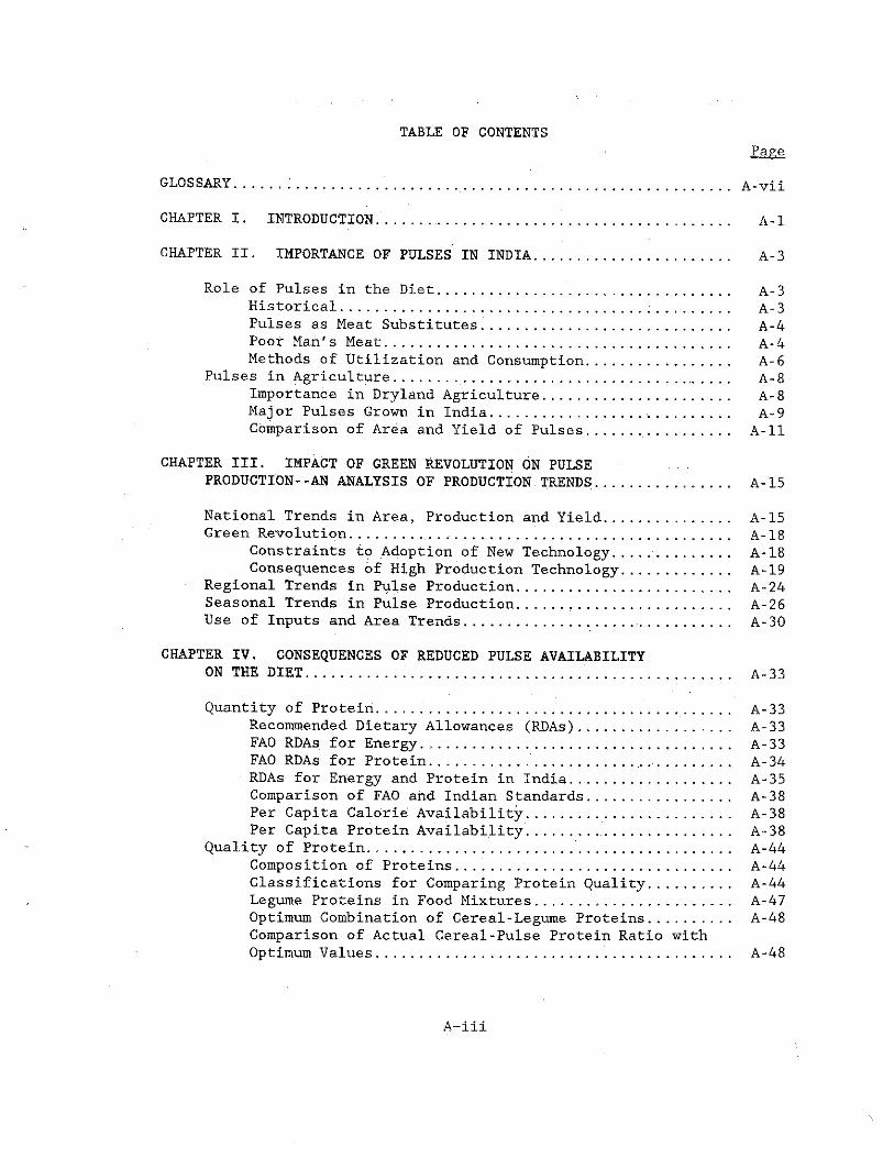
TABLE OF CONTENTSPage
GLOSSARY..... ............ A-vii
CHAFTER I. INTRODUCTION..... ................ ............. ....... A-1
CHAPTER II. IMPORTANCE OF PULSES IN INDIA......... ............. A-3
Role of Pulses in the Diet............................... . A-3Historical................................. A-3Pulses as Meat Substitutes............................. A-4Poor Man's Meat......................................... A-4Methods of Utilization and Consumption................. A-6
Pulses in Agriculture............ ......... ............ . A-8Importance in Dryland Agriculture....................... A-8Major Pulses Grown in India......................... ... A-9Comparison of Area and Yield of Pulses...... .......... A-11
CHAPTER III. IMPACT OF GREEN REVOLUTION ON PULSEPRODUCTION--AN ANALYSIS OF PRODUCTION TRENDS ................ A-15
National Trends in Area, Production and Yield....... . ...... A-15Green Revolution........ .................................... A-18
Constraints to Adoption of New Technology. . . . ......... A-18Consequences of High Production Technology............. A-19
Regional Trends in Pulse Production......................... A-24Seasonal Trends In Pulse Production..................... A-26Use of Inputs and Area Trends............................... A-30
CHAPTER IV. CONSEQUENCES OF REDUCED PULSE AVAILABILITYON THE DIET.......... ........................................ A-33
Quantity of Protein.... ...................................... A-33Recommended Dietary Allowances (RDAs).................. A-33FAO RDAs for Energy............................... ..... A-33FAO RDAs for Protein........... ............ ........... A-34RDAs for Energy and Protein in India. ................... A-35Comparison of FAO and Indian Standards......... ....... A-38Per Capita Calorie Availability........................ A-38Per Capita Protein Availability.................. A-38
Quality of Protein................................... A-44Composition of Proteins..................... A-44Classifications for Comparing Protein Quality........... A-44Legume Proteins in Food Mixtures............. ......... A-47Optimum Combination of Cereal-Legume Proteins........... A-48Comparison of Actual Cereal-Pulse Protein Ratio with Optimum Values.................................... A-48
A-iii
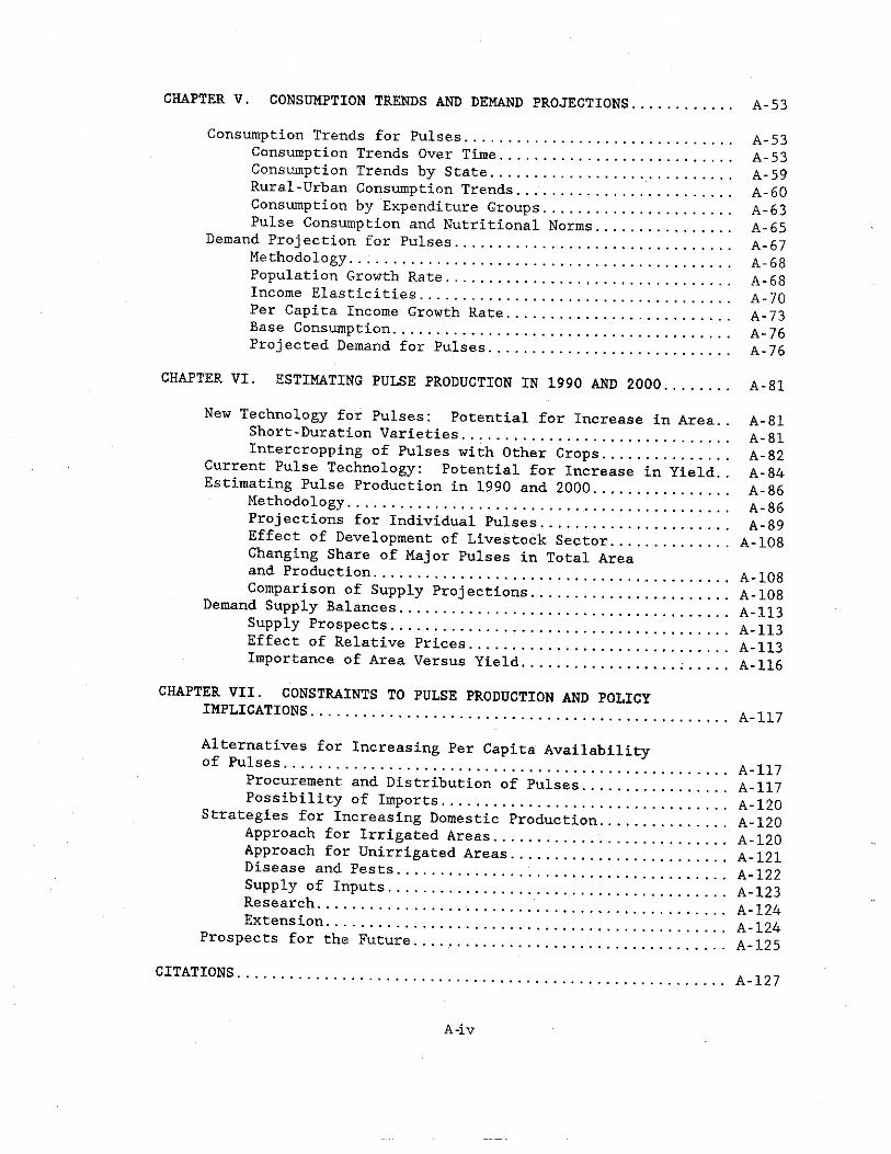
CHAPTER V. CONSUMPTION TRENDS AND DEMAND PROJECTIONS........... A-53
Consumption Trends for Pulses................................ A-53Consumption Trends Over Time.... ....................... A-53Consumption Trends by State............................ A-59Rural-Urban Consumption Trends...,..................... A-60Consumption by Expenditure Groups............... A-63Pulse Consumption and Nutritional Norms................ A-65
Demand Projection for Pulses............................. * * ’ A_67Methodology. . ............................................ A_68Population Growth Rate.................................. A -68Income Elasticities.................................... A-70Per Capita Income Growth Rate.......................... A-73Base Consumption................. A-76Projected Demand for Pulses............................ A-76
CHAPTER VI. ESTIMATING PULSE PRODUCTION IN 1990 AND 2000....... A-81
New Technology for Pulses: Potential for Increase in Area.. A-81Short-Duration Varieties.............................. A-81Intercropping of Pulses with Other Crops.............** A-82
Current Pulse Technology: Potential for Increase in Yield.. A-84Estimating Pulse Production in 1990 and 2000................ A -86
Methodology........................... ............ ’ * * ‘ ‘ A _g6Projections for Individual Pulses..................... * A _g9Effect of Development of Livestock Sector..............A-108Changing Share of Major Pulses in Total Areaand Production...... .......................... A-108Comparison of Supply Projections....................... A-108
Demand Supply Balances............................. [ * A-113Supply Prospects.................................... ’** A _ H 3Effect of Relative Prices............ .............. A-113Importance of Area Versus Yield........................A-116
CHAPTER VII. CONSTRAINTS TO PULSE PRODUCTION AND POLICYIMPLICATIONS............................. ........ A-117
Alternatives for Increasing Per Capita Availabilityof Pulses................... ............... A-117
Procurement and Distribution of Pulses..............' * * a -117Possibility of Imports................................ A-120
for Increasing Domestic Production. . . ........ . A-120Approach for Irrigated Areas. . . .......... A-120Approach for Unirrigated Areas......................... A-121Disease and Pests............................ * A-122Supply of Inputs............ ........... ....... A-123Research................. A-124Extension........................... A-124
Prospects for the Future........................ ’ ’ * ......A-125CITATIONS.......... *
A-iv
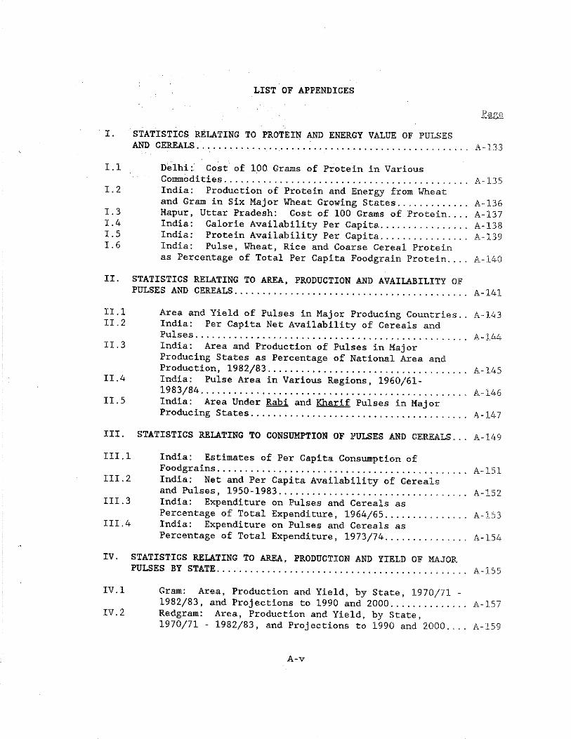
LIST OF APPENDICES
I. STATISTICS RELATING TO PROTEIN AND ENERGY VALUE OF PULSESAND CEREALS.......... ........................... ........... A-133
1.1 Delhi: Cost of 100 Grams of Protein in VariousCommodities.............. ........................ A-135
1-2 India: Production of Protein and Energy from Wheatand Gram in Six Major Wheat Growing States............ A-136
1.3 Hapur, Uttar Pradesh: Cost of 100 Grams of Protein.... A-1371-4- India: Calorie Availability Per Capita................ A-1381*5 India: Protein Availability Per Capita............. . A-1391*6 India: Pulse, Wheat, Rice and Coarse Cereal Protein
as Percentage of Total Per Capita Foodgrain Protein.... A-140
II. STATISTICS RELATING TO AREA, PRODUCTION AND AVAILABILITY OF PULSES AND CEREALS.....................
II. 1II. 2
11.3
11.4
II. 5
Area and Yield of Pulses in Major Producing Countries,. A-143India: Per Capita Net Availability of Cereals andPulses.................................................. a -144India: Area and Production of Pulses in MajorProducing States as Percentage of National Area andProduction, 1982/83...................................... A-145India: Pulse Area in Various Regions, 1960/61-1983/84................................................ . a -146India: Area Under Rabi and Kharif Pulses in Maj orProducing States........................................ A-147
III. STATISTICS RELATING TO CONSUMPTION OF PULSES AND CEREALS... A-149
111.1 India: Estimates of Per Capita Consumption ofFoodgrains....... ...................................... A-151
111.2 India: Net and Per Capita Availability of Cerealsand Pulses, 1950-1983..................... .......... . A-152
111.3 India: Expenditure on Pulses and Cereals asPercentage of Total Expenditure, 1964/65............. .. A-153
111.4 India: Expenditure on Pulses and Cereals asPercentage of Total Expenditure, 1973/74............... A-154
IV. STATISTICS RELATING TO AREA, PRODUCTION AND YIELD OF MAJOR PULSES BY STATE...................
IV.1 Gram: Area, Production and Yield, by State, 1970/71 -1982/83, and Projections to 1990 and 2000....... . A-157
IV,2 Redgram: Area, Production and Yield, by State,1970/71 - 1982/83, and Projections to 1990 and 2000.... A-159
A-v
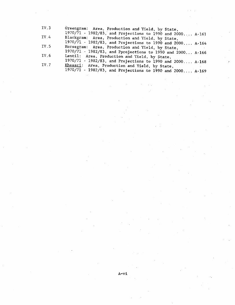
IV. 3
IV. 4
IV. 5
IV. 6 IV. 7
Greengram: Area, Production and Yield, by State,1970/71 - 1982/83, and Projections to 1990 and 2000.... Blackgram: Area, Production and Yield, by State,1970/71 - 1982/83, and Projections to 1990 and 2000.... Horsegram: Area, Production and Yield, by State,1970/71 - 1982/83, and Pprojections to 1990 and 2000... Lentil: Area, Production and Yield, by State,1970/71 - 1982/83, and Projections to 1990 and 2000.... Khesari: Area, Production and Yield, by State,1970/71 - 1982/83, and Projections to 1990 and 2000..,.
A-161
A-164
A-166
A-168
A-169
A-vi
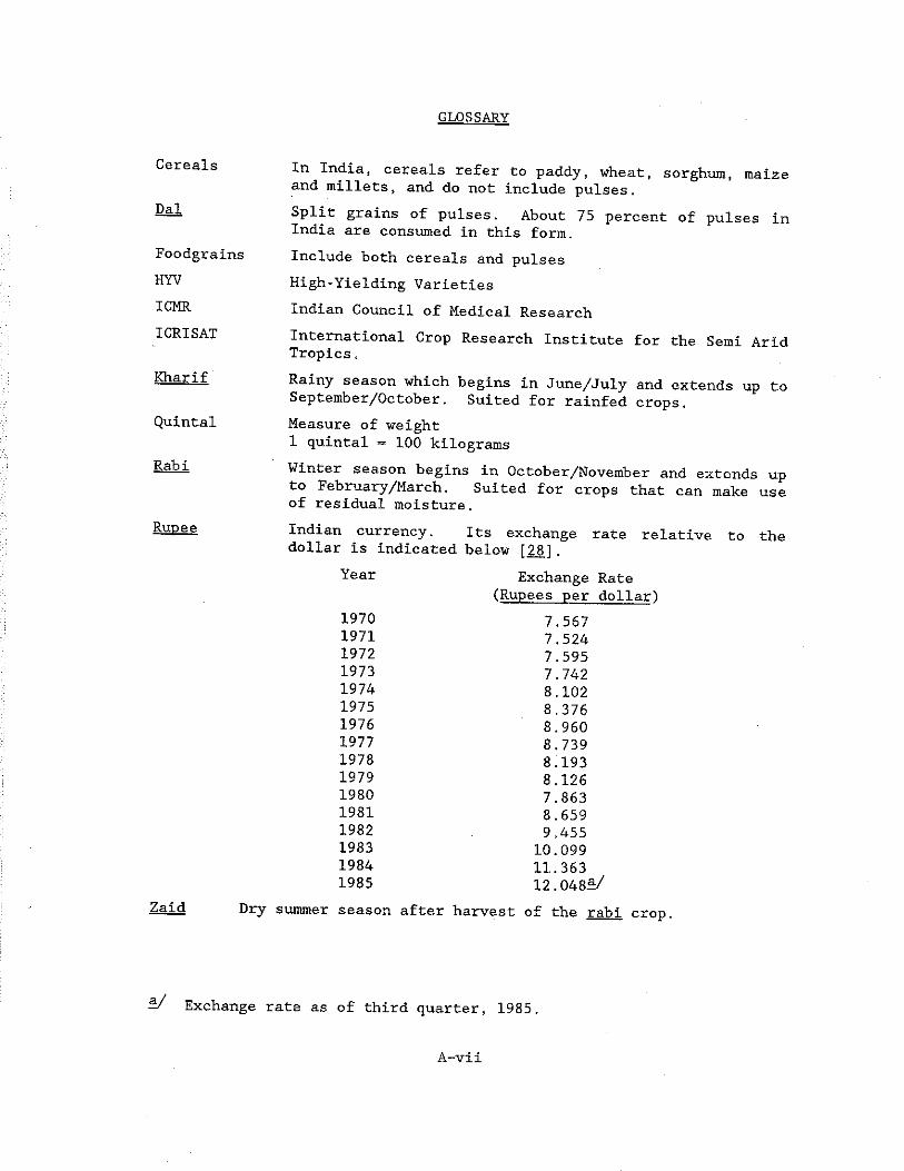
GLOSSARY
Cereals
Dal
FoodgrainsHYVICMRICRISAT
Kharif
Quintal
Rabi
In India, cereals refer to paddy, wheat, sorghum, maize and millets, and do not include pulses.Split grains of pulses. About 75 percent of pulses in India are consumed in this form.Include both cereals and pulsesHigh-Yielding VarietiesIndian Council of Medical ResearchInternational Crop Research Institute for the Semi Arid Tropics.Rainy season which begins in June/July and extends up to September/October. Suited for rainfed crops.Measure of weight 1 quintal = 100 kilogramsWinter season begins in October/November and extends up to February/March. Suited for crops that can make use of residual moisture.
Rupee
Zaid
Indian currency. Its exchange rate relative to the dollar is indicated below [28J.
Year Exchange Rate (Rupees per denar')
1970 7.5671971 7.5241972 7.5951973 7.7421974 8.1021975 8.3761976 8.9601977 8.7391978 8.1931979 8.1261980 7.8631981 8,6591982 9,4551983 10.0991984 11.3631985 12.048®:/
Dry summer season after harvest of the rabi crop.
®/ Exchange rate as of third quarter, 1985.
A-vii
CHAPTER I INTRODUCTION
*? the ^dian diet. EvenIndian meal. They are a rich source of '’r1*68 describe the average ment cereals in the diet ln a countr^ ? ln and’ as s“ch, comple- Of the population is vegetarian,. puTse J peroenta«eammo acid balance needed for nn™*7 essential m providing the maintenance of health. normal growth development and the
valuec^for^their " 3 P*>tein. pulses arepulses are able to u t m ^ T i r n T t i d3 ** legume croPs - As a group, efficiently than cereals. Their ability to^f” 6 and O r i e n t s more enhances their significance as crops suited f atmosPherlc nitrogen and specially for small and subsistence f J and rainfed areas,cost of inputs needed for high-yielding technology Can 111 aff0rd the
decaJs?dUCwi1r increasing p^pufatio'^iS £“ *>* <-er twoable decline in their pe/capitaavaila^ilit-T ln an appreci-grams per day in the early 1960s to atour ts ^ *811 fr°m about 65 the same period per capita wheat avail -35 .S ln the 1980s. in grams per^ day to 130 grams [36, p 141 [ ^ lncreased from around SO dramatic increase in wheat production a, ' he. latter was due to the tlon in the mid-1960s, based d u t h e Z Z t °f the Green E l u sive high-yielding varieties The eVelopment of fertilizer-respon- Revolution was to Increase total cereal o r V 0?.tribUtl°n °f tha G"aaa self-sufficient in food. Production of f d" ® make the oountry around 80 million metric tons intta lncreased frommetric tons in the 1980s [36 p 141, \ °oc t0 ar°Und 150 millionwheat production can be accTJ e d f o r'bv Percent of increased came from an increase in the area planted t-Slr? yields’ the remainder diverted from rabi pulses [6, p 71 Tn tb' 1^ ’ Part °f which "aa high-yielding varieties, even rice L , 197°s' with the spread ofregister a marked increase [52 p st0"’ ~glch had been aluSgish,similar breakthrough in pulse t^h’ ?' 5] ' There was, however, no levels. Consequently, hnd that v t n 5y’ and ylelds remained at low rabi season to wheat^nd ln tba
deelin71Se H ^ e v S , a signlficantthe^pre- and post-Green Revolution eras I i- avallabl-lity examined inavailability had ' i n c r e a s e d " ' — all P-tein cereals, especially wheat [511 This i ^ k i g h - y i e l d i n g variety quantity of protein supplied by pulses mpUed that the reduction in
A-1
A- 2
. 11 m s 2 ^ 2r . s s .°£2 s . 'ai« ... * " “ “ . 2 r r 2 « ” i , "sufficient quantity _ could fulftil both^ ^ ^ f ther ^ f<jr pulses.ment of the population, and th tein intake that is impor-However, it is not only the quan y d by the amino acid balancetant but also i - X L ^ t r e V r ^ ^ t o g e t h e r in tbe_ tight proportion6 provide the desirable amino acid balance whic possible in a diet composed only of cereals.
Pulses must therefore regain * ^ r h e w t a ^ o fhand, cereal P » « f » “ Z l to have here an apparenta growing population is to D •conflict between objectives.
It is the P” P°se of B tr e M i ~ ei ^ e^ s i b i l l t y CSherebyth°en paroduPcrt^nC Of bot£ cereals and pulses can be simultaneously increased.
The study is organ^e,I -importance of pulses m the die Lphasizes the role of legumeas well as current point of ™ « . ^ ems of small andcrops in rainfed agriculture and m the terming ysubsistence cultivators.
Chapter III analyzes past “ ends and ^fsent morfthan^ORevolution on pulse production. an ■ d lands. It is shownpercent of pulse area is c°nf™ continue to accrue from rainfed
diverted away from pulses into high-yielding cereal crops.
Chapter IV examines the effects of red.uoed dlet, hyPdefining -tritional nor- Tf%ul.. ’to cerealprotein. It is argued that a certai p P infinitelyprotein in the diet enhances its protein quality, preferable to a diet without pulses.
Chapter V deals with “ Sheets” and*6 food consumptionobtained from national food balan . t 1990 and 2000 basedsurveys. Demand projections are population and income“ o w ^ ^ r ^ i r r ^ t a f n e d “ c h a r e d toP Pthose derived on tbe basis of nutritional norms.
Chapter VI examines thedemand in 2000 can be met fro“ d°“ef ^ e pT o gress in pulse technology production continue. It’ *“ orp lth estimates of expansion m area tomade in recent years together wi project pulse production m 2000.
CHAPTER IIIMPORTANCE OF PULSES IN INDIA
Role of Pulses in the Diet
The two most Important groups of crops in world agriculture belong to the plant orders Gramineae (cereals and grasses) and Leguminosae (peas, beans and the grain, forage and green manure legumes) [68., p.l].
Pulses are the edible seeds of leguminous plants, which belong to the category of leguminosae. Although members of the same botanical family, a distinction is made between pulses and oilseeds. Leguminous seeds containing only small amounts of fat, e .g ., gram, redgram, greengram, blackgram, peas and lentil, are grouped together as pulses, whereas groundnut and soybean, with a higher fat content and used primarily for oil extraction, are categorized as oilseeds.
Pulses are valued for their high nutritional quality. Although the chemical composition is variable between species, all pulses are characterized by a high protein content— in fact, almost twice that of cereal grains. Their nutritional value is not confined to their usefulness as a source of vegetable protein. Pulses are also the source of vitamins and minerals. Nevertheless it is in their actual and potential value as a source of plant protein for human nutrition that their importance lies, Pulses are also valued for the variety, taste and texture that they add to a diet based on starchy staples.
Historical
While it is true that the nutritional quality of pulses was scientifically proven only in the 19th century, their importance as food was recognized from very early times. Pulses appear to have been among the earlier plants domesticated. Traces of wheat, peas and lentil have been found at archaeological sites in Turkey dating 5500 B.C, [2, p. 1]. Chinese literature records the cultivation of soybean with rice, wheat and barley between 3000 and 2000 B.C. Legumes featured in the cropping systems of the early Egyptian dynasties, and later in the Roman era several writers stressed their value for food and soil improvement [68, p. 2]. American Indians from, very early times raised beans among their maize. Vessels containing kidney beans were discovered in pre-Inca tombs in Peru [2J . Pigeonpea, a native plant of South Asia, is believed to be one of the oldest cultivated plants in the world and reference to it is found in ancient Hindu religious literature [10].
An interesting Biblical reference to legumes is found in the fourth chapter of Ezekiel. The bread or cakes to be eaten in limited quantity by Ezekiel during a period of fasting and penitence had to
A- 3
A - 4
contain--as well as wheat and barley--beans, lentils and vetches [2, P. 8].
It seems that throughout history, across vastly different geographical areas, a combination of a cereal pulse diet, though not regarded as a gourmet's delight, was wholesome and nutritional enough to maintain the health and survival of communities, especially those that depended primarily on plant nutrients for energy and protein.
Pulses as Meat Substitutes
Pulses are still an important component of the diets of many sections of populations in countries around the world. Although the pattern of pulse production and consumption varies with agroclimatic and cultural factors, there appears to be one element in common. The importance of pulses is especially marked in those communities where the supplies of animal protein have been limited. The greatest stimulus to the production and consumption of pulses has been a shortage of animal protein. This may be due to economical or cultural factors, or a combination of both.
In a country such as India, with an ancient civilization and settled conditions over periods of several millenia, population expanded and imposed a high pressure on the productive capacity of the land. This in turn necessitated an efficient use of land in meeting the protein requirements of the population. It is well known that the intermediate processing of plant protein by an animal, which is in turn consumed by humans, is wasteful in terms of energy. Therefore in a society with a high population density the most economical use of land implies a preference for plant over animal protein. Even if animals are reared, they are the kind that scavenge on leftovers and do not compete for land, as pigs and poultry do [59, pp. 82-83].
In India the situation is further aggravated by religious beliefs. The prohibition on the slaughter of cows for beef among all Hindus, and a ban on meat consumption of any kind for orthodox Hindus, accentuate the shortage of animal protein and consequently enhance the importance of pulse intake.
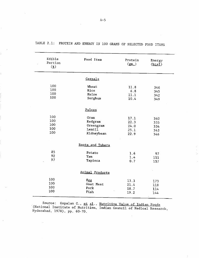
The value of pulses in the average diet is assesed from the fact that compared to most commonly consumed vegetable foods, they contain the highest level of protein per 100 grams of edible portion. Their protein content compares well with that of the meats usually eaten in India. This is evident from Table 2.1.
Poor Man's Meat
It is for the role that they play as meat substitutes, that pulses are often referred to as "poor man's meat." The phrase, however, seems to imply that pulses are considered socially inferior food. And as one progresses up the socio-economic ladder, the meat substitute, namely pulse protein, is replaced by animal protein. In most of the developed
A-5
TABLE 2.1: PROTEIN AND ENERGY IN 100 GRAMS OF SELECTED FOOD ITEMS
EdiblePortion
(1)Food Item Protein
(mJ>Energy('kcal't
Cereals100 Wheat 11.8 346100 Rice 6.8 345100 Maize 11.1 342100 Sorghum 10.4 349
Pulses100 Gram 17.1 360100 Redgram 22.3 335100 Gre engrain 24.0 334100 Lentil 25.1 343100 Kidneybean 22.9 346
Roots and Tubers85 Potato 1.6 9792 Yam 1.4 11197 Tapioca 0.7 157
Animal Products100 Egg 13.3 173100 Goat Meat 21.4 118100 Pork 18.7 114100 Fish 19.2 144
Source: Gopalan C., et al.} Nutritive Value of Indian FonHs(National Institute of Nutrition, Indian Council of Medical Research Hyderabad, 1978), pp. 60-70.
A-6
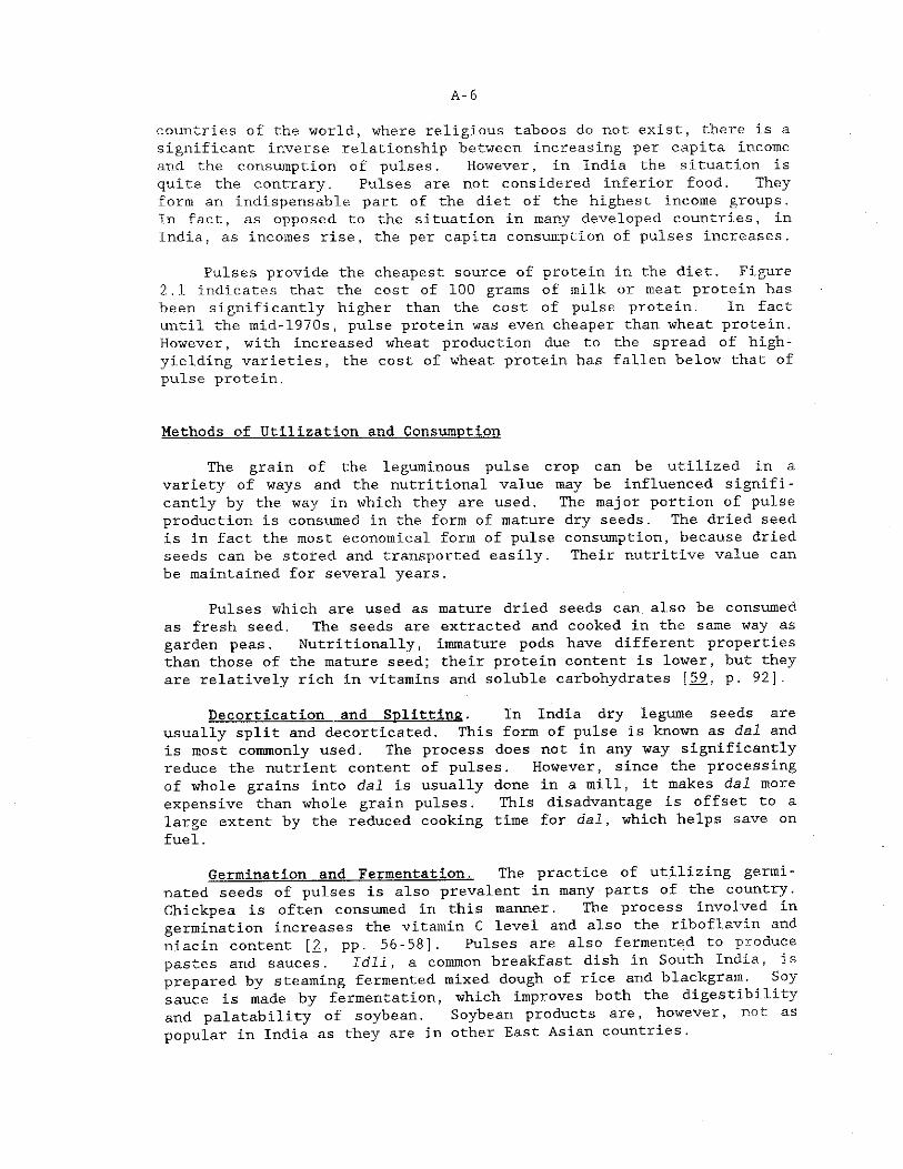
countries of the world, where religious taboos do not exist, there is a significant inverse relationship between increasing per capita income and the consumption of pulses. However, in India the situation is quite the contrary. Pulses are not considered inferior food. They form an indispensable part of the diet of the highest Income groups. In fact, as opposed to the situation in many developed countries, in India, as incomes rise, the per capita consumption of pulses increases.
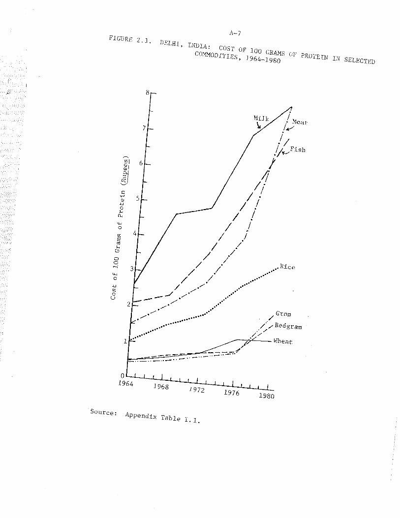
Pulses provide the cheapest source of protein in the diet. Figure 2.1 indicates that the cost of 100 grams of milk or meat protein has been significantly higher than the cost of pulse protein. In fact until the mid-1970s, pulse protein was even cheaper than wheat protein. However, with increased wheat production due to the spread of high- yielding varieties, the cost of wheat protein has fallen below that of pulse protein.
Methods of Utilization and Consumption
The grain of the leguminous pulse crop can be utilized in a variety of ways and the nutritional value may be influenced significantly by the way in which they are used. The major portion of pulse production is consumed in the form of mature dry seeds. The dried seed is in fact the most economical form of pulse consumption, because dried seeds can be stored and transported easily. Their nutritive value can be maintained for several years.
Pulses which are used as mature dried seeds can also be consumed as fresh seed. The seeds are extracted and cooked in the same way as garden peas. Nutritionally, Immature pods have different properties than those of the mature seed; their protein content is lower, but they are relatively rich in vitamins and soluble carbohydrates [59., p. 92].
Decortication and Splitting. In India dry legume seeds are usually split and decorticated. This form of pulse is known as dal and Is most commonly used. The process does not in any way significantly reduce the nutrient content of pulses. However, since the processing of whole grains into dal is usually done in a mill, it makes dal more expensive than whole grain pulses. This disadvantage is offset to a large extent by the reduced cooking time for dal, which helps save on fuel.
Germination and Fermentation. The practice of utilizing germinated seeds of pulses is also prevalent in many parts of the country. Chickpea is often consumed in this manner. The process involved in germination increases the vitamin C level and also the riboflavin and niacin content [2., pp. 56-58]. Pulses are also fermented to produce pastes and sauces. Idll, a common breakfast dish in South India, Is prepared by steaming fermented mixed dough of rice and blackgram. Soy sauce Is made by fermentation, which improves both the digestibility and palatability of soybean. Soybean products are, however, not as popular in India as they are in other East Asian countries.
f ig u r e 2 . 1DELH1’ If®IA: COST OF ion .
commodities, „ 6°“ 5 s of proteiw IN SELECTED
e 1.1.ource: Appendix Tabl
b , .T* r-u cereals. ^rcL 1
1Tnpd in combination the South, are- are usually cons florth and tic form the main
. / / / e b a s e d on wheat £ - ™ in which p u l s e s ° cereals fortional dieo^ „ stews, ana o . ^ with than t-neethersupplemented b y ^ P ^ from pulses r— ^ and rice cooked Conven-lnfrediunleaveled bread ( « / / rse in a poor man* s j e a l ^ _ ^ ^makmg n form the only little loss and appear-(KhlCl“ ethods of cooking Pulses o _ digestlbU3 , are" h hand cooking improves taste co a soft conother hand greengram, whenancl. /traditional weaning foods. _ & regular part ofUSe In addition to being ^ £orm of snacks
are widely very much the same
“ r r r “ . i » u ' f r . . r u r -/ y as popcorn. T ^ e fact makes the course ofsnacks made / / y of pulses census- ^ ^ j sweets m i g W
the Tince pulses In the ^ » j «tal woulda dal o St T o to 20 percent o f . take this _into coMi» ^ pulsehold consumer survey whfa / ' This situation co^ Survey, as we understate pulse ‘— / / / t e d by the National Sampconsumption v .Shall see m Chapter
ition in Indian agriculture. lndia.Pulses occupy a unique P - f ^ / u n d e r these crops » * M in
„ « u »— s , u - 5 0 v ” ’ i m ‘the country. .r?r tons ouri-fg, ^9 o/variatio/in seasonal conditions,function of van
^ nrvland_Agricult^£^- constitutes^ 7 7 where rainfed agriculture^^ ^
I n a 0 T n t ryo fUth e t l t a i cropped ^ a . ^ t h e c u ^ t han 9 0 j e r c e ^
" acquires a special i m p o ^ . rrlgated f-d' /ulses^ rainfallCh P d , production comes fr° ture stress with ients more°f dominantly in conditions dl moisture a out reason-predominan y able t0 u-lize oropg not only tur absence ofSi « eciently than cereal crops. ^ marginal lands m r_ Theyefficien y of foodgrains they g0 a step baen theable quantitxctem.cai £ertlm e i s U Leguminous f / S. "/rations in manure.. lmprove soil ferti y included productivereSt°rav Of Indian agriculture. / / elped to keep soils Pmf h r all farming systems and h nitr„gen.th/o/h their ability to f « atmosp
A- 9
Legumes differ from other food plants in having the property of synthesizing atmospheric nitrogen into plant nutrients. This special ability of leguminous crops to work symbiotically with rhizobia to produce nitrogen is a very important factor in the agriculture of developing countries, for it makes leguminous crops, to a large extent, independent of manures and fertilizers. The nitrogen gained from the atmosphere finds its way into animal and human protein and in a large measure into the soil as an agent of enrichment, leaving the fixed nitrogen in the soil for succeeding crops. Experiments have indicated that pulse crops may add to the soil an equivalent of 20 to 60 kilograms of nitrogen per hectare [46, p. 307], Since nitrogen is commonly the most limiting element in food production and costly in fertilizer, this special characteristic of pulse crops works to the advantage of the small and marginal cultivators, who can barely afford purchased inputs.
Another important characteristic of legumes is their deep root system which enables them to survive without irrigation even in the dry season, and makes them useful in dryland farming rotations. The roots penetrate the soil to considerable depths and bring up minerals and moisture to enrich the top soil. They also provide a channel for the movement of air and moisture within the soil when they decay. When the green leguminous crop is ploughed back, it provides green manuring and improves the organic matter status of the soil. The leaf drop enriches the soil humus. The thick planting of legumes for green manuring smothers the weeds and therefore loss of nutrients through weeds is also checked. The stems of the redgram shrub provide firewood and are also used for thatching.
Major Pulses Grown in India
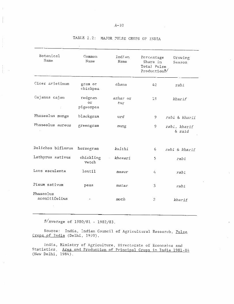
A large number of pulse crops are grown in India. The most important of these are gram (chickpea) and redgram (pigeonpea) which taken together account for nearly half of the total area under pulses and for about 60 percent of total production. The next in importance are pulses of the Phaseolus group, i.e., greengram, blackgram and moth. Table 2.2 lists the commonly cultivated pulses in India, and the seasons in which they are grown.
Three distinct seasons characterize much of India. The rainy or monsoon season, known as kharif usually begins in June and extends into October. More than 80 percent of the average annual rainfall occurs during these four months, in which rainfed crops are raised. The postmonsoon winter season, October through March, known as rabi is dry and cool and the days are short. During this period crops can be grown on residual moisture, frequently supplemented by a few light showers of the winter rains. The hot, dry summer season from March until rains begin again in June, is known as zaid. Any crops grown during this season require irrigation.
A - 10
TABLE 2.2: MAJOR PULSE CROPS OF INDIA
BotanicalName
CommonName
IndianName
Percentage Share in
GrowingSeason
Total Puls.eProduction:a/
Cicer arietinum gram or chickpea
chana 42 rabi
Cajanus cajan redgram arhar or 18 kharifor tur
pigeonpea
Phaseolus mungo blackgram urd 9 rabi &, kharif
Phaseolus aureus greengram mung 9 rabi, kharif6c zaid
Dolichos biflorus horsegram kulthi 6 rabi & kharifLathyrus sativus chickling
vetchkhesari 5 rabi
Lens esculenta lentil masur 4 rabi
Pisum sativum peas matar 3 rabi
Phaseolusaconitifolius moth 2 kharif
—/Average of 1980/81 - 1982/83.
Source: India, Indian Council of Agricultural Research, PulseCrons of India (Delhi, 1970).
India, Ministry of Agriculture, Directorate of Economics and Statistics, Area and Production of Principal Crons in India 1981-84 (New Delhi, 1984).
A-ll
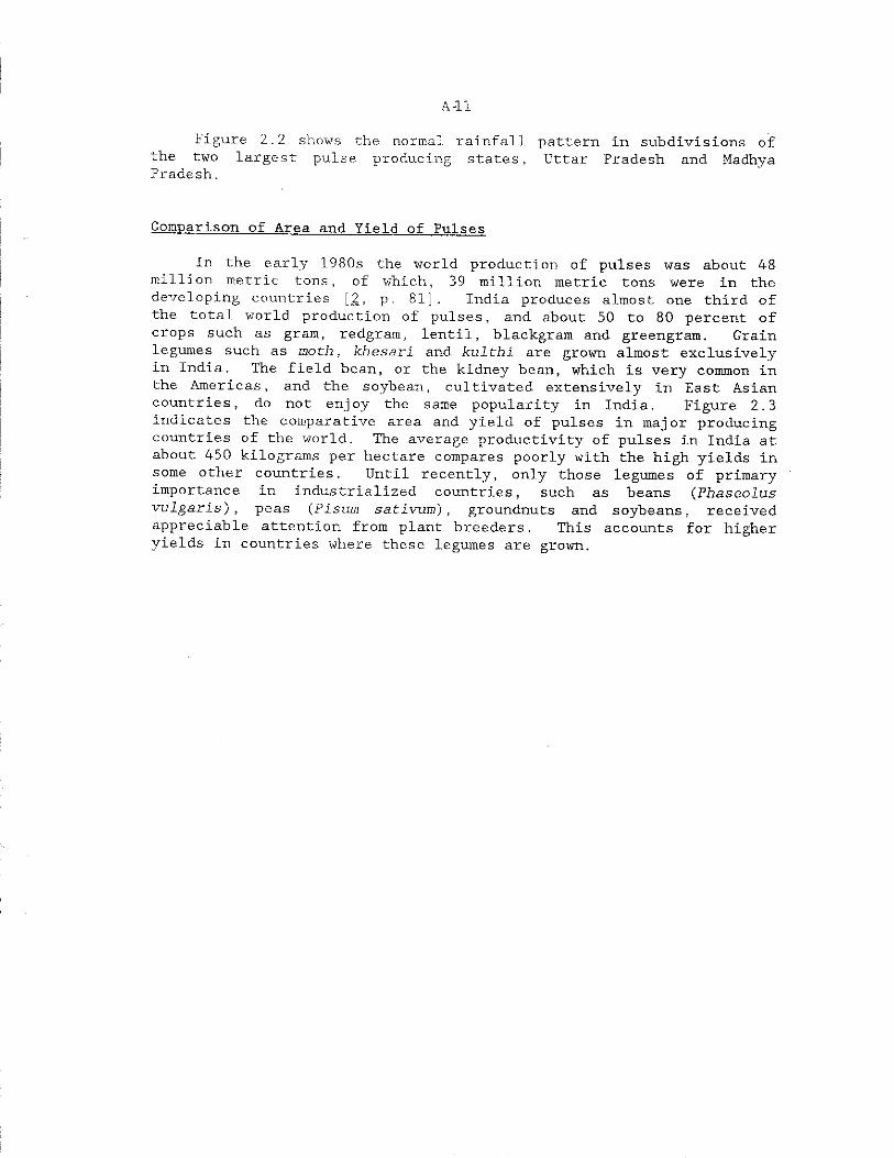
Figure 2.2 shows the normal rainfall pattern in subdivisions of the two largest pulse producing states. Uttar Pradesh and Madhya Pradesh.
Comparison of Area and Yield of Pulses
In the early 1980s the world production of pulses was about 48 million metric tons, of which, 39 million metric tons were in the developing countries [2, p . 81 ] . India produces almost one third ofthe total world production of pulses, and about 50 to 80 percent of crops such as gram, redgram, lentil, blackgram and greengram. Grain legumes such as moth, khesari and kulthi are grown almost exclusively In India. The field bean, or the kidney bean, which is very common in the Americas, and the soybean, cultivated extensively in East Asian countries, do not enjoy the same popularity in India. Figure 2.3 indicates the comparative area and yield of pulses In major producing countries of the world. The average productivity of pulses in India at about 450 kilograms per hectare compares poorly with the high yields in some other countries. Until recently, only those legumes of primary importance In Industrialized countries, such as beans (Phaseolus vulgaris), peas (Pisum sativum), groundnuts and soybeans, received appreciable attention from plant breeders. This accounts for higher yields in. countries where these legumes are grown.
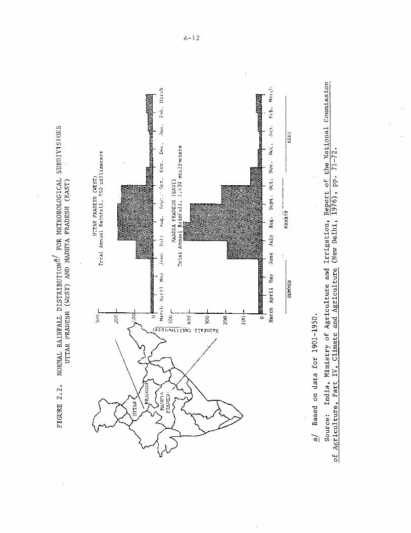
FIGURE 2
.2.
NORMAL R
AINFALL
DISTRIBUTION—
FOR METEOROLOGICAL S
UBDIVISIONS
UTTAR
PRADESH
(WEST) A
ND M
ADHY
A PRADESH
(EAST)
A -12
oCT\lrHoCluoCf-IcO-MctiTJCOXtCl)wcoPQ
co| Source:
India, M
inis
try
of A
griculture a
nd I
rrigation, R
eport
of t
he National
Commission
of A
griculture,
Part I
V, C
limate a
nd A
griculture (
New Delhi, 1
976),
pp.
71-72.
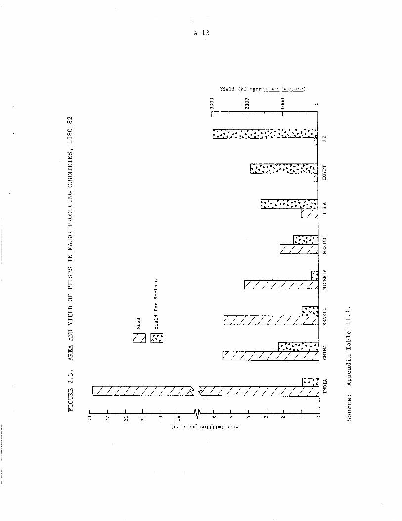
FIGURE 2
.3.
AREA AND YIELD O
F PULSES I
N MA
JOR
PRODUCING
COUNTRIES, 1
980-82
Yield (kilograms per hectare)ooo oooCN
ooo o
£2
ta
o
$BQ
<2W2U
< i—io20Ju1oCO
Appendix T
able II

CHAPTER IIIIMPACT OF GREEN REVOLUTION ON PULSE PRODUCTION:
AN ANALYSIS OF PRODUCTION TRENDS
In the years following the introduction, in the mid-1960s, of the new high-yielding varieties of wheat, area sown to wheat expanded substantially. This breakthrough in food production technology was accompanied by a significant shift in area from pulses to high-yielding varieties of cereals.
Despite the rise in price of pulses, in some cases quite significantly, the area under pulses continued to decline in many states. Other crops which suffered a loss In area were oilseeds and coarse cereals, particularly sorghum, millets and barley.
National Trends in Area. Production and Yield
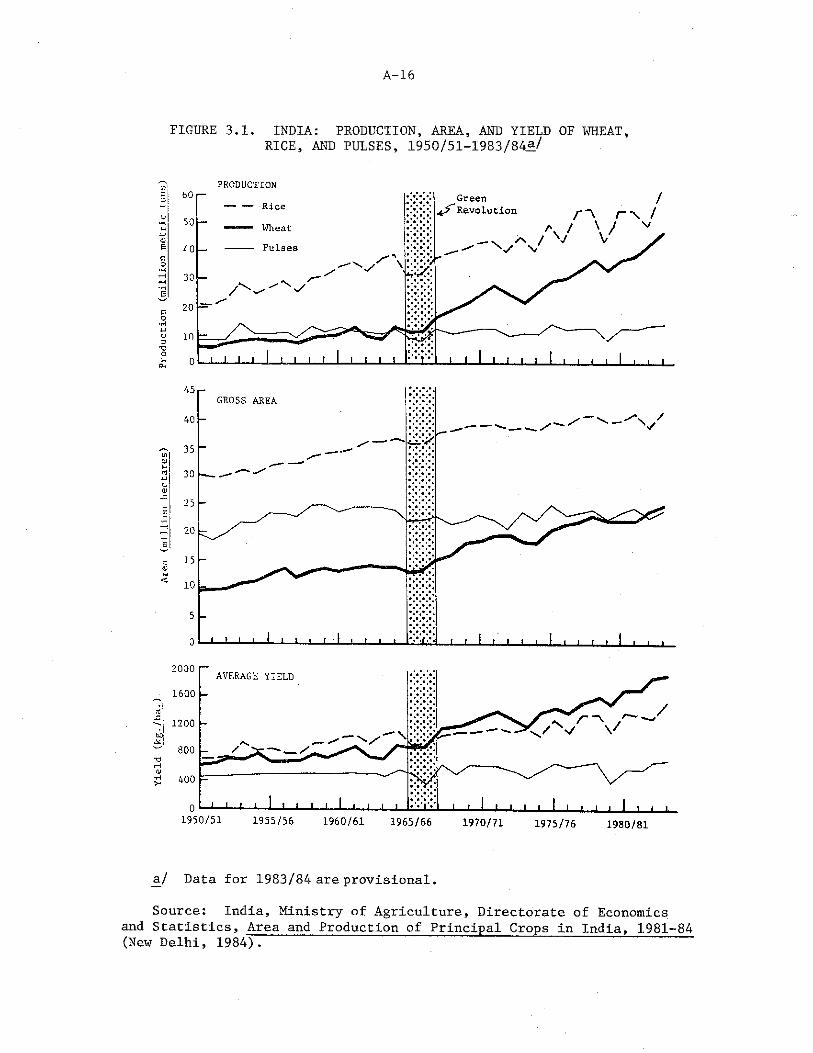
Production of pulses in India has been stagnant for the last two decades. This is due to the fact that area under pulses has fluctuated between 22 and 24 million hectares, and the yields per hectare have not registered any significant increase. This can be seen in Figure 3.1.
Wheat production, on the other hand, increased from 11 to 45 million metric tons, while rice production rose from 35 to around 60 million metric tons during the same period [36]. The increase in cereal production, especially wheat, has been sharper since the mid- 1960s. This came as a result of both increase in area and yield. The latter, due to the introduction of high-yielding varieties, was responsible for about 85 percent of the increased output. The expansion in area of cereals occurred partially at the expense of pulse area.
Production of cereals increased more than two and a half times between the early 1950s and the 1980s. The total production of pulses remained almost the same, with a wide range of fluctuations in between. The fluctuations were the result of variations in weather conditions. Since the bulk of pulse area is rainfed, the production of pulses is more directly and severely affected by abnormal rainfall conditions than cereals like wheat and rice, a sizable percentage of which are grown on irrigated lands.
At the national level the area trend for total pulses remained almost constant. From Figure 3.1 it is difficult to discern any marked increasing or decreasing tendency in the area.
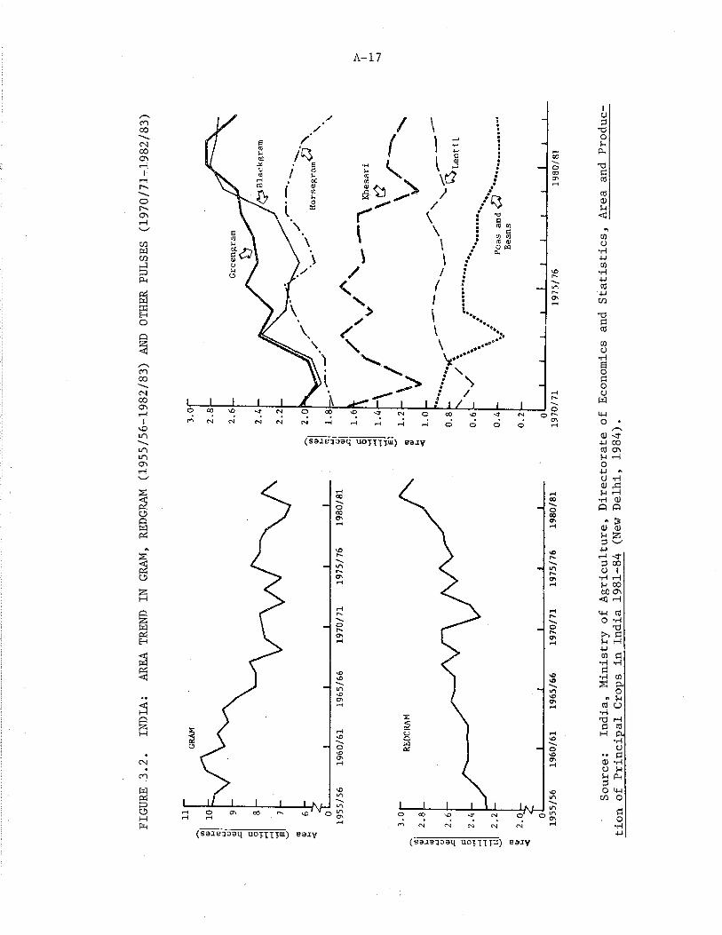
Figure 3.2, however, indicates that the area of gram, peas and beans, and Khessri was adversely affected, while redgram, greengram, and blackgram showed a positive trend. We may conclude, therefore,
A- 15
A-16
FIGURE 3.1, INDIA: PRODUCTION, AREA, AND YIELD OF WHEAT,RICE, AND PULSES, 1950/51-1983/84^/
a./ Data for 1983/84 are provisional.
Source: India, Ministry of Agriculture, Directorate of Economics!and Statistics, Area and Production of Principal Crops in India, 1981-84 (New Delhi, 1984).
FIGU
RE 3
.2.
INDIA:
AREA
TRE
ND I
N GRAM,
REDG
RAM
(195
5/56
-198
2/83
) AN
D OT
HER
PULS
ES (
1970
/71-
1982
/83)
A-17
uoy^TJ1*1) a a iy
r--r.<7\
r-.
sOv&tOVOCt
Source:
India, M
inis
try
of A
gric
ultu
re,
Dire
ctor
ate
of E
cono
mics
and
Sta
tist
ics,
Are
a and
Prod
uc
tion
of
Prin
cipa
l Cr
ops
in I
ndia
198
1-84
(New
Delh
i, 1
984).
A- 18
that all pulses were not affected similarly and uniformly due to the introduction of high-yielding variety of cereals. While some pulses were displaced from certain regions as a result of competition from high-yielding cereals, other pulses made positive gains in different regions.
To explain trends in pulse area at the national level, it is necessary to look closely at the impact that the high-yield production technology, introduced in the mid-1960s, had on cropping patterns in different parts of the country.
Green Revolution
The Green Revolution was characterized by high-yielding varieties of seeds together with a package of complementary inputs which were necessary if optimum output was to be achieved. Inputs included recommended doses of fertilizer, timely and assured irrigation, use of plant protection measures, precise agronomic practices and effective management techniques.
At the time that this new technology was introduced, two successive severe droughts in 1965/66 and 1966/67 had ravaged the land and raised doubts about the country's capacity to feed its population. Critics were advocating the application of "triage" and "lifeboat" formulae to food aid [25]. Food imports were at their highest between 1965 - 67, averaging about 9 million tons on the eve of the Green Revolution. HYVs were seen as the only possible solution to increasing food production. The possibility of the inegalitarian side effects of the Green Revolution, assuming that they could be clearly anticipated at that time, had to be weighed against the more urgent question of food shortages and high prices. The high-yielding technology seemed the only solution to the country's food problem.
Constraints to Adoption of New Technology
Irrigation. Irrigation was one of the essential inputs in high- yielding technology. In the mid-1960s Punjab, Haryana, and Uttar Pradesh had far better irrigation facilities than most other states [1ZI • Their climate and soil types were suited for wheat production. Coincidentally the first breakthrough in high-yielding varieties was with wheat, and the northern states were quick to adopt the new technology. In states like Madhya Pradesh, Rajasthan, Maharashtra and Orissa, where irrigation facilities were poor and rainfed agriculture predominated, the Green Revolution had only a marginal impact. Even today, more than 70 percent of cultivated area is rainfed and in years of poor monsoon, production in these regions is severely curtailed.
Subsistence Farming Conditions. In addition to the limitation imposed by the absence of assured irrigation was the constraint of
A- 19
small land holdings, About 70 percent of cultivators fall into the category of small and marginal farmers who operate holdings of less than two hectares, accounting for 25 percent of total cultivated area [37] . Returns from such farms are often too low for the farmer to afford high priced inputs such as fertilizers, pesticides, etc., which are essential for high-yielding varieties. There are indications that the small farmers also have greater difficulty in obtaining low cost credit from credit institutions than do owners of medium and large farms. This problem further impedes the small farmers' use of purchased inputs, and consequently the use of HYVs.
Consequences of High Production TechnologyEffect on Area and Productivity of Pulses. Farmers who could
afford the new technology found it profitable to cultivate their land more intensively. Owner operated farms became more profitable, and the old system of tenancy and share cropping fell out of practice. To make limited land resources more productive, cropping intensity was increased. This was made possible by the short-duration, high-yielding dwarf varieties of cereals, replacing traditional long-duration varieties. Pulses like redgram, with a long maturity period, became less favored in cropping patterns. Pulses like gram, because of their low yields, in competition with wheat, lost out to the higher yielding cereal. There was no breakthrough in the development of high-yielding pulse varieties. Consequently pulses were gradually eliminated from those farms which adopted HYVs and intensive cultivation techniques.
Traditionally the pattern of farming had been one of mixed cropping of cereals and pulses, or cereals and oilseeds. In the northern wheat growing belt, the popular combination was one of wheat and gram or wheat and mustard in the rabi season. The new technology, with increasing use of mechanization and intensive agronomic practices demanded that HYVs be planted in monocultures. As a result, the mixed cropping system fell into disuse, and with it a substantial area sown to pulses was lost.
Prime agricultural land was taken from gram and planted to HYVs of wheat in the rabi season. However, gram was not eliminated from the cropping pattern altogether. It was cultivated on a smaller scale on newly reclaimed and traditionally fallow areas with low quality soil, and still found favor on unirrigated lands. This resulted in the decline of gram yields.
Gram is an important pulse crop accounting for about 30 percent of area and 40 percent of total output of pulses. The decline in gram area compounded by low yields adversely affected total pulse production. So that any gains made by other pulses were negated by the downward trend of gram production. Declining availability resulted in an increase in the prices of gram as well as of other pulses. The prices of pulses rose much faster than those of coarse cereals which
A- 20
were also grown largely in rainfed conditions. It is quite likely, therefore, that some area sown to coarse grains was diverted to pulses.
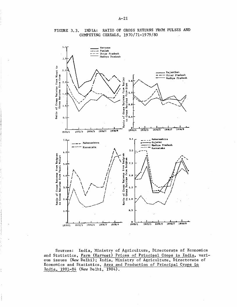
Because of nonavailability of data on net returns per hectare from pulses, a comparison is made between gross returns from pulses and competing cereals. Figure 3.3 Indicates that the ratio of gross returns per hectare from wheat relative to gram are higher in Punjab and Haryana than in Madhya Pradesh. In the former two states gram has been almost completely replaced by wheat in rabi. In Madhya Pradesh, however, it seems that gram Is profitably cultivated on unirrigated lands, since area under this crop is expanding in the state. It also appears that the ratio of gross returns from gram and redgram relative to coarse cereals like barley, millet and sorghum is such that these pulses are likely to find greater favor with farmers on unirrigated lands in the future.
Pulses were not competitive with high-yielding wheat and rice varieties on irrigated lands. But compared with coarse cereals in unirrigated conditions they appeared more profitable. So that area under gram shifted away from its native habitat in the Indo-Gangetic plain, as irrigation facilities increased there, into the rainfed regions of the central states like Rajasthan, and Madhya Pradesh.
Meanwhile in the mid-1970s technological breakthrough in pulses came in the form of development of short-duration varieties, especially of redgram, blackgram, and greengram. As a result the area under these pulses registered an appreciable increase in the last 10 years as can be seen from Figure 3.2.
Effect on Cost of Protein
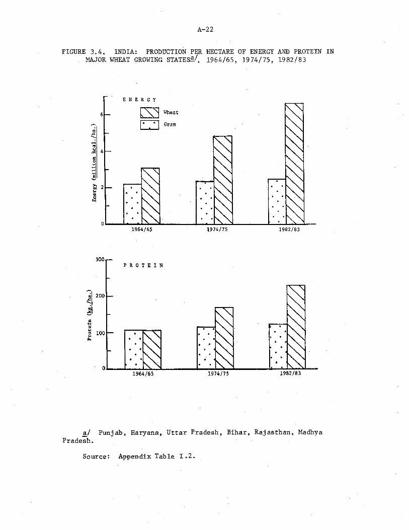
At yield levels obtaining in the mid-1960s, the production of energy from one hectare of wheat was only marginally greater than that from gram, as shown in Figure 3.4. However, by the mid-1970s, the production of energy per hectare from wheat increased appreciably, being more than double that from a hectare of gram. In the early 1980s, the energy contribution from wheat had increased further to almost three times that from a hectare of gram.
Protein production from a hectare of wheat and gram was almost equal in the mid-1960s. As a result of the spread of HYVs of wheat, protein production increased markedly. In the early 1980s the production of protein from a hectare of wheat was more than double that from gram. This shows that the net nutritional impact on the total production of calories and protein improved as a result of the Green Revolution [51] .
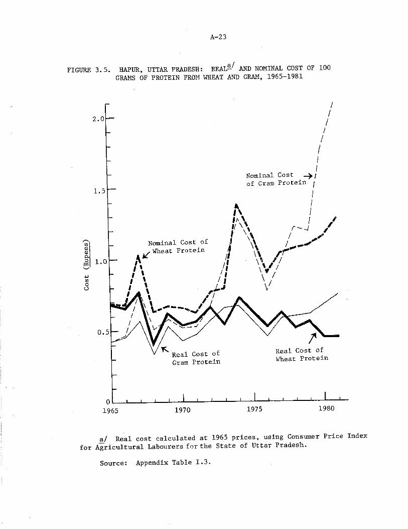
The increased yields had a favorable effect on the cost of protein. Figure 3.5 shows the real and nominal cost of 100 grams of protein during the last 15 years. The cost of protein was calculated from the wholesale prices of gram and wheat prevailing at Hapur Market
A-21
FIGURE 3.3. INDIA: RATIO OF GROSS RETURNS FROM PULSES ANDCOMPETING CEREALS* 1970/71-1979/80
Sources: India* Ministry of Agriculture* Directorate of Economicsand Statistics, Farm (Harvest) Prices of Principal Crops in India, vari ous issues (New Delhi); India, Ministry of Agriculture, Directorate of Economics and Statistics, Area and Production of Principal Crops in India, 1981-84 (New Delhi, 1984).
A-22
FIGURE 3.4. INDIA: PRODUCTION PER HECTARE OF ENERGY AND PROTEIN INMAJOR WHEAT GROWING STATE S§/, 1964/65, 1974/75, 1982/83
a_/ Punjab, Haryana, Uttar Pradesh, Bihar, Rajasthan, Madhya Pradesh.
Source: Appendix Table 1.2.
Cost
(Rupees)
A-23
FIGURE 3.5. HAPUR, UTTAR PRADESH: REAL— AND NOMINAL COST OF 100GRAMS OF PROTEIN FROM WHEAT AND GRAM, 1965-1981
a/ Real cost calculated at 1965 prices, using Consumer Price Index for Agricultural Labourers for the State of Uttar Pradesh.
Source: Appendix Table 1.3.
A- 24
in the State of Uttar Pradesh. Hapur Market was chosen on the basis of the assumption that the prices of pulses are most likely to be determined competitively here by the forces of supply and demand. Hapur Market is the largest market for agricultural produce in the State of Uttar Pradesh, which is the largest pulse producing state in the country.
In 1965 gram protein was cheapest at Rs 0.42 per 100 grams. However, in the early 1980s wheat protein claimed this distinction at Rs 0.44.
As a result of the Green Revolution and the spread of HYVs of wheat, it was possible for the real cost of protein in the early 1980s to remain at almost the same level as in the mid-1960s. This is one of the positive contributions of the Green Revolution.
Regional Trends in Pulse Production
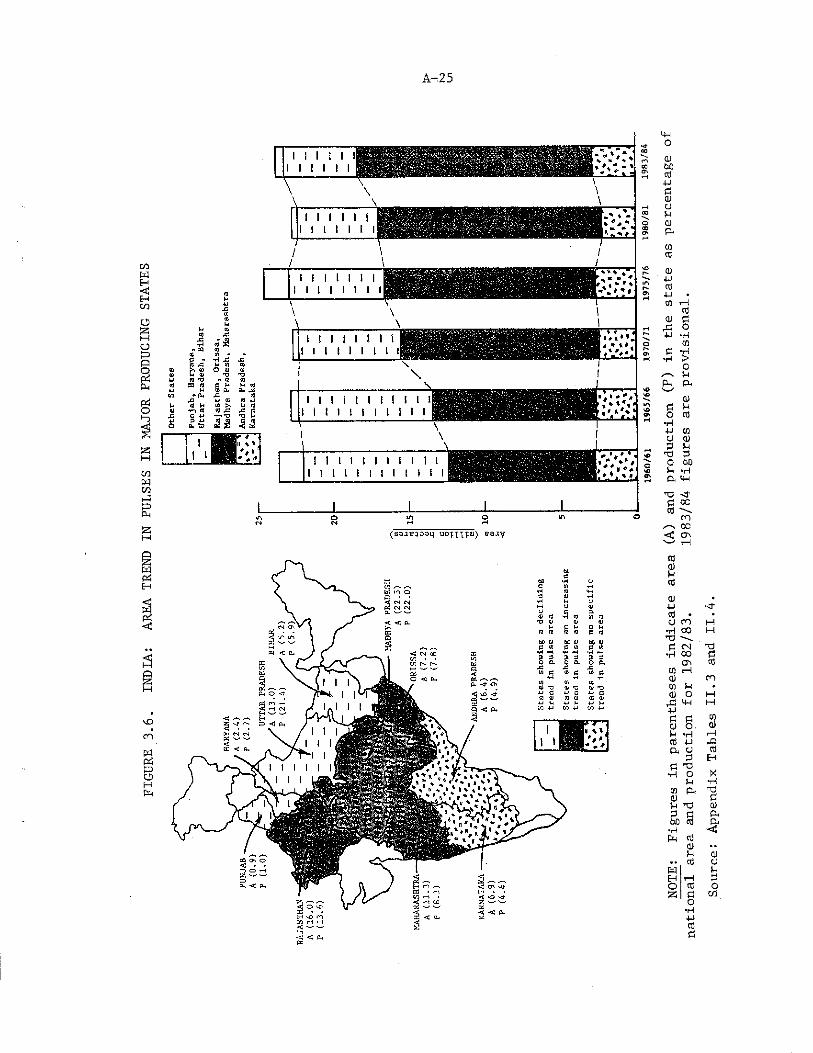
The major pulse producing states in India are shown in Figure 3.6. These 10 states together account for more than 90 percent of production and area under pulses.
The states of the Indo-Gangetic plain, comprising Punjab, Haryana, Uttar Pradesh and Bihar, which also constitute the wheat belt of the country, indicate a clear declining trend in area sown to pulses. The area in these states has declined from about 9.5 million hectares in the early 1960s to 5 million hectares in the early 1980s. In terms of national pulse area, the percentage share has fallen from about 40 percent to 20 percent.
As we have already seen in the preceding sections, at the national level there does not appear to be any discernible declining trend in pulse area. This Is most likely due to the fact that pulse area which was replaced in the Indo-Gangetic plain was gained by the Central Region, comprising states of Rajasthan, Madhya Pradesh, Maharashtra and Orissa. During the period under consideration, area under pulses in these states increased from 9.8 million to 13.3 million hectares, indicating an increase of 35 percent in terms of national pulse acreage.
The Southern Region, comprising states of Andhra Pradesh and Karnataka, did not display any clear trend in acreage, which remained almost constant during the period, accounting for a steady 12 percent of total pulse area [12] .
FIGU
RE 3
.6.
INDIA:
AREA
TRE
ND I
N PU
LSES
IN MA
JOR
PROD
UCIN
G ST
ATES
A-25
1960
/61
19
65/
66
1970
/71
19
75/
76
1980
/81
19
83/
84
NOTE:
Figu
res
in p
aren
thes
es i
ndic
ate
area
(A) a
nd p
rodu
ctio
n (P)
in t
he s
tate
as
perc
enta
ge o
fna
tion
al-a
rea
and
prod
ucti
on f
or 1
982/83.
1983
/84
figu
res
are
prov
isio
nal.
Source:
Appe
ndix
Tab
les
II.3 a
nd I
I.4.
A- 26
Seasonal Trends in Pulse Production
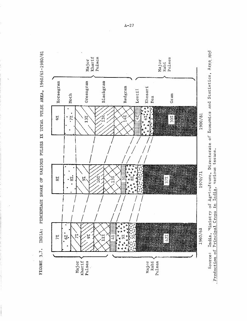
The maj or pulses are grown either in the rabi or kharif season. Gram , pea, Khesari and lentil constitute the maj or rabi pulses, while redgram, blackgram, greengram, horsegram and moth comprise the important kharif pulses. The percentage share of various pulses is shown in Figure 3.7 which indicates a declining trend at the national level in rabi pulses, and an increasing trend in kharif pulses. Pulses which show a declining trend are gram and pea which account for the trend in rabi pulses. On the other hand, almost all the kharif pulses point to an increasing area trend [12].
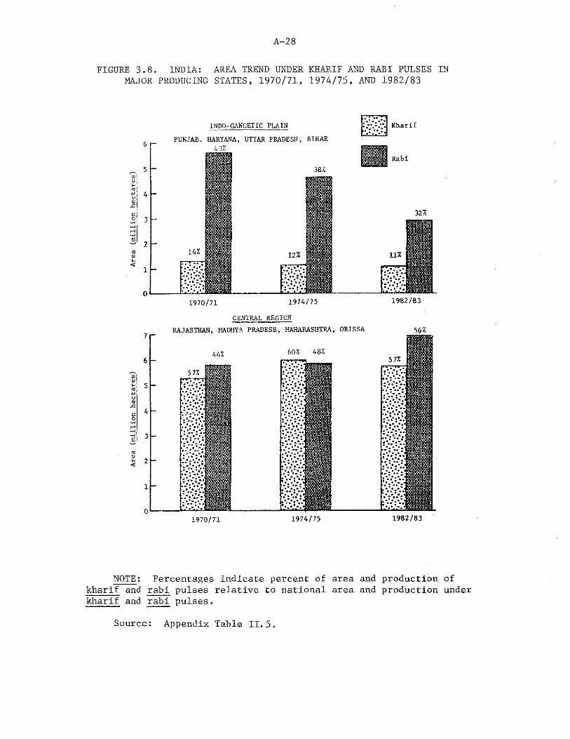
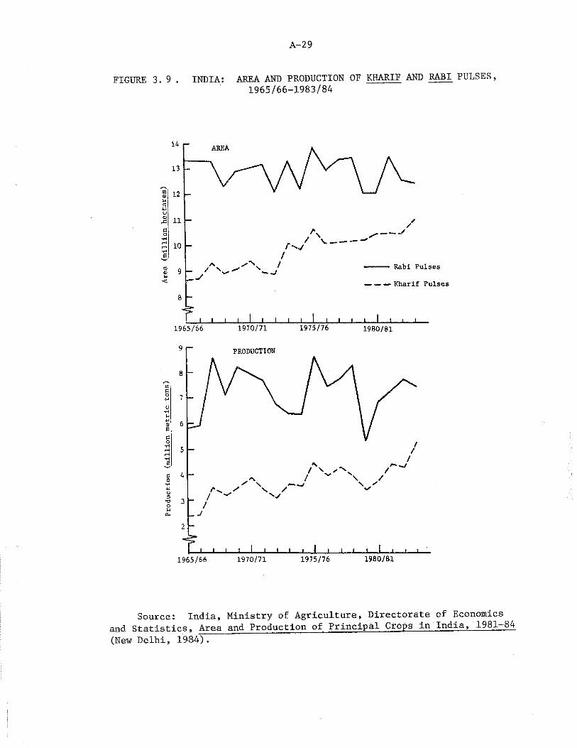
The trends are more visible if we look at kharif and rabi pulses in the two major pulse growing regions. The states of the Indo- Gangetic plain accounted for almost half the area under rabi pulses in the early 1970s, as shown in Figure 3.8. However, during the next 10 years, as a result of changes in cropping patterns and greater emphasis on cereals, this region began to lose its importance as the major rabi pulse producer. Within a decade the contribution of the Indo-Gangetic plain to the winter pulse area declined from half to less than a third. The central states, on the other hand, because of their dependence on rainfed agriculture had emerged as the main contributor towards kharif pulse area. Their share was more than four times that of the northern states. In the decade of the 1970s, however, in addition to maintaining their predominance in kharif pulse area, they displayed significant gains in rabi pulse area as well. It appears almost as though the area replaced in the Indo-Gangetic plain was compensated by a corresponding increase in the central region. No significant trend in rabi pulse area was reflected at the national level, as is evident from Figure 3.9. However, considerable annual fluctuations indicated the impact of changes in weather conditions. It is interesting to note that rabi pulse area recorded wider variations relative to kharif pulse area, and that rabi pulse production seems to be subject to greater variability than kharif pulses.
At the national level, kharif pulse area registered a small but perceptible increase. On closer examination it appears that the last 8 to 10 years have witnessed a more decisive change in area trend than the previous decade. This seems to be a logical outcome of the impact of improved and short-duration varieties of kharif pulses which have only recently begun to make their impact on the field.
It needs to be emphasized here that although the central states have now taken the lead in both rabi and kharif pulse area, the average productivity in the region leaves much to be desired. In the early 1980s the states of the Indo-Gangetic plain accounted for around 10 percent of kharif pulse area and more than 20 percent of total production. In the central states, on the other hand, production lagged behind, accounting for only 48 percent of the total despite a 57 percent share in acreage.
FIGU
RE 3
.7.
INDIA:
PERC
ENTA
GE S
HARE
OF
VARI
OUS
PULS
ES I
N TO
TAL
PULS
E AR
EA,
1960
/61-
1980
/81
A-27
b-l Pi *riO U •i-] Cdcd 3 S £4
C0Pi 0) O *H CD -r-i ,JQ iH Cd CtJ 3a pm
■ ____________./v________ AS 6 acd cd cdu Pi pi a ■H00 bO bO cd t—i Pta) S d*d pi ■H cdCO 4d QJ G bO 4-» COu 4-4 0) cd nd id Go 0 Pc tH 0) G JdPd a O PQ Pd hd
„/V ~\
&-S00
&-S00
/ / //
"FT"A -4 A * V fl ».76-1’**& 6-SCO 'J 00 *<d*•> %X-* A 4 *V .-2-sl
6-er.
/ / / I / / /
/ / /
/ / / /
or"-O'.
u *
v > T .’6-S . ' 6 ^<3 - <r Cb * lO
4 > * :•••;< ► 4 «► ; * i *
* *■1 - J U
Clcd
cd<upi<1COU•H4-1CO•H■Mcd4-1cn
-/ V-£•4 M—I CO O -H <U *1— 1 }-4 COcd cd ha 3 3W P-.
Prod
ucti
on o
f Pr
inci
pal
Crop
s in I
ndia
, va
riou
s
A-28
FIGURE 3.8. INDIA: AREA TREND UNDER KHARIF AND RABI PULSES INMAJOR PRODUCING STATES, 1970/71, 1974/75, AND 1982/83
7 r
6 -
2
IHDO-GANGETIC PLAINPUNJAB, HARYANA, UTTAR PRADESH, BIHAR
4 3%
: * ,”/J Kharif
1970/71 1974/75
CENTRAL REGIONRAJASTHAN, MADHYA PRADESH, MAHARASHTRA, ORISSA
44% 60% 48%
Rabi
1982/83
56%
1970/71 1974/75 1 9 82 /83
NOTE: Percentages indicate percent of area and production ofkharif and rabi pulses relative to national area and production under kharif and rabi pulses.
Source: Appendix Table II. 5.
A-29
FIGURE 3* 9 . INDIA: AREA AND PRODUCTION OF KHARIF AND RABI PULSES,1965/66-1983/84
Source: India, Ministry of Agriculture, Directorate of Economicsand Statistics, Area and Production of Principal Crops in India, 1981-84(New Delhi, 1984).
A- 30
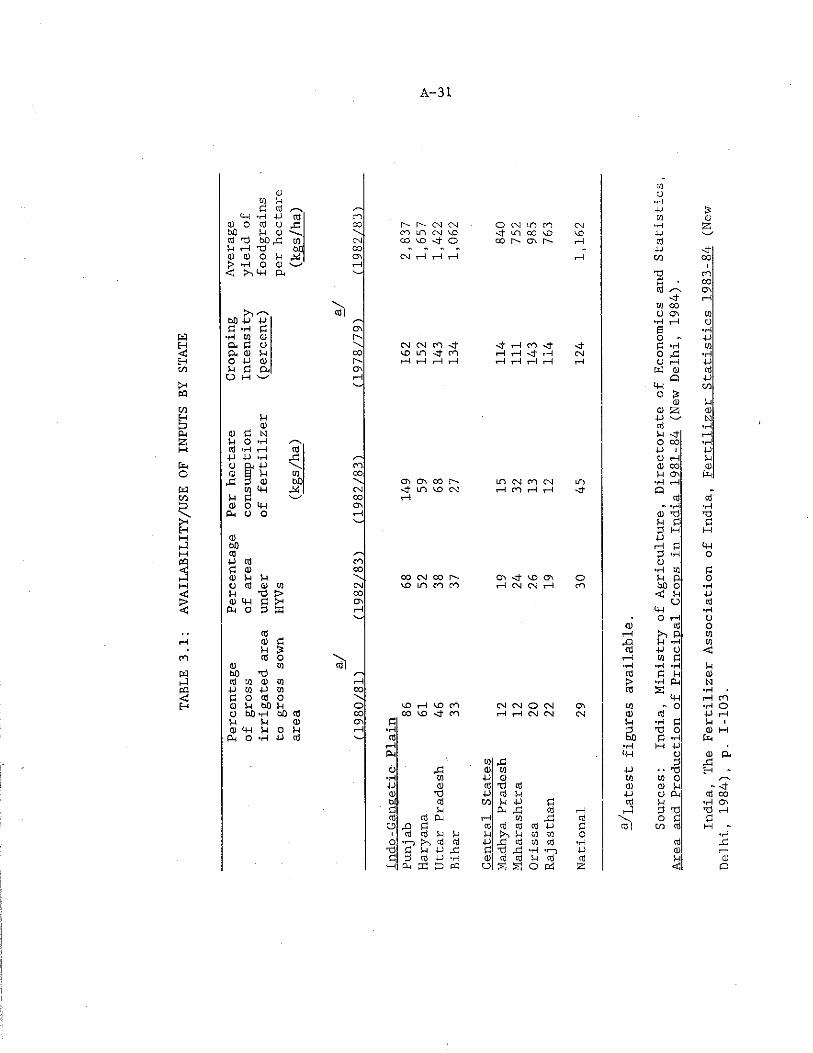
Use of Inputs and Area Trends
Irrigation is' one of the major inputs which has influenced cropping patterns over the last two decades. In fact there Is a positive correlation between increase In irrigated area, and the use of high-yielding varieties. Table 3.1 indicates that in states where the percentage of total Irrigated area to total cropped area is high, the use of HYVs and the consumption of fertilizer is greater. In states like Punjab, Haryana and Uttar Pradesh the cropping intensity is also higher relative to the central states.
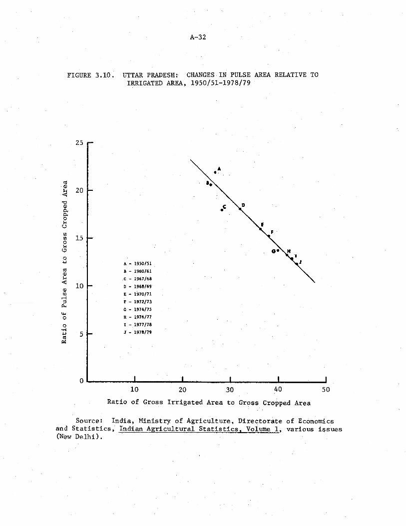
Figure 3.10 demonstrates, in the case of Uttar Pradesh, that as percentage of irrigated area increased the share of pulse area correspondingly declined. The relationship between increase in irrigated area and replacement of pulse acreage by HYV cereals is very significant [12] .
Since more than 70 percent of area cultivated in India is still rainfed, the major portion of pulse production in the future will continue to come from unirrigated areas. However, with the introduction of short-duration varieties, which can be cultivated as catch crops between the two major seasons, and with assured irrigation facilities, there will be a significant increase in pulse area in regions where short-duration varieties can be fitted into cropping patterns. This will be discussed in greater detail in later chapters.
TABL
E 3.1:
AVAI
LABI
LITY
/USE
OF
INPU
TS B
Y ST
ATE
A-31
gVi uP g t—V ,—,
4-f *1—[ P g cOCD o G o & 00bO p 01G Xi bO £ w CMP iH x> to COCD 0 o p ,21 CTl> *H o 01 *■—' rH
< 4H Pi '_
>1 '"v G iMW DP *H P OV
>H to Q r->Pi P O \Pi G P COO W d ) r~-P P Pi CT\U M i—1
'—■
PG
G P NP O *HG *H rH GP P *H ( P0 Pi P COG 0 P CO 0 0p 3 a) bO "•V
w 4H X CMP p 0 0G 0 4-1 D\PM O O i—HiGbOG /—VP G oOP G COG P P \O G 0 w CMP X) > 0 0G 4-1 P P-1 a v
Pm o P K iH
GCDP 3G O \
G w P IbO x ) /—■G to G m i—iP w P VI 00P o G 0 \G p bO P oO bO •H bO G COP p G cvG 4-1 p 0 P 1—1
Pm O P G
f1
i- r CM CM O CM m cO CM *T—1CO to CM VO Mt m 0 0 VO VO PCO VO Wt O CO i-'- C\ P- rH G- - - - - P <}■CvJ i—4 r—1 i—1 iH CO 0 0
X)1
COp ■ OOG '"M Ov
-G" iHM 0 0O ov VI
•H rH o0 •Ho - PCM CM CO M* -G i—i CO G- G P *H VI
VO in Mt CO 1—1 i—i <d- rH CM O ,P *HrH i—i i—1 t-l i-4 iH i-4 iH tH O rH P
W G GQ P
4H CO0 >
G pG G4 J w NG *HP <± rHO CO •HP i PO iH PG 0 0 GP Oi Pm
Ov C7\ 0 0 f"- m CM CO CM m *H iHp- in VO CM t—i CO rH rH Mt QrH G G
- ‘ H *HG X i XJH P PP M HP
i—i p 4-4P *H 0O
*H W P0 0 CM 0 0 r-" crv Mt VD CT\ o P P 0VO m cO CO i—t CM CM i—4 CO bO O •H
<d p Pu G
4H •HO rH a
CD oi—( fn P taP I P *H V)G P 0 <i— i w p•iH •H *H PG P P G> •h Pm NG a •H
4H r-4VD i—i VO CO CM CM O CM O ' to - O *H0 0 VO Mt CO p H 1—1 CM CM CM G G P
P •H P PP X 3 O GbO P -H P m
'r-4 IH P4-4 C G
w rP P .PA G M P> . . x !
M P G U1 W 0G G X ) G CD G P
x ) P G p P G P m a jG CO P p P G PP P m rP G I—1 PI P xJ
td Pm pH CO P ! G o p p,n P G G G P P G | co G HG G P P p P ffl VI 0
if— P n cd td p ,P G M G *H GP P p iP P X J ,P 'H *f—3 P GP G p l!“1 G G G P G G P
PM K P3 c q U s O Pd S <
coO
Pi
■G-COCl
*1—1,pi—!
CDa
A-32
FIGURE 3.10. UTTAR PRADESH: CHANGES IN PULSE AREA RELATIVE TOIRRIGATED AREA, 1950/51-1978/79
25
20
0P.&Ouu« 15ouoo•u
CO<0u< 10)w
10
oP-i
4-1oo■H4-1CtipcS
5
A - 1950/51
B - 1960/61
C - 1967/68
D - 1968/69
E - 1970/71
F - 1972/73
G - 1974/75
H - 1976/77
I - 1977/78
J - 1978/79
0 ------------1-------* -- 1...-..... .1______________L I10 20 30 40 50
Ratio of Gross Irrigated Area to Gross Cropped Area
Source: India, Ministry of Agriculture, Directorate of Economicsand Statistics, Indian Agricultural Statistics, Volume 1, various issues (New Delhi).
CHAPTER IVCONSEQUENCES OF REDUCED PULSE AVAILABILITY ON THE DIET
It was seen in the last chapter that as a consequence of the Green Revolution a significant area under rahi pulses shifted to wheat. This resulted in an overall reduction of per capita availability of pulses. In this chapter we examine the effects of reduced pulse availability on the quantity and quality of protein in the diet. The current per capita protein availability is compared to the Recommended Dietary Allowanc e (RDA.) to give an idea of the nutr i t ional s tatus o f the population. Similarly, the existing cereal-pulse protein ratio in the diet is measured against optimum values to determine the quality of protein.
The average Indian diet consists of a cereal staple, e.g., rice, wheat, sorghum or millets, together with a small amount of pulses and vegetables. Irrespective of the nature of the cereal, such a diet can meet the protein needs of the individual, provided sufficient quantity is consumed to satisfy energy requirements [64].
Quantity of Protein
Recommended Dietary Allowances (RDAs)
Individual food needs are determined by age, sex, body composition, level of activity, climate and state of health. RDAs serve as guideposts only for groups of people and are not meant to establish precise individual requirements for which they are often mistakenly used.
The recommended allowances for both energy and protein have been periodically modified. The trend of modification suggests that the recommended intakes have been overstated in the past [49] • The RDAs have consciously erred on the side of caution, both to incorporate a comfortable safety margin and to ensure that substantial variations in food needs among individuals will be covered. They are therefore not to be taken as minimum needs.
FAQ RDAs for Energy
The energy requirement is defined by the FAO/WHO Joint Ad Hoc Expert Committee on Energy and Protein Requirements (1971) as "the energy intake that is considered adequate to meet the energy needs of the average healthy person in a specified age/sex category" [20, p. 10] . The energy requirement is conventionally estimated on the basis of an arbitrarily defined "Reference Man and Woman," and depends largely on four interdependent variables: 1) physical activity,2) body size and composition, 3) age, and 4) climate and other
A- 33
A-34
ecological factors. Therefore adjustments in energy requirements need to be made for differences in these variables. Additional energy is needed for growth in childhood and adolescence as well as among women during pregnancy and lactation [20, p. 22],
The energy requirement varies significantly between activities. A classification of activities into light, moderate, very active and exceptionally active has been proposed simply as a guide by the committee, and in the absence of better information the adult population has been assumed to be, on average, moderately active.
The average energy requirement for a reference man of body weight 65 kilograms engaged in light activity is around 2700 kilocalories per day, whereas for exceptionally active work, it can be as high as 4000 kilocalories. Energy requirement is also a function of body weight. For an average male in light activity with a body weight of 50 kilograms, the per day energy requirement is only 2100 kilocalories, which increases to 3360 kilocalories for someone with body weight of 80 kilograms [20, p. 31].
For obvious reasons these recommendations are only broad approximations. A great deal more needs to be learnt about body metabolisms before accurate predictions can be made about energy requirements, and why some people can live on half the calories consumed by others and yet remain perfectly efficient. This again demonstrates that the RDAs include a considerable safety margin.
FAQ RDAs for Protein
The FAO/WHO Joint Ad Hoc Expert Committee (1971) has defined the safe level of protein intake" as "the amount of protein considered
necessary to meet the physiological needs and maintain the health of nearly all persons in a specified group." This level is the "safe level" and therefore higher than the average minimum requirement for protein.
Protein RDAs are a function of daily nitrogen loss, protein quality of the diet, age and sex. They have been estimated periodically by expert committees of the FAO. The early studies of the FAO indicated concern with malnutrition and insufficient protein availability. The recommendation of the FAO/WHO Joint-Expert Group (1963) for daily protein intake was 0.71 grams per kilogram of body weight and included a safety factor of 20 percent to cover the needs of members of population with higher than average requirements. For the reference man of body weight 65 kilograms this amounted to 46 grams of reference protein.
With increased research and knowledge in the field of nutrition, perceptions about malnutrition and protein requirements underwent
A- 35
considerable change. No longer was protein deficiency treated in isolation, but was considered as part of a larger problem of protein- energy malnutrition. It was emphasized that when a diet is deficient in calories, the apparent adequate protein in the diet is partly diverted from its primary function to the provision of energy.
The FAO/WHO Ad Hoc Expert Committee (1971) stressed this interrelationship between energy and protein, stating that "adequacy of energy intakes must receive first consideration, so that any additional protein supplied to meet the estimated protein needs will be efficiently utilized for this purpose" [20, p. 19],
The same committee found that the protein requirements determined by the 1963 Expert Group had been incorrectly assessed on two accounts. Firstly, the estimated nitrogen losses on which the protein needs were based had been overestimated by the previous committee and, secondly, the biological variation in nitrogen requirements assessed at 20 percent was found to be an underestimation.
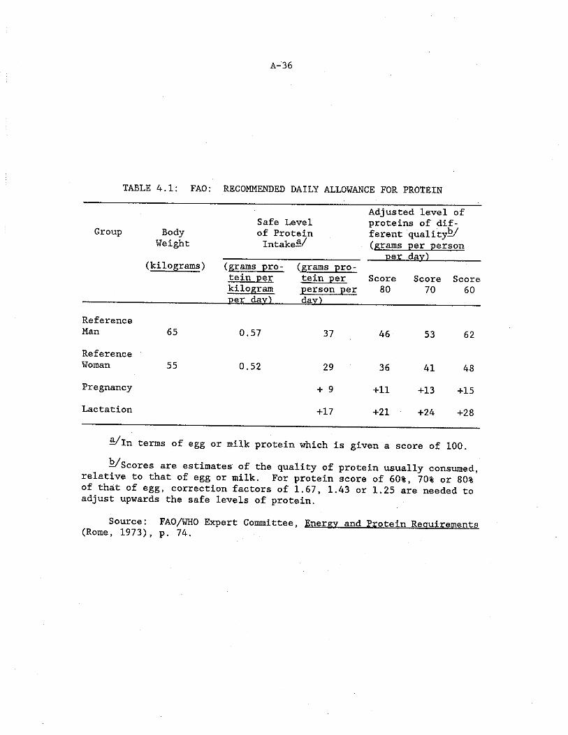
The 1971 expert panel consequently revised the estimates for protein intake, reducing the daily per capita recommendation for adults by almost a third: from 0.71 grams per kilogram of body weight to 0.57 grams for a man and 0.52 grams for a woman, that is, a daily intake of 37 grams for the reference man and 29 grams for the reference woman. The figures of 37 grams and 29 grams included a safety margin of 30 percent to account for individual variability. This is seen in Table 4.1.
RDAs for Energy and Protein in India
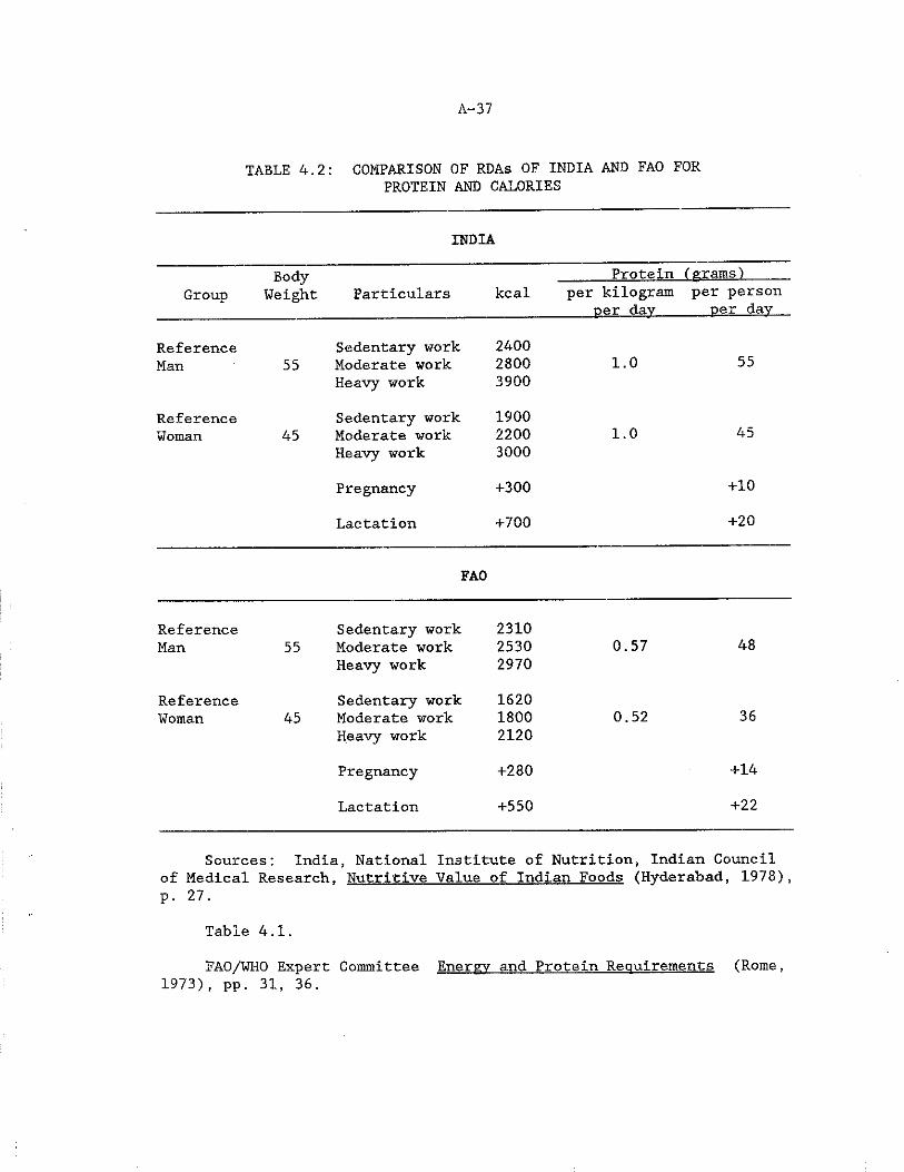
The RDA was first formulated in 1944 by the Nutrition Advisory Committee of the Indian Research Fund Association, now Indian Council of Medical Research. With increased information available on the subject, the recommendations for proteins and calories were revised in 1958 and 1968. The latest recommendations for the reference man weighing 55 kilograms and reference woman weighing 45 kilograms are shown in Table 4.2.
The allowance for protein recommended by the Nutrition Expert group of Indian Council of Medical Research for both reference man and woman is about one gram per kilogram of body weight per day and it is assumed that the dietary protein is derived from a mixture of vegetable foods [23, p. 27], This works out to 55 grams and 45 grams per day for reference man and woman respectively.
Calculated on the basis of FAO standards, the requirements of protein corresponding to safe level intake are 31 grams and 23 grams per day in terms of the ideal protein having a protein score of 100. However the average Indian diet has a protein quality much below ideal.
A-3 6
TABLE 4.1: FAO: RECOMMENDED DAILY ALLOWANCE FOR PROTEIN
Group BodyWeight
(kilograms)
Safe Level of Protein Intake-/
Adjusted level of proteins of different quality^/ (grams per person
Der dav)(grams pro- tein per kilogram ner dav)
(grams pro- tein per person per dav)
Score80
Score70
Score60
ReferenceMan 65 0.57 37 46 53 62ReferenceWoman 55 0.52 29 36 41 48Pregnancy + 9 +11 +13 +15Lactation +17 +21 +24 +28
-/in terms of egg or milk protein which is given a score of 100.
^/Scores are estimates of the quality of protein usually consumed, relative to that of egg or milk. For protein score of 60%, 70% or 80% of that of egg, correction factors of 1.67, 1.43 or 1.25 are needed to adjust upwards the safe levels of protein.
Source: FAO/WHO Expert Committee, Energy and Protein Requirements(Rome, 1973), p. 74.
A-37
TABLE 4.2: COMPARISON OF RDAs OF INDIA AND FAO FORPROTEIN AND CALORIES
INDIA
GroupBody
Weight Particulars kcalProtein (grams)
per kilogram oer dav
per person oer day
Reference Sedentary work 2400Man 55 Moderate work 2800 1.0 55
Heavy work 3900
Reference Sedentary work 1900Woman 45 Moderate work 2200 1.0 45
Heavy work 3000
Pregnancy +300 +10
Lactation +700 +20
FAO
Reference Sedentary work 2310Man 55 Moderate work 2530 0.57 48
Heavy work 2970
Reference Sedentary work 1620Woman 45 Moderate work 1800 0.52 36
Heavy work 2120
Pregnancy +280 +14
Lactation +550 +22
Sources: India, National Institute of Nutrition, Indian Councilof Medical Research, Nutritive Value of Indian Foods (Hyderabad, 1978), p. 27.
Table 4.1.
FAO/WHO Expert Committee Energy and Protein Requirements (Rome, 1973), pp. 31, 36.
A- 38
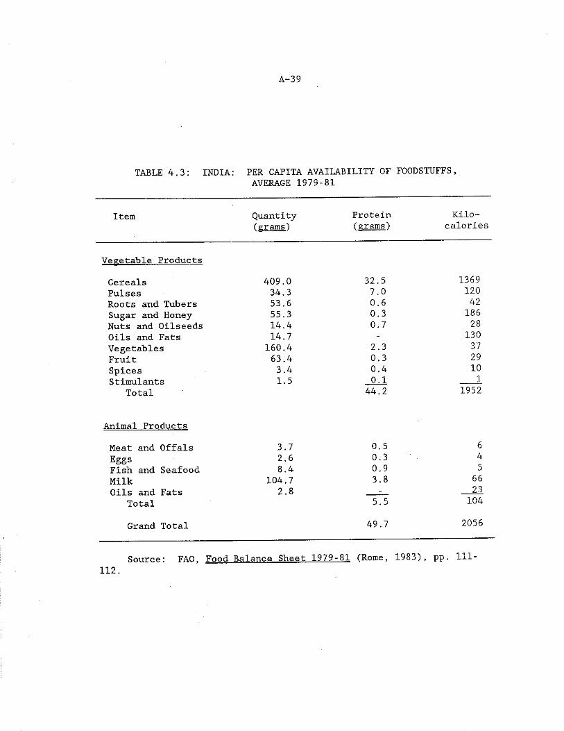
In the early 1980s the average per capita daily availability of foodstuffs, and their contribution to protein supply is shown in Table4.3. The protein .quality of single foods and food mixtures, together with various classifications for measuring protein quality, are discussed in detail later in the section on "Quality of Protein." At this point it is sufficient to say that the protein score of a diet such as the one shown in Table 4.3 is about 65 percent.
To allow for this lower protein quality the recommended allowances for protein intake, based on FAO standards, are adjusted upward by a factor of 1.54. As a result the RDAs for protein for Indian reference man and woman in moderate activity are estimated at 48 grams and 36 grams per day, respectively.
Comparison of FAO and Indian Standa-rHs
The comparison of the Indian and FAO standards is shown in Table 4.2. It can be seen that the Indian RDAs are about 15 percent higher for the reference man and 25 percent higher for the woman In the case of protein. For energy the Indian standard is about 10 percent higher for the reference man and 20 percent higher for the reference woman.
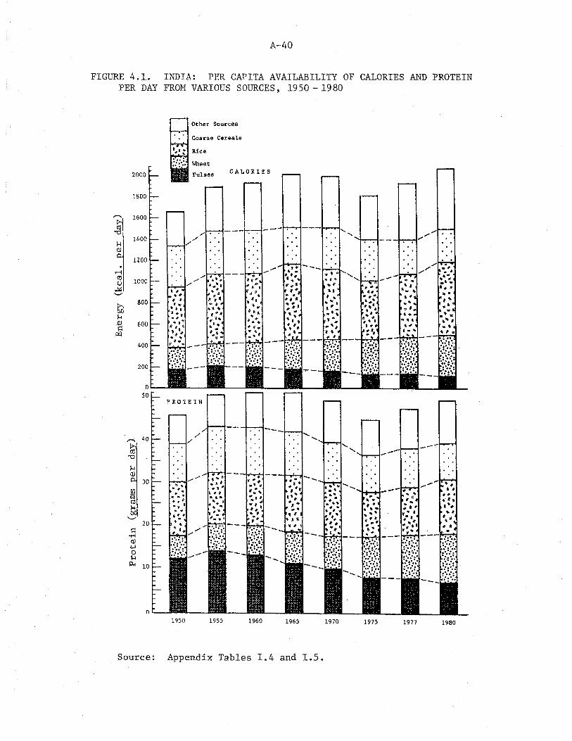
Per Capita Calorie Availability
Figure 4.1 indicates daily per capita availability of protein and calories and changes in the sources of supply over the last three decades. Foodgrains are the major source of both protein and energy in the average diet. They account for almost 85 percent of protein and 75 to 80 percent of energy intake.
Rice accounted for about 50 percent of total calories available from cereals in the early 1950s. This figure has remained almost constant. The share of calories from coarse grains like sorghum and millets fell from about 30 percent in the 1950s to 22 percent in the late 1970s. Percentage of calories from wheat increased from 17 percent in the early 1950s to 19 percent in the mid-1960s and more sharply after that to 28 percent in the 1980s.
The overall per capita energy availability over the last 30 years has fluctuated around 1900-2000 kilocalories, except during years of abnormal weather conditions. In terms of recommended allowances the per capita availability of energy was about 82 percent of the Indian RDA and 95 percent of FAO standards for adults engaged in moderate activity.
Per Capita Protein Availability
The per capita protein availability as shown in Figure 4.1, indicates that although supply sources have changed, the overall
A~39
TABLE 4.3: INDIA: PER CAPITA AVAILABILITY OF FOODSTUFFS,AVERAGE 1979-81
Item Quantity (grams)
Protein(grams)
Kilocalories
Vegetable Products
Cereals 409.0 32.5 1369Pulses 34.3 7.0 120Roots and Tubers 53.6 0.6 42Sugar and Honey 55.3 0.3 186Nuts and Oilseeds 14.4 0.7 28Oils and Fats 14.7 - 130Vegetables 160.4 2.3 37Fruit 63.4 0.3 29Spices 3.4 0.4 10Stimulants 1.5 0.1 1
Total 44,2 1952
Animal Products
Meat and Offals 3.7 0.5 6Eggs 2.6 0.3 4Fish and Seafood 8.4 0.9 5Milk 104.7 3.8 66Oils and Fats 2.8 - 23
Total 5.5 104
Grand Total 49.7 2056
Source: FAO, Food Balance Sheet 1979-81 (Rome, 1983), pp, 111-112.
A-40
FIGURE 4 PER
1. INDIA: PER CAPITA AVAILABILITY OFDAY FROM VARIOUS SOURCES, 1950 - 1980
CALORIES AND PROTEIN
1950 1 9 5 5 1960 1965 1970 1975 1977 1980
Source Appendix Tables 1.4 and 1.5
A- 41
protein level has remained almost constant at about 50 grams per capita per day. At 50 grams per capita per day the protein supply is well over the FAO recommendation. Even in terms of the Indian RDA, which includes a margin of safety over and above that of FAO standards, the protein availabilities do not appear inadequate.
This must, however, be read with the caveat that the data being considered here are average availabilities, determined from food balance sheets, and do not reflect food distribution between income groups or within households. , ■■ f,s .... .
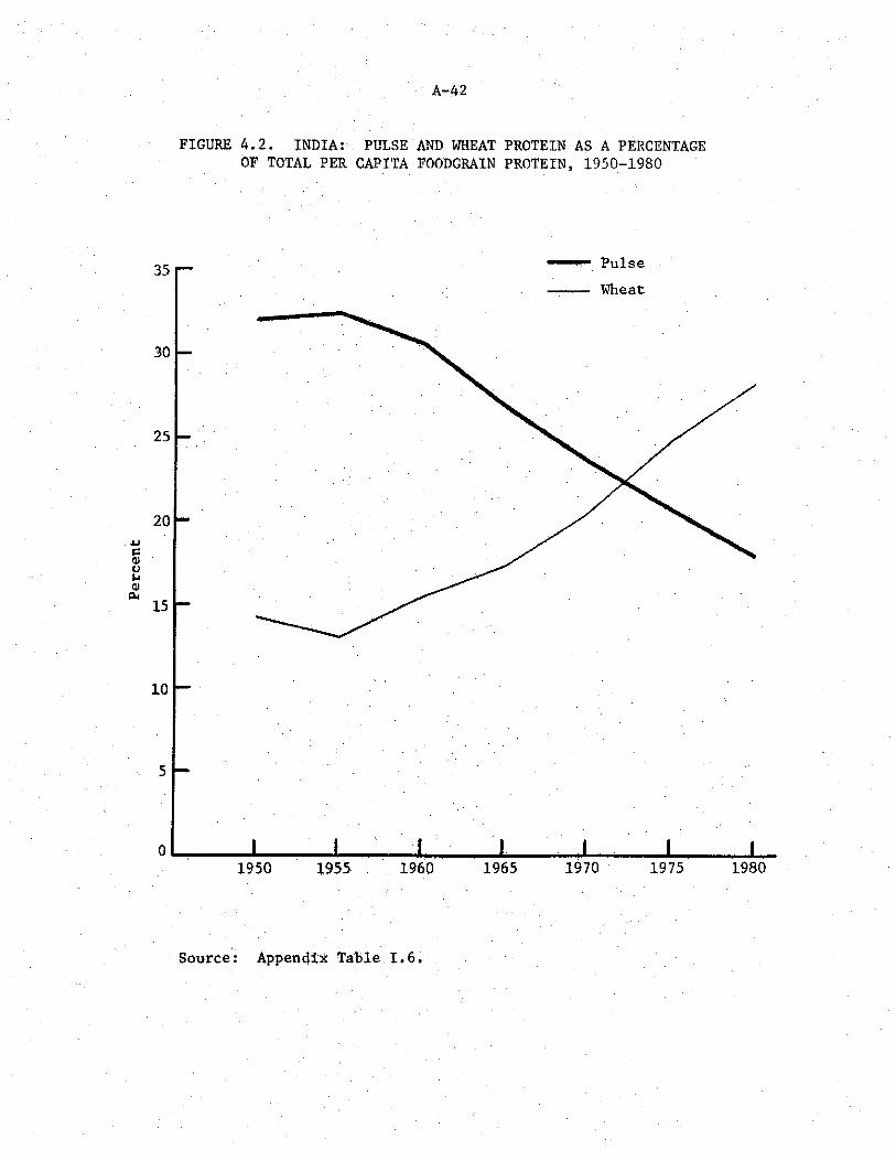
Figure 4.2 indicates that in the early 1950s pulses were one of the major sources of protein and accounted for over 32 percent of total protein supplied by all foodgrains. This declined to 26 percent in the mid-1960s and fell to an all time low of 18 percent in the early 1980s. During the same period, wheat protein was on the increase. The trend accelerated after the mid-1960s due to the Green Revolution. The protein gap created by reduced pulse availability was compensated by a corresponding increase in wheat protein, which rose from 15 percent to 28 percent. Changes in the share of rice and coarse cereal protein were not as marked as in the case of pulses and wheat, and overall the per capita availability of protein remained almost constant at about 50 grams per day. On the other hand the advantage of enhanced wheat production was an overall increase in the supply of energy as well.
As has been noted earlier, calories are generally the first limiting nutrient in the diet. With Increased wheat availability, this constraint was relaxed, enabling the protein being presently consumed to be utilized more fully and effectively.
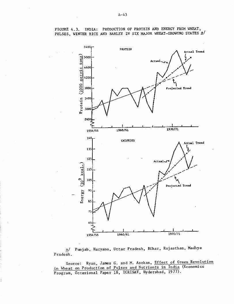
To measure the impact of the high-yielding varieties of wheat on nutrient availability, a study was conducted by Ryan and Asokan [51] based upon data from six major wheat producing states, Punjab, Haryana, Uttar Pradesh, Bihar, Madhya Pradesh and Rajasthan. A distinction was made between the pre- and post-Green Revolution period of the mid- 1960s. Figure 4.3 shows separate linear trend lines fitted to the combined nutrient production figures of all major crops in the six states for these two periods. The pre-Green Revolution lines were projected to indicate the situation if no HYVs of wheat had existed. On comparison of projected trend lines yith the actual existing situation, it was found that for both calories and protein, the actual trends were significantly higher than that which would have been produced had the Green Revolution not occurred. In fact in the absence of high-yielding wheat varieties, there would have been a reduction of 10 percent in the annual production of total protein and of 13.5 percent of total calories.
A-42
FIGURE 4.2. INDIA; PULSE AND WHEAT PROTEIN AS A PERCENTAGE OF TOTAL PER CAPITA FOODGRAIN PROTEIN, 1950-1980
Source: Appendix Table 1.6.
A-43
FIGURE 4.3. INDIA: PRODUCTION OF PROTEIN AND ENERGY FROM WHEAT,PULSES, WINTER RICE AND BARLEY IN SIX MAJOR WHEAT-GROWING STATES
a/ Punjab, Haryana, Uttar Pradesh, Bihar, Rajasthan, Madhya Pradesh.
Source: Ryan, James G. and M. Asokan, Effect of Green_Revolutionin Wheat on Production of Pulses and Nutrients in India (Economics Program, Occasional Paper 18, ICRISAT, Hyderabad, 1977).
A- 44
Quality of Protein
We have seen in the previous section that reduced pulse availability has not led to any significant reduction in the quantity of protein in the diet. The only change that has occurred has been the increasing substitution of pulse protein by cereal protein, mainly wheat. Does this in any way alter the quality of protein in the diet, and to what extent? To examine these issues, we first need to look at what is meant by quality of protein, and how it can be measured.
Composition of Proteins
Proteins themselves are a distinct group of compounds. They are composed of carbon, oxygen, hydrogen, nitrogen and some sulphur. The structure of a protein can be described as being a relatively long chain composed of identifiable links called amino acids. The term amino acid is a descriptive chemical name indicating the presence of a nitrogen containing functional group (amino) and a carboxylic acid functional group in each amino acid. There are believed to be 25 different amino acids that link together in innumerable combinations to form the proteins.
Amino acids are classified into groups as being essential or non- essential , The classification "nonessential'* simply indicates those amino acids which can be synthesized in sufficient quantities by the species in question, so that none needs be consumed. Essential amino acids are those which must be present in food, because the body is unable to synthesize them. Adult man requires eight essential amino acids [20, p. 53]. Table 4.4 shows the amino acid content of various foods.
Quality of protein is determined by the composition of its amino acid content and its digestibility. Various classifications have been arranged to measure a protein's quality or value. All are based on animal feeding experiments that evaluate a protein in terms of its capacity to support growth. Early it was learnt that whole egg protein ranked above all other proteins in quality. This is true because egg protein is highly digestible and its essential amino acid pattern most closely resembles the essential amino acid content of human protein. Therefore most classifications are arranged to compare all other proteins to egg protein.
Classifications for Comparing Protein Quality
Various classifications for comparing protein quality are shown in Table 4.5.
Biological Value (BV) of a protein represents the percentage of utilizable nitrogen in protein syntheses, and is expressed as:
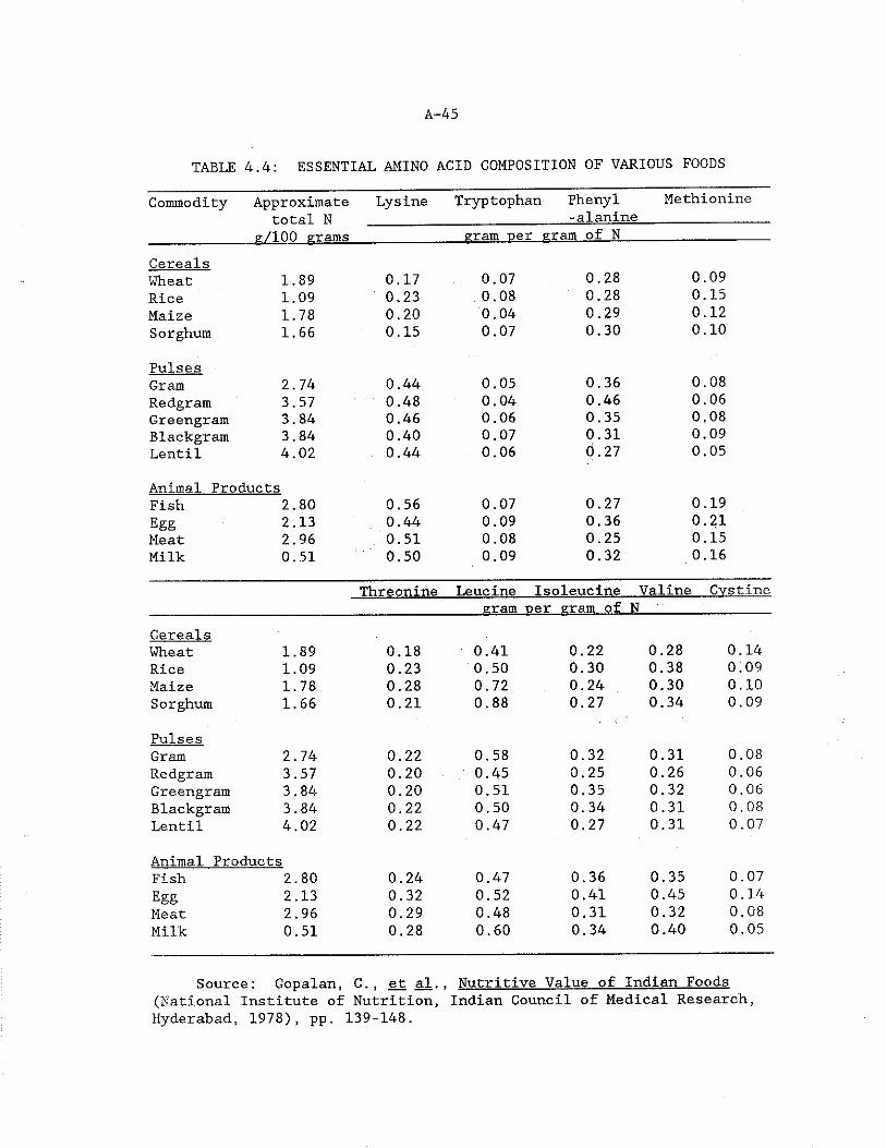
A-4 5
TABLE 4.4: ESSENTIAL AMINO ACID COMPOSITION OF VARIOUS FOODS
Commodity Approximate Lysine Tryptophan Phenyl Methioninetotal N -alanine
c/100 crams cram ner cram of NCerealsWheat 1.89 0.17 0.07 0.28 0.09Rice 1.09 0.23 0.08 0.28 0.15Maize 1.78 0.20 0.04 0.29 0.12Sorghum 1.66 0.15 0.07 0.30 0.10
PulsesGram 2.74 0.44 0.05 0.36 0.08Redgram 3.57 0.48 0.04 0.46 0.06Greengram 3.84 0.46 0.06 0.35 0,08Blackgram 3.84 0.40 0.07 0.31 0.09Lentil 4.02 0.44 0.06 0.27 0.05
Animal ProductsFish 2.80 0.56 0.07 0.27 0.19Egg 2.13 0.44 0.09 0.36 0.21Meat 2.96 0.51 0.08 0.25 0.15Milk 0.51 0.50 0.09 0.32 0.16
Threonine Leucine Isoleucine Valine Cvstinecram oer cram of N
CerealsWheat 1.89 0.18 0.41 0.22 0.28 0.14Rice 1.09 0.23 0.50 0.30 0.38 0.09Maize 1.78 0.28 0.72 0.24 0.30 0.10Sorghum 1.66 0.21 0.88 0.27 0.34 0.09
PulsesGram 2.74 0.22 0.58 0.32 0.31 0.08Redgram 3.57 0.20 0.45 0.25 0.26 0.06Greengram 3.84 0.20 0.51 0.35 0.32 0.06Blackgram 3.84 0.22 0.50 0.34 0.31 0.08Lentil 4.02 0.22 0.47 0.27 0.31 0.07
Animal ProductsFish 2.80 0.24 0.47 0.36 0.35 0.07Egg 2.13 0.32 0.52 0.41 0.45 0.14Meat 2.96 0.29 0.48 0.31 0.32 0.08Milk 0.51 0.28 0.60 0.34 0.40 0,05
Source: Gopalan, C. , et al. , Nutritive Value of Indian Foods(National Institute of Nutrition, Indian Council of Medical Research, Hyderabad, 1978), pp. 139-148.
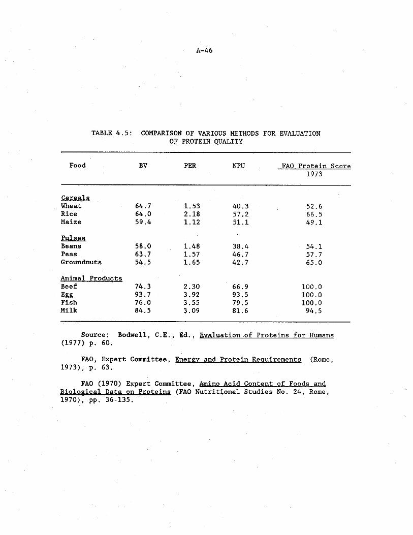
A-46
TABLE 4.5: COMPARISON OF VARIOUS METHODS FOR EVALUATIONOF PROTEIN QUALITY
Food BV PER NPU FAO Protein Score 1973
CerealsWheat 64.7 1.53 40.3 52.6Rice 64.0 2.18 57.2 66.5Maize 59.4 1.12 51.1 49.1
PulsesBeans 58.0 1.48 38.4 54.1Peas 63.7 1.57 46.7 57.7Groundnuts 54.5 1.65 42.7 65.0
Animal ProductsBeef 74.3 2.30 66.9 100.0Egg 93.7 3.92 93.5 100.0Fish 76.0 3.55 79.5 100.0Milk 84.5 3.09 81.6 94.5
Source: Bodwell, C.E., Ed., Evaluation of Proteins for Humans(1977) p. 60.
FAO, Expert Committee, Energy and Protein Requirements (Rome,1973), p. 63.
FAO (1970) Expert Committee, Amino Acid Content of Foods and Biological Data on Proteins (FAO Nutritional Studies No. 24, Rome,1970), pp. 36-135.
BV = Retained H in„ [1, p. 72],Absorbed N X
Retention of nitrogen expressed as a percentage of the nitrogen in the test diet gives Net Protein Utilization (NPU). NPU ■= nitrogen absorbed X Biological Value of the protein [1 p. 72].
Protein Efficiency Ratio (PER) is based on the increase in weight of young animals. PERs vary from 0 to 4. Most studies report PER values for legume proteins between 0.5 and 1.5, with the exceptional case of soybean, which is between 1.5 and 2.5. The range for cereal proteins varies between 1.0 to 2.0, while that for meat and egg proteins from 2.5 to 3.5 [1, p. 72]. The value of a protein depends upon the composition of its essential amino acids. The absence of a single essential amino acid reduces the Biological Value of a protein to zero.
The Protein Score is the percentage of the limiting amino acid in the protein set against the percentage in the ideal protein pattern as proposed by the FAO Committee on Protein Requirements [1, p. 73].
We observe from all four classifications that the protein values of legumes come somewhat low down in the scale. This is because legumes are limiting in sulphur containing amino acids, methionine and cystine. On the other hand, as can be seen from Table 4.4, they are rich sources of the amino acid lysine, which is limiting in most cereals.
It is necessary to emphasize here that pulses are generally not consumed as single foods, but in combination with cereals. So that it is not the value of pulse protein by itself, but in combination with cereal protein that is of nutritional importance.
A- 47
Legume Proteins in Food Mixtures
Pulse proteins supplement cereal proteins because they have a high lysine content and cereals are deficient in lysine. In the same way cereal proteins compensate pulse protein for low levels of sulphur- containing amino acids, methionine and cystine. A pulse and cereal food mixture leads to a higher quality of resultant protein.
Based on the FAO/WHO Report (1971) , Beaton and Swiss [4] have distinguished between three categories of diets: 1) diets rich in animal foods with a Protein Score of 80 percent relative to milk or egg protein, 2) mixed cereal legume diets, perhaps with small amounts of animal protein, with a Protein Score of 70 percent, and 3) cereal diets, with few other sources of protein, equivalent to a score of 60 percent.
A- 48
Optimum Combination of Cereal-Legume Proteins
There are certain proportions of cereal-legume mixtures that maximize the value of combined protein. Figure 4.4 shows the various combinations of maize and beans as well as rice and beans that lead to an optimum value of PER. A mixture of the two components leads to protein quality higher than that of the individual component [8., pp. 27-28].
The results in Figure 4.4 indicate that the maximum protein value is obtained when 50 percent of protein in the diet is derived from legumes and 50 percent from cereals, if the cereal is maize. In the case of rice and legume mixtures the maximum value is obtained when 80 percent of protein comes from rice and 20 percent from beans. Wheat combines in a 73 to 27 percent protein ratio with beans to give the maximum value of protein, which causes an increase in quality of about 50 percent [2, p . 31].
These results suggest the following inferences:
1) The quality of cereal-based diets can be improved by a higher level of legume intake.
2) For diets based on cereals, the poorer the quality of the cereal, the higher the level of legume protein needed to raise the quality of combined protein.
3) Intake of legumes above the optimum quality is likely to lead to a decrease in protein quality.
This last inference could well set the upper limit for per capita pulse consumption. Assuming that pulse production could be increased at will, and that the increased production would stimulate higher intakes, consumption of pulses beyond the optimum or desirable value would add nothing further to protein quality. In strictly nutritional and economical terms it would be wasteful.
Comparison of Actual Cereal-Pulse Protein Ratio With Optimum Values
Figure 4.5 shows the actual cereal-pulse protein combination based on per capita availability data [17]. During the 1950s the cerealpulse protein ratio was constant at 68:32. After the mid-1960s, this ratio fell continuously. In the late 1970s and early 1980s the pulse protein share was at an all time low of 82:18. It must be remembered that the cereal protein availability is composed of not just a single cereal protein, but of a combination of rice, wheat, and coarse cereals consisting of maize, sorghum and millets. Similarly pulse protein share is made up of protein from gram, redgram, and other pulses. Therefore the actual cereal-pulse protein ratio cannot be strictly compared to the optimum ratio obtaining for single cereal-pulse combinations as seen in Figure 4.4.
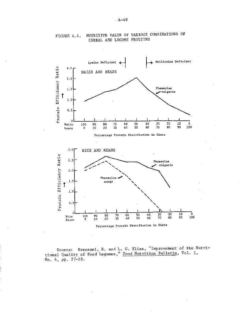
A~49
FIGURE 4.4. NUTRITIVE VALUE OF VARIOUS COMBINATIONS OF CEREAL AND LEGUME PROTEINS
Percentage Protein Distribution in Diets
10 0 90 100
Source: Bressani, R. and L. G. Elias, "Improvement of the Nutritional Quality of Food Legumes," Food Nutrition Bulletin, Vol. 1,No. 4, pp. 27-28.
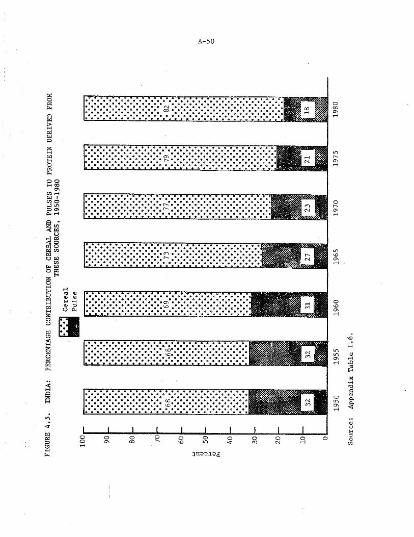
FIGU
RE 4
.5.
INDIA:
PERC
ENTA
GE C
ONTR
IBUT
ION
OF C
EREA
L AN
D PU
LSES
TO
PROT
EIN
DERI
VED
FROM
____
_ TH
ESE
SOUR
CES,
195
0-19
80A-5G
TTTTTTJ-TT T X T T TTTTTT
<N00
...............
OooOS
ITOs
" * .............. , « « I , , « -» f y » f t »
mO si—!
« aa a a a aa a a a a a
• r- •» r-. <or-.CTi
a * e at, 1JL• m». r-~
♦ ............... « « * * a » « -a— ■
mID
• ft ft ft• A • « °°ViCa * * * *a a a al« « t « « t « ................ , »—ft. A... A.
OvDCT\
i ni nCT\
iDM
• * a *a a a a
a a a a
■ m rC°(SO
Oi nCTi
J------ -L____ i — L___L Lo o o o o O o O O Oo 1—1
O s CO r"> iD n CO <N 1---1 Source:
Appe
ndix
Tab
le
A- 51
With this caveat in mind, we look at some of the broad trends. In the preceding section we have seen that if all cereal protein were to come from rice, the desired cereal-legume protein combination would be about 80:20. For a large section of the population the staple diet is rice, and therefore it can be presumed that the source for cereal protein is rice. In such a case, the actual rice-pulse protein ratio in the 1950s and 1960s was higher than the optimum combination. The ratio fell after the mid-1960s, but even in the early 1980s for a rice-based diet, the protein ratio was still adequate.
If we consider a totally wheat-based diet, the broad trends indicate that up to 1965, the desired cereal-pulse protein ratio of 73:27 was met. However, after the mid-1960s the ratio fell much below the optimum.
In the third case of a diet based on coarse cereals, the desired cereal-pulse protein ratio of 50:50 was never achieved. Even in the early 1950s when pulse availability was relatively comfortable, diets based solely on coarse cereals fell quite short of the desired level of protein quality.
Translated into quantities by weight of cereals and pulses, the desired rice-pulse ratio would be about 90:10, the wheat-pulse ratio 80:20, and the coarse grain-pulse ratio 70:30. As against these ratios, the cereal-pulse ratio by weight was about 85:15 up to the mid- 1960s and the average pulse availability was 65 grams per capita, implying that pulse availability was adequate to achieve the desired protein ratio if the cereal staple was either rice or wheat, but not a coarse cereal. After the mid-1960s pulse availability declined and the ratio fell. In fact in the early 1980s the average pulse availability was only 35 grams per capita and the cereal-pulse ratio by weight was 92:8.
We might therefore conclude that to achieve an optimum proportion of cereal-pulse protein, the cereal-pulse ratio by weight should be about 85:15 for diets based on wheat or rice, implying an average per capita pulse availability of about 65 grams per day. This figure, however, overestimates pulse requirement on two accounts. Firstly, as seen in Table 4.3, the average diet based on availabilities contains, in addition to cereals and pulses, other sources of protein including animal products. In fact, protein from other sources makes up about 15 to 20 percent, and animal protein alone about 10 percent of total available protein. Animal protein is high quality protein and the inclusion of animal products in the diet automatically reduces the pulse requirement. Secondly, the protein RDAs in India include an additional safety margin of 20 percent over and above that of FAO standards. This in turn inflates the pulse requirement.
Taking both factors into consideration, it seems not unreasonable to conclude that the figure of 65 grams per capita could be reduced by about 40 percent and the 85:15 by weight cereal-pulse ratio to 90.10, which would still result In the desired protein quality, provided, of
A- 52
course, enough energy was available in the diet to ensure that the protein was efficiently utilized. It needs, however, to be emphasized once again that the present analysis in terms of per capita pulse requirement is for an average person in moderate activity and is based upon availability rather than actual consumption data. It, therefore, has limited relevance and Is useful only to the extent that it serves as a broad guideline.
If the per capita availabilities of foodstuffs shown in Table 4.3 could be considered as an average diet, then the required quantity of pulses, based on the above argument, would be about 40 grams per day. Taking into consideration the fact that about 10 to 15 percent of pulses might be consumed in the form of snacks and savories and not in combination with cereals, the average requirement would need to be adjusted upwards by 10 percent to about 45 grams per day. The quantity of pulse intake recommended by the ICMR, on the other hand, is about 70 grams per capita pei; day [23, pp. 29-30]. In the light of the above discussion this figure would appear to be a substantial overestimation.
We can conclude, therefore, that as a result of the Green Revolution and the decline in the per capita availability of pulses, the quantity of protein has not been adversely affected; the decrease in the supply of pulse protein has been more than offset by the protein from additional cereal production.
There has, however, been a perceptible decline In the quality of protein. We have estimated that for a satisfactory protein quality based on a diet of rice or wheat, a minimum daily intake of about 45 grams of pulses is required, provided enough cereal is consumed to meet energy needs. The pulse availability per capita, since the mid-1960s, has fallen from about 70 grams to less than 40 grams per day.
Further, it must be remembered that availabilities do not indicate actual consumption. With average availabilities as low as 35 to 40 grams per day in the early 1980s, portions of the population in the lower income groups are most probably not able to consume the required minimum quantity of pulses. So the quality of protein in their diet is almost certainly well below the desired level.
CHAPTER VCONSUMPTION TRENDS AND DEMAND PROJECTIONS
In looking at pulse consumption we shall examine consumption trends over time, consumption by state, by rural and urban categories and by income class. There are two sources of information available for the purpose. Cross-sectional data on actual consumption, assessed directly from household consumption surveys, and time-series data as shown In national food balance sheets. The latter are, of course, disappearance data and do not reflect actual consumption.
Food balance sheet data, which indicate net availabilities, have limited use In the study of consumption trends, since they reflect only aggregates, and provide no distinction between rural and urban or different income classes. Our main data source is, therefore, the household consumption survey. However, these are not without error, as we discover in analyzing consumption trends over time. Food balance sheets can be used to advantage in cross-checking the reliability of household survey data.
The Food Balance Sheet data, henceforth referred to as FBS data, are available in India as time-series. The National Sample Survey data based on periodic household consumption surveys, henceforth referred to as NSS data, are available for a number of years, though not as time-series.
Consumption Trends for Pulses
Consumption Trends Over Time
Figure 5.1 shows the data on consumption of pulses and cereals, in quantitative terms, as obtained from the various rounds of the NSS. The latest available data are for 1973/74 (the 28th round) . The results for the 1977/78 (the 32nd round) consumption survey are not available as yet. The figure also indicates pulse and cereal availability as obtained from FBS data. The NSS estimate of cereals is 17 percent higher than implied in FBS data in 1973/74. But for pulses, NSS data show a level of consumption that is about 28 percent lower than production estimates.
The trend in pulse consumption, as indicated by the NSS data, shows a decline. This is corroborated by the trend in pulse availability as shown by the FBS data. The pulse consumption trends are in broad agreement, although there is considerable difference between the absolute values.
Weaknesses of the NSS Data. The NSS data on per capita consumption are ascertained on the basis of household consumption surveys. These surveys are based on scientifically selected sample households and are
A- 53
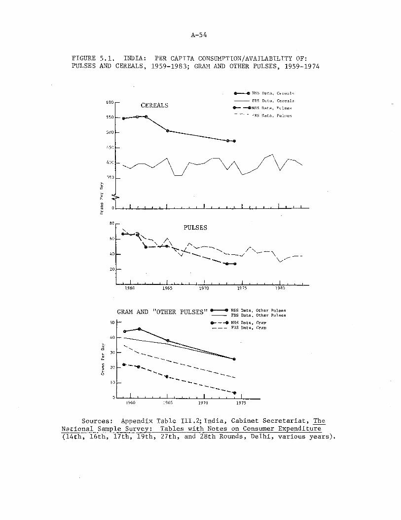
A-54
FIGURE 5.1. INDIA: PER CAPITA CONSUMPTION/AVAILABILITY OF:PULSES AND CEREALS, 1959-1983; GRAM AND OTHER PULSES, 1959-1974
NSS Data, Cereal?;
GRAM AND "OTHER PULSES" •— ® Data, other Pulses------ FBS Data, Other Pulses
Sources: Appendix Table III.2; India, Cabinet Secretariat, TheNational Sample Survey: Tables with Notes on Consumer Expenditure(14th, 16th, 17th, 19th, 27th, and 28th Rounds, Delhi, various years).
A- 55
conducted by trained full-time investigators of the NSS organization. The concepts and definitions used in the questionnaire have been standardized over the last two decades. The data have been used extensively in various studies to estimate food consumption trends, as well as incidence of poverty in the country [3., 53, 60] .
Some studies have concluded that consumption of cereals, as indicated by NSS data, is overestimated [52, 6j5] . It is argued that in households with low incomes some family members eat outside, and consequently their consumption goes unrecorded in the survey. In the high income groups, guests as well as employees of the household, laborers and servants, also share in the food, but are not counted as members [66, P- 134], This is corroborated by the fact that per capita calorie intake as obtained from the 26th round of the NSS (1971/72) showed a wide variation between the two extreme income groups. The highest group recorded an energy consumption of about 6000 kilocalories per capita per day and protein intake of 180 grams per day. For the lowest income group these figures were about 1500 calories and 46 grams, respectively [52., p . 80 ] . While the above argument can be applied to cereals to explain the higher bias in the NSS data, it would not be applicable to pulses or other more expensive food items.
Pulse consumption, as is seen from Figure 5.1, tends to be underestimated in the NSS data. There appear to be several reasons for this. First, the argument for a higher bias, as in the case of cereals, would not apply to the case of pulses which are a relatively expensive food item and therefore not as liberally dispensed as cereals, even in the upper income groups. Second, it must be remembered that the NSS data record consumption for households. This eliminates a significant category of establishments which are consumers of both cereals and pulses, such as charities, student hostels, restaurants and eating houses [66, p. 132]. There are certain other sectors which account more for pulses than cereals. These include temples and other places of worship, sweet shops and wayside stalls. Offerings in temples are largely made of sweets whose main ingredient is pulses, particularly gram. There is a strong likelihood that in household consumption surveys a significant portion of pulses consumed in this manner is not accounted for. Third, a sizable amount of pulses, especially gram, are consumed in the form of snacks and savories, often outside the home. With increasing urbanization, and improved mobility, the tradition of eating outside the home has gained considerable ground in the past two decades, as evidenced by the burgeoning of eating establishments in both urban and semi-rural areas. Since consumption surveys are based upon recalling consumption in the past 30 days, it is quite possible that due to memory lapse the quantity of pulses consumed in the form of snacks and savories is underestimated. Since the quantity of pulses consumed is small, being only about 10 to 20 percent by weight of cereals consumed, it is not surprising that a small fraction of this amount consumed outside the home goes unrecorded.
A- 56
In the absence of studies or surveys that might indicate the percentage of pulses consumed in the nonconventional manner, we must look at the available information in the NSS data. The latter does not provide any breakdown of individual pulses, which are grouped together as one category under "pulses and pulse products." It does, however, record gram as a separate group. This helps to some extent in estimating the degree of bias in the NSS data.
Figure 5.1 indicates the per capita consumption of gram and other pulses, and also their availabilities as determined by the FBS data. It appears likely that there is an underestimation of gram in the NSS data. In the case of other pulses, NSS data seem to be slightly overestimated, but the difference is small and there appears to be a converging trend between the two sets. It may, therefore, be reasonable to presume that gram is the main source of underestimation in the NSS data. The reader must, however, be cautioned that in view of the inadequate data and sketchy information on pulse consumption, any inferences regarding gram and total pulse consumption can at best be reasonable conjecture.
A comparison of NSS and FBS data for gram is seen in Table 5.1. The FBS data indicate that gram accounted for more than 40 percent of total pulse availability in the late 1950s and early 1960s, and that its share has been steadily falling. This appears reasonable in the light of our argument about the effect of HYVs of wheat replacing gram acreage after the mid-1960s. While the same trend is reflected in the NSS data, it can be observed that the percentage of consumption of gram to total pulse consumption is lower than that indicated by the availability data. Up to the mid-1960s the unaccounted gram consumption was about 13 percent. This seems to have increased in the mid-1970s to about 24 percent. One possible reason for the increase might be the fact that with reduced availability of gram and the consequent rise in prices, the average consumer cut down severely on the consumption of gram. However, in business establishments and eating houses consumption was not curtailed to the same extent as in households. This might perhaps explain the widening of the gap between the recorded household consumption and the average availability of gram.
The analysis is constrained by the unavailability of further data in the time-series. However, on the basis of the above discussion we may broadly infer that it is likely that after the mid-1960s the NSS data underestimate pulse consumption by about 15 to 20 percent. Since NSS data stop short in the year 1973/74, the alternative is to ascertain latest apparent consumption from the FBS data. Apart from the fact that FBS data do not reflect actual consumption, they suffer from other weaknesses as well.
Weaknesses of the FBS data. National Food Balance Sheets, published annually, give estimates of foodgrain availability. Separate estimates are available for wheat, rice, coarse cereals, gram and total
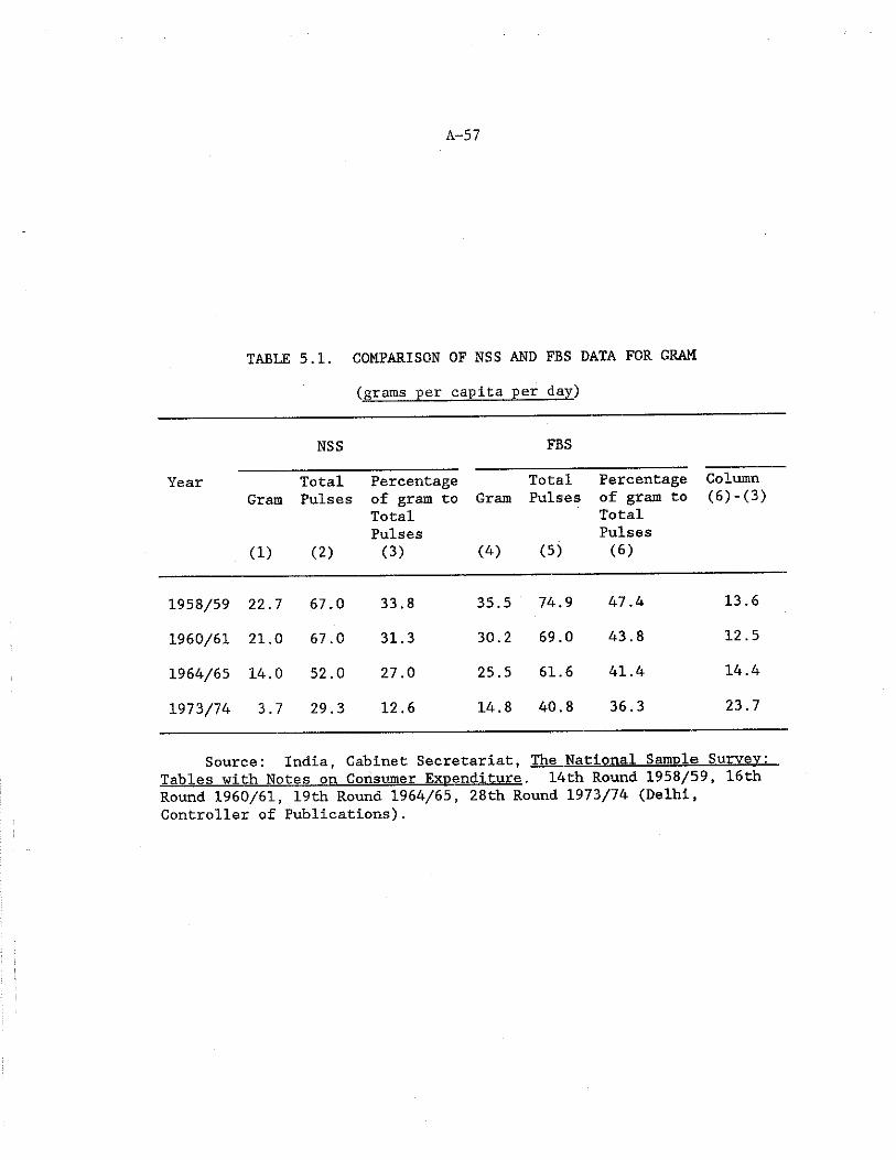
A-57
TABLE 5.1. COMPARISON OF NSS AND FBS DATA FOR GRAM
(grams per capita per day)
Year
NSS FBS
Gram
(1)
TotalPulses
(2)
Percentage of gram to Total Pulses (3)
Gram
W
TotalPulses
(5)
Percentage of gram to Total Pulses (6)
Column(6)-(3)
1958/59 22.7 67.0 33.8 35.5 74.9 47.4 13.6
1960/61 21.0 67.0 31.3 30.2 69.0 43.8 12.5
1964/65 14.0 52.0 27.0 25.5 61.6 41.4 14.4
1973/74 3.7 29.3 12.6 14.8 40.8 36.3 23.7
Source: India, Cabinet Secretariat, The National Sample Survey:Tables with Notes on Consumer Expenditure. 14th Round 1958/59, 16th Round 1960/61, 19th Round 1964/65, 28th Round 1973/74 (Delhi, Controller of Publications).
pulses [35] . The equation for net availability can be written as follows:
Net Availability = Gross Production - (Feed, Seed and Wastage,Processing Losses, Industrial Uses) ± Net International Trade ± Changes in Stocks
The FBS data, however, suffer from some shortcomings. The equation shows that net availability depends on gross production. Gross production in the case of pulses may be underestimated, since pulses are usually not grown on prime agricultural land but on marginal lands, and a small percentage of the latter might escape official notice. Redgram, or pigeonpea, has the appearance of a shrub and is often planted on the borders of regular fields to keep out intruders. It is quite likely that the area of redgram sown in this manner might fail to find mention in the official land records.
Another reason why production of pulses may be understated is the fact that pulses have traditionally been planted as mixed crops. Intercropping of pulses with maize, sorghum and sugarcane is still widely practiced. This might also lead to an underestimation in the area and production of pulses. However, in the absence of concrete data any attempt to adjust for underestimation would be arbitrary and lead to greater ambiguity in the official statistics.
Net availability also depends on changes in stocks. However, official records take into account only government stocks. There is no account of stocks privately held. Pulses are marketed almost exclusively by the private trade. It is difficult to collect data from the widespread and diverse range of private foodgrain traders, and no serious effort has been made by the government to collect them.
To account for feed, seed and wastage, the following allowances are made: rice 7.6 percent, wheat 12.1 percent, gram 22.1 percent,total cereals 12.5 percent and total pulses 12.5 percent [35]. The National Commission on Agriculture (NCA) adopted the following breakdown to account for a 12.5 percent allowance: 5.0 percent seed, 5.0percent livestock feed, and 2.5 percent wastage [33, p. 49].
Since 1976, when the NCA attributed a 5 percent share for feed, the real prices of pulses have risen considerably. As a result there may be a decline in the use of certain pulses as livestock feed. Gram, which was commonly used for feeding horses, finds lesser use for this purpose. On the other hand, with greater emphasis on dairying activities, pulses such as cowpeas and horsegram are being increasingly used. In the absence of more precise information on the changing pattern of pulses for feed use, it appears prudent to accept the 5 percent estimate of the NCA.
On the other hand, because of a 2.5 percent allowance for wastage, it seems that the FBS data overestimate pulse availability. In actual fact losses and wastage in pulses are more than 2.5 percent. One study
A- 58
A- 59
indicates that nearly 80 percent of the total loss of pulses is caused by insects, rodents and micro-organisms in storage, and pulses are more susceptible to .insect damage compared to other foodgrains like wheat, paddy and maize. The estimate attributes losses in storage due to insects as 5 percent for pulses, 2.5 percent for wheat, 2 percent for paddy and 3.5 percent for maize [4, p. 429] .
Yet another factor which affects the wastage component is that more than 75 percent of pulses produced are consumed in the form of dal [44. p. 405]. Conventional and traditional methods of milling whole grain pulses into dal remove anything between 10 and 25 percent of edible portion, and according to one estimate 1.5 million metric tons of pulses are lost annually in the process [43, p. 423].
An Expert Group (1967) set up by the Government estimated the losses for paddy, wheat and pulses at 11, 8 and 9.5 percent, respectively. The losses included post-harvest operations, processing, transporation and storage [43, p. 425]. On the other hand significant advances in technology over the last two decades have led to improved practices in pest and insect control, resulting in the reduction of losses. In the absence of concrete data, it is difficult to formulate a precise estimate of the current level of losses in pulses. Any attempt to alter the official figure of 12.5 percent would be arbitrary and would undermine the validity of the data.
While the NSS data give information about consumption across different expenditure classes, and FBS data provide the latest availabilities, neither of the sources gives any indication of food distribution within households. So that while food consumption or availabilities at the aggregate household level may seem adequate, deficiencies may exist for members within the same family. We have no statistics to determine how these deficiencies within the household may be skewed. It is, however, a well known fact that in traditional rural families the adult males receive the better portion of the meal both in terms of quantity and quality, while the younger members and the women must be satisfied with what remains.
Consumption Trends by State
Pulse consumption data by state in the 1960s and 1970s, in quantitative terms, are not available in published NSS data. Therefore data from an alternative source are examined to see if any useful trends emerge.
Diet Surveys. The National Institute of Nutrition, at Hyderabad, and the Nutrition Sections of the Departments of Public Health in State Governments carry out periodic diet surveys. The data collected by these agencies are compiled and published as the "Report of Nutrition Work done in States." During the period between 1960 and 1969, 575 surveys were conducted, covering a population of about 152,000 persons, in 13 states [22,, pp. 26-27].
A- 60
The average per capita daily consumption of pulses as obtained from these diet surveys is shown in Figure 5.2. The average per capita daily pulse consumption reported was about 34 grams during the period between 1960 and 1969. This is even lower than that obtained from the NSS data. The same surveys also indicate that the per capita consumption of cereals was about 370 grams, lower than the NSS data and also below that reported by FBS data. However, the data are not very useful since they have been averaged over a ten-year period and fail to indicate any trends in consumption.
The data obtained by these diet surveys should be used with a great deal of caution. Absolute values from these data have not been used anywhere in the present study. However, the results from the surveys can be used to suggest the relative trend in pulse consumption by state. This is seen in Figure 5.2.
As is to be expected, states which are major producers of pulses also have the higher per capita consumption. The two largest pulse producing states are Uttar Pradesh and Madhya Pradesh; each accounted for about 22 percent of total pulse production in the early 1980s . The diet surveys were conducted between 1960 and 1969. In the 1960s Uttar Pradesh and Madhya Pradesh accounted for about 30 and 15 percent, respectively, of total pulse production. These two states, together with Raj as than, also had the highest percentage of vegetarian population in the country [22, p . 48] , which is another reason for the higher production and consumption of pulses. A third factor is of interest here. The higher pulse consuming states also happen to be the states where the cereal staple is wheat. States where the cereal staple is rice, such as Andhra Pradesh, Karnataka, Kerala and Tamil Nadu, indicate lower pulse consumption. It was seen in Chapter IV that a desirable combination of cereal-pulse protein ratio is 73:27 when the cereal is wheat and 80:20 when the cereal is rice, thereby indicating that protein from rice is superior to that of wheat. Consequently rice requires relatively less pulse protein to supplement it.
It appears therefore that at least at the macro level, pulse production and consumption seem to have been naturally distributed in a nutritionally desirable manner.
Rural-Urban Consumption Trends
Figure 5.3 shows the average percentage expenditure in rural and urban areas on various food and nonfood items. Rural incomes are on an average 27 percent lower than urban incomes [52, p, 95] . In both rural and urban areas, consumers spend a major share of their income on food. In rural areas expenditure on food items is about 75 percent of total expenditure, while in urban areas it is about 65 percent.
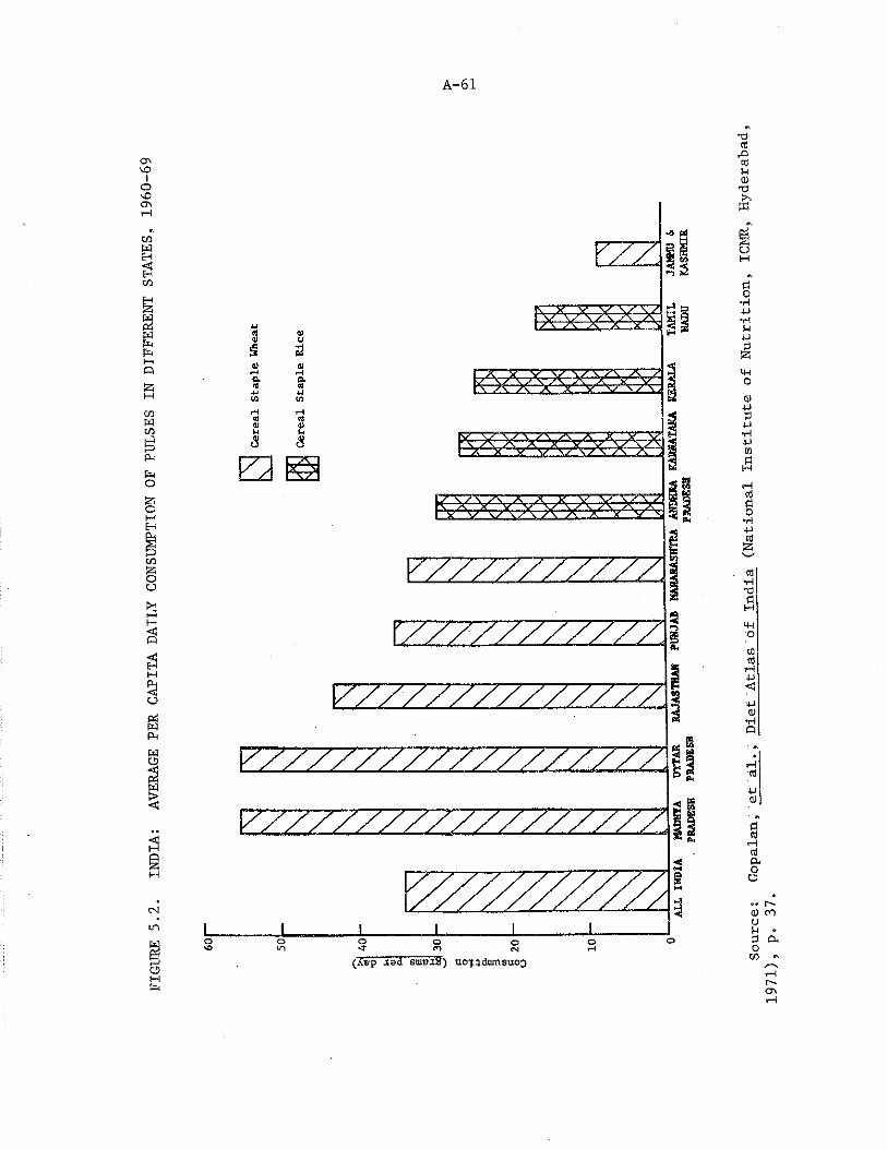
FIGU
RE 5
.2.
INDIA:
AVER
AGE
PER
CAPI
TA D
AILY
CON
SUMP
TION
OF
PULS
ES I
N DI
FFER
ENT
STATES,
1960
-69
A-61
1___ - I_____— I_________ 1________ I________ I________ Io o o o © o oo m < r © cm > -i
(jCbp .lad smeaS) uof dumsuo Source:
Gopa
lan,
et
dl.,
Diet
Atl
as o
f In
dia
(Nat
iona
l In
stit
ute
of N
utri
tion
, ICMR,
Hyde
raba
d,19
71),
p.
37
.
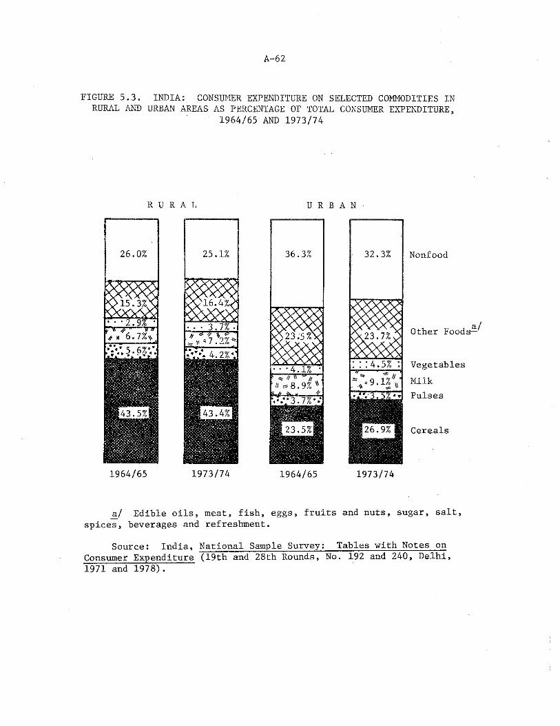
A-62
FIGURE 5.3. INDIA: CONSUMER EXPENDITURE ON SELECTED COMMODITIES INRURAL AND URBAN AREAS AS PERCENTAGE OF TOTAL CONSUMER EXPENDITURE,
1964/65 AND 1973/74
R U R A L
26.0%
1964/65
25.1%
1973/74
36.3%
B A N ■
32.3% Nonfood
JX2 3.7X0a /Other Foods—
:::4.5% : Vegetables,„V 'J'm™.,™,~ 9 1 y 1 * Milk
Pulses
1964/65
26,
1973/74
Cereals
_a/ Edible oils, meat, fish, eggs, fruits and nuts, sugar, salt, spices, beverages and refreshment.
Source: India, National Sample Survey: Tables with Notes on Consumer Expenditure (19th and 28th Rounds, No. 192 and 240, Delhi, 1971 and 1978).
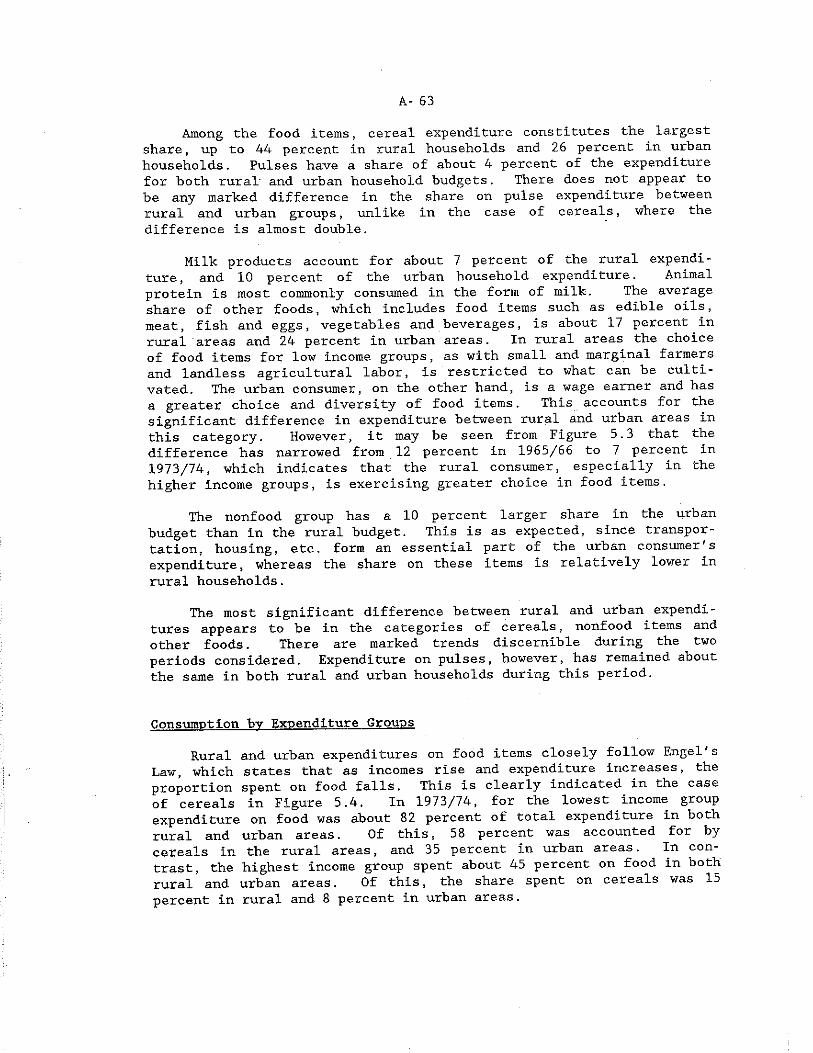
A- 63
Among the food items, cereal expenditure constitutes the largest share, up to 44 percent in rural households and 26 percent in urban households. Pulses have a share of about 4 percent of the expenditure for both rural' and urban household budgets. There does not appear to be any marked difference in the share on pulse expenditure between rural and urban groups, unlike in the case of cereals, where the difference is almost double.
Milk products account for about 7 percent of the rural expenditure , and 10 percent of the urban household expenditure. Animal protein is most commonly consumed in the form of milk. The average share of other foods, which includes food items such as edible oils, meat, fish and eggs, vegetables and beverages, is about 17 percent in rural areas and 24 percent in urban areas. In rural areas the choice of food items for low income groups, as with small and marginal farmers and landless agricultural labor, is restricted to what can be cultivated. The urban consumer, on the other hand, is a wage earner and has a greater choice and diversity of food items. This accounts for the significant difference in expenditure between rural and urban areas in this category. However, it may be seen from Figure 5.3 that the difference has narrowed from 12 percent in 1965/66 to 7 percent in 1973/74, which indicates that the rural consumer, especially in the higher income groups, is exercising greater choice in food items.
The nonfood group has a 10 percent larger share in the urban budget than in the rural budget. This is as expected, since transportation, housing, etc. form an essential part of the urban consumer ' s expenditure, whereas the share on these items is relatively lower in rural households.
The most significant difference between rural and urban expenditures appears to be in the categories of cereals, nonfood items and other foods. There are marked trends discernible during the two periods considered. Expenditure on pulses, however, has remained about the same in both rural and urban households during this period.
Consumption bv Expenditure GroupsRural and urban expenditures on food items closely follow Engel's
Law, which states that as incomes rise and expenditure increases, the proportion spent on food falls. This is clearly indicated in the case of cereals in Figure 5.4. In 1973/74, for the lowest income group expenditure on food was about 82 percent of total expenditure in both ^ural and urban areas. Of this, 58 percent was accounted for bycereals in the rural areas, and 35 percent in urban areas. In contrast, the highest income group spent about 45 percent on food in both rural and urban areas. Of this, the share spent on cereals was 15 percent in rural and 8 percent in urban areas.
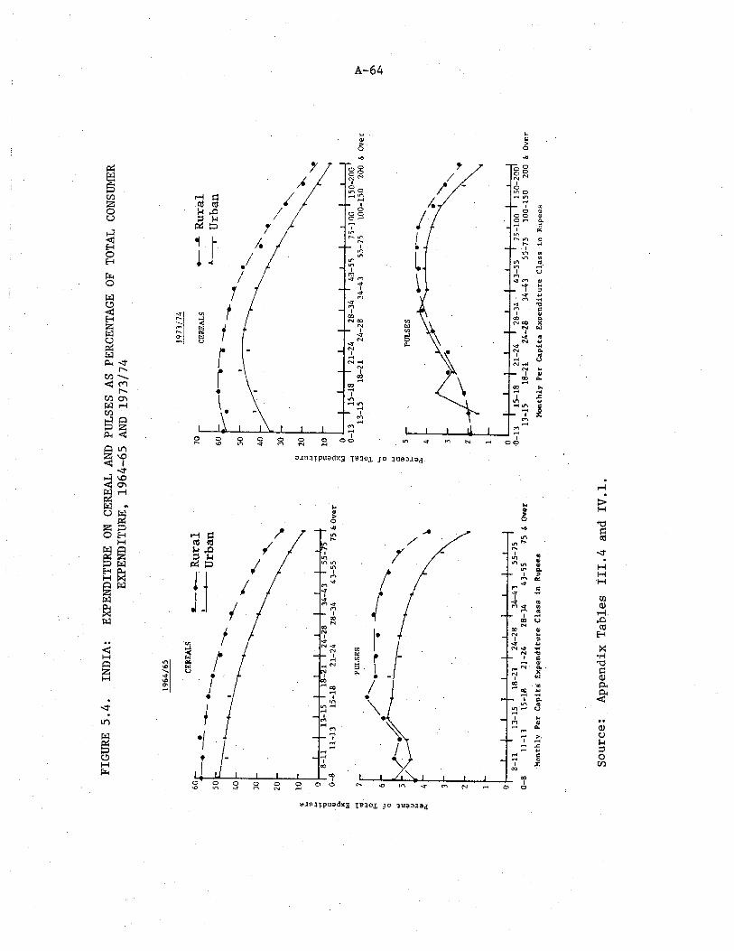
FIGU
RE 5
.4.
INDIA:
EXPE
NDIT
URE
ON C
EREA
L AN
D PU
LSES
AS
PERC
ENTA
GE O
F TO
TAL
CONS
UMER
EXPE
NDIT
URE,
196
4-65
AND
197
3/74
A-64
a-nUTpuadxa xe3ox jo
Source:
Appe
ndix
Tab
les
III.
4 an
d IV
.1.
A- 65
Expenditure on pulses varied between 2 and 4.5 percent in both rural and urban areas in 1973/74. However, there appears to have been a significant change between 1964/65 and 1973/74. The gap in expenditure on pulses seems to have narrowed between the rural and urban areas. In percentage terms the expenditure of all classes on pulses appears to have fallen during the period. This is possibly the result of an increase in the relative price of pulses during this period.
Looking at actual per capita consumption instead of expenditure, we find that there has been a decline in the per capita foodgrain consumption between 1964/65 and 1973/74. For cereals, the proportion of decline increases as one moves to a higher income group. The poorest 30 percent of the population experienced practically no change, the middle 40 percent had a 3.9 percent decline, and the wealthiest 30 percent experienced a 12.6 percent decline. This is shown in Figure5.1 and Table 5.2.
The decline in per capita pulse consumption was more significant.In fact the per capita consumption of pulses fell about 45 percent and
was shared almost equally between all income groups. FBS data also indicate that the pulse availability during this period declined. During this period there was on an average a 30 percent increase in the real price of pulses [53, p. 24]. It is quite possible that consumers may have substituted other foods such as vegetables for pulses in the diet.
Table 5.2 also indicates that the percentage expenditure on pulses registered a decline. The percentage of total expenditure on food was higher In 1973/74 than in 1964/65. In 1973/74, the percentage expenditure on other foods also increased. This adds credence to the hypothesis that the consumers may have substituted other food items for pulses[53] -
Pulse Consumption and Nutritional Norms
From Table 5 S2 it is evident that in the mid-1960s about 70 percent of the population had a per capita pulse consumption greater than 45 grams per day. It may be recalled that in Chapter IV it was estimated that a per capita intake of about 45 grams of pulses together with adequate quantity of cereal consumption to satisfy energy needs fulfilled the requirements of the recommended dietary allowance of protein. This would imply that 30 percent of the population in the lowest income groups could not afford adequate quantities of pulses, although the per capita availability of pulses during this period was more than 60 grams per day.
By the mid-1970s the situation had changed markedly. The per capita availability declined to about 40 grams per day, and the real price of pulses registered an increase of 30 percent. If the NSS data were accepted without adjusting for underestimation, we would conclude that the per capita pulse consumption of the entire population fell
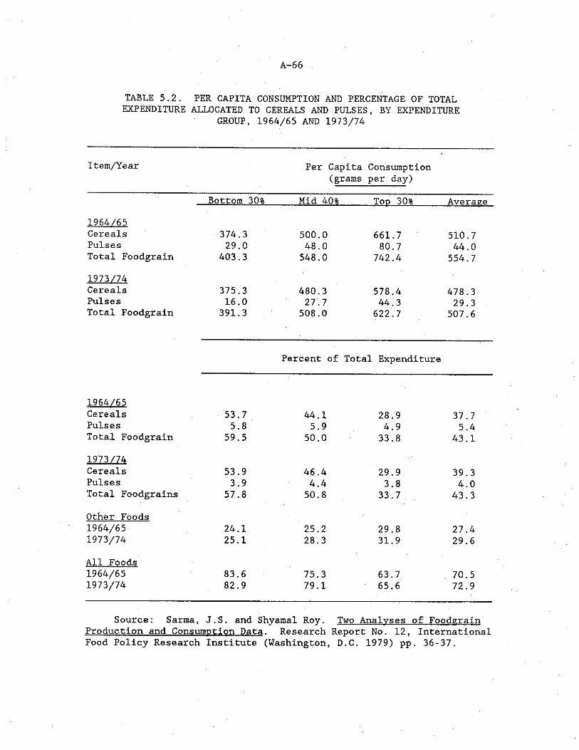
A-66
TABLE 5.2. PER CAPITA CONSUMPTION AND PERCENTAGE OF TOTALEXPENDITURE ALLOCATED TO CEREALS AND PULSES, BY EXPENDITURE
GROUP, 1964/65 AND 1973/74
Item/Year Per Capita Consumption (grams per day)
Bottom 30% Mid 40% Ton 30% Average1964/65Cereals 374.3 500.0 661,7 510.7Pulses 29.0 48.0 80.7 44.0Total Foodgrain 403.3 548.0 742.4 554.71973/74Cereals 375.3 480.3 578,4 478.3Pulses 16.0 27.7 44.3 29.3Total Foodgrain 391.3 508.0 622.7 507.6
Percent of Total Expenditure
1964/65Cereals 53.7 44.1 28.9 37.7Pulses 5.8 5.9 4.9 5.4Total Foodgrain 59.5 50.0 33.8 43.11973/74Cereals 53.9 46.4 29.9 39.3Pulses 3.9 4.4 3.8 4.0Total Foodgrains 57.8 50.8 33.7 43.3Other Foods1964/65 24.1 25.2 29.8 27.41973/74 25.1 28.3 31.9 29.6All Foods1964/65 83.6 75.3 63.7 70.51973/74 82.9 79.1 65,6 72.9
Source: Sarma, J.S. and Shyamal Roy. Two Analyses of FoodgrainProduction and Consumption Data. Research Report No. 12, InternationalFood Policy Research Institute (Washington, D.C. 1979) pp. 36-37.
A- 67
were accepted without adjusting for underestimation, we would conclude that the per capita pulse consumption of the entire population fell short of the nutritional norms. However, with a 15 percent adjustment for underestimation, the 30 percent of the population in the highest income groups would have had a per capita consumption of more than 45 grams per day. The remaining 70 percent would have had a diet that may have been sufficient in protein quantity but short of the desired protein quality.
In the early 1980s average pulse availability did not increase and was less than 40 grams per capita per day. Consumption data for this period are not available, so that it is not possible to determine the percentage of population unable to consume an adequate quantity of pulses. However, it can be seen that the situation has deteriorated since the mid-1970s. The real price of pulses has increased further. It is likely that income distribution over the last decade has not Improved. This assumption is based on available evidence which suggests that there has been little change in the distribution of incomes from the mid-1950s to the mid-1970s [52,, pp. 106-107].
With a stagnant availability, no change in Income distribution and an increase in the real prices, it appears reasonable to presume that more than 70-80 percent of the population are now unable to consume an adequate quantity of pulses. If the situation is not to worsen any further, efforts must be made to increase the per capita availability.
In the mid-1960s, when the per capita availability was about 60 grams per day, 30 percent of the population in the lower income bracket were unable to consume adequate quantities of pulses. The income distribution did not allow a significant percentage of the lower income groups to afford an adequate pulse intake despite sufficient availability.
We may conclude, therefore, that while planning for pulse production it might be prudent to make allowances for the income distribution factor. The Indian Council of Medical Research has recommended a per capita daily intake of about 70 grams of pulses per day. While this quantity appears considerably inflated from the nutritional point of view, it can be used as the desired availability while targeting pulse production. With an average availability of 70 grams per capita per day it is likely that more than 70-80 percent of the population will be able to consume about 45 grams of pulses per day.
Demand Prolection for Pulses
The growth in demand for pulses in general depends upon the following factors: 1) the rate of population growth,^ 2) the rate of growth of per capita income and, 3) the income elasticity of demand. Changes in the relative price of pulses and the distribution of income are also likely to influence demand.
A- 68
In deriving demand projections we have assumed constant prices. It is true that it would be more realistic to incorporate In the analysis possible trends of relative prices in the years to come. But in order to be able to make plausible assumptions about price trends, it is necessary to have a firm idea of the emerging supply demand balances. This is not easy. It is more practical to work out demand and supply projections at constant prices, identify the gap therein, and predict price trends using the price elasticity of demand.
Methodology
The method applied in this study for projecting demand is the following:
consumption projected = (base consumption)(demand growth rate) demand growth rate = (1 + p) [1 + (y)(e)]
where p = proportionate Increase in populationy = proportionate increase in per capita income e - income elasticity of demand.
High and low expected growth rates in population and per capita income, along with high and low estimations of income elasticities, are used to project to 1990 and 2000 a range of demand for pulses.
Population Growth Rate
The population of India in 1951 was 361 million, and had grown during the two previous decades at an approximate annual rate of 1.3 percent. The growth rate increased sharply during 1951-61 and 1961-71 to 2.16 percent and 2.48, percent respectively [63, p. 315]. Before the 1950s high birth and death rates kept the population growth rate low; however, during the 1950s, 1960s and 1970s high birth ratescoupled with rapidly falling death rates led to increasing rates of growth, as can be seen in Figure 5.5. In Figure 5.5, population growth since 1950 is plotted against its demographic determinants, the crude birth rate (CBR) and crude death rate (CDR).
Demographers hoped that the family planning efforts since the mid- 1960s would sharply decelerate the growth of population. Despite the spending of more than 10 billion rupees on family planning measures and the sterilization of more than 20 million people, the population grew by 2.47 percent annually in the 1970s, almost at the same rate as in the, 1960s [ 6_3, pp. 319-320], The 1981 census count exceeded the officially projected figures by about 13 million. On March 1, 1981, the population was more than 685 million [48]■
However, there is reason to believe that, after rising for most of the past three decades, the population growth rate is over its peak,
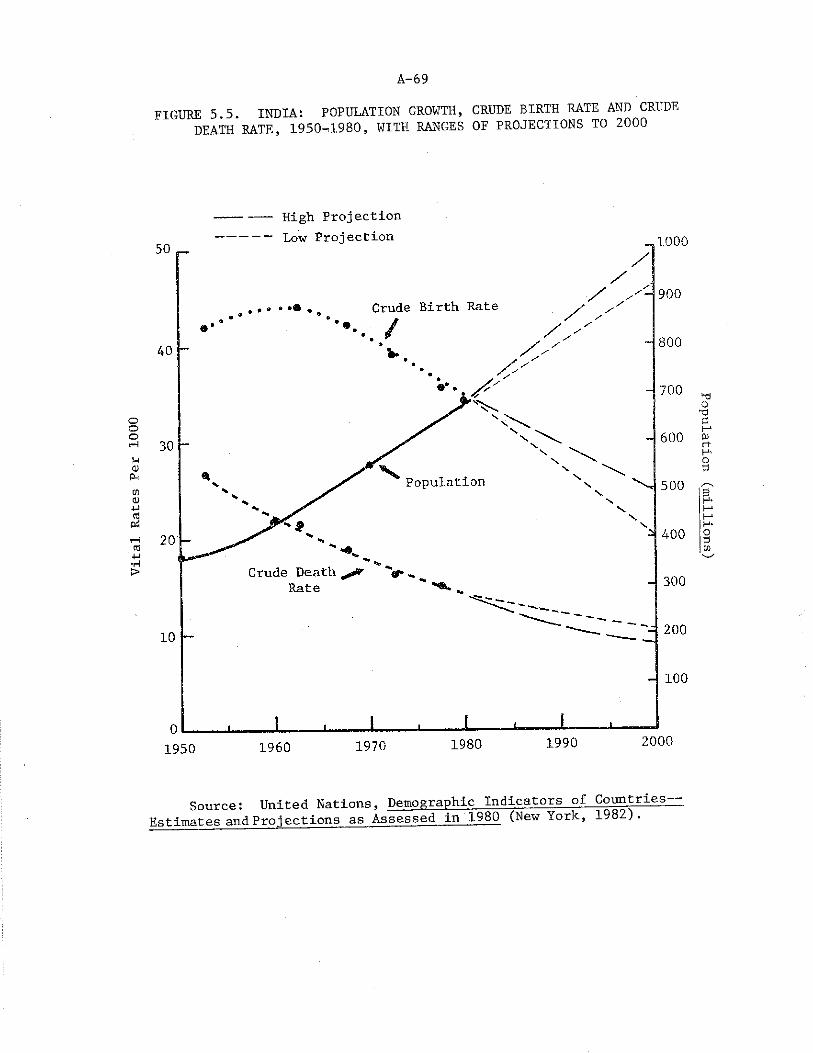
Vita
l Ra
tes
Per
1000
A-69
FIGURE 5.5. INDIA: POPULATION GROWTH, CRUDE BIRTH RATE AND CRUDEDEATH RATE, 1950-.1980, WITH RANGES OF PROJECTIONS TO 2000
High Projection
Source: United Nations, Demographic Indicators of CountriesEstimates and Projections as Assessed in 1980 (New York, 1982).
Population (millions)
A- 70
because the death rate will not fall as fast as in the past and the birth rate will continue to decline.
The reasons for optimism stem from the rapid expansion of health services in the country. As a result, there has been a significant decrease in infant and child mortality rates. With greater numbers of children surviving there is a strong likelihood that couples will have fewer children, thereby leading to a decline in the birth rate.
Another cause is the rapid rate of urbanization. Between 1961 and 1971, the annual rate of growth of urban population was 3.3 percent while the rate of growth of total population was 2.4 percent. During the decade of the 1970s, the urban population growth rate increased to3.7 percent [69, p. 190], Various demographic studies indicate that fertility rates have been lower in urban areas than in rural areas in recent years [9, p. 140], Consequently with a continuing rapid rate of urbanization, the birth rate is likely to fall.
There was a decline in the crude birth rate from an average of about 44 per thousand in the 1960s to 35 per thousand in the late 1970s. The death rate during this period fell from 22 per thousand to about 13 per thousand [69, p. 186],
For the purposes of this study, we define the high scenario as one where the birth rate in the 1980s remains almost the same as in the late 1970s implying thereby that the various population control measures have not had any significant impact in reducing the birth rate.
The UN high variant estimates for the first half of the 1980s, shown in Table 5.3, describe such a situation. The CBR at about 34 per thousand is almost the same as in the late 1970s. The UN low variant estimates for CBR are about 30 per thousand, which would reflect a scenario where family planning measures together with improved health facilities and urbanization have a significant impact in reducing therun ®
It therefore seems justified to use the UN high and low population variants to project a range of demand. The projections for population estimated by the Government of India, in the Seventh Five Year Plan document, also appear to justify the choice, since they lie within this range [37, pp. 11-12].'
Income Elasticities
The degree to which changes in income affect the quantity demanded depends upon the income elasticity of the commodity. Income elasticity is defined as the percentage change in quantity corresponding to a one percent change in income, other factors held constant.
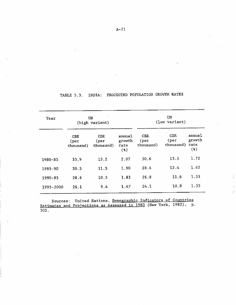
A-71
TABLE 5.3. INDIA: PROJECTED POPULATION GROWTH RATES
Year UN(high variant) (1
UNow variant)
CBR(per
thousand)
CDR(per
thousand)
annualgrowthrate<%>
CBR(per
thousand)
CDR(per
thousand)
annualgrowthrate(%)
1980-85 33.9 13.2 2.07 30.6 13.5 1.72
1985-90 30.5 11.5 1.90 28.6 12.4 1.62
1990-95 28.6 10.3 1.83 26.8 11.6 1.53
1995-2000 26.1 9.4 1.67 24.1 10.8 1.33
Sources: United Nations, Demographic Indicators of Countries Estimates and Projections as Assessed in 1980 (New York, 1982), p. 302.
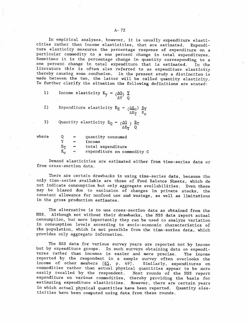
A- 72
In empirical analyses, however, it is usually expenditure elasticities rather than income elasticities, that are estimated. Expenditure elasticity measures the percentage response of expenditure on a particular commodity to a one percent change in total expenditures. Sometimes it is the percentage change in quantity corresponding to a one percent change in total expenditure that is estimated. In the literature this is often also referred to as expenditure elasticity thereby causing some confusion. In the present study a distinction is made between the two, the latter will be called quantity elasticity. To further clarify the situation the following definitions are stated:
1) Income elasticity Ey = (AQ\ YAY Q
2) Expenditure elasticity EE - ( M c) Ita e t e c
3) Quantity elasticity E q = /AQ \ E^AEt Q
Q quantity consumedY incomeET = total expenditureV > expenditure on commodity C
Demand elasticities are estimated either from time-series data or from cross-section data.
There are certain drawbacks in using time-series data, because the only time-series available are those of Food Balance Sheets, which do not indicate consumption but only aggregate availabilities. Even these may be biased due to exclusion of changes in private stocks, the constant allowance for nonfood use and wastage, as well as limitations in the gross production estimates.
The alternative is to use cross-section data as obtained from the NSS. Although not without their drawbacks, the NSS data report actual consumption, but more importantly they can be used to analyze variation in consumption levels according to socio-economic characteristics of the population, which is not possible from the time-series data, which provides only aggregate information.
The NSS data for various survey years are reported not by income but by expenditure groups. In such surveys obtaining data on expenditures rather than incomes is easier and more precise. The income reported by the respondent in a sample survey often overlooks the income of other members [65,, p . 49] . Similarly, expenditures on commodities rather than actual physical quantities appear to be more easily recalled by the respondent. Most rounds of the NSS report expenditure on various commodities, thereby providing the basis for estimating expenditure elasticities. However, there are certain years in which actual physical quantities have been reported. Quantity elasticities have been computed using data from these rounds.
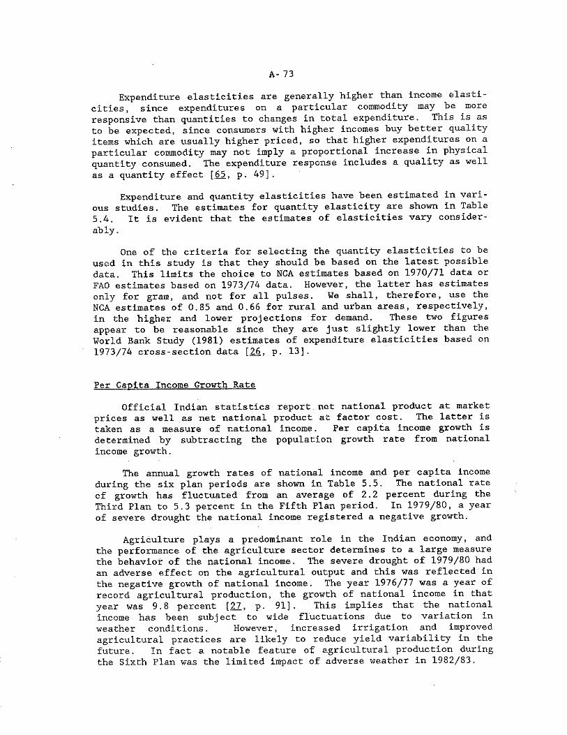
A- 73
Expenditure elasticities are generally higher than income elasticities, since expenditures on a particular commodity may be more responsive than quantities to changes in total expenditure. This is as to be expected, since consumers with higher incomes buy better quality items which are usually higher priced, so that higher expenditures on a particular commodity may not imply a proportional increase in physical quantity consumed. The expenditure response includes a quality as well as a quantity effect [65., p. 49] .
Expenditure and quantity elasticities have been estimated in various studies. The estimates for quantity elasticity are shown in Table5.4. It is evident that the estimates of elasticities vary considerably.
One of the criteria for selecting the quantity elasticities to be used in this study is that they should be based on the latest possible data. This limits the choice to NCA estimates based on 1970/71 data or FAO estimates based on 1973/74 data. However, the latter has estimates only for gram, and not for all pulses. We shall, therefore, use the NCA estimates of 0.85 and 0.66 for rural and urban areas, respectively, in the higher and lower projections for demand. These two figures appear to be reasonable since they are just slightly lower than the World Bank Study (1981) estimates of expenditure elasticities based on 1973/74 cross-section data [.26, p. 13] .
Per Capita Income Growth Rate
Official Indian statistics report net national product at market prices as well as net national product at factor cost. The latter is taken as a measure of national income. Per capita income growth is determined by subtracting the population growth rate from national income growth.
The annual growth rates of national income and per capita income during the six plan periods are shown in Table 5.5. The national rate of growth has fluctuated from an average of 2.2 percent during the Third Plan to 5,3 percent in the Fifth Plan period. In 1979/80, a year of severe drought the national income registered a negative growth.
Agriculture plays a predominant role in the Indian economy, and the performance of the agriculture sector determines to a large measure the behavior of the national income. The severe drought of 1979/80 had an adverse effect on the agricultural output and this was reflected in the negative growth of national income. The year 1976/77 was a year of record agricultural production, the growth of national income in that year was 9.8 percent [27., p . 91] . This Implies that the national income has been subj ect to wide fluctuations due to variation in weather conditions. However, increased irrigation and improved agricultural practices are likely to reduce yield variability in the future. In fact a notable feature of agricultural production during the Sixth Plan was the limited impact of adverse weather in 1982/83.
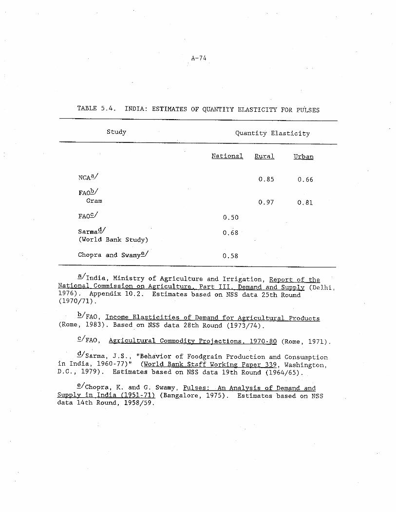
A-7 4
TABLE 5.4. INDIA: ESTIMATES OF QUANTITY ELASTICITY FOR PULSES
Study Quantity Elasticity
National Rural Urban
n c aV 0.85 0.66FA0—/
Gram 0.97 0.81f a o h/ 0.50Sarma^t/(World Bank Study)
0.68
Chopra and Swamy^/ 0.58
—/India, Ministry of Agriculture and Irrigation, Report of the National Commission on Agriculture. Part III. Demand and Supply (Delhi, 1976). Appendix 10.2. Estimates based on NSS data 25th Round (1970/71).
—/FAO, Income Elasticities of Demand for Agricultural Products (Rome, 1983). Based on NSS data 28th Round (1973/74).
-^FAO, Agricultural Commodity Projections. 1970-80 (Rome, 1971).
-^Sarma, J.S., "Behavior of Foodgrain Production and Consumption in India, 1960-77)" (World Bank Staff Working Paper 339. Washington, D.C., 1979). Estimates based on NSS data 19th Round (1964/65).
—/chopra, K, and G. Swamy, Pulses: An Analysis of Demand andSupply in India (1951-71) (Bangalore, 1975). Estimates based on NSS data 14th Round, 1958/59.
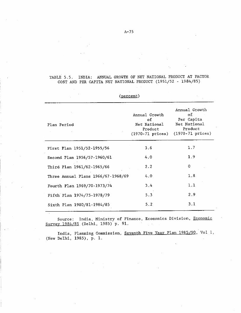
A-75
TABLE 5.5. INDIA: ANNUAL GROWTH OF NET NATIONAL PRODUCT AT FACTORCOST AND PER CAPITA NET NATIONAL PRODUCT (1951/52 - 1984/85)
(percent)
Plan Period
Annual Growth of
Net National Product
(1970-71 prices)
Annual Growth of
Per Capita Net National
Product(1970-71 prices)
First Plan 1951/52-1955/56 3.6 1.7
Second Plan 1956/57-1960/61 4.0 1.9
Third Plan 1961/62-1965/66 2.2 0
Three Annual Plans 1966/67-1968/69 4.0 1.8
Fourth Plan 1969/70-1973/74 3.4 1.1
Fifth Plan 1974/75-1978/79 5.3 2.9
Sixth Plan 1980/81-1984/85 5.2 3.1
Source: India, Ministry of Finance, Economic? Division, EconomicSurvey 1984/85 (Delhi. 1985) p. 91.
India, Planning Commission, Seventh Five Year Flan 1985/90, Vol 1, (New Delhi, 1985), p. 1.
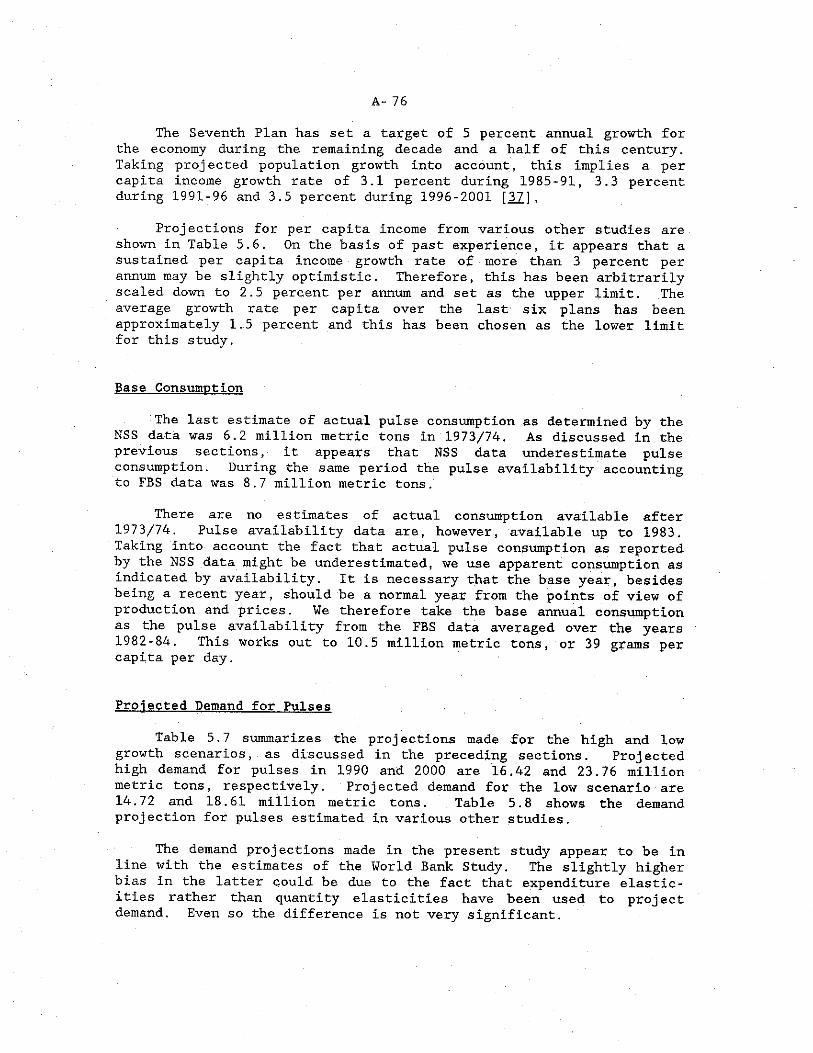
A- 76
The Seventh Plan has set a target of 5 percent annual growth for the economy during the remaining decade and a half of this century. Taking projected population growth into account, this implies a per capita income growth rate of 3.1 percent during 1985-91, 3.3 percent during 1991-96 and 3.5 percent during 1996-2001 [371.
Projections for per capita income from various other studies are shown in Table 5.6. On the basis of past experience, it appears that a sustained per capita income growth rate of more than 3 percent per annum may be slightly optimistic. Therefore, this has been arbitrarily scaled down to 2.5 percent per annum and set as the upper limit. The average growth rate per capita over the last six plans has been approximately 1.5 percent and this has been chosen as the lower limit for this study.
Base Consumption
The last estimate of actual pulse consumption as determined by the NSS data was 6.2 million metric tons in 1973/74. As discussed in the previous sections, it appears that NSS data underestimate pulse consumption. During the same period the pulse availability accounting to FBS data was 8.7 million metric tons.
There are no estimates of actual consumption available after 1973/74. Pulse availability data are, however, available up to 1983. Taking into account the fact that actual pulse consumption as reported by the NSS data might be underestimated, we use apparent consumption as indicated by availability. It is necessary that the base year, besides being a recent year, should be a normal year from the points of view of production and prices. We therefore take the base annual consumption as the pulse availability from the FBS data averaged over the years 1982-84. This works out to 10.5 million metric tons, or 39 grams per capita per day.
Projected Demand for Pulses
Table 5,7 summarizes the proj ections made for the high and low growth scenarios, as discussed in the preceding sections. Projected high demand for pulses in 1990 and 2000 are 16.42 and 23.76 million metric tons, respectively. Projected demand for the low scenario are 14.72 and 18.61 million metric tons. Table 5.8 shows the demand projection for pulses estimated in various other studies.
The demand projections made in the present study appear to be in line with the estimates of the World Bank Study. The slightly higher bias in the latter could be due to the fact that expenditure elasticities rather than quantity elasticities have been used to project demand. Even so the difference is not very significant.
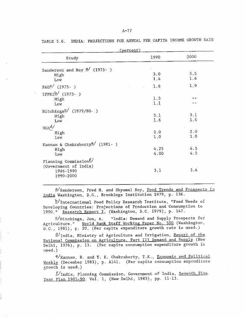
A-77
TABLE 5.6. INDIA: PROJECTIONS FOR ANNUAL PER CAPITA INCOME GROWTH RATE
('-percent)Study 1990 2000
Sanderson and Roy —/ (1975- )High 3.0 3.5Low 1.4 1.6
FA0£/ (1975- ) 1.6 1.9IFPRI—/ (1975- )
High 1.5 —
Low 1.1Hitchings^/ (1979/80- )
High 3.1 3.1Low 1.6 1.6
NCAd/High 2.0 2.0Low 1.0 1.0
Kannan & Chakraborty^/ (1981- )High 4.25 4.5Low 4.00 4.5
Planning Commission^/ (Government of India)
1986-1990 3.1 3.41990-2000
£*/Sanderson, Fred M. and Shyamal Royt Food Trends and Prospects in India Washington, D.C., Brookings Institution 1979, p. 136.
k/International Food Policy Research Institute, "Food Needs of Developing Countries: Projections of Production and Consumption to 1990." Research Report 3 . (Washington, D.C. 1979), p. 147.
£/Hitchings, Jon, A. "India: Demand and Supply Prospects for Agriculture." World Bank Staff Working Paper No. 500 (Washington, D.C., 1981), p. 20. (Per capita expenditure growth rate is used.)
<1/India, Ministry of Agriculture and Irrigation, Report of the National Commission on Agriculture. Part III Demand and Supply (New Delhi, 1976), p. 13. (Per capita consumption expenditure growth is used.)
®/Kannan, R. and T. K. Chakraborty, T.K., Economic and Political Weekly (December 1983), p. A141. (Per capita consumption expenditure growth is used.)
~/India, Planning Commission, Government of India, Seventh Five Year Plan 1985-90. Vol. 1, (New Delhi, 1985), pp. 11-13.
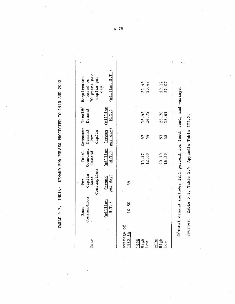
A-78
oooCM
O
OO sas
<HQs
mW9
p Hp (D P£ £ (X CD s’CD Os CO
(X £CD T J 8 cd oP 0) cd p cd •H
*i-I CO p *H T 3 rH£ cd bO PM iHc r p cdCD O 0 e
P i
i n r -* cm< t < f t H O
<t cn i--CM CM CM CM
VbOcdPCOcd&
£cd| - a p i^S.f t £ * 5
cd cd f t Hp a rHO CD s ’H Q aP f sCD x d cd co j h
p S cd3 cd P *H cd T>m a CD pL P£ CD Pm cd S i po a o V p
u p i
P £f t (!) £ Ocd a £ *p •p 3 cd f t £ho w e i—( •*
E-t £ P *P sO P ) 6o v -
£ocd
p p p w Wp CO a 6 cdp <X cd cd T 3
CM cd t f ) 3 Po CO S j P
£ *— P0 P
£o £
* r l Op *iH
P Q . r—1CO g rHcd 3 *H
CO s£o
o
pcd0)
> *
CM CM vO f t<t r-. r - so
t3§
v o < f c o c o T ii—I f t CM f I P
P CO
< t i - - o o<1- -cfr i n < f
- 0pP
4-1
po44
r s o o a s o sco co r-> cm
cm o vof t f t CM f t
P£PopCl)P
i n
CM
cnco co0)
1o£
■H
§i
4-1O
CD stfbD oocd 'P CM 0) CO t> O ' <i fl
S K- bD £ *i-l o S ►£
, £bO £ •H OIX! Pi
cdPo
H
> Sources:
Tabl
e 5.3, T
able
5.4,
Appe
ndix
Tab
le I
II.2.
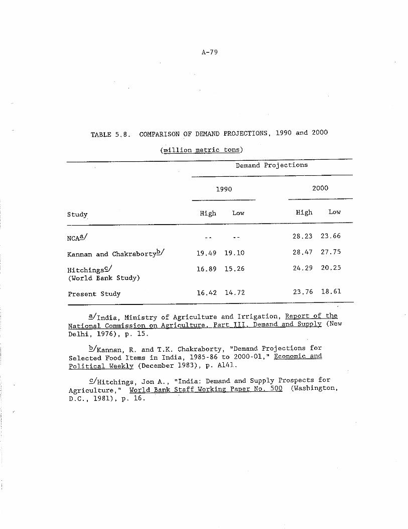
A-79
TABLE 5.8. COMPARISON OF DEMAND PROJECTIONS, 1990 and 2000
(million metric tons)Demand Projections
1990 2000
S tudy High Low High
NCA—/ ■- •- 28. 23 23..66
Kannan and Chakraborty-/ 19..49 19.,10 28..47 27..75
Hitchings^/ 16..89 15..26 24..29 20,.25(World Bank Study)
Present Study 16 .42 14..72 23,.76 18 .61
5/India, Ministry of Agriculture and Irrigation, Report of the National Commission on Agriculture. Fart III, Demand and Supply (New Delhi, 1976), p. 15.
k/Kannan, R. and T.K. Chakraborty, "Demand Projections for Selected Food Items In India, 1985-86 to 2000-01," Economic and Political Weekly (December 1983), p. A141.
£/Hitchings, Jon A., "India: Demand and Supply Prospects for Agriculture," World Bank Staff Working Paper No. 500 (Washington, D.C., 1981), p. 16.
A- 80
Compared to the present study, the demand proj ections made by Kannan and Chakraborty appear to be overestimated. The projected rates of income growth used in the study by Kannan and Chakraborty appear to be very optimistic and perhaps account for the overestimation of demand projections.
While interpreting the results of this study, the limitations of the data and the methodology need to be borne in mind. First, because of the dated and imprecise nature of actual consumption statistics, estimates of disappearance have been used as baseline consumption. This may not reflect actual consumption.
Second, to the extent that changes in income distribution might take place, demand would be affected according to marginal propensities to consume at various income levels. , No account of this has been taken.
t the absence of prices in the analysis is an obvious limitation to projections based on cross-sectional data. Relative prices are assumed to be constant, whereas they would respond to changing consumption patterns and production levels. The technology of the future may influence the relative prices of pulses, cereals, vegetables and animal products, and to the degree that dietary patterns are affected by these changes (which will depend upon the price elasticities of the different commodities), actual consumption levels will differ from the projections obtained in this study.
Other factors--such as future government policies regarding price supports, procurement, levies on producers or millers, and imposition of rationing--will also influence production and, ultimately, consumer demand. All have been ignored in this study.
Nonetheless, the study does provide a broad idea of the magnitude of the demand for pulses by the end of the century. The present availability of pulses is of the order of 11 million metric tons. With an estimated demand of about 24 million metric tons, based on the high scenario, production will have to more than double if the projected demand is to be met.
If the production trends of the past two decades are any indication, meeting the future demand for pulses is indeed a formidable task that challenges agricultural scientists and administrators alike.
CHAPTER VIESTIMATING PULSE PRODUCTION IN 1990 AND 2000
The -probable demand for pulses in 1990 and 2000 having been estimated, we now examine the potential for pulse production and the extent of the gap between demand and supply.
It was seen in Chapter III that one of the consequences of the Green Revolution was to shift acreage away from pulses to high-yielding variety cereals in irrigated areas where the response of the HYVs was greatest. In the northern wheat belt, where irrigation and HYVs spread faster than in any other part of the country, pulse acreage was most adversely affected. As a result, after the mid-1960s there was a shifting away of pulse area from the irrigated northern region into tne predominantly rainfed areas of central and peninsular states.
The last seven to eight years, however, have witnessed a small but perceptible change in the situation, as the new pulse technology in the form of short-duration varieties is spreading, and has begun to make an impact on the farmers' fields. This augurs well for the future of pulse production in the country. While the bulk of production will continue to come from rainfed areas, it is expected that production from irrigated areas will play an increasingly important role.
New Technology for Pulses: Potential for._Xncsgfl&e_lii_A££&
Short-Duration VarietiesThe breakthrough in pulse technology, unlike in the case of wheat
and rice, has not come in the form of high-yielding varieties, but in the development of short-duration varieties. These short-duration varieties have made it possible for double cropping to take place in areas where only a single crop was previously cultivated. The short- duration varieties have been developed mainly for redgram, greengrain and blackgram, which has made it possible for these pulses to fit into crop rotations which were not possible before. Pulses which previously competed with cereals for the same land have now begun to be sown during the season where the land would ordinarily be left fallow, leading to the possibility of double and triple cropping intensity.
Gram. It is by far the most important of pulse crops. Although a number of improved varieties have been developed, they respond to improved agricultural practices and a package of inputs. Gram continues to be a rabi crop and as such competes for land with other rabi cereals particularly high-yielding varieties of wheat. No majoi breakthrough has yet been achieved in evolving gram varieties which could be fitted in crop rotations to avoid competition with rabi cereals.
A- 81
A- 82
Redgram. The traditional varieties of redgram were almost perennial crops having a maturity period of 8 to 10 months. With the development of short-duration varieties, which mature after 5 to 6 months, redgram has become a seasonal crop, which can be fitted into annual rotations. The short-duration varieties have opened up vistas for double cropping as well as crop sequences which were not possible with the traditional varieties.
Varieties of redgram which mature in less than 150 days have made feasible a wheat-redgram rotation in the irrigated northern wheat growing region. It has been estimated that the production of redgram could be increased an additional 1.5 million tons from an expanded area of 1 million hectares by the early 1990s, in the states of Punjab Haryana, western Uttar Pradesh and Rajasthan alone, by the adoption of the wheat-redgram rotation [40, PP. 18-19]. The yield potential of these varieties is 1500 to 2000 kilograms per hectare [11, p. 32]. In Punjab the area under redgram increased almost six-fold during the years 1976/77 to 1982/83 [36, p. 135], However, the cultivation of short-duration redgram varieties in Punjab is still in its infancy, and in absolute terms the increased production has not made a significant contribution to overall production. Its importance lies in its scope for the future.
Greengrattr It is the new varieties of greengram which offer the largest potential for a major breakthrough in production in the next two decades. Short-duration varieties of greengram mature in less than 70 days. This very short period of maturity gives the crop a uniqueadvantage in cropping patterns. It need not compete with cereals in the traditional rabi and kharif seasons, but can be cultivated during the summer fallows, after the rabi crop has been harvested and before the kharif crop is sown. The fields are usually left vacant during this time. Since these are the hot, dry summer months, this kind of crop rotation requires irrigated land for short-duration greengram varieties.
With the spread of short-duration greengram varieties, there has been a marked expansion in area in the states of Uttar Pradesh, Orissa and Bihar. This can be seen from Figure 6.4. More importantly, farmers in irrigated areas are no longer restricted to double cropping' but can think in terms of triple cropping systems. It is now possible to practice a three crop rotation such as wheat-greengram-rice, wheat- greengram-maize or wheat-greengram-sorghum in the irrigated areas of the northern states [40], This is a major change for Indian agriculture .
Intercropping of Pulses with Other Crons
Another method of increasing area under pulses is through inter- cropping of legumes with cereals and other crops which result in bonus yields of pulses without significantly affecting the yield of the crop. main
A- 83
While the short-duration varieties are more suited to the irrigated areas, in rainfed regions long- and mid-duration varieties are being used in suitable intercrop combinations with cereals and other crops to increase the effective area under pulses. In fact, the traditional redgram varieties have seldom been cultivated as pure stands. Redgram is usually intercropped with sorghum, millets, or maize. This is one of the reasons why agricultural scientists believe that redgram production is grossly underestimated [56., p. 19] .
The ability of redgram to tolerate drought has made it a favored crop in low rainfall areas suitable for mixed cropping. In combination with sorghum, the long duration redgram crop allows the former unrestricted growth for the first four months. By the time the sorghum is ready for harvest, the redgram crop has sent its roots deep into the soil, using the residual moisture to thrive for the next four or five months, making a more complete use of the land than would have been possible through an alternate cropping pattern. It has been observed that such a crop combination makes the redgram less susceptible than a pure stand to wilt disease [46]. Long- and mid-duration redgram will continue to be an important crop in regions which are rainfed. With improved agronomic and cultural practices, the yields in intercropping systems can be increased further.
Studies in Andhra Pradesh have indicated that medium-duration redgram varieties can•be grown successfully as intercrops with short- duration pulses such as greengram and blackgram. Advantage is taken of the initial slow growth characteristic of the redgram crop. The greengram or blackgram crop yields about 400 to 600 kilograms per hectare in about 65 days, before redgram picks up growth. This not only results in an increase of pulse production per unit area, but also increases the income of the farmer [21].
In the state of Gujarat, where the area under redgram has increased significantly, the intercropping and relay cropping of redgram with millets, sorghum, other pulses and groundnut is opening up the possibilities of further expansion in area. Other pulses such as greengram, blackgram and cowpea have been tried In suitable combinations with cotton, sugarcane and fruit crops [55].
In rainfed regions the potential for expansion in area is likely to come, on the one hand, from increase in cropping intensity, and, on the other, with the cultivation of improved pulse varieties in suitable mixed and Intercropping systems with cereals, commercial and plantation crops [45].
Xn irrigated areas, the short-duration varieties which can be fit into a third cropping season are likely to gain popularity since they would not compete with cereals. The technology developed for summer greengram has already attained wide acceptability in many irrigated regions of the north. In addition to increasing pulse production, the summer pulse technology has created a significant employment potential during the lean period at an estimated 59 mandays
A- 84
per hectare during the life cycle of the crop [11, P- 34] . With the continued increase in irrigated area, it is estimated by Chandra that summer pulse area might rise to about 5 million hectares by 2000 [ 11, p. 34]. This appears to be an unduly optimistic estimate. Since the current area under greengram and blackgram cultivated during both rabi and kharif seasons is about 5.3 million hectares, it does not appear likely that acreage under the summer cultivation alone would increase by 5 million hectares.
Chandra [11] has identified an additional 9 million hectares of land that could be brought under pulse cultivation using the various technologies discussed above. These are described in Table 6.1. Considering that the current area under pulses is about 22 million hectares, this implies an increase of about 40 percent. It also suggests that of the increased area 67 percent is expected to come from irrigated lands, and that summer greengram and blackgram are likely to play an increasingly important role in the future.
Current Pulse Technology: Potential for Increase in Yield
Present pulse technology consists of a number of improved varieties of various pulses. With use of improved varieties and the recommended cultural practices, significant increase in the productivity of pulses has been achieved in national demonstrations on farmers' fields; however, such increases are not comparable to those achieved for wheat or rice.
With improved agronomic and cultural practices, the yields of gram have been known to increase from 2500 to 3000 kilograms per hectare, compared to a national average of about 700 kilograms per hectare F4o! p.19]. For pigeonpea, yields of 2100 kilograms per hectare arepossible, as against the present average of 700 kilograms per hectare [ 1, p. 291]. Other pulses have also responded significantly to improved management techniques [41, p. 291].
The recommended package of practices consists of [11]:
1) providing a minimum of one but preferably two irrigations whenever possible and moisture conservation practices on drylands,
2) use of seed inoculation with appropriate rhizobial culture,3) application of phosphatic fertilizer,4) timely weed control through pre-emergence weedicldes or
manual weeding, and5) providing plant protection cover.
Greengram and blackgram are mainly cultivated during the kharif season when they are highly susceptible to yellow mosaic virus (YMV) disease. Various estimates have shown that yields of these pulses can be reduced from 30 to 70 percent due to the incidence of YMV. This is one of the reasons why the yields of greengram and blackgram are among
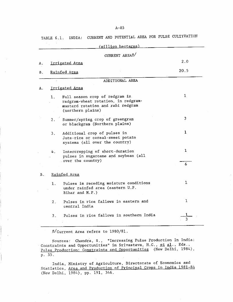
A-85
TABLE 6.1. INDIA: CURRENT AND POTENTIAL AREA FOR PULSE CULTIVATION
____ ___________________ (million hectares')___________________________—
CURRENT AREA—/9 nA. Irrigated Area
B. Ralnfed Area 20.5ADDITIONAL AREA
A, Irrigated Area1. Full season crop of redgram in 1
redgram-wheat rotation, in redgram-mustard rotation and rabL redgram (northern plains)
2. Summer/spring crop of greengram 3or blackgram (Northern plains)
3. Additional crop of pulses in 1Jute-rice or cereal-sweet potatosystems (all over the country)
4. Intercropping of short-duration 1pulses in sugarcane and soybean (allover the country) ---
6
B . Rainfed Area
1. Pulses in receding moisture conditions 1under rainfed area (eastern U.P.Bihar and M.P.)
2. Pulses in rice fallows in eastern and 1central India
3. Pulses in rice fallows in southern India __13
—/current Area refers to 1980/81.
Sources: Chandra, S., "Increasing Pulse Production In India:Constraints and Opportunities" in Srivastava, H.C., et al., Eds., Pulse Production: Constraints and Opportunities (New Delhi, 1984), p. 35.
India, Ministry of Agriculture, Directorate of Economics and Statistics, Area and Production of Principal Crops in India 1981-84 (New Delhi, 1984), pp. 191, 346.
A- 86
the lowest of the pulses, with an average of 400 kilograms per hectare. With the introduction of YMV-resistant varieties, there is a potential for increasing yields to 1500 kilograms per hectare, and increasing stability in production [11, p. 33].
The current pulse technology therefore has the potential to increase yields of pulses. However, in spite of the existing technology, productivity of pulses continues to remain at levels much below those obtained on national demonstration trials on farmers' fields. This is because the new technology requires intensive agronomic practices and superior management, and is often rejected by the farmer as beyond his means. This is evident from the fact that pulses continue to be grown on marginal lands, with low allocations of irrigation and fertilizer, despite evidence from experimental and on- farm trials about the positive response of these crops to modern inputs. If the impact of the technology is to be realized in the field, a greater effort is needed in the future to increase availability of improved varieties of seeds and other inputs, and to strengthen the extension system.
Estimating Pulse Production in 1990 and 2000Methodology
Projections of supply raise more complex problems than those of demand. To estimate the latter, there are a number of studies that provide reasonably good estimates of income and expenditure elasticities. Official statistics are available on population and income growth which can be used together with income elasticities to project future demand.
Compared to this, the limitations of the available knowledge of the production function, the problem of predicting the movement of prices and the lack of reliable information on price elasticities of supply, make it difficult to estimate pulse production possibilities over time with a sufficient degree of confidence.
If relative prices are to be used as an instrument to determine the future production of pulses, we need reliable empirical data on the extent of responsiveness of supply to price movements. For instance, if the price elasticity of supply for pulses was both positive and significant, an increasing trend in the relative price of pulses would imply a positive supply response and greater production. Figure 6.1 indicates what has happened to the relative price of pulses over the last two decades. The price fluctuations as evidenced in Figure 6.1 are so wide as to obscure any strong trend.
Also, reliable information on supply elasticities is not available . The problem is further complicated by the fact that supply responsiveness Is not uniform, but varies for different pulses, regions and time periods.
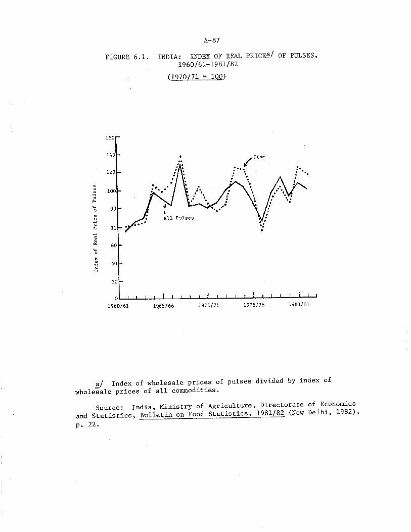
A-87
FIGURE 6.1. INDIA: INDEX OF REAL PRICE^/ OF PULSES,1960/61-1981/82
(1970/71 - 100)
a/ Index of wholesale prices of pulses divided by index of wholesale prices of all commodities.
Source: India, Ministry of Agriculture, Directorate of Economicsand Statistics, Bulletin on Food Statistics, 1981/82 (New Delhi, 1982),p. 22.
A-88
Several studies have been conducted on the acreage, rather than output, response of various crops to relative price movements. However, most of them have concentrated on cereals and cash crops [61, pp. 73-74]. Pulses have not merited enough attention, and sufficient information on price elasticities of acreage for pulses is not available .
However, on the basis of existing studies, it was found that supply elasticities, though positive, were of low magnitude for most of the major foodgrain crops of India. Gram was one of the crops included. This would imply that price by itself as a tool for increasing pulse production would not be very effective [42., p. 24] , unless yields could also be increased.
In spite of these limitations, it is necessary to provide some quantitative idea of the magnitudes of likely availabilities of pulses relative to demand m the projected period. This would serve as the basis for the formulation of long-term policies and programs.
A simple approach is therefore adopted for estimating pulse production. The magnitude of the projected supply is determined as a product of the projected area and the projected yield of pulses.
In using this approach the following assumptions are made:
1) that normal weather will prevail during the projected year,2) that relative prices will remain essentially constant,
although in reality relative prices will change, shifting both supply and demand to offset persistent large imbalances, and
3) that no major breakthrough in technology will occur resulting in dramatic increases in yield.
=*nd yield projections are made for individual major pulses in different states, and then totaled to obtain the national estimates. This procedure is adopted since area trends for various pulses are different in the major producing states, and the levels of yields also vary considerably.
Projections of supply are made on the basis of estimated compound growth rates of area under pulses during the period 1970/71 to 1982/83. The areas in 1990 and 2000 are projected by a simple extrapolation of past trends. Production is then estimated on two different assumptions regarding yields, giving high and low projections. There appears to be considerable year to year variation In the yield of various pulses in different states, and it is difficult in most cases to identify any clear trends in yields. Consequently, it is not possible to follow the method of extrapolation employed for area. Therefore, the following procedure has been adopted. The low scenario yield has been obtained by taking the average of the last five years, i.e., 1978/79 to 1982/83. The highest average yield achieved in any year in the state during the period 1970/71 to 1982/83 is set as the higher level. For example,
A- 89
Figure 6.3 shows that the yield of redgram in the state of Uttar Pradesh has varied between 588 kilograms in 1973/74 to 1540 kilograms per hectare in 1972/73. The latter was the highest yield achieved and has therefore been set as the upper level. In the case of Karnataka the yield has ranged from 331 kilograms per hectare in 1971/72 to a maximum of 695 in 1977/78. The high projection in the case of Karnataka has, therefore, been taken as 695 kilograms per hectare.
True, this procedure is arbitrary, but in the absence of any clear trends it is difficult to employ any other approach. Estimation is made more difficult by the fact that more than 90 percent of pulse area is rainfed and the yield of pulses in these areas will continue to fluctuate with variations in weather.
A second source of uncertainty in yields is the susceptibility of these crops to diseases and insects. While efforts are being made to ensure plant protection through the use of chemicals, the prohibitive cost of inputs for such measures has prevented any significant impact on the farmers' fields. This is likely to continue for some time in the future.
While double and triple yields have been obtained with the use of improved varieties and the recommended package of practices, these have been limited to demonstration plots and a very small percentage of farms. The yields in traditional farming systems have stagnated almost at the same level for the last three decades. The main reason for this is the fact that pulses are grown on marginal lands as low priority crops with little or no inputs. Unless a deliberate effort is made to change this attitude through extension and an improved supply of inputs, there is not much likelihood of a significant increase in yield. However, if there is a breakthrough in pulse technology resulting in high-yielding varieties, or a change in the attitude of cultivators towards using greater inputs for pulses, the yields of pulses might be higher than those projected in this study. But if trends of the past 10 years are any indication, this does not appear very likely.
Projections for Individual Pulses
Gram (Cicer arietinunO . Gram is cultivated as a rabi crop. It is raised with the help of residual moisture, generally after a kh&rif crop, and requires cool, dry weather conditions for optimum growth. The northern plains of India, including the states of Punjab, Haryana, Bihar, Uttar Pradesh, Madhya Pradesh and Rajasthan are best suited for gram production. Figure 6.2 shows the major gram producing states which together account for about 83 percent of area and 92 percent of production of gram. In the states of peninsular India it is a crop of minor importance, mainly because the winter season is shorter and milder, and horsegram fits better in crop rotations. The cultivation of gram also declines in the extreme eastern and western regions of the country.
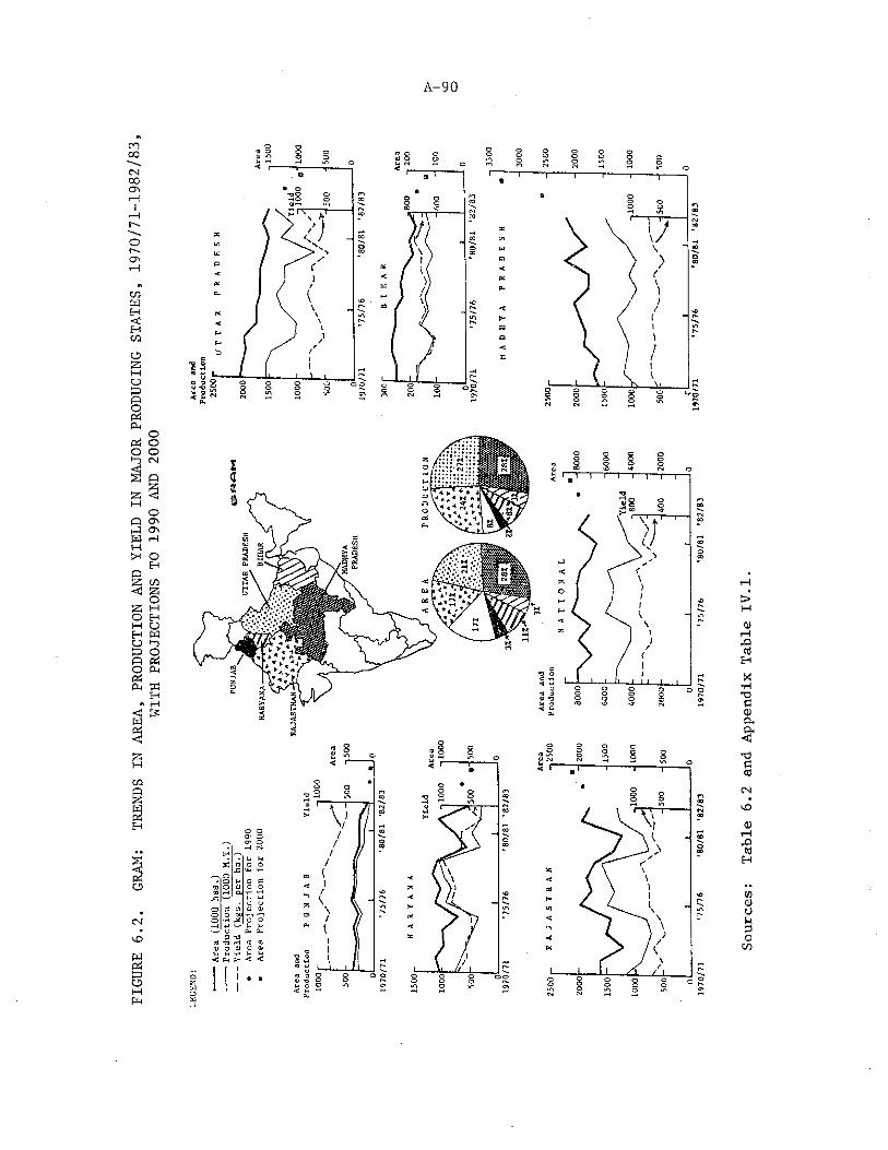
FIGU
RE 6
.2.
GRAM:
TREN
DS I
N AR
EA,
PROD
UCTI
ON A
ND Y
IELD
IN
MAJO
R PR
ODUC
ING
STAT
ES,
1970
/71-
1982
/83,
WITH
PRO
JECT
IONS
TO
1990
AND
2000
A-90
Sources:
Tabl
e 6.2
and
Appe
ndix
Tab
le I
V.1
A-91
The gram crop remains in the field from 4 to 6 months depending on the length of the cold season and the varieties grown, Gram is susceptible to frost but is fairly tolerant to drought because of its deep root system. This characteristic is made use of in various crop mixtures. Wheat grown on unirrigated land is often mixed with gram during seeding. In the event of weather conditions proving too dry for wheat, the gram crop compensates for loss in wheat yields. The wheat-gram mixture acts to some extent as an insurance against adverse weather. Gram is cultivated predominantly as a rainfed crop, only 20 percent of area under this crop being Irrigated [16, p. 347].
Table 6.2 indicates the projected area and production of gram by state. Production in 2000 is expected to rise by 20 percent based on the assumptions of the high scenario. It will increase from an average of 4.7 million tons during 1981-83 to 6 million tons in 2000.
At the national level the area under gram is likely to expand by 17 percent increasing from an average of 7.2 million hectares during 1981-83 to 8.5 million hectares In 2000. Gram acreage In Punjab, Haryana, Uttar Pradesh and Bihar is projected to decline, while in Madhya Pradesh and Rajasthan is expected to increase. In the future Madhya Pradesh and Rajasthan are likely to emerge by far the largest producers of gram. It appears that cultivation of gram will shift from Its native habitat in the Gangetic plain to the central states.
Redgram .(Calanus caian1) . Redgram Is the second most widely grownpulse crop. It accounts for about 13 percent of total pulse area and contributes 19 percent to total production. India produces over 80 percent of the world's total production of redgram [12, p. 81].
The crop is adaptable to a fairly wide range of climate and soils and is cultivated almost all over the country except in regions with excessive rainfall and waterlogging or in areas which are affected by severe frost. Its deep root system enables It to withstand moisture stress conditions; consequently it is widely grown in the semi-arid agricultural regions of the central and peninsular part of the country. The major redgram producing states are shown in Figure 6.3. They account for about 91 percent of total area under the crop and 89 percent of production.
The traditional redgram was a kharif crop and had a maturity period of eight to ten months. Development of short- and medium- duration varieties have made it possible to fit redgram into double cropping systems with wheat in a:reas of assured irrigation, such as the canal irrigated areas of Rajasthan, Punjab, western Uttar Pradesh, northern Madhya Pradesh and Haryana. These varieties planted in June-July with the onset of monsoon can be harvested in late October or early November, vacating the field in time for the wheat crop in rabi[4Z].
Short-duration varieties have made it possible to cultivate redgram in nontraditional areas as well as in nontraditional season.
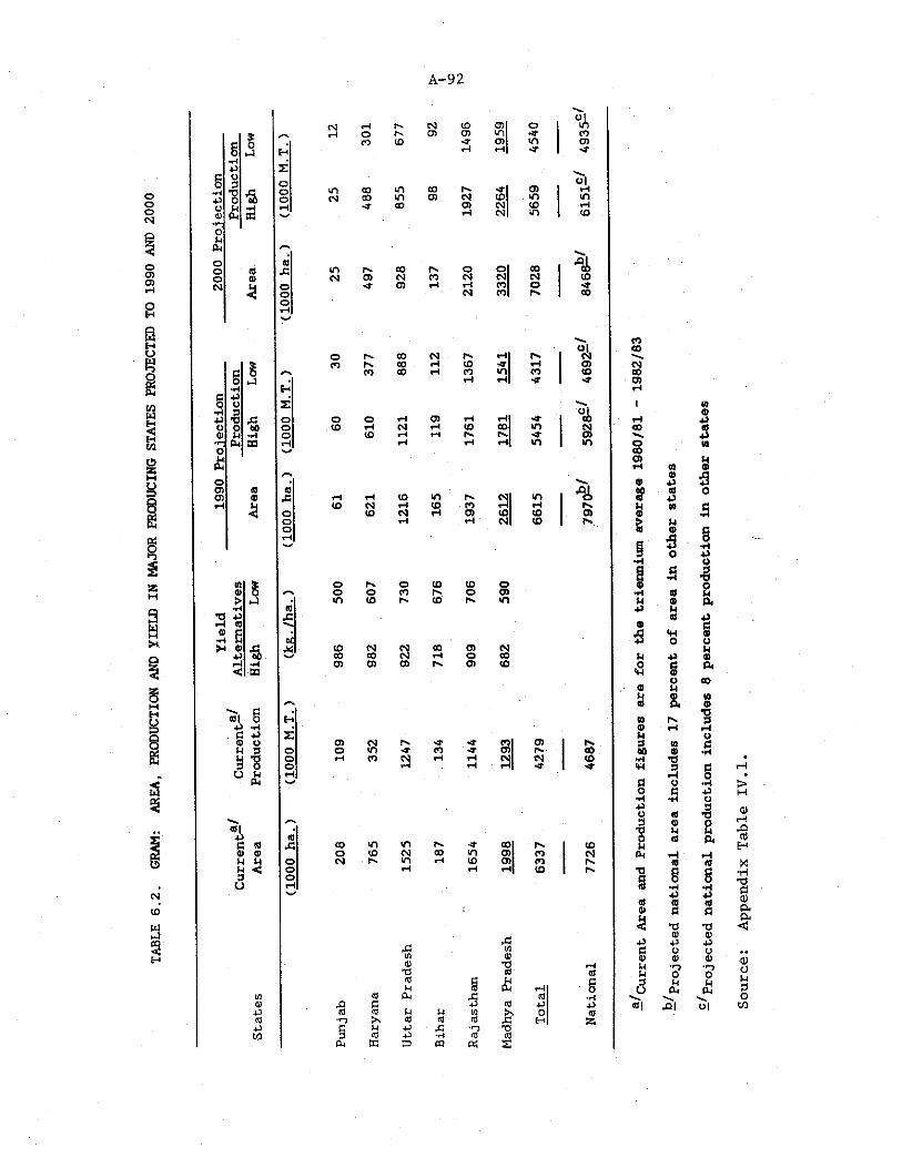
TABL
E 6.2.
GRAM
: AR
EA,
PROD
UCTI
ON AND
YIE
LD I
N MA
JOR
PROD
UCIN
G ST
ATES
PRO
JECT
ED T
O 1990 A
ND 2
000
A-92
■a-w3S
olrH pH CM to CD O ino ph m CD m ta COCO to -T CD in CDrH rH ■a- I sf
. ol00 m CO Ph ■a- CD rHCO m CD CM to m m
CO O) CM to rHH CM m 1 to
Ph CO p. O O CO %CD CM to N CM CM to-M" CD rH rH CO O -a-
CM to r- 1 CO
C s0 p ••H Hc P6 © si■H 3
P TJ P oU O 00 o« tH *rl o•i- Oh CO t*Ho h*uPHO •CD © ' ©CD ©rH
a oOorH
oCO
Oto
p. 00 CM P- rH Ph CMPh CO rH to -T rH CDCO CO rH CO m CO torH rH HT HP
‘—Ol© rH CD rH rH COrH CM H (O CO m CMto rH rH Ph Ph <s- CDrH rH rH w in
rH rH to m pH CM mto CM rH to CO rH rH PHto CM H CD (O to CDrH rH CM to pH
3 H3 EtH ©
P
o PH O to to Os o o CO PH o CDp fO m to pH to PH m
€b£
■a. ,*] to N CM CO CD CMH > CO CO CM rH O 00-H 0) CD CD Ph CD toffl
(01 5s -p>© o M 33 1° a
CD CM pH HP to CD P.o m HP to CD PH. 00rH CO CM rH H CM CM torH rH rH ■HP
•ia ©
r"H«
p CO »n m PH ■a- C0| Ph to© V o to CM CO m CD CO CMM H o CM PH n rH to 0)1 to PHM3
< oOrHH^
rH rH rH) to PH
P w© ©© *0TJ © ©© 9 M cM © D-( r-H ow © Ph p © © •rl© p g p 4) Pp © © H M w fo O ©© •n « © © J3 H 554-) G M P ■ P ■oto 3 © P -tH © ©PH S3 3 m pc; £
mtocoO)
oCOo>
9©
£I**H
3
a
pa©uM
8
*©i
«©p©pw©
5o5«©a*no■poM©APh
P<0*0©■ Po©"OoMO-i
“h.-Ql —^Pr
ojec
ted
nati
onal
pro
duct
ion
incl
udes
8 p
erce
nt p
rodu
ctio
n in
oth
er s
tate
s
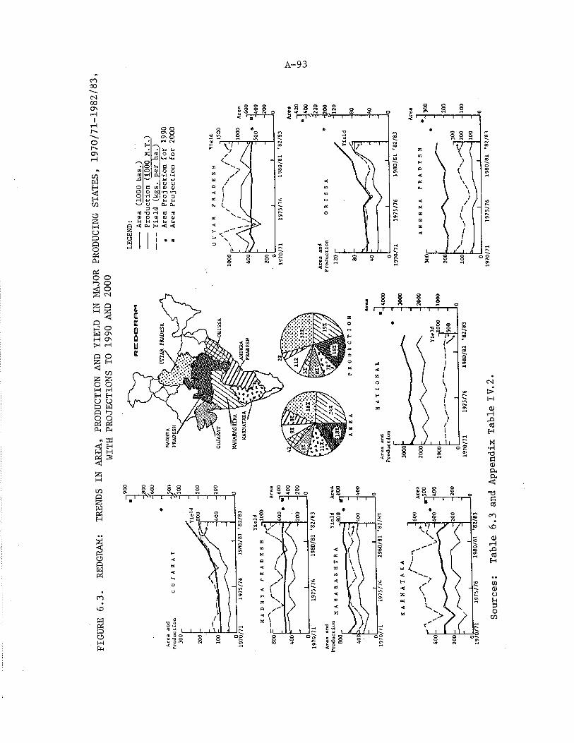
FIGU
RE 6
.3.
REDG
RAM:
TR
ENDS
IN
AREA*
PROD
UCTI
ON A
ND Y
IELD
IN
MAJO
R PR
ODUC
ING
STAT
ES,
1970
/71
1982
/83
WITH
PROJECTIONS T
O 19
90 A
ND 2
000
A-93
Sources:
Tabl
e 6.3
and
Appe
ndix
Tab
le I
V.2
A-94
Redgram can be profitably grown in the rabi season in fields vacated by maize, early paddy and minor millets in areas where the winter temperatures are mild. -Coastal regions of Orissa, parts of Madhya Pradesh, rice growing areas of Karnataka, Tamil Nadu and coastal Andhra Pradesh, where fields are often left fallow, are areas where redgram can be cultivated as a second crop. To make use of the residual moisture, the crop must be sown early in September [58].
The development of improved varieties of redgram suitable for intercropping with sorghum, millets, groundnut, cotton and other pulses, together with fitting short-duration varieties in new cropping patterns, has led to an increase in area of redgram in states like Gujarat, Orissa, Karnataka and Andhra Pradesh. This can be seen in Figure 6.3.
Table 6.3 indicates the projected area and production of redgram by state. Production in 2000 is estimated to rise by about 85 percent, increasing from an average of 2.0 million metric tons during 1981-83 to 3.5 million metric tons in 2000.
At the national level the area under redgram is proj ected to expand by about 50 percent, increasing from 2.9 million hectares to 4.2 million hectares. Uttar Pradesh, the largest producer at present, is expected to maintain its lead in 2000. However, Gujarat and Orissa are also likely to emerge as major producers. Of the 2.3 million hectare increase in area under this crop, Orissa, Gujarat and Karnataka are expected to account for more than 50 percent.
It was mentioned earlier that according to one estimate [40] the redgram acreage could be expanded by 1 million hectares in the states of Punjab, Haryana, Uttar Pradesh and Rajasthan. However, the Increase in acreage in these states has not yet shown up in the trends indicated by the official statistics. It appears that production of redgram is likely to increase largely in the unirrigated rainfed areas of the central and peninsular states, and to a smaller extent in the irrigated command areas of the northern plains.
Greengram (Phaseolus aureus1) and Blackgram (Fhaseolus muneo1). Greengram and blackgram each account for around 12 percent of total area and 9 percent of production. They are warm weather crops and are more widely and thinly spread than redgram. In the northern states, they are generally cultivated as kharif crops, while in the southern and central states they are grown in both the kharif and rabi seasons. Figures 6.4 and 6.5 show the major greengram and blackgram producing states.
The development of short-duration varieties of these two pulses probably offers the greatest potential for increase in production in the future. These short-duration varieties, which can be harvested in less than 70 days, can be fitted in double and triple cropping as well as intercropping sequences in nontraditional seasons without disturbing
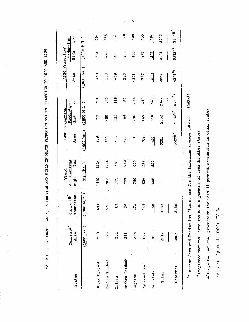
TABL
E 6.3.
REDG
RAM:
AREA,
PROD
UCTI
ON A
ND Y
IELD
IN MA
JOR
PROD
UCIN
G ST
ATES
PRO
JECT
ED T
O 1990 A
ND 2
000
A-95
x„00m
<r CD o CO m < r >n i—lO) *$- CO i"* CO CO CD 'T CO>n CO cn in < r CN m 0 0
H CN CNs '
o o jo CO CO o o CO 1". CO CNo m o o CO r-'. Hf COiH r » -T CO rH CO -a- CO rH mCO CO
njX 0 ) O 0 1 o CO r - . CO %CO CO o (N r*. -T CO CO < ro 'T m ~T CO CO 'O" CO (Nooi—l
CO
Xeo-nta
<T O CD O CO CO CO CNCO hj- rH CO r-. rH hj- ■fl H CNm CO rp CO CN) ip •a- COIN CN OlEh tp
so|CN
l U1Cl>o CO CD rH m CO O) 01 CN rH +1COo m CO m CO CO P CO CO CO Po i-* i—1 -51 CO CO CO 'v. torH CN CN oCO w
fd <0 X!lQ X CD o m CN rH CO C0| m rtH CO CN o r-* m o m o CN< o -r m CN CN m r-v -a- CN mo | to COorHvy
V) S <r <r rH CO to CO COa 0 rH rH CO H CO 00 CN> t-J * CN CN <n CN CO in m*P nf H rHP X(0E «0 ■a XI O CO CD CO o •fl’ m+i v ■T o CO rH CO CO CDrH •P m CO r-. CO 1". to CO< m rH
g0| 5 E-i+1 •P .3 P s0 o Hf CO CO O CN m CN CN COP 3 o <fl- C" 00 m r-. CO -fl- CO COM TD o CO CO rH CO rH CO o3 O o 1—i CNU H rH
Dh
01P3 w
0x o CO rH CO t o r-. c o l r-.
0 0 o CN o CO CN CO CN I—1 COP h o m m rH CN CN CO CO CO COs
U
< ooip
CN CN
X XX V) 0(0 1 0 00 T ) T J 0 r-H
T J 0 0 M 00 P P P 0 gp PLJ Ph X rH O
to Ph p 10 «l 0 •rt0 0 0 0 0 0 P P PP p >1 10 P P P 0 0 0id 0 X to X 0 0 g H S 3
p P T3 ■P - 0 • n%
Mt o P 0 (H 5 3 0
X s O < O s X
0X0 p
0 0 000 P0 0 3M P P0 w
£ M g0 *p
§ X P3 P o•H 0 M
s c0 •p p
•rH aM 0
P 0 p
0 0 gX op tp M
0 0tH ft0 p
*w 3 P0 rH
0 oP 0
0 0 0Q * T3
50 30 CO HJH O3 0 30 0 0 *P•rl T3
3 3rH 03 O •po a p•H ■p o
P 3O 0 ^33 0 0
T3 p P0 0 f tUPH rH H
0 0T J g 30 0 00 *p *P
p P0 0 00T| 3 3
£ T J T l0 0
P P Pg O Cl0 0 0P • o •DP o 03 p M
U PH PH0| X I O l
CN
>
•3EHX•H4)ftft<3
cuou3OCO
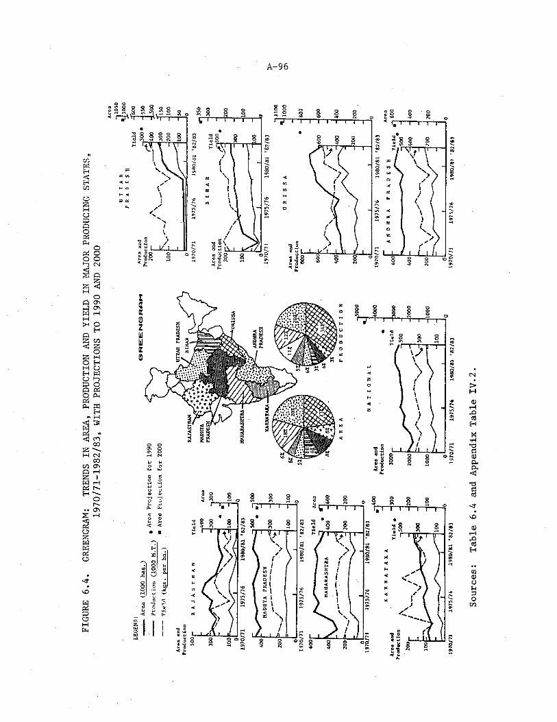
FIGU
RE 6
.4.
GREE
NGRA
M:
TREN
DS I
N AR
EA,
PROD
UCTI
ON A
ND Y
IELD
IN
MAJO
R PR
ODUC
ING
STAT
ES19
70/7
1-19
82/8
3, W
ITH
PROJ
ECTI
ONS
TO 1
990
AND
2000
A-96
Sour
ces:
Ta
ble
6.4
and
Appe
ndix
Tab
le I
V.2
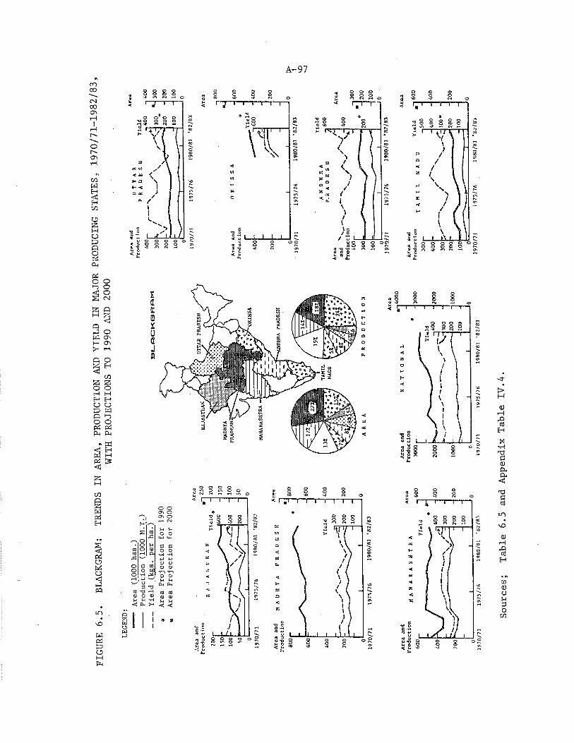
FIGU
RE 6
.5.
BLAC
KGRA
M:
TREN
DS I
N AREA,
PROD
UCTI
ON A
ND Y
IELD
IN MA
JOR
PROD
UCIN
G STATES,
1970
/71-
1982
/83,
WITH
PRO
JECT
IONS
TO
1990
AND
2000
A-97
£ a)ooU3 o 011—1 o<rC
o a too Q CjCo >7-1 ,21rH Uu
3 T303 ♦o ♦H4> o 0)U u< & ><
l-l S4o o
< <l! « aI
Sources;
Tabl
e 6.5
and
Appe
ndix
Tab
le I
V.4
A-98
the existing crop preferences of the farmer for remunerative cereal and cash crops.
In the irrigated areas of the northern states, summer greengram is being cultivated as a third crop. Area under greengram in Uttar Pradesh has increased significantly in the last five to six years with the spread of these varieties. In the rainfed areas of the central and southern states, fields traditionally left fallow after taking either a kharif or rabi crop are now being sown to short-duration greengram or blackgram. Due to double cropping there has been an increasing area trend in both pulses in almost all the states.
Tables 6.4 and 6.5 indicate that the area and production of greengram and blackgram are expected to increase significantly in the future. The estimated production of greengram in 2000 is likely to be more than double the present production, based on the assumptions of the high scenario. It will increase from an average of about 1 million tons during 1981-83 to 2.2 million tons in 2000. The acreage at the national level is expected to rise about 75 percent by the end of the century, increasing from an average of 2.8 million hectares during 1981-83 to 4.6 million hectares in 2000.
At present the major producers of greengram are Orissa, Andhra Pradesh and Maharashtra. In the future, Orissa is expected to maintain its lead; however, Uttar Pradesh is likely to emerge as the next major producer of greengram. Of the 1.8 million hectares increase in greengram acreage, almost 70 percent is likely to come from Orissa and Uttar Pradesh. In the latter the short-duration summer greengram varieties sown on irrigated land are projected to become the major contributers.
In the case of blackgram, too, production is expected to double by 2000, increasing from an average of about 1.0 million tons between 1981-83 to 1.8 million tons in 2000. The blackgram acreage at the national level could increase by as much as 45 percent, expanding from2.8 million hectares between 1981-83 to 3.9 million hectares in 2000. Orissa, Maharashtra, Andhra Pradesh and Madhya Pradesh are the major blackgram producers at present. In the future, Orissa and Madhya Pradesh are likely to maintain their relative importance. In addition, Tamil Nadu will emerge as a major producer. These three states together are expected to account for about 70 percent of the increase in area under this pulse crop.
Horsegram (Dolichos b if Torus'). Horsegram Is a crop primarily of peninsular India and is suited to cultivation during both rabi and kharif in dry regions and upland areas. This pulse crop accounts for about 8 percent of total area under pulses and 6 percent of production. The pulse is used for cattle feed as well as human consumption in the low income groups.
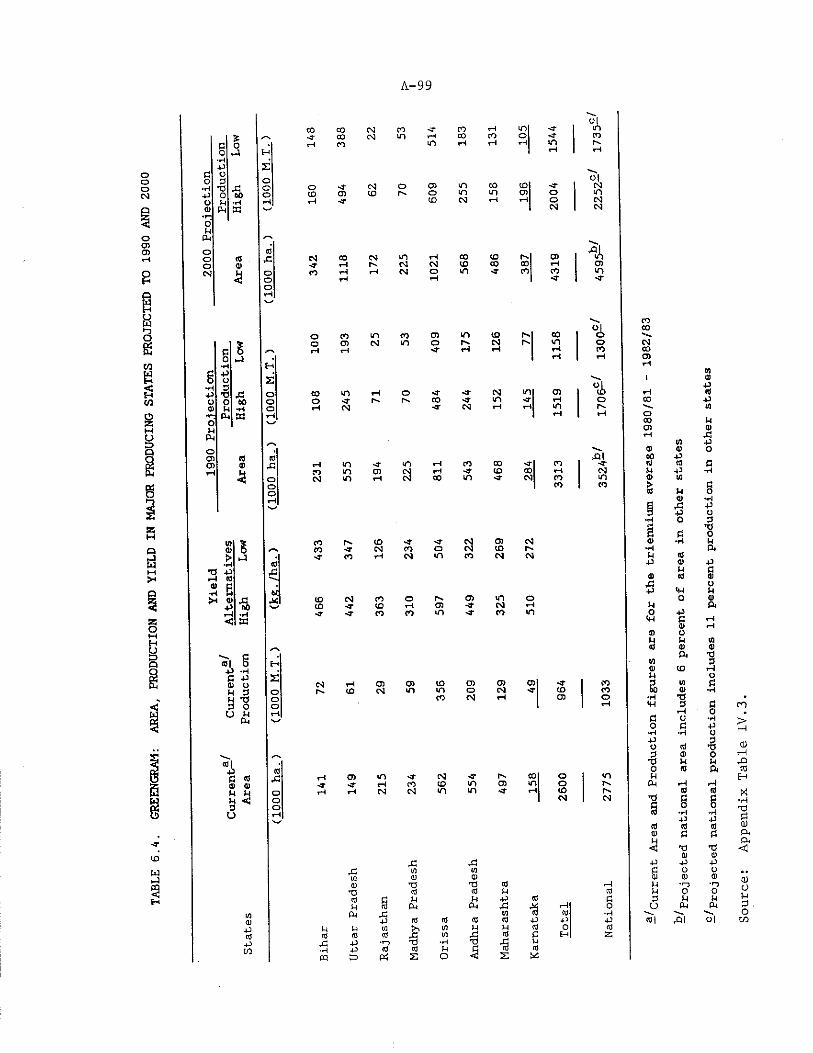
PROD
UCTI
ON AND
YIE
LD I
N MA
JOR
PROD
UCIN
G ST
ATES
PRO
JECT
ED T
O 1990 A
ND 2
000
A-99
towaH
S£ 00 t J H
■HP s
£ OO 3 o
*rH TS 43 oP O (0 ou P -rl t—t;a Pm EG
0M
Pm
o mo (3 4=o 0)eg H o< oo
rM
G S0 .-3•H Xc P6 O S•H aMi ■d 45 oO o 60 o0) Jm -H o*r- Pm W rH6 v-/wPm y'SO •Cl « (0a> 0) 43tH a ooorM
W0)> 1•d pr-i w■«mX
EQ>PrM<
•a
to45
6C421
olCO ao CM CO Mf CO rM m m< • CO CM CO rM CO CO o COrH CO m r"i H rM in r-.rH rM
Oleg o CO >n 00 CD MT CM05 CO o m »n CD O mCO CM rM rM o CMCM CM
CO CM m rH CO CO f- 0) •%1—1 r- CM <N CO CO CO rM O)rH rM CM o in ■3- CO CO inrH rH -T -T
O CO n CO CD in CO CO <3o CD CM in o CM r-' m OrM rM -3- rM rM rM COrM rH
CO n rH o MT *3- CM «1l O) COo •3- r- r-. CO -3- in < t \ rM OrM CM -3- CM rM h | in r-
1 rM rM
rH in in i—1 CO CO <t\ CO -rcn n 05 S! rH Mf CO 00 rM CMCM n i—1 00 in -3- Ml CO in
1 CO CO
CO r-» CO •3" -T CM O) CMCO < r CM CO O CM CO h.3" CO rM CM in CO CM CM
CO CM CO o r-. CD m oCO -T CO rM O) -3- CM rM-3- -3- CO CO m -T CO m
mlPa p0) o H 3 H -ga!u
rH CD O) CO CD O) CD -T CO(O CM m m o CM *3- CO CO
CO CM rM 0) orM
fi « a) 0)u
rH O) m ■3- CM <■ rv CO O m-3- rM CO CO in CD n OrH rM CM CM in m Mf rM COCM r -CM
4545 mm 01CD TJ-a (3(3 € MM (3 Pm
m (U 45 (3<L> P4 0 M M in X(3 (3 (3 (3 454 0 45 4-1 -rj -dCO - r l P (3 (3I n 50 P5 s:
45m0)-d (3 rM(3 P C3u +4 (3 GPm 4513 %
i—1CO 0♦«H
(3 (3 cd 40 M0 40m N P C3 o COm 45 (3 G H Jz;*H TS JG 1Mu a «J (3o <
CO00'-VCMCOCDrM
31l
40rM (303 40toOCO tMCD QJrM 45
CO 40Q) 060 40d to £M 40 t M
l/]> £(0 M 0
•rMs 45 403 +1 U
■H 0 3£ -d£ £ 0© •rl JM
»H P iP <3
40 a 40Pi £
© (3 0)45 O40 <CM JM
O 9!M PO 40
ClM £ rMd) rM
CD oM Vi0)P* •ato 3
© CD rMJM O3 cn £& -rl
•H ■d3 £rM 0
G o •rl0 £ P*tH ■H 0
40 cd 3O •o3 0
T3 H JM0 <3 P iMPm rM M(3 (3T5
§ e•H 8•rl
40 P<3 (3 CO£ £-O *d0) 0)
40 40 pG O 001 WM ■rjM O 03 JM uU p4 P4"-Sh
451 o| Source:
Appe
ndix
Tab
le I
V.
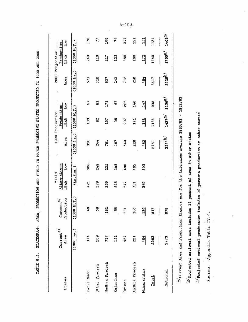
TABL
E 6.5.
BLAC
KGRA
M:
AREA,
PROD
UCTI
ON AND
YIE
LD I
N MA
JOR
PROD
UCIN
G ST
ATES
PRO
JECT
ED T
O 1990 A
ND 2
000
A-100.
d O5 X H*H .43 £c O0 3 o-Pi43 xO -5 ooO d -W pH© Ed w wodEdo CDo (D Xo ©CM H o
< oopH
olCO r>. CO Hf t". id i-HI-'. r. 00 r. •D* CM m CO OpH pH CO iH pH HfH H
o|O CO r'. in CF) CO IN CD O■4f pH i-H cm CO CO f'' -T CDCM pH CM pH CO pH pH 4fpH pH
tH o r>- CO CM o hC ir-. pH CO pH m o> pH CMm CO CO CM n- CM 'T -D- 0)CO 1 CO
d 80 i-J*H E-id 430 O £*H 343 •a X oO 0 bO o© d tH oEd w pHo wdEd p.o .CD « ©CD © XpH d< OoopH
r"» pH iH m o P'. CO 103 CO r o to HT CO mi-H CM pH rH O) pH1 pH
CO (N n- CO h* pH COCO CD O) CD CD n- CO mpH pH CM pH pH pHpH
CO HT pH CO CO CM pHpH CO CO -S’ CM CO COCO CM pH m CM Hf r-CM
CM-T
pHCO
% CO 03 m in CO m in0 o •T CM o CO CO oCO CM CM to Hf <■ CO
•aMMl pH 03 03 m rv pH 03CM n. m rH Hf m HT■M- CO CM m in n. CO
©I 54-3 ’H C 43o> od 3 CO 03 CM m pH O CD n»-T »n CO m CO CO CO pHpH CM rH pH COCOr>.o
«l-upi « V 0)g*u
©Aooo
•T 03 pv pH r-v pH •sr CO con- O CO m CM CO CO (N.pH CM Cn. pH cM hT COCM NN
CD(V4-3CD4-3tn
idnd Vi ©Vi © ©© x! X ©3 TD « © dTJ W M d IH 43(D M Ed a 0h id pH55 Ed © id © Vi ©43 © © 43»—1 IH Eo m ID d d 0'H « © ID id © Hi 4343 X© -1-5© ■Hd Xd •s£h 33 £ O ■3 £
CO00CMCO0 3
t00§
0)d©%
©IH
©
w©d3»
s■H40O0M01
4->dmuu3u
to©43©43to
Uffi50am®yO43Od8.
COp H
w©
o.5CD©MCD
CO843<0dX©4-3O©
.1-5odfdXI
' M ©43m
u©5O
43SH:
Ut4
8,O)
a
§•H43O•88a■d843<0dx©43U©■nO£o|
0)oJH3oCO
Appe
ndix
Tab
le I
V.4.
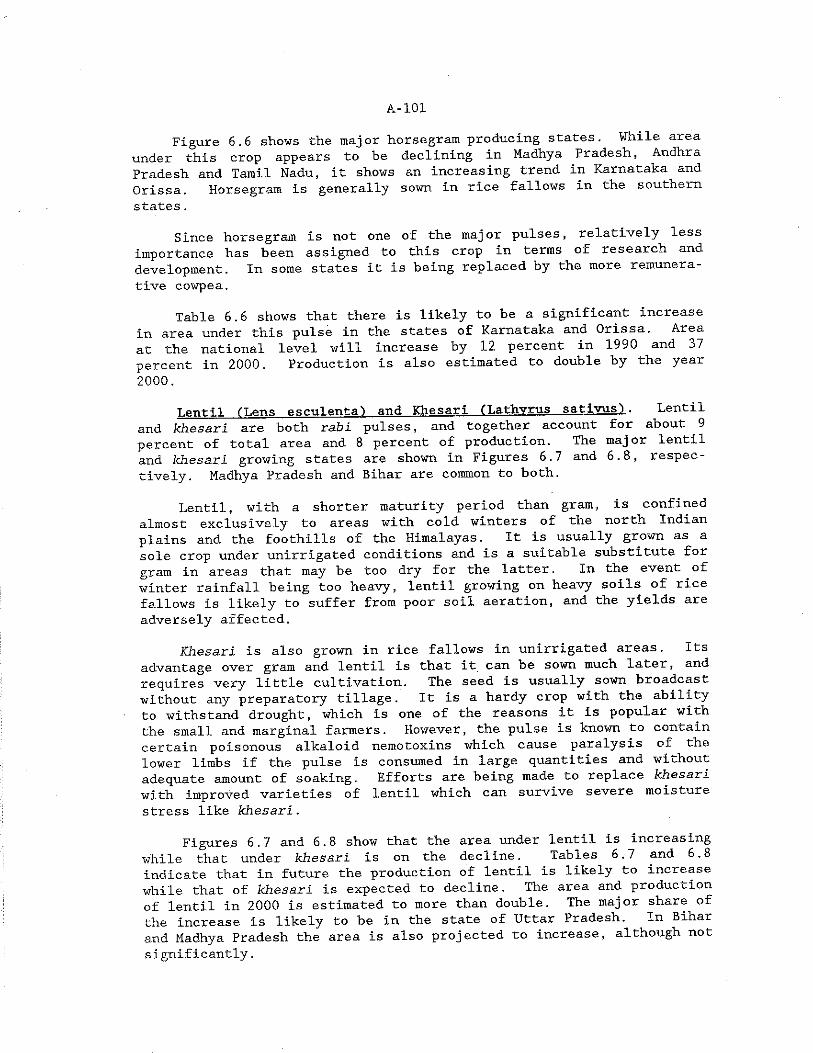
A-101
Figure 6.6 shows the major horsegram producing states. While area under this crop appears to be declining in Madhya Pradesh, Andhra Pradesh and Tamil Nadu, it shows an increasing trend in Karnataka and Orissa. Horsegram is generally sown in rice fallows in the southern states.
Since horsegram is not one of the major pulses, relatively less importance has been assigned to this crop in terms of research and development. In some states it is being replaced by the more remunerative cowpea.
Table 6.6 shows that there is likely to be a significant increase in area under this pulse in the states of Karnataka and Orissa. Area at the national level will increase by 12 percent in 1990 and 37 percent in 2000. Production is also estimated to double by the year 20 00 .
Lentil fLens esculenta') and Khesari (Lathyrus sativusj . Lentil and khesari are both rabi pulses, and together account for about 9 percent of total area and 8 percent of production. The major lentil and khesari growing states are shown in Figures 6.7 and 6.8, respectively. Madhya Pradesh and Bihar are common to both.
Lentil, with a shorter maturity period than gram, is confined almost exclusively to areas with cold winters of the north Indian plains and the foothills of the Himalayas. It is usually grown as a sole crop under unirrigated conditions and is a suitable substitute for gram in areas that may be too dry for the latter. In the event of winter rainfall being too heavy, lentil growing on heavy soils of rice fallows is likely to suffer from poor soil aeration, and the yields are adversely affected.
Khesari is also grown in rice fallows in unirrigated areas. Its advantage over gram and lentil is that it can be sown much later, and requires very little cultivation. The seed is usually sown broadcast without any preparatory tillage. It is a hardy crop with the ability to withstand drought, which is one of the reasons it is popular with the small and marginal farmers. However, the pulse is known to contain certain poisonous alkaloid nemo toxins which cause paralysis of the lower limbs if the pulse is consumed in large quantities and without adequate amount of soaking. Efforts are being made to replace khesari with improved varieties of lentil which can survive severe moisture stress like khesari.
Figures 6,7 and 6.8 show that the area under lentil is increasing while that under khesari Is on the decline. Tables 6.7 and 6.8 indicate that in future the production of lentil is likely to increase while that of khesari is expected to decline. The area and production of lentil in 2000 is estimated to more than double. The major share of the increase is likely to be in the state of Uttar Pradesh. In Bihar and Madhya Pradesh the area is also projected to increase, although not significantly.
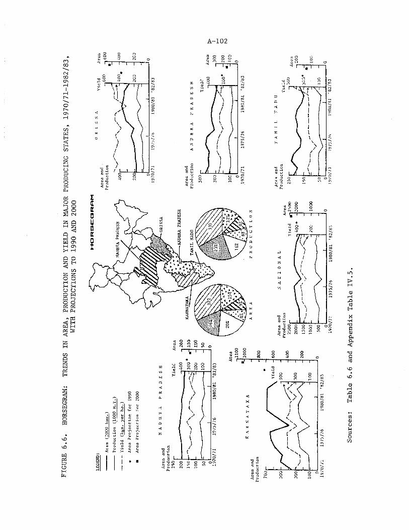
FIGU
RE 6
.6.
HORS
EGRA
M:
TREN
DS I
N AR
EA,
PROD
UCTI
ON A
ND Y
IELD
IN MA
JOR
PROD
UCIN
G STAT
ES,
1970
/71-
1982
/83,
WITH
PRO
JECT
IONS
TO
1990
AND
2000
A-102
Sources:
Tabl
e 6.6
and
Appe
ndix
Tab
le I
V.5
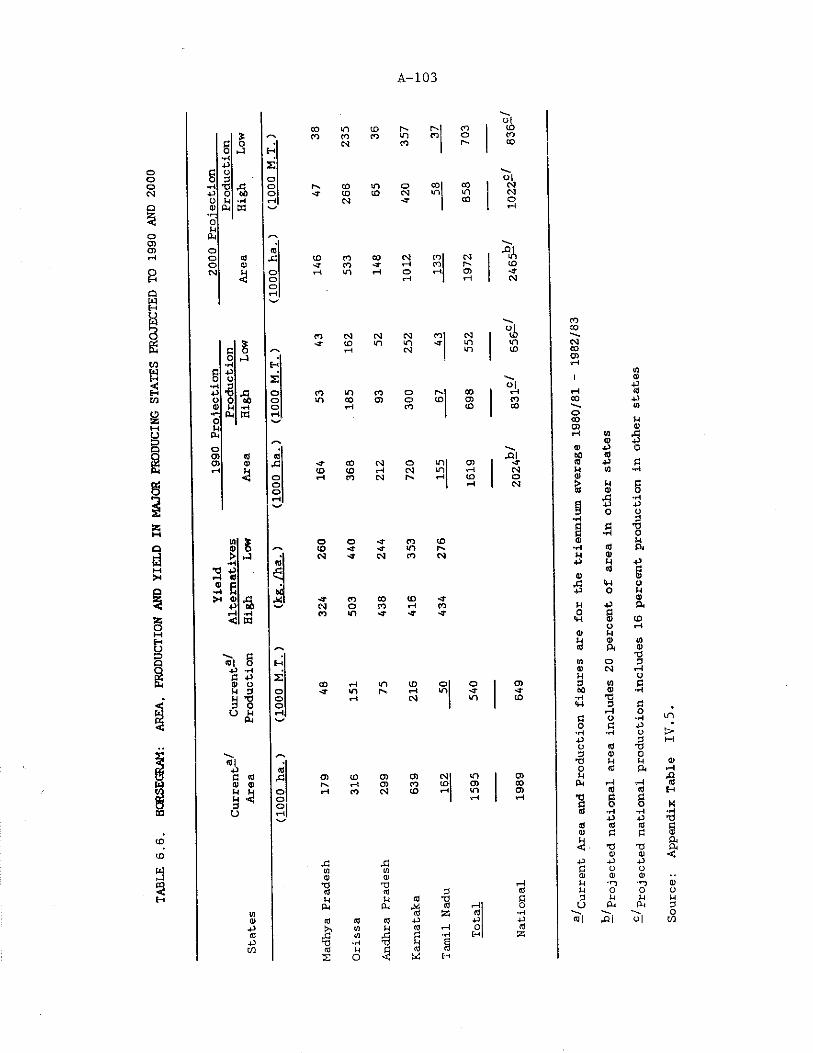
PROD
UCTI
ON A
ND Y
IELD
IN MA
JOR
PROD
UCIN
G ST
ATES
PRO
JECT
ED T
O 1990 A
ND 2
000
A-103
E■»<po0)opPhoooCM
t-4
•aK
©ai
3
■a•Hm
©
CO m to tv CO %CO CO CO m CO o to* CM CO rv CO
HE Vo olo tv 00 vn o 00 00 CMo a to to CM tn m CMrH CM a CO orH
(0 CD CO 00 CM CO CM 1 ^<T CO rH CO tv 1 to
o rH *n rH O T t 03 aoorH
rH rH I CM
oltn CM CM CM CO CM tom< T to tn m a mrH CM tn toH£OOo
CO m CO o (V CO>n 00 03 o to 03rH CO to
Hittoco
(0£1ooo
CD CM O m O) a<o to H CM tn rH CMrH to CM IV rH torH oCM
•o P rH ©© p •p p © p
o O a CO to6 to a a m tvhJ * CM -a- CM CO cm
atn
HT CO CO to aCM o CO i-H COCO m •a- ■a- -a
-v, C©1 o E-tP ’HP P £© OP 3 oH *3 oB o ou u rHPh
CO rH tn to o o O)■a tn tv i—t m ■a arH CM tn to
pp © © ©
u
«,cooo
to 0) 03 CM tn 1 CDrH 03 CO to O) 00CO CM to rH m CDrH [ rH
IDto
a•P J 3tn tn© ©
* 0 T J rHw © 3 ©p P © 73 s
1004 Put ©
SrH©
o•rH
© © © P P PP tv [/) P © 1—1 O ©© W ■P p *H EH S
P n *H P sCO © M P © (d
1 s O < w H
COCOCMCOoICOoCO03rH ©©W p60 ©© pM M©
P© ©
rPQ P3 o
*Hp pS •H©•rl ©P ©P P©V
£5 tpP 0
p P□ P5o
© pH ©3 P4
tn o© CMP3 to60 ©
■H T3<P 3
i—1P O0 P
*H •HPO ©3 ©
Tt MO ©P
(P H©
■a 8■ rlP
© ©© P
, *3©
p Pp O© ©p ■tnp 03 P
U PhV ,©1 rQ I —^
Proj
ecte
d na
tion
al p
rodu
ctio
n in
clud
es 1
6 pe
rcen
t pr
oduc
tion
in
othe
r st
ates
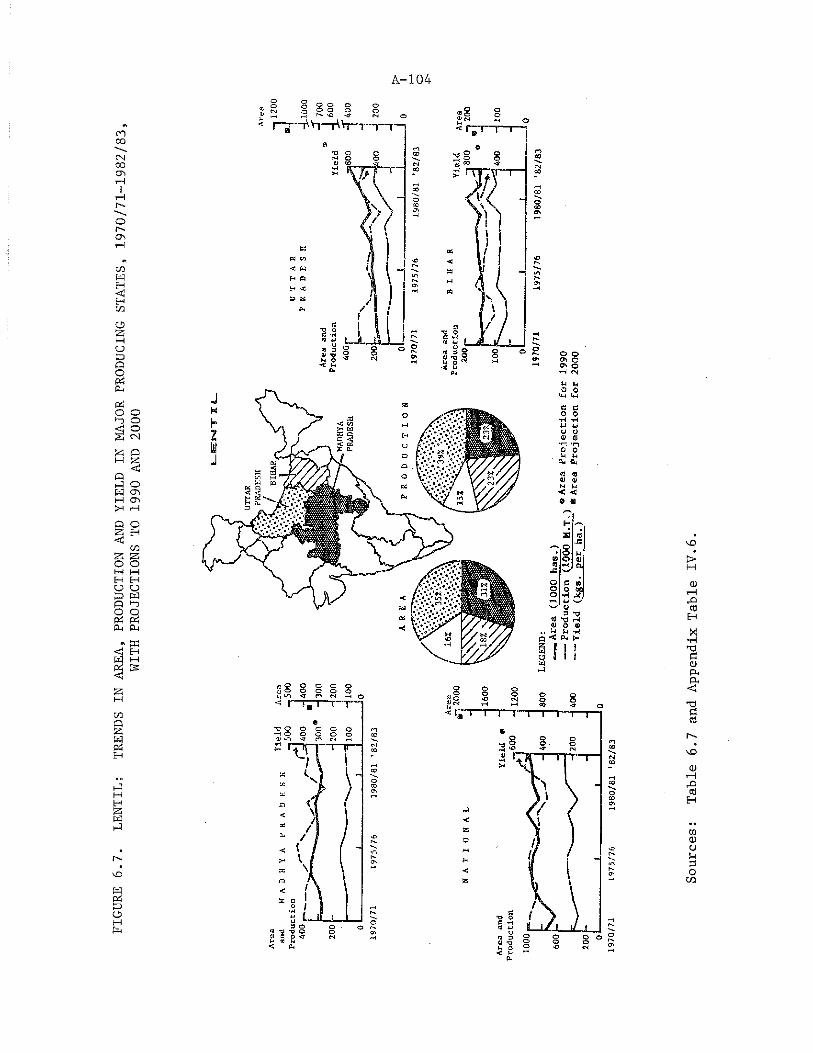
FIGU
RE 6
.7.
LENT
IL:
TREN
DS I
N AREA,
PROD
UCTI
ON A
ND Y
IELD
IN
MAJO
R PR
ODUC
ING
STATES,
1970
/71-
1982
/83,
WITH
PRO
JECT
IONS
TO
1990
AND
200
0
A-104
Sources:
Tabl
e 6.7
and
Appe
ndix
Tab
le I
V.6.
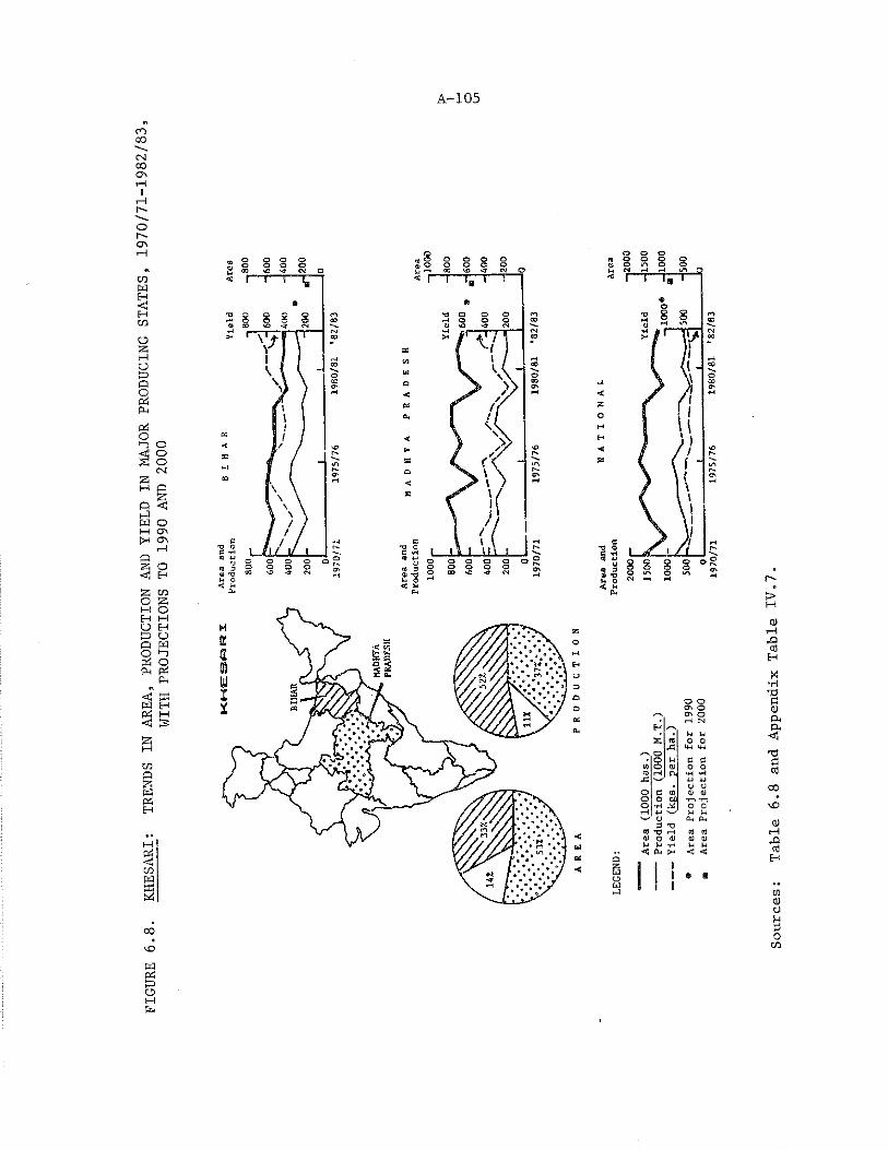
FIGU
RE 6
.8.
KHES
ARX:
TREN
DS X
N AREA,
PROD
UCTI
ON A
ND Y
IELD
IN MA
JOR
PROD
UCIN
G ST
ATES
, 19
70/7
1 1982/8
3,WI
TH P
ROJE
CTIO
NS T
O 1990 A
ND 2
000
A-105
fS03COoOQo*
SO
mO'
o o OS o as o
2 'Dffl t—I tti<u o d) a? a)U U 'r4 u u< p-t >-< <d <!
1I « ■ I
Sources:
Tabl
e 6.8
and
Appe
ndix
Tab
le I
V.7
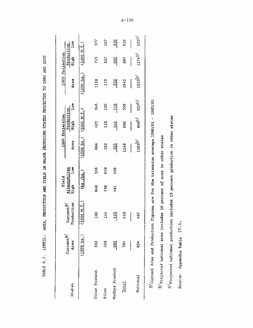
TABL
E 6.7.
LENT
IL;
AREA,
PROD
UCTI
ON A
ND Y
IELD
IN MA
JOR
PROD
UCIN
G ST
ATES
PRO
JECT
ED T
O 1990 A
ND 2
000
A-106
■&•hB
o|p* Oj O COo tH j rH inm rH CO CO o
oltn I'-l P-*rH CM CD O)r» rH CD O) HrH
CO CO OJ CO %i—f r-» m HP tnrH rH CO to CDH rH rH
$d 3o■H H
d 435 o E■rl 3+3 x d oO o 00 oV h *ri o■r; ft tn rH0uft /-NoCD <0 «CD © drH
ooorH
CO-a-CO
CO*nm°plmto
in CD CM to %OJ rH -3* CO Osr i—1 rH CD CO
>a- CM CO CD i ^cO CO CM -a- I toCO rH CO rH I COrH 1 tH
V)0)>•H
as5 e<u43
to CD COtH rH m»n to CO
«l 54-3 *H B +3
uCM -tf CO CD ] pCD rH rH H COrH H rH HP 4J-
"AB t00) 0)a su
CO CD IN Hf HPCO to CD CD in
oo
CO rH CM P- CD
dd wl/i ©(0 X
X <0<0 MJH ft r— t
w ft (00) Cfl 4343 n u tH 0CO <0 (0 d E-i43 43 d XW 43 'rH (0
d> pq E
g43to
Ul1 ©43rH c0CO 43WoCO HCD ©rH W d© 43© 43 Oto (0(0 43 B1H n *H©
> H Bt0 © 0d ■Hs 43 43p 0 O•H 3d B Xd •H 0© U-H (0 ftin ©43 H 43
©M Bto
d <H U43 O H(H 43 St,o atH © mo rH<0 HU © IQ(0 ft V
XID to 3© rH rHu O3 to s00 (1) ■H•H XtH 3 BrH OB O *H□ d 43•H *H O43 3O (0 X3 © 0X JH H0 « ftHft rH Hw to
•3 B fiB o O(0 *H *Hfij
43 43to to
® a d£ X xi
© ©43 43 43B o O0) © toJH ■rj "OH O 03 JH JH
U ft f tdll *ol
vO>
0)sH
•HXB®aa<®oM3OCO
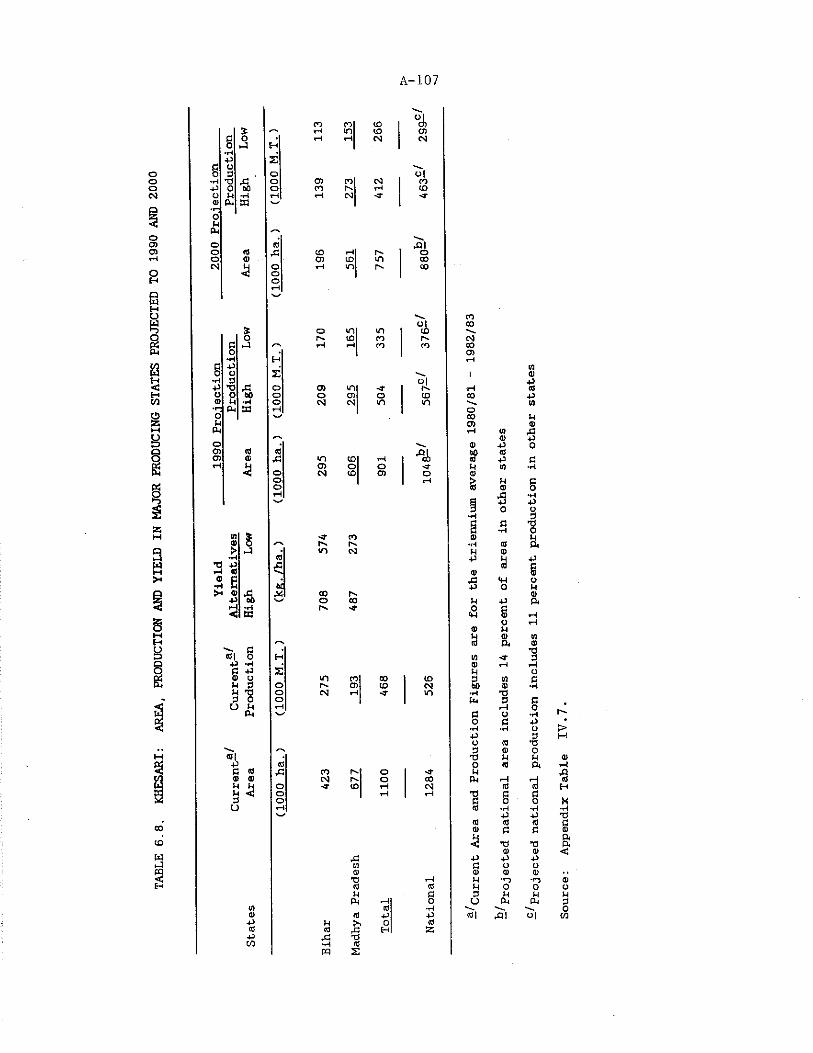
TABL
E 6.8.
KHES
ARI:
AR
EA,
PROD
UCTI
ON AND
YIE
LD I
N MA
JOR
PROD
UCIN
G ST
ATES
PRO
JECT
ED T
O 1990 A
ND 2
000
A-107
SO*-4
•5•Pm
•aw
3 *3 ffi u M 3 M TJ 3 OO nM Cm
*ASHM3L)
05CO
tOtoCM
CMrH•3"
°cj,O)IN
o!COto<r
<8 43143 (O rH oO) to tn COOOorH
in tn r» CO
or»-
aioCM
tnO)CM
-a-r-»m
coor-»
mr-CM
COr-*cm
mCOCO
srotn
oco
%
co
°rltoin
<TO
toCM
CO pv o ■a-CM p' o 00-a- to rH CMrH rH
Id0)PCOPw
43td®
T3 T—1td (0H 3
PM ■—i 0td •rH
td P ps O td
TJtd
2
H 5e
COCOCMtoCD
tdt ®ptdCO P**** tdo00 MO) ®xH td 43® Po p 066 t«<sr P 3t-t to ■po
> M 3td ® O43 •P
£3 P P3 0 o■P 3C 3 -3•H O0) M•H td ftM QP u Ptd 3® S43 (p oP 0 M®H P Pi0 35 rH
o rH® uH a td3 A ®•oto -a 3® rH rH
u o3 td 3t)0 ® •p■rl TJft 3 3>P O3 O *p0 3 P ♦*H •H o >P 3 Ho td T33 ® 0TJ u MO td ft i—tHft >—l H ’Std 3 H
TJ 3 33 0 0 H« *H *p •PP p U« td td 3® 3 3 ®ft<3 Tl td ft® 0) <p P p3 CJ o0) V Q • •M 'D •rj ®M 0 0 o3 M u uU PM PM 30tdi 43! o| m
A-108
Production of Khesari, on the other hand, is likely to decrease by 10 percent in 2000, and the area is expected to register a decline of about 25 percent during this period.
Effect of Development of Livestock Sector
The production of pulses in the future will also be affected by the development of the livestock sector. This will influence cropping patterns in the fields of farmers involved in dairy activities. Dual purpose pulse crops such as cowpea (which is presently not extensively grown) and guar bean (cyamopsis tetragonoloba), which provide fodder as well as grain, are likely to gain importance. [46].
Short-duration variety pulses, which are rapidly gaining popularity in irrigated areas, are likely to come into competition with green fodder legumes, where farmers are engaged in dairy activities. With increase in the number of crossbred cattle, this is likely to increase. For agricultural activities near urban centers, where there is a ready market for dairy products, the summer pulses will have to compete with green fodder as well as summer vegetables. This could result in some decline of pulse acreage. However, in the absence of data it is difficult to surmise to what extent pulse production would be affected.
Changing Share of Major Pulses in Total Area and Production
Projected pulse area and production is summarized in Table 6.9. Pulse production in the past has been dominated by gram, which accounts for about 32 percent of area and 44 percent of production. On the basis of high estimates, ' the position is likely to change in the future. The percentage share of gram in total area is likely to decline slightly from 32 percent to 30 percent in 2000; the share in production, however, is expected to decrease significantly from 44 to 34 percent. This can be seen from Figure 6.9. The major kharif pulses, on the other hand, are expected to increase in both area and production. Redgram, greengram and blackgram together are projected to account for 45 percent of total area in 2000, compared to 38 percent in 1981/82. Their share in production is likely to increase from 34 to 43 percent.
The future will see greater diversification in the production of pulses. While gram will continue to account for a significant share of production, it is the kharif pulses such as redgram, greengram and blackgram that are likely to play an increasingly important role in the pulse economy.
Comparison of Supply Projections
Table 6.10 summarizes the estimates for pulse production in 2000, made in various studies.
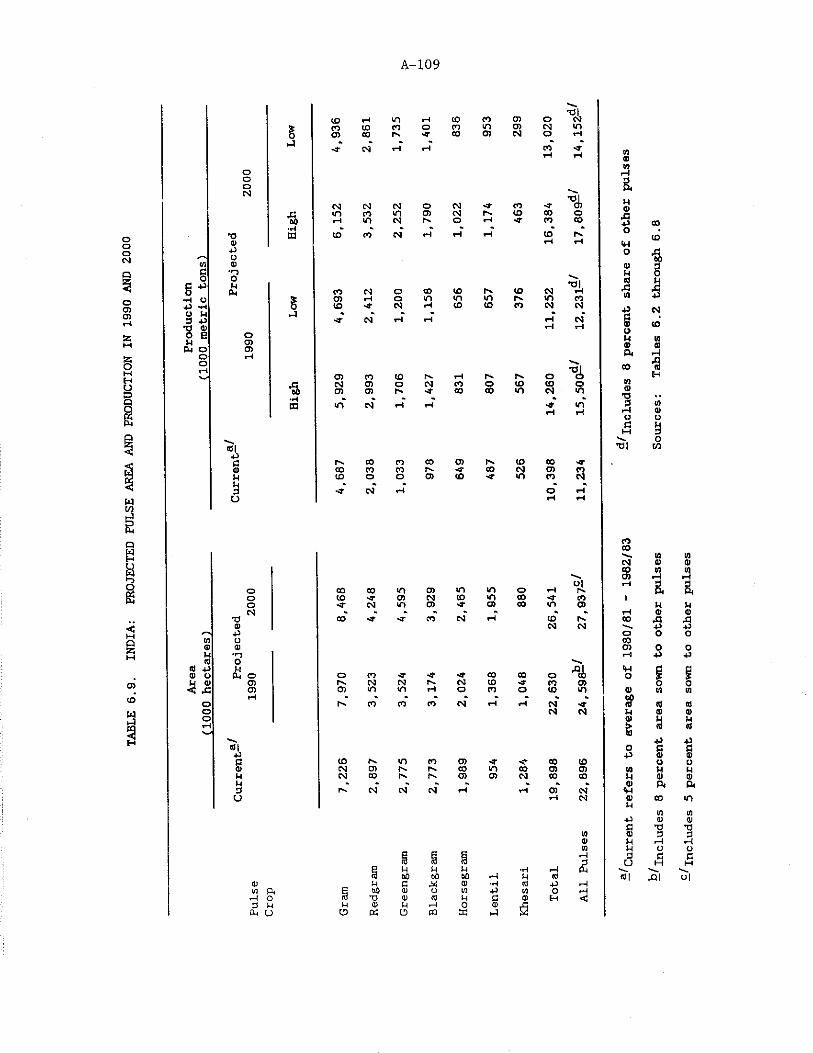
TABL
E 6.9.
INDIA:
PROJ
ECTE
D PU
LSE
AREA
AND
PRO
DUCT
ION
IN 1
990
AND
2000
A-109
I
o*§-MPL|
oooCM
*00)43Q0)•oouPH
oO)CD
-a•Hm
I
■aEH
1gP
O
tD rH in i—i CO COCO to co o CO mo> CO r*s •a- CO CD-a- os rH rH
CM cm CM O CM < rin CO m CD CM rsH m CM l-v O Hto CO CM rH rH H
CO CM o GO to PvCD rH o m m mto<r
-a-cm"
CMrH
rHrH
to to
CD CO to Pv rH PvCM 0) o CM CO OO) O) P*. ■a- GO 00m cm* rH rH
P«. cO to CO CD P-GO CO CO p* <? 00to■a-
oN*
orH
CD to •a*
Tf0) o CMCD CM mCM o rH
CO -a-t-H H Ul<U1/3i—lDft
•DJ nCO -a- CD mto CO O Ufn•& CO 00 5 CO
to" Pv otorH rH u
o a0) 3
to CMP «J A
oJjpv m CO ID 43
CO CM CM ■£ CMrH CM R *rH rH Vo to
u n® 0)a rH
*9O
00 COHto to O IDm CM m a)■d ,,
•a- m" 3 IQrH rH rH 0)U oa 9w 3oTJl CO
to CO 'a-CM O) tom CO CMo rHrH rH
toCOU w
CM 0 0CO ID w'sH O) rH i-H
Ul 1—i 3 3o CO 00 <n 0) m in o rH P* a ao to CD CM to in GO •a- CO io -a- CM to CD *a- CD CO m 03 P pCM H h * p* * * % h rH 0 0
Tf CO <f HP CO CM rH to Ph CO A xt0) CM CM 43 4343 o O Ow o CO0) 0 03 0 O
p •n H 43 43CO 010 43 0) o £ o o to sr •a- <f CO GO o *M
O g iP 0 ai p-. CM CM p* CM to HP CO CD 0 0< X! CD O) IT) vn H O CO o to m 0 w 0
o rH p- CO CO CO CM tH rH CM* HP » ft)o CM CM P 0 0o 0 pH > a 0«43 43ttt| O a c43 to 43 0 0a Pv <n CO CD ■a <P CO to U o0) CM CT) p* P* CO to CO O) CD 0 P p
p CM CO PN PH CD CD CM CO CO P 0 0M fc * h fc * * % 0 a a3 P- CM CM CM H rH 0) CM ttHu H CM 0 CO inP tft 043 0 0a Tt TJID 0 3 30 M rH rHW P o oE g E rH 3 3 Rto (0 TO 3 U M HP P P p ■H 1—J PM<3 GO GO GO rH p « 01 o|0) P G M 0) 'H is 43 r—1ID Pi P a0 ® Q ID 43 w 0 rHrH O c3 TJ 0 <0 P 0 0 H <33 W P 0 M r—I 0 CD Au o O EC r3 S
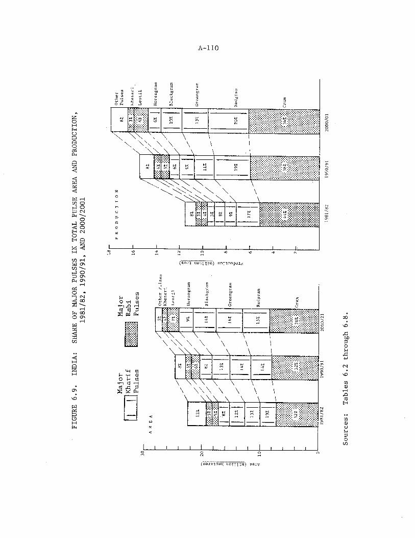
FIGU
RE 6
.9.
INDIA:
SHAR
E OF
MAJ
OR P
ULSE
S IN T
OTAL
PUL
SE A
REA
AND
PROD
UCTI
ON19
81/8
2, 1
990/
91,
AND
2000
/200
1
A-110
w
(ssjiuriDsn uoTIT™ ) b s .iv
Sources:
Tabl
es 6
.2 t
hrou
gh 6
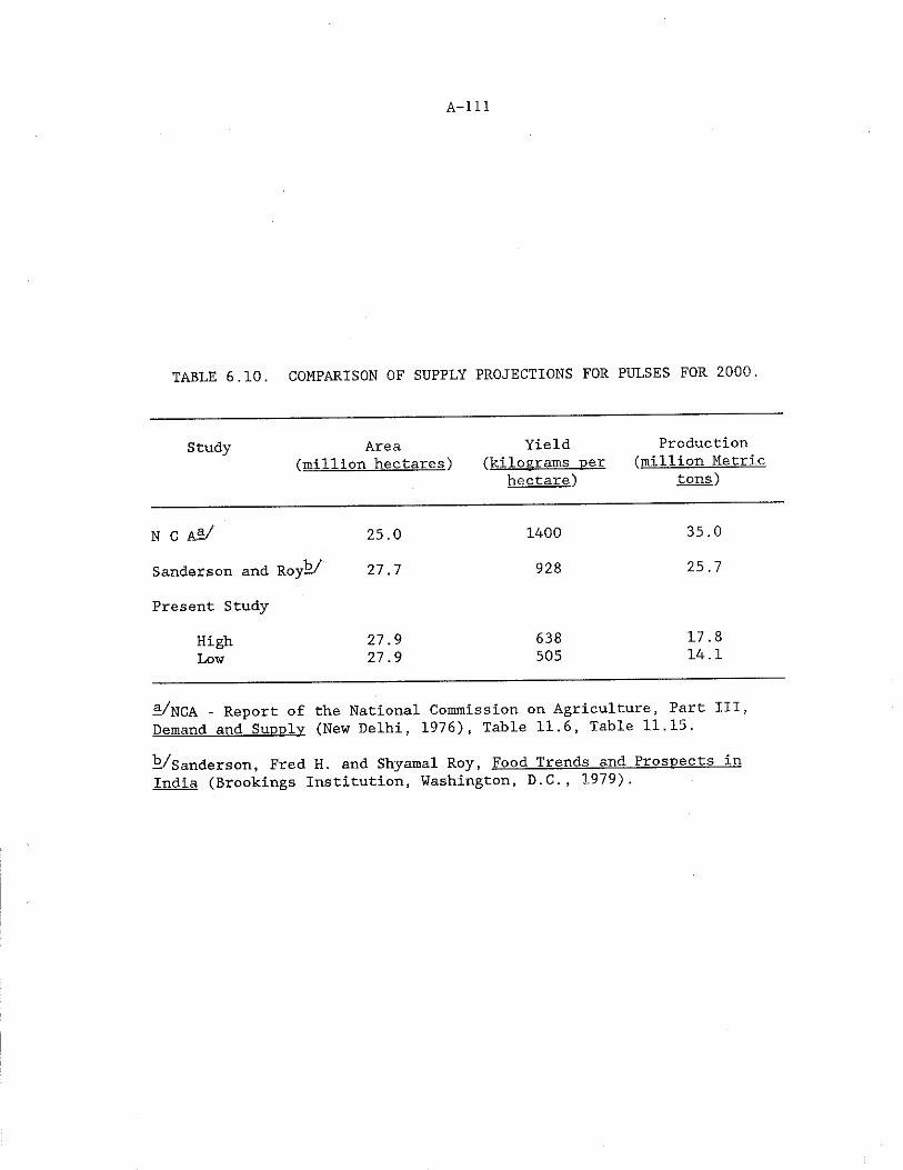
A— 111
TABLE 6.10. COMPARISON OF SUPPLY PROJECTIONS FOR PULSES FOR 2000.
Study Area(million hectares)
Yield(kilograms per
hectare)
Production (million Metric
tons)
N C A—/ 25.0 1400 35.0
Sanderson and Roy^/ 27.7 928 25.7
Present Study
High 27.9 638 17.8Low 27.9 505 14.1
S/n CA - Report of the National Commission on Agriculture, Part III, Demand and Supply (New Delhi, 1976), Table 11.6, Table 11.15.
—/Sanderson, Fred H. and Shyamal Roy, Food Trends and Prospects in India (Brookings Institution, Washington, D.C., 1979).
A-112
The NCA supply projections appear to be unrealistically high. It Is unlikely that average yields (which were 490 kilograms per hectare in the triennium 1981-83) will Increase to 1400 kilograms per hectare in 2000, unless there is a dramatic breakthrough in pulse technology on lines similar to that of wheat. Based upon past trends it does not appear likely that yields will triple in the next decade and a half. The NCA in their report of 1976 estimated that pulse production in 1985 would have reached 22 million tons, with average yields of the order of 900 kilograms per hectare. According to the latest official estimates available t albeit provisional, the pulse production in 1983/84 was only12.6 million tons and the average yield 541 kilograms per hectare. The projection for production at 35 million tons in 2000 appears to be quite unrealistic.
The projection for the year 2000 in Sanderson and Roy's study (1979) for pulse acreage is quite similar to that in the present study. However, projected yields per hectare are about 45 percent higher. We have seen that the major Impact of the new pulse technology lies in its ability to reduce the growing period of the crop, so that pulses can be fitted into cropping patterns which would ordinarily allow for the field to remain fallow. This would enable the cultivator to reap an additional harvest with minimum of inputs. It must be remembered that the bulk of pulses are still grown on marginal lands and do not receive as high a priority as cereals. Farmers are not willing to invest in the required inputs for pulses, which are necessary if yields are to be increased.
This implies that increased production is likely to come about as a result of increase in area, especially in regions where the pulse crop does not compete for land with high-yielding cereals, rather than through any dramatic increase in yields which are predicated on purchased inputs.
Another point to be noted is that the average yield of pulses is relatively higher in the northern states than in the central and southern states. The area trends indicate that pulse production is shifting away from the Gangetic plains into the central and peninsular regions. This would imply a negative effect on the overall productivity of pulses.
In light of this, the estimated average pulse yield of 928 kilograms per hectare by Sanderson and Roy appears to be unduly optimistic.
The target for pulse area and production for 1990 set by the Government of India in the*Seventh Five Year Plan (1985-90) is consistent with the estimates made in the present study for 1990, based on the high scenario. The estimated area for 1990 In the present study is 24.5 million hectares, whereas the targeted area in the Seventh Plan is25.7 million hectares. The estimated pulse production is 15.5 million tons. The target for production is set at 16 million tons [37, p. 6].
A-113
This implies an average yield of about 620 kilograms per hectare, which is almost in agreement with that of the present study.
Demand Supply Balances
Supply ProspectsThe demand and supply projections for all pulses are summarized in
Table 6.11 and illustrated in Figure 6.10. Under the low assumption scenario, production in 2000 is estimated to be 14.2 million metric tons, whereas for the high scenario it is 17.8 million metric tons. In both cases the supply is projected to fall short of the demand: by 4 million tons for the low scenario and 6 million tons for the high scenario. Compared to the requirements based on nutritional norms this gap will be wider still: by 3 and 11 million tons for the low and highscenario, respectively.
Effect of Relative Prices
One of the assumptions made while projecting pulse production was that the relative prices will remain constant. However, this is an unrealistic asssumption. Figure 6.10 indicates what has happened to the relative price of pulses over the last two decades. Although no trend is evident, pulse prices have fluctuated greatly from one year to another.
The prices of pulses vary more widely than many other crops because pulses are grown mainly in rainfed conditions and accordingly their production is prone to greater variation as a result of varying weather conditions. In years of short harvest prices rise rapidly and have the effect of choking back demand to ration the available supply.
If projected demand In 1990 and 2000 is to be met, prices will have to rise to encourage Increased production; alternatively the price rise could have the effect of dampening demand. Since price elasticities of supply for pulses are not available, it is not possible to predict the additional production which would result from a sustained increase in the relative price of pulses. However, estimates of price elasticity of demand for pulses are available. These are of the order of -0.6 [13]. We can, therefore, estimate the increase in the price of pulses which will be needed to close the demand-supply gap if the supply projections remained unchanged.
For the year 1990, the projected consumer demand for the high scenario Is 16.4 million tons, whereas the available supply is 15.5 million tons. If demand is to be reduced to meet the available supply, prices would have to rise at the rate of about 1 percent per annum from 1982/83 to 1990. For the year 2000, when the gap between projected demand and supply is wider still, the needed price increase would be greater: in fact, about 4 percent per annum from 1990 to 2000.
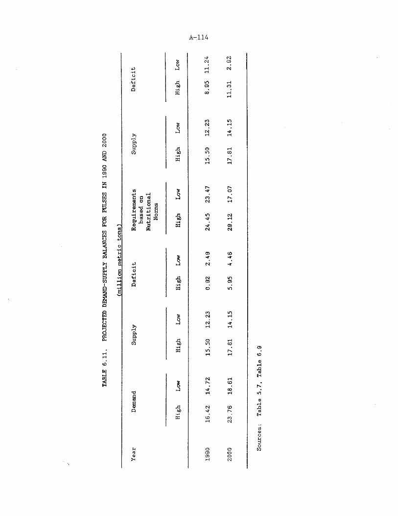
A-114
i
oooCM
oCDCD
as
-a- CMs CM CD0 * *
+ J t - i 1-4 CMr - i
O■l4
& m i—10 tto CD CO
Q '1-t • •t a CO t— '
1— 1
CO t ns c m i-40 •
ft! CM -3“ift r 4 r 4
ftft0 , U O i—f
W 60 m CO■H * *t d t n
H 1-4
r> -to > - T o
40 ****{ 0R (3 (0 ►-3 CO2 o g CM t—(E 6 w® T j aM 0 40 B•H W •H o rCj CMd « M as 60 i— l& ja 40 ■H0 0 c a 4 f CD
P4 is CM CM
CD ( 0
1- r •a-
+o CM •<r•H0
•H
- 4 CM c n0 60 CD o)Q •H -
id O c n
CO m% CM i-4o *ft! CM 4T
H i-4i-iftft0 00 O i— 1m 60 m CO
id i ni - i 1-4
CMg r>- ( 0
►J 0 0T33
i— i iH
§ 00 CM C0Q 60 ■d-
id C0 COt-4 cm
J-t O o0 CD o0 CD o
iH CM
CD100 i—(
*3
to0oH0Oin
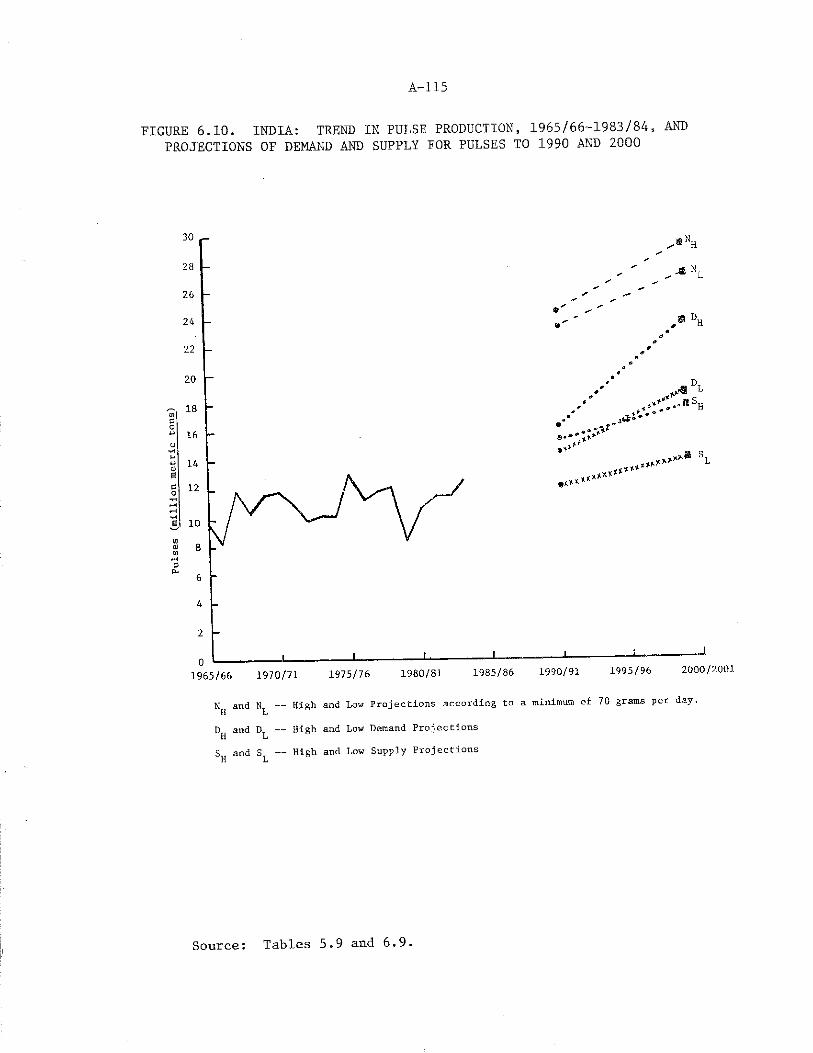
Puls
es (mil
lion
met
ric
tons
)
A-115
FIGURE 6.10. INDIA: TREND IN PULSE PRODUCTION, 1965/66-1983/84, ANDPROJECTIONS OF DEMAND AND SUPPLY FOR PULSES TO 1990 AND 2000
D and D — High and Low Demand Projections H LS and S — High and Low Supply Projections H L
Source: Tables 5.9 and 6.9.
A-116Importance of Area Versus Yield
Working on the assumption that the high scenarios for both supply and demand will obtain in 2000, the gap between demand and supply would be about 6 million metric tons. According to the projections for 2000, the area under pulses would be 27.9 million hectares and production17.8 million metric tons. This gives an average yield of 638 kilograms per hectare for all pulses combined. The average yield of all pulses for the triennium 1981-83 was 490 kilograms per hectare, which implies an annual growth rate in yield of 1.8 percent for all pulses for the period 1983-2000. If the projected demand of 23.8 million metric tons is to be met, an additional 6 million metric tons has to be produced and the average yield would need to increase to about 850 kilograms per hectare. This implies an annual yield growth rate of 4.3 percent. Compared to a growth rate of 0.3 percent per annum over the last three decades, with highest yield in the post-Green Revolution period being 533 kilograms per hectare in 1967/68 and 1975/76, it would appear unlikely that the growth rate of 4.3 percent can be achieved in the next 15 years.
It is evident that the development of short-duration varieties will increase the scope for double and triple cropping, as well as intercropping of pulses and thereby significantly increase the area under pulses. In fact it is projected that the area under pulses in 2000 is likely to be 27.9 million hectares as against a triennium average of 22,9 million hectares in 1981-83, implying an annual growth rate of 1.3 percent. However the new technology has not made any major breakthrough in terms of yield increases as was the case with HYV cereals. True, improved varieties with the recommended package of inputs do increase yields, but the average farmer is still not inclined
invest in inputs for pulses, which he expects to cultivate with a minimum of investment, so as to be able to reap maximum benefits from a bonus or catch crop. It is this very reason which makes it difficult to expect any major increases in yields of pulses in the future, unless there is a breakthrough in technology.
The high projections for 2000 indicate that more than 65 percent of increased production will result from an expansion in area, brought about to a large extent through increased cropping intensity and to a lesser extent by the replacement of coarse cereals and other less- favored crops in some areas. The contribution of increased yields is projected to be much less.
CHAPTER VIICONSTRAINTS TO PULSE PRODUCTION
AND POLICY IMPLICATIONS
The major problems confronting pulse production are:
1) competition with high-yielding variety cereals in irrigated areas because of low yields of pulse crops *
2) variability in yields, because of uncertain weather conditions, in unirrigated areas.
3) variability in yields because of susceptibility of pulse crops to disease and pests.
4) Inadequate availability of quality seeds of improved and short-duration varieties.
The factors constraining pulse production seem quite formidable and do not appear to lend themselves to easy resolution. It is therefore worth exploring alternative possibilities for increasing per capita availability. One option is to impose some kind of rationing on the existing supplies, through the process of procurement and distribution at subsidized prices in very much the same way as is done with wheat and rice. The other is to consider the possibility of imports. We shall examine the two options in the following sections.
Alternatives for Increasing Per Capita Availability of Pulses
Procurement and Distribution of PulsesTwo sets of administered prices are fixed by the Government of
India, based on the yearly recommendations of the Agricultural Prices Commission:
1) minimum support prices for major field crops are meant to be the floor levels below which the market prices would not be allowed to fall.
2) procurement prices in respect of kharif and rabi cereals at which the grain is to be domestically procured by public agencies for release through the public distribution system.
In the case of pulses, only minimum support prices are announced. These are in the nature of a long-term guarantee, assuring the producer of a minimum price for his crop [42,p. 12].
However, the market prices for pulses, set according to the forces of supply and demand, have tended to prevail at levels significantly
A-117
A-118
higher than the minimum support prices announced by the government. This is evident from Table 7.1.
If the government were to adopt a policy of procurement of pulses, and set a procurement price, it would have to be significantly higher than the minimum support price. In fact, if sizable stocks of pulses were to be purchased by government agencies, the price would probably have to be set well above the market price. Such a policy might provide some incentive to the producer, but it would drive the price of pulses higher, so that the situation of the lower income groups, who even now cannot afford an adequate intake pulses, would be further aggravated. To prevent that, government would have to distribute pulses through fair price shops at subsidized prices.
In Chapter IV it was seen that a certain proportion of cereal- pulse combination provided an optimum protein quality, determined by the Protein Efficiency Ratio (PER). If the quantity of pulses in the diet was increased beyond the critical ratio, it would add nothing further to the protein quality. In fact, experiments have shown that if pulse protein is increased beyond the optimum ratio, the quality of resultant protein actually begins to decline.
A second point which needs to be remembered is that rice-based diets require lesser amounts of pulses to complement the cereal protein than do wheat or coarse cereal-based diets. This is because rice protein is superior to wheat protein in terms of its amino acid makeup.
These facts may be utilized to distribute the limited quantity of pulses in the most nutritionally desired manner, and form a basis for rationing the existing supply of pulses. It is obvious that a small percentage of the population is consuming pulses in quantities which, in strictly nutritional terms, are quite wasteful, while many others may not be able to afford to consume any pulses at all, and are substituting vegetables, roots and tubers for this important protein source.
At present, the annual subsidy on foodgrains, mainly wheat and rice incurred by the government accounts for about 3-4 percent of the central government budget. The addition of pulses to the list of distributed commodities is not likely to burden the exchequer to any considerable extent. In theory, therefore, there is a strong case for rationing the existing supply of pulses.
However, there are a host of administrative problems associated with including pulses in the public distribution system. Storage of pulses on such a large scale would involve considerable losses during storage. It would imply an expansion in the bureaucratic structure of the marketing agencies of the state and central governments. With the government purchasing large stocks of pulses, the open market price of pulses would rise even more, increasing the possibility of black market trade in pulses.
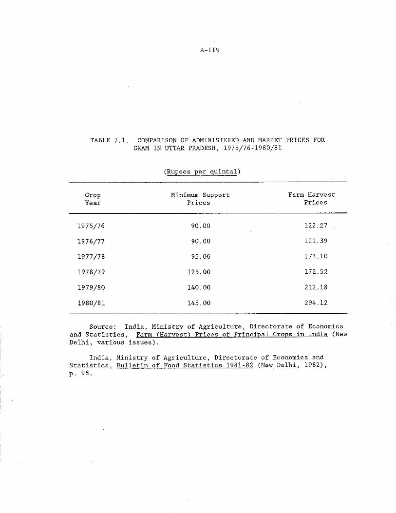
A-119
TABLE 7.1. COMPARISON OF ADMINISTERED AND MARKET PRICES FOR GRAM IN UTTAR PRADESH, 1975/76-1980/81
(Rupees per quintal)
CropYear
Minimum Support Prices
Farm Harvest Prices
1975/76 90.00 122.27
1976/77 90.00 121.39
1977/78 95.00 173.10
1978/79 125.00 172.52
1979/80 140.00 212.18
1980/81 145.00 294.12
Source: India, Ministry of Agriculture, Directorate of Economicsand Statistics, Farm ('Harvest') Prices of Principal Crops in India (New Delhi, various issues).
India, Ministry of Agriculture, Directorate of Economics and Statistics, Bulletin of Food Statistics 1981-82 (New Delhi, 1982), p. 98.
A-120
If these problems could be overcome and it could be ensured that through the public distribution system the lower income classes would have access to the commodity, it would appear reasonable to include pulses with wheat and rice in the procurement and distribution operations of the government--until such time as the production of pulses could be increased sufficiently to allow for an adequate availability.
Possibility of Imports
Imports would not appear to be a likely solution to the problem of increasing pulse availability.
The bulk of pulses traded on the world market are comprised of soybeans and groundnuts. Soybeans are not acceptable to the Indian consumer as a substitute for gram, redgram, blackgram or greengram in the diet. Although soybean is produced in the country, it has not become a popular item of food. Its main uses have been for oil extraction and other industrial purposes. The pulses most commonly consumed in India are not available in sufficient quantity in the international market. In fact, India produces about 75 percent of the world production of gram and over 90 percent of redgram, greengram and blackgram. Pulses such as khesari and horsegram are grown almost exclusively in this country.
Strategies For Increasing Domestic Production
The long-term strategy for improving per capita pulse availability is to make all possible efforts to increase domestic production. Such a policy would require optimum utilization of available resources and technological improvements leading to maximization of land and labor productivity. This would have to be backed by a streamlining of the input supply line, to ensure timely and adequate availability of quality seeds of improved short-duration varieties. A concerted effort is also needed in the sphere of extension services, which up until now have concentrated mainly upon increasing production of cereals and cash crops. There is a need to restructure priorities, such that pulse production programs at both the national and state level receive greater attention than they have done hitherto.
Approach for Irrigated Areas
It is clear that as irrigation facilities spread, traditional cropping patterns will be replaced by high-yielding variety cereals. This is as it should be, because the first priority in Indian agriculture is to increase cereal production to meet the energy needs of a growing population. However, inirrigated areas, where double cropping is already being practiced, the short-duration summer greengram and blackgram varieties have been successfully introduced. A far greater
A-121
potential to increase area through a triple cropping system exists in the northern wheat-growing belt of the country. A program of summer pulse production would enhance the income of the farmer and increase pulse production without confronting him with a choice between pulses and cereals. Additional area can be brought under short-duration varieties of greengram, cultivated with irrigation, in summer, after harvesting a crop of oilseeds, sugarcane, potato or wheat, and before planting the kharif crop paddy or maize [41, p. 291]. The concept of a triple cropping pattern, which should include summer pulses, must become as much a part of the agricultural scene in the next decade and a half as double cropping is today in the irrigated areas.
One of the main reasons for the wide fluctuations in the yield of pulses is the fact that most are grown in rainfed conditions. Variability in rainfall has a direct and significant effect on yields and consequently production. However, the expansion of pulse production in irrigated areas will lead to some stability in yields and have a positive effect on production of pulses as a whole.
Approach for Unirrigated Areas
By far the greatest potential for the production of pulses lies in the dryland rainfed areas in the regions comprising the central and southern states. Both gram in the rabi season and kharif pulses such as redgram, blackgram and greengram have potential in these regions. Area can be increased through double cropping where sufficient residual moisture makes a second crop possible. In the coastal regions of the central and southern states blackgram and greengram can be cultivated in rice fallows by making use of the residual moisture. Using mixed and intercropping systems, pulses can be grown as complementary rather than competing crops with cereals.
In the semi-arid areas pulses play an important role in the farming system. They generate food and income in a poor agro-climatic environment where many other crops would fail. In addition, they provide the cultivator with a low cost option to improve soil fertility without the use of purchased inputs [57, p . A139]. These special characteristics of pulse crops must be utilized to promote them in mixed and intercropping systems, together with appropriate cereal-pulse rotations, to maximize productivity in a deficient land resource base.
With the continued rise in the production of wheat and rice during the last two decades, the coarse cereals, sorghum, maize and millets, have lost their relative importance. In fact, many cultivators in the rainfed dryland areas no longer favor these crops, since the returns per hectare are often lower than those from pulses. It is quite likely that coarse cereals will find increasing use as animal feed in the future. It appears that the short-duration pulse varieties are already replacing coarse cereals profitably in many areas of the central and southern states.
A-122
The possibility of diversion of land from coarse cereals to pulses in rainfed areas holds considerable potential for the future, is a healthy one and needs to be encouraged. Pulses are nutritionally superior crops, and improve soil fertility as well. Coarse cereals, on the other hand, are inferior in terms of protein quality, and diets based solely on coarse cereals need large quantities of pulse protein to achieve the desirable amino acid balance. It, therefore, seems logical that, in the long run, coarse cereals be replaced to a large extent by pulses in the semi-arid regions, just as pulses are being replaced by the high-yielding variety superior cereals in the Irrigated areas.
Disease and Pests
Apart from vagaries in weather conditions, susceptibility of pulse crops to disease and pests is the main reason for the wide fluctuations in yields. Information on the incidence of different pulse diseases in various regions of the country is limited, except in the case of pigeonpea wilt and sterility mosaic disease. On individual farmer's fields the incidence of the disease is often so severe that the entire crop may be wiped out, resulting in a total loss to the farmer [52, p. A144].
Subsidies on insecticides and spray equipment indicate the importance of plant protection measures and the concern of the government for this important aspect of pulse production. However, so long as pulses are considered low resource base crops, generally grown in rainfed areas and often on marginal lands, a maj ority of farmers will be either unable or unwilling to afford the cost of chemical plant protection measures, in spite of the subsidy.
Integrated pest management based on judicious use of insecticides, biological controls, and appropriate cropping systems would help to stabilize yields. This is not an easy task and would require a major research and extension effort.
Breeding of disease resistant varieties would be an effective approach to the problem and considerable progress has been made. Redgram varieties resistant to wilt and sterility mosaic have been identified and released for national demonstrations by ICRISAT. In addition to these two wide-spread diseases, plant pathologists are working to develop resistance to' phytophthora blight.
A large number of varieties of gram resistant to wilt, dry root rot and black root rot have been developed. Also greengram and blackgram varieties resistant to yellow mosaic virus have been successfully introduced in the field. Efforts are in progress to develop varieties resistant to powdery mildew and leaf spot diseases [57] . However, if adequate quantities of seed of these disease resistant varieties are not made available to the farmers, the impact of this research will not be felt on the field.
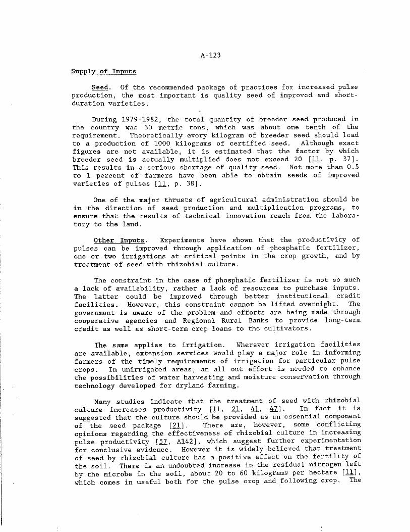
A-123
Supply of Inputs
Seed. Of the recommended package of practices for increased pulse production, the most important is quality seed of improved and short- duration varieties.
During 1979-1982, the total quantity of breeder seed produced in the country was 30 metric tons, which was about one tenth of the requirement. Theoretically every kilogram of breeder seed should lead to a production of 1000 kilograms of certified seed. Although exact figures are not available, it is estimated that the factor by which breeder seed is actually multiplied does not exceed 20 [11, p. 37]. This results in a serious shortage of quality seed. Not more than 0.5 to 1 percent of farmers have been able to obtain seeds of improved varieties of pulses [11, p. 38].
One of the major thrusts of agricultural administration should be in the direction of seed production and multiplication programs, to ensure that the results of technical innovation reach from the laboratory to the land.
Other Inputs. Experiments have shown that the productivity of pulses can be improved through application of phosphatic fertilizer, one or two irrigations at critical points in the crop growth, and by treatment of seed with rhizobial culture.
The constraint in the case of phosphatic fertilizer is not so much a lack of availability, rather a lack of resources to purchase inputs. The latter could be improved through better institutional credit facilities. However, this constraint cannot be lifted overnight. The government is aware of the problem and efforts are being made through cooperative agencies and Regional Rural Banks to provide long-term credit as well as short-term crop loans to the cultivators.
The same applies to irrigation. Wherever irrigation facilities are available, extension services would play a major role in informing farmers of the timely requirements of irrigation for particular pulse crops. In unirrigated areas, an all out effort is needed to enhance the possibilities of water harvesting and moisture conservation through technology developed for dryland farming.
Many studies indicate that the treatment of seed with rhizobial culture increases productivity [11, .21, 41, 47] . In fact it is suggested that the culture should be provided as an essential component of the seed package [21]. There are, however, some conflicting opinions regarding the effectiveness of rhizobial culture in increasing pulse productivity [.57, A142] , which suggest further experimentation for conclusive evidence. However it is widely believed that treatment of seed by rhizobial culture has a positive effect on the fertility of the soil. There is an undoubted increase in the residual nitrogen left by the microbe in the soil, about 20 to 60 kilograms per hectare [11], which comes in useful both for the pulse crop and following crop. The
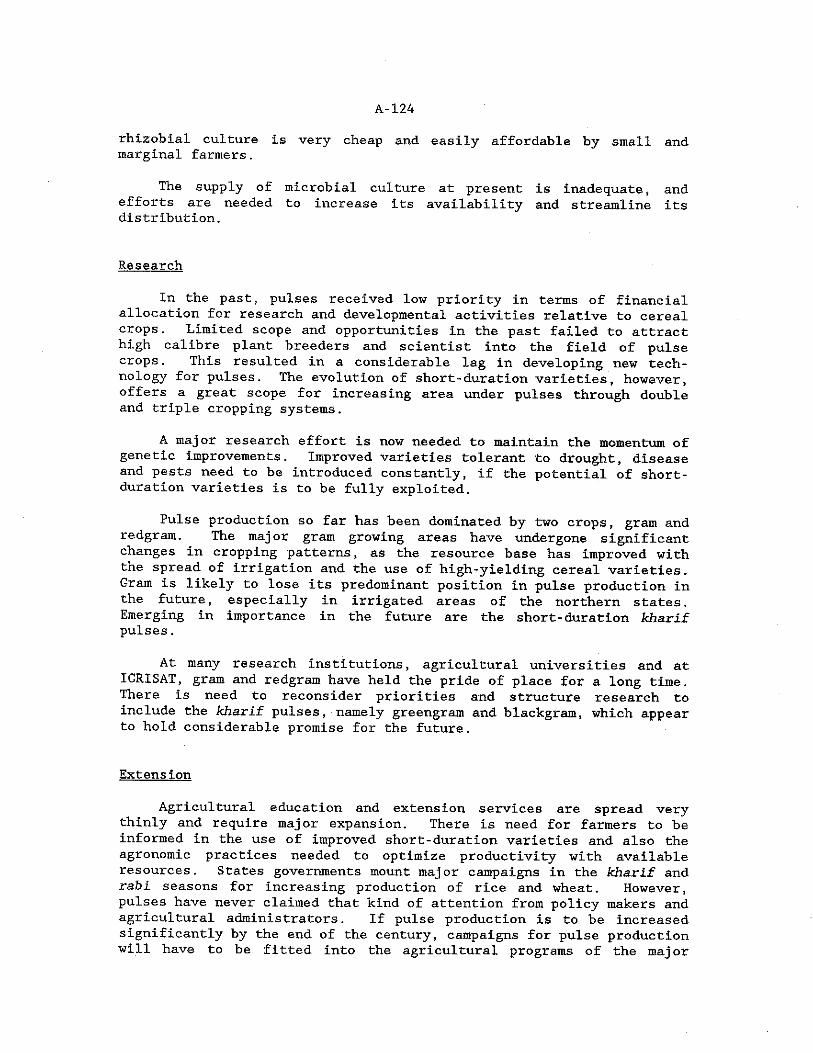
A-124
rhizobial culture Is very cheap and easily affordable by small and marginal farmers.
The supply of microbial culture at present is inadequate, and efforts are needed to increase its availability and streamline its distribution.
Research
In the past, pulses received low priority in terms of financial allocation for research and developmental activities relative to cereal crops. Limited scope and opportunities in the past failed to attract high calibre plant breeders and scientist into the field of pulse crops. This resulted in a considerable lag in developing new technology for pulses. The evolution of short-duration varieties, however, offers a great scope for increasing area under pulses through double and triple cropping systems.
A major research effort is now needed to maintain the momentum of genetic improvements. Improved varieties tolerant to drought, disease and pests need to be introduced constantly, if the potential of short- duration varieties is to be fully exploited.
Pulse production so far has been dominated by two crops, gram and redgram. The major gram growing areas have undergone significant changes in cropping patterns, as the resource base has improved with the spread of irrigation and the use of high-yielding cereal varieties. Gram is likely to lose its predominant position in pulse production in the future, especially in irrigated areas of the northern states. Emerging in importance in the future are the short-duration kharif pulses.
At many research institutions, agricultural universities and at ICRISAT, gram and redgram have held the pride of place for a long time. There is need to reconsider priorities and structure research to include the kharif pulses, namely greengram and blackgram, which appear to hold considerable promise for the future.
Extension
Agricultural education and extension services are spread very thinly and require major expansion. There is need for farmers to be informed in the use of improved short-duration varieties and also the agronomic practices needed to optimize productivity with available resources. States governments mount major campaigns in the kharif and rabi seasons for increasing production of rice and wheat. However, pulses have never claimed that kind of attention from policy makers and agricultural administrators. If pulse production is to be increased significantly by the end of the century, campaigns for pulse production will have to be fitted into the agricultural programs of the major
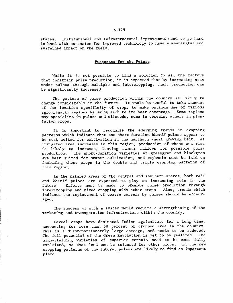
A-125
states. Institutional and infrastructural improvement need to go hand in hand with extension for improved technology to have a meaningful and sustained impact on the field.
Prospects for the Future
While it is not possible to find a solution to all the factors that constrain pulse production, it is expected that by increasing area under pulses through multiple and intercropping, their production can be significantly increased.
The pattern of pulse production within the country is likely to change considerably in the future. It would be useful to take account of the location specificity of crops to make optimum use of various agroclimatic regions by using each to its best advantage. Some regions may specialize in pulses and oilseeds, some in cereals, others in plantation crops.
It is important to recognize the emerging trends in cropping patterns which indicate that the short-duration kharif pulses appear to be most suited for cultivation in the northern wheat growing belt. As irrigated area increases in this region, production of wheat and rice is likely to increase, leaving summer fallows for possible pulse production. The short-duration varieties of greengram and blackgram are best suited for summer cultivation, and emphasis must be laid on including these crops in the double and triple cropping patterns of this region.
In the rainfed areas of the central and southern states, both rabi and kharif pulses are expected to play an increasing role in the future. Efforts must be made to promote pulse production through intercropping and mixed cropping with other crops. Also, trends which indicate the replacement of coarse cereals by pulses should be encouraged.
The success of such a system would require a strengthening of the marketing and transporation infrastructure within the country.
Cereal crops have dominated Indian agriculture for a long time, accounting for more than 60 percent of cropped area in the country. This is a disproportionately large acreage, and needs to be reduced. The full potential of the Green Revolution is yet to be realized. The high-yielding varieties of superior cereals need to be more fully exploited, so that land can be released for other crops. In the newcropping patterns of the future, pulses are likely to find an important place.

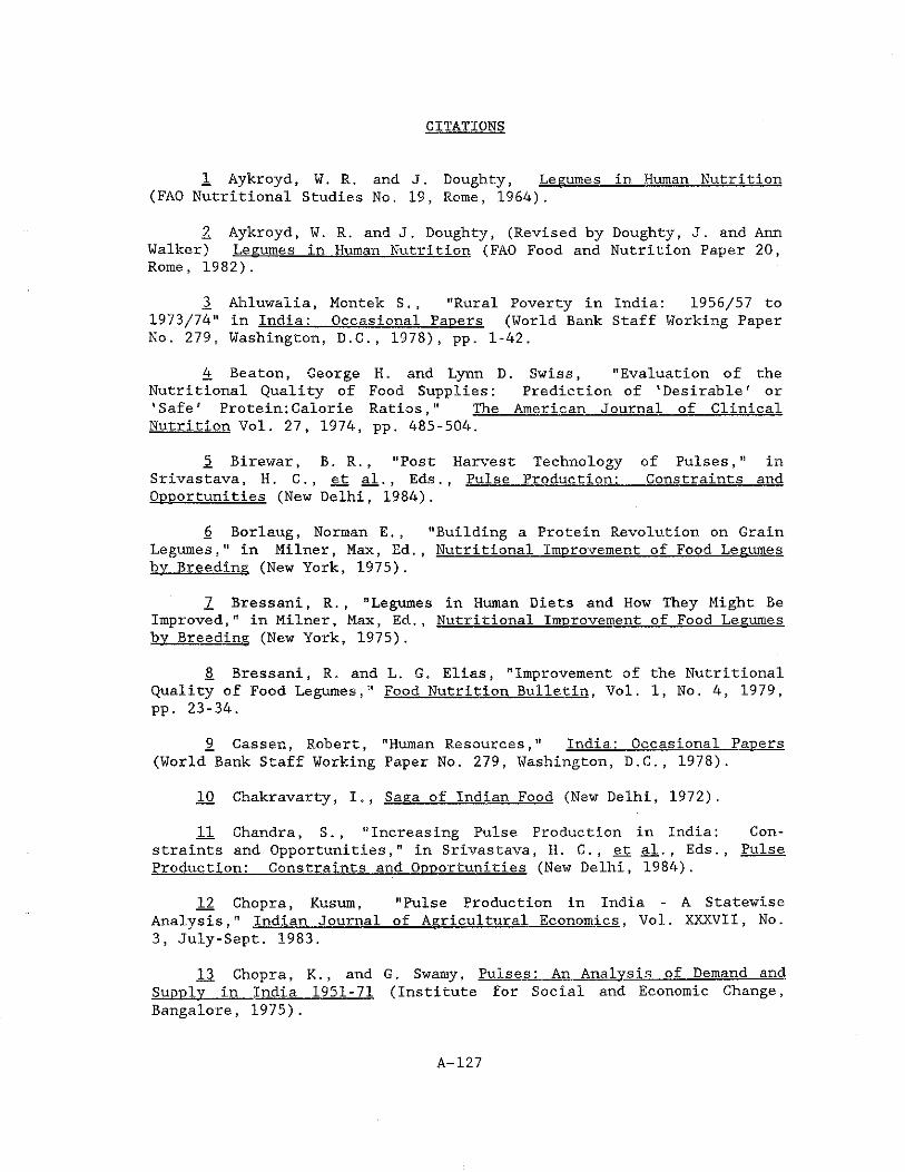
CITATIONS
1 Aykroyd, W. R. and J. Doughty, Legumes in Human Nutrition (FAO Nutritional Studies No. 19, Rome, 1964).
2 Aykroyd, W. R, and J. Doughty, (Revised by Doughty, J. and Ann Walker) Legumes in Human Nutrition (FAO Food and Nutrition Paper 20, Rome, 1982).
3 Ahluwalia, Montek S,, "Rural Poverty in India: 1956/57 to 1973/74" in India: Occasional Papers (World Bank Staff Working Paper No. 279, Washington, D.C., 1978), pp. 1-42.
4 Beaton, George H. and Lynn D. Swiss, "Evaluation of the Nutritional Quality of Food Supplies: Prediction of 'Desirablef or 'Safe' Protein;Calorie Ratios," The American Journal of Clinical Nutrition Vol. 27, 1974, pp. 485-504.
5. Birewar, B. R., "Post Harvest Technology of Pulses," in Srivastava, H. C ., et al. , Eds., Pulse Production: Constraints and Opportunities (New Delhi, 1984).
6 Borlaug, Norman E, , "Building a Protein Revolution on Grain Legumes," in Milner, Max, Ed., Nutritional Improvement of Food Legumes by Breeding (New York, 1975).
7 Bressani, R. , "Legumes in Human Diets and How They Might Be Improved," in Milner, Max, Ed., Nutritional Improvement of Food Legumes by Breeding (New York, 1975).
8. Bressani, R. and L. G. Elias, "Improvement of the Nutritional Quality of Food Legumes," Food Nutrition Bulletin. Vol. 1, No. 4, 1979, pp. 23-34.
9 Cassen, Robert, "Human Resources," India: Occasional Papers (World Bank Staff Working Paper No. 279, Washington, D.C., 1978).
10 Chakravarty, I., Saga of Indian Food (New Delhi, 1972).
11 Chandra, S. , "Increasing Pulse Production in India: Constraints and Opportunities," in Srivastava, H. C., et al., Eds., Pulse Production: Constraints and Opportunities (New Delhi, 1984).
12 Chopra, Kusum, "Pulse Production in India - A Statewise Analysis," Indian Journal of Agricultural Economics. Vol. XXXVII, No. 3, July-Sept. 1983.
13 Chopra, K . , and G . Swamy, Pulses: An Analysis of Demand and Supply in India 1951-71 (Institute for Social and Economic Change, Bangalore, 1975).
A-127
A-128
14 Chopra, R. N. , Evolution of Food Policy in India (Macmillan, New Delhi, 1981).
15 Dean, Gerald W. and Norman R. Collins, "Trade and WelfareEffects of EEC Tariff Policy: A Case Study of Oranges" Journal ofFarm Economics. November 1966.
16 Food and Agriculture Organization (FAO), Production Yearbook, various issues.
11 Food and Agriculture Organization (FAO). Food Balance Sheets (Rome, 1983).
18 Food and Agriculture Organization (FAO), Energy and Protein Requirements (FAO Food and Nutrition Series No. 4, Rome, 1965).
11 Food and Agriculture Organization (FAO), Legume Inoculants and Their Use (FAO Fertilizer and Plant Nutrition Service, Land and Water Development Division, Rome, 1984).
20 FAO/WHO Expert Committee, Energy and Protein Requirements 1971 (FAO Nutrition Meetings Report Series No. 52, Rome, 1973).
21 Gopala, Raju D. , "Constraints and Opportunities in IncreasingPulse Production in Andhra Pradesh" in Srivastava, H. C., et al., Ed., Pulse Production: Constraints and Opportunities (New Delhi, 1984).
22 Gopalan, C. , et at., Diet Atlas of India (National Institute of Nutrition, Indian Council of Medical Research, Hyderabad India1971).
23 Gopalan, C., et al., Nutritive Value of Indian Foods (NationalInstitute of Nutrition, Indian Council of Medical Research Hyderabad India, 1978). J
24 Hallsworth, E. G. , Ed., Nutrition of the Legumes (London, Butterworths Scientific Publications, 1958).
1974. 25 Hardin, Garrett, "Living on a Lifeboat," BioScience, Oct.
2,6 Hitchings, Jon, "India: Demand and Supply Prospects forIndia," (World Bank Staff Working Paper No. 500, Washington D C1981). 6 ’ * "
27 India, Ministry of Finance, Economic Division, Economic Survey ,1983-84 (Delhi, Controller of Publications, 1985).
2j| India, Ministry of Finance, Economic Division, Economic Survey 1984-85 (Delhi, Controller of Publications, 1986).
A~ 129
29 India, Cabinet Secretariat, The National Sample Survey: Tables with Notes on Consumer Expenditure (Seventeenth Round, September 1961 to July 1962, No. 184, Delhi, Controller of Publications, 1974).
30 _, The National Sample Survey: Tables with Notes onConsumer Expenditure (Nineteenth Round, July 1964 to June 1965, No. 192, Delhi, Controller of Publications, 1971).
31 . The National Sample Survey: Tables on ConsumerExpenditure (Twenty Eighth Round, October 1973 to June 1974, No. 240, Delhi, Controller of Publications, 1978).
32 India, Department of Statistics, National Survey Organization. The National Sample Survey: Tables on Consumer Expenditure (Twenty- seventh Round, July 1972 to September 1973, New Delhi, no date).
33 India, Ministry of Agriculture and Irrigation, Report of the National Commission on Agriculture. 1976. Fart III. Demand and Supply (Delhi, Controller of Publications, 1976).
34 India, Ministry of Agriculture, Directorate of Economics and Statistics, Agricultural Situation in India, various issues.
35 India, Ministry of Agriculture, Directorate of Economics and Statistics, Bulletin on Food Statistics, various issues.
36 India, Ministry of Agriculture, Directorate of Economics and Statistics, Area and Production of Principal Crops in India 1981-84 (New Delhi, 1984).
37 India, Planning Commission, Seventh Five Year Plan 1985-90 Vol. I and Vol, II (New Delhi, 1985).
38 India, Ministry of Agriculture, Directorate of Economics and Statistics, Indian Agricultural Statistics Vol, 1 . various issues.
39 India, Ministry of Agriculture, Directorate of Economics and Statistics, Farm (Harvest") Prices of Principal Crops in India, various issues.
40 Jain, H. K. , "Opportunities for Increasing Production of Pulses in India," in Srivastava, H. C., et al. , Eds., Pulse Production: Constraints and Opportunities (New Delhi, 1984).
41 Jeswani, L. M. and R. S. Saini, "Overview of Pulse Production: Retrospective and Prospective," in Srivastava, H. C. , et al. ,Eds., Pulse Production: Constraints and Opportunities (New Delhi,1984). 42 *
42 Kahlon, A. S. and D. S . Tyagi, Agricultural Price Policy inIndia (Allied Publishers, New Delhi, 1983),
A-130
41 Krishnamurthy, C. K. S., "Food Legumes - Production Processing and Utilization: Research Needs," in Srivastava, H. C. , et al, , Eds.,Pulse Production: Constraints and Opportunities (New Delhi, 1984).
44 Kurien, P. 0., "Processing Technologies of Pulses: Problemsand Prospects," in Srivastava, H. C. , et al. , Eds., Pulse Production: Constraints and Opportunities (New Delhi, 1984).
45 Lal,^ M. S., "Constraints and Opportunities for IncreasingPulse Production in Madhya Pradesh" in Srivastava, H. C., et al., Eds., Pulse Production:__Constraints and Opportunities (New Delhi, 1984).
46 Mehta, T. R. , "Pulses Could Play a Larger Role in Indian Agriculture," Indian Farming. Vol. 17, No. 11, Feb. 1968, pp. 23-25.
47 Pandya, B. P. and M. P. Pandey, "Increasing Pulse Productionin Northern Indian Plains--Constraints and Opportunities," in Srivastava, H. C., et al. , Eds., Pulse Production: Constraints andOpportunities (New Delhi, 1984).
48 Padmanabh, P., Registrar General and Census Commissioner,Census of India 1981:__Key Population Statistics (Centre for MonitoringIndian Economy, Bombay, Dec. 1983).
49 Poleman, Thomas T. , "World Food: Myth and Reality." WorldDevelopment. Vol. 5, Nos. 5-7, 1977.50 Ranga Rao, I. V., and A. K. Ray, "Stagnation in Production of
Pulses: A Quantitative Analysis," Agricultural Situation in IndiaAugust 1985, pp. 369-376.
51 Ryan, James G. and M. Asokan, Effect of Green Revolution in— 22— Production_of Pulses and Nutrients in India (Economics
Program, Occasional Paper 18, ICRISAT, Hyderabad, 1977).
52 Sanderson, Fred H. and Shyamal Roy, Food Trends and Prospects in India (Washington, D.C., Brookings Institution, 1979).
53 Sarma, J . S . and Shyamal Roy, Two Analyses of Indian Food- grain Production and Consumption Data (Research Report No. 12, International Food Policy Research Institute, Washington, D.C., 1979).
54 Shah, C. H. and C. N. Vakil, Eds,, Agricultural Development of India. Policy and Problems (Orient Longman, New Delhi, 1979).
55 Shah, R. M. , "Constraints and Opportunities for PulsesProduction in Gujarat State" in Srivastava, H. C., et al., Eds., Pulse Production: Constraints and Opportunities (New Delhi, 1984). 56 * *
56 Sharma, D. and J . M. Green, "Perspective of Pigeonpea andICRISAT's Breeding Program," in International Workshop on GrainLegumes. Jan. 13-16 (ICRISAT, Hyderabad, 1975).
A-131
57 Sharma, D. and N. S . Jodha, "Pulse Production in Semi Arid Regions of India: Constraints and Opportunities," Economic andPolitical Weekly. Dec. 1982, pp. A135-A147.
58. Singh, R. P .. "Constraints and Opportunities of Pulse Production in Drylands of India," In Srivastava, H. C., et al, , Pulse Production: Constraints and Opportunities (New Delhi, 1984).
59 Smartt, J ., Tropical Pulses (London, 1976).
60 Srinivasan, T, N. and Pranab K. Bardhan, Poverty and IncomeDistribution in India (Calcutta: Statistical Publishing Society,1974) ...
61 S r iniva s amur thy, A. P. and Rameshwari Varma, Agricultural Prices and Economic Development (Himalaya Publishing House, Bombay, 1984).
,62 Srivastava, H. C., et al. , Eds., Pulse Production: Con-straints and Opportunities (Oxford & IBH Publishing Co., New Delhi, 1984).
63 Statistical Yearbook for Asia and the Pacific 1982 (Economic and Social Commission for Asia and the Pacific, Bangkok, Thailand,1982) , pp. 315-323.
64 Sukhatme, P. V., "Incidence of Protein Deficiency in Relation to Different Diets in India," British Journal of Nutrition. Vol. 24, pp. 477-487.
65 Tomek, W. G. and K, L. Robinson, Agricultural Product Prices (Cornell University Press, Ithaca 1981).
66 Vaidy ana than, A,, "On the Validity of NSS Consumption Data, " Economic and Political Weekly. Jan. 18, 1986, pp. 129-137.
67 Vyas, V. S. and S. C. Bandyopadhyay, "National Food Policy in the Framework of a National Food Budget," Economic and Political Weekly. March 29, 1975, pp. 2-13.
68 Whyte, R. 0., G. Nilsson-Leissner, and H. C. Trumble, Legumes in Agriculture (FAO, Agriculture Division, Rome, 1953). 69
69 The World Bank, World Development Report 1983 (Washington, D.C., 1983).

APPENDIX I.STATISTICS RELATING TO PROTEIN AND ENERGY VALUE OF PULSES AND CEREALS
A-133

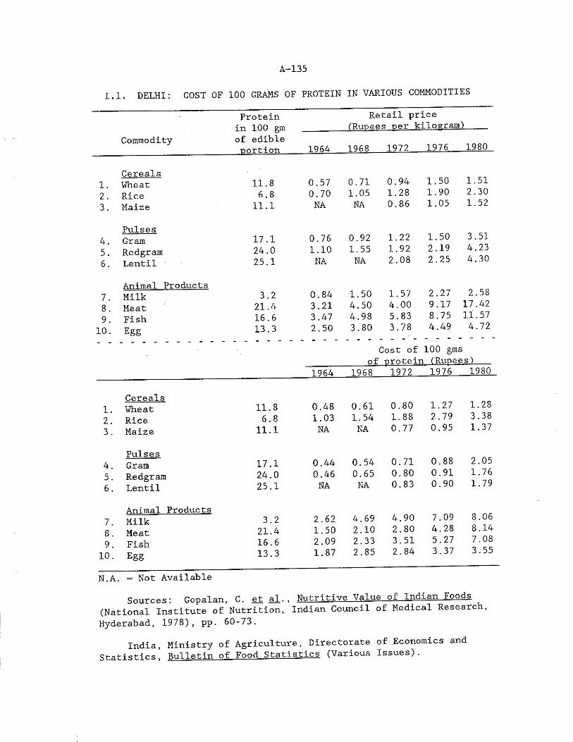
A-135
1,1. DELHI: COST OF 100 GRAMS OF PROTEIN IN VARIOUS COMMODITIES
Protein Retail pricein 100 gin ________ (Rupees per kilogram)----
Commodity of edible portion 1964 1968 1972 1976 1980
Cereals1 . Wheat 11.8 0.57 0.71 0.94 1.50 1.512. Rice 6.8 0.70 1.05 1.28 1.90 2.303. Maize 11.1 NA NA 0.86 1.05 1.52
Pulses4. Gram 17.1 0.76 0.92 1.22 1.50 3.515. Redgram 24.0 1.10 1.55 1.92 2.19 4.236. Lentil 25.1 NA NA 2.08 2.25 4.30
Animal Products7. Milk 3.2 0.84 1.50 1.57 2.27 2.588 . Meat 21.4 3.21 4.50 4.00 9.17 17.429. Fish 16.6 3.47 4.98 5.83 8.75 11.57
10. Egg 13.3 2.50 3.80 3.78 4.49 4.72
Cost of 100 ginsof protein (Rupees)
1964 1968 1972 1976 1980
Cereals1 . Wheat 11.8 0.48 0.61 0.80 1.27 1.282. Rice 6.8 1.03 1.54 1.88 2.79 3.383. Maize 11.1 NA NA 0.77 0.95 1.37
Pulses4. Gram 17.1 0.44 0.54 0.71 0.88 2.055. Redgram 24.0 0.46 0.65 0.80 0.91 1.766. Lentil 25.1 NA NA 0.83 0.90 1.79
Animal Products7. Milk 3.2 2.62 4.69 4.90 7.09 8.068. Meat 21.4 1.50 2.10 2.80 4.28 8.149. Fish 16.6 2.09 2.33 3.51 5.27 7.08
10. Egg 13.3 1.87 2.85 2.84 3.37 3.55
N.A. = Not AvailableSources: Gopalan, C. et al., Nutritive Value of Indian Foods
(National Institute of Nutrition, Indian Council of Medical Research, Hyderabad, 1978), pp. 60-73.
India, Ministry of Agriculture, Directorate of Economics and Statistics, Bulletin of Food Statistics (Various Issues).
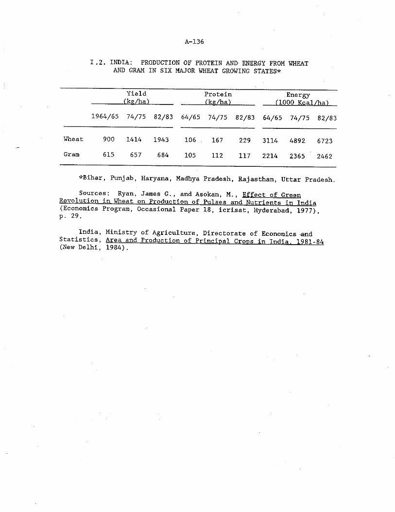
A-136
1.2. INDIA: PRODUCTION OF PROTEIN AND ENERGY FROM WHEATAND GRAM IN SIX MAJOR WHEAT GROWING STATES'*
Yield(ke/ha)
ProteinLks/ha)
Energy(1000 Real/ha)
1964/65 74/75 82/83 64/65 74/75 82/83 64/65 74/75 82/83
Wheat 900 1414 1943 106 167 229 3114 4892 6723Gram 615 657 684 105 112 117 2214 2365 2462
*Bihar, Punjab, Haryana, Madhya Pradesh, Rajasthan, Uttar Pradesh.
Sources: Ryan, James G., and Asokan, M., Effect of GreenRevolution in Wheat on Production of Pulses and Nutrients in India (Economics Program, Occasional Paper 18, icrisat, Hyderabad, 1977) p. 29.
India, Ministry of Agriculture, Directorate of Economics and Statistics, Area and Production of Principal Crons in India. 1981-84 (New Delhi, 1984).
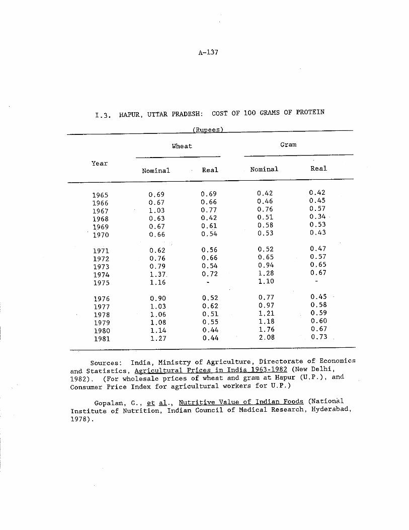
1.3. HAPUR, UTTAR PRADESH: COST OF 100 GRAMS OF PROTEIN
(Ruoees) .... ...................—
Year
Wheat Gram
Nominal Real Nominal Real
1965 0.69 0.69 0.42 0.421966 0.67 0.66 0.46 0.451967 1.03 0.77 0.76 0.571968 0,63 0.42 0.51 0.341969 0.67 0.61 0.58 0.531970 0,66 0.54 0,53 0.43
1971 0.62 0.56 0.52 0.471972 0.76 0.66 0.65 0.571973 0.79 0.54 0.94 0.651974 1.37 0.72 1.28 0.671975 1.16 - 1.10 “
1976 0.90 0.52 0.77 0.451977 1,03 0.62 0.97 0.581978 1.06 0.51 1.21 0.591979 1.08 0.55 1.18 0.601980 1.14 0.44 1.76 0.671981 1.27 0.44 2.08 0.73 ,
Sources: India, Ministry of Agriculture, Directorate of Economicsand Statistics. Agricultural Prices in Tndia 1963-1982 (New Delhi,1982). (For wholesale prices of wheat and gram at Hapur (U.P.), andConsumer Price Index for agricultural workers for U.P.)
Gopalan, C.. et al. . Nutritive Value of Indian Foods. (NationalInstitute of Nutrition, Indian Council of Medical Research, Hyderabad,1978).
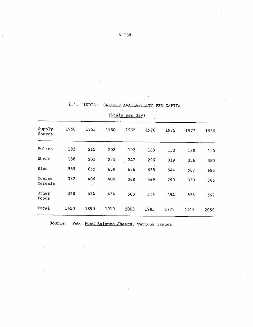
A-13 8
I.A. INDIA: CALORIE AVAILABILITY PER CAPITA
(Reals per day)
SupplySource
1950 1955 1960 1965 1970 1975 1977 1980
Pulses 183 215 202 192 169 132 138 120Wheat 188 203 235 247 296 319 336 380Rice 569 652 639 696 655 544 587 683CoarseCereals
332 406 400 368 349 290 330 306
OtherFoods
378 414 434 500 516 494 528 567
Total 1650 1890 1910 2003 1985 1779 1919 2056
Source : FAO, Food Balance Sheets. various issues.
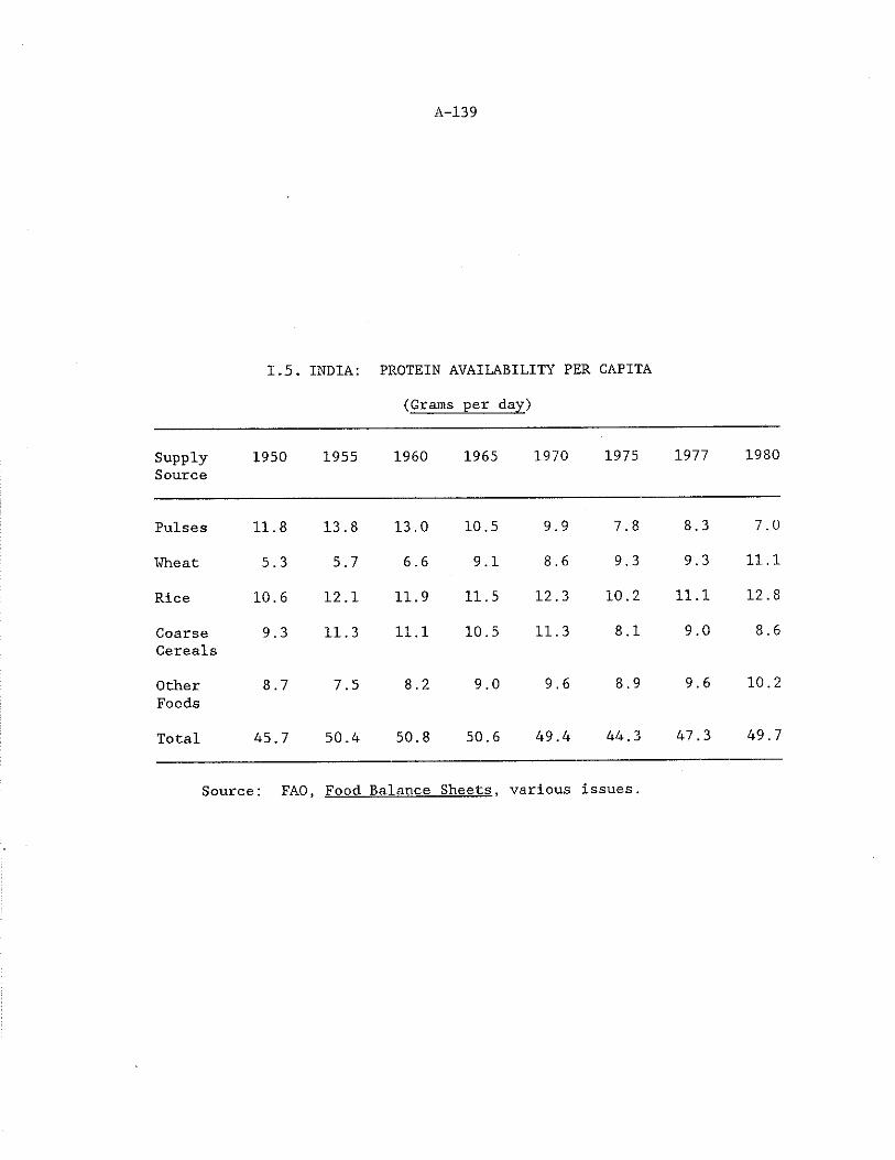
A-139
1.3. INDIA: PROTEIN AVAILABILITY PER CAPITA
(Grams per day)
SupplySource
1950 1955 1960 1965 1970 1975 1977 1980
Pulses 11.8 13.8 13.0 10.5 9.9 7.8 8.3 7.0
Wheat 5.3 5.7 6.6 9.1 8.6 9.3 9.3 11.1
Rice 10.6 12.1 11.9 11.5 12.3 10.2 11.1 12.8
CoarseCereals
9.3 11.3 11.1 10.5 11.3 8.1 9.0 8.6
OtherFoods
8.7 7.5 8.2 9.0 9.6 8.9 9.6 10.2
Total 45.7 50.4 50.8 50.6 49.4 44.3 47.3 49.7
Source: FAO, Food Balance Sheets. various issues.
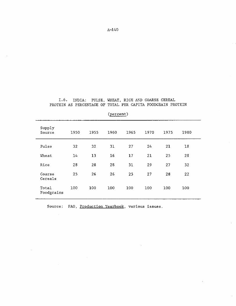
A-140
1.6. INDIA: PULSE, WHEAT, RICE AND COARSE CEREALPROTEIN AS PERCENTAGE OF TOTAL PER CAPITA FOODGRAIN PROTEIN
(percent)
SupplySource 1950 1955 1960 1965 1970 1975 1980
Pulse 32 32 31 27 24 21 18
Wheat 14 13 16 17 21 25 28
Rice 28 28 28 31 29 27 32
CoarseCereals
25 26 26 25 27 28 22
TotalFoodgrains
100 100 100 100 100 100 100
Source: FAO, Production Yearbook, various issues.
APPENDIX II.STATISTICS RELATING TO AREA, PRODUCTION AND AVAILABILITY
OF PULSES AND CEREALS
A-141

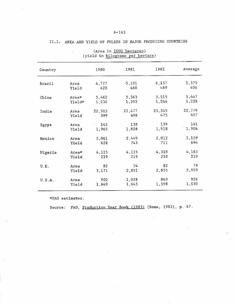
A-143
XX. 1. AREA AND YIELD OF PULSES IN MAJOR PRODUCING COUNTRIES
(Area in 1000 hectares)(yield in kilograms per hectare)
Country 1980 1981 1982 Average
Brazil AreaYield
.4,777420
5,191460
6,157489
5,375456
China Area*Yield*
5,4621,236
5,3631,203
5,5151,244
5,4471,228
India AreaYield
22,515399
22,477498
23,345475
22,779457
Egypt AreaYield
1451,965
1381,828
1391,918
141 ’ 1,904
Mexico AreaYield
2,061628
2,449743
2,012711
2,159694
Nigeria Area*Yield
4,115219
4,115219
4,318218
4,183219
U.K. AreaYield
823,171
742,851
822,855
792,959
U.S.A. AreaYield
9021,649
1,0281,643
8491,598
9261,630
*FA0 estimates.
Source: FAO, Production Year Book (1983) (Rome, 1983), p. 67.
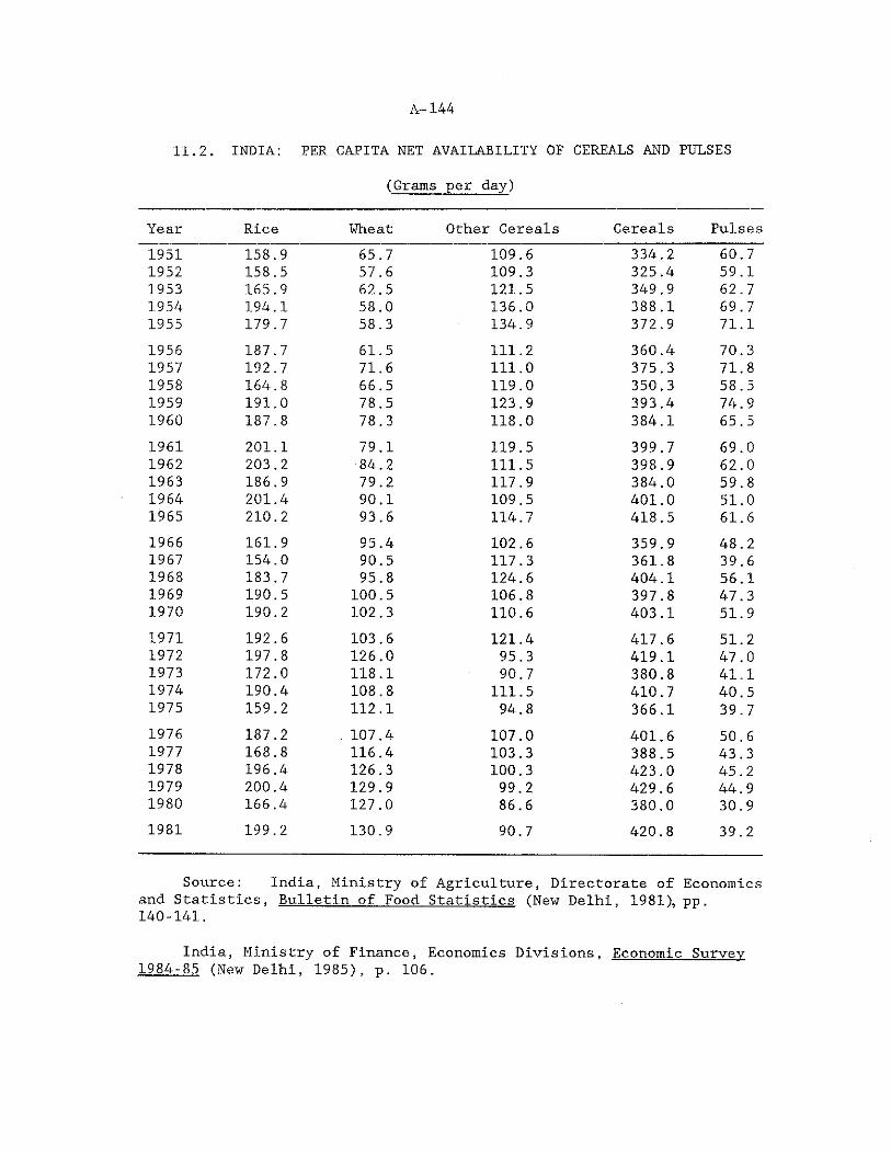
A-144
II. 2. INDIA: PER CAPITA NET AVAILABILITY OF CEREALS AND PULSES
(Grams per day)
Year Rice Wheat Other Cereals Cereals Pulses1951 158.9 65.7 109.6 334.2 60.71952 158.5 57.6 109.3 325.4 59.11953 165.9 62.5 121.5 349.9 62.71954 194.1 58.0 136.0 388.1 69.71955 179.7 58.3 134.9 372.9 71.11956 187.7 61.5 111.2 360.4 70.31957 192,7 71.6 111.0 375.3 71.81958 164.8 66.5 119.0 350.3 58.51959 191.0 78.5 123.9 393.4 74.91960 187.8 78.3 118.0 384.1 65.51961 201.1 79.1 119.5 399.7 69.01962 203.2 84.2 111.5 398.9 62.01963 186.9 79.2 117.9 384.0 59.81964 201.4 90.1 109.5 401.0 51.01965 210.2 93.6 114.7 418.5 61.61966 161.9 95.4 102.6 359.9 48.21967 154.0 90.5 117.3 361.8 39.61968 183.7 95.8 124.6 404.1 56.11969 190.5 100.5 106.8 397.8 47.31970 190.2 102.3 110.6 403.1 51.91971 192.6 103.6 121.4 417.6 51.21972 197.8 126.0 95.3 419.1 47.01973 172.0 118.1 90.7 380.8 41.11974 190.4 108.8 111.5 410.7 40.51975 159.2 112.1 94.8 366.1 39.71976 187.2 , 107.4 107.0 401.6 50.61977 168.8 116.4 103.3 388.5 43.31978 196.4 126.3 100.3 423.0 45.21979 200.4 129.9 99.2 429.6 44.91980 166.4 127.0 86.6 380.0 30.91981 199.2 130.9 90.7 420.8 39.2
Source: India, Ministry of Agriculture, Directorate of Economicsand Statistics, Bulletin of Food Statistics (New Delhi, 1981), pp.140-141.
India, Ministry of Finance, Economics Divisions, Economic Survey 1984-85 (New Delhi, 1985), p. 106.
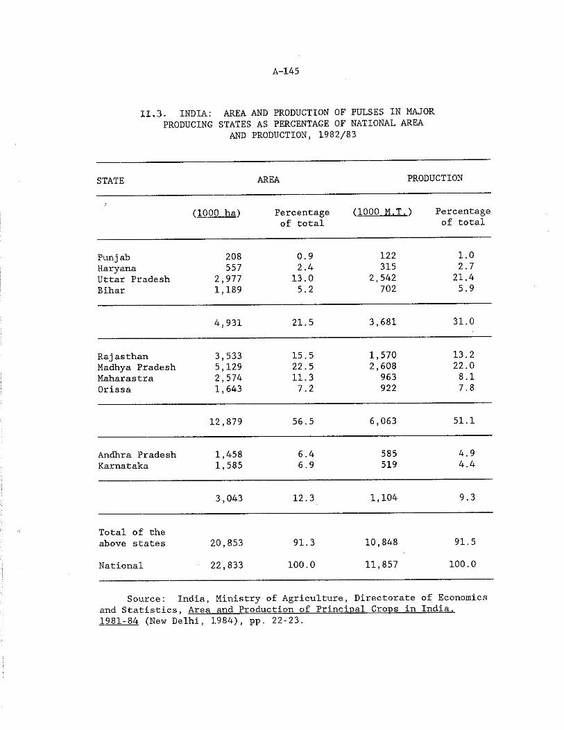
A-145
II.3. INDIA: AREA AND PRODUCTION OF PULSES IN MAJORPRODUCING STATES AS PERCENTAGE OF NATIONAL AREA
AND PRODUCTION, 1982/83
STATE AREA PRODUCTION
1 aOOO ha1) Percentage of total
aooo M.T.) Percentage of total
Punj ah 208 0.9 122 1.0Haryana 557 2.4 315 2,7Uttar Pradesh 2,977 13.0 2,542 21.4Bihar 1,189 5.2 702 5.9
4,931 21.5 3,681 31.0
Raj as than 3,533 15.5 1,570 13.2Madhya Pradesh 5,129 22.5 2,608 22.0Maharastra 2,574 11.3 963 8.1Orissa 1,643 7.2 922 7.8
12,879 56.5 6,063 51.1
Andhra Pradesh 1,458 6.4 585 4.9Karnataka 1,585 6.9 519 4.4
3,043 12.3 1,104 9.3
Total of theabove states 20,853 91.3 10,848 91.5
National 22,833 100.0 11,857 100.0
Source: India, Ministry of Agriculture, Directorate of Economicsand Statistics, Area and Production of Principal Crops in India,. 1981-84 (New Delhi, 1984), pp. 22-23.
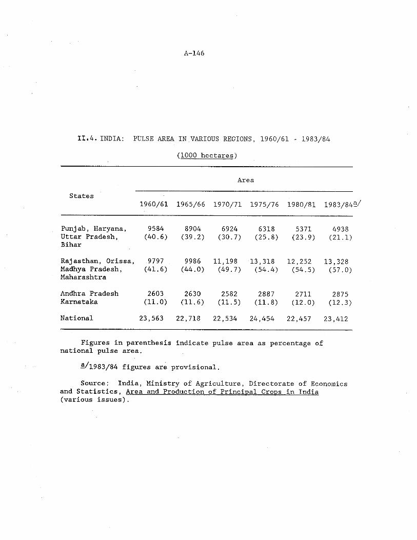
A-146
IX.4. INDIA: PULSE AREA IN VARIOUS REGIONS, 1960/61 - 1983/84
(1000 hectares)
Are;a
States1960/61 1965/66 1970/71 1975/76 1980/81 1983/84-
Punj ab, Haryana, 9584 8904 6924 6318 5371 4938Uttar Pradesh, Bihar
(40.6) (39.2) (30.7) (25.8) (23.9) (21.1)
Raj as than, Orissa, 9797 9986 11,198 13,318 12,252 13,328Madhya Pradesh, Maharashtra
(41.6) (44.0) (49.7) (54.4) (54.5) (57.0)
Andhra Pradesh 2603 2630 2582 2887 2711 2875Karnataka (11.0) (11.6) (11.5) (11.8) (12.0) (12.3)
National 23,563 22,718 22,534 24,454 22,457 23,412
Figures in parenthesis indicate pulse area as percentage of national pulse area.
5/l983/84 figures are provisional.
Source: India, Ministry of Agriculture, Directorate of Economicsand Statistics, Area and Production of Principal Crops In India (various issues).
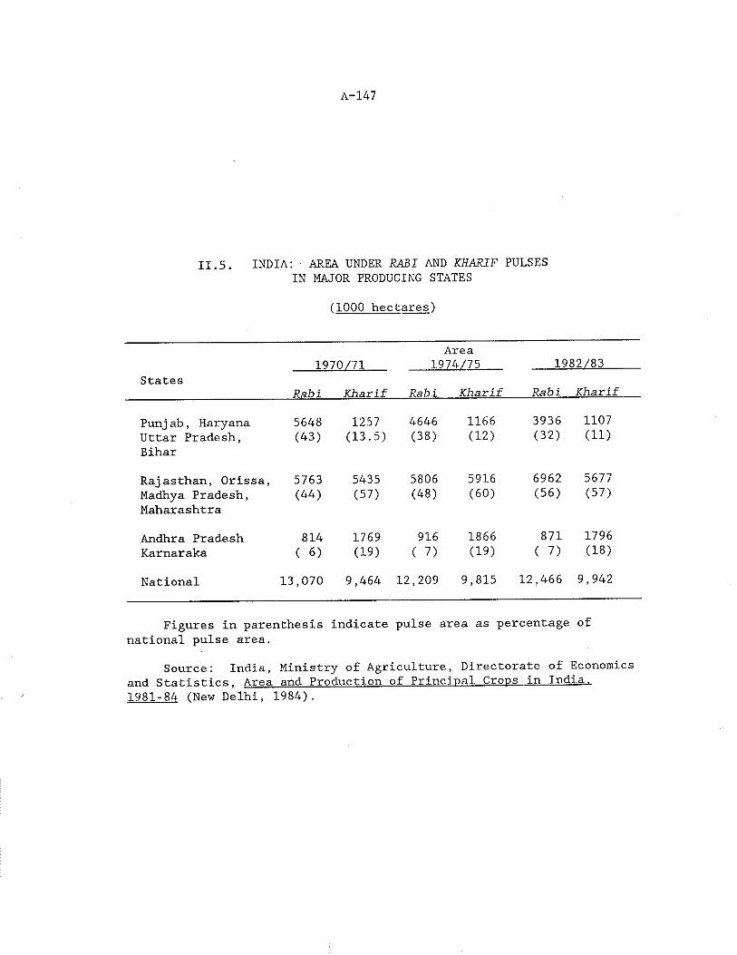
A-147
II.5. INDIA: AREA UNDER RABI AND KHARIF PULSESIN MAJOR PRODUCING STATES
(1000 hectares)
1970/71Area
1974/75 1982/83States
Rabi Kharif Rabi Kharif Rabi Kharif
Punj ab, Haryana 5648 1257 4646 1166 3936 1107Uttar Pradesh, Bihar
(43) (13.5) (38) (12) (32) (11)
Raj asthan, Orissa, 5763 5435 5806 5916 6962 5677Madhya Pradesh, Maharashtra
(44) (57) (48) (60) (56) (57)
Andhra Pradesh 814 1769 916 1866 871 1796Karnaraka ( 6) (19) ( 7) (19) ( 7) (18)
National 13,070 9,464 12,209 9,815 12,466 9,942
Figures in parenthesis indicate pulse area as percentage of national pulse area.
Source: India, Ministry of Agriculture, Directorate of Economicsand Statistics, Area and Production of Principal Crops in India, 1981-84 (New Delhi, 1984).

APPENDIX III.STATISTICS RELATING TO CONSUMPTION
OF PULSES AND CEREALS
A-14 9

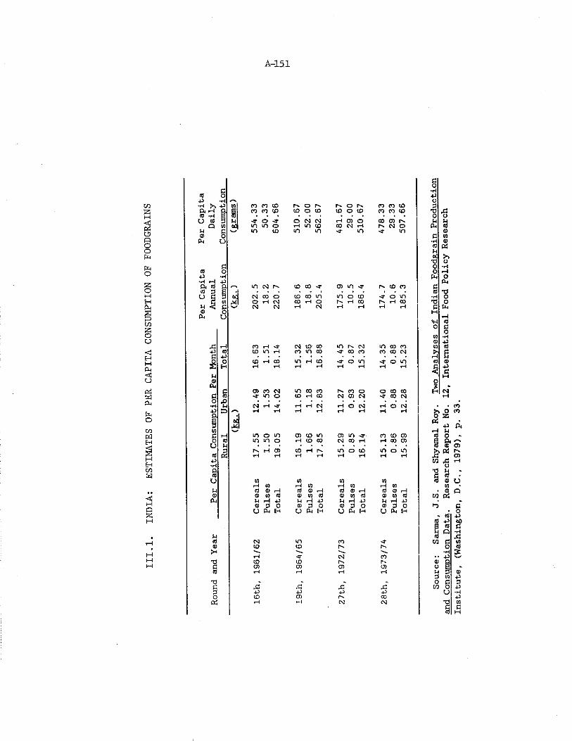
A-151
4-1 *HCO •H S to to to CO i>. o r-. o to to COIS Pi rH p to to CO to o CO to o to to to to1—l (0 E 3<T* u « 3 u -3- o o CM cm t-i O) o CO 0) P-.5 Q w tc m m o T—l m CO 00 CM CM oU u c
0) oin CO m in <r m m
n Pi OooIPpT_j « &o (3 O P, •*H •—1 p
Pi rt P m CM I"-. CO CO -T CD m <r CO too W P S • •H r i d ^ Of CM CO o CO CO in m o CO ■3- o mH 3 in o fl CM CO H o rH CO rH CO
M < C CM cm H (M H H rH H
x ft to 1—f <r CM to CO m CM m 00 top (0 to m rH CO m CO -3- CO CO CO CO CMB PO o CO iH CO m «-h to o m -T o m£ H rH rH rH rH rH rH rHW(1)Pi
B o> CO CM m CO to r-. CO O O CO COB S3 ■3- m O to f t c0 CM CD CM 00 CM0 X•H p CM* rH -9- iH rH CM t-i O CM rH o CMp S rs H rH rH rH rH rH rH rHp
to,51"W*
B rH tn O m CD CO m CD m CO CO CDo « m m o rH to 00 CM CO rH rH 00 CD
U uB rv H CD CO rH m o CO m o m
« Pi f t f t f t rH f l rH rH ftp•HP(0
o i/i tn ID IDf t CO f t CD fl ID pt| (D
P <3 Q) f l w 0) fl w 0) rH w ai fl(D a) Ul w a? ID <3 a) ID (d at w cs
Pi M ft p p f t P M f l P M rH pCD B 0 v P 0 a> P O a> p o
U Pi H U Pt H u Pi H U p H
MW CM m CO '3-<D to CO>H
rH <r CM COT3 CD ID 1". r-B CD CD CD CDW rH rH rH rH
TJ „ «B X X rB XP p p P po CO CD rv COPi 1—1 t-H CM CM
Source:
Sarma, Jf.S
. and Shyamal Roy.
Two Analyses o£ Indian Foodgrain Production
and Consumption Da
ta.
Research Report No.
12, I
nternational Food Policy Research
Institute, (
Washington,
D.C.,
1979), p
. 33.
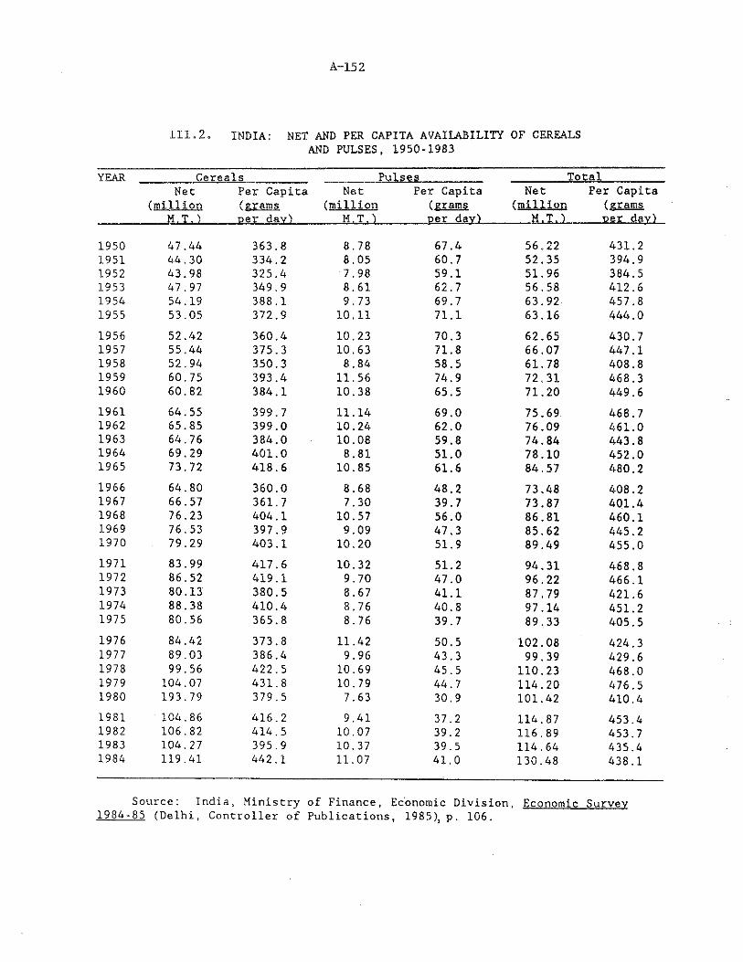
A-152
III. 2. INDIA: NET AND PER CAPITA AVAILABILITY OF CEREALSAND PULSES, 1950-1983
YEAR Cereals Pulses TotalNet Per Capita Net Per Capita Net Per Capita
(million (grams (million (grams (million (gramsM,T.) per day) — KLT.) per day) ___H.T.),__ _Be£..„day.)
1950 47.44 363.8 8.78 67.4 56.22 431.21951 44,30 334.2 8.05 60.7 52.35 394.91952 43.98 325.4 7.98 59.1 51,96 384.51953 47.97 349.9 8.61 62.7 56.58 412.61954 54.19 388.1 9.73 69.7 63.92 457.81955 53.05 372.9 10.11 71.1 63.16 444.01956 52.42 360.4 10.23 70.3 62.65 430.71957 55.44 375.3 10.63 71.8 66,07 447.11958 52.94 350.3 8.84 58.5 61.78 408,81959 60.75 393.4 11.56 74,9 72,31 468.31960 60.82 384.1 10.38 65.5 71.20 449.61961 64.55 399.7 11.14 69,0 75.69 468,71962 65.85 399.0 10.24 62.0 76.09 461.01963 64.76 384.0 10.08 59.8 74.84 443.81964 69.29 401.0 8.81 51.0 78.10 452.01965 73.72 418.6 10.85 61.6 84.57 480.21966 64.80 360.0 8.68 48.2 73.48 408.21967 66.57 361.7 7.30 39.7 73.87 401.41968 76.23 404.1 10.57 56.0 86.81 460.11969 76.53 397.9 9.09 47.3 85.62 445,21970 79.29 403,1 10.20 51.9 89.49 455.01971 83.99 417.6 10.32 51.2 94.31 468.81972 86.52 419.1 9.70 47.0 96,22 466.11973 80.13 380.5 8.67 41.1 87.79 421.61974 88.38 410,4 8.76 40.8 97.14 451.21975 80.56 365.8 8.76 39.7 89.33 405.51976 84.42 373.8 11.42 50.5 102.08 424.31977 89.03 386.4 9.96 43.3 99.39 429.61978 99.56 422.5 10.69 45.5 110.23 468.01979 104.07 431.8 10.79 44.7 114.20 476.51980 193.79 379.5 7.63 30.9 101.42 410.41981 104.86 416.2 9.41 37.2 114.87 453.41982 106.82 414.5 10.07 39.2 116.89 453.71983 104.27 395.9 10.37 39.5 114.64 435.41984 119.41 442.1 11.07 41.0 130.48 438.1
Source: India, Ministry of Finance, Economic Division, Economic Survey1984-85 (Delhi, Controller of Publications, 1985), p. 106.
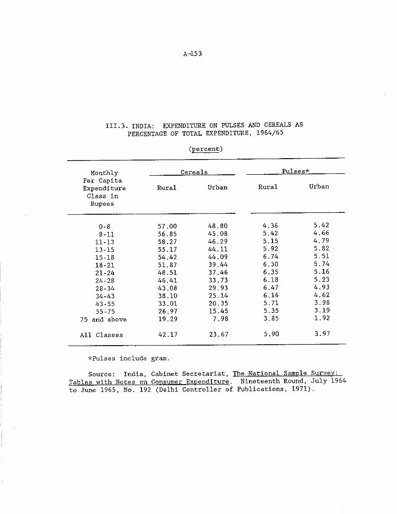
A-153
III.3. INDIA: EXPENDITURE ON PULSES AND CEREALS ASPERCENTAGE OF TOTAL EXPENDITURE, 1964/65
(percent)
Monthly ________ Cereals______ _ _______ Pulses*-----Per CapitaExpenditure Rural Urban Rural UrbanClass in Rupees
0-8 57.00 48.80 4.36 5.428-11 56.85 45.08 5.42 4.66
11-13 58.27 46.29 5.15 4.7913-15 55.17 44.11 5.92 5.8215-18 54.42 44.09 6.74 5.5118-21 51.87 39.44 6.30 5.7421-24 48.51 37.46 6.35 5.1624-28 46.41 33.73 6.18 5.2328-34 43.08 29.93 6.47 4.9334-43 38.10 25.14 6.16 4.6243-55 33.01 20.35 5.71 3.9855-75 26.97 15.45 5.35 3.19
75 and above 19.29 7.98 3.85 1.92
All Classes 42.17 23.67 5.90 3.97
*Pulses include gram.
Source: India, Cabinet Secretariat, The National Sample Survey:Tables with Notes on Consumer Expenditure. Nineteenth Round, July 1964 to June 1965, No. 192 (Delhi Controller of Publications, 1971).
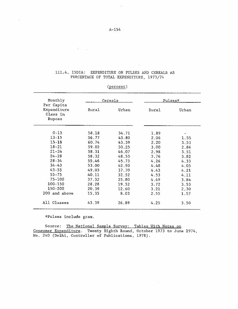
A-154
III.4. INDIA: EXPENDITURE ON PULSES AND CEREALS ASPERCENTAGE OF TOTAL EXPENDITURE, 1973/74
(percent)
Monthly Cereals Pulses*Per Capita Expenditure Rural Urban Rural UrbanClass in Rupees
0-13 58.18 34.71 1.89 -
13-15 56.77 43.80 2.06 1.5515-18 60.74 43.39 2.20 3.5318-21 59.02 50.25 3.00 2.8621-24 58.31 46.07 2.98 3.5124-28 58.32 48.53 3.76 3.8228-34 55.46 45.73 4.26 4.3334-43 53.00 42.90 4.48 4.0543-55 49.03 37.70 4.43 4.2155-75 40.11 32.52 4.53 4.1175-100 37.32 25.80 4.49 3.84
100-150 28.28 19.52 3.72 3.53150-200 20.39 12.60 3.21 2.30
200 and above 15.35 8.03 2.55 1.57All Classes 43.39 26.89 4.25 3.50
*Pulses include gram.
Source: The National Sample Survey: Tables With Notes onConsumer Expenditure. Twenty Eighth Round, October 1973 to June 1974, No. 240 (Delhi, Controller of Publications, 1978).
STATISTICS RELATING TO AREA, PRODUCTION AND YIELD OF MAJOR
PULSES BY STATE
APPENDIX IV.
ii
i
A-15 5

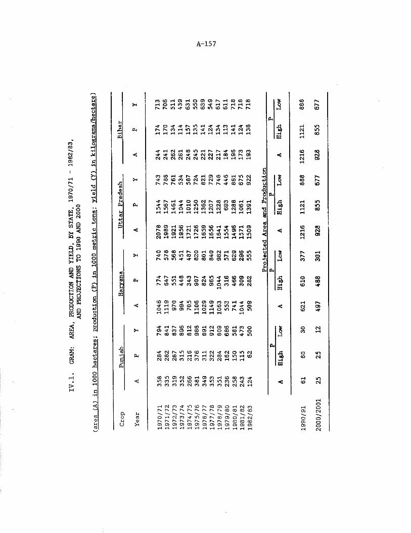
IV.1.
GRAM:
AREA,
PRODUCTION AND YIELD,
BY STATE,
19
70
/71
-
19
82
/83
,AND PROJECTIONS TO 1
990 AND
20
00
4-157
xn i D H Q H O C D O l N H t O e O C OH O H n n i n W ^ T H r l r l r l H(^p-.in^rtO'TitDintotor^r^r^
S*3
ua,nCQ
ft r^h>COrMin«'^-CN3CO*H-d'C\JfOH H H H r l r l H H H H r l H H
•rH
C<
X
-apHq>
w■poBooo
JH
ft
>H
Gft
eoD■aojhp
§&ea
ft
<
>-l
ooo
G■H
•8 ft
<3
■3’ <T(OlO<t, ^N N H O O O IM ))N N N N N N N N N H H H H <
n t D H ^ N ^ H O I B M D H t n N•joDlfltOCONNN'TvrlDNNr^f^r^»nmr^cor'f^'4-cou30)
■ t f - r - . r H ' T O O C M r ' - . C O C O C O r H r H■TiD(D'frnn0oNO)(O(DO)
C O O ) H l O H ( D O ) ( O H - J I D H O )scoNinNNiri'n'TioqiNOocfiO)0)M^(D(D(oin«jtnmN r H H r l H H H W r l H H H H
O l O « H N O r l O N H O ) ( D i O•TN I D m O N O ^ O J N N O I i / lp v t n < n - 4 - ' 4 - o o c o o o a ) i n t o c g > n
«TNH(op>is^in>Tta(DCiNN < r m ^ < » O N l D « S ' H ( D O a 3N ( O i n s r t o o ) o o o j o c o * T t o e M
■Offl+>0•n01Mft
ft
■sm
ft■a«
«3fflO'jiniDoimnnrt^o) ■JHNOl OON' TI Di n- t f - JO owojojf^T-HOi-tomr^otn r -1 i — t i — i r - i i — I r H r H
<3
■fHNIDNlDHNffl lDHCOO0 ) 4 M t 3 ) r l O D O ) H O t O ( O N Or ^ o o a o o o o o o j c o a s c o t D t n ' a - i n
%
ft^ N N i n i O l D W N ^ N O t f l NO O D O l D r l r t S H t M C D f O i n H O DN N N ( O N ( O P ) P ) N H H H
•S60
uMinoiNiOriooHiOffln^mtoHi/iicoo^inmtoin'fNn n n n N n n n n N N N H «!
<roa)Mn
i— \ <N CD -r to CO CO CD O rH CNJ CO(-» p-. p> t"- r-% r-* h- CO 00 00 COft M .0 (t) o iH (N CO <■ CD co r". CO CD O rH CMM 0) t"- PN I-- r-. r-* r-- r. P- CO CO COL> >H 01 O) CD cn 0) Ol CD O) Ol Ol CD Ol OlrH t—i rH rH rH i—i rH rH rH rH i— * rH rH
COCOCO
CM
torHCM
00CO00
CM
rH3r-.co
orHCD
CMCO
ot o
oto
to
2000/2001
25 25
12 497
488
301
928
855
677
928
855
677
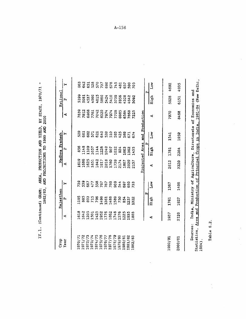
IV.1
. (Conti
nued
) GRAM
: AR
EA,
PROD
UCTI
ON A
ND Y
IELD,
BY S
TATE,
1970
/71
1982/83, A
ND P
ROJE
CTIO
NS T
O 1990 A
ND 2
000
A-158
! eo CM rH 00 O Ph O 00 m rH P-. o mj
>4 to -3- m CM r>. o CO r-» -a- CO m CJ o 1 Qto to to m in p- to to p-* -S' to tn P-
R3 PMG CD rH p- O) m o -3" o o> to CO CM CMO
CMOJ CO CD CD rH CO CM rH CO m CM HP CD*rl rH o m O O CO HT -S' r- CO to to O
eo m m HP ■ y Hf in m in m CO -a -a- m m&
CD eM 00 H OI o St" -a- CO m -a- CO m nCO H to to <■ CM p- r- o C0 CO to CM 5< CO CD 0) r-. o CO 0) CD r-» CD <n CO CM iHpH r- to r- r-. CO r- ph e' to to PH P-- 4JO0■p0tH
0) rH CM H rH o o o en in OJ rH -a- Pui *j s , 03 00 CO p - CM -a- CM rH CD CM CO S'- p- T3 0to m to (0 m to to <n tn m ■a- m to to 5 1-J■o s19M (9 PmPm CM to eo CD •3- to O ) P- CM sP CO CM m
CD(4 rjAd m -3" O «n <■ CM Hf o CO CM to to m •ifj t oC0 T—1 H O rH CM O CD o OJ o CO "5"li•o
rH rH «—* r-t rH rH rH rH rH rH TJOJ LT.-j« 0) to m rH CM p- 00 O OJ HT p- OJ Ph H-J
o. H 00 <M m -3" rH rH CO CO Ph o CM m 0)<1 to to ID CO CO 03 O r- r-. CO O rH •r-r-( rH rH rH rH rH CM rH rH CM H CM CM O
CM tOCD COCO CD-s- -a-CO rHco mCD rHin <o
o eop- toCDr-- co
rH O)-r mm orH rH
rH • &00 COr» cmrl CM
cm o«H CMto COCM CO
g&-Uw««PP04
CD CD PH r- CO Ph pH CD CD -a- fH O CO (S,CO CO to P h in to CO OJ O HP OJ m CO o IDr \ in to -3- m PH pH PH OJ in to to Ph rJ OrHPM
m in CO in CO CO rH CO OJ o HP pH CM rHo CO o H CD OJ to CO 00 <n tn m CM 60 IDH
00 CO P h Ph -a-rH COrH -3rH mrH PH CO 3 eorH ■Hn
r-*rH
CO CM »n rH m CM to CM CO to m m COrH -a- o O CM »n Ph to PH CM CO O CO40 to CM tn -»• CD PH oo PH to CM CD CO <3 0)tH rH rH rH rH rH rH rH rH rH rH rH rH rH
toCD-S'
p-cmOJ
oCMrHcm
rH CM CO •a- m to CO CD o rH CM COPH fH PH PH PH PH PH Ph P h 00 CO 00 COa M H -H. H-» H^ ■H. H H-^H S
0 (9 o t-H CM CO -a- m ID pH CO OJ O rH OJtH <D P- PH fn pH PH PH PH pH PH P h CO CO COu >H CD OJ OJ CD CD O CD CD CD OJ CD CD orH rH rH rH rH rH rH rH rH rH rH rH rH
rH rHO) O"ho oCD Ooj orH CM
Sources:
India, M
inis
try
of Agr
icul
ture
, Di
rect
orat
e of
Eco
nomi
cs a
ndSt
atis
tics
, Ar
ea a
nd P
rodu
ctio
n of
Pri
ncip
al C
rops
in
India. 1
981-84 (
New Delhi.
1984).
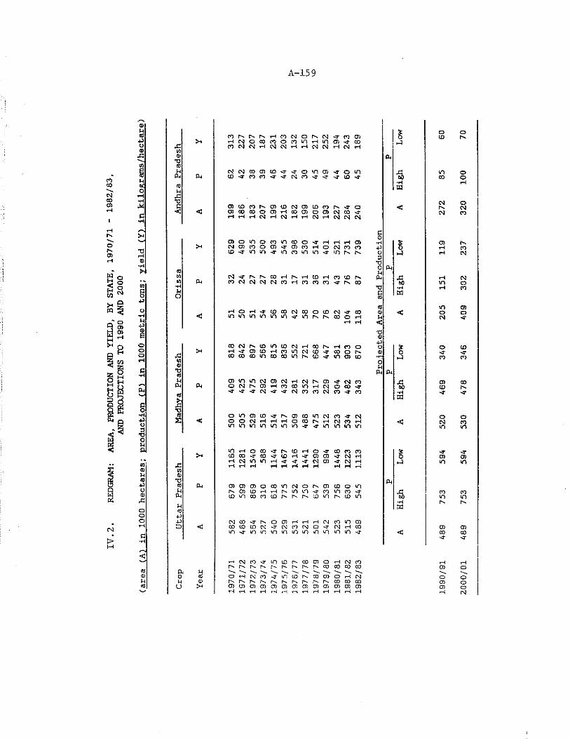
REDG
RAM:
AREA,
PROD
UCTI
ON AND
YIELD,
BY S
TATE,
1970
/71
- 1982/83,
AND
PROJ
ECTI
ONS
TO 1
990
AND
2000
A-159
0MfflO«gMlKO
C
TSi—(ffiEHing-pomi
oooCPM
+)O£TJOnotn®u«-po0
tN>
ooo
<00n0
£ oto p p p rH CO eg o IP eg a- to 03 8 CD>h rH eg o 00 CO o to in i—1 tn CD a COrd CO eg eg rH eg eg i—i H eg eg rH eg rH100 (MT3(0Ml CM N eg CO CD CO a -T O tn CD a- o tn•s mCM to a to to a a eg to a a a- to a CO
0 •HMlid*o egd CO to to P* CD CD eg O) CO to p a o <3 p
< <! Cl) CO CO o CD rH CO O) o CD eg 00 a eg1—1 rH tH eg i—1 eg i—i H eg rH eg eg eg
O) O m o CO m 00 o a rH rH rH CD g■rl S O)Eh eg CD CO o CD a CD to iH O eg to to 5 rHCD a tn tn a m to m tn ■a- tn p P O i-HsT30 PM0 MlWCM eg a p p CO tH P iH to i—i CO CO P CM rHto CO eg eg eg eg to H to to CO a p CO 60 miH -o iH i—1MO 6 m
rH o i—i a CO 00 eg CO o to eg a CO 00 ino<! tn tn m tn m >n a m p p 00 o 1-t Ml egrH rH <'O0
CO eg p CO m to eg i-t CO p rH CO O 3O $ oEh i—i a O) CO i—i to m eg CO -a- CO o P 0 o aCO CO CO tn to CO in P to <r m CD CO *r eg COto 00 tHT3<0 Ph PhM CM O) in tn eg CD eg rH eg p CD a eg to
■s CT)CM o eg p CD i—1 to CO in rH eg o CO a CDa a a eg a a eg CO CO eg CO a to *rl a0fci
m
•o« o tn CD to a P O) 00 tn eg to a eg o
£ < O o eg r-t t—1 i—1 o 00 i p rH eg to i—i <5 egtn tn m tn tn in tn a a m o tn tn m
in i—i o CO a P to i—i o a - CO to to a a>H CO CO a CO a CD i—t a CD CD a eg rH 8 CDrH eg tn m t-t a a a eg CD a eg rH m,d 1-1 rH rH I—t i—i i—i i—i i—i tH rH rHto0CM PM0 O ) CD CD o CO m eg o i p CD CO O mM p CD CD i—t 1—( p m tn a CO m to a toCM CO m CO to CO p p p CO m p to m tn•H pMl to
PP eg CO a p o CD rH tH rH eg CO m CDD < CO CO CO cg a eg CO eg O a - eg rH CO CDm a tn m tn m m m n m m m a < COa
t—i eg CO a tn to p CO CD o i—i eg to T--1r '. P p P p p p p p 03 CO CO CO CD
PM Ml ^— '^ fc0 0 o rH eg CO a tn to p □0 O ) o i—i eg OM 0 p p p P p p p p p P CO CO □0 CD
U Eh O CD CD CD CD CD CD CD CD CD CD CD CD CDrH i—i rH rH w rH rH i—1 rH rH r H rH i—i T—t 20
00/0
1 48
9 753
594
530
478
346
409
302
237
320
100
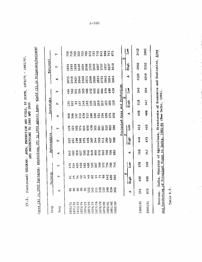
A-160
©u«43a. O
CO ©CO &
CM inCO £CD COiH woql 0rHrHP M
O CP- +MCDrM /■v!MSaTl
WH Ti< rHfH ©CO “M
43(0M«■f"
sm
p-i
CM
PM
CM U
P r-O (0 o iHM © p.U O)O)■Hi— i
CDoomcMintocMmcococDininOrHQ3C0CMC0P''C0rM'31 C0'S‘ P''rs.Nr^inr'NtDNr'tDWNiP
cocococO'3-CDinop'r^p»r-"tD®ooNor)CDNncoin«i(OHCOIDCD'J'COONOCONOINO)H H H H H N H H H r l H N H
cDco^riomcomtotDP'COOoon n n n n n n m n n n m n
«fMHvfmiON>n'?<JOoi50)(T)C,10NtO<nCDlOtDNroiP-3-ioco>ninin-y(otDtjDcoHr'3-
nntfiNtD'PicnoJininno)H H r l r I H r I N N N H H H
f f l ( D h N O ) I P O O H < - C ' » l »oocDr-tp^f-tcocMeomcoP-.mn n H M N o N n w n p j n N
l D H N 4 < r O O ) r l H r l O f l l f lh M O ) N n n i P t s r o N M o < 5
uirirootDtorv^rCDHOh'O) o i n a i D N O o i - J a i H B N C ) c n N H c o c o ^ M f O ^ - r t o ^ n
o c m c d p - c m c m c o o c D c o i o c o o <r 03 0 N O ) - T ^ M D M O O O C O (D<3-in(DmtjDuDtDUD«3r'r'tD
<a-<j'00)cstDcnr>(DcO'S-oinrvHOn0)(DC3)0)(I)N‘0ro-3'<rin>if'a'n'3'int,5in|Pf'r,'N
M M - 4 N N ® N < f ' - t t D N O i n-3-<3-cO'3-co-3-to~3-i~'-co-3-cocn
(OIDtDlQ'TN’Tl^NncOoOOJtowcooioiooHnincONiDH H H H H r l N N
PM
■a*M03
PMAtom
CM
P-<
a•a-CM
CMCDCDCM
COCMmCO
CO< rCM
CD*n<»
CD<r
CDOr%
cop»co
CDco<r
mm
CD00eM
CMCOtOCO
03CM•M-
MfCDCM
f'.HPCO
into-3
COP-*<r
p%'T
O)CDm
oCDco
cop-oo
r M C M C O ' T * n i O P > C O rs i— r~ r—un cdp. P-CD CD CD CD CD CD CD
CM CO -O' p. i— p"CD o 5—C CM CO rH rH o 0P- CO CO CO CO CD O CO M
— PMCO U) o rH CM o oP - r-v CO CO 00 CD o T3CD oi CD CD CD CD o CrM rH rH rH iH rH CM ©
too•H 43 w ■H4J «43 COT39(ftot 2 gowCMo©43 « u o43o© MTU co•H IQ rM 00 - CD© rHU3 •43 © i—t *H0 *o0 c•H M1 «CM W O P O& S43W r-t •M ©a st* s« M *H P-l T3 (3 »M M O
C•• ow© 43 O OM 0o n
i
COCD©
•8H
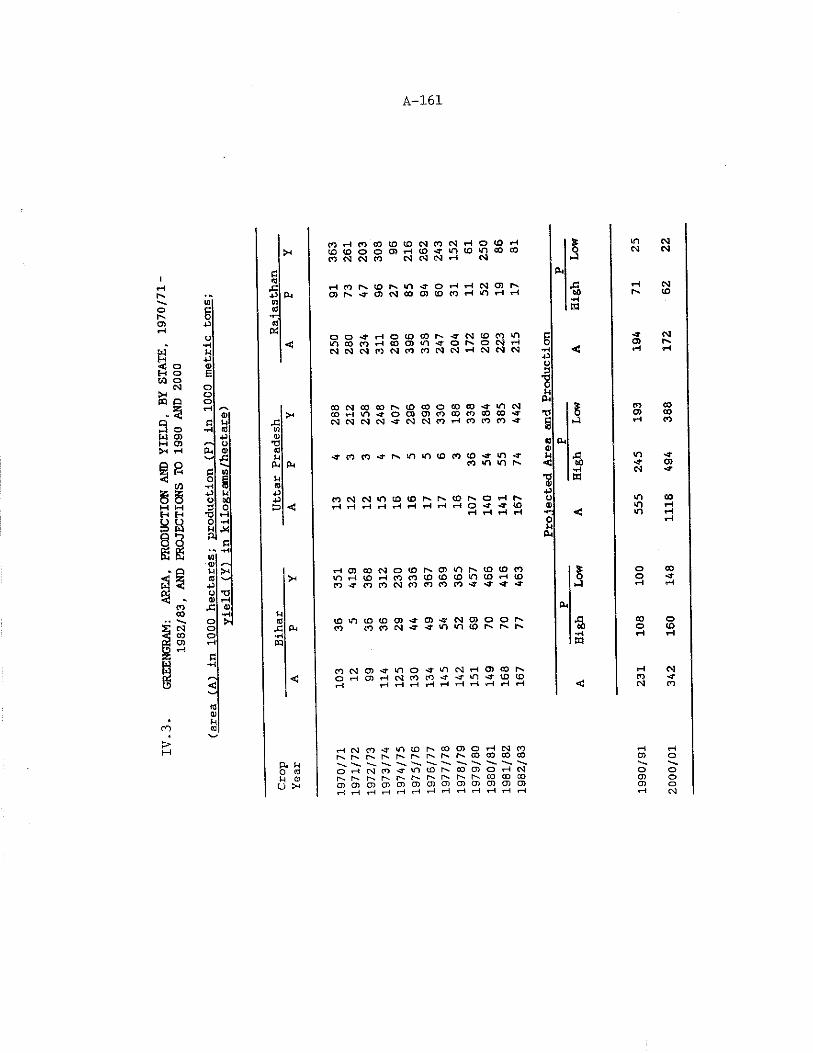
IV.3
. GR
EENG
RAM:
AR
EA,
PROD
UCTI
ON AND
YIELD,
BY S
TATE,
1970
/71 -
1982/83, A
ND P
ROJE
CTIO
NS T
O 1990 A
ND 2
000
A-161
P ) H ( 0 0 0 ( D I 0 N n N r l O ( D H ( D i D o o r o n t D ^ t n i o m c o f f l CO N N F3 CM CM CM »-l CM
+3U1 tor ©o *T"]•P PdO•HUP©EooofH ©R M JR•tH « to-P ©U -a£4 © ©,r up4R ©0 g u■H © w-P u PO X. 4-33 0 P3•a0 •Hu X9 Rw03u >4(04-3O 030)rHX ©*H U0 ©0 iC
pm
pmm
R
rltONCDNin-a-Ot-trlCMOTI'vO)h>TO3NOI3O)0(OHir)Hrt
OO^HOtOfflN'TNIDCOinl O C O C O H O C D i n ^ O S O N r lN N N M N n c O N N H N N N
f f l M O O C O N C O O D O C O C O ' f l - i O NoHin^oo)0)cocococo«3<jC S l N N N ' f M N C O H C O t O C O - f
^rtto-a-Ntnio^cotO'S-in'Tco m <n O'
CONNT)(DtDOOI0OOrlO H H H tH H H tH H H O CO
HO)®NOIDSO)tnO(D<£l(0inHCDHCOCOIOlDtDCDCDHCDCO-TCOCONCOCOCOCO^'T'T'J
(OWOt0CDO)'3-O3'S-C'3O)OOO* co fococsj'T'Tvnuotor^O'O'
CONO)'J'U10J3'lflNH(JlCOI\o H O ) H N n i o ^ ' f * n < f U 3 t i )r-1 H r l r l r l H H H H H H
PMJ3toca
1O0)■r0M
CM
PM
m coCM CM
«H CM1 (O
-T03
COO)
WO■3*CMininm
oo
COo
COCM<3©
NC0'f*0l0ls,c00)OrlC3(0h'r^f^h'r^r^r^r>cooococoPM H O © M 0) CJ >*o iH C". r-v03 co
cm co -d- in cor-. r-- I''- 0-*CO CO CO CD O l CD
CO 03r- r>03 03O H MCO CO CO CD 03 03
o0303 2000
/01
342
160
148
1118
494
388
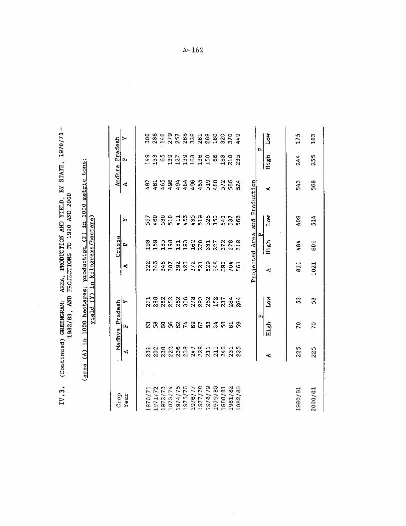
A-162
it".or>.o>
8awSheq
8
T)0)4J8o
ina0■po•<■1u4J<Daoooft
CDc kft «
+3Oft a>Nw" 13■*-.£ w0 g53+3 kO M3 0■o i—l0 ftk ,*!ft
RftinIDM ShID+3O *q<D >—113 0ftO MOOftnft/N<
130)k(3
0 CO 0 03 e- CO 03 ft 03 0 0 0 03 £ m13 0 CO a tn CO CO CO CO CO eg rx a 6 r>in CO eg ft eg eg CM CO eg CM ft CO CO a pi ftCD
•o PMtok CO to m O) i* 03 CO to O CO CO 0 m 13 aft ft a CO CD CO eg CO CO CO m CO CO ft CO 60 a
H ft iH 1—i ft f t 1—1 f t f t CM eg CMCfl mk
£*3fi r» ftt m CO a -a CO m 03 0 CM CO a £ CO
< <3 CO CO CO 03 03 CO 03 cO ft CO r~- CO eg 0 aa a a a a a a a m a m m in hH <3 m
-p00
*00k
PM1 . O 0 0 f t to in 03 CO 0 0 i-' CO s 03
>4 03 CO CO ft ft *n CO 1—t CM m a CO to r s S 0m a m m a a a m m CO m m m
§a
« Pmn) 0)m CO 03 m CO ft CO eg 0 ft e- eg CO 03 M 13 ain f t 03 m CO 03 CD 03 CO e- CO CM rv r- ft < 60 CO
ft f t H 1—1 1 f t f t 1—\ eg CO eg CO to to *H ak T3 &a
O CD
CM CO CO eg CO eg ft 03 00 0 a ft-PO f t
< CSJ a a CO 03 eg i". eg CM a 03 0 to CD f tCO CO CO CO CO a CO m CO to to n- m < CO
0M
PM
H CO eg eg eg 0 CO CO CM eg n- a a s CO13 Dh r*. 00 CO m CD ft r-> 03 m m CO CO CO 0 minA) eg eg eg eg eg CO eg eg CM f t eg eg CM pi
T3(0 Pmk
f t CO CO 0 CO eg a 03 e- CO a CO f t 03 13 0f t CO m to m CO 1 . CO CO m to m to m 60
to ft>
£t t
*3«
s f t eg 0 eg CO CO r» 00 f t f t to f t m m<3 CO 0 CO eg CO CO a eg f t ft a CO CM CM
CM eg eg CM eg eg CM eg eg eg eg eg CM <3 CM
m>M
ft M O CO M <D O >t
f t C M c o a i n c o r ' - c o c o o f t i N i c or^.r^r^Nr^r^r^f~sf^cocococoO H N n ^ ' n t D N o O O l O H Mror^r^r^r^-f^-r^r^-r^r^cococD0)0)0)0)0)0)0)0)0)0)0)0)01
o03CO 2000
/01
225
70
53
1021
60
9 514
568
255
183
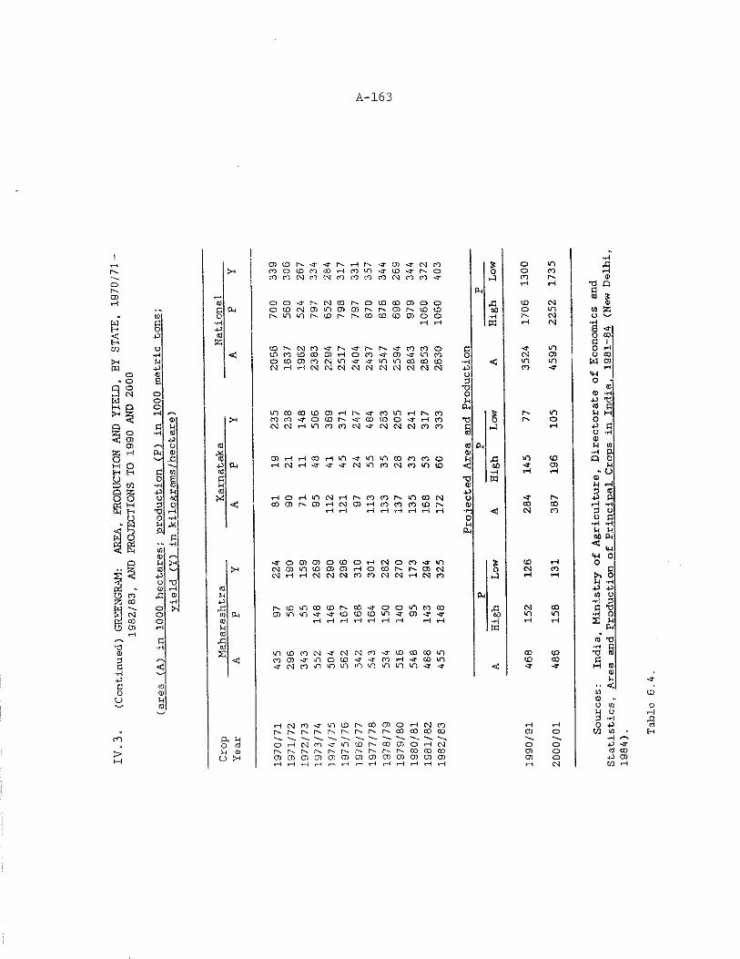
IV. 3
* (Continued) GREENGRAM:
AREA,
PRODUCTION AND YIELD,
BY STATE,
1970/71
1962/83, A
ND PROJECTIONS TO 1990 AND 2000
A-163
w■ - £w O£o pp cd
5Zo•HMpoEooo
lo
£ u■H S3
PO cdft CD
& %P
£ w COo E £•H (V wP M cdo W X£ o
T3 ftO ftU Mft £
-HU3t0)M > *53
-PO T JCD ft cO
r : CD ftPo >■ rCo U)o COft ft(0
£ n-H cd
£
<
(00)u(d
Pm
<
fu
C
>4
P h
C
CDto t"- -a <r ft 1—\ ft ■a CD CMCO * o nCDo CDCOoOft COn ~T CD ft o 0 o COco n CMco CMco COCOco CMco CO-a tP CO ft
ft ftPM
o o <r n. CMCO ft o ID <X) O) o o ,c ID CMo COCMCDn CDCDft ft CDft CDCO 00 o mf". m n ft CDft ft COCOCD CDo o ft CM
ft ft ft CM
COp- CMCO-a ft <r ft ft ■JT COCOo £ ■a- min to COCOCDft o CO•a- CD <a in CO 0 CM CDo COCDCOCMn -a <r m n 00 00 to ft < m inCMft ft CMCMCMCMCMCMCMCMCMCM p CO -r
o£TJ0P(Ti
m COCOCDCDft ft •a to in ft ft CO ft mto co -T o CDft <? COCDo ~a ft to T3 5 ft oCMCMft n COCOCM•a CMCMCMto to
§ p ft
53 P-iCDO) ft i—l co ft n -a m m 00 co COo p m CDft CMft <T -a -a CMn COCMco m ID < &0 -a CDft ftTJ0)PT—l o ft n CMft ft COco ft m to CM o -a ft
COCD ft CD ft CMCDft COCOto CD ft CD co COft ft ft ft ft ft ft ft ■n < CM CO
0PCM
-a O CDCD o ID O ft CMo CO-a n s CD ftcMCDn CD CDCDft o COft ft CDCM o CM toCMft ft CMCMCMCOCOCMCMft CMto .p ft ft
Pmft CDn COCDft CO-a- o o m CO00 CM 00CDm in -a •a CDID CDm -a CD-a ■a to n mft i—i ft ft ft ft ft ft ft *H ft ft
K
n ID COCM-a CMCMco 'T CD 00 co in 00 CDco CD•a n o ID *a ■a COft ■a COm CD CO-a CMco n n m m in n n m -a -a < <T -a
ft uO rtl M 01 U
f tCMto-aincof tcocoof tcMcor^r'-ftftftftftftft°oco cocoO f t C M c o - a i n t O f t C O C D O f t c M [ - ' • . f t f t f t f t f t f t f t f t f t c o o o c o 0 ) 0 ) 0 ) 0 ) 0 1 0 ) 0 ) 0 5 0 ) 0 ) 0 ) 0 ) 0 ) r—I ft ft ft i—; ft I ft ft ft ft ft ft
o oCD OO) Oft CM
Sources:
India, M
inistry of Agriculture,
Directorate of Economics and
Statistics,
Area and Production of Principal Crops in India.
1981-84
(New Delhi,
1984).
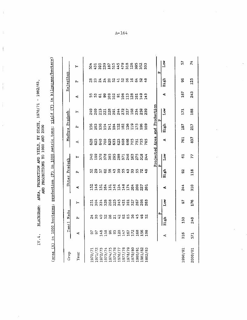
IV.4.
BLACKGRAM: AREA,
PRODUCTION AND YIELD,
BY STATE,
1970/71 - 1982/83,
AND PROJECTIONS TO 1990 AND 2000
A-164
©N(0Pu0)XIinLItsCo*r4MP
tH
P(0x;pV] <0 CL.
(d&<
vr^ino)Ninino)coiDinNnop3COcoa)ir4^rp^Ht\)cnincr)<n'fONH<n'a-'TOHnnnI
Pu,con-r-JONHNffiiDjrNcoN N N N N > n < f |ODHU)in-3' XJ60
ra^ n r i o x s N H o o n o o r i a i ninv)coa)ooa)Ot-f(MiO'T'3' <
-a-IT) P-.
IDO)
rvoo
TJ0)H
pu.PO•H■POP*0onp
Jp10a)T3<auP-.cl.
<
0)omi-tc0i-i<-MrvC0'T0)0)a i D ^ N N O i ^ N N m n i / i nN M N N N N M N N H N N N
(n(Dtom<ra3mfflinHNO)(D
pop■g
§
8a
X!60ta
co m o o oN N >T O Nto to to to
CO CO 00 ID tnCD CM tO CO OID ID (D ID N
<0h m in ©m m o pj"> ■<
<
o r o a i < o i n n c o H ( D c o i n c o < t'Tair^r^coa)coN*aitDr i-i'a'n H n n c n N M O N H N f O M
T>©Po©■»-OMP-i (U
sot-3
N O ) N N f f l n o ) i n n n n N O )incMintDin'Tcoinsrcomp^-a- ■a
N t D H - ^ H t D ^ O D ^ ^ O N H^ < r i n ^ m < r n ' T N O o N oH H H H H r l H H H N M M N <
H<r4C0fflinmrlHNMDnmocDMIDN'J-cMCDNIDOtDCMCDCOCOCMCMCD'TCOCOCMCMCM I3"O(055 CL.
•a-orocMcDr-tcMcMintomtocMNn'finNN'ftDiDiri'itM-inCl.
■a
H<
r^i^ooeotCDor'-r'.CMCOtococooLj-tnrooicM'TtDi^ioinCT)m
<
i".cn
torv
(O
INO)
<r•3"CM
i".0)
CDCD
toHCD<cd©u(C
aouuMid©
rlCJtO'tmiDNCOfflOHCJtON N I N I S f N f ' N I N ^ ' © © © ©OHNrt-TVHEMDOlOHNr r-'.i' r-'-r-r-r-r'-r-'-r'-oococo0 ) 0 ) 0 ) 0 ) 0 ) 0 ) 0 ) 0 ) 0 ) 0 5 0 1 0 ) 0 ) rHfHi—l«Hi—IrHi—li—I t—I H ri rl ri
O0)O) 2000/01
571
240
176
310
118
77
837
217
188
243
125
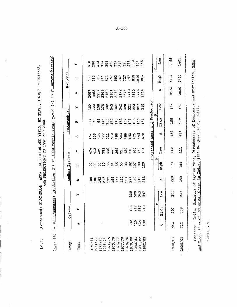
(Continued) BLACKGRAM: AREA,
PRODUCTION AND YIELD,
BY STATE,
1970/71 - 1982/03,
AND PROJECTIONS TO 1990 AND 2000
A-165
tC
C
*o
-pop-pwEooo
Pm
DTJopp]w0)P<0o<L>Aooo
«0)pSO
CM
Pm
Pm
cocjocr>'TCf)o<-'J-oaocO'T*nH W H H o m n - T N N n r a mn N n t o n n n n t o N o r t n
comcOMriHiNtorNiNiNOO-a-i n t o H M - N i P c n M - N ' n ^ P i PcoincDfNiotNtorNiNrNCPoco
r^.tor^aiCTjr-i^cg'TcnotO'TlDU3intDlDIDNINSrl(Ols'Ho c o C D c o i H s H O i H c o i N a o f N r ' .n h h n n n n n n n n n n
O N C O a J N M C J l N O V I C O N O )mcMorNO-a-'a-HrcMcMcMcorHN N N N n t o o t o n n N n n
mt mh in o m m m o N(O -r m N IN N
n oo to N h aIP O N N H H^ n co in ip ip
n o t h i—i n cd ■a- h- co <r mj-nt -a-
to to C5 o -a- m
CD cm CO CO
-t -a- *a- -a- <r
o o o m t D M r m o
O ID N N O) CD CO H rl H rl NCM COO) CO C-fNH
PH
JU
COlO
fNCM■a
r-N
|N
Pm I
CM
CM O -a- CO (O rl CO COCO -a- MT NT
CO~3-tn
05CMwCO
in to o rM HPm \A to CMMf o m m to CD S'*"rH *—iH tH tJ 1 -H 1 iH H1 S3 i«3 CM HfCO m m CM CD <3 C9m |N a- in y ■3"
o ID O O rH o s o rHCM in CD tH m o NT CMa - CO - a a IN •J- rH rH
0M
O i P m
CO CM IN, o O id t—5 CO05 O ) O 0 ) CM 1 0 IN e s
H rH $ tH H
r-N mJ- CM 05 CM 00 OCM * a CO i- l f—1 <1 CM mCM CM CM CM eM CM CM
o O) m IN k m SNCO CM < r ■a CD ■aCO m m m * 4 CM CO
ID fN IN oCM tH CO < r A . IN O)rM CM tM CM 60 05 CO
1 WCM CO
CM
rH CN] ro AT (n CD fN CO 05 O rH CM CO rH tHpN r. fN |N P'S r- CO CO CO CO 05 O
p* V N^ -—o od O rH CD m to 00 O) o r-t CM O ou Q) f. hv r-x IN IN r> IN CO CO CO 05 o
(j CD CD CD CD CD 05 05 CD CD U) 05 05 05 05 orH rH rH rH rH i—i rH rH rH rH rH tH rH rH CM
Sources:
India, M
inistry of Agriculture, D
irectorate of Economics and Statistics,
and Production o£ Principal Crops In Indi^_1981~84 (
New Delhi, 1
984).
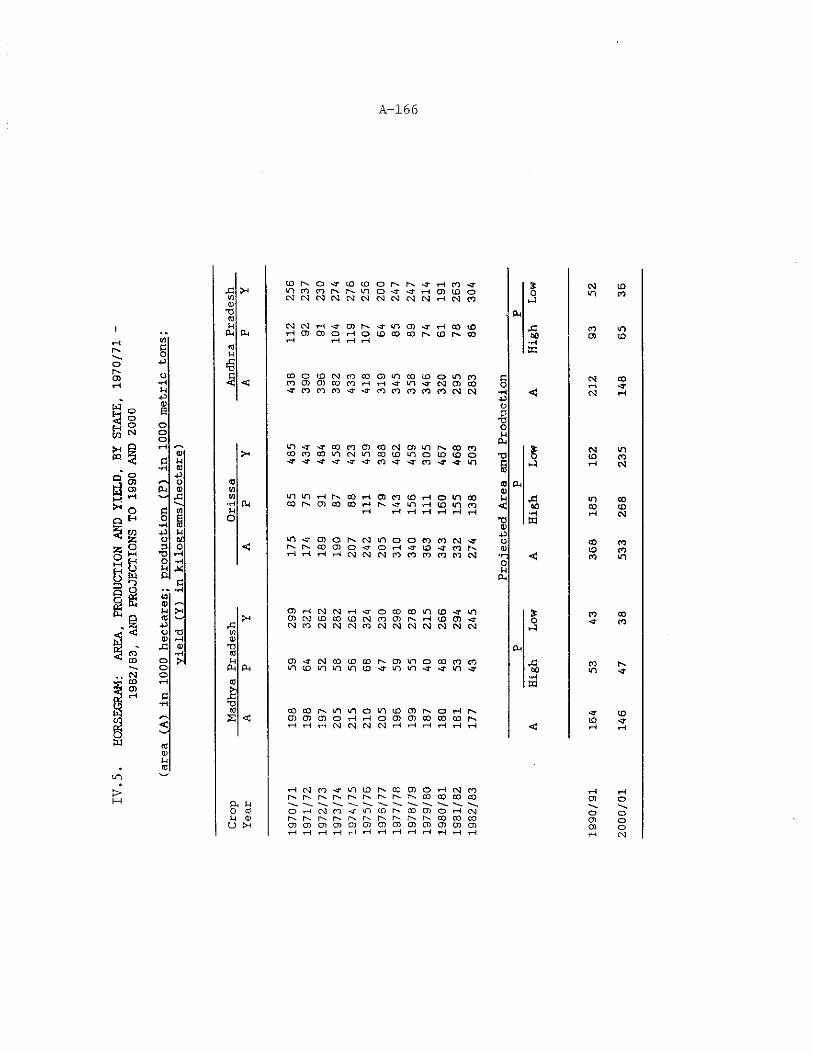
A—166
imoe-CD
m>
w£5■po•Hwp0eoooH ys®c niH COPoft ®yCd (0o £•H fgP t-tO 0£P oT3rHO •HM Mft
a
w<sMlfH«po *o0)rH-C (0*Ho MootHd-w<«0)Ml(0y_'
CD m o ya CD CD o r-y m ~T rH CO ■a- £fw m co CO rn r-y m o a a tH CD CD o o</](D eg eg eg eg eg eg eg eg eg eg iH eg COTi ft(0Ml CM eg eg tH a- CD m a- m CD a tH oo CD hGft tH CD CD o rH o CD CO CO IH, CO m 00 00cdH
tH yH tH tH »r|m
6g CO o CD eg CO 00 CD in CO CD o m CO C
< < CO CD CD co CO tH rH a m a eg CD 00 oa- CO CO co a- -3- CO co CO eo CO eg eg *HhhOPTJOtHCM
<
m -T a- co CO CD CO eg CD m m co CO %>-* 00 CO CO m eg m 00 CD m o co CD o T3 5ya ya -T ya a- a- CO a a CO ■a- a- m § rd<0 CO ftw 0)w CM rn rn tH rn co iH CD co CD y—( o <n co M td-h co m CD co 00 rH e-y a m rH CD m CO < Ck3M rH tH tH yH yH yH tH ♦Ho 13(D m
m ya CD o eg m o o CO CO eg ya+1Uc m rn 00 o> o <r o rH a CD ■a- CO rn 0)yH rH tH tH eg eg eg CO CO CO co CO eg <ouCM
CD iH eg eg rH a o CO CO >n CD a- m>H CD eg CD co CD eg CO CD ry tH CD CD a- oyG eg CO eg eg eg CO eg eg eg eg eg eg eg100)TS(0 ftM CM CD a- eg co CD CO m CD m o 00 co CO rGCM m co in in m ID a m m ya a- m ya 60(0 •Htofc1ydT3cd CO 00 f-y m m o m CD CD rn o tH rnE < CD CD CD o yH rH o CD CD CO CO co m
T—t rH rH eg eg eg eg yH iH rH rH tH tH <
rH eg CO a- m CD fn CO CD o y—1 eg COm e> e- m m m m r-y m CO CO CO COft Ml -y- yyy s N. -yy -yy yyy '—o (0 O rH eg CO a- m CD m CO CD O tH egMl <D e m m tH N m r-y pn m m CO CO co
U CD CD CD CD CD CD CD CD CD CD CD CD CDtH 1—l 1—1 1—1 rH T--1 i—1 i—1 1—l rH rH tH tH
eg idm co
co inCD CD
eg*heg
egco
in00
00COCO
CO-T
COm
a-CD
CDOCDCD 20
00/01
146
47
38
533
268
235
148
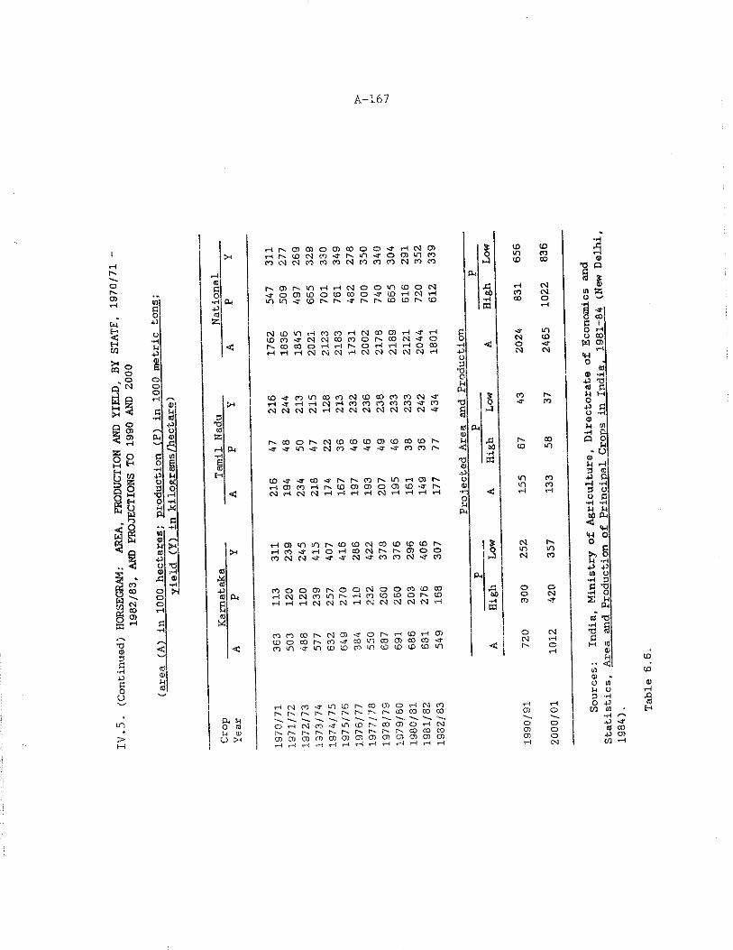
IV.5.
(Continued) HGRSEGRAM: AREA,
PRODUCTION AND YIELD, BY STATE,
1970/71
1982/83, A
ND PROJECTIONS TO 1990 AND 2000
A-167
i
Os
rH <t-xCD!Rj HS r43 •aH O <0pr] ssH ,C rHg ing *H
flj-H 843 R HO M3 oT3 pH0 >HRPI R* --pHMCD#"“nMCO N143O 'd0)r4 «£ ffi*P"o ► 43o CCo PPcdR M■H<cdCDncd
rHrxCDCDo CDCOO o XTtH03CD £ totH rxCO03COXTOxm <0o CDm CO Q inCO03INroCOCO03toCOCO 03COCO CO
ao>r-m tHt-103o o m CDo 03 43 Ho CDCOo COCOo XTCD tH 03rH to COinm xrCOOxOx-S’OxOxCOCOOxCD ■wER CO
N l D l O H n n H N O O O l H ^ Hcocoxro3C3cocoorxcor3xrorxcocootHsHf~xOtHiHiHooor l H H N N M H M N N C M N H
a. mO cdI-( <DU tn
tH 03 CO O' fx. fx- LD tO aj O) o rt N n(s N CO ffl CO CDM CD cTi CD r- r~ r— 00 CDo i-4 03
CO CO CO
03oC3
COCOCO0303o
inCOxr03
Rp icd xrco m coCO03CDcoCOCO03xr £ CD>4 rH xrtH tHc3iHCOCOCOCOCOxj-CO T3 o to03 0303 03 tH03030303030303xT § PI
idPRCDOx COO Ox03COCDCDCDCDCOCOrx w JG r 00PR xr XTm xr03CO-a-xrxTxrCOCOrx < 00 CO ma®
CO XT XT CO xfOxO'COr-xm tHCDrx o m COr4 CDCO tHrxCOCDCDo CDCDxrrx ® in CO< 03 tH03 03tHtHtH 03tHrHtHtH Q
< tH rHrPR
tH CDm m OxCDCD03coCDCOCDrx S (SI r>4 tH CO tHo tHQO03Oxrx U) o o o cn mCO Cs!03 x?Xfxr03~TCOco03xrCO N coPR
CO o O CDrxo O 03o o CO(D00 4 o oPM tH 0303 coinO'tHcoCDCDo rxCD 60 o CsitH tH■H 03C303tH03o3030303 tH ■H CO
CO COCO O'03CD o rx i—<CDtHCD o cqCD O oo rxcoxfCOm COCDCOCOxr C3 pH< co cn •xr inCOCDCOinCDCDCDCDin < OtH
30)O
o R 0 O COW rotr40
0 1 0 3 0 0 1 0 ) 0 1 0 ) 0 1 0 ) 0 ) 0 ) 0 1 ^r t H H H H
Q)MBaRo•HU$O&P P in v •H Ra ti*<H Os WPRcd T3 •H Tt R M «J 0)0)O mH o3 •H
i—1 tH o -PCD O CD tn
*H < xO o P x rCD o cd coCD o P CDtH 03 CD tH
COCO
0)rH*3H
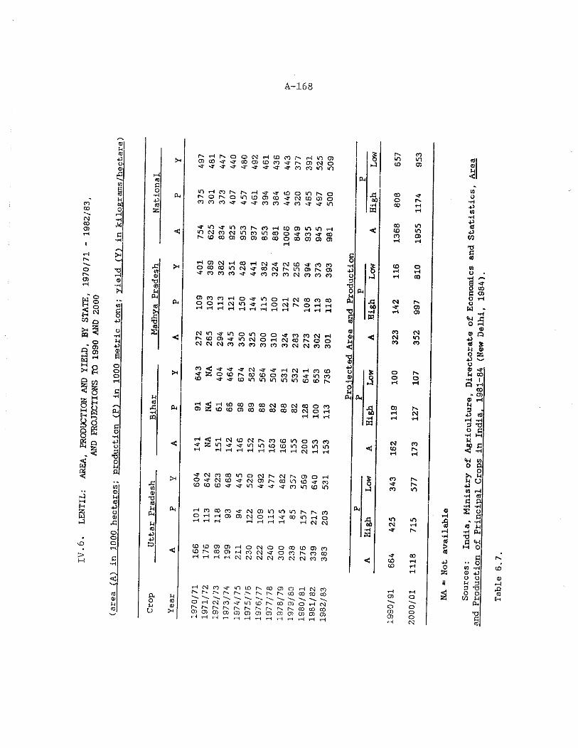
IV.6.
LENTIL:
AREA,
PRODUCTION AND YIELD,
BY STATE,
1970/71 - 1982/83,
AND PROJECTIONS TO 1990 AND 2000
(are
a (A
? in
10
00
he
cta
res
; p
rod
uc
tio
n
(P)
In
1000
m
etr
ic
tun
a-
yie
ld
(Y)
In
kll
oa
ram
a/h
ac
t.r^
A-168
TOPOXTOSS
«TOt3TOUft
TSTO£
nTOX•HCQ
XTOTOXI TO N ftMTO■PPS
ftO(-1U
ft
S H N O O N r l T O T O r N H i O O ) T O C O < c TOO)(DTO'5-|n O ) O J O sr sy sr sr
| O H n t s N H ^ , j - i o o i n N ONONoiniflojco-jrjtDrooTOTOTO^sr<{OTO"TTO<-^(n
«iNTOM>rinioa)o-Tn^(oN U D c O O C O C D C O o O O e O C D C J C n
O T O « m N < r ( O N N n o S N C 3 )'TCOcoco-s-.fl-cotorocMcococo
ft ® n CO H o ST no o r-f cm in <r rHrH r H rH i=t .-4 . - J
O 1-4 cm oo co coo N N O ri H
ft
K ^ l0 2 i n o o ^lv> W N HN N M T O f f l n c o n n N N n m
C2 ^ 2 ' I ' T(>J';5'<:r,H'NrHCOCD' j i o i D N c o i D o n w v M n n'S-<rtoTO»ninin!n5SN
^ ! S S 2 ® w ® n c o o c oT O t O C C e O C O C O f f l C O M O H
rH <sjs: H N I D N N f l t O I O O n c O^•j'jininTOTOinoininH H H r i H H H H f J H H
ft
^ ( N c o c o i n D M N N N a o dCO CO CD <3- srin^J-srsrcQintOin
H n c o n c N O ) i n « o i O N N no H r i o o i N o H ^ a n o r i o1— THiHrHrH H fsj cS!
f f i l f l O ) 0 ) H o N O O C O ( D O ) mc o r scoa)rHcocMsrocor''COCQHHHHMNcsjcvjforgrj^n
uTOTO5H
rH cm co 'i- in idN [V IS N f s r s
CO CD D-CM CO ST in ID rs . CO r" cs. (s, (v,
0 H N CO TO TO CO CO
01 O H N N TO TO TO’ 1 ’ 1 ” * ■* i -*• F F I UsJ UJ UJw ^ C J j o c D o c n c n c D C D Q C D r o
g•Ho3TJOuft
TJsTOTOM<XfTO40uTO•r—oMft
ft
fs CDm m TO(O o TOM<
ft
00 sro rv00 HrH
00 mCO >nro 0)rH rH
(O OH rHrH co
CM Pssr CDrH O)
CO 03CM mCO CO
ft
ft
oo
O)
CMCO
COSj-CO
<nCM-S’
-tCOCO
oCDO)
COrs
rsrsin
•3H
64J0S5
oooCNF
B•• oCO TO 40 O O M 3 3 *C O O CO in ftX!C:TO
XTOH
India, M
inistry of Agriculture,
Directorate of Economics and Statistics,
of Principal Crops in India, 1
981-84 (
New Delhi, 1
984).
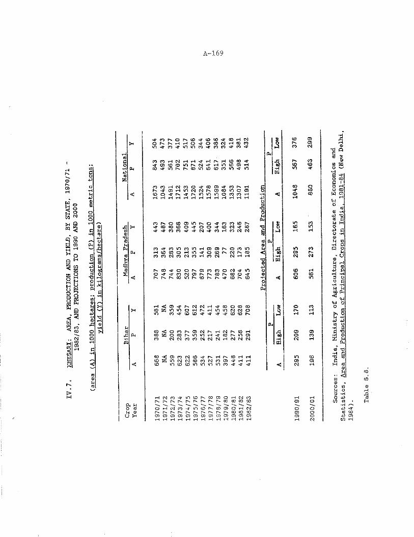
A-169
r->oe'en
XQ OH
S5 9
IQ
co03CMCOO)
c-.j>t—i
WC5CJn■p©Gooot—t/■>©c Mlft toft(JCM a),CXn [Qo gft to■P uO u3 0XI fto ftMlMft sftIQ4? /"NMlXto --1fto ft<0 I—lX! ©ftooofta•n<«0)Mca
PM
<3
,cw(DTJ<0MCM5)fcr£X3(C£
CM
X
U(0CM
<
Pc U O tt) M 0) Q X
-3- CO ft O ft to -3 to to tr 00 ft CM | | to U) io ft ft ft ft o -3- o 00 CM ft CO CO Q ft o> r*4m 's- co a - tn to CO •>3 CO CO a CO 3
pJCO CM <&TJ q
s *eo CO ft CM ft ft -3 ft ft ft ID CO ■a
■aft CO i
W ES■a- cn to o m ft CM a ft m to CD ft toCO -3 m ft ft 00 m to to co m a m ft 3 o
1 » t -O ooS Lco CO ft CM co o a c o CD -a- CO ft ft € CO © O ft
r- '3- CD ft m CM CM ft CD 00 in o CD o -S' t o \ O COto o <■ ft -r ft m m in o CO CO ft ft < o CO M Oft ft ft ft ft ft ft ft ft ft ft ft ft ft ft ft
O3 o 4X) ©O © ftn 40 T3p-t tn C:
CO ft O 00 CD m ft o a CO CO to ft 5 eo i4 HCO CO CO o •a o o - a to CM -3 cO XI 8 to in 0<r -3 - CO CO a - ■a- CM -3 co ft CO CM CM §
© 04
ft ft 40 fi8 ,HM n
© ft 0 -CO -3- co m CO in ft CD CD ft O CO m M
• 5tn eo Q 0
ft CO CO o ft m -3 O to ft CM ft CO < CD ft t-iCO CO CM CO CM CO ft CO CM CM ft ft CM CM * U
■8« ©
H i-M40 3 ©
1 00 *3- O o ft CD CO CO o cm a m O to ft 4J (Xo a - -a- co CM CD ft ft CO ft 00 o ■3 © o to ft fte- ft ft CO m ft to ft ft ■3- to ft to •r < to m 3 oo
u04
a c•H *H M U
*H 0ft <3 CD -S' ft CM CM *—! •a- 00 O CO eo $ © co OCO S5 m m o ft ft ft to in CM CM o Q ft ft Sm co <r to to -3- -a- a -a- to to ft M ft ft x oU ft
40 4004 M O ft 3
CO <3 O CO ft CD CM ft T—1 CM ft 00 ft■a
0 ) 03 a xi00 £; O CO ft m in ft CO ft m CD © CO ft oCO CM CM CO co CM CM CM ft CM CM CM
«CM ft £ u
04
ft XJ ft eCO < 0 ) CO CM to a ft ft ft CO ft ft m CD >0 S3to t z m cm CM CO CO CM CO CD ■3* ft ft CD CD ttto m to to m m m m CO -a- -a- •3 - < CM ft h-\ ©©
H•• < m 1© -o mU o3 ft
CM to ~T m to ft 00 CD o ft CM CO ft ft 0r ft ft ft ft ft ft ft ft 00 00 CO CO CD O in mft ft '-'v, fto ft CM CO <r m to ft CO CD O ft CM O o 40ft ft ft ft ft ft ft ft ft ft CO CO CO CD o to CQa> CD CD CD CD CD CD CD CD CD CD CD CD o> o 40 a>ft T—! ft ft r* ft ft ft ft ft ft ft ft i—1 CM m
00toaft■3H

COCONUTS AND OIL PALM IN THE INDIAN OILSEEDS ECONOMY
by J. V. Meenakshi
Copyright © 1986 by J. V. Meenakshi
TABLE OF CONTENTS
Page
GLOSSARY ............. . . ........................-............... B-ix
TECHNICAL NOTES ........ ........................................ B-xi
CHAPTER I. OILSEEDS IN INDIA: STAGNATING PRODUCTION,GROWING DEMAND...... ................... . . . ........ B-l
Performance of the Indian Oilseeds Economy. ............. . B-lAnticipated Demand. ............ .............................. B-2
Population. ................................. B-6Income.......... ............. .................... -..... B - 6Income Elasticity of Demand. ..................... . B-6
The Changed Import Structure................................ B-8The Objectives and Organization of this Study.............. B-ll
CHAPTER II. THE IMPACT OF THE GRAIN REVOLUTION ON THEOILSEEDS ECONOMY OF INDIA......................... B-13
The Green Revolution........... ............................. B-13The Impact on the Oilseeds......... ........................ B-15Area Trends in Major Producing States....................... B-16
Groundnut............................. B-16Rapeseed-mustard........ B-22Sesame. ................................................. B-26
Prospects for the Three Principal Oilseeds.......... ....... B-29Technological Factors..................................... B-29Institutional Considerations.................... B-30Prices ................................... .......... . B- 31
Prospects for Nontraditional Sources of Vegetable Oil...... B-33Soybean............................... B-33Sunflower .......... .............. ...................... B- 34Rice bran. .................................. B-34
Supply Projections................................... B-35Scope for Tree Sources of Vegetable Oil.................. . B-36
CHAPTER III. COCONUTS............................. B-39
Kalpavrksa, the Wish-Yielding Tree.............................. B-39Varieties of the Coconut Palm........ .............. . B-40Climatic requirements....... ......................... - B-40
Coconuts in India.......... B-40Coconuts in Kerala........ B-41
Production Characteristics......................... B-43Yields of Coconuts........................... B-44The Competition between Coconut and Paddy.............. B-49
B - i i i
Prospects for Increased Coconut (Oil) ProductionFinancial Feasibility...................Acreage Expansion.........................Yield Augmentation.......................
Supply Projections.......................Implications for Rice Imports..............
B- 51 B- 54 B- 55 B- 57 B- 58 B- 60
Page
CHAPTER IV. OIL PALM. B- 63The Miracle Palm.....................
Varieties of the Oil Palm.............Climatic Requirements.................
Oil Palm in India: A Brief History........Oil Palm in Kerala: Yeroor Estate..........
Production Characteristics.............Processing...................Economics of Cultivation...............
Palm in the Andaman and Nicobar Islands Prospects for Increased Palm Oil Production..
Yield Increases.................Area Limitations.....................
Supply Proj ections......................
CHAPTER V. IMPORTS VERSUS DOMESTIC PRODUCTION: SOME POLICY IMPLICATIONS.......
B- 63 B- 64 B- 64 B- 66 B- 69 B- 72 B- 77 B- 80 B- 87 B- 89 B- 89 B-91 B- 94
B- 97Imports or Domestic Production?. Policy Implications............ B- 99
B-104
CITATIONS. B-107APPENDICES B-117
B - iv
LIST OF APPENDICES
Page
I. STATISTICS. RELATING TO THE COMPETITIONBETWEEN CEREALS AND OILSEEDS................................. B-117
1.1 India: Area under Groundnut and itsCompeting Crops, by State, 1956/57 - 1980/81:
Guj arat............................................ B-119Tamil Nadu......................................... B-120Andhra Pradesh............. B-121Maharashtra........................................ B-122Karnataka.......................................... B-123
1.2 Gujarat: Area under Groundnut and itsCompeting Crops, by District, 1961/62 - 1973/74:
Amreli............................................. B-124Rajkot....... B-124Junagarh........................ B-125Jamnagar............................. B-125
1.3 India: Area under Rapeseed-Mustard and itsCompeting Crops, by State, 1956/57 - 1980/81:
Uttar Pradesh...................................... B-126Rajasthan. . . ........................................ B-127Madhya Pradesh..................................... B-128Haryana........ B-129
1.4 Uttar Pradesh: Area under Rapeseed-Mustard and itsCompeting Crops, by District, 1961/62 - 1973/74:
Etawah............................................. B-130Nainital........................................... B-130Agra............................................... B-131Kanpur............................................. B-131
1.5 India: Area under Sesame and itsCompeting Crops, by State, 1956/57 - 1980/81:
Orissa............................................. B-132Uttar Pradesh...................................... B-133Rajasthan.......................................... B-134Maharashtra........................................ B-135
II. STATISTICS RELATING TO COCONUT.............................. B-137
11.1 India: Area, Production and Yield of Coconuts,1956/57 - 1982/83....................................... B-139
11.2 India: Area, Production and Yield of Coconuts,by State, 1956/57 - 1982/83:
Kerala............................................. B-140Tamil Nadu......................................... B-141Karnataka.......................................... B-142Andhra Pradesh...................... B-143
B -v
II. 3
II.4
II .5
Kerala: Area, Production and Yield of Coconuts,by District, 1960/61 - 1980/81:
Trivandrum................................Quilon.......................... ..........Alleppey..................................Kottayam, Ernakulam, Idikki...............Palghat, Kozhikode, Mallappuram............Trichur...................................Cannanore.................................
Kerala: Area under Rice, Coconut and GrossCropped Area, by District, 1960/61 - 1977/78:
Trivandrum................................Quilon....................................Alleppey..................................Kottayam, Ernakulam, Idikki...............Palghat, Kozhikode, Mallappuram.......Trichur...................................Cannanore.................................
Kerala: Prices of Coconut Oil and Coconuts,1963 - 1981.................
B-144 B-145 B-146 B-147 B-148 B-149 B-150
B-151 B-152 B-153 B-154 B-155 B-156 B-157
B-158III. STATISTICS RELATING TO OIL PALM B-159111.1
111.2
111.3
111.4
III .5
III. 6
111.7
111.8
111.9
Yeroor Plantation: Area, Production and Yieldof Oil Palm, 1976/77 - 1985/86...................Yeroor Plantation: Area, Production and Yield of OilPalm, by Type of Planting Stock, 1976/77 - 1985/86....Yeroor Plantation: Monthly Rainfall,1976/77 - 1980/81.......................................Yeroor Plantation: Fresh Fruit Bunch Yields,by Month, 1976/77 - 1980/81............................Yeroor Plantation: Fresh Fruit Bunch Production,by Month, 1981/82 - 1985/86............................Yeroor Plantation: Total Expenditures,1980/81 - 1984/85.......................................Yeroor Plantation: Costs of Cultivation of MaturePlantations, 1978/79 - 1981/82.........................Yeroor Plantation: Costs of Cultivation of Matureversus Immature Plantations, 1978/79 - 1981/82........Yeroor Plantation: Net Revenue from Oil Palm Cultivation, by Type of Planting Stock, 1978/79 - 1981/82.... IV,
B-161
B-162
B-163
B-164
B-165
B-166
B-167
B-168
B-169IV, MISCELLANEOUS STATISTICS RELATING TO OILSEEDS
AND VEGETABLE OILS.......... B-171IV. 1
IV. 2
IV. 3
India: Area, Production and Yield ofGroundnut, 1956/57 - 1983/84.........India: Area, Production and Yield ofRapeseed-Mustard, 1956/57 - 1983/84... India: Area, Production and Yield ofSesame, 1956/57 - 1983/84............
B-173
B-174
B-175
B - v i
PageIV.4 India: Production of Major Vegetable Oils,
1960/61 - 1983/84.................................... B-176IV.5 India: Net Imports of Foodgrains and
Vegetable Oils, 1961 - 1984.................. B-177IV.6 India: Imports of Vegetable Oil, by Type,
1960/61 - 1983/84.............. B-178IV.7 World Production and Exports of Vegetable Oils,
1973/74 - 1983/84..................................... B-179IV.8 International and Domestic Prices of
Vegetable Oils, 1970 - 1982. ....... .................- * B-180IV.9 International Prices of Palm and Soybean Oils,
1970 - 1985........................................... B-181IV. 10 India: Minor Tree-Crop Oilseeds...................... B-183
V. MISCELLANEOUS CALCULATIONS.................................. B-185
V.l Calculation of the Relative Contribution of Price,Yield and Interaction Effects to Changes in TotalRevenues of Oilseeds and Vegetable Oils................ B-187
V.2 Calculation of the Internal Rate of Returnfor Coconuts......................................... B-189
V.3 Calculation of the Present Worth of Income fromPaddy Cultivation Compared to that fromMixed Paddy and Coconut Cultivation.......... B-190
V.4 Calculation of Kerala Rice Import Requirements(Rough Approximations)............................... B-193
V.5 Calculation of the Internal Rate of Returnfor Oil Palm.......................................... B-195
B - v i i

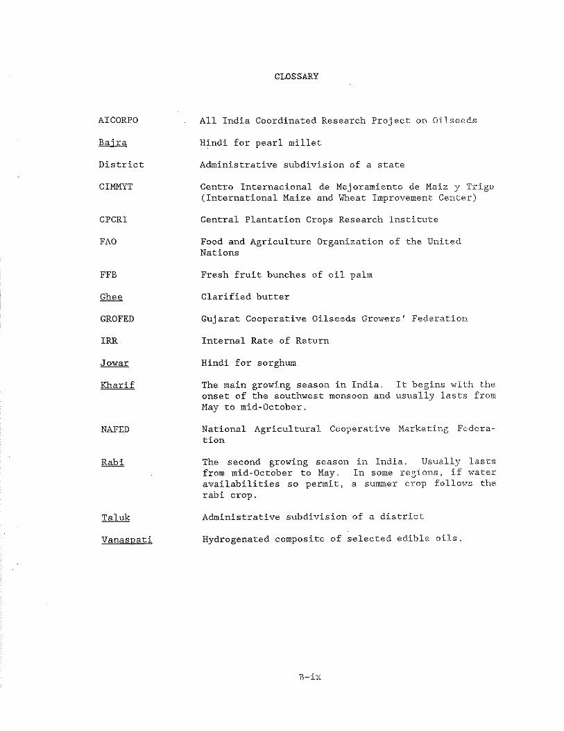
GLOSSARY
AICORPO All India Coordinated Research Project on Oilseeds
Baira Hindi for pearl millet
District Administrative subdivision of a state
CIMMYT Centro Internacional de Mej oramiento de Maiz y Trigo (International Maize and Wheat Improvement Center)
CPCRI Central Plantation Crops Research Institute
FAO Food and Agriculture Organization of the United Nations
FFB Fresh fruit bunches of oil palm
Ghee Clarified butter
GROFED Gujarat Cooperative Oilseeds Growers' Federation
IRR Internal Rate of Return
Jowar Hindi for sorghum
Kharif The main growing season in India, It begins with the onset of the southwest monsoon and usually lasts from May to mid-October.
NAFED National Agricultural Cooperative Marketing Federation
Rabi The second growing season in India. Usually lasts from mid-October to May. In some regions, If water availabilities so permit, a summer crop follows the rabi crop.
Taluk Administrative subdivision of a district
Vanasnati Hydrogenated composite of selected edible oils.
B - ix

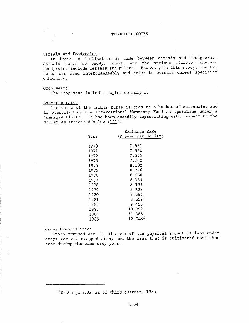
TECHNICAL NOTES
Cereals and Food-grains:In India, a distinction is made between cereals and foodgrains.
Cereals refer to paddy, wheat, and the various millets, whereas foodgrains include cereals and pulses. However, in this study, the two terms are used interchangeably and refer to cereals unless specified otherwise.
Cron year:The crop year in India begins on July 1.
Exchange rates:The value of the Indian rupee is tied to a basket of currencies and
is classifed by the International Monetary Fund as operating under a "managed float". It has been steadily depreciating with respect to the dollar as indicated below (121):
Gross Crooned Area:Gross cropped area is the sum of the physical amount of land under
crops (or net cropped area) and the area that is cultivated more than once during the same crop year.
YearExchange Rate
(Rupees per dollar)
1970197119721973197419751976197719781979198019811982198319841985
7.5677.5247.5957.7428.1028.3768.9608.7398.1938.1267.8638.6599.455
10.09911.36312.0481
^Exchange rate as of third quarter, 1985.
B -x x
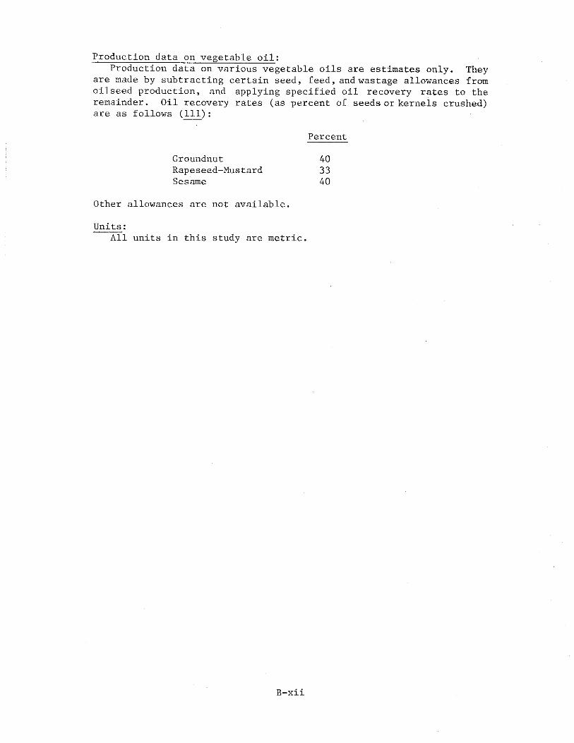
Production data on vegetable oil:Production data on various vegetable oils are estimates only. They
are made by subtracting certain seed, feed, and wastage allowances from oilseed production, and applying specified oil recovery rates to the remainder. Oil recovery rates (as percent of seeds or kernels crushed) are as follows (111):
Percent
Groundnut 40Rapeseed-Mustard 33Sesame 40
Other allowances are not available.
Units:All units in this study are metric.
B-xii
CHAPTER IOILSEEDS IN INDIA: STAGNATING PRODUCTION, GROWING DEMAND
Much of the interest in the Indian oilseeds economy has stemmed from India's large imports of vegetable oils recently. From being an importer of cereals and an exporter of vegetable oils in the 1960s, India has become an occasional and minor exporter of cereals, and a regular and major importer of vegetable oils. It currently imports over one million tons of vegetable oil at a cost of nearly seven billion rupees annually. This trade shift has occurred because the green revolution (which primarily benefited the cereals) did not extend to the oilseeds, and per capita production of oilseeds has declined. On the other hand, the demand for vegetable oils is expected to double by the year 2000 and, therefore, there is immediate need for augmenting their availability.
Performance of the Indian Oilseeds Economy
Oilseeds are important in the Indian agricultural economy. They constitute the second most important crop group (after cereals), occupying 11 percent of the total cropped area and contributing nearly 9 percent to the value of agricultural output. During 1981/82- 1983/84, they were grown on nearly 18 million hectares, yielding 12 million tons of oilseeds or approximately 3.3 million tons of vegetable oil (116; 118).1
The focus on annual oilseeds in this study is confined to groundnut, rapeseed-mustard, and sesame, because although several different oilseeds are cultivated in the country, these three account for nearly 80 percent of the area, 90 percent of the production of oilseeds, and over 70 percent of total vegetable oil production (computed from 116 and Appendix IV.4):
1 The production of vegetable oils refers to groundnut, rapeseed- mustard, sesame, safflower, nigerseed, cottonseed, and coconut oils, which are edible, as well as linseed and castor oils, which are nonedible. The area and production of oilseeds includes all of the above with the exception of coconut and cottonseed: this is because the production of coconut is measured in millions of nuts and therefore cannot be aggregated with that of the other oilseeds; and cottonseed is excluded because separate data on the amount of cottonseed production used in the manufacture of vegetable oil are not available. Most of cottonseed production is utilized as cattle feed.
B-1
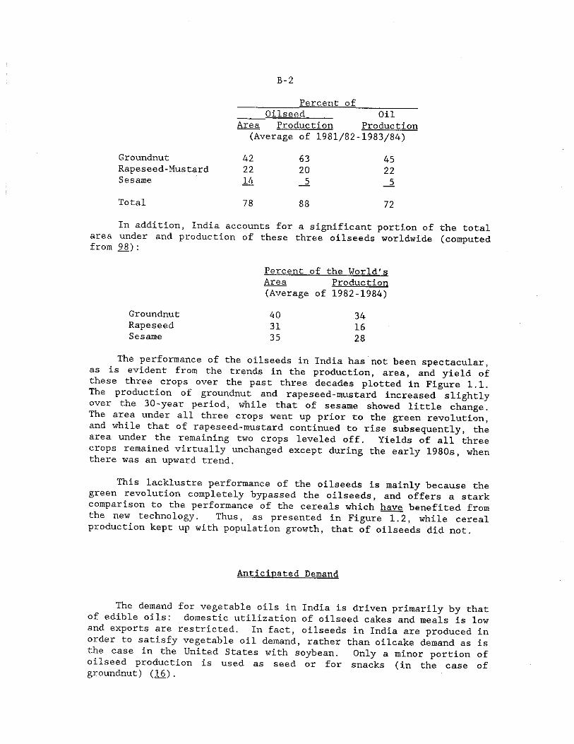
B-2
___________ Percent of________________Oilseed OilArea Production Production
(Average of 1981/82-1983/84)Groundnut 42 63 45Rapeseed-Mustard 22 20 22Sesame 14 _5 _5Total 78 88 72
In addition, India accounts for a significant portion of the total area under and production of these three oilseeds worldwide (computed from 98):
Percent of the World'sArea Production(Average of 1982-1984)
Groundnut 40 34Rapeseed 31 16Sesame 35 28
The performance of the oilseeds in India has not been spectacular, as is evident from the trends in the production, area, and yield of these three crops over the past three decades plotted in Figure 1.1. The production of groundnut and rapeseed-mustard increased slightly over the 30-year period, while that of sesame showed little change. The area under all three crops went up prior to the green revolution, and while that of rapeseed-mustard continued to rise subsequently, the area under the remaining two crops leveled off. Yields of all three crops remained virtually unchanged except during the early 1980s, when there was an upward trend.
Ihis lacklustre performance of the oilseeds is mainly because the green revolution completely bypassed the oilseeds, and offers a stark comparison to the performance of the cereals which have benefited from the new technology. Thus, as presented in Figure 1.2, while cereal production kept up with population growth, that of oilseeds did not.
Anticipated Demand
The demand for vegetable oils in India is driven primarily by that of edible oils: domestic utilization of oilseed cakes and meals Is low and exports are restricted. In fact, oilseeds in India are produced in order to satisfy vegetable oil demand, rather than oilcake demand as is the case in the United States with soybean. Only a minor portion of oilseed production is used as seed or for snacks (in the case of groundnut) (16).
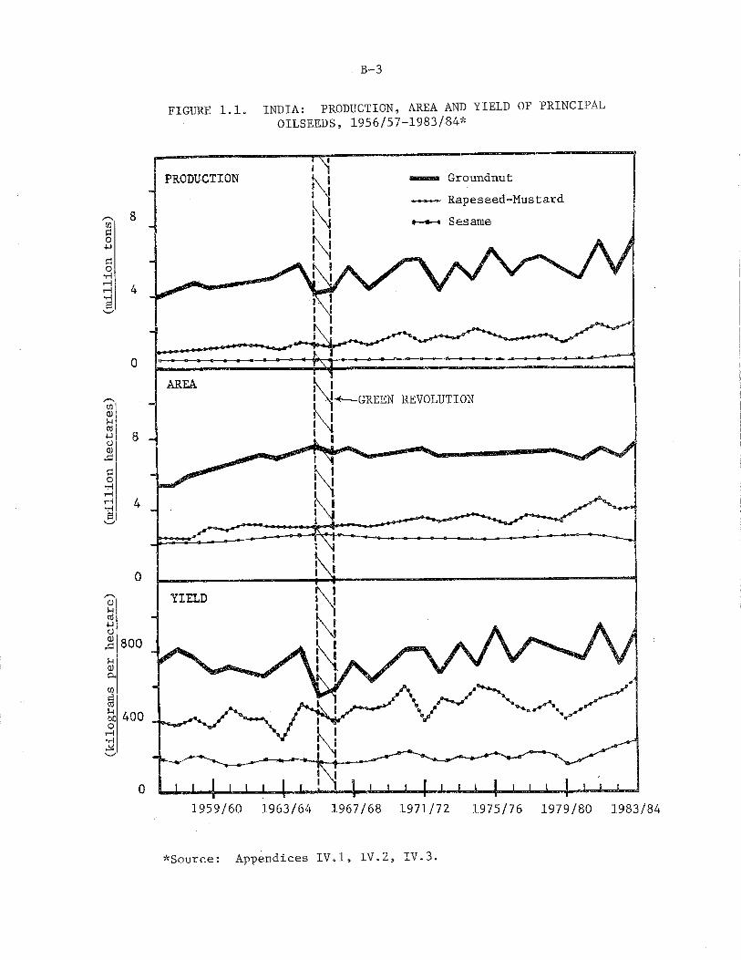
(kilograms p
er h
ecta
re)
(mil
lion
hec
tare
s)
(milli
on t
ons)
B-3
FIGURE 1.1. INDIA: PRODUCTION, AREA AND YIELD OF PRINCIPALOILSEEDS, 1956/57-1983/84*
*S o u rc e : A ppend ices I V . 1 , I V . 2 , I V . 3.
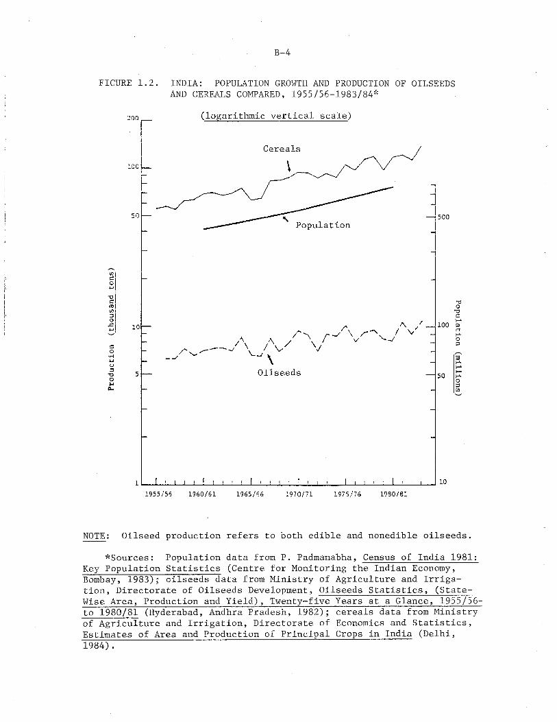
B-4
FIGURE 1.2. INDIA: POPULATION GROWTH AND PRODUCTION OF OILSEEDSAND CEREALS COMPARED, 1955/56-1983/84*
500
o■aa1 0 0 DJ rr
Oas'
50 osco
10
NOTE: Oilseed production refers to both edible and nonedible oilseeds.
*Sources: Population data from P. Padmanabha, Census of India 1981:Key Population Statistics (Centre for Monitoring the Indian Economy, Bombay, 1983); oilseeds data from Ministry of Agriculture and Irrigation, Directorate of Oilseeds Development, Oilseeds Statistics, (State- Wise Area, Production and Yield), Twenty-five Years at a Glance, 1955/56- to 1980/81 (Hyderabad, Andhra Pradesh, 1982); cereals data from Ministry of Agriculture and Irrigation, Directorate of Economics and Statistics, Estimates of Area and Production of Principal Crops in India (Delhi,1984).
B-5
Edible oils are used mainly as cooking media and constitute an essential component of the diet, being a major source of fatty acids. Their role as a protein source has also been recognized recently (.30) . Vanaspati. or hydrogenated vegetable oil (a composite of several oils), is also an important cooking medium. Expenditures on edible oils rank fourth in urban and rural food budgets: approximately five percent ofrural and seven percent of urban food expenditures are devoted to edible oils (123) , Nonedible oils are used in the manufacture of paints, varnishes and soaps, but constitute only 10 percent of all uses of vegetable oils (16.) . The current utilization of edible and nonedible oils averages 5 to 7 kilograms per capita, which is low compared to the world average of 10 kilograms per capita (48., p. 69).
The demand for an individual edible oil is directly related to income and population size, and is inversely related to its own price and the availability of substitutes. The various edible oils are substitutable to a large extent in use, although regional taste preferences do exist. For example, groundnut oil is popular inGujarat, coconut oil in Kerala, while mustard oil is preferred in Uttar Pradesh and West Bengal. Nonedible oil demand depends on additional factors: oil used in soap manufacture is also a function of theavailability of synthetic detergents, and the demand for oils used in paints and varnishes depends on the amount of construction activity during that year and the obtainability of synthetic paints (16. pp. 98-114).
One way to estimate the aggregate future demand for edible oils, assuming relative prices are constant, is to apply the rate of growth in demand to an appropriate base consumption level. The demand growth rate is computed as follows:
d = (1+p)(1+i.e)
where d is the growth rate in demandp is the percent growth in population i is the percent growth in income e is the income elasticity of demand
Since the demand projections are likely to be only as accurate as the parameters used in making them, it is best to develop a set of low and high demand scenarios, so as to delineate a range within which actual demand is likely to lie.
Ghee (clarified butter) , is also used for cooking but is not considered in this study: its use is limited and moreover declining in per capita terms consequent to the "white" (milk) revolution which resulted in lower spoilage rates and therefore greater quantities of milk being used for direct consumption.
B-6
Population
The growth rate of population in India is starting to decline, mainly because of decreases in the crude birth rate, and stood at 2.2 percent per annum as of the 1981 census (Figure 1.3). At that time, there were 685 million people in India (126) . It is reasonable toexpect that with economic development, the crude birth rate will continue to decline. According to projections made by the UnitedNations, if decreases in the fertility rate are less than expected, then population would stand at 997 million in 2000 and 1.14 billion in 2010. On the other hand, if family planning efforts are a great success, then population would be 927 million In 2000 and 1.02 billion In 2010 (127, p. 302). These figures form the basis of the growth rates used in this analysis.
Income
Per capita income in India has grown at approximately 1.5 percent since the green revolution,^ a period characterized by less-than- capacity industrial production. Therefore, a pessimistic income projection would be that the 1.5 percent rate of growth in per capita income will persist. A more optimistic projection would be to say that per capita income will grow at a somewhat arbitrary two percent. Data limitations preclude the consideration of changes in the savings rate which are assumed constant.
Income Elasticity of Demand
In order to project demand, it is necessary not only to know the growth in population and income, but also the percent of any Increased income that is spent on a good. This percentage is known as the income elasticity of demand and when total expenditures are used as proxy for income, it is formally defined as the proportionate change in the amount spent on a good given a unit change in total expenditures, all else remaining equal. For edible oils in India, various estimates (based on cross-section data) put the expenditure elasticity of demand at close to one (7, p. 34; 16, p. 127; 48, p. 13):
Source Year
National Commission on Agriculture 1970/71
Pavaskara 1970/71Harrison, Hitchings & Wall 1973/74
a: Excludes vanaspati
Estimated Expenditure______ Elasticity_____
Rural Urban
0.88 0.98--- 0.97----
1.00 1.01
o Refers to per annum compound rate of growth in real net national product (in 1970/71 prices) from 1966/67-1968/69 to 1981/82-1983/84 (121) .
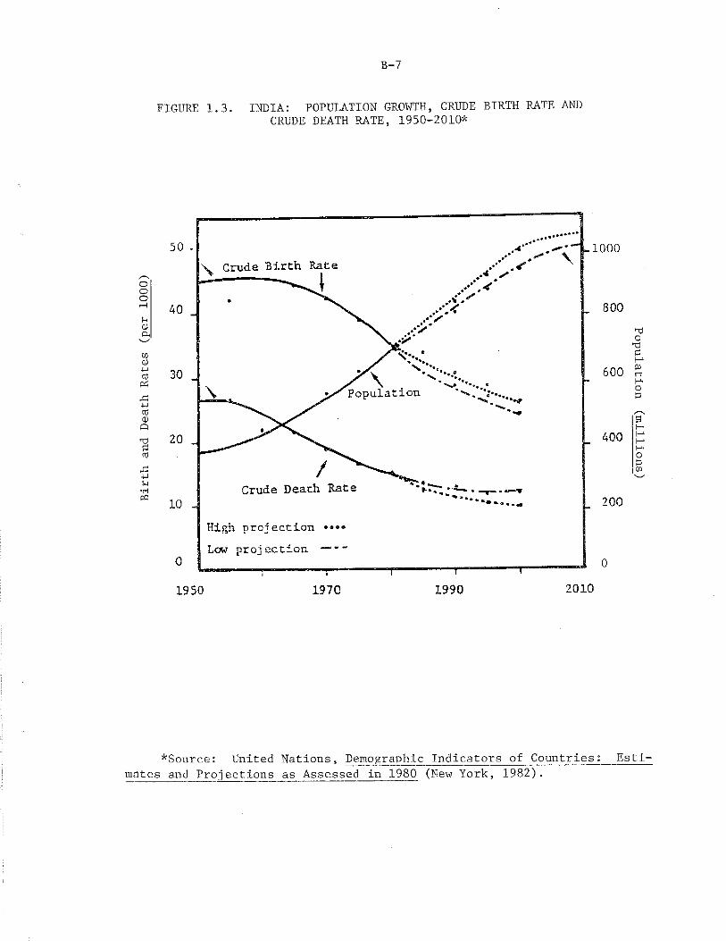
Birth
and Death
Rates
(per 1
000)
B-7
FIGURE 1.3. INDIA: POPULATION GROWTH, CRUDE BIRTH RATE ANDCRUDE DEATH RATE, 1950-2010*
*Source: United Nations, Demographic Indicators of Countries: Estimates and Projections as Assessed in 1980 (Mew York, 1982),
Population (millions)
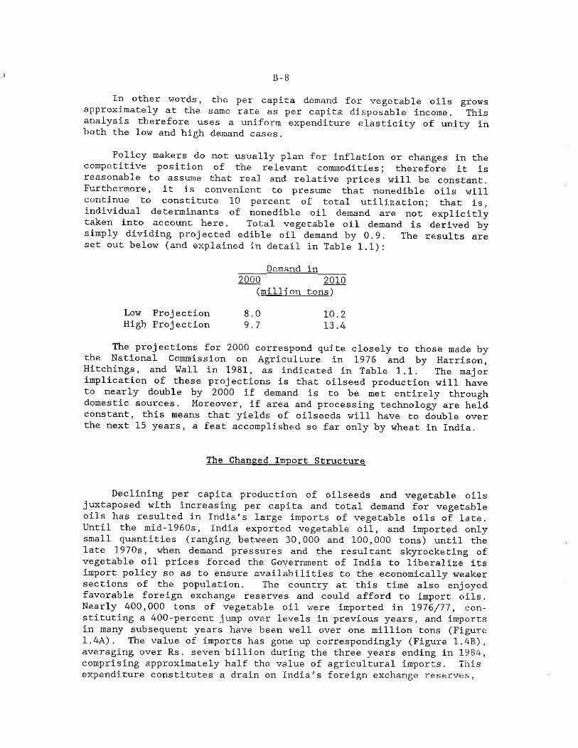
B-8
In other words, the per capita demand for vegetable oils grows approximately at the same rate as per capita disposable income. This analysis therefore, uses a uniform expenditure elasticity of unity in both the low and high demand cases.
Policy makers do not usually plan for inflation or changes in the competitive position of the relevant commodities; therefore it is reasonable to assume that real and relative prices will be constant. Furthermore, it is convenient to presume that nonedible oils will continue to constitute 10 percent of total utilization; that is, individual determinants of nonedible oil demand are not explicitly taken into account here. Total vegetable oil demand is derived by simply dividing projected edible oil demand by 0.9. The results are set out below (and explained in detail in Table 1.1):
_____Demand in_____2000 2010
(million tons)
Low Projection 8.0 10.2High Projection 9.7 13.4
The projections for 2000 correspond quite closely to those made by the National Commission on Agriculture in 1976 and by Harrison, Hitchings, and Wall in 1981, as indicated in Table 1.1. The major implication of these proj ections is that oilseed production will have to nearly double by 2000 if demand is to be met entirely through domestic sources. Moreover, if area and processing technology are held constant, this means that yields of oilseeds will have to double over the next 15 years, a feat accomplished so far only by wheat in India.
The Changed Import Structure
Declining per capita production of oilseeds and vegetable oils juxtaposed with increasing per capita and total demand for vegetable oils has resulted in India's large imports of vegetable oils of late. Until the mid-1960s, India exported vegetable oil, and imported only small quantities (ranging between 30,000 and 100,000 tons) until the late 1970s, when demand pressures and the resultant skyrocketing of vegetable oil prices forced the Government of India to liberalize its import policy so as to ensure availabilities to the economically weaker sections of the population. The country at this time also enjoyed favorable foreign exchange reserves and could afford to import oils. Nearly 400,000 tons of vegetable oil were imported in 1976/77, constituting a 400-percent jump over levels in previous years, and imports in many subsequent years have been well over one million tons (Figure 1.4A). The value of Imports has gone up correspondingly (Figure 1.4B), averaging over Rs. seven billion during the three years ending in 1984, comprising approximately half the value of agricultural imports. This expenditure constitutes a drain on India's foreign exchange reserves,
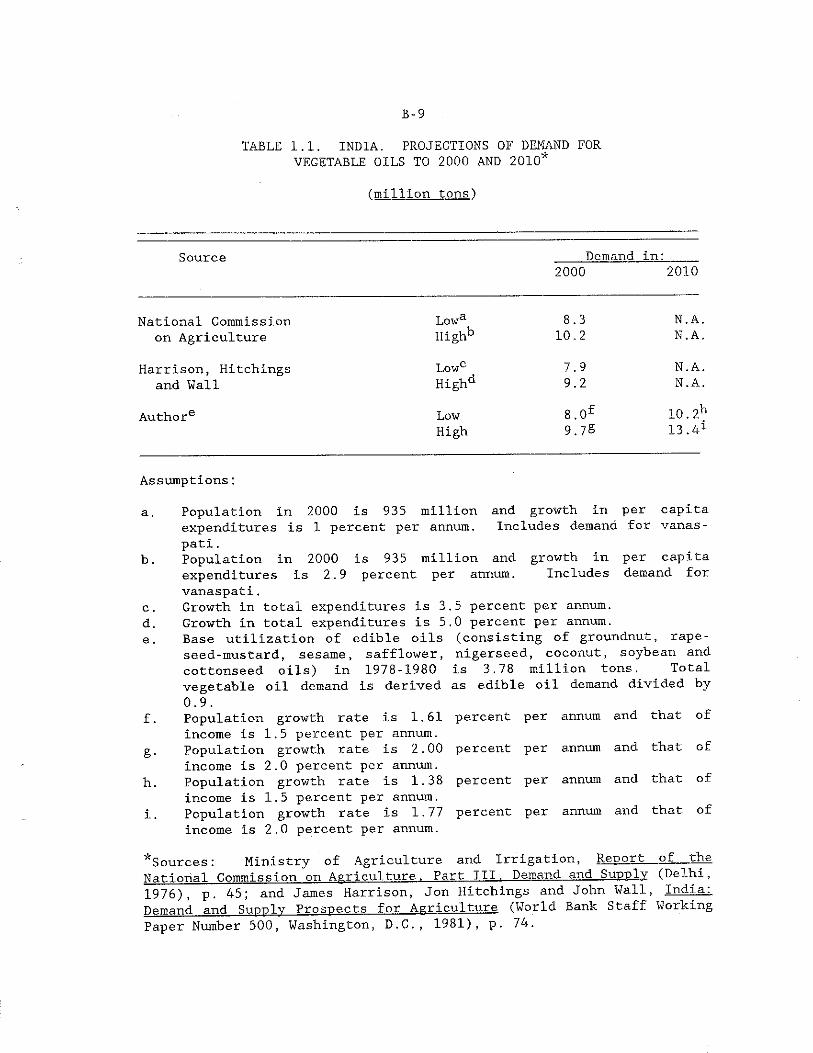
B-9
TABLE 1.1. INDIA. PROJECTIONS OF DEMAND FOR VEGETABLE OILS TO 2000 AND 2010*
fmillion tons)
Source ____Demand in:____2000 2010
National Commission Lowa 8.3 N . A.on Agriculture Highb 10.2 N . A
Harrison, Hitchings Lowc 7.9 N . Aand Wall Highd 9.2 N. A
Authore Low CO o i-ti 10.21
High 9.7^ 13.4
Assumptions:
a .
b.
c .d.e .
f .
S-h.
i.
Population in 2000 is 935 million and growth m per capita expenditures is 1 percent per annum. Includes demand for vanas- pati.Population in 2000 is 935 million and growth in per capita expenditures is 2.9 percent per annum. Includes demand for vanaspati.Growth in total expenditures is Growth in total expenditures is 5 Base utilization of edible oils seed-mustard, sesame, safflower, cottonseed oils) in 1978-1980 vegetable oil demand is derived 0.9.Population growth rate is 1.61income is 1.5 percent per annum. Population growth rate is 2.00income is 2.0 percent per annum. Population growth rate is 1.38income is 1.5 percent per annum. Population growth rate is 1.77income is 2.0 percent per annum.
.5 percent per annum.
.0 percent per annum.(consisting of groundnut, rape- nigerseed, coconut, soybean and is 3.78 million tons. Totalas edible oil demand divided by
percent per annum and that of
percent per annum and that of
percent per annum and that of
percent per annum and that of
^Sources: Ministry of Agriculture and Irrigation, Report of— the National Commission on Agriculture. Part III. Demand and^_SuppLy (Delhi, 1976), p. 45; and James Harrison, Jon Hitchings and John Wall, India,:, Demand and Supply Prospects for Agriculture (World Bank Staff Working Paper Number 500, Washington, D.C., 1981), p. 74.
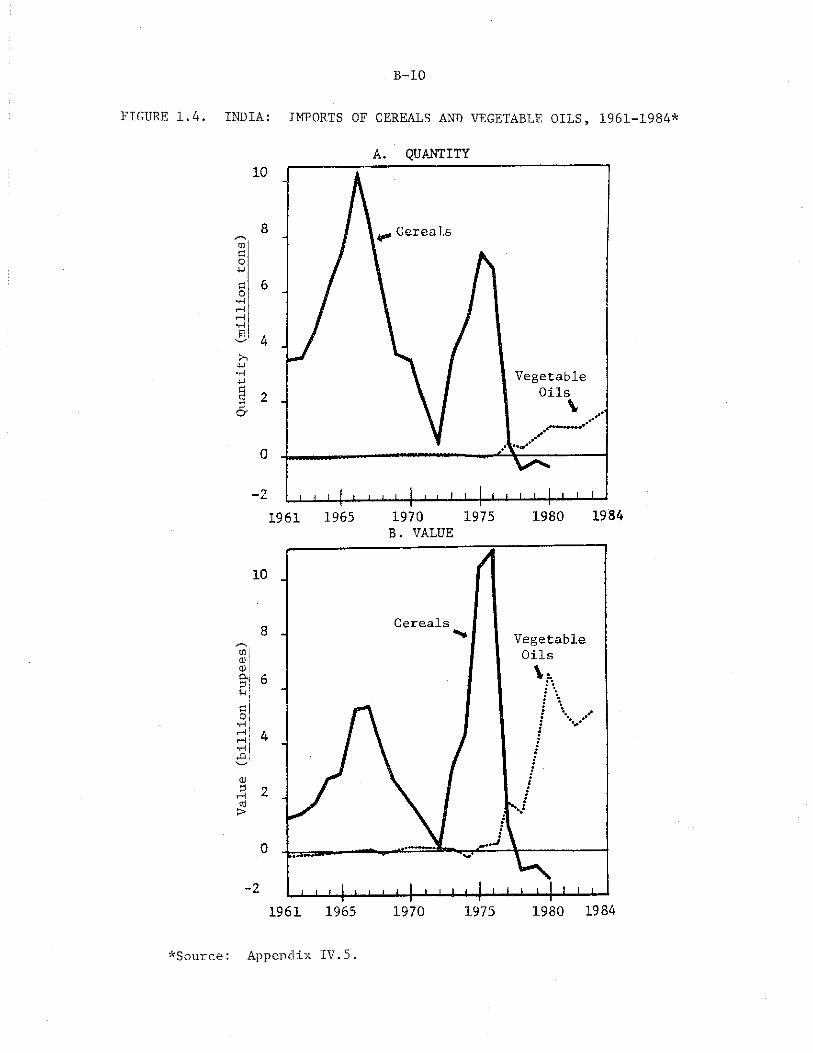
Valu
e (billion
rupee
s)
Quan
tity
(mi
llio
n to
ns)
B-10
FIGURE 1.4. INDIA: IMPORTS OF CEREALS AND VEGETABLE OILS, 1961-1984*
A. QUANTITY
B. VALUE
*Source: Appendix IV.5.
B- 11
and has replaced cereals expenditure as the second largest item on the import bill after petroleum (48, p. 69).
In addition to the increase in the quantity of imports, the composition of vegetable oil imports has diversified (Figure 1.5). Previously, soybean oil and palm oil constituted nearly all of India's imports of vegetable oil. Since the mid-1970s, however, rapeseed oil, groundnut oil and to a lesser extent, sunflower and linseed oils are also being imported, although soybean oil (from the United States and Brazil) and palm oil (from Malaysia) continue to dominate imports. The dependence on any one oil, nevertheless, has reduced considerably.
Until the late 1970s, vegetable oils could be imported free of customs duty. However, the Government of India felt that the benefits from such a policy "were not fully accruing to the consumers" (42, p. 10) and that private traders were making large profits by maximizing the difference between the landed price of imported oils and the domestic price through hoarding. Consequently in 1978 it channeled virtually all imports of vegetable oils through the State Trading Corporation of India. Also, since July 1981, the State Trading Corporation of India is being levied only a five percent ad valorem tax on its imports, while all other importers of vegetable oil are being charged a massive 150 percent ad valorem tax. This channelization has enabled the State Trading Corporation of India to monitor the international market effectively, and immediately use any downward price change to its advantage (42, pp. 10-11; .39., p. 1952).
The Objectives and Organization of This Study
There is immediate need for augmenting availabilities of vegetable oils. Supply projections for the annual oilseeds made in this study indicate that if past trends persist, then even with a low rate of growth in demand, demand will continue to outstrip supply. One option is to continue importing vegetable oils, but this requires the commitment of scarce foreign exchange. The other alternative is to encourage domestic production of oilseeds through extension of area or increase in yields. However, for the annual oilseeds, increases in area in a land-scarce country such as India are likely to occur at the expense of the cereals, and yield increases in the absence of high-yielding varieties of oilseeds are unlikely. On the other hand, the perennial (tree) oilseeds do not compete for land directly with the foodgrains and have the advantage that they yield the highest quantities of oil per unit land area.
The objectives of this study are: first, to detail the impact of the green revolution on the oilseeds economy of India (Chapter II); second, to determine prospects for two tree sources of vegetable oil, namely, coconuts (Chapter III) and oil palm (Chapter IV); and finally, to discuss means of augmenting availabilities by examining the tradeoffs between imports and domestic production (Chapter V). Most of the necessary data were collected from various government and nongovernment agencies in India during the summer of 1983.
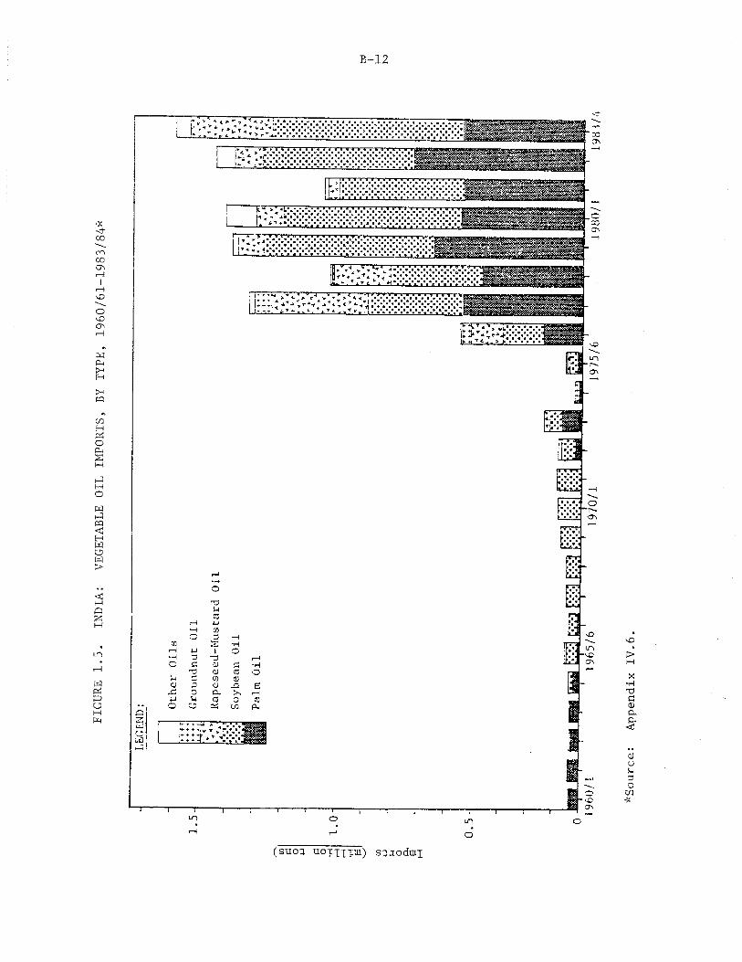
FIGU
RE 1
.5.
INDIA:
VEGE
TABL
E OI
L IMPORTS, B
Y TYPE,
1960
/61-
1983
/84*
B-12
(suoq. u o txx I ui) s^jodrax
*Soarce:
Appe
ndix
IV.
6,
CHAPTER IITHE IMPACT OF THE GRAIN REVOLUTION ON THE
OILSEEDS ECONOMY OF INDIA
The green revolution in India, which entailed the adoption of high-yielding varieties of seeds, together with an appropriate combination of fertilizer application and water and pest management techniques, has, in fact, been a grain revolution. Its impact on Indian agriculture has been differential; in particular, while the cereals have benefited from it, the oilseeds have not.
Oilseeds in India usually compete with the foodgrain crops for land. The green revolution, and the associated yield augmenting technology, where successful, have made cereal production more attractive, and because no such technology is available for the oilseeds, increasing proportions of land are being devoted to the foodgrain crops at the expense of the oilseeds.
In this chapter, the impact of the green revolution on the oilseeds economy of India is detailed through a comparison of the trends in the proportion of gross cropped area devoted to the oilseeds and the corresponding trends in their competing cereal crops. The discussion indicates that the prospects for the traditional sources of vegetable oil are limited because of a variety of technological and institutional factors, as are those for the nontraditional sources, namely, soybean, sunflower, and rice bran oils. Demand and supply projections suggest that if past trends persist, India will need to augment its vegetable oil supplies by 2.8 to 4,5 million tons by the year 2000, and 3.4 to 6.6 million tons by 2010.
The Green Revolutioril-
Prior to the green revolution, several programs were launched with a view to attaining self-sufficiency in foodgrains. These programs, in a sense, brought about the preconditions which later ensured the success of the green revolution. Notable among them were the "Grow More Food” campaign (1943), the "Community Development Programme" (1952), the "Intensive Agricultural District Programme" (1961), and the "Intensive Agricultural Area Programme" (1964) (21, p. 19). However, on the eve of the green revolution, after two severe drought years, "the food situation ... was, to say the least, alarming" (1, p.32).
1 This section draws on C.H. Hanumantha Rao (20), J.S. Sarma (21), and Biplab Dasgupta (1).
B- 13
B- 14
Production was not increasing fast enough to keep up with population growth, imports of food were high and showed no prospects of coming down, and food prices were increasing. Most of the production increases up to this point had come through the expansion of area, but there was not much new land that could be brought under cultivation.
Finally, in 1966/67, a "new strategy" for agricultural development was put into effect. It essentially entailed introducing high-yielding varieties of cereals, encouraging irrigation, increasing the availability and use of scientific inputs, arranging access to credit and assuring remunerative prices to farmers. Under the new program, high-yielding varieties of wheat (from CIMMYT in Mexico), rice (from the International Rice Research Institute in the Philippines) and maize and millet (bred in India) were introduced.
The high-yielding varieties of cereals were a tremendous success. They were insensitive to differences in day length, early maturing, and responded well in terms of grain yield to fertilizer application. From the time that the CIMMYT varieties were introduced, wheat production doubled by 1972/73 to 25 million tons and nearly quadrupled by 1983/84 to 40 million tons. Similarly, rice production increased from approximately 30 million tons in the mid-1960s to 53 million tons by the early 1980s (116). As a result, total food production continued to_rise and kept up with population growth.2 India attained near self-sufficiency in foodgrains by the late 1970s and had even built up a stock of nearly 20 million tons.
The green revolution changed the structure of agricultural production in India. There was an increase in total cropped area brought about through the extension of irrigation and the greater use of shorter duration varieties which meant that more than one crop could be grown during the same crop year. The importance of rabi crops increased consequent to the green revolution because of the increase In the production of wheat which is grown during the rabi season. Thus, the cropping calender underwent a basic change. Labor use also increased because of the rise in the number of crops that could be grown during the year.
Apart from these aggregate changes, the impact of the green revolution has been localized. Interregional disparities widened because the green revolution primarily benefited areas that had assured water supplies; that is, those that had good irrigation systems or adequate rainfall. States such as Punjab, Haryana, and Uttar Pradesh, and to a lesser extent Andhra Pradesh and Tamil Nadu accounted for most of the increase in foodgrain production in the post-high-yielding
2 C.H. Hanumantha Rao believes however, that "even without the green revolution, the growth rate [of foodgrain production] would have been maintained...." because the increasing population would have put upward pressure on prices and induced the farmer to produce more and the government to invest in irrigation and fertilizers (20).
B- 15
varieties period (116). Interpersonal disparities widened because the large and medium farmers with better access to credit facilities were able to take advantage of the new technology earlier than the smaller farmers.3 Finally, in terms of crops, apart from the cereals, most other crops did not benefit from the high-yielding variety technology. Wheat is the classical success story. In the mid-1960s, wheat constituted 15 percent of all of cereals production. By the early 1980s, its share had increased to 33 percent (116). In addition, high-yielding varieties of rice became popular in Andhra Pradesh and Tamil Nadu. Baira (pearl millet) was successful mainly in Gujarat.
The oilseeds were largely left out of the green revolution. No counterparts of the high-yielding varieties of cereals were developed for the oilseeds. The grain revolution acted to increase the relative profitability of the cereals vis-A-vis the competing oilseed crops, because, as Dr. C.H. Hanumantha Rao put it, "the High Yielding Varieties, typically, increase the profit per unit of the output, i.e., they lead to a reduction in the unit costs of production [as a proportion of output]...." (20, p. 75). Therefore, while cereal production kept up with population growth, oilseed production did not.
The Impact on the Oilseeds
Land allocation decisions are governed by changes in the relative profitabilities of the alternative crops: considerations such as subsistence needs, resource base, costs, prices, yields, riskiness of production, and the availability of assured markets are all taken Into account by the farmer when evaluating the relative gains of competing crops, and the resulting decision is reflected in the area actually planted. One can therefore detail the impact of the grain revolution on the oilseed economy by examining trends in the gross cropped area under the oilseeds as compared to the corresponding trends in the competing crops. To do this, it is better to use percent figures so as to account for the effect of increases in total cultivated area. In what follows, linear trend lines for each crop during the pre- and post-grain revolution periods are fitted to support conclusions that
3 Recognizing that the scale neutral technology was not necessarily resource neutral, special programs such as the Small Farmers Development Agencies and the Marginal Farmers and Agricultural Labourers' Development Agencies were set up to allow economically weaker sections of the population to participate in the benefits of the new technology. These programs were, by and large, not very successful because of ambiguities in the definitions of "small" and "marginal" farmers and also because concessional credit targeted to these farmers eventually found its way to the large farmers.
B- 16
are based on visual inspection.4 In addition, in order to get a very rough idea of the success of technology adoption in these cropsinformation on the adoption of high-yielding varieties and area irrigated, where relevant, is also included.
Area Trends in Major Producing StatesGroundnut
.Groundnut is grown primarily as a kharif crop. It is grown on marginal lands under unirrigated conditions, and usually competes with O^ar, bajra, and paddy, all of which are predominantly kharif crops (i-igure 2.1). Five states account for almost 90 percent of the area and production of groundnut in India (computed from 116):
Percent of India'sState Area(Average
Productionof 1981/82-1983/84)
Guj arat 29 27Andhra Pradesh 21 22Tamil Nadu 14 16Karnataka 12 10Maharashtra 11 11Total 87 86
Gujarat, groundnut competes primarily with bajra. Prior to the mid-1960s, groundnut gained area at the expense of bajra; however, following the introduction of hybrid bajra in the mid-1960s, groundnut ost its relative share in gross cropped area until the mid-1970s.
Since then, there has been an upward trend in groundnut acreage accompanied by a decline in bajra's area. Hybrid bajra has been particularly successful in Gujarat. Nearly seventy percent of the area under bajra is under high-yielding varieties as compared to the all-India average of 23 percent. Similarly nine percent of the bajra area in Gujarat is irrigated, while at the all-India level, the corresponding figure is five percent. There are no high-yielding varieties of groundnut and only two percent of the groundnut in Gujarat is irrigated, compared to eight percent for India as a whole.
The time periods are: for the pre-grain revolution period, 1956/57 to 1965/66, and for the post-grain revolution period, 1966/67 to 1980/81. It has been frequently argued that the two drought years, 1965/66 and 1966/67 should be excluded from the consideration of trends, because these were freak years, and as such, should be treated as outliers. In this instance, however, their inclusion did not, for the most part, alter the signs of the slopes of the trend lines.
While there are no "high-yielding varieties", "improved" varieties exist for all the oilseeds, however, they are not popular and there has been no significant yield increase since their introduction.
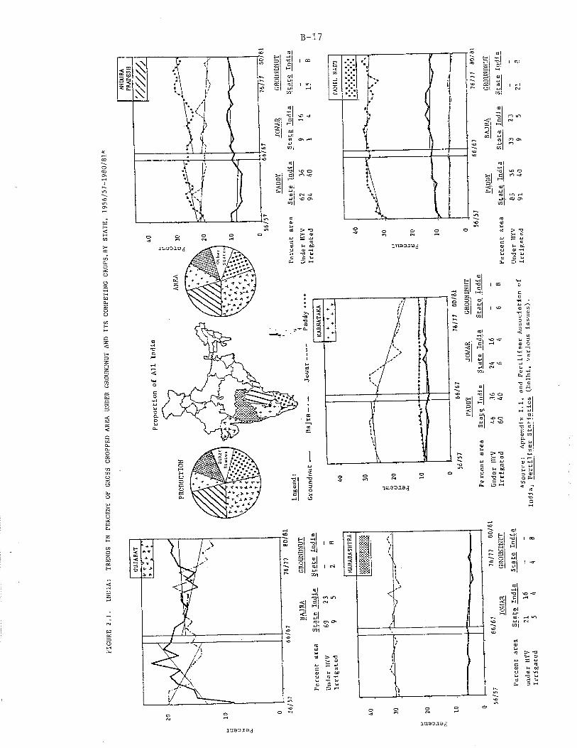
FIGU
RE 2
,].
INDI
A I
TREN
DS IN PE
RCEN
T OF G
ROSS
CRO
PPED
ARE
A UN
DER
GROU
NDNU
T AN
D ITS
COMP
ETIN
G CR
OPS,
BY STAT
E, 19
56/5
7-19
80/8
1*
B-17
2U33 JLB&
B- 18
In Andhra Pradesh, jowar and paddy compete with groundnut. From the late 1950s to the mid-1960s, paddy area increased at the expense of jowar and groundnut which exhibited a marginal decline. Following the grain revolution, area under paddy continued to increase and that under jowar fell while groundnut area remained the same. Jowar and groundnut continue to compete for land because for a given year, increases in jowar area are usually accompanied by a decrease in groundnut area and vice-versa. The introduction of high-yielding varieties of rice was quite successful in Andhra Pradesh. Over 60 percent of the area under paddy is planted to high-yielding varieties; in addition, more than 90 percent of rice is irrigated--both these figures are nearly twice the national averages. For jowar, only nine percent of the area is under high-yielding varieties and little over one percent is irrigated. The corresponding national figures are 16 percent and 4 percent, respectively. For groundnut, however, the proportion of irrigated area is higher than the national average.
In Tamil Nadu, area under groundnut increased slightly from the late 1950s until the mid-1960s as did that under paddy, accompanied by a slight decline in bajra. Subsequent to the grain revolution, paddy
groundnut areas remained stable while that under jowar declined steadily. The area under high-yielding variety bajra and that under irrigation in Tamil Nadu are higher than those at the all-India level. Similarly, high-yielding varieties of paddy have been adopted on a large scale in Tamil Nadu--85 percent of paddy area is planted to high-yielding varieties and over 90 percent is irrigated, more than twice the corresponding national averages, but, curiously, these factors have not been reflected in any increase in the relative area under these two crops. The implied loss in area under kharif groundnut has been more than counterbalanced by the increase in the area under summer^ groundnut which is grown under irrigated conditions, thus resulting in stable groundnut area even after the introduction of the new technology.
In Karnataka, prior to the grain revolution, area under groundnut remained stable while area under paddy and jowar, the major competitors , increased marginally. Subsequent to the green revolution, the area under groundnut and paddy was stable; however, jowar exhibited a steady decline. This is despite the fact that for the cereals, the state averages for the percent area under high-yielding varieties and under irrigation are higher than the all-India averages. Part of this decline in jowar area can be explained by the increase in the area under maize and other kharif crops.
Finally in Maharashtra, groundnut area was relatively stable prior to the mid-1960s as was that of jowar; since then, groundnut declined while area under jowar remained constant. As indicated by the statistics relating to the adoption of new technology, the area under high-yielding varieties of j owar is higher than the national average and the same is true of irrigated area under jowar. However, the percent of groundnut area irrigated in Maharashtra is nearly half the national average,
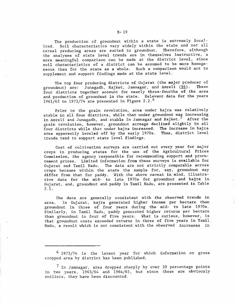
B- 19
The production of groundnut within a state is extremely localized. Soil characteristics vary widely within the state and not all cereal producing areas are suited to groundnut. Therefore, although the analyses of state level trends are in themselves instructive, a more meaningful comparison can be made at the district level, since soil characteristics of a district can be assumed to be more homogeneous than for the state as a whole. Such a comparison would act to supplement and support findings made at the state level.
The top four producing districts of Gujarat (the major producer of groundnut) are: Junagadh, Rajkot, Jamnagar, and Amreli (96). These four districts together account for nearly three-fourths of the area and production of groundnut in the state. Relevant data for the years 1961/62 to 1973/74 are presented in Figure 2.2.^
Prior to the grain revolution, area under bajra was relatively stable in all four districts, while that under groundnut was increasing in Amreli and Junagadh, and stable in Jamnagar and Rajkot. After the grain revolution, however, groundnut acreage declined slightly in all four districts while that under bajra increased. The increase in bajra area apparently leveled off by the early 1970s. Thus, district level trends tend to support state level findings.
Cost of cultivation surveys are carried out every year for major crops in producing states for the use of the Agricultural Prices Commission, the agency responsible for recommending support and procurement prices. Limited information from these surveys is available for Gujarat and Tamil Nadu. The data are not strictly comparable across crops because within the state the sample for, say, groundnut may differ from that for paddy. With the above caveat in mind, illustrative data for the mid- to late 1970s for groundnut and bajra in Gujarat, and, groundnut and paddy in Tamil Nadu, are presented in Table 2.1 .
The data are generally consistent with the observed trends in area. In Gujarat, bajra generated higher income per hectare than groundnut in three of four years during the mid- to late 19 70s. Similarly, in Tamil Nadu, paddy generated higher returns per hectare than groundnut in four of five years. What is curious, however, is that groundnut costs exceeded returns in three of five years in Tamil Nadu, a result which is not consistent with the observed increases in
6 1973/74 is the latest year for which information on gross cropped area by district has been published.
^ In Jamnagar, area dropped sharply by over 20 percentage pointsin two years, 1963/64 and 1964/65, but since these are obviouslyoutliers, they have been discounted.
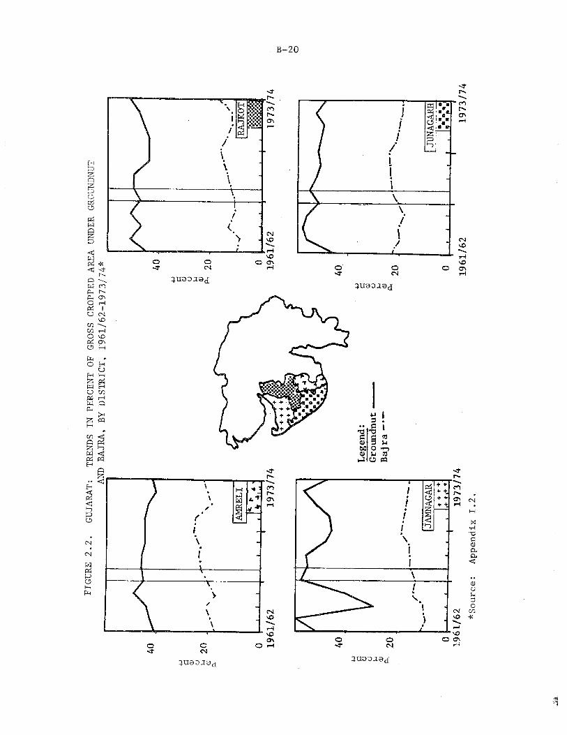
FIGU
RE 2
.2.
GUJARA
T:
TREN
DS I
N PE
RCEN
T OF
GRO
SS C
ROPP
ED A
REA
UNDE
R GR
OUND
NUT
____________________
AND
BAJRA, B
Y DI
STRI
CT,
1961
/62-
1973
/74*
B-20
'OO O O CT\<■ CM rH
.. C I T) 173
B d dCD 3 uao O *1*3<U u dhJ o «
^U9DJ9d
Vf
3 tin o a a
.■Bl'0
^Sou
rce:
Appe
ndix
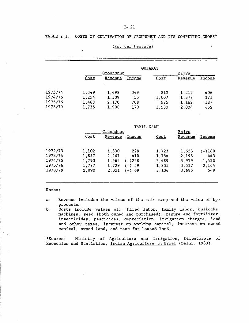
B- 21
TABLE 2.1. COSTS OF CULTIVATION OF GROUNDNUT AND ITS COMPETING CROPS*
(Rs. per hectare)
GUJARATGroundnut_______ _______________ Bai ra
Cost Revenue Income Cost Revenue Income
1973/74 1,349 1,698 349 813 1,219 4061974/75 1,254 1,309 55 1,007 1,378 3711975/76 1,463 2,170 708 975 1,162 1871978/79 1,735 1,906 170 1,583 2,034 452
GroundnutTAMIL NADU
Bai raCost Revenue Income Cost Revenue Income
1972/73 1,102 1,330 228 1,723 1,623 (-)1001973/74 1,857 2,267 410 1,754 2,198 4431974/75 1,793 1,565 (-)228 2,489 3,919 1,4301975/76 1,787 1,729 (-) 59 1,335 3,517 2,1641978/79 2,090 2,021 (-) 69 3,136 3,685 549
Notes:
a. Revenue includes the values of the main crop and the value of byproducts.
b. Costs include values of: hired labor, family labor, bullocks,machines, seed (both owned and purchased), manure and fertilizer, insecticides, pesticides, depreciation, irrigation charges, land and other taxes, interest on working capital, interest on owned capital, owned land, and rent for leased land.
^Source: Ministry of Agriculture and Irrigation, Directorate ofEconomics and Statistics, Indian Agriculture in Brief (Delhi, 1983).
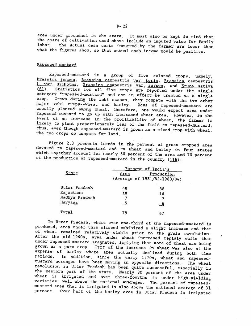
B- 22area under groundnut in the state. It must also be kept in mind that the costs of cultivation used above include an imputed value for family labor: the actual cash costs incurred by the farmer are lower than what the figures show, so that actual cash income would be positive.
Rapeseed-mustardRapeseed-mustard is a group of five related crops, namely,
bragsica juncea, Brggsica campestrls var. toria. Brassica cacroestris ^ich.Qtlp.a» ^£^Mca^_cjmpes^ls_..var. sarson. and Eruca sativa (bl). Statistics for all five crops are reported under the single
category "rapeseed-mustard" and can in effect be treated as a single crop. Grown during the rabi season, they compete with the two other major rabi crops - - wheat and barley. Rows of rapeseed-mustard are usually planted among wheat, therefore, one would expect area under rapeseed-mustard to go up with increased wheat area. However, in the event of an increase in the profitability of wheat, the farmer is lihely to plant proportionately less of the field to rapeseed-mustard; thus, even though rapeseed-mustard is grown as a mixed crop with wheat the two crops do compete for land. ’
Figure 2.3 presents trends in the percent of gross cropped area devoted to rapeseed-mustard and to wheat and barley in four states which together account for nearly 80 percent of the area and 70 percent of the production of rapeseed-mustard in the country (116):
Percent of India'sState Area Production
(Average of 1981/82-1983/84)Uttar Pradesh 48 38Rajasthan 18 16Madhya Pradesh 7 7Harvana -5Total 78 67
In Uttar Pradesh, where over one-third of the rapeseed-mustard is produced, area under this oilseed exhibited a slight increase and that of wheat remained relatively stable prior to the grain revolution. After the mid-1960s, area under wheat increased rapidly while that under rapeseed-mustard stagnated, implying that more of wheat was being grown as a pure crop. Part of the increase in wheat was also at the expense of barley where area actually declined during both time periods. In addition, since the early 1970s, wheat and rapeseed- mustard acreages have been moving in opposite directions. The wheat revolution in Uttar Pradesh has been quite successful, especially in the western part of the state. Nearly 80 percent of the area under wheat is irrigated and over three-fourths is under high-yielding varieties, well above the national averages. The percent of rapeseed- mustard area that is irrigated is also above the national average of 31 percent. Over half of the barley area in Uttar Pradesh is irrigated
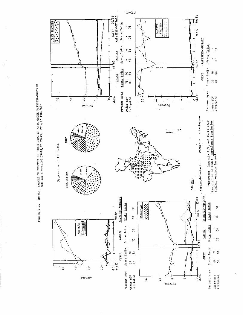
FIGU
RE 2
.3.
INDIA:
TREN
DS I
N PE
RCEN
T OF G
ROSS
CRO
PPED
ARE
A UN
DER
RAPE
SEED
-MUS
TARD
AND
ITS
COMP
ETIN
G CROPS, BY
STAT
E, 19
56/5
7-19
80/8
1*
B-23
X fwc « d *h ui CUT? (0 P. P *H <1 M aiM-l 3
wT3 1 <y C r*j
• CT3 ■HT3 o m C COat«a o fn j_j <r c/i
<UUoj > *a>• CJ J-J 3: 4JC coOJ u OGO CJ ~H "O Ma> c Cl, L3 h
WH
EAT
RA
PE
SEE
D-M
UST
AR
D
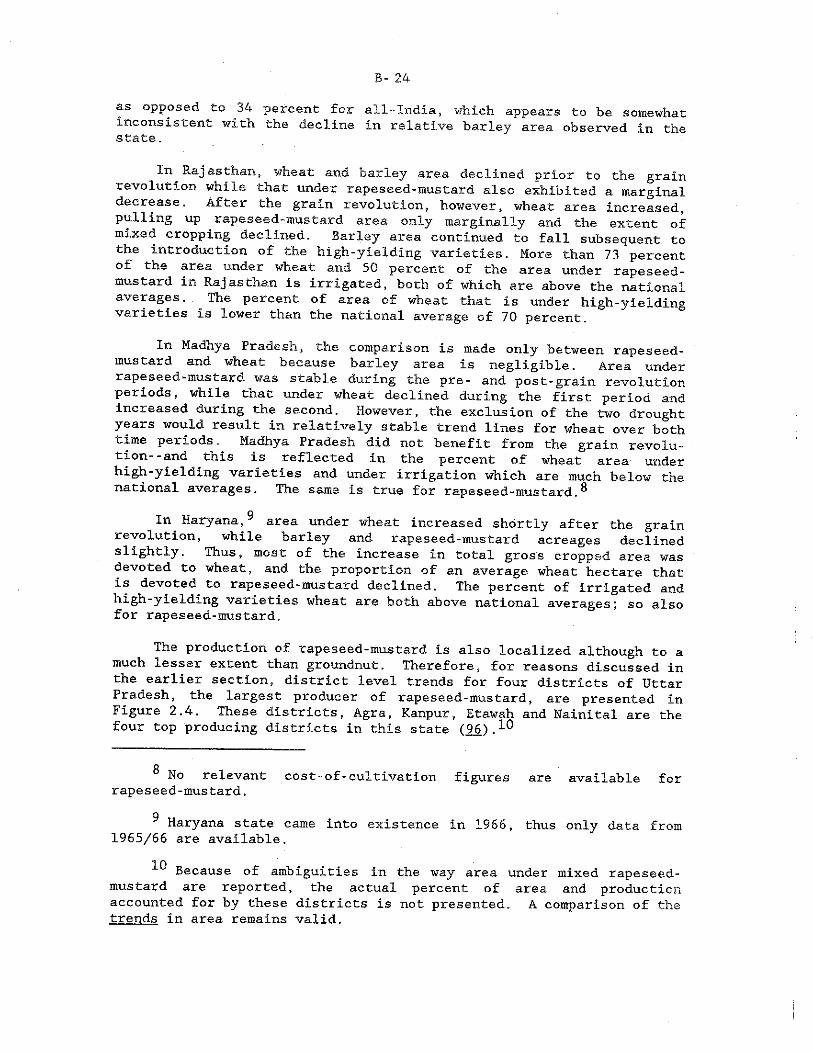
B- 24
as opposed to 34 percent for all-India, which appears to be somewhat inconsistent with the decline in relative barley area observed in the state.
In Rajasthan, wheat and barley area declined prior to the grain revolution while that under rapeseed-mustard also exhibited a marginal decrease. After the grain revolution, however, wheat area increased, pulling up rapeseed-mustard area only marginally and the extent of mixed cropping declined. Barley area continued to fall subsequent to the introduction of the high-yielding varieties. More than 73 percent of the area under wheat and 50 percent of the area under rapeseed- mustard in Raj as than is irrigated, both of which are above the national averages. The percent of area of wheat that is under high-yielding varieties is lower than the national average of 70 percent.
In Madhya Pradesh, the comparison is made only between rapeseed- mustard and wheat because barley area is negligible. Area under rapeseed-mustard was stable during the pre- and post-grain revolution periods, while that under wheat declined during the first period and increased during the second. However, the exclusion of the two drought years would result in relatively stable trend lines for wheat over both time periods. Madhya Pradesh did not benefit from the grain revolution- -and this is reflected in the percent of wheat area under high-yielding varieties and under irrigation which are much below the national averages. The same is true for rapeseed-mustard.®
In Haryana,8 9 area under wheat increased shortly after the grain revolution, while barley and rapeseed-mustard acreages declined slightly. Thus, most of the increase in total gross cropped area was devoted to wheat, and the proportion of an average wheat hectare that is devoted to rapeseed-mustard declined. The percent of irrigated and high-yielding varieties wheat are both above national averages; so also for rapeseed-mustard.
The production of rapeseed-mustard is also localized although to a much lesser extent than groundnut. Therefore, for reasons discussed in the earlier section, district level trends for four districts of Uttar Pradesh, the largest producer of rapeseed-mustard, are presented in Figure 2.4. These districts, Agra, Kanpur, Etawah and Nainital are the four top producing districts in this state (96).10
8 No relevant cost-of-cultivation figures are available forrapeseed-mustard.
9 Haryana state came into existence in 1966, thus only data from 1965/66 are available.
10 Because of ambiguities in the way area under mixed rapeseed- mustard are reported, the actual percent of area and production accounted for by these districts is not presented. A comparison of the trends in area remains valid.
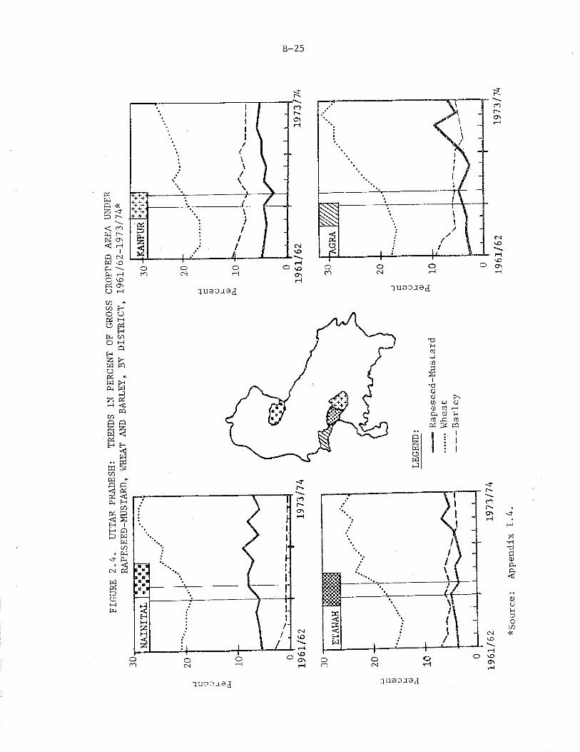
FIGURE 2
.4.
UTTAR PRADESH:
TRENDS I
N PERCENT
OF G
ROSS C
ROPPED ARE
A UNDER
RAPESEED-MUSTARD,
WHEAT
AND
BARLEY,
BY D
ISTRICT, 1961/62-1973/74*
auaojaj
T3UOju013Sl
-c iQJ0)CO u <u0 ) CO T-1P CD P3 £ C l
P 4 3
I fPQ
111
<rr~-
i*■HX)3CL)P-S'
Q)OM3OC/l4C
jl3 j
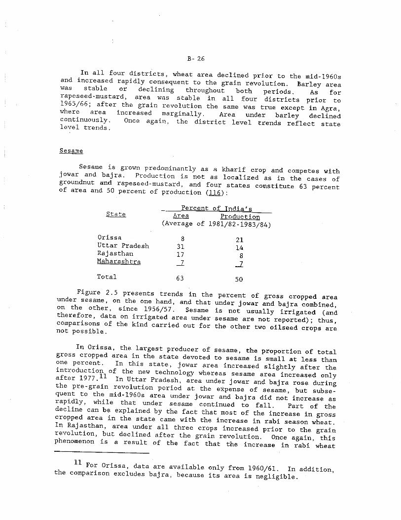
B- 26
^In all four districts, wheat area declined prior to the mid-1960s and increased rapidly consequent to the grain revolution. Barley area was stable or declining throughout both periods As for rapeseed-mustard, area was stable in all four districts prior to 1965/66, after^ the gra m revolution the same was true except in Agra w ere area increased marginally. Area under barley declinedcontinuously. Once again, the district level trends reflect state level trends.
Sesame
Sesame is grown predominantly as a kharif crop and competes with jowar and bajra. Production is not as localized as in the cases of groundnut and rapeseed-mustard, and four states constitute 63 percent of area and 50 percent of production (116):
Percent of India'sState Area Production(Average of 1981/82-1983/84)
Orissa 8 21Uttar Pradesh 31 14Raj asthan 17 8Maharashtra _ z _7Total 63 50
SUre 2'5 py sents trends in the percent of gross cropped area under sesame, on the one hand, and that under jowar and bajra combined,therefore h/ r SlnCe *956/57’ Sesame ls not usually irrigated (and therefore, data on irrigated area under sesame are not reported)- thuscomparisons of the kind carried out for the other two oilseed crops arenot possible. F ■
In Orissa, the largest producer of sesame, the proportion of total gross cropped area in the state_ devoted to sesame is small at less than* -t- )'frceJ1 * t^ls state, jowar area increased slightly after theafter^oy/ll 0fT nSW technoloSy whereas sesame area increased onlyafter 1977. _ In Uttar Pradesh, area under jowar and bajra rose duringauentrtoSthln T ? « n i0n Perl°d “ the expetlse of ^same, but subse?ranidlv n® l / Under J °war and baJ d i d not increase asapidly, while that under sesame continued to fall. Part of thedecline can be explained by the fact that most of the increase in gross cropped area m the state came with the increase in rabi season wheat.n Rajasthan, area under all three crops increased prior to the grain
revolution, but declined after the grain revolution. Once again Sthis phenomenon is a result of the fact that the increase in rabi'wheat 11
11 For Orissa, data are available the comparison excludes bajra, because only from 1960/61, In addition,
its area is negligible.
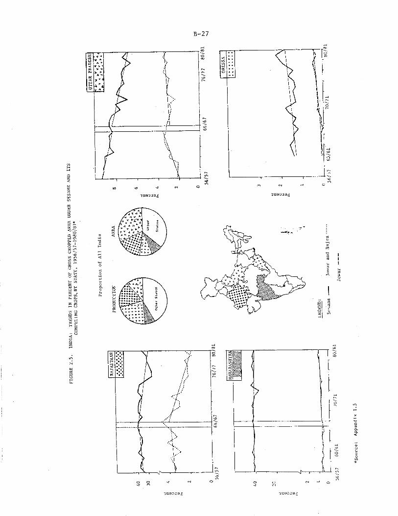
FIGU
RE 2
.5.
INDIA:
TREN
DS I
N PE
RCEN
T OF C
ROSS
CRO
PPED
ARE
A UN
DER
SESA
ME A
ND I
TSCO
MPET
ING
CROPS. BY
STATE.
19
56/5
7-19
B0/8
I*
B-27
^S
ou
rce
: A
pp
en
dix
B- 28
area r “ T t0 m°St °f the galn in total cultivated. n _ou§d high-yielding variety jovar and bajra were not verywhilea thant j^Sthan’ the Absolute area under the two millets increasedTowar h” SeSai“e decreased- Lastly, in Maharashtra, sesame,J war and bajra areas remained relatively stable prior to the erainrevolution; however, subsequently, there was a slight increase£ sesame area, but not in that of j owar or bajra.
The grain revolution, where successful, has thus served to negatively impact the competitive position of the oilseeds vis-A-vis he cereal crops. Moreover, even in areas not affected by the grain revolution, the oilseeds compete for land with the foodgrains & In addition, overall input use, including that of fertilizer, is lower for the oilseeds as compared to the cereals (78). There have been noandnmillaf % ° f ru6 m^ acls hiSh -yield“ S variety seeds of wheat, rice and millets for the oilseeds.
The effect of this technological backwardness on the part of revennf8 ^ n evident ^ °ne disaggregates the change in totalyield d • heotar® over the srain revolution period into real price,
r ? v T S? " effects in the largest producing states.1 As bdl0W’ f°r a.U CompetlnS oereal crops, real prices declined
J T lj and y venue “ creases were effected entirely through higher h-i s ' J‘n 7 1® case of rapeseed-mustard, however, price rises were solely responsible for increased revenue; yields for this crop actually^fclln®d- ,For. ses.amf’ the increase in prices was not enough to offsetd^d w r h OIh ln y7 eldS ’ s0 that revenue also fell. Only for groundnut did both yield and price increases contribute to higher revenues -
Crop Change in Yield PriceTotal Revenue Effect Effect
(1960/61 Rupees per hectare*)Interaction
Effect
GROUNDNUT (GUJARAT)Groundnut Baj ra
385.3263.6
178.4265.5
138,3 - 0.6
68.6 - 1.3
Rapeseed- RAPESEED-MUSTARD (UTTAR PRADESH)mustard
Wheat39.992.7
- 51.4 197.7
53,6 - 69.5
- 19,8- 35.5
SESAME (UTTAR PRADESH)13Sesame Jowar Baj ra
- 18.9 30.5 4.7
- 44.2 34.9 35.3
38.2- 3.5- 25.3
- 12.9- 0.9- 5.3
12 r\Detailed calculations are in Appendix V.l.13 Data for Orissa, the largest producer of sesame, are unavailable.
B- 29
Prospects for the Three Principal Oilseeds
Nearly two decades have passed since the first high-yielding varieties of wheat were introduced in India. The question now is whether any developments have occurred in the oilseeds economy since then, and what the implications are for the increased production of these crops. The following discussion indicates that although there have been a few success stories, by and large, the competitive position of the three principal oilseeds relative to the cereals is unlikely to change significantly in the near future.
Technological Factors
The poor production performance of the oilseeds is largely a result of the rainfed nature of their cultivation (only eight percent of the total area under cultivation is irrigated) (116), high-yield risk, and their vulnerability to pests and diseases.
Oilseeds research has not made much progress in India. The major responsibility for this research lies with the All India Coordinated Research Project on Oilseeds (AICORPO) which came into operation in 1968. In addition to the AICORPO and the research carried out in the State Agricultural University systems, several programs exist under the auspices of the Indian Council of Agricultural Research to undertake oilseeds research, notable among them being the The National Research Centre for Groundnut in Junagadh, Gujarat. The International Crop Research Institute for the Semi-Arid Tropics, in Hyderabad, India, also has a major groundnut research program. However, despite the institutional support, there have not been any maj or breakthroughs (61).
Part of the problem is that given the rainfed nature of most of oilseed cultivation, in order to ensure adoption by farmers, it is necessary to evolve varieties that are not only high-yielding, but are also drought-escaping, or drought and pest resistant, so as to diminish yield uncertainty. Some success in evolving drought resistant varieties has been reported at the National Research Centre for Groundnut, but apart from Gujarat, it has not been possible to duplicate these results elsewhere, pointing to the need for location-specific research (61).
In addition, there is a lack of proper coordination between the oilseed research institutes and the existing extension system, so that the little progress that is made on the research front does not get transmitted to the farmers, let alone allowing for feedback from the farmers to the researchers„
1^ For example, yields in national demonstrations for groundnut are often three to four times as high as those actually experienced by the farmers (78, p. 168). The difference is likely to be because of poor extension, but also because the cost of scientific cultivation practices necessary to bring about this increase in yield is very high. The proof of the seed is, after all, in the harvesting.
B- 30
^ i• ^ 0ther means of increasing yields is through the provision of wate3; supplies. It has been suggested (30, p. 11; 39 p . 256)
hat because irrigated yields of groundnut tend to be twice as high as unirrigated yields, incentives be provided to encourage the extension of groundnut cultivation on irrigated lands. Evidence indicates however that under irrigated conditions, farmers prefer to produce
ecr;-eidse(S:epir62i ) ted cereal ylelds are also Msher than unirrigat-
Institutional Considerations
- .The government has been actively involved in foodgrain markets ment Sand0Ul 1 ^ eS Commisslon- set “P in 1965, recommends procure- throupb tbeUPP°rv, PrlC6e l°r thS foodSrains> which are then enforced S so r w S 0f the F°0d Corporation of India (also set up in
S° government markets often parallel private markets forPurviewTf rt’ a ' ^0)i Th? oilseeds’ however, did not come under theP the Agricultural Prices Commission until 1976/77 and nogovernment agencies are involved in oilseed marketing,15 The’processing and marketing of oil is in the hands of a few traders who are in a position to exploit the farmers (12, p. 315; £7, p. 382).
n-n 00fartirally a? 3 resP°nse to this fact, the Gujarat Cooperative Oilseeds Growers Federation (GROFED) was set up In 1979 in majorproducing districts of Gujarat, in the belief that "by organisingorgaSsationUndthea C0Iml0di,:y SyStem’ and restinS with this farmers^ rganisation the management and control of technically superiorprocessing and marketing facilities, ... a greater proportion of the tradi^1onrTPt e I 3" bS Pald t0 thS producer in comparison to what thehigher nrices % CbnPday"a( M ' P' 1673)' The GR0FED offers to farmersg p ices, subsidized seeds, fertilizers, pesticides modernfarming equipment and a variety of other extension services ’ It owns two oil mills and has plans for constructing others Despite S e
0Sd“ " °i a .powerful oil lobby that controlled most of the process- g marketing of the oil in the state, the GROFED has been a
1982eSthenGROFEDat' from 43 oooperative societies in 1979, byof 68,lSo farmers (M)PaSSed °V" 971 S°°letleS wlth a total -mbershi^
in_ P^ellminary evaluations of the project in 1984 looked encourag-do not i n Z arflH ° \ villages which have cooperatives with those thft icated that, although the former on average incurred higher input costs, they received higher groundnut yields, higher prices Sandv i f b m t y nofmG R O F W h6Ctare than the latt6r continuedviability of GROFED s operation and the successful adaptability of sucha system to other producing areas and crops could very well result inan increase m the production of oilseeds.
15i exception, however, is the soybean marker ona ^Agricultural Cooperative Marketing Federation
ac ive y involved in purchasing and marketing soybeans.where the
(NAFED) is
B- 31
PricesIt is generally believed that increases in wholesale^ prices of
oilseeds and vegetable oils are not passed on to the farmer m the form of higher farm harvest prices, but rather that they are captured in the profit margins of the traders. A comparison of farm produce value with final produce value16 shows that in the case of groundnut for examp in bad years, the percent decrease in farm produce value is much higher than the percent decrease in final produce value. In good years the decrease in prices is usually associated with increased production. Producers lose much more relative to the traders m poor harvest years (66 p. A-115). In addition, evidence indicates that the sprea e the' farmers’ and intermediaries' share of retail price as een increasing over time, and furthermore, the farmer's share EflLja has declined by more then eight percentage points between 1962/63 and 1980/81 (74, p. 189). The corollary argument is that assuring theproducer of remunerative prices is one means of increasing t e pro uc- tion of oilseeds; therefore, it is advocated that support prices recommended by the Agricultural Prices Commission, which are current y much below farm harvest prices, be increased to reflect realisticmarket prices (12).
However, a comprehensive study put out in 1982 suggests that prices are not a major factor in influencing production decisions The study examined the relative importance of prices, yields, availabili y of water (both irrigation and rainfall), variability m yie prices and technological factors in the determination of groundnut acreage.17 It found that at the state level, m the southern states (Tamil Nadu and Andhra Pradesh), the presence of irrigation facilities and in the western states (Gujarat and Maharashtra), the availabi i y o-F high-yielding varieties of competing cereals, and price and yie uncertainty were the most important determinants of groundnut area In no instance did relative prices significantly influence area At J-h district level, similar conclusions held, with the exception that relative prices were important only in districts where irrigation facilities were present (13, pp. 116-143),
The supply elasticities with respect to price in this study were all positive but not statistically significant (13. PP' 7 44/ 45/ evidence from other studies is, however, mixed (Table 2. ). r e mo
16 Farm produce value was derived by multiplying annual groundnut production with corresponding farm harvest prices. Final produce value was calculated by taking groundnut oil production at average wholesale prices with adjustments for seasonal variations and also taking into account the value of oilcake in the domestic and interna- tional markets.
17 The time period covered in this study was 1963/64 to 1974/75 for Andhra Pradesh and Gujarat, and 1954/55 to 1974/75 for T a m i a u, Karnataka and Maharashtra. No distinction was made between the pre- and post-grain revolution periods.
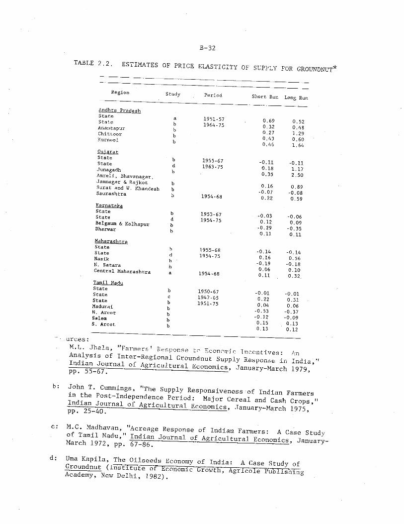
B-32
TABLE 2.2. ESTIMATES OF PRICE ELASTICITY OF SUPPLY FOR GROUNDNUT*
Region S tudy Period Short Run Long Run
Andhra PradeshStateStateAnantapurChittoorKurnool
Guj arat State State JunagadhAmreli, Bhavanagar, Jamnagar & Rajkot Surat and W. Khandesh Saurashtra
KarnatakaStateStateBelgaum & Kolhapur Dharwar
MaharashtraStateStateNasikN, SataraCentral Maharashtra
Tamil Nadu State State State Madurai N. Arcot Salem S. Arcot
1951-57 1964 - 75
1955-671963-75
1954-68
1 9 5 3 - 671 9 5 4 - 75
1955-681954-75
1954-68
1 9 5 0 - 67 1947-651 9 5 1 - 75
0 . 690. 320 . 2 70 . 4 30 . 4 6
- 0.110 . 180. 35
0 . 1 6- 0 .0 70.22
- 0 . 0 30 . 1 2
- 0 . 2 90 . 1 1
- 0 . 1 40. 16
- 0 . 1 90 . 0 60 . 11
- 0 . 0 10.220 . 0 4
- 0 . 5 3-0 . 1 20 . 1 50. 13
0 . 520 . 4 81. 290 . 6 01 . 6 4
- 0 . 1 11 . 172 . 5 0
0 . 8 9- 0 . 0 80 . 5 9
- 0 .0 60 . 0 9
- 0 . 3 50 . 1 1
- 0 . 1 40 . 5 6
- 0 . 1 80 . 1 00 . 32
- 0 . 0 10 . 3 10 . 06
- 0 . 3 7- 0 .0 90 . 1 30.12
-urces:M.L Jhala "Fanners1 Response to Economic Incentives: Annalysxs of Inter-Regional Groundnut Supply Response in India n
°f Agricultural Economics, January-March 1979,*
inhthI'Po T i n ! S’ T e ST ly f sP“ eness of Indian Farmers in tne Post-Independence Period: Major Cereal and rv^ma "^ XZZ-lT.Tnal °f Agricultural Economics. January-March 1975,*
ofCTamifNldn ’..'TCareaSeTReSPOnSe °f Indlan Fa™ ers: A Case StudyMarch Journgl-SL AR^"ltural Economics, January-
Uma Kapila, The Oilseeds Economy of India: A Case Study ofroundnut (Institute of EconomictFowth, AgricoleTdlETiiEiiV
Academy, New Delhi, 1982). b
B-33
confirm positive acreage response to price both in the short and long run, negative supply elasticities are not uncommon. The reason is that in areas where the competing crops are grown primarily for subsistence, the higher relative price of groundnut will not necessarily result in increased area under the oilseed unless the farmer is convinced that the income from groundnut will be sufficient for purchasing subsistence needs. In cases where the response to price has been negative, sowing-period rainfall and yield have played a greater role In determining acreage: if there is inadequate rainfall and yields are likely to be low, the farmer may not plant as much area to groundnut even if the relative price of groundnut increases (69).
In sum, a sound price policy alone would not be enough to bring about changes in the relative profitabilities of the oilseeds and the competing crops. As Kahlon and Tyagi, members of the Agricultural Prices Commission, argue, "in the case of such crops as oilseeds where technology is lacking, exclusive reliance on the price mechanism to induce production would prove to be an optical illusion...the resultant gain in production would be uncertain" (12,, p. 298).
Prospects for Nontraditional Sources of Vegetable Oil
The scope for expanded production of the traditional oilseeds is limited. However, there are other annual nontraditional sources of vegetable oil. The recognition that diversification in oilseeds was one means to increased vegetable oil production and reduced dependence on groundnut led the Indian government to encourage the production of these nontraditional sources of vegetable oils. Unfortunately, results to date have been minimal.
SoybeanFeasibility trials undertaken during the late 1960s indicated that
many regions in India were suited to the cultivation of soybean, and since India has traditionally imported soybean oil for use In the vanaspati industry, it was assured of a market. Therefore in 1971/72, the Government of India launched a soybean production project by providing good quality, cheap seeds, and various other subsidies. As the production of soybean oil increased, the NAFED stepped in to provide marketing facilities. It also enforced the government announced support prices by ensuring timely procurement and storage.
Grown primarily in Madhya Pradesh and Uttar Pradesh, area under soybean increased from 26,500 hectares in 1971/72 to 768,000 hectares in 1982/83. Production similarly grew from 10,300 tons to nearly 500,000 tons, over this period (116). However, during 1981/82-1983/84 soybean oil accounted for less than two percent of total vegetable oil
B- 341 Qproduction.0 One advantage in growing soybean is that it is a hardy
crop and is drought resistant; the major disadvantage of soybean is that its oil content is low--the main product of soybean is the meal whose use as cattle feed is not yet popular in India (2, pp. 168-173).
Sunflower
Although sunflower cultivation has been known for a long time in India, it was not until 1969 that its use as a source of vegetable oil was explored. The sunflower is characterized by high yields and drought resistance, and is also drought evading by virtue of being a short duration crop. The government implemented a sunflower scheme in the mid-1970s in the southern states of Tamil Nadu, Andhra Pradesh and Karnataka. By 1982/83, 225,000 tons of sunflower were being produced on 431,000 hectares nationwide (116). Average production of the oil during the early 1980s was 84,000 tons. The program was not a major success, however, because marketing channels for this new crop were not established properly, resulting in distress sales at low prices. In addition, seed multiplication programs had not stepped up production in order to meet demand (2., pp. 155-163).
Rice Bran
This oil is derived from the outer coating of rice called the bran. Rice bran is thus a product of rice milling. The extraction of oil requires that the milling be done in modern mills and not in the traditional hullers that predominate rice processing in India. That is, the production of rice bran oil depends not only on rice production but also on the proportion of rice that is processed in modern mills. Production of rice bran oil in India during 1977/78-1979/80 was 95,000 tons. The principal advantage of this oil is that increasing its production will not be at the expense of any other cereal crop. On the other hand, the major obstacles to Increased production are, first, that in areas where rice is processed in small quantities at a time, there are no arrangements for pooling the bran so as to accumulate enough for processing; and second, the oil has to be extracted soon after the separation of the bran from the rice in order to prevent rancidity and therefore, the bran cannot be stored for long periods of time (2, pp. 192-202). 18 19
18 As per unpublished data from the Directorate of Economics and Statistics, Ministry of Agriculture.
19 As per unpublished data from the Directorate of Economics and Statistics, Ministry of Agriculture.
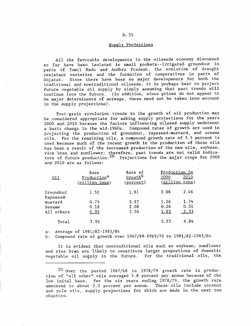
B- 35
Supnlv Projections
All the favorable developments in the oilseeds economy discussed so far have been isolated in small pockets--irrigated groundnut in parts of Tamil Nadu and Andhra Pradesh, the evolution of drought resistant varieties and the formation of cooperatives in parts of Gujarat. Since there have been no major developments for both the traditional and nontraditional oilseeds, it is perhaps best to project future vegetable oil supply by simply assuming that past trends will continue into the future. (In addition, since prices do not appear to be major determinants of acreage, these need not be taken into account in the supply projections).
Post-grain revolution trends in the growth of oil production may be considered appropriate for making supply projections for the years 2000 and 2010 because the factors influencing oilseed supply underwent a basic change in the mid-1960s. Compound rates of growth are used in projecting the production of groundnut, rapeseed-mustard, and sesame oils. For the remaining oils, a compound growth rate of 3.5 percent is used because much of the recent growth in the production of these oils has been a result of the increased production of the new oils, soybean, rice bran and sunflower; therefore, past trends are not valid indicators of future production.2^ Projections for the major crops for 2000 and 2010 are as follows:
Base Rate of Production inOil Productiona Growth^ 2000 2010
(million tons) (■percent) (million tons )
Groundnut 1.52 1.81 2.06 2.46Rapeseed-mustard 0.73 3.27 1.26 1.74Sesame 0.18 2.08 0.26 0.31All others 0,92 3.50 1.65 2.33
Total 3.35 5.23 6.84
a: Average of 1981/82-1983/84b : Compound rate of growth over 1967/68-1969/70 to 1981/82 -1983/84
It is evident that nontraditional oils such as soybean, sunflower and rice bran are likely to constitute larger proportions of domestic vegetable oil supply in the future. For the traditional oils, the 20
20 Over the period 1967/68 to 1978/79 growth rate in production of "all other" oils averaged 5.8 percent per annum because of the low inital base. For the six years ending 1978/79, the growth rate amounted to about 3.3 percent per annum. These oils include coconut and palm oils, supply projections for which are made in the next two chapters.
B- 36
increases in production are presumed to be effected primarily through increases in yield and processing efficiency and only marginally through increases in area under cultivation. When compared with the demand projections made in Chapter 1, this supply will not be sufficient to meet domestic demand and the demand-supply gap is likely to be on the order of 2.8 to 4.5 million tons in 2000 and 3.4 to 6.6 million tons in 2010:
Demand DeficitYear Low High supply
(million tons')Low High
2000 8.0 9.7 5.2 2.8 4.52010 10.2 13.4 6.8 3.4 6.6
Scope for Tree Sources of Vegetable Oil
Given that increases in the production of oilseeds through higher yields are unlikely in the short run, the only feasible means of augmenting production is through expansion of area. The annual oilseed crops, however, compete with foodgrain crops for land, and this competition has in the past resulted in more amounts of land being devoted to the foodgrains at the expense of the oilseeds. Therefore, in a land scarce country such as India, any attempts to expand area under the oilseeds would occur at the expense of foodgrains.
The achievement of food self-sufficiency is central to the formulation of the five-year economic plans in India. Although self-sufficiency in food was achieved by the late 1970s, it is still precarious since food imports may be necessary in some adverse years to meet possible deficits. Therefore, production increases in oils must occur through sources of vegetable oils that do not directly compete for land with other food crops.
One alternative is to consider tree sources of vegetable oil, for example, coconuts and oil palm.2^ These tree crops have the advantage 21
21 There are several other minor forest sources of vegetable oil such as sal, neem and mahua. which together can potentially yield one million tons of oil. Only 25 percent of this potential is realizable, however, because these trees are scattered in the forests and are not within easy access to roads. Moreover, they can be harvested only during a few days in a year and it is difficult to mobilize large amounts of labor for such a short period of time. Actual production averaged 103,000 tons during 1979/80-1981/82. Appendix IV.10 presents details.
B- 37
in that they yield the highest amounts of vegetable oil per hectare, as evidenced in the following table (14, p. 4; 48, p. 70) .2
Cron Oil Yield(kilograms per hectare')
Oil palm 5,000Coconut 615Sunflower 275Groundnut 201Rapeseed/mustard 161Soybean 120Sesame 82
In addition, perennial crops do not compete for land directly with the annuals, in the sense that, when a farmer plants a perennial crop, it is with the recognition that the land will not be used for anything else for the next 20-30 years, barring calamitous circumstances. In India, oil palm does not compete with the foodgrains for land; coconuts, on the other hand, are grown amongst paddy fields and thus do compete indirectly with this cereal. Chapter III looks at the potential for coconut production, a traditional crop in India. Chapter IV then considers prospects for oil palm, a new crop to India. The analysis is based on the structure and economics of production of these two crops.
22 oil palm yields are for Malaysia during the mid-1970's; remaining figures are for India and relate to the year 1978/79. Dataon average oil yields are unavailable.

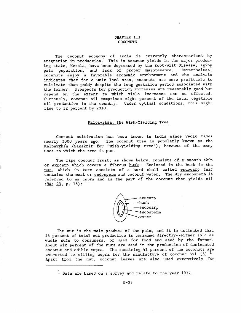
CHAPTER III COCONUTS
The coconut economy of India is currently characterized by stagnation in production. This is because yields in the major producing state, Kerala, have been depressed by the root-wilt disease, aging palm population, and lack of proper maintenance. Nevertheless, coconuts enjoy a favorable economic environment and the analysis indicates that for a unit land area, coconuts are more profitable to cultivate than paddy despite the long gestation period associated with the former. Prospects for production increases are reasonably good but depend on the extent to which yield increases can be effected. Currently, coconut oil comprises eight percent of the total vegetable oil production in the country. Under optimal conditions, this might rise to 12 percent by 2010.
Kaloavrksa. the Wish-Yielding Tree
Coconut cultivation has been known in India since Vedic times nearly 3000 years ago. The coconut tree is popularly known as the Kalpavrksa (Sanskrit for ”wish-yielding tree"), because of the many uses to which the tree is put.
The ripe coconut fruit, as shown below, consists of a smooth skin or exocarp which covers a fibrous husk. Enclosed In the husk is the nut. which in turn consists of a hard shell called endocarp that contains the meat or endosperm and coconut water. The dry endosperm is referred to as copra and is the part of the coconut that yields oil (94; 23, p. 15):
exocarphuskendocarpendospermwater
The nut is the main product of the palm, and it is estimated that 53 pex'cent of total nut production is consumed directly--either sold as whole nuts to consumers, or used for food and seed by the farmer. About six percent of the nuts are used in the production of desiccated coconut and edible copra. The remaining 41 percent of the coconuts are converted to milling copra for the manufacture of coconut oil (5). Apart from the nut, coconut leaves are also used extensively for
1 Data are based on a survey and relate to the year 1977.
B-39
B- 40
thatching roofs and making baskets. In addition, the husk of the coconut is the basic raw material for coir (hard fibre) manufacture, a major export commodity (90).
Varieties of Coconut Palm
There are two basic varieties of the coconut palm, each of which differs in yield patterns and input requirements. The Tall Variety palm grows to a height of 15-18 meters and lives up to 80-100 years. It starts bearing from six to seven years after planting and continues to yield until 75 years of age. In Kerala, the West Coast Tall variety is popular and under ideal management conditions, yields 60-80 nuts per palm per year. Oil yield from copra is a high 74 percent. The Tall variety palms usually cross-pollinate, and consequently, there is a high degree of genetic variability In the palms. The Dwarf Variety palm, as the name suggests, is relatively short, and grows to a height of five meters. It lives 35-40 years, and starts bearing earlier than the Tall variety at four to five years after planting. Yields are heavy, but tend to be Irregular. Input requirements for this variety are also said to be higher. The dwarf Chowghat Orange variety grown in Kerala yields about 90 nuts per palm per year and oil yield from copra is 66 percent. The Dwarf varieties, unlike the Tall, are usually self-pollinating. In addition to these two varieties, there are several hybrids (known as the DXT and TXD), which combine the longevity of the Tall with the high-yielding characteristic of the Dwarf (23 pp. 32-35; 52),
Climatic Requirements
The optimal conditions for coconut cultivation include (23. pp. 18-25):
mean annual temperatures of 27° C. The palm does not flourish in areas where average annual temperatures are less than 21° C or where there are considerable temperature fluctuations.
annual rainfall of 1000-3000 millimeters distributed evenly over the year.
well-drained soils in heavy rainfall areas, and water retentive soils in areas with poor rainfall. The coconut thrives particularly on sandy soils in coastal regions.
Coconuts in India
Four states in southern India (Kerala, Tamil Nadu, Karnataka and Andhra Pradesh) meet the climatic requirements for the cultivation of
B- 41
coconut, and account for nearly all of the coconut area and production in the country (116):
StatePercent of India's
Area Production(average for 1981/82-1983/84)
61 5011 2016 16_4 _492 92
area, and yield
Kerala Tamil Nadu Karnataka Andhra Pradesh
Total
presented in Figure 3.1, indicate that total production of coconuts increased until the early 1970s, but exhibited a declining trend since then caused by a sharp drop in production in Kerala (and to a much lesser extent in Andhra Pradesh), despite increases in Karnataka and Tamil Nadu. Area under coconuts grew rapidly in all states from the late 1950s to the mid-1970s. Subsequently, however, although area continued to increase in Andhra Pradesh, Karnataka and Tamil Nadu, this expansion was not enough to more than offset the fall In area in Kerala; thus, total area under coconuts remained unchanged during the late 1970s. Yields in Kerala and Andhra Pradesh have declined gradually, while in Karnataka and Tamil Nadu, there have been modest increases. At the national level, yields during the early 1980s were 20 percent lower than those in the mid- to late 1950s, because of the drop in yields in Kerala.
All-India trends are influenced most significantly by changes In the Kerala coconut economy because this state is the largest producer of coconuts; for this reason, the remainder of this chapter focuses on Kerala.
Coconuts in Kerala
Kerala lies in southwest India. It is characterized by a high population density of 655 persons per square kilometer, compared to 215 for all of India (126). The state receives the benefit of two monsoons --the North East monsoon from October to February, and the South West monsoon from June to September-- and most areas in Kerala receive in excess of 2000 millimeters of rain every year. Temperatures range from 21° C in the winter to 37° C in the summer and the state as a whole is thus ideally suited to the cultivation of coconut (104, p. 5).
The Kerala economy is essentially agricultural: this sector constitutes 43 percent of the net state domestic product (106, p. 159) and nearly 60 percent of the total geographical area is devoted to crops (107). Within the agricultural sector, rice cultivation predominates, followed by coconuts, which occupy 28 percent and 23 percent
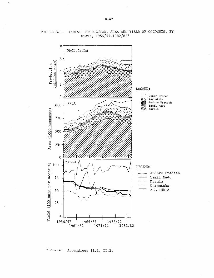
Yiel
d (100 n
uts
per
hect
are)
Area
(1000 h
ecta
res)
B-42
FIGURE, 3.1. INDIA: PRODUCTION, AREA AND YIELD OF COCONUTS, BY STATE, 1956/57-1982/83*
LEGEND:Other States Karnataka Andhra Pradesh Tamil Nadu Kerala
LEGEND:... Andhra Pradesh-- -— Tamil Nadu---- Kerala
Karnataka ---- ALL INDIA
^Source; Appendices II.1, II.2 .
B- 43Oof the gross cropped area in the state, respectively (104; 106) .
However, the grain revolution has not much affected Kerala rice cultivation and the state is currently food-deficit.
OKerala is divided into eleven administrative districts. The formation of two of these is recent in that they have each been carved out of two other districts without affecting the total area of the state. Mallappuram, formed during 1970/71, is composed of areas from the former Palghat and Kozhikode districts; and Idikki, formed in 1972/73 was created out of parts of the former Kottayam and Ernakulam districts. Since it was not possible to obtain information on the actual areas that went into the formation of these new districts, Mallappuram, Palghat and Kozhikode on the one hand, and Idikki, Kottayam and Ernakulam on the other, are each treated as a single region wherever necessary in this analysis.
Production Characteristics
Coconuts in Kerala are a small holder crop: an estimated 59 percent of the area under coconut is in holdings less than one hectare in size.^ Plantation scale coconut cultivation is virtually nonexistent and the production structure approximates perfect competition (105, p . 39):
Holding size Area under coconut(hectares) (percent)
0,02 - 0.99 591.00 - 1.99 202.00 - 3.99 144.00 - 9.99 6> 10.00 _1
Total 100
No information was available on the value added by each of these crops to the agricultural sector.
A twelfth district, Wynad, was formed from Cannanore and Kozhikode districts in 1981 but because the data series refer mainly to the sixties and the seventies, Wynad has been excluded from this discussion.
^ Another estimate puts 90 percent of the area under coconuts being grown in holdings less than one hectare in size (22>, p. 16). This difference is presumably because of differences in the definition of "area under coconut" - - most coconuts are grown among rice fields and these estimates probably exclude the area under rice.
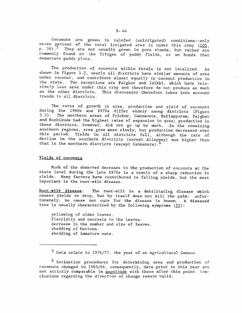
B- 44
Coconuts are grown in rainfed (unirrigated) conditions--only seven percent of the total irrigated area is under this crop (105, p. 36). They are not usually grown in pure stands, but rather are commonly found on the fringes of paddy fields, or on bunds that demarcate paddy plots.
The production of coconuts within Kerala is not localized. As shown in Figure 3.2, nearly all districts have similar amounts of area under coconut, and contribute almost equally to coconut production in the state. Two exceptions are Palghat and Idikki, which have relatively less area under this crop and therefore do not produce as much as the other districts. This discussion therefore takes into account trends in all districts.
The rates of growth in area, production and yield of coconuts during the 1960s and 1970s differ widely among districts (Figure 3.3). The northern areas of Trichur, Cannanore, Mallappuram, Palghat and Kozhikode had the highest rates of expansion in area; production in these districts, however, did not go up by much. In the remaining southern regions, area grew more slowly, but production decreased over this period. Yields in all districts fell, although the rate of decline In the southern districts (except Alleppey) was higher than that in the northern districts (except Cannanore).^
Yields of coconuts
Much of the observed decrease in the production of coconuts at the state level during the late 1970s is a result of a sharp reduction in yields. Many factors have contributed to falling yields, but the most important is the root-wilt disease.
Root-wilt disease: The root-wilt is a debilitating disease whichcauses yields to drop, but by itself does not kill the palm: unfortunately, no cause nor cure for the disease is known. A diseased tree is usually characterized by the following symptoms (53):
yellowing of older leaves. flaccidity and necrosis in the leaves, decrease in the number and size of leaves, shedding of buttons. shedding of immature nuts.
Data relate to 1976/77, the year of an Agricultural Census.fi Estimation procedures for determining area and production of
coconuts changed in 1965/66, consequently, data prior to this year are not strictly comparable in magnitude with those after this point. Conclusions regarding the direction of change remain valid.
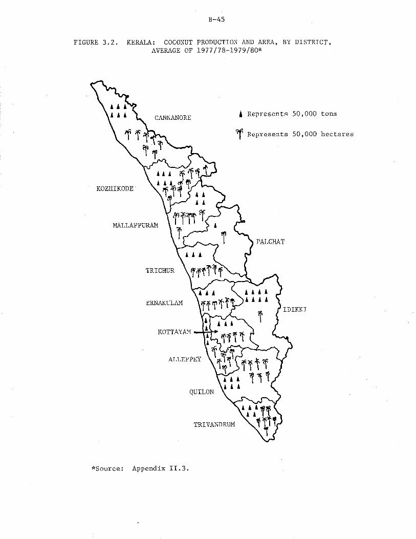
B-45
FIGURE 3.2. KERALA: COCONUT PRODUCTION AND AREA, BY DISTRICT,AVERAGE OF 1977/78-1979/80*
*Source: Appendix II.3.
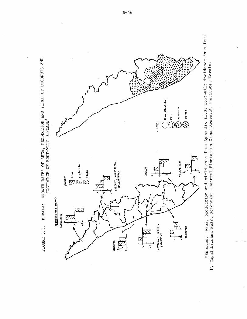
FIGU
RE 3
.3.
KERA
LA:
GROW
TH R
ATES
OF
AREA
, PR
ODUC
TION
AND
YIE
LD O
F CO
CONU
TS A
NDIN
CIDE
NCE
OF R
OOT-
WILT
DIS
EASE
*
B-46
*Sou
rces
: Ar
ea,
prod
ucti
on a
nd y
ield
dat
a fr
om A
ppen
dix
II.3;
root w
ilt
inci
denc
e da
ta f
rom
M. G
opal
akri
shna
Nair,
Sci
enti
st,
Cent
ral
Plan
tati
on C
rops
Res
earc
h In
stit
ute,
Kerala.
B- 47
The disease has reportedly affected palms in seven of 11 districts, as shown in Figure 3.3, beginning with Trivandrum in the south and going up to Trichur in the north. It is no coincidence that the central and southern districts which experienced the lowest rates of growth in coconut area have large tracts of palms categorized as severely diseased. In fact, nearly all of the severely diseased palms are located in these districts.
Estimates made in the late 1970s of the area that is affected range between 225,000 hectares and 270,000 hectares. The annual loss is put at 340 million nuts. These figures represent about 35-40 percent of the total area under coconuts and a loss amounting to a little more than 10 percent of total production (3_2; 89.) . This works out to an average yield loss attributable to the disease of approximately 1,360 nuts per hectare. The per palm productivity is affected as follows (53):
The root-wilt was first reported in Erattupetta (Meenachil) taluk in Kottayam district in 1882 after the occurrence of floods. Within the next decade, diseased trees were also reported from Alleppey and Quilon districts. However, it was not until 1970, when the Central Plantation Crops Research Institute (CPCRI) was set up as part of the research network of the Indian Council of Agricultural Research, that a comprehensive program was laid out to determine the epidemiology of the root-wilt (63., p. 15).
A feature of the disease is that the afflicted trees do not follow any consistent pattern; perfectly healthy trees are found next to diseased trees, Indicating that an aerial vector is responsible for the spread of the disease. Until recently, efforts to identify the cause and agent of spread of the disease were unsuccessful; however, new evidence indicates that the disease is caused by a mycoplasma, an organism in between a bacteria and a virus, but still, no cure has yet been discovered. Given this fact, planners have concentrated efforts on:a. Containing the disease to the boundaries delineated so far. To
this end, the Kerala Department of Agriculture, with financial assistance from the Indian Coconut Development Board and the World Bank, has tried to create a buffer zone between the completely healthy and diseased tracts by uprooting sick palms on the northern fringes of the diseased area, planting healthy seedlings free of cost to the farmer, and subsidizing their maintenance for
Disease index Yield(nuts per palm)
0 - 10 11 - 25 26 - 50 Over 50
50.333.722.519.0
B- 48
the^ first few years. Presumably, these palms would be closely monitored for any symptoms of the root-wilt (68).
b. Sponsoring a set of replanting incentives such as subsidies onfertilizers, seedlings, and irrigation facilities, in order to help eradicate diseased palms in key affected areas. This program is funded with the help of the erstwhile Agricultural Finance Corporation, the Coconut Development Board and the World Bank. For^ total replacement of all root-wilt affected palms, it is estimated that 50 million seedlings will be required, which is well outside the present capacity of the state seed nurseries (32 p. 10). ’
c. Identifying means of increasing production from the diseased palmsthemselves. Research has indicated that better management practices result in significantly higher yields from the sick palms themselves. For example, regular application of farm yard manure is reported to increase yields by 26 percent over a six year period. Intercropping tuber crops such as elephant foot yam and yam, irrigation and the application of chemical fertilizers, particularly magnesium sulphate, are reported to be other means of augmenting yields (89, p. 14; 53). These increases do not,however, fully compensate for the initial loss in yield caused by the disease. J
d. Identifying varieties of trees that are resistant or at least tolerant to the disease. Scientists at the Central Plantation Crops Research Institute claim to have found evidence that the "DXT hybrids are more productive and have a lower incidence of the disease when compared to the ordinary WCT [West Coast Tall] palms.... '* (.32; ,53.). Officials at the Coconut Development Board, on the other hand, challenging the sampling techniques on which the CPCRI results are based, argue that "... [the TXD and DXT hybrids] are also susceptible to the disease and are in no way different from the other types in the degree of susceptibility"; they concede, however, that in the absence of any other resistant Varieties, the DXT hybrids, by virtue of their early bearing and high-yielding characteristics, are the only choice for use in replantation (89, p. 14).
Although the root-wilt explains much of the observed decline in yields, it does not explain all of it. For example, a comparison of yields in the diseased tracts with those in areas not affected by the root-wilt reveals that the disease does not explain why Alleppey, where all taluks have a 20 percent or higher disease incidence, had the third highest average yield among all districts, while Cannanore, which is not affected by the disease at all, had the lowest yields during the late 1970s (Appendix II.3). Both these districts contribute about equally to total coconut production In the state. Thus, other factors have also contributed to declining yields. These include:
B- 49
Low proportion of bearing palms: Coconut seedlings in Kerala are being planted at a faster rate than that at which old trees are being removed, so that there is a net addition of area under coconuts without any production in the initial years„ In addition, theie are increasing numbers of old and virtually unproductive palms. Available data indicate that these factors have resulted in the proportion of the total palm population that is yielding to decline, causing per hectare yields to fall (70):^
Year Kerala Trivandrum Ouilon Alleppey Cannanore (percent bearing palms)
1963/641964/651965/66
66 61 68 68 6365 58 68 72 6064 56 66 71 60
Low yields per palm: Concomitantly, yields per bearing palm are low because the palm population is in general old: 34 percent of the trees are older than 40 years of age and therefore past peak productivity (47) . However, as the new seedlings planted in the mid-1960s have begun to mature, the per palm productivity has started to rise slowly in most districts, despite the increase in incidence of the root-wilt(70; 55):
Year Kerala Trivandrum Ouilon Alleppey Cannanore fruits per bearing palm per year)
1963/641964/651965/66
1975/761976/771977/78
30 32 30 32 2429 32 31 32 2729 31 32 31 26
35 41 37 36 2336 41 37 36 2232 40 30 32 25
Poor Quality Seeds: In addition, the lack of quality planting materials has also contributed to the poor yield performance of the coconuts in Kerala. It is estimated that a mere eight percent of total seed requirements are met by government nurseries, 18 percent by private nurseries, and 74 percent from the cultivators gardens themselves (70, p. 20). Area under hybrid varieties of coconuts is negligible, amounting at most to five percent of the area undercoconuts (72).
The Competition Between Coconut and FaddyThe area trends in coconuts can partly be explained by the compe
tition they face from paddy cultivation. Figure 3.4 presents trends m 7
7 Hore recent information is unavailable.
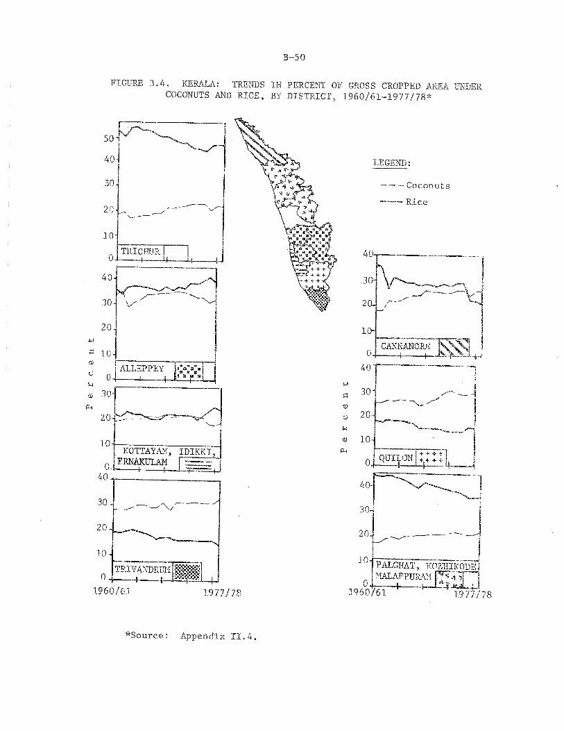
B-50
FIGURE 3.4. KERALA: TRENDS IN PERCENT OF GROSS CROPPED AREA UNDERCOCONUTS AND RICE, BY DISTRICT, 1960/61-1977/78*
LEGEND,»
~ — — Coconuts --- Rice
*Source: Appendix II.4.
B- 51
percent of gross cropped area under coconuts and rice. In all except the root-wilt afflicted districts, coconut area has been increasing at the expense of rice. This increase is likely to be long-term in nature because competition between coconut and paddy does not exist annually, but rather on a long term basis; once the land has been planted to coconuts, paddy is not likely to be sown for at least the next 20 - 30 years. In the root-wilt districts of Alleppey, Kottayam, Ernakulam and Idikki, coconut area has, in fact, lost to paddy since the early 1970s (these four districts account for nearly 30 percent of the area and production of coconuts in the state) . This explains why at the state level, area under coconuts declined slightly after the mid-1970s.
One of the primary reasons why farmers have tended to devote increased proportions of their gross cropped area to coconuts in most districts is because of the real increases in farm harvest prices of coconuts; this is despite the Land Utilization Act which prohibits the conversion of paddy lands to other uses. Paddy lands converted to coconuts reportedly increase 20 to 30 times in value (60.) . Unfortunately, time series data on the costs of cultivation of coconuts and paddy are not available; however, paddy costs (per hectare) are higher because of the larger labor requirements of this crop compared to those of coconut. Studies have indicated that the costs associated with paddy cultivation typically comprise half of the gross value of output, and the corresponding costs for coconuts comprise only 25 to 30 percent of the gross value of output (.93.; 47). The relative profitabilities of the two crops can therefore be evaluated by estimating net revenue per hectare, calculated by multiplying the relevant farm harvest price with yield per hectare for each year, and subtracting from it half of the product in the case of paddy and one fourth in the case of coconuts. As set out in Figure 3.5, coconuts have consistently generated higher revenue per hectare compared to paddy in Kerala.
Prospects for Increased Coconut (Oil') Production
Despite declining productivity, coconuts have enjoyed a favorable economic environment since the 1960s. Figure 3.6 presents trends in farm harvest prices of coconuts, and wholesale and retail prices of coconut oil in Kerala, deflated by the consumer price index over the period 1963 to 1981. Real prices in all three instances have gone up. In addition, the three prices have moved very closely, as further evidenced by the high correlation coefficients between pairs of prices as shown below (computed from data in Appendix II.5); 8
8 This result Is not very sensitive to changes in the cost percentages. Even if 45 percent of coconut and 30 percent of paddy revenue Is attributed to costs, the net income from coconut would still be higher than that from paddy.
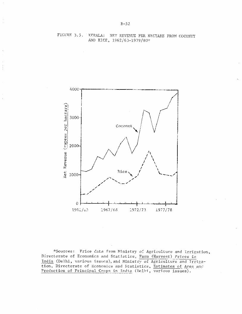
B-52
FIGURE 3.5. KERALA: NET REVENUE PER HECTARE FROM COCONUTAND RICE, 1962/63-1979/80-
^Sources: Price data from Ministry of Agriculture and Irrigation,Directorate of Economics and Statistics, Farm (Harvest) Prices in India (Delhi, various issues), and Ministry of Agriculture and Irrigation, Directorate of Economics and Statistics, Estimates of Area and Production of Principal Crops in India (Delhi, various issues).
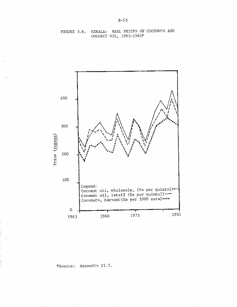
Price
(rupees)
B-53
FIGURE 3.6. KERALA: REAL PRICES OF COCONUTS ANDCOCONUT OIL, 1963-1981*
*Source: Appendix II.5.
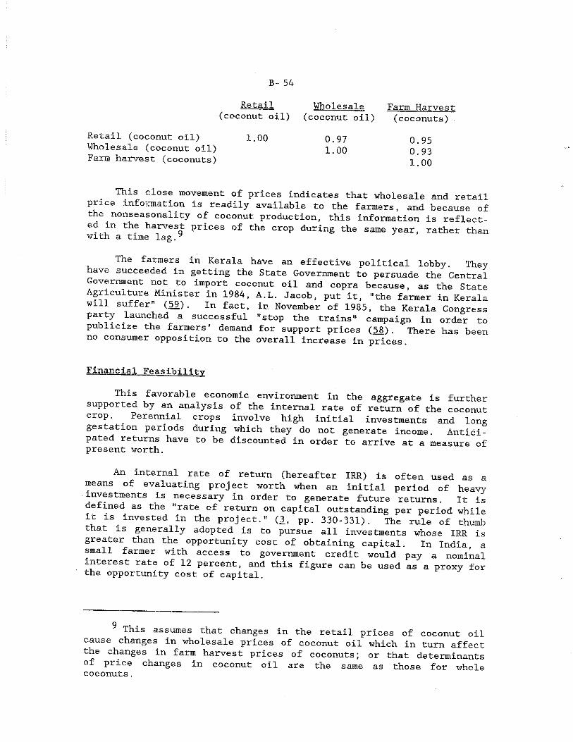
B- 54
Retail(coconut oil)
Wholesale (coconut oil)
Farm Harvest (coconuts)
Retail (coconut oil) 1.00 0.97 Wholesale (coconut oil) 1#00 Farm harvest (coconuts)
0.950.931.00
This close movement of prices indicates that wholesale and retail price information is readily available to the farmers, and because of the nonseasonality of coconut production, this information is reflect-ed in the harvest prices of the crop during the same year, rather than with a time lag,y
The farmers in Kerala have an effective political lobby. They have succeeded in getting the State Government to persuade the Central Government not to import coconut oil and copra because, as the State Agricuiture Minister in 1984, A.L. Jacob, put it, "the farmer in Kerala will suffer" (59). In fact, in November of 1985, the Kerala Congress party launched a successful "stop the trains" campaign in order to publicize the farmers' demand for support prices (58). There has been no consumer opposition to the overall increase in prices.
Financial Feasibility
This favorable economic environment in the aggregate is further supported by an analysis of the internal rate of return of the coconut crop. Perennial crops involve high initial investments and long gestation periods during which they do not generate income. Anticipated returns have to be discounted in order to arrive at a measure of present worth.
An internal rate of return (hereafter IRR) is often used as a means of evaluating project worth when an initial period of heavy investments is necessary in order to generate future returns. It is defined as the "rate of return on capital outstanding per period while it is Invested in the project." (3, pp. 330-331). The rule of thumb that Is generally adopted is to pursue all investments whose IRR is greater than the opportunity cost of obtaining capital. In India, a small farmer with access to government credit would pay a nominal Interest rate of 12 percent, and this figure can be used as a proxy for the opportunity cost of capital.
This assumes that changes in the retail prices of coconut oil cause changes in wholesale prices of coconut oil which in turn affect the changes in farm harvest prices of coconuts; or that determinantsof price changes in coconut oil are the same as those for whole coconuts.
B- 55
In order to estimate an IRR for coconuts, one needs to make a few assumptions. Farmers make planting decisions regarding perennial crops only after considering their long-term profitability; a reasonable measure of the farmer's planning horizon might be 30 years. In addition, perhaps the best way to approximate revenue is to multiply the average state yield of 4,500 nuts per hectare with the mean harvest price of Rs. 1.5 per nut. Unfortunately, the lack of reliable data does not permit the consideration of Income through such sources as the sale of coconut leaves used for thatching roofs and making baskets. The available data on costs relate to a pure stand of trees and were obtained for a typical one-hectare plot of coconuts from the CPCRI. The calculations and a detailed list of assumptions are presented in Appendix V.2. The resulting IRR works out to be 37 percent and thus, despite disease problems and poor maintenance, coconuts are extremely profitable; therefore, prospects for the expansion of its production are good.
The next Issue that needs examination is to what extent production increases can be effected through area expansion and yield augmentation.
Acreage ExpansionThe scope for bringing new, previously uncultivated lands under
coconut cultivation is limited. The coconut does not thrive well on hilly areas, which are the only remaining uncultivated lands in Kerala. In addition, as discussed earlier, increases in area under coconut tend to be at the expense of rice cultivation.
Acreage response studies have traditionally been based on the Nerlovian model of expected profitability of the crop vis-A-vis a competing crop, Such a model Is inappropriate in the present context * S
In any event, numerically, increasing the planning horizon beyond 30 years does not greatly influence the internal rate of return.
The Nerlovian model, modified for a perennial crop may be, forexamples of the form (31) :
X = a + bP + cS + u t t t t
where P = E P*.. / (n+1)t -r t+i
St = l St+i j (n+1)X = Area (or number of trees) planted in year t,
P* = The expected real producer price of coconut in year t+i,
S* . = The expected real producer price of an alternative crop in year t+i.
n - Expected age after which trees planted in year t cease toproduce, and
u = a disturbance term, t
B- 56
because it does not explicitly take into account the strategies a armer must adopt for meeting basic family needs during the initial six
or seven years of coconut cultivation which involve high investments but no returns. In addition, farmers are unlikely to switch out of rice completely because it is a semi-subsistence crop in Kerala and because, even though Kerala is a net importer of foodgrains, strong taste preferences exist for the local variety. strong
A co">Parison of the present worth of income generated throughP , y cultivation, on the one hand, and mixed cultivation of coconuts and paddy on the other, is one appropriate means of evaluating to what extent coconuts can replace paddy. This involves certain assumptions First, because rice is the staple food of the Kerala farmer, other crops can impinge on it only to a certain point. Therefore the 30 percent of gross cropped area currently under rice is taken to be the lower bound on acreage planted to paddy. Second, for reasons discussed
^ C°mPUtatl0nS arS Performed for a 30 year planning period. Third, the 12 percent cost of government loans is used as the opportu- nlty cost of obtaining capital. Although the value of land would presumably play an important role in a farmer's decision, this factor cannot be considered; data limitations preclude it. The analysis is done on a per hectare basis for the sake of simplicity.
The_gross value of output (or total revenue) is approximated bymultiplying farm harvest price with yield for 1977/78-1979/80 for the two crops and averaging these amounts. Costs of cultivation are taken into account m the manner discussed previously, so that net income from paddy amounts to 50 percent of the gross value of output, and that or coconuts, 75 percent of total revenue. This means that pure paddy
cultivation would fetch a net income of Rs. 1,029 per hectare, and coconuts would yield Rs. 3,918 per hectare. In addition, it makes sense to assume that sixth and seventh year yields for coconuts will be ower than the peak yield at the eighth year, and this translates into
P<;r^ Ctare fr°m six1fnd seven year old coconuts of Rs. 3,482 and Rs. 3,700, respectively. ^
It is instructive to compare the present worth of income generated from four alternative systems of mixed cropping with that generated from paddy alone. Detailed calculations are presented in Appendix V.3 but the results summarized below indicate that in all instances the present worth of an income stream from mixed coconut and ' rice cultivation is nearly one and a half times higher than that from rice cultivation alone.-3 12 13
12 Six year old coconuts are assumed to yield 4,000 nuts per hectare, and seven year old coconuts, 4,250 nuts per hectare.
13 The analysis is based on only one crop of paddy being grown during the year. Separate data on the cropping intensity of rice are not available, but even if one attributes the overall cropping intensity of 130 percent to paddy, then mixed cultivation continues to
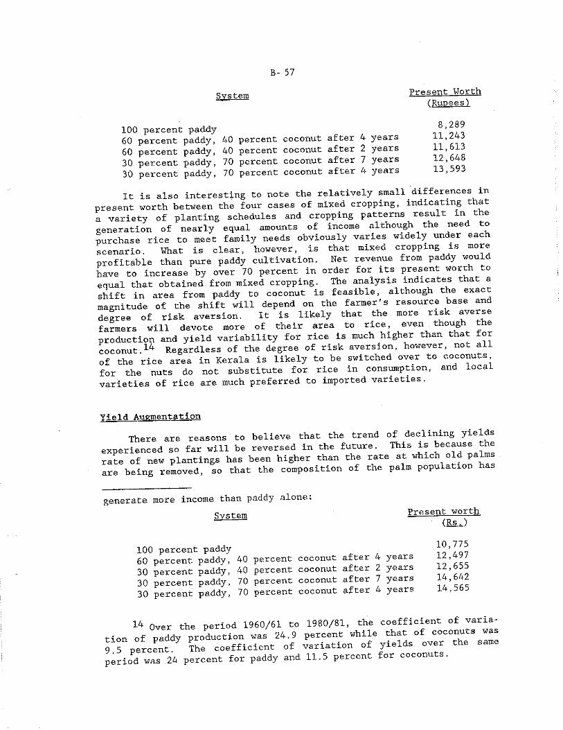
B- 57
System
100 percent paddy60 percent paddy, 40 percent coconut after 4 years60 percent paddy, 40 percent coconut after 2 years30 percent paddy, 70 percent coconut after 7 years30 percent paddy, 70 percent coconut after 4 years
Present Worth (Rupees')
8,28911,24311,61312,64813,593
It is also interesting to note the relatively small differences in present worth between the four cases of mixed cropping, indicating that a variety of planting schedules and cropping patterns result in the generation of nearly equal amounts of income although the need to purchase rice to meet family needs obviously varies widely under eac scenario. What is clear, however, is that mixed cropping is moreprofitable than pure paddy cultivation. Net revenue from paddy would have to increase by over 70 percent in order for its present worth to equal that obtained from mixed cropping. The analysis indicates that a shift in area from paddy to coconut is feasible, although the exact magnitude of the shift will depend on the farmer's resource base and degree of risk aversion. It is likely that the more risk averse farmers will devote more of their area to rice, even though the production and yield variability for rice is much higher than that for coconut * 14 Regardless of the degree of risk aversion, however, not all of the rice area in Kerala is likely to be switched over to coconuts, for the nuts do not substitute for rice in consumption, and loca. varieties of rice are much preferred to imported varieties.
Yield AugmentationThere are reasons to believe that the trend of declining yields
experienced so far will be reversed in the future. This is because the rate of new plantings has been higher than the rate at which old palm are being removed, so that the composition of the palm population ha
generate more income than paddy alone.System Present worth
( E i J
100 percent paddy60 percent paddy, 40 percent coconut after 4 years30 percent paddy, 40 percent coconut after 2 years30 percent paddy, 70 percent coconut after 7 years30 percent paddy, 70 percent coconut after 4 years
10,77512,49712,65514,64214,565
14 Over the period 1960/61 to 1980/81, the coefficient of varia- tion of paddy production was 24.9 percent while that of coco“ ts ™ 9 5 percent The coefficient of variation of yields over the period was 24 percent for paddy and 11.5 percent for coconuts.
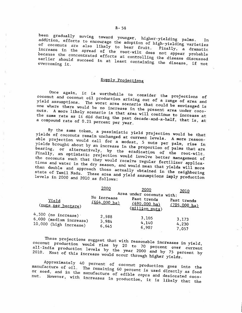
B- 58
addition, e X X X X c o X X t X X ^ • hi6her;yielditig_ palms. InOf coconuts are also likely to b e « fruit ^Ftnallv^5 V*rieties increase in the spread of the root-wilt X F U y ’ a dramaticbecause the concentrated efforts at control! i ^ ,appear Probableearlier should succeed in i llmg the disease discussedovercoming it “ at leaSt conta^ing the disease, if not
Supply Projections
coconut and C o c o n u t ^ i ^ p ^ d u ^ o ^ 6 r ^°* C° n s id e r th e P r o je c t io n s o f y ie ld assum ptions. The w X sX a X a slen arT o X a X c ° f “ “ ^one where th e re would be no in c re a s e in t h e X 1 6 e n v i s a S e d i sn u ts . A more l ik e l y s c e n a rio i s th a t a re a w m c X X u T t o 7 * “ * ^ th e same r a te as i t did during . . Z con tin u e to in c re a s e a ta compound rate of 0 21 ptXent per £ £ ‘too«»— “ • - * » « . that is, at
By the same to k en , a p essim i c f i p V1" i j y ie ld s o f coconuts remain unchanged a t J i r w t ? ™ ! . 1” AW° Uld be th a t able projection would call for a modest ? I 1 A “ore reason- y ie ld s brought about by an in c re a s e in t h e ’ nUt? per palm ’ r i s e in b e a r in g , or a l t e r n a t i v e l y b v the p ro p o rtio n o f palms th a t a reF in a l ly , an o p t im is t ic p r o je c t io n w o u l ^ X ^ i ^ ^ h ° f the th e coconuts such th a t thev wmilH • nvolve b e t t e r management o f t io n s and w ater in the d r y L l o n * * * * * * * * “ * * • * f e r t i l i z e r a p p lic a - than double and approach t W * nd * ould 1 t hat y ie ld s w i l l more s t a t e o f Tam il Nadu, These a re a a n d ^ ie ld ° t& ined ln the n eig h b orin g le v e ls in 2000 and 2010 as fo llo w s ; 7 ^ assumPtlo n s imP ly p rod u ctio n
Yield(nuts per hppfam'i
-,500 (no increase)6.000 (medium increase)10.000 (high increase)
2010under coconuts with:Past trends Past trends
2000Area
No increase 1664.000 h^
2,988 3,984 6,645
1690,000 (million nut.q'i
3,1054,1406,907
1705.000
3,1734,2307,057
coconut productlo^^ull^rise^ b^20h lncreases in yield>all-India production levels bv the ° percent ov®r current! M - - “ * *
e e u f S T S ' S . V « S n i° ' sTm t t l .or seed, and in the manufacture of edlbl*™ “ “X dir?°tly as fo°dnut. However, with increases in a * COPra anci desiccated coco-increases m production, it is likely that the
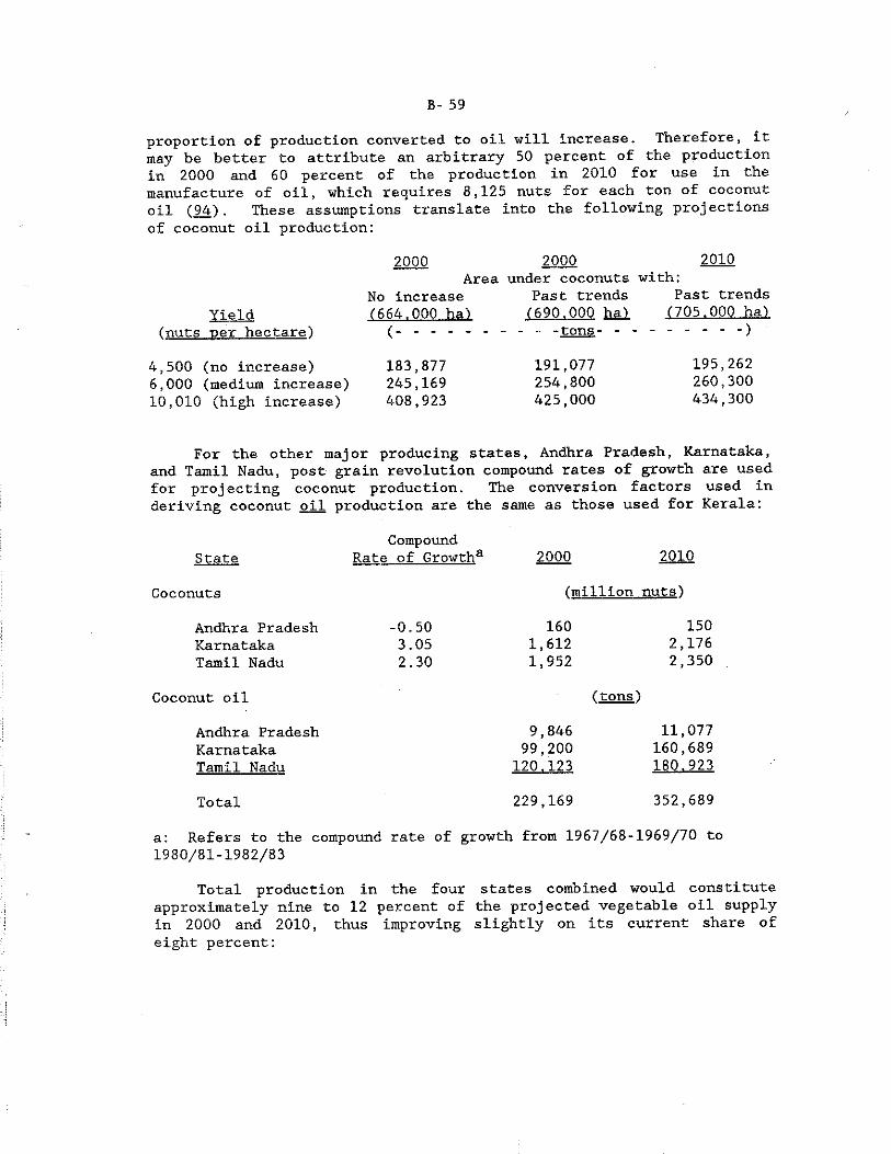
B- 59
proportion of production converted to oil will increase. Therefore, it may be better to attribute an arbitrary 50 percent of the production in 2000 and 60 percent of the production in 2010 for use in the manufacture of oil, which requires 8,125 nuts for each ton of coconut oil (94). These assumptions translate into the following projections of coconut oil production:
2000 2000 2010Area under coconuts with:
No increase Past trends Past trendsYield (664.000 ha > (690.000 hal (705,000 ha)
(nuts per hectare) -tons-
4,500 (no increase) 183,877 191,077 195,262 6,000 (medium increase) 245,169 254,800 260,300 10,010 (high increase) 408,923 425,000 434,300
For the other major producing states, Andhra Pradesh, Karnataka, and Tamil Nadu, post grain revolution compound rates of growth are used for projecting coconut production. The conversion factors used in deriving coconut oil production are the same as those used for Kerala:
CompoundRate of Growtha 2000 2010
(million nuts)
State
Coconuts
Andhra Pradesh Karnataka Tamil Nadu
-0.503.052.30
1601,6121,952
1502,1762,350
Coconut oil (tons)
Andhra Pradesh Karnataka Tamil Nadu
9,84699,200
120.123
11,077160,689180.923
Total 229,169 352,689
a: Refers to the compound rate of growth from 1967/68-1969/70 to1980/81-1982/83
Total production in the four states combined would constitute approximately nine to 12 percent of the projected vegetable oil supply in 2000 and 2010, thus improving slightly on its current share of eight percent:
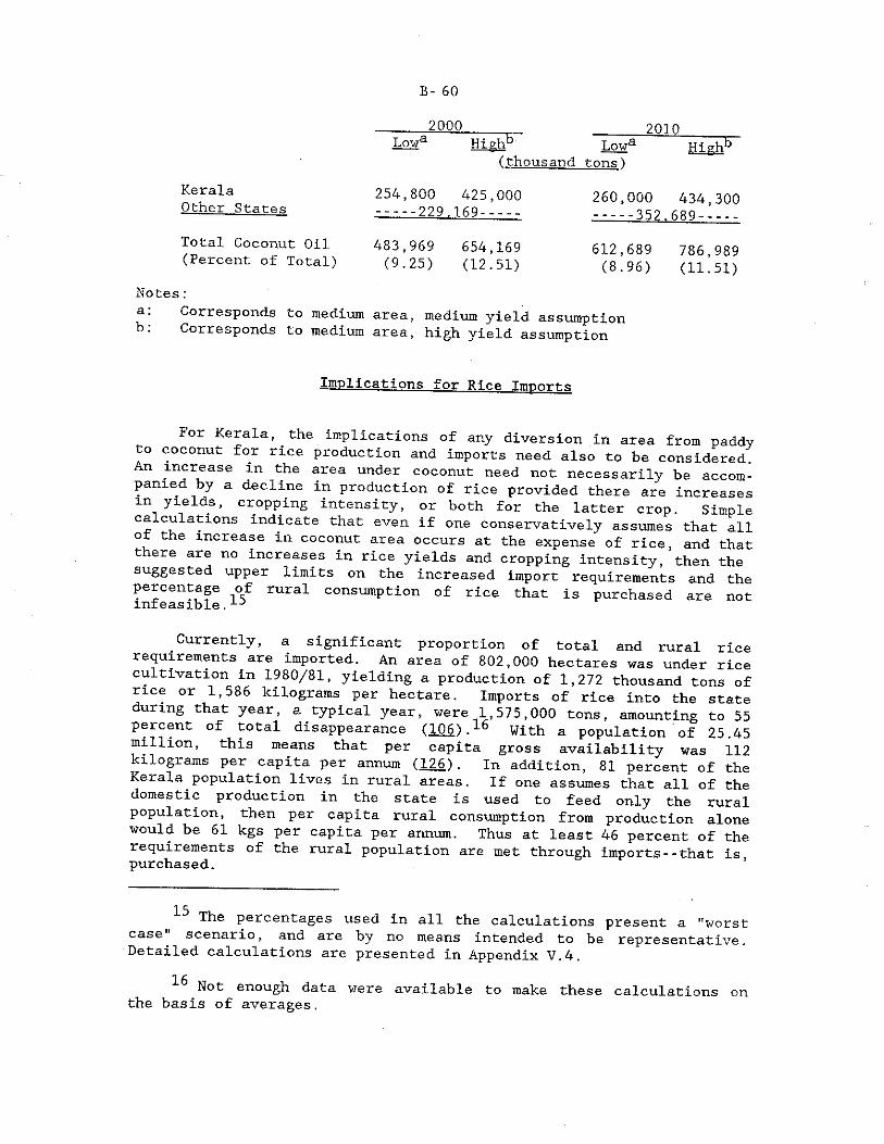
B- 60
----------2Q00 _______ 2010Lowa High5 "Tow1 High5
(thousand tons')Kerala Other States
Total Coconut Oil (Percent of Total)
254,800 425,000---- 229.169.....
483,969 654,169(9.25) (12.51)
260,000 434,300.... 352,689-----
612,689 786,989(8.96) (11.51)
Notes:a. Corresponds to medium area, medium yield assumptionb: Corresponds to medium area, high yield assumption
Implications for Rice imports
or Kerala, the implications of any diversion in area from paddy to coconut for rice production and imports need also to be considered. An increase in the area under coconut need not necessarily be accompanied by a decline in production of rice provided there are increases m yields, cropping intensity, or both for the latter crop. Simple calculations indicate that even if one conservatively assumes that all of the increase in coconut area occurs at the expense of rice, and that there are no increases in rice yields and cropping intensity, then the suggested upper limits on the increased import requirements and the percentage of rural consumption of rice that is purchased are not
Currently, a significant proportion of total and rural rice requirements are imported. An area of 802,000 hectares was under rice cultivation in 1980/81, yielding a production of 1,272 thousand tons of rice or 1,586 kilograms per hectare. Imports of rice into the state during that year, a typical year, were 1,575,000 tons, amounting to 55 percent of total disappearance (106).15 16 With a population of 25,45 million, this means that per capita gross availability was 112 kilograms per capita per annum (126). In addition, 81 percent of the Kerala population lives in rural areas. If one assumes that all of the domestic production in the state is used to feed only the rural population, then per capita rural consumption from production alone would be 61 kgs per capita per annum. Thus at least 46 percent of the requirements of the rural population are met through imports-- that is purchased. ’
15 The percentages used in all the calculations present a "worst case scenario, and are by no means intended to be representative. Detailed calculations are presented in Appendix V.4.
16 Not enough data were available to make these calculations on the basis of averages.
B- 61
If population between 1981 and 2000 continues to grow at the same rate as it did between 1971 and 1981, and if per capita availability of rice remains at 112 kgs per annum, then total requirements in 2000 would be 3,979,000 tons and in 2010, 4,742,000 tons. As for production, in 2000, 690,000 hectares under coconut would mean that 34,000 hectares would be diverted from rice; that is, 768,000 hectares would remain under rice, which would yield 1,218,000 tons of rice, implying that 70 percent of consumption needs will have to be imported. Similarly in 2010 •, 705,000 hectares under coconut implies the diversion of 53,000 hectares from rice to coconut „ Area under rice would therefore be 749,000 hectares which would result in 1,118,000 tons of rice, necessitating the import of 75 percent of rice requirements.
If 81 percent of the population continues to live in the rural areas, and all of domestic production is, as before, consumed on the farm, then 60 percent of rural rice requirements in 2000, and 70 percent in 2010 would have to be purchased.
When yield augmentation and increases in cropping intensity are taken into account, the proportion of requirements that would need to be met through imports would be much less. At any rate, given that 55 percent of rice requirements are currently met through imports and at least 46 percent of rural consumption needs are purchased, the above percentages are not unreasonable. The expansion in area under coconuts would not adversely affect the Kerala rice economy.
More than area, however, the key to higher coconut production in Kerala is better yields. Two major policies to ensure increased coconut yields merit consideration. First, as far as the root-wilt disease is concerned, research efforts must continue to concentrate on firmly establishing a cause for the disease, and determining a cure for it. Scientists in breeding programs may also consider using as parent material healthy trees found amidst diseased trees, as the former are likely to have natural resistance to the root-wilt. Second, there is also need for committing greater resources to developing seed farms that would supply quality seedlings at reasonable prices. Such a measure would reduce the costs of seeds as a percentage of production costs. A comparison of the targets set for the distribution of seedlings by the Kerala Department of Agriculture and actual achievements so far indicates that in the past few years, although achievements have exceeded targets with regard to the actual distribution of seedlings, the targets themselves have been low, in view of the fact that 50 million seedlings are required for the rejuvenation of rootwilt affected areas. In addition, the allocated budget for these programs has not been utilized to the fullest extent (55):
B- 62
Physical:______ _____ Financial:Year Target
("numberAchievement in thousands')
Target Achievement (100.000 Rs.)
1977/78 50 53 7 3.61978/79 50 52 7 3.41979/80 50 51 7 4.7
Stepped-up seedling production, however, needs also to be accompanied by an effective extension and distribution system. Kerala has recently switched to the "Training and Visit" system of extension, designed to promote increased communication between the farmer, the extension agent, and the research staff. It will be interesting to see if yield increases will be effected as a consequence of the new system.
The likely source of future increases in coconut (oil) production is through higher yields. In Kerala, although coconuts are profitable to cultivate, a combination of factors have kept yields of coconuts low; the ability of the farmers to overcome these technical constraints will determine the extent of production increases that can be expected from coconuts.
CHAPTER IV OIL PALM
Oil palm is the other major tree source of vegetable oil worth study: it yields the highest quantity of oil per hectare--higher than any other source of vegetable oil. Although a native of West Africa, most oil palm is now cultivated in East Asia. Palm oil has had the most dynamic performance among all the vegetable oils, thanks mainly to spectacular increases in Malaysia's production. Might the same success also be achieved in the regions of India that are climatically suited to oil palm cultivation?
This chapter reviews the performance of the first oil palm plantation in India and evaluates the economics of its cultivation. Supply projections for the years 2000 and 2010 made in this study indicate that India is not likely to replicate the Malaysian performance for two reasons: first, only 80,000 hectares are suitable for rainfed oil palm cultivation, and second, Indian yields have so far been low.
The Miracle Palm
The success of the palm oil industry worldwide has, in large part, been the result of Malaysia's decision to enter oil palm production in a major way. Although commercial plantings of oil palm in Malaysia began In 1917, oil palm was not a major contributor to the value of its total agricultural output--rubber was the mainstay of the economy then. By the early 1960s however, world prices of rubber had declined in real terms. The World Bank recommended that Malaysia diversify its base of agricultural production and accordingly, in 1961 the Malaysian government decided to actively encourage the cultivation of oil palm. Where ever suitable soils and climates were found, oil palm was promoted even at the expense of rubber. Vast jungles were cleared and planted to oil palm, and small holders were provided with heavy subsidies to replace rubber trees with oil palm. Thus, while between 1950 and 1959 area under oil palm grew at a modest rate of 5.5 percent, between 1959 and 1972 area increased at a phenomenal growth rate of16.2 percent.1 Additionally, investments in research produced significant yield increases. Malaysia's entry into large scale palm oil production resulted in a surge of world production and exports of the oil (14, p. 26). In the mid-1970s, palm oil accounted for 10 percent of world production and 25 percent of world exports of vegetable oils; by the early 1980s, it increased its share to 15 percent of
1 Area in 1950 was 31,567 hectares, in 1959, 50,992 hectares, and in 1972 was 358,968 hectares (14). The percentages refer to^compound rates of growth. Area has continued to increase through the mid-1980s.
B- 63
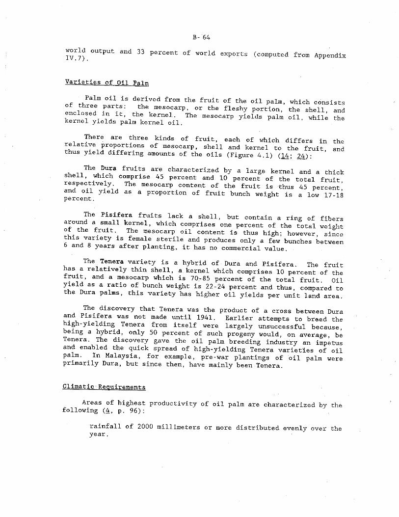
B- 64
output and 33 percent of world exports (computed from Appendix
Varieties of Oil Palm
Palm oil is derived from the fruit of the oil palm, of three parts: the mesocarp, or the fleshy portion, enclosed^ in it, the kernel. The mesocarp yields palm kernel yields palm kernel oil.
which consists the shell, and oil, while the
There are three kinds of fruit, each of which differs in relative proportions of mesocarp, shell and kernel to the fruit thus yield differing amounts of the oils (Figure 4 1) (14' 24)*
theand
The Dura fruits are characterized by a large kernel and a thick shell, which comprise 45 percent and 10 percent of the total fruit respectively The mesocarp content of the fruit is thus 45 percent’and oil yield as a proportion of fruit bunch weight is a low 17-18 percent.
The Pis if era fruits lack a shell, but contain a ring of fibers around a small kernel, which comprises one percent of the total weight of the fruit. The mesocarp oil content is thus high; however, since this variety is female sterile and produces only a few bunches between
and 8 years after planting, it has no commercial value.
The Tenera variety is a hybrid of Dura and Pisifera. The fruit as a relatively thin shell, a kernel which comprises 10 percent of the
fruit, and a mesocarp which is 70-85 percent of the total fruit. Oil yield as a ratio of bunch weight is 22-24 percent and thus, compared to the Dura palms, this variety has higher oil yields per unit land area.
The discovery that Tenera was the product of a cross between Dura and Pisifera was not made until 1941. Earlier attempts to breed the
yielding Tenera from itself were largely unsuccessful because, being a hybrid, only 50 percent of such progeny would, on average, be Tenera. The discovery gave the oil palm breeding industry an impetus and enabled the quick spread of high-yielding Tenera varieties of oil palm. In Malaysia, for example, pre-war plantings of oil palm were primarily Dura, but since then, have mainly been Tenera.
Climatic Requirements
Areas of highest productivity of oil palm are characterized by the following (4, p. 96):
rainfall of 2000 millimeters or more distributed evenly over the year.
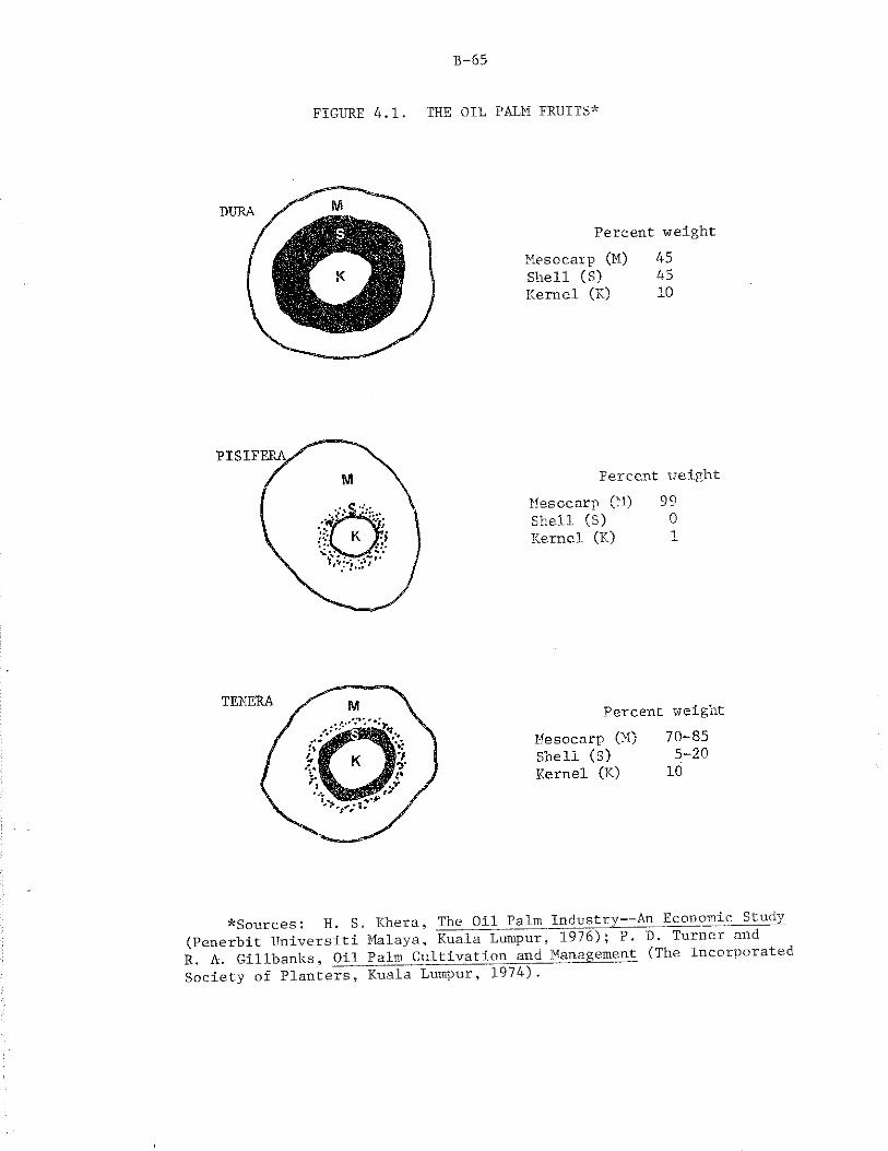
B-65
FIGURE 4.1. THE OIL PALM FRUITS*
Percent weightMesocarp (M) 45Shell (S) 45Kernel (K) 10
Percent weightMesocarp (M) 99Shell (S) 0Kernel (K) 1
*Sources: H. S. Khera, The Oil Palm Industry— An Economic__Study(Penerbit Universiti Malaya, Kuala Lumpur, 1976); P. D, Turner and R. A. Gillbanks, Oil Palm Cultivation and Management (The Incorporated Society of Planters, Kuala Lumpur, 1974).
B- 66
sunshine for at least five hours a day in all months and seven hours a day in some months.
Oil palm can be grown on most soils but four kinds of soils are generally thought to be unfavorable, these are: poorly drained soils,lateritic soils, very sandy coastal soils, and deep peat soils (4). Nevertheless, oil palm can be profitably cultivated under suboptimal conditions because it produces more oil per hectare than any other source of vegetable oil. As Figure 4.2 indicates, the only areas in India that satisfy the rainfall and temperature requirements are the western coast and the Andaman and Nicobar Islands.
The plantations are generally found in contiguous land areas. Oil palm fruits must be processed within 24 hours of harvest because the fruits have an enzyme, lipase, which starts to break down the oil into free fatty acids; and the higher the free fatty acid content, the harder it is to process. Therefore, the processing unit needs to be located within easy transporting distance to the site of production. A large capacity processing unit serves several hundred hectares of oil palm, and this factor, combined with the high costs of transportation, requires that the production area be contiguous.
a mean maximum temperature of 29° C to 33° C and a mean minimumtemperature of 22° C to 24° C.
Oil— Palm in India--A Brief History
Palm oil finds major uses in the soap, candle and tin plate industries. In addition, it is used extensively in margarines, salad oils, shortenings, cooking oils, confectionery and ice cream. Palm kernel oil is used in the manufacture of soap and in a variety of edible products, and is a close substitute for coconut oil (95).
Imports °f palm into India have taken place since the early 1960s. They have played an increasing role in the vegetable oil economy following import liberalization in 1978, when imports of palm oil jumped to a high 375,100 tons. Since then, annual imports have continued to remain well over 400,000 tons (Appendix IV.6). Commercialproduction of oil palm was, on the other hand, unknown in India until recent times.
Oil palm was introduced to India in 1834 when an ornamental tree was planted in the Sibapore Botanical Gardens in Calcutta (81). However, it was only in 1958 that the first experimental "African Red 2
2 Lateritic soils are defined here in the sense of soils that tend to dry out rapidly in the dry season, causing palms to suffer drought conditions even when the annual precipitation has been normal.
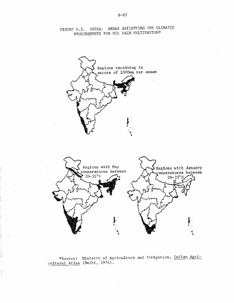
B-67
FIGURE 4.2. INDIA: AREAS SATISFYING THE CLIMATICREQUIREMENTS FOR OIL PALM CULTIVATION*
*Source: Ministry of Agriculture and Irrigation, Indian Agri_cultural Atlas (Delhi, 1974).
B- 68
RoL i^ 1” " !la1tatl°n WaS set UP by the Indian Central Oilseedsdistrict3 * * 6 Keralfl6 f 5 l f ^ ."“ I"?* statlon in Thodupuzha, Ernakulam * Ernakulam has an annual rainfall of 4000210 r t? r3"50dlc,trlbUtet ovor 8-9 tenths and t^paraturef hanging f Z21 C to 35 C over the year; it is therefore climatically suited to the cultivation of oil palm (104). Accordingly, in January 1961 the following plantings were made at the research station (51);
Variety
Dura X DuraDura X Pisifera (Tenera) Dura X Tenera
Number of seeds sown
2,0522 ,1001,038
made in 1 Ma^aysian and Nigerian Dura and Tenera wereSome t-rlJf96l’ ^ 53’ 1965 f*d 1969 ’ coverinS a total of 40 hectares.studies of Pi,antlnga Were als° made ln Andl>ra Pradesh. Early agronomiccultiwe<-rf hS perfor.manca of these plantings concluded that oil palm cultivation was certainly feasible in India (82; 83). F
During the early 1960s, private industries (notably, Hindustan Lever, Incorporated) exhibited an active interest in oil palm cultivation, however, plans remained on paper only," mainly because of theeditoriaietoP°tbe t th^ . 1Ixidiaxi Government to the initiative. As an
7 * f1 he Indian Oil and Soap Journal pointed out, "... paucityo un s was not the problem... [and] comprehensive technical and commercial data too had been collected" (62).
It was not until 1971 that an attempt was made to diversify them V V 866 production through oil palm. Commercial cultivation ont-* was started under the auspices of the Plantation Corporation of Kerala, Limited.J v
In 1973,^ a study team formally evaluated the prospects for oil pa m cu tivation in India based on the performance at the Thodupuzha epper Research Station. The report concluded that oil palm cultiva
tion was feasible in certain parts of India and could yield two and a halt tons of oil per hectare and an annual net return of 17 percent oninvestment. The report also pointed out that because of the three-month dry period in winter, "one cannot expect the yields as obtainedm Malaysia and Sumatra, where there is virtually no dry periodthroughout the year" (56). In subsequent years, as the scope of cultivation expanded, a separate company, Oil Palm India, Limited, was formed with headquarters in Kottayam, Kerala.
A total of 2000 hectares of forest land was allocated for oil palm cultivation in Punalur taluk of Quilon district, which is located just
3 The Plantation Corporation of Kerala is a public sector institution set up in 1962 to manage government-owned plantations--itsmain responsibilities involve rubber and cashew cultivation.
B- 69
north of Trivandrum district (Figure 4.3). Temperatures and rainfall at Punalur satisfy the minimum requirements for the cultivation of oil palm even though the soils are lateritic and, therefore, suboptimal. While Punalur is not the only location which meets the climatic requirements for the cultivation of oil palm, it is one of the few areas that has sufficiently large tracts of contiguous land available for cultivation.
There are five estates at Punalur, which have a total of 3,705 hectares under oil palm (25):
Estate
Yeroor
Area planted (hectares)
Yeroor 1,752Maravinchira 329
Ghithara 944
Kulathupuzha
KulathupuzhaArtppa
4002.8.0
Total 3,705
Yeroor estate is the earliest and is the only one that has started commercial yielding. Of the total 1,752 hectares that had been planted at Yeroor, 560 hectares were mature as of June 1986 . Commercial production had not yet begun on the other estates. For this reason, the rest of this discussion focuses on Yeroor plantation.
Oil Palm in Kerala--Yeroor Estate4
All of Yeroor estate is planted to high-yielding tenera seeds of various origins as indicated in the following table:
4 Most of the data for this section were gathered from the records maintained by Oil Palm India, Limited, Kottayam, and from discussions with their staff during July-August 1983. Supplementary data were obtained in June 1986, Some inconsistencies in the data- -which are yet to be resolved--do exist, but these do not influence the major conclusions ,
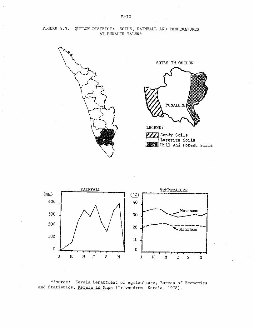
B-70
FIGURE 4:3. QUILON DISTRICT: SOILS, RAINFALL AND TEMPERATURESAT PUNALUR TALUK*
SOILS IN QUILON
RAINFALL TEMPERATURE
*Source: Kerala Department of Agriculture, Bureau of Economicsand Statistics, Kerala in Maps (Trivandrum, Kerala, 1978).
B- 71
leal! Hectares Planted Country of Origin
197119721973 1975 1979 1930
120202225503417283
MalaysiaNigeriaNigeriaNigeriaPapua, New Guinea IBBO5
Total 1,752
The seeds are grown in a nursery in polythene bags and transplanted between 12 and 18 months of age. Trees are placed in a triangular fashion nine meters apart so as to accommodate 135 trees per hectare„ This corresponds to the optimal spacing usually suggested: greater or lower tree densities would result in lower yields <4, p, 4X1). The trees are placed in pits of one meter radius in order to facilitate water and fertilizer absorption. Leguminous crops such as Fuerarla are grown in between until the trees mature.
Fertilizers are applied regularly to every palm and constitute one of the more expensive operations on the plantation. Experiments carried out at Yeroor indicate that yield responses to fertilization are significant, with 800 grams of Nitrogenous, 400 grams of Phosphatic and 1800 grams of Potassic fertilizers per year being required for maximum fresh fruit bunch production (FFB) (26) ■ The actual fertilization of mature palms i s as follows (25.) :
Harvesting of the palms is done when most of the fruits have changed color from dark purple to orange. A chisel is used for younger (smaller) palms and a sickle attached to a long bamboo pole is used for the taller palms. The harvested bunches are deposited on the sides of the roads to be picked up by trucks that transport bunches to the mill for processing.
A Superintendent is in charge of the nearly 1,752 hectares at Yeroor estate; in addition, there are four assistant superintendents and twenty-one field staff. In 1983, Yeroor estate employed 422 laborers on a permanent basis, or nearly one person for every four hectares. The workers are paid Rs. 14.38 per day (in 1983) and wages are adjusted every quarter. However, additional labor is hired as needed on a contractual basis, especially after the monsoons to control
5Institut de Recherches pour les Huiles et Oleagineaux.
First application Seco^application (grams ter mature.JBalffl)
NitrogenousPhosphaticPotassic
5001,250750 750
B- 72
weeds. Despite the labor intensity of this operation and the high wages prevalent in Kerala, manual weeding is evidently a cheaper operation than the.application of weedicides.
Production Characteristics
The overall performance of Yeroor estate has been poor. A etailed examination of production patterns reveals that the maior
contributing factors to this are water deficits and poor genetic stock. However, yield variations seem to exist between trees of different origins: in particular, the Malaysian stock have so far proved to bebetter than the African stock. This information then can be used to devise means of increasing total productivity.
The plantation has suffered frequently from moisture stress Droughts have occurred in years when most of the plantation consisted of immature trees which are particularly susceptible to dry weather■ the result has been that nearly 50 percent of the plantation is affected in one way or another by drought (49). In 1985/86, only 92 of
,he/otSreS Planted in 1971 ’ 189 of 202 hectares planted in1972 and 63 of the 225 hectares planted in 1973 were mature. This excludes palms that will suffer from stunted growth as a result of the drought.
The droughts have also had a direct impact on production. As indicated in Figure 4.4, although the extent of mature area has been increasing steadily every year, fresh fruit bunch production actually declined from the previous year's level in three year;" 1979/80 1982/83 and 1983/84. /
The yield performance of the estate has therefore been poor compared to what was anticipated in the project report as evidenced by the following data (76: 77):
Year from Actual Yields Predicted Yields ...planting (totLjfresh fruit bunch/hectare
5 1-1 1.96 3.4 3.77 3.0 6.28 2. 8 9. 99 1.9 12.410 2.3 12.411 2.2 12.5
One problem in examining trends in actual yields in sections where the plantation has been phased in, is that in a given year, the mature area consists of trees of various ages. This is especially important in young plantations where the difference in yield between a five year old tree and a ten year old tree is likely to be significant. A ten year old plantation where the majority of the trees are five year:- oxd
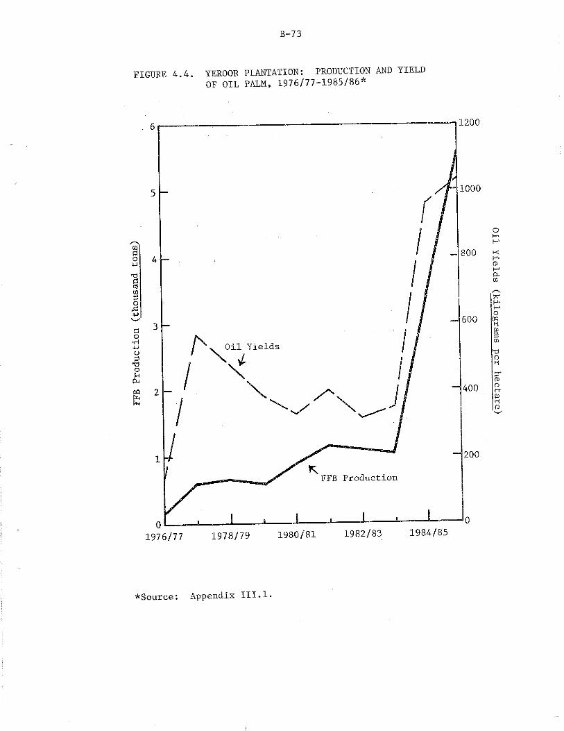
B-73
FIGURE 4.4. YEROOR PLANTATION: PRODUCTION AND YIELDOF OIL PALM, 1976/77-1985/86*
*Source: Appendix III.l.
Oil Yields (kilograms per hectare)
B-74
cannot be expected to yield amounts as high as a plantation where all the trees are ten years old. The comparison between actual and predicted yields at Yeroor is therefore not strictly valid because the actual phasing program was quite different than what was envisaged in the project report. Enough information is available, however, to back-calculate anticipated yields by age of the tree from the phasing schedule. In particular:
Total productionj = £ Area^ X Yield ^ ,i ^
where i = age of trees (5,6,...,11)j = production year (1,2,...,6)
Then,^ since total production, and area^ are known, the predicted age-wise yields y± can be sequentially estimated across production years by first calculating yield5 , using this information to calculateyield6 , and using the information on both yields to calculate yields and so on. ' ’
Actual yields are approximated by taking an average of all trees of the same age (across production years), weighted by the respective mature areas. Thus,
Yieldi - ( £ Area-n X Yield,,) / £ Area,J . *where i and j are as above.
The two sets of yields are also compared with yields experienced in Nigeria (where there is a strong dry season) and those found in Malaysia (where there is virtually no dry season). As indicated in the following table, actual yields in recent years have been less than half of what was anticipated in the project report; they are also less than half the yields obtained in Nigeria, and little over one tenth of the yields obtained in Malaysia (4, p. 238): 6
6. That is» since in the first year of production, the plantation
consists only of trees that are five years old, therefore,
Total Production.Yields = --- ------------- Izib Area. ^J=1
and from the second year of production:
Total production - (Area. _ . _ X Yield )Yield, = — -------------___________ 1=5,j=2 5'Area. , , „i=6,j=2
and so on.
B-75
Year NigeriaC p d.AU O.l 1Malavsia
from ..... --Yeroor-------- (Strong dry (No dryplanting Actual13 Predicted season) season)
(tons of FFB ner hectare) ■3 N.R. 0 0 12.804: N.R. 0 6.40 24.505 0.44 1.85 7.40 31.306 2.12 6.74 10.80 30.507" : 1.99 13.27 8.60 33,108; 2.69 10.15 10.30 33.109 3.31 10.15 10.30 33.1010 3.69 10.15 10.30 33.1011 4.61 10.15 10.30 33.10
a : Year of Planting = 0b: Estimates probably underreport true yields.N.R. - Not Reported.
In addition, there is a high degree of spatial and temporal variability in yields. An examination of fresh fruit bunch yield data by year of planting (Figure 4.5) indicates that the 1971 area has had the highest yields. This is the area that was planted to Malaysian seeds; areas planted to Nigerian seeds (1972 and 1973 areas) have lower yields, but have less variability.7 The better yield performance of the 1971 area is reflected in the higher average yields of the whole plantation initially. However, as the lower yielding. 1972 and 1973 areas began to constitute a larger proportion of total mature area, average yields fell, and- then recovered because of increased yields on all the plantings.8 ' Nevertheless, even the highest-yielding Malaysian stock are not performing well--yields' in India, are less than 40 percent of wlrat is commonly obtained in Malaysia.
Apart from droughts which occur once in a while, the region is also subject to a three to four month dry period every year. The
7 In 1985/86, the 1973 planting yielded an amount as high as the 1971 planting; however, it is not - clear whether this high yield will be sustained, or whether it represents a freak performance.
8 A FAO report cautions against making comparisons between the various planting stock. It indicates that although the original plantings come from different types of seeds, no records have been maitained on the origin of. .the seeds used for gap filling--replacing unsuccessful palms in the various areas. In addition, it may well be that the Malaysian stock exhibit vigorous yields soon after planting, and that the African stock take longer to achieve the same high yields. The point remains that what ever the reason, the 1971 area has had the highest yields among all the planting areas.
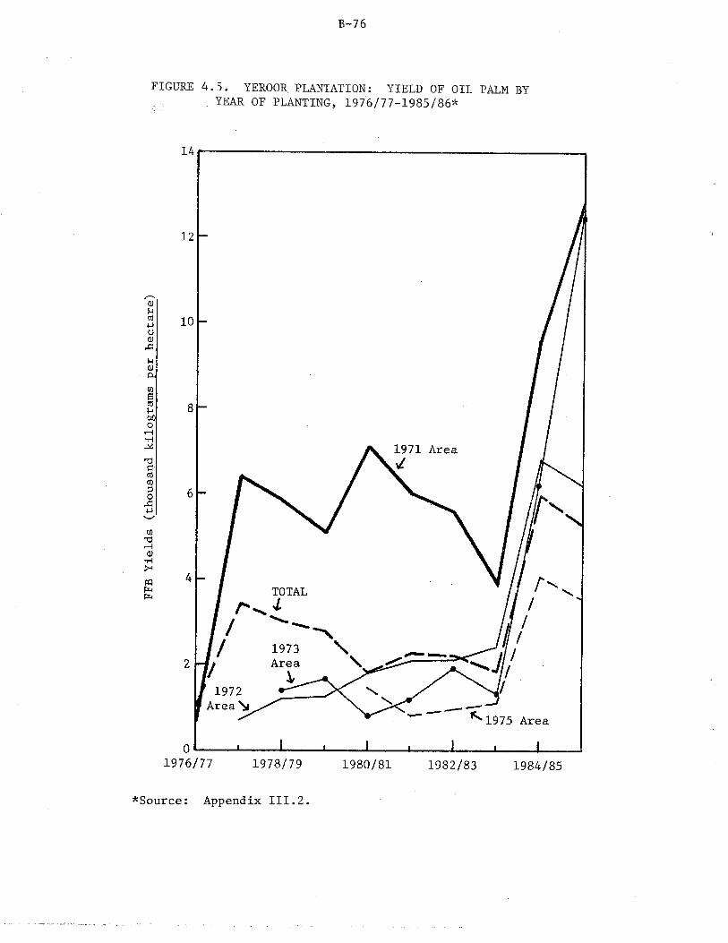
B-76
FIGURE 4.5. YEROOR PLANTATION: YIELD OF OIL PALM BYYEAR OF PLANTING, 1976/77-1985/86*
*Source: Appendix III.2.
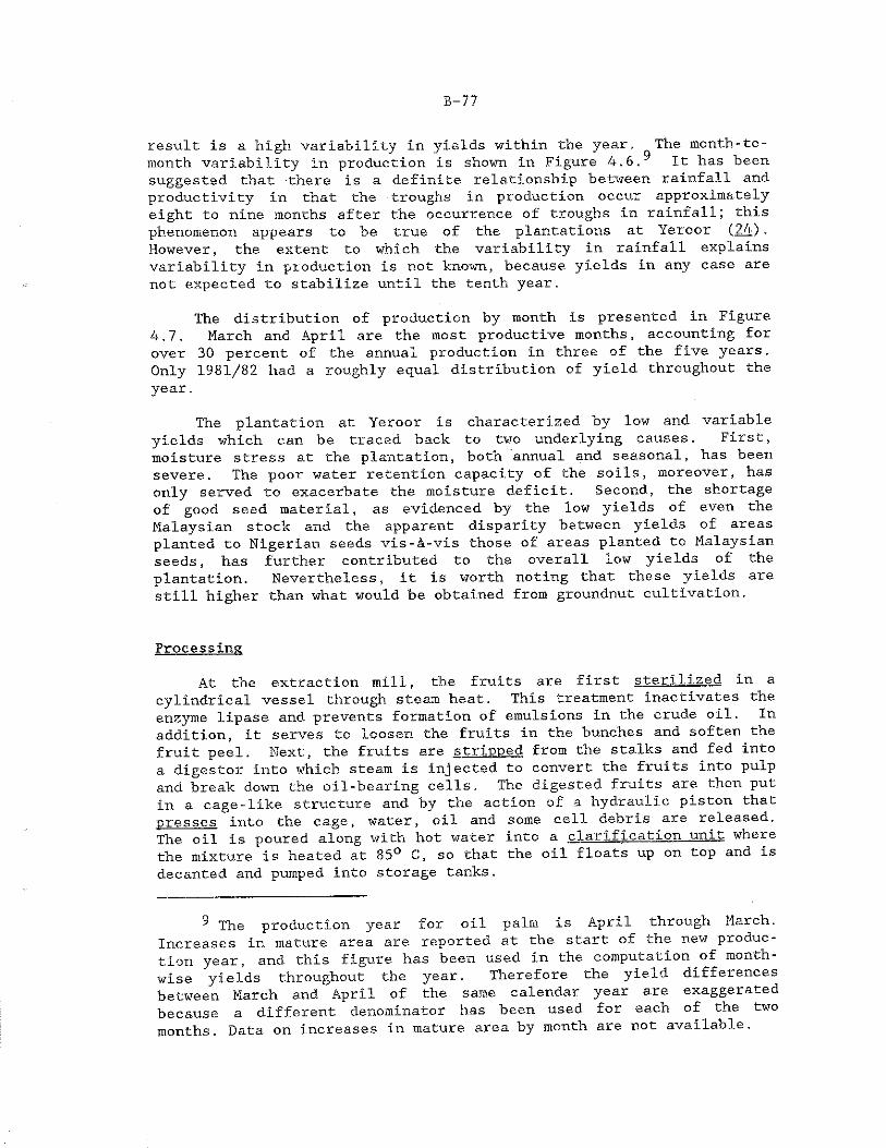
B-77
result is a high variability in yields within the year. The month-to- month variability in production is shown in Figure 4.6. It has been suggested that -there is a definite relationship between rainfall and productivity in that the troughs in production occur approximately eight to nine months after the occurrence of troughs in rainfall; this phenomenon appears to be true of the plantations at Yeroor (24) . However, the extent to which the variability in rainfall explains variability In production Is not known, because yields in any case are not expected to stabilize until the tenth year.
The distribution of production by month is presented In Figure 4.7. March and April are the most productive months, accounting for over 30 percent of the annual production in three of the five years. Only 1981/82 had a roughly equal distribution of yield throughout the year.
The plantation at Yeroor is characterized by low and variable yields which can be traced back to two underlying causes. First, moisture stress at the plantation, both annual and seasonal, has been severe. The poor water retention capacity of the soils, moreover, has only served to exacerbate the moisture deficit. Second, the shortage of good seed material, as evidenced by the low yields of even the Malaysian stock and the apparent disparity between yields of areas planted to Nigerian seeds vis-&-vis those of areas planted to Malaysian seeds, has further contributed to the overall low yields of the plantation. Nevertheless, it is worth noting that these yields are still higher than what would be obtained from groundnut cultivation.
ProcessingAt the extraction mill, the fruits are first sterilized in a
cylindrical vessel through steam heat. This treatment inactivates the enzyme lipase and prevents formation of emulsions in the crude oil. In addition, it serves to loosen the fruits in the bunches and soften the fruit peel. Next, the fruits are stripped from the stalks and fed into a digestor into which steam is injected to convert the fruits into pulp and break down the oil-bearing cells. The digested fruits are then put in a cage-like structure and by the action of a hydraulic piston that presses into the cage, water, oil and some cell debris are released. The oil is poured along with hot water into a clarification unit where the mixture is heated at 85° C, so that the oil floats up on top and is decanted and pumped into storage tanks. 9
9 The production year for oil palm is April through March. Increases in mature area are reported at the start of the new production year, and this figure has been used in the computation of month- wise yields throughout the year. Therefore the yield differences between March and April of the same calendar year are exaggerated because a different denominator has been used for each of the two months. Data on increases in mature area by month are not available.
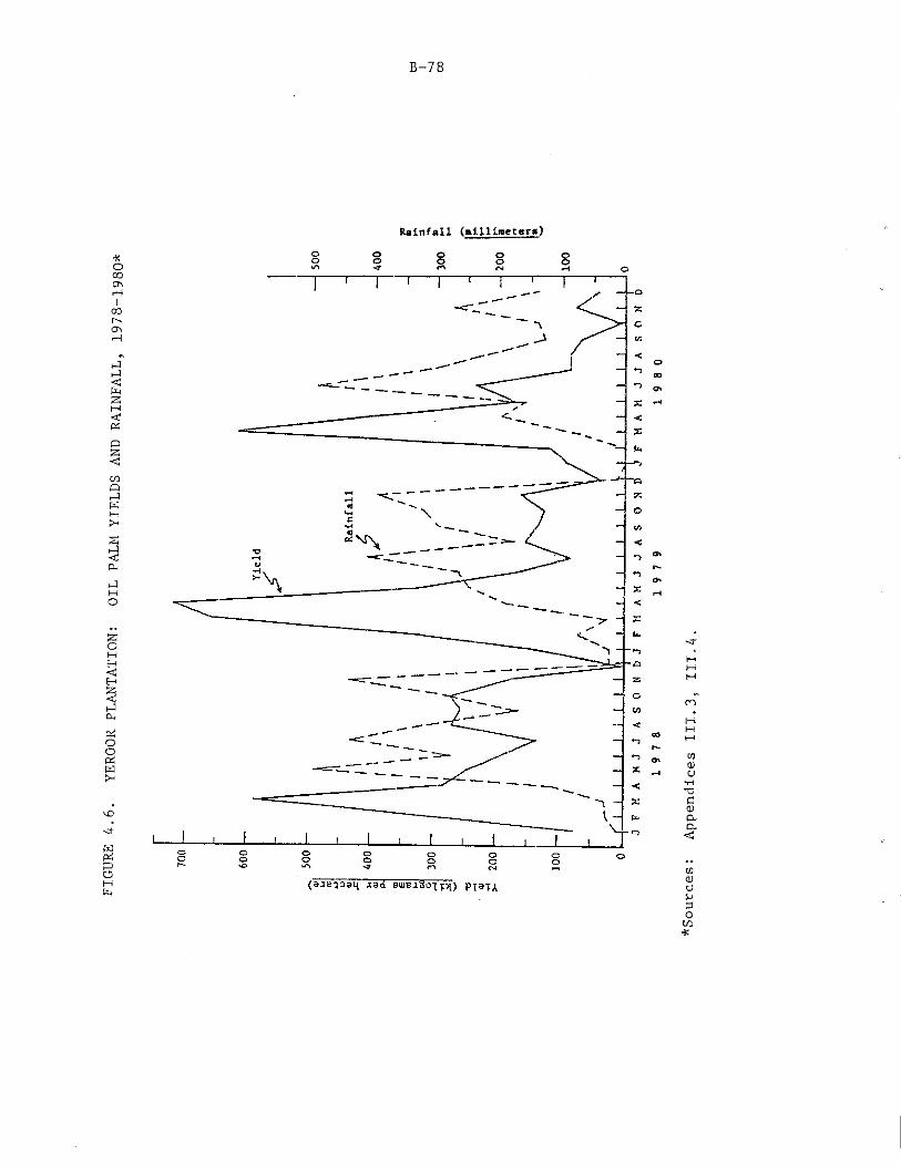
FIGU
RE 4
.6.
YERO
OR PLA
NTAT
ION:
OI
L PA
LM Y
IELD
S AN
D RA
INFA
LL,
1978
-198
0*
Rainfall (a l l l l i p e t e f * )
oo ©o g g g o
oco
h*
*Sou
rces
: Ap
pend
ices
III
.3,
III.
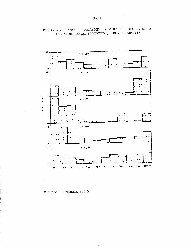
B-79
FIGURE 4.7. YEROOR PLANTATION; MONTHLY FFB PRODUCTION ASPERCENT OF ANNUAL PRODUCTION, 1981/82-1985/86*
^Source: Appendix III.5.
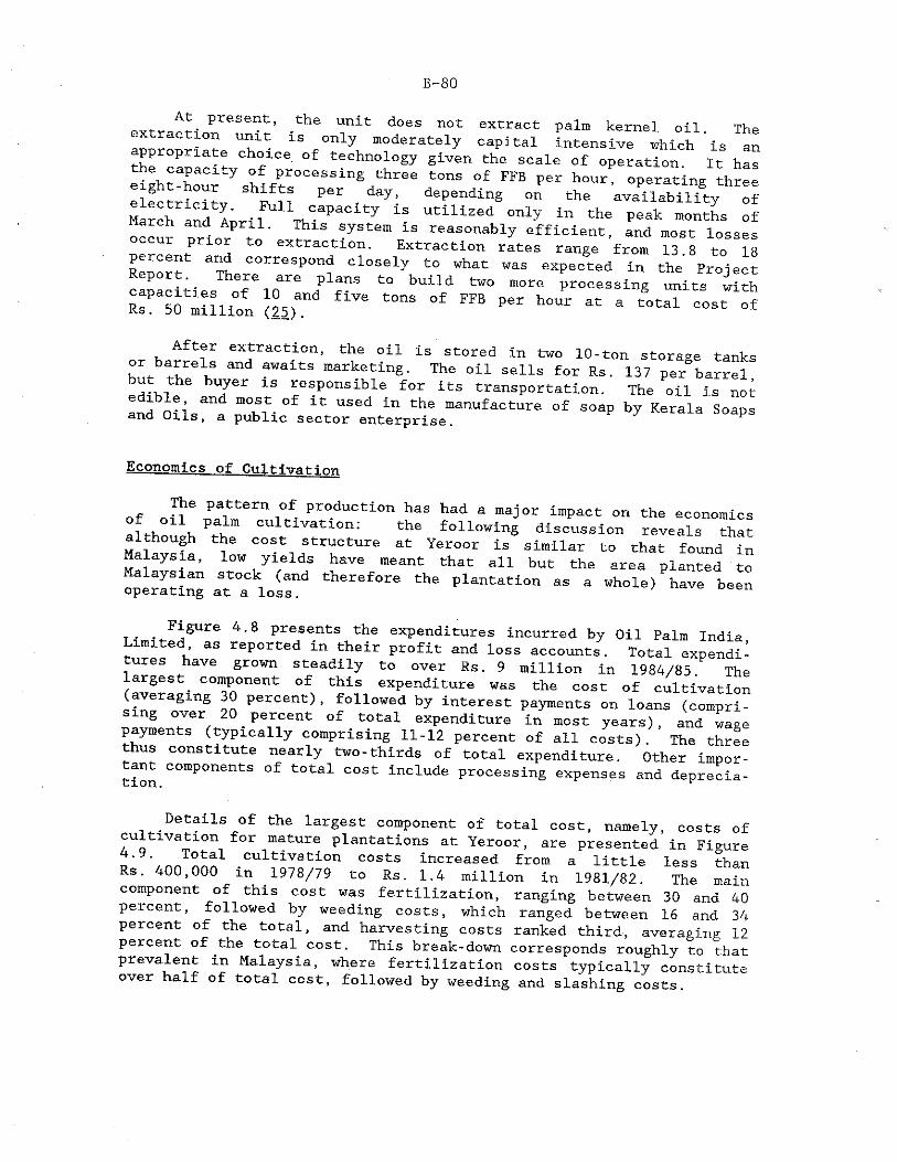
B-80
Present> .the unit does not extract palm kernel oil The extraction unit is only moderately capital intensive which is an appropriate choice of technology given the scale of operation. It haseiRht-hour''y sh!fr°0eSSinS/ hree ^ °f FFB Per h°Ur’ opiating three electricitv ^ P“ on the availability ofMarch and Lri! Tb°aPaC 7 “ Utlll2ed °«ly in the peak months of occur prior to evl e-7 m 7 S reasonably efficient, and most losses percent and corre actl°"- Extraction rates range from 13.8 to 18 Report P' f oiosely to what was expected in the Projectcapacities of in I 1?*® t0 bul1/ tW° more Pressing units withRs" 50 million (L) °f ^ ^ W at a total
„ , Aft®r extraction, the oil is stored in two 10-ton storage tanks or barrels and awaits marketing. The oil sells for Rs. 137 per barrelbahi hS tU,yer 1S resP°nslble for its transportation. The oil is notan^Oil’s " 7 ° ' 1C US6d ln the manufacture of soap by Kerala Soaps and Oils, a public sector enterprise. F
Economics of Cultivaf-lnn
of o n 6 p«aittern i°7 production has had a maj°n impact on the economics although the I ulttlvatl0n: the feliowing discussion reveals thatMnavsfi ^ cost structure at Yeroor is similar to that found inMalaysia, low yields have meant that all but the area planted tooperating a T a l o ^ ^ PUntati°n aS a whola> ba-
. Figure 4.8 presents the expenditures incurred by Oil Palm India Limited as reported in their profit and loss accounts. Total expenditures have grown steadily to over Rs. 9 million in 1984/85. The largest^ component of this expenditure was the cost of cultivation (averaging 30 percent), followed by interest payments on loans (comprising over 20 percent of total expenditure in most years), and wagepayments (typically comprising 11-12 percent of all costs). The three thus constitute nearly two-thirds of total expenditure. Other impor-an components of total cost include processing expenses and depreciation. c
Details of the largest component of total cost, namely, costs of cultivation for mature plantations at Yeroor, are presented in Figure .9. Total cultivation costs increased from a little less than
Rs. 400,000 in 1978/79 to Rs. 1.4 million in 1981/82. maincomponent of this cost was fertilization, ranging between 30 and 40 percent, followed by weeding costs, which ranged between 16 and 34 percent of the total, and harvesting costs ranked third, averaging 12 percent of the total cost. This break-down corresponds roughly to that prevalent in Malaysia, where fertilization costs typically constitute over half of total cost, followed by weeding and slashing costs.
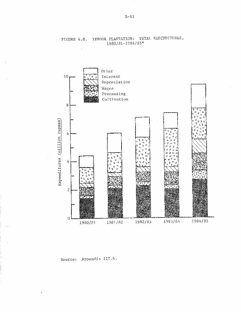
illion rupees
B-81
FIGURE 4*8. YEROOR PLANTATION: TOTAL EXPENDITURES1980/81-1984/85*
10
4:
Maf-t3■U•HSQJo.XM
OtherInterestDepreciationWagesProcessingCultivation
1980/81 1981/82 1982/83 1983/84 1984/85
Source: Appendix III. 6
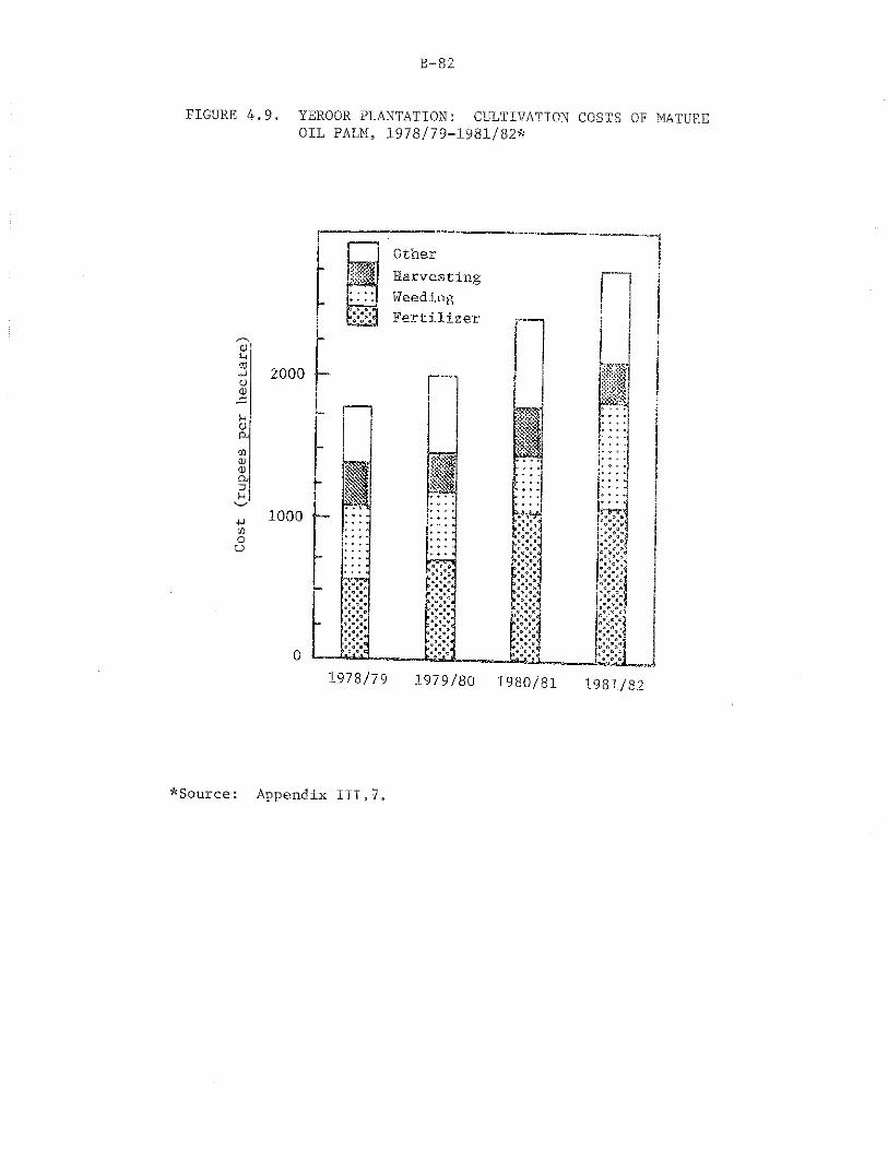
Cost (
rupees p
er h
ectare)
B"82
FIGURE .9. YEROOR PLANTATION: CULTIVATION COSTS OF MATUREOIL PALM* 1978/79-1981/82*
*Source Appendix III.7
B-83
It is also instructive to compare costs of cultivation by area of planting: (Figure 4.10). Mature plantations are typically more expensive to maintain than immature plantations, the difference amounting to nearly Rs. 1,000 per hectare. The 1971 area in both instances has in general higher per hectare costs than the other areas.
The primary source of revenue is the sale of palm oil. Total revenue generated from sales in 1985/86 was Rs. 5 million, well below the maintenance costs incurred for cultivation. Oil Palm India, Limited thus turned in losses for Its first eight years of operation; losses in 1984/85 amounted to Rs. 2.6 million. It is expected, however, that the company will break-even within the next two years.
The price of crude palm oil is fixed by Oil Palm India, Limited at around Rs. 8,000 per ton: the price of rice bran oil plus Rs. 600. u Rice bran oil is a close substitute for palm oil in use, except that rice bran oil requires hydrogenation, whereas palm oil does not, this is a factor taken into consideration in the determination of the Rs, 600 markup. This price is, nevertheless, less than what the government charges; imported palm oil is sold to wholesalers for Rs. 8,500 per ton. These prices are also less than the wholesale prices for coconut oil and groundnut oil.^
A comparison of costs and revenue per hectare for each of the areas reveals, as shown in Figure 4.11, that the 1971 planting, by virtue of its higher yields, consistently had the highest profits. 1 Profit margins for the other areas are low and even negative in some years. These profitability margins do not even take into account processing costs or capital expenditures.
If capital expenditures are Incorporated into the analysis through the computation of an internal rate of return, the plantation's financial viability becomes even more problematical. An IRR is only as sound a measure as the assumptions that underlie it. It is therefore reasonable to compute an IRR for a range of yield and price assumptions. A pessimistic projection would be that yields continue to be so low that at peak productivity, the plantation would yield only one ton
Data refer to 1982-1983.
H In 1981, the price of coconut oil in Kozhikode, Kerala was Rs. 13,775 per ton and that of groundnut oil in Rajkot, Gujarat was Rs. 10,398 per ton.
The amount of total revenue generated per hectare on each of the different plantings can be estimated by multiplying the FFB yields with a uniform extraction rate and sale price:
Total Revenue/ha area = FFB/ha area X extraction rate X price per ton
Costs refer to maintenance expenditures only.
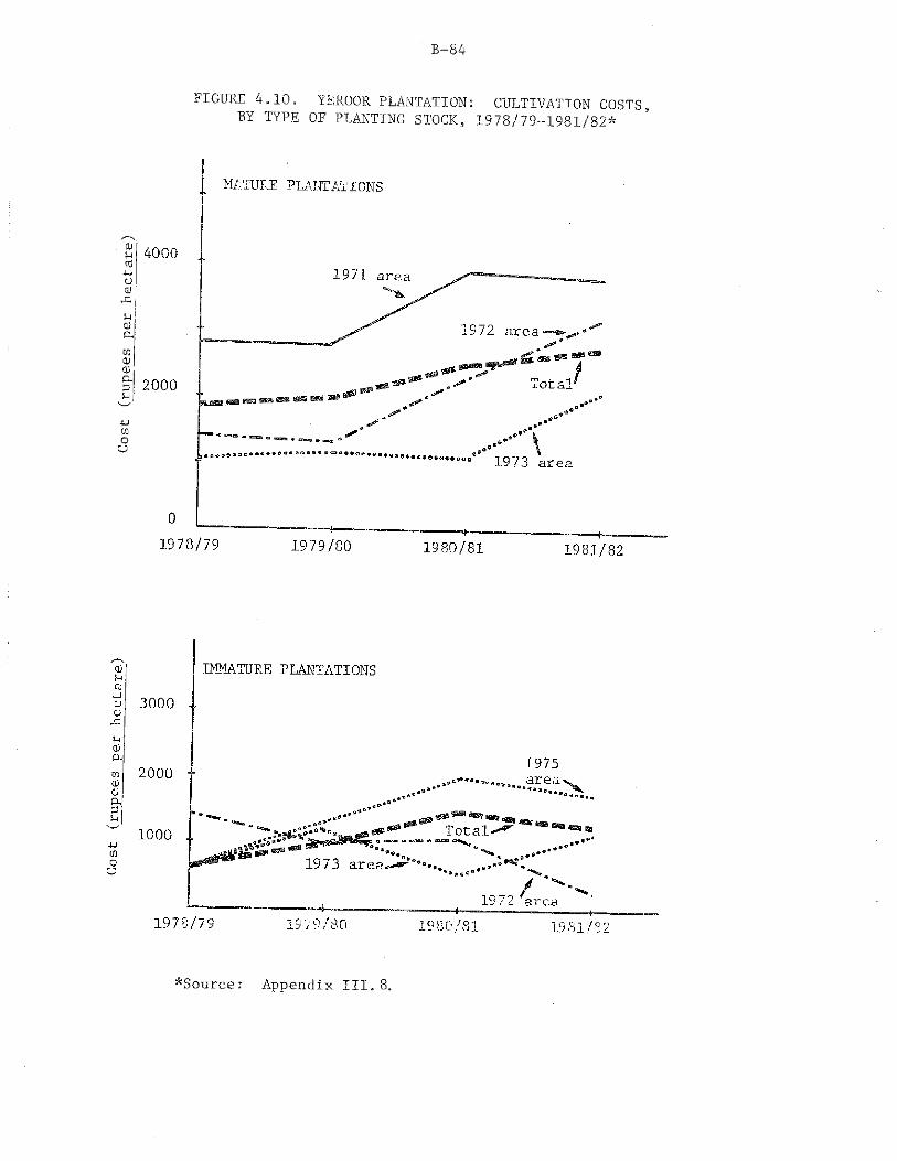
Cost (rup
ees
per hectare)
B-84
FIGURE 4,10. YEROOR PLANTATION: CULTIVATION COSTS,BY TYPE OF PLANTING STOCK, 1978/79-1981/82*
*S o u rc e : A ppend ix I I I . 8,
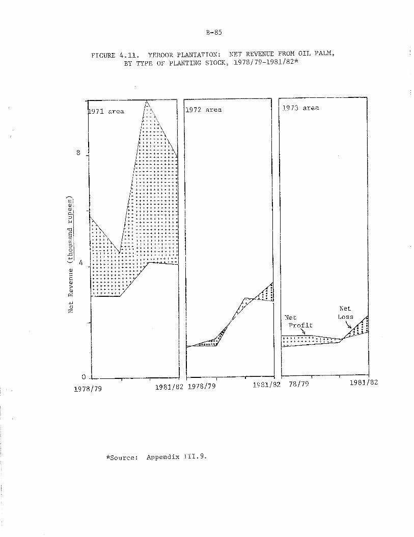
Net
Revenue
(thousand
rupees)
B-85
FIGURE 4.11. YEROOR PLANTATION: NET REVENUE FROM OIL PALM,BY TYPE OF PLANTING STOCK, 1978/79-1981/82*
*Sou .rce : A ppendix I I I . 9
B-86
of °l1 per hectare, and that the sale price of oil remains at Rs. 8 per Kilogram. A more optimistic view would be that yields on the plantation will improve through the provision of dry season irrigation and ultimately approach the yields obtained in the area planted to Malay- sian seeds of 2 tons of oil per hectare, and that prices rise to Rs 10 per kilogram (as they did in 1985 and 1986) (25).
In order to derive the cost-benefit stream, since actual data on costs and income are available for the first eleven years it is appropriate to use these figures, deflated by the consumer price index.or later years, it seems reasonable to assume that production costs
per mature hectare will be invariant at the eleventh year level, since harvesting costs typically comprise only 10-15 percent of total cultivation costs and the major costs of fertilization and weeding are unlikely to change with higher yields. Income may be calculated bysimply multiplying the yields and prices delineated above. The results are as follows : J-~>
Case
Current trends persistPrices are Rs. 8 per kilogram Oil yields are 1 ton per hectare
Prices IncreasePrices are Rs. 10 per kilogram Oil yields are 1 ton per hectare
Yields increasePrices are Rs. 8 per kilogram Oil yields are 2 tons per hectare
Prices and Yields increasePrices are Rs. 8.5 per kilogram
yields are 2 tons per hectare
IRR(percent1)
3
11
20
24If, once again, one takes the nominal interest rate of 12 percent ^he opportunity cost of obtaining capital, then the above results
dicate that persistent low yields will ultimately render the proiect unprofxt^ie. On the other hand, modest increases in yields* would result m significant increases in revenue to the extent that the project would be financially profitable. It is worth noting that the r e f r e s h assumPtl°n °f 1-5 tons per hectare is not unreasonable andin Malavsia <f ™ percent of the yields commonly experienced
om? Prl°! lncreases ara called for, but this increase islimited by the prices of competing oils.
13 Detailed calculations are in Appendix V.5.
B-87
Oil Palm in th e Andaman and N ico b a r Islands14
The Andaman and Nicobar Islands (Figure 4,12) are a series of Islands aligned North to South in the Bay of Bengal northwest of Malaysia. The Andaman Islands are very hilly and almost entirely covered with dense forests. The Nicobars are also covered with forests but contain some stretches of flat land. While fresh water is a constraint on the Andamans, this is not the case on the Nicobars. They have a combined area of 8,293 square kilometers and comprise a single administrative unit--a union territory, administered by a Chief Commissioner in the Ministry of Home Affairs. Settlers on the Islands come primarily from Bangladesh, Sri Lanka, Burma, and Kerala, Many tribal peoples are also found on the Nicobars (9.) .
The geographical proximity of the Islands to Malaysia and the nearly identical climatological conditions suggest that they would be an ideal setting for the cultivation of oil palm. Annual rainfall ranges between 2,750 millimeters and 3,250 millimeters and occurs nine months of the year. Temperatures, as the following table Indicates, range between 23° C and 33° C (9) :
Maximum ° CJanuary (coldest month) 30April (hottest month) 33
In 1972, the National Council of Applied Economic Research concluded that "while it is apparent that it would not be possible to resort to any large scale conversion of land for raising field crops ,.. the scope for adopting a plantation programme of commercially valuable crops should be fully examined, especially in the Nicobars" (9.) .
An experimental oil palm plantation was started in 19 75 by the Andaman Forest Department with a total of 150 hectares being planted during 1975 and 1976. The project was considered viable, and during 1979/80, the Andaman and Nicobar Island Forest Development Corporation was commissioned to undertake oil palm cultivation on Little Andaman Island on a commercial basis. The anticipated capital cost of the project was Rs. 91 million over a period of 15 years for cultivating a total of 2,400 hectares of oil palm. The Central Government's budgetary allocation in the Sixth Five Year Plan (1980-85) for this purpose was Rs. 30 million (10), As of 1984, 1300 hectares had been planted to oil palm, of which 340 hectares were yielding. 14
Minimum ° C2323
14 The discussion of oil palm cultivation on the Andaman and Nicobar Islands is necessarily limited because a visit to the islands was not possible. The data in this section are based on personal communication with the Divisional Manager of the plantations on the islands, Mr. Chakravarti (34).
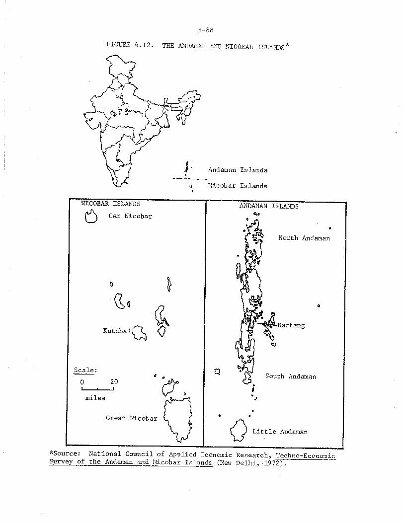
B-88
B-89
The FFB and oil yield figures for the islands compare unfavorably with yields obtained in Kerala: by the second year, FFB yields in Kerala were up .to 3,404 kilograms per hectare and 3,022 kilograms per hectare in the third year, as opposed to 1,713 and 1,177 kilograms per hectare on the islands. Extraction of oil on Little Andaman Island Is done by an "improved country method" and the extraction rates are much lower than those at Yeroor:
Year FFB/he c tare(mature) /kilograms')
Oil/hectare('kilograms')
Extraction rate (’percent')
1981/82a 944 94 101982/83a 1,713 156 91983/84b 1,177 124 11
a: Mature area approximately 160 hectaresb: Mature area approximately 340 hectares
These results are perhaps not quite so surprising in view of the fact that the Andaman and Nicobar Islands have suffered from less than normal rainfall in three of the last five years. It is also hard to draw firm conclusions because yields in the first few years of produc-tion are not considered to be indicative of the general pattern.
On the other hand, the costs of cultivation per hectare are, forthe most part, comparable with those in Kerala (34):
Year Total area Total cost Costs per hectare(hectares) (Rs. million) (RsO
1979/80 160 1.0 6,2501980/81 340 1.3 3,8241981/82 640 1.5 2,3441982/83 640 1.7 2,6561983/84 940 2.2 2,340
All of the nearly 80 tons of oil produced is sold, but no information is available as to who purchases the palm oil and at what price.
Prospects for Increased Palm Oil Production
Yield Increases
If the performance of the 560 mature hectares in Kerala is any indication of future trends, then clearly efforts to increase yield rates have to be an essential component of any viable expansion 15
15 Unfortunately, a detailed breakdown of these costs was not available.
B-90
program. The foregoing analysis points to two major avenues through which increases in yields may be brought about.
The first involves the use of better planting material. Portions of Yeroor estate planted to Nigerian stocks have tended to be neither hi-gh-yielding nor drought resistant as compared to the areas planted to Malaysian stocks. Therefore, assuming that the current Malaysian ban on the exports of seeds will continue, efforts should be channelized into vegetatively propogating the highest yielding palms on the plantation by means of tissue culture.16 In the long run, however, Oil Palm India,^ Limited must have access to high-yielding, drought-resistant varieties of oil palm. For example, although the average yield of palm oil in Malaysia is five tons of oil per hectare, yields as high as8,5 tons per hectare have been reported in some regions (33).
The second change involves providing dry season irrigation to the plantation so as to reduce annual moisture stress. Studies have shown that such measures can raise productivity significantly. For example, an experiment conducted at the Nigerian Institute for Oil Palm Research, where rainfall patterns are presumably similar to those obtained at Yeroor, found that dry season irrigation resulted in an average 25 percent increase in yields (29):
Year Irrigation in Percent No irrigation dry season increase
(kilograms per hectare1*1970 2021971 3781972 5651973 1771974 234
245 21.9523 38.4670 18,6215 21.5296 26.5
Average 311 390 25.3
However, in order to be effective, water in the dry season needs o be administered to the plantations consistently. Sporadic
applications of water have not succeeded in increasing yields. The plantation at Yeroor has the advantage that an irrigation canal serving the Kallada Irrigation Project runs right through the plantation and can easily serve the lower reaches of the estate. It may be necessary to employ lift irrigation techniques to serve palms at the higher reaches of the plantation. This can be an expensive operation, the costs and benefits of which need to be weighed before being undertaken. The relevant data for such an analysis were not available however, it is understood that a FAO/Banker's mission that visited n ia m 1978 at the request of the erstwhile Agricultural Finance
16, Although tissue culture methods have already been worked out inhe laboratory, field application procedures have not yet been established. J
B-91
Corporation evaluated dry season irrigation and deemed it a worthwhile investment.
In sum, the success with which increases in the yield rate can be brought about will determine the financial profitability of oil palm cultivation, which in turn will influence the rate of its expansion.
Area Limitations
Figure 4.2 broadly delineated regions that are climatologically suited to the cultivation of oil palm. It is understood that the FAO/Banker's Mission made a detailed assessment of the areas in India where oil palm could be grown under rainfed conditions and identified the five southern districts of Kerala, namely, Alleppey, Ernakulam, Kottayam, Quilon and Trivandrum, and the Andaman and Nicobar Islands as suitable, citing high dry-season moisture deficits as the key limiting factor in the selection of sites. Most other regions in India have a six to seven month dry period and while it is conceivable that these regions be brought under oil palm through irrigation systems, it is highly unlikely because providing water for such a long period continuously is extremely difficult and expensive.
In the Kerala districts, acreage under oil palm can be increased by either replacing competing crops such as coconut and paddy,, or by clearing forest lands. Evidence indicates, however, that this increase is not likely to occur.
Replacing coconut in Kerala: A case can be made that since the districts suitable for the cultivation of oil palm are also those most affected by the root wilt, the affected coconut palms can be replaced with oil palm trees (assuming that the oil palm tree is not affected by the disease). Such a substitution, however, would only be possible when the perceived economic returns from oil palm cultivation exceed those from coconut cultivation. Table 4.1 compares the costs and returns per hectare from the cultivation of these two crops for a "typical" year of peak production. Despite the fact that capital requirements for coconut differ significantly from those of oil palm (the former being a small holder crop and the latter being a plantation crop), capital costs are ignored in the comparison. Once again, three different scenarios are envisaged.
Under fair conditions, similar to present circumstances, coconuts enjoy a clear superiority over oil palm in terms of net revenue. Under good and ideal conditions, the margin is diminished although coconuts are still the favored crop. This bias, from the farmers' viewpoint, is strengthened by several considerations. First, there is no minimum land requirement for coconut. Second, the coconut tree has a longer life and a smaller capital requirement. Third, the coconut tree can be put to other uses (for example, the fruit can be consumed as food in times of food scarcity, the leaves can be used for thatching roofs and so on) and a value on these uses has not been taken into account in the

B-92
TABLE 4.1. COSTS AND RETURNS TO CULTIVATION FOR COCONUT AND OIL PALM
(Rs. per Hectare. 1982 prices'!
COCONUTS (WEST COAST TATJA_ Costs Revenue Net Return _________ OIL P A L M _________
Costs Revenue Net Return
Fair management:
l,340a 6,825b 5,485 6,404c 8,000d 1,596Good management:
3,268® 9,750f 6,482 6,404c 1,2750S 6,346Ideal management:
7,210h 21,000i 13,790 6,404c 17,000J 10,596
a: Only harvesting costs (from CPCRI)b: Assumes average yield of 4,559 nuts per hectare (state average for
1979/80-1980/81) and sale price of Rs. 1.5 per nut.c: Maintenance costs per hectare actually experienced.d: Assumes one ton of oil per hectare and sale price of Rs, 8/kilo-
gram.e: Assumes only fertilizer and harvesting costs (from CPCRI)f: With peak productivity of 6,500 nuts per hectare and sale price of
Rs. 1.5 per nut.g: Assumes 1.5 tons of oil per hectare and sale price of Rs. 8.5 per
kilogram.h: Includes irrigation, fertilizer, labor.i: Peak bearing ability of 80 nuts per palm and 175 palms per hectare
with sale price of Rs. 1.5 per nut.j: Assumes 2.0 tons of oil at peak productivity and a sale price of
Rs. 8.5/kilogram.
B-93
analysis. The oil palm does not enjoy these advantages, and therefore, it appears unlikely that coconut will be replaced by oil palm. Moreover, the difference in oil yields per hectare between oil palm and coconut actually being experienced is not significant enough to merit any intervention on the part of the government to encourage oil palm cultivation at the expense of coconuts. This conclusion differs markedly from that of the management of Oil Palm India, Limited, who are confident of oil palm's ability to replace coconut once the former's yields stabilize (25.) .Clearing forest lands: Kerala and the Andaman and Nicobar Islands areamong the few places in India where there are evergreen forests Attempts to expand acreage in these areas must take into account the environmental impact of such a measure. This analysis presumes that there will be no negative impact.
Among the five southern districts of Kerala suited to oil palm, only two, Quilon and Trivandrum, have any appreciable amounts of forestland (107):
Area under forests as a proportion of District total geographical area^Jpercentl—
Alleppey 0Ernakulam ^Kottayam ^QuilonTrivandrum 23
STATE 28
Of the nearly 236,000 hectares in Trivandrum and 50,000 he^ a^ in Quilon under forests, it is estimated that approximately 20 hectares are suited to the cultivation of oil palm. In the Andaman a Nicobar Islands, nearly 60,000 hectares are thought to be appropriate for oil palm. These plantations would be located on thei isl Little Andaman, Katchal, Great Nicobar and Bartang. It ls ^ot rhy much of the remaining 600,000 hectares under forests on the islandswcan not be put to oil palm.
Thus a total of 80,000 hectares can be brought under oil palm, an amount which is only 13 percent more than the annual a ^ i t i o B ^ ^ ^ ^palm area expected in Malaysia over the next l een ? ,... whichthese forests are protected by the Forest Conservancy Act ^ 8 0 which reauires prior approval of the Central Government before virgin forests :: T L t d o w n . V Act is said to have created nfor example, because of it, land. % seekingsin Kerala were not released m t i m e and n ^ this experience imported from Nigeria got overgrown (ii, 42). A“ h°“S“. manaEement ofpoints to the need for better planning on the Part of the -nagemen Oil Palm India, Limited,the point remains that this law is se s limit the expansion of oil palm area.
B-94
Supply Projections
India01MmitrdPr° T r 4 iOnH^- 1S 3 m°nOp0ly enterprise of Oil Palm„r7 ^ ’ Llmlted- The traditional price-dependent, supply-response modelIppropriatTein £ * “ U 3 priCe i- therefore notsetter this _ case because the monopolist is in fact a pricesetter. The monopolist m theory determines quantity by equating mar-L T o r ricrnUeT t0 marS-inal C°St’ 3nd then USeS the demand function &to t price. In practice, the upper limit on quantity is set bv the“ ““by °4atanofathllablle f°r 011 Palm Cultivation- and that on price isby that of the closest competing oil. Moreover, unlike the puremonopolist, profit maximization is not the sole objective of a govern-ment owned monopoly. 6 1
It is not possible to adequately consider all of the above factorstionsSof°thPaUClt^ °f / ata; therefore, as with coconuts, the projec-and Vield SUPP -y pal” 011 have t0 be based on alternative areafoUoyws FirsrP?f°^- v The threS assumPtl°ns are derived asm ' F r.st- ,lf tbe F°rest Conservancy Legislation acts as a blockpLntL wouTd10reln- aalm the" °nly the 3’700 hectares alreadyaref currentlv an„c Alta™ a“ vely, if all of thev» v ly aIl0l?ated for oil palm cultivation is planted then12 4°0 hectares (10,000 in Kerala, and 2,400 in the Andaman and Nicobar Islands) wouid result. Finally, if all the regions climaticaUy suitedunder thies croi Vatl°n "* eXpl°lted> then 80'000 Stares would be
As for yields, a low projection would be to assume that ther ^ H f t h e o™ 5 ^ ^ WlU " ° t lmpr°Ve and th a t 011remain at the one ton per hectare actually obtained at Yeroor (251 If however, there is dry season irrigation, and no severe annual Sough”1 5 tontrLenC\ W_hlle the plantation is young, then medium yields of ‘ * per hectare would be achieved. Furthermore, if there is a
tons " T f bette" material, then oil yieids as higl as 2tons per hectare would be possible. These area and yield assumptions suggest that production in 2000 and 2010 would be: P
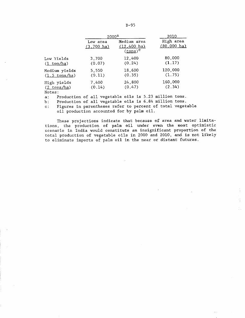
B-95
2000a _________ ___ 2010Low area Medium area High areaC3.700 ha) C12.400 ha)
C tons)cC 80.000 ha)
Low Yields 3,700 12,400 80,000Cl ton/ha) (0.07) (0.24) (1.17)Medium yields 5,550 18,600 120,000Cl.5 tons/ha) (0.11) (0.35) (1.75)High yields 7,400 24,800 160,000C2 tons/ha) Notes:
(0.14) (0.47) (2.34)
a: Production of all vegetable oils is 5.23 million tons.b: Production of all vegetable oils is 6.84 million tons.c : Figures in parentheses refer to percent of total vegetable
oil production accounted for by palm oil.
These projections indicate that because of area and water limita- tions , the produetion of palm oil under even the most optimistic scenario in India would constitute an insignificant proportion of the total production of vegetable oils in 2000 and 2010, and is not likely to eliminate imports of palm oil in the near or distant futures.

CHAPTER VIMPORTS VERSUS DOMESTIC PRODUCTION:
SOME' POLICY IMPLICATIONS
The Indian grain revolution has generally resulted in lower proportions of the gross cropped area being devoted to the oilseeds as compared to the foodgrains. In areas where the grain revolution has not been successful, this result does not hold, but, nevertheless, the oilseeds compete with the foodgrains for land. Therefore, because India is a land-scarce country, any attempts to increase production of annual oilseeds through area expansion would occur at the expense of foodgrains, thereby adversely affecting food self-sufficiency. For this reason, the tree sources of vegetable oil, coconuts and oil palm, were examined. It was found that while oil palm does not compete with any of the cereals, coconut does compete with paddy.
The major constraints to coconut production were Identified as the root-wilt disease, aging palm population, and the lack of proper maintenance. However, coconut cultivation is quite profitable in Kerala, and, as indicated by the analysis of mixed coconut and rice farming, given a choice, the farmer is likely to plant more area to coconuts as compared to rice, barring further spread in the root-wilt. With modest increases in yields, the production of coconuts and coconut oil in Kerala alone could rise several fold. However, since the base of production is small relative to the entire vegetable oil economy, this relatively optimistic scenario for coconut oil would leave unaltered the projections of "all other oils" made In Chapter 2.
The primary constraint to oil palm cultivation in India is the lack of suitable areas where it can be grown under rainfed conditions. Only a total of 80,000 hectares located in Kerala and the Andaman and Nicobar Islands have been identified as suitable. In addition, in areas where oil palm Is grown, dry season moisture deficits and the lack of quality planting materials have suppressed yields and consequently Inhibited production. Even if all the lands suited to the cultivation of oil palm were planted and yields improved, palm oil would not contribute more than two percent to the total expected production of vegetable oil in 2000 or 2010.
Thus the two tree crops would under optimal circumstances contribute only 13 percent to total vegetable oil production in the future. Proj ections made in this study indicate that total supply is likely to be 5.2 million tons In 2000 and nearly seven million tons in 2010 (Table 5.1). When compared with demand projections, it is evident that If past trends continue, domestic vegetable oil supply will not ^be sufficient to meet the demand, and the deficit will be 2.8-4.5 million tons In 2000 and 3.4-6.6 million tons In 2010.
B-97
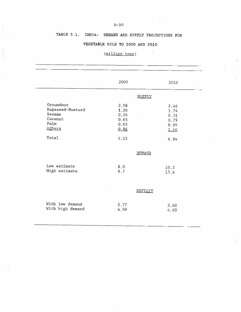
B-98
TABLE 5.1. INDIA: DEMAND AND SUPPLY PROJECTIONS FOR
VEGETABLE OILS TO 2000 AND 2010
(million tons')
2000 2010
SUPPLY
Groundnut 2.06 2.46Rapeseed-Mustard 1.26 1.74Sesame 0.26 0.31Coconut 0.65 0.79Palm 0.03 0.09Others 0.86 1.46Total 5.23 6.84
DEMAND
Low estimate 8.0 10.2High estimate 9,7 13.4
DEFICIT
With low demand With high demand
2.774.50
3.406.60
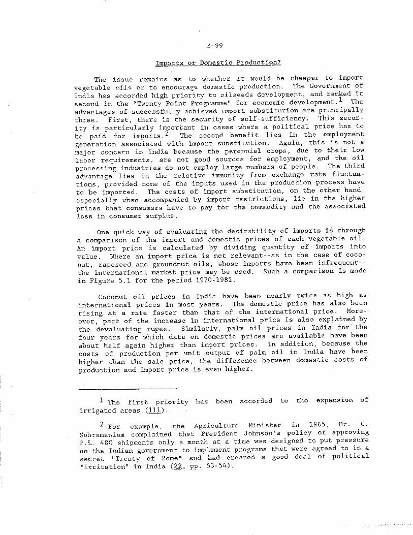
B-99
Imports or Domestic Production?
The issue remains as to whether it would, be cheaper to import vegetable oils or to encourage domestic production. The Government of India has accorded high priority to oilseeds development, and ranked it second in the ‘'Twenty Point Programme" for economic development. The advantages of successfully achieved import substitution are principally three. First, there is the security of self-sufficiency. This security is particularly important in cases where a political price has to be paid for imports. The second benefit lies in the employment generation associated with import substitution. Again, this is not a major concern in India because the perennial crops, due to their low labor requirements, are not good sources for employment, and the oil processing industries do not employ large numbers of people. The third advantage lies in the relative immunity from exchange rate fluctuations , provided none of the inputs used in the production process have to be imported. The costs of import substitution, on the other hand, especially when accompanied by import restrictions, lie in the higher prices that consumers have to pay for the commodity and the associated loss in consumer surplus.
One quick way of evaluating the desirability of imports is through a comparison of the import and domestic prices of each vegetable oil. An import price is calculated by dividing quantity of ' imports into value. Where an import price is not relevant--as in the case of coconut, rapeseed and groundnut oils, whose imports have been infrequent-- the international market price may be used. Such a comparison is made in Figure 5.1 for the period 1970-1982.
Coconut oil prices in India have been nearly twice as high as international prices in most years. The domestic price has also been rising at a rate faster than that of the international price. Moreover, part of the increase in international price is also explained by the devaluating rupee. Similarly, palm oil prices in India for the four years for which data, on domestic prices are available have been about half again higher than import prices. In addition, because the costs of production per unit output of palm oil in India have been higher than the sale price, the difference between domestic costs of production and import price is even higher. * 2
The first priority has been accorded to the expansion of irrigated areas (111).
2 For example, the Agriculture Minister in 1965, Mr. C . Subramaniam complained that President Johnson's policy of approving P.L. 480 shipments only a month at a time was designed to put pressure on the Indian government to Implement programs that were agreed to in a secret “Treaty of Rome" and had created a good deal of political “irritation" in India (22., pp. 53-54).
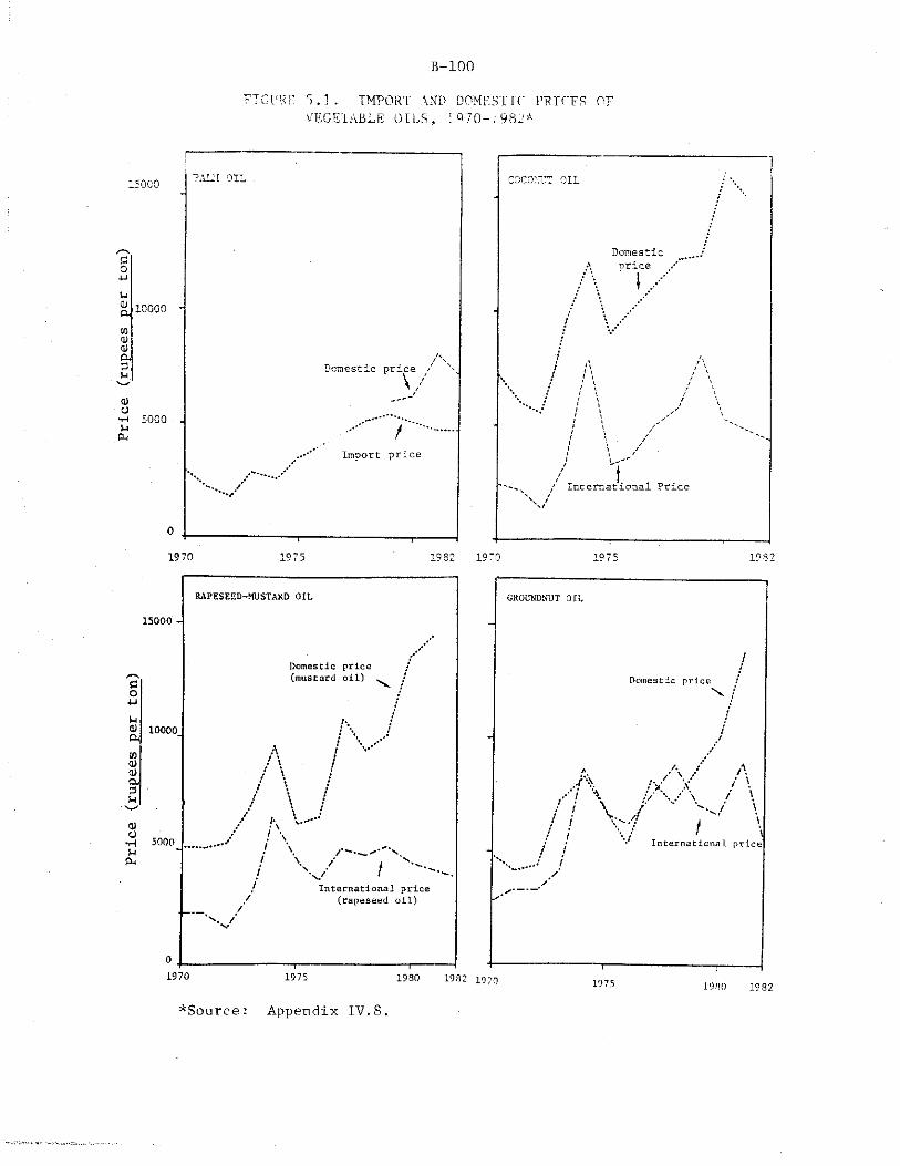
B-100
ETGDTE r>,]. IMPORT ANT DOMESTIC PETCES Of VEGETABLE OILS, ^ 70-1982*
—‘
.5000 PAD I Oil . cocoixt OIL /\
Domesticc0 *\ orice/ \ |
uCUO h 10000 - ■CO : v'0) tCDCU /\0 u
'— ✓Domestic price / \
\ / 1t / \
■, / / / \ \ 1 \ / \
CD / i \ :U ! \ v■H 5000 -/ ... J k / S
PM f 1 \ yImport price J \ f/
* \
f" / International Price
V /x/
0 -------------------------------------1-------1 -1970 1975 1982 19'0 1975 1982
RAPESEED-MUSTAW> O IL
15000 -
U<U&CO<1><Dex3
10000
<D•H 5000 M fX
D o m e s t ic p r i c e (m u s ta r d o i l )
*• ;/ A /: \ / \
/ \! \/ \
\ / /I n t e r n a t i o n a l p r i c e
( r a p e s e e d o i l )
V /
GROUNDNOT OIL
.r\y ' i \
// V./! i \ /
Domest ic price /V /
A / A
;■/ V / \/ / \y \ / \
/ !!//'
International price
1970 1975 1930 1932 1970 1975 1930 1982
^Source Appendix IV,8
B-101
As for the annual crops, the domestic price of mustard oil has been over one and a half times that of the international price of its close substitute, rapeseed oil. Furthermore, the domestic price of mustard oil has grown at a rate faster than that of the international price; in fact, international prices have fallen since 1978 in rupee (and therefore also in dollar) terms, while domestic prices have continued to rise. Groundnut oil prices in India have also been above international prices except in years when India has imported groundnut oil.3
Thus, in every instance, the unit cost of importing oils has been less than the domestic wholesale price, both before and after import liberalization in the late 1970s, and, therefore, one can conclude that ceteris paribus. augmenting domestic supplies with imports would be more economical. Availability of storage facilities at ports and transportation to major demand locations are also not likely to pose problems.
This conclusion would obviously be altered if the price advantage imports currently enj oy were to change. This can happen in several ways. First, If there is a technological breakthrough, the resultant increase in supply could lower the domestic price of the relevant oil. Second, if the rupee were to depreciate with respect to exporting country currencies, then import prices in rupee terms would increase. Third, the world supply and demand of vegetable oils could change such that international prices would go up. This could happen if demand were to increase at a rate faster than that of supply, if supply for some reason (such as disease) fell, or if trade restrictions were imposed.
An examination of the trends in international prices of the two oils that dominate world trade, palm oil and soybean oil (Figure 5.2), indicates that because of increasing supplies, real prices for both oils have generally declined since the mid-1970s (except during 1984 when all oil prices increased). This downward trend has been much more evident in the recent past, as is suggested by the price levels during the first 11 months of 1985. The decreases have occured in the case of soybean oil primarily because of increased EEC demand for meal which has resulted in greater crushings, and in the case of palm oil as a result of higher area and better rainfall in Malaysia. Current indications are that although this precipitous decline will not continue, prices are unlikely to rise In real terms because export availabilites are expected to be higher in the future (50).
World production and exports of vegetable oils have been rising over the past decade (Figure 5.3). Production has increased by nearly one and a half times, while exports have increased two-fold as a result of Malaysian palm oil, soybean oil from Brazil and the United States,
3 Since data on domestic prices of soybean oil are not available, a similar comparison for soybean oil could not be made,.
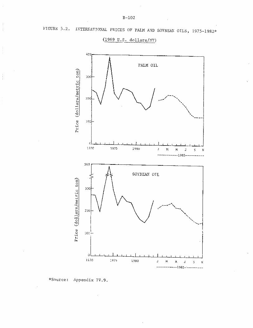
B-102
FIGURE 5.2. INTERNATIONAL PRICES OF PALM AND SOYBEAN OILS, 1975-1982*
(1969 U.S. dollars/MT)
cou■Huu0)aCOCO
OT3CL)O■HMPm
1985
1985— --------
^Source: Appendix IV.9.
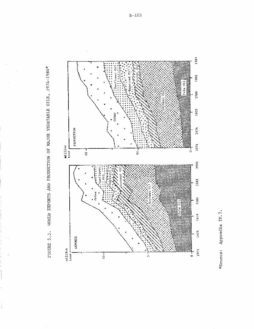
FIGU
RE 5
.3,
WORL
D EX
PORT
S AN
D PR
ODUC
TION
OF
MAJO
R VE
GETA
BLE
OILS
, 19
74-1
984*
B-103
*Source:
Appe
ndix
IV
B-1.04
and to a lesser extent, rapeseed and sunflower oils. There is no reason^ to expect that future export availabilities will fall. Mediumterm projections made by the Food and Agriculture Organization indicate that the volume of international trade in vegetable oils will continue to increase (although at a slower rate than in the 1970s), led primarily by palm oil, the production of which is expected to grow at seven percent per annum. This increase in palm oil is anticipated because recent developments in cloning, tissue culture and success with weevil pollination are resulting in higher yields (44). Area under oil palm m Malaysia alone is projected to increase by 60,000 hectares per year, reaching two million hectares by the year 2000. Furthermore, there has already been a rapid expansion in new plantings of oil palm in that country which will reach peak productivity in the next five to twenty years. even if not a single additional tree were to be planted, production of palm oil will continue to increase for several years. Therefore, according to the F.A.0., "the issue which is likely to become the most important in the development of the Malaysian oil palm sector is that of finding markets for the increased quantities that will become available for export" (46, p.3). The output of other oils is projected by the F.A.O. to grow at a more modest rate: soybean oilat 2.1 percent per annum; and cotton, groundnut, rapeseed and sunflower oils at between 2.5 and 4.0 percent per annum. Analysts at the U.S.D.A. concur with these projections. Increasing availabilities, combined with a slow-down in the demand for vegetable oils world-wide, are resulting in downward pressure on prices, thereby making vegetable oil imports even more attractive (45; 50).
Moreover, closing the demand-supply deficit of approximately three tons through imports would not be likely to result in signifi
cantly pushing up the world prices of vegetable oils. This is because Indian imports currently account for only ten percent of the total trade in vegetable oils; and a deficit of three million tons in the next 15 years would account for no more than 20 percent of current world trade. In addition, import values of edible oils constitute only about five percent of the total value of imports into India (121). If there are no real increases in the prices of vegetable oils, then a doubling of imports would result in an increase in the share of edible oils In the total value of current imports to no more than ten percent.
Policy Implications
At present, India does not enjoy a comparative advantage in oilseeds. Importing vegetable oil would be economical, but requires the expenditure of scarce foreign exchange. However, India will be operating in a buyers' market and can minimize foreign exchange expenditure by entering into long-term bilateral barter agreements. It can make use of the fact that most future increases in trade are likely to come from developing countries (41), and export commodities in which it does enjoy a comparative advantage, in exchange for vegetable oils. For
B-105
both countries, the gains from such trade are likely to be higher than those from trade on a commercial basis, particularly if lower transportation costs (because of geographical proximity) are involved^ or if protection from wide swings in exchange rates is sought. Malaysia is a country with whom trade on a barter basis could be particularly of mutual benefit. Over sixty percent of Malaysia's imports consists of manufactured commodities and investment goods such as machinery, items that India currently exports (40). India's Seventh Plan for economic development recognizes the need for industrial exports, and identifies engineering goods as one of the major sources of increased export earnings (11). Given India's large pool of skilled labor, there should be no problem in meeting Malaysia's specific requirements in exchange for palm oil. India can also offer its traditional export items such as coffee, tea and textiles in barter. Already, the Government of India has reached an agreement with the Government of the Philippines to import oil in exchange for textiles and iron ore (84)• Indonesia is yet another nation which may be amenable to long-term barter exchange arrangements.
As for countries with whom barter agreements are not feasible (because the benefit from barter does not accrue to the other nation), India can at least hedge against sudden changes in exchange rates by engaging in long-term contracts with trading agencies of exporting countries. Furthermore, India can augment foreign exchange earnings y actively encouraging the export of oilcake and meal (the domestic prices of which are lower than international prices) until such time as their use within India becomes popular.
These recommendations are not intended to undermine the importance of improvements In oilseed production. There is a need or etter coordination of research information. Regular contact and exchange of knowledge with international centers may well assist in t e eve °P™e^ of better yielding oilseeds. Within the country, oi^see s s ou e fully integrated into crop research and extension programs of the 4gri- cultural Universities and the State Agricultural Departments The requisite institutions are in place; what is necessary is o mo and utilize them efficiently.
But while research to achieve technological breakthroughs in thetraditional oilseeds and endeavors to identify and tap nontradltlonal oilseeds should continue, greater imports of vegetable oris table and not necessarily undesirable.

BOOKS
BIBLIOGRAPHY1
*1. Dasgupta, Biplab, Agrarian Change and the New Technology in_Jnidia (United Nations Research Institute for Social Development, Switzerland, 1977).
*2. George, P.S., Uma K. Srivastava and B.M. Desai, The OilseedsEconomy of India: An Analysis of Past Supply.and Projections for1985 (Indian Institute of Management, The Macmillan Company of India, Limited, Madras, India, 1978).
*3. Gittinger, J. Price, Economic Analysis of Agricultural Projects (Second Edition, The Johns Hopkins University Press, Baltimore, 1982) .
*4. Hartley, C.W.S., The Oil Palm (Elaeis guineensig_tIacaJ_l (Second Edition, Longman Group, Limited, New York, 1977).
*5. India, Directorate of Coconut Development, All India Market Survey of Coconut and Coconut Products: Utilization of Coconuts in India(Ernakulam, Kerala, 1977),
6 . India, Ministry of Agriculture and Irrigation,1 2 Directorate ofMarketing and Inspection, Agricultural Marketing in India;__Reporton the Marketing of Groundnuts in India (Second Edition, Delhi, 1953) .
*7. India, Ministry of Agriculture and Irrigation, Report of theNational Commission on Agriculture, Part III: Demand and Supply(Delhi, 1976),
8 . India, Ministry of Commerce, Civil Supplies and Cooperation,Report of the Study Group on a Long-Term Edible Oils Plan (New Delhi, 1978).
*9. India, National Council of Applied Economic Research, Techno- Economic Survey of the Andaman and Nicobar Islands (New Delhi,1972).
1Items marked with an asterisk are cited in the text and appendices.
2The Agriculture Ministry has over the years gone through several changes in name due to re-definitions of the organization's responsibilities. For the sake of simplicity, in this study, it is consistently referred to as the "Ministry of Agriculture and Irrigation."
B-107
B-108
*10.
*11.
*12.
*13.
*14.
15.
*16.
17.
18.
19.
*2 0 .
*21.
* 22.
*23.
India, Planning Commission, Sixth Five Year Plan 1980-85. Mid- Term Appraisal (Delhi, 1983).
India, Planning Commission, Seventh Five Year Plan 1985-90 (Delhi 1985).
Kahlon, A.S. and D.S. Tyagi, Agricultural Price Policy in India (Allied Publishers, Private Limited, New Delhi, 1983).
Kapila, bma, The Oilseeds Economy of Indiat A Case Study of Groundnut (Institute of Economic Growth, Agricole Publishing Academy, New Delhi, 1982).
Khera, Harcharan Singh, The Oil Palm Industry of Malaysia -- An Economic Study (Penerbit Universiti Malaya, Kuala Lumpur, 1976).
Narag, A.S., Marketing Strategy for Vegetable Oils in India (K.P. Bagchi and Company, New Delhi, 1981).
Pavaskar, Madhoo, Demand for Oils and Oilseeds (Tata Economic Consultancy Services, Popular Prakashan, Bombay, 1979).
Filial, P.P., Agricultural Development in Kerala (Agricole Publishing Academy, New Delhi, 1982).
Pushparaj, E. and Chew Pon Soon, The Oil Palm in Agriculture inthe Eighties.,;___ Report of the Proceedings of the InternationalConference on Oil Palm in Agriculture held in Kuala Lumpur from 17-20 July 1981 (The Incorporated Society of Planters, Malaysia 1982).
Ranade, C.G., K.H. Rao and D.G. Sah, Groundnut Marketing: A StudyofL Cooperative and Private Trade Channels (Indian Institute of Management, Ahmedabad, Gujarat, 1982).
Rao, C.H. Hanumantha, Technological Change and the Distribution of Gains in.Indian Agriculture (The Macmillan Company of India, Limited, Delhi, 1975).
Sarma, J.S., Agricultural Policy in India: Growth with Equity(International Development Research Centre, Ottawa, 1982).
Subramaniam, C,, The New Strategy in Indian Agriculture: TheFirst Decade and After (Vikas Publishing House, 1979).
Thamapan, P.K., Handbook on Coconut Palm (Oxford and IBH Publishing Company, New Delhi, 1982).
Turner, P.D., and R.A. Gillbanks, Oil Palm Cultivation and Management (The Incorporated Society of Planters, Kuala Lumpur, Malaysia, 1974).
*2 4 .
B-109
ARTICLES AND PAPERS
*25. Abraham, V..K. , Managing Director, Oil Palm India, Limited, Kotta- yam, Kerala, Personal Communication, October 10, 1985.
*26. Achutan-Nair, M. and C. Sreedharan, "Nutritional Studies on OilPalm in India" in E. Pushparaj and Chew Pon Soon, editors, The Oil Palm in Agriculture in the Eighties. Volume II (The Incorporated Society of Planters, Kuala Lumpur, 1982), pp. 201-210.
*27. Agricultural Situation in India. "Ordinance for Controlling the Diversion of Forest Land for Non-Forestry Use," December 1980,p . 686.
28. Askari, Hossien and John Cummings, "Estimating Agricultural Supply Response with the Nerlove Model: A Survey," InternationalEconomic Review. Volume 18, Number 2, June 1977, pp. 257-290.
*29. Aya, F.O. and B.M. Ojuederie, "The Effect of Supplementary Irrigation and Fertilizer Mixture on the Growth and Bunch Yields of Oil Palm" in D .A. Earp and W. Newall, editors, International Developments in Oil Palm: The Proceedings of the Malaysian InternationalAgricultural Oil Palm Conference held in Kuala Lumnur 14-17 June,. 1976 (The Incorporated Society of Planters, Malaysia, 1977).
*30. Bansil, P.C., "India's Crisis in Vegetable Oils: A Strategy forthe Eighties," Supplement to the Monthly Commentary on Indian Economic Conditions. Indian Institute of Public Opinion, Volume XXIV, Number 8.
*31. Bateman, Merrill, "Supply Relationships for Perennial Crops in the Less-Developed Areas," in Clifton Wharton, Jr., editor,Subsistence Agriculture and Economic Development (Aldine Publishing Company, Chicago, 1969).
*32. Bavappa, K.V.A., "Root (Wilt) Disease of Coconut -- Where andWhither," Indian Coconut Journal. Volume XIII, Number 9, January 1983, pp. 9-11.
*33. Bavappa, K.V.A., "Oil Palm -- Prospectus, Problems and Possibilities" (Agenda Paper for the Indian Council of Agricultural Research, Regional Committee Number 8 meeting, 1983, mimeo).
*34. Chakravarti, Divisional Manager (Planning and Development),Andaman and Nicobar Islands Forest and Plantation Development Corporation, Limited, Personal Communication, May 23, 1984. 35
35. Chetty, V.K., Shikha Jha and J. Kurien, "Price and Distribution Policies for Edible Oils" (Indian Statistical Institute, New Delhi, 1984).
B-110
37.
*38.
*39.
*40.
* 4 1 .
*42.
43.
*44.
*45.
*46.
*36. Cummings, John Thomas, "The Supply Responsiveness of Indian Farmers in the Post-Independence Period: Major Cereal and CashCrops," Indian Journal of Agricultural Economics. January-March 1975, pp, 25-40.
Das, Prafulla K., "Coconut Situation in India," Agricultural Situation in India. August 1983, pp. 275-282.
Economic and Political Weekly. "New Edible Oil Import Strategy," November 19, 1983.
Economic and Political Weekly. "Fanciful Plan for Oilseeds," February 16, 1985.
The Economist Intelligence Unit, Quarterly Economic Review of Malaysia, Brunei. Annual Supplement (London, 1984).
FAO, Committee on Commodity Problems, Inter-governmental Group on Oilseeds, Oils and Fats, Fourteenth Session, "Expanding Trade in Fats and Oils among Developing Countries -- Opportunities, Constraints and Policy Needs" (Rome, February 1980).
FAO, Committee on Commodity Problems, Inter-governmental Group on Oilseeds, Oils and Fats, Sixteenth Session, "Review of Oilseeds, Oils and Oilmeals Policies in IndiaK (Rome, 1982).
FAO, Committee on Commodity Problems, Inter-governmental Group on Oilseeds, Oils and Fats, "Evaluation of the Market Situation and Short-Term Outlook for Fats and Oils and for Oilcakes and Meals" (Rome, 1983).
FAO, Second African Palm Oil Processing Workshop, Nifor, Benin City, Nigeria, 5-9 December 1983, "Palm Oil and Palm Kernel Oil in the Context of the World Fats and Oils Economy" (Rome, November1983).
FAO, Committee on Commodity Problems, Inter-governmental Group on Oilseeds, Oils and Fats, "FAO Supply, Demand and Trade Projections to 1990: Oilseeds, Oils and Oilmeals" (Rome, December 1985).
FAO, Committee on Commodity Problems, Inter-governmental Group on Oilseeds, Oils and Fats, "Review of Oilseeds, Oils, Fats and Oilmeals Policies: Malaysia" (Rome, December 1985).
George, M.V., "Rehabilitation of Plantation Crops: An EconomicAnalysis" in Central Plantation Crops Research Institute, Proceedings of the First Annual Symposium on Plantation Crops, Agronomy. Soil Physiology and Economics of Plantation Crons (Kasaragod Kerala, 1978), pp. 462-473.
*47.
B-lll
*49. The Hindu. "Oil Palm Unit Gets Clearance," June 27, 1983.
*50. Holz, Allan, Foreign Agriculture Service, United States Department of Agriculture, Personal Communication, April 24, 1986.
*51. India, Indian Central Oilseeds Committee, (Fourteenth) Annual Report (Hyderabad, Andhra Pradesh, 1960-61).
*52. India, Indian Council of Agricultural Research, Central Plantation Crops Research Institute, "Promising Coconut Cultivars and Hybrids" (Kasaragod, Kerala, 1980).
*53. India, Indian Council of Agricultural Research, Central Plantation Crops Research Institute, "Coconut Root (Wilt) Disease -- A Practical Approach -- Contain the Disease and Live With It" (Technical Bulletin Number 8, Kasaragod, Kerala, October 1982).
54. India, Forest Department, Andaman and Nicobar Islands and Ministry of Agriculture, Directorate of Oilseeds Development, "Andaman Oil Palm Project: Revised Feasibility Report" (Hyderabad, October1974, mimeo).
*55. India, Kerala Department of Agriculture, "Status Paper on Coconut" (Trivandrum, 1983, mimeo).
*56. India, Kerala State Planning Board, Oil Palm Cultivation: AnEvaluation Report on the Oil Palm Station at Thodupuzha (Trivandrum, Kerala, 1973).
*57. India, Ministry of Agriculture and Irrigation, Directorate ofOilseeds Development, "A Note on Red Oil Palm" (Hyderabad, 1983, mimeo).
*58. India Abroad. "Kerala Coconut Aid Studied," November 29, 1985.
*59. India Today. "Kerala: Nutty State," February 29, 1984.
*60. Indian Express. "Paddy Cultivation on the Wane," July 5, 1983.
*61. Indian Farming. Special Number on Oilseeds Research, November 1982.
*62. Indian Oil and Soap Journal. Editorial, "When Will Oil Palm Cultivation Start?," Volume 37, 1971/72, pp. 269-270. *
*63. Jayasankar, N.P., "Current Trends in Coconut Root (Wilt) Disease," Indian Coconut Journal. Volume XIII, Number 9, January 1983, pp. 15-20.
*48. Harrison, James Q, , Jon A. Hitchings and John Wall, India: Demandand Supply Prospects for Agriculture (World Bank Staff WorkingPaper Number 500, Washington, D.C., 1981).
B-112
65.
*66.
67.
*68.
*69.
*70.
71.
*72.
73.
*74.
75.
* 6 4 . Jhala, M.L., "Farmers' Response to Economic Incentives: AnAnalysis of Inter-Regional Groundnut Supply Response in India," Indian Journal of Agricultural Economics. January-March 1979 pp. 55-67.
Jhala, M.L., "Static Demand Models of Individual Edible Oils in India 1951-1971," Anvesak. Volume X, Number 1, June 1980, pp. 105-114.
Jhala, M.L., "Restructuring Edible Oil and Oilseeds Economy of India," Economic and Political Weekly. Review of Agriculture, September, 1984, pp. A111-A128.
Joseph, P.T., "Economic Evaluation of Three Major Plantation Crops, namely Cashew, Rubber and Coconut in Kerala" in Central Plantation Crops Research Institute, Proceedings of the Third Annual Symposium on Plantation Crons. Agronomy, Soils Physiology, and Economics of Plantation Crons (Kasaragod, Kerala, 1980), pp. 404-414.
Kurien, N. John, "Subsidy for Removal and Rejuvenation of Root- Wilt Affected Palms in Kerala," Indian Coconut Journal. Volume XIII, Number 9, January 1983, pp. 24-27.
Madhavan, M.C., "Acreage Response of Indian Farmers: A Case Study of Tamil Nadu," Indian Journal of Agricultural Economics. January- March 1972, pp. 67-86.
Mathew, Jacob, "Patterns of Production and Productivity of Coconut in Kerala" in Central Plantation Crops Research Institute, Proceedings of the First Annual Symposium on Plantation Crons. Agronomy, Soils Physiology, and Economics of Plantation Crops (Kasaragod, Kerala, 1978), pp. 512-522.
Naidu, M.R., "Impact of Area, Rainfall and Prices on Production of Groundnut in Andhra Pradesh," Agricultural Situation in India. September, 1984, pp. 419-420.
Nair, M. Gopalakrishna, Scientist, Central Plantation Crops Research Institute, Personal Communication, July 21, 1983.
Narain, Dharm, "Growth of Productivity in Indian Agriculture," Department of Agricultural Economics Occasional Paper No. 93, Cornell University (Ithaca, New York, 1976).
Narappanavar, S.R. andV.P. Bharadwaj, "Farmers' and Intermediaries' Shares: A Study of Groundnut During 1962-63 to 1980-81,"Indian Journal of Agricultural Economics. April-June 1983, pp. 181-191.
Oil Palm India, Limited, "Annual Report" (Kottayam, Kerala, various issues).
B-113
*76. Oil Palm India, Limited, "Oil Palm Project Report for 2000 Hectares" (Kottayam, Kerala, undated, mimeo).
*77. Oil Palm India, Limited, "Project Report for Raising 1600 Hectares of Oil Palm" (Kottayam, Kerala, 1983, mimeo).
*78. Pandey, R.K., and Shanti Sarup, "The Oilseeds Gap," Commerce. October 23, 1982, pp. 615-620.
79. Pillai, N. Gopinathan, M. Sasikala and K. Mathen, "Epidemiology of Coconut Root (Wilt) Disease," Journal of Plantation Crops. Volume 8, Number 2, December 1980.
*80. Radha, K., "Occurence of Coconut Root (Wilt) Disease in Northern Kerala and a Possible Approach to Contain the Disease," Indian Coconut Journal. Volume XIII, Number 9, January 1983, pp. 28-31.
*81. Ravindran, R. and A. Ramachandran, "Oil Palm Cultivation in India" (Kottayam, Kerala, 1980, mimeo).
*82. Reddy, T. Obi, and S.D. Thirumala Rao, "Oil Palm of Indian Habitat II: Technology of Oil Palm in Kerala," Indian Oil and Soat>Journal, Volume 35, 1969, pp. 107-116.
*83. Reddy, T. Obi, and S.D. Thirumala Rao, "Oil Palm of Indian - Habitat," Oleaeineux. Volume 26, 1971, pp. 263-266.
*84. Roy, Shyamal, "Coconut Oil Situation in India -- Analysis ofTrends and Prospects," Agricultural Situation in India. May 1982.
*85. Shah, Tushar and Shrikant Modak, "Impact of NDDB's OilseedsProject on Farmers of Saurashtra," Economic and Political Weekly. September 24, 1984, pp. 1671-1676.
*86. Sharma, B.M. and Chhotan Singh, "Trends in Oilseeds Production," Eastern Economist. June 6, 1982, pp. 1278-1281.
*87. Singh, Kartar and Ranjana, "A New Strategy for Increasing Oilseeds Production: Lessons from Saurashtra's Experience with Groundnuts," Indian Journal of Agricultural Economics. July-September 1982, pp. 380-385.
88. Thampan, P.K. and A.S, Pankajakshan, "Two Decades of CoconutDevelopment in India - - A Review," Indian Coconut Journal. April 1981, pp. 1-7. *
*89. Thampan, P.K., "The Strategy of Coconut Development in theRoot-Wilt Affected Coconut Tracts in Kerala State," Indian Coconut Journal. Volume XIII, Number 9, January 1983, pp. 12-14.
B-114
*90. Thyagarajan, V., "Coconut (Cocos Nucifer) -- Its DevelopmentProblems and Programmes with Special Reference to Kerala" (Kerala State Planning Board, Trivandrum, Kerala, 1983, mimeo).
*91. Turner, P.D., "The Effects of Drought on Oil Palm Yields inSouth-East Asia and the South Pacific Region" in D .A. Earp and W. Newall, editors, International Developments in Oil Palm: TheProceedings of the Malaysian International Agricultural Oil Palm Conference held in Kuala Lumpur 14-17 June. 1976 (The Incorporated Society of Planters, Malaysia, 1977),
92. Unni, Jeemol, "Changes in the Cropping Pattern in Kerala: SomeEvidence of Substitution of Coconut for Rice 1960-61 to 1978-79," Economic and Political Weekly. September, 1983, pp. A100-A107.
*93. Unni, Jeemol, "Changes in the Cropping Pattern in Kerala"(unpublished PhD dissertation, Centre for Development Studies, Jawaharlal Nehru University, Kerala, 1983).
*94. The World Bank, Commodity Studies and Projections Division,Economic Analysis and Projections Department, Coconut Handbook (Washington, D .C ., 1984),
95. The World Bank, Commodity Studies and Projections Division,Economic Analysis and Projections Department, Palm Oil Handbook (Washington, D.C., 1984).
STATISTICAL SOURCES*96. Economic Intelligence Service, District Level Data for Key
Economic Indicators with over 60 Maps (Centre for Monitoring the Indian Economy, Bombay, May 1982).
97. FAO, Committee on Commodity Problems, Inter-governmental Group on Oilseeds, Oils and Fats, "International Market Price Information" (Rome, 1985).
*98. FAO, Production Yearbook (Rome, various issues).
*99. FAO, Trade Yearbook (Rome, various issues).
100. The Fertilizer Association of India, Fertilizer Statistics (New Delhi, various issues).
101. Foreign Agriculture Circular: Oilseeds and Products (UnitedStates Department of Agriculture, Washington, D.C., March 1984).
102. Foreign Agriculture Circular: Oilseeds and Products (UnitedStates Department of Agriculture, Washington, D.C., October 1984).
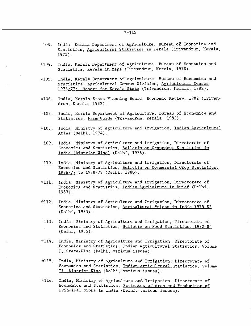
B-115
103. India, Kerala Department of Agriculture, Bureau of Economics and Statistics, Agricultural Statistics in Kerala (Trivandrum, Kerala,1975) .
*104. India, Kerala Department of Agriculture, Bureau of Economics and Statistics, Kerala in Mans (Trivandrum, Kerala, 1978).
*105. India, Kerala Department of Agriculture, Bureau of Economics and Statistics, Agricultural Census Division, Agricultural Census 1976/77: Report for Kerala State (Trivandrum, Kerala, 1982).
*106. India, Kerala State Planning Board, Economic Review. 1982 (Trivandrum, Kerala, 1982).
*107. India, Kerala Department of Agriculture, Bureau of Economics and Statistics, Farm Guide (Trivandrum, Kerala, 1983).
*108. India, Ministry of Agriculture and Irrigation, Indian Agricultural Atlas (Delhi, 1974).
109. India, Ministry of Agriculture and Irrigation, Directorate of Economics and Statistics, Bulletin on Groundnut Statistics in India (District-Wise) (Delhi, 1976).
110. India, Ministry of Agriculture and Irrigation, Directorate of Economics and Statistics, Bulletin on Commercial Crop Statistics. 1976-77 to 1978-79 (Delhi, 1980).
*111, India, Ministry of Agriculture and Irrigation, Directorate of Economics and Statistics, Indian Agriculture in Brief (Delhi,1983).
*112. India, Ministry of Agriculture and Irrigation, Directorate of Economics and Statistics, Agricultural Prices in India 1975-82 (Delhi, 1983).
113. India, Ministry of Agriculture and Irrigation, Directorate of Economics and Statistics, Bulletin on Food Statistics. 1982-84 (Delhi, 1985),
*114. India, Ministry of Agriculture and Irrigation, Directorate ofEconomics and Statistics, Indian Agricultural Statistics. VolumeI. State-Wise (Delhi, various issues).
*115. India, Ministry of Agriculture and Irrigation, Directorate ofEconomics and Statistics, Indian Agricultural Statistics. VolumeII. District-Wise (Delhi, various issues). *
*116. India, Ministry of Agriculture and Irrigation, Directorate of Economics and Statistics, Estimates of Area and Production of Principal Crons in India (Delhi, various issues).
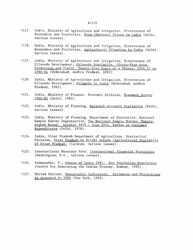
B-116
*117. India, Ministry of Agriculture and Irrigation, Directorate ofEconomics and Statistics, Farm (Harvest) Prices in India (Delhi, various issues).
*118. India, Ministry of Agriculture and Irrigation, Directorate ofEconomics and Statistics, Agricultural Situation in India (Delhi, various issues).
*119. India, Ministry of Agriculture and Irrigation, Directorate of Oilseeds Development, Oilseeds Statistics. (State-Wise Area. Production and Yield). Twenty-five Years at a Glance. 1956-57 to 1980-81 (Hyderabad, Andhra Pradesh, 1982).
*120. India, Ministry of Agriculture and Irrigation, Directorate of Oilseeds Development, Oilseeds in India (Hyderabad, Andhra Pradesh, 1983).
*121. India, Ministry of Finance, Economic Division, Economic Survey 1984-85 (Delhi, 1985).
*122. India, Ministry of Planning, National Accounts Statistics (Delhi, various issues).
*123. India, Ministry of Planning, Department of Statistics, National Sample Survey Organisation, The National Sample Survey. Twenty- eighth Round: October 1973 - June 1974, Tables on ConsumerExpenditures (Delhi, 1976).
*124. India, Uttar Pradesh Department of Agriculture, StatisticalDivision, Uttar Pradesh ke Krishi Ankade [Agricultural Statistics of Uttar Pradesh! (Lucknow, various issues).
*125. International Monetary Fund, International Financial Statistics (Washington, D.C., various issues).
*126. Padmanabha, P., Census of India 1981: Key Population Statistics(Centre for Monitoring the Indian Economy, Bombay, 1983). *
*127, United Nations, Demographic Indicators: Estimates and Projectionsas Assessed in 1980 (New York, 1982).
APPENDIX I.STATISTICS RELATING TO THE COMPETITION BETWEEN CEREALS AND OILSEEDS
B-117

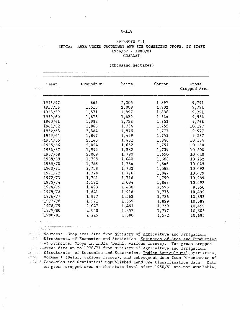
B-119
APPENDIX 1.1.INDIA: AREA UNDER GROUNDNUT AND ITS COMPETING CROPS, BY STATE
1956/57 - 1980/81 GUJARAT
(thousand hectares)
Year Groundnut Baj ra Cotton GrossCropped Area
1956/57 863 2,005 1,897 9,7911957/58 1,515 2,009 1,902 9,7911958/59 1,571 1,997 1,836 9,7911959/60 1,876 1,632 1,544 9,9341950/61 1,982 1,728 1,863 9,7681961/62 1,865 1,734 1,755 10,1271962/63 2,344 1,576 1,777 9,9771963/54 1,847 1,439 1,743 9,8871964/65 2,143 1,482 1,846 10,1341965/66 2,024 1,652 1,751 10,1881966/67 1,992 1,582 1,739 10,2001967/68 2,009 1,790 1,650 10,4201968/69 1,798 1,640 1,608 10,1821969/70 1,748 1,784 1,646 10,0451970/71 1,758 1,782 1,582 10,492■1971/72 1,778 1,776 1,847 10,4791972/73 1,741 1,716 1,790 10,2591973/74 1,582 2,034 1,863 10,4921974/75 1,493 1,430 1,596 8,8501975/76 1,641 1,916 1,778 10,4991976/77 1,887 1,563 1,726 10,3531977/78 1,971 1,369 1,829 10,3891978/79 2,047 1,461 1,759 10,4591979/80 2,040 1,257 1,717 10,6051980/81 2,125 1,380 1,572 10,695
Sources: Crop area data from Ministry of Agriculture and Irrigation,Directorate of Economics and Statistics, Estimates of Area and Production :of Principal Crops in India (Delhi, various issues). For gross cropped area: data up to 1976/77 from Ministry of Agriculture and Irrigation, Directorate of Economics and Statistics, Indian Agricultural Statistics. Volume I (Delhi, various issues); and subsequent data from Directorate of ■Economics and Statistics' unpublished Land Use Classification data. Data on gross cropped area at the state level after 1980/81 are not available.
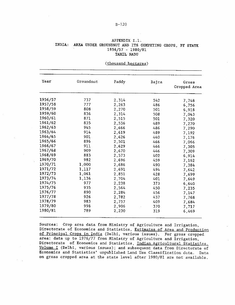
B-120
APPENDIX I.I.INDIA: AREA UNDER GROUNDNUT AND ITS COMPETING CROPS, BY STATE
1956/57 - 1980/81 TAMIL NADU
(thousand hectares')
Year Groundnut Paddy Bajra GrossCropped Area
1956/57 737 2,314 542 7,7481957/58 111 2,263 486 6,7561958/59 808 2,270 501 6,9181959/60 836 2,314 508 7,0431960/61 871 2,515 501 7,3201961/62 835 2,536 489 7,2701962/63 945 2,666 486 7,2901963/64 914 2,619 489 7,1921964/65 901 2,626 440 7,1761965/66 896 2,501 466 7,0661966/67 911 2,629 466 7,3051967/68 909 2,670 446 7,3091968/69 883 2,573 402 6,9141969/70 982 2,696 459 7,1621970/71 1,000 2,686 490 7,3841971/72 1,117 2,691 494 7,6421972/73 1,061 2,851 428 7,6991973/74 1,136 2,704 401 7,6491974/75 977 2,238 373 6,6401975/76 935 2,564 450 7,2351976/77 890 2,284 456 7,1471977/78 926 2,782 437 7,7681978/79 983 2,757 409 7,6841979/80 998 2,906 370 7,7171980/81 789 2,230 319 6,469
Sources: Crop area data from Ministry of Agriculture and Irrigation,Directorate of Economics and Statistics, Estimates of Area and Productionof Princinal Crons in India (Delhi, various (s r h r sV For gross croppedarea: data up to 1976/77 from Ministry of Agriculture and Irrigation,Directorate of ]Economicsi and Statistics. Indian Agricultural Statistics.Volume I (Delhi, various issues); and subsequent data from Directorate ofEconomics and Statistics' unpublished ;Land Use Classification data. Dataon gross cropped area at the state level after 1980/81. are not available.
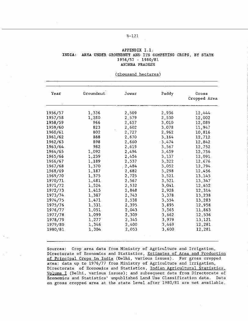
B-121
APPENDIX I.I.INDIA: AREA UNDER GROUNDNUT AND ITS COMPETING CROPS, BY STATE
1956/57 - 1980/81 ANDHRA PRADESH
(thousand hectares)
Year Groundnut Jowar Paddy GrossCropped Area
1956/57 1,336 2,509 2,936 12,4441957/58 1,280 2,579 2,530 12,0021958/59 966 2,657 3,010 12,0891959/60 823 2,602 3,078 11,9471960/61 802 2,727 2,962 10,8161961/62 888 2,670 3,164 12,7121962/63 898 2,660 3,474 12,8421963/64 982 2,619 3,567 12,7521964/65 1,092 2,494 3,459 12,7561965/66 1,239 2,454 3,137 12,0911966/67 1,189 2,537 3,322 12,67.61967/68 1,370 2,484 3,052 12,7941968/69 1,187 2,682 3,298 12,4561969/70 1,375 2,725 3,521 13,1451970/71 1,481 2,567 3,521 13,3471971/72 1,524 2,532 3,041 12,6521972/73 1,415 2,848 2,928 12,3141973/74 1,387 2,743 3,378 13,2381974/75 1,471 2,538 3,554 13,2831975/76 1,331 2,395 3,895 12,9581976/77 1,051 2,043 3,565 11,8631977/78 1,099 2,309 3,662 12,5361978/79 1,277 2,345 3,979 13,1211979/80 1,346 2,400 3,469 12,2811980/81 1,304 2,053 3,600 12,281
Sources: Crop area data from Ministry of Agriculture and Irrigation,Directorate of Economics and Statistics. Estimates of Area and Productionof Principal Crops in India (Delhi, various issues). For gross croppedarea: data up to 1976/77 from Ministry of Agriculture and Irrigation,Directorate of Economics; and Statistics, Indian Agricultural Statistics,Volume I (Delhi, various issues); and subsequent data from Directorate ofEconomics and Statistics' unpublished Land Use Classification data. Dataon gross cropped area at the state level after 1980/81 are not available.
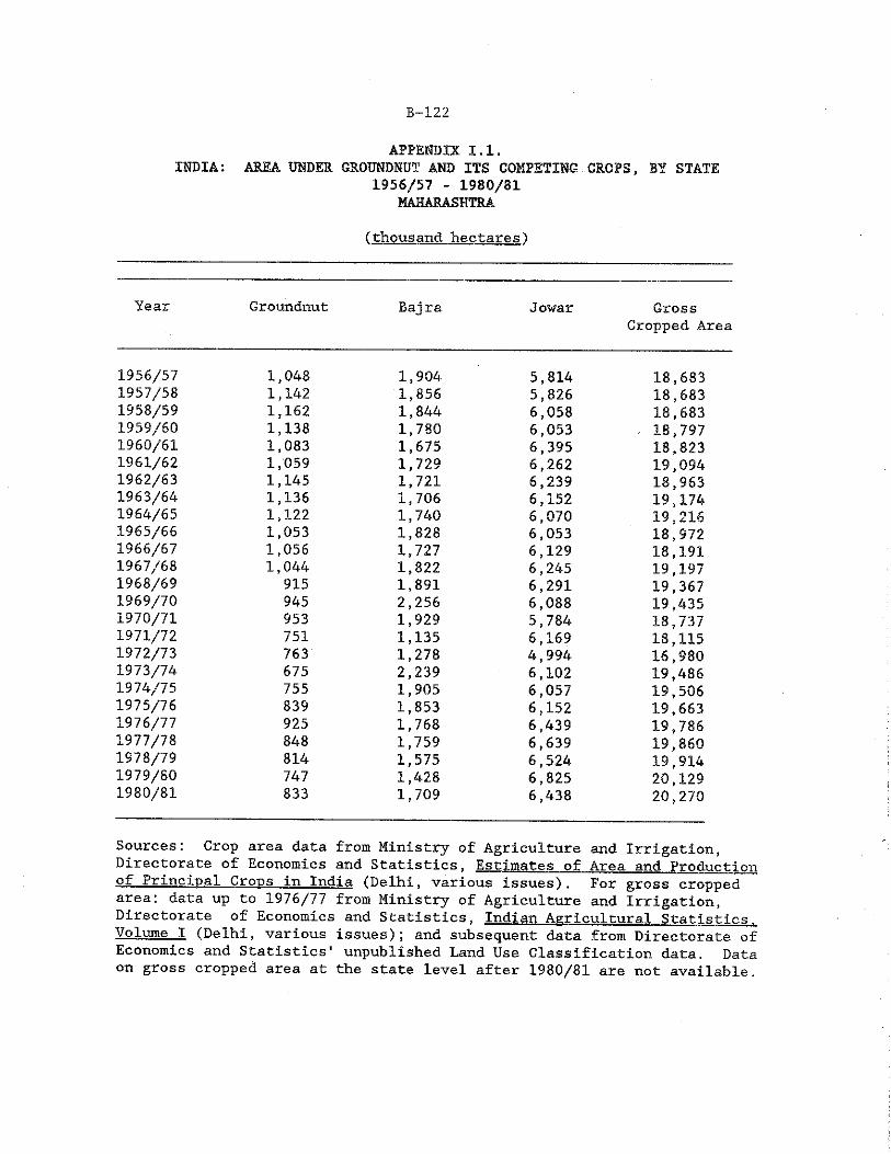
B-122
APPENDIX 1.1.INDIA: AREA UNDER GROUNDNUT AND ITS COMPETING CROPS, BY STATE
1956/57 - 1980/81 MAHARASHTRA
(thousand hectares')
Year Groundnut Bajra Jowar GrossCropped Area
1956/57 1,048 1,904 5,814 18,6831957/58 1,142 1,856 5,826 18,6831958/59 1,162 1,844 6,058 18,6831959/60 1,138 1,780 6,053 18,7971960/61 1,083 1,675 6,395 18,8231961/62 1,059 1,729 6,262 19,0941962/63 1,145 1,721 6,239 18,9631963/64 1,136 1,706 6,152 19,1741964/65 1,122 1,740 6,070 19,2161965/66 1,053 1,828 6,053 18,9721966/67 1,056 1,727 6,129 18,1911967/68 1,044 1,822 6,245 19,1971968/69 915 1,891 6,291 19,3671969/70 945 2,256 6,088 19,4351970/71 953 1,929 5,784 18,7371971/72 751 1,135 6,169 18,1151972/73 763 1,278 4,994 16,9801973/74 675 2,239 6,102 19,4861974/75 755 1,905 6,057 19,5061975/76 839 1,853 6,152 19,6631976/77 925 1,768 6,439 19,7861977/78 848 1,759 6,639 19,8601978/79 814 1,575 6,524 19,9141979/80 747 1,428 6,825 20,1291980/81 833 1,709 6,438 20,270
Sources: Crop area data from Ministry of Agriculture and Irrigation,Directorate of Economics and Statistics, Estimates of Area and Production of Principal Crops In India (Delhi, various issues). For gross cropped area: data up to 1976/77 from Ministry of Agriculture and Irrigation, Directorate of Economics and Statistics, Indian Agricultural Statistics Volume I (Delhi, various issues); and subsequent data from Directorate o Economics and Statistics' unpublished Land Use Classification data. Data on gross cropped area at the state level after 1980/81 are not available.
Hj
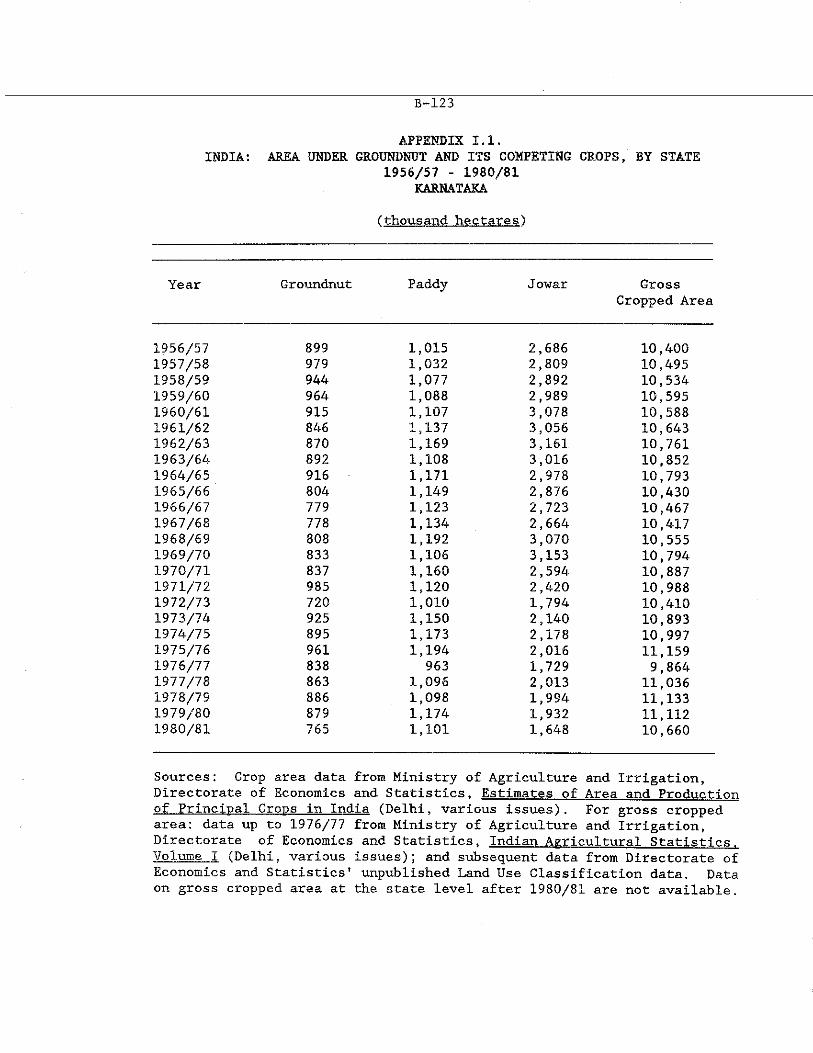
B-123
APPENDIX 1.1.INDIA: AREA UNDER GROUNDNUT AND ITS COMPETING CROPS, BY STATE
1956/57 - 1980/81 KARNATAKA
(thousand hectares)
Year Groundnut Paddy Jowar GrossCropped Area
1956/57 899 1,015 2,686 10,4001957/58 979 1,032 2,809 10,4951958/59 944 1,077 2,892 10,5341959/60 964 1,088 2,989 10,5951960/61 915 1,107 3,078 10,5881961/62 846 1,137 3,056 10,6431962/63 870 1,169 3,161 10,7611963/64 892 1,108 3,016 10,8521964/65 916 1,171 2,978 10,7931965/66 804 1,149 2,876 10,4301966/67 779 1,123 2,723 10,4671967/68 778 1,134 2,664 10,4171968/69 808 1,192 3,070 10,5551969/70 833 1,106 3,153 10,7941970/71 837 1,160 2,594 10,8871971/72 985 1,120 2,420 10,9881972/73 720 1,010 1,794 10,4101973/74 925 1,150 2,140 10,8931974/75 895 1,173 2,178 10,9971975/76 961 1,194 2,016 11,1591976/77 838 963 1,729 9,8641977/78 863 1,096 2,013 11,0361978/79 886 1,098 1,994 11,1331979/80 879 1,174 1,932 11,1121980/81 765 1,101 1,648 10,660
Sources: Crop area data from Ministry of Agriculture and Irrigation,Directorate of Economics and Statistics, Estimates of Area and Productionof Principal Crons in India (Delhi, various issues). For gross croppedarea: data up to 1976/77 from Ministry of Agriculture and Irrigation,Directorate of Economics and Statistics. Indian Agricultural Statistics.Volume I (Delhi, various issues); and jsubsequent data from Directorate ofEconomics and Statistics’ unpublished :Land Use Classification data. Dataon gross cropped area at the state level after 1980/81. are! not available.
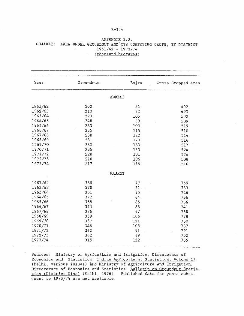
B-124
APPENDIX 1.2.GUJARAT: AREA UNDER GROUNDNUT AND ITS COMPETING CROPS, BY DISTRICT
1961/62 - 1973/74 (thousand hectares)
Year Groundnut Bajra Gross Cropped Area
AMRELI
1961/62 200 84 4921962/63 210 92 4931963/64 223 105 5021964/65 248 89 5091965/66 233 109 5191966/67 235 115 5101967/68 238 122 5141968/69 231 123 5161969/70 230 133 5171970/71 235 133 5241971/72 228 101 5261972/73 210 106 5081973/74 217 115 516
RAJKOT
1961/62 338 77 7591962/63 378 61 7331963/64 351 95 7461964/65 372 84 7361965/66 358 85 7561966/67 373 88 7411967/68 376 97 7681968/69 339 106 7781969/70 337 121 7601970/71 346 105 7871971/72 362 91 7911972/73 362 89 7521973/74 315 122 755
Sources: Ministry of Agriculture and Irrigation; Directorate ofEconomics and Statistics, Indian Agricultural Statistics, Volume II (Delhi, various issues) and Ministry of Agriculture and Irrigation, Directorate of Economics and Statistics, Bulletin on Groundnut Statistics (District-Wise) (Delhi, 1976). Published data for years subsequent to 1973/74 are not available.
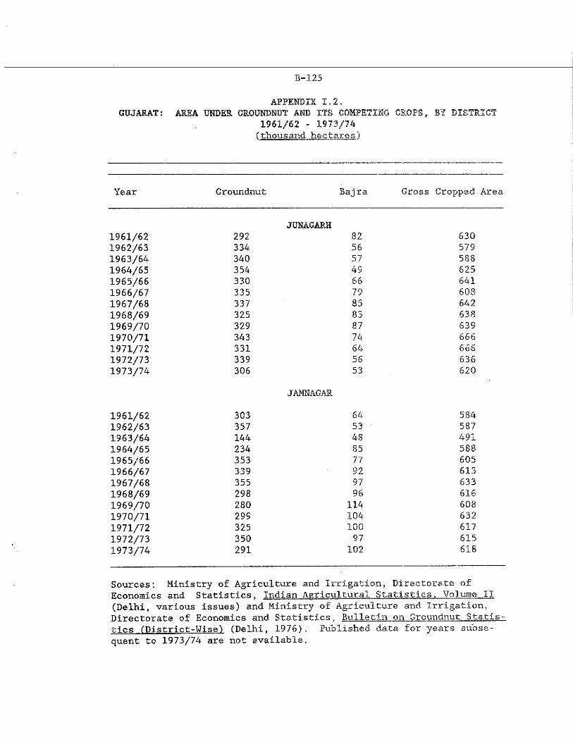
B-125
APPENDIX 1.2.GUJARAT: AREA UNDER GROUNDNUT AND ITS COMPETING CROPS, BY DISTRICT
1961/62 - 1973/74 (thousand hectares)
Year Groundnut Baj ra Gross Cropped Area
JUNAGARH1961/62 292 82 6301962/63 334 56 5791963/64 340 57 5881964/65 354 49 6251965/66 330 66 6411966/67 335 79 60S1967/68 337 85 6421968/69 325 83 6381969/70 329 87 6391970/71 343 74 6661971/72 331 64 6661972/73 339 56 63.61973/74 306 53 620
JAMNAGAR
1961/62 303 64 5841962/63 357 53 5871963/64 144 48 4911964/65 234 85 5881965/66 353 77 6051966/67 339 92 6131967/68 355 97 6331968/69 298 96 6161969/70 280 114 6081970/71 299 104 6321971/72 325 100 6171972/73 350 97 6151973/74 291 102 618
Sources: Ministry of Agriculture and Irrigation. Directorate ofEconomics and Statistics, Indian Agricultural Statistics. Volume II (Delhi, various issues) and Ministry of Agriculture and Irrigation, Directorate of Economics and Statistics, Bulletin on Groundnut Statistics (District-Wise) (Delhi, 1976). Published data for years subsequent to 1973/74 are not available.
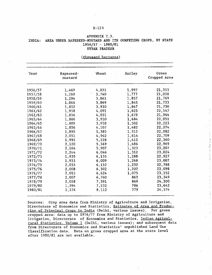
B-126
APPENDIX 1.3.INDIA: AREA UNDER RAPESEED-MUSTARD AND ITS COMPETING CROPS, BY STATE
1956/57 - 1980/81UTTAR PRADESH
(thousand hectares)
Year Rapeseed-mustard
Wheat Barley GrossCropped Area
1956/57 1,469 4,031 1,997 21,3531957/58 1,280 3,740 1,777 21,0581958/59 1,294 3,861 1,857 21,7691959/60 1,866 3,869 1,845 21,7331960/61 1,852 3,930 1,847 21,7301961/62 1,958 4,091 1,825 22,1471962/63 1,856 4,031 1,678 21,9641963/64 1,806 3,910 1,684 22,0511964/65 1,809 3,958 1,502 22,2231965/66 1,856 4,107 1,482 22,0741966/67 1,895 5,385 1,512 22,0821967/68 2,051 4,962 1,614 22,7091968/69 1,992 5,228 1,412 22,3601969/70 2,120 5,369 1,486 22,9691970/71 2,164 5,907 1,323 23,2071971/72 2,244 6,046 1,312 23,0241972/73 1,935 6,135 1,288 22,9271973/74 1,933 6,009 1,268 23,0071974/75 2,035 6,152 1,232 22,7881975/76 2,008 6,302 1,202 23,0981976/77 2,015 6,624 1,075 23,1521977/78 2,007 6,760 863 23,3491978/79 2,058 7,391 869 24,3001979/80 1,994 7,532 786 23,6421980/81 2,276 8,112 779 24,574
Sources: Crop area data from Ministry of Agriculture and Irrigation,Directorate of Economics and Statistics, Estimates of Area and Produc_-_ tion of Principal Crons in India (Delhi, various issues). For gross cropped area: data up to 1976/77 from Ministry of Agriculture and Irrigation, Directorate of Economics and Statistics, Indian Agricultural Statistics, Volume I (Delhi, various issues); and subsequent data from Directorate of Economics and Statistics' unpublished Land Use Classification data. Data on gross cropped area at the state level after 1980/81 are not available.
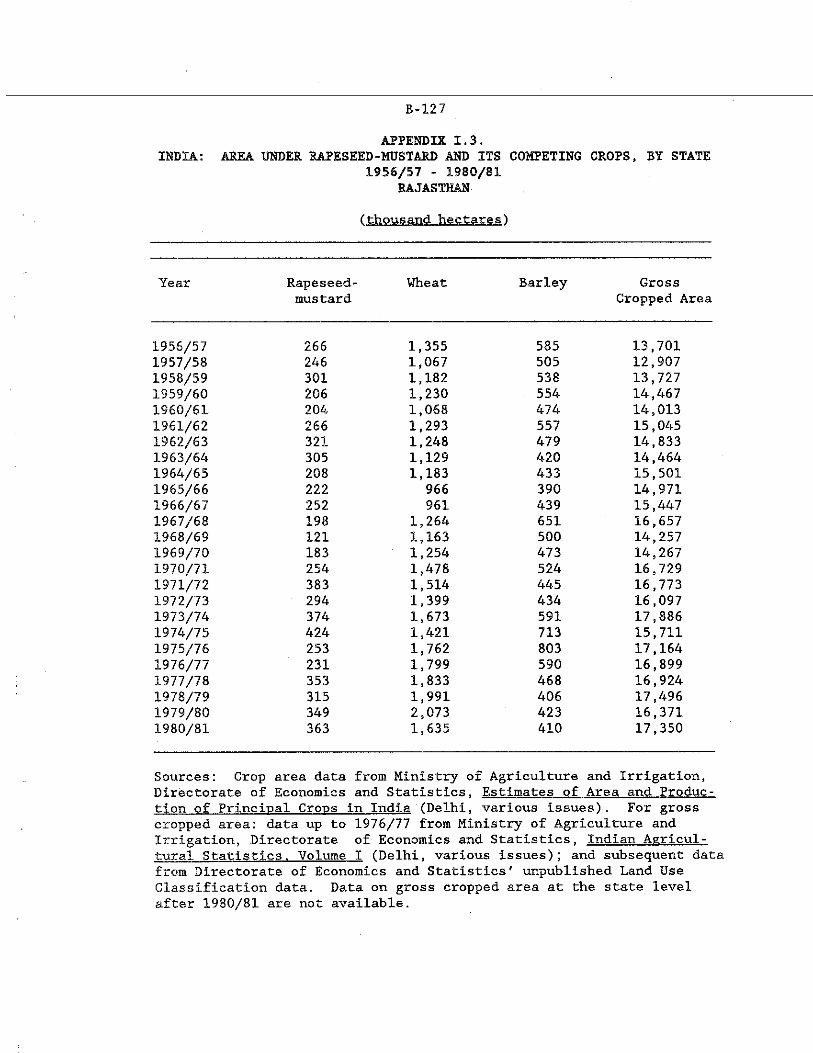
B-127
APPENDIX 1.3.INDIA: AREA UNDER RAPESEED-MUSTARD AND ITS COMPETING CROPS, BY STATE
1956/57 - 1980/81 RAJASTHAN
(thousand„hec_tare_s)
Year Rapeseed-mustard
Wheat Barley GrossCropped Area
1956/57 266 1,355 585 13,7011957/58 246 1,067 505 12,9071958/59 301 1,182 538 13,7271959/60 206 1,230 554 14,4671960/61 204 1,068 474 14,0131961/62 266 1,293 557 15,0451962/63 321 1,248 479 14,8331963/64 305 1,129 420 14,4641964/65 208 1,183 433 15,5011965/66 222 966 390 14,9711966/67 252 961 439 15,4471967/68 198 1,264 651 16,6571968/69 121 1,163 500 14,2571969/70 183 1,254 473 14,2671970/71 254 1,478 524 16,7291971/72 383 1,514 445 16,7731972/73 294 1,399 434 16,0971973/74 374 1,673 591 17,8861974/75 424 1,421 713 15,7111975/76 253 1,762 803 17,1641976/77 231 1,799 590 16,8991977/78 353 1,833 468 16,9241978/79 315 1,991 406 17,4961979/80 349 2,073 423 16,3711980/81 363 1,635 410 17,350
Sources: Crop area data from Ministry of Agriculture and Irrigation,Directorate of Economics and Statistics, Estimates of Area and Production of Principal Crons in India (Delhi. various issues). For gross cropped area: data up to 1976/77 from Ministry of Agriculture and Irrigation, Directorate of Economics and Statistics, Indian Agricultural Statistics. Volume I (Delhi, various issues); and subsequent data from Directorate of Economics and Statistics' unpublished Land Use Classification data. Data on gross cropped area at the state level after 1930/81 are not available.
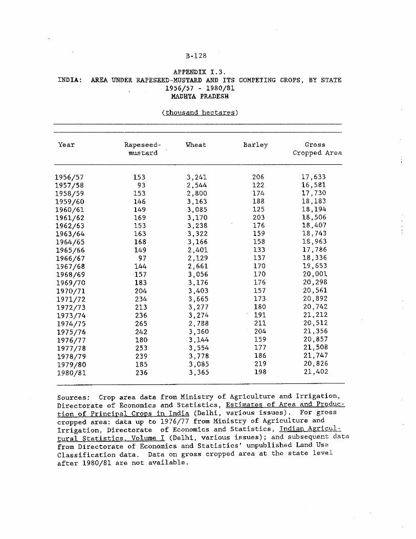
B-128
APPENDIX 1.3.INDIA: AREA UNDER RAPESEED-MUSTARD AND ITS COMPETING CROPS, BY STATE
1956/57 - 1980/81 MADHYA PRADESH
(thousand hectares)
Year Rapeseed- mustard
Wheat Barley GrossCropped Area
1956/57 153 3,241 206 17,6331957/58 93 2,544 122 16,5811958/59 153 2,800 174 17,7301959/60 146 3,163 188 18,1831960/61 149 3,085 125 18,1941961/62 169 3,170 203 18,5061962/63 153 3,238 176 18,4071963/64 163 3,322 159 18,7431964/65 168 3,166 158 18,9631965/66 149 2,401 133 17,7861966/67 97 2,129 137 18,3361967/68 144 2,661 170 19,6531968/69 157 3,056 170 20,0011969/70 183 3,176 176 20,2981970/71 204 3,403 157 20,5611971/72 234 3,665 173 20,8921972/73 213 3,277 180 20,7421973/74 236 3,274 191 21,2121974/75 265 2,788 211 20,5121975/76 242 3,360 204 21,3561976/77 180 3,144 159 20,8571977/78 253 3,554 177 21,5081978/79 239 3,778 186 21,7471979/80 185 3,085 219 20,8261980/81 236 3,365 198 21,402
Sources: Crop area data from Ministry of Agriculture and Irrigation,Directorate of Economics and Statistics, Estimates of Area and Produc_-_ tlon of Principal Crons in India (Delhi, various issues). For gross cropped area: data up to 1976/77 from Ministry of Agriculture and Irrigation, Directorate of Economics and Statistics, Indian Agricultural Statistics. Volume I (Delhi, various issues); and subsequent data from Directorate of Economics and Statistics' unpublished Land Use Classification data. Data on gross cropped area at the state level after 1980/81 are not available.
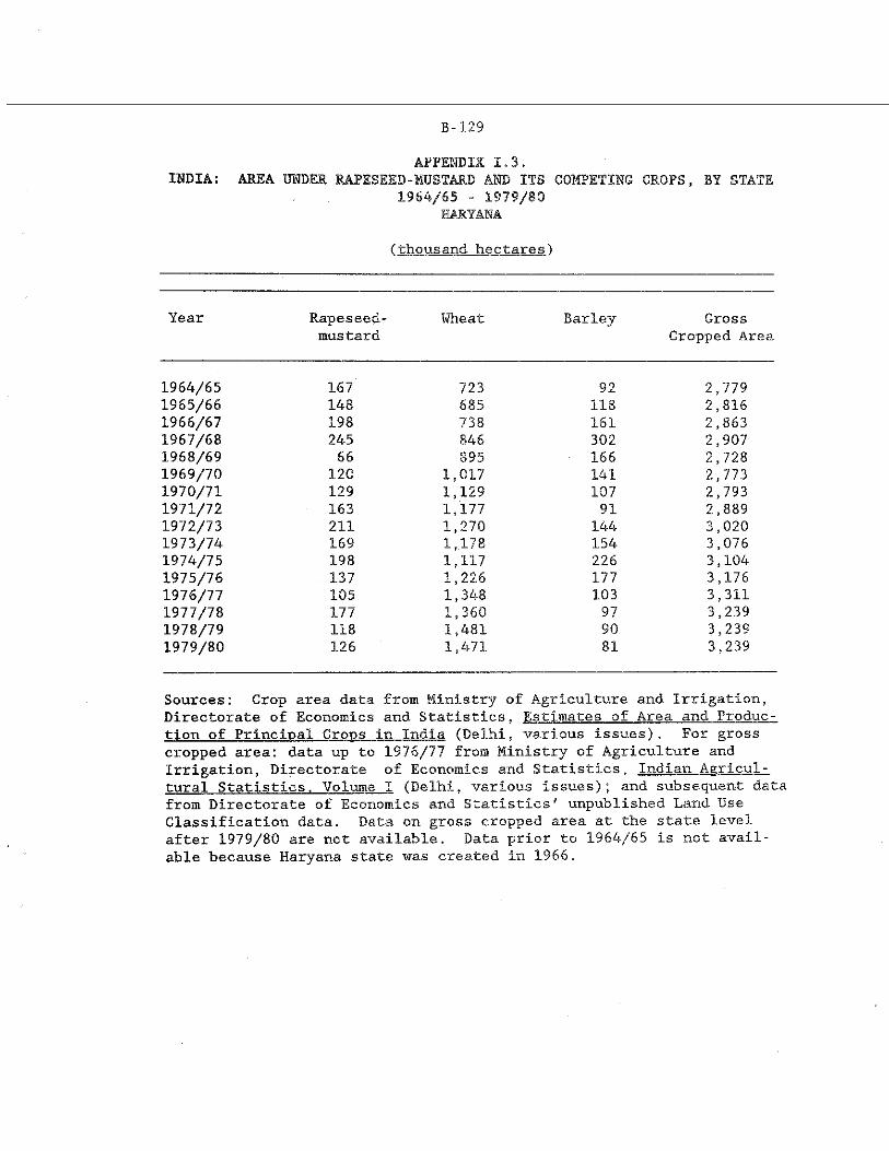
B-129
APPENDIX 1.3.INDIA: AREA UNDER RAPESEED-MUSTARD AND ITS COMPETING CROPS, BY STATE
1964/65 - 1979/80 HARYANA
(tho usandJiectar e_s)
Year Rapeseed- mustard
Wheat Barley GrossCropped Area
1964/65 167 723 92 2,7791965/66 148 685 118 2,8161966/67 198 738 161 2,8631967/68 245 846 302 2,9071968/69 66 895 166 2,7281969/70 120 1,017 141 2,7731970/71 129 1,129 107 2,7931971/72 163 1,177 91 2,8891972/73 211 1,270 144 3,0201973/74 169 1,178 154 3,0761974/75 198 1,117 226 3,1041975/76 137 1,226 177 3,1761976/77 105 1,348 103 3,3111977/78 177 1,360 97 3,2391978/79 118 1,481 90 3,2391979/80 126 1,471 81 3,239
Sources: Crop area data from Ministry of Agriculture and Irrigation,Directorate of Economics and Statistics, Estimates of Area and Production of Principal Crons in India (Delhi, various issues). For gross cropped area: data up to 1976/77 from Ministry of Agriculture and Irrigation, Directorate of Economics and Statistics, Indian Agricultural Statistics. Volume I (Delhi, various Issues); and subsequent data from Directorate of Economics and Statistics' unpublished Land Use Classification data. Data on gross cropped area at the state level after 1979/80 are not available. Data prior to 1964/65 is not available because Haryana state was created in 1966.
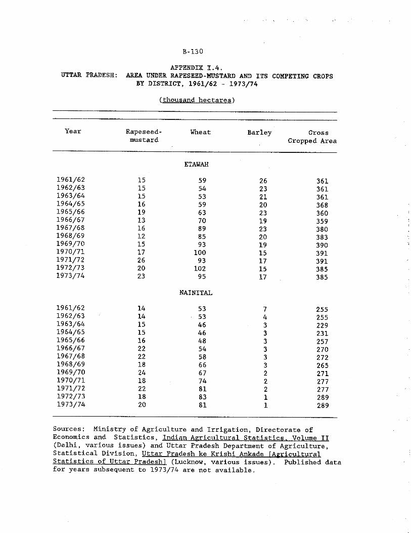
B-130
APPENDIX 1.4.UTTAR PRADESH: AREA UNDER RAPESEED-MUSTARD AND ITS COMPETING CROPS
BY DISTRICT, 1961/62 - 1973/74
(thousand hectares)
Year Rapeseed- Wheat Barley Grossmus tard Cropped Area
ETAWAH1961/62 15 59 26 3611962/63 15 54 23 3611963/64 15 53 21 3611964/65 16 59 20 3681965/66 19 63 23 3601966/67 13 70 19 3591967/68 16 89 23 3801968/69 12 85 20 3831969/70 15 93 19 3901970/71 17 100 15 3911971/72 26 93 17 3911972/73 20 102 15 3851973/74 23 95 17 385
NAINITAL1961/62 14 53 7 2551962/63 14 53 4 2551963/64 15 46 3 2291964/65 15 46 3 2311965/66 16 48 3 2571966/67 22 54 3 2701967/68 22 58 3 2721968/69 18 66 3 2651969/70 24 67 2 2711970/71 18 74 2 2771971/72 22 81 2 2771972/73 18 83 1 2891973/74 20 81 1 289
Sources: Ministry of Agriculture and Irrigation, Directorate ofEconomics and Statistics, Indian Agricultural Statistics. Volume II(Delhi, various issues) and Uttar Pradesh Department of Agriculture, Statistical Division, Uttar Pradesh ke Krishi Ankade \Agricultural Statistics of Uttar Pradeshl (Lucknow, various issues). Published data for years subsequent to 1973/74 are not available.
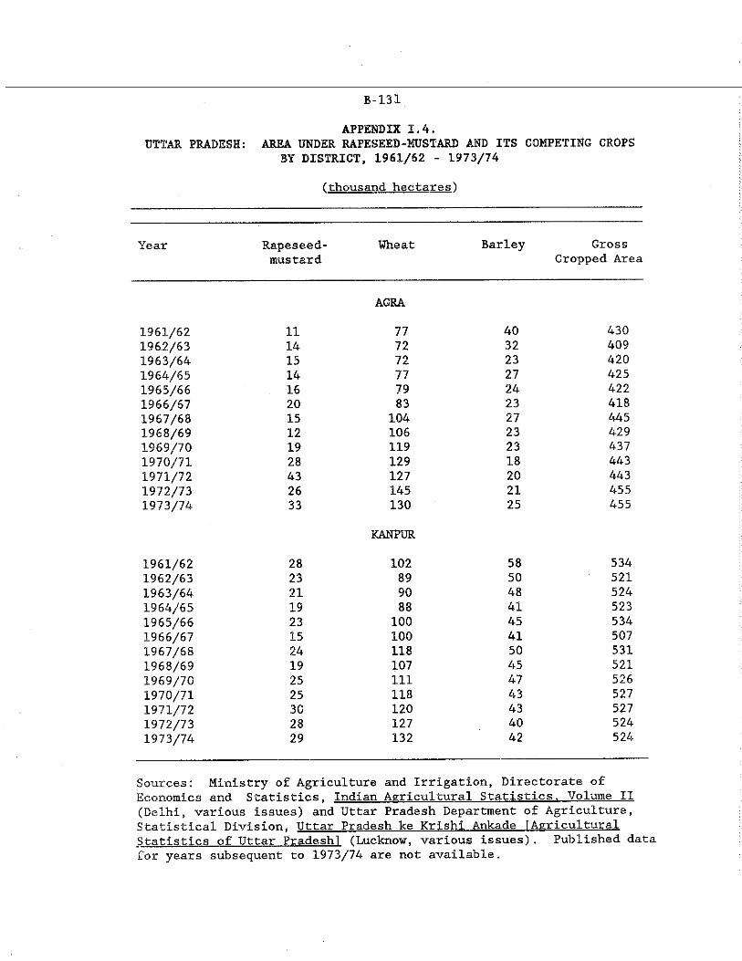
B-13I
APPENDIX 1.4.UTTAR PRADESH: AREA UNDER RAFESEED-MUSTARD AND ITS COMPETING CROPS
BY DISTRICT, 1961/62 - 1973/74(thousand hectares1)
Year Rapeseed-mustard
Wheat Barley GrossCropped Area
AGRA
1961/62 11 77 40 4301962/63 14 72 32 4091963/64 15 72 23 4201964/65 14 77 27 4251965/66 16 79 24 4221966/67 20 83 23 4181967/68 15 104 27 4451968/69 12 106 23 4291969/70 19 119 23 4371970/71 28 129 18 4431971/72 43 127 20 4431972/73 26 145 21 4551973/74 33 130 25 455
KANPUR
1961/62 28 102 58 5341962/63 23 89 50 5211963/64 21 90 48 5241964/65 19 88 41 5231965/66 23 100 45 5341966/67 15 100 41 5071967/68 24 118 50 5311968/69 19 107 45 5211969/70 25 111 47 5261970/71 25 118 43 5271971/72 30 120 43 5271972/73 28 127 40 5241973/74 29 132 42 524
Sources: Ministry of Agriculture and Irrigation, Directorate ofEconomics and Statistics. Indian Agricultural Statistics . Volume II(Delhi, various issues) and Uttar Pradesh Department of Agriculture,Statistical Division, Uttar Pradesh ke Krishi Ankade [Agricultural Statistics of Uttar Pradesh! (Lucknow, various issues). Published data for years subsequent to 1973/74 are not available.
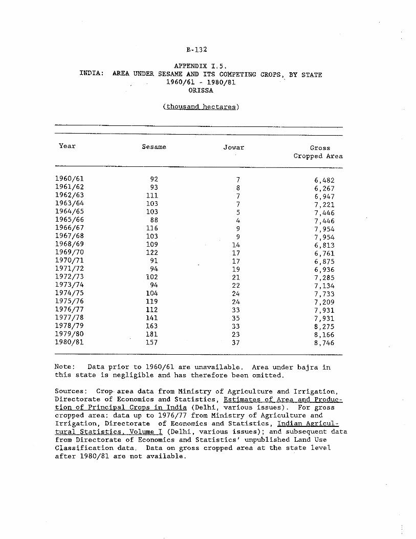
B-132
APPENDIX 1.5.INDIA: AREA UNDER SESAME AND ITS COMPETING CROPS, BY STATE
1960/61 - 1980/81 ORISSA
(thousand hectares')
Year Sesame Jowar GrossCropped Area
1960/61 92 7 6,4821961/62 93 8 6,2671962/63 111 7 6,9471963/64 103 7 7,2211964/65 103 5 7,4461965/66 88 4 7,4461966/67 116 9 7,9541967/68 103 9 7,9541968/69 109 14 6,8131969/70 122 17 6,7611970/71 91 17 6,8751971/72 94 19 6,9361972/73 102 21 7,2851973/74 94 22 7,1341974/75 104 24 7,7331975/76 119 24 7,2091976/77 112 33 7,9311977/78 141 35 7,9311978/79 163 33 8,2751979/80 181 23 8,1661980/81 157 37 8,746
Note: Data prior to 1960/61 are unavailable. Area under bajra inthis state is negligible and has therefore been omitted.
Sources: Crop area data from Ministry of Agriculture and Irrigation,Directorate of Economics and Statistics, Estimates of Area and Production of Principal Crops in India (Delhi, various Issues). For gross cropped area: data up to 1976/77 from Ministry of Agriculture and Irrigation, Directorate of Economics and Statistics, Indian Agricultural Statistics. Volume I (Delhi, various issues); and subsequent data from Directorate of Economics and Statistics' unpublished Land Use Classification data. Data on gross cropped area at the state level after 1980/81 are not available.
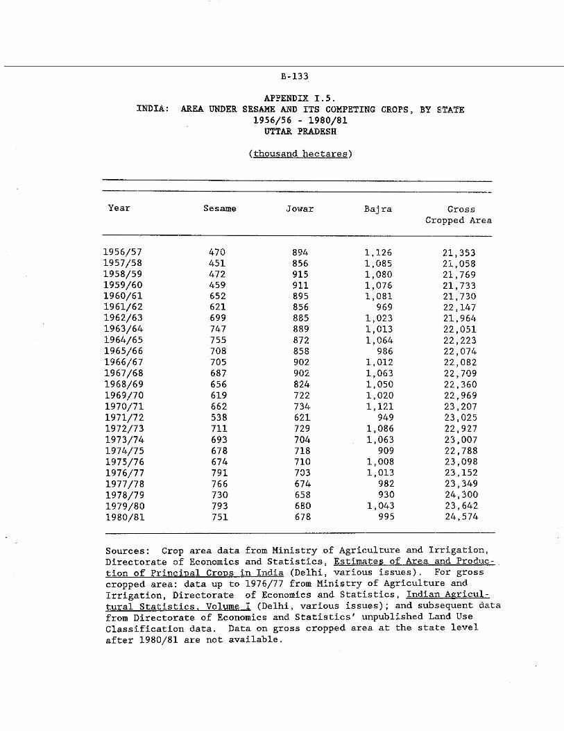
B-133
APPENDIX 1.5.INDIA: AREA UNDER SESAME AND ITS COMPETING CROPS, BY STATE
1956/56 - 1980/81 UTTAR PRADESH
(thousand hectares')
Year Sesame Jowar Baj ra GrossCropped Area
1956/57 470 894 1,126 21,3531957/58 451 856 1,085 21,0581958/59 472 915 1,080 21,7691959/60 459 911 1,076 21,7331960/61 652 895 1,081 21,7301961/62 621 856 969 22,1471962/63 699 885 1,023 21,9641963/64 747 889 1,013 22,0511964/65 755 872 1,064 22,2231965/66 708 858 986 22,0741966/67 705 902 1,012 22,0821967/68 687 902 1,063 22,7091968/69 656 824 1,050 22,3601969/70 619 722 1,020 22,9691970/71 662 734 1,121 23,2071971/72 538 621 949 23,0251972/73 711 729 1,086 22,9271973/74 693 704 1,063 23,0071974/75 678 718 909 22,7881975/76 674 710 1,008 23,0981976/77 791 703 1,013 23,1521977/78 766 674 982 23,3491978/79 730 658 930 24,3001979/80 793 680 1,043 23,6421980/81 751 678 995 24,574
Sources: Crop area data from Ministry of Agriculture and Irrigation,Directorate of Economics and Statistics, Estimates of Area and Production of Principal Crops in India (Delhi, various issues). For gross cropped area: data up to 1976/77 from Ministry of Agriculture and Irrigation, Directorate of Economics and Statistics, Indian Agricultural Statistics. Volume I (Delhi, various issues); and subsequent data from Directorate of Economics and Statistics' unpublished Land Use Classification data. Data on gross cropped area at the state level after 1980/81 are not available.
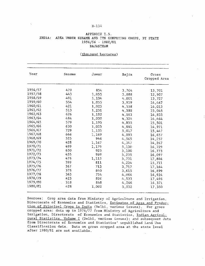
B-134
APPENDIX 1,5.INDIA: AREA UNDER SESAME AND ITS COMPETING CROPS,, BY STATE
1956/56 - 1980/81RAJASTHAN
(thousand hectares')
Year Sesame Jowar Baj ra GrossCropped Area
1956/57 479 854 3,764 13,7011957/58 443 1,055 3,888 12,9071958/59 491 1,104 4,001 ' 13,7271959/60 554 1,055 3,959 14,4671960/61 421 1,025 4,558 14,0131961/62 513 1,231 4,388 15,0451962/63 626 1,182 4,163 14,8331963/64 484 1,030 4,324 14,4641964/65 579 1,195 4,855 15,5011965/66 630 1,025 4,881 14,9711966/67 729 1,135 5,017 15,4471967/68 666 1,169 4,893 16,6571968/69 525 946 4,565 14,2571969/70 428 1,167 4,347 14,2671970/71 499 1,179 5,130 16,7291971/72 630 923 5,100 16,7731972/73 455 989 5,235 16,0971973/74 476 1,115 5,731 17,8861974/75 399 811 4,224 15,7111975/76 367 713 3,717 17,1641976/77 378 840 3,615 16,8991977/78 363 724 4,066 16,9241978/79 423 826 4,533 17,4961979/80 . 318 848 4,266 16,3711980/81 428 1,002 5,032 17,350
Sources: Crop area data from Ministry of Agriculture and Irrigation,Directorate of Economics and Statistics, Estimates of Area and Production of Principal Crons in India (Delhi, various issues). For gross cropped area: data up to 1976/77 from Ministry of Agriculture and Irrigation, Directorate of Economics and Statistics, Indian Agricultural Statistics. Volume I (Delhi, various issues); and subsequent data from Directorate of Economics and Statistics' unpublished Land Use Classification data. Data on gross cropped area at the state level after 1980/81 are not available.
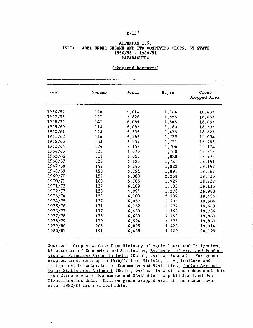
B-135
APPENDIX 1.5.INDIA: AREA UNDER SESAME AND ITS COMPETING CROPS, BY STATE
1956/56 - 1980/81 MAHARASHTRA
(thousand hectares')
Year Sesame Jowar Baj ra GrossCropped Area
1956/57 120 5,814 1,904 18,6831957/58 127 5,826 1,858 18,6831958/59 147 6,059 1,845 18,6831959/60 118 6,052 1,780 18,7971960/61 128 6,396 1,675 18,8231961/62 116 6,262 1,729 19,0941962/63 133 6,239 1,721 18,9631963/64 126 6,152 1,706 19,1741964/65 121 6,070 1,740 19,2161965/66 118 6,053 1,828 18,9721966/67 128 6,128 1,727 18,1911967/68 142 6,245 1,822 19,1971968/69 150 6,291 1,891 19,3671969/70 159 6,088 2,258 19,4351970/71 160 5,785 1,929 18,7371971/72 127 6,169 1,135 18,1151972/73 123 4,994 1,278 16,9801973/74 154 6,103 2,239 19,4861974/75 137 6,057 1,905 19,5061975/76 171 6,152 1,977 19,6631976/77 177 6,439 1,768 19,7861977/78 175 6,639 1,759 19,8601978/79 179 6,524 1,575 19,8601979/80 205 6,825 1,428 19,9141980/81 191 6,438 1,709 20,129
Sources: Crop area data from Ministry of Agriculture and Irrigation,Directorate of Economics and Statistics, Estimates of Area and Production of Principal Crops in India (Delhi, various issues). For gross cropped area: data up to 1976/77 from Ministry of Agriculture and Irrigation, Directorate of Economics and Statistics, Indian Agricultural Statistics. Volume I (Delhi, various issues); and subsequent data from Directorate of Economics and Statistics' unpublished Land Use Classification data. Data on gross cropped area at the state level after 1980/81 are not available.

APPENDIX II.STATISTICS RELATING TO COCONUT
B-137

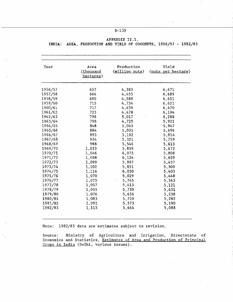
B-l-39
APPENDIX II.1.INDIA: AREA, PRODUCTION AND YIELD OF COCONUTS, 1956/57 - 1982/83
Year Area(thousand hectares)
Production (million nuts)
Yield(nuts Der hectare)
1956/57 657 4,383 6,6711957/58 666 4,455 6,6891958/59 690 4,589 6,6511959/60 715 4,734 6,6211960/61 717 4,639 6,4701961/62 723 4,478 6,1941962/63 798 5,017 6,2881963/64 798 4,725 5,9211964/65 848 5,043 5,9471965/66 884 5,035 5,6961966/67 893 5,192 5,8141967/68 924 5,321 5,7591968/69 988 5,546 5,6131969/70 1,033 5,859 5,6721970/71 1,046 6,075 5,8081971/72 1,088 6,124 5,6291972/73 1,099 5,997 5,4571973/74 1,102 5,851 5,3091974/75 1,116 6,030 5,4031975/76 1,070 5,829 5,4481976/77 1,075 5,765 5,3631977/78 1,057 5,413 5,1211978/79 1,055 5,730 5,4311979/80 1,076 5,636 5,2381980/81 1,083 5,720 5,2821981/82 1,091 5,573 5,1901982/83 1,113 5,664 5,088
Note: 1982/83 data are estimates subject to revision.
Source: Ministry of Agriculture and Irrigation, Directorate ofEconomics and Statistics, Estimates of Area and Production of PrincipalCrons in India (Delhi, various issues).
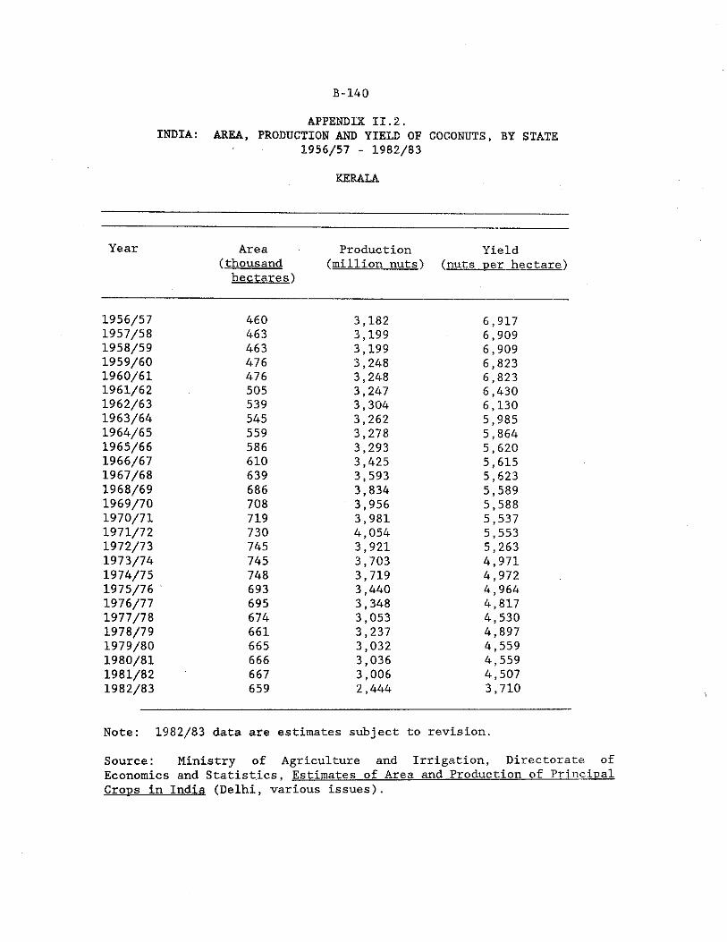
B-140
KERALA
APPENDIX II.2.INDIA: AREA, PRODUCTION AND YIELD OF COCONUTS, BY STATE
1956/57 - 1982/83
Year Area(thousand hectares)
Production (million nuts)
Yield(nuts per hectare)
1956/57 460 3,182 6,9171957/58 463 3,199 6,9091958/59 463 3,199 6,9091959/60 476 3,248 6,8231960/61 476 3,248 6,8231961/62 505 3,247 6,4301962/63 539 3,304 6,1301963/64 545 3,262 5,9851964/65 559 3,278 5,8641965/66 586 3,293 5,6201966/67 610 3,425 5,6151967/68 639 3,593 5,6231968/69 686 3,834 5,5891969/70 708 3,956 5,5881970/71 719 3,981 5,5371971/72 730 4,054 5,5531972/73 745 3,921 5,2631973/74 745 3,703 4,9711974/75 748 3,719 4,9721975/76 693 3,440 4,9641976/77 695 3,348 4,8171977/78 674 3,053 4,5301978/79 661 3,237 4,8971979/80 665 3,032 4,5591980/81 666 3,036 4,5591981/82 667 3,006 4,5071982/83 659 2,444 3,710
Note: 1982/83 data are estimates subject to revision.
Source: Ministry of Agriculture and Irrigation, Directorate ofEconomics and Statistics, Estimates of Area and Production of PrincipalCrops in India (Delhi, various issues).
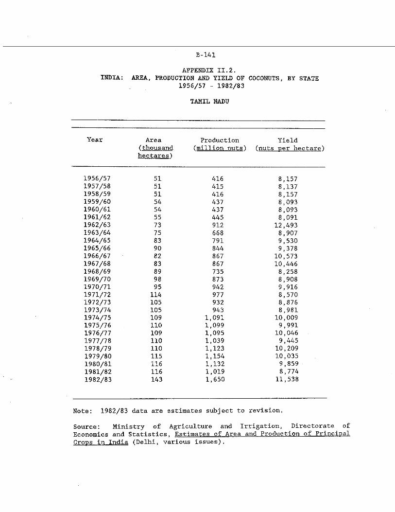
B-141
TAMIL NADU
APPENDIX II.2.INDIA: AREA, PRODUCTION AND YIELD OF COCONUTS, BY STATE
1956/57 - 1982/83
Year Area Production Yield(thousand (million nuts') (nuts per hectare)hectares)
1956/57 51 416 8,1571957/58 51 415 8,1371958/59 51 416 8,1571959/60 54 437 8,0931960/61 54 437 8,0931961/62 55 445 8,0911962/63 73 912 12,4931963/64 75 668 8,9071964/65 83 791 9,5301965/66 90 844 9,3781966/67 82 867 10,5731967/68 83 867 10,4461968/69 89 735 8,2581969/70 98 873 8,9081970/71 95 942 9,9161971/72 114 977 8,5701972/73 105 932 8,8761973/74 105 943 8,9811974/75 109 1,091 10,0091975/76 110 1,099 9,9911976/77 109 1,095 10,0461977/78 110 1,039 9,4451978/79 110 1,123 10,2091979/80 115 1,154 10,0351980/81 116 1,132 9,8591981/82 116 1,019 8,7741982/83 143 1,650 11,538
Note: 1982/83 data are estimates subject to revision.
Source: Ministry of Agriculture and Irrigation, Directorate ofEconomics and Statistics, Estimates of Area and Production of PrincipalCrops in India (Delhi, various issues).
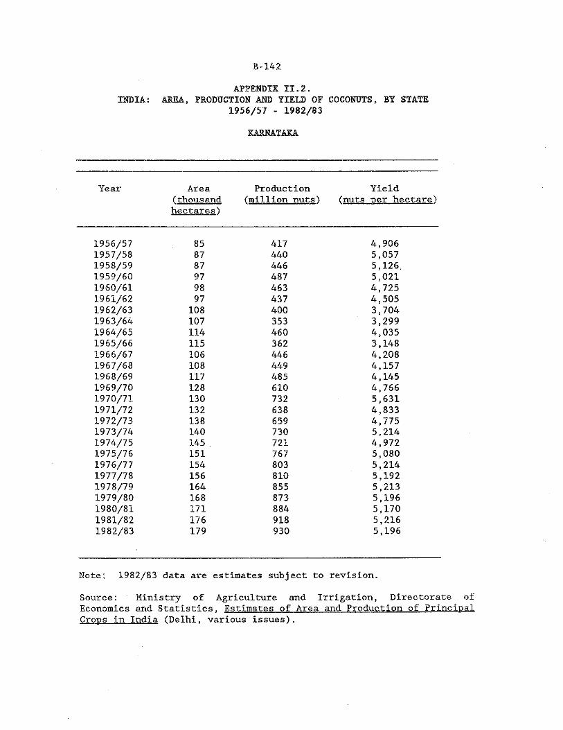
B -142
KARNATAKA
APPENDIX II.2.INDIA: AREA, PRODUCTION AND YIELD OF COCONUTS, BY STATE
1956/57 - 1982/83
Year Area(thous andhectares)
Production (million nuts)
Yield(nuts per hectare)
1956/57 85 417 4,9061957/58 87 440 5,0571958/59 87 446 5,126.1959/60 97 487 5,0211960/61 98 463 4,7251961/62 97 437 4,5051962/63 108 400 3,7041963/64 107 353 3,2991964/65 114 460 4,0351965/66 115 362 3,1481966/67 106 446 4,2081967/68 108 449 4,1571968/69 117 485 4,1451969/70 128 610 4,7661970/71 130 732 5,6311971/72 132 638 4,8331972/73 138 659 4,7751973/74 140 730 5,2141974/75 145 . 721 4,9721975/76 151 767 5,0801976/77 154 803 5,2141977/78 156 810 5,1921978/79 164 855 5,2131979/80 168 873 5,1961980/81 171 884 5,1701981/82 176 918 5,2161982/83 179 930 5,196
Note: 1982/83 data are estimates subject to revision.
Source: Ministry of Agriculture and. Irrigation, Directorate of Economics and Statistics, Estimates of Area and Production of Principal Crops in India (Delhi, various issues).
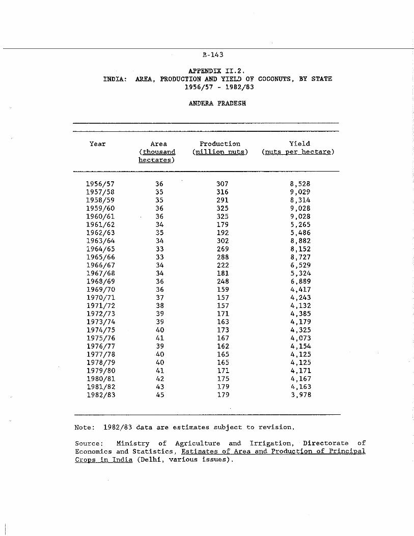
B-143
ANDHRA PRADESH
APPENDIX II.2.INDIA; AREA, PRODUCTION AND YIELD OF COCONUTS, BY STATE
1956/57 - 1982/83
Year Area(thousand hectares)
Production (million nuts)
Yield(nuts per hectare)
1956/57 36 307 8,5281957/58 35 316 9,0291958/59 35 291 8,3141959/60 36 325 9,0281960/61 36 325 9,0281961/62 34 179 5,2651962/63 35 192 5,4861963/64 34 302 8,8821964/65 33 269 8,1521965/66 33 288 8,7271966/67 34 222 6,5291967/68 34 181 5,3241968/69 36 248 6,8891969/70 36 159 4,4171970/71 37 157 4,2431971/72 38 157 4,1321972/73 39 171 4,3851973/74 39 163 4,1791974/75 40 173 4,3251975/76 41 167 4,0731976/77 39 162 4,1541977/78 40 165 4,1251978/79 40 165 4,1251979/80 41 171 4,1711980/81 42 175 4,1671981/82 43 179 4,1631982/83 45 179 3,978
Note: 1982/83 data are estimates subject to revision.
Source: Ministry of Agriculture and Irrigation, Directorate ofEconomics and Statistics, Estimates of Area and Production of PrincipalCrops in India (Delhi, various issues).
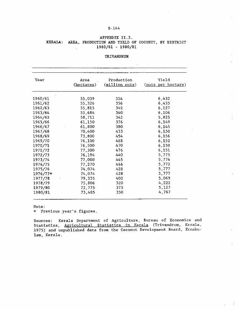
B-144
TRIVANDRUM
APPENDIX II.3.KERALA: AREA, PRODUCTION AND YIELD OF COCONUT, BY DISTRICT
1960/61 - 1980/81
Year Area(hectares')
Production (million nuts)
Yield(nuts per hectare)
1960/61 55,039 354 6,4321961/62 55,326 356 6,4351962/63 55,815 342 6,1271963/64 55,684 340 6,1061964/65 58,711 342 5,8251965/66 61,150 376 6,1491966/67 61,800 380 6,1451967/68 70,400 433 6,1501968/69 73,800 454 6,1561969/70 76,100 468 6,1521970/71 76,500 470 6,1501971/72 77,300 476 6,1511972/73 76,194 440 5,7751973/74 77,000 445 5,7741974/75 77,270 446 5,7721975/76 74,074 428 5,7771976/77* * 74,074 428 5,7771977/78 79,335 402 5,0691978/79 75,806 320 4,2221979/80 72,775 373 5,1271980/81 73,485 350 4,767
Note:* Previous year's figures.
Sources: Kerala Department of Agriculture, Bureau of Economics and Statistics, Agricultural Statistics in Kerala (Trivandrum, Kerala, 1975) and unpublished data from the Coconut Development Board, Ernaku- lam, Kerala.

B -1.45
QUILON
APPENDIX II.3.KERALA: AREA, PRODUCTION AND YIELD OF COCONUT, BY DISTRICT
1960/61 - 1980/81
Year Area(hectares)
Production (million nuts)
Yield(nuts per hectare)
1960/61 64,713 416 6,4281961/62 64,865 417 6,4291962/63 70,261 431 6,1341963/64 70,431 422 5,9921964/65 73,455 436 5,9361965/66 74,019 418 5,6471966/67 77,700 438 5,6411967/68 80,000 452 5,6441968/69 85,000 479 5,6401969/70 91,700 517 5,6421970/71 92,500 522 5,6411971/72 104,300 588 5,6391972/73 106,798 607 5,6841973/74 106,800 528 4,9461974/75 107,409 531 4,9441975/76 98,073 485 4,9461976/77* 98,073 485 4,9461977/78 93,465 391 4,1861978/79 87,563 357 4,0801979/80 81,381 314 3,8581980/81 84,488 333 3.936
Note:* Previous yearrs figures.
Sources: Kerala Department of Agriculture, Bureau of Economics andStatistics, Agricultural Statistics in Kerala (Trivandrum, Kerala, 1975) and unpublished data from the Coconut Development Board, Ernaku- lam, Kerala.
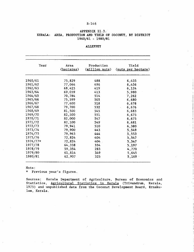
B-146
ALLEPPEY
APPENDIX II.3.KERALA: AREA, PRODUCTION AND YIELD OF COCONUT, BY DISTRICT
1960/61 - 1980/81
Year Area(hectares)
Production (million nuts)
Yield(nuts ner hectare)
1960/61 75,829 488 6,4351961/62 77,064 496 6,4361962/63 68,425 419 6,1241963/64 69,059 413 5,9801964/65 70,784 514 7,2621965/66 75,599 505 6,6801966/67 77,600 518 6,6781967/68 79,700 532 6,6761968/69 81,500 545 6,6831969/70 82,500 551 6,6751970/71 82,000 547 6,6751971/72 82,100 549 6,6811972/73 79,941 510 6,3801973/74 79,900 443 5,5491974/75 79,963 444 5,5531975/76 72,824 404 5,5471976/77* 72,824 404 5,5471977/78 64,338 334 5,1971978/79 59,354 283 4,7701979/80 61,814 349 5,6451980/81 62,907 325 5,169
Note:* Previous year's figures.
Sources: Kerala Department of Agriculture, Bureau of Economics and Statistics, Agricultural Statistics in Kerala (Trivandrum, Kerala, 1975) and unpublished data from the Coconut Development Board, Ernaku- lam, Kerala.
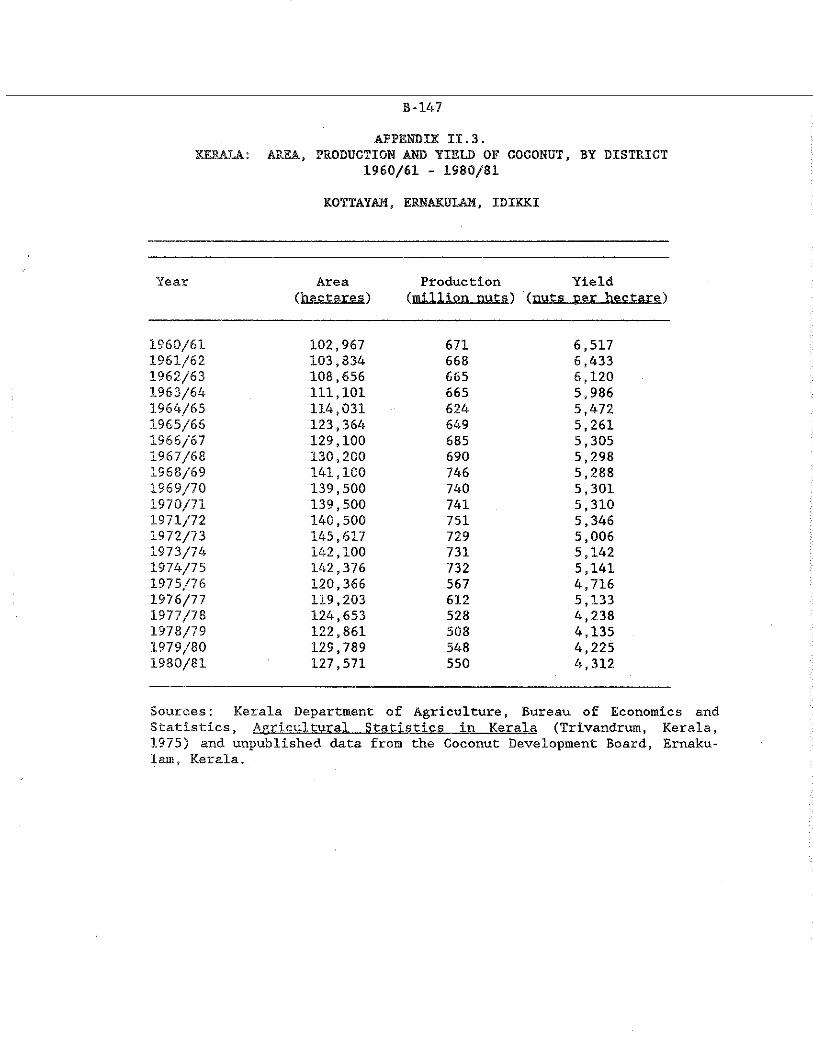
B-147
KOTTAYAM, ERNAKULAM, IDIKKI
APPENDIX II.3.KERALA: AREA, PRODUCTION AND YIELD OF COCONUT, BY DISTRICT
1960/61 - 1980/81
Year Area(hectares)
Production (million nuts)
Yield(tmts^perjhectare)
1960/61 102,967 671 6,5171961/62 103,834 668 6,4331962/63 108,656 665 6,1201963/64 111,101 665 5,9861964/65 114,031 624 5,4721965/66 123,364 649 5,2611966/67 129,100 685 5,3051967/68 130,200 690 5,2981968/69 141,100 746 5,2881969/70 139,500 740 5,3011970/71 139,500 741 5,3101971/72 140,500 751 5,3461972/73 145,617 729 5,0061973/74 142,100 731 5,1421974/75 142,376 732 5,1411975/76 120,366 567 4,7161976/77 119,203 612 5,1331977/78 124,653 528 4,2381978/79 122,861 508 4,1351979/80 129,789 548 4,2251980/81 127,571 550 4,312
Sources: Kerala Department of Agriculture, Bureau of Economics and Statistics, Agricultural Statistics in Kerala (Trivandrum, Kerala, 1975) and unpublished data from the Coconut Development Board, Ernaku- lam, Kerala.
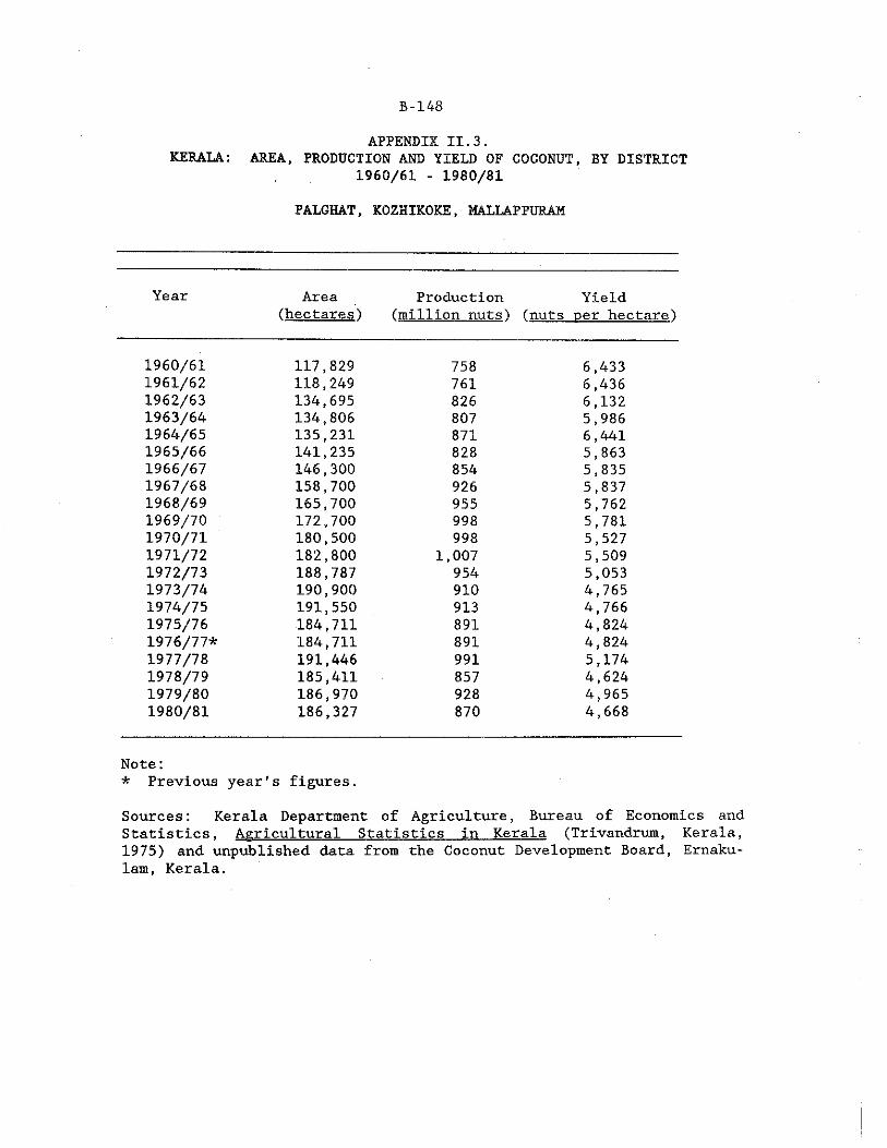
B-148
PALGHAT, KOZHIKOKE, MALLAPPURAM
APPENDIX II.3.KERALA: AREA, PRODUCTION AND YIELD OF COCONUT, BY DISTRICT
1960/61 - 1980/81
Year Area Production Yield(hectares) (million nuts) (nuts t>er hectare)
1960/61 117,829 758 6,4331961/62 118,249 761 6,4361962/63 134,695 826 6,1321963/64 134,806 807 5,9861964/65 135,231 871 6,4411965/66 141,235 828 5,8631966/67 146,300 854 5,8351967/68 158,700 926 5,8371968/69 165,700 955 5,7621969/70 172,700 998 5,7811970/71 180,500 998 5,5271971/72 182,800 1,007 5,5091972/73 188,787 954 5,0531973/74 190,900 910 4,7651974/75 191,550 913 4,7661975/76 184,711 891 4,8241976/77* 184,711 891 4,8241977/78 191,446 991 5,1741978/79 185,411 857 4,6241979/80 186,970 928 4,9651980/81 186,327 870 4,668
Note:* Previous year's figures.
Sources: Kerala Department of Agriculture, Bureau of Economics andStatistics, Agricultural Statistics in Kerala (Trivandrum, Kerala, 1975) and unpublished data from the Coconut Development Board, Ernaku- lam, Kerala.
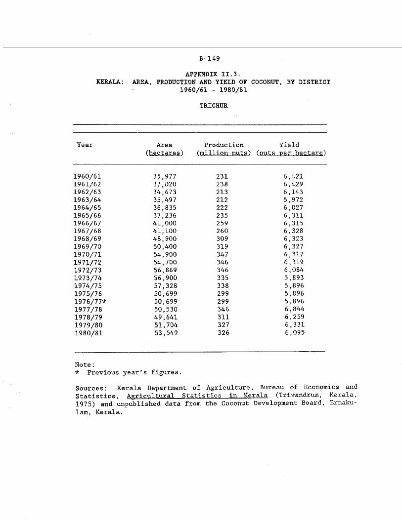
B-149
TRICHUR
APPENDIX II.3.KERALA: AREA, PRODUCTION AND YIELD OP COCONUT, BY DISTRICT
1960/61 - 1980/81
Year Area(hectares')
Production (million nuts)
Yield(nuts per hectare)
1960/61 35,977 231 6,4211961/62 37,020 238 6,4291962/63 34,673 213 6,1431963/64 35,497 212 5,9721964/65 36,835 222 6,0271965/66 37,236 235 6,3111966/67 41,000 259 6,3151967/68 41,100 260 6,3281968/69 48,900 309 6,3231969/70 50,400 319 6,3271970/71 54,900 347 6,3171971/72 54,700 346 6,3191972/73 56,869 346 6,0841973/74 56,900 335 5,8931974/75 57,328 338 5,8961975/76 50,699 299 5,8961976/77* * 50,699 299 5,8961977/78 50,530 346 6,8441978/79 49,641 311 6,2591979/80 51,704 327 6,3311980/81 53,549 326 6,095
Note:* Previous year's figures.
Sources: Kerala Department of Agriculture, Bureau of Economics andStatistics, Agricultural Statistics in Kerala (Trivandrum, Kerala, 1975) and unpublished data from the Coconut Development Board, Ernaku- lam, Kerala.
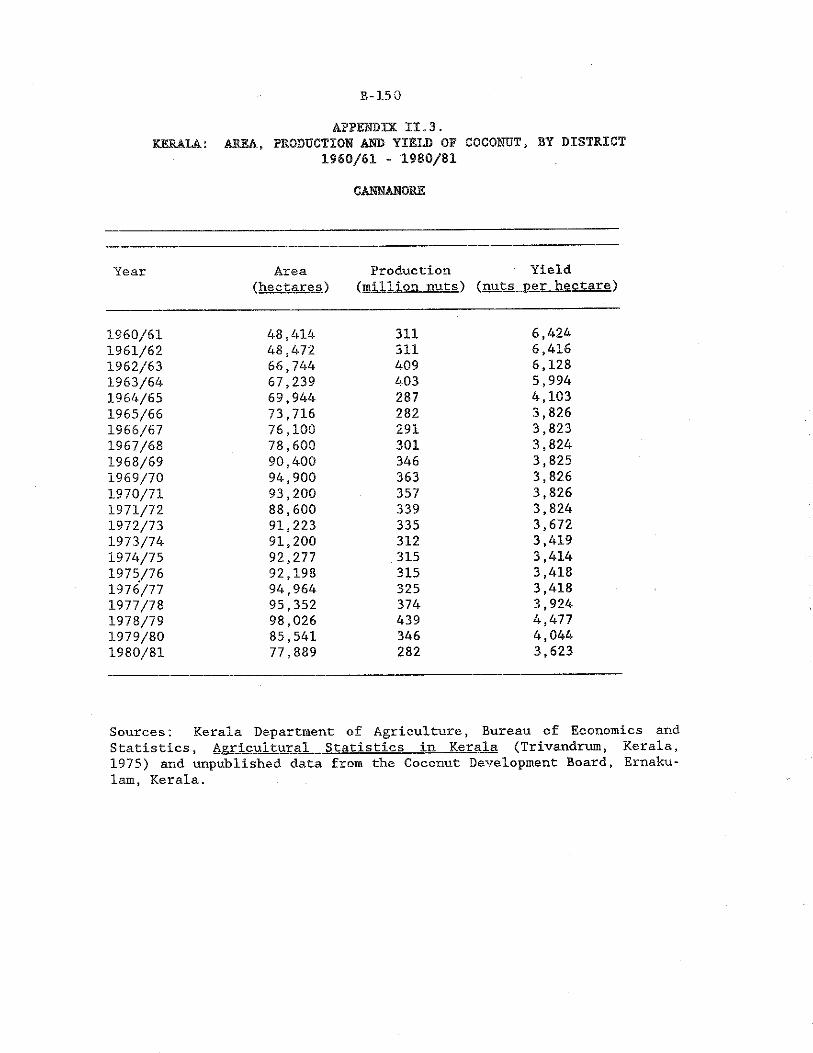
B-150
CANNANORE
APPENDIX II.3.KERALA: AREA, PRODUCTION AND YIELD OF COCONUT, BY DISTRICT
1960/61 - 1980/81
Year Area(hectares)
Production(million nuts)
Yield(nuts per hectare)
1960/61 48,4141961/62 48,4721962/63 66,7441963/64 67,2391964/65 69,9441965/66 73,7161966/67 76,1001967/68 78,6001968/69 90,4001969/70 94,9001970/71 93,2001971/72 88,6001972/73 91,2231973/74 91,2001974/75 92,2771975/76 92,1981976/77 94,9641977/78 95,3521978/79 98,0261979/80 85,5411980/81 77,889
311 6,424311 6,416409 6,128403 5,994287 4,103282 3,826291 3,823301 3,824346 3,825363 3,826357 3,826339 3,824335 3,672312 3,419315 3,414315 3,418325 3,418374 3,924439 4,477346 4,044282 3,623
Sources: Kerala Department of Agriculture, Bureau of Economics and Statistics, Agricultural Statistics in Kerala (Trivandrum, Kerala, 1975) and unpublished data from the Coconut Development Board, Ernaku- lam, Kerala.

B-151APPENDIX II.4.
KERALA: AREA UNDER RICE, COCONUT ANDGROSS CROPPED AREA, BY DISTRICT, 1960/61 - 1977/78
(hectares)
TRIVANDRUM
Year Rice CoconutGross
Cropped Area
1960/611961/621962/631963/641964/651965/661966/671967/681968/691969/701970/711971/721972/731973/741974/751975/761976/771977/78
37,41736,41138,53138,78938,60238,73439,03639,58339,96239,48939.49639.496 39,486 39,765 39,926 37,447 37,976 34,529
55,03955.326 55,815 56,864 58,711 61,150 61,762 70,401 73,885 67,137 76,51577.326 76,194 76,956 77,270 74,074 74,074* 79,335
196,610197,742198,106196,086197,222206,144215,550240,750235,230235,921242,996249,454249,023244,294246,663237,048241,670241,670*
Note:* Previous year's figures.
Sources: Kerala Bureau of Economics and Statistics, AgriculturalStatistics in Kerala (Trivandrum, Kerala, 1975) and unpublished data from the Central Plantation Crops Research Institute, Kasaragod, Kerala.
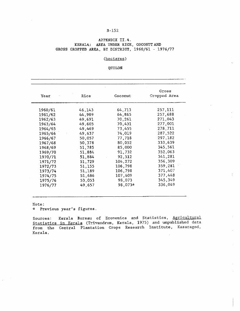
B-152
APPENDIX II.4.KERALA: AREA UNDER RICE, COCONUT AND
GROSS CROPPED AREA, BY DISTRICT, 1960/61 - 1976/77
(hectares)
QUILON
Year Rice CoconutGross
Cropped Area
1960/61 46,143 64,713 257,1111961/62 44,989 64,865 257,6881962/63 49,691 70,261 271,0431963/64 49,605 70,431 277,0011964/65 49,469 73,455 278,7111965/66 49,637 74,019 287,5221966/67 50,057 77,718 297,1821967/68 50,378 80,052 333,6391968/69 51,785 85,000 345,5611969/70 51,884 91,732 352,0631970/71 51,884 92,512 341,2811971/72 51,729 104,272 356,3091972/73 51,155 106,798 359,2811973/74 51,189 106,798 371,4071974/75 51,686 107,409 377,4481975/76 53,053 98,073 345,3491976/77 49,657 98,073* * 336,049
Note:* Previous year's figures.Sources: Kerala Bureau of Economics and Statistics, Agr i cultura1Statistics in Kerala (Trivandrum, Kerala, 1975) and unpub1ished data from the Central Plantation Crops Research Institute, Kasaragod, Kerala.
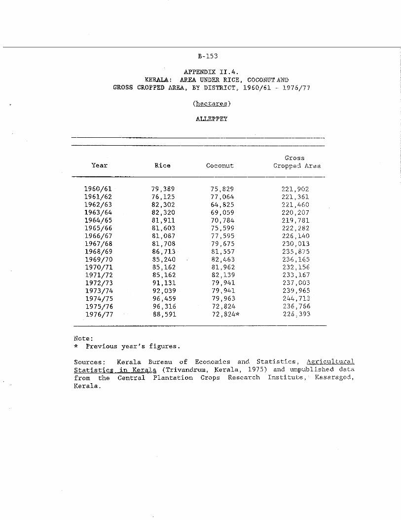
B-153
APPENDIX II.4.KERALA: AREA UNDER RICE, COCONUT AND
GROSS CROPPED AREA, BY DISTRICT, 1960/61 - 1976/77
(hectares)
ALLEPPEY
Year Rice CoconutGross
Cropped Area
1960/61 79,389 75,829 221,9021961/62 76,125 77,064 221,3611962/63 82,302 64,825 221,4601963/64 82,320 69,059 220,2071964/65 81,911 70,784 219,7811965/66 81,603 75,599 222,2821966/67 81,087 77,595 226,1401967/68 81,708 79,675 230,0131968/69 86,713 81,557 235,8751969/70 85,240 82,463 236,1651970/71 85,162 81,962 232,1561971/72 85,162 82,139 233,1671972/73 91,131 79,941 237,0031973/74 92,039 79,941 239,9651974/75 96,459 79,963 244,7131975/76 96,316 72,824 236,7661976/77 88,591 72,824* 226,393
Note:* Previous year's figures.
Sources: Kerala Bureau of Economics and Statistics, AgriculturalStatistics in Kerala (Trivandrum, Kerala, 1975) and unpublished data from the Central Plantation Crops Research Institute, Kasaragod, Kerala.
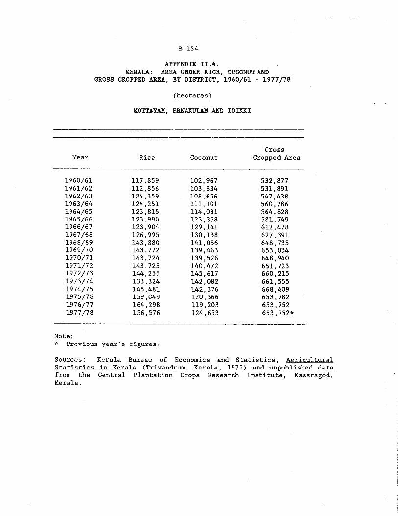
B-154
APPENDIX II.4.KERALA: AREA UNDER RICE, COCONUT AND
GROSS CROPPED AREA, BY DISTRICT, 1960/61 - 1977/78(hectares')
KOTTAYAM, ERNAKULAM AND IDIKKI
Year Rice CoconutGross
Cropped Area
1960/61 117,859 102,967 532,8771961/62 112,856 103,834 531,8911962/63 124,359 108,656 547,4381963/64 124,251 111,101 560,7861964/65 123,815 114,031 564,8281965/66 123,990 123,358 581,7491966/67 123,904 129,141 612,4781967/68 126,995 130,138 627,3911968/69 143,880 141,056 648,7351969/70 143,772 139,463 653,0341970/71 143,724 139,526 648,9401971/72 143,725 140,472 651,7231972/73 144,255 145,617 660,2151973/74 133,324 142,082 661,5551974/75 145,481 142,376 668,4091975/76 159,049 120,366 653,7821976/77 164,298 119,203 653,7521977/78 156,576 124,653 653,752*
Note:* Previous year's figures.
Sources: Kerala Bureau of Economics and Statistics, AgriculturalStatistics in Kerala (Trivandrum, Kerala, 1975) and unpublished data from the Central Plantation Crops Research Institute, Kasaragod, Kerala.
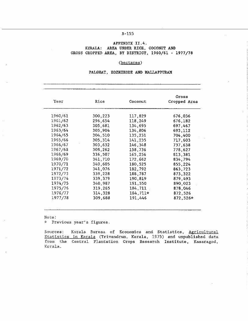
B-155
APPENDIX II.4.KERALA: AREA UNDER RICE, COCONUT AND
GROSS CROPPED AREA, BY DISTRICT, 1960/61 - 1977/78
(hectares)
PALGHAT, KOZHIKODE AND MALIAPPURAM
Year Rice CoconutGross
Cropped Area
1960/61 300,223 117,829 676,0361961/62 296,654 118,249 676,1821962/63 305,681 134,695 697,4671963/64 305,904 134,806 693,1121964/65 304,510 135,231 704,4001965/66 305,314 141,235 717,6031966/67 303,632 146,348 737,6381967/68 308,262 158,736 778,6271968/69 336,507 165,256 813,3811969/70 341,710 172,662 834,7941970/71 340,605 180,525 855,2241971/72 341,076 182,792 863,7231972/73 339,228 188,787 873,3221973/74 339,379 190,819 879,4931974/75 340,987 191,550 890,0231975/76 319,265 184,711 878,0461976/77 314,328 184,711* * 872,5261977/78 309,688 191,446 872,526*
Note:* Previous year's figures.
Sources: Kerala Bureau of Economics and Statistics, AgriculturalStatistics in Kerala (Trivandrum, Kerala, 1975) and unpublished data from the Central Plantation Crops Research Institute, Kasaragod,Kerala.
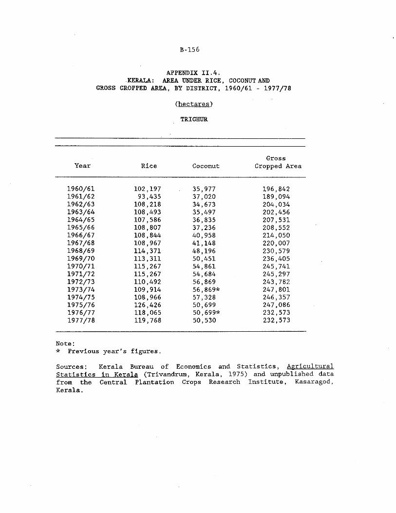
B-156
APPENDIX II.4.-KERALA: AREA UNDER RICE, COCONUT AND
GROSS CROPPED AREA, BY DISTRICT, 1960/61 - 1977/78(hectares)
TRICHUR
Year Rice CoconutGross
Cropped Area
1960/61 102,197 35,977 196,8421961/62 93,435 37,020 189,0941962/63 108,218 34,673 204,0341963/64 108,493 35,497 202,4561964/65 107,586 36,835 207,5311965/66 108,807 37,236 208,5521966/67 108,844 40,958 214,0501967/68 108,967 41,148 220,0071968/69 114,371 48,196 230,5791969/70 113,311 50,451 236,4051970/71 115,267 54,861 245,7411971/72 115,267 54,684 245,2971972/73 110,492 56,869 243,7821973/74 109,914 56,869* 247,8011974/75 108,966 57,328 246,3571975/76 126,426 50,699 247,0861976/77 118,065 50,699* 232,5731977/78 119,768 50,530 232,573
Note:* Previous year's figures.
Sources: Kerala Bureau of Economics and Statistics, AgriculturalStatistics in Kerala (Trivandrum, Kerala, 1975) and unpublished data from the Central Plantation Crops Research Institute, Kasaragod, Kerala.
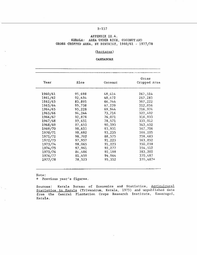
B-157
APPENDIX II.4.KERALA; AREA UNDER RICE, COCONUT AND
GROSS CROPPED AREA, BY DISTRICT, 1960/61 - 1977/78
(hectares)
GANNANORE
Year Rice CoconutGross
Cropped Area
1960/611961/621962/631963/641964/651965/661966/671967/681968/691969/701970/711971/721972/731973/741974/751975/761976/771977/78
95,698 92,434 83,895 95,738 95,228 94,244 92,878 93,65197.65398.653 98,692 98,702 97,957 98,065 97,961 84,486 81,459 78,523
48,414 48,472 66,744 67,239 69,944 73,716 76,071 78,571 90,393 93,931 93,235 88,57591.22391.223 92,277 92,198 94,964 95,352
267,514 267,283 307,222 312,056 316,974 322,492 318,933 333,012 343,402 367,706 366,205 358,683 363,852 350,038 354,512 383,202 370,487 370,487* *
Note:* Previous year's figures.
Sources: Kerala Bureau of Economics and Statistics, AgriculturalStatistics in Kerala (Trivandrum, Kerala, 1975) and unpublished datafrom the Central Plantation Crops Research Institute, Kasaragod, Kerala.
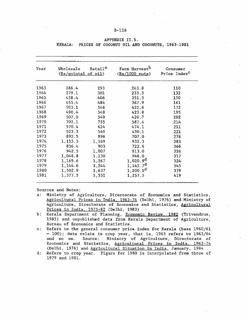
B-isa
APPENDIX II.5.KERALA: PRICES OF COCONUT OIL AND COCONUTS4 1963-1981
Year Wholesale Retail3- Farm Harvest^ Consumer(Rs/auintal of oil} (Rs/1000 nuts) Price Indexc
1963 286.4 293 243.8 1101964 279.1 301 233.3 1321965 438.4 406 351.3 1501966 455.4 484 367.9 1611967 503.1 546 422.6 1721968 490.4 548 423.8 1951969 507.0 549 420.7 2021970 702.1 755 587.4 2141971 570.4 624 474.1 2111972 523.3 549 430.1 2211973 892.5 896 707.0 2761974 1,153.3 1,169 932.3 3831975 836.4 903 722.6 3661976 942.5 1,007 813.0 3261977 1,048.8 1,130 948.0 3171978 1,169.6 1,267 1,020.9d 3241979 1,144.6 1,244 1,142.7d 3451980 1,502.9 1,637 l,200.1d 3791981 1,377.5 1,531 1,257.5 419
Sources and Notes:a: Ministry of Agriculture, Directorate of Economics and Statistics,
Agricultural Prices in India. 1963-74 (Delhi, 1976) and Ministry of Agriculture, Directorate of Economics and Statistics, Agricultural Prices in India. 1975-82 (Delhi, 1983)
b: Kerala Department of Planning, Economic Review. 1982 (Trivandrum,1983) and unpublished data from Kerala Department of Agriculture, Bureau of Economics and Statistics.
c: Refers to the general consumer price index for Kerala (base 1960/61= 100); data relate to crop year, that is, 1963 refers to 1963/64 and so on. Source: Ministry of Agriculture, Directorate ofEconomics and Statistics, Agricultural Prices in India. 1963-74 (Delhi, 1976) and Agricultural Situation in India. January, 1984
d: Refers to crop year. Figure for 1980 is interpolated from those of1979 and 1981.
APPENDIX III.STATISTICS RELATING TO OIL PALM
B-159

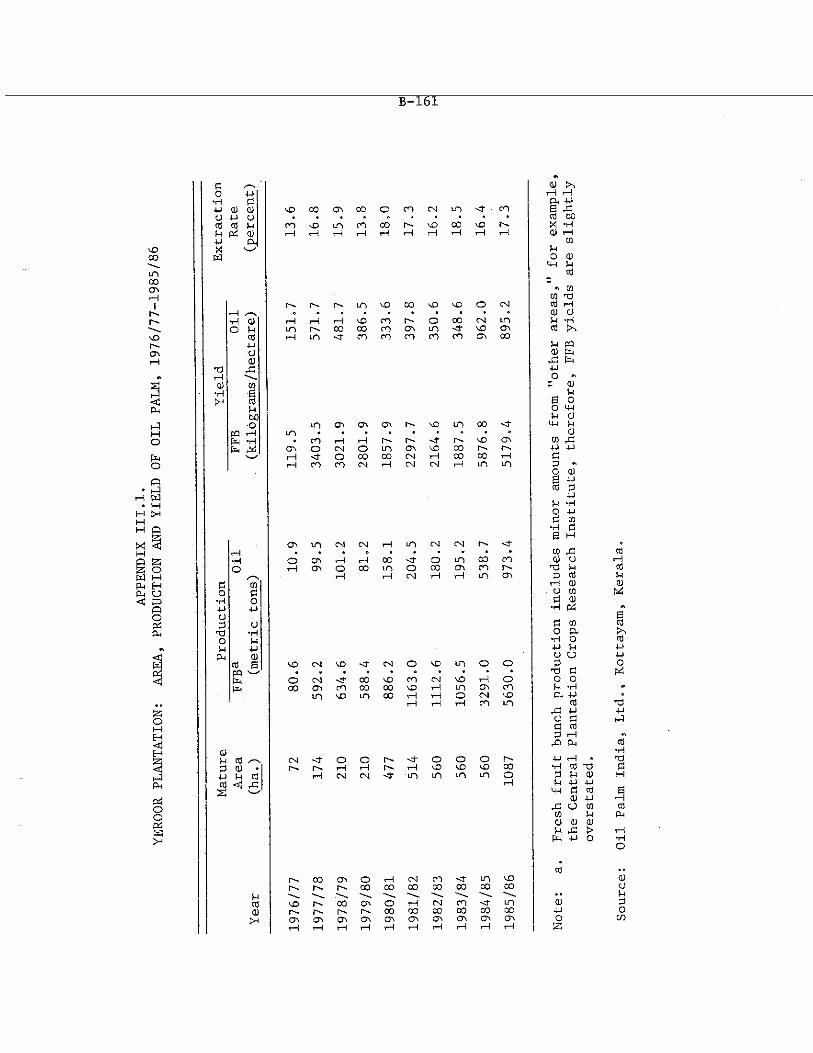
APPE
NDIX
III
.1.
YERO
OR PLANTATION:
AREA,
PRODUCTION AND YIE
LD O
F OIL
PALM,
1976/77-1985/86
B^TUT
d ✓ '"■s*1
cdo 4 J rH rH*H d p i 4 J4 J CD oj vD 0 0 a v 0 0 o CO CM n CO b - dCD 4-1 a • * * g g * g • • • d DOd d d DO vD n CO 0 0 p - vO 0 0 vD r^ . !*! -Hd Pi a> rH hH rH 1—1 rH rH rH i—l i—1 i—i QJ r-H4-1 Cu CO«
H for
s are
CO TD1 "- r-H r " . m VO 0 0 vO vO O CM d rH
T-~| g • e g g g • • • * QJ CD■rf a) i—1 i—i rH vO CO r - O 0 0 CM i n d ‘rHo d m p -. 0 0 0 0 CO OV n vO OV d f n
d i—i m •ct CO CO CO CO CO a v 0 04-1 d pqu CD
a j g d pH
TO ,G 4-1rH 0 *>
CD CO - QJ•H g J-Id B od O HHDO d CDO LO CTV a v 0V r - ID i n 0 0 •d- *4H d
pq rH LO • g . g g « • • g CD
Ph ■H • CO rH rH r- - P - < r P - vO OV cn g d
Fh OV o CM O i n OV vO 0 0 p - p-* 4-1 4-1'_<■ rH *st O 0 0 0 0 CM rH 0 0 0 0 rH d
rH CO CO CM i—i CM CM rH in in d * O QJB dd d4-1U *HO 4-1d co•rl dS HCTV in CM CM rH m CM CM p-
rH . g g g g g g g • CO gd•H O OV 1—1 I—1 00 MS’ O m 00 CO CD Oo OV o 00 in O 00 Ov CO 1". TO J-IrH i—i CM rH rH in Ov d dd CO rH QJO a O CO
•rH o d Q)4-1 4-1 *rf CdCDd O d cotD o &O d ■H O1-1 U 4-4 J-IpH aj u u
d g v O CM vO ■d- CM O vO m o O dp q ' __ . s ( g g g g » • • t o do CM - d 00 vO CO CM vO rH o o oF h 00 ov CO CO 00 I D rH in OV CO d *H
n v O in 00 rH rH o CM vO a * 4 JrH t— l i—i CO n d
0)d
g d 4 Jo d d dd rHgQ P4
d CM • d - o o ■d - o o o C " 4-1 rH
d 0) g t " - r - rH rH r - ' . rH VO vO vO 00 *H d4-1 d d r H CM CM m n in in o d dd <sj£ rH d 4-iS i d d
QJgd aCOQJ QJd g d
pH 4-1
dr- 00 OV O rH CM CO -cf in VDi'-- n- 00 00 00 00 00 00 00S-l VO n- 00 OV o i—! CM CO •<r m CDGJ r- e' p*. r-- 00 00 CO 00 00 00 + JJ>H ov en ov OV CTV OV OV OV OV CTV orH I-1 rH r - 1 i—1 rH rH rH rH rH S3 So
urce:
Oil
Palm India,
Ltd.,
Kottayam,
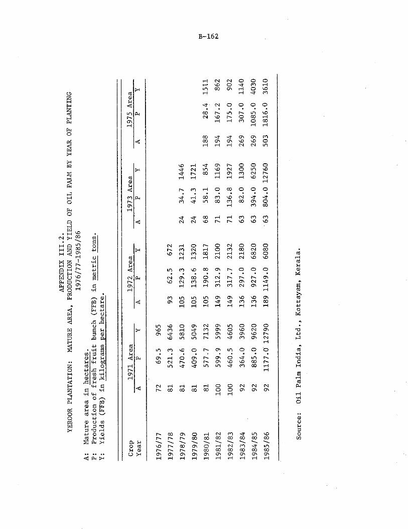
APPE
NDIX
III
.2.
YERO
OR P
LANT
ATIO
N:
MATU
RE A
REA,
PRO
DUCT
ION
AND
YIEL
D OE
OIL
PAL
M BY
YEA
R OF
PLA
NTIN
G19
76/7
7-19
85/8
6
B-162
cnPJop i
a• HU
* r f
QJp p u[ p toEp p i
CJQJ
rC 1-JhaC P i3 0)
X PP
P I 0)* 'H s
w rt cOa) M Piu 4H 6 0rt op> XI i—IO cna QJ
x : um a
F3 •H■H <+-t
o /"NCO ppoj a Phu 0 P hCO * r l 'w '
■M<u O CDPi 3 HO
1---1p i O QJrt Pt ' r tS P-«
- < pH |>H
rH CM CM o o orH vO o CO rH<n 00 OV rH o vO
fti rH rH *4t COQJ
< j Hfr CM o o o o• • • « • •
m Ph CO r - m r - ' in vOCM vO t" . o 00 rH
Ov rH rH CO o 001—I 1—1 rH
00 < r av OV CO<4 00 OV CT\ vD VD o
rH rH rH CM CM i n
VO rH <3- OV O O Q>H < r CM m vD CM o m VO
< r r^. 00 t—1 Ov cO CM h -cO rH rH 1--1 vO CMQJ rH
C cO 1—1 O 00 o O oCO Ph Ht rH CO CO VD CM <3-r-> CO <T m 00 CO 00 OV OOv rH CO 00rH
<0- <T 00 tH rH CO CO CO<3 CM CM vO r>. C"- vO vO vO
CM rH O r~- o CM o O o>H I-'. CO CM H o CO 00 CM 00 •
vO CM CO 00 1—1 rH rH 00 o rtcO H rH CM cm CM vO vO rHQJ «Pi pj
<3 n CO VO 00 av r-. O o o QJ
CM PH CM CSV 00 o CM I-'. OVvO CM CO av rH i—i Ov CM - a A
av rH rH rH CO CO CM Ov rH B»—i rt
bCO i n i n i n av Ov vO vO Ov rt< 3 av O o o MJ* MT CO CO CO p i
rH rH rH rH i—! rH rHo
m MO o OV CM OV n O O o •> 1 vD CO !—f -Mf CO OV o vO CM Ov TO
OV Mj* 00 o t—1 av vO Ov VO r~- PIvO n m LO CO Ov CM i J
rHcO AQJ n CO vO o a v i n O O o «Pi •rt
< 3 Ph Ov rH o av f~r Ov o m C'-vo CM h - o r - . Ov vO vO CO f" . (3
rH n < r m m CO 0 0 rH MrH
OV erH rHrt
CM t-i rH rH o o CM CM CM P4<0 f-- CO 00 00 0 0 o o OV OV OV
\—i rH rH*r!O
a!uPiPt
r^. 00 OV o rH CM CO ~cr i n vO Or^. r - ' 00 00 00 00 CO 00 00 cn
& H "'-H.O cO vD 00 OV o 1—1 CM CO •cf nP! QJ c - r^. 00 00 CO 00 00 00
a >H Ov a v o v a v a v OV Ov OV av avt—1 rH rH H T—l 1—1 rH rH rH rH
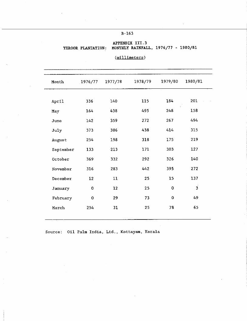
B-163
APPENDIX III.3YEROOR PLANTATION: MONTHLY RAINFALL, 1976/77 - 1980/81
(millimeters)
Month 1976/77 1977/78 1978/79 1979/80 1980/81
April 336 140 115 184 201
May 164 438 495 248 158
June 142 359 272 267 494
July 373 386 438 414 315
Augus t 254 198 318 175 219
September 133 213 171 303 127
October 369 332 292 326 140
November 316 283 442 395 272
December 12 11 25 15 137
January 0 12 25 0 3
February 0 29 73 0 49
March 254 31 25 78 65
Source: Oil Palm India, Ltd., Kottayam, Kerala
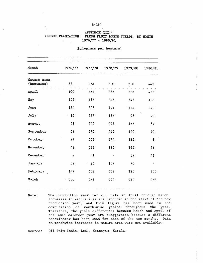
B-164
(kilograms per hectare)
APPENDIX III.4YEROOR PLANTATION: FRESH FRUIT BUNCH YIELDS, BY MONTH
1976/77 - 1980/81
Month 1976/77 1977/78 1978/79 1979/80 1980/81
Mature area (hectares) 72 174 210 210 442April 100 131 288 728 433May 102 137 248 343 168June 174 208 194 174 242
July 15 257 137 93 90
August 28 240 275 156 87
September 59 270 259 140 70
October 97 556 274 132 8
November 42 583 185 162 78
December 7 41 - 39 46
January 52 83 159 90 -
February 147 308 338 125 255
March 300 592 665 625 394
Note: The production year for oil palm in April through March.Increases in mature area are reported at the start of the new production year, and this figure has been used in the computation of month-wise yields throughout the year. Therefore, the yield differences between March and April of the same calender year are exaggerated because a different denominator has been used for each of the two months. Data on monthwise increases in mature area were not available.
Source: Oil Palm India, Ltd., Kottayam, Kerala.
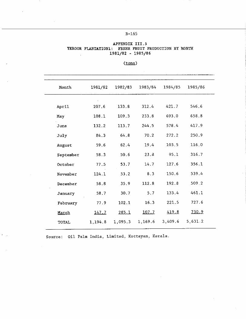
B-165
( tons)
APPENDIX III.5YEROOR PLANTATION!: FRESH FRUIT PRODUCTION BY MONTH
1981/82 - 1985/86
Month 1981/82 1982/83 1983/84 1984/85 1985/86
April 207.6 133.8 312.4 421.7 546.6
May 108.1 109.3 233.8 693.0 658.8
June 132.2 113.7 244.5 578.4 417.9
July 84.3 64.8 70.2 272.2 250.9
August 59.6 62.4 19.4 103.5 116.0
September 58.3 50.6 23.8 95.1 316.7
October 77.5 53.7 14.7 127.6 356.1
November 124.1 53.2 8.3 150.6 539,4
December 58.8 35.9 112.8 192.8 509.2
J anuary 58.7 30.7 5.7 133.4 461.1
February 77.9 102.1 16.3 221.5 727.6
March 147.7 285.1 107.7 419.8 730.9
TOTAL 1,194.8 1,095.3 1,169.6 3,409.6 5,631.2
Source: Oil Palm India, Limited, Kottayam, Kerala,
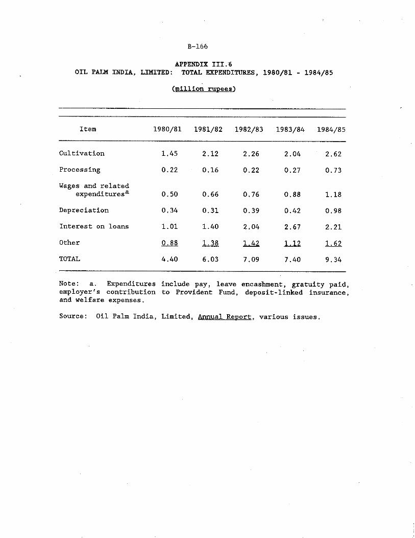
B-166
APPENDIX III.6OIL PALM INDIA, LIMITED: TOTAL EXPENDITURES, 1980/81 - 1984/85
(million rupees^
Item 1980/81 1981/82 1982/83 1983/84 1984/85
Cultivation 1.45 2.12 2.26 2.04 2.62Processing 0.22 0.16 0.22 0.27 0.73Wages and related
expend!turesa 0.50 0.66 0.76 0.88 1.18Depreciation 0.34 0.31 0.39 0.42 0.98Interest on loans 1.01 1.40 2.04 2.67 2.21Other 0.88 1.38 1.42 1.12 1.62TOTAL 4.40 6.03 7.09 7.40 9.34
Note: a. Expenditures include pay, leave encashment, gratuity paid, employer's contribution to Provident Fund, deposit-linked insurance, and welfare expenses.
Source: Oil Palm India, Limited, Annual Report, various issues.
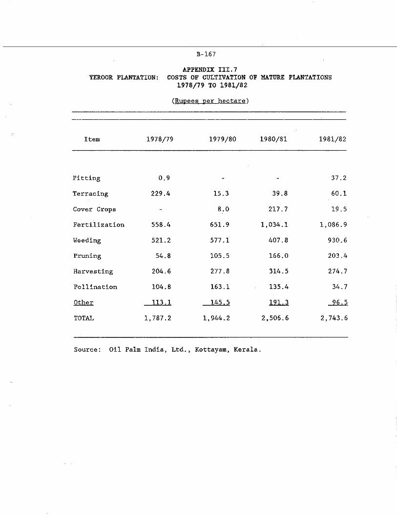
B-167
(Rupees per hectare)
APPENDIX III. 7YEROOR PLANTATION: COSTS OF CULTIVATION OF MATURE PLANTATIONS
1978/79 TO 1981/82
Item 1978/79 1979/80 1980/81 1981/82
Pitting 0.9 37.2
Terracing 229.4 15.3 39.8 60.1
Cover Crops -• 8.0 217.7 19.5
Fertilization 558.4 651.9 1,034.1 1,086.9
Weeding 521.2 577.1 407.8 930.6
Pruning 54.8 105.5 166.0 203.4
Harvesting 204.6 277.8 314.5 274.7
Pollination 104.8 163.1 135.4 34.7
Other 113.1 145.5 191.3 96.5
TOTAL 1,787.2 1,944.2 2,506.6 2,743.6
Source: Oil Palm India, Ltd., Kottayam, Kerala.
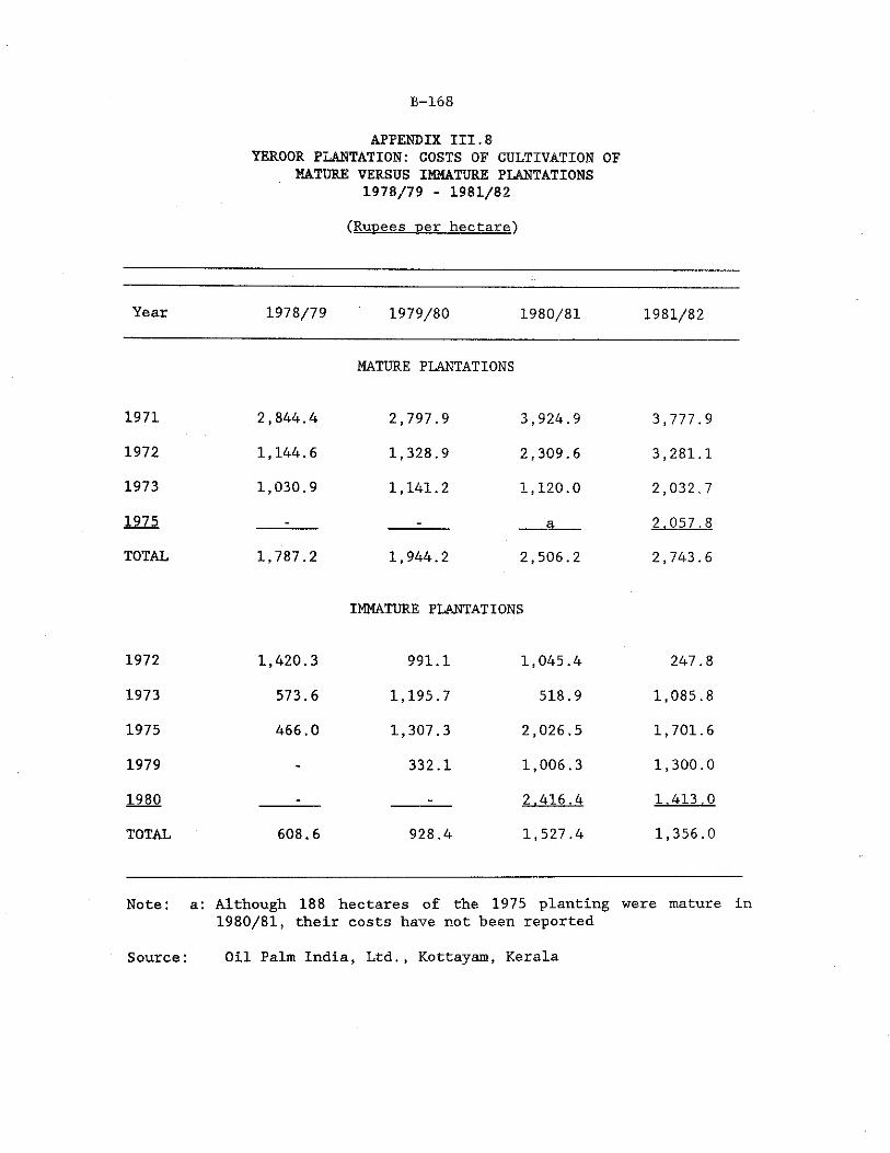
B-168
APPENDIX III.8YEROOR PLANTATION: COSTS OF CULTIVATION OF
MATURE VERSUS IMMATURE PLANTATIONS 1978/79 - 1981/82
(Rupees per hectare)
Year 1978/79 1979/80 1980/81 1981/82
MATURE PLANTATIONS
1971 2,844.4 2,797.9 3,924.9 3,777.9
1972 1,144.6 1,328.9 2,309.6 3,281.11973 1,030.9 1,141.2 1,120.0 2,032.71975 _ a 2.057.8
TOTAL 1,787.2 1,944.2 2,506.2 2,743.6
IMMATURE PLANTATIONS
1972 1,420.3 991.1 1,045.4 247.8
1973 573.6 1,195.7 518.9 1,085.8
1975 466.0 1,307.3 2,026.5 1,701.6
1979 - 332.1 1,006.3 1,300.0
1980 w* 2.416.4 1.413.0
TOTAL 608.6 928.4 1,527.4 1,356.0
Note: a: Although 188 hectares of the 1975 planting were mature in1980/81, their costs have not been reported
Source: Oil Palm India, Ltd., Kottayam, Kerala
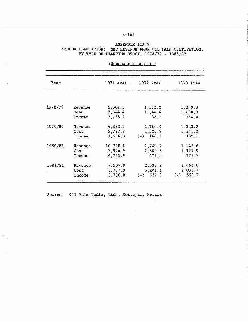
B-169
APPENDIX III.9YEROOR PLANTATION: NET REVENUE FROM OIL PALM CULTIVATION,
BY TYPE OF PLANTING STOCK, 1978/79 - 1981/82
(Rupees per hectare)
Year 1971 Area ■ 1972 Area 1973 Area
1978/79 RevenueCostIncome
5,582.52,844,42,738.1
I, 183,2II, 44.6
38.7
1,389.31,030.9
358.4
1979/80 RevenueCostIncome
4.333.92.797.9 1,536.0
1,164.0 1,328.9
(-) 164.8
1.323.21.141.2
182.1
1980/81 RevenueCostIncome
10,718.83.924.96.783.9
2,780.92,309.6
471.3
1,248.61,119.9
128.7
1981/82 RevenueCostIncome
7.507.93.777.9 3,730.0
2,628.2 3,281.1
(-) 652.9
1,463.0 2,032,7
(-) 569.7
Source: Oil Palm India, Ltd., Kottayam, Kerala

APPENDIX IV.
MISCELLANEOUS STATISTICS RELATING TO OILSEEDS AND VEGETABLE OILS
B- 171

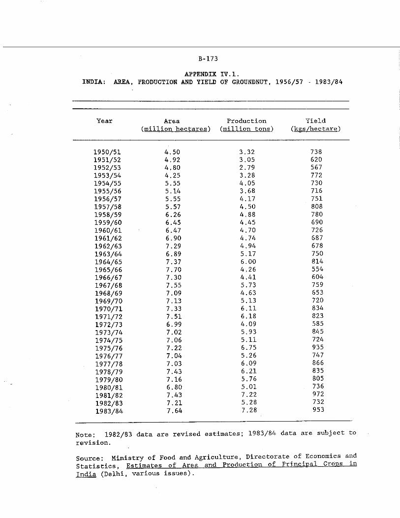
B-173
INDIA: AREA,APPENDIX
PRODUCTION AND YIELDIV. 1.OF GROUNDNUT, 1956/57 - 1983/84
Year Area(million hectares)
Production ("million tons)
Yield(kgs/hectare)
1950/51 4.50 3.32 7381951/52 4.92 3.05 6201952/53 4.80 2.79 5671953/54 4.25 3.28 7721954/55 5.55 4.05 7301955/56 5.14 3.68 7161956/57 5.55 4.17 7511957/58 5.57 4.50 8081958/59 6.26 4.88 7801959/60 6.45 4.45 6901960/61 6.47 4.70 7261961/62 6.90 4.74 6871962/63 7.29 4.94 6781963/64 6.89 5.17 7501964/65 7.37 6.00 8141965/66 7.70 4.26 5541966/67 7.30 4.41 6041967/68 7.55 5.73 7591968/69 7.09 4.63 6531969/70 7.13 5.13 7201970/71 7.33 6.11 8341971/72 7.51 6.18 8231972/73 6.99 4.09 5851973/74 7.02 5.93 8451974/75 7.06 5.11 7241975/76 7.22 6.75 9351976/77 7.04 5.26 7471977/78 7.03 6.09 8661978/79 7.43 6.21 8351979/80 7.16 5.76 8051980/81 6.80 5.01 7361981/82 7.43 7.22 9721982/83 7,21 5.28 7321983/84 7.64 7.28 953
Note: 1982/83 data are revised estimates; 1983/84 data are subject torevision.Source: Ministry of Food and Agriculture, Directorate of Economics andStatistics, Estimates of Area and Production of Principal Cro&s^nIndia (Delhi, various issues).
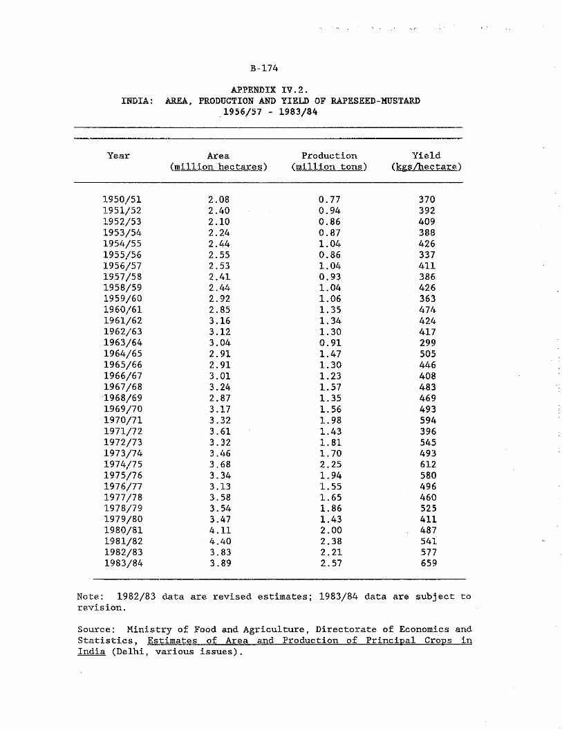
B-174
APPENDIX IV.2.INDIA: AREA, PRODUCTION AND YIELD OF RAPESEED-MUSTARD
1956/57 - 1983/84
Year Area(million hectares)
Production (million tons)
Yield(kgs/hectare)
1950/51 2.08 0.77 3701951/52 2.40 0.94 3921952/53 2.10 0.86 4091953/54 2.24 0.87 3881954/55 2.44 1.04 4261955/56 2.55 0.86 3371956/57 2.53 1.04 4111957/58 2.41 0.93 3861958/59 2.44 1.04 4261959/60 2.92 1.06 3631960/61 2.85 1,35 4741961/62 3.16 1.34 4241962/63 3.12 1.30 4171963/64 3.04 0.91 2991964/65 2.91 1.47 5051965/66 2.91 1.30 4461966/67 3.01 1.23 4081967/68 3.24 1.57 4831968/69 2.87 1.35 4691969/70 3.17 1.56 4931970/71 3.32 1.98 5941971/72 3.61 1.43 3961972/73 3.32 1.81 5451973/74 3.46 1.70 4931974/75 3.68 2.25 6121975/76 3.34 1.94 5801976/77 3.13 1.55 4961977/78 3.58 1.65 4601978/79 3.54 1,86 5251979/80 3.47 1.43 4111980/81 4.11 2.00 4871981/82 4.40 2.38 5411982/83 3.83 2.21 5771983/84 3.89 2.57 659
Note: 1982/83 data are revised estimates; 1983/84 data are subject torevision.
Source: Ministry of Food and Agriculture, Directorate of Economics andStatistics, Estimates of Area and Production of Principal Crons inIndia (Delhi, various issues).
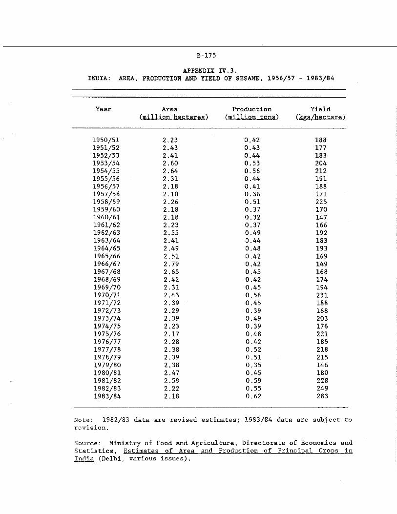
B-175
APPENDIX IV.3.INDIA: AREA, PRODUCTION AND YIELD OF SESAME, 1956/57 - 1983/84
Year Area(million hectares')
Production ('million tons')
Yield
1950/51 2.23 0.42 1881951/52 2.43 0.43 1771952/53 2.41 0.44 1831953/54 2.60 0.53 2041954/55 2.64 0.56 2121955/56 2.31 0.44 1911956/57 2.18 0.41 1881957/58 2.10 0.36 1711958/59 2.26 0.51 2251959/60 2.18 0.37 1701960/61 2.18 0.32 1471961/62 2.23 0.37 1661962/63 2.55 0.49 1921963/64 2.41 0.44 1831964/65 2.49 0.48 1931965/66 2.51 0.42 1691966/67 2.79 0.42 1491967/68 2.65 0.45 1681968/69 2.42 0.42 1741969/70 2.31 0.45 1941970/71 2.43 0.56 2311971/72 2.39 0.45 1881972/73 2.29 0.39 1681973/74 2.39 0.49 2031974/75 2.23 0.39 1761975/76 2.17 0.48 2211976/77 2.28 0.42 1851977/78 2.38 0.52 2181978/79 2.39 0.51 2151979/80 2.38 0.35 1461980/81 2.47 0.45 1801981/82 2.59 0.59 2281982/83 2.22 0.55 2491983/84 2.18 0.62 283
Note: 1982/83 data are revised estimates; 1983/84 data are subject trevision.
Source: Ministry of Food and Agriculture, Directorate of Economics andStatistics, Estimates of Area and Production of Principal Crops inIndia (Delhi, various issues).
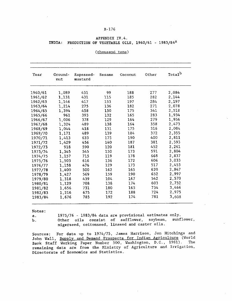
B-176
APPENDIX IV.4,INDIA: PRODUCTION OF VEGETABLE OILS, 1960/61 - 1983/84a
(thousand tons)
Year Groundnut
Rapeseed-mustard
Sesame Coconut Other Total*3
1960/61 1,089 431 99 188 277 2,0841961/62 1,131 431 115 185 282 2,1441962/63 1,146 417 153 197 284 2,1971963/64 1,214 275 136 182 271 2,0781964/65 1,394 458 150 175 341 2,5181965/66 961 393 132 165 283 1,9341966/67 1,006 378 129 164 279 1,9561967/68 1,324 489 138 164 358 2,4731968/69 1,044 418 131 175 316 2,0841969/70 1,171 489 139 184 372 2,3551970/71 1,413 633 175 190 400 2,8111971/72 1,429 456 140 187 381 2,5931972/73 918 590 120 181 452 2,2611973/74 1,345 545 150 173 591 2,8041974/75 1,157 715 119 178 668 2,8371975/76 1,503 616 136 172 606 3,0331976/77 1,158 476 129 173 517 2,4531977/78 1,400 500 162 165 620 2,8471978/79 1,427 569 159 190 652 2,9971979/80 1,318 439 104 167 542 2,5701980/81 1,129 708 138 174 603 2,7521981/82 1,656 731 180 165 734 3,4661982/83 1,216 675 172 188 724 2,9751983/84 1,676 785 192 174 781 3,608
Notes:a. 1975/76 - 1983/84 data are provisional estimates only.b. Other oils consist of safflower, soybean, sunflower,
nigerseed, cottonseed, linseed and castor oils.
Sources: For data up to 1974/75, James Harrison, Jon Hitchings andJohn Wall, Supply and Demand Prospects for Indian Agriculture (World Bank Staff Working Paper Number 500, Washington, D.C., 1981). The remaining data are from the Ministry of Agriculture and Irrigation, Directorate of Economics and Statistics.
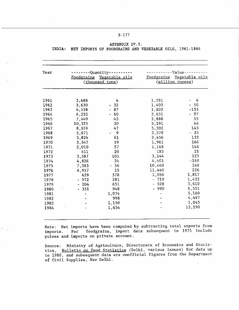
B-177
APPENDIX IV.5.INDIA: NET IMPORTS OF FOODGRAINS AND VEGETABLE OILS, 1961-1984
Year ------ -Quantity----------Foodgrains Vegetable oils
(thous and tons)
------- ---Value----------Foodgrains Vegetable oils
(million rupees)
1961 3,488 4 1,291 - 61962 3,630 - 32 1,403 - 501963 4,538 - 87 1,820 -1331964 6,252 - 60 2,651 - 971965 7,449 43 2,888 551966 10,325 30 5,191 461967 8,659 47 5,302 1431968 5,671 - 9 3,578 - 251969 3,824 61 2,456 1321970 3,547 59 1,961 1661971 2,010 57 1,168 1461972 411 20 183 211973 3,587 103 3,144 1251974 4,826 24 4,401 -1691975 7,383 - 56 10,460 1481976 6,917 15 11,440 2261977 629 378 1,056 1,8171978 - 572 281 - 719 1,4321979 - 204 651 - 528 3,6101980 - 351 948 - 990 6,5511981 - 1,074 - 5,1601982 ~ 998 - 4,4971983 - 1,150 - 5,0451984 - 1,634 - 13,190
Note: Net imports have been computed by subtracting total exports from imports. For foodgrains, import data subsequent to 1975 include pulses and imports on private account.
Source: Ministry of Agriculture, Directorate of Economics and Statistics, Bulletin on Food Statistics (Delhi, various issues) for data up to 1980, and subsequent data are unofficial figures from the Department of Civil Supplies, New Delhi.
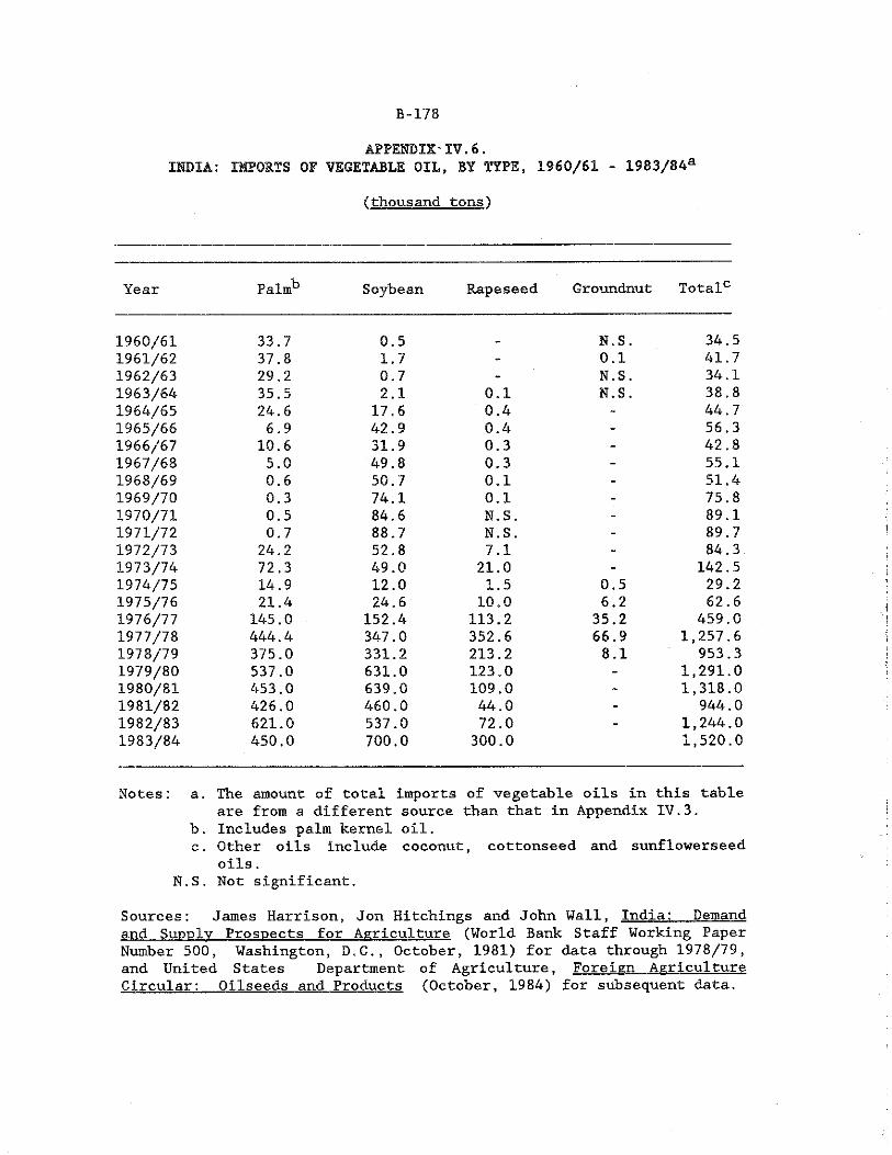
B-17B
APPENDIX-IV.6.INDIA: IMPORTS OF VEGETABLE OIL, BY TYPE, 1960/61 - 1983/84a
(thousand tons)
Year Palmb Soybean Rapeseed Groundnut Total0
1960/61 33.7 0.5 N.S. 34.51961/62 37.8 1.7 - 0.1 41.71962/63 29.2 0.7 - N.S. 34.11963/64 35.5 2.1 0.1 N.S. 38.81964/65 24.6 17.6 0.4 - 44.71965/66 6.9 42.9 0.4 - 56.31966/67 10.6 31.9 0.3 - 42.81967/68 5.0 49.8 0.3 - 55,11968/69 0.6 50.7 0.1 - 51.41969/70 0.3 74.1 0.1 - 75.81970/71 0.5 84.6 N.S. - 89.11971/72 0.7 88.7 N.S. - 89.71972/73 24.2 52.8 7.1 - 84.31973/74 72.3 49.0 21.0 - 142.51974/75 14.9 12.0 1.5 0.5 29.21975/76 21.4 24.6 10.0 6.2 62.61976/77 145.0 152.4 113.2 35.2 459.01977/78 444.4 347.0 352.6 66.9 1,257.61978/79 375.0 331.2 213.2 8.1 953.31979/80 537.0 631.0 123.0 - 1,291.01980/81 453.0 639.0 109.0 - 1,318.01981/82 426.0 460.0 44.0 - 944,01982/83 621.0 537.0 72.0 - 1,244.01983/84 450.0 700.0 300.0 1,520.0
Notes: a. The amount of total imports of vegetable oils in this tableare from a different source than that in Appendix IV.3.
b. Includes palm kernel oil.c. Other oils include coconut, cottonseed and sunflowerseed
oils.N .S . Not significant.
Sources: James Harrison, Jon Hitchings and John Wall, India: Demand and Supply Prospects for Agriculture (World Bank Staff Working Paper Number 500, Washington, D.C., October, 1981) for data through 1978/79, and United States Department of Agriculture, Foreign Agriculture Circular: Oilseeds and Products (October, 1984) for subsequent data.
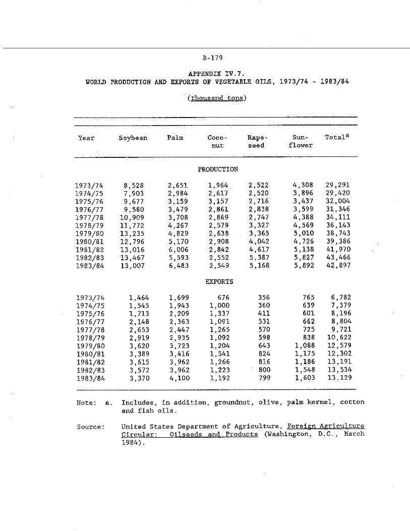
B-179
APPENDIX IV.7.WORLD PRODUCTION AND EXPORTS OF VEGETABLE OILS , 1973/74 - 1983/84
(thousand tons)
Year Soybean Palm Coconut
Rape-seed
Sun- Totala flower
PRODUCTION
1973/74 8,528 2,651 1,964 2,522 4,308 29,2911974/75 7,903 2,984 2,617 2,520 3,896 29,4201975/76 9,677 3,159 3,157 2,716 3,437 32,0041976/77 9,580 3,479 2,861 2,838 3,599 31,3461977/78 10,909 3,708 2,869 2,747 4,388 34,1111978/79 11,772 4,267 2,579 3,327 4,569 36,1431979/80 13,235 4,829 2,638 3,365 5,010 38,7431980/81 12,796 5,170 2,908 4,042 4,726 39,3861981/82 13,016 6,006 2,842 4,617 5,138 41,9701982/83 13,467 5,593 2,552 5,387 5,827 43,4661983/84 13,007 6,483 2,549
EXPORTS
5,168 5,892 42,897
1973/74 1,464 1,699 676 356 765 6,7821974/75 1,545 1,943 1,000 360 639 7,3791975/76 1,713 2,209 1,337 411 601 8,1961976/77 2,148 2,363 1,091 531 662 8,8041977/78 2,653 2,447 1,265 570 725 9,7211978/79 2,919 2,935 1,092 598 838 10,6221979/80 3,620 3,723 1,204 643 1,088 12,5791980/81 3,389 3,416 1,341 824 1,175 12,3021981/82 3,615 3,962 1,266 816 1,186 13,1911982/83 3,572 3,962 1,223 800 1,548 13,5341983/84 3,370 4,100 1,192 799 1,603 13,129
Note: a. Includes, In addition, groundnut, olive, palm kernel, cottonand fish oils.
Source: United States Department of Agriculture, Foreign AgricultureCircular: Oilseeds and Products (Washington, D.C., March1984).
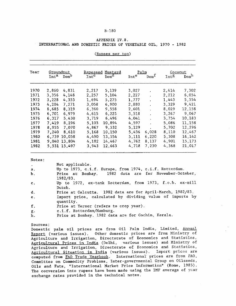
B-180
APPENDIX I?.8,INTERNATIONAL AND DOMESTIC PRICES OF VEGETABLE OIL, 1970 - 1982
(Rupees per ton)
Year Groundnut Inta Domb
Raoeseed Mustard Palm Intc Domb Inte Dom^
Coconut Int§ Domb
1970 2,860 4,831 2,217 5,139 3,027 2,414 7,3021971 3,356 4,148 2,257 5,104 2,227 2,212 6,0541972 3,228 4,353 1,694 5,275 1,777 1,443 5,5541973 4,204 7,271 3,058 6,900 2,880 3,329 9,4211974 8,685 8,319 6,360 9,558 2,601 8,029 12,1581975 6,701 6,979 4,615 6,225 3,518 3,267 9,0671976 6,317 5,430 3,719 6,496 4,041 3,754 10,1831977 7,419 8,296 5,103 10,894 4,597 5,086 11,1581978 8,955 7,070 4,867 9,532 5,129 5,702 12,2961979 7,240 8,610 5,168 10,150 5,436 6,028 8,110 12,4671980 6,739 10,058 4,490 13,554 5,111 6,220 5,308 16,1421981 9,040 13,804 4,182 14,467 4,762 8,137 4,901 15,1731982 5,531 15,497 3,943 12,663 4,718 7,230 4,368 21,017
Notes:. Not applicable,a. Up to 1973, c .i .f . Europe, from 1974, c.i.f. Rotterdam,b. Price at Bombay, 1982 data are for November-October,
1982/83.c . Up to 1972, ex-tank Rotterdam, from 1973, f .o,b. ex-mill
Dutch.d. Price at Calcutta. 1982 data are for April-March, 1982/83.e . Import price, calculated by dividing value of imports by
quantity.f. Price at Yeroor (refers to crop year).g. c.i.f. Rotterdam/Hamburg.h. Price at Bombay. 1982 data are for Cochin, Kerala.
Sources:Domestic palm oil prices are from Oil Palm India, Limited, Annual Report (various issues). Other domestic prices are from Ministry of Agriculture and Irrigation, Directorate of Economics and Statistics, Agricultural Prices in India (Delhi, various issues) and Ministry of Agriculture and Irrigation, Directorate of Economics and Statistics, Agricultural Situation in India (various issues), Import prices are computed from FAQ Trade Yearbook. International prices are from FAO, Committee on Commodity Problems, Inter-governmental Group on Oilseeds, Oils and Fats, "International Market Price Information" (Rome, 1985). The conversion into rupees have been made using the IMF average of year exchange rates provided in the technical notes.
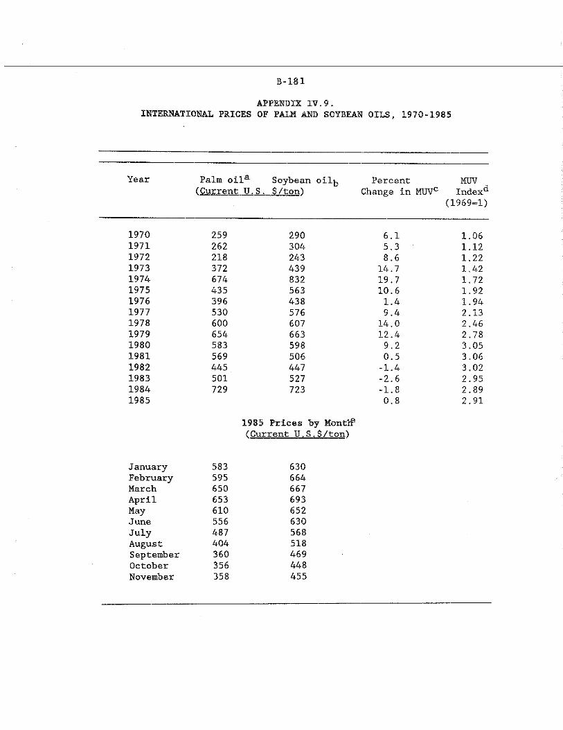
B-18X
APPENDIX IV.9.INTERNATIONAL PRICES OF PALM AND SOYBEAN OILS, 1970-1985
Year Palm oila (Current U.S.
Soybean oil-u S/ton')
PercentChange in MUVC
MUVIndex^
(1969=1)
1970 259 290 6.1 1.061971 262 304 5.3 1.121972 218 243 8.6 1.221973 372 439 14.7 1.421974 674 832 19.7 1.721975 435 563 10.6 1.921976 396 438 1.4 1.941977 530 576 9.4 2.131978 600 607 14.0 2.461979 654 663 12.4 2.781980 583 598 9.2 3.051981 569 506 0.5 3.061982 445 447 -1.4 3.021983 501 527 -2.6 2.951984 729 723 -1.8 2.891985
1985 Prices by Montlf (Current U.S.$/ton)
0.8 2.91
J anuary 583 630February 595 664March 650 667April 653 693May 610 652June 556 630July 487 568August 404 518September 360 469October 356 448November 358 455
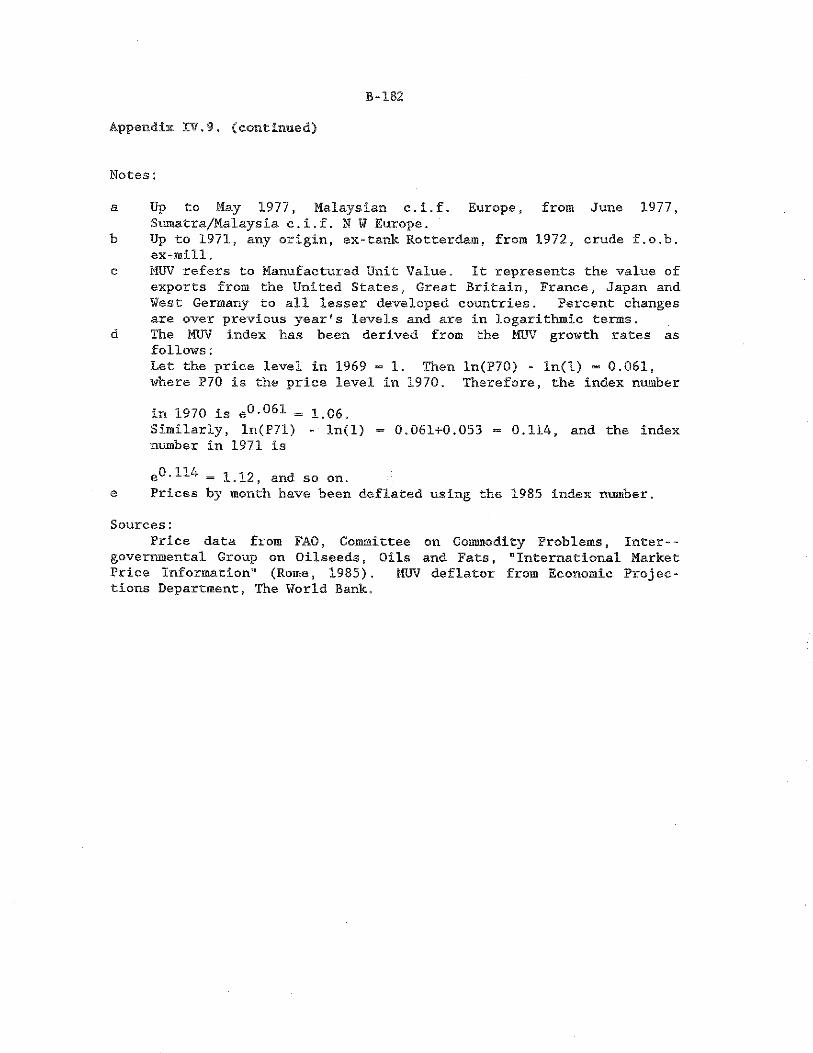
B-182
Appendix IV. 9. (continued)
Notes:
a Up to May 1977, Malaysian c . i. f. Europe, from June 1977,Sumatra/Malaysia c.i.f. If i Europe.
b Up to 1971, any origin, ex-tank Rotterdam, from 1972, crude f.o.b. ex-mill.
c MUV refers to Manufactured Unit Value. It represents the value of exports from the United States, Great Britain, France, Japan and West Germany to all lesser developed countries. Percent changes are over previous year's levels and are in logarithmic terms.
d The MUV index has been derived from the MUV growth rates asfollows:Let the price level in 1969 - 1. Then ln(P70) - ln(l) - 0.061, where P70 is the price level in 1970. Therefore, the index number
in 1970 is e0 -051 - 1.06.Similarly, ln(P71) - ln(X) - 0.061+0.053 - 0.114, and the indexnumber in 1971 ise0 .114 = \ \2, and so on.
e Prices by month have been deflated using the 1985 index number.
Sources:Price data from FAO, Committee on Commodity Problems, Inter- -
governmental Group on Oilseeds, Oils and Fats, "International MarketPrice Information" (Rome, 1985) . MUV deflator from Economic Projec-tions Department, The World Bank.
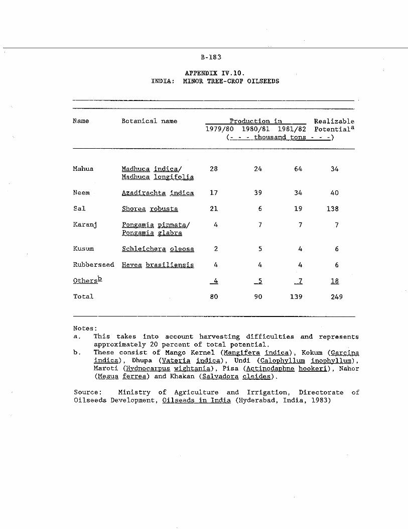
B-183
APPENDIX IV.10.INDIA: MINOR TREE-CROP OILSEEDS
Name Botanical name Production in Realizable1979/80
(-1980/81 1981/82 - - thousand tons
Potential1 - - -)
Mahua Madhuca indica,/ Madhuca longifolia
28 24 64 34
Neem. Azadirachta indica 17 39 34 40
Sal Shores robusta 21 6 19 138
Karanj Pongamia pinnate/ Pongamia glabra
4 7 7 7
Kusum Schleichera oleosa 2 5 4 6
Rubberseed Hevea brasiliensis 4 4 4 6Others^ _4 _5 JL 18Total 80 90 139 249
Notes:a. This takes into account hairvesting difficulties and represents
approximately 20 percent of total potential,b. These consist of Mango Kernel (Mans if era indies') . Kokum (Garcina
indica) , Dhupa (Vateria indie a) , Undi (Calonhvllum. inonhvllum') , Maroti (Hvdnocarpus wightania), Pisa (Actinodaphne hookeri) , Nahor (Mesua ferrea) and Khakan (Salvadora cleides).
Source: Ministry of Agriculture and Irrigation, Directorate ofOilseeds Development, Oilseeds in India (Hyderabad, India, 1983)

APPENDIX V.MISCELLANEOUS CALCULATIONS
B-185

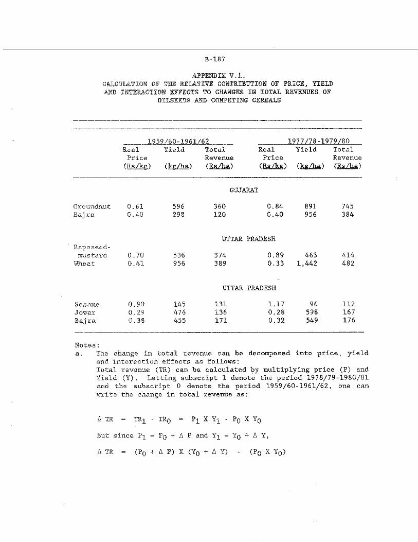
B-187
APPENDIX V.l.CALCULATION OF THE RELATIVE CONTRIBUTION OF PRICE, YIELD AND INTERACTION EFFECTS TO CHANGES IN TOTAL REVENUES OF
OILSEEDS AND COMPETING CEREALS
_ _1959J60_-1931/M____Real Yield TotalPrice Revenue(Rs/kg) (kg/ha) (Rs/ha)
1977/78-1979/80 Real Yield Total Price Revenue(Rs/kg) (kg/ha) (Rs/ha)
GUJARAT
Groundnut 0.61 596 360 0.84 891 745Baj ra 0.40 298 120 0.40 956 384
UTTAR PRADESHRapeseed-mustard 0.70 536 374 0.89 463 414
'Wheat 0.41 956 389 0.33 1,442 482
UTTAR PRADESH
Sesame 0.90 145 131 1.17 96 112Jowar 0.29 476 136 0.28 598 167Bajra 0.38 455 171 0.32 549 176
Notes:a. The change in total revenue can be decomposed into price, yield
and interaction effects as follows:Total revenue (TR) can he calculated by multiplying price (P) and Yield (Y). Letting subscript 1 denote the period 1978/79-1980/81 and the subscript 0 denote the period 1959/60-1961/62, one can write the change in total revenue as:
A TR = TRX - TR0 = Pi_ X Yx - F0 X Y0But since ?£ - P0 + A P and Yj_ = Y0 + A Y,
A TR - <F0 4- A P) X (Y0 + A Y) - <P0 X Y0)
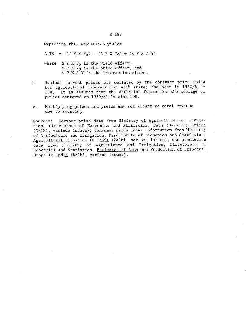
B-188
Expanding this expression yields
A TR - (A Y X P0) + (A P X Y0) + (A P X A Y)
where A Y X Pq is the yield effect,A P X Y q i s the price effect, and A P X A Y is the interaction effect.
b. Nominal harvest prices are deflated by the consumer price index for agricultural laborers for each state; the base is 1960/61 = 100. It is assumed that the deflation factor for the average of prices centered on 1960/61 is also 100.
c. Multiplying prices and yields may not amount to total revenue due to rounding.
Sources: Harvest price data from Ministry of Agriculture and Irrigation, Directorate of Economics and Statistics, Farm (Harvest) Pricey (Delhi, various issues); consumer price index information from Ministry of Agriculture and Irrigation, Directorate of Economics and Statistics, Agricultural Situation in India (Delhi, various issues); and production data from Ministry of Agriculture and Irrigation, Directorate of Economics and Statistics, Estimates of Area and Production of Principal Crons in India (Delhi, various issues).
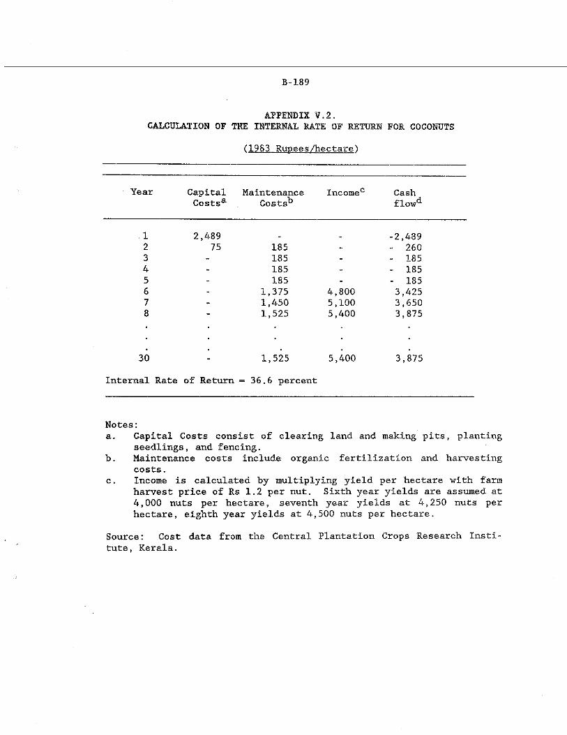
B-189
APPENDIX V.2.CALCULATION OF TEE INTERNAL RATE OF RETURN FOR COCONUTS
(1983 Rupees/heetare)
Year CapitalCostsa
MaintenanceCosts^
Income0 Cashflowd
1 2,489 -2,4892 75 185 - - 2603 - 185 - - 1854 - 185 - - 1855 - 185 - - 1856 - 1,375 4,800 3,4257 - 1,450 5,100 3,6508 1,525 5,400 3,875
30•
1,525 5,400 3,875
Internal Rate of Return - 36.6 percent
Notes:a. Capital Costs consist of clearing land and making pits, planting
seedlings, and fencing.b. Maintenance costs Include organic fertilization and harvesting
costs.c . Income is calculated by multiplying yield per hectare with farm
harvest price of Rs 1.2 per nut. Sixth year yields are assumed at 4,000 nuts per hectare, seventh year yields at 4,250 nuts per hectare, eighth year yields at 4,500 nuts per hectare.
Source: Gost data from the Central Plantation Crops Research Institute, Kerala.
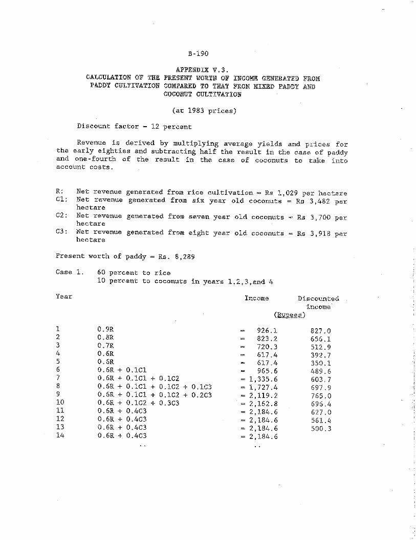
B-190
APPENDIX ¥.3.CALCULATION OF THE PRESENT WORTH OF INCOME GENERATED FROM PADDY CULTIVATION COMPARED TO THAT FROM MIXED PADDY AND
COCONUT CULTIVATION(at 1983 prices)
Discount factor =* 12 percent
Revenue is derived by multiplying average yields and prices for the early eighties and subtracting half the result in the case of paddy and one-fourth of the result in the case of coconuts to take into account costs.
R: Net revenue generated from rice cultivation - Rs 1,029 per hectareCl: Net revenue generated from six year old coconuts - Rs 3,482 per
hectareC2: Net revenue generated from seven- year old coconuts * Rs 3,700 per
hectareC3: Net revenue generated from eight year old coconuts - Rs 3,918 per
hectare
Present worth of paddy - Rs. 8,289
Case 1. 60 percent to rice10 percent to coconuts in years 1,2,3,and 4
Year
1 0.9R2 0.8R3 0.7R4 0.6R5 0.6R6 0,. 6R + 0.,1C17 0.,6R + 0.,1C1 + 0,, 1C28 0,. 6R + 0, 1C1 + 0,, 1C2 + 0 ,, 1C39 0., 6R + o'.1C1 + 0,. 1C2 + 0 ,, 2C310 0,. 6R + 0.,XC2 -f 0., 3C311 0.. 6R + 0., 4C312 0,,6R + 0.,4C313 0,, 6R + 0., 4C314 0,. 6R 4- 0..4C3
Income D is counts d(Ranees')
income
926.1 827.0823.2 656.1720.3 512.9617.4 392.7617.4 350.1965.6 489.6
1,335.6 603.71,727.4 697.92,119.2 765.02,162.8 696.42,184.6 627.02,184.6 561.42.184.62.184.6
500.3
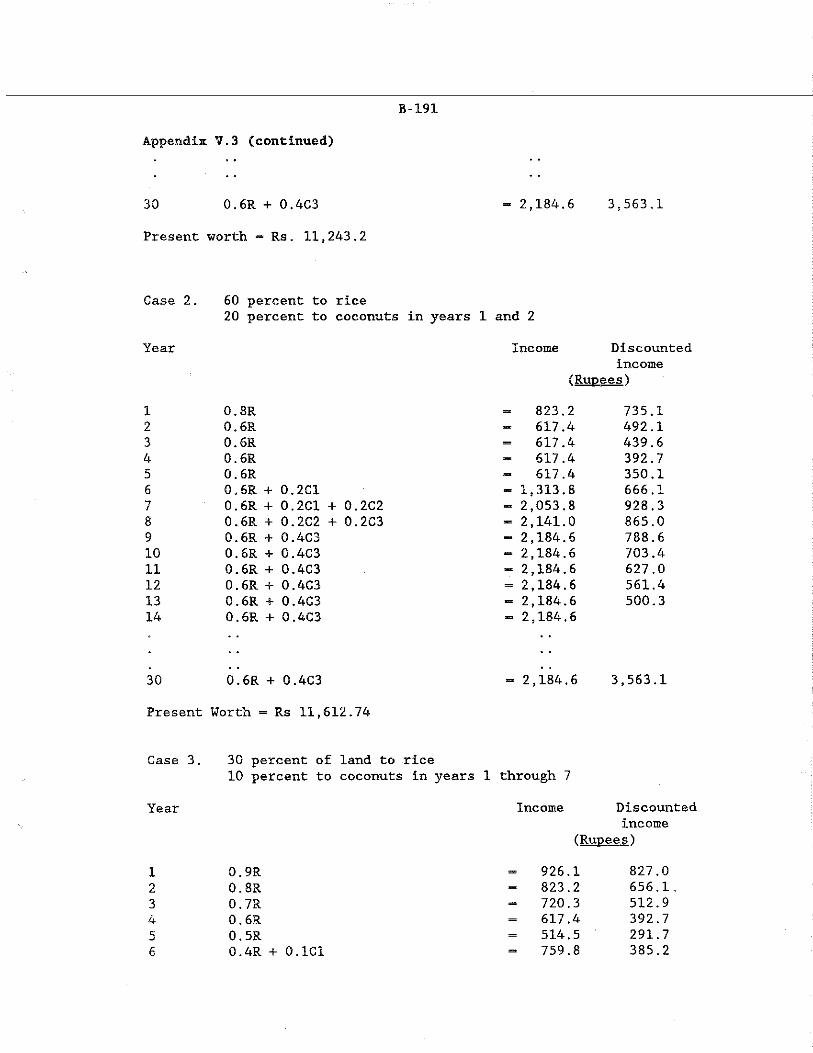
B-191
Appendix V.3 (continued)
30 0.6R + 0.4C3 - 2,184.6 3,563,1
Present worth = Rs. 11,243.2
Case 2. 60 percent to rice20 percent to coconuts in years 1 and 2
Year Income Discouniincome
(Rupees)
1 0.8R 823.2 735.12 0.6R - 617.4 492.13 0.6R = 617.4 439.64 0.6R — 617.4 392.75 0.6R — 617.4 350.16 0.6R + 0.2C1 1,313.8 666.17 0.6R + 0.2C1 + 0.2C2 - 2,053.8 928.38 0.6R + 0.2C2 + 0.2C3 2,141.0 865.09 0.6R + 0.4C3 — 2,184.6 788.610 0.6R + 0.4C3 *= 2,184.6 703.411 0.6R + 0.4C3 — 2,184.6 627.012 0.6R + 0.4C3 2,184.6 561.413 0.6R + 0.4C3 — 2,184.6 500.314 0.6R + 0.4C3 2,184.6
30 0.6R + 0.4C3 2,184.6 3,563.1
Present Worth = Rs 11,612.74
Case 3. 30 percent of land to rice10 percent to coconuts in years 1 through 7
Year Income Discountedincome
(Rupees)
1 0.9R 926.1 827.02 0.8R 823.2 656.13 0.7R 720.3 512.94 0.6R 617.4 392.75 0.5R 514.5 291.76 0.4R + 0.1C1 759.8 385.2
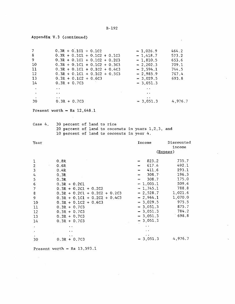
B-192Appendix V.3 (continued)
7 0.3R + 0.1C1 + 0.1C28 0.3R + 0.1C1 + 0.1C2 +9 0.3R + 0.1C1 + 0.1C2 +10 0.3R + 0.1C1 + 0.1C2 +11 0.3R + 0.1C1 + 0.1C2 +12 0.3R + 0.1C1 + 0.1C2 +13 0.3R + 0.1C2 + 0.6C314 0.3R + 0.7C3
30 0.3R + 0.7C3
= 1,026.9 464.20.1C3 = 1,418.7 573.20.2C3 « 1,810.5 653.60.3C3 = 2,202.3 709.10.4C3 = 2,594.1 744.50.5C3 = 2,985.9 767.4
= 3,029.5 693.8= 3,051.3
= 3,051.3 4,976
Present worth — Rs 12,648.1
Case 4. 30 percent of land to rice20 percent of land to coconuts in years 1,2,3, and 10 percent of land to coconuts in year 4.
Year Income DiscountedIncome
(Rupees)
1 0 . 8 R = 8 2 3 . 2 7 3 5 . 72 0 . 6 R = 6 1 7 . 4 4 9 2 . 13 0 . 4 R = 4 1 1 . 6 2 9 3 . 14 0 . 3 R = 3 0 8 . 7 1 9 6 . 35 0 . 3 R 3 0 8 . 7 1 7 5 . 06 0 . 3 R + 0 . 2 C 1 - 1 , 0 0 5 . 1 5 0 9 . 67 0 . 3 R + 0 . 2 C 1 + 0 . 2 C 2 1 , 7 4 5 . 1 7 8 8 . 88 0 . 3 R + 0 . 2 C 1 + 0 . 2 C 2 + 0 . 2 C 3 - 2 , 5 2 8 . 7 1 , 0 2 1 . 69 0 . 3 R + 0 . 1 C 1 + 0 . 2 C 2 + 0 . 4 C 3 = 2 , 9 6 4 . 1 1 , 0 7 0 . 01 0 0 . 3 R + 0 . 1 C 2 + 0 . 6 C 3 3 , 0 2 9 . 5 9 7 5 . 51 1 0 . 3 R + 0 . 7 C 3 = 3 , 0 5 1 . 3 8 7 5 . 712 0 . 3 R + 0 . 7 C 3 = 3 , 0 5 1 . 3 7 8 4 . 213 0 . 3 R + 0 . 7 C 3 3 , 0 5 1 . 3 6 9 8 . 81 4 0 . 3 R + 0 . 7 C 3 - 3 , 0 5 1 . 3
30 0.3R + 0.7C3 3,051.3 4,976.7
Present worth = Rs 13,593.1
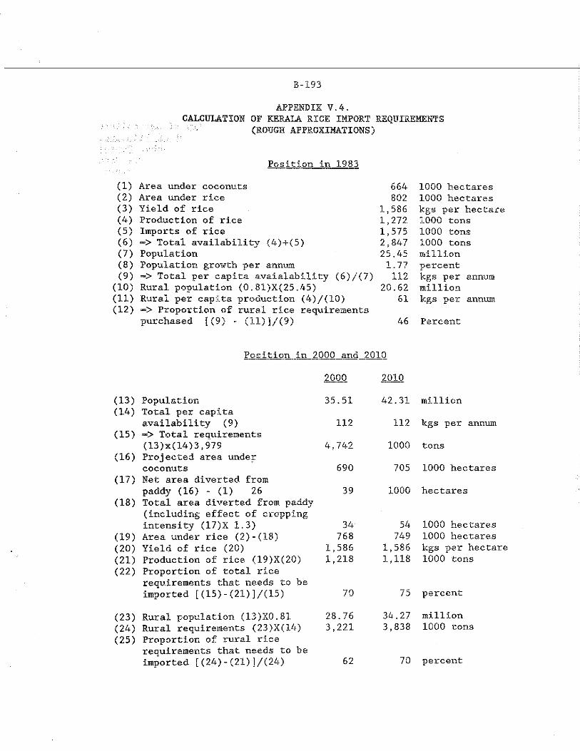
B-193
APPENDIX V. 4,CALCULATION OF KERALA RICE IMPORT REQUIREMENTS x (ROUGH APPROXIMATIONS)
Position in 1983
(1) Area under coconuts 664 1000 hectares(2) Area under rice 802 1000 hectares(3) Yield of rice 1,586 kgs per hectare(4) Production of rice 1,272 1000 tons(5) Imports of rice 1,575 1000 tons(6) => Total availability (4)+(5) 2,847 1000 tons(7) Population 25.45 million(8) Population growth per annum 1.77 percent(9) —> Total per capita avaialability (6)/(7) 112 kgs per annum
(10) Rural population (0.81)X(25.45) 20.62 million(11) Rural per capita production (4)/(10) 61 kgs per annum(12) -> Proportion of rural rice requirements
purchased [(9) - (11)]/(9) 46 Percent
Position in 2000 and 2010
(13) Population
2000
35.51
2010
42.31 million(14) Total per capita
availability (9) 112 112 kgs per annum(15) -> Total requirements
(13)x(14)3,979 4.742 1000 tons(16) Projected area under
coconuts 690 705 1000 hectares(17) Net area diverted from
paddy (16) - (1) 26 39 1000 hectares(18) Total area diverted from paddy
(including effect of cropping intensity (17)X 1.3) 34 54 1000 hectares
(19) Area under rice (2)-(18) 768 749 1000 hectares(20) Yield of rice (20) 1,586 1,586 kgs per hectare(21) Production of rice (19)X(20) 1,218 1,118 1000 tons(22) Proportion of total rice
requirements that needs to be imported [(15)-(21)]/(15) 70 75 percent
(23) Rural population (13)X0.81 28.76 34.27 million(24) Rural requirements (23)X(14) 3,221 3,838 1000 tons(25) Proportion of rural rice
requirements that needs to be imported [(24)-(21)]/(24) 62 70 percent
B-194Appendix V.4 (continued)
Sources: Area, production and yield data from Ministry of Agriculture and Irrigation, Estimates of Area. Production and Yield of Principal Crops in India (Delhi, 1985); population data from Padmanabha, Census of India, 1981: Key Population Statistics (Bombay, 1983); imports data from India, Kerala State Planning Board, Economic Review. 1983 (Trivandrum, 1983).
%
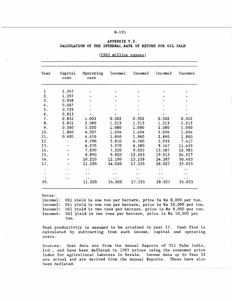
B-195APPENDIX V.5.
CALCULATION OF THE INTERNAL RATE OF RETURN FOR OIL PALMQ983 million rupees')
Year Capital Operating Incoiael Income2 Income3 Income4cost cost
1 1 .,247 - - - - -2 . 1 .,197 - - - - -3 . 0 .,958 - - - - -4 . 0 .,687 - - - - -5 . 0 .,725 - - - - -6 . 0 ,,813 - - - - -
7 . 0 .,832 1 . 00 3 0 . 502 0 . 502 0 . 502 0 ,,5028 . 2 .. 85 1 2 . 5 8 0 1 . 213 1 . 213 1 . 213 1 .,2139 . 0 ., 58 0 3 . 0 5 0 1 . 08 0 1 ., 080 1 . 0 8 0 1 ., 080
1 0 . 1 .. 84 0 4 ., 507 1 . 6 5 4 1 ., 6 5 4 1 . 65 4 1 ., 6 5 41 1 . 0 ,, 68 0 6 ., 4 1 0 1 . 8 6 0 1 ., 860 1 . 860 1 ., 8 6 01 2 . - 6 ., 2 9 0 3 ., 810 4 ., 760 5 . 933 7 .. 4171 3 . - 6.,970 5.,270 6.,580 9.,147 11.,43314. - 7..830 7..220 9,,025 13.,587 16..98315. - 8,.890 9..810 12..263 19..613 24..51716. - 10,.210 12..190 15..238 24..387 30,.48317. “ 11,.220 14,.020 17,.525 28..027 35,.033
30. 11.220 14.020 17 .525 28.027 35.033
Notes: Incomel: Income2: Income3: Income4:
Oil yield is one ton per hectare, price is Rs 8,000 per ton. Oil yield is one ton per hectare, price is Rs 10,000 per ton. Oil yield is two tons per hectare, price is Rs 8,000 per ton. Oil yield is two tons per hectare, price is Rs 10,000 per ton.
Peak productivity Is assumed to be attained in year 17. Cash flow is calculated by subtracting from each income, capital and operating costs.Sources: Cost data are from the Annual Reports of Oil Palm India,Ltd. , and have been deflated to 1983 prices using the consumer price index for agricultural laborers in Kerala. Income data up to Year 11 are actual and are derived from the Annual Reports. These have also been deflated.

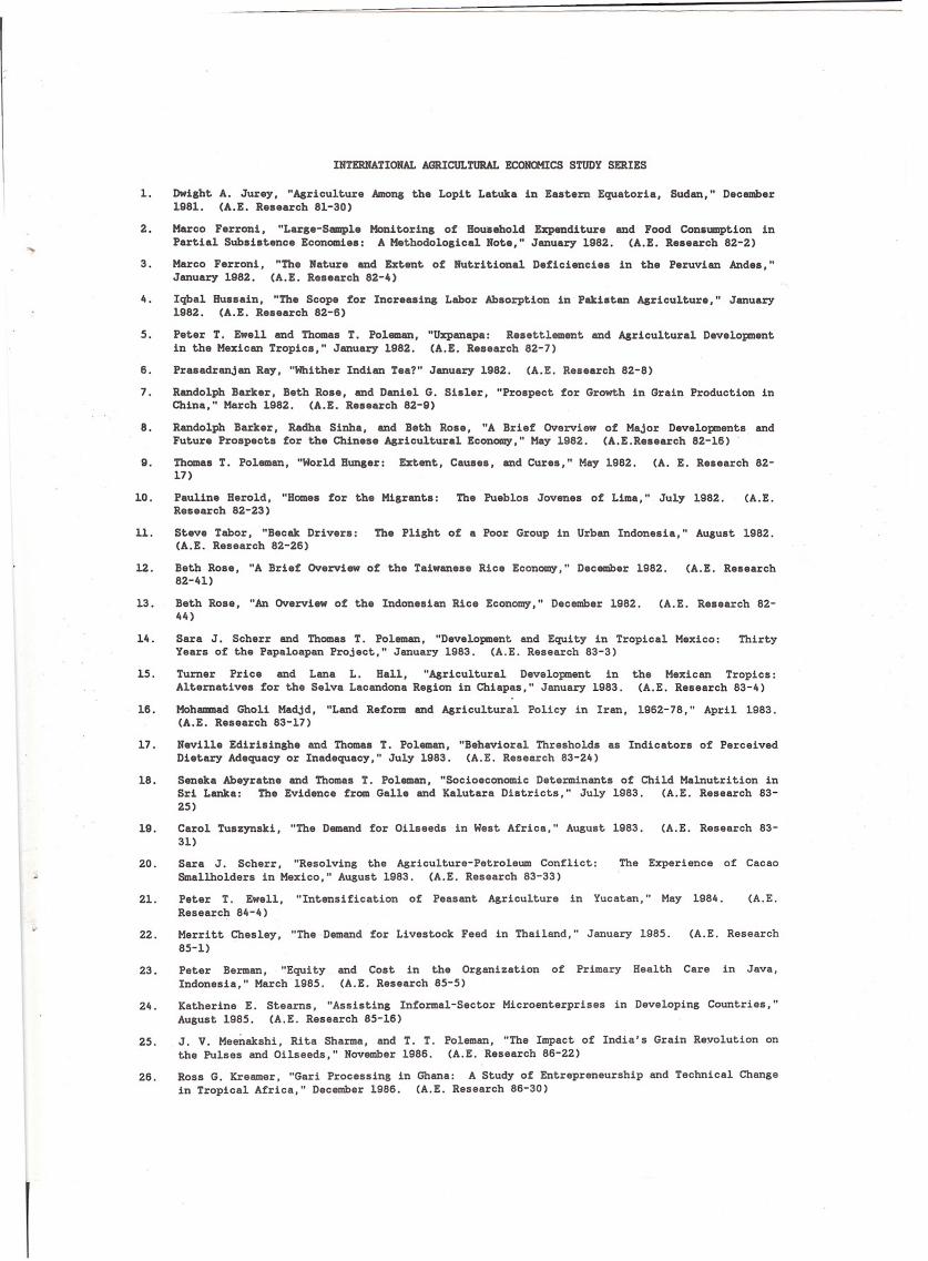
INTERNATIONAL AGRICULTURAL ECONOMICS STUDY SERIES
1. Dwight A. Jurey, "Agriculture Among the Lopit Latuka in Eastern Equatoria, Sudan," December1981. (A.E. Research 81-30)
2. Marco Ferroni, "Large-Sample Monitoring of Household Expenditure and Food Consumption inPartial Subsistence Economies: A Methodological Note,” January 1982. (A.E. Research 82-2)
3. Marco Ferroni, "The Nature and Extent of Nutritional Deficiencies in the Peruvian Andes,"January 1982. (A.E. Research 82-4)
4. Iqbal Hussain, "The Scope for Increasing Labor Absorption in Pakistan Agriculture," January1982. (A.E. Research 82-6)
5. Peter T. Ewell and Thomas T. Poleman, "Uxpanapa: Resettlement and Agricultural Developmentin the Mexican Tropics," January 1982. (A.E. Research 82-7)
6. Prasadranjan Ray, "Whither Indian Tea?" January 1982. (A.E. Research 82-8)
7. Randolph Barker, Beth Rose, and Daniel G. Sisler, "Prospect for Growth in Grain Production inChina," March 1982. (A.E. Research 82-9)
8. Randolph Barker, Radha Sinha, and Beth Rose, "A Brief Overview of Major Developments andFuture Prospects for the Chinese Agricultural Economy," May 1982. (A.E.Research 82-16)
9. Thomas T. Poleman, "World Hunger: Extent, Causes, and Cures," May 1982. (A. E. Research 82-17)
10. Pauline Herold, "Homes for the Migrants: The Pueblos Jovenes of Lima," July 1982. (A.E.Research 82-23)
11. Steve Tabor, "Becak Drivers: The Plight of a Poor Group in Urban Indonesia," August 1982.(A.E. Research 82-26)
12. Beth Rose, "A Brief Overview of the Taiwanese Rice Economy,” December 1982. (A.E. Research82-41)
13. Beth Rose, "An Overview of the Indonesian Rice Economy," December 1982. (A.E. Research 82-44)
14. Sara J. Scherr and Thomas T. Poleman, "Development and Equity in Tropical Mexico: ThirtyYears of the Papaloapan Project," January 1983. (A.E. Research 83-3)
15. Turner Price and Lana L. Hall, "Agricultural Development in the Mexican Tropics:Alternatives for the Selva Lacandona Region in Chiapas," January 1983. (A.E. Research 83-4)
16. Mohammad Gholi Madjd, "Land Reform and Agricultural Policy in Iran, 1962-78," April 1983. (A.E. Research 83-17)
17. Neville Edirisinghe and Thomas T. Poleman, "Behavioral Thresholds as Indicators of PerceivedDietary Adequacy or Inadequacy," July 1983. (A.E. Research 83-24)
18. Seneka Abeyratne and Thomas T. Poleman, "Socioeconomic Determinants of Child Malnutrition inSri Lanka: The Evidence from Galle and Kalutara Districts," July 1983. (A.E. Research 83-25)
19. Carol Tuszynski, "The Demand for Oilseeds in West Africa," August 1983. (A.E. Research 83-31)
20. Sara J. Scherr, "Resolving the Agriculture-Petroleum Conflict: The Experience of CacaoSmallholders in Mexico," August 1983. (A.E. Research 83-33)
21. Peter T. Ewell, "Intensification of Peasant Agriculture in Yucatan," May 1984. (A.E.Research 84-4)
22. Merritt Chesley, "The Demand for Livestock Feed in Thailand," January 1985. (A.E. Research85-1)
23. Peter Berman, "Equity and Cost in the Organization of Primary Health Care in Java,Indonesia," March 1985. (A.E. Research 85-5)
24. Katherine E. Stearns, "Assisting Informal-Sector Microenterprises in Developing Countries,"August 1985. (A.E. Research 85-16)
25. J. V. Meenakshi, Rita Sharma, and T. T. Poleman, "The Impact of India’s Grain Revolution onthe Pulses and Oilseeds," November 1986. (A.E. Research 86-22)
26. Ross G. Kreamer, "Gari Processing in Ghana: A Study of Entrepreneurship and Technical Changein Tropical Africa," December 1986. (A.E. Research 86-30)