agricultural production economics - university of kentucky
TRANSCRIPT
Agricultural Production Economics
THE ART OF PRODUCTION THEORYTHE ART OF PRODUCTION THEORY
DAVID L. DEBERTINUniversity of Kentucky
This is a book of full-color illustrations intended for use as a companion to 428-page Agricultural Production Economics, Second Edition. Each of the 98 pages of illustrations is a large, full-color version of the corresponding numbered figure in the b k A i lt l P d ti E i S d Editi Thbook Agricultural Production Economics, Second Edition. The illustrations are each a labor of love by the author representing a combination of science and art. They combine modern computer graphics technologies with the author’s skills as both as a production economist and as a technical graphics artist.
T h l i d i ki th ill t ti t th l tiTechnologies used in making the illustrations trace the evolution of computer graphics over the past 30 years. Many of the hand-drawn illustrations were initially drawn using the Draw Partnerroutines from Harvard Graphics®. Wire-grid 3-D illustrations were created using SAS Graph®. Some illustrations combine hand-drawn lines using Draw Partner and the draw features of Mi f P P i ® i h d hi fMicrosoft PowerPoint® with computer-generated graphics from SAS®. As a companion text to Agricultural Production Economics, Second Edition, these color figures display the full vibrancy of the modern production theory of economics.
© 2012 David L Debertin© 2012 David L. Debertin
David L. DebertinUniversity of Kentucky,Department of Agricultural Economics400 C.E.B. Bldg.Lexington, KY 40546-0276
All rights reserved. No part of this book may be reproduced or transmitted in any form or by any means, without permission from the author.
Debertin, David L.Agricultural Production EconomicsThe Art of Production TheoryThe Art of Production Theory
1. Agricultural production economics2. Agriculture–Economic aspects–Econometric models
ISBN- 13: 978-1470129262 2
ISBN- 10: 1470129264
BISAC: Business and Economics/Economics/Microeconomics
SupplyPrice
Demand(New Income)
p
p
1
2
Demand(Old Income)
q Quantityq1 21 2
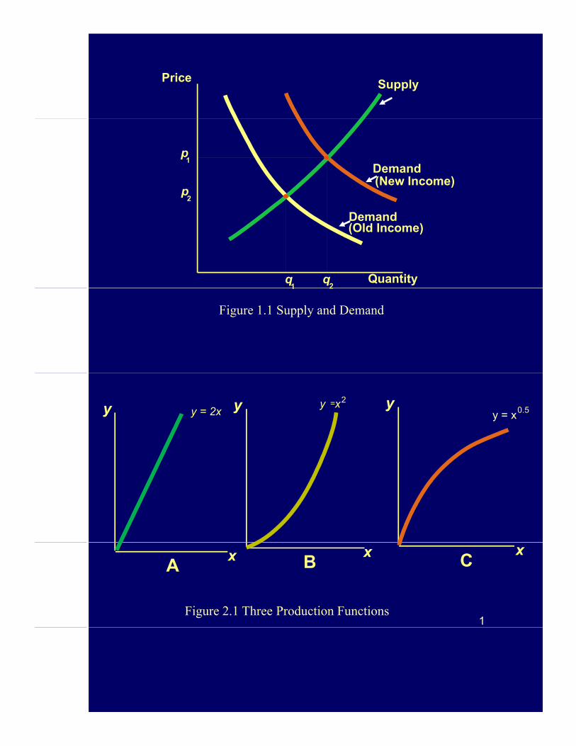
Figure 1.1 Supply and Demand
y y x= 2y y = 2x
yy = x0.5
1
xxA B
xC
Figure 2.1 Three Production Functions

C
y
D
y = f(x)
y
x
B
A x
2
Figure 2.2 Approximate and Exact MPP

SlopeEq als
yor
TPP
Slope EqualsMPP EqualsMaximumAPP Maximum
APP
EqualsZero
MaximumTPP
TPPy = f(x )
InflectionSlope
Equals
y = f(x1)
Inflection
Point
EqualsAPP
MPP
APPor
x
B
AMaximum
MPP
x x1 1
o *
1Maximum
APP
APP0 MPP
3
xMPP 1
Figure 2.3 A Neoclassical Production Function

TPP
120
140y = 136.96
TPP Maximum
TPP
80
100
y = 85.98
APP Maximum
40
60y = 56.03
MPP MaximumInflection Point
0
20
0 50 100 150 200
1
1.1
1.21.01 0.94 MPP = APP
60.87 91.30 181.60
x
MPPAPP
0.3
0.4
0.5
0.6
0.7
0.8
0.9
1
APP
0
0.1
0.2
-0.1
-0.2
-0.3
0 50 100 150 200
0 MPP
MPP
x
4
Figure 2.4 TPP, MPP and APP for Corn (y) Response toNitrogen (x) Based on Table 2.5 Data

MPP
+
0
fff
1
2
3
MPP
+
0
fff
1
2
3
MPP
+
0
fff
1
2
3
MPP
+
0
ff1
2
MPPMPP
MPP
MPP> 0> 0> 0
> 0> 0
= 0
> 0> 0< 0
> 0= 0
(a) (b) (c) (d)
- - - -
MPP
+
0
fff
1
2
3MPP
+
0
fff
1
2
3 MPP
+
0
fff
1
2
3
MPPMPPMPP
> 0< 0> 0
> 0< 0
= 0
> 0< 0< 0
(e) (f) (g)
-
MPP
+
0
fff
1
2
3
- -
MPP
+
0
fff
1
2
3
MPP
+
0
fff
1
2
3
MPP
+
0
ff1
2
MPP
< 0< 0< 0
< 0< 0
= 0
< 0< 0> 0
< 0= 0
(h) (i) (j) (k)
-
MPP
+
0
fff
1
2
3
-
MPP
+
0
fff
1
2
3
MPP
+
0
fff
1
2
3
- -MPP
MPP MPP MPP
MPPMPPMPP
< 0> 0> 0
< 0> 0
= 0
< 0> 0< 0
(l) (m) (n)
- - -
Figure 2.5 MPP’s for the Production Function y = f(x)
5

Ep
Ep Ep
> 1 0 < < 1 < 0MPP
APPor
y,
B
Ep> 1
A
B
E p =1
0
APP
xC
MPP-
6
Figure 2.6 MPP, APP and the Elasticity of Production

TVPTVP$
pyor
pTPPTVP
InflectionPoint
x
VMP
AVPpMPP
$
MFC
AVP
MFC
AVPpAPP
0
7
VMPx
Figure 3.1 The Relationship Between TVP, VMP, AVP, and MFC

ZeroSlope
TFCZeroProfit$
MaximumTVP
TVPMaximumProfit
MaximumAVP
Parallel
TVPTFC
InflectionP i t
ZeroProfit
MaximumVMP
ParallelPoint
MinimumProfit Maximum
Profit
X*MaximumVMP
VMP =MFC
MinimumProfitVMP =MFC
AVP =p APPo
MFC =v
x
v o
0
VMPAVPMFC
$
o
MaximumProfit
ZeroVMP
xVMP
0
0
Profit$$
8
MinimumProfit
ZeroProfit
ZeroProfitx*
Profit
x
Figure 3.2 TVP, TFC, VMP, MFC and Profit

600
547.86547.69$
300
400
500
520.62520.69
Profit
TVP
100
200
00 40 80 120 160 200 240
181.595179.322
x
500
600
546.28 547.86$
TFC
300
400
500467.69 466.14
Profit
TVP
100
200
174 642 181 595
TFC
Profit
9
00 40 80 120 160 200 240
174.642 181.595
x
Figure 3.3 TVP, TFC and Profit (Top and Second Panel)
500
600
541.26$
547.86
300
400390.75 384.42
100
200
181.595167.236
00 40 80 120 160 200 240
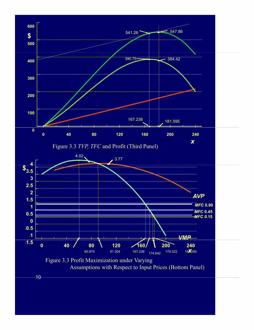
xFigure 3.3 TVP, TFC and Profit (Third Panel)
4
4.023.77
1.5
2
2.5
3
3.5
4$
AVP
0
0.5
1
-0.5
-1 VMP
MFC 0.90
MFC 0.45MFC 0.15
10
-1.50 40 80 120 160 200 240
x
Figure 3.3 Profit Maximization under VaryingAssumptions with Respect to Input Prices (Bottom Panel)
91.304 181.595179.322167.23660.870 174.642
10

y
TPP
A B C
Stage I Stage II Stage III
xy
MPP
APP
x
0
11
MPP
Figure 3.4 Stages of Production and the Neoclassical Production Function

CD
$
MFC
RevenuePer Unit
CostPerUnit
B
D
E
AVP
Loss
0x* x
VMP
A
Figure 3.5 If VMP is Greater than AVP, the Farmer Will Not Operate
$
MFCVMP
0
MFC
MFC
12
x
VMP
Figure 3.6 The Relationship Between VMP and MFC Illustrating the Imputed Value of an Input

SRMC1
SRAC2
SRMC5
SRAC5
LRAC
$
SRAC1SRMC2
SRAC2
SRMC3SRAC3
SRMC4
SRAC4
y
Figure 4.1 Short and Long Run Average and Marginal Cost with Envelope Long Run Average Cost
13

TCTC
VC orTVC
$Minimumslope ofTC
Minimumslope ofTVC
Inflection Point
FC
y
$
MC
AC*
MC
ACAVC
AVC*
B
A
14
FC = k
AFC*
Figure 4.2 Cost Functions on the Output Side
AFC
y
14

ACAFCAC
+
$
∞
AVC
AVC AFC
AFC
MC
Stage II Stage III
0
AFCAFCAFC
y* y
-
MC
15
-
Figure 4.3 Behavior of Cost Curves as OutputApproaches a Technical Maximum y*
∞
pp y

TC
TVC$
TR
$
Parallel
y
p
FC
Parallel
MC
y$
MR
AFC
AVC
ACMR = p
y
y0
$+ Zero
Profit
Maximum Profit
Profit
16
-Minimum Profit
Figure 4.4 Cost Functions and Profit Functions

500
600
$TR
300
400
500TC
VC
0
100
200 Maximum Profit
ProfitFC
7
0
-1000 20 40 60 80 100 120 140
Zero Profity = ~ 115
y
$
4
5
6
MR
$
AC
MC
1
2
3
AFC
ACAVC
17
00 20 40 60 80 100 120 140
AFC
y
Figure 4.5 The Profit-Maximizing Output Level Based on Data Contained in Table 4.1Based on Data Contained in Table 4.1

Y Y
MaximumTPP
MaximumAPP
45o
TPP
MaximumMPP
(InflectionPoint)
X Y
$$TVCTC = vx
Point)
V
X
MinimumAVC
MinimumMC(InflectionPoint)
v = price of x
YX
X
Figure 4 6 A Cost Function as an Inverse Production Function
18
Figure 4.6 A Cost Function as an Inverse Production Function

p3
AVC
MC = Supply
$
p1
p2
p3
y
Figure 4.7 Aggregate Supply When the Ratio MC/AC = 1/band b is less than 1
19
Y
Corn Yield
134
136
Y
120
136
114
121
127
130
20
40
6080
X120
40
60
8088
104
101
106
X
96
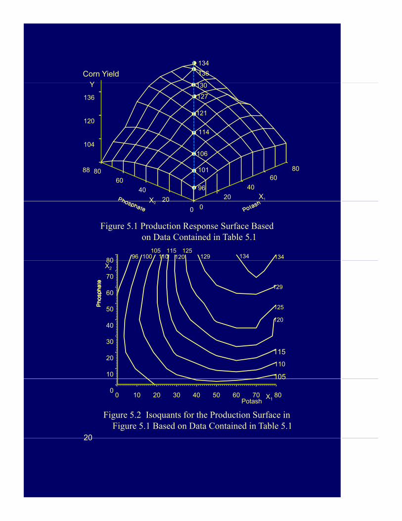
Figure 5.1 Production Response Surface Based on Data Contained in Table 5.1
8096 100 1101 120 129 134 134
115105 125
00
20X2
X2
50
60
70
80
129
125
120
10
20
30
40120
115
110
105
20
Figure 5.2 Isoquants for the Production Surface in Figure 5.1 Based on Data Contained in Table 5.1
X1Potash
00 10 20 30 40 50 60 70 80
105
20
x2
2x
21
2
1x
x
x x
y 0
1
2
x
x
Figure 5 3 Illustration of Diminishing MRS x x
1
21
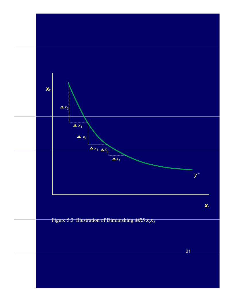
Figure 5.3 Illustration of Diminishing MRS x1x2

Figure 5.4 Isoquants and a Production Surface (Panel A)
22
Figure 5.4 Isoquants and a Production Surface (Panel B)

Figure 5.4 Isoquants and a Production Surface (Panel C)
23
Figure 5.4 Isoquants and a Production Surface (Panel D)

Figure 5.4 Isoquants and a Production Surface (Panel E)
Y
167
250
1416
1820
1618
200
83
24Figure 5.4 Isoquants and a Production Surface (Panel F)
02
46
810
1214
02
46
810
1214
16
X2
X1
X1X2
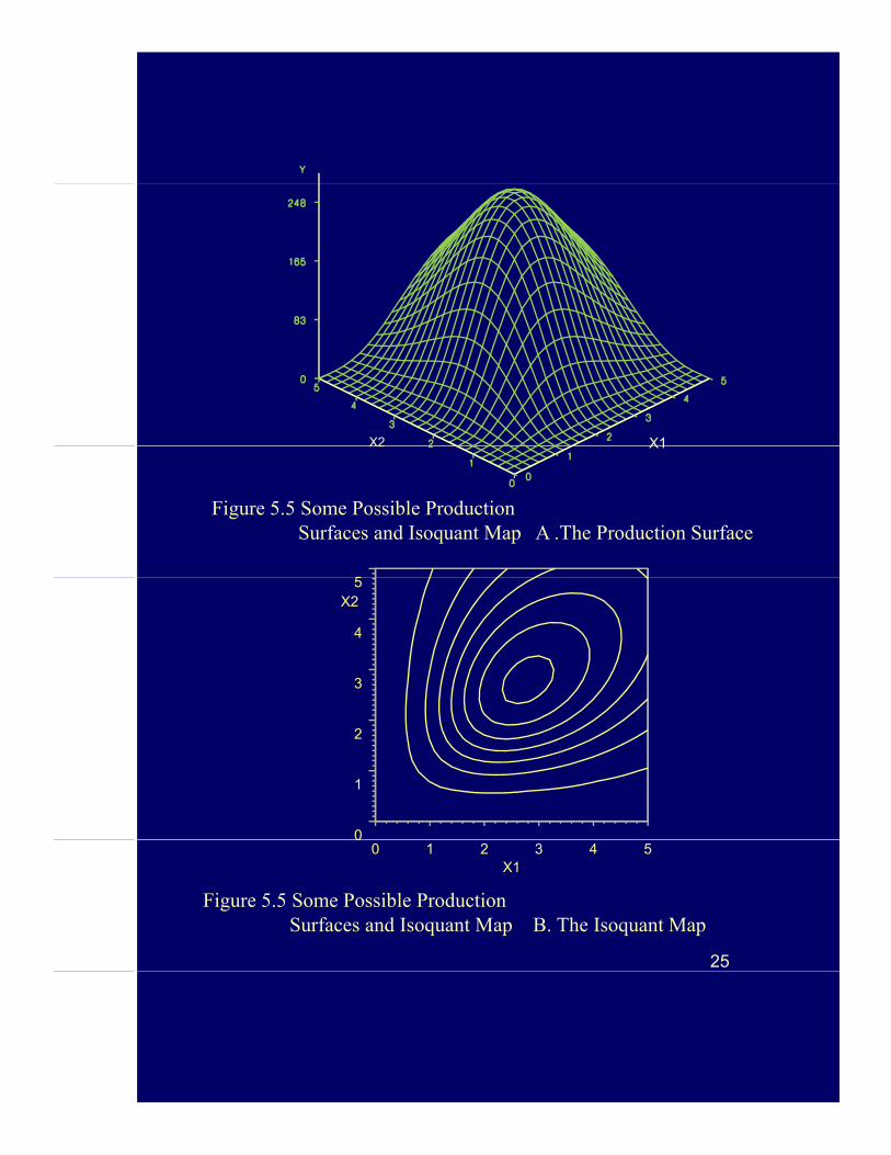
Figure 5.5 Some Possible ProductionSurfaces and Isoquant Map A .The Production Surface
5
X1X2
X2
3
4
5
0
1
2
25
0
X10 1 2 3 4 5
Figure 5.5 Some Possible ProductionSurfaces and Isoquant Map B. The Isoquant Map
Y
6.67
10.00
68
10
68
100.00
3.33
02
46
X2
02
46
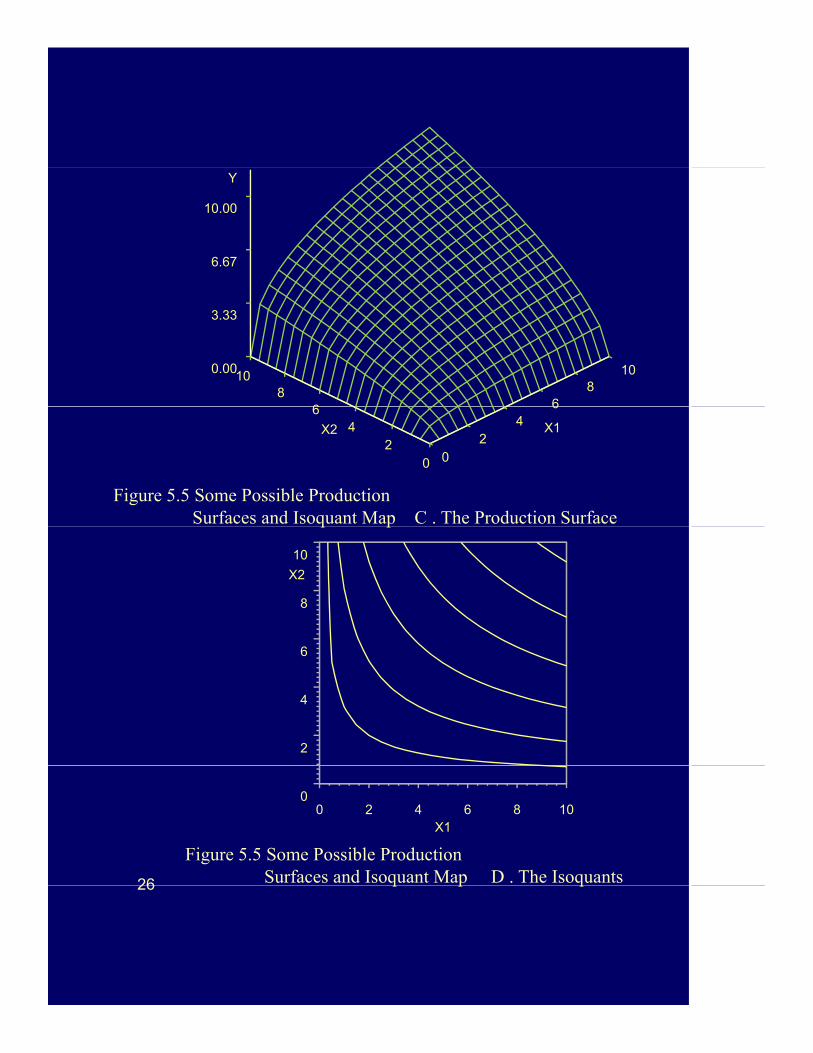
Figure 5.5 Some Possible ProductionSurfaces and Isoquant Map C . The Production Surface
X1
q p
X2
8
10
2
4
6
26
0
X10 2 4 6 8 10
Figure 5.5 Some Possible ProductionSurfaces and Isoquant Map D . The Isoquants26 q p q

YY
6.67
10.0
68
10
810
0.00
3.33
0
2
4
6
X2
0
2
4
6
Figure 5.5 Some Possible Production Surfaces and Isoquant MapsE. The Production Surface
X1
X2
6
8
10
2
4
6
27
0
X10 2 4 6 8 10
Figure 5.5 Some Possible Production Surfaces and Isoquant MapsF. The Isoquants
Y
3.67
6.83
10.00
2.44.3
6.28.1
10.0
2 44.3
6.28.1
10.0
0.50
X2X1
0.50.52.4
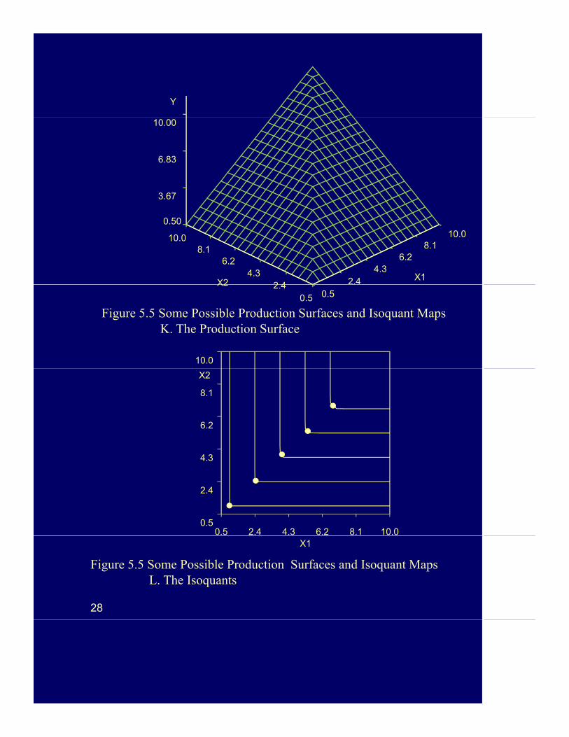
Figure 5.5 Some Possible Production Surfaces and Isoquant MapsK. The Production Surface
X2
10.0
X2
6.2
8.1
0.5
2.4
4.3
0.5 2.4 4.3 6.2 8.1 10.0
28
X1
Figure 5.5 Some Possible Production Surfaces and Isoquant MapsL. The Isoquants

Y
10.00
3.33
6.67
02
46
810
X2
02
46
8100.00
X1
00
Figure 5.5 Some Possible Production Surfaces and Isoquant MapsG. The Production Surface
10
X2
6
8
0
2
4
0 2 4 6 8 10
29
X10 2 4 6 8 10
Figure 5.5 Some Possible Production Surfaces and Isoquant MapsH. The Isoquants
Y
0.181
-0.100
0.040
2.4
4.3
6.2
8.110.0
2.4
4.3
6.2
8.110.0
X2 X1
-0.241
0.50.5
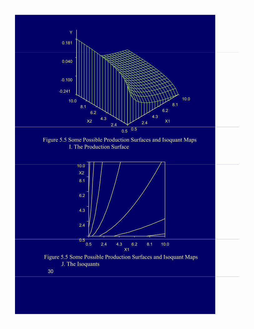
Figure 5.5 Some Possible Production Surfaces and Isoquant MapsI. The Production Surface
10 0
X2
6.2
8.1
10.0
0 5
2.4
4.3
30
0.5
X10.5 2.4 4.3 6.2 8.1 10.0
Figure 5.5 Some Possible Production Surfaces and Isoquant MapsJ. The Isoquants
3.0
x
1.8
for
Ridge Linefor x
x
x
x2 *2.4
2
1
Ridge Line
0.6
1.2
for x2
x2***
x2**
0.00.0 0.6 1.2 1.8 2.4 3.0
y
x 1
y = f (x 1 | x 2 *)
y = f (
y = f (x 1
x 1 x 2 *** |
| x 2** )
)
31
0.0 0.6 1.2 1.8 2.4 3.0x1
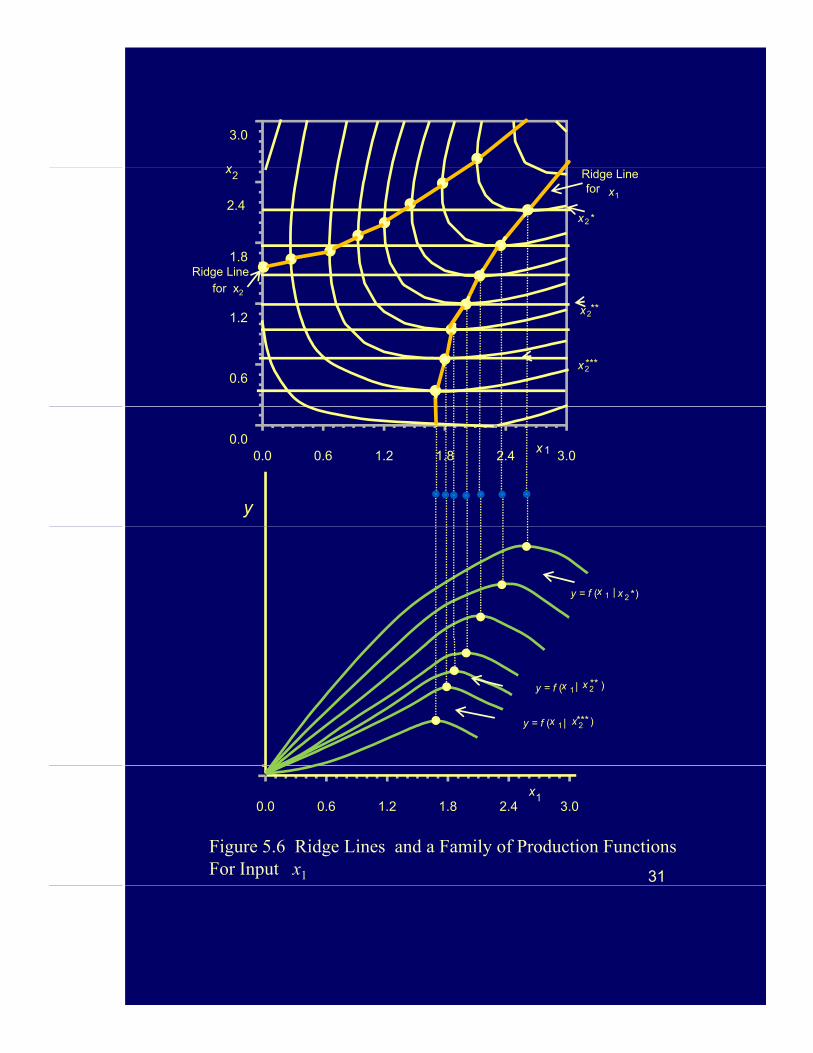
Figure 5.6 Ridge Lines and a Family of Production FunctionsFor Input x1

Y
50 00
Maximum
33.33
50.00
8
10
8
100.00
16.67
Figure 6 1 Alternative Surfaces and Contours Illustrating
0
2
4
6
X1X2
0
2
4
6
8
A. The Surface
Figure 6.1 Alternative Surfaces and Contours Illustrating Second Order Conditions
X2
8
10
2
4
6
Maximum
32
Figure 6.1 Alternative Surfaces and Contours Illustrating Second Order Conditions
B. The Contour Lines
0
X10 2 4 6 8 10
32

Y
-16.67
0.00
6
8
10
6
8
10-50.00
-33.33
Minimum
Figure 6.1 Alternative Surfaces and Contours Illustrating Second Order Conditions
C. The Surface0
2
4
6
X1X2
0
2
4
6
X2
8
10
2
4
6
Minimum
33
Figure 6.1 Alternative Surfaces and Contours Illustrating Second Order Conditions
D. The Contour Lines 0
X10 2 4 6 8 10
Y
25.00
8 33
8.33
25.00
Saddle
6
8
10
6
8
10-25.00
-8.33
0
2
4X1X2
0
2
4
6
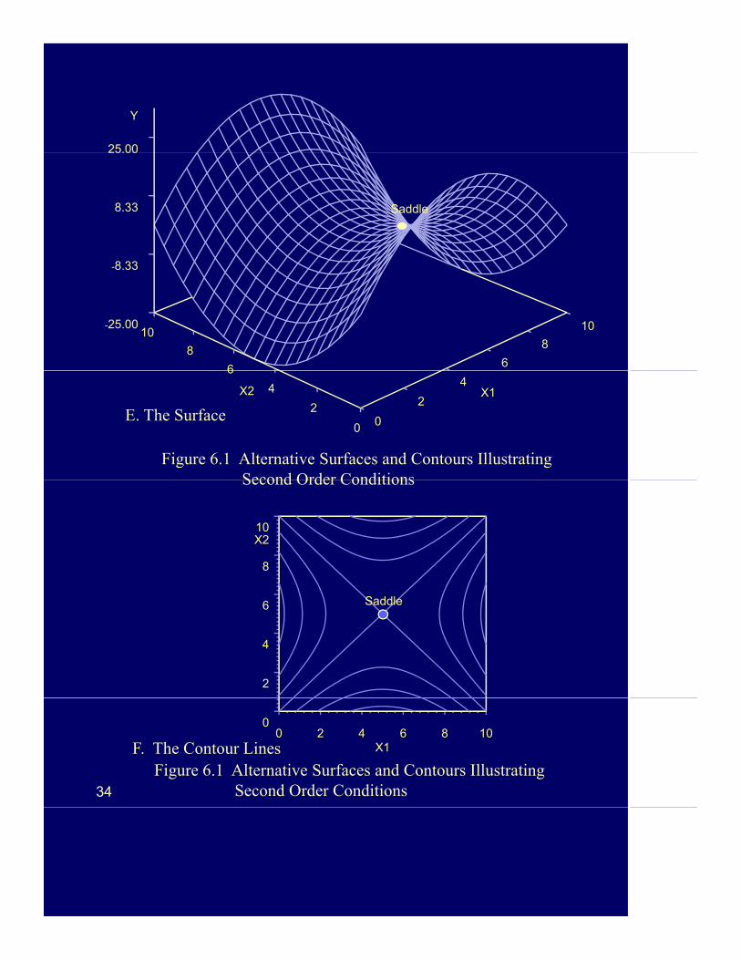
Figure 6.1 Alternative Surfaces and Contours Illustrating Second Order Conditions
E. The Surface
Second Order Conditions
X2
8
10
2
4
6 Saddle
34
Figure 6.1 Alternative Surfaces and Contours Illustrating Second Order Conditions
F. The Contour Lines
0
X10 2 4 6 8 10

Y
8.33
25.00
Saddle
8
10
8
10-25.00
-8.33
0
2
4
6
X1X2
0
2
4
6
8
Figure 6.1 Alternative Surfaces and Contours Illustrating
G. The Surface
Second Order Conditions
X2
8
10
S
2
4
6 Saddle
35
Figure 6.1 Alternative Surfaces and Contours Illustrating Second Order Conditions
H. The Contour Lines0
X10 2 4 6 8 10
Y
220
127
47
220
Saddle
1
3
5
1
3
5-300
-127 Saddle
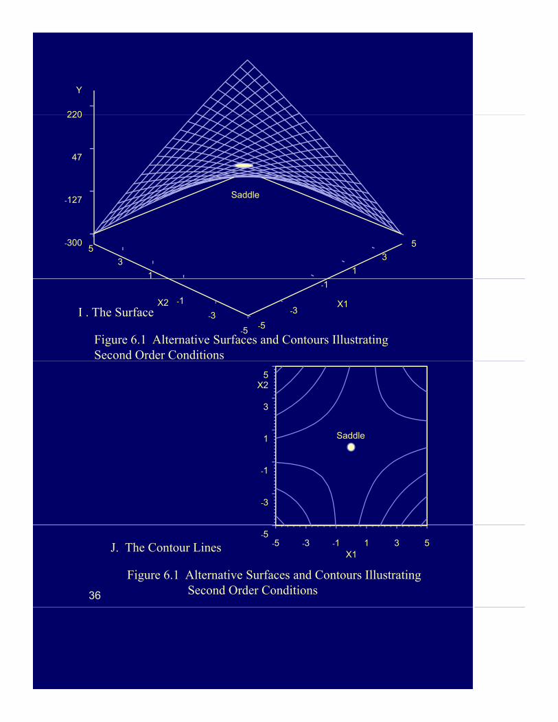
Figure 6.1 Alternative Surfaces and Contours Illustrating Second Order Conditions
-5
-3X1X2
-5
-3
-1
-1
I . The Surface
X2
1
3
5
Saddle
-3
-1
36
Figure 6.1 Alternative Surfaces and Contours Illustrating Second Order Conditions
J. The Contour Lines-5
X1-5 -3 -1 1 3 5
Y
200
-147
27
Saddle
1
1
3
5
1
3
5-320
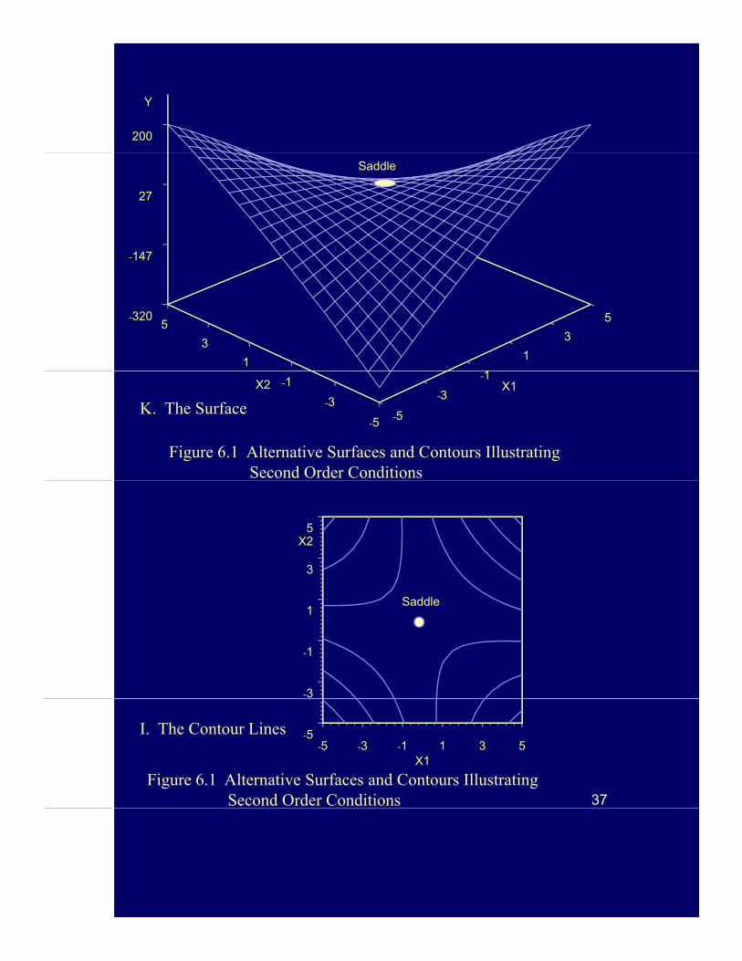
Figure 6.1 Alternative Surfaces and Contours Illustrating Second Order Conditions
-5
-3
-1X1X2
-5
-3
-1
K. The Surface
X2
3
5
-3
-1
1Saddle
37Figure 6.1 Alternative Surfaces and Contours Illustrating
Second Order Conditions
I. The Contour Lines -5
X1-5 -3 -1 1 3 5
Y
379
Global Maximum
126
253
379
Saddle Local MaxLocal MaxSaddle
48
1216
20
X24
812
16200
Top Panel
LocalSaddleSaddle
Local Max
Minimum
X1
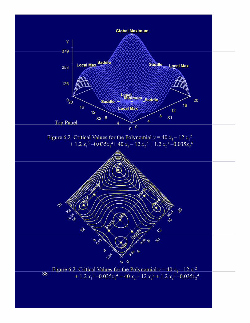
Figure 6.2 Critical Values for the Polynomial y = 40 x1 – 12 x12
+ 1.2 x13 –0.035x1
4+ 40 x2 – 12 x22 + 1.2 x2
3 –0.035x24
00
p
Figure 6.2 Critical Values for the Polynomial y = 40 x1 – 12 x12
38g y y 1 1
+ 1.2 x13 –0.035x1
4 + 40 x2 – 12 x22 + 1.2 x2
3 –0.035x24
X2
2 4
3.0C /v2
o
Expansion
1.2
1.8
2.4
v1
ExpansionPath
0.0
0.6
0.0 0.6 1.2 1.8 2.4 3.0
v
C /v1
2
o
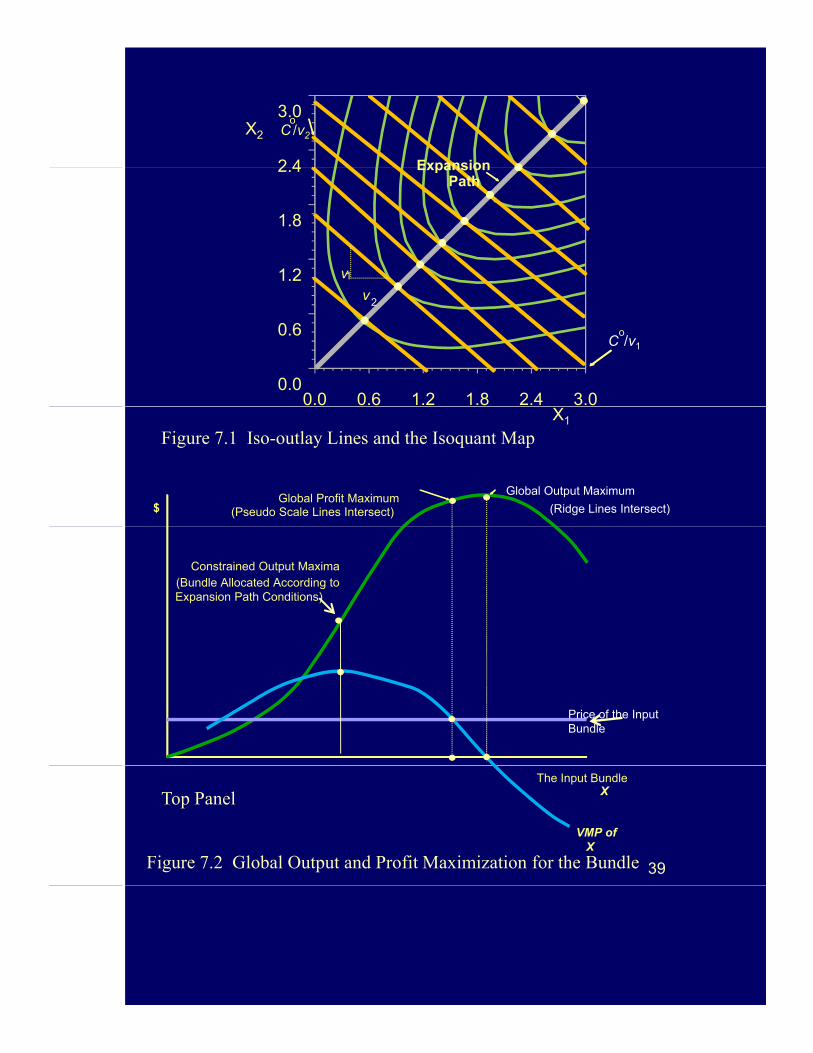
Figure 7.1 Iso-outlay Lines and the Isoquant Map
Global Profit Maximum(Pseudo Scale Lines Intersect)$ (Ridge Lines Intersect)
Global Output Maximum
X1
Constrained Output Maxima(Bundle Allocated According toExpansion Path Conditions)
Price of the Input Bundle
39
The Input BundleX
VMP ofX
Figure 7.2 Global Output and Profit Maximization for the Bundle
Top Panel
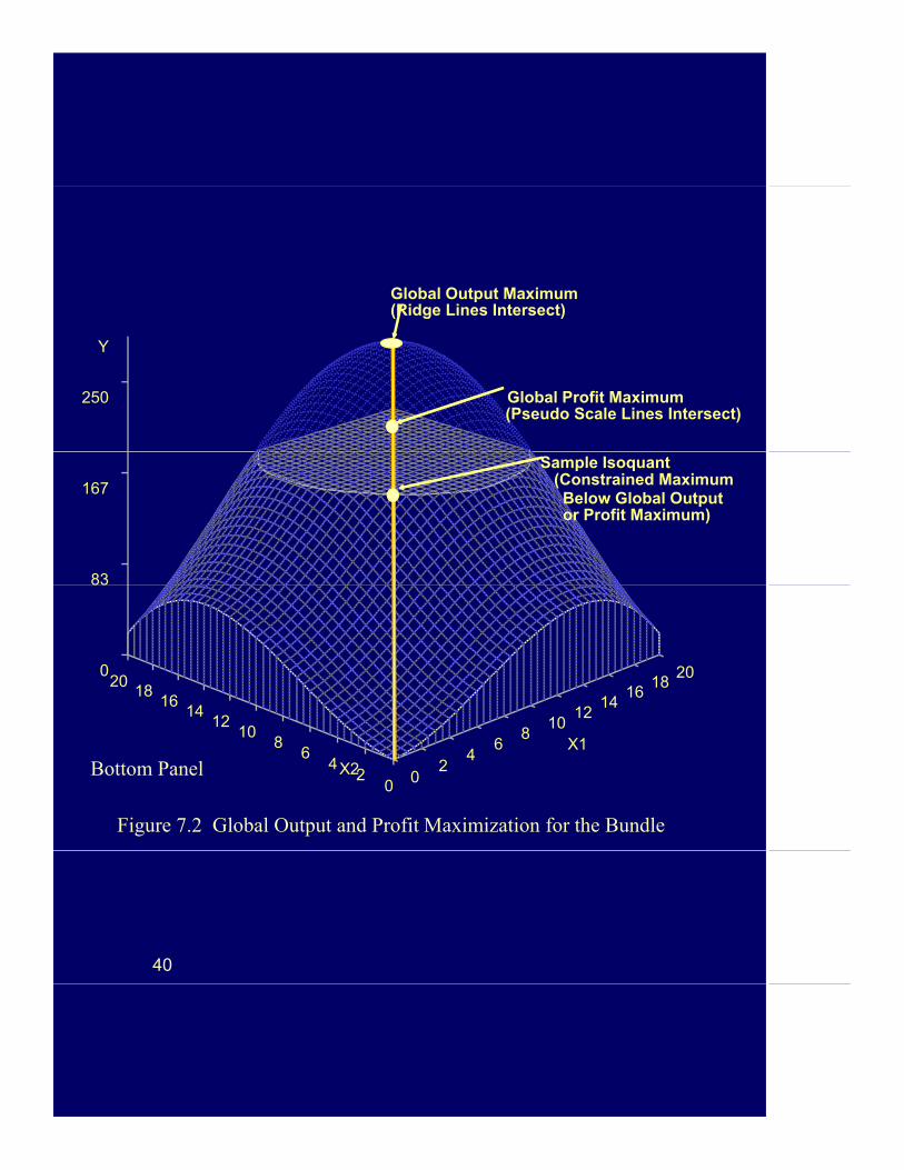
Global Output Maximum(Ridge Lines Intersect)
Y
250
( g )
Global Profit Maximum(Pseudo Scale Lines Intersect)
83
167
Sample Isoquant(Constrained MaximumBelow Global Outputor Profit Maximum)
1012
1416
1820
1214
1618
200
83
02
46
810
12
X1
02
46
810
12
Figure 7.2 Global Output and Profit Maximization for the Bundle
Bottom Panel X2
40

X2
16
18
20
8
10
12
14
x2*
Point onRidgeLine
Point onPseudoScaleLine
2
4
6
8
0
X1
0 2 4 6 8 10 12 14 16 18 20
$ Profit Maximumfor x Holding
*
Output Maximumfor x1 Holding
x2 constant at x2*
2constant at x
2x
1
py = f (x1 | x2* ) = TVP
0 2 4 6 8 10 12 14 16 18 20
MFC = v1
41
X1
VMP x | x *2
Figure 7.3 Deriving a Point on a Pseudo Scale Line
1
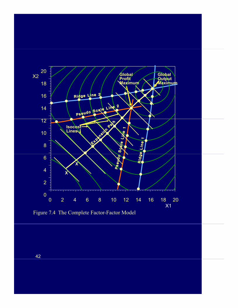
X2
18
20GlobalProfitMaximum
GlobalOutputMaximum
12
14
16
18 Maximum Maximum
8
10
12IsocostLines
2
4
6X
X
00 2 4 6 8 10 12 14 16 18 20
Figure 7.4 The Complete Factor-Factor ModelX1
42

Y
Global Output Maximum
Gl b l P fit M i
167
250 Global Profit Maximum
ConstrainedOutput Maximum
83
Output Maximum
46
810
1214161820
0
24
68
1012
1416 18 20
X1X2 4
02
02
Figure 7.5 Constrained and Global Profit and Output Maxima along the Expansion Path
X2
43

$
Global Revenue Maximization
Global Profit Maximization
Revenue,Profit
153
250
153
250Global Profit Maximization
Ridge Line 1
Pseudo Scale Line 1
Ridge Line 2
Pseudo Scale Line 2
-40
57
16 18 201820-40
57
0 0
0 2 4 6 8 10 12 14 16
X1X2024681012141618
Total Revenue Surface Profit Surface
Figure 8.1 TVP- and Profit-Maximizing Surfaces
44

X2
16
18
20
16
18
20
Global Output Max
10
12
14
16
10
12
14
16
Global Profit Max
4
6
8
10
4
6
8
10
0
2
4
X0 2 4 6 8 10 12 14 16 18 20
0
2
4
0 2 4 6 8 10 12 14 16 18 20X1
Isorevenue Lines Isoprofit Lines
Figure 8.2 Isorevenue and Isoproduct Contours
45
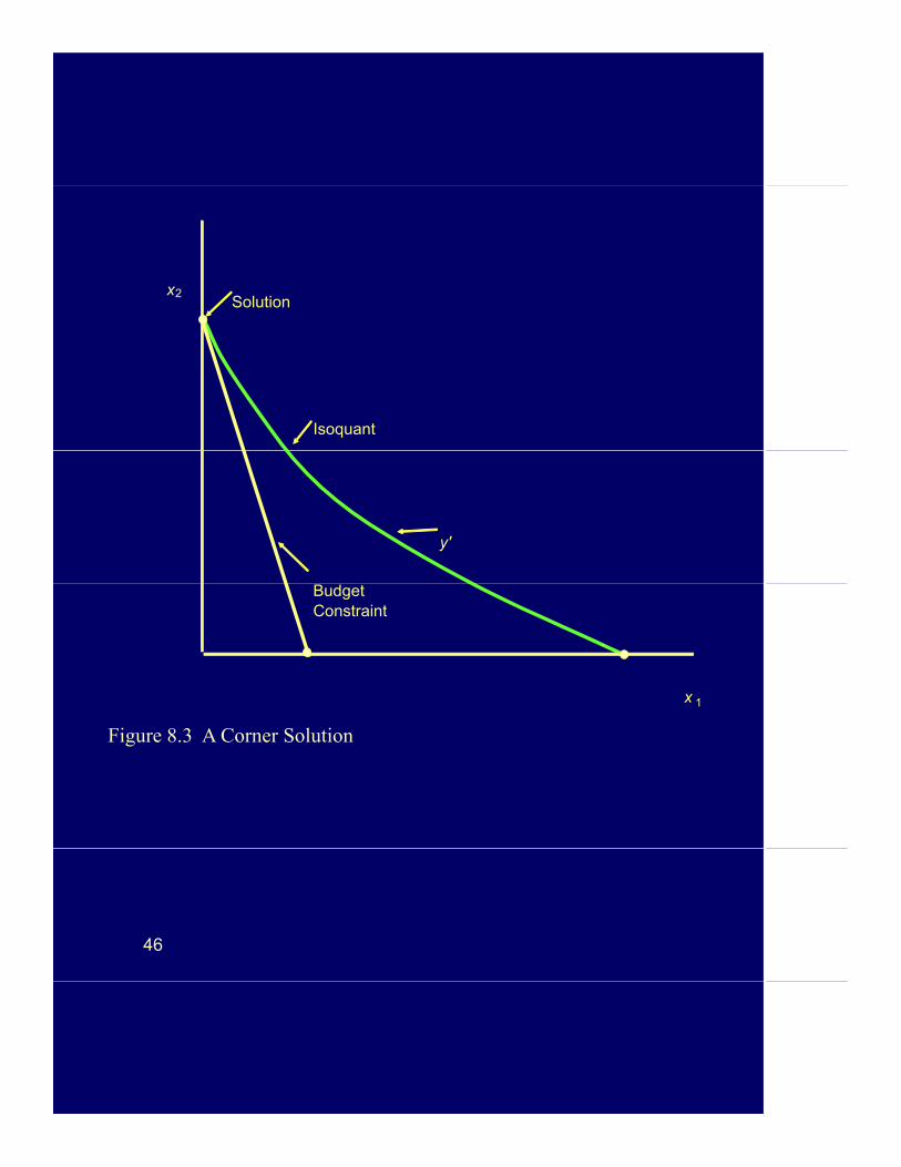
x2Solution
Isoquant
y'
x
BudgetConstraint
1
Figure 8.3 A Corner Solution
46

Y
250
83
167
200
46
810
1214
1618
20
X168
1012
141618
A B C
0 02
4X22
46
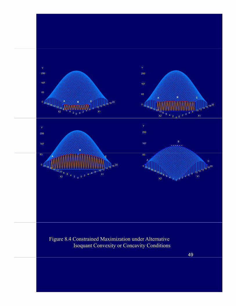
Figure 8.4 A. Point B Less than A and C
Y
167
250
0
83
20
A B C
002
200
24
68
1012
1416
1820
X1X2 4
68
1012
1416
18
47Figure 8.4 B. Point B Equal to A and C
Y
167
250
B
20200
83
161818
A
B
C
002 2
46
810
1214
16
X1X2 4
68
1012
1416
18
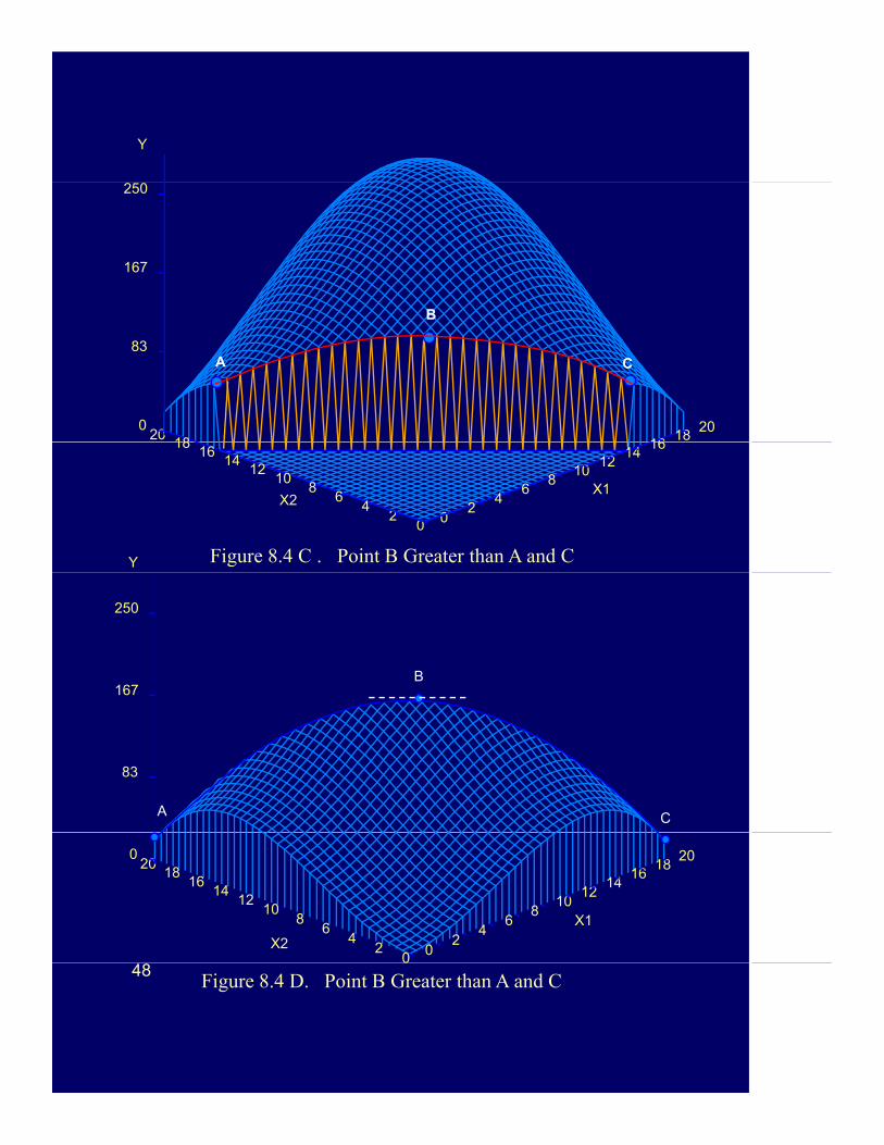
Figure 8.4 C . Point B Greater than A and CY
167
250
B
83
CA
182020
0
02
46
810
1214
16
X1
X20
24
68
1012
1416
18
480
Figure 8.4 D. Point B Greater than A and C
Y
167
250
Y
167
250
2 4 6 8 10
16 18 20
X1X2024681012
200
83
167
1214 141618
A B C
2 4 6 8
16 18 20
X1X20246810
200
83
167
10 12 1412141618
A B C
0
00
Y
167
250
B
Y
167
250
B
16 1820
X20
2
200
83
C
24
68
10 12 14
X146
81012141618
A
16 18 20200
83
8 10 12 14
X11012141618
A C
2X2 024 4 668
00
49
Figure 8.4 Constrained Maximization under Alternative Isoquant Convexity or Concavity Conditions

18
20GlobalOutputMaximum
LandGlobalProfit
Maximum= 1
12
14
16= 0
8
10
12
L* L*R
B C
A
2
4
6
X
X
R
00 2 4 6 8 10 12 14 16 18 20
X (a bundle of all inputs but land)
50
Figure 8.5 The Acreage Allotment Problem
50

2
BC
D
2
C
D
40
x x
1
A
B
1
A
B
C
30
0A > AB > BC > CD0 0
0A < AB < BC < CDxx
403020
1020
10
2
B
C
D
30
40
x
1
A
B
20
30
0 0A = AB = BC = CD x
10
Figure 9.1 Economies, Diseconomies and Constant Returns to ScaleFor a Production Function with Two Inputs
51

X2
10
6
8
2
4
0
X1
0 2 4 6 8 10
Figure 10.1 Isoquants for the Cobb-Douglas Production Function
52
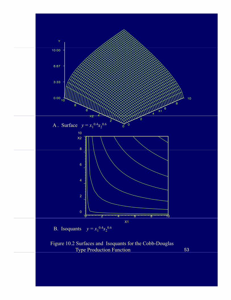
A . Surface y = x10.4x2
0.6
X2
8
10
4
6
8
0
2
0 2 4 6 8 10
53
X1
B. Isoquants y = x10.4x2
0.6
Figure 10.2 Surfaces and Isoquants for the Cobb-Douglas Type Production Functionyp
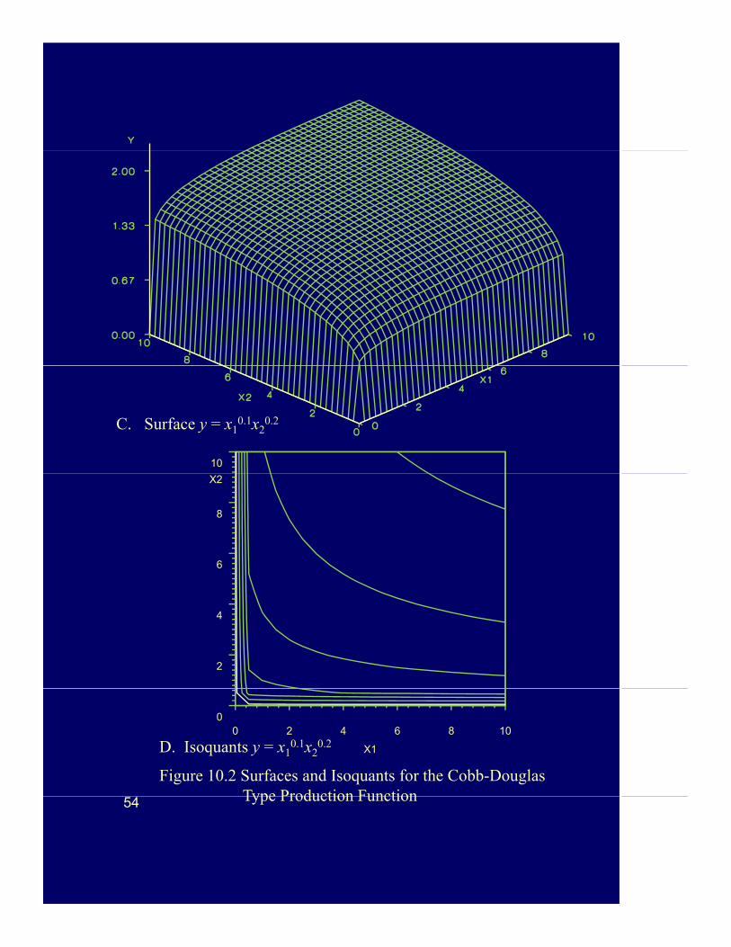
C. Surface y = x10.1x2
0.2
10
X2
6
8
2
4
0
X1
0 2 4 6 8 10
D. Isoquants y = x10.1x2
0.2
Figure 10.2 Surfaces and Isoquants for the Cobb-Douglas Type Production Function54 Type Production Function
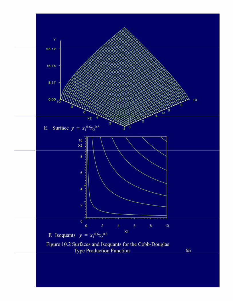
E. Surface y = x10.6x2
0.8
X2
10
6
8
2
4
55Figure 10.2 Surfaces and Isoquants for the Cobb-Douglas
Type Production Function
0
X1
0 2 4 6 8 10
F. Isoquants y = x10.6x2
0.8
yp

G . Surface y = x10.4x2
1.5
X2
10
6
8
0
2
4
X1
0 2 4 6 8 10
H. Isoquants y = x10.4x2
1.5
Figure 10.2 Surfaces and Isoquants for the Cobb-Douglas Type Production Function
56
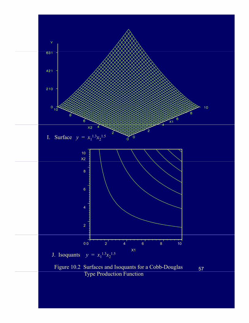
I. Surface y = x11.3x2
1.5
X2
10
6
8
2
4
57
X1
0 2 4 6 8 100
J. Isoquants y = x11.3x2
1.5
Figure 10.2 Surfaces and Isoquants for a Cobb-Douglas Type Production Function
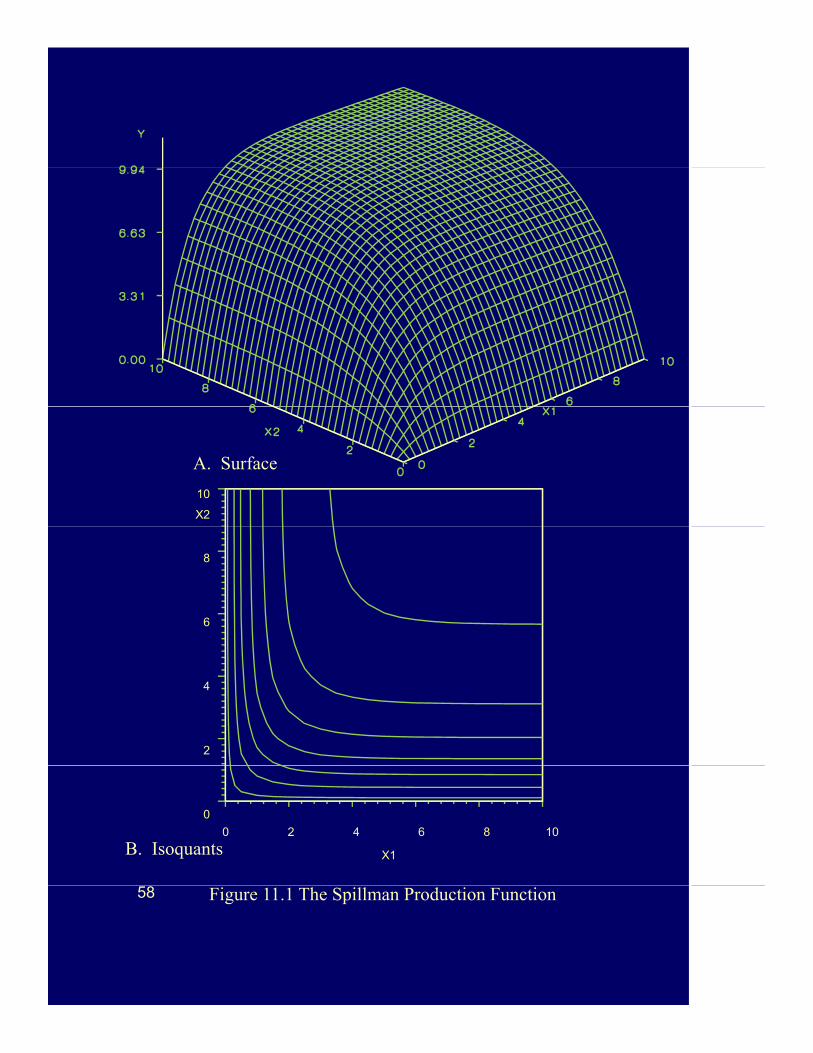
A. Surface
X2
10
6
8
2
4
0
X1
0 2 4 6 8 10
B. Isoquants
58 Figure 11.1 The Spillman Production Function

X2
3
22
-Ridge Line 2
MaximumOutput
2
1
00 1 2 31
X10 1 2 3
1
1
Figure 11.2 Isoquants and Ridge Lines for the Transcendental, = 2; = = 0
-
59
1 = 2 -2; 1 = 3 = 0
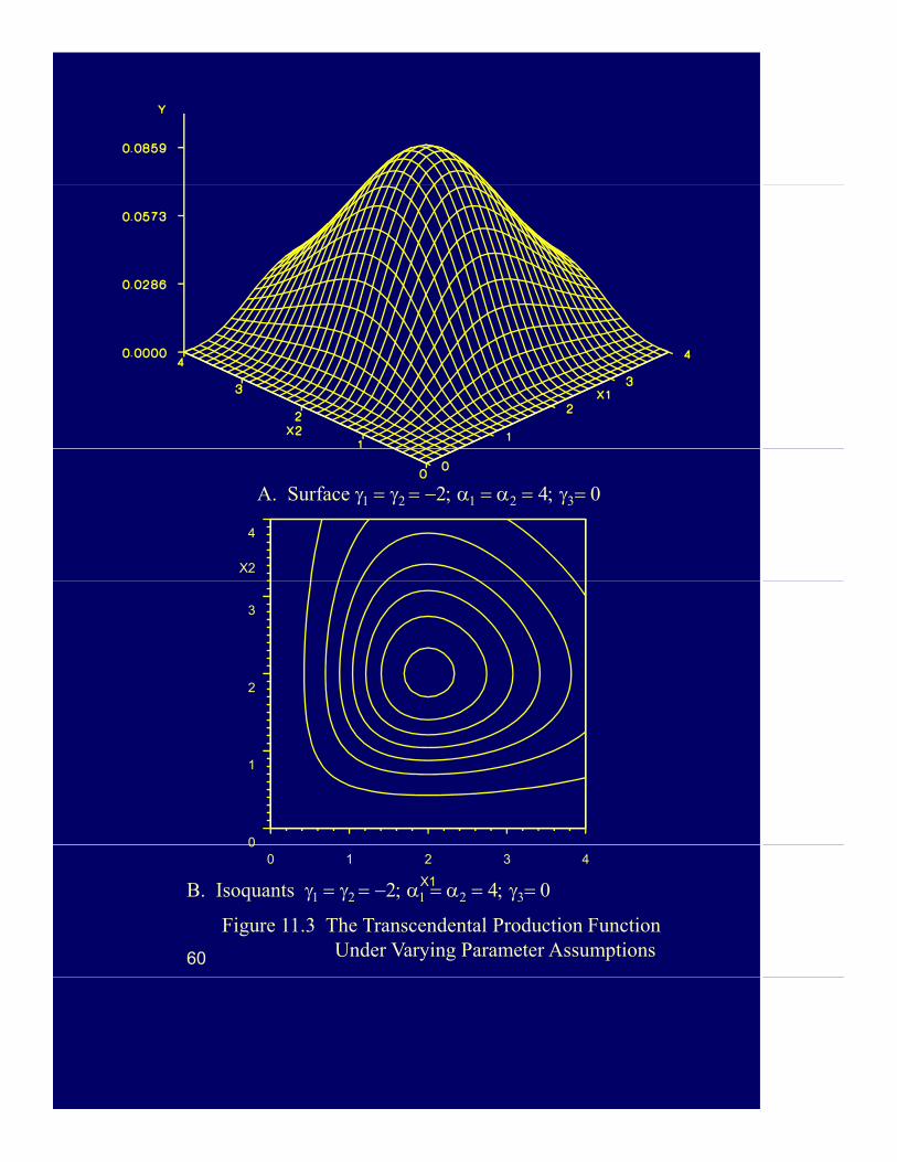
A. Surface
X2
4
2
3
0
1
60
0
X1
0 1 2 3 4
B. Isoquants
Figure 11.3 The Transcendental Production Function Under Varying Parameter Assumptions
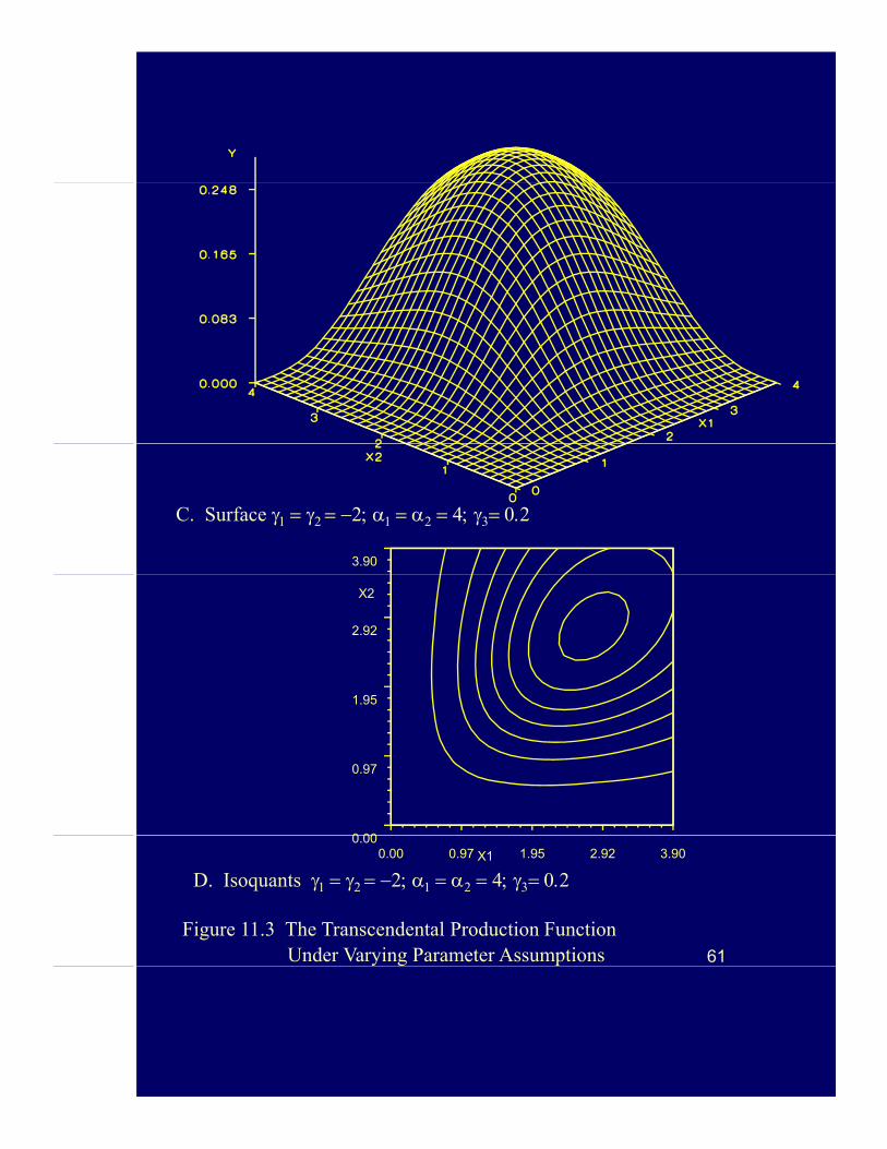
C. Surface
3.90
X2
1.95
2.92
0 00
0.97
61
X10.00
0.00 0.97 1.95 2.92 3.90
D. Isoquants
Figure 11.3 The Transcendental Production Function Under Varying Parameter Assumptions

E . Surface
4
X2
3
4
1
2
62
X1
0 1 2 3 40
F. Isoquants
Figure 11.3 The Transcendental Production Function Under Varying Parameter Assumptions62 y g p
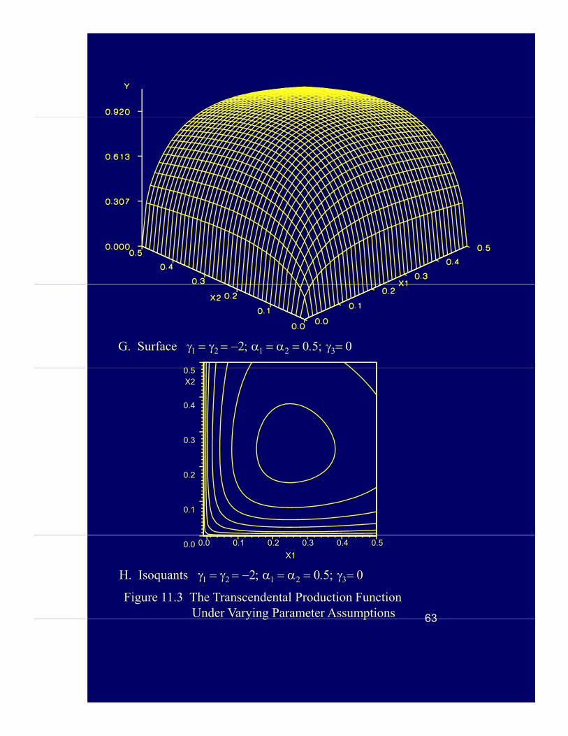
G. Surface
0 5X2
0.3
0.4
0.5
0.1
0.2
63
X1
0.0 0.1 0.2 0.3 0.4 0.50.0
H. Isoquants
Figure 11.3 The Transcendental Production Function Under Varying Parameter Assumptions 63y g p
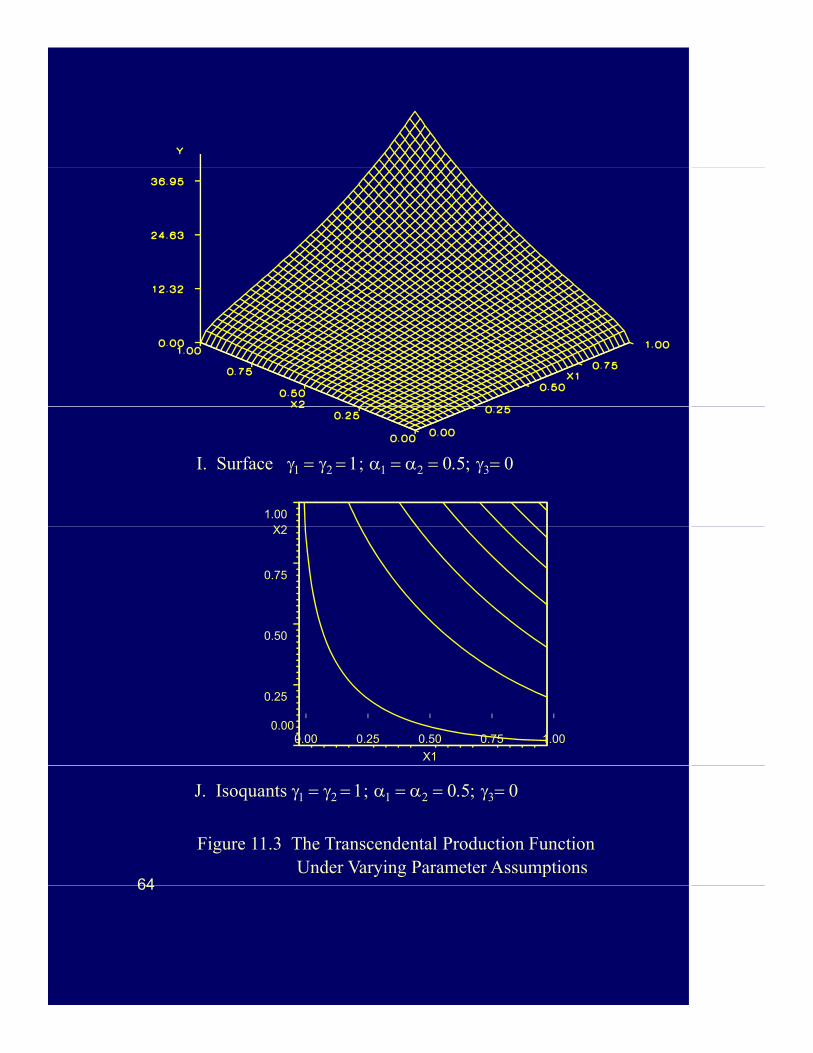
I. Surface
X21.00
X2
0.50
0.75
0.00
X1
0.00 0.25 0.50 0.75 1.00
0.25
64
J. Isoquants
Figure 11.3 The Transcendental Production Function Under Varying Parameter Assumptions
64

A. Surface
X220
8
12
16
X1
0 4 8 12 16 200
4
65
Figure 11.4 The Polynomial y = x1 + x1
2 – 0.05 x13 + x2 + x2
2 – 0.05 x23 + 0.4 x1 x2
B Isoquants

FFx2
M
H
P2
P
D
K Midpoint
y*
P1B
C J A E L G0 X1
66
Figure 12.1 The Arc Elasticity of Substitution
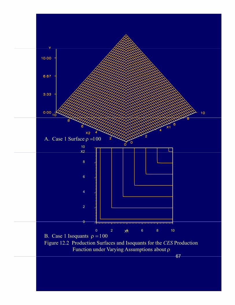
A. Case 1 Surface
X210X2
6
8
0
2
4
67
0
X10 2 4 6 8 10
B. Case 1 Isoquants Figure 12.2 Production Surfaces and Isoquants for the CES Production
Function under Varying Assumptions about 67
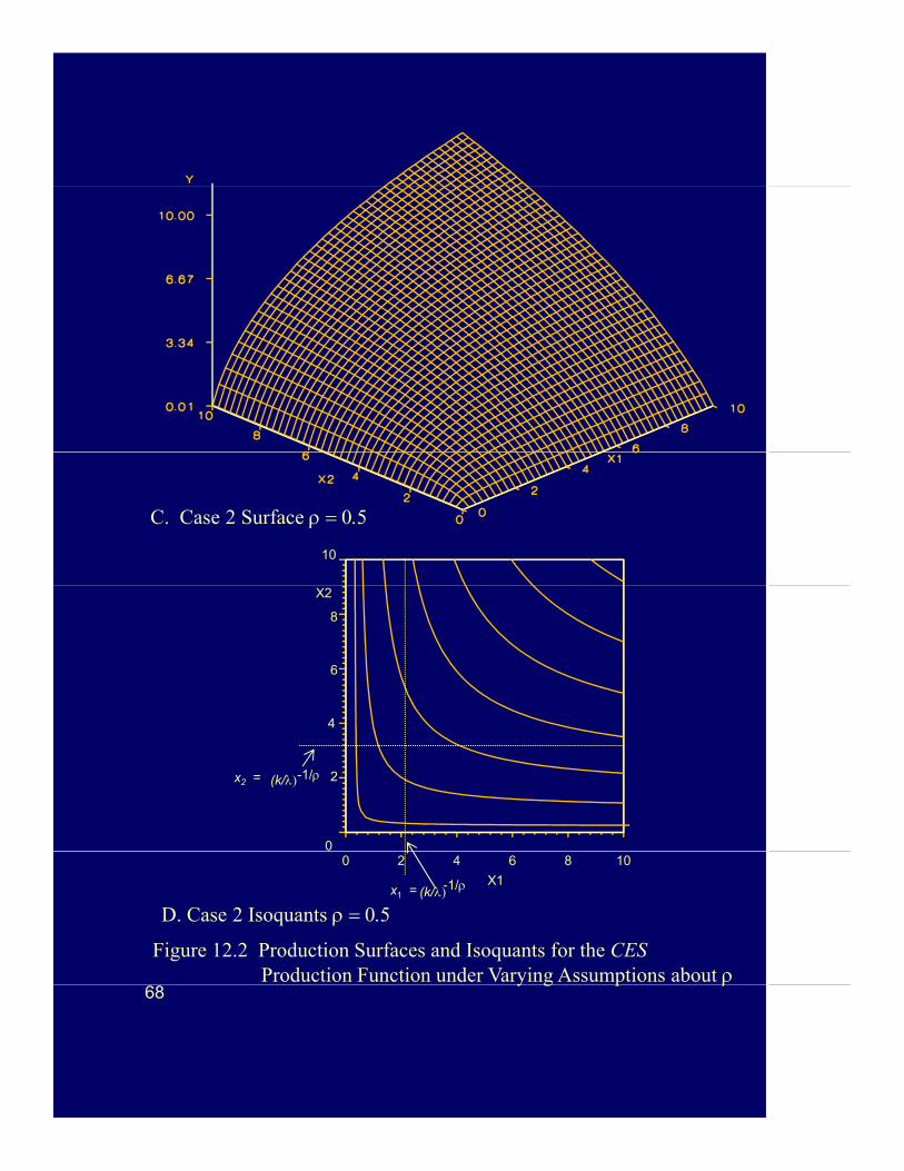
C. Case 2 Surface
10
X2
4
6
8
0
4
-1/(k/ 2x2 =
X1
0 2 4 6 8 10
-1/
D. Case 2 Isoquants
Figure 12.2 Production Surfaces and Isoquants for the CES Production Function under Varying Assumptions about
x1 = (k/
68y g p
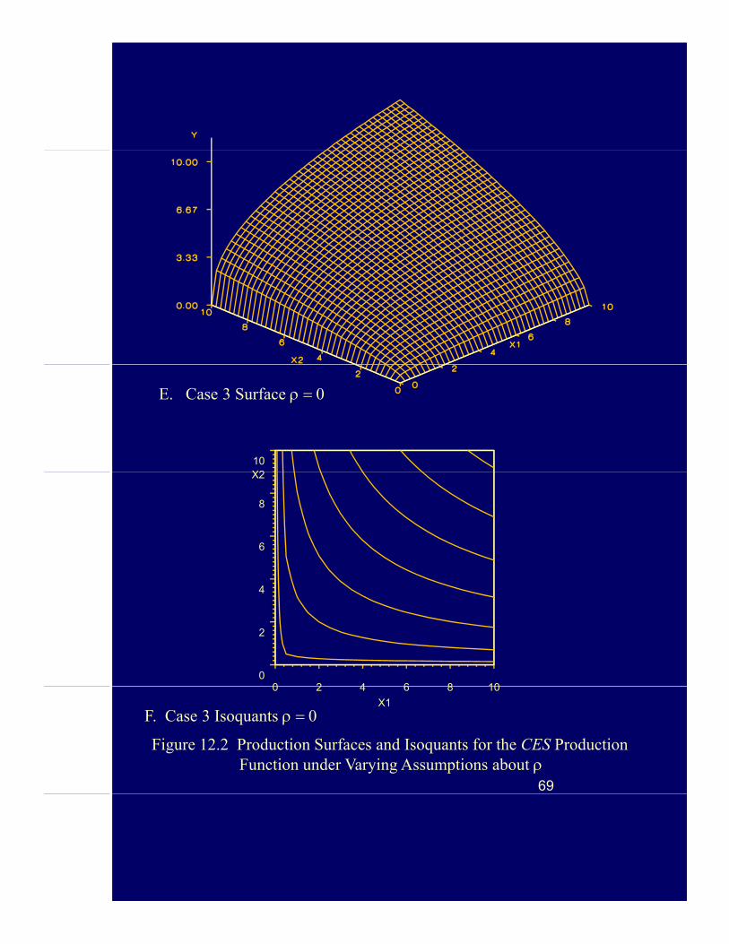
E. Case 3 Surface
X210X2
6
8
0
2
4
0 2 4 6 8 10
69
X1
0 2 4 6 8 10
F. Case 3 Isoquants
Figure 12.2 Production Surfaces and Isoquants for the CES Production Function under Varying Assumptions about

G. Case 4 Surface
X210
4
6
8
0
2
X10 2 4 6 8 10
70
J Case 4 Isoquants
Figure 12.2 Production Surfaces and Isoquants for the CES Production Function under Varying Assumptions about

I . Case 5 Surface approaches -1
X2
8
10
4
6
8
0
2
X10 2 4 6 8 10
J Case 5 Isoquants approaches 1
71
J. Case 5 Isoquants approaches -1
Figure 12.2 Production Surfaces and Isoquants for the CES Production Function under Varying Assumptions about
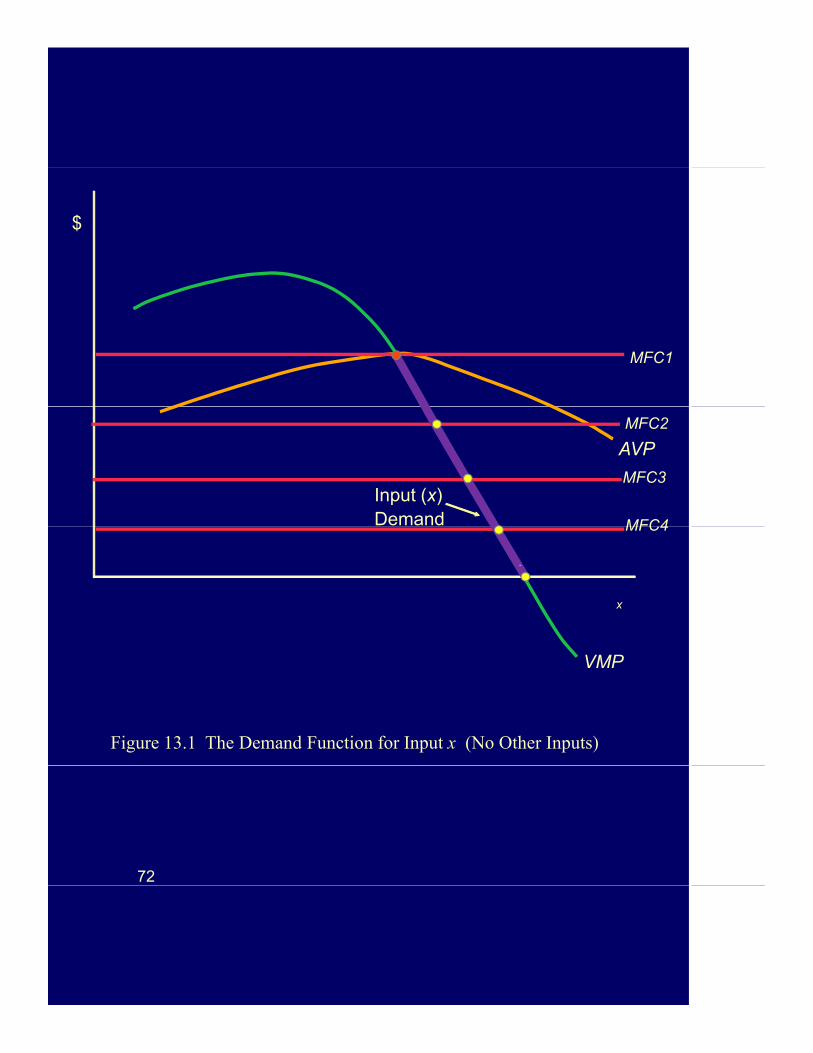
$
MFC1
MFC2
AVP
DemandInput (x)
MFC3
MFC4
x
MFC4
VMP
Figure 13.1 The Demand Function for Input x (No Other Inputs)
72
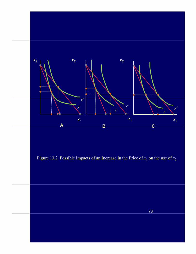
x2 x2x2
"
1
y'
y"
y"y'
y"y'
A B C
x xx11
B C
Figure 13.2 Possible Impacts of an Increase in the Price of x1 on the use of x2
73
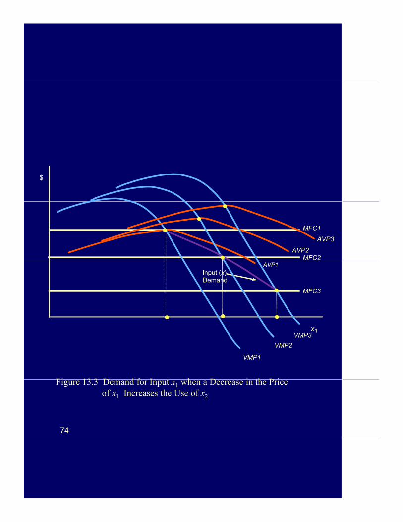
$
AVP2MFC2
AVP3
MFC1
MFC3
Input (x) Demand
AVP1
x
VMP1
VMP2
VMP31
Fi 13 3 D d f I t h D i th P i
74
Figure 13.3 Demand for Input x1 when a Decrease in the Price of x1 Increases the Use of x2

p
Maximum TR
TotalRevenue
TR = ay – by2
|Ep| = 1|Ep| > 1
Demandp = a - by
|Ep| < 1
yM T
|Ep| = - Ep
Marginal Revenue
0
MR = a - 2by
75
Figure 14.1 Total Revenue, Marginal Revenue,and the Elasticity of Demand
$ $
n
TVP
p TPP
p
p TPPo
n
p TPPo
TPP
TVP
p TPP
xxo
x n
xxo
x n
$
A B
TVP
p TPP
p TPPo
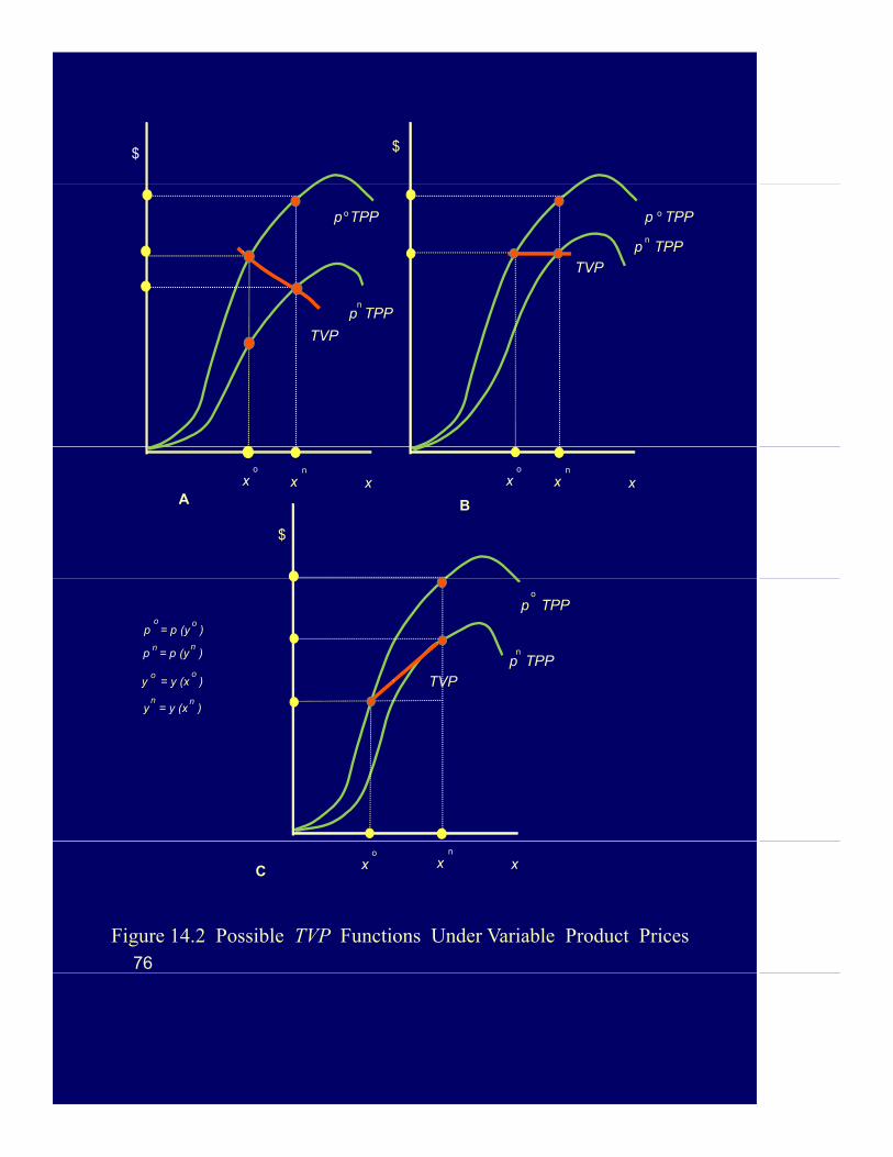
p = p (y )
p = p (y )
y = y (x )
y = y (x )
o o
o o
n n
n n n
y y (x )
76
xxo
x n
C
Figure 14.2 Possible TVP Functions Under Variable Product Prices

Guns
ProductionPossibilities Curve
Bundle X o
Possibilities Curve
for a Resource
Butter
77
Figure 15.1 A Classic Production Possibilities Curve
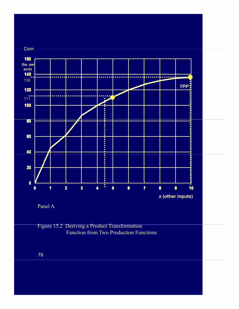
Corn
136
Corn
(bu. per acre)
TPP
111
Panel A
Fi 15 2 D i i P d t T f ti
x (other inputs)
78
Figure 15.2 Deriving a Product Transformation Function from Two Production Functions
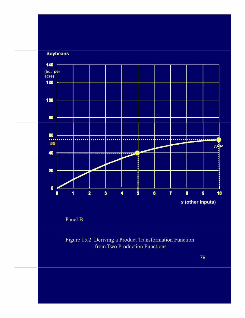
Soybeans
(bu. per acre)
55TPP
Panel B
x (other inputs)
79
Figure 15.2 Deriving a Product Transformation Function from Two Production Functions
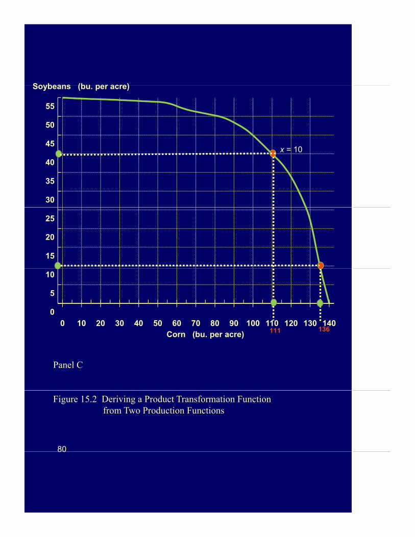
Soybeans (bu per acre)
45
50
55
Soybeans (bu. per acre)
30
35
40
45x = 10
15
20
25
0
5
10
0 10 20 30 40 50 60 70 80 90 100 110 120 130 140111 136111 136
Corn (bu. per acre)
Panel C
80
Figure 15.2 Deriving a Product Transformation Function from Two Production Functions
80

y y SupplementaryRange
22 g
yy
y
y yComplementary Range
Competitive Supplementary1
1
22
y y
Complementary Joint
11
81
Figure 15.3 Competitive, Supplementary, Complementary and Joint Products
p y
81

X
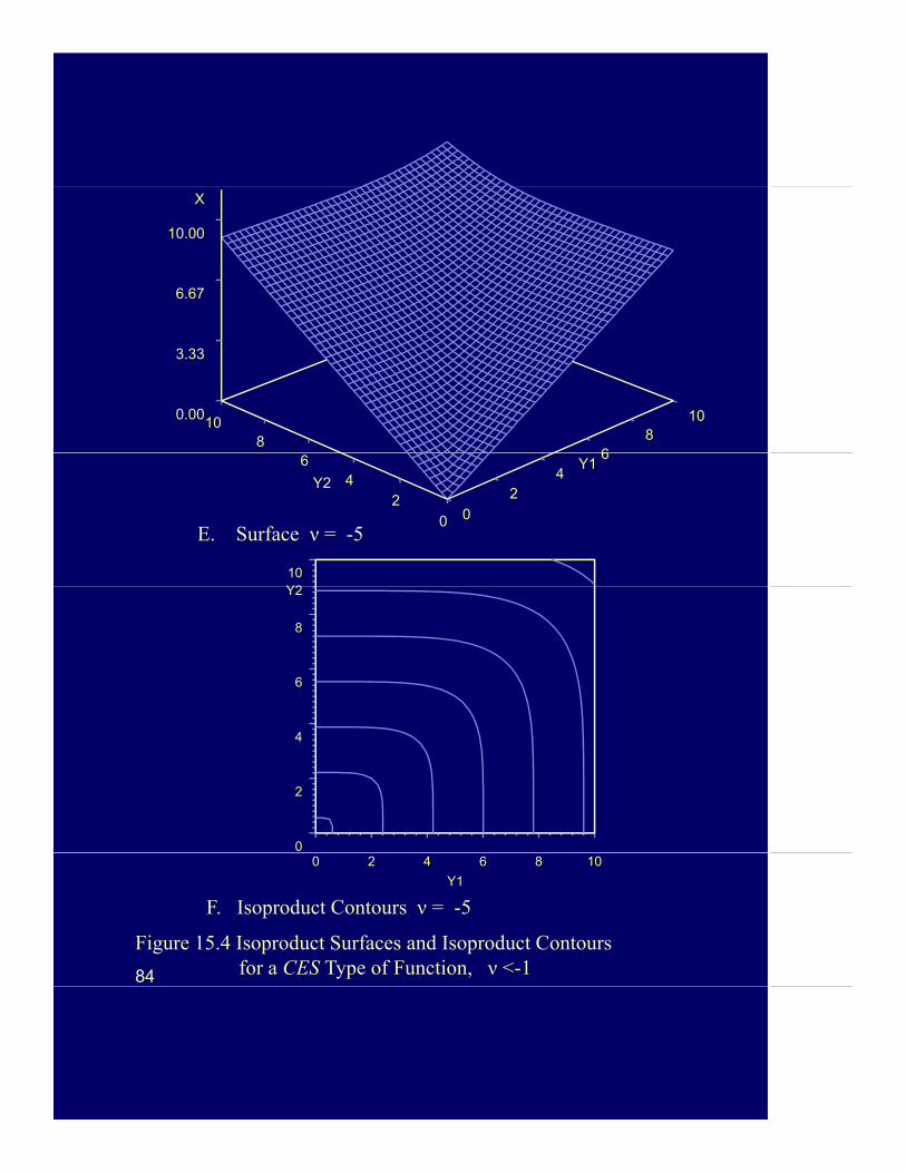
A. Surface ν approaches -1
Y1 Y2
6
8
10
Y2
0 2 4 6 8 100
2
4
82
Figure 15.4 Isoproduct Surfaces and Isoproduct Contours for a CES Type of Function, ν <-1
B. Isoproduct Contours ν approaches -1
0 2 4 6 8 10
Y1
82

XX
6.67
10.00
68
10
Y168
100.01
3.34
0
24
Y1Y2
0
24
C. Surface ν = -2
Y210
4
6
8
0
2
Y1
0 2 4 6 8 10
83
Y1D. Isoproduct Contours ν = -2
Figure 15.4 Isoproduct Surfaces and Isoproduct Contours for a CES Type of Function, ν <-1
X
6.67
10.00
68
10
810
0.00
3.33
0
24
6Y1
Y2
0
24
6
E. Surface ν = -5
Y210Y2
6
8
0
2
4
84
Y1
0 2 4 6 8 10
F. Isoproduct Contours ν = -5
Figure 15.4 Isoproduct Surfaces and Isoproduct Contours for a CES Type of Function, ν <-1

X
3 33
6.67
10.00
46
810
Y1Y2 4
68
100.00
3.33
02
Y2
02
G. Surface ν = -200
Y210
4
6
8
0
2
4
Y1
0 2 4 6 8 10
85
Y1
H. Isoproduct Contours ν = -200
Figure 15.4 Isoproduct Surfaces and Isoproduct Contours for a CES Type of Function, ν <-1
86
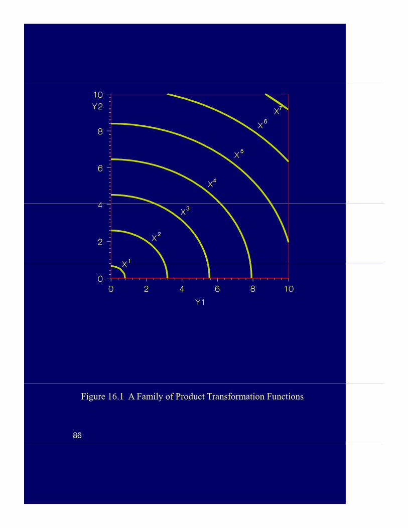
Figure 16.1 A Family of Product Transformation Functions
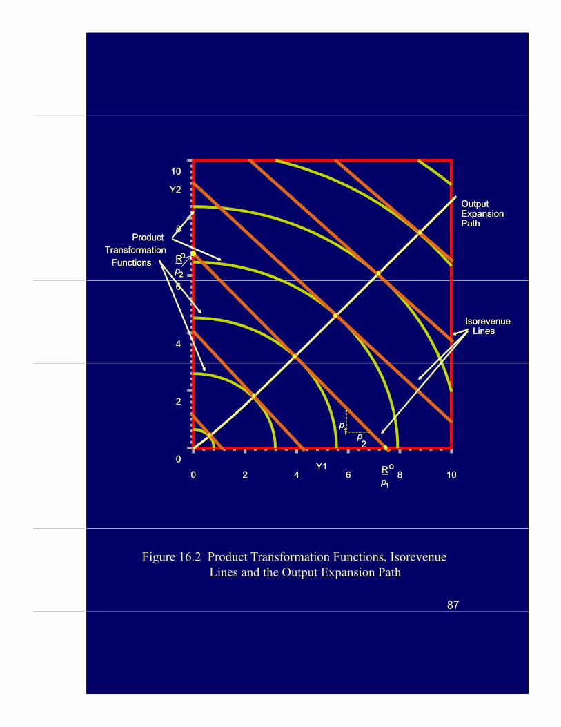
Y2Y2
1010
88ProductProduct
TransformationTransformation
OutputOutputExpansionExpansionPathPath
RRpp22
ooFunctionsFunctions
44
66
IsorevenueIsorevenueLinesLines
22
pp
2211 pp
00
00 22 44 66 88 1010
22
RRpp11
ooY1Y1
87
Figure 16.2 Product Transformation Functions, IsorevenueLines and the Output Expansion Path

TobaccoGlobal
f
10Output
ExpansionPath
Output PseudoScale LineFor Other Crops(Y)
Output PseudoScale Line for
TobaccoMaximum
Profit
6
8
B
(Y)
A
T*
2
4
CT
00 2 4 6 8 10 12 Y
Figure 16.3 An Output Quota
88

Forage
(z )2
Isoquants for
MRSx1x2
z1z2
= RPT
Beef Production
ProductTransformationFunction forGrain and
Forage
Grain andForage
Grain (z )1
(z )2
Sell
Line p
pz1
z2
ProduceIsorevenue
Isocost or
Produce Purchase Grain (z )1
Figure 17.1 An Intermediate Product Model89
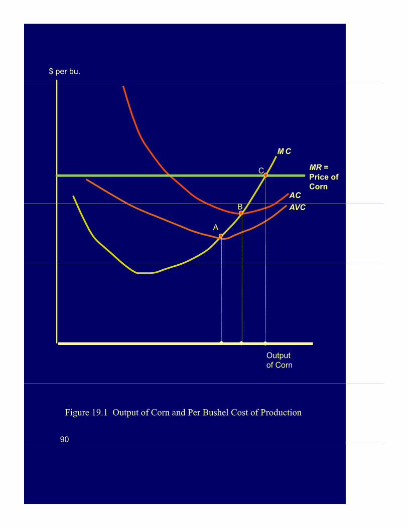
$ per bu.
B
C
M C
MR =Price ofCorn
AC
B AVC
A
Output of Corn
90
Figure 19.1 Output of Corn and Per Bushel Cost of Production

Probabilitiesand Outcomes
ProbabilitiesAnd Outcomesand Outcomes
are KnownAnd OutcomesAre not known
Risky Events Uncertain Events
91
Figure 20.1 A Risk and Uncertainty Continuum

Utility UtilityUtility Utility
Income IncomeRisk-Averse Risk-Neutral
Utility
92
Income
Figure 20.2 Three Possible Functions Linking Utility to Income
Risk-Preferrer
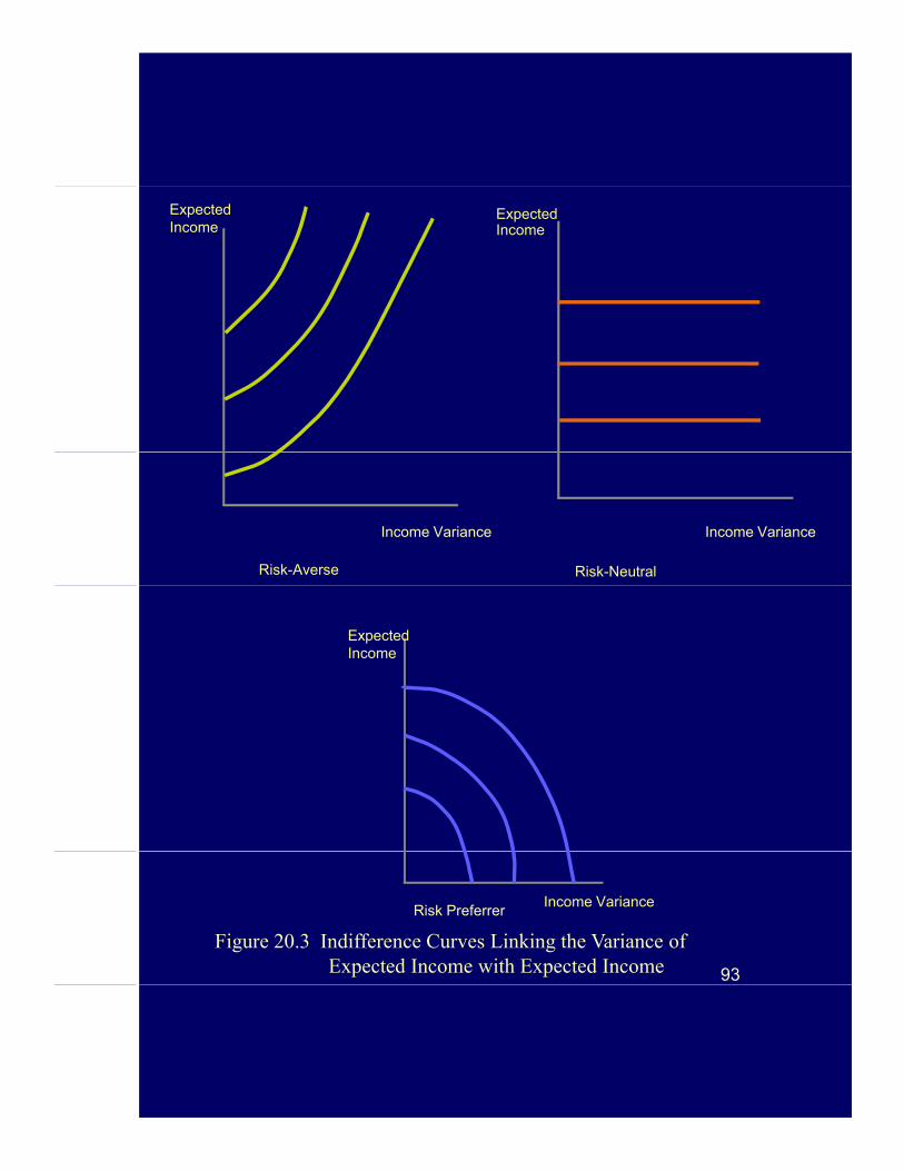
ExpectedIncome
ExpectedIncome
Risk-Neutral
Income Variance
Risk-Averse
Income Variance
Expected Income
93
Figure 20.3 Indifference Curves Linking the Variance of Expected Income with Expected Income
Risk PreferrerIncome Variance
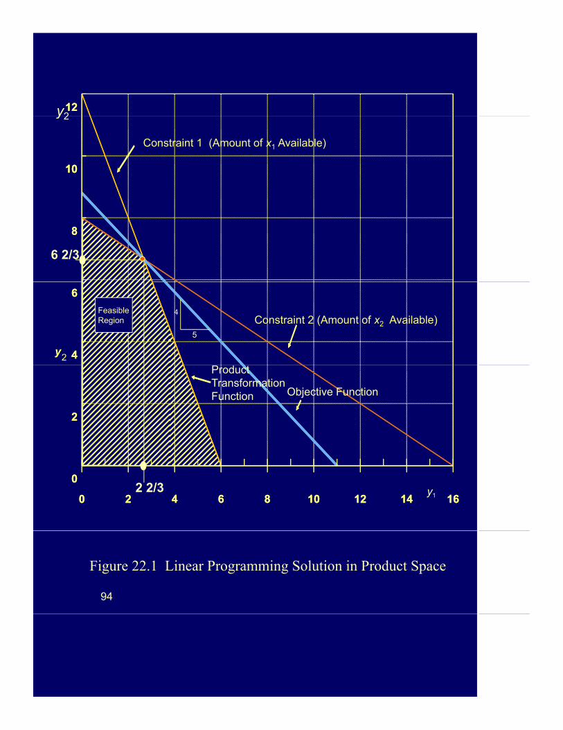
1212y2
1010
y2
Constraint 1 (Amount of x1 Available)
88
6 2/3
y 4
6
4
6
FeasibleRegion Constraint 2 (Amount of x2 Available)
5
4
2
22
ProductTransformationFunction Objective Function
FeasibleRegion
4
0
0 2 4 6 8 10 12 14 16
0
0 2 4 6 8 10 12 14 162 2/3 y1
94
Figure 22.1 Linear Programming Solution in Product Space
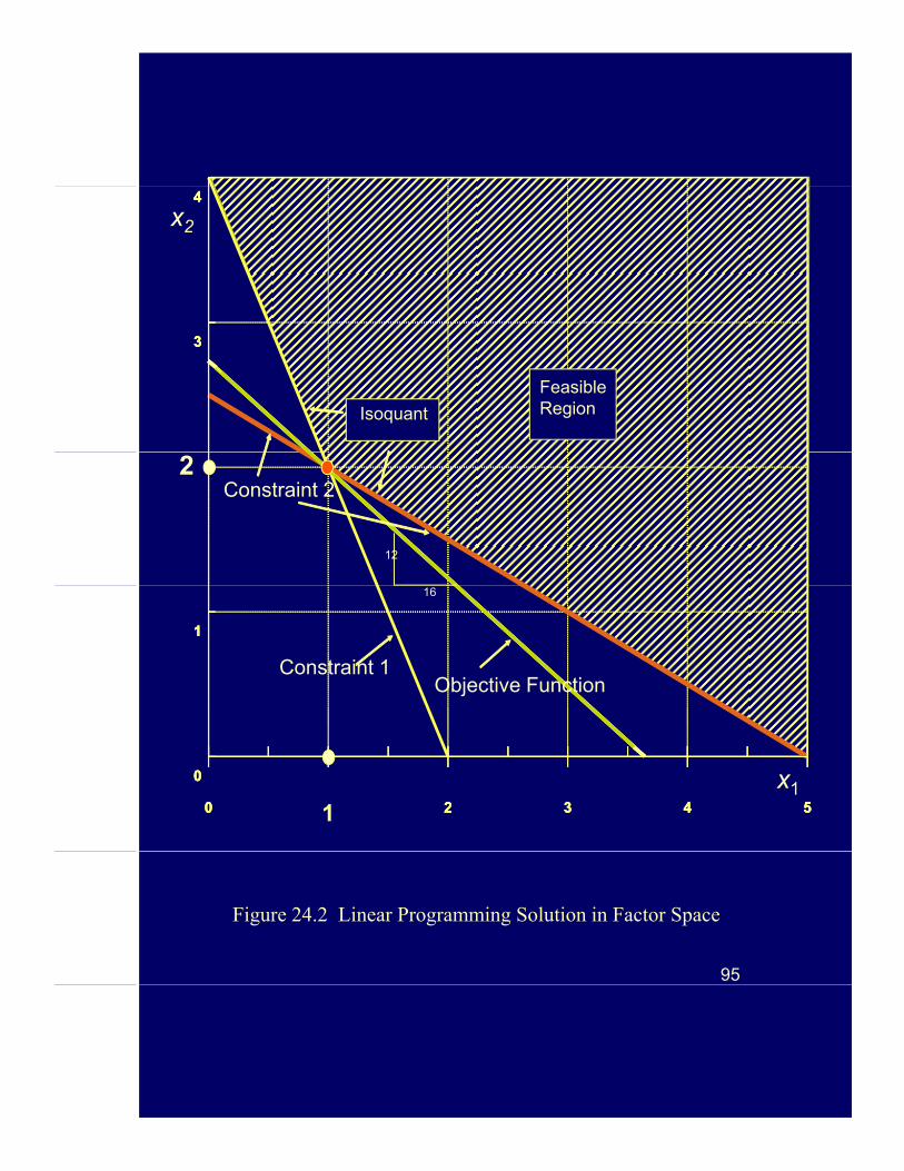
444
x2
Feasible
Isoquant
333
FeasibleRegionIsoquant
Constraint 2
12
2
111
Objective Function
16
Constraint 1
0
0 1 2 3 4 5
0
0 2 3 4 5
0
0 2 3 4 5
x1
95
Figure 24.2 Linear Programming Solution in Factor Space

x2x2
x1 x1
x2
Diagram A Diagram B
96
x1Diagram C
Figure 23.1 Some Possible Impacts of Technological Change
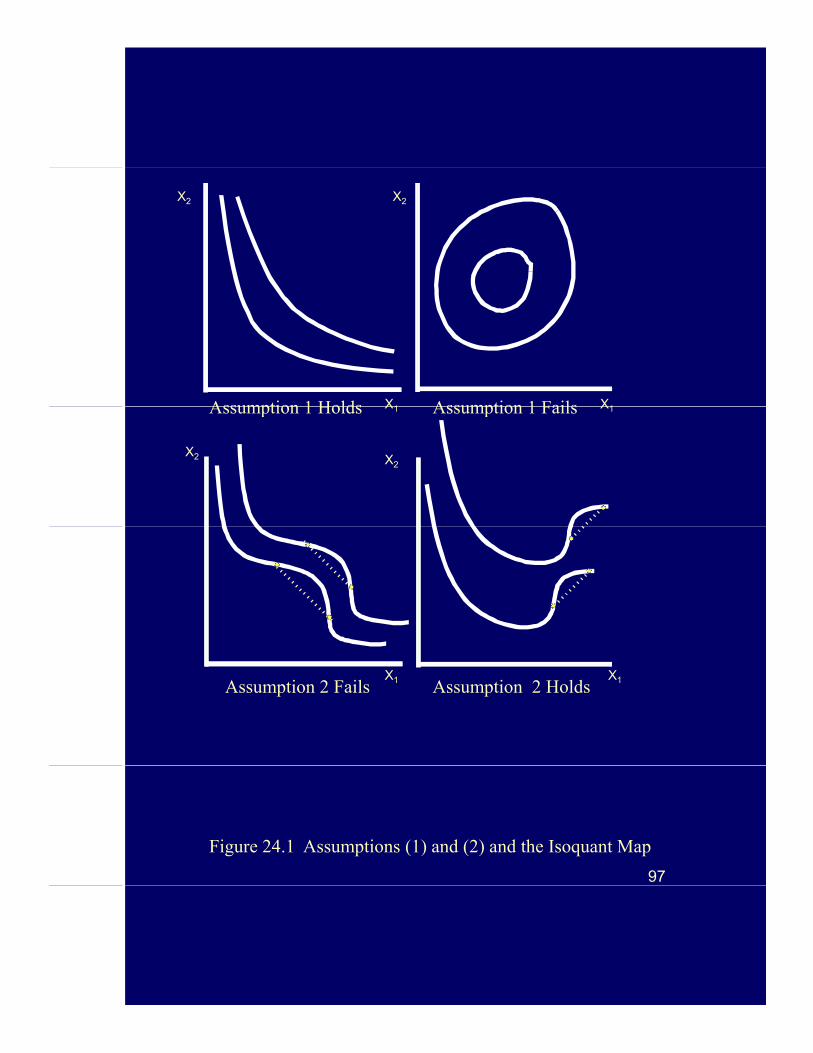
X2X2
Assumption 1 Holds Assumption 1 FailsX1 X1Assumption 1 Holds Assumption 1 FailsX1 X1
X2 X2
Assumption 2 Fails Assumption 2 HoldsX1X1
Figure 24.1 Assumptions (1) and (2) and the Isoquant Map
97
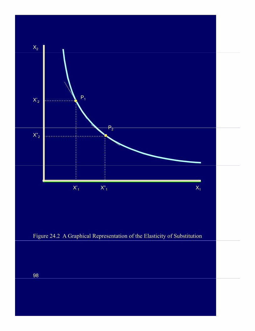
X2
P1
P
X’2
P2
X”2
X’1 X”1 X1
Figure 24.2 A Graphical Representation of the Elasticity of Substitution
98