core shielded distribution power cables based on non

1558-1748 (c) 2017 IEEE. Personal use is permitted, but republication/redistribution requires IEEE permission. See http://www.ieee.org/publications_standards/publications/rights/index.html for more information.

This article has been accepted for publication in a future issue of this journal, but has not been fully edited. Content may change prior to final publication. Citation information: DOI 10.1109/JSEN.2017.2756905, IEEE SensorsJournal

Energization-Status Identification of Three-Phase Three-

Core Shielded Distribution Power Cables Based on Non-

Destructive Magnetic Field Sensing

Ke ZHU, Student Member, IEEE, W. K. LEE, and Philip W. T. PONG*, Senior Member, IEEE

Abstract— Three-phase three-core distribution power cables

are widely deployed in power distribution networks and are

continually being extended to address the ever-increasing power

demand in modern metropolises. Unfortunately, there are high

risks for the repair crew to operate on energized distribution

power cables which can cause deadly consequences such as

electrocution and explosion. The predominant energization-status

identification techniques used today are either destructive or only

applicable to un-shielded power cables. Moreover, the

background interferences affect the sensing technique reliability.

In this paper, we have developed a non-destructive energization-

status identification technique to identify energized three-phase

three-core distribution power cables by measuring magnetic fields

around the cable surface. The analysis shows that the magnetic-

field-distribution pattern as a function of azimuth around the

cable surface of the energized (current- or voltage-energized)

three-phase three-core distribution power cable is distinguishable

from the de-energized one. The non-idealities of phase currents

and cable geometry were also discussed, and the proposed method

still works under these circumstances. The sensing platform for

implementing this technique was developed accordingly,

consisting of magnetoresistive (MR) sensors, a triple-layered

magnetic shielding and a data acquisition system. The technique

was demonstrated on a 22-kV three-phase three-core distribution

power cable, and the energized status of the cable can be

successfully identified. The proposed technique does not damage

cable integrity by piercing the cable, or exposing the repair crew

to hazardous high-voltage conductors. The platform is easy to

operate and it can significantly improve the situational awareness

for the repair crew, and enhance the stability of power distribution

networks.

Index Terms— three-phase three-core distribution power cable,

energized status, magnetic sensing, distribution power network

I. INTRODUCTION

HREE-PHASE three-core distribution power cables are

widely deployed in the power distribution system which

acts as the last link in the chain of supplying the power to

the customers. Though these power cables are less susceptible

by weather-related outages (e.g., thunderstorms, heavy snows

[1-3]) as they are typically hidden underground, maintenance

tasks are regularly performed by the repair crew to inspect

defective cables (e.g., insulation deterioration, mechanical

cracks and even wire break points), or to splice power cables

for re-structuring the distribution power networks [4-7].

Nonetheless, there are high risks for the repair crew to operate

on energized distribution power cables (i.e., cables that

connected with the high-voltage power supply). For the repair

crew conducting on-site work, they must be highly alerted of

these energized power cables because contacting with a high-

voltage conductor can cause deadly consequences such as

explosion and flashover. Due to the continued distribution

power network expansion, administrative changes, poor record-

keeping, or other reasons, the topological representation of the

power distribution network may not be completely accurate and

up-to-date. Therefore, it is difficult for the repair crew to locate

and identify the energized three-phase three-core distribution

power cables accurately and safely based on the information

from the control station when implementing the onsite tasks [8].

Researchers and industrial companies have developed a

handful of techniques to identify the energized power cables for

safeguarding the safety of the repair crew [9-11]. However, the

predominant detection techniques today are either destructive

in nature or only applicable for the un-shielded power cables.

The SPIKE tool [12], for example, pierces through the cable

insulation to make electrical contact with the internal conductor

and thus inextricably damages the cable. The penetration into

the cable not only causes irreversible damage to the integrity of

the cable, but also exposes workers to a potentially hazardous

situation with high-voltage conductors. Robots have been

developed to replace the human work of penetrating the cables,

but the damage to the power cables is still unavoidable [13, 14].

Though a handful of non-destructive techniques have been

developed for improving the situation, the strong dependence

of the cable type (i.e., un-shielded power cable) limits their

usage. Notably, electric fields are generated from the energized

conductors and the related technique is developed [15, 16].

Nevertheless, the detection of the electric field is only

applicable for un-shielded (i.e. without metallic sheath)

distribution power cables as the electric fields terminate on the

earthed metallic sheath of the shielded cables. Moreover, since

the onsite environment is very complicated with background

interferences, the reliability of devices can be adversely

affected. For instance, a technique of attaching fiber optic

acoustic sensors on the cable surface was developed based on

the detection of acoustic vibrations that are associated with the

energized cables [17]. However, the de-energized cables can be

mistaken as the energized ones since the optical fiber sensing

system is not immune to ambient power-line-frequency electro-

magnetic noises and thus it may provide unreliable results.

Therefore, it is worthwhile to develop a non-destructive and

reliable technique applicable for identifying the energized

cables for both shielded and un-shielded cables.

T

This research is supported by the Seed Funding Program for Basic Research, Seed Funding Program for Applied Research and Small Project Funding Program from the University of Hong Kong, ITF Tier 3 funding (ITS-104/13, ITS-214/14), and University Grants Committee of HK (AoE/P-04/08). The authors would like to thank the Hongkong Electric Company Limited, Hong Kong for assisting the onsite experiment. *Corresponding email: [email protected].



Magnetic sensing for identifying the energized cables is a

promising solution [18, 19]. Firstly, the magnetic fields are

emanated outside the energized cables both for current-

energized (i.e., with load current) and voltage-energized

statuses (i.e., the charging current exists when the cable is

disconnected from the load but remains connected with the

power supply) [20, 21]. This makes the non-contact detection

possible without the need to penetrate into the cable, which is

beneficial to both cable integrity and personnel safety.

Secondly, the magnetic fields are still measurable around the

shielded cable since the metallic sheath is not a high-

permeability material [22, 23]. Furthermore, the ambient

magnetic interference can be effectively eliminated by a

magnetic shielding to ensure the accuracy and reliability of this

technique. Therefore, it can be feasible and reliable to identify

the shielded energized cables by non-destructive magnetic

sensing.

In this paper, a novel non-destructive energization-status

identification technique based on the recognition of RMS

magnetic-field-distribution pattern as a function of azimuth

around the cable surface is proposed for identifying the

energized (current- or voltage-energized) three-phase three-

core distribution power cables. The content of this paper is as

follows. In Section II, the magnetic field distribution patterns

of all cable statuses (i.e., current-, voltage- and de-energized)

were analyzed. The non-idealities of phase currents and cable

geometry were also discussed. Based on the findings, a sensing

platform hardware consisting of a magnetoresistive (MR)

sensor array and a triple-layered magnetic shielding was

designed to measure magnetic field around the cable surface in

Section III. In Section IV, the proposed technique was

experimentally verified on a 22-kV three-phase three-core

distribution power cable in a substation. The final conclusions

and future work are presented in Section V.

II. Magnetic Field Distribution of Current-, Voltage-,

and De-Energized Three-Phase Three-Core Power Cables

In order to distinguish the energization-status of a three-

phase three-core distribution power cable, the RMS magnetic-

field-distribution pattern around the cable surface was studied

for current-, voltage- and de-energized statuses respectively in

this Section. The primary voltages for distribution power cables

are 11 and 22 kV in Hong Kong (United States: 7.2, 12.47, 25,

and 34.5 kV; United Kingdom, Australia and New Zealand: 11

and 22 kV ; South Africa: 11 kV and 22 kV [24]). In this paper,

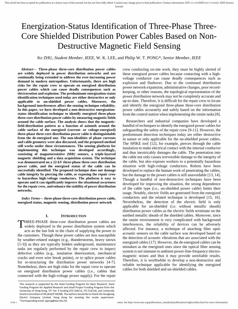
a typical three-phase three-core armored 22-kV XLPE stranded

power cable was demonstrated as an example. Its structure is

shown in Fig. 1. Each phase conductor is surrounded by a thin

tape screen (also named as Hochstadter shield [25]), which is

used to equalize the electrical stress on the insulation. Each tape

screen is connected to the metallic sheath by the wires at both

ends, and then the wires are grounded. The three-phase three-

core conductors are assumed to be ideally equidistant to the

cable center. The electromagnetic properties of each component

are described by the relative permeability ( 𝝁𝒓 ), relative

permittivity (𝝐𝒓), and conductivity (𝝈𝒓) as listed in Table. I.

Fig. 1. 22-kV three-phase three-core armored XLPE stranded power cable

structure. Radius: (1) phase conductor, 10 mm; (2) tape screen, 15 mm (inner)

and 15.5 mm (outer); (3) metallic sheath: 40 mm (inner) and 42 mm (outer).

TABLE I ELECTROMAGNETIC PROPERTY OF 22-KV THREE-PHASE

THREE-CORE ARMORED XLPE DISTRIBUTION POWER CABLE

Element 𝝁𝒓 𝝐𝒓 𝝈𝒓 (s/m)

Phase conductor

(Copper) 1.0 1.0 5.8×107

Insulation

(XLPE) 1.0 2.3 0.0

Tape Screen

(Copper) 1.0 1.0 5.8×107

Filler

(Polypropylene) 1.0 2.3 0.0

Metallic sheath

(Steel) 40 1.0 1.1×107

A. Current-energized status

Only the load currents flow through the phase conductors

when the cable is current-energized. The RMS magnetic flux

density () at an arbitrary point P (r,θ) around the cable surface

is calculated as [26]

=3𝜇𝐼

2√2𝜋√

𝑠4+𝑠2𝑟2

𝑟6−2𝑠3𝑟3 cos(3𝜃)+𝑠6 (1)

where r is the distance from the measurement point to the

center, the azimuth of point P is θ with respect to the horizontal

direction, and I is the load current of the three-phase power

cable (Fig. 2). Eq. (1) shows that the RMS magnetic flux

density around the cable surface repeats at an interval of 2/3 π

with three crests and troughs as a function of the azimuth of the

cable center.



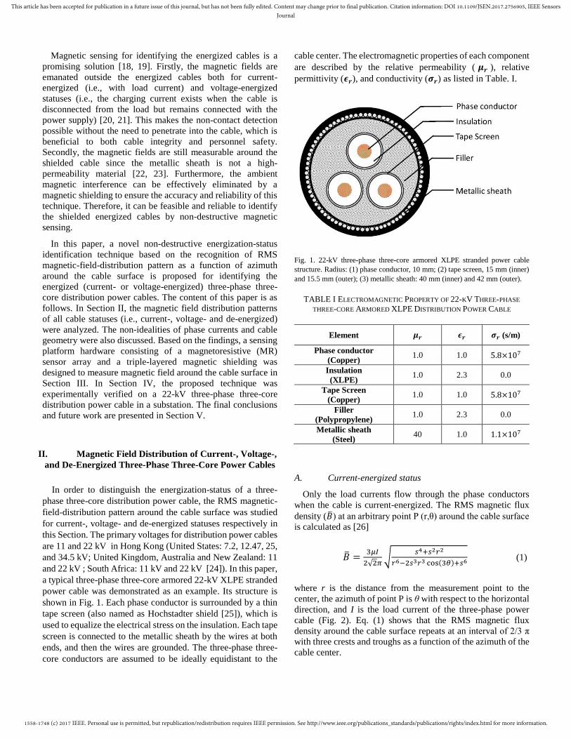
Fig. 2. Magnetic flux density measured at a sensing point (P) around the three-

phase three-core conductors (three red dots for phase A, B and C) at various

azimuth (θ).

The magnitude of the magnetic flux density around the cable

surface with a rated phase current of 1 A was simulated by

FEM. The RMS magnetic flux density was about 10 mG around

the cable surface (Fig. 3(a)). According to Eq. (1), the RMS

magnetic-field-distribution pattern around the cable surface

would exhibit a pattern of three peaks and three troughs, which

was confirmed by the FEM results as shown in Fig. 3(b). The

load current of a current-energized cable is typically ranged

from tens to hundreds of amperes (only under some rare

extreme cases with very light loading conditions that the load

current becomes several amperes) [27-29]. As such, the RMS

magnetic-field-distribution pattern around the cable surface

typically range from hundreds of mG (i.e., tens amperes of load

current) to thousands of mG (i.e., hundreds of amperes of load

current). To conclude, the RMS magnetic-field-distribution

pattern around the cable surface as a function of the azimuth

around the cable surface shows a pattern of three peaks and

three troughs with typically magnitude from hundreds or even

up to thousands of mG.

B. Voltage-energized status

There is no load current flowing on the three-phase three-core

conductors when the cable is voltage-energized; however, there

are capacitive charging currents which are incurred due to the

fact that the phase conductors are still connected to the power

source with the alternating voltage [30, 31]. The magnetic field

distribution around the cable surface was evaluated from the

charging current as follows.

Firstly, the unit resistance of the phase conductor and the tape

screen, and the unit capacitance between them were calculated.

The resistance is proportional to its electrical resistivity and

length, and is inversely proportional to the cross-sectional area.

As such, the unit resistance of the phase conductor (𝑅) and the

tape screen (𝑟) can be calculated as

𝑅 = 𝜌𝑝𝑐 1

𝜋𝑡2 (2)

𝑟 = 𝜌𝑡𝑠1

𝜋(𝐷𝑜2−𝐷𝑖

2) (3)

where 𝜌𝑝𝑐 , 𝜌𝑡𝑠 are the resistivity of phase conductor and the

tape screen, 𝑡 is the radius of the conductor, and 𝐷𝑖 , 𝐷𝑜 are the

inner and outer radius of the tape screen, respectively. The

equivalent capacitor (𝐶0 in Fig. 4) between the cable phase

conductor and the earthed tape screen can be calculated as [32]

𝐶0 =𝜀𝑟

41.4𝑙𝑜𝑔10𝐷𝑖𝑡

×10−9 (4)

where 𝜀𝑟 is the relative permittivity of the insulation between

the phase conductor and the tape screen.

Secondly, the charging current distribution and magnitude

along the cable was studied. One phase of the power cable (the

Fig. 3. Magnetic flux density around the current-energized cable surface with

a rated current of 1 A simulated by FEM. (a) Magnitude of magnetic field

around the cable surface denoted by the color bar. (b) RMS magnetic flux

density around the cable: radius (R), 60 mm; azimuth (𝜃) ranges from 0 to

360°.



other two are only with 120° phase angle differences) was

taken as an example by being divided piecewise with the

corresponding lumped elements in the equivalent electric

circuit model (Fig. 5(a)). The lumped resistors of the phase

conductor are denoted as R1, R2, …, Rn, the lumped resistors of

the tape screen as r1, r2, …, rn, and the lumped equivalent

capacitors formed between the phase conductor and the tape

screen as C1, C2, …, Cn. The charging current for the 600-m

length 22-kV power cable (50 Hz) was simulated as an example

by dividing the cable into 12 pieces (i.e., n=12). Accordingly,

the charging current flowing on the phase conductor (𝐼𝑐𝑜𝑛𝑑) and

the tape screen (𝐼𝑡𝑠) on a certain section (n) can be attained as

𝐼𝑐𝑜𝑛𝑑(𝑛) = 𝐼𝑛 (5)

𝐼𝑡𝑠(𝑛) = 𝐼0 − 𝐼𝑛 (6)

by solving these equations

(𝑅1 + 𝑟1 +1

𝑗𝜔𝐶1) 𝐼1 −

1

𝑗𝜔𝐶1𝐼2 − 𝑟1𝐼0 = 𝑈 (7)

−1

𝑗𝜔𝐶𝑛−1𝐼𝑛−1 + (𝑅𝑛 + 𝑟𝑛 +

1

𝑗𝜔𝐶𝑛−1+

1

𝑗𝜔𝐶𝑛) 𝐼𝑛 −

1

𝑗𝜔𝐶𝑛𝐼𝑛+1 − 𝑟𝑛𝐼0 = 0 (n=2, 3, 4,…, 10, 11) (8)

−1

𝑗𝜔𝐶11𝐼11 + (𝑅12 + 𝑟12 +

1

𝑗𝜔𝐶11+

1

𝑗𝜔𝐶12) 𝐼12 − 𝑟12𝐼0 = 0 (9)

− ∑ 𝑟𝑖𝐼𝑖12𝑖=1 + (∑ 𝑟𝑖

12𝑖=1 )𝐼0 = 0 (10)

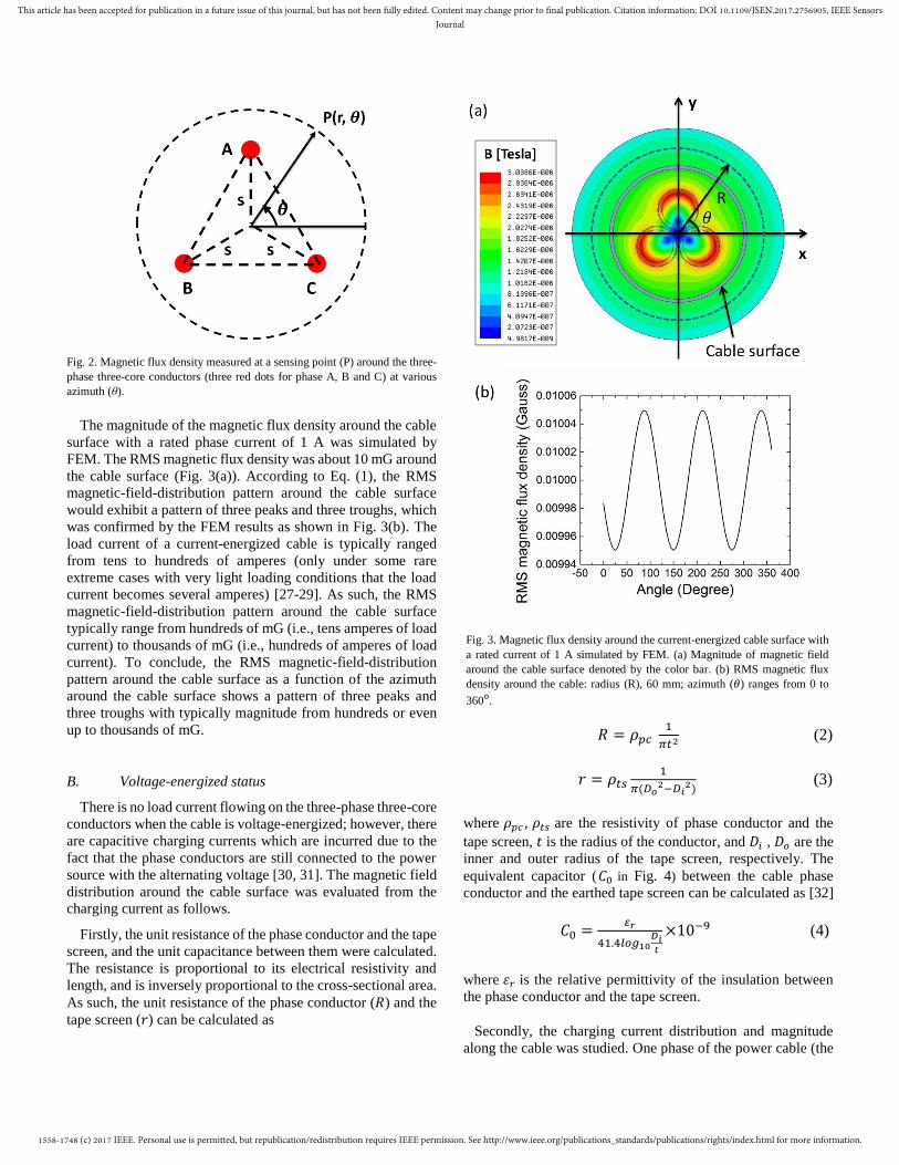
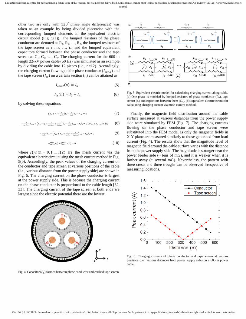
where 𝐼(𝑛)(n = 0, 1, … , 12) are the mesh current via the

equivalent electric circuit using the mesh current method in Fig.

5(b). Accordingly, the peak values of the charging current on

the conductor and tape screen at various positions of the cable

(i.e., various distance from the power supply side) are shown in

Fig. 6. The charging current on the phase conductor is largest

at the power supply side. This is because the charging current

on the phase conductor is proportional to the cable length [32,

33]. The charging current of the tape screen at both ends are

largest since the electric potential there are the lowest.

Fig. 4. Capacitor (𝐶0) formed between phase conductor and earthed tape screen.

Fig. 5. Equivalent electric model for calculating charging current along cable.

(a) One phase is modeled by lumped resistors of phase conductor (Rn), tape

screen (rn) and capacitors between them (Cn). (b) Equivalent electric circuit for

calculating charging current via mesh current method.

Finally, the magnetic field distribution around the cable

surface measured at various distances from the power supply

side were simulated by FEM (Fig. 7). The charging currents

flowing on the phase conductor and tape screen were

substituted into the FEM model as only the magnetic fields in

X-Y plane are measured similarly to those generated from load

current (Fig. 4). The results show that the magnitude level of

magnetic field around the cable surface varies with the distance

from the power supply side. The magnitude is stronger near the

power feeder side (~ tens of mG), and it is weaker when it is

farther away (~ several mG). Nevertheless, the pattern with

three crests and three troughs can be observed irrespective of

measuring locations.

Fig. 6. Charging currents of phase conductor and tape screen at various

positions (i.e., various distances from power supply side) on a 600-m power

cable.



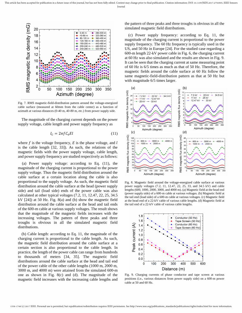
Fig. 7. RMS magnetic-field-distribution pattern around the voltage-energized

cable surface (measured at 60mm from the cable center) as a function of

azimuth at various distances (0-40 m, 40-80 m, etc.) from power supply side.

The magnitude of the charging current depends on the power

supply voltage, cable length and power supply frequency as

𝐼𝐶 = 2𝜋𝑓𝐶0𝐸𝑙 (11)

where 𝑓 is the voltage frequency, 𝐸 is the phase voltage, and 𝑙 is the cable length [32, 33]). As such, the relations of the

magnetic fields with the power supply voltage, cable length,

and power supply frequency are studied respectively as follows:

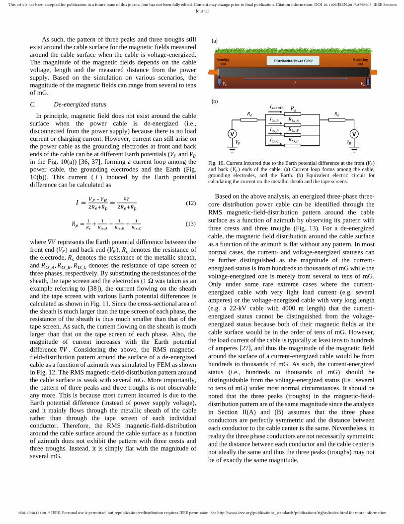
(a) Power supply voltage: according to Eq. (11), the

magnitude of the charging current is proportional to the power

supply voltage. Thus the magnetic field distribution around the

cable surface at a certain location along the cable is also

proportional to the supply voltage. As such, the magnetic field

distribution around the cable surface at the head (power supply

side) and tail (load side) ends of the power cable was also

calculated at other typical voltages (7.2, 11, 12.47, 22, 25, 34.5

kV [24]) at 50 Hz. Fig. 8(a) and (b) show the magnetic field

distribution around the cable surface at the head and tail ends

of the 600-m cable at various supply voltages. The result shows

that the magnitude of the magnetic fields increases with the

increasing voltages. The pattern of three peaks and three

troughs is obvious in all the simulated magnetic field

distributions.

(b) Cable length: according to Eq. 11, the magnitude of the

charging current is proportional to the cable length. As such,

the magnetic field distribution around the cable surface at a

certain section is also proportional to the cable length. In

practice, the length of the power cable can range from hundreds

to thousands of meters [34, 35]. The magnetic field

distributions around the cable surface at the head and tail end

of the power cable of the other cable lengths (1000 m, 2000 m,

3000 m, and 4000 m) were attained from the simulated 600-m

one as shown in Fig. 8(c) and (d). The magnitude of the

magnetic field increases with the increasing cable lengths and

the pattern of three peaks and three troughs is obvious in all the

simulated magnetic field distributions.

(c) Power supply frequency: according to Eq. 11, the

magnitude of the charging current is proportional to the power

supply frequency. The 60 Hz frequency is typically used in the

US, and 50 Hz in Europe [24]. For the studied case regarding a

600-m length 22-kV power cable in Fig. 6, the charging current

at 60 Hz was also simulated and the results are shown in Fig. 9.

It can be seen that the charging current at same measuring point

of 60 Hz is 6/5 times as much as that of 50 Hz. Therefore, the

magnetic fields around the cable surface at 60 Hz follow the

same magnetic-field-distribution pattern as that at 50 Hz but

with magnitude 6/5 times larger.

Fig. 8. Magnetic field around the voltage-energized cable surface at various

power supply voltages (7.2, 11, 12.47, 22, 25, 33, and 34.5 kV) and cable

lengths (600, 1000, 2000, 3000, and 4000 m). (a) Magnetic field at the head end (power supply side) of a 600-m cable at various voltages. (b) Magnetic field at

the tail end (load side) of a 600-m cable at various voltages. (c) Magnetic field

at the head end of a 22-kV cable of various cable lengths. (d) Magnetic field at the tail end of a 22-kV cable of various cable lengths.

Fig. 9. Charging currents of phase conductor and tape screen at various

positions (i.e., various distances from power supply side) on a 600-m power

cable at 50 and 60 Hz.



As such, the pattern of three peaks and three troughs still

exist around the cable surface for the magnetic fields measured

around the cable surface when the cable is voltage-energized.

The magnitude of the magnetic fields depends on the cable

voltage, length and the measured distance from the power

supply. Based on the simulation on various scenarios, the

magnitude of the magnetic fields can range from several to tens

of mG.

C. De-energized status

In principle, magnetic field does not exist around the cable

surface when the power cable is de-energized (i.e.,

disconnected from the power supply) because there is no load

current or charging current. However, current can still arise on

the power cable as the grounding electrodes at front and back

ends of the cable can be at different Earth potentials (𝑉𝐹 and 𝑉𝐵

in the Fig. 10(a)) [36, 37], forming a current loop among the

power cable, the grounding electrodes and the Earth (Fig.

10(b)). This current ( 𝐼 ) induced by the Earth potential

difference can be calculated as

𝐼 =𝑉𝐹 – 𝑉𝐵

2𝑅𝑒+𝑅𝑝=

∇𝑉

2𝑅𝑒+𝑅𝑝 (12)

𝑅𝑝 =1

𝑅𝑠+

1

𝑅𝑡𝑠_𝐴+

1

𝑅𝑡𝑠_𝐵+

1

𝑅𝑡𝑠_𝐶 (13)

where ∇𝑉 represents the Earth potential difference between the

front end (𝑉𝐹) and back end (𝑉𝐵), 𝑅𝑒 denotes the resistance of

the electrode, 𝑅𝑠 denotes the resistance of the metallic sheath,

and 𝑅𝑡𝑠_𝐴, 𝑅𝑡𝑠_𝐵, 𝑅𝑡𝑠_𝐶 denotes the resistance of tape screen of

three phases, respectively. By substituting the resistances of the

sheath, the tape screen and the electrodes (1 Ω was taken as an

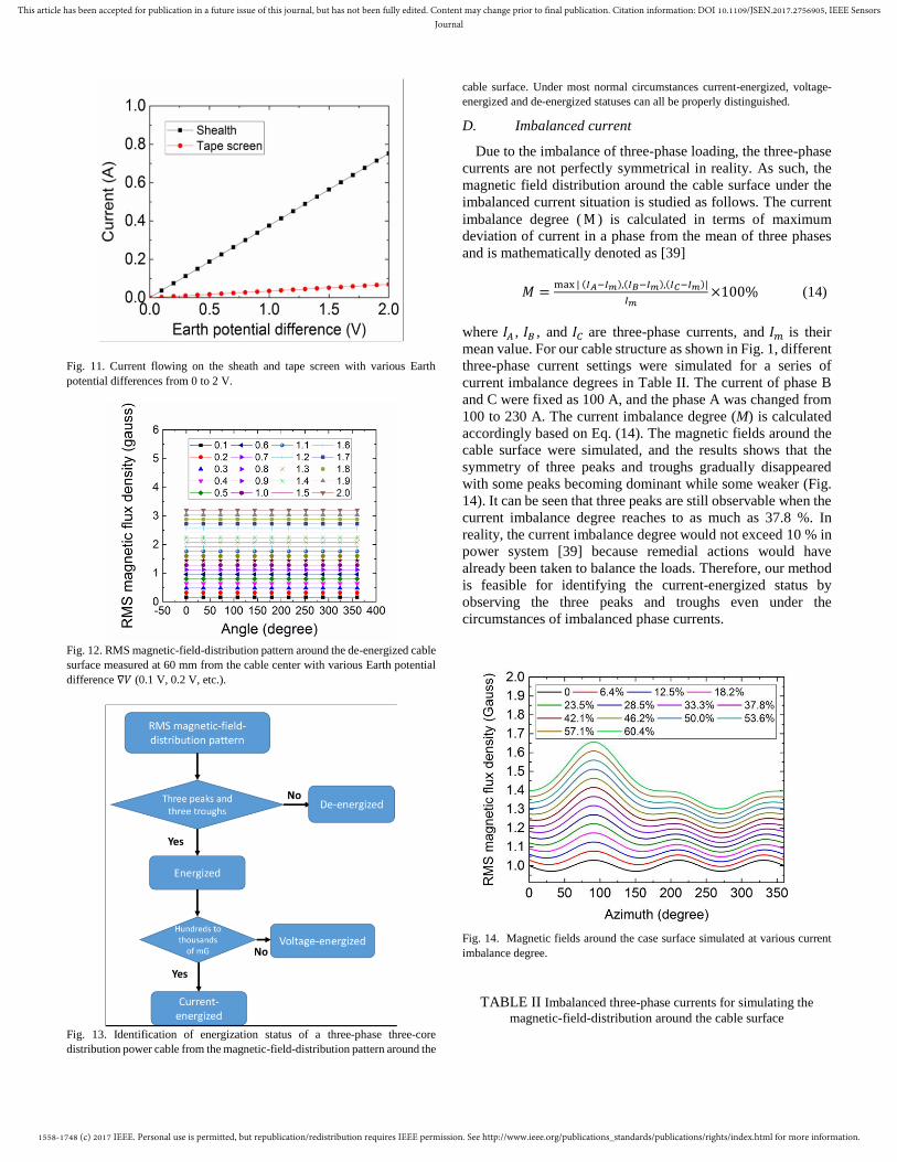
example referring to [38]), the current flowing on the sheath

and the tape screen with various Earth potential differences is

calculated as shown in Fig. 11. Since the cross-sectional area of

the sheath is much larger than the tape screen of each phase, the

resistance of the sheath is thus much smaller than that of the

tape screen. As such, the current flowing on the sheath is much

larger than that on the tape screen of each phase. Also, the

magnitude of current increases with the Earth potential

difference ∇𝑉 . Considering the above, the RMS magnetic-

field-distribution pattern around the surface of a de-energized

cable as a function of azimuth was simulated by FEM as shown

in Fig. 12. The RMS magnetic-field-distribution pattern around

the cable surface is weak with several mG. More importantly,

the pattern of three peaks and three troughs is not observable

any more. This is because most current incurred is due to the

Earth potential difference (instead of power supply voltage),

and it mainly flows through the metallic sheath of the cable

rather than through the tape screen of each individual

conductor. Therefore, the RMS magnetic-field-distribution

around the cable surface around the cable surface as a function

of azimuth does not exhibit the pattern with three crests and

three troughs. Instead, it is simply flat with the magnitude of

several mG.

Fig. 10. Current incurred due to the Earth potential difference at the front (𝑉𝐹)

and back (𝑉𝐵 ) ends of the cable. (a) Current loop forms among the cable, grounding electrodes, and the Earth. (b) Equivalent electric circuit for

calculating the current on the metallic sheath and the tape screens.

Based on the above analysis, an energized three-phase three-

core distribution power cable can be identified through the

RMS magnetic-field-distribution pattern around the cable

surface as a function of azimuth by observing its pattern with

three crests and three troughs (Fig. 13). For a de-energized

cable, the magnetic field distribution around the cable surface

as a function of the azimuth is flat without any pattern. In most

normal cases, the current- and voltage-energized statuses can

be further distinguished as the magnitude of the current-

energized status is from hundreds to thousands of mG while the

voltage-energized one is merely from several to tens of mG.

Only under some rare extreme cases where the current-

energized cable with very light load current (e.g. several

amperes) or the voltage-energized cable with very long length

(e.g. a 22-kV cable with 4000 m length) that the current-

energized status cannot be distinguished from the voltage-

energized status because both of their magnetic fields at the

cable surface would be in the order of tens of mG. However,

the load current of the cable is typically at least tens to hundreds

of amperes [27], and thus the magnitude of the magnetic field

around the surface of a current-energized cable would be from

hundreds to thousands of mG. As such, the current-energized

status (i.e., hundreds to thousands of mG) should be

distinguishable from the voltage-energized status (i.e., several

to tens of mG) under most normal circumstances. It should be

noted that the three peaks (troughs) in the magnetic-field-

distribution pattern are of the same magnitude since the analysis

in Section II(A) and (B) assumes that the three phase

conductors are perfectly symmetric and the distance between

each conductor to the cable center is the same. Nevertheless, in

reality the three phase conductors are not necessarily symmetric

and the distance between each conductor and the cable center is

not ideally the same and thus the three peaks (troughs) may not

be of exactly the same magnitude.



Fig. 11. Current flowing on the sheath and tape screen with various Earth

potential differences from 0 to 2 V.

Fig. 12. RMS magnetic-field-distribution pattern around the de-energized cable

surface measured at 60 mm from the cable center with various Earth potential

difference ∇𝑉 (0.1 V, 0.2 V, etc.).

Fig. 13. Identification of energization status of a three-phase three-core

distribution power cable from the magnetic-field-distribution pattern around the

cable surface. Under most normal circumstances current-energized, voltage-

energized and de-energized statuses can all be properly distinguished.

D. Imbalanced current

Due to the imbalance of three-phase loading, the three-phase

currents are not perfectly symmetrical in reality. As such, the

magnetic field distribution around the cable surface under the

imbalanced current situation is studied as follows. The current

imbalance degree ( M ) is calculated in terms of maximum

deviation of current in a phase from the mean of three phases

and is mathematically denoted as [39]

𝑀 =max | (𝐼𝐴−𝐼𝑚),(𝐼𝐵−𝐼𝑚),(𝐼𝐶−𝐼𝑚)|

𝐼𝑚×100% (14)

where 𝐼𝐴 , 𝐼𝐵 , and 𝐼𝐶 are three-phase currents, and 𝐼𝑚 is their

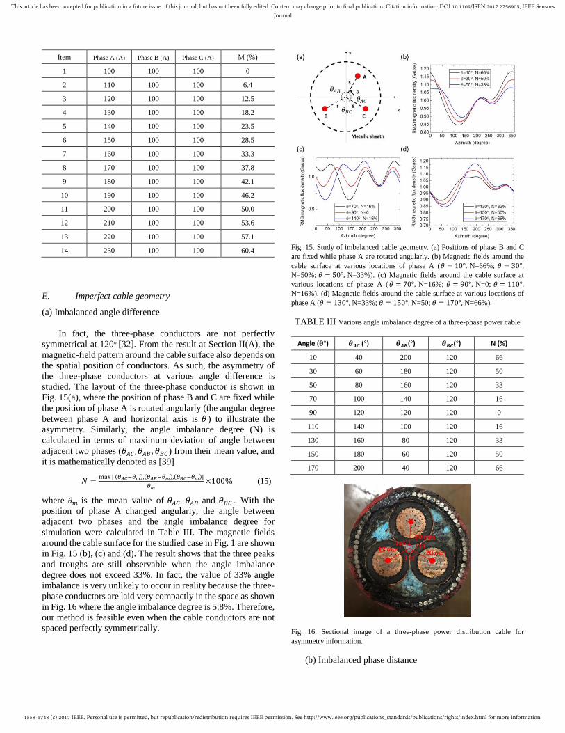
mean value. For our cable structure as shown in Fig. 1, different

three-phase current settings were simulated for a series of

current imbalance degrees in Table II. The current of phase B

and C were fixed as 100 A, and the phase A was changed from

100 to 230 A. The current imbalance degree (M) is calculated

accordingly based on Eq. (14). The magnetic fields around the

cable surface were simulated, and the results shows that the

symmetry of three peaks and troughs gradually disappeared

with some peaks becoming dominant while some weaker (Fig.

14). It can be seen that three peaks are still observable when the

current imbalance degree reaches to as much as 37.8 %. In

reality, the current imbalance degree would not exceed 10 % in

power system [39] because remedial actions would have

already been taken to balance the loads. Therefore, our method

is feasible for identifying the current-energized status by

observing the three peaks and troughs even under the

circumstances of imbalanced phase currents.

Fig. 14. Magnetic fields around the case surface simulated at various current

imbalance degree.

TABLE II Imbalanced three-phase currents for simulating the

magnetic-field-distribution around the cable surface



Item Phase A (A) Phase B (A) Phase C (A) M (%)

1 100 100 100 0

2 110 100 100 6.4

3 120 100 100 12.5

4 130 100 100 18.2

5 140 100 100 23.5

6 150 100 100 28.5

7 160 100 100 33.3

8 170 100 100 37.8

9 180 100 100 42.1

10 190 100 100 46.2

11 200 100 100 50.0

12 210 100 100 53.6

13 220 100 100 57.1

14 230 100 100 60.4

E. Imperfect cable geometry

(a) Imbalanced angle difference

In fact, the three-phase conductors are not perfectly

symmetrical at 120° [32]. From the result at Section II(A), the

magnetic-field pattern around the cable surface also depends on

the spatial position of conductors. As such, the asymmetry of

the three-phase conductors at various angle difference is

studied. The layout of the three-phase conductor is shown in

Fig. 15(a), where the position of phase B and C are fixed while

the position of phase A is rotated angularly (the angular degree

between phase A and horizontal axis is 𝜃 ) to illustrate the

asymmetry. Similarly, the angle imbalance degree (N) is

calculated in terms of maximum deviation of angle between

adjacent two phases (𝜃𝐴𝐶 , 𝜃𝐴𝐵 , 𝜃𝐵𝐶) from their mean value, and

it is mathematically denoted as [39]

𝑁 =max | (𝜃𝐴𝐶−𝜃𝑚),(𝜃𝐴𝐵−𝜃𝑚),(𝜃𝐵𝐶−𝜃𝑚)|

𝜃𝑚×100% (15)

where 𝜃𝑚 is the mean value of 𝜃𝐴𝐶 , 𝜃𝐴𝐵 and 𝜃𝐵𝐶 . With the

position of phase A changed angularly, the angle between

adjacent two phases and the angle imbalance degree for

simulation were calculated in Table III. The magnetic fields

around the cable surface for the studied case in Fig. 1 are shown

in Fig. 15 (b), (c) and (d). The result shows that the three peaks

and troughs are still observable when the angle imbalance

degree does not exceed 33%. In fact, the value of 33% angle

imbalance is very unlikely to occur in reality because the three-

phase conductors are laid very compactly in the space as shown

in Fig. 16 where the angle imbalance degree is 5.8%. Therefore,

our method is feasible even when the cable conductors are not

spaced perfectly symmetrically.

Fig. 15. Study of imbalanced cable geometry. (a) Positions of phase B and C

are fixed while phase A are rotated angularly. (b) Magnetic fields around the

cable surface at various locations of phase A (𝜃 = 10°, N=66%; 𝜃 = 30°, N=50%; 𝜃 = 50°, N=33%). (c) Magnetic fields around the cable surface at

various locations of phase A ( 𝜃 = 70°, N=16%; 𝜃 = 90°, N=0; 𝜃 = 110°, N=16%). (d) Magnetic fields around the cable surface at various locations of

phase A (𝜃 = 130°, N=33%; 𝜃 = 150°, N=50; 𝜃 = 170°, N=66%).

TABLE III Various angle imbalance degree of a three-phase power cable

Angle (𝛉°) 𝜽𝑨𝑪 (°) 𝜽𝑨𝑩(°) 𝜽𝑩𝑪(°) N (%)

10 40 200 120 66

30 60 180 120 50

50 80 160 120 33

70 100 140 120 16

90 120 120 120 0

110 140 100 120 16

130 160 80 120 33

150 180 60 120 50

170 200 40 120 66

Fig. 16. Sectional image of a three-phase power distribution cable for

asymmetry information.

(b) Imbalanced phase distance



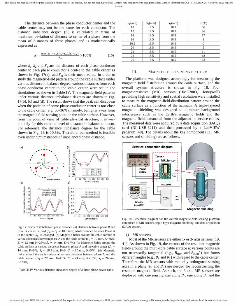
The distance between the phase conductor center and the

cable center may not be the same for each conductor. The

distance imbalance degree (K) is calculated in terms of

maximum deviation of distance to center of a phase from the

mean of distances of three phases, and is mathematically

expressed as

𝐾 =max | (𝑆1−𝑆𝑚),(𝑆2−𝑆𝑚),(𝑆3−𝑆𝑚)|

𝑆𝑚×100% (16)

where 𝑆1, 𝑆2 and 𝑆3 are the distance of each phase-conductor

center to each phase conductor’s center to the cable center as

shown in Fig. 17(a), and 𝑆𝑚 is their mean value. In order to

study the magnetic-field pattern around the cable surface under

various distance imbalance degree, various distances from each

phase-conductor center to the cable center were set in the

simulations as shown in Table IV. The magnetic-field patterns

under various distance imbalance degrees are shown in Fig.

17(b), (c) and (d). The result shows that the peak can disappear

when the position of some phase-conductor center is too close

to the cable center (e.g., K=36%), namely, being far away from

the magnetic field sensing point on the cable surface. However,

from the point of view of cable physical structure, it is very

unlikely for this extreme level of distance imbalance to occur.

For reference, the distance imbalance degree for the cable

shown in Fig. 16 is 10.5%. Therefore, our method is feasible

even under circumstances of imbalanced phase distance.

Fig. 17. Study of imbalanced phase distance. (a) Distance between phase B and

C to the center is fixed (𝑆2 = 𝑆3 = 18.5 𝑚𝑚) while distance between Phase A

to the center (𝑆1) is changed. (b) Magnetic fields around the cable surface at

various distances between phase A and the cable center (𝑆1 = 10 mm, K=36%;

𝑆1 = 12 mm, K=26%; 𝑆1 = 14 mm, K=17%). (c) Magnetic fields around the

cable surface at various distances between phase A and the cable center (𝑆1 =16 mm, K=9%; 𝑆1 = 18.5 mm, K=0; 𝑆1 = 20 mm, K=5%). (d) Magnetic

fields around the cable surface at various distances between phase A and the

cable center ( 𝑆1 = 22 mm, K=11%; 𝑆1 = 24 mm, K=18%; 𝑆1 = 26 mm, K=23%).

TABLE IV Various distance imbalance degree of a three-phase power cable

𝑆1(mm) 𝑆2(mm) 𝑆3(mm) K (%)

10 18.5 18.5 36

12 18.5 18.5 26

14 18.5 18.5 17

16 18.5 18.5 9

18.5 18.5 18.5 0

20 18.5 18.5 5

22 18.5 18.5 11

24 18.5 18.5 18

26 18.5 18.5 23

III. MAGNETIC-FIELD-SENSING PLATFORM

The platform was designed accordingly for measuring the

magnetic field distribution around the cable surface, and the

overall system structure is shown in Fig. 18. Four

magnetoresistive (MR) sensors (HMC2003, Honeywell)

providing high sensitivity and spatial resolution were installed

to measure the magnetic-field-distribution pattern around the

cable surface as a function of the azimuth. A triple-layered

magnetic shielding was designed to eliminate background

interference such as the Earth’s magnetic fields and the

magnetic fields emanated from the adjacent in-service cables.

The measured data were acquired by a data acquisition (DAQ)

card (NI USB-6211) and then processed by a LabVIEW

program [40]. The details about the key component (i.e., MR

sensors and shielding) are as follows.

Fig. 18. Schematic diagram for the overall magnetic-field-sensing platform

comprised of MR sensors, triple-layer magnetic shielding, and data acquisition

(DAQ) system.

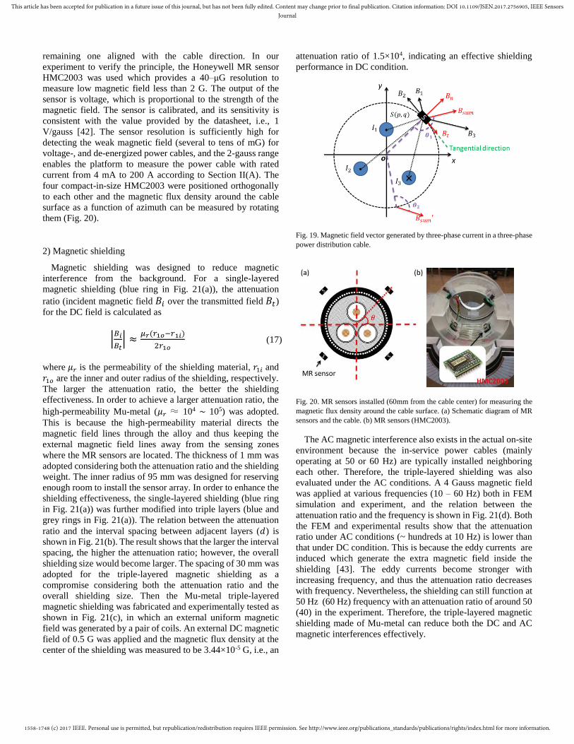
1) MR sensors

Most of the MR sensors are either 1- or 3- axis sensors [19,

41]. As shown in Fig. 19, the vectors of the resultant magnetic

fields around the multi-core cable surface at various points are

not necessarily tangential (e.g., 𝐵𝑠𝑢𝑚 and 𝐵𝑠𝑢𝑚′ ) but forms

different angles (e.g., 𝜃1 and 𝜃2) with regard to the cable center.

Therefore, the MR sensors with mutually orthogonal sensing

axes in a plane (𝐵𝑡 and 𝐵𝑛) are needed for reconstructing the

resultant magnetic field. As such, the 3-axis MR sensors are

deployed with one sensing axis along 𝐵𝑡 , one along 𝐵𝑛 and the



remaining one aligned with the cable direction. In our

experiment to verify the principle, the Honeywell MR sensor

HMC2003 was used which provides a 40–μG resolution to

measure low magnetic field less than 2 G. The output of the

sensor is voltage, which is proportional to the strength of the

magnetic field. The sensor is calibrated, and its sensitivity is

consistent with the value provided by the datasheet, i.e., 1

V/gauss [42]. The sensor resolution is sufficiently high for

detecting the weak magnetic field (several to tens of mG) for

voltage-, and de-energized power cables, and the 2-gauss range

enables the platform to measure the power cable with rated

current from 4 mA to 200 A according to Section II(A). The

four compact-in-size HMC2003 were positioned orthogonally

to each other and the magnetic flux density around the cable

surface as a function of azimuth can be measured by rotating

them (Fig. 20).

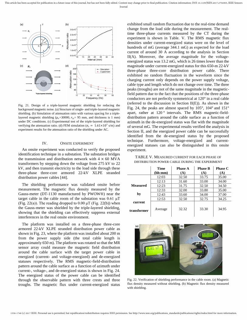
2) Magnetic shielding

Magnetic shielding was designed to reduce magnetic

interference from the background. For a single-layered

magnetic shielding (blue ring in Fig. 21(a)), the attenuation

ratio (incident magnetic field 𝐵𝑖 over the transmitted field 𝐵𝑡)

for the DC field is calculated as

|𝐵𝑖

𝐵𝑡| ≈

𝜇𝑟(𝑟1𝑜−𝑟1𝑖)

2𝑟1𝑜 (17)

where 𝜇𝑟 is the permeability of the shielding material, 𝑟1𝑖 and

𝑟1𝑜 are the inner and outer radius of the shielding, respectively.

The larger the attenuation ratio, the better the shielding

effectiveness. In order to achieve a larger attenuation ratio, the

high-permeability Mu-metal (𝜇𝑟 ≈ 104 ∼ 105) was adopted.

This is because the high-permeability material directs the

magnetic field lines through the alloy and thus keeping the

external magnetic field lines away from the sensing zones

where the MR sensors are located. The thickness of 1 mm was

adopted considering both the attenuation ratio and the shielding

weight. The inner radius of 95 mm was designed for reserving

enough room to install the sensor array. In order to enhance the

shielding effectiveness, the single-layered shielding (blue ring

in Fig. 21(a)) was further modified into triple layers (blue and

grey rings in Fig. 21(a)). The relation between the attenuation

ratio and the interval spacing between adjacent layers (𝑑) is

shown in Fig. 21(b). The result shows that the larger the interval

spacing, the higher the attenuation ratio; however, the overall

shielding size would become larger. The spacing of 30 mm was

adopted for the triple-layered magnetic shielding as a

compromise considering both the attenuation ratio and the

overall shielding size. Then the Mu-metal triple-layered

magnetic shielding was fabricated and experimentally tested as

shown in Fig. 21(c), in which an external uniform magnetic

field was generated by a pair of coils. An external DC magnetic

field of 0.5 G was applied and the magnetic flux density at the

center of the shielding was measured to be 3.44×10-5 G, i.e., an

attenuation ratio of 1.5×104, indicating an effective shielding

performance in DC condition.

Fig. 19. Magnetic field vector generated by three-phase current in a three-phase

power distribution cable.

Fig. 20. MR sensors installed (60mm from the cable center) for measuring the

magnetic flux density around the cable surface. (a) Schematic diagram of MR

sensors and the cable. (b) MR sensors (HMC2003).

The AC magnetic interference also exists in the actual on-site

environment because the in-service power cables (mainly

operating at 50 or 60 Hz) are typically installed neighboring

each other. Therefore, the triple-layered shielding was also

evaluated under the AC conditions. A 4 Gauss magnetic field

was applied at various frequencies (10 – 60 Hz) both in FEM

simulation and experiment, and the relation between the

attenuation ratio and the frequency is shown in Fig. 21(d). Both

the FEM and experimental results show that the attenuation

ratio under AC conditions (~ hundreds at 10 Hz) is lower than

that under DC condition. This is because the eddy currents are

induced which generate the extra magnetic field inside the

shielding [43]. The eddy currents become stronger with

increasing frequency, and thus the attenuation ratio decreases

with frequency. Nevertheless, the shielding can still function at

50 Hz (60 Hz) frequency with an attenuation ratio of around 50

(40) in the experiment. Therefore, the triple-layered magnetic

shielding made of Mu-metal can reduce both the DC and AC

magnetic interferences effectively.



Fig. 21. Design of a triple-layered magnetic shielding for reducing the

background magnetic noise. (a) Structure of single- and triple-layered magnetic

shielding. (b) Simulation of attenuation ratio with various spacing for a triple-

layered magnetic shielding (𝜇𝑟=30000, 𝑟1𝑖= 95 mm, and thickness is 1 mm)

under DC conditions. (c) Experimental test of the triple-layered shielding for

verifying the attenuation ratio. (d) FEM simulation (𝜎𝑟 = 1.61×107 s/m) and

experiment results for the attenuation ratio of the shielding under AC.

IV. ONSITE EXPERIMENT

An onsite experiment was conducted to verify the proposed

identification technique in a substation. The substation bridges

the transmission and distribution network with 4 × 60 MVA

transformers by stepping down the voltage from 275 kV to 22

kV, and then transmit electricity to the load side through these

three-phase three-core armored 22-kV XLPE stranded

distribution power cables [44].

The shielding performance was validated onsite before

measurement. The magnetic flux density measured by the

Gauss-meter (DT-1130 manufactured by PWOW®) near the

target cable in the cable room of the substation was 0.61 μT

(Fig. 22(a)). The reading dropped to 0.00 μT (Fig. 22(b)) when

the Gauss-meter was shielded by the triple-layered shielding,

showing that the shielding can effectively suppress external

interferences in the real onsite environment.

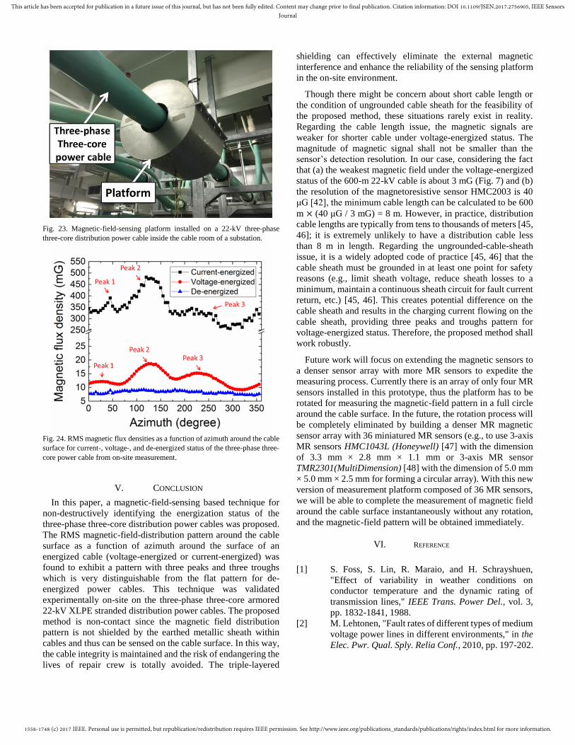
The platform was installed on a three-phase three-core

armored 22-kV XLPE stranded distribution power cable as

shown in Fig. 23, where the platform was installed about 200 m

from the power supply side (the total cable length is

approximately 650 m). The platform was rotated so that the MR

sensor array could measure the magnetic field distribution

around the cable surface with the target power cable in

energized (current- and voltage-energized) and de-energized

statuses respectively. The RMS magnetic-field-distribution

pattern around the cable surface as a function of azimuth under

current-, voltage-, and de-energized status is shown in Fig. 24.

The energized status of the power cable can be identified

through the observable pattern with three crests and three

troughs. The magnetic flux under current-energized status

exhibited small random fluctuation due to the real-time demand

change from the load side during the measurement. The real-

time three-phase currents measured by the CT during the

experiment is shown in Table. V. The RMS magnetic flux

densities under current-energized status were on the level of

hundreds of mG (average 344.1 mG) as expected for the load

current of around 30 A according to the analysis in Section

II(A). Moreover, the average magnitude for the voltage-

energized status was 13.2 mG, which is 26 times lower than the

magnitude under current-energized status for this 650-m 22-kV

three-phase three-core distribution power cable. There

exhibited no random fluctuation in the waveform since the

charging current only depends on the power supply voltage,

cable type and length which do not change over time. The three

peaks (troughs) are not of the same magnitude in the magnetic-

field pattern due to the fact that the positions of the three-phase

conductors are not perfectly symmetrical at 120° in a real cable

(referred to the discussion in Section II(E)). As shown in the

Fig. 24, the peaks are almost spaced by 105°, 104° and 151°

apart, rather at 120 ° intervals. The RMS magnetic-field-

distribution pattern around the cable surface as a function of

azimuth in the de-energized status was flat with the magnitude

of several mG. The experimental results verified the analysis in

Section II, and the energized power cable can be successfully

identified from the de-energized status by the proposed

technique. Furthermore, voltage-energized and current-

energized statuses can also be distinguished in this onsite

experiment.

TABLE V. MEASURED CURRENT FOR EACH PHASE OF

DISTRIBUTION POWER CABLE DURING THE EXPERIMENT

Time

(hh:mm)

Phase A

(A)

Phase B

(A)

Phase C

(A)

Measured

by

current

transformer

12:03 32.50 33.75 35.00

12:13 31.60 33.00 34.00

12:23 31.75 32.50 34.50

12:33 32.00 33.80 35.00

12:43 33.60 34.00 37.00

12:53 32.50 32.75 34.25

Average 32.32 33.30 34.95

Fig. 22. Verification of shielding performance in the cable room. (a) Magnetic

flux density measured without shielding. (b) Magnetic flux density measured

with shielding.



Fig. 23. Magnetic-field-sensing platform installed on a 22-kV three-phase

three-core distribution power cable inside the cable room of a substation.

Fig. 24. RMS magnetic flux densities as a function of azimuth around the cable

surface for current-, voltage-, and de-energized status of the three-phase three-

core power cable from on-site measurement.

V. CONCLUSION

In this paper, a magnetic-field-sensing based technique for

non-destructively identifying the energization status of the

three-phase three-core distribution power cables was proposed.

The RMS magnetic-field-distribution pattern around the cable

surface as a function of azimuth around the surface of an

energized cable (voltage-energized or current-energized) was

found to exhibit a pattern with three peaks and three troughs

which is very distinguishable from the flat pattern for de-

energized power cables. This technique was validated

experimentally on-site on the three-phase three-core armored

22-kV XLPE stranded distribution power cables. The proposed

method is non-contact since the magnetic field distribution

pattern is not shielded by the earthed metallic sheath within

cables and thus can be sensed on the cable surface. In this way,

the cable integrity is maintained and the risk of endangering the

lives of repair crew is totally avoided. The triple-layered

shielding can effectively eliminate the external magnetic

interference and enhance the reliability of the sensing platform

in the on-site environment.

Though there might be concern about short cable length or

the condition of ungrounded cable sheath for the feasibility of

the proposed method, these situations rarely exist in reality.

Regarding the cable length issue, the magnetic signals are

weaker for shorter cable under voltage-energized status. The

magnitude of magnetic signal shall not be smaller than the

sensor’s detection resolution. In our case, considering the fact

that (a) the weakest magnetic field under the voltage-energized

status of the 600-m 22-kV cable is about 3 mG (Fig. 7) and (b)

the resolution of the magnetoresistive sensor HMC2003 is 40

μG [42], the minimum cable length can be calculated to be 600

m × (40 μG / 3 mG) = 8 m. However, in practice, distribution

cable lengths are typically from tens to thousands of meters [45,

46]; it is extremely unlikely to have a distribution cable less

than 8 m in length. Regarding the ungrounded-cable-sheath

issue, it is a widely adopted code of practice [45, 46] that the

cable sheath must be grounded in at least one point for safety

reasons (e.g., limit sheath voltage, reduce sheath losses to a

minimum, maintain a continuous sheath circuit for fault current

return, etc.) [45, 46]. This creates potential difference on the

cable sheath and results in the charging current flowing on the

cable sheath, providing three peaks and troughs pattern for

voltage-energized status. Therefore, the proposed method shall

work robustly.

Future work will focus on extending the magnetic sensors to

a denser sensor array with more MR sensors to expedite the

measuring process. Currently there is an array of only four MR

sensors installed in this prototype, thus the platform has to be

rotated for measuring the magnetic-field pattern in a full circle

around the cable surface. In the future, the rotation process will

be completely eliminated by building a denser MR magnetic

sensor array with 36 miniatured MR sensors (e.g., to use 3-axis

MR sensors HMC1043L (Honeywell) [47] with the dimension

of 3.3 mm × 2.8 mm × 1.1 mm or 3-axis MR sensor

TMR2301(MultiDimension) [48] with the dimension of 5.0 mm

× 5.0 mm × 2.5 mm for forming a circular array). With this new

version of measurement platform composed of 36 MR sensors,

we will be able to complete the measurement of magnetic field

around the cable surface instantaneously without any rotation,

and the magnetic-field pattern will be obtained immediately.

VI. REFERENCE

[1] S. Foss, S. Lin, R. Maraio, and H. Schrayshuen,

"Effect of variability in weather conditions on

conductor temperature and the dynamic rating of

transmission lines," IEEE Trans. Power Del., vol. 3,

pp. 1832-1841, 1988.

[2] M. Lehtonen, "Fault rates of different types of medium

voltage power lines in different environments," in the

Elec. Pwr. Qual. Sply. Relia Conf., 2010, pp. 197-202.



[3] G. J. Anders, I. o. Electrical, and E. Engineers, Rating

of electric power cables in unfavorable thermal

environment: Wiley, 2005.

[4] L. Bertling, R. Allan, and R. Eriksson, "A reliability-

centered asset maintenance method for assessing the

impact of maintenance in power distribution systems,"

IEEE Trans. Power Syst., vol. 20, pp. 75-82, 2005.

[5] T. Kubota, Y. Takahashi, S. Sakuma, M. Watanabe,

M. Kanaoka, and H. Yamanouchi, "Development of

500-kV XLPE cables and accessories for long distance

underground transmission line-Part I: insulation

design of cables," IEEE Trans. Power Del., vol. 9, pp.

1741-1749, 1994.

[6] A. Ukil, H. Braendle, and P. Krippner, "Distributed

temperature sensing: review of technology and

applications," IEEE Sensors J., vol. 12, pp. 885-892,

2012.

[7] R. H. Bhuiyan, R. A. Dougal, and M. Ali, "Proximity

coupled interdigitated sensors to detect insulation

damage in power system cables," IEEE Sensors J.,

vol. 7, pp. 1589-1596, 2007.

[8] F. Li, W. Qiao, H. Sun, H. Wan, J. Wang, Y. Xia, Z.

Xu, and P. Zhang, "Smart transmission grid: Vision

and framework," IEEE Trans. Smart Grid, vol. 1, pp.

168-177, 2010.

[9] S. L. Christopherson, E. C. Gillard, D. A. Gilliland,

and K. E. Monsen, "Device and method for directly

injecting a test signal into a cable," ed: Google Patents,

2004.

[10] T. D. Walsh, N. Reinhardt, and J. M. Feldman, "Cable

status testing," ed: Google Patents, 1988.

[11] SebaKMT. 'Principles of Cable & Pipe Location',

2011. Available: http://www.ausolutions.com.au/pdf-

library/vLocPro-Theory-Presentation_V1-41.pdf.

[Accessed: 12- Dec- 2016].

[12] SPIKE. 'SPIKE Tool Speficiations', 2005. Available:

http://www.spiketool.com/SPIKEhome.html.

[Accessed: 12- Dec- 2016].

[13] T. Walsh and T. Feldman. "Shielded cable is tested to

determine if it is energized", 2006. Available:

http://ieeepcic.com/wp-

content/uploads/2016/10/Test-Before-Touch-PCIC-

2006.pdf. [Accessed: 12- Dec- 2016].

[14] B. Jiang, A. P. Sample, R. M. Wistort, and A. V.

Mamishev, "Autonomous robotic monitoring of

underground cable systems," in the 12th Intl. Conf. on

Advanced Robotics, 2005, pp. 673-679.

[15] S. Cristina and M. Feliziani, "A finite element

technique for multiconductor cable parameters

calculation," IEEE Trans. Magn., vol. 25, pp. 2986-

2988, 1989.

[16] P. Klaudy and J. Gerhold, "Practical conclusions from

field trials of a superconducting cable," IEEE Trans.

Magn., vol. 19, pp. 656-661, 1983.

[17] S. Short, A. Mamishev, T. Kao, and B. Russell,

"Evaluation of methods for discrimination of

energized underground power cables," Electr. Pow.

Syst. Res., vol. 37, pp. 29-38, 1996.

[18] A. B. Gill, Y. Huang, J. Spencer, and I. Gloyne-

Philips, "Electromagnetic fields emitted by high

voltage alternating current offshore wind power cables

and interactions with marine organisms," in Proc. of

the Electromag. in Current and Energy, 2012.

[19] J. Lenz and S. Edelstein, "Magnetic sensors and their

applications," IEEE Sensors J., vol. 6, pp. 631-649,

2006.

[20] H. Kaimori, A. Kameari, and K. Fujiwara, "FEM

computation of magnetic field and iron loss in

laminated iron core using homogenization method,"

IEEE Trans. Magn., vol. 43, pp. 1405-1408, 2007.

[21] G. Ries and S. Takács, "Coupling losses in finite

length of superconducting cables and in long cables

partially in magnetic field," IEEE Trans. Magn., vol.

17, pp. 2281-2284, 1981.

[22] C. Schifreen and W. Marble, "Charging Current

Limitations in Operation or High-Voltage Cable Lines

[includes discussion]," Trans. of the American Inst. of

Elect. Eng., vol. 75, 1956.

[23] E. Ghafar-Zadeh and M. Sawan, "Charge-based

capacitive sensor array for CMOS-based laboratory-

on-chip applications," IEEE Sensors J., vol. 8, pp.

325-332, 2008.

[24] Wikipedia. 'Electric power distribution', 2016. .

Available:

https://en.wikipedia.org/wiki/Electric_power_distribu

tion. [Accessed: 19- Jan- 2017].

[25] Wikipedia. 'High-voltage cable', 2016. Available:

https://en.wikipedia.org/wiki/High-voltage_cable.

[Accessed: 19- Jan- 2017].

[26] F. Moro and R. Turri, "Accurate Calculation of the

Right-of-Waywidth for Power Line Magnetic Field

Impact Assessment," Prog. Electromagn. Res., vol.

37, pp. 343-364, 2012.

[27] J. Nahman and M. Tanaskovic, "Determination of the

current carrying capacity of cables using the finite

element method," Electr. Pow. Syst. Res., vol. 61, pp.

109-117, 2002.

[28] H. Li, K. Tan, and Q. Su, "Assessment of underground

cable ratings based on distributed temperature

sensing," IEEE Trans. Power Del., vol. 21, pp. 1763-

1769, 2006.

[29] G. Gela and J. Dai, "Calculation of thermal fields of

underground cables using the boundary element

method," IEEE Trans. Power Del., vol. 3, pp. 1341-

1347, 1988.

[30] P. C. Chao, "Energy harvesting electronics for

vibratory devices in self-powered sensors," IEEE

sensors J., vol. 11, pp. 3106-3121, 2011.

[31] J.-C. Liu, Y.-S. Hsiung, and M. S.-C. Lu, "A CMOS

micromachined capacitive sensor array for fingerprint

detection," IEEE Sensors J., vol. 12, pp. 1004-1010,

2012.

http://www.ausolutions.com.au/pdf-library/vLocPro-Theory-Presentation_V1-41.pdf

http://www.ausolutions.com.au/pdf-library/vLocPro-Theory-Presentation_V1-41.pdf

http://www.spiketool.com/SPIKEhome.html

http://ieeepcic.com/wp-content/uploads/2016/10/Test-Before-Touch-PCIC-2006.pdf



https://en.wikipedia.org/wiki/Electric_power_distribution

https://en.wikipedia.org/wiki/Electric_power_distribution

https://en.wikipedia.org/wiki/High-voltage_cable



[32] V. K. Mehta. "Underground Cables", 2011.

Available:

http://202.74.245.22:8080/xmlui/bitstream/handle/12

3456789/112/Ch-11.pdf. [Accessed: 12- Dec- 2016].

[33] PRYSMIAN. "General calculations excerpt from

PRYSMIAN's wire and cable engineering guide",

2006. Available:

http://na.prysmiangroup.com/en/business_markets/m

arkets/industrial/downloads/engineering-

guide/General_Calculations_Rev_4.pdf. [Accessed:

Dec-12- 2016].

[34] J. Lee, H. Ryoo, S. Choi, K. Nam, S. Jeong, and D.

Kim, "Signal Processing Technology for Fault

Location System in Underground Power Cable," in

IEEE/PES Trans. Dist. Conf., 2006.

[35] S. Mukoyama, S. Maruyama, M. Yagi, Y. Yagi, N.

Ishii, O. Sato, M. Amemiya, H. Kimura, and A.

Kimura, "Development of 500m HTS power cable in

super-ACE project," Cryogenics, vol. 45, pp. 11-15,

2005.

[36] L. M. Popovic, "Efficient reduction of fault current

through the grounding grid of substation supplied by

cable line," IEEE Trans. Power Del., vol. 15, pp. 556-

561, 2000.

[37] X. Chen, Y. Cheng, X. Wang, S. Shi, and Y. Zhao,

"Analysis of current flowing in the ground wire of

XLPE cable and modification of grounding mode,"

High Volt. Eng. , vol. 32, pp. 87-88, 2006.

[38] G. Eduful, J. E. Cole, and P. Okyere, "Optimum mix

of ground electrodes and conductive backfills to

achieve a low ground resistance," in the 2nd Intl. Conf.

On Adaptive Scie. & Tech., 2009.

[39] Amickracing. 'Voltage and current unbalance', 2005.

Available:

http://www.hvac.amickracing.com/Electrical%20Info

rmation/Current%20Unbalance.pdf. [Accessd: 19-

June- 2017].

[40] R. Bitter, T. Mohiuddin, and M. Nawrocki, LabVIEW:

Advanced programming techniques: CRC Press, 2006.

[41] M. J. Caruso, "Applications of magnetoresistive

sensors in navigation systems," SAE Technical Paper

0148-7191, 1997.

[42] Honeywell. "3-Axis magnetic sensor hybrid

HMC2003", 2011. Available:

https://physics.ucsd.edu/neurophysics/Manuals/Hone

ywell/HMC_2003.pdf. [Accessed: 12- Dec- 2016].

[43] K. L. Kaiser, Electromagnetic shielding: Crc Press,

2005.

[44] K. Zhu, H. A. N. W, W. K. Lee, and P. Pong, "On-Site

Non-Invasive Current Monitoring of Multi-Core

Underground Power Cables with a Magnetic-Field

Sensing Platform at a Substation," IEEE Sensors J.,

vol. 17, pp. 1837-1848, 2017.

[45] D. Tziouvaras, "Protection of high-voltage AC cables,"

in the IEEE Conf. on Advanced Metering, Protection,

Control, Communication, and Distributed Resources,

2006.

[46] J. M. Nahman, V. B. Djordjevic, D. D. Salamon, “Grounding effects of HV and MV underground cables associated with urban distribution substations, ” IEEE

Trans. Power Del., vol.17 , pp.111-116 ,2002.

[47] Honeywell. 'Three-axis magnetic sensor HMC1043L',

2013. Available: http://ow.ly/68m730dJUL1. .

[Accessed: 19- Jul- 2017].

[48] Multi-Dimention. 'TMR2301: 3-axis TMR linear

sensor', 2017. Available:

http://www.dowaytech.com/en/1877.html. [Accessed:

19- Jul- 2017].

Ke ZHU (S’12) received the B.E. degree

in electrical engineering from China Three

Gorges University (CTGU), Yichang,

China, in 2013, and is pursuing the Ph.D.

degree in electrical and electronic

engineering (EEE) at the University of

Hong Kong (HKU). His current research

and academic interests focus on

computational electromagnetics, electric

power transmission monitoring, and application of

magnetoresistive (MR) sensors in smart grid.

Wing Kin Lee received the B.Sc. degree,

the M.Sc. degree from the University of

Hong Kong, in 1976 and 1988,

respectively, and the M.B.A. degree from

the Chinese University of Hong Kong in

1990. He is a professional in electrical

services and power engineering, and

currently as a Senior Teaching Consultant

in the University of Hong Kong. He earned industrial

experience while involved with power and communication

utility companies in Hong Kong. His current research interests

include smart grid demand side management, electrical load

signature, and vertical transportation.

Philip W. T. Pong (SM’13) is a physicist

and electrical engineer working on

magnetoresistive magnetic field sensors

and smart grid at the Department of

Electrical and Electronic Engineering

(EEE), the University of Hong Kong

(HKU). He received a Ph.D. in

engineering from the University of

Cambridge in 2005. He was a postdoctoral researcher at the

Magnetic Materials Group at the National Institute of Standards

and Technology (NIST) for three years. In 2008, he joined the

HKU engineering faculty as an assistant professor working on

tunneling magnetoresistance (TMR) sensors, and the

application of magnetoresistive sensors in smart grid.

http://202.74.245.22:8080/xmlui/bitstream/handle/123456789/112/Ch-11.pdf

http://202.74.245.22:8080/xmlui/bitstream/handle/123456789/112/Ch-11.pdf

http://na.prysmiangroup.com/en/business_markets/markets/industrial/downloads/engineering-guide/General_Calculations_Rev_4.pdf



http://www.hvac.amickracing.com/Electrical%20Information/Current%20Unbalance.pdf

http://www.hvac.amickracing.com/Electrical%20Information/Current%20Unbalance.pdf

https://physics.ucsd.edu/neurophysics/Manuals/Honeywell/HMC_2003.pdf

https://physics.ucsd.edu/neurophysics/Manuals/Honeywell/HMC_2003.pdf

http://ow.ly/68m730dJUL1

http://www.dowaytech.com/en/1877.html

core shielded distribution power cables based on non

Documents