Tectonophysics 470 (2009) 243–256

Contents lists available at ScienceDirect

Tectonophysics

j ourna l homepage: www.e lsev ie r.com/ locate / tecto

Converted phases analysis of the Campi Flegrei caldera using active seismic data

T.M. Blacic a,⁎, D. Latorre b,1, J. Virieux c,2, M. Vassallo d,3

a UMR Geosciences Azur, Sophia Antipolis, Franceb Istituto Nazionale di Geofisica e Vulcanologia, CNT, Roma, Italyc Laboratoire de Géophysique Interne et Tectonophysique, Université Joseph Fourier, Grenoble, Franced Università degli Studi di Napoli “Federico II,” Naples, Italy

⁎ Corresponding author. Present address: University o766 6679.

E-mail addresses: tblacic@uwyo.edu (T.M. Blacic), laJean.Virieux@obs.ujf-grenoble.fr (J. Virieux), vassallo@n

1 Fax: +39 06 51 86 05 07.2 Fax: +33 04 76 82 81 01.3 Fax: +39 08 12 42 03 34.

0040-1951/$ – see front matter © 2008 Elsevier B.V. Adoi:10.1016/j.tecto.2008.12.006

a b s t r a c t

a r t i c l e i n f o

Article history:

We applied a type of depth Received 29 November 2007Received in revised form 20 November 2008Accepted 4 December 2008Available online 13 December 2008

Keywords:Converted phasesMigrationSeismic imagingCampi Flegrei

migration for converted seismic phases to active and passive seismic data setsfrom the Campi Flegrei volcanic region in southern Italy. The migration method is based on the diffractionsummation migration technique. Travel times to grid points in a volume were calculated in smooth P and S-velocity models and trace energy near the calculated converted phase time was stacked over multiplesources at one receiver. Weighting factors based on Snell's Law at an arbitrarily oriented local interface wereapplied to better focus trace energy. PP reflection images from the active data set provide increased detail toimages of the caldera rim from other studies. The migrated images also show features near 2–3 km in depthbeneath Pozzuoli City, which may be associated with an over-pressured gas volume, as suggested by othergeophysical investigations. Possible deeper features near 4 km depth may be related to the presence of thecarbonate basement or may image a previously undetected feature, such as a small body of stronglythermometamorphosed volcanic rock. The current passive earthquake data set from the 1984 ground upliftepisode was not well suited to the converted phases analysis due to narrow P–S windows and high noiselevels in the traces. However, two stations provide confirmation and extension of imaged features in theactive data.

© 2008 Elsevier B.V. All rights reserved.

1. Introduction

The Campi Flegrei caldera is an active volcanic system lying westof Vesuvius volcano and the city of Naples in a densely populatedarea of southern Italy (Fig. 1). It last erupted in 1538 (Rosi and Sbrana,1987) but seismic, fumarolic, and ground deformation continue tothe present day (De Natale et al., 1991; Avallone et al., 1999; Chiodiniet al., 2001; Troise et al., 2007). In fact, ground deformation is moredramatic here than at any other volcano on Earth. The backgroundlong-term ground deformation at Campi Flegrei is subsidence at arate of about 1.5–1.7 cm/year (Troise et al., 2007), however, the 1538eruption was preceded by 5–8 m of uplift (Dvorak and Gasparini,1991; Dvorak and Mastrolorenzo, 1991). After the eruptionsubsidence resumed until the recent uplift period began in 1969.Since then there have been two episodes of rapid uplift with peakrates of 1 m/year in 1969–1972 and in 1982–1984 (Barberi et al.,1984). Both were accompanied by increased microseismicity, though

f Wyoming, USA. Fax: +1 307

torre@ingv.it (D. Latorre),a.infn.it (M. Vassallo).

ll rights reserved.

this increase above background levels was much stronger in 1982–1984. Ground uplift ultimately reached a maximum of 1.8 m recordedin the town of Pozzuoli, part of which was evacuated (Barberi et al.,1984). Fortunately, no eruption occurred and by January 1985 seismicactivity had dropped off and slow subsidence again began, althoughthe area still remains above the pre-1982 level. As of November 2004,uplift has again started, though at a considerably slower rate than in1982–1984 (Troise et al., 2007), accompanied by swarms of micro-earthquakes at depths between 0.5 and 4 km (Saccorotti et al., 2007).These recent uplift episodes are thought to result from input ofmagmatic fluids from a shallow magma chamber into shalloweraquifers (Troise et al., 2007).

The threat of future eruptions and/or destructive ground deforma-tion has prompted a number of active and passive seismic studies inthe Campi Flegrei region. Background seismicity at Campi Flegrei isvery low with only a few events of magnitude N1 recorded per year,except when there is an uplift episode at which time thousands ofsuch events can occur over a short period (De Natale et al., 2006).Using earthquake data from the 1982–1984 uplift episode, Aster andMeyer (1988) identified a low Vp, high Vp/Vs ratio volume centerednear the city of Pozzuoli which was later associated with a low Qpanomaly (de Lorenzo et al., 2001). Based on modeling of P–Sconversions in teleseismic data, Ferrucci et al. (1992) proposed thepresence of a magma body at 4–5 km depth at the center of thecaldera. De Natale et al. (1995) analyzed focal mechanisms of the

244 T.M. Blacic et al. / Tectonophysics 470 (2009) 243–256

1982–1984 microearthquakes and interpreted them as characterizinga ring-shaped normal fault system inside the caldera. This model aswell as several later models (e.g., Wohletz et al., 1999; Troise et al.,2003) assumed the presence of a magma chamber like that proposedby Ferrucci et al. (1992), however, recent seismic tomography studieshave found no evidence of a magma chamber within the upper ~6 kmbeneath the caldera (Zollo et al., 2003; Judenherc and Zollo, 2004;Vanorio et al., 2005; Chiarabba and Moretti, 2006; Battaglia et al.,2008). What they have found are remnants of the buried caldera rimboth in the Bay of Pozzuoli at 1–3 km depth, as well as on thelandward side of the caldera at 2 km depth. Bruno (2004) foundevidence of several volcanic vents located along the inferred buriedcaldera rim spanning the Bay of Pozzuoli using legacy seismicreflection, gravity, and magnetic data. Evidence of over-pressuredgas-bearing formations at a depth of about 2–4 km has been detectedas a low Vp/Vs anomaly beneath the caldera and the city of Pozzuoli(Vanorio et al., 2005; Chiarabba and Moretti, 2006). A seismicreflection study using three-component ocean bottom seismometerdata has confirmed the presence of a supercritical fluid-bearingformation at 3 km depth as well as low velocity zone 1 km thick at7.5 km depth associated with a mid-crust, partial melting zone (Zolloet al., 2008). This magma sill lies at a depth similar to the proposeddepth of the magma sill beneath Mt. Vesuvius (Auger et al., 2001)suggesting the possibility that the two volcanic centers are fed by asingle magma reservoir (Zollo et al., 2008).

In September of 2001, an active marine seismic experiment calledSERAPIS (Seismic Reflection/Refraction Acquisition Project for Ima-ging complex volcanic Structures) was carried out in the Bay of Naplesand Bay of Pozzuoli in order to investigate the caldera structure and itsfeeding system (Zollo et al., 2003). During this experiment, ~5000shots were produced by the vessel Le Nadir of Ifremer and recorded onan array of ocean bottom seismometers (OBS) and land stations. Asubset of the SERAPIS active data set was combined with earthquakesources from the 1982–1984 uplift episode that occurred in the CampiFlegrei caldera to produce high-resolution 3-D tomographic P- and S-velocity models of the caldera (Battaglia et al., 2008). These modelsconfirm the presence of the caldera rim imaged as a high P-velocityanomaly at about 1–1.5 km depth in the southern part of the Bay ofPozzuoli. A very high Vp/Vs anomaly was found beneath the city ofPozzuoli at ~1 km depth, and a low Vp/Vs anomaly was imaged atabout 4 km depth below much of the caldera.

In this paper we investigate the subsurface structure of the CampiFlegrei caldera by applying a type of depth migration for convertedphases to active as well as passive data sets for the Campi Flegrei area.This migration method has been previously applied to passive datasets in the Gulf of Corinth region (Latorre, 2004) and theMolise regionin southern Italy (Latorre et al., 2008). The active and passive parts ofthe Battaglia et al. (2008) and SERAPIS data set were analyzedseparately. The active data set provided good coverage across thecaldera for both PP and PS reflected phases. However, the acquisitiongeometry of the passive data set was not well suited to the convertedphases analysis presented here. Most stations lay almost directlyabove the earthquake hypocenters resulting in short P–S timewindows. Although some possible converted phases could be detectedin the traces, the small P–S windows and energetic S-arrivals limitedthe coverage to small areas around each station thus resulting in avery poor image. Therefore, we use the passive data only to confirmsome of the features we find in the images from the active data set.

The converted phases migration method is well suited for regionswith complex velocity structure like Campi Flegrei. Tomographicstudies show “smooth” velocity variations obtained by only invertingP- and/or S-first arrival times (Aster and Meyer, 1988; Zollo et al.,2003; Judenherc and Zollo, 2004; Vanorio et al., 2005; Chiarabba andMoretti, 2006; Battaglia et al., 2008). By migrating converted reflectedwaves in depth we image impedance contrasts (high frequencystructures) that provide increased detail of some subsurface struc-

tures and thereby complement as well as confirm the tomographicimages. Although for large data sets like the one used in this study thecomputation cost is not trivial, it is yet less than that required bymoresophisticated methods such as full-waveform tomography techniques(e.g., Ravaut et al., 2004). Moreover, the full-waveform tomographyrequires a seismic folding difficult to reach for each focal point of themedium, providing room for a simpler investigation such as the onewe suggest. Sources of error associatedwith this method (e.g., effect ofvelocity model, grid size, and attenuation) are discussed in detail insection 3.

2. Data

We investigated two data sets from the Campi Flegrei region: anactive marine seismic data set consisting of OBS and land stationrecordings of airgun sources, and a passive data set consisting of landstation (temporary and permanent) recordings of microearthquakesources.

The active seismic data used here is a subset of the SERAPISexperiment performed in September of 2001. Approximately 5000shots were produced by an array of synchronized airguns; 12 16-literairguns were used offshore and 6 in the Bay of Pozzuoli and near theshore. Receivers included 70 three-component OBS, 66 three-component land stations, and 18 vertical-component land stations.The OBS were equipped with 4.5 Hz sensors and continuous recordingdevices, while almost all on-land stations were equipped with 1 Hzsensors.Within the Campi Flegrei area, shots were spaced 125m apartalthough some lines were re-shot to attain a shot spacing close to63 m. The SERAPIS experiment thus resulted in a density of coveragethat approaches commercial exploration surveys and allows us tostack seismic traces. This makes the data set well suited toinvestigations of geologic hazards in the Campi Flegrei area.

For the converted phases analysis, we selected data from a subsetof the SERAPIS data used by Battaglia et al. (2008) in a recent 3-Dseismic tomography study of Pozzuoli Bay. We chose three-compo-nent stations that have at least 300 shots with P-wave first arrivalpicks. Thus, our active data set includes: 1528 shots, 33 OBS (41778source–receiver pairs), and 13 3-component land stations (7484source–receiver pairs). Selected stations and shots are shown in Fig. 2.

We can identify as many as three coherent secondary phases atsome receivers by visual inspection of traces (Fig. 3). OBS receiversrecorded a strong phase arriving just after or with the first arrival, asshown in selected traces for OBS O12 (phase A, Fig. 3). Phase A isnoticeable on all three components with higher frequency content inthe horizontal components. We treat this phase as a PP reflection froma shallow interface. A second and in some cases third secondary phasecan be discerned later in the traces at some receivers (phases B and C,Fig. 3). These arrivals are visible in all three components but are oftenstronger on horizontal components in un-normalized traces. Theselater phases sometimes appear to have higher frequency content thanthe phase A, but the complexity of the signal makes interpretationdifficult. We treat the phases B and C as being either PP or PS reflectedphases from deeper interfaces. Records from land stations are moredifficult to interpret due to higher noise levels but most stations showat least one coherent secondary phase in one or more componentrecords.

We also examine passive data selected from that used by Battagliaet al. (2008) in their tomography study in order to complement themigration results from the active data. During the 1982–1984 upliftepisode, the University of Wisconsin undertook a field experimentdeploying a temporary network of 21 three-component digital short-period seismometers (Aster and Meyer, 1988). As part of the SERAPISproject, data from this experiment was compiled and re-picked.Battaglia et al. (2008) chose earthquakes with azimuth gaps in stationcoverage b180°, root mean square (RMS) of arrival time residualsb0.5 s, at least 3 S-picks, at least 4 P-picks, and a vertical location error

Fig.1. (a) Locationmap of Campi Flegrei. Inset shows location of region in southern Italy. (b) Gravimetric interpretationmap constrained by gravity observations and geothermal welllog data (modified after AGIP,1987). (c) 2-D interpretivemodel of the gravimetric profile observed along the line (solid line in b) crossing theMofetewells, Baia, Pozzuoli City and thePianura quarter (modified after AGIP, 1987). The location of the S. Vito 8 well (S8) is from Bruno (2004).

245T.M. Blacic et al. / Tectonophysics 470 (2009) 243–256

Fig. 2. Receiver (triangles) and shot (dots) locations for SERAPIS active data set used in the converted phases analysis. Bold box outlines target area for imaging.

246 T.M. Blacic et al. / Tectonophysics 470 (2009) 243–256

b1 km (determined by hypo71). In addition, we only consideredstations with at least 90 events.

3. Methodology

The migration imaging technique is based on the diffractionsummation method (e.g., Yilmaz, 2001). The target volume is brokeninto a regular 3-D grid. Each grid point is considered to represent alocal arbitrarily oriented interface (all having a common orientation)where seismic reflection and transmission is assumed to occur. Wethen sum weighted trace energy along complex quasi-hyperbolicpaths, whose shapes are determined by the velocity structure of themedium, and map the summed energy to the corresponding gridpoints in space in order to build the image. Only kinematic andgeometrical aspects of the migration procedure are considered; we donot take geometric spreading or wavelet-shaping factors into account.

The background velocity model is assumed to be smooth enoughthat ray theory can be applied throughout the volume resulting intravel times that are consistent with arrival times in the trace data.Into this smooth background we introduce sharp oriented interfacesat grid points where we assume reflection and transmission of wavesoccurs. Alternatively, the grid points can be considered as pointscatterers by not assuming an interface orientation at each grid point.The method works with all kinds of reflected waves with the as-sumption (common to all migration techniques) that they are primaryreflections.

We analyze the data in receiver gathers. For each receiver, ourmigration procedure consists of three steps after data preparation:

(1) Calculate travel times from each source and receiver to each imagepoint, (2) Determine weighting coefficients based on Snell's Law, and(3) Stack converted energy at each image point.

3.1. Travel time computation

Travel times are computed for each source-grid point and each gridpoint–receiver couple in the heterogeneous but smooth 3-D P- and S-wave velocity models as illustrated in Fig. 4(a). At each grid point firstarrival P- and S-waves are taken into account. First we use the finitedifference solution of the eikonal equation in a fine grid to construct Pand S first arrival travel time fields in the entire medium (Podvin andLecomte, 1991). Then, we re-compute more accurate travel timesalong the rays by tracing backwards from each source and eachreceiver to each grid point and then integrating the slowness fieldalong the rays (Latorre et al., 2004).

3.2. Determine Snell's Law weights

We consider a local oriented interface at each grid point andexamine the rays hitting this surface for each source–receiver pair. Theinterface orientation is arbitrary and is the same for all grid points. TheSnell's Law weighting factor is calculated as the cosine of the angle θbetween the computed grid point–receiver ray direction and the raydirection predicted by Snell's Law (see Fig. 4b). This weight is equal toone when Snell's Law is perfectly satisfied and decreases towards zeroas the calculated rays move farther away from the condition predictedby Snell's Law. Reflections and transmissions are considered

247T.M. Blacic et al. / Tectonophysics 470 (2009) 243–256

separately so that source–receiver pairs with the wrong ray geometryat the grid point (i.e., reflection-like geometry when we are con-sidering transmissions and vice versa) are given a weight of zero.

Fig. 3. Sample traces for station O12. Map at right shows location of the selected shots (highliis identified as phase A. To provide an example of how phase A appears in the traces it is highlalso be detected. Phase B is highlighted in selected traces in red, and phase C in yellow. Greenpick times. Traces are band pass filtered, 5–35 Hz. (For interpretation of the references to c

Then, only source-grid point–receiver paths with cos(θ)≥0.5 areconsidered. In addition, ray paths that resemble “upside downreflections” (i.e., rays reflecting from the underside of an interface)

ghted in red). Maximum offset is approximately 3050m. A strong early secondary phaseighted in purple for a selection of traces. Two later secondary phases, phases B and C, canline shows time for a mute designed to remove phase Awhile the blue line marks the P-olour in this figure legend, the reader is referred to the web version of this article.)

Fig. 4. (a) Cartoon illustrating shot-grid point–receiver geometry for active data. Each grid point can be considered to represent a local interface with arbitrary orientation, asexpressed by grid points with gray oriented interface and normal vector. All local interfaces have a common orientation. (b) Cartoon illustrating ray geometry at a single grid point fora single source–receiver pair. The angle θ defines the difference between the ray we calculate from the tomography models and the ray predicted by Snell's law.

248 T.M. Blacic et al. / Tectonophysics 470 (2009) 243–256

can also be down-weighted. Applying these weights to the tracesfocuses energy and mitigates the limited folding by smearing out“smiles” in the image.

3.3. Stack converted phase energy

For one receiver, we stack trace energy at each grid point fromall sources with ray paths that satisfy the Snell's Law requirement(cos(θ)≥0.5). Traces are first filtered, muted (if desired), and thennormalized. Single component or three-component normalization

Fig. 5. Comparison between migrated images (vertical component) for a PP reflected phase(right) finer grid (250 by 250 by 200 m) over a smaller volume in space. (Top) Sample horizoused to make the summed images. Selected stations are: O01, O02, O04, O06, O08, O09, O12

can be performed. The maximum trace amplitude is selected fromwithin a narrow window twin around the calculated convertedphase time and Snell's Law weight coefficients are applied (again, ifdesired). Note that if the Snell's Law weights are not applied theimage points are considered as point diffractors.

Weighted seismic energy is stacked over multiple sources bysumming the amplitude squared. The final image for one receiver isthen normalized by the maximum stacked trace energy in the model.In the images, each grid point is represented by a pixel whose colorindicates the relative amount of focused seismic energy. High relative

using different grid spacing: (left) grid used in the analysis (500 by 500 by 200 m), andntal X–Y slices. (Bottom) Sample vertical X–Z slices. Triangles show locations of stations, O13, O16, O18, O22, O23, O26, O29, O30, O32, O46, BA3, BAI, NIS, OAS, PO3, and STH.

249T.M. Blacic et al. / Tectonophysics 470 (2009) 243–256

values relate to high energy focusing and can be interpreted as themost likely boundaries where observed phases may be generated.

To combine images from multiple stations we simply sum theenergy at each grid point and divide the sum by the number of stationscontributing a non-zero value to the sum. The stacked energy grid foreach station is normalized by the maximum value in the grid beforethe sum over multiple stations is performed. Summing a large numberof station images tends to blur out the image, therefore we selectstations using a trial and error method while referring to individualstation images to obtain the best image for each case.

Attenuation is an important factor, especially in volcanic areas suchas Campi Flegrei. In our method, we do not take into accountamplitude variations because we only consider kinematic aspects ofthe migration procedure. We stack seismic energy (amplitudesquared) and normalize traces after appropriate muting beforestacking. In this way we eliminate effects of source–receiver distance,restoring weak signals that may be due to attenuation, but we also donot allow for cancellation of wavelet phases along the migrationellipses. We thus perform a preserved amplitude migration where wepreserve amplitude ratios along each trace (or each set of 3-component traces when 3-component normalization is used) ratherthan a true amplitude migration. Although this is a simplification, itallows us to ignore effects of unknown phase conversions at thewater/seafloor boundary and mitigates poor knowledge of the sourceexcitation and instrument calibration errors. In the future, it may bepossible to analyze true amplitudes by including source and receiverresponse corrections and geometrical spreading calculations in the

Fig. 6. Comparison of migrated images (vertical component) for a PP reflected phase construchorizontal X–Y image slices for a single station, O30. (Bottom) Comparison of vertical X–Z i

procedure. However, we find that useful results can still be obtainedwith our current kinematic migration scheme.

3.4. Application of converted phases migration method to active data

It is well known that the effectiveness of migration techniquesdepends on the velocity model. In our migration model, errors in thevelocity model result in bad estimation of both converted wave traveltimes and Snell's Law coefficients with, consequently, defocusing ofconverted wave energy. The velocity model from Battaglia et al.(2008) has been obtained using an expanded version of our data setand, more importantly, the same algorithm for travel time computa-tion. It is thus themost appropriate velocitymodel for our study as it iskinematically consistent with our data. All other velocity models ofthe area (Aster and Meyer, 1988; Judenherc and Zollo, 2004; Vanorioet al., 2005; Chiarabba and Moretti, 2006) are not adequate for ourstudy because they have been obtained using a different part of ourdata set (either active or passive data) and/or different travel timealgorithms.

In the first step of ourmethod, we calculate first arrival travel timesfor P- and S-waves in the 3-D tomographic models of Battaglia et al.(2008). The target volume dimensions are 16×16 km horizontally,extending from zero to 7 km in depth; horizontal area of coverage isshown in Fig. 2 by the bold box. Grid points are spaced 500 m in the Xand Y directions, and 200 m in the Z direction. Airguns such as thoseused in the SERAPIS experiment produce peak energy around 7 to10 Hz (e.g. Kramer et al., 1968). For an average P-wave velocity of

ted including and not including the Snell's Lawweight coefficients. (Top) Comparison ofmage slices from a summed image using 23 stations (same stations as in Fig. 5).

250 T.M. Blacic et al. / Tectonophysics 470 (2009) 243–256

3500m/s in the upper 3 km of themodel, the dominantwavelength ofour sources in this part of the model is ~350–500 m. Because thenumber of receivers and sources constituted a large data set foranalysis by our method with significant processing times, we used ahorizontal grid size that is on the large side at 500 m. Our vertical gridspacing of 200 m should allow us to define depths of features in ourimages without significant aliasing effects. We compared migratedimages at this grid spacing to images obtained for a smaller gridvolume (X–Y–Z=10 by 9 by 6 km)with grid spacing of 250m in X andY, and 200 m in Z. In Fig. 5, the images show the same focusing ofenergy at the same locations in the model, although the image isblurred slightly when the grid size is larger.

We apply Snell's Law weighting coefficients for a horizontal localinterface to the grid points as it is the simplest geometry and wedo not assume that we know a priori the orientation of subsurfacereflectors. For a more detailed discussion of the sensitivity of theresulting image to the orientation of the local interfaces see Latorreet al. (2008). We note here that the assumption of horizontal inter-faces is a good compromise when the orientation of subsurfacefeatures is not known in advance. As for classical migration methods,we do not expect to be able to image steeply dipping interfaces(greater than 45° dip). Despite the relatively large number of sourcesand receivers in our data set, we find that treating grid points as pointscatterers does not result in a clear image and that the Snell's Lawweights are needed to focus the image (Fig. 6). Note that in the imagefor a single station in Fig. 6 we see nearly concentric elliptical bands ofenergy in the image without the Snell's Law weights. This is due tomigration ellipses from multiple sources overlapping over broadsurfaces and is a result of our acquisition geometry. When the Snell'sLaw weights are applied we remove much of this bias and greatlyimprove the focusing of the image. In the summed image for multiplestations in Fig. 6 we see brighter energy in the image without theweights applied. This is because the images are normalized by thegreatest energy in the entire model space. When the weights are

Fig. 7. Sample traces for different selection window length, twin. Traces from station O06, vezero. Traces are unfiltered. Solid line and arrow denote P-pick time at−1.0 s Time of zero corlocated at X3.5 km, Y=−2.5 km, and Z=3 km.

applied the summed image shows the greatest focusing of energy in adifferent part of the model than is shown in the selected slice. Whenapplying the Snell's Law weights we also remove energy resultingfrom “upside down” reflections. This kind of energy can be seen inFigs. 5 and 6 as the yellow image points just below the receivers. Inthese images, the additional reduction in the Snell's Law weights forrays with upside down reflection geometry has not been applied.

Traces for all OBS were filtered using a zero phase shift Butter-worth band filter with corner frequencies of 5 and 35 Hz. Some landstations were noisier than others, so band pass corner frequencieswere chosen individually for each land station (range of lower corner:1–10 Hz, range of upper corner: 20–40 Hz).

Latorre et al. (2008) showed that the choice of the trace windowlength twin can influence the final image. Thus, we investigateddifferent values of twin in order to determine the optimal choice for ourdata set. Sample traces showing the trace window around thecalculated converted phase time are shown in Fig. 7. A very small twin

of±0.004 s corresponds to taking awindowover±dt for theOBSdata,where dt is the trace sample spacing (land stations had greater dt of0.008 or 0.01s). For twin=±0.004 the sample trace shows that wehave missed the maximum amplitude of the phase. However, for twin

of ±0.05 and ±0.1 s we see that we have captured the maximumamplitude of the phase in our window. The use of a small windowlength implies the ideal condition in which computed travel times areperfectly consistent with background velocity models and source andreceiver locations. In reality, this is never the case. In the velocitymodelused in our study (Battaglia et al., 2008), residual times have an RMS of0.07 s, which indicates some discrepancy between the model and P-and S-arrival times. Therefore, we consider twin≤±0.07 s suitable fortaking into account discrepancies of the datawith respect to the velocitymodels. Based on this, we choose twin=±0.05 s for our analysis.

After the converted phases migration analysis has been completedfor each station we combine individual station images to obtain asummed image including results from as many stations as possible.

rtical component, with the selection window shown in gray shading centered on timeresponds to the calculated converted phase time for a PP reflection phase at a grid point

251T.M. Blacic et al. / Tectonophysics 470 (2009) 243–256

Our procedure for choosing which station images to sum together isbased strictly on a trial and error method with qualitative imageassessment done “by eye.” A great number of different combinationsof station images was tried until a set was found that showed themost“real” features (features near the center of the model volume whererays were densest and which were surrounded by areas of markedlyweaker focused energy) and the least edge artifacts. This time con-

Fig. 8. Horizontal X–Y (top) and vertical X–Z (bottom) image slices for PP reflected phasestations O06, O07, O08, O09, O11, O12, O13, O14, O16, O17, HC2, and NIS. Pink line in paneinterpretation of the references to colour in this figure legend, the reader is referred to the

suming trial and error method was necessary because there was noprogressive improvement in image quality as the number of stationsused to construct the image increased even though we normalizedeach station image before summing. Some individual stations hadunexpected effects on the summed image causing an overall decreasein image contrast or loss of “real” features imaged by several stationsin favor of a bright feature imaged by only one station. In addition,

(phase A), vertical component. Traces are not muted. Summed images are shown forl for Z=1.0 km at upper left shows location of center X–Z slice at Y=−1.5 km. (Forweb version of this article.)

252 T.M. Blacic et al. / Tectonophysics 470 (2009) 243–256

some station images had very bright edge artifacts located just insidethe region of non-zero energy focusing. Station O30 in Fig. 6 withSnell's Law weights applied illustrates a mild case of these artifacts inthe two orange boxes at the southernmost edge of the central imagedregion (non-gray region). Thus, each summed image shown here isthe final choice selected after looking at tens of possible stationcombinations. In the future, it may be possible to augment a moreautomated and quantitative method of image quality assessment thatwill speed this process by using image analysis tools.

4. Results and discussion

The acquisition geometry for the active experiment with sourcesabove the ground surface (just below the water surface) is likely toresult in strong reflection phases and weak or unnoticeable trans-mitted phases from rays that turn at depth and travel back upwardsthrough the medium. Thus, we focus our investigation on PP and PSreflected phases. We consider the phase A (Fig. 3) as a PP reflectionand analyze it applying no mute to the traces. We then focus on thephases B and C by applying a mute to remove the portion of the traceup to and including phase A (i.e., amplitude before the green line inFig. 3 is zeroed).

4.1. Results for phase A

Using a selection of stations to produce a summed image for PPreflections without muting traces, we are able to imagewhat has been

Fig. 9. Vertical X–Z image slices for PP reflections, vertical component. Traces have beenmutethe same stations as in Fig. 5. Arrows highlight features discussed in the text. (For interpretversion of this article.)

interpreted in other studies as part of the caldera rim in the southernpart of the Bay of Pozzuoli (near Y=−1 km in Fig. 8). This feature iscaptured in the P- and S-velocity models of Battaglia et al. (2008) usedin our study. In their models it appears as a high velocity feature atdepths of 1–1.5 km Our X–Y and X–Z images in Fig. 8 show PP energyfocusing over depths of 1.2 to 2.0 km in the same location as the highvelocity features found in tomography models. Vertical X–Z slices(bottom of Fig. 8) show that we can image this feature well; there is adistinct drop in focusing below ~2 km above the broad deeper feature.

4.2. Results for phases B and C

PP reflection images for individual stations when phase A wasmuted out showed features at a variety of depths, but most stationsshowed focused energy near 2.5 km and/or 4 km depth. We selected23 stations to produce the summed image in Fig. 9. The shallowfeature near 2.5 km depth is most clear in the northern part of the Bayof Pozzuoli at Y=2 km (highlighted with an arrow in Fig. 9). Furthersouth at Y=1 km, a deeper feature is visible farther to the west nearX=−1.5 km. Near the mouth of the bay at Y=−1.5 km, two shallowfeatures at the east and west sides of the bay can be discerned.

The summed image of PS reflections from a set of 25 selectedstations is shown in Fig. 10. PS reflection images showed focusing ofenergy near 2 km depth in many individual station images. Somestations showed energy focused deeper, near 3.5 to 5 km depth. Thesummed image (Fig. 10) primarily shows energy focused near 2 kmdepth across most of the caldera in the Bay of Pozzuoli.

d to remove phase A. Color palette is the same as in Fig. 8. Summed images are shown foration of the references to colour in this figure legend, the reader is referred to the web

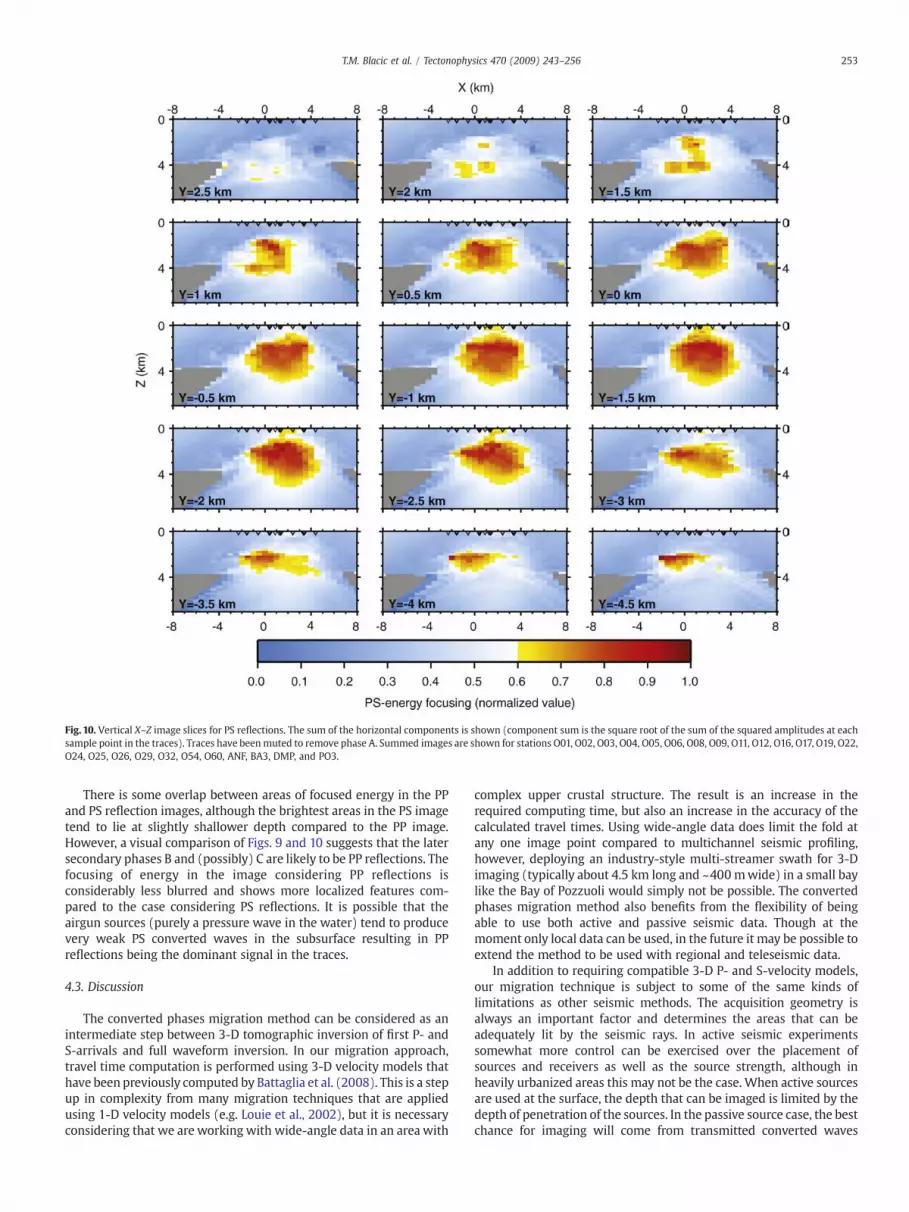
Fig. 10. Vertical X–Z image slices for PS reflections. The sum of the horizontal components is shown (component sum is the square root of the sum of the squared amplitudes at eachsample point in the traces). Traces have beenmuted to remove phase A. Summed images are shown for stations O01, O02, O03, O04, O05, O06, O08, O09, O11, O12, O16, O17, O19, O22,O24, O25, O26, O29, O32, O54, O60, ANF, BA3, DMP, and PO3.

253T.M. Blacic et al. / Tectonophysics 470 (2009) 243–256

There is some overlap between areas of focused energy in the PPand PS reflection images, although the brightest areas in the PS imagetend to lie at slightly shallower depth compared to the PP image.However, a visual comparison of Figs. 9 and 10 suggests that the latersecondary phases B and (possibly) C are likely to be PP reflections. Thefocusing of energy in the image considering PP reflections isconsiderably less blurred and shows more localized features com-pared to the case considering PS reflections. It is possible that theairgun sources (purely a pressure wave in the water) tend to producevery weak PS converted waves in the subsurface resulting in PPreflections being the dominant signal in the traces.

4.3. Discussion

The converted phases migration method can be considered as anintermediate step between 3-D tomographic inversion of first P- andS-arrivals and full waveform inversion. In our migration approach,travel time computation is performed using 3-D velocity models thathave been previously computed by Battaglia et al. (2008). This is a stepup in complexity from many migration techniques that are appliedusing 1-D velocity models (e.g. Louie et al., 2002), but it is necessaryconsidering that we are working with wide-angle data in an area with

complex upper crustal structure. The result is an increase in therequired computing time, but also an increase in the accuracy of thecalculated travel times. Using wide-angle data does limit the fold atany one image point compared to multichannel seismic profiling,however, deploying an industry-style multi-streamer swath for 3-Dimaging (typically about 4.5 km long and ~400 mwide) in a small baylike the Bay of Pozzuoli would simply not be possible. The convertedphases migration method also benefits from the flexibility of beingable to use both active and passive seismic data. Though at themoment only local data can be used, in the future it may be possible toextend the method to be used with regional and teleseismic data.

In addition to requiring compatible 3-D P- and S-velocity models,our migration technique is subject to some of the same kinds oflimitations as other seismic methods. The acquisition geometry isalways an important factor and determines the areas that can beadequately lit by the seismic rays. In active seismic experimentssomewhat more control can be exercised over the placement ofsources and receivers as well as the source strength, although inheavily urbanized areas this may not be the case. When active sourcesare used at the surface, the depth that can be imaged is limited by thedepth of penetration of the sources. In the passive source case, the bestchance for imaging will come from transmitted converted waves

254 T.M. Blacic et al. / Tectonophysics 470 (2009) 243–256

traveling upward from the sources to the receivers; the depth of thehypocenters will thus control the depth of imaging. Noise is also alimiting factor, particularly when working with weaker secondarysignals. Many of the land stations at Campi Flegrei were too noisy topermit the identification of any reflected phases, thereby limiting theextent of coverage of the images. We note, however, that it is notnecessary to strictly identify the secondary phase(s) in order to applythis migrationmethod.When a phase can be detected in the traces butnot positively identified as, say, a PP reflection or a PS reflection, thenas we have done in this study, imaging can be attempted for eachexpected phase and the quality of energy focusing in the images canbe compared to determine themost likely phase type. At this time, thecomparison of images must be done in a qualitative “by eye” methodbut a future improvement could include automated image qualityanalysis, which would also aid in choosing groups of receiver imagesto sum together.

Where there are strong, positively identified secondary phases (inactive or passive three-component seismograms) a clear image can beobtained by this method that provides a useful complement to smoothvelocity models from tomography (Latorre et al., 2008) with a smallercomputational effort compared to full-waveform inversion. In theCampi Flegrei case, we see that even when the secondary phases arenot as sharp and easy to identify we can still obtain a useful image thatcan confirm the presence of features detected by other means (Bruno,2004; Judenherc and Zollo, 2004; Vanorio et al., 2005) and providenew details.

The migrated images of PP reflections contribute considerabledetail to the caldera rim structure based on gravity, well logs andtomographic inversions of first arrival times.We image the caldera rimat two depths.When considering phase Awe can image part of the rimat a shallow depth of ~1.2–2 km spanning the mouth of the Bay ofPozzuoli (Fig. 8). When phase A is muted out we can image a deeperportion of the caldera rim around 2.4–2.6 km depth (Figs. 9, 11).Tomographic images do not capture these two distinct horizons; theyimage sections of a ring-shaped region of high velocities over a depthrange of ~0.8–3 km (Zollo et al., 2003; Judenherc and Zollo, 2004;Vanorio et al., 2005; Chiarabba and Moretti, 2006; Battaglia et al.,2008). However, a scattering image of Campi Flegrei obtained byTramelli et al. (2006) using coda wave envelopes showed portions ofthe caldera rim on land aswell as in the Bay of Pozzuoli at depths of 1-2km, which agrees with our images of the shallower portion of thecaldera rim. Gravity studies provide maps of the aerial extent of thedense volcanic and metavolcanic materials that make up the calderarim (AGIP, 1987; Florio et al., 1999; Zollo et al., 2003; Judenherc andZollo, 2004), and the lack of depth resolution can bemitigated by tyinggravitymodels intowell log data (e.g., AGIP,1987; see Fig.1). However,

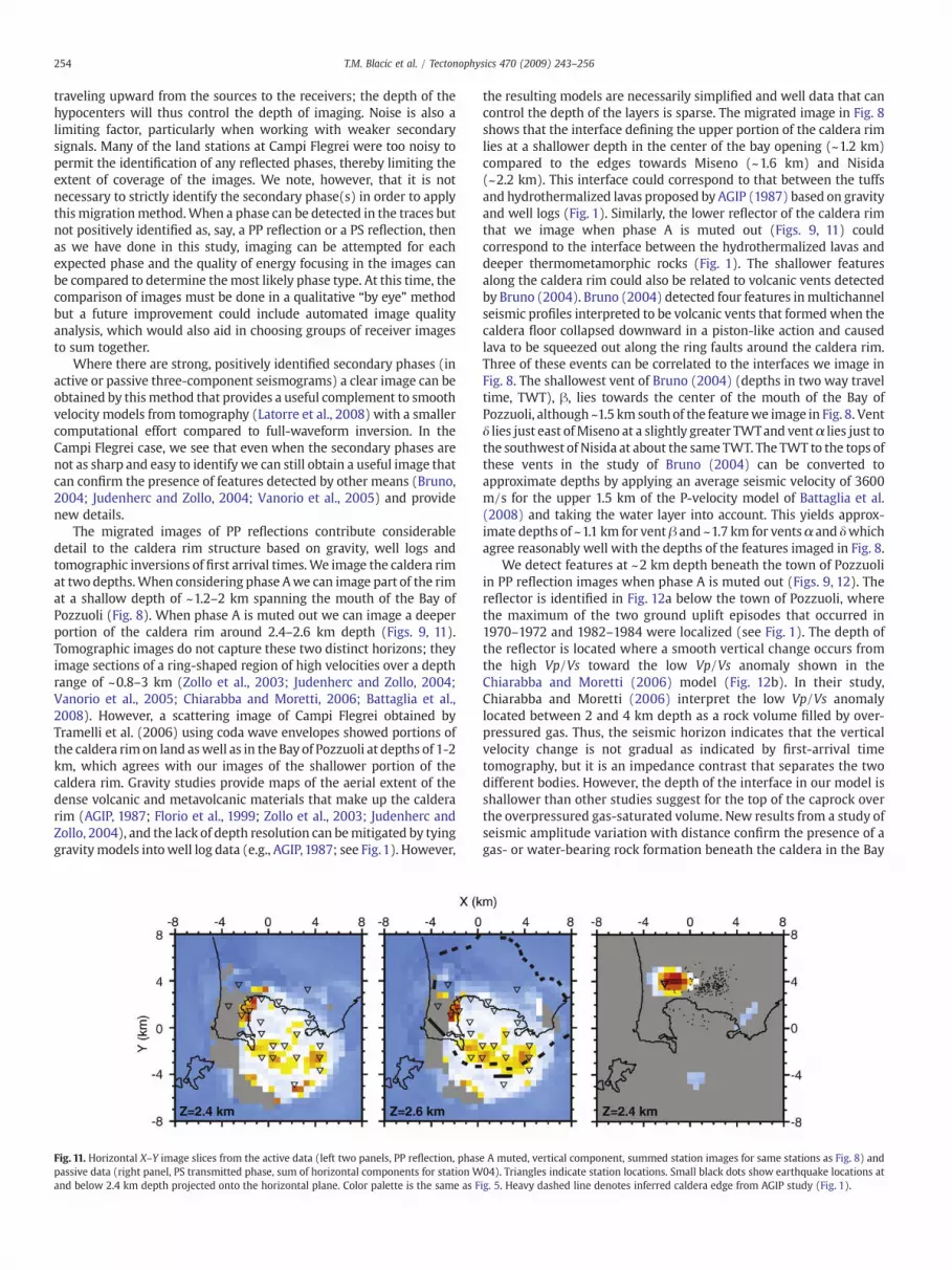
Fig. 11. Horizontal X–Y image slices from the active data (left two panels, PP reflection, phaspassive data (right panel, PS transmitted phase, sum of horizontal components for station Wand below 2.4 km depth projected onto the horizontal plane. Color palette is the same as F

the resulting models are necessarily simplified and well data that cancontrol the depth of the layers is sparse. The migrated image in Fig. 8shows that the interface defining the upper portion of the caldera rimlies at a shallower depth in the center of the bay opening (~1.2 km)compared to the edges towards Miseno (~1.6 km) and Nisida(~2.2 km). This interface could correspond to that between the tuffsand hydrothermalized lavas proposed by AGIP (1987) based on gravityand well logs (Fig. 1). Similarly, the lower reflector of the caldera rimthat we image when phase A is muted out (Figs. 9, 11) couldcorrespond to the interface between the hydrothermalized lavas anddeeper thermometamorphic rocks (Fig. 1). The shallower featuresalong the caldera rim could also be related to volcanic vents detectedby Bruno (2004). Bruno (2004) detected four features inmultichannelseismic profiles interpreted to be volcanic vents that formedwhen thecaldera floor collapsed downward in a piston-like action and causedlava to be squeezed out along the ring faults around the caldera rim.Three of these events can be correlated to the interfaces we image inFig. 8. The shallowest vent of Bruno (2004) (depths in two way traveltime, TWT), β, lies towards the center of the mouth of the Bay ofPozzuoli, although ~1.5 km south of the featurewe image in Fig. 8. Ventδ lies just east ofMiseno at a slightly greater TWTand ventα lies just tothe southwest of Nisida at about the same TWT. The TWT to the tops ofthese vents in the study of Bruno (2004) can be converted toapproximate depths by applying an average seismic velocity of 3600m/s for the upper 1.5 km of the P-velocity model of Battaglia et al.(2008) and taking the water layer into account. This yields approx-imate depths of ~1.1 km for vent β and ~1.7 km for ventsα and δwhichagree reasonably well with the depths of the features imaged in Fig. 8.

We detect features at ~2 km depth beneath the town of Pozzuoliin PP reflection images when phase A is muted out (Figs. 9, 12). Thereflector is identified in Fig. 12a below the town of Pozzuoli, wherethe maximum of the two ground uplift episodes that occurred in1970–1972 and 1982–1984 were localized (see Fig. 1). The depth ofthe reflector is located where a smooth vertical change occurs fromthe high Vp/Vs toward the low Vp/Vs anomaly shown in theChiarabba and Moretti (2006) model (Fig. 12b). In their study,Chiarabba and Moretti (2006) interpret the low Vp/Vs anomalylocated between 2 and 4 km depth as a rock volume filled by over-pressured gas. Thus, the seismic horizon indicates that the verticalvelocity change is not gradual as indicated by first-arrival timetomography, but it is an impedance contrast that separates the twodifferent bodies. However, the depth of the interface in our model isshallower than other studies suggest for the top of the caprock overthe overpressured gas-saturated volume. New results from a study ofseismic amplitude variation with distance confirm the presence of agas- or water-bearing rock formation beneath the caldera in the Bay

e A muted, vertical component, summed station images for same stations as Fig. 8) and04). Triangles indicate station locations. Small black dots show earthquake locations atig. 5. Heavy dashed line denotes inferred caldera edge from AGIP study (Fig. 1).

Fig. 12. (a) Horizontal and (b) vertical image slices for PP reflections, traces muted to remote phase A. Stations used to make summed image are the same as in Fig. 8. Color palette isthe same as Fig. 5. In (a) thin line marks location of vertical profiles shown in (b). In (b), upper panel, arrows highlight features discussed in the text. Lower panel shows isolines ofVp/Vsmodel proposed by Chiarabba andMoretti (2006). Gray dots show earthquake locations projected onto the vertical plane. (For interpretation of the references to colour in thisfigure legend, the reader is referred to the web version of this article.)

255T.M. Blacic et al. / Tectonophysics 470 (2009) 243–256

of Pozzuoli and place its top at 2.7 km depth (Zollo et al., 2008). Arecent 3-D inversion of gravity at Campi Flegrei indicates that thelow-density caldera fill material reaches down to at least 2.4 kmdepth (Russo, 2007) in the Bay of Pozzuoli. 2-D and 3-D modeling ofthe ground displacement at Campi Flegrei yield best fits to thedisplacement pattern when the source is placed 2.5 to 3 km belowthe ground surface (Russo, 2007). This suggests that the caprock ofthe gas-bearing formation lies near the bottom of the caldera fill,possibly coinciding with the transition from caldera fill to morecoherent rock at the bottom of the caldera at ~2.4–2.5 km depth.Vanorio et al. (2005) image a shallow high Vp/Vs anomaly and adeeper low Vp/Vs anomaly beneath Pozzuoli with the transitionbetween them occurring over depths of ~1.5–3 km. Based on rockphysics modeling, they interpret the deeper, low Vp/Vs anomaly torepresent overpressured gas-bearing rocks at supercritical condi-tions. Following Aster and Meyer (1988), the shallower high Vp/Vsanomaly was interpreted as rocks containing brine likely due tosteam condensation at the lower temperatures measured at thosedepths by AGIP (1987). These results agree with a placement of thecaprock between 2 and 3 km depth with our model providing theshallowest estimate. We note, however, that seismic tomographymethods tend to blur features in depth and thus provide an averagedepth for regions of anomalously low or high Vp/Vs. It may be thatwe are imaging the topmost surface of the caprock where theimpedance contrast is high.

A deeper feature can be tentatively identified in our migratedimages lying near 4 km depth (Fig. 9). This could be related to thecarbonate basement detected by tomography at approximately thesame depth (Judenherc and Zollo, 2004), however we note that theJudenherc and Zollo (2004)model did not have good resolution at thisdepth to constrain this interpretation. It is important to note thatalthough first arrival tomography methods are limited in the depththat can be resolved, when we work with reflected waves we caninvestigate much deeper structures (e.g., Zollo et al., 2008). As thecarbonate basement is believed to be continuous beneath this region,we can speculate that the impedance contrast is low and/or there is alimitation in our data set (e.g., low signal to noise ratio at thesedepths) which prevents us from imaging this interface in other areasof our model. A more likely alternative interpretation is that we areimaging part of the thermometamorphic complex described by AGIP(1987, Fig. 1). The interface we see is certainly weaker and appearssmeared in depth compared to other features in our images (Fig. 9),thus it is likely that we are imaging the top of a small body of morestrongly metamorphosed volcanic rock (possibly due to a localfracture which allowed magmatic liquids to reach this locale) or asmall and possibly older vent like those detected by Bruno (2004).

Fig. 11 shows that the passive data are independent data that canbe used to complement and constrain the results from the active datawhere the coverage of the two data sets lie close to each other,although the area of coverage resulting from the passive data is muchsmaller and the regions of coverage from each station overlap onlyover very small areas. When we consider PS transmitted phasesgenerated by the earthquakes, station W04 images a bright interfaceat 2.4 km to thewest of the S. Vito 8 well (Fig. 1). As reported by Bruno(2004), deposits recovered in the well at shallow depths are mainlycomposed of tuffs and lavas, while all the rock samples from 2.350 kmto 2.868 km (the well bottom) are composed of strongly thermo-metamorphosed lavas. Thus, the bright interface at 2.4 km is perfectlycompatible with the well data and corresponds to the top of thethermo-metamorphic body, also in agreement with the AGIP model(1987, Fig. 1). Unfortunately, except for station W14, other passivestations did not provide additional confirmation of the active results.Station W14 did provide an image of a feature centered at ~3 kmdepth just to the north of Nisida, which may correspond to part of thethermometamorphic volcanic rocks found in the S. Vito 8 well (Fig. 1).Thus, we can argue that the passive data shows a continuation of thisfeature to the north. This improves our confidence that the featureswe image are real features in the subsurface.

5. Conclusions

We applied a form of 3-D converted phases migration to activeseismic data from the SERAPIS project at Campi Flegrei caldera toimage subsurface reflections. Focusing on PP reflected phases, weimaged features at different depths in our model. We were able torecover part of the caldera rim at two depths in the southern part ofthe Bay of Pozzuoli: 1.2 to 2.0 km depth when we considered an earlyphase in the traces, and 2.4–2.6 km when this early phase wasremoved and later phases were analyzed. The shallower caldera rimfeature can be related to the transition from tuffs and loose caldera fillto denser hydrothermalized lava. Locations and depths of the shallowfeatures also correlate with several volcanic vents detected inmultichannel seismic data. The deeper caldera rim feature maycorrelate to the transition from hydrothermalized lavas to rocks thathave undergone a greater degree of thermometamorphism. Migratedimages also showed focusing of trace energy at 2–3 km beneath thetown of Pozzuoli and near 4 km depth beneath the western portion ofthe Bay of Pozzuoli. The shallower feature could mark the top of thecaprock over a volume of overpressured gas-saturated rock imaged byseismic tomography and seismic amplitude variation with distancestudies. The deeper feature in our images is less clear, but could berelated to the presence of the carbonate basement below the caldera

256 T.M. Blacic et al. / Tectonophysics 470 (2009) 243–256

or to a small volcanic vent. The image from passive data constrainedby well logs provides some confirmation of the deeper caldera rimfeature imaged by the active data and shows a continuation of thisfeature on land to the north.

Acknowledgements

We would like to thank Aldo Zollo at the University of Naples formaking the SERAPIS active and passive seismic data available for thisstudy. We thank Guido Russo for providing us with some details of hisresults prior to their publication and Claudio Chiarabba and MilenaMoretti for providing us with their Vp/Vsmodel to prepare Fig. 12. Wealso wish to thank two anonymous reviewers for their constructivecomments, which resulted in a great improvement to this manuscript.Partial support was provided through the Italian grant “INGV-DPC V4/02” and French grant “ANR-05-CATT-011-04.” Some figures shown inthis paper were drawn using the Generic Mapping Tools software(Wessel and Smith, 1991).

References

AGIP, 1987. Geologia e geofisica del sistema geotermico dei Campi Flegrei, ServiziCentrali per l'Esplorazione, SERG-MMSEG, San Donato.

Aster, R.C., Meyer, R.P., 1988. Three-dimensional velocity structure and hypocenterdistribution in the Campi Flegrei caldera, Italy. Tectonophysics 149, 195–218.

Auger, E., Gasparini, P., Vieieux, J., Zollo, A., 2001. Seismic evidence of an extendedmagmatic sill under Mt. Vesuvius. Science 294, 1510–1511.

Avallone, A., Zollo, A., Briole, P., Delacourt, C., Beauducel, F., 1999. Subsidence of CampiFlegrei (Italy) detected by SAR interferometry. Geophys. Res. Lett. 26, 3165–3168.

Barberi, F., Corrado, G., Innocenti, F., Luongo, G., 1984. Phlegraen fields 1982–1984: briefchronicle of a volcano emergency in a densely populated area. Bull. Volcanol. 47,175–185.

Battaglia, J., Zollo, A., Virieux, J., Dello Iacono, D., 2008. Merging active and passive datasets in traveltime tomography: the case study of Campi Flegrei caldera (SouthernItaly). Geophys. Prospect. 56, 555–573.

Bruno, P.P.G., 2004. Structure and evolution of the Bay of Pozzuoli (Italy) using marineseismic reflection data: implications for collapse of the Campi Flegrei caldera. Bull.Volcanol. 66, 342–355. doi:10.1007/s00445-003-0315-9.

Chiarabba, C., Moretti, M., 2006. An insight into unrest phenomena at the Campi Flegreicaldera from Vp and Vp/Vs tomography. Terra Nova 18, 373–379.

Chiodini, G., Frondini, F., Cardellini, C., Granieri, D., Marini, L., Ventura, G., 2001. CO2

degassing and energy release at Solfatara Volcano, Campi Flegrei, Italy. J. Geophys.Res. 106, 16,213–16,221.

de Lorenzo, S., Zollo, A., Mongelli, F., 2001. Source parameters and three-dimensionalattenuation structure from the inversion of microearthquake pulse width data: Qpimaging and inferences on the thermal state of the Campi Flegrei caldera (southernItaly). J. Geophys. Res. 106, 16,265–16,286.

DeNatale, G., Pingue, F., Allard, P., Zollo, A.,1991. Geophysical and geochemicalmodellingof the 1982–1984 unrest phenomena at Campi Flegrei Caldera, southern Italy.J. Volcanol. Geotherm. Res. 48, 199–222.

De Natale, G., Zollo, A., Ferraro, A., Virieux, J., 1995. Accurate fault mechanismdeterminations for a 1984 earthquake swarm at Campi Flegrei caldera (Italy)during an unrest episode: implications for volcanological research. J. Geophys. Res.100, 24,167–24,185.

De Natale, G., Troise, C., Pingue, F., Mastrolorenzo, G., Pappalardo, L., Boschi, E., 2006. TheCampi Flegrei Caldera: unrest mechanisms and hazards. In: Troise, C., De Natale, G.,Kilburn, C.R.J. (Eds.), Mechanisms of Activity and Unrest at Large Calderas. Spec.Publ. — Geol. Soc. Lond., vol. 269, pp. 25–45.

Dvorak, J.J., Gasparini, P., 1991. History of earthquakes and vertical movement in CampiFlegrei caldera, Southern Italy: comparison of precursory events to the A.D. 1538eruption of Monte Nuovo and activity since 1968. J. Volcanol. Geotherm. Res. 48,77–92.

Dvorak, J.,Mastrolorenzo,G.,1991. Themechanismsof recent vertical crustalmovements inCampi Flegrei caldera, southern Italy. Spec. Pap. Geol. Soc. Am. 263 54 pp.

Ferrucci, F., Hirn, A., De Natale, G., Virieux, J., Mirabile, L., 1992. P–SV conversions at ashallow boundary beneath Campi Flegrei caldera (Italy): evidence for the magmachamber. J. Geophys. Res. 97, 15,351–15,359.

Florio, G., Fedi, M., Cella, F., Rapolla, A., 1999. The Campanian Plain and Phlegrean Fields:structural setting from potential field data. J. Volcanol. Geotherm. Res. 91, 361–379.

Judenherc, S., Zollo, A., 2004. The Bay of Naples (southern Italy): constraints on thevolcanic structures inferred from a dense seismic array. J. Geophys. Res.109, B10312.doi:10.1029/2003JB002876.

Kramer, F.S., Peterson, R.A., Walters, W.C. (Eds.), 1968. Seismic Energy Sources — 1968Handbook, Pasadena, Bendix United Geophysical.

Latorre, D. (2004), Imagerie sismique du milieu de propagation à partir des ondesdirectes et converties: application à la région d'Aigion (Golfe de Corinthe, Grèce),PhD thesis, Université de Nice-Sophia Antipolis, France. (in French).

Latorre, D., Virieux, J., Monfret, T., Monteiller, V., Vanorio, T., Got, J.L., Lyon-Caen, H.,2004. A new seismic tomography of Aigion area (Gulf of Corinth, Greece) from the1991 data set. Geophys. J. Int. 159, 1013–1031.

Latorre, D., De Gori, P., Chiarabba, C., Amato, A., Virieux, J., Monfret, T., 2008. Three-dimensional kinematic depth migration of converted waves: application to the2002 Molise aftershock sequence (southern Italy). Geophys. Prospect. 56, 587–600.

Louie, J.N., Chávez-Pérez, S., Henrys, S., Bannister, S., 2002. Multimode migration ofscattered and converted waves for the structure of the Hikurangi slab interface,New Zealand. Tectonophysics 355, 227–246.

Podvin, P., Lecomte, I., 1991. Finite difference computation of travel times in verycontrasted velocity models: a massively parallel approach and its associated tools.Geophys. J. Int. 105, 271–284.

Ravaut, C., Operto, S., Improta, L., Virieux, J., Herrero, A., Dell'Aversana, P., 2004.Multiscale imaging of complex structures from multifold wide-aperture seismicdata by frequency-domain full-waveform tomography: application to a thrust belt.Geophys. J. Int. 159, 1032–1056.

Rosi, M., Sbrana, A., 1987. Phlegraean fields. CNR Quad. Ric. Sci. 114 (9), 175.Russo, G., (2007), Personal communication, 16 and 23 November.Saccorotti, G., Petrosino, S., Bianco, F., Castellano, M., Galluzzo, D., La Rocca, M., Del

Pezzo, E., Zaccarelli, L., Cusano, P., 2007. Seismicity associated with the 2004–2006renewed ground uplift at Campi Flegrei Caldera. Italy, Phys. Earth Plan. Int. 165,14–24.

Troise, D., Pingue, F., De Natale, G., 2003. Coulomb stress changes at calderas: modelingthe seismicity of Campi Flegrei (southern Italy). J. Geophys. Res. 108 (B6), 2292.doi:10.1029/2002/JB002006.

Troise, C., De Natale, G., Pingue, F., Obrizzo, F., DeMartino, P., Tammaro, U., Boschi, E., 2007.Renewed ground uplift at Campi Flegrei caldera (Italy): new insight on magmaticprocesses and forecast. Geophys. Res. Lett. 34, L03301. doi:10.1029/2006GL028545.

Vanorio, T., Virieux, J., Capuano, P., Russo, G., 2005. Three-dimensional seismictomography from P wave and S wave microearthquake travel times and rockphysics characterization of the Campi Flegrei Caldera. J. Geophys. Res. 110, B03201.doi:10.1029/2004JB003102.

Wessel, P., Smith, W., 1991. Free software helps maps and display data. EOS 72, 441.Wohletz, K., Civetta, L., Orsi, G., 1999. Thermal evolution of the Phlegraean magmatic

system. J. Volcanol. Geotherm. Res. 91, 381–414.Yilmaz, O., 2001. Seismic Data Analysis: Processing, Inversion and Interpretation of

Seismic Data. Society of Exploration Geophysicists, Tulsa, Oklahoma.Zollo, A., Judenherc, S., Auger, E., Auria, L.D., Virieux, J., Capuano, P., Chiarabba, C., de

Franco, R., Markis, J., Michelini, A., Musacchio, G., 2003. Evidence for the buried rimof Campi Flegrei caldera from3-d active seismic imaging. Geophys. Res. Lett. 30 (19).doi:10.1029/2003GL018173.

Zollo, A., Maerklin, N., Vassallo, M., Dello Iacono, D., Virieux, J., Gasparini, P., 2008.Seismic reflections reveal a massive melt layer feeding Campi Flegrei caldera.Geophys. Res. Lett. 35, L12306. doi:10.1029/2008GL034242.