construction of an extended library of adult male 3d models: rationale and results

Construction of an extended library of adult male 3D models: rationale and results

This content has been downloaded from IOPscience. Please scroll down to see the full text.

Download details:

IP Address: 210.211.125.25

This content was downloaded on 28/09/2013 at 05:01

Please note that terms and conditions apply.

2011 Phys. Med. Biol. 56 7659

(http://iopscience.iop.org/0031-9155/56/23/020)

View the table of contents for this issue, or go to the journal homepage for more

Home Search Collections Journals About Contact us My IOPscience

iopscience.iop.org/page/terms

http://iopscience.iop.org/0031-9155/56/23

http://iopscience.iop.org/0031-9155

http://iopscience.iop.org/

http://iopscience.iop.org/search

http://iopscience.iop.org/collections

http://iopscience.iop.org/journals

http://iopscience.iop.org/page/aboutioppublishing

http://iopscience.iop.org/contact

http://iopscience.iop.org/myiopscience

IOP PUBLISHING PHYSICS IN MEDICINE AND BIOLOGY

Phys. Med. Biol. 56 (2011) 7659–7692 doi:10.1088/0031-9155/56/23/020

Construction of an extended library of adult male 3Dmodels: rationale and results

D Broggio1, J Beurrier, M Bremaud, A Desbree, J Farah, C Huet andD Franck

Institut de Radioprotection et de Surete Nucleaire (IRSN), DRPH/SDI/LEDI, BP-17, F92262Fontenay-aux-Roses, France

E-mail: [email protected]

Received 1 August 2011, in final form 5 October 2011Published 15 November 2011Online at stacks.iop.org/PMB/56/7659

AbstractIn order to best cover the possible extent of heights and weights of male adultsthe construction of 25 whole body 3D models has been undertaken. Sucha library is thought to be useful to specify the uncertainties and relevanceof dosimetry calculations carried out with models representing individuals ofaverage body heights and weights. Representative 3D models of Caucasianbody types are selected in a commercial database according to their heightand weight, and 3D models of the skeleton and internal organs are designedusing another commercial dataset. A review of the literature enabled one tofix volume or mass target values for the skeleton, soft organs, skin and fatcontent of the selected individuals. The composition of the remainder tissue isfixed so that the weight of the voxel models equals the weight of the selectedindividuals. After mesh and NURBS modelling, volume adjustment of theselected body shapes and additional voxel-based work, 25 voxel models with109 identified organs or tissue are obtained. Radiation transport calculationsare carried out with some of the developed models to illustrate potential uses.The following points are discussed throughout this paper:

• justification of the fixed or obtained models’ features regarding availableand relevant literature data;

• workflow and strategy for major modelling steps;• advantages and drawbacks of the obtained library as compared with other

works.The construction hypotheses are explained and justified in detail since futurecalculation results obtained with this library will depend on them.

(Some figures may appear in colour only in the electronic version)

1 Author to whom any correspondence should be addressed.

0031-9155/11/237659+34$33.00 © 2011 Institute of Physics and Engineering in Medicine Printed in the UK 7659

http://dx.doi.org/10.1088/0031-9155/56/23/020

mailto:[email protected]

http://stacks.iop.org/PMB/56/7659

7660 D Broggio et al

1. Introduction

The recent release of ICRP Publication 110 (ICRP 2009) of male and female referencecomputational phantoms and the book of Xu and Eckerman (2010) definitely evidence thewide use of three-dimensional (3D) models of the human body. For ionizing radiation studies,the voxel format, up to now mandatory in most used Monte Carlo codes, represents a complex3D geometry as a collection of right parallelepipeds, the 3D equivalent of pixels. FollowingZankl et al (1988), several voxel models have been developed from medical images, tryingto best follow ICRP and ICRU recommendations (Xu et al 2000, Kramer et al 2003, Ferrariand Gualdrini 2005). Apart from such models following international recommendations formale and female average individuals, more specific models have been developed such as thepregnant female model or the paediatric family. These two works started with modellingthe medical images (Shi and Xu 2004, Lee et al 2005) and later included mesh and NURBSmodelling (Xu et al 2007, Lee et al 2007). Mesh, NURBS or hybrid models are so calledsince they are built with professional 3D modelling software and stored in specific formats.Such formats enable the storing of medical image contours and sophisticated transformations.Ultimately, such models can be developed without any input medical image, as illustrated inCassola et al (2010).

Realistic human models have made it possible to specify the validity of calculationscarried out with mathematical phantoms whose realism was debatable. In short, it turnsout that radiation protection quantities are not that different when mathematical or voxelreference models are compared (ICRP 2009). Relevant differences are however noted whenmathematical and voxel models are compared, for some specific organs (ICRP 2009) orfor the foetus (Taranenko and Xu 2008), newborn (Staton et al 2006) or paediatric (Leeet al 2006) cases. Moreover, realistic human models should help specifying the accuracyand significance of dose calculations based on average reference individuals but applied toindividuals significantly different from the average. In order to systematically study thevariation of dosimetric quantities with the body type it is suitable to rely on a relatively largesample of models. In this case, it can be expected that a tendency, or even rather generalrules, could be derived. The radiation protection consequences of the body-type differencebetween Asian models and their ICRP or Caucasian counterparts have been illustrated (Saitoet al 2001, Kinase et al 2003, Zhang et al 2007). Variation with the body type of specificabsorbed fractions and photon conversion coefficients has been studied for a small numberof male and female voxel models presenting significant height and weight differences (Zanklet al 2003, Fill et al 2004). Johnson et al (2009) have recently released 25 adult male modelsand 15 paediatric female models corresponding to percentile individuals. Na et al (2010) havealso recently shown that it is possible to adjust a reference 3D model to percentile individuals.

This work and the two above cited studies are an attempt to broaden the available bodytypes, mainly defined by height and weight, of male adult models. In this work, the constructionof 25 full-body male 3D models has been undertaken. Representative Caucasian body shapeshave been selected from a database of individuals optically scanned. Target values havebeen defined for the internal organ masses, fat per cent, skin mass and remainder tissuecomposition of these individuals. The modelling was carried out using not only mesh andNURBS modelling, but also voxel modelling. The current version of 3D models includes109 organs and tissue adapted to the selected body shapes. The construction hypotheses areexplained and justified in detail since future calculation results obtained with this library willdepend on them. Finally, using some of the developed models, illustrative radiation transportcalculation results are shown for internal and external dosimetry issues and in vivo monitoringissues.

Construction of an extended library of adult male 3D models: rationale and results 7661

2. Materials and methods

2.1. Selection of individuals in the CAESAR database

2.1.1. The CAESAR database. The CAESAR database (SAE 2011) is a commerciallyavailable collection of male and female 3D models constructed from optical scanning ofindividuals. For each model, 45 precisely defined anthropometric parameters, measuredby trained personnel, are reported. The individuals included in the database were selectedfollowing a sampling strategy by age, race and gender, as recommended by ISO standards.For each cell of the sample population the target number of individuals was calculated sothat the mean stature of the sample is within 10 mm of the true population mean with 95%confidence (Robinette et al 2002). The European edition of the database, used in this work,contains 412 individuals scanned in Italy and 566 scanned in the Netherlands. The individualswere optically scanned in standing position with the legs and arms apart. Individuals wore athin cap covering and plastering down the air and a tight-fitting pairs of short. The samplingstrategy, scanning protocol, description of measurements and illustrations of the 3D modelscan be found in (Robinette et al 2002, 2003, 2006).

2.1.2. Selected individuals. From the European edition, male individuals have been selectedso that each one represents a height and weight class (HW class). Four 12-cm height classes,from 158 to 206 cm, and nine 12-kg weight classes, from 43 to 151 kg have been defined.The HW classes have been defined so that one class centre is (176 cm, 73 kg), the heightand weight of the ICRP reference male. The extents (12 cm, 12 kg) were chosen to limit thenumber of selected individuals while trying to maintain a satisfying sampling of the CAESARdatabase. Considering the reported height (H) and weight (W ) of individuals, their distancefrom the centre (Hc, Wc) of a HW class was calculated using

D2 =(

H − HC

3cm

)2

+

(W − WC

3kg

)2

.

If D < 1, the individual can be the class representative. When several individuals met thiscondition, the one with the smallest D was the class representative. When possible, individualsscanned in Italy were preferred since the associated 3D models contain fewer holes.

Applying the above selection condition, 22 individuals were selected; among the 36possible classes some were empty (no CAESAR male individuals in these classes) and othersdid not contain an individual meeting the selection condition. For the class centred at (176 cm,73 kg) the selected individual has H = 177 cm and W = 73.1 kg. Three additional individualswere selected in order to have representative individuals of larger HW classes. Table 1 givesthe height, weight, age, body mass index (BMI = W kg/H2

m) of selected individuals and theHW class they represent. Hereafter, for simplicity, individuals are called according to theshort names given in table 1. The height and weight of the M1C individual are very closeto those of the reference male computational phantom (RMCP) of ICRP Publication 110.Figure A1 presents the H and W chart of male individuals included in the European editionof the CAESAR database. This figure also shows the HW classes, the H and W of selectedindividuals and for comparison the H and W of percentile individuals selected in Johnsonet al (2009) and Na et al (2010).

2.2. Target value fixing

2.2.1. Scaling factor for internal organs and the skeleton. Studying a sample of 581 adultmale subjects Heymsfield et al (2007, 2008) have given for the bone mineral mass (BMM, in

7662D

Broggio

etal

Table 1. Main features of selected individuals.

Height class (cm) 164 ± 6 176 ± 6Weight class (kg) 49 ± 6 61 ± 6 73 ± 6 85 ± 6 97 ± 6 109 ± 6 49 ± 6 61 ± 6 73 ± 6 85 ± 6 97 ± 6 109 ± 6 133 ± 6

Model’s shortname M0A M0B M0C M0D M0E M0F M1A M1B M1C M1D M1E M1F M1H

Measured height (cm) 162.7 164 164 165.5 163.5 163.8 174.3 176 177 176.3 175 173.7 178.8

Measured weight (kg) 50.8 60.2 71.9 85.3 95 106.9 50.2 61.6 73.1 85.3 95.7 110.4 133

BMI (kg m−2) 19.2 22.4 26.7 31.1 35.5 39.8 16.5 19.9 23.3 27.4 31.2 36.6 41.6

Age (year) 18 35 30 29 56 55 23 19 28 31 40 44 39

Height class (cm) – 188 ± 6 200 ± 6 170 ± 12 194 ± 12 206 ± 12Weight class (kg) 145 ± 6 73 ± 6 85 ± 6 97 ± 6 109 ± 6 121 ± 6 133 ± 6 97 ± 6 109 ± 6 121 ± 6 145 ± 6 127 ± 12

Shortname M1I M2C M2D M2E M2F M2G M2H M3E M3F EX1 EX2 EX3

Measured height (cm) 178.5 188.7 187.3 189 189.1 187.4 188.1 200.4 200.3 172.6 193.4 205.4

Measured weight (kg) 143.9 72.5 84.9 96.9 108.8 122.1 133.6 96 110.3 120.3 146.6 127.5

BMI (kg m−2) 45.2 20.4 24.2 27.1 30.4 34.8 37.8 23.9 27.5 40.4 39.2 30.2

Age (year) 49 24 19 20 36 40 37 27 40 54 49 63


Table 2. Scaling factors for the skeleton and soft organs.

Height (cm) kH kF kC Fixed volume scaling factor (k)

164 0.84 0.81 0.8–0.95 0.84176 1 1 1 1188 1.17 1.24 1.05–1.2 1.2200 1.36 1.54 1.1–1.4 1.4

kg) and bone mass (BM), as a function of height (H, in cm). Since we are more interestedin relative variations than in absolute values, it is convenient to take H0 = 176 cm and use ascaling factor; for example, the scaling factor for the BM is simply written as

k = BM(H)

BM(H0).

The scaling factors for BM and BMM are very close and we thus keep their mean:

kH = 0.5((H/H0)

2.51 + (H/H0)2..33) .

Studying a sample of 176 male subjects another equation was given for the BMM (Ferrettiet al 1998), which gives

kF = exp(0.018(H − H0)).

Studying 355 adult male cadavers, height-dependant linear equations were given for the massof nine soft organs (Clairand et al 2000, De La Grandmaison et al 2001). Despite the slope ofthe linear equation varies largely depending on the organ, the scaling factors, kc, for the nineorgans are relatively close. In table 2, the minimum and maximum values of kc are reportedwith kH and kF.

For the defined height classes, the scaling factors given in table 2 are in notable agreement;table 2 also reveals that in each class the range of scaling factors is distinct from the otherclasses. This supports the intuitive idea that the skeleton and soft organs grow identically untilreaching their adult size (at least from the adolescence). For the 188 and 200 cm individuals,the fixed scaling factors are the rounding of kH (biggest sample, composite scaling factor).From the k values of table 2, linear interpolation gives k = 1 for EX1, k = 1.3 for EX2 andk = 1.5 for EX3. The fixed scaling factors are only a working hypothesis that should leadto the design of acceptable organs for average individuals. The following references brieflyillustrate that alternative approaches have been developed for some organs or for more generalcases.

Hepper et al (1960) have studied the lung case. Daugirdas et al (2008) have compiledequations for the liver case. The mass of the brain has been studied by Heymsfield et al (2009)and Ho et al (1980). For the heart case, alternative approaches can be found in Hitosugi et al(1999), Seo et al (2000) and Pritchett et al (2003). A general approach for group of organsand tissue has also been developed by Martin (1984) and Kerr (1988).

2.2.2. Fat per cent and full-body volume fixing. Many techniques enabling us to measureor deduce the body fat fraction of individuals have been reported (Tolli et al 1998, Wanget al 1998). Thus, many relations are available to calculate the fat content from individualcharacteristics and, for the non-specialists, it is quite difficult to select one approach or another.As a consequence, the results of ten relations given in appendix B have been averaged for


Figure 1. Fixed F% of body weight (F%) for each individual. The bar corresponds to the averagevalue deduced from ten relations found in the literature. The 4 black points correspond to anincrease of 3% from the average value.

each individual. When the relation gave the lean body mass the fat mass per cent (F%) wascalculated from the weight:

F% = 100(1 − LBM/W),

following the definitions given in Hentschel et al (2005). For each individual, the average ofF% is plotted in figure 1 where the error bar is the standard deviation over all the relations.For four individuals (M0D, M2F, EX1 and EX2), F% was increased by 3% (of body weight).Without this increase, the calculation of the remainder tissue composition would have given anegative fraction for one component of the remainder (cf 2.5 and 3.1.3). Despite the disputablesignificance of the error bar, it can be noted that for relatively underweight individuals errorbars are large, whereas for other individuals the uncertainty is around 5% of body weight.For the M1C individual, the fat per cent of the body weight is (20 ± 2)% which is the valuerecommended in ICRP Publication 89 (ICRP 2002).

The Siri equation relates the body density (ρ, in g cm−3) and the F% of body weight (Siri1956):

F% = 495/ρ − 450. (1)

Even if this equation is based on a two-compartment model, it has been found reliable bymany specialists (Lean et al 1996, Prior et al 1997, Guo et al 1999). Once F% has been fixed,the Siri density is calculated, which gives the target volume for selected individuals since theirweight is known.

2.2.3. Skin density fixing. In ICRP Publication 23 (ICRP 1975) the skin is defined as dermisand epidermis and represents 3.7% of the body weight. In ICRP Publication 89 it is 4.5% ofthe body weight, and in the RMCP it is a single-voxel layer representing 5.1% of the bodyweight. Thus, the skin grossly weights as much as two brains and its mass must be fixed asrealistically as possible, using the same density for all models. In the voxel models the skinvolume will be fixed by the construction algorithm. We thus need a target skin density thatwill make the skin mass as realistic as possible. For this purpose, we use the mass of the bodysurface area (BSA) as an intermediate quantity.

The H and W of the selected individuals were used to calculate their BSA, accordingto the Dubois and Dubois, Haycock and Mosteller relations, as given in Verbraecken et al


(2006). To calculate the mass of the BSA, the thickness (t, in g cm−2) was needed. From ICRPPublication 23, t = 0.143 g cm−2 was deduced. Using a surface area of 8 × 2.137 = 17.1 mm2

per skin voxel t = 0.233 g cm−2 was deduced from the RMCP. Since no other relevant valueswere found in the literature, the average was adopted: t = 0.188 g cm−2. In ICRP Publication89, it is recalled that this value is between 0.115 and 0.225 g cm−2. Figure C1 shows the skinmass per cent of all the individuals for the three used relations. Considering these values andaveraging over all individuals and relations, the skin mass represents 4.5% of the body weight.

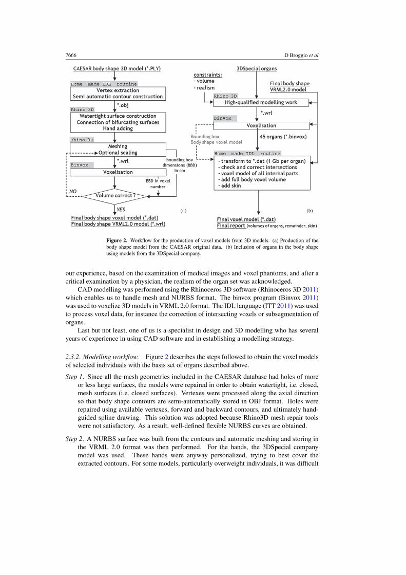
As a consequence, after the construction of the skin volume (Vskin) in the voxel models,and knowing the weight (W ) of the selected individuals, the skin density (ρskin) is obtained byminimizing the following quantity:

χ∗2 = 1

25

25∑i=1

(ρskinVskin,i − 0.045Wi

0.045Wi

)2

. (2)

If the skin volume is correctly developed, it can even be hoped that the skin mass of voxelmodels agrees better with the above relations than with the fixed fraction of body weight.

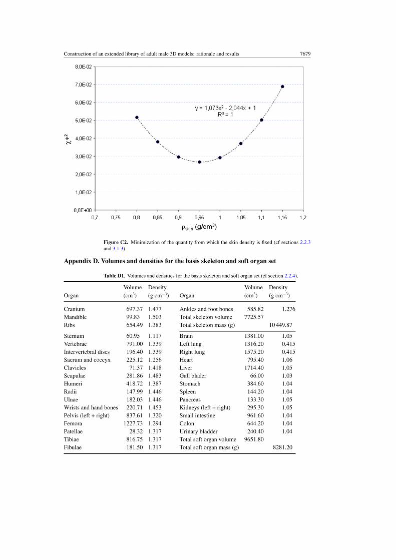
2.2.4. Basis organs used for the construction of 3D models. Reference volumes, givenin table D1, were fixed for 31 bones and 14 soft organs and for the 176 cm height class.This reference set of organs was modelled using computer-aided design (CAD) software.Subsegmentation of these organs and addition of smaller organs was performed using voxelmodelling. The reference volumes have been deduced by merging or splitting organs of theRMCP.

The cortical, spongiosa and medullary parts of the RMCP have been merged, and thecartilage distributed to the bones of table D1 in proportion of their volume fraction in RMCP.The sum of the left and right volumes is listed in table D1, but in the 3D constructionprocess sides were distinguished. The volumes for ulna, radius, tibia, fibula and patella area compromise between available literature data (McInroy et al 1985, ICRP 1975) and theconstraint to match the volumes defined in RMCP. The sum of vertebrae and disks volumesis 987 cm3 (vertebrae of RMCP plus 163 cm3 of trunk cartilage). The basis volumes for softorgans were also fixed by merging volumes of the RMCP, taking into account wall and content,if defined.

The densities given in table D1 were obtained from the masses and volumes of RMCP-merged organs. Table D1 gives a total mass of 10 450 g for the skeleton, in perfect agreementwith table 4.1 of ICRP Publication 110.

The volumes given in table D1 were taken from the RMCP and as, noted in ICRPPublication 110, a few organs do not respect the volume requirements of ICRP Publication89. This choice was made in order to ease the comparison of future calculations based on themodels presented here and others based on the RMCP.

2.3. Modelling tools and workflow

2.3.1. Modelling tools and techniques. The organs of the 3D models are taken from thefull-body model provided by the 3DSpecial company (3DSpecial 2011). For the cranium,mandible and pelvis the ‘P1 VRML 2.0’ set and for other organs the ‘A1 VRML 2.0’ set wereused. The small intestine was fully redesigned using NURBS formats since the provided onewas not suitable. As stated in the documentation from 3DSpecial, the 3D models of organshave been developed from medical images, discussed with anatomists and checked by thequalified personnel. The same set of 3D organs was recently used by (Zhang et al 2009) todevelop a male and female model matching the requirements of ICRP Publication 89. From


(a) (b)

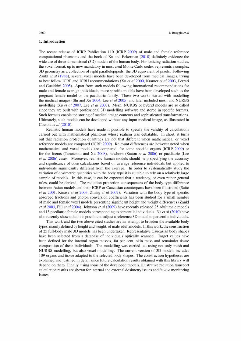
Figure 2. Workflow for the production of voxel models from 3D models. (a) Production of thebody shape model from the CAESAR original data. (b) Inclusion of organs in the body shapeusing models from the 3DSpecial company.

our experience, based on the examination of medical images and voxel phantoms, and after acritical examination by a physician, the realism of the organ set was acknowledged.

CAD modelling was performed using the Rhinoceros 3D software (Rhinoceros 3D 2011)which enables us to handle mesh and NURBS format. The binvox program (Binvox 2011)was used to voxelize 3D models in VRML 2.0 format. The IDL language (ITT 2011) was usedto process voxel data, for instance the correction of intersecting voxels or subsegmentation oforgans.

Last but not least, one of us is a specialist in design and 3D modelling who has severalyears of experience in using CAD software and in establishing a modelling strategy.

2.3.2. Modelling workflow. Figure 2 describes the steps followed to obtain the voxel modelsof selected individuals with the basis set of organs described above.

Step 1. Since all the mesh geometries included in the CAESAR database had holes of moreor less large surfaces, the models were repaired in order to obtain watertight, i.e. closed,mesh surfaces (i.e. closed surfaces). Vertexes were processed along the axial directionso that body shape contours are semi-automatically stored in OBJ format. Holes wererepaired using available vertexes, forward and backward contours, and ultimately hand-guided spline drawing. This solution was adopted because Rhino3D mesh repair toolswere not satisfactory. As a result, well-defined flexible NURBS curves are obtained.

Step 2. A NURBS surface was built from the contours and automatic meshing and storing inthe VRML 2.0 format was then performed. For the hands, the 3DSpecial companymodel was used. These hands were anyway personalized, trying to best cover theextracted contours. For some models, particularly overweight individuals, it was difficult


to distinguish two near contours from a single contour, i.e. at the crotch point and axillaryfossa level. Nevertheless, it was checked that these junctions are correctly positionedwith an uncertainty that does not exceed 2 cm at worst.

Step 3. Once a VRML 2.0 watertight, i.e. a closed surface, model was obtained voxelizationwas performed. The voxel size was fixed so that the dimensions of the bounding boxes ofvoxel and VRML 2.0 models are equal. The VRML 2.0 models were optionally scaledfor full-body volume adjustment.

Step 4. All the organs defined in table D1 were adapted so that they fit in the full-body shapemodels and match the volume requirements defined by the adopted scaling factor. Thegeneral method and some technical details regarding the adjustment of internal organsand skeleton to the obtained body shape models are given in section 2.4.1. Once a VRML2.0 model was obtained bones and soft organs were voxelized separately in the samereference frame and then merged into a unique voxel model. Intersections of voxelizedorgans were unavoidable and were corrected with an algorithm that propagates the bordersof intersecting objects. Parts of internal organs that sticked out of the body shape weresimply removed and the skin was then added.

To build the skin, the same algorithm is used for all models. Air neighbouring voxels areidentified in axial planes and defined as skin; this makes a single voxel layer like in theRMCP. Supplementary skin voxels are also defined at the top and bottom of models, atthe fingertips, crotch point, etc, so that the models are properly closed by a skin layer. Toensure a coherent building of skin for all models, random addition or deletion of voxels,that would enable us to reach a fixed target volume, is not allowed.

2.4. Inclusion of organs in 3D models

2.4.1. Skeleton and soft organs. The 3DSpecial organs and bones defined in section 2.2.4were adjusted to the M1C model to agree with target volumes. The obtained organs were thenadapted to all other models applying the height class scaling factor. To ensure the realismof the 3D models produced, anatomic tables (Netter 2004, Rouviere and Delmas 1979) wereused and also a human anatomy drawing manual (Simblet and Davis 2002). Moreoverthe advice of a medical doctor was taken into account all along the design process. AvailableCT scans, voxel phantoms and other internet resources were also used when needed. Sincethe methods to adapt the 3DSpecial organs to the M1C model and the M1C organs to othermodels are similar, this latter case is described hereafter.

Step 1. All soft organs and bones were together scaled along the axial direction to fit with theheight of the 3D body shapes. A 2D scaling was then applied in the axial plane so thatthe total scaling factor equals the factor fixed in table 2. At this stage the needed volumeswere obtained but additional adjustments must be made to position the organs and bonesin each individual.

Step 2. The cranium was adapted; for this purpose, it was divided into its main bones, whichallowed proper handling of trimmed surfaces and proper use of mesh tools. Most ofrhino3D mesh tools were used to fit the cranium with the head shape while trying topreserve the target volume. To fit the head shape, sagittal and coronal views were usedand also ‘anchor’ points such as the ears, arch of the eyebrow and bottom of the chin forthe mandible. The foramen magnum was properly positioned where the head joins theneck. The brain was positioned and transformed inside the skull during this stage, so thatwith its volume constraint, the brain sometimes did not fill in entirely the skull volume.


Step 3. The soft organs, thoracic bones and the vertebral column were moved together so thatthe top of the vertebral column fits with the foramen magnum. Then the ‘3D control cage’tool, mandatory to avoid the creation of intersections, was used for position adjustments.Useful anchors were the crotch level, the iliac crest or the shoulders. After cage tool,mesh offset were used to finalize the volumes.

Step 4. Small scaling and rotations were performed on arm and leg bones to better fit theindividual body shapes; used anchors were the knee and elbow. The hands and feet boneswere also scaled, translated, rotated and caged to fit in the available space.

2.4.2. Subsegmentation of organs and addition of glands. Voxel models with the organs andbones defined in table D1 were modified to include subparts of bones and soft organs; smallvolume organs were also added to these models. This work was performed directly on voxelmodels without CAD modelling.

Following ICRP Publication 110, the cortical, spongiosa and medullary parts of bones,as well as wall and contents of some soft organs, were built. For a given organ, the volumeof the outer shell, Vshell, (cortical part for bones, wall for soft organs) was calculated with thefollowing relations:

Vshell = ρVo

ρ∗(1 + 1/f ∗m)

ρ∗ = �m + Mshell

�m/ρcart + Mshell/ρshell; f ∗

m = �m + Mshell

Mcore.

(3)

The volume of the modified organ is Vo, ρ is its density as given in table D1, Mshell and Mcore

are the masses of the shell and interior of the organs, ρshell and ρcart (1.10 g cm−3) are the shelland cartilage densities given in ICRP Publication 110. �m is the mass of the cartilage that wasattributed to the bones defined in table D1. For soft organs �m is zero and thus ρ

∗reduces to

the wall density and fm∗ reduces to the mass ratio of the wall and content. The above relationsensure that the mass of the divided organ is conserved and that the mass ratio of the shell andinterior is as defined in ICRP Publication 110. Since the cartilage mass is included in thecortical part of bones, the cortical density is not 1.92 g cm−3 as defined by ICRP Publication110 but ρ∗. The shell voxels were built with an algorithm similar to the one used for buildingthe skin.

The medullary content was included where it is defined in the RMCP. The relativepositioning found in the RMCP was conserved as well as the densities of spongiosa andmedullary content given in ICRP Publication 110. The number of voxels was found byadapting equation (3) and the used algorithm consisted in replacing the interior of bones byplanes corresponding to the medullary part.

An algorithm to include left and right eyes, adrenals, testes as well as the pituitary gland,the tonsils, the thymus and the prostate, was developed. The pituitary gland and the tonsilshave been modelled as ellipsoids after examination of the RMCP. For the eight other glandsthe shapes given in Cristy and Eckerman (1987) and in Stabin (1994) have been used. Thereference masses given in ICRP Publication 89 and the scaling factors of table 2 were used.The algorithm consisted in specifying a starting position for the gland that is included. Ifintersections were found at this position, small displacements were tested, and if this failedthe organ shape was modified so that the final target volume is obtained.

The thyroid and oesophagus were also included in voxel models. For the thyroid, voxelizedversions of the 3DSpecial thyroid model were included with an algorithm similar to that forother glands. For the oesophagus, reference positions were provided to another algorithm


which includes the same voxel pattern at reference positions and interpolates between them.The exact mass target is obtained by random addition or deletion of voxels.

2.5. Composition of the remainder tissue

In the voxel 3D models, muscle, fat tissue and organs not currently included are merged ina single remainder tissue. To make its composition as realistic as possible, it is made upof muscle, fat and ‘other tissue’. It is needed to define ‘other tissue’ to take into accountexcluded organs and connective tissues (tendons, fascia, periarticular tissue) which should notbe confused with muscle.

The muscle and ‘other tissue’ contents are calculated so that the weight of the voxel modelequals the weight of the corresponding selected individual, taking into account built organs.It is thus requested to adjust the volumes of muscle (VMu) and ‘other tissues’ (Vo) so that theweight of these volumes (W ∗) satisfies

W ∗ = WModel − WBuilt − WFat·WModel is the weight of the individual given in table 1, WBuilt is the weight of the built voxelorgans and W Fat is known from above. Using the muscle and ‘other tissue’ densities, we have{

W ∗ = ρMuVMu + ρoVo

V ∗ = VMu + Vo = VFB − VBuilt − VFat.

V∗ is known if the volume of the full body (VFB) has been built. Thus, VMu and Vo can becalculated as {

VMu = (W ∗ − ρoV∗)/(ρMu − ρo)

Vo = V ∗ − VMu.(4)

To fix ρo the M1C model is considered, and it is also assumed that the muscle mass is 29 kg,like in the RMCP. By definition ρo is

ρo = WM1C − WBuilt − WFat − WMu

VM1C − VBuilt − VFat − VMu· (5)

Finally, the density of the remainder tissue (ρRem) is

ρRem = WMu + WFat + Wo

VMu + VFat + Vo= WFB − WBuilt

VFB − VBuilt·

3. Results and discussion

3.1. Main feature of achieved voxel models

3.1.1. General feature and achieved organ masses. All the M2, M3, EX models and theM1A model have 972 voxel layers in the axial direction, other models have 744 voxel layers.The voxel volumes are model dependent but quite homogeneous, between 5.55 and 8.74 mm3.The size of the bounding box enclosing the model varies from about 57 × 106 (M1C) to140 × 106 (EX1) voxels. The number of voxels defining the full-body shape varies from7.4 × 106 (M1B) to 21.6 × 106 (EX1) which corresponds to 58.2 and 120 L.

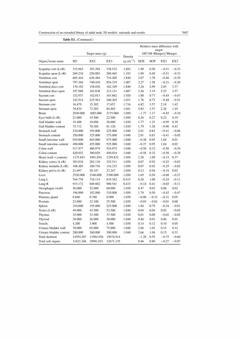
Table E1 gives the masses of organs and bones for the 25 voxel models. Except forM1A, the volume of skeleton plus soft organs has been built within ±1% (within ±0.5% for15 models). Except for M0D and M1B, the soft organs total volume is built within ±1%(±0.5% for 18 models). Except for M1A and M3E the skeleton total volume is built within±1% (±0.5% for 15 models).


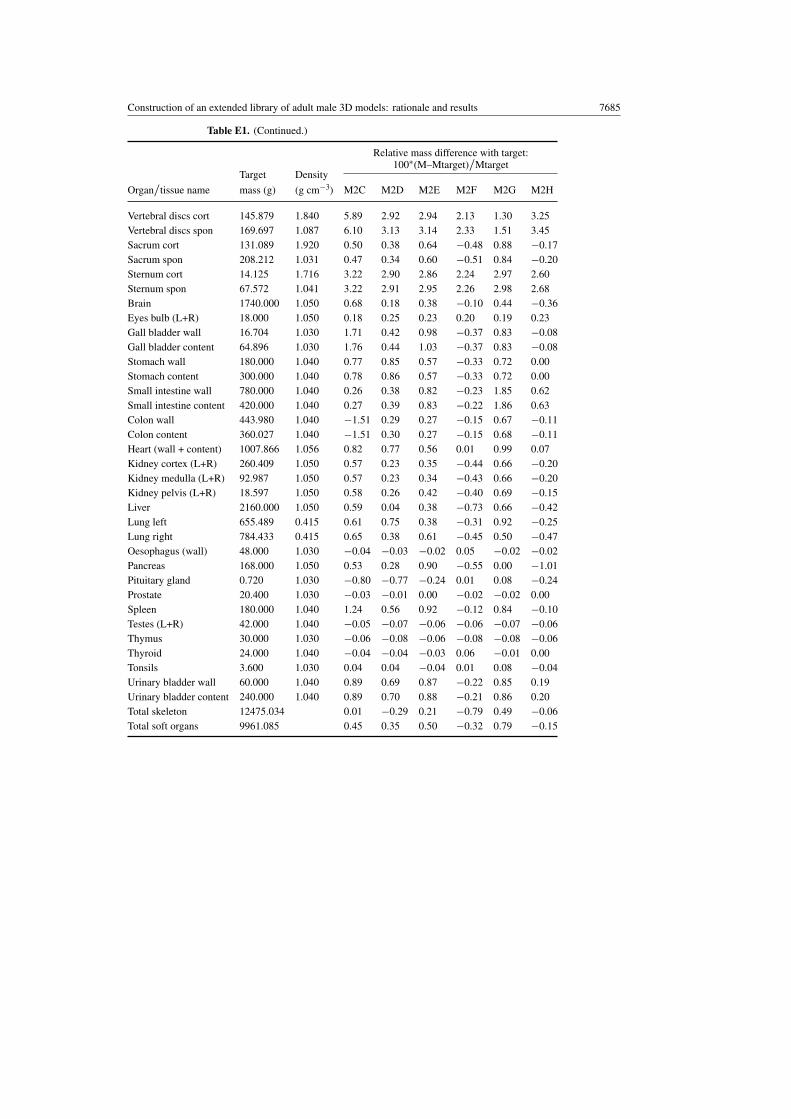
For most of the organs listed in table E1, the mass agreement with the target value is within±3%. However, in some cases it is impossible to reach the target value. For example, thecrania of the M1A and M3E models have a respective deficit of 150 and 260 g, simply becausethe head shape of these models cannot contain the requested volume. Similarly, for M1A theworst disagreement (−38%) is obtained for the clavicles because the model is too thin to adjustthe required volume. For most models, the hands, pelvis and cranium are the organs for whichit is the most difficult to reach the target mass. Additional work in the modelling process couldimprove the agreement between targeted and achieved volumes; anyway, it is not believedthat these improvements would be significant and the volume agreement presented here isconsidered to be acceptable. Figures 3 and 4 illustrate the difference in body types of the builtmodels and the result of organ inclusion in the body shapes.

3.1.2. Achieved full-body density and height of voxel models. In order to reach the Siridensity given by equation (1), 14 VRML2.0 models were uniformly contracted in the axialplane to obtain the theoretical volume (height was preserved). The full-body density ofachieved models, the Siri density and the volume correction factors are given in table E2.For the M1A model, the scaling was important (−15%) but for seven models it was −4%.After volume adjustment, the Siri density is obtained for all models within ± 0.02 g cm−3.The density of the M1C voxel model is 1.05 g cm−3, the RMCP has a density of 1.03 gcm−3 and the MAX06 phantom (Kramer et al 2006) has a density of 1.01 g cm−3. Themain goal of the volume adjustment was to make the full-body density decrease with weightfor all height classes. After the scaling, a decreasing trend with weight is indeed obtained.Despite the fact that the decrease is not monotonic (e.g. compare the density of M0D andM0E or M2C and M2D in table E2), the obtained differences between the achieved densityand the Siri density are small enough to be disregarded. Moreover, it is expected that thevolume adjustment will enable us to reach a realistic composition for the remainder tissue(cf section 3.1.3).

As shown in table E2, the height of voxel models is not necessarily in agreement withthe measured height of the selected individuals. For seven voxel models, the height is greaterthan the measured one, the two maximum deviations are 0.8 and 1.2 cm, and other differencesare less than 0.6 cm. For these seven models, it must be admitted that, apart from intrinsiclimitation of the scanning process, the hair under the cap may have been confused with thehead. For all other models, the voxel height is less than the measured one, which couldbe expected since the models are standing with legs apart. For seven of these models, thedifference is less than 1 cm, for ten it is between 1 and 3 cm, and the maximum difference is5.2 cm for EX3. If the voxel and CAESAR reported heights agree within 1 cm, the differencecan be attributed to the standing position with legs apart. In other cases, it can account fora part of the difference but presumably not all. Other possible reasons can be cited but notproven: intrinsic limitations of the scanning process, slight bending of the head or trunk, meshrepair and voxelization processes. The combination of these reasons might explain differencein height less than 2 or 2.5 cm. For EX3, the CAESAR documentation states that the subjectis a giant and his head is tilted in the standing scan. No additional transformation was madeto scale the model to their reported height. Since the obtained models are intended to berepresentative of a height and weight class, small differences in the achieved and reportedheight should not dramatically affect the relevance of future calculations.

3.1.3. Skin density and composition of the remainder tissue. As explained in section 2.2.3,the skin volume is built with the same method for all models and equation (2) is then applied


Figure 3. Illustration of the body-type difference of constructed models. The M0, M1 and M2models are shown at the same scale. The models at the bottom are shown at the same scale, but itis different than the scale used for the models above.

Figure 4. Illustration of organs and skeleton inclusion in the body shapes, mesh rendering with3DStudio.


Figure 5. Comparison of different predictions giving the muscle mass of selected individuals andcomparison with the muscle mass attributed to the voxel models of this work.

so that the skin mass is as close as possible to 4.5% of the body weight. As shown infigure C2, ρskin = 0.95 g cm−3 perfectly solves the problem. As expected, and as shown infigure C1, a good agreement with the skin mass percentages deduced from the selected BSArelations is obtained. For all of the voxel models, the agreement with one of this relation iswithin ± 0.5% of the body weight. The skin density adopted here is clearly different from the1.09 g cm−3 of ICRP Publication 110 but it is here intended to best describe 25 individualsusing only one density. Moreover, the agreement shown in figure C1 tends to prove that theconstructed body shapes are indeed representative of individuals with the selected heights andweights and that the skin masses are realistic. The skin mass of M1C is 3669 g while it is3728 g for the RMCP.

Once the skin density is fixed, equation (5) is used and it is found that ρo = 1.3 g cm−3,while ICRP Publication 23 gives 1.2 g cm−3 for connective tissues.

Once ρo is fixed, equation (4) is used to calculate the composition of the remainder tissuewhich is given in table E3 for all models. For the muscle tissue of M1C, 28.5 kg were obtainedwhen 29 kg were expected; this small disagreement is due to the differences between targetedand achieved organs’ mass. The volume of fat and ‘other tissue’ is 21.3 L (22.2 kg) when itis 21.5 L (21 kg) for RMCP ‘residual tissues’. The density of the remainder tissue is between0.99 and 1.1 g cm−3; again a decreasing trend with weight and BMI is found. The musclemass is between 34% and 44% of the body weight for all models. The ‘other tissue’ mass isbetween 1% and 17% of the body weight and it presents large variations among models. ForM0D, M2F, EX1-2, equation (4) would have given negative masses for the ‘other tissue’ if thefat per cent had not been increased (cf Section 2.2.2).

While many relations have been proposed to calculate F%, there are fewer to calculate themuscle mass. Nevertheless, the relation of Gallagher et al (1997) which gives the appendicularskeletal muscle mass as a function of age, two relations by Janssen et al (2000) which give theskeletal muscle mass as a function of weight and a relation by Lee et al (2000) which givesthe skeletal muscle mass as a function of weight, height, age, sex and ethnic origin were usedto compare the muscle mass attributed to voxel models. Figure 5 shows that the voxel muscle


masses are not in agreement with the first three relations but in better agreement with the lastone; at least the increasing trend with weight is found for all height classes. Finally, the fat and(muscle+other) weight per cent of body weight are given in figure E1 as a function of BMI.From the construction of the fat content, a linear trend dominates, but for the (muscle+other),a similar trend is noted. While the fat percentage increases with BMI, the (muscle+other)percentage decreases, but slower than the increase in fat; this supports the intuitive idea that theproduction of fat is accompanied by a limited production of muscle and other tissues helpingin carrying the body fat.

3.1.4. Comparison with other approaches. The library presented here has advantages anddrawbacks as compared with available libraries (Johnson et al 2009, Na et al 2010) or comparedwith the RMCP. Moreover, recent developments regarding the deformation of 3D humanmodels suggest that new techniques and tools could help in the design of future libraries.

The models presented here do not include as many organs as those cited above. Somesource organs like ET1 and ET2 are not yet included; other organs represent merged versionsof RMCP organs (e.g. the colon is not divided into several parts). Even if it is not a tremendousadvantage, we have distinguished left and right and included bones not defined in the RMCP.To ease comparison with the RMCP, volumes were taken from it, while in Johnson et al andNa et al the volumes were taken from ICRP Publication 89.

The Johnson et al library has been derived from an initial model based on medical images.The internal organs used in this work are derived from a commercial model. Even if otherauthors used this commercial model (Zhang et al 2009) and we acknowledge its quality, thedegree of realism of our initial model cannot be discussed as deeply as the one of Johnsonet al.

In the two libraries cited above, the body shapes have been constructed by deformationof an initial model. In Johnson et al the deformations were guided by anthropometricmeasurements. In Na et al, scaling of an initial model was applied to obtain the desiredheight and then adjusted with the MakeHuman software (MakeHuman 2011). In our case, thebody shapes were selected in a database and not manually transformed; a final 2D scaling wasnevertheless applied to 14 models.

In Johnson et al and Na et al, prior target values were not fixed for the organs andskeleton since they were transformed or scaled with the body shape. In this work, prior targetvalues were fixed for the organs and skeleton and the composition of the remainder tissue waspersonalized. Even if this approach is a simplification, it is believed to be reasonable androbust and it also offers a systematic framework for fixing target values. The results for theskin mass, the full-body density and the remainder composition have been discussed. Thesefeatures are indicators of the quality of the achieved models; at least they demonstrate thecoherence of the construction method.

Whatever the advantages and drawbacks of our library and other libraries, it is believedthat they will successfully enable sensitivity studies of dosimetric quantities with body type.These libraries are not intended to achieve personal dosimetry but intended to reveal trends onglobal dosimetric estimator like effective dose. Moreover, disposing of several models builtindependently with different methods should enable us to better assess the dose sensitivity toorgan positioning or tissue composition.

Finally, it must be noted that high-level algorithms and methods have been developedto analyse and transform 3D mesh models of the human body, as presented in Allenet al (2003), Azouz et al (2006) and Hasler et al (2009). Thanks to such methods it ispossible to generate in a few seconds various body shapes (Procrustica 2011). These methodsseem extremely promising for further developments of human models dedicated to radiation


Figure 6. Comparison of absorbed doses to organs for the RMCP, M0B, M1C and M2F modelsfor 0.5 MeV photon in AP irradiation geometry.

transport calculations. However, to our knowledge, such methods have never been applied formodels including internal organs. Moreover, these methods focus on designing volumes, andattributing reasonable weight to the designed shapes might require additional work.

3.2. Illustrative radiation transport calculations

The M1C model (177 cm, 73.1 kg), the M0B (164 cm, 60.2 kg), the M2F (189 cm, 108.8 kg)and the RMCP are used to carry out illustrative dosimetry calculations. The M0B and M2Fmodels have been chosen since they are very close in height and weight to the 5th and 95thpercentile individuals modelled in Na et al (2010), cf figure A1. Simulation results of in vivomeasurement are presented for 13 models of the developed library.

3.2.1. External dosimetry. Absorbed organ doses were calculated with the MCNPX MonteCarlo code (Pelowitz 2005) for a 0.5 MeV photon beam in AP irradiation geometry. Asuccessful calculation with the RMCP of the stomach wall absorbed dose per air kerma forseveral energies enabled us to validate the calculation method. Figure 6 presents the ratio ofabsorbed doses to organ. Comparison of the M1C and RMCP models show that the agreementis very good for some organs (adrenals, brain, skin, etc) but differences, up to ±20%, arenoted for other organs (stomach wall, spleen, urinary bladder wall). These differences areattributed to different organ depths and positions in the M1C and RMCP models. The dosedifference for most of organs is about 10% between M0B and M1C, except for a few organs,and it turns out that the doses are slightly smaller for M0B than for M1C. One could expectthe contrary if one only thinks in terms of the shielding effect. But, in fact, the organs of M0Bare smaller than those of M1C and there is only 12 kg difference between the two models; asa consequence the organs of M0B are slightly deeper than those of M1B, which can explain


Figure 7. Comparison of SAF for the RMCP, M0B, M1C and M2F models.

the results. In contrast, there is a difference of 36 kg between M1C and M2F and doses toorgans are typically 20% lower for M2F, except for the skin and the brain which is consistentwith the anatomy of the models.

3.2.2. Internal dosimetry. Specific absorbed fractions (SAF) were calculated for energiesbetween 10 keV and 5 MeV and for some organs of interest, as chosen in Marine et al (2010).The calculation method has already been validated in prior work (Hadid et al 2010). Figure 7shows that for energies above 40 keV, the relative difference in SAF for RMCP and M1C isconstant; there is a 20% difference for the SAF (lungs←liver) but it is limited to 10% in thetwo other cases. For the three examples shown, the dose is higher for M0B than for M1C, andsmaller for M2F than for M1C. This trend could be explained since the organs of M0B are onthe average closer to each other than in M1C, and those of M1C closer than those of M2F.

As in the case of external dosimetry, no general conclusion can be drawn from particularexamples; for this purpose, all models should be used and synthetic dose indicator like effectivedose should be studied to reveal general trends.

3.2.3. In vivo counting studies. The mobile unit of IRSN is used to carry out routine orspecial in vivo counting measurements. The counting system consists of two broad-energygermanium detectors (crystal thickness: 30 mm, crystal surface: 50 cm2) which were modelledand validated. The detector model provided by the manufacturer was slightly modified, suchas in Liye et al (2006), to obtain good agreement between well-defined experiments andsimulation results. The final validation consisted in simulating the calibration curve for the70 kg St Petersburg phantom (Kovtun et al 2000). The maximum difference between simulatedand experimental counting efficiency was 4.7% at 1332 keV.

Simulated and experimental counting efficiencies are shown on the left side offigure 8 for a 137Cs homogenous contamination and the same distance between detectorsand the skin. In this case, both the RMCP and the M1C models give counting efficiencies invery good agreement with the experiment. Simulated counting efficiencies are shown for 13


Figure 8. Comparison of counting efficiencies for several models in the case of caesiumcontamination.

voxel models on the right side of figure 8. The simulation took into account the biokineticdistribution of 137Cs (Leggett et al 2003) and the routine measurement protocol which specifiesthe distance between the back of the monitored subject and the detectors. For the studied cases,the difference in counting efficiencies can be as high as 30% (M0A versus M2E). This kindof studies enables us to improve measurement protocols or to improve the interpretation ofmeasurements.

4. Conclusion

A library of 25 full-body adult male 3D models has been constructed in order to extend thebody type diversity of currently available models. Such a library is thought to be useful fordosimetry calculations where the body type does not need to be patient specific but where asingle average body type is not sufficient.

Three-dimensional body shape models of representative Caucasian individuals have beenselected in a commercial database. Volume or mass target values were fixed for the skeleton,soft organs, skin and fat content of the selected individuals. An initial commercial model ofsoft organs and skeleton has been modified with CAD tools so that organ masses and volumesmatch those of the RMCP. This model was adapted to the selected body shapes according tofixed target values. After voxelization, inclusion of small volume organs and subsegmentationwere performed. The final models include 109 organs (left and right pairs are distinguished).

The obtained organ masses are shown to be in good agreement with the target valuesdeduced from relevant literature data. The skin mass, the composition of the remainder tissueand the whole body density are also shown to be in reasonable agreement with literaturedata. The advantages and limitations of the methods, modelling strategy and result have beendiscussed regarding similar works. Even if the anatomical realism was sometimes sacrificedto achieve fixed target values, it is believed that it should not affect dramatically the relevanceof calculations carried out with the models.


Illustrative results for radiation transport calculations have been given. No generalconclusion can be drawn from particular examples; for this purpose, all models should beused and synthetic dose indicator, like effective dose, should be studied to reveal generaltrends. Future work will consist in making this library publically available, undertakingsystematic calculations and improving the models.

Acknowledgments

Dr Gianfranco Gualdrini (ENEA, Bologna) is thanked for inspiring this work with his talkgiven at the ICRS-RPSD conference in 2008. Dr Gianfranco Gualdrini and Dr Paolo Ferrari(ENEA, Bologna) are also thanked for careful reading of the manuscript and useful comments.Cecile Challeton-de Vathaire (MD, IRSN, Fontenay-aux-Roses) is thanked for medical adviceduring the 3D modelling. Dr Patrick Min is thanked for efficient support with the BinVoxprogram. Fabien Dournac (MS) is thanked for providing computing tricks. Frazier Bronsonfrom the Canberra Company is thanked for providing MCNP models of detectors. Jean-Rene Jourdain, Jean-Michel Deligne, Michelle Agarande (IRSN/DRPH) are thanked foradministrative support.

Appendix A. Individuals selected in the European edition of the CAESAR database

Figure A1. Height and weight of individuals selected in the European edition of the CAESARdatabase, comparison with individuals selected in other studies, and definition of HW classes usedin this study.


Appendix B. Relations used to obtain the fat mass per cent of selected individuals

Table B1. Relations used for the calculation of the F% of selected individuals.

Relation Units, comments Reference

F% = 0.567 × waist+ waist = waist circumference Lean et al 19960.101 × age − 31.8 in mm, age in yearsF% = 0.353 × waist + 0.756× Same as above; triceps = Lean et al 1996triceps + 0.235 × age − 26.4 triceps skinfolds in mmLBM = 1.1 × weight − 120× kg and cm Sugawara et al 1999(weight/height)2

LBM = W(1 − 0.012 W

H 2 + W is weight in kg, H is height Pieterman et al 20020.023a − 0.162) in meter, a is age in years

F% = 1.20 W

H 2 + 0.23a − 16.2 Same units as above. Sex Deurenberg et al 1991taken into account

F% = 1.294 W

H 2 + 0.20a − 19.4 Same units as above. Sex Deurenberg et al 1998taken into account

F% = 71.5 − 1210 H 2

W‘Garrow and Webster’ Jebb et al 2000relation, same units as above

F% = 100(0.454 − 0.031 H

W− Deduced from ‘Bruce et al Carlsson et al 2004

16.53W

+ 0.0779 a

W) relation’, same units as above

but H in cm

F% = 59.3 − 26.7 H

W+ 1919.6

Wkg and cm Boddy et al 1972

F% = 55.4 − 943.8 H 2

W+ 0.087a kg, metre, years. Sex and Gallagher et al 2000

ethnicity taken into account

Appendix C. Data relative to the skin construction of voxel models

Figure C1. Comparison of skin mass (in per cent of body weight) as predicted by three equationsfor the BSA and using a thickness of 0.188 g cm−2 for the skin, and as obtained in the voxel models(cf sections 2.2.3, 2.3.2, 3.1.3).


Figure C2. Minimization of the quantity from which the skin density is fixed (cf sections 2.2.3and 3.1.3).

Appendix D. Volumes and densities for the basis skeleton and soft organ set

Table D1. Volumes and densities for the basis skeleton and soft organ set (cf section 2.2.4).

Volume Density Volume DensityOrgan (cm3) (g cm−3) Organ (cm3) (g cm−3)

Cranium 697.37 1.477 Ankles and foot bones 585.82 1.276Mandible 99.83 1.503 Total skeleton volume 7725.57Ribs 654.49 1.383 Total skeleton mass (g) 10 449.87

Sternum 60.95 1.117 Brain 1381.00 1.05Vertebrae 791.00 1.339 Left lung 1316.20 0.415Intervertebral discs 196.40 1.339 Right lung 1575.20 0.415Sacrum and coccyx 225.12 1.256 Heart 795.40 1.06Clavicles 71.37 1.418 Liver 1714.40 1.05Scapulae 281.86 1.483 Gall blader 66.00 1.03Humeri 418.72 1.387 Stomach 384.60 1.04Radii 147.99 1.446 Spleen 144.20 1.04Ulnae 182.03 1.446 Pancreas 133.30 1.05Wrists and hand bones 220.71 1.453 Kidneys (left + right) 295.30 1.05Pelvis (left + right) 837.61 1.320 Small intestine 961.60 1.04Femora 1227.73 1.294 Colon 644.20 1.04Patellae 28.32 1.317 Urinary bladder 240.40 1.04Tibiae 816.75 1.317 Total soft organ volume 9651.80Fibulae 181.50 1.317 Total soft organ mass (g) 8281.20


Appendix E. Features of achieved voxel models.

Table E1. Target mass, density and relative mass difference of achieved organs (versus targetmass) for all models.

Relative mass difference with target:100∗(M–Mtarget)/Mtarget

Target Density

Organ/tissue name mass (g) (g cm−3) M0A M0B M0C M0D M0E M0F

Adrenals (L+R) 11.760 1.030 0.04 0.04 −0.05 0.02 0.03 0.03Humeri cort (L+R) 223.074 1.908 0.07 −0.45 0.42 −1.05 −0.25 −0.12Humeri spon (L+R) 205.472 1.180 −0.14 −0.65 0.21 −1.25 −0.45 −0.33Humeri medu (L+R) 59.317 0.980 0.92 0.41 1.29 −0.20 0.61 0.74Ulnae cort (L+R) 126.315 1.910 −0.02 −0.49 0.13 −1.14 −0.35 −0.61Ulnae spon (L+R) 84.287 1.108 −0.18 −0.65 −0.02 −1.29 −0.50 −0.75Ulnae medu (L+R) 10.503 0.980 1.22 0.70 1.30 0.03 0.82 0.60Radii cort (L+R) 102.693 1.910 0.79 −0.53 0.48 −0.61 −0.02 −0.12Radii spon.(L+R) 68.526 1.108 0.63 −0.68 0.36 −0.74 −0.16 −0.25Radii med (L+R) 8.538 0.980 2.02 0.61 1.65 0.54 1.24 1.03Wrists and hand bones cort (L+R) 152.125 1.909 −10.03 5.41 4.58 5.34 −1.43 4.98Wrists and hand bones spon (L+R) 117.256 1.108 −10.11 5.32 4.48 5.24 −1.51 4.88Clavicles cort (L+R) 40.440 1.909 −5.77 −1.07 −0.14 −1.09 −0.03 −0.88Clavicles spon (L+R) 44.570 1.151 −5.62 −0.91 0.05 −0.93 0.14 −0.71Cranium cort 486.322 1.881 −0.56 −0.63 −0.30 −0.63 −1.93 −1.56Cranium spon 378.890 1.157 −0.63 −0.69 −0.37 −0.69 −2.00 −1.63Femora cort (L+R) 479.970 1.882 −0.10 −0.65 0.31 −1.30 −0.49 −1.06Femora spon (L+R) 764.949 1.116 −0.18 −0.73 0.23 −1.37 −0.57 −1.13Femora med (L+R) 89.608 0.980 −0.23 −0.78 0.17 −1.43 −0.63 −1.19Tibiae cort (L+R) 355.107 1.887 3.22 2.81 3.62 2.27 2.76 2.79Tibiae spon (L+R) 482.363 1.112 −0.93 −1.32 −0.55 −1.84 −1.38 −1.35Tibiae med (L+R) 66.083 0.980 0.61 0.23 1.00 −0.31 0.16 0.20Fibulae cort (L+R) 80.783 1.887 −0.50 −0.56 −0.19 −1.93 −0.78 −0.36Fibulae spon (L+R) 120.007 1.112 1.11 1.06 1.43 −0.33 0.83 1.25Patellae cort (L+R) 12.605 1.887 3.21 −1.32 1.05 0.83 −5.63 −3.84Patellae spon (L+R) 18.725 1.112 4.94 0.36 2.89 2.61 −3.94 −2.20Ankles and foot bones cort (L+R) 201.370 1.878 −0.21 −0.76 −0.10 −1.67 −1.04 −0.69Ankles and foot bones spon (L+R) 426.535 1.108 −0.23 −0.77 −0.11 −1.69 −1.05 −0.70Mandible cort 63.961 1.920 −0.29 0.32 0.59 −0.92 −3.56 0.01Mandible spon 62.076 1.228 −0.30 0.30 0.57 −0.92 −3.57 0.00Pelvis cort (L+R) 356.551 1.837 2.57 2.25 2.63 0.89 1.53 1.39Pelvis spon (L+R) 572.191 1.123 2.56 2.25 2.62 0.89 1.52 1.38Ribs cort 323.484 1.849 −1.30 −0.20 0.64 −1.01 −0.64 −0.27Ribs spon 436.850 1.165 −1.35 −0.25 0.59 −1.06 −0.69 −0.32Scapulae cort (L+R) 189.578 1.892 −0.44 0.19 0.55 −1.03 −0.08 −0.50Scapulae spon (L+R) 161.540 1.183 −0.44 0.19 0.55 −1.03 −0.08 −0.49Vertebrae cort 411.267 1.840 0.69 0.96 0.94 −0.43 −1.05 0.05Vertebrae spon 478.419 1.087 0.88 1.15 1.14 −0.24 −0.85 0.24Vertebral disks cort 102.115 1.840 6.79 0.75 1.95 1.89 4.65 3.57Vertebral disks spon 118.788 1.087 7.00 0.95 2.15 2.09 4.87 3.79Sacrum cort 91.762 1.920 0.42 0.29 0.81 −1.02 −1.09 0.35Sacrum spon 145.748 1.031 0.37 0.26 0.78 −1.05 −1.13 0.32Sternum cort 9.888 1.716 2.42 2.64 3.28 1.54 1.47 1.99


Table E1. (Continued.)


Target Density

Organ/tissue name mass (g) (g cm−3) M0A M0B M0C M0D M0E M0F

Sternum spon 47.300 1.041 2.52 2.69 3.31 1.61 1.54 2.02Brain 1218.000 1.050 0.40 0.32 0.83 −2.81 −0.30 −0.30Eyes bulb (L+R) 12.600 1.050 0.24 0.24 0.26 0.23 0.26 0.26Gall bladder wall 11.693 1.030 1.00 0.46 1.14 −0.78 −0.71 −0.03Gall bladder content 45.427 1.030 1.03 0.51 1.17 −0.75 −0.69 −0.02Stomach wall 126.000 1.040 0.52 0.39 1.10 −0.34 −0.27 0.10Stomach content 210.000 1.040 0.52 0.39 1.11 −0.33 −0.26 0.11Small intestine wall 546.000 1.040 0.52 0.12 0.35 −0.83 0.79 0.57Small intestine content 294.000 1.040 0.52 0.13 0.36 −0.82 0.80 0.58Colon wall 310.786 1.040 0.37 0.42 0.74 −0.66 −0.36 −0.21Colon content 252.019 1.040 0.37 0.42 0.74 −0.66 −0.36 −0.21Heart (wall + content) 705.506 1.056 0.84 0.67 0.83 −0.41 −0.15 0.06Kidney cortex (L+R) 182.286 1.050 0.12 −0.13 0.60 −0.73 −0.57 −0.24Kidney medulla (L+R) 65.091 1.050 0.13 −0.13 0.61 −0.73 −0.57 –0.23Kidney pelvis (L+R) 13.018 1.050 0.16 −0.09 0.65 −0.64 −0.50 −0.21Liver 1512.000 1.050 0.75 0.39 0.58 −1.18 −0.94 −0.27Lung left 458.843 0.415 0.68 0.60 0.76 −0.84 −0.56 −0.25Lung right 549.103 0.415 0.47 0.20 0.89 −0.95 −0.68 −0.24Oesophagus (wall) 33.600 1.030 0.03 0.03 0.04 0.06 −0.01 −0.01Pancreas 117.600 1.050 −0.51 −0.51 0.63 −1.36 −0.57 −0.47Pituitary gland 0.504 1.030 −0.21 −0.21 −0.67 −0.78 −1.02 −1.02Prostate 14.280 1.030 −0.04 −0.04 −0.02 −0.03 −0.02 −0.02Spleen 126.000 1.040 1.04 0.21 0.64 −0.83 −0.48 0.12Testes (L+R) 29.400 1.040 −0.03 −0.03 −0.06 −0.02 −0.03 −0.03Thymus 21.000 1.030 −0.02 −0.02 −0.03 −0.01 −0.02 −0.02Thyroid 16.800 1.040 0.02 0.02 0.03 0.07 −0.02 −0.02Tonsils 2.520 1.030 0.04 0.04 0.10 0.02 0.21 0.21Urinary bladder wall 42.000 1.040 0.86 0.51 1.11 −0.57 −0.26 0.00Urinary bladder content 168.000 1.040 0.87 0.52 1.12 −0.56 −0.25 0.00Total skeleton 8732.524 0.08 0.32 0.89 −0.41 −0.34 0.02Total soft organs 6972.760 0.56 0.34 0.71 −1.15 −0.36 −0.10



Relative mass difference with target: 100∗(M–Mtarget)/MtargetTarget Density

Organ/tissue name mass (g) (g cm−3) M1A M1B M1C M1D M1E M1F M1H M1I EX1

Adrenals (L+R) 14.000 1.030 0.09 0.03 −0.01 0.00 0.00 0.05 0.08 0.01 0.03

Humeri cort (L+R) 265.565 1.908 −0.34 0.09 −0.71 −0.68 0.08 −0.20 −0.16 −0.15 −0.60

Humeri spon (L+R) 244.609 1.180 −0.55 −0.11 −0.91 −0.89 −0.13 −0.41 −0.36 −0.35 −0.81

Humeri medu (L+R) 70.616 0.980 0.52 0.95 0.14 0.16 0.94 0.65 0.70 0.71 0.25

Ulnae cort (L+R) 150.375 1.910 −0.93 0.67 −0.05 −0.88 −0.19 −0.79 −0.05 −1.24 −0.46

Ulnae spon (L+R) 100.342 1.108 −1.09 0.52 −0.22 −1.03 −0.33 −0.93 −0.20 −1.39 −0.61

Ulnae medu (L+R) 12.503 0.980 0.25 1.84 1.15 0.29 0.96 0.37 1.15 −0.10 0.75

Radii cort (L+R) 122.254 1.910 −2.62 −0.50 −7.92 −2.59 0.58 −0.40 −0.80 −0.74 −0.27

Radii spon (L+R) 81.578 1.108 −2.77 −0.64 −8.04 −2.74 0.43 −0.54 −0.92 −0.86 −0.42

Radii med (L+R) 10.164 0.980 −1.40 0.67 −6.89 −1.45 1.76 0.78 0.39 0.38 0.94

Wrists and hand bones 181.102 1.909 −2.62 −3.59 −4.21 −5.74 −2.01 −11.35 −2.19 3.81 −1.96

cort (L+R)

Wrists and hand bones 139.59 1.108 −2.71 −3.66 −4.29 −5.82 −2.10 −11.44 −2.27 3.72 −2.06

spon (L+R)

Clavicles cort (L+R) 48.143 1.909 −38.09 −0.44 −0.77 −0.29 −0.22 −7.27 −0.42 −0.82 −0.75

Clavicles spon (L+R) 53.060 1.151 −37.99 −0.26 −0.57 −0.16 −0.06 −7.09 −0.27 −0.67 −0.58

Cranium cort 578.955 1.881 −14.53 −0.07 −1.52 0.57 −0.67 −1.15 −0.91 −0.57 −6.86

Cranium spon 451.060 1.157 −14.58 −0.14 −1.59 0.50 −0.74 −1.21 −0.98 −0.63 −6.93

Femora cort (L+R) 571.393 1.882 −0.38 0.95 −0.37 −1.36 −0.45 −0.92 −0.65 −1.51 −0.99

Femora spon (L+R) 910.653 1.116 −0.46 0.87 −0.45 −1.44 −0.52 −1.00 −0.73 −1.58 −1.06

Femora med (L+R) 106.676 0.980 −0.51 0.82 −0.50 −1.49 −0.58 −1.06 −0.78 −1.64 −1.12

Tibiae cort (L+R) 422.747 1.887 3.31 3.35 2.82 2.05 2.32 2.57 2.55 2.37 2.67

Tibiae spon (L+R) 574.242 1.112 −0.85 −0.80 −1.31 −2.05 −1.80 −1.56 −1.58 −1.75 −1.46

Tibiae med (L+R) 78.670 0.980 0.71 0.75 0.23 −0.53 −0.26 −0.02 −0.04 −0.22 0.08

Fibulae cort (L+R) 96.170 1.887 −0.12 −0.36 −0.76 −1.64 0.12 −0.69 −1.33 0.07 −0.31

Fibulae spon (L+R) 142.865 1.112 1.51 1.26 0.86 −0.05 1.75 0.93 0.28 1.72 1.30

Patellae cort (L+R) 15.006 1.887 2.08 3.28 2.63 −3.53 2.79 −5.97 1.08 −4.35 −4.94

Patellae spon (L+R) 22.292 1.112 3.77 5.03 4.45 −1.88 4.64 −4.30 2.95 −2.72 −3.29

Ankles and foot bones 239.726 1.878 −2.54 −0.77 −1.74 −3.24 −1.02 −1.43 −1.42 −1.24 −0.74

cort (L+R)

Ankles and foot bones 507.780 1.108 −2.56 −0.79 −1.76 −3.25 −1.03 −1.44 −1.44 −1.26 −0.76

spon (L+R)

Mandible cort 76.144 1.920 −1.13 −1.33 −0.55 −0.23 −0.11 1.73 −0.49 −0.40 −0.12

Mandible spon 73.900 1.228 −1.14 −1.33 −0.57 −0.24 −0.11 1.71 −0.49 −0.40 −0.13

Pelvis cort (L+R) 424.465 1.837 1.26 2.80 1.68 0.29 2.40 1.58 −0.41 1.00 1.64

Pelvis spon (L+R) 681.180 1.123 1.25 2.80 1.67 0.28 2.39 1.57 −0.42 0.99 1.63



Relative mass difference with target : 100∗(M–Mtarget)/MtargetTarget Density

Organ/tissue name mass (g) (g cm−3) M1A M1B M1C M1D M1E M1F M1H M1I EX1

Ribs cort 385.100 1.849 −1.03 0.90 −0.77 −0.81 −0.03 −0.58 −0.89 −0.26 −0.27

Ribs spon 520.060 1.165 −1.08 0.85 −0.81 −0.86 −0.08 −0.63 −0.94 −0.31 −0.31

Scapulae cort (L+R) 225.688 1.892 −2.78 0.27 −0.23 −1.11 0.11 −0.50 −0.03 −0.28 −0.43

Scapulae spon (L+R) 192.310 1.183 −2.78 0.27 −0.23 −1.11 0.11 −0.50 −0.03 −0.28 −0.43

Vertebrae cort 489.603 1.840 −1.92 1.43 0.01 −0.36 0.57 0.77 −0.41 −0.63 0.39

Vertebrae spon 569.546 1.087 −1.73 1.63 0.21 −0.17 0.77 0.96 −0.22 −0.44 0.58

Vertebral discs cort 121.566 1.840 11.04 4.37 1.97 1.26 1.82 4.02 3.21 4.10 1.41

Vertebral discs spon 141.414 1.087 11.26 4.59 2.17 1.46 2.02 4.24 3.42 4.31 1.61

Sacrum cort 109.241 1.920 −0.36 0.80 −0.24 −2.25 0.66 0.73 −0.46 −0.64 −0.37

Sacrum spon 173.510 1.031 −0.40 0.76 −0.28 −2.28 0.63 0.69 −0.49 −0.67 −0.41

Sternum cort 11.771 1.716 3.57 3.89 2.15 2.09 2.77 2.10 2.07 1.80 2.16

Sternum spon 56.310 1.041 3.61 3.90 2.22 2.20 2.78 2.14 2.11 1.85 2.16

Brain 1450.000 1.050 −1.11 1.11 −0.62 0.76 0.74 1.09 0.19 0.11 −0.60

Eyes bulb (L+R) 15.000 1.050 0.21 0.23 0.22 0.23 0.23 0.23 0.22 0.18 0.22

Gall bladder wall 13.920 1.030 0.88 2.06 −0.37 −1.14 0.69 1.00 −0.55 −0.56 0.53

Gall bladder content 54.080 1.030 0.89 2.09 −0.32 −1.10 0.74 1.01 −0.52 −0.56 0.55

Stomach wall 150.000 1.040 −0.14 1.08 1.34 −1.20 2.19 0.73 −0.10 −0.38 −0.22

Stomach content 250.000 1.040 −0.14 1.09 1.35 −1.20 2.19 0.73 −0.09 −0.37 −0.22

Small intestine wall 650.000 1.040 0.49 1.33 −0.33 −1.63 0.82 1.09 −0.72 −0.50 1.43

Small intestine content 350.000 1.040 0.50 1.34 −0.32 −1.63 0.83 1.10 −0.71 −0.49 1.43

Colon wall 369.984 1.040 −0.27 1.48 −1.31 −2.49 −0.58 0.83 −0.66 −0.22 −0.16

Colon content 300.023 1.040 −0.27 1.48 −1.31 −2.49 −0.58 0.83 −0.65 −0.22 −0.16

Heart (wall + content) 839.888 1.056 −0.01 1.55 0.24 −0.07 1.03 1.21 0.18 0.04 −0.13

Kidney cortex (L+R) 217.007 1.050 0.16 0.94 −0.07 −2.83 0.79 0.90 −0.30 −0.17 −0.63

Kidney medulla (L+R) 77.489 1.050 0.16 0.94 −0.07 −2.82 0.81 0.90 −0.30 −0.16 −0.63

Kidney pelvis (L+R) 15.498 1.050 0.21 1.00 −0.01 −2.78 0.84 0.95 −0.26 −0.11 −0.59

Liver 1800.000 1.050 −0.37 1.34 −0.52 −1.55 0.24 0.38 −0.88 −0.77 −0.24

Lung left 546.241 0.415 −0.82 1.09 0.13 0.02 0.98 1.11 0.12 −0.03 −0.60

Lung right 653.694 0.415 −0.52 1.03 −0.27 −0.56 0.62 0.71 −0.14 −0.45 0.01

Oesophagus (wall) 40.000 1.030 −0.08 0.00 0.04 0.02 0.02 0.02 0.07 −0.01 −0.09

Pancreas 140.000 1.050 −1.68 0.36 −0.20 −2.13 0.45 0.35 −0.76 −0.45 −0.12

Pituitary gland 0.600 1.030 −0.56 −0.27 −1.21 −0.46 −0.46 −0.31 −0.03 −0.55 −0.05

Prostate 17.000 1.030 −0.03 −0.02 −0.03 −0.03 −0.03 −0.02 −0.03 −0.04 −0.01

Spleen 150.000 1.040 −0.18 1.37 0.75 0.20 1.26 1.46 0.38 0.24 −0.24

Testes (L+R) 35.000 1.040 −0.03 −0.02 −0.02 −0.02 −0.02 −0.01 −0.01 −0.01 −0.02

Thymus 25.000 1.030 −0.02 −0.03 −0.03 −0.04 −0.04 −0.03 −0.03 −0.03 −0.02

Thyroid 20.000 1.040 −0.09 0.01 0.03 0.03 0.03 −0.01 0.05 0.00 −0.09

Tonsils 3.000 1.030 0.03 0.00 0.15 0.08 0.08 0.19 −0.03 0.01 0.14

Urinary bladder wall 50.000 1.040 0.17 1.45 0.22 −1.18 0.93 1.00 −0.23 −0.07 −0.03

Urinary bladder content 200.000 1.040 0.18 1.47 0.23 −1.17 0.94 1.01 −0.21 −0.06 −0.03

Total skeleton 10449.943 −2.08 0.77 −0.46 −0.87 0.17 −0.47 −0.46 −0.21 −0.76

Total soft organs 8447.424 −0.35 1.23 −0.27 −0.87 0.64 0.85 −0.31 −0.29 −0.08




Target Density

Organ/tissue name mass (g) (g cm−3) M2C M2D M2E M2F M2G M2H

Adrenals (L+R) 16.800 1.030 0.13 0.15 0.14 0.15 0.08 0.14Humeri cort (L+R) 318.678 1.908 0.46 0.30 0.30 −0.82 0.84 0.09Humeri spon (L+R) 293.531 1.180 0.25 0.09 0.10 −1.02 0.63 −0.11Humeri medu (L+R) 84.739 0.980 1.33 1.17 1.17 0.03 1.71 0.95Ulnae cort (L+R) 180.450 1.910 0.28 −0.10 0.49 −0.58 0.56 −0.24Ulnae spon (L+R) 120.410 1.108 0.12 −0.25 0.32 −0.72 0.41 −0.40Ulnae medu (L+R) 15.004 0.980 1.48 1.11 1.71 0.59 1.79 0.96Radii cort (L+R) 146.704 1.910 −0.07 −0.10 0.45 −0.42 0.25 −0.59Radii spon (L+R) 97.894 1.108 −0.22 −0.25 0.31 −0.57 0.09 −0.75Radii med (L+R) 12.197 0.980 1.12 1.06 1.66 0.76 1.46 0.62Wrists and hand bones cort (L+R) 217.322 1.909 −6.06 −7.60 −6.46 −5.77 −3.30 −5.32Wrists and hand bones spon (L+R) 167.508 1.108 −6.14 −7.69 −6.54 −5.86 −3.39 −5.40Clavicles cort (L+R) 57.772 1.909 −0.60 −0.56 0.48 −0.58 0.17 −1.40Clavicles spon (L+R) 63.672 1.151 −0.45 −0.41 0.64 −0.44 0.33 −1.23Cranium cort 694.746 1.881 −4.66 −5.94 −2.47 −4.90 −1.32 −1.73Cranium spon 541.272 1.157 −4.73 −6.01 −2.54 −4.97 −1.39 −1.80Femora cort (L+R) 685.671 1.882 0.22 −0.06 0.04 −0.99 0.05 −0.56Femora spon (L+R) 1092.784 1.116 0.14 −0.13 −0.03 −1.06 −0.02 −0.64Femora med (L+R) 128.011 0.980 0.09 −0.19 −0.09 −1.12 −0.07 −0.70Tibiae cort (L+R) 507.296 1.887 3.69 3.48 3.28 2.49 2.79 2.80Tibiae spon (L+R) 689.090 1.112 −0.48 −0.69 −0.88 −1.63 −1.35 −1.33Tibiae med (L+R) 94.404 0.980 1.08 0.86 0.67 −0.09 0.20 0.20Fibulae cort (L+R) 115.404 1.887 −0.57 −0.41 −0.34 −1.09 0.05 −0.74Fibulae spon (L+R) 171.438 1.112 1.05 1.21 1.28 0.52 1.68 0.87Patellae cort (L+R) 18.007 1.887 5.31 2.32 −0.67 4.02 0.07 3.76Patellae spon (L+R) 26.750 1.112 7.11 4.07 1.04 5.77 1.79 5.49Ankles and foot bones cort (L+R) 287.671 1.878 1.06 0.04 −0.06 −1.06 −0.25 0.29Ankles and foot bones spon (L+R) 609.336 1.108 1.04 0.02 −0.08 −1.07 −0.27 0.28Mandible cort 91.373 1.920 −0.86 −1.05 −1.20 −0.60 0.40 −0.58Mandible spon 88.680 1.228 −0.89 −1.07 −1.21 −0.63 0.39 −0.59Pelvis cort (L+R) 509.358 1.837 2.83 2.59 2.48 1.85 2.70 1.77Pelvis spon (L+R) 817.416 1.123 2.82 2.58 2.48 1.84 2.69 1.76Ribs cort 462.120 1.849 −1.26 −0.50 0.50 −0.44 0.67 0.20Ribs spon 624.072 1.165 −1.31 −0.54 0.45 −0.49 0.62 0.15Scapulae cort (L+R) 270.826 1.892 0.79 0.33 0.35 −0.78 0.72 −0.36Scapulae spon (L+R) 230.772 1.183 0.79 0.33 0.34 −0.79 0.72 −0.35Vertebrae cort 587.524 1.840 −0.29 0.58 0.89 −0.24 1.42 0.24Vertebrae spon 683.455 1.087 −0.10 0.78 1.08 −0.05 1.62 0.43




Target Density

Organ/tissue name mass (g) (g cm−3) M2C M2D M2E M2F M2G M2H

Vertebral discs cort 145.879 1.840 5.89 2.92 2.94 2.13 1.30 3.25Vertebral discs spon 169.697 1.087 6.10 3.13 3.14 2.33 1.51 3.45Sacrum cort 131.089 1.920 0.50 0.38 0.64 −0.48 0.88 −0.17Sacrum spon 208.212 1.031 0.47 0.34 0.60 −0.51 0.84 −0.20Sternum cort 14.125 1.716 3.22 2.90 2.86 2.24 2.97 2.60Sternum spon 67.572 1.041 3.22 2.91 2.95 2.26 2.98 2.68Brain 1740.000 1.050 0.68 0.18 0.38 −0.10 0.44 −0.36Eyes bulb (L+R) 18.000 1.050 0.18 0.25 0.23 0.20 0.19 0.23Gall bladder wall 16.704 1.030 1.71 0.42 0.98 −0.37 0.83 −0.08Gall bladder content 64.896 1.030 1.76 0.44 1.03 −0.37 0.83 −0.08Stomach wall 180.000 1.040 0.77 0.85 0.57 −0.33 0.72 0.00Stomach content 300.000 1.040 0.78 0.86 0.57 −0.33 0.72 0.00Small intestine wall 780.000 1.040 0.26 0.38 0.82 −0.23 1.85 0.62Small intestine content 420.000 1.040 0.27 0.39 0.83 −0.22 1.86 0.63Colon wall 443.980 1.040 −1.51 0.29 0.27 −0.15 0.67 −0.11Colon content 360.027 1.040 −1.51 0.30 0.27 −0.15 0.68 −0.11Heart (wall + content) 1007.866 1.056 0.82 0.77 0.56 0.01 0.99 0.07Kidney cortex (L+R) 260.409 1.050 0.57 0.23 0.35 −0.44 0.66 −0.20Kidney medulla (L+R) 92.987 1.050 0.57 0.23 0.34 −0.43 0.66 −0.20Kidney pelvis (L+R) 18.597 1.050 0.58 0.26 0.42 −0.40 0.69 −0.15Liver 2160.000 1.050 0.59 0.04 0.38 −0.73 0.66 −0.42Lung left 655.489 0.415 0.61 0.75 0.38 −0.31 0.92 −0.25Lung right 784.433 0.415 0.65 0.38 0.61 −0.45 0.50 −0.47Oesophagus (wall) 48.000 1.030 −0.04 −0.03 −0.02 0.05 −0.02 −0.02Pancreas 168.000 1.050 0.53 0.28 0.90 −0.55 0.00 −1.01Pituitary gland 0.720 1.030 −0.80 −0.77 −0.24 0.01 0.08 −0.24Prostate 20.400 1.030 −0.03 −0.01 0.00 −0.02 −0.02 0.00Spleen 180.000 1.040 1.24 0.56 0.92 −0.12 0.84 −0.10Testes (L+R) 42.000 1.040 −0.05 −0.07 −0.06 −0.06 −0.07 −0.06Thymus 30.000 1.030 −0.06 −0.08 −0.06 −0.08 −0.08 −0.06Thyroid 24.000 1.040 −0.04 −0.04 −0.03 0.06 −0.01 0.00Tonsils 3.600 1.030 0.04 0.04 −0.04 0.01 0.08 −0.04Urinary bladder wall 60.000 1.040 0.89 0.69 0.87 −0.22 0.85 0.19Urinary bladder content 240.000 1.040 0.89 0.70 0.88 −0.21 0.86 0.20Total skeleton 12475.034 0.01 −0.29 0.21 −0.79 0.49 −0.06Total soft organs 9961.085 0.45 0.35 0.50 −0.32 0.79 −0.15



Target mass (g)Relative mass difference with

target: 100∗(M–Mtarget)/MtargetDensity

Organ/tissue name M3 EX2 EX3 (g cm−3) M3E M3F EX2 EX3

Adrenals (L+R) 19.600 18.200 21.000 1.030 −0.06 −0.04 −0.07 0.16Humeri cort (L+R) 371.790 345.234 398.347 1.908 1.69 0.96 −1.11 −0.09Humeri spon (L+R) 342.453 317.992 366.914 1.180 1.48 0.74 −1.30 −0.30Humeri medu (L+R) 98.862 91.800 105.924 0.980 2.56 1.82 −0.26 0.76Ulnae cort (L+R) 210.526 195.488 225.563 1.910 1.39 0.64 −0.29 −0.42Ulnae spon (L+R) 140.479 130.445 150.513 1.108 1.22 0.48 −0.45 −0.58Ulnae medu (L+R) 17.504 16.254 18.755 0.980 2.62 1.85 0.89 0.77Radii cort (L+R) 171.155 158.930 183.380 1.910 0.38 0.83 −0.75 −0.41Radii spon (L+R) 114.209 106.051 122.367 1.108 0.24 0.68 −0.89 −0.56Radii med (L+R) 14.230 13.213 15.246 0.980 1.56 2.05 0.45 0.81Wrists and hand bones 253.542 235.432 271.652 1.909 −6.21 −6.68 −1.46 −9.93

cort (L+R)Wrists and hand bones 195.426 181.467 209.385 1.108 −6.30 −6.76 −1.55 −10.01spon (L+R)

Clavicles cort (L+R) 67.400 62.586 72.215 1.909 1.13 1.13 −1.20 0.08Clavicles spon (L+R) 74.284 68.978 79.590 1.151 1.29 1.32 −1.06 0.24Cranium cort 810.537 752.642 868.433 1.881 −17.89 −3.12 −4.11 −3.15Cranium spon 631.484 586.378 676.590 1.157 −17.94 −3.19 −4.18 −3.22Femora cort (L+R) 799.950 742.810 857.089 1.882 1.44 0.40 −0.99 −1.06Femora spon (L+R) 1274.914 1183.849 1365.980 1.116 1.36 0.32 −1.06 −1.13Femora med (L+R) 149.346 138.679 160.014 0.980 1.31 0.27 −1.12 −1.19Tibiae cort (L+R) 591.846 549.571 634.121 1.887 0.52 3.20 1.78 2.55Tibiae spon (L+R) 803.939 746.515 861.363 1.112 −3.52 −0.95 −2.31 −1.58Tibiae med (L+R) 110.138 102.271 118.005 0.980 −2.01 0.59 −0.79 −0.04Fibulae cort (L+R) 134.638 125.021 144.256 1.887 1.15 0.53 −1.35 −0.74Fibulae spon (L+R) 200.011 185.725 214.298 1.112 2.80 2.16 0.26 0.87Patellae cort (L+R) 21.008 19.508 22.509 1.887 5.26 3.12 −1.17 3.36Patellae spon (L+R) 31.208 28.979 33.438 1.112 6.99 4.91 0.60 5.15Ankles and foot bones 335.616 311.644 359.589 1.878 −1.16 1.78 −1.13 −0.08

cort (L+R)Ankles and foot bones 710.892 660.114 761.670 1.108 −1.17 1.77 −1.14 −0.10

spon (L+R)Mandible cort 106.602 98.987 114.216 1.920 −4.01 0.24 −0.72 −1.02Mandible spon 103.460 96.070 110.850 1.228 −4.04 0.23 −0.72 −1.03Pelvis cort (L+R) 594.251 551.805 636.698 1.837 0.03 2.90 1.26 1.61Pelvis spon (L+R) 953.652 885.534 1021.770 1.123 0.03 2.90 1.26 1.60Ribs cort 539.140 500.630 577.650 1.849 1.31 0.68 −0.21 −0.20Ribs spon 728.084 676.078 780.090 1.165 1.27 0.63 −0.26 −0.24



Target mass (g)

Relative mass difference withtarget:

100∗(M–Mtarget)/MtargetDensity

Organ/tissue name M3 EX2 EX3 (g cm−3) M3E M3F EX2 EX3

Scapulae cort (L+R) 315.963 293.394 338.532 1.892 1.90 0.50 −0.51 −0.33Scapulae spon (L+R) 269.234 250.003 288.465 1.183 1.89 0.49 −0.51 −0.33Vertebrae cort 685.444 636.484 734.405 1.840 2.07 1.39 −0.40 −0.39Vertebrae spon 797.364 740.410 854.319 1.087 2.27 1.58 −0.21 −0.20Vertebral discs cort 170.192 158.036 182.349 1.840 3.28 2.99 2.05 3.37Vertebral discs spon 197.980 183.838 212.121 1.087 3.48 3.19 2.25 3.57Sacrum cort 152.937 142.013 163.862 1.920 1.80 0.77 −0.45 −0.47Sacrum spon 242.914 225.563 260.265 1.031 1.76 0.73 −0.48 −0.51Sternum cort 16.479 15.302 17.657 1.716 4.82 3.57 2.18 1.42Sternum spon 78.834 73.203 84.465 1.041 4.85 3.57 2.26 1.45Brain 2030.000 1885.000 2175.000 1.050 −1.77 1.17 −0.45 −0.10Eyes bulb (L+R) 21.000 19.500 22.500 1.050 0.26 0.27 0.22 0.19Gall bladder wall 19.488 18.096 20.880 1.030 1.77 1.23 −0.95 0.39Gall bladder content 75.712 70.304 81.120 1.030 1.79 1.28 −0.90 0.43Stomach wall 210.000 195.000 225.000 1.040 2.01 0.82 −0.41 −0.06Stomach content 350.000 325.000 375.000 1.040 2.01 0.83 −0.41 −0.05Small intestine wall 910.000 845.000 975.000 1.040 −0.38 0.95 1.04 0.01Small intestine content 490.000 455.000 525.000 1.040 −0.37 0.95 1.04 0.02Colon wall 517.977 480.979 554.975 1.040 −0.58 0.32 −0.50 −0.29Colon content 420.032 390.029 450.034 1.040 −0.58 0.32 −0.50 −0.29Heart (wall + content) 1175.843 1091.854 1259.832 1.056 2.38 1.09 −0.15 0.37Kidney cortex (L+R) 303.810 282.110 325.511 1.050 0.07 0.92 −0.25 −0.03Kidney medulla (L+R) 108.485 100.736 116.233 1.050 0.07 0.92 −0.25 −0.02Kidney pelvis (L+R) 21.697 20.147 23.247 1.050 0.12 0.94 −0.19 0.02Liver 2520.000 2340.000 2700.000 1.050 1.65 0.56 −0.68 −0.27Lung L 764.738 710.114 819.362 0.415 0.26 1.00 −0.24 −0.11Lung R 915.172 849.802 980.541 0.415 −0.14 0.41 −0.65 −0.11Oesophagus (wall) 56.000 52.000 60.000 1.030 0.47 0.03 0.06 0.02Pancreas 196.000 182.000 210.000 1.050 1.79 0.50 −0.42 −0.47Pituitary gland 0.840 0.780 0.900 1.030 −0.06 −0.31 −0.31 0.05Prostate 23.800 22.100 25.500 1.030 −0.03 −0.01 −0.01 0.00Spleen 210.000 195.000 225.000 1.040 1.84 0.79 −0.34 −0.01Testes (L+R) 49.000 45.500 52.500 1.040 0.04 0.04 0.02 −0.05Thymus 35.000 32.500 37.500 1.030 0.01 0.00 −0.02 −0.02Thyroid 28.000 26.000 30.000 1.040 0.46 0.01 0.06 0.01Tonsils 4.200 3.900 4.500 1.030 0.14 0.12 0.10 0.05Urinary bladder wall 70.000 65.000 75.000 1.040 2.66 1.03 0.15 0.32Urinary bladder content 280.000 260.000 300.000 1.040 2.66 1.04 0.15 0.33Total skeleton 14554.207 13584.926 15674.914 −1.28 0.55 −0.75 −0.60Total soft organs 11621.266 10981.651 12671.135 0.46 0.80 −0.27 −0.07


Table E2. Volume correction factor, Siri density, density of voxel models and height differencewith selected individuals.

Model M0A M0B M0C M0D M0E M0F M1A M1B M1C M1D M1E M1F M1H M1I

Applied volume correction factor 0.94 0.94 0.94 – – – 0.85 0.94 0.96 0.94 0.96 0.96 – –

Siri density (g cm−3) 1.07 1.06 1.05 1.03 1.02 1.01 1.08 1.07 1.05 1.04 1.03 1.02 1.01 1.00

Achieved density (g cm−3) 1.07 1.07 1.05 1.02 1.03 1.02 1.08 1.06 1.05 1.05 1.02 1.02 1.02 1.01

�H (cm) a −0.2 1.1 −0.4 −1.2 2.1 2.4 0.3 −0.3 −0.1 0.7 −0.6 1.1 2.5 −0.8

Model M2C M2D M2E M2F M2G M2H M3E M3F EX1 EX2 EX3

Applied volume correction factor 0.96 0.92 0.96 – – – 0.96 – – – 0.96

Siri density (g cm−3) 1.06 1.05 1.05 1.03 1.02 1.02 1.05 1.04 1.00 1.00 1.02

Achieved density (g cm−3) 1.04 1.05 1.05 1.02 1.02 1.02 1.04 1.03 1.00 1.01 1.03

�H (cm) a 0.1 0.7 1.4 2 2.7 0.5 2.1 0.1 0.6 1.4 5.2

a Caesar reported height—voxel model height.

Table E3. Composition of the remainder tissue of achieved voxel models.

Remainder tissue Mass fraction in remainder

Model Volume (L) Mass (kg) Density (g cm−3) Muscle Fat Other

M0A 29.95 32.32 1.08 0.569 0.189 0.242M0B 38.88 41.61 1.07 0.491 0.266 0.243M0C 50.74 52.91 1.04 0.549 0.315 0.136M0D 65.14 66.18 1.02 0.524 0.420 0.056M0E 73.93 75.87 1.03 0.452 0.432 0.116M0F 86.76 87.60 1.01 0.458 0.484 0.058

M1A 26.14 28.81 1.10 0.485 0.174 0.341M1B 37.18 39.35 1.06 0.605 0.229 0.166M1C 48.45 50.77 1.05 0.562 0.289 0.149M1D 59.96 62.96 1.05 0.481 0.336 0.183M1E 72.30 72.95 1.01 0.590 0.401 0.009M1F 86.19 87.51 1.02 0.486 0.447 0.067M1H 108.44 109.69 1.01 0.444 0.487 0.069M1I 120.24 120.44 1.00 0.439 0.525 0.036

M2C 44.25 45.89 1.04 0.647 0.270 0.083M2D 55.43 58.30 1.05 0.510 0.312 0.178M2E 66.55 69.86 1.05 0.522 0.309 0.169M2F 80.71 81.77 1.01 0.524 0.430 0.046M2G 94.11 94.83 1.01 0.559 0.426 0.015M2H 104.33 106.07 1.02 0.438 0.474 0.089

M3E 63.36 65.08 1.03 0.650 0.301 0.049M3F 77.59 78.70 1.01 0.608 0.371 0.021

EX1 98.18 97.47 0.99 0.450 0.549 0.001EX2 117.41 116.93 1.00 0.427 0.553 0.020EX3 91.67 94.02 1.03 0.429 0.449 0.122


Figure E1. Fat mass (triangles) and muscle mass (squares) in per cent of body weight, as a functionof body mass index for all voxel models.

References

Allen B, Curless B and Popovic Z 2003 The space of human body shapes: reconstruction and parameterization fromrange scans ACM Trans. Graph. 22 587–94

Azouz Z B, Rioux M, Shu C and Lepage R 2006 Characterizing human shape variation using 3D anthropometric dataVis. Comput. 22 302–14

Binvox 2011 http://www.cs.princeton.edu/∼min/binvox/ (last accessed July 2011)Boddy K, King P C, Hume R and Weyers E 1972 The relation of total body potassium to height, weight, and age in

normal adults J. Clin. Pathol. 25 512–17Carlsson E, Bosaeus I and Nordgren S 2004 Body composition in patients with short bowel syndrome: an

assessment by bioelectric impedance spectroscopy (BIS) and dual-energy absorptiometry (DXA) Eur. J. Clin.Nutr. 58 853–59

Cassola V F, Lima V J, Kramer R and Khoury H J 2010 FASH and MASH: female and male adult human phantomsbased on polygon mesh surfaces: I. Development of the anatomy Phys. Med. Biol. 55 133–62

Clairand I, Bouchet L G, Ricard M, Durigon M, Di P M and Aubert B 2000 Improvement of internal dose calculationsusing mathematical models of different adult heights Phys. Med. Biol. 45 2771–85

Cristy M and Eckerman K F 1987 Specific absorbed fractions of energy at various ages Internal Photon Sources: I.Methods ORNL/TM-8381/V1 (Oak Ridge, TN: Oak Ridge National Laboratory)

Daugirdas J T, Levin N W, Kotanko P, Depner T A, Kuhlmann M K, Chertow G M and Rocco M V 2008 Comparisonof proposed alternative methods for rescaling dialysis dose: resting energy expenditure, high metabolic rateorgan mass, liver size, and body surface area Semin. Dial. 21 377–84

De La Grandmaison G L, Clairand I and Durigon M 2001 Organ weight in 684 adult autopsies: new tables for acaucasoid population Forensic Sci. Int. 119 149–54

Deurenberg P, Weststrate J A and Seidell J C 1991 Body mass index as a measure of body fatness: age- and sex-specificprediction formulas Br. J. Nutr. 65 105–14

Deurenberg P, Yap M and Van Staveren W A 1998 Body mass index and percent body fat: a meta analysis amongdifferent ethnic groups Int. J. Obes. 22 1164-71

Ferrari P and Gualdrini G 2005 An improved MCNP version of the NORMAN voxel phantom for dosimetry studiesPhys. Med. Biol. 50 4299–316

Ferretti J L, Capozza R F, Cointry G R, Garciaa S L, Plotkin H, Filgueira M L A and Zanchetta J R 1998 Gender-relateddifferences in the relationship between densitometric values of whole-body bone mineral content and lean bodymass in humans between 2 and 87 years of age Bone 22 683–90

http://dx.doi.org/10.1145/882262.882311

http://dx.doi.org/10.1007/s00371-006-0006-6

http://www.cs.princeton.edu/~min/binvox/

http://dx.doi.org/10.1136/jcp.25.6.512

http://dx.doi.org/10.1038/sj.ejcn.1601886

http://dx.doi.org/10.1088/0031-9155/55/1/009

http://dx.doi.org/10.1088/0031-9155/45/10/304

http://dx.doi.org/10.1111/j.1525-139X.2008.00483.x

http://dx.doi.org/10.1016/S0379-0738(00)00401-1

http://dx.doi.org/10.1079/BJN19910073

http://dx.doi.org/10.1038/sj.ijo.0800741

http://dx.doi.org/10.1088/0031-9155/50/18/005

http://dx.doi.org/10.1016/S8756-3282(98)00046-5


Fill U A, Zankl M, Petoussi-Henss N, Siebert M and Regulla D 2004 Adult female voxel models of different statureand photon conversion coefficients for radiation protection Health Phys. 86 253–72

Gallagher D, Heymsfield S B, Heo M, Jebb S A, Murgatroyd P R and Sakamoto Y 2000 Healthy percentage body fatranges: an approach for developing guidelines based on body mass index Am. J. Clin. Nutr. 72 694–701

Gallagher D, Visser M, De Meersman R E, Sepulveda D, Baumgartner R N, Pierson R N, Harris T andHeymsfield S B 1997 Appendicular skeletal muscle mass: effects of age, gender, and ethnicity J. Appl.Physiol. 83 229–39

Guo S S, Zeller C, Chumlea W C and Siervogel R M 1999 Aging, body composition, and lifestyle: the Felslongitudinal study Am. J. Clin. Nutr. 70 405–11

Hadid L, Desbree A, Schlattl H, Franck D, Blanchardon E and Zankl M 2010 Application of the ICRP/ICRU referencecomputational phantoms to internal dosimetry: calculation of specific absorbed fractions of energy for photonsand electrons Phys. Med. Biol. 55 3631–41

Hasler N, Stoll C, Sunkel M, Rosenhahn B and Seidel H P 2009 A statistical model of human pose and body shapeComput. Graph. Forum 28 337–46

Hentschel M, Paul D, Korsten-Reck U, Mix M, Muller F, Merk S, Moser E and Brink I 2005 Can body volume bedetermined by PET? Eur. J. Nucl. Med. Mol. Imaging 32 564–68

Hepper N G, Fowler W S and Helmholz H F 1960 Relationship of height to lung volume in healthy men Dis. chest37 314–20

Heymsfield S B, Chirachariyavej T, Rhyu I J, Roongpisuthipong C, Heo M and Pietrobelli A 2009 Differencesbetween brain mass and body weight scaling to height: potential mechanism of reduced mass-specific restingenergy expenditure of taller adults J. Appl. Physiol. 106 40–8

Heymsfield S B, Gallagher D, Mayer L, Beetsch J and Pietrobelli A 2007 Scaling of human body composition tostature: new insights into body mass index Am. J. Clin. Nutr. 86 82–91

Heymsfield S B, Gallagher D, Mayer L, Beetsch J and Pietrobelli A 2008 Scaling of human body composition tostature: new insights into body mass index Am. J. Clin. Nutr. 88 810 (erratum)

Hitosugi M, Takatsu A, Kinugasa Y and Takao H 1999 Estimation of normal heart weight in Japanese subjects:development of a simplified normal heart weight scale Leg. Med. 1 80–85

Ho K, Roessmann U, Straumfjord J V and Monroe G 1980 Analysis of brain weight: II. Adult brain weight in relationto body height, weight, and surface area Arch. Pathol. Lab. Med. 104 640–45

ICRP 1975 Report of the task group on reference man ICRP Publication 23 (Oxford: Pergamon)ICRP 2002 Basic anatomical and physiological data for use in radiological protection: reference values ICRP

Publication 89 (Oxford: Pergamon)ICRP 2009 Adult reference computational phantoms ICRP Publication 110 (Oxford: Pergamon)ITT 2011 http://www.ittvis.com/language/en-us/productsservices/idl.aspx (last accessed July 2011)Janssen I, Heymsfield S B, Wang Z and Ross R 2000 Skeletal muscle mass and distribution in 468 men and women

aged 18–88 yr J. Appl. Physiol. 89 81–8Jebb S A, Cole T J, Doman D, Murgatroyd P R and Prentice A M 2000 Evaluation of the novel Tanita

body-fat analyser to measure body composition by comparison with a four-compartment model Br. J. Nutr.83 115–22

Johnson P B, Whalen S R, Wayson M, Juneja B, Lee C and Bolch W E 2009 Hybrid patient-dependentphantoms covering statistical distributions of body morphometry in the US adult and pediatric populationProc. IEEE 97 2060–75

Kerr D A 1988 An anthropometric method for the fractionation of skin, adipose, muscle, bone and residual tissuemasses in males and females age 6 to 77 years MSc Thesis Simon Fraser University

Kinase S, Zankl M, Kuwabara J, Sato K, Noguchi H, Funabiki J and Saito K 2003 Evaluation of specific absorbedfractions in voxel phantoms using Monte Carlo simulation Radiat. Prot. Dosim. 105 557–63

Kovtun A N, Firsanov V B, Fominykh V I and Isaakyan G A 2000 Metrological parameters of the unified calibrationwhole-body phantom with gamma-emitting radionuclides Radiat. Prot. Dosim. 89 239–42

Kramer R, Khoury H J, Vieira J W and Lima V J M 2006 MAX06 and FAX06: update of two adult human phantomsfor radiation protection dosimetry Phys. Med. Biol. 51 3331–46

Kramer R, Vieira J W, Khoury H J, Lima F R A and Fuelle D 2003 All about MAX: a male adult voxel phantom forMonte Carlo calculations in radiation protection dosimetry Phys. Med. Biol. 48 1239–62

Lean M E J, Han T S and Deurenberg P 1996 Predicting body composition by densitometry from simple anthropometricmeasurements Am. J. Clin. Nutr. 63 4–14

Lee C, Lee C and Bolch W E 2006 Age-dependent organ and effective dose coefficients for external photons: acomparison of stylized and voxel-based paediatric phantoms Phys. Med. Biol. 51 4663–88

Lee C, Lodwick D, Hasenauer D, Williams J L, Lee C and Bolch W E 2007 Hybrid computational phantoms of themale and female newborn patient: NURBS-based whole-body models Phys. Med. Biol. 52 3309–33

http://dx.doi.org/10.1097/00004032-200403000-00003

http://dx.doi.org/10.1088/0031-9155/55/13/004

http://dx.doi.org/10.1111/j.1467-8659.2009.01373.x

http://dx.doi.org/10.1007/s00259-004-1714-7

http://dx.doi.org/10.1152/japplphysiol.91123.2008

http://dx.doi.org/10.1016/S1344-6223(99)80017-0

http://www.ittvis.com/language/en-us/productsservices/idl.aspx

http://dx.doi.org/10.1109/JPROC.2009.2032855

http://dx.doi.org/10.1088/0031-9155/51/14/003

http://dx.doi.org/10.1088/0031-9155/48/10/301

http://dx.doi.org/10.1088/0031-9155/51/18/014

http://dx.doi.org/10.1088/0031-9155/52/12/001


Lee C, Williams J L, Lee C and Bolch W E 2005 The UF series of tomographic computational phantoms of pediatricpatients Med. Phys. 32 3537–48

Lee R, Wang Z, Heo M, Ross R, Janssen I and Heymsfield S 2000 Total-body skeletal muscle mass: developmentand cross-validation of anthropometric prediction models Am. J. Clin. Nutr. 72 796–803

Leggett R W, Williams L R, Melo D R and Lipsztein J L 2003 A physiologically based biokinetic model for cesiumin the human body Sci. Total Environ. 317 235–55

Liye L, Jizeng M, Franck D, de Carlan L and Binquan Z 2006 Monte Carlo efficiency transfer method for full energypeak efficiency calibration of three type HPGe detectors: a coaxial N-type, a coaxial P-type and four BEGedetectors Nucl. Instrum. Methods A 564 608–13

MakeHuman 2011 http://www.makehuman.org/ (last accessed July 2011)Marine P M, Stabin M G, Fernald M J and Brill A B 2010 Changes in radiation dose with variations in human

anatomy: larger and smaller normal-stature adults J. Nucl. Med. 51 806–11Martin A D 1984 An anatomical basis for assessing human body composition: evidence from 25 dissections

PhD Thesis Simon Fraser UniversityMcInroy J F, Boyd H A, Eutsler B C and Romero D 1985 The U.S. Transuranium Registry report of the

241 Am content of a whole body: part IV. Preparation and analysis of the tissues and bones Health Phys.49 587–621

Na Y H, Zhang B, Zhang J, Caracappa P F and Xu X G 2010 Deformable adult human phantoms for radiationprotection dosimetry: anthropometric data representing size distributions of adult worker populations andsoftware algorithms Phys. Med. Biol. 55 3789–811

Netter Frank H 2004 Atlas D’anatomie Humaine 3rd edn (Paris: Masson)Pelowitz D B 2005 MCNPX user’s manual version 2.5.0 Los Alamos National Laboratory Report LA-CP-05–0369Pieterman R, Willemsen A, Appel M, Pruim J, Koeter G, Vaalburg W and Groen H 2002 Visualisation and assessment

of the protein synthesis rate of lung cancer using carbon-11 tyrosine and positron emission tomography Eur. J.Nucl. Med. 29 243–47

Prior B M, Cureton K J, Modlesky C M, Evans E M, Sloniger M A, Saunders M and Lewis R D 1997 In vivo validationof whole body composition estimates from dual-energy x-ray absorptiometry J. Appl. Physiol. 83 623–30

Pritchett A M, Jacobsen S J, Mahoney D W, Rodeheffer R J, Bailey K R and Redfield M M 2003 Left atrial volumeas an index of left atrial size: a population-based study J. Am. Coll. Cardiol. 41 1036–43

Procrustica 2011 http://www.humanshape.net/ (last accessed July 2011)Rhinoceros 3D 2011 http://www.rhino3d.com/ (last accessed July 2011)Robinette K 2003 An investigation of 3D anthropometric shape: descriptors for database mining PhD Thesis

University of CincinnatiRobinette K M and Daanen H A M 2006 Precision of the CAESAR scan-extracted measurements Appl.

Ergon. 37 259–65Robinette K et al 2002 Civilian American and European Surface Anthropometry Resource (CAESAR) Final Report:

Summary Technical Report AFRL-HE-WP-TR-2002-0169 vol 1 (Wright-Patterson Air Force Base, OH: UnitedStates Air Force Research Laboratory)

Rouviere H and Delmas A 1979 Anatomie Humaine Tome 1–3 11th edn (Paris: Masson)SAE 2011 http://store.sae.org/caesar/ (last accessed July 2011)Saito K, Wittmann A, Koga S, Ida Y, Kamei T, Funabiki J and Zankl M 2001 Construction of a computed tomographic

phantom for a Japanese male adult and dose calculation system Radiat. Environ. Biophys. 40 69–76Seo J S, Lee S Y, Won K J, Kim D J, Sohn D S, Yang K M, Cho S H, Park J D, Lee K H and Kim H D 2000

Relationship between normal heart size and body indices in Korean J. Korean Med. Sci. 15 641–46Shi C and Xu X G 2004 Development of a 30-week-pregnant female tomographic model from computed tomography

(CT) images for Monte Carlo organ dose calculations Med. Phys. 31 2491–97Simblet S and Davis J 2002 Anatomie Pour L’artiste (Paris: Dessain et Tolra)Siri W E 1956 The gross composition of the body Adv. Biol. Med. Phys. 4 239–80Stabin M G 1994 A model of the prostate gland for use in internal dosimetry J. Nucl. Med. 35 516–20Staton R J, Lee C, Lee C, Williams M D, Hintenlang D E, Arreola M M, Williams J L and Bolch W E 2006 Organ

and effective doses in newborn patients during helical multislice computed tomography examination Phys. Med.Biol. 51 5151–66

Sugawara Y, Zasadny K R, Neuhoff A W and Wahl R L 1999 Re-evaluation of the standardized uptake value forFDG: variations with body weight and methods for correction Radiology 213 521–25

Taranenko V and Xu X G 2008 Fluence to absorbed foetal dose conversion coefficients for photons in 50 keV–10 GeV calculated using RPI-P model Radiat. Prot. Dosim. 131 159–66

Tolli J, Bengtsson B A, Bosaeus I, Johansson G and Alpsten M 1998 A comparison of different methods to measurebody composition in patients Appl. Radiat. Isot. 49 469–72

http://dx.doi.org/10.1118/1.2107067

http://dx.doi.org/10.1016/S0048-9697(03)00333-4

http://dx.doi.org/10.1016/j.nima.2006.03.013

http://www.makehuman.org/

http://dx.doi.org/10.2967/jnumed.109.073007

http://dx.doi.org/10.1088/0031-9155/55/13/015

http://dx.doi.org/10.1007/s00259-001-0699-8

http://dx.doi.org/10.1016/S0735-1097(02)02981-9

http://www.humanshape.net/

http://www.rhino3d.com/

http://dx.doi.org/10.1016/j.apergo.2005.07.009

http://store.sae.org/caesar/

http://dx.doi.org/10.1007/s004110000082

http://dx.doi.org/10.1118/1.1778836

http://dx.doi.org/10.1088/0031-9155/51/20/005

http://dx.doi.org/10.1093/rpd/ncn163

http://dx.doi.org/10.1016/S0969-8043(97)00225-X


Verbraecken J, Van De Heyning P, De Backer W and Van Gaal L 2006 Body surface area in normal-weight, overweight,and obese adults: a comparison study Metab. Clin. Exp. 55 515–24

Wang Z M, Deurenberg P, Guo S S, Pietrobelli A, Wang J, Pierson R N and Heymsfield S B 1998 Six-compartmentbody composition model: inter-method comparisons of total body fat measurement Int. J. Obes. 22 329–37

Xu X G, Chao T C and Bozkurt A 2000 VIP-MAN: an image-based whole-body adult male model constructedfrom color photographs of the visible human project for multi-particle Monte Carlo calculations HealthPhys. 78 476–86

Xu X G and Eckerman K F 2010 Handbook of Anatomical Models for Radiation Dosimetry (Boca Raton, FL: Taylorand Francis)

Xu X G, Taranenko V, Zhang J and Shi C 2007 A boundary-representation method for designing whole-body radiationdosimetry models: pregnant females at the ends of three gestational periods: RPI-P3, -P6 and -P9 Phys. Med.Biol. 52 7023–44

Zankl M, Petoussi-Henss N, Fill U and Regulla D 2003 The application of voxel phantoms to the internal dosimetryof radionuclides Radiat. Prot. Dosim. 105 539–48

Zankl M, Veit R, Williams G, Schneider K, Fendel H, Petoussi N and Drexler G 1988 The construction ofcomputer tomographic phantoms and their application in radiology and radiation protection Radiat. Environ.Bioph. 27 153–64

Zhang B, Ma J, Liu L and Cheng J 2007 CNMAN: A Chinese adult male voxel phantom constructed from colorphotographs of a visible anatomical data set Radiat. Prot. Dosim. 124 130–36

Zhang J, Na Y H, Caracappa P F and Xu X G 2009 RPI-AM and RPI-AF, a pair of mesh-based, size-adjustable adultmale and female computational phantoms using ICRP-89 parameters and their calculations for organ doses frommonoenergetic photon beams Phys. Med. Biol. 54 5885–08

3DSpecial 2011 http://www.3dspecial.com/ (last accessed July 2011)

http://dx.doi.org/10.1016/j.metabol.2005.11.004

http://dx.doi.org/10.1038/sj.ijo.0800590

http://dx.doi.org/10.1097/00004032-200005000-00003

http://dx.doi.org/10.1088/0031-9155/52/23/017

http://dx.doi.org/10.1007/BF01214605

http://dx.doi.org/10.1093/rpd/ncm184

http://dx.doi.org/10.1088/0031-9155/54/19/015

http://www.3dspecial.com/

construction of an extended library of adult male 3d models: rationale and results

Documents