constraint-based planning and scheduling techniques for
TRANSCRIPT

Constraint-based Planning and SchedulingTechniques for the Optimized Management of
Business Processes
Irene Barba Rodrıguez, 48861238-S
Supervised by Dr. Carmelo Del Valle Sevillano
Thesis Dissertation submitted to the Department of Computer Languagesand Systems of the University of Sevilla in partial fulfilment
of the requirements for the degree of Ph.D. in Computer Science.
(Thesis Dissertation)


Agradecimientos
A traves de estas lıneas quiero expresar mi agradecimiento a todas aquellas per-sonas que me han apoyado durante estos anos.
En especial, agradecer al Dr. Carmelo Del Valle Sevillano, director de estatesis, la orientacion, el seguimiento y la supervision continua de la misma, ademasde su paciencia y el apoyo recibido a lo largo de esta investigacion.
Agradezco especialmente a la Dra. Barbara Weber la gran ayuda desintere-sada recibida, el interes mostrado por mi trabajo, sus valiosas aportaciones a estainvestigacion, y los buenos consejos recibidos.
Quisiera hacer extensiva mi gratitud a mis companeros y amigos del Depar-tamento de Lenguajes y Sistemas Informaticos por tantas risas, confidencias, ymomentos compartidos tanto dentro como fuera del trabajo. Un sincero agradec-imiento a los miembros del grupo de investigacion Quivir por su amistad, apoyo,ayuda en todo momento, y colaboracion.
Un agradecimiento muy especial merece la comprension, paciencia y el animorecibidos de mi familia y amigos, que me han acompanado tanto en los momentosde crisis como en los momentos de felicidad. El desarrollo deesta tesis nuncahubiera sido posible sin el amparo incondicional de mis padres, Manolo y Carmen,de mi hermano Dani y Josefi, y sin las continuas sonrisas de misninos Rocıo, Saray Dani Jr. Gracias a Rafa que, de forma incondicional, entendio mis ausencias ymis malos momentos siempre con una sonrisa, gracias por hacer facil lo difıcil.
Muchas gracias a todos.
i

Acknowledgements
Through these lines I want to express my gratitude to all those who have supportedme over these years.
Especially thank Dr. Carmelo Del Valle Sevillano, advisor of this thesis, forhis guidance and continuous supervision of the thesis, as well as for his patienceand support during this research.
I am especially grateful to Dr. Barbara Weber for her disinterested help, herinterest in my work, her valuable contributions to this research, and her goodadvices.
I would like to extend my gratitude to my colleagues and friends of the Depar-tamento de Lenguajes y Sistemas Informaticos for many laughter, confidences,and shared moments both inside and outside of work. A sincerethanks to themembers of Quivir research group for their friendship, support, help at all time,and collaboration.
A special thanks to my family and friends for their understanding, patience andencouragement, who have accompanied me both in times of crisis and in times ofhappiness. The development of this thesis would never have been possible withoutthe unconditional support of my parents, Manolo and Carmen,my brother Daniand Josefi, and without the constant smiles of my children Rocio, Sara and DaniJr. Thanks to Rafa who, unconditionally, understood my absences and my badtimes always with a smile, thanks for making the difficult easy.
Thank you very much everyone.
iii

Resumen
Un proceso de negocio (business process, BP) se puede definircomo un conjuntode actividades que se ejecutan de forma coordinada en un entorno organizativo ytecnico, y que conjuntamente alcanzan un objetivo de negocio. Hoy en dıa, existeun interes creciente en la alineacion de los sistemas de informacion de forma ori-entada a procesos, y por lo tanto se considera de vital importancia la gestion eficazde los BPs (business process management, BPM). Una instancia de un proceso denegocio es analoga a un plan en inteligencia artificial (AI). Ademas, en BPM,un plan tambien debe incluir una asignacion adecuada de recursos a las activi-dades del proceso (scheduling). Por lo tanto, existe un interes creciente en aplicartecnicas de planning y scheduling (P&S) para la mejora del ciclo de vida de BPM.Teniendo en cuenta que en general los problemas de P&S incluyen restriccionesy la optimizacion de ciertas funciones objetivo, la programacion con restricciones(constraint programming, CP) proporciona un framework adecuado para mode-lar y resolver este tipo de problemas. Ademas, existe bastante paralelismo entreCP y los lenguajes de modelado de BPs basados en restricciones. En la presentememoria de Tesis, se aplican tecnicas de P&S basadas en restricciones en difer-entes etapas del ciclo de vida de BPM de forma coordinada paramejorar ası elproceso completo de gestion de los BPs.
Concretamente, en primer lugar, se propone la aplicacion de tecnicas de P&Sa especificaciones de procesos de negocio declarativas paragenerar planes opti-mizados de ejecucion de BPs. Dichos planes pueden ser utilizados para asistir alos usuarios durante diferentes etapas del ciclo de vida de BPM, de forma que cier-tas funciones objetivos sean optimizadas. Estos planes de ejecucion optimizadospueden ser utilizados en varias aplicaciones innovadoras,por ejemplo, (1) asistira los usuarios durante la ejecucion de BPs flexibles en la optimizacion de ciertasfunciones objetivo mediante la generacion de recomendaciones, ya que incremen-tar la flexibilidad tıpicamente implica decrementar la gu´ıa para el usuario, y portanto la ejecucion de BPs declarativos supone en general unreto significativo paralos usuarios que lo ejecutan; y (2) generar automaticamente modelos de BPs op-timizados, ya que la especificacion imperativa y manual de los modelos de losBPs puede ser un problema muy complejo, consumir gran cantidad de recursos
v

vi
temporales y humanos, causar algunos errores, y puede dar lugar a modelos nooptimizados.
En segundo lugar, la presente memoria de Tesis incluye una propuesta para elmodelado y la ejecucion de BPs que conllevan la seleccion yel orden de las activi-dades a ejecutar (planning), ademas de la asignacion adecuada de recursos (sche-duling), considerando la optimizacion de varias funciones objetivo y el alcancede ciertos objetivos. La principal novedad es que todas las decisiones (incluso laseleccion de actividades) se toman en run-time considerando los valores reales deejecucion, y por lo tanto los BPs se gestionan de forma flexible y eficiente.
Abstract
A business process (BP) consists of a set of activities whichare performed in coor-dination in an organizational and technical environment, and which jointly realizea business goal. Nowadays, there exists a growing interest in aligning informa-tion systems in a process-oriented way as well as in the effective management ofBPs (Business Process Management, BPM). An instance of a BP is analogous toa plan in Artificial Intelligence (AI). In BPM, a plan also includes allocation ofresources and target start and end times (scheduling). Therefore, the applicationof planning and scheduling (P&S) techniques to enhance the BPM life cycle hasbeen analyzed in many research works in past years. Since P&Sproblems in-clude constraints and certain objective functions need to be optimized, constraintprogramming (CP) supplies a suitable framework for modelling and solving theseproblems. Furthermore, several parallels between CP and constraint-based BPmodelling languages exist. In the current Thesis Dissertation, constraint-basedP&S techniques are applied at different stages of the BPM life cycle in a coordi-nated way to improve overall system functionality.
Specifically, in a first place, the application of P&S techniques to declara-tive process specifications to generate optimized BP enactment plans is proposed.These optimized plans can then be used in several interesting and innovative ap-plications, e.g., (1) assisting users during flexible process execution to optimizeperformance goals of the processes through recommendations, since increasingflexibility typically implies decreased user guidance by the BPM and thus posessignificant challenges to its users; and (2) automatic generation of optimized BPmodels, since the manual specification of imperative BP models can form a verycomplex problem, can consume a great quantity of time and human resources,may cause some failures, and may lead to non-optimized models.
Secondly, the current Thesis Dissertation presents a proposal for modellingand enacting BPs that involve the selection and the orderingof the activities to beexecuted (planning), besides the resource allocation (scheduling), considering theoptimization of several objective functions and the reach of some goals. The mainnovelty of this proposal is that all decisions (even the activity selection) are taken
vii

viii
in run-time considering the actual parameters of the execution, and hence the BPis managed in an efficient and flexible way.
Contents
List of Figures xii
List of Tables xvii
1 Introduction 11.1 Generalities. . . . . . . . . . . . . . . . . . . . . . . . . . . . . 11.2 Motivation and Contributions. . . . . . . . . . . . . . . . . . . . 21.3 Structure. . . . . . . . . . . . . . . . . . . . . . . . . . . . . . . 51.4 Publications. . . . . . . . . . . . . . . . . . . . . . . . . . . . . 61.5 Research Projects. . . . . . . . . . . . . . . . . . . . . . . . . . 8
2 Background 92.1 Business Process Management. . . . . . . . . . . . . . . . . . . 9
2.1.1 BPM Life Cycle . . . . . . . . . . . . . . . . . . . . . . 102.1.2 Process Modelling. . . . . . . . . . . . . . . . . . . . . 12
2.2 Planning & Scheduling. . . . . . . . . . . . . . . . . . . . . . . 192.2.1 Scheduling. . . . . . . . . . . . . . . . . . . . . . . . . 192.2.2 Planning . . . . . . . . . . . . . . . . . . . . . . . . . . 222.2.3 Integrating P&S . . . . . . . . . . . . . . . . . . . . . . 24
2.3 Constraint Programming. . . . . . . . . . . . . . . . . . . . . . 242.3.1 Constraint Satisfaction Problems. . . . . . . . . . . . . . 252.3.2 Solving the CSP. . . . . . . . . . . . . . . . . . . . . . 272.3.3 Constraint Programming for Planning and Scheduling. . 30
2.4 AI Planning and Scheduling for BPM. . . . . . . . . . . . . . . 312.4.1 P&S for the Process Design & Analysis Phase. . . . . . 332.4.2 P&S for the Process Enactment Phase. . . . . . . . . . . 33
3 From Constraint-based Specifications to Optimized BP EnactmentPlans 353.1 Introduction. . . . . . . . . . . . . . . . . . . . . . . . . . . . . 35
3.1.1 Motivation . . . . . . . . . . . . . . . . . . . . . . . . . 35
ix
x CONTENTS
3.1.2 Contribution . . . . . . . . . . . . . . . . . . . . . . . . 353.2 ConDec-R. . . . . . . . . . . . . . . . . . . . . . . . . . . . . . 37
3.2.1 Extending ConDec with Estimates and Resource Availa-bilities . . . . . . . . . . . . . . . . . . . . . . . . . . . . 38
3.2.2 Extending ConDec with Parallel Execution of Activities . 393.3 From ConDec-R to Optimized Enactment Plans. . . . . . . . . . 41
3.3.1 Translating the ConDec-R Model as a CSP Model. . . . 413.3.2 Global Constraints and Filtering Rules. . . . . . . . . . . 453.3.3 Solving the COP. . . . . . . . . . . . . . . . . . . . . . 48
3.4 Empirical Evaluation. . . . . . . . . . . . . . . . . . . . . . . . 493.4.1 Experimental Design. . . . . . . . . . . . . . . . . . . . 493.4.2 Experimental Results and Data Analysis. . . . . . . . . . 52
3.5 Related Work. . . . . . . . . . . . . . . . . . . . . . . . . . . . 54
4 User Recommendations for the Optimized Execution of BPs 554.1 Introduction. . . . . . . . . . . . . . . . . . . . . . . . . . . . . 55
4.1.1 Motivation . . . . . . . . . . . . . . . . . . . . . . . . . 554.1.2 Contribution . . . . . . . . . . . . . . . . . . . . . . . . 55
4.2 Method for Generating Recommendations. . . . . . . . . . . . . 564.2.1 Generating Recommendations on Possible Next Execu-
tion Steps. . . . . . . . . . . . . . . . . . . . . . . . . . 574.3 A Running Example . . . . . . . . . . . . . . . . . . . . . . . . 60
4.3.1 Build-time Phase. . . . . . . . . . . . . . . . . . . . . . 624.3.2 Run-time Phase. . . . . . . . . . . . . . . . . . . . . . . 62
4.4 Empirical Evaluation. . . . . . . . . . . . . . . . . . . . . . . . 644.4.1 Search Algorithms. . . . . . . . . . . . . . . . . . . . . 654.4.2 Experimental Design. . . . . . . . . . . . . . . . . . . . 714.4.3 Experimental Results and Data Analysis. . . . . . . . . . 76
4.5 Discussion and Limitations. . . . . . . . . . . . . . . . . . . . . 804.6 Related Work. . . . . . . . . . . . . . . . . . . . . . . . . . . . 81
5 From Optimized BP Enactment Plans to Optimized BP Models 835.1 Introduction. . . . . . . . . . . . . . . . . . . . . . . . . . . . . 83
5.1.1 Motivation . . . . . . . . . . . . . . . . . . . . . . . . . 835.1.2 Contribution . . . . . . . . . . . . . . . . . . . . . . . . 84
5.2 From Optimized Enactment Plans to Optimized Business ProcessModels . . . . . . . . . . . . . . . . . . . . . . . . . . . . . . . 86
5.3 A Running Example . . . . . . . . . . . . . . . . . . . . . . . . 885.3.1 The Travel Agency Problem. . . . . . . . . . . . . . . . 885.3.2 ConDec-R Specification for the Travel Agency Problem. 88
CONTENTS xi
5.3.3 Optimized Enactment Plan and Optimized BP Model forthe Travel Agency Problem. . . . . . . . . . . . . . . . . 89
5.3.4 Dynamic Programming for Combining Solutions of theTravel Agency Problem . . . . . . . . . . . . . . . . . . 92
5.4 Empirical Evaluation. . . . . . . . . . . . . . . . . . . . . . . . 945.4.1 Experimental Design. . . . . . . . . . . . . . . . . . . . 945.4.2 Experimental Results and Data Analysis. . . . . . . . . . 96
5.5 Discussion and Limitations. . . . . . . . . . . . . . . . . . . . . 995.6 Related Work. . . . . . . . . . . . . . . . . . . . . . . . . . . . 100
6 Planning and Scheduling of Business Processes in Run-Time 1036.1 Introduction. . . . . . . . . . . . . . . . . . . . . . . . . . . . . 103
6.1.1 Motivation . . . . . . . . . . . . . . . . . . . . . . . . . 1036.1.2 Contribution . . . . . . . . . . . . . . . . . . . . . . . . 103
6.2 Framework for the Enactment of BPs Involving P&S Decisions . . 1066.3 A Case of Study. . . . . . . . . . . . . . . . . . . . . . . . . . . 108
6.3.1 The Multi-mode Repair Planning Problem. . . . . . . . . 1086.3.2 BPMN Model for the Multi-mode Repair Planning Problem117
6.4 Empirical Evaluation. . . . . . . . . . . . . . . . . . . . . . . . 1216.4.1 Experimental Design. . . . . . . . . . . . . . . . . . . . 1216.4.2 Experimental Results and Data Analysis. . . . . . . . . . 124
6.5 Related Work. . . . . . . . . . . . . . . . . . . . . . . . . . . . 127
7 Conclusions 129
8 Future Work 133
Appendices 137
A ConDec-R Templates 137
B Filtering Rules for ConDec-R Templates 143B.1 Existence(A, N). . . . . . . . . . . . . . . . . . . . . . . . . . . 143B.2 Absence(A, N) . . . . . . . . . . . . . . . . . . . . . . . . . . . 144B.3 Exactly(A, N) . . . . . . . . . . . . . . . . . . . . . . . . . . . . 144B.4 Responded Existence(A, B). . . . . . . . . . . . . . . . . . . . . 145B.5 CoExistence(A, B) . . . . . . . . . . . . . . . . . . . . . . . . . 145B.6 Precedence(A, B). . . . . . . . . . . . . . . . . . . . . . . . . . 146B.7 Response(A, B). . . . . . . . . . . . . . . . . . . . . . . . . . . 147B.8 Succession(A, B). . . . . . . . . . . . . . . . . . . . . . . . . . 147B.9 Alternate Precedence(A, B). . . . . . . . . . . . . . . . . . . . . 148B.10 Alternate Response(A, B). . . . . . . . . . . . . . . . . . . . . . 148
xii CONTENTS
B.11 Alternate Succession(A, B). . . . . . . . . . . . . . . . . . . . . 151B.12 Chain Precedence(A, B). . . . . . . . . . . . . . . . . . . . . . 151B.13 Chain Response(A, B). . . . . . . . . . . . . . . . . . . . . . . 152B.14 Chain Succession(A, B). . . . . . . . . . . . . . . . . . . . . . . 154B.15 Responded Absence(A, B) and Not CoExistence (A, B). . . . . . 154B.16 Negation Response, Precedence, Succession. . . . . . . . . . . . 155B.17 Negation Alternate Precedence(A, B). . . . . . . . . . . . . . . 155B.18 Negation Alternate Response(A, B). . . . . . . . . . . . . . . . 156B.19 Negation Alternate Succession(A, B). . . . . . . . . . . . . . . . 157B.20 Negation Chain Succession(A, B). . . . . . . . . . . . . . . . . 157
C Algorithms for Generating BPMN Models 159C.1 Complexity Analysis . . . . . . . . . . . . . . . . . . . . . . . . 166
D AI Techniques for Solving the Multi-mode Repair Planning Problem 169D.1 Constraint-based Approach. . . . . . . . . . . . . . . . . . . . . 169
D.1.1 Variables of the CSP. . . . . . . . . . . . . . . . . . . . 169D.1.2 Constraints of the CSP. . . . . . . . . . . . . . . . . . . 171
D.2 PDDL Specification. . . . . . . . . . . . . . . . . . . . . . . . . 175
Bibliography 181
List of Figures
2.1 Typical BPM Life Cycle. . . . . . . . . . . . . . . . . . . . . . . 112.2 Simple Constraint-based Model.. . . . . . . . . . . . . . . . . . 152.3 Some BPMN elements.. . . . . . . . . . . . . . . . . . . . . . . 182.4 Example of BPMN model.. . . . . . . . . . . . . . . . . . . . . 192.5 A disjunctive graph for a job shop problem.. . . . . . . . . . . . 202.6 Constraint Programming.. . . . . . . . . . . . . . . . . . . . . . 252.7 Map coloring problem.. . . . . . . . . . . . . . . . . . . . . . . 27
3.1 AI P&S techniques for the generation of optimized BP enactmentplans. . . . . . . . . . . . . . . . . . . . . . . . . . . . . . . . . 37
3.2 ConDec-R process model specification.. . . . . . . . . . . . . . 383.3 From ConDec-R specification to BP enactment plan.. . . . . . . 403.4 RepeatedActivity and SchedulingActivity types. . . . . . . . . . 423.5 Filtering Rule for the Existence Template. . . . . . . . . . . . . 453.6 Filtering Rule for the Precedence Template. . . . . . . . . . . . 463.7 Filtering Rule for the Alternate Precedence Template. . . . . . . 47
4.1 Generating Recommendations on Possible Next ExecutionSteps.. 584.2 Build-time for the Running Example.. . . . . . . . . . . . . . . 614.3 Run-time for the Running Example.. . . . . . . . . . . . . . . . 634.4 Generic ConDec Models.. . . . . . . . . . . . . . . . . . . . . . 724.5 Experimental results regarding build-time phase.. . . . . . . . . 774.6 Experimental results regarding run-time phase.. . . . . . . . . . 804.7 Average quality of solutions which are found by any technique
after 0%, 25%, 50% and 75% of the BP enactment.. . . . . . . . 81
5.1 AI P&S techniques for the generation of optimized BP models. . . 855.2 ConDec-R Specification for the Travel Agency Problem.. . . . . 905.3 Optimized Gantt chart and BPMN for the Travel Agency Problem
for #P = 4, #A = 1 and #B = 1.. . . . . . . . . . . . . . . . . . . 92
xiii
xiv LIST OF FIGURES
5.4 Optimized Gantt chart and BPMN for the Travel Agency Problemfor #P = 4, #A = 2 and #B = 2.. . . . . . . . . . . . . . . . . . . 93
5.5 Overall completion time depending on #A #B.. . . . . . . . . . . 98
6.1 Planning & Scheduling of general BPs in run-time.. . . . . . . . 1046.2 Planning & Scheduling of Repair Planning BP in run-time.. . . . 1056.3 Architecture for enacting BPs which involve P&S decisions. . . . 1076.4 Connection graph representing the reparable system ABCDE. . . . 1096.5 The And/Or graph for a reparable system made of five components.1126.6 The simplified repair And/Or graph for a reparable systemmade
of five components.. . . . . . . . . . . . . . . . . . . . . . . . . 1136.7 Types of Relations . . . . . . . . . . . . . . . . . . . . . . . . . 1146.8 The extended simplified repair And/Or graph with relations (5)
and (6) between tasks. . . . . . . . . . . . . . . . . . . . . . . . 1156.9 Transformation from And/Or Graph relations to BPMN relations . 1176.10 Example of the repair And/Or graph for a reparable system made
of three components.. . . . . . . . . . . . . . . . . . . . . . . . 1196.11 BPMN diagram of the repair problem of Fig. 6.10.. . . . . . . . 120
A.1 Precedence templates whennt(B)> 0. . . . . . . . . . . . . . . . 138
B.1 Filtering Rule for the Existence Template. . . . . . . . . . . . . 143B.2 Filtering Rule for the Absence Template. . . . . . . . . . . . . . 144B.3 Filtering Rule for the Exactly Template. . . . . . . . . . . . . . 144B.4 Filtering Rule for the Responded Existence Template. . . . . . . 145B.5 Filtering Rule for the CoExistence Template. . . . . . . . . . . . 146B.6 Filtering Rule for the Precedence Template. . . . . . . . . . . . 146B.7 Filtering Rule for the Response Template. . . . . . . . . . . . . 147B.8 Filtering Rule for the Alternate Precedence Template. . . . . . . 149B.9 Filtering Rule for the Alternate Response Template. . . . . . . . 150B.10 Filtering Rule for the Chain Precedence Template. . . . . . . . . 152B.11 Filtering Rule for the Chain Response Template. . . . . . . . . . 153B.12 Filtering Rule for the Responded Absence Template. . . . . . . . 154B.13 Filtering Rule for the Negation Response Template. . . . . . . . 155B.14 Filtering Rule for the Negation Alternate Precedence Template . . 156B.15 Filtering Rule for the Negation Alternate Response Template . . . 156B.16 Filtering Rule for the Negation Chain Succession Template . . . . 158
C.1 UML Diagram of Types for the Optimized BPMN Generation.. . 161
D.1 The extended simplified repair And/Or graph with relations (5)and (6) between tasks. . . . . . . . . . . . . . . . . . . . . . . . 171

LIST OF FIGURES xv
D.2 PDDL specification for theconnection, repair anddisconnection-to-connectionactions.. . . . . . . . . . . . . . . . . . . . . . . . 177
D.3 PDDL specification for themoveandchange-configurationactions.178D.4 PDDL Problem specification of Fig. D.1.. . . . . . . . . . . . . 178

List of Tables
2.1 Concepts mapping between AI P&S and BPM.. . . . . . . . . . 32
3.1 Results on a set of ConDec-R problems from JSS instances. . . . 53
4.1 BP activities. . . . . . . . . . . . . . . . . . . . . . . . . . . . . 614.2 Generic constraint-based BP models.. . . . . . . . . . . . . . . . 734.3 Type and Complexity of ConDec-R Filtering Rules.. . . . . . . . 744.4 Independent variables.. . . . . . . . . . . . . . . . . . . . . . . 754.5 Response variables in build-time.. . . . . . . . . . . . . . . . . . 754.6 Response variables in run-time.. . . . . . . . . . . . . . . . . . . 764.7 ID for the considered Relation-Negation.. . . . . . . . . . . . . . 764.8 Average percentage of optimal solutions found in 5-minutes time
limit when considering all techniques.. . . . . . . . . . . . . . . 78
5.1 Activities of the travel agency problem.. . . . . . . . . . . . . . 895.2 Templates of the travel agency problem.. . . . . . . . . . . . . . 915.3 Response variables. . . . . . . . . . . . . . . . . . . . . . . . . 945.4 %OCT of the best solution found and method (CP or DP) that
reaches it . . . . . . . . . . . . . . . . . . . . . . . . . . . . . . 955.5 %Busy A versus #P. . . . . . . . . . . . . . . . . . . . . . . . . 995.6 %Busy B versus #P. . . . . . . . . . . . . . . . . . . . . . . . . 99
6.1 Number of And, Or nodes (average). . . . . . . . . . . . . . . . 1216.2 Fraction of Optimal solutions which are found by CBP. . . . . . 1226.3 Execution time (average) with CBP. . . . . . . . . . . . . . . . 1236.4 Fraction of better solutions for problems including 10%multi-
mode activities with CBP. . . . . . . . . . . . . . . . . . . . . . 1246.5 Execution time (average) with SGPlan. . . . . . . . . . . . . . . 1256.6 Fraction of better solutions for problems including 10%multi-
mode activities with SGPlan. . . . . . . . . . . . . . . . . . . . 1256.7 Fraction of SGPlan better or equal solutions (compared to CBP) . 126
xvii

xviii LIST OF TABLES
D.1 Cost Constraints. . . . . . . . . . . . . . . . . . . . . . . . . . . 174D.2 Predicates for the repair planning problem. . . . . . . . . . . . . 175D.3 Functions for the repair planning problem. . . . . . . . . . . . . 176


Chapter 1
Introduction
1.1 Generalities
Nowadays, a growing interest in aligning information systems in a process-orientedway exists (Dumas et al., 2005; Weske, 2007) as well as in the effective manage-ment of business processes (BPs). A BP consists of a set of activities which areperformed in coordination in an organizational and technical environment (Weske,2007), and which jointly realize a business goal. Business Process Management(BPM) can be seen as supporting BPs using methods, techniques, and softwareto design, enact, control and analyze operational processes involving humans, or-ganizations, applications, and other sources of information (van der Aalst et al.,2003). Similarly, Workflow Management Systems (van der Aalst and van Hee,2002; Georgakopoulos et al., 1995) consist of methods and technologies for mana-ging the flow of work in organizations. In a related way, BPM Systems (BPMSs)are software tools that support the management of the BPs.
Traditional BPM life cycle (Weske, 2007) includes several phases: (1) ProcessDesign & Analysis, i.e., BPs are identified, reviewed, validated, and representedby business process models, (2) System Configuration, i.e.,BPs are implementedby configuring a BPM system, (3) Process Enactment, i.e., theBPM system con-trols the execution of BP instances as defined in the BP model,and (4) Evaluation,i.e., information regarding the BP enactment is evaluated in order to identify andimprove the quality of the BP model and their implementations.
An instance of a business process is analogous to a plan in AI.In AI planning(Ghallab et al., 2004), the activities to be executed are not established, i.e., beforegenerating a plan. Therefore, it is necessary to select the activities to be executedfrom a set of alternatives and to establish an ordering.
Moreover, the execution of most BPs entails, in some way, scheduling deci-sions since the activities to be executed may compete for some shared resources.
1
2 CHAPTER 1. INTRODUCTION
In these cases, it is necessary to allocate the resources in asuitable way, usuallyoptimizing some objectives. During process execution, scheduling decisions aretypically made by the BPM systems (BPMSs), by automaticallyassigning activi-ties to resources (Russell et al., 2005). The area of scheduling (Brucker and Knust,2006; Pinedo, 2008) includes problems in which it is necessary to determine anenactment plan for a set of activities related by temporal constraints. Furthermore,the execution of every activity requires the use of resources, hence they may com-pete for limited resources.
Taking into account the parallels between Planning & Scheduling (P&S) andBPM, currently there exists a growing interest in the application of P&S tech-niques to enhance different stages of the BPM life cycle. However, from our pointof view, several connections between both disciplines remain to be exploited. Inthe current Thesis Dissertation, P&S techniques are applied at different stages ofthe BPM life cycle in a coordinated way to improve overall system functionality.
Since a P&S problem includes constraints and the optimization of certain ob-jective functions, constraint programming (CP) (Rossi et al., 2006) supplies asuitable framework for modelling and solving problems involving P&S aspects(Salido, 2010). Furthermore, a wide scope of BP constraint-based modelling lan-guages are used and analyzed in many research works. Severalparallels betweenCP and constraint-based BP modelling languages exist, and hence CP seems tobe promising for modelling and solving problems related to BPM. In the currentThesis Dissertation, several constraint-based proposalsare analyzed for modellingand solving P&S problems related to BPM.
1.2 Motivation and Contributions
Typically, business processes are specified in an imperative way, i.e., an activitysequence that will result in obtaining the related corporate goal is defined. How-ever, declarative BP models are increasingly used and theirusage allows the userto specify what has to be done instead of having to specify howit has to be done.Declarative BP model specifications facilitate the human work involved, avoidfailures, and obtain a better optimization, since the tacitnature of human know-ledge is often an obstacle to eliciting accurate process models (Ferreira and Fer-reira, 2006).
The advantages of using declarative languages for BP modelling instead ofimperative languages are discussed in several studies, e.g., (Wainer et al., 2004;Pesic et al., 2007; Rychkova et al., 2008a; Fahland et al., 2009, 2010; Pichleret al., 2011). Such advantages includes support for partial workflows (Waineret al., 2004), absence of over-specification (Pesic et al., 2007), and provision ofmore maneuvering room for end users (Pesic et al., 2007).
1.2. MOTIVATION AND CONTRIBUTIONS 3
Due to their flexible nature, frequently several ways to execute declarativeprocess models exist, i.e., different enactment plans can be related to the samedeclarative BP model. Each one of these plans leads, in general, to get differentvalues for several objective functions (e.g., overall completion time or cost) sothat certain enactment plans are considered optimal regarding to some objectivefunctions.
In this way, an AI-based method forgenerating optimized BP enactmentplans from declarative process specifications(cf. Chapter3) is proposed in or-der to optimize the performance of a process, according to objective functionslike minimizing the overall completion time. For the generation of these op-timized enactment plans, activities to be executed have to be selected and or-dered (planning problem (Ghallab et al., 2004)) considering both control-flowand resource constraints (scheduling problem (Brucker and Knust, 2006; Pinedo,2008)). For P&S the activities such that the process objective function is opti-mized, a constraint-based approach is proposed which is in charge of determininghow it has to be done in order to satisfy the constraints imposed by the declarativeproblem specifications, and to attain an optimization of certain objective func-tions. The generation of optimized BP enactment plans from declarative processspecifications can greatly improve the overall BPM life cycle (Weske, 2007), e.g.,the optimized plans can be used for simulation (Rozinat et al., 2009), time pre-diction (van der Aalst et al., 2011), recommendations (Schonenberg et al., 2008;Haisjackl and Weber, 2010; Barba et al., 2011), and generation of optimized BPmodels (R-Moreno et al., 2007; Alves et al., 2008; Gonzalez-Ferrer et al., 2009;Barba and Del Valle, 2011b), which are innovative and interesting topics to beaddressed in BPM environments nowadays.
Specifically, these optimized BP enactment plans are used for giving usersof flexible BPMSs recommendations during run-time(cf. Chapter4) in theProcess Enactment phase so that performance objective functions of processes areoptimized. As mentioned, due to their flexible nature, frequently several ways toexecute declarative process models exist. Typically, given a certain partial trace(reflecting the current state of the process instances), users can choose from seve-ral enabled activities which activity to execute next. Thisselection, however, canbe quite challenging since performance goals of the processshould be considered,and users often do not have an understanding of the overall process. Moreover, op-timization of objective functions requires that resource capacities are considered.Therefore, recommendation support is needed during BP execution, especially forinexperienced users (van Dongen and van der Aalst, 2005). In our proposal, re-commendations on possible next steps are generated taking the partial trace andthe optimized plans into account. Furthermore, in the proposed approach, replan-ning is supported if actual traces deviate from the optimized enactment plans.
4 CHAPTER 1. INTRODUCTION
Other interesting application of the generated optimized BP enactment planswhich is addressed in the current work is supporting processanalysts in the BPDesign & Analysis phase by automaticallygenerating optimized imperative BPmodels(cf. Chapter5). The BP Design & Analysis phase has the goal to gene-rate a BP model, i.e., to define the set of activities and the execution constraintsbetween them (Weske, 2007), by formalizing the informal BP description using aparticular BP modelling notation. This phase plays an important role in the BPMlife cycle, since it greatly influences the remaining phasesof this cycle. Busi-ness process models are usually defined manually by businessanalysts throughimperative languages considering activity properties, constraints imposed on therelations between the activities as well as different performance objectives. Fur-thermore, allocating resources is an additional challengesince scheduling maysignificantly impact business process performance. Therefore, the manual speci-fication of process models can be very complex and time-consuming, potentiallyleading to non-optimized models or even errors can be generated. Moreover, theresult of process modelling is typically a static plan of actions, which is diffi-cult to adapt to changing procedures or to different business goals. To overcomethese problems, the automatic generation of optimized imperative BP models fromconstraint-based specifications is proposed through creating optimized BP enact-ment plans (cf. Chapter3). In this way, process models can be adapted to chang-ing procedures or to different business goals, since imperative process models candynamically be generated from static constraint-based specifications. Moreover,the automatic generation of BP models can deal with complex problems of greatsize in a simple way. Therefore, a wide study of several aspects can be carriedout, such as those related to the requirement of resources ofdifferent roles, orthe estimated completion time for the BP enactment, by starting from differentdeclarative specifications.
On the other hand, the execution of most BPs entails, in some way, schedu-ling decisions since the activities to be executed may compete for some sharedresources. In these cases, it is necessary to allocate the resources in a suitableway, usually optimizing some objectives. During process execution, schedulingdecisions are typically made by the BPM systems (BPMSs), by automatically as-signing activities to resources (Russell et al., 2005). To lesser measure, planningproblems are present in BP executions when, in some points, several possible exe-cution branches exist, and the selection of the suitable onedepends on the BPgoal and/or on the optimization of some functions. Since BP models are typicallyspecified in an imperative way, most of the planning decisions are taken in themodelling phase. Specifically, the ordering and the selection of the activities tobe executed (planning) in the BP enactment are specified in the BP design time,when only estimated values for several parameters can be analyzed. However,there are BPs which entail complex planning decisions whichcan greatly be in-
1.3. STRUCTURE 5
fluenced by the values of several unpredictable parameters,whose actual valueis known in run time. In this way, a proposal formodelling and enacting BPsthat involve P&S decisions(cf. Chapter6) is presented. The main contribu-tion is that both P&S decisions are taken in BP run-time, providing the processmanagement with efficiency and flexibility, and avoiding thedrawbacks of takingthese decisions during the design phase. As an example, a complex and represen-tative problem including P&S, the repair planning problem,is managed throughthe proposed approach. For solving this problem, a constraint-based approach isproposed. Moreover, a PDDL specification together with the results obtained bya generic planer are analyzed.
1.3 Structure
The rest of the document is organized as follows:
• Chapter2 includes background related to the areas which are addressedin the current Thesis Dissertation, i.e., (1) business process management,(2) planning & scheduling, and (3) constraint programming.Moreover, theconnections and parallels which are given between these areas are analyzed.
• Chapter3 details the constraint-based approach which is used for P&Sthe BP activities so that optimized enactment plans are generated fromconstraint-based specifications.
• Chapter4 includes how the generated optimized enactment plans are usedto improve the Process Enactment phase by generating recommendationsduring run-time.
• Chapter5 describes how the generated optimized BP enactment plans areused to enhance the Process Design & Analysis phase by automatically ge-nerating optimized imperative BP models.
• Chapter6 details our proposal for modelling and enacting BP that involveplanning and scheduling decisions in run-time so that Process Design &Analysis and Process Enactment phases are leveraged.
• Chapter7 summarizes the main conclusions which were obtained duringthe development of this thesis.
• Lastly, Chapter8 shows some future work which is intended to be ad-dressed.
6 CHAPTER 1. INTRODUCTION
1.4 Publications
During the development of the current Thesis Dissertation,some research workshave been published in different Workshops, Conferences and Journals. Thesepublications1 support the validation of the scientific quality of this thesis.
1. Irene Barba, Barbara Weber, Carmelo Del Valle.”Supporting the Opti-mized Execution of Business Processes through Recommendations”. 7thInternational Workshop on Business Process Intelligence (BPI 2011,Ran-ked as CORE C in ERA Conference Ranking), BPM 2011 Workshops,Part I, Springer LNBIP Vol. 99, pp. 135-140, 2012.
2. Irene Barba, Carmelo Del Valle.”A Constraint-based Approach for Plan-ning and Scheduling Repeated Activities”. ICAPS 201121st InternationalWorkshop on Constraint Satisfaction Techniques for Planning and Sche-duling Problems (COPLAS 2011, Ranked as CORE B in ERA Confe-rence Ranking), pp. 55-62, 2011.
3. Irene Barba, Carmelo Del Valle.”A Planning and Scheduling Perspectivefor Designing Business Processes from Declarative Specifications”. 3rdInternational Conference on Agents and Artificial Intelligence (ISBN:978-989-8425-40-9) (ICAART 2011, Ranked as CORE C in ERA Con-ference Ranking), Vol. 1, pp. 562-569, 2011.
4. Irene Barba, Carmelo Del Valle.”Planning and Scheduling of BusinessProcesses in Run-Time: A Repair Planning Example”. 19th InternationalConference on Information Systems Development (ISD 2010,Ranked asCORE A in ERA Conference Ranking), Information Systems Deve-lopment, Business Systems and Services: Modeling and Development(ISBN: 978-1-4419-9645-9 e-ISBN: 978-1-4419-9790-6), Springer, pp.75-88, 2011.
5. Carmelo Del Valle, Antonio Marquez, Irene Barba.”A CSP Model forSimple Non-reversible and Parallel Repair Plans”.Journal of IntelligentManufacturing (ISSN: 0956-5515 e-ISSN: 1572-8145, ImpactFactor:1.081 (15/38 Q2)), Vol. 21(1), pp. 165-174, 2010.
6. Irene Barba, Carmelo Del Valle.”A Job-Shop Scheduling Model of Soft-ware Development Planning for Constraint-based Local Search”. Inter-national Journal of Software Engineering and Its Applications (ISSN:1738-9984), Vol. 4(4), pp. 1-16, 2010.
1The publications has been chronologically ordered starting from the most recent publications,and ending with the oldest publications.
1.4. PUBLICATIONS 7
7. Irene Barba, Carmelo Del Valle.”Una Propuesta PDDL para la Planifi-cacion de la Reparacion como Proceso de Negocio”. Apoyo a la Decisionen Ingenierıa del Software (ADIS2010)Actas de los Talleres de las Jor-nadas de Ingenierıa del Software y Bases de Datos (ISSN: 1988-3455),Vol. 4(1), pp. 11-22, 2010.
8. Irene Barba, Carmelo Del Valle, Diana Borrego.”A Multiobjective Cons-traint Optimization Model for Multimode Repair Plans”.Proceedings ofthe 6th International Conference on Informatics in Control, Automa-tion and Robotics (ISBN: 978-989-8111-99-9) (ICINCO 2009), INSTICCPress, Vol. 1, pp. 355-358, 2009.
9. Irene Barba, Carmelo Del Valle, Diana Borrego.”A Constraint-based Modelfor Multi-objective Repair Planning”.14th IEEE International Confe-rence on Emerging Technologies and Factory Automation (ISBN: 978-1-4244-2728-4, ISSN: 1946-0759) (ETFA 2009), art. no. 5347038, 2009.
10. Diana Borrego, Rafael M. Gasca, Marıa Teresa Gomez-Lopez, Irene Barba.”Choreography Analysis for Diagnosing Faulty Activities in Business-to-Business Collaboration”.20th International Workshop on Principles ofDiagnosis (DX 2009), pp. 171-178, 2009.
11. Irene Barba, Carmelo Del Valle, Diana Borrego.”PDDL Specification forMulti-objective Repair Planning”.CAEPIA 2009 Workshop on Planning,Scheduling and Constraint Satisfaction, Springer LNCS Vol. 1548, pp.21-33, 2009.
12. Irene Barba, Carmelo Del Valle, Diana Borrego.”A Constraint-based Job-Shop Scheduling Model for Software Development Planning”.Apoyo a laDecision en Ingenierıa del Software (ADIS2010)Actas de los Talleres delas Jornadas de Ingenierıa del Software y Bases de Datos (ISSN 1988-3455), Vol. 3(1), pp. 1-12, 2009.
13. Irene Barba, Carmelo Del Valle, Diana Borrego.”A Job-Shop SchedulingModel for Constraint-Based Local Search”.IBERAMIA 2008 Workshopon Planning, Scheduling and Constraint Satisfaction (ISBN: 972886207-5), pp. 7-18, 2008.
14. Diana Borrego, Rafael M. Gasca, Marıa Teresa Gomez-Lopez, Irene Barba.”Diagnosing Business Processes Execution using Choreography Analysis”.Apoyo a la Decision en Ingenierıa del Software (ADIS2010)Actas de losTalleres de las Jornadas de Ingenierıa del Software y Bases de Datos(ISSN 1988-3455), Vol. 2, No. 3, pp. 13-24, 2008.

8 CHAPTER 1. INTRODUCTION
15. Irene Barba, Diana Borrego, Carmelo Del Valle, Rafael M. Gasca. ”In-ferencia de Cronicas Temporales con Programacion Logica Inductiva paraPrediccion de Evoluciones”.XII Conferencia de la Asociacion Espanolapara la Inteligencia Artificial (ISBN: 978-84-611-8846-8)(CAEPIA 2007),Vol. 1, pp. 347-356, 2007.
16. Rafael M. Gasca, Carmelo Del Valle, Vıctor Cejudo, Irene Barba.”Im-proving the Computational Efficiency in Symmetrical Numeric ConstraintSatisfaction Problems”.XI Conferencia de la Asociacion Espanola parala Inteligencia Artificial (CAEPIA 2005), Springer LNAI Vol . 4177, pp.269-279, 2006.
1.5 Research Projects
The development of the current Thesis Dissertation has beenframed in and fundedby some research projects2.
1. Tecnicas para la diagnosis, confiabilidad y optimizacion en los sistemasde gestion de procesos de negocio.Ministerio de Ciencia e InnovacionTIN2009-13714(01/01/2010 - 31/12/2012).
2. OPBUS: Mejora de la calidad de procesos mediante tecnologıas de op-timizacion y tolerancia a fallos.Consejerıa de Innovacion, Ciencia y Em-presa(13/01/2009 - 12/01/2011).
3. Automatizacion de la deteccion, diagnosis y tolerancia a fallos en sis-temas con incertidumbre y en sistemas distribuidos.Ministerio de Edu-cacion y Ciencia DPI2006-15476-C02-00(01/10/2006 - 30/09/2009).
4. TELMEDIA: Monitorizaci on y deteccion remota de desviaciones enterapias con tecnicas inteligentes.CITIC (15/06/2005 - 30/05/2006).
2The research projects has been chronologically ordered starting from the most recent projects,and ending with the oldest projects.
Chapter 2
Background
The current Thesis Dissertation combines aspects of Planning and Scheduling(P&S) and Constraint Programming (CP) in order to improve different stages ofthe Business Process Management (BPM) life cycle. Section2.1 provides back-grounds regarding BPM, Section2.2 gives an overview of planning and schedu-ling, and Section2.3 describes the constraint programming paradigm. Finally,Section2.4 includes how P&S techniques can be applied in order to enhance dif-ferent stages of a typical BPM life cycle, and summarizes themost related works.
2.1 Business Process Management
In the last years, the effective management of business processes (cf. Def.1) inorganizations became more important, since they need to adapt to the new com-mercial conditions, as well as to respond to competitive pressures, considering thebusiness environment and the evaluation of their information systems. Moreover,in enterprizes an increasing interest in the management of businesses by usingprocesses exists.
Definition 1. A Business Process(BP) can be defined as a set of related struc-tured activities whose execution produce a specific serviceor product required bya particular customer.
In order to use and manage business processes, business analysts need to spe-cify the BPs through BP models (cf. Def.2) by using a BP modelling language.In the literature, a wide spectrum of paradigms for BP modelling are presented,each one entailing different levels of accuracy in the BP elicitation, e.g., declara-tive and imperative paradigms (cf. Sect.2.1.2). Some examples of BP models areshown in Figs.2.2, 2.3, which are explained later.
9
10 CHAPTER 2. BACKGROUND
Definition 2. A business process modelconsists of a set of activity models andexecution constraints between them (Weske, 2007).
The modelling of the processes plays an important role in theoverall manage-ment of BPs (Business Process Management, BPM, cf. Def.3) (Davenport, 1993;Georgakopoulos et al., 1995). In the current business world, the economic successof an enterprize increasingly depends on its effectivenessin the management ofits BPs, and hence BPM is an interesting research area which is being widely ana-lyzed nowadays. In a related way, BPM Systems (cf. Def.4) are software toolsthat support the management of the BPs.
Definition 3. Business Process Management(BPM) can be seen as supportingBPs using methods, techniques, and software to design, enact, control and analyzeoperational processes involving humans, organizations, applications, documentsand other sources of information (van der Aalst et al., 2003).
Definition 4. A Business Process Management System(BPMS) is a generic soft-ware system that is driven by explicit process representations to coordinate theenactment of business processes (Weske, 2007).
Similarly to BPMSs, Workflow Management Systems (van der Aalst and vanHee, 2002; Georgakopoulos et al., 1995) consist of methods and technologies thatallow managing the flow of work in organizations. In some cases, the softwareBP management tools use temporal information and ignore, insome ways, theresources to be used, considering them unlimited. This may not be adequate indifferent situations, for example when limited resources can be required by dif-ferent activities at overlapped periods of time. In this way, resource allocation isonly considered to a limited degree in existing BPMSs, and istypically done du-ring run-time by assigning work to resources. In this ThesisDissertation, resourceperspective is also considered in the BP modelling step, since resource allocationsand scheduling may significantly impact business process performance.
2.1.1 BPM Life Cycle
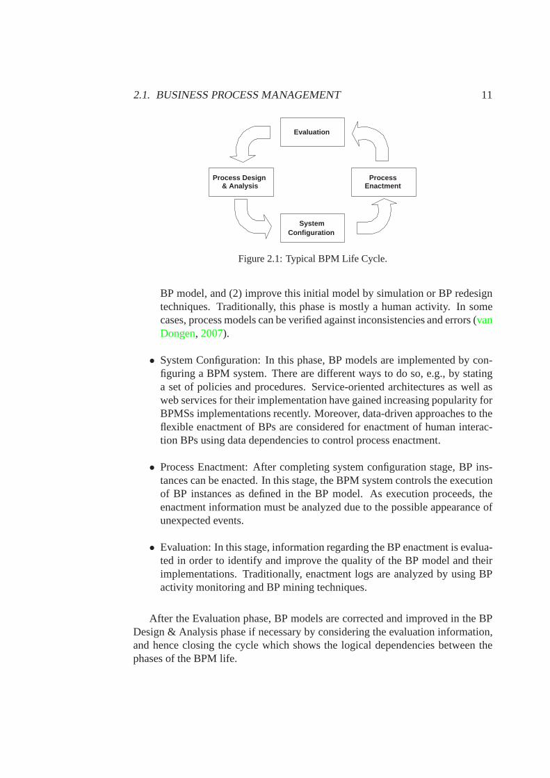
Traditional BPM Life Cycle (Weske, 2007) (cf. Fig. 2.1) includes several stageswhich are related to each other. These stages are organized in a cyclical structurewhich shows the logical dependencies between them:
• Process Design & Analysis: In this stage, BPs are identified,reviewed, va-lidated, and represented by business process models (cf. Def. 2), so thatthe informal BP description is formalized using a particular BP modellingnotation. Two steps are considered to create a BP model: (1) draw an initial
2.1. BUSINESS PROCESS MANAGEMENT 11
Process Design & Analysis
Evaluation
System Configuration
Process Enactment
Figure 2.1: Typical BPM Life Cycle.
BP model, and (2) improve this initial model by simulation orBP redesigntechniques. Traditionally, this phase is mostly a human activity. In somecases, process models can be verified against inconsistencies and errors (vanDongen, 2007).
• System Configuration: In this phase, BP models are implemented by con-figuring a BPM system. There are different ways to do so, e.g.,by statinga set of policies and procedures. Service-oriented architectures as well asweb services for their implementation have gained increasing popularity forBPMSs implementations recently. Moreover, data-driven approaches to theflexible enactment of BPs are considered for enactment of human interac-tion BPs using data dependencies to control process enactment.
• Process Enactment: After completing system configuration stage, BP ins-tances can be enacted. In this stage, the BPM system controlsthe executionof BP instances as defined in the BP model. As execution proceeds, theenactment information must be analyzed due to the possible appearance ofunexpected events.
• Evaluation: In this stage, information regarding the BP enactment is evalua-ted in order to identify and improve the quality of the BP model and theirimplementations. Traditionally, enactment logs are analyzed by using BPactivity monitoring and BP mining techniques.
After the Evaluation phase, BP models are corrected and improved in the BPDesign & Analysis phase if necessary by considering the evaluation information,and hence closing the cycle which shows the logical dependencies between thephases of the BPM life.
12 CHAPTER 2. BACKGROUND
In this Thesis Dissertation, the BP Design & Analysis phase is widely analy-zed since this phase plays an important role in the BPM life cycle for any improve-ment initiative, and it greatly influences the remaining phases of this cycle. TheBP Design & Analysis phase has the goal to generate a BP model,i.e., to definethe set of activities and the execution constraints betweenthem (Weske, 2007), byformalizing the informal BP description using a particularBP modelling notation.Section2.1.2introduces the main paradigms which are used for BP modelling.
2.1.2 Process Modelling
In the literature, a wide spectrum of paradigms for BP modelling are presented.These different paradigms can be roughly categorized into the two followingclasses:
• The declarative BP paradigm focuses on what has to be done instead ofhaving to specify how it has to be done. Declarative BP modelscapturethe regulatory and internal directives of the business processes in order torestrict possible options of activity execution. Due to their flexible nature,frequently several ways to execute declarative process models exist. Dif-ferent declarative approaches have been proposed, such as the use of cons-traints, rules, event conditions or other (logical) expressions (e.g., (Dourishet al., 1996; Joeris, 2000; Wainer and De Lima Bezerra, 2003; van der Aalstet al., 2009; Goedertier and Vanthienen, 2009)).
• The imperative BP paradigm focuses on defining a precise activity sequencewhich establishes how a given set of tasks has to be performed(e.g., (Zis-man, 1977; Ellis and Nutt, 1993; BPMN, 2011)).
In our proposals, we consider declarative and imperative models. Regardingdeclarative models, we focus on constraint-based models, and regarding impera-tive languages, we consider BPMN.
Constraint-based BP Models
Recently, constraint-based approaches have received increased interest (Vander-feesten et al., 2008; Pesic, 2008), since they suggest a fundamentally differentway of describing BPs which seems to be promising in respect of the support ofhighly dynamic processes (Vanderfeesten et al., 2008; Pesic, 2008). Irrespectiveof the chosen approach, requirements imposed by the BPs needto be reflected bythe process model. This means that desired behavior must be supported by theprocess model, while forbidden behavior must be prohibited(Pesic et al., 2007;
2.1. BUSINESS PROCESS MANAGEMENT 13
van der Aalst et al., 2009; Montali, 2009). While imperative process models spe-cify exactly how things have to be done, declarative processmodels focus on whatshould be done.
In the literature, several rule-based and constraint-based languages for decla-rative BP modelling are proposed, among which the work (Glance et al., 1996)proposes BP grammars for the definition of rules in order to deal with activitiesand documents. In (Dourish et al., 1996), the prototype Freeflow is presented,which includes a constraint-based process modelling formalism, and the use ofdeclarative dependency relationships. Moreover, (Wainer and De Lima Bezerra,2003) presents a constraint-based proposal for rules which constrain the BP enact-ment through preconditions and postconditions of the activities, together with ad-ditional conditions which must hold in general. In a similarway, (Joeris, 2000)presents a flexible workflow enactment based on event-condition-action (ECA)rules. Furthermore, (Lu et al., 2006) proposes a temporal constraint network forBP execution in order to define selection and scheduling constraints through theuse of temporal intervals.
In our proposal we use ConDec (van der Aalst and Pesic, 2006a) as a basisfor the BP control-flow specification. ConDec is a graphical language based onLinear Temporal Logic (LTL) (Clarke Jr. et al., 1999) for modelling and enactingdynamic business processes. It uses an open set of templates, i.e., parameteri-zed graphical representations of LTL formulas, for the definition of relationshipsbetween activities. These relationships related to the templates must be satisfiedduring the execution phase. Each template has a name, a graphical representationand a semantics given by a LTL formula. LTL (Clarke Jr. et al., 1999) is a widelyused temporal logic for specifying temporal properties that includes four opera-tors in addition to classical logical operators, i.e.,always, eventually, until andnext time. Besides ConDec (Pesic, 2008), some research works concerning BPsbased on LTL can be found. As an example, (Liu et al., 2007) proposes a methodfor the automatic verification of BP models that are translated to finite state ma-chines through compliance rules that are translated to LTL.Similarly, (Halle andVillemaire, 2008) presents an algorithm for the runtime monitoring of BP proper-ties, expressed in an extension of LTL. Moreover, (Awad et al., 2011) proposesan approach for synthesizing process templates out of compliance requirementsexpressed in LTL, and these templates are used as a basis for negotiation amongbusiness and compliance experts. Furthermore, (Elgammal et al., 2011) performsa comparative analysis between three languages (LTL, CTL and FCL) which canbe used as the formal foundation of BP compliance requirements.
We consider ConDec to be a suitable language, since it allowsthe specifi-cation of BP activities together with the constraints whichmust be satisfied forcorrect BP enactment and for the goal to be achieved. Moreover, ConDec allowsto specify a wide set of BP models of varied nature, flexibility and complexity in

14 CHAPTER 2. BACKGROUND
a simple way. Furthermore, ConDec has been widely referenced in past years inthe context of BPM (e.g., (Lamma et al., 2007; Ly et al., 2008; Montali, 2009;Chesani et al., 2009)). ConDec is based on constraint-based BP models (cf. Def.5), i.e., including information about (1) activities that can be performed as well as(2) constraints prohibiting undesired process behavior.
Definition 5. A constraint-based process modelS= (A,CBP) consists of a set ofactivities A1, and a set of constraints CBP prohibiting undesired execution beha-vior. For each activity a∈ A, resource constraints can be specified by associatinga role with that activity. The activities of a constraint-based process model can beexecuted arbitrarily often if not restricted by any constraints.
Constraints can be added to a ConDec model to specify forbidden behavior,restricting the desired behavior (for a description of the complete set of cons-traints, cf. (van der Aalst and Pesic, 2006a)). ConDec basic templates can bedivided into 3 groups:
1. Existenceconstraints: unary relationships concerning the number oftimesone activity is executed. As an example, Exactly(N, A) specifies that Amust be executed exactly N times.
2. Relation constraints: positive binary relationships used to establish whatshould be executed. As an example, Precedence(A, B) specifies that to exe-cute activity B, activity A needs to be executed before.
3. Negationconstraints: negative binary relationships used to forbidthe exe-cution of activities in specific situations. As an example, NotCoexistence(A,B) specifies that if B is executed, then A cannot be executed, and vice versa.
An interesting extension which has been considered for ConDec templatesis the inclusion ofChoice constraints (Pesic, 2008), which are n-ary constraintsexpressing the need of executing some activities belongingto a set of possiblechoices, independently of the other constraints.
In ConDec, while unary relationships describe constraintsrelated to one ac-tivity (e.g., existence constraints), binary constraintsdescribe relationships bet-ween activities (e.g., precedence constraints). Binary templates are composed bya source activity (cf. Def.6) and a sink activity (cf. Def.7), which correspondto the beginning and the end of the arrow related to the specific template in thegraphical notation of ConDec, respectively.
1In this Thesis Dissertation, the BP activities are considered to be primitive, i.e., they are notcomposed by other BP activities.
2.1. BUSINESS PROCESS MANAGEMENT 15
�
��
�
��������
�� ������ ���
�������������� ����� ������
� � �
���������� �
����������� �
��
��
��
��
� �
� �
��������� �������������� �����
�������� ���� ��� ������� ��� ������� ���������� ���������
��������� ��������� ������
��� �!�������"
����������� ��������� ������
��� �!�������"
��� �!����������"
��� �!�������"����������������#� �
�$� �!����"��������������������#� �
�%� �!�������"����������������#� �
�
�&��� #���'�� ��������� ������ #��� �'���
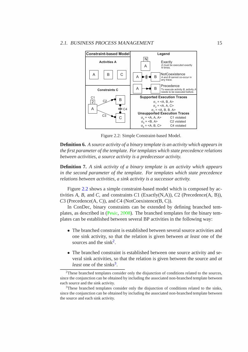
Figure 2.2: Simple Constraint-based Model.
Definition 6. A source activity of a binary template is an activity which appears inthe first parameter of the template. For templates which state precedence relationsbetween activities, a source activity is a predecessor activity.
Definition 7. A sink activity of a binary template is an activity which appearsin the second parameter of the template. For templates whichstate precedencerelations between activities, a sink activity is a successor activity.
Figure2.2 shows a simple constraint-based model which is composed by ac-tivities A, B, andC, and constraintsC1 (Exactly(N,A)),C2 (Precedence(A, B)),C3 (Precedence(A, C)), andC4 (NotCoexistence(B, C)).
In ConDec, binary constraints can be extended by defining branched tem-plates, as described in (Pesic, 2008). The branched templates for the binary tem-plates can be established between several BP activities in the following way:
• The branched constraint is established between several source activities andone sink activity, so that the relation is given betweenat leastone of thesources and the sink2.
• The branched constraint is established between one source activity and se-veral sink activities, so that the relation is given betweenthe source andatleastone of the sinks3.
2These branched templates consider only the disjunction of conditions related to the sources,since the conjunction can be obtained by including the associated non-branched template betweeneach source and the sink activity.
3These branched templates consider only the disjunction of conditions related to the sinks,since the conjunction can be obtained by including the associated non-branched template betweenthe source and each sink activity.
16 CHAPTER 2. BACKGROUND
In ConDec (van der Aalst and Pesic, 2006a), the fact of considering atomic ac-tivities is recognized as being a major problem. Similar to ConDec, the languagesConDec++ (Montali, 2009) (an extension of ConDec) and Saturn (Demeyer et al.,2010) are constraint-based workflow definition languages based on LTL which,unlike ConDec, consider non-atomic activities that can be started, completed orcancelled at a later time, and overlapped with other activities.
Once a BP is modelled through a constraint-based modelling language, the BPcan be executed. As the execution of a BP model proceeds, information regardingthe executed activities can be recorded in an execution trace (cf. Def. 8). Infor-mation related to past process execution can be very valuable, since it can be usedfor many purposes, e.g., process mining (van der Aalst et al., 2011) or generatingestimates (cf. Chapter3).
Definition 8. Let S= (A,CBP) be a constraint-based process model with activityset A and constraint set CBP. Then: Atrace σ is composed by a sequence ofstarting and completing events< e1,e2, ...en > regarding activity executions ai ,a∈ A, i.e., events can be:
1. start(ai, r jk, t), i.e., the i-th execution of activity a using k-th resource withrole j is started at time t.
2. comp(ai , t), i.e., the i-th execution of activity a is completed at time t.
Related to the process execution trace, is the concept of process instance. Spe-cifically, a process instance (cf. Def.9) represents a concrete execution of aconstraint-based model and its execution state is reflectedby the execution trace.
Definition 9. Let S= (A,C) be a constraint-based process model with activity setA and constraint set C. Then: Aprocess instanceI = (S,σ) on S is defined by Sand a corresponding traceσ.
A running process instanceI is in statesatisfied if its current partial traceσsatisfies all constraints stated inC. Furthermore, an instance is in stateviolated,if the partial trace violates any constraint stated inC and there is no suffix that canbe added to satisfy them. Figure2.2 includes examples of traces of satisfied andviolated instances4 for a constraint-based model.
During the BP enactment, considering a constraint-based model and a spe-cific related process instance, only certain activities areenabled to be executednext (cf. Def. 10). This selection, however, can be quite challenging since per-formance goals of the process (e.g., minimization of overall completion time)
4For the sake of clarity, only completed events for activity executions are included in the tracerepresentation.
2.1. BUSINESS PROCESS MANAGEMENT 17
should be considered, and users often do not have an understanding of the over-all process. Moreover, optimization of performance goals requires that resourcecapacities are considered. Therefore, recommendation support is needed duringBP execution, especially for inexperienced users (van Dongen and van der Aalst,2005) (cf. Chapter4).
Definition 10. Let S= (A,C) be a constraint-based process model with activityset A and constraint set C, and I= (S,σ) be a corresponding process instancewith partial traceσ. Then: An activity ai of instance I isenabledat time T iffai can be started and the instance state of I is not violated afterwards; i.e., forσ =< e1,e2, ...en >, we obtainσ′l =< e1,e2, ...en,start(ai,R jk,T) > afterwardsand instance(S,σ′) is not in state violated.
For example, for the partial traceσ1 of Fig. 2.2, B is enabled, whileA is notenabled due toC1, andC is not enabled due toC4.
Due to the flexible nature of constraint-based models, frequently several waysto execute constraint-based process models exist. Therefore, there are differentways to executed a constraint-based process model in such a way that all cons-traints are fulfilled, i.e., the process goal is reached (cf.Def. 11). For example,traces5 < AAB> and< AAC> are two valid ways of executing the constraint-based model of Fig.2.2, while trace< AABC> is invalid due toC4.
Definition 11. Thegoal of a BP is specified through the constraints which mustbe satisfied in the BP enactment.
The different valid execution alternatives, however, can vary greatly in respectto their quality, i.e., how well different performance objective functions (cf. Def.12) like minimizing cycle time can be achieved.
Definition 12. The objective functionof a BP is the function to be optimizedduring the BP enactment.
An objective function which is considered in this Thesis Dissertation is theoverall completion time of processes, i.e., time needed to complete all processinstances which were planned for a certain period.
Business Process Model and Notation
The Business Process Model and Notation (BPMN) (BPMN, 2011) is a standardfor modelling BP flows and web services, and provides a graphical notation for
5For the sake of clarity, traces represent sequences of activities so that no parallelism is consi-dered in the examples, i.e., only completed events for activity executions are included in the tracerepresentation.
18 CHAPTER 2. BACKGROUND
�����������
� ������������������������
���������� �������
���������������
� ���������
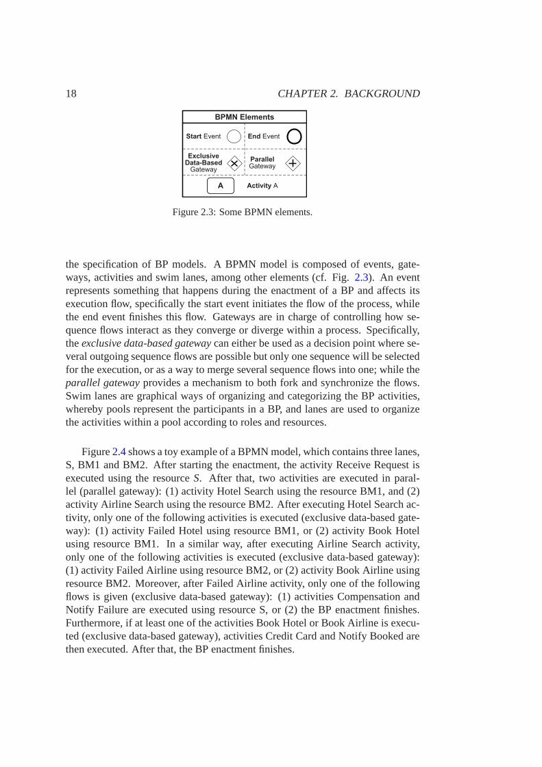
Figure 2.3: Some BPMN elements.
the specification of BP models. A BPMN model is composed of events, gate-ways, activities and swim lanes, among other elements (cf. Fig. 2.3). An eventrepresents something that happens during the enactment of aBP and affects itsexecution flow, specifically the start event initiates the flow of the process, whilethe end event finishes this flow. Gateways are in charge of controlling how se-quence flows interact as they converge or diverge within a process. Specifically,theexclusive data-based gatewaycan either be used as a decision point where se-veral outgoing sequence flows are possible but only one sequence will be selectedfor the execution, or as a way to merge several sequence flows into one; while theparallel gatewayprovides a mechanism to both fork and synchronize the flows.Swim lanes are graphical ways of organizing and categorizing the BP activities,whereby pools represent the participants in a BP, and lanes are used to organizethe activities within a pool according to roles and resources.
Figure2.4shows a toy example of a BPMN model, which contains three lanes,S, BM1 and BM2. After starting the enactment, the activity Receive Request isexecuted using the resourceS. After that, two activities are executed in paral-lel (parallel gateway): (1) activity Hotel Search using theresource BM1, and (2)activity Airline Search using the resource BM2. After executing Hotel Search ac-tivity, only one of the following activities is executed (exclusive data-based gate-way): (1) activity Failed Hotel using resource BM1, or (2) activity Book Hotelusing resource BM1. In a similar way, after executing Airline Search activity,only one of the following activities is executed (exclusivedata-based gateway):(1) activity Failed Airline using resource BM2, or (2) activity Book Airline usingresource BM2. Moreover, after Failed Airline activity, only one of the followingflows is given (exclusive data-based gateway): (1) activities Compensation andNotify Failure are executed using resource S, or (2) the BP enactment finishes.Furthermore, if at least one of the activities Book Hotel or Book Airline is execu-ted (exclusive data-based gateway), activities Credit Card and Notify Booked arethen executed. After that, the BP enactment finishes.

2.2. PLANNING & SCHEDULING 19
�����������
�������
�������
����
������
�������
������
������
����
��
����
���
����
��
�������
������
�������
����
���
������
����
����
�����
����
����
����
�������
���
� !
� "
�
Figure 2.4: Example of BPMN model.
2.2 Planning & Scheduling
Planning (cf. Sect.2.2.2) and scheduling (cf. Sect.2.2.1) are two rather relatedareas, and hence many actual problems involve both of them (cf. Sect. 2.2.3).However, these areas also present some differences. Both the similarities and themain differences are discussed in the current section.
2.2.1 Scheduling
The area of scheduling (Brucker and Knust, 2006; Pinedo, 2008) includes pro-blems in which it is necessary to determine an enactment planfor a set of knownactivities related by temporal constraints. Moreover, theexecution of every acti-vity requires the use of resources, hence they may compete for limited resources.In general, the goal in scheduling is to find a feasible plan which satisfies bothtemporal and resource constraints. Resource constraints lead to establish a spe-cific ordering between activities which share the same resource, providing theproblem with NP-hard complexity (Garey and Johnson, 1979). Several objectivefunctions are usually considered to be optimized, in most cases related to temporalmeasures (e.g., minimization of completion time), or considering the optimal useof resources.
In scheduling, an activity refers to a task which needs to be executed during aspecific amount of time units, usually without interruption(i.e., preemptive sche-duling), and using certain specific resources.
A quite general scheduling problem is called Resource-Constrained ProjectScheduling Problem (RCPSP, cf. (Brucker and Knust, 2006)). RCPSPs are speci-fied by a set of activities which are related by precedence constraints6. Moreover,for the execution of each activity, several units of many resources may be required.
6”Activity a precedes activity b” means that activity b cannot start before a is finished
20 CHAPTER 2. BACKGROUND
���
���
���
���
���
���
���
���
���
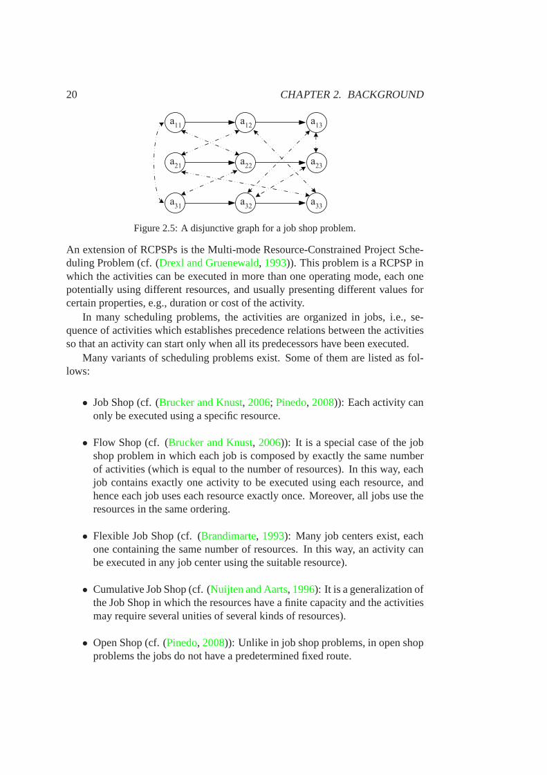
Figure 2.5: A disjunctive graph for a job shop problem.
An extension of RCPSPs is the Multi-mode Resource-Constrained Project Sche-duling Problem (cf. (Drexl and Gruenewald, 1993)). This problem is a RCPSP inwhich the activities can be executed in more than one operating mode, each onepotentially using different resources, and usually presenting different values forcertain properties, e.g., duration or cost of the activity.
In many scheduling problems, the activities are organized in jobs, i.e., se-quence of activities which establishes precedence relations between the activitiesso that an activity can start only when all its predecessors have been executed.
Many variants of scheduling problems exist. Some of them arelisted as fol-lows:
• Job Shop (cf. (Brucker and Knust, 2006; Pinedo, 2008)): Each activity canonly be executed using a specific resource.
• Flow Shop (cf. (Brucker and Knust, 2006)): It is a special case of the jobshop problem in which each job is composed by exactly the samenumberof activities (which is equal to the number of resources). Inthis way, eachjob contains exactly one activity to be executed using each resource, andhence each job uses each resource exactly once. Moreover, all jobs use theresources in the same ordering.
• Flexible Job Shop (cf. (Brandimarte, 1993): Many job centers exist, eachone containing the same number of resources. In this way, an activity canbe executed in any job center using the suitable resource).
• Cumulative Job Shop (cf. (Nuijten and Aarts, 1996): It is a generalization ofthe Job Shop in which the resources have a finite capacity and the activitiesmay require several unities of several kinds of resources).
• Open Shop (cf. (Pinedo, 2008)): Unlike in job shop problems, in open shopproblems the jobs do not have a predetermined fixed route.
2.2. PLANNING & SCHEDULING 21
Typically, the so-called disjunctive graph (Blazewic et al., 2000) is used torepresent schedules for the job shop problem (cf. Fig.2.5). A disjunctive graphG= (V,C,D) is composed by:
• A setV of nodes, each one representing an activity.
• A set of edges which link the nodes. Two kinds of edges can be distin-guished:
– Precedence edgesC (conjunctions), which correspond to the prece-dence constraints. They are directed arcs which link activities whichare included in the same job.
– Resource edgesD (disjunctions), which correspond to the resourceconstraints. They are non-directed arcs which link the activities whichare executed using the same resource.
In this way, a solution to the problem consists of establishing a direction forthe undirected arcs, being feasible if there are no cycles. As an example, Fig.2.57 shows the disjunctive graph representation for a simple jobshop schedulingproblem which includes 3 jobs, each one containing 3 activities.
There are many typical objective functions to be consideredin scheduling pro-blems. Some of them are listed as follows:
• Makespan: It refers to the time in which the execution of all activities havefinished.
• Tardiness: It refers to the delay of all jobs or activities regarding a specificdue date.
• Total Weighted Tardiness: It consists of a generalization of the tardiness, inwhich ∑ j∈Jobsw j ×Tj is minimized, wherew j usually refers to an impor-tance factor related to jobj, e.g., holding cost per unit time, andTj refers tothe delay of jobj regarding a specific due date.
• Number of Tardy Jobs: It refers to the number of jobs which do not meettheir due dates.
• Total Weighted Completion Time: It consists on minimizing∑ j∈Jobsw j ×Cj , wherew j usually refers to an importance factor related to jobj, andCj
refers to the completion time of jobj.
• Objectives related to the use of the resources by the activities, e.g., balanceduse of resources.
7ai j refers to the j-th activity of the job i.
22 CHAPTER 2. BACKGROUND
2.2.2 Planning
In a wider perspective, in Artificial Intelligence (AI) planning (Ghallab et al.,2004), the activities to be executed are not established a priori, hence it is nece-ssary to select them from a set of alternatives and to establish an ordering. Inplanning problems, usually the optimization of certain objective functions is con-sidered.
Taking the goals to be achieved into account, different planning strategies canbe used for representing and reasoning about planning scenarios, e.g., ClassicalPlanning (Fikes and Nilsson, 1971; Lekavy and Navrat, 2007), Hierarchical TaskNetwork (HTN) (Erol et al., 1994), Decision-Theoretic Planning (Joshi et al.,2011), Case-based Planning (Hammond, 1990) and Reactive Planning (Fernan-des et al., 1983).
In order to reuse the same algorithms for solving different kinds of problems,and to solve the same problem using different algorithms, (1) domains for repre-senting the problems, and (2) algorithms for solving the problems are specified ina separated way (domain-independent planning). For solving a specific problem,a domain-independent planner takes as input the problem specification and thedomain information.
The first strategy which was proposed for representing and reasoning aboutplanning scenarios was Classical Planning (Fikes and Nilsson, 1971; Lekavy andNavrat, 2007). The basic idea of Classical Planning consists of finding a sequenceof actions which will modify the initial state of the world into a final state wherethe goal holds. The specification of Classical Planning problems is composed by:
• A set of literals from the propositional calculus which can be positive ornegative and which represent the goal to be achieved.
• A set of literals from the propositional calculus which can be positive ornegative and which represent the initial state, also known as initial condi-tions.
• A set of actions which are characterized by STRIPS operators. A STRIPSoperator is a parameterized template used for stating a set of possible ac-tions. Each action is composed by:
– A set of preconditions: set of positive or negative literalswhich mustbe true for executing a specific action.
– A set of effects: set of positive or negative literals which become trueafter the execution of the action.
As mentioned before, for executing an activity, all the literals included in theprecondition of the activity need to be true. Therefore, at each stage, there is a set
2.2. PLANNING & SCHEDULING 23
of possible activities to be executed which depends on the literals which are truein that moment (state of the world, i.e., a set of atoms or literals that define howthe objects of the model relate to each other and their properties). Each time aspecific activity is executed, the set of literals which are true changes, and hencethe set of possible activities to be executed also changes. In this way, the state ofthe world evolves.
A solution for a planning problem is determined by a sequenceof activitieswhich reaches the final state from the initial state.
Planning Domain Definition Language
The Planning Domain Definition Language (PDDL) (Ghallab and et al., 1998) isa language for the definition of classical planning domains and problems which isused by the planning community. Specification in PDDL includes two separateditems: a domain file for predicates and actions, and a problemfile for objects, ini-tial state and goal specification. Moreover, PDDL supports several characteristics,such as basic STRIPS-style actions, conditional effects, universal quantificationover dynamic universes, specification of safety constraints, etc.
PDDL 2.2 (Hoffmann and Edelkamp, 2005), an extension of PDDL, includesmore characteristics: it allows handling of numeric values, the actions can have aduration, and it is capable to deal with plan objective functions, derived predicatesand timed initial literals.
In 2006, PDDL 3.0 (Gerevini and Long, 2006) was developed as an extensionof PDDL, by allowing the user to express strong and soft constraints about thestructure of the desired plans, as well as strong and soft problem goals.
The definition of thedomain for a PDDL specification contains differentitems:
• Predicates: Outstanding properties of objects; can be trueor false.
• Functions (Fluents): Allow handling of numeric values. They are used inactions preconditions or effects and their values are givenin the problemfile.
• (Durative) Actions/Operators: Ways of changing the state of the world.
The PDDLproblem defines the next items:
• Objects: Outstanding things in the world.
• Initial state: Initial state of the world.
• Goal specification: Things that must be true.
24 CHAPTER 2. BACKGROUND
• Objective function: Plan quality measures (metrics).
Once a problem is modelled through PDDL, a generic or specialized plannercan be used to obtain the required solution, e.g., UCPOP (Weld, 1994), Graph-plan (Blum and Furst, 1997), SHOP2 (Nau et al., 2003), VHPOP (Younes andSimmons, 2003) or SGPlan (Chen et al., 2006).
2.2.3 Integrating P&S
Planning and scheduling are rather related areas since bothdeal with the temporalplanning of activities. The main difference between both areas is that in schedu-ling the activities to be planned are known and that it alwaysinvolves the resourceperspective, while in planning the activities which will beincluded in the planneed to be determined and resource constraints are not always considered.
Many works which combined P&S can be found, since several actual problemsinvolve both of them. A problem involving P&S is characterized by: (1) there isa goal to be reached through the execution of a sequence of activities which areunknown a priori (planning), and (2) each of these activities has a specific dura-tion and requires a specific resource to be executed, so that temporal constraintsexist between the execution of activities, and certain (temporal) objective functionneeds to be optimized (scheduling).
Some of the extensions to scheduling that have been considered, such as alter-native resources and process alternatives, lead to models that are closer to plan-ning, as problems involving choice of actions are often regarded as planning pro-blems (Smith et al., 2000).
Some planning techniques are not able to represent or reasonwith resources,metric quantities or continuous time. Moreover, planning techniques do not ty-pically consider optimization. Therefore, there are many works which extendclassical planning techniques in order to deal with resources (Drabble and Tate,1994; Laborie and Ghallab, 1995), metric quantities (Koehler, 1998; Penberthyand Weld, 1994), and optimization criterions (Wolfman and Weld, 1999; Vossenet al., 1999). Furthermore, there exist works which extend planning techniques inorder to allow working with continuous time and temporal constraints (Penberthyand Weld, 1994; Smith and Weld, 1999).
2.3 Constraint Programming
Constraint Programming (CP, cf. Fig.2.6) is a software technology which is usedfor modelling and solving a wide scope of problems of varied nature which pursue
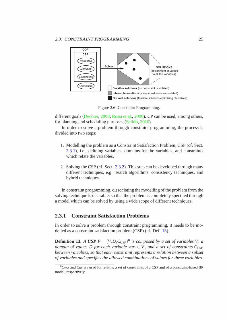
2.3. CONSTRAINT PROGRAMMING 25
Solver
Feasible solutions (no constraint is violated)
Infeasible solutions (some constraints are violated)
Optimal solutions (feasible solutions optimizing objectives)
COP
Objectives
CSP
Variables
Constraints
DomainsSOLUTIONS
(assignment of values
to all the variables)
Figure 2.6: Constraint Programming.
different goals (Dechter, 2003; Rossi et al., 2006). CP can be used, among others,for planning and scheduling purposes (Salido, 2010).
In order to solve a problem through constraint programming,the process isdivided into two steps:
1. Modelling the problem as a Constraint Satisfaction Problem, CSP (cf. Sect.2.3.1), i.e., defining variables, domains for the variables, and constraintswhich relate the variables.
2. Solving the CSP (cf. Sect.2.3.2). This step can be developed through manydifferent techniques, e.g., search algorithms, consistency techniques, andhybrid techniques.
In constraint programming, dissociating the modelling of the problem from thesolving technique is desirable, so that the problem is completely specified througha model which can be solved by using a wide scope of different techniques.
2.3.1 Constraint Satisfaction Problems
In order to solve a problem through constraint programming,it needs to be mo-delled as a constraint satisfaction problem (CSP) (cf. Def.13).
Definition 13. A CSPP = (V,D,CCSP)8 is composed by a set of variables V , a
domain of values D for each variable vari ∈ V, and a set of constraints CCSP
between variables, so that each constraint represents a relation between a subsetof variables and specifies the allowed combinations of values for these variables.
8CCSP andCBP are used for relating a set of constraints of a CSP and of a constraint-based BPmodel, respectively.
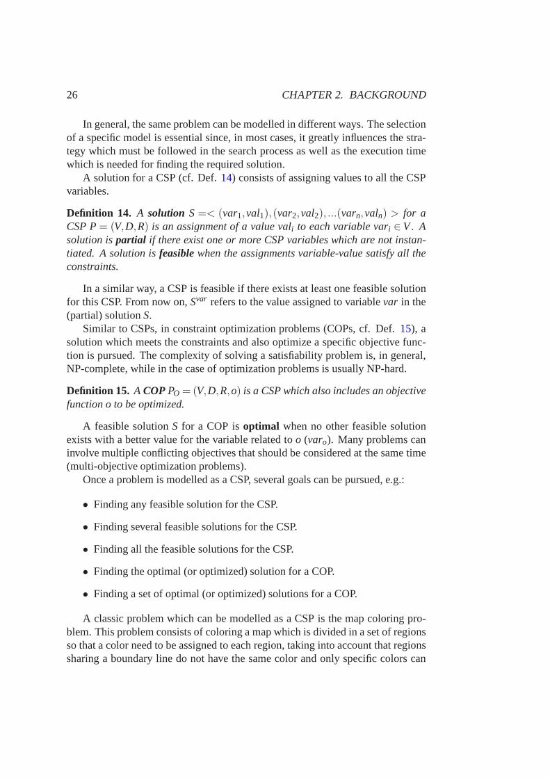
26 CHAPTER 2. BACKGROUND
In general, the same problem can be modelled in different ways. The selectionof a specific model is essential since, in most cases, it greatly influences the stra-tegy which must be followed in the search process as well as the execution timewhich is needed for finding the required solution.
A solution for a CSP (cf. Def.14) consists of assigning values to all the CSPvariables.
Definition 14. A solution S=< (var1,val1),(var2,val2), ...(varn,valn) > for aCSP P= (V,D,R) is an assignment of a value vali to each variable vari ∈V. Asolution ispartial if there exist one or more CSP variables which are not instan-tiated. A solution isfeasiblewhen the assignments variable-value satisfy all theconstraints.
In a similar way, a CSP is feasible if there exists at least onefeasible solutionfor this CSP. From now on,Svar refers to the value assigned to variablevar in the(partial) solutionS.
Similar to CSPs, in constraint optimization problems (COPs, cf. Def. 15), asolution which meets the constraints and also optimize a specific objective func-tion is pursued. The complexity of solving a satisfiability problem is, in general,NP-complete, while in the case of optimization problems is usually NP-hard.
Definition 15. A COPPO = (V,D,R,o) is a CSP which also includes an objectivefunction o to be optimized.
A feasible solutionS for a COP isoptimal when no other feasible solutionexists with a better value for the variable related too (varo). Many problems caninvolve multiple conflicting objectives that should be considered at the same time(multi-objective optimization problems).
Once a problem is modelled as a CSP, several goals can be pursued, e.g.:
• Finding any feasible solution for the CSP.
• Finding several feasible solutions for the CSP.
• Finding all the feasible solutions for the CSP.
• Finding the optimal (or optimized) solution for a COP.
• Finding a set of optimal (or optimized) solutions for a COP.
A classic problem which can be modelled as a CSP is the map coloring pro-blem. This problem consists of coloring a map which is divided in a set of regionsso that a color need to be assigned to each region, taking intoaccount that regionssharing a boundary line do not have the same color and only specific colors can
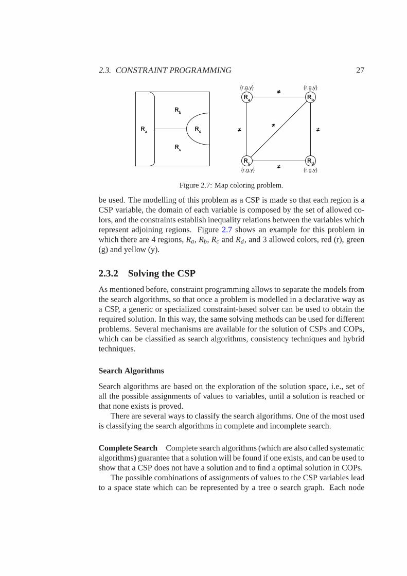
2.3. CONSTRAINT PROGRAMMING 27
��
��
��
��
��
��
��
��
������� �������
������� �������
Figure 2.7: Map coloring problem.
be used. The modelling of this problem as a CSP is made so that each region is aCSP variable, the domain of each variable is composed by the set of allowed co-lors, and the constraints establish inequality relations between the variables whichrepresent adjoining regions. Figure2.7 shows an example for this problem inwhich there are 4 regions,Ra, Rb, Rc andRd, and 3 allowed colors, red (r), green(g) and yellow (y).
2.3.2 Solving the CSP
As mentioned before, constraint programming allows to separate the models fromthe search algorithms, so that once a problem is modelled in adeclarative way asa CSP, a generic or specialized constraint-based solver canbe used to obtain therequired solution. In this way, the same solving methods canbe used for differentproblems. Several mechanisms are available for the solution of CSPs and COPs,which can be classified as search algorithms, consistency techniques and hybridtechniques.
Search Algorithms
Search algorithms are based on the exploration of the solution space, i.e., set ofall the possible assignments of values to variables, until asolution is reached orthat none exists is proved.
There are several ways to classify the search algorithms. One of the most usedis classifying the search algorithms in complete and incomplete search.
Complete Search Complete search algorithms (which are also called systematicalgorithms) guarantee that a solution will be found if one exists, and can be used toshow that a CSP does not have a solution and to find a optimal solution in COPs.
The possible combinations of assignments of values to the CSP variables leadto a space state which can be represented by a tree o search graph. Each node
28 CHAPTER 2. BACKGROUND
of the search tree represents a partial assignment of valuesto a set of variables.The root node of the search tree represents the case in which any variable is ins-tantiated, while the leaf nodes represent the cases in whichall the variables areinstantiated.
There are many systematic search algorithms, most of them are based onchronological backtracking (Mouhoub et al., 2003).
Incomplete Search Incomplete search algorithms consist of exploring only cer-tain regions of the state space so that, in general, the reachof a (optimal) solutioncan not be guaranteed. They are widely used due to the complete search usu-ally requires a high cost. Local or stochastic search algorithms are examples ofincomplete algorithms.
Local search algorithms typically start generating a first solution of a givenproblem instance (in a random or a heuristic way), which may be infeasible, sub-optimal or incomplete. This initial solution is iteratively improved so that thevalue for the objective function is optimized in the case of COPs, or the numberof inconsistencies are reduced in the case of CSPs. In most cases, these algorithmsfinish after certain tries or iterations have been completed, or when the requiredsolution is found.
A wide scope of local search algorithms can be found in the literature, e.g., ge-netic algorithms (Mitchell, 1998), simulated annealing (Kirkpatrick et al., 1983),taboo search (Glover, 1989), and Greedy Randomized Adaptive Search Procedure(GRASP) (Feo and Resende, 1989, 1995). Different local search algorithms varyin the way in which improvements are achieved, and in particular, in the way inwhich situations are handled when no direct improvement is possible.
Moreover, some algorithms combine systematic and local search techniques,e.g, Large Neighborhood Search (LNS) (Pisinger and Ropke, 2010).
Consistency Techniques
They are also called constraint propagation techniques, and refer to any reasoningwhich consists in explicitly forbidding values or combinations of values for somevariables of a problem because a given subset of its constraints cannot be satisfiedotherwise (Rossi et al., 2006). In a related way, the inference process consists ofevolving from a problem P to an equivalent problem P’, i.e., exactly having thesame set of feasible solutions, which presents a smaller solution space, and hence,which is easier to solve.
Concepts related to different grades of consistency (cf. Defs. 16, 17, 18, and19) typically have a great relevancy in consistency techniques.
2.3. CONSTRAINT PROGRAMMING 29
Definition 16. A CSP= (V,D,CCSP) presentsnode consistencyiff every unaryconstraint∈ CCSP on a variable is satisfied by all values in the domain of thevariable, and vice versa.
Definition 17. A CSP= (V,D,CCSP) presentsarc consistencyiff for all pairs ofCSP variables(var1,var2)|var1,var2 ∈ V, for each value of var1 in the domainof var1 there is some value in the domain of var2 that satisfy all the constraintsstated in CCSPbetween var1 and var2, and vice versa.
Definition 18. A CSP= (V,D,CCSP) presentspath consistencyiff all pairs ofCSP variables(var1,var2)|var1,var2 ∈ V present path consistency with all theother variables∈V. A pair of variables var1 and var2 presents path consistencywith a third variable var3 iff for every pair of values(val1,val2) that satisfies thebinary constraint between var1 and var2, there exists a value val3 in the domainof var3 such that(val1,val3) and (val2,val3) satisfy the constraint between var1
and var3 and between var2 and var3, respectively.
Definition 19. A CSP= (V,D,CCSP) presentsi-consistencyiff all tuples of i-1variables present i-consistency with all the other variables. A tuple of i-1 va-riables is i-consistent with another variable if every consistent evaluation of thei-1 variables can be extended with a value of the other variable while preservingconsistency. In a related way, strong i-consistency is given when all j≤ i presentj-consistency.
In this way, 2-consistency coincides with arc consistency if the problem isnode-consistent, while 3-consistency coincides with pathconsistency only if allconstraints are binary.
Many algorithms has been proposed in literature for establishing arc consis-tency in a CSP, e.g., the pioneersAC1, AC2 andAC3 (Mackworth, 1977) or therecentAC3bit (Lecoutre and Vion, 2008).
Consistency techniques can be complete or incomplete, as explained as fol-lows.
Complete Inference The inference is called complete when after performingthe inference process, the problem has a direct solution, e.g., adaptive consistencyalgorithm (Larrosa and Meseguer, 2003).
Incomplete Inference The inference is called incomplete when after perfor-ming the inference process, the problem does not have a direct solution, and hencea search for finding a solution needs to be performed, e.g., arc consistency.
To improve the modelling of the problems and to efficiently handle the cons-traints in the search for solutions, constraint-based proposals may includeglobal
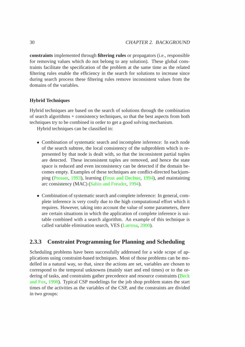
30 CHAPTER 2. BACKGROUND
constraints implemented throughfiltering rules or propagators (i.e., responsiblefor removing values which do not belong to any solution). These global cons-traints facilitate the specification of the problem at the same time as the relatedfiltering rules enable the efficiency in the search for solutions to increase sinceduring search process these filtering rules remove inconsistent values from thedomains of the variables.
Hybrid Techniques
Hybrid techniques are based on the search of solutions through the combinationof search algorithms + consistency techniques, so that the best aspects from bothtechniques try to be combined in order to get a good solving mechanism.
Hybrid techniques can be classified in:
• Combination of systematic search and incomplete inference: In each nodeof the search subtree, the local consistency of the subproblem which is re-presented by that node is dealt with, so that the inconsistent partial tuplesare detected. These inconsistent tuples are removed, and hence the statespace is reduced and even inconsistency can be detected if the domain be-comes empty. Examples of these techniques are conflict-directed backjum-ping (Prosser, 1993), learning (Frost and Dechter, 1994), and maintainingarc consistency (MAC) (Sabin and Freuder, 1994).
• Combination of systematic search and complete inference: In general, com-plete inference is very costly due to the high computationaleffort which itrequires. However, taking into account the value of some parameters, thereare certain situations in which the application of completeinference is sui-table combined with a search algorithm. An example of this technique iscalled variable elimination search, VES (Larrosa, 2000).
2.3.3 Constraint Programming for Planning and Scheduling
Scheduling problems have been successfully addressed for awide scope of ap-plications using constraint-based techniques. Most of those problems can be mo-delled in a natural way, so that, since the actions are set, variables are chosen tocorrespond to the temporal unknowns (mainly start and end times) or to the or-dering of tasks, and constraints gather precedence and resource constraints (Beckand Fox, 1998). Typical CSP modelings for the job shop problem states the starttimes of the activities as the variables of the CSP, and the constraints are dividedin two groups:
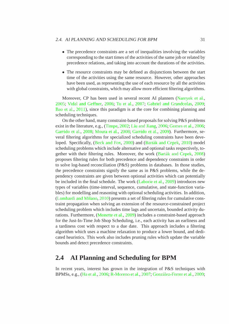
2.4. AI PLANNING AND SCHEDULING FOR BPM 31
• The precedence constraints are a set of inequalities involving the variablescorresponding to the start times of the activities of the same job or related byprecedence relations, and taking into account the durations of the activities.
• The resource constraints may be defined as disjunctions between the starttime of the activities using the same resource. However, other approacheshave been used, as representing the use of each resource by all the activitieswith global constraints, which may allow more efficient filtering algorithms.
Moreover, CP has been used in several recent AI planners (Nareyek et al.,2005; Vidal and Geffner, 2006; Tu et al., 2007; Gabriel and Grandcolas, 2009;Bao et al., 2011), since this paradigm is at the core for combining planning andscheduling techniques.
On the other hand, many constraint-based proposals for solving P&S problemsexist in the literature, e.g., (Timpe, 2002; Liu and Jiang, 2006; Gomes et al., 2006;Garrido et al., 2008; Moura et al., 2008; Garrido et al., 2009). Furthermore, se-veral filtering algorithms for specialized scheduling constraints have been deve-loped. Specifically, (Beck and Fox, 2000) and (Bartak and Cepek, 2010) modelscheduling problems which include alternative and optional tasks respectively, to-gether with their filtering rules. Moreover, the work (Bartak and Cepek, 2008)proposes filtering rules for both precedence and dependencyconstraints in orderto solve log-based reconciliation (P&S) problems in databases. In those studies,the precedence constraints signify the same as in P&S problems, while the de-pendency constraints are given between optional activities which can potentiallybe included in the final schedule. The work (Laborie et al., 2009) introduces newtypes of variables (time-interval, sequence, cumulative,and state-function varia-bles) for modelling and reasoning with optional schedulingactivities. In addition,(Lombardi and Milano, 2010) presents a set of filtering rules for cumulative cons-traint propagation when solving an extension of the resource-constrained projectscheduling problem which includes time lags and uncertain,bounded activity du-rations. Furthermore, (Monette et al., 2009) includes a constraint-based approachfor the Just-In-Time Job Shop Scheduling, i.e., each activity has an earliness anda tardiness cost with respect to a due date. This approach includes a filteringalgorithm which uses a machine relaxation to produce a lowerbound, and dedi-cated heuristics. This work also includes pruning rules which update the variablebounds and detect precedence constraints.
2.4 AI Planning and Scheduling for BPM
In recent years, interest has grown in the integration of P&Stechniques withBPMSs, e.g., (Ha et al., 2006; R-Moreno et al., 2007; Gonzalez-Ferrer et al., 2009;
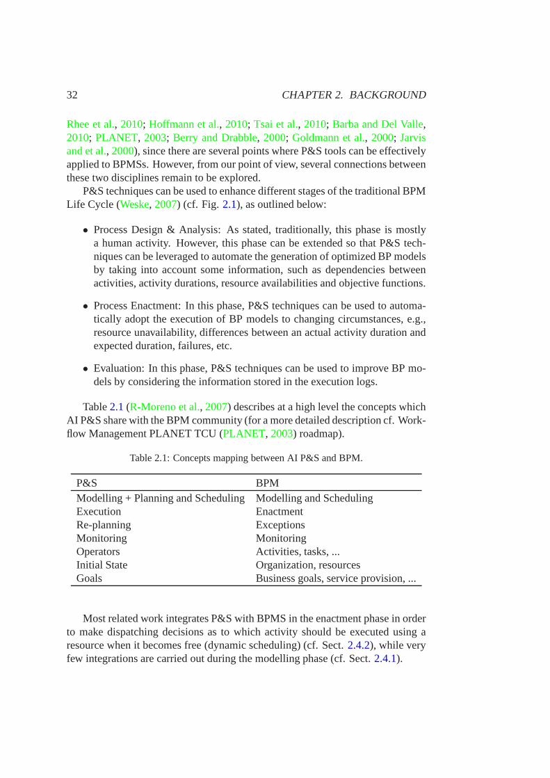
32 CHAPTER 2. BACKGROUND
Rhee et al., 2010; Hoffmann et al., 2010; Tsai et al., 2010; Barba and Del Valle,2010; PLANET, 2003; Berry and Drabble, 2000; Goldmann et al., 2000; Jarvisand et al., 2000), since there are several points where P&S tools can be effectivelyapplied to BPMSs. However, from our point of view, several connections betweenthese two disciplines remain to be explored.
P&S techniques can be used to enhance different stages of thetraditional BPMLife Cycle (Weske, 2007) (cf. Fig. 2.1), as outlined below:
• Process Design & Analysis: As stated, traditionally, this phase is mostlya human activity. However, this phase can be extended so thatP&S tech-niques can be leveraged to automate the generation of optimized BP modelsby taking into account some information, such as dependencies betweenactivities, activity durations, resource availabilitiesand objective functions.
• Process Enactment: In this phase, P&S techniques can be usedto automa-tically adopt the execution of BP models to changing circumstances, e.g.,resource unavailability, differences between an actual activity duration andexpected duration, failures, etc.
• Evaluation: In this phase, P&S techniques can be used to improve BP mo-dels by considering the information stored in the executionlogs.
Table2.1(R-Moreno et al., 2007) describes at a high level the concepts whichAI P&S share with the BPM community (for a more detailed description cf. Work-flow Management PLANET TCU (PLANET, 2003) roadmap).
Table 2.1: Concepts mapping between AI P&S and BPM.
P&S BPMModelling + Planning and Scheduling Modelling and SchedulingExecution EnactmentRe-planning ExceptionsMonitoring MonitoringOperators Activities, tasks, ...Initial State Organization, resourcesGoals Business goals, service provision, ...
Most related work integrates P&S with BPMS in the enactment phase in orderto make dispatching decisions as to which activity should beexecuted using aresource when it becomes free (dynamic scheduling) (cf. Sect. 2.4.2), while veryfew integrations are carried out during the modelling phase(cf. Sect.2.4.1).
2.4. AI PLANNING AND SCHEDULING FOR BPM 33
2.4.1 P&S for the Process Design & Analysis Phase
In (Gonzalez-Ferrer et al., 2009), the BP information is provided through an exe-cution/interchange language, XPDL. The XPDL file is analyzed to obtain a work-flow pattern decomposition, which is translated into the HTN-PDDL language.This is used as the input of a planner, and the resulting planscould be interpretedas workflow instances. In a similar way, (Alves et al., 2008) presents a proposalfor the automatic generation of BP models in workflow systems, based on ge-netic techniques for the optimized planning and schedulingof BP activities. In(Alves et al., 2008), the BP information is provided through the XPDL language,which is translated into PDDL, and the generated BP model is also specified inXPDL. The XPDL language lacks some power for the correct representation ofcomplex workflow patterns (van der Aalst, 2003). Specifically, only serial, parallelsplit-join, and parallel exclusive-OR templates are considered in (Gonzalez-Ferreret al., 2009).
In a related way, in (R-Moreno et al., 2007), planning tools are used for thesemi-automatic generation of BP models, by considering theknowledge intro-duced through BP Reengineering languages. This knowledge is translated intopredicate logic terms in order to be handled by a planner, andan updated BPmodel is obtained. The process information is provided through an object-orientedstructure modelling tool that follows a rule-based approach.
Additionally, (Hoffmann et al., 2010) proposes a planning formalism for themodelling of BPs through an SAP specification (Status and Action Management,SAM), which is a variant of PDDL.
Furthermore, (Ferreira and Ferreira, 2006) proposes to refine BP models bycombining learning and planning techniques, starting fromprocesses which arenot fully described. (Ferreira and Ferreira, 2006) needs past process executionsand examples provided by the user to apply learning techniques. Moreover, (Fer-reira and Ferreira, 2006) does not considered the optimization of any objectivefunction in the generation of the plans.
2.4.2 P&S for the Process Enactment Phase
Most of the related works integrate scheduling tools in BPM systems for the enact-ment phase, in order to take dispatching decisions as to which activity should beexecuted using a resource when it becomes free (dynamic scheduling). As fol-lows, a representative set of them are briefly summarized.
One of the first works, (Zhao and Stohr, 1999), develops a framework fortemporal workflow management, including turnaround-time predication, time al-location, and task prioritization.

34 CHAPTER 2. BACKGROUND
In a related way, the work (Son and Kim, 2001) proposes a schema for ma-ximizing the number of workflow instances satisfying a predetermined deadline,based on a method to determine the critical activities.
Moreover, the work (Ha et al., 2006) proposes a set of process execution rulesbased on individual worklists, and develops algorithms forthe task assignment inorder to maximize the overall process efficiency, while taking resource capacitiesinto account.
Furthermore, the work (Rhee et al., 2010) presents a Theory of Constraints(TOC)-based method for the improvement of the efficiency of BPs.
Recently, the work (Tsai et al., 2010) proposes distributed server architecturefor the management of the BP workflow, and presents techniques for the dynamicallocation of the resources.
Related to decision support systems, (Ozbayrak and Bell, 2003) develops aknowledge-based decision support system (KBDSS) for short-term schedulingin flexible manufacturing systems (FMS). This work considers the optimizationof the efficient use of the machining cells by using a knowledge-based expertsystem in order to support the decision making process. Moreover, (Chaturvediet al., 1993) manages multiple objectives in a hierarchical way. In a related way,(Thompson and Goodale, 2006) addresses the scheduling of a group of employeeswhich present different productivity considering the stochastic nature of customerarrivals and replans during run-time when estimates are incorrect.
Chapter 3
From Constraint-basedSpecifications to Optimized BPEnactment Plans
3.1 Introduction
3.1.1 Motivation
Typically, business processes are specified in an imperative way, i.e., an activitysequence that will result in obtaining the related corporate goal is defined. How-ever, declarative BP models are increasingly used and theirusage allows the userto specify what has to be done instead of having to specify howit has to be done.Declarative BP model specifications facilitate the human work involved, avoidfailures, and obtain a better optimization, since the tacitnature of human know-ledge is often an obstacle to eliciting accurate process models (Ferreira and Fer-reira, 2006).
The advantages of using declarative languages for BP modelling instead ofimperative languages, i.e., support for partial workflows (Wainer et al., 2004),absence of over-specification (Pesic et al., 2007), and provision of more maneu-vering room for end users (Pesic et al., 2007), are discussed in several studies,e.g., (Rychkova et al., 2008a; Fahland et al., 2009, 2010; Pichler et al., 2011).
3.1.2 Contribution
Due to their flexible nature, frequently several ways to execute declarative processmodels exist. Therefore, there are several enactment plansrelated to a specific de-clarative model, each one presenting specific values for different objective values,
35
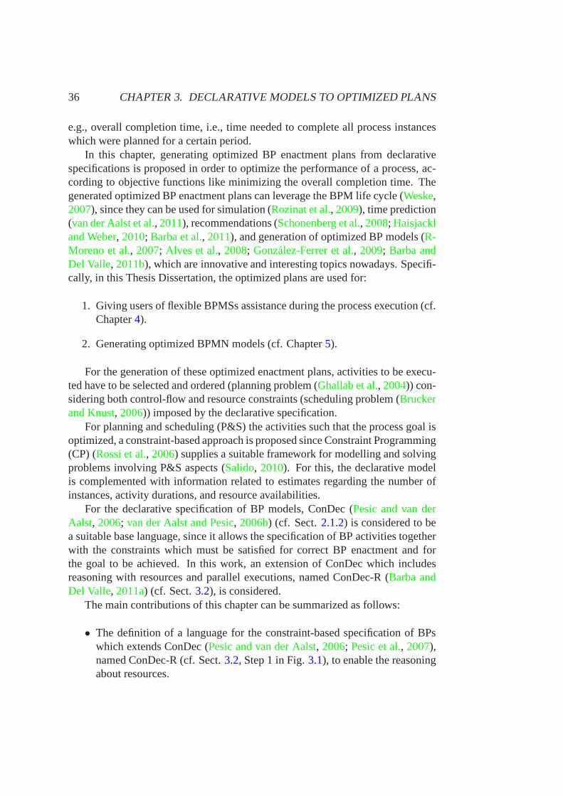
36 CHAPTER 3. DECLARATIVE MODELS TO OPTIMIZED PLANS
e.g., overall completion time, i.e., time needed to complete all process instanceswhich were planned for a certain period.
In this chapter, generating optimized BP enactment plans from declarativespecifications is proposed in order to optimize the performance of a process, ac-cording to objective functions like minimizing the overallcompletion time. Thegenerated optimized BP enactment plans can leverage the BPMlife cycle (Weske,2007), since they can be used for simulation (Rozinat et al., 2009), time prediction(van der Aalst et al., 2011), recommendations (Schonenberg et al., 2008; Haisjackland Weber, 2010; Barba et al., 2011), and generation of optimized BP models (R-Moreno et al., 2007; Alves et al., 2008; Gonzalez-Ferrer et al., 2009; Barba andDel Valle, 2011b), which are innovative and interesting topics nowadays. Specifi-cally, in this Thesis Dissertation, the optimized plans areused for:
1. Giving users of flexible BPMSs assistance during the process execution (cf.Chapter4).
2. Generating optimized BPMN models (cf. Chapter5).
For the generation of these optimized enactment plans, activities to be execu-ted have to be selected and ordered (planning problem (Ghallab et al., 2004)) con-sidering both control-flow and resource constraints (scheduling problem (Bruckerand Knust, 2006)) imposed by the declarative specification.
For planning and scheduling (P&S) the activities such that the process goal isoptimized, a constraint-based approach is proposed since Constraint Programming(CP) (Rossi et al., 2006) supplies a suitable framework for modelling and solvingproblems involving P&S aspects (Salido, 2010). For this, the declarative modelis complemented with information related to estimates regarding the number ofinstances, activity durations, and resource availabilities.
For the declarative specification of BP models, ConDec (Pesic and van derAalst, 2006; van der Aalst and Pesic, 2006b) (cf. Sect.2.1.2) is considered to bea suitable base language, since it allows the specification of BP activities togetherwith the constraints which must be satisfied for correct BP enactment and forthe goal to be achieved. In this work, an extension of ConDec which includesreasoning with resources and parallel executions, named ConDec-R (Barba andDel Valle, 2011a) (cf. Sect.3.2), is considered.
The main contributions of this chapter can be summarized as follows:
• The definition of a language for the constraint-based specification of BPswhich extends ConDec (Pesic and van der Aalst, 2006; Pesic et al., 2007),named ConDec-R (cf. Sect.3.2, Step 1 in Fig.3.1), to enable the reasoningabout resources.
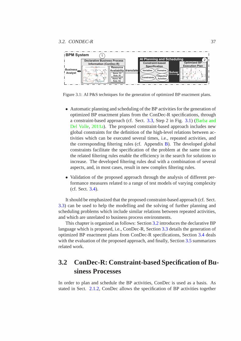
3.2. CONDEC-R 37
������������ ��� �����
���������������������
�� �����
������������������
�������
����������� ���
����� �
������������ !�"� �����
��#!� ���
������$
������$
��� ��������� �
!%�����������
!����&�������
��� ������ '�(�����
��������
������
'%����)� ��
*+�����������
�
�
Figure 3.1: AI P&S techniques for the generation of optimized BP enactment plans.
• Automatic planning and scheduling of the BP activities for the generation ofoptimized BP enactment plans from the ConDec-R specifications, througha constraint-based approach (cf. Sect.3.3, Step 2 in Fig.3.1) (Barba andDel Valle, 2011a). The proposed constraint-based approach includes newglobal constraints for the definition of the high-level relations between ac-tivities which can be executed several times, i.e., repeated activities, andthe corresponding filtering rules (cf. AppendixB). The developed globalconstraints facilitate the specification of the problem at the same time asthe related filtering rules enable the efficiency in the search for solutions toincrease. The developed filtering rules deal with a combination of severalaspects, and, in most cases, result in new complex filtering rules.
• Validation of the proposed approach through the analysis ofdifferent per-formance measures related to a range of test models of varying complexity(cf. Sect.3.4).
It should be emphasized that the proposed constraint-basedapproach (cf. Sect.3.3) can be used to help the modelling and the solving of further planning andscheduling problems which include similar relations between repeated activities,and which are unrelated to business process environments.
This chapter is organized as follows: Section3.2introduces the declarative BPlanguage which is proposed, i.e., ConDec-R, Section3.3details the generation ofoptimized BP enactment plans from ConDec-R specifications,Section3.4 dealswith the evaluation of the proposed approach, and finally, Section3.5summarizesrelated work.
3.2 ConDec-R: Constraint-based Specification of Bu-siness Processes
In order to plan and schedule the BP activities, ConDec is used as a basis. Asstated in Sect.2.1.2, ConDec allows the specification of BP activities together
38 CHAPTER 3. DECLARATIVE MODELS TO OPTIMIZED PLANS
(2) Estimates (3) Resource Availabilities
ConDec-R Specification (1) ConDec
control-flow resource
requirements
Figure 3.2: ConDec-R process model specification.
with the constraints which must be satisfied for correct BP enactment and for thegoal to be achieved. ConDec is based on constraint-based BP models (cf. Def.5 on page14), and resource constraints can be specified for each BP activity byassociating a role with that activity. Constraints can be added to a ConDec modelto specify forbidden behavior, restricting the desired behavior (for a descriptionof the complete set of constraints, cf. (van der Aalst and Pesic, 2006a)). In thisway, ConDec basic templates can be divided into existence, relation and negationconstraints.
The basic ConDec-R templates, extending the ConDec templates (van derAalst and Pesic, 2006a), together with its formal specification through constraintsand some examples of valid and invalid traces are listed inAppendix A.
To make ConDec usable for our concrete application, an extension of Con-Dec (named ConDec-R) is defined in this chapter, as detailed in Sect.3.2.1andSect. 3.2.2. ConDec-R supports all constraints described in (van der Aalst andPesic, 2006a) and additionally provides extended support for branched templates,as described in (Montali, 2009).
3.2.1 Extending ConDec with Estimates and Resource Availa-bilities
To support the direct reasoning of resources (which is not possible in ConDec)ConDec is extended with estimates of activity durations andthe specification ofresource availabilities. In short, a ConDec-R process model specification (cf. Def.20on page39, Fig. 3.2) extends a ConDec model (cf. Fig.3.2(1)), i.e., specifyingcontrol-flow and resource requirements, by including:
• The estimated duration of each activity (cf. Fig.3.2(2)). Estimates canbe obtained by interviewing business experts or by analyzing past processexecutions (e.g., by calculating the average values of the parameters to beestimated from event logs). Moreover, both approaches can be combined toget more reliable estimates.
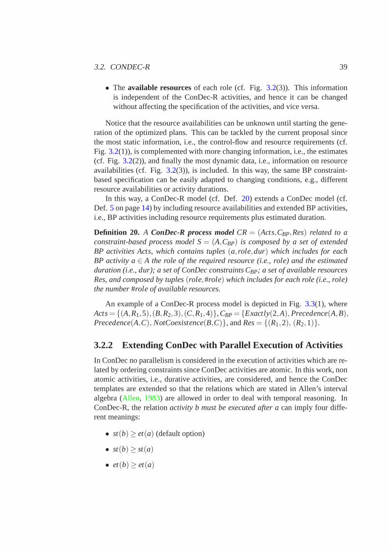
3.2. CONDEC-R 39
• The available resourcesof each role (cf. Fig.3.2(3)). This informationis independent of the ConDec-R activities, and hence it can be changedwithout affecting the specification of the activities, and vice versa.
Notice that the resource availabilities can be unknown until starting the gene-ration of the optimized plans. This can be tackled by the current proposal sincethe most static information, i.e., the control-flow and resource requirements (cf.Fig. 3.2(1)), is complemented with more changing information, i.e., the estimates(cf. Fig. 3.2(2)), and finally the most dynamic data, i.e., information onresourceavailabilities (cf. Fig.3.2(3)), is included. In this way, the same BP constraint-based specification can be easily adapted to changing conditions, e.g., differentresource availabilities or activity durations.
In this way, a ConDec-R model (cf. Def.20) extends a ConDec model (cf.Def. 5 on page14) by including resource availabilities and extended BP activities,i.e., BP activities including resource requirements plus estimated duration.
Definition 20. A ConDec-R process modelCR= (Acts,CBP,Res) related to aconstraint-based process model S= (A,CBP) is composed by a set of extendedBP activities Acts, which contains tuples(a, role,dur) which includes for eachBP activity a∈ A the role of the required resource (i.e., role) and the estimatedduration (i.e., dur); a set of ConDec constraints CBP; a set of available resourcesRes, and composed by tuples(role,#role) which includes for each role (i.e., role)the number#role of available resources.
An example of a ConDec-R process model is depicted in Fig.3.3(1), whereActs= {(A,R1,5),(B,R2,3),(C,R1,4)},CBP= {Exactly(2,A),Precedence(A,B),Precedence(A,C), NotCoexistence(B,C)}, andRes= {(R1,2), (R2,1)}.
3.2.2 Extending ConDec with Parallel Execution of Activities
In ConDec no parallelism is considered in the execution of activities which are re-lated by ordering constraints since ConDec activities are atomic. In this work, nonatomic activities, i.e., durative activities, are considered, and hence the ConDectemplates are extended so that the relations which are stated in Allen’s intervalalgebra (Allen, 1983) are allowed in order to deal with temporal reasoning. InConDec-R, the relationactivity b must be executed after acan imply four diffe-rent meanings:
• st(b)≥ et(a) (default option)
• st(b)≥ st(a)
• et(b)≥ et(a)
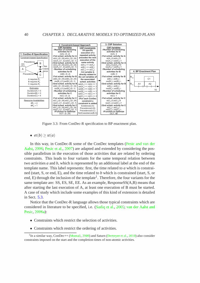
40 CHAPTER 3. DECLARATIVE MODELS TO OPTIMIZED PLANS
�������������� ��
��
���
���
�� ��
��
���� ��������
���� ��������
���� ��������
�
��
�
���������
��������
�����������
�����������
�����������
���������������������
���������
� �
� � ��
�����
� ������!"����#$���%���� �
&������
&������
��� �����'�("�(�����
���������� ����������������� � ��!
��"���������#�����)�*�++�,
�������� ����"�$�����#����
��)*�++��,-����
��)*�++��,
������)*�++�,-��(��
��)*�++�,
��%� ���� ����"�$�����#����
��)*�++��,-����
��)*�++��,
������)*�++�,-��(��
��)*�++�,
��������������� � ��!
��"����������
������)�*�++�,
�������� ����"�$������
������)*�++��,-����
��)*�++��,
������)*�,-��(��
��)*�++�,
��%� ���� ����"�$������
������)*�++��,-����
��)*�++��,
������)*�,-��(��
��)*�++�,
��������������� � ��!
��"����������
�����)�*�++�,
�������� ����"�$������
������)*�++��,-����
��)*�++��,
������)*�++�,-��(��
��)*�++�,
��%� ���� ����"�$����������
��)*�++��,-����
��)*�++��,
������)*�++�,-��(��
��)*�++�,
��&��������'����(�.�/)�*�++��,
�������������
��#�������
�)����������
������ ���"�$
���� ��������)
�)�����������
�������"�$
�������0������
��
�������0������
��
�������0������
��
�����"����� ����
��� $��� �� ��
�������"����� �����
����������
��� ����"����
��(��������������1���
��(��������������1���
��(��������������1���
��(��������������1���
��(��������������1���
��(��������������1���
��&������������
���������
������������ �
� ���������2��
�����������2��
�����������2��
� �� � ���������2��
%��������������� �#������ *�������� ����
���������� ����������������� � ��!
��"���������#�����)��
�������� ����"�$�����#����
��)�-����
��)�
������)�-��(��
��)�
��%� ���� ����"�$�����#����
��)�-����
��)��
������)�-��(��
��)�
��������������� � ��!
��"����������
������)��
�������� ����"�$������
������)!-����
��)!
������)!-��(��
��)!
��%� ���� ����"�$������
������)!-����
��)!
������)!-��(��
��)!
��������������� � ��!
��"����������
�����)��
�������� ����"�$������
������)�-����
��)3
������)�-��(��
��)�
��%� ���� ����"�$����������
��)!-����
��)!
������)!-��(��
��)!
��&��������'����(�.�/)��+
Figure 3.3: From ConDec-R specification to BP enactment plan.
• et(b)≥ st(a)
In this way, in ConDec-R some of the ConDec templates (Pesic and van derAalst, 2006; Pesic et al., 2007) are adapted and extended by considering the pos-sible parallelism in the execution of those activities thatare related by orderingconstraints. This leads to four variants for the same temporal relation betweentwo activitiesa andb, which is represented by an additional label at the end of thetemplate name. This label represents: first, the time related toa which is constrai-ned (start, S, or end, E), and the time related tob which is constrained (start, S, orend, E) through the inclusion of the template1. Therefore, the four variants for thesame template are: SS, ES, SE, EE. As an example, ResponseSS(A,B) means thatafter starting the last execution of A, at least one execution of B must be started.A case of study which include some examples of this kind of extension is detailedin Sect.5.3.
Notice that the ConDec-R language allows those typical constraints which areconsidered in literature to be specified, i.e. (Sadiq et al., 2005; van der Aalst andPesic, 2006a):
• Constraints which restrict the selection of activities.
• Constraints which restrict the ordering of activities.
1In a similar way, ConDec++ (Montali, 2009) and Saturn (Demeyer et al., 2010) also considerconstraints imposed on the start and the completion times ofnon-atomic activities.
3.3. FROM CONDEC-R TO OPTIMIZED ENACTMENT PLANS 41
• Constraints which restrict the requirements of resources.
3.3 From ConDec-R to Optimized Enactment Plans
In this section, the complete process which is proposed to generate BP enactmentplans from a ConDec-R specification through constraint programming is detailed(cf. Fig. 3.3). As stated, BP activities and constraints are specified in aConDec-Rmodel (cf. Step 1 in Fig.3.3, Sect.3.2) so that frequently several feasible ways toexecute this model exist. Each specific feasible execution of a ConDec-R modelleads to a specific value for the function to optimize. In general, there can be morethan one optimal execution, i.e., feasible solution leading to a minimal completiontime2. In order to generate optimal (or optimized) execution plans for a specificConDec-R model3, a constraint-based approach for P&S the BP activities (cf.Step 2 in Fig. 3.3) is proposed. The obtained plans, i.e., solutions to the COP(cf. Step 3 in Fig.3.3), optimize the specified objective function (cf. Def.12on page17) and satisfy all the constraints which are stated in the specification ofthe problem, i.e., reaches the specified goal (cf. Def.11 on page17). Lastly,the generated plans are visualized as Gantt chart (Gantt, 1913) (cf. Step 4 in Fig.3.3) which illustrates the start and the end times of the activities together with theassigned resource.
3.3.1 Translating the ConDec-R Model as a CSP Model
As first step of the constraint-based approach, the Condec-Rmodel needs to betranslated to a CSP. Regarding the CSP model of the proposed constraint-basedapproach, BP activities (repeated activities, cf. Def.21), which can be executedarbitrarily often if not restricted by any constraints, aremodelled as a sequence ofoptional scheduling activities (cf. Def.22). This is required since each executionof a BP activity is considered as one single activity which needs to be allocatedto a specific resource and temporarily placed in the enactment plan, i.e., statingvalues for its start and end times.
In this way, there are two main types in the proposed CSP model(cf. Fig. 3.4):
1. A type representing the BP activities, namedRepeatedActivity.
2In this chapter the overall completion time as objective function is considered. However, notethat the proposal can be easily extended to support further objective functions like cost.
3Notice that although the generation of optimal solutions isdesirable, optimized solutions areacceptable for problems which present NP-complexity, suchas the considered problems, sincefinding the optimal solution cannot been ensured in all cases.
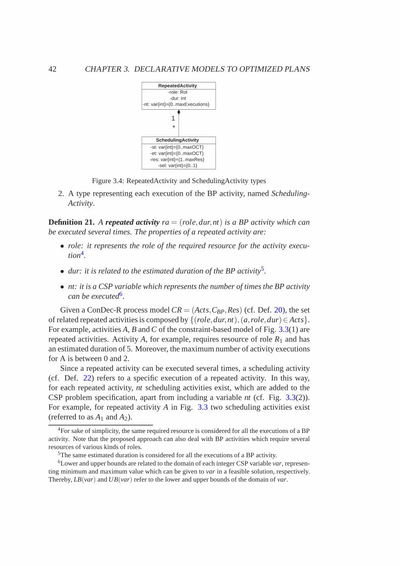
42 CHAPTER 3. DECLARATIVE MODELS TO OPTIMIZED PLANS
1 *
-role: Rol -dur: int
-nt: var{int}={0..maxExecutions}
RepeatedActivity
SchedulingActivity
-st: var{int}={0..maxOCT} -et: var{int}={0..maxOCT} -res: var{int}={1..maxRes}
-sel: var{int}={0..1}
Figure 3.4: RepeatedActivity and SchedulingActivity types
2. A type representing each execution of the BP activity, namedScheduling-Activity.
Definition 21. A repeated activityra = (role,dur,nt) is a BP activity which canbe executed several times. The properties of a repeated activity are:
• role: it represents the role of the required resource for theactivity execu-tion4.
• dur: it is related to the estimated duration of the BP activity5.
• nt: it is a CSP variable which represents the number of times the BP activitycan be executed6.
Given a ConDec-R process modelCR= (Acts,CBP,Res) (cf. Def. 20), the setof related repeated activities is composed by{(role,dur,nt),(a, role,dur)∈Acts}.For example, activitiesA, B andC of the constraint-based model of Fig.3.3(1) arerepeated activities. ActivityA, for example, requires resource of roleR1 and hasan estimated duration of 5. Moreover, the maximum number of activity executionsfor A is between 0 and 2.
Since a repeated activity can be executed several times, a scheduling activity(cf. Def. 22) refers to a specific execution of a repeated activity. In this way,for each repeated activity,nt scheduling activities exist, which are added to theCSP problem specification, apart from including a variablent (cf. Fig. 3.3(2)).For example, for repeated activityA in Fig. 3.3 two scheduling activities exist(referred to asA1 andA2).
4For sake of simplicity, the same required resource is considered for all the executions of a BPactivity. Note that the proposed approach can also deal withBP activities which require severalresources of various kinds of roles.
5The same estimated duration is considered for all the executions of a BP activity.6Lower and upper bounds are related to the domain of each integer CSP variablevar, represen-
ting minimum and maximum value which can be given tovar in a feasible solution, respectively.Thereby,LB(var) andUB(var) refer to the lower and upper bounds of the domain ofvar.
3.3. FROM CONDEC-R TO OPTIMIZED ENACTMENT PLANS 43
Definition 22. Ascheduling activitysa= (st,et, res,sel) represents a specific exe-cution of a repeated activity, where:
• st: it is a CSP variable indicating the start time of the activity execution(each execution of a BP activity needs to be temporarily placed in the enact-ment plan).
• et: it is a CSP variable indicating the end time of the activity execution (eachexecution of a BP activity needs to be temporarily placed in the enactmentplan).
• res: it is a CSP variable representing the resource used for the execution(identified by a number between 1 and #role(role(res))).
• sel: it is a CSP variable indicating whether or not the scheduling activity isselected to be executed (cf. Fig.3.3(2)).
Moreover, an additional CSP variable representing the objective function to beoptimized, i.e., the overall completion time in the contextof the current proposal,namedOCT, is also included in the CSP model:OCT= maxa∈Acts(et(ant(a)))
7.In order to ensure the consistency between the CSP variables, several cons-
traints have to be added to the CSP (cf. Fig.3.3(2)):
• ∀i : 1 ≤ i < UB(nt(a)) : et(ai) ≤ st(ai+1), i.e., a specific execution of arepeated activity precedes the next execution of the same activity.
• ∀i : 1 ≤ i ≤ UB(nt(a)) : sel(ai) = nt(a) >= i, i.e., thent variable of therepeated activity is directly related to thesel variables of the associatedscheduling activities, e.g., ifnt(a) = 2, thensel(a1) = 1, sel(a2) = 1 and∀i : nt(a)< i ≤UB(nt(a)),sel(ai) = 0.
Furthermore, for each ConDec template, a global constraintis added to theCSP model, i.e.,Existence(2,A), Precedence(A,B), Precedence(A,C), andNot−Coexistence(B,C) for the constraint-based model depicted in Fig.3.3.
Definition 23. A CSP-ConDec problemrelated to a ConDec-R process modelCR= (Acts,CBP,Res) (cf. Def. 20 on page39) is a COP Po = (V,D,CCSP,o) (cf.Def. 15 on page26) where:
• The set of variables V is composed by all the CSP variables included in thepresented CSP model plus the CSP variable related to the overall comple-tion time (OCT), i.e., V= {nt(a),a∈Acts}∪{st(ai),et(ai), res(ai),sel(ai),a∈ Acts, i ∈ [1..UB(nt(a))]}∪OCT.
7ai refers to the scheduling activity related to the i-th execution of the repeated activitya.
44 CHAPTER 3. DECLARATIVE MODELS TO OPTIMIZED PLANS
• The set of domains D is composed by the domain of each CSP variable v,D(v), i.e.:
D = {D(nt(a)) = {0..MC}, a∈ Acts}∪
{D(st(ai)) = {0..MC× ∑a∈Acts
dur(a)},a∈ Acts, i ∈ [1..UB(nt(a))]}∪
{D(et(ai)) = {0..MC× ∑a∈Acts
dur(a)},a∈ Acts, i ∈ [1..UB(nt(a))]}∪
{D(res(ai)) = {1..#role(role(a))},a∈ Acts, i ∈ [1..UB(nt(a))]}∪
{D(sel(ai)) = {0..1},a∈ Acts, i ∈ [1. . .UB(nt(a))]}
where MC is the maximum cardinality for the BP activities (established byexistence relations in the constraint-based model).
• The set of constraints CCSP is composed by the global constraints (imple-mented by the filtering rules, cf. AppendixB) related to the ConDec-R cons-traints included in CBP together with the constraints from the proposed CSPmodel, i.e.:
– ∀i : 1≤ i < nt(a) : et(ai)≤ st(ai+1)
– ∀i : 1≤ i ≤UB(nt(a)) : sel(ai) = nt(a)≥ i
for each repeated activity a∈ Acts.
• The objective function o is minimizing the OCT variable.
Figure3.3 includes the translation from a ConDec-R specification intoa CSPso that the CSP variables and constraints are stated as explained in Def. 23 (cf.Step 2). In general, for each repeated activitya, a CSP variablent is added to theCSP model. Thereby, the value forLB(nt(a)) is initially set to 0 (it will be auto-matically updated during the solving process if an existence constraint is addedthrough the corresponding filtering rule, cf. AppendixB), and forUB(nt(a))a rough initial estimate is made by considering the maximum obligatory cardi-nality of all repeated activities which is stated by existence constraints. For theconstraint-based model depicted in Fig.3.3, for example, the upper bound forall repeated activities is initially set to 2 (due to the existence constraint relatedto activity A). This value states the minimumnt for all BP activities ensuring afeasible solution (the optimal solution, however, in general includes lower valuesof nt for several activities).
Moreover,LB(OCT) is initially set to 08, andUB(OCT) is estimated as themaximum cardinality times the sum of the duration of all the BP activities, i.e.,
8LB(OCT) can be also initialized to other different values, e.g., maximum duration of all themandatory activities.
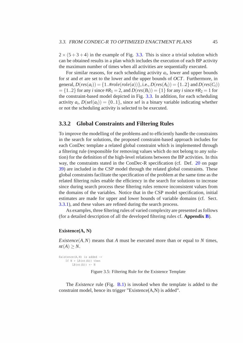
3.3. FROM CONDEC-R TO OPTIMIZED ENACTMENT PLANS 45
2× (5+3+4) in the example of Fig.3.3. This is since a trivial solution whichcan be obtained results in a plan which includes the execution of each BP activitythe maximum number of times when all activities are sequentially executed.
For similar reasons, for each scheduling activityai , lower and upper boundsfor st andet are set to the lower and the upper bounds ofOCT. Furthermore, ingeneral,D(res(ai))= {1..#role(role(a))}, i.e.,D(res(Ai))= {1..2} andD(res(Ci))= {1..2} for anyi since #R1 = 2, andD(res(Bi)) = {1} for anyi since #R2 = 1 forthe constraint-based model depicted in Fig.3.3. In addition, for each schedulingactivity ai, D(sel(ai)) = {0..1}, sincesel is a binary variable indicating whetheror not the scheduling activity is selected to be executed.
3.3.2 Global Constraints and Filtering Rules
To improve the modelling of the problems and to efficiently handle the constraintsin the search for solutions, the proposed constraint-basedapproach includes foreach ConDec template a related global constraint which is implemented througha filtering rule (responsible for removing values which do not belong to any solu-tion) for the definition of the high-level relations betweenthe BP activities. In thisway, the constraints stated in the ConDec-R specification (cf. Def. 20 on page39) are included in the CSP model through the related global constraints. Theseglobal constraints facilitate the specification of the problem at the same time as therelated filtering rules enable the efficiency in the search for solutions to increasesince during search process these filtering rules remove inconsistent values fromthe domains of the variables. Notice that in the CSP model specification, initialestimates are made for upper and lower bounds of variable domains (cf. Sect.3.3.1), and these values are refined during the search process.
As examples, three filtering rules of varied complexity are presented as follows(for a detailed description of all the developed filtering rules cf.Appendix B).
Existence(A, N)
Existence(A,N) means thatA must be executed more than or equal toN times,nt(A)≥ N.
Existence(A,N) is added ->If N > LB(nt(A)) then
LB(nt(A)) <- N
Figure 3.5: Filtering Rule for the Existence Template
The Existencerule (Fig. B.1) is invoked when the template is added to theconstraint model, hence its trigger ”Existence(A,N) is added”.
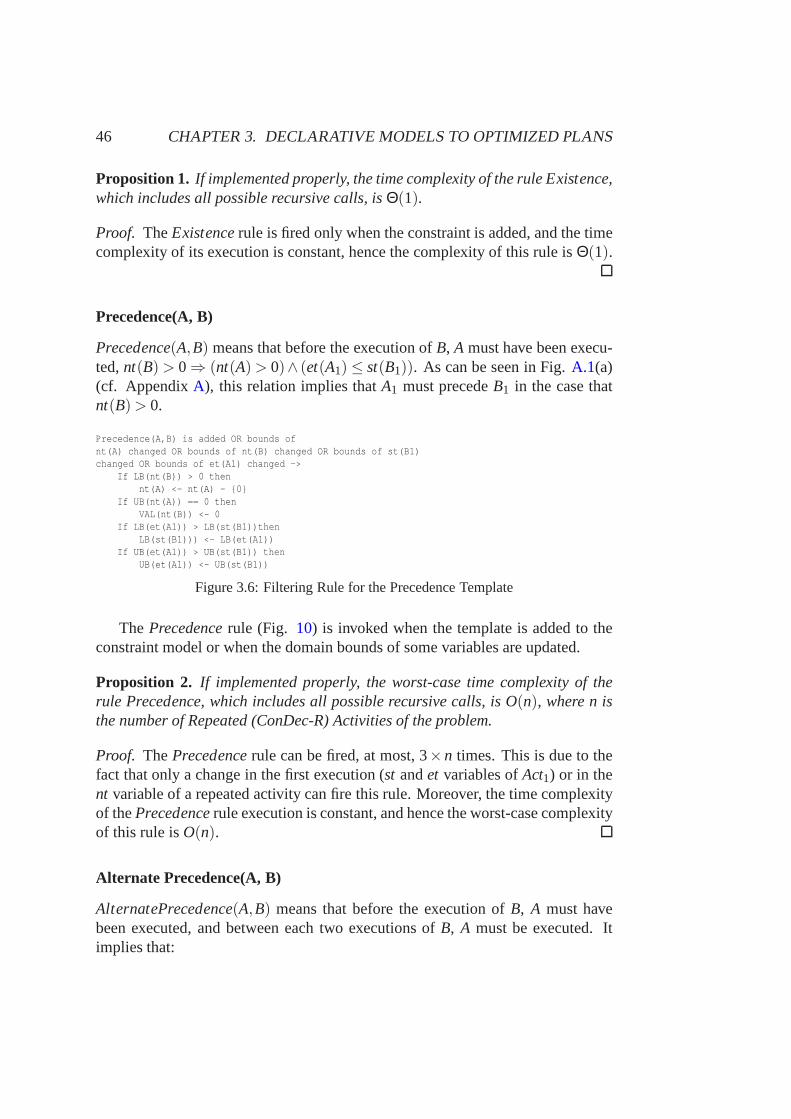
46 CHAPTER 3. DECLARATIVE MODELS TO OPTIMIZED PLANS
Proposition 1. If implemented properly, the time complexity of the rule Existence,which includes all possible recursive calls, isΘ(1).
Proof. TheExistencerule is fired only when the constraint is added, and the timecomplexity of its execution is constant, hence the complexity of this rule isΘ(1).
Precedence(A, B)
Precedence(A,B) means that before the execution ofB, A must have been execu-ted,nt(B)> 0⇒ (nt(A)> 0)∧ (et(A1) ≤ st(B1)). As can be seen in Fig.A.1(a)(cf. AppendixA), this relation implies thatA1 must precedeB1 in the case thatnt(B)> 0.
Precedence(A,B) is added OR bounds ofnt(A) changed OR bounds of nt(B) changed OR bounds of st(B1)changed OR bounds of et(A1) changed ->
If LB(nt(B)) > 0 thennt(A) <- nt(A) - {0}
If UB(nt(A)) == 0 thenVAL(nt(B)) <- 0
If LB(et(A1)) > LB(st(B1))thenLB(st(B1))) <- LB(et(A1))
If UB(et(A1)) > UB(st(B1)) thenUB(et(A1)) <- UB(st(B1))
Figure 3.6: Filtering Rule for the Precedence Template
The Precedencerule (Fig. 10) is invoked when the template is added to theconstraint model or when the domain bounds of some variablesare updated.
Proposition 2. If implemented properly, the worst-case time complexity oftherule Precedence, which includes all possible recursive calls, is O(n), where n isthe number of Repeated (ConDec-R) Activities of the problem.
Proof. ThePrecedencerule can be fired, at most, 3×n times. This is due to thefact that only a change in the first execution (st andet variables ofAct1) or in thent variable of a repeated activity can fire this rule. Moreover,the time complexityof thePrecedencerule execution is constant, and hence the worst-case complexityof this rule isO(n).
Alternate Precedence(A, B)
AlternatePrecedence(A,B) means that before the execution ofB, A must havebeen executed, and between each two executions ofB, A must be executed. Itimplies that:
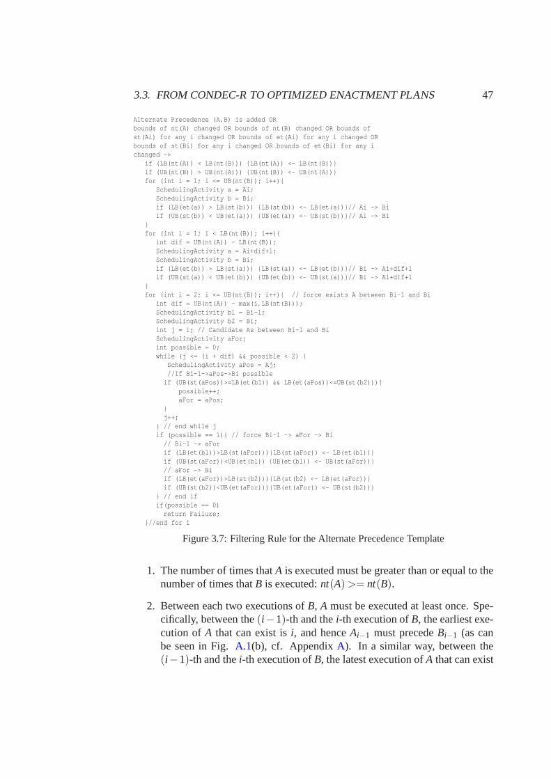
3.3. FROM CONDEC-R TO OPTIMIZED ENACTMENT PLANS 47
Alternate Precedence (A,B) is added ORbounds of nt(A) changed OR bounds of nt(B) changed OR bounds ofst(Ai) for any i changed OR bounds of et(Ai) for any i changed ORbounds of st(Bi) for any i changed OR bounds of et(Bi) for any ichanged ->
if (LB(nt(A)) < LB(nt(B))) {LB(nt(A)) <- LB(nt(B))}if (UB(nt(B)) > UB(nt(A))) {UB(nt(B)) <- UB(nt(A))}for (int i = 1; i <= UB(nt(B)); i++){
SchedulingActivity a = Ai;SchedulingActivity b = Bi;if (LB(et(a)) > LB(st(b))) {LB(st(b)) <- LB(et(a))}// Ai -> Biif (UB(st(b)) < UB(et(a))) {UB(et(a)) <- UB(st(b))}// Ai -> Bi
}for (int i = 1; i < LB(nt(B)); i++){
int dif = UB(nt(A)) - LB(nt(B));SchedulingActivity a = Ai+dif+1;SchedulingActivity b = Bi;if (LB(et(b)) > LB(st(a))) {LB(st(a)) <- LB(et(b))}// Bi -> Ai+dif+1if (UB(st(a)) < UB(et(b))) {UB(et(b)) <- UB(st(a))}// Bi -> Ai+dif+1
}for (int i = 2; i <= UB(nt(B)); i++){ // force exists A between Bi-1 and Bi
int dif = UB(nt(A)) - max(i,LB(nt(B)));SchedulingActivity b1 = Bi-1;SchedulingActivity b2 = Bi;int j = i; // Candidate As between Bi-1 and BiSchedulingActivity aFor;int possible = 0;while (j <= (i + dif) && possible < 2) {
SchedulingActivity aPos = Aj;//If Bi-1->aPos->Bi possible
if (UB(st(aPos))>=LB(et(b1)) && LB(et(aPos))<=UB(st(b2))){possible++;aFor = aPos;
}j++;
} // end while jif (possible == 1){ // force Bi-1 -> aFor -> Bi
// Bi-1 -> aForif (LB(et(b1))>LB(st(aFor))){LB(st(aFor)) <- LB(et(b1))}if (UB(st(aFor))<UB(et(b1)) {UB(et(b1)) <- UB(st(aFor))}// aFor -> Biif (LB(et(aFor))>LB(st(b2))){LB(st(b2) <- LB(et(aFor))}if (UB(st(b2))<UB(et(aFor))){UB(et(aFor)) <- UB(st(b2))}
} // end ifif(possible == 0)
return Failure;}//end for i
Figure 3.7: Filtering Rule for the Alternate Precedence Template
1. The number of times thatA is executed must be greater than or equal to thenumber of times thatB is executed:nt(A)>= nt(B).
2. Between each two executions ofB, A must be executed at least once. Spe-cifically, between the(i−1)-th and thei-th execution ofB, the earliest exe-cution of A that can exist isi, and henceAi−1 must precedeBi−1 (as canbe seen in Fig.A.1(b), cf. AppendixA). In a similar way, between the(i−1)-th and thei-th execution ofB, the latest execution ofA that can exist
48 CHAPTER 3. DECLARATIVE MODELS TO OPTIMIZED PLANS
is i +nt(A)−nt(B), and henceBi must precedeAi+nt(A)−nt(A)+1. This canalso be seen in Fig.A.1(b), where the possible activities to be executedbetween the(i−1)-th and thei-th execution ofB are framed within the dot-ted rectangle.∀i : 2≤ i ≤ nt(B) : ∃ j : i ≤ j ≤ i +nt(A)−nt(B) : st(A j) ≥et(Bi−1)∧et(A j))≤ st(Bi).
3. BeforeB, A must be executed:st(B1)≥ et(A1).
Proposition 3. If implemented properly, the worst-case time complexity ofthe ruleAlternatePrecedence, which includes all possible recursive calls, is O(n×nt3),where n is the number of Repeated Activities of the problem, and nt is the upperbound of the variable nt(Act) domain. This upper bound obtains the same valuefor all the ConDec-R activities.
Proof. TheAlternatePrecedencerule can be fired, at most,n+2×n×nt times.This is due to the fact that a change in any execution of any activity (st andetvariables ofActi) or in thent variable of an activity can fire this rule. Moreover,the time complexity of theAlternatePrecedencerule execution isO(nt2), andhence the worst-case time complexity of this rule isO(n×nt3).
3.3.3 Solving the COP
Once the problem is modelled, several constraint-based mechanisms can be usedto obtain the solution for the COP, i.e., optimized enactment plans (cf. Def.24).Since the generation of optimized plans presents NP-complexity (Garey and John-son, 1979), it is not possible to ensure the optimality of the generated plans for allthe cases. The developed constraint-based approach, however, allows solving theconsidered problems in an efficient way, as demonstrated in Sect.3.4.
Definition 24. A BP enactment planis composed by:
1. The number of times each BP activity is executed.
2. The start and the completion times for each activity execution.
3. The resource which is used for each activity execution.
In general, when optimizing a CSP variable, if a feasible solution which isknown exists, the value of the variable to optimize in the known solution canbe used for discarding large subsets of fruitless candidates by using upper andlower estimated bounds of the quantity being optimized during the search process.Thus, if a known feasible solutionS for the problem to solve exists, the objectivevalue for this solution (SOCT) is a valuable information which can be added to the
3.4. EMPIRICAL EVALUATION 49
constraint model through the constraintOCT < SOCT. Thus, some non optimalcandidates, i.e., candidates whoseOCT value cannot be less thanSOCT in anycase, are discarded during the search, increasing the efficiency in the search forsolutions.
Moreover, in the proposed approach, during the search process, some of thevalues which only lead to non-feasible solutions, i.e., inconsistent values, are re-moved from the domains of the CSP variables through the developed filteringrules (cf. AppendixB) in order to reduce the search space by maintaining arcconsistency (cf. Def.17on page29).
In the proposed approach, the developed filtering rules and CSP modelling (cf.Sect. 3.3.1) are implemented such that they maintain the arc consistency for allpairs of CSP variables during all the search process.
There are a wide scope of search algorithms of varied nature which can be usedfor finding optimal/optimized solutions to the COPs. In general, the suitability andefficacy of each search algorithm highly depend on the specific problem to solve.For this reason, different search strategies are tested in the empirical evaluation ofeach chapter related to the generation of optimized enactment plans from ConDec-R specifications (cf. Sect.3.4, Sect.4.4, and Sect.5.4).
A proof-of-concept prototype has been implemented througha web-based ap-plication, which allows for the generation of optimized enactment plans fromConDec-R specifications, and it can be accessed at:
http://regula.lsi.us.es/OptBPPlanner9
3.4 Empirical Evaluation
In order to evaluate the effectiveness of the proposal, a controlled experiment isconducted. Section3.4.1 describes the design underlying the experiment, andSection3.4.2shows the experimental results and the data analysis.
3.4.1 Experimental Design
Purpose: The purpose of the experimental evaluation is to determine the efficacyof the proposed constraint-based approach for generating optimized plans. As faras the developed filtering rules greatly influence and improve the efficiency of thesearch, it has been considered suitable to compare the results obtained by: first,the proposal with propagators (i.e., filtering rules) and the related high-level global
9Only non-branched templates and the default option in the ordering constraints, i.e., ES, areconsidered in this prototype.
50 CHAPTER 3. DECLARATIVE MODELS TO OPTIMIZED PLANS
constraints; and secondly, with neither propagators nor global constraints (in thiscase, the equivalent local constraints are included)10.
Experimental Design: The behavior of five representative propagators aretested: Exactly, Existence, Precedence, Alternate and Chain Precedence. Theresults obtained with two proposals, which use the same variables, are comparedto study the efficiency:
1. With propagators: the user-defined constraints are used for the establish-ment of the high-level relations between the ConDec-R activities. In thiscase, the proposed filtering algorithms are responsible forremoving incon-sistent values from the domain of the variables.
2. Without propagators: the relations between the activities are establisheddirectly through basic constraints, as shown in AppendixA.
Objects: Due to the use of a specific and new language, it has been impossibleto find a set of public benchmarks for ConDec-R problems.
ConDec-R problems can be modelled as an extension of scheduling problems.In this way, a set of well-known job shop scheduling (cf. Sect. 2.2.1) benchmarks(FT06 (6x6), FT10 (10x10), ABZ06 (10x10), LA21 (15x10), LA36 (15x15)) havebeen extended for use in the empirical evaluation in the following way:
• In a job shop scheduling problem, the activities are executed only once. Forthis evaluation, the cardinality of a random percentagep% of activities hasbeen set to a valuec greater than one, in order to test the behavior of theproposal when some repeated activities are executed several times. In Table3.1, the columnCard= c(p%) refers to extensions to job shop schedulingproblems in a way that the cardinality of a random percentagep% of ac-tivities has been set to a valuec. In order to minimize the influence of therandom component in the performance measures which are considered, 50random instances are generated for each problem so that average values arereported.
• In a job shop scheduling problem, all the temporal relationsbetween activi-ties are precedence relations, i.e., ”A precedes B” means that A must finishbefore B starts. This relation can be modelled through several ConDec-Rtemplates, e.g., Precedence, Response, or Succession. Formodelling thetemporal relations of job shop scheduling problems in ConDec, the Prece-dence template has been selected although other options canalso be used.Moreover, in order to consider more complex relations between the repeated
10Due to the fact that the analyzed relations are introduced inthis work for the first time, therehas not been possible to find a previously developed solver which deals with these relations.
3.4. EMPIRICAL EVALUATION 51
activities, the alternate and chain precedence relations11 are also consideredin the following way: in the original problemP, all the precedence relationsbetween the activities of the same job are changed to alternate precedencerelations (this is represented byPAlt. in Table3.1) and chain precedencerelations (this is represented byPChainin Table3.1).
Setting the cardinality ofp% activities to a valuev> 1, can result in a solutionwhere there arep′% activities (p′ > p) with cardinalityv. For example, each ac-tivity a with nt(a) = v implies that for allb whereAlternatePrecedence(b,a) orChainPrecedence(b,a) hold, thennt(b)≥ nt(a) must be satisfied (the same logicapplies for all the activitiescsuch thatAlternatePrecedence(c,b)orChainPrece−dence(c,b), etc).
Notice that the scheduling benchmarks with the lowest complexity are thosethat only include precedence relations and have the lowest cardinality for the ac-tivities.
Independent Variables:For the empirical evaluation, the random percentageof activities set to a cardinality higher than 1,p%, and the value for this cardinality,c are taken as independent variables.
Response Variables:Some performance measures are reported (Table3.1):
• BMP : Number of instances for which the makespan found by the proposal
with propagators is shorter than the makespan found withoutpropagators.
• BM: Number of instances for which the makespan found by the proposalwithout propagators is shorter than the makespan found withpropagators.
• BTP: Number of instances for which the solutions found by both proposals
obtain the same makespan value, but the proposal with propagators is faster.The values related to this variable appear between bracketsin Table3.1, andit is only included in the case that it is greater than one.
• BT : Number of instances for which the solutions found by both proposalsobtain the same makespan value, but the proposal without propagators isfaster. The values related to this variable appear between brackets in Table3.1, and it is only included in the case that it is greater than one.
Experimental Execution: For both proposals, a complete search approachhas been applied: first, the variables related to the number of times that eachactivity is executed are instantiated. The search procedure then determines the
11Alternate Precedence(A, B) means that before the executionof B, A must have been executed,and between each two executions ofB, A must be executed. In a similar way, Chain Precedence(A,B) means that immediately beforeB, A must be executed. For more details, cf. AppendixA.
52 CHAPTER 3. DECLARATIVE MODELS TO OPTIMIZED PLANS
order of execution of the activities within each resource ateach step, such thatthe next resource to be ranked is selected depending on its slack. Within eachresource, the activities are ranked in a non-deterministicway.
For the experiments, each algorithm is run until it finds the optimal solutionor until a 5-minute CPU time limit has been reached. The machine for all ex-periments is an Intel Core2, 2.13 GHz, 1.97 GB memory, running Windows XP.In order to solve the constraint-based problems (cf. Sect.3.3), the developed al-gorithms have been integrated with the system COMET (Dynadec, 2011), whichis able to generate high-quality solutions for highly constrained problems in anefficient way.
3.4.2 Experimental Results and Data Analysis
As stated before, several experimental results are shown inTable3.1. After ana-lyzing these values, some conclusions can be obtained:
• For problems with only precedence relations, the solutionsfor the two pro-posals are very similar. In this case, the problem is simply aJob Shop pro-blem, and COMET includes efficient mechanisms for solving schedulingproblems.
• For problems with alternate and chain precedence relations, the proposalwithout propagators obtains better solutions for problemswith lower com-plexity (or cardinality). When the percentage of activities with greater car-dinality increases, the proposal with propagators proves better than the otherproposal in almost all instances.
In short, the proposal without propagators obtains better solutions for pro-blems of lower complexity (only precedence relations, low cardinality), while theproposal with propagators is much better for more complex problems, and henceit seems to be better for general cases12.
12Notice that a limited empirical evaluation is carried out, and hence the conclusions which areobtained are dependent on the considered problems.
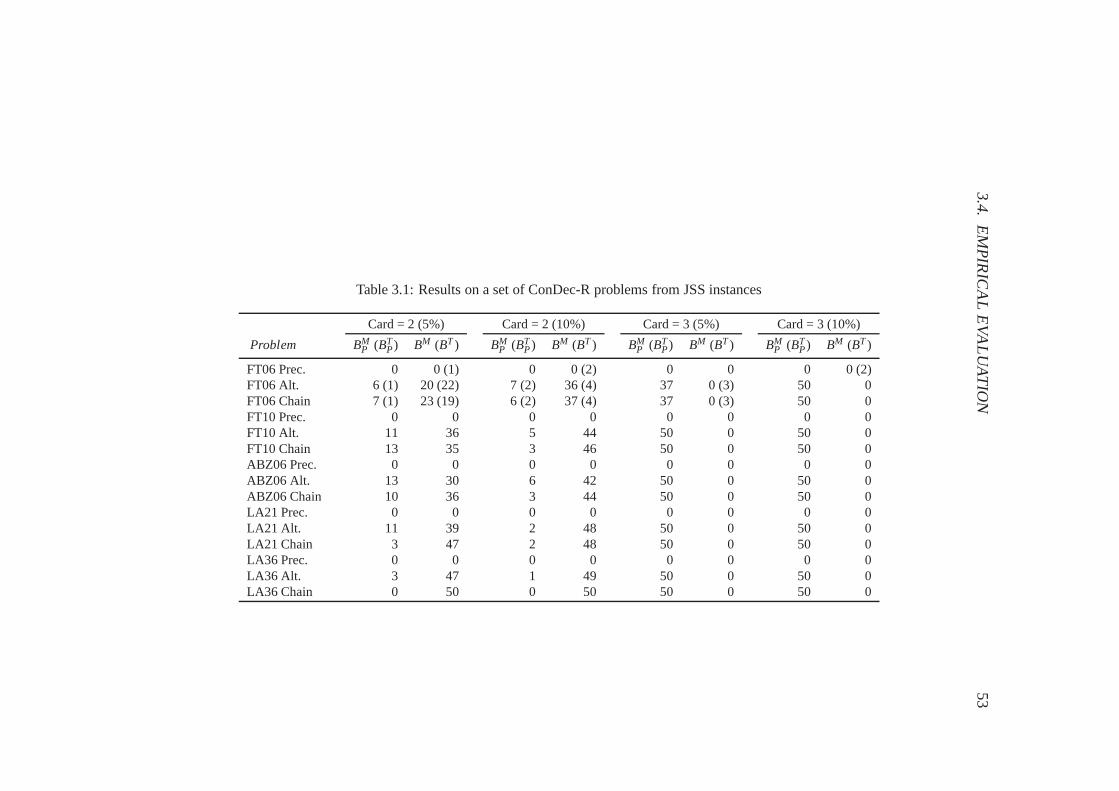
3.4.E
MP
IRIC
AL
EVA
LUAT
ION
53
Table 3.1: Results on a set of ConDec-R problems from JSS instances
Card = 2 (5%) Card = 2 (10%) Card = 3 (5%) Card = 3 (10%)
Problem BMP (BT
P) BM (BT) BMP (BT
P) BM (BT ) BMP (BT
P) BM (BT) BMP (BT
P) BM (BT)
FT06 Prec. 0 0 (1) 0 0 (2) 0 0 0 0 (2)FT06 Alt. 6 (1) 20 (22) 7 (2) 36 (4) 37 0 (3) 50 0FT06 Chain 7 (1) 23 (19) 6 (2) 37 (4) 37 0 (3) 50 0FT10 Prec. 0 0 0 0 0 0 0 0FT10 Alt. 11 36 5 44 50 0 50 0FT10 Chain 13 35 3 46 50 0 50 0ABZ06 Prec. 0 0 0 0 0 0 0 0ABZ06 Alt. 13 30 6 42 50 0 50 0ABZ06 Chain 10 36 3 44 50 0 50 0LA21 Prec. 0 0 0 0 0 0 0 0LA21 Alt. 11 39 2 48 50 0 50 0LA21 Chain 3 47 2 48 50 0 50 0LA36 Prec. 0 0 0 0 0 0 0 0LA36 Alt. 3 47 1 49 50 0 50 0LA36 Chain 0 50 0 50 50 0 50 0
54 CHAPTER 3. DECLARATIVE MODELS TO OPTIMIZED PLANS
3.5 Related Work
In recent years, several filtering algorithms for specialized scheduling constraintshave been developed. Specifically, (Beck and Fox, 2000) and (Bartak and Cepek,2010) model scheduling problems which include alternative and optional tasksrespectively, together with their propagators. Furthermore, the work (Bartak andCepek, 2008) proposes propagators for both precedence and dependency cons-traints in order to solve log-based reconciliation (P&S) problems in databases.In those studies, the precedence constraints mean the same as in P&S problems,while the dependency constraints are given between optional activities which canpotentially be included in the final schedule. The work (Laborie et al., 2009)introduces new types of variables (time-interval, sequence, cumulative, and state-function variables) for modelling and reasoning with optional scheduling activi-ties. In the current chapter, the proposed model and propagation for the optionalactivities are very similar to the proposal presented in (Laborie et al., 2009).
Regarding the works (Beck and Fox, 2000), (Bartak and Cepek, 2008), (Bartakand Cepek, 2010) and (Laborie et al., 2009), the main contribution from the de-veloped propagators is the complex reasoning about severalcombined innovativeaspects, such as the alternating executions of repeated activities together with thevariable number of times which these activities are executed (i.e. alternate andchain relations). Furthermore, the areas of application ofthose studies are unre-lated to those of the presented proposal.
Additionally, there exist some proposals which could be used to generate opti-mized enactment plans for BPs from constraint-based process specifications. Spe-cifically, (Pesic, 2008) proposes the generation of a non-deterministic finite stateautomaton from constraint-based specifications based on Linear Temporal Logic(LTL) which represents exactly all traces that satisfy the LTL formulas. Whenextending this approach by including estimates, the overall completion time of allthe traces could then be calculated (e.g., (van der Aalst et al., 2011)). However,the big disadvantage following such an approach would be that the process of ge-nerating the automaton from the declarative specificationsis NP complete, and,unlike the proposed approach, no heuristic can be used. In a similar way, CLIMB(Montali, 2009) could be used to generate quality traces from declarative specifi-cations, and calculate its completion time. Then, the best traces could be selected.Unlike the proposed approach, (Montali, 2009) does neither consider optimalitynor resource availabilities. Therefore, this would only cover the planning part ofthe current proposal, but not the scheduling aspects addressed by the proposedapproach.
Chapter 4
User Recommendations for theOptimized Execution of BPs
4.1 Introduction
4.1.1 Motivation
In the current dynamic business world the economic success of an enterprize in-creasingly depends on its ability to react to changes in its enterprize in a quick andflexible way. Therefore, flexible BPMSs (cf. Def.4 on page10) are required toallow companies to rapidly adjust their BP (cf. Def.1 on page9) to changes inthe environment (van der Aalst and Jablonski, 2000). The specification of processproperties in a declarative way is an important step towardsthe flexible manage-ment of BPMSs (van der Aalst et al., 2009).
As mentioned, due to their flexible nature, frequently several ways to executedeclarative process models exist. Typically, given a certain partial trace (reflectingthe current state of the process instances), users can choose from several enabledactivities which activity to execute next. This selection,however, can be quitechallenging since performance goals of the process (e.g., minimization of overallcompletion time) should be considered, and users often do not have an understan-ding of the overall process. Moreover, optimization of performance goals requiresthat resource capacities are considered. Therefore, recommendation support isneeded during BP execution, especially for inexperienced users (van Dongen andvan der Aalst, 2005).
4.1.2 Contribution
In order to support users of flexible BPMSs during process execution in opti-mizing performance goals like minimizing the overall completion time (i.e., time
55
56 CHAPTER 4. RECOMMENDATIONS FOR EXECUTING BPS
needed to complete all process instances which were plannedfor a certain pe-riod), in this chapter the use of optimized enactment plans which are generatedfrom declarative BP specifications (cf. Chapter3) is proposed for giving recom-mendations.
Recommendations on possible next steps are then generated taking the partialtrace and the optimized plans into account. In the proposed approach, replanningis supported if actual traces deviate from the optimized enactment plans (e.g.,because estimates turned out to be inaccurate).
In order to evaluate the effectiveness of the proposed recommendation system,different constraint-based algorithms are applied to a range of test models of vary-ing complexity. The suitability of the proposed approach istested regarding both(1) build-time, i.e., for the generation of complete optimized plans before startingthe BP enactment; and (2) run-time, i.e., for the generationof partial, optimizedplans by considering the actual partial trace of the processas the execution of theprocess proceeds (replanning). The results indicate that the proposed approachproduces a satisfactory number of suitable solutions, i.e., solutions which are op-timal in most cases and quite good in other cases1.
The main contributions of this chapter can be summarized as follows:
• Method for generating recommendations to users of flexible BPMSs duringrun time (cf. Sect.4.2 (Barba et al., 2011)). For this, optimized enactmentplans which are generated from constraint-based specifications (cf. Chapter3) are used.
• Validation of the proposed approach through the analysis ofdifferent per-formance measures related to a range of test models of varying complexity(cf. Sect.4.4).
This chapter is organized as follows: Sect.4.2 includes an overview of theproposed approach, Sect.4.3 shows the application of the proposed approach toa running example, Sect.4.4shows some experimental results, Sect.4.5presentsa critical discussion of the proposed approach, and finally,Sect.4.6 summarizesrelated work.
4.2 Method for Generating Recommendations
As stated, constraint-based processes offer much flexibility. Typically, given aconstraint-based process model and a certain partial trace, users can choose from
1Notice that a limited empirical evaluation is carried out, and hence the conclusions which areobtained are dependent on the considered problems.
4.2. METHOD FOR GENERATING RECOMMENDATIONS 57
several enabled activities which activity to execute next,which is a challengingselection in most cases. In order to address this challenge,an approach to assistusers during process execution in optimizing performance goals like minimizingthe overall completion time is proposed. Specifically, users of flexible BPMSs aresupported during process execution by a recommendation service which providesrecommendations on how to proceed best with the execution. Hereby, a recom-mendation (cf. Def.25) is composed by one or more enabled activities (cf. Def.10 on page17) to be executed next, together with their resource allocations sinceboth control-flow and resource perspectives are considered.
Definition 25. A recommendationis composed by a set of pairs(ai,Rjk) sugges-ting to start the i-th execution of activity a using resourceRjk
2.
For example, the recommendation< (A1,R01),(B2,R12) > suggests to startthe first execution of activityA using resourceR01 and the second execution ofactivity B using resourceR12.
The recommendation service is based on optimized enactmentplans which arealready generated during build-time by P&S all BP activities (cf. Chapter3) andfurther optimized during run-time (cf. Fig.4.1). Recommendations are suggestedduring the BP execution at timeT when the partial trace of the BP is part of one ofthe considered optimized enactment plans which contains one or more activitieswhich start right at timeT. In this way, at specific times of the process execution,the recommendation system generates the recommendations by considering: (1)the optimized enactment plans, (2) the partial traces (cf. Def. 8 on page16) ofthe process instances to be optimized, and (3) the resource availabilities (cf. Sect.4.2.1). Thereby, the recommendation service ensures that not only single processinstances get optimized, but the whole set of instances which is planned to beexecuted within a certain timeframe, hence allowing for a global optimization.
4.2.1 Generating Recommendations on Possible Next Execu-tion Steps
This section describes how the generated optimized plans (cf. Chapter3) are thenused for assisting users during process execution. At run-time, process instances(cf. Def. 9 on page16) are executed by authorized users (a in Fig. 4.1). At anypoint during the execution of a process instance, the user can select from the setof enabled activities (cf. Def.10 on page17) what to do next. However, to guidethe user to optimize the overall process goals, recommendations (cf. Def.25) are
2Rjk refers to the k-th resource with rolej.
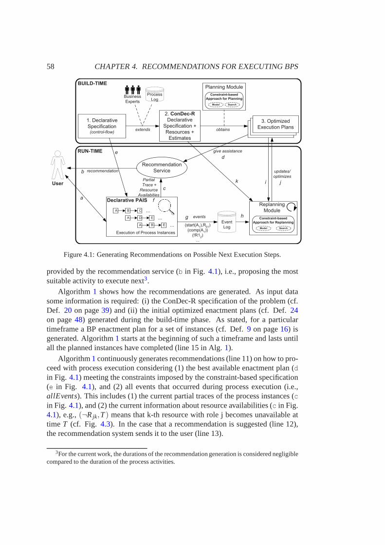
58 CHAPTER 4. RECOMMENDATIONS FOR EXECUTING BPS
������������
�����������������������
�����������
���������
�������������
����������
�������
�����������
��������������
���� ���
������
��
���
� �����
!�������
�����
�������
����������������
���������������������
����� ������
�������������
�����
�������
��������
��������
������������
� � ���
�����������
��������������
�����������
��������������
��������������
������
"��"#�$%�
&�$
"����"#�$$
"'���$
���
# (!
# ��
# �!
���
���
���
���������!������
�������������������)�������
����������������
�����������������������
����� ������
��������
���������
���������
*�����
����
��
���������������
������� �*�����
�
�
! �
�
�
�
�
"
Figure 4.1: Generating Recommendations on Possible Next Execution Steps.
provided by the recommendation service (b in Fig. 4.1), i.e., proposing the mostsuitable activity to execute next3.
Algorithm 1 shows how the recommendations are generated. As input datasome information is required: (i) the ConDec-R specification of the problem (cf.Def. 20 on page39) and (ii) the initial optimized enactment plans (cf. Def.24on page48) generated during the build-time phase. As stated, for a particulartimeframe a BP enactment plan for a set of instances (cf. Def.9 on page16) isgenerated. Algorithm1 starts at the beginning of such a timeframe and lasts untilall the planned instances have completed (line 15 in Alg.1).
Algorithm1 continuously generates recommendations (line 11) on how topro-ceed with process execution considering (1) the best available enactment plan (din Fig. 4.1) meeting the constraints imposed by the constraint-based specification(e in Fig. 4.1), and (2) all events that occurred during process execution(i.e.,allEvents). This includes (1) the current partial traces of the process instances (cin Fig. 4.1), and (2) the current information about resource availabilities (c in Fig.4.1), e.g.,(¬Rjk,T) means that k-th resource with role j becomes unavailable attime T (cf. Fig. 4.3). In the case that a recommendation is suggested (line 12),the recommendation system sends it to the user (line 13).
3For the current work, the durations of the recommendation generation is considered negligiblecompared to the duration of the process activities.
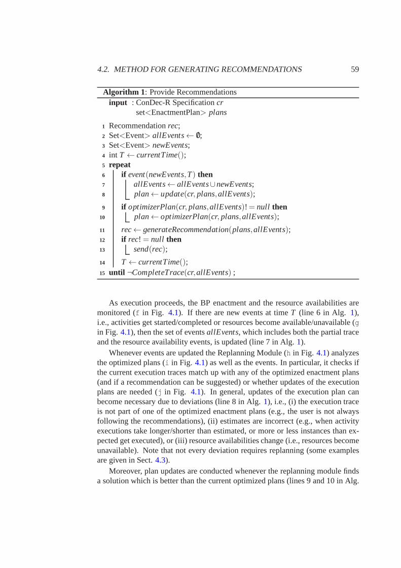
4.2. METHOD FOR GENERATING RECOMMENDATIONS 59
Algorithm 1 : Provide Recommendationsinput : ConDec-R Specificationcr
set<EnactmentPlan> plans
Recommendationrec;1
Set<Event> allEvents← /0;2
Set<Event> newEvents;3
int T ← currentTime();4
repeat5
if event(newEvents,T) then6
allEvents← allEvents∪newEvents;7
plan← update(cr, plans,allEvents);8
if optimizerPlan(cr, plans,allEvents)! = null then9
plan← optimizerPlan(cr, plans,allEvents);10
rec← generateRecommendation(plans,allEvents);11
if rec! = null then12
send(rec);13
T← currentTime();14
until ¬CompleteTrace(cr,allEvents) ;15
As execution proceeds, the BP enactment and the resource availabilities aremonitored (f in Fig. 4.1). If there are new events at timeT (line 6 in Alg. 1),i.e., activities get started/completed or resources become available/unavailable (gin Fig. 4.1), then the set of eventsallEvents, which includes both the partial traceand the resource availability events, is updated (line 7 in Alg. 1).
Whenever events are updated the Replanning Module (h in Fig. 4.1) analyzesthe optimized plans (i in Fig. 4.1) as well as the events. In particular, it checks ifthe current execution traces match up with any of the optimized enactment plans(and if a recommendation can be suggested) or whether updates of the executionplans are needed (j in Fig. 4.1). In general, updates of the execution plan canbecome necessary due to deviations (line 8 in Alg.1), i.e., (i) the execution traceis not part of one of the optimized enactment plans (e.g., theuser is not alwaysfollowing the recommendations), (ii) estimates are incorrect (e.g., when activityexecutions take longer/shorter than estimated, or more or less instances than ex-pected get executed), or (iii) resource availabilities change (i.e., resources becomeunavailable). Note that not every deviation requires replanning (some examplesare given in Sect.4.3).
Moreover, plan updates are conducted whenever the replanning module findsa solution which is better than the current optimized plans (lines 9 and 10 in Alg.
60 CHAPTER 4. RECOMMENDATIONS FOR EXECUTING BPS
1). The Replanning Module is continuously searching for a better plan by con-sidering the event log during BP execution, provided that the current plan is notoptimal. If plan updates are required, the Replanning Module needs to accessthe extended constraint-based specification of the process(k in Fig. 4.1) to gene-rate new optimized plans considering both the estimates andthe constraint-basedspecification. If necessary, the replanning, i.e., the generation of new optimizedenactment plans, is carried out by applying a constraint-based approach for P&Sthe BP activities (cf. Chapter3).
Despite the NP-complexity of the considered problems, in general replanningis less time consuming than initial planning, since most of the information aboutprevious generated plans can usually be reused, and CSP variable values becomeknown as execution proceeds (cf. Sect.4.4).
A running example illustrating the complete process is detailed in Sect.4.3.
4.3 A Running Example
In this section, the proposed approach is used for managing recommendationsduring a hypothetical execution of a running example which represents a travelagency. This agency manages holiday bookings by offering clients the followingthree services: transport, accommodation, and guided excursions. After the clientrequest is carried out, the agency must write a report which contains the infor-mation in answer to the request, which will then be sent to theclient. Besidesmanaging the client requests, people who work in the agency must perform fur-ther activities related to management, and accounting tasks. The number of clientrequests (P), management tasks (M) and accounting tasks (A)which must be dealtwith during a working day is known at the beginning of the day,hence it is ne-cessary to organize the work considering the estimated workload. The objectiveto be considered by the agency is to minimize the overall completion time of thedaily processes. However, this example can easily be extended in order to considerthe optimization of further objective functions, such as cost. In the travel agency,optimized BP enactment plans must be created every day to generate recommen-dations about the activities to be executed and the correct ordering. The activitieswhich must be executed to deal with the client requests, management and account-ing tasks are detailed in Table4.1. For activities which are executed more thanonce, each execution must finish before the next execution can start. Moreover,in order to simplify the analyzed problem, all the executions of the same activityrequire a resource of the same role with the same duration is assumed4.
4Note that the proposed approach can deal with BP activities which require several resourcesof various kinds of roles, since the considered problems aremodeled as scheduling problems withoptional activities, where the resources have a discrete capacity.
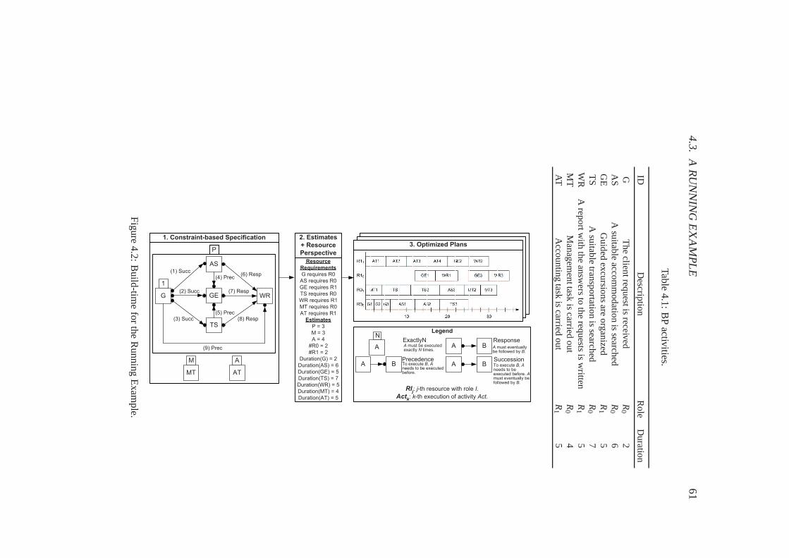
4.3.A
RU
NN
ING
EX
AM
PLE
61
Table4.1:
BP
activities.
IDD
escriptio
nR
ole
Du
ration
GT
he
clientreq
uestis
receivedR
02
AS
Asu
itable
accom
mo
datio
nis
searched
R0
6G
EG
uid
edexcu
rsion
sare
org
anized
R1
5T
SA
suitab
letran
spo
rtation
issearch
edR
07
WR
Arep
ortw
ithth
ean
swers
toth
ereq
uests
isw
rittenR1
5M
TM
anag
emen
ttaskis
carriedo
ut
R0
4A
TA
ccou
ntin
gtask
iscarried
ou
tR
15
������������ ����������������������������������
��
�
��
�
�
��
��
��
��
��� ��
���� ��
���� ��
�������
�������
�������
�
�������
�������
�������
�����������
��������
��������
������
� �������
����� �������
������ �������
������ ������
������ �������
������ ������
������ �������
������ ������
��������
�����
�����
�����
������
�����
! �"#�$%������
! �"#�$%�������
! �"#�$%�������
! �"#�$%�������
! �"#�$%�������
! �"#�$%�������
! �"#�$%�������
�����&�%��
!"��
� ' �$��(�� #���)��%��&��#$�*���(�� #�&*�+$��,
�
-�("�#./-��0 �#�*���(�� #�&�("�#./���#�0��,
����$%��� ' ��0 �#��1�%# "../
*��+$..$2�&�*/���
� ������$%� ' �$��(�� #���)��
%��&��#$�*��(�� #�&�*�+$��,��0 �#��1�%# "../�*�+$..$2�&�*/���
���3��4#5����$ ����2�#5��$.����
����3��4#5��(�� #�$%�$+�"�#�1�#/���
Figure
4.2:B
uild-time
forthe
Running
Exam
ple.
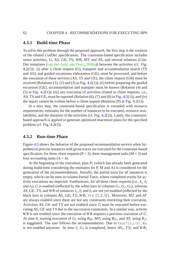
62 CHAPTER 4. RECOMMENDATIONS FOR EXECUTING BPS
4.3.1 Build-time Phase
To solve this problem through the proposed approach, the first step is the creationof the related ConDec specification. The constraint-based specification includesseven activities, G, AS, GE, TS, WR, MT and AT, and several relations (Con-Dec templates (van der Aalst and Pesic, 2006a)) between the activities (cf. Fig.4.2(1)): (i) after a client request (G), transport and accommodation search (TSand AS), and guided excursions elaboration (GE), must be processed, and beforethe execution of these services (AS, TS and GE), the client request (GR) must bereceived (Relations (1), (2) and (3) in Fig.4.2(1)); (ii) before preparing the guidedexcursion (GE), accommodation and transport must be known (Relation (4) and(5) in Fig. 4.2(1)); (iii) any execution of activities related to client requests, i.e.,AS, TS and GE, must be reported (Relation (6), (7) and (8) in Fig. 4.2(1)); and (iv)the report cannot be written before a client request (Relation (9) in Fig.4.2(1)).
In a next step, the constraint-based specification is extended with resourcerequirements, estimates for the number of instances to be executed, resource avai-labilities, and the duration of the activities (cf. Fig.4.2(2)). Lastly, the constraint-based approach is applied to generate optimized enactment plans for the specifiedproblem (cf. Fig.4.2(3)).
4.3.2 Run-time Phase
Figure4.3shows the behavior of the proposed recommendation service when hy-pothetical process instances with given traces are executed for the constraint-basedspecification, for three client requests (P = 3), three management tasks (M = 3) andfour accounting tasks (A = 4).
At the beginning of the execution, planP1 (which has already been generatedduring build-time considering the estimates for P, M and A) is considered for thegeneration of the recommendations. Initially, the partialtrace for all instances isempty, which can be seen in column Partial Trace, where completed events for ac-tivity executions are depicted. Furthermore, for all threeclient requests (i.e.,I1, I2andI3), G is enabled (reflected by the white bars in columnsG1,G2,G3), whereasAS, GE, TS, andWRof instancesI1, I2 andI3 are not yet enabled (reflected by theblack bars in columnsASi ,GEi,TSi ,WRi,∀i ∈ {1,2,3}). Moreover,MT andATare always enabled since there are not any constraints restricting their execution.Activities AS, GE andTSare not enabled sinceG must be executed before exe-cutingAS, GE andTSdue to the succession constraints. In a similar way, activityWRis not enabled since the execution ofWRrequires a previous execution ofG.At time 0, starting execution ofG1 usingR00, MT1 usingR01, andAT1 usingR11
is suggested. The user follows the recommendation. Due toExactly 1(G), G1
is not enabled anymore. At time 2,G1 is completed, henceAS1, TS1 andWR1
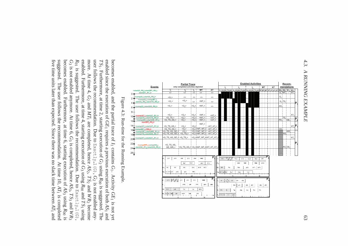
4.3.A
RU
NN
ING
EX
AM
PLE
63
0
2
4
6
8
10
12
14
16
18
20
22
24
26
Enabled Activities Recom-
mendations
R00
R01
R10
I1
I2
<start(G1,R0
0),start(MT
1,R0
1),
start(AT1,R1
1)>
Partial Traceonly completed activities depicted
I1
I2
G1 -
G2
<comp(G1),start(G
2,R0
0)> <G
1>
<> <>
<comp(AT1),start(AT
2,R1
1)>
Events
G1
WR1TS
1GE
1AS
1G
2WR
2TS2
GE2
AS2
MT AT
MT
MT1
MT3
MT2
AT
AT1
AT4
AT3
AT2 R1
1
<comp(G2),comp(MT
1),
start(G3,R0
0),start(TS
1,R0
1)>
<comp(G3),start(AS
1,R0
0)>
<comp(TS1),start(TS
2,R0
1)>
<comp(AS1),start(GE
1,R1
0),
start(MT2,R0
0)>
<comp(AT2),start(AT
3,R1
1)>
<comp(MT2),(!R0
0)>
<comp(GE1),start(WR
1,R1
0)>
<comp(TS2),start(AS
2,R0
1)>
<comp(AT3),start(AT
4,R1
1)>
<comp(WR1),comp(AS
2),
start(GE2,R1
0),start(AS
3,R0
1)>
I3
I3
G3
WR3TS
3GE
3AS
3
MT1
AT1
<G2><G
1> G
3TS
1
AS1
<G3><G
1> <G
2>
AT2
<G1> <G
2> <G
3>
<G1,
TS1> TS
2
GE1
AS2
AT3
<G2>
AS2
WR1
<G2>
<AT1>
<AT1>
<AT1>
<AT1,
AT2>
<MT1>
<MT1>
<MT1>
<MT1>
<MT1>
<MT1>
<MT1,MT
2>
<G2>
<G2><G
1,TS
1,AS
1>
<G1,
TS1,
AS1>
<G1,
TS1,AS
1>
<G1,TS
1,AS
1,GE
1> <G
2>
<G2,TS
2>
<AT1,
AT2>
<AT1,
AT2>
<AT1,
AT2>
<AT1,
AT2,
AT3>
AS2
AT4
AS3GE
2
<G2,
TS2>
<G2,
TS2,
AS2>
<G3>
<G3>
<G3>
<G3>
<G3>
<G3>
<G3>
<G3>
<MT1,MT
2>
<MT1,MT
2>
<MT1,
MT2>
<MT1,
MT2><AT
1,AT
2,AT
3>
<>
<>
<>
<>
<>
<>
<>
<>
<>
<>
<G1,TS
1,AS
1,GE
1>
<G1,TS
1,AS
1,GE
1>
<G1,TS
1,AS
1,
GE1,
WR1>
P1
P2
P3
P4
P1
P2
P3 P
4
Figure
4.3:R
un-time
forthe
Running
Exam
ple.
beco
mes
enab
led,
and
the
partialtrace
of
I1co
ntain
sG1 .
Activity
GE
1is
no
tyeten
abled
since
the
executio
no
fG
E1
requ
iresa
previo
us
executio
no
fbo
thA
S1
and
TS
1 .F
urth
ermo
re,attime
2,startin
gexecu
tion
of
G2
usin
gR
00is
sug
gested
.T
he
user
follow
sth
ereco
mm
end
ation
.D
ue
toExactly
1(G),G2
isn
oten
abled
any-m
ore.
At
time
4,G
2an
dM
T1
areco
mp
leted,
hen
ceAS2 ,
TS
2an
dW
R2
beco
me
enab
led.
Fu
rtherm
ore,attim
e4
,starting
executio
no
fG
3u
singR
00an
dT
S1
usin
gR
01is
sug
gested
.T
he
user
follow
sth
ereco
mm
end
ation
.D
ue
toExactly
1(G),G
3is
no
tenab
ledanym
ore.
Attim
e6
,G
3is
com
pleted
,hen
ceAS3 ,T
S3
andW
R3
beco
mes
enab
led.
Fu
rtherm
ore,
attim
e6
,startin
gexecu
tion
ofA
S3
usin
gR
00is
sug
gested
.T
he
user
follow
sth
ereco
mm
end
ation
.A
ttim
e1
0,
AT
1is
com
pleted
fivetim
eu
nits
laterthan
expected
.S
ince
there
was
no
slackt
ime
betw
eenAT
1an
d
64 CHAPTER 4. RECOMMENDATIONS FOR EXECUTING BPS
AT2, P1 becomes outdated, and the replanning module generatesP2 consideringthe new conditions.
At time 10, based onP2 starting execution ofAT2 usingR11 is suggested. Theuser follows the recommendation. At time 11,TS1 is completed. Furthermore,at time 11, starting execution ofTS2 usingR01 is suggested. The user followsthe recommendation. At time 12,AS1 is completed, henceGE1 becomes enabled.Furthermore, at time 12, starting execution ofAS2 usingR00 andGE1 usingR10
is suggested. The user decides to partially follow the recommendation, so that,instead of executingAS2 she decides to startMT2. After this unexpected decision,P2 becomes invalid, and the replanning module generatesP3 considering the newconditions.
At time 15,AT2 is completed. Furthermore, at time 15, based onP3, startingexecution ofAT3 usingR11 is suggested. The user follows the recommendation.At time 16, MT2 is completed. Furthermore, at time 16, an unexpected eventoccurs (i.e., resourceR00 became unavailable), henceP3 is no longer valid, andthe replanning module generatesP4 considering the new conditions.
At time 17,GE1 is completed. Furthermore, at time 17, based onP4, startingexecution ofWR1 usingR10 is suggested. The user follows the recommendation.At time 18,TS2 is completed. Furthermore, at time 18, starting execution of AS2
usingR01 is suggested. The user follows the recommendation. At time 20, AT3
is completed. Furthermore, at time 20, starting execution of AT4 using R11 issuggested. The user follows the recommendation. At time 24,WR1 is completedtwo time units later than expected. Even with the occurrenceof this unexpectedevent,P4 is still valid due to the slack time betweenWR1 andGE2. Moreover,at time 24,AS2 is completed, henceGE2 becomes enabled. Furthermore, at time24, starting execution ofAS3 usingR01 andGE2 usingR10 is suggested. The userfollows the recommendation. The remaining activities are executed as expectedby consideringP4.
In this way, the recommendation service supports users of flexible BPMSsduring process execution to optimize the overall process performance goals, byconsidering optimized enactment plans which are updated when necessary.
4.4 Empirical Evaluation
In order to evaluate the effectiveness of the proposed approach, a controlled ex-periment has been conducted. Section4.4.1describes efficient search algorithmsfor solving the CSP used for the empirical evaluation of the current chapter, Sec-tion 4.4.2describes the design underlying the experiment, and Sect.4.4.3showsthe experimental results and the data analysis.
4.4. EMPIRICAL EVALUATION 65
4.4.1 Search Algorithms
Once a CSP is modelled, several constraint-based mechanisms can be used toobtain the required solution. In this section, some search algorithms which effi-ciently deal with CSP-ConDec problems are introduced.
In the current chapter, existing methods are adapted and applied, specificallycomplete search (Rossi et al., 2006), incomplete search (Rossi et al., 2006), andGRASP (Feo and Resende, 1989, 1995) (cf. Sect. 2.2), for solving the specificconsidered problems and their suitability for the generation of recommendationsis also evaluated.
In general, when optimizing a CSP variable, if a feasible solution which isknown exists, the value of the variable to optimize in the known solution canbe used for discarding large subsets of fruitless candidates by using upper andlower estimated bounds of the quantity being optimized during the search process(cf. Sect. 3.3.3). Thus, if a known feasible solutionS for the problem to solveexists, the objective value for this solution (SOCT) is a valuable information whichcan be added to the constraint model through the constraintOCT < SOCT. Thus,some non optimal candidates, i.e., candidates whoseOCT value cannot be lessthanSOCT in any case, are discarded during the search, and hence increases theefficiency in the search for solutions.
Moreover, in the proposed approach, during the search process, some of thevalues which only lead to non-feasible solutions, i.e., inconsistent values, are re-moved from the domains of the CSP variables in order to reducethe search spacethrough maintaining arc consistency (cf. Def.17 on page29).
In the proposed approach, the developed filtering rules (cf.AppendixB) andCSP modelling (cf. Sect.3.3.1) are implemented such that they maintain the arcconsistency for all pairs of CSP variables during all the search process.
Proposition 4. Let S be the best complete solution, i.e., with fewest overall com-pletion time, which can be obtained for a CSP-ConDec problemP by consideringcertain fixed values for all nt variables (ntAct1,ntAct2, ...,ntAct#Act), i.e., Snt(Acti) =ntActi ,∀i ∈ {1. . .#Act}. Let S′ be the best complete solution which can be obtainedfor P by considering certain fixed values for all nt variables(ntAct1,ntAct2, . . . ,nt′Acti
,
. . . ,ntAct#Act, nt′Acti= ntActi +1). Then: S′OCT < SOCT is not possible.
Proof. Let PO = (V,D,R,O) be a CSP-ConDec problem (cf. Def.23on page43)related to a ConDec-R process modelCR= (Acts,C,Res) (cf. Def. 20 on page39). Increasing the number of times a repeated activity is executed has differenteffects depending on the kind of high-level constraints stated inC:
• Case 1: 6 ∃c ∈ C of type Alternateor Chain, i.e., including disjunctionsrelated to existential forms since these relations imply that between each
66 CHAPTER 4. RECOMMENDATIONS FOR EXECUTING BPS
two executions of a specific BP activity, at least one execution of anotherspecific BP activity must exist (cf. AppendixA). In this case, the CSPwhich is obtained after instantiating all thent variables can be representedby a precedence graph, i.e., an acyclic directed graph wherenodes corre-spond to activities and there is an arc fromA to B if A must precedeB. Inthis way, the fact of increasing the value of anynt variable results in inclu-ding one additional scheduling activity in the previous precedence graph.Therefore, the new CSP, resulted from increasing one of thent variables(i.e., adding a new scheduling activity), can be represented by a precedencegraph which extends the previous graph by including the precedence cons-traints in which the new scheduling activity is involved. Taking into accountthatOCT= max(et(Actnt(Act))),∀Act∈ A, increasing the number of times arepeated activity is executed does not make improving the optimal solutionpossible.
• Case 2:∃c ∈C of typeAlternateor Chain, i.e., some disjunctions relatedto the existential forms of alternate and chain templates (cf. AppendixA)exist. These disjunctions can result in having a set of possible alternativeprecedence graphsPGs, so that one of the graphs included in the setPGsleads to the optimal solution of the problem. The fact of increasing oneof thent variables results in adding a new scheduling activity to theprece-dence graph (together with the precedence constraints in which this activityis involved in). Moreover, the existential relations can bemodified due toadding this new activity. The fact of adding all these new relations betweenactivities implies that each graph which belongs to the new set of prece-dence graphsPGs′ corresponds to a reinforcement of some of the originalgraphs which belonged toPGs, and hence any graph belonging toPGs′ canlead to a solution with lessOCT value.
As stated, the arc consistency for all pairs of CSP variablesis maintained du-ring entire the search process. In the proposed approach, after posting all ConDecrelations between the BP activities, i.e., adding the arc consistent filtering rules,all thent variables are instantiated toLB(nt). If the resulting CSP is feasible, thenthe optimal solution for this CSP is also an optimal solutionfor the original CSP-ConDec problem (Prop.4). Otherwise, when the resulting CSP is unfeasible,the values of thent variables are increased step by step. In this way, the optimalsolution is searched by considering the CSP which is obtained as a result of instan-tiatingnt variables in the first feasible solution which is found, i.e., for the fewestfeasible values ofnt. This optimal solution is also the optimum for the originalCSP-ConDec problem (Prop.4). Usually, the instantiation of allnt variables to
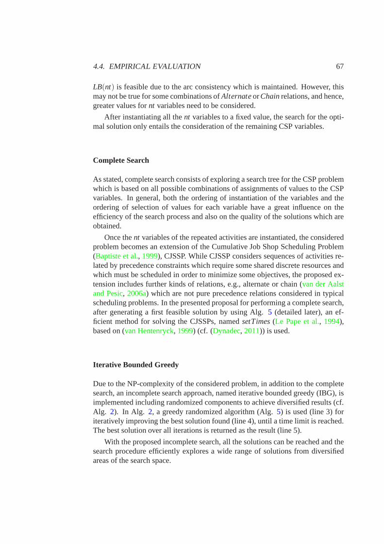
4.4. EMPIRICAL EVALUATION 67
LB(nt) is feasible due to the arc consistency which is maintained. However, thismay not be true for some combinations ofAlternateorChainrelations, and hence,greater values fornt variables need to be considered.
After instantiating all thent variables to a fixed value, the search for the opti-mal solution only entails the consideration of the remaining CSP variables.
Complete Search
As stated, complete search consists of exploring a search tree for the CSP problemwhich is based on all possible combinations of assignments of values to the CSPvariables. In general, both the ordering of instantiation of the variables and theordering of selection of values for each variable have a great influence on theefficiency of the search process and also on the quality of thesolutions which areobtained.
Once thent variables of the repeated activities are instantiated, theconsideredproblem becomes an extension of the Cumulative Job Shop Scheduling Problem(Baptiste et al., 1999), CJSSP. While CJSSP considers sequences of activities re-lated by precedence constraints which require some shared discrete resources andwhich must be scheduled in order to minimize some objectives, the proposed ex-tension includes further kinds of relations, e.g., alternate or chain (van der Aalstand Pesic, 2006a) which are not pure precedence relations considered in typicalscheduling problems. In the presented proposal for performing a complete search,after generating a first feasible solution by using Alg.5 (detailed later), an ef-ficient method for solving the CJSSPs, namedsetTimes(Le Pape et al., 1994),based on (van Hentenryck, 1999) (cf. (Dynadec, 2011)) is used.
Iterative Bounded Greedy
Due to the NP-complexity of the considered problem, in addition to the completesearch, an incomplete search approach, named iterative bounded greedy (IBG), isimplemented including randomized components to achieve diversified results (cf.Alg. 2). In Alg. 2, a greedy randomized algorithm (Alg.5) is used (line 3) foriteratively improving the best solution found (line 4), until a time limit is reached.The best solution over all iterations is returned as the result (line 5).
With the proposed incomplete search, all the solutions can be reached and thesearch procedure efficiently explores a wide range of solutions from diversifiedareas of the search space.
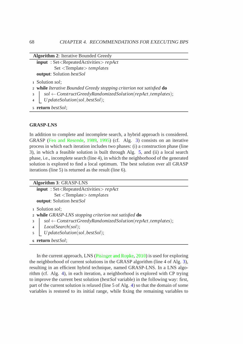
68 CHAPTER 4. RECOMMENDATIONS FOR EXECUTING BPS
Algorithm 2 : Iterative Bounded Greedyinput : Set<RepeatedActivities> repAct
Set<Template> templatesoutput: SolutionbestSol
Solutionsol;1
while Iterative Bounded Greedy stopping criterion not satisfieddo2
sol←ConstructGreedyRandomizedSolution(repAct, templates);3
U pdateSolution(sol,bestSol);4
return bestSol;5
GRASP-LNS
In addition to complete and incomplete search, a hybrid approach is considered.GRASP (Feo and Resende, 1989, 1995) (cf. Alg. 3) consists on an iterativeprocess in which each iteration includes two phases: (i) a construction phase (line3), in which a feasible solution is built through Alg.5, and (ii) a local searchphase, i.e., incomplete search (line 4), in which the neighborhood of the generatedsolution is explored to find a local optimum. The best solution over all GRASPiterations (line 5) is returned as the result (line 6).
Algorithm 3 : GRASP-LNSinput : Set<RepeatedActivities> repAct
Set<Template> templatesoutput: SolutionbestSol
Solutionsol;1
while GRASP-LNS stopping criterion not satisfieddo2
sol←ConstructGreedyRandomizedSolution(repAct, templates);3
LocalSearch(sol);4
U pdateSolution(sol,bestSol);5
return bestSol;6
In the current approach, LNS (Pisinger and Ropke, 2010) is used for exploringthe neighborhood of current solutions in the GRASP algorithm (line 4 of Alg. 3),resulting in an efficient hybrid technique, named GRASP-LNS. In a LNS algo-rithm (cf. Alg. 4), in each iteration, a neighborhood is explored with CP tryingto improve the current best solution (bestSolvariable) in the following way: first,part of the current solution is relaxed (line 5 of Alg.4) so that the domain of somevariables is restored to its initial range, while fixing the remaining variables to
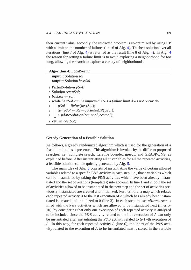
4.4. EMPIRICAL EVALUATION 69
their current value; secondly, the restricted problem is re-optimized by using CPwith a limit on the number of failures (line 6 of Alg.4). The best solution over alliterations (line 7 of Alg.4) is returned as the result (line 8 of Alg.4). In Alg. 4the reason for setting a failure limit is to avoid exploring aneighborhood for toolong, allowing the search to explore a variety of neighborhoods.
Algorithm 4 : LocalSearchinput : Solutionsoloutput: SolutionbestSol
PartialSolutionpSol;1
SolutiontempSol;2
bestSol← sol;3
while bestSol can be improved AND a failure limit does not occurdo4
pSol←Relax(bestSol);5
tempSol← Re−optimizeCP(pSol);6
U pdateSolution(tempSol,bestSol);7
return bestSol;8
Greedy Generation of a Feasible Solution
As follows, a greedy randomized algorithm which is used for the generation of afeasible solutions is presented. This algorithm is invokedby the different proposedsearches, i.e., complete search, iterative bounded greedy, and GRASP-LNS, asexplained before. After instantiating allnt variables for all the repeated activities,a feasible solution can be quickly generated by Alg.5.
The main idea of Alg.5 consists of instantiating the value of certain allowedvariables related to a specific P&S activity in each step, i.e., those variables whichcan be instantiated by taking the P&S activities which have been already instan-tiated and the set of relations (templates) into account. Inline 1 and 2, both the setof activities allowed to be instantiated in the next step andthe set of activities pre-viously instantiated are created and initialized. Furthermore, a map which relateseach repeated activityA to the last execution ofA which has already been instan-tiated is created and initialized to 0 (line 3). In each step,the setallowedActsisfilled with the P&S activities which are allowed to be instantiated next (lines 5-10), by considering that only one execution of each repeatedactivity is analyzedto be included since the P&S activity related to the i-th execution of A can onlybe instantiated after instantiating the P&S activity related to (i-1)-th execution ofA. In this way, for each repeated activityA (line 6), the index of the P&S acti-vity related to the execution ofA to be instantiated next is stored in the variable
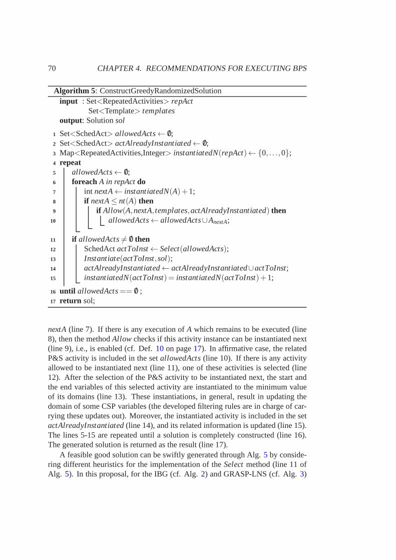
70 CHAPTER 4. RECOMMENDATIONS FOR EXECUTING BPS
Algorithm 5 : ConstructGreedyRandomizedSolutioninput : Set<RepeatedActivities> repAct
Set<Template> templatesoutput: Solutionsol
Set<SchedAct> allowedActs← /0;1
Set<SchedAct> actAlreadyInstantiated← /0;2
Map<RepeatedActivities,Integer> instantiatedN(repAct)←{0, . . . ,0};3
repeat4
allowedActs← /0;5
foreach A in repActdo6
int nextA← instantiatedN(A)+1;7
if nextA≤ nt(A) then8
if Allow(A,nextA, templates,actAlreadyInstantiated) then9
allowedActs← allowedActs∪AnextA;10
if allowedActs6= /0 then11
SchedActactToInst← Select(allowedActs);12
Instantiate(actToInst,sol);13
actAlreadyInstantiated← actAlreadyInstantiated∪actToInst;14
instantiatedN(actToInst)= instantiatedN(actToInst)+1;15
until allowedActs== /0 ;16
return sol;17
nextA(line 7). If there is any execution ofA which remains to be executed (line8), then the methodAllow checks if this activity instance can be instantiated next(line 9), i.e., is enabled (cf. Def.10 on page17). In affirmative case, the relatedP&S activity is included in the setallowedActs(line 10). If there is any activityallowed to be instantiated next (line 11), one of these activities is selected (line12). After the selection of the P&S activity to be instantiated next, the start andthe end variables of this selected activity are instantiated to the minimum valueof its domains (line 13). These instantiations, in general,result in updating thedomain of some CSP variables (the developed filtering rules are in charge of car-rying these updates out). Moreover, the instantiated activity is included in the setactAlreadyInstantiated(line 14), and its related information is updated (line 15).The lines 5-15 are repeated until a solution is completely constructed (line 16).The generated solution is returned as the result (line 17).
A feasible good solution can be swiftly generated through Alg. 5 by conside-ring different heuristics for the implementation of theSelectmethod (line 11 ofAlg. 5). In this proposal, for the IBG (cf. Alg.2) and GRASP-LNS (cf. Alg.3)
4.4. EMPIRICAL EVALUATION 71
searches, in order to get diversified results each time Alg.5 is invoked, theSelectmethod is implemented (heuristic) so that the activities are selected by consideringthe probabilityπ(A) of selecting an activityA as:
π(A) = 1/r(A)∑B∈Acts1/r(B)
wherer(A) denote the rank ofA when all the candidates are ranked accordingto their earliest start time.
On the other hand, for the complete search, the heuristic which is consideredselects the activity with the lowest starting time, i.e., the most promising one, sincefor the considered complete search Alg.5 is only used for generating an initialsolution. In most cases, this initial solution will be improved as the completesearch proceed.
Notice that for a feasible combination ofnt values, Alg.5 always generates afeasible solution, since the arc consistency is maintainedduring all the process bythe developed filtering rules.
4.4.2 Experimental Design
In this section, the design underlying the experiment is detailed.Purpose: The purpose of the empirical evaluation is to analyze the behavior
of the proposed approach in the generation of optimal enactment plans from ex-tended ConDec specifications (including estimates), in order to test the suitabilityof the proposed approach for giving recommendations, in terms of performanceand quality of recommendations. In particular, to investigate in how far diffe-rent search algorithms are suitable for solving the considered problems is aimed.Specifically, three search algorithms are tested for solving the generated models(cf. Sect.4.4.1), i.e., complete search (CP), iterative bounded greedy (IBG), andhybrid search (GRASP-LNS). Since the underlying strategies of the consideredsearch techniques are completely different, to investigate under which circums-tances each one is the most suitable for obtaining the solution of certain problemsis aimed. Moreover, to find out whether these techniques are complementary isanalyzed, and hence whether they can be used in a combined wayfor obtaining agood solution. The suitability of the proposed approach is tested regarding both(1) build-time, i.e., generation of complete optimized plans before starting theBP enactment; and (2) run-time, i.e., generation of (partial) optimized plans byconsidering the actual partial trace of the process as the execution of the processproceeds.
Objects: The empirical evaluation considers different ConDec models takingsome important characteristics into account in the generation of the models: (i)correctness, i.e., the ConDec models must represent feasible problems withoutconflicts (i.e., there are some traces that satisfy the model) and must not include
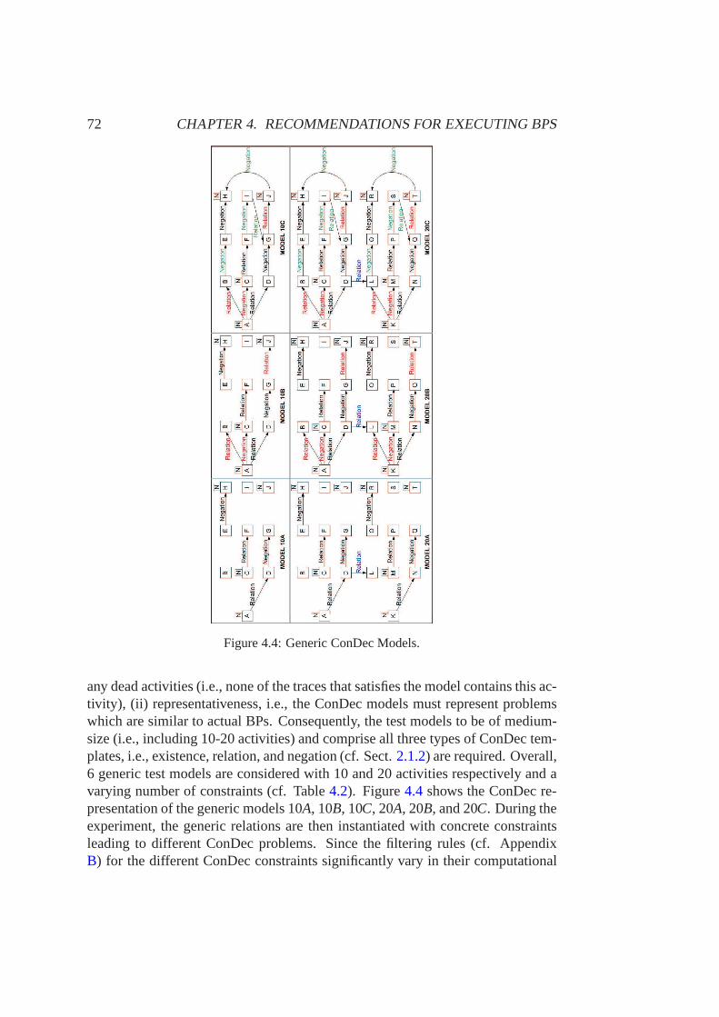
72 CHAPTER 4. RECOMMENDATIONS FOR EXECUTING BPS
Figure 4.4: Generic ConDec Models.
any dead activities (i.e., none of the traces that satisfies the model contains this ac-tivity), (ii) representativeness, i.e., the ConDec modelsmust represent problemswhich are similar to actual BPs. Consequently, the test models to be of medium-size (i.e., including 10-20 activities) and comprise all three types of ConDec tem-plates, i.e., existence, relation, and negation (cf. Sect.2.1.2) are required. Overall,6 generic test models are considered with 10 and 20 activities respectively and avarying number of constraints (cf. Table4.2). Figure4.4 shows the ConDec re-presentation of the generic models 10A, 10B, 10C, 20A, 20B, and 20C. During theexperiment, the generic relations are then instantiated with concrete constraintsleading to different ConDec problems. Since the filtering rules (cf. AppendixB) for the different ConDec constraints significantly vary intheir computational
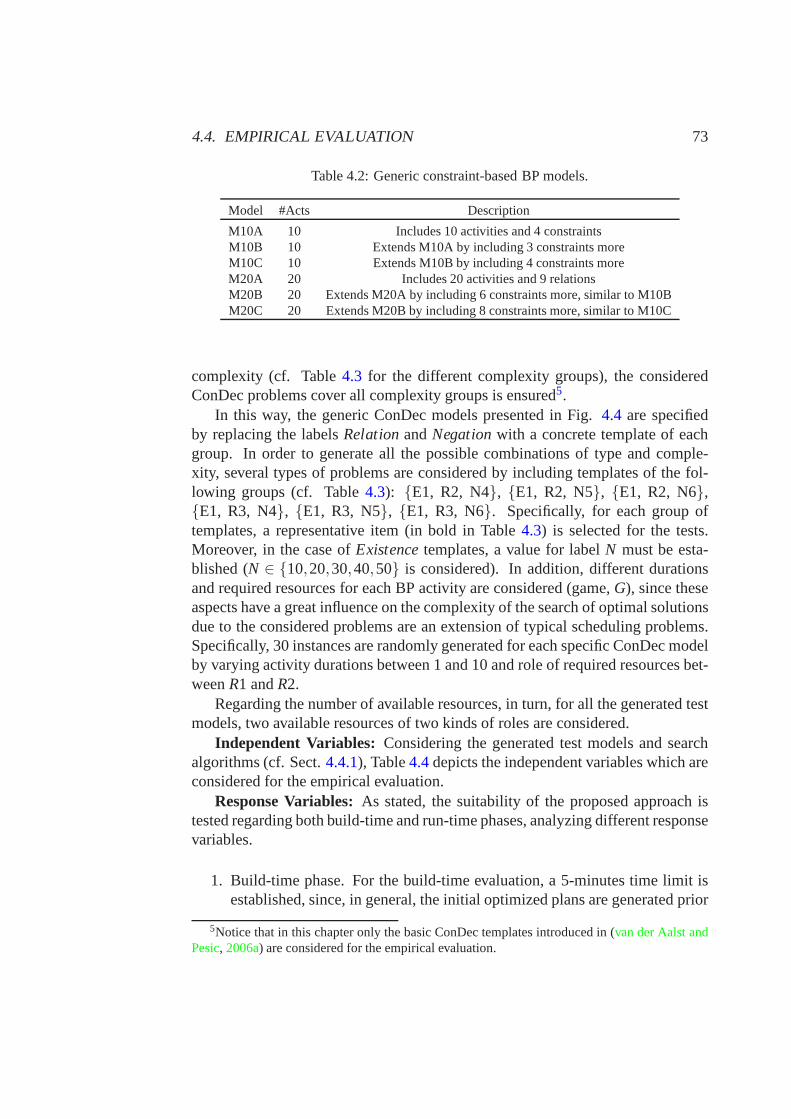
4.4. EMPIRICAL EVALUATION 73
Table 4.2: Generic constraint-based BP models.
Model #Acts Description
M10A 10 Includes 10 activities and 4 constraintsM10B 10 Extends M10A by including 3 constraints moreM10C 10 Extends M10B by including 4 constraints moreM20A 20 Includes 20 activities and 9 relationsM20B 20 Extends M20A by including 6 constraints more, similar to M10BM20C 20 Extends M20B by including 8 constraints more, similar to M10C
complexity (cf. Table4.3 for the different complexity groups), the consideredConDec problems cover all complexity groups is ensured5.
In this way, the generic ConDec models presented in Fig.4.4 are specifiedby replacing the labelsRelationandNegationwith a concrete template of eachgroup. In order to generate all the possible combinations oftype and comple-xity, several types of problems are considered by includingtemplates of the fol-lowing groups (cf. Table4.3): {E1, R2, N4}, {E1, R2, N5}, {E1, R2, N6},{E1, R3, N4}, {E1, R3, N5}, {E1, R3, N6}. Specifically, for each group oftemplates, a representative item (in bold in Table4.3) is selected for the tests.Moreover, in the case ofExistencetemplates, a value for labelN must be esta-blished (N ∈ {10,20,30,40,50} is considered). In addition, different durationsand required resources for each BP activity are considered (game,G), since theseaspects have a great influence on the complexity of the searchof optimal solutionsdue to the considered problems are an extension of typical scheduling problems.Specifically, 30 instances are randomly generated for each specific ConDec modelby varying activity durations between 1 and 10 and role of required resources bet-weenR1 andR2.
Regarding the number of available resources, in turn, for all the generated testmodels, two available resources of two kinds of roles are considered.
Independent Variables: Considering the generated test models and searchalgorithms (cf. Sect.4.4.1), Table4.4depicts the independent variables which areconsidered for the empirical evaluation.
Response Variables:As stated, the suitability of the proposed approach istested regarding both build-time and run-time phases, analyzing different responsevariables.
1. Build-time phase. For the build-time evaluation, a 5-minutes time limit isestablished, since, in general, the initial optimized plans are generated prior
5Notice that in this chapter only the basic ConDec templates introduced in (van der Aalst andPesic, 2006a) are considered for the empirical evaluation.
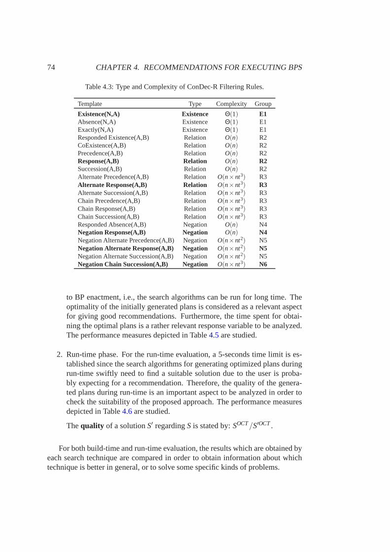
74 CHAPTER 4. RECOMMENDATIONS FOR EXECUTING BPS
Table 4.3: Type and Complexity of ConDec-R Filtering Rules.
Template Type Complexity Group
Existence(N,A) Existence Θ(1) E1Absence(N,A) Existence Θ(1) E1Exactly(N,A) Existence Θ(1) E1Responded Existence(A,B) Relation O(n) R2CoExistence(A,B) Relation O(n) R2Precedence(A,B) Relation O(n) R2Response(A,B) Relation O(n) R2Succession(A,B) Relation O(n) R2Alternate Precedence(A,B) Relation O(n×nt3) R3Alternate Response(A,B) Relation O(n×nt3) R3Alternate Succession(A,B) Relation O(n×nt3) R3Chain Precedence(A,B) Relation O(n×nt3) R3Chain Response(A,B) Relation O(n×nt3) R3Chain Succession(A,B) Relation O(n×nt3) R3Responded Absence(A,B) Negation O(n) N4Negation Response(A,B) Negation O(n) N4Negation Alternate Precedence(A,B) NegationO(n×nt2) N5Negation Alternate Response(A,B) Negation O(n×nt2) N5Negation Alternate Succession(A,B) NegationO(n×nt2) N5Negation Chain Succession(A,B) Negation O(n×nt3) N6
to BP enactment, i.e., the search algorithms can be run for long time. Theoptimality of the initially generated plans is considered as a relevant aspectfor giving good recommendations. Furthermore, the time spent for obtai-ning the optimal plans is a rather relevant response variable to be analyzed.The performance measures depicted in Table4.5are studied.
2. Run-time phase. For the run-time evaluation, a 5-secondstime limit is es-tablished since the search algorithms for generating optimized plans duringrun-time swiftly need to find a suitable solution due to the user is proba-bly expecting for a recommendation. Therefore, the qualityof the genera-ted plans during run-time is an important aspect to be analyzed in order tocheck the suitability of the proposed approach. The performance measuresdepicted in Table4.6are studied.
Thequality of a solutionS′ regardingS is stated by:SOCT/S′OCT.
For both build-time and run-time evaluation, the results which are obtained byeach search technique are compared in order to obtain information about whichtechnique is better in general, or to solve some specific kinds of problems.
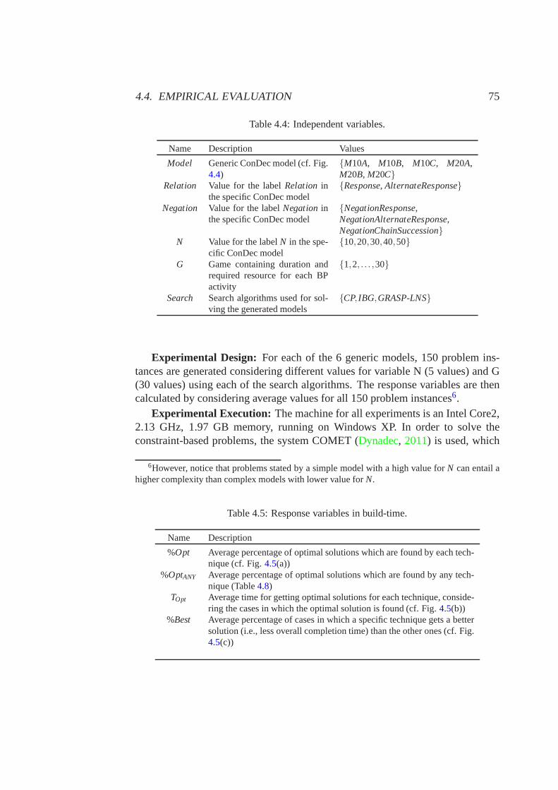
4.4. EMPIRICAL EVALUATION 75
Table 4.4: Independent variables.
Name Description Values
Model Generic ConDec model (cf. Fig.4.4)
{M10A, M10B, M10C, M20A,M20B, M20C}
Relation Value for the labelRelation inthe specific ConDec model
{Response, AlternateResponse}
Negation Value for the labelNegationinthe specific ConDec model
{NegationResponse,NegationAlternateResponse,NegationChainSuccession}
N Value for the labelN in the spe-cific ConDec model
{10,20,30,40,50}
G Game containing duration andrequired resource for each BPactivity
{1,2, . . . ,30}
Search Search algorithms used for sol-ving the generated models
{CP, IBG,GRASP-LNS}
Experimental Design: For each of the 6 generic models, 150 problem ins-tances are generated considering different values for variable N (5 values) and G(30 values) using each of the search algorithms. The response variables are thencalculated by considering average values for all 150 problem instances6.
Experimental Execution: The machine for all experiments is an Intel Core2,2.13 GHz, 1.97 GB memory, running on Windows XP. In order to solve theconstraint-based problems, the system COMET (Dynadec, 2011) is used, which
6However, notice that problems stated by a simple model with ahigh value forN can entail ahigher complexity than complex models with lower value forN.
Table 4.5: Response variables in build-time.
Name Description
%Opt Average percentage of optimal solutions which are found by each tech-nique (cf. Fig.4.5(a))
%OptANY Average percentage of optimal solutions which are found by any tech-nique (Table4.8)
TOpt Average time for getting optimal solutions for each technique, conside-ring the cases in which the optimal solution is found (cf. Fig. 4.5(b))
%Best Average percentage of cases in which a specific technique gets a bettersolution (i.e., less overall completion time) than the other ones (cf. Fig.4.5(c))
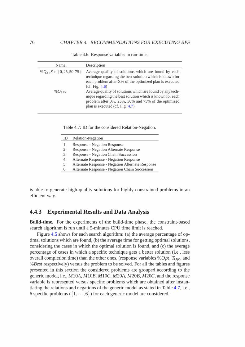
76 CHAPTER 4. RECOMMENDATIONS FOR EXECUTING BPS
Table 4.6: Response variables in run-time.
Name Description
%QX ,X ∈ {0,25,50,75} Average quality of solutions which are found by eachtechnique regarding the best solution which is known foreach problem after X% of the optimized plan is executed(cf. Fig. 4.6)
%QANY Average quality of solutions which are found by any tech-nique regarding the best solution which is known for eachproblem after 0%, 25%, 50% and 75% of the optimizedplan is executed (cf. Fig.4.7)
Table 4.7: ID for the considered Relation-Negation.
ID Relation-Negation
1 Response - Negation Response2 Response - Negation Alternate Response3 Response - Negation Chain Succession4 Alternate Response - Negation Response5 Alternate Response - Negation Alternate Response6 Alternate Response - Negation Chain Succession
is able to generate high-quality solutions for highly constrained problems in anefficient way.
4.4.3 Experimental Results and Data Analysis
Build-time. For the experiments of the build-time phase, the constraint-basedsearch algorithm is run until a 5-minutes CPU time limit is reached.
Figure4.5shows for each search algorithm: (a) the average percentageof op-timal solutions which are found, (b) the average time for getting optimal solutions,considering the cases in which the optimal solution is found, and (c) the averagepercentage of cases in which a specific technique gets a better solution (i.e., lessoverall completion time) than the other ones, (response variables %Opt, TOpt, and%Bestrespectively) versus the problem to be solved. For all the tables and figurespresented in this section the considered problems are grouped according to thegeneric model, i.e.,M10A, M10B, M10C, M20A, M20B, M20C, and the responsevariable is represented versus specific problems which are obtained after instan-tiating the relations and negations of the generic model as stated in Table4.7, i.e.,6 specific problems ({1, . . . ,6}) for each generic model are considered.
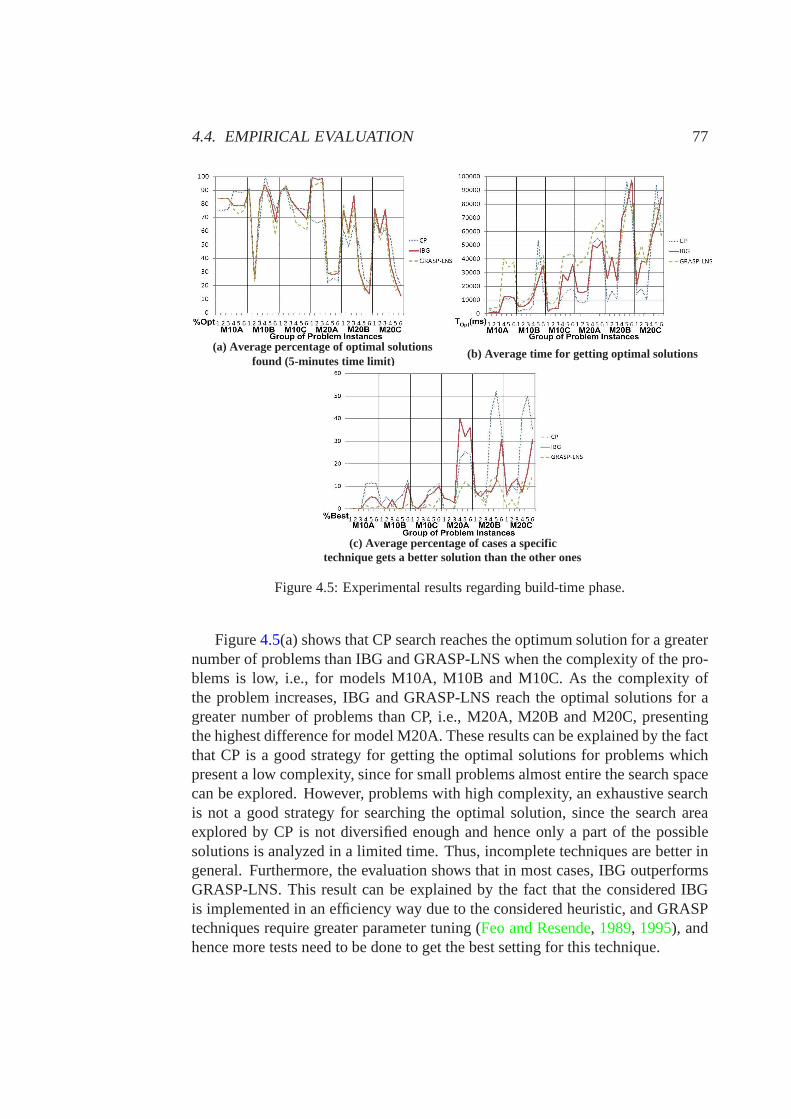
4.4. EMPIRICAL EVALUATION 77
(a) Average percentage of optimal solutions found (5-minutes time limit)
(b) Average time for getting optimal solutions
(c) Average percentage of cases a specific technique gets a better solution than the other ones
Figure 4.5: Experimental results regarding build-time phase.
Figure4.5(a) shows that CP search reaches the optimum solution for a greaternumber of problems than IBG and GRASP-LNS when the complexity of the pro-blems is low, i.e., for models M10A, M10B and M10C. As the complexity ofthe problem increases, IBG and GRASP-LNS reach the optimal solutions for agreater number of problems than CP, i.e., M20A, M20B and M20C, presentingthe highest difference for model M20A. These results can be explained by the factthat CP is a good strategy for getting the optimal solutions for problems whichpresent a low complexity, since for small problems almost entire the search spacecan be explored. However, problems with high complexity, anexhaustive searchis not a good strategy for searching the optimal solution, since the search areaexplored by CP is not diversified enough and hence only a part of the possiblesolutions is analyzed in a limited time. Thus, incomplete techniques are better ingeneral. Furthermore, the evaluation shows that in most cases, IBG outperformsGRASP-LNS. This result can be explained by the fact that the considered IBGis implemented in an efficiency way due to the considered heuristic, and GRASPtechniques require greater parameter tuning (Feo and Resende, 1989, 1995), andhence more tests need to be done to get the best setting for this technique.
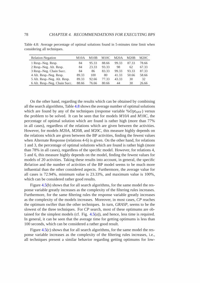
78 CHAPTER 4. RECOMMENDATIONS FOR EXECUTING BPS
Table 4.8: Average percentage of optimal solutions found in5-minutes time limit whenconsidering all techniques.
Relation-Negation M10A M10B M10C M20A M20B M20C
1 Resp.-Neg. Resp. 84 95.33 88.66 99.33 87.33 78.662 Resp.-Neg. Alt. Resp. 84 23.33 93.33 98 62 67.333 Resp.-Neg. Chain Succ. 84 86 83.33 99.33 93.33 87.334 Alt. Resp.-Neg. Resp. 89.33 100 80 41.33 50.66 58.665 Alt. Resp.-Neg. Alt. Resp. 89.33 92.66 77.33 43.33 30 326 Alt. Resp.-Neg. Chain Succ. 88.66 76.66 80.66 44 30 26.66
On the other hand, regarding the results which can be obtained by combiningall the search algorithms, Table4.8shows the average number of optimal solutionswhich are found by any of the techniques (response variable %OptANY) versusthe problem to be solved. It can be seen that for modelsM10A andM10C, thepercentage of optimal solution which are found is rather high (more than 77%in all cases), regardless of the relations which are given between the activities.However, for modelsM20A, M20B, andM20C, this measure highly depends onthe relations which are given between the BP activities, finding the fewest valueswhen Alternate Response (relations 4-6) is given. On the other hand, for relations1 and 3, the percentage of optimal solutions which are found is rather high (morethan 78% in all cases), regardless of the specific model. However, for relations 4,5 and 6, this measure highly depends on the model, finding the fewest values formodels of 20 activities. Taking these results into account,in general, the specificRelationand the number of activities of the BP model seems to be much moreinfluential than the other considered aspects. Furthermore, the average value forall cases is 72.94%, minimum value is 23.33%, and maximum value is 100%,which can be considered rather good results.
Figure4.5(b) shows that for all search algorithms, for the same model the res-ponse variable greatly increases as the complexity of the filtering rules increases.Furthermore, for the same filtering rules the response variable greatly increasesas the complexity of the models increases. Moreover, in mostcases,CP reachesthe optimum swifter than the other techniques. In turn,GRASP, seems to be theslowest of the three techniques. ForCP search, most of these optimums are ob-tained for the simplest models (cf. Fig.4.5(a)), and hence, less time is required.In general, it can be seen that the average time for getting optimums is less than100 seconds, which can be considered a rather good result.
Figure4.5(c) shows that for all search algorithms, for the same model the res-ponse variable increases as the complexity of the filtering rules increases, i.e.,all techniques present a similar behavior regarding getting optimums for low-
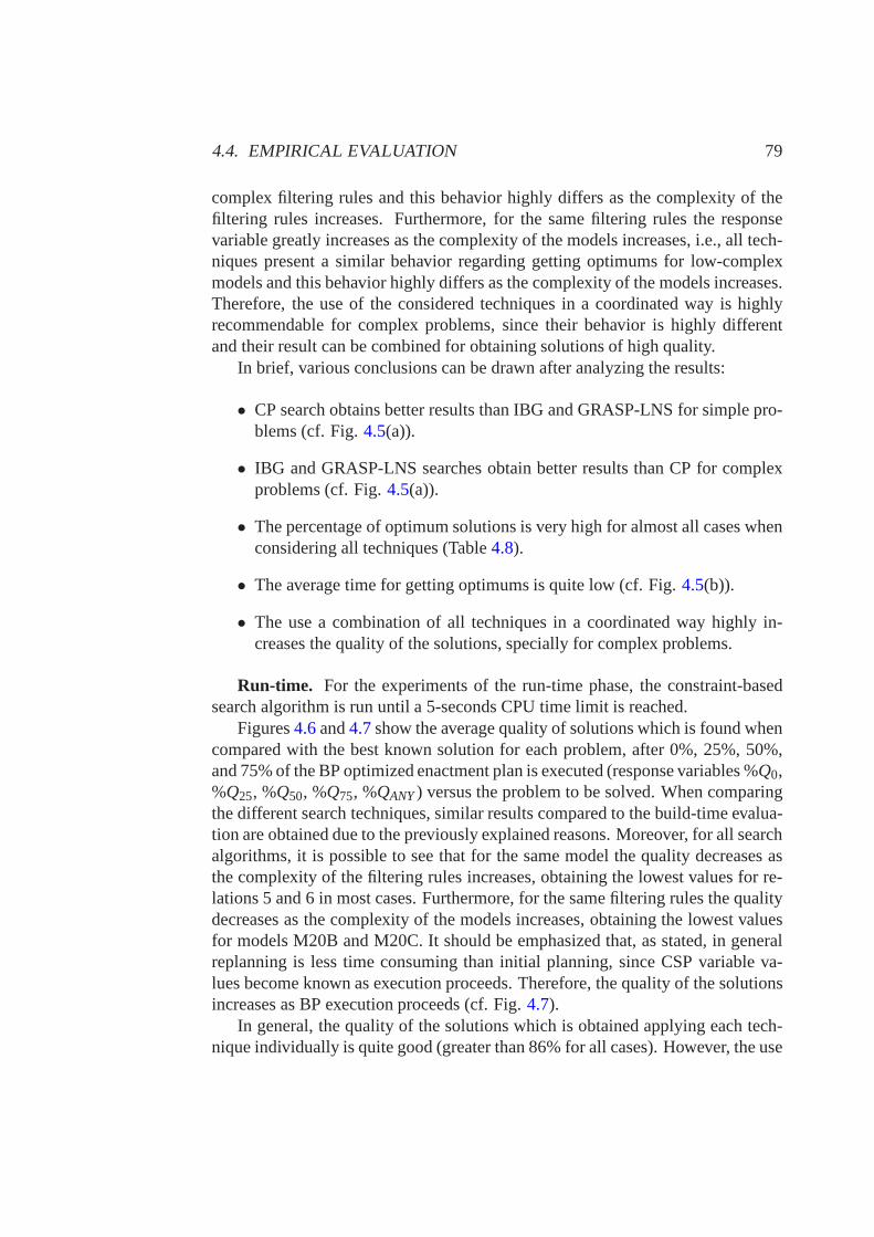
4.4. EMPIRICAL EVALUATION 79
complex filtering rules and this behavior highly differs as the complexity of thefiltering rules increases. Furthermore, for the same filtering rules the responsevariable greatly increases as the complexity of the models increases, i.e., all tech-niques present a similar behavior regarding getting optimums for low-complexmodels and this behavior highly differs as the complexity ofthe models increases.Therefore, the use of the considered techniques in a coordinated way is highlyrecommendable for complex problems, since their behavior is highly differentand their result can be combined for obtaining solutions of high quality.
In brief, various conclusions can be drawn after analyzing the results:
• CP search obtains better results than IBG and GRASP-LNS for simple pro-blems (cf. Fig.4.5(a)).
• IBG and GRASP-LNS searches obtain better results than CP forcomplexproblems (cf. Fig.4.5(a)).
• The percentage of optimum solutions is very high for almost all cases whenconsidering all techniques (Table4.8).
• The average time for getting optimums is quite low (cf. Fig.4.5(b)).
• The use a combination of all techniques in a coordinated way highly in-creases the quality of the solutions, specially for complexproblems.
Run-time. For the experiments of the run-time phase, the constraint-basedsearch algorithm is run until a 5-seconds CPU time limit is reached.
Figures4.6and4.7show the average quality of solutions which is found whencompared with the best known solution for each problem, after 0%, 25%, 50%,and 75% of the BP optimized enactment plan is executed (response variables %Q0,%Q25, %Q50, %Q75, %QANY) versus the problem to be solved. When comparingthe different search techniques, similar results comparedto the build-time evalua-tion are obtained due to the previously explained reasons. Moreover, for all searchalgorithms, it is possible to see that for the same model the quality decreases asthe complexity of the filtering rules increases, obtaining the lowest values for re-lations 5 and 6 in most cases. Furthermore, for the same filtering rules the qualitydecreases as the complexity of the models increases, obtaining the lowest valuesfor models M20B and M20C. It should be emphasized that, as stated, in generalreplanning is less time consuming than initial planning, since CSP variable va-lues become known as execution proceeds. Therefore, the quality of the solutionsincreases as BP execution proceeds (cf. Fig.4.7).
In general, the quality of the solutions which is obtained applying each tech-nique individually is quite good (greater than 86% for all cases). However, the use
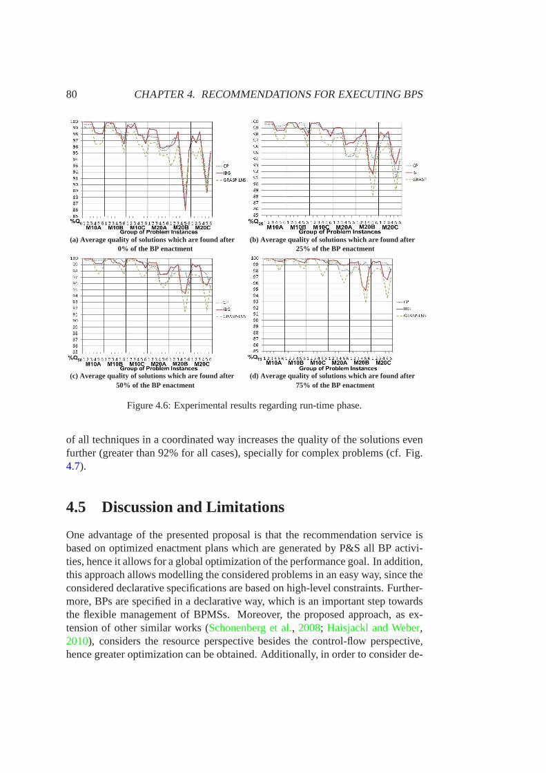
80 CHAPTER 4. RECOMMENDATIONS FOR EXECUTING BPS
(a) Average quality of solutions which are found after 0% of the BP enactment
(b) Average quality of solutions which are found after 25% of the BP enactment
(c) Average quality of solutions which are found after 50% of the BP enactment
(d) Average quality of solutions which are found after 75% of the BP enactment
Figure 4.6: Experimental results regarding run-time phase.
of all techniques in a coordinated way increases the qualityof the solutions evenfurther (greater than 92% for all cases), specially for complex problems (cf. Fig.4.7).
4.5 Discussion and Limitations
One advantage of the presented proposal is that the recommendation service isbased on optimized enactment plans which are generated by P&S all BP activi-ties, hence it allows for a global optimization of the performance goal. In addition,this approach allows modelling the considered problems in an easy way, since theconsidered declarative specifications are based on high-level constraints. Further-more, BPs are specified in a declarative way, which is an important step towardsthe flexible management of BPMSs. Moreover, the proposed approach, as ex-tension of other similar works (Schonenberg et al., 2008; Haisjackl and Weber,2010), considers the resource perspective besides the control-flow perspective,hence greater optimization can be obtained. Additionally,in order to consider de-
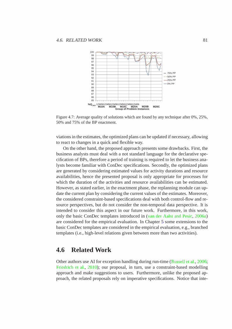
4.6. RELATED WORK 81
85 86 87 88 89 90 91 92 93 94 95 96 97 98 99
100
1 2 3 4 5 6 1 2 3 4 5 6 1 2 3 4 5 6 1 2 3 4 5 6 1 2 3 4 5 6 1 2 3 4 5 6
75% PP
50% PP
25% PP
0% PP
M10A M10B M10C M20A M20B M20C %Q ANY
Group of Problem Instances
Figure 4.7: Average quality of solutions which are found by any technique after 0%, 25%,50% and 75% of the BP enactment.
viations in the estimates, the optimized plans can be updated if necessary, allowingto react to changes in a quick and flexible way.
On the other hand, the proposed approach presents some drawbacks. First, thebusiness analysts must deal with a not standard language forthe declarative spe-cification of BPs, therefore a period of training is requiredto let the business ana-lysts become familiar with ConDec specifications. Secondly, the optimized plansare generated by considering estimated values for activitydurations and resourceavailabilities, hence the presented proposal is only appropriate for processes forwhich the duration of the activities and resource availabilities can be estimated.However, as stated earlier, in the enactment phase, the replanning module can up-date the current plan by considering the current values of the estimates. Moreover,the considered constraint-based specifications deal with both control-flow and re-source perspectives, but do not consider the non-temporal data perspective. It isintended to consider this aspect in our future work. Furthermore, in this work,only the basic ConDec templates introduced in (van der Aalst and Pesic, 2006a)are considered for the empirical evaluation. In Chapter5 some extensions to thebasic ConDec templates are considered in the empirical evaluation, e.g., branchedtemplates (i.e., high-level relations given between more than two activities).
4.6 Related Work
Other authors use AI for exception handling during run-time(Russell et al., 2006;Friedrich et al., 2010); our proposal, in turn, use a constraint-based modellingapproach and make suggestions to users. Furthermore, unlike the proposed ap-proach, the related proposals rely on imperative specifications. Notice that inte-
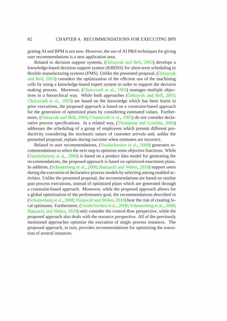
82 CHAPTER 4. RECOMMENDATIONS FOR EXECUTING BPS
grating AI and BPM is not new. However, the use of AI P&S techniques for givinguser recommendations is a new application area.
Related to decision support systems, (Ozbayrak and Bell, 2003) develops aknowledge-based decision support system (KBDSS) for short-term scheduling inflexible manufacturing systems (FMS). Unlike the presentedproposal, (Ozbayrakand Bell, 2003) considers the optimization of the efficient use of the machiningcells by using a knowledge-based expert system in order to support the decisionmaking process. Moreover, (Chaturvedi et al., 1993) manages multiple objec-tives in a hierarchical way. While both approaches (Ozbayrak and Bell, 2003;Chaturvedi et al., 1993) are based on the knowledge which has been learnt inprior executions, the proposed approach is based on a constraint-based approachfor the generation of optimized plans by considering estimated values. Further-more, (Ozbayrak and Bell, 2003; Chaturvedi et al., 1993) do not consider decla-rative process specifications. In a related way, (Thompson and Goodale, 2006)addresses the scheduling of a group of employees which present different pro-ductivity considering the stochastic nature of customer arrivals and, unlike thepresented proposal, replans during run-time when estimates are incorrect.
Related to user recommendations, (Vanderfeesten et al., 2008) generates re-commendations to select the next step to optimize some objective functions. While(Vanderfeesten et al., 2008) is based on a product data model for generating therecommendations, the proposed approach is based on optimized enactment plans.In addition, (Schonenberg et al., 2008; Haisjackl and Weber, 2010) support usersduring the execution of declarative process models by selecting among enabled ac-tivities. Unlike the presented proposal, the recommendations are based on similarpast process executions, instead of optimized plans which are generated througha constraint-based approach. Moreover, while the proposedapproach allows fora global optimization of the performance goal, the recommendations described in(Schonenberg et al., 2008; Haisjackl and Weber, 2010) bear the risk of creating lo-cal optimums. Furthermore, (Vanderfeesten et al., 2008; Schonenberg et al., 2008;Haisjackl and Weber, 2010) only consider the control-flow perspective, while theproposed approach also deals with the resource perspective. All of the previouslymentioned approaches optimize the execution of single process instances. Theproposed approach, in turn, provides recommendations for optimizing the execu-tion of several instances.
Chapter 5
From Optimized BP EnactmentPlans to Optimized BP Models
5.1 Introduction
5.1.1 Motivation
The Process Design & Analysis phase plays an important role in the BPM life cy-cle for any improvement initiative, since it greatly influences the remaining phasesof this cycle. In addition, also run-time aspects are important for BP improvement,e.g., resource allocation and scheduling may significantlyimpact business processperformance.
Traditionally, two steps are considered in the BP Design & Analysis phaseto create a BP model (Aguilar-Saven, 2004). The first step consists of analyzingthe business process, e.g., by interviewing stakeholders (people involved in theprocess), in order to draw an initial BP model (as-is model).Secondly, in orderto improve this initial model, different techniques can be employed like simula-tion (Barjis and Verbraeck, 2010) or BP redesign (Reijers, 2003), resulting in thegeneration of a to-be model. Typically, different quality dimensions like time,cost, flexibility and quality can be differentiated (Reijers, 2003) between whichtrade-off decisions have to be made when creating a BP design. Once a certainprocess design has been chosen and implemented, business processes are execu-ted according to this design1. During process execution, scheduling decisions arethen typically made by the BPM systems (BPMSs), by automatically assigningactivities to resources (Russell et al., 2005).
In most cases, the overall process of creating a BP model is carried out manua-lly by business analysts, who specify the BP information through an imperative
1In this chapter, the assumption that there is a BPMS executing the BPs is made.
83
84 CHAPTER 5. OPTIMIZED PLANS TO OPTIMIZED BP MODELS
language by choosing between several different alternative designs the one whichbest meets the performance goals of the organization. Therefore, analysts mustdeal with several aspects in order to generate a suitable BP model, such as: (1)the activity properties, e.g., activity duration, resource or role which is requiredfor activity execution, (2) the relations between the activities, i.e., control-flowof the BP, and (3) the optimization of several objectives, e.g., minimization ofcompletion time. The manual specification of imperative BP models can there-fore form a very complex problem, i.e., it can consume a greatquantity of timeand human resources, may cause certain failures, and may lead to non-optimizedmodels since the tacit nature of human knowledge is often an obstacle to elicitingaccurate process models (Ferreira and Ferreira, 2006).
Moreover, the result of process modelling is typically a static plan of action,which is difficult to adapt to changing procedures or to different business goals(Ferreira and Ferreira, 2006).
Not only the process design, but also the allocation of resources during processexecution has a great influence on process performance. However, schedulingis only considered to a limited degree in existing BPMSs, andis typically doneduring run-time by assigning activities to resources.
5.1.2 Contribution
To support process analysts in the definition of optimized BPmodels, a methodfor automatically generating imperative BP models using AIplanning techniquesfrom constraint-based specifications (which describe the activities to be execu-ted as well as constraints to be considered) is suggested. Unlike imperative mo-dels, the specification of process properties in a declarative way, e.g., using aconstraint-based specification, only requires process designers to state what hasto be done instead of having to specify how it has to be done. The proposed AI-based approach, in turn, is in charge of determining how it isto be done in orderto satisfy the constraints imposed by de constraint-based problem specifications,and to attain an optimization of certain objective functions (e.g., minimization ofcompletion time). For this optimization, scheduling is done on a short-term ba-sis by considering the optimization of a set of instances, which is typically notconsidered in most BPMSs.
Figure5.1 provides an overview of the proposed approach. Consideringtheconstraint-based specifications as a starting point (cf. Fig. 5.1(1)), enactmentplans can automatically be generated (cf. Fig.5.1(2)), as detailed in Chapter3.The generated enactment plans are then automatically translated into a BPMNmodel (BPMN, 2011) (cf. Fig. 5.1(3)), which can be then further improved by abusiness analyst, where necessary. In most cases, BPMN models can be translatedinto an execution language (Ouyang et al., 2006), such as BPEL (BPEL, 2007),
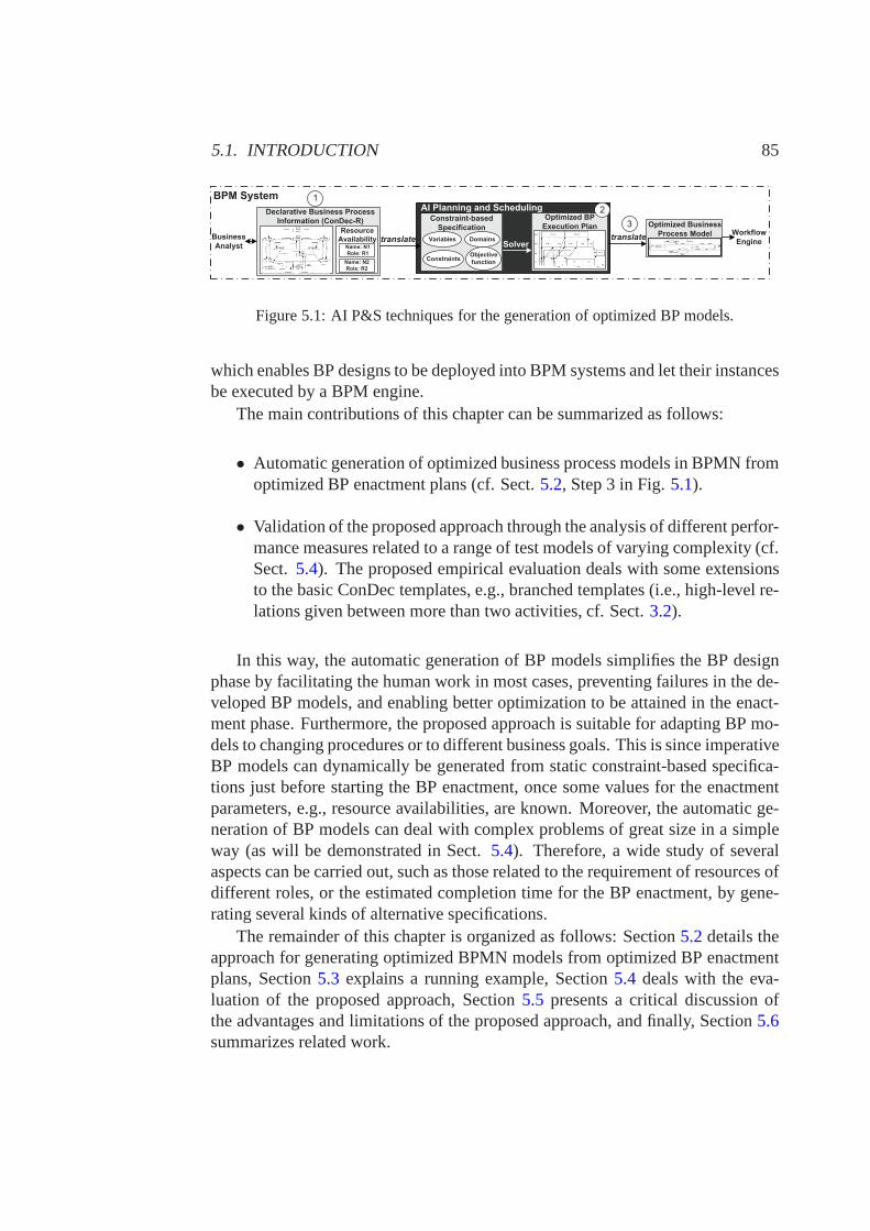
5.1. INTRODUCTION 85
Declarative Business Process
Information (ConDec-R)
Resource
AvailabilityName: N1
Role: R1
translateBusiness
Analyst
Optimized Business
Process Model Workflow
Engine
AI Planning and Scheduling
BPM System
Name: N2
Role: R2
translate
Constraint-based
Specification
SolverVariables
ConstraintsObjective
function
Domains
Optimized BP
Execution Plan
1
2
3
Figure 5.1: AI P&S techniques for the generation of optimized BP models.
which enables BP designs to be deployed into BPM systems and let their instancesbe executed by a BPM engine.
The main contributions of this chapter can be summarized as follows:
• Automatic generation of optimized business process modelsin BPMN fromoptimized BP enactment plans (cf. Sect.5.2, Step 3 in Fig.5.1).
• Validation of the proposed approach through the analysis ofdifferent perfor-mance measures related to a range of test models of varying complexity (cf.Sect. 5.4). The proposed empirical evaluation deals with some extensionsto the basic ConDec templates, e.g., branched templates (i.e., high-level re-lations given between more than two activities, cf. Sect.3.2).
In this way, the automatic generation of BP models simplifiesthe BP designphase by facilitating the human work in most cases, preventing failures in the de-veloped BP models, and enabling better optimization to be attained in the enact-ment phase. Furthermore, the proposed approach is suitablefor adapting BP mo-dels to changing procedures or to different business goals.This is since imperativeBP models can dynamically be generated from static constraint-based specifica-tions just before starting the BP enactment, once some values for the enactmentparameters, e.g., resource availabilities, are known. Moreover, the automatic ge-neration of BP models can deal with complex problems of greatsize in a simpleway (as will be demonstrated in Sect.5.4). Therefore, a wide study of severalaspects can be carried out, such as those related to the requirement of resources ofdifferent roles, or the estimated completion time for the BPenactment, by gene-rating several kinds of alternative specifications.
The remainder of this chapter is organized as follows: Section 5.2details theapproach for generating optimized BPMN models from optimized BP enactmentplans, Section5.3 explains a running example, Section5.4 deals with the eva-luation of the proposed approach, Section5.5 presents a critical discussion ofthe advantages and limitations of the proposed approach, and finally, Section5.6summarizes related work.
86 CHAPTER 5. OPTIMIZED PLANS TO OPTIMIZED BP MODELS
5.2 From Optimized Enactment Plans to OptimizedBusiness Process Models
Section3.3 has described how optimized BP enactment plans can be generatedfrom ConDec-R specifications. This section describes how a BPMN model canbe generated from an optimized BP enactment plan. Notice that the imperativeBP model can be generated just before starting the BP enactment by consideringthe actual values of the resource availabilities.
The generated BPMN model includes the same activities to be executed in thesame ordering and also using the same resources than the enactment plan. Foreach role in the BP enactment plan, a BPMN pool (cf. Def.26) is created, whichcontains as many lanes as number of available resources for that role.
Definition 26. A BPMN pool BPMNPool= (role,#role) is a pool of a BPMNmodel, which is composed of#role lanes.
Moreover, for each scheduling activity in the BP enactment plan a BPMNactivity (cf. Def. 27) is created. Additionally, one start and one end activitiesareincluded in the BPMN model.
Definition 27. A BPMN activity BPMNAct= (pool, lane,dur,st) is an activityof a BPMN model placed in the lane named lane of the pool named pool, withduration dur and start time st.
One of the most important aspects to be considered for the generation of op-timized BPMN models are the precedence relations between the BPMN activities(scheduling activities, cf. Def.22 on page43). For establishing these precedencerelations the values for the start and the end times of the scheduling activities inthe enactment plan are considered. These precedence relations are then used as abasis for generating BPMN models (cf. Def.31) from BP enactment plans. Somerelated definitions are given below:
Definition 28. In a BP enactment plan regarding a CSP solution S, a schedulingactivity ai is apredecessorof another scheduling activity bj , ai ∈ predecessors(b j),if the relation Set(ai) ≤ Sst(b j) holds due to resource or template relations.
Definition 29. In a BP enactment plan, a scheduling activity ai is a direct prede-cessorof another scheduling activity bj , ai ∈ DP(b j), if ai ∈ predecessors(b j) ∧6 ∃ck ∈ predecessors(b j) | ai ∈ predecessors(ck).
Definition 30. In a BP enactment plan, a scheduling activity ai is anindirect pre-decessorof another scheduling activity bj , ai ∈ IP(b j), if ai ∈ predecessors(b j)∧∃ck ∈ predecessors(b j) | ai ∈ predecessors(ck).
5.2. FROM OPTIMIZED PLANS TO OPTIMIZED MODELS 87
Definition 31. ABPMN modelBPMN= (Pools,Activities,Predecessors) relatedto a ConDec-R process model CR= (Acts,CBP,Res) (cf. Def.20on page39) andto a solution S of the related CSP-ConDec problem (cf. Def.23 on page43) is aBP model specified through the BPMN language, where:
• The set of pools is composed by:
Pools= {BPMNPool(role,#role),(role,#role)∈ Res}.
• The set of activities is composed by:
Activities=
{BPMNAct(role(a),Sres(ai),dur(a),Sst(ai)),a∈ Acts, i ∈ [1..nt(a)]}
∪ {start= BPMNAct(P0,L0,0,0)}
∪ {end= BPMNAct(P0,L0,0,maxa∈Acts,i∈[1..nt(a)]et(ai))}.
• The set of predecessors is composed by:
Predecessors=
{(start,ai),a∈ Acts, i ∈ [1..nt(a)],Sst(ai) = 0}∪{(ant(a),end),
a∈ Acts, 6 ∃bi , i ∈ [1..nt(b)],b∈ Acts, | ant(a) ∈ predecessors(bi)}∪
{(bi,c j), i ∈ [1..nt(b)],b∈ Acts, j ∈ [1..nt(c)],c∈ Acts, | bi ∈ DP(c j)}.
In this way, the precedence relations between activities are stated so that:
• The start activity is predecessor of all scheduling activities whosest valueis equal to 0.
• The activities which are not predecessors of any other activity, are prede-cessor of the end activity.
• In general, one activitybi is predecessor of another activityc j iff bi is directpredecessor ofc j .
The setPredecessorsis represented in the BPMN model by BPMN connec-tions between a source activityai and a sink activityb j , in the case thatai is theonly predecessor ofb j , or by a parallel merging gateway between a set of sourceactivities Sourcesand a sink activityb j in the case thatb j has more than onepredecessor.
The pseudocode and complexity analysis of the algorithms which were de-veloped for generating BPMN models from optimized BP enactment plans areincluded inAppendix C.
88 CHAPTER 5. OPTIMIZED PLANS TO OPTIMIZED BP MODELS
5.3 A Running Example
In this section, a running example, the travel agency problem, is developed inorder to clarify the overall proposed approach. First, the proposed problem is de-tailed (cf. Sect.5.3.1), together with its ConDec-R specification (cf. Sect.5.3.2).The generated optimized enactment plan and the corresponding BP model repre-sentation are then shown and explained (cf. Sect.5.3.3). The running exampledeals with a set of representative templates in order to illustrate various kinds ofrelations which can be given between activities of businessprocesses.
5.3.1 The Travel Agency Problem
The analyzed running example represents an agency which manages holiday boo-kings by offering clients the following three services: transport, accommodation,and guided excursions. For some of the services the travel agency can ask a travelcompany to help in managing some client requests. After all the client requestsare carried out, the agency must write a report which contains the information inanswer to the requests, which will then be sent to the clients. For efficiency rea-sons, the agency creates only one report a day, hence it must be written after allthe requests are carried out.
The activities which can be executed in order to deal with theclient requestsare detailed in Table5.1.
Assume that the travel agency wants to minimize the responsetime for theclients (end time of the client-report activity). For this the agency not only con-siders the number of client requests (#P), which is known at the beginning of eachworking day, but also the number of resources available in the agency (role A, #A)and the number of available resources in the company (role B,#B).
5.3.2 ConDec-R Specification for the Travel Agency Problem
In order to solve this problem through the proposed approach, the first step is thecreation of the related ConDec-R specification (cf. Fig.5.2). Since a ConDec-Rspecification contains two parts which are independent, these parts can be speci-fied separately fostering their reuse:
• Information about the BP activities (required resources, durations, as wellas unary templates) and the high-level relations which are given betweenthe BP activities2 (cf. Fig. 5.2A; Table5.2).
• Information about the roles and available resources (cf. Fig. 5.2B).
2ConDec-R relations are detailed in Section3.2.
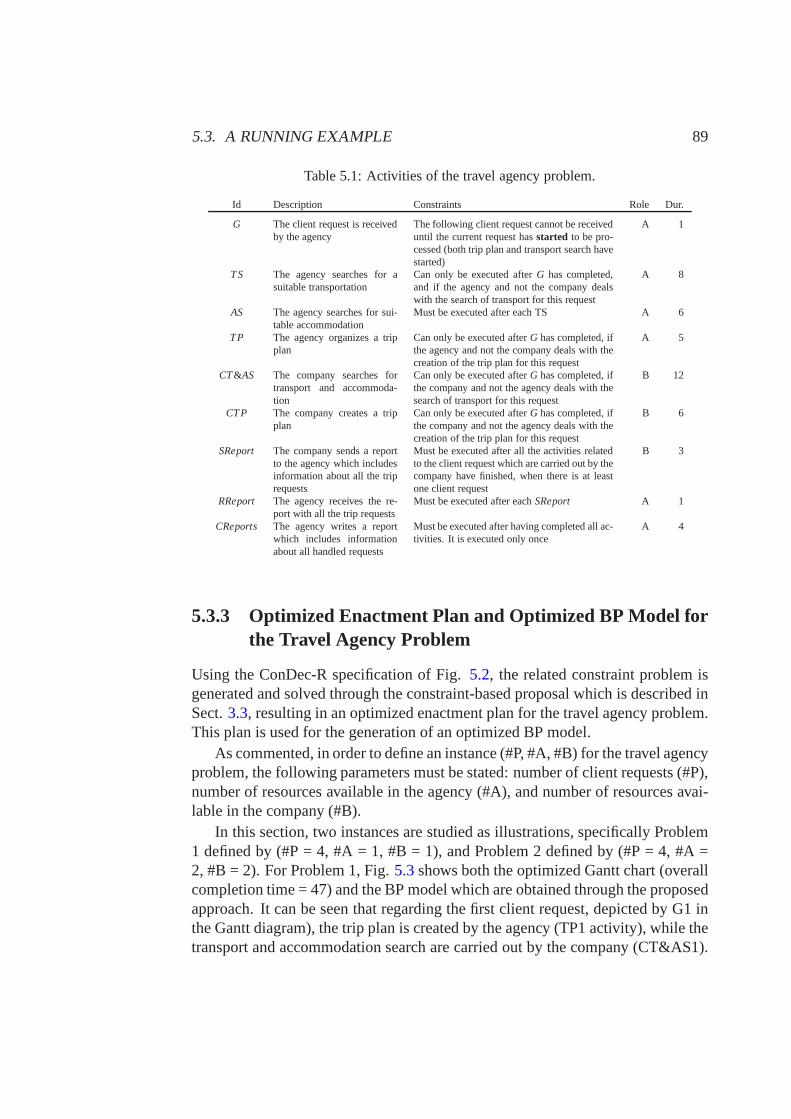
5.3. A RUNNING EXAMPLE 89
Table 5.1: Activities of the travel agency problem.
Id Description Constraints Role Dur.
G The client request is receivedby the agency
The following client request cannot be receiveduntil the current request hasstarted to be pro-cessed (both trip plan and transport search havestarted)
A 1
TS The agency searches for asuitable transportation
Can only be executed afterG has completed,and if the agency and not the company dealswith the search of transport for this request
A 8
AS The agency searches for sui-table accommodation
Must be executed after each TS A 6
TP The agency organizes a tripplan
Can only be executed afterG has completed, ifthe agency and not the company deals with thecreation of the trip plan for this request
A 5
CT&AS The company searches fortransport and accommoda-tion
Can only be executed afterG has completed, ifthe company and not the agency deals with thesearch of transport for this request
B 12
CTP The company creates a tripplan
Can only be executed afterG has completed, ifthe company and not the agency deals with thecreation of the trip plan for this request
B 6
SReport The company sends a reportto the agency which includesinformation about all the triprequests
Must be executed after all the activities relatedto the client request which are carried out by thecompany have finished, when there is at leastone client request
B 3
RReport The agency receives the re-port with all the trip requests
Must be executed after eachSReport A 1
CReports The agency writes a reportwhich includes informationabout all handled requests
Must be executed after having completed all ac-tivities. It is executed only once
A 4
5.3.3 Optimized Enactment Plan and Optimized BP Model forthe Travel Agency Problem
Using the ConDec-R specification of Fig.5.2, the related constraint problem isgenerated and solved through the constraint-based proposal which is described inSect.3.3, resulting in an optimized enactment plan for the travel agency problem.This plan is used for the generation of an optimized BP model.
As commented, in order to define an instance (#P, #A, #B) for the travel agencyproblem, the following parameters must be stated: number ofclient requests (#P),number of resources available in the agency (#A), and numberof resources avai-lable in the company (#B).
In this section, two instances are studied as illustrations, specifically Problem1 defined by (#P = 4, #A = 1, #B = 1), and Problem 2 defined by (#P = 4,#A =2, #B = 2). For Problem 1, Fig.5.3shows both the optimized Gantt chart (overallcompletion time = 47) and the BP model which are obtained through the proposedapproach. It can be seen that regarding the first client request, depicted by G1 inthe Gantt diagram), the trip plan is created by the agency (TP1 activity), while thetransport and accommodation search are carried out by the company (CT&AS1).
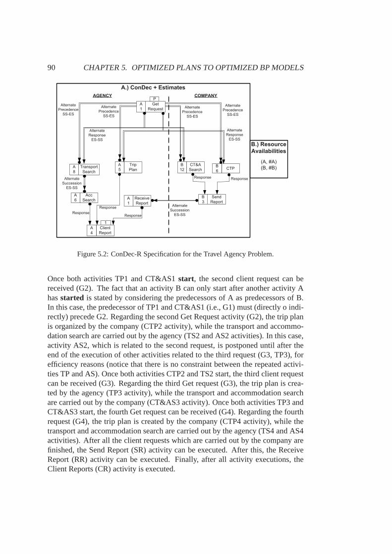
90 CHAPTER 5. OPTIMIZED PLANS TO OPTIMIZED BP MODELS
����������
� ������������
�������
�������
�
�� �
�
�
�
����
����
�
�
�
�����
������
�����
�����
������
�����
�����
������
�����
�����
������
�����
�����
������
�����
�����
������
�����
�����
� �������
�����
������
������
������������
�����
� �������
�����
����
����
�
��������
����!
�
"
��#�
����!
�
�$ ����
%
���
����
�
&���'
����
�
�
���
����!
�
%
������ �������
������
����������������������
Figure 5.2: ConDec-R Specification for the Travel Agency Problem.
Once both activities TP1 and CT&AS1start, the second client request can bereceived (G2). The fact that an activity B can only start after another activity Ahasstarted is stated by considering the predecessors of A as predecessors of B.In this case, the predecessor of TP1 and CT&AS1 (i.e., G1) must (directly o indi-rectly) precede G2. Regarding the second Get Request activity (G2), the trip planis organized by the company (CTP2 activity), while the transport and accommo-dation search are carried out by the agency (TS2 and AS2 activities). In this case,activity AS2, which is related to the second request, is postponed until after theend of the execution of other activities related to the thirdrequest (G3, TP3), forefficiency reasons (notice that there is no constraint between the repeated activi-ties TP and AS). Once both activities CTP2 and TS2 start, the third client requestcan be received (G3). Regarding the third Get request (G3), the trip plan is crea-ted by the agency (TP3 activity), while the transport and accommodation searchare carried out by the company (CT&AS3 activity). Once both activities TP3 andCT&AS3 start, the fourth Get request can be received (G4). Regarding the fourthrequest (G4), the trip plan is created by the company (CTP4 activity), while thetransport and accommodation search are carried out by the agency (TS4 and AS4activities). After all the client requests which are carried out by the company arefinished, the Send Report (SR) activity can be executed. After this, the ReceiveReport (RR) activity can be executed. Finally, after all activity executions, theClient Reports (CR) activity is executed.
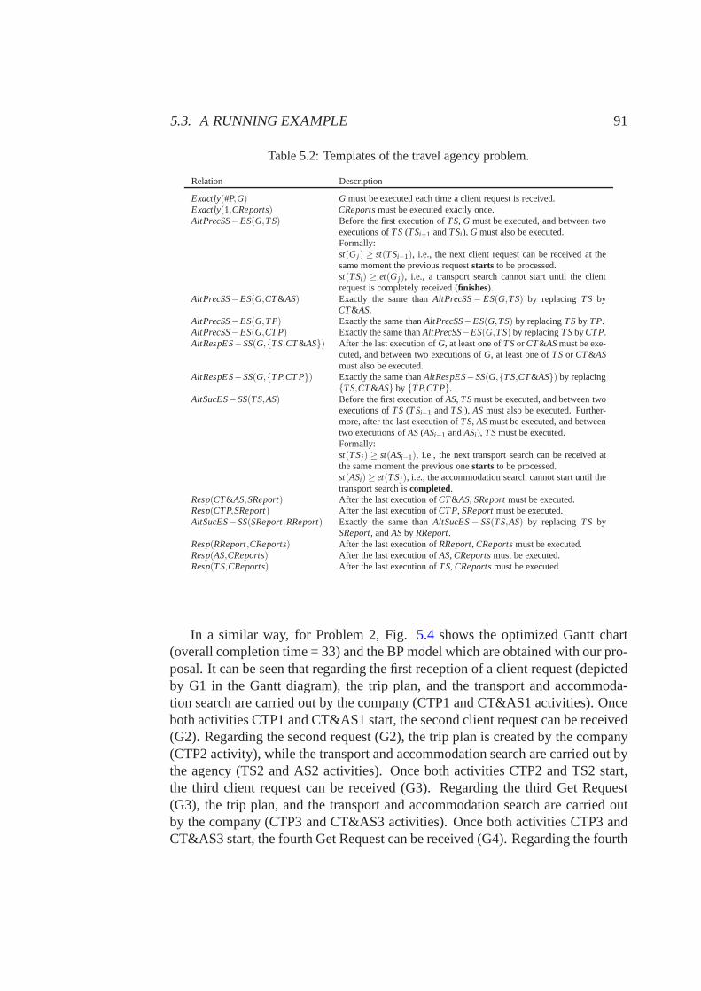
5.3. A RUNNING EXAMPLE 91
Table 5.2: Templates of the travel agency problem.
Relation Description
Exactly(#P,G) G must be executed each time a client request is received.Exactly(1,CReports) CReportsmust be executed exactly once.AltPrecSS−ES(G,TS) Before the first execution ofTS, G must be executed, and between two
executions ofTS(TSi−1 andTSi ), G must also be executed.Formally:st(G j ) ≥ st(TSi−1), i.e., the next client request can be received at thesame moment the previous requeststarts to be processed.st(TSi) ≥ et(G j ), i.e., a transport search cannot start until the clientrequest is completely received (finishes).
AltPrecSS−ES(G,CT&AS) Exactly the same thanAltPrecSS− ES(G,TS) by replacingTS byCT&AS.
AltPrecSS−ES(G,TP) Exactly the same thanAltPrecSS−ES(G,TS) by replacingTSby TP.AltPrecSS−ES(G,CTP) Exactly the same thanAltPrecSS−ES(G,TS) by replacingTSbyCTP.AltRespES−SS(G,{TS,CT&AS}) After the last execution ofG, at least one ofTSorCT&ASmust be exe-
cuted, and between two executions ofG, at least one ofTSor CT&ASmust also be executed.
AltRespES−SS(G,{TP,CT P}) Exactly the same thanAltRespES−SS(G,{TS,CT&AS}) by replacing{TS,CT&AS} by {TP,CTP}.
AltSucES−SS(TS,AS) Before the first execution ofAS, TSmust be executed, and between twoexecutions ofTS(TSi−1 andTSi ), ASmust also be executed. Further-more, after the last execution ofTS, ASmust be executed, and betweentwo executions ofAS(ASi−1 andASi ), TSmust be executed.Formally:st(TSj ) ≥ st(ASi−1), i.e., the next transport search can be received atthe same moment the previous onestarts to be processed.st(ASi)≥ et(TSj ), i.e., the accommodation search cannot start until thetransport search iscompleted.
Resp(CT&AS,SReport) After the last execution ofCT&AS, SReportmust be executed.Resp(CTP,SReport) After the last execution ofCTP, SReportmust be executed.AltSucES−SS(SReport,RReport) Exactly the same thanAltSucES− SS(TS,AS) by replacingTS by
SReport, andASby RReport.Resp(RReport,CReports) After the last execution ofRReport, CReportsmust be executed.Resp(AS,CReports) After the last execution ofAS, CReportsmust be executed.Resp(TS,CReports) After the last execution ofTS, CReportsmust be executed.
In a similar way, for Problem 2, Fig.5.4 shows the optimized Gantt chart(overall completion time = 33) and the BP model which are obtained with our pro-posal. It can be seen that regarding the first reception of a client request (depictedby G1 in the Gantt diagram), the trip plan, and the transport and accommoda-tion search are carried out by the company (CTP1 and CT&AS1 activities). Onceboth activities CTP1 and CT&AS1 start, the second client request can be received(G2). Regarding the second request (G2), the trip plan is created by the company(CTP2 activity), while the transport and accommodation search are carried out bythe agency (TS2 and AS2 activities). Once both activities CTP2 and TS2 start,the third client request can be received (G3). Regarding thethird Get Request(G3), the trip plan, and the transport and accommodation search are carried outby the company (CTP3 and CT&AS3 activities). Once both activities CTP3 andCT&AS3 start, the fourth Get Request can be received (G4). Regarding the fourth
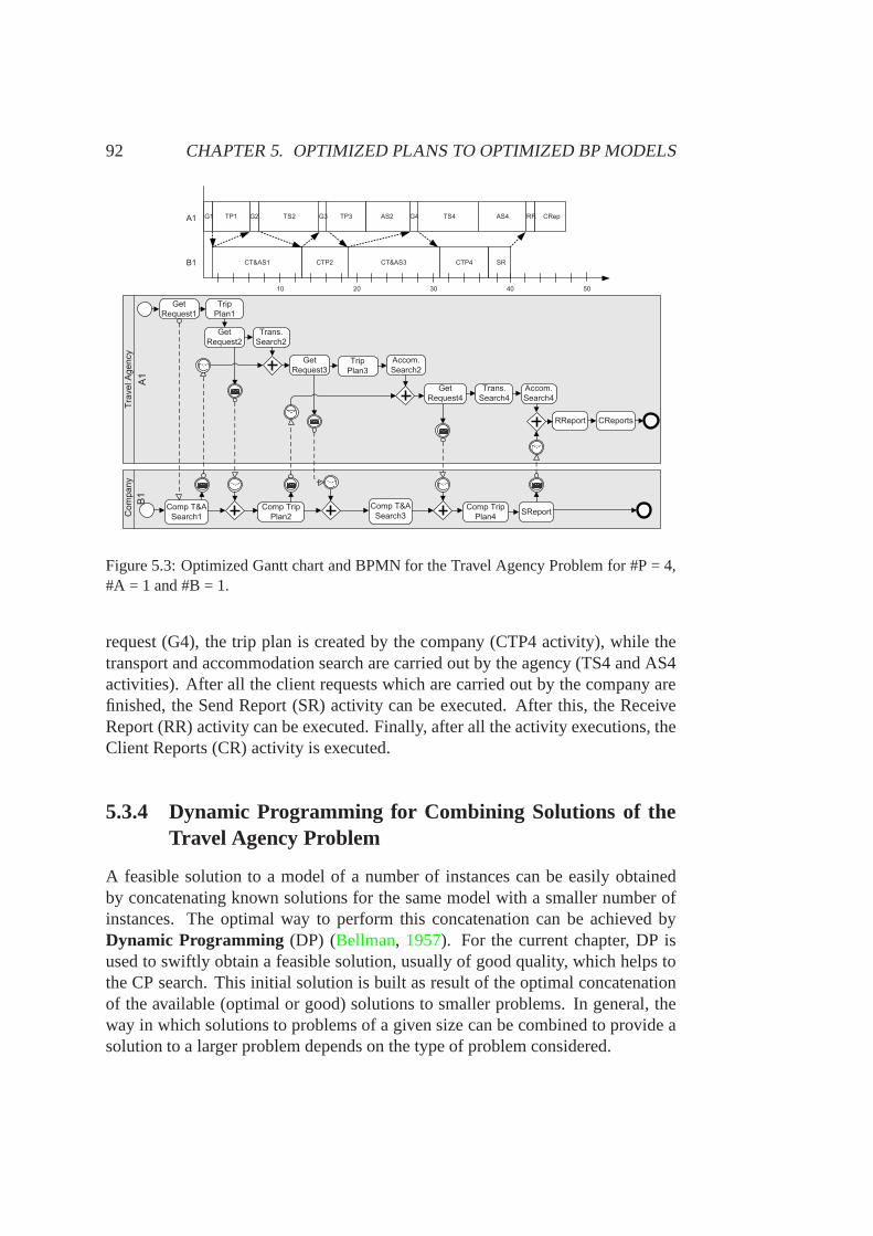
92 CHAPTER 5. OPTIMIZED PLANS TO OPTIMIZED BP MODELS
10 50403020
B1
A1
CT&AS1 CT&AS3CTP2 CTP4 SR
RRG3G2 G4TP1 TS2 TP3 AS2 AS4TS4 CRepG1
Tra
ve
l A
ge
ncy
Get
Request1
Trip
Plan1
CReportsRReport
A1
Get
Request3
Trans.
Search2
Accom.
Search2
Co
mp
an
y
Comp T&A
Search1SReport
Comp Trip
Plan2
Get
Request2
Trip
Plan3
Comp T&A
Search3
Get
Request4
Trans.
Search4
Accom.
Search4
Comp Trip
Plan4
B1
Figure 5.3: Optimized Gantt chart and BPMN for the Travel Agency Problem for #P = 4,#A = 1 and #B = 1.
request (G4), the trip plan is created by the company (CTP4 activity), while thetransport and accommodation search are carried out by the agency (TS4 and AS4activities). After all the client requests which are carried out by the company arefinished, the Send Report (SR) activity can be executed. After this, the ReceiveReport (RR) activity can be executed. Finally, after all theactivity executions, theClient Reports (CR) activity is executed.
5.3.4 Dynamic Programming for Combining Solutions of theTravel Agency Problem
A feasible solution to a model of a number of instances can be easily obtainedby concatenating known solutions for the same model with a smaller number ofinstances. The optimal way to perform this concatenation can be achieved byDynamic Programming (DP) (Bellman, 1957). For the current chapter, DP isused to swiftly obtain a feasible solution, usually of good quality, which helps tothe CP search. This initial solution is built as result of theoptimal concatenationof the available (optimal or good) solutions to smaller problems. In general, theway in which solutions to problems of a given size can be combined to provide asolution to a larger problem depends on the type of problem considered.
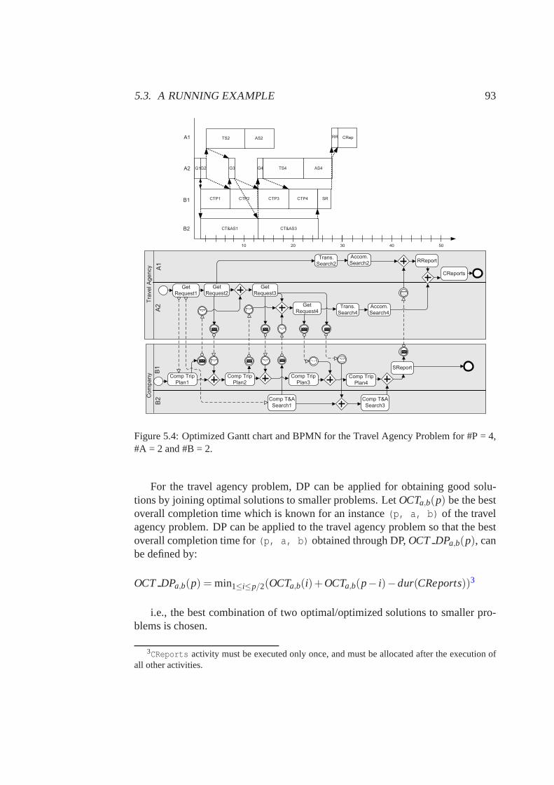
5.3. A RUNNING EXAMPLE 93
Tra
ve
l A
ge
ncy
Get
Request1
CReports
RReport
A2
Get
Request3
Trans.
Search2
Accom.
Search2
Co
mp
an
y
Comp T&A
Search1
SReport
Comp Trip
Plan1
Get
Request2
Comp T&A
Search3
Get
Request4Trans.
Search4
Accom.
Search4
Comp Trip
Plan2
A1
B2
B1
Comp Trip
Plan3Comp Trip
Plan4
10 50403020
B2
B1
A2
A1
CT&AS1 CT&AS3
TS2 AS2 CRepRR
SRCTP2CTP1 CTP4CTP3
G4G2 AS4TS4G3G1
Figure 5.4: Optimized Gantt chart and BPMN for the Travel Agency Problem for #P = 4,#A = 2 and #B = 2.
For the travel agency problem, DP can be applied for obtaining good solu-tions by joining optimal solutions to smaller problems. LetOCTa,b(p) be the bestoverall completion time which is known for an instance(p, a, b) of the travelagency problem. DP can be applied to the travel agency problem so that the bestoverall completion time for(p, a, b) obtained through DP,OCT DPa,b(p), canbe defined by:
OCT DPa,b(p) = min1≤i≤p/2(OCTa,b(i)+OCTa,b(p− i)−dur(CReports))3
i.e., the best combination of two optimal/optimized solutions to smaller pro-blems is chosen.
3CReports activity must be executed only once, and must be allocated after the execution ofall other activities.
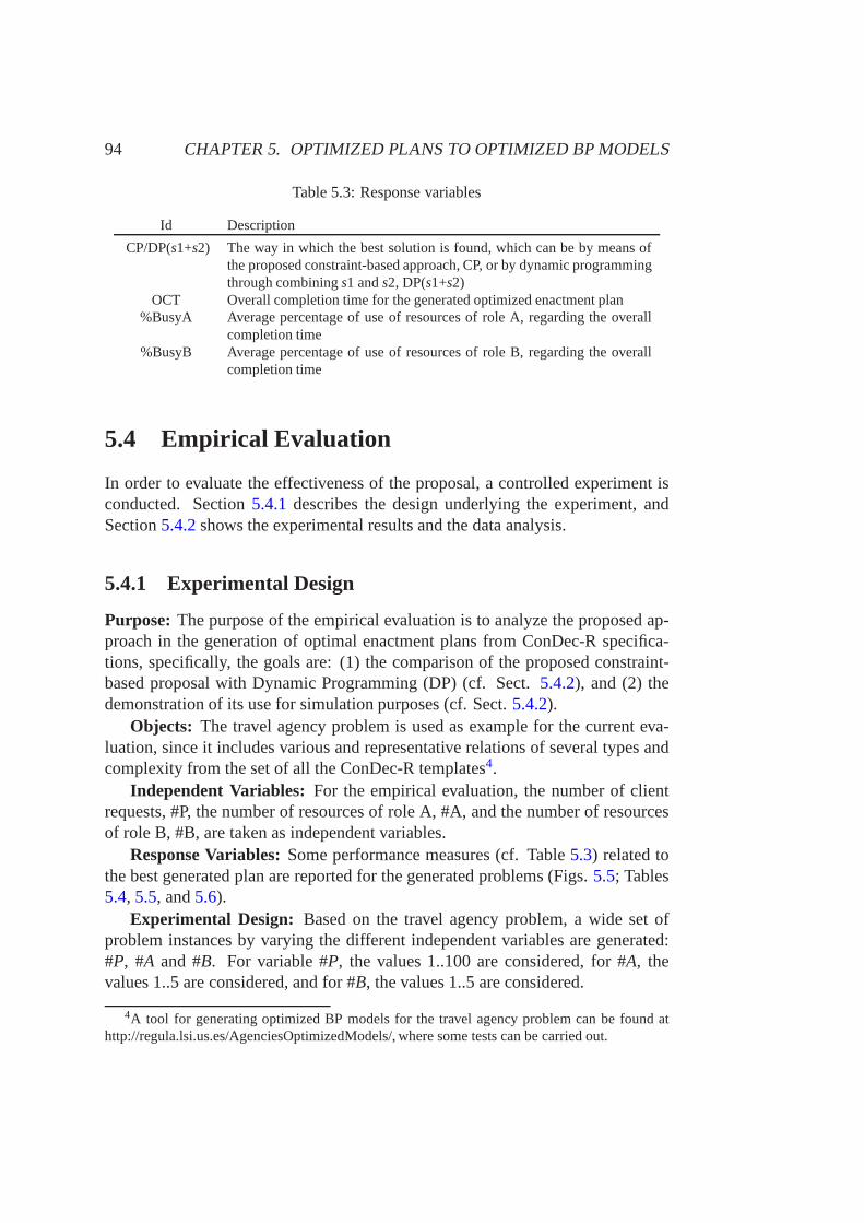
94 CHAPTER 5. OPTIMIZED PLANS TO OPTIMIZED BP MODELS
Table 5.3: Response variables
Id Description
CP/DP(s1+s2) The way in which the best solution is found, which can be by means ofthe proposed constraint-based approach, CP, or by dynamic programmingthrough combinings1 ands2, DP(s1+s2)
OCT Overall completion time for the generated optimized enactment plan%BusyA Average percentage of use of resources of role A, regarding the overall
completion time%BusyB Average percentage of use of resources of role B, regarding the overall
completion time
5.4 Empirical Evaluation
In order to evaluate the effectiveness of the proposal, a controlled experiment isconducted. Section5.4.1 describes the design underlying the experiment, andSection5.4.2shows the experimental results and the data analysis.
5.4.1 Experimental Design
Purpose: The purpose of the empirical evaluation is to analyze the proposed ap-proach in the generation of optimal enactment plans from ConDec-R specifica-tions, specifically, the goals are: (1) the comparison of theproposed constraint-based proposal with Dynamic Programming (DP) (cf. Sect.5.4.2), and (2) thedemonstration of its use for simulation purposes (cf. Sect.5.4.2).
Objects: The travel agency problem is used as example for the current eva-luation, since it includes various and representative relations of several types andcomplexity from the set of all the ConDec-R templates4.
Independent Variables: For the empirical evaluation, the number of clientrequests, #P, the number of resources of role A, #A, and the number of resourcesof role B, #B, are taken as independent variables.
Response Variables:Some performance measures (cf. Table5.3) related tothe best generated plan are reported for the generated problems (Figs.5.5; Tables5.4, 5.5, and5.6).
Experimental Design: Based on the travel agency problem, a wide set ofproblem instances by varying the different independent variables are generated:#P, #A and #B. For variable #P, the values 1..100 are considered, for #A, thevalues 1..5 are considered, and for #B, the values 1..5 are considered.
4A tool for generating optimized BP models for the travel agency problem can be found athttp://regula.lsi.us.es/AgenciesOptimizedModels/, where some tests can be carried out.
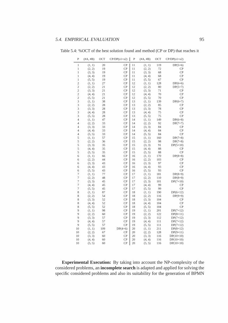
5.4. EMPIRICAL EVALUATION 95
Table 5.4: %OCT of the best solution found and method (CP or DP) that reaches it
P (#A, #B) OCT CP/DP(s1+s2) P (#A, #B) OCT CP/DP(s1+s2)
1 (1, 1) 20 CP 11 (1, 1) 119 DP(5+6)1 (2, 2) 19 CP 11 (2, 2) 72 CP1 (3, 3) 19 CP 11 (3, 3) 68 CP1 (4, 4) 19 CP 11 (4, 4) 68 CP1 (5, 5) 19 CP 11 (5, 5) 67 CP2 (1, 1) 27 CP 12 (1, 1) 128 DP(6+6)2 (2, 2) 21 CP 12 (2, 2) 80 DP(5+7)2 (3, 3) 21 CP 12 (3, 3) 71 CP2 (4, 4) 21 CP 12 (4, 4) 70 CP2 (5, 5) 21 CP 12 (5, 5) 70 CP3 (1, 1) 38 CP 13 (1, 1) 139 DP(6+7)3 (2, 2) 28 CP 13 (2, 2) 85 CP3 (3, 3) 28 CP 13 (3, 3) 78 CP3 (4, 4) 28 CP 13 (4, 4) 75 CP3 (5, 5) 28 CP 13 (5, 5) 75 CP4 (1, 1) 47 CP 14 (1, 1) 149 DP(6+8)4 (2, 2) 33 CP 14 (2, 2) 92 DP(7+7)4 (3, 3) 33 CP 14 (3, 3) 84 CP4 (4, 4) 33 CP 14 (4, 4) 84 CP4 (5, 5) 33 CP 14 (5, 5) 84 CP5 (1, 1) 57 CP 15 (1, 1) 160 DP(7+8)5 (2, 2) 36 CP 15 (2, 2) 98 DP(7+8)5 (3, 3) 35 CP 15 (3, 3) 91 DP(5+10)5 (4, 4) 35 CP 15 (4, 4) 88 CP5 (5, 5) 35 CP 15 (5, 5) 88 CP6 (1, 1) 66 CP 16 (1, 1) 170 DP(8+8)6 (2, 2) 44 CP 16 (2, 2) 103 CP6 (3, 3) 43 CP 16 (3, 3) 97 CP6 (4, 4) 43 CP 16 (4, 4) 93 CP6 (5, 5) 43 CP 16 (5, 5) 93 CP7 (1, 1) 77 CP 17 (1, 1) 181 DP(8+9)7 (2, 2) 48 CP 17 (2, 2) 110 DP(8+9)7 (3, 3) 45 CP 17 (3, 3) 101 DP(7+10)7 (4, 4) 45 CP 17 (4, 4) 99 CP7 (5, 5) 45 CP 17 (5, 5) 99 CP8 (1, 1) 87 CP 18 (1, 1) 190 DP(6+12)8 (2, 2) 54 CP 18 (2, 2) 116 DP(9+9)8 (3, 3) 52 CP 18 (3, 3) 104 CP8 (4, 4) 52 CP 18 (4, 4) 104 CP8 (5, 5) 52 CP 18 (5, 5) 104 CP9 (1, 1) 98 CP 19 (1, 1) 201 DP(7+12)9 (2, 2) 60 CP 19 (2, 2) 122 DP(8+11)9 (3, 3) 57 CP 19 (3, 3) 112 DP(7+12)9 (4, 4) 57 CP 19 (4, 4) 111 DP(7+12)9 (5, 5) 57 CP 19 (5, 5) 111 DP(7+12)
10 (1, 1) 109 DP(4+6) 20 (1, 1) 211 DP(8+12)10 (2, 2) 67 CP 20 (2, 2) 128 DP(9+11)10 (3, 3) 60 CP 20 (3, 3) 116 DP(10+10)10 (4, 4) 60 CP 20 (4, 4) 116 DP(10+10)10 (5, 5) 60 CP 20 (5, 5) 116 DP(10+10)
Experimental Execution: By taking into account the NP-complexity of theconsidered problems, anincomplete searchis adapted and applied for solving thespecific considered problems and also its suitability for the generation of BPMN
96 CHAPTER 5. OPTIMIZED PLANS TO OPTIMIZED BP MODELS
models from constraint-based specifications is evaluated.This incomplete searchincludesrandomized componentsin order to diversify the search. By means ofthis approach, a first feasible solution is quickly found by arandomized greedyalgorithm. The same greedy algorithm is used for iteratively improving the bestsolution found until a time limit is reached. Through this incomplete search, allthe solutions can be reached and the search procedure efficiently explores a widerange of solutions from diversified areas of the search space.
For the experiments, the constraint-based search algorithm is run until a 10-minute CPU time limit is reached. The machine for all experiments is an IntelCore2, 2.13 GHz, 1.97 GB memory, running on Windows XP. In order to solvethe constraint-based problems (cf. Sect.3.3, the developed algorithms have beenintegrated with the system COMET (Dynadec, 2011), which is able to generatehigh-quality solutions for highly constrained problems inan efficient way.
5.4.2 Experimental Results and Data Analysis
As commented, the purpose of the empirical evaluation is twofold, i.e., analy-zing the suitability of the proposed approach through a comparison with DP, andthrough the use for simulation.
Comparison with DP
Dynamic programming (Bellman, 1957), DP, is a widely used technique in sol-ving optimization problems, leading to solutions of high quality in most cases.Specifically, for the travel agency problem, DP can be applied (cf. Sect.5.3.4).We would like to evaluate whether the constraint-based proposal usually improvesthe solution of good quality which can be obtained by DP, i.e., works efficiently.In this way, DP is used for generating a first feasible solution of good quality.As discussed, CP tries to improve known solutions by taking advantages of theinformation about their objective value.
Table5.4 shows the overall completion time for the best solutions which arefound for some representative instances, together with themethod (either dynamicprogramming (DP) or constraint programming (CP)) which finds the best solution(column CP/DP(s1+s2) in Table5.4). Thereby DP(s1+s2) means that the bestsolution is found by dynamic programming through combinings1 ands2. It canbe observed that for 1≤ #P≤ 14, the constraint-based approach obtains bettersolutions than DP for almost all of the instances. Moreover,for 15≤ #P≤ 18,in some cases DP obtains the best solution, and in other casesCP obtains the bestsolution. Moreover, for 19≤ #P≤ 20, DP obtains solutions that are better thanor equal to those obtained through CP for all the instances. Furthermore, it seemsthat the solutions for #P ={6, 7, 8, 9, 10 and 12} are largely optimized since
5.4. EMPIRICAL EVALUATION 97
they widely appear in the DP solutions. The results (cf. Table 5.4) show thatthe proposed constraint-based approach, i.e., CP, is able to improve the solutionobtained by DP in most of the cases. This shows that the proposed constraint-based approach works efficiently in the generation of optimized enactment plans,and hence, for the automatic generation of optimized BPMN models.
In short, the presented data indicates that for the generation of optimized BPmodels, CP enables complex problems to be solved in a more efficient way thanthey would be through other alternative methods, such as DP or the manual speci-fication of BP models.
Additionally, when #P increases, the complexity of the problem rises sharply,and hence the manual treatment of the problem would become almost inextricable.In contrast, when using the presented approach an optimizedsolution for largeproblems, such as for #P= 100 can be obtained in only 10 minutes.
Threats to validity: There are several factors which may threaten the validityof the presented experiments for the attainment of generalizable conclusions:
• The specific characteristics of the running example, i.e., the empirical eva-luation only considers a concrete problem with a specific number of BPactivities and specific relations between the BP activities.
• The way in which the optimal/optimized solutions for problems of a certainsize are combined in order to obtain solutions for larger problems is spe-cific for the considered running example. In most cases, feasible solutionsfor larger problems can be generated by concatenating solutions to smallerproblems through dynamic programming. However, the way in which solu-tions to problems of a given size can be combined to provide a solution to alarger problem depends on the type of problem considered.
Use for Simulation
The proposed approach can be used for simulation purposes inthe BP Design &Analysis phase in order to study the relevance of several parameters in the qualityof the generated plans, e.g., resource availability. As an example, the relevanceof the number of available resources for the travel agency problem is analyzed asfollows.
Figure5.5 shows the completion time of the best BP enactment plan (over-all completion time) which is generated through the proposed approach. In bothgraphics of Fig.5.5, the overall completion time is shown depending on the num-ber of resources of roles A and B. First, the considered resources are groupedaccording to #A (Fig.5.5.(a)). Secondly, the considered resources are groupedaccording to #B (Fig.5.5.(b)). It can be seen, in most cases, that the overall com-pletion time greatly decreases as #A increases. Additionally, in most cases, the
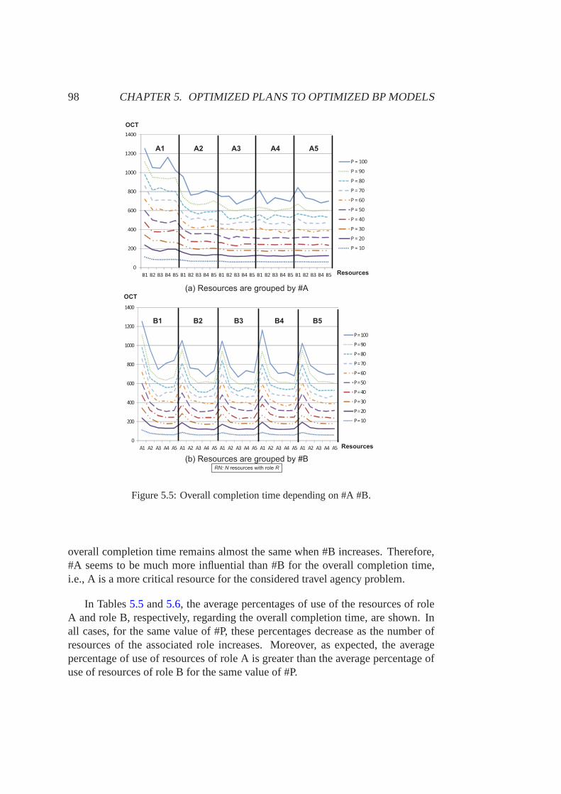
98 CHAPTER 5. OPTIMIZED PLANS TO OPTIMIZED BP MODELS
����������������� ��������
����������������� ��������
�
���
���
���
���
����
����
����
�� �� �� �� � �� �� �� �� � �� �� �� �� � �� �� �� �� � �� �� �� �� �
������
��� �
�����
�����
�����
����
�����
�����
�����
�����
�� ��������
�
���
���
���
���
����
����
����
�� �� �� �� � �� �� �� �� � �� �� �� �� � �� �� �� �� � �� �� �� �� �
������
��� �
�����
�����
�����
����
�����
�����
�����
�����
�� ��������
��� �
���
���
��� �
�����������������������
Figure 5.5: Overall completion time depending on #A #B.
overall completion time remains almost the same when #B increases. Therefore,#A seems to be much more influential than #B for the overall completion time,i.e., A is a more critical resource for the considered travelagency problem.
In Tables5.5 and5.6, the average percentages of use of the resources of roleA and role B, respectively, regarding the overall completion time, are shown. Inall cases, for the same value of #P, these percentages decrease as the number ofresources of the associated role increases. Moreover, as expected, the averagepercentage of use of resources of role A is greater than the average percentage ofuse of resources of role B for the same value of #P.
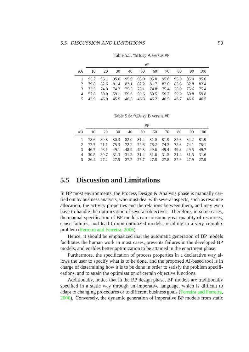
5.5. DISCUSSION AND LIMITATIONS 99
Table 5.5: %Busy A versus #P
#P
#A 10 20 30 40 50 60 70 80 90 100
1 95.2 95.1 95.0 95.0 95.0 95.0 95.0 95.0 95.0 95.02 79.8 82.6 81.4 83.1 82.2 81.7 82.6 83.3 82.8 82.43 73.5 74.8 74.3 75.5 75.1 74.8 75.4 75.9 75.6 75.44 57.8 59.0 59.1 59.6 59.6 59.5 59.7 59.9 59.8 59.85 43.9 46.0 45.9 46.5 46.3 46.2 46.5 46.7 46.6 46.5
Table 5.6: %Busy B versus #P
#P
#B 10 20 30 40 50 60 70 80 90 100
1 78.6 80.8 80.3 82.0 81.4 81.0 81.9 82.6 82.2 81.92 72.7 71.1 75.3 72.2 74.6 76.2 74.3 72.8 74.1 75.13 46.7 48.1 49.1 48.9 49.3 49.6 49.4 49.3 49.5 49.74 30.5 30.7 31.3 31.2 31.4 31.6 31.5 31.4 31.5 31.65 26.4 27.2 27.5 27.7 27.7 27.8 27.8 27.9 27.9 27.9
5.5 Discussion and Limitations
In BP most environments, the Process Design & Analysis phaseis manually car-ried out by business analysts, who must deal with several aspects, such as resourceallocation, the activity properties and the relations between them, and may evenhave to handle the optimization of several objectives. Therefore, in some cases,the manual specification of BP models can consume great quantity of resources,cause failures, and lead to non-optimized models, resulting in a very complexproblem (Ferreira and Ferreira, 2006).
Hence, it should be emphasized that the automatic generation of BP modelsfacilitates the human work in most cases, prevents failuresin the developed BPmodels, and enables better optimization to be attained in the enactment phase.
Furthermore, the specification of process properties in a declarative way al-lows the user to specify what is to be done, and the proposed AI-based tool is incharge of determining how it is to be done in order to satisfy the problem specifi-cations, and to attain the optimization of certain objective functions.
Additionally, notice that in the BP design phase, BP models are traditionallyspecified in a static way through an imperative language, which is difficult toadapt to changing procedures or to different business goals(Ferreira and Ferreira,2006). Conversely, the dynamic generation of imperative BP models from static
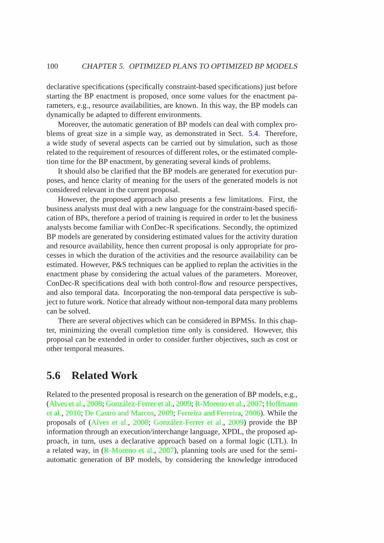
100 CHAPTER 5. OPTIMIZED PLANS TO OPTIMIZED BP MODELS
declarative specifications (specifically constraint-based specifications) just beforestarting the BP enactment is proposed, once some values for the enactment pa-rameters, e.g., resource availabilities, are known. In this way, the BP models candynamically be adapted to different environments.
Moreover, the automatic generation of BP models can deal with complex pro-blems of great size in a simple way, as demonstrated in Sect.5.4. Therefore,a wide study of several aspects can be carried out by simulation, such as thoserelated to the requirement of resources of different roles,or the estimated comple-tion time for the BP enactment, by generating several kinds of problems.
It should also be clarified that the BP models are generated for execution pur-poses, and hence clarity of meaning for the users of the generated models is notconsidered relevant in the current proposal.
However, the proposed approach also presents a few limitations. First, thebusiness analysts must deal with a new language for the constraint-based specifi-cation of BPs, therefore a period of training is required in order to let the businessanalysts become familiar with ConDec-R specifications. Secondly, the optimizedBP models are generated by considering estimated values forthe activity durationand resource availability, hence then current proposal is only appropriate for pro-cesses in which the duration of the activities and the resource availability can beestimated. However, P&S techniques can be applied to replanthe activities in theenactment phase by considering the actual values of the parameters. Moreover,ConDec-R specifications deal with both control-flow and resource perspectives,and also temporal data. Incorporating the non-temporal data perspective is sub-ject to future work. Notice that already without non-temporal data many problemscan be solved.
There are several objectives which can be considered in BPMSs. In this chap-ter, minimizing the overall completion time only is considered. However, thisproposal can be extended in order to consider further objectives, such as cost orother temporal measures.
5.6 Related Work
Related to the presented proposal is research on the generation of BP models, e.g.,(Alves et al., 2008; Gonzalez-Ferrer et al., 2009; R-Moreno et al., 2007; Hoffmannet al., 2010; De Castro and Marcos, 2009; Ferreira and Ferreira, 2006). While theproposals of (Alves et al., 2008; Gonzalez-Ferrer et al., 2009) provide the BPinformation through an execution/interchange language, XPDL, the proposed ap-proach, in turn, uses a declarative approach based on a formal logic (LTL). Ina related way, in (R-Moreno et al., 2007), planning tools are used for the semi-automatic generation of BP models, by considering the knowledge introduced
5.6. RELATED WORK 101
through BP Reengineering languages. In (R-Moreno et al., 2007), they proposean object-oriented structure modelling tool that follows their own rule-based ap-proach, while the use of an extension of ConDec, a widely referenced languagein the context of BPM (e.g., (Ly et al., 2008; Montali, 2009)), which also al-lows a higher level of abstraction is proposed in the currentchapter. Additionally,(Hoffmann et al., 2010) proposes a planning formalism for the modelling of BPsthrough an SAP specification (Status and Action Management,SAM), which isa variant of PDDL. Unlike the proposed approach, neither theresource perspec-tive nor the optimization of several instances are considered since in (Hoffmannet al., 2010) each non-deterministic action (i.e., activity) cannot berepeated in thegenerated solution. Moreover, (De Castro and Marcos, 2009) presents a service-oriented approach which transforms high-level BP models into web service com-position models. This approach uses UML to specify the BP models from anMDA point of view, which lacks an implementation view of BP models (Owenand Raj, 2003), in contrast to ConDec, which is a graphical and specific languagefor the modelling of BPs. Furthermore, (Ferreira and Ferreira, 2006) proposes torefine BP models by combining learning and planning techniques, starting fromprocesses which are not fully described. Unlike the proposed approach, (Ferreiraand Ferreira, 2006) needs past process executions and examples provided by theuser to apply learning techniques. Moreover, (Ferreira and Ferreira, 2006) doesnot consider the optimization of any objective function in the generation of theplans. Furthermore, in (Ferreira and Ferreira, 2006) executable plans are genera-ted, while the generation of BP models is proposed in the current approach whichare specified in a standard language, i.e., BPMN, which can also be improved bybusiness analysts if necessary.
On the other hand, related to the combined used of declarative and imperativemodels, (Rychkova et al., 2008b) proposes the use of declarative BP models forspecifying processes independently of a particular environment in order to alignoptional process customizations. This information is complemented with impe-rative BP specifications which contain information relatedto the control flow ofthe processes, often specific to a given environment. In (Rychkova et al., 2008b)both declarative and imperative BP models need to be (manually) specified, whilein the proposed approach the optimized imperative models are automatically ge-nerated. Lastly, (Caron and Vanthienen, 2011) analyzes the need of transitionsbetween different BP modelling paradigms, i.e., declarative, imperative and hy-brid proposals, supporting the presented proposal.

Chapter 6
Planning and Scheduling of BusinessProcesses in Run-Time
6.1 Introduction
6.1.1 Motivation
The execution of most BPs entails, in some way, scheduling decisions since the ac-tivities to be executed may compete for some shared resources. In these cases, it isnecessary to allocate the resources in a suitable way, usually optimizing some ob-jectives. Scheduling decisions are typically made by the BPM systems (BPMSs)during process execution by automatically assigning activities to resources (Rus-sell et al., 2005).
To lesser measure, planning problems are present in BP executions when, insome points, several possible execution branches exist, and the selection of thesuitable one depends on the BP goal and/or on the optimization of some criteri-ons. Since BP models are typically specified in an imperativeway, most of theplanning decisions are taken in the modelling phase. Specifically, the ordering andthe selection of the activities to be executed (planning) inthe BP enactment arespecified in the BP design time, when only estimated values for several parameterscan be analyzed.
There are BPs which entail complex planning decisions whichcan greatly beinfluenced by the values of several unpredictable parameters, whose actual valueis known in run time.
6.1.2 Contribution
In this chapter, a proposal for modelling and enacting BPs that involve planningand scheduling (P&S) decisions (cf. Sect.2.2.3) is presented. The main contri-
103
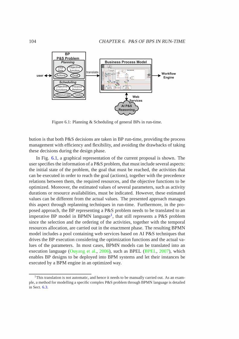
104 CHAPTER 6. P&S OF BPS IN RUN-TIME
�������������
���������������� ��
���
��������
�����
��������
������
������
�
�����������������
�����
����
��������
��������
�������
����������
��������
�������
�������� �����
��������
��������
Figure 6.1: Planning & Scheduling of general BPs in run-time.
bution is that both P&S decisions are taken in BP run-time, providing the processmanagement with efficiency and flexibility, and avoiding thedrawbacks of takingthese decisions during the design phase.
In Fig. 6.1, a graphical representation of the current proposal is shown. Theuser specifies the information of a P&S problem, that must include several aspects:the initial state of the problem, the goal that must be reached, the activities thatcan be executed in order to reach the goal (actions), together with the precedencerelations between them, the required resources, and the objective functions to beoptimized. Moreover, the estimated values of several parameters, such as activitydurations or resource availabilities, must be indicated. However, these estimatedvalues can be different from the actual values. The presented approach managesthis aspect through replanning techniques in run-time. Furthermore, in the pro-posed approach, the BP representing a P&S problem needs to betranslated to animperative BP model in BPMN language1, that still represents a P&S problemsince the selection and the ordering of the activities, together with the temporalresources allocation, are carried out in the enactment phase. The resulting BPMNmodel includes a pool containing web services based on AI P&Stechniques thatdrives the BP execution considering the optimization functions and the actual va-lues of the parameters. In most cases, BPMN models can be translated into anexecution language (Ouyang et al., 2006), such as BPEL (BPEL, 2007), whichenables BP designs to be deployed into BPM systems and let their instances beexecuted by a BPM engine in an optimized way.
1This translation is not automatic, and hence it needs to be manually carried out. As an exam-ple, a method for modelling a specific complex P&S problem through BPMN language is detailedin Sect.6.3.
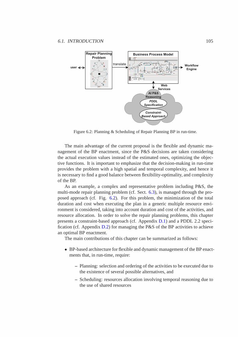
6.1. INTRODUCTION 105
����
���������������� ��
������
������
���
��������
���������
��������������
�����
�����
��������
����
����������
�� ���� ��
������������
Figure 6.2: Planning & Scheduling of Repair Planning BP in run-time.
The main advantage of the current proposal is the flexible anddynamic ma-nagement of the BP enactment, since the P&S decisions are taken consideringthe actual execution values instead of the estimated ones, optimizing the objec-tive functions. It is important to emphasize that the decision-making in run-timeprovides the problem with a high spatial and temporal complexity, and hence itis necessary to find a good balance between flexibility-optimality, and complexityof the BP.
As an example, a complex and representative problem including P&S, themulti-mode repair planning problem (cf. Sect.6.3), is managed through the pro-posed approach (cf. Fig.6.2). For this problem, the minimization of the totalduration and cost when executing the plan in a generic multiple resource envi-ronment is considered, taking into account duration and cost of the activities, andresource allocation. In order to solve the repair planning problems, this chapterpresents a constraint-based approach (cf. AppendixD.1) and a PDDL 2.2 speci-fication (cf. AppendixD.2) for managing the P&S of the BP activities to achievean optimal BP enactment.
The main contributions of this chapter can be summarized as follows:
• BP-based architecture for flexible and dynamic management of the BP enact-ments that, in run-time, require:
– Planning: selection and ordering of the activities to be executed due tothe existence of several possible alternatives, and
– Scheduling: resources allocation involving temporal reasoning due tothe use of shared resources
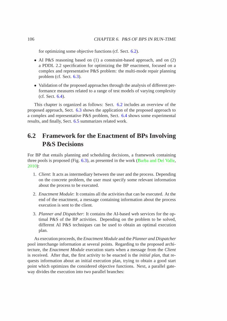
106 CHAPTER 6. P&S OF BPS IN RUN-TIME
for optimizing some objective functions (cf. Sect.6.2).
• AI P&S reasoning based on (1) a constraint-based approach, and on (2)a PDDL 2.2 specification for optimizing the BP enactment, focused on acomplex and representative P&S problem: the multi-mode repair planningproblem (cf. Sect.6.3).
• Validation of the proposed approaches through the analysisof different per-formance measures related to a range of test models of varying complexity(cf. Sect.6.4).
This chapter is organized as follows: Sect.6.2 includes an overview of theproposed approach, Sect.6.3 shows the application of the proposed approach toa complex and representative P&S problem, Sect.6.4 shows some experimentalresults, and finally, Sect.6.5summarizes related work.
6.2 Framework for the Enactment of BPs InvolvingP&S Decisions
For BP that entails planning and scheduling decisions, a framework containingthree pools is proposed (Fig.6.3), as presented in the work (Barba and Del Valle,2010):
1. Client: It acts as intermediary between the user and the process. Dependingon the concrete problem, the user must specify some relevantinformationabout the process to be executed.
2. Enactment Module: It contains all the activities that can be executed. At theend of the enactment, a message containing information about the processexecution is sent to the client.
3. Planner and Dispatcher: It contains the AI-based web services for the op-timal P&S of the BP activities. Depending on the problem to besolved,different AI P&S techniques can be used to obtain an optimal executionplan.
As execution proceeds, theEnactment Moduleand thePlanner and Dispatcherpool interchange information at several points. Regardingto the proposed archi-tecture, theEnactment Moduleexecution starts when a message from theClientis received. After that, the first activity to be enacted is the initial plan, that re-quests information about an initial execution plan, tryingto obtain a good startpoint which optimizes the considered objective functions.Next, a parallel gate-way divides the execution into two parallel branches:
6.2. ENACTMENT OF BPS INVOLVING P&S DECISIONS 107
En
actm
en
t M
odu
le
Initial
Plan
Update
plan
Clie
nt
Input
Data
Pla
nn
er
&
Dis
patc
her
Receive
dataSend
message
Initial Plan
GenerationUpdate plan
@
@
@@
Branch 2
Branch 1 Plan Enactment
T1 or
T2or
…
Tn?
T1
...
Tn
T2
...
Activity
Execution
@
@
...
Figure 6.3: Architecture for enacting BPs which involve P&Sdecisions.
• Plan enactment (Branch 1 in Fig.6.3): This branch contains the actual P&Sactivities that can be executed in order to solve the problem. It should beemphasized that all the possible alternative activities tobe selected are in-cluded in this branch. In this way, P&S methods are used to automaticallyselect and order the suitable activities during the enactment phase, in orderto obtain an optimal execution plan. In theEnactment Module, when anexclusive data-based gateway is reached during the plan execution, the waythat must be followed is established by the information previously receivedfrom thePlanner and Dispatcherpool. In this way, selecting the most sui-table activity considering the goal to be reached and the objective functionto be optimized is required (planning decision). Moreover,for the activitieswhich require the same resources to be executed, this pool establishes theexecution ordering. Therefore, resources need to be allocated to activitiesby considering the objective function to be optimized (scheduling decision).
• Optimization process (Branch 2 in Fig.6.3): For the proposed architecture,one of the most important aspects in the plan execution is theoptimality.In order to improve it, an optimization process is carried out during all theplan execution, due to, basically, two reasons:
– The execution plan which was initially generated can be non-optimal,since the generation of optimal plans presents NP-complexity (Gareyand Johnson, 1979), and hence it is not possible to ensure the opti-mality of the generated plans for all the cases in a specific executiontime.
108 CHAPTER 6. P&S OF BPS IN RUN-TIME
– The actual parameters of the enactment can be different fromthe esti-mated ones, e.g., different activity duration or resource availability. Inthese cases, the optimized plan needs to be updated by considering theactual state of the BP execution.
Taking both reasons into account, a loop updating activity that is conti-nuously trying to improve the current solution is included,considering theactual values of the parameters. In order to do this, a web service based onP&S techniques (Update plan) is invoked. When a better solution is found,the current plan is updated and this information is used to decide the wayto follow in the OR gateways. Lastly, this loop finishes when the completeplan is successfully enacted.
In Sect. 6.3, a specific example is modelled through the proposed genericframework.
6.3 A Case of Study
In the current chapter, a generic framework for modelling and enacting BPs whichinclude P&S decisions is presented (cf. Sect.6.2). As an example, the multi-moderepair planning problem (cf. Sect.6.3.1) is managed through this architecture (cf.Sect.6.3.2).
6.3.1 The Multi-mode Repair Planning Problem
Some of the applications involving P&S issues are maintenance and repair plan-ning, where there may be a cascading set of choices for actions, facilities, toolsor personnel, which affect the duration of the plans (Smith et al., 2000). In pastyears, the effective management of maintenance and repair planning in organiza-tions became more important, since the system complexity isincreasing as wellas there exist several limitations of the technology which is used to maintain it.Maintenance and repair planning includes a wide scope of problems. Specifically,assembly and disassembly planning are very important in themanufacturing ofproducts and its life cycles. They involve the identification, selection and sequen-cing of assembly/disassembly operations, which can be specified by their effectson the parts. The identification of assembly/disassembly operations is usuallytackled by analyzing the product structure and the feasibility of each possible ac-tivity (Homem de Mello and Sanderson, 1991; Calton, 1999), and usually leads tothe set of all feasible plans.
In this chapter, the complete repair process of a reparable system (cf. Def.32)is considered.
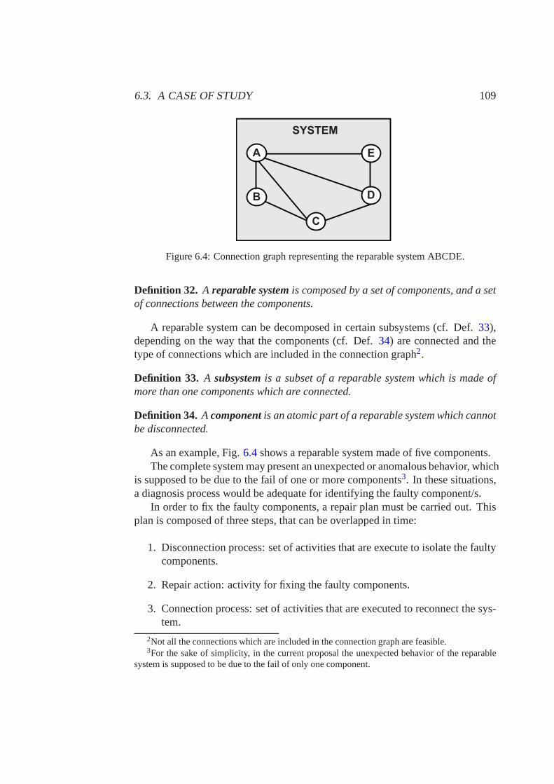
6.3. A CASE OF STUDY 109
A
SYSTEM
E
B D
C
Figure 6.4: Connection graph representing the reparable system ABCDE.
Definition 32. A reparable systemis composed by a set of components, and a setof connections between the components.
A reparable system can be decomposed in certain subsystems (cf. Def. 33),depending on the way that the components (cf. Def.34) are connected and thetype of connections which are included in the connection graph2.
Definition 33. A subsystemis a subset of a reparable system which is made ofmore than one components which are connected.
Definition 34. A componentis an atomic part of a reparable system which cannotbe disconnected.
As an example, Fig.6.4shows a reparable system made of five components.The complete system may present an unexpected or anomalous behavior, which
is supposed to be due to the fail of one or more components3. In these situations,a diagnosis process would be adequate for identifying the faulty component/s.
In order to fix the faulty components, a repair plan must be carried out. Thisplan is composed of three steps, that can be overlapped in time:
1. Disconnection process: set of activities that are execute to isolate the faultycomponents.
2. Repair action: activity for fixing the faulty components.
3. Connection process: set of activities that are executed to reconnect the sys-tem.
2Not all the connections which are included in the connectiongraph are feasible.3For the sake of simplicity, in the current proposal the unexpected behavior of the reparable
system is supposed to be due to the fail of only one component.
110 CHAPTER 6. P&S OF BPS IN RUN-TIME
Taking these steps into account, a feasible repair plan can be seen as a (mini-mum) set of activities that begins with the disconnection ofthe complete system,fixes the faulty components, and finishes with the connectionof the completesystem. In the current proposal, two kinds of activities areconsidered, i.e., con-nection/disconnection activities (cf. Def.35 and36) and auxiliary activities (cf.Def. 37 and38).
Definition 35. A connection activityis an activity which obtains one subsystemby connecting several subsystems or components. It is executed by using an esta-blished resource with a particular configuration.
Definition 36. A disconnection activityis an activity which obtains several sub-systems or components by disconnecting one subsystem. It isexecuted by usingan established resource with a particular configuration.
For the sake of clarity, only two subsystems are considered to be connected ina connection activity and obtained after a disconnection activity.
Moreover, auxiliary activities are required since the connection/disconnectionactivities are executed at different locations, and the resources can be used withdifferent configurations. Auxiliary activities can be classified into set-up opera-tions (cf. Def.37) and transportation operations (cf. Def.38).
Definition 37. A set-up operationis an auxiliary operation which changes theconfiguration of a resource. It is required when two successive activities withdifferent configuration use that resource.
Definition 38. A transportation operationis an auxiliary operation which trans-ports a subsystem between locations. It is required when thelocation where thesubsystem is obtained is different from the location where that subsystem is re-quired. In the current chapter, different resources are considered to be placed atdifferent locations.
All activities which are considered, i.e., connection/disconnection and auxi-liary activities, have an associated duration and cost.
In the considered repair planning problem, the connection/disconnection ac-tivities (cf. Def. 35 and36) can be executed in more than one operating mode(multi-mode), each one using different resources or configuration, and possiblydifferent duration and cost. Taking this into account, there can be several optionsto connect several subsystems to obtain another one, or disconnect one subsystemto obtain several ones.
For the considered repair planning problem, two assumptions are supposed:
• (A1) All activities are reversible, i.e., if a connection activity which con-nects several subsystemsS1,S2, . . . ,Sk to obtain another subsystemSexists,
6.3. A CASE OF STUDY 111
then a disconnection activity which disconnect the subsystem S to obtainthe subsystemsS1,S2, . . . ,Sk is also included, and vice versa.
• (A2) Subsystems that do not include the faulty components are not discon-nected.
Taking (A1) and (A2) into account, in the connection process, other subsys-tems different from the ones generated by the disconnectionprocess can appear,depending on how they are joined. Moreover, disconnection activities only han-dle subsystems that contain the faulty component, whereas connection activitieshandle subsystems that may contain or not the faulty component. In general,plans are not linear sequences of activities, unlike reversible plans. Although thedisconnection process is linear, the connection process can contain activities thatmay execute in parallel with others. Furthermore, it is possible that the connectionprocess starts before the disconnection process has finished, and there may be aparallel execution of the two types of activities.
A typical objective to be pursued in repair problems is the minimization of theelapsed time of the plan, i.e., the time in which the reparable system is reconnectedafter the reparation (called makespan). In the current approach, the total cost ofthe complete repair plan is also considered for minimization. Therefore, a multi-objective optimization is pursued, encompassing both objective functions, timeand cost.
And/Or Graph Representation
In the literature, there are several structures that can be used for representing theconsidered repair planning problem. The And/Or graph (Homem de Mello andSanderson, 1990) is one of the most suitable ones, since it allows to represent theset of all feasible connection/disconnection plans in a natural and compact way(cf. Def. 39).
Definition 39. TheAnd/Or graphwhich represents a repair planning problem iscomposed by:
• Or nodes: they correspond to subsets of components of the reparable sys-tem, meaning that the root node represents the whole system (cf. Def. 32),while non-leaf nodes represent subsystems (cf. Def.33), and leaf nodes areindividual components (cf. Def.34).
• And nodes: they represent the activities which connect/disconnect the sub-systems (cf. Def.35 and 36). In this way, a downward edge decomposesa system or subsystem in several subsystems, while an upwardedge can be
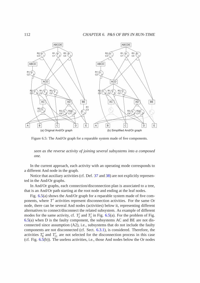
112 CHAPTER 6. P&S OF BPS IN RUN-TIME
������������� �������� ���������������� ��������
�����
����
���
��
�
�� ��
� � � �
���
���
���
���
���
��
��!
��"
���#
��$ ��
��
%�
��
%�
��
%�
�
%�
��
%�
��
%�
��
%�
��
%�
�"
%�
��
�����
����
���
��
�
�� ��
� � � �
���
���
���
���
���
��
��!
��"
���#
��$ ��
��
%�
��
%�
��
%�
�
%�
��
%�
��
%�
��
%�
��
%�
�"
%�
��
%�
��
%�
��
Figure 6.5: The And/Or graph for a reparable system made of five components.
seen as the reverse activity of joining several subsystems into a composedone.
In the current approach, each activity with an operating mode corresponds toa different And node in the graph.
Notice that auxiliary activities (cf. Def.37and38) are not explicitly represen-ted in the And/Or graphs.
In And/Or graphs, each connection/disconnection plan is associated to a tree,that is an And/Or path starting at the root node and ending at the leaf nodes.
Fig. 6.5(a) shows the And/Or graph for a reparable system made of five com-ponents, whereT ′ activities represent disconnection activities. For the same Ornode, there can be several And nodes (activities) below it, representing differentalternatives to connect/disconnect the related subsystem. As example of differentmodes for the same activity, cf.T ′2 andT ′3 in Fig. 6.5(a). For the problem of Fig.6.5(a) when D is the faulty component, the subsystems AC and BE are not dis-connected since assumption (A2), i.e., subsystems that do not include the faultycomponents are not disconnected (cf. Sect.6.3.1), is considered. Therefore, theactivitiesT ′8 andT ′11 are not selected for the disconnection process in this case(cf. Fig. 6.5(b)). The useless activities, i.e., those And nodes below the Or nodes
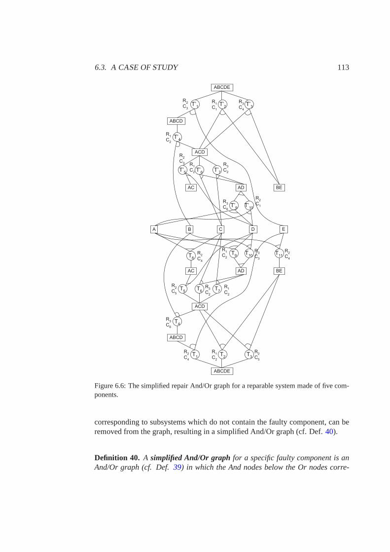
6.3. A CASE OF STUDY 113
�����
����
���
��
�
�� ��
� � �
���
��
��
���
���
��
���
���
���
�����
����
���
�� �� ��
�
��
�
�
��
��
�
��
��
���
�
�
�
��
�
�
��
�
�
�
�
�� �
�
��
�
��
��
�
�
�
�
��
��
�
�
�
�
�
��
��
�
�
�
��
��
�
�
�
�
�
��
Figure 6.6: The simplified repair And/Or graph for a reparable system made of five com-ponents.
corresponding to subsystems which do not contain the faultycomponent, can beremoved from the graph, resulting in a simplified And/Or graph (cf. Def. 40).
Definition 40. A simplified And/Or graphfor a specific faulty component is anAnd/Or graph (cf. Def.39) in which the And nodes below the Or nodes corre-
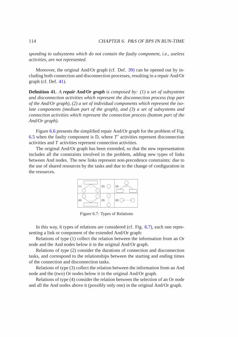
114 CHAPTER 6. P&S OF BPS IN RUN-TIME
sponding to subsystems which do not contain the faulty component, i.e., uselessactivities, are not represented.
Moreover, the original And/Or graph (cf. Def.39) can be opened out by in-cluding both connection and disconnection processes, resulting in a repair And/Orgraph (cf. Def.41).
Definition 41. A repair And/Or graph is composed by: (1) a set of subsystemsand disconnection activities which represent the disconnection process (top partof the And/Or graph), (2) a set of individual components which represent the iso-late components (medium part of the graph), and (3) a set of subsystems andconnection activities which represent the connection process (bottom part of theAnd/Or graph).
Figure6.6presents the simplified repair And/Or graph for the problem of Fig.6.5 when the faulty component is D, whereT ′ activities represent disconnectionactivities andT activities represent connection activities.
The original And/Or graph has been extended, so that the new representationincludes all the constraints involved in the problem, adding new types of linksbetween And nodes. The new links represent non-precedence constraints: due tothe use of shared resources by the tasks and due to the change of configuration inthe resources.
...
...
(1) (2) (3)
(4) (5) (6)
Figure 6.7: Types of Relations
In this way, 6 types of relations are considered (cf. Fig.6.7), each one repre-senting a link or component of the extended And/Or graph:
Relations of type (1) collect the relation between the information from an Ornode and the And nodes below it in the original And/Or graph.
Relations of type (2) consider the durations of connection and disconnectiontasks, and correspond to the relationships between the starting and ending timesof the connection and disconnection tasks.
Relations of type (3) collect the relation between the information from an Andnode and the (two) Or nodes below it in the original And/Or graph.
Relations of type (4) consider the relation between the selection of an Or nodeand all the And nodes above it (possibly only one) in the original And/Or graph.
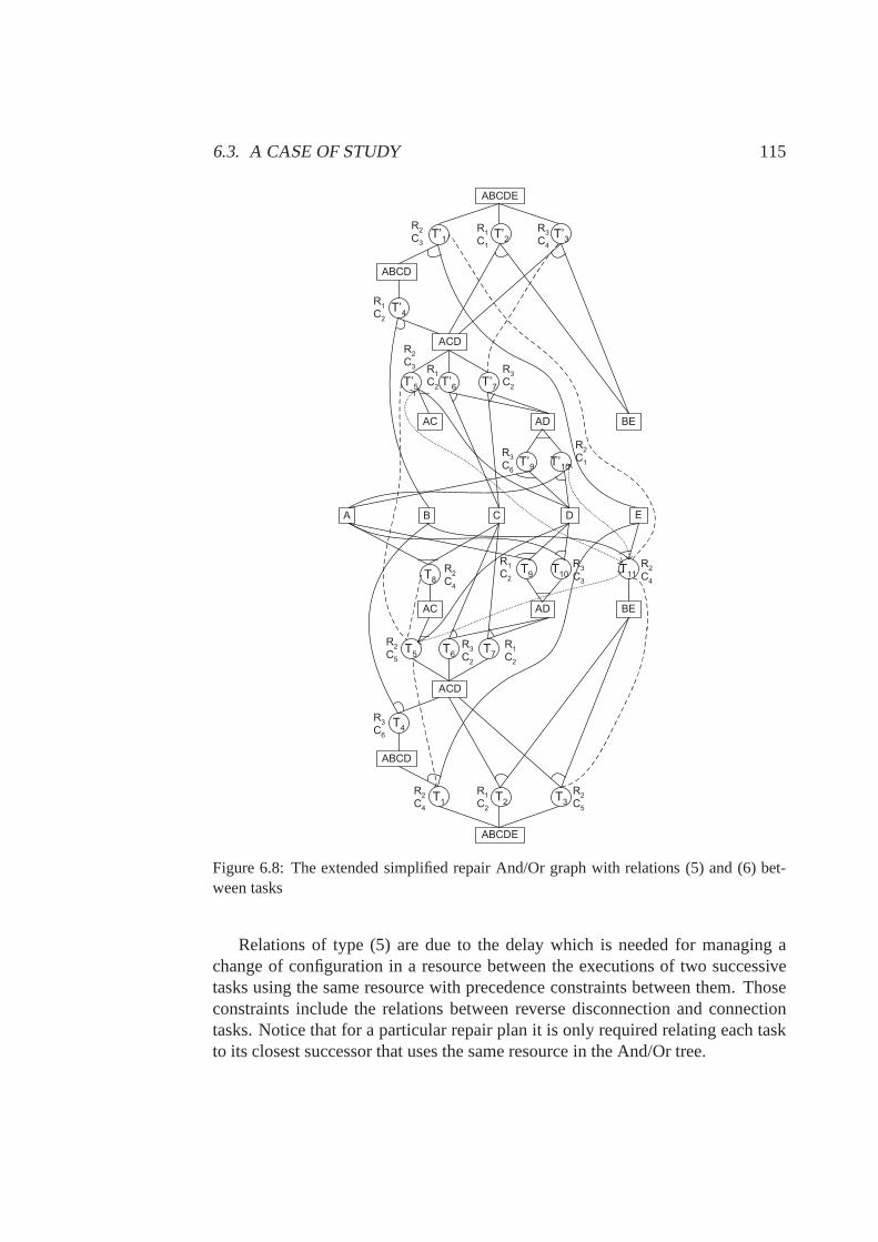
6.3. A CASE OF STUDY 115
ABCDE
ABCD
ACD
AC
A
AD BE
B C D
T’3
T’2
T’1
T’7
T’9
T’4
T’5
T’6
T’10
ABCDE
ABCD
ACD
AC AD BE
E
T3
T2
T1
T7
T9
T4
T5
T6
T10T
8
T11
R2
C3
R1
C1
R3
C4
R1
C2
R2
C3 R
1
C2
R3
C2
R3
C6
R2
C1
R2
C4
R3
C3
R1
C2
R2
C4
R2
C5
R3
C2
R1
C2
R3
C6
R2
C4
R1
C2
R2
C5
Figure 6.8: The extended simplified repair And/Or graph withrelations (5) and (6) bet-ween tasks
Relations of type (5) are due to the delay which is needed for managing achange of configuration in a resource between the executionsof two successivetasks using the same resource with precedence constraints between them. Thoseconstraints include the relations between reverse disconnection and connectiontasks. Notice that for a particular repair plan it is only required relating each taskto its closest successor that uses the same resource in the And/Or tree.
116 CHAPTER 6. P&S OF BPS IN RUN-TIME
Relations of type (6) consider the relation between the tasks which are notrelated by precedence constraints and which use the same resource.
Types (1), (2), (3) and (4) come from the relations between the nodes includedin the original graph, while types (5) and (6) come from the use of (same or dif-ferent) resources by the different tasks, and they are related to new links betweentasks in the extended And/Or graph.
As an example, Fig.6.8 shows an extension of the And/Or graph which ispresented in Fig.6.6by including relations of types (5) and (6).
The And/Or graphs represent the system structure through components re-lations, that remains permanent despite of different required resources or faultycomponents. Taking this into account, for the same graph there can be severalrepair problems by varying the faulty components or the required resources.
The And/Or graphs can be used as a basis for representing someproblemsthat involve both P&S, including the repair planning problem, since it allows toshow important P&S characteristics, such as alternative activities or precedencerelations. Moreover, in general, the And/Or graphs can be easily extended in orderto include other aspects. One important advantage of this representation is that theAnd/Or graph shows the activities that can be executed in parallel.
Multi-objective Optimization
Many problems, such as planning and scheduling problems, can involve multi-ple conflicting objectives that should be considered at the same time. In multi-objective optimization problems, that have been studied for several decades (Chan-kong and Haimes, 1983; Miettinen, 1999; Ehrgott, 2005; Coello, 2006), usuallyno unique solution exists but a set of nondominated solutions can be found. Thesesolutions are also known as Pareto optimal solutions, i.e.,for obtaining a betterfeasible solution in one of the objectives, it is necessary to deteriorate, at least,another one objective. Two typical objectives pursued in planning and schedulingproblems, used in this chapter, are the minimization of the total time and cost ofthe resulting plan. Typically, these two objectives are in conflict, and hence it isnot possible to find a plan which is optimum for both objectives. In these cases,optimized plans which present a good balance between the considered objectivesare pursued.
In order to solve multi-objective optimization problems, there are, basically,three approaches:
• Defining a new objective function that can be optimized with single objec-tive solvers, such as the weighted-sum method (Zadeh, 1963; Koski, 1985;Kim, 2006), that minimizes∑wi fi , wherewi ≥ 0 for each objective functionfi considered. It is advisable to normalize the objectives with some scaling
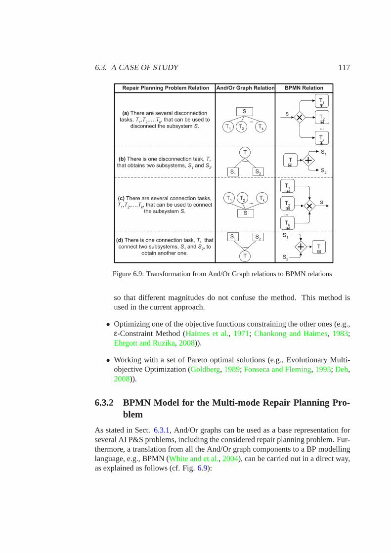
6.3. A CASE OF STUDY 117
��
�
��
��
�
��
��
��
��
��
��
��
����������� ������ ����� ������ ��������������������� ������
������������������ �����������
�������������
��������������� ���
����������������������
���������������� ������������������
�������������������������� ��
��
���������������������������������
���������
��������������� �����������
�������������
��������������������������������������
������������������������ ��
�����
�����������������
���
���
�������
�
��
��
��
���
���
���
��������
��
��
�� ���
Figure 6.9: Transformation from And/Or Graph relations to BPMN relations
so that different magnitudes do not confuse the method. Thismethod isused in the current approach.
• Optimizing one of the objective functions constraining theother ones (e.g.,ε-Constraint Method (Haimes et al., 1971; Chankong and Haimes, 1983;Ehrgott and Ruzika, 2008)).
• Working with a set of Pareto optimal solutions (e.g., Evolutionary Multi-objective Optimization (Goldberg, 1989; Fonseca and Fleming, 1995; Deb,2008)).
6.3.2 BPMN Model for the Multi-mode Repair Planning Pro-blem
As stated in Sect.6.3.1, And/Or graphs can be used as a base representation forseveral AI P&S problems, including the considered repair planning problem. Fur-thermore, a translation from all the And/Or graph components to a BP modellinglanguage, e.g., BPMN (White and et al., 2004), can be carried out in a direct way,as explained as follows (cf. Fig.6.9):
118 CHAPTER 6. P&S OF BPS IN RUN-TIME
(a) The fact that there are several disconnection activities that can be used todisconnect the same subsystem is modelled in BPMN by an exclusive gatewaywith that subsystem as input and as many outputs as disconnection activities,each one related to each disconnection activity.
(b) The fact that there is one disconnection activity that obtains two subsystemsis modelled in BPMN by a parallel gateway with that activity as input and twooutputs, each one related to each subsystem.
(c) The fact that there are several connection activities that can be used to con-nect the same subsystem is modelled in BPMN by an exclusive gateway withas many inputs as connection activities, each one related toeach connectionactivity, and with the resulting subsystem as output.
(d) The fact that there is one connection activity that connects two subsystems ismodelled in BPMN by a parallel gateway with two inputs, each one related toeach subsystem, and with the connection activity as output.
As stated, the auxiliary activities (cf. Def.37 and Def. 38) are not explici-tly represented in the And/Or graphs. However, they need to be included in theresulting BPMN in order to be executed. Therefore, BPMN activities related toauxiliary activities are added to the BPMN model when necessary, i.e.:
• set-up operationsare included between two successive activities which usethe same resource with different configurations, e.g.,T ′2 andT ′4 in Fig. 6.10.TheChange of configurationactivity, provided that it is necessary, can beexecuted in parallel with the treatment of the subsystems which are obtainedafter the activity enactment (cf. Fig.6.11(b)). The dots in Fig.6.11(b) re-present the treatment of the subsystem/s which result afterthe executionof the activity. This treatment depends on the specific subsystem. For ex-ample, after executingT ′2, the subsystemsA andBC are obtained (cf. Fig.6.11(a)). In this case, the treatment of both subsystems, e.g., Move BC?,can be performed in parallel to the change of configuration ofresourceR2
(i.e., resource which is used byT ′2).
The Change of configurationactivity is also controlled by thePlanner &Dispatchermodule since its execution causes the resource lock, that influ-ences the BP enactment. Moreover, the decisions about if this activity isexecuted or not and when it is executed depend on P&S decisions which aretaken by thePlanner & Dispatcherpool.
transportation operationsare included between two successive activitieswhich manage the same subsystem and use different resources(locations),
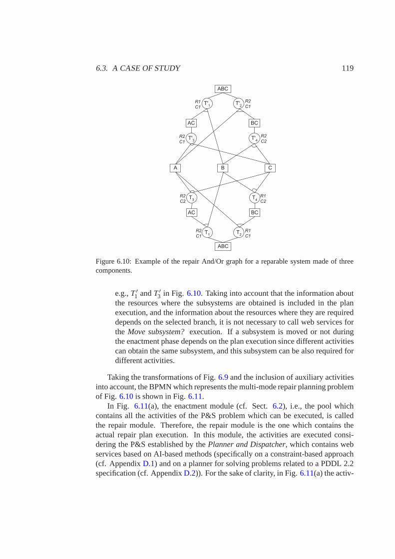
6.3. A CASE OF STUDY 119
� � �
���
���
���
��
���
��
��
��
��
��
��
��
��
��
��
���
��
��
��
��
��
�
��
��
��
��
��
��
��
��
Figure 6.10: Example of the repair And/Or graph for a reparable system made of threecomponents.
e.g.,T ′1 andT ′3 in Fig. 6.10. Taking into account that the information aboutthe resources where the subsystems are obtained is includedin the planexecution, and the information about the resources where they are requireddepends on the selected branch, it is not necessary to call web services forthe Move subsystem?execution. If a subsystem is moved or not duringthe enactment phase depends on the plan execution since different activitiescan obtain the same subsystem, and this subsystem can be alsorequired fordifferent activities.
Taking the transformations of Fig.6.9and the inclusion of auxiliary activitiesinto account, the BPMN which represents the multi-mode repair planning problemof Fig. 6.10is shown in Fig.6.11.
In Fig. 6.11(a), the enactment module (cf. Sect.6.2), i.e., the pool whichcontains all the activities of the P&S problem which can be executed, is calledthe repair module. Therefore, the repair module is the one which contains theactual repair plan execution. In this module, the activities are executed consi-dering the P&S established by thePlanner and Dispatcher, which contains webservices based on AI-based methods (specifically on a constraint-based approach(cf. AppendixD.1) and on a planner for solving problems related to a PDDL 2.2specification (cf. AppendixD.2)). For the sake of clarity, in Fig.6.11(a) the activ-
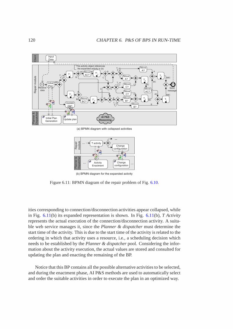
120 CHAPTER 6. P&S OF BPS IN RUN-TIME�����������
������
����
�����
����
������
����
����
���������
����������
�������
������
�������
�����
����
��
!��
��
"�
��#
�$
!�
"
��
!�
�#
��
�����������
%������������������
!
"�
��
!�
��
"�
���
���
����
�#�
����
�$�
��
!
�
"
"
"
!�
� �
�
��
��
��
��� !�
"
"�
!
!�
!"�
!"�
!"�
��
"��
�#��
�$�
��
!��
"�
�
�
��
&�'�"� (��������)����������������������
������������*�+,������-�������
�����.������������*����&+'
������
����
���������
����������
!������*
/��������
������
��-��������
���������*������
��-��������
000
000000
&+'�"� (��������-�������.������������*
���
�
�
��
������
�� ����
��$
Figure 6.11: BPMN diagram of the repair problem of Fig.6.10.
ities corresponding to connection/disconnection activities appear collapsed, whilein Fig. 6.11(b) its expanded representation is shown. In Fig.6.11(b), T Activityrepresents the actual execution of the connection/disconnection activity. A suita-ble web service manages it, since thePlanner & dispatchermust determine thestart time of the activity. This is due to the start time of theactivity is related to theordering in which that activity uses a resource, i.e., a scheduling decision whichneeds to be established by thePlanner & dispatcherpool. Considering the infor-mation about the activity execution, the actual values are stored and consulted forupdating the plan and enacting the remaining of the BP.
Notice that this BP contains all the possible alternative activities to be selected,and during the enactment phase, AI P&S methods are used to automatically selectand order the suitable activities in order to execute the plan in an optimized way.
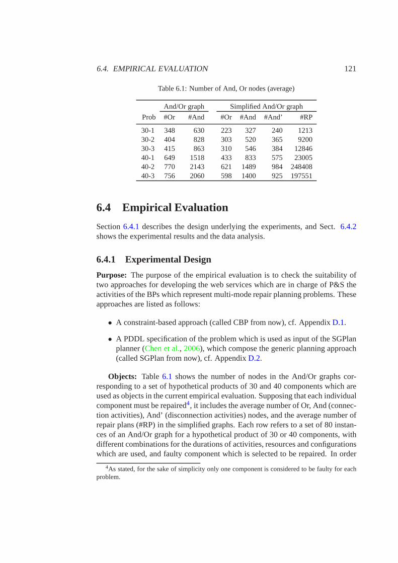
6.4. EMPIRICAL EVALUATION 121
Table 6.1: Number of And, Or nodes (average)
And/Or graph Simplified And/Or graph
Prob #Or #And #Or #And #And’ #RP
30-1 348 630 223 327 240 121330-2 404 828 303 520 365 920030-3 415 863 310 546 384 1284640-1 649 1518 433 833 575 2300540-2 770 2143 621 1489 984 24840840-3 756 2060 598 1400 925 197551
6.4 Empirical Evaluation
Section6.4.1describes the design underlying the experiments, and Sect.6.4.2shows the experimental results and the data analysis.
6.4.1 Experimental Design
Purpose: The purpose of the empirical evaluation is to check the suitability oftwo approaches for developing the web services which are in charge of P&S theactivities of the BPs which represent multi-mode repair planning problems. Theseapproaches are listed as follows:
• A constraint-based approach (called CBP from now), cf. Appendix D.1.
• A PDDL specification of the problem which is used as input of the SGPlanplanner (Chen et al., 2006), which compose the generic planning approach(called SGPlan from now), cf. AppendixD.2.
Objects: Table 6.1 shows the number of nodes in the And/Or graphs cor-responding to a set of hypothetical products of 30 and 40 components which areused as objects in the current empirical evaluation. Supposing that each individualcomponent must be repaired4, it includes the average number of Or, And (connec-tion activities), And’ (disconnection activities) nodes,and the average number ofrepair plans (#RP) in the simplified graphs. Each row refers to a set of 80 instan-ces of an And/Or graph for a hypothetical product of 30 or 40 components, withdifferent combinations for the durations of activities, resources and configurationswhich are used, and faulty component which is selected to be repaired. In order
4As stated, for the sake of simplicity only one component is considered to be faulty for eachproblem.
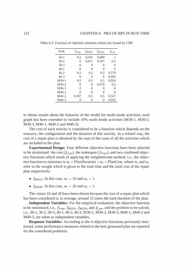
122 CHAPTER 6. P&S OF BPS IN RUN-TIME
Table 6.2: Fraction of Optimal solutions which are found by CBP
Prob fTime fMO20 fMO10 fCost
30-1 0,5 0,591 0,898 130-2 0 0,011 0,307 0,530-3 0 0 0 040-1 0 0 0 040-2 0,5 0,5 0,5 0,57940-3 0 0 0 0,045
M30-1 0,5 0,5 0,5 0,954M30-2 0 0 0,079 0,5M30-3 0 0 0 0M40-1 0 0 0 0M40-2 0,397 0,5 0,5 0,557M40-3 0 0 0 0,023
to obtain results about the behavior of the model for multi-mode activities, eachgraph has been extended to include 10% multi-mode activities (M30-1, M30-2,M30-3, M40-1, M40-2 and M40-3).
The cost of each activity is considered to be a function whichdepends on theresource, the configuration and the duration of this activity. In a related way, thecost of a repair plan is obtained by the sum of the costs of all the activities whichare included in the plan.
Experimental Design: Four different objective functions have been selectedto be minimized: the cost (fCost), the makespan (fTime), and two combined objec-tive functions which result of applying the weighted-sum method, i.e., the objec-tive function to minimize iswt×PlanDuration+wc×PlanCost, wherewt andwc
refer to the weight which is given to the total time and the total cost of the repairplan respectively:
• fMO10: In this case,wt = 10 andwc = 1.
• fMO20: In this case,wt = 20 andwc = 1.
The values 10 and 20 have been chosen because the cost of a repair plan whichhas been considered is, in average, around 15 times the totalduration of the plan.
Independent Variables: For the empirical evaluation, the objective functionto be minimized, i.e.,fTime, fMO10, fMO20, and fCost, and the problem to be solved,i.e., 30-1, 30-2, 30-3, 40-1, 40-2, 40-3, M30-1, M30-2, M30-3, M40-1, M40-2 andM40-3, are taken as independent variables.
Response Variables:According to the 4 objective functions previously men-tioned, some performance measures related to the best generated plan are reportedfor the considered problems:
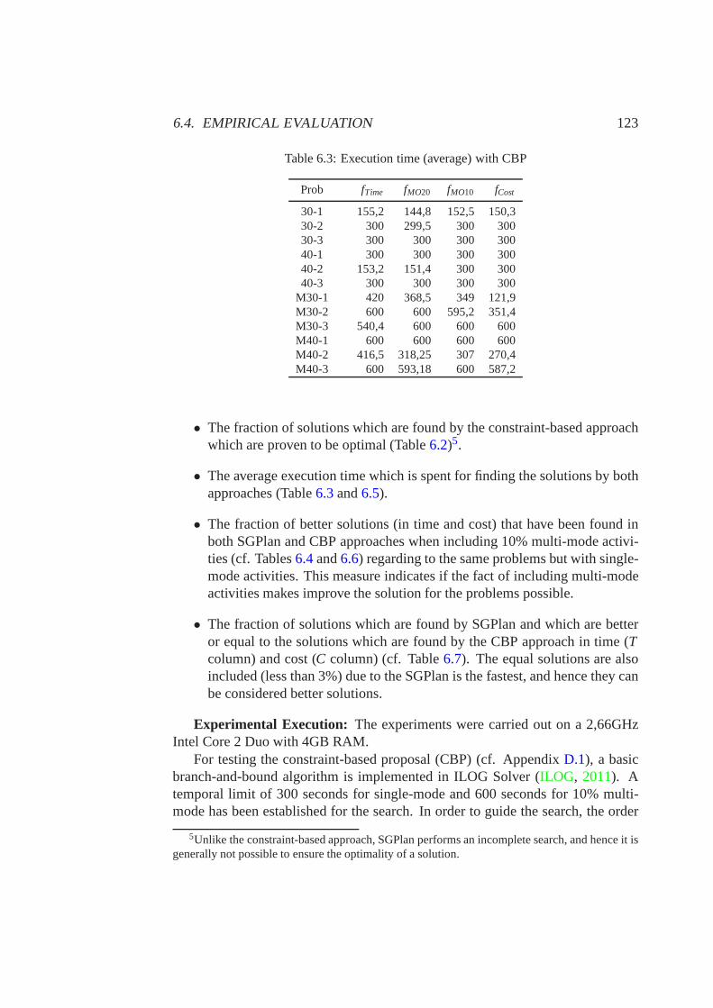
6.4. EMPIRICAL EVALUATION 123
Table 6.3: Execution time (average) with CBP
Prob fTime fMO20 fMO10 fCost
30-1 155,2 144,8 152,5 150,330-2 300 299,5 300 30030-3 300 300 300 30040-1 300 300 300 30040-2 153,2 151,4 300 30040-3 300 300 300 300
M30-1 420 368,5 349 121,9M30-2 600 600 595,2 351,4M30-3 540,4 600 600 600M40-1 600 600 600 600M40-2 416,5 318,25 307 270,4M40-3 600 593,18 600 587,2
• The fraction of solutions which are found by the constraint-based approachwhich are proven to be optimal (Table6.2)5.
• The average execution time which is spent for finding the solutions by bothapproaches (Table6.3and6.5).
• The fraction of better solutions (in time and cost) that havebeen found inboth SGPlan and CBP approaches when including 10% multi-mode activi-ties (cf. Tables6.4and6.6) regarding to the same problems but with single-mode activities. This measure indicates if the fact of including multi-modeactivities makes improve the solution for the problems possible.
• The fraction of solutions which are found by SGPlan and whichare betteror equal to the solutions which are found by the CBP approach in time (Tcolumn) and cost (C column) (cf. Table6.7). The equal solutions are alsoincluded (less than 3%) due to the SGPlan is the fastest, and hence they canbe considered better solutions.
Experimental Execution: The experiments were carried out on a 2,66GHzIntel Core 2 Duo with 4GB RAM.
For testing the constraint-based proposal (CBP) (cf. Appendix D.1), a basicbranch-and-bound algorithm is implemented in ILOG Solver (ILOG, 2011). Atemporal limit of 300 seconds for single-mode and 600 seconds for 10% multi-mode has been established for the search. In order to guide the search, the order
5Unlike the constraint-based approach, SGPlan performs an incomplete search, and hence it isgenerally not possible to ensure the optimality of a solution.
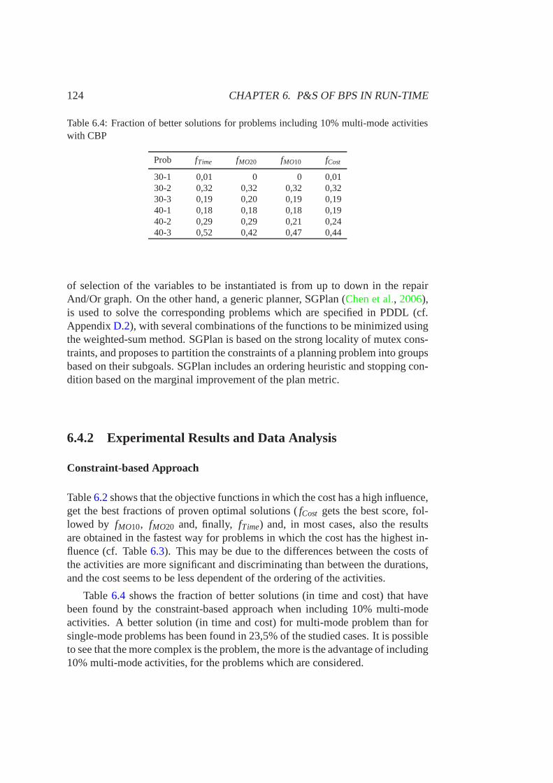
124 CHAPTER 6. P&S OF BPS IN RUN-TIME
Table 6.4: Fraction of better solutions for problems including 10% multi-mode activitieswith CBP
Prob fTime fMO20 fMO10 fCost
30-1 0,01 0 0 0,0130-2 0,32 0,32 0,32 0,3230-3 0,19 0,20 0,19 0,1940-1 0,18 0,18 0,18 0,1940-2 0,29 0,29 0,21 0,2440-3 0,52 0,42 0,47 0,44
of selection of the variables to be instantiated is from up todown in the repairAnd/Or graph. On the other hand, a generic planner, SGPlan (Chen et al., 2006),is used to solve the corresponding problems which are specified in PDDL (cf.AppendixD.2), with several combinations of the functions to be minimized usingthe weighted-sum method. SGPlan is based on the strong locality of mutex cons-traints, and proposes to partition the constraints of a planning problem into groupsbased on their subgoals. SGPlan includes an ordering heuristic and stopping con-dition based on the marginal improvement of the plan metric.
6.4.2 Experimental Results and Data Analysis
Constraint-based Approach
Table6.2shows that the objective functions in which the cost has a high influence,get the best fractions of proven optimal solutions (fCost gets the best score, fol-lowed by fMO10, fMO20 and, finally, fTime) and, in most cases, also the resultsare obtained in the fastest way for problems in which the costhas the highest in-fluence (cf. Table6.3). This may be due to the differences between the costs ofthe activities are more significant and discriminating thanbetween the durations,and the cost seems to be less dependent of the ordering of the activities.
Table6.4 shows the fraction of better solutions (in time and cost) that havebeen found by the constraint-based approach when including10% multi-modeactivities. A better solution (in time and cost) for multi-mode problem than forsingle-mode problems has been found in 23,5% of the studied cases. It is possibleto see that the more complex is the problem, the more is the advantage of including10% multi-mode activities, for the problems which are considered.
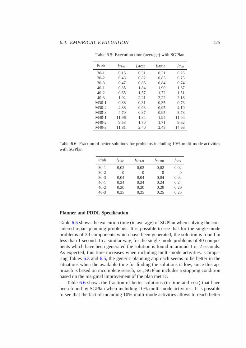
6.4. EMPIRICAL EVALUATION 125
Table 6.5: Execution time (average) with SGPlan
Prob fTime fMO20 fMO10 fCost
30-1 0,15 0,31 0,31 0,2630-2 0,43 0,82 0,83 0,7530-3 0,47 0,86 0,84 0,7440-1 0,85 1,84 1,90 1,6740-2 0,65 1,57 1,72 1,5140-3 1,02 2,21 2,22 2,18
M30-1 0,88 0,31 0,35 0,73M30-2 4,88 0,93 0,95 4,10M30-3 4,70 0,87 0,95 3,73M40-1 11,96 1,84 1,94 11,04M40-2 9,53 1,70 1,71 9,62M40-3 11,81 2,40 2,45 14,63
Table 6.6: Fraction of better solutions for problems including 10% multi-mode activitieswith SGPlan
Prob fTime fMO20 fMO10 fCost
30-1 0,02 0,02 0,02 0,0230-2 0 0 0 030-3 0,04 0,04 0,04 0,0440-1 0,24 0,24 0,24 0,2440-2 0,20 0,20 0,20 0,2040-3 0,25 0,25 0,25 0,25
Planner and PDDL Specification
Table6.5shows the execution time (in average) of SGPlan when solvingthe con-sidered repair planning problems. It is possible to see thatfor the single-modeproblems of 30 components which have been generated, the solution is found inless than 1 second. In a similar way, for the single-mode problems of 40 compo-nents which have been generated the solution is found in around 1 or 2 seconds.As expected, this time increases when including multi-modeactivities. Compa-ring Tables6.3 and6.5, the generic planning approach seems to be better in thesituations when the available time for finding the solutionsis low, since this ap-proach is based on incomplete search, i.e., SGPlan includesa stopping conditionbased on the marginal improvement of the plan metric.
Table6.6 shows the fraction of better solutions (in time and cost) that havebeen found by SGPlan when including 10% multi-mode activities. It is possibleto see that the fact of including 10% multi-mode activities allows to reach better
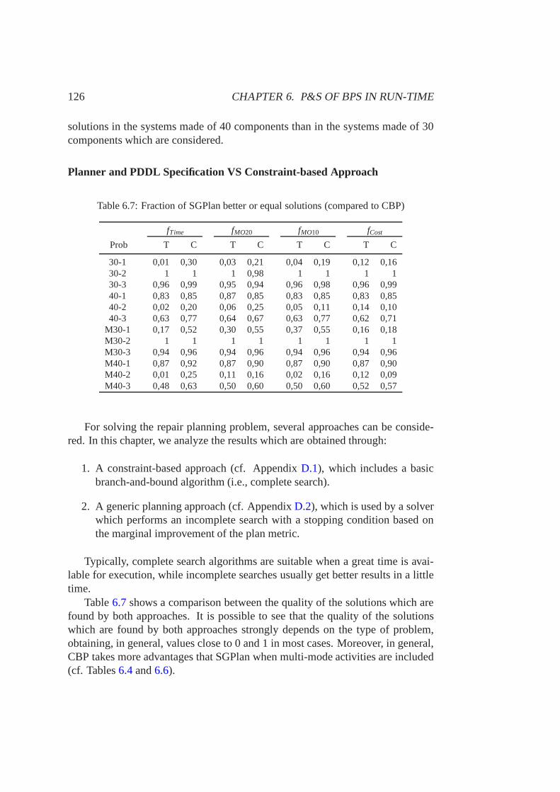
126 CHAPTER 6. P&S OF BPS IN RUN-TIME
solutions in the systems made of 40 components than in the systems made of 30components which are considered.
Planner and PDDL Specification VS Constraint-based Approach
Table 6.7: Fraction of SGPlan better or equal solutions (compared to CBP)
fTime fMO20 fMO10 fCost
Prob T C T C T C T C
30-1 0,01 0,30 0,03 0,21 0,04 0,19 0,12 0,1630-2 1 1 1 0,98 1 1 1 130-3 0,96 0,99 0,95 0,94 0,96 0,98 0,96 0,9940-1 0,83 0,85 0,87 0,85 0,83 0,85 0,83 0,8540-2 0,02 0,20 0,06 0,25 0,05 0,11 0,14 0,1040-3 0,63 0,77 0,64 0,67 0,63 0,77 0,62 0,71
M30-1 0,17 0,52 0,30 0,55 0,37 0,55 0,16 0,18M30-2 1 1 1 1 1 1 1 1M30-3 0,94 0,96 0,94 0,96 0,94 0,96 0,94 0,96M40-1 0,87 0,92 0,87 0,90 0,87 0,90 0,87 0,90M40-2 0,01 0,25 0,11 0,16 0,02 0,16 0,12 0,09M40-3 0,48 0,63 0,50 0,60 0,50 0,60 0,52 0,57
For solving the repair planning problem, several approaches can be conside-red. In this chapter, we analyze the results which are obtained through:
1. A constraint-based approach (cf. AppendixD.1), which includes a basicbranch-and-bound algorithm (i.e., complete search).
2. A generic planning approach (cf. AppendixD.2), which is used by a solverwhich performs an incomplete search with a stopping condition based onthe marginal improvement of the plan metric.
Typically, complete search algorithms are suitable when a great time is avai-lable for execution, while incomplete searches usually getbetter results in a littletime.
Table6.7shows a comparison between the quality of the solutions which arefound by both approaches. It is possible to see that the quality of the solutionswhich are found by both approaches strongly depends on the type of problem,obtaining, in general, values close to 0 and 1 in most cases. Moreover, in general,CBP takes more advantages that SGPlan when multi-mode activities are included(cf. Tables6.4and6.6).
6.5. RELATED WORK 127
6.5 Related Work
Several research groups have integrated AI techniques withBPM systems. Asfollows, some of the similar works are briefly described, explaining the main dif-ferences between them and the current approach.
Some related works integrate P&S tools in BPM systems for themodellingphase, such as (Alves et al., 2008; Gonzalez-Ferrer et al., 2009; R-Moreno et al.,2007; Hoffmann et al., 2010; De Castro and Marcos, 2009; Ferreira and Ferreira,2006). These works generate the BP model during the build-time, without ta-king into account the actual values of the parameters which are known in run-time. Consequently, the initial optimization plan can be obsolete due to the non-updating aspect. On a different way, the current proposal, in order to update theplan in run-time, maintains all the possible alternatives in the BP model, takinginto account the actual values of the parameters for updating the P&S of the ac-tivities.
On the other hand, most of the related works integrate scheduling tools inBPM systems for the enactment phase, in order to take dispatching decisions asto which activity should be executed using a resource when itbecomes free (dy-namic scheduling). As follows, a representative set of themare briefly summa-rized. One of the first works, (Zhao and Stohr, 1999), developed a frameworkfor temporal workflow management, including turnaround time predication, timeallocation, and activity prioritization. In a related way,(Son and Kim, 2001) pro-poses a schema for maximizing the number of workflow instances satisfying apredetermined deadline, based on a method for finding out thecritical activities.Moreover, (Ha et al., 2006) proposes a set of process execution rules based onindividual worklists, and it develops algorithms for the activity assignment in or-der to maximize the overall process efficiency, taking the resources capacitiesinto account. Furthermore, (Rhee et al., 2008) presents a Theory of Constraints(TOC)-based method for improving the efficiency of BPs. Additionally, (Tjoaet al., 2010) presents an approach for dynamic activity and resource allocationusing risk-aware business process simulations to facilitate and improve the plan-ning and the analysis of the BP activities.
There are several differences between the works (Zhao and Stohr, 1999; Sonand Kim, 2001; Ha et al., 2006; Rhee et al., 2008) and the current approach. First,in the current proposal the selection of the activities to beexecuted (planning)is done in run-time, besides the resource allocation, whilethe previously sum-marized works only consider the prioritization of the activities using the sameresource (scheduling). Secondly, the current approach consider several objectivefunctions, while the other works only focus on the temporal aspects of the pro-cesses for allocating the resources.
128 CHAPTER 6. P&S OF BPS IN RUN-TIME
Related to the proposed approach, (Marrella and Mecella, 2011) presents atechnique which is based on continuous planning in order to automatically copewith unexpected changes. The dynamic domain of the processes is specifiedthrough a second-order logic formalism (SitCalc), and a high level interpreter(IndiGolog) is used to control the execution of the actions in the BP enactment.Unlike our approach, any objective function is considered to be optimized. More-over, while our approach is based on translating P&S problems to the standardBPMN language (and hence the models can be usually executed by a BPM en-gine), in (Marrella and Mecella, 2011) the process activities need to be specifiedin SitCalc and be executed through IndiGolog.
To the best of our knowledge, there is not any proposal for selecting the suita-ble activities in run-time in order to optimize some functions in BP environmentsas well as considering reaching several goals (planning).
Related to And/Or graphs for representing P&S problems, a similar represen-tation can be found in (Bartak and O., 2007), that proposes an extension of tem-poral networks by parallel and alternative branching to represent some kinds ofP&S problems. Furthermore, in (Bae et al., 2004) the concept of blocks that canclassify BP flows into several patterns: iterative block, serial block and parallelblock includingAND andORstructures, is proposed.
Related to assembly planning, most approaches used for choosing optimal as-sembly plans employ different kind of rules in order to avoiddifficult activitiesor awkward intermediate subassemblies (Homem de Mello and Sanderson, 1991;Goldwasser and Motwani, 1999). In other context, disassembly planning has beenobject of different studies, varying from maintenance or repair purposes to recycleor recovery of useful materials (Li and Zhang, 1995; Lambert, 1997, 1999). Dif-ferent techniques have been used for solving those problems, from mathematicalprogramming to a variety of methods related to artificial intelligence (Lambert,2003).
Chapter 7
Conclusions
The research works which are presented in this document are based on the combi-nation of several research areas which have been widely referenced and explored:planning and scheduling (P&S), constraint programming (CP), and business pro-cess management (BPM).
Although the interest in the application of artificial intelligence techniques,and in particular P&S and CP, to improve the management of business processeshas grown in last years, there are some interesting and innovative points whichwere unexploited and which are addressed in the current Thesis Dissertation.
Specifically, a constraint-based approach forgenerating optimized BP enact-ment plans from declarative process specifications(cf. Chapter3) is proposedin order to optimize the performance of a process, accordingto objective functionslike minimizing the overall completion time. This approachovercomes the pro-blems which are related to imperative BP model specifications due to the tacit na-ture of human knowledge is often an obstacle to eliciting accurate process models(Ferreira and Ferreira, 2006). As mentioned in previous chapters, the generatedoptimized BP enactment plans can be apply to greatly improvethe overall BPMlife cycle (Weske, 2007). Two of these applications are detailed in the currentThesis Dissertation: (1) giving users of flexible BPMSs recommendations duringrun-time, and (2) generating optimized imperative BP models.
The former approach consists ongiving users of flexible BPMSs recommen-dations during run-time (cf. Chapter4) so that performance objective functionsof processes are optimized. Due to their flexible nature, frequently several waysto execute declarative process models exist. Typically, given a certain partial trace(i.e., reflecting the current state of the process instances), users can choose fromseveral enabled activities which activity to execute next.This selection, how-ever, can be quite challenging since performance goals of the process should beconsidered, and users often do not have an understanding of the overall process.Moreover, optimization of objective functions requires that resource capacities are
129
130 CHAPTER 7. CONCLUSIONS
considered. Therefore, recommendation support is needed during BP execution,especially for inexperienced users (van Dongen and van der Aalst, 2005). In ourproposal, recommendations on possible next steps are generated taking the partialtrace and the optimized plans into account. Furthermore, inthe proposed ap-proach, replanning is supported if actual traces deviate from the optimized enact-ment plans.
The latter approach, i.e.,generating optimized imperative BP models fromdeclarative specifications(cf. Chapter5) is motivated due to BP models are usu-ally defined manually by business analysts through imperative languages. Fur-thermore, allocating resources is an additional challengesince scheduling maysignificantly impact business process performance. Therefore, the manual speci-fication of process models can be very complex and time-consuming, potentiallyleading to non-optimized models or even errors can be generated. Moreover, theresult of process modelling is typically a static plan of actions, which is difficultto adapt to changing procedures or to different business goals. With the proposedapproach, process models can be adapted to changing procedures or to differentbusiness goals, since imperative process models can dynamically be generatedfrom static constraint-based specifications. Moreover, the automatic generation ofBP models can deal with complex problems of great size in a simple way. There-fore, a wide study of several aspects can be carried out, suchas those related tothe requirement of resources of different roles, or the estimated completion timefor the BP enactment, by starting from different declarative specifications.
Lastly, a proposal formodelling and enacting BPs that involve P&S deci-sions (cf. Chapter6) is presented. The execution of most BPs entails, in someway, scheduling decisions since the activities to be executed may compete forsome shared resources. In these cases, it is necessary to allocate the resourcesin a suitable way, usually optimizing some objectives. During process execu-tion, scheduling decisions are typically made by the BPM systems (BPMSs), byautomatically assigning activities to resources (Russell et al., 2005). To lessermeasure, planning problems are present in BP executions when, in some points,several possible execution branches exist, and the selection of the suitable onedepends on the BP goal and/or on the optimization of some functions. Since BPmodels are typically specified in an imperative way, most of the planning deci-sions are taken in the modelling phase. Specifically, the ordering and the selectionof the activities to be executed (planning) in the BP enactment are specified in theBP design time, when only estimated values for several parameters can be analy-zed. However, there are BPs which entail complex planning decisions which cangreatly be influenced by the values of several unpredictableparameters, whose ac-tual value is known in run time. The main contribution of the proposed approachis that both P&S decisions are taken in BP run-time, providing the process mana-

131
gement with efficiency and flexibility, and avoiding the drawbacks of taking thesedecisions during the design phase.
The motivation and the interest related to all the approaches which are pre-sented in the current document are strongly justified. Furthermore, discussions re-lated to the advantages, drawbacks and limitations of each proposal are included.In addition, the validation of the proposed approaches through the analysis of dif-ferent performance measures related to a range of test models of varying comple-xity is included. Moreover, the most related work together with the overcomingsand innovations of the proposed approaches are also presented.

Chapter 8
Future Work
In the current document, several research works are presented. All the proposedapproaches can be extended by including interesting aspects which remain to beexploited in its related fields.
In a first place, regarding the generation of optimized enactment plans fromdeclarative process specifications (cf. Chapter3), the next ideas are intended tobe explored:
• The inclusion of more general templates in the considered BPdeclarativespecifications, e.g., choice or metric temporal constraints (Montali, 2009).
• The analysis of further objective functions, e.g., cost or robustness, andthe optimization of all the overall these functions at the same time (multi-objective optimization).
• The consideration of the non-temporal data perspective in the declarativeprocess specification (Montali, 2009).
All these extensions have a great influence in giving users offlexible BPMSsrecommendations for the optimized execution of BPs (cf. Chapter 4) and in thegeneration of optimized BP models from declarative specifications (cf. Chapter5), since the generation of optimized enactment plan are usedas a starting pointfor both proposals.
Furthermore, there are other interesting applications of the generated opti-mized enactment plans which are intended to be explored, such that:
• Simulation: Simulation of BPs can be effectively used for analyzing pro-cesses and for improving BP models. BP simulation presents a”fast-forward”view on a current business process, so that the generated simulation modelscan accurately reflect the real-world process of interest. One interesting ap-plication of BP simulation is to identify unbalances between the resources
133
134 CHAPTER 8. FUTURE WORK
required for executing a particular process and the available resources (Rei-jers and van der Aalst, 1999). Moreover, the effects of alternative resourcesschedules can be investigated. As future work, a simulationengine cananalyze the generated BP enactment plans for making simulations from thedeclarative BP model, and the results can be studied in orderto analyze andto enhance the current BP model (Process Design & Analysis phase of BPMlife cycle (Weske, 2007)).
• Time Prediction: There are many scenarios where it is usefulto have relia-ble time predictions (van der Aalst et al., 2011). As future work, the genera-ted optimized BP enactment plans can be used by a prediction engine since,as stated, time information is available. For a given process instance state,the expected completion time for instances and activities can be calculatedby taking the end time of the remaining activities of the optimized plansinto account.
Related to giving users of flexible BPMSs recommendations for the optimizedexecution of BPs (cf. Chapter4), the integration of the proposed approach witha testsuite for recommendations in ConDec (Westergaard, 2011) is intended tobe achieved. In this testsuite, a model of user behavior can be specified. Theproposal of this integration consists of checking the suitability of the proposedapproach when simulating the actual execution of the BPs.
Regarding the generation of optimized BP models from declarative specifi-cations (cf. Chapter5), obtaining configurable process models from several op-timized plans is intended. These configurable process models can be generatedby extracting the common parts of the original process models, creating a singlecopy of them, and appending the differences as branches of configurable connec-tors (La Rosa et al., 2010). In this way, the generated configurable models captureall the behavior of the original models.
On the other hand, related to the proposal for planning and scheduling BPs inrun-time (cf. Chapter6), it is intended to analyze further kinds of BP problems in-volving planning and scheduling aspects. Furthermore, a bidirectional translationbetween planning languages, as PDDL, and BP model or execution languages, isintended to be explored. Moreover, further objective functions can be considered.

Appendices
135

Appendix A
ConDec-R Templates
As stated, in general, if not restricted by any constraints BP activities are assumedto be executed several times (Pesic and van der Aalst, 2006). Henceforth,nt(A)refers to the number of times that the repeated activityA is executed;Ai representsthe P&S activity related to the i-th execution ofA; andst(Ai) andet(Ai) repre-sent the start and the end times ofAi , respectively. It should be clarified that theconstraints∀i : 1≤ i < nt(A) : et(Ai)≤ st(Ai+1) hold for each repeated activityA.
In Fig. A.1, some representative examples of ConDec-R templates are graphi-cally represented. Specifically, three precedence relations between two repeatedactivities,A andB, are shown. As stated earlier, several executions of the sameBP activity can be modelled as a sequence of single P&S activities. In this figure,the P&S activityAi represents the i-th execution of the repeated activity A (Ai),and the arrow represents:
• A precedence relation between two P&S activitiesAi andB j , when it ap-pears between two activities, which means thatet(Ai)≤ st(B j).
• A precedence relation between a P&S activityAi and a setS of P&S ac-tivities, when it appears between an activity and a dotted rectangle whichencloses a set of activities, which means that∃B j ∈ S: et(Ai)≤ st(B j).
• A precedence relation between a setS of P&S activities and a P&S acti-vity B j , when it appears between a dotted rectangle which encloses aset ofactivities, and an activity, which means that∃Ai ∈ S: et(Ai)≤ st(B j).
In a similar way, a special arrow (wider than the other arrowsand with a bigdot in its origin) which appears between two P&S activities,A andB, shows thatA must be executedimmediately beforeB (et(A) = st(B)). In a similar way, thiscan be defined for a set of activities. More details about Fig.A.1 are shown in thedefinition of the related templates.
137
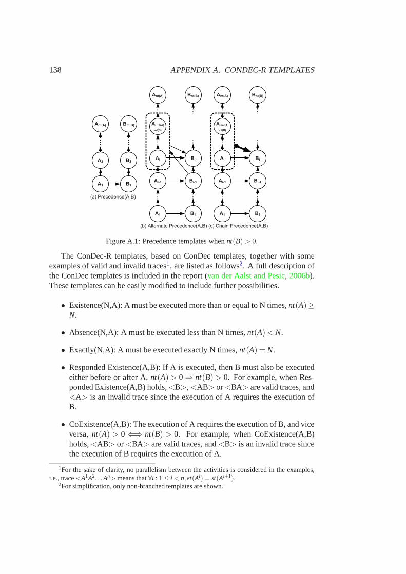
138 APPENDIX A. CONDEC-R TEMPLATES
(a) Precedence(A,B)
A1
A2
Ant(A)
...
B1
B2
Bnt(B)
...
(b) Alternate Precedence(A,B)
A1
Ai
Ant(A)
B1
Ai-1
...
Ai+nt(A)
-nt(B)
Bi
Bnt(B)
Bi-1
...
......
......
(c) Chain Precedence(A,B)
A1
Ai
Ant(A)
B1
Ai-1
...
Ai+nt(A)
-nt(B)
Bi
Bnt(B)
Bi-1
...
......
......
Figure A.1: Precedence templates whennt(B)> 0.
The ConDec-R templates, based on ConDec templates, together with someexamples of valid and invalid traces1, are listed as follows2. A full description ofthe ConDec templates is included in the report (van der Aalst and Pesic, 2006b).These templates can be easily modified to include further possibilities.
• Existence(N,A): A must be executed more than or equal to N times,nt(A)≥N.
• Absence(N,A): A must be executed less than N times,nt(A)< N.
• Exactly(N,A): A must be executed exactly N times,nt(A) = N.
• Responded Existence(A,B): If A is executed, then B must alsobe executedeither before or after A,nt(A) > 0⇒ nt(B) > 0. For example, when Res-ponded Existence(A,B) holds,<B>, <AB> or<BA> are valid traces, and<A> is an invalid trace since the execution of A requires the execution ofB.
• CoExistence(A,B): The execution of A requires the execution of B, and viceversa,nt(A) > 0⇐⇒ nt(B) > 0. For example, when CoExistence(A,B)holds,<AB> or<BA> are valid traces, and<B> is an invalid trace sincethe execution of B requires the execution of A.
1For the sake of clarity, no parallelism between the activities is considered in the examples,i.e., trace<A1A2. . .An> means that∀i : 1≤ i < n,et(Ai) = st(Ai+1).
2For simplification, only non-branched templates are shown.
139
• Precedence(A,B): Before the execution of B, A must have beenexecuted,nt(B)> 0⇒ (nt(A)> 0)∧(et(A1)≤ st(B1)). As can be seen in Fig.A.1(a),this relation implies thatA1 must precedeB1 in the case thatnt(B)> 0. Forexample, when Precedence(A,B) holds,<ABBBA> is a valid trace, and<BAABB> is an invalid trace since the first B is executed before any A.
• Response(A,B): After the execution of A, B must be executed,nt(A)> 0⇒(nt(B)> 0)∧ (st(Bnt(B))≥ et(Ant(A))). For example, when Response(A,B)holds,<BAABB> is a valid trace, and<ABBBA> is an invalid trace sinceafter the last execution of A, B is not executed.
• Succession(A,B): Relations Precedence(A,B) and Response(A,B) hold. Forexample, when Succession(A,B) holds,<ABABB> is a valid trace, and<BABBA> is an invalid trace since the first B is executed before any A(moreover, after the last execution of A, B is not executed).
• Alternate Precedence(A,B): Before the execution of B, A must have beenexecuted, and between each two executions of B, A must be executed. Thisimplies that:
1. The number of times that A is executed must be greater than or equalto the number of times that B is executed:nt(A)≥ nt(B).
2. Between each two executions of B, A must be executed at least once.Specifically, between the(i − 1)-th and thei-th execution of B, theearliest execution of A that can exist isi, and henceAi−1 must precedeBi−1 (as can be seen in Fig.A.1(b)). In a similar way, between the(i−1)-th and thei-th execution ofB, the latest execution ofA that canexist isi +nt(A)−nt(B), and henceBi must precedeAi+nt(A)−nt(B)+1.This can also be seen in Fig.A.1(b), where the possible activitiesto be executed between the(i−1)-th and thei-th execution ofB areframed within the dotted rectangle.∀i : 2≤ i ≤ nt(B) : ∃ j : i ≤ j ≤i +nt(A)−nt(B) : st(A j)≥ et(Bi−1)∧et(A j)≤ st(Bi).
3. Before the execution of B, A must be executed:st(B1) ≥ et(A1).
For example, when Alternate Precedence(A,B) holds,<ABAABABA > isa valid trace, and<ABAABBAA > is an invalid trace since between thesecond and the third execution of B, there is not any A.
• Alternate Response(A,B): After the execution of A, B must beexecuted,and between each two executions of A, there must be at least one executionof B. This implies:
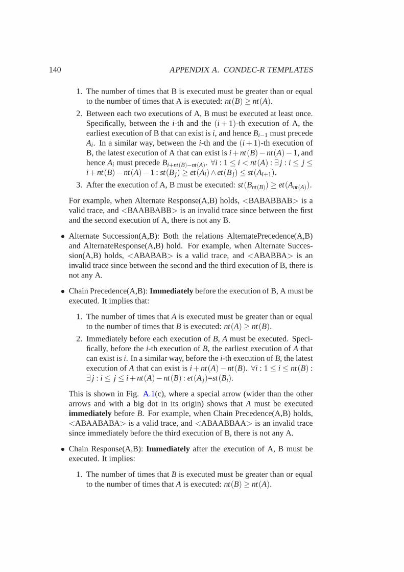
140 APPENDIX A. CONDEC-R TEMPLATES
1. The number of times that B is executed must be greater than or equalto the number of times that A is executed:nt(B)≥ nt(A).
2. Between each two executions of A, B must be executed at least once.Specifically, between thei-th and the(i + 1)-th execution of A, theearliest execution of B that can exist isi, and henceBi−1 must precedeAi . In a similar way, between thei-th and the(i +1)-th execution ofB, the latest execution of A that can exist isi +nt(B)−nt(A)−1, andhenceAi must precedeBi+nt(B)−nt(A). ∀i : 1≤ i < nt(A) : ∃ j : i ≤ j ≤i +nt(B)−nt(A)−1 : st(B j)≥ et(Ai)∧et(B j)≤ st(Ai+1).
3. After the execution of A, B must be executed:st(Bnt(B))≥ et(Ant(A)).
For example, when Alternate Response(A,B) holds,<BABABBAB> is avalid trace, and<BAABBABB> is an invalid trace since between the firstand the second execution of A, there is not any B.
• Alternate Succession(A,B): Both the relations AlternatePrecedence(A,B)and AlternateResponse(A,B) hold. For example, when Alternate Succes-sion(A,B) holds,<ABABAB> is a valid trace, and<ABABBA> is aninvalid trace since between the second and the third execution of B, there isnot any A.
• Chain Precedence(A,B):Immediately before the execution of B, A must beexecuted. It implies that:
1. The number of times thatA is executed must be greater than or equalto the number of times thatB is executed:nt(A)≥ nt(B).
2. Immediately before each execution ofB, A must be executed. Speci-fically, before thei-th execution ofB, the earliest execution ofA thatcan exist isi. In a similar way, before thei-th execution ofB, the latestexecution ofA that can exist isi +nt(A)−nt(B). ∀i : 1≤ i ≤ nt(B) :∃ j : i ≤ j ≤ i +nt(A)−nt(B) : et(A j)=st(Bi).
This is shown in Fig.A.1(c), where a special arrow (wider than the otherarrows and with a big dot in its origin) shows thatA must be executedimmediately beforeB. For example, when Chain Precedence(A,B) holds,<ABAABABA > is a valid trace, and<ABAABBAA > is an invalid tracesince immediately before the third execution of B, there is not any A.
• Chain Response(A,B):Immediately after the execution of A, B must beexecuted. It implies:
1. The number of times thatB is executed must be greater than or equalto the number of times thatA is executed:nt(B)≥ nt(A).
141
2. Immediately after each execution ofA, B must be executed. Specifi-cally, before thei-th execution ofA, the earliest execution ofB thatcan exist isi. In a similar way, after thei-th execution ofA, the lat-est execution ofB that can exist isi +nt(B)−nt(A)−1. ∀i : 1≤ i ≤nt(A) : ∃ j : i ≤ j ≤ i +nt(B)−nt(A)−1 : st(B j)=et(Ai).
For example, when Chain Response(A,B) holds,<BABABBAB> is a validtrace, and<BAABBABB> is an invalid trace since immediately after thefirst execution of A, there is not any B.
• Chain Succession(A,B): Both the relations Chain Precedence(A,B) and Cha-in Response(A,B) hold. For example, when Chain Succession(A,B) holds,<ABABAB> is a valid trace, and<ABABBA> is an invalid trace sinceimmediately before the third execution of B, there is not anyA.
• Responded Absence and Not CoExistence(A,B): If B is executed, then Acannot be executed, and vice versa,((nt(A)> 0) · (nt(B)> 0)) == 0. Forexample, when Responded Absence(A,B) holds,<A> or <B> are validtraces, and<BA> is an invalid trace.
• Negation Response, Negation Precedence, Negation Succession(A,B): Af-ter the execution of A, B cannot be executed, i.e., the last execution of Bmust finish before the start of the first execution of A (nt(A)> 0∧nt(B)>0)⇒ et(Bnt(B)) ≤ st(A1)). For example, when Negation Succession(A,B)holds,<BBBA> is a valid trace, and<BBAB> is an invalid trace since thethird B is executed after A.
• Negation Alternate Precedence(A,B): Between two executions of B, A can-not be executed,nt(B)≥ 2⇒∀i : 1≤ i ≤ nt(A) : et(Ai)≤ st(B1)∨st(Ai)≥et(Bnt(B)). For example, when Negation Alternate Precedence(A,B) holds,<AABBA> is a valid trace, and<ABABA> is an invalid trace since bet-ween the first and the second execution of B, A is executed.
• Negation Alternate Response(A,B): Between two executionsof A, B can-not be executed,nt(A) ≥ 2⇒ ∀1≤ i ≤ nt(B) : et(Bi) ≤ st(A1)∨ st(Bi) ≥et(Ant(A)). For example, when Negation Alternate Response(A,B) holds,<BBAAB> is a valid trace, and<BABAB> is an invalid trace since bet-ween the first and the second execution of A, B is executed.
• Negation Alternate Succession(A,B): Both the relations Negation AlternatePrecedence(A,B) and Negation Alternate Response(A,B) hold. For exam-ple, when Negation Alternate Succession(A,B) holds,<AABB> is a valid

142 APPENDIX A. CONDEC-R TEMPLATES
trace, and<AABBA> is an invalid trace since between the second and thethird execution of A, B is executed.
• Negation Chain Succession(A,B): B cannot be executed immediately afterthe execution of A,∀i : 1≤ i ≤ nt(B) :¬∃ j : 1≤ j ≤ nt(A) : et(A j) = st(Bi).For example, when Negation Chain Succession(A,B) holds,<BACBA>is a valid trace, and<BABA> is an invalid trace since the second B isexecuted immediately after A.
The ConDec-R templates can be classified either in unary (only one parameter,e.g., ExistenceN or AbsenceN) or binary (two parameters, e.g., Response or ChainSuccession) templates.
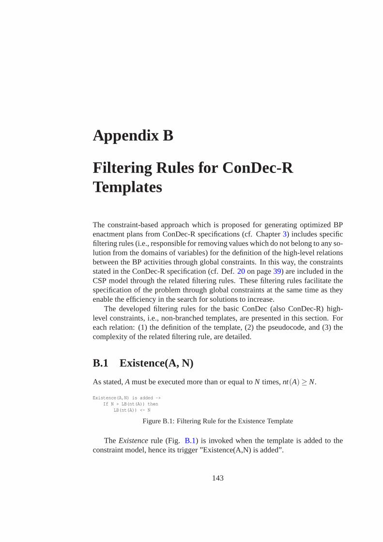
Appendix B
Filtering Rules for ConDec-RTemplates
The constraint-based approach which is proposed for generating optimized BPenactment plans from ConDec-R specifications (cf. Chapter3) includes specificfiltering rules (i.e., responsible for removing values which do not belong to any so-lution from the domains of variables) for the definition of the high-level relationsbetween the BP activities through global constraints. In this way, the constraintsstated in the ConDec-R specification (cf. Def.20 on page39) are included in theCSP model through the related filtering rules. These filtering rules facilitate thespecification of the problem through global constraints at the same time as theyenable the efficiency in the search for solutions to increase.
The developed filtering rules for the basic ConDec (also ConDec-R) high-level constraints, i.e., non-branched templates, are presented in this section. Foreach relation: (1) the definition of the template, (2) the pseudocode, and (3) thecomplexity of the related filtering rule, are detailed.
B.1 Existence(A, N)
As stated,A must be executed more than or equal toN times,nt(A)≥ N.
Existence(A,N) is added ->If N > LB(nt(A)) then
LB(nt(A)) <- N
Figure B.1: Filtering Rule for the Existence Template
The Existencerule (Fig. B.1) is invoked when the template is added to theconstraint model, hence its trigger ”Existence(A,N) is added”.
143
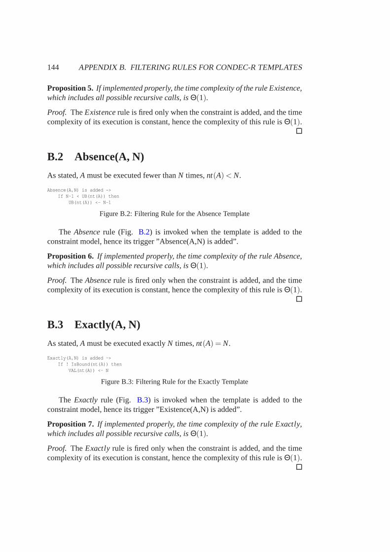
144 APPENDIX B. FILTERING RULES FOR CONDEC-R TEMPLATES
Proposition 5. If implemented properly, the time complexity of the rule Existence,which includes all possible recursive calls, isΘ(1).
Proof. TheExistencerule is fired only when the constraint is added, and the timecomplexity of its execution is constant, hence the complexity of this rule isΘ(1).
B.2 Absence(A, N)
As stated,A must be executed fewer thanN times,nt(A)< N.
Absence(A,N) is added ->If N-1 < UB(nt(A)) then
UB(nt(A)) <- N-1
Figure B.2: Filtering Rule for the Absence Template
The Absencerule (Fig. B.2) is invoked when the template is added to theconstraint model, hence its trigger ”Absence(A,N) is added”.
Proposition 6. If implemented properly, the time complexity of the rule Absence,which includes all possible recursive calls, isΘ(1).
Proof. TheAbsencerule is fired only when the constraint is added, and the timecomplexity of its execution is constant, hence the complexity of this rule isΘ(1).
B.3 Exactly(A, N)
As stated,A must be executed exactlyN times,nt(A) = N.
Exactly(A,N) is added ->If ! IsBound(nt(A)) then
VAL(nt(A)) <- N
Figure B.3: Filtering Rule for the Exactly Template
The Exactly rule (Fig. B.3) is invoked when the template is added to theconstraint model, hence its trigger ”Existence(A,N) is added”.
Proposition 7. If implemented properly, the time complexity of the rule Exactly,which includes all possible recursive calls, isΘ(1).
Proof. TheExactlyrule is fired only when the constraint is added, and the timecomplexity of its execution is constant, hence the complexity of this rule isΘ(1).
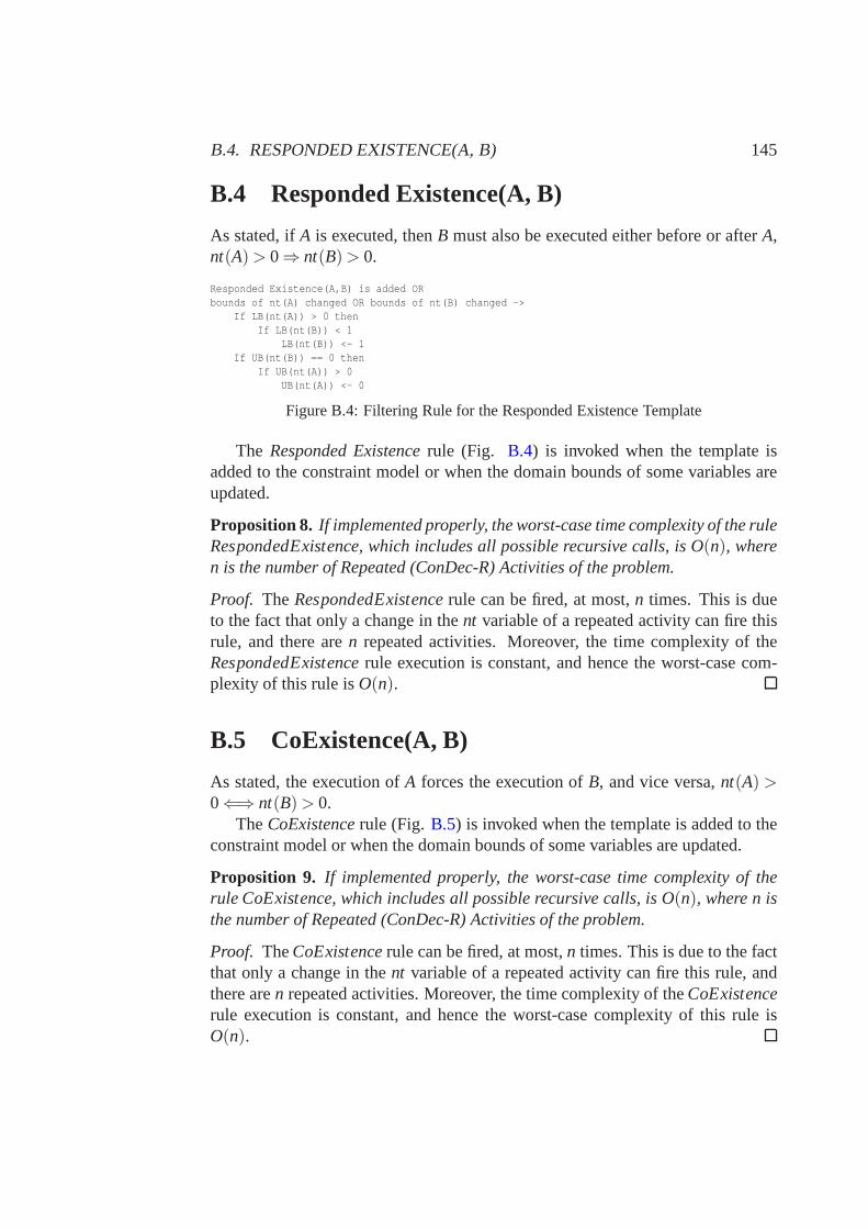
B.4. RESPONDED EXISTENCE(A, B) 145
B.4 Responded Existence(A, B)
As stated, ifA is executed, thenB must also be executed either before or afterA,nt(A)> 0⇒ nt(B)> 0.
Responded Existence(A,B) is added ORbounds of nt(A) changed OR bounds of nt(B) changed ->
If LB(nt(A)) > 0 thenIf LB(nt(B)) < 1
LB(nt(B)) <- 1If UB(nt(B)) == 0 then
If UB(nt(A)) > 0UB(nt(A)) <- 0
Figure B.4: Filtering Rule for the Responded Existence Template
The Responded Existencerule (Fig. B.4) is invoked when the template isadded to the constraint model or when the domain bounds of some variables areupdated.
Proposition 8. If implemented properly, the worst-case time complexity ofthe ruleRespondedExistence, which includes all possible recursive calls, is O(n), wheren is the number of Repeated (ConDec-R) Activities of the problem.
Proof. TheRespondedExistencerule can be fired, at most,n times. This is dueto the fact that only a change in thent variable of a repeated activity can fire thisrule, and there aren repeated activities. Moreover, the time complexity of theRespondedExistencerule execution is constant, and hence the worst-case com-plexity of this rule isO(n).
B.5 CoExistence(A, B)
As stated, the execution ofA forces the execution ofB, and vice versa,nt(A) >0⇐⇒ nt(B)> 0.
TheCoExistencerule (Fig. B.5) is invoked when the template is added to theconstraint model or when the domain bounds of some variablesare updated.
Proposition 9. If implemented properly, the worst-case time complexity oftherule CoExistence, which includes all possible recursive calls, is O(n), where n isthe number of Repeated (ConDec-R) Activities of the problem.
Proof. TheCoExistencerule can be fired, at most,n times. This is due to the factthat only a change in thent variable of a repeated activity can fire this rule, andthere aren repeated activities. Moreover, the time complexity of theCoExistencerule execution is constant, and hence the worst-case complexity of this rule isO(n).
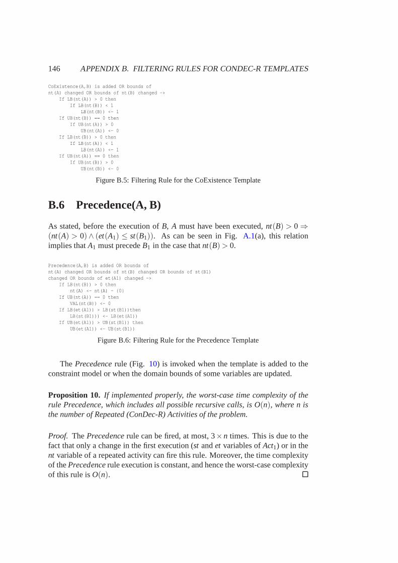
146 APPENDIX B. FILTERING RULES FOR CONDEC-R TEMPLATES
CoExistence(A,B) is added OR bounds ofnt(A) changed OR bounds of nt(B) changed ->
If LB(nt(A)) > 0 thenIf LB(nt(B)) < 1
LB(nt(B)) <- 1If UB(nt(B)) == 0 then
If UB(nt(A)) > 0UB(nt(A)) <- 0
If LB(nt(B)) > 0 thenIf LB(nt(A)) < 1
LB(nt(A)) <- 1If UB(nt(A)) == 0 then
If UB(nt(B)) > 0UB(nt(B)) <- 0
Figure B.5: Filtering Rule for the CoExistence Template
B.6 Precedence(A, B)
As stated, before the execution ofB, A must have been executed,nt(B) > 0⇒(nt(A) > 0)∧ (et(A1) ≤ st(B1)). As can be seen in Fig.A.1(a), this relationimplies thatA1 must precedeB1 in the case thatnt(B)> 0.
Precedence(A,B) is added OR bounds ofnt(A) changed OR bounds of nt(B) changed OR bounds of st(B1)changed OR bounds of et(A1) changed ->
If LB(nt(B)) > 0 thennt(A) <- nt(A) - {0}
If UB(nt(A)) == 0 thenVAL(nt(B)) <- 0
If LB(et(A1)) > LB(st(B1))thenLB(st(B1))) <- LB(et(A1))
If UB(et(A1)) > UB(st(B1)) thenUB(et(A1)) <- UB(st(B1))
Figure B.6: Filtering Rule for the Precedence Template
The Precedencerule (Fig. 10) is invoked when the template is added to theconstraint model or when the domain bounds of some variablesare updated.
Proposition 10. If implemented properly, the worst-case time complexity oftherule Precedence, which includes all possible recursive calls, is O(n), where n isthe number of Repeated (ConDec-R) Activities of the problem.
Proof. ThePrecedencerule can be fired, at most, 3×n times. This is due to thefact that only a change in the first execution (st andet variables ofAct1) or in thent variable of a repeated activity can fire this rule. Moreover,the time complexityof thePrecedencerule execution is constant, and hence the worst-case complexityof this rule isO(n).
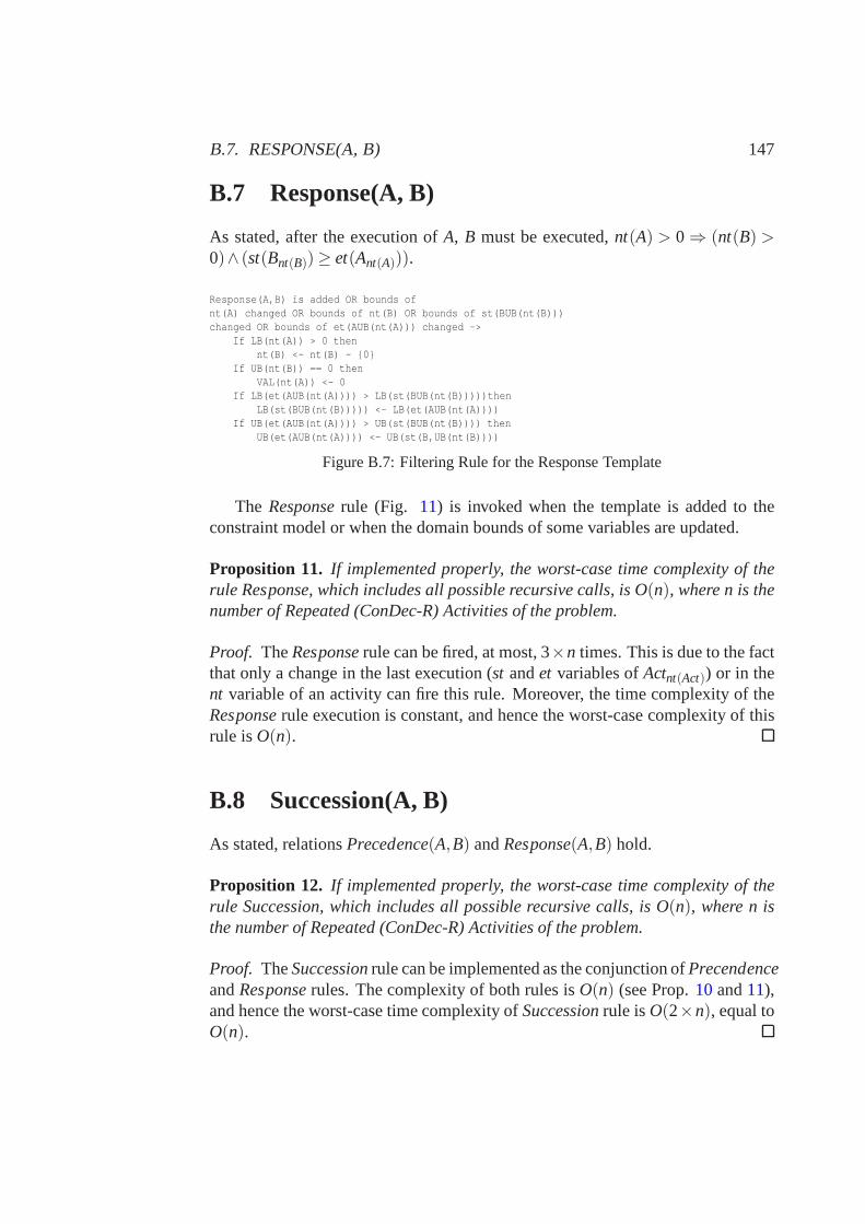
B.7. RESPONSE(A, B) 147
B.7 Response(A, B)
As stated, after the execution ofA, B must be executed,nt(A) > 0⇒ (nt(B) >0)∧ (st(Bnt(B))≥ et(Ant(A))).
Response(A,B) is added OR bounds ofnt(A) changed OR bounds of nt(B) OR bounds of st(BUB(nt(B)))changed OR bounds of et(AUB(nt(A))) changed ->
If LB(nt(A)) > 0 thennt(B) <- nt(B) - {0}
If UB(nt(B)) == 0 thenVAL(nt(A)) <- 0
If LB(et(AUB(nt(A)))) > LB(st(BUB(nt(B)))))thenLB(st(BUB(nt(B))))) <- LB(et(AUB(nt(A))))
If UB(et(AUB(nt(A)))) > UB(st(BUB(nt(B)))) thenUB(et(AUB(nt(A)))) <- UB(st(B,UB(nt(B))))
Figure B.7: Filtering Rule for the Response Template
The Responserule (Fig. 11) is invoked when the template is added to theconstraint model or when the domain bounds of some variablesare updated.
Proposition 11. If implemented properly, the worst-case time complexity oftherule Response, which includes all possible recursive calls, is O(n), where n is thenumber of Repeated (ConDec-R) Activities of the problem.
Proof. TheResponserule can be fired, at most, 3×n times. This is due to the factthat only a change in the last execution (st andet variables ofActnt(Act)) or in thent variable of an activity can fire this rule. Moreover, the timecomplexity of theResponserule execution is constant, and hence the worst-case complexity of thisrule isO(n).
B.8 Succession(A, B)
As stated, relationsPrecedence(A,B) andResponse(A,B) hold.
Proposition 12. If implemented properly, the worst-case time complexity oftherule Succession, which includes all possible recursive calls, is O(n), where n isthe number of Repeated (ConDec-R) Activities of the problem.
Proof. TheSuccessionrule can be implemented as the conjunction ofPrecendenceandResponserules. The complexity of both rules isO(n) (see Prop.10 and11),and hence the worst-case time complexity ofSuccessionrule isO(2×n), equal toO(n).
148 APPENDIX B. FILTERING RULES FOR CONDEC-R TEMPLATES
B.9 Alternate Precedence(A, B)
As stated, before the execution ofB, A must have been executed, and betweeneach two executions ofB, A must be executed. It implies that:
1. The number of times thatA is executed must be greater than or equal to thenumber of times thatB is executed:nt(A)>= nt(B).
2. Between each two executions ofB, A must be executed at least once. Speci-fically, between the(i−1)-th and thei-th execution ofB, the earliest execu-tion of A that can exist isi, and henceAi−1 must precedeBi−1 (as can be seenin Fig. A.1(b)). In a similar way, between the(i−1)-th and thei-th execu-tion of B, the latest execution ofA that can exist isi +nt(A)−nt(B), andhenceBi must precedeAi+nt(A)−nt(A)+1. This can also be seen in Fig.A.1(b),where the possible activities to be executed between the(i−1)-th and thei-th execution ofB are framed within the dotted rectangle.∀i : 2≤ i ≤ nt(B) :∃ j : i ≤ j ≤ i +nt(A)−nt(B) : st(A j)≥ et(Bi−1)∧et(A j))≤ st(Bi).
3. BeforeB, A must be executed:st(B1)≥ et(A1).
Proposition 13. If implemented properly, the worst-case time complexity oftherule AlternatePrecedence, which includes all possible recursive calls, is O(n×nt3), where n is the number of Repeated Activities of the problem,and nt is theupper bound of the variable nt(Act) domain. This upper bound obtains the samevalue for all the ConDec-R activities.
Proof. TheAlternatePrecedencerule can be fired, at most,n+2×n×nt times.This is due to the fact that a change in any execution of any activity (st andetvariables ofActi) or in thent variable of an activity can fire this rule. Moreover,the time complexity of theAlternatePrecedencerule execution isO(nt2), andhence the worst-case time complexity of this rule isO(n×nt3).
B.10 Alternate Response(A, B)
As stated, after the execution ofA, B must be executed, and between each twoexecutions ofA, there must be at least one execution ofB. It implies:
1. The number of times thatB is executed must be greater than or equal to thenumber of times thatA is executed:nt(B)>= nt(A).
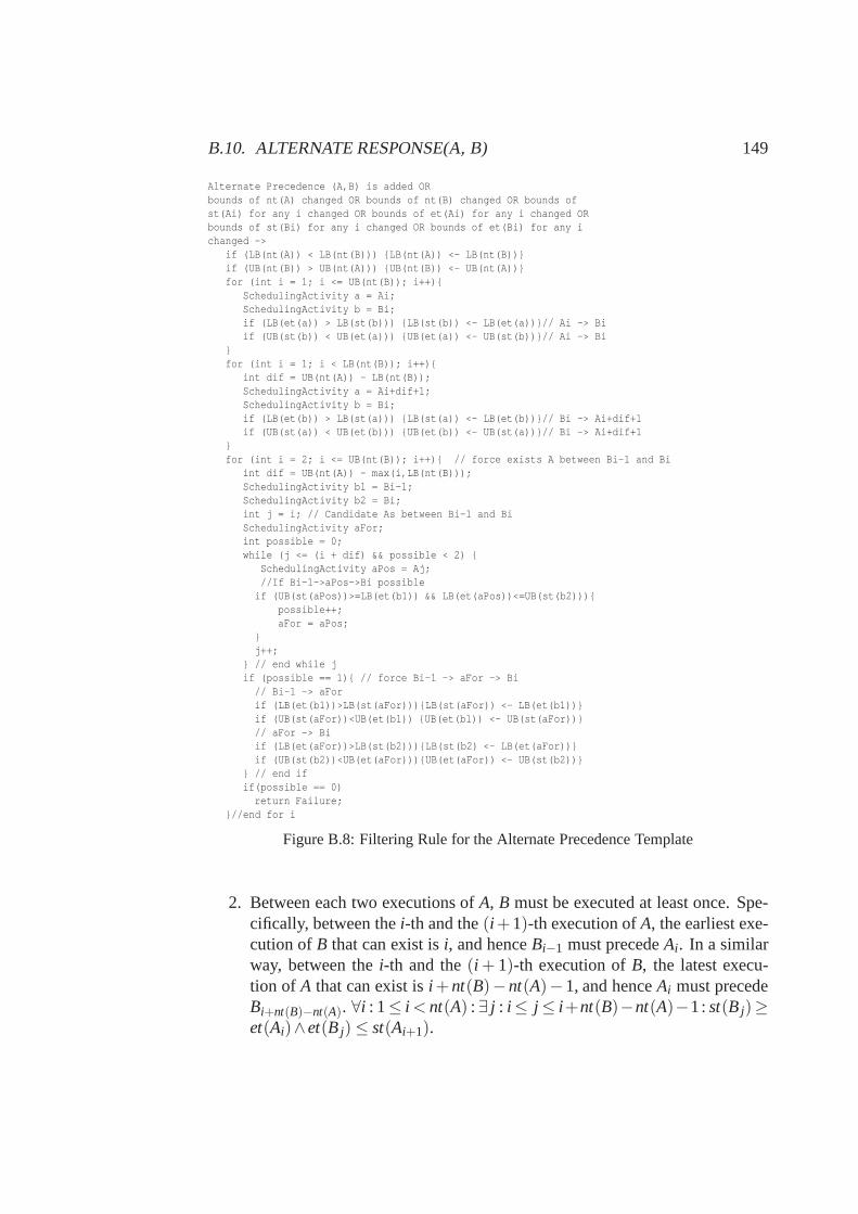
B.10. ALTERNATE RESPONSE(A, B) 149
Alternate Precedence (A,B) is added ORbounds of nt(A) changed OR bounds of nt(B) changed OR bounds ofst(Ai) for any i changed OR bounds of et(Ai) for any i changed ORbounds of st(Bi) for any i changed OR bounds of et(Bi) for any ichanged ->
if (LB(nt(A)) < LB(nt(B))) {LB(nt(A)) <- LB(nt(B))}if (UB(nt(B)) > UB(nt(A))) {UB(nt(B)) <- UB(nt(A))}for (int i = 1; i <= UB(nt(B)); i++){
SchedulingActivity a = Ai;SchedulingActivity b = Bi;if (LB(et(a)) > LB(st(b))) {LB(st(b)) <- LB(et(a))}// Ai -> Biif (UB(st(b)) < UB(et(a))) {UB(et(a)) <- UB(st(b))}// Ai -> Bi
}for (int i = 1; i < LB(nt(B)); i++){
int dif = UB(nt(A)) - LB(nt(B));SchedulingActivity a = Ai+dif+1;SchedulingActivity b = Bi;if (LB(et(b)) > LB(st(a))) {LB(st(a)) <- LB(et(b))}// Bi -> Ai+dif+1if (UB(st(a)) < UB(et(b))) {UB(et(b)) <- UB(st(a))}// Bi -> Ai+dif+1
}for (int i = 2; i <= UB(nt(B)); i++){ // force exists A between Bi-1 and Bi
int dif = UB(nt(A)) - max(i,LB(nt(B)));SchedulingActivity b1 = Bi-1;SchedulingActivity b2 = Bi;int j = i; // Candidate As between Bi-1 and BiSchedulingActivity aFor;int possible = 0;while (j <= (i + dif) && possible < 2) {
SchedulingActivity aPos = Aj;//If Bi-1->aPos->Bi possible
if (UB(st(aPos))>=LB(et(b1)) && LB(et(aPos))<=UB(st(b2))){possible++;aFor = aPos;
}j++;
} // end while jif (possible == 1){ // force Bi-1 -> aFor -> Bi
// Bi-1 -> aForif (LB(et(b1))>LB(st(aFor))){LB(st(aFor)) <- LB(et(b1))}if (UB(st(aFor))<UB(et(b1)) {UB(et(b1)) <- UB(st(aFor))}// aFor -> Biif (LB(et(aFor))>LB(st(b2))){LB(st(b2) <- LB(et(aFor))}if (UB(st(b2))<UB(et(aFor))){UB(et(aFor)) <- UB(st(b2))}
} // end ifif(possible == 0)
return Failure;}//end for i
Figure B.8: Filtering Rule for the Alternate Precedence Template
2. Between each two executions ofA, B must be executed at least once. Spe-cifically, between thei-th and the(i +1)-th execution ofA, the earliest exe-cution ofB that can exist isi, and henceBi−1 must precedeAi . In a similarway, between thei-th and the(i + 1)-th execution ofB, the latest execu-tion of A that can exist isi +nt(B)−nt(A)−1, and henceAi must precedeBi+nt(B)−nt(A). ∀i : 1≤ i < nt(A) : ∃ j : i≤ j ≤ i+nt(B)−nt(A)−1:st(B j)≥et(Ai)∧et(B j)≤ st(Ai+1).
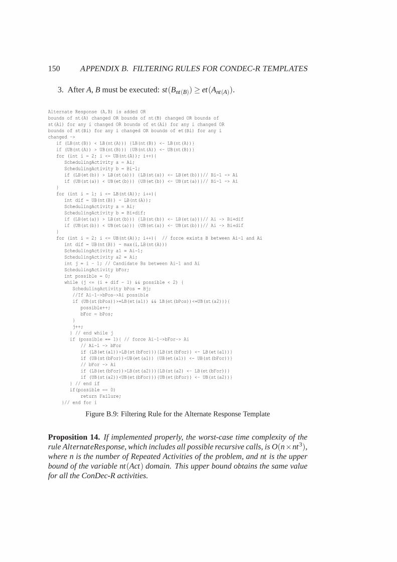
150 APPENDIX B. FILTERING RULES FOR CONDEC-R TEMPLATES
3. After A, B must be executed:st(Bnt(B))≥ et(Ant(A)).
Alternate Response (A,B) is added ORbounds of nt(A) changed OR bounds of nt(B) changed OR bounds ofst(Ai) for any i changed OR bounds of et(Ai) for any i changed ORbounds of st(Bi) for any i changed OR bounds of et(Bi) for any ichanged ->
if (LB(nt(B)) < LB(nt(A))) {LB(nt(B)) <- LB(nt(A))}if (UB(nt(A)) > UB(nt(B))) {UB(nt(A)) <- UB(nt(B))}for (int i = 2; i <= UB(nt(A)); i++){
SchedulingActivity a = Ai;SchedulingActivity b = Bi-1;if (LB(et(b)) > LB(st(a))) {LB(st(a)) <- LB(et(b))}// Bi-1 -> Aiif (UB(st(a)) < UB(et(b))) {UB(et(b)) <- UB(st(a))}// Bi-1 -> Ai
}for (int i = 1; i <= LB(nt(A)); i++){
int dif = UB(nt(B)) - LB(nt(A));SchedulingActivity a = Ai;SchedulingActivity b = Bi+dif;if (LB(et(a)) > LB(st(b))) {LB(st(b)) <- LB(et(a))}// Ai -> Bi+difif (UB(st(b)) < UB(et(a))) {UB(et(a)) <- UB(st(b))}// Ai -> Bi+dif
}for (int i = 2; i <= UB(nt(A)); i++){ // force exists B between Ai-1 and Ai
int dif = UB(nt(B)) - max(i,LB(nt(A)))SchedulingActivity a1 = Ai-1;SchedulingActivity a2 = Ai;int j = i - 1; // Candidate Bs between Ai-1 and AiSchedulingActivity bFor;int possible = 0;while (j <= (i + dif - 1) && possible < 2) {
SchedulingActivity bPos = Bj;//If Ai-1->bPos->Ai possibleif (UB(st(bPos))>=LB(et(a1)) && LB(et(bPos))<=UB(st(a2))){
possible++;bFor = bPos;
}j++;
} // end while jif (possible == 1){ // force Ai-1->bFor-> Ai
// Ai-1 -> bForif (LB(et(a1))>LB(st(bFor))){LB(st(bFor)) <- LB(et(a1))}if (UB(st(bFor))<UB(et(a1)) {UB(et(a1)) <- UB(st(bFor))}// bFor -> Aiif (LB(et(bFor))>LB(st(a2))){LB(st(a2) <- LB(et(bFor))}if (UB(st(a2))<UB(et(bFor))){UB(et(bFor)) <- UB(st(a2))}
} // end ifif(possible == 0)
return Failure;}// end for i
Figure B.9: Filtering Rule for the Alternate Response Template
Proposition 14. If implemented properly, the worst-case time complexity oftherule AlternateResponse, which includes all possible recursive calls, is O(n×nt3),where n is the number of Repeated Activities of the problem, and nt is the upperbound of the variable nt(Act) domain. This upper bound obtains the same valuefor all the ConDec-R activities.
B.11. ALTERNATE SUCCESSION(A, B) 151
Proof. The AlternateResponserule can be fired, at most,n+ 2× n× nt times.This is due to the fact that a change in any execution of any activity (st andetvariables ofActi) or in thent variable of an activity can fire this rule. Moreover,the time complexity of theAlternateResponserule execution isO(nt2), and hencethe worst-case time complexity of this rule isO(n×nt3).
B.11 Alternate Succession(A, B)
As stated, relationsAlternatePrecedence(A,B)andAlternateResponse(A,B)hold.
Proposition 15. If implemented properly, the worst-case time complexity oftherule AlternateSuccession, which includes all possible recursive calls, is O(n×nt3), where n is the number of Repeated Activities of the problem,and nt is theupper bound of the variable nt(Act) domain. This upper bound obtains the samevalue for all the ConDec-R activities.
Proof. The AlternateSuccessionrule can be implemented as the conjunction ofAlternatePrecendenceand AlternateResponserules. The complexity of bothrules isO(n× nt3) (see Prop.13 and14), and hence the worst-case time com-plexity of AlternateSuccessionrule isO(2×n×nt3), equal toO(n×nt3).
B.12 Chain Precedence(A, B)
As stated,immediately beforeB, A must be executed. It implies that:
1. The number of times thatA is executed must be greater than or equal to thenumber of times thatB is executed:nt(A)>= nt(B).
2. Immediately before each execution ofB, A must be executed. Specifically,before thei-th execution ofB, the earliest execution ofA that can existis i. In a similar way, before thei-th execution ofB, the latest executionof A that can exist isi + nt(A)− nt(B). ∀i : 1≤ i ≤ nt(B) : ∃ j : i ≤ j ≤i +nt(A)−nt(B) : et(A j)=st(Bi).
Proposition 16. If implemented properly, the worst-case time complexity oftherule ChainPrecedence, which includes all possible recursive calls, is O(n×nt3),where n is the number of Repeated Activities of the problem, and nt is the upperbound of the variable nt(Act) domain. This upper bound obtains the same valuefor all the ConDec-R activities.
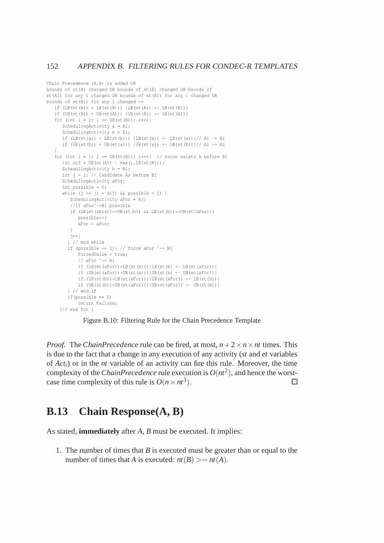
152 APPENDIX B. FILTERING RULES FOR CONDEC-R TEMPLATES
Chain Precedence (A,B) is added ORbounds of nt(A) changed OR bounds of nt(B) changed OR bounds ofet(Ai) for any i changed OR bounds of st(Bi) for any i changed ORbounds of et(Bi) for any i changed ->
if (LB(nt(A)) < LB(nt(B))) {LB(nt(A)) <- LB(nt(B))}if (UB(nt(B)) > UB(nt(A))) {UB(nt(B)) <- UB(nt(A))}for (int i = 1; i <= UB(nt(B)); i++){
SchedulingActivity a = Ai;SchedulingActivity b = Bi;if (LB(et(a)) > LB(st(b))) {LB(st(b)) <- LB(et(a))}// Ai -> Biif (UB(st(b)) < UB(et(a))) {UB(et(a)) <- UB(st(b))}// Ai -> Bi
}for (int i = 1; i <= UB(nt(B)); i++){ // force exists A before Bi
int dif = UB(nt(A)) - max(i,LB(nt(B)));SchedulingActivity b = Bi;int j = i; // Candidate As before BiSchedulingActivity aFor;int possible = 0;while (j <= (i + dif) && possible < 2) {
SchedulingActivity aPos = Aj;//If aPos’->Bi possibleif (LB(et(aPos))<=UB(st(b)) && LB(st(b))<=UB(et(aPos)))
possible++;aFor = aPos;
}j++;
} // end whileif (possible == 1){ // force aFor ’-> Bi
forcedValue = true;// aFor ’-> Biif (LB(et(aFor))>LB(st(b))){LB(st(b) <- LB(et(aFor))}if (UB(et(aFor))>UB(st(b))){UB(st(b) <- UB(et(aFor))}if (LB(st(b))<LB(et(aFor))){LB(et(aFor)) <- LB(st(b))}if (UB(st(b))<UB(et(aFor))){UB(et(aFor)) <- UB(st(b))}
} // end ifif(possible == 0)
return Failure;}// end for i
Figure B.10: Filtering Rule for the Chain Precedence Template
Proof. TheChainPrecedencerule can be fired, at most,n+2×n×nt times. Thisis due to the fact that a change in any execution of any activity (st andet variablesof Acti) or in thent variable of an activity can fire this rule. Moreover, the timecomplexity of theChainPrecedencerule execution isO(nt2), and hence the worst-case time complexity of this rule isO(n×nt3).
B.13 Chain Response(A, B)
As stated,immediately afterA, B must be executed. It implies:
1. The number of times thatB is executed must be greater than or equal to thenumber of times thatA is executed:nt(B)>= nt(A).
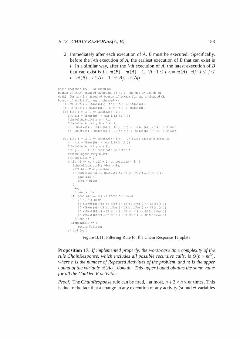
B.13. CHAIN RESPONSE(A, B) 153
2. Immediately after each execution ofA, B must be executed. Specifically,before thei-th execution ofA, the earliest execution ofB that can exist isi. In a similar way, after thei-th execution ofA, the latest execution ofBthat can exist isi +nt(B)−nt(A)−1. ∀i : 1≤ i <= nt(A) : ∃ j : i ≤ j ≤i +nt(B)−nt(A)−1 : st(B j)=et(Ai).
Chain Response (A,B) is added ORbounds of nt(A) changed OR bounds of nt(B) changed OR bounds ofet(Ai) for any i changed OR bounds of st(Bi) for any i changed ORbounds of et(Bi) for any i changed ->
if (LB(nt(B)) < LB(nt(A))) {LB(nt(B)) <- LB(nt(A))}if (UB(nt(A)) > UB(nt(B))) {UB(nt(A)) <- UB(nt(B))}for (int i = 1; i <= LB(nt(A)); i++){
int dif = UB(nt(B)) - max(i,LB(nt(A)))SchedulingActivity a = Ai;SchedulingActivity b = Bi+dif;if (LB(et(a)) > LB(st(b))) {LB(st(b)) <- LB(et(a))}// Ai -> Bi+difif (UB(st(b)) < UB(et(a))) {UB(et(a)) <- UB(st(b))}// Ai -> Bi+dif
}for (int i = 1; i <= UB(nt(A)); i++){ // force exists B after Ai
int dif = UB(nt(B)) - max(i,LB(nt(A)))SchedulingActivity a = Ai;int j = i - 1; // Candidate Bs after AiSchedulingActivity bFor;int possible = 0;while (j <= (i + dif - 1) && possible < 2) {
SchedulingActivity bPos = Bj;//If Ai->bPos possibleif (UB(st(bPos))>=LB(et(a)) && LB(et(bPos))<=UB(st(a))){
possible++;bFor = bPos;
}j++;
} // end whileif (possible == 1){ // force Ai’->bFor
// Ai ’-> bForif (LB(et(a))>LB(st(bFor))){LB(st(bFor)) <- LB(et(a))}if (UB(et(a))>UB(st(bFor))){UB(st(bFor)) <- UB(et(a))}if (LB(st(bFor))<LB(et(a)) {LB(et(a)) <- LB(st(bFor))}if (UB(st(bFor))<UB(et(a)) {UB(et(a)) <- UB(st(bFor))}
} // end ifif(possible == 0)
return Failure;}// end for i
Figure B.11: Filtering Rule for the Chain Response Template
Proposition 17. If implemented properly, the worst-case time complexity oftherule ChainResponse, which includes all possible recursivecalls, is O(n× nt3),where n is the number of Repeated Activities of the problem, and nt is the upperbound of the variable nt(Act) domain. This upper bound obtains the same valuefor all the ConDec-R activities.
Proof. TheChainResponserule can be fired, , at most,n+2×n×nt times. Thisis due to the fact that a change in any execution of any activity (st andet variables
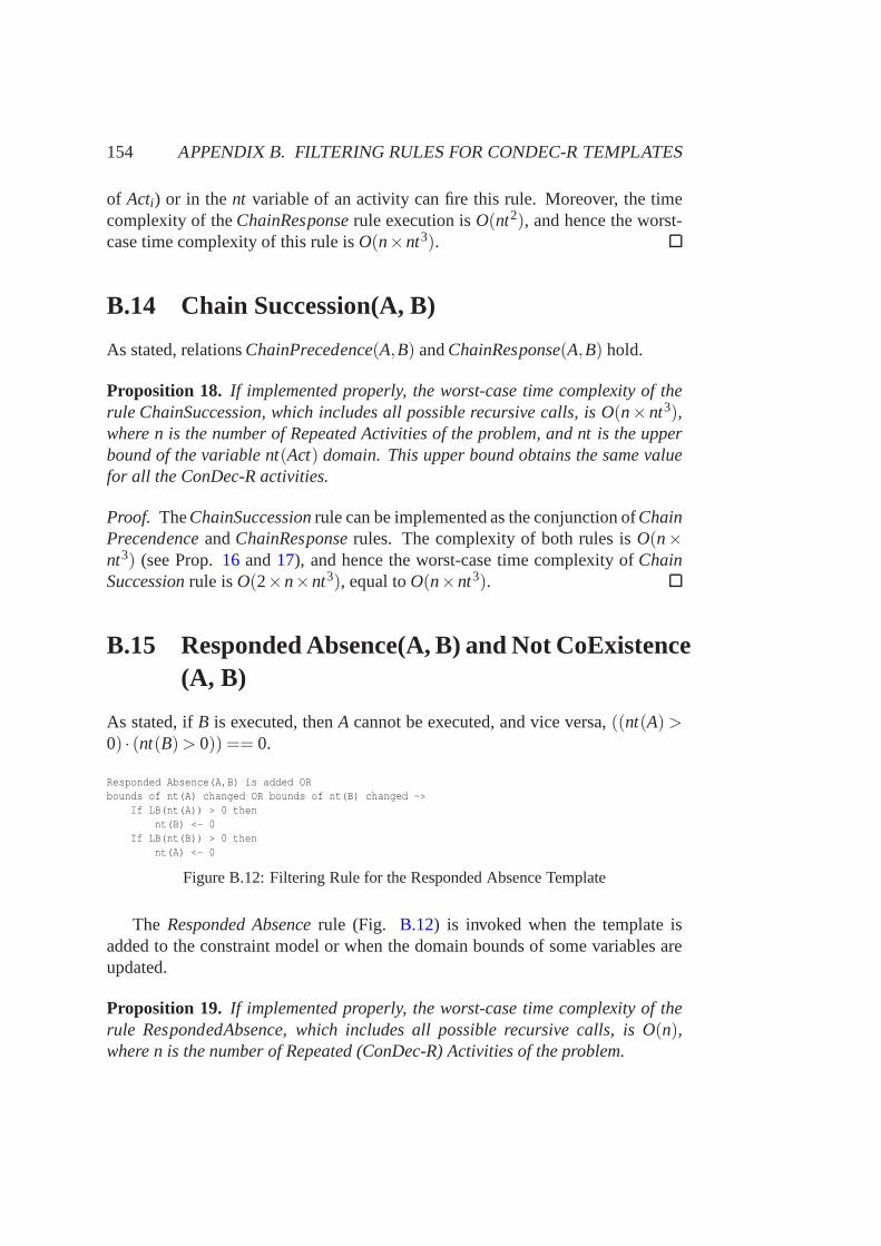
154 APPENDIX B. FILTERING RULES FOR CONDEC-R TEMPLATES
of Acti) or in thent variable of an activity can fire this rule. Moreover, the timecomplexity of theChainResponserule execution isO(nt2), and hence the worst-case time complexity of this rule isO(n×nt3).
B.14 Chain Succession(A, B)
As stated, relationsChainPrecedence(A,B) andChainResponse(A,B) hold.
Proposition 18. If implemented properly, the worst-case time complexity oftherule ChainSuccession, which includes all possible recursive calls, is O(n×nt3),where n is the number of Repeated Activities of the problem, and nt is the upperbound of the variable nt(Act) domain. This upper bound obtains the same valuefor all the ConDec-R activities.
Proof. TheChainSuccessionrule can be implemented as the conjunction ofChainPrecendenceandChainResponserules. The complexity of both rules isO(n×nt3) (see Prop.16 and17), and hence the worst-case time complexity ofChainSuccessionrule isO(2×n×nt3), equal toO(n×nt3).
B.15 Responded Absence(A, B) and Not CoExistence(A, B)
As stated, ifB is executed, thenA cannot be executed, and vice versa,((nt(A)>0) · (nt(B)> 0)) == 0.
Responded Absence(A,B) is added ORbounds of nt(A) changed OR bounds of nt(B) changed ->
If LB(nt(A)) > 0 thennt(B) <- 0
If LB(nt(B)) > 0 thennt(A) <- 0
Figure B.12: Filtering Rule for the Responded Absence Template
The Responded Absencerule (Fig. B.12) is invoked when the template isadded to the constraint model or when the domain bounds of some variables areupdated.
Proposition 19. If implemented properly, the worst-case time complexity oftherule RespondedAbsence, which includes all possible recursive calls, is O(n),where n is the number of Repeated (ConDec-R) Activities of the problem.
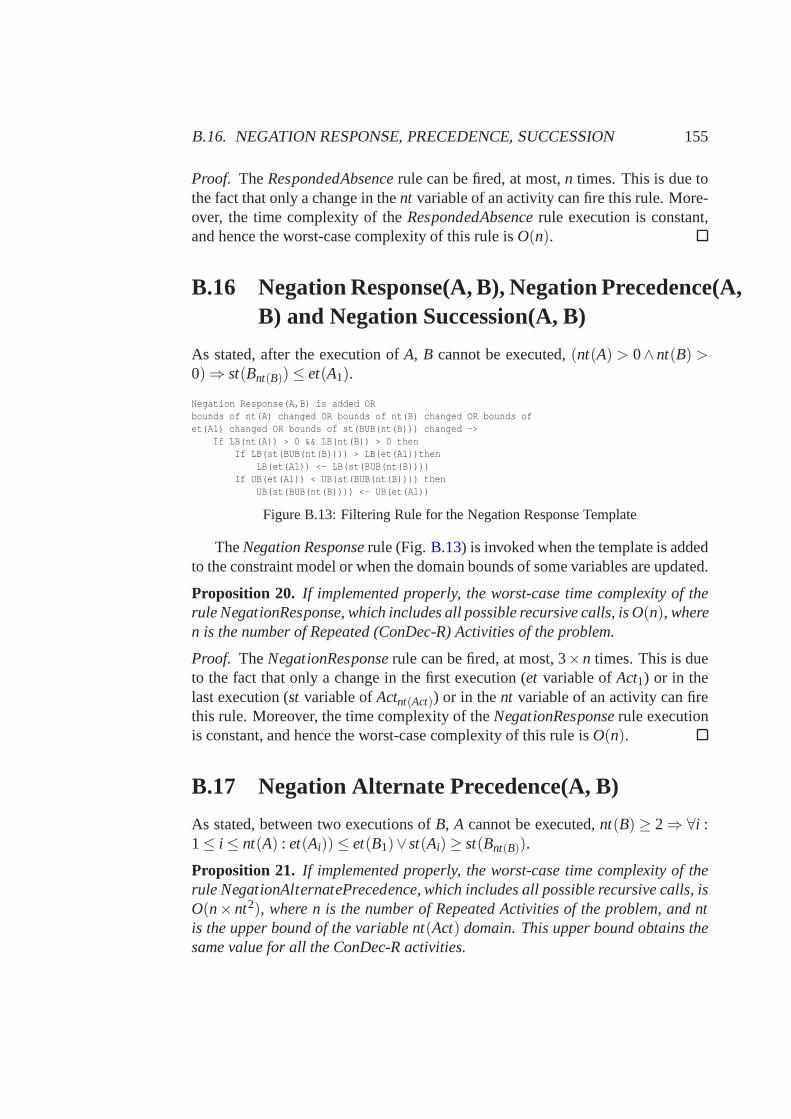
B.16. NEGATION RESPONSE, PRECEDENCE, SUCCESSION 155
Proof. TheRespondedAbsencerule can be fired, at most,n times. This is due tothe fact that only a change in thent variable of an activity can fire this rule. More-over, the time complexity of theRespondedAbsencerule execution is constant,and hence the worst-case complexity of this rule isO(n).
B.16 Negation Response(A, B), Negation Precedence(A,B) and Negation Succession(A, B)
As stated, after the execution ofA, B cannot be executed,(nt(A) > 0∧nt(B) >0)⇒ st(Bnt(B))≤ et(A1).
Negation Response(A,B) is added ORbounds of nt(A) changed OR bounds of nt(B) changed OR bounds ofet(A1) changed OR bounds of st(BUB(nt(B))) changed ->
If LB(nt(A)) > 0 && LB(nt(B)) > 0 thenIf LB(st(BUB(nt(B)))) > LB(et(A1))then
LB(et(A1)) <- LB(st(BUB(nt(B))))If UB(et(A1)) < UB(st(BUB(nt(B)))) then
UB(st(BUB(nt(B)))) <- UB(et(A1))
Figure B.13: Filtering Rule for the Negation Response Template
TheNegation Responserule (Fig.B.13) is invoked when the template is addedto the constraint model or when the domain bounds of some variables are updated.
Proposition 20. If implemented properly, the worst-case time complexity oftherule NegationResponse, which includes all possible recursive calls, is O(n), wheren is the number of Repeated (ConDec-R) Activities of the problem.
Proof. TheNegationResponserule can be fired, at most, 3×n times. This is dueto the fact that only a change in the first execution (et variable ofAct1) or in thelast execution (st variable ofActnt(Act)) or in thent variable of an activity can firethis rule. Moreover, the time complexity of theNegationResponserule executionis constant, and hence the worst-case complexity of this rule isO(n).
B.17 Negation Alternate Precedence(A, B)
As stated, between two executions ofB, A cannot be executed,nt(B) ≥ 2⇒ ∀i :1≤ i ≤ nt(A) : et(Ai))≤ et(B1)∨st(Ai)≥ st(Bnt(B)).
Proposition 21. If implemented properly, the worst-case time complexity oftherule NegationAlternatePrecedence, which includes all possible recursive calls, isO(n×nt2), where n is the number of Repeated Activities of the problem,and ntis the upper bound of the variable nt(Act) domain. This upper bound obtains thesame value for all the ConDec-R activities.
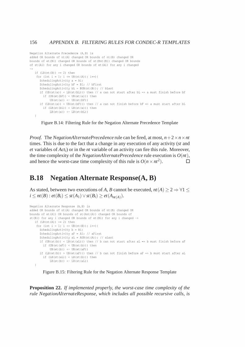
156 APPENDIX B. FILTERING RULES FOR CONDEC-R TEMPLATES
Negation Alternate Precedence (A,B) isadded OR bounds of nt(A) changed OR bounds of nt(B) changed ORbounds of et(B1) changed OR bounds of st(Bnt(B)) changed OR boundsof st(Ai) for any i changed OR bounds of et(Ai) for any i changed->
if (LB(nt(B)) >= 2) thenfor (int i = 1; i <= UB(nt(A)); i++){
SchedulingActivity a = Ai;SchedulingActivity bF = B1; // bFirstSchedulingActivity bL = BUB(nt(B)); // bLastif (UB(st(a)) < LB(st(bL))) then // a can not start after bL => a must finish before bF
if (UB(et(bF)) < UB(et(a))) thenUB(et(a)) <- UB(et(bF))
if (LB(et(a)) > UB(et(bF))) then // a can not finish before bF => a must start after bLif (LB(st(bL)) < LB(st(a))) then
LB(st(a)) <- LB(st(bL))}
Figure B.14: Filtering Rule for the Negation Alternate Precedence Template
Proof. TheNegationAlternatePrecedencerule can be fired, at most,n+2×n×nttimes. This is due to the fact that a change in any execution ofany activity (st andet variables ofActi) or in thent variable of an activity can fire this rule. Moreover,the time complexity of theNegationAlternatePrecedencerule execution isO(nt),and hence the worst-case time complexity of this rule isO(n×nt2).
B.18 Negation Alternate Response(A, B)
As stated, between two executions ofA, B cannot be executed,nt(A)≥ 2⇒∀1≤i ≤ nt(B) : et(Bi)≤ st(A1)∨st(Bi)≥ et(Ant(A)).
Negation Alternate Response (A,B) isadded OR bounds of nt(A) changed OR bounds of nt(B) changed ORbounds of et(A1) OR bounds of st(Ant(A)) changed OR bounds ofst(Bi) for any i changed OR bounds of et(Bi) for any i changed ->
if (LB(nt(A)) >= 2) thenfor (int i = 1; i <= UB(nt(B)); i++){
SchedulingActivity b = Bi;SchedulingActivity aF = A1; // aFirstSchedulingActivity aL = AUB(nt(A)); // aLastif (UB(st(b)) < LB(st(aL))) then // b can not start after aL => b must finish before aF
if (UB(et(aF)) < UB(et(b))) thenUB(et(b)) <- UB(et(aF))
if (LB(et(b)) > UB(et(aF))) then // b can not finish before aF => b must start after aLif (LB(st(aL)) < LB(st(b))) then
LB(st(b)) <- LB(st(aL))}
Figure B.15: Filtering Rule for the Negation Alternate Response Template
Proposition 22. If implemented properly, the worst-case time complexity oftherule NegationAlternateResponse, which includes all possible recursive calls, is
B.19. NEGATION ALTERNATE SUCCESSION(A, B) 157
O(n×nt2), where n is the number of Repeated Activities of the problem,and ntis the upper bound of the variable nt(Act) domain. This upper bound obtains thesame value for all the ConDec-R activities.
Proof. TheNegationAlternateResponserule can be fired, at most,n+2×n×nttimes. This is due to the fact that a change in any execution ofany activity (st andet variables ofActi) or in thent variable of an activity can fire this rule. Moreover,the time complexity of theNegationAlternateResponserule execution isO(nt),and hence the worst-case time complexity of this rule isO(n×nt2).
B.19 Negation Alternate Succession(A, B)
As stated, relationsNegationAlternatePrecedence(A,B) andNegationAlternateResponse(A,B) hold.
Proposition 23. If implemented properly, the worst-case time complexity oftherule NegationAlternateSuccession, which includes all possible recursive calls, isO(n×nt2), where n is the number of Repeated Activities of the problem,and ntis the upper bound of the variable nt(Act) domain. This upper bound obtains thesame value for all the ConDec-R activities.
Proof. The NegationAlternateSuccessionrule can be implemented as the con-junction ofNegationAlternatePrecendenceandNegationAlternateResponserules.The complexity of both rules isO(n×nt2) (see Prop.21 and22), and hence theworst-case time complexity ofNegationAlternateSuccessionrule is O(2× n×nt2), equal toO(n×nt2).
B.20 Negation Chain Succession(A, B)
As stated,B cannot be executed immediately after the execution ofA, ∀i : 1≤ i ≤nt(B) : ¬∃ j : 1≤ j ≤ nt(A) : et(A j) = st(Bi).
Proposition 24. If implemented properly, the worst-case time complexity oftherule NegationChainSuccession, which includes all possible recursive calls, isO(n× nt3), where n is the number of Repeated Activities of the problem,andnt is the upper bound of the variable nt(Act) domain. This upper bound obtainsthe same value for all the ConDec-R activities.
Proof. The NegationChainSuccessionrule can be fired, at most,n+ 2× n× nttimes. This is due to the fact that a change in any execution ofany activity (st andet variables ofActi) or in thent variable of an activity can fire this rule. Moreover,

158 APPENDIX B. FILTERING RULES FOR CONDEC-R TEMPLATES
Negation Chain Succession (A,B) isadded OR bounds of nt(A) changed OR bounds of nt(B) changed ORet(Ai) for any i is bound OR st(Bi) for any i is bound ->
for (int i = 1; i <= UB(nt(A)); i++){SchedulingActivity a = Ai;if(IsBound(et(a))){
int aVal = Value(et(a));for (int j = 1; j <= UB(nt(B)); j++){
SchedulingActivity b = Bj;if(MemberOf(aVal,st(b)))RemoveValue(aVal,st(b));
}}
}for (int i = 1; i <= UB(nt(B)); i++){
SchedulingActivity b = Bi;if(IsBound(st(b))){
int bVal = Value(st(b));for (int j = 1; j <= UB(nt(A)); j++){
SchedulingActivity a = Aj;if(MemberOf(bVal,et(a)))RemoveValue(bVal,et(a));
}}
}
Figure B.16: Filtering Rule for the Negation Chain Succession Template
the time complexity of theNegationChainSuccessionrule execution isO(nt2),and hence the worst-case time complexity of this rule isO(n×nt3).
Appendix C
Algorithms for Generating BPMNModels
In order to develop the algorithm to generate the BP models from the optimizedenactment plans (cf. Alg.6), certain related types are stated, as shown in Fig.C.1 (UML diagram). It should be clarified that, at this point of the process, theCSP variables are instantiated, hence all the information is known (nt variable foreach BP activity,st variable for each scheduling activity, resource in which eachscheduling activity is executed, etc). The types which appear in the UML diagramare as follows:
• OptimizedPlan: This represents the generated optimized enactment plan.Moreover, it contains the information related to the input problem. Thistype contains properties regarding a set of roles, a set of repeated activi-ties (ConDec-R activities), and a set of templates which relate the repeatedactivities.
• RepeatedAct: This represents the ConDec-R activities. Each repeated ac-tivity contains information about the required role, the estimated duration,the set of scheduling activities which represent the execution of each BPactivity, and the number of times this repeated activity is executed (propertynt).
• Role: This represents a role, and it is composed of the set of resourcesavailable for this role.
• Resource: This represents a resource. This type contains properties regar-ding a list of scheduling activities which are executed in that resource, or-dered by the start time.
159
160 APPENDIX C. ALGORITHMS FOR GENERATING BPMN MODELS
• Template: This represents the high-level relations which are given betweenthe repeated activities. In order to consider the branched constraints (Sect.3.2), two specializations are included to allow the relations between onesource and several sinks (TemplateSinks), and between several sources andone sink (TemplateSources). The methodincludePredof a template up-dates the information of the BPMN model by including the precedence re-lations which are implied by that template (more details aregiven later inthis section during the presentation of the algorithms). For the generation ofthe BPMN model, the template relations are considered for the connectionof the BPMN activities.
• P&SAct: This represents each execution of a repeated activity. This typecontains properties regarding the start and the end times ofthe activity, to-gether with the resource used by the scheduling activity. Since each P&SActis related to a specific BPMNAct, the P&SAct type provides themethodtoBPMNActin order to obtain the related BPMNAct from a P&SAct.
• BPMNModel: This represents the BPMN model that is generated. Thismodel is composed of a set of BPMN activities, a set of pools, aset ofgates, and a set of connections.
• BPMNAct: This represents a BPMN activity. This type contains propertiesregarding the pool and the lane where the activity is allocated, together withthe estimated duration and start time.
• Pool: This represents a BPMN pool. Each pool is associated toa specificrole and is composed of a set of lanes.
• Lane: This represents a BPMN lane. Each lane is associated toa specificresource.
• Gate: This represents a BPMN gate. In order to consider parallel merginggateways, a specialization, named ParallelM, is developed.
• ParallelM: This represents a parallel merging gateway. This type containsproperties regarding a set of inputs (BPMN activities), andone output (BP-MN activity).
• Connection: This represents a precedence connection between two BPMNactivities,a andb.
The types which are presented in the UML diagram of Fig.C.1 are usedfor the development of the algorithms for the automatic generation of optimizedBPMN models from enactment plans (cf. Algs.6, 7, 8, 9 and10). Generic types
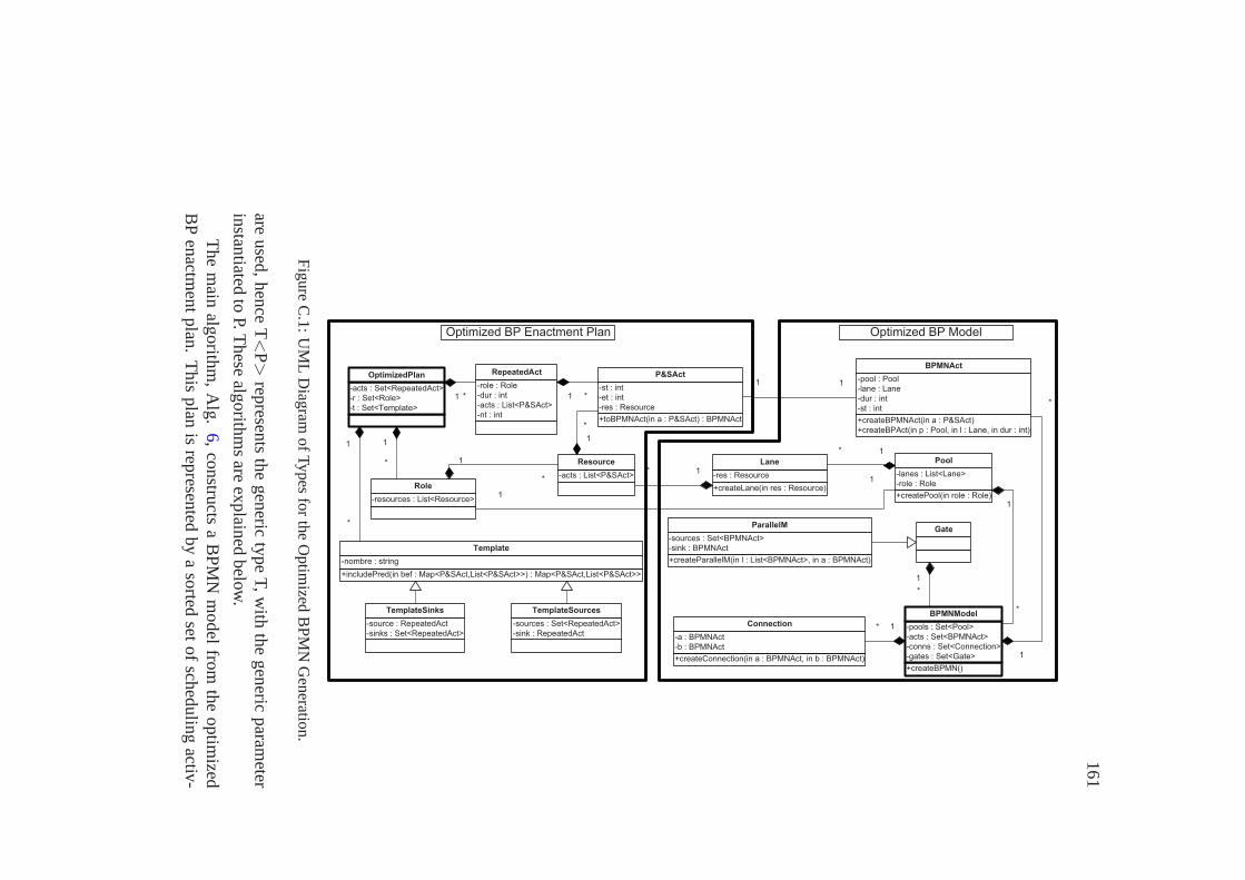
16
1
��������������� ���������
����
���������� �������
��������
����������������������������
������������������������������������������������
�����������
����������
���������
��������
�� ��
��������������������������
����������� ����
�����������
���
����������������������������
��������������
����
�������������
����������� �����
���������� ��������
����������� ����������
�!��������� "����
�������
�������������������������� ������������������������
������������� ��������
����#���������
��������
����������������$�%����� ���������� �������������� ���������� ��������
���&$���������!
��������
���������������������������������
��������
��������
��������������
�� ��
�����������
���������
���������� �������
��������
�������� ��
����
������� ����������������������������$����������
�����������
�$���������
����������
' (
'
(
'(
'
(
'
(
'(
'
(
'
'
���������� ������������
������� �����
������� )�&������
������������
' (
'
(
'
(
'
(
' '
'(
��������������������
����#������ ������������
�������������
������������� ������������
����#�������������
���������������
*���&�+������,����&�������� *���&�+�����������
Figure
C.1:
UM
LD
iagramofTypes
forthe
Optim
izedB
PM
NG
eneration.
areu
sed,
hen
ceT<P>
represen
tsth
eg
eneric
type
T,w
ithth
eg
eneric
param
eterin
stantiated
toP.T
hese
algo
rithm
sare
explain
edb
elow.
Th
em
ainalg
orith
m,
Alg
.6,co
nstru
ctsa
BP
MN
mo
delfro
mth
eo
ptim
izedB
Pen
actmen
tp
lan.
Th
isp
lanis
represen
tedb
ya
sorted
seto
fsch
edu
ling
activ-
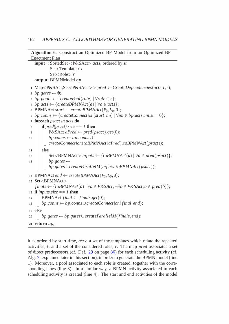
162 APPENDIX C. ALGORITHMS FOR GENERATING BPMN MODELS
Algorithm 6 : Construct an Optimized BP Model from an Optimized BPEnactment Plan
input : SortedSet<P&SAct> acts, ordered bystSet<Template> tSet<Role> r
output: BPMNModelbp
Map<P&SAct,Set<P&SAct>> pred←CreateDependencies(acts, t, r);1
bp.gates← /0;2
bp.pools←{createPool(role) | ∀role∈ r};3
bp.acts←{createBPMNAct(a) | ∀a∈ acts};4
BPMNAct start← createBPMNAct(P0,L0,0);5
bp.conns←{createConnection(start, ini) | ∀ini ∈ bp.acts, ini.st= 0};6
foreach psact in actsdo7
if pred(psact).size == 1then8
P&SAct aPred← pred(psact).get(0);9
bp.conns← bp.conns∪10
createConnection(toBPMNAct(aPred), toBPMNAct(psact));
else11
Set<BPMNAct> inputs←{toBPMNAct(a) | ∀a∈ pred(psact)};12
bp.gates←13
bp.gates∪createParallelM(inputs, toBPMNAct(psact));
BPMNAct end← createBPMNAct(P0,L0,0);14
Set<BPMNAct>15
f inals←{toBPMNAct(a) | ∀a∈ P&SAct,¬∃b∈ P&SAct,a∈ pred(b)};if inputs.size == 1then16
BPMNAct f inal← f inals.get(0);17
bp.conns← bp.conns∪createConnection( f inal,end);18
else19
bp.gates← bp.gates∪createParallelM( f inals,end);20
return bp;21
ities ordered by start time,acts; a set of the templates which relate the repeatedactivities,t; and a set of the considered roles,r. The mappred associates a setof direct predecessors (cf. Def.29 on page86) for each scheduling activity (cf.Alg. 7, explained later in this section), in order to generate the BPMN model (line1). Moreover, a pool associated to each role is created, together with the corre-sponding lanes (line 3). In a similar way, a BPMN activity associated to eachscheduling activity is created (line 4). The start and end activities of the model
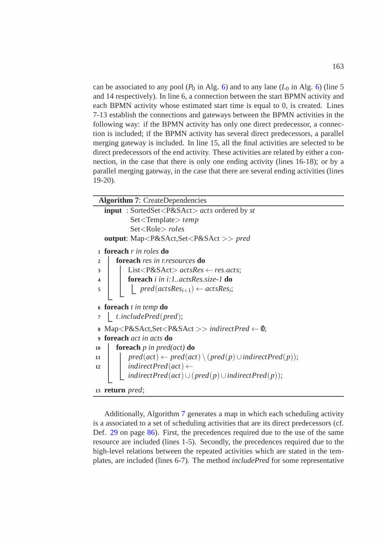
163
can be associated to any pool (P0 in Alg. 6) and to any lane (L0 in Alg. 6) (line 5and 14 respectively). In line 6, a connection between the start BPMN activity andeach BPMN activity whose estimated start time is equal to 0, is created. Lines7-13 establish the connections and gateways between the BPMN activities in thefollowing way: if the BPMN activity has only one direct predecessor, a connec-tion is included; if the BPMN activity has several direct predecessors, a parallelmerging gateway is included. In line 15, all the final activities are selected to bedirect predecessors of the end activity. These activities are related by either a con-nection, in the case that there is only one ending activity (lines 16-18); or by aparallel merging gateway, in the case that there are severalending activities (lines19-20).
Algorithm 7 : CreateDependenciesinput : SortedSet<P&SAct> actsordered byst
Set<Template> tempSet<Role> roles
output: Map<P&SAct,Set<P&SAct>> pred
foreach r in rolesdo1
foreach res in r.resourcesdo2
List<P&SAct> actsRes← res.acts;3
foreach i in i:1..actsRes.size-1do4
pred(actsResi+1)← actsResi;5
foreach t in tempdo6
t.includePred(pred);7
Map<P&SAct,Set<P&SAct>> indirectPred← /0;8
foreach act in actsdo9
foreach p in pred(act)do10
pred(act)← pred(act)\ (pred(p)∪ indirectPred(p));11
indirectPred(act)←12
indirectPred(act)∪ (pred(p)∪ indirectPred(p));
return pred;13
Additionally, Algorithm7 generates a map in which each scheduling activityis a associated to a set of scheduling activities that are itsdirect predecessors (cf.Def. 29 on page86). First, the precedences required due to the use of the sameresource are included (lines 1-5). Secondly, the precedences required due to thehigh-level relations between the repeated activities which are stated in the tem-plates, are included (lines 6-7). The methodincludePredfor some representative
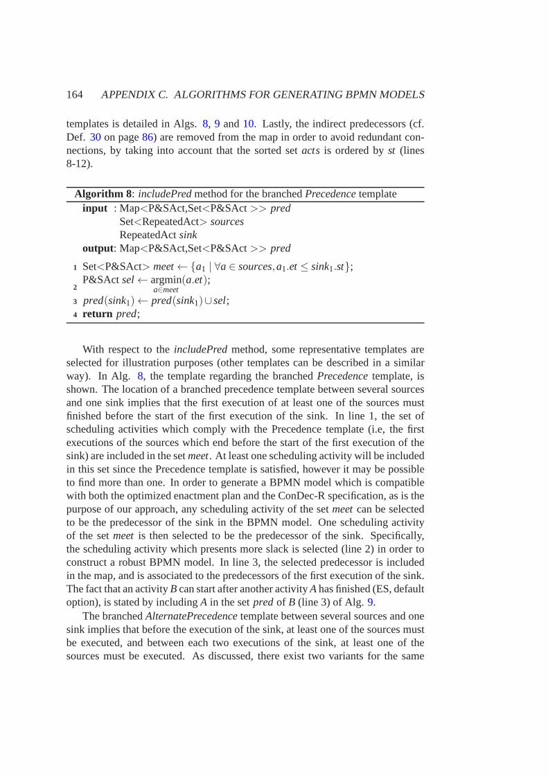
164 APPENDIX C. ALGORITHMS FOR GENERATING BPMN MODELS
templates is detailed in Algs.8, 9 and10. Lastly, the indirect predecessors (cf.Def. 30 on page86) are removed from the map in order to avoid redundant con-nections, by taking into account that the sorted setacts is ordered byst (lines8-12).
Algorithm 8 : includePredmethod for the branchedPrecedencetemplateinput : Map<P&SAct,Set<P&SAct>> pred
Set<RepeatedAct> sourcesRepeatedActsink
output: Map<P&SAct,Set<P&SAct>> pred
Set<P&SAct> meet←{a1 | ∀a∈ sources,a1.et≤ sink1.st};1
P&SAct sel← argmina∈meet
(a.et);2
pred(sink1)← pred(sink1)∪sel;3
return pred;4
With respect to theincludePredmethod, some representative templates areselected for illustration purposes (other templates can bedescribed in a similarway). In Alg. 8, the template regarding the branchedPrecedencetemplate, isshown. The location of a branched precedence template between several sourcesand one sink implies that the first execution of at least one ofthe sources mustfinished before the start of the first execution of the sink. Inline 1, the set ofscheduling activities which comply with the Precedence template (i.e, the firstexecutions of the sources which end before the start of the first execution of thesink) are included in the setmeet. At least one scheduling activity will be includedin this set since the Precedence template is satisfied, however it may be possibleto find more than one. In order to generate a BPMN model which iscompatiblewith both the optimized enactment plan and the ConDec-R specification, as is thepurpose of our approach, any scheduling activity of the setmeetcan be selectedto be the predecessor of the sink in the BPMN model. One scheduling activityof the setmeet is then selected to be the predecessor of the sink. Specifically,the scheduling activity which presents more slack is selected (line 2) in order toconstruct a robust BPMN model. In line 3, the selected predecessor is includedin the map, and is associated to the predecessors of the first execution of the sink.The fact that an activityBcan start after another activityAhas finished (ES, defaultoption), is stated by includingA in the setpredof B (line 3) of Alg. 9.
The branchedAlternatePrecedencetemplate between several sources and onesink implies that before the execution of the sink, at least one of the sources mustbe executed, and between each two executions of the sink, at least one of thesources must be executed. As discussed, there exist two variants for the same
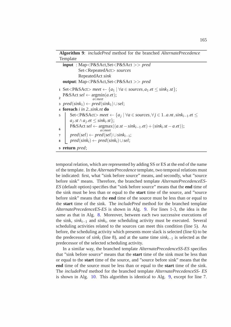
165
Algorithm 9 : includePredmethod for the branchedAlternatePrecedenceTemplate
input : Map<P&SAct,Set<P&SAct>> predSet<RepeatedAct> sourcesRepeatedActsink
output: Map<P&SAct,Set<P&SAct>> pred
Set<P&SAct> meet←{a1 | ∀a∈ sources,a1.et≤ sink1.st};1
P&SAct sel← argmina∈meet
(a.et);2
pred(sink1)← pred(sink1)∪sel;3
foreach i in 2..sink.ntdo4
Set<P&SAct> meet←{a j | ∀a∈ sources,∀ j ∈ 1..a.nt,sinki−1.et≤5
a j .st∧a j .et≤ sinki.st};P&SAct sel← argmax
a∈meet((a.st−sinki−1.et)+(sinki.st−a.et));
6
pred(sel)← pred(sel)∪sinki−1;7
pred(sinki)← pred(sinki)∪sel;8
return pred;9
temporal relation, which are represented by adding SS or ES at the end of the nameof the template. In theAlternatePrecedencetemplate, two temporal relations mustbe indicated: first, what ”sink before source” means, and secondly, what ”sourcebefore sink” means. Therefore, the branched templateAlternatePrecedenceES-ES(default option) specifies that ”sink before source” means that theend time ofthe sink must be less than or equal to thestart time of the source, and ”sourcebefore sink” means that theend time of the source must be less than or equal tothe start time of the sink. TheincludePredmethod for the branched templateAlternatePrecedenceES-ESis shown in Alg. 9. For lines 1-3, the idea is thesame as that in Alg.8. Moreover, between each two successive executions ofthe sink,sinki−1 and sinki, one scheduling activity must be executed. Severalscheduling activities related to the sources can meet this condition (line 5). Asbefore, the scheduling activity which presents more slack is selected (line 6) to bethe predecessor ofsinki (line 8), and at the same timesinki−1 is selected as thepredecessor of the selected scheduling activity.
In a similar way, the branched templateAlternatePrecedenceSS-ESspecifiesthat ”sink before source” means that thestart time of the sink must be less thanor equal to thestart time of the source, and ”source before sink” means that theend time of the source must be less than or equal to thestart time of the sink.The includePredmethod for the branched templateAlternatePrecedenceSS- ESis shown in Alg. 10. This algorithm is identical to Alg.9, except for line 7.
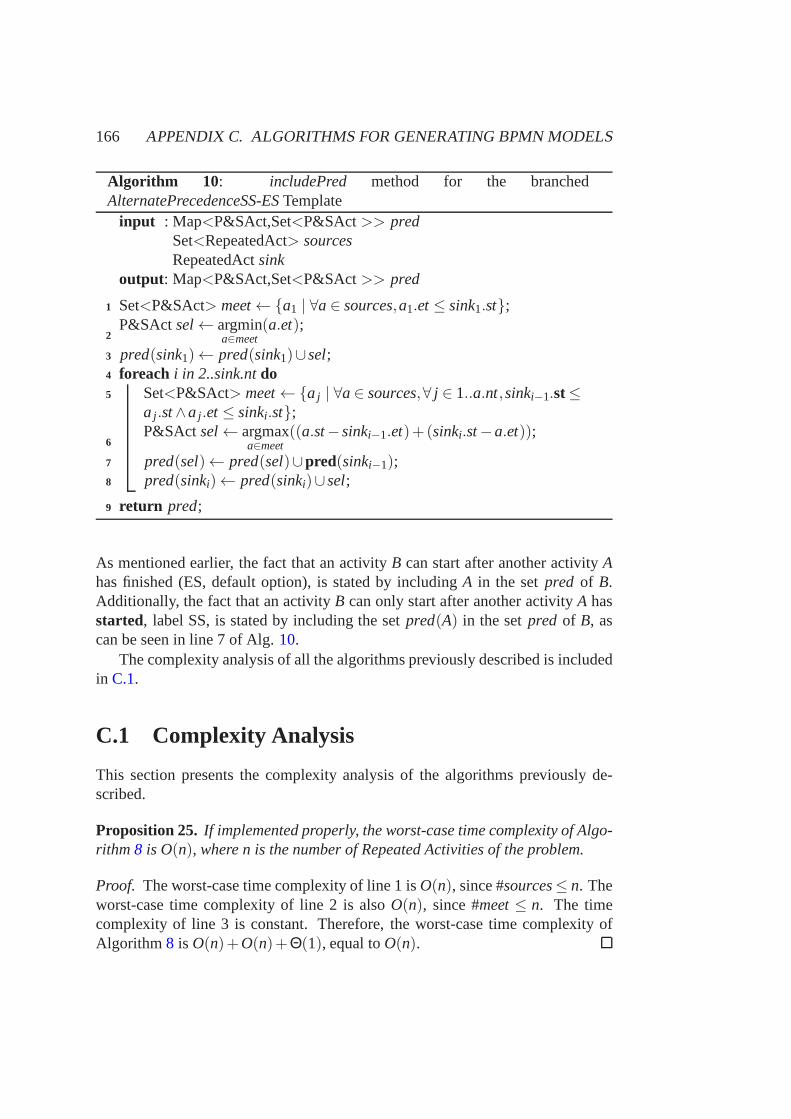
166 APPENDIX C. ALGORITHMS FOR GENERATING BPMN MODELS
Algorithm 10 : includePred method for the branchedAlternatePrecedenceSS-ESTemplate
input : Map<P&SAct,Set<P&SAct>> predSet<RepeatedAct> sourcesRepeatedActsink
output: Map<P&SAct,Set<P&SAct>> pred
Set<P&SAct> meet←{a1 | ∀a∈ sources,a1.et≤ sink1.st};1
P&SAct sel← argmina∈meet
(a.et);2
pred(sink1)← pred(sink1)∪sel;3
foreach i in 2..sink.ntdo4
Set<P&SAct> meet←{a j | ∀a∈ sources,∀ j ∈ 1..a.nt,sinki−1.st≤5
a j .st∧a j .et≤ sinki.st};P&SAct sel← argmax
a∈meet((a.st−sinki−1.et)+(sinki.st−a.et));
6
pred(sel)← pred(sel)∪pred(sinki−1);7
pred(sinki)← pred(sinki)∪sel;8
return pred;9
As mentioned earlier, the fact that an activityB can start after another activityAhas finished (ES, default option), is stated by includingA in the setpred of B.Additionally, the fact that an activityB can only start after another activityA hasstarted, label SS, is stated by including the setpred(A) in the setpred of B, ascan be seen in line 7 of Alg.10.
The complexity analysis of all the algorithms previously described is includedin C.1.
C.1 Complexity Analysis
This section presents the complexity analysis of the algorithms previously de-scribed.
Proposition 25. If implemented properly, the worst-case time complexity ofAlgo-rithm 8 is O(n), where n is the number of Repeated Activities of the problem.
Proof. The worst-case time complexity of line 1 isO(n), since #sources≤ n. Theworst-case time complexity of line 2 is alsoO(n), since #meet≤ n. The timecomplexity of line 3 is constant. Therefore, the worst-casetime complexity ofAlgorithm 8 is O(n)+O(n)+Θ(1), equal toO(n).
C.1. COMPLEXITY ANALYSIS 167
Proposition 26. If implemented properly, the worst-case time complexity ofAl-gorithms9 and10 is O(n×nt), where n is the number of Repeated Activities ofthe problem, and nt is the maximum number of times that a repeated activity isexecuted.
Proof. The worst-case time complexity of line 1 isO(n), since #sources≤ n. Theworst-case time complexity of line 2 is alsoO(n), since #meet≤ n. The timecomplexity of line 3 is constant. The worst-case time complexity of lines 4-8 isO(n× nt) since lines 5-7 (with complexityO(n) from the proof of Proposition25) are executed at mostnt times. Therefore, the worst-case time complexity ofAlgorithms9 and10 is O(n)+O(n)+Θ(1)+O(n×nt) equal toO(n×nt).
Proposition 27. If implemented properly, the worst-case time complexity ofAlgo-rithm 7 is O(t×n×nt+nps2), where n is the number of Repeated Activities of theproblem, nt is the maximum number of times that a repeated activity is executed,t is the number of templates that appear in the definition of the problem, and npsis the number of scheduling activities in the optimized plan.
Proof. The time complexity of line 1-5 isΘ(nps), since each scheduling activityis considered exactly once (each activity uses a specific resource of a specific role).The worst-case time complexity of lines 6-7 isO(t×n×nt), since the worst-casetime complexity of the methodincludePredis O(n× nt) (Proposition26), andthis method is invokedt times. The worst-case time complexity of lines 9-12 isO(nps2), since for each scheduling activity, its predecessors (at most, nps) areconsidered. Therefore, the worst-case time complexity of Algorithm 7 is O(t×n×nt+nps2).
Proposition 28. If implemented properly, the worst-case time complexity ofAlgo-rithm 6 is O(t×n×nt+nps2), where n is the number of Repeated Activities of theproblem, nt is the maximum number of times that a repeated activity is executed,t is the number of templates that appear in the definition of the problem, and npsis the number of scheduling activities in the optimized plan.
Proof. The worst-case time complexity of line 1 isO(t×n×nt+nps2), by Propo-sition27. The worst-case time complexity of line 3 isO(n), since #role≤ n. Thetime complexity of line 4 isΘ(nps). The worst-case time complexity of lines 6and 15 isO(nps). The time complexity of lines 7-13 isΘ(nps). Therefore, theworst-case time complexity of Algorithm6 is O(t×n×nt+nps2).

Appendix D
AI Techniques for Solving theMulti-mode Repair PlanningProblem
AI-based techniques for solving the multi-mode repair planning problem are pre-sented, specifically: (1) a constraint-based approach (cf.AppendixD.1), and (2)a PDDL specification (cf. AppendixD.2).
D.1 Constraint-based Approach
In this section, the constraint-based approach for solvingthe multi-mode repairplanning problem is presented (cf. (Barba et al., 2009a)). According to the con-sidered problems (cf. Sect.6.3), the time and resource constraints, typical fromscheduling, would be modified to conditional constraints taking into account thattasks (and subsystems) may not appear in the solution. Most of the ideas aretaken from (Del Valle et al., 2010), but the assumptions considered in this workwill result in modifying most constraints and in adding others: apart from the op-timization of the duration, the minimization of the total cost is pursued, resultingin a multi-objective optimization problem, and multi-modetasks are considered(cf. (Barba et al., 2009a)).
D.1.1 Variables of the CSP
Four kinds of CSP variables have been defined: selection, resource, time and costvariables.
Selection variables. For each And node, two boolean variables represent if theconnection and disconnection tasks are selected for the solution, s(T) ands(T ′)
169
170 APPENDIX D. AI TECHNIQUES
respectively. Furthermore, for each Or node, two boolean variables represent ifthe subsystemSappears in the connection and disconnection processes,s(S) ands′(S) respectively.
Resource variables. For each And node,M(T) andM(T ′) show the resourcesused, andC f(T) andC f(T′) are the necessary configuration on them for the con-nection and disconnection tasks respectively. These values are data of the pro-blem. On the other hand, the resource where a subsystem is obtained after thecorresponding disconnection and connection task, are represented by the varia-blesm′(S) andm(S) respectively, that are variables of the CSP.
Time variables. For each And node, the durations of the associated tasksDur(T) andDur(T ′) are established. Due to the auxiliary operations,∆cht(M,C f,C f ′) denotes the time needed for changing the configuration of theresourceMfrom C f to C f ′, and∆mov(S,M,M′) denotes the time needed for transporting thesubsystemS from resourceM to resourceM′. Finally, a componentC to be re-paired is associated to a temporal delay∆subst(C), corresponding to the reparationor substitution of the faulty component. These values are data of the problem.
On the other hand, for each And node, the CSP variables related to the timeare: its starting times,ti(T) andti(T ′) and ending times,t f (T) andt f (T ′). For eachOr node, the times when it is obtained after connection,tOR(S), and disconnection,t ′OR(S).
Cost variablesFor each And node, it is considered: its connection and dis-connection cost,Cost(Ti) andCost(T′i ) respectively. Regarding to the auxiliaryoperations,Costcht(M,C f,C f ′) denotes the cost of changing the configuration ofthe resourceM from C f to C f ′, andCostmov(S,M,M′) denotes the cost of trans-porting the subsystemS from resourceM to resourceM′. Furthermore, a com-ponentC to be repaired is associated to a costCostsubst(C), corresponding to thereparation or substitution of the faulty component.
On the other hand, for each And node, the selection of the correspondingtask T may be associated some additional costs, as explained in Sect. D.1.2:first, the variablecostmov(Ti) represents the possible costs which are associatedto the movement of subsystems tom(T), if this resource is different from theone where the subsystem were previously obtained; and secondly, the variablecostcht(Ti) represents the possible costs of change of configuration, ifm(T) hasbeen previously used with a different one. These variables are linked to the Andnodes because the costs are due to the selection of the corresponding task.
Finally, a variable that represents the total cost of a plan,costtotal, has beenused in order to minimize this objective function. Therefore, a multi-objectiveoptimization is pursued, encompassing both objective functions, time and cost.
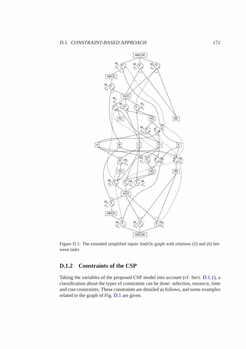
D.1. CONSTRAINT-BASED APPROACH 171
ABCDE
ABCD
ACD
AC
A
AD BE
B C D
T’3
T’2
T’1
T’7
T’9
T’4
T’5
T’6
T’10
ABCDE
ABCD
ACD
AC AD BE
E
T3
T2
T1
T7
T9
T4
T5
T6
T10T
8T
11
M2
C3
M1
C1
M3
C4
M1
C2
M2
C3 M
1
C2
M3
C2
M3
C6
M2
C1
M2
C4
M3
C3
M1
C2
M2
C4
M2
C5
M3
C2
M1
C2
M3
C6
M2
C4
M1
C2
M2
C5
Figure D.1: The extended simplified repair And/Or graph withrelations (5) and (6) bet-ween tasks
D.1.2 Constraints of the CSP
Taking the variables of the proposed CSP model into account (cf. Sect.D.1.1), aclassification about the types of constraints can be done: selection, resource, timeand cost constraints. These constraints are detailed as follows, and some examplesrelated to the graph of Fig.D.1 are given.
172 APPENDIX D. AI TECHNIQUES
Selection Constraintscollect the relations between the boolean variables thatrepresent if the tasks are selected for the solution and if the subsystems appearsin the repair process. A special case is for the complete system and for thefaulty component, which will be always part of the solution,so s′(ABCDE) =s(ABCDE) = s′(D) = s(D) = true.
Related to relations of type (1) (cf. Sect.6.3.1), constraints which relate the se-lection of disconnection tasksT ′ and connection tasksT with the selection of sub-systems are included:s′(S)⇔XORT′i ∈succ(S)(s(T
′i )) ands(S)⇔XORTi∈succ(S)(s(Ti))
(examples′(ABCDE)⇔ (XOR(s(T′1),s(T′2),s(T
′3))).
Related to relations of type (3) (cf. Sect.6.3.1), the obligatory selection of thetwo Or nodes if the And node is selected is considered:s(T′)⇒ s′(S1)∧ s′(S2)ands(T)⇒ s(S1)∧s(S2) (examples(T′1)⇒ s′(ABCD)∧s′(E)).
Related to relations of type (4) (cf. Sect.6.3.1), constraints which relate the se-lection of disconnection tasksT ′ and connection tasksT with the selection of sub-systems are included:s′(S)⇔XORT′i ∈pred(S)(s(T
′i )) ands(S)⇔XORTi∈pred(S)(s(Ti))
(examples(ACD)⇔ XOR(s(T2),s(T3),s(T4))).Resource Constraintsconsider the relations between the resources used in
the connection and disconnection tasks, and the resources where the subsystemsare obtained after them.
Related to relations of type (1) (cf. Sect.6.3.1), the resourcem where asubsystem is generated after a connection task is the resource used by this task:s(Ti)⇒m(S) = M(Ti) (examples(T10)⇒m(AD) = M(T10)).
Related to relations of type (3) (cf. Sect.6.3.1), the resourcem′ where asubsystem is generated after a disconnection task is the resource used by this task:s(T′i )⇒m′(S1) = m′(S2) = M(T′i ) (examples(T′9)⇒m′(A) = m′(D) = M(T ′9)).
Time Constraints collect the relations between the start and the end times ofthe tasks, and the time when the subsystems are obtained. Initially, t ′OR(ABCDE)=0.
Related to relations of type (1) (cf. Sect.6.3.1), these constraints establishthe disconnection timest ′OR and connection timestOR of Or nodes related to thestart times of the disconnection tasks or the end times of theconnection tasks:s(T′i )⇒ ti(T ′i )≥ t ′OR(S)+∆mov(S,m′(S),M(T′i )) ands(Ti)⇒ t f (Ti) = tOR(S) (ex-amples(T ′1)⇒ ti(T ′1)≥ t ′OR(ABCDE)+∆mov(ABCDE,m′(ABCDE),M(T′1))).
Related to relations of type (2) (cf. Sect.6.3.1), these constraints consider theend time of the tasks related to the start time and its durations: s(T′i )⇒ t f (T ′i ) =ti(T ′i )+Dur(T ′i ) ands(Ti)⇒ t f (Ti) = ti(Ti)+Dur(Ti) (examples(T′1)⇒ t f (T′1) =ti(T ′1)+Dur(T′1)).
Related to relations (3) (cf. Sect.6.3.1), constraints which relate the equal-ity constraints between the disconnection times of the Or nodest ′OR and the endtime of a disconnection task T’ which is placed above them in the original And/Or
D.1. CONSTRAINT-BASED APPROACH 173
graph, together with the precedence between the connectiontime of the Or nodestORand the start times of the connection tasks T (And nodes) are included:s(T′i )⇒t f (T ′i ) = t ′OR(S1) = t ′OR(S2).
Furthermore, the possible delays due to the transportationof subsystems bet-ween different resources are considered:s(Ti)⇒ ti(Ti)≥ tOR(S1)+∆mov(S1,m(S1),M(Ti)) ands(Ti)⇒ ti(Ti) ≥ tOR(S2)+∆mov(S2,m(S2),M(Ti)) (examples(T ′10)⇒t f (T ′10) = t ′OR(A) = t ′OR(D)).
Related to relations of type (5) (cf. Sect.6.3.1), constraints which relate ataskTi and its closest predecessor taskTj using the same resourcem, taking intoaccount the possible change of configuration are considered: (s(Ti)∧ s(Tj))⇒ti(Tj) ≥ t f (Ti) + ∆cht(m,C f(Ti),C f(Tj)) (example(s(T′1)∧ s(T′10)) ⇒ ti(T′10) ≥t f (T ′1) + ∆cht(M2, C f(T ′1), C f(T ′10))).
Moreover, since the solution may contain non-reverse tasks, each disconnec-tion task must be related to each closest successor connection task that uses thesame resource. Furthermore, when both tasks use the same configuration, theresulting constraint is superfluous and can be eliminated.
For each two tasksTi andTj requiring the same resourcem, with no precedenceconstraint among them and which may belong to the same repairplan, the cons-traints of type (6) (cf. Sect.6.3.1) express the two possible orders of execution ofthe tasks:(s(Ti)∧ s(Tj))⇒ (ti(Ti) ≥ t f (Tj)+∆cht(m,C f(Tj),C f(Ti))∨ ti(Tj) ≥t f (Ti)+∆cht(m,C f(Ti),C f(Tj))) (example(s(T8)∧s(T11))⇒ ti(T8) ≥ t f (T11) +∆cht(M2,C f(T11), C f(T8)) ∨ ti(T11) ≥ t f (T8) + ∆cht (M2, C f(T8),C f(T11))).
For theOr leaf nodes (including those that do not include the faulty compo-nent)t ′OR andtOR are equals, except for the faulty component, in which the delaycorresponding to the reparation is considered.
Cost Constraints: In the repair process of a component in a complete system,the cost of a plan can be established by the aggregated costs associated to theexecution of the selected tasks. The total cost of selectinga taskTi involves:
• the execution cost of the task,Cost(Ti) (related to relation (2))
• the cost associated to the possible movement of one or two subsystems fromone resource to another,costmov(Ti):
– in disconnection tasksT ′i , it is necessary to take into account the pos-sible movement of the subsystem related to the Or nodes aboveitin the original And/Or graph, related to relation (1),costmov(T′i ) =Costmov(S,m′(S),M(T′i ))
– in connection tasksTi , it is necessary to take into account the pos-sible movement of the two subsystems related to Or nodes below itin the original And/Or graph, related to relation (3),costmov(Ti) =Costmov(S1,m(S1),M(Ti))+Costmov(S2,m(S2),M(Ti))
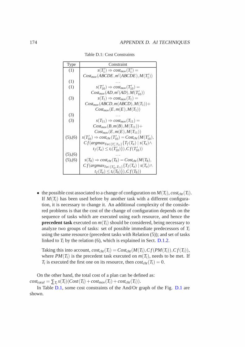
174 APPENDIX D. AI TECHNIQUES
Table D.1: Cost Constraints
Type Constraint(1) s(T ′1)⇒ costmov(T ′1) =
Costmov(ABCDE,m′(ABCDE),M(T′1))(1) . . .(1) s(T ′10)⇒ costmov(T ′10) =
Costmov(AD,m′(AD),M(T ′10))(3) s(T1)⇒ costmov(T1) =
Costmov(ABCD,m(ABCD),M(T1))+Costmov(E,m(E),M(T1))
(3) . . .(3) s(T11)⇒ costmov(T11) =
Costmov(B,m(B),M(T11))+Costmov(E,m(E),M(T11))
(5),(6) s(T ′10)⇒ costcht(T ′10) =Costcht(M(T ′10),C f(argmaxTa∈{T ′1 ,T11}{Tf (Ta) | s(Ta)∧
t f (Ta)≤ ti(T ′10)}),C f(T ′10))(5),(6) . . .(5),(6) s(T8)⇒ costcht(T8) =Costcht(M(T8),
C f(argmaxTa∈{T ′10,T11}{Tf (Ta) | s(Ta)∧
t f (Ta)≤ ti(T8)}),C f(T8))
• the possible cost associated to a change of configuration onM(Ti), costcht(Ti).If M(Ti) has been used before by another task with a different configura-tion, it is necessary to change it. An additional complexityof the conside-red problems is that the cost of the change of configuration depends on thesequence of tasks which are executed using each resource, and hence theprecedent taskexecuted onm(Ti) should be considered, being necessary toanalyze two groups of tasks: set of possible immediate predecessors ofTi
using the same resource (precedent tasks with Relation (5)); and set of taskslinked toTi by the relation (6), which is explained in Sect.D.1.2.
Taking this into account,costcht(Ti) =Costcht(M(Ti),C f(PM(Ti)),C f(Ti)),wherePM(Ti) is the precedent task executed onm(Ti), needs to be met. IfTi is executed the first one on its resource, thencostcht(Ti) = 0.
On the other hand, the total cost of a plan can be defined as:costtotal = ∑Ti
s(Ti)(Cost(Ti)+costmov(Ti)+costcht(Ti)).In TableD.1, some cost constraints of the And/Or graph of the Fig.D.1 are
shown.
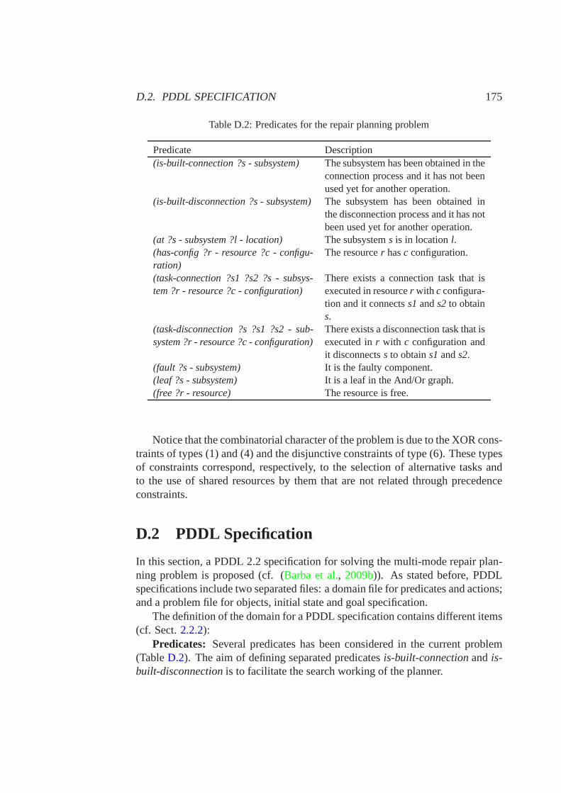
D.2. PDDL SPECIFICATION 175
Table D.2: Predicates for the repair planning problem
Predicate Description(is-built-connection ?s - subsystem) The subsystem has been obtained in the
connection process and it has not beenused yet for another operation.
(is-built-disconnection ?s - subsystem)The subsystem has been obtained inthe disconnection process and it has notbeen used yet for another operation.
(at ?s - subsystem ?l - location) The subsystems is in locationl.(has-config ?r - resource ?c - configu-ration)
The resourcer hasc configuration.
(task-connection ?s1 ?s2 ?s - subsys-tem ?r - resource ?c - configuration)
There exists a connection task that isexecuted in resourcer with cconfigura-tion and it connectss1ands2 to obtains.
(task-disconnection ?s ?s1 ?s2 - sub-system ?r - resource ?c - configuration)
There exists a disconnection task that isexecuted inr with c configuration andit disconnectss to obtains1ands2.
(fault ?s - subsystem) It is the faulty component.(leaf ?s - subsystem) It is a leaf in the And/Or graph.(free ?r - resource) The resource is free.
Notice that the combinatorial character of the problem is due to the XOR cons-traints of types (1) and (4) and the disjunctive constraintsof type (6). These typesof constraints correspond, respectively, to the selectionof alternative tasks andto the use of shared resources by them that are not related through precedenceconstraints.
D.2 PDDL Specification
In this section, a PDDL 2.2 specification for solving the multi-mode repair plan-ning problem is proposed (cf. (Barba et al., 2009b)). As stated before, PDDLspecifications include two separated files: a domain file for predicates and actions;and a problem file for objects, initial state and goal specification.
The definition of the domain for a PDDL specification containsdifferent items(cf. Sect.2.2.2):
Predicates: Several predicates has been considered in the current problem(TableD.2). The aim of defining separated predicatesis-built-connectionandis-built-disconnectionis to facilitate the search working of the planner.
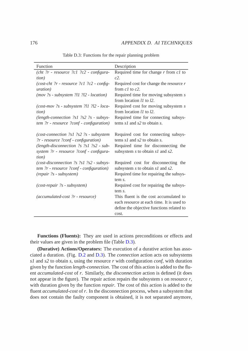
176 APPENDIX D. AI TECHNIQUES
Table D.3: Functions for the repair planning problem
Function Description(cht ?r - resource ?c1 ?c2 - configura-tion)
Required time for changer from c1 toc2.
(cost-cht ?r - resource ?c1 ?c2 - config-uration)
Required cost for change the resourcerfrom c1 to c2.
(mov ?s - subsystem ?l1 ?l2 - location) Required time for moving subsystemsfrom locationl1 to l2.
(cost-mov ?s - subsystem ?l1 ?l2 - loca-tion)
Required cost for moving subsystemsfrom locationl1 to l2.
(length-connection ?s1 ?s2 ?s - subsys-tem ?r - resource ?conf - configuration)
Required time for connecting subsys-temss1ands2 to obtains.
(cost-connection ?s1 ?s2 ?s - subsystem?r - resource ?conf - configuration)
Required cost for connecting subsys-temss1ands2 to obtains.
(length-disconnection ?s ?s1 ?s2 - sub-system ?r - resource ?conf - configura-tion)
Required time for disconnecting thesubsystems to obtains1ands2.
(cost-disconnection ?s ?s1 ?s2 - subsys-tem ?r - resource ?conf - configuration)
Required cost for disconnecting thesubsystems to obtains1ands2.
(repair ?s - subsystem) Required time for repairing the subsys-tems.
(cost-repair ?s - subsystem) Required cost for repairing the subsys-tems.
(accumulated-cost ?r - resource) This fluent is the cost accumulated toeach resource at each time. It is used todefine the objective functions related tocost.
Functions (Fluents): They are used in actions preconditions or effects andtheir values are given in the problem file (TableD.3).
(Durative) Actions/Operators: The execution of a durative action has asso-ciated a duration. (Fig.D.2 andD.3). Theconnectionaction acts on subsystemss1ands2 to obtains, using the resourcer with configurationconf, with durationgiven by the functionlength-connection. The cost of this action is added to the flu-entaccumulated-costof r. Similarly, thedisconnectionaction is defined (it doesnot appear in the figure). The repair action repairs the subsystems on resourcer,with duration given by the functionrepair. The cost of this action is added to thefluentaccumulated-costof r. In the disconnection process, when a subsystem thatdoes not contain the faulty component is obtained, it is not separated anymore,
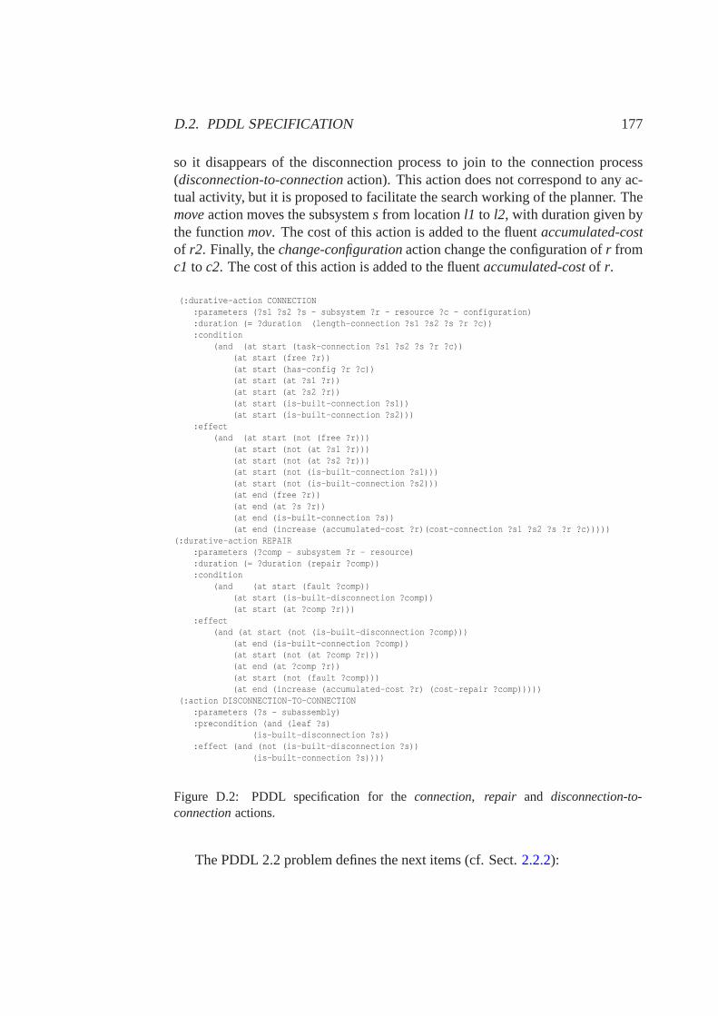
D.2. PDDL SPECIFICATION 177
so it disappears of the disconnection process to join to the connection process(disconnection-to-connectionaction). This action does not correspond to any ac-tual activity, but it is proposed to facilitate the search working of the planner. Themoveaction moves the subsystems from locationl1 to l2, with duration given bythe functionmov. The cost of this action is added to the fluentaccumulated-costof r2. Finally, thechange-configurationaction change the configuration ofr fromc1 to c2. The cost of this action is added to the fluentaccumulated-costof r.
(:durative-action CONNECTION:parameters (?s1 ?s2 ?s - subsystem ?r - resource ?c - configuration):duration (= ?duration (length-connection ?s1 ?s2 ?s ?r ?c)):condition
(and (at start (task-connection ?s1 ?s2 ?s ?r ?c))(at start (free ?r))(at start (has-config ?r ?c))(at start (at ?s1 ?r))(at start (at ?s2 ?r))(at start (is-built-connection ?s1))(at start (is-built-connection ?s2)))
:effect(and (at start (not (free ?r)))
(at start (not (at ?s1 ?r)))(at start (not (at ?s2 ?r)))(at start (not (is-built-connection ?s1)))(at start (not (is-built-connection ?s2)))(at end (free ?r))(at end (at ?s ?r))(at end (is-built-connection ?s))(at end (increase (accumulated-cost ?r)(cost-connection ?s1 ?s2 ?s ?r ?c)))))
(:durative-action REPAIR:parameters (?comp - subsystem ?r - resource):duration (= ?duration (repair ?comp)):condition
(and (at start (fault ?comp))(at start (is-built-disconnection ?comp))(at start (at ?comp ?r)))
:effect(and (at start (not (is-built-disconnection ?comp)))
(at end (is-built-connection ?comp))(at start (not (at ?comp ?r)))(at end (at ?comp ?r))(at start (not (fault ?comp)))(at end (increase (accumulated-cost ?r) (cost-repair ?comp)))))
(:action DISCONNECTION-TO-CONNECTION:parameters (?s - subassembly):precondition (and (leaf ?s)
(is-built-disconnection ?s)):effect (and (not (is-built-disconnection ?s))
(is-built-connection ?s))))
Figure D.2: PDDL specification for theconnection, repair and disconnection-to-connectionactions.
The PDDL 2.2 problem defines the next items (cf. Sect.2.2.2):
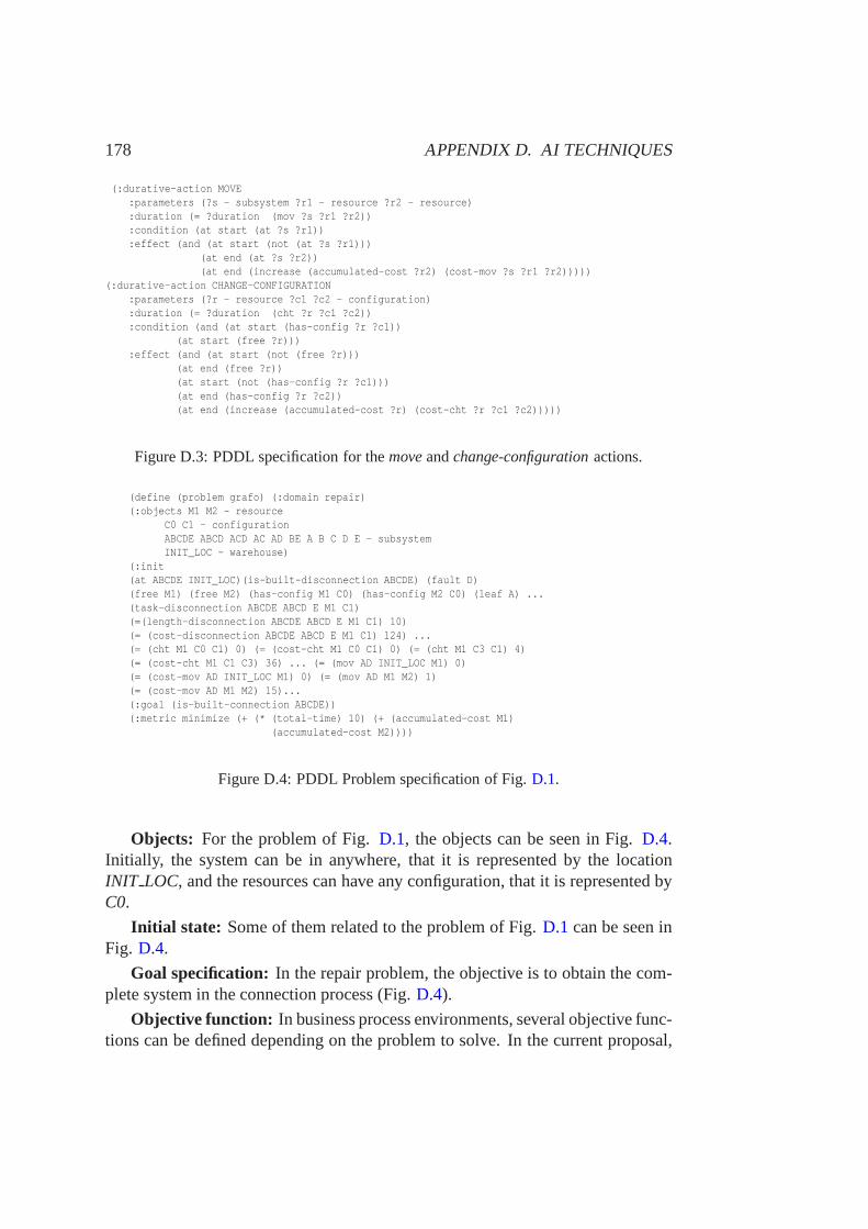
178 APPENDIX D. AI TECHNIQUES
(:durative-action MOVE:parameters (?s - subsystem ?r1 - resource ?r2 - resource):duration (= ?duration (mov ?s ?r1 ?r2)):condition (at start (at ?s ?r1)):effect (and (at start (not (at ?s ?r1)))
(at end (at ?s ?r2))(at end (increase (accumulated-cost ?r2) (cost-mov ?s ?r1 ?r2)))))
(:durative-action CHANGE-CONFIGURATION:parameters (?r - resource ?c1 ?c2 - configuration):duration (= ?duration (cht ?r ?c1 ?c2)):condition (and (at start (has-config ?r ?c1))
(at start (free ?r))):effect (and (at start (not (free ?r)))
(at end (free ?r))(at start (not (has-config ?r ?c1)))(at end (has-config ?r ?c2))(at end (increase (accumulated-cost ?r) (cost-cht ?r ?c1 ?c2)))))
Figure D.3: PDDL specification for themoveandchange-configurationactions.
(define (problem grafo) (:domain repair)(:objects M1 M2 - resource
C0 C1 - configurationABCDE ABCD ACD AC AD BE A B C D E - subsystemINIT_LOC - warehouse)
(:init(at ABCDE INIT_LOC)(is-built-disconnection ABCDE) (fault D)(free M1) (free M2) (has-config M1 C0) (has-config M2 C0) (leaf A) ...(task-disconnection ABCDE ABCD E M1 C1)(=(length-disconnection ABCDE ABCD E M1 C1) 10)(= (cost-disconnection ABCDE ABCD E M1 C1) 124) ...(= (cht M1 C0 C1) 0) (= (cost-cht M1 C0 C1) 0) (= (cht M1 C3 C1) 4)(= (cost-cht M1 C1 C3) 36) ... (= (mov AD INIT_LOC M1) 0)(= (cost-mov AD INIT_LOC M1) 0) (= (mov AD M1 M2) 1)(= (cost-mov AD M1 M2) 15)...(:goal (is-built-connection ABCDE))(:metric minimize (+ (* (total-time) 10) (+ (accumulated-cost M1)
(accumulated-cost M2))))
Figure D.4: PDDL Problem specification of Fig.D.1.
Objects: For the problem of Fig.D.1, the objects can be seen in Fig.D.4.Initially, the system can be in anywhere, that it is represented by the locationINIT LOC, and the resources can have any configuration, that it is represented byC0.
Initial state: Some of them related to the problem of Fig.D.1 can be seen inFig. D.4.
Goal specification: In the repair problem, the objective is to obtain the com-plete system in the connection process (Fig.D.4).
Objective function: In business process environments, several objective func-tions can be defined depending on the problem to solve. In the current proposal,

D.2. PDDL SPECIFICATION 179
some objective functions have been selected to be minimized, one of them appearsin Fig. D.4.
In this section, a PDDL 2.2 specification for solving a specific P&S problem,the multi-mode repair planning problem, has been explained. Similar P&S pro-blems can be solved in a related way.

Bibliography
Aguilar-Saven, R., 2004. Business process modelling: Review and framework.International Journal of Production Economics 90 (2), 129 –149.
Allen, J., 1983. Maintaining knowledge about temporal intervals. In: Proc. Com-munications of the ACM. pp. 832–843.
Alves, F. S. R., Guimares, K. F., Fernandes, M. A., 2008. Integrating planning andscheduling based on genetic algorithms to an workflow system. In: Proc. CEC.pp. 3766–3775.
Awad, A., Gore, R., Thomson, J., Weidlich, M., 2011. An iterative approach forbusiness process template synthesis from compliance rules. In: Proc. Caise. pp.406–421.
Bae, J., Bae, H., Kang, S., Kim, Y., 2004. Automatic control of workflow pro-cesses using eca rules. IEEE Transactions on Knowledge and Data Engineering16 (8), 1010–1023.
Bao, F., Chintabathina, S., Morales, A., Rushton, N., Watson, R., Zhang, Y., 2011.A temporally expressive planner based on answer set programming with cons-traints: Preliminary design. In: Proc. LPNMR. pp. 398–414.
Baptiste, P., Le Pape, C., Nuijten, W., 1999. Satisfiabilitytests and time-bound ad-justments for cumulative scheduling problems. Annals of Operations Research92, 305 – 333.
Barba, I., Del Valle, C., 2010. Planning and Scheduling of Business Processes inRun-Time: A Repair Planning Example. In: Proc. ISD. Springer, pp. 75–88.
Barba, I., Del Valle, C., 2011a. A Constraint-based Approach for Planning andScheduling Repeated Activities. In: Proc. COPLAS. pp. 55–62.
Barba, I., Del Valle, C., 2011b. A Planning and Scheduling Perspective for De-signing Business Processes from Declarative Specifications. In: Proc. Icaart.Vol. 1. pp. 562–569.
181
182 BIBLIOGRAPHY
Barba, I., Del Valle, C., Borrego, D., 2009a. A Constraint-based Model for Multi-objective Repair Planning. In: Proc. ETFA. pp. 234–241, art. no. 5347038.
Barba, I., Del Valle, C., Borrego, D., 2009b. PDDL Specification for Multi-objective Repair Planning. In: Proc. CAEPIA 2009 Workshop on Planning,Scheduling and Constraint Satisfaction. pp. 21–33.
Barba, I., Weber, B., Del Valle, C., 2011. Supporting the Optimized Execution ofBusiness Processes through Recommendations. In: Proc. BPI. Springer LNCS(In press).
Barjis, J., Verbraeck, A., 2010. The relevance of modeling and simulation in en-terprise and organizational study. In: Proc. EOMAS. pp. 15–26.
Bartak, R., Cepek, O., 2008. Incremental filtering algorithms for precedence anddependency constraints. International Journal on Artificial Intelligence Tools17 (1), 205–221.
Bartak, R., Cepek, O., 2010. Incremental propagation rules for a precedence graphwith optional activities and time windows. Transactions ofthe Institute of Mea-surement and Control 32 (1), 73–96.
Bartak, R., O., C., 2007. Temporal networks with alternatives: complexity andmodel. In: Proc. FLAIRS. pp. 641–646.
Beck, J., Fox, M., 1998. A generic framework for constraint-directed search andscheduling. AI Magazine 19 (4), 101 – 130.
Beck, J., Fox, M., 2000. Constraint-directed techniques for scheduling alternativeactivities. International Journal on Artificial Intelligence 121, 211–250.
Bellman, R., 1957. Dynamic Programming. Princeton University Press, Princeton,NJ.
Berry, P., Drabble, B., 2000. Swim: An ai-based system for organizational mana-gement. In: The 2nd NASA Intl. WS on Planning and Scheduling for Space.NASA.
Blazewic, J., Pesh, E., Sterna, M., 2000. The disjunctive graph machine repre-sentation of the job shop scheduling problem. European Journal of OperationalResearch 127 (2), 317–331.
Blum, A., Furst, M., 1997. Fast planning through planning graph analysis. Artifi-cial Intelligence 90 (1-2), 281–300.
BIBLIOGRAPHY 183
BPEL, 2007. Web Services Business Process Execution Language Ver-sion 2.0: OASIS Standard.http://docs.oasis-open.org/wsbpel/2.0/wsbpel-v2.0.html, [Online; accessed 09-November-2011].
BPMN, 2011. Business Process Model and Notation (BPMN), Version 2.0.http://www.omg.org/spec/BPMN/2.0/, [Online; accessed 09-November-2011].
Brandimarte, P., 1993. Routing and scheduling in a flexible job shop by tabusearch. Annals of Operations Research 41 (3), 157 – 183.
Brucker, P., Knust, S., 2006. Complex Scheduling (GOR-Publications). Springer-Verlag New York, Inc., Secaucus, NJ, USA.
Calton, T., 1999. Advancing design-for-assembly. the nextgeneration in assemblyplanning. In: IEEE International Symposium on Assembly andTask Planning.pp. 57 – 62.
Caron, F., Vanthienen, J., 2011. An exploratory approach toprocess lifecycle tran-sitions from a paradigm-based perspective. In: Proc. BPMDSand EMMSAD.pp. 178–185.
Chankong, V., Haimes, Y., 1983. Multiobjective Decision Making Theory andMethodology. Elsevier.
Chaturvedi, A., Hutchinson, G., Nazareth, D., 1993. Supporting complex real-time decision making through machine learning. Decision Support Systems10 (2), 213–233.
Chen, Y., Hsu, C., Wah, B., 2006. Temporal planning using subgoal partitioningand resolution in sgplan. Journal of Artificial Intelligence Research 26, 323–369.
Chesani, F., Lamma, E., Mello, P., Montali, M., Riguzzi, F.,Storari, S., 2009. Ex-ploiting inductive logic programming techniques for declarative process min-ing. In: Proc. ToPNoC. pp. 278–295.
Clarke Jr., E., Grumberg, O., Peled, D., 1999. Model Checking. The MIT Press.
Coello, C., 2006. Evolutionary multi-objective optimization: A historical view ofthe field. IEEE Computational Intelligence Magazine 1 (1), 28–36.
Davenport, T. H., 1993. Process innovation: reengineeringwork through informa-tion technology. Harvard Business School Press.
184 BIBLIOGRAPHY
De Castro, V., Marcos, E., 2009. Towards a service-orientedmda- based approachto the alignment of business processes with it systems: fromthe business modelto a web service composition model. International Journal of Cooperative In-formation Systems 18 (2), 225 – 260.
Deb, K., 2008. Introduction to evolutionary multiobjective optimization. 5252LNCS, 59–96.
Dechter, R., 2003. Constraint Processing. Morgan KaufmannPublishers.
Del Valle, C., Marquez, A., Barba, I., 2010. A CSP model for simple non-reversible and parallel repair plans. Journal of Intelligent Manufacturing 21 (1),165–174.
Demeyer, R., Van Assche, M., Langevine, L., Vanhoof, W., 2010. Declarativeworkflows to efficiently manage flexible and advanced business processes. In:Proc. PPDP. pp. 209–218.
Dourish, P., Holmes, J., MacLean, A., Marqvardsen, P., Zbyslaw, A., 1996.Freeflow: Mediating between representation and action in workflow systems.In: Proc. CSCW. pp. 190–198.
Drabble, B., Tate, A., 1994. The use of optimistic and pessimistic resource profilesto inform search in an activity based planner. In: Proc. AIPS. pp. 243–248.
Drexl, A., Gruenewald, J., 1993. Nonpreemptive multi-moderesource-constrained project scheduling. IIE Transactions (Institute of Industrial Engi-neers) 25 (5), 74–81.
Dumas, M., van der Aalst, W., ter Hofstede, A. (Eds.), 2005. Process-Aware Infor-mation Systems: Bridging People and Software through Process Technology.Wiley-Interscience, Hoboken, NJ.
Dynadec, 2011. Comet Downloads.http://dynadec.com/support/downloads/, [Online; accessed 09-November-2011].
Ehrgott, M., 2005. Multicriteria Optimization. Springer Berlin.
Ehrgott, M., Ruzika, S., 2008. Improvedε-constraint method for multiobjectiveprogramming. Journal of Optimization Theory and Applications 138 (3), 375–396.
Elgammal, A., Turetken, O., Van Den Heuvel, W., Papazoglou,M., 2011. Onthe formal specification of regulatory compliance: A comparative analysis. In:Proc. ICSOC Workshops. pp. 27–38.
BIBLIOGRAPHY 185
Ellis, C., Nutt, G., 1993. Modeling and enactment of workflowsystems. In: Proc.PETRI NETS. Springer Berlin / Heidelberg, pp. 1–16.
Erol, K., Hendler, J., Nau, D., 1994. HTN planning: Complexity and expressivity.In: Proc. of 20th AAAI Conference. pp. 1123–1128.
Fahland, D., Lubke, D., Mendling, J., Reijers, H., Weber, B., Weidlich, M., Zugal,S., 2009. Declarative versus imperative process modeling languages: The issueof understandability. In: Proc. BPMDS 2009 and EMMSAD 2009.pp. 353–366.
Fahland, D., Mendling, J., Reijers, H., Weber, B., Weidlich, M., Zugal, S., 2010.Declarative versus imperative process modeling languages: The issue of main-tainability. In: Proc. BPM Workshops. pp. 477–488.
Feo, T., Resende, M., 1989. A probabilistic heuristic for a computationally diffi-cult set covering problem. Operations Research Letters 8, 67–71.
Feo, T., Resende, M., 1995. Greedy randomized adaptive search procedures. Jour-nal of Global Optimization 6, 109–133.
Fernandes, R., Lange, F., Burchett, R., Happ, H., Wirgau, K., 1983. Large scalereactive power planning. IEEE transactions on power apparatus and systemsPAS-102 (5), 1083–1088.
Ferreira, H., Ferreira, D., 2006. An integrated life cycle for workflow managementbased on learning and planning. International Journal of Cooperative Informa-tion Systems 15 (4), 485 – 505.
Fikes, R., Nilsson, N., 1971. Strips: A new approach to the application of theoremproving to problem solving. Artificial Intelligence 2, 189–208.
Fonseca, C., Fleming, P., 1995. An overview of evolutionaryalgorithms in multi-objective optimization. Evolutionary Computation 3 (1), 1–16.
Friedrich, G., Fugini, M., Mussi, E., Pernici, B., Tagni, G., 2010. Exception Han-dling for Repair in Service-Based Processes. IEEE Transactions on SoftwareEngineering 36 (2), 198–215.
Frost, D., Dechter, R., 1994. Dead-end driven learning. In:Proc. of the NationalConference on Artificial Intelligence. pp. 294–300.
Gabriel, G., Grandcolas, S., 2009. Searching optimal parallel plans: A filteringand decomposition approach. pp. 576–580.
186 BIBLIOGRAPHY
Gantt, H., 1913. Work, wages, and profits. Engineering Magazine Co.
Garey, M. R., Johnson, D. S., 1979. Computers and Intractability: A Guide to theTheory of NP-Completeness. New York, NY, USA: W. H. Freeman &Co.
Garrido, A., Arangu, M., Onaindia, E., 2009. A constraint programming formula-tion for planning: From plan scheduling to plan generation.Journal of Schedu-ling 12 (3), 227–256.
Garrido, A., Onaindia, E., Sapena, O., 2008. Planning and scheduling in an e-learning environment. a constraint-programming-based approach. EngineeringApplications of Artificial Intelligence 21 (5), 733–743.
Georgakopoulos, D., Hornick, M., Sheth, A., 1995. An Overview of WorkflowManagement: From Process Modeling to Workflow Automation Infrastructure.Distributed and Parallel Databases 3, 119–153.
Gerevini, A., Long, D., 2006. Preferences and soft constraints in pddl3. In: ICAPS2006 Ws on Preferences and Soft Constraints in Planning. pp.46 – 53.
Ghallab, M., et al., 1998. Pddl - the planning domain definition language. Tech.rep., CVC TR-98-003/DCS TR-1165.
Ghallab, M., Nau, D., Traverso, P., 2004. Automated Planning: Theory and Prac-tice. Morgan Kaufmann, Amsterdam.
Glance, N., Pagani, D., Pareschi, R., 1996. Generalised process structure gram-mars (GPSG) for flexible representations of work. In: Press,A. (Ed.), Proc.CSCW. pp. 190–198.
Glover, F., 1989. Tabu search part i. Orsa Journal on Computing 1 (3), 190–206.
Goedertier, S., Vanthienen, J., 2009. An overview of declarative process modelingprinciples and languages. In: Proc. ABIS. pp. 51 – 58.
Goldberg, D., 1989. Genetic Algorithms in Search, Optimization and MachineLearning. Addison Wesley, Reading.
Goldmann, S., Munch, J., Holz, H., 2000. Distributed Process Planning Supportwith MILOS. International Journal of Software Engineeringand KnowledgeEngineering 10 (4), 511–525.
Goldwasser, M. H., Motwani, R., 1999. Complexity measures for assembly se-quences. International Journal of Computational Geometryand Applications 9,371 – 418.

BIBLIOGRAPHY 187
Gomes, C., Van Hoeve, W., Selman, B., 2006. Constraint programming for dis-tributed planning and scheduling. Vol. SS-06-04. pp. 157–158.
Gonzalez-Ferrer, A., Fernandez-Olivares, J., Castillo, L., 2009. JABBAH: A JavaApplication Framework for the Translation Between Business Process Modelsand HTN. In: Proc. ICKEPS. pp. 28–37.
Ha, B., Bae, J., Park, Y., Kang, S., 2006. Development of process execution rulesfor workload balancing on agents. Data & Knowledge Engineering 56 (1), 64–84.
Haimes, Y., Lasdon, L., Wismer, D., 1971. On a bicriterion formulation of the pro-blems of integrated system identification and system optimization. IEEE Trans-actions on Systems, Man, and Cybernetics 1, 296–297.
Haisjackl, C., Weber, B., 2010. User Assistance During Process Execution - AnExperimental Evaluation of Recommendation Strategies. In: Proc. BPI.
Halle, S., Villemaire, R., 2008. Runtime monitoring of message-based workflowswith data. In: EDOC. IEEE Computer Society, pp. 63–72.
Hammond, K., 1990. Case-based planning: A framework for planning from expe-rience. Cognitive Science 14 (3), 385–443.
Hoffmann, J., Edelkamp, S., 2005. The deterministic part ofipc-4: an overview.Journal of Artificial Intelligence Research 24 (1), 519–579.
Hoffmann, J., Weber, I., Kraft, F., 2010. SAP speaks PDDL. In: Proc. AAAI. pp.1096–1101.
Homem de Mello, L., Sanderson, A., 1990. And/or graph representation of as-sembly plans. IEEE Transactions on Robotics and Automation6(2), 188–189.
Homem de Mello, L., Sanderson, A., 1991. A correct and complete algorithm forthe generation of mechanical assembly sequences. IEEE Transactions Robotic& Automation 27 (2), 228 – 240.
ILOG, 2011. IBM ILOG CPLEX CP Optimizer.http://www-01.ibm.com/software/integration/optimization/cplex-cp-optimizer/, [Online;accessed 09-November-2011].
Jarvis, P., et al., 2000. Applying intelligent workflow management in the chemi-cals industries. In: The workflow handbook 2001, Published in association withthe Workflow Management Coalition (WfMC). L. Fisher (Ed.).
188 BIBLIOGRAPHY
Joeris, G., 2000. Decentralized and flexible workflow enactment based on taskcoordination agents. In: Springer-Verlag (Ed.), Proc. Caise. pp. 41–62.
Joshi, S., Kersting, K., Khardon, R., 2011. Decision-theoretic planning with gen-eralized first-order decision diagrams. Artificial Intelligence 175 (18), 2198–2222.
Kim, I.Y., D. W. O., 2006. Adaptive weighted sum method for multiobjectiveoptimization: A new method for pareto front generation. Structural and Multi-disciplinary Optimization 31 (2), 105–116.
Kirkpatrick, S., Gelatt, C., Vecchi, M., 1983. Optimization by simulated anneal-ing. Science 220 (4598), 671–680.
Koehler, J., 1998. Planning under resource constraints. In: Proc. ECAI. pp. 489–493.
Koski, J., 1985. Defectiveness of weighting method in multicriterion optimiza-tion of structures. Communications in Numerical Methods inEngineering 1 (6),333–337.
La Rosa, M., Dumas, M., Uba, R., Dijkman, R., 2010. Merging business processmodels. pp. 96–113.
Laborie, P., Ghallab, M., 1995. Planning with sharable resource constraints. In:Proc. IJCAI. pp. 1643–1649.
Laborie, P., Rogerie, J., Shaw, P., Vilım, P., 2009. Reasoning with Condi-tional Time-Intervals. Part II: An Algebraical Model for Resources. In: Proc.FLAIRS.
Lambert, A., 1997. Optimal disassembly of complex products. International Jour-nal of Production Research 35, 2509 – 2523.
Lambert, A., 1999. Optimal disassembly sequence generation for combined ma-terial recycling and part reus. In: IEEE International Symposium on Assemblyand Task Planning. pp. 146 – 151.
Lambert, A., 2003. Disassembly sequencing: a survey. International Journal ofProduction Research 41 (16), 3721–3759.
Lamma, E., Mello, P., Montali, M., Riguzzi, F., Storari, S.,2007. Inducing decla-rative logic-based models from labeled traces. In: Proc. BPM. pp. 344–359.
BIBLIOGRAPHY 189
Larrosa, J., 2000. Boosting search with variable elimination. In: Proc. CP. pp.291–305.
Larrosa, J., Meseguer, P., 2003. Algoritmos para satisfaccin de restricciones. In-teligencia Artificial: Revista Iberoamericana de Inteligencia Artificial 20, 31–42.
Le Pape, C., Couronne, P., Vergamini, D., Gosselin, V., 1994. Time-versus-capacity compromises in project scheduling. In: Proc. PlanSIG. pp. 498–502.
Lecoutre, C., Vion, J., 2008. Enforcing arc consistency using bitwise operations.Constraint Programming Letters 2, 21–35.
Lekavy, M., Navrat, P., 2007. Expressivity of STRIPS-Likeand HTN-Like Plan-ning. In: Proc. KES-AMSTA. pp. 121–130.
Li, W., Zhang, C., 1995. Design for disassembly analysis forenvironmentallyconscious design and manufacturing. In: ASME International Mechanical En-gineering Congress. pp. 969 – 976.
Liu, Y., Jiang, Y., 2006. Lp-tpop: Integrating planning andscheduling throughconstraint programming. In: Proc. PRICAI. pp. 844–848.
Liu, Y., Muller, S., Xu, K., 2007. A static compliance-checking framework forbusiness process models. IBM Systems Journal 46 (2), 335–362.
Lombardi, M., Milano, M., 2010. Constraint based scheduling to deal with uncer-tain durations and self-timed execution. In: Proc. CP. pp. 383–397.
Lu, R., Sadiq, S., Padmanabhan, V., Governatori, G., 2006. Using a temporalconstraint network for business process execution. In: Australian Computer So-ciety, I. (Ed.), Proc. ADC. pp. 157–166.
Ly, L., Rinderle, S., P., D., 2008. Integration and verification of semantic cons-traints in adaptive process management systems. Data & Knowledge Engineer-ing 64 (1), 3 – 23.
Mackworth, A., 1977. Consistency in networks of relations.Artificial Intelligence8 (1), 99–118.
Marrella, A., Mecella, M., 2011. Continuous Planning for Solving Business Pro-cess Adaptivity. In: Proc. BPMDS and EMMSAD. pp. 118–132.
Miettinen, K., 1999. Nonlinear Multiobjective Optimization. Kluwer AcademicDordrecht.
190 BIBLIOGRAPHY
Mitchell, M., 1998. An Introduction to Genetic Algorithms.MIT Press.
Monette, J., Deville, Y., Van Hentenryck, P., 2009. Just-in-time scheduling withconstraint programming. pp. 241–248.
Montali, M., 2009. Specification and Verification of Declarative Open Interac-tion Models: a Logic-Based Approach. Ph.D. thesis, Department of Electron-ics, Computer Science and Telecommunications Engineering, University ofBologna.
Mouhoub, M., Sadaoui, S., Sukpan, A., 2003. Chronological backtracking versusformal methods for solving CSPs. In: Proc. of the International Conference onArtificial Intelligence IC-AI 2003. pp. 270–275.
Moura, A., De Souza, C., Cire, A., Lopes, T., 2008. Heuristics and constraint pro-gramming hybridizations for a real pipeline planning and scheduling problem.pp. 455–462.
Nareyek, A., Freuder, E., Fourer, R., Giunchiglia, E., Goldman, R., Kautz, H.,Rintanen, J., Tate, A., 2005. Constraints and ai planning. IEEE Intelligent Sys-tems 20 (2), 62 – 72.
Nau, D., Au, T., Ilghami, O., Kuter, U., Murdock, J., Wu, D., Yaman, F., 2003.Shop2: An htn planning system. Journal of Artificial Intelligence Research 20,379–404.
Nuijten, W., Aarts, E., 1996. Sequencing with earliness andtardiness penalties: areview. European Journal of Operational Research 90 (2), 269 – 284.
Ouyang, C., van der Aalst, W., Dumas, M., ter Hofstede, A., 2006.Translating BPMN to BPEL.http://citeseerx.ist.psu.edu/viewdoc/download?doi=10.1.1.79.3072&rep=rep1&type=pdf, [Online; accessed09-November-2011].
Owen, M., Raj, J., 2003. BPMN and Business Process Management Introduc-tion to the New Business Process Modeling Standard.http://www.omg.org/bpmn/Documents/6AD5D16960.BPMN_and_BPM.pdf, [Online; accessed 09-November-2011].
Ozbayrak, M., Bell, R., 2003. A knowledge-based decision support system forthe management of parts and tools in FMS. Decision Support Systems 35 (4),487–515.
Penberthy, J., Weld, D., 1994. Temporal planning with continuous change. In:Proc. AAAI. pp. 1010–1015.
BIBLIOGRAPHY 191
Pesic, M., 2008. Constraint-Based Workflow Management Systems: ShiftingControl to Users. Ph.D. thesis, Eindhoven University of Technology, Eind-hoven.
Pesic, M., Schonenberg, M., Sidorova, N., van der Aalst, W.,2007. Constraint-Based Workflow Models: Change Made Easy. In: OTM Conferences(1). pp.77–94.
Pesic, M., van der Aalst, W., 2006. A declarative approach for flexible businessprocesses management. In: Proc. BPM Workshops. pp. 169–180.
Pichler, P., Weber, B., Zugal, S., Pinggera, J., Mendling, J., Reijers, H., 2011.Imperative versus Declarative Process Modeling Languages: An EmpiricalInvestigation. In: Proc. ER-BPM (accepted). [Online; http://zugal.info/wp-content/uploads/2011/07/erbpm 2011.pdf; accessed 8-September-2011].
Pinedo, M., 2008. Scheduling - Theory, Algorithms, and Systems. Springer.
Pisinger, D., Ropke, S., 2010. Large neighborhood search. International Series inOperations Research & Management Science 146 (13), 399–420.
PLANET, 2003. Network home page: European network of excellence inai planning.http://planet.dfki.de/index.html, [Online; accessed 09-November-2011].
Prosser, P., 1993. An empirical study of phase transitions in binary constraintsatisfaction problems. Artificial Intelligence 81, 81–109.
R-Moreno, M., Borrajo, D., Cesta, A., Oddi, A., 2007. Integrating planning andscheduling in workflow domains. Expert Systems with Applications 33 (2),389–406.
Reijers, H., 2003. Design and Control of Workflow Processes.Springer-VerlagBerlin, Heidelberg.
Reijers, H., van der Aalst, W., 1999. Short-term simulation: bridging the gapbetween operational control and strategic decision making. In: Proc. IASTEDConference on Modeling and Simulation. p. 417421.
Rhee, S., Cho, N., Bae, H., 2008. Increasing the efficiency ofbusiness processesusing a theory of constraints. Information Systems Frontiers, 1–13.
Rhee, S., Cho, N., Bae, H., 2010. Increasing the efficiency ofbusiness processesusing a theory of constraints. Information Systems Frontiers 12 (4), 443–455.
192 BIBLIOGRAPHY
Rossi, F., van Beek, P., Walsh, T. (Eds.), 2006. Handbook of Constraint Program-ming. Elsevier.
Rozinat, A., Wynn, M., van der Aalst, W., ter Hofstede, A., Fidge, C., 2009.Workflow simulation for operational decision support. Data& Knowledge En-gineering 68 (9), 834–850.
Russell, N., van der Aalst, W., ter Hofstede, A., 2006. Workflow Exception Pat-terns. In: Proc. Caise. pp. 288–302.
Russell, N., van der Aalst, W., ter Hofstede, A., Edmond, D.,2005. Workflow re-source patterns: Identification, representation and tool support. In: Proc. Caise.pp. 216–232.
Rychkova, I., Regev, G., Wegmann, A., 2008a. High-level design and analysisof business processes: The advantages of declarative specifications. In: Proc.RCIS. pp. 99–110.
Rychkova, I., Regev, G., Wegmann, A., 2008b. Using declarative specifications inbusiness process design. International Journal of Computer Science and Appli-cations 5 (3b), 45 – 68.
Sabin, D., Freuder, E., 1994. Contradicting convectional wisdom in constraintsatisfaction. In: Proc. ECAI. pp. 125–129.
Sadiq, S. W., Orlowska, M. E., Sadiq, W., 2005. Specificationand validation ofprocess constraints for flexible workflows. Information Systems 30 (5), 349–378.
Salido, M., 2010. Introduction to planning, scheduling andconstraint satisfaction.Journal of Intelligent Manufacturing 21 (1), 1–4.
Schonenberg, H., Weber, B., van Dongen, B., van der Aalst, W., 2008. Supportingflexible processes through recommendations based on history. In: Proc. BPM.pp. 51–66.
Smith, D., Frank, J., Jonsson, A., 2000. Bridging the gap between planning andscheduling. Knowledge Engineering Review 15(1), 47–83.
Smith, D., Weld, D., 1999. Temporal planning with mutual exclusion reasoning.In: Proc. IJCAI. pp. 139–144.
Son, J., Kim, M., 2001. Improving the performance of time-constrained workflowprocessing. Journal of Systems and Software 58 (3), 211–219.
BIBLIOGRAPHY 193
Thompson, G., Goodale, J., 2006. Variable employee productivity in workforcescheduling. European Journal of Operational Research 170 (2), 376–390.
Timpe, C., 2002. Solving planning and scheduling problems with combined inte-ger and constraint programming. OR Spectrum 24 (4), 431–448.
Tjoa, S., Jakoubi, S., Goluch, S., Kitzler, G., 2010. Planning dynamic activity andresource allocations using a risk-aware business process management approach.In: Proc. ARES. pp. 268–274.
Tsai, C., Huang, K., Wang, F., Chen, C., 2010. A distributed server architecturesupporting dynamic resource provisioning for BPM-oriented workflow mana-gement systems. Journal of Systems and Software 83 (8), 1538–1552.
Tu, P., Son, T., Pontelli, E., 2007. CPP: A constraint logic programming basedplanner with preferences. In: Proc. LPNMR. pp. 290–296.
van der Aalst, W., 2003. Patterns and XPDL: A critical Evaluation of the XMLProcess Definition Language. In: QUT Technical report FIT-TR-2003-06. pp.1–30.
van der Aalst, W., Jablonski, S., 2000. Dealing with workflowchange: identifica-tion of issues and solutions. International Journal of Computer Systems Scienceand Engineering 15 (5), 267–276.
van der Aalst, W., Pesic, M., 2006a. DecSerFlow: Towards a Truly DeclarativeService Flow Language. In: LNCS 4184. pp. 1–23.
van der Aalst, W., Pesic, M., 2006b. Specifying, discovering, and monitoring ser-vice flows: Making web services process-aware. In: Technical Report BPM-06-09, BPMcenter.org.
van der Aalst, W., Pesic, M., Schonenberg, H., 2009. Declarative workflows: Bal-ancing between flexibility and support. Computer Science - Research and De-velopment 23 (2), 99–113.
van der Aalst, W., Schonenberg, M., Song, M., 2011. Time prediction based onprocess mining. Information Systems 36 (2), 450–475.
van der Aalst, W., ter Hofstede, A., Weske, M., 2003. Business Process Manage-ment: A Survey. In: Proc. BPM. pp. 1–12.
van der Aalst, W., van Hee, K., 2002. Workflow Management: Models, Methods,and Systems. MIT Press.
194 BIBLIOGRAPHY
van Dongen, B., 2007. Process Mining and Verification. Ph.D.thesis, EindhovenUniversity of Technology, Eindhoven.
van Dongen, B., van der Aalst, W., 2005. A Meta Model for Process Mining Data.In: Proc. Caise, 17th Edition. pp. 309–320.
van Hentenryck, P., 1999. The OPL Optimization ProgrammingLanguage. MITPress.
Vanderfeesten, I., Reijers, H., van der Aalst, W., 2008. Product based workflowsupport: A recommendation service for dynamic workflow execution. In: Tech-nical Report BPM-08-03, BPMcenter.org.
Vidal, V., Geffner, H., 2006. Branching and pruning: An optimal temporal poclplanner based on constraint programming. Artificial Intelligence 170 (3), 298–335.
Vossen, T., Ball, M., Lotem, A., Nau, D., 1999. On the use of integer programmingmodels in ai planning. The Knowledge Engineering Review 15 (1).
Wainer, J., Bezerra, F., Barthelmess, P., 2004. Tucupi: a flexible workflow systembased on overridable constraints. In: Proc. SAC. pp. 498–502.
Wainer, J., De Lima Bezerra, F., 2003. Constraint-based flexible workflows. In:Proc. CRIWG. pp. 151–158.
Weld, D., 1994. Introduction to least commitment planning.AI Magazine 15 (4),27–61.
Weske, M., 2007. Business Process Management: Concepts, Methods, Technol-ogy. Springer.
Westergaard, M., 2011. Access/cpn 2.0: A high-level interface to coloured petrinet models. In: Proc. PETRI NETS. pp. 328–337.
White, S., et al., 2004. Business Process Modeling Notation(BPMN), Workingdraft, Version 1.0.
Wolfman, S., Weld, D., 1999. Combining linear programming and satisfiabilitysolving for resource planning. The Knowledge Engineering Review 15 (1).
Younes, H., Simmons, R., 2003. VHPOP: Versatile heuristic partial order planner.Journal of Artificial Intelligence Research 20, 405–430.
Zadeh, L., 1963. Optimality and non-scalar-valued performance criteria. IEEETransactions on Automatic Control 8, 59–60.

BIBLIOGRAPHY 195
Zhao, J., Stohr, E., 1999. Temporal workflow management in a claim handlingsystem. SIGSOFT: Software Engineering Notes 24 (2), 187–195.
Zisman, M., 1977. Representation, Specification and Automation of Office Pro-cedures. Ph.D. thesis, Wharton School.