a benchmarking service for the evaluation and comparison of scheduling techniques

www.elsevier.com/locate/compind

Computers in Industry 58 (2007) 656–666

A Benchmarking Service for the evaluation and comparison of

scheduling techniques

Sergio Cavalieri a,*, Sergio Terzi a, Marco Macchi b

a Department of Industrial Engineering, University of Bergamo, Dalmine, BG, Italyb Department of Economics, Management and Industrial Engineering, Politecnico di Milano, Milano, Italy

Available online 13 June 2007

Abstract

Scheduling decisions constitute the last decision-making phase of the production planning and control process. From the industrial side, the

adoption of highly reactive and efficient scheduling and control systems strongly affects the level of productivity and utilization of a manufacturing

system, particularly under the pressure of shortened product cycles, reduced batch sizes and a broader variety of items to be produced. In the

meanwhile, from the research side, there has been a considerable amount of works done in the area of manufacturing systems control, even if they

still remain ‘‘unheard voices’’ in industry. Hence, in the scheduling world there is a risk of miscommunication between academics and industrial

users.

Aim of the paper is to provide a comprehensive view of the rationale, the conceptual model, the development efforts and first applicative

experiences of the Benchmarking Service, a research initiative which has been carried out within the activities of the Special Interest Group on

Benchmarking and Performance Measurement of the IMS Network of Excellence. In particular, the paper details the PMS-ESS conceptual

framework developed for assessing the level of quality of a scheduling solution in terms of efficiency, robustness and flexibility.

# 2007 Elsevier B.V. All rights reserved.

Keywords: Scheduling evaluation; Benchmarking; Performance measurement; Plant management

1. Introduction

Competitive firms are operating today in global and

worldwide markets. Manufacturers are experiencing a lumpy

market demand for their products, with ever shorter requested

lead times and order quantities as well as frequent changes in

product specifications. In this context, within the production

planning and control process, scheduling plays undoubtedly a

critical role. It is the final temporal decision-making phase

where industrial managers have to act for fixing any short

noticed variations preserving at the same time expected

medium-term efficiency performance.

According to Kempf et al. [6], the most general definition of

a scheduling problem is that of ‘‘assigning scarce resources to

competing activities over a given time horizon to obtain the best

possible system performance’’. Referring specifically to factory

* Corresponding author.

E-mail addresses: [email protected] (S. Cavalieri),

[email protected] (S. Terzi), [email protected] (M. Macchi).

0166-3615/$ – see front matter # 2007 Elsevier B.V. All rights reserved.

doi:10.1016/j.compind.2007.05.004

scheduling, the resources are machines and workforce, and the

competing activities are jobs that require processing on the

resources.

Several scheduling approaches exist, from the traditional

off-line scheduling systems, which elaborate a production plan

(e.g. according to static rules and algorithms) for a specific plan

period, to on-line production scheduling systems, which are

intrinsically able to modify an existing schedule or regenerate a

completely new one for managing upcoming events which

could alter the original plan.

Despite the flourish of heterogeneous proposals, a dichot-

omy is actually affecting the world of scheduling. Researchers

are often detached from industrial reality, proposing answers to

simple examples and toy cases. On the contrary, practitioners

have clear difficulties in explaining their requirements and

exploiting the opportunities which could come out from the

industrial exploitation of the new advanced scheduling

approaches.

The main purpose of the present paper is to provide a

comprehensive view of a research initiative, carried out in the

last years within the activities of the IMS-NoE Special Interest

mailto:[email protected]



http://dx.doi.org/10.1016/j.compind.2007.05.004

S. Cavalieri et al. / Computers in Industry 58 (2007) 656–666 657

Group (SIG) on Benchmarking and Performance Measurement

of Production Scheduling Systems. The research community

involved in the SIG has been mainly interested in promoting the

adoption of a Benchmarking methodology for testing and

evaluating scheduling solutions in order to identify the best

solution for one industrial problem.

This idea has turned into reality with the instantiation of the

Benchmarking Service within the IMS-NoE web site [7], freely

accessible to all the registered members. The available

prototype of the Benchmarking Service is a web-based arena,

where production systems would be described and different

production scheduling policies would be evaluated and

compared under a common simulation environment.

The paper is organized as follows: Section 2 summarizes the

rationale behind the developed Benchmarking Service; Section

3 introduces the framework developed for supporting the

description of a test case; Section 4 explores the main

requirements of the evaluation of a scheduling system; Sections

5 and 6 illustrate the proposed PMS-ESS with an applicative

example; Section 7 provides the main conclusions of the paper.

2. Rationale of the Benchmarking Service

Finding a scheduling system as a panacea for solving all the

issues which could arise in a production environment is quite

pretentious. Indeed, one of the main sources of miscommu-

nication between the research and the industrial world is the

difficulty to clearly and objectively ascertain the real domain of

applicability of a scheduler for a specific industrial problem.

In literature, there are several approaches to the scheduling

problem, which can be classified using alternative criteria,

referring in particular to shop-floor layouts (from single-

machine problems to complex job-shops), to scheduling

techniques (ranging from elementary dispatching rules to

multi-layered holonic systems) or to the level of uncertainty of

the production environment (deterministic models versus

event-triggered reactive schedulers) [21–23].

However, a clear understanding of the performance of

scheduling systems and their impact on the outcome of the

manufacturing system as a whole is still missing [6]. The need

Fig. 1. The Benchmark

for suitable Benchmarking platforms is not unique to

production scheduling; other research communities, as is the

case of artificial intelligence, have in the past pointed out

similar needs [24,25].

In particular, what is still missing today is [15]:

� a

ing

set of emulations of underlying production systems that is

representative for industry; this set cannot be restricted to the

typical Operations Research models but addresses issues such

as the handling of empty containers, batching, matching,

uncertain processing outcomes;

� a
set of scenarios for those underlying systems that
adequately reflects the dynamics of industrial systems; this

includes breakdowns, maintenance, processing time varia-

tions, inaccurate data, missing data, late data, rush orders,

cancellations;

� a
standardized interface to connect control/scheduling
systems to such emulations of underlying systems;

� a
Benchmark management system that supports the user in
defining and executing Benchmarks; this includes a user-

friendly Graphical User Interface (GUI)-based subsystem,

that could significantly lower the threshold for novel users,

and more advanced facilities in which expressiveness is the

main concern.

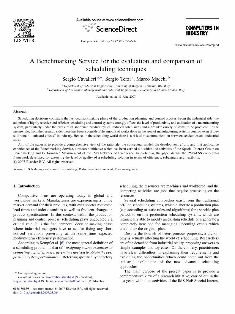
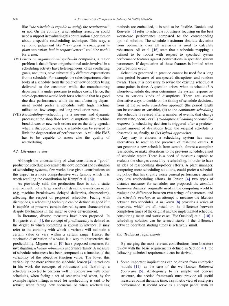
The Benchmarking Service (BS) aims to overcome these

issues by providing a framework, which should enable

developers of control systems and production engineers to

meet in the virtual world and test/evaluate how well they match

up (Fig. 1). Within this vision, there are three main involved

actors: (a) industrial users, (b) researchers and (c) technology

vendors. The involvement of the three profiles of actors derives

from the different point of views that each of them has on the

design of production plants and connected management logics.

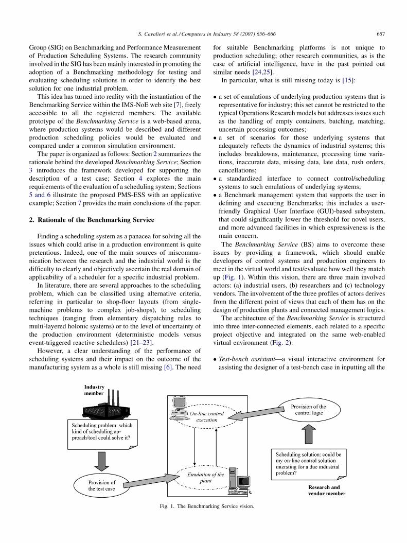
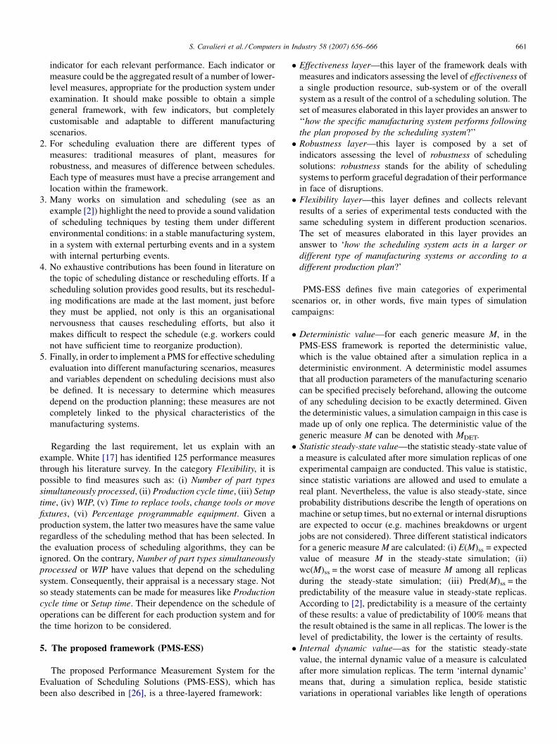
The architecture of the Benchmarking Service is structured

into three inter-connected elements, each related to a specific

project objective and integrated on the same web-enabled

virtual environment (Fig. 2):

� T
est-bench assistant—a visual interactive environment for
assisting the designer of a test-bench case in inputting all the

Service vision.

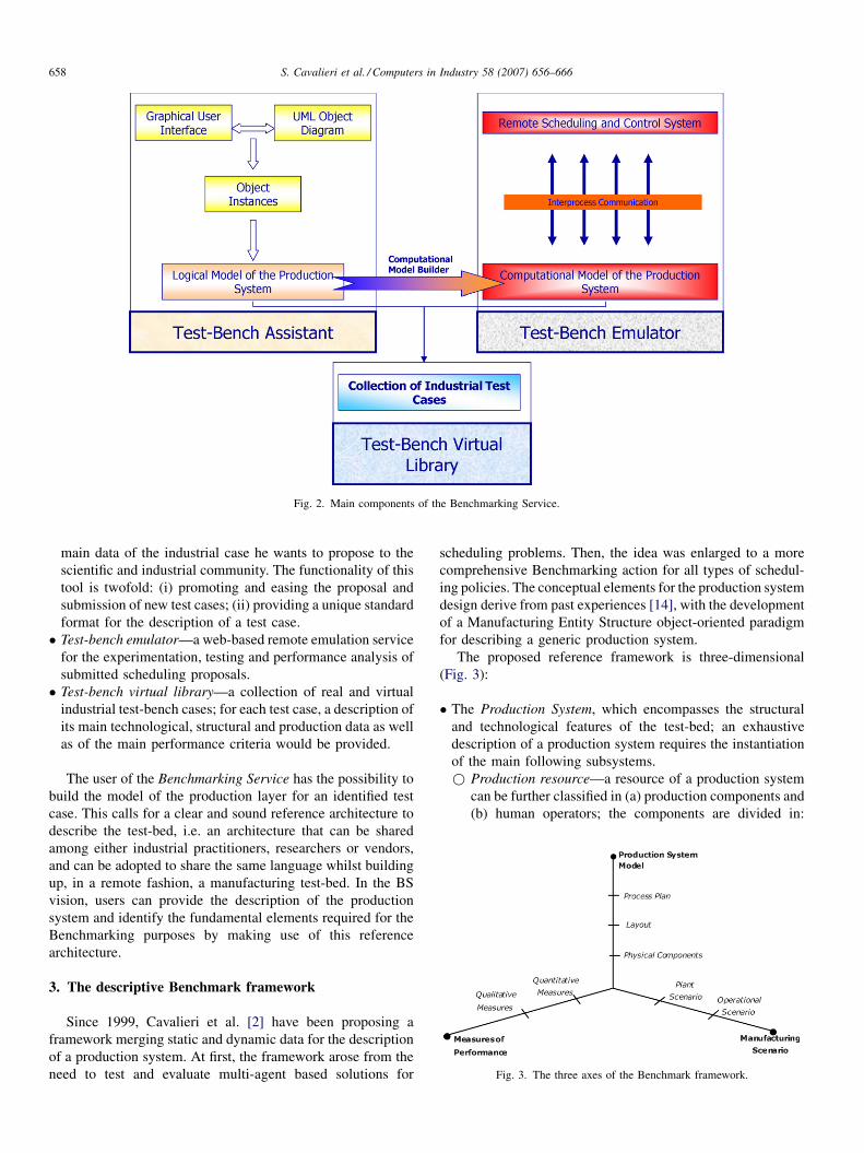
Fig. 2. Main components of the Benchmarking Service.

S. Cavalieri et al. / Computers in Industry 58 (2007) 656–666658

main data of the industrial case he wants to propose to the

scientific and industrial community. The functionality of this

tool is twofold: (i) promoting and easing the proposal and

submission of new test cases; (ii) providing a unique standard

format for the description of a test case.

� T
est-bench emulator—a web-based remote emulation service
for the experimentation, testing and performance analysis of

submitted scheduling proposals.

� T

Fig. 3. The three axes of the Benchmark framework.

est-bench virtual library—a collection of real and virtual

industrial test-bench cases; for each test case, a description of

its main technological, structural and production data as well

as of the main performance criteria would be provided.

The user of the Benchmarking Service has the possibility to

build the model of the production layer for an identified test

case. This calls for a clear and sound reference architecture to

describe the test-bed, i.e. an architecture that can be shared

among either industrial practitioners, researchers or vendors,

and can be adopted to share the same language whilst building

up, in a remote fashion, a manufacturing test-bed. In the BS

vision, users can provide the description of the production

system and identify the fundamental elements required for the

Benchmarking purposes by making use of this reference

architecture.

3. The descriptive Benchmark framework

Since 1999, Cavalieri et al. [2] have been proposing a

framework merging static and dynamic data for the description

of a production system. At first, the framework arose from the

need to test and evaluate multi-agent based solutions for

scheduling problems. Then, the idea was enlarged to a more

comprehensive Benchmarking action for all types of schedul-

ing policies. The conceptual elements for the production system

design derive from past experiences [14], with the development

of a Manufacturing Entity Structure object-oriented paradigm

for describing a generic production system.

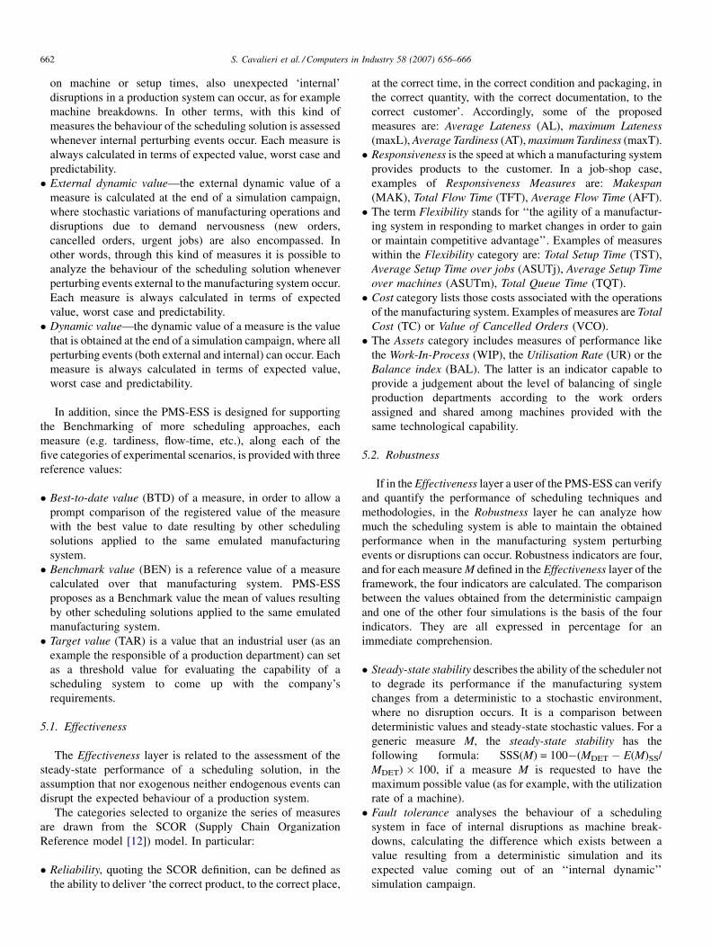
The proposed reference framework is three-dimensional

(Fig. 3):

� T
he Production System, which encompasses the structural
and technological features of the test-bed; an exhaustive

description of a production system requires the instantiation

of the main following subsystems.

* Production resource—a resource of a production system

can be further classified in (a) production components and

(b) human operators; the components are divided in:


processors (machining stations), storage (buffers), and

transporters (transportation systems).

* Process plan—the technological features are captured by

the process plans of the products being processed in the

plant; a process plan models a sequence of operations that

have to be performed for a given product; it is composed

by several object classes (operations) and only one object

class (part), which is the class of the production entity to

be processed.

* Production planning—the planning of the production

activity is represented with three interconnected, but

independent classes: (a) the Production Planning class,

which reproduces the long-term planning horizon (i.e.

from 6 months to 1 year), (b) the Work Order class, which

represents the monthly mid-term planning horizon and (c)

the Job class, which models the weekly low-term planning

horizon.

� T
he manufacturing scenario—the definition of a manufac-
turing scenario aims at collecting events or activities

dependent on the dynamic behaviour of the manufacturing

domain. A manufacturing scenario can be split into two sub-

scenarios according to the generating domain.

* Plant scenario, which is related to the dynamic behaviour

of the plant; this scenario collects events or activities

related to the functioning of the production components,

such as: (a) machine breakdown, which is due to

maintenance parameters and busy times (Mean Time

Between Failures/Mean Time To Repair); (b) stochastic

variations on set-up times and operation processing times;

(c) stochastic variations on transport service time, which

also depends on the type of transporter being selected

(serial or parallel); (d) material arrivals, being dependent

from suppliers.

* Operational scenario, which considers the way the release

of the production plan is conceived, and in particular the

definition of: production orders to be scheduled (type of

products and lot quantity); expected release dates;

expected due dates; other scheduling conditions, if

required (e.g. product costs or product quality).

� T
he Measures of Performance to be used, in order to allow for
an objective comparison between the results of different

scheduling approaches on the same test case.

Further details on the first two dimensions of the framework

are given in other contributions from the same authors [11,15].

In particular, in [15] the object classes of the framework with an

Unified Modelling Language (UML) notation are reported.

The following sections will be devoted to the latter axis

related to the definition of a proper set of performance

measures.

4. Main requirements for the evaluation of schedulingsystems

In the Benchmarking Service, the role of performance

measures is particularly important. Performance evaluation

should include all relevant aspects, as the quality of the

scheduling and control software, its deployment effort in a shop

floor and the productivity of the shop floor system itself.

Moreover, performance evaluation should be industrially

relevant, to refrain diffidence of industrial practitioners and

to provide them with a critical analysis of the performance of

the scheduling systems under investigation.

Performance measurement is a large research topic:

performance measures are used to evaluate, control and

improve production processes, but are also used to compare the

performance of different organisations, plants, departments,

teams and individuals. In literature, basic performance

scheduling indicators are well acknowledged and shared

(e.g. makespan, tardiness, lateness, flow time, setup time,

working time, . . .), and usually, though most of them are

defined for a single job, their values are normally aggregated, in

order to calculate mean and total values among all jobs.

4.1. Basic requirements

Since scheduling is highly context-dependent, some basic

requirements of a performance measurement system (PMS) for

scheduling evaluation can be highlighted:

(I) O
pen and easily customisable—given the heterogeneity
of production systems, a PMS for scheduling evaluation

has to be a framework open to different typologies of

users and production environments, easily applicable and

customisable in order to comprehend different possible

manufacturing systems and scenarios.

(II) E
ffective comparison of schedule quality—an industrial
practitioner could be interested in taking into account

various scheduling techniques and policies; conse-

quently, the PMS has to be capable to compare alternative

planning and scheduling practices.

(III) M
easuring the efficiency of a production system—
according to the previous requirements, an industrial

practitioner could be interested to know not only relevant

measures for scheduling, but also all the operational

measures that can be gathered from a shop floor. For

example, in a job-shop the setup time can be not

dependent on the job sequences, so, for the sake of

scheduling comparison, it can be ignored. However, for a

plant manager the knowledge of total setup-time could be

an important measure in order to estimate the required

workforce labour to support production.

(IV) P
erformance evaluation at diverse levels—each level of
an enterprise needs a specific set of performance

measures but, moving up to the corporate hierarchy,

measures and indicators tend to be expressed more and

more in aggregated terms; whereas at the lowest level a

set of single atomic measures can be useful and effective,

at upper levels managers need some synthetic indicators.

(V) Q
uantitative data and symbolic judgments—an industrial
user could be interested whether a certain production

schedule can satisfy one or more specifications (e.g. a

certain target value of the production makespan could be

needed). In this case, he is searching for a boolean result,


like ‘‘the schedule is capable to satisfy the requirement’’

or not. On the contrary, a scheduling researcher could

need a support in evaluating his optimisation algorithm or

about a specific rescheduling technique. This way, a

symbolic judgement like ‘‘very good in costs, good in

plant saturation, bad in responsiveness’’ could be useful

for a user.

(VI) F
ocus on organisational goals—in companies, a major
problem is that different organisational units involved in a

scheduling activity have heterogeneous, often conflicting

goals, and, thus, have substantially different expectations

from a schedule. For example, the sales department often

looks at a schedule from the point of view of orders being

delivered to the customer, while the manufacturing

department is under pressure to reduce costs. Hence, the

sales department would look for a schedule that has good

due date performance, while the manufacturing depart-

ment would prefer a schedule with high machine

utilisation, few setups, and long production runs.

(VII) R
escheduling—scheduling is a nervous and dynamic
process; at the shop floor level, disruptions like machine

breakdowns or new rush orders are on the daily agenda;

when a disruption occurs, a schedule can be revised to

limit the degeneration of performances. A valuable PMS

has to be capable to assess also the quality of

rescheduling.

4.2. Literature review

Although the understanding of what constitutes a ‘‘good’’

production schedule is central to the development and evaluation

of scheduling systems, few works have given contributions on

this aspect in a more comprehensive way (among which it is

worth recalling the contribution by Kempf et al. [6]).

As previously said, the production floor is not a static

environment, but a large variety of dynamic events can occur

(e.g. machine breakdowns, delayed deliveries, absenteeism),

affecting the respect of proposed schedules. Facing with

disruptions, a scheduling technique can be defined as good if it

is capable to preserve certain desired system characteristics

despite fluctuations in the inner or outer environment.

In literature, diverse measures have been proposed. In

Bongaerts et al. [1], the concept of predictability is defined as

the degree to which something is known in advance. It may

refer to the certainty with which a variable will maintain a

certain value or vary within a certain range. Hence, the

stochastic distribution of a value is a way to characterize the

predictability. Mignon et al. [9] have proposed measures for

investigating schedule robustness under uncertainty. A measure

of schedule robustness has been computed as a function of the

variability of the objective function value. The lower this

variability, the more robust the schedule. Jensen [4] introduces

in his work the concepts of robustness and flexibility: a

schedule expected to perform well in comparison with other

schedules, when facing a set of scenarios and when, by for

example right-shifting, is used for rescheduling is said to be

robust; when facing new scenarios or when rescheduling

methods are embedded, it is said to be flexible. Daniels and

Kouvelis [3] refer to schedule robustness focusing on the best

worst-case performance compared to the corresponding

optimal solution. The schedule maximum absolute deviation

from optimality over all scenarios is used to calculate

robustness. Ali et al. [16] state that a schedule mapping is

defined to be robust with respect to specified system

performance features against perturbations in specified system

parameters, if degradation of these features is limited when

perturbations occur.

Schedules generated in practice cannot be used for a long

time period because of unexpected disruptions and random

events. Thus, it is necessary to revise the existing schedule at

some points in time. A question arises: when-to-schedule? A

when-to-schedule decision determines the system responsive-

ness to various kinds of disruptions. There are several

alternative ways to decide on the timing of schedule decisions,

from (i) the periodic scheduling approach (the period length

can be constant or variable), (ii) to the continuous scheduling

(the schedule is revised after a number of events, that change

system state, occur), or (iii) to adaptive scheduling or controlled

response (a scheduling decision is triggered after a predeter-

mined amount of deviations from the original schedule is

observed), or, finally, to (iv) hybrid approaches.

Any way is chosen, a scheduling system has many

alternatives to react to the presence of real-time events. It

can generate a new schedule from scratch, almost a complete

reschedule, or make alterations to the previous schedule, a sort

of schedule repair. There is a need of measures capable to

evaluate the changes caused by rescheduling, in order to have

an idea of rescheduling shop-floor efforts. A plant manager,

comparing more scheduling solutions, could prefer a schedul-

ing policy that has slightly worse general performance, against

very low rescheduling efforts. In Jensen [4] two types of

distance measures for schedules are proposed: the absolute

Hamming distance, originally used in the computing world to

evaluate the difference between two strings of characters, and

the schedule overlap, as an attempt to measure the likeness

between two schedules. Also Goren [8] provides a series of

measures, which are all based on the difference between

completion times of the original and the implemented schedule,

considering mean and worst cases. For Ouelhadj et al. [10] a

scheduling solution can be termed stable if the difference

between operation starting times is relatively small.

4.3. Technical requirements

By merging the most relevant contributions from literature

review with the basic requirements defined in Section 4.1, the

following technical requirements can be derived.

1. S
ome important implications can be driven from enterprise
models [11], as the case of the well-known Balanced

Scorecard [5]. Analogously to its simple and concise

structure, the needed framework must provide all useful

measures but, at the same time, a synthetic view of enterprise

performance. It should serve as a cockpit panel, with an


indicator for each relevant performance. Each indicator or

measure could be the aggregated result of a number of lower-

level measures, appropriate for the production system under

examination. It should make possible to obtain a simple

general framework, with few indicators, but completely

customisable and adaptable to different manufacturing

scenarios.

2. F
or scheduling evaluation there are different types of
measures: traditional measures of plant, measures for

robustness, and measures of difference between schedules.

Each type of measures must have a precise arrangement and

location within the framework.

3. M
any works on simulation and scheduling (see as an
example [2]) highlight the need to provide a sound validation

of scheduling techniques by testing them under different

environmental conditions: in a stable manufacturing system,

in a system with external perturbing events and in a system

with internal perturbing events.

4. N
o exhaustive contributions has been found in literature on
the topic of scheduling distance or rescheduling efforts. If a

scheduling solution provides good results, but its reschedul-

ing modifications are made at the last moment, just before

they must be applied, not only is this an organisational

nervousness that causes rescheduling efforts, but also it

makes difficult to respect the schedule (e.g. workers could

not have sufficient time to reorganize production).

5. F
inally, in order to implement a PMS for effective scheduling
evaluation into different manufacturing scenarios, measures

and variables dependent on scheduling decisions must also

be defined. It is necessary to determine which measures

depend on the production planning; these measures are not

completely linked to the physical characteristics of the

manufacturing systems.

Regarding the last requirement, let us explain with an

example. White [17] has identified 125 performance measures

through his literature survey. In the category Flexibility, it is

possible to find measures such as: (i) Number of part types

simultaneously processed, (ii) Production cycle time, (iii) Setup

time, (iv) WIP, (v) Time to replace tools, change tools or move

fixtures, (vi) Percentage programmable equipment. Given a

production system, the latter two measures have the same value

regardless of the scheduling method that has been selected. In

the evaluation process of scheduling algorithms, they can be

ignored. On the contrary, Number of part types simultaneously

processed or WIP have values that depend on the scheduling

system. Consequently, their appraisal is a necessary stage. Not

so steady statements can be made for measures like Production

cycle time or Setup time. Their dependence on the schedule of

operations can be different for each production system and for

the time horizon to be considered.

5. The proposed framework (PMS-ESS)

The proposed Performance Measurement System for the

Evaluation of Scheduling Solutions (PMS-ESS), which has

been also described in [26], is a three-layered framework:

� E
ffectiveness layer—this layer of the framework deals with
measures and indicators assessing the level of effectiveness of

a single production resource, sub-system or of the overall

system as a result of the control of a scheduling solution. The

set of measures elaborated in this layer provides an answer to

‘‘how the specific manufacturing system performs following

the plan proposed by the scheduling system?’’

� R
obustness layer—this layer is composed by a set of
indicators assessing the level of robustness of scheduling

solutions: robustness stands for the ability of scheduling

systems to perform graceful degradation of their performance

in face of disruptions.

� F
lexibility layer—this layer defines and collects relevant
results of a series of experimental tests conducted with the

same scheduling system in different production scenarios.

The set of measures elaborated in this layer provides an

answer to ‘how the scheduling system acts in a larger or

different type of manufacturing systems or according to a

different production plan?’

PMS-ESS defines five main categories of experimental

scenarios or, in other words, five main types of simulation

campaigns:

� D
eterministic value—for each generic measure M, in the
PMS-ESS framework is reported the deterministic value,

which is the value obtained after a simulation replica in a

deterministic environment. A deterministic model assumes

that all production parameters of the manufacturing scenario

can be specified precisely beforehand, allowing the outcome

of any scheduling decision to be exactly determined. Given

the deterministic values, a simulation campaign in this case is

made up of only one replica. The deterministic value of the

generic measure M can be denoted with MDET.

� S
tatistic steady-state value—the statistic steady-state value of
a measure is calculated after more simulation replicas of one

experimental campaign are conducted. This value is statistic,

since statistic variations are allowed and used to emulate a

real plant. Nevertheless, the value is also steady-state, since

probability distributions describe the length of operations on

machine or setup times, but no external or internal disruptions

are expected to occur (e.g. machines breakdowns or urgent

jobs are not considered). Three different statistical indicators

for a generic measure M are calculated: (i) E(M)ss = expected

value of measure M in the steady-state simulation; (ii)

wc(M)ss = the worst case of measure M among all replicas

during the steady-state simulation; (iii) Pred(M)ss = the

predictability of the measure value in steady-state replicas.

According to [2], predictability is a measure of the certainty

of these results: a value of predictability of 100% means that

the result obtained is the same in all replicas. The lower is the

level of predictability, the lower is the certainty of results.

� I
nternal dynamic value—as for the statistic steady-state
value, the internal dynamic value of a measure is calculated

after more simulation replicas. The term ‘internal dynamic’

means that, during a simulation replica, beside statistic

variations in operational variables like length of operations


on machine or setup times, also unexpected ‘internal’

disruptions in a production system can occur, as for example

machine breakdowns. In other terms, with this kind of

measures the behaviour of the scheduling solution is assessed

whenever internal perturbing events occur. Each measure is

always calculated in terms of expected value, worst case and

predictability.

� E
xternal dynamic value—the external dynamic value of a
measure is calculated at the end of a simulation campaign,

where stochastic variations of manufacturing operations and

disruptions due to demand nervousness (new orders,

cancelled orders, urgent jobs) are also encompassed. In

other words, through this kind of measures it is possible to

analyze the behaviour of the scheduling solution whenever

perturbing events external to the manufacturing system occur.

Each measure is always calculated in terms of expected

value, worst case and predictability.

� D
ynamic value—the dynamic value of a measure is the value
that is obtained at the end of a simulation campaign, where all

perturbing events (both external and internal) can occur. Each

measure is always calculated in terms of expected value,

worst case and predictability.

In addition, since the PMS-ESS is designed for supporting

the Benchmarking of more scheduling approaches, each

measure (e.g. tardiness, flow-time, etc.), along each of the

five categories of experimental scenarios, is provided with three

reference values:

� B
est-to-date value (BTD) of a measure, in order to allow a
prompt comparison of the registered value of the measure

with the best value to date resulting by other scheduling

solutions applied to the same emulated manufacturing

system.

� B
enchmark value (BEN) is a reference value of a measure
calculated over that manufacturing system. PMS-ESS

proposes as a Benchmark value the mean of values resulting

by other scheduling solutions applied to the same emulated

manufacturing system.

� T
arget value (TAR) is a value that an industrial user (as an
example the responsible of a production department) can set

as a threshold value for evaluating the capability of a

scheduling system to come up with the company’s

requirements.

5.1. Effectiveness

The Effectiveness layer is related to the assessment of the

steady-state performance of a scheduling solution, in the

assumption that nor exogenous neither endogenous events can

disrupt the expected behaviour of a production system.

The categories selected to organize the series of measures

are drawn from the SCOR (Supply Chain Organization

Reference model [12]) model. In particular:

� R
eliability, quoting the SCOR definition, can be defined as
the ability to deliver ‘the correct product, to the correct place,

at the correct time, in the correct condition and packaging, in

the correct quantity, with the correct documentation, to the

correct customer’. Accordingly, some of the proposed

measures are: Average Lateness (AL), maximum Lateness

(maxL), Average Tardiness (AT), maximum Tardiness (maxT).

� R
esponsiveness is the speed at which a manufacturing system
provides products to the customer. In a job-shop case,

examples of Responsiveness Measures are: Makespan

(MAK), Total Flow Time (TFT), Average Flow Time (AFT).

� T
he term Flexibility stands for ‘‘the agility of a manufactur-
ing system in responding to market changes in order to gain

or maintain competitive advantage’’. Examples of measures

within the Flexibility category are: Total Setup Time (TST),

Average Setup Time over jobs (ASUTj), Average Setup Time

over machines (ASUTm), Total Queue Time (TQT).

� C
ost category lists those costs associated with the operations
of the manufacturing system. Examples of measures are Total

Cost (TC) or Value of Cancelled Orders (VCO).

� T
he Assets category includes measures of performance like
the Work-In-Process (WIP), the Utilisation Rate (UR) or the

Balance index (BAL). The latter is an indicator capable to

provide a judgement about the level of balancing of single

production departments according to the work orders

assigned and shared among machines provided with the

same technological capability.

5.2. Robustness

If in the Effectiveness layer a user of the PMS-ESS can verify

and quantify the performance of scheduling techniques and

methodologies, in the Robustness layer he can analyze how

much the scheduling system is able to maintain the obtained

performance when in the manufacturing system perturbing

events or disruptions can occur. Robustness indicators are four,

and for each measure M defined in the Effectiveness layer of the

framework, the four indicators are calculated. The comparison

between the values obtained from the deterministic campaign

and one of the other four simulations is the basis of the four

indicators. They are all expressed in percentage for an

immediate comprehension.

� S
teady-state stability describes the ability of the scheduler not
to degrade its performance if the manufacturing system

changes from a deterministic to a stochastic environment,

where no disruption occurs. It is a comparison between

deterministic values and steady-state stochastic values. For a

generic measure M, the steady-state stability has the

following formula: SSS(M) = 100�(MDET � E(M)SS/

MDET) � 100, if a measure M is requested to have the

maximum possible value (as for example, with the utilization

rate of a machine).

� F
ault tolerance analyses the behaviour of a scheduling
system in face of internal disruptions as machine break-

downs, calculating the difference which exists between a

value resulting from a deterministic simulation and its

expected value coming out of an ‘‘internal dynamic’’

simulation campaign.

S. Cavalieri et al. / Computers in

� R
eactivity evaluates how well the scheduler is capable to
react to exogenous perturbing events, i.e. the ability not to

degrade its performance changing from a deterministic to an

external dynamic environment.

� D
ynamic stability provides a measure of the degree of
scheduler ability when facing stochastic variations and

generic disruptions.

In the development of PMS-ESS there is the need to adopt

measures capable to evaluate the impact of changes caused by

rescheduling. A production manager, in comparing two

scheduling policies having similar general performance,

would prefer the one that causes minor changes in the

production schedule. Thus, number and types of changes in the

schedule is an important parameter in order to assess the

quality of a schedule. Within the PMS-ESS, three indicators

drawn from literature are considered under the Robustness

layer: (i) the Relative Hamming Distance (RHD), ii) the

Schedule Overlap (SO), both introduced by [4], and (iii) the

Starting Time Difference (STD); the latter sums up all the

differences of starting operation times between the real

implemented schedule and the off-line schedule for each

operation.

These three measures are quite important in presence of not

deterministic simulation campaigns. These measures are

accompanied by reference values, too.

5.3. Flexibility

One of the most quoted definitions of flexibility is ‘‘the

ability to respond effectively to changing circumstances’’.

Changing circumstances can be a change in the size of the

manufacturing system, in the type of manufacturing system or a

change in a production plan. The user of the PMS-ESS, through

this layer, can better understand the capability of a scheduling

system to adapt to medium-long term changes. An increase in

number of machines or a change in production plan, in fact, can

not be excluded during the manufacturing environment

lifecycle.

In the Flexibility layer, the three main dimensions are

compared in terms of:

� S
calability stands for the ability of a scheduling system not to
degrade its performance with respect to the time needed for

computation as well as with respect to measures like

tardiness, cycle time, etc., if the size of the manufacturing

system increases or decreases. A series of simulations/

emulations are executed and the results are compared with

results obtained with other scheduling techniques or

considering best-to-date results.

� P
lan flexibility is the ability of a scheduling system not to
degrade its performance following different production plans

as for example in terms of product mix flexibility or load

flexibility.

� R
econfigurability measures the level of applicability of the
same scheduling methodology to different types of produc-

tion system.

Results are graphically compared using aggregated mea-

sures, derived from the other two layers. Measures from

Effectiveness and Robustness layers are aggregated using the

Technique for Order Preference by Similarity to Ideal Solution

(TOPSIS) [13] (Robustness TOPSIS Performance Indexes

RTPI and Effectiveness TOPSIS Performance Indexes ETPI).

TOPSIS inputs are made up of several sets (two sets are at least

needed) of values to be compared, and the relative weights that

the user wants to assign to each attribute. The output is a series

of values, in number equal to the sets of attributes, in a range

between zero and one. These values are the indexes ranking

preference order for each set in order to compare them.

Through the TOPSIS method, the values (one value for each

measure) of each indicator can be compared with the set of

best-to-date values, with the set of Benchmarking values and

with some sets of values obtained using other scheduling

techniques.

6. Application of the PMS-ESS

In [26] the PMS-ESS has been applied for the evaluation of

the quality of schedules currently applied to a shop-floor of the

motorcycle business unit of an Italian company producing

automotive braking systems. In this paper, we propose a

comparison between a market-like multi-agent architecture

with other three scheduling techniques, one based on the

scheduling architecture with supervisor, adapted from [18,19],

while the other two by using heuristic techniques (one mainly

based on a SPT-based rule, the other on an EDD-based rule).

The results hereafter explained are functional to a better

explanation of the structure and content of the PMS-ESS

framework, rather than to a thorough understanding of the

reasons behind the different behaviour of the compared

approaches.

The analysis has been conducted under more simulation

campaigns focusing on four scheduling measures which,

as defined in Section 5.1, are related to the reliability

category: Average Lateness (AL), Average Tardiness (AT),

Average Flow-Time (AFT) and percentage of Delayed

Orders (%DO).

The plant emulated is a flow-shop, with four couples of

manufacturing machines: two lathes, two milling machines,

two drilling machines and two grinders. Each machine has an

infinite capacity buffer. The data considered are the output

values of simulation replicas. For each scheduling system and

for each simulation campaign the values are obtained from

seven replicas. In the deterministic case, only one replica has

been run.

The multi-agent architecture (hereafter abbreviated as

MAA) is the technique under testing, whereas the results from

the other three techniques are supposed to be the reference data

to perform the comparison with. Table 1 shows the output

values of the simulation replicas carried out on the MAA

model.

Table 2 reports mean, predictability and worst case values

for each measure and for each campaign for assessing the

level of effectiveness of the MAA model, while Table 3 sums

Industry 58 (2007) 656–666 663

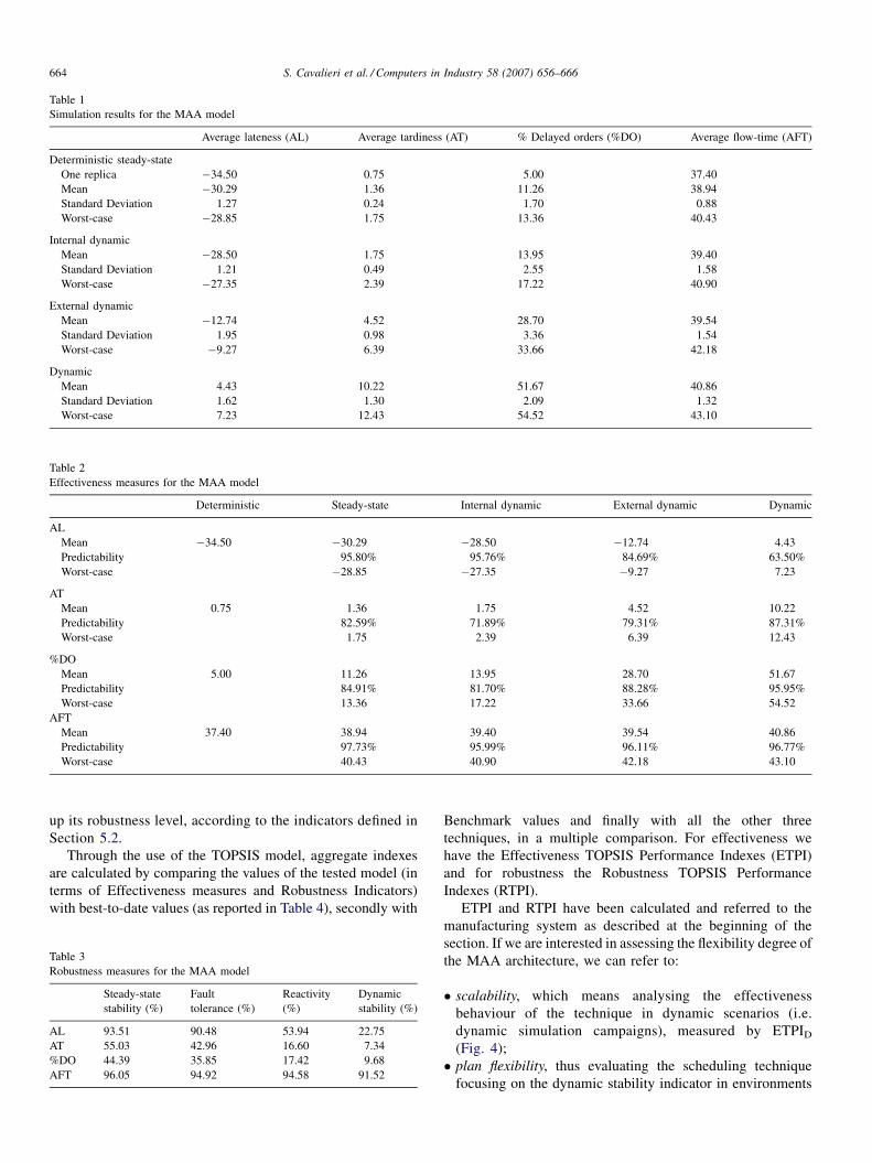
Table 1

Simulation results for the MAA model

Average lateness (AL) Average tardiness (AT) % Delayed orders (%DO) Average flow-time (AFT)

Deterministic steady-state

One replica �34.50 0.75 5.00 37.40

Mean �30.29 1.36 11.26 38.94

Standard Deviation 1.27 0.24 1.70 0.88

Worst-case �28.85 1.75 13.36 40.43

Internal dynamic

Mean �28.50 1.75 13.95 39.40


Worst-case �27.35 2.39 17.22 40.90

External dynamic

Mean �12.74 4.52 28.70 39.54


Worst-case �9.27 6.39 33.66 42.18

Dynamic

Mean 4.43 10.22 51.67 40.86


Worst-case 7.23 12.43 54.52 43.10

Table 2

Effectiveness measures for the MAA model

Deterministic Steady-state Internal dynamic External dynamic Dynamic

AL

Mean �34.50 �30.29 �28.50 �12.74 4.43

Predictability 95.80% 95.76% 84.69% 63.50%

Worst-case �28.85 �27.35 �9.27 7.23

AT

Mean 0.75 1.36 1.75 4.52 10.22

Predictability 82.59% 71.89% 79.31% 87.31%

Worst-case 1.75 2.39 6.39 12.43

%DO

Mean 5.00 11.26 13.95 28.70 51.67

Predictability 84.91% 81.70% 88.28% 95.95%

Worst-case 13.36 17.22 33.66 54.52

AFT

Mean 37.40 38.94 39.40 39.54 40.86

Predictability 97.73% 95.99% 96.11% 96.77%

Worst-case 40.43 40.90 42.18 43.10


up its robustness level, according to the indicators defined in

Section 5.2.

Through the use of the TOPSIS model, aggregate indexes

are calculated by comparing the values of the tested model (in

terms of Effectiveness measures and Robustness Indicators)

with best-to-date values (as reported in Table 4), secondly with

Table 3

Robustness measures for the MAA model

Steady-state

stability (%)

Fault

tolerance (%)

Reactivity

(%)

Dynamic

stability (%)

AL 93.51 90.48 53.94 22.75

AT 55.03 42.96 16.60 7.34

%DO 44.39 35.85 17.42 9.68

AFT 96.05 94.92 94.58 91.52

Benchmark values and finally with all the other three

techniques, in a multiple comparison. For effectiveness we

have the Effectiveness TOPSIS Performance Indexes (ETPI)

and for robustness the Robustness TOPSIS Performance

Indexes (RTPI).

ETPI and RTPI have been calculated and referred to the

manufacturing system as described at the beginning of the

section. If we are interested in assessing the flexibility degree of

the MAA architecture, we can refer to:

� s
calability, which means analysing the effectiveness
behaviour of the technique in dynamic scenarios (i.e.

dynamic simulation campaigns), measured by ETPID

(Fig. 4);

� p
lan flexibility, thus evaluating the scheduling technique
focusing on the dynamic stability indicator in environments

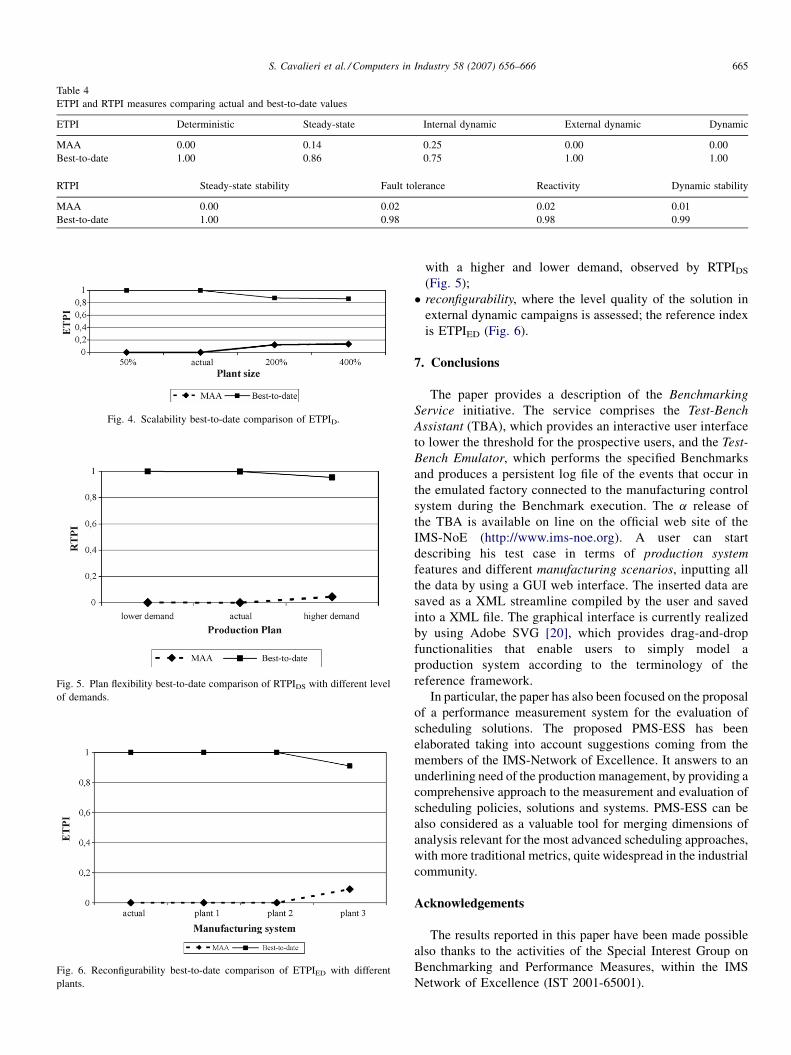
Table 4

ETPI and RTPI measures comparing actual and best-to-date values

ETPI Deterministic Steady-state Internal dynamic External dynamic Dynamic

MAA 0.00 0.14 0.25 0.00 0.00

Best-to-date 1.00 0.86 0.75 1.00 1.00

RTPI Steady-state stability Fault tolerance Reactivity Dynamic stability

MAA 0.00 0.02 0.02 0.01

Best-to-date 1.00 0.98 0.98 0.99

Fig. 4. Scalability best-to-date comparison of ETPID.

Fig. 5. Plan flexibility best-to-date comparison of RTPIDS with different level

of demands.

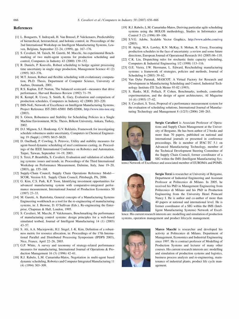
Fig. 6. Reconfigurability best-to-date comparison of ETPIED with different

plants.


with a higher and lower demand, observed by RTPIDS

(Fig. 5);

� r
econfigurability, where the level quality of the solution in
external dynamic campaigns is assessed; the reference index

is ETPIED (Fig. 6).

7. Conclusions

The paper provides a description of the Benchmarking

Service initiative. The service comprises the Test-Bench

Assistant (TBA), which provides an interactive user interface

to lower the threshold for the prospective users, and the Test-

Bench Emulator, which performs the specified Benchmarks

and produces a persistent log file of the events that occur in

the emulated factory connected to the manufacturing control

system during the Benchmark execution. The a release of

the TBA is available on line on the official web site of the

IMS-NoE (http://www.ims-noe.org). A user can start

describing his test case in terms of production system

features and different manufacturing scenarios, inputting all

the data by using a GUI web interface. The inserted data are

saved as a XML streamline compiled by the user and saved

into a XML file. The graphical interface is currently realized

by using Adobe SVG [20], which provides drag-and-drop

functionalities that enable users to simply model a

production system according to the terminology of the

reference framework.

In particular, the paper has also been focused on the proposal

of a performance measurement system for the evaluation of

scheduling solutions. The proposed PMS-ESS has been

elaborated taking into account suggestions coming from the

members of the IMS-Network of Excellence. It answers to an

underlining need of the production management, by providing a

comprehensive approach to the measurement and evaluation of

scheduling policies, solutions and systems. PMS-ESS can be

also considered as a valuable tool for merging dimensions of

analysis relevant for the most advanced scheduling approaches,

with more traditional metrics, quite widespread in the industrial

community.

Acknowledgements

The results reported in this paper have been made possible

also thanks to the activities of the Special Interest Group on

Benchmarking and Performance Measures, within the IMS

Network of Excellence (IST 2001-65001).

http://www.ims-noe.org/


References

[1] L. Bongaerts, Y. Indrayadi, H. Van Brussel, P. Valckenaers, Predictability

of hierarchical, heterarchical, and holonic control, in: Proceedings of the

2nd International Workshop on Intelligent Manufacturing Systems, Leu-

ven, Belgium, September 22–24, (1999), pp. 167–176.

[2] S. Cavalieri, M. Taisch, M. Garetti, M. Macchi, An experimental Bench-

marking of two multi-agent systems for production scheduling and

control, Computers in Industry 43 (2000) 139–152.

[3] R. Daniels, P. Kouvelis, Robust scheduling to hedge against processing

time uncertainty in single stage production, Management Science 41 (2)

(1995) 363–376.

[4] M.T. Jensen, Robust and flexible scheduling with evolutionary computa-

tion, Ph.D. Thesis, Department of Computer Science, University of

Aarhus, Denmark, 2001.

[5] R.S. Kaplan, D.P. Norton, The balanced scorecard—measures that drive

performance, Harvard Business Review (1992) 71–79.

[6] K. Kempf, R. Uzsoy, S. Smith, K. Gary, Evaluation and comparison of

production schedules, Computers in Industry 42 (2000) 203–220.

[7] IMS-NoE, Network of Excellence on Intelligent Manufacturing Systems,

Project Reference IST-2001-65001 IMS-02006, http://www.ims-noe.org

(2003).

[8] S. Goren, Robustness and Stability for Scheduling Policies in a Single

Machine Environment, M.Sc. Thesis, Bilkent University, Ankara, Turkey,

2002.

[9] D.J. Mignon, S.J. Honkomp, G.V. Reklaitis, Framework for investigating

schedule robustness under uncertainty, Computers in Chemical Engineer-

ing 19 (Suppl.) (1995) S615–S620.

[10] D. Ouelhadj, P. Cowling, S. Petrovic, Utility and stability measures for

agent-based dynamic scheduling of steel continuous casting, in: Proceed-

ings of the IEEE International Conference on Robotics and Automation,

Taipei, Taiwan, September 14–19, 2003.

[11] S. Terzi, P. Brambilla, S. Cavalieri, Evaluation and validation of schedul-

ing systems: issues and trends, in: Proceedings of the Third International

Workshop on Performance Measurement, Dalmine, Italy, June 19–20,

(2003), pp. 155–168.

[12] Supply-Chain Council, Supply Chain Operations Reference Model—

SCOR, Version 8.0, Supply Chain Council, Pittsburgh, PA, 2006.

[13] G. Kim, C.S. Park, K.P. Yoon, Identifying investment opportunities for

advanced manufacturing system with comparative-integrated perfor-

mance measurement, International Journal of Production Economics 50

(1997) 23–33.

[14] M. Garetti, A. Bartolotta, General concepts of a Manufacturing Systems

Engineering workbench as a tool for the re-engineering of manufacturing

systems, in: J. Browne, D. O’Sullivan (Eds.), Re-engineering the Enter-

prise, Chapman & Hall, London, 1995.

[15] S. Cavalieri, M. Macchi, P. Valckenaers, Benchmarking the performance

of manufacturing control systems: design principles for a web-based

simulated testbed, Journal of Intelligent Manufacturing 14 (1) (2003)

43–57.

[16] S. Ali, A.A. Maciejewski, H.J. Siegel, J.-K. Kim, Definition of a robust-

ness metric for resource allocation, in: Proceedings of the 17th Interna-

tional Parallel and Distributed Processing Symposium (IPDPS 2003),

Nice, France, April 22–26, 2003.

[17] G.P. White, A survey and taxonomy of strategy-related performance

measures for manufacturing, International Journal of Operations & Pro-

duction Management 16 (3) (1996) 42–61.

[18] R.J. Rabelo, L.M. Camarinha-Matos, Negotiation in multi-agent based

dynamic scheduling, Robotics and Computer Integrated Manufacturing 11

(4) (1994) 303–309.

[19] R.J. Rabelo, L.M. Camarinha-Matos, Deriving particular agile scheduling

systems using the HOLOS methodology, Studies in Informatics and

Control 5 (2) (1996) 89–106.

[20] S.V.G. Adobe, Scalable Vector Graphics, http://www.adobe.com/svg

(2003).

[21] H. Aytug, M.A. Lawley, K.N. McKay, S. Mohan, R. Uzsoy, Executing

production schedules in the face of uncertainty: a review and some future

directions, European Journal of Operational Research 161 (2005) 86–110.

[22] C.K. Liu, Dispatching rules for stochastic finite capacity scheduling,

Computers & Industrial Engineering 1/2 (1998) 113–116.

[23] G.E. Vieira, J.W. Herrmann, L. Edward, Rescheduling manufacturing

systems: a framework of strategies, policies and methods, Journal of

Scheduling 6 (2003) 39–62.

[24] Van Dyke Parunak, MASCOT: A Virtual Factory for Research and

Development in Manufacturing Scheduling and Control, Industrial Tech-

nology Institute-ITI Tech Memo 93-02 (1993).

[25] S. Hanks, M.E. Pollack, P. Cohen, Benchmarks, testbeds, controlled

experimentation, and the design of agent architectures, AI Magazine

14 (4) (1993) 17–42.

[26] S. Cavalieri, S. Terzi, Proposal of a performance measurement system for

the evaluation of scheduling solutions, International Journal of Manufac-

turing Technology and Management 8 (1/2/3) (2006) 248–263.

Sergio Cavalieri is Associate Professor of Opera-

tions and Supply Chain Management at the Univer-

sity of Bergamo. He has been author of 2 books and

more than 70 papers, published on national and

international journals or presented in conference

proceedings. He is member of IFAC-TC 5.1 on

Advanced Manufacturing Technology, member of

the Technical Development Steering Committee of

the Supply Chain Council, former coordinator of a

SIG within the IMS (Intelligent Manufacturing Sys-

tems) Network of Excellence and associated member of EUROMA and POMS.

Sergio Terzi is researcher at University of Bergamo,

Department of Industrial Engineering and Assistant

Professor at Politecnico di Milano. In 2005, he

received his PhD in Management Engineering from

Politecnico di Milano and his PhD in Production

Engineering from the University Henri Poincare

Nancy I. He is author and co-author of more than

40 papers at national and international level. He is

former coordinator of a SIG within the IMS (Intel-

ligent Manufacturing Systems) Network of Excel-

lence. His current research interests are: modelling and simulation of production

systems, operation management and product lifecycle management.

Marco Macchi is researcher and developed his

activity at Politecnico di Milano, Department of

Management, Economics and Industrial Engineering

since 1997. He is contract professor of Modelling of

Production Systems and lecturer of many other

courses. His current research interests are: modelling

and simulation of production systems and logistics,

business process analysis and re-engineering, main-

tenance of industrial plants, product life cycle man-

agement.

http://www.ims-noe.org/

http://www.adobe.com/svg

a benchmarking service for the evaluation and comparison of scheduling techniques

Documents