benchmarking and industry performance
TRANSCRIPT

Benchmarking and Industry Performance
Thijs ten Raa�
June 2009
Abstract
Benchmarking is formalized by a linear program that determines the
e¢ ciency of a �rm relative to its peers and is used to determine the e¢ -
ciency of an industry. The overall e¢ ciency is shown to be underestimated
by mean �rm e¢ ciency and the bias is zero if and only if the �rm shadow
prices of the inputs and outputs generated by the benchmarking programs
are equal across �rms. Otherwise the bias provides an e¢ ciency measure
for the organization of the industry.
A main contribution of this paper is the interrelation of productivity
analysis and the theory of industrial organization. A proposition proves
that an industrial organization is e¢ cient in the sense of productivity
�Department of Econometrics and Operations Research, Tilburg University, P.O. Box
90153, 5000 LE Tilburg, The Netherlands. Phone: +31-13-4662365; fax: +31-13-4663280;
e-mail: [email protected]. I am grateful to Thanh Le Phuoc for good research assistance,
William Weber for making his data set available, Shawna Grosskopf and Sverre Kittelsen for
literature references, and Knox Lovell for telling me to analyze entry and exit.
1

analysis if and only if it is supportable in the entry-proofness sense of
Sharkey and Telser (1978).
The known decomposition of performance in e¢ ciency change and
technical change is augmented with a term for the industrial organization
e¢ ciency change. The performance measure is shown to be consistent
with the Solow residual and Malmquist indices for its components are
given. An analysis of the Japanese banking industry illustrates and the
dynamic e¤ects of entry and exit can be accommodated.
JEL Classi�cation Numbers: L10, D24, O47
Keywords: Scope (dis)economies, Industrial Organization, E¢ ciency,
Aggregation, Productivity
2

1 Introduction
The theory of benchmarking can be traced back to Farrell (1957) and an easy
introduction is given in Diewert�s (2005) tutorial. The present, formal devel-
opment connects benchmarking to the measurement of industrial organization
(in)e¢ ciencies and to economic performance measures. I de�ne benchmark-
ing through a function that maps two arguments, namely the object to be
benchmarked�a �rm�and the backdrop against which it is benchmarked�the
industry�into a scalar, namely the e¢ ciency of the �rm. However simplistic,
a �rm can be represented by the pair of its input vector and its output vector.
The mapping summarizes a program that determines how much more output
the �rm could produce with its inputs if it would reallocate them to the activi-
ties implicit in the other �rms. The output maximizing reallocation identi�es
the best practice technologies or benchmarks for the �rm under consideration
and the inverse of the output expansion de�nes its e¢ ciency.
The performance of a �rm will be measured by its output/input ratio or
productivity�a concept that I will connect explicitly to the aforementioned ef-
�ciency function. This performance measure may be increased by e¢ ciency
change or technical change. The �rst element re�ects a relative movement of a
�rm in the direction of the best practice frontier while the latter element rep-
resents a shift of the frontier. Aggregate performance may rise more than �rm
performance scores suggest, if resources are better allocated between �rms. The
latter component is the industrial organization e¤ect and this paper quanti�es
it.
3

Debreu (1951) recognized imperfections in economic organization as a source
of aggregate ine¢ ciency and Diewert (1983) analyzed them for open economies,
focussing on price distortions. I operationalize these ideas, without using ex-
ternal price information (such as the world prices an open economy faces). In
discrete time the operationalization will be expressed in terms of Malmquist
indices, which are discrete time variants of productivity growth measures. An-
other novelty is that my theory of benchmarking extends my interrelationship
of two value-based performance measures, namely Diewert�s (1993) price in-
dex measurement and Solow�s (1957) residual analysis, from the back-of-the-
envelope calculation for production functions (ten Raa, 2005) to the activity
framework.
If relatively productive �rms grow relatively fast, the industry will im-
prove its performance, even when no �rm exhibits technical change or e¢ ciency
change. The insight is closely related to shift-share or (de)composition analy-
sis (Denny, Fuss, Waverman ,1981 and Balk, 2003). For example, aggregating
industry productivities to total productivity growth, Wol¤�s (1985, formula 23)
decomposition analysis includes a composition e¤ect, and Jorgenson, Ho, and
Stiroh (2003, formula 53) capture allocative e¢ ciency changes. Yet there is
more to the performance of a composite such as an industry than micro or �rm
performance and composition e¤ects. While this decomposition seems clear
at the micro level and has been applied to the macro level (Färe et al., 1994),
Blackorby and Russell (1999) and Briec, Dervaux and Leleu (2003) have shown
that things do not add up except under restrictive conditions. Bartelsman
4

and Doms� (2000, p. 571) understanding that "Aggregated productivity can
be computed as the share-weighted average of individual productivity" is not
exactly right. The �rst proposition of this paper will show that aggregated
performance is less. There is a bias (ten Raa, 2005) and I will show that it
re�ects the industrial organization or, more precisely, the departure from an
optimal organization. In a framework for the measurement of all performance
components�technical change, e¢ ciency change and industrial organization�I
consolidate price and non-price based approaches, combining insights of com-
position analysis (which is neutral with respect to optimality issues) and of
benchmarking (which is all about optimality but bears little on composition
e¤ects).
A main contribution of this paper is the interrelation of productivity analysis
and the theory of industrial organization. A proposition proves that an indus-
trial organization is e¢ cient (in the sense of productivity analysis) if and only
if it is supportable in Sharkey and Telser�s (1978) sense of being entry-proof.
The e¢ ciency/productivity literature boasts di¤erent econometric techniques
and many econometricians feel strong about this. Roughly speaking the trade-
o¤ is between functional form limitations and robustness. In this theoretical
paper, robustness is no issue however and it would be limiting and distracting
to establish my propositions in a functional form framework. The exercise is
one similar to Data Envelopment Analysis which is not robust�although there is
recent bootstrapping work that e¤ectively addresses the defect (Simar and Wil-
son, 2007)�but a functional form framework is less suitable for this theoretical
5

paper.
The organization of the paper is as follows. The linear program is analyzed
in section 2. Exploiting duality theory, I show that benchmarking is consistent
with the price index approach to performance measurement. Much insight is
gained by benchmarking not a �rm but the entire industry. Section 3 uses
the aggregation bias to measure the ine¢ ciency of the industry. It relates this
normative e¢ ciency concept with the positive concept of supportability. Section
4 traces time changes of e¢ ciency through both the object to be benchmarked
and the reference benchmark, showing that the former transmits productivity
growth and the latter technical change. Exploiting duality theory once more, I
show that this dynamic benchmarking is consistent with the growth accounting
concept of the Solow residual. Discrete time approximations are presented
in section 5, including the industrial organization e¤ect. Section 6 applies
the theory to measure the evolution of the industrial organization of Japanese
banking. Section 7 shows how the basic model can be modi�ed to accommodate
entry and exit of �rms and other departures. Section 8 concludes.
6

2 Benchmarking: price analysis
Denote �rm i�s input vector by xi and its output vector by yi, i = 1; :::; I.1
Input vectors have a common dimension, output vectors have a common dimen-
sion, and these two dimensions may di¤er. For example, inputs can be labor,
capital, and land, while outputs may be numerous goods and services. Some
commodities can be both input and output. However simplistic, an industrial
organization can be represented by the allocation (xi; yi)i=1;:::;I , which is de-
noted brie�y by (x; y). If I = 1, the industrial organization is a monopoly;
if I = 2, it is a duopoly. If y is a diagonal matrix, we have monopolistic
competition. If x is a row vector, we have an input price taking industry, for
which inputs can be aggregated to �cost.� The e¢ ciency of a �rm is determined
by benchmarking its structure (xi; yi) against the industrial organization (x; y).
This is a comparison between the actual output level and the best practice
output level achievable with the available input vector, just as Farrell�s (1957)
productive e¢ ciency measurement technique and Shephard�s (1970) output dis-
tance function. The idea is to reallocate the input, xi, over all the activities
j = 1; :::; I, and to run the latter with intensities �j , as to in�ate the output, yi,
by an expansion factor 1=":
1All I need are �rms� input and output data. This simplicity has a price: I miss perfor-
mance failures on the demand side. However, a theoretical underpinning of this supply side
approach is given in ten Raa (2008), where it is demonstrated that my supply side e¢ ciency
measure is conservative (in the sense of underestimating full ine¢ ciency) and sharp (attained
by certain demand functions).
7
max";�j�0
1=" :X
�jxj � xi; yi=" �
X�jy
j (1)
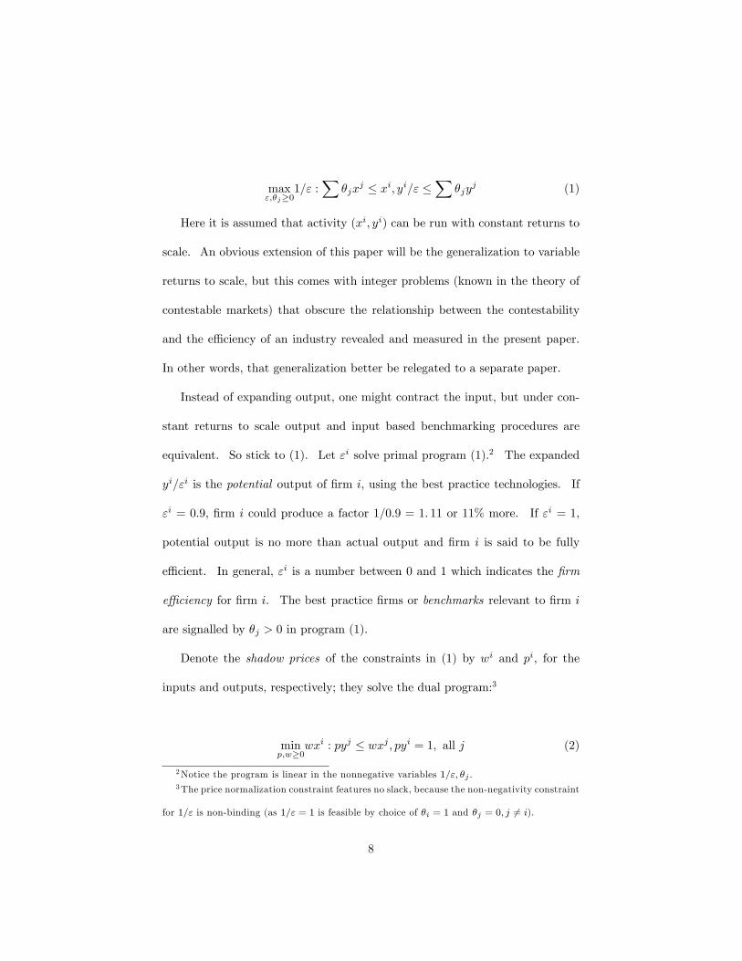
Here it is assumed that activity (xi; yi) can be run with constant returns to
scale. An obvious extension of this paper will be the generalization to variable
returns to scale, but this comes with integer problems (known in the theory of
contestable markets) that obscure the relationship between the contestability
and the e¢ ciency of an industry revealed and measured in the present paper.
In other words, that generalization better be relegated to a separate paper.
Instead of expanding output, one might contract the input, but under con-
stant returns to scale output and input based benchmarking procedures are
equivalent. So stick to (1). Let "i solve primal program (1).2 The expanded
yi="i is the potential output of �rm i, using the best practice technologies. If
"i = 0:9, �rm i could produce a factor 1=0:9 = 1: 11 or 11% more. If "i = 1,
potential output is no more than actual output and �rm i is said to be fully
e¢ cient. In general, "i is a number between 0 and 1 which indicates the �rm
e¢ ciency for �rm i. The best practice �rms or benchmarks relevant to �rm i
are signalled by �j > 0 in program (1).
Denote the shadow prices of the constraints in (1) by wi and pi, for the
inputs and outputs, respectively; they solve the dual program:3
minp;w�0
wxi : pyj � wxj ; pyi = 1; all j (2)
2Notice the program is linear in the nonnegative variables 1="; �j .3The price normalization constraint features no slack, because the non-negativity constraint
for 1=" is non-binding (as 1=" = 1 is feasible by choice of �i = 1 and �j = 0; j 6= i).
8
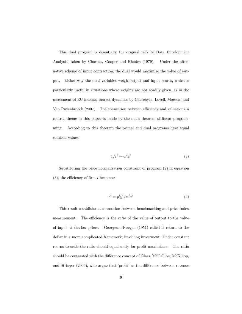
This dual program is essentially the original tack to Data Envelopment
Analysis, taken by Charnes, Cooper and Rhodes (1979). Under the alter-
native scheme of input contraction, the dual would maximize the value of out-
put. Either way the dual variables weigh output and input scores, which is
particularly useful in situations where weights are not readily given, as in the
assessment of EU internal market dynamics by Cherchyea, Lovell, Moesen, and
Van Puyenbroeck (2007). The connection between e¢ ciency and valuations�a
central theme in this paper�is made by the main theorem of linear program-
ming. According to this theorem the primal and dual programs have equal
solution values:
1="i = wixi (3)
Substituting the price normalization constraint of program (2) in equation
(3), the e¢ ciency of �rm i becomes:
"i = piyi=wixi (4)
This result establishes a connection between benchmarking and price index
measurement. The e¢ ciency is the ratio of the value of output to the value
of input at shadow prices. Georgescu-Roegen (1951) called it return to the
dollar in a more complicated framework, involving investment. Under constant
reurns to scale the ratio should equal unity for pro�t maximizers. The ratio
should be contrasted with the di¤erence concept of Glass, McCallion, McKillop,
and Stringer (2006), who argue that �pro�t�as the di¤erence between revenue
9
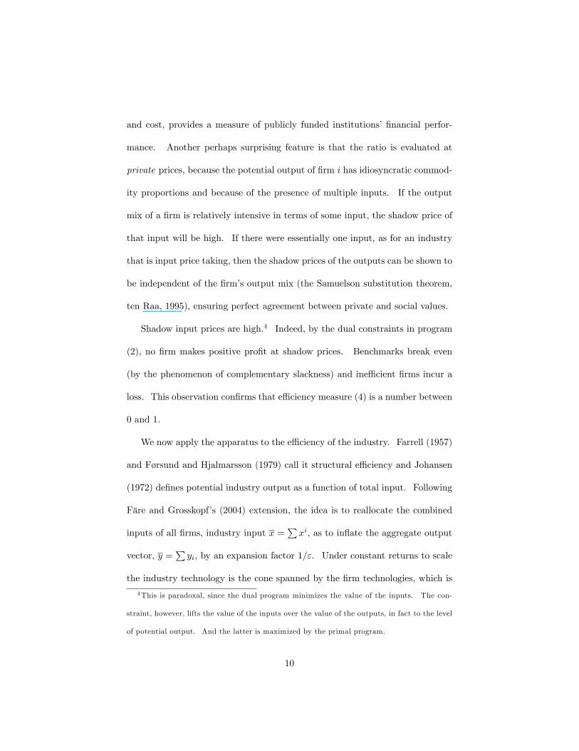
and cost, provides a measure of publicly funded institutions��nancial perfor-
mance. Another perhaps surprising feature is that the ratio is evaluated at
private prices, because the potential output of �rm i has idiosyncratic commod-
ity proportions and because of the presence of multiple inputs. If the output
mix of a �rm is relatively intensive in terms of some input, the shadow price of
that input will be high. If there were essentially one input, as for an industry
that is input price taking, then the shadow prices of the outputs can be shown to
be independent of the �rm�s output mix (the Samuelson substitution theorem,
ten Raa, 1995), ensuring perfect agreement between private and social values.
Shadow input prices are high.4 Indeed, by the dual constraints in program
(2), no �rm makes positive pro�t at shadow prices. Benchmarks break even
(by the phenomenon of complementary slackness) and ine¢ cient �rms incur a
loss. This observation con�rms that e¢ ciency measure (4) is a number between
0 and 1.
We now apply the apparatus to the e¢ ciency of the industry. Farrell (1957)
and Førsund and Hjalmarsson (1979) call it structural e¢ ciency and Johansen
(1972) de�nes potential industry output as a function of total input. Following
Färe and Grosskopf�s (2004) extension, the idea is to reallocate the combined
inputs of all �rms, industry input x =Pxi, as to in�ate the aggregate output
vector, y =Pyi, by an expansion factor 1=". Under constant returns to scale
the industry technology is the cone spanned by the �rm technologies, which is
4This is paradoxal, since the dual program minimizes the value of the inputs. The con-
straint, however, lifts the value of the inputs over the value of the outputs, in fact to the level
of potential output. And the latter is maximized by the primal program.
10

the same technology as the reference technology in the �rm e¢ ciency program
(1). The only modi�cation to the latter is, therefore, the replacement of �rm
resources and output target by industry resources x and output target y:
max";�j�0
1=" :X
�jxj � x; y=" �
X�jy
j (5)
Let " solve program (5). It is a number between 0 and 1 which indicates
the industry e¢ ciency. The best practice �rms or benchmarks relevant to the
industry are signalled by �j > 0 in program (5). Denote the shadow prices of the
constraints in program (5) by w and p, for the inputs and outputs, respectively;
these industry prices solve the dual program:
minp;w�0
wx : pyj � wxj ; py = 1; all j (6)
Analogous to equation (3), potential output increases by the following factor:
1=" = wx (7)
Analogous to equation (4), industry e¢ ciency becomes:5
" = py=wx (8)
Again, the e¢ ciency is the ratio of the value of output to the value of input.
5Since prices are in the numerator and the denominator of formula (8), the price normal-
ization in (6) is a wash.
11

3 Industrial organization: an e¢ ciency measure
Proposition 1 establishes a one-sided relationship between the e¢ ciencies of the
�rms and the e¢ ciency of the industry. The gap in the relationship will be
used to quantify the e¢ ciency of the industrial organization.
Proposition 1. Industry e¢ ciency is less than the market share weighted
harmonic mean of the �rm e¢ ciencies: " � 1=P
si
"i , where si = pyi=py are the
market shares evaluated at the prices determined by dual program (6).
Proof. In the dual program (2), consider the socially optimal prices p=pyi
and w=pyi (which need not be privately optimal). The denominator has been
chosen as to ful�l the price normalization constraint in program (2) and the
inequality constraint carries over from program (6). In short, these prices are
feasible with respect to program (2). But by their suboptimality (in this pri-
vate minimization program), (w=pyi)xi � wixi or wxi � pyiwixi = pyi="i,
using equation (3). Summing and invoking equation (7) and the price normal-
ization constraint of (6), we obtain 1=" = wx = wPxi �
Ppyi="i =
Psi="i.
Inverting, industry e¢ ciency becomes " � 1=P
si
"i . Q.E.D.
The next proposition shows that the gap is zero if and only if the private
prices of the �rms coincide. The su¢ ciency part is reminiscent of Koopmans
(1957) result that the industry pro�t function equals the sum of the �rm pro�t
12
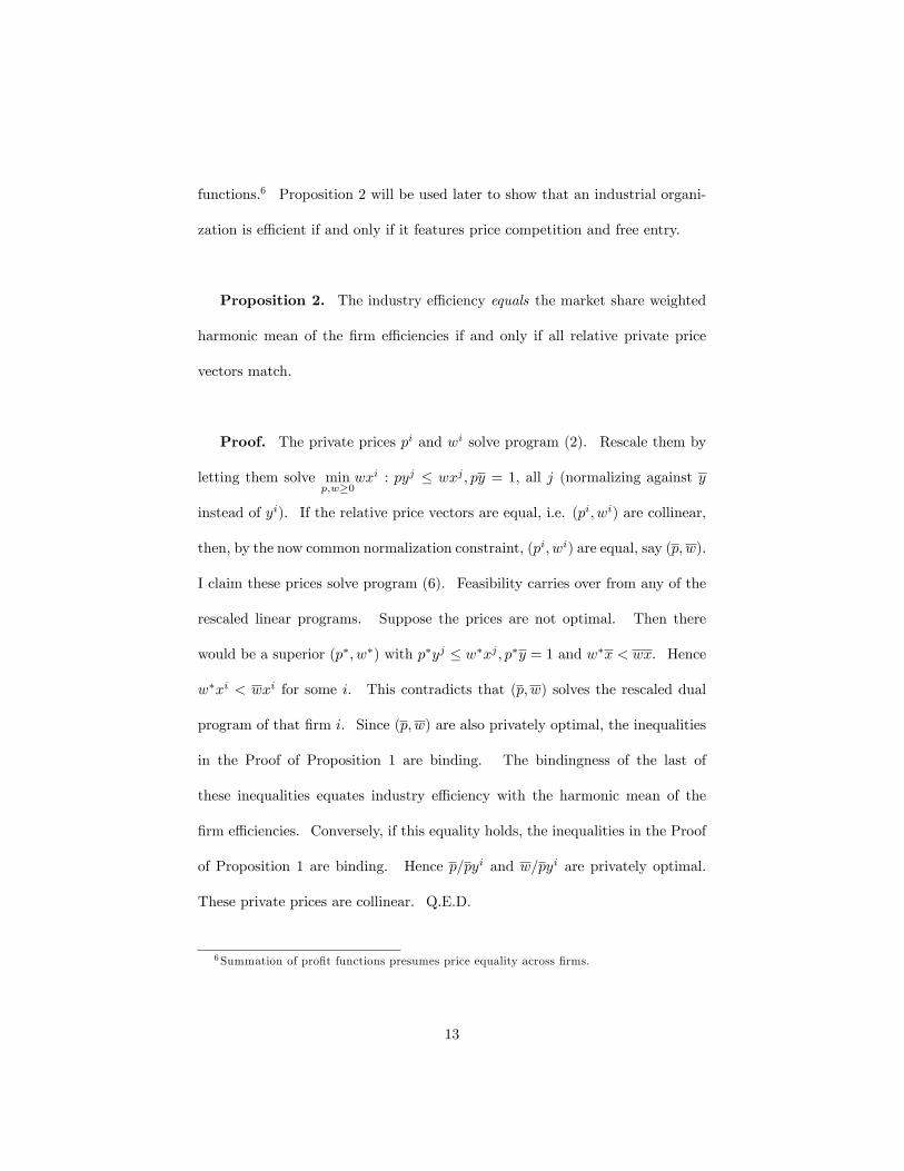
functions.6 Proposition 2 will be used later to show that an industrial organi-
zation is e¢ cient if and only if it features price competition and free entry.
Proposition 2. The industry e¢ ciency equals the market share weighted
harmonic mean of the �rm e¢ ciencies if and only if all relative private price
vectors match.
Proof. The private prices pi and wi solve program (2). Rescale them by
letting them solve minp;w�0
wxi : pyj � wxj ; py = 1; all j (normalizing against y
instead of yi). If the relative price vectors are equal, i.e. (pi; wi) are collinear,
then, by the now common normalization constraint, (pi; wi) are equal, say (p; w).
I claim these prices solve program (6). Feasibility carries over from any of the
rescaled linear programs. Suppose the prices are not optimal. Then there
would be a superior (p�; w�) with p�yj � w�xj ; p�y = 1 and w�x < wx. Hence
w�xi < wxi for some i. This contradicts that (p; w) solves the rescaled dual
program of that �rm i. Since (p; w) are also privately optimal, the inequalities
in the Proof of Proposition 1 are binding. The bindingness of the last of
these inequalities equates industry e¢ ciency with the harmonic mean of the
�rm e¢ ciencies. Conversely, if this equality holds, the inequalities in the Proof
of Proposition 1 are binding. Hence p=pyi and w=pyi are privately optimal.
These private prices are collinear. Q.E.D.
6Summation of pro�t functions presumes price equality across �rms.
13

The reason that industry e¢ ciency is less than mean �rm e¢ ciency is that
the industrial organization is suboptimal. It is a form of allocative ine¢ ciency.
Firms better be split or merged, specialize or diversify. The optimal industrial
organization is determined by the benchmarks in program (5). Suboptimality
is signalled by a distortion between private and social prices (Proposition 2).
The e¢ ciency of the industrial organization can thus be measured by the ratio
of the industry e¢ ciency to the mean �rm e¢ ciency, or, using Proposition 1:
De�nition 1. The e¢ ciency of an industrial organization, (x; y), equals
"IO = "Psi="i, where si are the market shares evaluated at the prices deter-
mined by dual program (6).
Notice that by Proposition 1 the e¢ ciency of an industrial organization is
a number between 0 and 1, with the latter value representing full e¢ ciency
according to Proposition 2.
Examples. 1. Consider an industry with equally e¢ cient �rms: "i = ".
Then by Proposition 1, " � 1=P
si
"i = ". Hence industry e¢ ciency is less than
�rm e¢ ciency. The e¢ ciency of the industrial organization is "IO = "=".
2. Consider an industry that produces a single good from labor and capital.
Three �rms each produce one unit of output. Firm 1 uses just one unit of labor,
�rm 2 uses just one unit of capital, and �rm 3 uses 1/3 units of both inputs.
Since �rm 1 has labor only, the technologies of �rms 2 and 3 (which employ
14

capital) are of no use. There is no potential increase of its output. The same
conclusion holds for �rm 2. Firm 3 could reallocate its labor and capital to the
technologies employed by �rms 1 and 2, respectively, but its output would go
down from 1 to 2/3. Hence no �rm has scope for an increase in output. All
potential outputs are equal to the observed outputs and, therefore, all �rms are
100% e¢ cient. The industry, however, is not e¢ cient. If �rms 1 and 2 would
merge and adopt the technology of �rm 3, the new �rm would be three times as
big as �rm 3, hence produce three units of output, which is one more than they
produce using their own technologies. Potential output is four units (instead of
three), so that the expansion factor is 4/3 and, therefore, the industry e¢ ciency
is 3/4 or only 75%. The e¢ ciency of the industrial organization is 75/100 =
0.75 or 75%. The industry would do better if the two specialized �rms would
merge.
3. It is straightforward to construct an example where the industry would
do better if a �rm were split: Simply substitute diseconomies of scope for the
economies of scope in Example 2, by letting �rm 3 use 2/3 units of both inputs
(instead of the 1/3 in Example 2).
4. Add a fourth �rm to Example 2, with the same inputs as �rm 3, but
only 1/2 a unit of output. Clearly, �rm 4 could produce a full unit of output
(adopting the technology of �rm 3). Its e¢ ciency is 50%. In the present
example, the outputs are 1, 1, 1, 0.5. The market shares are 2/7, 2/7, 2/7,
1/7. The �rm e¢ ciencies are 100%, 100%, 100%, 50%. The harmonic mean is
1=Psi="i = 1=( 2=71:00 +
2=71:00 +
2=71:00 +
1=70:50 ) or 87.5% . For the industry potential
15

output is three for �rms 1 and 2 jointly (see Example 2) and one for �rms 3 and
4 each, hence �ve in total (instead of three and a half), so that the expansion
factor is 5/3.5 and, therefore, the industry e¢ ciency is 3.5/5 or only 70%. The
e¢ ciency of the industrial organization is 70/87.5 = 0.8 or 80%.
An immediate consequence of De�nition 1 is the following.
Proposition 3. Industry e¢ ciency is the product of (market share weighted
harmonic) mean �rm e¢ ciency and the e¢ ciency of the industrial organization.
Proposition 3 will enable us to re�ne the decomposition of productivity
growth in technical change and e¢ ciency change in the next section, but �rst I
make an observation on the connection between the e¢ ciency and the support-
ability of an industrial organization in a contestable market.
In a contestable market, a potential entrant can tap the incumbents�technol-
ogy and the entry costs are zero; see Baumol, Panzar and Willig (1982). Their
solution concept is that of a sustainable industrial organization. The de�nition
of sustainability involves demand conditions, but a simple, necessary condition
is Sharkey and Telser�s (1978) supportability, and that is all I need.7
7Students of the history of economic thought recognize this as another instance where
the returns to scale (which are implicitly constant in benchmarking) determine if values are
determined by the supply side or in interaction with the demand side: the classical and
neo-classical points of view.
16

De�nition 2. An industrial organization (xi; yi)i=1;:::;I is supportable by
price vector (p; w) if the latter renders every incumbent �rm pro�table (wxi �
pyi), but any potential entrant unpro�table (P�jx
j � xe; ye �P�jy
j ; �j �
0) wxe � pye).
The next result connects the benchmark industrial organization involving
price competition plus free entry with e¢ cient outcomes. In fact, Proposition
4 articulates the Baumol and Fischer (1978, p. 461) intuition that "it would
be highly surprising if there were not a rough correspondence between the most
economical market form and what actually occurs" and extends Baumol, Panzar
and Willig�s (1982) proposition that in a sustainable industry con�guration total
industry cost must be minimized.
Proposition 4. An industrial organization is supportable if and only if it
is fully e¢ cient and comprises fully e¢ cient �rms.
Proof. Let me �rst prove the only if part, which is known, at least for given
input prices. So let the industrial organization be supportable by (p; w). I claim
that the normalized supporting prices p=pyi and w=pyisolve the dual program
of an incumbent �rm, (2). For this purpose, take �j = 1 and �k = 0; k 6= j in
De�nition 2. Then xj � xe; ye � yj ) wxe � pye. In particular, wxj � pyj .
(In fact, the inequality is binding by the �rst condition in De�nition 2.) This
shows that the �rst constraint in (2) is met. The second constraint is met by
17

the normalization by pyi. The value of the objective function in (2) must be
at least wxi � pyi according to the �rst constraint in (2) with j = i. By the
�rst condition in De�nition 2 this lower bound pyi is not exceeded by wxi of
De�nition 2, which renders the latter optimal in (2).
By equation (4), �rm i is fully e¢ cient. Moreover, since the relative prices
solving dual program (2) are common to all incumbent �rms, Proposition 2
applies and the industry e¢ ciency is also 1. Substituting these �ndings in
De�nition 1, it follows that the industrial organization must be fully e¢ cient.
To prove the converse, consider a fully e¢ cient industrial organization com-
prising fully e¢ cient �rms. By Proposition 2, there is a common price vector
(p; w) such that p=pyi and w=pyi are privately optimal. I claim that (p; w) sup-
ports the industrial organization. By equation (4), wxi = pyi. LetP�jx
j � xe
and ye �P�jy
j ; �j � 0. Then wxe � wP�jx
j � pP�jy
j � pye, where the
middle inequality holds term by term in view of the constraints in program (2)
that characterizes the privately optimal prices. Q.E.D.
4 Productivity growth: the recovery of the Solow
residual
Extending ten Raa�s (2005) back-of-the-envelope calculation for production func-
tions, I will now connect the present activity framework with neoclassical growth
accounting, particularly the Solow (1957) residual. This residual is the di¤er-
18
ence between the output and input growth rates and measures technical change
in a competitive environment. Both growth rates are share-weighted expres-
sions, using competitive valuations. In a noncompetitive environment the resid-
ual also captures e¢ ciency change. Since the latter concept is de�ned by the
benchmarking program (1), which features no prices, a little work has to be done
to make the connection. Introduce time by subscripting inputs and outputs,
as well as the derived constructs, using the symbol t. Firm i has input and
output vectors xit and yit, i = 1; :::; I. By benchmarking, yit="
it is derived, the
potential output of �rm i. Its e¢ ciency is indicated by "it, a number between
0 and 1. As a percentage, e¢ ciency change is:
ECit =d
dt"it="
it (9)
To bring in the technical change component of productivity growth, con-
sider two polar cases. First, if the production possibilities of the industry
remain constant, but �rm i improves its output/input ratio (or productivity),
approaching the production possibility frontier, the better internal organization
yields positive e¢ ciency change, while technical change is zero. Second, if �rm i
has a constant output/input ratio, but the production possibility frontier of the
industry shifts out, the better external organization implies negative e¢ ciency
change for the �rm. In this case e¢ ciency change and technical change cancel
and the �rm has zero productivity growth. In either case, e¢ ciency change and
technical change sum to the �rm�s productivity growth:
19

PGit = ECit + TC
it (10)
At this junction equation (10) is intuitive. E¢ ciency change has been
de�ned, in equation (9), but technical change and productivity growth not yet
and the equation must be demonstrated. Technical change manifests itself as a
shift of the production possibility frontier. At each point of time, the frontier
is determined by the industrial organization (xt; yt). The e¢ ciency of �rm i
is determined by program (1). Its input-output pair, (xit; yit), is benchmarked
against (xt; yt). Formally, program (1) determines the e¢ ciency of �rm i as a
function of (xit; yit) and (xt; yt). Hence we may write "it = e((xit; y
it); (xt; yt)),
where mapping e summarizes the e¢ ciency program. Now the program that
determines the e¢ ciency of the industry, (5), has precisely the same structure as
that for the �rms (the only di¤erence is that the pair of total input and output
vectors replace the role of a �rm�s pair), hence the same mapping e governs
the relationship between the data and industry e¢ ciency. The only di¤erence
is that it benchmarks the industry input-output pair, (xt; yt). Consequently,
program (5) may be written as "t = e((xt; yt); (xt; yt)), with the same mapping
e. Mapping e has two arguments, the input-output pair that is benchmarked,
(xit; yit) in case of the �rm, and the industry constellation that determines the
frontier, (xt; yt). The structure of program (1) or (5) is independent of time,
so that time does not enter the function as a separate argument. Denote the
20
two partial derivatives of the mapping by e1 and e2.8 By total di¤erentiation,
the e¢ ciency change of �rm i is:
dedt ((x
it; y
it); (xt; yt))=e((x
it; y
it); (xt; yt))
= e1((xit; y
it); (xt; yt))
ddt (x
it; y
it)=e((x
it; y
it); (xt; yt))
+ e2((xit; yit); (xt; yt))
ddt (xt; yt)=e((x
it; y
it); (xt; yt))
(11)
The measurement of technical change is subtle. If �rm i stays put�(xit; yit) =
constant�but potential output increases, there must be technical progress. Now
an increase in potential output, 1="it, is equivalent to a decrease in e¢ ciency, "it.
Hence a negative second partial derivative�which captures the external e¤ect�
indicates technical progress. Indeed, if a �rm is �xed, but it becomes less
e¢ cient, it must be that the benchmarks have moved out. In short, technical
change is measured by:
TCit = �e2((xit; yit); (xt; yt))d
dt(xt; yt)=e((x
it; y
it); (xt; yt)) (12)
Finally, productivity growth of �rm i ought to be de�ned irrespective the
shift of the production possibility frontier. Productivity growth is de�ned by
the e¤ect of its own inputs and outputs on the e¢ ciency performance of the
�rm:
PGit = e1((xit; y
it); (xt; yt))
d
dt(xit; y
it)=e((x
it; y
it); (xt; yt)) (13)
8Both are row vectors, because either argument has a number of components: the number
of commodities and the I-fold of the number of commodities, respectively. The partial
derivatives capture the shadow prices, as revealed by the ensuing analysis.
21

The internal versus external approaches to the concepts of productivity
growth and technical change, respectively, is consistent with Solow�s (1957)
residual of �rm i, which is de�ned by pitddty
it=p
ityit � wit ddtx
it=w
itxit. The reason
is that our partial derivatives of the e¢ ciency function involves the pricing of
input and output changes according to the marginal products of the �rm. More
precisely, Proposition 5 proves that expression (13) equals the Solow residual.
It completes the connect between the benchmarking and neoclassical approaches
to productivity.
Proposition 5. Productivity growth is measured by the Solow residual:
PGit = pitddty
it=p
ityit � wit ddtx
it=w
itxit.
Proof. The proof is by duality analysis. Mapping e�s �rst (sub)argument,
xit, lists the bound in program (1). The partial derivative of the objective value,
1="it, with respect to this bound is the shadow price wit. By the chain rule,
�1"i2t
@"it@xit
= wit. Mapping e�s next (sub)argument, yit, is a coe¢ cient in program
(1). Setting up the Lagrangian function and application of the envelop theorem
yields that the partial derivative of the objective value, 1="it, with respect to
coe¢ cient yit is �pit(1="it) . By the chain rule, �1"i2t
@"it@yit
= �pit(1="it). Substi-
tuting these in expression (13), we obtain PGit = (�wit"i2t ; pit"it) ddt (xit; y
it)="
it =
(pitddty
it� "itw
itddtx
it)=p
ityit = p
itddty
it=p
ityit � wit ddtx
it=w
itxit, by the price normaliza-
tion constraint of program (2) and equation (4). Q.E.D.
22
Summarizing, e¢ ciency change is de�ned by (9), technical change by (12),
productivity growth by (13), and the former two sum to the latter by equation
(11), which con�rms our intuitive equation (10).
Things look only slightly di¤erent at the level of the industry. Now in-
dustry input and output, (xt; yt), are benchmarked against the frontier. The
productivity growth of the industry is:
PGt = e1((xt; yt); (xt; yt))d
dt(xt; yt)=e((xt; yt); (xt; yt)) (14)
This expression is basically a summation of the �rm productivity growth
rates, (13), with the modi�cation that private shadow prices have been replaced
by social values. This di¤erence constitutes precisely the aggregation bias un-
covered by ten Raa (2005). The same di¤erence between private and social
valuations causes a bias in the aggregation of technical change, (12), but here it
is a minor phenomenon, speci�c to the nonparametric approach. Consequently,
the productivity aggregation bias is basically equal to the e¢ ciency aggregation
bias, or, invoking Proposition 3, the industrial organization e¤ect. The next sec-
tion will explain the role of industrial organization in the performance measure
of productivity.
23

5 Malmquist indices
In discrete time a fascinating thought construct is to benchmark a �rm against
the industry at a di¤erent period. One may hope that the e¢ ciency of a �rm
benchmarked against the industry in the next period, e((xit; yit); (xt+1; yt+1)),
is low. The basic idea of the Malmquist productivity index is to trace �rm i
from period t to t+1 and to measure the change in e¢ ciency relative to a �xed
benchmark. For example, benchmarking against the second period yields
e((xit+1; yit+1); (xt+1; yt+1))�e((xit; yit); (xt+1; yt+1)). This di¤erence expres-
sion is a discrete time version of the numerator of productivity growth expression
(13). E¢ ciency change contributes to the �rst term and technical change to
the second term. The discrete time frame prompts two minor modi�cations.
First, Malmquist indices are ratios instead of level changes, so that the dif-
ference expression turnse((xit+1;y
it+1);(xt+1;yt+1))
e((xit;yit);(xt+1;yt+1))
.9 Second, Caves, Christensen,
and Diewert (1982) point out that one could just as well benchmark against
the previous period, which would yielde((xit+1;y
it+1);(xt;yt))
e((xit;yit);(xt;yt))
. Färe et al. (1989)
resolve this multiplicity by taking the geometric average of the two possibilities
is taken. In short, the Malmquist productivity index is de�ned by:
M it =
se((xit+1; y
it+1); (xt; yt))
e((xit; yit); (xt; yt))
�e((xit+1; y
it+1); (xt+1; yt+1))
e((xit; yit); (xt+1; yt+1))
(15)
Färe et al. (1989) decompose the index (15) in e¢ ciency change and technical
9At a �rst order Taylor approximation this is equivalent to a change of variable, to the
exponential function. For example, a growth rate of 1% will yield an index of 1.01. It is
customary though to stick to the percentage format in reporting Malmquist indices.
24

change as follows:
M it =
e((xit+1;yit+1);(xt+1;yt+1))
e((xit;yit);(xt;yt))
�r
e((xit;yit);(xt;yt))
e((xit;yit);(xt+1;yt+1))
� e((xit+1;yit+1);(xt;yt))
e((xit+1;yit+1);(xt+1;yt+1))
(16)
The �rst quotient in decomposition (16) measures the increase in e¢ ciency
from time t to time t + 1. The remainder (the square root) contains two
quotients in which the �rm is �xed (at time t, respectively t + 1), but the
benchmark moves; this measures technical change.
Turning from �rm i to the industry, benchmark industry input and output
against the frontier. Comparison with the �rm index (15) shows that the
inudstry Malmquist productivity index becomes:
M t =
se((xt+1; yt+1); (xt; yt))
e((xt; yt); (xt; yt))�e((xt+1; yt+1); (xt+1; yt+1))
e((xt; yt); (xt+1; yt+1))(17)
Proposition 6. The Malmquist productivity index aggregates the change
in the e¢ ciency of the industrial organization, �rm e¢ ciency changes, and tech-
nical change:
M t ="IOt+1"IOt
�Psit=e((x
it;y
it);(xt;yt))P
sit+1=e((xit+1;y
it+1);(xt+1;yt+1))
�
�r
e((xt;yt);(xt;yt))e((xt;yt);(xt+1;yt+1))
� e((xt+1;yt+1);(xt;yt))
e((xt+1;yt+1);(xt+1;yt+1))
The �rst quotient measures the change in the e¢ ciency of the industrial
organization. Firm e¢ ciencies are aggregated in the second quotient by the
market share weighted harmonic mean and market shares are evaluated at the
25

shadow prices of the industry e¢ ciency program (5). The square root measures
technical change.10
Proof. Apply formula (16) to the industry and substitute, using De�nition
1, for e((xt; yt); (xt; yt)) = "IOt =
Psit=e((x
it; y
it); (xt; yt)) and similar for
e((xt+1; yt+1); (xt; yt)). Q.E.D.
6 Illustration
Consider the Japanese banks (i = 1; :::; I = 136) over a �ve year period (t =
1992; :::; 1996).11 There are three inputs (labor, capital, and funds from cus-
tomers) and two outputs (loans and other investments). Formally we have a
panel of inputs and outputs, (xit; yit). For the four transitions between periods
Thanh Le Phuoc has computed the dynamic performance measure of produc-
tivity growth, and, applying Proposition 3, its decomposition in the industrial
organization e¤ect, �rms e¢ ciency change and technical change. The results
are in Table 1.12
10 In view of the previous note, we essentially have the sum of the three e¤ects.11Fukuyama and Weber (2002) kindly made available their data. The data were obtained
by extracting Nikkei�s data tape of bank �nancial statements. Six banks had missing data
and were excluded. These were Akita Akebono, Bank of Tokyo, Hanwa, Hyogo, Midori, and
Taiheiyo.12When Malmquist indices and its components are properly reported as fractions of the
order 1, the product of the components equals total productivity growth. When reported
as percentages, the components sum to total factor productivity growth, up to a �rst order
26

Table 1.
The three contributions to the performance of the Japanese banking industry
Period Industrial Firms Technical Total
Organization E¢ ciency Change Productivity
1992-1993 0.07% -0.51% 0.52% 0.08%
1993-1994 0.57% 0.31% -0.58% 0.29%
1994-1995 -0.45% 0.35% 1.28% 1.18%
1995-1996 0.23% 0.70% 2.19% 3.15%
Total, annualized 0.11% 0.21% 0.85% 1.17%
The results permit a diagnosis of the Japanese banking industry. In the
mid 1990s Japanese banking showed a solid performance of 1.17% productivity
growth per year, much due to a �nal sprint. The bulk was due to technical
change, think of advances in electronic banking. The second biggest chunk was
due to e¢ ciency change at the bank level, think of the spread of ATMs. Last
and least, the industrial reorganization contributed to the Japanese banking
productivity growth. Various explanations can be advanced to understand
these di¤erent contributions, such as R&D, competitive pressure, and changes
Taylor approximation. This and rounding errors explain why not all row �gures add.
27

in bankruptcy procedures. Many observers feel that there is scope for a bigger
role of the industrial reorganization of Japanese banking. True or not, the �rst
task seems to be the measurement of its share in productivity growth and that
can now be ticked o¤ the research agenda.
7 Entry and exit and other departures of the
model
An important source of productivity growth is the entry and exit of relatively
productive and relatively unproductive �rms (Bartelsman and Doms, 2000).
Diewert and Fox (2005) discuss and illustrate the decomposition problems. My
approach resolves some of their issues, since prices are endogenous. However,
the aggregation bias issue must be handled.
An analysis of entry and exit requires the consideration of di¤erent numbers
of �rms at the beginning and end of a period. Thus, denote the number of �rms
at time t by It. Moreover, we must consider entrants and exitors. There is a
slight time asymmetry. The novelty of entrants�technologies means they were
not available in the past, but the oldness of exitors�technologies does not mean
they are no longer available in the future. Old technologies become obsolete
economically (unpro�table). Tulkens and Vanden Eeckaut (1995) model this
asymmetry by means of sequential Malmquist indices. While entrants are
modelled as new �rms, exitors continue to exist, but become dormant�with
zero output and input levels.
28

Denote the number of entrants by Et. Then It+1 = It + Et and the
partition of �rms at time t + 1 in incumbents and entrants reads It+1 =
It [ Et = f1; :::; It; It + 1; :::; It + Etg. Denote the total input-output com-
binations of incumbents by (xt+1; yt+1)I = (xIt+1; y
It+1) and similar for the
entrants. Similarly, the industrial organization at time t + 1 can be writ-
ten (xt+1; yt+1) = ((xt+1; yt+1)I ; (xt+1; yt+1)
E). Industry e¢ ciency becomes
"t+1 = e((xt+1; yt+1)I + (xt+1; yt+1)
E ; (xt+1; yt+1)I ; (xt+1; yt+1)
E), where the
�rst argument is equal to (xt+1; yt+1).
By Proposition 1, industry e¢ ciency is less than the market share weighted
harmonic mean of the �rm e¢ ciencies. It is straightforward to extend this
aggregation result to groups of �rms. In other words, industry e¢ ciency is less
than the market share weighted harmonic mean of the group of incumbent �rms
and the group of entrants. The di¤erence is the ine¢ ciency involved with the
suboptimal balance between entrants and incumbents. Incumbents�e¢ ciency
is "It+1 = e((xt+1; yt+1)I ; (xt+1; yt+1)
I ; (xt+1; yt+1)E) and entrants�e¢ ciency is
similar. Denote the market share for incumbents by sIt+1 = pt+1yIt+1=pt+1yt+1,
where the prices are determined by the year t+ 1 version of dual program (6),
and similar for the entrants. Then "t+1 � 1=(sIt+1"It+1
+sEt+1"Et+1
). This extension of
Proposition 1 from �rms to subclasses of �rms suggests the following variations
of De�nition 1 and Proposition 6.
De�nition 3. The e¢ ciency of entry, ((x; y)I ; (x; y)E), equals "E =
"( sI
"I+ sE
"E), where sI and sE are the market shares of incumbents and entrants,
29

respectively, evaluated at the prices determined by dual program (6).
Proposition 7. The Malmquist productivity index aggregates the e¢ -
ciency of entry, incumbent and entrant e¢ ciency changes, and technical change:
M t = "Et+1 �
1"t
sIt+1
"It+1
+sEt+1
"Et+1
�r
e((xt;yt);(xt;yt))e((xt;yt);(xt+1;yt+1))
� e((xt+1;yt+1);(xt;yt))
e((xt+1;yt+1);(xt+1;yt+1))
The �rst factor measures the dynamic industrial organization e¤ect. In-
cumbent and entrant e¢ ciency changes are aggregated in the second quotient
by the market share weighted harmonic mean and market shares are evaluated
at the shadow prices of the industry e¢ ciency program (5). The square root
measures technical change.
The middle factor accounts for the e¢ ciency change of incumbent and en-
trants at an aggregated level, including not only �rm e¢ ciency changes but
also the (static) industrial organization e¤ect. This detail can be inserted as
follows. Application of Proposition 3, 1=" =Psi="i
"IO, to the incumbents and
entrants transforms the middle factor in Proposition 7 to
1"t
sIt+1
"It+1
+sEt+1
"Et+1
=Psit="
it
"IOt=�sIt+1
PI s
it+1="
it+1
"IOIt+1+ sEt+1
PE s
it+1="
it+1
"IOEt+1
�.
This expression is a combination of �rm e¢ ciency changes, "it+1="it, entrants
e¢ ciencies, "it+1, and industrial organization e¤ects, "IOIt+1 ="
IOIt and "IOEt+1 .
Entry and exit is not the only departure from the basic model. The next
one is markups. I de�ned an industrial organization by an allocation of in-
puts and outputs between the �rms. All prices encountered in the analysis
30

were endogenous, competitive prices. Even if the observed market prices are
di¤erent, the competitive prices remain the right ones for the measurement of
performance, just as in macroeconomics the Solow (1957) residual measures
productivity growth if the value shares are based on competitive prices. To
investigate the role of markups the observed prices must be included in the
de�nition of an industrial organization and comparison with the shadow prices
generated by the model yields the markups. Are markups good or bad for
our performance indicator? The neoclassical answer is �bad,� since they fa-
cilitate slack, and the Schumpeterian argument is �good,� since they facilitate
Research & Development funding. Not surprisingly, the evidence is not signi�-
cant, but ten Raa and Mohnen (2008) have scratched the surface, decomposing
the markups in capital and labor components. The �rst one is �good�and the
second not, suggesting that both the neoclassicals and the Schumpeterians have
a point, but that the mechanisms di¤er (di¤erent factor markets).
Another, related departure of the basic model is to bring in increasing, de-
creasing or variable returns to scale. The latter is the counterpart of the
U-shaped average cost curves and encompasses the former two. This variation
drives a wedge between the technologies used in the �rm and the industry ef-
�ciency programs, (1) and (5), which has to be speci�ed (Färe and Grosskopf,
2004). Following Koopmans (1957) and Johansen (1972) variable returns to
scale can be modeled by letting intensities sum to unity in the �rm e¢ ciency
program and to the number of �rms in the industry e¢ ciency program. The
number of �rms in the industry e¢ ciency program can be allowed to vary. The
31

program becomes a mixed integer-linear program and, perhaps surprisingly, du-
ality analysis can still be exploited to modify the results (ten Raa, 2009). While
the relationship with the theory of contestable markets becomes less clean, the
application to performance decomposition in �rm terms and an industrial or-
ganization e¤ect remains equally simple. The latter e¤ect remains given by
the ratio of De�nition 1; the only modi�cation remaining the inclusion of the
adding-up constraints in the e¢ ciency programs.
8 Conclusion
An industry may perform better, in the sense of productivity growth, by tech-
nical progress or by e¢ ciency change. Both sources of growth have been de-
composed in �rm contributions, but the aggregation is known to be imperfect.
The bias in the aggregation of the e¢ ciencies of the �rm re�ects the allocative
ine¢ ciency in an industry. This industrial organization e¤ect can be measured
by the change in the ratio of the industry e¢ ciency to the market share weighted
harmonic mean of the �rm e¢ ciencies. The measure can be extended to capture
the dynamic industrial organization e¤ect of entry and exit.
32

References
[1] Balk, B.M. �The Residual: On Monitoring and Benchmarking Firms, In-
dustries, and Economies with Respect to Productivity,�Journal of Produc-
tivity Analysis 20, 1, 5-47 (2003)
[2] Bartelsman, E.J. and M. Doms, �Understanding Productivity: Lessons
from Longitudinal Microdata,�Journal of Economic Literature 38, 3, 569-
94 (2000)
[3] Baumol, W.J. and D. Fischer, �Cost-Minimizing Number of Firms and
Determination of Industry Structure,� Quarterly Journal of Economics,
92, 3, 439-68 (1978)
[4] Baumol, W.J., J.C. Panzar and R.D. Willig, Contestable Markets and the
Theory of Industry Structure, Harcourt Brace Jovanovich, New York (1982)
[5] Briec, W., B. Dervaux and H. Leleu, �Aggregation of Directional Distance
Functions and Industrial E¢ ciency,� Journal of Economics 79, 3, 237-61
(2003)
[6] Blackorby, C. and R.R. Russell, �Aggregation of E¢ ciency Indices,�Jour-
nal of Productivity Analysis 12, 1, 5-20 (1999)
[7] Caves, D.W., L.R. Christensen, and W.E. Diewert, �The Economic Theory
of Index Numbers and the Measurement of Input, Output and Productiv-
ity,�Econometrica 50, 6, 1393-1414 (1982)
33

[8] Charnes, A., W.W.Cooper and E. Rhodes, �Measuring the E¢ ciency of
Decision Making Units,�European Journal of Operational Research 2, 6,
429-44 (1978)
[9] Cherchye, L., C.A. Knox Lovell, W. Moesen, and T. Van Puyenbroeck,
�One Market, One number? A Composite Indicator Assessment of EU In-
ternal Market Dynamics,�European Economic Review 51, 3, 749-79 (2007)
[10] Debreu, G., �The Coe¢ cient of Resource Utilization,�Econometrica 19, 3,
273-292 (1951)
[11] Denny, M., M. Fuss and Waverman L., �The Measurement and Interpreta-
tion of Total Factor Productivity in Regulated Industries,�in T.G. Cowing
and R.E. Stevenson, eds., Productivity Measurement in Regulated Indus-
tries, Academic Press, New York (1981)
[12] Diewert, W.E., �The Measurement of Waste within the Production Sector
of an Open Economy,�Scandinavian Journal of Economics 85, 2, 159-79
(1983)
[13] Diewert, W.E., Essays in Index Number Theory, North-Holland, Amster-
dam (1993)
[14] Diewert, W.E. �Benchmarking and the Nonparametric Approach to Per-
formance Measurement,�Tutorial presented at the University Autonoma
of Barcelona (2005)
34

[15] Diewert, W. E., and K.J. Fox , �On Measuring the Contribution of Entering
and Exiting Firms to Aggregate Productivity Growth,�Discussion Paper
No. 05-02, Department of Economics, University of British Columbia (2005)
[16] Färe, R., and S. Grosskopf, New Directions: E¢ ciency and Productivity,
Kluwer Academic Publishers, Boston (2004)
[17] Färe, R., S. Grosskopf, B. Lindgren, and P. Roos, �Productivity Develop-
ment in Swedish Hospitals: a Malmquist Output Index Approach,�Discus-
sion paper No. 89-3, Southern Illinois University, Illinois (1989)
[18] Farrell, M.J., �The Measurement of Production E¢ ciency,�Journal of the
Royal Statistical Society Series A, 120, 253-78 (1957)
[19] Førsund, F.R., and L. Hjalmarsson, �Generalised Farrell Measures of Ef-
�ciency: An Application to Milk Processing in Swedish Dairy Plants,�
Economic Journal 89, 294-315 (1979)
[20] Fukuyama, H., and W.L. Weber, �Estimating Output Allocative E¢ ciency
and Productivity Change: Application to Japanese Banks,�European Jour-
nal of Operational Research 137, 177-190, 2002
[21] Georgescu-Roegen, N. �The Aggregate Linear Production Function and
Its Applications to von Neumann�s Economic Model,� In: T. Koopmans,
Editor, Activity Analysis of Production and Allocation, Wiley, New York,
98�115 (1951)
35

[22] Glass, J.C., G. McCallion, D.G. McKillop, and K. Stringer, �A �Technically
Level Playing-Field� Pro�t E¢ ciency Analysis of Enforced Competition
Between Publicly Funded Institutions,�European Economic Review 50, 6,
1601-26 (2006)
[23] Johansen, L., Production Functions, North-Holland, Amsterdam (1972)
[24] Jorgenson, D., M. Ho and K. Stiroh, �Growth of US Industries and In-
vestments in Information Technology and Higher Education,� Economic
Systems Research 15, 3, 279-325 (2003)
[25] Koopmans, T.C., Three Essays on the State of Economic Science, McGraw-
Hill, New York (1957)
[26] Sharkey, W.W., and L.G. Telser, �Supportable Cost Functions for the Mul-
tiproduct Firm,�Journal of Economic Theory 18, 23-27 (1978)
[27] Shephard, R.W., Theory of Cost and Production Functions, Princeton Uni-
versity Press, Princeton (1970)
[28] Simar, L., and P.W. Wilson, �Estimation and Inference in Two-Stage,
Semi-Parametric Models of Production Processes,� Journal of Economet-
rics 136, 1, 31-64 (2007)
[29] Solow, R.M. �Technical Change and the Aggregate Production Function,�
The Review of Economics and Statistics 39, 3, 312-320 (1957)
[30] ten Raa, T., �The Substitution Theorem,� Journal of Economic Theory
66, 2, 632-36 (1995)
36

[31] ten Raa, T., �Aggregation of Productivity Indices: The Allocative E¢ -
ciency Correction,�Journal of Productivity Analysis 24, 2, 203-09 (2005)
[32] ten Raa, T., �Debreu�s Coe¢ cient of Resource Utilization, the Solow resid-
ual, and TFP: The Connection by Leontief Preferences,� Journal of Pro-
ductivity Analysis 30, 191-99 (2008)
[33] ten Raa, T., The Economics of Benchmarking �Performance Measurement
for Competitive Advantage, Palgrave Macmillan, Houndmills and New York
(2009)
[34] ten Raa, T., and P. Mohnen �Competition and Performance: The Di¤erent
Roles of Capital and Labor,�Journal of Economic Behavior and Organi-
zation 65, 3-4, 573-84 (2008)
[35] Tulkens, H., and P. Vanden Eeckaut, �Non-parametric E¢ ciency, Progress
and Regress Measure for Panel Data: Methodological Aspects,�European
Journal of Operational Research 80, 474-499 (1995)
[36] Wol¤, E.N. �Industrial Composition, Interindustry E¤ects, and the U.S.
Productivity Slowdown,�The Review of Economics and Statistics 67, 2,
268-77 (1985)
37