conceptual and numerical models of dissolved solids in the
TRANSCRIPT
U.S. Department of the InteriorU.S. Geological Survey
Scientific Investigations Report 2018–5108
Prepared in cooperation with the Bureau of Reclamation
Conceptual and Numerical Models of Dissolved Solids in the Colorado River, Hoover Dam to Imperial Dam, and Parker Dam to Imperial Dam, Arizona, California, and Nevada

Cover. Large picture: Colorado River looking downstream, Imperial National Wildlife Refuge near Cabin Lake, Arizona. Small pictures (from upper left to lower right): Hoover Dam, Parker Dam, and Imperial Dam.�1IPUPHSBQIT�CZ�"MJTTB�$PFT �6�4��(FPMPHJDBM�4VSWFZ�
Conceptual and Numerical Models of Dissolved Solids in the Colorado River, Hoover Dam to Imperial Dam, and Parker Dam to Imperial Dam, Arizona, California, and Nevada
By David W. Anning, Alissa L. Coes, and Jon P. Mason
Prepared in cooperation with the Bureau of Reclamation
Scientific Investigations Report 2018–5108
U.S. Department of the InteriorU.S. Geological Survey
U.S. Department of the InteriorRYAN K. ZINKE, Secretary
U.S. Geological SurveyJames F. Reilly II, Director
U.S. Geological Survey, Reston, Virginia: 2018
For more information on the USGS—the Federal source for science about the Earth, its natural and living resources, natural hazards, and the environment—visit https://www.usgs.gov or call 1–888–ASK–USGS.
For an overview of USGS information products, including maps, imagery, and publications, visit https://store.usgs.gov.
Any use of trade, firm, or product names is for descriptive purposes only and does not imply endorsement by the U.S. Government.
Although this information product, for the most part, is in the public domain, it also may contain copyrighted materials as noted in the text. Permission to reproduce copyrighted items must be secured from the copyright owner.
Suggested citation:Anning, D.W., Coes, A.L., and Mason, J.P., 2018, Conceptual and numerical models of dissolved solids in the Colorado River, Hoover Dam to Imperial Dam, and Parker Dam to Imperial Dam, Arizona, California, and Nevada: U.S. Geological Survey Scientific Investigations Report 2018–5108, 34 p., https://doi.org/10.3133/sir20185108.
ISSN 2328-0328 (online)
iii
AcknowledgmentsThe authors thank Ed Virden, Hong Nguyen-DeCorse, Jon Weiss, and Jim Prairie at the
Bureau of Reclamation for their input on data compilation and conceptual model development.
ContentsAbstract ...........................................................................................................................................................1Introduction and Problem Statement .........................................................................................................1
Purpose and Scope ..............................................................................................................................4Description of Study Area ...................................................................................................................4
Data Compilation ............................................................................................................................................5Measured Data......................................................................................................................................5
Discharge Data.............................................................................................................................5Dissolved-Solids Data .................................................................................................................7
Data-Quality Assessment ..................................................................................................7Computation of Daily Mean Dissolved-solids Concentrations ......................................................7
Method Using Monthly to Bimonthly Dissolved-solids Data ................................................8Method Using Daily Specific Conductance Data ...................................................................8Method Using Monthly to Bimonthly Specific Conductance Data ......................................8
Computation of Dissolved-solids Loads and Flow-Weighted Concentrations ...........................9Conceptual Model..........................................................................................................................................9
Approach ................................................................................................................................................9Results ....................................................................................................................................................9
Numerical Model .........................................................................................................................................19Approach ..............................................................................................................................................19
Parker Dam to Imperial Dam Model .......................................................................................19Hoover Dam to Imperial Dam Model ......................................................................................22
Results ..................................................................................................................................................23Parker Dam to Imperial Dam Model .......................................................................................23Hoover Dam to Imperial Dam Model ......................................................................................26Comparison of Root-mean Square Error and Measurement Error ....................................28Model Sensitivity and Insight for Running Model Scenarios .............................................29
Summary and Conclusions .........................................................................................................................32References Cited..........................................................................................................................................33
Appendixes
1. Parker Dam to Imperial Dam and Hoover Dam to Imperial Dam numerical model of dissolved-solids concentrations for the Colorado River at Imperial Dam
2. Parker Dam to Imperial Dam numerical model simulation and Hoover Dam to Imperial Dam numerical model simulation, and model conversions, statistics, estimations, and coefficients
[Available for download at https://doi.org/10.3133/sir20185108]
iv
Figures
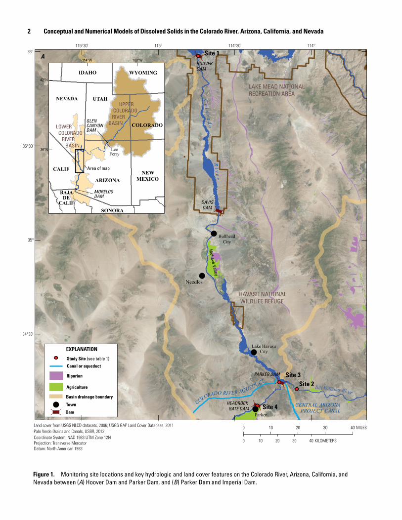
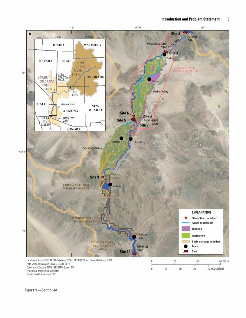
1. Monitoring site locations and key hydrologic and land cover features on the ColoradoRiver, Arizona, California, and Nevada between Hoover Dam and Parker Dam, andParker Dam and Imperial Dam ...................................................................................................2
2. Cumulative monthly mean water loss from the Colorado River between Hoover Damand Imperial Dam, 1990–2016 ...................................................................................................11
3. Mean monthly discharge for the Colorado River below Hoover Dam, the ColoradoRiver below Parker Dam, and the Colorado River above Imperial Dam, normalized tothe mean annual discharge of the Colorado River below Hoover Dam, 1990–2016 ........11
4. Cumulative monthly mean dissolved-solids load loss from the Colorado Riverbetween: Hoover Dam and Parker Dam and Parker Dam and Imperial Dam,1990–2016; and Parker Dam and Imperial Dam .....................................................................12
5. Monthly mean discharge for the Bill Williams River near Parker, monthly meandissolved-solids load for the Colorado River below Parker Dam, and daily meandissolved-solids load for the Bill Williams River near Parker, 1990–2016 .........................13
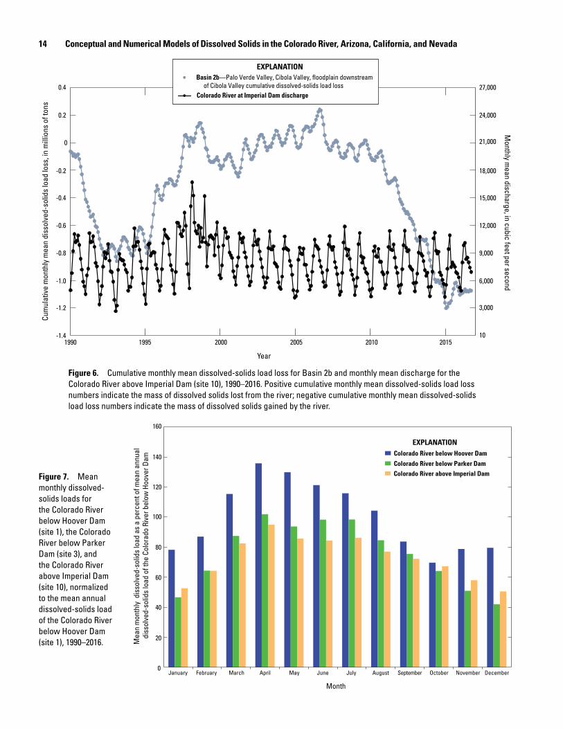
6. Cumulative monthly mean dissolved-solids load loss for Basin 2b and monthly meandischarge for the Colorado River above Imperial Dam, 1990–2016 ....................................14
7. Mean monthly dissolved-solids loads for the Colorado River below Hoover Dam,the Colorado River below Parker Dam, and the Colorado River above Imperial Dam,normalized to the mean annual dissolved-solids load of the Colorado River belowHoover Dam, 1990–2016 .............................................................................................................14
8. Monthly flow-weighted dissolved-solids concentration difference between theColorado River below Hoover Dam and below Parker Dam, and between theColorado River below Parker Dam and above Imperial Dam, 1990–2016 ..........................15
9. Monthly flow-weighted dissolved-solids concentration difference between theColorado River below Hoover Dam and Parker Dam, and between the ColoradoRiver below Parker Dam and above Imperial Dam, plotted against monthlyevapotranspiration for the Colorado River and the associated floodplain, 1998–2010 ...15
10. Monthly flow-weighted dissolved-solids concentration difference between theColorado River below Hoover Dam and below Parker Dam, and between the ColoradoRiver below Parker Dam and above Imperial Dam, plotted against average of monthlyprecipitation 1990–2016 .............................................................................................................16
11. Monthly flow-weighted dissolved-solids concentration difference between theColorado River below Hoover Dam and below Parker Dam, and between the ColoradoRiver below Parker Dam and above Imperial Dam, plotted against monthly meandischarge for the Colorado River, 1990–2016 .........................................................................17
12. Monthly flow-weighted dissolved-solids concentration difference between theColorado River below Hoover Dam and below Parker Dam, and the Colorado Riverbelow Parker Dam and above Imperial Dam, 1990–2016 .....................................................18
13. Observed and simulated monthly flow-weighted dissolved-solids concentrations forthe Colorado River above Imperial Dam from 1990 to 2016 from the Parker Dam toImperial Dam model and plotted against one another .........................................................23
14. Residual error for the Parker Dam to Imperial Dam model, 1990–2016 .............................2415. Observed and simulated monthly flow-weighted dissolved-solids concentrations for
the Colorado River above Imperial Dam from 1990 to 2016 from the Hoover Dam toImperial Dam model and plotted against one another .........................................................27
16. Residual error for the Hoover Dam to Imperial Dam model, 1990–2016 ............................28
v
Tables
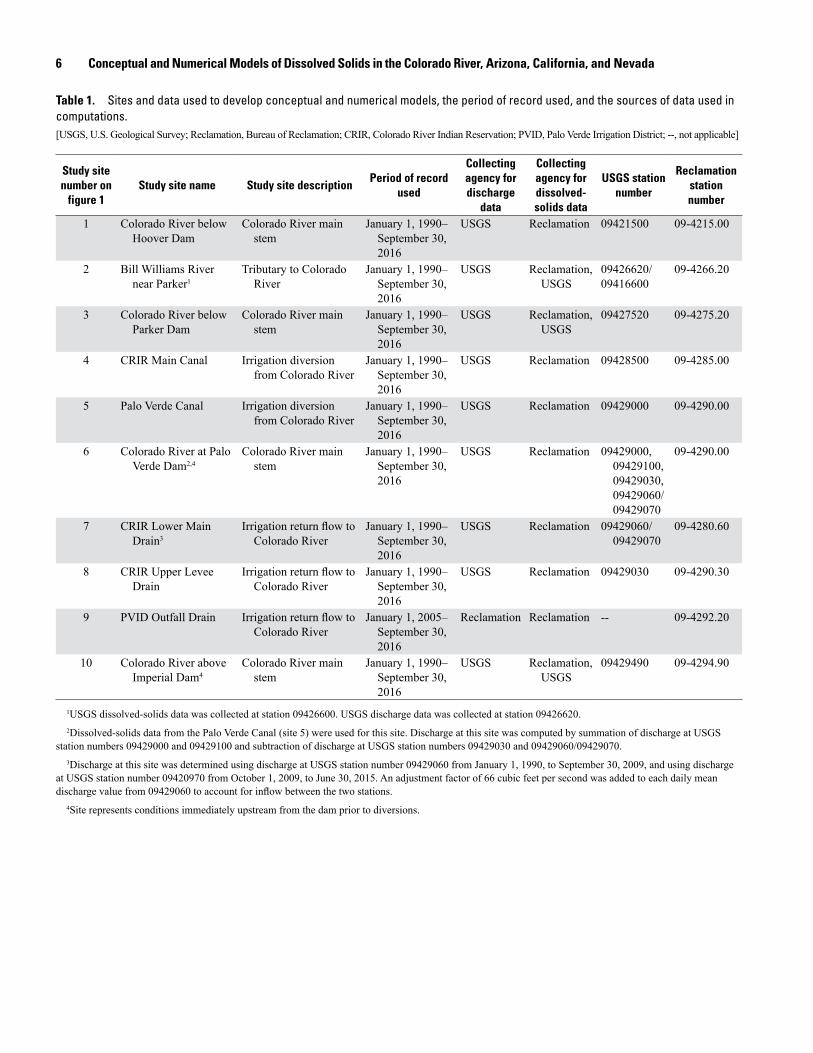
1. Sites and data used to develop conceptual and numerical models, the period of record used, and the sources of data used in computations ..................................................................6
2. Mean monthly discharge and dissolved-solids load for sites 1–10, expressed as a percentage of mean annual discharge and dissolved-solids load at the Colorado River below Hoover Dam ...........................................................................................................................10
3. Description of data sources and representation of components of the numerical model ......20 4. Constraints for the coefficients of the Hoover Dam to Imperial Dam and Parker Dam to
Imperial Dam numerical models ....................................................................................................21 5. Additional constraints for Hoover Dam to Imperial Dam numerical model coefficients ....22 6. Estimated numerical model coefficients for the Parker Dam to Imperial Dam model and
for the Hoover Dam to Imperial Dam model ................................................................................22 7. Model diagnostics for the calibration and verification periods for the Parker Dam to
Imperial Dam model and the Hoover Dam to Imperial Dam model .........................................25 8. Root-mean squared error of model simulations by month for the calibration and
verification periods of the Parker Dam to Imperial Dam model and the Hoover Dam to Imperial Dam model ..........................................................................................................................25
9. Sensitivity of simulated concentrations from the Parker Dam to Imperial Dam model to the four measured model input variables ....................................................................................30
10. Sensitivity of simulated concentrations from the Hoover Dam to Imperial Dam numerical model to the four measured model input variables ................................................31
11. Statistical distribution of the four measured model input variables and of the observed monthly flow-weighted dissolved-solids concentration at Imperial Dam, 1990–2016 ........31
vi
Conversion Factors
[Inch/Pound to International System of Units]
Supplemental InformationSpecific conductance is given in microsiemens per centimeter at 25 degrees Celsius (µS/cm at 25 °C). Concentrations of chemical constituents in water are given in milligrams per liter (mg/L). Loads of chemical constituents in water are given in tons per day (ton/d), where one ton equals 2,000 pounds.
AbbreviationsCNWR Cibola National Wildlife Refuge
CRIR Colorado River Indian Reservation
HNWR Havasu National Wildlife Refuge
NWIS National Water Information System
PVID Palo Verde Irrigation District
RMSE root mean square error
USGS U.S. Geological Survey
Multiply By To obtaininch (in.) 25.4 millimeter (mm)foot (ft) 0.3048 meter (m)mile (mi) 1.609 kilometer (km)acre 0.004047 square kilometer (km2)square mile (mi2) 2.590 square kilometer (km2)acre-foot (acre-ft) 1,233 cubic meter (m3)cubic foot per second (ft3/s) 28.3 liter per second (L/s)ton per day (ton/d) 0.9072 metric ton per day
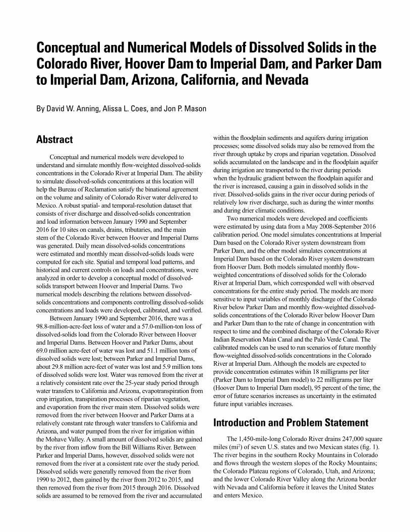
AbstractConceptual and numerical models were developed to
understand and simulate monthly flow-weighted dissolved-solids concentrations in the Colorado River at Imperial Dam. The ability to simulate dissolved-solids concentrations at this location will help the Bureau of Reclamation satisfy the binational agreement on the volume and salinity of Colorado River water delivered to Mexico. A robust spatial- and temporal-resolution dataset that consists of river discharge and dissolved-solids concentration and load information between January 1990 and September 2016 for 10 sites on canals, drains, tributaries, and the main stem of the Colorado River between Hoover and Imperial Dams was generated. Daily mean dissolved-solids concentrations were estimated and monthly mean dissolved-solids loads were computed for each site. Spatial and temporal load patterns, and historical and current controls on loads and concentrations, were analyzed in order to develop a conceptual model of dissolved-solids transport between Hoover and Imperial Dams. Two numerical models describing the relations between dissolved-solids concentrations and components controlling dissolved-solids concentrations and loads were developed, calibrated, and verified.
Between January 1990 and September 2016, there was a 98.8-million-acre-feet loss of water and a 57.0-million-ton loss of dissolved-solids load from the Colorado River between Hoover and Imperial Dams. Between Hoover and Parker Dams, about 69.0 million acre-feet of water was lost and 51.1 million tons of dissolved solids were lost; between Parker and Imperial Dams, about 29.8 million acre-feet of water was lost and 5.9 million tons of dissolved solids were lost. Water was removed from the river at a relatively consistent rate over the 25-year study period through water transfers to California and Arizona, evapotranspiration from crop irrigation, transpiration processes of riparian vegetation, and evaporation from the river main stem. Dissolved solids were removed from the river between Hoover and Parker Dams at a relatively constant rate through water transfers to California and Arizona, and water pumped from the river for irrigation within the Mohave Valley. A small amount of dissolved solids are gained by the river from inflow from the Bill Williams River. Between Parker and Imperial Dams, however, dissolved solids were not removed from the river at a consistent rate over the study period. Dissolved solids were generally removed from the river from 1990 to 2012, then gained by the river from 2012 to 2015, and then removed from the river from 2015 through 2016. Dissolved solids are assumed to be removed from the river and accumulated
Conceptual and Numerical Models of Dissolved Solids in the Colorado River, Hoover Dam to Imperial Dam, and Parker Dam to Imperial Dam, Arizona, California, and Nevada
By David W. Anning, Alissa L. Coes, and Jon P. Mason
within the floodplain sediments and aquifers during irrigation processes; some dissolved solids may also be removed from the river through uptake by crops and riparian vegetation. Dissolved solids accumulated on the landscape and in the floodplain aquifer during irrigation are transported to the river during periods when the hydraulic gradient between the floodplain aquifer and the river is increased, causing a gain in dissolved solids in the river. Dissolved-solids gains in the river occur during periods of relatively low river discharge, such as during the winter months and during drier climatic conditions.
Two numerical models were developed and coefficients were estimated by using data from a May 2008-September 2016 calibration period. One model simulates concentrations at Imperial Dam based on the Colorado River system downstream from Parker Dam, and the other model simulates concentrations at Imperial Dam based on the Colorado River system downstream from Hoover Dam. Both models simulated monthly flow-weighted concentrations of dissolved solids for the Colorado River at Imperial Dam, which corresponded well with observed concentrations for the entire study period. The models are more sensitive to input variables of monthly discharge of the Colorado River below Parker Dam and monthly flow-weighted dissolved-solids concentrations of the Colorado River below Hoover Dam and Parker Dam than to the rate of change in concentration with respect to time and the combined discharge of the Colorado River Indian Reservation Main Canal and the Palo Verde Canal. The calibrated models can be used to run scenarios of future monthly flow-weighted dissolved-solids concentrations in the Colorado River at Imperial Dam. Although the models are expected to provide concentration estimates within 18 milligrams per liter (Parker Dam to Imperial Dam model) to 22 milligrams per liter (Hoover Dam to Imperial Dam model), 95 percent of the time, the error of future scenarios increases as uncertainty in the estimated future input variables increases.
Introduction and Problem StatementThe 1,450-mile-long Colorado River drains 247,000 square
miles (mi2) of seven U.S. states and two Mexican states (fig. 1). The river begins in the southern Rocky Mountains in Colorado and flows through the western slopes of the Rocky Mountains; the Colorado Plateau regions of Colorado, Utah, and Arizona; and the lower Colorado River Valley along the Arizona border with Nevada and California before it leaves the United States and enters Mexico.
2 Conceptual and Numerical Models of Dissolved Solids in the Colorado River, Arizona, California, and Nevada
Study Site (see table 1)
EXPLANATION
Canal or aqueduct
Riparian
Agriculture
Basin drainage boundary
Town
A
HAVASU NATIONAL WILDLIFE REFUGE
LAKE MEAD NATIONAL RECREATION AREA
Parker
Bullhead City
Lake Havasu City
Needles
PARKER DAM
HEADROCK GATE DAM
HOOVERDAM
Mohave Valley
Site 2
Site 1
Land cover from USGS NLCD datasets, 2006; USGS GAP Land Cover Database, 2011Palo Verde Drains and Canals, USBR, 2012Coordinate System: NAD 1983 UTM Zone 12NProjection: Transverse MercatorDatum: North American 1983
0 10 20 30 40 MILES
0 10 20 30 40 KILOMETERS
DAVISDAM
Site 3
CENTRAL ARIZONA PROJECT CANALSite 4
C o l o r a d o R i v e r
COLORADO RIVER AQUEDUCTBill Williams River
114°114°30'115°115°30'36°
35°30'
35°
34°30'
108°W114°W
42°N
36°N
WYOMING
COLORADO
BAJA DE
CALIF
UTAH
IDAHO
NEVADA
ARIZONA NEWMEXICO
CALIF
SONORA
UPPER COLORADO RIVER BASIN
LOWER COLORADO RIVER BASIN
Area of map
Dam
Lee Ferry
GLEN CANYON DAM
MORELOSDAM
Figure 1. Monitoring site locations and key hydrologic and land cover features on the Colorado River, Arizona, California, and Nevada between (A) Hoover Dam and Parker Dam, and (B) Parker Dam and Imperial Dam.
Introduction and Problem Statement 3
Source: Esri, DigitalGlobe, GeoEye, i-cubed, USDA, USGS, AEX,Getmapping, Aerogrid, IGN, IGP, swisstopo, and the GIS UserCommunity
114°114°30'115°
34°
33°30'
33°
COLORADO RIVER INDIAN RESERVATION
PICACHO STATERECREATION
AREA
Color
ado
River
CIBOLA NATIONAL WILDLIFE REFUGE
IMPERIAL NATIONALWILDLIFE REFUGE
Parker
Poston
EhrenbergBlythe
Cibola
Martinez Lake
PARKERDAM
HEADROCK GATEDAM
PALO VERDEDAM
IMPERIALDAM
Parker S
trip
Parker Valley
Palo Verde Valley
CibolaValley
Site 10
Site 9
Site 6
Site 4
Site 3
Land cover from USGS NLCD datasets, 2006; USGS GAP Land Cover Database, 2011Palo Verde Drains and Canals, USBR, 2012
Site 5Site 8
Site 7
0 10 20 30 MILES
0 10 20 30 40 KILOMETERSCoordinate System: NAD 1983 UTM Zone 12NProjection: Transverse MercatorDatum: North American 1983
108°W114°W
42°N
36°N
WYOMING
COLORADO
BAJA DE
CALIF
UTAH
IDAHO
NEVADA
ARIZONA NEWMEXICO
CALIF
SONORA
UPPER COLORADO RIVER BASIN
LOWER COLORADO RIVER BASIN
Lee Ferry
Area of map
Study Site (see table 1)
EXPLANATION
Canal or aqueduct
Riparian
Agriculture
Basin drainage boundary
Town
Dam
GLEN CANYON DAM
MORELOSDAM
B
Figure 1.—Continued
4 Conceptual and Numerical Models of Dissolved Solids in the Colorado River, Arizona, California, and Nevada
The Colorado River is highly regulated with an extensive system of dams, reservoirs, and aqueducts that divert about 90 percent of the river’s water in the United States for agricultural and municipal uses. There are 15 dams on the main stem of the Colorado River in the United States, which can collectively store about 58.3 million acre-feet (acre-ft) of water in associated reservoirs. Lee Ferry, located 17 miles downstream of Glen Canyon Dam, is the division point between the Upper and Lower Colorado River Basins, and the river flow at this point is the principal factor in allocating water to the seven U.S. states and two Mexican states that have water rights.
The Utilization of Waters of the Colorado and Tijuana Rivers and of the Rio Grande treaty of 1944 guarantees that 1.5 million acre-ft of Colorado River water is annually delivered from the United States to Mexico. Minute 242 states that water delivered to Mexico upstream from Morelos Dam, on the United States-Mexico border, must have an average annual salinity of no more than 115 parts per million (ppm; ±30 ppm) over the average annual salinity of Colorado River waters at Imperial Dam, located 26.1 river miles upstream of Morelos Dam (fig. 1B; International Boundary and Water Commission, 1973). For conversion, 1 ppm is approximately equivalent to 1 milligram per liter (mg/L) for water with dissolved-solids concentrations less than 7,000 mg/L (Hem, 1992). Salinity is defined as dissolved solids calculated by the summation of major constituents.
To meet the binational agreement on the volume and salinity of Colorado River water delivered to Mexico, the correct volume of groundwater must be added to, or withheld from, the river just upstream from Morelos Dam. In order for Bureau of Reclamation (referred to herein as Reclamation) operators to optimize this volume of groundwater, the river salinity must be estimated at Imperial Dam from the current month through the end of the calendar year. River salinity at Imperial Dam, however, fluctuates on hourly to decadal time scales, resulting in uncertainty in groundwater volume calculations.
Purpose and Scope
The objective of this study was to provide Reclamation with the capability to simulate Colorado River salinity (as dissolved solids) at Imperial Dam in order for operators to better quantify the volume of groundwater required to be added to, or withheld from, the river each month. This report presents (1) a conceptual model of the spatial and temporal variability of dissolved solids at Imperial Dam and the factors that control such variability, and (2) two numerical models that are founded on the conceptual model and allow for scenario development of dissolved-solids concentrations at Imperial Dam based on conditions within the contributing area and at the upstream boundaries of the models. The upstream boundary of the first
numerical model is Parker Dam, and the upstream boundary of the second numerical model is Hoover Dam.
Description of Study Area
The study area is located within the Lower Colorado River Basin and is defined by the contributing drainage area between Hoover Dam and Imperial Dam on the Arizona-California border (fig. 1). The study focuses on the river and its floodplain; the floodplain is defined as the part of the Colorado River valley that was historically inundated by floods prior to the construction of dams (Owen-Joyce and Raymond, 1996). Between Hoover and Imperial Dams, the Colorado River meanders to divide the floodplain into Mohave, Parker, Palo Verde, and Cibola Valleys.
In 2010, approximately 149,300 acres (51 percent) of the floodplain between Hoover Dam and Imperial Dam were agricultural and 143,928 acres (49 percent) were riparian vegetation (Bureau of Reclamation, 2014). Agricultural acreage within the study area is dependent on Colorado River water that is either diverted into canals or pumped from the river and transported to agricultural areas in the floodplain for irrigation. Unused water and irrigation return flows are returned to the river through a complex system of wasteways, spillways, and drains.
Between Hoover Dam and Davis Dam, the Colorado River is confined by bedrock with small riparian areas at the mouths of tributary streams (Owen-Joyce and Raymond, 1996). This reach of the river is within the Lake Mead National Recreation Area and contains no agricultural acreage.
Mohave Valley begins about 6 miles below Davis Dam and lies mostly within Arizona. Land use within the valley was about 25 percent agricultural acreage in 2010 (Bureau of Reclamation, 2014). Agricultural areas are irrigated with water pumped from the Colorado River; irrigation returns flow through the groundwater system. Downstream of Mohave Valley, the Colorado River is confined by bedrock within the Havasu National Wildlife Refuge (HNWR), which extends to Lake Havasu, above Parker Dam. Within HNWR, Colorado River water is diverted to and from Topock Marsh through an inlet and an outlet, respectively. Water is diverted from the Colorado River just above Parker Dam to California through the Colorado River Aqueduct, and to Arizona through the Central Arizona Project Canal. The Bill Williams River is a regulated tributary that discharges to the Colorado River just above Parker Dam.
Parker Dam is the start of the Parker Strip-Parker Valley reach of the Colorado River. The Parker Strip is a short, thin stretch of the floodplain between Parker Dam and Parker Valley; Parker Valley makes up the remainder of this reach. Most of the floodplain in Parker Valley lies in Arizona within the Colorado River Indian Reservation (CRIR). Land use within the valley was about 62 percent agricultural acreage in 2010 (Bureau of Reclamation, 2014). Water is diverted from the Colorado River to croplands in Arizona at Headgate Rock Dam through the CRIR
Data Compilation 5
Main Canal. Irrigation return flows are returned to the river near the Poston Wasteway and the CRIR Wasteway, which contain return flows from both the CRIR Main Canal and the CRIR Upper Levee Drain; and just below Palo Verde Dam through the Palo Verde Drain and the CRIR Lower Main Drain.
Palo Verde Valley begins below the Palo Verde Dam and lies mostly within California. Land use within the valley was about 94 percent agricultural acreage in 2010 (Bureau of Reclamation, 2014). At Palo Verde Dam, water is diverted from the river to croplands in the valley through the Palo Verde Canal. Irrigation return flows are returned to the river through 10 spillways and drains, the largest of which is the Palo Verde Irrigation District (PVID) Outfall Drain.
Cibola Valley is southeast of Palo Verde Valley, and spans both sides of the river within Arizona and California. Colorado River water is diverted to and from Cibola Lake, within Cibola National Wildlife Refuge (CNWR), through an inlet and an outlet, respectively. South of Cibola Valley, the floodplain narrows and the river flows through an area dominated by phreatophytes in the CNWR, the Imperial National Wildlife Refuge, and Picacho State Recreation Area. The downstream boundary of this reach (and of the study area) is Imperial Dam. Land use within Cibola Valley and downstream to Imperial Dam was 15 percent agricultural acreage and 85 percent riparian acreage in 2010 (Bureau of Reclamation, 2014). Agricultural areas within Cibola Valley are irrigated with water pumped from the Colorado River; irrigation returns flow through the groundwater system.
Floodplain sediments comprise the upper water-bearing unit of the Colorado River aquifer, called the floodplain aquifer. This unit is 0 to 180 feet (ft) thick and is highly permeable (Wilson and Owen-Joyce, 1994). A small quantity of direct runoff from occasional intense rainfall infiltrates into the floodplain aquifer along the edges of the floodplain through tributaries to the Colorado River (Wilson and Owen-Joyce, 1994). Most of the recharge to the aquifer, however, occurs artificially as diverted river water is applied to agricultural fields during irrigation. Drainage ditches within the agricultural areas of Parker and Palo Verde Valleys intersect the water table of the floodplain aquifer and remove excess irrigation water. Drains may also include a minor amount of naturally recharged tributary water (Leake and others, 2013).
Data CompilationThe approach of this study was to first generate a high-
spatial- and high-temporal-resolution dataset of discharge and dissolved-solids information between January 1990 and September 2016 for 10 sites on canals, drains, tributaries, and the main stem of the Colorado River between Hoover Dam and Imperial Dam (table 1; fig. 1). This dataset included computed daily dissolved-solids concentrations and loads for each
site. Sites were chosen on the basis of their available data and relevance to dissolved-solids controls in the study area.
Measured Data
Data used to compute daily dissolved-solids concentrations and loads included measured daily mean discharge, measured monthly to bimonthly dissolved-solids samples, and measured daily specific conductance measurements available from 10 sites. The period January 1, 1990, through September 30, 2016, was used for nine of the sites. At one site (PVID Outfall Drain), however, daily mean discharge data were only available from January 1, 2005, through September 30, 2016.
Discharge DataDaily mean discharges and monthly mean discharges
used for this study were obtained from continuous discharge data measured by a network of 10 streamflow gaging stations (sites) operated by the U.S. Geological Survey (USGS) and Reclamation (table 1). Four sites were located on the main stem of the Colorado River, one site was located on a tributary to the river, two sites were located on irrigation canals that divert water from the river, and three sites were located on drains that return water to the river. All USGS discharge data are archived in the USGS National Water Information System database (NWIS; U.S. Geological Survey, 2017) and all Reclamation discharge data are archived at https://doi.org/10.5066/F7SQ8ZN4.
Discharge data were not available at the site on the Colorado River at Palo Verde Dam (site 6). Discharge at this site was computed by summing discharge from the Colorado River below Palo Verde Dam (USGS station number 09429100) and from the Palo Verde Canal (USGS station number 09429000), then subtracting discharge from the CRIR Upper Levee Drain (USGS station number 09429030) and the CRIR Lower Main Drain (USGS station numbers 09429060 and 09429070).
Discharge at the site on the CRIR Lower Main Drain (site 7) was determined from discharge measured at two gaging stations. Discharge data were available from January 1, 1990, to September 30, 2010, at USGS station number 09429060. This station was replaced by USGS station number 09429070, for which discharge data were available from October 1, 2009, to June 30, 2015. Station 09429070 is located about 2.5 miles downstream of station 09429060, and a large area of irrigated cropland lies between the two sites; drainage from irrigation most likely enters the drain between the old and new stations. Both stations were in operation from October 1, 2009, to September 30, 2010, which allowed for comparison of daily mean discharges measured at both stations. On average, there was about 66 cubic feet per second (ft3/s) more flow at 09429070 compared to 09429060 during this period. To compensate for this discrepancy in discharge, 66 ft3/s was added
6 Conceptual and Numerical Models of Dissolved Solids in the Colorado River, Arizona, California, and Nevada
Table 1. Sites and data used to develop conceptual and numerical models, the period of record used, and the sources of data used in computations. [USGS, U.S. Geological Survey; Reclamation, Bureau of Reclamation; CRIR, Colorado River Indian Reservation; PVID, Palo Verde Irrigation District; --, not applicable]
Study site number on
figure 1Study site name Study site description Period of record
used
Collecting agency for discharge
data
Collecting agency for dissolved-solids data
USGS station number
Reclamation station number
1 Colorado River below Hoover Dam
Colorado River main stem
January 1, 1990–September 30, 2016
USGS Reclamation 09421500 09-4215.00
2 Bill Williams River near Parker1
Tributary to Colorado River
January 1, 1990–September 30, 2016
USGS Reclamation, USGS
09426620/09416600
09-4266.20
3 Colorado River below Parker Dam
Colorado River main stem
January 1, 1990– September 30, 2016
USGS Reclamation, USGS
09427520 09-4275.20
4 CRIR Main Canal Irrigation diversion from Colorado River
January 1, 1990– September 30, 2016
USGS Reclamation 09428500 09-4285.00
5 Palo Verde Canal Irrigation diversion from Colorado River
January 1, 1990– September 30, 2016
USGS Reclamation 09429000 09-4290.00
6 Colorado River at Palo Verde Dam2,4
Colorado River main stem
January 1, 1990– September 30, 2016
USGS Reclamation 09429000, 09429100, 09429030, 09429060/ 09429070
09-4290.00
7 CRIR Lower Main Drain3
Irrigation return flow to Colorado River
January 1, 1990– September 30, 2016
USGS Reclamation 09429060/ 09429070
09-4280.60
8 CRIR Upper Levee Drain
Irrigation return flow to Colorado River
January 1, 1990– September 30, 2016
USGS Reclamation 09429030 09-4290.30
9 PVID Outfall Drain Irrigation return flow to Colorado River
January 1, 2005– September 30, 2016
Reclamation Reclamation -- 09-4292.20
10 Colorado River above Imperial Dam4
Colorado River main stem
January 1, 1990– September 30, 2016
USGS Reclamation, USGS
09429490 09-4294.90
1USGS dissolved-solids data was collected at station 09426600. USGS discharge data was collected at station 09426620.2Dissolved-solids data from the Palo Verde Canal (site 5) were used for this site. Discharge at this site was computed by summation of discharge at USGS
station numbers 09429000 and 09429100 and subtraction of discharge at USGS station numbers 09429030 and 09429060/09429070.3Discharge at this site was determined using discharge at USGS station number 09429060 from January 1, 1990, to September 30, 2009, and using discharge
at USGS station number 09420970 from October 1, 2009, to June 30, 2015. An adjustment factor of 66 cubic feet per second was added to each daily mean discharge value from 09429060 to account for inflow between the two stations.
4Site represents conditions immediately upstream from the dam prior to diversions.
Data Compilation 7
to each daily mean discharge at station 09429060 from January 1, 1990, to September 30, 2009.
Dissolved-Solids DataDissolved-solids data (calculated as the sum of the major
constituents of bicarbonate, calcium, carbonate, chloride, fluoride, magnesium, nitrate, potassium, silicon dioxide, sodium, and sulfate) were obtained from a network of 10 sampling stations operated by the USGS and Reclamation (table 1). USGS and Reclamation dissolved-solids data from the same (or proximal) stations were combined where data were available from both agencies. The frequency of dissolved-solids data at nine of the sites varied from bimonthly to monthly; at site 2, dissolved-solids data was collected from 2 to 15 times per year on an irregular schedule because of its intermittent streamflow. The period of the dissolved-solids data was the same period as the discharge data. All USGS dissolved-solids data are archived in the USGS National Water Information System database (U.S. Geological Survey, 2017) and all Reclamation dissolved-solids data are archived at https://doi.org/10.5066/F7SQ8ZN4.
Data-Quality AssessmentReplicate samples are two or more water samples that are
collected, prepared, and analyzed in the same manner such that they are considered to be essentially identical, and are used to estimate the variability of analytical results inherently related to the environment, sampling procedures, and lab procedures (Mueller and others, 2015). There were 34 dissolved-solids replicate sample pairs collected by the USGS and Reclamation at the study sites between January 1990 and February 2017 (https://doi.org/10.5066/F7SQ8ZN4). A bias-corrected log-log regression model (Mueller and others, 2015) was used to model the variability, as standard deviation, of the replicates. This model is based on the approximately linear relation between the logarithms of replicate standard deviation and mean concentration, where
log(SD)=B0+B1log(C) (1)
where SD is the replicate standard deviation; B0 is the intercept of the regression line,
estimated by least-squares; B1 is the slope of the regression line, estimated
by least-squares; and C is the mean replicate concentration, or
concentration of a single sample.Standard deviation residuals from the log-log equation are
then retransformed back to their original units; the mean of the retransformed standard deviation residuals is the bias-correction factor (bcf). The bcf is multiplied by the estimated standard deviations of each replicate in order to express the modeled standard deviation (SDM):
(2)
The variability of the dissolved-solids sample concentrations in this study was determined to be
1.179{10[-1.628+0.735log(C)]}. (3)
Using equation 3, the variability of the measured dissolved solids concentrations at the Colorado River above Imperial Dam ranges from 2.5 to 4.5 mg/L, with an average variability of 3.5 mg/L, or about 0.5 percent.
An additional quality assessment of the monthly to bimonthly dissolved-solids data (calculated as the sum of major constituents) was completed in order to understand data quality and to remove any samples or values deemed erroneous. The ratio of cations to anions within each sample was computed. Samples with a ratio value that was greater than 1.20 or less than 0.80 were removed from the dataset. The ratio of dissolved-solids concentration calculated as the sum of constituents to dissolved-solids concentration determined by residue on evaporation was computed. Samples with a ratio value that was greater than 1.20 or less than 0.80 were removed from the dataset. The ratio of dissolved-solids concentration calculated as the sum of constituents to specific conductance was computed. Samples with ratios having large deviations from the long-term trend were removed. In total, 94 samples (1.9 percent of the total samples) were removed based on the above data assessments. In addition, the quality assessment also determined that 34 pairs of samples were incorrectly coded as being collected at identical sites, dates, and times; this resulted in the removal of an additional 68 samples (1.4 percent of the total samples) because the correct dates and times for these samples could not be determined.
For the Colorado River above Imperial Dam (site 10), the ratios of the dissolved-solids concentration calculated as the sum of constituents to specific conductance generally ranged from about 0.60 to 0.64 with no increasing or decreasing trends during the period January 1990 through September 2016, with an average ratio of 0.619. There is, however, an anomalous period from about January 2005 through April 2008 when ratios ranged from about 0.54 to 0.62, with an average ratio of 0.582. In March 2008, Reclamation conducted an internal review of sample collection, handling, and analysis procedures at this site to determine the cause of inconsistent water-quality data (Hong Nguyen-DeCorse, Bureau of Reclamation, written commun., March 8, 2016). The review led to the implementation of minor corrections to field sampling and laboratory procedures for water-quality sampling at all sites. In addition, the analytical laboratory began using a new inductively coupled plasma mass spectrometer for cation analysis.
Computation of Daily Mean Dissolved-solids Concentrations
Daily mean dissolved-solids concentrations were estimated for nine of the sites using one of three methods depending on the type of data available and the numerical model requirements. At sites 4–9, a method using discrete monthly to bimonthly dissolved-solids data was used. At site 10, the Colorado River SDM = bcf{10
[B0 + B1 log(C)]}
8 Conceptual and Numerical Models of Dissolved Solids in the Colorado River, Arizona, California, and Nevada
above Imperial Dam, a method using daily specific conductance data was used. At site 1, the Colorado River at Hoover Dam, and site 3, the Colorado River at Parker Dam, a method using monthly to bimonthly specific conductance data was used. Daily mean dissolved-solids concentrations were not estimated for site 2, the Bill Williams River near Parker, because of large periods of time with no dissolved-solids data.
Method Using Monthly to Bimonthly Dissolved-solids Data
Daily mean dissolved-solids concentrations were initially estimated for sites 4–9 by using a regression between monthly to bimonthly dissolved-solids concentrations and stream discharge and also by taking into account the components of time and season. The statistical model, Weighted Regression on Time, Discharge, and Season (WRTDS) developed by Hirsch and others (2010), was applied to the data by using the R package Exploration and Graphics for River Trends (EGRET; Hirsch and De Cicco, 2015) and the R Project for Statistical Computing (R Development Core Team, 2011). The WRTDS model, however, did not provide a satisfactory fit between actual and estimated dissolved-solids concentrations. Although this estimation approach is commonly used in many studies, the lack of fit is not surprising when considering the difference between the Colorado River and a natural stream. In a natural stream, dissolved-solids concentrations are typically a mixture two major sources of water—high-concentration base flow and low-concentration runoff. As a result of the contrast in source-water concentrations, natural stream concentrations generally decrease as a larger portion of the streamflow comes from runoff. For regulated streams such as the Colorado River, however, concentrations of higher flows from reservoir releases may not be that much different than those in base flows and the relative contribution of base flow to total streamflow may be small. This is especially true immediately downstream from large reservoirs, where stream concentrations reflect reservoir contents and exhibit little variation whereas reservoir release discharges vary greatly.
Daily mean dissolved-solids concentrations at sites 4–9 were, therefore, estimated from monthly to bimonthly dissolved-solids data using an interpolation approach. Linear interpolation between monthly to bimonthly dissolved-solids concentrations was done using the R Project for Statistical Computing (R Development Core Team, 2011), and a daily time step was used to obtain a value that could be used as a daily concentration. A LOESS (local regression) smooth function was subsequently applied to the linearly interpolated daily data to account for uncertainty related to measurement errors, and the result was the daily series of concentration data representing dissolved-solids conditions for the station.
Method Using Daily Specific Conductance DataFor site 10, the Colorado River above Imperial Dam,
Reclamation determines daily specific conductance from four
samples collected at 6-hour intervals. Daily dissolved-solids concentrations were computed by Reclamation from this daily specific-conductance data by using an interpretation of bimonthly dissolved-solids and specific-conductance data at this site.
For the Colorado River at Imperial Dam, Reclamation determines the ratio of dissolved-solids concentration to specific conductance for each bimonthly sample. The following 2 weeks of daily specific-conductance data are then multiplied by this ratio to determine the daily dissolved-solids concentrations for those 2 weeks. As previously discussed, however, the ratio from about January 2005 through April 2008 is biased low because of sampling and analytical procedural issues. Therefore, in this study, daily mean dissolved-solids concentrations for the Colorado River at Imperial Dam were recalculated by using corrected ratios and daily specific-conductance data for the periods of January 1990 through April 2008, and May 2008 through September 2016. Different ratios were calculated for the periods before and after May 2008 to take into account the implementation of new field sampling and laboratory procedures. The corrected ratios were determined by computing the ratio of dissolved-solids concentration (in mg/L) to specific conductance (in microsiemens per centimeter [µS/cm]) for each bimonthly sample between January 1990 through December 2004, and May 2008 through September 2016; the period of January 2005 to April 2008 was excluded. The average corrected ratio for January 1990 through December 2004 was determined to be 0.625, and each daily specific-conductance value prior to May 2008 was multiplied by this average corrected ratio to compute daily dissolved-solids values. For May 2008 through September 2016, the average corrected ratio was determined to be 0.623, and each daily specific-conductance value after May 2008 was multiplied by this average corrected ratio to compute daily dissolved-solids values. Implementing this approach reduced the root mean square error (RMSE) of the residuals from preliminary numerical models by more than one-third, which validated this recalculation and suggests that others may also benefit from using the recalculated concentrations.
Method Using Monthly to Bimonthly Specific Conductance Data
For sites representing conditions at the upstream boundaries of the two numerical models, Colorado River below Hoover Dam (site 1) and Colorado River below Parker Dam (site 3), Reclamation required the ability to use either specific conductance or dissolved solids concentration as an input variable. Daily mean specific conductance concentrations at sites 1 and 3 were estimated from monthly to bimonthly specific conductance data using an interpolation approach. Linear interpolation between monthly to bimonthly specific conductance concentrations was done using the R Project for Statistical Computing (R Development Core Team, 2011), and a daily time step was used to obtain a value that could be used as a daily concentration.
To convert daily specific conductance values to daily dissolved-solids values, the ratio of dissolved-solids
Conceptual Model 9
concentration (in mg/L) to specific conductance (in µS/cm) for each monthly to bimonthly sample was determined for each site. The average ratios for the periods of January 1990 through April 2008, and May 2008 through September 2016 were then calculated for each site. Different ratios were calculated for the periods before and after May 2008 to take into account the implementation of new field sampling and laboratory procedures. For site 1, the average corrected ratio for January 1990 through April 2008 was determined to be 0.623, and each daily specific-conductance value prior to May 2008 was multiplied by this average corrected ratio to compute daily dissolved-solids values; for May 2008 through September 2016, the average corrected ratio was determined to be 0.616, and each daily specific-conductance value after May 2008 was multiplied by this average corrected ratio to compute daily dissolved-solids values. For site 3, the average corrected ratio for January 1990 through April 2008 was determined to be 0.638, and each daily specific-conductance value prior to May 2008 was multiplied by this average corrected ratio to compute daily dissolved-solids values; for May 2008 through September 2016, the average corrected ratio was determined to be 0.616, and each daily specific-conductance value after May 2008 was multiplied by this average corrected ratio to compute daily dissolved-solids values.
Computation of Dissolved-solids Loads and Flow-weighted Concentrations
Daily mean dissolved-solids loads (Wd, in tons per day [ton/d]) were computed for the nine sites with daily mean dissolved-solids concentrations (table 1). Discharge and dissolved-solids data were often not recorded at the exact same site, but from two different stations in proximity to one another (table 1). Daily loads were computed by multiplying daily mean discharge (Qd, in ft3/s) by daily dissolved-solids concentration (Cd, in mg/L), with unit conversions, as follows
Wd = Qd×Cd×2.696122e-3 (4)
Daily mean dissolved-solids loads were averaged to obtain monthly mean dissolved-solids loads (Wm; in ton/d) (https://doi.org/10.5066/F7SQ8ZN4). Monthly mean flow-weighted concentrations (Cm, in mg/L) were then computed by dividing monthly mean dissolved-solid load (Wm; in ton/d) by monthly mean discharge (Qm; in ft3/s) with unit conversions using the following equation
(5)
Monthly mean dissolved-solids loads and flow-weighted concentrations were not calculated for site 2, the Bill Williams River near Parker, because daily mean dissolved-solids concentrations could not be calculated for this site and because this site has many months with zero discharge (https://doi.org/10.5066/F7SQ8ZN4). Instead, daily mean dissolved-solids
loads were calculated for days with samples by using instantaneous dissolved-solids concentrations and daily mean discharges (https://doi.org/10.5066/F7SQ8ZN4).
Conceptual Model
Approach
In order to develop a conceptual understanding of dissolved-solids transport in the Colorado River between Hoover and Imperial Dams, monthly mean discharges and monthly mean dissolved-solids loads from January 1990 to September 2016 were analyzed (https://doi.org/10.5066/F7SQ8ZN4). Dissolved-solids loads were chosen for the conceptual model instead of concentrations because changes in dissolved-solids loads are typically related to physical transport processes rather than geochemical processes; and, it is easier to identify the effects of physical transport processes on loads than on concentrations.
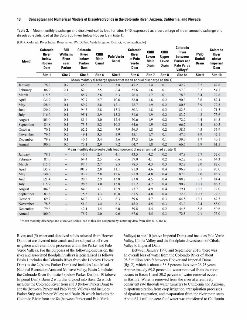
To examine spatial and temporal variability, monthly mean discharge and dissolved-solids load data were averaged by month (weighted by the number of days in each month) over the January 1990 to September 2016 period at each of the 10 sites to determine mean monthly discharges and dissolved-solids loads (https://doi.org/10.5066/F7SQ8ZN4). These data were spatially normalized by dividing the mean monthly discharges and dissolved-solids loads for each site by the mean annual discharge and dissolved-solids load for the Colorado River below Hoover Dam (site 1) and then multiplying by 100 to express the values as a percentage (table 2). Such normalization makes it easier to compare the data to average conditions at the upstream boundary of the study area and makes it easier to track the transport of mass of water and dissolved solids through the system. Parker and Palo Verde Valleys, as well as their canals and drains to and from the river, overlap in the area of Palo Verde Dam (fig. 1). Consequently, a new site called site 8a, the Colorado River between Parker and Palo Verde Valleys, was established by summing data for sites 6, 7, and 8. This site represents the east-west boundary between Parker and Palo Verde Valleys and separates all inflows and outflows between the river and each valley.
ResultsThere are five main pathways for Colorado River surface
water flow and dissolved-solids transport between Hoover and Imperial Dams: (1) water and dissolved solids released from Hoover Dam that remain within the main stem of the Colorado River and travel through to Imperial Dam, (2) water and dissolved solids released from Hoover Dam that are pumped from the river and are subject to off-river irrigation and return flow processes within the Mohave and Cibola Valleys, (3) water and dissolved solids released from Hoover Dam that are diverted to California through the Colorado River Aqueduct and to Arizona through the Central Arizona Project Canal, (4) water and dissolved solids that are transported to the Colorado River from the Bill Williams
Cm =Wm
Qm × 2.696122e−3
10 Conceptual and Numerical Models of Dissolved Solids in the Colorado River, Arizona, California, and Nevada
River, and (5) water and dissolved solids released from Hoover Dam that are diverted into canals and are subject to off-river irrigation and return flow processes within the Parker and Palo Verde Valleys. For the purposes of the following discussion, the river and associated floodplain valleys is generalized as follows: Basin 1 includes the Colorado River from site 1 (below Hoover Dam) to site 2 (below Parker Dam) and includes Lake Mead National Recreation Area and Mohave Valley; Basin 2 includes the Colorado River from site 3 (below Parker Dam) to 10 (above Imperial Dam). Basin 2 is further divided into Basin 2a which includes the Colorado River from site 3 (below Parker Dam) to site 8a (between Parker and Palo Verde Valleys) and includes Parker Strip and Parker Valley; and Basin 2b which includes the Colorado River from site 8a (between Parker and Palo Verde
Table 2. Mean monthly discharge and dissolved-solids load for sites 1–10, expressed as a percentage of mean annual discharge and dissolved-solids load at the Colorado River below Hoover Dam (site 1).
[CRIR, Colorado River Indian Reservation; PVID, Palo Verde Irrigation District; --, not applicable]
Month
Colorado River
below Hoover
Dam
Bill Williams
River near
Parker
Colorado River
below Parker
Dam
CRIR Main Canal
Palo Verde Canal
Colorado River
at Palo Verde Dam
CRIR Lower Main Drain
CRIR Upper Levee Drain
Colorado River
between Parker and Palo Verde
Valleys1
PVID Outfall Drain
Colorado River above
Imperial Dam
Site 1 Site 2 Site 3 Site 4 Site 5 Site 6 Site 7 Site 8 Site 8a Site 9 Site 10Mean monthly discharge (percent of mean annual discharge at site 1)
January 78.2 0.7 45.0 2.3 3.8 41.2 1.4 0.1 42.7 3.2 42.8 February 86.9 2.1 62.6 2.5 6.4 55.6 1.6 0.1 57.3 3.2 54.7 March 115.5 3.0 85.7 2.6 8.3 76.4 1.7 0.1 78.3 3.4 72.8 April 134.9 0.6 97.7 2.7 10.6 88.0 1.8 0.2 90.0 3.6 82.4 May 128.6 0.1 89.9 2.8 12.1 78.7 1.9 0.2 80.8 3.9 72.5 June 120.9 0.1 94.3 2.8 13.3 80.3 1.8 0.2 82.3 4.1 71.5 July 116.0 0.1 95.1 2.9 13.2 81.6 1.9 0.2 83.7 4.3 73.6 August 105.0 0.1 81.4 3.0 12.4 70.6 1.9 0.2 72.7 4.4 64.5 September 84.8 0.1 73.5 3.2 10.3 64.6 1.9 0.2 66.7 4.4 60.5 October 70.1 0.1 62.2 3.2 7.9 56.5 1.8 0.2 58.5 4.3 55.9 November 79.5 0.2 49.1 3.3 5.9 45.1 1.7 0.1 47.0 3.9 47.1 December 79.8 0.1 40.5 3.4 5.6 37.3 1.6 0.1 39.0 3.7 40.1 Annual 100.0 0.6 73.1 2.9 9.2 64.7 1.8 0.2 66.6 3.9 61.5
Mean monthly dissolved-solids load (percent of mean annual load at site 1)January 78.3 -- 46.6 2.4 4.1 43.5 4.2 0.2 47.9 7.7 52.6 February 87.0 -- 64.4 2.5 6.6 57.9 4.1 0.2 62.2 7.6 64.3 March 115.5 -- 87.5 2.7 8.5 78.3 4.3 0.3 82.8 8.0 82.6 April 135.9 -- 101.9 2.8 11.1 91.9 4.6 0.4 96.9 8.5 95.0 May 130.0 -- 93.8 2.8 12.6 81.9 4.8 0.4 87.0 9.0 85.7 June 121.4 -- 98.3 2.9 13.8 83.8 4.5 0.4 88.7 9.7 84.4 July 115.9 -- 98.5 3.0 13.8 85.2 4.7 0.4 90.2 10.1 86.3 August 104.3 -- 84.6 3.1 12.9 73.7 4.9 0.4 79.1 10.2 77.0 September 83.8 -- 75.5 3.3 10.8 67.5 4.8 0.4 72.6 10.3 72.2 October 69.7 -- 64.2 3.3 8.3 59.6 4.7 0.3 64.5 10.1 67.3 November 78.8 -- 51.0 3.4 6.3 48.2 4.5 0.3 53.0 9.4 58.0 December 79.6 -- 42.1 3.5 6.0 39.8 4.4 0.2 44.5 8.8 50.6 Annual 100.0 -- 75.7 3.0 9.6 67.6 4.5 0.3 72.5 9.1 73.0
1 Mean monthly discharge and dissolved-solids load at this site computed by summing data from sites 6, 7, and 8.
Valleys) to site 10 (above Imperial Dam), and includes Palo Verde Valley, Cibola Valley, and the floodplain downstream of Cibola Valley to Imperial Dam.
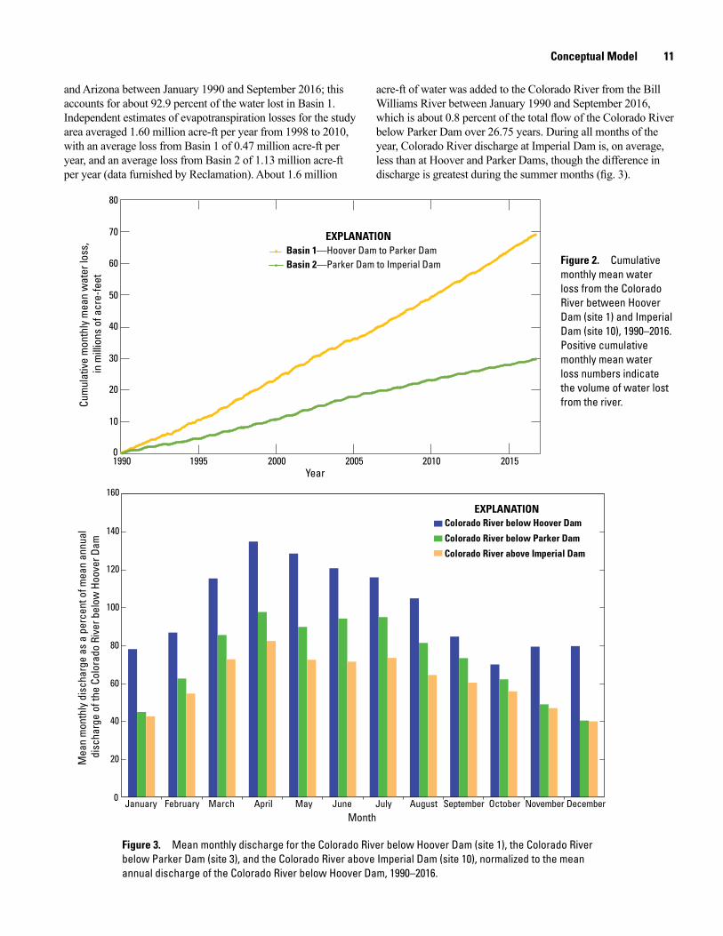
Between January 1990 and September 2016, there was an overall loss of water from the Colorado River of about 98.8 million acre-ft between Hoover and Imperial Dams (fig. 2), which is about a 38.5 percent loss over 26.75 years. Approximately 69.8 percent of water removal from the river occurs in Basin 1, and 30.2 percent of water removal occurs in Basin 2. Water is removed from the river at a relatively consistent rate through water transfers to California and Arizona, evapotranspiration from crop irrigation, transpiration processes of riparian vegetation, and evaporation from the river main stem. About 64.1 million acre-ft of water was transferred to California
Conceptual Model 11
and Arizona between January 1990 and September 2016; this accounts for about 92.9 percent of the water lost in Basin 1. Independent estimates of evapotranspiration losses for the study area averaged 1.60 million acre-ft per year from 1998 to 2010, with an average loss from Basin 1 of 0.47 million acre-ft per year, and an average loss from Basin 2 of 1.13 million acre-ft per year (data furnished by Reclamation). About 1.6 million
Figure 2. Cumulative monthly mean water loss from the Colorado River between Hoover Dam (site 1) and Imperial Dam (site 10), 1990–2016. Positive cumulative monthly mean water loss numbers indicate the volume of water lost from the river.
Figure 3. Mean monthly discharge for the Colorado River below Hoover Dam (site 1), the Colorado River below Parker Dam (site 3), and the Colorado River above Imperial Dam (site 10), normalized to the mean annual discharge of the Colorado River below Hoover Dam, 1990–2016.
Basin 1—Hoover Dam to Parker DamBasin 2—Parker Dam to Imperial Dam
Cum
ulat
ive
mon
thly
mea
n w
ater
loss
, in
mill
ions
of a
cre-
feet
40
50
60
70
80
Year1990 1995 2000 2005 2010 2015
EXPLANATION
10
20
30
0
acre-ft of water was added to the Colorado River from the Bill Williams River between January 1990 and September 2016, which is about 0.8 percent of the total flow of the Colorado River below Parker Dam over 26.75 years. During all months of the year, Colorado River discharge at Imperial Dam is, on average, less than at Hoover and Parker Dams, though the difference in discharge is greatest during the summer months (fig. 3).
AAXXXX_fig 01
Colorado River below Hoover DamColorado River below Parker Dam
Mea
n m
onth
ly d
isch
arge
as
a pe
rcen
t of m
ean
annu
al
disc
harg
e of
the
Colo
rado
Riv
er b
elow
Hoo
ver D
am
0
20
40
60
80
100
120
140
160
MonthJanuary February March April May June July August September October November December
EXPLANATION
Colorado River above Imperial Dam
12 Conceptual and Numerical Models of Dissolved Solids in the Colorado River, Arizona, California, and Nevada
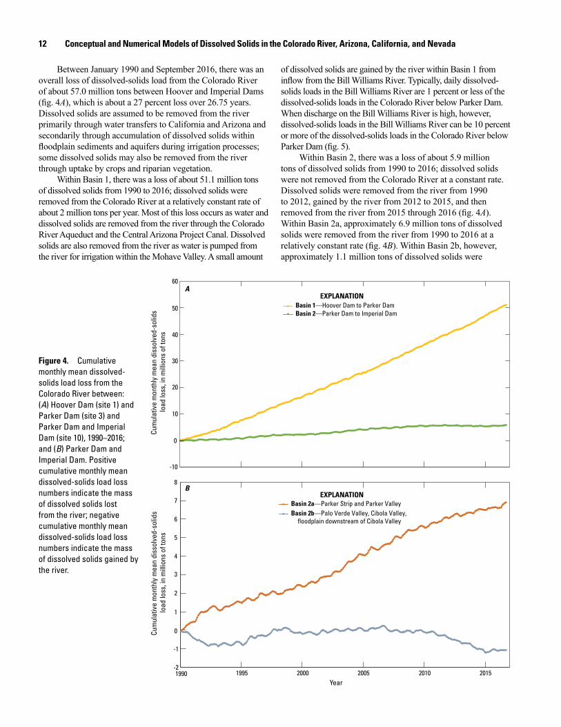
Between January 1990 and September 2016, there was an overall loss of dissolved-solids load from the Colorado River of about 57.0 million tons between Hoover and Imperial Dams (fig. 4A), which is about a 27 percent loss over 26.75 years. Dissolved solids are assumed to be removed from the river primarily through water transfers to California and Arizona and secondarily through accumulation of dissolved solids within floodplain sediments and aquifers during irrigation processes; some dissolved solids may also be removed from the river through uptake by crops and riparian vegetation.
Within Basin 1, there was a loss of about 51.1 million tons of dissolved solids from 1990 to 2016; dissolved solids were removed from the Colorado River at a relatively constant rate of about 2 million tons per year. Most of this loss occurs as water and dissolved solids are removed from the river through the Colorado River Aqueduct and the Central Arizona Project Canal. Dissolved solids are also removed from the river as water is pumped from the river for irrigation within the Mohave Valley. A small amount
Figure 4. Cumulative monthly mean dissolved-solids load loss from the Colorado River between: (A) Hoover Dam (site 1) and Parker Dam (site 3) and Parker Dam and Imperial Dam (site 10), 1990–2016; and (B) Parker Dam and Imperial Dam. Positive cumulative monthly mean dissolved-solids load loss numbers indicate the mass of dissolved solids lost from the river; negative cumulative monthly mean dissolved-solids load loss numbers indicate the mass of dissolved solids gained by the river.
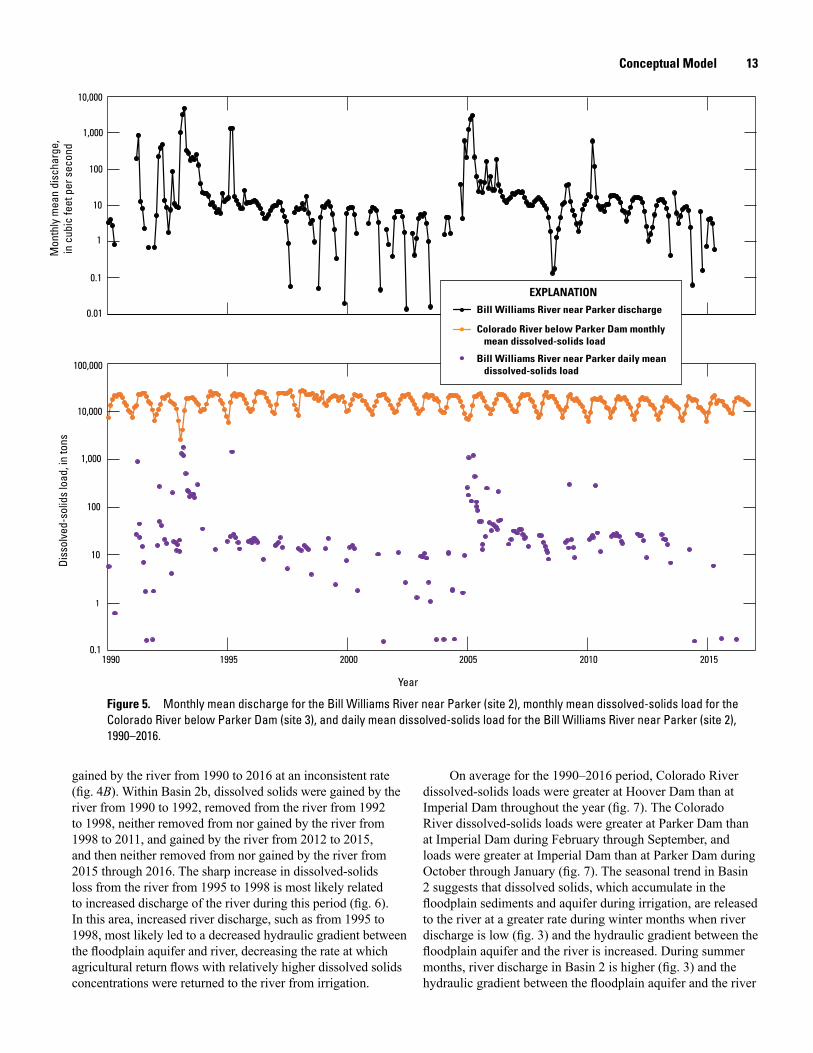
of dissolved solids are gained by the river within Basin 1 from inflow from the Bill Williams River. Typically, daily dissolved-solids loads in the Bill Williams River are 1 percent or less of the dissolved-solids loads in the Colorado River below Parker Dam. When discharge on the Bill Williams River is high, however, dissolved-solids loads in the Bill Williams River can be 10 percent or more of the dissolved-solids loads in the Colorado River below Parker Dam (fig. 5).
Within Basin 2, there was a loss of about 5.9 million tons of dissolved solids from 1990 to 2016; dissolved solids were not removed from the Colorado River at a constant rate. Dissolved solids were removed from the river from 1990 to 2012, gained by the river from 2012 to 2015, and then removed from the river from 2015 through 2016 (fig. 4A). Within Basin 2a, approximately 6.9 million tons of dissolved solids were removed from the river from 1990 to 2016 at a relatively constant rate (fig. 4B). Within Basin 2b, however, approximately 1.1 million tons of dissolved solids were
Cum
ulat
ive
mon
thly
mea
n di
ssol
ved-
solid
s lo
ad lo
ss, i
n m
illio
ns o
f ton
s
-10
0
10
30
50
60
20
40
Basin 1—Hoover Dam to Parker DamBasin 2—Parker Dam to Imperial Dam
EXPLANATION
Basin 2a—Parker Strip and Parker ValleyBasin 2b—Palo Verde Valley, Cibola Valley,
floodplain downstream of Cibola Valley
Cum
ulat
ive
mon
thly
mea
n di
ssol
ved-
solid
s lo
ad lo
ss, i
n m
illio
ns o
f ton
s 5
7
8
4
6
B
A
-1
0
1
2
3
-21990 1995 2000 2005 2010 2015
Year
EXPLANATION
Conceptual Model 13
10,000
1
10
100
1,000
0.01
0.1
Mon
thly
mea
n di
scha
rge,
in
cub
ic fe
et p
er s
econ
dDi
ssol
ved-
solid
s lo
ad, i
n to
ns
10,000
1
10
100
1,000
0.1
100,000
1990 200520001995 20152010
Year
Bill Williams River near Parker discharge
Colorado River below Parker Dam monthly mean dissolved-solids load
EXPLANATION
Bill Williams River near Parker daily mean dissolved-solids load
Figure 5. Monthly mean discharge for the Bill Williams River near Parker (site 2), monthly mean dissolved-solids load for the Colorado River below Parker Dam (site 3), and daily mean dissolved-solids load for the Bill Williams River near Parker (site 2), 1990–2016.
gained by the river from 1990 to 2016 at an inconsistent rate (fig. 4B). Within Basin 2b, dissolved solids were gained by the river from 1990 to 1992, removed from the river from 1992 to 1998, neither removed from nor gained by the river from 1998 to 2011, and gained by the river from 2012 to 2015, and then neither removed from nor gained by the river from 2015 through 2016. The sharp increase in dissolved-solids loss from the river from 1995 to 1998 is most likely related to increased discharge of the river during this period (fig. 6). In this area, increased river discharge, such as from 1995 to 1998, most likely led to a decreased hydraulic gradient between the floodplain aquifer and river, decreasing the rate at which agricultural return flows with relatively higher dissolved solids concentrations were returned to the river from irrigation.
On average for the 1990–2016 period, Colorado River dissolved-solids loads were greater at Hoover Dam than at Imperial Dam throughout the year (fig. 7). The Colorado River dissolved-solids loads were greater at Parker Dam than at Imperial Dam during February through September, and loads were greater at Imperial Dam than at Parker Dam during October through January (fig. 7). The seasonal trend in Basin 2 suggests that dissolved solids, which accumulate in the floodplain sediments and aquifer during irrigation, are released to the river at a greater rate during winter months when river discharge is low (fig. 3) and the hydraulic gradient between the floodplain aquifer and the river is increased. During summer months, river discharge in Basin 2 is higher (fig. 3) and the hydraulic gradient between the floodplain aquifer and the river
14 Conceptual and Numerical Models of Dissolved Solids in the Colorado River, Arizona, California, and Nevada
Figure 6. Cumulative monthly mean dissolved-solids load loss for Basin 2b and monthly mean discharge for the Colorado River above Imperial Dam (site 10), 1990–2016. Positive cumulative monthly mean dissolved-solids load loss numbers indicate the mass of dissolved solids lost from the river; negative cumulative monthly mean dissolved-solids load loss numbers indicate the mass of dissolved solids gained by the river.
Basin 2b—Palo Verde Valley, Cibola Valley, floodplain downstream of Cibola Valley cumulative dissolved-solids load lossColorado River at Imperial Dam discharge
Cum
ulat
ive
mon
thly
mea
n di
ssol
ved-
solid
s lo
ad lo
ss, i
n m
illio
ns o
f ton
sM
onthly mean discharge, in cubic feet per second
Year
-1.2
-1.0
-0.8
-0.6
-0.4
-0.2
0
0.2
0.4
-1.41990 1995 2000 2005 2010 2015
EXPLANATION
10
3,000
6,000
9,000
12,000
15,000
18,000
21,000
24,000
27,000
Figure 7. Mean monthly dissolved-solids loads for the Colorado River below Hoover Dam (site 1), the Colorado River below Parker Dam (site 3), and the Colorado River above Imperial Dam (site 10), normalized to the mean annual dissolved-solids load of the Colorado River below Hoover Dam (site 1), 1990–2016. M
ean
mon
thly
dis
solv
ed-s
olid
s lo
ad a
s a
perc
ent o
f mea
n an
nual
di
ssol
ved-
solid
s lo
ad o
f the
Col
orad
o Ri
ver b
elow
Hoo
ver D
am
0
20
40
60
80
100
120
140
160
Month
January February March April May June July August September October November December
Colorado River below Hoover DamColorado River below Parker Dam
EXPLANATION
Colorado River above Imperial Dam
Conceptual Model 15
is decreased, decreasing the rate at which dissolved solids are returned to the river.
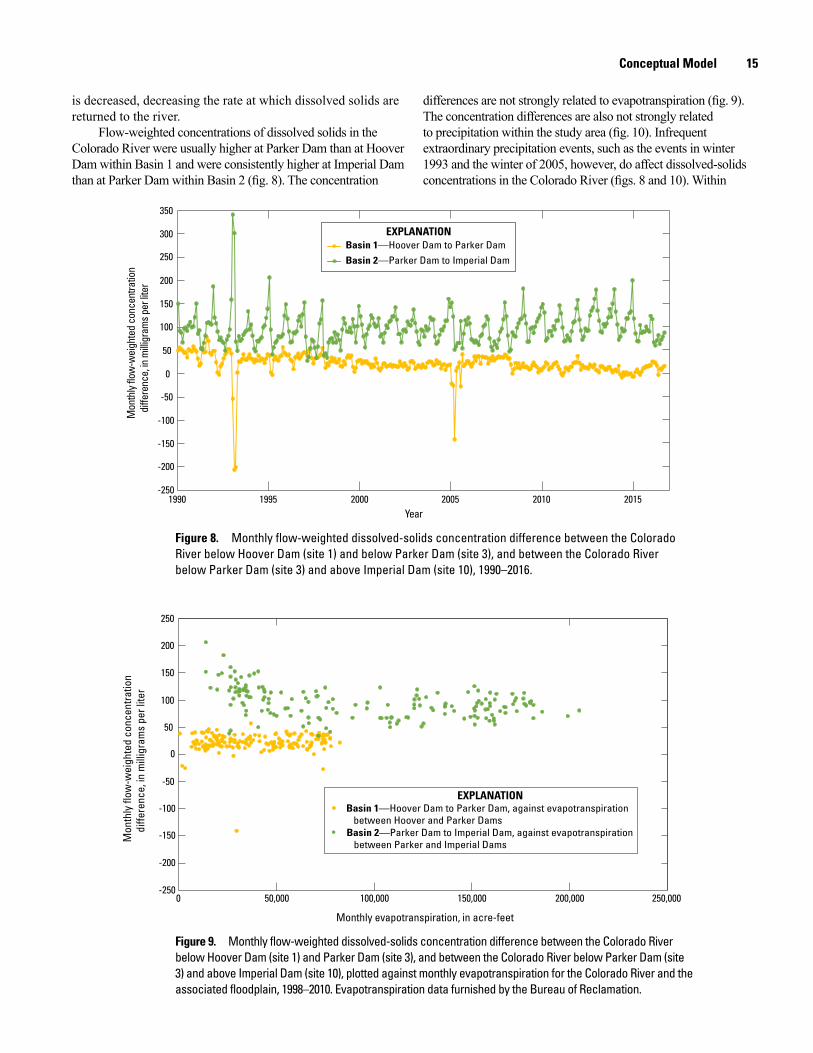
Flow-weighted concentrations of dissolved solids in the Colorado River were usually higher at Parker Dam than at Hoover Dam within Basin 1 and were consistently higher at Imperial Dam than at Parker Dam within Basin 2 (fig. 8). The concentration
Figure 8. Monthly flow-weighted dissolved-solids concentration difference between the Colorado River below Hoover Dam (site 1) and below Parker Dam (site 3), and between the Colorado River below Parker Dam (site 3) and above Imperial Dam (site 10), 1990–2016.
Figure 9. Monthly flow-weighted dissolved-solids concentration difference between the Colorado River below Hoover Dam (site 1) and Parker Dam (site 3), and between the Colorado River below Parker Dam (site 3) and above Imperial Dam (site 10), plotted against monthly evapotranspiration for the Colorado River and the associated floodplain, 1998–2010. Evapotranspiration data furnished by the Bureau of Reclamation.
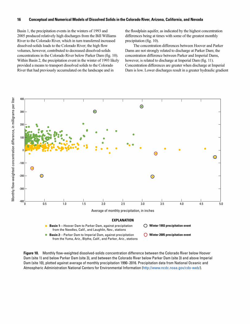
differences are not strongly related to evapotranspiration (fig. 9). The concentration differences are also not strongly related to precipitation within the study area (fig. 10). Infrequent extraordinary precipitation events, such as the events in winter 1993 and the winter of 2005, however, do affect dissolved-solids concentrations in the Colorado River (figs. 8 and 10). Within
Mon
thly
flow
-wei
ghte
d co
ncen
tratio
n d
iffer
ence
, in m
illigr
ams p
er lit
er
350
300
250
200
150
100
50
0
1990 1995 2000 2005 2010 2015
-50
-250
-200
-150
-100
Year
Basin 1—Hoover Dam to Parker DamBasin 2—Parker Dam to Imperial Dam
EXPLANATION
Mon
thly
flow
-wei
ghte
d co
ncen
tratio
n
diff
eren
ce, i
n m
illig
ram
s pe
r lite
r
Monthly evapotranspiration, in acre-feet
0
50
100
150
200
250
0 50,000 100,000 150,000 200,000 250,000
-200
-150
-100
-50
-250
Basin 1—Hoover Dam to Parker Dam, against evapotranspiration between Hoover and Parker DamsBasin 2—Parker Dam to Imperial Dam, against evapotranspiration between Parker and Imperial Dams
EXPLANATION
16 Conceptual and Numerical Models of Dissolved Solids in the Colorado River, Arizona, California, and Nevada
Basin 1, the precipitation events in the winters of 1993 and 2005 produced relatively high discharges from the Bill Williams River to the Colorado River, which in turn transferred increased dissolved-solids loads to the Colorado River; the high flow volumes, however, contributed to decreased dissolved-solids concentrations in the Colorado River below Parker Dam (fig. 10). Within Basin 2, the precipitation event in the winter of 1993 likely provided a means to transport dissolved solids to the Colorado River that had previously accumulated on the landscape and in
the floodplain aquifer, as indicated by the highest concentration differences being at times with some of the greatest monthly precipitation (fig. 10).
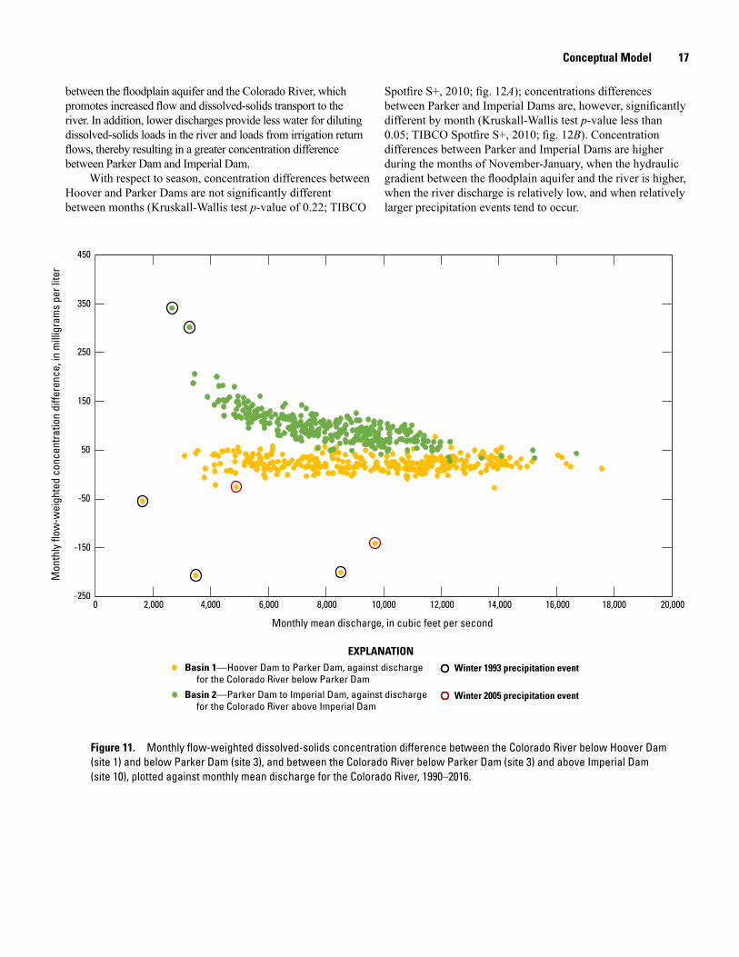
The concentration differences between Hoover and Parker Dams are not strongly related to discharge at Parker Dam; the concentration difference between Parker and Imperial Dams, however, is related to discharge at Imperial Dam (fig. 11). Concentration differences are greater when discharge at Imperial Dam is low. Lower discharges result in a greater hydraulic gradient
Figure 10. Monthly flow-weighted dissolved-solids concentration difference between the Colorado River below Hoover Dam (site 1) and below Parker Dam (site 3), and between the Colorado River below Parker Dam (site 3) and above Imperial Dam (site 10), plotted against average of monthly precipitation 1990–2016. Precipitation data from National Oceanic and Atmospheric Administration National Centers for Environmental Information (http://www.ncdc.noaa.gov/cdo-web/).
Mon
thly
flow
-wei
ghte
d co
ncen
tratio
n di
ffere
nce,
in m
illig
ram
s pe
r lite
r
0
-100
100
-200
200
-300
300
-400
400
0 0.5 1.0 1.5 2.0 2.5 3.0 3.5
Average of monthly precipitation, in inches
5.04.54.0
Basin 1—Hoover Dam to Parker Dam, against precipitation from the Needles, Calif., and Laughlin, Nev., stationsBasin 2—Parker Dam to Imperial Dam, against precipitation from the Yuma, Ariz., Blythe, Calif., and Parker, Ariz., stations
EXPLANATIONWinter 1993 precipitation event
Winter 2005 precipitation event
Conceptual Model 17
Figure 11. Monthly flow-weighted dissolved-solids concentration difference between the Colorado River below Hoover Dam (site 1) and below Parker Dam (site 3), and between the Colorado River below Parker Dam (site 3) and above Imperial Dam (site 10), plotted against monthly mean discharge for the Colorado River, 1990–2016.
Monthly mean discharge, in cubic feet per second
Mon
thly
flow
-wei
ghte
d co
ncen
tratio
n di
ffere
nce,
in m
illig
ram
s pe
r lite
r
EXPLANATIONBasin 1—Hoover Dam to Parker Dam, against discharge for the Colorado River below Parker DamBasin 2—Parker Dam to Imperial Dam, against discharge for the Colorado River above Imperial Dam
Winter 1993 precipitation event
Winter 2005 precipitation event
-250
-150
-50
50
150
250
350
450
0 2,000 4,000 6,000 8,000 10,000 12,000 14,000 16,000 18,000 20,000
between the floodplain aquifer and the Colorado River, which promotes increased flow and dissolved-solids transport to the river. In addition, lower discharges provide less water for diluting dissolved-solids loads in the river and loads from irrigation return flows, thereby resulting in a greater concentration difference between Parker Dam and Imperial Dam.
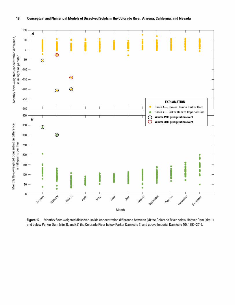
With respect to season, concentration differences between Hoover and Parker Dams are not significantly different between months (Kruskall-Wallis test p-value of 0.22; TIBCO
Spotfire S+, 2010; fig. 12A); concentrations differences between Parker and Imperial Dams are, however, significantly different by month (Kruskall-Wallis test p-value less than 0.05; TIBCO Spotfire S+, 2010; fig. 12B). Concentration differences between Parker and Imperial Dams are higher during the months of November-January, when the hydraulic gradient between the floodplain aquifer and the river is higher, when the river discharge is relatively low, and when relatively larger precipitation events tend to occur.
18 Conceptual and Numerical Models of Dissolved Solids in the Colorado River, Arizona, California, and NevadaM
onth
ly fl
ow-w
eigh
ted
conc
entra
tion
diffe
renc
e,in
mill
igra
ms
per l
iter
-250
-200
-150
-100
-50
0
50
100
-300
A
February
January
May
April
March
August
July
June
December
November
October
September
Mon
thly
flow
-wei
ghte
d co
ncen
tratio
n di
ffere
nce,
in m
illig
ram
s pe
r lite
r
50
100
150
200
250
300
350
400
0
Month
B
Basin 1—Hoover Dam to Parker Dam
Basin 2—Parker Dam to Imperial Dam
Winter 1993 precipitation event
Winter 2005 precipitation event
EXPLANATION
Figure 12. Monthly flow-weighted dissolved-solids concentration difference between (A) the Colorado River below Hoover Dam (site 1) and below Parker Dam (site 3), and (B) the Colorado River below Parker Dam (site 3) and above Imperial Dam (site 10), 1990–2016.
Numerical Model 19
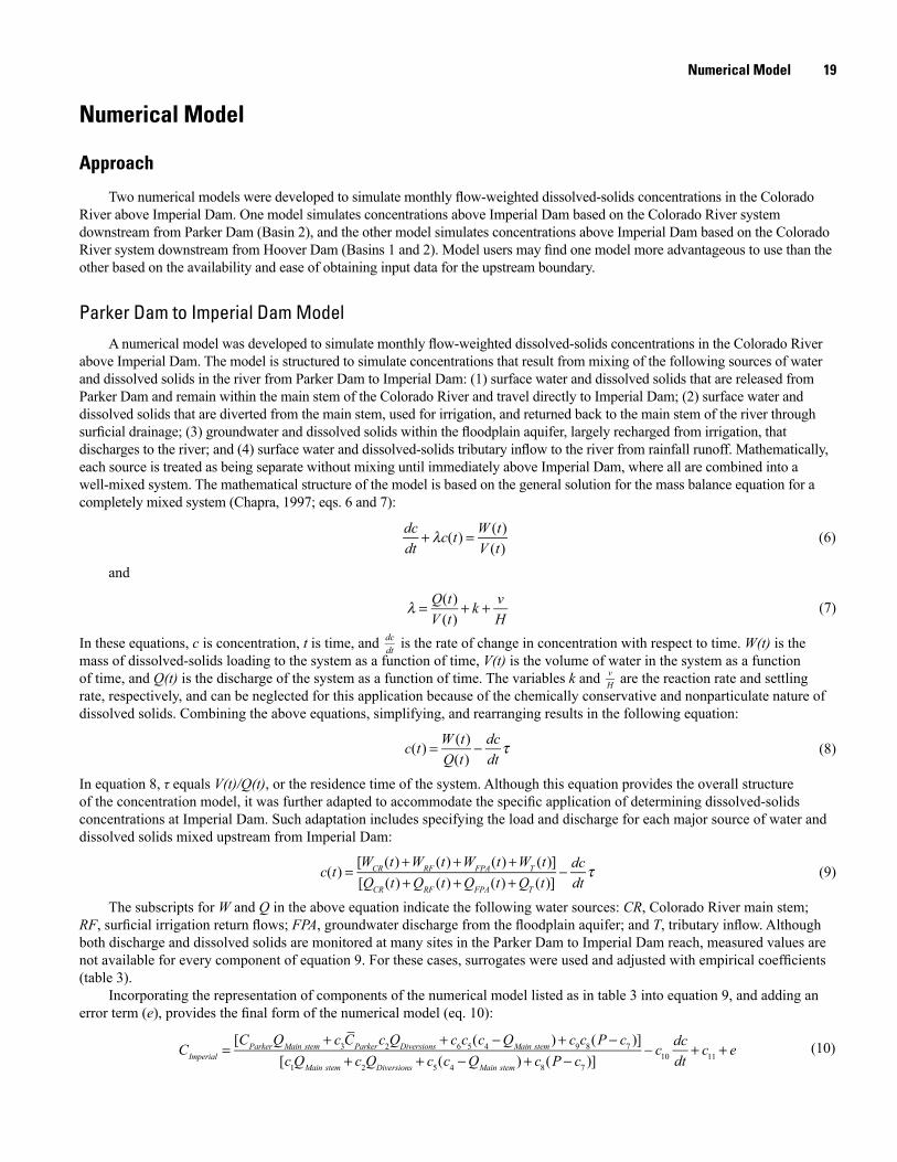
Numerical Model
Approach
Two numerical models were developed to simulate monthly flow-weighted dissolved-solids concentrations in the Colorado River above Imperial Dam. One model simulates concentrations above Imperial Dam based on the Colorado River system downstream from Parker Dam (Basin 2), and the other model simulates concentrations above Imperial Dam based on the Colorado River system downstream from Hoover Dam (Basins 1 and 2). Model users may find one model more advantageous to use than the other based on the availability and ease of obtaining input data for the upstream boundary.
Parker Dam to Imperial Dam ModelA numerical model was developed to simulate monthly flow-weighted dissolved-solids concentrations in the Colorado River
above Imperial Dam. The model is structured to simulate concentrations that result from mixing of the following sources of water and dissolved solids in the river from Parker Dam to Imperial Dam: (1) surface water and dissolved solids that are released from Parker Dam and remain within the main stem of the Colorado River and travel directly to Imperial Dam; (2) surface water and dissolved solids that are diverted from the main stem, used for irrigation, and returned back to the main stem of the river through surficial drainage; (3) groundwater and dissolved solids within the floodplain aquifer, largely recharged from irrigation, that discharges to the river; and (4) surface water and dissolved-solids tributary inflow to the river from rainfall runoff. Mathematically, each source is treated as being separate without mixing until immediately above Imperial Dam, where all are combined into a well-mixed system. The mathematical structure of the model is based on the general solution for the mass balance equation for a completely mixed system (Chapra, 1997; eqs. 6 and 7): (6)
and
(7)
In these equations, c is concentration, t is time, and dcdt is the rate of change in concentration with respect to time. W(t) is the mass of dissolved-solids loading to the system as a function of time, V(t) is the volume of water in the system as a function of time, and Q(t) is the discharge of the system as a function of time. The variables k and vH are the reaction rate and settling rate, respectively, and can be neglected for this application because of the chemically conservative and nonparticulate nature of dissolved solids. Combining the above equations, simplifying, and rearranging results in the following equation:
(8)
In equation 8, τ equals V(t)/Q(t), or the residence time of the system. Although this equation provides the overall structure of the concentration model, it was further adapted to accommodate the specific application of determining dissolved-solids concentrations at Imperial Dam. Such adaptation includes specifying the load and discharge for each major source of water and dissolved solids mixed upstream from Imperial Dam:
(9)
The subscripts for W and Q in the above equation indicate the following water sources: CR, Colorado River main stem; RF, surficial irrigation return flows; FPA, groundwater discharge from the floodplain aquifer; and T, tributary inflow. Although both discharge and dissolved solids are monitored at many sites in the Parker Dam to Imperial Dam reach, measured values are not available for every component of equation 9. For these cases, surrogates were used and adjusted with empirical coefficients (table 3).
Incorporating the representation of components of the numerical model listed as in table 3 into equation 9, and adding an error term (e), provides the final form of the numerical model (eq. 10):
(10)
dcdt
+ λc(t) =W (t)V (t)
λ = Q(t)V (t)
+ k + vH
c(t) =[WCR(t)+WRF (t)+WFPA(t)+WT (t)][QCR(t)+QRF (t)+QFPA(t)+QT (t)]
− dcdt
τ
CImperial =[CParkerQMain stem + c3CParkerc2QDiversions + c6c5(c4 −QMain stem )+ c9c8(P − c7 )]
[c1QMain stem + c2QDiversions + c5(c4 −QMain stem )+ c8(P − c7 )]− c10
dcdt
+ c11 + e
c(t) =W (t)Q(t)
− dcdt
τ
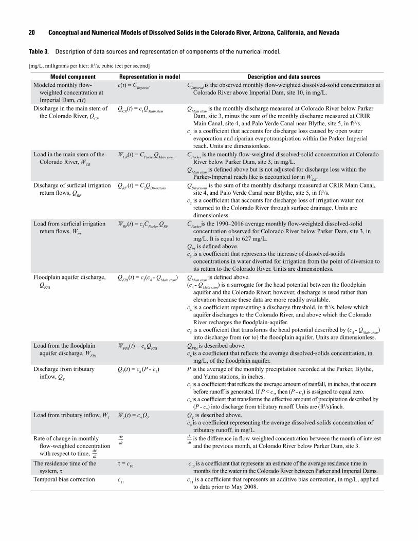
20 Conceptual and Numerical Models of Dissolved Solids in the Colorado River, Arizona, California, and Nevada
Model component Representation in model Description and data sourcesModeled monthly flow-
weighted concentration at Imperial Dam, c(t)
c(t) = CImperial CImperial is the observed monthly flow-weighted dissolved-solid concentration at Colorado River above Imperial Dam, site 10, in mg/L.
Discharge in the main stem of the Colorado River, QCR
QCR(t) = c1QMain stem QMain stem is the monthly discharge measured at Colorado River below Parker Dam, site 3, minus the sum of the monthly discharge measured at CRIR Main Canal, site 4, and Palo Verde Canal near Blythe, site 5, in ft3/s.
c1 is a coefficient that accounts for discharge loss caused by open water evaporation and riparian evapotranspiration within the Parker-Imperial reach. Units are dimensionless.
Load in the main stem of the Colorado River, WCR
WCR(t) = CParkerQMain stem CParker is the monthly flow-weighted dissolved-solid concentration at Colorado River below Parker Dam, site 3, in mg/L.
QMain stem is defined above but is not adjusted for discharge loss within the Parker-Imperial reach like is accounted for in WCR.
Discharge of surficial irrigation return flows, QRF
QRF (t) = C2QDiversions QDiversions is the sum of the monthly discharge measured at CRIR Main Canal, site 4, and Palo Verde Canal near Blythe, site 5, in ft3/s.
c2 is a coefficient that accounts for discharge loss of irrigation water not returned to the Colorado River through surface drainage. Units are dimensionless.
Load from surficial irrigation return flows, WRF
WRF(t) = c3CParker QRF CParkeris the 1990–2016 average monthly flow-weighted dissolved-solid concentration observed for Colorado River below Parker Dam, site 3, in mg/L. It is equal to 627 mg/L.
QRF is defined above.c3 is a coefficient that represents the increase of dissolved-solids
concentrations in water diverted for irrigation from the point of diversion to its return to the Colorado River. Units are dimensionless.
Floodplain aquifer discharge, QFPA
QFPA(t) = c5(c4 ˗ QMain stem) QMain stem is defined above.(c4 ˗ QMain stem) is a surrogate for the head potential between the floodplain
aquifer and the Colorado River; however, discharge is used rather than elevation because these data are more readily available.
c4 is a coefficient representing a discharge threshold, in ft3/s, below which aquifer discharges to the Colorado River, and above which the Colorado River recharges the floodplain-aquifer.
c5 is a coefficient that transforms the head potential described by (c4 ˗ QMain stem) into discharge from (or to) the floodplain aquifer. Units are dimensionless.
Load from the floodplain aquifer discharge, WFPA
WFPA(t) = c6 QFPA QFPA is described above.c6 is a coefficient that reflects the average dissolved-solids concentration, in
mg/L, of the floodplain aquifer.Discharge from tributary
inflow, QT
QT(t) = c8 (P ˗ c7) P is the average of the monthly precipitation recorded at the Parker, Blythe, and Yuma stations, in inches.
c7 is a coefficient that reflects the average amount of rainfall, in inches, that occurs before runoff is generated. If P < c7, then (P ˗ c7) is assigned to equal zero.
c8 is a coefficient that transforms the effective amount of precipitation described by (P ˗ c7) into discharge from tributary runoff. Units are (ft3/s)/inch.
Load from tributary inflow, WT WT(t) = c9 QT QT is described above.c9 is a coefficient representing the average dissolved-solids concentration of
tributary runoff, in mg/L. Rate of change in monthly
flow-weighted concentration with respect to time, dcdt
is the difference in flow-weighted concentration between the month of interest and the previous month, at Colorado River below Parker Dam, site 3.
The residence time of the system, τ
τ = c10 c10 is a coefficient that represents an estimate of the average residence time in months for the water in the Colorado River between Parker and Imperial Dams.
Temporal bias correction c11 c11 is a coefficient that represents an additive bias correction, in mg/L, applied to data prior to May 2008.
dcdt
Table 3. Description of data sources and representation of components of the numerical model.
[mg/L, milligrams per liter; ft3/s, cubic feet per second]
dcdt
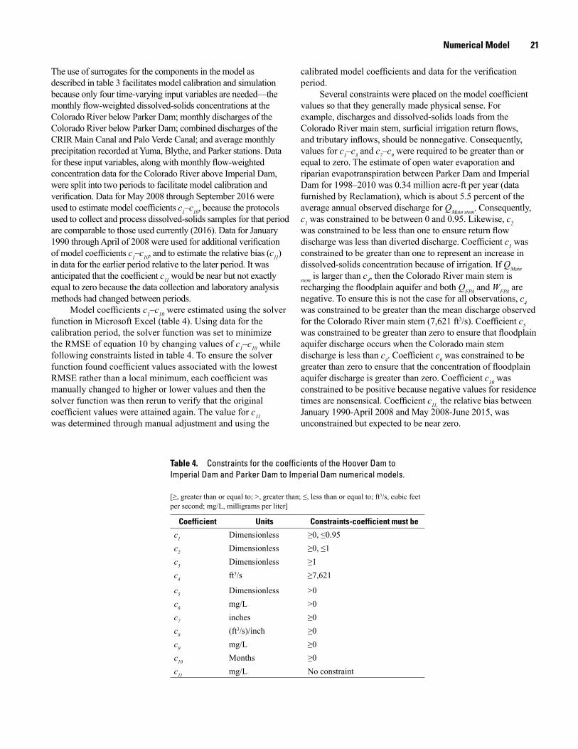
Numerical Model 21
The use of surrogates for the components in the model as described in table 3 facilitates model calibration and simulation because only four time-varying input variables are needed—the monthly flow-weighted dissolved-solids concentrations at the Colorado River below Parker Dam; monthly discharges of the Colorado River below Parker Dam; combined discharges of the CRIR Main Canal and Palo Verde Canal; and average monthly precipitation recorded at Yuma, Blythe, and Parker stations. Data for these input variables, along with monthly flow-weighted concentration data for the Colorado River above Imperial Dam, were split into two periods to facilitate model calibration and verification. Data for May 2008 through September 2016 were used to estimate model coefficients c1–c10, because the protocols used to collect and process dissolved-solids samples for that period are comparable to those used currently (2016). Data for January 1990 through April of 2008 were used for additional verification of model coefficients c1–c10, and to estimate the relative bias (c11) in data for the earlier period relative to the later period. It was anticipated that the coefficient c11 would be near but not exactly equal to zero because the data collection and laboratory analysis methods had changed between periods.
Model coefficients c1–c10 were estimated using the solver function in Microsoft Excel (table 4). Using data for the calibration period, the solver function was set to minimize the RMSE of equation 10 by changing values of c1–c10 while following constraints listed in table 4. To ensure the solver function found coefficient values associated with the lowest RMSE rather than a local minimum, each coefficient was manually changed to higher or lower values and then the solver function was then rerun to verify that the original coefficient values were attained again. The value for c11 was determined through manual adjustment and using the
Table 4. Constraints for the coefficients of the Hoover Dam to Imperial Dam and Parker Dam to Imperial Dam numerical models.
[≥, greater than or equal to; >, greater than; ≤, less than or equal to; ft3/s, cubic feet per second; mg/L, milligrams per liter]
Coefficient Units Constraints-coefficient must bec1 Dimensionless ≥0, ≤0.95c2 Dimensionless ≥0, ≤1c3 Dimensionless ≥1c4 ft3/s ≥7,621
c5 Dimensionless >0c6 mg/L >0c7 inches ≥0c8 (ft3/s)/inch ≥0c9 mg/L ≥0c10 Months ≥0c11 mg/L No constraint
calibrated model coefficients and data for the verification period.
Several constraints were placed on the model coefficient values so that they generally made physical sense. For example, discharges and dissolved-solids loads from the Colorado River main stem, surficial irrigation return flows, and tributary inflows, should be nonnegative. Consequently, values for c1–c3 and c7–c9 were required to be greater than or equal to zero. The estimate of open water evaporation and riparian evapotranspiration between Parker Dam and Imperial Dam for 1998–2010 was 0.34 million acre-ft per year (data furnished by Reclamation), which is about 5.5 percent of the average annual observed discharge for QMain stem. Consequently, c1 was constrained to be between 0 and 0.95. Likewise, c2 was constrained to be less than one to ensure return flow discharge was less than diverted discharge. Coefficient c3 was constrained to be greater than one to represent an increase in dissolved-solids concentration because of irrigation. If QMain
stem is larger than c4, then the Colorado River main stem is recharging the floodplain aquifer and both QFPA and WFPA are negative. To ensure this is not the case for all observations, c4 was constrained to be greater than the mean discharge observed for the Colorado River main stem (7,621 ft3/s). Coefficient c5 was constrained to be greater than zero to ensure that floodplain aquifer discharge occurs when the Colorado main stem discharge is less than c4. Coefficient c6 was constrained to be greater than zero to ensure that the concentration of floodplain aquifer discharge is greater than zero. Coefficient c10 was constrained to be positive because negative values for residence times are nonsensical. Coefficient c11, the relative bias between January 1990-April 2008 and May 2008-June 2015, was unconstrained but expected to be near zero.
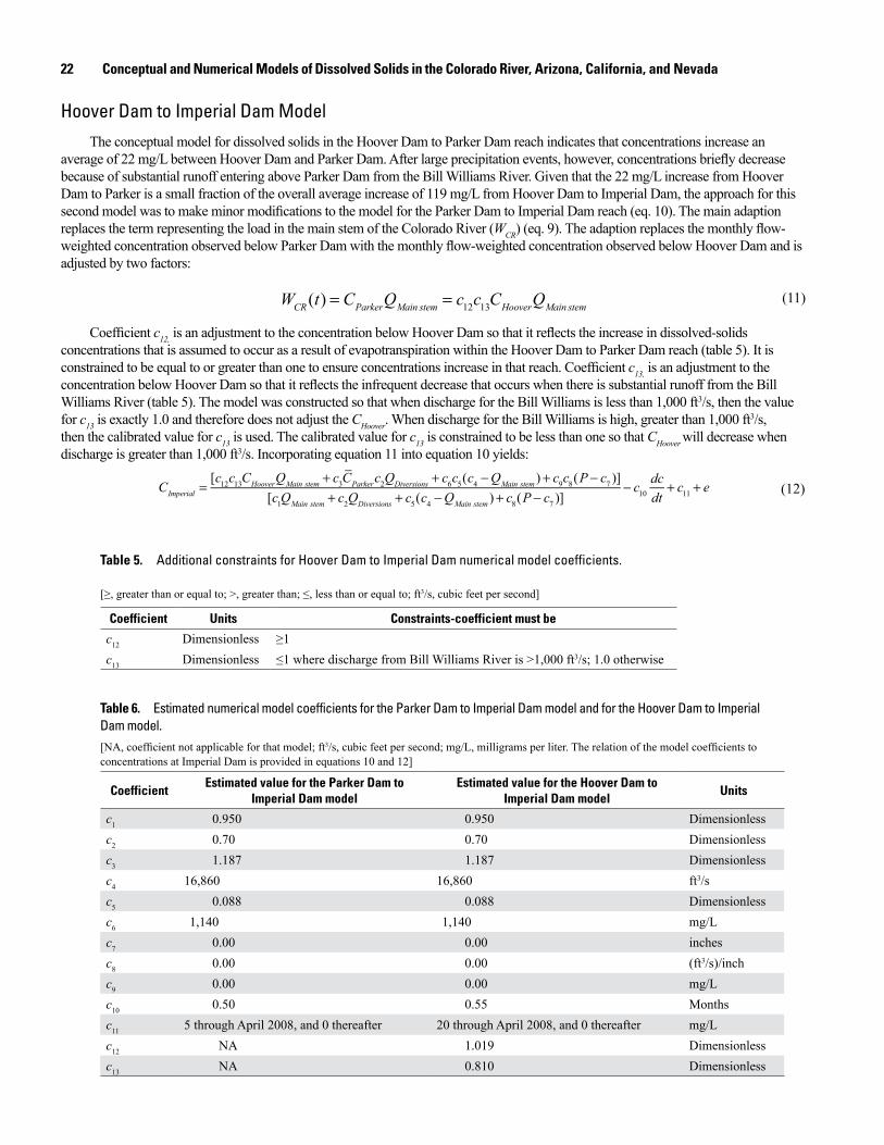
22 Conceptual and Numerical Models of Dissolved Solids in the Colorado River, Arizona, California, and Nevada
Hoover Dam to Imperial Dam ModelThe conceptual model for dissolved solids in the Hoover Dam to Parker Dam reach indicates that concentrations increase an
average of 22 mg/L between Hoover Dam and Parker Dam. After large precipitation events, however, concentrations briefly decrease because of substantial runoff entering above Parker Dam from the Bill Williams River. Given that the 22 mg/L increase from Hoover Dam to Parker is a small fraction of the overall average increase of 119 mg/L from Hoover Dam to Imperial Dam, the approach for this second model was to make minor modifications to the model for the Parker Dam to Imperial Dam reach (eq. 10). The main adaption replaces the term representing the load in the main stem of the Colorado River (WCR) (eq. 9). The adaption replaces the monthly flow-weighted concentration observed below Parker Dam with the monthly flow-weighted concentration observed below Hoover Dam and is adjusted by two factors:
(11)
Coefficient c12, is an adjustment to the concentration below Hoover Dam so that it reflects the increase in dissolved-solids concentrations that is assumed to occur as a result of evapotranspiration within the Hoover Dam to Parker Dam reach (table 5). It is constrained to be equal to or greater than one to ensure concentrations increase in that reach. Coefficient c13, is an adjustment to the concentration below Hoover Dam so that it reflects the infrequent decrease that occurs when there is substantial runoff from the Bill Williams River (table 5). The model was constructed so that when discharge for the Bill Williams is less than 1,000 ft3/s, then the value for c13 is exactly 1.0 and therefore does not adjust the CHoover. When discharge for the Bill Williams is high, greater than 1,000 ft3/s, then the calibrated value for c13 is used. The calibrated value for c13 is constrained to be less than one so that CHoover will decrease when discharge is greater than 1,000 ft3/s. Incorporating equation 11 into equation 10 yields:
(12)CImperial =[c12c13CHooverQMain stem + c3CParkerc2QDiversions + c6c5(c4 −QMain stem )+ c9c8(P − c7 )]
[c1QMain stem + c2QDiversions + c5(c4 −QMain stem )+ c8(P − c7 )]− c10
dcdt
+ c11 + e
Table 5. Additional constraints for Hoover Dam to Imperial Dam numerical model coefficients.
[≥, greater than or equal to; >, greater than; ≤, less than or equal to; ft3/s, cubic feet per second]
Coefficient Units Constraints-coefficient must bec12 Dimensionless ≥1c13 Dimensionless ≤1 where discharge from Bill Williams River is >1,000 ft3/s; 1.0 otherwise
Table 6. Estimated numerical model coefficients for the Parker Dam to Imperial Dam model and for the Hoover Dam to Imperial Dam model. [NA, coefficient not applicable for that model; ft3/s, cubic feet per second; mg/L, milligrams per liter. The relation of the model coefficients to concentrations at Imperial Dam is provided in equations 10 and 12]
Coefficient Estimated value for the Parker Dam to Imperial Dam model
Estimated value for the Hoover Dam to Imperial Dam model Units
c1 0.950 0.950 Dimensionlessc2 0.70 0.70 Dimensionlessc3 1.187 1.187 Dimensionlessc4 16,860 16,860 ft3/s c5 0.088 0.088 Dimensionlessc6 1,140 1,140 mg/Lc7 0.00 0.00 inchesc8 0.00 0.00 (ft3/s)/inchc9 0.00 0.00 mg/Lc10 0.50 0.55 Monthsc11 5 through April 2008, and 0 thereafter 20 through April 2008, and 0 thereafter mg/Lc12 NA 1.019 Dimensionlessc13 NA 0.810 Dimensionless
WCR(t) = CParkerQMain stem = c12c13CHooverQMain stem
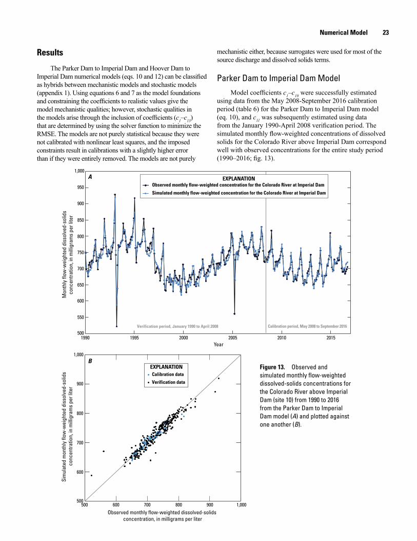
Numerical Model 23
Results
The Parker Dam to Imperial Dam and Hoover Dam to Imperial Dam numerical models (eqs. 10 and 12) can be classified as hybrids between mechanistic models and stochastic models (appendix 1). Using equations 6 and 7 as the model foundations and constraining the coefficients to realistic values give the model mechanistic qualities; however, stochastic qualities in the models arise through the inclusion of coefficients (c1–c13) that are determined by using the solver function to minimize the RMSE. The models are not purely statistical because they were not calibrated with nonlinear least squares, and the imposed constraints result in calibrations with a slightly higher error than if they were entirely removed. The models are not purely
mechanistic either, because surrogates were used for most of the source discharge and dissolved solids terms.
Parker Dam to Imperial Dam ModelModel coefficients c1–c10 were successfully estimated
using data from the May 2008-September 2016 calibration period (table 6) for the Parker Dam to Imperial Dam model (eq. 10), and c11 was subsequently estimated using data from the January 1990-April 2008 verification period. The simulated monthly flow-weighted concentrations of dissolved solids for the Colorado River above Imperial Dam correspond well with observed concentrations for the entire study period (1990–2016; fig. 13).
Observed mon th ly flow-weig h ted con cen tration for th e Colorado River at Imperial Dam
Simulated mon th ly flow-weig h ted con cen tration for th e Colorado River at Imperial Dam
Calibration period, May 2008 to September 2016Verification period, Jan uary 1990 to April 2008
Mon
thly
flow
-wei
ghte
d di
ssol
ved-
solid
s
conc
entra
tion,
in m
illig
ram
s pe
r lite
r
500
550
600
650
700
750
800
850
900
950
1,000
1990 1995 2000 2005 2010 2015Year
EXPLANATIONA
B
Calibration dataVerification data
Sim
ulat
ed m
onth
ly fl
ow-w
eigh
ted
diss
olve
d-so
lids
conc
entra
tion,
in m
illig
ram
s pe
r lite
r
500
600
700
800
900
1,000
Observed monthly flow-weighted dissolved-solids concentration, in milligrams per liter
500 600 700 800 900 1,000
EXPLANATION Figure 13. Observed and simulated monthly flow-weighted dissolved-solids concentrations for the Colorado River above Imperial Dam (site 10) from 1990 to 2016 from the Parker Dam to Imperial Dam model (A) and plotted against one another (B).
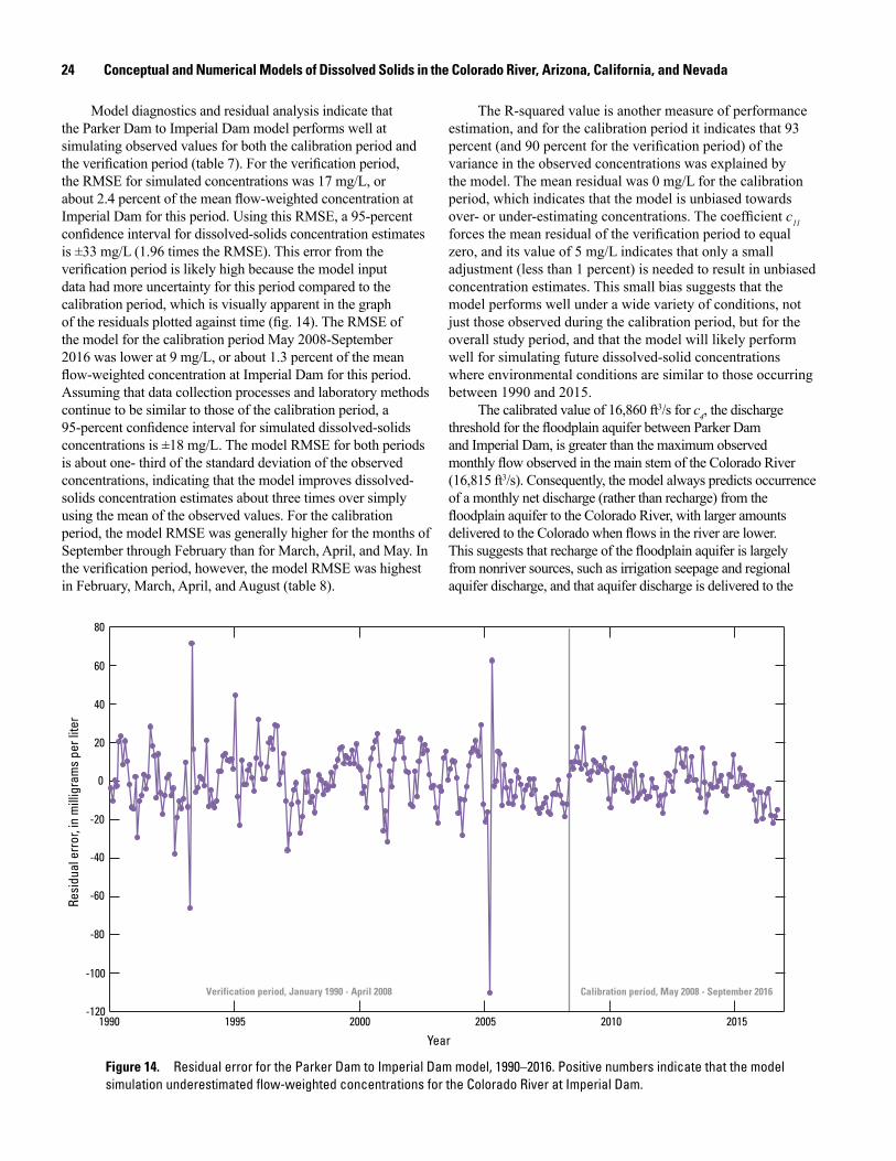
24 Conceptual and Numerical Models of Dissolved Solids in the Colorado River, Arizona, California, and Nevada
Model diagnostics and residual analysis indicate that the Parker Dam to Imperial Dam model performs well at simulating observed values for both the calibration period and the verification period (table 7). For the verification period, the RMSE for simulated concentrations was 17 mg/L, or about 2.4 percent of the mean flow-weighted concentration at Imperial Dam for this period. Using this RMSE, a 95-percent confidence interval for dissolved-solids concentration estimates is ±33 mg/L (1.96 times the RMSE). This error from the verification period is likely high because the model input data had more uncertainty for this period compared to the calibration period, which is visually apparent in the graph of the residuals plotted against time (fig. 14). The RMSE of the model for the calibration period May 2008-September 2016 was lower at 9 mg/L, or about 1.3 percent of the mean flow-weighted concentration at Imperial Dam for this period. Assuming that data collection processes and laboratory methods continue to be similar to those of the calibration period, a 95-percent confidence interval for simulated dissolved-solids concentrations is ±18 mg/L. The model RMSE for both periods is about one- third of the standard deviation of the observed concentrations, indicating that the model improves dissolved-solids concentration estimates about three times over simply using the mean of the observed values. For the calibration period, the model RMSE was generally higher for the months of September through February than for March, April, and May. In the verification period, however, the model RMSE was highest in February, March, April, and August (table 8).
The R-squared value is another measure of performance estimation, and for the calibration period it indicates that 93 percent (and 90 percent for the verification period) of the variance in the observed concentrations was explained by the model. The mean residual was 0 mg/L for the calibration period, which indicates that the model is unbiased towards over- or under-estimating concentrations. The coefficient c11 forces the mean residual of the verification period to equal zero, and its value of 5 mg/L indicates that only a small adjustment (less than 1 percent) is needed to result in unbiased concentration estimates. This small bias suggests that the model performs well under a wide variety of conditions, not just those observed during the calibration period, but for the overall study period, and that the model will likely perform well for simulating future dissolved-solid concentrations where environmental conditions are similar to those occurring between 1990 and 2015.
The calibrated value of 16,860 ft3/s for c4, the discharge threshold for the floodplain aquifer between Parker Dam and Imperial Dam, is greater than the maximum observed monthly flow observed in the main stem of the Colorado River (16,815 ft3/s). Consequently, the model always predicts occurrence of a monthly net discharge (rather than recharge) from the floodplain aquifer to the Colorado River, with larger amounts delivered to the Colorado when flows in the river are lower. This suggests that recharge of the floodplain aquifer is largely from nonriver sources, such as irrigation seepage and regional aquifer discharge, and that aquifer discharge is delivered to the
Figure 14. Residual error for the Parker Dam to Imperial Dam model, 1990–2016. Positive numbers indicate that the model simulation underestimated flow-weighted concentrations for the Colorado River at Imperial Dam.
Resi
dual
err
or, i
n m
illig
ram
s pe
r lite
r
Calibratio n perio d, May 2008 - September 2016Verificatio n perio d, Jan u ary 1990 - April 2008
-100
-80
-60
-40
-20
0
20
40
60
1990 1995 2000 2005 2010 2015
Year
80
-120
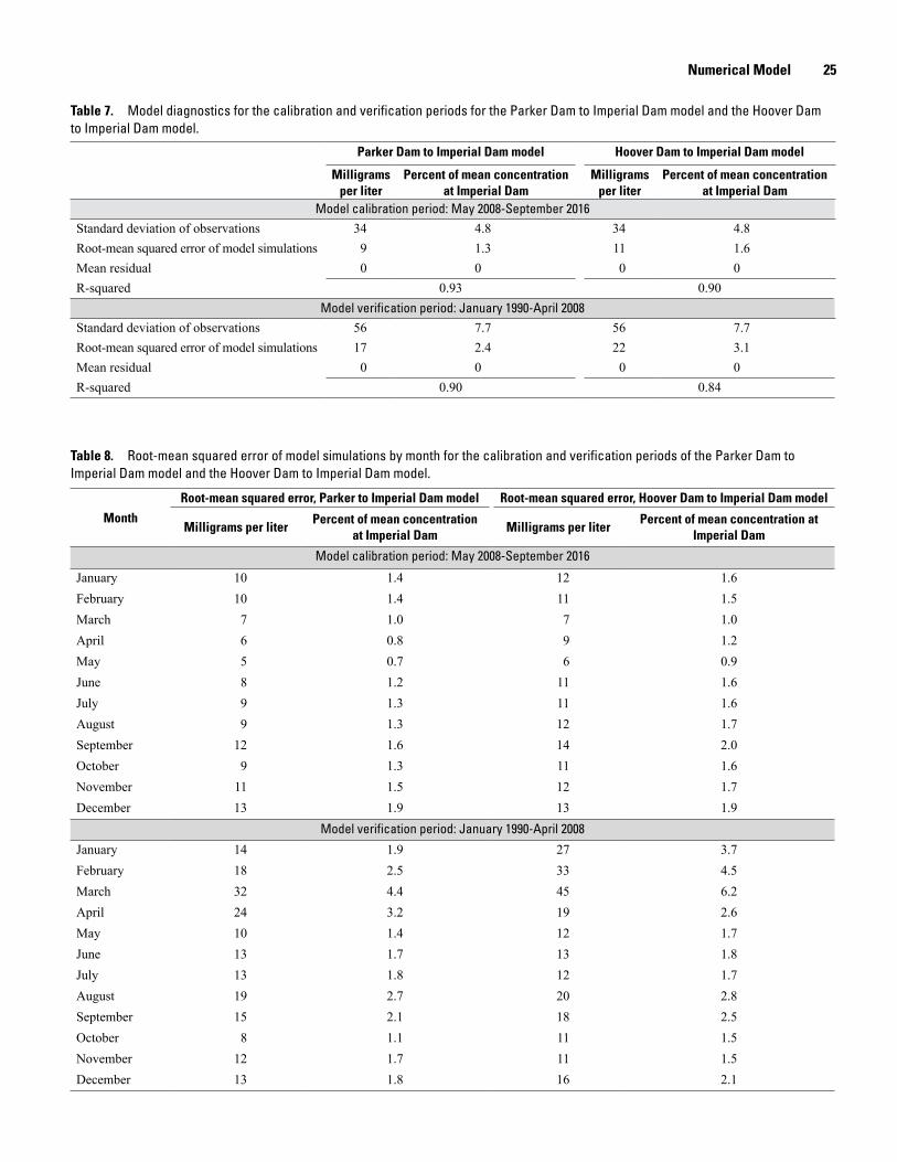
Numerical Model 25
Table 7. Model diagnostics for the calibration and verification periods for the Parker Dam to Imperial Dam model and the Hoover Dam to Imperial Dam model.
Parker Dam to Imperial Dam model Hoover Dam to Imperial Dam model
Milligrams per liter
Percent of mean concentration at Imperial Dam
Milligrams per liter
Percent of mean concentration at Imperial Dam
Model calibration period: May 2008-September 2016Standard deviation of observations 34 4.8 34 4.8Root-mean squared error of model simulations 9 1.3 11 1.6Mean residual 0 0 0 0R-squared 0.93 0.90
Model verification period: January 1990-April 2008Standard deviation of observations 56 7.7 56 7.7Root-mean squared error of model simulations 17 2.4 22 3.1Mean residual 0 0 0 0R-squared 0.90 0.84
Table 8. Root-mean squared error of model simulations by month for the calibration and verification periods of the Parker Dam to Imperial Dam model and the Hoover Dam to Imperial Dam model.
MonthRoot-mean squared error, Parker to Imperial Dam model Root-mean squared error, Hoover Dam to Imperial Dam model
Milligrams per liter Percent of mean concentration at Imperial Dam Milligrams per liter Percent of mean concentration at
Imperial DamModel calibration period: May 2008-September 2016
January 10 1.4 12 1.6February 10 1.4 11 1.5March 7 1.0 7 1.0April 6 0.8 9 1.2May 5 0.7 6 0.9June 8 1.2 11 1.6July 9 1.3 11 1.6August 9 1.3 12 1.7September 12 1.6 14 2.0October 9 1.3 11 1.6November 11 1.5 12 1.7December 13 1.9 13 1.9
Model verification period: January 1990-April 2008January 14 1.9 27 3.7February 18 2.5 33 4.5March 32 4.4 45 6.2April 24 3.2 19 2.6May 10 1.4 12 1.7June 13 1.7 13 1.8July 13 1.8 12 1.7August 19 2.7 20 2.8September 15 2.1 18 2.5October 8 1.1 11 1.5November 12 1.7 11 1.5December 13 1.8 16 2.1
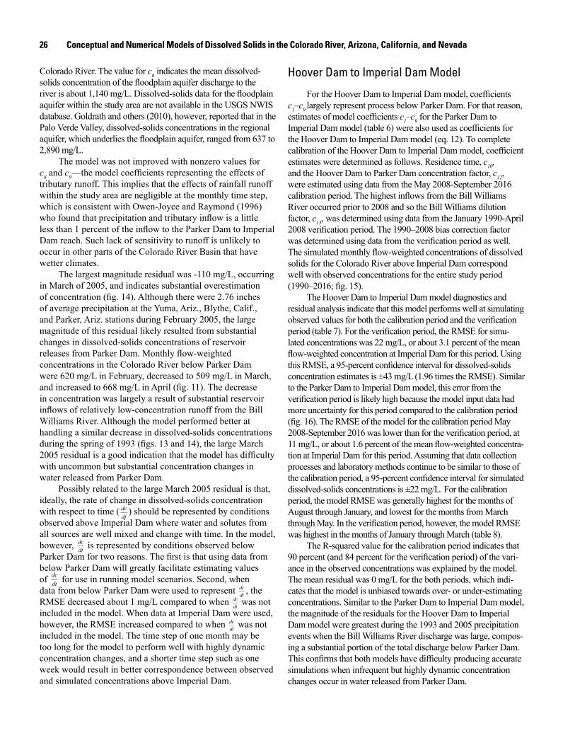
26 Conceptual and Numerical Models of Dissolved Solids in the Colorado River, Arizona, California, and Nevada
Colorado River. The value for c6 indicates the mean dissolved-solids concentration of the floodplain aquifer discharge to the river is about 1,140 mg/L. Dissolved-solids data for the floodplain aquifer within the study area are not available in the USGS NWIS database. Goldrath and others (2010), however, reported that in the Palo Verde Valley, dissolved-solids concentrations in the regional aquifer, which underlies the floodplain aquifer, ranged from 637 to 2,890 mg/L.
The model was not improved with nonzero values for c8 and c9—the model coefficients representing the effects of tributary runoff. This implies that the effects of rainfall runoff within the study area are negligible at the monthly time step, which is consistent with Owen-Joyce and Raymond (1996) who found that precipitation and tributary inflow is a little less than 1 percent of the inflow to the Parker Dam to Imperial Dam reach. Such lack of sensitivity to runoff is unlikely to occur in other parts of the Colorado River Basin that have wetter climates.
The largest magnitude residual was -110 mg/L, occurring in March of 2005, and indicates substantial overestimation of concentration (fig. 14). Although there were 2.76 inches of average precipitation at the Yuma, Ariz., Blythe, Calif., and Parker, Ariz. stations during February 2005, the large magnitude of this residual likely resulted from substantial changes in dissolved-solids concentrations of reservoir releases from Parker Dam. Monthly flow-weighted concentrations in the Colorado River below Parker Dam were 620 mg/L in February, decreased to 509 mg/L in March, and increased to 668 mg/L in April (fig. 11). The decrease in concentration was largely a result of substantial reservoir inflows of relatively low-concentration runoff from the Bill Williams River. Although the model performed better at handling a similar decrease in dissolved-solids concentrations during the spring of 1993 (figs. 13 and 14), the large March 2005 residual is a good indication that the model has difficulty with uncommon but substantial concentration changes in water released from Parker Dam.
Possibly related to the large March 2005 residual is that, ideally, the rate of change in dissolved-solids concentration with respect to time ( dc
dt) should be represented by conditions
observed above Imperial Dam where water and solutes from all sources are well mixed and change with time. In the model, however, dcdt is represented by conditions observed below Parker Dam for two reasons. The first is that using data from below Parker Dam will greatly facilitate estimating values of dcdt for use in running model scenarios. Second, when data from below Parker Dam were used to represent dcdt , the RMSE decreased about 1 mg/L compared to when dc
dt was not
included in the model. When data at Imperial Dam were used, however, the RMSE increased compared to when dcdt was not included in the model. The time step of one month may be too long for the model to perform well with highly dynamic concentration changes, and a shorter time step such as one week would result in better correspondence between observed and simulated concentrations above Imperial Dam.
Hoover Dam to Imperial Dam Model
For the Hoover Dam to Imperial Dam model, coefficients c1–c9 largely represent process below Parker Dam. For that reason, estimates of model coefficients c1–c9 for the Parker Dam to Imperial Dam model (table 6) were also used as coefficients for the Hoover Dam to Imperial Dam model (eq. 12). To complete calibration of the Hoover Dam to Imperial Dam model, coefficient estimates were determined as follows. Residence time, c10, and the Hoover Dam to Parker Dam concentration factor, c12, were estimated using data from the May 2008-September 2016 calibration period. The highest inflows from the Bill Williams River occurred prior to 2008 and so the Bill Williams dilution factor, c13, was determined using data from the January 1990-April 2008 verification period. The 1990–2008 bias correction factor was determined using data from the verification period as well. The simulated monthly flow-weighted concentrations of dissolved solids for the Colorado River above Imperial Dam correspond well with observed concentrations for the entire study period (1990–2016; fig. 15).
The Hoover Dam to Imperial Dam model diagnostics and residual analysis indicate that this model performs well at simulating observed values for both the calibration period and the verification period (table 7). For the verification period, the RMSE for simu-lated concentrations was 22 mg/L, or about 3.1 percent of the mean flow-weighted concentration at Imperial Dam for this period. Using this RMSE, a 95-percent confidence interval for dissolved-solids concentration estimates is ±43 mg/L (1.96 times the RMSE). Similar to the Parker Dam to Imperial Dam model, this error from the verification period is likely high because the model input data had more uncertainty for this period compared to the calibration period (fig. 16). The RMSE of the model for the calibration period May 2008-September 2016 was lower than for the verification period, at 11 mg/L, or about 1.6 percent of the mean flow-weighted concentra-tion at Imperial Dam for this period. Assuming that data collection processes and laboratory methods continue to be similar to those of the calibration period, a 95-percent confidence interval for simulated dissolved-solids concentrations is ±22 mg/L. For the calibration period, the model RMSE was generally highest for the months of August through January, and lowest for the months from March through May. In the verification period, however, the model RMSE was highest in the months of January through March (table 8).
The R-squared value for the calibration period indicates that 90 percent (and 84 percent for the verification period) of the vari-ance in the observed concentrations was explained by the model. The mean residual was 0 mg/L for the both periods, which indi-cates that the model is unbiased towards over- or under-estimating concentrations. Similar to the Parker Dam to Imperial Dam model, the magnitude of the residuals for the Hoover Dam to Imperial Dam model were greatest during the 1993 and 2005 precipitation events when the Bill Williams River discharge was large, compos-ing a substantial portion of the total discharge below Parker Dam. This confirms that both models have difficulty producing accurate simulations when infrequent but highly dynamic concentration changes occur in water released from Parker Dam.
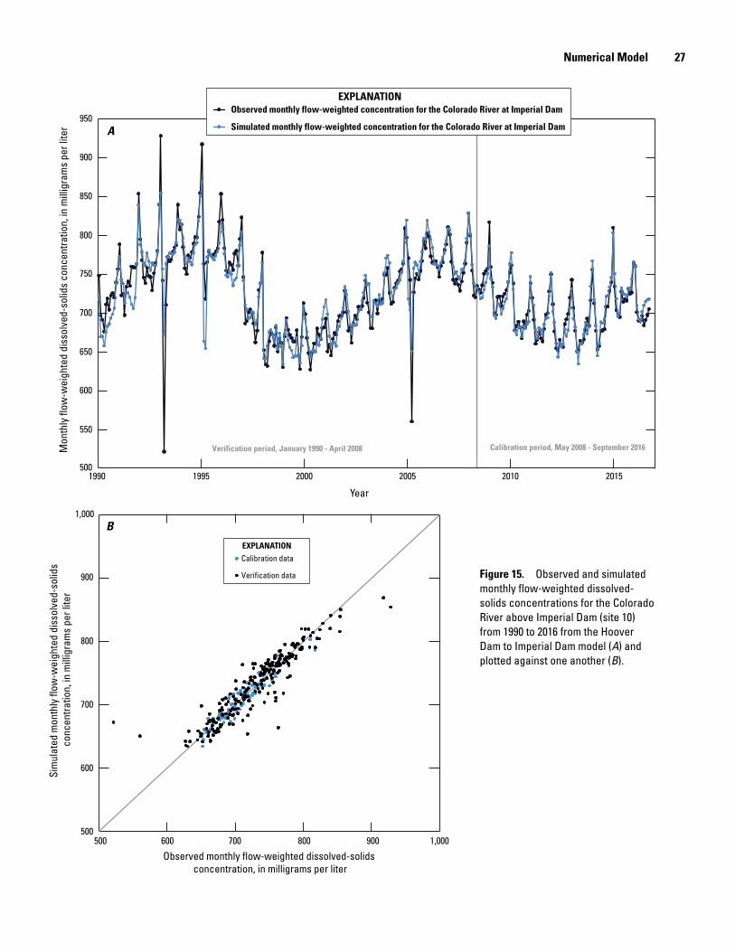
Numerical Model 27
Observed mo n th ly flo w-weig h ted co n cen tratio n fo r th e Co lo rado River at Imperial Dam
Simulated mo n th ly flo w-weig h ted co n cen tratio n fo r th e Co lo rado River at Imperial Dam
Calibratio n perio d, May 2008 - September 2016Verificatio n perio d, Jan uary 1990 - April 2008
A
Mon
thly
flow
-wei
ghte
d di
ssol
ved-
solid
s co
ncen
tratio
n, in
mill
igra
ms
per l
iter
500
550
600
650
700
750
800
850
900
950
1990 1995 2000 2005 2010 2015
Year
EXPLANATION
B
Calibration data
Verification data
Sim
ulat
ed m
onth
ly fl
ow-w
eigh
ted
diss
olve
d-so
lids
conc
entra
tion,
in m
illig
ram
s pe
r lite
r
500
600
700
800
900
1,000
Observed monthly flow-weighted dissolved-solids concentration, in milligrams per liter
500 600 700 800 900 1,000
EXPLANATION
Figure 15. Observed and simulated monthly flow-weighted dissolved-solids concentrations for the Colorado River above Imperial Dam (site 10) from 1990 to 2016 from the Hoover Dam to Imperial Dam model (A) and plotted against one another (B).
28 Conceptual and Numerical Models of Dissolved Solids in the Colorado River, Arizona, California, and Nevada
Interpretations of model coefficients c1-c9 made for the Parker Dam to Imperial Dam model also apply to the Hoover Dam to Imperial Dam model, and the values for coefficients c10-c13 provide additional hydrologic insight. The value for coefficient c10, residence time, is slightly larger for the Hoover Dam to Imperial Dam model than the Parker Dam to Imperial Dam model, which is expected as that reach is longer and residence time therefore should be longer. The value for coefficient c11 (20 mg/L, or 2.8 percent of the average concentration at Imperial Dam) is 15 mg/L greater than that for the Parker Dam to Imperial Dam model, which indicates a greater amount of bias for this model that occurs between the verification period and the calibration period. If the gain in concentration between Hoover Dam and Parker Dam is attributed largely to evapotranspiration, then the value for coefficient c12 (1.019) suggests that the average rate of open water evaporation and riparian evapotranspiration is about 1.9 percent of the average flow in that reach. This is a slight underestimation compared to Reclamation’s estimate that average annual open water evaporation and riparian evapotranspiration loss in this reach from 1998–2010 was 4.0 percent of the average flow below Hoover Dam (data furnished by Reclamation). The value for coefficient c13 (0.81) indicates that the concentration in the main stem of the Colorado River below Parker Dam is reduced about 19 percent when there are high flows entering from the Bill Williams
Figure 16. Residual error for the Hoover Dam to Imperial Dam model, 1990–2016. Positive numbers indicate that the model simulation underestimated flow-weighted concentrations for the Colorado River at Imperial Dam.
Resi
dual
err
or, i
n m
illig
ram
s pe
r lite
r
Calibratio n perio d, May 2008 - September 2016Verificatio n perio d, Jan u ary 1990 - April 2008
-160
-80
-40
0
40
80
1990 1995 2000 2005 2010 2015
Year
120
-120
River. The 1993 high flow event in the Bill Williams River reduced the dissolved solids concentration in the Colorado River below Parker Dam by about 14 percent.
Comparison of Root-mean Square Error and Measurement Error
A coarse-scale error analysis indicates that measurement error of the model input data is small, but composes a substantial component of the RMSE for the Parker Dam to Imperial Dam and the Hoover Dam to Imperial Dam models. An approximation of the measurement error included in the RMSE for the Parker Dam to Imperial Dam model can be estimated as the square root of the sum of squared percent errors for each measured term in equation 10, assuming such errors are not correlated. For the Parker Dam to Imperial Dam model, measurement data come from two dissolved-solids monitoring stations and from three discharge monitoring stations. For this analysis, measurement error of monthly dissolved-solids concentrations is assumed to be about equal to the previously noted sample concentration variability of about 0.5 percent for the Colorado River above Imperial Dam. This error neglects the decrease in uncertainty that results from using multiple samples to determine the monthly concentration estimate, the increase in uncertainty that results from using simple mathematical procedures for estimating
Numerical Model 29
monthly concentrations from the sample concentrations, and the increase in uncertainty that results from bias associated with the sampling and analysis of the dissolved-solids data that is not included in the sample variability estimate. For the monthly discharge data, it is assumed that the measurement error for each station is about 0.40 percent. This estimate is based on the median estimated uncertainty for annual discharge at Colorado River below Parker Dam, 1995–99 (Anning, 2002). The actual measurement error for monthly discharges is likely greater because the time period of one month is shorter than one year, but this will be neglected given the coarse nature of this analysis. Given these estimates for error in individual measurements and combining them in quadrature, the resultant coarse estimate of measurement error contained in the model input data is (0.52+0.52+0.42+0.42+0.42)0.5=0.9 percent. Consequently, measurement error within the model input data accounts for a substantial portion of the resulting RMSE for the Parker Dam to Imperial Dam model (0.9 of the 1.3 percent for the calibration period, and 0.9 of the 2.4 percent for the verification period). Neglecting the contribution of error from the Bill Williams River measurements, the coarse estimate of measurement error for the Hoover Dam to Imperial Dam is the same as that for the Parker Dam to Imperial Dam model, 0.9 percent.
Model Sensitivity and Insight for Running Model Scenarios The use of the Parker Dam to Imperial Dam model may be preferred because the RMSE of this model is 2 mg/L lower
than the Hoover Dam to Imperial model, assuming equal ability to obtain model input data. If model input data are more readily available, or accurate, for the Hoover Dam to Imperial Dam model, then it is likely worth the small increase in uncertainty for using this model over the Parker to Imperial model. Use of either model (eqs. 10 and 12) requires the simulation analyst to assemble input datasets (appendix 2). In order to put an appropriate amount of resources into assembling input variable data, the analyst needs to understand the sensitivity of the simulated concentrations at Imperial Dam to each input variable. Sensitivity for the Parker Dam to Imperial Dam model was assessed by examining the changes in simulated concentrations that result from changing the input data across the distribution of their observed values for the study period. Equation 10 describes the model in a form that facilitates understanding how concentrations at Imperial Dam are a function of the flows and loads of four water and solute sources. For use in simulating concentrations for various scenarios, however, the equation can be simplified by replacing the terms with the calibrated model coefficients (table 6) and measured input variables based on relations described in equation 10:
(13)
In this simplification, c11 is zero and therefore equation 13 is valid for simulating concentrations after April 2008. Equation 13 is not only more convenient than equation 10 for simulating concentrations of future scenarios, but it also benefits
the sensitivity analysis in that it reduces dependence between variables. In equation 10 there are four input variables; however, these are various combinations of five observed values measured in three locations (dissolved-solids concentrations for the current month and for the previous month below Parker Dam, discharge below Parker Dam, and discharge diverted into two different canals; table 3). Because the model input variables are combinations, they are not completely independent. In addition, there could be correlations between some variables, such as discharge below Parker Dam and discharge for diversions into the canals.
For the sensitivity analysis, three of the four input variables (CParker, QParker, QDiversions, and dcdt of equation 13 were held constant at their median value, and dissolved-solids concentrations were simulated while values for the fourth variable was varied from its minimum value, 5th percentile, 10th percentile, 25th percentile, 50th percentile, 75th percentile, 90th percentile, 95th percentile, and maximum value (table 9). Examining the difference in concentration simulations for the 95th percentile and the 5th percentile of input data, the largest magnitude changes in concentration are -121 mg/L for the monthly discharge at the Colorado River below Parker Dam, and 114 mg/L for the monthly flow-weighted concentration at the Colorado River below Parker Dam. The difference in simulations for the 95th percentile and the 5th percentile of rate of change in concentration data with respect to time, and of combined discharge at CRIR Main Canal and Palo Verde Main Canal, are considerably smaller at -12 mg/L and 27 mg/L, respectively.
The sensitivity analysis was repeated but for the Hoover Dam to Imperial Dam model (table 10). Given the similar math-ematical structure for the two models, results are very similar. For use in simulating concentrations for various scenarios the model can be simplified by replacing the terms with the calibrated model coefficients (table 6) and measured input variables based on relations described in equation 12: (14)
In this simplification, c11 is zero and therefore equation 14 is valid for simulating concentrations after April 2008. In addition, the model user must supply the value for c13 as equal to 0.81 if discharge for the Bill Williams River exceeds 1,000 ft3/s, or equal to 1.0 otherwise.
CImperial =[(CParker −100.32)QParker + (621.29−CParker )QDiversions +1,691,395]
[(0.862)QParker − (0.162)QDiversions +1,483.68]− 0.50 dc
dt
CImperial =[(1.019C13CHoover −100.32)QParker + (621.29−1.019C13CHoover )QDiversions +1,691,395]
[(0.862)QParker − (0.162)QDiversions +1,483.68]− 0.50 dc
dt
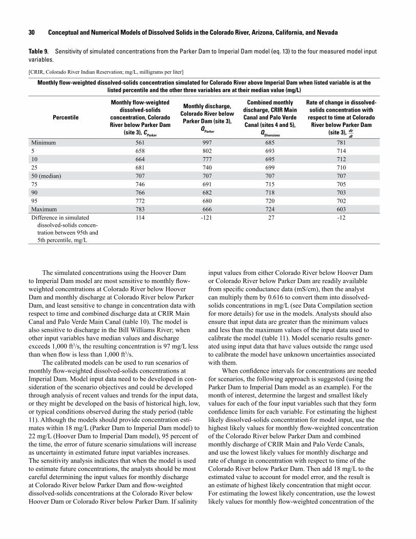
30 Conceptual and Numerical Models of Dissolved Solids in the Colorado River, Arizona, California, and Nevada
The simulated concentrations using the Hoover Dam to Imperial Dam model are most sensitive to monthly flow-weighted concentrations at Colorado River below Hoover Dam and monthly discharge at Colorado River below Parker Dam, and least sensitive to change in concentration data with respect to time and combined discharge data at CRIR Main Canal and Palo Verde Main Canal (table 10). The model is also sensitive to discharge in the Bill Williams River; when other input variables have median values and discharge exceeds 1,000 ft3/s, the resulting concentration is 97 mg/L less than when flow is less than 1,000 ft3/s.
The calibrated models can be used to run scenarios of monthly flow-weighted dissolved-solids concentrations at Imperial Dam. Model input data need to be developed in con-sideration of the scenario objectives and could be developed through analysis of recent values and trends for the input data, or they might be developed on the basis of historical high, low, or typical conditions observed during the study period (table 11). Although the models should provide concentration esti-mates within 18 mg/L (Parker Dam to Imperial Dam model) to 22 mg/L (Hoover Dam to Imperial Dam model), 95 percent of the time, the error of future scenario simulations will increase as uncertainty in estimated future input variables increases. The sensitivity analysis indicates that when the model is used to estimate future concentrations, the analysts should be most careful determining the input values for monthly discharge at Colorado River below Parker Dam and flow-weighted dissolved-solids concentrations at the Colorado River below Hoover Dam or Colorado River below Parker Dam. If salinity
Table 9. Sensitivity of simulated concentrations from the Parker Dam to Imperial Dam model (eq. 13) to the four measured model input variables.
Monthly flow-weighted dissolved-solids concentration simulated for Colorado River above Imperial Dam when listed variable is at the listed percentile and the other three variables are at their median value (mg/L)
Percentile
Monthly flow-weighted dissolved-solids
concentration, Colorado River below Parker Dam
(site 3), CParker
Monthly discharge, Colorado River below Parker Dam (site 3),
QParker
Combined monthly discharge, CRIR Main Canal and Palo Verde Canal (sites 4 and 5),
QDiversions
Rate of change in dissolved-solids concentration with
respect to time at Colorado River below Parker Dam
(site 3), dcdt
Minimum 561 997 685 7815 658 802 693 71410 664 777 695 71225 681 740 699 71050 (median) 707 707 707 70775 746 691 715 70590 766 682 718 70395 772 680 720 702Maximum 783 666 724 603Difference in simulated
dissolved-solids concen-tration between 95th and 5th percentile, mg/L
114 -121 27 -12
[CRIR, Colorado River Indian Reservation; mg/L, milligrams per liter]
input values from either Colorado River below Hoover Dam or Colorado River below Parker Dam are readily available from specific conductance data (mS/cm), then the analyst can multiply them by 0.616 to convert them into dissolved-solids concentrations in mg/L (see Data Compilation section for more details) for use in the models. Analysts should also ensure that input data are greater than the minimum values and less than the maximum values of the input data used to calibrate the model (table 11). Model scenario results gener-ated using input data that have values outside the range used to calibrate the model have unknown uncertainties associated with them.
When confidence intervals for concentrations are needed for scenarios, the following approach is suggested (using the Parker Dam to Imperial Dam model as an example). For the month of interest, determine the largest and smallest likely values for each of the four input variables such that they form confidence limits for each variable. For estimating the highest likely dissolved-solids concentration for model input, use the highest likely values for monthly flow-weighted concentration of the Colorado River below Parker Dam and combined monthly discharge of CRIR Main and Palo Verde Canals, and use the lowest likely values for monthly discharge and rate of change in concentration with respect to time of the Colorado River below Parker Dam. Then add 18 mg/L to the estimated value to account for model error, and the result is an estimate of highest likely concentration that might occur. For estimating the lowest likely concentration, use the lowest likely values for monthly flow-weighted concentration of the
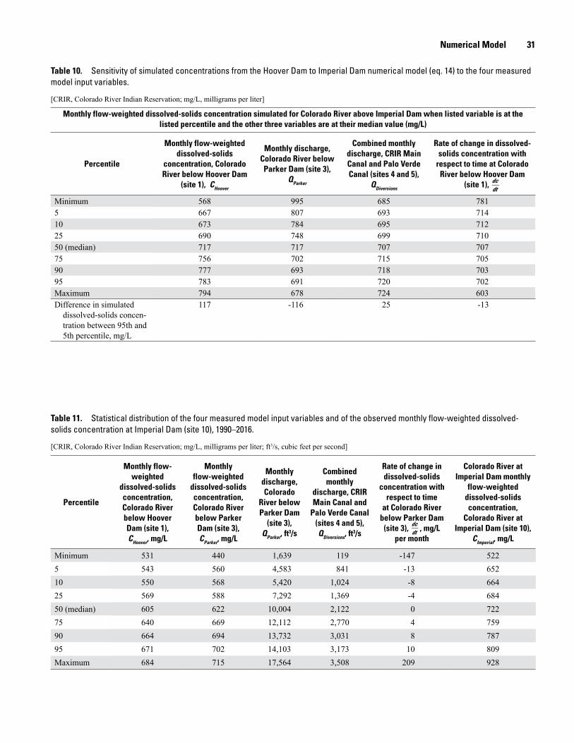
Numerical Model 31
Table 10. Sensitivity of simulated concentrations from the Hoover Dam to Imperial Dam numerical model (eq. 14) to the four measured model input variables.
[CRIR, Colorado River Indian Reservation; mg/L, milligrams per liter]
Monthly flow-weighted dissolved-solids concentration simulated for Colorado River above Imperial Dam when listed variable is at the listed percentile and the other three variables are at their median value (mg/L)
Percentile
Monthly flow-weighted dissolved-solids
concentration, Colorado River below Hoover Dam
(site 1), CHoover
Monthly discharge, Colorado River below Parker Dam (site 3),
QParker
Combined monthly discharge, CRIR Main Canal and Palo Verde Canal (sites 4 and 5),
QDiversions
Rate of change in dissolved-solids concentration with
respect to time at Colorado River below Hoover Dam
(site 1), dcdt
Minimum 568 995 685 7815 667 807 693 71410 673 784 695 71225 690 748 699 71050 (median) 717 717 707 70775 756 702 715 70590 777 693 718 70395 783 691 720 702Maximum 794 678 724 603Difference in simulated
dissolved-solids concen-tration between 95th and 5th percentile, mg/L
117 -116 25 -13
Table 11. Statistical distribution of the four measured model input variables and of the observed monthly flow-weighted dissolved-solids concentration at Imperial Dam (site 10), 1990–2016.
Percentile
Monthly flow-weighted
dissolved-solids concentration, Colorado River below Hoover Dam (site 1), CHoover, mg/L
Monthly flow-weighted
dissolved-solids concentration, Colorado River below Parker Dam (site 3), CParker, mg/L
Monthly discharge, Colorado
River below Parker Dam
(site 3), QParker, ft
3/s
Combined monthly
discharge, CRIR Main Canal and
Palo Verde Canal (sites 4 and 5), QDiversions, ft
3/s
Rate of change in dissolved-solids
concentration with respect to time
at Colorado River below Parker Dam
(site 3), dcdt , mg/L
per month
Colorado River at Imperial Dam monthly
flow-weighted dissolved-solids concentration,
Colorado River at Imperial Dam (site 10),
CImperial, mg/L
Minimum 531 440 1,639 119 -147 5225 543 560 4,583 841 -13 65210 550 568 5,420 1,024 -8 66425 569 588 7,292 1,369 -4 68450 (median) 605 622 10,004 2,122 0 72275 640 669 12,112 2,770 4 75990 664 694 13,732 3,031 8 78795 671 702 14,103 3,173 10 809Maximum 684 715 17,564 3,508 209 928
[CRIR, Colorado River Indian Reservation; mg/L, milligrams per liter; ft3/s, cubic feet per second]
32 Conceptual and Numerical Models of Dissolved Solids in the Colorado River, Arizona, California, and Nevada
Colorado River below Parker Dam and combined monthly discharge of CRIR Main and Palo Verde Canals, and use the highest likely values for monthly discharge and rate of change in concentration with respect to time of the Colorado River below Parker Dam. Then subtract 18 mg/L from the estimated value to attain the lowest likely concentration that might occur. A similar approach is suggested for the Hoover Dam to Imperial Dam model, with the exception that the uncertainty is 22 mg/L, and one would use concentrations and concentration changes over time from Colorado River below Hoover Dam rather than Colorado River below Parker Dam.
On a final note, any major physical changes made within the contributing area between Hoover Dam and Imperial Dam, especially in the floodplain or the channel of the Colorado River, could alter the source and transport characteristics of dissolved solids within the reach and may require model recalibration. Such changes could include new diversions, improvement of drainage systems, substantial channel alterations, or widespread changes in agricultural practices. As monitoring of model input data continues, the model calibration can be verified by entering those data into the model and assessing how well the observed and predicted monthly flow-weighted concentrations at Imperial Dam correspond over time. Consistent and significant deviations of residuals from zero may indicate the need to recalibrate the model.
Summary and ConclusionsThe objective of this study was to provide the Bureau
of Reclamation with the capability to simulate salinity (as dissolved solids) of the Colorado River at Imperial Dam. The ability to simulate dissolved-solids concentrations at this location will aid Reclamation in meeting the binational agreement on the volume and salinity of Colorado River water delivered to Mexico. A robust spatial- and temporal-resolution dataset was generated that consists of river discharge and dissolved-solids concentration and load information between January 1990 and September 2016 for 10 sites on canals, drains, tributaries, and the main stem of the Colorado River between Hoover and Imperial Dams. Daily mean dissolved-solids concentrations were estimated, and monthly mean dissolved-solids loads were computed for each site. Spatial and temporal load patterns, and historical and current controls on loads and concentrations, were analyzed in order to develop a conceptual model of dissolved-solids transport between Hoover and Imperial Dams. Two numerical models describing the relations between dissolved-solids concentrations and components controlling dissolved-solids concentration loads were developed, calibrated, and verified.
Between January 1990 and September 2016, there was a 98.8-million-acre-ft loss of water and a 57.0-million-ton loss of dissolved-solids load from the Colorado River between
Hoover and Imperial Dams. Between Hoover and Parker Dams, about 69.0 million acre-ft of water was lost and 51.1 million tons of dissolved solids were lost; between Parker and Imperial Dams, about 29.8 million acre-ft of water was lost and 5.9 million tons of dissolved solids were lost. Water was removed from the river at a relatively consistent rate over the 25-year study period through water transfers to California and Arizona, evapotranspiration from crop irrigation, transpiration processes of riparian vegetation, and evaporation from the river main stem. Dissolved solids were removed from the river between Hoover and Parker Dams at a relatively constant rate through water transfers to California and Arizona, and water pumped from the river for irrigation within the Mohave Valley. The river gains a small amount of dissolved solids from inflow from the Bill Williams River. Between Parker and Imperial Dams, however, dissolved solids were not removed from the river at a consistent rate over the study period. Dissolved solids were generally removed from the river from 1990 to 2012, then gained by the river from 2012 to 2015, and then removed from the river from 2015 through 2016. Dissolved solids are assumed to be removed from the river and accumulated within the floodplain sediments and aquifers during irrigation processes; some dissolved solids may also be removed from the river through uptake by crops and riparian vegetation. Dissolved solids accumulated on the landscape and in the floodplain aquifer during irrigation are transported to the river, causing a gain in dissolved solids in the river, during periods when the hydraulic gradient between the floodplain aquifer and the river is increased. Dissolved-solids gains in the river occur during periods of relatively low river discharge, such as during the winter months and during drier climatic conditions.
Two numerical models were developed to simulate monthly flow-weighted dissolved-solids concentrations in the Colorado River at Imperial Dam; one for the Parker Dam to Imperial Dam reach, and another for the Hoover Dam to Imperial Dam reach. Model coefficients of both models were estimated using data from the May 2008-September 2016 calibration period, and the simulated concentrations of dissolved solids correspond well with observed concentrations for the entire study period (1990–2016). The models are more sensitive to monthly discharge at the Colorado River below Parker Dam and monthly flow-weighted dissolved-solid concentrations of the Colorado River below Parker Dam (or Hoover Dam) than to the rate of change in concentration with respect to time and the combined discharge of the CRIR Main Canal and Palo Verde Canal. The calibrated models can be used to run scenarios of monthly flow-weighted dissolved-solids concentrations at Imperial Dam. The models should provide concentration estimates within 18 mg/L (Parker Dam to Imperial Dam model) to 22 mg/L (Hoover Dam to Imperial Dam model) 95 percent of the time, but future scenario error will increase as uncertainty in the estimated future input variables increases.
References Cited 33
References CitedAnning, D.W., 2002, Standard errors of annual discharge and
change in reservoir content data from selected stations in the lower Colorado River streamflow-gaging station network, 1995–99: U.S. Geological Survey Water-Resources Investigations Report 01-4240, 81 p.
Bureau of Reclamation, 2014, Estimates of evapotranspiration and evaporation along the Lower Colorado River, calendar year 2010: Bureau of Reclamation, 106 p. [Available at http://www.usbr.gov/lc/region/g4000/4200Rpts/LCRASRpt/2010/report10.pdf.]
Chapra, S.C., 1997, Surface water-quality modeling: Long Grove, Ill., McGraw-Hill, 844 p.
Goldrath, D.A., Wright, M.T., and Belitz, K., 2010, Groundwater-quality data in the Colorado River study unit, 2007—Results from the California GAMA program: U.S. Geological Survey Data Series 474, 66 p., accessed April 20, 2017, at http://pubs.usgs.gov/ds/474/.
Hem, J.D., 1992, Study and interpretation of the chemical characteristics of natural water: U.S. Geological Survey Water Supply Paper 2254, 263 p. [Available at http://pubs.usgs.gov/wsp/wsp2254/pdf/wsp2254a.pdf.]
Hirsch, R.M., and De Cicco, L.A., 2015, User guide to Exploration and Graphics for RivEr Trends (EGRET) and dataRetrieval—R packages for hydrologic data (ver. 2.0, February 2015): U.S. Geological Survey Techniques and Methods, book 4, chap. A10, 93 p. [Available at http://dx.doi.org/10.3133/tm4A10.]
Hirsch, R.M., Moyer, D.L., and Archfield, S.A., 2010, Weighted Regressions on Time, Discharge, and Season (WRTDS), with an application to Chesapeake Bay River inputs: Journal of the American Water Resources Association, v. 46, no. 5, p. 857–880. [Available at http://onlinelibrary.wiley.com/doi/10.1111/j.1752-1688.2010.00482.x/full.]
International Boundary and Water Commission, 1973, Permanent and definitive solution to the international problem of the salinity of the Colorado River: International Boundary and Water Commission, Minute no. 242, August 30, 1973. [Available at http://www.ibwc.gov/Files/Minutes/Min242.pdf.]
Leake, S.A, Owen-Joyce, S.J., and Heilman, J.A., 2013, Potential depletion of surface water in the Colorado River and agricultural drains by groundwater pumping in the Parker-Palo Verde-Cibola area, Arizona and California: U.S. Geological Survey Scientific Investigations Report 2013–5134, 13 p. [Available at https://pubs.er.usgs.gov/publication/sir20135134.]
Mueller, D.K., Schertz, T.L., Martin, J.D., and Sandstrom, M.W., 2015, Design, analysis, and interpretation of field quality-control data for water-sampling projects: U.S. Geological Survey Techniques and Methods, book 4, chap. C4, 54 p. [Available at http://dx.doi.org/10.3133/tm4C4.]
Owen-Joyce, S.J., and Raymond, L.H., 1996, An accounting system for water and consumptive use along the Colorado River, Hoover Dam to Mexico: U.S. Geological Survey Water-Supply Paper 2407, 94 p. [Available at https://pubs.er.usgs.gov/publication/wsp2407.]
R Development Core Team, 2011, R—A language and environment for statistical computing: R Foundation for Statistical Computing, Vienna, Austria. [Available at http://www.R-project.org/.]
TIBCO Spotfire S+, 2010, TIBCO Spotfire S+ 8.2 for Windows User’s Guide: TIBCO Software Inc., 568 p., accessed April 13, 2017, at https://docs.tibco.com/pub/spotfire_s_plus/8.2.0_november_2010/pdf/TIB_sf_s+_8.2.0_win_user_guide.pdf.
U.S. Geological Survey, 2017, National Water Information System―Web interface: U.S. Geological Survey web page, accessed April 13, 2017, at http://dx.doi.org/10.5066/F7P55KJN.
Wilson, R.P., and Owen-Joyce, S.J., 1994, Method to identify wells that yield water that will be replaced by Colorado River water in Arizona, California, Nevada, and Utah: U.S. Geological Survey Water-Resources Report 94-4005, 19 map sheets, 36 p. [Available at https://pubs.er.usgs.gov/publication/wri944005.]
34 Conceptual and Numerical Models of Dissolved Solids in the Colorado River, Arizona, California, and Nevada
Appendixes
Appendix 1. Parker Dam to Imperial Dam and Hoover Dam to Imperial Dam numerical model of dissolved-solids concentrations for the Colorado River at Imperial Dam.
Appendix 2. Parker Dam to Imperial Dam numerical model simulation and Hoover Dam to Imperial Dam numerical model simulation, and model conversions, statistics, estimations, and coefficients.
Appendix files are available online only, and may be accessed at https://doi.org/10.3133/sir20185108.

Menlo Park Publishing Service Center, CaliforniaManuscript approved August 3, 2018Edited by Katherine JacquesLayout and design by Cory Hurd

Anning and others—Conceptual and Num
erical Models of Dissolved Solids in the Colorado River, Arizona, California, and Nevada—
Scientific Investigations Report 2018–5108
ISSN 2328-0328 (online)https://doi.org/10.3133/sir20185108