computational modeling of the nonlinear stochastic dynamics
TRANSCRIPT
Computational Mechanics manuscript No.(will be inserted by the editor)
Computational modeling of the nonlinear stochastic dynamics ofhorizontal drillstrings
Americo Cunha Jr · Christian Soize · Rubens Sampaio
Received: date / Accepted: date
Abstract This work intends to analyze the nonlinear
stochastic dynamics of drillstrings in horizontal config-
uration. For this purpose, it considers a beam theory,
with effects of rotatory inertia and shear deformation,
which is capable of reproducing the large displacements
that the beam undergoes. The friction and shock effects,
due to beam/borehole wall transversal impacts, as well
as the force and torque induced by bit-rock interaction,
are also considered in the model. Uncertainties of bit-
rock interaction model are taken into account using a
parametric probabilistic approach. Numerical simula-
tions have shown that the mechanical system of inter-
est has a very rich nonlinear stochastic dynamics, which
generate phenomena such as bit-bounce, stick-slip, and
transverse impacts. A study aiming to maximize the
drilling process efficiency, varying drillstring velocitiesof translation and rotation is presented. Also, the work
presents the definition and solution of two optimizations
problems, one deterministic and one robust, where the
objective is to maximize drillstring rate of penetration
into the soil respecting its structural limits.
A. Cunha Jr (corresponding author)Universidade do Estado do Rio de Janeiro, Instituto deMatematica e Estatıstica, Departamento de MatematicaAplicada, Rua Sao Francisco Xavier, 524, Pav. Joao Lyra,Bl. B, Sala 6032, Rio de Janeiro, 20550-900, BrasilE-mail: [email protected]
A. Cunha Jr · C. SoizeUniversite Paris-Est, Laboratoire Modelisation et Simula-tion Multi Echelle, MSME UMR 8208 CNRS, 5, BoulevardDescartes 77454, Marne-la-Vallee, FranceE-mail: [email protected]
A. Cunha Jr · R. SampaioPUC–Rio, Departamento de Engenharia Mecanica, Rua M.de Sao Vicente, 225 - Rio de Janeiro, 22451-900, BrasilE-mail: [email protected]
Keywords nonlinear dynamics · horizontal drillstring ·uncertainty quantification · parametric probabilistic
approach · robust optimization
1 Introduction
High energy demands of 21st century make that fossil
fuels, like oil and shale gas, still have great importance
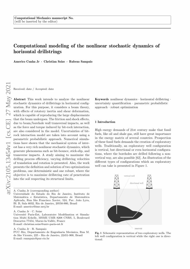
in the energy matrix of several countries. Prospection
of these fossil fuels demands the creation of exploratory
wells. Traditionally, an exploratory well configuration
is vertical, but directional or even horizontal configura-
tions, where the boreholes are drilled following a non-
vertical way, are also possible [62]. An illustration of the
different types of configurations which an exploratorywell can take is presented in Figure 1.
reservoir
vertical well
directional well
Fig. 1 Schematic representation of two exploratory wells. Theleft well configuration is vertical while the right one is direc-tional.
arX
iv:2
105.
1345
4v1
[cs
.CE
] 2
7 M
ay 2
021
2 A. Cunha Jr et al.
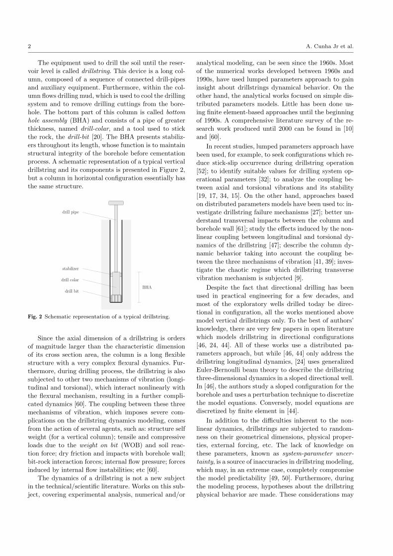
The equipment used to drill the soil until the reser-
voir level is called drillstring. This device is a long col-
umn, composed of a sequence of connected drill-pipes
and auxiliary equipment. Furthermore, within the col-
umn flows drilling mud, which is used to cool the drilling
system and to remove drilling cuttings from the bore-
hole. The bottom part of this column is called bottom
hole assembly (BHA) and consists of a pipe of greater
thickness, named drill-colar, and a tool used to stick
the rock, the drill-bit [20]. The BHA presents stabiliz-
ers throughout its length, whose function is to maintain
structural integrity of the borehole before cementation
process. A schematic representation of a typical vertical
drillstring and its components is presented in Figure 2,
but a column in horizontal configuration essentially has
the same structure.
drill pipe
drill colar
drill bit
stabilizer
BHA
Fig. 2 Schematic representation of a typical drillstring.
Since the axial dimension of a drillstring is orders
of magnitude larger than the characteristic dimension
of its cross section area, the column is a long flexible
structure with a very complex flexural dynamics. Fur-
thermore, during drilling process, the drillstring is also
subjected to other two mechanisms of vibration (longi-
tudinal and torsional), which interact nonlinearly with
the flexural mechanism, resulting in a further compli-
cated dynamics [60]. The coupling between these three
mechanisms of vibration, which imposes severe com-
plications on the drillstring dynamics modeling, comes
from the action of several agents, such as: structure self
weight (for a vertical column); tensile and compressive
loads due to the weight on bit (WOB) and soil reac-
tion force; dry friction and impacts with borehole wall;
bit-rock interaction forces; internal flow pressure; forces
induced by internal flow instabilities; etc [60].
The dynamics of a drillstring is not a new subject
in the technical/scientific literature. Works on this sub-
ject, covering experimental analysis, numerical and/or
analytical modeling, can be seen since the 1960s. Most
of the numerical works developed between 1960s and
1990s, have used lumped parameters approach to gain
insight about drillstrings dynamical behavior. On the
other hand, the analytical works focused on simple dis-
tributed parameters models. Little has been done us-
ing finite element-based approaches until the beginning
of 1990s. A comprehensive literature survey of the re-
search work produced until 2000 can be found in [10]
and [60].
In recent studies, lumped parameters approach have
been used, for example, to seek configurations which re-
duce stick-slip occurrence during drillstring operation
[52]; to identify suitable values for drilling system op-
erational parameters [32]; to analyze the coupling be-
tween axial and torsional vibrations and its stability
[19, 17, 34, 15]. On the other hand, approaches based
on distributed parameters models have been used to: in-
vestigate drillstring failure mechanisms [27]; better un-
derstand transversal impacts between the column and
borehole wall [61]; study the effects induced by the non-
linear coupling between longitudinal and torsional dy-
namics of the drillstring [47]; describe the column dy-
namic behavior taking into account the coupling be-
tween the three mechanisms of vibration [41, 39]; inves-
tigate the chaotic regime which drillstring transverse
vibration mechanism is subjected [9].
Despite the fact that directional drilling has been
used in practical engineering for a few decades, and
most of the exploratory wells drilled today be direc-
tional in configuration, all the works mentioned above
model vertical drillstrings only. To the best of authors’
knowledge, there are very few papers in open literature
which models drillstring in directional configurations
[46, 24, 44]. All of these works use a distributed pa-
rameters approach, but while [46, 44] only address the
drillstring longitudinal dynamics, [24] uses generalized
Euler-Bernoulli beam theory to describe the drillstring
three-dimensional dynamics in a sloped directional well.
In [46], the authors study a sloped configuration for the
borehole and uses a perturbation technique to discretize
the model equations. Conversely, model equations are
discretized by finite element in [44].
In addition to the difficulties inherent to the non-
linear dynamics, drillstrings are subjected to random-
ness on their geometrical dimensions, physical proper-
ties, external forcing, etc. The lack of knowledge on
these parameters, known as system-parameter uncer-
tainty, is a source of inaccuracies in drillstring modeling,
which may, in an extreme case, completely compromise
the model predictability [49, 50]. Furthermore, during
the modeling process, hypotheses about the drillstring
physical behavior are made. These considerations may
Computational modeling of the nonlinear stochastic dynamics of horizontal drillstrings 3
be or not be in agreement with reality and should in-
troduce additional inaccuracies in the model, known as
model uncertainty induced by modeling errors [56, 57].
This source of uncertainty is essentially due to the use of
simplified computational model for describing the phe-
nomenon of interest and, usually, is the largest source of
inaccuracy in computational model responses [56, 57].
Therefore, for a better understanding of the drill-
string dynamics, these uncertainties must be modeled
and quantified. In terms of quantifying these uncer-
tainties for vertical drillstrings, the reader can see [59],
where external forces are modeled as random objects
and the method of statistical linearization is used along
with the Monte Carlo (MC) method to treat the stochas-
tic equations of the model. Other works in this line in-
clude: [41, 39], where system-parameter and model un-
certainties are considered using a nonparametric prob-
abilistic approach; and [43, 40], which use a standard
parametric probabilistic approach to take into account
the uncertainties of the system parameters. Regarding
the works that model directional configurations, only
[44] considers the uncertainties, which, in this case, are
related to the friction effects due to drillstring/borehole
wall contact.
From what is observed above, considering only the
theoretical point of view, the study of drillstring nonlin-
ear dynamics is already a rich subject. However, a good
understanding of its dynamics also has significant im-
portance in applications. For instance, it is fundamental
to predict the fatigue life of the structure [33] and the
drill-bit wear [68]; to analyze the structural integrity of
an exploratory well [14]; to optimize the drill-bit rate of
penetration (ROP) of into the soil [42], and the last is
essential to reduce cost of production of an exploratory
well.
In this sense, this study aims to analyze the three-
dimensional nonlinear dynamics of a drillstring in hor-
izontal configuration, taking into account the system-
parameter uncertainties. Through this study it is ex-
pected to gain a better understanding of drillstring physics
and, thus, to improve drilling process efficiency, and
maximize the column ROP accordingly. All results pre-
sented here were developed in the thesis of [12].
The rest of this work is organized as follows. Sec-
tion 2 presents the mechanical system of interest in
this work, its parametrization and modeling from the
physical point of view. Mathematical formulation of
initial/boundary value problem that describes the me-
chanical system behavior, as well as the conservative
dynamics associated, is shown in section 3. The compu-
tational modeling of the problem, which involves model
equations discretization, reduction of the discretized dy-
namics, the algorithms for numerical integration and
solution of nonlinear system of algebraic equations, can
be seen in section 4. The probabilistic modeling of un-
certainties is presented in section 5. Results of numeri-
cal simulations are presented and discussed in section 6.
Finally, in section 7, the main conclusions are empha-
sized, and some paths to future works are pointed out.
2 Physical model for the problem
2.1 Definition of the mechanical system
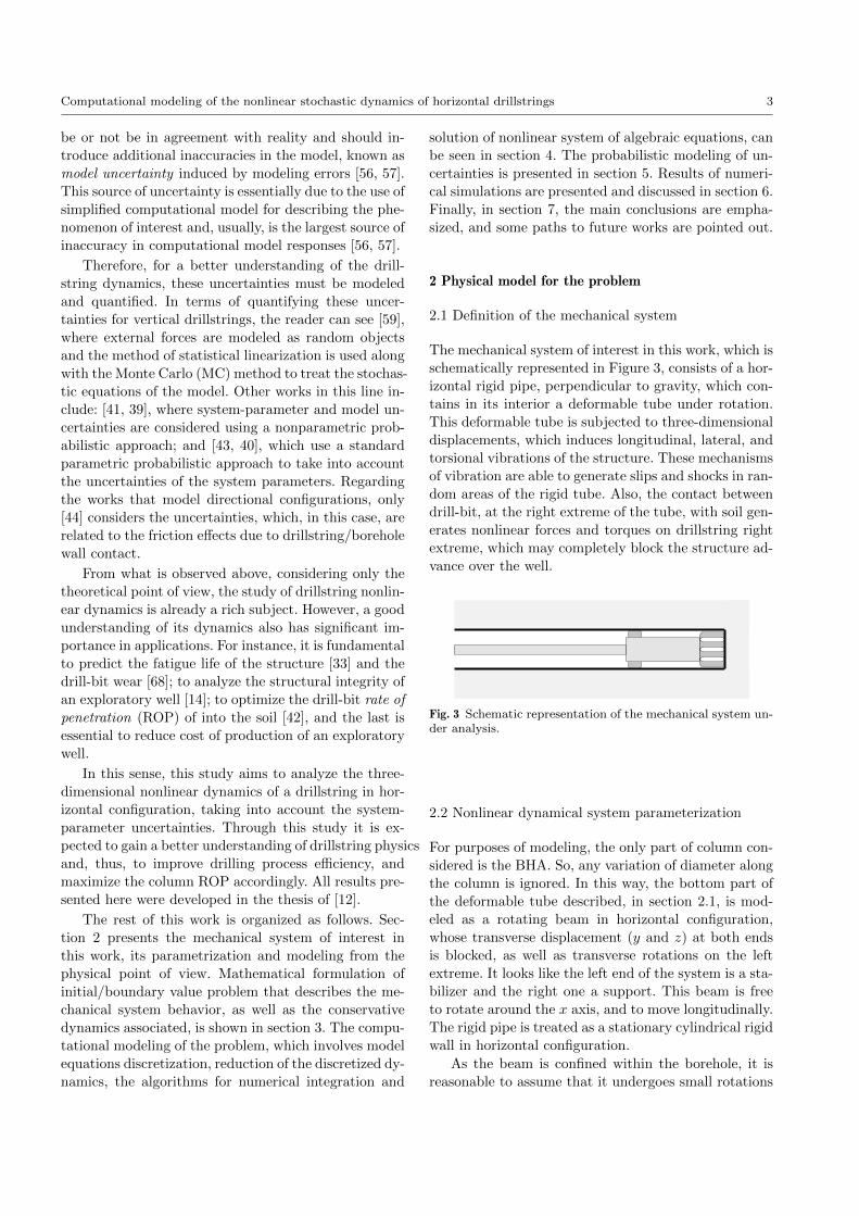
The mechanical system of interest in this work, which is
schematically represented in Figure 3, consists of a hor-
izontal rigid pipe, perpendicular to gravity, which con-
tains in its interior a deformable tube under rotation.
This deformable tube is subjected to three-dimensional
displacements, which induces longitudinal, lateral, and
torsional vibrations of the structure. These mechanisms
of vibration are able to generate slips and shocks in ran-
dom areas of the rigid tube. Also, the contact between
drill-bit, at the right extreme of the tube, with soil gen-
erates nonlinear forces and torques on drillstring right
extreme, which may completely block the structure ad-
vance over the well.
Fig. 3 Schematic representation of the mechanical system un-der analysis.
2.2 Nonlinear dynamical system parameterization
For purposes of modeling, the only part of column con-
sidered is the BHA. So, any variation of diameter along
the column is ignored. In this way, the bottom part of
the deformable tube described, in section 2.1, is mod-
eled as a rotating beam in horizontal configuration,
whose transverse displacement (y and z) at both ends
is blocked, as well as transverse rotations on the left
extreme. It looks like the left end of the system is a sta-
bilizer and the right one a support. This beam is free
to rotate around the x axis, and to move longitudinally.
The rigid pipe is treated as a stationary cylindrical rigid
wall in horizontal configuration.
As the beam is confined within the borehole, it is
reasonable to assume that it undergoes small rotations
4 A. Cunha Jr et al.
in transverse directions. On the other hand, large dis-
placements are observed in x, y, and z, as well as large
rotations around the x-axis. Therefore, the analysis that
follows uses a beam theory which assumes large rotation
in x, large displacements in the three spatial directions,
and small deformations [5].
Seeking not to make the mathematical model exces-
sively complex, this work will not model the fluid flow
inside the beam, nor the dissipation effects induced by
the flow on the system dynamics.
Due to the horizontal configuration, the beam is un-
der action of the gravitational field, which induces an
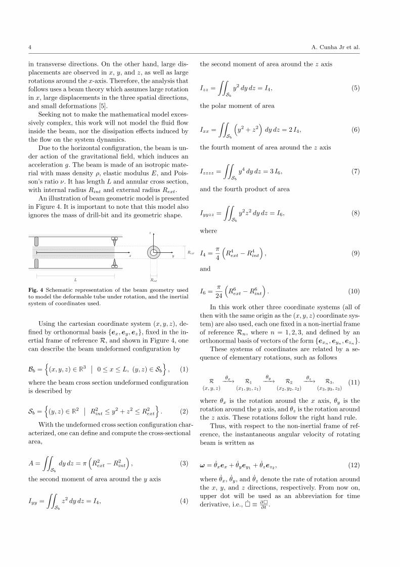
acceleration g. The beam is made of an isotropic mate-
rial with mass density ρ, elastic modulus E, and Pois-
son’s ratio ν. It has length L and annular cross section,
with internal radius Rint and external radius Rext.
An illustration of beam geometric model is presented
in Figure 4. It is important to note that this model also
ignores the mass of drill-bit and its geometric shape.
x
L
y
z
Rext
Rint
Fig. 4 Schematic representation of the beam geometry usedto model the deformable tube under rotation, and the inertialsystem of coordinates used.
Using the cartesian coordinate system (x, y, z), de-
fined by orthonormal basis ex, ey, ez, fixed in the in-
ertial frame of reference R, and shown in Figure 4, one
can describe the beam undeformed configuration by
Bb =
(x, y, z) ∈ R3∣∣ 0 ≤ x ≤ L, (y, z) ∈ Sb
, (1)
where the beam cross section undeformed configuration
is described by
Sb =
(y, z) ∈ R2∣∣ R2
int ≤ y2 + z2 ≤ R2ext
. (2)
With the undeformed cross section configuration char-
acterized, one can define and compute the cross-sectional
area,
A =
∫∫Sbdy dz = π
(R2ext −R2
int
), (3)
the second moment of area around the y axis
Iyy =
∫∫Sbz2 dy dz = I4, (4)
the second moment of area around the z axis
Izz =
∫∫Sby2 dy dz = I4, (5)
the polar moment of area
Ixx =
∫∫Sb
(y2 + z2
)dy dz = 2 I4, (6)
the fourth moment of area around the z axis
Izzzz =
∫∫Sby4 dy dz = 3 I6, (7)
and the fourth product of area
Iyyzz =
∫∫Sby2z2 dy dz = I6, (8)
where
I4 =π
4
(R4ext −R4
int
), (9)
and
I6 =π
24
(R6ext −R6
int
). (10)
In this work other three coordinate systems (all of
then with the same origin as the (x, y, z) coordinate sys-
tem) are also used, each one fixed in a non-inertial frame
of reference Rn, where n = 1, 2, 3, and defined by an
orthonormal basis of vectors of the form exn, eyn , ezn.
These systems of coordinates are related by a se-
quence of elementary rotations, such as follows
R θx−−−→ R1
θy−−−→ R2θz−−−→ R3,
(x, y, z) (x1, y1, z1) (x2, y2, z2) (x3, y3, z3)(11)
where θx is the rotation around the x axis, θy is the
rotation around the y axis, and θz is the rotation around
the z axis. These rotations follow the right hand rule.
Thus, with respect to the non-inertial frame of ref-
erence, the instantaneous angular velocity of rotating
beam is written as
ω = θxex + θyey1 + θzez2 , (12)
where θx, θy, and θz denote the rate of rotation around
the x, y, and z directions, respectively. From now on,
upper dot will be used as an abbreviation for time
derivative, i.e., ≡ ∂∂t .
Computational modeling of the nonlinear stochastic dynamics of horizontal drillstrings 5
Referencing vector ω to the inertial frame of refer-
ence, and using the assumption of small rotations in
transversal directions, one obtains
ω =
θx + θzθyθy cos θx − θz sin θxθy sin θx + θz cos θx
. (13)
Regarding the kinematic hypothesis adopted for beam
theory, it is assumed that the three-dimensional dis-
placement of a beam point, occupying position (x, y, z)
at instant of time t, can be written as
ux(x, y, z, t) = u− yθz + zθy, (14)
uy(x, y, z, t) = v + y (cos θx − 1)− z sin θx,
uz(x, y, z, t) = w + z (cos θx − 1) + y sin θx,
where ux, uy, and uz respectively denote the displace-
ment of a beam point in x, y, and z directions. More-
over, u, v, and w are the displacements of a beam neu-
tral fiber point in x, y, and z directions, respectively.
Finally, it is possible to define the vectors
r =
x
y
z
, v =
u
v
w
, and θ =
θxθyθz
, (15)
which, respectively, represent the position of a beam
point, the velocity of a neutral fiber point, and the rate
of rotation of a neutral fiber point.
Note that the kinematic hypothesis of Eq.(14) is ex-
pressed in terms of three spatial coordinates (x, y, and
z) and six field variables (u, v, w, θx, θy, and θz).
It is important to mention that, as the analysis as-
sumed small rotations in y and z, this kinematic hy-
pothesis presents nonlinearities, expressed by trigono-
metric functions, only in θx. Besides that, since a beam
theory is employed, the field variables in Eq.(14) depend
only on the spatial coordinate x and time t. Therefore,
although the kinematic hypothesis of Eq.(14) is three-
dimensional, the mathematical model used to describe
the beam nonlinear dynamics is one-dimensional.
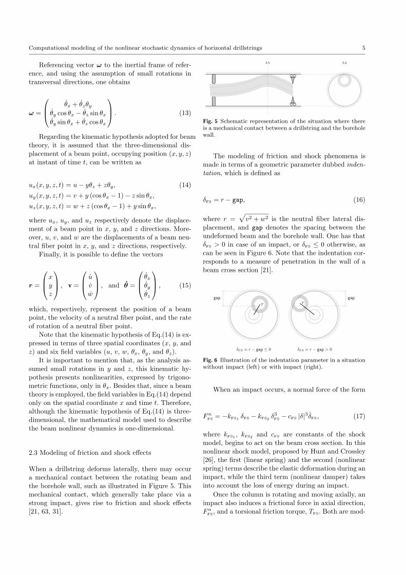
2.3 Modeling of friction and shock effects
When a drillstring deforms laterally, there may occur
a mechanical contact between the rotating beam and
the borehole wall, such as illustrated in Figure 5. This
mechanical contact, which generally take place via a
strong impact, gives rise to friction and shock effects
[21, 63, 31].
AAAA
Fig. 5 Schematic representation of the situation where thereis a mechanical contact between a drillstring and the boreholewall.
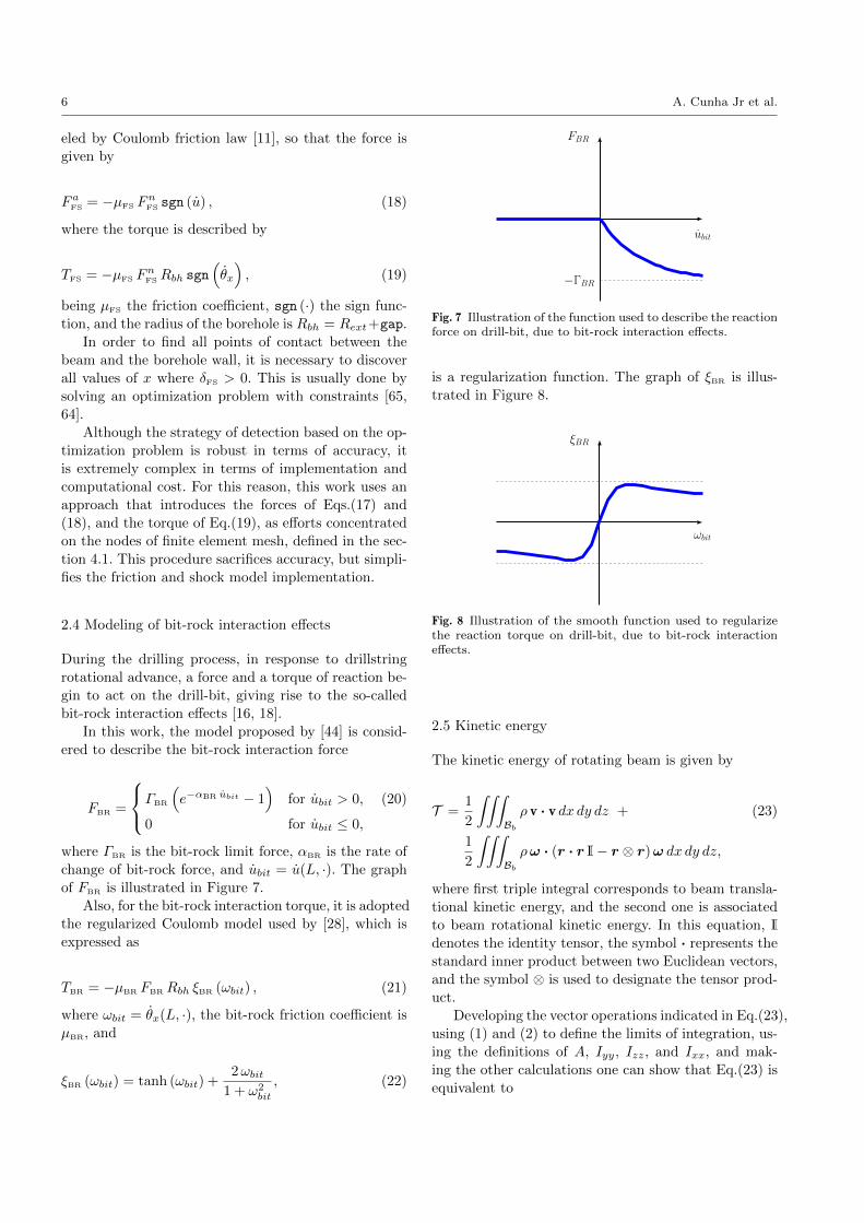
The modeling of friction and shock phenomena is
made in terms of a geometric parameter dubbed inden-
tation, which is defined as
δFS = r − gap, (16)
where r =√v2 + w2 is the neutral fiber lateral dis-
placement, and gap denotes the spacing between the
undeformed beam and the borehole wall. One has that
δFS > 0 in case of an impact, or δFS ≤ 0 otherwise, as
can be seen in Figure 6. Note that the indentation cor-
responds to a measure of penetration in the wall of a
beam cross section [21].
gap
rgap
r
δFS = r − gap ≤ 0 δFS = r − gap > 0
Fig. 6 Illustration of the indentation parameter in a situationwithout impact (left) or with impact (right).
When an impact occurs, a normal force of the form
FnFS = −kFS1 δFS − kFS2 δ3FS − cFS |δ|3δFS, (17)
where kFS1, kFS2
and cFS are constants of the shock
model, begins to act on the beam cross section. In this
nonlinear shock model, proposed by Hunt and Crossley
[26], the first (linear spring) and the second (nonlinear
spring) terms describe the elastic deformation during an
impact, while the third term (nonlinear damper) takes
into account the loss of energy during an impact.
Once the column is rotating and moving axially, an
impact also induces a frictional force in axial direction,
F aFS, and a torsional friction torque, TFS. Both are mod-
6 A. Cunha Jr et al.
eled by Coulomb friction law [11], so that the force is
given by
F aFS = −µFS FnFS sgn (u) , (18)
where the torque is described by
TFS = −µFS FnFSRbh sgn
(θx
), (19)
being µFS the friction coefficient, sgn (·) the sign func-
tion, and the radius of the borehole is Rbh = Rext+gap.
In order to find all points of contact between the
beam and the borehole wall, it is necessary to discover
all values of x where δFS > 0. This is usually done by
solving an optimization problem with constraints [65,
64].
Although the strategy of detection based on the op-
timization problem is robust in terms of accuracy, it
is extremely complex in terms of implementation and
computational cost. For this reason, this work uses an
approach that introduces the forces of Eqs.(17) and
(18), and the torque of Eq.(19), as efforts concentrated
on the nodes of finite element mesh, defined in the sec-
tion 4.1. This procedure sacrifices accuracy, but simpli-
fies the friction and shock model implementation.
2.4 Modeling of bit-rock interaction effects
During the drilling process, in response to drillstring
rotational advance, a force and a torque of reaction be-
gin to act on the drill-bit, giving rise to the so-called
bit-rock interaction effects [16, 18].
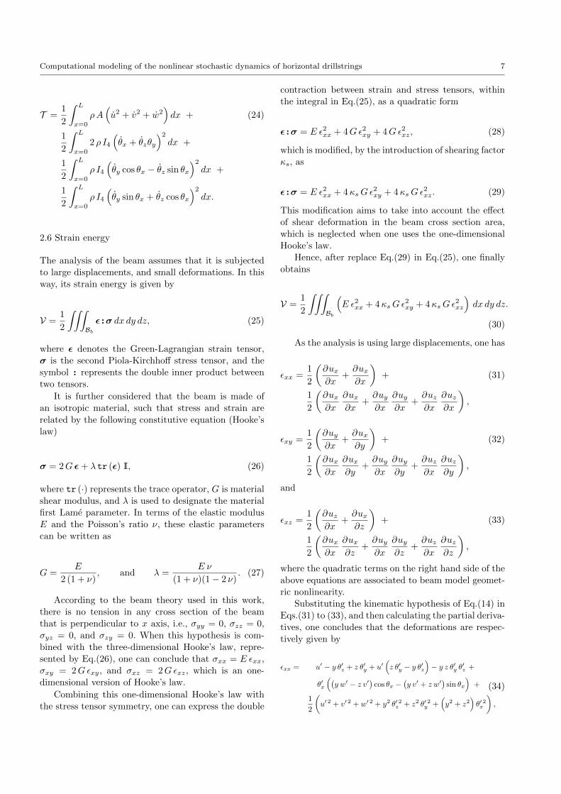
In this work, the model proposed by [44] is consid-
ered to describe the bit-rock interaction force
FBR =
ΓBR
(e−αBR ubit − 1
)for ubit > 0, (20)
0 for ubit ≤ 0,
where ΓBR is the bit-rock limit force, αBR is the rate of
change of bit-rock force, and ubit = u(L, ·). The graph
of FBR is illustrated in Figure 7.
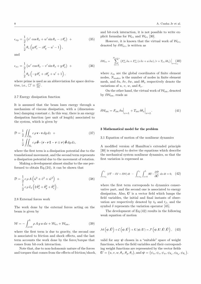
Also, for the bit-rock interaction torque, it is adopted
the regularized Coulomb model used by [28], which is
expressed as
TBR = −µBR FBRRbh ξBR (ωbit) , (21)
where ωbit = θx(L, ·), the bit-rock friction coefficient is
µBR, and
ξBR (ωbit) = tanh (ωbit) +2ωbit
1 + ω2bit
, (22)
ubit
FBR
−ΓBR
Fig. 7 Illustration of the function used to describe the reactionforce on drill-bit, due to bit-rock interaction effects.
is a regularization function. The graph of ξBR is illus-
trated in Figure 8.
ωbit
ξBR
Fig. 8 Illustration of the smooth function used to regularizethe reaction torque on drill-bit, due to bit-rock interactioneffects.
2.5 Kinetic energy
The kinetic energy of rotating beam is given by
T =1
2
∫∫∫Bb
ρ v · v dx dy dz + (23)
1
2
∫∫∫Bb
ρω · (r · r I− r ⊗ r)ω dx dy dz,
where first triple integral corresponds to beam transla-
tional kinetic energy, and the second one is associated
to beam rotational kinetic energy. In this equation, I
denotes the identity tensor, the symbol · represents the
standard inner product between two Euclidean vectors,
and the symbol ⊗ is used to designate the tensor prod-
uct.
Developing the vector operations indicated in Eq.(23),
using (1) and (2) to define the limits of integration, us-
ing the definitions of A, Iyy, Izz, and Ixx, and mak-
ing the other calculations one can show that Eq.(23) is
equivalent to
Computational modeling of the nonlinear stochastic dynamics of horizontal drillstrings 7
T =1
2
∫ L
x=0
ρA(u2 + v2 + w2
)dx + (24)
1
2
∫ L
x=0
2 ρ I4
(θx + θzθy
)2dx +
1
2
∫ L
x=0
ρ I4
(θy cos θx − θz sin θx
)2dx +
1
2
∫ L
x=0
ρ I4
(θy sin θx + θz cos θx
)2dx.
2.6 Strain energy
The analysis of the beam assumes that it is subjected
to large displacements, and small deformations. In this
way, its strain energy is given by
V =1
2
∫∫∫Bb
ε :σ dx dy dz, (25)
where ε denotes the Green-Lagrangian strain tensor,
σ is the second Piola-Kirchhoff stress tensor, and the
symbol : represents the double inner product between
two tensors.
It is further considered that the beam is made of
an isotropic material, such that stress and strain are
related by the following constitutive equation (Hooke’s
law)
σ = 2G ε+ λ tr (ε) I, (26)
where tr (·) represents the trace operator, G is material
shear modulus, and λ is used to designate the material
first Lame parameter. In terms of the elastic modulus
E and the Poisson’s ratio ν, these elastic parameters
can be written as
G =E
2 (1 + ν), and λ =
E ν
(1 + ν)(1− 2 ν). (27)
According to the beam theory used in this work,
there is no tension in any cross section of the beam
that is perpendicular to x axis, i.e., σyy = 0, σzz = 0,
σyz = 0, and σzy = 0. When this hypothesis is com-
bined with the three-dimensional Hooke’s law, repre-
sented by Eq.(26), one can conclude that σxx = E εxx,
σxy = 2Gεxy, and σxz = 2Gεxz, which is an one-
dimensional version of Hooke’s law.
Combining this one-dimensional Hooke’s law with
the stress tensor symmetry, one can express the double
contraction between strain and stress tensors, within
the integral in Eq.(25), as a quadratic form
ε :σ = E ε2xx + 4Gε2xy + 4Gε2xz, (28)
which is modified, by the introduction of shearing factor
κs, as
ε :σ = E ε2xx + 4κsGε2xy + 4κsGε
2xz. (29)
This modification aims to take into account the effect
of shear deformation in the beam cross section area,
which is neglected when one uses the one-dimensional
Hooke’s law.
Hence, after replace Eq.(29) in Eq.(25), one finally
obtains
V =1
2
∫∫∫Bb
(E ε2xx + 4κsGε
2xy + 4κsGε
2xz
)dx dy dz.
(30)
As the analysis is using large displacements, one has
εxx =1
2
(∂ux∂x
+∂ux∂x
)+ (31)
1
2
(∂ux∂x
∂ux∂x
+∂uy∂x
∂uy∂x
+∂uz∂x
∂uz∂x
),
εxy =1
2
(∂uy∂x
+∂ux∂y
)+ (32)
1
2
(∂ux∂x
∂ux∂y
+∂uy∂x
∂uy∂y
+∂uz∂x
∂uz∂y
),
and
εxz =1
2
(∂uz∂x
+∂ux∂z
)+ (33)
1
2
(∂ux∂x
∂ux∂z
+∂uy∂x
∂uy∂z
+∂uz∂x
∂uz∂z
),
where the quadratic terms on the right hand side of the
above equations are associated to beam model geomet-
ric nonlinearity.
Substituting the kinematic hypothesis of Eq.(14) in
Eqs.(31) to (33), and then calculating the partial deriva-
tives, one concludes that the deformations are respec-
tively given by
εxx = u′ − y θ′z + z θ′y + u′(z θ′y − y θ′z
)− y z θ′y θ′z +
θ′x
((y w′ − z v′
)cos θx −
(y v′ + z w′
)sin θx
)+
1
2
(u′ 2 + v′ 2 + w′ 2 + y2 θ′ 2z + z2 θ′ 2y +
(y2 + z2
)θ′ 2x
),
(34)
8 A. Cunha Jr et al.
εxy =1
2
(v′ cos θx + w′ sin θx − z θ′x
)+ (35)
1
2θz
(y θ′z − zθ′y − u′ − 1
),
and
εxz =1
2
(w′ cos θx − v′ sin θx + y θ′x
)+ (36)
1
2θy
(−y θ′z + zθ′y + u′ + 1
),
where prime is used as an abbreviation for space deriva-
tive, i.e., ′ ≡ ∂∂x .
2.7 Energy dissipation function
It is assumed that the beam loses energy through a
mechanism of viscous dissipation, with a (dimension-
less) damping constant c. In this way, there is an energy
dissipation function (per unit of length) associated to
the system, which is given by
D =1
2
∫∫Sbc ρ v · v dy dz + (37)
1
2
∫∫Sbc ρ θ · (r · r I− r ⊗ r) θ dy dz,
where the first term is a dissipation potential due to the
translational movement, and the second term represents
a dissipation potential due to the movement of rotation.
Making a development almost similar to the one per-
formed to obtain Eq.(24), it can be shown that
D =1
2c ρA
(u2 + v2 + w2
)+ (38)
1
2c ρ I4
(2 θ2x + θ2y + θ2z
).
2.8 External forces work
The work done by the external forces acting on the
beam is given by
W = −∫ L
x=0
ρAg w dx+WFS +WBR, (39)
where the first term is due to gravity, the second one
is associated to friction and shock effects, and the last
term accounts the work done by the force/torque that
comes from bit-rock interaction.
Note that, due to non-holonomic nature of the forces
and torques that comes from the effects of friction/shock,
and bit-rock interaction, it is not possible to write ex-
plicit formulas for WFS and WFS [30].
However, it is known that the virtual work of WFS,
denoted by δWFS, is written as
δWFS =
Nnodes∑m=1
(F aFS δu+ FnFS (v δv + w δw) /r + TFS δθx
) ∣∣∣x=xm
(40)
where xm are the global coordinates of finite element
nodes, Nnodes is the number of nodes in finite element
mesh, and δu, δv, δw, and δθx respectively denote the
variations of u, v, w, and θx.
On the other hand, the virtual work ofWBR, denoted
by δWBR, reads as
δWBR = FBR δu∣∣∣x=L
+ TBR δθx
∣∣∣x=L
. (41)
3 Mathematical model for the problem
3.1 Equation of motion of the nonlinear dynamics
A modified version of Hamilton’s extended principle
[30] is employed to derive the equations which describe
the mechanical system nonlinear dynamics, so that the
first variation is expressed as
∫ tf
t=t0
(δT − δV + δW) dt −∫ tf
t=t0
∫ L
x=0
δU · ∂D∂U
dx dt = 0, (42)
where the first term corresponds to dynamics conser-
vative part, and the second one is associated to energy
dissipation. Also, U is a vector field which lumps the
field variables, the initial and final instants of obser-
vation are respectively denoted by t0 and tf , and the
symbol δ represents the variation operator [45].
The development of Eq.(42) results in the following
weak equation of motion
M(ψ, U
)+ C
(ψ, U
)+K (ψ,U) = F
(ψ,U , U , U
), (43)
valid for any ψ chosen in a “suitable” space of weight
functions, where the field variables and their correspond-
ing weight functions are represented by the vector fields
U =(u, v, w, θx, θy, θz
), andψ =
(ψu, ψv, ψw, ψθx , ψθy , ψθz
).
Computational modeling of the nonlinear stochastic dynamics of horizontal drillstrings 9
Furthermore,
M(ψ, U
)=
∫ L
x=0
ρA (ψu u+ ψv v + ψw w) dx + (44)∫ L
x=0
ρ I4
(2ψθx θx + ψθy θy + ψθz θz
)dx,
represents the mass operator,
C(ψ, U
)=
∫ L
x=0
c ρA (ψu u+ ψv v + ψw w) dx + (45)∫ L
x=0
c ρ I4
(2ψθx θx + ψθy θy + ψθz θz
)dx,
is the damping operator,
K (ψ,U) =
∫ L
x=0
E Aψ′u u′ dx + (46)∫ L
x=0
E I4
(ψ′θy θ
′y + ψ′θz θ
′z
)dx +∫ L
x=0
2κsGI4 ψ′θx θ′x dx +∫ L
x=0
κsGA(ψθy + ψ′w
) (θy + w′
)dx +∫ L
x=0
κsGA(ψθz − ψ′v
) (θz − v′
)dx,
is the stiffness operator, and
F(ψ,U , U , U
)= FKE
(ψ,U , U , U
)+ (47)
FSE (ψ,U) + FFS (ψ,U) +
FBR
(ψ, U
)+ FG (ψ) ,
is the force operator, which is divided into five parts. A
nonlinear force due to inertial effects
FKE = −∫ L
x=0
2 ρ I4 ψθx
(θy θz + θy θz
)dx (48)
+
∫ L
x=0
2 ρ I4 ψθy
(θy θ
2z + θx θz
)dx
−∫ L
x=0
2 ρ I4 ψθz
(θy θx + θ2y θz
)dx
−∫ L
x=0
2 ρ I4 ψθz
(θx θy + 2 θy θy θz
)dx,
a nonlinear force due to geometric nonlinearity
FSE =
∫ L
x=0
(ψθx Γ1 + ψθy Γ2 + ψθz Γ3
)dx + (49)∫ L
x=0
(ψ′u Γ4 + ψ′v Γ5 + ψ′w Γ6
)dx +∫ L
x=0
(ψ′θxΓ7 + ψ′θy Γ8 + ψ′θz Γ9
)dx,
a nonlinear force due to friction and shock effects
FFS =
Nnodes∑m=1
(F aFS ψu + FnFS (v ψv + wψw) /r + TFS ψθx
) ∣∣∣x=xm
(50)
a nonlinear force due to bit-rock interaction
FBR = FBR ψu
∣∣∣x=L
+ TBR ψθx
∣∣∣x=L
, (51)
and a linear force due to gravity
FG = −∫ L
x=0
ρAg ψw dx. (52)
The nonlinear functions Γn, with n = 1, · · · , 9, in
Eq.(49) are very complex and, for sake of space limita-
tion, are not presented in this section. But they can be
seen in Appendix A.
The model presented above is an adaptation, for
horizontal drillstrings, of the model proposed by [41,
39] to describe the nonlinear dynamics of vertical drill-strings. To be more precise, in the reference problem
gravity is parallel to drillstring main axis, while in this
work, it is perpendicular to the structure primal direc-
tion. Therefore, the former problem primarily addresses
the dynamics of a column, while the new problem deals
with the dynamics of a beam. Also, the original problem
treated the nonlinear dynamics around a pre-stressed
equilibrium configuration, while the new problem does
not consider the dynamics around any particular con-
figuration. It is worth mentioning that changes made in
the modeling of friction and shock effects are significant.
For instance, a nonlinear shock model that also takes
into account the dissipation of energy during an impact
is introduced, in contrast to the reference work, that
only consider the linear elastic deformation effects. In
addition, the boundary conditions are different, as well
as the bit-rock interaction model. On the other hand,
for the sake of simplicity, the fluid structure interac-
tion effects, considered in reference work are neglected
in this study.
10 A. Cunha Jr et al.
3.2 Initial conditions
With regard to mechanical system initial state, it is
assumed that the beam presents neither displacement
nor rotations, i.e., u(x, 0) = 0, v(x, 0) = 0, w(x, 0) = 0,
θx(x, 0) = 0, θy(x, 0) = 0, and θz(x, 0) = 0. These field
variables, except for u and θx, also have initial velocities
and rate of rotations equal to zero, i.e. v(x, 0) = 0,
w(x, 0) = 0, θy(x, 0) = 0, and θz(x, 0) = 0.
It is also assumed that, initially, the beam moves
horizontally with a constant axial velocity V0, and ro-
tates around the x axis with a constant angular velocity
Ω. Thereby, one has that u(x, 0) = V0, and θx(x, 0) = Ω.
Projecting the initial conditions in a“suitable”space
of weight functions, weak forms for them are obtained,
respectively, given by
M(ψ,U(0)
)=M (ψ,U0) , (53)
and
M(ψ, U(0)
)=M
(ψ, U0
), (54)
where U0 = (0, 0, 0, 0, 0, 0) and U0 = (V0, 0, 0, Ω, 0, 0).
In formal terms, the weak formulation of the initial–
boundary value problem that describes the mechanical
system nonlinear dynamics consists in find a vector field
U , “sufficiently regular”, which satisfies the weak equa-
tion of motion given by Eq.(43) for all “suitable” ψ,
as well as the weak form of initial conditions, given by
Eqs.(53), and (54) [25].
3.3 Associated linear conservative dynamics
Consider the linear homogeneous equation given by
M(ψ, U
)+K (ψ,U) = 0, (55)
obtained from Eq.(43) when one discards the damping,
and force operators, and which is valid for all ψ in the
space of weight functions.
Suppose that Eq.(55) has a solution of the form
U = eiωtφ, where ω is a natural frequency (in rad/s),
φ is the associated normal mode, and i =√−1 is
the imaginary unit. Replacing this expression of U in
Eq.(55) and using the linearity of operatorsM, and K,
one gets
(−ω2M (ψ,φ) +K (ψ,φ)
)eiωt = 0, (56)
which is equivalent to
−ω2M (ψ,φ) +K (ψ,φ) = 0, (57)
a generalized eigenvalue problem.
Since operator M is positive-definite, and opera-
tor K is positive semi-definite, the generalized eigen-
value problem above has a denumerable number of solu-
tions. The solutions of this eigenproblem have the form
(ω2n,φn), where ωn is the n-th natural frequency and
φn is the n-th normal mode [23].
Also, the symmetry of operators M, and K implies
the following orthogonality relations
M (φn,φm) = δnm, and K (φn,φm) = ω2n δnm, (58)
where δnm represents the Kronecker delta symbol. See
[23] for more details.
The generalized eigenvalue problem of Eq.(57), as
well as the properties of (58), will be useful to construct
a reduced order model for discretized dynamical system
which approximates the solution of the weak initial–
boundary value problem of Eqs.(43), (53), and (54).
4 Computational model for the problem
4.1 Discretization of the nonlinear dynamics
To proceed with the discretization of the weak initial–
boundary value problem of Eqs.(43), (53), and (54),
which describes the rotating beam nonlinear dynamics,
it is used the standard finite element method (FEM)
[25], where the spaces of basis and weight functions are
constructed by the same (finite dimensional) class of
functions.
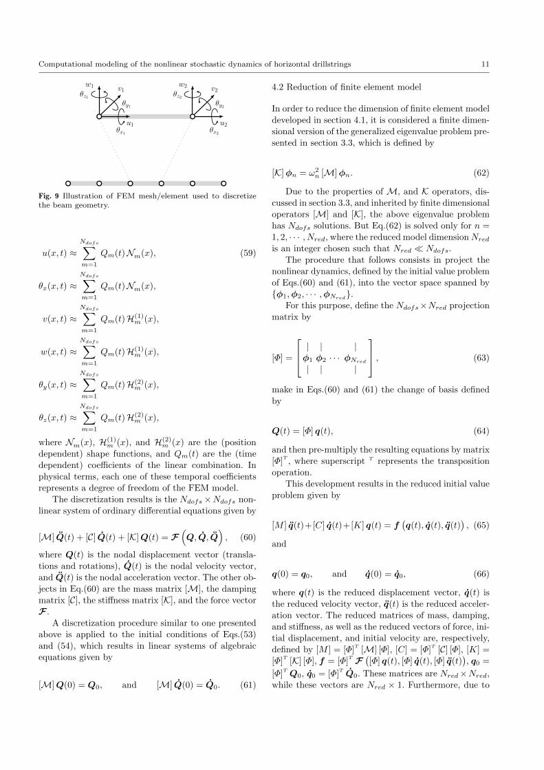
In this procedure, the beam geometry is discretized
by a FEM mesh with Nelem finite elements. Each one of
these elements is composed by two nodes, and each one
of these nodes has six degrees of freedom associated,
one for each field variable in the beam model described
in section 3.1. Thus, the number of degrees of freedom
associated with FEM model is Ndofs = 6(Nelem + 1).
An illustration of FEM mesh/element can be seen in
Figure 9.
Concerning the shape functions, it is adopted an in-
terdependent interpolation scheme which avoids shear-
locking effect [38]. This scheme uses, for transverse dis-
placements/rotations, Hermite cubic polynomials, and,
for the fields of axial displacement/torsional rotation,
affine functions [2].
Thus, each field variable of the physical model is ap-
proximated by a linear combination of basis functions,
in such way that
Computational modeling of the nonlinear stochastic dynamics of horizontal drillstrings 11
u1
v1w1
θx1
θy1
θz1
u2
v2w2
θx2
θy2
θz2
Fig. 9 Illustration of FEM mesh/element used to discretizethe beam geometry.
u(x, t) ≈Ndofs∑m=1
Qm(t)Nm(x), (59)
θx(x, t) ≈Ndofs∑m=1
Qm(t)Nm(x),
v(x, t) ≈Ndofs∑m=1
Qm(t)H(1)m (x),
w(x, t) ≈Ndofs∑m=1
Qm(t)H(1)m (x),
θy(x, t) ≈Ndofs∑m=1
Qm(t)H(2)m (x),
θz(x, t) ≈Ndofs∑m=1
Qm(t)H(2)m (x),
where Nm(x), H(1)m (x), and H(2)
m (x) are the (position
dependent) shape functions, and Qm(t) are the (time
dependent) coefficients of the linear combination. In
physical terms, each one of these temporal coefficients
represents a degree of freedom of the FEM model.
The discretization results is the Ndofs×Ndofs non-
linear system of ordinary differential equations given by
[M] Q(t) + [C] Q(t) + [K]Q(t) = F(Q, Q, Q
), (60)
where Q(t) is the nodal displacement vector (transla-
tions and rotations), Q(t) is the nodal velocity vector,
and Q(t) is the nodal acceleration vector. The other ob-
jects in Eq.(60) are the mass matrix [M], the damping
matrix [C], the stiffness matrix [K], and the force vector
F .
A discretization procedure similar to one presented
above is applied to the initial conditions of Eqs.(53)
and (54), which results in linear systems of algebraic
equations given by
[M]Q(0) = Q0, and [M] Q(0) = Q0. (61)
4.2 Reduction of finite element model
In order to reduce the dimension of finite element model
developed in section 4.1, it is considered a finite dimen-
sional version of the generalized eigenvalue problem pre-
sented in section 3.3, which is defined by
[K]φn = ω2n [M]φn. (62)
Due to the properties of M, and K operators, dis-
cussed in section 3.3, and inherited by finite dimensional
operators [M] and [K], the above eigenvalue problem
has Ndofs solutions. But Eq.(62) is solved only for n =
1, 2, · · · , Nred, where the reduced model dimensionNredis an integer chosen such that Nred Ndofs.
The procedure that follows consists in project the
nonlinear dynamics, defined by the initial value problem
of Eqs.(60) and (61), into the vector space spanned by
φ1,φ2, · · · ,φNred.
For this purpose, define the Ndofs×Nred projection
matrix by
[Φ] =
| | |φ1 φ2 · · · φNred
| | |
, (63)
make in Eqs.(60) and (61) the change of basis defined
by
Q(t) = [Φ] q(t), (64)
and then pre-multiply the resulting equations by matrix
[Φ]T, where superscript T represents the transposition
operation.
This development results in the reduced initial value
problem given by
[M ] q(t)+[C] q(t)+[K] q(t) = f(q(t), q(t), q(t)
), (65)
and
q(0) = q0, and q(0) = q0, (66)
where q(t) is the reduced displacement vector, q(t) is
the reduced velocity vector, q(t) is the reduced acceler-
ation vector. The reduced matrices of mass, damping,
and stiffness, as well as the reduced vectors of force, ini-
tial displacement, and initial velocity are, respectively,
defined by [M ] = [Φ]T
[M] [Φ], [C] = [Φ]T
[C] [Φ], [K] =
[Φ]T
[K] [Φ], f = [Φ]T F
([Φ] q(t), [Φ] q(t), [Φ] q(t)
), q0 =
[Φ]TQ0, q0 = [Φ]
TQ0. These matrices are Nred×Nred,
while these vectors are Nred × 1. Furthermore, due to
12 A. Cunha Jr et al.
the orthogonality properties defined by Eq.(58), that
are inherited by the operators in finite dimension, these
matrices are diagonal.
Thus, although the initial value problem of Eqs.(65)
and (66) is apparently similar to the one defined by
Eqs.(60) and (61), the former has a structure that makes
it much more efficient in terms of computational cost,
and so, it will be used to analyze the nonlinear dynam-
ics under study.
4.3 Integration of discretized nonlinear dynamics
In order to solve the initial value problem of Eqs.(65)
and (66), it is employed the Newmark method [35],
which defines the following implicit integration scheme
qn+1 = qn + (1− γ)∆t qn + γ∆t qn+1, (67)
qn+1 = qn+∆t qn+
(1
2− β
)∆t2 qn+β ∆t2 qn+1, (68)
where qn, qn and qn are approximations to q(tn), q(tn)
and q(tn), respectively, and tn = n∆t is an instant
in a temporal mesh defined over the interval [t0, tf ],
with an uniform time step ∆t. The parameters γ and
β are associated with accuracy and stability of the nu-
merical scheme [25], and for the simulations reported
in this work they are assumed as γ = 1/2 + α, and
β = 1/4(1/2 + γ
)2, with α = 15/1000.
Handling up properly Eqs.(67) and (68), and the dis-
crete version of Eq.(65), one arrives in a nonlinear sys-
tem of algebraic equations, with unknown vector qn+1,
which is represented by
ˆ[K]qn+1 = fn+1 (qn+1) , (69)
where ˆ[K] is the effective stiffness matrix, and fn+1 is
the (nonlinear) effective force vector.
4.4 Incorporation of boundary conditions
As can be seen in Figure 4, the mechanical system has
the following boundary conditions: (i) left extreme with
no transversal displacement, nor transversal rotation;
(ii) right extreme with no transversal displacement. It
is also assumed that the left end has: (iii) constant axial
and rotational velocities in x, respectively equal to V0and Ω.
Hence, for x = 0, it is true that u(0, t) = V0 t,
v(0, t) = 0, w(0, t) = 0, θx(0, t) = Ω t, θy(0, t) = 0,
and θz(0, t) = 0. On the other hand, for x = L, one has
v(L, t) = 0, and w(L, t) = 0.
The variational formulation presented in section 3.1,
was made for a free-free beam, i.e. the above geometric
boundary conditions were not considered. For this rea-
son, they are included in the formulation as constraints,
using the Lagrange multipliers method [25]. The details
of this procedure are presented below.
Observe that the boundary conditions can be rewrit-
ten in matrix form as
[B]Q(t) = h(t), (70)
where the constraint matrix [B] is 8 × Ndofs and has
almost all entries equal to zero. The exceptions are
[B]ii = 1 for i = 1, · · · , 6, [B]7(Ndofs−5) = 1, and
[B]8(Ndofs−4) = 1. The constraint vector is given by
h(t) =
u(0, t)
v(0, t)
w(0, t)
θx(0, t)
θy(0, t)
θz(0, t)
v(L, t)
w(L, t)
. (71)
Making the change of basis defined by Eq.(64), one
can rewrite Eq.(70) as
[B] q(t) = h(t), (72)
where the 8×Nred reduced constraint matrix is defined
by [B] = [B] [Φ].
The discretization of Eq.(72) results in
[B] qn+1 = hn+1, (73)
where hn+1 is an approximation to h(tn+1). This equa-
tion defines the constraint that must be satisfied by the
variational problem “approximate solution”.
In what follows it is helpful to think that Eq.(69)
comes from the minimization of an energy functional
qn+1 7→ F (qn+1), which is the weak form of this non-
linear system of algebraic equations.
Then, one defines the Lagrangian as
L (qn+1,λn+1) = F (qn+1) + λT
n+1
([B] qn+1 − hn+1
), (74)
Computational modeling of the nonlinear stochastic dynamics of horizontal drillstrings 13
being the (time-dependent) Lagrange multipliers vector
of the form
λn+1 =
λ1(tn+1)
λ2(tn+1)
λ3(tn+1)
λ4(tn+1)
λ5(tn+1)
λ6(tn+1)
λ7(tn+1)
λ8(tn+1)
. (75)
Invoking the Lagrangian stationarity condition one
arrives in the following (Nred + 8)× (Nred + 8) system
of nonlinear algebraic equations
[ˆ[K] [B]
T
[B] [0]
](qn+1
λn+1
)=
(fn+1
hn+1
), (76)
where [0] is a 8 × 8 null matrix. The unknowns are
qn+1 and λn+1, and must be solved for each instant
of time in the temporal mesh, in order to construct
an approximation to the mechanical system dynamic
response.
The solution of the nonlinear system of algebraic
equations, defined by Eq.(76), is carried out first ob-
taining and solving a discrete Poisson equation for λn+1
[22], and then using the first line of (76) to obtain qn+1.
To solve these equations, a procedure of fixed point iter-
ation is used in combination with a process of successive
over relaxation [66].
5 Probabilistic modeling of system-parameter
uncertainties
The mathematical model used to describe the physical
behavior of the mechanical system is an abstraction of
reality, and its use does not consider some aspects of
the problem physics. Regarding the system modeling,
either the beam theory used to describe the structure
dynamics [41], as the friction and shock model used
[26] are fairly established physical models, who have
gone through several experimental tests to prove their
validity, and have been used for many years in similar
situations. On the other hand, the bit-rock interaction
model adopted in this work, until now was used only
in a purely numeric context [44], without any experi-
mental validation. Thus, it is natural to conclude that
bit-rock interaction law is the weakness of the model
proposed in this work.
In this sense, this work will focus on modeling and
quantifying the uncertainties that are introduced in the
mechanical system by bit-rock interaction model. For
convenience, it was chosen to use a parametric proba-
bilistic approach [56], where only the uncertainties of
system parameters are considered, and the maximum
entropy principle is employed to construct the proba-
bility distributions.
5.1 Probabilistic framework
Let X be a real-valued random variable, defined on a
probability space (,,P), for which the probability dis-
tribution PX(dx) on R admits a density x 7→ pX(x) with
respect to dx. The support of the probability density
function (PDF) pX will be denoted by SuppX ⊂ R. The
mathematical expectation of X is defined by
E [X] =
∫SuppX
x pX(x) dx , (77)
and any realization of random variable X will be de-
noted by X(θ) for θ ∈ . Let mX = E [X] be the mean
value, σ2X = E
[(X−mX)
2]
be the variance, and σX =√σ2X be the standard deviation of X. The Shannon en-
tropy of pX is defined by S (pX) = −E[ln pX(X)
].
5.2 Probabilistic model for bit-rock interface law
Recalling that bit-rock interaction force and torque are,
respectively, given by Eqs.(20) and (21), the reader can
see that this bit-rock interface law is characterized by
three parameters, namely, αBR, ΓBR, and µBR. The con-
struction of the probabilistic model for each one param-
eter of these parameters, which are respectively mod-
eled by random variables BR, BR, and BR, is pre-
sented below.
5.3 Distribution of force rate of change
As the rate of change αBR is positive, it is reasonable to
assume SuppBR =]0,∞[. Therefore, the PDF of BR is
a nonnegative function pBR, such that
∫ +∞
α=0
pBR(α) dα = 1. (78)
It is also convenient to assume that the mean value
of BR is a known positive number, denoted by mBR,
i.e.,
E [BR] = mBR> 0. (79)
14 A. Cunha Jr et al.
One also need to require that
E[ln (BR)
]= qBR
, |qBR| < +∞, (80)
which ensures, as can be seen in [53, 54, 55], that the
inverse of BR is second order random variable. This
condition is necessary to guarantee that the stochastic
dynamical system associated to this random variable is
of second order, i.e., it has finite variance. Employing
the principle of maximum entropy one need to maxi-
mize the entropy function S (pBR), respecting the con-
straints imposed by (78), (79) and (80).
The desired PDF corresponds to the gamma distri-
bution and is given by
pBR(α) = 1]0,∞[(α)1
mBR
(1
δ2BR
)1/δ2BR
× 1
Γ (1/δ2BR)
(α
mBR
)1/δ2BR−1
exp
(−α
δ2BRmBR
),
(81)
where the symbol 1]0,∞[(α) denotes the indicator func-
tion of the interval ]0,∞[, 0 ≤ δBR= σBR
/mBR<
1/√
2 is a type of dispersion parameter, and
Γ (z) =
∫ +∞
y=0
yz−1 e−y dy, (82)
is the gamma function.
5.4 Distribution of limit force
The parameter ΓBR is also positive, in a way that
SuppBR =]0,∞[, and consequently
∫ +∞
γ=0
pBR(γ) dγ = 1. (83)
The hypothesis that the mean is a known positive
number mBR is also done, i.e.,
E [BR] = mBR> 0, (84)
as well as that the technical condition, required for the
stochastic dynamical system associated be of second or-
der, is fulfilled, i.e.
E[ln (BR)
]= qBR
, |qBR| < +∞. (85)
In a similar way to the procedure presented in sec-
tion 5.3, it can be shown that PDF of maximum entropy
is also gamma distributed, and given by
pBR(γ) = 1]0,∞[(γ)1
mBR
(1
δ2BR
)1/δ2BR
× 1
Γ (1/δ2BR)
(γ
mBR
)1/δ2BR−1
exp
(−γ
δ2BRmBR
).
(86)
5.5 Distribution of friction coefficient
With respect to the parameter µBR, one know it is non-
negative and bounded above by the unity. Thus, one
can safely assume that SuppBR = [0, 1], so that the
normalization condition read as
∫ 1
µ=0
pBR(µ) dµ = 1. (87)
The following two conditions are also imposed
E[ln (BR)
]= q1BR
, |q1BR| < +∞, (88)
E[ln (1− BR)
]= q2BR
, |q2BR| < +∞, (89)
representing a weak decay of the PDF of BR in 0+ and
1− respectively [53, 54, 55]. Evoking again the principle
of maximum entropy considering now as known infor-
mation the constraints defined by (87), (88), and (89)
one has that the desired PDF is given by
pBR(µ) = 1[0,1](µ)Γ (a+ b)
Γ (a)Γ (b)µa−1 (1− µ)
b−1, (90)
which corresponds to the beta distribution
The parameters a and b are associated with the
shape of the probability distribution, and can be re-
lated with mBRand δBR
by
a =mBR
δ2BR
(1
mBR
− δ2BR− 1
), (91)
and
b =mBR
δ2BR
(1
mBR
− δ2BR− 1
)(1
mBR
− 1
). (92)
Computational modeling of the nonlinear stochastic dynamics of horizontal drillstrings 15
5.6 Stochastic nonlinear dynamical system
Due to the randomness of parameters BR, BR, and
BR, the mechanical system physical behavior is now
described, for all θ in Θ, by the stochastic nonlinear
dynamical system defined by
[M ] q(t, θ) + [C] q(t, θ) + [K] q(t, θ) = f (q, q, q) , (93)
q(0, θ) = q0, and q(0, θ) = q0, a.s. (94)
where q(t) is the random reduced displacement vector,
q(t) is the random reduced velocity vector, and q(t) is
the random reduced acceleration vector, and f is the
random reduced nonlinear force vector.
The methodology used to calculate the propagation
of uncertainties through this stochastic dynamical sys-
tem is Monte Carlo (MC) method [29], employing a
strategy of parallelization described in [13].
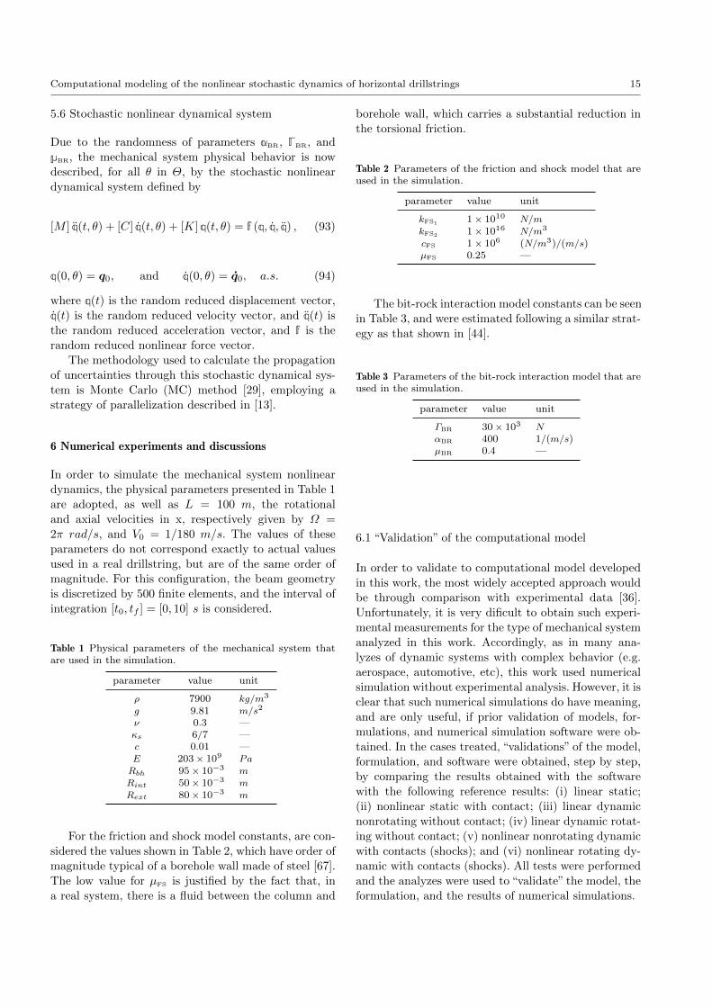
6 Numerical experiments and discussions
In order to simulate the mechanical system nonlinear
dynamics, the physical parameters presented in Table 1
are adopted, as well as L = 100 m, the rotational
and axial velocities in x, respectively given by Ω =
2π rad/s, and V0 = 1/180 m/s. The values of these
parameters do not correspond exactly to actual values
used in a real drillstring, but are of the same order of
magnitude. For this configuration, the beam geometry
is discretized by 500 finite elements, and the interval of
integration [t0, tf ] = [0, 10] s is considered.
Table 1 Physical parameters of the mechanical system thatare used in the simulation.
parameter value unit
ρ 7900 kg/m3
g 9.81 m/s2
ν 0.3 —κs 6/7 —c 0.01 —E 203× 109 Pa
Rbh 95× 10−3 m
Rint 50× 10−3 m
Rext 80× 10−3 m
For the friction and shock model constants, are con-
sidered the values shown in Table 2, which have order of
magnitude typical of a borehole wall made of steel [67].
The low value for µFS is justified by the fact that, in
a real system, there is a fluid between the column and
borehole wall, which carries a substantial reduction in
the torsional friction.
Table 2 Parameters of the friction and shock model that areused in the simulation.
parameter value unit
kFS1 1× 10¹⁰ N/m
kFS2 1× 10¹⁶ N/m3
cFS 1× 10⁶ (N/m3)/(m/s)µFS 0.25 —
The bit-rock interaction model constants can be seen
in Table 3, and were estimated following a similar strat-
egy as that shown in [44].
Table 3 Parameters of the bit-rock interaction model that areused in the simulation.
parameter value unit
ΓBR 30× 103 NαBR 400 1/(m/s)µBR 0.4 —
6.1 “Validation” of the computational model
In order to validate to computational model developed
in this work, the most widely accepted approach would
be through comparison with experimental data [36].
Unfortunately, it is very dificult to obtain such experi-
mental measurements for the type of mechanical system
analyzed in this work. Accordingly, as in many ana-
lyzes of dynamic systems with complex behavior (e.g.
aerospace, automotive, etc), this work used numerical
simulation without experimental analysis. However, it is
clear that such numerical simulations do have meaning,
and are only useful, if prior validation of models, for-
mulations, and numerical simulation software were ob-
tained. In the cases treated, “validations” of the model,
formulation, and software were obtained, step by step,
by comparing the results obtained with the software
with the following reference results: (i) linear static;
(ii) nonlinear static with contact; (iii) linear dynamic
nonrotating without contact; (iv) linear dynamic rotat-
ing without contact; (v) nonlinear nonrotating dynamic
with contacts (shocks); and (vi) nonlinear rotating dy-
namic with contacts (shocks). All tests were performed
and the analyzes were used to “validate” the model, the
formulation, and the results of numerical simulations.
16 A. Cunha Jr et al.
6.2 Modal analysis of the mechanical system
In this section, the modal content of the mechanical sys-
tem is investigated. This investigation aims to identify
the natural frequencies of the system, and, especially,
to check the influence of slenderness ratio, defined as
the ratio between beam length and external diameter,
in the natural frequencies distribution.
Therefore, the dimensionless frequency band for the
problem is assumed as being B = [0, 4], with the dimen-
sionless frequency defined by
f∗ =f L
cL, (95)
where f is the dimensional frequency (Hz), and cL =√E/ρ is the longitudinal wave velocity. Once it was
defined in terms of a dimensionless frequency, the band
of analysis does not change when the beam length is
varied. Also, the reader can check that this band is rep-
resentative for the mechanical system dynamics, once
the beam rotates at 2π rad/s, which means that it is
excited at 1 Hz.
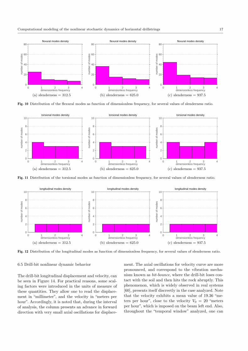
In Figure 10 one can see the distribution of the flex-
ural modes as a function of dimensionless frequency, for
several values of slenderness ratio. Clearly it is observed
that the flexural modes are denser in the low frequency
range. Further, when the slenderness ratio increases,
the modal density in the low frequencies range tend to
increase.
A completely different behavior is observed for the
torsional and longitudinal (traction-compression) modes
of vibration, as can be seen in Figures 11 and 12, re-
spectively. One can note that, with respect to these two
modes of vibration, the modal distribution is almost
uniform with respect to dimensionless frequency, and
invariant to changes in the slenderness ratio.
It may also be noted from Figures 10 to 12 that
lowest natural frequencies are associated with flexural
mechanism. This is because beam flexural stiffness is
much smaller than torsional stiffness, which, in turn, is
less than axial stiffness. In other words, it is much easier
to bend the beam than twisting it. However, twists the
beam is easier than buckling it.
The dimensionless frequency band adopted in the
analysis corresponds to a maximum dimensional fre-
quency of fmax = 4 cL/L. In this way, a nominal time
step of ∆t = (2 fmax)−1 is adopted for time integration.
This time step is automatically refined by the algorithm
of integration, whenever necessary, to capture the shock
effects.
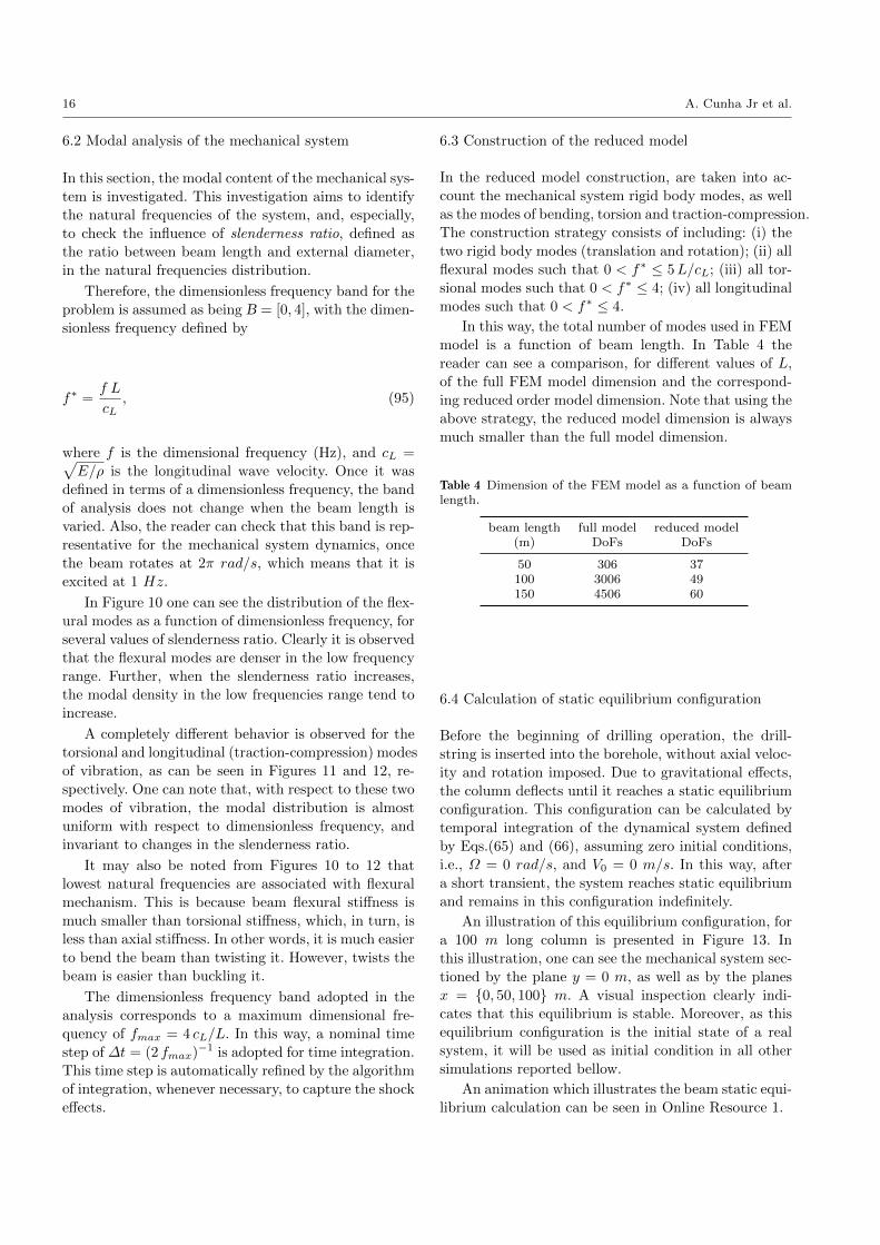
6.3 Construction of the reduced model
In the reduced model construction, are taken into ac-
count the mechanical system rigid body modes, as well
as the modes of bending, torsion and traction-compression.
The construction strategy consists of including: (i) the
two rigid body modes (translation and rotation); (ii) all
flexural modes such that 0 < f∗ ≤ 5L/cL; (iii) all tor-
sional modes such that 0 < f∗ ≤ 4; (iv) all longitudinal
modes such that 0 < f∗ ≤ 4.
In this way, the total number of modes used in FEM
model is a function of beam length. In Table 4 the
reader can see a comparison, for different values of L,
of the full FEM model dimension and the correspond-
ing reduced order model dimension. Note that using the
above strategy, the reduced model dimension is always
much smaller than the full model dimension.
Table 4 Dimension of the FEM model as a function of beamlength.
beam length full model reduced model(m) DoFs DoFs
50 306 37100 3006 49150 4506 60
6.4 Calculation of static equilibrium configuration
Before the beginning of drilling operation, the drill-
string is inserted into the borehole, without axial veloc-
ity and rotation imposed. Due to gravitational effects,
the column deflects until it reaches a static equilibrium
configuration. This configuration can be calculated by
temporal integration of the dynamical system defined
by Eqs.(65) and (66), assuming zero initial conditions,
i.e., Ω = 0 rad/s, and V0 = 0 m/s. In this way, after
a short transient, the system reaches static equilibrium
and remains in this configuration indefinitely.
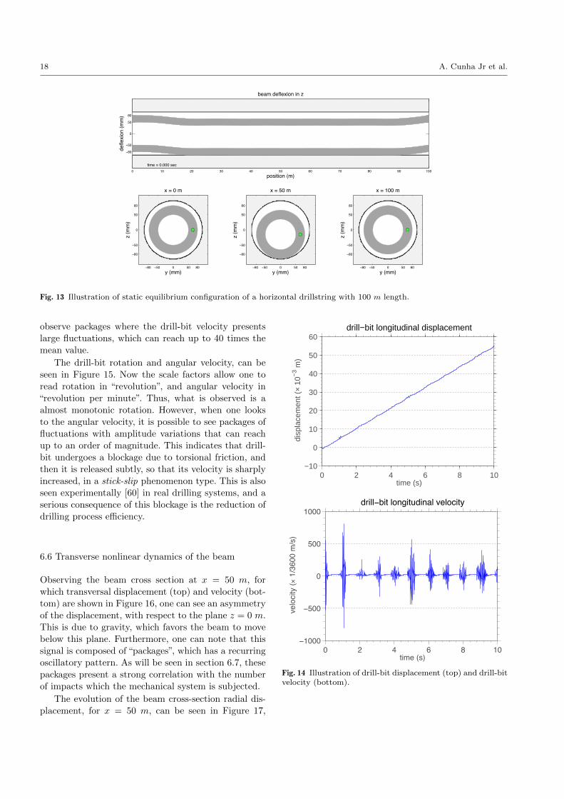
An illustration of this equilibrium configuration, for
a 100 m long column is presented in Figure 13. In
this illustration, one can see the mechanical system sec-
tioned by the plane y = 0 m, as well as by the planes
x = 0, 50, 100 m. A visual inspection clearly indi-
cates that this equilibrium is stable. Moreover, as this
equilibrium configuration is the initial state of a real
system, it will be used as initial condition in all other
simulations reported bellow.
An animation which illustrates the beam static equi-
librium calculation can be seen in Online Resource 1.
Computational modeling of the nonlinear stochastic dynamics of horizontal drillstrings 17
0 1 2 3 40
20
40
60
80
dimensionless frequency
num
ber
of m
odes
flexural modes density
(a) slenderness = 312.5
0 1 2 3 40
20
40
60
80
dimensionless frequency n
umbe
r of
mod
es
flexural modes density
(b) slenderness = 625.0
0 1 2 3 40
20
40
60
80
dimensionless frequency
num
ber
of m
odes
flexural modes density
(c) slenderness = 937.5
Fig. 10 Distribution of the flexural modes as function of dimensionless frequency, for several values of slenderness ratio.
0 1 2 3 40
2
4
6
8
10
dimensionless frequency
num
ber
of m
odes
torsional modes density
(a) slenderness = 312.5
0 1 2 3 40
2
4
6
8
10
dimensionless frequency
num
ber
of m
odes
torsional modes density
(b) slenderness = 625.0
0 1 2 3 40
2
4
6
8
10
dimensionless frequency
num
ber
of m
odes
torsional modes density
(c) slenderness = 937.5
Fig. 11 Distribution of the torsional modes as function of dimensionless frequency, for several values of slenderness ratio.
0 1 2 3 40
2
4
6
8
10
dimensionless frequency
num
ber
of m
odes
longitudinal modes density
(a) slenderness = 312.5
0 1 2 3 40
2
4
6
8
10
dimensionless frequency
num
ber
of m
odes
longitudinal modes density
(b) slenderness = 625.0
0 1 2 3 40
2
4
6
8
10
dimensionless frequency
num
ber
of m
odes
longitudinal modes density
(c) slenderness = 937.5
Fig. 12 Distribution of the longitudinal modes as function of dimensionless frequency, for several values of slenderness ratio.
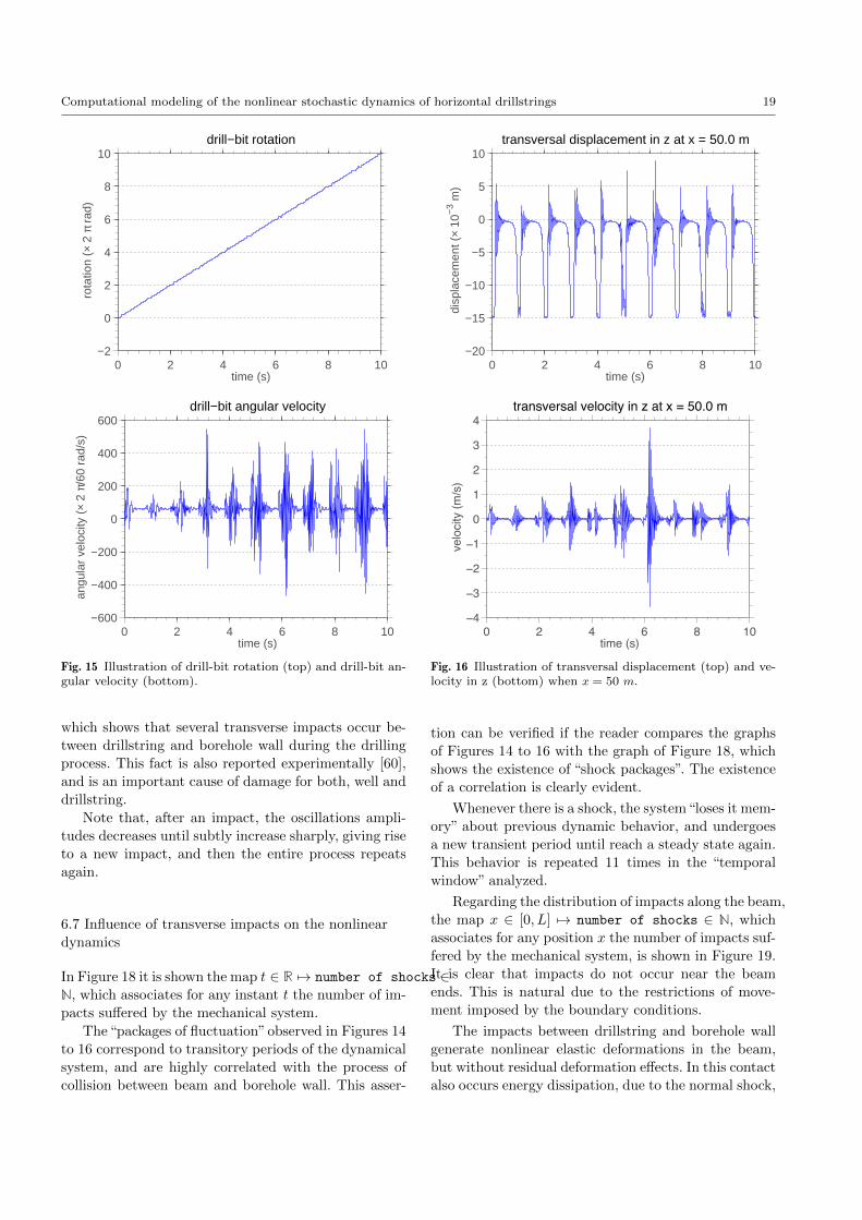
6.5 Drill-bit nonlinear dynamic behavior
The drill-bit longitudinal displacement and velocity, can
be seen in Figure 14. For practical reasons, some scal-
ing factors were introduced in the units of measure of
these quantities. They allow one to read the displace-
ment in “millimeter”, and the velocity in “meters per
hour”. Accordingly, it is noted that, during the interval
of analysis, the column presents an advance in forward
direction with very small axial oscillations for displace-
ment. The axial oscillations for velocity curve are more
pronounced, and correspond to the vibration mecha-
nism known as bit-bounce, where the drill-bit loses con-
tact with the soil and then hits the rock abruptly. This
phenomenon, which is widely observed in real systems
[60], presents itself discreetly in the case analyzed. Note
that the velocity exhibits a mean value of 19.36 “me-
ters per hour”, close to the velocity V0 = 20 “meters
per hour”, which is imposed on the beam left end. Also,
throughout the “temporal window” analyzed, one can
18 A. Cunha Jr et al.
0 10 20 30 40 50 60 70 80 90 100
−80
−50
0
50
80
beam deflexion in z
position (m)
defle
xion
(mm
)
time = 0.000 sec
−80 −50 0 50 80
−80
−50
0
50
80
x = 0 m
y (mm)
z (m
m)
−80 −50 0 50 80
−80
−50
0
50
80
x = 50 m
y (mm)
z (m
m)
−80 −50 0 50 80
−80
−50
0
50
80
x = 100 m
y (mm)
z (m
m)
Fig. 13 Illustration of static equilibrium configuration of a horizontal drillstring with 100 m length.
observe packages where the drill-bit velocity presents
large fluctuations, which can reach up to 40 times the
mean value.
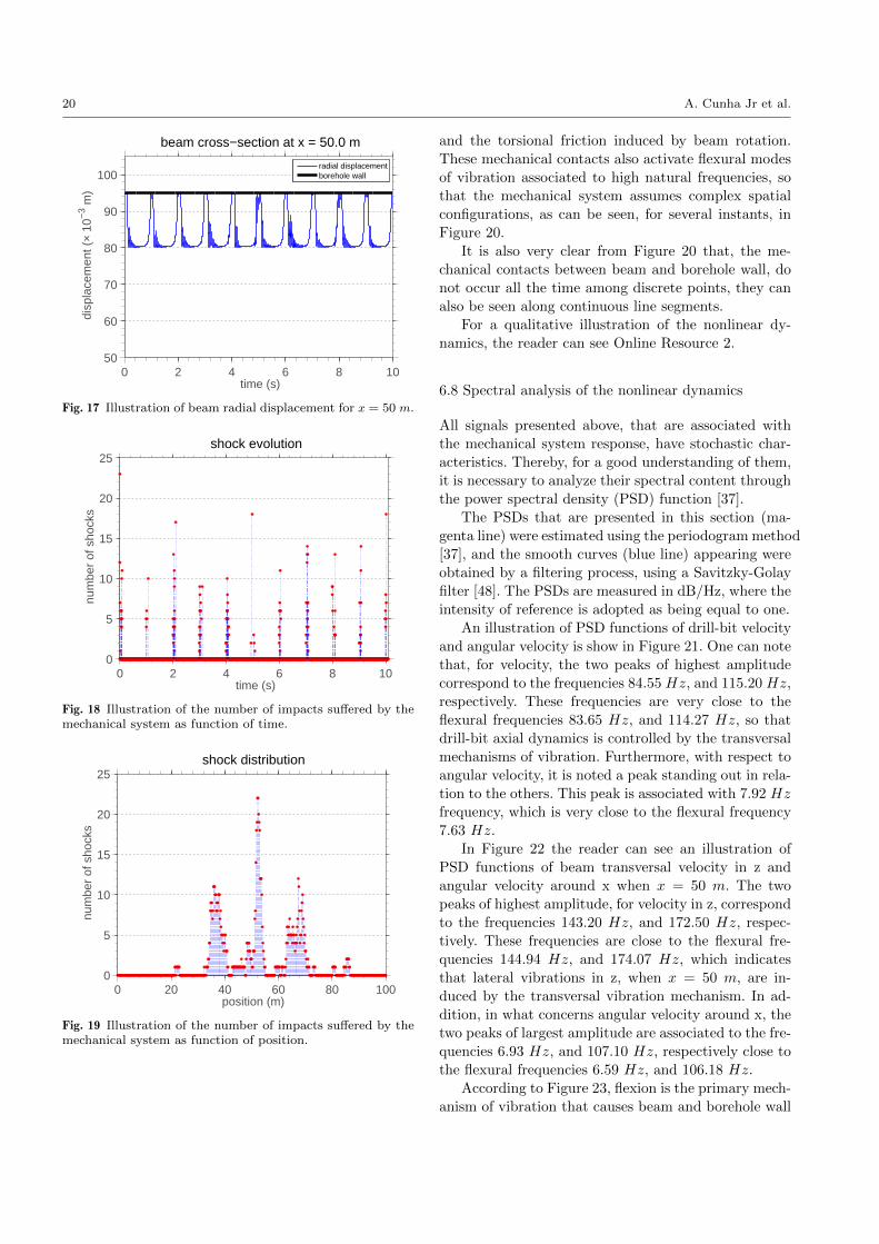
The drill-bit rotation and angular velocity, can be
seen in Figure 15. Now the scale factors allow one to
read rotation in “revolution”, and angular velocity in
“revolution per minute”. Thus, what is observed is a
almost monotonic rotation. However, when one looks
to the angular velocity, it is possible to see packages of
fluctuations with amplitude variations that can reach
up to an order of magnitude. This indicates that drill-
bit undergoes a blockage due to torsional friction, and
then it is released subtly, so that its velocity is sharply
increased, in a stick-slip phenomenon type. This is also
seen experimentally [60] in real drilling systems, and a
serious consequence of this blockage is the reduction of
drilling process efficiency.
6.6 Transverse nonlinear dynamics of the beam
Observing the beam cross section at x = 50 m, for
which transversal displacement (top) and velocity (bot-
tom) are shown in Figure 16, one can see an asymmetry
of the displacement, with respect to the plane z = 0 m.
This is due to gravity, which favors the beam to move
below this plane. Furthermore, one can note that this
signal is composed of “packages”, which has a recurring
oscillatory pattern. As will be seen in section 6.7, these
packages present a strong correlation with the number
of impacts which the mechanical system is subjected.
The evolution of the beam cross-section radial dis-
placement, for x = 50 m, can be seen in Figure 17,
0 2 4 6 8 10−10
0
10
20
30
40
50
60
time (s)
dis
plac
emen
t (×
10−
3 m)
drill−bit longitudinal displacement
0 2 4 6 8 10−1000
−500
0
500
1000
time (s)
vel
ocity
(× 1
/360
0 m
/s)
drill−bit longitudinal velocity
Fig. 14 Illustration of drill-bit displacement (top) and drill-bitvelocity (bottom).
Computational modeling of the nonlinear stochastic dynamics of horizontal drillstrings 19
0 2 4 6 8 10−2
0
2
4
6
8
10
time (s)
rot
atio
n (×
2 π
rad
)
drill−bit rotation
0 2 4 6 8 10−600
−400
−200
0
200
400
600
time (s)
ang
ular
vel
ocity
(×
2 π/
60 r
ad/s
)
drill−bit angular velocity
Fig. 15 Illustration of drill-bit rotation (top) and drill-bit an-gular velocity (bottom).
which shows that several transverse impacts occur be-
tween drillstring and borehole wall during the drilling
process. This fact is also reported experimentally [60],
and is an important cause of damage for both, well and
drillstring.
Note that, after an impact, the oscillations ampli-
tudes decreases until subtly increase sharply, giving rise
to a new impact, and then the entire process repeats
again.
6.7 Influence of transverse impacts on the nonlinear
dynamics
In Figure 18 it is shown the map t ∈ R 7→ number of shocks ∈N, which associates for any instant t the number of im-
pacts suffered by the mechanical system.
The“packages of fluctuation”observed in Figures 14
to 16 correspond to transitory periods of the dynamical
system, and are highly correlated with the process of
collision between beam and borehole wall. This asser-
0 2 4 6 8 10−20
−15
−10
−5
0
5
10
time (s)
dis
plac
emen
t (×
10−
3 m)
transversal displacement in z at x = 50.0 m
0 2 4 6 8 10−4
−3
−2
−1
0
1
2
3
4
time (s)
vel
ocity
(m/s
)
transversal velocity in z at x = 50.0 m
Fig. 16 Illustration of transversal displacement (top) and ve-locity in z (bottom) when x = 50 m.
tion can be verified if the reader compares the graphs
of Figures 14 to 16 with the graph of Figure 18, which
shows the existence of “shock packages”. The existence
of a correlation is clearly evident.
Whenever there is a shock, the system“loses it mem-
ory” about previous dynamic behavior, and undergoes
a new transient period until reach a steady state again.
This behavior is repeated 11 times in the “temporal
window” analyzed.
Regarding the distribution of impacts along the beam,
the map x ∈ [0, L] 7→ number of shocks ∈ N, which
associates for any position x the number of impacts suf-
fered by the mechanical system, is shown in Figure 19.
It is clear that impacts do not occur near the beam
ends. This is natural due to the restrictions of move-
ment imposed by the boundary conditions.
The impacts between drillstring and borehole wall
generate nonlinear elastic deformations in the beam,
but without residual deformation effects. In this contact
also occurs energy dissipation, due to the normal shock,
20 A. Cunha Jr et al.
0 2 4 6 8 1050
60
70
80
90
100
time (s)
dis
plac
emen
t (×
10−
3 m)
beam cross−section at x = 50.0 m
radial displacementborehole wall
Fig. 17 Illustration of beam radial displacement for x = 50 m.
0 2 4 6 8 100
5
10
15
20
25
time (s)
num
ber
of s
hock
s
shock evolution
Fig. 18 Illustration of the number of impacts suffered by themechanical system as function of time.
0 20 40 60 80 1000
5
10
15
20
25
position (m)
num
ber
of s
hock
s
shock distribution
Fig. 19 Illustration of the number of impacts suffered by themechanical system as function of position.
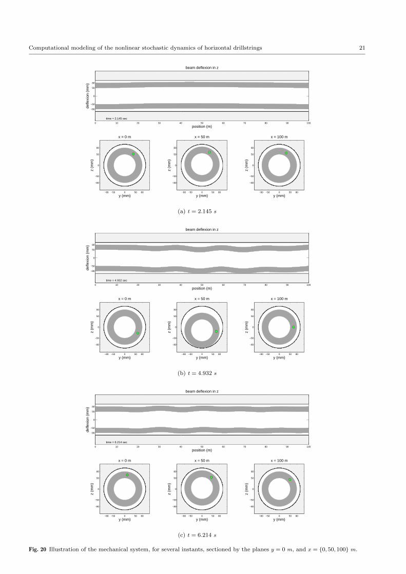
and the torsional friction induced by beam rotation.
These mechanical contacts also activate flexural modes
of vibration associated to high natural frequencies, so
that the mechanical system assumes complex spatial
configurations, as can be seen, for several instants, in
Figure 20.
It is also very clear from Figure 20 that, the me-
chanical contacts between beam and borehole wall, do
not occur all the time among discrete points, they can
also be seen along continuous line segments.
For a qualitative illustration of the nonlinear dy-
namics, the reader can see Online Resource 2.
6.8 Spectral analysis of the nonlinear dynamics
All signals presented above, that are associated with
the mechanical system response, have stochastic char-
acteristics. Thereby, for a good understanding of them,
it is necessary to analyze their spectral content through
the power spectral density (PSD) function [37].
The PSDs that are presented in this section (ma-
genta line) were estimated using the periodogram method
[37], and the smooth curves (blue line) appearing were
obtained by a filtering process, using a Savitzky-Golay
filter [48]. The PSDs are measured in dB/Hz, where the
intensity of reference is adopted as being equal to one.
An illustration of PSD functions of drill-bit velocity
and angular velocity is show in Figure 21. One can note
that, for velocity, the two peaks of highest amplitude
correspond to the frequencies 84.55 Hz, and 115.20 Hz,
respectively. These frequencies are very close to the
flexural frequencies 83.65 Hz, and 114.27 Hz, so that
drill-bit axial dynamics is controlled by the transversal
mechanisms of vibration. Furthermore, with respect to
angular velocity, it is noted a peak standing out in rela-
tion to the others. This peak is associated with 7.92 Hz
frequency, which is very close to the flexural frequency
7.63 Hz.
In Figure 22 the reader can see an illustration of
PSD functions of beam transversal velocity in z and
angular velocity around x when x = 50 m. The two
peaks of highest amplitude, for velocity in z, correspond
to the frequencies 143.20 Hz, and 172.50 Hz, respec-
tively. These frequencies are close to the flexural fre-
quencies 144.94 Hz, and 174.07 Hz, which indicates
that lateral vibrations in z, when x = 50 m, are in-
duced by the transversal vibration mechanism. In ad-
dition, in what concerns angular velocity around x, the
two peaks of largest amplitude are associated to the fre-
quencies 6.93 Hz, and 107.10 Hz, respectively close to
the flexural frequencies 6.59 Hz, and 106.18 Hz.
According to Figure 23, flexion is the primary mech-
anism of vibration that causes beam and borehole wall
Computational modeling of the nonlinear stochastic dynamics of horizontal drillstrings 21
0 10 20 30 40 50 60 70 80 90 100
−80
−50
0
50
80
beam deflexion in z
position (m)
defle
xion
(m
m)
time = 2.145 sec
−80 −50 0 50 80
−80
−50
0
50
80
x = 0 m
y (mm)
z (m
m)
−80 −50 0 50 80
−80
−50
0
50
80
x = 50 m
y (mm)
z (m
m)
−80 −50 0 50 80
−80
−50
0
50
80
x = 100 m
y (mm)
z (m
m)
(a) t = 2.145 s
0 10 20 30 40 50 60 70 80 90 100
−80
−50
0
50
80
beam deflexion in z
position (m)
defle
xion
(m
m)
time = 4.932 sec
−80 −50 0 50 80
−80
−50
0
50
80
x = 0 m
y (mm)
z (m
m)
−80 −50 0 50 80
−80
−50
0
50
80
x = 50 m
y (mm)
z (m
m)
−80 −50 0 50 80
−80
−50
0
50
80
x = 100 m
y (mm)
z (m
m)
(b) t = 4.932 s
0 10 20 30 40 50 60 70 80 90 100
−80
−50
0
50
80
beam deflexion in z
position (m)
defle
xion
(m
m)
time = 6.214 sec
−80 −50 0 50 80
−80
−50
0
50
80
x = 0 m
y (mm)
z (m
m)
−80 −50 0 50 80
−80
−50
0
50
80
x = 50 m
y (mm)
z (m
m)
−80 −50 0 50 80
−80
−50
0
50
80
x = 100 m
y (mm)
z (m
m)
(c) t = 6.214 s
Fig. 20 Illustration of the mechanical system, for several instants, sectioned by the planes y = 0 m, and x = 0, 50, 100 m.
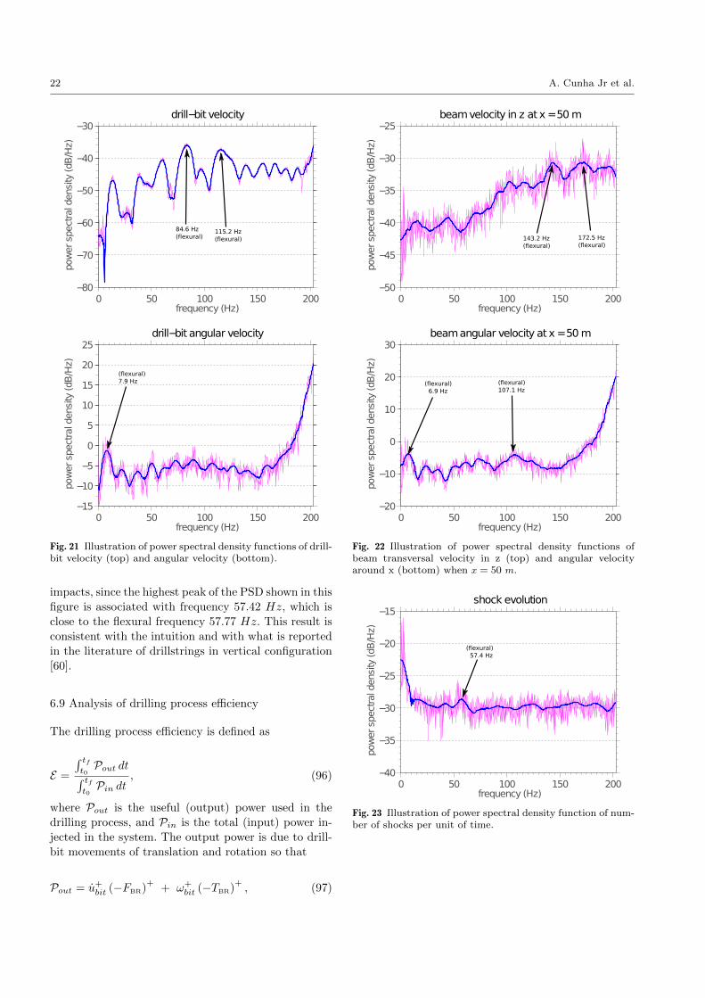
22 A. Cunha Jr et al.
0 50 100 150 200−80
−70
−60
−50
−40
−30
frequency (Hz)
pow
erspectraldensity
(dB
/Hz)
drill−bit velocity
84.6 Hz
(flexural)115.2 Hz
(flexural)
0 50 100 150 200−15
−10
−5
0
5
10
15
20
25
frequency (Hz)
pow
erspectraldensity
(dB
/Hz)
drill−bit angular velocity
(flexural)
7.9 Hz
Fig. 21 Illustration of power spectral density functions of drill-bit velocity (top) and angular velocity (bottom).
impacts, since the highest peak of the PSD shown in this
figure is associated with frequency 57.42 Hz, which is
close to the flexural frequency 57.77 Hz. This result is
consistent with the intuition and with what is reported
in the literature of drillstrings in vertical configuration
[60].
6.9 Analysis of drilling process efficiency
The drilling process efficiency is defined as
E =
∫ tft0Pout dt∫ tf
t0Pin dt
, (96)
where Pout is the useful (output) power used in the
drilling process, and Pin is the total (input) power in-
jected in the system. The output power is due to drill-
bit movements of translation and rotation so that
Pout = u+bit (−FBR)+
+ ω+bit (−TBR)
+, (97)
0 50 100 150 20050
45
40
35
30
25
frequency (Hz)
pow
er s
pect
ral d
ensi
ty (dB
/Hz)
beam velocity in z at x = 50 m
143.2 Hz(flexural)
172.5 Hz(flexural)
0 50 100 150 200−20
−10
0
10
20
30
frequency (Hz)
pow
erspectraldensity
(dB
/Hz)
beamangular velocity at x =50 m
(flexural)
6.9 Hz
(flexural)
107.1 Hz
Fig. 22 Illustration of power spectral density functions ofbeam transversal velocity in z (top) and angular velocityaround x (bottom) when x = 50 m.
0 50 100 150 20040
35
30
25
20
15
frequency (Hz)
pow
er s
pect
ral d
ensi
ty (dB
/Hz)
shock evolution
(flexural) 57.4 Hz
Fig. 23 Illustration of power spectral density function of num-ber of shocks per unit of time.
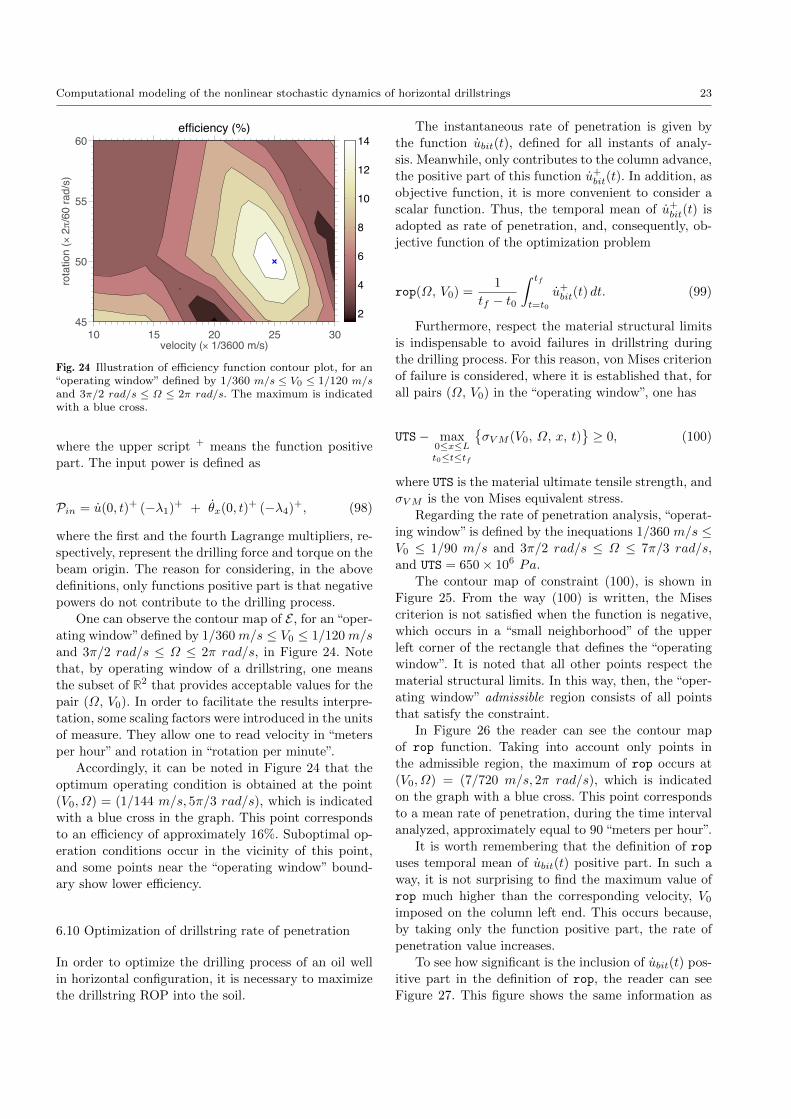
Computational modeling of the nonlinear stochastic dynamics of horizontal drillstrings 23
velocity (× 1/3600 m/s)
rota
tion
(× 2//
60 ra
d/s)
efficiency (%)
10 15 20 25 3045
50
55
60
2
4
6
8
10
12
14
Fig. 24 Illustration of efficiency function contour plot, for an“operating window” defined by 1/360 m/s ≤ V0 ≤ 1/120 m/s
and 3π/2 rad/s ≤ Ω ≤ 2π rad/s. The maximum is indicatedwith a blue cross.
where the upper script + means the function positive
part. The input power is defined as
Pin = u(0, t)+ (−λ1)+ + θx(0, t)+ (−λ4)+, (98)
where the first and the fourth Lagrange multipliers, re-
spectively, represent the drilling force and torque on the
beam origin. The reason for considering, in the above
definitions, only functions positive part is that negative
powers do not contribute to the drilling process.
One can observe the contour map of E , for an “oper-
ating window”defined by 1/360 m/s ≤ V0 ≤ 1/120 m/s
and 3π/2 rad/s ≤ Ω ≤ 2π rad/s, in Figure 24. Note
that, by operating window of a drillstring, one meansthe subset of R2 that provides acceptable values for the
pair (Ω, V0). In order to facilitate the results interpre-
tation, some scaling factors were introduced in the units
of measure. They allow one to read velocity in “meters
per hour” and rotation in “rotation per minute”.
Accordingly, it can be noted in Figure 24 that the
optimum operating condition is obtained at the point
(V0, Ω) = (1/144 m/s, 5π/3 rad/s), which is indicated
with a blue cross in the graph. This point corresponds
to an efficiency of approximately 16%. Suboptimal op-
eration conditions occur in the vicinity of this point,
and some points near the “operating window” bound-
ary show lower efficiency.
6.10 Optimization of drillstring rate of penetration
In order to optimize the drilling process of an oil well
in horizontal configuration, it is necessary to maximize
the drillstring ROP into the soil.
The instantaneous rate of penetration is given by
the function ubit(t), defined for all instants of analy-
sis. Meanwhile, only contributes to the column advance,
the positive part of this function u+bit(t). In addition, as
objective function, it is more convenient to consider a
scalar function. Thus, the temporal mean of u+bit(t) is
adopted as rate of penetration, and, consequently, ob-
jective function of the optimization problem
rop(Ω, V0) =1
tf − t0
∫ tf
t=t0
u+bit(t) dt. (99)
Furthermore, respect the material structural limits
is indispensable to avoid failures in drillstring during
the drilling process. For this reason, von Mises criterion
of failure is considered, where it is established that, for
all pairs (Ω, V0) in the “operating window”, one has
UTS− max0≤x≤Lt0≤t≤tf
σVM (V0, Ω, x, t)
≥ 0, (100)
where UTS is the material ultimate tensile strength, and
σVM is the von Mises equivalent stress.
Regarding the rate of penetration analysis, “operat-
ing window” is defined by the inequations 1/360 m/s ≤V0 ≤ 1/90 m/s and 3π/2 rad/s ≤ Ω ≤ 7π/3 rad/s,
and UTS = 650× 106 Pa.
The contour map of constraint (100), is shown in
Figure 25. From the way (100) is written, the Mises
criterion is not satisfied when the function is negative,
which occurs in a “small neighborhood” of the upper
left corner of the rectangle that defines the “operating
window”. It is noted that all other points respect the
material structural limits. In this way, then, the “oper-
ating window” admissible region consists of all points
that satisfy the constraint.
In Figure 26 the reader can see the contour map
of rop function. Taking into account only points in
the admissible region, the maximum of rop occurs at
(V0, Ω) = (7/720 m/s, 2π rad/s), which is indicated
on the graph with a blue cross. This point corresponds
to a mean rate of penetration, during the time interval
analyzed, approximately equal to 90 “meters per hour”.
It is worth remembering that the definition of rop
uses temporal mean of ubit(t) positive part. In such a
way, it is not surprising to find the maximum value of
rop much higher than the corresponding velocity, V0imposed on the column left end. This occurs because,
by taking only the function positive part, the rate of
penetration value increases.
To see how significant is the inclusion of ubit(t) pos-
itive part in the definition of rop, the reader can see
Figure 27. This figure shows the same information as
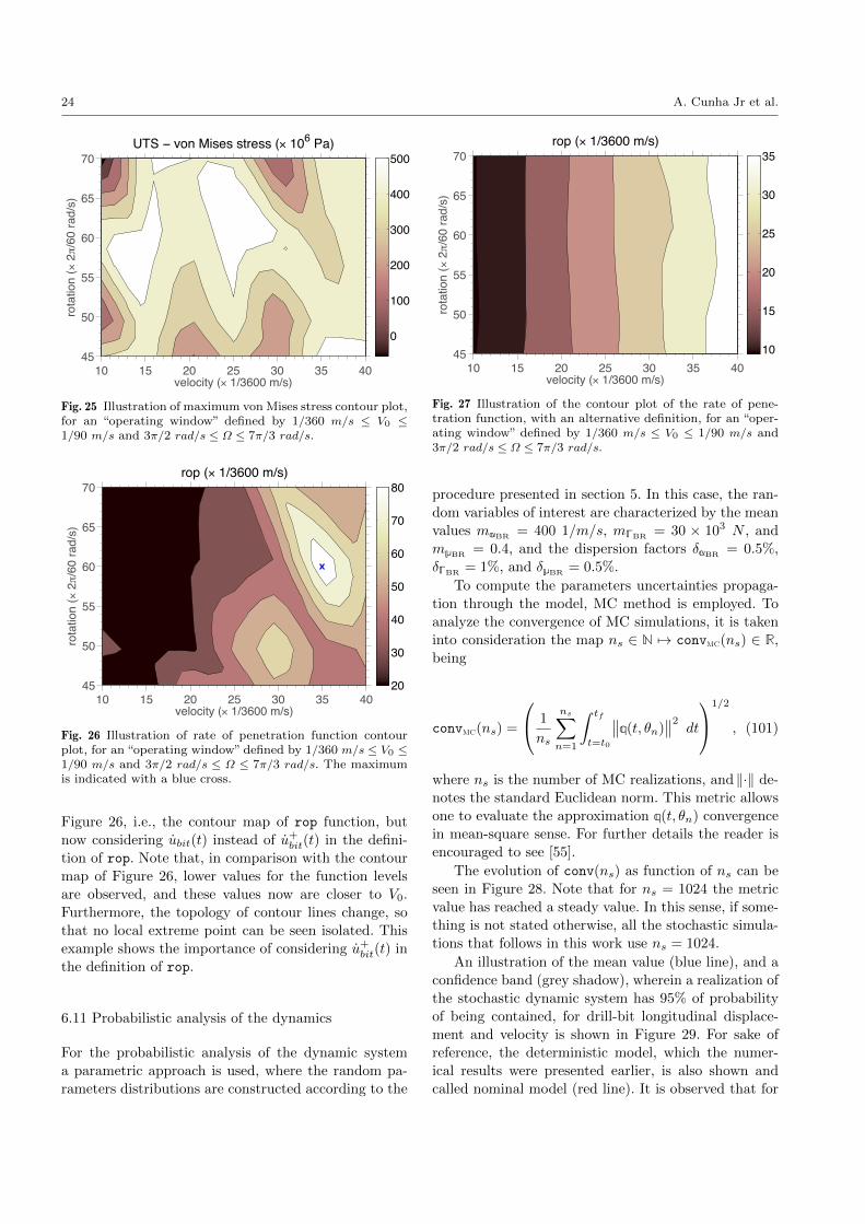
24 A. Cunha Jr et al.
velocity (× 1/3600 m/s)
rota
tion
(× 2//
60 ra
d/s)
UTS − von Mises stress (× 106 Pa)
10 15 20 25 30 35 4045
50
55
60
65
70
0
100
200
300
400
500
Fig. 25 Illustration of maximum von Mises stress contour plot,for an “operating window” defined by 1/360 m/s ≤ V0 ≤1/90 m/s and 3π/2 rad/s ≤ Ω ≤ 7π/3 rad/s.
velocity (× 1/3600 m/s)
rota
tion
(× 2//
60 ra
d/s)
rop (× 1/3600 m/s)
10 15 20 25 30 35 4045
50
55
60
65
70
20
30
40
50
60
70
80
Fig. 26 Illustration of rate of penetration function contourplot, for an “operating window” defined by 1/360 m/s ≤ V0 ≤1/90 m/s and 3π/2 rad/s ≤ Ω ≤ 7π/3 rad/s. The maximumis indicated with a blue cross.
Figure 26, i.e., the contour map of rop function, but
now considering ubit(t) instead of u+bit(t) in the defini-
tion of rop. Note that, in comparison with the contour
map of Figure 26, lower values for the function levels
are observed, and these values now are closer to V0.
Furthermore, the topology of contour lines change, so
that no local extreme point can be seen isolated. This
example shows the importance of considering u+bit(t) in
the definition of rop.
6.11 Probabilistic analysis of the dynamics
For the probabilistic analysis of the dynamic system
a parametric approach is used, where the random pa-
rameters distributions are constructed according to the
velocity (× 1/3600 m/s)
rota
tion
(× 2//
60 ra
d/s)
rop (× 1/3600 m/s)
10 15 20 25 30 35 4045
50
55
60
65
70
10
15
20
25
30
35
Fig. 27 Illustration of the contour plot of the rate of pene-tration function, with an alternative definition, for an “oper-ating window” defined by 1/360 m/s ≤ V0 ≤ 1/90 m/s and3π/2 rad/s ≤ Ω ≤ 7π/3 rad/s.
procedure presented in section 5. In this case, the ran-
dom variables of interest are characterized by the mean
values mBR= 400 1/m/s, mBR
= 30 × 103 N , and
mBR= 0.4, and the dispersion factors δBR
= 0.5%,
δBR = 1%, and δBR = 0.5%.
To compute the parameters uncertainties propaga-
tion through the model, MC method is employed. To
analyze the convergence of MC simulations, it is taken
into consideration the map ns ∈ N 7→ convMC(ns) ∈ R,
being
convMC(ns) =
1
ns
ns∑n=1
∫ tf
t=t0
∥∥q(t, θn)∥∥2 dt
1/2
, (101)
where ns is the number of MC realizations, and ‖·‖ de-
notes the standard Euclidean norm. This metric allows
one to evaluate the approximation q(t, θn) convergence
in mean-square sense. For further details the reader is
encouraged to see [55].
The evolution of conv(ns) as function of ns can be
seen in Figure 28. Note that for ns = 1024 the metric
value has reached a steady value. In this sense, if some-
thing is not stated otherwise, all the stochastic simula-
tions that follows in this work use ns = 1024.
An illustration of the mean value (blue line), and a
confidence band (grey shadow), wherein a realization of
the stochastic dynamic system has 95% of probability
of being contained, for drill-bit longitudinal displace-
ment and velocity is shown in Figure 29. For sake of
reference, the deterministic model, which the numer-
ical results were presented earlier, is also shown and
called nominal model (red line). It is observed that for
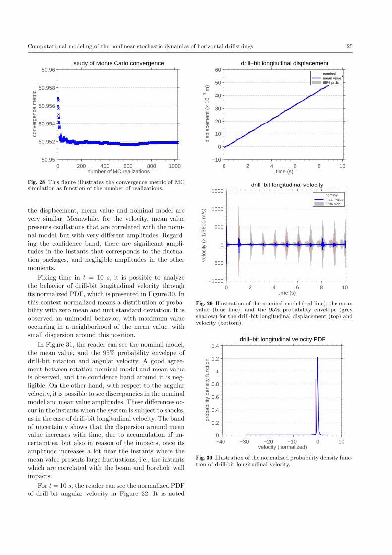
Computational modeling of the nonlinear stochastic dynamics of horizontal drillstrings 25
0 200 400 600 800 100050.95
50.952
50.954
50.956
50.958
50.96
number of MC realizations
con
verg
ence
met
ric
study of Monte Carlo convergence
Fig. 28 This figure illustrates the convergence metric of MCsimulation as function of the number of realizations.
the displacement, mean value and nominal model are
very similar. Meanwhile, for the velocity, mean value
presents oscillations that are correlated with the nomi-
nal model, but with very different amplitudes. Regard-
ing the confidence band, there are significant ampli-
tudes in the instants that corresponds to the fluctua-
tion packages, and negligible amplitudes in the other
moments.
Fixing time in t = 10 s, it is possible to analyze
the behavior of drill-bit longitudinal velocity through
its normalized PDF, which is presented in Figure 30. In
this context normalized means a distribution of proba-
bility with zero mean and unit standard deviation. It is
observed an unimodal behavior, with maximum value
occurring in a neighborhood of the mean value, with
small dispersion around this position.
In Figure 31, the reader can see the nominal model,
the mean value, and the 95% probability envelope of
drill-bit rotation and angular velocity. A good agree-
ment between rotation nominal model and mean value
is observed, and the confidence band around it is neg-
ligible. On the other hand, with respect to the angular
velocity, it is possible to see discrepancies in the nominal
model and mean value amplitudes. These differences oc-
cur in the instants when the system is subject to shocks,
as in the case of drill-bit longitudinal velocity. The band
of uncertainty shows that the dispersion around mean
value increases with time, due to accumulation of un-
certainties, but also in reason of the impacts, once its
amplitude increases a lot near the instants where the
mean value presents large fluctuations, i.e., the instants
which are correlated with the beam and borehole wall
impacts.
For t = 10 s, the reader can see the normalized PDF
of drill-bit angular velocity in Figure 32. It is noted
0 2 4 6 8 10−10
0
10
20
30
40
50
60
time (s)
dis
plac
emen
t (×
10−
3 m)
drill−bit longitudinal displacement
nominal mean value 95% prob.
0 2 4 6 8 10−1000
−500
0
500
1000
1500
time (s)
vel
ocity
(×
1/36
00 m
/s)
drill−bit longitudinal velocity
nominal mean value 95% prob.
Fig. 29 Illustration of the nominal model (red line), the meanvalue (blue line), and the 95% probability envelope (greyshadow) for the drill-bit longitudinal displacement (top) andvelocity (bottom).
−40 −30 −20 −10 0 100
0.2
0.4
0.6
0.8
1
1.2
1.4
velocity (normalized)
pro
babi
lity
dens
ity fu
nctio
n
drill−bit longitudinal velocity PDF
Fig. 30 Illustration of the normalized probability density func-tion of drill-bit longitudinal velocity.
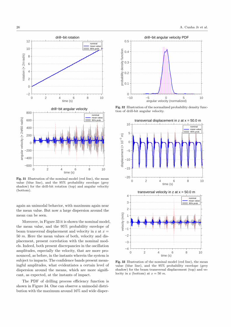
26 A. Cunha Jr et al.
0 2 4 6 8 10−2
0
2
4
6
8
10
12
time (s)
rot
atio
n (×
2π
rad/
s)
drill−bit rotation
nominal mean value 95% prob.
0 2 4 6 8 10−600
−400
−200
0
200
400
600
800
time (s)
ang
ular
vel
ocity
(×
2π/6
0 ra
d/s)
drill−bit angular velocity
nominal mean value 95% prob.
Fig. 31 Illustration of the nominal model (red line), the meanvalue (blue line), and the 95% probability envelope (greyshadow) for the drill-bit rotation (top) and angular velocity(bottom).
again an unimodal behavior, with maximum again near
the mean value. But now a large dispersion around the
mean can be seen.
Moreover, in Figure 33 it is shown the nominal model,
the mean value, and the 95% probability envelope of
beam transversal displacement and velocity in z at x =
50 m. Here the mean values of both, velocity and dis-
placement, present correlation with the nominal mod-
els. Indeed, both present discrepancies in the oscillation
amplitudes, especially the velocity, that are more pro-
nounced, as before, in the instants wherein the system is
subject to impacts. The confidence bands present mean-
ingful amplitudes, what evidentiates a certain level of
dispersion around the means, which are more signifi-
cant, as expected, at the instants of impact.
The PDF of drilling process efficiency function is
shown in Figure 34. One can observe a unimodal distri-
bution with the maximum around 16% and wide disper-
−10 −5 0 5 100
0.1
0.2
0.3
0.4
0.5
angular velocity (normalized)
pro
babi
lity
dens
ity fu
nctio
n
drill−bit angular velocity PDF
Fig. 32 Illustration of the normalized probability density func-tion of drill-bit angular velocity.
0 2 4 6 8 10−20
−15
−10
−5
0
5
10
time (s)
dis
plac
emen
t (×
10−
3 m)
transversal displacement in z at x = 50.0 m
nominal mean value 95% prob.
0 2 4 6 8 10−4
−3
−2
−1
0
1
2
3
4
time (s)
vel
ocity
(m
/s)
transversal velocity in z at x = 50.0 m
nominal mean value 95% prob.
Fig. 33 Illustration of the nominal model (red line), the meanvalue (blue line), and the 95% probability envelope (greyshadow) for the beam transversal displacement (top) and ve-locity in z (bottom) at x = 50 m.
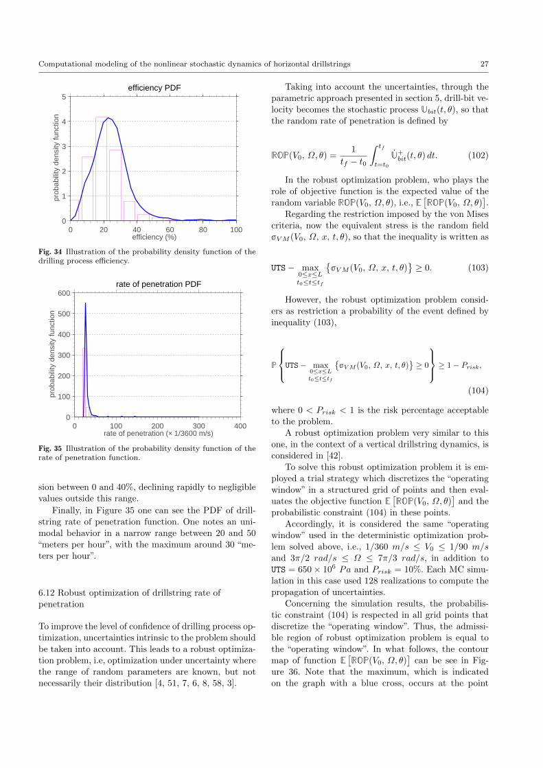
Computational modeling of the nonlinear stochastic dynamics of horizontal drillstrings 27
0 20 40 60 80 1000
1
2
3
4
5
efficiency (%)
pro
babi
lity
dens
ity fu
nctio
n
efficiency PDF
Fig. 34 Illustration of the probability density function of thedrilling process efficiency.
0 100 200 300 4000
100
200
300
400
500
600
rate of penetration (× 1/3600 m/s)
pro
babi
lity
dens
ity fu
nctio
n
rate of penetration PDF
Fig. 35 Illustration of the probability density function of therate of penetration function.
sion between 0 and 40%, declining rapidly to negligible
values outside this range.
Finally, in Figure 35 one can see the PDF of drill-
string rate of penetration function. One notes an uni-
modal behavior in a narrow range between 20 and 50
“meters per hour”, with the maximum around 30 “me-
ters per hour”.
6.12 Robust optimization of drillstring rate of
penetration
To improve the level of confidence of drilling process op-
timization, uncertainties intrinsic to the problem should
be taken into account. This leads to a robust optimiza-
tion problem, i.e, optimization under uncertainty where
the range of random parameters are known, but not
necessarily their distribution [4, 51, 7, 6, 8, 58, 3].
Taking into account the uncertainties, through the
parametric approach presented in section 5, drill-bit ve-
locity becomes the stochastic process Ubit(t, θ), so that
the random rate of penetration is defined by
ROP(V0, Ω, θ) =1
tf − t0
∫ tf
t=t0
U+bit(t, θ) dt. (102)
In the robust optimization problem, who plays the
role of objective function is the expected value of the
random variable ROP(V0, Ω, θ), i.e., E[ROP(V0, Ω, θ)
].
Regarding the restriction imposed by the von Mises
criteria, now the equivalent stress is the random field
VM (V0, Ω, x, t, θ), so that the inequality is written as
UTS− max0≤x≤Lt0≤t≤tf
VM (V0, Ω, x, t, θ)
≥ 0. (103)
However, the robust optimization problem consid-
ers as restriction a probability of the event defined by
inequality (103),
P
UTS− max0≤x≤Lt0≤t≤tf
VM (V0, Ω, x, t, θ)
≥ 0
≥ 1− Prisk,
(104)
where 0 < Prisk < 1 is the risk percentage acceptable
to the problem.
A robust optimization problem very similar to this
one, in the context of a vertical drillstring dynamics, is
considered in [42].
To solve this robust optimization problem it is em-
ployed a trial strategy which discretizes the “operating
window” in a structured grid of points and then eval-
uates the objective function E[ROP(V0, Ω, θ)
]and the
probabilistic constraint (104) in these points.
Accordingly, it is considered the same “operating
window” used in the deterministic optimization prob-
lem solved above, i.e., 1/360 m/s ≤ V0 ≤ 1/90 m/s
and 3π/2 rad/s ≤ Ω ≤ 7π/3 rad/s, in addition to
UTS = 650× 106 Pa and Prisk = 10%. Each MC simu-
lation in this case used 128 realizations to compute the
propagation of uncertainties.
Concerning the simulation results, the probabilis-
tic constraint (104) is respected in all grid points that
discretize the “operating window”. Thus, the admissi-
ble region of robust optimization problem is equal to
the “operating window”. In what follows, the contour
map of function E[ROP(V0, Ω, θ)
]can be see in Fig-
ure 36. Note that the maximum, which is indicated
on the graph with a blue cross, occurs at the point
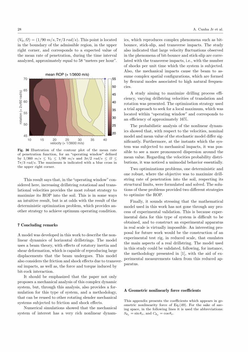
28 A. Cunha Jr et al.
(V0, Ω) = (1/90 m/s, 7π/3 rad/s). This point is located
in the boundary of the admissible region, in the upper
right corner, and corresponds to a expected value of
the mean rate of penetration, during the time interval
analyzed, approximately equal to 58 “meters per hour”.
velocity (× 1/3600 m/s)
rota
tion
(× 2//
60 ra
d/s)
mean ROP (× 1/3600 m/s)
10 15 20 25 30 35 4045
50
55
60
65
70
20
25
30
35
40
45
50
55
Fig. 36 Illustration of the contour plot of the mean rateof penetration function, for an “operating window” definedby 1/360 m/s ≤ V0 ≤ 1/90 m/s and 3π/2 rad/s ≤ Ω ≤7π/3 rad/s. The maximum is indicated with a blue cross inthe upper right corner.
This result says that, in the“operating window”con-
sidered here, increasing drillstring rotational and trans-
lational velocities provides the most robust strategy to
maximize its ROP into the soil. This is in some ways
an intuitive result, but is at odds with the result of the
deterministic optimization problem, which provides an-
other strategy to achieve optimum operating condition.
7 Concluding remarks
A model was developed in this work to describe the non-
linear dynamics of horizontal drillstrings. The model
uses a beam theory, with effects of rotatory inertia and
shear deformation, which is capable of reproducing large
displacements that the beam undergoes. This model
also considers the friction and shock effects due to transver-
sal impacts, as well as, the force and torque induced by
bit-rock interaction.
It should be emphasized that the paper not only
proposes a mechanical analysis of this complex dynamic
system, but, through this analysis, also provides a for-
mulation for this type of system, and a methodology,
that can be reused to other rotating slender mechanical
systems subjected to friction and shock effects.
Numerical simulations showed that the mechanical
system of interest has a very rich nonlinear dynam-
ics, which reproduces complex phenomena such as bit-
bounce, stick-slip, and transverse impacts. The study
also indicated that large velocity fluctuations observed
in the phenomena of bit-bounce and stick-slip are corre-
lated with the transverse impacts, i.e., with the number
of shocks per unit time which the system is subjected.
Also, the mechanical impacts cause the beam to as-
sume complex spatial configurations, which are formed
by flexural modes associated to high natural frequen-
cies.
A study aiming to maximize drilling process effi-
ciency, varying drillstring velocities of translation and
rotation was presented. The optimization strategy used
a trial approach to seek for a local maximum, which was
located within “operating window” and corresponds to
an efficiency of approximately 16%.
The probabilistic analysis of the nonlinear dynam-
ics showed that, with respect to the velocities, nominal
model and mean value of the stochastic model differ sig-
nificantly. Furthermore, at the instants which the sys-
tem was subjected to mechanical impacts, it was pos-
sible to see a more pronounced dispersion around the
mean value. Regarding the velocities probability distri-
butions, it was noticed a unimodal behavior essentially.
Two optimizations problems, one deterministic and
one robust, where the objective was to maximize drill-
string rate of penetration into the soil, respecting its
structural limits, were formulated and solved. The solu-
tions of these problems provided two different strategies
to optimize the ROP.
Finally, it sounds stressing that the mathematical
model used in this work has not gone through any pro-
cess of experimental validation. This is because exper-
imental data for this type of system is difficult to be
obtained, and to construct an experimental apparatus
in real scale is virtually impossible. An interesting pro-
posal for future work would be the construction of an
experimental test rig, in reduced scale, that emulates
the main aspects of a real drillstring. The model used
in this study could be validated, following, for instance,
the methodology presented in [1], with the aid of ex-
perimental measurements taken from this reduced ap-
paratus.
A Geometric nonlinearly force coefficients
This appendix presents the coefficients which appears in ge-ometric nonlinearity force of Eq.(49). For the sake of sav-ing space, in the following lines it is used the abbreviations:Sθx = sin θx, and Cθx = cos θx.
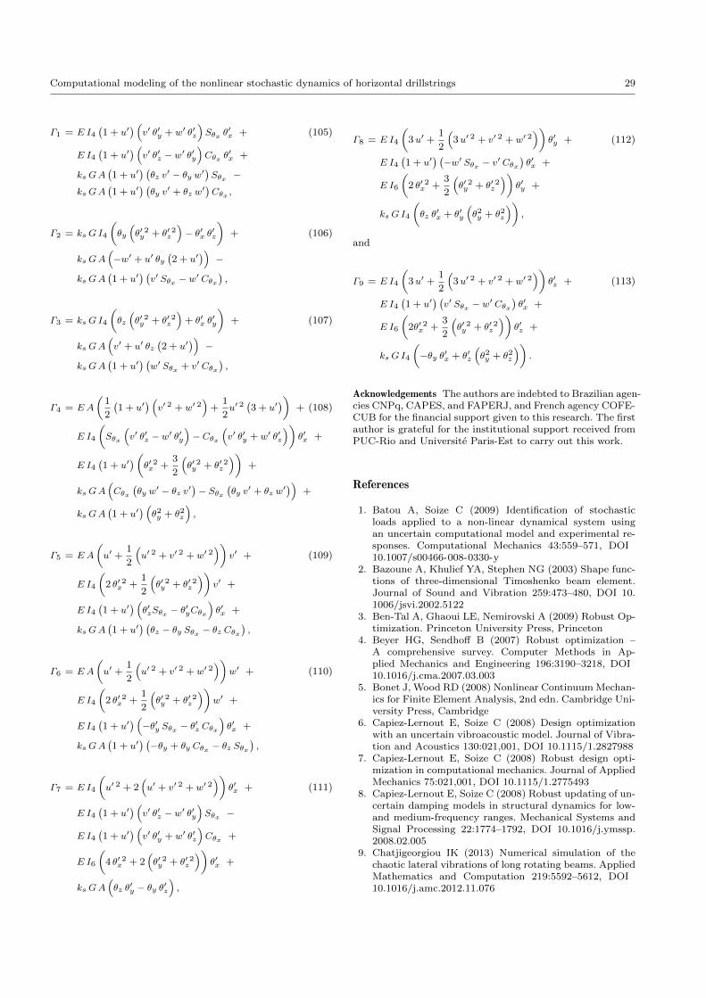
Computational modeling of the nonlinear stochastic dynamics of horizontal drillstrings 29
Γ1 = E I4(1 + u′
) (v′ θ′y + w′ θ′z
)Sθx θ
′x + (105)
E I4(1 + u′
) (v′ θ′z − w′ θ′y
)Cθx θ
′x +
ksGA(1 + u′
) (θz v′ − θy w′
)Sθx −
ksGA(1 + u′
) (θy v′ + θz w
′)Cθx ,Γ2 = ksGI4
(θy
(θ′ 2y + θ′ 2z
)− θ′x θ′z
)+ (106)
ksGA(−w′ + u′ θy
(2 + u′
))−
ksGA(1 + u′
) (v′ Sθx − w
′ Cθx),
Γ3 = ksGI4
(θz
(θ′ 2y + θ′ 2z
)+ θ′x θ
′y
)+ (107)
ksGA(v′ + u′ θz
(2 + u′
))−
ksGA(1 + u′
) (w′ Sθx + v′ Cθx
),
Γ4 = EA
(1
2
(1 + u′
) (v′ 2 + w′ 2
)+
1
2u′ 2
(3 + u′
))+ (108)
E I4
(Sθx
(v′ θ′z − w′ θ′y
)− Cθx
(v′ θ′y + w′ θ′z
))θ′x +
E I4(1 + u′
)(θ′ 2x +
3
2
(θ′ 2y + θ′ 2z
))+
ksGA(Cθx
(θy w
′ − θz v′)− Sθx
(θy v′ + θz w
′)) +
ksGA(1 + u′
) (θ2y + θ2z
),
Γ5 = EA
(u′ +
1
2
(u′ 2 + v′ 2 + w′ 2
))v′ + (109)
E I4
(2 θ′ 2x +
1
2
(θ′ 2y + θ′ 2z
))v′ +
E I4(1 + u′
) (θ′zSθx − θ
′yCθx
)θ′x +
ksGA(1 + u′
) (θz − θy Sθx − θz Cθx
),
Γ6 = EA
(u′ +
1
2
(u′ 2 + v′ 2 + w′ 2
))w′ + (110)
E I4
(2 θ′ 2x +
1
2
(θ′ 2y + θ′ 2z
))w′ +
E I4(1 + u′
) (−θ′y Sθx − θ
′z Cθx
)θ′x +
ksGA(1 + u′
) (−θy + θy Cθx − θz Sθx
),
Γ7 = E I4
(u′ 2 + 2
(u′ + v′ 2 + w′ 2
))θ′x + (111)
E I4(1 + u′
) (v′ θ′z − w′ θ′y
)Sθx −
E I4(1 + u′
) (v′ θ′y + w′ θ′z
)Cθx +
E I6
(4 θ′ 2x + 2
(θ′ 2y + θ′ 2z
))θ′x +
ksGA(θz θ′y − θy θ′z
),
Γ8 = E I4
(3u′ +
1
2
(3u′ 2 + v′ 2 + w′ 2
))θ′y + (112)
E I4(1 + u′
) (−w′ Sθx − v
′ Cθx)θ′x +
E I6
(2 θ′ 2x +
3
2
(θ′ 2y + θ′ 2z
))θ′y +
ksGI4
(θz θ′x + θ′y
(θ2y + θ2z
)),
and
Γ9 = E I4
(3u′ +
1
2
(3u′ 2 + v′ 2 + w′ 2
))θ′z + (113)
E I4(1 + u′
) (v′ Sθx − w
′ Cθx)θ′x +
E I6
(2θ′ 2x +
3
2
(θ′ 2y + θ′ 2z
))θ′z +
ksGI4
(−θy θ′x + θ′z
(θ2y + θ2z
)).
Acknowledgements The authors are indebted to Brazilian agen-cies CNPq, CAPES, and FAPERJ, and French agency COFE-CUB for the financial support given to this research. The firstauthor is grateful for the institutional support received fromPUC-Rio and Universite Paris-Est to carry out this work.
References
1. Batou A, Soize C (2009) Identification of stochasticloads applied to a non-linear dynamical system usingan uncertain computational model and experimental re-sponses. Computational Mechanics 43:559–571, DOI10.1007/s00466-008-0330-y
2. Bazoune A, Khulief YA, Stephen NG (2003) Shape func-tions of three-dimensional Timoshenko beam element.Journal of Sound and Vibration 259:473–480, DOI 10.1006/jsvi.2002.5122
3. Ben-Tal A, Ghaoui LE, Nemirovski A (2009) Robust Op-timization. Princeton University Press, Princeton
4. Beyer HG, Sendhoff B (2007) Robust optimization –A comprehensive survey. Computer Methods in Ap-plied Mechanics and Engineering 196:3190–3218, DOI10.1016/j.cma.2007.03.003
5. Bonet J, Wood RD (2008) Nonlinear Continuum Mechan-ics for Finite Element Analysis, 2nd edn. Cambridge Uni-versity Press, Cambridge
6. Capiez-Lernout E, Soize C (2008) Design optimizationwith an uncertain vibroacoustic model. Journal of Vibra-tion and Acoustics 130:021,001, DOI 10.1115/1.2827988
7. Capiez-Lernout E, Soize C (2008) Robust design opti-mization in computational mechanics. Journal of AppliedMechanics 75:021,001, DOI 10.1115/1.2775493
8. Capiez-Lernout E, Soize C (2008) Robust updating of un-certain damping models in structural dynamics for low-and medium-frequency ranges. Mechanical Systems andSignal Processing 22:1774–1792, DOI 10.1016/j.ymssp.2008.02.005
9. Chatjigeorgiou IK (2013) Numerical simulation of thechaotic lateral vibrations of long rotating beams. AppliedMathematics and Computation 219:5592–5612, DOI10.1016/j.amc.2012.11.076
30 A. Cunha Jr et al.
10. Chevallier A (2000) Nonlinear Stochastic Drilling Vibra-tions. Ph.D Thesis, Rice University, Houston
11. Cull SJ, Tucker RW (1999) On the modelling of Coulombfriction. Journal of Physics A: Mathematical and General32:2103–2113, DOI 10.1088/0305-4470/32/11/006
12. Cunha Jr A (2015) Modeling and Uncertainty Quantifi-cation in the Nonlinear Stochastic Dynamics of a Hori-zontal Dsrillstrings. D.Sc. Thesis, Pontifıcia UniversidadeCatolica do Rio de Janeiro / Universite Paris-Est
13. Cunha Jr A, Nasser R, Sampaio R, Lopes H, Breit-man K (2014) Uncertainty quantification through MonteCarlo method in a cloud computing setting. ComputerPhysics Communications 185:1355––1363, DOI 10.1016/j.cpc.2014.01.006, DOI 10.1016/j.cpc.2014.01.006
14. Davies RJ, Almond S, Ward RS, Jackson RB, AdamsC, Worrall F, Herringshaw LG, Gluyas JG, WhiteheadMA (in press) Oil and gas wells and their integrity:Implications for shale and unconventional resource ex-ploitation. Marine and Petroleum Geology DOI http://dx.doi.org/10.1016/j.marpetgeo.2014.03.001
15. Depouhon A, Detournay E (2014) Instability regimes andself-excited vibrations in deep drilling systems. Journal ofSound and Vibration 333:2019–2039, DOI 10.1016/j.jsv.2013.10.005
16. Detournay E, Richard T, Shepherd M (2008) Drilling re-sponse of drag bits: Theory and experiment. InternationalJournal of Rock Mechanics & Mining Sciences 45:1347–1360, DOI 10.1016/j.ijrmms.2008.01.010
17. Divenyi S, Savi MA, Wiercigroch M, Pavlovskaia E(2012) Drill-string vibration analysis using non-smoothdynamics approach. Nonlinear Dynamics 70:1017–1035,DOI 10.1007/s11071-012-0510-3
18. Franca LFP (2010) Drilling action of roller-cone bits:modeling and experimental validation. Journal of EnergyResources Technology 132:043,101–1–043,101–9, DOI10.1115/1.4003168
19. Franca LFP, Weber HI (2004) Experimental and numer-ical study of a new resonance hammer drilling modelwith drift. Chaos, Solitons & Fractals 21:789–801, DOI10.1016/j.chaos.2003.12.064
20. Freudenrich C, Strickland J (2001) How Oil DrillingWorks.http://www.howstuffworks.com/oil-drilling
21. Gilardi G, Sharf I (2002) Literature survey of contactdynamics modelling. Mechanism and Machine Theory37:1213–1239, DOI 10.1016/S0094-114X(02)00045-9
22. Golub GH, Van Loan CF (2013) Matrix Computations,4th edn. The Johns Hopkins University Press, Baltimore
23. Hagedorn P, DasGupta A (2007) Vibrations and Wavesin Continuous Mechanical Systems. Wiley, Chichester
24. Hu Y, Di Q, Zhu W, Chen Z, Wang W (2012) Dynamiccharacteristics analysis of drillstring in the ultra-deepwell with spatial curved beam finite element. Journalof Petroleum Science and Engineering 82—83:166–173,DOI 10.1016/j.petrol.2012.01.011
25. Hughes TJR (2000) The Finite Element Method. DoverPublications, New York
26. Hunt KH, Crossley FE (1975) Coefficient of restitutioninterpreted as damping in vibroimpact. Journal of Ap-plied Mechanics 42:440–445, DOI 10.1115/1.3423596
27. Jansen JD (1993) Nonlinear Dynamics of Oilwell Drill-strings. Ph.D Thesis, TU Delft, Amsterdam
28. Khulief YA, Al-Sulaiman FA, Bashmal S (2007) Vibra-tion analysis of drillstrings with self-excited stick–slip os-cillations. Journal of Sound and Vibration 299:540–558,DOI 10.1016/j.jsv.2006.06.065
29. Kroese DP, Taimre T, Botev ZI (2011) Handbook ofMonte Carlo Methods. Wiley, New Jersey
30. Lanczos C (1986) The Variational Principles of Mechan-ics, 4th edn. Dover Publications, New York
31. Litewka P, Wriggers P (2002) Frictional contact between3D beams. Computational Mechanics 28:26–39, DOI 10.1007/s004660100266
32. Liu X, Vlajic N, Long X, Meng G, Balachandran B (2013)Nonlinear motions of a flexible rotor with a drill bit:stick-slip and delay effects. Nonlinear Dynamics 72:61–77, DOI 10.1007/s11071-012-0690-x
33. Macdonald KA, Bjune JV (2007) Failure analysis of drill-strings. Engineering Failure Analysis 14:1641–1666, DOI10.1016/j.engfailanal.2006.11.073
34. Nandakumar K, Wiercigroch M (2013) Stability analysisof a state dependent delayed, coupled two DOF modelof drill-stringvibration. Journal of Sound and Vibration332:2575–2592, DOI 10.1016/j.jsv.2012.12.020
35. Newmark NM (1959) A method of computation for struc-tural dynamics. Journal of the Engineering MechanicsDivision 85:67–94
36. Oberkampf WL, Roy CJ (2010) Verification and Val-idation in Scientific Computing. Cambridge UniversityPress, Cambridge
37. Oppenheim AV, Schafer RW (2009) Discrete-Time SignalProcessing, 3rd edn. Prentice Hall, Englewood Cliffs, N.J.
38. Reddy JN (1997) On locking-free shear deformablebeam finite elements. Computer Methods in AppliedMechanics and Engineering 149:113–132, DOI 10.1016/S0045-7825(97)00075-3
39. Ritto TG (2010) Numerical Analysis of the NonlinearDynamics of a Drill-string with Uncertainty Modeling.D.Sc. Thesis, Pontifıcia Universidade Catolica do Rio deJaneiro / Universite Paris-Est
40. Ritto TG, Sampaio R (2012) Stochastic drill-string dy-namics with uncertainty on the imposed speed and onthe bit-rock parameters. International Journal for Un-certainty Quantification 2:111–124, DOI 10.1615/Int.J.UncertaintyQuantification.v2.i2
41. Ritto TG, Soize C, Sampaio R (2009) Non-linear dynam-ics of a drill-string with uncertain model of the bit–rockinteraction. International Journal of Non-Linear Mechan-ics 44:865–876, DOI 10.1016/j.ijnonlinmec.2009.06.003
42. Ritto TG, Soize C, Sampaio R (2010) Robust optimiza-tion of the rate of penetration of a drill-string usinga stochastic nonlinear dynamical model. ComputationalMechanics 45:415–427, DOI 10.1007/s00466-009-0462-8
43. Ritto TG, Soize C, Sampaio R (2010) Stochasticdynamics of a drill-string with uncertain weight-on-hook. Journal of the Brazilian Society of Mechani-cal Sciences and Engineering 32:250–258, DOI 10.1590/S1678-58782010000300008
44. Ritto TG, Escalante MR, Sampaio R, Rosales MB (2013)Drill-string horizontal dynamics with uncertainty on thefrictional force. Journal of Sound and Vibration 332:145–153, DOI 10.1016/j.jsv.2012.08.007
45. Sagan H (1992) Introduction to the Calculus of Varia-tions. Dover Publications, New York
46. Sahebkar SM, Ghazavi MR, Khadem SE, Ghayesh MH(2011) Nonlinear vibration analysis of an axially movingdrillstring system with time dependent axial load and ax-ial velocity in inclined well. Mechanism and Machine The-ory 46:743–760, DOI 10.1016/j.mechmachtheory.2010.12.003
47. Sampaio R, Piovan M, Lozano GV (2007) Coupledaxial/torsional vibrations of drill-strings by means of
Computational modeling of the nonlinear stochastic dynamics of horizontal drillstrings 31
non-linear model. Mechanics Research Communications34:497–502, DOI 10.1016/j.mechrescom.2007.03.005
48. Savitzky A, Golay MJE (1964) Smoothing and dif-ferentiation of data by simplified least squares proce-dures. Analytical Chemistry 36:1627–1639, DOI 10.1021/ac60214a047
49. Schueller GI (1997) A state-of-the-art report on com-putational stochastic mechanics. Probabilistic Engineer-ing Mechanics 12:197–321, DOI 10.1016/S0266-8920(97)00003-9
50. Schueller GI (2007) On the treatment of uncertainties instructural mechanics and analysis. Computers & Struc-tures 85:235–243, DOI 10.1016/j.compstruc.2006.10.009
51. Schueller GI, Jensen HA (2008) Computational methodsin optimization considering uncertainties – an overview.Computer Methods in Applied Mechanics and Engineer-ing 198:2–13, DOI 10.1016/j.cma.2008.05.004
52. Silveira M, Wiercigroch M (2009) Low dimensional mod-els for stick-slip vibration of drill-strings. Journal ofPhysics: Conference Series 181:012,056, DOI 10.1088/1742-6596/181/1/012056
53. Soize C (2000) A nonparametric model of random un-certainties for reduced matrix models in structural dy-namics. Probabilistic Engineering Mechanics 15:277–294,DOI 10.1016/S0266-8920(99)00028-4
54. Soize C (2001) Maximum entropy approach for modelingrandom uncertainties in transient elastodynamics. Jour-nal of the Acoustical Society of America 109:1979–1996,DOI 10.1121/1.1360716
55. Soize C (2005) A comprehensive overview of a non-parametric probabilistic approach of model uncertain-ties for predictive models in structural dynamics. Journalof Sound and Vibration 288:623–652, DOI 10.1016/j.jsv.2005.07.009
56. Soize C (2012) Stochastic Models of Uncertainties inComputational Mechanics. Amer Society of Civil Engi-neers, Reston
57. Soize C (2013) Stochastic modeling of uncertainties incomputational structural dynamics — recent theoreti-cal advances. Journal of Sound and Vibration 332:2379––2395, DOI 10.1016/j.jsv.2011.10.010
58. Soize C, Capiez-Lernout E, Ohayon R (2008) Robust up-dating of uncertain computational models using experi-mental modal analysis. AIAA Journal 46:2955–2965
59. Spanos PD, Chevallier AM, Politis NP (2002) Nonlin-ear stochastic drill-string vibrations. Journal of Vibrationand Acoustics 124:512–518, DOI 10.1115/1.1502669
60. Spanos PD, Chevallier AM, Politis NP, Payne ML (2003)Oil and gas well drilling: a vibrations perspective. TheShock and Vibration Digest 35:85–103
61. Trindade MA, Wolter C, Sampaio R (2005)Karhunen–Loeve decomposition of coupled ax-ial/bending vibrations of beams subject to impacts.Journal of Sound and Vibration 279:1015–1036, DOI10.1016/j.jsv.2003.11.057
62. Willoughby D (2005) Horizontal Directional Drilling(HDD): Utility and Pipeline Applications. McGraw-Hill,New York
63. Wriggers P (2006) Computational Contact Mechanics,2nd edn. Springer, New York
64. Wriggers P, Zavarise G (2004) Computational ContactMechanics. In: Stein E, de Borst R, Hughes TJR (eds)Encyclopedia of Computational Mechanics, vol 2, Wiley,Hoboken, pp 195–226, DOI 10.1002/0470091355.ecm033
65. Wriggers P, Wagner W, Stein E (1987) Algorithms fornon-linear contact constraints with application to stabil-
ity problems of rods and shells. Computational Mechanics2:215–230, DOI 10.1007/BF00571026
66. Young DM (2003) Iterative Solution of Large Linear Sys-tems. Dover Publications, New York
67. Zhang Y, Sharf I (2009) Validation of nonlinear viscoelas-tic contact force models for low speed impact. Journal ofApplied Mechanics 76:051,002, DOI 10.1115/1.3112739
68. Zhu X, Liu Y, Tong H (2014) Analysis of reamer failurebased on vibration analysis of the rock breaking in hor-izontal directional drilling. Engineering Failure Analysis37:64 – 74, DOI 10.1016/j.engfailanal.2013.11.016