computational collapse of quantum state with application to oblivious transfer
TRANSCRIPT
BR
ICS
RS
-03-37C
repeauetal.:
Com
putationalCollapse
ofQuantum
State
with
Application
toO
bliviousTransfer
BRICSBasic Research in Computer Science
Computational Collapse of Quantum Statewith Application to Oblivious Transfer
Claude CrepeauPaul DumaisDominic MayersLouis Salvail
BRICS Report Series RS-03-37
ISSN 0909-0878 November 2003
Copyright c© 2003, Claude Crepeau & Paul Dumais & DominicMayers & Louis Salvail.BRICS, Department of Computer ScienceUniversity of Aarhus. All rights reserved.
Reproduction of all or part of this workis permitted for educational or research useon condition that this copyright notice isincluded in any copy.
See back inner page for a list of recent BRICS Report Series publications.Copies may be obtained by contacting:
BRICSDepartment of Computer ScienceUniversity of AarhusNy Munkegade, building 540DK–8000 Aarhus CDenmarkTelephone: +45 8942 3360Telefax: +45 8942 3255Internet: [email protected]
BRICS publications are in general accessible through the World WideWeb and anonymous FTP through these URLs:
http://www.brics.dkftp://ftp.brics.dkThis document in subdirectory RS/03/37/
Computational Collapse of Quantum State withApplication to Oblivious Transfer
Claude Crépeau1?, Paul Dumais1??, Dominic Mayers2? ? ?, and Louis Salvail3†
1 School of Computer Science, McGill University, {crepeau|dumais}@cs.mcgill.ca2 IQI, California Institute of Technology, [email protected] BRICS‡, FICS§, Dept. of Computer Science, University of Århus,
Abstract. Quantum 2-party cryptography differs from its classicalcounterpart in at least one important way: Given blak-box access to aperfect commitment scheme there exists a secure 1−2 quantum oblivioustransfer. This reduction proposed by Crépeau and Kilian was proved se-cure against any receiver by Yao, in the case where perfect commitmentsare used. However, quantum commitments would normally be based oncomputational assumptions. A natural question therefore arises: Whathappens to the security of the above reduction when computationallysecure commitments are used instead of perfect ones?In this paper, we address the security of 1−2 QOT when computationallybinding string commitments are available. In particular, we analyse thesecurity of a primitive called Quantum Measurement Commitment whenit is constructed from unconditionally concealing but computationallybinding commitments. As measuring a quantum state induces an irre-versible collapse, we describe a QMC as an instance of “computationalcollapse of a quantum state”. In a QMC a state appears to be collapsedto a polynomial time observer who cannot extract full information aboutthe state without breaking a computational assumption.We reduce the security of QMC to a weak binding criteria for the stringcommitment. We also show that secure QMCs implies QOT using astraightforward variant of the reduction above.
1 Introduction
Quantum 2-party cryptography differs from its classical counterpart in at leastone important way: Given blak-box access to a perfect commitment scheme there? Part of this research was done while visiting University of Århus and was funded by
Québec’s FQRNT and MDER, and Canada’s NSERC and MITACS.?? Part of this research was funded by NSERC
? ? ? This work has been supported in part by the National Science Foundation underGrant No. EIA-0086038.
† Part of this research was funded by European projects QAIP and PROSECCO.‡ Funded by the Danish National Research Foundation.§ FICS, Foundations in Cryptography and Security, funded by the Danish Natural
Sciences Research Council.
exists a secure 1 − 2 quantum oblivious transfer (i.e. 1-2 QOT) scheme[5, 3, 4].Classically, it is known that such a reduction is unlikely to exist [9]. By 1-2 QOTwe mean a standard oblivious transfer of two classical messages using quantumcommunication. In [5], Crépeau and Kilian have shown how 1-2 QOT can be ob-tained from perfect commitments (i.e. the CK protocol). The security analysisof the CK protocol was provided by Crépeau in [4] with respect to receivers re-stricted to perform only immediate and complete measurements. The assumptionwas relaxed in [14] by showing that privacy for the sender is garanteed againstany individual measurements applied by the receiver. The security against anyreceiver was obtained by Yao in [19]. This important paper provides a full proofof security for 1-2 QOT when constructed from perfect commitments under theassumption that the quantum channel is error-free. Yao’s result was then gener-alized by Mayers[12] for the case of noisy quantum channel [3] and where stringsare transmitted instead of bits. Mayers then reduced the security of quantumkey distribution to the security of such a generalized 1-2 QOT. If 2-party cryp-tography in the quantum world seems to rely upon weaker assumptions than itsclassical counterpart, it also shares some of its limits. As it was shown in [11, 13,10], no statistically binding and concealing quantum bit commitment can exist.On the other hand, quantum commitments can be based upon physical[16] andcomputational[7, 6] assumptions. A natural question arises: What happens to thesecurity of the CK protocol when computationally secure commitments are usedinstead of perfect ones? It should be stressed that Yao’s proof does not applyin this case since it relies heavily upon the fact that the commitment scheme ismodelled by a classical black-box (i.e. one with classical inputs and outputs). Theproof is information theoretic provided the sender and the receiver have black-box access to perfect commitments. For Yao’s proof to apply, the committingphase should be modelled by the transmission of a classical bit to a third partywho conceals it to the receiver until the opening phase. Although any uncondi-tionally binding commitment scheme defines such a classical bit, unconditionallyconcealing commitments do not (i.e. both committed values can be explained bythe information provided to the receiver). In this paper, we address the securityof 1-2 QOT when computationally binding string commitments are available. Inparticular, we analyse the security of a primitive called Quantum MeasurementCommitment (i.e. QMC) when it is constructed from unconditionally concealingbut computationally binding commitments. We reduce the security of QMC toa weak binding criteria for the string commitment. We also show that secureQMCs implies 1-2 QOT using a straightforward variant of the CK protocol. Itfollows that unlike Yao’s proof (and the proof in [14]), our security proof applieswhen computionally binding commitments are used.
The CK protocol can be seen as a quantum reduction of 1-2 OT to bit com-mitment. To see how it works, consider the BB84 coding scheme[2, 5] for classicalbit b into a random state in { b〉+, b〉×}.The random θ ∈ {+,×} used to encodeb into the quantum state b〉θ, is called the transmission basis.Since only orthog-onal quantum states can be distinguished with certainty, the transmitted bit b isnot received perfectly by the receiver, Alice, who does not know the transmission
2
basis. The coding scheme also specifies what an honest Alice should be doingwith the received state b〉θ. She picks θ ∈R {+,×} and measures b〉θ withmeasurement Mθ that distinguishes perfectly orthogonal states 0〉θ and 1〉θ.IfBob and Alice follow honestly the BB84 coding scheme then b is received withprobability 1 when θ = θ whereas a random bit is received when θ 6= θ. In otherwords, If Bob announces the transmission basis a the end of the transmissionthen the BB84 coding scheme implements a Rabin’s oblivious transfer [15] fromBob to Alice provided she is honest. Otherwise, Alice can easily cheat the pro-tocol by postponing the measurement until the basis is announced. In this caseshe gets the transmitted bit all the time. In order to make the BB84 transmis-sion resistant to active adversaries, the CK protocol uses n BB84 transmissionswhere for each of them, Alice is asked to commit upon the measurements andoutcomes prior the announcement of the transmission bases by Bob.
We call Quantum Measurement Commitment (or QMC) the primitive thatallows Alice to provide Bob with evidences of measurements she claims havingperformed on n BB84 qubits before the announcement of θ ∈ {+,×}n. Imple-menting a QMC is simply done by sending a string commitment containing (θ, b)to Bob where θ ∈ {+,×}n is the measurements Alice claims having performedand b ∈ {0, 1}n are the outcomes. The classical bit encoded in the transmissionis defined as the value of some predicate f(b1, . . . , bn). Once the QMC has beenperformed, Alice should be unable to evaluate f(b1, . . . , bn) even given the knowl-edge of the transmission bases θ. A computational collapse occurred if, given thetransmission basis θ, f(b1, . . . , bn) cannot be determined efficiently. The CK pro-tocol constructs a 1-2 QOT from a QMC with f(b1, . . . , bn) ≡ ⊕n
i=1bi. A QMCis therefore a universal primitive for secure 2-party computation (of classicalfunctions).
Our contribution. In this paper, we address the question of determining howthe binding property of the string commitment scheme used for implementing aQMC enforces its security. As already pointed out in [7, 6], quantum bit com-mitment schemes satisfy different binding properties than classical ones. Thedifference becomes more obvious when string commitments are taken into ac-count. In Sect. 3.1, we generalize the computational binding criteria of [7] tothe case where commitments are made to strings of size ` ∈ Θ(n) for n thesecurity parameter, and ` some value depending on n. Intuitively, for a classof functions F ⊆ {f : {0, 1}` → {0, 1}m}, with m < ` both depending on n,we say that a string commitment scheme is F–binding if for all f ∈ F , for allcommitment prepared by the sender, and for a random y ∈R {0, 1}m, the com-mitment cannot be opened efficiently to any s ∈ {0, 1}` such that f(s) = y withsuccess probability significantly better than 1/2m. The smaller m is comparedto `, the weaker is the F–binding criteria. We relate the security of QMC to aweak form of the F–binding property. We assume that a QMC is made usinga computationally binding and unconditionally concealing string commitmentcontaining the bases θ ∈ {+,×}n and the results b ∈ {0, 1}n obtained by Al-ice after Bob’s transmission of b〉θ. We then define the security of a QMC by
3
the following game between Alice and Bob. Bob selects a challenge c ∈R {0, 1}.If c = 0, Alice unveils all measurements and outcomes which Bob verifies (bytesting that θi = θi ⇒ bi = bi). If c = 1, Bob announces the transmission basisθ ∈R {+,×}n and Alice tries to maximize her bias on b’s parity. Let ps be Al-ice’s probability of success when c = 0 and let ε be Alice’s expected bias whenc = 1. First, notice that if ps + 2ε = 2 then the QMC is not accomplishinganything since Alice can always unveil perfectly (ps = 1) and bias the parity ofb as she likes (ε = 1/2). In this case it is impossible to build a secure OT fromthat QMC. However, as we will see in Section 3.2, an honest Alice can alwaysachieve ps + 2ε = 1 and thus all adversaries such that ps + 2ε ≤ 1 are consideredtrivial. Our main contribution describes how ps and ε relate to the Fn
m–bindingcriteria of the string commitment for Fn
m a class of functions with small rangem ∈ O(polylog(n)). In Sect. 5, we give a black-box reduction of any good quan-tum adversary against QMC into one against the string commitent Fn
m–bindingcriteria. We show that if ps + 4ε2 ≥ 1 + δ(n) for non-negligible δ(n), then thestring commitment is not Fn
m–binding. In Sect. 6, we show that the converse con-dition ε ≤ √1 + δ(n)− ps/2 (for negligible δ(n)) is sufficient to build a secure1-2 QOT. We construct a 1-2 QOT along the same lines than the CK protocolby invoking O(n) times a QMC built from a Fn
m-binding string commitmentscheme. After making sure that ps is sufficiently close to 1 for a large fraction ofall QMC executions, we show how to obtain a correct and private (according thedefinition of [4] adapted the obvious way to deal with computational securityagainst the receiver) 1-2 QOT.
Our reduction shows that using computationally binding commitments onecan enforce a computational or apparent collapse of quantum information. Usingsuch a QMC allows to construct a 1-2 QOT that is unconditionally secure againstBob (i.e. the sender) and computationally secure against Alice (i.e. the receiver)provided the string commitment scheme used to construct the QMC is Fn
m-binding. As for the quantum version of the Goldreich-Levin theorem[1] and thecomputationally binding commitments of [7] and [6], our result clearly indicatesthat 2-party quantum cryptography in the computational setting can be basedupon different if not weaker assumptions than its classical counterpart.
2 Preliminaries
Notations and Tools. In the following, poly(n) stands for any polynomial in n.We write A(n) < poly(n) for “A(n) is smaller than any polynomial provided n issufficiently large” and A(n) ≤ poly(n) (resp. A(n) ≥ poly(n)) means that A(n) isupper bounded by some polynomial (resp. lower bounded by some polynomial).For w ∈ {0, 1}n, x � w means that xi = 0 for all 1 ≤ i ≤ n such that wi = 0(x belongs to the support of w). We denote by “�” the string concatenationoperator. For w ∈ {0, 1}n, we write [w] ≡ ⊕n
i=1wi. For w, z ∈ {0, 1}n, we write|w| for the Hamming weight of w, ∆(w, z) = |w ⊕ z| for the Hamming distance,and w � z ≡ ⊕n
i=1wi · zi is the boolean inner product. Notation ‖u‖ denotesthe Euclidean norm of u and u† denotes its complex conjugate transposed. The
4
following well-known identity will be useful,
(∀y ∈ {0, 1}n)[y 6= 0n ⇒∑
x∈{0,1}n
(−1)x�y = 0]. (1)
Next lemma, proven in Appendix A, provides a generalization of the parallelo-gram identity:
Lemma 1. Let A ⊆ {0, 1}n be a set of bitstrings. Let {vw,z}w,z be any familyof vectors indexed by w ∈ {0, 1}n and z ∈ A that satisfies,
(∀s, t ∈ {0, 1}n, s 6= t)[∑w
∑z1∈A:w⊕z1=sz2∈A:w⊕z2=t
(−1)w�(z1⊕z2)〈vw,z1,vw,z2〉 = 0] (2)
Then, ∑w
‖∑z∈A
(−1)w�zvw,z‖2 =∑
w∈{0,1}n
∑z∈A
‖vw,z‖2. (3)
Finally, for θ, b ∈ {0, 1}n, we define ∆�(θ, b) = {(θ, b) ∈ {0, 1}n ×{0, 1}n|(∀i, 1 ≤ i ≤ n)[θi = θi ⇒ bi = bi]}. It is easy to verify that#∆�(θ, b) = 3n and that (θ ⊕ τ, b⊕ β) ∈ ∆�(θ, b) iff β � τ .
Quantum Stuff. The basis { 0〉, 1〉} denotes the computational or rectilinearor “+” basis for H2. When the context requires, we write b〉+ to denote thebit b in the rectilinear basis. The diagonal basis, denoted “×”, is defined as{ 0〉×, 1〉×} where 0〉× = 1√
2( 0〉 + 1〉) and 1〉× = 1√
2( 0〉 − 1〉). States
0〉, 1〉, 0〉× and 1〉× are the four BB84 states. For any x ∈ {0, 1}n and θ ∈{+,×}n, the state x〉θ is defined as⊗n
i=1 xi〉θi. In the following, we write P+,0 ≡
P0 = 0〉〈0 , P+,1 ≡ P1 = 1〉〈1 , P×,0 = 0〉×〈0 and P×,1 = 1〉×〈1 for theprojections along the four BB84 states. We define measurements M+ ≡ {P0,P1}and M× ≡ {P×,0,P×,1} allowing to distinguish the BB84 encoded bit in thecomputational and diagonal basis respectively. For θ ∈ {+,×}n, measurementMθ is the composition of measurements Mθi for 1 ≤ i ≤ n. In order to simplifythe notation, we sometimes associate the rectilinear basis “+” with bit 0 and thediagonal basis with bit 1. We map sequences of rectilinear and diagonal basesinto bitstrings the obvious way.
We refer to [7, 6] for a more complete description of how quantum protocolsare modeled by quantum circuits. We denote by UG an universal set of quantumgates. The complexity of a quantum circuit C is simply the number ‖C‖UG ofelementary gates in C. In the following, we use the two Pauli (unitary) trans-formations σX (bit flip) and σZ (conditional phase shift) defined for b ∈ {0, 1}as, σX : b〉 7→ 1− b〉 and σZ : b〉 7→ (−1)b b〉. Assuming U is a one qubitoperation and s ∈ {0, 1}n, we write U⊗s = ⊗n
i=1Ui where Ui = 12 if si = 0and Ui = U if si = 1. U⊗s is therefore a conditional application of U on eachof n registers depending upon the value of s. The maximally entangled stateΦ+
n 〉 = 2−n/2∑
x∈{0,1}n x〉⊗ x〉 will be useful in our reduction. This state caneasily be constructed from scratch by a circuit of O(n) elementary gates.
5
3 Definitions
3.1 Computationally Binding Quantum String Commitment
In the following we shall always refer to A as the sender and B as the receiver ofsome commitment. Such a scheme can be specified by two families of protocolsCAB = {(CA
n , CBn )}n>0, and OAB = {(OA
n , OBn )}n>0 where each pair defined A’s
and B’s circuits for the committing and the opening phase respectively. A `-stringcommitment allows to commit upon strings of length ` for n a security parameter.The committing stage generates the state ψs〉 = (CA
n � CBn ) s〉A 0〉B when A
commits to s ∈ {0, 1}`. The opening stage is executed from the shared stateψs〉 and produces ψfinal〉 = (OA
n �OBn ) ψs〉. In [7], a natural security criteria
for computationally binding but otherwise concealing quantum bit commitmentschemes was introduced. In the following, we generalize this approach for stringcommitment schemes.
An adversary A = {(CAn , O
An )}n>0 for the binding condition is such that
ψ〉 = (CAn � CB
n ) 0〉A 0〉B is generated during the committing stage. The dis-honest opening circuit OA
n tries to open s ∈ {0, 1}l given as an extra inputin state s〉X . Given the final state ψfinal〉 = (OA
n � OBn ) s〉X ψ〉AB
we de-fine ps(n) as the probability to open s ∈ {0, 1}` with success. More precisely,ps(n) = ‖QB
s ψfinal〉‖2 where QBs is B’s projection operator on the subspace
leading to accept the opening of s. The main difference between quantum andclassical commitments is the impossibility in the quantum case to determine thecommitted string s after the committing phase of the protocol. Classically, thiscan be done by fixing the parties’ random tapes so s becomes uniquely deter-mined. In other words, a quantum adversary able to open any string s withprobability p(s) is not necessarily able to compute simultaneously the openingsof all or even a subset of all strings s. In particular, classical security prooftechniques like rewinding have no quantum analogue[8, 17]. A committer (to aconcealing commitment) can always commit upon any superposition of valuesfor s that will remain such until the opening phase. A honest committer doesnot necessarily know a single string that can be unveiled with non-negligibleprobability of success. Suppose a quantum `–string commitment scheme hascommitting circuit CA
n � CBn and let ψ(s)〉AB = (CA
n � CBn ) s〉A 0〉B. If the
committer starts with superposition∑
s
√ps(n) s〉, for any probability distri-
bution {(ps(n), s)}s∈{0,1}` , then the state obtained after the committing phasewould be:
∑s∈{0,1}`
√ps(n) ψ(s)〉AB = CA
n � CBn
(
∑s∈{0,1}`
√ps(n) s〉A)⊗ 0〉B
. (4)
Equation (4) is a valid commitment to a superposition of strings that will alwaysallow the sender to unveil s with probability ps(n). The honest strategy describedin (4) achieves
∑s ps(n) = 1. In [7], the binding condition is satisfied if no
adversary can do significantly better than what is achievable by (4) in the special
6
case ` = 1. More precisely, a bit commitment scheme is computationally bindingif for all poly-time adversaries A:
p0(n) + p1(n) < 1 + 1/poly(n) (5)
where pb(n) is the probability for A to open bit b with success. Extending thisdefinition to the case where ` ∈ Θ(n) must be done with care however. The ob-vious generalization of (5) to the requirement
∑s∈{0,1}` ps(n) < 1+1/poly(n) is
too strong whenever ` ∈ Θ(n). For example, if ` = n and ps(n) = 2−n(1 + 1p(n) )
for all strings s ∈ {0, 1}n then A’s behavior is indistinguishable in polynomialtime from what is achievable with the honest state (4) resulting from distribu-tion {(2−n, s)}s. Any such attack that cannot be distinguished from the honestbehavior should hardly be considered successful. On the other hand, defininga successful adversary A as one who can open s and s′ (s 6= s′) such thatps(n) + ps′(n) ≥ 1 + 1/p(n) is in general too weak when one tries to reduce thesecurity of a protocol to the security of the string commitment used by thatprotocol (as we shall see for QMCs). Breaking a protocol could be reduced tobreaking the string commitment scheme in a more subtle way. In general, thepossibility to commit upon several strings in superposition can be used by theadversary to make his attack against the binding condition even more peculiar.Instead of trying to open a particular string s ∈ {0, 1}`, an attacker could beinterested in opening any s ∈ {0, 1}` such that f(s) = y for some functionf : {0, 1}` → {0, 1}m with m ≤ `. Henceforth, we call such an attack an f-attack. We shall see in the following that the security of QMC is guaranteedprovided the string commitment does not allow the committer to mount such anf -attack for any f ∈ F where F is a special class of functions. Such an adversaryis defined by a family of interactive quantum circuits Af = {(CA
n , OAn )}n>0 such
that ψ〉 = (CAn � CB
n ) 0〉A 0〉B is the state generated during the committingphase of the protocol and ψ(y)〉 = (OA
n � OBn ) y〉X ψ〉AB
is the state (hope-fully) allowing to open s ∈ {0, 1}` such that f(s) = y. The probability to succeedduring the opening stage is,
pfy(n) = ‖
∑s∈{0,1}`:f(s)=y
QBs ψ(y)〉‖2, (6)
where QBs is B’s projector operator leading to accept the opening of s ∈ {0, 1}`.
The following binding criteria takes into account such attacks:
Definition 1. Let F ⊆ {f : {0, 1}` → {0, 1}m} be a set of functions wherem ≤ `. A `-string commitment scheme is computationally F -binding if for anyf ∈ F and any adversary Af such that ‖Af‖UG ≤ poly(n), we have∑
y∈{0,1}m
pfy(n) < 1 + 1/poly(n) where pf
y(n) is defined as in (6). (7)
Notice that all natural attacks can be expressed by an appropriate class offunctions F . In general, the smaller m is with respect to `, the weaker is the
7
F–binding criteria. A class of functions of particular interest is built out ofs1(x, y) = x, s2(x, y) = y, and s3(x, y) = x⊕y for all x, y ∈ {0, 1}. Let In
m be theset of subsets of {1, . . . , n} having size m. For I ∈ In
m, let SnI = {s : {0, 1}2n →
{0, 1}m|(∃j ∈ {1, 2, 3}m)(∀x, y ∈ {0, 1}n)[s(x, y) = �h∈Isjh(xh, yh)]}, we define:
Fnm =
{f : {0, 1}2n → {0, 1}m|(∃I ∈ In
m)[f ∈ SnI ]}.
In other words, Fnm contains the set of functions f such that each of the m
output bit of f(x, y) is a bit of either x or y or x ⊕ y. Notice that no quantumstring commitment has been formally shown F -binding for a non-trivial F . Webelieve however that the commitment of [6] can be turned into a Fn
m-bindingstring commitment for small m but this analysis is beyond the scope of thispaper.
3.2 Commitment to Quantum Measurement
Quantum Measurement Commitment (QMC) is a primitive allowing the receiverof random qubits to show the sender that they have been measured without dis-closing any further information (i.e. unconditionally) about the measurementand the outcome. As discussed in the Sect. 1, this primitive is the main ingredi-ent in order to provide security in 1-2 QOT against the receiver A. In this paperwe restrict our attention to quantum transmission of random BB84 qubits. Themeasurements performed by the receiver are, for each transmission, indepen-dently chosen in {M+,M×}. We model QMCs by the following game betweenthe sender B and the receiver A:
1. B sends n random BB84 qubits in state b〉θ for b ∈R {0, 1}n and θ ∈R
{+,×}n,2. A applies measurement Mθ for θ ∈R {+,×}n producing classical outcomeb ∈ {0, 1}n,
3. A uses a 2n-string commitment in order to commit to (θ, b) toward B,4. B picks and announces a random challenge c ∈R {0, 1},
– If c = 0 then A opens (θ, b) and B verifies that bi = bi for all i such thatθi = θi, otherwise B aborts,
– If c = 1 then B announces θ and A tries to bias [b].
A wants to maximize both her success probability when unveiling and the biason [b] whenever θ is announced. This is almost identical to the receiver’s situ-ation in the CK protocol[5]. Since we only consider unconditionally concealingstring commitments, B gets information about A’s measurements and resultsonly if they are unveiled. As we shall see next, this flavor of commitments al-lows A to postpone her measurement until the unveiling stage. The commitmentstage should nevertheless ensure B that A cannot use this ability for improvingher situation compared to the case where she measures completely before com-mitting. In other words, although this flavor of commitment cannot force A tomeasure upon the committing stage, it should do as such through the actions ofa computationally bounded A.
8
We model the adversary A by a family of interactive quantum circuitsA = {(CA
n , OAn , En)}n>0 where CA
n and OAn are A’s circuits for the commit-
ting and the opening phases. Circuit En allows to extract the parity of b uponthe announcement of basis θ. Circuit CA
n works upon A’s internal registers HA
together with the register Hchannel storing the BB84 qubits. We denote by
ψθ,b〉AB = (CAn � CB
n ) b〉channelθ , (8)
the resulting state after the committing phase (step 3). This state should allowA to succeed both challenges with good probability. By linearity, we have thatfor all θ, b, x ∈ {0, 1}n,
ψθ,b〉 = 2−|x|2
∑y:y�x
(−1)b�x⊕b�y ψθ⊕x,b⊕y〉, (9)
where θ ⊕ x defines a new basis in which ψθ,b〉 is represented. The probabilityto open with success pok
(θ,b)(n), when b〉θ was sent, is
pok(θ,b)(n) =
∑(θ,b)∈∆�(θ,b)
‖QB(θ,b)
(OAn �OB
n ) ψθ,b〉‖2 = ‖Q∗(θ,b) ψθ,b〉‖2, (10)
for QB(θ,b)
the projection operator applied upon B’s registers and leading to a valid
opening of (θ, b) ∈ {0, 1}2n. The opening of (θ, b) is accepted by B iff (θ, b) ∈∆�(θ, b). For simplicity, circuits OA
n � OBn can be included in the description
of QB(θ,b)
so the opening process can be seen as a single projection Q∗(θ,b) =∑
(θ,b)∈∆�(θ,b) QB(θ,b)
. Therefore, the expected probability of success pok(n) is,
pok(n) =14n
∑b∈{0,1}n
∑θ∈{+,×}n
pok(θ,b)(n). (11)
When c = 1, A should be able, given the announcement of θ, to extractinformation about the parity [b].The extractor En has access to an extra registerHΘ storing the basis θ ∈ {+,×}n. The extractor stores the guess for [b] inregister H⊕. The bias εθ,b(n) provided by the extractor when the qubits wereinitially in state b〉θ is
12
+ εθ,b(n) = ‖P⊕[b](En ⊗ 1B) θ〉Θ 0〉⊕ ψθ,b〉AB‖2, (12)
where P⊕[b] is applied upon the output register H⊕. The expected value ε(n) forthe bias provided by En is simply,
ε(n) =14n
∑b∈{0,1}n
∑θ∈{+,×}n
εθ,b(n). (13)
We characterize A’s behavior against QMC by both pok(n) and ε(n). Indepen-dently of the string commitment scheme used, there always exists A∗ preparing
9
a superposition of attacks that 1) succeeds with probability 1 during the openingand 2) provides [b] with certainty. Such an attack can be implemented as follows:
ψ∗θ,b〉 = α(CAn � CB
n ) b〉channelθ + β(CA
n � CBn ) 0n〉channel
+n (14)
where |α|2+|β|2 = 1 and CAn and CB
n are the honest circuits for committing. Thestate ψ∗θ,b〉 is a superposition of the honest behavior with probability |α|2 andthe trivial attack consisting in not measuring the qubits received with probability|β|2. The expected probability of success p∗(n) is
p∗(n) = |α|2 + |β|2(34)n ≈ |α|2 (15)
since with probability |α|2 an honest QMC was executed and with probability|β|2 a QMC to the fixed state 0n〉θ was made. In the later case, the probabilityto pass B’s test is (3/4)n. The expected bias satisfies
ε∗(n) =|α|22
(12)n +
|β|22
≈ |β|22
(16)
since with probability |α|2 a QMC to b〉θ is recovered (in which case a nonzerobias on [b] occurs only when θ = θ) and with probability |β|2 a QMC to a dummyvalue is made thus allowing to extract [b] perfectly. Such an attack does notenable the committer to break the binding property of the string commitmentbut nevertheless achieves: p∗(n)+2ε∗(n) > 1. We define two flavors of adversariesagainst QMC. The first flavor captures any adversary that achieves anythingbetter than the trivial adversary A∗ defined in (14). The second flavor capturesstronger adversaries for which our reduction will be shown to produce attacksagainst the Fn
m–binding property of the string commitment.
Definition 2. An adversary A = {(CAn , O
An , En)}n>0 against QMC is δ(n)–
non-trivial if pok(n) + 2ε(n) ≥ 1 + δ(n), and δ(n)–good if pok(n) + 4ε(n)2 ≥1 + δ(n) for pok(n) and ε(n) defined as in (11) and (13) respectively.
Notice that if A is not δ(n)-good (or δ(n)-non-trivial) then an upper bound onthe expected bias ε(n) can be obtained from a lower bound on pok(n). This ishow we use QMCs for implementing oblivious transfer in Sect. 6.
4 The Reduction
Using a good adversary A against QMC, we would like to build an adversaryagainst the Fn
m-binding property of the underlying string commitment. In thissection, we provide the first step of the reduction given that A’s parity extractoris perfect (i.e. it always returns the parity of the committed string). We constructa circuit built from A allowing to prepare a commitment into which any ψθ,b〉can be inserted efficiently at the opening stage. In Sect. 5, we show how to usethis circuit for attacking the binding property of the string commitment.
10
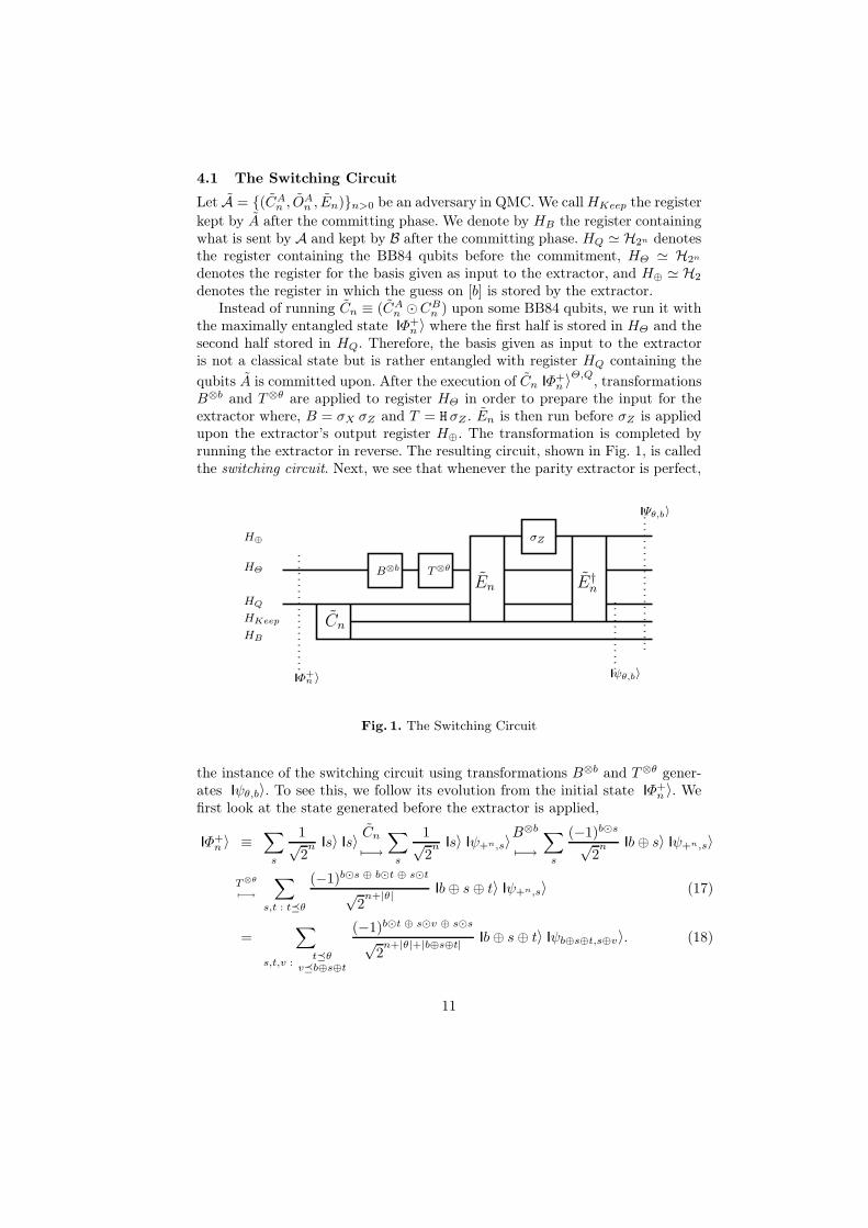
4.1 The Switching Circuit
Let A = {(CAn , O
An , En)}n>0 be an adversary in QMC. We callHKeep the register
kept by A after the committing phase. We denote by HB the register containingwhat is sent by A and kept by B after the committing phase. HQ ' H2n denotesthe register containing the BB84 qubits before the commitment, HΘ ' H2n
denotes the register for the basis given as input to the extractor, and H⊕ ' H2
denotes the register in which the guess on [b] is stored by the extractor.Instead of running Cn ≡ (CA
n �CBn ) upon some BB84 qubits, we run it with
the maximally entangled state Φ+n 〉 where the first half is stored in HΘ and the
second half stored in HQ. Therefore, the basis given as input to the extractoris not a classical state but is rather entangled with register HQ containing thequbits A is committed upon. After the execution of Cn Φ+
n 〉Θ,Q, transformationsB⊗b and T⊗θ are applied to register HΘ in order to prepare the input for theextractor where, B = σX σZ and T = H σZ . En is then run before σZ is appliedupon the extractor’s output register H⊕. The transformation is completed byrunning the extractor in reverse. The resulting circuit, shown in Fig. 1, is calledthe switching circuit. Next, we see that whenever the parity extractor is perfect,
T⊗θ
HQ
Cn
ψθ,b〉
HKeep
σZ
Ψθ,b〉
E†nEn
HB
H⊕
HΘ
Φ+n 〉
B⊗b
Fig. 1. The Switching Circuit
the instance of the switching circuit using transformations B⊗b and T⊗θ gener-ates ψθ,b〉. To see this, we follow its evolution from the initial state Φ+
n 〉. Wefirst look at the state generated before the extractor is applied,
Φ+n 〉 ≡
∑s
1√2
n s〉 s〉 Cn
7−→∑
s
1√2
n s〉 ψ+n,s〉B⊗b
7−→∑
s
(−1)b�s
√2
n b⊕ s〉 ψ+n,s〉
T⊗θ
7−→∑
s,t : t�θ
(−1)b�s ⊕ b�t ⊕ s�t
√2
n+|θ| b⊕ s⊕ t〉 ψ+n,s〉 (17)
=∑
s,t,v :t�θ
v�b⊕s⊕t
(−1)b�t ⊕ s�v ⊕ s�s
√2
n+|θ|+|b⊕s⊕t| b⊕ s⊕ t〉 ψb⊕s⊕t,s⊕v〉. (18)
11
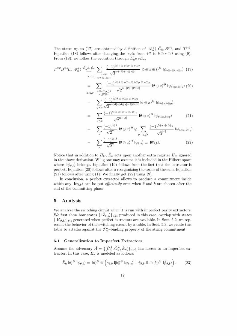
The states up to (17) are obtained by definition of Φ+n 〉, Cn, B
⊗b, and T⊗θ.Equation (18) follows after changing the basis from +n to b ⊕ s ⊕ t using (9).From (18), we follow the evolution through E†nσZEn,
T⊗θB⊗bCn Φ+n 〉 E†nσzEn
7−→∑
s,t,v :t�θ
v�b⊕s⊕t
(−1)b�t ⊕ s�v ⊕ v�v
√2
n+|θ|+|b⊕s⊕t| b⊕ s⊕ t〉Θ ψb⊕s⊕t,s⊕v〉 (19)
=∑
x,y,v :v⊕x⊕y�θ
v�θ⊕x
(−1)b�θ ⊕ b�x ⊕ b�y ⊕ v�y
√2
n+|θ|+|θ⊕x| θ ⊕ x〉Θ ψθ⊕x,b⊕y〉 (20)
=∑y�x
(−1)b�θ ⊕ b�x ⊕ b�y
√2
n+|θ|+|θ⊕x|−2|θ∧x| θ ⊕ x〉Θ ψθ⊕x,b⊕y〉
=∑y�x
(−1)b�θ ⊕ b�x ⊕ b�y
√2
n+|x| θ ⊕ x〉Θ ψθ⊕x,b⊕y〉 (21)
=∑
x
(−1)b�θ
√2
n θ ⊕ x〉Θ ⊗∑
y : y�x
(−1)b�x ⊕ b�y
√2|x| ψθ⊕x,b⊕y〉
=∑
x
(−1)b�θ
√2
n θ ⊕ x〉Θ ψθ,b〉 ≡ Ψθ,b〉. (22)
Notice that in addition to HΘ, En acts upon another extra register H⊕ ignoredin the above derivation. W.l.g one may assume it is included in the Hilbert spacewhere ψθ,b〉 belongs. Equation (19) follows from the fact that the extractor isperfect. Equation (20) follows after a reorganizing the terms of the sum. Equation(21) follows after using (1). We finally get (22) using (9).
In conclusion, a perfect extractor allows to produce a commitment insidewhich any ψθ,b〉 can be put efficiently even when θ and b are chosen after theend of the committing phase.
5 Analysis
We analyze the switching circuit when it is run with imperfect parity extractors.We first show how states { Ψθ,b〉}θ,b, produced in this case, overlap with states{ Ψθ,b〉}θ,b generated when perfect extractors are available. In Sect. 5.2, we rep-resent the behavior of the switching circuit by a table. In Sect. 5.3, we relate thistable to attacks against the Fn
m–binding property of the string commitment.
5.1 Generalization to Imperfect Extractors
Assume the adversary A = {(CAn , O
An , En)}n>0 has access to an imperfect ex-
tractor. In this case, En is modeled as follows:
En θ〉Θ ψθ,b〉 = θ〉Θ ⊗(γθ,b [b]〉⊕ ϕθ,b〉+ γθ,b 1⊕ [b]〉⊕ ϕθ,b〉
). (23)
12

Without loss of generality, we may assume that both γθ,b and γθ,b are real positivenumbers such that |γθ,b|2 ≥ 1
2 (i.e. arbitrary phases can be added to ϕθ,b〉 andϕθ,b〉). According (13), the expected bias provided by En is,
ε(n) ≡ 4−n∑
θ
∑b
εθ,b(n) = 4−n∑
θ
∑b
∣∣∣∣|γθ,b|2 − 12
∣∣∣∣ . (24)
Compared to the case where the extractor is perfect, only the effect of transfor-mation E†nσZEn needs to be recomputed. From (23), we obtain,
(E†nσZEn) θ〉 ψθ,b〉 = (−1)[b] θ〉 ⊗ ( ψθ,b〉+ eθ,b) , (25)
where the error vector eθ,b satisfies θ〉 ⊗ eθ,b ≡ −2γθ,bE†n( θ〉 1⊕ [b]〉⊕ ϕθ,b〉).
The final state Ψθ,b〉, produced by the switching circuit, can be obtained easilyfrom (19) using (25). We get that Ψθ,b〉 = E†nσzEnT
⊗θB⊗bCn Φ+n 〉 satisfies:
Ψθ,b〉 =∑y�x
(−1)b�θ ⊕ b�x ⊕ b�y
√2
n+|x| θ ⊕ x〉 ⊗ ( ψθ⊕x,b⊕y〉+ eθ⊕x,b⊕y) . (26)
Splitting the inner sum of (26) after distributing the tensor product gives,
Ψθ,b〉 = Ψθ,b〉+ F θ,b. (27)
The first part Ψθ,b〉 = (2−n/2∑
x(−1)b�θ θ〉)⊗ ψθ,b〉 is exactly what one getswhen the switching circuit is run with a perfect extractor (see (22)). The secondpart is the error term for which next lemma gives a characterization.
Lemma 2. Consider the switching circuit built from adversary A ={(CA
n , OAn , En)}n>0. Then,
4−n∑
θ
∑b
‖F θ,b‖2 ≤ 2− 4ε(n).
Proof. Let θ be fixed. Using the definition of F θ,b, we get
2−n∑
b∈{0,1}n
‖F θ,b‖2 = 2−n∑
b
‖∑y�x
(−1)b�θ⊕b�x⊕b�y
√2
n+|x| θ ⊕ x〉 ⊗ eθ⊕x,b⊕y‖2
= 2−n∑
b
‖∑
x
(−1)b�θ⊕b�x
√2
n+|x| θ ⊕ x〉∑
y:y�x
(−1)b�yeθ⊕x,b⊕y‖2
= 2−2n−|x|∑x
∑b
‖∑
y:y�x
(−1)b�yeθ⊕x,b⊕y‖2, (28)
where (28) is obtained from the orthogonality of all eθ⊕x,b⊕y when x varies,and from Pythagoras theorem. We now apply Lemma 1 to (28) with A = {y ∈{0, 1}n|y � x}, w ≡ b,z ≡ y, and vw,z ≡ eθ⊕x,b⊕y. We first verify that thecondition expressed in (2) is satisfied:
13
∑b
∑y1∈A:b⊕y1=s
∑y2∈A:b⊕y2=t
(−1)b�(y1⊕y2)〈eθ⊕x,b⊕y1, eθ⊕x,b⊕y2〉 =
〈eθ⊕x,s, eθ⊕x,t〉∑
b:b⊕s�x,b⊕t�x
(−1)b�(s⊕t) = 0,
from an identity equivalent to (1) since b runs aver all substrings in the supportof s ⊕ t � x. We therefore apply the conclusion of Lemma 1 to get that for allx ∈ {0, 1}n,∑
b
‖∑
y:y�x
(−1)b�yeθ⊕x,b⊕y‖2 =∑
y:y�x
∑b
‖eθ⊕x,b⊕y‖2 ≤ 2n+|x|(2−4ε(n)). (29)
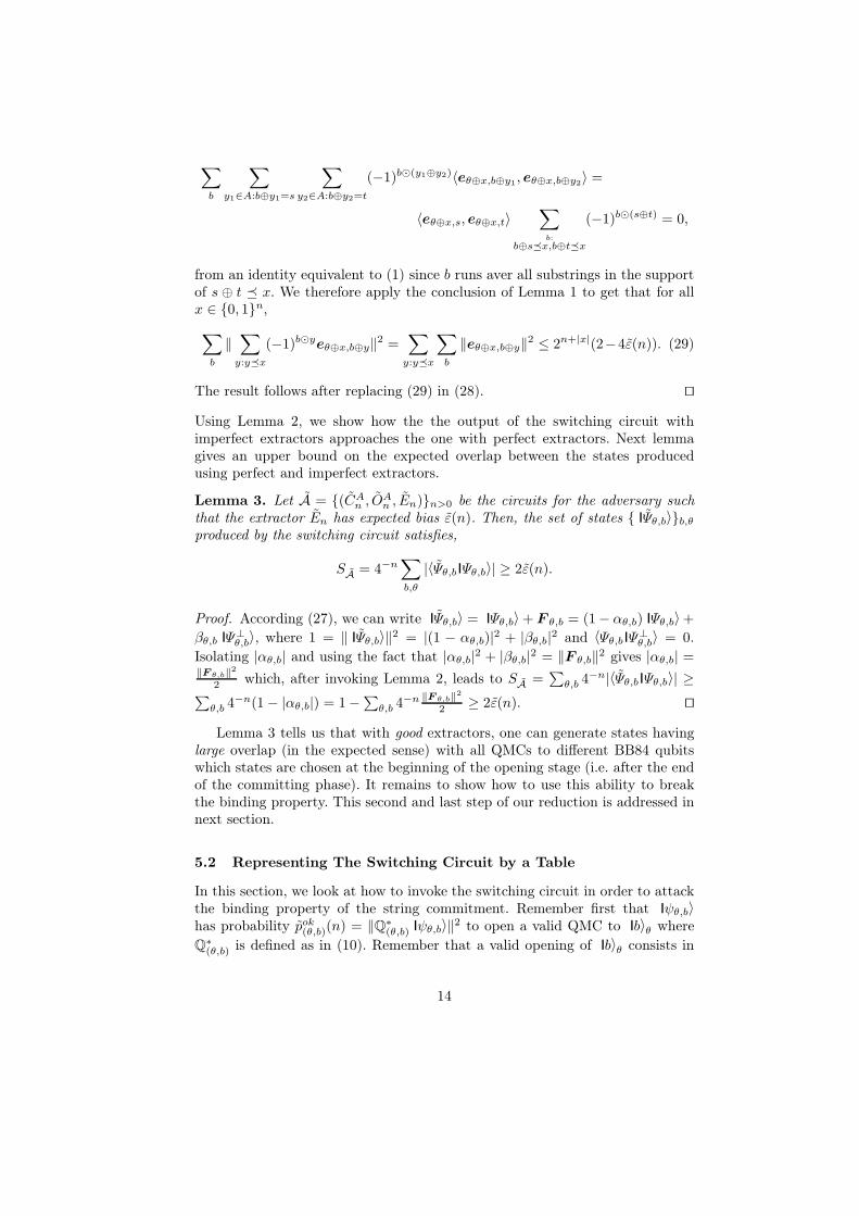
The result follows after replacing (29) in (28). utUsing Lemma 2, we show how the the output of the switching circuit withimperfect extractors approaches the one with perfect extractors. Next lemmagives an upper bound on the expected overlap between the states producedusing perfect and imperfect extractors.
Lemma 3. Let A = {(CAn , O
An , En)}n>0 be the circuits for the adversary such
that the extractor En has expected bias ε(n). Then, the set of states { Ψθ,b〉}b,θ
produced by the switching circuit satisfies,
SA = 4−n∑b,θ
|〈Ψθ,b Ψθ,b〉| ≥ 2ε(n).
Proof. According (27), we can write Ψθ,b〉 = Ψθ,b〉+ F θ,b = (1− αθ,b) Ψθ,b〉+βθ,b Ψ⊥θ,b〉, where 1 = ‖ Ψθ,b〉‖2 = |(1 − αθ,b)|2 + |βθ,b|2 and 〈Ψθ,b Ψ
⊥θ,b〉 = 0.
Isolating |αθ,b| and using the fact that |αθ,b|2 + |βθ,b|2 = ‖F θ,b‖2 gives |αθ,b| =‖F θ,b‖2
2 which, after invoking Lemma 2, leads to SA =∑
θ,b 4−n|〈Ψθ,b Ψθ,b〉| ≥∑θ,b 4−n(1− |αθ,b|) = 1−∑θ,b 4−n ‖F θ,b‖2
2 ≥ 2ε(n). utLemma 3 tells us that with good extractors, one can generate states having
large overlap (in the expected sense) with all QMCs to different BB84 qubitswhich states are chosen at the beginning of the opening stage (i.e. after the endof the committing phase). It remains to show how to use this ability to breakthe binding property. This second and last step of our reduction is addressed innext section.
5.2 Representing The Switching Circuit by a Table
In this section, we look at how to invoke the switching circuit in order to attackthe binding property of the string commitment. Remember first that ψθ,b〉has probability pok
(θ,b)(n) = ‖Q∗(θ,b) ψθ,b〉‖2 to open a valid QMC to b〉θ where
Q∗(θ,b) is defined as in (10). Remember that a valid opening of b〉θ consists in
14
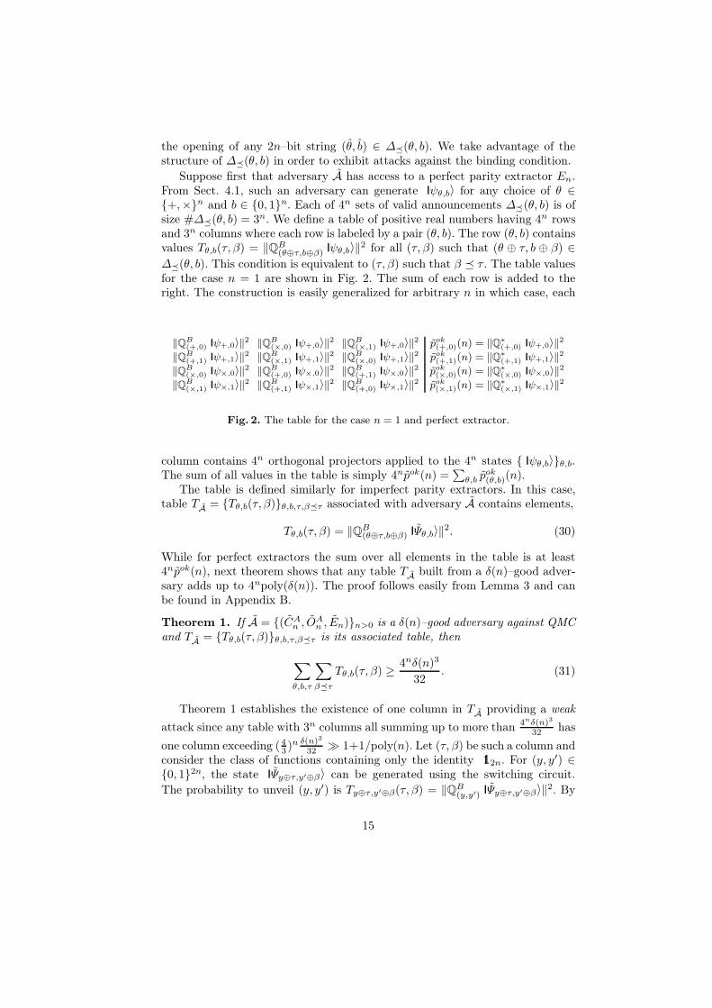
the opening of any 2n–bit string (θ, b) ∈ ∆�(θ, b). We take advantage of thestructure of ∆�(θ, b) in order to exhibit attacks against the binding condition.
Suppose first that adversary A has access to a perfect parity extractor En.From Sect. 4.1, such an adversary can generate ψθ,b〉 for any choice of θ ∈{+,×}n and b ∈ {0, 1}n. Each of 4n sets of valid announcements ∆�(θ, b) is ofsize #∆�(θ, b) = 3n. We define a table of positive real numbers having 4n rowsand 3n columns where each row is labeled by a pair (θ, b). The row (θ, b) containsvalues Tθ,b(τ, β) = ‖QB
(θ⊕τ,b⊕β) ψθ,b〉‖2 for all (τ, β) such that (θ ⊕ τ, b ⊕ β) ∈∆�(θ, b). This condition is equivalent to (τ, β) such that β � τ . The table valuesfor the case n = 1 are shown in Fig. 2. The sum of each row is added to theright. The construction is easily generalized for arbitrary n in which case, each
‖QB(+,0) ψ+,0〉‖2 ‖QB
(×,0) ψ+,0〉‖2 ‖QB(×,1) ψ+,0〉‖2 pok
(+,0)(n) = ‖Q∗(+,0) ψ+,0〉‖2
‖QB(+,1) ψ+,1〉‖2 ‖QB
(×,1) ψ+,1〉‖2 ‖QB(×,0) ψ+,1〉‖2 pok
(+,1)(n) = ‖Q∗(+,1) ψ+,1〉‖2
‖QB(×,0) ψ×,0〉‖2 ‖QB
(+,0) ψ×,0〉‖2 ‖QB(+,1) ψ×,0〉‖2 pok
(×,0)(n) = ‖Q∗(×,0) ψ×,0〉‖2
‖QB(×,1) ψ×,1〉‖2 ‖QB
(+,1) ψ×,1〉‖2 ‖QB(+,0) ψ×,1〉‖2 pok
(×,1)(n) = ‖Q∗(×,1) ψ×,1〉‖2
Fig. 2. The table for the case n = 1 and perfect extractor.
column contains 4n orthogonal projectors applied to the 4n states { ψθ,b〉}θ,b.The sum of all values in the table is simply 4npok(n) =
∑θ,b p
ok(θ,b)(n).
The table is defined similarly for imperfect parity extractors. In this case,table TA = {Tθ,b(τ, β)}θ,b,τ,β�τ associated with adversary A contains elements,
Tθ,b(τ, β) = ‖QB(θ⊕τ,b⊕β) Ψθ,b〉‖2. (30)
While for perfect extractors the sum over all elements in the table is at least4npok(n), next theorem shows that any table TA built from a δ(n)–good adver-sary adds up to 4npoly(δ(n)). The proof follows easily from Lemma 3 and canbe found in Appendix B.
Theorem 1. If A = {(CAn , O
An , En)}n>0 is a δ(n)–good adversary against QMC
and TA = {Tθ,b(τ, β)}θ,b,τ,β�τ is its associated table, then
∑θ,b,τ
∑β�τ
Tθ,b(τ, β) ≥ 4nδ(n)3
32. (31)
Theorem 1 establishes the existence of one column in TA providing a weakattack since any table with 3n columns all summing up to more than 4nδ(n)3
32 hasone column exceeding (4
3 )n δ(n)2
32 � 1+1/poly(n). Let (τ, β) be such a column andconsider the class of functions containing only the identity 12n. For (y, y′) ∈{0, 1}2n, the state Ψy⊕τ,y′⊕β〉 can be generated using the switching circuit.The probability to unveil (y, y′) is Ty⊕τ,y′⊕β(τ, β) = ‖QB
(y,y′) Ψy⊕τ,y′⊕β〉‖2. By
15
construction, we have∑
(y,y′) pf(y,y′)(n) =
∑(y,y′) Ty⊕τ,y′⊕β(τ, β) > 1+1/poly(n)
which provides an attack against the string commitment’s 12n–binding propertyin accordance with (7). As we pointed out in Sect. 3.1 however, this attackmight not even be statistically distinguishable from the trivial adversary. Thisimplies that proving a string commitment computationally 12n-binding wouldbe impossible. In the next section, we find stronger attacks allowing to relax thebinding property required for secure QMC.
5.3 Strong Attacks Against the String Commitment
We now show that the table TA, built out of any δ(n)–good adversary A, containsan attack against the Fn
m–binding property of the 2n–string commitment withm ∈ O(polylog(n)) whenever δ(n) ≥ 1/poly(n). We show this using a countingargument. We cover uniformly the table TA with all attacks in Fn
m. Theorem 1is then invoked in order to conclude that for some f ∈ Fn
m, condition (7) doesnot hold.
Attacking the binding condition according to a function f ∈ Fnm is done
by grouping columns in TA as described in (6) and discussed in more detailsin Appendix C. The number of lines involved in such an attack is clearly 2m
while the number of columns can be shown to be 2m3n−m (for information seeAppendix C and Lemma 4 below). This means that any attack in Fn
m coverst = 3n−m4m elements in TA. The quality of such an attack is characterized bythe sum of all elements in the sub-array defined by the attack since this sumcorresponds to the value of (7). Let tA = 3n4n be the total number of elementsin TA and let sA be its sum. The following lemma, proved in Appendix D, showsthat all attacks in Fn
m cover TA uniformly:
Lemma 4. All f -attacks with f ∈ Fnm cover TA uniformly, that is, each element
in TA belongs to exactly a = C(m,n)4m attacks each of size t = 3n−m4m.
Let s∗ be the maximum of (7) for all f -attacks with f ∈ Fnm. Clearly, a · s∗ ≥
a·t·sAtA
since by Lemma 4, the covering of TA by f ∈ Fnm is uniform and a · t/tA
is the number of times TA is generated by attacks in Fnm. In other words,
a · s∗ ≥ a · t · sAtA
=a · t · sA
3n4n⇒ s∗ ≥ t · sA
3n4n=
4m · sA3m4n
. (32)
Assuming that A is δ(n)–good, Theorem 1 tells us that sA ≥ 4nδ(n)3
32 so (32)implies that,
s∗ ≥ δ(n)34m
32 · 3m≥ 1 + 1/poly(n), (33)
for any m ≥ dlog 43
(32
δ(n)3
)e. Equation (33) guarantees that for at least one
f ∈ Fnm, condition (7) is not satisfied thereby providing an attack against
the Fnm–binding criteria. Moreover, since δ(n) ≥ 1/poly(n) it is sufficient that
m ∈ O(polylog(n)). It follows that at least one f -attack in Fnm is statistically
distinguishable from any trivial one.
16
6 The Main Result and Its Application
Putting together Theorem 1 and (33) leads to our main result:
Theorem 2 (Main). Any δ(n)–good adversary A against QMC can breakthe Fn
m–binding property of the string commitment it is built upon for m ∈O(log 1
δ(n) ) using a circuit of size O(‖A‖UG).
Theorem 2 can be applied for the construction of 1-2 QOT in the computationalsetting. We can use QMCs for building a weak 1-2 QOT such that:
– the sender has no information about the receiver’s selection bit and,– the receiver, according Theorem 2, can only extract a limited amount of
information about both bits.
This weak flavor of 1-2 QOT is easily obtained by the following primitive, calledWn, accepting B’s input bits (β0, β1) and A’s selection bit s (i.e this constructionis very similar to the CK protocol[5]):
ProtocolWn
1. B and A run the committing phase of a QMC (i.e. built from a Fnm-binding string
commitment scheme) upon b〉θ for b ∈R {0, 1}n, θ ∈R {+,×}n picked by B,2. B chooses c ∈R {0, 1} and announces it to A,
– if c = 0 then A unveils the QMC, if unveil succeeds then A and B returnto 1 otherwise B aborts,
– if c = 1 then B announces θ, A announces a partition I0, I1 ⊆ {1, . . . , n}such that for all i ∈ Is the measurements were made in basis θi = θi, then Bannounces a0, a1 ∈ {0, 1} s.t. β0 = a0 ⊕i∈I0 bi and β1 = ⊕i∈I1bi:• A does her best to guess (b0, b1) ≈ (
Li∈I0
bi,L
i∈I1bi).
Clearly, Wn is a correct 1-2 QOT since an honest receiver A can always get bitβs = bs ⊕ as. A’s information about the other bit can be further reduced usingthe following simple protocol accepting B’s input bits (β0, β1) and the selectionbit s for the honest receiver:
Protocol R-Reduce(t,Wn)
1. W is executed t times, with random inputs (β0i, β1i), i = 1..t for the sender andinput s for the receiver such that β01 ⊕ . . .⊕ β0t = β0 and β11 ⊕ . . .⊕ β1t = β1.
2. The receiver computes the XOR of all bits received, that is βs = ⊕ti=1βsi.
Classically, it is straightforward to see that the receiver’s information about one-out-of-two bit decreases exponentially in t. We say that a quantum adversary Aagainst R-Reduce(t,Wn) is promising if it runs in poly-time and the probabilityto complete the execution is non-negligible. Using Theorem 2, it is not difficultto show that A’s information about one of the transmitted bits also decreasesexponentially in t whenever A is promising:
Theorem 3. For any promising receiver A in R-Reduce(t,Wn) and for all exe-cutions, there exists s ∈ {0, 1} such that A’s expected bias on βs is negligible int (even given βs).
17
A sketch of proof can be found in Appendix E. It relies upon the fact that anypromising adversary must run almost all Wn with pok(n) > 1− δ for any δ > 0.Using Theorem 2, this means that independently for each of those executions1 ≤ i ≤ t, one bit βsi out of (β0i, β1i) cannot be guessed with bias better thanεmax(δ) << 1
2 . In this case, the bias on βs can be shown to be negligible in t.Clearly, the sender B in R-Reduce(t,Wn) cannot get any non-negligible
amount of information about A’s selection bit when the commitments are sta-tistically concealing. This remark together with Theorem 3 and the correctnessof R-Reduce(t,Wn) lead to:
Corollary 1. A correct and private 1-2 QOT can be based upon any Fnm-binding
and statistically concealing quantum string commitment scheme. The resulting1-2 QOT statistically hides the selection bit and computationally hides one outof two transmitted bits.
In other words, building 1-2 QOT upon Theorem 2 allows for an easy securityproof in the computational setting. Our analysis assumes for simplicity that Aand B have access to a perfect quantum channel. Nevertheless, noise may betolerated if we construct 1-2 QOT along the lines of BBCS [3] instead of CK [5].
7 Open Questions
An obvious open problem is how to build Fnm-string commitments from computa-
tionally binding bit commitment schemes. In particular, how one can transformthe computationally binding bit commitments of [7] and [6] into Fn
m–bindingstring commitments? This would show that QMCs and therefore 1-2 QOT canbe based upon any one-way permutation[7] and/or any one-way function[6]. Itis an open question whether or not Theorem 2 holds for δ(n)–non-trivial ad-versaries against QMC. Such an extension would show that our reduction froman adversary to QMC into one against the binding condition is to some extentoptimal. It is also of interest to find attacks against weaker binding properties.
Finally, it would be very interesting to formally prove the security of theCK protocol using Theorem 2. This would result in a proof of security that, inaddition to apply in the computational setting, would be based upon a com-pletely different approach than Yao’s proof [19]. Moreover, the CK protocol ismore practical than our construction since it only requires a constant numberof rounds with fewer qubits transmitted (i.e. Θ(n) vs. Θ(tn)). It would also beuseful to prove Corollary 1 in the case where the quantum channel is noisy.
References
1. Adcock, M.,and R. Cleve, “A Quantum Goldreich-Levin Theorem with Crypto-graphic Applications”, In proceedings of 19th International Symposium on Theoret-ical Aspects of Computer Science (STACS 2002),LNCS, vol. 2285,Springer-Verlag,2002, pp. 323–334.
18
2. Bennett, C. H., and G. Brassard, “Quantum cryptography: Public key dis-tribution and coin tossing”, In Proceedings of IEEE International Conference onComputers, Systems, and Signal Processing, 1984, pp. 175–179.
3. Bennett, C. H., G. Brassard, C. Crépeau and M.-H. Skubiszewska, “Prac-tical Quantum Oblivious Transfer”, In Advances in Cryptology –CRYPTO’91 :Proceedings, LNCS, vol. 576, Springer-Verlag, 1992, pp. 362–371.
4. Crépeau, C., “Quantum Oblivious Transfer”, Journal of Modern Optics, vol. 41,no 12, 1994, pp. 2445–2454.
5. Crépeau, C. and J. Kilian, “Achieving oblivious transfer using weakened se-curity assumptions”, Proceedings of 29th IEEE Symposium on the Foundations ofComputer Science, 1988, pp. 42–52.
6. Crépeau, C., F. Légaré, and L. Salvail, “How to Convert the Flavor of aQuantum Bit Commitment”, In Advances in Cryptology –EUROCRYPT’01 : Pro-ceedings, LNCS, vol. 2045, Springer-Verlag, 2001, pp. 60–77.
7. Dumais, P., D. Mayers, and L. Salvail, “Perfectly Concealing Quantum BitCommitment From Any Quantum One-Way Permutation”, In Advances in Cryp-tology –EUROCRYPT’00 : Proceedings, LNCS, vol. 1807, Springer-Verlag, 2000,pp. 300–315.
8. van de Graaf, J., Towards a Formal Definition of Security for Quantum Proto-cols, Ph.D. thesis, Computer Science and Operational Research Department, Uni-versité de Montréal, 1997.
9. Impagliazzo, R. and S. Rudich, “Limits on Provable Consequences of One-WayPermutations”, In Advances in Cryptology –CRYPTO’88 : Proceedings, LNCS,vol. 403, Springer-Verlag, 1989, pp. 2–7.
10. Lo, H.–K.,and H.F. Chau, “Is quantum Bit Commitment Really Possible?”,Physical Review Letters, vol. 78, no 17, 1997, pp. 3410–3413.
11. Mayers, D., “The Trouble With Quantum Bit Commitment”, available athttp://xxx.lanl.gov/abs/quant-ph/9603015, 1996.
12. Mayers, D., “Quantum Key Distribution and String Oblivious Transfer in NoisyChannels”, In Advances in Cryptology –CRYPTO’96 : Proceedings, LNCS, vol. 1109, Springer-Verlag, 1996, pp. 343–357.
13. Mayers, D., “Unconditionally Secure Quantum Bit Commitment is Impossible”,Physical Review Letters, vol. 78, no 17, 1997, pp. 3414–3417.
14. Mayers, D., and L. Salvail,“Quantum Oblivious Transfer is Secure Against AllIndividual Measurements”, In Proceedings of the Workshop on Physics and Com-putationm, PhysComp’94, Dallas, 1994, pp. 69–77.
15. Rabin, M. O., “How to exchange secrets by oblivious transfer”, Technical MemoTR–81, Aiken Computation Laboratory, Harvard University, 1981.
16. Salvail, L., "Quantum Bit Commitment From a Physical Assumption", In Ad-vances in Cryptology –CRYPTO’98 : Proceedings, LNCS, vol. 1462 , Springer-Verlag, 1998, pp. 338–354.
17. Watrous, J, “Limits on the Power of Quantum Statistical Zero-Knowledge”, Pro-ceedings of the 43rd Annual Symposium on Foundations of Computer Science, 2002,pp. 495–504.
18. Yao, A. C., “Theory and Applications of Trapdoor Functions”, Proceedings of the23rd IEEE Symposium on Foundations of Computer Science, 1982, pp. 80–91.
19. Yao, A. C., “Security of Quantum Protocols Against Coherent Measurements”,Proceedings of the 27th ACM Symposium on Theory of Computing, 1995, pp. 67–75.
19
A Proof of Lemma 2
First, we prove the following related claim:
Claim. Let {uw,z}w,z be any family of vectors, indexed by w, z ∈ {0, 1}n, thatsatisfies,
(∀s, t ∈ {0, 1}n, s 6= t)[∑w
∑z1:w⊕z1=sz2:w⊕z2=t
(−1)w�(z1⊕z2)〈uw,z1 ,uw,z2〉 = 0] (34)
Then, ∑w
‖∑
z
(−1)w�zuw,z‖2 =∑
w,z∈{0,1}n
‖uw,z‖2. (35)
Proof. We carry out the calculation for (35):∑w
‖∑
z
(−1)w�zuw,z‖2 =∑w
〈∑z1
(−1)w�z1uw,z1,∑z2
(−1)w�z2uw,z2〉
=∑
w,z1,z2
(−1)w�(z1⊕z2)〈uw,z1 ,uw,z2〉
=∑w,z
‖uw,z‖2 +∑
w,z1,z2:z1 6=z2
(−1)w�(z1⊕z2)〈uw,z1,uw,z2〉.(36)
We now re-arrange the terms in the right-hand part of (36):∑w,z1,z2:z1 6=z2
(−1)w�(z1⊕z2)〈uw,z1,uw,z2〉 =∑w,z1
∑z2:z2 6=z1
(−1)w(z1⊕z2)∑
s:w⊕z1=st:w⊕z2=t
〈uw,z1,uw,z2〉
=∑
s,t:s 6=tw
∑z1:w⊕z1=sz2:w⊕z2=t
(−1)w(z1⊕z2)〈uw,z1 ,uw,z2〉
= 0, (37)
where (37) follows from condition (34). Replacing (37) in (36) concludes theproof. utProof (Lemma 1). Follows from the Claim after setting uw,z = vw,z if z /∈ Aand uw,z = 0 if z ∈ A. It is easy to verify that if condition (2) is satisfied by{vw,z}w,z then {uw,z}w,z satisfies (34). Our result then follows from (35). ut
B Proof of Theorem 1
Proof. We use Lemma 3 together with the fact that A is δ(n)–good. From Lemma3, any δ(n)–good adversary is such that,
pok(n) +∑θ,b
4−n|〈Ψθ,b Ψθ,b〉|2 =
20

4−n∑θ,b
(pok(θ,b)(n) + |〈Ψθ,b Ψθ,b〉|2
)≥ 1 + δ(n). (38)
Let δθ,b = pok(θ,b)(n) + |〈Ψθ,b Ψθ,b〉|2 − 1 be such that δ = 4−n
∑θ,b δθ,b. The sum
of any row (θ, b) ∈ TA is given by,
‖Q∗(θ,b) Ψθ,b〉‖2 ≥
‖Q∗(θ,b)
(|〈Ψθ,b Ψθ,b〉| Ψθ,b〉 −
√1− |〈Ψθ,b Ψθ,b〉|2 Ψ⊥θ,b〉
)‖2, (39)
where Ψ⊥θ,b〉 is any state orthogonal to Ψθ,b〉. Now, notice that we can
always write Ψθ,b〉 =√pok(θ,b)(n) ξθ,b〉 +
√1− pok
(θ,b)(n) ξ⊥θ,b〉 for ξθ,b〉 =
Q∗(θ,b) Ψθ,b〉/
√pok(θ,b)(n) and ξ⊥θ,b〉 = ( 1− Q∗
(θ,b)) Ψθ,b〉/√
1− pok(θ,b)(n). We can
also write Ψ⊥θ,b〉 = αθ,b ξθ,b〉+ βθ,b ξ⊥θ,b〉+ ζθ,b Λθ,b〉 where Λθ,b〉 is orthogonalto both ξθ,b〉 and ξ⊥θ,b〉 and where |αθ,b|2 + |βθ,b|2 + |ζθ,b|2 = 1. Since by con-
struction 〈Ψθ,b Ψ⊥θ,b〉 = 0, it is easy to verify that |αθ,b| ≤
√1− pok
(θ,b)(n). In order
to simplify the notation, we let cθ,b = 〈Ψθ,b Ψθ,b〉. Using the above observations,we re-write (39) as,
‖Q∗(θ,b) Ψθ,b〉‖2 ≥ ‖(cθ,b
√pok(θ,b)(n)−
√(1 − |cθ,b|2)(1 − pok
(θ,b)(n))) ξθ,b〉‖2(40)
=(√
|cθ,b|2pok(θ,b)(n)−
√(1 − |cθ,b|2)(1 − pok
(θ,b)(n)))2
=(√
|cθ,b|2pok(θ,b)(n)−
√|cθ,b|2pok
(θ,b)(n)− δθ,b
)2
(41)
≥ δ2θ,b
4, (42)
where (40) comes from definitions of Ψθ,b〉 and Ψθ,b〉 in terms of ξθ,b〉, (41)comes from the definition of δθ,b, and (42) follows from the fact that (
√a −√
a− b)2 ≥ b2/4 for any 0 ≤ b ≤ a ≤ 1. Since A is δ(n)–good, we use (38) toconclude that the set G = {(θ, b)|δθ,b ≥ δ(n)/2} must satisfy #G ≥ 4nδ(n)/2.Any (θ, b) ∈ G is such that (42) is at least δ(n)2
4 . The result follows easily from∑θ,b ‖Q∗
(θ,b) Ψθ,b〉‖2 ≥∑
(θ,b)∈G ‖Q∗(θ,b) Ψθ,b〉‖2 ≥ 4nδ(n)3
32 . ut
C Implementing an f -attack From the Switching Circuit
In this appendix, we briefly describe how one can use the switching circuit inorder to attack the binding property of the string commitment relative to somefunction f ∈ Fn
m. We call such an attack an f -attack since its purpose is totry to open s ∈ f−1(y) for any y ∈ {0, 1}m. To make the description easier,let us consider the case n = 1 resulting in table TA shown at Fig. 3 (this is
21
‖QB(+,0) Ψ+,0〉‖2 ‖QB
(×,0) Ψ+,0〉‖2 ‖QB(×,1) Ψ+,0〉‖2
‖QB(+,1) Ψ+,1〉‖2 ‖QB
(×,1) Ψ+,1〉‖2 ‖QB(×,0) Ψ+,1〉‖2
‖QB(×,0) Ψ×,0〉‖2 ‖QB
(+,0) Ψ×,0〉‖2 ‖QB(+,1) Ψ×,0〉‖2
‖QB(×,1) Ψ×,1〉‖2 ‖QB
(+,1) Ψ×,1〉‖2 ‖QB(+,0) Ψ×,1〉‖2
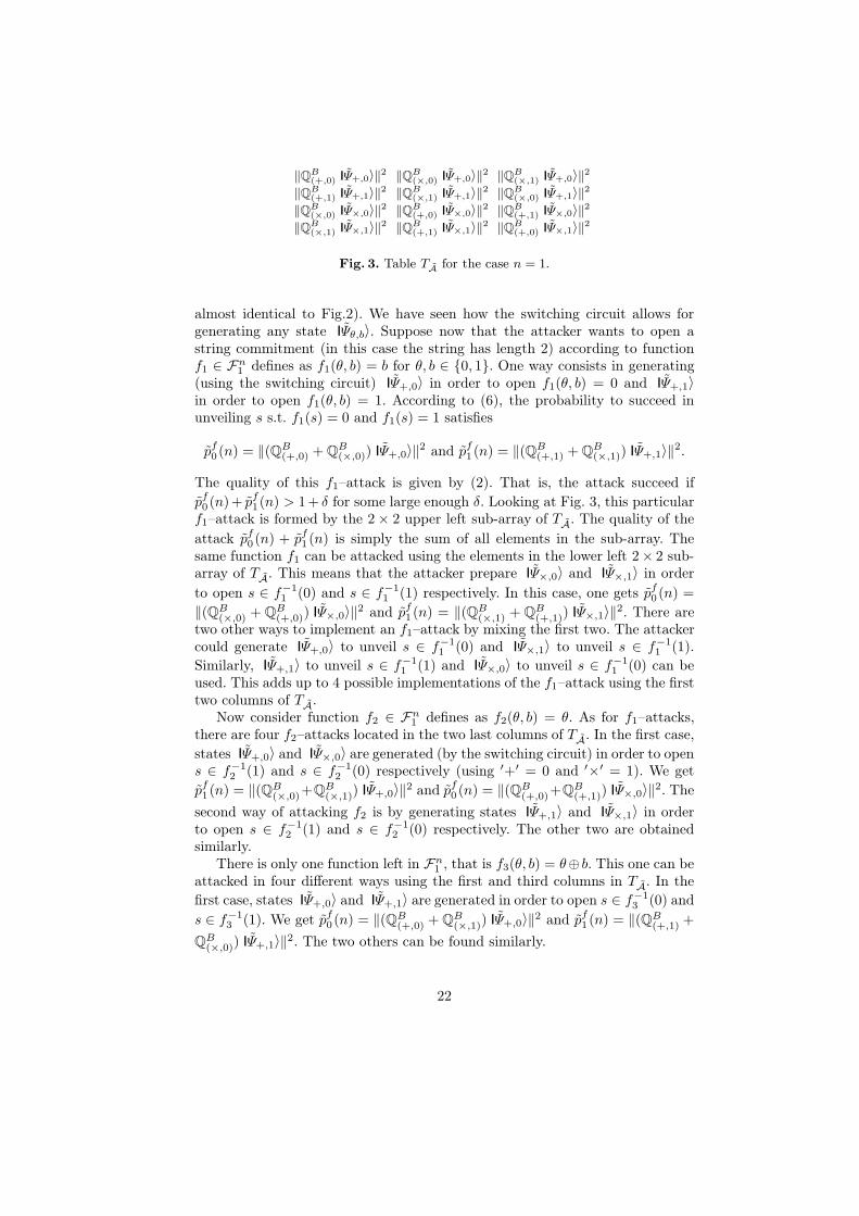
Fig. 3. Table TA for the case n = 1.
almost identical to Fig.2). We have seen how the switching circuit allows forgenerating any state Ψθ,b〉. Suppose now that the attacker wants to open astring commitment (in this case the string has length 2) according to functionf1 ∈ Fn
1 defines as f1(θ, b) = b for θ, b ∈ {0, 1}. One way consists in generating(using the switching circuit) Ψ+,0〉 in order to open f1(θ, b) = 0 and Ψ+,1〉in order to open f1(θ, b) = 1. According to (6), the probability to succeed inunveiling s s.t. f1(s) = 0 and f1(s) = 1 satisfies
pf0 (n) = ‖(QB
(+,0) + QB(×,0)) Ψ+,0〉‖2 and pf
1 (n) = ‖(QB(+,1) + QB
(×,1)) Ψ+,1〉‖2.
The quality of this f1–attack is given by (2). That is, the attack succeed ifpf0 (n)+ pf
1(n) > 1+ δ for some large enough δ. Looking at Fig. 3, this particularf1–attack is formed by the 2× 2 upper left sub-array of TA. The quality of theattack pf
0 (n) + pf1 (n) is simply the sum of all elements in the sub-array. The
same function f1 can be attacked using the elements in the lower left 2× 2 sub-array of TA. This means that the attacker prepare Ψ×,0〉 and Ψ×,1〉 in orderto open s ∈ f−1
1 (0) and s ∈ f−11 (1) respectively. In this case, one gets pf
0 (n) =‖(QB
(×,0) + QB(+,0)) Ψ×,0〉‖2 and pf
1 (n) = ‖(QB(×,1) + QB
(+,1)) Ψ×,1〉‖2. There aretwo other ways to implement an f1–attack by mixing the first two. The attackercould generate Ψ+,0〉 to unveil s ∈ f−1
1 (0) and Ψ×,1〉 to unveil s ∈ f−11 (1).
Similarly, Ψ+,1〉 to unveil s ∈ f−11 (1) and Ψ×,0〉 to unveil s ∈ f−1
1 (0) can beused. This adds up to 4 possible implementations of the f1–attack using the firsttwo columns of TA.
Now consider function f2 ∈ Fn1 defines as f2(θ, b) = θ. As for f1–attacks,
there are four f2–attacks located in the two last columns of TA. In the first case,states Ψ+,0〉 and Ψ×,0〉 are generated (by the switching circuit) in order to opens ∈ f−1
2 (1) and s ∈ f−12 (0) respectively (using ′+′ = 0 and ′×′ = 1). We get
pf1 (n) = ‖(QB
(×,0)+QB(×,1)) Ψ+,0〉‖2 and pf
0 (n) = ‖(QB(+,0)+QB
(+,1)) Ψ×,0〉‖2. Thesecond way of attacking f2 is by generating states Ψ+,1〉 and Ψ×,1〉 in orderto open s ∈ f−1
2 (1) and s ∈ f−12 (0) respectively. The other two are obtained
similarly.There is only one function left in Fn
1 , that is f3(θ, b) = θ⊕ b. This one can beattacked in four different ways using the first and third columns in TA. In thefirst case, states Ψ+,0〉 and Ψ+,1〉 are generated in order to open s ∈ f−1
3 (0) ands ∈ f−1
3 (1). We get pf0 (n) = ‖(QB
(+,0) + QB(×,1)) Ψ+,0〉‖2 and pf
1 (n) = ‖(QB(+,1) +
QB(×,0)) Ψ+,1〉‖2. The two others can be found similarly.
22
Remark that any element in TA belongs to exactly 4 attacks and that anyattack uses exactly 4 elements in TA. This is what we mean when we say that allattacks in Fn
1 covers TA uniformly. The construction can easily be generalizedfor arbitrary n. The number of rows of TA uses in any f–attack (f ∈ Fn
m) is2m and the number of columns is 2m3n−m. That is, the number of elements inTA involved in such an f–attack is 4m3n−m. As we shall see in Lemma 4, thecovering remains uniform for all values of n.
D Proof of Lemma 4
Lemma 4 follows from the combinatorial lemma 5 below. To make the statementof this combinatorial lemma more succinct we first set the stage for it.
Let T be a 4n lines by 3n columns array. The lines are indexed by the 4n
strings (θ, b) ∈ {0, 1}n × {0, 1}n. The columns are indexed by the 3n strings(τ, β) ∈ {0, 1}n × {0, 1}n such that β � τ .
We now consider sub-arrays of T . Each sub-array will be composed of cellslying at the intersections of 2m lines of T and 3n−m2m columns of T . Any choiceof the following 3n parameters will define a unique sub-array and different choicesof parameters will define different sub-arrays:
r1, r2, . . . , rn ∈ {0, 1, 2, 3}, (43)u1, u2, . . . , un ∈ {0, 1}, (44)v1, v2, . . . , vn ∈ {0, 1} (45)
subject to the condition
#{j : rj 6= 0} = m. (46)
Accordingly, there will be C(m,n)3m4n different sub-arrays.Let us fix a choice for rj ∈ {0, 1, 2, 3}, uj , vj ∈ {0, 1} for all j ∈ {1, . . . , n} sat-
isfying (46). We now describe the sub-array defined by that choice. The column(τ, β) is part of the sub-array if and only if:
rj = 0 =⇒ (τj , βj) ∈ {(0, 0), (1, 0), (1, 1)} i.e.: βj � τj , (47)rj = 1 =⇒ (τj , βj) ∈ {(1, 0), (1, 1)} i.e.: τj = 1, (48)rj = 2 =⇒ (τj , βj) ∈ {(0, 0), (1, 0)} i.e.: βj = 0, (49)rj = 3 =⇒ (τj , βj) ∈ {(0, 0), (1, 1)} i.e.: βj = τj . (50)
The line (θ, b) is part of the sub-array if and only if:
rj = 0 =⇒ (θj , bj) ∈ {(uj, vj)}, (51)rj = 1 =⇒ (θj , bj) ∈ {(0, uj), (1, vj)}, (52)rj = 2 =⇒ (θj , bj) ∈ {(uj, 0), (vj , 1)}, (53)rj = 3 =⇒ (θj , bj) ∈ {(uj, uj), (vj , 1− vj)}. (54)
23
One can easily verify that the lines (47) to (54) define a 2m×3n−m2m sub-array,thus containing 3n−m4m cells, and that different choices of the parameters (43)to (45) will lead to different sub-arrays.
We can now state and prove the combinatorial lemma:
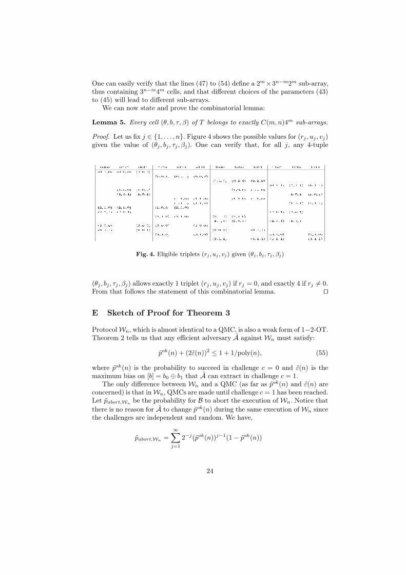
Lemma 5. Every cell (θ, b, τ, β) of T belongs to exactly C(m,n)4m sub-arrays.
Proof. Let us fix j ∈ {1, . . . , n}. Figure 4 shows the possible values for (rj , uj , vj)given the value of (θj , bj , τj , βj). One can verify that, for all j, any 4-tuple
0000 0010 0011 0100 0110 0111 1000 1010 1011 1100 1110 1111
(0; 0; 0) (0; 0; 0) (0; 0; 0)
(0; 0; 1) (0; 0; 1) (0; 0; 1)
(0; 1; 0) (0; 1; 0) (0; 1; 0)
(0; 1; 1) (0; 1; 1) (0; 1; 1)
(1; 0; 0) (1; 0; 0) (1; 0; 0) (1; 0; 0)
(1; 0; 1) (1; 0; 1) (1; 0; 1) (1; 0; 1)
(1; 1; 0) (1; 1; 0) (1; 1; 0) (1; 1; 0)
(1; 1; 1) (1; 1; 1) (1; 1; 1) (1; 1; 1)
(2; 0; 0) (2; 0; 0) (2; 0; 0) (2; 0; 0)
(2; 0; 1) (2; 0; 1) (2; 0; 1) (2; 0; 1)
(2; 1; 0) (2; 1; 0) (2; 1; 0) (2; 1; 0)
(2; 1; 1) (2; 1; 1) (2; 1; 1) (2; 1; 1)
(3; 0; 0) (3; 0; 0) (3; 0; 0) (3; 0; 0)
(3; 0; 1) (3; 0; 1) (3; 0; 1) (3; 0; 1)
(3; 1; 0) (3; 1; 0) (3; 1; 0) (3; 1; 0)
(3; 1; 1) (3; 1; 1) (3; 1; 1) (3; 1; 1)
Fig. 4. Eligible triplets (rj , uj , vj) given (θj , bj , τj , βj)
(θj , bj , τj , βj) allows exactly 1 triplet (rj , uj , vj) if rj = 0, and exactly 4 if rj 6= 0.From that follows the statement of this combinatorial lemma. ut
E Sketch of Proof for Theorem 3
ProtocolWn, which is almost identical to a QMC, is also a weak form of 1−2-OT.Theorem 2 tells us that any efficient adversary A against Wn must satisfy:
pok(n) + (2ε(n))2 ≤ 1 + 1/poly(n), (55)
where pok(n) is the probability to succeed in challenge c = 0 and ε(n) is themaximum bias on [b] = b0 ⊕ b1 that A can extract in challenge c = 1.
The only difference between Wn and a QMC (as far as pok(n) and ε(n) areconcerned) is that inWn, QMCs are made until challenge c = 1 has been reached.Let pabort,Wn be the probability for B to abort the execution of Wn. Notice thatthere is no reason for A to change pok(n) during the same execution of Wn sincethe challenges are independent and random. We have,
pabort,Wn =∞∑
j=1
2−j(pok(n))j−1(1− pok(n))
24
>1− pok(n)
2⇒ pok(n) > 1− 2pabort,Wn . (56)
Let In = {(I0, I1)|I0 ∪ I1 = {1, . . . , n}, I0 ∩ I1 = ∅} be the set of possibleannouncements for A in Wn. Let I = (I0, I1) ∈ In be the set of positionsannounced by A’s during an execution of Wn. We define fI(b) as the 2-bitoutput function:
fI(b) ≡ (⊕i∈I0
bi,⊕i∈I1
bi).
For s ∈ {0, 1} and b ∈ {0, 1}n, let hI(b, s) ≡ fI(b)[s] where fI(b)[s] denotesthe s-th output bit of fI(b). Let QPoly(n) and QPoly(n,t) be the classesof families of polynomial-size quantum circuits in one and two variables respec-tively having one-bit output. Let Cδ be the non-uniform class of all families ofpolynomial size quantum circuits allowing to run Wn with success probabilityat least 1− δ. That is, any family {Cn}n>0 ∈ Cδ can be used to define the com-mitting phase of an adversary A = {(Cn, ·)}n>0 against Wn where Cn allowsfor pabort,Wn ≤ δ given n is large enough. For simplicity, we abuse the nota-tion by writing the output state of the committing phase on b〉θ as Cn b〉θalthough formally, Cn is the circuit obtained by combining A’s and B’s inter-active circuits. Let Gn be a quantum circuit with a one-bit output register soGn · (Cn b〉θ) defines a probability distribution over the possible outcomes forthe measurement in the computational basis of Gn’s output register. When wewrite out {Gn · (Cn b〉θ)⊗ θ〉} we are not only designating the value of Gn’soutput register but any classical mapping from the output into {0, 1}. Using thisconvention, Pr (hI(b, s) 6= out {Gn · (Cn b〉θ)⊗ θ〉}) ≥ 1
2 − ε, means that anyclassical mapping from the value of the output register to {0, 1} has expectedprobability of error at least 1
2 − ε in guessing the value of hI(b, s).Using (56), we get that A also defines an adversary against QMC with
pok(n) ≥ 1− 2δ. From (55), we conclude that
ε(n) ≤√
2δ + 1
poly(n)
2(57)
given the output of any family of poly-size quantum circuits {Gn}n>0 ∈QPoly(n). Remember that ε(n) is the maximum expected bias on hI(b, 0) ⊕hI(b, 1) for any announcement I ∈ In. The following lemma follows easily fromTheorem 2, it tells us that for each execution of Wn, there exists s ∈ {0, 1} suchthat hI(b, s) cannot be guessed with arbitrary precision. The proof proceedsby contradiction showing that if both bits hI(b, 0) and hI(b, 1) can be guessedrespectively by G0
n and G1n with probability larger than 1−2ε(n)
10 then A couldattack a QMC with success probability pok(n) ≥ 1−2δ and expected bias largerthan
√2δ + 1/poly(n)/2 contradicting (55).
Lemma 6.(∀{Cn}n>0 ∈ Cδ)(∀I ∈ In)(∃s ∈ {0, 1})(∀{Gn}n>0 ∈ QPoly(n))(∀n > n0)[
Pr (hI(b, s) 6= out {Gn · (Cn b〉θ)⊗ θ〉}) ≥ 1− 2ε(n)10
],
(58)
25
where the probability is taken over θ ∈R {+,×}n and b ∈R {0, 1}n and whereε(n) is the function of δ and n defined in (57).
Proof. Assume any committing circuit Cn ∈ Cδ for an arbitrary value of δ. Wenow verify that (58) follows from (55). Suppose predicate f(b) = hI(b, 0) ⊕hI(b, 1) cannot be guessed by any circuit in poly(n) (i.e. given as input the state(Cn b〉θ) ⊗ θ〉) with expected bias larger than εA. Assume for a contradictionthat there exists G0
n, G1n ∈ poly(n) such that
A1: Pr(hI(b, 0) = out
{G0
n · (Cn b〉θ)⊗ θ〉}) ≥ 12 + ε0, and
A2: Pr(hI(b, 1) = out
{G1
n · (Cn b〉θ)⊗ θ〉}) ≥ 12 + ε1,
where as usual the probabilities are taken over b, θ ∈R {0, 1}n. We denote by ε0θ,b
and ε1θ,b the bias of G0n and G1
n on hI(b, 0) and hI(b, 1) respectively for a fixedinput state b〉θ. That is,
ε0 = 4−n∑θ,b
ε0θ,b and ε1 = 4−n∑θ,b
ε1θ,b.
Given G0n and G1
n we can easily construct a circuit for guessing f(b). The guessfor f(b) will be x⊕y with probability ‖PyG
1n(G0
n)†PxG0n(Cn b〉θ)⊗ θ〉‖2. In other
words, the guessing circuit for f(b) simply runs G0n, stores its classical output
x ∈ {0, 1}, undoes G0n before running G1
n providing classical output y ∈ {0, 1}.Let perr(b, θ) be the error probability of such a procedure when the initial inputstate is b〉θ. We have,
perr(b, θ) = ‖PouthI(b,1)G
1n(G0
n)†( 1− PouthI(b,0))G
0n(Cn b〉θ)⊗ θ〉+
( 1− PouthI(b,1))G
1n(G0
n)†PouthI(b,0)G
0n(Cn b〉θ)⊗ θ〉‖2
= ‖PouthI(b,1)G
1n(G0
n)†( 1− PouthI(b,0))G
0n(Cn b〉θ)⊗ θ〉‖2 +
‖( 1− PouthI(b,1))G
1n(G0
n)†PouthI(b,0)G
0n(Cn b〉θ)⊗ θ〉‖2(59)
≡ ‖A‖2 + ‖B‖2.
By definition, we have that G0n(Cn b〉θ) θ〉 =
√12 + ε0θ,b hI(b, 0)〉 φ0
θ,b〉 +√12 − ε0θ,b hI(b, 0)〉 φ0
θ,b〉 and G1n(Cn b〉θ) θ〉 =
√12 + ε1θ,b hI(b, 1)〉 φ1
θ,b〉 +√12 − ε1θ,b hI(b, 1)〉 φ1
θ,b〉. We now apply these specifications for G0n and G1
n
to each part, ‖A‖2 and ‖B‖2, appearing in (59). The first part can be rewrittenas,
‖A‖2 = ‖PouthI(b,1)G
1n(Cn b〉θ)⊗ θ〉 − Pout
hI(b,1)G1n(G0
n)†√
12
+ ε0θ,b hI(b, 0)〉 φ0θ,b〉‖2
= ‖PouthI(b,1)G
1n(Cn b〉θ)⊗ θ〉 −
PouthI(b,1)G
1n
((Cn b〉θ) θ〉 −
√12− ε0θ,b(G
0n)† hI(b, 0)〉 φ0
θ,b〉)‖2
26
≤ ‖√
12− ε0θ,bP
outhI(b,1)G
1n(G0
n)† hI(b, 0)〉 φ0
θ,b〉‖2 ≤12− ε0θ,b.
Similarly, one can show that ‖B‖2 ≤ 2(1− ε0θ,b − ε1θ,b) which leads to,
perr(b, θ) ≤ 2(54− 3ε0θ,b
2− ε1θ,b).
The probability of success psuc(b, θ) = 1 − perr(b, θ) in guessing f(b) from b〉θtherefore satisfies, psuc(b, θ) ≥ 3ε0θ,b + 2ε1θ,b − 3
2 . Using assumptions A1 and A2with ε0, ε1 ≥ ε, we get that the expected probability of success psuc, over allchoices of b, θ ∈R {0, 1}n, satisfies:
psuc = 4−n∑b,θ
psuc(b, θ) ≥ 5ε− 32.
It follows that the expected bias ε(G0n, G
1n) on f(b) provided by such circuit built
from G0n and G1
n is,
ε(G0n, G
1n) = psuc − 1
2≥ 5ε− 2.
Since our circuit is in poly(n), it follows that ε(G0n, G
1n) ≤ εA otherwise, there
would be an efficient extractor with expected bias better than εA from state(Cn b〉θ) θ〉 with Cn ∈ Cδ in contradiction with the definition of εA. In otherwords, ε ≤ εA+2
5 , which means that for at least one s ∈ {0, 1}, for all Gn ∈poly(n),
Pr (hI(b, s) 6= out {Gn · (Cn b〉θ)⊗ θ〉}) ≥ 12− ε ≥ 1− 2εA
10.
Equation (58) follows. utLet pabort(`) be the probability that B aborts the execution no later than
during the `–th call to Wn in R-Reduce. Let pstop(`+ 1) be the probability thatgiven the first ` calls toWn were successful, B aborts during the `+1-th executionof Wn. We have,
pabort(1) = pabort,Wn and (60)pabort(`+ 1) = pabort(`) + (1− pabort(`))pstop(`+ 1). (61)
In order for A’s success probability 1− pabort(t) to be non-negligible in t, pstop(`)must be small for most executions ` ∈ [1 . . . t]. Let δ > 0 and α > 0 be twoarbitrary constants. Assuming pstop(`) > δ for all ` ∈ L with #L ≥ αt thenpabort(t) ≥ 1 − (1 − δ)αt. In other words, if pstop(`) > δ for a constant fractionof the t executions then 1 − pabort(t) is negligible in t. In general, an adversaryA against R-Reduce(t,Wn) is modeled by a family of quantum circuits A ={(Cn,t, G
0n,t, G
1n,t)}n,t>0 where Cn runs the committing phase and circuits G0
n
and G1n extract information about b0 and b1 respectively. Promising adversaries
in R-Reduce(t,Wn) are defined as follows:
27
Definition 3. A polynomial size adversary A = {(Cn,t, G0n,t, G
1n,t)}n,t>0
against R-Reduce(t,Wn) is promising if pabort(t) ≤ 1 − 1p(t) for some
p(t) ∈ poly(t).
We now consider the limitations implied by (58) to any adversary A againstR-Reduce(t,Wn). Let b〉θ = ⊗t
i=1 b(i)〉θ(i) be the random n · t BB84 qubitspicked and sent by B. The following lemma links promising adversaries againstR-Reduce(t,Wn) to Lemma 6. It tells us that if A is promising then there existsa large subset L of all executions of Wn in R-Reduce(t,Wn) for which indepen-dently of each other, predicates hI(b`, s), ` ∈ L cannot be guessed with arbitraryprecision given the output of any polynomial size circuit.
Lemma 7. Assume the security parameters n and t in R-Reduce(t,Wn) arepolynomially related. Then,
(∀δ > 0)(∀γ > 0)(∀ promising A = {(Cn,t, ·)}n,t>0)(∃L ⊆ {1, . . . , t} : #L > (1− γ)t)(∀` ∈ L)
(∀I ∈ In)(∃s ∈ {0, 1})(∀{Gn,t}n,t>0 ∈ QPoly(n,t))Pr(hI(b(`), s) 6= out {Gn,t (Cn,t b〉θ)⊗ θ〉} |{(b(j), θ(j))}j 6=`
)≥
1−√
2δ + 1
poly(n)
10
(62)
where the probability is computed over b = b(1), . . . , b(t), and θ = θ(1), . . . , θ(t)
for b(i) ∈R {0, 1}n and θ(i) ∈R {0, 1}n for all i ∈ {1, . . . , t}.Proof. Let δ ∈ [0, 1
2 [ be a constant. Let L ⊆ {1, . . . , t} be the subset of allexecutions ` ∈ {1, . . . , t} of Wn in R-Reduce(t,Wn) such that pAstop(`) > δ. SinceA = {(Cn,t, ·)}n,t>0 is a good adversary, we have
1− 1p(t)
≥ pabort(t) ≥ 1− (1 − δ)#L, (63)
which implies that,∀γ ∈]0, 1[,#L ≤ γt, (64)
provided t is large enough. Let L = {1, . . . , t} \ L be the set of all executions` ∈ {1, . . . , t} of Wn such that pAstop(`) ≤ δ. By construction, we have that
∀γ > 0,#L > (1 − γ)t, (65)
provided t is large enough. We now pick any ` ∈ L for which execution we applyLemma 6. This is possible since using Cn,t, one can build C′n,t implementingA’s algorithm against Wn with pabort,Wn < 1 − δ. A’s behavior in Wn is de-fined by circuit C′n,t running Cn,t upon any known ⊗`−1
i=1 b(i)〉θ(i) until the `− 1first executions of Wn were successful (none of them aborted). Then, B’s stateb(`)〉θ(`) transmitted in Wn is given as input to Cn,t which by definition satisfies
28
pabort,Wn < 1 − δ. Clearly, the size of C′n,t is polynomial in the size of Cn,t.Therefore, {C ′n,t}n,t>0 ∈ Cδ allowing us to invoke Lemma 6 whenever n and tare polynomially related. Since the same is true independently for all ` ∈ L, weconclude (62) after replacing εA in (58) using (57). ut
>From Lemma 7, we would like to conclude that given any announcementI = (I(0), I(1), . . . , I(t)) during R-Reduce(t,Wn), the amplification function
gI(b(1), . . . , b(t), s) ≡t⊕
i=1
hI(i)(b(i), s) ∈ {0, 1} (66)
is such that for s ∈ {0, 1}, the value gI(b(1), . . . , b(t), s) cannot be guessed withbias non-negligible in t. Next theorem follows from Lemma 7 and is equivalentto Theorem 3:
Theorem 4 (Security Against the Receiver). Let n and t be polynomiallyrelated security parameters in R-Reduce(t,Wn). Then,
(∀δ > 0)(∀γ > 0)(∀ promising A = {(Cn,t, ·)}n,t>0)(∀I ∈ Itn)(∃s ∈ {0, 1})
(∀{Gn,t}n,t>0 ∈ QPoly(n,t))[Pr(gI(b(1), . . . , b(t), s) 6= out{Gn,t (Cn,t b〉θ)⊗ θ〉}
)≥ 1
2− 2−αt
],
(67)
for α = (1−γ)2 log 5
4+√
δand where the probability is computed over b =
b(1), . . . , b(t), and θ = θ(1), . . . , θ(t) for b(i) ∈R {0, 1}n and θ(i) ∈R {0, 1}n forall i ∈ {1, . . . , t}.Proof. For s ∈ {0, 1},β ∈ {0, 1}, and I ⊆ {1, . . . , n}t, let
Zβ(I , s) = {(b(1), . . . , b(t))|gI(b(1), . . . , b(t), s) = β, b(`) ∈ {0, 1}n for ` ∈ 1..t}
be the set of strings b(1), . . . , b(t) that would lead to the transfer of β ∈ {0, 1}when A’s selection bit is s. Since n and t are polynomially related, we now showthat Lemma 7 implies,
(∀δ > 0)(∀γ > 0)(∀ good A = {(Cn,t, ·)}n,t>0)(∀I ⊆ {1, . . . , n})(∀{Gn,t}n,t>0 ∈ QPoly(n,t))(∃s ∈ {0, 1})
Pr((b(1), . . . , b(t)) /∈ Zβ(I , s) ∧ out {Gn,t (Cn,t b〉θ)⊗ θ〉} = β
)≥
1− (4+√
δ5 )(1−γ)t/2
2
,(68)
provided n and t are large enough and where δ ≡ 2δ + 1poly(n) . Since guessing
gI(b(1), . . . , b(t), s) given the output of Gn,t is equivalent to determining whether
29
(b(1), . . . , b(t)) ∈ Zβ(I, s) then (67) follows from (68). We now establish (68).From Lemma 7, there exists a subset of positions L, #L > (1 − γ)t such thatindependently for each ` ∈ L, any family of polynomial size quantum circuits has
error probability pe ≥1−
q2δ+ 1
poly(n)
10 when guessing hI(`)(b(`), s`) for at least ones` ∈ {0, 1}. This holds for any announcement I(`) made by A for the `-th execu-tion ofWn in R-Reduce(t,Wn). Given any announcement I = (I(1), . . . , I(t)), andfor all {Gn,t}n,t>0 ∈ QPoly(n,t), the output of circuit Gn,t guesses hI(`)(b(`), s`)with error probability pe independently for each ` ∈ L. Let s be defined suchthat m = #{` ∈ L|s` = s} is maximized. Clearly, m ≥ (1 − γ)t/2 for anyγ > 0. It is a well-known fact that the parity of m independently distributedboolean variables, each occurring with probability pe < 1/2, is 1 with probabil-ity q(m, pe) = (1 − (1 − 2pe)m)/2. That is, given the output of any Gn,t, theprobability that (b(1), . . . , b(t)) /∈ Zβ(I, s) is at least q(m, pe). Equation (68) is
simply q( (1−γ)t2 ,
1−q
2δ+ 1poly(n)
10 ) and (67) follows. utTheorem 4 establishes that any good adversary A’s can only guessgI(b(1), . . . , b(t), s) with negligible bias using polynomial size families of quan-tum circuits. We conclude the security of R-Reduce(t,Wn) against any poly-timedishonest receiver as stated in Theorem 3.
30
Recent BRICS Report Series Publications
RS-03-37 Claude Crepeau, Paul Dumais, Dominic Mayers, and LouisSalvail. Computational Collapse of Quantum State with Appli-cation to Oblivious Transfer. November 2003. 30 pp.
RS-03-36 Ivan B. Damgard, Serge Fehr, Kirill Morozov, and Louis Sal-vail. Unfair Noisy Channels and Oblivious Transfer. November2003.
RS-03-35 Mads Sig Ager, Olivier Danvy, and Jan Midtgaard. A Func-tional Correspondence between Monadic Evaluators and Ab-stract Machines for Languages with Computational Effects.November 2003. 31 pp.
RS-03-34 Luca Aceto, Willem Jan Fokkink, Anna Ingolfsdottir, and BasLuttik. CCS with Hennessy’s Merge has no Finite EquationalAxiomatization. November 2003. 37 pp.
RS-03-33 Olivier Danvy. A Rational Deconstruction of Landin’s SECDMachine. October 2003. 32 pp. This report supersedes theearlier BRICS report RS-02-53.
RS-03-32 Philipp Gerhardy and Ulrich Kohlenbach. Extracting Her-brand Disjunctions by Functional Interpretation. October 2003.17 pp.
RS-03-31 Stephen Lack and Paweł Sobocinski. Adhesive Categories. Oc-tober 2003. 25 pp.
RS-03-30 Jesper Makholm Byskov, Bolette Ammitzbøll Madsen, andBjarke Skjernaa. New Algorithms for Exact Satisfiability. Oc-tober 2003. 31 pp.
RS-03-29 Aske Simon Christensen, Christian Kirkegaard, and AndersMøller. A Runtime System for XML Transformations in Java.October 2003. 15 pp.
RS-03-28 Zoltan Esik and Kim G. Larsen. Regular Languages Definableby Lindstrom Quantifiers. August 2003. 82 pp. This report su-persedes the earlier BRICS report RS-02-20.
RS-03-27 Luca Aceto, Willem Jan Fokkink, Rob J. van Glabbeek, andAnna Ingolfsdottir. Nested Semantics over Finite Trees areEquationally Hard. August 2003. 31 pp.