static collapse and topological cuts
TRANSCRIPT

1
Static Collapse and Topological Cuts
Santiago Grijalva and Peter W. Sauer University of Illinois at Urbana-Champaign
Urbana, IL 61801 USA [email protected], [email protected]
Abstract This paper explores the relationships between power system static collapse and flows in topological cuts. It seeks a “local” detection of this “global” phenomenon. The paper proposes a method capable of identifying a limiting cut which has this property. This method is based on the concepts of “bus through flow” and a bus static transfer stability limit (BSTSL), both defined here. Exploration of the limitations of power transfer through buses and topological cuts provides insight on the mechanisms for static collapse and points to remedial actions to extend its margin. 1. Introduction
A transfer of power across a transmission system can be defined as a balanced variation of the net bus active power injections. The transfer is denoted by pT, where p is a scalar parameter representing the size of the transfer in per unit or megawatts, and T=TSell + TBuy is a vector formed by selling and buying bus participation factors such that 1
Sell ii PF∈ =∑ T and 1Buy ii PF∈ = −∑ T , which
define the transfer direction. The parameter p may also represent system loading, in which case the entries of TBuy are proportional to the load and those of TSell depend on the dispatch method, typically generator participation factors.
As p increases more power is transferred from the source to the sink and the operating state of the system varies accordingly. If p continues to increase the system will eventually reach a point p* where the solution to the power flow problem ceases to exists. We define this as the point of static collapse. In this paper we consider only the condition where static collapse coincides with the singularity of the power flow Jacobian. Thus static collapse and singularity of the power flow Jacobian are used interchangeably. Static collapse immediately precipitated by encountering control limits [1] is not pursued in this paper.
Static collapse has been studied for the last few decades and is well documented in the literature [2-10]. However, there is little work on the physical interpretation of static collapse, and in particular on the relation of static collapse with grid topology and the flows of power. Deregulation,
higher demand and low investment in transmission have resulted in higher inter-area transfers and systems operating closed to their loading margin [11,12]. Recent events in the Northeast emphasize the need of enhanced tools to monitor static collapse and methods to interpret its physical meaning.
The goal of this paper is to provide more intuitive ways to conceptualize static collapse. Static collapse phenomena can be associated to the topology of the grid, by establishing a relationship between transfer capability either of the system or groups of elements with the mathematical conditions reported in the literature. We offer a physical interpretation of static collapse by establishing the relations of the singularity of the power flow Jacobian to the transfer limits of lines, buses and topological cuts. In the next sections we introduce the concepts of line static transfer stability limit (STSL), the bus static transfer stability limit (BSTSL), and the cut static transfer stability limit (CSTSL), which represents the physical cause of static collapse. 2. Background 2.1 Voltage Control Areas
Static collapse is known to be related to voltage support and reactive power resources [2]. Hence, generator reactive power limits and limits of transformers with changing taps play an important role in the system loadability and the proximity to the collapse point [3]. The relation between bus voltages and reactive support close to the point of collapse can be studied using Q-V curves [3]
In [13] it is shown that static collapse associated with the Jacobian singularity is caused by loss of voltage controllability, i.e., the ability to affect the voltages in a certain group of buses, called the voltage control area (VCA). As the point of collapse is approached, the buses in a VCA experience the same voltage behavior and have similar Q-V curves reflecting both the need and response to voltage regulation. The concept of VCA constitutes an important step in relating static collapse phenomena to the topology of the system. Nevertheless, it can be shown that collapse can occur even with perfect voltage control and unlimited reactive resources at every bus in a system. Thus voltage controllability is a cause, but not the only cause of collapse. Furthermore, most systems today are heavily compensated and can present collapse with good voltages. This is an indication not of voltage control problems, but rather of excessive transfers (large angles).
Presented at 38th Annual Hawaii International Conference on Systems Science, Waikoloa, HI, Jan. 5-8,2005
2
References [13,14] suggest that the VCA is connected to the rest of the system by a “weak” boundary. However, there is no known method to calculate the boundary limit. In this paper we explore the nature of the boundary and how the limitations of lines, buses and network cuts ultimately create a limit that coincides with the point of static collapse. 2.2 The Line STSL and Relations to Collapse.
Given a transfer pT, the active and reactive flows of a line are computed as:
2 cos( )jk j jk j k jk j k jkP V G V V Y θ θ α= − − + (1)
2 2 sin( )shjk j jk j jk j k jk j k jkQ V B V B V V Y θ θ α= − − − − + (2)
Where the bus angles j jV θ depend on p and the line
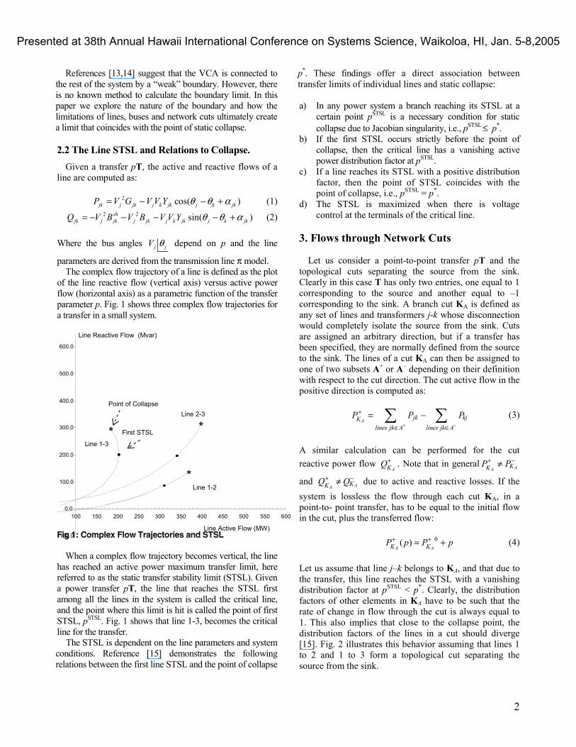
parameters are derived from the transmission line π model. The complex flow trajectory of a line is defined as the plot
of the line reactive flow (vertical axis) versus active power flow (horizontal axis) as a parametric function of the transfer parameter p. Fig. 1 shows three complex flow trajectories for a transfer in a small system.
Fig 1: Complex Flow Trajectories and STSL
When a complex flow trajectory becomes vertical, the line
has reached an active power maximum transfer limit, here referred to as the static transfer stability limit (STSL). Given a power transfer pT, the line that reaches the STSL first among all the lines in the system is called the critical line, and the point where this limit is hit is called the point of first STSL, pSTSL. Fig. 1 shows that line 1-3, becomes the critical line for the transfer.
The STSL is dependent on the line parameters and system conditions. Reference [15] demonstrates the following relations between the first line STSL and the point of collapse
p*. These findings offer a direct association between transfer limits of individual lines and static collapse:
a) In any power system a branch reaching its STSL at a
certain point pSTSL is a necessary condition for static collapse due to Jacobian singularity, i.e., pSTSL ≤ p*.
b) If the first STSL occurs strictly before the point of collapse, then the critical line has a vanishing active power distribution factor at pSTSL.
c) If a line reaches its STSL with a positive distribution factor, then the point of STSL coincides with the point of collapse, i.e., pSTSL = p*.
d) The STSL is maximized when there is voltage control at the terminals of the critical line.
3. Flows through Network Cuts
Let us consider a point-to-point transfer pT and the
topological cuts separating the source from the sink. Clearly in this case T has only two entries, one equal to 1 corresponding to the source and another equal to –1 corresponding to the sink. A branch cut KA is defined as any set of lines and transformers j-k whose disconnection would completely isolate the source from the sink. Cuts are assigned an arbitrary direction, but if a transfer has been specified, they are normally defined from the source to the sink. The lines of a cut KA can then be assigned to one of two subsets A+ or A– depending on their definition with respect to the cut direction. The cut active flow in the positive direction is computed as:
A jk kjK
lines jk A lines jk A
P P P+ −
+
∈ ∈
= −∑ ∑ (3)
A similar calculation can be performed for the cut reactive power flow
AKQ+ . Note that in general AA KKP P+ −≠
and AA KKQ Q+ −≠ due to active and reactive losses. If the system is lossless the flow through each cut KA, in a point-to- point transfer, has to be equal to the initial flow in the cut, plus the transferred flow:
0( )A AK KP p P p+ += + (4)
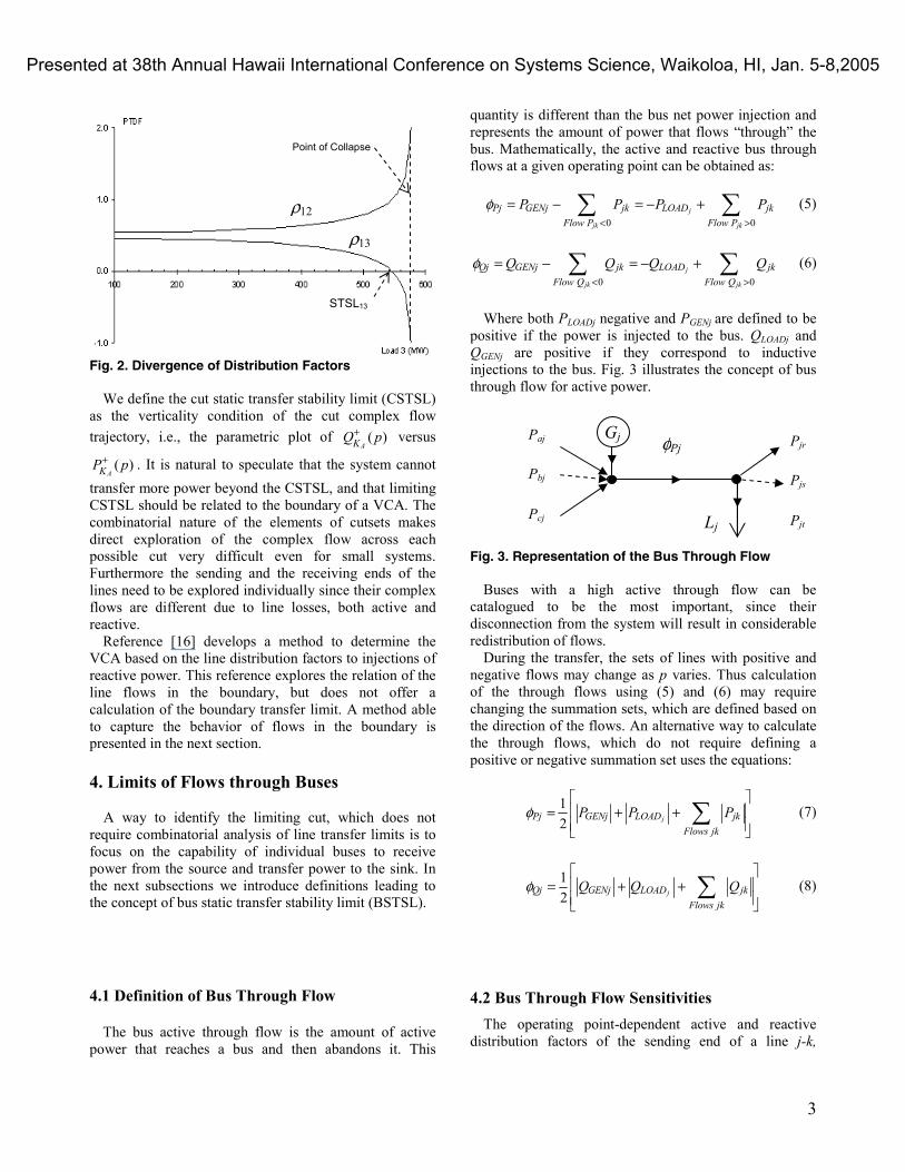
Let us assume that line j–k belongs to KA, and that due to the transfer, this line reaches the STSL with a vanishing distribution factor at pSTSL < p*. Clearly, the distribution factors of other elements in KA have to be such that the rate of change in flow through the cut is always equal to 1. This also implies that close to the collapse point, the distribution factors of the lines in a cut should diverge [15]. Fig. 2 illustrates this behavior assuming that lines 1 to 2 and 1 to 3 form a topological cut separating the source from the sink.
-100.0
0.0
100.0
200.0
300.0
400.0
500.0
600.0
100 150 200 250 300 350 400 450 500 550 600
Line 2-3
Line 1-2
First STSL
Point of Collapse
Line 1-3
Line Active Flow (MW)
Line Reactive Flow (Mvar)
*
*
*
Presented at 38th Annual Hawaii International Conference on Systems Science, Waikoloa, HI, Jan. 5-8,2005
3
Fig. 2. Divergence of Distribution Factors
We define the cut static transfer stability limit (CSTSL) as the verticality condition of the cut complex flow trajectory, i.e., the parametric plot of ( )
AKQ p+ versus
( )AKP p+ . It is natural to speculate that the system cannot
transfer more power beyond the CSTSL, and that limiting CSTSL should be related to the boundary of a VCA. The combinatorial nature of the elements of cutsets makes direct exploration of the complex flow across each possible cut very difficult even for small systems. Furthermore the sending and the receiving ends of the lines need to be explored individually since their complex flows are different due to line losses, both active and reactive.
Reference [16] develops a method to determine the VCA based on the line distribution factors to injections of reactive power. This reference explores the relation of the line flows in the boundary, but does not offer a calculation of the boundary transfer limit. A method able to capture the behavior of flows in the boundary is presented in the next section. 4. Limits of Flows through Buses
A way to identify the limiting cut, which does not require combinatorial analysis of line transfer limits is to focus on the capability of individual buses to receive power from the source and transfer power to the sink. In the next subsections we introduce definitions leading to the concept of bus static transfer stability limit (BSTSL). 4.1 Definition of Bus Through Flow
The bus active through flow is the amount of active power that reaches a bus and then abandons it. This
quantity is different than the bus net power injection and represents the amount of power that flows “through” the bus. Mathematically, the active and reactive bus through flows at a given operating point can be obtained as:
0 0j
jk jk
Pj GENj jk LOAD jkFlow P Flow P
P P P Pφ< >
= − = − +∑ ∑ (5)
0 0j
jk jk
Qj GENj jk LOAD jkFlow Q Flow Q
Q Q Q Qφ< >
= − = − +∑ ∑ (6)
Where both PLOADj negative and PGENj are defined to be
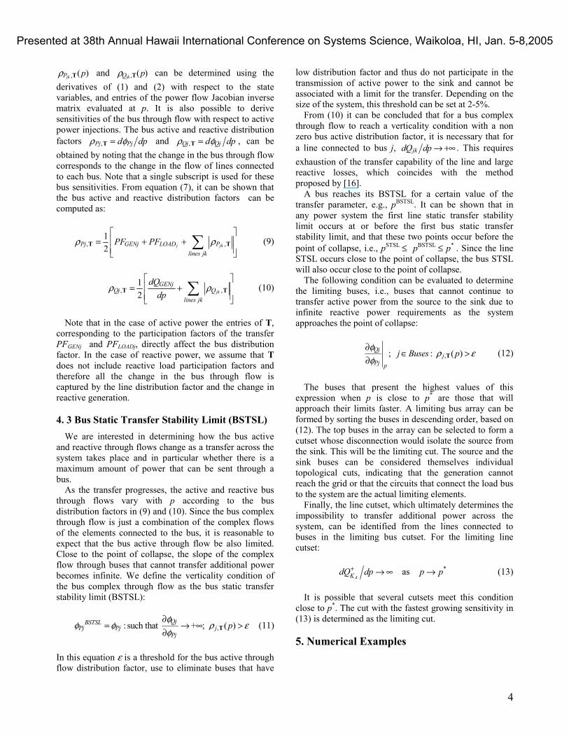
positive if the power is injected to the bus. QLOADj and QGENj are positive if they correspond to inductive injections to the bus. Fig. 3 illustrates the concept of bus through flow for active power. Fig. 3. Representation of the Bus Through Flow
Buses with a high active through flow can be catalogued to be the most important, since their disconnection from the system will result in considerable redistribution of flows.
During the transfer, the sets of lines with positive and negative flows may change as p varies. Thus calculation of the through flows using (5) and (6) may require changing the summation sets, which are defined based on the direction of the flows. An alternative way to calculate the through flows, which do not require defining a positive or negative summation set uses the equations:
12 jPj GENj LOAD jk
Flows jk
P P Pφ = + +
∑ (7)
12 jQj GENj LOAD jk
Flows jk
Q Q Qφ = + +
∑ (8)
4.2 Bus Through Flow Sensitivities The operating point-dependent active and reactive
distribution factors of the sending end of a line j-k,
ρ12
ρ13
Point of Collapse
STSL13
GjPaj
Pbj
Pcj
Pjr
Pjs
Pjt Lj
φPj
Presented at 38th Annual Hawaii International Conference on Systems Science, Waikoloa, HI, Jan. 5-8,2005
4
, ( )jkP pρ T and , ( )jkQ pρ T can be determined using the derivatives of (1) and (2) with respect to the state variables, and entries of the power flow Jacobian inverse matrix evaluated at p. It is also possible to derive sensitivities of the bus through flow with respect to active power injections. The bus active and reactive distribution factors ,Pj Pjd dpρ φ=T and ,Qj Qjd dpρ φ=T , can be obtained by noting that the change in the bus through flow corresponds to the change in the flow of lines connected to each bus. Note that a single subscript is used for these bus sensitivities. From equation (7), it can be shown that the bus active and reactive distribution factors can be computed as:
, ,
12 j jkPj GENj LOAD P
lines jk
PF PFρ ρ = + +
∑T T (9)
, ,
12 jk
GENjQj Q
lines jk
dQdp
ρ ρ = +
∑T T (10)
Note that in the case of active power the entries of T,
corresponding to the participation factors of the transfer PFGENj and PFLOADj, directly affect the bus distribution factor. In the case of reactive power, we assume that T does not include reactive load participation factors and therefore all the change in the bus through flow is captured by the line distribution factor and the change in reactive generation. 4. 3 Bus Static Transfer Stability Limit (BSTSL)
We are interested in determining how the bus active and reactive through flows change as a transfer across the system takes place and in particular whether there is a maximum amount of power that can be sent through a bus.
As the transfer progresses, the active and reactive bus through flows vary with p according to the bus distribution factors in (9) and (10). Since the bus complex through flow is just a combination of the complex flows of the elements connected to the bus, it is reasonable to expect that the bus active through flow be also limited. Close to the point of collapse, the slope of the complex flow through buses that cannot transfer additional power becomes infinite. We define the verticality condition of the bus complex through flow as the bus static transfer stability limit (BSTSL):
,: such that + ; ( )QjBSTSLPj Pj j
Pjp
φφ φ ρ ε
φ∂
= → ∞ >∂ T (11)
In this equation ε is a threshold for the bus active through flow distribution factor, use to eliminate buses that have
low distribution factor and thus do not participate in the transmission of active power to the sink and cannot be associated with a limit for the transfer. Depending on the size of the system, this threshold can be set at 2-5%.
From (10) it can be concluded that for a bus complex through flow to reach a verticality condition with a non zero bus active distribution factor, it is necessary that for a line connected to bus j, jkdQ dp → +∞ . This requires exhaustion of the transfer capability of the line and large reactive losses, which coincides with the method proposed by [16].
A bus reaches its BSTSL for a certain value of the transfer parameter, e.g., pBSTSL. It can be shown that in any power system the first line static transfer stability limit occurs at or before the first bus static transfer stability limit, and that these two points occur before the point of collapse, i.e., pSTSL ≤ pBSTSL ≤ p* . Since the line STSL occurs close to the point of collapse, the bus STSL will also occur close to the point of collapse.
The following condition can be evaluated to determine the limiting buses, i.e., buses that cannot continue to transfer active power from the source to the sink due to infinite reactive power requirements as the system approaches the point of collapse:
,; : ( )Qjj
Pj p
j Buses pφ ρ εφ
∂∈ >
∂ T (12)
The buses that present the highest values of this
expression when p is close to p* are those that will approach their limits faster. A limiting bus array can be formed by sorting the buses in descending order, based on (12). The top buses in the array can be selected to form a cutset whose disconnection would isolate the source from the sink. This will be the limiting cut. The source and the sink buses can be considered themselves individual topological cuts, indicating that the generation cannot reach the grid or that the circuits that connect the load bus to the system are the actual limiting elements.
Finally, the line cutset, which ultimately determines the impossibility to transfer additional power across the system, can be identified from the lines connected to buses in the limiting bus cutset. For the limiting line cutset:
AKdQ dp+ → ∞ as *p p→ (13) It is possible that several cutsets meet this condition
close to p*. The cut with the fastest growing sensitivity in (13) is determined as the limiting cut. 5. Numerical Examples
Presented at 38th Annual Hawaii International Conference on Systems Science, Waikoloa, HI, Jan. 5-8,2005
5
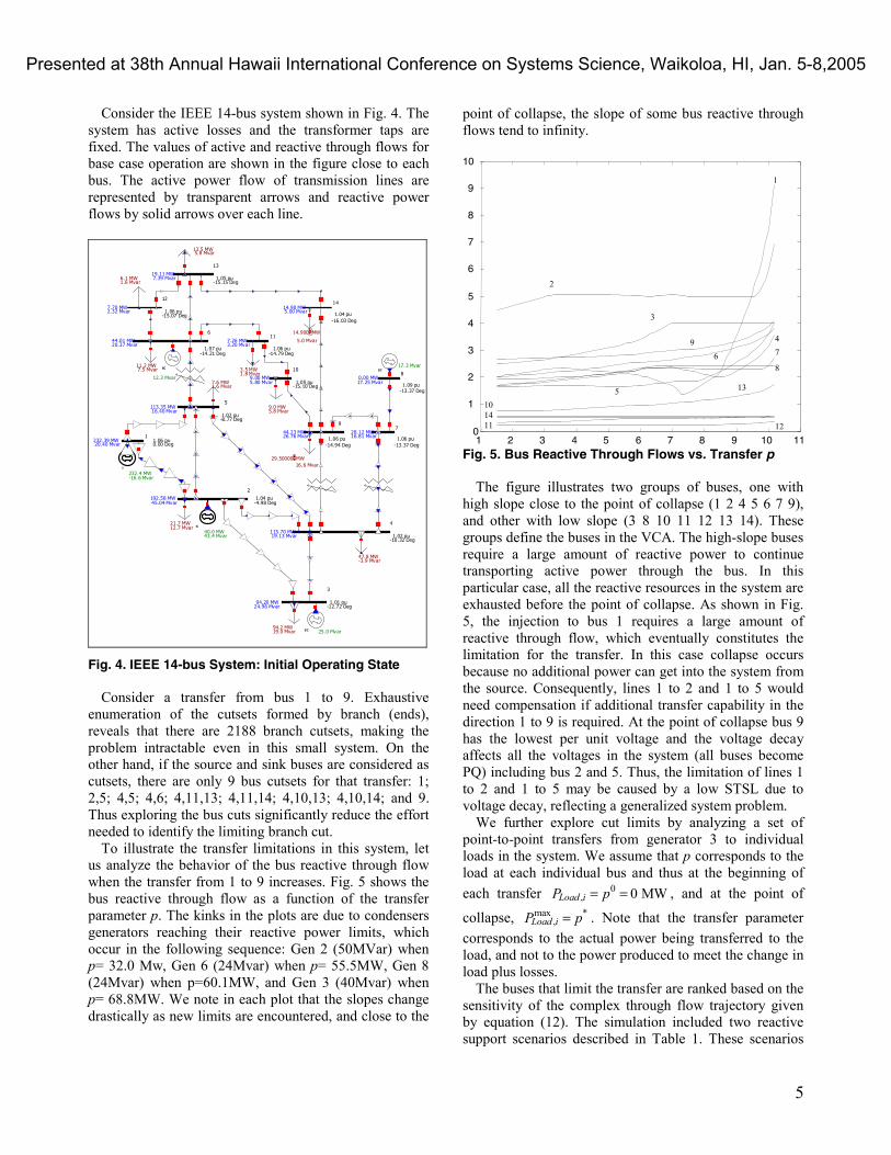
Consider the IEEE 14-bus system shown in Fig. 4. The system has active losses and the transformer taps are fixed. The values of active and reactive through flows for base case operation are shown in the figure close to each bus. The active power flow of transmission lines are represented by transparent arrows and reactive power flows by solid arrows over each line.
G
G
SCSC
SC
1 1.06 pu 0.00 Deg
232.39 MW 20.40 Mvar
2
1.04 pu -4.98 Deg
192.58 MW 45.04 Mvar
5
1.02 pu -8.77 Deg
113.35 MW 16.40 Mvar
3
1.01 pu-12.72 Deg
94.20 MW 24.96 Mvar
4
1.02 pu-10.32 Deg
115.70 MW 19.13 Mvar
6
1.07 pu-14.21 Deg
44.01 MW 20.37 Mvar
11
1.06 pu-14.79 Deg
7.26 MW 3.20 Mvar
12
1.06 pu-15.07 Deg
7.70 MW 2.32 Mvar
13
1.05 pu-15.15 Deg
19.11 MW 7.39 Mvar
10
1.05 pu-15.10 Deg
9.00 MW 5.80 Mvar
14
1.04 pu-16.03 Deg
14.90 MW 5.00 Mvar
9
1.06 pu-14.94 Deg
44.23 MW 26.76 Mvar
7
1.06 pu-13.37 Deg
28.12 MW 16.81 Mvar
8
1.09 pu-13.37 Deg
0.00 MW 17.25 Mvar
13.5 MW 5.8 Mvar
14.900 MW
5.0 Mvar
16.6 Mvar 29.50000 MW
1.6 Mvar 6.1 MW
11.2 MW 7.5 Mvar
7.6 MW 1.6 Mvar
47.8 MW -3.9 Mvar
21.7 MW 12.7 Mvar
94.2 MW 19.0 Mvar
1.8 Mvar 3.5 MW
9.0 MW 5.8 Mvar
232.4 MW -16.6 Mvar
40.0 MW 43.4 Mvar
25.0 Mvar
17.3 Mvar
12.3 Mvar
Fig. 4. IEEE 14-bus System: Initial Operating State
Consider a transfer from bus 1 to 9. Exhaustive enumeration of the cutsets formed by branch (ends), reveals that there are 2188 branch cutsets, making the problem intractable even in this small system. On the other hand, if the source and sink buses are considered as cutsets, there are only 9 bus cutsets for that transfer: 1; 2,5; 4,5; 4,6; 4,11,13; 4,11,14; 4,10,13; 4,10,14; and 9. Thus exploring the bus cuts significantly reduce the effort needed to identify the limiting branch cut.
To illustrate the transfer limitations in this system, let us analyze the behavior of the bus reactive through flow when the transfer from 1 to 9 increases. Fig. 5 shows the bus reactive through flow as a function of the transfer parameter p. The kinks in the plots are due to condensers generators reaching their reactive power limits, which occur in the following sequence: Gen 2 (50MVar) when p= 32.0 Mw, Gen 6 (24Mvar) when p= 55.5MW, Gen 8 (24Mvar) when p=60.1MW, and Gen 3 (40Mvar) when p= 68.8MW. We note in each plot that the slopes change drastically as new limits are encountered, and close to the
point of collapse, the slope of some bus reactive through flows tend to infinity.
Fig. 5. Bus Reactive Through Flows vs. Transfer p The figure illustrates two groups of buses, one with
high slope close to the point of collapse (1 2 4 5 6 7 9), and other with low slope (3 8 10 11 12 13 14). These groups define the buses in the VCA. The high-slope buses require a large amount of reactive power to continue transporting active power through the bus. In this particular case, all the reactive resources in the system are exhausted before the point of collapse. As shown in Fig. 5, the injection to bus 1 requires a large amount of reactive through flow, which eventually constitutes the limitation for the transfer. In this case collapse occurs because no additional power can get into the system from the source. Consequently, lines 1 to 2 and 1 to 5 would need compensation if additional transfer capability in the direction 1 to 9 is required. At the point of collapse bus 9 has the lowest per unit voltage and the voltage decay affects all the voltages in the system (all buses become PQ) including bus 2 and 5. Thus, the limitation of lines 1 to 2 and 1 to 5 may be caused by a low STSL due to voltage decay, reflecting a generalized system problem.
We further explore cut limits by analyzing a set of point-to-point transfers from generator 3 to individual loads in the system. We assume that p corresponds to the load at each individual bus and thus at the beginning of each transfer 0
, 0 MWLoad iP p= = , and at the point of
collapse, max *,Load iP p= . Note that the transfer parameter
corresponds to the actual power being transferred to the load, and not to the power produced to meet the change in load plus losses.
The buses that limit the transfer are ranked based on the sensitivity of the complex through flow trajectory given by equation (12). The simulation included two reactive support scenarios described in Table 1. These scenarios
1
9
8
7 6
5
4
3
2
10 14 11 12
13
1 2 3 4 5 6 7 8 9 10 110
1
2
3
4
5
6
7
8
9
10
Presented at 38th Annual Hawaii International Conference on Systems Science, Waikoloa, HI, Jan. 5-8,2005
6
will illustrate how system reactive support affects the limiting elements for each transfer.
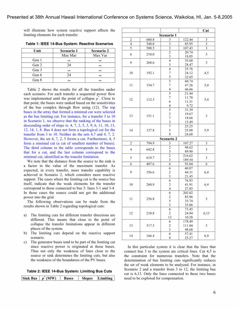
Table 1: IEEE 14-Bus System: Reactive Scenarios
Unit Scenario 1 Scenario 2 Max Mar Max Var
Gen 1 ∞ ∞ Gen 2 24 ∞ Gen 3 ∞ ∞ Gen 6 24 ∞ Gen 8 ∞ ∞
Table 2 shows the results for all the transfers under
each scenario. For each transfer a sequential power flow was implemented until the point of collapse p*. Close to that point, the buses were ranked based on the sensitivities of the bus complex through flow using (12). The top buses in the array that formed a minimal cut were selected as the bus limiting cut. For instance, for a transfer 3 to 10 in Scenario 1, we observe that the ranking of the buses in descending order of slope is: 4, 7, 2, 5, 3, 9, 6, 11, 10, 13, 12, 14, 1, 8. Bus 4 does not form a topological cut for the transfer from 3 to 10. Neither do the sets 4,7 and 4, 7, 2. However, the set 4, 7, 2, 5 forms a cut. Furthermore, 4, 5 form a minimal cut (a cut of smallest number of buses). The third column in the table corresponds to the buses that for a cut, and the last column correspond to the minimal cut, identified as the transfer limitation.
We note that the distance from the source to the sink is a factor in the value of the maximum transfer. As expected, in every transfer, more transfer capability is achieved in Scenario 2, which considers more reactive support. The cases where the limiting cut is the source bus itself, indicate that the weak elements for the transfer correspond to those connected to bus 3: lines 3-1 and 3-4. In those cases the source could not get the additional power into the grid.
The following observations can be made from the results shown in Table 2 regarding topological cuts:
a) The limiting cuts for different transfer directions are
different. This means that close to the point of collapse the transfer limitations appear in different places of the system.
b) The limiting cuts depend on the reactive support scenario.
c) The generator buses tend to be part of the limiting cut since reactive power is originated at those buses. Thus not only the weakness of lines close to the source or sink determines the limiting cuts, but also the weakness of the boundaries of the PV buses.
Table 2: IEEE 14-Bus System: Limiting Bus Cuts
Sink Bus p* (MW) Buses Slopes Limiting
Cut Scenario 1
2 680.8 3 122.44 3 4 548.0 3 85.95 3 5 508.5 3 107.43 3
6 210.0 2 3
20.74 18.05 3
9 268.6 4 3
35.68 28.47 3
10 192.1 4 7 5
25.76 24.12 22.65
4,5
11 154.7 5 7 4
60.74 47.26 46.66
5,4
12 112.3
5 7 6 4
21.44 11.78 11.51
9.72
5,4
13 151.1
5 2 7 3
31.39 19.67 18.66 15.49
3
14 127.8 7 5 9
25.25 25.08 24.68
5,9
Scenario 2 2 794.9 3 107.27 3
4 642.8 2 3
98.62 89.90 3
5 619.7 2 3
216.62 189.54 3
6 407.6 6 93.04 6
9 356.6 6 2 3
60.07 44.31 21.45
6,4
10 260.9 6 2 4
76.93 41.91 27.85
6,4
11 256.8
6 2 5 3
202.02 85.96 35.74 35.06
3
12 210.8 6 2
13
73.45 24.94 10.58
6,13
13 317.3 6 2 3
178.49 111.04 48.68
3
14 166.4 6 9
57.41 25.27 6,9
In this particular system it is clear that the lines that
connect bus 3 to the system are critical lines. Cut 4,5 is the constraint for numerous transfers. Note that the determination of bus limiting cuts significantly reduces the set of weak elements to be analyzed. For instance, in Scenario 2 and a transfer from 3 to 12, the limiting bus cut is 6,13. Only the lines connected to these two buses need to be explored for compensation.
Presented at 38th Annual Hawaii International Conference on Systems Science, Waikoloa, HI, Jan. 5-8,2005
7
From the numerical point of view, the identification of the bus cuts provides an effective mechanism to determine transfer limitations regarding collapse: lines connected to buses in the bus cutset form a weak boundary that could otherwise transfer more active power.
From the operations point of view, the cut transfer limit provides a physical interpretation that relates collapse phenomenon to topology: no additional active power can be send through the limiting cut beyond the cut stability limit. As the transfer increases, the trajectory of each cut complex flow presents an increasing slope, which allows identifying the transfer constraint.
Further research on this topic will include potential determination of cutsets including contingency analysis, and use of sensitivity factors to determine the limiting cutset. 6. Conclusions
A relation between static collapse and topological cuts has been established in this paper. As a transfer increases, individual transmission elements, nodes and topological cuts reach transfer limitations originated in the complex flow equations of individual transmission lines. Collapse occurs ultimately due to the impossibility of transferring additional power through a topological cut. The concept of bus through flow has been introduced as a mechanism to determine a bus cutset that constitutes the limitation for additional transfers. The determination is based on the sensitivities of the bus through flow.
The limiting cut depends on the transfer direction, operating conditions of the system and heavily on the reactive power support. The ability of a reactive power source to inject power into the grid seems to be a primary factor in the formation of the limiting cutset and the value of the margin to collapse. 7. References [1] I. Dobson, Liming Lu, “Voltage collapse precipitated by
the immediate change of stability when generator reactive power limits are encountered”, IEEE Transactions on Circuits and Systems-I: Fundamental Theory and Applications, vol. 39, no. 9, pp. 762-766, September 1992.
[2] T. Van Cutsem, C. Vournas, “Voltage Stability of Electric Power Systems”, Kluwer, Massachusetts, 1998.
[3] IEEE/PES Power System Stability Subcommittee, “Voltage stability assessment, procedures and guides”, Final Report, January 2001.
[4] I. Dobson and L. Lu, “Computing an optimum direction in control space to avoid saddle node bifurcation and voltage collapse in electric power systems”, IEEE Transactions on Automatic Control, vol. 37, No. 10, pp. 1616-1620, October 1992.
[5] V. Ajjarapu, C. Christy, “The continuation power flow: a tool for steady state voltage stability analysis”, IEEE Transactions on Power Systems, vol. 7, no 1, pp. 416-423, Feb. 1992.
[6] H.D. Chiang, A. J. Flueck, K.S. Shah, N. Balu, “CPFLOW: a practical tool for tracing power system steady-state stationary behavior due to load and generation variations”, IEEE Transactions on Power Systems, vol. 10, no. 2, pp. 623-634, May 1995.
[7] I.A. Hiskens, R. Davy, “Exploring the power flow solution space boundary”, IEEE Transactions on Power Systems, vol.16, no.3, pp. 389-395, August 2001
[8] H. D. Chiang, C. S. Wang, and A. J. Flueck, “Look-ahead voltage and load margin contingency selection functions for large-scale power systems,” IEEE Transactions on Power Systems, vol. 12, no. 1, pp. 173–180, Feb. 1997.
[9] G. C. Ejebe, G. D. Irisarri, S. Mokhtari, O. Obadina, P. Ristanovic, and J. Tong, “Methods for contingency screening and ranking for voltage stability analysis of power system”, IEEE Transaction on Power Systems, vol. 11, no. 1, pp. 350–356, Feb. 1996.
[10] C. A. Cañizares, “Calculating Optimal System Parameters to Maximize the Distance to Saddle-node Bifurcations”, IEEE Transactions on Circuits and Systems-I: Fundamental Theory and Applications, Vol. 45, No. 3, March 1998, pp. 225-237.
[11] H. Wan, J. D. McCalley, V. Vittal, “Risk based voltage security assessment”, IEEE Transactions on Power Systems, vol. 15, no. 4, pp. 1247-1254, November 2000.
[12] W. Rosehart, C. Canizares, V. Quintana, “Cost of voltage security in electricity markets,” IEEE Power Engineering Society Summer Meeting, 2000, vol. 4, pp. 2115-2120.
[13] R.A. Schlueter, I. Hu, M.W. Chang, J.C. Lo, and A. Costi, “Methods for determining proximity to voltage collapse,” IEEE Transactions on Power Systems, Vol. 6, No. 2, pp. 285-292, 1991.
[14] T. Lie, R.A. Schlueter, P.A. Rusche, and R. Rhoades, “Methods of Identifying Weak Transmission Network Stability Boundaries”, IEEE Transactions on Power System, Vol. 8, No. 1, pp. 293-301, February 1993.
[15] S. Grijalva, “Complex Flow-Based Nonlinear ATC Screening”, Ph.D. Dissertation, University of Illinois at Urbana-Champaign, Urbana, IL, June 2002.
[16] C.A. Aumuller, T.K. Saha, "Determination of Power system Coherent Bus Groups by Novel Sensitivity-Based Method for Voltage Stability Assessment," IEEE Transaction on Power Systems, Vol. 18, No. 3, August 2003, pp. 1157-1164.
Presented at 38th Annual Hawaii International Conference on Systems Science, Waikoloa, HI, Jan. 5-8,2005