INITIAL VALUE FORMALISM FORLEMAITRE-TOLMAN-BONDI COLLAPSE

P. D. LASKY1, A. W. C. LUN1 and R. B. BURSTON12

(January 10, 2007)

Abstract

Formulating a dust filled spherically symmetric metric utilizing the 3 + 1 for-malism for general relativity, we show that the metric coefficients are com-pletely determined by the matter distribution throughout the spacetime. Fur-thermore, the metric describes both inhomogeneous dust regions and alsovacuum regions in a single coordinate patch, thus alleviating the need forcomplicated matching schemes at the interfaces. In this way, the system isestablished as an initial-boundary value problem, which has many benefits forits numerical evolution. We show the dust part of the metric is equivalent tothe class of Lemaitre-Tolman-Bondi (LTB) metrics under a coordinate trans-formation. In this coordinate system, shell crossing singularities (SCS) areexhibited as fluid shock waves, and we therefore discuss possibilities for thedynamical extension of shell crossings through the initial point of formationby borrowing methods from classical fluid dynamics. This paper fills a void inthe present literature associated with these collapse models by fully developingthe formalism in great detail. Furthermore, the applications provide examplesof the benefits of the present model.

1. Introduction

It is well established that naked singularities arise from the gravitationalcollapse of inhomogeneous, spherically symmetric dust spheres in generalrelativity [23, 8, 4, 15]. One type of these are shell-crossing singularities(SCS), which are not perceived to violate cosmic censorship due to theirweak nature (see e.g. [20] and references therein). However, difficultiesoften arise in the interpretation of the physical nature of SCS due to thefour-dimensional construction of spacetime solutions usually having little or

1Centre for Stellar and Planetary Astrophysics, School of Mathematical Sciences, MonashUniversity, Wellington Rd, Melbourne 3800, Australia2Max Planck Institute for Solar System Research, 37191 Katlenburg-Lindau, Germanyc© Australian Mathematical Society XXXX, Serial-fee code 0334-2700/XX

1

arX

iv:g

r-qc

/060

6003

v2 1

7 A

ug 2

007

no resemblance to our intuitive perception of the universe. Therefore, weutilize the 3 + 1 formalism for general relativity to model the spacetime asan initial value problem in a single coordinate patch. In this way the SCSare akin to shock waves in fluid mechanics, and therefore our perception andunderstanding of the solutions are greatly enhanced.

The 3 + 1 formalism involves specifying data on an initial Cauchy hy-persurface, and subsequently evolving through time. The ten Einstein fieldequations (EFEs) are decomposed into four constraint equations which mustbe satisfied on every spacelike hypersurface, and six evolution equations.Furthermore, they can be supplemented by the integrability conditions forthe EFEs, which are the Bianchi identities. The once contracted Bianchiidentities in four dimensional spacetimes provide 16 conditions, whilst thetwice contracted provide the remaining four pieces of information, which arethe conservation of energy-momentum equations.

We apply the 3 + 1 formalism for the EFEs and Bianchi identities tothe case of a spherically symmetric sphere of inhomogeneous dust. Thisarticle acts to fill a void in the literature created by [9, 10] by deriving theformalism in full detail. Furthermore, while [9] and [10] used more generalfluids, analytic solutions for the equations derived therein are extremelydifficult to find, and hence the equations are awkward to interpret. It istherefore pertinent to simplify the fluid in order to extract analytic solutionssuch that the full strength of the formalism can be displayed. The dustapplication we present in this article is solved analytically, and hence agreater understanding of the structure of the equations is gained. One ofour main results from the dust section is that the metric coefficients arecompletely determined by the energy-momentum fields. Furthermore, todetermine the matter, and hence the entire spacetime, only the specificationof the matter distribution on the initial hypersurface is required.

We show our solution under a coordinate transformation is equivalentto the class of Lemaitre-Tolman-Bondi (LTB) solutions [12, 21, 3]. Further-more, the line element is such that an exterior vacuum region, namely theSchwarzschild spacetime expressed in a generalized form of the Painleve-Gullstrand (PG) coordinates [18, 7], is described using the same coordinatepatch. In this way, the work is related to that of [1] and [6] who, in a sin-gle coordinate patch describe the Oppenheimer-Snyder (OS) collapse [17],i.e. a Friedmann-Robertson-Walker (FRW) interior joined to an exteriorSchwarzschild spacetime. As the FRW spacetime belongs to the class ofLTB spacetimes, our work is a generalization of [1] and [6].

The evolution of the system is determined by two, first order equationsin the matter fields. The nature of these equations is such that multi-valued solutions in the mass can develop given smooth initial data. Theseare equivalent to the SCS discussed, and we analyse the initial conditionsnecessary for these to occur. Furthermore, we discuss a method for extendingthese SCS beyond their point of initial formation utilizing classical fluid

2

dynamics methods. In this way, we show when a globally naked SCS forms(i.e. beyond the apparent horizon) it will evolve to become a locally nakedsingularity, and eventually evolve into a Schwarzschild singularity at r = 0.

As all aspects of the solutions we present can be solved explicitly in termsof the initial data, the authors believe this formulation is of great value fortesting numerical evolution codes. In particular, the evolution of such asystem contains many complications, including the formation of SCSs, aswell as the interface between the two regions of the spacetime. Numericalcodes are extremely well developed to handle shock waves from classical fluiddynamics, and the same methods can be employed in the relativistic regime.However, the evolution of the interface between the two regions may be ofmore primary concern. In particular, the advantage of having both regionsin a single coordinate patch implies no extra work in the code is requiredat the moving boundary. One simply sets up the initial Cauchy data, withthe matter terms going to zero at some finite radius, and the evolution willnaturally take care of the free boundary.

The structure of the paper is as follows. In section 2 we derive thegeneral form of the LTB metric and analyse the solution. In section 3 welook at the initial and boundary conditions required for the specificationof the spacetime, and also look at the formation of the apparent horizon.In 5 we reduce the system to the marginally bound case and derive theinitial conditions that provide shock waves. Finally, in section 6 we look ata specific example of the evolution of the system with a shock wave.

Geometrized units are employed throughout whereby G = c = 1. Greekindices run from 0 . . . 3 and Latin from 1 . . . 3. The Einstein summationconvention is used, index conventions follow [14] and dΩ2 is the line elementfor the two-sphere.

2. The Metric

Here, we pedagogically derive the spacetime metric to be used for theremainder of the article. This metric is beneficial as it describes both aninterior dust region as well as an exterior vacuum region without the needfor complicated matching schemes across the interface. In particular, bothregions are represented not by two separate line elements patched together,but as a single, all encompassing, line element. In this way, the metric wederive is a generalization of the PG vacuum solution to include dust in anyregion of the spacetime desired.

The derivation of the metric utilizes the 3 + 1 formalism for generalrelativity. This is a powerful method that allows the resulting spacetime tobe represented as an initial value problem. In this way, initial Cauchy data isprescribed and the subsequent evolution depends continuously on the initialdata. Although analytic solutions are provided here, the authors believe

3

the resulting class of spacetimes provides excellent test-beds for numericalschemes; in particular for gravitational collapse.

2.1. ADM equations The decomposition of the EFEs into a 3+1 systemis otherwise known as the ADM formalism [2]. Solving the equations in thisform establishes a metric appropriate to an initial value problem.

Consider a four-dimensional spacetime foliated with three-dimensionalspacelike hypersurfaces. We denote the four-coordinates with xµ :=

(t, xi

),

and a spherically symmetric line element can be reduced for dust, withoutloss of generality, to

ds2 = −(α2 − U2β2

)dt2 + 2U2βdtdr + U2dr2 + r2dΩ2. (1)

where α = α(t, r) is the lapse function, U = U(t, r) and β = β(t, r) is theradial component of the shift vector.

The energy-momentum tensor for dust is given by

Tµν = ρnµnν , (2)

where ρ is the energy-density, and nµ is the normal vector field tangent tothe fluid lines. We demand three properties for the normal vector, given bytwo equations

nαnα = −1 and n[µ∇νnσ] = 0, (3)

where∇µ is the unique four-covariant derivative operator. The first equationin (3) implies the vector nµ is both timelike and normalized, and the secondequation implies the normal vector is hypersurface forming. Utilizing theline element (1) and both equations in (3), one can show the normal vectorin component form is given by

nµ =1α

(1,−β, 0, 0) . (4)

Using the normal vector, the EFEs, Gµν = 8πTµν , can be decomposedinto four constraint equations which must be satisfied on each spacelikehypersurface. These are the Hamiltonian constraint

3R+23K2 −AijAij = 16πρ, (5)

where 3R is the three-Riemann scalar, Aij and K are the trace-free part andtrace of the extrinsic curvature respectively. There are three momentumconstraints

DjAij =23DiK, (6)

4

where Di is the unique three-covariant derivative operator. The remainingsix equations are the evolution equations,

2LnK =K2 +32AijA

ij +12

3R− 2αDiDiα, (7)

LnAij =13KAij − 2AikAjk + 3Rij −

13⊥ij 3R

− 1αDiDjα+

13α⊥ij DkDkα, (8)

where Ln is the Lie derivative operator with respect to the normal vector.Equations (5-8) are the ADM equations, and these need to be supple-

mented with the conservation of energy-momentum equations

∇αTαµ = 0. (9)

These can be decomposed giving the continuity equation which, for dustreduces to

K = Ln (ln ρ) , (10)

and the Euler equations which, in dust, are

ρ Di (lnα) = 0. (11)

As we are considering systems with non-vanishing energy density, equation(11) along with the form of the normal vector (4), is enough to show thelapse function is only a function of the time coordinate. Utilizing coordinatefreedom, we set the lapse function to unity without loss of generality,

α = 1. (12)

This physically implies that the dust particles are moving along timelikegeodesics of the spacetime, which is a result of there being zero pressure.

2.2. Governing equations We begin by putting the metric (1), intothe ADM system of equations. Noting that the Lie derivative acting on ascalar function, ψ, is simply

Lnψ = nα∂αψ

=∂ψ

∂t− β∂ψ

∂r, (13)

helps to recognize patterns in the systems of equations. In particular, weimmediately find the radial component of equation (6) reduces to

LnU = 0. (14)

5

This term, and its derivatives appear readily throughout the system of equa-tions. Substituting (14) into the remaining equations implies the rest of thesystem reduces to a complicated set of differential equations in U , ρ and β.

Applying various combinations of the 3 + 1 EFEs results in being ableto write the system algebraically in U and ρ, leaving only derivatives of theshift function β. In particular, combining (5) and (8) we find the derivativesof U cancel and a relation between ρ and derivatives of the shift results in

r2Lnβ = 4π∫ r

σ=0ρ (t, σ)σ2dσ := M(t, r), (15)

where we have defined a “mass” function according to a Newtonian defi-nition. We note here that this function does not physically represent themass of the system as a Newtonian volume element has been used. How-ever, this function arises in a natural way. Furthermore, we will show thatthis is precisely the mass function commonly defined in the LTB spacetimes.Furthermore, in a vacuum region of the spacetime where the energy den-sity vanishes, the mass function simply becomes a constant. We will seethat this vacuum spacetime is given by the Schwarzschild spacetime in ageneralization of the Painleve-Gullstrand coordinates (see section 2.5).

Adding equation (7) to six times the radial component of equation (8)enables derivatives of U to again cancel, resulting, after some algebra, in

U2 =1

1 + β2 − 2rLnβ. (16)

We now find that the final metric function U is related to the shift, andtherefore, implicitly related to the energy density. Thus for dust, the spher-ically symmetric metric in the form given by (1) is entirely dependant onthe initial matter field.

Now by substituting (16) into (14) we find a second order evolutionequation solely on the shift

0 = Ln(β2 − 2rLnβ

). (17)

Summarily, the line element takes the form

ds2 = −dt2 +(βdt+ dr)2

1 + β2 − 2rLnβ+ r2dΩ2, (18)

where β is given by a solution of equation (17) and is further constrainedby the requirement that the signature of the spacetime be Lorentzian, β2 −2rLnβ > −1.

Due to the method of deriving the metric, we note that it is conduciveto an initial value formulation. In particular, the evolution of the systemis governed by the second order partial differential equation (17). To solve

6

this equation one must pose boundary and initial data, which is discussedin section 3.

The physical realization this method has brought is due to the mannerin which it was derived. Many methods for solving the EFEs require simplysolving for the full four-dimensional spacetime with minimal consideration ofthe physics until the solution has been found. It is then difficult to decipherthe physics due to the seemingly arbitrary nature of the coordinates. Byspecifying spacelike hypersurfaces and allowing for the subsequent evolutionof the system, we have reduced the problem to one that relates closer to thephysical intuition grasped from everyday life.

2.3. Gravitoelectromagnetism Another important set of equationswhich can be solved alongside the ADM equations (5-8) and the conserva-tion equations (10-11) are the remaining Bianchi identities. In four dimen-sions one can go to the once contracted Bianchi identities without loss ofgenerality. By introducing the Weyl conformal curvature tensor, the oncecontracted Bianchi identities can be expressed in terms of the energy mo-mentum tensor

∇αCαµνσ = 8π(∇[νTσ]µ +

13gµ[ν∇σ]Tα

α

). (19)

The Weyl tensor can be decomposed into two spatial, trace free, gravito-electromagnetic (GEM) tensors, known as the electric and magnetic confor-mal curvatures, Eij and Bij respectively, where

Eij : = Ciαjβnαnβ, (20)

Bij : =12εαiβγC

βγδjn

αnδ. (21)

The electric conformal curvature is a measure of the tidal forces presentin the spacetime, analogous to the tidal tensor in Newtonian gravitation.The magnetic conformal curvature has no Newtonian analogue, and is insome sense a measure of the intrinsic rotation associated with the space-time [5]. Therefore, while Bij = 0 in spherical symmetry, we note that itwill have non-trivial contributions for spacetimes with less symmetries. Forexample, one aim of the current program of research is to generalize thismethod to include the family of Robinson-Trautman solutions which con-tain gravitational radiation. These spacetimes will begin with a non-zeromagnetic curvature. However one in these scenarios that this contributionwill be “radiated away” in the form of gravitational radiation such thatthe steady-state solution is spherically symmetric. Furthermore, a radiat-ing, axially-symmetric spacetime will have two components of the magneticcurvature. One component will be associated with the intrinsic angular mo-mentum of the spacetime, and will remain once the system has radiatedto a steady-state. The other component associated with the gravitational

7

radiation will be radiated away in the vein associated with the Robinson-Trautman solutions.

As mentioned, for spherically symmetric dust the magnetic curvaturetensor vanishes and the only contribution to the Weyl tensor is from theelectric curvature. The trace-free nature of the electric curvature, as well asthe spherical symmetry imposed, implies it has the simple form

Eij = diag(−2λ, λ, λ), (22)

where λ = λ(t, r) is the tidal forces associated with the spacetime. Decom-posing the Bianchi identities, given Bij = 0, yields two non-trivial equations

DkEki =8π3Diρ, (23)

LnEij− ⊥ij EklAkl + 5A(ikEj)k −

13EijK = 4πρAij . (24)

Equation (23) can be integrated by using the form of the electric curvature(22), and by substituting the definition for the mass (15), to give the tidalforces for the spacetime

λ = −r3∂

∂r

(M

r3

). (25)

We note that in a vacuum region, the mass function is constant, and thetidal forces therefore become

λs =Ms

r3, (26)

which is the familiar form known for the Schwarzschild spacetime. Thesequantities will become important for the discussion of shock formation insection 5.1.

The other non-trivial GEM equation (24) can be calculated using equa-tions (15) and (22), and also substituting (25), and it simply gives an inte-grability check for the evolution equation which will be given for the massfunction (see section 2.4, in particular equation (35b)).

2.4. Equivalence with LTB We have derived the reduced field equa-tions (17), for the line element (18) that represents spherically symmetricdust. We now show that this can be transformed into LTB coordinates(τ,R, θ, φ).

Let r be a function of both the new time and new radial coordinates,i.e., r = r(τ,R), and also let t = τ , then let

∂r(τ,R)∂τ

= −β. (27)

8

In this new coordinate system, the normal vector has the form nµ′

=(1, 0, 0, 0), and the observer is now comoving with the fluid. In these co-ordinates the Lie derivative of a scalar function is simply the derivative withrespect to the new temporal coordinate, τ , and the condition given by (17)becomes

∂

∂τ

[(∂r(τ,R)∂τ

)2

+ 2r(τ,R)∂2r(τ,R)∂τ2

]= 0. (28)

This is a third order differential equation in the function r(τ,R), and canbe integrated twice to yield(

∂r(τ,R)∂τ

)2

= E(R) +2m(R)r(τ,R)

, (29)

where E(R) and m(R), known as the energy and Misner-Sharp mass [13] re-spectively, are functions of integration. Furthermore, rearranging the metricwe find

ds2 = −dτ2 +

(∂r(τ,R)∂R

)2

1 + E(R)dR2 + r(τ,R)2dΩ2. (30)

Equations (30) and (29) are the standard form of the LTB metric [12, 21, 3].The function E(R), arbitrary up to the constraint E(R) > −1, is a

measure of the energy of a shell at a radius R [20]. Therefore, this functionbeing equal to zero is equivalent to saying the particles at infinity have zerokinetic energy.

It was found during the above transformation that this energy functioncan be expressed in terms of the shift function in our coordinates

E(R) = β2 − 2rLnβ, (31)

which is simply the first integral of equation (17).Transferring back into the original coordinates, we note that the energy

function is a function of t and r. Furthermore, substituting equation (31)back through (17), we see

LnE = 0. (32)

Now, substituting the mass defined in equation (15) back into (31) gives

β2 = E +2Mr, (33)

from which we can further show this implies

LnM = 0. (34)

9

Finally, the above equations can be put back through the line element, andwe find the resulting system can be summarized by the metric and twoconstraint equations

ds2 = dt2+

(√E + 2M/r dt+ dr

)2

1 + E+ r2dΩ2. (35a)

∂M

∂t−√E +

2Mr

∂M

∂r= 0 (35b)

∂E

∂t−√E +

2Mr

∂E

∂r= 0 (35c)

Equations (35b) and (35c) provide a coupled system of differential equationswhich are solved concurrently to determine the dynamics of the system.

We note that the positive root of equation (33) has been selected as thisrepresents a collapsing model. Choosing the negative root is equivalent to re-versing the time coordinate, and therefore gives an expanding, cosmologicaltype model.

2.5. Vacuum Regions While we have derived this solution as a dustproblem, we note that these coordinates also describe vacuum regions. Thisis shown by simply letting the energy density vanish at some radii on theinitial hypersurface. This implies that the mass function becomes constant,and thus equation (35b) is trivially satisfied. Therefore, vacuum regionsof the system are described by the line element (35a) and equation (35c)with M = Ms ∈ R. We describe this system as the “generalized Painleve-Gullstrand” (GPG) coordinates1 as they reduce to the usual PG coordinates[18, 7] for the particular case of E = 0. Evaluating the Einstein tensor forthe GPG metric we find it vanishes as expected. This is therefore a vacuumsolution of the field equations, and spherical symmetry along with Birkhoff’stheorem implies this solution must be diffeomorphic to the Schwarzschildmetric.

However, the vacuum solution described by (35a) and (35c) is actually afamily of solutions parametrized by the energy function. Therefore, for allsolutions of equation (35c), there will exist a coordinate transformation tothe Schwarzschild metric, in coordinates (T, r, θ, φ). This transformation isgiven by solutions to the following coupled system of differential equations(

∂t

∂T

)2

=1 + E, (36a)(1− 2Ms

r

)∂t

∂r=

√2Ms

r+ E. (36b)

1A more detailed analysis of these vacuum coordinates will be presented in a future article.

10

To show this is a valid coordinate transformation amounts to showingthat there exists a solution of (36), which is done by checking the integra-bility conditions. That is, by differentiating equation (36a) with respect tothe radial coordinate, and equation (36b) with respect to the temporal co-ordinate, one can show the partial derivatives commute providing equation(35c) is satisfied. Therefore, providing the energy function is a solution of(35c), the coordinate transformation is valid, and applying the coordinatetransformation yields

ds2 = −(

1− 2Ms

r

)dT 2 +

dr2

1− 2Ms/r+ r2dΩ2, (37)

which is exactly the Schwarzschild metric.

3. Initial and Boundary Conditions

We can now establish the initial and boundary data required to solve thesystem of equations that describe the spacetime. We are required to specifyan energy density for the initial hypersurface. Due to the formulation of thesolution, this energy density can take any form, including vanishing for finiteregions. For example, if one wanted to study the gravitational collapse ofa spherical body, then one specifies an appropriate energy density out to afinite radius, at which point the energy density is allowed to vanish beyondthat radii. However, one can also study the collapse of concentric shells ofmatter; for example by specifying successive Heaviside step functions for theinitial density. The robustness of the formalism allows for the study of anyinitial configuration of spherically symmetric dust.

Whatever form the initial energy density takes, we can evaluate theinitial mass function through the definition given by equation (15). Forvacuum regions, this mass function reduces to a constant. We therefore havethe initial conditions for the mass function throughout the initial spacelikehypersurface.

The data for the energy function is a little more tricky. By expressingequation (35b) in terms of the energy function, and substituting equation(15), after some algebra we find

E(0, r ≤ r∂) =

∫ r0 ∂ρ∂t

∣∣∣t=0

σ2dσ

ρ(0, r)r2

2

− 8πr

∫ r

0ρ(0, σ)σ2dσ. (38)

Therefore, the energy function is found by specifying two terms, namely

∂ρ

∂t

∣∣∣∣t=0

and ρ(0, r). (39)

11

While this works for the non-vacuum regions, one still has the freedom tochoose the form of the energy function for the vacuum regions. However, ifall regions of the spacetime are to be described by a single coordinate patch,then one can employ continuity of the energy function across the interface ofthe matter filled and vacuum regions to determine the boundary conditionsfor the vacuum region.

4. Apparent horizon

No discussion of gravitational collapse is complete without contemplatingthe apparent horizon. We shall now show that the coordinate system usedherein allows for the description of the apparent horizon in a clear andconcise manner.

The apparent horizon is defined as the boundary of the closure of theunion of all trapped regions on a Cauchy surface [22]. An alternate, butequivalent definition is given by the surface with a vanishing expansion fac-tor, Θ, which is defined as the divergence of a congruence of null geodesics

Θ := ∇αkα. (40)

Here kµ is a null vector which is everywhere tangential to the congruenceof radial null geodesics. To derive this null vector, we must look at theequations of motion describing the null geodesics in the spacetime. Theseare given by the Lagrangian, L, and the Euler-Lagrange equations,

2L (xµ, xµ) =1

1 + E

[−(

1− 2Mr

)t2 + 2

√2Mr

+ Etr + r2

]= 0, (41)

0 =d

dλ

∂L∂t− ∂L∂t

and 0 =d

dλ

∂L∂r− ∂L∂r, (42)

where a dot denotes differentiation with respect to the affine parameteralong the geodesics, λ. Furthermore, we have used spherical symmetry toimply that the apparent horizon will only depend on the radial and temporalcoordinates, i.e. θ = φ = 0.

The three equations (41,42) can now be integrated to solve for t and rin terms of a single constant of integration and the metric coefficients. Thenull vector kµ := xµ can then be expressed

kµ =

[√

1 + E , 1 + E −√

1 + E

√2Mr

+ E , 0, 0

], (43)

where the constant of integration has been scaled to unity without loss ofgenerality. Taking the divergence of this quantity, as indicated by equation

12

(40), one finds the expansion factor vanishes along the surface given by theimplicit parametric equation

r (t) = 2M (t, r (t)) . (44)

This remarkably simple form is true for all choices of initial conditions. Fur-thermore, at the interface between the matter and vacuum regions, the massfunction simply becomes the Schwarzschild mass, and the horizon reducesto the familiar event horizon in the Schwarzschild spacetime.

5. Marginally Bound Solution

For the remainder of the article we only consider the case where theenergy function, E(R), vanishes. Known as the marginally bound case2,this model provides a simpler example than the non-zero energy case. Themarginally bound system is described by the line element and single condi-tion on the mass

ds2 = −dt2 +

(√2Mrdt+ dr

)2

+ r2dΩ2, (45a)

∂M

∂t−√

2Mr

∂M

∂r= 0. (45b)

Equation (45b) is a first order, quasi-linear partial differential equationwhich governs the dynamics of the system. The fact that this can easilybe written in conservation form is important to the numerical analysis ofthe system. In particular, systems that can be written in conservation formare preferred since the convergence (if it exists) to weak solutions of theequations are guaranteed by the Lax-Wendroff theorem [11].

The general solution to (45b) is given implicitly by

M = F(

23r3/2 + t

√2M), (46)

where F is a function of integration. To find the particular solution, andhence determine the dynamics of the system, one simply requires the inputof an initial mass distribution. This initial data can be expressed in terms ofthe energy density, which is translated into an initial mass via the definition(15).

The nature of equation (46) is such that given smooth initial data, thesolution can evolve to be multi-valued for the mass function, violating phys-ical intuition regarding the behaviour of mass. These multi-valued solutions

2E(R) < 0 is the bound case and E(R) > 0 is the unbound case.

13

correspond to SCS in general relativity, and are also described by mathe-matical shock waves in this formalism. The solution prior to the formationof these shocks is described by the classical solution of the differential equa-tion (45b) while after the formation of the shock the solution can still beevolved utilizing a weak solution.

5.1. Classical Solution By analyzing the characteristics of (45b), wecan determine the point at which the classical solution fails, and also theinitial conditions required for this to occur at some point within the collapseprocess.

The characteristics of equation (45b) can be represented by introducinga parameter ξ, such that

t = t(ξ), r = r(ξ) and M = M(ξ). (47)

Furthermore, by defining t(0) = 0 without loss of generality, and defining anew parameter s := r(0), we see M (t(0), r(0)) = M (0, s) := M0(s). Now,the characteristics are given by the parametric equations

M = M0(s), t = ξ, (48a)

r3/2 = s3/2−32ξ√

2M0(s). (48b)

The solution becoming multi-valued corresponds to the intersection of thecharacteristic curves, which is interpreted as when the transformation (ξ, s)→(t, r) becomes non-invertible. That is, the determinant of the Jacobian oftransformation vanishes. Therefore, to find conditions for the formation ofthe shock, we must solve

J :=

∣∣∣∣∣∂t∂ξ

∂t∂s

∂r∂ξ

∂r∂s

∣∣∣∣∣ = 0. (49)

It is trivial to show from equations (48) that

J = 0 ⇔ ∂r

∂s= 0. (50)

This condition is equivalent to

t =√

2sM0

M ′0, (51)

r =s1/3(

1− 3M0

M ′0

)2/3

, (52)

where a prime denotes differentiation with respect to s. We are only con-cerned with shocks that occur in the first quadrant of the (t, r) plane. There-fore, we must determine the conditions on M0 and M ′0 which imply theJacobian vanishes.

14

As s = r(t = 0), we see s ∈ [0,∞) . Furthermore, ρ ≥ 0 and M0(s)is defined by letting t = 0 in equation (15), implying M0(s) ≥ 0 for all s.Therefore, by demanding t > 0 in (51), we see

M ′0 > 0. (53)

This will only not hold true when ρ(0, r) = 0 for some finite range of r, asthis will imply M ′0 = 0. Therefore, the characteristics emanating from radiifor which there is a vanishing energy density will never cross, as expected.

Now, demanding r > 0 in equation (52) implies, after some manipulation

d

ds

(M0

s3

)> 0. (54)

Thus, shocks occur in the first quadrant of the (t, r) plane if for any finiterange of s ∈ [0,∞), the inequality in (54) is satisfied.

Finally, letting t = 0 in (25) implies the “tidal force” at t = 0 is

λ(0, s) = −s3d

ds

(M0

s3

), (55)

and considering s > 0, the inequality in (54) is equivalent to

λ(0, r) < 0. (56)

Summarily, we have proved the following theorem:

Shell-Crossing theorem 5.1. SCS occur in marginally bound LTBcollapse if and only if λ(0, r) < 0 for some finite range of r ∈ [0,∞) .

Conversely, if λ(0, r) ≥ 0 for all r, then shock waves will not form.Furthermore, the initial time for the shock to begin, denoted ts, can bedetermined solely from the initial conditions by taking the minimum of (51),

ts =√

2 min√

sM0

M ′0

. (57)

5.2. Weak Solution The solution is satisfied classically until the pointwhere the characteristics first cross. This is the initial point of the shocksurface, and beyond this point the solution to equation (45b) is only givenby a weak solution. The analysis of the weak solution is made simpler byputting the equation into conservation form. This is done by rescaling theradial coordinate such that r := r3/2, implying

∂M

∂t+

∂

∂rf(M) = 0, (58)

where f(M) := −√

2 M3/2. The weak solution is defined as follows: considera test function ψ ∈ C1 which vanishes everywhere outside a rectangle defined

15

by 0 ≤ t ≤ T and a ≤ r ≤ b, and also on the lines t = T , a = r and b = r(for some a, b and T ∈ R). A weak solution is defined to be a solution of∫ T

t=0

∫ b

r=a

(M∂ψ

∂t+f(M)

∂ψ

∂r

)drdt

+∫ b

r=aM0(r)ψ(0, r)dr = 0, (59)

for all test functions ψ.The weak solution contains a world-line whereby the solution contains

a jump discontinuity which is the shock surface. This world-line can beexpressed parametrically in terms of the time coordinate, i.e. rs(t). Eitherside of the shock, the solution is satisfied by the usual classical solutiondiscussed in section 5.1.

A method for evolving shocks beyond the initial point of formation,utilized in many classical scenarios, is to introduce a viscosity term into thedifferential equation,

∂M

∂t+

∂

∂rf(M) = ε

∂2M

∂r2. (60)

Here, ε → 0+ near r = rs(t), and is zero elsewhere. This has the effectof smoothing out the shock into a travelling wave solution. Despite thespacetime being pressureless, we can imagine when particles begin to getextremely close to one another, as is the case just before a shock beginsto occur, a force would begin to play a role that kept these particles fromgetting too close.

Utilizing the viscosity term in the differential equation, we can derivea condition on the shock known as the Rankine-Hugionot condition, whichgives the velocity of the shock (see for e.g. [19]). This is given by

Vs :=drsdt

=[f(M)]+−

[M ]+−, (61)

where

[. . .]+− := limr→r+s

− limr→r−s

. (62)

This result can be transformed back into the radial coordinate utilized inthe metric, and the velocity of the shock is found to be

Vs :=drsdt

=−2√

23√r

[M3/2

]+−

[M ]+−. (63)

We note that the smoothing either side of the shock necessarily implies thatthe mass is still a monotonically increasing function in the positive radial

16

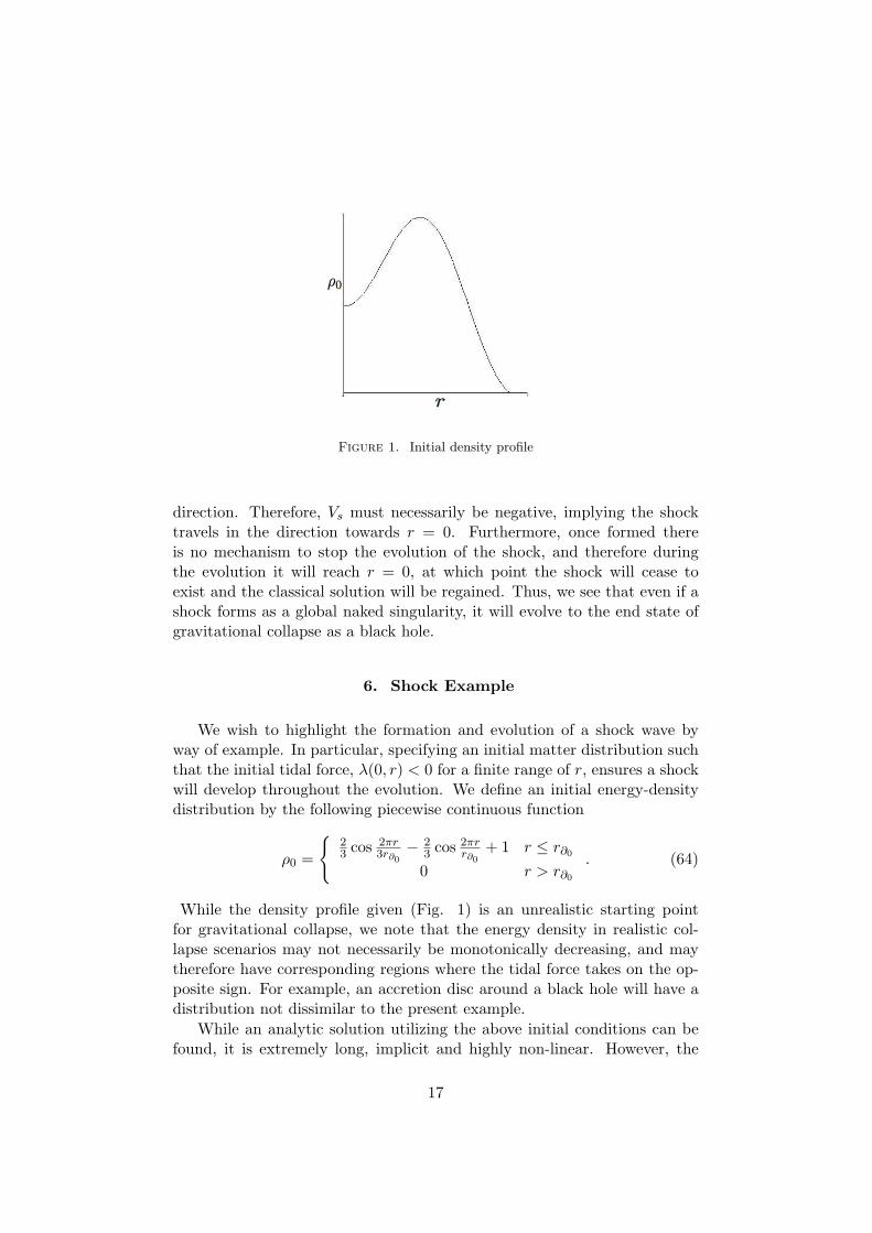
Figure 1. Initial density profile

direction. Therefore, Vs must necessarily be negative, implying the shocktravels in the direction towards r = 0. Furthermore, once formed thereis no mechanism to stop the evolution of the shock, and therefore duringthe evolution it will reach r = 0, at which point the shock will cease toexist and the classical solution will be regained. Thus, we see that even if ashock forms as a global naked singularity, it will evolve to the end state ofgravitational collapse as a black hole.

6. Shock Example

We wish to highlight the formation and evolution of a shock wave byway of example. In particular, specifying an initial matter distribution suchthat the initial tidal force, λ(0, r) < 0 for a finite range of r, ensures a shockwill develop throughout the evolution. We define an initial energy-densitydistribution by the following piecewise continuous function

ρ0 =

23 cos 2πr

3r∂0− 2

3 cos 2πrr∂0

+ 1 r ≤ r∂00 r > r∂0

. (64)

While the density profile given (Fig. 1) is an unrealistic starting pointfor gravitational collapse, we note that the energy density in realistic col-lapse scenarios may not necessarily be monotonically decreasing, and maytherefore have corresponding regions where the tidal force takes on the op-posite sign. For example, an accretion disc around a black hole will have adistribution not dissimilar to the present example.

While an analytic solution utilizing the above initial conditions can befound, it is extremely long, implicit and highly non-linear. However, the

17

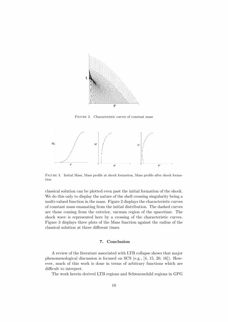
Figure 2. Characteristic curves of constant mass

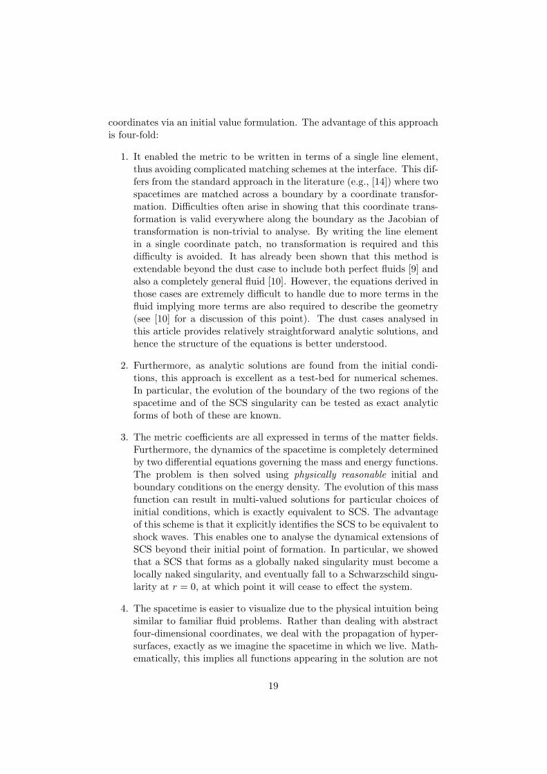
Figure 3. Initial Mass, Mass profile at shock formation, Mass profile after shock forma-tion

classical solution can be plotted even past the initial formation of the shock.We do this only to display the nature of the shell crossing singularity being amulti-valued function in the mass. Figure 2 displays the characteristic curvesof constant mass emanating from the initial distribution. The dashed curvesare those coming from the exterior, vacuum region of the spacetime. Theshock wave is represented here by a crossing of the characteristic curves.Figure 3 displays three plots of the Mass function against the radius of theclassical solution at three different times.

7. Conclusion

A review of the literature associated with LTB collapse shows that majorphenomenological discussion is focused on SCS (e.g., [4, 15, 20, 16]). How-ever, much of this work is done in terms of arbitrary functions which aredifficult to interpret.

The work herein derived LTB regions and Schwarzschild regions in GPG

18

coordinates via an initial value formulation. The advantage of this approachis four-fold:

1. It enabled the metric to be written in terms of a single line element,thus avoiding complicated matching schemes at the interface. This dif-fers from the standard approach in the literature (e.g., [14]) where twospacetimes are matched across a boundary by a coordinate transfor-mation. Difficulties often arise in showing that this coordinate trans-formation is valid everywhere along the boundary as the Jacobian oftransformation is non-trivial to analyse. By writing the line elementin a single coordinate patch, no transformation is required and thisdifficulty is avoided. It has already been shown that this method isextendable beyond the dust case to include both perfect fluids [9] andalso a completely general fluid [10]. However, the equations derived inthose cases are extremely difficult to handle due to more terms in thefluid implying more terms are also required to describe the geometry(see [10] for a discussion of this point). The dust cases analysed inthis article provides relatively straightforward analytic solutions, andhence the structure of the equations is better understood.

2. Furthermore, as analytic solutions are found from the initial condi-tions, this approach is excellent as a test-bed for numerical schemes.In particular, the evolution of the boundary of the two regions of thespacetime and of the SCS singularity can be tested as exact analyticforms of both of these are known.

3. The metric coefficients are all expressed in terms of the matter fields.Furthermore, the dynamics of the spacetime is completely determinedby two differential equations governing the mass and energy functions.The problem is then solved using physically reasonable initial andboundary conditions on the energy density. The evolution of this massfunction can result in multi-valued solutions for particular choices ofinitial conditions, which is exactly equivalent to SCS. The advantageof this scheme is that it explicitly identifies the SCS to be equivalent toshock waves. This enables one to analyse the dynamical extensions ofSCS beyond their initial point of formation. In particular, we showedthat a SCS that forms as a globally naked singularity must become alocally naked singularity, and eventually fall to a Schwarzschild singu-larity at r = 0, at which point it will cease to effect the system.

4. The spacetime is easier to visualize due to the physical intuition beingsimilar to familiar fluid problems. Rather than dealing with abstractfour-dimensional coordinates, we deal with the propagation of hyper-surfaces, exactly as we imagine the spacetime in which we live. Math-ematically, this implies all functions appearing in the solution are not

19

necessarily arbitrary, but are more appropriately based on physicalintuition.

Acknowledgements

The authors wish to thank Brien Nolan for useful discussions. All cal-culations were checked using the computer algebra program Maple.

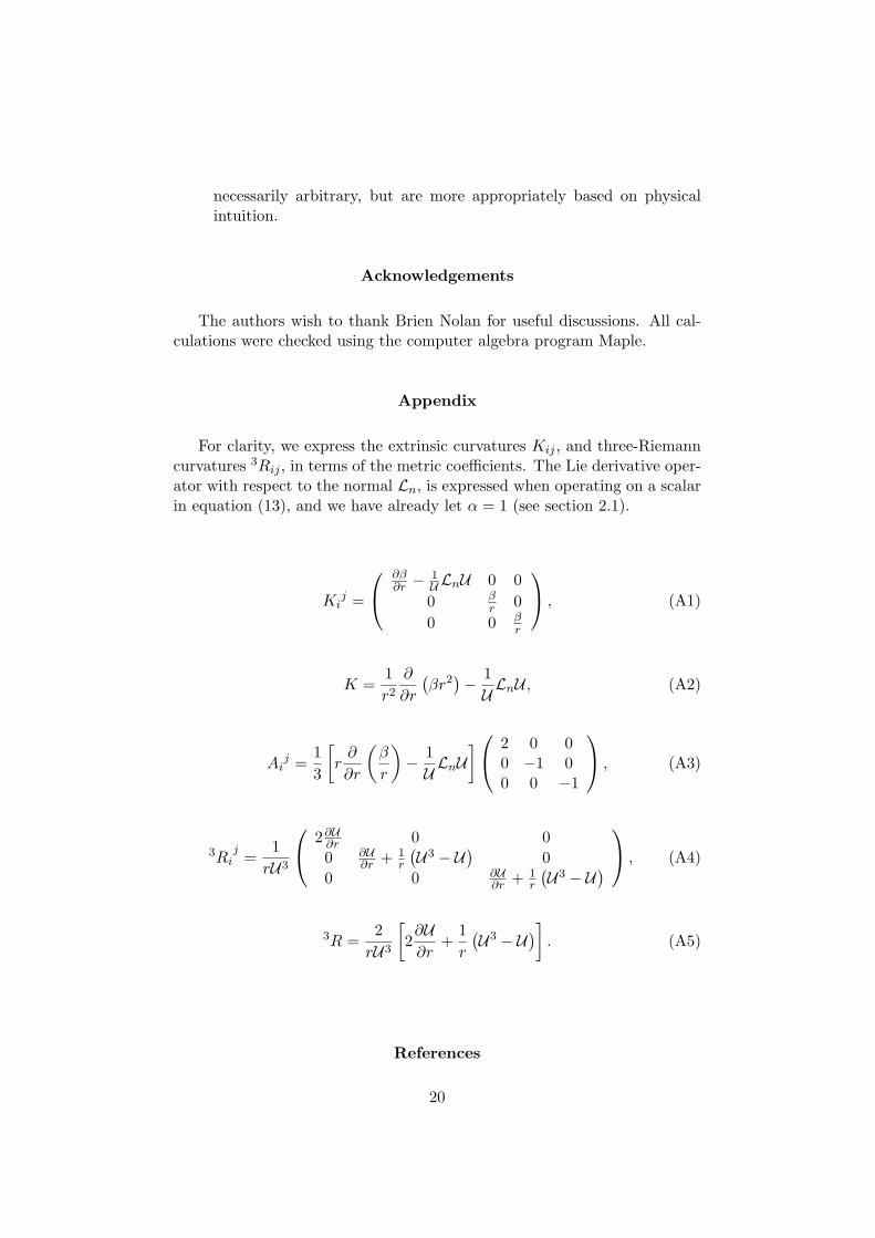
Appendix

For clarity, we express the extrinsic curvatures Kij , and three-Riemanncurvatures 3Rij , in terms of the metric coefficients. The Lie derivative oper-ator with respect to the normal Ln, is expressed when operating on a scalarin equation (13), and we have already let α = 1 (see section 2.1).

Kij =

∂β∂r −

1ULnU 0 00 β

r 00 0 β

r

, (A1)

K =1r2

∂

∂r

(βr2)− 1ULnU , (A2)

Aij =

13

[r∂

∂r

(β

r

)− 1ULnU

] 2 0 00 −1 00 0 −1

, (A3)

3Rij =

1rU3

2∂U∂r 0 00 ∂U

∂r + 1r

(U3 − U

)0

0 0 ∂U∂r + 1

r

(U3 − U

) , (A4)

3R =2rU3

[2∂U∂r

+1r

(U3 − U

)]. (A5)

References

20

[1] R.J. Adler, J. D. Bjorken, P. Chen and J.S. Liu, “Simple analytic models of gravi-tational collapse”, Am. J. Phys. 73 (12) (2005) 1148–59, arXiv:gr-qc/0502040.

[2] R. Arnowitt, S. Deser and C. W. Misner, “The dynamics of general relativity”, inGravitation: An introduction to Current Research (ed. Witten), (John Wiley andSons, Inc., New York, 1962).

[3] H. Bondi, “Spherically symmetrical models in general relativity”, Mon. Not. Roy.Astron. Soc. 107 (1947) 410–25.

[4] D. Christodoulou, “Violation of cosmic censorship in the gravitational collapse of adust cloud”, Commun. Math. Phys. 93 (1984) 171–95.

[5] G. F. R. Ellis, “Relativistic cosmology”, in General Relativity and Cosmology (ed.B. K. Sachs), (Academic, New York, 1971) 104–82.

[6] R. Gautreau and J. M. Cohen, “Gravitational collapse in a single coordinate system”,Am. J. Phys. 63 (1995) 991–9.

[7] A. Gullstrand, “Allegemeine losung des statischen einkorper-problems in der ein-steinchen gravitations theorie”, Arkiv. Mat. Astron. Fys 16 (1922) 1–15.

[8] H. Muller Zum Hagen, P. Yodzis and H. J. Seifert, “On the occurrence of nakedsingularities in general relativity ii”, Commun. Math. Phys. 37 (1974) 29–40.

[9] P. D. Lasky and A. W. C. Lun, “Generalized lemaitre-tolman-bondi solutions withpressure”, Phys. Rev. D 74 (2006) 084013.

[10] P. D. Lasky and A. W. C. Lun, “Spherically symmetric collapse of general fluids”,Phys. Rev. D 75 (2007) 024031.

[11] P. D. Lax and B. Wendroff, “Systems of conservation laws”, Commun. Pure. Appl.Math. 13 (1960) 217–37.

[12] G. Lemaitre, “L’univers en expansion”, Ann. Soc. Sci. Bruxelles A 53 (1933) 51.

[13] C. W. Misner and D. H. Sharp, “Relativistic equations for adiabatic, sphericallysymmetric gravitational collapse”, Phys. Rev. 136 (2) (1964) B571–6.

[14] C. W. Misner, K. S. Thorne and J. A. Wheeler, Gravitation (Freeman, New York,1973).

[15] R. P. A. C. Newman, “Strengths of naked singularities in tolman-bondi-spacetimes”,Class. Quantum Grav. 3 (1986) 527–539.

[16] B. C. Nolan and F. C. Mena, “Geometry and topology of singularities in sphericaldust collapse”, Class. Quantum Grav. 19 (2002) 2587–605.

[17] J. R. Oppenheimer and H. Snyder, “On continued gravitational contraction”, Phys.Rev. 56 (1939) 455–9.

[18] P. Painleve, “La mecanique classique et la theorie de la relativite”, C. R. Acad. Sci.173 (1921) 677–80.

[19] J. Smoller, Shock Waves and Reaction-Diffusion Equations (Springer-Verlag NewYork Inc., New York, 1983).

21

[20] P. Szekeres and A. Lun, “What is a shell crossing singularity”, J. Austral. Math.Soc. Ser. B. 41 (1999) 167–79.

[21] R. C. Tolman, “Effect of inhomogeneity on cosmological models”, Proc. Nat. Acad.Sci. USA 20 (1934) 169–76.

[22] R. Wald, General Relativity (U. of Chicago Press, 1984).

[23] P. Yodzis, H. J. Seifert and H. Muller zum Hagen, “On the occurrence of nakedsingularities in general relativity”, Commun. Math. Phys. 34 (1973) 135–48.

22