comparative kinetic analysis of caco3/cao reaction ... - mdpi
TRANSCRIPT

applied sciences
Article
Comparative Kinetic Analysis of CaCO3/CaOReaction System for Energy Storage andCarbon Capture
Larissa Fedunik-Hofman 1 , Alicia Bayon 2,* and Scott W. Donne 1
1 Discipline of Chemistry, University of Newcastle, Callaghan, NSW 2308, Australia;[email protected] (L.F.-H.); [email protected] (S.W.D.)
2 CSIRO Energy, P.O. Box 330, Newcastle, NSW 2300, Australia* Correspondence: [email protected]
Received: 20 September 2019; Accepted: 23 October 2019; Published: 29 October 2019
Featured Application: Kinetic parameters for the development of CaCO3/CaO reactor systems forcarbon capture and storage and thermochemical energy storage.
Abstract: The calcium carbonate looping cycle is an important reaction system for processes suchas thermochemical energy storage and carbon capture technologies, which can be used to lowergreenhouse gas emissions associated with the energy industry. Kinetic analysis of the reactionsinvolved (calcination and carbonation) can be used to determine kinetic parameters (activation energy,pre-exponential factor, and the reaction model), which is useful to translate laboratory-scale studies tolarge-scale reactor conditions. A variety of methods are available and there is a lack of consensus onthe kinetic parameters in published literature. In this paper, the calcination of synthesized CaCO3 ismodeled using model-fitting methods under two different experimental atmospheres, including 100%CO2, which realistically reflects reactor conditions and is relatively unstudied kinetically. Results arecompared with similar studies and model-free methods using a detailed, comparative methodologythat has not been carried out previously. Under N2, an activation energy of 204 kJ mol−1 is obtainedwith the R2 (contracting area) geometric model, which is consistent with various model-fitting andisoconversional analyses. For experiments under CO2, much higher activation energies (up to 1220 kJmol−1 with a first-order reaction model) are obtained, which has also been observed previously. Thecarbonation of synthesized CaO is modeled using an intrinsic chemical reaction rate model and anapparent model. Activation energies of 17.45 kJ mol−1 and 59.95 kJ mol−1 are obtained for the kineticand diffusion control regions, respectively, which are on the lower bounds of literature results. Theexperimental conditions, material properties, and the kinetic method are found to strongly influencethe kinetic parameters, and recommendations are provided for the analysis of both reactions.
Keywords: kinetics; solid–gas reactions; carbonate looping; calcium looping; thermochemical energystorage; carbon capture and storage
1. Introduction
The calcium looping cycle is an important process which can reduce greenhouse gases emissionsinto the atmosphere through a variety of applications. Research into the use of calcium looping (CaL)has found the system to be highly suitable for processes such as thermochemical energy storage(TCES) [1–4] and carbon capture and storage (CCS) [1,5–9].
The CaL cycle consists of two reactions, which are theoretically reversible. In the endothermicdecomposition (calcination) reaction, calcium carbonate (CaCO3) absorbs energy to produce a metal
Appl. Sci. 2019, 9, 4601; doi:10.3390/app9214601 www.mdpi.com/journal/applsci

Appl. Sci. 2019, 9, 4601 2 of 19
oxide (CaO or lime) and CO2. The exothermic carbonation reaction occurs at a lower temperatureand/or higher CO2 partial pressure and releases thermal energy, which can be used to drive a powercycle [1,10]. The reactions are described by the following expression:
CaCO3 (s) CaO (s) + CO2 (g) (1)
where the reaction enthalpy at standard conditions is −178.4 kJ mol−1.The study of reaction kinetics is highly applicable to the practical implementation of the CaL
cycle for use in energy storage or carbon capture. Reaction kinetics are needed for the design ofreactors for CaL, for which several system configurations exist. A typical configuration consists of twointerconnected circulating fluidized bed reactors, a calciner and carbonator [11–14]. Kinetic reactionmodels suitable for the conditions of interest in CaL have been specifically studied [12,15–19] and havehelped in the design of reactors [11,13,14,20–22].
There are two key challenges associated with performing a kinetic analysis of CaL systems,although the reactions have been extensively studied (i.e., [23–27]). The first is the disparity in theactivation energies suggested for both calcination and carbonation [28], and the second is the lack ofconsensus on the reaction mechanisms [29,30].
The calcination of CaCO3 has been studied using a variety of kinetic analysis methods, includingthe Coats–Redfern method, the Agarwal and Sivasubramanium method, the Friedman (isoconversional)method, and generalized methods such as pore models and grain models [30]. Calcination activationenergies varying between 164 and 225 kJ mol−1 have been obtained for various forms of limestone andsynthetic CaCO3 under inert atmospheres [30], while studies carried out under CO2 have producedvalues of activation energy (Ea, kJ mol−1) which are as high as 2105 kJ mol−1 [31]. A consensus onthe reaction mechanism has not been established. The intrinsic chemical reaction is considered to bethe rate-limiting step by most authors [30]. However, some consider the initial diffusion of CO2 as arate-limiting step [32] and some studies indicate that mass transport is significant [33–35].
Numerous studies suggest that the carbonation reaction takes place in two stages: An initial rapidconversion (kinetic control region) followed by a slower plateau (diffusion control region) [29,30]. Themost commonly applied reaction models which are used to determine kinetic parameters include theso-call generalized methods, which include shrinking core models, pore models, grain models, andapparent (semi-empirical) models [28,30,36,37]. Modeling of the carbonation reaction considers severalmechanisms, such as nucleation and growth, impeded CO2 diffusion, or geometrical constraints relatedto the shape of the particles and pore size distribution of the powder [26].
For the initial kinetic control region of carbonation, typical values of Ea are 19–29 kJ mol−1 insynthetic CaO or natural lime [30], although slightly larger values (i.e., 39–46 [38,39] and 72 kJ mol−1 [37])have been reported. In the kinetic control region, Ea has been reported to be independent of materialproperties and morphology (although variation in kinetic parameters for synthetic CaO and naturallime may suggest otherwise [30]), while morphological effects have a greater influence in the diffusioncontrol region, leading to a greater disparity in diffusion activation energies [28]. The diffusion regioncontrol region takes place after a compact layer of the product CaCO3 develops on the outer region ofthe CaO particle at the product–reactant interface [40]. There is a lack of consensus on the diffusionmechanism (gas or solid state diffusion), as well as the diffusing species (CO2 gas molecules, CO3
2−
ions, or O2− ions) [29]. It is suggested that the diffusion mechanism may change depending on whetherthe sample is porous or non-porous [29] and values of Ea vary between 100 and 270 kJ mol−1 insynthetic CaO or natural lime [30].
The effect of experimental conditions on kinetic parameters is also an important considerationto address. Thermogravimetric experiments in the literature are typically performed using an inertatmosphere for calcination and a mixed inert/CO2 atmosphere for carbonation [30]. However, this maynot replicate reactor conditions for CCS and TCES applications. The coupling of concentrating solarpower with CaL using a closed CO2 cycle has been proposed for its high thermoelectric efficiencies [1,23].
Appl. Sci. 2019, 9, 4601 3 of 19
This system conducts both calcination and carbonation under pure CO2 and has been tested in a smallnumber of studies [23,24,41].
This paper presents a kinetic analysis of synthesized CaCO3 and CaO using several methods:Coats–Redfern method, master plots, and generalized methods. Synthetic materials have been usedto eliminate the effects of impurities. Experiments were carried out using two types of experiments:calcination under inert atmosphere and carbonation under mixed/inert atmosphere; and calcinationand carbonation under 100% CO2. The kinetic analysis of calcination and carbonation under 100%CO2 is particularly relevant in some reactor configurations and is rarely carried out [24]. In order tocomplete the calcination reaction within a short residence time, pilot plants for CO2 capture currentlyemploy high CO2 partial pressures in the calciner (70–90%) and high temperatures (>900 C) [42,43],which are chosen to ensure a practical calcination rate [44]. However, most laboratory-scale tests areperformed under inert gas atmospheres or with low concentrations of CO2, as opposed to under highCO2 volume concentrations, which accelerates material sintering [23]. This study is unique in that ituses realistic reactor conditions using a sintering-resistant material.
As a means of validation, the kinetic parameters obtained with different methods were comparedagainst each other and with published literature. There are no prior studies which directly comparemodel-fitting methods such as Coats–Redfern and master plot methods to isoconversional andgeneralized methods (to the best of the authors’ knowledge). The objectives were therefore to: First,compare kinetic parameters and mechanisms obtained by different methods of kinetic analysis, andsecond, to compare kinetic parameters and mechanisms obtained by different experimental conditions(reaction atmospheres) in order to find the best description of the reaction mechanisms.
2. Materials and Methods
2.1. Material Synthesis
Pechini-synthesized CaO (denoted as P-CaO or P-CaCO3 in its carbonate form) was preparedfollowing the steps described by Jana, de la Peña O’Shea [45], which is also detailed in the experimentalprocedure of Fedunik-Hofman et al. [24]. First, 48 g of citric acid (CA; C6H8O7; Sigma-Aldrich, 99.5%purity; 0.25 mol) was added to 100 mL of distilled water (Milli-Q >18.2 MΩ cm). The mixture wasstirred at 70 C until totally dissolved. Then, 11.8 g of the metal precursor Ca(NO3)2 (Sigma-Aldrich;99.0% purity; 0.05 mol) was then added to the solution with a precursor to CA molar ratio of 1:5.The solution was stirred for 3 hours before the temperature was increased to 90 C. Next, 9.23 mLof ethylene glycol (EG; HOCH2CH2OH; Sigma-Aldrich; 99.8% purity; 0.033 mol) was added with amolar ratio of CA to EG of 3:2. The resulting solution was further stirred at the same temperatureto remove the excess solvent until the solution became a viscous resin. This resin was subsequentlydried in an oven at 180 C for 5 hours. The sample was then ground with an agate mortar and pestleto achieve fine particles and then calcined in a tube furnace. The furnace was programmed to heatfrom ambient temperature to 400 C (10 C min−1 heating rate), where it was held for 2 hours, beforeheating to 900 C and held for 4 hours. After calcination, the sample was ground again to ensure veryfine particles were obtained. The experimental procedure is described in the schematic in Figure 1.

Appl. Sci. 2019, 9, 4601 4 of 19Appl. Sci. 2019, 9, x FOR PEER REVIEW 4 of 21
131
Figure 1. Materials synthesis procedure using Pechini synthesis. 132
2.2. Cycling Analysis 133
The extent of conversion with cycling was monitored by thermogravimetric analysis (TGA) 134 using a SETSYS Evolution 1750 TGA-DSC from Setaram. Two different experimental conditions were 135 performed in order to carry out the different kinetic analysis methods. 136
To carry out a kinetic analysis using the Coats–Redfern method, non-isothermal calcination and 137 carbonation was performed under two atmospheric conditions: Calcination under inert atmosphere 138 (100% N2; maximum temperature 850 °C) followed by carbonation under a mixed atmosphere (25% 139 v/v CO2); and calcination and carbonation under 100% CO2 (maximum temperature 1000 °C). A total 140 gas flow of 20 mL min-1 was used for both conditions. Experimental conditions are detailed in Table 141 1. For each experiment, ~18 mg of P-CaO (powder sample) was placed into a 100 μL alumina crucible 142 and subjected to a temperature ramp from ambient to the maximum temperature, followed by 143 subsequent cooling to ambient temperature. The experiment was repeated for four different heating 144 rates (2.5, 5, 10, and 15 °C min-1). 145
To implement generalized methods of kinetic analysis (i.e., intrinsic chemical reaction rate 146 model and apparent model), it was necessary to carry out carbonation under isothermal conditions. 147 For this case, P-CaO was heated to the set temperature (see Table 1) under 100% N2 and held 148 isothermally for 20 minutes. After this time, the gaseous atmosphere was adjusted to introduce 25% 149 v/v CO2 and held isothermally for 40 minutes to allow for carbonation. The sample was then cooled 150 to ambient temperature. The heating and cooling rates were 10 °C min-1 and a constant gas flow of 20 151 mL min-1 was maintained. 152
For all experiments, a blank was performed under the same conditions and subtracted from each 153 experiment to correct weight signal drifts. For the decomposition reaction of P-CaCO3 to P-CaO, the 154 extent of reaction, α, was determined using the fractional weight loss: 155
i
i f
m m(t)α
m m
(2)
where mi is the initial mass of the sample in grams, m(t) is the mass of the sample in grams after t minutes 156 and mf is the final mass of the sample in grams (after calcination). The carbonation conversion of P-CaO 157 to P-CaCO3 was calculated as follows: 158
Figure 1. Materials synthesis procedure using Pechini synthesis.
2.2. Cycling Analysis
The extent of conversion with cycling was monitored by thermogravimetric analysis (TGA)using a SETSYS Evolution 1750 TGA-DSC from Setaram. Two different experimental conditions wereperformed in order to carry out the different kinetic analysis methods.
To carry out a kinetic analysis using the Coats–Redfern method, non-isothermal calcination andcarbonation was performed under two atmospheric conditions: Calcination under inert atmosphere(100% N2; maximum temperature 850 C) followed by carbonation under a mixed atmosphere (25%v/v CO2); and calcination and carbonation under 100% CO2 (maximum temperature 1000 C). A totalgas flow of 20 mL min−1 was used for both conditions. Experimental conditions are detailed in Table 1.For each experiment, ~18 mg of P-CaO (powder sample) was placed into a 100 µL alumina crucible andsubjected to a temperature ramp from ambient to the maximum temperature, followed by subsequentcooling to ambient temperature. The experiment was repeated for four different heating rates (2.5, 5,10, and 15 C min−1).
To implement generalized methods of kinetic analysis (i.e., intrinsic chemical reaction rate modeland apparent model), it was necessary to carry out carbonation under isothermal conditions. For thiscase, P-CaO was heated to the set temperature (see Table 1) under 100% N2 and held isothermallyfor 20 minutes. After this time, the gaseous atmosphere was adjusted to introduce 25% v/v CO2 andheld isothermally for 40 minutes to allow for carbonation. The sample was then cooled to ambienttemperature. The heating and cooling rates were 10 C min−1 and a constant gas flow of 20 mL min−1
was maintained.For all experiments, a blank was performed under the same conditions and subtracted from each
experiment to correct weight signal drifts. For the decomposition reaction of P-CaCO3 to P-CaO, theextent of reaction, α, was determined using the fractional weight loss:
α =mi −m(t)mi −m f
(2)
where mi is the initial mass of the sample in grams, m(t) is the mass of the sample in grams after tminutes and mf is the final mass of the sample in grams (after calcination). The carbonation conversionof P-CaO to P-CaCO3 was calculated as follows:
X(t) =(
m(t) −mi
mX=1
)×
(MCaCO3
MCaCO3 −MCaO
)(3)

Appl. Sci. 2019, 9, 4601 5 of 19
where m(t) is the mass of the sample in grams after t minutes under the carbonation atmosphere, mi isthe initial mass of the sample in grams (before carbonation), mX = 1 is the theoretical mass of the samplein grams after 100% carbonation conversion (43.97% mass gain), and M is the molar mass in g mol−1.
This expression differs slightly from the means of calculating carbonation conversion usuallyutilized in literature [46]. The rationale is that prior to calcination in the thermogravimetric analyzer,P-CaO may still include CaCO3 phases due to incomplete calcination in the furnace and adsorption ofatmospheric CO2. As a result, m(t) must be measured with reference to the theoretical mass after 100%carbonation conversion (which would occur during the first temperature ramp), as opposed to theinitial mass of P-CaO.
Table 1. Experimental conditions for kinetic analyses.
Calcination Carbonation
Experiment Temp.(C) Atmosphere Isotherm
(min)Temp.(C) Atmosphere Isotherm
(min)
Non-isothermal(mixed N2/CO2) 850 N2 0 – 75 v/v% N2
25 v/v% CO20
Non-isothermal(100% CO2) 1000 CO2 0 – CO2 0
Isothermal 650/700/750 N2 20 650/700/750 75 v/v% N225 v/v% CO2
40
3. Kinetic Analysis Methodology
Methods for solid–gas reactions are either differential, based on the differential form of the reactionmodel, f(α), or integral, based on the integral form g(α) [47].The expression for g(α) is the generalexpression of the integral form:
g(α) =∫ α
0
dαf (α)
= A∫ t
0exp
(−Ea
RT
)h(P)dt (4)
where A is the pre-exponential factor (min−1), R is the universal gas constant (kJ mol−1 K−1), T isthe temperature (K), and h(P) is the pressure dependence term (dimensionless). Non-isothermalexperiments employ a heating rate (β in K min−1) which is constant with time, leading to Equations (5)and (6) [48].
dαdT
=Aβ
exp(−Ea
RT
)h(P) f (α) (5)
g(α) =Aβ
∫ T
0exp
(−Ea
RT
)h(P)dT (6)
Equation (5) is the starting point for differential methods of kinetic analysis, such as the Friedman(isoconversional) method. This method calculates Ea independently of a reaction model and requiresmultiple data sets [49]. It is referred to as a model-free technique as it avoids assumptions abouta reaction mechanism and can identify multi-step reactions. This method is explained in detailedelsewhere [24,30].
Equation (6) is the starting equation for many integral methods of evaluating non-isothermalkinetic parameters with constant β. One example is the Coats–Redfern integral approximation method,referred to as a model-fitting method of kinetic analysis.
Model-fitting methods aim to determine the kinetic parameters of the reaction model integralby fitting obtained data to various known solid-state kinetic models and generally omit the pressuredependence term h(P) [47]. Kinetic models for reaction mechanisms can be categorized using differentalgebraic functions for f (α) and g(α), which can be found in Fedunik-Hofman et al. [30]. The generalprinciple of model-fitting methods is to minimize the difference between the experimentally measuredand calculated data for the given reaction rate expression [47].

Appl. Sci. 2019, 9, 4601 6 of 19
3.1. Coats–Redfern Integral Approximation Method
Integral approximation methods replace the integral in Equation (6) with an integral approximationfunction, Q(x), where x is equal to Ea/RT. The integral can therefore be expressed by the followingexpression (complete derivations can be obtained in previously published works [30]):
g(α) =AREaβ
T2exp(−Ea
RT
)Q(x) (7)
Many approximations for Q(x) exist and the Coats–Redfern approach is a commonly-used example:
Q(x) =(x− 2)
x(8)
Q(x) changes slowly with values of x and is close to unity [47]. Plots of ln[g(α)/T2
]versus 1/T
(Arrhenius plots) will result in a straight line for which the slope and intercept are Ea and A [50]:
ln[
g(α)T2
]= −
(Ea
R
)( 1T
)+ ln
[AREaβ
](1−
2RTav
Ea
)(9)
where Tav is the average temperature over the course of the reaction [51].In order to find the kinetic parameters, Arrhenius plots for each g(α) mechanism can be produced.
One pair of Ea and A for each mechanism can be obtained by linear data-fitting and the mechanism ischosen from the data fit with the best linear correlation coefficient (R2) [47].
Coats–Redfern cannot be applied to simultaneous multi-step reactions, although it can adequatelyrepresent a multi-step process with a single rate-limiting step [47]. For reactions with consecutive steps,the reaction can be split into multiple steps and model-fitting can be carried out for each step [47].
3.2. Master Plots
Master plots are characteristic curves independent of the condition of measurement which areobtained from experimental data [52]. In this paper, master plots were used to validate the reactionmechanism suggested by the Coats–Redfern method. One type of master plot is the Z(α) method,which is derived from a combination of the differential and integral forms of the reaction mechanism.Z(α) is defined as follows:
Z(α) = f (α)g(α) (10)
An alternative integral approximation for g(α) to the Coats–Redfern approximation in Equation (9)
is π(x)x , where π(x) is a polynomial function of x, for which several approximations exist [53,54]; i.e.:
π(x) =x3 + 18x2 + 88x + 96
x4 + 20x3 + 120x2 + 240x + 120(11)
Experimental values of Z(α) can be obtained with the following equation, which is derived inpreviously published works [30]:
Z(α) =dαdt
T2[π(x)βT
](12)
For each of the reaction mechanisms, theoretical master plot curves can be plotted with Equation (10)(using the approximate algebraic functions f (α) described elsewhere [30]) and experimental valueswith Equation (12). The experimental values will provide a good fit for the theoretical curve with thesame mechanism. As the experimental points have not been transformed into functions of the kineticmodels, no prior assumptions are made for the kinetic mechanism [30].

Appl. Sci. 2019, 9, 4601 7 of 19
3.3. Compensation Effect
Isoconversional methods, such as the Friedman method, do not explicitly suggest a reactionmodel. However, if the reaction model can be reasonably approximated with single-step reactionkinetics (if Ea does not vary significantly with α), the reaction mechanism can be determined using thecompensation effect, which is described in detail elsewhere [24,30]. In this method, the isoconversionalanalysis of CaCO3 calcination in Fedunik-Hofman et al. [24] is used to determine the average kineticparameters (Eo and Ao), which are used to reconstruct the reaction model; i.e.:
g(α) =A0
β
∫ Tα
0exp
(−E0
RT
)dT (13)
Equation (13) is then plotted against the theoretical reaction models (see Section 3.1). In this way,experimental and theoretical curves can be compared to suggest a reaction mechanism.
3.4. Generalized Models for Kinetic Analysis of CaO Carbonation
In CaL, the calcination reaction commonly follows a thermal decomposition process that canbe approximated by model-fitting and model-free methods. However, the carbonation reaction ismore complex and is believed to be controlled by several mechanisms such as nucleation and growth,impeded CO2 diffusion, or geometrical constraints related to the shape of the particles and poresize distribution of the powder [26]. Therefore, instead of using a purely kinetics-based approachfor analysis of carbonation, functional forms of f (α) have been proposed to reflect these diversemechanisms. This approach is referred to by Pijolat et al. as a generalized approach [55] and leadsto a rate equation with both thermodynamic variables (e.g., temperature and partial pressures) andmorphological variables [55].
Numerous studies suggest that the carbonation reaction takes place in two stages: An initial rapidconversion (kinetic control region) followed by a slower plateau (diffusion control region) [29]. Thesestages are generally analyzed separately using different models, and this approach is taken to performa kinetic analysis for the carbonation reaction. Interested readers are directed to a previously publishedreview paper for an extended discussion of generalized methods [30].
3.4.1. Chemical Reaction Control Region: Intrinsic Reaction Rate Model
The kinetic control region of the carbonation reaction is generally considered to be limited byheterogeneous surface chemical reaction kinetics, with the driving force for the reaction being thedifference between bulk CO2 pressure and equilibrium CO2 pressure [56]. This region is typicallydescribed by the kinetic reaction rate constant ks (m4 mol−1 s−1), which is considered to be an intrinsicproperty of the material [7].
In this paper, the carbonation of P-CaO is modeled using the grain model used by Sun et al. todetermine the intrinsic rate constants of the CaO–CO2 reaction [56]. Under kinetic control, the reactionrate, R (min−1), is described by:
R =dX
dt(1−X(t))2/3= 3r (14)
where r is the grain model reaction rate (min−1), which is assumed to be constant over the kineticcontrol region. In integral form the reaction rate can be expressed as:[
1− (1−X(t))1/3]= r× t (15)
Appl. Sci. 2019, 9, 4601 8 of 19
Plotting 1–(1–X(t))13 versus t will produce a straight line plot due to the constant reaction rate.
Values of r can be determined for each isothermal experiment and are taken to represent the truereaction rate at the zero conversion point [56], i.e.:
r0 = r (16)
The specific reaction rate can also be expressed in power law form as:
R = 3r(1−X(t))−1/3 = 56ks(PCO2 − PCO2,eq
)nS (17)
where ks is the intrinsic chemical reaction rate constant (mol m−2 s−1 kPa−n), PCO2 − PCO2,eq is thedifference between the equilibrium and partial pressure of CO2, n is the reaction order, and S is thespecific surface area (m2 g−1). Sun et al. determined that at CO2 partial pressures greater than 10 kPa,the reaction order n is zero-order [56]. At time 0, the following relationships are therefore established:
ks = k0exp(−Ea
RT
)(18)
where k0 is the pre-exponential factor (mol. m2 s−1). An Arrhenius plot of slope lnr0 vs 1/T can thereforebe produced to determine the kinetic parameters Ea and k0:
lnr0 = ln(
56k0S0
3
)−
Ea
RT(19)
The intrinsic chemical reaction rate constant ks (calculated using Equation (18)) can be convertedto the rate constant k (min−1) by means of:
k = ksSMCaO (20)
3.4.2. Diffusion Control Region: Apparent Model
Following the kinetic control region, the reaction slows and becomes diffusion-limited [40].A simplified generalized model (referred to as an apparent model) has been developed for thecarbonation of CaO by Lee [37]. This model does not involve the use of morphological parameters andis described by the following equations:
X(t) = Xu
[1− exp
(−
kXu
t)]
(21)
X(t) =Xut
(Xu/k) + t(22)
where Xu is the ultimate conversion of CaO to CaCO3 and k is the reaction rate (min−1). A constant b isintroduced to represent the time taken to attain half the ultimate conversion: X = Xu/2 at t = b. Xu canthen be expressed as:
Xu = kb (23)
Substituting Equation (23) into Equation (22) leads to:
X(t) =kbt
b + t(24)
To determine the constants k and b using the least squares method, the equation is written inlinear form:
1X(t)
=1k
(1t
)+
1kb
(25)

Appl. Sci. 2019, 9, 4601 9 of 19
An Arrhenius plot can then be produced using the following relationship [57]:
ln(k) = −Ea
R
( 1T
)+ lnA (26)
The kinetic parameters Ea (kJ mol−1) and A (min−1) can therefore be obtained, as well as thediffusion rate constant k (min−1).
4. Results of Kinetic Modeling
4.1. Calcination Kinetics Comparative Analysis
Calcination kinetics were modeled using Coats–Redfern, master plots, and isoconversionalmethods with compensation effects for two different atmospheres, as explained previously (seeSection 3.1). The Coats–Redfern analysis under 100% N2 will be discussed first. Figure 2a displaysthe Coats–Redfern Arrhenius plots for all of the theoretical reaction models (see Section 3.1), whileFigure 2b shows selected reaction models with the highest correlation coefficients, which are alsopresented in Table 2.Appl. Sci. 2019, 9, x FOR PEER REVIEW 10 of 21
A2
A3
A4
R2
R3
F1
F2
F3
D1
D2
D3
D4
0.00099 0.00102 0.00105 0.00108-24
-22
-20
-18
-16
-14
-12
-10
ln[g
()/
T2]
1/T (K-1)
a)
A2 A2 data fit
A3 A3 data fit
A4 A4 data fit
F1 F1 data fit
0.00096 0.00099 0.00102 0.00105 0.00108-19
-18
-17
-16
-15
-14
-13
-12ln
[g(
)/T
2]
1/T (K-1)
b)
293
Figure 2. Coats–Redfern Arrhenius plots for P-CaCO3 (10 K min-1) under 100% N2: (a) All models; (b) 294 selected models with highest R2 values. 295
Table 2. Kinetic parameters for calcination obtained from P-CaCO3 (100% N2 atmosphere) (average 296 over four heating rates) compared with literature results (CaCO3 decomposition under inert 297 atmosphere). 298
Kinetic model Ea (kJ mol-1) A (min-1)
Correlation
coefficient (R2)
Material and
reference
A2 108.73 3.5 × 10⁴ 0.9924 P-CaCO3
This work
A3 67.11 1.7 × 10² 0.9913 This work
A4 46.30 1.1 × 101 0.9900 This work
R2 203.57 2.1 × 10⁹ 0.9995 This work
R3 213.12 5.0 × 10⁹ 0.9982 This work
F1 233.59 2.3 × 10¹¹ 0.9933 This work
D1 371.14 1.0 × 10¹⁸ 0.9985 This work
R2 180.12 1.2 × 10⁷ - CaCO3 [50]
F1 190.46 3.4 × 10⁷ - CaCO3 [58]
R3 187.1 - - CaCO3 [54]
D1 224.21 3.0 ×· 104 - CaCO3 [59]
The kinetic models are classified as follows. A2–4 are the Avrami–Erofeyev nucleation models, where 2–4 refer 299 to the exponential in the algebraic function. R2–3 are the geometric contraction models, where R2 uses a 300 contracting area model and R3 uses a contracting volume model. F1 refers to a first-order reaction model and 301 D1 to a first-order diffusion model. 302
Correlation coefficients are seen to be very high for all reaction mechanisms, while calculated 303 activation energies vary between 47 and 370 kJ mol-1. By a small margin, the highest correlation 304 coefficient is produced by the R2 geometric model, which determined an Ea of 204 kJ mol-1. These 305 kinetic parameters are typical for the calcination of CaCO3 under an inert atmosphere. Literature 306 results generally produce values of Ea between 180 and 224 kJ mol-1 [30], showing a lack of consensus 307 on the calcination reaction model (see Table 2). Physical descriptions of the reaction models 308 referenced in Table 2 are provided in a review of kinetics applied to CaL [30]. 309
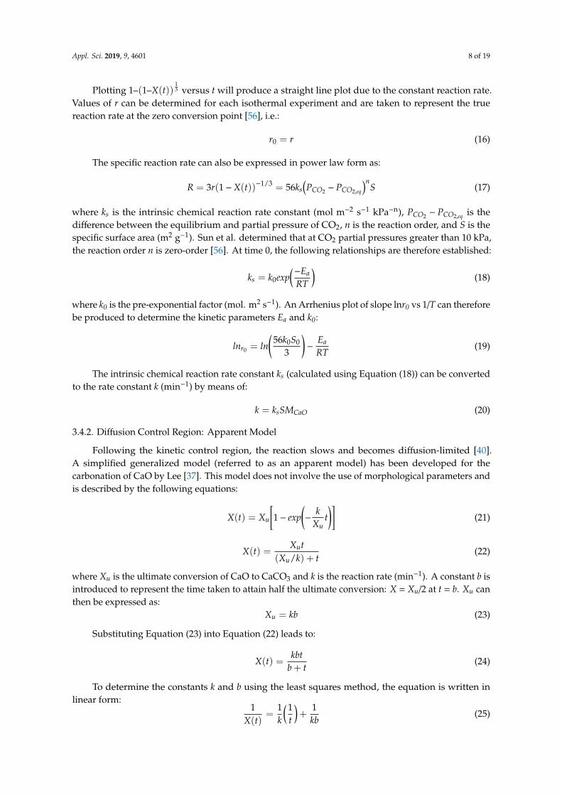
As for the experiment under N2, Coats–Redfern Arrhenius plots (Figure 3) and kinetic 310 parameters for selected reaction models (Table 3) are presented for an experiment under 100% CO2. 311 Under this atmosphere, calculated activation energies are much higher, ranging from 300 to 600 kJ 312 mol-1 when modeled by the nucleation models to 1200 kJ mol-1 when fitted with a first-order model. 313 This is due to the high gradients in the Arrhenius plots under 100% CO2, which mathematically leads 314 to high activation energies. High values of Ea are also obtained in the few literature studies carried 315
Figure 2. Coats–Redfern Arrhenius plots for P-CaCO3 (10 K min−1) under 100% N2: (a) All models;(b) selected models with highest R2 values.
Table 2. Kinetic parameters for calcination obtained from P-CaCO3 (100% N2 atmosphere) (average overfour heating rates) compared with literature results (CaCO3 decomposition under inert atmosphere).
Kinetic Model Ea (kJ mol−1) A (min−1)Correlation
Coefficient (R2)Material and
Reference
A2 108.73 3.5 × 10⁴ 0.9924 P-CaCO3This work
A3 67.11 1.7 × 10² 0.9913 This workA4 46.30 1.1 × 101 0.9900 This workR2 203.57 2.1 × 10⁹ 0.9995 This workR3 213.12 5.0 × 10⁹ 0.9982 This workF1 233.59 2.3 × 10¹¹ 0.9933 This workD1 371.14 1.0 × 10¹⁸ 0.9985 This workR2 180.12 1.2 × 10⁷ - CaCO3 [50]F1 190.46 3.4 × 10⁷ - CaCO3 [58]R3 187.1 - - CaCO3 [54]D1 224.21 3.0 ×· 104 - CaCO3 [59]
The kinetic models are classified as follows. A2–4 are the Avrami–Erofeyev nucleation models, where 2–4 refer tothe exponential in the algebraic function. R2–3 are the geometric contraction models, where R2 uses a contractingarea model and R3 uses a contracting volume model. F1 refers to a first-order reaction model and D1 to a first-orderdiffusion model.
Appl. Sci. 2019, 9, 4601 10 of 19
Correlation coefficients are seen to be very high for all reaction mechanisms, while calculatedactivation energies vary between 47 and 370 kJ mol−1. By a small margin, the highest correlationcoefficient is produced by the R2 geometric model, which determined an Ea of 204 kJ mol−1. Thesekinetic parameters are typical for the calcination of CaCO3 under an inert atmosphere. Literatureresults generally produce values of Ea between 180 and 224 kJ mol−1 [30], showing a lack of consensuson the calcination reaction model (see Table 2). Physical descriptions of the reaction models referencedin Table 2 are provided in a review of kinetics applied to CaL [30].
As for the experiment under N2, Coats–Redfern Arrhenius plots (Figure 3) and kinetic parametersfor selected reaction models (Table 3) are presented for an experiment under 100% CO2. Under thisatmosphere, calculated activation energies are much higher, ranging from 300 to 600 kJ mol−1 whenmodeled by the nucleation models to 1200 kJ mol−1 when fitted with a first-order model. This is dueto the high gradients in the Arrhenius plots under 100% CO2, which mathematically leads to highactivation energies. High values of Ea are also obtained in the few literature studies carried out under100% CO2 [31,60]. Caldwell et al. attribute this to the fact that the temperature range of decompositionbecomes higher and narrower as the percentage of CO2 increases, resulting in a higher apparentactivation energy [31].
Appl. Sci. 2019, 9, x FOR PEER REVIEW 11 of 21
out under 100% CO2 [31,60]. Caldwell et al. attribute this to the fact that the temperature range of 316 decomposition becomes higher and narrower as the percentage of CO2 increases, resulting in a higher 317 apparent activation energy [31]. 318
A2
A3
A4
R2
R3
F1
F2
F3
D1
D2
D3
D4
0.00079 0.00080 0.00081 0.00082
-26
-24
-22
-20
-18
-16
-14
-12
-10
-8
ln[g
()/
T2]
1/T (K-1)
a)
A2 A2 data fit
A3 A3 data fit
A4 A4 data fit
0.000800 0.000808 0.000816-16
-15
-14
-13
ln[g
()/
T2]
1/T (K-1)
b)
319
Figure 3. Coats–Redfern Arrhenius plots for P-CaCO3 (10 K min-1) under 100% CO2: (a) All models; 320 (b) selected models with highest R2 values. 321
Examining the correlation coefficients suggests that the reaction mechanism of P-CaCO3 322 decomposition under CO2 can be modeled by a first-order reaction or Avrami nucleation A2 and A3 323 (see Table 3). Correlation coefficients are seen to be lower than the models under N2 (see Table 2). As 324 for the inert atmosphere, there is no consensus on the reaction model in published literature. 325
Intraparticle and transport resistances may affect reaction rates and reaction mechanisms and 326 have been suggested as the cause of large values of Ea for CaCO3 calcination [60]. In a decomposition 327 mechanism where the reaction advances inwards from the outside of the particle, smaller particles 328 will decompose more quickly [30,61]. If particle sizes are too large, it has been suggested that the 329 reaction may become limited by mass transport, as opposed to the chemical reaction. However, the 330 influence of particle sizes has been found to be small at high CO2 partial pressures [33], so 331 intraparticle mass transport effects on the kinetic parameters can be ruled out as the cause of the 332 overestimated kinetic parameters for the experiments under 100% CO2. [7]. 333
Table 3. Kinetic parameters for calcination obtained from P-CaO material (100% CO2 atmosphere; 334 average over four heating rates) compared with literature results. 335
Kinetic model Ea (kJ mol-1) A (min-1)
Correlation
coefficient (R2)
Material and
reference
A2 599.6 3.4 × 1027 0.9788 P-CaCO3
This work
A3 419.9 4.5 × 10¹⁹ 0.9781 This work
A4 309.9 6.2 × 10¹⁴ 0.9774 This work
F1 1219.2 2.9 × 1054 0.9795 This work
R3 1037.6 3.9 × 1040
- CaCO3 [60]
2nd order 2104.6 1090
- CaCO3 [31]
From the comparison of experiments under different atmospheres, it is evident that calculated 336 activation energies can be highly variable. Although there is believed to be a single, intrinsic 337 activation energy for the calcination reaction, values determined experimentally with model-fitting 338 methods have been described as “effective” activation energies [48]. For the experiment under 100% 339 CO2, in particular, the large disparity in activation energies determined by different reaction models 340
Figure 3. Coats–Redfern Arrhenius plots for P-CaCO3 (10 K min−1) under 100% CO2: (a) All models;(b) selected models with highest R2 values.
Table 3. Kinetic parameters for calcination obtained from P-CaO material (100% CO2 atmosphere;average over four heating rates) compared with literature results.
Kinetic Model Ea (kJ mol−1) A (min−1)Correlation
Coefficient (R2)Material and
Reference
A2 599.6 3.4 × 1027 0.9788 P-CaCO3This work
A3 419.9 4.5 × 10¹⁹ 0.9781 This workA4 309.9 6.2 × 10¹⁴ 0.9774 This workF1 1219.2 2.9 × 1054 0.9795 This workR3 1037.6 3.9 × 1040 - CaCO3 [60]
2nd order 2104.6 1090 - CaCO3 [31]
Examining the correlation coefficients suggests that the reaction mechanism of P-CaCO3
decomposition under CO2 can be modeled by a first-order reaction or Avrami nucleation A2 and A3(see Table 3). Correlation coefficients are seen to be lower than the models under N2 (see Table 2).As for the inert atmosphere, there is no consensus on the reaction model in published literature.
Intraparticle and transport resistances may affect reaction rates and reaction mechanisms andhave been suggested as the cause of large values of Ea for CaCO3 calcination [60]. In a decompositionmechanism where the reaction advances inwards from the outside of the particle, smaller particles will

Appl. Sci. 2019, 9, 4601 11 of 19
decompose more quickly [30,61]. If particle sizes are too large, it has been suggested that the reactionmay become limited by mass transport, as opposed to the chemical reaction. However, the influenceof particle sizes has been found to be small at high CO2 partial pressures [33], so intraparticle masstransport effects on the kinetic parameters can be ruled out as the cause of the overestimated kineticparameters for the experiments under 100% CO2. [7].
From the comparison of experiments under different atmospheres, it is evident that calculatedactivation energies can be highly variable. Although there is believed to be a single, intrinsic activationenergy for the calcination reaction, values determined experimentally with model-fitting methods havebeen described as “effective” activation energies [48]. For the experiment under 100% CO2, in particular,the large disparity in activation energies determined by different reaction models (310–1220 kJ mol−1)and the lower correlation coefficients suggest that model-fitting methods may be unsuitable forcalcination under 100% CO2. An alternative is the use of model-free methods to determine kineticparameters, as in the previous study of Fedunik-Hofman et al., which used the isoconversionalFriedman method to obtain kinetic parameters which vary over the course of the reaction [24].
For both experimental atmospheres, rate constants could not be evaluated using model-fittingmethods, as the Coats–Redfern method produced unreasonably large values of k(T). This is becauseboth k(T) and f(α) vary simultaneously under non-isothermal conditions. This causes the Arrheniusparameters for non-isothermal experiments to be highly variable and exhibit a strong dependence onthe reaction model (see Table 3) [62]. It has been established that the rate constant cannot be viablypredicted by model-fitting methods due to the ambiguity of the kinetic triplet [62]. As suggestedpreviously, isoconversional methods are an alternative means of determining rate constants [24].
As a means of comparison and to aid in a selection of a reaction mechanism, a master plotwas produced using the experimental data (non-isothermal experiments carried out under bothexperimental atmospheres).
Examining the Z(α) master plot in Figure 4a for calcination under N2, there is good correlationbetween the experimental data points and the R3 geometric model, which is most pronounced for theexperiments performed at 10 and 15 K min−1. The lower heating rates experiments show a poorer fit,which could be the result of heat transfer effects. This result correlates with the mechanism suggestedby the Coats–Redfern method, which produces high correlation coefficients for both geometric modelsR2 and R3, as well as literature results (see Table 2).
Appl. Sci. 2019, 9, x FOR PEER REVIEW 12 of 21
(310–1220 kJ mol-1) and the lower correlation coefficients suggest that model-fitting methods may be 341 unsuitable for calcination under 100% CO2. An alternative is the use of model-free methods to 342 determine kinetic parameters, as in the previous study of Fedunik-Hofman et al., which used the 343 isoconversional Friedman method to obtain kinetic parameters which vary over the course of the 344 reaction [24]. 345
For both experimental atmospheres, rate constants could not be evaluated using model-fitting 346 methods, as the Coats–Redfern method produced unreasonably large values of k(T). This is because 347 both k(T) and f(α) vary simultaneously under non-isothermal conditions. This causes the Arrhenius 348 parameters for non-isothermal experiments to be highly variable and exhibit a strong dependence on 349 the reaction model (see Table 3) [62]. It has been established that the rate constant cannot be viably 350 predicted by model-fitting methods due to the ambiguity of the kinetic triplet [62]. As suggested 351 previously, isoconversional methods are an alternative means of determining rate constants [24]. 352
As a means of comparison and to aid in a selection of a reaction mechanism, a master plot was 353 produced using the experimental data (non-isothermal experiments carried out under both 354 experimental atmospheres). 355
Examining the Z(α) master plot in Figure 4a for calcination under N2, there is good correlation 356 between the experimental data points and the R3 geometric model, which is most pronounced for the 357 experiments performed at 10 and 15 K min-1. The lower heating rates experiments show a poorer fit, 358 which could be the result of heat transfer effects. This result correlates with the mechanism suggested 359 by the Coats–Redfern method, which produces high correlation coefficients for both geometric 360 models R2 and R3, as well as literature results (see Table 2). 361
0.0 0.2 0.4 0.6 0.8 1.00.0
0.2
0.4
0.6
0.8
1.0
1.2
1.4
Z(
A2
A3
A4
F1
F2
F3
R2
R3
D1
D2
Z( 2.5K min-1)
Z( 5K min-1)
Z( 10K min-1)
Z( 15K min-1)
a)
0.0 0.2 0.4 0.6 0.8 1.00.0
0.2
0.4
0.6
0.8
1.0
1.2
1.4
Z(
A2
A3
A4
F1
F2
F3
R2
R3
D1
D2
Z( 2.5K min-1)
Z( 5K min-1)
Z( 10K min-1)
Z( 15K min-1)
b)
362
Figure 4. Master plot for P-CaCO3 calcination: (a) Under 100% N2; (b) under 100% CO2. 363
For calcination under CO2 (Figure 4b), a good correlation exists for the experimental data points 364 and the Avrami curves A2 and A3, as well as the first-order chemical reaction model F1. Different 365 experimental heating rates are seen to suggest different mechanisms. For example, the 2.5 K min-1 366 heating rate suggests the mechanism is A3, while 5 K min-1 suggests A2 and 10 K min-1 suggests F1. 367 It is important to note that F1 is a special case of Avrami nucleation [63], as can be seen by the identical 368 shape of the curves, which only differ in magnitude due to the different coefficient n in g(α). 369 Differences in the magnitude of the curves for different heating rates could be the result of heat 370 transfer effects. Therefore, it can be concluded that the calcination reaction under CO2 is a nucleation 371 process. The reaction mechanism suggested by the master plot generally reflects those in the 372 literature carried out using generalized (non-model-fitting) methods, which are summarized 373 elsewhere [30]. Studies typically suggest that the decomposition reaction can be modeled by either 374 Avrami nucleation [26] or first-order chemical reaction F1 [32,58], which is logical when taking into 375 account that F1 is a special case of nucleation. 376
As a further means of comparison, the model-fitting results presented previously were 377 compared with published results which employed the isoconversional Friedman method, carried out 378 by the authors using the same experimental data [24]. The results of the analysis are summarized in 379 Table 4, which also presents average values of Ea over the course of the reaction (Eo). A detailed 380
Figure 4. Master plot for P-CaCO3 calcination: (a) Under 100% N2; (b) under 100% CO2.
For calcination under CO2 (Figure 4b), a good correlation exists for the experimental data pointsand the Avrami curves A2 and A3, as well as the first-order chemical reaction model F1. Differentexperimental heating rates are seen to suggest different mechanisms. For example, the 2.5 K min−1
heating rate suggests the mechanism is A3, while 5 K min−1 suggests A2 and 10 K min−1 suggestsF1. It is important to note that F1 is a special case of Avrami nucleation [63], as can be seen by theidentical shape of the curves, which only differ in magnitude due to the different coefficient n in g(α).Differences in the magnitude of the curves for different heating rates could be the result of heat transfer

Appl. Sci. 2019, 9, 4601 12 of 19
effects. Therefore, it can be concluded that the calcination reaction under CO2 is a nucleation process.The reaction mechanism suggested by the master plot generally reflects those in the literature carriedout using generalized (non-model-fitting) methods, which are summarized elsewhere [30]. Studiestypically suggest that the decomposition reaction can be modeled by either Avrami nucleation [26] orfirst-order chemical reaction F1 [32,58], which is logical when taking into account that F1 is a specialcase of nucleation.
As a further means of comparison, the model-fitting results presented previously were comparedwith published results which employed the isoconversional Friedman method, carried out by theauthors using the same experimental data [24]. The results of the analysis are summarized in Table 4,which also presents average values of Ea over the course of the reaction (Eo). A detailed explanation ofthe assumption of single-step reaction kinetics is presented elsewhere [30]. The equilibrium pressure,P0 (kPa), of the gaseous product is seen to have a significant influence on dα/dt and, hence, theactivation energies under the 100% CO2 atmosphere [24] (see Table 4).
Table 4. Kinetic parameters for calcination obtained from P-CaO material using the Friedmanmethod [24].
Experimental Atmosphere CO2 N2
Ea (kJ mol−1) 430–171 171–147Eo (kJ mol−1) 307 164
Aα (min−1) 3.8 × 1034–2.9 × 10⁵ 1.5 × 10⁷–3.7 × 10⁴
Ao (min−1) – 3.13· 106
Max k (min−1) 0.023 0.012
The compensation effect was used as an alternative means of determining a reaction mechanismfor calcination. This method was only applied for calcination under N2, due to the large variation inkinetic parameters under CO2 [24] (see Section 3.3). Figure 5 shows a comparison of the experimentaland theoretical reaction models, which are compared to suggest a reaction mechanism. The plotshows that the best fitting reaction mechanism is the R2 (contracting area) geometric reaction model,which produces a correlation coefficient of 0.9919. This model also produced a high correlationcoefficient in the Coats–Redfern analysis (R2 > 0.999; see Table 2). The activation energy determinedwith Coats–Redfern is 30% higher than the average Friedman value (213 compared to 164 kJ mol−1),although the values are still within the range obtained in the literature for CaCO3 calcination [30].In conclusion, the R2 model (contracting area) is the mechanism which most accurately models thecalcination of CaCO3 under pure N2, in agreement with the literature [50], which has been verifiedusing both Coats–Redfern and compensation effect methods.
Appl. Sci. 2019, 9, x FOR PEER REVIEW 13 of 21
explanation of the assumption of single-step reaction kinetics is presented elsewhere [30]. The 381 equilibrium pressure, P0 (kPa), of the gaseous product is seen to have a significant influence on dα/dt 382 and, hence, the activation energies under the 100% CO2 atmosphere [24] (see Table 4). 383
Table 4. Kinetic parameters for calcination obtained from P-CaO material using the Friedman method 384 [24]. 385
Experimental atmosphere CO2 N2
Ea (kJ mol-1) 430–171 171–147
Eo (kJ mol-1) 307 164
Aα (min-1) 3.8 × 1034–2.9 × 10⁵ 1.5 × 10⁷–3.7 × 10⁴
Ao (min-1) – 3.13· 106
Max k (min-1) 0.023 0.012
The compensation effect was used as an alternative means of determining a reaction mechanism 386 for calcination. This method was only applied for calcination under N2, due to the large variation in 387 kinetic parameters under CO2 [24] (see Section 3.3). Figure 5 shows a comparison of the experimental 388 and theoretical reaction models, which are compared to suggest a reaction mechanism. The plot 389 shows that the best fitting reaction mechanism is the R2 (contracting area) geometric reaction model, 390 which produces a correlation coefficient of 0.9919. This model also produced a high correlation 391 coefficient in the Coats–Redfern analysis (R2 > 0.999; see Table 2). The activation energy determined 392 with Coats–Redfern is 30% higher than the average Friedman value (213 compared to 164 kJ mol-1), 393 although the values are still within the range obtained in the literature for CaCO3 calcination [30]. In 394 conclusion, the R2 model (contracting area) is the mechanism which most accurately models the 395 calcination of CaCO3 under pure N2, in agreement with the literature [50], which has been verified 396 using both Coats–Redfern and compensation effect methods. 397
It is important to note that the nucleation models and the R2 reaction model are proposed as the 398 mechanisms most consistent with kinetic data for calcination of CaCO3 under 100% CO2 and N2, 399 respectively. As set out by Vyazovkin and Wight in their discussion of the solid state reactions and 400 the extraction of Arrhenius parameters from thermal analysis, one of the fundamental tenets of 401 chemical kinetics is that no reaction mechanism can ever be proved on the basis of kinetic data alone 402 [64]. Despite not allowing for complete isolation of the experimental reaction without influence from 403 physical processes (i.e., diffusion, adsorption, desorption), the suggested reaction models are useful 404 for drawing reasonable mechanistic conclusions. 405
0.2 0.4 0.6 0.80
1
2
3
g(
A2
A3
A4
F1
F2
F3
R2
R3
D1
D2
D3
D4
g(
406
Figure 5. Comparison of theoretical reaction models and experimental model-fitting curve 407 (compensation effect) for calcination under N2. 408
4.2. Carbonation Kinetics Comparative Analysis 409
Figure 5. Comparison of theoretical reaction models and experimental model-fitting curve(compensation effect) for calcination under N2.
Appl. Sci. 2019, 9, 4601 13 of 19
It is important to note that the nucleation models and the R2 reaction model are proposed asthe mechanisms most consistent with kinetic data for calcination of CaCO3 under 100% CO2 andN2, respectively. As set out by Vyazovkin and Wight in their discussion of the solid state reactionsand the extraction of Arrhenius parameters from thermal analysis, one of the fundamental tenetsof chemical kinetics is that no reaction mechanism can ever be proved on the basis of kinetic dataalone [64]. Despite not allowing for complete isolation of the experimental reaction without influencefrom physical processes (i.e., diffusion, adsorption, desorption), the suggested reaction models areuseful for drawing reasonable mechanistic conclusions.
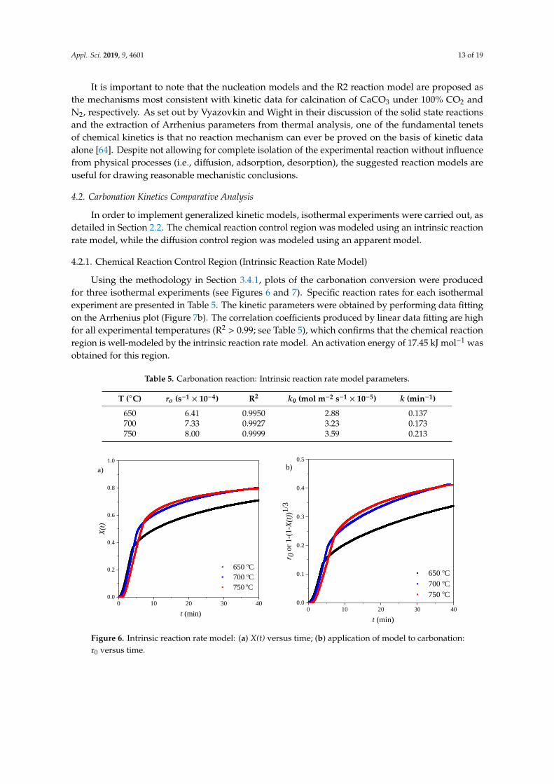
4.2. Carbonation Kinetics Comparative Analysis
In order to implement generalized kinetic models, isothermal experiments were carried out, asdetailed in Section 2.2. The chemical reaction control region was modeled using an intrinsic reactionrate model, while the diffusion control region was modeled using an apparent model.
4.2.1. Chemical Reaction Control Region (Intrinsic Reaction Rate Model)
Using the methodology in Section 3.4.1, plots of the carbonation conversion were producedfor three isothermal experiments (see Figures 6 and 7). Specific reaction rates for each isothermalexperiment are presented in Table 5. The kinetic parameters were obtained by performing data fittingon the Arrhenius plot (Figure 7b). The correlation coefficients produced by linear data fitting are highfor all experimental temperatures (R2 > 0.99; see Table 5), which confirms that the chemical reactionregion is well-modeled by the intrinsic reaction rate model. An activation energy of 17.45 kJ mol−1 wasobtained for this region.
Table 5. Carbonation reaction: Intrinsic reaction rate model parameters.
T (C) ro (s−1 × 10⁻⁴) R2 k0 (mol m−2 s−1 × 10⁻⁵) k (min−1)
650 6.41 0.9950 2.88 0.137700 7.33 0.9927 3.23 0.173750 8.00 0.9999 3.59 0.213
Appl. Sci. 2019, 9, x FOR PEER REVIEW 14 of 21
In order to implement generalized kinetic models, isothermal experiments were carried out, as 410 detailed in Section 2.2. The chemical reaction control region was modeled using an intrinsic reaction 411 rate model, while the diffusion control region was modeled using an apparent model. 412
4.2.1. Chemical Reaction Control Region (Intrinsic Reaction Rate Model) 413
Using the methodology in Section 3.4.1, plots of the carbonation conversion were produced for 414 three isothermal experiments (see Figures 6 and 7). Specific reaction rates for each isothermal 415 experiment are presented in Table 5. The kinetic parameters were obtained by performing data fitting 416 on the Arrhenius plot (Figure 7b). The correlation coefficients produced by linear data fitting are high 417 for all experimental temperatures (R2 > 0.99; see Table 5), which confirms that the chemical reaction 418 region is well-modeled by the intrinsic reaction rate model. An activation energy of 17.45 kJ mol-1 was 419 obtained for this region. 420
0 10 20 30 400.0
0.2
0.4
0.6
0.8
1.0
650 oC
700 oC
750 oC
X(t
)
t (min)
a)
0 10 20 30 400.0
0.1
0.2
0.3
0.4
0.5
650 oC
700 oC
750 oC
r 0 o
r 1-(
1-X
(t))
1/3
t (min)
b)
421
Figure 6. Intrinsic reaction rate model: (a) X(t) versus time; (b) application of model to carbonation: r0 422 versus time. 423
0 1 2 3 4 5 60.00
0.05
0.10
0.15
0.20
650 oC
700 oC
750 oC
1-(
1-X
(t))
1/3
t (min)
a)
0.00095 0.00100 0.00105 0.00110-7.4
-7.3
-7.2
-7.1
ln(r0)
data fit
ln(r
0)
1/T (K-1)
b)
424
Figure 7. Intrinsic reaction rate model: (a) Data fitting with model; (b) Arrhenius plot. 425
Table 5. Carbonation reaction: Intrinsic reaction rate model parameters. 426
T (°C) ro (s-1 × 10⁻⁴) R2 k0 (mol m-2 s-1 × 10-
5)
k (min-1)
650 6.41 0.9950 2.88 0.137
700 7.33 0.9927 3.23 0.173
Figure 6. Intrinsic reaction rate model: (a) X(t) versus time; (b) application of model to carbonation:r0 versus time.

Appl. Sci. 2019, 9, 4601 14 of 19
Appl. Sci. 2019, 9, x FOR PEER REVIEW 14 of 21
In order to implement generalized kinetic models, isothermal experiments were carried out, as 410 detailed in Section 2.2. The chemical reaction control region was modeled using an intrinsic reaction 411 rate model, while the diffusion control region was modeled using an apparent model. 412
4.2.1. Chemical Reaction Control Region (Intrinsic Reaction Rate Model) 413
Using the methodology in Section 3.4.1, plots of the carbonation conversion were produced for 414 three isothermal experiments (see Figures 6 and 7). Specific reaction rates for each isothermal 415 experiment are presented in Table 5. The kinetic parameters were obtained by performing data fitting 416 on the Arrhenius plot (Figure 7b). The correlation coefficients produced by linear data fitting are high 417 for all experimental temperatures (R2 > 0.99; see Table 5), which confirms that the chemical reaction 418 region is well-modeled by the intrinsic reaction rate model. An activation energy of 17.45 kJ mol-1 was 419 obtained for this region. 420
0 10 20 30 400.0
0.2
0.4
0.6
0.8
1.0
650 oC
700 oC
750 oC
X(t
)
t (min)
a)
0 10 20 30 400.0
0.1
0.2
0.3
0.4
0.5
650 oC
700 oC
750 oC
r 0 o
r 1-(
1-X
(t))
1/3
t (min)
b)
421
Figure 6. Intrinsic reaction rate model: (a) X(t) versus time; (b) application of model to carbonation: r0 422 versus time. 423
0 1 2 3 4 5 60.00
0.05
0.10
0.15
0.20
650 oC
700 oC
750 oC
1-(
1-X
(t))
1/3
t (min)
a)
0.00095 0.00100 0.00105 0.00110-7.4
-7.3
-7.2
-7.1
ln(r0)
data fit
ln(r
0)
1/T (K-1)
b)
424
Figure 7. Intrinsic reaction rate model: (a) Data fitting with model; (b) Arrhenius plot. 425
Table 5. Carbonation reaction: Intrinsic reaction rate model parameters. 426
T (°C) ro (s-1 × 10⁻⁴) R2 k0 (mol m-2 s-1 × 10-
5)
k (min-1)
650 6.41 0.9950 2.88 0.137
700 7.33 0.9927 3.23 0.173
Figure 7. Intrinsic reaction rate model: (a) Data fitting with model; (b) Arrhenius plot.
4.2.2. Diffusion Control Region (Apparent Model)
Using the methodology described in Section 3.4.2, an apparent model was used to determine thekinetic parameters of the diffusion control region. Data fitting plots are shown in Figures 8 and 9 andapparent model parameters are recorded in Table 6.
Appl. Sci. 2019, 9, x FOR PEER REVIEW 15 of 21
750 8.00 0.9999 3.59 0.213
4.2.2. Diffusion Control Region (Apparent Model) 427
Using the methodology described in Section 3.4.2, an apparent model was used to determine the 428 kinetic parameters of the diffusion control region. Data fitting plots are shown in Figures 8 and 9 and 429 apparent model parameters are recorded in Table 6. 430
Table 6. Carbonation reaction: Apparent model parameters. 431
T (°C) k (min-1) b (min) Xu
650 0.098 8.80 0.863
700 0.158 5.54 0.875
750 0.210 4.16 0.872
0.0 0.2 0.4 0.60
2
4
6
8
10
650 oC
700 oC
750 oC
1/X
(t)
1/t (min-1)
a)
0.0 0.1 0.2 0.31.0
1.2
1.4
1.6
1.8
2.0
2.2
2.4
650 oC
700 oC
750 oC
1/X
(t)
1/t (min-1)
b)
432
Figure 8. Apparent model: (a) 1/X(t) versus time; (b) data fitting for diffusion control region. 433
0.00095 0.00100 0.00105 0.00110
-6.4
-6.2
-6.0
-5.8
-5.6 ln(k)
Data fit
ln(k
)
1/T (K-1)
a)
10 20 30 400.2
0.4
0.6
0.8
650 oC
700 oC
750 oC
650 oC predicted
700 oC predicted
750 oC predicted
X(t
)
t (min)
b)
434
Figure 9. Apparent model: (a) Arrhenius plot for diffusion region; (b) conversion predicted using 435 apparent model compared to original data. 436
In order to validate the model, the obtained values of Xu and k were used to calculate X(t) 437 (Equation (23)) and plotted against the isothermal data for the diffusion region. Figure 9b shows a 438 good agreement between experimental data and the model. The kinetic parameters were obtained by 439 performing data fitting on the Arrhenius plot (Figure 9a). An activation energy of 59.95 kJ mol-1 was 440 calculated for this region. 441
Figure 8. Apparent model: (a) 1/X(t) versus time; (b) data fitting for diffusion control region.
Appl. Sci. 2019, 9, x FOR PEER REVIEW 15 of 21
750 8.00 0.9999 3.59 0.213
4.2.2. Diffusion Control Region (Apparent Model) 427
Using the methodology described in Section 3.4.2, an apparent model was used to determine the 428 kinetic parameters of the diffusion control region. Data fitting plots are shown in Figures 8 and 9 and 429 apparent model parameters are recorded in Table 6. 430
Table 6. Carbonation reaction: Apparent model parameters. 431
T (°C) k (min-1) b (min) Xu
650 0.098 8.80 0.863
700 0.158 5.54 0.875
750 0.210 4.16 0.872
0.0 0.2 0.4 0.60
2
4
6
8
10
650 oC
700 oC
750 oC
1/X
(t)
1/t (min-1)
a)
0.0 0.1 0.2 0.31.0
1.2
1.4
1.6
1.8
2.0
2.2
2.4
650 oC
700 oC
750 oC
1/X
(t)
1/t (min-1)
b)
432
Figure 8. Apparent model: (a) 1/X(t) versus time; (b) data fitting for diffusion control region. 433
0.00095 0.00100 0.00105 0.00110
-6.4
-6.2
-6.0
-5.8
-5.6 ln(k)
Data fit
ln(k
)
1/T (K-1)
a)
10 20 30 400.2
0.4
0.6
0.8
650 oC
700 oC
750 oC
650 oC predicted
700 oC predicted
750 oC predicted
X(t
)
t (min)
b)
434
Figure 9. Apparent model: (a) Arrhenius plot for diffusion region; (b) conversion predicted using 435 apparent model compared to original data. 436
In order to validate the model, the obtained values of Xu and k were used to calculate X(t) 437 (Equation (23)) and plotted against the isothermal data for the diffusion region. Figure 9b shows a 438 good agreement between experimental data and the model. The kinetic parameters were obtained by 439 performing data fitting on the Arrhenius plot (Figure 9a). An activation energy of 59.95 kJ mol-1 was 440 calculated for this region. 441
Figure 9. Apparent model: (a) Arrhenius plot for diffusion region; (b) conversion predicted usingapparent model compared to original data.

Appl. Sci. 2019, 9, 4601 15 of 19
Table 6. Carbonation reaction: Apparent model parameters.
T (C) k (min−1) b (min) Xu
650 0.098 8.80 0.863700 0.158 5.54 0.875750 0.210 4.16 0.872
In order to validate the model, the obtained values of Xu and k were used to calculate X(t)(Equation (23)) and plotted against the isothermal data for the diffusion region. Figure 9b shows agood agreement between experimental data and the model. The kinetic parameters were obtained byperforming data fitting on the Arrhenius plot (Figure 9a). An activation energy of 59.95 kJ mol−1 wascalculated for this region.
Kinetic parameters for both the kinetic and diffusion control regions are presented in Table 7 andcompared with selected literature results. Lee states that k can be regarded as the intrinsic chemicalreaction rate constant ks [37], as well as the diffusion constant D, although the different units meanthat it cannot be directly compared with reaction rate constants for studies such as those using poremodels [17].
Table 7. Carbonation reaction: Kinetic parameters. ks and D are averages over the temperature range650, 700, and 750 C. S is provided in as-synthesized state or after one cycle.
Kinetic Control Region
Reference This Work Sun et al. [56]Lee [37]
Data: Bhatia andPerlmutter [25]
Lee [37]Data: Guptaand Fan [39]
Grasa et al.[17]
Material P-CaO Strassburglimestone Calcined limestone
Calcinedprecipitated
CaCO3
Katowicelimestone
Method Intrinsic reaction ratemodel
Intrinsicreaction rate
modelApparent model Apparent
model Pore model
T (C) k (min−1)650 0.24 0.97 0.925 * 0.858 –700 0.27 0.81 – – –750 0.30 0.67 – – –
S (m2 g−1) 13.8 29 15.6 12.8 12.9 **Ea (kJ mol−1) 17.45 24.0 72.2 72.7 19.2
ks (m4 kmol−1 s−1) 3.34 × 10⁻⁶ 4.68 × 10⁻⁶ 6.0 × 10⁻⁷ – 5.29 × 10⁻⁶
Diffusion control region
Method Apparent model – Apparent model Apparentmodel Pore model
T (C) k (min−1)650 0.098 – 0.344 * 0.357 –700 0.158 – – – –750 0.210 – – – –
Ea (kJ mol−1) 59.95 – 189.3 102.5 163D (m2 s−1) – – – 4.32 × 10⁻⁶ –
* Calculated at 655 C [37]; ** calculated from specific surface area (m2 m−3) assuming ρ (non-porous CaCO3) of2710 kg m−3.
For both the chemical reaction and diffusion control regions, the reaction rates and values of Xu
(see Table 6) tend to increase with increasing temperature, which is consistent with reaction kineticsincreasing with higher temperatures (as described by Arrhenius relationships; i.e., Equation (4)). Thereaction rates for P-CaO are seen to be slightly slower than those in the literature. The activationenergies of P-CaO are also slightly lower than expected for both the kinetic control region (literaturevalues typically fall between 20 and 32 kJ mol−1) and the diffusion region (literature values are typicallybetween 80 and 200 kJ mol−1 ) [30].
The variation in the activation energies has been attributed to the differences in morphology andtexture of the CO2 sorbent [46,56]. While it has been suggested that morphology of CaO does not
Appl. Sci. 2019, 9, 4601 16 of 19
greatly influence kinetics in the kinetic control region [28], outlying values have been attributed todiffusion limitations in the material [37]. Lee postulated that lower activation energies are associatedwith microporous materials that are susceptible to pore plugging, which would limit diffusion of CO2,and is also associated with low carbonation conversion [37]. A study by Grasa et al. determined amuch higher diffusion Ea of 163 kJ mol−1 for mesoporous limestone [17], which has been associatedwith resistance to pore plugging [39]. In the case of P-CaO, however, BET analysis showed that thematerial was largely nonporous, with the majority of pore volume in the macroporous region [24].Nevertheless, the lower diffusion activation energy could be the result of incomplete carbonationconversion (see Table 6).
Cycling experiments with P-CaO performed elsewhere [24] show good performance with cycling,which suggests that the reaction rates, although initially slower than other materials, will be retainedwith subsequent cycles. Future analysis could involve calculation of kinetic parameters after multipleisothermal cycles. Carrying out a kinetic analysis with another generalized method is also recommended,as the apparent method uses only a small number of data points to produce an Arrhenius equation.
5. Conclusions
This paper has presented a comparative kinetic analysis of the reactions for CaL, using bothinert atmospheres/low CO2 concentrations, as is typically performed in the literature, and the morerarely-used 100% CO2 atmosphere. Additionally, it has discussed the validity of model-fitting methodsin direct comparison with isoconversional and generalized methods, which has not been carried outpreviously. The experimental conditions, material properties, and the kinetic method have been foundto strongly influence the kinetic parameters for both calcination and carbonation reactions. The mainconclusions of the study are summarized as follows:
For the calcination of synthesized CaCO3 under N2, an Ea of 204 and 233.6 kJ mol−1 was obtainedby model-fitting using the R2 geometric model and F1 model, respectively, which is consistent with theliterature results. Calcination of the same material determined an average Ea of 164 kJ mol−1 using anisoconversional method. The compensation effect also suggested that the best reaction model was R2.For calcination under CO2, much higher values of Ea were obtained, i.e., 310 kJ mol−1 with A4 (Avraminucleation) and 1220 kJ mol−1 with the F1 model, while isoconversional results ranged between 170and 530 kJ mol−1, which was attributed to the major morphological changes in the material underCO2 [24].
From this study, we can conclude that a multiple heating-rate isoconversional method, suchas Friedman, should first be carried out to arrive at non-mechanistic parameters. It will also showwhether the kinetic parameters vary over the course of the reaction. Then, if the activation energydoes not vary significantly under the experimental atmosphere (as is the case for calcination of CaCO3
under inert gas), the compensation effect can be used to suggest a reaction model. As a means ofcomparison, a model-fitting method such as Coats–Redfern can be applied over the whole reaction todetermine kinetic parameters based on several reaction models. This can be corroborated with masterplots. Where applicable, the reaction model with the highest correlation coefficient can be comparedwith the results of the isoconversional analysis. If the same kinetic parameters are obtained, greaterconfidence can be placed in the results of the analysis.
If the activation energy does vary significantly under the experimental atmosphere (as is thecase for calcination of CaCO3 under CO2), the Coats–Redfern method is not recommended, as thediscrete values of kinetic parameters will not capture the variation in reaction kinetics. Additionally,the compensation effect cannot be applied, as it requires single values of kinetic parameters. In thiscase, an isoconversional analysis is the best option for obtaining kinetic parameters.
The carbonation of synthesized CaO was modeled using an intrinsic chemical reaction ratemodel (for the kinetic control region) and apparent model (for the diffusion region), and subsequentlycompared with the literature. An activation energy of 17.45 kJ mol−1 was obtained for the kinetic controlregion, and 59.95 kJ mol−1 for the diffusion region. Lower values of Ea compared to the literature could
Appl. Sci. 2019, 9, 4601 17 of 19
be attributed to the incomplete carbonation conversion. For this synthesized material, the generalizedmodels proved to model the two carbonation regions with high accuracy. For further studies, materialcharacterization (i.e., scanning/transmission electron microscopy, physisorption characterization,and/or porosimetry) is recommended prior to selecting a generalized kinetic analysis method.
Author Contributions: Conceptualization, L.F.-H. and A.B.; methodology, L.F.-H. and A.B.; formal analysis,L.F.-H.; investigation, L.F.-H.; writing—original draft preparation, L.F.-H.; writing—review and editing, L.F.-H.and A.B.; supervision, A.B. and S.W.D.
Funding: This research received funding from the Australian Solar Thermal Research Institute (ASTRI), a programsupported by the Australian Government through the Australian Renewable Energy Agency (ARENA).
Conflicts of Interest: The authors declare no conflicts of interest. The funders had no role in the design of thestudy; in the collection, analyses, or interpretation of data; in the writing of the manuscript; or in the decision topublish the results.
References
1. Bayon, A.; Bader, R.; Jafarian, M.; Fedunik-Hofman, L.; Sun, Y.; Hinkley, J.; Miller, S.; Lipinski, W.Techno-economic assessment of solid–gas thermochemical energy storage systems for solar thermal powerapplications. Energy 2018, 149, 473–484. [CrossRef]
2. Edwards, S.; Materic, V. Calcium looping in solar power generation plants. Sol. Energy 2012, 86, 2494–2503.[CrossRef]
3. Angerer, M.; Becker, M.; Härzschel, S.; Kröper, K.; Gleis, S.; Vandersickel, A.; Spliethoff, H. Design of aMW-scale thermo-chemical energy storage reactor. Energy Rep. 2018, 4, 507–519. [CrossRef]
4. Ströhle, J.; Junk, M.; Kremer, J.; Galloy, A.; Epple, B. Carbonate looping experiments in a 1 MWth pilot plantand model validation. Fuel 2014, 127, 13–22. [CrossRef]
5. André, L.; Abanades, S.; Flamant, G. Screening of thermochemical systems based on solid-gas reversiblereactions for high temperature solar thermal energy storage. Renew. Sustain. Energy Rev. 2016, 64, 703–715.[CrossRef]
6. Stanmore, B.R.; Gilot, P. Review: Calcination and carbonation of limestone during thermal cycling for CO2
sequestration. Fuel Process. Technol. 2005, 86, 1707–1743. [CrossRef]7. Grasa, G.; Abanades, J.C.; Alonso, M.; González, B. Reactivity of highly cycled particles of CaO in a
carbonation/calcination loop. Chem. Eng. J. 2008, 137, 5615–5667. [CrossRef]8. King, P.L.; Wheeler, V.M.; Renggli, C.J.; Palm, A.B.; Wilson, S.A.; Harrison, A.L.; Morgan, B.; Nekvasil, H.;
Troitzsch, U.; Mernagh, T.; et al. Gas–Solid Reactions: Theory, Experiments and Case Studies Relevant toEarth and Planetary Processes. Rev. Mineral. Geochem. 2018, 84, 1–56. [CrossRef]
9. Boot-Handford, M.E.; Abanades, J.C.; Anthony, E.J.; Blunt, M.J.; Brandani, S.; Mac Dowell, N.; Fernández, J.R.;Ferrari, M.-C.; Gross, R.; Hallett, J.P.; et al. Carbon capture and storage update. Energy Environ. Sci. 2014, 7,130–189. [CrossRef]
10. Hanak, D.P.; Manovic, V. Calcium looping with supercritical CO2 cycle for decarbonisation of coal-firedpower plant. Energy 2016, 102, 343–353. [CrossRef]
11. Shimizu, T.; Hirama, T.; Hosoda, H.; Kitano, K.; Inagaki, M.; Tejima, K. A Twin Fluid-Bed Reactor for Removalof CO2 from Combustion Processes. Chem. Eng. Res. Des. 1999, 77, 62–68. [CrossRef]
12. Martínez, I.; Grasa, G.; Murillo, R.; Arias, B.; Abanades, J.C. Kinetics of Calcination of Partially CarbonatedParticles in a Ca-Looping System for CO2 Capture. Energy Fuels 2012, 26, 1432–1440. [CrossRef]
13. Diego, M.; Martinez, I.; Alonso, M.; Arias, B.; Abanades, J. Calcium looping reactor design for fluidized-bedsystems. In Calcium and Chemical Looping Technology for Power Generation and Carbon Dioxide (CO2) Capture;Fennell, P., Anthony, B., Eds.; Woodhead Publishing: Cambridge, UK, 2015; pp. 107–138.
14. Alonso, M.; Rodriguez, N.; Gonzalez, B.; Arias, B.; Abanades, J.C. Capture of CO2 during low temperaturebiomass combustion in a fluidized bed using CaO. Process description, experimental results and economics.Energy Procedia 2011, 4, 795–802. [CrossRef]
15. Bouquet, E.; Leyssens, G.; Schönnenbeck, C.; Gilot, P. The decrease of carbonation efficiency of CaO alongcalcination–carbonation cycles: Experiments and modelling. Chem. Eng. Sci. 2009, 64, 2136–2146. [CrossRef]
16. Sun, P.; Grace, J.R.; Lim, C.J.; Anthony, E.J. A discrete-pore-size-distribution-based gas-solid model and itsapplication to the CaO + CO2 reaction. Chem. Eng. Sci. 2008, 63, 57–70. [CrossRef]

Appl. Sci. 2019, 9, 4601 18 of 19
17. Grasa, G.; Murillo, R.; Alonso, M.; Abanades, J.C. Application of the random pore model to the carbonationcyclic reaction. AIChE J. 2009, 55, 1246–1255. [CrossRef]
18. Yue, L.; Lipinski, W. Thermal transport model of a sorbent particle undergoing calcination–carbonationcycling. AIChE J. 2015, 61, 2647–2656. [CrossRef]
19. Yue, L.; Lipinski, W. A numerical model of transient thermal transport phenomena in a high-temperaturesolid–gas reacting system for CO2 capture applications. Int. J. Heat Mass Transf. 2015, 85, 1058–1068. [CrossRef]
20. Lasheras, A.; Ströhle, J.; Galloy, A.; Epple, B. Carbonate looping process simulation using a 1D fluidized bedmodel for the carbonator. Int. J. Greenh. Gas Control 2011, 5, 686–693. [CrossRef]
21. Romano, M. Coal-fired power plant with calcium oxide carbonation for postcombustion CO2 capture. EnergyProcedia 2009, 1, 1099–1106. [CrossRef]
22. Martínez, I.; Murillo, R.; Grasa, G.; Abanades, J.C. Integration of a Ca-looping system for CO2 capture in anexisting power plant. Energy Procedia 2011, 4, 1699–1706. [CrossRef]
23. Sarrión, B.; Perejón, A.; Sánchez-Jiménez, P.E.; Pérez-Maqueda, L.A.; Valverde, J.M. Role of calcium loopingconditions on the performance of natural and synthetic Ca-based materials for energy storage. J. CO2 Util.2018, 28, 374–384. [CrossRef]
24. Fedunik-Hofman, L.; Bayon, A.; Hinkley, J.; Lipinski, W.; Donne, S.W. Friedman method kinetic analysis ofCaO-based sorbent for high-temperature thermochemical energy storage. Chem. Eng. Sci. 2019, 200, 236–247.[CrossRef]
25. Bhatia, S.K.; Perlmutter, D.D. Effect of the product layer on the kinetics of the CO2-lime reaction. AIChE J.1983, 29, 79–86. [CrossRef]
26. Valverde, J.M.; Sanchez-Jimenez, P.E.; Perez-Maqueda, L.A. Limestone calcination nearby equilibrium:Kinetics, CaO crystal structure, sintering and reactivity. J. Phys. Chem. C 2015, 119, 1623–1641. [CrossRef]
27. Ingraham, T.R.; Marier, P. Kinetic studies on the thermal decomposition of calcium carbonate. Can. J. Chem.Eng. 1963, 41, 170–173. [CrossRef]
28. Salaudeen, S.A.; Acharya, B.; Dutta, A. CaO-based CO2 sorbents: A review on screening, enhancement,cyclic stability, regeneration and kinetics modelling. J. CO2 Util. 2018, 23, 179–199. [CrossRef]
29. Kierzkowska, A.M.; Pacciani, R.; Müller, C.R. CaO-based CO2 sorbents: From fundamentals to thedevelopment of new, highly effective materials. ChemSusChem 2013, 6, 1130–1148. [CrossRef]
30. Fedunik-Hofman, L.; Bayon, A.; Donne, S.W. Kinetics of Solid-Gas Reactions and Their Application toCarbonate Looping Systems. Energies 2019, 12, 2981. [CrossRef]
31. Caldwell, K.M.; Gallagher, P.K.; Johnson, D.W. Effect of thermal transport mechanisms on the thermaldecomposition of CaCO3. Thermochim. Acta 1977, 18, 15–19. [CrossRef]
32. Rodriguez-Navarro, C.; Ruiz-Agudo, E.; Luque, A.; Rodriguez-Navarro, A.B.; Ortega-Huertas, M. Thermaldecomposition of calcite: Mechanisms of formation and textural evolution of CaO nanocrystals. Am. Mineral.2009, 94, 578–593. [CrossRef]
33. Khinast, J.; Krammer, G.F.; Brunner, C.; Staudinger, G. Decomposition of limestone: The influence of CO2
and particle size on the reaction rate. Chem. Eng. Sci. 1996, 51, 623–634. [CrossRef]34. Dai, P.; González, B.; Dennis, J.S. Using an experimentally-determined model of the evolution of pore
structure for the calcination of cycled limestones. Chem. Eng. J. 2016, 304, 175–185. [CrossRef]35. García-Labiano, F.; Abad, A.; de Diego, L.F.; Gayán, P.; Adánez, J. Calcination of calcium-based sorbents at
pressure in a broad range of CO2 concentrations. Chem. Eng. Sci. 2002, 57, 2381–2393. [CrossRef]36. Li, Z.; Sun, H.; Cai, N. Rate equation theory for the carbonation reaction of CaO with CO2. Energy Fuels 2012,
26, 4607–4616. [CrossRef]37. Lee, D.K. An apparent kinetic model for the carbonation of calcium oxide by carbon dioxide. Chem. Eng. J.
2004, 100, 71–77. [CrossRef]38. Nouri, S.M.M.; Ebrahim, H.A. Kinetic study of CO2 reaction with CaO by a modified random pore model.
Pol. J. Chem. Technol. 2016, 18, 93–98. [CrossRef]39. Gupta, H.; Fan, L.-S. Carbonation−Calcination Cycle Using High Reactivity Calcium Oxide for Carbon
Dioxide Separation from Flue Gas. Ind. Eng. Chem. Res. 2002, 41, 4035–4042. [CrossRef]40. Mess, D.; Sarofim, A.F.; Longwell, J.P. Product layer diffusion during the reaction of calcium oxide with
carbon dioxide. Energy Fuels 1999, 13, 999–1005. [CrossRef]41. Bouineau, V.; Pijolat, M.; Soustelle, M. Characterisation of the chemical reactivity of a CaCO3 powder for its
decomposition. J. Eur. Ceram. Soc. 1998, 18, 1319–1324. [CrossRef]
Appl. Sci. 2019, 9, 4601 19 of 19
42. Manovic, V.; Charland, J.-P.; Blamey, J.; Fennell, P.S.; Lu, D.Y.; Anthony, E.J. Influence of calcination conditionson carrying capacity of CaO-based sorbent in CO2 looping cycles. Fuel 2009, 88, 1893–1900. [CrossRef]
43. Valverde, J.M.; Sanchez-Jimenez, P.E.; Perez-Maqueda, L.A. Calcium-looping for post-combustion CO2
capture. On the adverse effect of sorbent regeneration under CO2. Appl. Energy 2014, 126, 161–171. [CrossRef]44. Symonds, R.T.; Lu, D.Y.; Manovic, V.; Anthony, E.J. Pilot-Scale Study of CO2 Capture by CaO-Based Sorbents
in the Presence of Steam and SO2. Ind. Eng. Chem. Res. 2012, 51, 7177–7184. [CrossRef]45. Jana, P.; de la Peña O’Shea, V.A.; Coronado, J.M.; Serrano, D.P. Cobalt based catalysts prepared by Pechini
method for CO2-free hydrogen production by methane decomposition. Int. J. Hydrogen Energy 2010, 35,10285–10294. [CrossRef]
46. Zhou, Z.; Xu, P.; Xie, M.; Cheng, Z.; Yuan, W. Modeling of the carbonation kinetics of a synthetic CaO-basedsorbent. Chem. Eng. Sci. 2013, 95, 283–290. [CrossRef]
47. Vyazovkin, S.; Burnham, A.K.; Criado, J.M.; Pérez-Maqueda, L.A.; Popescu, C.; Sbirrazzuoli, N. ICTACKinetics Committee recommendations for performing kinetic computations on thermal analysis data.Thermochim. Acta 2011, 520, 1–19. [CrossRef]
48. Urbanovici, E.; Popescu, C.; Segal, E. Improved iterative version of the Coats-Redfern method to evaluatenon-isothermal kinetic parameters. J. Therm. Anal. Calorim. 1999, 58, 683–700. [CrossRef]
49. Sanders, J.P.; Gallagher, P.K. Kinetic analyses using simultaneous TG/DSC measurements Part I:Decomposition of calcium carbonate in argon. Thermochim. Acta 2002, 388, 115–128. [CrossRef]
50. Ninan, K.N.; Krishnan, K.; Krishnamurthy, V.N. Kinetics and mechanism of thermal decomposition of insitugenerated calcium carbonate. J. Therm. Anal. 1991, 37, 1533–1543. [CrossRef]
51. Vyazovkin, S.; Wight, C. Model-Free and Model-Fitting Approaches to Kinetic Analysis of Isothermal andNonisothermal Data. Thermochim. Acta 1999, 340, 53–68. [CrossRef]
52. Criado, J.M.; Málek, J.; Ortega, A. Applicability of the master plots in kinetic analysis of non-isothermal data.Thermochim. Acta 1989, 147, 377–385. [CrossRef]
53. Vyazovkin, S. Estimating Reaction Models and Preexponential Factors. In Isoconversional Kinetics of ThermallyStimulated Processes; Springer International Publishing: Berlin/Heidelberg, Germany, 2015; pp. 41–50.
54. Yue, L.; Shui, M.; Xu, Z. The decomposition kinetics of nanocrystalline calcite. Thermochim. Acta 1999, 335,121–126. [CrossRef]
55. Pijolat, M.; Favergeon, L. Kinetics and mechanisms of solid-gas reactions. In Handbook of Thermal Analysis andCalorimetry, 2nd ed.; Sergey, V., Nobuyoshi, K., Christoph, S., Eds.; Elsevier: Amsterdam, The Netherlands,2018; Volume 6, pp. 173–212.
56. Sun, P.; Grace, J.R.; Lim, C.J.; Anthony, E.J. Determination of intrinsic rate constants of the CaO-CO2 reaction.Chem. Eng. Sci. 2008, 63, 47–56. [CrossRef]
57. Lee, D.K.; Min, D.Y.; Seo, H.; Kang, N.Y.; Choi, W.C.; Park, Y.K. Kinetic Expression for the CarbonationReaction of K2CO3/ZrO2 Sorbent for CO2 Capture. Ind. Eng. Chem. Res. 2013, 52, 9323–9329. [CrossRef]
58. Maitra, S.; Chakrabarty, N.; Pramanik, J. Decomposition kinetics of alkaline earth carbonates by integralapproximation method. Ceramica 2008, 54, 268–272. [CrossRef]
59. Maitra, S.; Bandyopadhyay, N.; Das, S.; Pal, A.J.; Pramanik, M.J. Non-isothermal decomposition kinetics ofalkaline earth metal carbonates. J. Am. Ceram. Soc. 2007, 90, 1299–1303. [CrossRef]
60. Gallagher, P.K.; Johnson, D.W. Kinetics of the thermal decomposition of CaCO3 in CO2 and some observationson the kinetic compensation effect. Thermochim. Acta 1976, 14, 255–261. [CrossRef]
61. Lee, J.-T.; Keener, T.; Knoderera, M.; Khang, S.-J. Thermal decomposition of limestone in a large scalethermogravimetric analyzer. Thermochim. Acta 1993, 213, 223–240. [CrossRef]
62. Vyazovkin, S.; Wight, C.A. Isothermal and non-isothermal kinetics of thermally stimulated reactions of solids.Int. Rev. Phys. Chem. 1998, 17, 407–433. [CrossRef]
63. Khawam, A.; Flanagan, D.R. Solid-state kinetic models: Basics and mathematical fundamentals. J. Phys.Chem. B 2006, 110, 17315–17328. [CrossRef]
64. Vyazovkin, S.; Wight, C.A. Kinetics in Solids. Annu. Rev. Phys. Chem. 1997, 48, 125–149. [CrossRef] [PubMed]
© 2019 by the authors. Licensee MDPI, Basel, Switzerland. This article is an open accessarticle distributed under the terms and conditions of the Creative Commons Attribution(CC BY) license (http://creativecommons.org/licenses/by/4.0/).